Decadal North Pacific sea surface temperature variability

and the associated global climate anomalies

in a coupled general circulation model

Sang-Wook Yeh and Ben P. Kirtman1

Center for Ocean-Land-Atmosphere Studies, Calverton, Maryland, USA

Received 18 March 2004; revised 1 July 2004; accepted 19 July 2004; published 22 October 2004.

[1] We explore the characteristics of decadal North Pacific sea surface temperature (SST)variability along with its relationship to global climate variations based on the analysis of along-term coupled model simulation (300 years). Two key regions of North Pacificdecadal variability, i.e., the western North Pacific (WNP) and central North Pacific(CNP) SST variability, are defined. While the global atmospheric patterns associated withdecadal WNP variability are localized around east Asia and the western North Pacific,those of decadal CNP variability have both a local and a remote manifestation. Themidlatitude response to decadal CNP variability is examined on the basis of El Nino andSouthern Oscillation (ENSO) variability on interannual and decadal timescales.Decadal CNP variability can destructively or constructively interfere with the midlatituderesponse to interannual ENSO variability. INDEX TERMS: 1620 Global Change: Climate

dynamics (3309); 3339 Meteorology and Atmospheric Dynamics: Ocean/atmosphere interactions (0312,

4504); 4215 Oceanography: General: Climate and interannual variability (3309); KEYWORDS: decadal North

Pacific SST variability, global climate variations, midlatitude response

Citation: Yeh, S.-W., and B. P. Kirtman (2004), Decadal North Pacific sea surface temperature variability and the associated global

climate anomalies in a coupled general circulation model, J. Geophys. Res., 109, D20113, doi:10.1029/2004JD004785.

1. Introduction

[2] It is known that the Pacific Ocean has a rich spectrumof interannual to decadal climate variability [Nitta andYamada, 1989; Trenberth and Hurrell, 1994; Alexander,1992; Graham, 1994; Miller et al., 1994; Lau and Nath,1994; Mantua et al., 1997; Nakamura et al., 1997; Gieseand Carton, 1999; Garreaud and Battisti, 1999; Yeh andKirtman, 2003]. There are also indications that Pacificdecadal variability is an important component of globalclimate variations [Graham, 1995; Lau and Weng, 1999].[3] Current studies have suggested that there are two

important kinds of decadal variability in the Pacific, i.e.,North Pacific decadal variability [Deser and Blackmon,1995; Deser et al., 1996; Robertson, 1996; Nakamura etal., 1997; Miller et al., 1998; Deser et al., 1999; Schneideret al., 2002; Wu et al., 2003] and ENSO-like decadalvariability [Deser and Blackmon, 1995; Y. Zhang et al.,1998; Knutson and Manabe, 1998]. The causes of NorthPacific and ENSO-like decadal variability remain unclear.In one view, both North Pacific and ENSO-like decadalvariability result from tropical processes alone [Trenberth,1990; Jacobs et al., 1994]. However, several recent obser-vational and modeling studies indicate that North Pacific

decadal variability is generated in midlatitudes and issubsequently communicated to the tropics by atmosphericor oceanic teleconnections which generate ENSO-like de-cadal variability [Gu and Philander, 1997; Nonaka et al.,2002; Kleeman et al., 1999; Pierce et al., 2000; R.-H. Zhanget al., 1998; McPhaden and Zhang, 2002].[4] Further studies on North Pacific decadal variability

suggest that there are two modes of sea surface temperature(SST) variability in the North Pacific [Deser and Blackmon,1995; Nakamura et al., 1997; Mestas-Nunez and Enfield,1999; Miller and Schneider, 2000; Seager et al., 2001;Barlow et al., 2001; Schneider et al., 2002; Wu and Liu,2003]. One is the SST variability around the subpolar frontincluding the Kuroshio-Oyashio Extension (KOE) in thewestern part of the North Pacific basin. The other is thevariability around the subtropical front associated withtropical and subtropical variability in the central part ofthe North Pacific. Hereafter, we will refer the SST variabil-ity over all timescales in the western part of the NorthPacific basin as the WNP variability. Similarly, the SSTvariability in the central part of the North Pacific will becalled as the CNP variability.[5] Many theories have recently been proposed to explain

the origin of North Pacific decadal variations. The possiblemechanisms include internal atmospheric dynamics, mid-latitude ocean-atmosphere interactions, tropical teleconnec-tive forcing and intrinsic ocean variability [Latif andBarnett, 1994; Jin, 1997; Nakamura et al., 1997; Millerand Schneider, 2000; Seager et al., 2001; Schneider et al.,2002; Wu and Liu, 2003; Yeh and Kirtman, 2004]. With the

JOURNAL OF GEOPHYSICAL RESEARCH, VOL. 109, D20113, doi:10.1029/2004JD004785, 2004

1Also at School of Computational Science, George Mason University,Fairfax, Virginia, USA.

Copyright 2004 by the American Geophysical Union.0148-0227/04/2004JD004785

D20113 1 of 14

wealth of potential mechanisms of North Pacific decadalSST variability, its modulation effects on the NorthernHemisphere midlatitude response to ENSO have beeninvestigated in a number of pervious studies using bothobservational data and coupled model simulations [Peng etal., 1997; Mantua et al., 1997; Gershunov and Barnett,1998; Bond and Harrison, 2000; Lee et al., 2002; Alexanderet al., 2002]. While the influence of the North Pacific on theclimate variability of the United States has received muchattention [Barlow et al., 2001], links between the globalteleconnections associated with decadal North Pacific SSTvariability are not particularly well documented. Moreover,there are a few studies regarding how regional North Pacificdecadal SST variability is associated with global climatevariations. There is currently no consensus on whetherglobal climate anomalies are sensitive to regional NorthPacific SST variability or not.[6] It is difficult to tell whether North Pacific decadal

SST variability is associated with global climate anomaliesbased on observational studies alone, primarily due to dataavailability issues. In this paper we document how thisvariability may connect to global climate variations in aCGCM. Specifically, we investigate the characteristics of(quasi-) decadal WNP and CNP variability with periods of7 years or longer in boreal winter and the associated globalclimate variations in a long-term (300 years) coupled modelsimulation. We do not rely on complex statistical methodsand have not made an attempt to explain the physicalmechanism that drives the North Pacific decadal SSTvariability. The complex statistical methods have notyielded consistent results and the theories on physicalmechanisms are still under debate.[7] Both the decadal WNP and the CNP variability in a

CGCM have significant warm and cold states withoutpreferred periodicity. The global climate patterns associatedwith the decadal WNP variability during winter exhibit alocal manifestation around east Asia and the western NorthPacific, while those of decadal CNP variability have both alocal manifestation and a remote teleconnection. One of theissues we wish to document is how much of the decadalCNP associated atmospheric variability constructively ordestructively interferes with the ENSO forced midlatituderesponse. The model results presented here suggest thatdecadal CNP variability is associated with interannualENSO related climate variations in midlatitudes.

2. Model

[8] The atmospheric component of coupled model is theCenter for Ocean-Land-Atmosphere (COLA) atmospheregeneral circulation model (AGCM) with triangular trunca-tion at wave number 42 and 18 vertical levels. The oceanmodel is adapted from the Geophysical Fluid DynamicsLaboratory (GFDL) modular ocean model [Rosati andMiyakoda, 1988; Pacanowski et al., 1993] version 3(MOM3). The model’s spatial domain is global in longitudeand extends from 75�S to 65�N in latitude. The grid has 240uniformly spaced points in longitude. There are 134 pointsin latitude with higher resolution near the equator expandingto a maximum of 0.5� resolution at 11�N.[9] The component models are anomaly coupled in terms

of heat, momentum and fresh water [Kirtman et al., 2002].

The coupling frequency of the model is once a day withdaily mean values being exchanged between the ocean andthe atmosphere. A more complete description of the modeland its variability is presented in the Appendix. Thesimulation has been run for 400 years and all of the analysisshown here is based on the data for the last 300 years.

3. Decadal WNP and CNP Variability Over theNorth Pacific

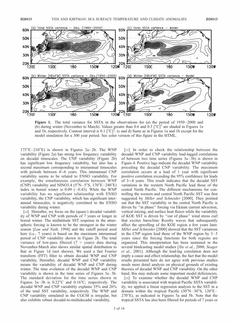
[10] We first show the observed total variance of monthlymean SST anomalies (SSTAs) about the climatologicalannual cycle in Figure 1a. The observed monthly SSTAare taken from January 1950 to December 2000 which wasanalyzed by the National Centers for Environmental Pre-diction (NCEP; Reynolds and Smith [1994]). The strongestSSTA variance is zonally extended with a basin-scalestructure centered near 40�N from the western and centralNorth Pacific (Figure 1a). During the boreal winter(November to March), the observed SSTA variance hastwo modes which are concentrated near two major oceanicfronts associated with the northern oceanic subpolar gyreand the subtropical front in the western and central NorthPacific, respectively (Figure 1b) [Nakamura et al., 1997].[11] Figures 1c and 1d are the same as in Figures 1a

and 1b except that the data used comes from the modelsimulation. The structure of the simulated SSTA variance(Figure 1c) has two centers of action to the south of 50�N:(1) a band of strong SSTA variance centered near 40�N thatextends zonally from the coast of Asia into the central NorthPacific (i.e., WNP variability) and (2) a band of variancethat is oriented to the northeast and southwest between30�N�40�N, (i.e., CNP variability). The WNP variability iscoincident with the simulated Kuroshio extension in themodel and the CNP variability, which is oriented to thenortheast-southwest in the central North Pacific, is associ-ated with the variability of the subtropical gyre in the model[Yeh and Kirtman, 2004]. During the boreal winter season(Figure 1d), the spatial pattern is similar to Figure 1c, withtwo centers of action in the western and central NorthPacific, respectively. The simulated SSTA variance in theNorth Pacific exhibits a rather similar structure year-roundwith comparable magnitude (not shown).[12] The geographical pattern of the model’s North

Pacific SSTA variance over the entire calendar yearhas some similarities and differences with observations(Figures 1a and 1c). The simulated North Pacific SSTAvariance stretches from the coast of Asia into the centralNorth Pacific, which seems to be in agreement with obser-vations. The center of action, which is oriented to thenortheast-southwest in the central North Pacific, has somemarked differences from observations. In particularly, it hastoo much of a northeast-southwest tilt, is situated too in thecentral and southern North Pacific. Moreover, the magnitudeof the North Pacific SSTAvariance simulated in the model issmaller than the observations. In spite of these differences,the simulated SSTA variance in boreal winter captures thedominant structure of the observations with a zonallyextended structure and a northeast-southwest orientation inthe North Pacific (Figures 1b and 1d).[13] The power spectrum of WNP variability (37�N–

47�N, 140�E–175�E) and CNP variability (29�N–39�N,

D20113 YEH AND KIRTMAN: SEA SURFACE TEMPERATURE AND CLIMATE ANOMALIES

2 of 14

D20113

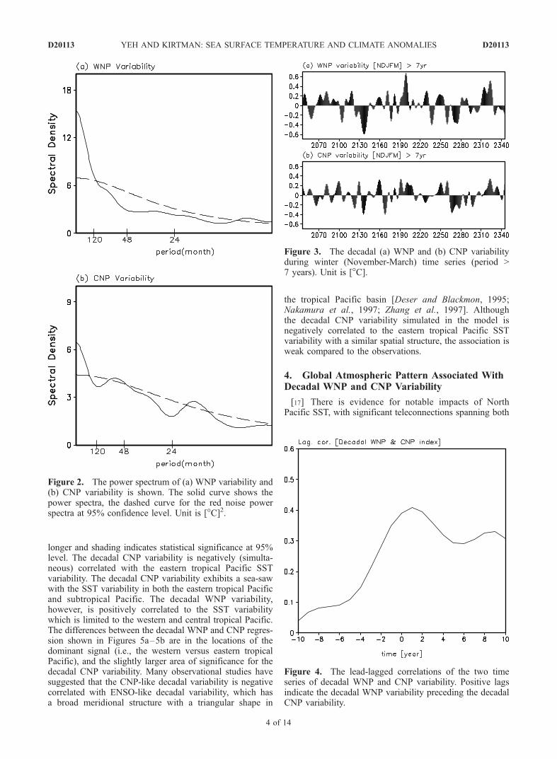
175�E–210�E) is shown in Figures 2a–2b. The WNPvariability (Figure 2a) has strong low frequency variabilityon decadal timescales. The CNP variability (Figure 2b)has significant low frequency variability, but also has asecond maximum corresponding to interannual timescaleswith periods between 4�6 years. This interannual CNPvariability seems to be related to ENSO variability. Forexample, the simultaneous correlation between WNP(CNP) variability and NINO3.4 (5�N–5�S, 170�E–240�E)index in boreal winter is 0.09 (�0.43). While the WNPvariability has no significant relationship with ENSOvariability, the CNP variability, which has significant inter-annual timescales, is negatively correlated to the ENSOvariability during winter.[14] Hereafter, we focus on the (quasi-) decadal variabil-

ity of WNP and CNP with periods of 7 years or longer inboreal winter. The midlatitude SST response to the atmo-spheric forcing is known to be the strongest in the winterseason [Lau and Nath, 1994] and the cutoff period usedhere (i.e., 7 years) is based on the maximum interannualperiod of CNP variability shown in Figure 2b. The totalvariance of low-pass filtered (7 > years) data duringNovember-March also shows similar spatial distribution tothat in Figure 1d (not shown). We used a fast Fouriertransform (FFT) filter to obtain decadal WNP and CNPvariability. Hereafter, decadal WNP and CNP variabilitymeans the variability of decadal WNP and CNP duringwinter. The time evolution of the decadal WNP and CNPvariability is shown in the time series of Figures 3a–3b.The standard deviation for the time series shown inFigures 3a–3b is 0.22�C and 0.16�C, respectively. Thedecadal WNP and CNP variability explains 35% and 26%of the total SST variability, respectively. The WNP andCNP variability simulated in the CGCM is irregular, butalso exhibits robust decadal-to-multidecadal variability.

[15] In order to check the relationship between thedecadal WNP and CNP variability lead-lagged correlationsof between two time series (Figures 3a–3b) is shown inFigure 4. Positive lags indicate the decadal WNP variabilitypreceding the decadal CNP variability. The maximumcorrelation occurs at a lead of 1 year with significantpositive correlation exceeding the 95% confidence for leadsof 3�4 years. This result indicates that the decadal SSTvariations in the western North Pacific lead those of thecentral North Pacific. The different mechanisms for con-trolling the western and central North Pacific SST was firstsuggested by Miller and Schneider [2000]. They pointedout that the SST variability in the central North Pacific isdriven by ‘‘in phase’’ forcing via Ekman current advection,vertical mixing, and surface heat fluxes while the variabilityof KOE SST is driven by ‘‘out of phase’’ wind stress curlthat excites baroclinic Rossby waves that subsequentlyaffect the upwelling of the KOE region a few years later.Miller and Schneider [2000] showed that the SST variationsin the CNP region lead those of the WNP region by 3–5years since the forcing functions for both regions areorganized. This interpretation has been sustained in theseveral hindcasting model studies [Xie et al., 2000; Seageret al., 2001]. Although the lead-lag correlation does notimply a cause and effect relationship, the fact that the modelresults presented here do not agree with previous studiesneeds more detail analysis on physical grounds of existingtheories of decadal WNP and CNP variability. On the otherhand, this may indicate some important model deficiencies.[16] To examine whether the decadal WNP and CNP

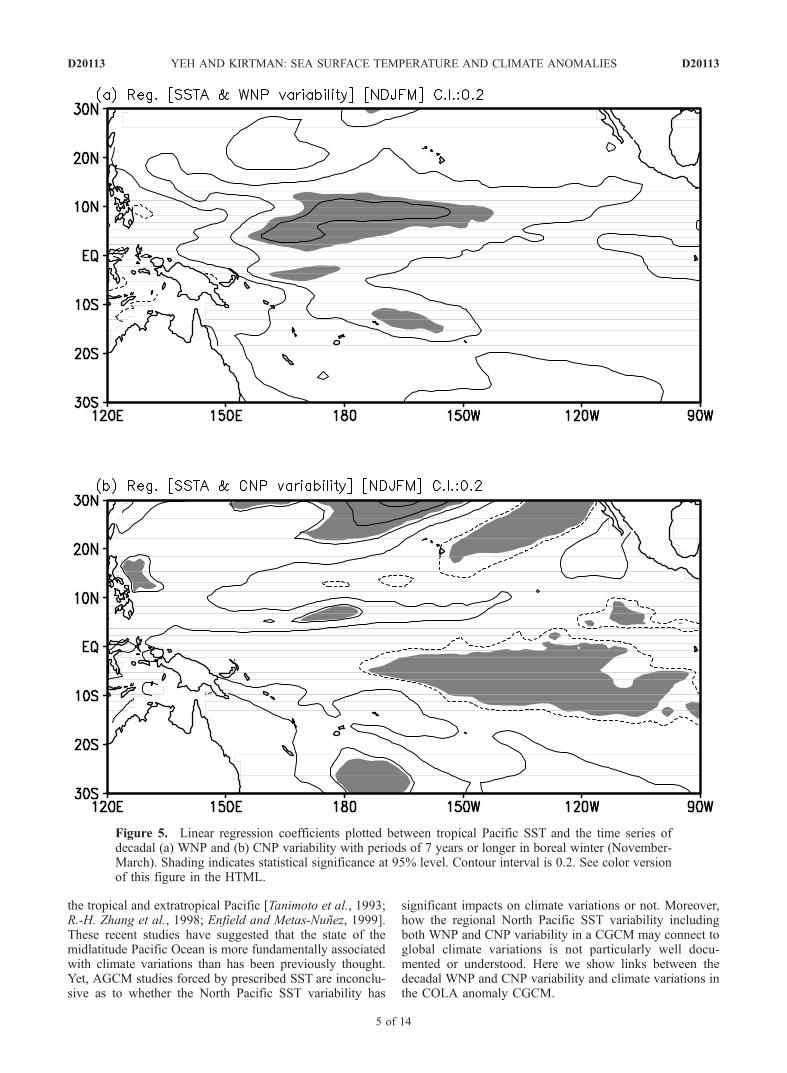
variability is associated with tropical Pacific SSTA variabil-ity, we applied a linear regression analysis to the SST in adomain within the tropical Pacific (30�N–30�S, 120�E–270�E), as indicated in Figures 5a and 5b. Note that thetropical SSTA has also been filtered for periods of 7 years or

Figure 1. The total variance for SSTA in the observations for (a) the period of 1950–2000 and(b) during winter (November to March). Values greater than 0.6 and 0.3 [�C]2 are shaded in Figures 1aand 1b, respectively. Contour interval is 0.1 [�C]2. (c and d) Same as in Figures 1a and 1b except for themodel simulation for a 300 year period. See color version of this figure in the HTML.

D20113 YEH AND KIRTMAN: SEA SURFACE TEMPERATURE AND CLIMATE ANOMALIES

3 of 14

D20113

longer and shading indicates statistical significance at 95%level. The decadal CNP variability is negatively (simulta-neous) correlated with the eastern tropical Pacific SSTvariability. The decadal CNP variability exhibits a sea-sawwith the SST variability in both the eastern tropical Pacificand subtropical Pacific. The decadal WNP variability,however, is positively correlated to the SST variabilitywhich is limited to the western and central tropical Pacific.The differences between the decadal WNP and CNP regres-sion shown in Figures 5a–5b are in the locations of thedominant signal (i.e., the western versus eastern tropicalPacific), and the slightly larger area of significance for thedecadal CNP variability. Many observational studies havesuggested that the CNP-like decadal variability is negativecorrelated with ENSO-like decadal variability, which hasa broad meridional structure with a triangular shape in

the tropical Pacific basin [Deser and Blackmon, 1995;Nakamura et al., 1997; Zhang et al., 1997]. Althoughthe decadal CNP variability simulated in the model isnegatively correlated to the eastern tropical Pacific SSTvariability with a similar spatial structure, the association isweak compared to the observations.

4. Global Atmospheric Pattern Associated WithDecadal WNP and CNP Variability

[17] There is evidence for notable impacts of NorthPacific SST, with significant teleconnections spanning both

Figure 2. The power spectrum of (a) WNP variability and(b) CNP variability is shown. The solid curve shows thepower spectra, the dashed curve for the red noise powerspectra at 95% confidence level. Unit is [�C]2.

Figure 3. The decadal (a) WNP and (b) CNP variabilityduring winter (November-March) time series (period >7 years). Unit is [�C].

Figure 4. The lead-lagged correlations of the two timeseries of decadal WNP and CNP variability. Positive lagsindicate the decadal WNP variability preceding the decadalCNP variability.

D20113 YEH AND KIRTMAN: SEA SURFACE TEMPERATURE AND CLIMATE ANOMALIES

4 of 14

D20113

the tropical and extratropical Pacific [Tanimoto et al., 1993;R.-H. Zhang et al., 1998; Enfield and Metas-Nunez, 1999].These recent studies have suggested that the state of themidlatitude Pacific Ocean is more fundamentally associatedwith climate variations than has been previously thought.Yet, AGCM studies forced by prescribed SST are inconclu-sive as to whether the North Pacific SST variability has

significant impacts on climate variations or not. Moreover,how the regional North Pacific SST variability includingboth WNP and CNP variability in a CGCM may connect toglobal climate variations is not particularly well docu-mented or understood. Here we show links between thedecadal WNP and CNP variability and climate variations inthe COLA anomaly CGCM.

Figure 5. Linear regression coefficients plotted between tropical Pacific SST and the time series ofdecadal (a) WNP and (b) CNP variability with periods of 7 years or longer in boreal winter (November-March). Shading indicates statistical significance at 95% level. Contour interval is 0.2. See color versionof this figure in the HTML.

D20113 YEH AND KIRTMAN: SEA SURFACE TEMPERATURE AND CLIMATE ANOMALIES

5 of 14

D20113

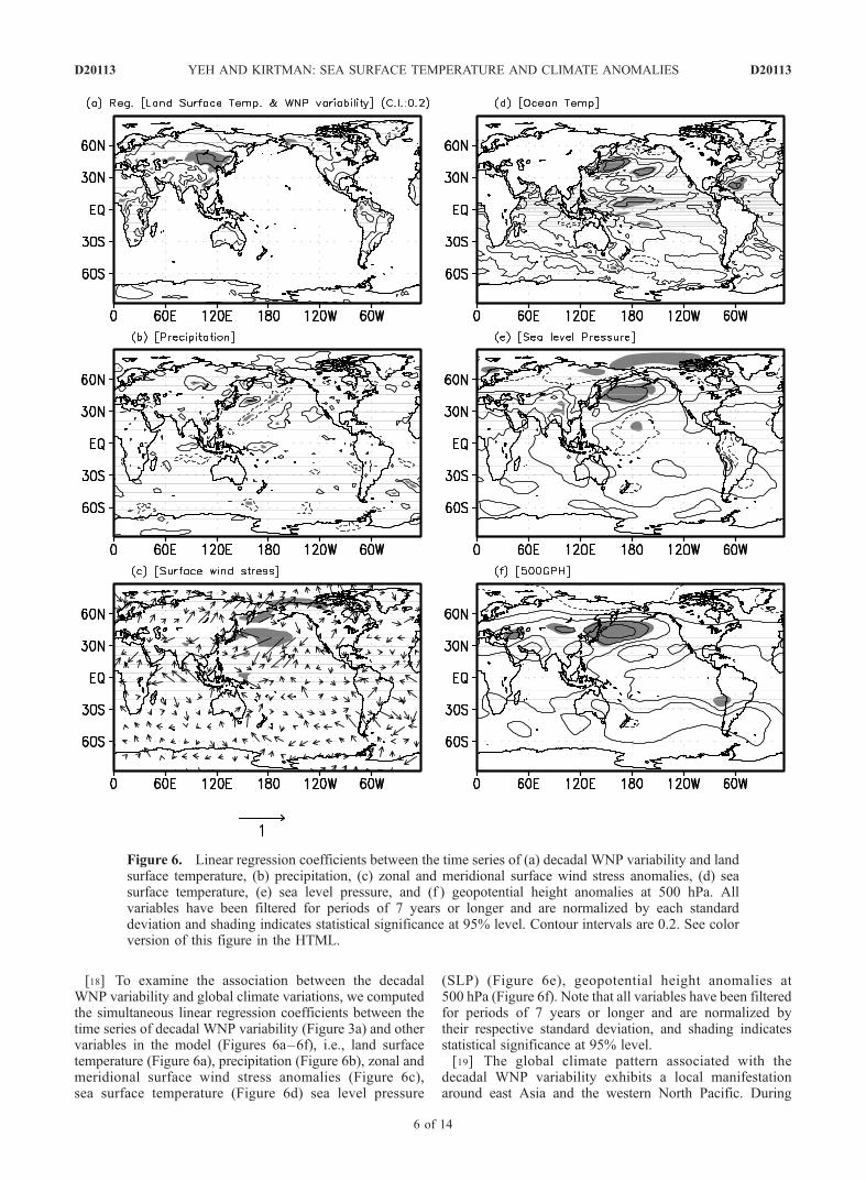
[18] To examine the association between the decadalWNP variability and global climate variations, we computedthe simultaneous linear regression coefficients between thetime series of decadal WNP variability (Figure 3a) and othervariables in the model (Figures 6a–6f), i.e., land surfacetemperature (Figure 6a), precipitation (Figure 6b), zonal andmeridional surface wind stress anomalies (Figure 6c),sea surface temperature (Figure 6d) sea level pressure

(SLP) (Figure 6e), geopotential height anomalies at500 hPa (Figure 6f). Note that all variables have been filteredfor periods of 7 years or longer and are normalized bytheir respective standard deviation, and shading indicatesstatistical significance at 95% level.[19] The global climate pattern associated with the

decadal WNP variability exhibits a local manifestationaround east Asia and the western North Pacific. During

Figure 6. Linear regression coefficients between the time series of (a) decadal WNP variability and landsurface temperature, (b) precipitation, (c) zonal and meridional surface wind stress anomalies, (d) seasurface temperature, (e) sea level pressure, and (f ) geopotential height anomalies at 500 hPa. Allvariables have been filtered for periods of 7 years or longer and are normalized by each standarddeviation and shading indicates statistical significance at 95% level. Contour intervals are 0.2. See colorversion of this figure in the HTML.

D20113 YEH AND KIRTMAN: SEA SURFACE TEMPERATURE AND CLIMATE ANOMALIES

6 of 14

D20113

the warm state of decadal WNP variability (Figure 6d), theland surface temperature within east Asia is significantlyabove normal (Figure 6a) with anomalous high pressureover the western North Pacific from surface to 500 hPa(Figures 6e–6f). Consistent with anomalous high pressure,there is distinct gyre system, which is centered at 50�N(Figure 6c) in the western part of the North Pacific basinwith a strong sea surface temperature gradient (Figure 6d).This seems to be connected to the subpolar gyre in theocean. There is, however, no significant pattern of precip-itation associated with the decadal WNP variability exceptfor a very limited region around the western North Pacific.[20] The surface wind stress associated with decadal

WNP variability is reasonably consistent with the SST-windrelationship in midlatitudes [Davis, 1976, 1978; Weare,1977; Cayan, 1992; Lau and Nath, 1994]. The anticyclonicwinds in the western North Pacific are coincident with thewarm state of decadal WNP variability. When the easterlyanomalies are stronger, SSTAs are warmer. Easterly windanomalies reduce the total wind speed, warming the oceanmixed layer by reducing the fluxes of sensible and latentheat, weakening entrainment and enhancing the warmadvection by Ekman currents in this region where thepoleward SST gradient is strong (Figures 1d and 6d). Theanomalous easterly winds in the western North Pacific alsoseems to be related to the variability of land surfacetemperature within east Asia. The warm land surfacetemperature within east Asia (Figure 6a) may be due toinflow of warm moist air masses from the western NorthPacific during winter (Figure 6d).[21] The same analysis is applied to the association

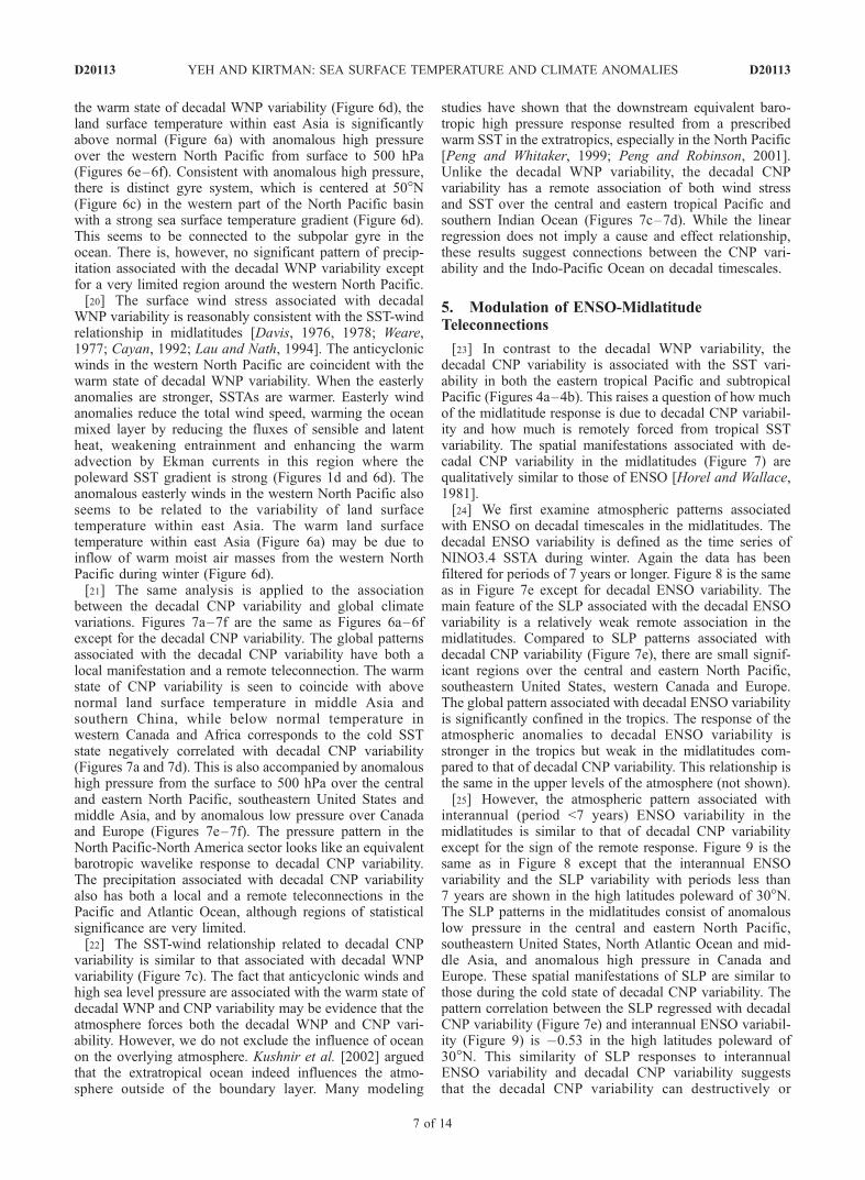
between the decadal CNP variability and global climatevariations. Figures 7a–7f are the same as Figures 6a–6fexcept for the decadal CNP variability. The global patternsassociated with the decadal CNP variability have both alocal manifestation and a remote teleconnection. The warmstate of CNP variability is seen to coincide with abovenormal land surface temperature in middle Asia andsouthern China, while below normal temperature inwestern Canada and Africa corresponds to the cold SSTstate negatively correlated with decadal CNP variability(Figures 7a and 7d). This is also accompanied by anomaloushigh pressure from the surface to 500 hPa over the centraland eastern North Pacific, southeastern United States andmiddle Asia, and by anomalous low pressure over Canadaand Europe (Figures 7e–7f). The pressure pattern in theNorth Pacific-North America sector looks like an equivalentbarotropic wavelike response to decadal CNP variability.The precipitation associated with decadal CNP variabilityalso has both a local and a remote teleconnections in thePacific and Atlantic Ocean, although regions of statisticalsignificance are very limited.[22] The SST-wind relationship related to decadal CNP

variability is similar to that associated with decadal WNPvariability (Figure 7c). The fact that anticyclonic winds andhigh sea level pressure are associated with the warm state ofdecadal WNP and CNP variability may be evidence that theatmosphere forces both the decadal WNP and CNP vari-ability. However, we do not exclude the influence of oceanon the overlying atmosphere. Kushnir et al. [2002] arguedthat the extratropical ocean indeed influences the atmo-sphere outside of the boundary layer. Many modeling

studies have shown that the downstream equivalent baro-tropic high pressure response resulted from a prescribedwarm SST in the extratropics, especially in the North Pacific[Peng and Whitaker, 1999; Peng and Robinson, 2001].Unlike the decadal WNP variability, the decadal CNPvariability has a remote association of both wind stressand SST over the central and eastern tropical Pacific andsouthern Indian Ocean (Figures 7c–7d). While the linearregression does not imply a cause and effect relationship,these results suggest connections between the CNP vari-ability and the Indo-Pacific Ocean on decadal timescales.

5. Modulation of ENSO-MidlatitudeTeleconnections

[23] In contrast to the decadal WNP variability, thedecadal CNP variability is associated with the SST vari-ability in both the eastern tropical Pacific and subtropicalPacific (Figures 4a–4b). This raises a question of how muchof the midlatitude response is due to decadal CNP variabil-ity and how much is remotely forced from tropical SSTvariability. The spatial manifestations associated with de-cadal CNP variability in the midlatitudes (Figure 7) arequalitatively similar to those of ENSO [Horel and Wallace,1981].[24] We first examine atmospheric patterns associated

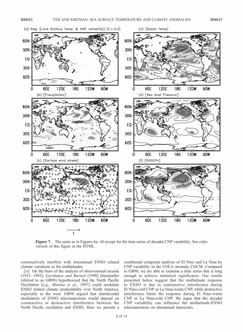
with ENSO on decadal timescales in the midlatitudes. Thedecadal ENSO variability is defined as the time series ofNINO3.4 SSTA during winter. Again the data has beenfiltered for periods of 7 years or longer. Figure 8 is the sameas in Figure 7e except for decadal ENSO variability. Themain feature of the SLP associated with the decadal ENSOvariability is a relatively weak remote association in themidlatitudes. Compared to SLP patterns associated withdecadal CNP variability (Figure 7e), there are small signif-icant regions over the central and eastern North Pacific,southeastern United States, western Canada and Europe.The global pattern associated with decadal ENSO variabilityis significantly confined in the tropics. The response of theatmospheric anomalies to decadal ENSO variability isstronger in the tropics but weak in the midlatitudes com-pared to that of decadal CNP variability. This relationship isthe same in the upper levels of the atmosphere (not shown).[25] However, the atmospheric pattern associated with

interannual (period <7 years) ENSO variability in themidlatitudes is similar to that of decadal CNP variabilityexcept for the sign of the remote response. Figure 9 is thesame as in Figure 8 except that the interannual ENSOvariability and the SLP variability with periods less than7 years are shown in the high latitudes poleward of 30�N.The SLP patterns in the midlatitudes consist of anomalouslow pressure in the central and eastern North Pacific,southeastern United States, North Atlantic Ocean and mid-dle Asia, and anomalous high pressure in Canada andEurope. These spatial manifestations of SLP are similar tothose during the cold state of decadal CNP variability. Thepattern correlation between the SLP regressed with decadalCNP variability (Figure 7e) and interannual ENSO variabil-ity (Figure 9) is �0.53 in the high latitudes poleward of30�N. This similarity of SLP responses to interannualENSO variability and decadal CNP variability suggeststhat the decadal CNP variability can destructively or

D20113 YEH AND KIRTMAN: SEA SURFACE TEMPERATURE AND CLIMATE ANOMALIES

7 of 14

D20113

constructively interfere with interannual ENSO relatedclimate variations in the midlatitudes.[26] On the basis of the analysis of observational records

(1933–1993), Gershunov and Barnett [1998] (hereinafterreferred to as GB98) hypothesized that the North PacificOscillation [e.g., Mantua et al., 1997] could modulateENSO related climate predictability over North America,especially in the west. GB98 argued that interdecadalmodulation of ENSO teleconnections would depend onconstructive or destructive interference between theNorth Pacific oscillation and ENSO. Here we present a

conditional composite analysis of El Nino and La Nina byCNP variability in the COLA anomaly CGCM. Comparedto GB98, we are able to examine a time series that is longenough to achieve statistical significance. Our resultspresented below suggest that the midlatitude responseto ENSO is due to constructive interference duringEl Nino-cold CNP or La Nina-warm CNP, while destructiveinterference limits the response during El Nino-warmCNP or La Nina-cold CNP. We argue that the decadalCNP variability can influence the midlatitude-ENSOteleconnections on interannual timescales.

Figure 7. The same as in Figures 6a–6f except for the time series of decadal CNP variability. See colorversion of this figure in the HTML.

D20113 YEH AND KIRTMAN: SEA SURFACE TEMPERATURE AND CLIMATE ANOMALIES

8 of 14

D20113

[27] Table 1 shows the number of conditional compositesof El Nino and La Nina by CNP state during period of 300years. The El Nino and La Nina events in Table 1 aredefined when the time series of interannual ENSO variabil-ity are more than one standard deviation away from thelong-term mean. During the period of the 300 winters in theCGCM, 102 El Nino and La Nina active winters areconditionally composited based on CNP (Table 1).[28] Figures 10a–10b display the mean SLP for El Nino

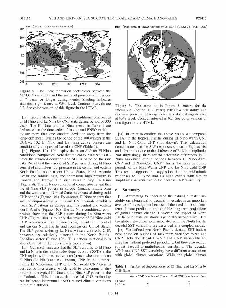
conditional composites. Note that the contour interval is 0.3times the standard deviation and SLP is based on the rawdata. Recall that the associated SLP patterns during El Ninoconsist of anomalous low pressure in the central and easternNorth Pacific, southeastern United States, North AtlanticOcean and middle Asia, and anomalous high pressure inCanada and Europe and vice versa during La Nina(Figure 9). The El Nino conditional composites reveal thatthe El Nino SLP pattern in Europe, Canada, middle Asiaand the west coast of United States is enhanced during coldCNP periods (Figure 10b). By contrast, El Nino winters thatare contemporaneous with warm CNP periods exhibit aweak SLP pattern in Europe and the central and easternNorth Pacific (Figure 10a). The La Nina conditional com-posites show that the SLP pattern during La Nina-warmCNP (Figure 10c) is roughly the reverse of El Nino-coldCNP. Anomalous high pressure is significant in the centraland eastern North Pacific and southeastern United States.The SLP patterns during La Nina winters with cold CNP,however, are relatively distorted in the North Pacific-Canadian sector (Figure 10d). This pattern relationship isalso identified in the upper levels (not shown).[29] Our result suggests that the SLP response to El Nino

and La Nina in the midlatitudes depends on the SSTA in theCNP region with constructive interference when there is anEl Nino (La Nina) and cold (warm) CNP. In the contrast,during El Nino-warm CNP or La Nina-cold CNP there isdestructive interference, which tends to weakening or dis-tortion of the typical El Nino and La Nina SLP pattern in themidlatitudes. This indicates that decadal CNP variabilitycan influence interannual ENSO related climate variationsin the midlatitudes.

[30] In order to confirm the above results we comparedSSTAs in the tropical Pacific during El Nino-Warm CNPand El Nino-Cold CNP (not shown). This calculationdemonstrates that the SLP responses shown in Figures 10aand 10b are not due to the difference of El Nino amplitude.Not surprisingly, there are no detectable differences in ElNino amplitude during periods between El Nino-WarmCNP and El Nino-Cold CNP. This is the same as duringperiods of La Nina-Warm CNP and La Nina-Cold CNP.This result supports the suggestion that the midlatituderesponses to El Nino and La Nina events with similaramplitudes are sensitive to the decadal CNP variability.

6. Summary

[31] Attempting to understand the natural climate vari-ability on interannual to decadal timescales is an importantavenue of investigation because of the need for both short-term climate prediction and credible long-term projectionsof global climate change. However, the impact of NorthPacific on climate variations is generally inconclusive. Herethe global teleconnections associated with the North Pacificdecadal SST variability are described in a coupled model.[32] We defined two North Pacific decadal SST indices

here based on regions of maximum variance: WNP andCNP. Both the decadal WNP and CNP variability areirregular without preferred periodicity, but they also exhibitrobust decadal-to-multidecadal variability. The decadalWNP and CNP SST variability have different associationswith global climate variations. While the global climate

Figure 9. The same as in Figure 8 except for theinterannual (period < 7 years) NINO3.4 variability andsea level pressure. Shading indicates statistical significanceat 95% level. Contour interval is 0.2. See color version ofthis figure in the HTML.

Table 1. Number of Subcomposite of El Nino and La Nina by

CNP State

Warm CNP, Number of Cases Cold CNP, Number of Cases

El Nino 21 32La Nina 31 18

Figure 8. The linear regression coefficients between theNINO3.4 variability and the sea level pressure with periodsof 7 years or longer during winter Shading indicatesstatistical significance at 95% level. Contour intervals are0.2. See color version of this figure in the HTML.

D20113 YEH AND KIRTMAN: SEA SURFACE TEMPERATURE AND CLIMATE ANOMALIES

9 of 14

D20113

Figure 10. The mean SLP for El Nino conditional composites based on (a) warm and (b) cold CNP.(c and d) Same as in Figures 10a and 10b except for La Nina conditional composites. Contour interval is0.3 times the standard deviation, and shading indicates positive value. See color version of this figure inthe HTML.

D20113 YEH AND KIRTMAN: SEA SURFACE TEMPERATURE AND CLIMATE ANOMALIES

10 of 14

D20113

patterns associated with the decadal WNP variability exhibita local manifestation, the decadal CNP variability showsa remarkable association with variability poleward of30 degrees latitude in the Northern Hemisphere.[33] The midlatitude response to decadal CNP variability

is examined on the basis of ENSO variability on interannualand decadal timescales. The atmospheric patterns associatedwith decadal ENSO variability are significantly confined tothe tropics. On the other hand, the midlatitude response tointerannual ENSO variability indicates constructive or de-structive interference depending on the state of decadalCNP variability. The SLP response to El Nino and La Ninain the midlatitudes is more constructive during winterscharacterized by relatively cold and warm CNP states,respectively. By contrast, El Nino-warm CNP or La Nina-cold state of CNP destructively interferes, which tends toweakening or distortion of the typical El Nino and La Ninaresponse in the midlatitudes. Our results suggest that theSLP response to El Nino and La Nina in the midlatitudesdepends on the decadal SSTA in the CNP region. Thisindicates that decadal CNP variability can modulate inter-annual ENSO related climate variations in midlatitudes.

Appendix A

[34] Here we present a brief description of COLA anom-aly coupled model. Additional details can be found in thework of Kirtman et al. [2002]. The COLA anomaly coupledmodel is identical with COLA coupled model except for thecoupling strategy. The intent of the anomaly couplingstrategy is to prevent the rapid climate drift seen in theCGCMs. The main idea for the anomaly coupling strategy isthat the ocean and atmosphere exchange predicted anoma-lies, which are computed relative to their own modelclimatologies, while the climatology upon which theanomalies are superimposed in specified from observationsor model-based estimates of observations.[35] The anomaly coupling strategy requires atmospheric

model climatologies of momentum, heat and freshwaterflux, and ocean model SST climatology. Similarly, ob-served climatologies of momentum, heat and freshwaterflux, and SST are also required. The model climatologiesare defined by separate uncoupled extended simulations ofthe ocean and atmospheric models. In the case of theatmosphere, the model climatology is computed from a30-year (1961–1990) integration with observed specifiedSST. The atmospheric initial state is taken from thisintegration. This SST is also used to define the observedSST climatology. The observed SST data set is describedin the work of Smith et al. [1996]. In the case of the oceanmodel SST climatology, an extended uncoupled oceanmodel simulation is made using 30 years of 1000mbNCEP-NCAR reanalysis winds. As with the SST, thisobserved wind stress product is used to define the ob-served momentum flux climatology. The heat flux and thefreshwater flux in this ocean-only simulation is parame-terized using damping of SST and sea surface salinity toobserved conditions with a 100-day timescale. The heatand freshwater flux ‘‘observed’’ climatologies are thencalculated from the results of the extended ocean-onlysimulation. The ocean and atmosphere model exchangesdaily mean fluxes of heat, momentum, and freshwater and

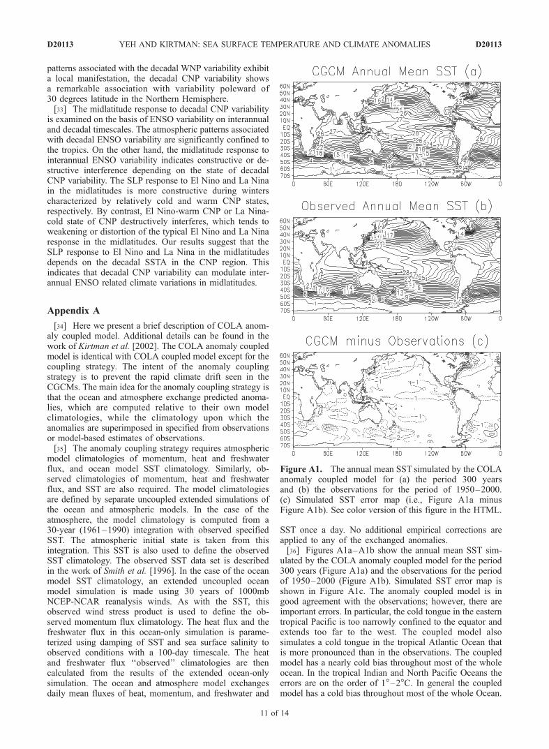
SST once a day. No additional empirical corrections areapplied to any of the exchanged anomalies.[36] Figures A1a–A1b show the annual mean SST sim-

ulated by the COLA anomaly coupled model for the period300 years (Figure A1a) and the observations for the periodof 1950–2000 (Figure A1b). Simulated SST error map isshown in Figure A1c. The anomaly coupled model is ingood agreement with the observations; however, there areimportant errors. In particular, the cold tongue in the easterntropical Pacific is too narrowly confined to the equator andextends too far to the west. The coupled model alsosimulates a cold tongue in the tropical Atlantic Ocean thatis more pronounced than in the observations. The coupledmodel has a nearly cold bias throughout most of the wholeocean. In the tropical Indian and North Pacific Oceans theerrors are on the order of 1�–2�C. In general the coupledmodel has a cold bias throughout most of the whole Ocean.

Figure A1. The annual mean SST simulated by the COLAanomaly coupled model for (a) the period 300 yearsand (b) the observations for the period of 1950–2000.(c) Simulated SST error map (i.e., Figure A1a minusFigure A1b). See color version of this figure in the HTML.

D20113 YEH AND KIRTMAN: SEA SURFACE TEMPERATURE AND CLIMATE ANOMALIES

11 of 14

D20113

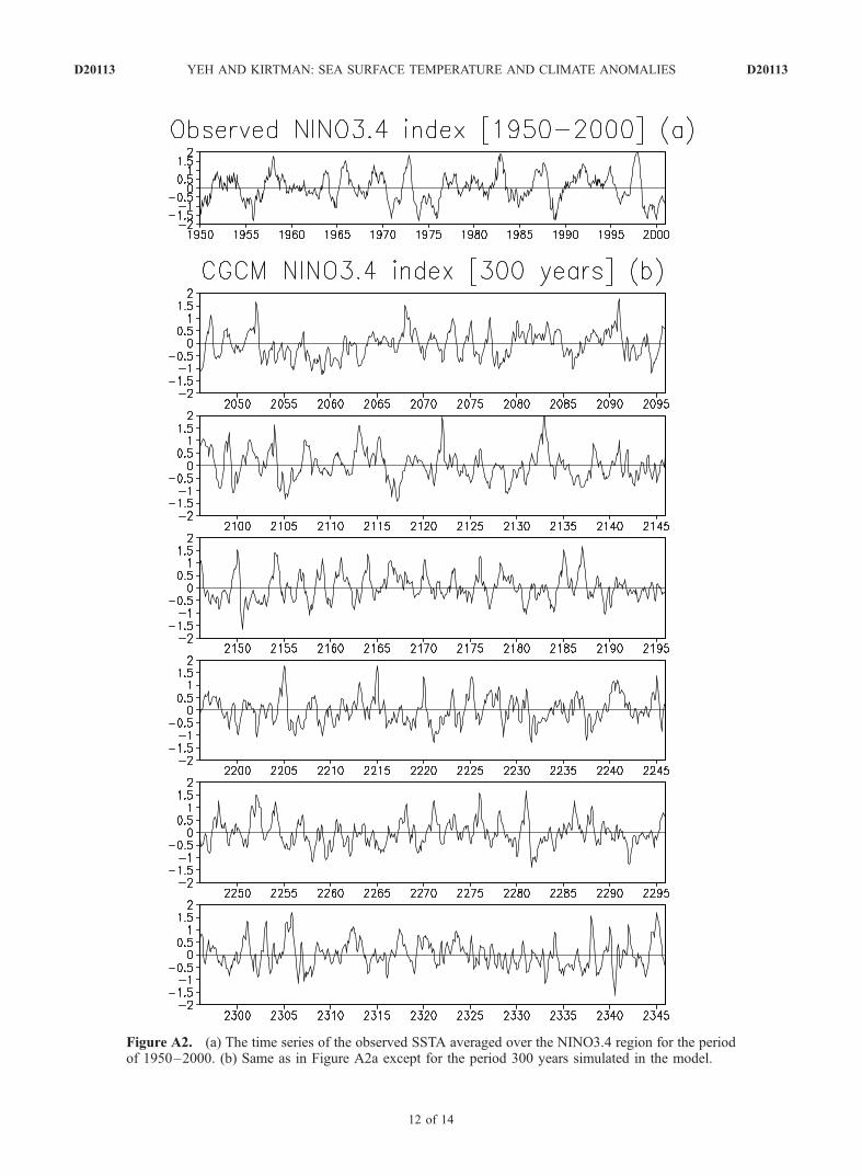
Figure A2. (a) The time series of the observed SSTA averaged over the NINO3.4 region for the periodof 1950–2000. (b) Same as in Figure A2a except for the period 300 years simulated in the model.

D20113 YEH AND KIRTMAN: SEA SURFACE TEMPERATURE AND CLIMATE ANOMALIES

12 of 14

D20113

[37] Figure A2a shows the time series of the observedSSTA averaged over the NINO3.4 region for the period of1950–2000. Figure A2b is the same as in Figure A2aexcept for the period 300 years simulated in the model.The ENSO events in the model simulation are irregular andthe amplitude of warm and cold events is reasonable, withpeaks in the neighborhood of �1.5�C to +2.0�C. Onestandard deviation of the NINO3.4 index in the model(0.54�C) is smaller than that of the observations (0.76�C),which is, in part, due to the narrow meridional scale. Theamplitude at the equator is comparable to observations.Power spectral analysis of simulation yields a broad peakbetween two and four years (not shown). The dominanttimescales in simulation is shorter compared to that inobservations for the period of 1950–2000.

[38] Acknowledgments. The authors are grateful to three anonymousreviewers, who provided many suggestions that have improved thismanuscript. The authors are also indebted to B. Huang and D. Straus fortheir careful reading. This research was supported by grants from theNational Science Foundation ATM-9814295 and ATM-0122859, theNational Oceanic and Atmospheric Administration NA16-GP2248, andNational Aeronautics and Space Administration NAG5-11656.

ReferencesAlexander, M. A. (1992), Midlatitude atmosphere-ocean interaction duringEl Nino, I. The North Pacific Ocean, J. Clim., 5, 944–958.

Alexander, M. A., I. Blade, M. Newman, J. R. Lanzante, N.-C. Lau, andJ. D. Scott (2002), The atmospheric bridge: The influence of ENSOteleconnections on air-sea interaction over the global oceans, J. Clim.,16, 2205–2231.

Barlow, M., S. Nigam, and E. H. Berbery (2001), ENSO, Pacific decadalvariability, and U.S. summertime precipitation, drought, and stream flow,J. Clim., 14, 2105–2128.

Bond, N. A., and D. E. Harrison (2000), The Pacific decadal oscillation, air-sea interaction and central north Pacific winter atmospheric regimes,Geophys. Res. Lett., 27, 731–734.

Cayan, D. R. (1992), Latent and sensible heat flux anomalies over thenorthern oceans: Driving the sea surface temperature, J. Phys. Oceanogr.,22, 859–881.

Davis, R. E. (1976), Predictability of sea surface temperature and sea levelpressure anomalies over the North Pacific Ocean, J. Phys. Oceanogr., 6,249–266.

Davis, R. E. (1978), Predictability of sea level pressure anomalies over theNorth Pacific Ocean, J. Phys. Oceanogr., 8, 233–246.

Deser, C., and M. L. Blackmon (1995), On the relationship between tropicaland North Pacific sea surface temperature variations, J. Clim., 8, 1677–1680.

Deser, C., M. A. Alexander, and M. S. Timlin (1996), Upper-ocean thermalvariations in the North Pacific during 1970–1991, J. Clim., 9, 1840–1855.

Deser, C., M. A. Alexander, and M. S. Timlin (1999), Evidence for a wind-driven intensification of the Kuroshio Current Extension from the 1970sto the 1980s, J. Clim., 12, 1697–1706.

Enfield, D. B., and A. M. Mestas-Nunez (1999), Multiscale variability inglobal sea surface temperatures and their relationships with troposphericclimate pattern, J. Clim., 12, 2719–2733.

Garreaud, R., and D. Battisti (1999), Interannual (ENSO) and interdecadal(ENSO-like) variability in the Southern Hemisphere tropospheric circula-tion, J. Clim., 12, 2113–2123.

Gershunov, A., and T. P. Barnett (1998), Interdecadal modulation of ENSOteleconnection, Bull. Am. Meteorol. Soc., 79, 2715–2725.

Giese, B. S., and J. A. Carton (1999), Interannual and decadal variability inthe tropical and midlatitude Pacific Ocean, J. Clim., 12, 3402–3418.

Graham, N. E. (1994), Decadal-scale climate variability in the tropical andNorth Pacific during the 1970s and 1980s: Observations and modelresults, Clim. Dyn., 10, 135–162.

Graham, N. E. (1995), Simulation of recent global temperature trends,Science, 267, 666–671.

Gu, D., and S. G. H. Philander (1997), Interdecadal climate fluctuations thatdepend on exchanges between the tropics and extratropics, Science, 275,805–807.

Horel, J. D., and J. M. Wallace (1981), Planetary-scale atmospheric phe-nomena associated with the Southern Oscillation, Mon. Weather Rev.,109, 813–829.

Jacobs, G. A., H. E. Hurlburt, J. C. Kindle, E. J. Metzger, J. L. Mitchell,W. J. Teague, and A. J. Wallcraft (1994), Decadal-scale trans-Pacificpropagation and warming effects of an El Nino anomaly, Nature, 370,360–363.

Jin, F.-F. (1997), A theory of interdecadal climate variability of the NorthPacific atmosphere-ocean system, J. Clim., 10, 1821–1835.

Kirtman, B. P., Y. Fan, and E. K. Schneider (2002), The COLA globalcoupled and anomaly coupled ocean-atmosphere GCM, J. Clim., 15,2301–2320.

Kleeman, R., J. P. McCreary Jr., and B. A. Klinger (1999), A mechanismfor generating ENSO decadal variability, Geophys. Res. Lett., 26, 1743–1746.

Knutson, X., and S. Manabe (1998), Model assessment of decadal varia-bility and trends in the tropical Pacific ocean, J. Clim., 11, 2273–2296.

Kushnir, Y., W. A. Robinson, I. Blade, N. M. J. Hall, S. Peng, and R. Sutton(2002), Atmospheric GCM response to extratropical SST anomalies:Synthesis and evaluation, J. Clim., 15, 2233–2256.

Latif, M., and T. P. Barnett (1994), Causes of decadal climate variabilityover the North Pacific and North America, Science, 266, 634–637.

Lau, K.-M., and H. Weng (1999), Interannual, decadal-interdecadal, andglobal warming signals in sea surface temperature during 1955–97,J. Clim., 12, 1257–1267.

Lau, N.-C., and M. J. Nath (1994), A modeling study of the relative roles ofthe tropical and extratropical SST anomalies in the variability of theglobal atmosphere-ocean system, J. Clim., 7, 1184–1207.

Lee, E.-J., J.-G. Jhun, and I.-S. Kang (2002), The characteristic variabilityof boreal wintertime atmospheric circulation in El Nino events, J. Clim.,15, 892–904.

Mantua, J. N., S. R. Hare, Y. Zhang, J. M. Wallace, and R. C. Francis(1997), A Pacific interdecadal climate oscillation with impacts on salmonproduction, Bull. Am. Meteorol. Soc., 78, 1069–1080.

McPhaden, M. J., and D. Zhang (2002), Slowdown of the meridionaloverturning circulation in the upper Pacific Ocean, Nature, 415, 603–608.

Mestas-Nunez, M. A., and D. B. Enfield (1999), Rotated global modes ofnon-ENSO sea surface temperature variability, J. Clim., 12, 2734–2746.

Miller, A. J., and N. Schneider (2000), Interdecadal climate regime dy-namics in the North Pacific Ocean: Theories, observations and ecosystemimpacts, Prog. Oceanogr., 27, 257–260.

Miller, A. J., D. R. Cayan, T. P. Barnett, N. E. Graham, and J. M. Oberhuber(1994), Interdecadal variability of the Pacific Ocean: Model response toobserved heat flux and wind stress anomalies, Clim. Dyn., 9, 287–302.

Miller, A. J., D. R. Cayan, and W. B. White (1998), Awestward-intensifieddecadal change in the North Pacific thermocline and gyre-scale circula-tion, J. Clim., 11, 3112–3127.

Nakamura, H., G. Lin, and T. Yamagata (1997), Decadal climate variabilityin the North Pacific during the recent decades, Bull. Am. Meteorol. Soc.,78, 2215–2225.

Nitta, T., and S. Yamada (1989), Recent warming of tropical sea surfacetemperature and its relationship to the Northern Hemisphere circulation,J. Meteorol. Soc. Jpn., 67, 375–382.

Nonaka, M., S. Xie, and J. P. McCreary (2002), Decadal variations in thesubtropical cells and equatorial pacific SST, Geophys. Res. Lett., 29(7),1116, doi:10.1029/2001GL013717.

Pacanowski, R. C., K. Dixon, and A. Rosati (1993), The GFDL modularocean model users guide, version 1.0, GFDL Ocean Group Tech. Rep. 2,77 pp., Geophys. Fluid Dyn. Lab., Princeton, N. J.

Peng, S., and W. A. Robinson (2001), Relationships between atmosphericinternal variability and the responses to an extratropical SST anomaly,J. Clim., 14, 2943–2959.

Peng, S., and J. S. Whitaker (1999), Mechanisms determining the atmo-spheric response to midlatitude SST anomalies, J. Clim., 12, 1393–1408.

Peng, S., W. A. Robinson, and M. P. Hoerling (1997), The modeled atmo-spheric response to midlatitude SST anomalies and its dependence onbackground circulation states, J. Clim., 10, 971–987.

Pierce, D. W., T. P. Barnett, and M. Latif (2000), Connections between thePacific ocean tropics and midlatitudes on decadal timescales, J. Clim., 13,1173–1194.

Reynolds, R. W., and T. M. Smith (1994), Improved global sea surfacetemperature analysis using optimum interpolation, J. Clim., 7, 929–948.

Robertson, A. W. (1996), Interdecadal variability over the North Pacific in amulti-century climate simulation, Clim. Dyn., 12, 227–241.

Rosati, A., and K. Miyakoda (1988), A general circulation model for upperocean circulation, J. Phys. Oceanogr., 18, 1601–1626.

Schneider, N., A. J. Miller, and D. W. Pierce (2002), Anatomy of NorthPacific decadal variability, J. Clim., 15, 586–605.

Seager, R., Y. Kushnir, N. Naik, M. A. Cane, and J. A. Miller (2001), Wind-driven shifts in the latitude of the Kuroshio-Oyashio extension and gen-eration of SST anomalies on decadal timescales, J. Clim., 14, 4249–4265.

D20113 YEH AND KIRTMAN: SEA SURFACE TEMPERATURE AND CLIMATE ANOMALIES

13 of 14

D20113

Smith, T. M., R. W. Reynolds, R. E. Livezey, and D. C. Stokes (1996),Reconstruction of historical sea surface temperature using empiricalorthogonal functions, J. Clim., 9, 1403–1420.

Tanimoto, Y., N. Iwasaka, K. Hanawa, and Y. Toba (1993), Characteristicvariations of sea surface temperature with multiple timescales in theNorth Pacific, J. Clim., 6, 1153–1160.

Trenberth, K. E. (1990), Recent observed interdecadal climate changes inthe Northern Hemisphere, Bull. Am. Meteorol. Soc., 71, 988–993.

Trenberth, K. E., and J. W. Hurrell (1994), Decadal atmosphere-oceanvariations in the Pacific, Clim. Dyn., 9, 303–319.

Weare, B. C. (1977), Empirical orthogonal analysis of Atlantic ocean sur-face temperature, Q. J. R. Meteorol. Soc., 103, 467–478.

Wu, L., and Z. Liu (2003), Decadal variability in the North Pacific: Theeastern North Pacific mode, J. Clim., 16, 3111–3131.

Wu, L., Z. Liu, R. Gallimore, R. Jacob, D. Lee, and Y. Zhong (2003),Pacific decadal variability: The tropical Pacific mode and the NorthPacific mode, J. Clim., 16, 1101–1120.

Xie, S.-P., T. Kunitani, A. Kubokawa, M. Nonaka, and S. Hosoda (2000),Interdecadal thermocline variability in the North Pacific for 1958–97: AGCM simulation, J. Phys. Oceanogr., 30, 2798–2813.

Yeh, S.-W., and B. P. Kirtman (2003), On the relationship between theinterannual and decadal SST variability in the North Pacific and TropicalPacific Ocean, J. Geophys. Res., 108(D11), 4344, doi:10.1029/2002JD002817.

Yeh, S.-W., and B. P. Kirtman (2004), The impact of internal atmosphericvariability on the North Pacific SST variability, Clim. Dyn., doi:10.1007/s00382-004-0399-8.

Zhang, R.-H., L. M. Rothstein, and A. J. Busalacchi (1998), Origin ofwarming and El Nino change on decadal scales in the tropical PacificOcean, Nature, 391, 879–883.

Zhang, Y., J. M. Wallace, and D. S. Battisti (1997), ENSO-like interdecadalvariability: 1900–93, J. Clim., 10, 1004–1020.

Zhang, Y., J. R. Norris, and J. M. Wallace (1998), Seasonality of large-scaleatmosphere-ocean interaction over the North Pacific, J. Clim., 11, 2473–2481.

�����������������������B. P. Kirtman and S.-W. Yeh, Center for Ocean-Land-Atmosphere

Studies, 4041 Powder Mill Road, Suite 302, Calverton, MD 20705, USA.(swyeh@cola.iges.org)

D20113 YEH AND KIRTMAN: SEA SURFACE TEMPERATURE AND CLIMATE ANOMALIES

14 of 14

D20113