Correction and Optimization of 4D aircraft trajectories by ...

HAL Id: tel-02372770https://tel.archives-ouvertes.fr/tel-02372770

Submitted on 20 Nov 2019

HAL is a multi-disciplinary open accessarchive for the deposit and dissemination of sci-entific research documents, whether they are pub-lished or not. The documents may come fromteaching and research institutions in France orabroad, or from public or private research centers.

L’archive ouverte pluridisciplinaire HAL, estdestinée au dépôt et à la diffusion de documentsscientifiques de niveau recherche, publiés ou non,émanant des établissements d’enseignement et derecherche français ou étrangers, des laboratoirespublics ou privés.

Correction and Optimization of 4D aircraft trajectoriesby sharing wind and temperature information

Karim Legrand

To cite this version:Karim Legrand. Correction and Optimization of 4D aircraft trajectories by sharing wind and temper-ature information. Other. INSA de Toulouse, 2019. English. NNT : 2019ISAT0011. tel-02372770

https://tel.archives-ouvertes.fr/tel-02372770

https://hal.archives-ouvertes.fr

THÈSEEn vue de l’obtention du

DOCTORAT DE L’UNIVERSITÉ DE TOULOUSE

Délivré par l'Institut National des Sciences Appliquées deToulouse

Présentée et soutenue par

Karim LEGRAND

Le 28 juin 2019

Correction et Optimisation de trajectoires d'avions 4D parpartage d'informations de vent et de température

Correction and Optimization of 4D aircraft trajectories by sharing wind and temperature information

Ecole doctorale : AA - Aéronautique, Astronautique

Spécialité :

Unité de recherche :

Laboratoire de Recherche ENAC

Thèse dirigée par

Daniel DELAHAYE et Christophe RABUT

Jury

M. Li WEIGANG, RapporteurM. John HAUSER, Rapporteur

M. Eric FERON, RapporteurMme Aude RONDEPIERRE, ExaminatriceM. Daniel DELAHAYE, Directeur de thèse

M. Christophe RABUT, Co-directeur de thèse

Résumé

Cette thèse a pour origine les changements dans la gestion du trafic aérien. Actuellement, des

retards liés à la saturation de l’espace aérien sont imposés aux vols. Des initiatives de moderni-

sation des systèmes gérant le trafic aérien, ont vu le jour, aux Etats-Unis, en Europe et au Japon.

Ces projets optimisent les arrivées sur les aéroports, ce qui nécessite le partage des informations

relatives à la trajectoire, leur gestion collaborative, et l’utilisation de cette trajectoire partagée et

gérée comme plan de vol commun. Dans ce contexte une cohérence sur les estimés de survol est

nécessaire, au moins entre le système de gestion de vol embarqué et le système de gestion du trafic

aérien. Certaines techniques ont permis l’augmentation de capacité de l’espace aérien, mais les

infrastructures aéroportuaires ont fait apparaître de nouveaux goulots d’étranglement. Une prédic-

tion de trajectoire à 30 secondes est nécessaire.

Aujourd’hui au moins deux plans de vols existent, l’un à bord de l’avion, accessible aux pilotes

via le FMS, l’autre au sol, accessible aux contrôleurs aériens via des outils informatiques. Ini-

tialement synchronisés, ces deux plans de vol ne le sont plus dès le décollage de l’avion. Depuis

le sol, en zone de couverture radar, la trajectoire d’un avion est une suite de plots matérialisant

ses positions, et permettant de calculer sa vitesse sol. Sa trajectoire future est calculée à partir

du plan de vol déposé, de sa vitesse propre, du vent et de la température prévus sur cette route,

d’où une erreur liée au calcul de cette vitesse propre. Il faut ensuite calculer la vitesse sol sur la

future trajectoire à partir d’informations météorologiques prévues sur cette dernière. Toute erreur

de prédiction météo biaise ainsi le calcul de la future trajectoire.

Dans un Boeing 737/400, la vitesse est calculée à partir de la centrale aérodynamique et de la cen-

trale à inertie, qui calcule le vecteur vitesse propre et un vecteur vent instantanés. Le calculateur de

vol les combine avec, lorsque renseigné, le vent prévu sur les segments suivants de la trajectoire,

pour calculer les estimés.

Ainsi, au sol et en vol, les méthodes de calcul et les données disponibles diffèrent. Le vent et la

température étant deux paramètres omniprésents et subis, il nous a semblé nécessaire de réfléchir

à la façon de limiter le biais qu’ils entrainent sur les calculs de trajectoire.

Dans cette thèse nous présentons les bouleversements dans les systèmes de gestion du trafic aérien,

les enjeux du calcul de trajectoire, et sa nécessité.

Nous avons été surpris par le nombre d’outils de calculs de trajectoire. Ce que nous avons pu

apprendre sur ces systèmes est résumé, nous dressons un état de l’art, et comparons les systèmes

"sol" et "bord". Les outils de modélisation de trajectoire et les systèmes de coordonnées présentés,

mettent en évidence différentes modélisations des trajectoires.

Nous avons découvert que l’attitude (i.e. orientation) de l’avion n’etaient pris en compte que par

les systèmes embarqués, c’est pourquoi nous avons présenté les outils permettant de la modéliser,

ainsi que trois modélisations d’un avion et des forces agissant sur lui.

Notre concept "Wind Networking" améliore la prévision des trajectoires, par mise à jour des in-

formations de vent diponibles à bord d’un avion, à l’aide d’informations de vent d’avions voisins.

Les informations de 8000 vols sont traitées. L’algorithme de mise à jour et les structures de stock-

age sont présentées. Les effets de la température sur les performances d’un avion sont abordés,

permettant la prise en compte de la température. Nous traitons du calcul de trajectoires optimales

en présence d’un vent prédit, pour remplacer les actuelles routes Nord Atlantique, et aboutir à des

groupes de trajectoires optimisées et robustes.

La conclusion de cette thèse présente d’autres champs d’applications du partage de vents, et aborde

les besoins en nouvelles infrastructures et protocoles de communication.

1

Abstract

This thesis is motivated by the changes in air traffic management. Today, flights are delayed due to

airspace saturation. Initiatives to modernize the air traffic management system have been launched

in the United States, Europe and Japan. These projects optimize arrivals at airports, which requires

the sharing of trajectory information, its collaborative management, and the use of this shared and

managed trajectory as a common flight plan. In this context, consistency on estimated waypoints

overflight times is necessary, at least between the aircraft flight management system and the air

traffic management system. Some new techniques have increased airspace capacity, but airport in-

frastructure has created new bottlenecks. A 30 seconds accuracy trajectory prediction is required

to remove the runway throughput limitations.

Today at least two flight plans exist, one on board the aircraft, accessible to pilots via the FMS,

the other on the ground, accessible to air traffic controllers via computer tools. Initially synchro-

nized, these two flight plans are no longer synchronized as soon as the aircraft takes off. From the

ground, in a radar coverage area, an aircraft’s trajectory is a series of plots that materialize its posi-

tions and allow its ground speed calculation. Its future trajectory is computed from the filed flight

plan, its filled true air speed, and the wind and temperature forecast on its route. This computation

method leads to an erroneous true air speed. The ground speed on the future trajectory must then

be calculated from weather forecasts on the future trajectory. Any error in weather prediction thus

biases the calculation of the future trajectory.

To illustrate the difference between on-board and ground trajectory predictors, we used the Boeing

737/400. In its Flight Management System, the speed is calculated from the air data computer and

the inertial reference unit, which calculates the instantaneous true air speed and a wind vectors.

The flight management computer combines them with, when inserted by the flight crew, the ex-

pected wind on the next segments of the trajectory to calculate the waypoints estimates.

Thus, on the ground and in flight, the calculation methods and data available differ. Since wind

and temperature are two parameters that are omnipresent and suffered, we tried to think about how

to limit the bias they cause on trajectory calculations.

In this thesis we start by presenting the upheavals in air traffic management systems, the challenges

of trajectory computation, and its necessity.

We were surprised by the number of trajectory computation tools. What we have learned about

these systems is summarized, we draw up a state of the art, and compare the "ground" and "on-

board" prediction systems. The trajectory modeling tools and coordinate systems presented high-

light differences in trajectory modeling.

We discovered that the attitude (i.e. orientation) of the aircraft was only taken into account by the

on-board systems, which is why we presented the mathematical tools to model it, as well as three

models of an aircraft and the forces acting on it.

Our "Wind Networking" concept improves trajectory prediction by updating the wind information

available on board an aircraft with wind information from neighboring aircraft. The information

of 8000 flights is processed. The update algorithm and storage structures are presented. The ef-

fects of temperature on aircraft performance are discussed, allowing temperature to be taken into

account in the trajectory prediction. We discuss the computation of optimal trajectories in the

presence of a predicted wind, to replace the current North Atlantic Tracks, and lead to optimized

and robust groups of trajectories.

The conclusion of this thesis presents other fields of wind sharing applications, and addresses the

need for new communications infrastructures and protocols.

3

Contents

List of Figures ix

List of Tables xiii

Acronyms xv

List of Symbols xxiii

1 Introduction 1-1

1.1 Air Traffic Management Changes . . . . . . . . . . . . . . . . . . . . . . . . . . 1-1

1.2 Trajectory Prediction Problem . . . . . . . . . . . . . . . . . . . . . . . . . . . 1-2

2 The Trajectory Prediction challenge in the new ATM systems 2-1

2.1 ICAO Global ATM Operational Concept . . . . . . . . . . . . . . . . . . . . . . 2-1

2.1.1 History . . . . . . . . . . . . . . . . . . . . . . . . . . . . . . . . . . . 2-1

2.1.2 Concept presentation . . . . . . . . . . . . . . . . . . . . . . . . . . . . 2-2

Airspace Organization and Management . . . . . . . . . . . . . . . . . . 2-3

Demand and Capacity Balancing . . . . . . . . . . . . . . . . . . . . . . 2-3

Aerodrome Operations . . . . . . . . . . . . . . . . . . . . . . . . . . . 2-3

Traffic Synchronization . . . . . . . . . . . . . . . . . . . . . . . . . . . 2-4

Conflict Management . . . . . . . . . . . . . . . . . . . . . . . . . . . . 2-4

Airspace User Operations . . . . . . . . . . . . . . . . . . . . . . . . . 2-4

ATM Service Delivery Management . . . . . . . . . . . . . . . . . . . . 2-4

Information Services . . . . . . . . . . . . . . . . . . . . . . . . . . . . 2-5

Tentative summary on ICAO Global ATM Operational Concept . . . . . 2-5

2.2 European Single European Sky ATM Research initiative . . . . . . . . . . . . . 2-5

2.2.1 Introduction . . . . . . . . . . . . . . . . . . . . . . . . . . . . . . . . . 2-5

2.2.2 Collaborative Decision Making . . . . . . . . . . . . . . . . . . . . . . 2-6

2.2.3 System Wide Information Management . . . . . . . . . . . . . . . . . . 2-6

2.2.4 Trajectory Based Operations . . . . . . . . . . . . . . . . . . . . . . . . 2-7

2.3 United States of America Next Generation Air Transportation System initiative . 2-8

2.3.1 Introduction . . . . . . . . . . . . . . . . . . . . . . . . . . . . . . . . . 2-8

2.3.2 User Focus . . . . . . . . . . . . . . . . . . . . . . . . . . . . . . . . . 2-8

2.3.3 Distributed Decision Making . . . . . . . . . . . . . . . . . . . . . . . . 2-9

2.3.4 Net-Centric Operations (Network-Enabled Information Access) . . . . . 2-9

2.3.5 Trajectory Based Operations (TBO) . . . . . . . . . . . . . . . . . . . . 2-10

2.4 Japan Collaborative Action for Renovation of Air Transport Systems . . . . . . . 2-10

2.4.1 Introduction . . . . . . . . . . . . . . . . . . . . . . . . . . . . . . . . . 2-10

2.4.2 Trajectory Based Operation . . . . . . . . . . . . . . . . . . . . . . . . 2-11

2.4.3 Complete information-sharing and Collaborative decision-making . . . . 2-12

2.5 Two CARATS, NEXTGEN, and SESAR common particular features . . . . . . . 2-12

2.5.1 System Wide Information Management . . . . . . . . . . . . . . . . . . 2-13

2.5.2 Trajectory Based Operations . . . . . . . . . . . . . . . . . . . . . . . . 2-14

2.6 Conclusions on meteorology, TBO and SWIM . . . . . . . . . . . . . . . . . . . 2-15

i

2.7 Automatic Dependent Surveillance - Broadcast . . . . . . . . . . . . . . . . . . 2-15

2.7.1 Introduction . . . . . . . . . . . . . . . . . . . . . . . . . . . . . . . . . 2-15

2.7.2 Automatic Dependent Surveillance - Broadcast (ADS-B) principle and

advantages . . . . . . . . . . . . . . . . . . . . . . . . . . . . . . . . . 2-15

ADS-B OUT . . . . . . . . . . . . . . . . . . . . . . . . . . . . . . . . 2-16

ADS-B IN . . . . . . . . . . . . . . . . . . . . . . . . . . . . . . . . . 2-17

Ground-Based information services . . . . . . . . . . . . . . . . . . . . 2-18

Automatic Dependent Surveillance - Contract . . . . . . . . . . . . . . . 2-18

2.7.3 Conclusions on ADS-B . . . . . . . . . . . . . . . . . . . . . . . . . . . 2-19

3 Trajectory Prediction state of the art and mathematics 3-1

3.1 Introduction . . . . . . . . . . . . . . . . . . . . . . . . . . . . . . . . . . . . . 3-1

3.2 Trajectory Prediction state of the art . . . . . . . . . . . . . . . . . . . . . . . . 3-2

3.2.1 The problem of trajectory prediction systems classification . . . . . . . . 3-3

3.2.2 Trajectory Prediction (TP) Structure and Terminology . . . . . . . . . . 3-3

3.2.3 Trajectory predictors common assumptions . . . . . . . . . . . . . . . . 3-4

3.3 Trajectory predictors comparisons . . . . . . . . . . . . . . . . . . . . . . . . . 3-5

3.3.1 Input state data . . . . . . . . . . . . . . . . . . . . . . . . . . . . . . . 3-6

3.3.2 Constraints handled . . . . . . . . . . . . . . . . . . . . . . . . . . . . . 3-8

Lateral constraints . . . . . . . . . . . . . . . . . . . . . . . . . . . . . 3-8

Vertical constraints . . . . . . . . . . . . . . . . . . . . . . . . . . . . . 3-11

3.3.3 Behavior models used . . . . . . . . . . . . . . . . . . . . . . . . . . . 3-15

Lateral behavior models . . . . . . . . . . . . . . . . . . . . . . . . . . 3-15

Vertical behavior models . . . . . . . . . . . . . . . . . . . . . . . . . . 3-17

3.3.4 Mathematical models used in operational trajectory predictors . . . . . . 3-20

Integration methods . . . . . . . . . . . . . . . . . . . . . . . . . . . . 3-20

Lateral Math Models . . . . . . . . . . . . . . . . . . . . . . . . . . . . 3-21

Vertical Math Models . . . . . . . . . . . . . . . . . . . . . . . . . . . . 3-21

3.3.5 Output trajectory data . . . . . . . . . . . . . . . . . . . . . . . . . . . 3-22

3.4 Experimental Trajectory Prediction Mathematical models . . . . . . . . . . . . . 3-23

3.5 Modeling the trajectory . . . . . . . . . . . . . . . . . . . . . . . . . . . . . . . 3-24

3.5.1 ARINC 424 . . . . . . . . . . . . . . . . . . . . . . . . . . . . . . . . . 3-25

3.5.2 Other mathematical models . . . . . . . . . . . . . . . . . . . . . . . . 3-25

3.5.3 Trajectory segments characteristics . . . . . . . . . . . . . . . . . . . . 3-26

3.6 Reference frames . . . . . . . . . . . . . . . . . . . . . . . . . . . . . . . . . . 3-26

3.6.1 Standards . . . . . . . . . . . . . . . . . . . . . . . . . . . . . . . . . . 3-27

3.6.2 Standards equivalent coordinate systems . . . . . . . . . . . . . . . . . . 3-28

3.6.3 Number of coordinate systems to consider . . . . . . . . . . . . . . . . . 3-28

3.7 Aircraft attitude . . . . . . . . . . . . . . . . . . . . . . . . . . . . . . . . . . . 3-28

3.7.1 DCM . . . . . . . . . . . . . . . . . . . . . . . . . . . . . . . . . . . . 3-30

3.7.2 Euler angles . . . . . . . . . . . . . . . . . . . . . . . . . . . . . . . . . 3-31

3.7.3 Quaternions . . . . . . . . . . . . . . . . . . . . . . . . . . . . . . . . . 3-32

3.7.4 Angle-axis representation . . . . . . . . . . . . . . . . . . . . . . . . . 3-32

3.8 Modeling the airplane and the forces acting on it . . . . . . . . . . . . . . . . . . 3-33

3.8.1 Modeling the plane motion using vectors classical dynamics . . . . . . . 3-33

3.8.2 Modeling the plane motion using tensor flight dynamics . . . . . . . . . 3-35

3.8.3 Modeling the aircraft motion using energy . . . . . . . . . . . . . . . . . 3-37

3.9 Numerical integration . . . . . . . . . . . . . . . . . . . . . . . . . . . . . . . . 3-41

3.10 Wind, temperature, trajectory prediction . . . . . . . . . . . . . . . . . . . . . . 3-42

3.11 Conclusions on Trajectory Prediction . . . . . . . . . . . . . . . . . . . . . . . . 3-42

ii

4 Wind Networking 4-1

4.1 Introduction . . . . . . . . . . . . . . . . . . . . . . . . . . . . . . . . . . . . . 4-1

4.2 The Wind Networking concept . . . . . . . . . . . . . . . . . . . . . . . . . . . 4-2

4.3 Algorithm . . . . . . . . . . . . . . . . . . . . . . . . . . . . . . . . . . . . . . 4-5

4.3.1 What the algorithm does ? . . . . . . . . . . . . . . . . . . . . . . . . . 4-5

4.3.2 Algorithm validation . . . . . . . . . . . . . . . . . . . . . . . . . . . . 4-10

Trajectories test sets . . . . . . . . . . . . . . . . . . . . . . . . . . . . 4-10

4D grid . . . . . . . . . . . . . . . . . . . . . . . . . . . . . . . . . . . 4-11

4.4 Algorithm implementation . . . . . . . . . . . . . . . . . . . . . . . . . . . . . 4-12

4.4.1 Programming paradigm and language choice . . . . . . . . . . . . . . . 4-12

4.4.2 Program structure . . . . . . . . . . . . . . . . . . . . . . . . . . . . . . 4-14

4.4.3 Trajectories reading and organizing . . . . . . . . . . . . . . . . . . . . 4-16

4.4.4 Wind update . . . . . . . . . . . . . . . . . . . . . . . . . . . . . . . . 4-16

4.4.5 Trajectories prediction using predicted and true wind . . . . . . . . . . . 4-16

4.4.6 Trajectories prediction using updated wind . . . . . . . . . . . . . . . . 4-16

4.4.7 Computation considerations . . . . . . . . . . . . . . . . . . . . . . . . 4-18

4.5 Results . . . . . . . . . . . . . . . . . . . . . . . . . . . . . . . . . . . . . . . . 4-20

4.5.1 Wind Estimates Performances . . . . . . . . . . . . . . . . . . . . . . . 4-20

4.5.2 Trajectory Prediction Performances . . . . . . . . . . . . . . . . . . . . 4-23

4.5.3 Estimated Time of Arrival predictions . . . . . . . . . . . . . . . . . . . 4-25

4.6 Conclusions . . . . . . . . . . . . . . . . . . . . . . . . . . . . . . . . . . . . . 4-27

5 Wind and Temperature Networking 5-1

5.1 Introduction . . . . . . . . . . . . . . . . . . . . . . . . . . . . . . . . . . . . . 5-1

5.2 The ICAO standard atmosphere . . . . . . . . . . . . . . . . . . . . . . . . . . . 5-2

5.3 Aircraft operations . . . . . . . . . . . . . . . . . . . . . . . . . . . . . . . . . 5-2

5.4 Temperature and Speed Considerations . . . . . . . . . . . . . . . . . . . . . . . 5-3

5.4.1 Relations between Mach number, True Air Speed and Temperature . . . 5-3

5.4.2 Still air relation between Ground Speed and Temperature . . . . . . . . . 5-4

5.4.3 Temperature and One Engine Inoperative (OEI) level off altitude . . . . . 5-4

5.4.4 Temperature and aircraft aerodynamic ceiling . . . . . . . . . . . . . . . 5-6

5.4.5 Temperature and aircraft service ceiling . . . . . . . . . . . . . . . . . . 5-7

5.4.6 Temperature and engine performance . . . . . . . . . . . . . . . . . . . 5-8

5.5 Trajectory Prediction Problem . . . . . . . . . . . . . . . . . . . . . . . . . . . 5-9

5.6 FMC considerations . . . . . . . . . . . . . . . . . . . . . . . . . . . . . . . . . 5-10

5.7 Wind and Temperature Networking concept . . . . . . . . . . . . . . . . . . . . 5-10

5.8 Algorithm . . . . . . . . . . . . . . . . . . . . . . . . . . . . . . . . . . . . . . 5-11

5.9 Algorithm implementation . . . . . . . . . . . . . . . . . . . . . . . . . . . . . 5-13

5.9.1 Program structure . . . . . . . . . . . . . . . . . . . . . . . . . . . . . . 5-13

5.9.2 Effect of temperature on True Air Speed . . . . . . . . . . . . . . . . . . 5-13

5.9.3 Constant Mach number assumption and particular case of turboprop aircraft 5-16

5.10 Results . . . . . . . . . . . . . . . . . . . . . . . . . . . . . . . . . . . . . . . . 5-16

5.10.1 Wind/Temp Estimates Performances . . . . . . . . . . . . . . . . . . . . 5-16

5.10.2 Trajectory Prediction Performances . . . . . . . . . . . . . . . . . . . . 5-17

5.11 Conclusion . . . . . . . . . . . . . . . . . . . . . . . . . . . . . . . . . . . . . 5-18

6 Trajectory Optimization 6-1

6.1 Introduction . . . . . . . . . . . . . . . . . . . . . . . . . . . . . . . . . . . . . 6-1

6.2 Wind Optimal Trajectory Computation . . . . . . . . . . . . . . . . . . . . . . . 6-3

6.2.1 Wind Grid Computation and Interpolation . . . . . . . . . . . . . . . . . 6-3

Generate the wind grid . . . . . . . . . . . . . . . . . . . . . . . . . . . 6-3

Wind data interpolation . . . . . . . . . . . . . . . . . . . . . . . . . . . 6-4

6.2.2 Bellman Algorithm . . . . . . . . . . . . . . . . . . . . . . . . . . . . . 6-4

6.3 Trajectory Clustering Algorithm . . . . . . . . . . . . . . . . . . . . . . . . . . 6-8

iii

6.3.1 Mathematical Distance Between Trajectories . . . . . . . . . . . . . . . 6-8

Introduction . . . . . . . . . . . . . . . . . . . . . . . . . . . . . . . . . 6-8

Current Trajectory Distances . . . . . . . . . . . . . . . . . . . . . . . . 6-9

Representation . . . . . . . . . . . . . . . . . . . . . . . . . . . . . . . 6-11

Trajectories as mappings . . . . . . . . . . . . . . . . . . . . . . . . . . 6-11

Parametrization invariance . . . . . . . . . . . . . . . . . . . . . . . . . 6-12

Trajectories registration . . . . . . . . . . . . . . . . . . . . . . . . . . 6-12

Distance based on Homotopy between Trajectories . . . . . . . . . . . . 6-13

6.3.2 Clustering Algorithm . . . . . . . . . . . . . . . . . . . . . . . . . . . . 6-15

6.4 Results . . . . . . . . . . . . . . . . . . . . . . . . . . . . . . . . . . . . . . . . 6-17

6.5 Conclusion . . . . . . . . . . . . . . . . . . . . . . . . . . . . . . . . . . . . . 6-20

7 Conclusion 7-1

7.1 Introduction . . . . . . . . . . . . . . . . . . . . . . . . . . . . . . . . . . . . . 7-1

7.2 Trajectory prediction . . . . . . . . . . . . . . . . . . . . . . . . . . . . . . . . 7-1

7.2.1 Air Traffic Control (ATC) side . . . . . . . . . . . . . . . . . . . . . . . 7-1

7.2.2 Air Operator Certificate (AOC) side . . . . . . . . . . . . . . . . . . . . 7-2

Recent changes in long haul flights : Extended Diversion Time Opera-

tions (EDTO)/Extended Range Twin-engine Operations (ETOPS) 7-2

Weather forecast . . . . . . . . . . . . . . . . . . . . . . . . . . . . . . 7-3

World Area Forecast System structure . . . . . . . . . . . . . . . . . . . 7-3

Flight over high mountains . . . . . . . . . . . . . . . . . . . . . . . . . 7-4

7.3 Point of Equal Time . . . . . . . . . . . . . . . . . . . . . . . . . . . . . . . . . 7-4

7.4 Point of No Return . . . . . . . . . . . . . . . . . . . . . . . . . . . . . . . . . 7-5

7.5 Wind and Temperature Networking implementation . . . . . . . . . . . . . . . . 7-6

7.5.1 Air to Air communication . . . . . . . . . . . . . . . . . . . . . . . . . 7-6

7.5.2 Ground to Air and Air to Ground communication . . . . . . . . . . . . . 7-7

7.6 Summary . . . . . . . . . . . . . . . . . . . . . . . . . . . . . . . . . . . . . . 7-7

A Reference frames and time references A-1

A.1 Introduction . . . . . . . . . . . . . . . . . . . . . . . . . . . . . . . . . . . . . A-1

A.2 Reference frames . . . . . . . . . . . . . . . . . . . . . . . . . . . . . . . . . . A-2

A.2.1 Inertial reference frame . . . . . . . . . . . . . . . . . . . . . . . . . . . A-2

A.2.2 The ECI frame (E, xI , yI , zI) . . . . . . . . . . . . . . . . . . . . . . . . A-2

A.2.3 The ECEF non-inertial frame . . . . . . . . . . . . . . . . . . . . . . . A-2

A.2.4 The WGS84 non-inertial frame . . . . . . . . . . . . . . . . . . . . . . A-3

A.2.5 The fixed non-inertial NED frame FE(O, xE , yE , zE) . . . . . . . . . . . . A-4

A.2.6 The fixed non-inertial ENU frame FENUE(O, xENUE

, yENUE, zENUE

) . . . . A-4

A.2.7 The vehicle carried non-inertial NED frame Fo(G, xo, yo, zo) . . . . . . . A-5

A.2.8 The non-inertial body frame Fb(G, xb, yb, zb) . . . . . . . . . . . . . . . A-5

A.2.9 The non-inertial aerodynamic frame Fa(G, xa, ya, za) . . . . . . . . . . . A-6

A.2.10 The kinematic or flight-path frame Fk (G, xk, yk, zk) . . . . . . . . . . . . A-7

A.2.11 The geodetic coordinate system (λgeodetic,Φgeodetic, h) . . . . . . . . . . . A-7

A.3 Angles and transformation matrices between frames . . . . . . . . . . . . . . . . A-9

A.3.1 Matrix of transformation between frames . . . . . . . . . . . . . . . . . A-9

A.3.2 Ambiguity about the definition of the transformation matrix . . . . . . . A-10

A.3.3 Sequential transformations . . . . . . . . . . . . . . . . . . . . . . . . . A-11

A.3.4 Transformation from ellipsoidal geodetic coordinate to Earth-Center,

Earth-Fixed (ECEF) Cartesian coordinate . . . . . . . . . . . . . . . . . A-13

A.3.5 Transformation from ECEF Cartesian coordinate system to ellipsoidal

geodetic coordinate system . . . . . . . . . . . . . . . . . . . . . . . . . A-14

A.3.6 Transformation from Earth-Centered Inertial (ECI) frame to ECEF frame A-14

A.3.7 Transformation from ECEF frame to fixed North-East-Down (NED)

frame FE(O, xE , yE , zE) . . . . . . . . . . . . . . . . . . . . . . . . . . . A-15

iv

A.3.8 Transformation from fixed NED frame to fixed East North Up (ENU)

frame . . . . . . . . . . . . . . . . . . . . . . . . . . . . . . . . . . . . A-15

A.3.9 Transformation from moving NED frame Fo(G, xo, yo, zo) to Fb body frameA-16

A.3.10 Transformation from moving NED frame Fo(G, xo, yo, zo) to Fa aerody-

namic frame . . . . . . . . . . . . . . . . . . . . . . . . . . . . . . . . A-16

A.3.11 Transformation from body frame Fb to the aerodynamic frame Fa . . . . A-17

A.3.12 Transformation from body frame Fb to the kinematic frame Fk . . . . . . A-17

A.3.13 Transformation from kinematic frame Fk to the aerodynamic frame Fa . A-17

A.3.14 Transformation from moving NED (G, xo, yo, zo) frame to Fk kinematic

frame . . . . . . . . . . . . . . . . . . . . . . . . . . . . . . . . . . . . A-18

A.4 Time Systems . . . . . . . . . . . . . . . . . . . . . . . . . . . . . . . . . . . . A-19

Appendices A-1

B Direction cosine . . . . . . . . . . . . . . . . . . . . . . . . . . . . . . . . . . . B-1

B.1 Introduction . . . . . . . . . . . . . . . . . . . . . . . . . . . . . . . . . B-1

B.2 Transformation . . . . . . . . . . . . . . . . . . . . . . . . . . . . . . . B-1

B.3 Direction cosine matrix . . . . . . . . . . . . . . . . . . . . . . . . . . . B-2

B.3.1 Derivation . . . . . . . . . . . . . . . . . . . . . . . . . . . . . . . . . . B-2

B.3.2 Properties . . . . . . . . . . . . . . . . . . . . . . . . . . . . . . . . . . B-2

DCM matrix transpose and inverse matrices . . . . . . . . . . . . . . . . B-2

Number of DCM matrix independent variables . . . . . . . . . . . . . . B-3

B.4 Rotation and Orientation . . . . . . . . . . . . . . . . . . . . . . . . . . B-4

B.5 Conclusions . . . . . . . . . . . . . . . . . . . . . . . . . . . . . . . . . B-4

C Euler angles . . . . . . . . . . . . . . . . . . . . . . . . . . . . . . . . . . . . . C-1

C.1 Introduction . . . . . . . . . . . . . . . . . . . . . . . . . . . . . . . . . C-1

C.2 Principal rotations . . . . . . . . . . . . . . . . . . . . . . . . . . . . . C-1

C.3 Flight dynamics Euler angles convention . . . . . . . . . . . . . . . . . C-2

C.3.1 Euler angles (1, 2, 3) rotation convention . . . . . . . . . . . . . . . . . C-2

C.3.2 Euler angles (3, 2, 1) orientation convention . . . . . . . . . . . . . . . . C-3

C.3.3 Euler angles as used in Flight Dynamics . . . . . . . . . . . . . . . . . . C-4

C.4 Conversion from Euler angles to rotation matrix . . . . . . . . . . . . . . C-5

C.5 Computer graphics . . . . . . . . . . . . . . . . . . . . . . . . . . . . . C-8

D ARINC 424 Legs . . . . . . . . . . . . . . . . . . . . . . . . . . . . . . . . . . D-1

D.1 T/P Leg types . . . . . . . . . . . . . . . . . . . . . . . . . . . . . . . . D-1

D.1.1 Introduction . . . . . . . . . . . . . . . . . . . . . . . . . . . . . . . . . D-1

D.1.2 IF - Initial Fix leg type . . . . . . . . . . . . . . . . . . . . . . . . . . . D-1

D.1.3 TF - Tracking Between Two Fixes leg type . . . . . . . . . . . . . . . . D-1

D.1.4 RF - Constant radius arc leg type . . . . . . . . . . . . . . . . . . . . . . D-2

D.1.5 CF - Course to a Fix leg type . . . . . . . . . . . . . . . . . . . . . . . . D-2

D.1.6 DF - Direct to a Fix leg type . . . . . . . . . . . . . . . . . . . . . . . . D-2

D.1.7 FA - Fix to an Altitude leg type . . . . . . . . . . . . . . . . . . . . . . D-3

D.1.8 FC - Course from a Fix to an Along Track Distance leg type . . . . . . . D-3

D.1.9 FD - Course from a Fix to a DME Distance leg type . . . . . . . . . . . D-3

D.1.10 FM - Course from a Fix to a Manual Termination leg type . . . . . . . . D-3

D.1.11 CA - Course to an Altitude leg type . . . . . . . . . . . . . . . . . . . . D-3

D.1.12 CD Course to a DME Distance leg type . . . . . . . . . . . . . . . . . . D-4

D.1.13 CI - Course to a Next Leg Intercept leg type . . . . . . . . . . . . . . . . D-4

D.1.14 CR - Course to a Radial Termination leg type . . . . . . . . . . . . . . . D-4

D.1.15 AF - Constant DME Arc to a Fix leg type . . . . . . . . . . . . . . . . . D-4

D.1.16 VA - Heading to Altitude leg type . . . . . . . . . . . . . . . . . . . . . D-5

D.1.17 VD - Heading to a DME Distance leg type . . . . . . . . . . . . . . . . D-5

D.1.18 VI - Heading to a Next Leg Intercept leg type . . . . . . . . . . . . . . . D-5

D.1.19 VM - Heading to a Manual Termination leg type . . . . . . . . . . . . . D-5

D.1.20 VR - Heading to a Radial Termination leg type . . . . . . . . . . . . . . D-6

v

D.1.21 PI - Procedure Turn to Intercept leg type . . . . . . . . . . . . . . . . . . D-6

D.1.22 HA - Hold to an Altitude leg type . . . . . . . . . . . . . . . . . . . . . D-6

D.1.23 HF - Hold to a Fix leg type . . . . . . . . . . . . . . . . . . . . . . . . . D-6

D.1.24 HM - Hold to a Manual Termination leg type . . . . . . . . . . . . . . . D-7

D.2 ARINC 424 23 Path-Terminator legs matrix . . . . . . . . . . . . . . . . D-8

D.3 RNAV procedures Path-Terminator legs matrix . . . . . . . . . . . . . . D-9

E Quaternions . . . . . . . . . . . . . . . . . . . . . . . . . . . . . . . . . . . . . E-1

E.1 Introduction . . . . . . . . . . . . . . . . . . . . . . . . . . . . . . . . . E-1

E.2 Vector rotation and vector transformation . . . . . . . . . . . . . . . . . E-1

E.3 Quaternions definition . . . . . . . . . . . . . . . . . . . . . . . . . . . E-2

E.4 Quaternion algebra . . . . . . . . . . . . . . . . . . . . . . . . . . . . . E-2

E.4.1 Quaternion equality and addition . . . . . . . . . . . . . . . . . . . . . . E-2

E.4.2 Quaternion multiplication . . . . . . . . . . . . . . . . . . . . . . . . . E-2

E.4.3 Quaternions product matrix algebra . . . . . . . . . . . . . . . . . . . . E-3

E.4.4 Quaternion complex conjugate . . . . . . . . . . . . . . . . . . . . . . . E-4

E.4.5 Quaternion norm . . . . . . . . . . . . . . . . . . . . . . . . . . . . . . E-4

E.4.6 Quaternion inverse . . . . . . . . . . . . . . . . . . . . . . . . . . . . . E-4

E.5 Quaternions and geometry . . . . . . . . . . . . . . . . . . . . . . . . . E-5

E.5.1 Some more quaternion algebra . . . . . . . . . . . . . . . . . . . . . . . E-5

E.5.2 General formula . . . . . . . . . . . . . . . . . . . . . . . . . . . . . . E-6

E.5.3 Angles and quaternion . . . . . . . . . . . . . . . . . . . . . . . . . . . E-7

E.5.4 Particular quaternion product . . . . . . . . . . . . . . . . . . . . . . . . E-7

E.6 Quaternion as rotation operator . . . . . . . . . . . . . . . . . . . . . . E-8

E.6.1 Proof . . . . . . . . . . . . . . . . . . . . . . . . . . . . . . . . . . . . E-8

Operator Lq linearity . . . . . . . . . . . . . . . . . . . . . . . . . . . . E-8

Operator Lq norm conservation . . . . . . . . . . . . . . . . . . . . . . . E-8

Operator Lq is a rotation . . . . . . . . . . . . . . . . . . . . . . . . . . E-8

E.6.2 Multiple Rotations . . . . . . . . . . . . . . . . . . . . . . . . . . . . . E-10

F Ordinary Differential Equations Integration Methods . . . . . . . . . . . . . . . F-1

F.1 Taylor’s theorem . . . . . . . . . . . . . . . . . . . . . . . . . . . . . . F-1

F.2 Landau notation . . . . . . . . . . . . . . . . . . . . . . . . . . . . . . F-3

F.3 Approximation of derivatives via divided differences . . . . . . . . . . . F-3

F.3.1 First-order approximation . . . . . . . . . . . . . . . . . . . . . . . . . F-3

Forward difference approximation . . . . . . . . . . . . . . . . . . . . . F-3

Backward difference approximation . . . . . . . . . . . . . . . . . . . . F-4

F.3.2 second-order approximation . . . . . . . . . . . . . . . . . . . . . . . . F-4

F.4 Forward Euler’s method for initial value problems . . . . . . . . . . . . F-5

F.5 Backward Euler’s method for initial value problems . . . . . . . . . . . . F-7

F.6 Euler’s method variants . . . . . . . . . . . . . . . . . . . . . . . . . . . F-9

F.6.1 Midpoint method . . . . . . . . . . . . . . . . . . . . . . . . . . . . . . F-10

F.6.2 The trapezoidal method . . . . . . . . . . . . . . . . . . . . . . . . . . . F-10

F.7 The Taylor series method . . . . . . . . . . . . . . . . . . . . . . . . . . F-11

F.7.1 Order-two Taylor Serie method TS(2) . . . . . . . . . . . . . . . . . . . F-11

F.7.2 Order-three Taylor Serie method TS(3) . . . . . . . . . . . . . . . . . . F-14

F.7.3 Order-p Taylor Serie method TS(p) . . . . . . . . . . . . . . . . . . . . F-16

F.8 The Runge-Kutta methods . . . . . . . . . . . . . . . . . . . . . . . . . F-17

F.8.1 1-stage Runge-Kutta RK1 . . . . . . . . . . . . . . . . . . . . . . . . . F-18


RK2 and the Heun’s method . . . . . . . . . . . . . . . . . . . . . . . . F-19

RK2 and the explicit midpoint method . . . . . . . . . . . . . . . . . . . F-21

RK2 and the Ralston’s method . . . . . . . . . . . . . . . . . . . . . . . F-23



vi

F.9 Conclusion . . . . . . . . . . . . . . . . . . . . . . . . . . . . . . . . . F-29

G International Civil Aviation Organization (ICAO) standard atmosphere . . . . . . G-1

G.1 Introduction . . . . . . . . . . . . . . . . . . . . . . . . . . . . . . . . . G-1

G.2 Atmosphere, International Standard according to EASA . . . . . . . . . G-2

G.3 The ICAO standard atmosphere . . . . . . . . . . . . . . . . . . . . . . G-2

G.3.1 Constants and characteristics . . . . . . . . . . . . . . . . . . . . . . . . G-3

G.3.2 The hydrostatic equation and the perfect gas law . . . . . . . . . . . . . G-3

The hydrostatic equation . . . . . . . . . . . . . . . . . . . . . . . . . . G-3

The perfect gas law . . . . . . . . . . . . . . . . . . . . . . . . . . . . . G-4

G.3.3 Geopotential and geometric heights . . . . . . . . . . . . . . . . . . . . G-5

G.3.4 Gravity and geopotential height . . . . . . . . . . . . . . . . . . . . . . G-6

G.3.5 ICAO standard atmosphere state definition . . . . . . . . . . . . . . . . G-9

G.3.6 Atmospheric composition and mean molar mass . . . . . . . . . . . . . G-9

G.3.7 The perfect gas law applied to the ICAO standard atmosphere . . . . . . G-9

G.3.8 Physical characteristics of the atmosphere at mean sea level . . . . . . . G-9

G.3.9 Temperature and vertical temperature gradient (lapse rate) . . . . . . . . G-10

G.3.10 Pressure . . . . . . . . . . . . . . . . . . . . . . . . . . . . . . . . . . . G-11

G.3.11 Density and specific weight . . . . . . . . . . . . . . . . . . . . . . . . G-12

G.3.12 Speed of sound . . . . . . . . . . . . . . . . . . . . . . . . . . . . . . . G-13

G.4 Off-standard atmospheric models . . . . . . . . . . . . . . . . . . . . . G-13

G.5 Matlab R© and Simulink R© implementations . . . . . . . . . . . . . . . . . G-13

G.6 Conclusion . . . . . . . . . . . . . . . . . . . . . . . . . . . . . . . . . G-14

Bibliography BiB – 1

Index Ind - 1

vii

List of Figures

1.1 Trajectory Prediction Limitations . . . . . . . . . . . . . . . . . . . . . . . . . 1-3

1.2 Wind And Temperature Networking Concept . . . . . . . . . . . . . . . . . . . 1-4

2.1 Examples of Air Traffic Management Modernization Programs Worldwide . . . 2-1

2.2 ICAO seven Air Traffic Management (ATM) concept components . . . . . . . . 2-2

2.3 Single European Sky ATM Research (SESAR) System Wide Information Man-

agement concept source : SESAR fact sheet 01/2011 [126] . . . . . . . . . . . . . . 2-6

2.4 SESAR 4 Dimensions trajectory concept source : SESAR factsheet 02/2010 [127] . 2-7

2.5 Next Generation Air Transportation System (NextGen) Information Stakehold-

ers source : CONOPS for the NextGen Air Transportation System. Version 3.2 [85] . . . 2-9

2.6 NextGen Phases of Flight source : FAA . . . . . . . . . . . . . . . . . . . . . . . 2-10

2.7 Collaborative Action for Renovation of Air Transport Systems (CARATS) trajectory-

based ATM operation source : CARATS report 2010 [136] . . . . . . . . . . . . . . 2-11

2.8 CARATS’s System Wide Information Management (SWIM) concept source :

CARATS report 2010 [136] . . . . . . . . . . . . . . . . . . . . . . . . . . . . . . 2-12

2.9 Daily Automated Meteorological DAta Relay (AMDAR) Reports . . . . . . . . 2-13

2.10 ADS-B principle and standards . . . . . . . . . . . . . . . . . . . . . . . . . . 2-16

2.11 ADS-B data exchanges . . . . . . . . . . . . . . . . . . . . . . . . . . . . . . . 2-17

2.12 ADS-B data exchanges . . . . . . . . . . . . . . . . . . . . . . . . . . . . . . . 2-19

3.1 Trajectory Prediction (TP) Process Flow . . . . . . . . . . . . . . . . . . . . . . 3-4

3.2 Trajectory Prediction (TP) Data Flow . . . . . . . . . . . . . . . . . . . . . . . 3-4

3.3 Palm Springs, CA RNAV (RNP) Rwy 13R . . . . . . . . . . . . . . . . . . . . . 3-11

3.4 B737 NG Climb Profile . . . . . . . . . . . . . . . . . . . . . . . . . . . . . . . 3-14

3.5 B737 NG VNAV PATH descent Profile . . . . . . . . . . . . . . . . . . . . . . . 3-15

3.6 Path stretching method . . . . . . . . . . . . . . . . . . . . . . . . . . . . . . . 3-16

3.7 Point merge method . . . . . . . . . . . . . . . . . . . . . . . . . . . . . . . . . 3-17

3.8 Positional discrepancy due to different geodetic reference datum source : WGS 84 IM-

PLEMENTATION MANUAL [39] . . . . . . . . . . . . . . . . . . . . . . . . . . 3-27

3.9 Apollo LEM Display and Keyboard Assembly - c© NASA . . . . . . . . . . . . 3-31

3.10 Axis-angle rotation . . . . . . . . . . . . . . . . . . . . . . . . . . . . . . . . . 3-32

3.11 BADA Frames, Forces and angles . . . . . . . . . . . . . . . . . . . . . . . . . 3-37

3.12 NACA 2415 profile Lift Coefficient . . . . . . . . . . . . . . . . . . . . . . . . 3-39

4.1 Oceanic Wind Networking Concept . . . . . . . . . . . . . . . . . . . . . . . . 4-2

4.2 upper WINds and upper air TEMperatures (WINTEM) data used for forecast

and stated valid time . . . . . . . . . . . . . . . . . . . . . . . . . . . . . . . . 4-3

4.3 B737/800 FMC data link source : Boeing 737 Flight Crew Operations Manual . . . . 4-4

4.4 B737/800 FMC weather request source : Boeing 737 Flight Crew Operations Manual 4-4

4.5 Grid Used For Neighbor Detection . . . . . . . . . . . . . . . . . . . . . . . . . 4-6

4.6 Predicted & True Wind Grid . . . . . . . . . . . . . . . . . . . . . . . . . . . . 4-7

4.7 Other Aircraft Measures . . . . . . . . . . . . . . . . . . . . . . . . . . . . . . 4-7

4.8 Wind Field Grid Computation . . . . . . . . . . . . . . . . . . . . . . . . . . . 4-8

4.9 Wind Field Interpolation . . . . . . . . . . . . . . . . . . . . . . . . . . . . . . 4-8

ix

4.10 Algorithm Block Diagram . . . . . . . . . . . . . . . . . . . . . . . . . . . . . 4-10

4.11 Data Structures defined for Wind Networking computations . . . . . . . . . . . . 4-13

4.12 Control.java file structure . . . . . . . . . . . . . . . . . . . . . . . . . . . . . . 4-14

4.13 Trajectories reading and organizing . . . . . . . . . . . . . . . . . . . . . . . . . 4-15

4.14 Waypoints ETEs calculations according to predicted and true winds . . . . . . . 4-17

4.15 Waypoints ETEs update calculations according to updated winds . . . . . . . . . 4-18

4.16 Computation time versus number of trajectories . . . . . . . . . . . . . . . . . . 4-19

4.17 Computation time versus number of points . . . . . . . . . . . . . . . . . . . . . 4-19

4.18 Mean number of point per trajectory versus number of points . . . . . . . . . . . 4-19

4.19 True & Predicted Updated Winds . . . . . . . . . . . . . . . . . . . . . . . . . . 4-20

4.20 Number of updated trajectories . . . . . . . . . . . . . . . . . . . . . . . . . . . 4-21

4.21 Per Trajectory Wind Prediction Error . . . . . . . . . . . . . . . . . . . . . . . . 4-21

4.22 Per Trajectory Updated Wind Error . . . . . . . . . . . . . . . . . . . . . . . . . 4-22

4.23 Wind Estimate Improvement Areas . . . . . . . . . . . . . . . . . . . . . . . . . 4-23

4.24 Mean Predicted Wind and Updated Wind errors . . . . . . . . . . . . . . . . . . 4-23

4.25 Aircraft Position Time Estimates . . . . . . . . . . . . . . . . . . . . . . . . . . 4-24

4.26 Average Predicted and Updated Time errors . . . . . . . . . . . . . . . . . . . . 4-24

4.27 Winds impact on ETAs . . . . . . . . . . . . . . . . . . . . . . . . . . . . . . . 4-26

4.28 ∆ET Atrue/pred − ∆ET Atrue/up . . . . . . . . . . . . . . . . . . . . . . . . . . . . 4-26

5.1 True Airspeed at Mach 0.79 . . . . . . . . . . . . . . . . . . . . . . . . . . . . 5-3

5.2 Still air along track position shift after 1 hour flight (Mach 0.79) . . . . . . . . . 5-4

5.3 Boeing 737/400 one engine operative level off Flight Level . . . . . . . . . . . . 5-5

5.4 Boeing 737/400 one engine operative level off Flight Level - Anti-Ice ON . . . . 5-5

5.5 Determination of the flight envelope . . . . . . . . . . . . . . . . . . . . . . . . 5-6

5.6 FL360 WINTEM at 18:00 UTC 27 January 2016 . . . . . . . . . . . . . . . . . 5-11

5.7 Other aircraft wind measures are the blue arrows ; at each point ~Xi we also get

a temperature measure Ti. Red arrows represent the Wind/Temp field interpolation. 5-12

5.8 Data Structures defined for Wind and Temperature Networking computations . . 5-14

5.9 New Control.java file structure . . . . . . . . . . . . . . . . . . . . . . . . . . . 5-15

6.1 Jet Streams locations . . . . . . . . . . . . . . . . . . . . . . . . . . . . . . . . 6-1

6.2 North Atlantic Tracks transition points . . . . . . . . . . . . . . . . . . . . . . . 6-3

6.3 Metric interpolation . . . . . . . . . . . . . . . . . . . . . . . . . . . . . . . . . 6-4

6.4 Graph used for the wind optimal trajectory design. . . . . . . . . . . . . . . . . 6-4

6.5 Information contained in each node . . . . . . . . . . . . . . . . . . . . . . . . 6-5

6.6 Spherical geographical coordinates and Cartesian coordinates . . . . . . . . . . . 6-6

6.7 Great circle between origin Po and destination Pd . . . . . . . . . . . . . . . . . 6-6

6.8 Information contained in links . . . . . . . . . . . . . . . . . . . . . . . . . . . 6-7

6.9 Determination of a mathematical distance . . . . . . . . . . . . . . . . . . . . . 6-8

6.10 Supremum norm distance . . . . . . . . . . . . . . . . . . . . . . . . . . . . . . 6-9

6.11 Different trajectories with same sup distance . . . . . . . . . . . . . . . . . . . . 6-10

6.12 Area distance between trajectories with the same origin-destination pairs . . . . . 6-10

6.13 Area distance between trajectories with or without crossings. . . . . . . . . . . . 6-10

6.14 Smooth path between two curves . . . . . . . . . . . . . . . . . . . . . . . . . . 6-14

6.15 Structure of the grid used for homotopy energy minimization. . . . . . . . . . . . 6-14

6.16 On this metric space each trajectory is represented by a point (blue point). . . . . 6-15

6.17 In this example the algorithm find eleven clusters with different features. . . . . . 6-16

6.18 Overall structure of the algorithm . . . . . . . . . . . . . . . . . . . . . . . . . . 6-16

6.19 Overall structure of the algorithm . . . . . . . . . . . . . . . . . . . . . . . . . . 6-17

6.20 Example of wind distribution over the Atlantic ocean . . . . . . . . . . . . . . . 6-17

6.21 Wind optimal trajectories for the first wind sample set (January 09, 2016) . . . . 6-18

6.22 Cluster produced for the first wind sample set. The cluster which has the most

representatives is represented in red. . . . . . . . . . . . . . . . . . . . . . . . . 6-18

x

6.23 Wind optimal trajectories for the second wind sample set (February, 14 2016) . . 6-19

6.24 Cluster produced for the second wind sample set. . . . . . . . . . . . . . . . . . 6-19

A.1 Earth-Centered coordinates . . . . . . . . . . . . . . . . . . . . . . . . . . . . A-3

A.2 WGS84 Reference Frame . . . . . . . . . . . . . . . . . . . . . . . . . . . . . A-4

A.3 Fixed and Moving North-East-Down (NED) axes system . . . . . . . . . . . . . A-5

A.5 Body axes System (top view) . . . . . . . . . . . . . . . . . . . . . . . . . . . . A-6

A.4 Body axes system . . . . . . . . . . . . . . . . . . . . . . . . . . . . . . . . . A-6

A.6 geocentric and geodetic latitudes . . . . . . . . . . . . . . . . . . . . . . . . . . A-8

B.1 Rotation versus Orientation . . . . . . . . . . . . . . . . . . . . . . . . . . . . . B-4

C.3 Right-handed rotation about the new x"-axis . . . . . . . . . . . . . . . . . . . . C-6

C.1 Right-handed rotation about the z-axis . . . . . . . . . . . . . . . . . . . . . . . C-6

C.2 Right-handed rotation about the new y’-axis . . . . . . . . . . . . . . . . . . . . C-6

D.1 IF-Leg . . . . . . . . . . . . . . . . . . . . . . . . . . . . . . . . . . . . . . . . D-1

D.2 TF-Leg . . . . . . . . . . . . . . . . . . . . . . . . . . . . . . . . . . . . . . . D-2

D.3 RF-Leg . . . . . . . . . . . . . . . . . . . . . . . . . . . . . . . . . . . . . . . D-2

D.4 CF-Leg . . . . . . . . . . . . . . . . . . . . . . . . . . . . . . . . . . . . . . . D-2

D.5 DF-Leg . . . . . . . . . . . . . . . . . . . . . . . . . . . . . . . . . . . . . . . D-2

D.6 FA-Leg . . . . . . . . . . . . . . . . . . . . . . . . . . . . . . . . . . . . . . . D-3

D.7 FC-Leg . . . . . . . . . . . . . . . . . . . . . . . . . . . . . . . . . . . . . . . D-3

D.8 FD-Leg . . . . . . . . . . . . . . . . . . . . . . . . . . . . . . . . . . . . . . . D-3

D.9 FM-Leg . . . . . . . . . . . . . . . . . . . . . . . . . . . . . . . . . . . . . . . D-3

D.10 CA-Leg . . . . . . . . . . . . . . . . . . . . . . . . . . . . . . . . . . . . . . . D-4

D.11 CD-Leg . . . . . . . . . . . . . . . . . . . . . . . . . . . . . . . . . . . . . . . D-4

D.12 CI-Leg . . . . . . . . . . . . . . . . . . . . . . . . . . . . . . . . . . . . . . . . D-4

D.13 CR-Leg . . . . . . . . . . . . . . . . . . . . . . . . . . . . . . . . . . . . . . . D-4

D.14 AF-Leg . . . . . . . . . . . . . . . . . . . . . . . . . . . . . . . . . . . . . . . D-5

D.15 VA-Leg . . . . . . . . . . . . . . . . . . . . . . . . . . . . . . . . . . . . . . . D-5

D.16 VD-Leg . . . . . . . . . . . . . . . . . . . . . . . . . . . . . . . . . . . . . . . D-5

D.17 VI-Leg . . . . . . . . . . . . . . . . . . . . . . . . . . . . . . . . . . . . . . . . D-5

D.18 VM-Leg . . . . . . . . . . . . . . . . . . . . . . . . . . . . . . . . . . . . . . . D-6

D.19 VR-Leg . . . . . . . . . . . . . . . . . . . . . . . . . . . . . . . . . . . . . . . D-6

D.20 PI-Leg . . . . . . . . . . . . . . . . . . . . . . . . . . . . . . . . . . . . . . . . D-6

D.21 HA-Leg . . . . . . . . . . . . . . . . . . . . . . . . . . . . . . . . . . . . . . . D-6

D.22 HF-Leg . . . . . . . . . . . . . . . . . . . . . . . . . . . . . . . . . . . . . . . D-7

D.23 HM-Leg . . . . . . . . . . . . . . . . . . . . . . . . . . . . . . . . . . . . . . . D-7

E.1 Lq(n) components . . . . . . . . . . . . . . . . . . . . . . . . . . . . . . . . . . E-9

F.1 ex approximation on [−1, 1] using Taylor’s theorem . . . . . . . . . . . . . . . . F-2

F.2 Error in ex approximation on [−1, 1] using Taylor’s theorem . . . . . . . . . . . F-3

F.3 Forward Euler’s method approximate solutions of Y ′(t) = −2Y(t) + sin t, Y(0) = 1

for different h values . . . . . . . . . . . . . . . . . . . . . . . . . . . . . . . . F-7

F.4 Backward Euler’s method approximate solutions of Y ′(t) = −2Y(t) + sin t, Y(0) = 1


F.5 TS(2) method approximate solutions of Y ′(t) = −2Y(t) + sin t, Y(0) = 1 for differ-

ent h values . . . . . . . . . . . . . . . . . . . . . . . . . . . . . . . . . . . . . F-13

F.6 TS(3) method approximate solutions of Y ′(t) = −2Y(t) + sin t, Y(0) = 1 for differ-

ent h values . . . . . . . . . . . . . . . . . . . . . . . . . . . . . . . . . . . . . F-16

F.7 RK2 Heun’s method approximate solutions of Y ′(t) = −2Y(t) + sin t, Y(0) = 1 for

different h values . . . . . . . . . . . . . . . . . . . . . . . . . . . . . . . . . . F-20

xi

F.8 RK2 explicit midpoint method approximate solutions of Y ′(t) = −2Y(t) + sin t,

Y(0) = 1 for different h values . . . . . . . . . . . . . . . . . . . . . . . . . . . F-22

F.9 RK2 Ralston’s method approximate solutions of Y ′(t) = −2Y(t) + sin t, Y(0) = 1


F.10 "Classical" RK3 method approximate solutions of Y ′(t) = −2Y(t) + sin t, Y(0) = 1


F.11 "Classical RK4 method approximate solutions of Y ′(t) = −2Y(t) + sin t, Y(0) = 1


F.12 Error comparison for approximate solutions of Y ′(t) = −2Y(t) + sin t, Y(0) = 1 for

h = 18 . . . . . . . . . . . . . . . . . . . . . . . . . . . . . . . . . . . . . . . . F-29

G.1 Vertical forces in an atmosphere in hydrostatic equilibrium . . . . . . . . . . . . G-3

G.2 ICAO standard atmosphere temperature . . . . . . . . . . . . . . . . . . . . . . G-11

G.3 ICAO standard atmosphere pressure . . . . . . . . . . . . . . . . . . . . . . . . G-12

xii

List of Tables

3.1 Input State Data comparison . . . . . . . . . . . . . . . . . . . . . . . . . . . . 3-8

3.2 Lateral Constraints Comparison . . . . . . . . . . . . . . . . . . . . . . . . . . 3-10

3.3 Speeds Vertical Constraints Comparison . . . . . . . . . . . . . . . . . . . . . . 3-12

3.4 Altitude Constraints Comparison . . . . . . . . . . . . . . . . . . . . . . . . . . 3-13

3.5 Waypoint speed constraints . . . . . . . . . . . . . . . . . . . . . . . . . . . . . 3-14

3.6 Typical climb behaviors . . . . . . . . . . . . . . . . . . . . . . . . . . . . . . . 3-18

3.7 Typical cruise behavior models . . . . . . . . . . . . . . . . . . . . . . . . . . . 3-18

3.8 Typical descent behaviors models . . . . . . . . . . . . . . . . . . . . . . . . . 3-19

3.9 Trajectory Predictors Output Data . . . . . . . . . . . . . . . . . . . . . . . . . 3-22

3.10 TFD versus Gibbs vector mechanics . . . . . . . . . . . . . . . . . . . . . . . . 3-36

4.1 WINTEM flight levels availability . . . . . . . . . . . . . . . . . . . . . . . . . 4-3

4.2 Predicted & Updated Wind Error . . . . . . . . . . . . . . . . . . . . . . . . . 4-22

4.3 Predicted & Updated Time Errors . . . . . . . . . . . . . . . . . . . . . . . . . 4-24

5.1 Wind and temperature errors statistics. This table shows the evolution of the

average wind-temp errors with the number of aircraft in aircraft. . . . . . . . . . 5-17

5.2 Average Time Errors for different prediction horizon times. The first line shows

the average time prediction error without Wind Networking, the second one

with Wind Networking. . . . . . . . . . . . . . . . . . . . . . . . . . . . . . . . 5-17

5.3 Average Time Errors for different prediction horizon times with and without

Temp Networking. . . . . . . . . . . . . . . . . . . . . . . . . . . . . . . . . . 5-18

5.4 Average Time Errors for different prediction horizon times with and without

WindTemp Networking. . . . . . . . . . . . . . . . . . . . . . . . . . . . . . . 5-18

D.1 ARINC 424 Path/Terminator legs matrix . . . . . . . . . . . . . . . . . . . . . . D-8

D.2 RNAV Path/Terminator Legs Matrix . . . . . . . . . . . . . . . . . . . . . . . . D-9

F.1 Forward Euler’s method solution of Y ′(t) = −2Y(t) + sin t, Y(0) = 1 for h = 14 . . . F-6



F.4 Backward Euler’s method solution of Y ′(t) = −2Y(t) + sin t, Y(0) = 1 for h = 14 . . F-8



F.7 TS(2) method solution of Y ′(t) = −2Y(t) + sin t, Y(0) = 1 for h = 14 . . . . . . . . . F-13


F.9 TS(2) method solution of Y ′(t) = −2Y(t) + sin t, Y(0) = 1 for h = 116 . . . . . . . . F-13



F.12 TS(3) method solution of Y ′(t) = −2Y(t) + sin t, Y(0) = 1 for h = 116 . . . . . . . . F-16

F.13 Runge-Kutta s-stage Butcher tableau . . . . . . . . . . . . . . . . . . . . . . . . F-18

F.14 Runge-Kutta 1-stage Butcher tableau . . . . . . . . . . . . . . . . . . . . . . . . F-18

F.15 Runge-Kutta 2-stage generic Butcher tableau . . . . . . . . . . . . . . . . . . . F-19

F.16 Heun’s method Butcher tableau . . . . . . . . . . . . . . . . . . . . . . . . . . . F-20

xiii

F.17 RK2 Heun’s method solution of Y ′(t) = −2Y(t) + sin t, Y(0) = 1 for h = 14 . . . . . F-20



F.20 Explicit midpoint method Butcher tableau . . . . . . . . . . . . . . . . . . . . . F-21

F.21 RK2 explicit midpoint method solution of Y ′(t) = −2Y(t) + sin t, Y(0) = 1 for h = 14 F-22



F.24 Ralston’s method Butcher tableau . . . . . . . . . . . . . . . . . . . . . . . . . F-23

F.25 RK2 Ralston’s method solution of Y ′(t) = −2Y(t) + sin t, Y(0) = 1 for h = 14 . . . . F-23



F.28 "Classical" Runge-Kutta 3-stage Butcher tableau . . . . . . . . . . . . . . . . . F-25

F.29 "Classical" RK3 method solution of Y ′(t) = −2Y(t) + sin t, Y(0) = 1 for h = 14 . . . F-26



F.32 "Classical" Runge-Kutta 4-stage Butcher tableau . . . . . . . . . . . . . . . . . F-27




G.1 ICAO standard atmosphere - Temperatures and vertical temperature gradients . . G-10

xiv

Acronyms

1090ES ADS-B 1090 MHz Extended Squitter

3DOF three degree of freedom

4DCo-GC 4 Dimension Contracts and Guidance and Control

4D 4 Dimensions

4DT Four-Dimensional Trajectory

4-DT 4-Dimensional Trajectory

6DOF six degree of freedom

A-CDM Airport-Collaborative Decision-Making

ACARS Aircraft Communications Addressing and Reporting System

ACAS Airborne Collision Avoidance System

AD AeroDromes

ADC Air Data Computer

ADS Automatic Dependent Surveillance

ADS-B Automatic Dependent Surveillance - Broadcast

ADS-C Automatic Dependent Surveillance - Contract

ADS-R Automatic Dependent Surveillance - Rebroadcast

AFDS Autopilot Flight Director System

AGL Above Ground Level

AIAA American Institute of Aeronautics and Astronautics

AIP Aeronautical Information Publication

AIRAC Aeronautical Information Regulation And Control

AMDAR Automated Meteorological DAta Relay

AMSL Above Mean Sea Level

ANSI American Nation Standards Institute

ANSP Air Navigation Service Provider

AO Aerodrome Operations

AOC Air Operator Certificate

xv

AOM Airspace Organization and Management

API Application Programming Interfaces

APM Aircraft Performance Model

APU Auxiliary Power Unit

ARINC Aeronautical Radio, Incorporated

ASBU Aviation System Block Upgrade

ASM AirSpace Management

A/T AutoThrottle

ATA Actual Time of Arrival

ATC Air Traffic Control

ATM Air Traffic Management (Gestion du trafic aérien)

ATMCP Air Traffic Management Operational Concept Panel

ATS Air Traffic Services

AUO Airspace User Operations

BADA Base of Aircraft DAta

BDS Comm-B Data Selector

BIH Bureau International de l’Heure

BUFR Binary Universal Form for the Representation of meteorological data

CARATS Collaborative Action for Renovation of Air Transport Systems

CAS Calibrated AirSpeed

CAT Clear Air Turbulence

CCD Continuous Climb Departure

CDA Continuous Descent Approach

CDO Continuous Descent Operations

CI Cost Index

CDM Collaborative Decision Making

CDTI Cockpit Display Traffic Information

CDU Control Display Units

CFIT Controlled Flight Into Terrain

CM Conflict Management

CNS/ATM Communications, Navigation and Surveillance/Air Traffic Management

COSPAR COmmittee on SPAce Research

COI Communities Of Interest

xvi

CP Critical Point

CPDLC Controller-Pilot Data-Link Communications

DAE Differential and Algebraic Equations

DCB Demand and Capacity Balancing

DCM Direction Cosine Matrix

DIS Distributed Interactive Simulation

DME Distance Measuring Equipment

DSNA Direction des Services de la Navigation Aérienne

DST Decision Support Tools

DVB Digital Video Broadcasting

EASA European Aviation Safety Agency

ECEF Earth-Center, Earth-Fixed

ECI Earth-Centered Inertial

ECON PATH DES ECONomy PATH DEScent

ECON SPD DES ECONomy SPeeD DEScent

E/D End of Descent

EDTO Extended Diversion Time Operations

EFIS Electronic Flight Information System

ENAC Ecole Nationale de l’Aviation Civile

ENR EN Route

ENU East North Up

EPS Ensemble Prediction Systems

ERA Earth’s Rotation Angle

ETA Estimated Time of Arrival

ETE Estimated Time En route

ETO Estimated Time Over

ETOPS Extended Range Twin-engine Operations

ETP Equal Time Point

EUROCONTROL European Organization for the Safety of Air Navigation

FAA Federal Aviation Administration

FAF Fianl Approach Fix

FANS Future Air Navigation System

FCU Flight Control Unit

xvii

FFS Full Flight Simulator

FIR Flight Information Region

FIS-B Flight Information Service Broadcast

FL Flight Level

FLARM FLight AlaRM

FMC Flight Management Computer

FMS Flight Management System

FOC Flight Operations Centers

FPA Flight Path Angle

FPD Flight Path Director

FPL Filed flight PLan

FPV Flight Path Vector

GAME General Aircraft Modelling Environment

GATMOC Global Air Traffic Management Operational Concept

GNSS Global Navigation Satellite System

GPS United States Global Positioning System

GPU Graphics Processing Unit

GPWS Ground Proximity Warning System

GRIB2 GRIdded Binary or General Regularly-distributed Information in Binary form edition 2

GRS 80 Geodetic Reference System 1980

GPST GPS Time

GS Ground Speed

GST Greenwich Sideral Time

HF High Frequency

IAG International Association of Geodesy

IATA International Air Transport Association

IAS Indicated Air Speed

IAU International Astronomical Union

ICAO International Civil Aviation Organization

ICRF International Celestial Reference System

IEEE Institute of Electrical and Electronics Engineers

IERS International Earth Rotation and Reference Systems Service

IFR Instrument Flight Rules

xviii

ILS Instrument Landing System

INMARSAT INternational MARitime SATellite

INS Inertial Navigation Systems

IP Internet Protocol

IPS Ice Protection System

IRU Inertial Reference Unit

IRS Inertial Reference System

ISA International Standard Atmosphere

ISO International Standards Organization

ISP Internet Service Provider

IT Information Technology

IVP Initial Value Problem

IWP Integrated Work Plan

JPDO Joint Planning and Development Office

JVM Java Virtual Machine

LDG Landing

LSM Least Squares Minimisation Method

LNAV Lateral NAVigation

LPV Localiser Performance with Vertical guidance

LSK Line Select Key

LVL CHG LeVeL CHanGe

MCP Mode Control Panel

MLAT MultiLATeration

MNT Mach Number Technique

MSL Mean Sea Level

NAM Nautical Air Miles

NAS United States National Airspace System

NASA National Aeronautics and Space Administration

NAT North Atlantic Track

NAT-OTS North ATlantic Organized Track System

NCO Net-Centric Operations

NED North-East-Down

NextGen Next Generation Air Transportation System

xix

NGM Nautical Ground Miles

NOAA National Oceanic and Atmospheric Administration

NWP Numerical Weather Prediction

OAT Outside Air Temperature

ODE Ordinary Differential Equation

OEI One Engine Inoperative

OpenGL Open Graphics Language

PANS-OPS Procedures for Air Navigation Services and Aircraft OPerationS

PATH DES PATH DEScent

PBN Performance Based Navigation

PET Point of Equal Time

PFD Primary Flight Display

PM Point Mass

PNR Point of No Return

PPOS Present POSition

PSR Primary Surveillance Radar

QFE Atmospheric pressure (Q) at Field (aerodrome) Elevation (or at runway threshold)

QNH Atmospheric pressure (Q) at Nautical Height

RF leg Radius to Fix leg

RLat Reduced Lateral separation

RMP Required Monitoring Performance

RNAV aRea NAVigation

RNP Required Navigation Performance

RNP AR Required Navigation Performance Authorization Required

RPAV Remotely Piloted Aerial Vehicle

RLatSM Reduced Lateral Separation Minimum

RTA Required Time of Arrival

RUC-1 original Rapid Update Cycle

RUC-2 Rapid Update Cycle Version 2

RVSM Reduced Vertical Separation Minima

SATCOM Satellite Communications

SBAS Satellite-Based Augmentation System

SDM ATM Service Delivery Management

xx

SESAR Single European Sky ATM Research

SESAR JU SESAR Joint Undertaking

SID Standard Instrument Departure

SLOP Strategic Lateral Offset Procedures

SLS Airbus Satellite Landing System

SMR Surface Movement Radar

SOP Standard Operating Procedures

SPD DES SPeeD DEScent

SSR Secondary Surveillance Radar

STAR STandard instrument ARrival

SWIM System Wide Information Management

TACAN TACtical Air Navigation system

TAI International Atomic Time

TAS True Air Speed

TAT Total Air Temperature

TBO Trajectory Based Operations

TCAS Traffic Alert and Collision Avoidance System

TCP Transmission Control Protocol

TDT Terrestrial Dynamical Time

TERPS TERminal instrument ProcedureS

TFD Tensor Flight Dynamics

TGT SPD Target Speed

TIS-B Traffic Information System - Broadcast

TMA Terminal Maneuvering Area

T/O Take Off

TOC Top Of Climb

T/C Top of Climb

TOD Top Of Descent

T/D Top Of Descent

TP Trajectory Prediction

TRS Terrestrial Reference System

TS Traffic Synchronization

TT Terrestrial Time

xxi

UAT Universal Access Transceiver 978 MHz

UAV Unmanned Aerial Vehicle

UDP User Datagram Protocol

USA United States of America

UT Universal Time

UT0 Universal Time 0

UT1 Universal Time 1

UTC Coordinated Universal Time

V/B Vertical Bearing

V/B Vertical Bearing

VHF Very High frequency

V/S Vertical Speed

VDL-M4 ADS-B VHF Data Link Mode 4

VNAV Vertical NAVigation

VOR VHF Omnidirectional Range

VSAT Very Small Aperture Terminal

WAFC World Area Forecast Center

WAFS World Area Forecast System

WAM Wide-Area Multilateration

WGS84 World Geodetic System 1984

WGS-84 World Geodetic System 1984

WGS 84 World Geodetic System 1984

WINTEM upper WINds and upper air TEMperatures

WMO World Meteorological Organization

WN Wind Networking

WPT WayPoinT

WTN Wind and Temperature Networking

xxii

List of Symbols

a semimajor axis

g0 standard acceleration due to gravity

g acceleration due to gravity

h geodetic height, i.e. ellipsoidal height

h geometric altitude, i.e. Mean Sea Level altitude or orthometric height

m mass of the aircraft

p angular velocity component in body frame about forwards axis (to the nose)

p angular acceleration component in body frame about forwards axis (to the nose)

q angular velocity component in body frame about starboard axis (along the right wing)

q angular acceleration component in body frame about starboard axis (along the right wing)

r angular velocity component in body frame about downwards axis (perpendicular to the

wings)

r angular acceleration component in body frame about downwards axis (perpendicular to

the wings)

t0 Celsius sea level temperature

u linear velocity component in body frame forwards (to the nose)

u linear acceleration component in body frame forwards (to the nose)

v linear velocity component in body frame starboard (along the right wing)

v linear acceleration component in body frame starboard (along the right wing)

w linear velocity component in body frame downwards (perpendicular to the wings)

w linear acceleration component in body frame downwards (perpendicular to the wings)

CD drag coefficient

CL lift coefficient

H geopotential altitude

M Mach number

Nd Destination node

NM Nautical Mile

No Source (origin) node

xxiii

P0 sea level atmospheric pressure

QFE Atmospheric pressure at aerodrome elevation (or at runway threshold)

QNH Altimeter sub-scale setting to obtain elevation when on the ground

T0 sea level temperature

Ts static air temperature

Tt total air temperature

VT AS true air speed

WE East wind component

WN North wind component

α angle of attack

λgeodetic geodetic longitude

φ bank angle

Φgeodetic geodetic latitude

ρ air density

ρ0 sea level atmospheric density

θl origin node to destination node link bearing with respect to North

θW wind bearing with respect to North

I3x3 identity matrix 3x3

xxiv

Chapter 1

Introduction

1.1 Air Traffic Management Changes

The current Air Traffic Management (ATM) system is based on a sectorized airspace and predeter-

mined routes. Routes and sectors are operated according to the air traffic flow through AirSpace

Management (ASM). When the air traffic volume exceeds the air traffic control capacity, air traffic

controllers instruct ground delays (i.e slots), air delays (speed reductions, holds, ...) or alterna-

tive routes. Current improvements come from the design and the implementation of automated

flight paths that rely on Performance Based Navigation (PBN) to facilitate airspace design, traffic

flow management and runways utilization. Air Traffic Management is composed of a number of

complementary systems :

• AirSpace Management (ASM)

• Air Traffic Flow and Capacity Management (ATFCM)

• Air Traffic Control (ATC).

These systems together, make sure that flights are safe and on schedule.

Initiatives, based on 1998 ICAO Global ATM Operational Concept [65], have been taken to im-

prove the safety and efficiency of air transportation through major projects like NextGen [84] in

the USA, SESAR [121] in Europe and CARATS [22] in Japan. All these projects need to optimize

the arrivals to airports through the emerging Trajectory Based Operations (TBO) concept. The

TBO is based on knowing and sharing the current and planned aircraft positions. This means that

aircraft are constrained in a spatio-temporal space, i.e a 4 Dimensions (4D) space (x, y, z, and time

t).

Some of the expected benefits are [118] : traffic synchronization, organized flow of traffic, flexible

capacity management, adjustments in airspace capacity to variations in demand and delegation of

separation to flight deck.

NextGen, SESAR and CARATS rely on the 4D trajectory concept. By introducing a fourth pa-

rameter in the trajectory, time constraints on specific waypoints may be negotiated between the

flight crew and the air traffic controllers in order to sequence the traffic and to reduce congestion

in sectors. This new concept introduces time-based management in all phases of flight.

To address the flexibility requested by air carriers, these projects assume that a 4D trajectory is

negotiated via a datalink between the ATC and the aircraft before push-back and up to the arrival

gate. The data are exchanged directly between the aircraft’s Flight Management System (FMS)1

1In the present report we may use the term Flight Management System (FMS) instead of Flight Management

Computer (FMC) and vice versa. Strictly, the Flight Management Computer is a part of the Flight Management System

which generally includes other sub-systems like the Air Data Computer (ADC), the Inertial Reference Unit (IRU), ...

1-1

and Air Traffic Management ground systems.

The flip side of the coin is that more precise information is required on the aircraft position at any

given moment, i.e current position and predicted positions, or in other words the look-ahead time

must be increased. As explained in [96] errors in wind estimation lead to ground speed errors and

cumulative along-track error between -8 NM2 and +8 NM when the wind has not been updated

during the last 30 minutes. Practically for a jet flying at 0.8M3 it means 1 minute ahead or behind

schedule over the next half hour expected position.

Trajectory prediction capabilities are an essential part for most, if not all, Air Traffic Management

Decision Support Tools (DST). Most of the DST are provided with their own unique trajectory

prediction capability and the main objective of our work is to improve trajectory prediction by

providing accurate meteorological data to aircraft FMS, and to ATM trajectory predictors.

Controllers monitor the air traffic situation by surveillance system. This system is critical for all

ATC operations other than at control towers in good visibility, when the controllers can directly

observe the air traffic. A key concept of future ATM systems is Required Monitoring Perfor-

mance (RMP), which is intended to specify for a monitoring system, for a given sector of airspace,

and/or for a phase of operation, an aircraft trajectory prediction capability and its related accuracy,

integrity and availability. Surveillance grants both aircraft tactical separation, and strategic plan-

ning of traffic flows. The primary objective of the surveillance function is to support the following

types of airspace management functions :

• Short Term Separation Assurance

• Medium Term Separation Assurance

• Medium Term Airspace Planning

• Strategic/Long Term Planning and Flow Management

Future flow management systems goals to transition from a departure managed system to an ar-

rival managed system. An accurate 4D trajectory prediction from departure to arrival enables a

technology for strategic management, by providing accurate state and intent information for long

term path predictions.

1.2 Trajectory Prediction Problem

When a controller observes traffic on the radar screen, he (she) tries to identify convergent aircraft

that may be in conflict in the near future, in order to apply maneuvers that will keep them sepa-

rated. The problem is then to estimate the next aircraft positions within a 10 to 30 minutes time

horizon. A 4 Dimensions trajectory prediction contains data specifying the predicted horizontal

and vertical positions of an aircraft over a given time period. The ability to accurately predict

trajectories for different types of aircraft under different flight conditions, which include external

actions (pilot, ATC, ...) and atmospheric influences (wind, temperature, ...), is an important factor

when determining the accuracy and effectiveness of an ATM system.

A major concern when dealing with trajectory prediction is the ability to assess a goodness-of-fit

value to the forecast trajectory compared with the original one. Many different factors may distort

the prediction, their weights depend on the forecast time horizon. Theoretically, the knowledge

of the flight dynamics equations for a given aircraft, the intended flight plan and exogenous pa-

rameters like temperature, wind and ATC controllers instructions should be enough to accurately

model a trajectory from departure to destination. Unfortunately, many of these factors are un-

known or partially known. A classical way of modeling such uncertainties is to assume that they

21 NM stands for 1 Nautical Mile, i.e. 1852 m.3The Mach Number (M) is the ratio between the aircraft true air speed and the local speed of sound.

1-2

Figure 1.1 – Trajectory Prediction Limitations

are realizations of some random process (known from statistical estimators that can be computed

using measured data). This induces a residual noise of trajectory prediction that comes after a time

integration with a growing covariance matrix indicating that the estimated position is less and less

accurate. The current limit is around 15 minutes if one wants to keep trajectory prediction usable,

specially for early conflicts detection.

The problem of aircraft trajectory prediction involves many uncertain factors such as wind, tem-

perature, pressure, aircraft weight, etc... Their influence strongly affects the quality of prediction

when time horizon increases. Due to the stochastic nature of such perturbation factors, trajectory

prediction becomes inefficient after a given period of time. Fig. 1.1 illustrates the trajectory pre-

diction error evolving with time. On this figure, t is the current position timestamp known without

bias, t + 30 min and t + 60 min denote the future prediction horizon, arrows show the possible

future aircraft position range. The range of possible positions after 60 min of flight time is greater

than the range after 30 min of flight time.

Several efforts have been made to improve the trajectory prediction by better wind estimation [97,

24, 114, 27, 63]. Our work addresses two of the above uncertain factors the wind and the temper-

ature. Let’s explain how our approach differs.

The main goal of this work is to measure the potential benefit produced by sharing wind/temper-

ature measures between aircraft (this concept will be called Wind/Temp Networking (WTN)), and

between aircraft and ground stations. To reach this goal, aircraft measure their local atmospheric

data, i.e temperature T (x, y, z, t) and pressure, calculate the local wind vector−−−−−−−−−→W(x, y, z, t) and the

local air density ρ(x, y, z, t), and broadcast them to the other aircraft and to ground stations. Having

such distributed weather information, each aircraft is able to estimate an enhanced local wind/tem-

perature map as a function of location (3D) and time. These updated wind/temp fields could be

shared with other aircraft and/or with ground systems. Using this enhanced weather information,

each aircraft is able to improve drastically its own trajectory prediction. Fig. 1.2 summarizes this

concept.

Let’s go over the organization of this report. We start off Chapter 2 by describing the future ATM

systems under development in the North America, in Europe and in Japan. We describe current

Automatic Dependent Surveillance - Broadcast (ADS-B) in relation to Traffic Alert and Collision

Avoidance System (TCAS), and Automatic Dependent Surveillance - Contract (ADS-C). Then

we introduce TP state of the art, from the Air Traffic Control side.

In chapter 3 we present the new approach chosen by the Federal Aviation Administration (FAA)

and European Organization for the Safety of Air Navigation (EUROCONTROL) to specify the

trajectory predictors. We summarize the state of the art, by focusing on the different approaches

taken to model the trajectory and the airplane. We detail the problem of using disparate reference

systems, and the limitations of the point mass models with the change in aircraft attitude. We com-

pare the airborne trajectory predictors (FMS) and the ATM trajectory predictors. We present the

new requirements on the transmission of the aircraft intend, and its flight parameters. Finally we

present the three main formalisms used to derive and integrate the airplane movement equations.

Once solved, these equations provide the aircraft future trajectory.

Chapter 4 details the concept of sharing wind information between aircraft, explains the imple-

1-3

Figure 1.2 – Wind And Temperature Networking Concept

mentation of the algorithms for the Wind Networking (WN) concept, and gives results obtained

with different trajectories sets.

In Chapter 5 we detail our Wind and Temperature Networking (WTN) concept. We first present

the standard atmosphere as it is used, at least, to compute air temperature, mach number, air pres-

sure and air density. Then we describe the WTN concept, the add-ons to the WN algorithms we

made to take into account the temperature, and the observed results.

Chapter 6 deals with trajectory planning and optimisation under wind and temperature uncertain-

ties. The 2D plan hypothesis is used as airliners must fly on assigned flight levels, most of them

being between 33000 and 41000 feet. The "free routing" ATM concept does not include free alti-

tude flying.

Chapter 7 concludes our report and gives some directions for future works, including new ideas

for satellite communications over oceanic/remote airspace.

Several appendices have been added to present different mathematical tools used by trajectory

predictors.

Appendix A deals with reference frames used to derive the aircraft equation of motion. These

reference systems become fundamental as soon as the aircraft is no longer represented by a point

mass model. The annex details the angles and transformation matrices between frames.

Appendix B presents the Direction Cosine Matrix, a popular mathematical tool used by some tra-

jectory predictors to change the representation of an arbitrary vector from one coordinate system

1-4

to an other one.

Appendix C is related to Euler angles that specify the rotation, or the orientation, of a rigid body

using three consecutive principal rotations. It concerns trajectory predictors not using a point mass

model. New importance of aircraft orientation is explained in chapter 3.

Appendix D list the Aeronautical Radio, Incorporated (ARINC) 424 legs used in the navigation

database to model trajectories, mainly Standard Instrument Departures (SIDs) and STandard in-

strument ARrivals (STARs). Know by flight crews, and procedure designers, these legs are an

essential part of Performance Based Navigation (PBN).

Appendix E briefly present quaternions, a mathematical tool increasingly used for calculations

related to the orientation or rotation of a solid. Quaternions tend to replace Euler’s angles for

calculations in 3D animations.

Appendix F review some numerical methods to integrate Initial Value Problem (IVP) equations.

It does not describe the Adams-Bashforth second-order predictor method currently in use by Full

Flight Simulator (FFS), but describe the Euler and Runge-Kutta integration methods used in ex-

isting ATM trajectory predictors.

Appendix G details some of the ICAO standard atmosphere model properties.

1-5

Chapter 2

The Trajectory Prediction challenge in

the new ATM systems

This chapter presents the ATM systems projects at the 2025 horizon and the associated new tech-

nologies. It starts with a presentation of the ICAO ATM concept, as it will be used to present,

and compare some aspects we are interested in, of the three major running projects, the Japanese

CARATS, the US NextGen and European SESAR. Others Air Traffic Management modernization

programs started as shown on figure 2.1 from United States Government Accountability Office

document GAO-15-608 [141]. Next, new technologies are introduced, and finally the TPs chal-

lenge is explained.

Figure 2.1 – Examples of Air Traffic Management Modernization Programs Worldwide

2.1 ICAO Global ATM Operational Concept

2.1.1 History

Traditional ATM system is based on a sectorized airspace and predetermined routes. Because of

the continued growth in civil aviation, demand often exceeds ATM system available capacity to

accommodate air traffic. To keep civil aviation vitality, ICAO anticipated for a safe, secure, ef-

2-1

ficient and environmentally sustainable global air navigation system at regional and national levels.

In the 1980s it was admitted that the approach to the provision of Air Traffic Services (ATS) and

the air navigation system was limiting factors to aviation growth and improvements in safety, effi-

ciency and regularity.

As early as 1983 the ICAO Council established the Special Committee on Future Air Navigation

System (FANS) to develop recommendations for the future development of air navigation for civil

aviation for the next twenty-five years. The FANS concept was endorsed in September 1991 under

the name of « Communications, Navigation and Surveillance/Air Traffic Management (CNS/ATM)

systems ». In 1993 the ICAO published the Global Coordinated Plan for Transition to ICAO

CNS/ATM Systems. Finally in 1998, after admitting that the advancements in CNS technologies

should only serve to support ATM, the ICAO revised the Global Coordinated Plan to make it a

« dynamic » document known as the Global Air Navigation Plan for CNS/ATM Systems (Global

Plan, Doc 9750 [65]).

At the same time several States and all ICAO regions started thinking of ATM implementation

programs to improve aviation operations using CNS/ATM technologies. Quickly it appeared that

a comprehensive concept of an integrated and global ATM system was needed to establish opera-

tional requirements, to select and to inter-operate the appropriate technologies.

To develop the concept, the ICAO Air Navigation Commission established the Air Traffic Man-

agement Operational Concept Panel (ATMCP) described in the « Global Air Traffic Management

Operational Concept (GATMOC) » known as ICAO-Doc-9854 [74] adopted during the 11th Air

Navigation Conference in 2003. That operational concept tries to be independent of technology.

In 2010, ICAO intensified its efforts to meet the global airspace interoperability needs, while

maintaining safety aspects. Finally in 2012, the 12th Air Navigation Conference endorsed the

Global Air Navigation Plan 4th edition, which introduces the Aviation System Block Upgrade

(ASBU) methodology, presents air navigation policies and establishes a technological road map

to support the needed evolution.

2.1.2 Concept presentation

Figure 2.2 – ICAO seven ATM concept components

As stated in [74] « An operational concept is a statement of "what" is envisaged. It is a vision

statement. It is not a technical manual or blueprint nor does it detail "how" things will be en-

abled. The ATM system is a system that provides air traffic management through the collaborative

integration of humans, information, technology, facilities and services, supported by air, ground

and/or space-based communications, navigation and surveillance ».

2-2

The concept is based on services and their integration. It describes how an integrated global

ATM system should operate using an information rich environment, where most issues are solved

strategically using collaborative processes, technology should not be an end in itself.

The concept can be described with seven components (that we will refer indifferently as function or

component) plus a service of information exchange and management. Every component interacts

with the six remaining in a complex way, and every component is mandatory to make the concept

functioning. Figure 2.2 depicts the concept. Let’s briefly describe the seven components.

Airspace Organization and Management

In the concept, the airspace is considered as an usable continuous resource. Its allocation and

use are flexible and equitable. This airspace should accommodate current and new users like

Unmanned Aerial Vehicle (UAV) and transiting space-vehicles (the horizon is at least 2025).

As opposed to today sectorized organization, the airspace management must be dynamic, flexible

and demand services based. The airspace organization will allow users to fly optimum flight tra-

jectories from gate to gate. Such organization means that well known structured route systems

will disappear. Even if sovereignty on airspace is kept, airspace organization should be global.

Demand and Capacity Balancing

Demand and capacity balancing stands for reducing ATM system constraints. It’s a collaborative

process that should grant equitable access to airspace resources, take into account user prefer-

ences, and ensure that demand on airspace resource stays below airspace capacity. The process

takes place in three stages defined as strategic, pre-tactical, and tactical.

The strategic stage starts months before the day when demand and capacity are balanced. During

this stage assets are optimized to provide a basis for predictable allocation and scheduling. Most

problems should be solved during this stage using an information rich environment and collabo-

ration between aerodrome community, airspace providers, airspace users, ATM service providers,

ATM support industry, ICAO, regulatory authorities and states.

The pre-tactical stage starts a few hours before the time when demand and capacity are balanced.

Adjustments to cope with unbalance are still possible on the assets, the resources allocation, the

projected trajectories, and the airspace organization.

The tactical stage starts nearly at the time when demand and capacity are balanced. The process

focuses mainly on demand management taking into consideration weather conditions, infrastruc-

ture status, resources allocations and disruptions in schedules causing unbalance. The process

operates in nearly real time and resort to dynamic airspace organization and trajectories schedul-

ing or modification.

Aerodrome Operations

This function describes the aerodrome functionality in terms of information acquisition and de-

livery, access to facility, demand on airspace, limits on usability... The main optimization criteria

is to provide sufficient aerodrome capacity. Airside activities should minimize runway occupancy

time and allow all weather operations. Landside activities (e.g customs and security checks, bag-

gage handling, fuel supply, aircraft deicing, runway snow cleaning...) must be taken into account

as they impact aerodrome operations.

2-3

Traffic Synchronization

This function should mainly take place during the strategic stage, and refers to the establishment

and maintenance of a safe, orderly and efficient flow of air traffic. Both ground and airborne parts

of ATM should be considered. The optimization criteria is the traffic ordering to maximize runway

throughput using 4-D control (i.e flights are given a time profile to follow), and delegation of

maintenance of spacing to flight deck.

Conflict Management

This function will limit the risk of collision between aircraft and hazards like Controlled Flight

Into Terrain (CFIT) [13], collision with surface vehicles or obstructions during ground operations.

As in 2.1.2, three stages (referred as layers in ICAO Global Air Traffic Management Operational

Concept) are defined for the conflict management function.

The strategic conflict management is the first stage that ends at flight push-back. It uses Airspace

Organization and Management, Demand and Capacity Balancing and Traffic Synchronization

components to manage conflicts.

The separation provision is the second stage (i.e layer) and is used when strategic conflict man-

agement cannot be used efficiently or fails. It is an iterative process applied to conflict horizon, it

starts with the detection of conflict based on aircraft current and predicted positions, in relation to

known hazards. It should be noted that this stage introduces the new concepts of « separator » and

« self-separation ». The separator is the agent responsible for separation provision for a conflict,

and can be either the airspace user (e.g the flight crew or the UAV remote pilot), or a separation

provision provider (e.g ATC center). Self-separation is the situation where the airspace user is the

separator for its activity in respect of one or more hazards. Full-separation means that airspace

user is the separator for its activity in respect of all hazards.

The collision avoidance is the third stage of conflict management and must start when the separa-

tion mode has been compromised. Collision avoidance systems like Ground Proximity Warn-

ing System (GPWS), Airborne Collision Avoidance System (ACAS), TCAS, FLight AlaRM

(FLARM)1 are not part of separation provision, but are considered as part of the ATM safety

management. The third stage can be seen as « the last chance » before the hazard.

Airspace User Operations

Airspace User Operations function refers to the Air Traffic Management related aspects of flight

operations. This function must operates with diverse airspace user missions like air transport,

military missions, aerial work and recreation flights. It must be able to accommodate manned

aircraft and Remotely Piloted Aerial Vehicle (RPAV) operations. This implies sharing airspace

user operational information with the ATM systems, and fusing situation awareness and conflict

management. As one of the expected benefit of the new ATM system is the possibility for the

airspace users to fly preferred trajectory, this function introduces the 4-D trajectory management

according to flight conditions and ATM resources.

ATM Service Delivery Management

The ATM Service Delivery Management function will manage the balance and consolidation of

the on-request basis decisions, the time horizon and the conditions under which they are made.

When ATM services are requested, the process has to provide a flight trajectory based on user

wishes and preferences, on the constraints and opportunities from the other services, and on the

1Optimized for light aircraft electronic system used to selectively alert pilots to potential collisions

2-4

operational situation available information. ATM Service Delivery Management (SDM) will man-

age the responsibilities for the various services and the absence of dysfunction, and will designed

a predetermined separator (please refer to 2.1.2) for separation provision.

The ATM Service Delivery Management function, when delivering trajectories will have to take

into account aircraft performances characteristics, and manage flights by trajectories, i.e the ATM

system and the flight deck agree on a gate to gate trajectory, and this agreement will be confirmed

by clearances.

Information Services

The function of information services, even if not listed as a ATM Concept « component », underlies

all the seven components as they need to be linked. The shared information must be accredited,

of quality, and time dependent. The information services, by providing relevant aeronautical data,

will contribute to increase aviation safety (one major factor contributing to Tenerife airport March

27 , 1977, deadliest accident in aviation history disaster, was a lack of situation awareness [12]

corrected by the installation of a Surface Movement Radar (SMR) after the disaster).

This function will have to prevent information overload, typically information to a flight will be

tailored and filtered, and accessible dynamically as the flight is planned and progresses, through

channels on the ground, or through satellite channels. Meteorological information is of the utmost

importance, as it is used to :

• optimize flight trajectory planning and prediction (e.g compliance to 4D-trajectory agree-

ment), thus improving safety through better conflict management (please refer to 2.1.2)

• anticipate adverse weather that may result in rerouting, diverting or rescheduling

• anticipate runway throughput reduction (e.g low visibility operations)

• anticipate aircraft performances characteristics (all turbine or jet engines performances de-

pend on temperature)

Tentative summary on ICAO Global ATM Operational Concept

The ICAO GATMOC points that :

• A coordination is needed between the different ATM systems to make a Global dynamic and

flexible ATM system ;

• The airspace is a resource available to users who want to fly their optimized trajectories and

not the classical structured ATC routes ;

• Trajectory must be considered from gate to gate, and seen as 4D trajectories

index4D trajectory ;

• Aircraft separation may be delegated to flight crew ;

• Information sharing and management is a must to get the ATM system working, particularly

those related to situation awareness and meteorological information.

2.2 European Single European Sky ATM Research initiative

2.2.1 Introduction

It can be said that the project started in 1999, with the communication from the European Com-

mission to the Council of Europe and the European Parliament of the « The creation of the single

European sky - COM(1999) 614 final/2 » document [25]. The Commission was pointing out « In

Europe today one flight in three is not on time. The average delay is 20 minutes and this can

stretch up to several hours at peak periods ». This communication was followed by Regulation

2-5

(EC) No 549/2004 laying down the framework for the creation of the Single European Sky, by the

first (2004) and second (2009) regulatory packages on the Single European Sky (SES I and SES

II). The SES2+ proposal was made in June 2013.

The Single European Sky ATM Research program was established in 2004 to organize these politi-

cians defined objectives. The program is managed by the SESAR Joint Undertaking (SESAR JU),

a public-private partnership directly in charge of the development and the update of the European

ATM Master Plan [124], [122], [123]. SESAR was initially staged in three phases :

• 2005-2008 : Definition phase

• 2008-2013 : Development phase

• 2014-2020 : Deployment phase

The project went far behind schedule, and the deployment phase, planned to end in 2020, has been

postponed to 2035. SESAR 2012 six key features listed in the European ATM Master Plan [122,

page 7] have been embedded in more abstractly defined features [123, page 38].

We present below three SESAR features related to our works, and stated by SESAR « The ex-

change of trajectory information made possible through information management, supported by

system-wide information management (SWIM), will enhance collaborative decision-making at a

network level. » [123, page 14].

2.2.2 Collaborative Decision Making

SESAR focuses mainly on Airport-Collaborative Decision-Making whereas DSNA (French ANSP),

one of the SESAR Joint Undertaking partners, addresses the En-route Collaborative Decision

Making (CDM) [103]. SESAR idea is « to improve information sharing at airports, thereby im-

proving the efficiency and predictability of flights » [123, page 35] whereas some go beyond this

limitation, putting CDM in the En-Route flight phase.

2.2.3 System Wide Information Management

Figure 2.3 – SESAR System Wide Information Management concept

source : SESAR fact sheet 01/2011 [126]

2-6

The SWIM concept as been presented in SESAR fact sheet 01/2011 [126] and can be illustrated by

Single European Sky ATM Research figure 2.3, where the key change is considering the airplane

as a node of the information system. The concept can be seen as a digital data transmission

system, dedicated to access and exchange of accurate and timely information. This system must

be interoperable.

2.2.4 Trajectory Based Operations

According to SESAR [127], « The four-dimensional (4D) trajectory or ’business trajectory’ is key

to the concept of the future Air Traffic Management system being developed by the Single European

Sky ATM Research program... Detailed positional information for the aircraft throughout the flight

will be exchanged with all service providers on the route, as well as ascent and descent paths, and

times will be agreed with departure and arrival airports in advance.. Greater certainty about the

positions of every airspace user in the sky at any given moment will improve safety as well as

flight predictability. ». This SESAR key concept is illustrated by figure 2.4 extracted from SESAR

SESAR factsheet 02/2010 : Business Trajectory / ’4D’ Trajectory [127].

Once agreed, the 4D trajectory becomes the reference trajectory, this means that the aircraft has

to fly it, which means respecting the timing whatever the meteorological conditions are. This is

where our wind and temperature networking concept arises as the Outside Air Temperature limits

the engines performance and as the effective wind (i.e wind component on the aircraft flight path)

accelerates or slows the aircraft. The 4D trajectory concept is also related to :

• continuous climb (Continuous Climb Departure)

• continuous descent (Continuous Descent Approach)

• optimum flight level as cruise flight level

as airlines will ask for them to optimize fuel consumption. Airlines will also try to make that

trajectory schedule, as any deviation will also change the gate occupancy time, the connecting

flights schedules, ...

Figure 2.4 – SESAR 4 Dimensions trajectory concept

source : SESAR factsheet 02/2010 [127]

2-7

2.3 United States of America Next Generation Air Transportation

System initiative

2.3.1 Introduction

The concept of a Next Generation Air Transportation System was endorsed by “The Vision 100 -

Century of Aviation Reauthorization Act”, signed into law in December 2003 [1]. It was a new,

multi-year, multi-agency effort to develop an air transportation system for the year 2025 and be-

yond. The US airlines constraints in en route airspace and near U.S. airports began resulting in

flight delays and schedule disruptions. In 2004 the Joint Planning and Development Office (JPDO)

was founded within the FAA to carry out cross-agency collaboration, long-term planning, and pri-

vate sector involvement in NextGen. JPDO had to develop an integrated plan for NextGen project

development and implementation, and had to provide annual updates for this plan. In 2008 the

JPDO issued the Integrated Work Plan completing Vision 100 major deliverables.

As with SESAR, NextGen went far behind schedule and the US Congress eliminated $12 million

in funding for the JPDO in the Fiscal Year 2014 Consolidated Appropriations Act it passed in Jan-

uary [142]. The FAA created a new Interagency Planning Office to coordinate federal investment

in NextGen.

NextGen was initially staged in three epochs, each one splitted in two phases [98] :

• 2006-2015 : Core Technologies, Capabilities & Systems Engineering

[-] development 2006-2011

[-] implementation 2010-2015

• 2012-2019 : Mid-term Transition to NextGen



• 2014-2020 : NextGen Solutions Fully Integrated and Operating



We present below two NextGen key characteristics followed by two « key NextGen concepts iden-

tified as necessary to achieve the NextGen goals and objectives » [85, page ES-2].

2.3.2 User Focus

NextGen states « A major theme is an emphasis on providing more flexibility and tailored infor-

mation to users, while reducing the need for government intervention and control of resources.

NextGen enables operational and market freedom through greater situational awareness and data

accessibility... More efficient procedures allow reductions in separation between aircraft... Many

aircraft will have the ability to perform self-separation, spacing, and merging tasks to precisely

navigate and execute Four-Dimensional Trajectory (4DT)... Along with navigation accuracy, these

aircraft will have improved levels of cooperative surveillance performance via transmission and

receipt of real-time cooperative surveillance information. Aircraft will also have the ability to ob-

serve and share up-to-date weather information... Many operators will have sophisticated flight

and fleet planning capabilities to manage their operations » [85, pages 1-3, 1–4].

This characteristics summarizes the transformation of the today, clearance based, United States

ATM system. The user focus brings new concepts, takes advantages of new technologies, in-

cluding those of networks and telecommunications. It also need changes in policies and business

models.

2-8

2.3.3 Distributed Decision Making

Collaborative Decision Making belongs to NextGen key characteristics as its Concept Of Op-

erations states « To the maximum extent possible, decisions are made at the local level with an

awareness of system-wide implications. This includes an increased level of decision-making abil-

ity by the flight crew and Flight Operations Centers (FOC). Stakeholder decisions are informed

by access to a comprehensive information exchange environment and a transformed Collabora-

tive Decision Making process that allows wide access to information by all parties (both airborne

and on the ground)... This information environment enables more timely access to information

and increased situational awareness while providing consistency of information among decision

makers. » [85, page 1-4].

One new idea is the possibility to delegate some decision-making to the flight crew and the FOC.

Examples of such decision could be changes in trajectory to cope with adverse weather condi-

tions or decrease in trajectory separation. Such decisions are today subject to air traffic controller

clearance, except for emergency situations like icing or TCAS resolution maneuver.

2.3.4 Net-Centric Operations (Network-Enabled Information Access)

Figure 2.5 – NextGen Information Stakeholders

source : CONOPS for the NextGen Air Transportation System. Version 3.2 [85]

This concept refers to the network that provides « secure information access, available in real-time

for Communities Of Interest and air transportation domains. ». Net-Centric Operations (NCO) is

the realization of a real-time, globally interconnected network environment, which incorporates

infrastructure, systems, processes, and individuals to enable an enhanced information sharing ap-

proach to aviation transportation. The concept is illustrated by NextGen figure 2.5.

2-9

Outside the NextGen program, the FAA identified in the existing United States National Airspace

System some legacy information systems entirely unconnected. In 2007 the FAA established the

System Wide Information Management, primary to implement a set of Information Technology

principles in the United States National Airspace System (NAS), secondary to support data sharing

requirements for NextGen, i.e providing the its digital backbone.

2.3.5 Trajectory Based Operations (TBO)

Figure 2.6 – NextGen Phases of Flight

source : FAA

Trajectory Based Operations is defined by NextGen as « The use of 4D trajectories

index4D trajectory as the basis for planning and executing all flight operations supported by the

air navigation service provider. » [85, page B-9]. This concept can be seen by air traffic controllers

as the transition from surveillance based control (through radars, controllers know where the air-

craft are and estimate planned future position), to trajectory based control (controllers know were

the aircraft will be through trajectory sharing with the aircraft). From the flight crew it can be seen

as the transition from clearance based operation to flying the pilot pre-programmed (or uploaded)

route. The flight is operated as a 4 dimensional continuum flight path from gate-to-gate. Behind

TBO, the idea is to reduce separation between aircraft to increase airspace capacity.

NextGen approach to TBO has evolved, as it now considers the whole flight, from gate to gate, as

illustrated by figure 2.6. Event not depicted on figure 2.6, the time dimension is taken into account

through the use of the adjectives enhanced, streamlined, and efficient ; which can be reformulated

as no delay between the gate and the runway, continuous climb to optimal flight level, continuous

descent arrival, and no delay from the runway exit point to the gate.

2.4 Japan Collaborative Action for Renovation of Air Transport Sys-

tems

2.4.1 Introduction

Collaborative Action for Renovation of Air Transport Systems initiative began in 2007 and the

first meeting of the study group took place in April 23, 2009 [136, page 52]. Traffic congestion

2-10

was not the only driver behind the project. Solving the Tokyo congestion problem is a real issue,

as Narita and Haneda airports together account for 747 000 aircraft movements per year [138], but

there is also an political goal in the Asia-Pacific region, as stated in [136, page 1] « Japan needs

to draw up and carry out a growth strategy, capitalizing on its strengths in order to sustain its

economic growth and enhance its international position ». From the very beginning collaboration

with SESAR and NextGen was considered [136, page 5]. CARATS was phased into three phases :

• 2009-2010 Development of long-term vision

Establishment of Study Group

Development and promulgation of CARATS

• 2010-2011 Development of roadmap for each measures

Establishment of “Committee for Promoting Renovation of the Air Traffic System”

Consideration of concrete measures and development of roadmap

• 2011-2025 Implementation of the measures

Short-term measures implementation

Long-term measures research & development, followed by their implementation

CARATS takes a cautious approach « In the short term, we will implement initial renovation of the

air traffic systems, mainly by using already established technologies and methods. In the medium

term, we will upgrade the air traffic systems by using technologies and methods whose timing for

implementation can be reasonably determined. ». It defines eight « directions of change » and we

present below two of them.

2.4.2 Trajectory Based Operation

Figure 2.7 – CARATS trajectory-based ATM operation

source : CARATS report 2010 [136]

CARATS will shift to ATM operation along 4-Dimensional Trajectory (4-DT) operation, which

considers the whole Japan Flight Information Region as one airspace, manages the entire flight

trajectory from departure to arrival of all aircraft concerned in an integrated manner, and introduces

time-based management in all phases of flight. This operation allows operators to choose their

preferred route and coordination takes place as early as when setting schedules. The trajectory

could be updated up to push back, depending on airspace and meteorological conditions. When

2-11

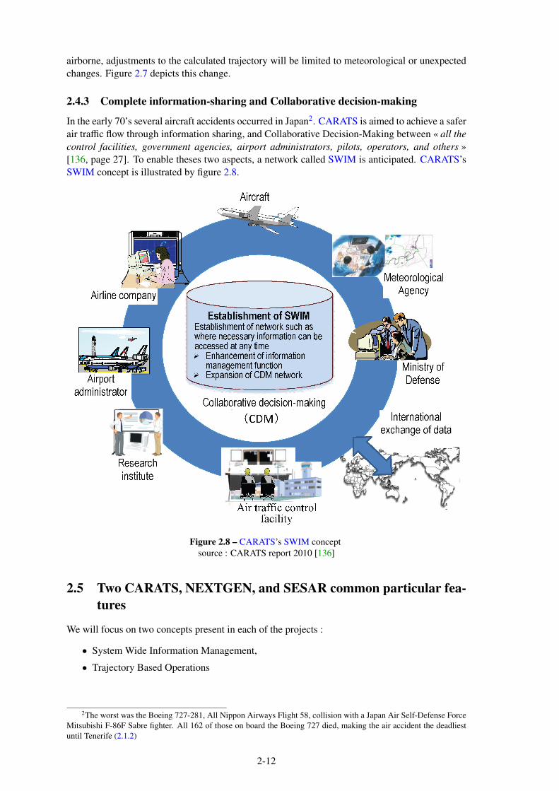
airborne, adjustments to the calculated trajectory will be limited to meteorological or unexpected

changes. Figure 2.7 depicts this change.

2.4.3 Complete information-sharing and Collaborative decision-making

In the early 70’s several aircraft accidents occurred in Japan2. CARATS is aimed to achieve a safer

air traffic flow through information sharing, and Collaborative Decision-Making between « all the

control facilities, government agencies, airport administrators, pilots, operators, and others »

[136, page 27]. To enable theses two aspects, a network called SWIM is anticipated. CARATS’s

SWIM concept is illustrated by figure 2.8.

Figure 2.8 – CARATS’s SWIM concept

source : CARATS report 2010 [136]

2.5 Two CARATS, NEXTGEN, and SESAR common particular fea-

tures

We will focus on two concepts present in each of the projects :

• System Wide Information Management,

• Trajectory Based Operations

2The worst was the Boeing 727-281, All Nippon Airways Flight 58, collision with a Japan Air Self-Defense Force

Mitsubishi F-86F Sabre fighter. All 162 of those on board the Boeing 727 died, making the air accident the deadliest

until Tenerife (2.1.2)

2-12

2.5.1 System Wide Information Management

In the three projects, the SWIM concept is listed, and the need for Information Services has been

identified since years by the ICAO (2.1.2) who issued an interim advance edition to the SWIM

concept [78] to help harmonization and interoperability. We are interested in the meteorological

part of SWIM as it is listed in CARATS as « Meteorological Agency » (Fig. 2.8), in NextGen as

« Weather Providers » (Fig. 2.5), and in SESAR as « MET Service Provider » (Fig. 2.3).

The idea is not new, the Australian Automated Meteorological DAta Relay system, which be-

came operational in 1986 on Ansett [147, page 8], was the first operational AMDAR system. The

World Meteorological Organization3 held the Inaugural Meeting of the AMDAR in Geneva on 17

March 1998. Since, the program has matured (see figure 2.94, showing the evolution of AMDAR

daily reports over time) and as shown in April 2016 World Meteorological Organization (WMO)

AMDAR Observing System Newsletter, AMDAR observations counts for 650 000 among the

700 000 aircraft-based meteorological daily observations [148].

Figure 2.9 – Daily AMDAR Reports

Our work deals with wind and temperature networking and as shown in figures 2.3, 2.5, 2.8, the

aircraft is a network node. Let’s focus on SWIM and meteorological information provided by

aircraft. Accuracy of automated observations of wind and temperature from airliners has already

been studied in the United States by Stanley G. Benjamin, Barry E. Schwartz and Rodney E. Cole

[17]. The study was based on aircraft reports using Aircraft Communications Addressing and Re-

porting System (ACARS) messages, so with the limitation of 220 characters per message. The

study showed an estimated horizontal wind standard deviation error of 2.1 knots for wind obser-

vations and about 0.5 K for temperature observations for flight levels between FL235 and FL300.

An other United States study [120] from Barry E. Schwartz, Stanley G. Benjamin, Steven M.

Green and Matthew R. Jardin showed that RMS vector differences between observations and fore-

casts, from either the original Rapid Update Cycle (RUC-1) or the Rapid Update Cycle Version

3The World Meteorological Organization is a United Nations agency responsible for the standardization of obser-

vations and the international exchange of weather data4Source : https://www.wmo.int/pages/prog/www/GOS/ABO/data/statistics

2-13

2 (RUC-2)5,6, increased as wind speed increased, and correspondingly, as altitude increased and

toward winter months. It pointed out the difficulty to develop a reliable ACARS observational

database.

Since, avionics has improved and has led to aRea NAVigation (RNAV) and Required Navigation

Performance (RNP) based en route procedures. As explained in ICAO document 4444 [73], En-

Route procedures are normally based on RNP 4 or higher. Where necessary and appropriate, they

may be based on RNP 1. This means that today operations are mainly based on United States

Global Positioning System (GPS) ground track and ground speed calculations. Compared to the

late 90’s and the early 2000’s, the ADC calculations for wind speed and direction are more accu-

rate, as ground speed and true track are more accurate.

A study has been conducted in to estimate winds at different flight levels using information (plane

positions and observed ground velocities) available on public flight tracking websites [86]. Of

course Outside Air Temperature (OAT) could not be derived from these information, and the True

Air Speed was estimated from the Filed flight PLan (FPL) filed speed. As most airliners fly at

constant Mach Number7, the calculations could be biased when temperature deviates from Inter-

national Standard Atmosphere temperature. Anyway the study combined ground speed and air-

speed of planes at different positions, with publicly available National Oceanic and Atmospheric

Administration Winds Aloft forecasts, through a probabilistic graphical model. It showed better

trajectory prediction using Gaussian Process Regression, than using National Oceanic and Atmo-

spheric Administration (NOAA) Winds Aloft forecasts. It also presented an approach to select

ideal subsets of planes, that might be of interest to optimize the SWIM air bandwidth.

2.5.2 Trajectory Based Operations

TBO is common to the three projects, and they all rely on 4D trajectories. As stated in 2.1.2 it

refers to the possibility for the airspace users to fly preferred trajectory, from gate to gate. To

implement 4D trajectories

index4D trajectory, airplanes will have to cross at scheduled time the points along the trajectory.

This scheduling has to be managed to reduce conflict, and trajectory adjustments will be required,

specially during the transition phase between airspace-based and trajectory based operations. To

minimize these adjustments, predictability of the trajectory must be improved, and the idea is to

use both the calculations done by the aircraft Flight Management System and ground based ATM

trajectory prediction tools. If both systems could be fully automated, their accuracy would be

limited by at least two external parameters : the wind (in calculating the ground speed) and the

temperature (as auto-throttle equipped airliners fly at constant Mach Number). As a long term

solution, the European 4 Dimension Contracts and Guidance and Control (4DCo-GC) project [26]

was dedicated to explain and analyze the 4D contract concept to solve the TBO concept trajectory

prediction problem.

NextGen and SESAR Trajectory Based Operations philosophy have been compared in [35], point-

ing out one major difference, SESAR assumes that the aircraft FMS predicted trajectory is the

most accurate, as the FMS knows about aircraft performance limitations (e.g engines N18 lim-

its, actual take-off weight, current aircraft weight, ...) and encountered wind ; whereas NextGen

assumes that the ground system has a better knowledge of the traffic, and therefore has a better

situational awareness.

5The original Rapid Update Cycle (RUC-1) was an atmospheric prediction system that consisted primarily of a

numerical forecast model and an analysis system to initialize the model. This system was cycling on itself in a 3-h

intermittent data assimilation cycle.6The Rapid Update Cycle Version 2 (RUC-2) took over RUC-1 and was using hourly assimilated observations.7Dimensionless quantity representing the ratio of true airspeed to the local speed of sound.8N1 represents the rotation speed of the turbine shaft

2-14

Our works seem closer to SESAR approach as we plan to share the temperature information not

only for speed calculations, but also for engines performance limitations (as service ceiling may

be limited by powerplant for significant deviation above International Standard Atmosphere (ISA)

OAT)

2.6 Conclusions on meteorology, TBO and SWIM

TBO requires accurate, available and reliable information on weather parameters or events that

may change the forecast negotiated aircraft trajectory. Beyond probabilistic meteorological fore-

casts, observational data may also be used as inputs both in FMS and ground trajectory prediction.

Many aircraft data are available in those areas where accurate TP is needed (area of very dense

traffic).

A transmission network including ground and air segments is mandatory to exchange the aircraft

information (current and future positions, speed, ...) and weather parameters. TP can be calculated

on board or on ground, but in both cases, meteorological and aircraft performance data are inputs

needed by the calculation. Once done, the TP has to be shared to optimize air space usage.

Wind and temperature networking may also be used for safety as unpredicted icing conditions or

Clear Air Turbulence (CAT) may be encountered. It happened when airliners, certified to fly into

icing conditions, encountered icing theirs Ice Protection System failed to eliminate (e.g airspeed

pitot probes [4]).

2.7 Automatic Dependent Surveillance - Broadcast

2.7.1 Introduction

Automatic Dependent Surveillance - Broadcast (ADS-B) is a growing surveillance technology

that allows air traffic controllers to track equipped aircraft and airport ground vehicles. It does not

require any radar, aircraft and vehicles broadcast their position and other parameters (see figure

2.10). The ADS-B system consists of aircraft avionics and a ground infrastructure. It is expected

to replace radar as for traffic surveillance.

ADS-B is cited as a key « NextGen Technologies » [85, page 3-3], by SESAR as « a necessary

measure to support future ATM » [125, page 20], and listed by CARATS as an « Enabler » within

the 55 measures to reach the long term vision [153, page 6].

The FAA plans to use the ADS-B as the primary means of surveillance, and to support reduced

separation and delegated separation.EUROCONTROL CASCADE Program9 corner stones are

ADS-B and Wide-Area Multilateration (WAM)10.

2.7.2 ADS-B principle and advantages

ADS-B concept emerged in the 90’s with the needs of more flexible and more efficient airspace

use ; and with the idea of reducing the surveillance costs. ADS-B relies on two bases components :

• a device to calculate the aircraft (or vehicle) position,

• a device to broadcast the position (and other information) via a data link.

9The CASCADE Program co-ordinates the deployment of initial ADS-B applications and Wide-Area Multilatera-

tion (WAM) in Europe.10WAM is a surveillance technique that exploits the 1090 MHz transmissions from aircraft.

2-15

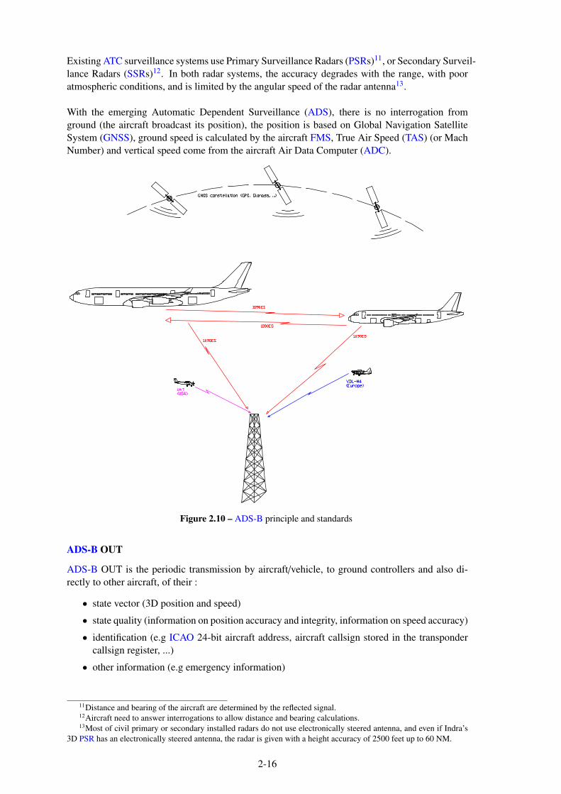
Existing ATC surveillance systems use Primary Surveillance Radars (PSRs)11, or Secondary Surveil-

lance Radars (SSRs)12. In both radar systems, the accuracy degrades with the range, with poor

atmospheric conditions, and is limited by the angular speed of the radar antenna13.

With the emerging Automatic Dependent Surveillance (ADS), there is no interrogation from

ground (the aircraft broadcast its position), the position is based on Global Navigation Satellite

System (GNSS), ground speed is calculated by the aircraft FMS, True Air Speed (TAS) (or Mach

Number) and vertical speed come from the aircraft Air Data Computer (ADC).

Figure 2.10 – ADS-B principle and standards

ADS-B OUT

ADS-B OUT is the periodic transmission by aircraft/vehicle, to ground controllers and also di-

rectly to other aircraft, of their :

• state vector (3D position and speed)

• state quality (information on position accuracy and integrity, information on speed accuracy)

• identification (e.g ICAO 24-bit aircraft address, aircraft callsign stored in the transponder

callsign register, ...)

• other information (e.g emergency information)

11Distance and bearing of the aircraft are determined by the reflected signal.12Aircraft need to answer interrogations to allow distance and bearing calculations.13Most of civil primary or secondary installed radars do not use electronically steered antenna, and even if Indra’s

3D PSR has an electronically steered antenna, the radar is given with a height accuracy of 2500 feet up to 60 NM.

2-16

over a data link approved by the airspace aviation authority.

Three ADS-B data have been standardized (see figure 2.10) :

• ADS-B 1090 MHz Extended Squitter (1090ES) is globally harmonized as the ADS-B inter-

operable datalink14 [68, Chapter 5]

• Universal Access Transceiver 978 MHz (UAT) in the United States of America (USA) [67,

Chapter 12]

• ADS-B VHF Data Link Mode 4 (VDL-M4) in the Scandinavian countries and in the Russian

Federation [67, Chapter 6]

Even if 1090ES has been internationally coordinated, there are three standards developed in the

United States of America : RTCA/DO-260, RTCA/DO-260A and RTCA/DO-260B that cor-

respond respectively to ICAO Doc 9871 Version 0, 1 and 2. The European standard EURO-

CAE/ED102A is equivalent to RTCA/DO-260B.

Due to the different information that ADS-B may transmit, the ADS-B transmitter has to obtain

data from other aircraft systems. Examples of such systems are secondary sources for navigation

(e.g redundant Global Navigation Satellite System, Inertial Navigation Systems), Air Data Com-

puter to get the barometric altitude and the True Air Speed, pilot input device, Flight Management

System for equipped aircraft, Traffic Alert and Collision Avoidance System... (see figure 2.11).

Figure 2.11 – ADS-B data exchanges

ADS-B IN

Aircraft can be equipped with ADS-B receivers to receive ADS-B signals from other aircraft,

from ground vehicles or from ground stations Automatic Dependent Surveillance - Rebroad-

cast (ADS-R). Such equipped aircraft could also receive, from the ground, additional data from

other aircraft not transmitting ADS-B OUT or transmitting with a different ADS-B technology.

ADS-B IN refers to the airborne function that permit to receive, process and display surveillance

data transmitted by the ADS-B OUT functions installed in other aircraft/vehicle.

After on-board processing, the received traffic information (ADS-B, ADS-R, Traffic Information

System - Broadcast (TIS-B) and TCAS) is displayed on a Cockpit Display Traffic Information

(CDTI). The final goal of ADS-B IN applications is to transfer some or all separation responsibility

to the cockpit. These applications are at various stages of development, some are at the prototype

status, others are already standardized. All belong to one of the following categories :

• Situational awareness where traffic information is displayed in the cockpit, as information

only and without changes to the pilot or controller responsibilities.

14Mode S extended squitter contains an additional 56-bit data block compared to the conventional Mode S. ADS-B

information is broadcast in separate messages.

2-17

• Extended situational awareness where alerts and indications helps the crew to fly with re-

duced aircraft separation standards.

• Spacing applications where the crew is required to achieve and maintain a given longitudinal

or vertical spacing with an aircraft. Even if the crew is given ATC instructions, the ATC

controller keeps the responsibility of separation.

• Delegated separation where the ATC controller delegates separation responsibility and tasks,

from a designated aircraft, to the crew. It is a clearance limited in time, space, and scope.

Separation responsibility for all other aircraft remains with the ATC controller.

• Self-separation where the crew have to separate their aircraft from all surrounding traffic,

according to separation standards and flight rules.

Among the five above categories, the last three require Trajectory Prediction (TP). This TP can be

done on board using a supplemental traffic computer, or on ground using ATC trajectory prediction

tools. Considering the oceanic (i.e long haul) flights and the lack of permanent data link, the on

board TP for the surrounding aircraft seems to be unavoidable.

Compared to TCAS, the traffic situation displayed on the Cockpit Display Traffic Information

(CDTI) provides much more information.

Ground-Based information services

ADS-B also offers ground services than can be grouped into three categories :

• Automatic Dependent Surveillance - Rebroadcast (ADS-R) is a ground based traffic infor-

mation service that transmit to aircraft ATC known surrounding traffic. It can be seen as a

gateway between 1090ES and the others standards (2.7.2). An example of such application

is the rebroadcast of ADS-B information received with UAT or VDL-M4 standards from

Unmanned Aerial Vehicle (UAV) [76] to ADS-B IN aircraft.

• Traffic Information System - Broadcast (TIS-B) is a ground based traffic information service

that receives traffic surveillance information from surveillance systems based on radars (e.g

military traffic, airport ground movements, MultiLATeration (MLAT)15...) and ADS-B. Af-

ter processing and correlating the traffic data is transmitted to ADS-B IN equipped aircraft.

• Flight Information Service Broadcast (FIS-B) is the ground-to-air broadcast of meteorolog-

ical and aeronautical information. As this service uses the UAT for transmission, it is not

considered as part of the ADS-B.

As in the three cases, the current aircraft current position is broadcast and there is no need for

Trajectory Prediction.

Automatic Dependent Surveillance - Contract

As opposed to ADS-B, Automatic Dependent Surveillance - Contract (ADS-C) is an exchange

between one aircraft transmitting Automatic Dependent Surveillance (ADS) data and one ground

station requesting this ADS data. The messages are sent to the controlling ATC, not broadcast

to the others aircraft. An analogy can be done between ADS-B and ADS-C ; and User Datagram

Protocol (UDP) and Transmission Control Protocol (TCP) both Internet Protocols (IPs)16. The first

of each provides a connectionless datagram service, whereas the second of each uses a connected

transmission. ADS-C relies on specific agreements between a ground system and an aircraft, the

aircraft sends specific aircraft data in different groups of an ADS-C report, one group is dedicated

to Meteorological information [75] (see figure 2.12).

15Multilateration is a surveillance system which can utilize data received from aircraft transmitting in response to

Mode A/C transponder, SSR Mode S or ADS-B avionics.16Many streaming media applications on the Internet and private networks use IP multicast technique which is based

on UDP.

2-18

Figure 2.12 – ADS-B data exchanges

2.7.3 Conclusions on ADS-B

Many countries are deploying ADS-B ground stations networks to improve traffic surveillance

over regions lacking radar coverage (e.g over Hudson Bay in Canada and in the center of Aus-

tralia), and/or for cost-savings. The collected surveillance information has better accuracy and

better refresh rate than those of the current SSR based systems. The data is displayed with con-

ventional radar data on the controller display terminal. To detect potential conflict, Trajectory

Prediction (TP) can be done on the ground stations networks computers, using new algorithms as

the ADS-B OUT permits calculations based on the aircraft state vector ADS-B-StateVector. We

can assume that in a near future meteorological information will be transmitted via ADS-B using

1090ES standard.

2-19

Chapter 3

Trajectory Prediction state of the art

and mathematics

3.1 Introduction

Trajectory Prediction (TP) is an estimation problem, as opposed to filtering or smoothing, where

the time at which an estimate is desired occurs after the last available measurement[56]. Its goal

is to compute the aircraft 4 Dimensions position in the future knowing its initial state. Mathemat-

ically, it is described as a time-ordered set of aircraft state vectors. Most of the currently deployed

trajectory predictors assume that the aircraft maintain a constant altitude, velocity and accelera-

tion. TP is linked to separation management and its accuracy affects the strategic en route conflict

probe, and the tactical conflict alert. The final goal of improving the TP is to increase the airspace

capacity by reducing the minimum separation between aircraft (e.g. horizontally from 5 NM to 3

NM) while reducing the occurrence of false trajectory conflict alerts, and preventing the miss of

valid trajectory conflict alerts.

This separation reduction means that two aircraft following the same route are only separated by

about 40 seconds at high altitude (assuming an average Mach number of .78 means a speed around

7.5 NM/minute), and less than 1.15 minutes below 10 000 ft (assuming the aircraft maintain 250

knots below 10 000 ft1). These new constraints make it essential to take into account the changes

on the aircraft attitude, as those changes generally suggest a change of trajectory (e.g. a change in

the bank angle corresponds to a change in the roll rate, itself followed by a heading change).

Said in other words, to comply with the new separation requirements, a trajectory predictor may

be able to measure position and orientation of an airplane, and also to track their rates of change.

Trajectory prediction has also been addressed by military organizations for more than fifty years,

for fire control in air-to-air, ground-to-air or sea-to-air operations. In this problem, a sensor system

tracks the current position and sometimes the orientation of a flying target. The prediction process

is similar as military organizations predict target position at the time of hit, i.e. the projectile’s time

of flight to reach target. Civilian organizations predict trajectories to avoid hit with a safety margin.

The goal of this chapter is :

• To present some of the existing tools and approaches to predict aircraft trajectories.

• To give an idea of the diversity and the complexity of the type of trajectories described in

the aeronautical SIDs, STARs, and approach charts, as the prediction must be done from

take-off to landing.

1According to [69][Appendix 4.] : “When the height of the transition altitude is lower than 3 050 m (10 000 ft)

AMSL, FL 100 should be used in lieu of 10 000 ft.”.

3-1

• To present today airplane FMS capabilities in terms of trajectory modelisation and predic-

tion. This step seemed essential to us, as according to EUROCONTROL, “the performance

of a trajectory engine can be determined by comparison with actual aircraft motion, often

approximated with the FMS” [38].

The first part of this chapter consists of sections 3.2 and 3.3. It gives an overview of today tra-

jectory predictors, it gives some details on the computations done by Flight Management Sys-

tems (FMSs). Comparing FMSs did not seem essential to us as, even if there is less than 10 man-

ufacturers, all the FMSs provide the same navigation functions, i.e. Lateral NAVigation (LNAV)

and Vertical NAVigation (VNAV). They all use the same navigation databases, and describe the

trajectories the same way : using ARINC 424 format.

Our personal feeling is that the functioning of the FMSs is rather unknown to air traffic controllers,

in particular their ability to respect the SIDs and STAR published altitude and speed constraints.

It is indeed the changes in speed and altitude constraints, compared to those published, imposed

by ATC controllers, that force flight crews to return to more primitive FMSs operating modes, and

reduce the accuracy of the trajectory in the space and time domains.

The comparison between ground and airborne predictors makes reading the chapter more difficult,

because of the presence of comparative tables. We have chosen to retain them for future reference.

The hidden objective of this first part is to show that the calculations made by the FMSs are much

finer and more precise than we imagine.

The second part goes deeper in the modeling tools for the trajectory (section 3.4), and in the ref-

erence frames (section 3.6) used to derive the equations of motion. We chose to describe ARINC

424 legs as they are used within all FMS to code the trajectories (including approaches and in-

strument procedures), whereas ground predictors use ICAO Document 4444 [73], as specified in

EUROCONTROL Specification for Trajectory Prediction [38, p. 19].

The third part (section 3.7) deals with aircraft attitude calculation as it is not taken into account by

today civilian ATC trajectory predictors.

The fourth part (section 3.8) focuses on modeling the plane motion and deriving the equations,

using vectors classical dynamics, tensor flight dynamics and energ.

3.2 Trajectory Prediction state of the art

Hundreds of papers have been written on Trajectory Prediction (TP) and conflict detection2. Most

of these papers have been reviewed by the Federal Aviation Administration (FAA) in « Literature

Survey of Trajectory Predictor Technology » [16]. Among them 282 where classified as relevant

to separation management, and 20 papers where identified as presenting unique approach to Tra-

jectory Prediction. A detailed synthesis of these 20 papers has already been presented in [16].

TP has led to the development of numerous systems, some operational, others limited to studies

or evaluations. All opinions converge on the need for an accurate trajectory prediction for Trajec-

tory Based Operations. To reduce the effort duplication, between the FAA, EUROCONTROL,

and other organizations working on tools and predictor development, a common Action Plan

(EUROCONTROL/FAA Action Plan 16) has been started [40]. One objective of this action plan

is the definition of a trajectory predictor standard, which describes the functions that have to be

implemented.

2Conflict detection occurs when minimum separation (e.g. En Route 5 NM horizontaly and 1000 ft vertically)

between at least two aircraft is lost, either in the lateral plan or the vertical plan.

3-2

3.2.1 The problem of trajectory prediction systems classification

The trajectory prediction systems (or tools) can be classified in different ways :

• airborne versus ground systems [144],

• systems using deterministic versus probabilistic approaches,

• by the model used for calculation [96] : full six degree-of-freedom model, point mass model

and macroscopic model (e.g. Base of Aircraft DAta (BADA)),

• by the flight phase location focused on, e.g. En Route operations versus Terminal Area

operations,

• by their client conflict detection application (20-minute look-ahead time strategic conflict

probe versus 3-minute look-ahead time tactical conflict alert),

Approaches with unclassified calculation model have also been proposed :

• In [93] and [91], machine learning technique is used to predict trajectories without modeling

the aircraft performance, the approach procedures and the airspace. The system uses past

trajectory and meteorological data to train the predictive model. One can anticipate that

predicted trajectories may not be accurate just after a change in an airport STAR or SID,

that may affect trajectory and speed restrictions.

• Only past radar tracks, and no physical or aeronautical parameters, are used in [137] to

calculate the aircraft future position. This approach is based on local linear functional re-

gression that considers data preprocessing, localizing and solving linear regression using

wavelet decomposition. The forecasts of such a system are defeated when a crew requests

a non-nominal descent or climb profile, e.g. request to maintain high speed descent and ap-

proach when behind schedule, or requesting a visual approach that generally save between

5 to 10 minutes of flight time.

• In [45], neural networks are trained using a set of real trajectories and then used to forecast

new ones in the vertical plane.

Clearly the previous classifications rely on a mix on how the system works, and what it does.

They do not allow trajectory prediction systems comparison, and there was a need for a definition

of a common, generic structure to describe the TP functionality. To fill this gap, the FAA and

EUROCONTROL issued the « SESAR-NextGen Aligned TP Structure and Terminology - AP16

White Paper » [42]. Let’s summarize some key points of this document.

3.2.2 TP Structure and Terminology

The FAA and EUROCONTROL agreed to describe TP from two views (without distinguishing

airborne and ground systems) :

• from a process perspective

• from a data perspective

The process view is summarized in figure 3.1. Our work, dealing with wind and temperature

updates, modifies in nearly real time the meteorological conditions inputs. A glance at figure 3.1

clearly shows its impact on the TP.

3-3

Figure 3.1 – Trajectory Prediction (TP) Process Flow

The data view, summarized in figure 3.2, identifies the interfaces and the key data sets. The

computation block at the bottom of figure 3.2 is in charge of the trajectory computation. The

Trajectory Engine uses the Behavior Model3, and mathematical models for meteorological data

and aircraft performance.

Figure 3.2 – Trajectory Prediction (TP) Data Flow

3.2.3 Trajectory predictors common assumptions

Most trajectory prediction systems use simplifying assumptions. As a non accelerating, non rotat-

ing reference frame (i.e. inertial reference frame) is needed to use Newton’s laws, approximations

are introduced in the equations of motion to obtain the equations for flight over a non rotating flat

Earth.

3Ordered list of maneuvers, starting at the Initial Condition, which the aircraft will perform to meet the trajectory

constraints.

3-4

Simplifying assumptions are also made on the airplane :

• even if most airplane structures are flexible (within some limits), the airplane is considered

as a rigid body,

• as fuel is consumed by the engines, the airplane is a variable-mass body,

• the airplane is subjected to aerodynamic, gravitational and propulsive forces,

• for airplane motion considered from an ATC control center, the earth approximates an iner-

tial reference frame.

Previous assumptions lead to the equations governing the motion of translation and rotation of a

plane [64] :

1. kinematic equations dealing with the geometry of translational and rotational motion,

2. dynamic equations relating forces to translational acceleration and moments to rotational

acceleration,

3. equations defining the changes in mass versus time,

4. equations giving the position of the control surfaces (ailerons, elevators, rudder, flaps, lead-

ing edge slats,...) and other moving parts (e.g. landing gear, fuel transfer, ...) as a function

of time.

The enumerated set of equations is generally referred as six degree of freedom (6DOF) equations

of motion. The relationships between the forces and the moments applied to the airplane must be

provided by the airplane and the engine manufacturers to solve these equations. These equations

are the highest degree of sophistication used within the Level D simulators intended to train air-

crews.

Another simplification is to assume that most trajectory analysis involve small aircraft rotation

rates. Doing so, it is possible to consider the rotation rates as negligible, and disregard the effect

of control surface deflections on aerodynamics forces. This means decoupling the translational

equations from the rotational equations. The calculations use only the translational equations, and

the trajectory is studied using the so called three degree of freedom (3DOF) equations of motion.

In these models only thrust and drag are considered as the hypothesis of lift compensating weight

is made.

One can also only consider the aircraft macroscopic behavior in a macroscopic model (also known

as fully kinematic model). In that case rate of climb (or descent), rate of acceleration (or deceler-

ation) are expressed as functions of parameters like altitude, temperature, wind, ... The required

data to compute the trajectory are limited to the aircraft rates of change.

As modeling techniques differ, how can trajectory predictors be compared ?

3.3 Trajectory predictors comparisons

To compare existing trajectory predictors, the following criteria can be used [144] :

• Input state data

• Constraints handled

• Behavior models used

• Math models used

• Output trajectory data

We chose to focus on comparing ground trajectory predictors to airborne trajectory predictors

(called FMSs or FMCs), as EUROCONTROL suggests to assess the performance of a trajectory

engine, by comparing its output to those of a FMS. Airborne predictors seem more accurate, and as

they are the primary "on-board" tool for Performance Based Navigation (PBN) operations, which

3-5

is the foundation for the ATC modernization initiatives. Comparisons are made using mainly the

Boeing 737NG FMS as we got some parts of the Boeing documentation4.

The FMS includes the following elements :

• the Flight Management Computer (FMC) system

• the Autopilot Flight Director System (AFDS)

• the AutoThrottle (A/T)

• the Inertial Reference System (IRS)

• the United States Global Positioning System (GPS)

3.3.1 Input state data

Input state data are used to define :

• airplane trajectory initial conditions (position, attitude, fuel on board, total mass, ...)

• airplane initial lateral and vertical maneuvers,

• airplane intends

Let’s detail some of the today used input state data.

Airplane trajectory initial conditions are needed before any computational process, as future posi-

tion will be obtained by a simple integration of speed, or a double integration of the acceleration.

Obviously, at least the initial position and the initial speed or acceleration must be known, and

that is where the problems start for 4D trajectory prediction. Looking back at ICAO global ATM

concept summary 2.1.2, at SESAR SWIM (2.2.3), NextGen Net-Centric Operations (2.3.4) and

CARATS SWIM (2.4.3), there is no doubt about the need to share information between different

ATC centers, not necessarily in the same country, and between airplanes and ground stations (air-

plane considered as a data network node).

The sharing of information is facilitated by the use of standards5, and unfortunately airborne and

ground systems do not always use the same coordinate systems, e.g. (World Geodetic System

1984 (WGS84) versus local Cartesian Coordinate system), moreover different countries do not

use the same projections (see 3.8). The current trend is to move all data to WGS84, but even in

this case some systems code the position in WGS84 (latitude, longitude, altitude), other in WGS84

(X, Y, Z), both use their own algorithms to perform the calculation, sometimes done with another

data format.

The same kind of problems exist for the trajectory description, airplanes’ FMS use ARINC 4246

to describe and store the aircraft planned route, ATC ground trajectory predictors follow ICAO

Doc 4444 to extract trajectory from filed flight plan [38]. In other words, we can say that FMS and

ground trajectory predictors have their own version of the trajectory to be flown. This may lead

to undetected discrepancies, or even errors on the trajectory segments when converting from one

system to the other7.

To complicate the whole, navigation data is needed to code airplane intents. For this reason it may

be considered as an input state data. This navigation data come from many sources of information,

4The two work horses of today short to medium haul airplanes are the Boeing 737NG and the Airbus A318-A321,

unfortunately we did not get the Airbus documentation5Examples can be taken from the Internet who could not have been deployed without a worldwide deployed TCP/IP

protocol, or from the mobile phone with its roaming facilities.6ARINC 424-20 was published on Dec 5, 2011.7FAA Advisory Circular 120-29A : GPS stand alone systems, while accurately flying to locations specified in

WGS84 coordinate frame, may not necessarily fly the path over the ground intended by the procedure if the specification

of that path uses a datum significantly different than WGS84.

3-6

and is manipulated by different organizations before it is coded in an on board or a ground tra-

jectory predictor. Noticeable differences between charts and databases have already been pointed

out, as the discrepancies that may exist between a ground and a on board trajectory predictor,

following its 28 days navigation database update cycle (Aeronautical Information Regulation And

Control (AIRAC) cycle)8.

Most today operational trajectory predictors receive, within input state data, the aircraft type, the

true heading, the altitude, the ground speed, the vertical speed, and the time stamp of the initial

position.

Other important initial parameters giving the airplane status may affect trajectory prediction, and

its accuracy :

• flight state : level flight, turning, climbing, leveling off, accelerating, reducing speed ;

• airplane flying status : flying according to flight plan, diverted, in an "MAYDAY"9 or "PAN"

(the two last cases should grant special treatment to the trajectory, including optimal emer-

gency trajectory calculation) ;

• airplane operational condition : fully operational, on engine out, depressurized (the two last

cases imply at least constraint on the trajectory) ;

• aircraft weight (directly affecting assumed future performance for the prediction) ;

• aircraft initial position actual pressure and temperature (affecting calculation of true airspeed

and aircraft performance if a deviation from ISA atmosphere is observed) ;

• local meteorological conditions : Clear Air Turbulence (CAT) can force the crew to reduce

the aircraft’s speed (e.g. on a Boeing 737/300, the severe turbulence air penetration speed is

280KIAS/0.73M, whichever is lower)

The above missing parameters are already identified, and explain why today ATC centers request

more parameters from the aircraft through ADS-B reports and why next generation ATC systems

will also use trajectory prediction information given by the airplane FMSs.

As trajectory prediction depends on input state data, we should compare these data for on board

FMSs and ATC (i.e. ground) trajectory predictors. Table 3.1 summarizes some of them, including

parameters influencing the performance of the aircraft.

From the previous paragraphs it can be concluded that the FMSs have much more information

relating to the initial and current state of the aircraft than ground predictors. These information

are entered by the flight crew during the preflight process of the FMC, or provided by others

systems (e.g. ADC, IRS, navigation receivers, engine and fuel systems, ...). FMS also has more

information about local (space dependency) and present (time dependency) weather conditions.

8The AIRAC effective dates are published in ICAO Document 8126, the Aeronautical Information Services Man-

ual. The AIRAC cycle was adopted in 1964 and further improved over the years.9Emergency Status is part of ADS-B messages

3-7

Table 3.1 – Input State Data comparison

Input State Data Airplane FMSGround Trajectory Predic-

torComments

Position WGS84 and altitudeCartesian (x,y) & altitude,

or WGS84 & altitude

Different map projections for

Cartesian (x,y). ADS-B man-

dates WGS84 position & geo-

metric altitude. Barometric pres-

sure altitude is part of ADS-B

transmitted data.

Magnetic Heading FMS providedHeading is part of ADS-B trans-

mitted data.

True Course FMS provided

Initiated from flight plan,

or ADS-B ground track

angle data

TimeTime associated to current

position

Time of first radar plot or

ADS-B report

AttitudeFMS provided roll, pitch,

yaw angles

Ground systems need several

radar tracks to identify a turn.

Vertical rate is part of ADS-B

message.

SpeedMach number, CAS, TAS,

GSGS, TAS or Mach number

For ground systems TAS and

Mach number come from the

filed flight plan. ADS-B trans-

mits horizontal velocity.

Engine information

(status of the engine

bleed air valves, engine

malfunction)

Set by the flight crew, or

automatically

Standard parameters

known from engine manu-

facturer data

Airplane configuration

(flaps, slats, speed brake

positions, trim setting...)

Set by the flight crew for

Take Off (T/O), descent,

approach, Landing (LDG)

Weight

Calculated by the FMS

using T/O weight and fuel

consumption

T/O Weight is available from

loadsheet at push-back

Local weather con-

straints (e.g. speed

reduction due to tur-

bulence)

Flight crew manually en-

tered Mach number or

speed limit

Area of thunderstorms

may be anticipated by Met

forecast

Actual weather infor-

mation (deviation from

ISA, actual wind, icing

conditions...)

Measured by the airplane

sensors and used by the

FMS

May be implemented using

WTN

FMC : icing conditions and

turbulence are monitored by the

flight crew. Selection of anti-ice

systems and/or speed restriction

is known to the FMS.

Navigation database

FMS database updated as

per AIRAC cycle (FAA &

EASA regulation for air

carriers)

Generally extracted from

AIP ENR and AD parts

Update cycle for ground trajec-

tory predictors may differ from

AIRAC cycle

3.3.2 Constraints handled

A trajectory predictor generates, if possible, a trajectory satisfying the imposed lateral and/or

vertical constraints on the aircraft trajectory.

Lateral constraints

Lateral constraints make it possible to define the trajectory of the aircraft in the horizontal plane.

They determine where the trajectory starts or ends, and how the different WayPoinTs (WPTs)10

are joined (straight lines, great circles, ...). Existing ground trajectory predictors lack tools, as soon

as junctions are made using others than great circles arcs [144]. They are able to handle holding

10ICAO waypoint definition : a specified geographical location used to define an RNAV route or the flight path of

an aircraft employing RNAV [66].

3-8

patterns11 and WPT capture.

Table 3.2 compares FMSs and ground predictors lateral constraints mainly related to RNAV. We

choose to use ARINC 424 terminology summarized in Appendix D. It is the worldwide standard

for avionics systems, and there is no standard for ground predictors. Only currently FMSs imple-

mented Path/Terminator are presented. Bold written legs are recommended for RNAV leg types,

and italics written legs are mainly used for start and ends of procedures.

All the ATC renovation plans presented in chapter 2, have to predict aircraft trajectory from gate to

gate. To achieve this goal, keeping in mind that runways may have one take-off or landing every 90

seconds, at busiest hours, the trajectory prediction accuracy may be expected near 1 minute. This

means that ground predictors will have to handle ground tracks for holding patterns and Radius to

Fix legs (RF legs). Consistency between the FMSs loaded trajectories and their calculated ETEs,

will be hard to check with those of ground systems if both are not using common databases, for

routes and procedures.

Aircraft sequencing is today achieved by ATC controllers using speed restriction, temporary change

on heading, holding pattern, and point merging. The last one is a new sequencing method, on

RNAV route or procedure, that includes a level arc segment, until receiving a ’Direct To’ vector

to a Merge Point. According to EUROCONTROL, it promises a significant increase of trajectory

predictability and reduced track dispersion12.

Attention should be given to RF leg, that defines a circle of specified radius enabling an aircraft to

fly a precise curved flight path relative to the surface of the Earth. RF legs are similar to a DME

arc segment from a VOR/DME or TACAN, and they are limited only by the airplane bank angle.

They provide access to airports where radio waves ground-based navigational facilities can not be

used. A nice example of RF leg is the Palm Springs, CA RNAV (RNP) Rwy 13R (see Fig. 3.3).

The described procedure is 55.5 NM length, i.e. taking into account the speed limit, its duration

is more that 15 minutes. Outside obstacle clearance, this type of leg may also be used for noise

abatement trajectory design.

Table 3.2 shows that FMCs handle much more lateral constraints than ground predictors. This can

be explained as they need to interface with the autopilot systems, and provide LNAV guidance.

Goals, when developing the software, were to fly charted instruments procedure with the autopilot

engaged. ARINC 424 versions were revised to describe most of the evolving SIDs and STARs,

i.e. to strictly follow a published procedure. Ground predictors were generally not designed to

cover all flight phases, but just the phase the airplane are in a specific ATC sector.

Differences between columns 2 and 3 of Table 3.2 can also be explained by the Air Traffic Control

organization in busy Terminal Maneuvering Area (TMA). Most of the time, aircraft enter the

TMA by waypoints, with often altitude and sometimes speed constraints. Beyond these waypoints,

aircraft are radar vectored by approach control to the landing runway. When established on final,

aircraft control is transferred to the airport control tower. As long as this modus operandi is kept,

there is no need to model the approach and the final trajectories. The flip side of the coin is a

significant uncertainty as to the duration of the flight from the mandatory arrival waypoint to the

touchdown point.

11Even if they are not able to build the race track.12International Air Transport Association (IATA) position is more reserved as the complete merge arc becomes part

of the trip, leading to extra fuel mandatory uplift, and additional planned flight time. Amendments to regulations are

proposed to solve these two issues.

3-9

Table 3.2 – Lateral Constraints Comparison

Lateral constraint FMSGround Trajectory Pre-

dictorComments

IF Initial Fix ARINC 424 implemented Implemented

TF Track to Fix ARINC 424 implemented Implemented

HF Racetrack to Fix ARINC 424 implemented Not implementedFMC automatically exits after one

circuit.

HA Racetrack to Alti-

tude (provided for a climb

in the holding pattern)

ARINC 424 implemented Not implemented

On reaching the terminating al-

titude, FMC exit the circuit after

crossing the fix.

HM Racetrack to Man-

ual terminationARINC 424 implemented Not implemented

Flight crew intervention to exit the

racetrack.

RF Radius to Fix FMS model dependent Not implemented

CF Course to Fix ARINC 424 implemented Not implementedCourse is flown making adjustment

for wind.

DF Direct to Fix ARINC 424 implementedImplemented as way-

point capture

On ground predictors, waypoint

capture can be coupled with Cap-

ture Delay Time.

FA Fix to Altitude ARINC 424 implemented Not implementedFA leg is flown making adjustment

for wind.

CA Course to Altitude ARINC 424 implemented Not implementedCourse is flown making adjustment

for wind.

VA Heading to Altitude ARINC 424 implemented Not implemented No correction made for wind.

FM Fix to Manual termi-

nationARINC 424 implemented Not implemented

FM leg is flown making adjustment

for wind.

VM Heading to Manual

terminationARINC 424 implemented Not implemented No correction made for wind.

VI Heading to Intercept ARINC 424 implemented Not implemented

Trajectory start ARINC 424 implemented Implemented

For ground predictors, trajectory

start or sector transfer point. On

B737 FMS start point is checked

with IRS position.

AF DME Arc to Fix ARINC 424 implemented not implementedNot RNAV but used in terminal

procedures, ILS approaches, ...

Fly-over turn ARINC 424 implemented Implemented Classic ICAO fly plan legs.

Fly-by turn ARINC 424 implemented Not always implementedTrajectory depends on aircraft

speed and bank angle.

Company Route ARINC 424 implemented Not implemented FMC : company policy.

En-route Airways ARINC 424 implemented Implemented

ATC Preferred Routes Not implemented Implemented

Trajectory end ARINC 424 implemented Implemented

For ground predictors, trajectory

may ends at the point the aircraft

exits the ATC sector.

Strategic Lateral Offset

Procedures (SLOP)FMS model dependent Not implemented

3-10

3000

1000

5000

3000

5000

7000

1000

3000

5000

70009000 1000

529

516

475

TWR

583

P

P

P

V3

13R

31L

31R

0.8

% U

P

13L

4952 X 75

xx

10000 X 150

0.7

% U

P

1.0

% D

OW

N

310°

130° 4 NM

YOCUL

LACIV

FIVUT

NUDCI

RW13R

(3.8)

M

SA R

W13R 25 NM

12700

6000

WASAK

LACIV

NUDCI

2900

RNAV (RNP) Z RWY 13R

(PSP)PALM SPRINGS INTL

33°50'N-116°30'W

PALM SPRINGS, CALIFORNIA

L

RNAV (RNP) Z RWY 13R

PALM SPRINGS, CALIFORNIA

(PSP)PALM SPRINGS INTL

AL-545 (FAA)

YAGUS

MISSED APCH FIX

(IAF)

(4.7)

700

00

6000

4400

10834

487

(RNP 0.30)

5813

5677

5600

5460

AUTHORIZATION REQUIRED

TCH 45

GP 3.00°

DCBACATEGORY

HOPLI

RNP 0.30 DA

RNP 0.17 DA

5148

3853

3364

2999

2916

2703

24781980

1687

1623

1617

1541

1452

1353

1329

1323

1162

1078

1045989

893

857

781

769

758

683

632

562

JEXOT

(FAF)

RW13R

130° to

D

TRM4000

Max 210 KIAS

(VGSI Angle 3.00/TCH 41).

VGSI and descent angles not coincident

812-1 361 (400-1 )

882-1 431 (500-1 )

JEVOK

(7.8)

1

8000

70

(5.2)

(6.8)

(1.9)

3800

5 NM 3.7 NM

(3.7)

253°

10000(7)

7100

(13.3)

(5)

129°

130°

11000

9000

TRM

THERMAL

(RNP 0.30)

9000

(IAF)

SBONO

FERNN

(IAF)

CUXIT

WASAK

(IF)

1713

3.8 NM

RW13R

ELEV 476 TDZE 451

T

A NA

122.95

UNICOMCLNC DEL

128.35 121.9

GND CONPALM SPRINGS TOWER

(CTAF)L119.7 377.05

ATIS

118.25135.275 251.1

126.7 370.95

SOCAL APP CON

130°

APP CRS

Apt Elev

TDZE

Rwy Idg 6857

451

476

REIL Rwys 13L, 13R, 31L, and 31R

MIRL Rwy 13L-31R

HIRL Rwy 13R-31L

(2.9)

2900

38004400

FIVUT

2900

JEXOT

(RNP 0.30)

(RADAR REQD)

130°

1.9 NM 2.9 NM

Procedure NA when control tower closed.

RF required. GPS required.

1°C (34°F) or above 54°C (130°F).

For uncompensated Baro-VNAV systems, procedure NA below

16315

Amdt 1 10NOV16

Max 210 KIAS

Max 210 KIAS

900

and hold.

climbing left turn to 4000 direct TRM VORTAC

MISSED APPROACH: Climb to 900 then

14

14

12

12

7100 to C

UXIT

328°

(20.7) TRM

THERMAL

(5.9)

328°

7100

airway radials 263 CW 021.

on TRM VORTAC

Procedure NA for arrival

SW

-3, 1

2 O

CT

20

17

to 0

9 N

OV

20

17

SW

-3,

12

OC

T 2

01

7

to

09

NO

V 2

01

7

Figure 3.3 – Palm Springs, CA RNAV (RNP) Rwy 13R

Vertical constraints

Vertical constraints make it possible to define the trajectory of an aircraft in the vertical plane, and

are often associated with speed restrictions. Trajectory prediction is done by integrating the air-

craft energy balance equations, or equations of motion, where aircraft weight, altitude and speed

3-11

varies. Lift, drag, and engine thrust varies also with altitude, complicating the integration. Con-

straints are also added by the aircraft flight envelope, ATC flight plan imposed altitudes and/or

speed restrictions, and company fuel or time saving considerations.

Concerning Europe, national flights (i.e. short haul flights) in western countries spend one third,

to one half of their flight time in climb, descend and approach13. They represent a significant part

of air traffic and gate occupancy, and to reach a 1 minute accuracy in trajectory prediction, special

attention should be paid to vertical constraints.

Table 3.3 compares usual speed vertical constraints for both ground and airborne predictors (FMS

or FMC).

Table 3.3 – Speeds Vertical Constraints Comparison

Speed vertical constraint FMSGround Trajectory Predic-

torComments

Cruise speed (Mach number,

Calibrated AirSpeed (CAS),

TAS

Implemented ImplementedFMC : available after Cost Index (CI)

entry at preflight

Climb speed (Mach number,

CAS, TAS)Implemented Implemented

FMC : have full access to Mach

number, CAS, TAS through ADC ;

both LNAV and VNAV engaged,

or both LNAV and LeVeL CHanGe

(LVL CHG) engaged. Ground predic-

tors use FPL filed Mach number or

TAS.

Descent speed (Mach number,

CAS)Implemented Implemented

FMC : Both LNAV and VNAV en-

gaged, .

Approach speed Implemented Not always implementedDepends on high-lift devices settings

and aircraft weight.

Hold speed Implemented Not implementedDepends on aircraft weight, altitude

and holding pattern design.

Take Off speed Implemented Not implemented

Depends on type of take-off, aircraft

weight, high-lift devices setting,

meteo.

Engine Out speed Implemented Not implementedFMC : called from ENG OUT CLB,

ENG OUT CRZ pages

SID, approaches, STAR speed

limit altitude, 250 kt below

FL100

Implemented Not always implementedFMC : available with both LNAV and

VNAV engaged.

Table 3.3 shows that ground predictors hardly handle the airplane speed changes, when reaching

the approach phase of a flight. For long terminal procedures or approaches (e.g. Fig. 3.3) this may

prevent the predictor to reach an accuracy close to 1 minute.

These results are not surprising, we find the same results as for lateral constraints, the approach

phase of the flights is not modeled . This can also be explained by the fact that ATC controllers

instruct speed constraints for that phase, up to 4 NM miles to final, and that the length of the radar

vectored flight path is known for each aircraft category. Knowledge of aircraft speed, wind in the

vicinity of the airport and the ground distance to go to touchdown permit, with an uncertainty,

landing time estimation.

Table 3.4 compares usual altitude constraints.

13On a 737 NG, the climb phase begins at the thrust reduction altitude - 1500 ft AGL - and extends to the Top of

Climb (T/C) point (airplane reaches the cruise altitude entered on the PERF INIT page). The descent phase begins at

the Top Of Descent (T/D) point or when either a level change or vertical speed descent is initiated, it extends to the

beginning of the approach phase. The approach phase begins two nautical miles from the first waypoint of a published

approach or approach transition selected from the ARRIVALS page, or 2000 feet of destination airport elevation.

3-12

Table 3.4 – Altitude Constraints Comparison

Altitude constraint FMS Ground Trajectory Predictor Comments

Cruise Altitude Implemented ImplementedFMC : flight crew entry in

TRIP/CRZ ALT field

Interim Altitude Implemented Implemented

FMC : Both LNAV and VNAV

engaged, flight crew has to delete

next FMC altitude constraint via

Mode Control Panel (MCP) ALT

SEL and ALT INTV switch.

Transition altitude Implemented Most often implementedFMC : TRANS ALT in preflight

PERF INIT page.

Acceleration segment

(V2 + 10, V2 + 25 to climb

speed)

ImplementedNot Implemented (no need as

duration is few seconds)

Thrust reduction Implemented Not needed

FMC : normally 1500 ft AGL.

Change in the angle of climb and

the in vertical speed, normally

CAS is maintained (ICAO Noise

Abatement Departure Procedure).

WPT AT Implemented ImplementedFMC : AT XXXXX field in the

Climb Page

WPT AT or ABOVE Implemented Implemented

FMC : known bug in release Up-

date U10.8, corrected. VNAV de-

scent path is predicted backwards.

RTE LEGS page. Both LNAV and

VNAV must be engaged.

WPT AT or BELOW Implemented Not always implemented

FMC : RTE LEGS page, both

LNAV and VNAV must be en-

gaged.

WPT Window altitude Implemented Not always implementedFMC : Both LNAV and VNAV

engaged.

WPT Remain AT Implemented Not always implemented

FMC : ARINC 424 coded or flight

crew entry via Control Display

Units (CDU) or MCP.

WPT Change AT Implemented Not always implementedFMC : Both LNAV and VNAV

engaged.

Optimal step altitude ImplementedNot Implemented (not needed

by ATC)

FMC : step climb altitude may be

entered in CRZ page STEP altitude

field.

Vertical constraints are often associated with speed restrictions, e.g. speed limit below 10 000 ft

(see table 3.3). These constraints may also be associated with waypoint, i.e. the constraint starts

at the vertical of the waypoint. For example the approach depicted on Fig. 3.3 shows both altitude

and speed restrictions associated with waypoints :

• AT SBONO there is no waypoint speed restriction, but below 10000 feet Mean Sea Level

(MSL) - 250 Indicated Air Speed (IAS) knots applies if the aircraft is between 10000 ft and

9000 ft.

• AT SBONO the altitude must be at least 9000 ft (cross at or above)

• AT JEVOK altitude must be at least 10000 ft and speed maximum 210 kts

• AT YAGUS altitude must be at least 8000 ft and speed maximum 210 kts

Table 3.5 shows some speed restrictions associated to waypoints14 15.

14Most FMSs limit the speed to give an overspeed margin.15Airspeeds can be entered into the FMC as CAS or Mach number, within the range MIN SPD/MAX SPD entered

by the flight crew in the PERF INIT page

3-13

Table 3.5 – Waypoint speed constraints

Waypoint speed

constraintFMS

Ground Trajectory Predic-

torComments

IAS, CAS AT

altitudeImplemented Implemented

Speed starts AT ImplementedImplemented most of the

timeFMC : LNAV and VNAV engaged.

Speed ends AT Implemented Implemented

FMC : ARINC 424 coded or flight

crew speed restriction entry. LNAV

and VNAV engaged

Initiate Mach num-

ber ATImplemented Not implemented

FMC : speed constraints can be

entered as CAS or Mach number.

End Mach number

ATImplemented Not implemented

FMC : speed constraints can be

entered as CAS or Mach number.

Time AT WPT Implemented ImplementedFMC : Required Time of Arrival

(RTA) Progress page

Delay AT Not implemented Implemented

FMC : use of RTA function, or

HOLD key (HOLD AT or HOLD

AT Present Position).

Flight Path Angle

(FPA) changeImplemented Not Implemented

FMC : Default is 3.0 degrees.

Valid entries are from 2.0 to 5.5

degrees.

Vertical Speed Implemented Not implemented

FMC : calculated by the FMC but

manually entered by the crew via

the MCP.

Some comments should be added concerning the presence of the "Flight Path Angle (FPA) change"

in Table 3.5. The FPA is the angle of the aircraft relative to the horizon. Combined with the air-

plane track, it gives the pilot the Flight Path Vector (FPV), hence the instantaneous trajectory of

the aircraft. It is a speed constraint since it is equal to the ratio of the airplane vertical speed to

its ground speed. It should be implemented in ground trajectory predictor as it instantaneously

show a trend to deviate from a nominal flight path. Airbus implemented on its aircraft Primary

Flight Display (PFD) both the FPV and Flight Path Director (FPD) to allow pilots to fly from non

precision approaches to precision-like approaches.

Let’s see how this constraints look like on a climb and on a descent.

Figure 3.4 depicts a typical B737NG climb profile, using above waypoint speed and altitude limi-

tations.

Figure 3.4 – B737 NG Climb Profile

Figure 3.5 depicts a typical B737NG VNAV PATH descent profile, using above waypoint speed

3-14

and altitude limitations.

Figure 3.5 – B737 NG VNAV PATH descent Profile

The present subsection ends the description of the common aircraft trajectories, and the ways to

implement them in a computer program. Let’s now describe common aircraft maneuvers.

3.3.3 Behavior models used

As written in [16], behavior models define the maneuvers that can be predicted. They are generally

as matryoshka dolls, i.e. general maneuvers that can be split in elementary maneuvers. Figures

3.4 and 3.5 show this kind of decomposition for typical climb and descent. Referring at table 3.2

provides the implemented lateral behavior models.

Lateral behavior models

Ground and airborne trajectory predictors were both using great circle navigation, i.e. spherical

Earth hypothesis, but last FMSs software releases replaced great circles with WGS84 paths16.

As shown is table 3.2, FMSs implement much more lateral behavior models than ground predic-

tors. For an aircraft in straight flight, the following RNAV and non RNAV maneuvers are not

available in ground predictors :

• track from fix to an altitude (FA leg),

• track from fix to manual termination (FM leg),

• constant course to a WPT (CF leg),

• constant course to an altitude (CA leg),

• constant heading to intercept (VI leg),

• constant heading to an altitude (VA leg),

• constant heading to a manual termination (VM leg), e.g. radar vectors,

In the same way, some turns models, as the following no RNAV legs, are not available in ground

predictors :

• Distance Measuring Equipment (DME) arc to WPT (AF leg),

• fix to procedure turn (PI leg),

The turn model radius from fix to fix (RF leg) is also unavailable in ground predictors, but also in

some FMSs.

16This is in line with the ICAO recommendation from the "WGS 84 IMPLEMENTATION MANUAL" [39], and

with recent approvals for aircraft equipped with dual GNSS approved as a primary means of navigation.

3-15

Fly-over17 and Fly-by18 waypoints are implemented in both trajectory predictor categories. To

allow the fly-over when previous or next segment are not straight, two sub-types are defined, the

"Begins at the turn WPT", and the "Ends at the turn WPT".

Route interception maneuvers are generally only available in FMSs :

• course to a DME distance (CD leg),

• course to intercept (CI leg),

Sequencing maneuvers are generally available in both ground and airborne trajectory predictors.

ATC generally use these maneuvers for sequencing the arriving airplanes in order to maintain op-

timum landing rate, i.e. landing runway throughput.

Most, if not all, FMSs implement ARINC 424 racetrack course reversal to fix (HF leg) to add delay

on any point of the route (B737 NG FMC HOLD key plus WPT or Present POSition (PPOS))19.

Unfortunately ground predictors do not implement this path/terminator leg.

ATC uses path stretching method (see Fig. 3.6), or point merge sequencing method to add delay

on a trajectory. The first method is implemented in some ground predictors, it is a planned vec-

toring path that has predetermined waypoints normally known to the FMS, pilot and ATC. The

procedure can be issued to increase separation in addition to speed control methods. Clearance has

to be manually loaded into the FMS for execution, and allows the FMS to fly the aircraft on the

Continuous Descent Operations (CDO). Path stretching method is implemented in some ground

predictors, but not in FMSs (no ARINC 424 part of a procedure), as the aircraft leaves its trajec-

tory following ATC request for track to fix. If the point is early inserted in the FMS route, LNAV

and VNAV PATH modes are kept engaged, and the CDO is recalculated. Otherwise, LNAV and

VNAV PATH modes may be recovered when the airplane returns to its planned route.

Figure 3.6 – Path stretching method

The point merge sequencing20 (see Fig. 3.7) is implemented in FMS via the concerned approach.

The published procedure includes the full length of the sequencing legs, leading to two main

drawbacks : load of additional fuel for the flight, and erroneous arrival time as each sequencing leg

Estimated Time Over (ETO) is computed (e.g. 6 min Estimated Time of Arrival (ETA) variation

for Paris CDG merge points). This method is not yet implemented in ground predictors as the

DME Arc to Fix leg is not implemented.

17A waypoint at which a turn is initiated in order to join the next segment of a route or procedure [66].18A waypoint which requires turn anticipation to allow tangential interception of the next segment of a route or

procedure [66].19Racetracks parts of approaches or procedures are automatically loaded when selecting the approach or the proce-

dure.20The aircraft follows an RNAV routing, most of the time including a level flight arc segment until directed to fly to

the merge point.

3-16

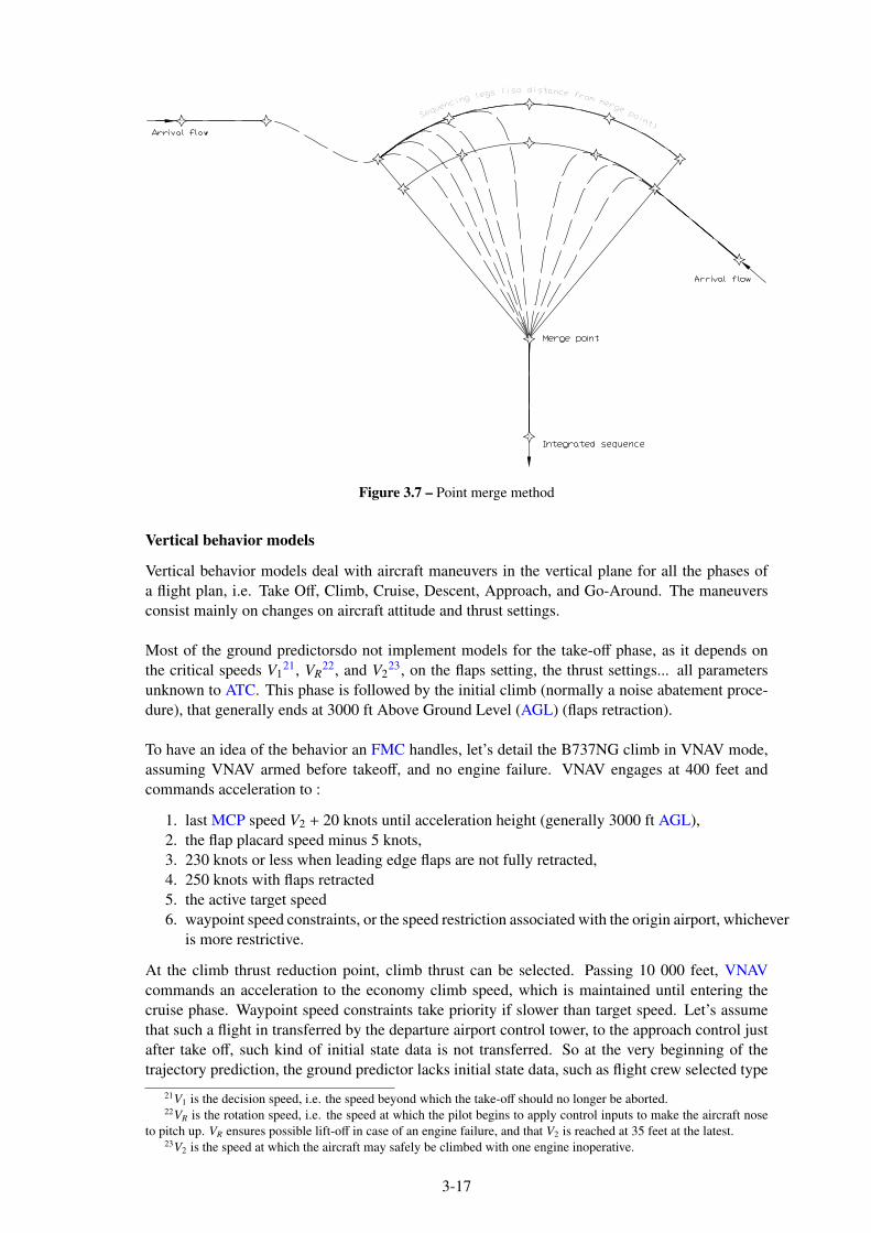
Figure 3.7 – Point merge method

Vertical behavior models

Vertical behavior models deal with aircraft maneuvers in the vertical plane for all the phases of

a flight plan, i.e. Take Off, Climb, Cruise, Descent, Approach, and Go-Around. The maneuvers

consist mainly on changes on aircraft attitude and thrust settings.

Most of the ground predictorsdo not implement models for the take-off phase, as it depends on

the critical speeds V121, VR

22, and V223, on the flaps setting, the thrust settings... all parameters

unknown to ATC. This phase is followed by the initial climb (normally a noise abatement proce-

dure), that generally ends at 3000 ft Above Ground Level (AGL) (flaps retraction).

To have an idea of the behavior an FMC handles, let’s detail the B737NG climb in VNAV mode,

assuming VNAV armed before takeoff, and no engine failure. VNAV engages at 400 feet and

commands acceleration to :

1. last MCP speed V2 + 20 knots until acceleration height (generally 3000 ft AGL),

2. the flap placard speed minus 5 knots,

3. 230 knots or less when leading edge flaps are not fully retracted,

4. 250 knots with flaps retracted

5. the active target speed

6. waypoint speed constraints, or the speed restriction associated with the origin airport, whichever

is more restrictive.

At the climb thrust reduction point, climb thrust can be selected. Passing 10 000 feet, VNAV

commands an acceleration to the economy climb speed, which is maintained until entering the

cruise phase. Waypoint speed constraints take priority if slower than target speed. Let’s assume

that such a flight in transferred by the departure airport control tower, to the approach control just

after take off, such kind of initial state data is not transferred. So at the very beginning of the

trajectory prediction, the ground predictor lacks initial state data, such as flight crew selected type

21V1 is the decision speed, i.e. the speed beyond which the take-off should no longer be aborted.22VR is the rotation speed, i.e. the speed at which the pilot begins to apply control inputs to make the aircraft nose

to pitch up. VR ensures possible lift-off in case of an engine failure, and that V2 is reached at 35 feet at the latest.23V2 is the speed at which the aircraft may safely be climbed with one engine inoperative.

3-17

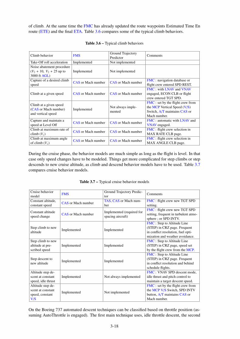
of climb. At the same time the FMC has already updated the route waypoints Estimated Time En

route (ETE) and the final ETA. Table 3.6 compares some of the typical climb behaviors.

Table 3.6 – Typical climb behaviors

Climb behavior FMSGround Trajectory

PredictorComments

Take-Off roll acceleration Implemented Not implemented

Noise abatement procedure

(V2 + 10, V2 + 25 up to

3000 ft AGL)

Implemented Not implemented

Capture of a desired climb

speedCAS or Mach number CAS or Mach number

FMC : navigation database or

flight crew entered SPD REST.

Climb at a given speed CAS or Mach number CAS or Mach number

FMC : with LNAV and VNAV

engaged, ECON CLB or flight

crew entered TGT SPD.

Climb at a given speed

(CAS or Mach number)

and vertical speed

ImplementedNot always imple-

mented

FMC : set by the flight crew from

the MCP Vertical Speed (V/S)

Switch, A/T maintains CAS or

Mach number.

Capture and maintain a

speed at Level OffCAS or Mach number CAS or Mach number

FMC : automatic with LNAV and

VNAV engaged.

Climb at maximum rate of

climb (Vy)CAS or Mach number CAS or Mach number

FMC : flight crew selection in

MAX RATE CLB page.

Climb at maximum angle

of climb (Vx)CAS or Mach number CAS or Mach number

FMC : flight crew selection in

MAX ANGLE CLB page.

During the cruise phase, the behavior models are much simple as long as the flight is level. In that

case only speed changes have to be modeled. Things get more complicated for step climbs or step

descends to new cruise altitude, as climb and descend behavior models have to be used. Table 3.7

compares cruise behavior models.

Table 3.7 – Typical cruise behavior models

Cruise behavior

modelFMS


torComments

Constant altitude,

constant speedCAS or Mach number

TAS, CAS or Mach num-

ber

FMC : flight crew new TGT SPD

setting.

Constant altitude

speed changeCAS or Mach number

Implemented (required for

spacing aircraft)

FMC : flight crew new TGT SPD

setting, frequent in turbulent atmo-

sphere ; or SPD INTV.

Step climb to new

altitudeImplemented Implemented

FMC : Step to Altitude Line

(STEP) in CRZ page. Frequent

in conflict resolution, fuel opti-

mization and weather avoidance.

Step climb to new

altitude at pre-

scribed speed

Implemented Implemented


(STEP) in CRZ page, speed set

by the flight crew from the MCP.

Step descent to

new altitudeImplemented Implemented


(STEP) in CRZ page. Frequent

in conflict resolution and behind

schedule flights.

Altitude step de-

scent at constant

speed, idle thrust

Implemented Not always implemented

FMC : VNAV SPD descent mode,

idle thrust and pitch control to

maintain a target descent speed.

Altitude step de-

scent at constant

speed, constant

V/S

Implemented Not implemented

FMC : set by the flight crew from

the MCP V/S Switch, SPD INTV

button, A/T maintains CAS or

Mach number.

On the Boeing 737 automated descent techniques can be classified based on throttle position (as-

suming AutoThrottle is engaged). The first main technique uses, idle throttle descent, the second

3-18

one partial throttle descent. Each of these two main techniques can be refined is a PATH DE-

Scent (PATH DES) or SPeeD DEScent (SPD DES). The FMC handles mainly two idle thrust

behaviors :

1. In a ECONomy PATH DEScent (ECON PATH DES) descent the FMC uses idle thrust and

pitch controlpitch control to maintain a vertical path, similar to a glideslope in 3 dimensions.

The indicated Target Speed (TGT SPD) is used for "planing purposes" only. There is no at-

tempt to maintain the TGT SPD unless the airplane gets out its flight envelope. PATH DES

guarantees crossing altitudes and varies the pitch angle to make the altitude. Speed is sacri-

ficed and the pilot is responsible for speed control. The end of descent altitude is the altitude

restriction for the End of Descent (E/D) waypoint.

2. In a ECONomy SPeeD DEScent (ECON SPD DES), the FMC uses idle thrust and pitch to

maintain a target descent speed, similar to a Level Change descent. SPD DES is not path

constrained ; i.e. if the airplane is above the path, the flight crew must select speed brakes

or increase the TGT SPD. Speed will not vary and the airplane may or may not follow a

crossing restriction. The end of descent altitude is 1,000 feet above destination airport or,

the lowest "AT" altitude constraint, whichever is lower.

In both cases the TGT SPD is computed by the FMC.

If manual entry is made by the pilot, e.g. 0.72M in the ECON PATH DES page, or the ECON SPD DES

page, TGT SPD field, the manual PATH DES or the manual SPD DES page for that value displays

respectively M.720 SPD DES and M.720 SPD DES.

If a PATH descend, i.e. a descent that guarantees crossing altitudes, is not available the TGT SPD

field is blank.

The preceding detailed descent modes presentation shows that the previous behaviors can hardly

be modeled by ground predictors, as they have no idea of the descent mode chosen by the crew.

Atmosphere complicates further the problems, as engine bleed air (used for anti-ice) put throttle

above full idle. For precise descent path calculation, the B737 Descent Forecast Page FMC page

allow the flight crew may enter forecast wind data, for up to three descent altitudes, and the alti-

tude that anti-icing is turned on and off. This kind of information changes the aircraft performance

at fixed flight levels, and is not known to the ground predictors. Table 3.8 compares the descent

behaviors models.

Table 3.8 – Typical descent behaviors models

Descent behavior

modelFMS


torComments

Constant speed

descentImplemented

Implemented using TAS,

CAS or Mach

FMC : SPD DES mode using CAS

or Mach.

Constant speed and

constant V/SImplemented Not implemented

FMC : flight crew setting via

MCP.

Constant speed and

constant FPAImplemented Implemented

FMC : flight crew setting via MCP

SPD INTV button, entered runway

extension fix.

Idle thrust Implemented Implemented FMC : VNAV PATH

Non Idle thrust

(anti-ice ON)Implemented Not implemented

FMC : altitude layer with anti-ice

ON (TAI ON/OFF) flight crew

entry.

Constant FPA Implemented Implemented

FMC : part of a ARINC 424 proce-

dure or flight crew entered runway

extension fix.

Level Off during

descent at specific

speed

Implemented ImplementedFMC : ALT INTV followed by

SPD INTV

3-19

Descent is today a matter of concern as Continuous Descent Operations (CDO) is recommended

[72], and should be initiated from the highest possible level to reduce fuel burn, noise and emis-

sions. For both ground and airborne predictors, the descent calculation will use the forecast winds,

which are inevitably different to the actual descent winds. Our work on Wind and Temperature

Networking (WTN) may provide to both airplanes and ground predictors, accurate and updated

wind and temperature information.

At this place of reading, tools for trajectory description and aircraft behavior have been presented,

and the reader should have an idea of what has to be modeled. Next step is to select the mathe-

matics tools to simulate the airplane flying its trajectory.

3.3.4 Mathematical models used in operational trajectory predictors

Integration methods

In the present subsection "integration" of equation, is the technique used to solve ordinary differ-

ential equations Ordinary Differential Equations, or a set of Differential and Algebraic Equationss.

Operational ground or airborne trajectory predictors use mathematical models either to solve equa-

tions of motion, or geometric algorithms to predict trajectories.

Some systems integrate equations of motion to define the lateral path, but most of the time, the

lateral path is geometrically approximated. The B737NG FMSs performs geometric approxima-

tion, this could be explained by the fact that the horizontal trajectory is made of a sequence of

waypoints, defined by WGS84 coordinates. The lateral path is defined in terms of straight seg-

ments and arcs of circle, which begin and end at either fixed or floating geographical point. The

FMC monitors the cross-track and the track angle error to issue commands to the Autopilot Flight

Director System (AFDS). The AFDS maintains the airplane on the ground track, and the FMS

knows about current and future TAS, current winds and position. Thus Ground Speed (GS) cal-

culation can be done for the current24 and the next segments. Ground predictors may proceed the

same way, but with assumed TAS and winds.

If outside a cruise phase, a new integration is then performed to get the vertical path25. This

integration is done forward, or backward, for both the vertical and the longitudinal equations of

motion, giving versus time, altitude, and longitudinal position along the ascending or descending

trajectory.

Ground predictors integration methods use :

i) Forward Euler’s method

ii) Backward Euler’s method

iii) Runge-Kutta 2nd order method

or a combination of the three methods26. Details on i), ii), iii) are given in Appendix F.

For airborne trajectory predictors, i.e. FMSs and FMCs the integration methods are kept secret by

their manufacturers.

24The instantaneous ground speed is calculated not by the FMC but by the IRS. Wind speed and wind direction

(true) is also calculated by the IRS using TAS provided by the ADC.25Lateral path and vertical path are interdependent as they are coupled through the ground speed parameter.26We were not able to find out whether the combination of Forward and Backward Euler is used to check if both

generated trajectories are similar.

3-20

Lateral Math Models

Lateral math models are used to calculate the path between two waypoints, i.e the path of the leg

if we use ARINC 424 terminology. Straight segments and arcs of circle have to been modeled.

Most of the predictors use constant course or great circles for the straight segments, new FMS use

WGS84 pseudo circles. Arcs of circle are modeled using constant radius turn implementation or

variable bank angle implementation.

Vertical Math Models

Vertical math models can be divided in two categories :

1. Math models requiring aircraft thrust knowledge, to solve equations for trajectory predic-

tion ;

2. Math models solving constant altitude equations for trajectory prediction.

The first category generally use kinetic equations of motion (see 3.4) and thrust models27 includ-

ing :

• Max cruise,

• Maximum climb,

• Idle thrust,

• Derated maximum climb (minus 3% or minus 6% of maximum climb on B737NG),

• Take-off,

• Derated take-off,

• Maximum continuous

The vertical models can be further broken down, according to whether they use constant vertical

speed, constant Flight Path Angle or combination of constant vertical speed and constant horizon-

tal speed.

The second category generally use kinematic equations of motion, and a defined acceleration/de-

celeration rate function of the altitude. Ground predictors use only one of the two previous models,

whereas FMS use both.

On the B737NG, two more math models, based on polynomial equations, are used to model the

ground roll acceleration and the constant CAS take-off. The duration of this phase does not jus-

tify such a detailed modeling by the ground trajectory predictors. On commercial airplanes, the

trip fuel includes the fuel for take-off and accurate fuel predictions have to been calculated by the

FMC, this explains their need to model the take-off and the initial climb phases.

All the trajectory predictors need the Aircraft Performance Model (APM) for the airplane they are

predicting the trajectory. APM includes jet, turboprop , and reciprocating engines models. The

model database stores in a aircraft/engine model data like thrust, fuel flows, flight envelope, thrust

limits, speeds, acceleration/deceleration rates... The same database may be used by trajectory pre-

dictors using kinetics or kinematics models. EUROCONTROL BADA28 APM is used to provide

performance for nearly 400 types of aircraft.

APMs used by FMS generally contain more detailed data as they model a single aircraft, and get

full access to the aircraft manufacturer performance data, even those confidential, for all configu-

rations (e.g. clean, take-off, approach, landing, engine out ...).

27All thrust limit values depend on outside air temperature.28BADA Aircraft Performance Model differs as it is based on the Total Energy Model (rate of work done by forces

acting on the aircraft = rate of increase in potential and kinetic energy), rather than on classical equations of motion.

It models thrust and drag of the aircraft, and calculates the resulting horizontal and vertical motion of the aircraft

considered as a point-mass.

3-21

Having the Input state data, the constraints handled, the airplane behavior models, and the mathe-

matics tools to simulate the flight, it is time to calculate the trajectory.

3.3.5 Output trajectory data

As shown on figure 3.2, the predicted trajectory is one of the exports provided by the trajectory

predictor. Ground predictors return data related to lateral trajectory at each predicted point like :

• X,Y coordinates related to a local reference system (see 3.6)

• Latitude/Longitude

• Position along path

• True course

• Heading (magnetic or true)

• Turn waypoint

• Turn radius

• Turn center

The B737NG FMS outputs Cross-track Error (XTK ERROR). It does not return any predicted po-

sition, but returns a set of straight lines and arcs. This can be explained as it calculates, after flight

crew entrance of desired route and flight data, commands for manual (flight director) or automatic

(autopilot) flight path control. The airplane is supposed to be on its predicted track, already en-

tered. From 3.3.4 we learned that the lateral path was geometrically approximated, and that the

trajectory is described as a series of straight segments and arcs of circle, so the FMS outputs are

in accordance with its trajectory design. All the navigational computations are based on an FMC

system position derived from both Inertial Reference System (IRS)29 Position L/R, and the radio

position (obtained from both GPS Position L/R, DME-DME, ILS LOC, or VOR/DME updating

when these radio aids are available). The current position, WGS84 coordinates, is available and

may be transmitted via a downlink POSITION REPORT, if the company datalink option is avail-

able.

Trajectory predictors, apart from providing Estimated Time Over over waypoints, also output ver-

tical and speed data. Table 3.9 compares some of them for ground and airborne predictors.

Table 3.9 – Trajectory Predictors Output Data

Descent behavior model FMSGround Trajectory Predic-

torComments

Predicted altitude Implemented Implemented

Mach Implemented Not always implemented

CAS Implemented Not always implemented

TAS Implemented Implemented

GS Implemented Implemented

Vertical Speed Not implemented Implemented FMS : IRS data.

Flight Path Angle Implemented Not always implemented

FMSs generally do not output the Ground Speed (GS) through their trajectory prediction function,

as it is solely responsible for computing the predicted aircraft profile along the entire specified rout-

ing. GS calculation is carried out by the IRS or GPS subsystems of the FMS. It will be included

on the Mode S Enhanced Surveillance parameters for all airplanes, with a maximum cruising true

airspeed capability greater than 250 knots, operating in Instrument Flight Rules (IFR) within the

29The IRS L/R (Left/Right) senses and computes linear accelerations and angular turning rates about each of the

airplane’s axis. It combines them with air data inputs to compute Attitude ( pitch, roll, and yaw), position (latitude

and longitude), true and magnetic heading, inertial velocity vectors, linear accelerations, angular rates, track angle,

wind speed and direction, inertial altitude, vertical speed and acceleration, ground speed, drift angle, flight path angle

and acceleration. Barometric altitude is used to stabilize the vertical navigation, , i.e. the vertical velocity and inertial

altitude outputs.

3-22

European airspace by 7 June 202030.

Due to its guidance objective, the B737NG FMS provides the following specific descent informa-

tion not available on ground predictors :

• FPA is the actual flight path angle based on current ground speed and vertical speed, that is,

the present vertical bearing being flown.

• Vertical Bearing (V/B) is the vertical bearing direct from current position on the WPT/ALT

line, that is, the flight path angle required if flying direct to the active (i.e. next) waypoint

and altitude on the WPT/ALT line of the CDU.

• V/S is the required vertical speed, in feet per minute and based on current ground speed, to

fly the displayed V/B.

The B737NG FMS outputs also a Vertical Descent Path Deviation (VERT DEV), current deviation

(feet HI or LO) from the computed vertical path, to the Control Display Unitss (CDUs) and to the

Electronic Flight Information System (EFIS) map display. This deviation is always in relation to

the path descent profile.

Having an idea of the output trajectory data, let’s see how the airplane is modeled using classical

mechanics.

3.4 Experimental Trajectory Prediction Mathematical models

The FAA report « Literature Survey of Trajectory Predictor Technology » [16] classified the subset

of 20 papers (3.2) using mathematical models as follows :

1. Point-Mass models : the rotational moments are ignored, i.e. models using 3DOF equations

of motion. One limitation of such models is the inability to model a holding pattern, which

mean an time prediction error of at least four minutes for a 1 minute holding pattern.

2. Kinematics models : only position, heading and speed data are considered. This models

deals mainly with the geometry of translational and rotational motion, the aircraft perfor-

mance parameters are ignored, i.e. the motion is studied without considering its causes.

3. Kinetic models : moments and aircraft performance parameters are taken into account.

Forces (thrust/drag, lift/weight) acting on the airplane are modeled. Its performance con-

straints (climb or descent rate, speeds, altitudes,...), its flight envelope may or may not be

taken into account.

4. Other models : models that do not fall in one of the three above categories.

The FAA report pointed out that most of the subset of 20 papers (3.2) use Point-Mass model and

even mentioned « the overwhelming number of papers that used point-mass models ».

A more simple classification can be chosen :

• Kinematics models : studies the motion of objects without consideration of the circum-

stances leading to the motion.

• Dynamics models : studies the relationship between the motion of objects and its causes.

30When flying in an area covered by Radar, information provided by Air Navigation Service Providers (ANSPs)

show that the value of GS is not providing a significantly better accuracy than the ground speed calculated by the

surveillance data processing systems [23].

3-23

Pilots hardly understand the difficulties of predicting an airplane trajectory for an ATC ground sta-

tion as they all filled this kind of "navigation log" for their first enroute flights. The main difference

between their "navigation log" and the ATC assumed airplane trajectory is the available informa-

tion. For pilots, they knew the route that they will fly, and they had all the detailed information to

calculate each leg. They had the last meteorological forecast, and the detailed information on their

airplane performances. This is to say that to predict an airplane trajectory, three parts need to be

modeled :

• the atmosphere,

• the trajectory,

• the airplane.

Concerning the airplane, Trajectory Prediction (TP) deals with the analysis of its motion. If we

agree that Newton’s laws and the slide rule took men to the moon (and back alive on the Earth),

we should agree that trajectory analysis could be done using a deterministic approach. This choice

being made, the equations governing the movement of the airplane can be obtained using several

formalisms :

• vectors formalism flight dynamics,

• tensor flight dynamics,

• energy formalism,

The axis systems used to resolve the forces acting on an airplane are discussed in section 3.6 and

detailed in Appendix A. The shape and complexity of the equations depend on the chosen axis

system.

Finally numerical integration has to be performed to calculate the output trajectory.

3.5 Modeling the trajectory

At the beginning of RNAV, the avionics systems were designed to fly the aircraft only from point to

point, and the trajectory was modeled as a string of individual path geometry segments consisting

of :

• a start point

• a line to point

With the evolution of avionics, trajectories with arc to point segments31 appeared, and much more

sophisticated segments. Even with today "Free Trajectory" concept, SIDs, STARs, TMA and in-

strument approaches must be designed to depart from, or to arrive to, an airport. These trajectories

must be flyable automatically with modern FMSs and autopilots. From this constraint comes the

need for the navigation data to be stored and and loaded. ARINC 424 is the recommended stan-

dard for the preparation and transmission of data for the assembly of airborne system navigation

databases. Both lateral and vertical navigation can be coded using ARINC 424.

A series of leg types coded sequentially into a navigation database makes a flight procedure (e.g.

SID). The navigation database allows FMSs or GPS navigators to create a continuous display of

navigational data, thus enabling an aircraft to be flown along a specific route.

31Based on the ellipsoid model taken for WGS84 coordinates, flying at constant altitude between two points is not

exactly an arc.

3-24

3.5.1 ARINC 424

ARINC 424 has nothing to do with a mathematical representation of the 3 dimensions airspace,

but it can describes IFR routes and procedures, designed using standardized specifications and

criteria :

• ICAO PANS-OPS Doc 8168 volume II in Europe,

• TERminal instrument ProcedureS in the USA

ARINC 424 data, associated with the aircraft navigation system software, provides a source of

navigation reference. ARINC 424 leg types provide vertical guidance and ground track for a spe-

cific flight procedure, thus they provide repeatable flight tracks for the procedure design. The path

and terminator concept describes the navigation database leg type. In other words, a path/ter-

minator is a means of prescribing the way in which a path must be flown, and how the path must

be terminated32. ARINC 424 describes 23 leg types by their path and terminator (among them,

11 path/terminators are available in the majority of aircraft that are expected to be approved to fly

RNAV SID, STAR and Approaches, i.e. not all legs type are supported with roll steering guidance).

When reaching the terminator, the next leg is automatically sequenced, thus a series of leg types

are coded into a navigation database to make a flight procedure. Using FMS and autopilot the

aircraft can be flown, automatically, along a specific route. Vertical navigation can also be coded.

ARINC 424 is also used for En Route navigation, as all airway segments in all databases are Track

to a Fix legs (TF legs). This type of path/terminator leg is the great circle track between two fixes.

Even for transcontinental flights tracks as the Reduced Lateral separation (RLat) North ATlantic

Organized Track System (NAT-OTS)33, the great circle track between two fixes is a Track to a Fix

(TF) Leg.

Thinking about implementation, one must consider that each of the 23 path/terminators could be

followed by each of the other 23 path/terminators, and that ARINC 424 denies some legs to follow

other particular legs.

It seems obvious that if aircraft fly ARINC 424 trajectories, those must be available in any tra-

jectory predictor, as at least constraints (see Fig. 3.2). This explains also the agreement on not

distinguishing airborne and ground systems pointed out in 3.2.2.

3.5.2 Other mathematical models

More complex mathematical models can be used to interpolate a given set of waypoints [30].

Interpolating methods uses :

• Lagrange or Hermite interpolation polynomials

• Piecewise linear, quadratic, cubic or cubic splines interpolation,

• Bèzier Approximation Curve,

• Uniform B-Splines of degree zero, one or three,

• Principal Component Analysis when trajectories samples are available.

These models are mainly used during the design of a procedure, or during an optimization phase.

Once design and implementation are completed, the procedure must be translated into ARINC

424 database to be flyable by an FMS/autopilot system, or a cheapest FMS/autopilot system, i.e.

an autoflight system.

32Two characters in the database are associated to every path/terminator : the first column specifies the path to be

flown and the second column specifies how the path should be stopped. For example (CI) specifies that the equipment

should fly a course and that it should end at next path interception.33RLat will allow aircraft to be separated laterally by a minimum of 25 NM (previous separation was 1 of latitude,

i.e. 60 NM), improving the efficiency of North Atlantic operations.

3-25

3.5.3 Trajectory segments characteristics

Beyond the modeling of the segment, each must be assigned a characteristics. This characteristic

is listed by ARINC 702A-4 standard defining the characteristics of an advanced FMC system. It

was updated in November 2014, to add winds and temperature definitions, as required to support

4D trajectory operations in NextGen and SESAR airspace environments. This update encouraged

us to continue our work on Wind and Temperature Networking, i.e. sharing wind and temperature

among aircraft. The listed characteristics are :

• Start of climb

• Level-off

• Unnamed fix (e.g. a user defined waypoint to optimize the routing)

• Runway

• Top of climb

• Crossover altitude

• Aircraft projection

• Start of descent

• Top of descent

• Transition altitude/level

• Non-flyable

• RTA point

• End of descent

• Speed change

• Discontinuity

• Clearance Altitude Level off

A lot of mathematical models exist for aircraft trajectory design and representation [30], but for

the time being, discontinuities (e.g. open-ended flight maneuvers such as vectoring to a fix along

the final approach course prior to the Fianl Approach Fix (FAF)) are not taken into account by

trajectory predictions systems.

Airlines, air navigation database providers and avionics providers agreed on the elements of the

trajectory to model using ARINC 424, it is now necessary to set up the mathematical tools to

represent this trajectory. It’s time to present coordinates and frames.

3.6 Reference frames

As trajectory predictors goal is to predict the aircraft future 4D position, coordinate and frame

systems are needed to locate those positions, independently of any mathematical operation (e.g.

derivation or integration). There is not yet a standard definition about frames and coordinate

systems. Definitions were given in 2003 by Brian L. Stevens and Frank L. Lewis [134] :

• Reference frame : three or more noncolinear points on a rigid body define a reference frame.

The location of a point or vector in a frame is expressed using a specified coordinate system.

• Coordinate system : a measurement system for locating points in space and attached to a

reference frame.

They were revised in 2016 by Brian L. Stevens, Frank L. Lewis and Eric N. Johnson [135] in :

• Frame of Reference : A rigid body or set of rigidly related points that can be used to establish

distances and directions (denoted by Fi, Fe, etc.). In general, a subscript used to indicate a

frame will be lowercase, while a subscript used to indicate a point will be uppercase.

• Coordinate System : A measurement system for locating points in a frame of reference.

We may have multiple coordinate systems (with no relative motion) within one frame of

reference, and we sometimes loosely refer to them also as "frames".

3-26

The problem of the standardization of coordinate systems should not be underestimated, as both

EUROCONTROL and the Institute of Geodesy and Navigation (IfEN) stressed in 1998 in the

first pages of their "WGS 84 IMPLEMENTATION MANUAL" [39] : “Thus - the main source

of systematic errors is the non-use of a common geodetic reference datum for quoting the radar

positions and its solution is to derive the radar positions in a common system.”. No doubt that this

standardization must be addressed in Trajectory Prediction to avoid the problem shown in figure

3.8 from [39].

In the present document, and particularly in Appendix A, we associated to each frame a Cartesian

coordinate system, we thus speak of a frame as a coordinate system associated to a frameCoordinate

system associated to a frame! (Coordinate system associated to a frame!).

Radar

Datum 1

Radar

Datum 2

Horizontal Aircraft

Position

Datum 2Datum 1

Positional discrepancy ≈ 100m - 3000m

Figure 3.8 – Positional discrepancy due to different geodetic reference datum

source : WGS 84 IMPLEMENTATION MANUAL [39]

3.6.1 Standards

At least four standards try to define coordinate systems :

• ISO [53], published in 1988, gives basic definitions and deals with aircraft motion relative to

the atmosphere, assumed to be at rest or in translational motion at constant velocity relative

to the Earth. It describes axis systems, angles, velocities and angular velocities.

• ANSI/AIAA R-004-1992 [5] defines atmospheric and space flight vehicle coordinate sys-

tems.

• IEEE 1278 Distributed Interactive Simulation (DIS) [2] uses Geocentric Coordinates for the

3-D location of an entity. Position and orientation are taken into account, using WGS84

elliptical Earth model. Units in meters and radians.

• ANSI/AIAA S-119-2011 [54] was built above American Nation Standards Institute (ANSI)

and International Standards Organization (ISO) standards to spell out several conventions

for axis systems, unambiguous variable names, abbreviations of units of measure and sign

conventions for use in modeling flight dynamic vehicles.

Unfortunately these standards use orthogonal right-handed triads, whereas airplane navigation use

latitude, longitude and altitude. ICAO position on the matter is clear, as stated in “ICAO adopts,

as a standard, the geodetic reference system WGS84 and develops appropriate ICAO material,

particularly in respect of Annexes 434 and 1535, in order to ensure a rapid and comprehensive im-

34Aeronautical Charts.35Aeronautical Information service.

3-27

plementation of the WGS84 geodetic reference system.”.

The ISO/IEC 18026:2009(E) standard "Information technology - Spatial Reference Model (SRM)"

[81], supports unambiguous specification of the positions, directions, distances, and times associ-

ated with spatial information, e.g. aircraft position. It defines algorithms for precise transformation

of these properties between spatial reference frames, but seems not be used in aviation.

3.6.2 Standards equivalent coordinate systems

The "Geocentric Earth-Fixed Coordinate System" described in ANSI/AIAA S-119-2011 [54] is

identical to IEEE 1278 DIS [2] "Geocentric Cartesian Coordinate System".

The "Body Coordinate System" in ANSI/AIAA S-119-2011 [54] is identical to the IEEE 1278

DIS [2] "Entity Coordinates System".

3.6.3 Number of coordinate systems to consider

The minimum number of coordinate systems to consider to derive the equations of motion of an

airplane depends on literature and on simplifying assumptions. If aircraft stability is not con-

cerned, the following axes systems are cited :

• Nelson (1989) [101] considers the "aircraft body-fixed reference frame" (A.2.8) and the

"inertial reference frame" (A.2.5).

• Yechout (2003) [152] considers the "Body Axis System" (A.2.8), the "Earth Axis System".

• According to Diston (2009) [32], we should consider the "Platform Axis System" (A.2.8),

the "Ground Axis System" (A.2.5), the "Navigational Axis System" (A.2.7), and the "Earth-

Centred Axis Systems" (A.2.3).

• For Durham (2013) [33], the "inertial reference frame" (A.2.2), the "earth-centered reference

frame" (A.2.3), the "earth-fixed reference frame" (A.2.5), the "local-horizontal reference

frame", the "Body-fixed reference frames" (A.2.8) ant its variants, the "Wind-axis system"

(A.2.9) and the "Atmospheric reference frame" should be considered.

The reference frames used to resolve the forces acting on an airplane, and to define its position are

detailed in Appendix A. Due to the existence of different coordinate systems, the equations take

different forms, and comparisons between trajectory predictors are made more difficult. Further-

more the calculated variables differ also, complicating the interoperability of the different predic-

tors.

3.7 Aircraft attitude

From section 3.6, we learned that we need a minimum of two reference frames to derive the equa-

tions of motion, before solving them to get the aircraft position. In other words, to fully determine

an airplane position and orientation in a three dimensional Euclidean space, we need two orthonor-

mal bases. The orientation of the axis directions of one of the basis with respect to the other need

also to be known. In aviation this orientation is called attitude and concerns mainly the orienta-

tion of the body frame (A.2.8) with respect to the Earth fixed NED frame (A.2.5). From modern

airliners to UAVs, flight navigation and control use strapdown Inertial Navigation Systems36, i.e

the sensors are attached rigidly ("strapped down") to the airplane body. Three accelerometers, and

three gyroscopes are needed because an aircraft can simultaneously accelerate and rotate about

three axes37. The input axis of one accelerometer is always in the longitudinal axis, one is in the

lateral axis, and one is in the vertical axis. The gyroscope are mounted such that one gyro senses

36Strapdown indicates that the gyroscopes and accelerometers are mounted solidly to the aircraft, eliminating the

need for gimbals, bearings, and torque motors to keep the sensors level with the surface of the earth.37New liner IRSs use Ring Laser Gyro The laser gyroscopes and microprocessors to maintain a stable platform

mathematically, rather than mechanically.

3-28

roll, one senses pitch, and the other senses yaw.

Each accelerometer measures the motion of the aircraft in one of the three directions of travel,

while the three gyroscopes are used to obtain the attitude (orientation). Accelerations are com-

puted analytically using Direction Cosine Matrix (DCM) relating body coordinated and local level

navigation frames. The DCM elements are calculated using strapdown body mounted gyro out-

puts. With the information from these sensors, the heading, speed and position of the aircraft can

be computed, provided the following are available :

• initial position (Gate position position is normally entered through the FMC CDU during

FMS preflight)

• barometric altitude (provided by the altimeter),

• true airspeed (provided by the Air Data Computer (ADC)),

• local vertical (self alignment during the flight crew full alignment of the IRS),

• initial heading (self alignment during the flight crew full alignment of the IRS),

Trajectory predictors using Point-Mass models were little concerned by attitude, but the ARINC

702A Supplement 3, modified the ’Trajectory Reporting - Aircraft State Data’ to include the roll

angle. Attitude seems to start to be considered, as 4D Trajectory Based Operations need trajectory

predictors able to model (and anticipate) turns and holding patterns.

From the pilots point of view, taking into account the attitude of the aircraft is an evidence, as from

the first flying lessons they learned that the primary effect of each main flight control (elevators,

ailerons and rudder) is to pitch, roll or yaw the airplane. At constant power, pitching the aircraft

first changes its vertical trajectory, rolling the aircraft first changes its horizontal trajectory. They

learned that at constant power, any change in the aircraft attitude, specially the pitch and the bank

angle changes the trajectory. All this can be explained by the moments caused by displacing the

primary control surfaces.

As mentioned in 3.2.3, the flight dynamics models based on the 6DOF equations of motion models

provide the best accuracy, but they are expensive to develop and greedy in computing resources.

During the past, these two pitfalls were bypassed as ATM trajectory predictors were using Aircraft

Performance Model kinematics methods (EUROCONTROL General Aircraft Modelling Envi-

ronment (GAME), look-up table models) or hybrid kinetic methods (EUROCONTROL Base of

Aircraft DAta (BADA)).

On the same time, aircraft manufacturers were using 6DOF equations of motion models for aircraft

design information, flight tests and certification. The produced performance tables were stored in

their FMS performance database. In other words, the performance database contains the average

model of the aircraft and the engines, i.e. the aerodynamic and engine models. The attitude of

the aircraft was a concern at the very beginning, not only because of the design using the 6DOF

model, but also as the primary source of attitude, velocity, and position information were the Iner-

tial Reference System (IRS).

With the new accuracy requirements of ATM trajectory prediction, and the lack of time to de-

velop new ground trajectory predictors, the requirements for aircraft reports evolved to Mode S

Enhanced Surveillance (EHS)38 . The new transponders maintain avionics data in 256 different 56

bit wide Binary Data Store (BDS) Registers, that can be loaded with information readable by ATC

ground system. The detailed information can be found in ICAO Doc. 9871 AN/464 [79], but we

are particularly interested in the following Comm-B39 Data Selector (BDS) :

38Liners compliance deadline within Europe : 7 June 202039Comm-B : a 112-bit reply containing the 56-bit MB message field. This field is used by the downlink Standard

Length Message, ground-initiated and broadcast protocols [79].

3-29

• BDS code 4,0 - Selected vertical intention, provide ready access to information about the

aircraft’s current vertical intentions, in order to improve the effectiveness of conflict probes

and to provide additional tactical information to controllers.

• BDS code 5,0 - Track and turn report, used to provide track and turn data to the ground

systems.

• BDS code 6,0 - Heading and speed report, to provide track and turn data to the ground

systems.

Looking at the content of these Comm-B Data Selector fields, we get :

• BDS code 4,0 : MCP/FCU selected altitude, FMS selected altitude, barometric pressure

setting, target alt source.

• BDS code 5,0 : roll angle, true track angle, ground speed, track angle rate, True Air

Speed (TAS).

• BDS code 6,0 : magnetic heading, Indicated Air Speed (IAS), Mach number, barometric

altitude, inertial vertical velocity.

This development confirmed our continued work on the Wind and Temperature Networking. ATC

now requires aircraft to provide magnetic heading, true track, ground speed, and air speed infor-

mation. Associated with magnetic declination, this information makes it possible to calculate the

direction and strength of the wind (thus reproducing the calculations already carried out on board

by the IRS coupled to the ADC).

The evolution of the transponder requirements also show that, following airplane spacing reduction

and needs of future Air Traffic Management systems, aircraft attitude is now taken into account,

and must be addressed by future ground trajectory predictors. How then to represent the aircraft

orientation in the 3D space ? What mathematical tools are available ?

This leads us to Leonhard Euler (1707-1783) theorem40 stating, any arbitrarily oriented reference

frame may be aligned to an other reference frame by three successive rotations about the axes of

the reference frame. The order of the rotations may by arbitrary but matters, the same axis may

not be used twice in the sequence.

We had in our work to go to Airplane Flight Dynamics, to understand how to represent an aircraft

orientation. We found out that the above theorem, is used in the three main formalisms to represent

the changes to an airplane orientation (i.e. attitude) :

• the Direction Cosine Matrix (DCM)

• the Euler angles (widely used due to inertial navigation systems),

• the quaternions

An alternate formalism can also be used, the angle-axis rotation.

Following the difficulties we encountered in finding a synthesis of the different formalisms, we

included them as appendixes, for future references.

3.7.1 DCM

Direction Cosine Matrix is more related to vector projection41 than to rotation. If a is a vector, it

can be expressed in terms of its coordinates in a frame F1, of unit vectors (i1, j1,k1) with :

a = ax1i1 + ay1j1 + az1k1

40"Any two independent orthonormal coordinate frames can be related by a sequence of rotations not more than three

about coordinate axes, where no two successive rotations may be about the same axis". In other words, "a sequence of

rotations about successive orthonormal coordinate frames will rotate the first frame into the second"41In Appendix B, we referred a projection as an orientation.

3-30

If we define a second frame F2, of unit vectors (i2, j2,k2), and we want to express a in terms of its

coordinates in frame F2, we get :

a = ax2i2 + ay2j2 + az2k2

The operation takes the vector coordinates from one axis system F1 and re-expresses them with

respect to another axis system F2. The Direction Cosine Matrix (DCM) is the matrix that relates

unit vectors defining frame F2 to unit vectors defining frame F1.

The confusion comes from the fact that the mathematical principles are the same between a projec-

tion and a rotation. In a projection, the vector remains fixed and the reference axis system rotates,

whereas in a rotation, the vector rotates and the reference axis system remains the same. Failing

in distinguishing rotation and projection (i.e. orientation) has consequences on the sequencing of

elementary rotations.

Full details on the matter are given in Appendix B.

3.7.2 Euler angles

Euler angles42 sequence specifies an attitude (i.e. orientation) by applying three consecutive prin-

cipal rotations (see 3.7).

Historically Euler angles were used to describe the attitude of vehicles or industrial robots. They

are by far the most popular approach, but they suffer one potentially serious problem : the well

known gimbal lock. This problem was already identified in the Apollo space program (see figure

3.9 and its "gimbal lock" warning indicator) [61] and was prevented by constraining angles [62, p.

10]. These constraints are not a problem for a passengers aircraft, but may be for a fighter aircraft,

or an aerobatics aircraft.

Angles may be measured with respect to fixed space (e.g. ECEF or NED frame), or with respect

to the rotating airplane. In aerospace Tait-Bryan angles are used, i.e. Euler angles which are fixed

with respect to the moving object. Graphics libraries (e.g. OPENGL) provide functions such as

rotateX, rotateY, etc., which are effectively Tait-Bryan angles.

Figure 3.9 – Apollo LEM Display and Keyboard Assembly - c© NASA

The yaw, pitch and roll of an aircraft to which pilots refer are Euler angles, the difference being that

the axis system is carried by the aircraft itself, i.e. the non-inertial body-fixed frame (G, xb, yb, zb)

described in A.2.8.

A detailed description of the Euler angles is provided in Appendix C.

42An Euler angle is an angle of rotation about a coordinate axis.

3-31

3.7.3 Quaternions

Quaternions are widely used in military flight simulators where aerobatics maneuvers are usual,

and also in computer graphics and control theory. They enable the Euler angles to be computed

but avoid the singularity when pitch attitude reaches 90, and are superior for the accuracy and

speed of the calculations [46, p. 21]. The main advantages of using quaternions are :

• avoiding gimbal lock,

• improving computation (successive multiplications are faster and more accurate for quater-

nions than for matrices),

• ease of normalization after many calculations,

• ease of interpolation between quaternions to smoothly rotate objects

Details on quaternions operation are given in Appendix E

3.7.4 Angle-axis representation

Euler proved that any rotation R in R3 can be represented using a single rotation about some axis.

The rotation can be represented in two parts : a vector n along the axis of rotation, and a scalar θ

corresponding to a rotation around the axis. Figure 3.10 illustrates that property : the u vector is

rotated (using the right hand rule) about n through the angle θ, to give the vector v. The n does

not need to be unit vector, but most of the time it is taken as, to constrain four values to three

degrees of freedom, corresponding to the three degrees of freedom necessary for 3D rotations.

(u

‖u‖ ,v

‖u‖ ,n) forms an orthonormal basis for R3 that induces the standard orientation.

The rotation R is usually represented in terms of R(n, θ) or Rn(θ). The rotation formula is given

by :

v = (cos θ)u + (1 − cos θ)(u × n)n + (sin θ)n × u (3.1a)

v = u + (1 − cos θ)n × (n·u) + (sin θ)n × u (3.1b)

x

y

z

un

θ

v

Figure 3.10 – Axis-angle rotation

Compared to other mathematical rotating tools, the Rodrigues’ rotation formula involves no coor-

dinates system, and the rotation angle can be arbitrarily large.

Reference frames section 3.6 and aircraft attitude section 3.7, showed us the available tools to

locate an airplane and its attitude. Next step consist of modeling the airplane and the forces acting

on it, to derive the equations giving the position and the orientation (i.e. attitude).

3-32

3.8 Modeling the airplane and the forces acting on it

As explained in 3.2.3 and 3.4, airplane can be modeled using kinematics or kinetic models. Kine-

matics models are used to solve the following equation :

d(position)

dt= velocity or using arrows for vectors

d(−−−−−−−→position)

dt=−−−−−−→velocity (3.2)

We will not discuss kinematic models as their predictions are based on flight-average information,

from lookup tables, in order to obtain cruise speed, descent rate, and other factors for each aircraft

for a given altitude and temperature. These models are not using Aircraft Performance Model

and seems lacking of the accuracy requested by the ATM modernization initiatives. They are also

based on empirical data collected on flights not always using Continuous Descent Operations, and

whose initial intent may have been altered by ATC instructions. As mentioned in 3.2.2, both the

FAA and EUROCONTROL are looking for trajectory predictors that make usage of the APM.

Let’s then focus on kinetics models.

3.8.1 Modeling the plane motion using vectors classical dynamics

This formalism is the most used [101] and states Newton’s second law as invariant with respect to

inertial coordinate systems. Newton’s second law is related to the translational degrees of freedom,

and yields the translational equations ; Euler’s law controls the attitude dynamics, and produces

the attitude equations. The center of mass of the airplane is used as the reference point, to decouple

the translational and attitude motions.

Following this statement, equations should be derived in an inertial frame, e.g. an ECI frame (see

A.2.2) and can be summarized as [19] :

mAI,G =∑

i

Fexti (3.3a)

dHII,G

dt=

∑

i

MFextG,i (3.3b)

Fexti are the external forces (aerodynamic, propulsivec, weight) as shown on figure 3.11, HI,G is

the angular momentum about the center of mass G, and MFextG,i are the moments of the external

forces about the center of mass G.

Equations 3.3 states that the mass m multiplied by inertial acceleration, equals the sum of the

external forces ; and the time derivative of the angular momentum equals, the sum of the moments

of the external forces.

As written :

• equation 3.3a is Newton’s second law, where the mass m is assumed to be constant, as

Newton’s second law states that the time rate of change of linear momentumd(mV)

dtequals

the sum of the externally applied forces f.

• equation 3.3b is exactly Euler’s law, stating the inertial time rate of change of the angular

momentum equals the externally applied moments.

Many books simplify the derivation of the equations by using the ECEF frame (see A.2.3), so do

not take in consideration the change of orientation of the ECEF frame with respect to the ECI

frame (i.e. neglecting the rotation of the Earth as a function of time and the curvature of the Earth

as a function of position).

From equation 3.3a the Earth environment influence can be seen as :

• gravity varies with altitude and position,

3-33

• thermodynamics state of the air changes aerodynamics and propulsive forces.

Newton’s second law applied to an airplane is related to its acceleration, this is to say to the second

derivative of the airplane position, or to the first derivative of the airplane speed. The six degree of

freedom equations have been derived in many books [19], [133], [135], [37] but can be condensed

as follows [6] using classical flight dynamics notations, and computed in the in the body frame

Fb(G, xb, yb, zb) (see A.2.8) :

u = fu(Fu,m, θ, φ, ψ) v = fv(Fv,m, θ, φ, ψ) w = fw(Fw,m, θ, φ, ψ) (3.4a)

u =

∫

udt v =

∫

vdt w =

∫

wdt (3.4b)

p = fp(Mp, J, θ, φ, ψ) q = fq(Mq, J, θ, φ, ψ) r = fr(Mr, J, θ, φ, ψ) (3.4c)

p =

∫

pdt q =

∫

qdt r =

∫

rdt (3.4d)

Where :

∑

i

MFextG,i =

Fu

Fv

Fw

represents the sum of external forces projected on frame Fb(G, xb, yb, zb).

m is the mass of the airplane, (θ, φ, ψ) are the three Euler angles ( pitch, roll, yaw) describing its

orientation.

∑

i

MFextG,i =

Mp

Mq

Mr

represents the sum of the moments of the external forces projected on frame Fb(G, xb, yb, zb), and

J the airplane inertia matrix.

Vbk

represents the vector Vk projected on frame Fb(G, xb, yb, zb) with :

Vbk =

u

v

w

Vk is the kinematic velocity, i.e. the velocity of the aircraft with respect to the Earth. The integra-

tion of Vk gives the trajectory.

The kinematic angular velocity,Ωk is the angular velocity of the aircraft relative to the Earth with :

Ωbk =

p

q

r

the components (p, q, r) being respectively the roll, pitch and yaw rate. As the body frame is linked

to the aircraft, Ωbk= Ωb

b

The fu, fv, fw functions are used to compute the linear acceleration from the forces, the fp, fq, frfunctions to compute the angular acceleration from the moments. Both equations 3.3 and 3.4 are

the same equations derived in different frames.

Once resolved equations 3.4 variables are used to derive the speed, the position, the roll rate, the

pitch rate, the yaw rate, and the attitude of the aircraft in the NED frame :

VN = t(u, v,w, θ, φ, ψ) VE = t(u, v,w, θ, φ, ψ) VD = t(u, v,w, θ, φ, ψ) (3.5a)

3-34

PN =

∫

VNdt PE =

∫

VEdt PD =

∫

VDdt (3.5b)

θ = t(p, q, r) φ = t(p, q, r) ψ = t(p, q, r) (3.5c)

θ =

∫

θdt φ =

∫

φdt ψ =

∫

ψdt (3.5d)

where :

VNED =

VN

VE

VD

is the kinematic speed vector expressed in the North-East-Down frame.

The position vector expressed in the NED frame is :

PNED =

PN

PE

PD

Using transformation matrices from Appendix A, the position vector can be expressed in the Earth-

Center, Earth-Fixed frame, using Cartesian or WGS84 coordinates.

The t scalar transformations (3.5c) are derived from computation of transformation matrices be-

tween frames (see Appendix A).

3.8.2 Modeling the plane motion using tensor flight dynamics

Tensors fly dynamics models flight dynamics with Cartesian tensors invariant under coordinate or

time transformations. A time operator, the rotational time derivative is used to model flight dy-

namics, in a form invariant under time dependent coordinate transformations. The starting axiom

is that the laws of physics are independent of coordinate systems. The idea was to first model

physics, then to introduce coordinate systems for computation, the point of arrival being that ten-

sors are converted to matrices for computation. This concept was presented by Peter H. Zipfel

[155] at the second Atmospheric Flight Mechanics conference in 1972 (computation was not pre-

sented as neither the IBM PC or the Apple II were born).

This formalism defines a displacement vector for a point B as sBA, where A is a second point,

not necessarily the origin of a coordinate system43. It states that A is a point of frame A, a frame

being an unbounded continuous sets of points over the Euclidean three-dimensions space whose

distances are time invariant44, and which possess a subset of at least three non collinear points

[154]. In 3.8.1 Gibbs vector mechanics is used, and the position is always given with respect to

the origin O of a coordinate system, even if the coordinate system is not chosen.

The method works as follows [154] :

1. formulation of vehicle dynamics in invariant tensor form,

2. introduction of coordinate systems for component presentation,

3. formulation of problems in matrices for computer programming and numerical solutions.

Table 3.10 summarizes the formalism with the following notations :

43In tensor flight dynamics, as described by Zipfel [155], [154], coordinate systems are mathematical abstracts

without physical existence. They relate the components of a vector to Euclidean space. They have measure and

direction, but no common origin.44An other definition is : a frame is a physical entity that models a physical object, consisting of points without

relative movement.

3-35

• scalars considered as zeroth-order tensor and represented using regular fonts,

• vectors (e.g. position, speed, ...) are considered as first-order tensors, and represented by

bolded lower-case letters,

• second-order tensors (e.g. moment of inertia of a body referred to a reference point) are

(represented by bolded upper-case letters).

Table 3.10 – TFD versus Gibbs vector mechanics

Parameter Tensor Flight Dynamics Gibbs vector mechanics

Position sBA

−→r = −−→OB or

r = OB =

xB

yB

zB

OB : O part of implied

coordinate system. sBA :

simple geometric picture,

arrow from A to B, with the

head at B .

Position in a

second framesBA = sBC = s

r = O′B =

x′By′Bz′B

C belongs to frame C but

coincides with point A of

frame A.

Speed vAB =

d

dtsBA = DAsBA v =

dr

dt

[∗]A is a coordinate system

associated with frame A.

Superscript next to the

variable indicates a frame,

not a coordinate system.

DA∗ is the rotational time

derivative with respect to

frame A.

Speed & coordi-

nate system

[

vAB

]A=

d

dt[sBA]A =

[

dsBA

dt

]A

v =dr

dt

Superscript outside the

bracket designates a coordi-

nate system.

Speed in different

frames

[

DC s]A=

[

DA s]A+

[

ΩAC

]A[s]A dr

dt

∣∣∣∣∣C

=dr

dt

∣∣∣∣∣A

+ ωA/C × r

DCs = DAs + ΩACs,

where ΩAC is the skew

symmetric tensor of the

angular velocity vector ωAC

of frame A with respect to

frame C.[

DA s]A=

[

ds

dt

]A

because the coordinate

system [∗]A is associated

with frame A.

Speed in different

frames

[

DC s]A=

[

ds

dt

]A

+ [T ]AC

dT

dt

AC

[s]A

[∗]C is the coordinate sys-

tem associated with frame

C, [T ]AC is the transfor-

mation matrix of coordi-

nates A with respect to C,

[s]A = [T ]AC [s]C .

Speed in different

frames & differ-

ent coordinate

systems

[

DC s]D= [T ]DA

[

DC s]A

]D is an arbitrary allowable

coordinate system. The

rotational time derivative[

DC s]A

transforms like a

first-order tensor

Speed in different

frames & differ-

ent coordinate

systems

[

DC s]D= [T ]DA

[

ds

dt

]A

+ [T ]AC

dT

dt

AC

[s]A

Using Tensor Flight Dynamics the fly dynamics equations can be written as :

DIp = f (3.6a)

DIl = m (3.6b)

Where DI is the rotational time derivative of a vector or tensor with respect to frame I, p the linear

momentum vector, f the external force vector, l is the angular momentum and m the externally

applied moment. These equations are valid in any coordinate system.

3-36

Figure 3.11 – BADA Frames, Forces and angles

Comparing equations 3.6a and 3.6b, with equations 3.3a and 3.3b, we find the same terms, with

the limitation that equations 3.3 are only valid, when derived in an inertial frame associated to a

coordinate system.

3.8.3 Modeling the aircraft motion using energy

Base of Aircraft DAta (BADA) 3 family is a pseudo kinetic aircraft model mainly used in the

ATC simulations, the remainder of this section is related to it. A set of simplified equations is

used to model the aircraft during climb, cruise and descent phases. Figure 3.11 summarize the

forces taken into account by the model. The forces are represented in different frames described in

Appendix A. The center of pressure CP is the point through which the total aerodynamic force can

be thought to be acting, the center of mass CM or G is the point through which the other forces can

be thought to be acting. For stability reasons, the center of mass is always in front of the center

of pressure for a civil aircraft, as it certification requires a naturally stable aircraft throughout the

whole flight envelope. Let’s detail the forces and the angles :

• The thrust delivered by the engines is supposed to be aligned with the aircraft fuselage (i.e.

lies in the xbzb plan), its direction is the Gxb axis of the body frame45 (see A.2.8).

• The weight is aligned with the Gxo axis of the North-East-Down (NED) frame (see A.2.7).

• The drag is aligned with the Gxa axis of the aerodynamic frame (see A.2.9).

• The lift is perpendicular to Gxaya plane of the aerodynamic frame.

• α is the aerodynamic angle of attack, i.e. the angle between the Gxb axis of the body frame

and the plane Gxaya.

• γ is the flight path angle, i.e. the angle between the Gxa axis and the horizontal plane Gxoyo

of the NED frame.

• θ is the pitch angle, i.e. the angle between the Gx axis of the body frame and the plane

Gxoyo.

To derive BADA equations the following assumption are made :

• The sideslip angle β between the body frame and the aerodynamic frame is zero, i.e. the

flight is balanced (for pilots : ball is centered - coordinated flight)46.

45Generally the thrust is tilted up at an angle αT with the fuselage reference line so that the a positive αT correspond

to a component of thrust in the negative zb direction [135].46This means that the stability-axes coordinate system (not presented in Appendix A, but defined in [135, p. 76])

3-37

• The center of pressure and the center of mass coincide.

• the stability-axes coordinate system is an inertial reference frame (as Newton’s second law

will be used to derive the equations).

Projected in the NED frame, the forces give :∑

FxNED= L cos(

π

2+ γ) + T cos(α + γ) + D cos(π + γ) = −L sin γ + T cos(α + γ) − D cos γ

= −L sin γ + T cos(γ + α) − D cos γ∑

FzNED= W + L cos(

π

2+ γ +

π

2) + D cos(π + γ +

π

2) + T cos(α + γ +

π

2)

= −L cos γ +W − T sin(γ + α) + D sin(γ)

In the NED BADA equations are :∑

FxNED= −L sin γ + T cos(γ + α) − D cos γ (3.7)

∑

FzNED= −L cos γ +W − T sin(γ + α) + D sin(γ) (3.8)

Projected in the aerodynamic frame (β = 0), the forces give :∑

Fxa= (T − D) cosα +W cos(

3π

2− γ) = (T − D) cosα −W sin γ

∑

Fza= −L +W cos(2π − γ − α) = −L +W cos(γ + α)

Taking the ATM community axis orientation with the vertical axis up, and α = 047, we get the

standard BADA [102] starting equations :∑

Fhor = T − D −W sin γ (3.9a)

∑

Fvert = L −W cos γ (3.9b)

By rearranging equation 3.9b, taking V = ‖TAS‖, and using Newton’s second law we get :

mdV

dt= T − D −W sin γ (Newton’s second law)

mVdV

dt= TV − DV −WV sin γ ⇔ mV

dV

dt= TV − DV −W

dh

dtwhere

dh

dtis the vertical speed

Wdh

dt+ mV

dV

dt= (T − V)V ⇔ mg0

dh

dt+ mV

dV

dt= (T − D)V

d(mg0h)

dt+

d( 12 mV2)

dt= (T − D)V m is supposed to be constant

dUpot

dt+

dUkin

dt= Force.speed = power

Where Upot is the potential energy, Ukin the kinetic energy, V the true airspeed and h is the geode-

tic altitude (the assumption of a standard constant gravity field derives in identical geodetic and

geopotential altitudes).

The BADA total energy rate equation can be written as [102] :

mg0dh

dt+ mV

dV

dt= (T − D)V (3.10)

Equation 3.10 shows four variables, and to be solved, thrust and drag must be expressed with

respect to speed. Drag could be resolved using equation 3.9b as in level flight the vertical acceler-

ation is zero, and so∑

Fvert is :

0 =∑

Fvert ⇔ 0 = L−W cos γ ⇔ L = W cos γ ⇔ 1

2ρCLS V2 = mg0 cos γ ⇔ CL =

2mg0 cos γ

ρS V2

coincides with the aerodynamic frame.47Most transport jets fly in cruise at an angle of attack round 3 or 4 degrees

3-38

−10 −5 0 5 10 15

−1

−0.5

0

0.5

1

1.5

α()

CL

NACA 2415 Lift Coefficient

Figure 3.12 – NACA 2415 profile Lift Coefficient

To take into account the turns, the lift coefficient formula is multiplied by 1/ cos φ, where φ is the

aircraft bank angle during the turn48.

CL =2mg0 cos γ

ρS V2 cos φ(3.11)

The obtained result for CL seems not related to the angle of attack α, but this is due to the simpli-

fications done on the equations. Figure 3.12 shows a typical NACA profile CL variation with α,

obtained from experimental results.

Once the lift coefficient CL expressed as a function of the true airspeed, it is possible to calculate

the drag coefficient CD as drag coefficient can be expressed as :

CD = CDmin+ kC2

L +CDi

Where :

• CDmin+ kC2

Lrepresents the parasite drag (i.e. drag not generated by the lift), with CDmin

representing its minimum value for the aircraft, and kC2L

characterizing the aircraft attitude,

i.e. dependent of the angle of attack.

• CDiis the lift induced drag.

Generally kC2L

and CDiare grouped as :

CDi+ kC2

L =C2

L

πARe(3.12)

With AR =b2

Sthe Aspect Ratio, b the wing span, S the wing reference area, and e the Oswald

efficiency factor. Finally, the the drag polar is given by :

CD = CDmin+

C2L

πARe(3.13)

Or using BADA conventions

CD = CD0 +CD2C2L (3.14)

with CD0 the parasite drag coefficient, and CD2 the induced drag coefficient.

Drag can be expressed as D =1

2ρS V2CD and substituting 3.11 in 3.14, we get :

D =1

2ρS V2(CD0+CD2C2

L) =1

2ρS V2CD0+

1

2ρS V2

22m2g20

cos2 γ

ρ2S 2V4 cos2 φ=

1

2ρS V2CD0+

2m2g20

cos2 γ

ρS V2 cos2 φ

48During a level turn equation 3.9b becomes L cos φ = mg0, giving1

2ρS V2CL cos φ = mg0.

3-39

We introduce BADA notation [102] d0 =1

2k1S CD0 and d2 =

2g20

k1SCD2, where k1 = (

1852

3600)2 is a

units conversion factor, to get :

D = d0ρV2 + d2m2 cos2 γ

ρV2 cos2 φ(3.15)

BADA family 3 drag polar coefficients CD0 and CD2 values depend on the airplane configuration,

speedbrakes usage is modeled by a drag multiplication factor of 1.6 [102].

Equation 3.10 still have three variables and cannot be resolved. BADA models the maximum

thrust49 with respect to geodetic altitude h, under ISA conditions for the three different engine

types, jet, turboprop, and piston engines using [107] :

(Tmax climb)IS A = t0 − t1h + t21

V− t3

h

V+ t4h2 with

t2 = t3 = 0, for jet

t1 = t4 = 0, for turboprop

t3 = t4 = 0, for piston

t1, t2, t3, t4 ≥ 0

(3.16)

The t1, t2, t3, t4 factors depend on the aircraft type and engines. Deviation from ISA is taken into

account via :

Tmax climb = (Tmax climb)IS A [1 −CTc5(∆TIS A −CTc4)] where CTc5 and CTc4 depend on the aircraft.

(3.17)

Thrust is finally modeled as follows for the different phases of flight :

• Maximum climb thrust : Tmax climb is used for both take-off and climb phases.

• Maximum cruise thrust : Tcruise max = CTcrTmax climb.

• Descent thrust for high altitude : Tdes,high = CTdes,highTmax climb.

• Descent thrust for low altitude : Tdes,low = CTdes,lowTmax climb.

• Descent thrust for approach : Tdes,low = CTdes,appTmax climb.

• Descent thrust for landing : Tdes,ld = CTdes,ldTmax climb.

• Reduced climb thrust : taken into account by the Cpow,red = 1 −Cred

mmax − mact

mmax − mmin

, where

Cred depends on the altitude and the aircraft.

Equation 3.10 still have three variables, and BADA finally introduces the Energy Share Factor

(ESF) by rearranging equation 3.10 :

mg0dh

dt+mV

dV

dt= mg0

dh

dt+mV

dV

dh

dh

dt= mg0

(

dh

dt+

V

g0

dV

dh

dh

dt

)

= mg0

(

1 +V

g0

dV

dh

)

dh

dt= (T−D)V

(3.18)

Giving :

dh

dt=

(T − D)V

mg0

1

1 +V

g0

dV

dh

⇔ dh

dt=

(T − D)V

mg0f M (3.19a)

ESF = f M = 1

1 +V

g0

dV

dh

(3.19b)

As written in [102], the Energy Share Factor f M specifies how much of the available power is

allocated to climb as opposed to acceleration while following a selected speed profile during climb,

it can be expressed as a function of the Mach number. f M is expressed for several common flight

conditions :

49For propeller aircraft power should be written instead of thrust.

3-40

• flight at a constant Mach number above the tropopause,

• flight at a constant Mach number below the tropopause,

• flight at a constant Calibrated AirSpeed above the tropopause,

• flight at a constant Calibrated AirSpeed below the tropopause,

Most of the time a flight phase is flown using a constant Calibrated AirSpeed or Mach number,

particularly for planes equipped with auto-throttle. Using BADA airline performance data, the

speed schedule for climb, cruise and descent phases is known, f M can be expressed with respect

to these values. In the other cases, f M takes fixed values 0.3 or 1.7 depending of the aircraft

climbing or descending, accelerating or decelerating.

Using BADA model, trajectory can be generated by solving the first order differential equations

system :

dh

dt=

(T − D)V

mg0f M gives the aircraft altitude h

dr

dt= V cos γ gives the aircraft horizontal distance r

dm

dt= −Fcons gives the aircraft mass from fuel consumption Fcons

(3.20)

with the initial conditions r0, h0, m0.

3.9 Numerical integration

All the three previously described plane models lead to the same final stage to derive the trajec-

tory : the numerical integration. Models using 6DOF equations of motion model require much

more computing capacity, as the differential system is less simplified than for a 3DOF model. On

board FMS use aircraft performance databases to store aircraft performance tables corresponding

to different aircraft states, reducing this way the computing demand. ATM trajectory predictor use

compressed version of this tables, as they have to manage many different aircraft types.

In any case, the computation ends with a first order differential equations system to solve, and

mainly Euler and Runge-Kutta integration methods are used, although higher order methods may

be used. Based of the number of installed FMS, one can say that these methods are accurate,

robust and reliable.

The constraints on the computation are not the same on an FMS and on a ground trajectory pre-

dictor. The first one runs a real-time software, that must compute its results within a specified

time, and must handle data transfers from other systems (e.g. Inertial Reference Unit, Air Data

Computer, ...), requiring an interrupt mechanism. For such a real time system, the integration step

length and the rate at which the solution is computed are generally linked. These constraints do

not apply on ground trajectory predictors.

As explained in [87], elapsed time is the independent variable on which all other variables are

assumed to depend. Outside a real time context, it is possible to choose any independent variable

as the primary independent variable, provided that the other variables can be expressed as a dif-

ferentiable function of this variable. This is exactly what has been done in equation 3.18 with :

dV

dt=

dV

dh

dh

dt(3.21)

where the speed as been expressed with a differential relative to the altitude. This may be used for

spatio-temporal weather variables, such as wind and temperature, as their variations are generally

more dependent on space than on time, during a period of several minutes50.

50This feature is used in the B737 FMC, where the wind is considered as position dependent, and the values used

for the computations use a blending of the crew entered wind, and the sensed wind at current position. As explained in

3-41

The trajectory predictor described in [87], implemented in NASA’s Traffic Aware Planner, sug-

gests to use the altitude as an independent variable, during phases where the airplane is always

climbing, or always descending. For this particular trajectory predictor this may be possible be-

cause of the separation between the math and the behavior models, and the choice of the Object-

Oriented Programming paradigm.

3.10 Wind, temperature, trajectory prediction

The present chapter showed us that wind and temperature change the trajectory prediction. Details

will be given in chapter 4 and chapter 5, but let us summarize what we have learned so far.

Wind is obviously affecting trajectory prediction as it changes the ground speed. So from take-off

to touch down, all the phases of flight are affected. Concerning airborne trajectory predictors, i.e.

FMS or FMC, both predicted winds (crew entered) and locally measured winds are used for the

calculations. Both are available with the limit of the validity, and the accuracy, of the forecast

winds, specially for long haul flights over unmanned area (oceans, deserts, polar regions, ...). For

ground predictors, the limited access to the actual winds in the area where the airplane is flying,

and will fly, is an identified issue (remember the evolution of the transponder and the requirements

on theADS-B).

From an operational point of view, wind affects the calculation of the Top Of Descent (TOD) (Top

Of Climb (TOC) calculations are less critical51), and has to be taken into account by the flight

crews and the ATC controllers. The firsts are concerned with a smooth descent following the

selected VNAV profile, using ideally idle thrust and without speedbrakes. Idle thrust means low

noise descent, which make people living near airport arrival trajectories more happy. Speedbrakes

means late descent, i.e. too long cruise phase, which equals to poor fuel optimization. The ATC

controllers are concerned with approaches and landings sequencing, and late descent and usage of

speebrakes means managing changes in aircraft rates of descent and true air speed, i.e. increase in

workload.

Temperature effect on trajectory prediction is so true, that the Boeing 737 FMS cannot be preflight

without entering a temperature. It affects take-off and climb profiles, as airlines use reduced thrust

take-offs and climbs to extend the life of aircraft engines. So this parameter mainly affects engine

performances, therefore directly true airspeed, and vertical speed. It also affects the highest flight

level a long haul liner can reach, straight after take off. For the ATC side of trajectory prediction,

a wrong temperature estimation may result in aircraft unable to fly the planned flight levels, and

disagreement between expected climb profiles and actual ones. This last point may be critical on

conflict detection, in high density TMA, where departing traffic may cross arriving traffic. Effect

of the temperature on the TAS, and on the flight safety will be detailed in chapter 5.

3.11 Conclusions on Trajectory Prediction

Trajectory Prediction is at the heart of NextGen and SESAR projects. Due to the large number

of proposed TP systems, the FAA and EUROCONTROL started in 2004 a joint standardization

process [40]. At the time of writing the present document the standardization is not yet effective

[44].

Many different trajectory predictors exist, most of them use a point mass model, with the excep-

tion of those integrated in aircraft FMS. All the ATM modernization projects rely on the share on

Bill BULFER B737 FMC user’s guide [20], when the airplane is within 2000 ft vertically and/or 100 NM from a point

at which predicted wind are defined, the FMC modifies the predicted at that point based on current wind and distance

to that point. Time is not considered to update the wind as the airplame flies.51It may be critical when estimating and monitoring of fuel consumption.

3-42

information about the aircraft state and trajectory. Taking According to IEEE definition, interop-

erability is the ability of two or more systems or components to exchange information and to use

the information that has been exchanged.

Following the present chapter tentative state of the art presentation, this interoperability seems to

be difficult to reach as :

• There is little convergence on the description of the trajectory, as the de-facto standard

ARINC 424 is only implemented in the FMSs. This may lead to different situation aware-

ness between the flight crews and the ATC controllers. Thinking about the tendency to

reduce aircraft separation, this issue may be critical if a common description of the trajec-

tory is not adopted. Fortunately, the NASA’s Traffic Aware Planner initiative models try to

use a trajectory description similar to ARINC 424, and BADA 4 tries also to model turns

and holds.

• The reference frames and the coordinate systems are still disparate, but the tendency is to

move to WGS84T, i.e. ECEF frame, latitude, longitude and altitude.

• Current operational ATC trajectory predictors are based on point mass model, and will not

benefit from requirement of transmitting the aircraft roll angle, and track angle rate. Point

mass model should be adapted to cope with this solid dynamics parameters.

Concerning the modeling of the airplane, the tendency move to sharing the information on air-

craft performances, as Boeing and Airbus agreed to provide such data to EUROCONTROL, who

shared it with the NASA. Cooperation between the United States and Europe seems to improve

in that domain [40]. Unfortunately BADA 4 seems less "open source" than BADA 3. We can

wonder about this strategy to keep sources confidential, as Internet success came from the TCP/IP

protocol, whose development was originally funded by the United States Department of Defense

through Defense Advanced Research Projects Agency (DARPA).

Today tendency seems to separate the aircraft modeling from the numerical integration, as de-

scribed in section 3.8.2, "model the physics first, separately from the mathematical integration".

This leads to Object-Oriented Programming, advocated for a long time by Peter H. Zipfel [154].

The underlying physics, and the simplifying assumptions (see 3.8.3) must not be forgotten.

This chapter presented deterministic methods for predicting the aircraft trajectory, as these pre-

dictions deal also with flight safety. These methods reiterate the choice made during the Apollo

space program, where the emphasis was given to modeling the spacecraft dynamics as accurately

as possible, as no one landed on the moon before Neil Armstrong. Today many data are available

on airplane and flight trajectories, therefore other methods try to use genetic algorithm [14], [49].

Comparison on computing time, accuracy and robustness must be performed, to decide whether

these new methods may substitute or complement classical ones.

Remotely Piloted Aerial Vehicles will soon share the civil airspace, and trajectory predictors may

be able to model these "airplane" as the human in the loop is not on board. The loss of commu-

nication between the remote pilot and his "drone" must be considered. This mean that trajectory

prediction for these particular flying objects must be accurate and reliable, the European Organi-

zation for the Safety of Air Navigation (EUROCONTROL) is already considering this issue.

Finally the budget devoted to research and development of new ground based trajectory predictors

must be considered. Today aircraft carry avionics able to comply with Required Navigation Per-

formance requirements, and to transmit accurate time and position data on the future trajectory.

Shall we simplify the trajectory prediction using this position estimations ?

3-43

Chapter 4

Wind Networking

4.1 Introduction

The problem of aircraft trajectory prediction involves many uncertain factors such as wind, pres-

sure, aircraft weight, etc... Their influence strongly affects the quality of prediction when time

horizon increases. Let us briefly describe some of them.

• Weight. Aircraft weight mainly depends on number of passengers, luggage, freight and fuel

on board.

• Pilot Actions. Such actions are taken to follow the flight plan, to avoid adverse weather

conditions or when controllers change the flight path for conflict resolution purpose.

• Wind. Wind is the major factor impacting trajectory prediction, as it has a direct influence

on the ground speed. Furthermore, wind uncertainty is spread in time and in space.

• Temperature. Air temperature is linked to air density (ρ) which drives :

aircraft lift L =1

2cLρS V2 (4.1a)

and aircraft drag D =1

2cDρS V2 (4.1b)

where S is the wing surface, V is the aircraft air speed1, cL is the coefficient of lift (ratio

of the lift pressure to the dynamic pressure), and cD the coefficient of drag (ratio of the

drag pressure to the dynamic pressure). It is also linked to the thrust limit of the engines.

Maintaining a given Mach under increased temperature conditions equals increasing true

air speed, and in warm temperatures thrust limit may prevent the crew from maintaining the

flight plan mach number. As for the wind, temperature error is spread in time and space.

• Aircraft Trajectory Model. Several aircraft trajectory models can be applied for trajectory

prediction with more or less accuracy. The more information about aircraft is available, the

better the prediction will be produced by such a model. Any model induces a modeling

error, which has to be minimized in order to improve the trajectory prediction. In this sense,

the aircraft model choice is also a limiting factor. All aircraft models, including tabular

ones, are based on solving ordinary differential equations. The control input includes initial

conditions and model parameters. Refinement (and computational complexity) ranges from

tabular to many degrees of freedom. There is always a trade-off between accuracy and

smoothness.

• Measurement errors. The main measurement error is due to the radar trackers used to esti-

mate the aircraft current position. It can be reduced when the ATC software use the aircraft

own measured WGS84 GPS position provided through the ADS-B.

1 1

2ρV2 is the dynamic pressure.

4-1

Several efforts have been made to improve the trajectory prediction by better wind estimation [97,

24, 114, 27, 63].

Our work tried to improve Trajectory Prediction (TP) accuracy, not by estimating the wind errors

but by continuously updating the wind data available on board, using the wind data available from

the neighboring aircraft. The wind data refresh cycle could be reduced to less than 15 minutes

using this concept.

This concept has already been studied for oceanic airspace and has produced very good results [115].

In this case, each aircraft back propagates its measured wind to the next following aircraft on the

same oceanic track as shown on Fig. 4.1. The benefit associated to such wind sharing concept

reduces the time error at reporting position from few minutes to few seconds.

Estimated Wind True Wind Updated Wind

Figure 4.1 – Oceanic Wind Networking Concept

In our work we studied the benefits of such a concept for tactical application mainly to improve

the near term trajectory prediction. In the present chapter :

• the first part describes the wind networking concept and how it could be applied to aircraft

trajectory prediction

• the second part presents the algorithm used to implement the Wind Networking (WN), and

proposes smooth vector interpolation approach

• the third part summarizes algorithm implementation

• the last part introduces the framework used for the simulations and demonstrates the benefit

of WN on trajectory prediction for a large airspace (France airspace).

4.2 The Wind Networking concept

The Wind Networking concept is based on modern aircraft capacity to measure atmospheric data

through their Air Data Computers (ADCs). Plenty of accurate temperature wind data are available

in every controlled or uncontrolled airspace. These measurements may be provided not only by

airliners’s Flight Management Computers (FMCs) like Honeywell AIMS (Boeing 777), or cor-

porate jets FMC like the Rockwell Collins FMS-6000 (Bombardier Challenger 604), but also by

cheap FMC like the Garmin 1000 (Cessna 172, 206).

Compared to forecast winds available through aviation meteorological services, the measured

wind is not derived from meteorological observations, statistics and various mathematical models.

4-2

As the airplane measurements are available for low flight levels (e.g Cessna 172), mid flight levels

(e.g ATR 42/72) or upper flight levels (e.g Gulfstream G550), the wind measures sampling levels

differ from those of the WINTEM forecasts, issued in chart form, for specific levels (see table 4.1),

by the Aviation Weather Services.

FL 20 50 100 140 180 240 270 300 320 340 360 390 410 450 530

Pressure(hPa) 950 850 700 600 500 400 350 300 275 250 225 200 175 150 100

Table 4.1 – WINTEM flight levels availability

The upper WINds and upper air TEMperatures (WINTEM) charts are based on data observed 12

hours before the valid time, they are generally issued every 3 hours, and have a validity of +/- 3

hours of the stated valid times (see Fig. 4.2). As for a long haul flight, the flight time can exceed

16 hours (or distance of at least 7 600 nautical miles), without update the meteorological data are

no more valid.

Figure 4.2 – WINTEM data used for forecast and stated valid time

Practically, this means that if during the flight preparation, the most favorable route was chosen

based on the effects of winds, this route may not be the most favorable one, three hours after take-

off. Without taking into account the winds, any rerouting initiated by the crew will be the great

circle between current position and destination, as it is the shortest ground distance between two

points on the earth’s surface. This means that outside TP considerations, the update of the wind

data has an operational interest2. Sharing wind information between aircraft increases the update

rate and the number of available sample wind data.

Let’s first think about data transmission. Today, modern FMS include data link functions allowing

2During cruise, the CRUISE Page, helps the pilot to determine if it is advantageous to step climb. To prevent

the FMC to use its measured wind as the assumed true wind at the Step To altitude for making altitude-wind trade

computations, the pilot must enter new wind. For the descent, the Boeing 737 FMC computes the VNAV path to the

first crossing restriction with idle thrust, speed brakes retracted, and a wind speed that decreases with altitude. It uses

default wind unless the crew updates this data on the DES FORECASTS Page. Updated crew data inputs to this page

allow the FMC to accurately fly the descent.

4-3

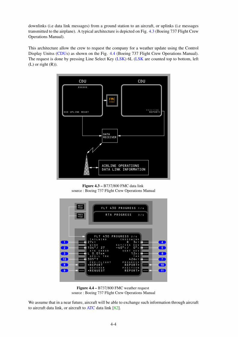
downlinks (i.e data link messages) from a ground station to an aircraft, or uplinks (i.e messages

transmitted to the airplane). A typical architecture is depicted on Fig. 4.3 (Boeing 737 Flight Crew

Operations Manual).

This architecture allow the crew to request the company for a weather update using the Control

Display Unitss (CDUs) as shown on the Fig. 4.4 (Boeing 737 Flight Crew Operations Manual).

The request is done by pressing Line Select Key (LSK) 6L (LSK are counted top to bottom, left

(L) or right (R)).

DATARECEIVER

AIRLINE OPERATIONSDATA LINK INFORMATION

CDU

FMCP/RST

X XXXXX

KNILPUXXX AE YDR

CDU

>TROPERNOITISOP

Figure 4.3 – B737/800 FMC data link

source : Boeing 737 Flight Crew Operations Manual

REHTAEW ISOP NOIT

HGILF-ERP T GORP SSER

KRTL-SPG SAT

RORREKTX TREV VED

DNIW AS ASI/T VED

034TLF GORP SSER 4/2

DNIWLIAT SSORC DNIW

TK72 R TK3

72/o401 4- /Co0 C

o0

MN10.0L IH21

To503 4 TK62

TROPER< PER >TRO

TSEUQER< PER >TRO

034TLF GORP SSER 4/1

PATR ERGOR SS 4/3

4

5

7

6

10

11

1

2

3

8

9

12

PAGE

NEXT

PAGEPREV

Figure 4.4 – B737/800 FMC weather request

source : Boeing 737 Flight Crew Operations Manual

We assume that in a near future, aircraft will be able to exchange such information through aircraft

to aircraft data link, or aircraft to ATC data link [82].

4-4

During every controlled or non-controlled flight, an aircraft crosses control sectors and aircraft

trajectories. If by any mean past data derived from its ADC is stored on board, it can be transferred

to :

• other aircraft planning to fly a trajectory in the vicinity of the already flown trajectory,

• and/or to Air Traffic Control Center in charge of the already crossed airspace.

In order to illustrate the Wind Networking (WN) concept, we will consider the B737 practical

case. Most crews use a technical flight plan prepared by the company operations to fill the Flight

Management System (FMS) route. Taking the example of Smith Industries B737 FMS, the crew

is supposed to fill the wind for the chosen cruising level (CRZ WIND) field in the FMS, which

linearly interpolates the climb wind from zero to the top of climb wind value, and propagates it to

the route legs if the route has already been entered.

To verify the fuel balance and the ETAs before take-off, the crew is supposed to enter (or uplink)

the predicted winds in the FMS. On very short flights, most of the time, there is little reason to en-

ter several en route winds. On long range flights, omitting forecast winds, or filling the FMS with

erroneous winds, may lead up to erroneous fuel consumption predictions ending with a diverting

flight. Obviously, as soon as airborne, accurate wind values are needed to give most accurate ETAs

and fuel predictions.

The Wind Networking (WN) concept is simple, each time a more recent wind is available, it has

to be "uplinked" to the FMS. This update is not limited to one flight level (e.g the currently

or planned flight level), but provides an update of the predicted winds actually encountered by

previous flying aircraft. Some advantages are better after take-off fuel consumption estimations

(i.e better chances for a true optimal flight level), better trajectory prediction (e.g accurate ETA,

better Top Of Descent (TOD) estimation for idle thrust descents [132] and Continuous Descent

Approach (CDA) [83, 130] which also means less noise on overflown cities during the descend

and approaches phases [131]).

The concept is summarized in both (see Fig. 1.2) :

• near real time aircraft/aircraft wind information sharing,

• near real time aircraft/ground wind information sharing.

4.3 Algorithm

4.3.1 What the algorithm does ?

The algorithm developed to demonstrate the benefit of tactical wind networking concept is based

on wind prediction improvement, by using wind measurements from other aircraft in the 4D vicin-

ity of a given aircraft.

First we consider a large set of aircraft in order to have relevant statistical results. In our case, we

will consider the traffic over a European country.

For each trajectory sample, one must be able to locate the neighboring aircraft in a 4 dimensions

space. The naive approach consists in a pairwise comparison which is dramatically inefficient. For

instance, if we consider 8 000 trajectories over the French airspace with an average observation

time of two hours, sampled every 10 seconds (radar period), we get 8 000 × 2 × 360 = 5 760 000

samples. This means that if we want to find the neighboring aircraft for a given sample, we have

to compute for each trajectory point 7999×360×2 = 5 759 280 distances, and identify the closest

ones. Furthermore, this computation has to be done for every trajectory sample, meaning that the

total number of distance computation is 8000 × 5 759 280 ≃ 3, 3 × 1013.

4-5

Let’s take a sample with a distance calculation between the two aircraft at a given time. The first

one is at P1, the second one at P2, both positions are taken at the same time and expressed in

Earth-Center, Earth-Fixed (ECEF) frame :

P1 ,

3866325.95

−1035492.18

4962901.00

P2 ,

3701734.76

−581359.30

5158737.00

Being optimistic, let’s assume one distance computation costs 10−7 second, the duration of the

whole distances computation lasts ≃ 921 hours, which is far too much.

1

2

3

4

5

6

7

8

9

10

1 2 3 4 5 6 7 8 9 10

Figure 4.5 – Grid Used For Neighbor Detection

In order to avoid this brute force computation, a 4D grid has been built in which each trajectory

sample has been inserted. Each point of the 8 000 trajectories is thus identified by four grid co-

ordinates (three space coordinates, one time coordinate). An example of such a grid is given on

Fig. 4.5 where we are searching current trajectory (red dot) neighbors. As shown on the figure,

only the samples located in the red square will be checked in terms of distance to the red dot. A

2D grid has been used for representation, but the real grid has been built in 4D. Each sample (red

dot in the figure) has coordinates, (5, 6) in the example and only the neighboring boxes have to be

checked. In order to validate this approach, one must select the boxes dimensions.

In a first step, wind maps are inserted in the 4D grid as shown on Fig. 4.6 where the predicted

wind (magenta arrows) and the true wind (red arrows) are stored on each grid point.

Then, each trajectory is inserted in the grid, and the computation of the trajectory prediction im-

provement is done into two steps. The first step updates, when possible, the wind on trajectories,

meaning having some aircraft which has already measured some wind in the current aircraft 4D

neighborhood (in space and in time). For our application, neighborhood means areas where the

wind does not change too much with time. In other words we define a time validity period ±∆t for

the validity of the wind measurement.

4-6

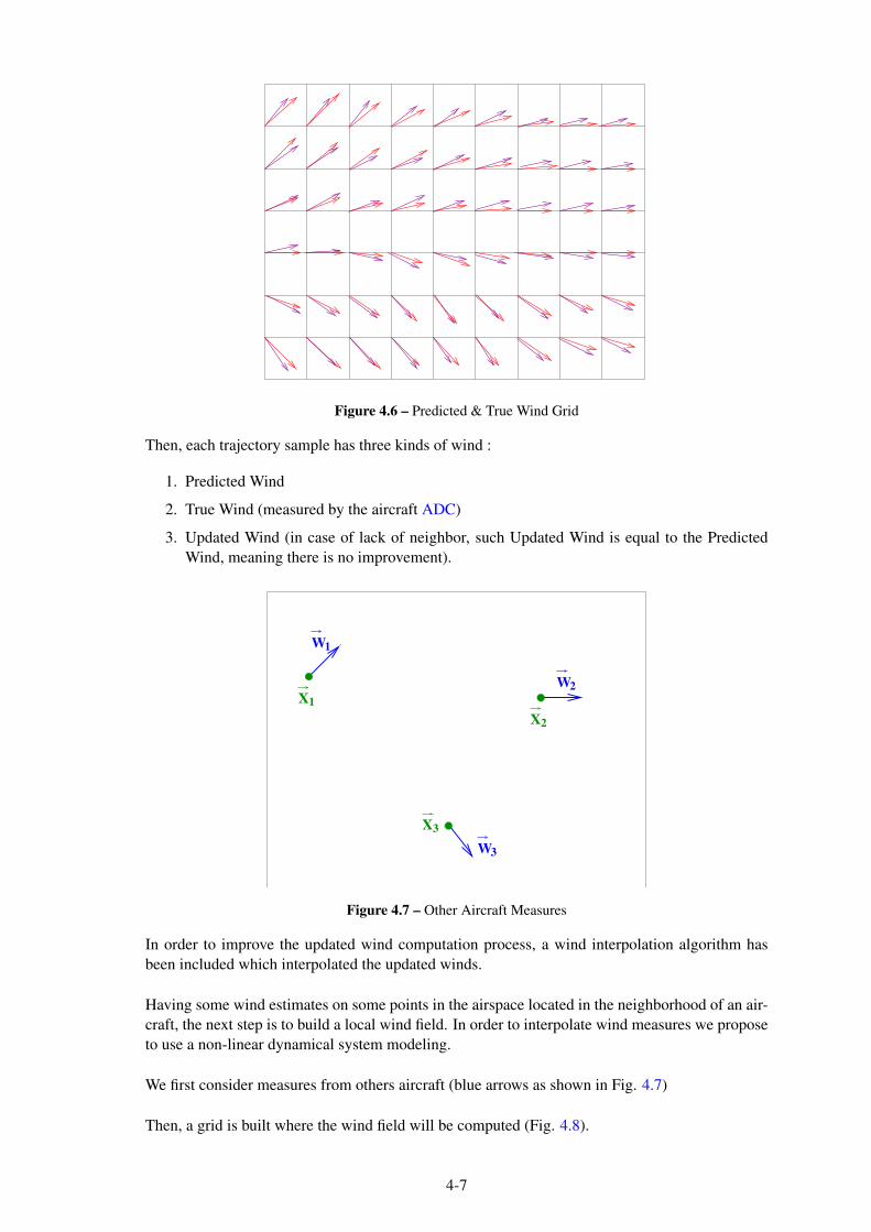
Figure 4.6 – Predicted & True Wind Grid

Then, each trajectory sample has three kinds of wind :

1. Predicted Wind

2. True Wind (measured by the aircraft ADC)

3. Updated Wind (in case of lack of neighbor, such Updated Wind is equal to the Predicted

Wind, meaning there is no improvement).

X1

X3

X2

W1

W2

W3

Figure 4.7 – Other Aircraft Measures

In order to improve the updated wind computation process, a wind interpolation algorithm has

been included which interpolated the updated winds.

Having some wind estimates on some points in the airspace located in the neighborhood of an air-

craft, the next step is to build a local wind field. In order to interpolate wind measures we propose

to use a non-linear dynamical system modeling.

We first consider measures from others aircraft (blue arrows as shown in Fig. 4.7)

Then, a grid is built where the wind field will be computed (Fig. 4.8).

4-7

Figure 4.8 – Wind Field Grid Computation

On such grid, the wind field is then computed as shown on Fig. 4.9.

Figure 4.9 – Wind Field Interpolation

To build such a wind field, a non-linear dynamical system summarized by the following equation

has been used :

~X(t) = ~f (~X) (4.2)

where ~X is the state vector of the system (~X = [x, y, z]T ) and ~f the vectors field (i.e. f is a spatial

evolution function of the dynamic model). This equation describes system which integral curves

may fit the observed trajectories. It associates a speed vector ~X = ~V to a position in the space

coordinates ~X, and then synthesizes a particular vectors field.

Based on the observations of the aircraft (positions, speed vectors), the dynamical system has

to be adjusted with the minimum error. This fitting is done with a Least Squares Minimisation

Method (LSM) method for which the following criterion is used :

E1 =

i=N∑

i=1

‖~Vi − ~f (~Xi)‖2 (4.3)

where N is the number of observations, ~Vi = ~V(Xi) = [Vix(~X),Viy(~X),Viz(~X)]T and ~f a function

which minimizes the interpolation criterion E1.

4-8

Note that it is always possible to determine a non-linear dynamic system interpolating a set of

data. In fact, an infinite number of functions ~f exist which allow us to minimize the criterion E1

(with min(E1) = 0).

As described in Luca Amodei and Mohammed-Najib Benbourhim article [8], a unique solution

can be obtained by introducing an additional regularity criterion E2 :

E2 = α

∫

R3

‖∇div ~f (~X) ‖2dxdydz + β

∫

R3

‖∇(rot ~f (~X))x ‖2dxdydz

+ β

∫

R3

‖∇(rot ~f (~X))y ‖2dxdydz

+ β

∫

R3

‖∇(rot ~f (~X))z ‖2dxdydz

(4.4)

Where ∇ is the three dimensional nabla operator. ‖ ‖ is the usual euclidean norm of R3.

div ~f (~X) = ∂x( ~f (~X))x + ∂y( ~f (~X))y + ∂z( ~f (~X))z (4.5a)

rot ~f (~X) =

(rot( ~f (~X))x

(rot( ~f (~X))y

(rot( ~f (~X))z

=

∂y( ~f (~X))z − ∂z( ~f (~X))y

∂z( ~f (~X))x − ∂x( ~f (~X))z

∂x( ~f (~X))y − ∂y( ~f (~X))x

(4.5b)

‖∇div ~f (~X) ‖2 = (∂xdiv ~f (~X))2 + (∂ydiv ~f (~X))2 + (∂zdiv ~f (~X))2 (4.5c)

‖∇(rot ~f (~X))x ‖2 = (∂x (∂y( ~f (~X))z − ∂z( ~f (~X))y))2 (4.5d)

‖∇(rot ~f (~X))y ‖2 = (∂y (∂z( ~f (~X))x − ∂x( ~f (~X))z))2 (4.5e)

‖∇(rot ~f (~X))z ‖2 = (∂z (∂x( ~f (~X))y − ∂y( ~f (~X))x))2 (4.5f)

A coupling between ~V components is achieved by the divergence (div) and rotational (rot) op-

erators. α, β, are fixed real positive constants controlling the relative weight on the gradient of

the divergence and rotational fields. This explicit control on divergence and rotational operators

is well suited for wind interpolations, as most of the time great differences are observed in the

magnitudes of the divergent and rotational parts of wind field.

The joint minimization of E1 and E2 induces a unique function ~f :

~f (~X) =

N∑

i=1

Φ(‖~X − ~Xi‖).~ai + A.~X + ~B (4.6)

where ~ai is the parameter vector (one for each observation).

A.~X + ~B is obtained from the linear dynamical system modeling, as described in Daniel Delahaye

and Stéphane Puechmorel article [28].

Matrix Φ (associated vector spline) is given by : Φ(‖~X − ~Xi‖) = Q(‖~X − ~Xi‖3)

where Q is the matrix operator :

Q =

1α∂

2xx +

1β (∂2

yy + ∂2zz) ( 1

α − 1β )∂2

xy ( 1α − 1

β )∂2xz

( 1α − 1

β )∂2xy

1α∂

2yy +

1β (∂2

xx + ∂2zz) ( 1

α − 1β )∂2

yz

( 1α − 1

β )∂2xz ( 1

α − 1β )∂2

yz1α∂

2zz +

1β (∂2

xx + ∂2yy)

(4.7)

Regression of the non-linear dynamic system is carried out using the least squares minimiza-

tion method, with the difference that the number of parameters to determine is much higher (⇒A, ~B, ~ai (i ∈ 1, ..,N) i.e. a total of 3N+12 parameters).

This model thus allows us to construct a regular field which is perfectly fitted to the observations

(min(E1) = 0).

4-9

Flow chart 4.10 summarizes our algorithm for WindNetworking.

Start

Read trajectories data within a 3D spatial horizon and a time horizon

Limit the airspace to spatial horizon and split it in 3D boxes

Generate predicted and true winds in each 3D box

Set predicted and true winds along

each trajectory within spatial horizon

Exclude from spatial horizon the 3D boxes without flight

For each trajectory waypoint keep only the other trajectories already flown

For each trajectory waypoint check for neighboring aircrafts

update next waypoints winds with true winds

from neighbors within the validity time interval

Update wind interpolation

For each trajectory update ETAs

compute difference between current and previous ETAs

compute cumulative error

ETA errors

updated 4D trajectories linked to true winds spatio temporal database

Stop

Figure 4.10 – Algorithm Block Diagram

4.3.2 Algorithm validation

Trajectories test sets

To study the effects of wind predictions on trajectory predictions we use three trajectories test sets :

• a 50 trajectories file,

• a 1000 trajectories file,

• a 8000 trajectories file.

giving aircraft parameters. These trajectories come from a one day actual traffic, recorded by

radar over France. They provide us with aircraft positions and speeds. The smallest file is used to

validate the calculations, the second one to verify the efficiency of the algorithms, and finally the

biggest file is used to establish statistics and to verify their ability to handle 24 hours traffic over

France.

The files are organized sequentially. The first line contains the number of trajectories. Then, the

file uses a sequence of lines containing the information for each waypoint on a particular trajectory.

4-10

Each waypoint sequence is separated by a line containing the number of points in the trajectory.

line number 01 NbVols: 50

line number 02 NbPlots: 89

line number 03 0:19:0 5974 147823 458 -43 303 1290

line number ... ...

line number [(line number 02 value + 2)] 0:41:0 15754 146329 450 -23 370 0

line number [(line number 02 value+2)+1] NbPlots: 420

line number [(line number 02 value+2)+2] 0:52:0 -33071 176625 447 -114 390 0

line number ... ...

Let’s detail with the above example the file structure :

• the first line contains the number of trajectories the file contains, in the preceding case 50

(NbVols: 50),

• the second line gives the number of aircraft positions for the first trajectory, in the above

case 89 waypoints (NbPlots: 89 ),

• the third line first trajectory waypoint information (hh:mm:ss x y Vx Vy FL Vz), and will

be described below,

• the line numbered [(line number 02 value + 2)] contains the information related to the last

waypoint of the first trajectory

• the line numbered [(line number 02 value+2)+1] gives the number of waypoints for the

second trajectory, in the above case 420 waypoints NbPlots: 420,

• the line numbered [(line number 02 value+2)+2] contains information related to the first

waypoint of the second trajectory,

• ...

For each trajectory, the information related to a waypoint is stored in a line organized as follows :

hh:mm:ss x y Vx Vy FL Vz

• hh:mm:ss is a time stamp for the aircraft position,

• x is the abscissa of the airplane position, in a Cartesian reference frame, expressed in meters,

• y is the ordinate of the airplane position, in a Cartesian reference frame, expressed in meters,

• Vx is the x component of the recorded aircraft ground speed3,

• Vy is the y component of the recorded aircraft ground speed4,

• FL is the aircraft flight level returned by the aircraft mode S transponder. This information

allows a 3-Dimensional positioning of the aircraft as it gives, in hundred of feet, the height

above the 1013.25 hPa isobar5.

• Vz is the vertical speed, expressed in ft/min returned by the aircraft mode S transponder.

4D grid

To perform a trajectory calculation, a 4 dimensions space is needed. All trajectories calculations

are made in a 4D "volume" defined by a Xmin, Xmax,Ymin,Ymax,Zmin,Zmax geographical space,

"coupled" with a time space Tmin,Tmax. The minimum and maximum values of these variables

are chosen in such a way that the 4D grid contains all the trajectories. Each trajectory point is time

3For our test we assumed that the recorded trajectories were recorded with a wind equals to zero, which means that

we assumed Vx as a True Air Speed4For our test which assumed that the recorded trajectories were recorded with a wind equals to zero, we means that

we assumed Vy as a True Air Speed5The 1013.25 hPa (29.92 inches of mercury) isobar corresponds to the standard atmospheric pressure at sea level

according International Standard Atmosphere.

4-11

stamped and once [Tmin,Tmax] is defined, each trajectory is reduced to its waypoints whose time

stamps falls in [Tmin,Tmax].

The 4D grid can be seen as a way to limit the studied airspace to some control sectors, with the

opportunity to group Air Traffic Control sectors on time basis (e.g night shifts), or on geographical

areas.

4.4 Algorithm implementation

This section details our implementation of the Wwind Networking concept, tested on 8000 trajec-

tories.

4.4.1 Programming paradigm and language choice

We made the choice to use Java general-purpose programming environment as it was designed for

the following four primary goals [52] :

• Comprise a container for application code to run inside,

• Provide a secure execution environment as compared to C/C++,

• Take memory management out of the hands of developers,

• Provide a cross-platform execution environment.

The Java programming environment is made of the Java language, and the supporting runtime

i.e. the Java Virtual Machine (JVM). As the JVM has been ported to run on a large number of

environments, from Blu-ray players to mainframes, we bet that code written in Java could work

on both FMC and ATC servers. We also chose Java programming language to benefit from the

Java platform (i.e. Java runtime environment or the core Java Application Programming Inter-

facess (APIs)) predefined set of Java classes, which exist on every Java installation.

Once the language chosen, we had to decide between two programming paradigms : object-

oriented which groups code together with the state the code modifies, or procedural which groups

code into functions. As we decided to go Java, we chose to use Object-oriented programming.

We tried to create a class as a collection of fields that hold values and methods that operate on

those values. Put another way, a class defines a new reference type made of data fields, such as the

FDPoint type, and methods (i.e. procedures, functions, or subroutines) that operate on that data.

We also tried to use classes to define entities that usually represent something in the real world.

For example we used the FDPoint.java to define a new reference type : FDPoint. In the real world

it is a four dimensions point belonging to an aircraft trajectory. The FDPoint object is an instance

of the FDPoint.java class, created by instantiating the FDPoint.java class with the new keyword

and invoking its constructor. A FDPoint object is a value of that type, it represents the state a

single point of a trajectory.

Thinking the same way, trajectories are made of sets of FDPoint, thus we used the FDPointSet.java

class to create an object representing these sets, and to define the methods operating on these sets

(e.g. adding a FDPoint to a set, displaying a set of FDPoint).

When we designed our classes, we though about the data an object will need to know about itself,

and we also designed the methods that operate on that data. Figure 4.11 summarizes the data

structures we used to perform our calculations.

4-12

Fig

ure

4.1

1–

Data

Stru

ctures

defi

ned

for

Win

dN

etwo

rkin

gco

mp

utatio

ns

4-13

4.4.2 Program structure

The program is controlled by a main program called Control.java summarized by flowchart Fig.

4.12. This program calls the Java classes to perform its subroutines.

Start

CatsFileInput.readCatsFile(NOM_GEN, userNbTraj)

WindFDCube.createWindFDCube()

WindFDCube.generateInitialWinds()

FDTrajectorySet.truePredWindSet()

FDTrajectorySet.truePredTimeSet()

FDTrajectorySet.memoIndexFDTrajectorySet()

FDTrajectorySet.windUpdateComputation()

FDTrajectorySet.upDatedTimeSet()

FDTrajectorySet.computeWindNormError()

FDTrajectorySet.computeMeanDeltaTimePred()

FDTrajectorySet.computeMeanDeltaTimeUpDated()

FDTrajectorySet.computeMeanPredError(horizon)

FDTrajectorySet.computeMeanUpDatedError(horizon)

FDTrajectorySet.writeFile(NOM_GEN)

WriteStat.writeFileTab()

WriteStat.writeFileCsv()

Stop

Figure 4.12 – Control.java file structure

4-14

Start

CATS file name

Read trajectories file

Read first file line

nbTrajs=number of trajectories

create an FDTrajectorySet array to store the nbTrajs trajectories data

FOR cptTraj<nbTrajs

Read next file line

nbPoints=number of points of the trajectory

flightId=cptTraj

create an empty set of 4D points for the current trajectory

FOR cptPoint<nbPoints

read : position overflying time, position, altitude, speed, vertical speed

convert units to s, m, m/s

point

within

studied

airspace

• translate position and time to volume and time origins

• find the (i, j, k) space box the point belongs to

• add this 4D point to the set of 4D points for the current trajectory

add the set of 4D points for the current

trajectory to the FDTrajectorySet array

fdTrajArray[cptTraj]

Stop

yes

no

Figure 4.13 – Trajectories reading and organizing

4-15

4.4.3 Trajectories reading and organizing

The program uses 8000 trajectories that need to be read from a file, and then organized according

to the airspace being studied. Flowchart 4.13 describes this processing.

4.4.4 Wind update

For each (i, j, k) 3D space elementary box the wind is updated provided that :

• a plane crossed the box,

• others aircraft have flown through that box in the past,

• the others aircraft that flew through the box did it within the validity time interval. This va-

lidity time interval was set to one hour, but could be reduced (e.g. 900 s for short haul flights)

or increased (e.g. 10800 s for long haul flights) using the TIME_VALIDITY_WIND_NEIGH con-

stant6.

The implementation uses Java Map interfaces, particularly the TreeMap and the SortedMap ones.

4.4.5 Trajectories prediction using predicted and true wind

For each trajectory, the waypoints ETEs are updated using the forecast winds. Flowchart 4.14

describes this update process. We chose to define currentPredError = currentDeltaTrue −currentDeltaPred as it is the time that has to be added to the ETEs calculated without wind. Let’s

assume that the crew does not assign any wind in the FMC7, consequently currentDeltaPred

is zero, the ETEs calculations and updates rely only on the aircraft sensed winds. In case of

tail wind, as GS is greater than TAS, currentDeltaTrue is a negative value, and the trajectory

prediction update gives waypoints before schedule, what makes sense.

4.4.6 Trajectories prediction using updated wind

When possible, the ETEs of each waypoint is updated using wind data shared by aircraft hav-

ing flown in the same area a few time ago. The process is similar to the one described in

4.4.5. Flowchart 4.15 summarizes the update of the trajectories prediction.We chose to define

currentU pDatedError = currentDeltaTrue − currentDeltaU pDated as it is the time that has to

be added to the ETEs calculated without wind. Let’s assume that there is no neighbor, in that case

currentDeltaUpDated is zero, the ETEs calculations and updates rely only on the aircraft sensed

winds. In case of tail wind, as GS is greater than TAS, currentDeltaTrue is a negative value, and

the trajectory prediction update gives waypoints before schedule, what makes sense.

6We chose one hour for the time interval of validity of the wind data as it is the value of current Numerical Weather

Prediction (NWP) models for their Rapid Update Cycling approach in the assimilation cycle of observations. Aviation

weather forecast are available every three hours, or every one hour7For the Boeing 737 Smith FMC, this means no wind being entered in the CRZ WIND field of the PERF INIT

page, or in the RTE DATA page.

4-16

Start

arrayFDPoint[]

Initialization : wowTime = wowTime of the first

trajectory point included in the studied airspace,

trueT ime0 = predTime0 = wowTime, ∆TimePred0 = 0

FOR each (xi, yi, zi) 4D point

distance =

√

(xi+1 − xi)2 + (yi+1 − yi)

2

tasXMean = 12(tasXi + tasXi+1) ; tasY Mean = 1

2(tasYi + tasYi+1)

T AS =√

tasXMean2 + tasY Mean2

wXMean = 12(trueWindXi + trueWindXi+1)

wY Mean = 12(trueWindYi + trueWindYi+1)

gsXMean = tasXMean + wXMean

gsY Mean = tasY Mean + wY Mean

GS =

√

gsXMean2 + gsY Mean2

currentDeltaTrue =distance

GS− distance

T AS

currentDeltaTruei+1 = currectDeltaTrue

trueT ime = trueT ime + currentDeltaTrue

trueT imei+1 = trueT ime

wXMean = 12(predWindXi + predWindXi+1)

wY Mean = 12(predWindYi + predWindYi+1)



GS =

√


currentDeltaPred =distance

GS− distance

T AS

predTime = predTime + currentDeltaPred

predTimei+1 = predTime

deltaT imePred = trueT ime − predTime

deltaT imePredi+1 = deltaT imePred

currentPredError = currentDeltaTrue − currentDeltaPred

currentPredErrori+1 = currentPredError

updated arrayFDPoint[]

Stop

Figure 4.14 – Waypoints ETEs calculations according to predicted and true winds

4-17

Start

arrayFDPoint[]

Initialization : wowTime = wowTime of the first trajectory

point included in the studied airspace, trueTime = trueTime

of the first trajectory point included in the studied airspace,

upDatedTime0 = wowTime, trueT ime = trueT ime0, ∆TimeU pDated0 = 0

FOR each (xi, yi, zi) 4D point

distance =

√

(xi+1 − xi)2 + (yi+1 − yi)

2

tasXMean = 12(tasXi + tasXi+1) ; tasY Mean = 1

2(tasYi + tasYi+1)

T AS =√

tasXMean2 + tasY Mean2

wXMean = 12(upDatedXi + upDatedXi+1)

wY Mean = 12(upDatedWindYi + upDatedWindYi+1)



GS =

√


currentDeltaU pDated =distance

GS− distance

T AS

currentDeltaU pDatedi+1 = currentDeltaU pDated

upDatedTime = upDatedTime + currentDeltaU pDated

upDatedTimei+1 = upDatedTime

trueT ime = trueT imei+1

currentDeltaTrue = currentDeltaTruei+1

deltaT imeU pDated = trueT ime − upDatedTime

deltaT imeU pDatedi+1 = deltaT imeU pDated

currentU pDatedError = currentDeltaTrue − currentDeltaU pDated

currentU pDatedErrori+1 = currentU pDatedError

updated arrayFDPoint[]

Stop

Figure 4.15 – Waypoints ETEs update calculations according to updated winds

4.4.7 Computation considerations

The code has been tested over test sets of made of 50, 1000 and 8000 trajectories. For 1000

trajectories, the results were available in less than 23 seconds on a laptop running on a Intel(R)

Celeron(R) CPU 847 @ 1.10 GHz, and with 8 GB of RAM. Increasing the number of trajectories

beyond 3000, increases the computation time beyond 4 minutes as shown on figure 4.16. If we

consider the total number of waypoints, the computation time reaches 4 minutes when the number

of waypoints passes 700000 (see figure 4.17). Even if the average number of waypoints varies

between trajectories, it stays within the [220, 243] range (see figure 4.18). Above the value of

3000 trajectories, the computation time should be tested on an other hardware with higher RAM

capacity and better CPU, as both memory storage and CPU capacity are involved, respectively

through the Java TreeMaps and through the mathematical computations.

4-18

102 103 104

0

10

20

Number of trajectories

Co

mp

uta

tio

nti

me

(min

)

Figure 4.16 – Computation time versus number of trajectories

104 105 106

0

10

20

Number of waypoints

Co

mp

uta

tio

nti

me

(min

)

Figure 4.17 – Computation time versus number of points

102 103 104

220

225

230

235

240


Mea

nn

um

ber

of

po

ints

per

traj

ecto

ry

Figure 4.18 – Mean number of point per trajectory versus number of points

We did not consider changing the airspace sampling rate (i.e. varying the size of the 3D space

elementary box - see 4.4.4), as we were not working on a real time application. Our goal was to

demonstrate that wind sharing improves trajectory prediction. The algorithm is able to produce

results, in a repetitive and stable manner, with 8000 flights which represent 1 766 964 waypoints,

and 24 hours aircraft traffic over France.

4-19

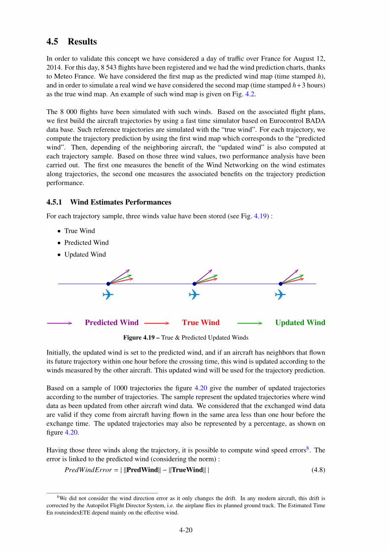
4.5 Results

In order to validate this concept we have considered a day of traffic over France for August 12,

2014. For this day, 8 543 flights have been registered and we had the wind prediction charts, thanks

to Meteo France. We have considered the first map as the predicted wind map (time stamped h),

and in order to simulate a real wind we have considered the second map (time stamped h+3 hours)

as the true wind map. An example of such wind map is given on Fig. 4.2.

The 8 000 flights have been simulated with such winds. Based on the associated flight plans,

we first build the aircraft trajectories by using a fast time simulator based on Eurocontrol BADA

data base. Such reference trajectories are simulated with the “true wind”. For each trajectory, we

compute the trajectory prediction by using the first wind map which corresponds to the “predicted

wind”. Then, depending of the neighboring aircraft, the “updated wind” is also computed at

each trajectory sample. Based on those three wind values, two performance analysis have been

carried out. The first one measures the benefit of the Wind Networking on the wind estimates

along trajectories, the second one measures the associated benefits on the trajectory prediction

performance.

4.5.1 Wind Estimates Performances

For each trajectory sample, three winds value have been stored (see Fig. 4.19) :

• True Wind

• Predicted Wind

• Updated Wind

Predicted Wind True Wind Updated Wind

Figure 4.19 – True & Predicted Updated Winds

Initially, the updated wind is set to the predicted wind, and if an aircraft has neighbors that flown

its future trajectory within one hour before the crossing time, this wind is updated according to the

winds measured by the other aircraft. This updated wind will be used for the trajectory prediction.

Based on a sample of 1000 trajectories the figure 4.20 give the number of updated trajectories

according to the number of trajectories. The sample represent the updated trajectories where wind

data as been updated from other aircraft wind data. We considered that the exchanged wind data

are valid if they come from aircraft having flown in the same area less than one hour before the

exchange time. The updated trajectories may also be represented by a percentage, as shown on

figure 4.20.

Having those three winds along the trajectory, it is possible to compute wind speed errors8. The

error is linked to the predicted wind (considering the norm) :

PredWindError = | ‖PredWind‖ − ‖TrueWind‖ | (4.8)

8We did not consider the wind direction error as it only changes the drift. In any modern aircraft, this drift is

corrected by the Autopilot Flight Director System, i.e. the airplane flies its planned ground track. The Estimated Time

En routeindexETE depend mainly on the effective wind.

4-20

0 200 400 600 800 1,0000

200

400

600

800

1,000


Nu

mb

ero

fu

pd

ated

traj

ecto

ries

10

20

30

40

50

60

70

80

90

100

Po

urc

enta

ge

of

up

dat

edtr

ajec

tori

es

Figure 4.20 – Number of updated trajectories

Having computed this error for each trajectory sample, it is possible to build a “WindPredError

map” (see Fig. 4.21) where the wind prediction error on each trajectory sample is represented.

The former information is given in three dimensions but is here represented as a 2D graph. The

error is computed in terms of norm. The red areas indicate an error of 15 knots. The red dots

represent the areas with the biggest errors and the blue dots those with the smallest errors. In this

case (Predicted Wind Error) we have only red areas because the wind has not be updated due to

lack of neighboring aircraft.

Figure 4.21 – Per Trajectory Wind Prediction Error

This computation has also been done for the updated wind errors :

U pdatedWindError = | ‖UpdatedWind‖ − ‖TrueWind‖ | (4.9)

The associated map is given on Fig. 4.22. We can notice that the red dots have disappeared in high

4-21

Figure 4.22 – Per Trajectory Updated Wind Error

traffic density areas, and that we have much more blue areas, mainly in the high traffic density ar-

eas. The aircraft located in low traffic density areas do not benefit from other aircraft data, and do

not improve their wind estimates (but their needs for wind updating is less critical as the conflict

risk is lower because the traffic spreads out).

Finally, we have computed the Wind Networking Improvement by computing the difference be-

tween wind error :

Improvement = | PredWindError − U pdatedWindError | (4.10)

This value is positive and is higher when the improvement is also higher. As for the previous

values, we can also compute a map for this improvement (see Fig. 4.23). We have just changed

the color representation by setting green color for large improvement, thus the green areas locate

where wind networking brings the most improvement (high traffic density areas).

The second analysis we have performed is linked to the impact of the number of aircraft on the

Wind Networking performances. For that we consider several aircraft densities and we compute

the mean value of each error. Table 4.2 and Fig. 4.24 summarize those results.

NbTraj 100 1 000 3 000 5 000 8 000

PredErr (kts) 5.11 5.13 5.12 5.11 5.14

UpdatedErr (kts) 3.23 0.95 0.64 0.5 0.48

Table 4.2 – Predicted & Updated Wind Error

For those experiments, we took the first 100 trajectories of the day, then the first 1 000 and so

on. With the first 1 000 trajectories, the impact of the Wind Networking is already significant, the

wind error drops down from 5.13 knots to 0.95 knots; which is 81 % improvement. This results

are illustrated on figure Fig. 4.24.

4-22

Figure 4.23 – Wind Estimate Improvement Areas

0 100 200 300 400 500 600 700 800 900 1,0000

1

2

3

4

5

6


Mea

nP

red

icte

dW

ind

Err

or

(kts

)

0

2

4

6

Mea

nU

pd

ated

Win

dE

rro

r(k

ts)

Figure 4.24 – Mean Predicted Wind and Updated Wind errors

4.5.2 Trajectory Prediction Performances

In order to validate the trajectory prediction performance, we consider that aircraft have to predict

their future position at a given horizon all along their trajectory. As shown on Fig. 4.25, at a given

location, an aircraft predicts the time it will pass a given point on its future trajectory. Three times

have been computed : the True Time, the Predicted Time and the Updated Time.

4-23

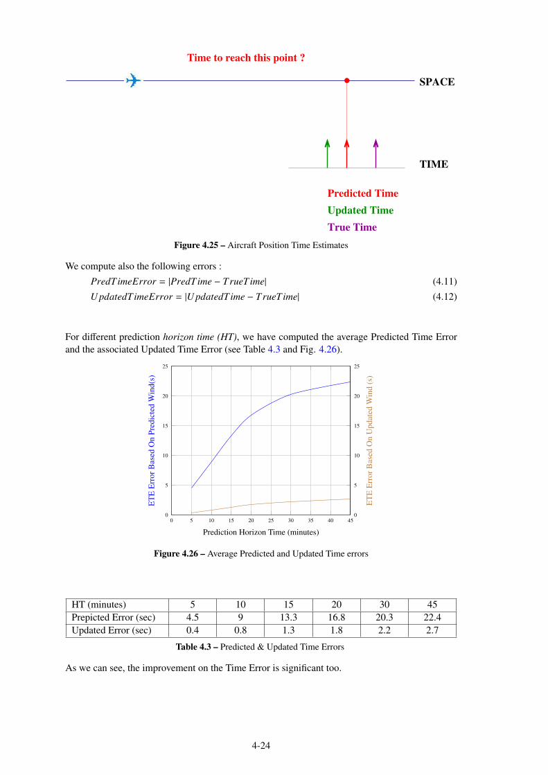
SPACE

Predicted Time

Updated Time

TIME

True Time

Time to reach this point ?

Figure 4.25 – Aircraft Position Time Estimates

We compute also the following errors :

PredTimeError = |PredTime − TrueTime| (4.11)

U pdatedTimeError = |U pdatedTime − TrueTime| (4.12)

For different prediction horizon time (HT), we have computed the average Predicted Time Error

and the associated Updated Time Error (see Table 4.3 and Fig. 4.26).

0 5 10 15 20 25 30 35 40 450

5

10

15

20

25

Prediction Horizon Time (minutes)

ET

EE

rro

rB

ased

On

Pre

dic

ted

Win

d(s

)

0

5

10

15

20

25E

TE

Err

or

Bas

edO

nU

pd

ated

Win

d(s

)

Figure 4.26 – Average Predicted and Updated Time errors

HT (minutes) 5 10 15 20 30 45

Prepicted Error (sec) 4.5 9 13.3 16.8 20.3 22.4

Updated Error (sec) 0.4 0.8 1.3 1.8 2.2 2.7

Table 4.3 – Predicted & Updated Time Errors

As we can see, the improvement on the Time Error is significant too.

4-24

4.5.3 Estimated Time of Arrival predictions

Today airports operations require the transfer of large volumes of baggage and passengers between

flights. This explains how the hub-and-spoke system 9 became the norm for most major airlines

(e.g. Paris CDG for Air France, London Heathrow for British Airways, Frankfurt for Lufthansa...).

Errors in Estimated Time of Arrival (ETA) have a direct impact on the efficiency of these systems,

as they change the Runway System Capacity10 and the gates assignments to arriving flights (the

ground controllers use the flight schedule to examine the capacity of gates to accommodate the

incoming flights).

For these reasons we tried to study the effect of Wind Networking on the Estimated Time of

Arrival. We calculate for the predicted and the updated wind, and for each trajectory the following

quantities :

ET Atrue

ET Apredicted

ET Aupdated

(4.13)

Then, for different numbers of trajectories, we calculated :

Min(ET Atrue − ET Apredicted)

Max(ET Atrue − ET Apredicted)

Max(ET Atrue − ET Apredicted) − Min(ET Atrue − ET Apredicted)

Min(ET Atrue − ET Aupdated)

Max(ET Atrue − ET Aupdated)

Max(ET Atrue − ET Aupdated) − Min(ET Atrue − ET Aupdated)

(4.14)

And finally :

∆ET Atrue/pred = Max(ET Atrue − ET Apredicted) − Min(ET Atrue − ET Apredicted)

∆ET Atrue/up = Max(ET Atrue − ET Aupdated) − Min(ET Atrue − ET Aupdated)(4.15)

We plotted results from equation 4.15 on figure 4.27, where the benefit of Wind Networking is

illustrated as the curve Max(ET Atrue −ET Apredicted)−Min(ET Atrue −ET Apredicted) lies above the

curve Max(ET Atrue − ET Aupdated) − Min(ET Atrue − ET Aupdated).

To quantify the benefit of Wind Networking, we plotted :

∆ET Atrue/pred − ∆ET Atrue/up (4.16)

as shown on figure 4.28.

9A hub is a central airport that flights are routed through, and spokes are the routes that planes take out of the hub

airport.10The Runway System Capacity is primarily dependent on the runway occupancy times of, and on the separation

standards applied to, successive mixed categories aircraft.

4-25

30 200 400 600 800 1,0000

200

400

600


∆E

TA

true/

pre

d(s

)

0

200

400

600

∆E

TA

true/

up

(s)

Figure 4.27 – Winds impact on ETAs

30 200 400 600 800 1,0000

100

200

300


ET

AE

rro

rR

edu

ctu

ctio

n(s

)

Figure 4.28 – ∆ET Atrue/pred − ∆ET Atrue/up

The shapes of curves from figures 4.27 and 4.28 may look strange, but can be explained by the

fact that the 1000 trajectories contain randomly distributed turboprop and jet aircraft trajectories.

The effect of a 15 knots variation in the wind speed is not the same on a turboprop flying at 270

knots, and on a jet flying at 480 knots, on one side the headwind represents 5.5% of the True Air

Speed, on the other side 3%.

Having plotted ∆ET Atrue/pred − ∆ET Atrue/up in figure 4.28, we calculated its mean value using :

∆ET Atrue/pred − ∆ET Atrue/up =1

1000 − 30

∫ 1000

30

[

∆ET Atrue/pred − ∆ET Atrue/up

]

(x)dx (4.17)

As we did not have a functional expression for∆ET Atrue/pred−∆ET Atrue/up, we used MATLAB R© trapzfunction for the numeric integration. The computed mean value equals 148 seconds.

Let’s try to explain ∆ET Atrue/pred − ∆ET Atrue/up value of 148.1204 seconds :

• This value was calculated from 1000 trajectories described by 211 652 waypoints, which

means a value of 212 waypoints per trajectory. As the waypoints where sampled every 15

4-26

seconds, this also means that the average trajectory flight time is around 53 minutes11, i.e.

3180 seconds. We can then conclude that Wind Networking improves trajectory prediction

by a mean percentage of 4.65 % for a wind variation of 10 knots (as this was the maximum

variation between the predicted wind and the updated wind).

• This also means that the trajectory prediction may be improved by 2 min 28 seconds, which

may be of interest when considering Runway System Capacity and gate assignment.

• This value is a mean value, and may be more than 3 or 4 minutes if we were considering

non jet aircraft trajectories. Considering separation standards of 1 : 30 minutes applied to

successive aircraft in the traffic mix, such values should be considered.

4.6 Conclusions

Beyond operational concerns, flight safety as a main goal needs also accurate TP. Some accidents

(CFIT, collision, ...) or incidents (loss of separation, wake vortex encounter, airspace infringe-

ment, ...) were due to poor TP.

As planned in the future ATM concepts (SESAR, NextGen, CARATS), the concept of 4D Trajec-

tory Based Operations will be the cornerstone of those new systems. In this 4D Trajectory Based

Operations framework, one must be able to locate accurately aircraft in the 4D (3D+T) space in

order to improve traffic synchronization, sequencing and merging, overload detection, etc...

In order to reach these goals, trajectory prediction has to be improved so as to reduce the uncer-

tainty of the future position of aircraft. One of the major Trajectory Prediction limiting factor is

the wind along the future trajectory.

Aircraft at their current position, measure the wind with a very good accuracy and based on the

future technology, it is reasonable to consider that aircraft would be able to share this wind infor-

mation shortly with ground (e.g Maastricht Upper Area Control Centre Controller-Pilot Data-Link

Communications (CPDLC)) and other aircraft.

We have developed a Wwind Networking concept in order to improve the trajectory prediction.

In the first part of the present chapter, this concept has been described and we have investigated

the potential applications for Air Traffic Management. We have proposed an algorithm to simulate

this concept, in which we have also proposed a methodology for wind measures interpolation.

The concept has then been tested on a realistic airspace (France) with 8 000 daily flights, includ-

ing short, medium and long haul ones, jet and turboprop aircraft. The improvement on both wind

estimate and trajectory prediction has been demonstrated with very hopeful results.

Future research will also measure the impact of the Wwind Networking concept on the conflict

detection improvement. We will investigate in the next chapter the possibility to improve the tem-

perature estimate by the same kind of concept. As a matter of fact temperature also influences the

Trajectory Prediction by the mean of air density and speed of sound. It may also be of some inter-

est for carriers when choosing their optimal flight levels, as the propulsion ceilingof a jet aircraft

is a limiting factor.

Apart from trajectory prediction, wind is a factor which may justify operations considerably above

or below optimum altitude. For example, a favorable wind component may have an effect on

ground speed which more than compensates for the loss in air range. Flight crew members, using

11This time should not be interpreted as the duration of the flight, but as the average time of presence of the aircraft,

within the space under study.

4-27

the applicable table, can determine the break-even wind (advantage necessary or disadvantage that

can be tolerated) to maintain the same range at another altitude. The concept of Wind Networking

can also help to make the right decision in this context.

4-28

Chapter 5

Wind and Temperature Networking

5.1 Introduction

In chapter 4 we studied the main longitudinal (along-track) error source between the predicted and

the actual trajectory due to wind estimation1 .

Even if the main longitudinal error source between the predicted and the actual trajectory is linked

to wind estimation, temperature wrong estimation may also lead to ETE prediction errors. In

chapter 4 we measured the potential benefit produced by sharing wind measures between aircraft.

In the present chapter we will try to improve the trajectory prediction by sharing the wind and the

temperature information between aircraft. Addressing the temperature came when we noticed that,

at least the cruising phase of many flights is performed at constant Mach number. Maintaining a

given Mach number under changing temperatures equals changing the true air speed.

Based on the current performances of Air Traffic Control systems, controllers are able to efficiently

detect conflict 20 minutes in advance ; for a larger horizon time (look-ahead time), the induced

trajectory prediction uncertainty strongly reduces the reliability of the conflict detection. However,

a conflict predicted in a distant future can be managed as a message of increased attention for the

aircraft concerned. The trajectories are modified in this case, as soon as the conflict is confirmed.

Outside trajectory prediction considerations, temperature is also involved in flight safety through

the following parameters :

• ETOPS range capabilities for a twin jet,

• level off altitude in case of engine failure,

• 1.3g flight envelope determination2.

• fuel estimation

as temperature changes engine performances.

For fuel calculations, Boeing considers an increase/decrease fuel flow of 3% per 10C above/be-

low ISA temperature.

The goal of our work work is to measure the potential benefit produced by sharing wind/tem-

perature measurements between aircraft (this concept will be called Wind and Temperature Net-

working (WTN)indexWTN. To reach this goal, aircraft measure (temperature and pressure) and

calculate (wind and density) their local atmospheric data and broadcast them to the other aircraft.

Having such distributed weather information, each aircraft is able to compute an enhanced local

1We will sometimes use Flight Management Computer (FMC) in place of Flight Management System (FMS) and

vice-versa, in any case it must be read as the on-board computer system, that manages the airplane and the flight.2The FMC determines maximum altitudes considering a given cruise weight and maneuver capability.

5-1

wind/temperature map as a function of location (3D) and time. These updated wind/temp fields

could be shared with other aircraft and/or with ground systems. Using this enhanced weather in-

formation, each aircraft is able to improve drastically its own trajectory prediction, and the safety

of its high altitude operations. This concept has been simulated in the French airspace with 8 000

flights. Comparisons have been investigated on trajectory prediction performances with and with-

out wind/temp networking. Statistics have been conducted in order to measure the benefit of such

concept in both time and space dimensions, showing higher improvement in high traffic areas, as

expected.

The first part of this chapter deals with safety issues related to temperature and engine perfor-

mance. It details how temperature may affect flight safety. Sharing an updated temperature field

may reduce such hazards.

The second part of the chapter describes the wind/temp networking concept and how it could be

applied to aircraft trajectory prediction. The third part presents the algorithm used to implement

the WTN and proposes smooth vector interpolation approach. The fourth part introduces the

framework used for our simulations and demonstrates the benefit of WTN of trajectory prediction

for a large airspace (France airspace).

5.2 The ICAO standard atmosphere

The ICAO document Doc 7488/3 [77] standard specifies the characteristics of an ICAO standard

atmosphere. This atmosphere “is intended for use in calculations in the design of aircraft, in

presenting test results of aircraft and their components under identical conditions, and to facilitate

standardization in the development and calibration of instruments.”. A brief description of the

ICAO standard atmosphere is given in Appendix G.

5.3 Aircraft operations

When considering high altitude flight (i.e above FL250 [47]), most jet transport aircraft are thrust

limited and operated at constant Mach number M (the ratio of air speed to speed of sound), and

it has become conventional to use Mach number as an indication of flight speed. For example

the North Atlantic Tracks (NATs) are operated at constant flight levels and constant Mach number

(Mach Number Technique 3) to keep the aircraft separation without radar coverage.

All flights are flown with the autopilot engaged (at least to meet the Reduced Vertical Separation

Minima (RVSM) requirements) and, when equipped, with the auto-throttle engaged. Along an

airplane trajectory, the OAT changes, and so does its TAS above the crossover altitude4, if the

Mach number is kept constant. As the TAS changes the GS changes (even with constant wind)

and the ETE of each route way-point changes. Both the TP calculated on board, or by the ATC

tools become false.

Outside TP concerns, OAT must be considered as airlines Standard Operating Procedures (SOP)

recommend, when flying at Optimum Altitude, that crews should be aware of temperature. High

temperatures and high altitudes reduce engines output power, thus above ISA temperature devia-

tions may reduce altitude capability.

3[80] : Mach Number Technique (MNT) is used to improve the utilisation of airspace on long route segments

where ATC has only position reports to ensure longitudinal separation between flights is maintained. When two or

more aircraft are operating along the same route at the same flight level and maintaining the same Mach number, the

time interval between them is more likely to remain constant than by using any other method.4Altitude at which a specified CAS and Mach value represent the same TAS. Above this altitude the Mach number

is the controlling speed.

5-2

To measure the impact of temperature changes on TP, we need to link the TAS to the temperature.

5.4 Temperature and Speed Considerations

5.4.1 Relations between Mach number, True Air Speed and Temperature

Air pressures and Mach number M are related through the following equation [77] :

M2 =2

γ − 1

[

(pt

ps

)γγ−1 − 1

]

(5.1)

Where γ is the specific gas ratio constant (also defined as the adibatic index or the heat capacity

ratio - for air at standard conditions γ = 1.4 [77], [9])5, pt is the total pressure measured by a

Pitot tube, ps is the static pressure obtained from a static pressure orifice or by some independent

means. The speed of sound a in m/s is given by equation (see equation G.43) :

a =√

γRTs (5.2)

Where R is the air specific gas constant 287.05287 J/(K.kg), Ts is the static air temperature in

Kelvin and is related to the measured total air temperature Tt, by :

Ts =Tt

1 +γ − 1

2M2

=Tt

1 + 0.2M2(5.3)

Strictly speaking :

Tt =1 + 0.2M2

1 + 0.2Kr M2TTic (5.4)

where Kr is the total air temperature probe non-dimensional recovery factor (determined via flight

test), and TTic is the instrument corrected, indicated total air temperature in degrees K. Looking to

the Tt given for ISA temperatures and Mach 0.79 in Boeing B737/8006 flight planning and perfor-

mance [55], we found that Kr ≃ 1.

By computing the Mach number from equation (5.1), the static air temperature from equation (5.3)

and the sound speed from equation (5.2), we can compute the air speed using the Mach number

definition by :

T AS = aM =√

γRTsM (5.5)

Flying at a constant altitude and constant Mach number, a change in OAT, leads to a change in the

TAS as shown on figure 5.1 for above ISA deviations.

260 280 300 320 340 360 380 400450

460

470

480

490

Flight Level

0.7

9M

corr

esp

on

din

gT

AS

(kt)

ISA

ISA+5

ISA+10

Figure 5.1 – True Airspeed at Mach 0.79

5Using ICAO symbols, γ is noted κ in Appendix G.6Boeing 737-800 with CFM56-7B26 engines.

5-3

5.4.2 Still air relation between Ground Speed and Temperature

On board trajectory prediction is calculated using inertial speed, GPS speed or both of them. These

two speeds (or their combination) are relative to ground, called Ground Speed (GS) and given by :

−−→GS =

−−−→T AS +

−→W (5.6)

where−→W is the wind vector. Combining equation (5.6) and equation (5.5) shows that the static air

temperature (i.e OAT) affects GS, thus the trajectory prediction. If we consider an airplane flying

in still air, i.e−→W =

−→0 , the ground speed equals the true air speed. If we take the same values than

in figure 5.1, and we consider the aircraft position after one hour of flight, the true airspeed scale

can be replaced by a distance scale in Nautical Miles, and we get figure 5.27.

The choice of 0.79M was dictated by the fact that most liners cruising speed is within the range

[.75M, .85M], with the Boeing 737 and Airbus 320 families around .79M.

260 280 300 320 340 360 380 400450

460

470

480

490

Flight Level

0.7

9M

stil

lai

ral

on

gtr

ack

1h

ou

rp

osi

tio

nsh

ift

(NM

)

ISA

ISA+5

ISA+10

Figure 5.2 – Still air along track position shift after 1 hour flight (Mach 0.79)

Figure 5.2 shows that in still air, flying at a constant Mach number of 0.79, leads to a position error

of 5 nautical miles per hour, for 5 deviation above ISA. In other words, after one hour cruise, the

airplane is five nautical miles ahead its scheduled trajectory at a constant Mach number of 0.798.

We can conclude that flying between flight levels 250 and 410, with an ISA deviation of 5 has the

same effect than flying in ISA with 5 knots tail wind.

5.4.3 Temperature and One Engine Inoperative (OEI) level off altitude

The one engine inoperative level off altitude is an issue for twin engine jets flying over moun-

tainous areas. Figure 5.3 shows the one engine inoperative Net Level Off Weight for a Boeing

737/4009, for two different temperature deviations to ISA+10. It shows a decrease of 1000 feet,

for a airplane mass between 50 and 60 tonnes, for a five degrees temperature deviation above

ISA+10.

Let’s take an example with a B737/400 overflying mountains (e.g. Cordillera of the Andes), at

a mass of 60 tonnes, in ISA atmosphere at its current position. Following an engine failure, the

flight crew will perform the engine failure or shutdown procedure, and will initiate a driftdown to

7By maintaining its Mach number at .79, the aircraft will have flown in ISA conditions of approximately 475

nautical miles, ISA+5 conditions of approximately 480 nautical miles, and ISA+10 conditions of approximately 485

nautical miles.8A negative deviation to ISA gives the same results, but the plane is behind schedule, as TAS is reduced.9Boeing 737-400 with CFM56-3 23.5K engines.

5-4

reach a level off altitude, at which a long range cruise to an alternate destination may be initiated.

In case of temperature deviation of five degrees above ISA, along the diversion route, obstacles

clearance may become an issue.

Let’s take a second example where safety may be engaged due to temperature. We keep the aircraft

of our previous example, and we assume that during the driftdown, there is visible moisture, e.g.

clouds. Atmosphere is supposed to be ISA+10, and in this case isotherm zero will be at 12500

feet10, companies Standard Operating Procedures (SOP) require switching ANTI-ICE systems

"ON" as soon as there is visible moisture, with an OAT below 5 Celsius. So in our example this

means that ANTI-ICE systems will be turned off at 10000 ft during the descent11.

35 40 45 50 55 60 65100

150

200

250

300

Mass (t)

Lev

eloff

alti

tud

e(F

L)

ISA+10

ISA+15

ISA+20

Figure 5.3 – Boeing 737/400 one engine operative level off Flight Level

Figure 5.4 shows the effect of the ANTI-ICE systems on the One Engine Inoperative Net Level Off

performances (the change of the slopes at 17000 feet are due to the supply of Auxiliary Power Unit

(APU) bleed air, instead of engine bleed air, to the pressurization and air conditioning systems).

In the present case this leads to a decrease of one engine inoperative Net Level off altitude of :

• 3200 feet above 17000 feet

• 2000 feet from 17000 feet to 10000 feet

35 40 45 50 55 60 65100

150

200

250

300

Mass (t)

Lev

eloff

alti

tud

e(F

L)

ISA+10

ISA+10, ENGINE A/I ON

ISA+10, ENGINE and WING A/I ON

Figure 5.4 – Boeing 737/400 one engine operative level off Flight Level - Anti-Ice ON

10The ISA temperature lapse rate is 2 per 1000 f t, giving (2

1000× 5000 +

2

10002 × 7500) = 25C ft.

11In the present case assuming an OAT of 5 C gives a Total Air Temperature (TAT) of 5.5 C (see 5.3) for a

descent at .74M, which means that the crew may switch off the ANTI-ICE lower if following Boeing 10 C TAT

recommendation.

5-5

5.4.4 Temperature and aircraft aerodynamic ceiling

Airliners fly in the transonic speed range, where the lift and drag coefficients are determined by

the angle of attack α and the Mach number M, i.e. one polar is no longer sufficient to calculate

the drag for the clean configuration. Local shock waves appear and degrade the airflow along

the lifting surfaces, as a consequence the total amount of lift decreases. This leads to small and

rapid movements of the primary flight control surfaces, and to vibration of the airframe. This

phenomena is similar to the low speed buffet accompanying the stall of low speed aircraft, but the

physical phenomenon is not the same. We now have buffet that can occur at very low speed, i.e.

low-speed buffet ; and very high speeds buffet, i.e. high-speed buffet. The buffet margin is the

speed difference between the normal cruise speed and the buffet speeds. This gives a limit to the

flight envelope.

For low subsonic aircraft, plotting the lift coefficient versus α gives the maximum lift coefficient

CLmaxand the corresponding αCLmax

for each aerodynamic configuration. At high altitude, the low

subsonic polars CL(α) and CD(α) become CL(α,Mach) and CD(α,Mach) [140], as shown on fig-

ure 5.5a.

0.2 0.3 0.4 0.5 0.6 0.7 0.8 0.90

0.2

0.4

0.6

0.8

1

1.2

Mach

CL

CL

nmg12γPM2S

(a) Lift coefficient versus Mach

0.2 0.3 0.4 0.5 0.6 0.7 0.8 0.90

0.2

0.4

0.6

Mach

CLM

2

CL M2

nmg12γPS

(b) CL M2 versus Mach

Figure 5.5 – Determination of the flight envelope

According to European Aviation Safety Agency (EASA) Certification Specifications for Large

Aeroplanes CS-25, the flight load factor represent the ratio of the aerodynamic force component

acting normal to the assumed longitudinal axis of the aeroplane, to the weight of the aeroplane.

The lift equation under the load factor n can written as :

nmg =1

2ρS V2

T AS CL (5.7)

With VT AS the true air speed, ρ the air density, S the wings area, g the standard acceleration due

to gravity, m the airplane mass, and CL the lift coefficient. We can substitute : VT AS = aM where

a is the sound speed, and M the Mach number to get :

nmg =1

2ρS a2M2CL (5.8)

Remembering from the perfect gas law, and the definition of the speed sound, we can write :

a =√

γRT (5.9a)

ρ =P

RT(5.9b)

5-6

Where γ is the dimensionless adiabatic index12, R = 287.05287 J/(K.kg) the specific gas constant,

P the air pressure and T the air temperature. Substituting 5.9a and 5.9b in 5.8 give us the two

following equations :

n2

γS

mg

P= CLM2 (5.10a)

n2

γS

mg

P× 1

M2= CL (5.10b)

In straight level flight in still air, n = 1. When CL = CLmaxthe lift limit is reached, and from this

point, if the angle of attack increases, a stall occurs. This is the aerodynamic ceiling of the aircraft.

At high altitude, in straight level flight, an aircraft may face gusts or CAT, but it must keep ma-

neuvering capabilities. Therefore, it is common to select the buffet-onset boundary safety margins

for n = 1.3. The range of speeds is found using figures 5.5a or 5.5b and n = 1.3. As long as we

can find two values M1 and M2 defining a range [M1,M2] where :

∀M ∈ [M1,M2] , 1.32

γS

mg

P≤ CLM2 (5.11a)

∀M ∈ [M1,M2] , 1.32

γS

mg

P× 1

M2≤ CL (5.11b)

assuming thrust is not limiting cruise speed, there is a range of speeds [M1,M2] inside which the

airplane can flight safely, at a mass of m, and at an altitude given by the pressure altitude P.

Generally, the curves 5.5a or 5.5b are plotted for different value pairs (m, P) at a given n. The

particular case where n = 1 and M1 = M2 gives the aerodynamic ceiling (pressure P) of the

aircraft at the mass m. We can then conclude that the aerodynamic ceiling of an aircraft only

depends on the aircraft mass and the pressure altitude, for a fixed CLmaxand a fixed M13.

5.4.5 Temperature and aircraft service ceiling

Service ceiling has been introduced and is defined as that altitude at which, with all engines op-

erating, the maximum rate of climb that can be attained is 500 feet per minute (2.5 m/s) for jet

aircraft and 100 feet per minute (0.5 m/s) for piston/propeller airplanes. We will focus in the

present section on jet aircraft.

Power is defined as the time derivative of the work. For an airplane in steady level flight, it is the

product of the thrust and TAS, and it has to compensate the drag. The power required for steady,

level flight can be expressed as :

Preq = TNreqVT AS = DcruiseVT AS (5.12)

Where TNreqis the required thrust and Dcruise the total drag at cruising level. By introducing again

the parasite drag and the lift induced drag, equation 5.12 can be rewritten as :

TNreq= CD0

1

2ρV2

T AS S︸︷︷︸

+2ε(mg)2

ρV2T AS

S︸︷︷︸

= parasite drag + induced drag

(5.13)

12γ =cp

cv

is the ratio of the specific heat of air at constant pressure to its specific heat at constant volume.

13According to CS 25.251(e)2, the "maneuver or aerodynamic ceiling", for any particular mass, is that altitude at

which the low-speed buffet and the high-speed buffet coincide.

5-7

The form of drag is the same that the one in equation 3.15 where D = d1ρV2 + d2m2 cos2 γ

ρV2 cos2 φwith

cos γ = 0 and cos φ = 0 for straight level flight. The term ε can be found from equation 3.12,

which gives ε =1

πARe.

The condition to sustain level flight can be written TNreq≤ TNavail

, TNavailbeing the available thrust.

We have the :

TNreq= CD0

1

2ρV2

T AS S +2ε(mg)2

ρV2T AS

S(5.14a)

CD0

1

2ρV2

T AS S − TNreq+

2ε(mg)2

ρV2T AS

S= 0 (5.14b)

CD0

1

2ρV4

T AS S − TNreqV2

T AS +2ε(mg)2

ρS= 0 (5.14c)

Equation 5.14c is a quadratic equation of the form ax2 + bx + c = 0 with :

a =1

2CD0

ρS (5.15a)

b = −TNreq(5.15b)

c =2ε(mg)2

ρS= 0 (5.15c)

x = V2T AS (5.15d)

This equation has solutions if its discriminant b2−4ac is greater or equal to zero, and the solutions

are :−b −

√b2 − 4ac

2aand−b +

√b2 − 4ac

2a. The condition to sustain level flight becomes :

T 2Nreq− 4

1

2CD0

ρS2ε(mg)2

ρS≥ 0 ⇔T 2

Nreq− 4CD0

ε(mg)2 ≥ 0

⇔(TNreq− 2mg

√

CD0ε)(TNreq

+ 2mg√

CD0ε) ≥ 0

⇔(TNreq− 2mg

√

CD0ε) ≥ 0

⇔TNreq≥ 2mg

√

CD0ε

(5.16)

Finally equation 5.14c has solutions if :

TNavail≥ TNreq

≥ 2mg√

CD0ε (5.17)

For commercial jet aircraft the service ceiling is lower than the maximum altitude where inequal-

ity 5.17 is verified14, as it is the density altitude at which the maximum rate of climb is 500 ft/min.

If the service ceiling is below the aerodynamic ceiling, inequality 5.17 shows that it only depends

on engine performance15.

5.4.6 Temperature and engine performance

Engine performance comparison is based on generalized parameters calculated from the following

main propulsion parameters :

• thrust TN,

14That altitude is the absolute ceiling, i.e. the maximum altitude at which an aircraft can keep a steady straight level

flight.15Some aircraft may be limited to a lower altitude by the pressurization system.

5-8

• fuel flow m f ,

• rotational speed rpm (low-pressure rotor rpm (%) N1, or high-pressure rotor rpm (%) N2),

• true airspeed VT AS or Mach number M,

• air temperature T ,

• air pressure P,

• engine diameter d,

Various equations are used to approximate the thrust TN , some include polynomials as the follow-

ing [51] :

TN

δ= c1 + c2M + c3h + c4h2 + c5T + c6

(

N1√θ

)

+ c7

(

N1√θ

)2

(5.18)

where the ci coefficients are determined empirically from an engines database, δ =P

P0is the pres-

sure ratio to sea level standard pressure, N1 is the low-pressure rotor rpm (in %), θ =T

T0is the

temperature ratio to sea level standard temperature, M is the Mach number, and h is the altitude.

BADA uses a simpler formula [102] :

TNcruise= CTcrTNcruise

= CTcrCTc,1 ×(

1 −Hp

CTc,2+CTc,3H2

p

)

×(

1 −CTc,3∆Te f f

)

(5.19)

with ∆Te f f = T − T0 − CTc,4, 0 ≤ ∆Te f f × CTc,5 ≤ 0.4 and CTc,5 ≥ 0. The CTc,i coefficients

are provided by the BADA aircraft model, Hp is the geopotential pressure altitude, and CTcr is a

coefficient applied to the climb thrust.

Both thrust formula correct thrust for ISA deviation :

• formula 5.18 uses c5T ,N1√θ

,

(

N1√θ

)2

• formula 5.19 uses ∆Te f f = T − T0 −CTc,4

The present subsection shows that temperature is critical for engine performance. It may be critical

for flights over the NAT-OTS where airplane may need to climb near their service ceiling to avoid

head winds that can be above 150 knots, or when flying polar routes16 where fuel freezing is a

concern.

5.5 Trajectory Prediction Problem

As explained in chapter 2, the next step in ATM systems is the 4D trajectory negotiation between

the ATC and the flight deck, which means accurate ETEs and ETA that cannot be computed, with-

out reliable prediction of two spatio-temporal data : the wind and the temperature. Both data are

requested through the ADS-C reports.

As reliable wind and temperature are available from the aircraft, future ATM systems will use part

of the trajectory prediction computed on board, and part of the meteorological data measured on

board. All these data are handled by the FMS.

16In late 1998, the Russian government gave the right to open four polar routes - designated Polar 1, 2, 3 and 4.

These routes are today operated for flights between Asia and North America.

5-9

5.6 FMC considerations

The Flight Management Computer (FMC) provides at least the primary navigation and flight plan-

ning for the aircraft. It includes navigation, flight planning and trajectory prediction functions. To

support these interrelated functions, the FMC interfaces ADCs, GPS, IRUs, ... The FMS becomes

a primary player in : the future ATM RNP airspace, data-linked clearances and weather informa-

tion, aircraft trajectory-based traffic management, time navigation for aircraft flow control, ...).

To compute the trajectory predictions, the FMS needs forecast conditions for temperatures and

winds that will be encountered during the flight. The wind model is typically based on an entered

wind magnitude and direction at specified altitudes, merged with the actual sensed wind [145].

Future FMS software revisions may include the inputs of winds via a data link, using a geograph-

ical current wind grid ground maintained database.

Temperature profile is extrapolated from forecast temperature derived from the International Civil

Aviation Organization (ICAO) standard atmosphere [77] with an offset (ISA deviation) obtained

from pilot entries, and/or from the actual sensed temperature [145]. Air pressure allows converting

speed between calibrated airspeed, Mach number, and true airspeed using equation (5.1), equation

(5.2), equation (5.3) and equation (5.5).

5.7 Wind and Temperature Networking concept

In order to illustrate the Wind/Temp Networking concept we will, again, consider the Boeing 737

practical case. Most crews use a technical flight plan prepared by the company operations to fill

the FMS route. Taking the example of Smith Industries B737 FMS, the crew is supposed to fill the

wind for the chosen cruising level (CRZ WIND) field in the FMS. The FMS linearly interpolates

the climb wind and temperature from zero to the top of climb, and propagates it to the route legs

if the route has already been entered.

To verify the fuel balance and the ETAs, the crew is supposed to enter (or uplink), before take-off,

the predicted wind and temperature in the FMS. On very short flights, most of the time, there is

little reason to enter several en route winds and top of climb temperature. On long range flights

omitting forecast winds and temperature, or filling the FMS with erroneous winds and temperature,

may lead up to :

• incorrect estimation of engine performance (i.e. climb capabilities) ;

• erroneous fuel consumption prediction ;

• inaccurate ETA ;

• incorrect Point of Equal Time17 calculation ;

• incorrect Point of Safe Return18 calculation ;

Let’s have a closer look at how the FMS uses the temperature entered by the pilot and the sensed

temperature. During the first 5000 feet of the climb phase, if no aspirated TAT probe interface

exists, pilot-entered information (if available) is used for performance predictions. Above 5000

feet, but more than 2000 feet below T/C (i.e. cruise) altitude, the temperature used for predictions

is a linear interpolation between current outside air temperature and the pilot-entered T/C outside

air temperature. This often results in a non-standard temperature lapse rate. When the aircraft is

within 2000 feet of T/C (i.e. cruise) altitude, the current outside air temperature and the standard

17The Point of Equal Time (PET), i.e. Critical Point (CP), i.e. Equal Time Point (ETP), is an aircraft position,

related to two suitable airfields, from which the flight time to either airfield is the same.18The point of safe return (PSR) is the furthest point from the departure aerodrome that an aircraft can fly and still

return to base within its safe endurance (i.e. without using the fuel reserves that are required).

5-10

lapse rate are used for predictions. All other flight phases use current (i.e sensed) outside air tem-

perature, pilot entered value is not used. In other words, except during climb, the Boeing 737 FMS

uses the sensed temperature for its calculations.

Let’s take an example of a flight taking off from Aberdeen at 18 UTC bound to Paris on January

27th, 2016 with a FL360 cruising level, and a cruise Mach number of 0.78. According to mete-

orological forecast (Fig. 5.6) the first sensed temperature at cruise level will be −47C and will

decrease to −61C during the flight. The first trajectory prediction calculated reaching the T/C will

be inaccurate as, even with an accurate winds, the GS is biased as the TAS will change with the

temperature (assuming the airplane is autothrottle equipped, and flies at constant Mach number).

Our concept is simple, each time a more recent wind/temp is available, it should be "uplinked"

to the FMS. This update is not limited to one flight level (e.g the currently or planned flight

level), but provides an update of the predicted winds and temperature actually encountered by

previous flying aircraft. Some advantages are better after take-off fuel consumption estimations

(i.e. better chances for choosing a true optimal flight level due to airplane mass variation), better

trajectory prediction (e.g accurate ETA), better TOD estimation for idle thrust descents [132] and

CDA [83, 130] which also means less noise on overflown cities during the descend and approaches

phases [131].

The concept may be summarized in both (see figure 1.2) :

• near real time aircraft/aircraft wind/temp information sharing,

• near real time aircraft/ground wind/temp information sharing.

Données du Mercredi 27 janvier 2016 à 17:37 UTC

Figure 5.6 – FL360 WINTEM at 18:00 UTC 27 January 2016

5.8 Algorithm

The algorithm is similar to the algorithm used for Wind Networking (WN). The same 4D grid has

been built in which each trajectory sample has been inserted. Each point of the 8000 trajectories is

still identified by four grid coordinates for which only local neighbors in the grid are checked. In a

5-11

first step, wind/temp maps are inserted in this 4D grid. Then, each trajectory is inserted in the grid

and the computation of the trajectory prediction improvement is done into two steps. The first step

updates, when possible, the wind/temp on each trajectories sample, meaning having some aircraft

which has already measured some wind/temp in the current aircraft 4D neighborhood (in space

and in time). Again, for our application, neighborhood means areas where the wind/temp does not

change too much with time. Then, each trajectory sample has again three kinds of wind/temp :

• Predicted Wind/Temp,

• True Wind/Temp,

• Updated Wind/Temp,

in case of lack of neighbor, such Updated Wind/Temp is equal to the Predicted Wind/Temp, mean-

ing there is no improvement.

In order to improve the updated wind/temp computation process, a wind/temp interpolation algo-

rithm has been included which interpolated the updated winds/temps. Having some wind/temp

estimates on some points in the airspace located in the neighborhood of an aircraft, the next step

is to build a local wind/temp field. In order to interpolate wind/temp measurements we propose to

use a non linear dynamical system modeling.

We first consider measures from others aircraft blue arrows on figure 5.7. Then, a grid is built

where the wind/temp fields will be computed (figure 5.7).

T T T T T T T

T

T

T

T

T

T T T T T T T T

T T T T T T T T

T T T T T T T T

TTTTTT T

T T T T T T T T

TT

T

T

Figure 5.7 – Other aircraft wind measures are the blue arrows ; at each point ~Xi we also get a temperature

measure Ti. Red arrows represent the Wind/Temp field interpolation.

To build such a wind/temp fields, non linear dynamical systems summarized by the following

equation has been used :

~W = ~X(t) = ~f (~X) T = θ(~X) (5.20)

where ~X is the state vector of the system (~X = [x, y, z]T ), ~f the wind field, and θ(~X) the temperature

field. These equations associate a vector speed ~X and a scalar to a given position in the space

coordinate ~X. Based on the observations of the aircraft (positions, speed vectors), the dynamical

systems have to be adjusted with the minimum error. This fitting is done again with a Least

Squares Minimization method (LSM) method for which the following criteria are used :

EW =

i=N∑

i=1

‖ ~Wi − ~f (~Xi)‖2 ET =

i=N∑

i=1

‖Ti − θ(~Xi)‖2 (5.21)

where N is the number of observations.

Our algorithm can be summarized by the following steps :

1. Generate predicted and true winds/temps in each 3D box.

5-12

2. Set predicted and true winds/temps along each trajectory.

3. For each trajectory sample check for neighboring aircraft in the spatial dimension. Among

those neighbors consider only the ones with a limited horizon time in the past.

4. Based on those neighbor wind/temp samples update wind/temp interpolation.

5. For each trajectory update ETAs and compute difference between current and predicted

ETAs.

5.9 Algorithm implementation

To implement the Wind Temp Networking, we took the same approach than the one taken for the

Wind Networking implementation. We

• modified the data structures (see green parts on figure 5.8) to take into account the temper-

ature for each trajectory point.

• modified the methods (i.e. procedures, functions, or subroutines) operating on those data

structure.

• added new data structures to deal with temperature (see green parts on figure 5.8).

• added new methods for temperature related computations.

The data structures linked to the winds remained unchanged. Most of the Wind Networking (WN)

algorithms have been, reused as the temperature corrections were first applied to the True Air

Speed (TAS). From there, the program sequencing remained the same. The present section ex-

plains the changes performed within the WN code.

5.9.1 Program structure

The Control.java (see 4.4.2) class has been modified to sequence the new calculations. The new

sequence is summarized in figure 5.9.

5.9.2 Effect of temperature on True Air Speed

The method used to calculate the Ground Speed (GS) in the the Wind Networking (WN) im-

plementation has been modified to first correct the True Air Speed (TAS) for the temperature

(assuming flight at constant Mach number), as equation 5.5 gives :

T AS predicted = T AS true ×√

Tpredicted

Ttrue

= T AS true × predRatio (5.22a)

T AS updated = T AS true ×√

Tupdated

Ttrue

= T AS true × upDatedRatio (5.22b)

Then the winds are taken into account to calculate the GS, which allows waypoints’ ETEs calcu-

lations.

5-13

Fig

ure

5.8

–D

ataS

tructu

resd

efin

edfo

rW

ind

and

Tem

peratu

reN

etwo

rkin

gco

mp

utatio

ns

5-14

Start

CatsFileInput.readCatsFile(NOM_GEN, userNbTraj)

WindTempFDCube.createWindTempFDCube()

WindTempFDCube.generateTruePredWind()

WindTempFDCube.generateTruePredTemp()

FDTrajectorySet.truePredWindTempSet()

FDTrajectorySet.truePredTimeSet()

FDTrajectorySet.memoIndexPDPointSet()

FDTrajectorySet.windTempUpdateComputation()

FDTrajectorySet.upDatedTimeSet()

FDTrajectorySet.computeWindNormErrors()

FDTrajectorySet.computeMeanPredWindNormErrors()

FDTrajectorySet.computeMeanUpdateWindNormErrors()

FDTrajectorySet.computeMeanPredTempErrors()

FDTrajectorySet.computeMeanUpdateTempErrors()

FDTrajectorySet.computeMeanDeltaTimePred()

FDTrajectorySet.computeMeanDeltaTimeUpdated()

FDTrajectorySet.computeMeanPredError(horizon)

FDTrajectorySet.computeMeanUpDatedError(horizon)

FDTrajectorySet.writeFile(NOM_GEN)

Stop

Figure 5.9 – New Control.java file structure

5-15

5.9.3 Constant Mach number assumption and particular case of turboprop aircraft

Taking temperature into account did not pose any major problems, as the algorithms developed

for Wind Networking (see section 4.4) were hierarchical and modular, and the data used for the

calculations structured. Thanks to Java that allowed us to easily build data structures.

Temperature variation as a function of altitude was modeled by the ICAO standard atmosphere19.

The Java code for this modeling has been developed in a independent reusable package. For our

simulation we assumed that the airplanes fly at constant Mach number, which may not be the case

for turboprop airplanes. That particular case of flying at constant TAS can be taken into account by

adding a flag linked to the aircraft type (included in the mandatory ICAO flight plan for any flight

inside a RVSM airspace). This flag will limit the WTN to WN, i.e. no temperature correction.

5.10 Results

In order to validate this concept we have considered chapter 5 traffic. For this day, 8543 flights

have been registered and we used the WINTEM map predictions shown on figure 5.6, thanks to

Meteo France. We have considered the first map as the wind/temp prediction time stamped h, and

in order to simulate a real wind/temp we have considered a second map time stamped h + 3 hours

as the true wind/temp.

The 8000 flights have been simulated with such winds and temperatures. Based on the asso-

ciated flight plans, we first build the aircraft trajectories by using a fast time simulator based on

EUROCONTROL BADA data base. Such reference trajectories are simulated with the “true wind”

and “true temperature”.

For each trajectory, we compute the trajectory prediction by using the first wind/temp map which

corresponds to the “Pred-Wind” and “Pred-Temp”. Then, depending of the neighbor aircraft,

the “updated wind” and “updated temp” are also computed at each trajectory sample. Based

on those three wind/temp values, two performance analysis have been performed. The first one

measures the benefit of the Wind Temp Networking on the wind/temp estimates along trajectories,

the second one measures the associated benefits on the trajectory prediction performance.

5.10.1 Wind/Temp Estimates Performances

For each trajectory sample, three winds/temps value have been stored (the True Wind/Temp, the

Predicted Wind/Temp, the Updated Wind/Temp).

Initially, the updated wind/temp is set to the Predicted Wind/Temp and if an aircraft has neighbors,

this wind/temp is updated according to the winds/temps measured by the other aircraft. This

updated wind/temp will be used for the trajectory prediction. Having those three winds/temp

along the trajectory, it is possible to compute wind/temp errors. The first temperature error is

linked to the predicted and true temperatures :

PredTempError = | PredTemp − TrueTemp | (5.23)

The second temperature error is linked to the updated and true temperatures :

U pdatedTempError = | U pdatedTemp − TrueTemp | (5.24)

Errors related to the wind estimation have already been detailed in chapter 4.

19As mentionned in ICAO document 7488 [77] : The ICAO standard atmosphere is intended for use in calculations

in the design of aircraft, in presenting test results of aircraft and their components under identical conditions, and to

facilitate standardization in the development and calibration of instruments.

5-16

The second analysis we have performed is linked to the impact of the number of aircraft on the

Wind Temp Networking performances. For that we consider several aircraft densities and we com-

pute the mean value of each error. The following tables summarizes those results. The first table

(see table 5.1) show wind/temp error statistics.

NbTraj 100 1 000 3 000 5 000 8 000

WindPredErr(knots) 5.11 5.13 5.12 5.11 5.14

WindUpd-Err(knots) 2.30 0.78 0.64 0.5 0.48

TempPredErr(degrees) 3.00 3.01 3.01 3.01 3.01

TempUpd-Err(degrees) 1.45 0.45 0.39 0.38 0.37

Table 5.1 – Wind and temperature errors statistics. This table shows the evolution of the average

wind-temp errors with the number of aircraft in aircraft.

For those experiments, we took the first 100 trajectories of the day, then the first 1000 and so on.

With the first 1000 trajectories, the impact of the Wind Temp Networking is already significant,

the wind error drops down from 5.13 knots to 0.78 knots and the temperature error from 3.01

degree to 0.4 degree.

5.10.2 Trajectory Prediction Performances

As in chapter 5, in order to validate the trajectory prediction performance, we consider that aircraft

has to predict their future position at a given horizon time all along their trajectory as shown on

figure 4.25.

For a given location, three times are computed (the True Time, the Predicted Time and the Updated

Time).

We compute also the following errors :

PredTimeError = |PredTime − TrueTime| (5.25a)

U pdatedTimeError = |U pdatedTime − TrueTime| (5.25b)

For different prediction horizon time (HT), we have computed the average Predicted Time Error

and the associated Updated Time Error.

The first simulation has been done by using Wind Networking only (see table 5.2) ; in this case

we consider that the predicted temperature is the same as the true temperature and only wind pre-

diction undergoes errors (which is not the case in the real world). As we can see on the table the

impact of the Wind Networking concept is significant for all horizon times.

HT(minutes) 5 10 15 20 30 45

PreDErr(sec) 4.5 9 13.3 16.8 20.3 22.4

UpdErr (sec) 0.4 0.8 1.3 1.8 2.2 2.7

Table 5.2 – Average Time Errors for different prediction horizon times. The first line shows the average

time prediction error without Wind Networking, the second one with Wind Networking.

The same experiment has been done by considering Temp Networking only (see table 5.3). In

this case we consider that the predicted wind is the same as the true wind and only temperature

prediction undergoes errors.

5-17

HT(minutes) 5 10 15 20 30 45

PreDErr(sec) 1.99 3.91 5.78 7.32 9.15 10.34

UpdErr (sec) 0.47 0.97 1.54 2.06 2.7 3.33

Table 5.3 – Average Time Errors for different prediction horizon times with and without Temp

Networking.

Finally both prediction errors have been included in the simulation which is the case for the real

situations (see table 5.4), giving :

HT(minutes) 5 10 15 20 30 45

PreDErr(sec) 5.2 10.42 15.68 20.20 25.97 29.0

UpdErr (sec) 0.7 1.41 2.21 3.10 3.83 4.75

Table 5.4 – Average Time Errors for different prediction horizon times with and without WindTemp

Networking.

It must be noticed that in this table 5.4 case, initial prediction error is the biggest due to the effects

of both errors (wind and temperature).

5.11 Conclusion

In this chapter, we presented a means to reduce the error on trajectory prediction, due to erro-

neous temperature assumption, for aircraft cruising at constant Mach number. We explained that

the Boeing 737 FMS uses sensed temperature to calculate ETEs of waypoints outside the climb

phase. Our results showed that improvement on the trajectory prediction can be achieved by using

expected temperature along the planned trajectory. Temperature networking is a way of sharing

this data, with or without using ground relay, but FMS software enhancement is needed to take

advantage of the expected along track temperature.

Outside trajectory prediction, we explained how temperature affects flight safety through engine

performances limitations. Its importance is more critical for long range twin engines jets, particu-

larly for those performing ETOPS or polar operations.

5-18

Chapter 6

Trajectory Optimization

6.1 Introduction

With the development of aviation industry, the increase of the fuel fees and the improvement of the

environmental awareness, more and more airlines have paid attention to reduce fuel consumption

during daily flight operations. Airlines pursue to minimize the adverse effects of headwinds, or

maximize the beneficial effect of tailwinds when planning flight trajectories.

Jet streams are narrow bands of strong wind in the upper levels of the atmosphere, moving east-

ward at altitudes between FL260 and FL490 (refer to jet stream profile of the world shown in

figure 6.1). Their flows often shift to the North and South, and their speeds vary between 70 knots

and more than 235 knots1. They follow the boundaries between hot and cold air.

Therefore, the flights of east-west routes (e.g. between Europe and USA) are affected more sig-

nificantly by en-route winds than the flights of North-South routes.

In order to achieve the best flight performance in terms of the flight time and the fuel consumption,

airlines may adjust the flight trajectories based on en-route wind profiles. Consequently, it is nec-

essary to consider en-route wind effects when planning flight trajectories. However, it is difficult

to identify the most suitable trajectory in a complex wind field. The wind directions and strength

are varying in different regions, at different altitudes and different times. Even though the problem

is complex to solve, it may benefit airlines in terms of on-time performance and fuel cost if the

Figure 6.1 – Jet Streams locations

1These speeds have to be compared with the aircraft true air speed of about 450 knots, and explain why aircraft fly

with the jet stream or above it.

6-1

optimal long-haul routes are able to be planned. The Wind Networking (WN) concept offers more

accurate wind profiles.

Planning optimal trajectories is a rich and dynamic research domain with many application areas

like robotics, space or aviation. Depending on the problems’ needs, the issues are different in

nature and so are the techniques used to solve them. Here, we are interested in finding the global

optimal path in presence of currents in a two dimensional space (optimization is performed for

given flight levels). Several methods, such as Dijkstra algorithm [31] or A* algorithm [59], dis-

cretize the domain and work on the generated network to find the optimal path. These algorithms

are very efficient but the computed solution is restricted to the network. Some others algorithms

work on the continuous space.

Those algorithms are based on front propagation methods such as Level Set methods, Fast March-

ing methods and Ordered Upwind methods. These different algorithms are developed by Sethian

in [128]. In [106], Petres adapts the Fast Marching Method to path planning for Autonomous

Underwater Vehicles taking into account underwater currents. However, his algorithm cannot be

applied to vehicles featuring behaviors more complex than a linear reaction to currents. In [7],

Alton uses the Ordered Upwind algorithm with the Semi-Lagrangian method to generate optimal

trajectories.

However, uncertainties related to the trajectory such as those in the weather conditions, cannot be

fully eliminated ; therefore, deviations between the actual and predicted trajectories are unavoid-

able2. Wind is one of the most critical issue in the dispersion linked to predicted trajectory.

Usually, aircraft are optimizing trajectory in order to minimize some criteria : cost index, fuel,

time, etc... The Flight Management System (FMS) knowledge of its environmental constraints is

incomplete and/or uncertain, as :

• the aircraft sensors only sense close surrounding airspace,

• the crew entered weather data (winds and temperature) are based on meteorological predic-

tions.

When such planning is done in presence of wind one must take also into account the robustness3

of the planned trajectory. As a matter of fact airlines prefer to fly less efficient trajectories in terms

of fuel but with a higher robustness.

In this chapter, we address this robust trajectory planning in presence of wind with some uncer-

tainties, as weather forecasts usually propose several possible situations by producing Ensemble

Prediction. Ensemble Prediction Systems (EPS) are an approach to weather forecasting that has

been adopted by the Numerical Weather Prediction centers in order to characterize and quantify the

uncertainty inherent to prediction [58]. This concept cannot be captured with deterministic fore-

casts. This prediction technique involves generating a representative sample of the possible future

states of the atmosphere. This collection of individual forecasts, called members, is generated by

modifying the initial conditions and/or the meteorological model equations or parameters [11, 95].

The chapter is organized as follows. The first part describes the algorithm used to compute wind

optimal trajectories with a focus on building the network used by such algorithm. The second part

presents the clustering algorithm and introduces a new mathematical distance between trajecto-

ries. The third part gives some results obtained by applying this new concept to weather data with

different dispersion over the Atlantic Ocean. It also shows how such algorithm can identify robust

2The crew usually change temporarily the airplane trajectory to avoid storm cells (normally considered as no-fly

zones).3Robustness is a proactive strategy that can be defined as the ability of a supply chain to resist change without

adapting its initial stable configuration [146].

6-2

wind optimal trajectories.

6.2 Wind Optimal Trajectory Computation

6.2.1 Wind Grid Computation and Interpolation

We consider a 3DOF point-mass model for a fixed-wing aircraft flying though the North Atlantic

Ocean. As an assumption, only cruise phase of the flight is considered not only for the simplicity

purposes, but also because the climb and the descend phases count each for 20 minutes of the total

flight duration (generally more than 6 hours). Additionally, we assume that the aircraft is flying at

constant flight level. In this chapter, we do not take temperature issue into account4. As a result,

we note that based on those assumptions, more complex problems can be simulated by applying

this methodology easily.

We compute the optimal trajectory based on the wind predictions with a classical Bellman algo-

rithm. In order to use Bellman algorithm to solve the problem, we need first to build a wind grid

which stores wind data information, as at constant TAS the flight time between two nodes depends

only on the air distance (Nautical Air Miles (NAM)) 5.

Generate the wind grid

Figure 6.2 – North Atlantic Tracks transition points

4Even if the Mach Number Technique is used by subsonic turbojet aircraft for a relevant portion of the en-route

phase of their flight in the North ATlantic Organized Track System (NAT-OTS) [80], the temperature is assumed to be

constant, and its effect on trajectory prediction is not considered (see chapter 5).5If we denote Nautical Ground Miles (NGM) the distance between two points in the Earth-Center, Earth-Fixed

(ECEF), the time to fly between these two points is t =NGM

GS=

NAM

T AS, leading to NAM =

∥∥∥∥

−−−→T AS

∥∥∥∥

∥∥∥∥

−−−→T AS +

−→W

∥∥∥∥

NGM.

6-3

We generate a grid of size N × M nodes on the North Atlantic Ocean. The area from latitude 30

to latitude 70 and from longitude -90 to longitude 10 is taken into account6. Each integer latitude

and longitude point is regarded as a node. In order to generate smooth trajectories, we divide each

latitude and longitude into 10 boxes. As a result, a 400 × 1000 grid table is generated.

We could also have cut the grid into 2 boxes, to be consistent with the transition points of the

North Atlantic tracks spaced 0.5 degrees of latitude apart as shown on figure 6.2.

Wind data interpolation

Note that, the wind data only contain the information at integer latitude and longitude node and we

need to have the information at all nodes. We use Shepard’s Method [129] to do such interpolation.

Let F(P) be a function of the point P = (x, y) defined for all P in the real plane R2, the value at

point P is the weighted average of the values at nearby 4 data points P1, P2, P3 and P4 (integer

nodes). Denote the value of F at Pi by Fi and di be the distance between Pi and the generic point

P in R2 (See figure 6.3). The result was established by the function :

F(P) =

4∑

i=1

Fi

∏

j,i

d j

/

4∑

i=1

∏

j,i

d j

(6.1)

Figure 6.3 – Metric interpolation

6.2.2 Bellman Algorithm

In order to generate wind optimal trajectories, we start building a graph G = N ,L, or G = (V, E),

based on the wind grid (see figure 6.4), for which the set N represents the nodes (i.e. vertices)

and L the links (i.e. edges). Each node stores the following information : Latitude φ, longitude λ,

altitude z, the East wind component WE and the North wind component WN .

Figure 6.4 – Graph used for the wind optimal trajectory design.

Based on those initial data coming from the wind grid, we compute also the wind norm given by :

‖ ~W‖ =√

W2E+W2

N(6.2)

630N < latitude < 70N, 90W < longitude < 10E

6-4

at each node and the associated wind bearing θW (see figure 6.5). This bearing defines the ori-

entation of the wind vector with respect to the North, sometimes named the azimuth. It is the

intersection angle between the northern part of the meridian passing through the point where the

wind is estimated or measured, and the curve arc the wind vector is tangent to. The bearing is

restricted to 0 ≤ θW ≤ 3607.

W

WE

WN θ

(λ,θ,z)

W

Figure 6.5 – Information contained in each node

As it can be seen on figure 6.4, we have structured our graph into layers in order to speed up

the Bellman algorithm. As a matter of fact, thanks to this structure, only one Bellman algorithm

iteration is requested to find the minimum path.

Each node has also a list of successive neighbors which are represented by the blue links on fig-

ure 6.48. Each node (except the extreme North and extreme South) has some neighbors in the

North direction and in the South direction (in our case, two in the North and two in the South),

and one in the East direction. Such limitation will ensure smooth trajectory, avoiding sharp turns.

There is no straight North, or straight South neighbor as the NAT-OTS are not flown using 0 or

180 tracks, even when changing from one track to another.

Each link l ∈ L = (N≀,N⌈) connects one origin node No and one destination node Nd. The great

circle distance of link l, dl is given by the following formula :

dl = R. arcsin(‖~Pd ∧ ~Po‖) (6.3a)

dl = R. arccos(~Pd · ~Po) (6.3b)

where ~Po = (xo, yo, zo)T ~Pd = (xd, yd, zd)T are the Cartesian coordinates of the nodes No and Nd,

∧ is the vector product and R is the radius of the earth (assumed to be spherical).

The arctan2 function (see equation A.48) can also be used giving the better conditioned for all

angles formula :

dl = R. arctan2(‖~Pd ∧ ~Po‖, ~Pd · ~Po) (6.4)

For a given node P (see figure 6.6), the Cartesian coordinates are given by the following formula :

~P =

x = R.cos(φ). cos(λ)

y = R. cos(φ). sin(λ)

z = R. sin(φ)

(6.5)

7Caution should be taken when the wind comes from aeronautical meteorological data, where the wind direction is

the direction from which the wind is blowing. The convention used in Figure 6.5 chooses the wind direction in which

the wind blows as the wind direction.8Standard separation between adjacent tracks is one degree of latitude minimum at significant points, and Reduced

Lateral Separation Minimum (RLatSM) are limited to half degree, thus it is very unlikely that an aircraft is allowed to

change route, for a track beyond the two closest.

6-5

x

y

z

P

O

xy

z

φ

λ

North Pole

South Pole

Greenwich meridian (0 longitude)

Equator (0 latitude)

Figure 6.6 – Spherical geographical coordinates and Cartesian coordinates

x

y

z

Po

Pd

O

xo

yo

zo

xd

yd

zd

φo

φd

λo

λd

- θl

North Pole

South Pole

Greenwich meridian (0 longitude)

Equator (0 latitude)

Figure 6.7 – Great circle between origin Po and destination Pd

Each link contains also its associated link bearing θl (see figures 6.8 and 6.7) which is given by

the following formula :

θl(No,Nd) = arctan2 (y, x)

y = sin(∆λ). cos(φd)

x = cos(φo). sin(φd) − sin(φo). cos(φd). cos(∆λ)

∆λ = λd − λo

(6.6)

Where arctan2 is defined in equation A.48.

6-6

θl

(λd,φd)

(λd,φ)

(λd,φo)

(λo,φ)

(λo,φd)

(λo,φo)

Figure 6.8 – Information contained in links

Since arctan2 returns values in the range ]−π, π], to normalize the result to a compass bearing (in

the range [0, 2π[), with negative values transformed into the range ]π, 2π[, 2π needs to be added at

modulo 2π.

Given θl from equation 6.6, one can now compute the wind along-track component on each ex-

tremities of the link l (TWlo and TWld) :

TWo = ‖ ~Wo‖. cos(θl − θWo) (6.7a)

TWd = ‖ ~Wd‖. cos(θl − θWd) (6.7b)

Defining the wind along-track component using equation 6.7, gives positive values for tail winds,

and negative values for head winds. Those two wind along-track components are then averaged

and associated to each link :

TWl =TWO + TWd

2(6.8)

This last wind along-track component will be used for the cost associated to each link in the

shortest path computation. To compute the wind optimal trajectory, we will consider for each

link, the time needed by aircraft to connect node No to node Nd. This time tl is given by :

tl =dl

T AS + TWl

=R. arctan2(‖~Pd ∧ ~Po‖, ~Pd · ~Po)

T AS + TWl

(6.9)

where T AS is the true airspeed of the aircraft.

Having a graph with layer structure, we have implemented a Bellman-Ford’s algorithm for finding

the shortest between a node at the extreme left (No) and all the nodes at the extreme right (Nd)9 10.

The algorithm is organized into three steps :

STEP 1: Initialization This step initializes distances (dist) from sources to all vertices as infinite

and distance to source itself as 0.

9Dijkstra algorithm cannot be used in our case as it assumes nonnegative link weights (i.e. edge weights). In the

real life equation 6.9 shows that it is very unlikely to obtain a negative value for tl, as generally aircraft TASs are greater

than headwinds. Nevertheless we can imagine a turboprop like a Lockheed Martin C-130J Super Hercules crossing the

North Atlantic at FL310, a step climb, or an engine failure may lead to a negative tl due to the TAS reduction...10Moreover, if there is a holding pattern on the trajectory, it can be modelled by a positive weight cycle, supported

by the Bellman-Ford’s algorithm, but not supported by the Dijkstra’s algorithm.

6-7

STEP 2 : Propagation The source node is first considered and its associated neighboring links.

Starting from the source node NO = src (first column) and for each link associated to No the

algorithm marks the neighboring nodes of NO = src with the following rule :

• if dist[Nd] > dist[No] + dl then update dist[Nd]⇒ dist[Nd] = dist[No] + dl (keep in node

Nd the node No which has been use for this update)

Shift to the next column (column 2) and apply the same rule to all nodes which have been updated

in order to propagate the distance update to the third column.

This process is repeated until the propagation reach the last column (on the right).

STEP 3 : Path building If one wants to compute the shortest path for the source node src to any

destination nodes on the right (dest), one first select a destination node among the nodes belonging

to the last column (column number K). Select the node NK−1 in column K − 1 which has updated

the dest node in column K. Then, select the node NK−2 in column K − 2 which has updated the

node NK−1 in column K − 1 and so on until the source node is reached in this back propagation

process.

For each weather sample, such minimum time path algorithm is computed in order to create a set

of wind optimal trajectories that has to be clustered.

6.3 Trajectory Clustering Algorithm

6.3.1 Mathematical Distance Between Trajectories

Introduction

In a vector space, distances are very well defined. If we consider two points ~P1 = (x1, y1)T and~P2 = (x2, y2)T in a plane, with a Cartesian coordinates system (see figure 6.9), the distance between

them can be computed with the classical formula of the Euclidean distance, as shown on figure 6.9 :

d(~P1, ~P2) =

√

(x2 − x1)2 + (y2 − y1)2 (6.10)

On the left part of figure 6.9 two points ~P1 and ~P2 has been drawn for which the classical Euclidean

distance is shown in red. On the right, two trajectories are drawn (γ1, γ2) for which one want to

determine a mathematical distance.

P1

P2

γ2

1γDistance

Distance= ?

Figure 6.9 – Determination of a mathematical distance

What is the distance, if now the points ~P1 and ~P2 are replaced by two trajectories γ1 and γ2 ?

Trajectories are infinite dimension mathematical objects which are not easy to manipulate. We are

looking for a mathematical distance between trajectories (γ1 and γ2) with the following properties :

6-8

• d(γ1(t), γ2(t)) = 0 ⇒ γ1(t) = γ2(t)

• d(γ1(t), γ2(t)) = d(γ2(t), γ1(t))

• d(γ1(t), γ2(t)) + d(γ2(t), γ3(t)) ≥ d(γ1(t), γ3(t))

One of the main results of this paper is the establishment of such mathematical distance between

aircraft trajectories.

Current Trajectory Distances

An aircraft trajectory is a time sequence of coordinates representing the aircraft path over a period

of time and may be represented by a N-uple :T = (x1, y1, z1, t1), (x2, y2, z2, t2), ..., (xN , yN , zN , tN)where N is the duration.

The simplest metric used for computing the distance between a pair of trajectories T a and T b is

the mean of coordinate distance, which is given as :

m1(T a,T b) =1

N

N∑

n=1

dn (6.11)

where the displacement between the positions is calculated using the Cartesian distance

dn = [(xan − xb

n)2 + (yan − yb

n)2 + (zan − zb

n)2]12 (6.12)

Note that, the mean of distance metric makes three critical assumptions :

1. the durations of both trajectories are the same : Na = Nb = N

2. the coordinates are synchronized tan = tb

n

3. the time sampling rate is constant tan+1− ta

n = tam+1− ta

m

It is obvious that the mean of distance is very sensitive to the partial mismatches and cannot deal

with the distortions in time.

To provide more descriptive information, the second order statistics such as median, variance,

minimum and maximum distance may be incorporated. For instance variance trajectory distance

is defined as :

m2(T a,T b) =1

N

N∑

n=1

(dn − m1(T a,T b))2 (6.13)

Although these statistics supply extra information, they inherit (even amplify) the shortcomings of

the ordinary mean of distance metric m1. Besides, none of the above metrics is sufficient enough

by itself to make an accurate assessment of the similarity.

Another possible candidate for the distance between two trajectories γ1 and γ2 will simply be to

take the supremum norm (see figure 6.10), that is :

d∞(γ1, γ2) = sups∈R‖γ1(s) − γ2(s)‖ (6.14)

d 8

γ1(t)

γ (t)2

OD

Figure 6.10 – Supremum norm distance

6-9

Since γ1 and γ2 are constant outside bounded intervals of R, the supremum is well defined. How-

ever, this metric is not sensitive to global properties of curves. In the figure 6.11, the curves γ1 and

γ2 are at the same distance from γ3 but have very different shapes.

γ

γ

3

γ2

1

Figure 6.11 – Different trajectories with same sup distance

From an operational point of view, γ1 is just a shifted copy of γ3 while γ2 will probably not be

realistic.

For trajectories γ1, γ2 with the same origin-destination pairs, as shown on figure 6.12, γ1 − γ2 can

be defined as a compactly supported mapping and an area distance between trajectories can be

defined :

d2(γ1, γ2) =

(∫

R

‖γ1(t) − γ2(t)‖2 dt

) 12

(6.15)

d2 ~ area γ1(t)

γ (t)2

OD

Figure 6.12 – Area distance between trajectories with the same origin-destination pairs

An extension of such area based distance metric is proposed in [100]. The crossing points of two

paths (where T a(pi) = T b(p j)) are used to define regions Q j, j = 1, .., J between trajectories (see

figure 6.13).

1γ

2γ

1γ

2γ

Q 1

Q 1Q 2

Q 3

Figure 6.13 – Area distance between trajectories with or without crossings.

For each region, a polygon model is generated and the enclosed area is found by the parameterized

6-10

shape. The resulting distance is given by :

m3(T a,T b) =

N∑

n=1

area(Q j) (6.16)

This metric can handle more complex trajectories, however it is sensitive to entanglements of the

trajectory, it discards the time continuity, and fails to distinguish two trajectories in opposite di-

rections. Furthermore, it is not adapted to 3D trajectories.

In order to introduce our new mathematical distance between trajectories, one must first give some

representation definitions.

Representation

Since objects of interest are aircraft trajectories, we need to find an adapted framework in which

computations may be made on trajectories as a whole. There are basically two ways of under-

standing what a trajectory is :

• The time/position approach (i.e. trajectory is defined as a set of aircraft positional informa-

tion ordered by time, or variables along the trajectory, such as latitude, longitude, altitude

are viewed as time series). In this case, a trajectory can be represented as a mapping from

a bounded interval of R (the life time of the trajectory) to R3 or R6 depending on whether

speed is part of the data or not. Since there is an explicit dependence on time, there is a need

to calibrate trajectories with time shifts for all applications involving trajectory comparison.

We will see in the following that there is nevertheless a mean of reducing the problem so

that origin of time is automatically calibrated.

• The shape approach. Here, trajectories are understood as paths, and time is not directly

relevant, e.g. trajectories may be represented in terms of line segment sequences, or ordered

sequence of points T = [p1, p2, ..., pn] that are connected with straight line segments. From

a more formal point of view, we take the quotient of the trajectories understood as mappings

by the group of diffeomorphisms acting on time, so that we may assume that the underlying

life time of trajectories is always the interval [0, 1]. This is the right framework for dealing

with major flows estimation. The time information in trajectories is disregarded, and focus

is given on the shape information only. With such approach a trajectory can be partitioned

by turning points (i.e. landmarks) with heading changing over a threshold.

Trajectories as mappings

We will assume in the following that trajectories are given as mappings from a compact interval of

R to R3. The case of mappings from R to R6 (that is with explicit speed, for example as given by

radar tracking filter) can be derived with minor changes and thus will not be addressed here. Since

physical trajectories are smooth unless there is a perturbing noise, we made the choice to take all

trajectories as smooth mappings from a compact interval of R to R3.

The first point to deal with is the necessary calibration of the origin of time for trajectories com-

parison. Remembering that there is an explicit dependence on time, one cannot just time shift one

trajectory in time in order to make it coincident with another in order to compare them : this will

result in forgetting distortions in time, that is trajectories with the same range (as mappings) but

different positions at different times may become equal.

Since we choose to compare trajectories as mappings, a good candidate for computing the distance

will be to integrate over time (like for the area distance) and to evaluate a mean error instead of

the raw sum of squares :

dT (γ1, γ2)2 =1

2T

∫ T

−T

‖γ1(t) − γ2(t)‖2dt (6.17)

6-11

with T > 0. Or, if we allow the mean to be weighted :

dT (γ1, γ2)2 =1

T

∫

R

h(t/T )‖γ1(t) − γ2(t)‖2dt (6.18)

and h a positive summable function such that :

∫

R

h(u)du = 1 (6.19)

The formula 6.18 defines a semi-distance between trajectories γ1 and γ2 [29].

The previous family of semi-distances has nice features because of the scaling ability, but since

it is not a single metric, it is difficult to use standard algorithms based on distances (for example,

classification algorithms). There is thus a need for another definition of proximity between trajec-

tories that will yield a single value while capturing interesting global characteristics.

Before introducing our homotopic distance between trajectories one must introduce how do we

cope with time difference between trajectories.

Parametrization invariance

A very important constraint to take into account is the parametrization invariance : the shape of an

object (e.g. a trajectory) is independent on the way its contour is followed. In his seminal paper,

Kendall introduced the notion of shape manifold [88] : the originality of its work was the use of a

differential geometry setting to implicitly enforce the invariance with respect to shape-preserving

transformations. Curves were represented as finite sequences of distinguished points, called land-

marks. Some related algorithms were eventually designed for air traffic analysis applications. In

a study conducted by the MITRE Corporation on behalf of the FAA [36], a spectral clustering

algorithm was applied to sampled trajectories. Only the distance between landmarks was used, no

invariance under euclidean transformations were imposed. Due to the high computational com-

plexity, a random projection was first applied to the data in order to reduce the dimension of the

samples.

The most important limitation of this approach is that the shape of the trajectories is not taken

into account when applying the clustering procedure unless a re-sampling procedure based on arc-

length is applied : changing the time parametrization of the flight paths will induce a change in

the classification.

Methods based on times series as surveyed in [94, 113] are appealing, but turn out to be inade-

quate for the present application. Finally, functional data statistics [50, 111] provides a powerful

framework, still lacking the re-parametrization invariance.

In this section, flight paths will be modeled as points in an infinite dimensional Riemanian mani-

fold. An intrinsic notion of distance exists in this setting and is defined as the infimum of the length

of the paths connecting two points. Having this at hand allows the use of standard, distance based

algorithms like k-means, k-mediods (i.e. partitioning around medoids) or hierarchical clustering.

Trajectories registration

A flight path may be modeled as a smooth curve γ : [a, b] → R3 that maps a time to a position.

Two distinct trajectories γ1, γ2 are most of the time defined on different time intervals, say [a1, b1]

(resp. [a2, b2]) for γ1 (resp. γ2), making the comparison between them quite awkward. This

issue is well known in the field of functional data statistics as the registration problem. Here

our first step is to align the trajectories by some time shift, as each trajectory starts at a arbitrary

time. In a formal sense, it amounts to find a pair (φ1, φ2) of strictly increasing diffeomorphisms

6-12

φ1 : [0, 1]→ [a1, b1], φ2 : [0, 1]→ [a2, b2] such that the transformed curves γ1φ1, γ2φ2, defined

on the common interval [0, 1], are as similar as possible. The special problem instance :

minφ1,φ2

∫ 1

0

‖γ1 φ1(t) − γ2 φ2(t)‖2 dt

gives the Fréchet distance11 between γ1, γ2.

Computing the optimal φ1, φ2 is a difficult task, unless the curves are assumed to be polygonal.

Furthermore, as mentioned in [111], the registration procedure may remove some important fea-

tures from the data : the extra degree of freedom provided by the so-called warping functions

φ1, φ2 may have the detrimental effect of registering curves that do not need it [112]. A discrete

relative to the Fréchet distance is known as dynamic time warping and may be used to compare

sampled sequences. Nevertheless, it suffers from the same drawback.

On the end of the other scale, a much simple procedure is to select only affine transformations for

the warping functions. Given a trajectory γ : [a, b]→ R3, the affine registration is γ φ with :

φ : t ∈ [0, 1] 7→ a + (b − a)t

It amounts to shift the time origin so as to make it coincident with 0, then to scale by the length

b − a of the time interval.

In between, registration procedures based on time landmarks or monotonic polynomial approxi-

mation may be used [112]. Most of the time, a penalty criterion must be added to the similarity

measure in order to avoid the over-registration phenomenon. It worth mentioning a special pro-

cedure, that will be used in the sequel, that is more in line with geometry. Given a smooth curve

γ : [a, b]→ R3, its arc-length is the smooth mapping :

s : t ∈ [a, b] 7→∫ t

a

‖γ′(u)‖du

The length lγ of the curve is just s(b). Assuming that γ′ never vanishes, s is strictly increasing,

thus invertible. It induces a warping function :

ξ : t ∈ [0, 1] 7→ s−1(tlγ) ∈ [a, b]

that is characterized by the property :

∀t ∈]0, 1[, ‖Dtγ ξ(t)‖ = lγ

where Dt stands for the derivative with respect to t. This warping function is intimately related to

the landmarks approach of [88], as sampling evenly in the interval [0, 1] will result in a geometric

even sampling on the curve itself (with respect to arc-length). It will be denoted as the arc-length

warping in the sequel.

Distance based on Homotopy between Trajectories

In order to compute the distance between two trajectories (γ1,γ2), a time regularization is first

applied to both trajectories. Then, an homotopy Φ between γ1,γ2 is built for which its associate

energy is computed for extrating a distance metric (such distance has been developed by S. Puech-

morel [110]).

11An intuitive definition of the Fréchet distance is to imagine that a dog and its handler are walking on their

respective curves. Both can control their speed but can only go forward. The Fréchet distance of these two curves is the

minimal length of any leash necessary for the dog and the handler to move from the starting points of the two curves to

their respective endpoints [10].

6-13

Let a be the origin of the trajectory γ. We have : γ(t) = a+∫ t

0γ′(s)ds, so a couple (a, γ′) (∈ R×R3)

with γ′ compactly supported defines a trajectory.

An homotopy between (a, γ′1) and (b, γ′

2) is a continuous mapping Φ : [0, 1] → R × R3 such that

Φ(0) = (a, γ′1) , Φ(1) = (b, γ′

2). Intuitively, an homotopy is a continuous deformation between two

trajectories (see figure 6.14), i.e. continuously "warp"’ or "morph" one trajectory into another.

(a, )1(t)γ ’

(t)γ ’2

(b, )

1γ ’(u)

du

1γ ’(u)d( )

dudvu

vu initial point

Figure 6.14 – Smooth path between two curves

The deformation energy between γ1 and γ2 is linked to the distance between those trajectories and

can be computed with the energy of the homotopy between γ1 and γ2 :

E(Φ) =

∫ 1

0

∥∥∥∥∥

∂vu

∂u

∥∥∥∥∥

2

+

∫

R

∥∥∥∥∥

∂γ′u(s)

∂u

∥∥∥∥∥

2

ds

du (6.20)

In the case of a linear homotopy (which is the simplest one), the associated energy is given by :

Φ0(u, s) =(

[(1 − u).a + u.b] ,[

(1 − u).γ′1(s) + u.γ′2(s)])

(6.21a)

E(Φ0) = ‖b − a‖2 +∫

R

∥∥∥γ′1(s) − γ′2(s)

∥∥∥

2ds (6.21b)

There is an infinite number of homotopies shifting from γ1 to γ2 and our problem is to find the

one with the minimum energy.

The deformation energy of a shape homotopy is obtained with a slight change in the expression

for trajectories.

E(Φ) =

∫ 1

0

∥∥∥∥∥

∂vu

∂u

∥∥∥∥∥

2

+

∫

R

∥∥∥∥∥

∂γ′u(s)

∂u

∥∥∥∥∥

2

.∥∥∥γ′u(s)

∥∥∥ ds

du (6.22)

In order to compute such energy, a grid on the homotopy connecting γ1 to γ2 is built, as shown on

figure 6.15.

(a, )1(t)γ ’

(t)γ ’2

(b, )

x,y,z

Figure 6.15 – Structure of the grid used for homotopy energy minimization.

6-14

This grid help us to compute an approximation of summation used in E(Φ). As shown, each grid

red point has 2D coordinates (x,y), for which the optimization algorithm searches the z coordi-

nates, which minimize the energy E(Φ) of the homotopy connecting γ1 to γ2. One can show that

such problem is convex (from the optimization theory point of view) and gradient like method

can be used to find the associated minimum (quadratic programming has been used to solved this

problem efficiently).

This distance can now be used in any distance-based clustering algorithm.

6.3.2 Clustering Algorithm

We consider a set of trajectories computed with the Bellman algorithm for each wind sample

map. Having defined a distance between trajectories, one can gather together such trajectories in

order to create clusters by using an adaptive clustering algorithm (hierarchical clustering). Such

a clustering algorithm aims to partition the trajectory set into K clusters. To reach this goal,

trajectories are consider as points in the associated metric space (see figure 6.16).

Figure 6.16 – On this metric space each trajectory is represented by a point (blue point).

This algorithm uses two parameters, dmin and dmax, to respectively fuse clusters and create new

clusters. Initially, each trajectory is considered as the centroid of a cluster. We then apply the three

following principles one after the other :

• if two centroids are at a distance lower than dmin, we fuse them into a single cluster, of

which the resulting centroid is the barycenter of the two initial centroids. The barycenter is

computed the following way :

µi =1

N

i=N∑

i=1

γi (6.23)

• a new individual is aggregated to a cluster if its distance from the closest centroid is lower

than dmax and in this case we compute the new global centroid.

• Otherwise, we create a new cluster containing the single trajectory.

The number of clusters is also a result of the algorithm. An example of clustering resust is given

on figure 6.17.

6-15

Figure 6.17 – In this example the algorithm find eleven clusters with different features.

For each cluster c, one can compute also the following features :

• Number of trajectories in the cluster Nc ;

• Mean trajectory which is the cluster centroid (γc) ;

• Dispersion of the cluster

Nc∑

i=1

∥∥∥γ j − γc

∥∥∥

2(6.24)

where ‖.‖ is the norm in the trajectory metric space.

The overall processing on the trajectory clustering algorithm can be summarized by the figure 6.18

γ1 γ

Ν

Trajectory 1 Trajectory N

Registration

Clustering

Trajectories

Distance

Computation

Clusters

Registration

Figure 6.18 – Overall structure of the algorithm

This clustering algorithm has been used to classify trajectories produced by the Bellman algorithm

(see figure 6.19).

6-16

γΝ

γ1

Interpolation

Clustering

Sample 1

Wind

Interpolation

Costs

Computation

Bellman Bellman

Costs

Computation

Wind

Sample N

Trajectories

Clusters

Figure 6.19 – Overall structure of the algorithm

6.4 Results

This section presents the initial results that has been produced by these new algorithms. First we

have consider two wind samples over the Atlantic ocean from two different days (January 09, 2016

and February, 14 2016). An example of such map is given on figure 6.20.

Figure 6.20 – Example of wind distribution over the Atlantic ocean

Those two days present different wind dispersion data, with 34 wind samples at each point of the

wind grid (which resolution is one degree).

Based on those wind data, we have applied the algorithm in order to compute the wind optimal

6-17

route between two points. The origin has been set at ~Po=(lat, long): (λ=30, θ=-90) and the desti-

nation at ~Pd(lat, long): (λ=60, θ=10).

The first data sample presents less dispersion and may result in a better planing in terms of ro-

bustness. The Bellman algorithm has been applied 34 times between points ~Po and ~Pd and has

generated 34 trajectories that have been represented on figure 6.21.

70

60

50

40

30

−90 −80 −70 −60 −50 −40 −30 −20 −10 0 10

Lat

itude

in d

g

Longitude in dg

Figure 6.21 – Wind optimal trajectories for the first wind sample set (January 09, 2016)

Those trajectories have been clustered, thanks to the new distance that has been developed. Two

clusters have been extracted as it can be seen on figure 6.22. The first cluster gather together 30

trajectories and the second one 4 trajectories. The trajectories belonging to the first cluster are

more robust and may be considered as the most robust wind optimal trajectories between ~Po and~Pd. Fortunately, the best trajectory in terms of flight duration belongs also to cluster 1 (Flight time

11h34 ; to compute this flight time, a TAS of 450 kts has been considered). The best trajectory in

cluster 2 has a flight time of 11h47. If the situation was opposite, one has to balance the associated

robustness, which is linked to the number of representative in each cluster, with the associated

flight duration.

70

60

50

40

30

−90 −80 −70 −60 −50 −40 −30 −20 −10 0 10

Longitude in dg

Lat

itude

in d

g

Figure 6.22 – Cluster produced for the first wind sample set. The cluster which has the most representatives

is represented in red.

The second wind sample data from February, 14 2016 is more critical in this sense. This day has

much more dispersion in the wind data and the trajectories produced by the Bellman algorithm are

also more spread as it can be seen on figure 6.23.

6-18

70

60

50

40

30

−90 −80 −70 −60 −50 −40 −30 −20 −10 0 10L

atit

ude

in d

gLongitude in dg

Figure 6.23 – Wind optimal trajectories for the second wind sample set (February, 14 2016)

Those trajectories have been also clustered and the associated cluster are represented on fig-

ure 6.24. In this case, nine clusters have been extracted with a maximum of five representative. In

this case, there is not a big difference between cluster in terms of representative number, and we

can say that the associated robustness is the same. In this case, one must select the one with the

minimum flight duration.

70

60

50

40

30

−90 −80 −70 −60 −50 −40 −30 −20 −10 0 10

Longitude in dg

Lat

itude

in d

g

Figure 6.24 – Cluster produced for the second wind sample set.

6-19

6.5 Conclusion

This chapter has introduced a new approach for designing robust wind optimal trajectories. A

methodology for computing wind along-track component on each link on a grid network over the

Atlantic Ocean has been introduced. First, wind has been interpolated on a more accurate grid,

then wind along-track component formula on each link has been established and wind along-track

component on each link has been computed. Based on this network an efficient adaptation of the

Bellman algorithm has been proposed, thanks to the layers structure of the associated graph. In

order to cluster trajectories produced by Bellman algorithm a hierarchical clustering algorithm has

been developed and a new exact mathematical distance between trajectories has been introduced.

This new methodology has been successfully applied to real wind data in order to identify robust

wind optimal trajectories.

6-20

Chapter 7

Conclusion

7.1 Introduction

Our thesis focused on predicting two meteorological parameters : the wind and the Outside Air

Temperature (OAT). In this conclusion chapter, we will try to explain why the Wind and Tem-

perature Networking (WTN) concept seemed to us of primary focus, when considering aviation

issues like airports congestion and aircraft flows management, Air Operator Certificate (AOC)

constraints. We will also show that the WTN is of little importance for the calculation of the Point

of No Return (PNR). We will finally propose a telecommunications architecture to support wind

and temperature networking over large geographic areas.

7.2 Trajectory prediction

7.2.1 Air Traffic Control (ATC) side

Trajectory prediction seen from the ATC side has been studied since decades (please refer to chap-

ters 2 and 3). It is critical for safety, as separation has to be maintained between aircraft. Its

accuracy and reliability must be improved as Air Traffic is now facing airports congestion. An

area for improvement is the increase of runway throughput1, by reducing aircraft separation by

less than 2.5 NM (recent EUROCONTROL experiment on Vienna airport showed that controllers

were able to deliver 55 movements an hour per runway).

Most passenger aircraft fall into the ICAO categories C and D, with respective speeds at threshold

within [121; 140] knots and [141, 165] knots. This means that time separation, for two consecu-

tive aircraft may be within the range [1′05”, 1′14”] for category C aircraft, and [0′54”, 1′04”] for

category D aircraft. These figures show that the accuracy of the trajectory prediction must be in

the order of one minute, if one wants to manage aircraft flows as continuous flows, from departure

airport to destination airport. We explained in chapters 4 and 5 that both wind and temperature

errors lead to errors on trajectory prediction. We believe that the Wind and Temperature Network-

ing (WTN) concept will drastically reduce the errors on the trajectory prediction.

By way of comparison, today’s accepted accuracy on a flight over the North Atlantic is three min-

utes, as discrepancies of 3 minutes or more between an ETA/Actual Time of Arrival (ATA) at a

waypoint must be considered as an operational error, and must be reported to the North Atlantic

Central Monitoring Agency [80].

1Throughput is defined as the number of aircraft that use the runway system per unit time, in a use pattern obeying

the arrival-departure ratio and aircraft fleet mix. The fleet mix is the percentage of each aircraft type that uses the airport

[15].

7-1

7.2.2 Air Operator Certificate (AOC) side

Recent changes in long haul flights : Extended Diversion Time Operations (EDTO)/Extended

Range Twin-engine Operations (ETOPS)

U.S. Federal Regulations FAR 121.161, adopted 1953, restricted during years, N registered twin

engine airplanes, to routes within one hour of an adequate airport (some countries were using

ICAO limit to 90 minutes at all-engine speed). Boeing 767/200, TWA Flight 810 from Boston to

Paris on 1st February 1985, was the first revenue passenger flight under the 120-minutes ETOPS

rule. This was the beginning of the transcontinental twin-engine flights era, which partly explains

the Airbus 340 production shutdown in 2011, and the semi-commercial failure of the Airbus A380.

Today European regulation [43] limits the maximum distance from an adequate aerodrome for

two-engine airliners without an ETOPS approval, to the distance flown in 60 minutes at the One

Engine Inoperative (OEI) cruising speed. The same regulation defines ETOPS approval categories

for airliners :

• Approval for 90 minutes or less diversion time,

• Approval for diversion time above 90 minutes up to 180 minutes,

• Approval for diversion time above 180 minutes.

ICAO Annex 6 [71] has been updated for Extended Diversion Time Operations (EDTO).

On the aircraft manufacturers side, new long haul twins are all certified for Extended Range Twin-

engine Operations (ETOPS) greater than 180 min :

• the Boeing 777 received its ETOPS beyond 180 min certification in 2011, the Boeing 787 in

2014 (despite National Transportation Safety Board released a report on December 1, 2014

on the batteries). To day both aircraft have the ETOPS 330 min capability.

• the Airbus A350 is designed to offer a basic 180 min ETOPS capability and two optional

ETOPS capabilities, i.e. ETOPS 300 min (2000 NM) and ETOPS 370 min (2500 NM).

In summary, today long haul twin jets can fly routes as far as 370 minutes (6 hours 10 minutes)

from an adequate airport2. The mandatory approval of the aircraft operator for EDTO, is based

on a time and not on a distance, through the concept of Maximum Diversion Time.

Once the aircraft certified, its operator, if operating under EASA regulation, can apply for an

ETOPS Operational Approval as described in [43], based on the routes it plans to fly. At this

point the weather forecasts must be taken into account, as the operator should comply with the

requirements common to all categories, which states :

• Release Considerations - Weather : To forecast terminal and en-route weather, an operator

should only use weather information systems that are sufficient reliable and accurate in the

proposed area of operation.

• Release Considerations - Fuel : Fuel should be sufficient to comply with the critical fuel

scenario as described in Appendix 4 to this AMC3.

2Adequate aerodrome means an aerodrome on which the aircraft can be operated, taking account of the applicable

performance requirements and runway characteristics3AMC 20-6 rev.2 Appendix 4 : The aeroplane is required to carry sufficient fuel taking into account the forecast

wind and weather to fly to an ETOPS route alternate assuming the greater of :

(1) A rapid decompression at the most critical point followed by descent to a 10000 ft or a higher altitude...

(2) Flight at the approved one-engine-inoperative cruise speed assuming a rapid decompression and a simultaneous

engine failure at the most critical point followed by descent to a 10000 ft or a higher altitude...

(3) Flight at the approved one-engine-inoperative cruise speed assuming an engine failure at the most critical point

followed by descent to the one-engine-inoperative cruise altitude.

7-2

To comply with these requirements, reliable and accurate weather forecasts are needed, and the

wind is a critical parameter as it is directly linked to the ground speed, which gives the time to fly

between two geographical positions. Let’s explain why without wind networking, wind predic-

tions will not be reliable.

Weather forecast

For passengers transportation, one must be able to predict how the weather, and climate, will

evolve. Weather deals with flights dispatch, and climate with long term flights planning (e.g.

routes selection and planning for seasonal flights). In both cases the understanding of the physical

processes which govern atmospheric behavior, and a range of observations of what the atmosphere

is doing at prevision time, are needed. Numerical Weather Predictions (NWPs) are methods of

weather forecasting using equations to describe the flow of fluids. To solve those equations, initial

and boundary conditions must be given.

Looking at the areas crossed by ETOPS routes, one can notice the absence of human presence,

weather stations, and airports... This situation is already well known and accepted, as carriage of

High Frequency (HF) radio and/or INternational MARitime SATellite (INMARSAT) are manda-

tory for revenue flights over Oceanic airspaces.

Extending ETOPS beyong 180 minutes, means that the nearest alternate airport may be at 1200 NM.

How can the NWPs predict the wind between the airplane position and the alternate airport, with-

out weather observations (i.e. initial conditions) on the planned route ? In this particular case,

Wind Networking may provide helpful wind data, except if the diversion is due to a depressuriza-

tion, as the diverting airplane may be flying at FL100, a flight level generally not flown on ETOPS

routes.

World Area Forecast System structure

Another Wind and Temperature Networking’s advantage can be explained by examining the or-

ganization of the aviation weather forecast system. Today real-time meteorological information

broadcasts for aviation purposes is provided by two World Area Forecast Centers (WAFCs), the

UK Met Office (mainly covers Europe, Asia, Indian Ocean and Africa), and Washington NOAA

(mainly covers America and the Pacific Ocean)4. Among the provided type of data we can find :

• the Wind and Temperature charts and SIGWX charts (Significant Weather Chart) for SWH

(high levels) and SWM (medium levels) ;

• the GRIdded Binary or General Regularly-distributed Information in Binary form edition

2 (GRIB2) messages

• the Binary Universal Form for the Representation of meteorological data (BUFR) messages

Each of these two centers operates its own satellite-based broadcast system to distribute data to

airports all over the world. The forecasts are valid for 06, 09, 12, 15,18, 21, 24, 27, 30, 33 and 36

hours after the time of the synoptic data on which they are based.

The current organization of aeronautical meteorology is therefore not adapted to the updating of

weather data on board aircraft. The latter, if not INMARSAT equipped, remain dependent on fore-

casts that have not been updated. The data transmission rate in HF does not allow the transmission

of weather data. The exchange of weather data, i.e. Wind and Temperature Networking (WTN)

4The World Area Forecast System (WAFS) is defined in ICAO Annex 3 [70], Meteorological Service for Interna-

tional Air Navigation, as "A worldwide system by which world area forecast centres provide aeronautical meteorologi-

cal en-route forecasts in uniform standardized formats.".

7-3

in Very High frequency (VHF) frequency is therefore of interest, since the radio ranges between

aircraft are in the order of several hundred nautical miles.

Flight over high mountains

An AOC holder when setting a route must take into consideration engine or pressurization failures

during flight. The loss of a power unit, or a depressurization will necessitate a "driftdown" to a

stabilizing pressure altitude. In the first case the goal is to get an available thrust that can equal

the required thrust to allow level off flight. In the second case the available oxygen flow rate is

limited to a maximum duration, and the flight has to be continued at an altitude, where oxygen is

no longer required. As explained is the chapter 5 engine performances are limited by temperature.

Following an engine failure in climb or during cruise, obstacles clearance (terrain and obstruc-

tions) along the route must be granted. The AOC holder has two options : 1000 ft clearance when

the airplane is able to level flight, or 2000 ft clearance in case of a a driftdown procedure. These

constraints bring an operational limitation as the takeoff weight must allow the airplane to meet

these performance en route, thus payload may be limited.

As explained in chapter 5 the level off flight level depends on the airplane mass at the time of

the engine failure, and on the Outside Air Temperature. During the planning phase the airline

route evaluation is based on temperature statistics, and the engine failure escape maneuvers rec-

ommended to the flight crew may not be adapted the actual weather conditions. The FMS one

engine inoperative pages, may also mislead the flight crew as the level off altitude is based one

data extracted from the FMS performance database using the sensed temperature.

Driftdown procedures are most of the time off track routes, and off track temperatures may differ

from sensed temperature. A simple 5 C underestimation of the temperature gives for a Boeing

737-300 at 110000 lbs weight a 1500 ft lower level off altitude. Long haul flights are today per-

formed by twin engines airliners, thus the one engine inoperative level off altitude is a major issue

for flights crossing the Himalaya mountains.

Temperature Networking will improve the safety of flights over high terrain, mainly those over the

Andes in South America, the Himalayas between India and Tibet, and the Hindu Kush regions of

Central Asia.

7.3 Point of Equal Time

The Point of Equal Time (PET)5, is that track position, in relation to two suitable airfields A and

B, from which it is the same time for an aircraft to fly to A or B. These two airfields could be the

departure and destination airports, or any two airfields accessible from the aircraft’s position, and

sometimes far from the airplane trajectory.

The PET allows the flight crew to decide quickly which of the two diversion airfields is the closer

in time if there is a system emergency, or other event such as a serious illness on board. The on

board fuel (trip fuel, contingency allowance, holding and alternate fuel...) allows the aircraft to

fly from the PET to either nominated airfield. The PET is a time problem. Its calculation may

seem outdated at Flight Management System (FMS) era, but recent statistics show a significant

and increasing diversion rate due to passenger medical emergencies. A recent study points out 1

in-flight medical emergency per 604 flights [104], an other one shows 1 emergency in 63 flights

[60]. We are therefore facing a problem where the calculation of Point of Equal Time (PET) must

be accurate and not erroneous. It is reasonable to believe that an airline will be prosecuted very

5Also named Critical Point (CP) or Equal Time Point (ETP)

7-4

soon, in the event of the death of a passenger following a diversion too long, or too late.

Let’s see how this PET is calculated between airport A and airport B in case of a passenger medical

emergency. Given :

• dAB : distance between airfield A and airfield B

• x : distance from airfield A to PET

• GS xA : Ground Speed from PET to airfield A

• GS xB : Ground Speedfrom PET to airfield B

• T AS : True Air Speed

• WTCxA : Wind along-Track Component from PET to airfield A

• WTCxB : Wind along-Track Component from PET to airfield B

and writing time to fly from PET to A equals time to fly from PET to B gives :

x

GS xA

=dAB − x

GS xB

⇔ x = dAB

GS xA

GS xA +GS xB

(7.1a)

x = dAB

T AS +WTCxA

T AS +WTCxA + T AS +WTCxB

(7.1b)

x = dAB · (1 +WTCxA

T AS) · 1

2 +WTCxA +WTCxB

T AS

(7.1c)

Equation 7.1c is the general formula for the PET. It shows that once A and B chosen, the PET

position depends on the True Air Speed (TAS), the Wind along-Track Component from PET to

airfield A, and the Wind along-Track Component from PET to airfield B.

Equation 7.1c shows that the greater the ratios Wind along-Track Component to TAS are, the

greater the error on the PET position is. Practically crews calculate two PET, one with all engines

running (used for medical emergencies or technical issues excluding those with one engine inop-

erative), one with one engine inoperative (Pre-planned Engine Failure PET). In the first case the

all engine running TAS is used for the calculation, in the second case the One Engine Inoperative

TAS is used.

Finally we can conclude that the Wind and Temperature Networking concept will reduce the PET

position shift, particularly for the Pre-planned Engine Failure PET.

7.4 Point of No Return

The Point of No Return (PNR)6 is the furthest point along a planned route to which an aircraft

can fly and return to the departure airfield, or departure alternate, without consuming the manda-

tory reserves of fuel that are required overhead its departure airfield, or departure alternate, in the

event of the aircraft returning from the Point of No Return (PNR). The time an aircraft can fly

without using the required reserve fuel is called the safe endurance. During passengers transport

this calculation is systematically performed when the destination is remote (isolated destination

according to ICAO Doc 9976) and there are no en-route diversions available7.

Compared to the PET calculation, the PNR problem is problem related to the aircraft fuel flow.

Let’s see how this PNR is calculated between airport A and airport B in case of no engine failure.

Given :

6Also called Point of Safe Return7Point of No Return (PNR) is also calculated when predicted destination weather is below landing minima, runway

condition or landing aids may not allow a landing, political situation is likely to deteriorate, system malfunction occurs

that would be best fixed at home base...

7-5

• E : safe endurance in time units (e.g. hours, minutes, ...)

• T : time from departure airfield to PNR (in same time units than E)

• E − T : time to return from the PNR to the departure airfield (in same time units than E)

• GS out : ground speed to the PNR

• GS home : ground speed on return to the departure airfield

and writing time to fly to PNR equals time to return to the departure airfield :

(E − T ) ·GS home = T ·GS out ⇔ T = EGS home

GS home +GS out

(7.2)

By resuming the development that led to the PET formula 7.1c, we can write equation 7.2 as :

T = E · (1 + WTChome

T AS) · 1

2 +WTChome +WTCout

T AS

(7.3)

In the present case WTChome = −WTCout, thus the single leg time to fly to PNR formula can be

rewritten as :

T =E

2· (1 + WTChome

T AS) (7.4)

The distance to fly to the PNR is given by :

dPNR = GS out ·E

2· (1 + WTChome

T AS) (7.5a)

dPNR = (T AS +WTCout) ·E

2· (1 + WTChome

T AS) (7.5b)

dPNR =E

2· (T AS −WTChome) · (1 + WTChome

T AS) (7.5c)

dPNR =E

2· (T AS −

WTC2home

T AS) (7.5d)

Equation 7.5d shows that :

• when there is no wind, the distance to PNR equals T AS · E

2,

• whenever there is wind, the distance to PNR is less than the still air one.

We can conclude the wind moves the point of no return, reducing the distance to reach it. Flight

safety is therefore not affected if the wind forecasts are incorrect. So wind sharing is not relevant

for the calculation of the PNR in the case of a single leg flight to an isolated aerodrome.

7.5 Wind and Temperature Networking implementation

7.5.1 Air to Air communication

The basic principle of the Wind and Temperature Networking is sharing meteorological data

between aircraft. Today, two kinds of communication are established between aircraft : voice

communications via the aeronautical VHF frequency band, and TCAS communications via the

1.03, 1.09 GHz radio frequencies. This means that antenna for these frequencies ranges are al-

ready installed. The simplest idea is then to implement additional hardware and software to deal

with the meteorological data sharing.

7-6

The challenge is then to define standards for both the hardware and the software, both will need

to be certified before being installed. Historically avionics standards were set by the Aeronautical

Radio, Incorporated (ARINC), which means it should be involved in the process.

WTN is useless if not interfaced with the FMS, as the idea is to fill automatically the flight plans

with the meteorological data. Obviously aircraft manufacturers and FMS manufacturers should

also be involved to interface their proprietary software and interfaces to the new meteorological

equipment. The Boeing 787 flies thanks to 7 million lines of computer code pointed out in the

National Aeronautics and Space Administration (NASA) report "NASA Study on Flight Software

Complexity" [34], this figure gives an idea of the challenge. Interfacing with existing FMS sys-

tems has been done during the implementation of the ADS-B or the TCAS, so it is feasible.

Experts in cybersecurity should also be involved, as aviation relies more and more on information

and communication technology. This kind of threat has already been addressed by the FAA [48]

on airborne software systems.

7.5.2 Ground to Air and Air to Ground communication

If one wants to extend the sharing of meteorological data between aircraft beyond the radio hori-

zon, and within a wide area, e.g. the NAT airspace, satellite communications must be used [41].

Furthermore to update meteorological data on such an airspace, storage capacity and computing

power are needed. For these reasons ground facilities are needed to take full advantage of Wind

and Temperature Networking.

Future aircraft ADS-B reports will include wind and temperature parameters and will be transmit-

ted to ATC via Satellite Communications (SATCOM). This data will be collected and processed

by ground systems. The challenge will be to distribute weather data to aircraft that request it, see

all aircraft, in a cost and efficient manner.

This kind of operation has already been performed to disseminate meteorological data from WAFC

to airport stations. SADIS 2G provided until July 2016 a point to multi-point service on a 24-hour

basis via the INTELSAT 904 satellite. The data were downlinked via a global beam to users any-

where in the EUR, AFI and MID Regions.

One can imagine a system designed to deliver meteorological data to aircraft flying in the NAT

airspace using Internet Protocol, multicast on user datagram protocol (UDP) encapsulated in

Digital Video Broadcasting (DVB) satellite signals. Which such an architecture the request is

done by any aircraft within the area, via a single SATCOM request, all the other aircraft belong-

ing to the same multicast group will benefit from the update. This asymmetric protocol have been

intensively tested and deployed by Internet Service Provider (ISP) to reach customers in remote ar-

eas using Very Small Aperture Terminal (VSAT) terminals and a low speed terrestrial transmission

lines.

7.6 Summary

We demonstrated that Wind and Temperature Networking (WTN) improves trajectory prediction

and flight safety. New ATC systems will need WTN to be able to manage aircraft from take-off to

landing, with a time accuracy in the order of the minute.

The technology to implement the WTN is already available, but standardization must be done for

inter-operability.

7-7

Thinking about future "free routing" and ecological benefits, trajectories optimization will also

take advantage of WTN as shown in chapter 6.

7-8

Appendix A

Reference frames and time references

A.1 Introduction

Most of the ground trajectory predictors uses the aircraft point of mass model, i.e the aircraft is a

moving point which mass is concentrated at the aircraft’s center of gravity. However, an assumed

rigid aircraft has six degree of freedom :

• it can move

– forward,

– sideways,

– down,

• it can rotate about it axes with

– yaw,

– pitch,

– roll.

Six variables are needed to describe the state of such a system, which means solving six simultane-

ous equations to get the variables values. These six equations are known as the aircraft equations

of motion. From simplifying assumptions, it is possible to reduce the number of equations. For

example, most ground trajectory predictors focus on aircraft position and velocity, and do not

need the aircraft attitude ; whereas FMSs in charge of trajectory prediction and flight management

(lateral and vertical guidance, thrust settings, fuel calculations...) need it. The complexity of the

equations used varies with the degree of knowledge required for the system status.

Most trajectory predictors focus on deterministic models used to calculate the trajectories of air-

craft, as only two fundamental mechanical laws are needed to get the general equations. These

deterministic models can be grouped into three classes (including their own subclasses) :

• three degree of freedom (3DOF) models including custom variable mass models,

• six degree of freedom (6DOF) models using Euler angles and quaternion representations,

• Point Mass (PM) models dealing with fourth- and sixth-order point mass equations,

Models uses several references frames and coordinate systems to predict the trajectory, and ac-

cordingly the form of the equations of motion varies. Reference frames can be :

• a Earth-Centered Inertial (ECI) system,

• a Earth-Center, Earth-Fixed (ECEF) non-inertial system,

A-1

• a fixed non-inertial North-East-Down (NED) axes system,

• a fixed non-inertial East North Up (ENU) axes system,

• a moving non-inertial North-East-Down (NED) axes system,

• a non-inertial body axes system,

• a non-inertial wind axes system,

• a kinematic or flight-path axes system.

The main goal of using different frames is to write the equations in a user friendly form, i.e find-

ing a frame of reference in which the laws of mechanics take their simplest form. For example,

modeling external aerodynamics and propulsive efforts in the body coordinate system simplifies

the equations.

Each frame is associated to a coordinate system : cartesian (X, Y, Z), ellipsoidal (λ, Φ, h), spher-

ical (R, θ, λ). Transformation of a coordinate system into another can be performed in two steps :

a translation of the origin and a rotation of the coordinate axes. The above three first reference

systems are usually the reference frames from which relative frames are defined.

As soon as kinematic has to be studied, time derivation of position vectors appears, and time is

concerned to define the frames position.

A.2 Reference frames

A.2.1 Inertial reference frame

An inertial frame is a non accelerating motion reference frame (not necessary fixed as it can move

with a constant translational velocity). In an inertial frame, the unit vectors are not rotating with re-

spect to an absolute reference system, and Newton’s second law holds : f orce = mass × acceleration.

Such a frame is needed to apply the equations of mechanics.

A.2.2 The ECI frame (E, xI , yI , zI)

The Earth-Centered Inertial (ECI) frame is a mixed inertial system. It is oriented with respect to

the Sun. Its origin is fixed at the center of gravity of the Earth. The zI-axis points northward along

the Earth’s rotation axis (north polar axis), the xI-axis points outward in the Earth’s equatorial

plane exactly at the Sun (vernal equinox), the y-axis points into the eastward quadrant, perpen-

dicular to the xIzI plane so as to satisfy the right hand rule (see figure A.1). The xI-axis and the

yI-axis keep a fixed direction in space (thus the axes are centered in the earth but they do not rotate

with the earth).

A detailed description of such a frame is given in [105] for the International Celestial Reference

System (ICRF), which is kinematically non-rotating with respect to the ensemble of distant extra-

galactic objects. It was aligned close to the mean equator and dynamical equinox of J2000.01 for

continuity with previous fundamental reference systems.

A.2.3 The ECEF non-inertial frame (E, xECEF , yECEF , zECEF)

The Earth-Center, Earth-Fixed (ECEF) frame is a non-inertial frame, associated with a Cartesian

coordinate system, that rotates with the Earth. Its origin is fixed at the center of gravity of the

Earth (ECEF and ECI have the same origin), the zECEF-axis points northward (i.e 90 latitude)

along the Earth’s rotation axis, the xECEF-axis points outward along the intersection of the Earth’s

1Event (epoch) at the geocenter and at the date 2000 January 1.5 TT = Julian Date 2451545.0 TT

A-2

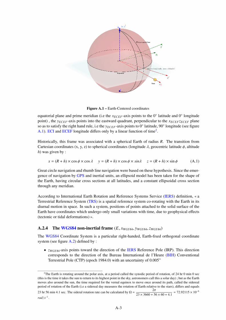
Figure A.1 – Earth-Centered coordinates

equatorial plane and prime meridian (i.e the xECEF-axis points to the 0 latitude and 0 longitude

point) , the yECEF-axis points into the eastward quadrant, perpendicular to the xECEFzECEF plane

so as to satisfy the right hand rule, i.e the yECEF-axis points to 0 latitude, 90 longitude (see figure

A.1). ECI and ECEF longitude differs only by a linear function of time2.

Historically, this frame was associated with a spherical Earth of radius R. The transition from

Cartesian coordinates (x, y, z) to spherical coordinates (longitude λ, geocentric latitude φ, altitude

h) was given by :

x = (R + h) × cos φ × cos λ y = (R + h) × cos φ × sinλ z = (R + h) × sin φ (A.1)

Great circle navigation and rhumb line navigation were based on these hypothesis. Since the emer-

gence of navigation by GPS and inertial units, an ellipsoid model has been taken for the shape of

the Earth, having circular cross sections at all latitudes, and a constant ellipsoidal cross section

through any meridian.

According to International Earth Rotation and Reference Systems Service (IERS) definition, « a

Terrestrial Reference System (TRS) is a spatial reference system co-rotating with the Earth in its

diurnal motion in space. In such a system, positions of points attached to the solid surface of the

Earth have coordinates which undergo only small variations with time, due to geophysical effects

(tectonic or tidal deformations) ».

A.2.4 The WGS84 non-inertial frame (E, xWGS 84, yWGS 84, zWGS 84)

The WGS84 Coordinate System is a particular right-handed, Earth-fixed orthogonal coordinate

system (see figure A.2) defined by :

• zWGS 84-axis points toward the direction of the IERS Reference Pole (IRP). This direction

corresponds to the direction of the Bureau International de l’Heure (BIH) Conventional

Terrestrial Pole (CTP) (epoch 1984.0) with an uncertainty of 0.005”

2The Earth is rotating around the polar axis, at a period called the synodic period of rotation, of 24 hr 0 min 0 sec

(this is the time it takes the sun to return to its highest point in the sky, astronomers call this a solar day) ; but as the Earth

moves also around the sun, the time required for the vernal equinox to move once around its path, called the sidereal

period of rotation of the Earth (i.e a sidereal day measures the rotation of Earth relative to the stars), differs and equals

23 hr 56 min 4.1 sec. The sideral rotation rate can be calculated by Ω =2π

23 × 3660 + 56 × 60 + 4.1= 72.92115 × 10−6

rad/s−1.

A-3

Figure A.2 – WGS84 Reference Frame

• xWGS 84-axis points the the intersection of the IERS Reference Meridian (IRM) and the plane

passing through the origin and normal to the zWGS 84. The IRM is coincident with the BIH

Zero Meridian (epoch 1984.0) with an uncertainty of 0.005”

• xWGS 84 completes a right-handed, ECEF orthogonal coordinate system.

Its origin is fixed at the center of gravity of the Earth like the ECEF and ECI frames.

A.2.5 The fixed non-inertial NED frame FE(O, xE, yE, zE)

The fixed NED system is a non-inertial system with its origin O fixed at the surface of the Earth’s

geoid (e.g radar site). Its axes are oriented along the geodetic directions defined by the Earth’s

surface. The axis are defined as follows (See figure A.3) :

• The xE-axis points North parallel to the geoid surface, in the polar direction (geodetic

North).

• The yE-axis points East parallel to the geoid surface, along a latitude curve (geodetic East).

• The zE-axis points downward, toward the Earth’s surface, antiparallel to the surface’s out-

ward normal −→n (on the hypothesis that Earth is a sphere, −→n and gravitational attraction −→gare collinear).

Three numbers represent the aircraft position, one represents the position along the northern axis,

one along the eastern axis, and one represents vertical position. This frame, based on the WGS84

ellipsoid model, it is mainly used for navigation. It is also named Normal Earth-fixed frame

FE(O, xE , yE , zE) [19].

This frame can also be referenced as FNEDE(O, xNEDE

, yNEDE, zNEDE

).

A.2.6 The fixed non-inertial ENU frame FENUE(O, xENUE

, yENUE, zENUE

)

The fixed ENU system is a non-inertial system with its origin O fixed at the surface of the Earth’s

geoid (e.g radar site). Its axes are oriented along the geodetic directions defined by the Earth’s

surface. The axis are defined as follows :

• The xENUE-axis points North parallel to the geoid surface, in the polar direction (geodetic

North).

• The yENUE-axis points East parallel to the geoid surface, along a latitude curve (geodetic

East).

A-4

Figure A.3 – Fixed and Moving North-East-Down (NED) axes system

• The zENUE-axis points upward, outward the Earth’s surface, parallel to the surface’s outward

normal −→n (on the hypothesis that Earth is a sphere, −→n and gravitational attraction −→g are

collinear).

Three numbers represent the aircraft position, one represents the position along the eastern

axis, one along the northern axis, and one represents vertical position. This frame, based

on the WGS84 ellipsoid model, may be prefered to NED because altitude increases in the

upward direction.

A.2.7 The vehicle carried non-inertial NED frame Fo(G, xo, yo, zo)

This coordinate system is associated with the aircraft position. Its axes are not fixed in orientation

with respect to the airplane. The frame origin is located at the aircraft center of mass G. The axis

are defined as follows (see figure A.3) :

• The xo-axis points toward the ellipsoid north (geodetic North), therefore North of point G

and not of point O.

• The yo-axis points toward the ellipsoid east (geodetic East).

• The zo-axis points downward along the ellipsoid normal at the G position.

Thus the Gxo-axis is not parallel to OxE-axis.

A.2.8 The non-inertial body frame Fb(G, xb, yb, zb)

The non-inertial body-fixed frame (G, xb, yb, zb) has its origin and orientation fixed to the moving

plane (See figures A.4 and A.5). It assumes the aircraft is rigid and has an exact symmetry. Its

origin is at the plane center of mass G, and

• The xb-axis points through the nose of the craft, a positive rotation about the xb-axis corre-

sponds to right wing down.

• The yb-axis points to the right of the xb-axis (facing in the pilot’s direction of view), per-

pendicular to the xb-axis. A positive rotation about the yb-axis corresponds to nose pitch

up.

• The zb-axis points down through the bottom the aircraft, perpendicular to the xbyb plane and

satisfying the right hand rule. A positive rotation about the zb-axis corresponds to a positive

counter-clockwise rotation in yaw.

A-5

Figure A.5 – Body axes System (top view)

Figure A.4 – Body axes system

A.2.9 The non-inertial aerodynamic frame Fa(G, xa, ya, za)

The non-inertial aerodynamic coordinate system (G, xa, ya, za) has its origin at the rigid aircraft

center of mass G. The coordinate system orientation is defined relative to the airplane’s aerody-

namic velocity vector−→Va. This frame is also named air-path frame [19, p. 17].

The orientation of the aerodynamic coordinate axes is fixed by the velocity−→Va the following way :

A-6

• The xa-axis is coincident with the velocity vector and points in the direction of−→Va

3.

• The ya-axis points to the right of the xa-axis (facing in the direction of−→Va), perpendicular to

the xa-axis.

• The za-axis points perpendicular to the xaya plane to satisfy the right hand rule with respect

to the xa and ya axes, and is in the aircraft symmetrical plane xbyb.

The xa-axis and the ya-axis are located in the aircraft instantaneous plane of motion. This frame

introduces two rotation angles :

• αa the aerodynamic angle of attack,

• βa the aerodynamic sideslip angle

Both angles are used for transformation from the body frame to the aerodynamic coordinate frame.

This frame is also named the wind axes system in [64, p. 18].

A.2.10 The kinematic or flight-path frame Fk (G, xk, yk, zk)

The non inertial flight path coordinate system (G, xk, yk, zk) is a moving reference frame, and has

its origin at the rigid aircraft center of mass G.

The orientation of the kinematic coordinate axes is fixed by the kinematic velocity−→Vk

4 the follow-

ing way :

• The xk-axis is coincident with the velocity vector relative to the inertial reference frame and

points in the direction of−→Vk.

• The yk-axis points to the right of the xk-axis (facing in the direction of−→Vk), perpendicular to

the xk-axis and to the gravity vector.

• The zk-axis is located within the vertical plane formed by the flight path and gravity vector.

The coordinate system is defined by two rotations Z αk (kinematic angle of attack) and βk (kine-

matic sideslip angle). Both are used for the transformation from the body frame Fb to kinematic

frame Fk.

A.2.11 The geodetic coordinate system (λgeodetic,Φgeodetic, h)

The geodetic coordinate uses an ellipsoid model for the shape of the Earth. Longitude in geode-

tic coordinate is the same as in ECEF frame with spherical Earth model, and geodetic latitude is

defined as the angle between the equatorial plane and the normal to the reference ellipsoid sur-

face. This system is widely used for navigation using either United States Global Positioning

System (GPS) or Inertial Navigation Systems (INS), or both. INS alignment is with respect to

the local vertical, which does not generally pass through the center of the Earth as the Earth is

not spherical. GPS positioning uses such a coordinate system where the ellipsoid parameters are

called WGS84 ellipsoid parameters.

3At time t the center of mass G of the aircraft occupies a certain position in the atmosphere. In the absence of the

airplane, this position would have been occupied by the W particle of air,−→Va is velocity of G relative to that particle

−→Va =

d−−−−→WGE

dt[19].

4−→Vk is the kinematic velocity of the center of mass G of the aircraft. It is defined relative to the Earth fixed NED

frame by−→Vk =

d−−−→OGE

dt[19].

A-7

The latitude in such a geodetic system is defined with reference to the local normal to ensure that

for two points, with Lat1 and Lat2 latitude, located along the same meridian, the local vertical

turns of Lat2 − Lat1 when moving from one point to another.

The geodetic coordinate system, even if defined using the ECEF frame, is not a Cartesian coordi-

nate system (see figure A.6), the position of a point is given by its :

• longitude λgeodetic, with π < λgeodetic ≤ π

• geodetic latitude Φgeodetic, with−π2< Φgeodetic <

π

2

• orthometric height h measured along the (curved) plumbline (i.e measured along the surface

normal, h = d(O,G) on figure A.6).

O

G

EC Φgeocentric Φgeodetic

Figure A.6 – geocentric and geodetic latitudes

This coordinate system uses the following common intermediate functions or parameters associ-

ated with oblate ellipsoids :

major semi-axis : a (A.2)

minor semi-axis : b (A.3)

flattening : f = 1 − b

a(A.4)

first eccentricity : e2 = 1 − (b

a)2 (A.5)

radius of curvature in the prime vertical : RN(Φgeodetic) =a

√

1 − e2sin2Φgeodetic

(A.6)

radius of curvature in the meridian : RM(Φgeodetic) =a(1 − e2)

(√

1 − e2sin2Φgeodetic)3

(A.7)

RM(Φgeodetic) is the radius of curvature along lines of constant longitude, RN(Φgeodetic) is the radius

A-8

of curvature along lines of constant latitude. Calculation can be done using WGS84 parameters :

a = 6378137 m (A.8)

b = 6356752.31424518 m (A.9)

1

f= 298.257223563 (A.10)

e = 0.0818191908426215 (A.11)

A.3 Angles and transformation matrices between frames

A.3.1 Matrix of transformation between frames

A vector can be defined as a segment of a line with direction, or as its projection on a reference

system (O, x, y, z), i.e frame. The first form does not depend on any reference system, whereas the

second depends directly on the coordinate system in terms of its components. We use a superscript

i to represent the vector−→X in the frame Fi, and the following notations for vectors :

•−→Xi represents the vector

−→X projected on frame Fi.

• Xi =

xi

yi

zi

represents the vector components matrix.

The transformation between two different orthogonal, right-hand sided, reference frames Fi and

F j can be modeled by a matrix of transformation . The matrix i j is the transformation matrix

from the frame Fi to the frame F j.

Xi = i jXj (A.12)

All of the transformation matrices are orthonormal, their inverse is equivalent to their transpose

and their determinant is equal to 1 :

−1i j =

ti j = ji (A.13)

det(i j) = 1 (A.14)

By successively rotating one reference system about three of its own principal axes, it is possible

to achieve any possible orientation for the reference frame.

The elementary rotations about the three principle axes use the following transformation matrices :

A rotation through an angle of αx radians about the x-axis is defined as :

01(αx) =

1 0 0

0 cosαx − sinαx

0 sinαx cosαx

(A.15)

X0 = 01X1 (A.16)

A rotation through an angle of αy radians about the y-axis is defined as :

01(αy) =

cosαy 0 sinαy

0 1 0

− sinαy 0 cosαy

(A.17)

A-9

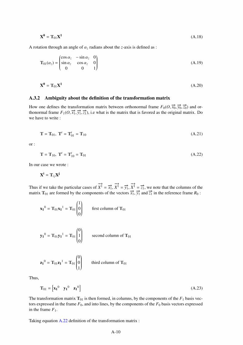
X0 = 01X1 (A.18)

A rotation through an angle of αz radians about the z-axis is defined as :

01(αz) =

cosαz − sinαz 0

sinαz cosαz 0

0 0 1

(A.19)

X0 = 01X1 (A.20)

A.3.2 Ambiguity about the definition of the transformation matrix

How one defines the transformation matrix between orthonormal frame F0(O,−→x0,−→y0,−→z0) and or-

thonormal frame F1(O,−→x1,−→y1,−→z1), i.e what is the matrix that is favored as the original matrix. Do

we have to write :

= 01, t = t

01 = 10 (A.21)

or :

= 10, t = t

10 = 01 (A.22)

In our case we wrote :

Xi = i jXj

Thus if we take the particular cases of−→X1 =

−→x1,−→X1 =

−→y1,−→X1 =

−→z1, we note that the columns of the

matrix 01 are formed by the components of the vectors −→x1, −→y1 and −→z1 in the reference frame R0 :

x10 = 01x1

1 = 01

1

0

0

first column of 01

y10 = 01y1

1 = 01

0

1

0

second column of 01

z10 = 01z1

1 = 01

0

0

1

third column of 01

Thus,

01 =[

x10 y1

0 z10]

(A.23)

The transformation matrix 01 is then formed, in columns, by the components of the F1 basis vec-

tors expressed in the frame F0, and into lines, by the components of the F0 basis vectors expressed

in the frame F1.

Taking equation A.22 definition of the transformation matrix :

A-10

• a rotation through an angle of αx radians about the x-axis would have been defined by the

transformation matrix :

10(αx) =

1 0 0

0 cosαx sinαx

0 − sinαx cosαx

(A.24)

• a rotation through an angle of αy radians about the y-axis would have been defined by the

transformation matri :

10(αy) =

cosαy 0 − sinαy

0 1 0

sinαy 0 cosαy

(A.25)

• a rotation through an angle of αz radians about the z-axis would have been defined by the

transformation matrix :

10(αz) =

cosαz sinαz 0

− sinαz cosαz 0

0 0 1

(A.26)

The transformation matrix 10 is then formed, in rows, by the components of the F1 basis vectors

expressed in the frame F0, and into columns, by the components of the F0 basis vectors expressed

in the frame F1.

A.3.3 Sequential transformations

Any orientation between frame F0 and frame F3 can be achieved by composing three elemen-

tal rotations. Assuming that the F3 rotating coordinate system is rigidly attached to the plane

rigid body, its orientation can be calculated from three successive rotations using two intermediate

frames F1 and F2 as follow :

• Frame F1 is obtained by rotating the frame F0 about the axis OzO of a ψ angle, resulting in

the following transformation matrix :

01(ψ) =

cosψ − sinψ 0

sinψ cosψ 0

0 0 1

(A.27)

With

X0 = 01X1

• Frame F2 is obtained by rotating the frame F1 about the axis Oy1 of a θ angle, resulting in


12(θ) =

cos θ 0 sin θ

0 1 0

− sin θ 0 cos θ

(A.28)

Where transformation matrix 12 is formed, in columns, by the components of the F2 basis

vectors expressed in the transformed frame F1, and with

X1 = 12X2

A-11

• Frame F3 is obtained by rotating the frame F2 about the axis Ox2 of a ϕ angle, resulting in


23(ϕ) =

1 0 0

0 cosϕ − sinϕ

0 sinϕ cosϕ

(A.29)

Where transformation matrix 23 is formed, in columns, by the components of the F3 basis

vectors expressed in the transformed frame F2, and with

X2 = 23X3

By substituting X1 and X2 we have :

X0 = 01X1 = 0112X2 = 011223X3 = 03X3

with :

03 = 011223 (A.30)

and :

03 =

cos θ cosψ cosψ sin θ sinϕ − cosϕ sinψ cosϕ cosψ sin θ + sinϕ sinψ

cos θ sinψ sin θ sinϕ sinψ + cosϕ cosψ cosϕsinθ sinψ − cosψ sinϕ

− sin θ cos θ sinϕ cos θ cosϕ

(A.31)

finally giving :

X0 = 03X3 (A.32)

Using equation A.21 to define the transformation matrix, the direct transformation matrix from the

first to the third cascading reference frame is found by successive matrix multiplications of each

relative transformation matrix, in the same order than the rotations. This definition is used in [19,

p. 29].

Using equation A.22 to define the transformation matrix, the rotation matrices are :

10(ψ) =

cosψ sinψ 0

− sinψ cosψ 0

0 0 1

(A.33)

21(θ) =

cos θ 0 − sin θ

0 1 0

sin θ 0 cos θ

(A.34)

32(ϕ) =

1 0 0

0 cosϕ sinϕ

0 − sinϕ cosϕ

(A.35)

X3 = 32X2 = 3221X1 = 322110X0 = 30X0

with :

30 = 322110 (A.36)

and :

30 =

cos θ cosψ cos θ sinψ − sin θ

cosψ sin θ sinϕ − cosϕ sinψ sin θ sinϕ sinψ + cosϕ cosψ cos θ sinϕ

cosϕ cosψ sin θ + sinϕ sinψ cosϕ sin θ sinψ − cosψ sinϕ cos θ cosϕ

(A.37)

A-12

finally giving :

X3 = 30X0 (A.38)

Using formula A.22, the direct transformation matrix from the first to the third cascading reference

frame is found by successive matrix multiplications of each relative transformation matrix, in

reverse order than the rotations. This definition is used in [133, p. 47].

Using formula A.21, we found that :

X0 = 03X3

which can be written :

X3 = t03X0

with :

t03 =

cos θ cosψ cos θ sinψ − sin θ

cosψ sin θ sinϕ − cosϕ sinψ sin θ sinϕ sinψ + cosϕ cosψ cos θ sinϕ

cosϕ cosψ sin θ + sinϕ sinψ cosϕ sin θ sinψ − cosψ sinϕ cos θ cosϕ

(A.39)

Finally both A.22 and A.37 definitions lead to the same result if care is taken on the original matrix

choice, and on the matrix multiplication order during successive frame rotations.

A.3.4 Transformation from ellipsoidal geodetic coordinate to ECEF Cartesian co-

ordinate

Different methods of transforming geodetic coordinates to geocentric coordinates are used [21].

The geodetic to geocentric transformation (i.e given the latitude, longitude, and height finding the

Cartesian coordinate) is fairly simple and the relationships are well known and detailed below.

Problems existed for the reverse transformation until pure inverse relationship were established

[109], [57].

Coordinates transformation from geodetic coordinate to ECEF coordinate is done through map-

ping equations, as expressed in ellipsoidal coordinates λgeodetic, Φgeodetic, h.

xECEF = (RN(Φgeodetic) + h) cosΦgeodetic cos λgeodetic (A.40)

yECEF = (RN(Φgeodetic) + h) cosΦgeodetic sin λgeodetic (A.41)

zECEF =[

(1 − e2)RN(Φgeodetic) + h]

sinΦgeodetic (A.42)

where RN and e are respectively defined in equations A.6 and A.5.

Equations A.40, A.41, A.42 are only valid if the ellipsoidal geodetic system is based on the Green-

wich meridian.

Example : Taking the Ecole Nationale de l’Aviation Civile (ENAC) coordinates from a hand held

GPS we have using equations A.40, A.41, A.42 :

Geodetic WGS84 :

Φgeodetic = 4333′56.6”N

λgeodetic = 128′49.3”E

h = 6 m

giving ECEF :

xECEF = 4627322.397 m

yECEF = 119583.543 m

zECEF = 4373259.642 m

The used h is the height above the ellipsoid, i.e height value that is delivered by GPS satellite

observations. It is not the gravity-related height value which is normally used for national mapping

and leveling operations5.

5The gravity-related height H is usually the height above mean sea level, in aviation it is given by an altimeter,

with altimeter setting set to Atmospheric pressure (Q) at Nautical Height (QNH). Equations A.40, A.41, A.42 work

A-13

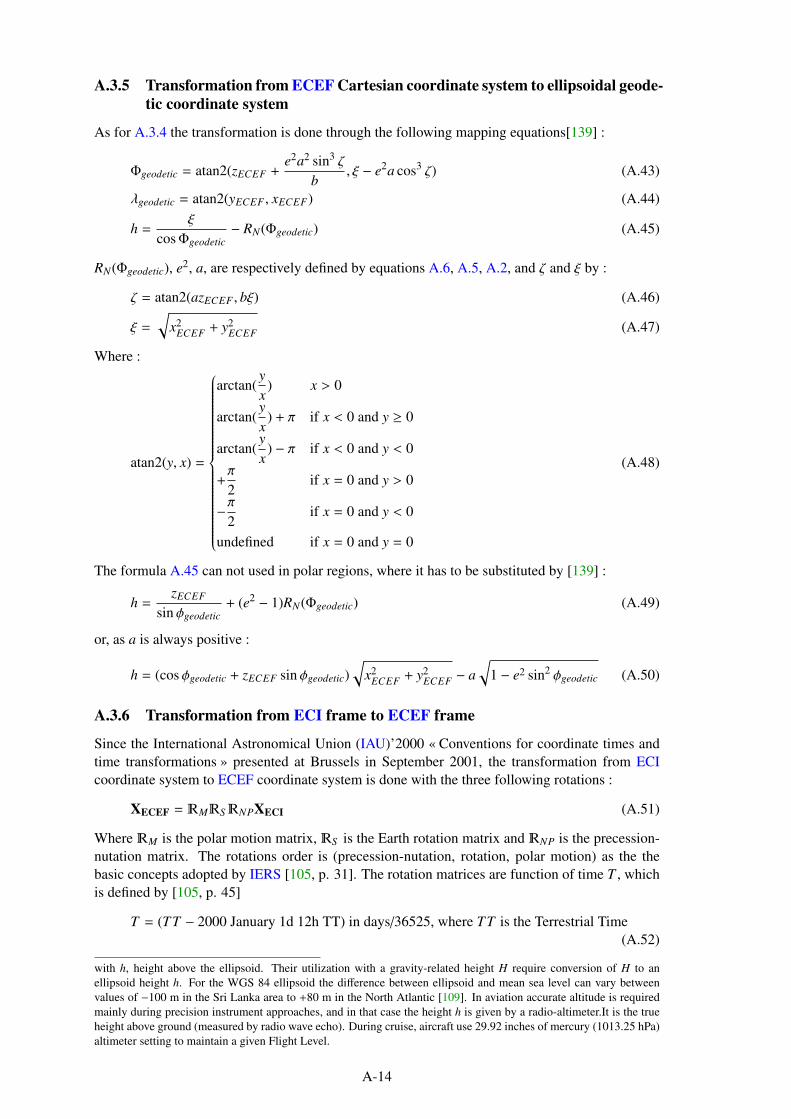
A.3.5 Transformation from ECEF Cartesian coordinate system to ellipsoidal geode-

tic coordinate system

As for A.3.4 the transformation is done through the following mapping equations[139] :

Φgeodetic = atan2(zECEF +e2a2 sin3 ζ

b, ξ − e2a cos3 ζ) (A.43)

λgeodetic = atan2(yECEF , xECEF) (A.44)

h =ξ

cosΦgeodetic

− RN(Φgeodetic) (A.45)

RN(Φgeodetic), e2, a, are respectively defined by equations A.6, A.5, A.2, and ζ and ξ by :

ζ = atan2(azECEF , bξ) (A.46)

ξ =

√

x2ECEF

+ y2ECEF

(A.47)

Where :

atan2(y, x) =

arctan(y

x) x > 0

arctan(y

x) + π if x < 0 and y ≥ 0

arctan(y

x) − π if x < 0 and y < 0

+π

2if x = 0 and y > 0

−π2

if x = 0 and y < 0

undefined if x = 0 and y = 0

(A.48)

The formula A.45 can not used in polar regions, where it has to be substituted by [139] :

h =zECEF

sin φgeodetic

+ (e2 − 1)RN(Φgeodetic) (A.49)

or, as a is always positive :

h = (cos φgeodetic + zECEF sin φgeodetic)

√

x2ECEF

+ y2ECEF

− a

√

1 − e2 sin2 φgeodetic (A.50)

A.3.6 Transformation from ECI frame to ECEF frame

Since the International Astronomical Union (IAU)’2000 « Conventions for coordinate times and

time transformations » presented at Brussels in September 2001, the transformation from ECI

coordinate system to ECEF coordinate system is done with the three following rotations :

XECEF = MSNPXECI (A.51)

Where M is the polar motion matrix, S is the Earth rotation matrix and NP is the precession-

nutation matrix. The rotations order is (precession-nutation, rotation, polar motion) as the the

basic concepts adopted by IERS [105, p. 31]. The rotation matrices are function of time T , which

is defined by [105, p. 45]

T = (TT − 2000 January 1d 12h TT) in days/36525, where TT is the Terrestrial Time

(A.52)

with h, height above the ellipsoid. Their utilization with a gravity-related height H require conversion of H to an

ellipsoid height h. For the WGS 84 ellipsoid the difference between ellipsoid and mean sea level can vary between

values of −100 m in the Sri Lanka area to +80 m in the North Atlantic [109]. In aviation accurate altitude is required

mainly during precision instrument approaches, and in that case the height h is given by a radio-altimeter.It is the true

height above ground (measured by radio wave echo). During cruise, aircraft use 29.92 inches of mercury (1013.25 hPa)

altimeter setting to maintain a given Flight Level.

A-14

In a first approach, and for our navigation purposes we can neglect the precession-nutation and the

polar motion. We thus make the hypothesis that the transformation from the ECI frame to ECEF

frame is a simple rotation about the zI axis by the Earth’s Rotation Angle (ERA) ϑ defined by :

ϑ = 2π(0.7790572732640 + 1.00273781191135448) × Tu (A.53)

with Tu = Julian UT1 date − 2451545.0 (A.54)

UT1 = UTC + ∆UT1 (see A.4 for UT1 definition) (A.55)

According to [105] S = 3(ϑ) giving the rotation matrix

S = 3(ϑ) =

cosϑ sinϑ 0

− sinϑ cosϑ 0

0 0 1

with XECEF = S XECI

According to our definition for a rotation through an angle ϑ about the zECI-axis the transformation

matrix is :

ECIECEF(ϑ) =

cosϑ − sinϑ 0

sinϑ cosϑ 0

0 0 1

with XECI = ECIECEFXECEF (A.56)

A.3.7 Transformation from ECEF frame to fixed NED frame FE(O, xE, yE, zE)

The origin O of the NED frame is defined by longitude λ = λOgeodetic, geodetic latitudeΦ=ΦOgeodetic,

and height h. The coordinates xECEFO

, yECEFO

, zECEFO

of O are calculated using equations A.40,

A.41, A.42, and two rotations are needed :

• one rotation about the axis zECEF , through an angle of longitude λ (yECEF is led to the y1

intermediate axis) ,

• one rotation about the axis y1 through an angle of −π2− Φ (z1 intermediate axis is led to zE).

giving the two transformation matrices :

ECEF1 =

cos λ − sin λ 0

sin λ cos λ 0

0 0 1

and

1E =

cos(−π2 − Φ) 0 sin(−π2 − Φ)

0 1 0

− sin(−π2 − Φ) 0 cos(−π2 − Φ)

=

− sin(Φ 0 − cosΦ

0 1 0

cosΦ 0 − sinΦ

finally giving

ECEFE = ECEF11E =

− sinΦ cos λ − sin λ − cos λ cosΦ

− sin λ sinΦ cos λ − sin λ cosΦ

cosΦ 0 − sinΦ

(A.57)

A.3.8 Transformation from fixed NED frame to fixed ENU frame

The coordinate of the ENU frame unit vectors expressed in the NED frame are respectively

(0, 1, 0), (1, 0, 0), (0, 0,−1) giving the transformation matrix (cf. A.3.2) :

NEDE ENUE=

0 1 0

1 0 0

0 0 −1

(A.58)

With

XNEDE = NEDENUXENUE

A-15

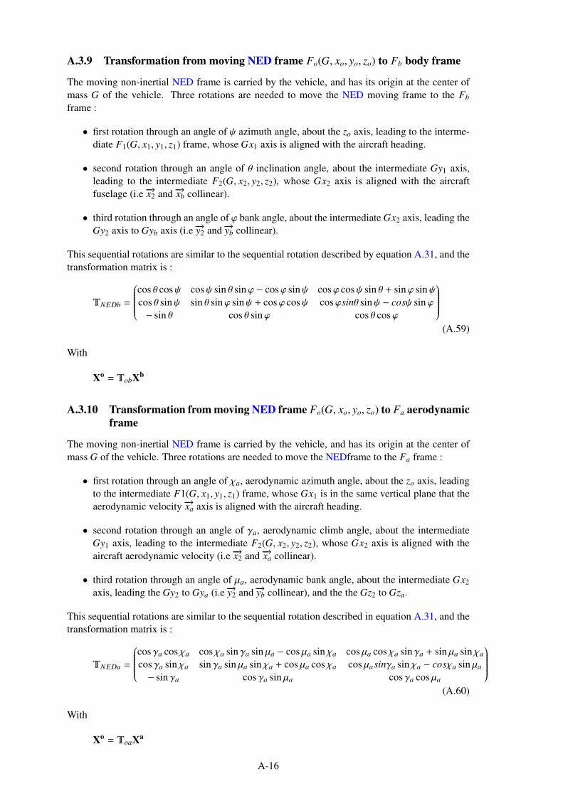
A.3.9 Transformation from moving NED frame Fo(G, xo, yo, zo) to Fb body frame

The moving non-inertial NED frame is carried by the vehicle, and has its origin at the center of

mass G of the vehicle. Three rotations are needed to move the NED moving frame to the Fb

frame :

• first rotation through an angle of ψ azimuth angle, about the zo axis, leading to the interme-

diate F1(G, x1, y1, z1) frame, whose Gx1 axis is aligned with the aircraft heading.

• second rotation through an angle of θ inclination angle, about the intermediate Gy1 axis,

leading to the intermediate F2(G, x2, y2, z2), whose Gx2 axis is aligned with the aircraft

fuselage (i.e −→x2 and −→xb collinear).

• third rotation through an angle of ϕ bank angle, about the intermediate Gx2 axis, leading the

Gy2 axis to Gyb axis (i.e −→y2 and −→yb collinear).

This sequential rotations are similar to the sequential rotation described by equation A.31, and the

transformation matrix is :

NEDb =

cos θ cosψ cosψ sin θ sinϕ − cosϕ sinψ cosϕ cosψ sin θ + sinϕ sinψ

cos θ sinψ sin θ sinϕ sinψ + cosϕ cosψ cosϕsinθ sinψ − cosψ sinϕ

− sin θ cos θ sinϕ cos θ cosϕ

(A.59)

With

Xo = obXb

A.3.10 Transformation from moving NED frame Fo(G, xo, yo, zo) to Fa aerodynamic

frame

The moving non-inertial NED frame is carried by the vehicle, and has its origin at the center of

mass G of the vehicle. Three rotations are needed to move the NEDframe to the Fa frame :

• first rotation through an angle of χa, aerodynamic azimuth angle, about the zo axis, leading

to the intermediate F1(G, x1, y1, z1) frame, whose Gx1 is in the same vertical plane that the

aerodynamic velocity −→xa axis is aligned with the aircraft heading.

• second rotation through an angle of γa, aerodynamic climb angle, about the intermediate

Gy1 axis, leading to the intermediate F2(G, x2, y2, z2), whose Gx2 axis is aligned with the

aircraft aerodynamic velocity (i.e −→x2 and −→xa collinear).

• third rotation through an angle of µa, aerodynamic bank angle, about the intermediate Gx2

axis, leading the Gy2 to Gya (i.e −→y2 and −→yb collinear), and the the Gz2 to Gza.

This sequential rotations are similar to the sequential rotation described in equation A.31, and the

transformation matrix is :

NEDa =

cos γa cos χa cos χa sin γa sin µa − cos µa sin χa cos µa cos χa sin γa + sin µa sin χa

cos γa sin χa sin γa sin µa sin χa + cos µa cos χa cos µasinγa sin χa − cosχa sin µa

− sin γa cos γa sin µa cos γa cos µa

(A.60)

With

Xo = oaXa

A-16

A.3.11 Transformation from body frame Fb to the aerodynamic frame Fa

As the axis Gxa is carried by the aerodynamic velocity−→Va, only two rotations are needed to trans-

form Fb to Fa :

• first rotation through an angle of −αa, where αa is the aerodynamic angle of attack, about

the right wing axis Gyb, leading to the intermediate F1(G, x1, y1, z1) frame, whose axis

Gz1 = Gza belongs to the airplane symmetric plane xbzb.

• second rotation through an angle of βa, where βa is the aerodynamic sideslip angle about

the axis Gz1, leading to the final frame Fa.

The two transformation matrices are :

b1 =

cos(−αa) 0 sin(−αa)

0 1 0

− sin(−αa) 0 cos(−αa)

and 1a =

cos βa − sin βa 0

sin βa cos βa 0

0 0 1

giving the sequential transformation matrix :

ba = b11a =

cosαa cos βa − sin βa cosαa − sinαa

sin βa cos βa 0

sinαa cos βa − sinαa sin βa cosαa

with Xb = baXa (A.61)

A.3.12 Transformation from body frame Fb to the kinematic frame Fk

As the axis Gxb is carried by the kinematic velocity−→Vk, only two rotations are needed to transform

Fb to Fk :

• first rotation through an angle of −αk, where αk is the kinematic angle of attack, about

the right wing axis Gyb, leading to the intermediate F1(G, x1, y1, z1) frame, whose axis

Gz1 = Gzk belongs to the airplane symmetric plane xbzb.

• second rotation through an angle of βk, where βk is the kinematic sideslip angle about the

axis Gz1, leading to the final frame Fk.

The two transformation matrices are :

b1 =

cos(−αk) 0 sin(−αk)

0 1 0

− sin(−αk) 0 cos(−αk)

and 1a =

cos βk − sin βk 0

sin βk cos βk 0

0 0 1

giving the sequential transformation matrix :

bk = b11k =

cosαk cos βk − sin βk cosαk − sinαk

sin βk cos βk 0

sinαk cos βk − sinαk sin βk cosαk

with Xb = bkXk (A.62)

A.3.13 Transformation from kinematic frame Fk to the aerodynamic frame Fa

The transformation will connect the kinematic velocity−→Vk to the aerodynamic velocity

−→Va through

angles relative to the wind6.The transformation is performed using three rotations :

• first rotation through an angle of −αw, where αw is the wind angle of attack, about the axis

Gyk, leading to the intermediate F1(G, x1, y1, z1) frame, whose Gz1 axis belongs to the xkzx

plane,

6If the wind velocity is−→Vw, we have

−→Vk =

−→Va +

−→Vw.

A-17

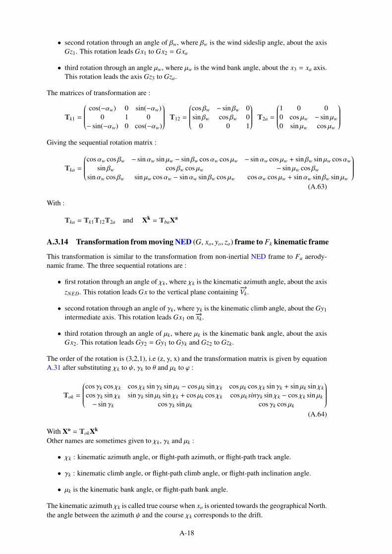
• second rotation through an angle of βw, where βw is the wind sideslip angle, about the axis

Gz1. This rotation leads Gx1 to Gx2 = Gxa

• third rotation through an angle µw, where µw is the wind bank angle, about the x3 = xa axis.

This rotation leads the axis Gz3 to Gza.

The matrices of transformation are :

k1 =

cos(−αw) 0 sin(−αw)

0 1 0

− sin(−αw) 0 cos(−αw)

12 =

cos βw − sin βw 0

sin βw cos βw 0

0 0 1

2a =

1 0 0

0 cos µw − sin µw

0 sin µw cos µw

Giving the sequential rotation matrix :

ka =

cosαw cos βw − sinαw sin µw − sin βw cosαw cos µw − sinαw cos µw + sin βw sin µw cosαw

sin βw cos βw cos µw − sin µw cos βw

sinαw cos βw sin µw cosαw − sinαw sin βw cos µw cosαw cos µw + sinαw sin βw sin µw

(A.63)

With :

ka = k1122a and Xk = baXa

A.3.14 Transformation from moving NED (G, xo, yo, zo) frame to Fk kinematic frame

This transformation is similar to the transformation from non-inertial NED frame to Fa aerody-

namic frame. The three sequential rotations are :

• first rotation through an angle of χk, where χk is the kinematic azimuth angle, about the axis

zNED. This rotation leads Gx to the vertical plane containing−→Vk.

• second rotation through an angle of γk, where γk is the kinematic climb angle, about the Gy1

intermediate axis. This rotation leads Gx1 on −→xk.

• third rotation through an angle of µk, where µk is the kinematic bank angle, about the axis

Gx2. This rotation leads Gy2 = Gy1 to Gyk and Gz2 to Gzk.

The order of the rotation is (3,2,1), i.e (z, y, x) and the transformation matrix is given by equation

A.31 after substituting χk to ψ, γk to θ and µk to ϕ :

ok =

cos γk cos χk cos χk sin γk sin µk − cos µk sin χk cos µk cos χk sin γk + sin µk sin χk

cos γk sin χk sin γk sin µk sin χk + cos µk cos χk cos µksinγk sin χk − cos χk sin µk

− sin γk cos γk sin µk cos γk cos µk

(A.64)

With Xo = okXk

Other names are sometimes given to χk, γk and µk :

• χk : kinematic azimuth angle, or flight-path azimuth, or flight-path track angle.

• γk : kinematic climb angle, or flight-path climb angle, or flight-path inclination angle.

• µk is the kinematic bank angle, or flight-path bank angle.

The kinematic azimuth χk is called true course when xo is oriented towards the geographical North.

the angle between the azimuth ψ and the course χk corresponds to the drift.

A-18

A.4 Time Systems

Since the development of satellites three time systems are used, and have to be mentioned as the

GPS is becoming the primary navigation system. Three times are used :

• The sideral time defined as the hour angle of the Vernal Equinox (i.e. or the Aries point)7, it

measures the Earth’s rotation8. If the previous measure is counted from Greenwich merid-

ian, the sideral time is called Greenwich Sideral Time (GST). The Universal Time (UT) is

the Greenwich (0 longitude) hour of the apparent sun, supposed orbiting uniformly in the

equatorial plane, despite variations in the rotation of the Earth. It is from 0 hours at mid-

night at the time of the September equinox in Greenwich, with unit of duration the mean

solar day. Universal Time 0 (UT0) represents the initial values of Universal Time obtained

by optical observations of star transits at various astronomical observatories. Due to Earth’s

angular velocity variations, sideral time has to be adjusted. Some of these variations are due

to the polar motion of the Earth, and Universal Time 1 (UT1)9 defined by equation A.55 is

the universal time corrected for the polar motion.

• International Atomic Time (TAI) is the International Atomic Time scale, a statistical timescale

based on a large number of atomic clocks. Each GPS satellite carries its each free-running

atomic clock, which provide GPS Time (GPST). Coordinated Universal Time (UTC)10 is

kept within 0.9 seconds of UT1 by the introduction of one-second steps to UTC, the « leap

second »11. This ensures that UTC differs from TAI by an integral number of seconds.

• Dynamical Time replaced ephemeris time as the independent argument in dynamical theo-

ries and ephemerides It is a uniformly-scaled time used to describe the motion of bodies in

a gravitational field. Its unit of duration is based on the orbital motions of the Earth, Moon,

and planets. Terrestrial Time (TT), (also called Terrestrial Dynamical Time (TDT)12 13.

Times relationships are as follows :

T AI = GPS T + 19.0 s (A.65)

T AI = T DT − 32.184 s (A.66)

T AI = UTC + nsec (A.67)

UT1 = UTC + ∆UT1 (A.68)

∆UT1 can be obtained on the ground from the IERS, and is also broadcast by the GPS satellites

in Message Type 32 - Earth Orientation Parameters (EOP).

7Two types of Aries point can be considered : Mean Aries point which is the intersection of mean equator with

the Ecliptic (effect of precession over the earth rotation axis is taken into account) ; True Aries point which is the

intersection between the true equator with the Ecliptic (effects of precession and nutation of earth rotation pole are

taken into account).8of the distant, so-called fixed, stars,9UT1 gives the precise angular coordinate of the Earth about its spin axis.

10Coordinated Universal Time (UTC) is the basis for civil time today.11Leap second adjustments were performed 27 times from 1972 to January 201712In 1991 the IAU redefined TDT and renamed it TT13The epoch designated "J2000.0" is specified as Julian date 2451545.0 TT, or 2000 January 1, 12h TT.

A-19

Appendix B

Direction cosine

B.1 Introduction

Flight dynamics requires various frames to simplify the expression of the forces acting on an air-

plane. Once expressed, these forces need to be summed in a common reference frame where

Newton’s second law will be used to obtain the second derivative of the airplane position, finally

giving after integration its position.

The direction cosine matrix is one of the transformations taking the representation of an arbitrary

vector from one coordinate systems to an other one. To derive the direction cosine matrix we

choose a pure mathematics formalism which will subsequently be linked to section A.3.

B.2 Transformation

Consider r a point in the 3 dimensional Euclidean space, and E1 and E2 two vector spaces with

respective orthonormal bases (x1, y1, z1) and (x2, y2, z2).

The representation of r with respect to each basis is :

r = rx1· x1 + ry1

· y1 + rz1· z1, with r =

rx1

ry1

rz1

=

r • x1

r • y1

r • z1

= (rx1

, ry1, rz1

)T (B.1a)

r = rx2· x2 + ry2

· y2 + rz2· z2, with r =

rx2

ry2

rz2

=

r • x2

r • y2

r • z2

= (rx2

, ry2, rz2

)T (B.1b)

Let’s this coordinate transformation from E1 to E2 be denoted :

ΩE1→E2: (rx1

, ry1, rz1

) 7−→ (rx2, ry2

, rz2) (B.2)

This is a linear transformation, thus it can be realized as a matrix multiplication :

r =

rx2

ry2

rz2

= ΩE1→E2

rx1

ry1

rz1

=

a11 a12 a13

a21 a22 a23

a31 a32 a33

rx1

ry1

rz1

(B.3)

Where

a11 = x1 • x2 a12 = y1 • x2 a13 = z1 • x2

a21 = x1 • y2 a22 = y1 • y2 a23 = z1 • y2

a31 = x1 • z2 a32 = y1 • z2 a33 = z1 • z2

(B.4)

B-1

B.3 Direction cosine matrix

B.3.1 Derivation

By definition of a orthonormal base, each base vector satisfy the following :

‖x1‖ = ‖y1‖ = ‖z1‖ = ‖x2‖ = ‖y2‖ = ‖z2‖ = 1

∀(i = 1, 2, 3) & ( j = 1, 2, 3) xi • xj = ‖xi‖ · ‖xj‖ cos (xi, xj) = cos (xi, xj)

∀(i = 1, 2, 3) & ( j = 1, 2, 3) yi • yj = ‖yi‖ · ‖yj‖ cos (yi, yj) = cos (yi, yj)

∀(i = 1, 2, 3) & ( j = 1, 2, 3) zi • zj = ‖zi‖ · ‖zj‖ cos (zi, zj) = cos (zi, zj)

∀(i = 1, 2, 3) & ( j = 1, 2, 3) xi • yj = ‖xi‖ · ‖yj‖ cos (xi, yj) = cos (xi, yj)

∀(i = 1, 2, 3) & ( j = 1, 2, 3) xi • zj = ‖xi‖ · ‖zj‖ cos (xi, zj) = cos (xi, zj)

∀(i = 1, 2, 3) & ( j = 1, 2, 3) yi • zj = ‖yi‖ · ‖zj‖ cos (yi, zj) = cos (yi, zj)

(B.5)

Looking at equation B.4, we can notice that each dot product is the cosine of the angle between

two base vectors, this explains why this matrix is called Direction Cosine Matrix .

rx2

ry2

rz2

= ΩE1→E2

rx1

ry1

rz1

=

cos (x1, x2) cos (y1, x2) cos (z1, x2)

cos (x1, y2) cos (y1, y2) cos (z1, y2)

cos (x1, z2) cos (y1, z2) cos (z1, z2)

rx1

ry1

rz1

(B.6)

Remark B.1. The columns of the matrix are the basis vectors (x1, y1, z1) in coordinate represen-

tation (x2, y2, z2).

Remark B.2. The rows (or columns of the transpose matrix) are the basis vectors (x2, y2, z2) in

coordinate representation (x1, y1, z1).

B.3.2 Properties

DCM matrix transpose and inverse matrices

We could also have take the coordinate transformation from E2 to E1 as follows :

ΩE2→E1: (rx2

, ry2, rz2

) 7−→ (rx1, ry1

, rz1) (B.7)

and write :

r =

rx1

ry1

rz1

= ΩE2→E1

rx2

ry2

rz2

=

b11 b12 b13

b21 b22 b23

b31 b32 b33

rx2

ry2

rz2

(B.8)

Using the same reasoning as in B.3.1, we can find that :

rx1

ry1

rz1

= ΩE2→E1

rx2

ry2

rz2

=

cos (x2, x1) cos (y2, x1) cos (z2, x1)

cos (x2, y1) cos (y2, y1) cos (z2, y1)

cos (x2, z1) cos (y2, z1) cos (z2, z1)

rx2

ry2

rz2

(B.9)

Using the property that for all vectors u and v, cos (u, v) = cos (v,u), and comparing equations

B.6 and B.9 we can conclude :

ΩE2→E1= Ω−1

E1→E2= ΩT

E1→E2(B.10)

B-2

Number of DCM matrix independent variables

The DCM matrix does not depend on the vector that has to be expressed from one coordinate

system to the other one. If we take :

u =

ux1

uy1

uz1

1

=

1

0

0

1

then, u =

ux2

uy2

uz2

2

=

cos (x1, x2)

cos (x1, y2)

cos (x1, z2)

2

(B.11a)

v =

vx1

vy1

vz1

1

=

0

1

0

1

then, v =

vx2

vy2

vz2

2

=

cos (y1, x2)

cos (y1, y2)

cos (y1, z2)

2

(B.11b)

w =

wx1

wy1

wz1

1

=

0

0

1

1

then, w =

wx2

wy2

wz2

2

=

cos (z1, x2)

cos (z1, y2)

cos (z1, z2)

2

(B.11c)

As ‖u‖ = ‖v‖ = ‖w‖ = 1, we can write :

cos2 (x1, x2) + cos2 (x1, y2) + cos2 (x1, z2) = 1 (B.12a)

cos2 (y1, x2) + cos2 (y1, y2) + cos2 (y1, z2) = 1 (B.12b)

cos2 (z1, x2) + cos2 (z1, y2) + cos2 (z1, z2) = 1 (B.12c)

As u ⊥ v ⊥ w, we can write :

cos (x1, x2) cos (y1, x2) + cos (x1, y2) cos (y1, y2) + cos (x1, z2) cos (y1, z2) = 0 (B.13a)

cos (y1, x2) cos (z1, x2) + cos (y1, y2) cos (z1, y2) + cos (y1, z2) cos (z1, z2) = 0 (B.13b)

cos (x1, x2) cos (z1, x2) + cos (x1, y2) cos (z1, y2) + cos (x1, z2) cos (z1, z2) = 0 (B.13c)

Which by recalling equation B.4 can also be written :

a211 + a2

21 + a231 = 1 (B.14a)

a212 + a2

22 + a223 = 1 (B.14b)

a213 + a2

32 + a233 = 1 (B.14c)

a11 · a12 + a21 · a22 + a31 · a32 = 0 (B.14d)

a12 · a13 + a22 · a23 + a32 · a33 = 0 (B.14e)

a11 · a13 + a21 · a23 + a31 · a33 = 0 (B.14f)

Equation B.14 shows that even if the DCM matrix has nine variables, they are six non linear

equations due to the orthogonality of the columns. As a result, they are only three independent

variables.

Using Euler’s rotation theorem in a three-dimensional space, it can be said that the linear transfor-

mation of equation B.2 is a rotation operation : the matrix ΩE1→E2has a unit eigenvector n = −→n

giving the axis of rotation, and three eigenvalues : 1, eiθ, e−iθ.

ΩE1→E2n = |eiθ| n = |e−iθ| n = n (B.15)

The angle of rotation is given by θ and we can use, for that rotation, the notation :

Rn(θ) (B.16)

for the rotation operator about the axis defined by n and the angle θ

Looking at Eulers’s theorem, at appendix A and at present appendix, it seems that orientation (i.e

attitude) and rotation are the same kind of transformations.

B-3

B.4 Rotation and Orientation

Let’s detail why changes in orientation (i.e attitude) and rotation are not equivalent. Figure B.1

tries to explain the difference.

x

y

Oz

M

xM

yM

M’

x′M

y′Mψ

(a) Rotation

x1

y1

Oz1, z2

x2y2

M

xM1

yM1

xM2

yM2

ψ

(b) Orientation

Figure B.1 – Rotation versus Orientation

In figure B.1a the vector OM undergoes a rotation of ψ about the Oz axis. The resultant vector is

OM′ and the coordinates of the two vectors, expressed in the same base are related by :

x′M

y′M

z′M

= Rz(ψ)

xM

yM

zM

=

cosψ − sinψ 0

sinψ cosψ 0

0 0 1

xM

yM

zM

(B.17)

In figure B.1b the vector OM does not undergoes a rotation, but its coordinates are expressed

in two different bases. The second base (O, x2, y2, z2) is obtained from the rotation of the first

base (O, x1, y1, z1) by an angle ψ about the Oz axis. If we note Ωz(ψ) the orientation Ω1→2 ,

the coordinates of OM expressed in the two different bases are linked by the Direction Cosine

Matrix :

x2

y2

z2

= Ωz(ψ)

x1

y1

z1

=

cosψ sinψ 0

− sinψ cosψ 0

0 0 1

x1

y1

z1

(B.18)

In both cases (fig. B.1a and fig. B.1b) the same axis of rotation is used, with the same angle of

rotation, however the linear operations are the inverses of each other :

Rz(ψ) = ΩTz (ψ) and Rz(ψ)ΩT

z (ψ) = I3x3 (B.19)

Remark B.3. An operator such as Rz(ψ) is called a rotation operator, where as an operator such

as Ω(ψ) is called an orientation operator.

Remark B.4. To transform coordinates back from (O, x2, y2, z2) to (O, x1, y1, z1) the rotation ma-

trix may be used.

x1

y1

z1

= Ω−1

z (ψ)

x2

y2

z2

= Rz(ψ)

x2

y2

z2

(B.20)

The same kind of remark as already been pointed out in appendix A (see A.3.2).

B.5 Conclusions

Rotation and orientation (i.e. attitude) are very confusing, as the used terminology depends on

the domain where there are used. The best clarification we founded was in an Open Graphics

Language (OpenGL) tutorial :

B-4

• An orientation is a state : "The object’s orientation is..."

• A rotation is an operation : "Apply this rotation to the object"

That is, when you apply a rotation, you change the orientation (i.e. the attitude). Both can be

represented with the same tools, which leads to the confusion.

B-5

Appendix C

Euler angles

C.1 Introduction

As stated in 3.7.2, Euler angles are a specification of a rotation, or an orientation, obtained by ap-

plying three consecutive principal rotations. Considering only right handed bases, they are twelve

ways to choose the sequence of rotations. Each order defines an Euler angles convention .

Any arbitrary coordinate frame may be completely related to a new distinct arbitrary coordinate

frame using any one of the twelve different Euler angles sequences : xyz, xzy, xyx, xzx, yzx, yxz,

yzy, yxy, zxy, zyx, zxz, zyz. The yxz means a rotation about the initial y-axis, followed by a rotation

about the new x-axis, followed by a rotation about the newer z-axis.

C.2 Principal rotations

In a three dimensions Euclidean an orthonormal basis may be represented by the coordinates

tuples :

x =

1

0

0

= (1, 0, 0)T y =

0

1

0

= (0, 1, 0)T z =

0

0

1

= (0, 0, 1)T (C.1)

with respect to that basis.

A principal axis of rotation is an axis of rotation using one of the three unit vectors. A rotation

about such an axis is called a principal rotation. Rx(α), Ry(β), Rz(γ) denote the three rotation

operators through the respective angles α, β, γ modulo 2π.

If we start from the (x, y, z) we can write :

• When it is rotated by a principal rotation Rx(α), the resulted basis will have orientation

Ωx(α) with respect to the frame (x, y, z)

• When it is rotated by a principal rotationRy(β), the resulted basis will have orientationΩy(β)

with respect to the frame (x, y, z)

• When it is rotated by a principal rotation Rz(γ), the resulted basis will have orientationΩz(γ)

with respect to the frame (x, y, z)

The three principal rotations may be defined about the original axes, or about the successively ro-

tated axis, which is generally done in flight dynamics. To distinguish between the two definitions,

we will call (x1, y1, z1) the space fixed coordinates (generally the NED frame defined in A.2.5),

and (x2, y2, z2) the body fixed coordinates (e.g. Fb(G, xb, yb, zb) defined in A.2.8).

C-1

C.3 Flight dynamics Euler angles convention

Flight dynamics uses axes (z, y, x) also knows as (3, 2, 1). Some times this convention is called

(x, y, z) or (1, 2, 3). As explained in appendix A and B, the order of the rotations matters, so

how can we get the same results using (3, 2, 1) or (1, 2, 3). The confusion arises from the im-

precision on the reference taken for axes of rotation, the (1, 2, 3) convention considers rotation

about the original axes, whereas the (3, 2, 1) considers rotation about the successively rotated axis.

C.3.1 Euler angles (1, 2, 3) rotation convention

Let’s first consider the case of rotation of a point M (see figure B.1a). This convention specifies

the principal rotations about the space-fixed principal axes as follows :

The first rotation is by an angle φ about the x-axis gives :

x′M

y′M

z′M

= Rx(φ)

xM

yM

zM

=

1 0 0

0 cos φ − sin φ

0 sin φ cos φ

xM

yM

zM

(C.2a)

The second rotation is by an angle θ about the y-axis gives :

x′′M

y′′M

z′′M

= Ry(θ)

x′M

y′M

z′M

=

cos θ 0 sin θ

0 1 0

− sin θ 0 cos θ

x′M

y′M

z′M

(C.2b)

The third rotation is by an angle ψ about the z-axis gives :

x′′′M

y′′′M

z′′′M

= Rz(ψ)

x′′M

y′′M

z′′M

=

cosψ − sinψ 0

sinψ cosψ 0

0 0 1

x′′M

y′′M

z′′M

(C.2c)

Combining the three equations C.2a, C.2b, C.2c we get :

x′′′M

y′′′M

z′′′M

= Rz(ψ)

x′′M

y′′M

z′′M

= Rz(ψ)Ry(θ)

x′M

y′M

z′M

= Rz(ψ)Ry(θ)Rx(φ)

xM

yM

zM

(C.3)

showing that the combined rotation is :

Rz(ψ)Ry(θ)Rx(φ) (C.4)

giving after development :

x′′′M

y′′′M

z′′′M

=

cos θ cosψ − sinψ cos φ + sin θ sin φ cosψ sin φ sinψ + sin θ cos ρ cosψ

sinψ cos θ cos φ cosψ + sin θ sin φ sinψ − sin φ cosψ + sin θ sinψ cos φ

− sin θ sin φ cos θ cos θ cos φ

xM

yM

zM

(C.5)

Equation C.5 makes it possible to calculate point M coordinates, in the fixed base, after the three

sequential rotations. In the present case the object has been "oriented" and equation C.5 gives its

new coordinates in the fixed base. Only one base is used for all calculations.

This sequence of rotations is known as the 1-2-3 rotation sequence, since the first rotation occurs

about the first axis of the initial frame, the second rotation occurs about the second axis of the

same initial frame, and the third rotation occurs about the third axis of the initial frame again.

C-2

C.3.2 Euler angles (3, 2, 1) orientation convention

As explained in B.4, orientation deals with, at least, two bases (O, x1, y1, z1), (O, x2, y2, z2), and

with expressing coordinates in either bases.

Let’s ΩE2→E1be the orientation operator between the two bases, and u = (x, y, z)T a vector of the

space. We have, according to Appendix B :

r =

rx1

ry1

rz1

= ΩE2→E1

rx2

ry2

rz2

(C.6a)

or

r =

rx2

ry2

rz2

= ΩE1→E2

rx1

ry1

rz1

(C.6b)

Flight dynamics uses Euler angles to specify aircraft attitude (i.e. orientation) with respect to

a fixed coordinates system, and to derive equations of motion. As three rotations are needed to

achieve any orientation with respect to (O, x1, y1, z1), we need two intermediate bases (O, x′, y′, z′)and (O, x”, y”, z”) to change the orientation from (O, x1, y1, z1) to (O, x2, y2, z2) initially aligned.

Let’s first consider the following sequence of rotation expressed in the fixed coordinates system,

assumed to be (O, x1, y1, z1). The following sequence :

• first rotation is by an angle ψ about the z1-axis, and rotates (O, x1, y1, z1) to (O, x′, y′, z′)

• second rotation is by an angle θ about the y1-axis, and rotates (O, x′, y′, z′) to (O, x”, y”, z”)

• third rotation is by an angle φ about the x1-axis, and rotates (O, x”, y”, z”) to (O, x2, y2, z2)

gives :

r =

rx′

ry′

rz′

= ΩE1→E′

rx1

ry1

rz1

= Ωz1

(ψ)

rx1

ry1

rz1

(C.7)

then

r =

rx”

ry”

rz”

= ΩE′→E”

rx′

ry′

rz′

= Ωy1

(θ)

rx′

ry′

rz′

= Ωy1

(θ)Ωz1(ψ)

rx1

ry1

rz1

(C.8)

finally

r =

rx2

ry2

rz2

= ΩE”→E2

rx”

ry”

rz”

= Ωx1

(φ)

rx”

ry”

rz”

= Ωx1

(φ)Ωy1(θ)Ωz1

(ψ)

rx1

ry1

rz1

= ΩE1→E2

rx1

ry1

rz1

(C.9)

Equation C.9 shows that the orientation operator between the two bases is given by :

ΩE1→E2= Ωx1

(φ)Ωy1(θ)Ωz1

(ψ) (C.10)

Let’s find the final matrix. From B.9, we get :

rxa

rya

rza

= ΩEb→Ea

rxb

ryb

rzb

=

cos (xb, xa) cos (yb, xa) cos (zb, xa)

cos (xb, ya) cos (yb, ya) cos (zb, ya)

cos (xb, za) cos (yb, za) cos (zb, za)

rxb

ryb

rzb

(C.11)

C-3

The orientation operators are :

ΩE1→E′ = Ωz1(ψ) =

cosψ cos(π

2− ψ) 0

cos(π

2+ ψ) cosψ 0

0 0 1

=

cosψ + sinψ 0

− sinψ cosψ 0

0 0 1

(C.12a)

ΩE′→E” = Ωy1(θ) =

cos θ 0 cos(π

2+ θ)

0 1 0

cos(π

2− θ) 0 cos θ

=

cos θ 0 − sin θ

0 1 0

+ sin θ 0 cos θ

(C.12b)

ΩE”→E2= Ωx1

(φ) =

1 0 0

0 cos φ cos(π

2− φ)

0 cos(π

2+ φ) cos φ

=

1 0 0

0 cos φ + sin φ

0 − sin φ cos φ

(C.12c)

Finally giving :

ΩE1→E2= Ωx1

(φ)Ωy1(θ)Ωz1

(ψ) =

cos θ cosψ sinψ cos θ − sin θ

− sinψ cos φ + sin φ sin θ cosψ cos φ cosψ + sin φ sin θ sinψ sin φ cos θ

sin φ sinψ + sin θ cos φ cosψ − sin φ cosψ + sin θ sinψ cos φ cos φ cos θ

(C.13)

C.3.3 Euler angles as used in Flight Dynamics

To change the orientation from (O, x1, y1, z1) to (O, x2, y2, z2), flight dynamics usage is to ex-

press Euler rotations in the moving base (O, x2, y2, z2) and in the intermediate bases (O, x′, y′, z′),(O, x”, y”, z”). Most often the body frame (G, xb, yb, zb) is the moving frame, its alignment is done

at the gate with the NED frame 1.

The first rotation by an angle ψ (aircraft heading in aircraft and aerospace applications) clockwise

about the z′-axis gives :

x1

y1

z1

= ΩE′→E1

x′

y′

z′

= Ωz′(ψ)

x′

y′

z′

=

cosψ cos(π

2+ ψ) 0

cos(π

2− ψ) cosψ 0

0 0 1

x′

y′

z′

=

cosψ − sinψ 0

sinψ cosψ 0

0 0 1

x′

y′

z′

(C.14a)

The second rotation by an angle θ (aircraft pitch or elevation in aircraft and aerospace applications)

clockwise about the y′-axis gives :

x′

y′

z′

= ΩE′′→E′

x′′

y′′

z′′

= Ωy′(θ)

x′′

y′′

z′′

=

cos θ 0 cos(π

2− θ)

0 1 0

cos(π

2+ θ) 0 cos θ

=

cos θ 0 + sin θ

0 1 0

− sin θ 0 cos θ

x′′

y′′

z′′

(C.14b)

The third rotation by an angle φ (aircraft bank angle in aircraft and aerospace applications) clock-

wise about the x”-axis gives :

x′′

y′′

z′′

= ΩE2→E′′

x2

y2

z2

= Ωx′′(φ)

x2

y2

z2

=

1 0 0

0 cos φ cos(π

2+ φ)

0 cos(π

2− φ) cos φ

x2

y2

z2

=

1 0 0

0 cos φ − sin φ

0 + sin φ cos φ

x2

y2

z2

1Alignment define the orientation of the aircraft "frame" (body frame) and the geographic reference frame (NED

frame).

C-4

(C.14c)

Combining equations C.14a, C.14b, C.14c we have :

x1

y1

z1

= ΩE′→E1

x′

y′

z′

= ΩE′→E1

ΩE′′→E′

x′′

y′′

z′′

= ΩE′→E1

ΩE′′→E′ΩE2→E′′

x2

y2

z2

= Ωz′(ψ)Ωy′(θ)Ωx′′(φ)

x2

y2

z2

(C.15)

Thus the final orientation is given by :

ΩE2→E1= Ωz′(ψ)Ωy′(θ)Ωx”(φ) (C.16)

and

ΩE2→E1=

cos θ cosψ − sinψ cos φ + sin φ sin θ cosψ sin φ sinψ + sin θ cos φ cosψ

sinψ cos θ cos φ cosψ + sin φ sin θ sinψ − sin φ cosψ + sin θ sinψ cos φ

− sin θ sin φ cos θ cos φ cos θ

(C.17)

Comparing equations C.13 and C.17, the calculations give :

ΩE2→E1= Ωz′(ψ)Ωy′(θ)Ωx”(φ) = ΩT

E1→E2= (Ωx1

(φ)Ωy1(θ)Ωz1

(ψ))T (C.18)

This result allows us to conclude the discussion on the Euler angles and the rotation sequences.

The Euler angles (3,2,1) orientation convention gives two differents orientation operators whether

the orientation operators are expressed in the intermediate frames, or in the initial frame. The

(3,2,1) orientation convention we used is described in [3], [33], [135]. This was also explained in

Appendix A.

This convention is variously called Tait-Bryan angles, Cardano angles, or nautical angles, with the

following definitions :

• −π ≤ φ ≤ π is the roll or bank angle, primarily controlled through the ailerons

• −π2≤ θ ≤ π

2is the pitch angle, primarily controlled trough the elevator

• 0 ≤ ψ ≤ 2π is the yaw angle, mainly controlled through the rudder 2

C.4 Conversion from Euler angles to rotation matrix

Let’s illustrate subsection C.3.3 by an example :

• First rotation by an angle ψ = 20 clockwise about the z′-axis (Fig. C.1),

• Second rotation by an angle θ = 15 clockwise about the y′-axis (Fig. C.2),

• The third rotation by an angle φ = 60 clockwise about the x”-axis (Fig. C.3).

2ψ when called heading is not controlled through the rudder.

C-5

x1

y1

z1

x2

x”

x2 = (0.90767, 0.33037,−0.25882)T

y2

y”

y2 = (0.03961, 0.5465, 0.83652)T

φ

z2

z”

z2 = (0.4178,−0.76955, 0.48296)T

φ

(φ, θ, ψ)=(60,15,20)

Figure C.3 – Right-handed rotation about the new x"-axis

x1

y1

z1

x′

x′ = (0.9397, 0.34203, 0.0)T

ψ

y′

y′ = (−0.34203, 0.9397, 0.0)T

ψ

z′z′ = (0.0, 0.0, 1.0)T

(φ, θ, ψ)=(0,0,20)

Figure C.1 – Right-handed rotation about the z-axis

x1

y1

z1

x”

x′

x” = (0.90767, 0.33037,−0.25882)Tθ

y”

y′

y” = (−0.34203, 0.9397, 0.0)T

z”

z′

z” = (0.24321, 0.08852, 0.96593)T

θ

(φ, θ, ψ)=(0,15,20)

Figure C.2 – Right-handed rotation about the new y’-axis

Using equations C.2c to calculate (x′, y′, z′), C.2a for (x′′, y′′, z′′) from (x′, y′, z′), and C.2b for

(x2, y2, z2) from (x′′, y′′, z′′) ; the final base coordinates, expressed in the initial base are given by :

x2 =

0.90767

0.33037

−0.25882

y2 =

0.03961

0.5465

0.83652

z2 =

0.4178

−0.76955

0.48296

(C.19)

C-6

From equation B.6 we learned that :

rx2

ry2

rz2

= ΩE1→E2

rx1

ry1

rz1

and that the columns of ΩTE1→E2

are the basis vectors (x2, y2, z2) in coordinate representation

(x1, y1, z1). We can then write :

ΩTE1→E2

=

0.90767 0.03961 0.4178

0.33037 0.5465 −0.76955

−0.25882 0.83652 0.48296

or ΩE1→E2

=

0.90767 0.33037 −0.25882

0.03961 0.5465 0.83652

0.4178 −0.76955 0.48296

(C.20)

From section B.4 we remember that rotation and orientation are inverse linear operation, thus

rotation matrix to move a point M to a point M′ following the sequence ψ = 20 clockwise about

the z′-axis (Fig. C.1), θ = 15 clockwise about the y′-axis (Fig. C.2), and φ = 60 clockwise about

the x”-axis (Fig. C.3) is given by equation C.20 :

R(ψ, θ, φ) = ΩTE1→E2

=

0.90767 0.03961 0.4178

0.33037 0.5465 −0.76955

−0.25882 0.83652 0.48296

(C.21)

MatlabR© 3 Robotics System ToolboxTM provides functions for transforming coordinates, among

them the eul2rotm converts Euler angles to rotation matrix as follows :

rotm = eul2rotm(eul) converts a set of Euler angles, eul, to the corresponding rotation matrix,

rotm. Taking the values of our example we get :

>> psi=(20/180)∗pi; theta=pi∗(15/180); phi=pi∗(60/180);

>> eul=[psi theta phi];

>> rotmZYX=eul2rotm(eul,’ZYX’)

rotmZYX =

0.9077 0.0396 0.4178

0.3304 0.5465 −0.7695−0.2588 0.8365 0.4830

Using this matrix to calculate (x2, y2, z2) gives :

>> X=[1 0 0]’; Y=[0 1 0]’; Z=[0 0 1]’;

X2=rotmZYX∗X, Y2=rotmZYX∗Y, Z2=rotmZYX∗Z

X2 =

0.9077

0.3304

−0.2588

Y2 =

0.0396

0.5465

0.8365

Z2 =

0.4178

−0.76950.4830

3MATLAB R© is a registered product of The MathWorks, Inc., 1 Apple Hill Drive, Natick, MA 01760-2098,

UNITED STATES http://www.mathworks.com.

C-7

as expected from our calculations in equation C.21.

MatlabR© Aerospace ToolboxTM provides axes transformations function angle2dcm, that converts

rotation angles to direction cosine matrix. Using this function with our example gives :

>> psi=(20/180)∗pi; theta=pi∗(15/180); phi=pi∗(60/180);

>> dcm = angle2dcm( psi, theta, phi, ’ZYX’ )

dcm =

0.9077 0.3304 −0.25880.0396 0.5465 0.8365

0.4178 −0.7695 0.4830

which is the value we found in equation C.20 for ΩE1→E2.

C.5 Computer graphics

Some words must be said about Graphics Processing Units (GPUs) originally designed to render

graphics. They are capable of massive parallel calculation that can be exploited for general calcu-

lation.

During our code development, we had to perform the same mathematical calculation on thousands

of waypoints, and we though using GPU "data parallelism" in case CPU limit is reached. As we

did not consider airplane orientation, we did not used matrix multiplication, and this limit was

never reached.

We decided to add this current section as a reminder of OpenGL built in routines for object trans-

lation and rotation, that can be used to handle airplane six degrees of freedom.

The matrix derived in equation C.5 is used in computer graphics as a sub matrix of the 4 × 4 ma-

trices used to define transformations in three-dimensional Euclidean space.

In this science, a point is defined as a tuple (x, y, z, 1) and a vector as a tuple (x, y, z, 0), with

x, y, z ∈ R.

The main transformations are as follows :

• The identity transformation doesn’t change anything.

• The translation moves the origin to the point[

−tx,−ty,−tz, 1]T

, i.e. translates (x, y, z)T to

(x + tx, y + ty, z + tz)T .

• The scaling multiplies x, y, z values respectively by sx, sy, sz.

• The rotation rotates the frame counterclockwise through an angle θ about the given axis.

Using computer graphics formalism, the matrices look like :

1 0 0 0

0 1 0 0

0 0 1 0

0 0 0 1

Identity (C.22a)

1 0 0 tx

0 1 0 ty0 0 1 tz0 0 0 1

Translation (C.22b)

C-8

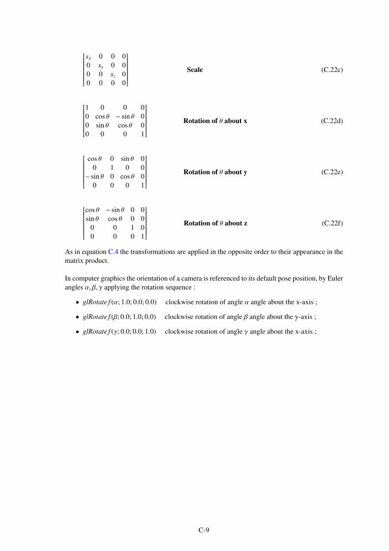
sx 0 0 0

0 sy 0 0

0 0 sz 0

0 0 0 0

Scale (C.22c)

1 0 0 0

0 cos θ − sin θ 0

0 sin θ cos θ 0

0 0 0 1

Rotation of θ about x (C.22d)

cos θ 0 sin θ 0

0 1 0 0

− sin θ 0 cos θ 0

0 0 0 1

Rotation of θ about y (C.22e)

cos θ − sin θ 0 0

sin θ cos θ 0 0

0 0 1 0

0 0 0 1

Rotation of θ about z (C.22f)

As in equation C.4 the transformations are applied in the opposite order to their appearance in the

matrix product.

In computer graphics the orientation of a camera is referenced to its default pose position, by Euler

angles α, β, γ applying the rotation sequence :

• glRotate f (α; 1.0; 0.0; 0.0) clockwise rotation of angle α angle about the x-axis ;

• glRotate f (β; 0.0; 1.0; 0.0) clockwise rotation of angle β angle about the y-axis ;

• glRotate f (γ; 0.0; 0.0; 1.0) clockwise rotation of angle γ angle about the x-axis ;

C-9

Appendix D

ARINC 424 Legs

D.1 T/P Leg types

D.1.1 Introduction

The Path and Terminator concept allows coding of a flight path, including SIDs, STARs, Terminal

Area Procedures, and Approach Procedures. Charted procedures are translated into a sequence of

ARINC 424 legs in the navigation database. Flight plans are entered, by the flight crew, into the

FMS (or the RNAV system) during the preflight. The RNAV system interprets the ARINC 424

"language" to provide the desired navigation function, by using procedures from the navigation

database and chaining them together.

There are 23 leg types that have been created to translate into RNAV systems "computer language".

Standard RNAV procedures use 12 P/T legs types, and 4 are used for Required Navigation Perfor-

mance Authorization Required (RNP AR) applications.

The Path logically describes how the aircraft flies to the Terminator (track, course, heading).

The Terminator is the event or condition (fix, altitude, distance, manual) that causes the RNAVsystem

to switch to the next leg.

The following subsections describe the 23 leg types, and illustrate them using figures from Federal

Aviation Administration (FAA) year 2017 document “FAA-H-8083-16B - Instrument Procedures

Handbook”.

D.1.2 IF - Initial Fix leg type

The Initial Fix or IF Leg defines a database fix as a point in space. It is only required to define the

beginning of a route or procedure.

ＦＩ＃ＯＨＪ３；３ﾓ＃

Ｆｒｘｕｖｈ＃ｌｖ＃ｉｏｒｚｑ＃ｐｄｎｌｑｊ＃ｄｇｍｘｖｗｐｈｑｗ＃ｉｒｕ＃ｚｌｑｇ＃

ＩＤ＃ＯＨＪ

３；３ﾓ＃

Ｘｑｖｓｈｆｌｉｌｈｇ＃ｓｒｖｌｗｌｒｑ＃

；／３３３＊＃

ＩＤ＃ｏｈｊ＃ｌｖ＃ｉｏｒｚｑ＃ｐｄｎｌｑｊ＃ｄｇｍｘｖｗｐｈｑｗ＃ｉｒｕ＃ｚｌｑｇ＃

Figure D.1 – IF-Leg

D.1.3 TF - Tracking Between Two Fixes leg type

Track to a Fix or TF Leg defines a great circle track over ground between two databases fixes. It is

the preferred type for straight legs. Course or heading can be mentioned on charts, but procedures

designers should ensure TF leg is used for coding.

D-1

TF LEG



ＩＤ＃ＯＨＪ

３；３ﾓ＃


；／３３３＊＃


Figure D.2 – TF-Leg

D.1.4 RF - Constant radius arc leg type

Constant Radius Arc or RF Leg defines a constant radius turn between two database fixes, lines

tangent to the arc and a center fix.

NextsegmentRF

LEG

ARC

CENTER

FIX

Pre

vio

us

seg

men

t



ＩＤ＃ＯＨＪ

３；３ﾓ＃


；／３３３＊＃


Figure D.3 – RF-Leg

D.1.5 CF - Course to a Fix leg type

Course to a Fix or CF Leg defines a specified course to a specific database fix. TF legs should be

used instead of CF whenever possible to avoid magnetic variation issues.



ＩＤ＃ＯＨＪ

３；３ﾓ＃


；／３３３＊＃


Figure D.4 – CF-Leg

D.1.6 DF - Direct to a Fix leg type

Direct to a Fix or DF Leg defines an unspecified track starting from an undefined position to a

specified fix. When designing a procedure, it should be take into account that the FMS flight path

depends on initial aircraft heading (e.g. depending on the initial heading, a left or a right turn may

be initiated to join the specified fixe).



DF LEG

Unspecified position

ＩＤ＃ＯＨＪ

３；３ﾓ＃


；／３３３＊＃


Figure D.5 – DF-Leg

D-2

D.1.7 FA - Fix to an Altitude leg type

Fix to an Altitude or FA Leg defines a specified track over ground from a database fix to a specified

altitude at an unspecified position.



ＩＤ＃ＯＨＪ

３；３ﾓ＃


；／３３３＊＃


Figure D.6 – FA-Leg

D.1.8 FC - Course from a Fix to an Along Track Distance leg type

Track from a Fix to a Distance or FC Leg defines a specified track over ground from a database

fix for a specific distance.

FC LEG

9 NM080°

ＩＰ＃ＯＨＪ３；３ﾓ＃

Ｐｄｑｘｄｏ＃ｗｈｕｐｌｑｄｗｌｒｑ＃

ＩＰ＃ｏｈｊ＃ｌｖ＃ｉｏｒｚｑ＃ｐｄｎｌｑｊ＃ｄｇｍｘｖｗｐｈｑｗ＃ｉｒｕ＃ｚｌｑｇ＃

ＦＤ＃ＯＨＪ＃３＜３ﾓ＃


＜／３３３＊＃Ｆｒｘｕｖｈ＃ｌｖ＃ｉｏｒｚｑ＃ｐｄｎｌｑｊ＃ｄｇｍｘｖｗｐｈｑｗ＃ｉｒｕ＃ｚｌｑｇ＃

Figure D.7 – FC-Leg

D.1.9 FD - Course from a Fix to a DME Distance leg type

Track from a Fix to a DME Distance or FD Leg defines a specified track over ground from a

database fix to a specific DME Distance which is from a specific database DME Navaid.

FD LEG D 10

080°







Figure D.8 – FD-Leg

D.1.10 FM - Course from a Fix to a Manual Termination leg type

From a Fix to a Manual termination or FM Leg defines a specified track over ground from a

database fix until Manual termination of the leg.







Figure D.9 – FM-Leg

D.1.11 CA - Course to an Altitude leg type

Course to an Altitude or CA Leg defines a specified course to a specific altitude at an unspecified

position.

D-3







Figure D.10 – CA-Leg

D.1.12 CD Course to a DME Distance leg type

Course to a DME Distance or CD Leg defines a specified course to a specific DME Distance which

is from a specific database DME Navaid.







CD LEG

090°

D 10

Figure D.11 – CD-Leg

D.1.13 CI - Course to a Next Leg Intercept leg type

Course to an Interceptor CI Leg defines a specified course to intercept a subsequent leg.







CI LEG

090° 070°

Next leg

Figure D.12 – CI-Leg

D.1.14 CR - Course to a Radial Termination leg type

Course to a Radial termination or CR Leg defines a course to a specified Radial from a specific

database VHF Omnidirectional Range (VOR) Navaid.







CR LEG

120°

170°

Figure D.13 – CR-Leg

D.1.15 AF - Constant DME Arc to a Fix leg type

Arc to a Fix or AF Leg defines a track over ground at specified constant distance from a database

DME Navaid.

D-4

＃＃＃＃＃＃＃＃

＃

Ｅｒｘｑｇｄｕ｜＃ｕｄｇｌｄ

ｏ＃５７８ﾓ＃

Ｇ４３ＤＩ

ＯＨＪ＃

ＹＤ＃ＯＨＪ＃


；／３３３＊＃

３＜３ﾓ＃

Ｑｒ＃ｆｒｕｕｈｆｗｌｒｑ＃ｐｄｇｈ＃ｉｒｕ＃ｚｌｑｇ＃

ＹＰ＃ＯＨＪ＃Ｐｄｑｘｄｏ＃ｗｈｕｐｌｑｄｗｌｒｑ３：３ﾓ＃


Figure D.14 – AF-Leg

D.1.16 VA - Heading to Altitude leg type

Heading to an Altitude termination or VA Leg defines a specified heading to a specific Altitude

termination at an unspecified position.

＃＃＃＃＃＃＃＃

＃


ｏ＃５７８ﾓ＃

Ｇ４３ＤＩ

ＯＨＪ＃



；／３３３＊＃

３＜３ﾓ＃




Figure D.15 – VA-Leg

D.1.17 VD - Heading to a DME Distance leg type

Heading to a DME Distance termination or VD Leg defines a specified heading terminating at a

specified DME Distance from a specific database DME Navaid.

＃＃＃＃＃＃＃＃

＃


ｏ＃５７８ﾓ＃

Ｇ４３ＤＩ

ＯＨＪ＃



；／３３３＊＃

３＜３ﾓ＃


VD LEG

090°

D 10



Figure D.16 – VD-Leg

D.1.18 VI - Heading to a Next Leg Intercept leg type

Heading to an Interceptor VI Leg defines a specified heading to intercept the subsequent leg at an

unspecified position.

＃＃＃＃＃＃＃＃

＃


ｏ＃５７８ﾓ＃

Ｇ４３ＤＩ

ＯＨＪ＃



；／３３３＊＃

３＜３ﾓ＃


VI LEG

090° 070°

Next leg



Figure D.17 – VI-Leg

D.1.19 VM - Heading to a Manual Termination leg type

Heading to a Manual termination or VM Leg defines a specified heading until a Manual termi-

nation.

D-5

＃＃＃＃＃＃＃＃

＃


ｏ＃５７８ﾓ＃

Ｇ４３ＤＩ

ＯＨＪ＃



；／３３３＊＃

３＜３ﾓ＃




Figure D.18 – VM-Leg

D.1.20 VR - Heading to a Radial Termination leg type

Heading to a Radial termination or VR Leg defines a specified heading to a specified radial from

a specific database VOR Navaid.

＃＃＃＃＃＃＃＃

＃


ｏ＃５７８ﾓ＃

Ｇ４３ＤＩ

ＯＨＪ＃



；／３３３＊＃

３＜３ﾓ＃




VR LEG

120°

170°

Figure D.19 – VR-Leg

D.1.21 PI - Procedure Turn to Intercept leg type

Procedure Turn or PI Leg defines a course reversal starting at a specific database fix, includes

Outbound Leg followed by a left or right turn and 180 degree course reversal to intercept the next

leg.

PI

063°

018°

ＫＤ／＃ＫＩ／＃ＫＰ＃

３：９ﾓ＃

Ｓｕｈｙｌｒ

ｘｖ＃ｏｈｊ

ＫＤ＃０＃Ｗｈｕｐｌｑｄｗｈｖ＃ｄｗ＃ｄｑ＃ｄｏｗｌｗｘｇｈ＃ＫＩ＃０＃Ｗｈｕｐｌｑｄｗｈｖ＃ｄｗ＃ｗｋｈ＃ｉｌ｛＃ｄｉｗｈｕ＃ｒｑｈ＃ｒｕｅｌｗ＃ＫＰ＃０＃Ｐｄｑｘｄｏｏ｜＃ｗｈｕｐｌｑｄｗｈｇ＃

Figure D.20 – PI-Leg

D.1.22 HA - Hold to an Altitude leg type

HA leg defines racetrack pattern or course reversals at a specified database fix terminating at an

altitude.

ＫＤ＃

３：９ﾓ

Ｓｕｈｙｌｒ

ｘｖ＃ｏｈｊ

ＫＤ＃０＃Ｗｈｕｐｌｑｄｗｈｖ＃ｄｗ＃ｄｑ＃ｄｏｗｌｗｘｇｈ

Figure D.21 – HA-Leg

D.1.23 HF - Hold to a Fix leg type

HF leg defines racetrack pattern or course reversals at a specified database fix terminating at the

fix after a single pattern.

D-6

ＫＩ＃

３：９ﾓ

Ｓｕｈｙｌｒ

ｘｖ＃ｏｈｊ

ＫＩ＃０＃Ｗｈｕｐｌｑｄｗｈｖ＃ｄｗ＃ｗｋｈ＃ｉｌ｛＃ｄｉｗｈｕ＃ｒｑｈ＃ｒｕｅｌｗ

Figure D.22 – HF-Leg

D.1.24 HM - Hold to a Manual Termination leg type

HM leg defines racetrack pattern or course reversals at a specified database fix with a manual

termination.

ＫＰ＃

３：９ﾓ

Ｓｕｈｙｌｒ

ｘｖ＃ｏｈｊ

ＫＰ＃０＃Ｐｄｑｘｄｏｏ｜＃ｗｈｕｐｌｑｄｗｈｇ＃

Figure D.23 – HM-Leg

D-7

D.2 ARINC 424 23 Path-Terminator legs matrix

The following table summarizes the 23 Path-Terminator legs defined in ARINC 424.

Table D.1 – ARINC 424 Path/Terminator legs matrix

Terminator

PathFix to

Track from

fix toCourse to Heading to Direct to Racetrack

DME Arc

to

Radius

from Fix

Fix IF TF CF DF HF AF RF

Altitude FA CA VA HA

Manual Termi-

nationFM VM HM

Distance FC

DME Distance FD CD VD

Intercept CI VI

Radial CR VR

Procedure

TurnPI

D-8

D.3 RNAV procedures Path-Terminator legs matrix

RNAV procedures do not use all of the 23 P/T legs. The following table shows "Best Practices"

leg types in teal cells. Legs type used mainly at start and end of procedures are shown in green

cells.

Table D.2 – RNAV Path/Terminator Legs Matrix

Terminator

PathFix to

Track from

fix toCourse to Heading to Direct to Racetrack

DME Arc

to

Radius

from Fix

Fix IF TF CF DF HF AF RF

Altitude FA CA VA HA

Manual Termi-

nationFM VM HM

Distance FC

DME Distance FD CD VD

Intercept CI VI

Radial CR VR

Procedure

TurnPI

D-9

Appendix E

Quaternions

The purpose of this appendix is to provide details to quaternions operation and calculation. We

will ignore the set of quaternions no-commutative division ring properties1 2, details can be found

in [143], [116] and [90].

Opinions differ on the inventor of the quaternions, some say Olinde Rodrigues invented the quater-

nions before Hamilton, but for sure, in 1853 Sir William Rowan Hamilton (1805-1865) published

his book "Lectures on Quaternions". Hamilton was looking for a 3D equivalent to complex num-

bers.

Representing an aircraft attitude by a quaternion uses Euler’s rotational theorem which states that

a transformation from one orthonormal coordinate system to another can be done by a single

rotation about a vector ~n along some axis of rotation, and a scalar θ corresponding to a rotation

around that axis.

E.1 Introduction

Quaternions can be used as aircraft attitude representation parameter. They have no singularity

when pitch attitude reaches 90, and they are computationally less intense compared to Euler

angles, or Direction Cosine Matrix (DCM). They can be used to :

• represent airplane’s attitude in a coordinates system,

• calculate an attitude from one time to an other, by integrating the airplane equation of mo-

tion,

• perform coordinates transformation from one frame to an other one.

E.2 Vector rotation and vector transformation

As explained in 3.7.1 and B.4, a rotation of a vector ~u represented in a coordinates system S 1 is

an operation, which modifies ~u in a vector ~v in S 1, as illustrated in figure 3.10. If ~u and S 1 are

represented in an other coordinates system S 3, the rotation changes the representation of the vector

~u in S 1 and S 3.

Transformations are described in B.2. A coordinate transformation is an operation which trans-

forms the coordinates in S 1 of any vector ~u into its coordinates in S 2. If ~u, S 1 and S 2 are repre-

sented in a third coordinates system S 3, the transformation does not change the orientation of ~u in

1The division ring is also called a division algebra, or "skew field" is a ring in which every nonzero element has a

multiplicative inverse, but multiplication is not necessarily commutative. In French, the term "corps non commutatif"

is used.2A ring is said to be a division ring if its nonzero elements form a group under multiplication.

E-1

S 3. We can also say that a transformation is a coordinate frame rotation from frame S 1 to frame

S 2.

E.3 Quaternions definition

In the present appendix we will use p, q or r to denote a quaternion. We will also use i, j, k, or~i, ~j, ~k, for the standard orthonormal basis of IR3 considered as a three dimensional space. With

these notations, vectors can be written as column triplet u = (u1, u2, u3)T , u, or ~u 3. The standard

orthonormal basis can also be written as :

i = (1, 0, 0)T

j = (0, 1, 0)T

k = (0, 0, 1)T

if we follow the convention we used in Appendix C. A quaternion may be represented as a quadru-

plets of real numbers, i.e. an element of IR4 the following way :

q = (q0, q1, q2, q3)T

where q0, q1, q2, q3 are scalars. An alternative notation is :

q = q0 + q

with q0 being the scalar part of quaternion q and q = iq1 + jq2 + kq3 the vector part. The scalars

q0, q1, q2, q3 are called the components of the quaternion.

E.4 Quaternion algebra

E.4.1 Quaternion equality and addition

Two quaternions p = p0 + ip1 + jp2 + kp3 and q = q0 + iq1 + jq2 + kq3 are equals if and only if

their components are equal :

p = q⇔

p0 = q0

p1 = q1

p2 = q2

p3 = q3

Addition of quaternion follows that for quadruplets of real numbers :

p + q = p0 + q0 + i(p1 + q1) + j(p2 + q2) + k(p3 + q3)

E.4.2 Quaternion multiplication

The product of a quaternion and a scalar is defined the same way than the product of a vector and

a scalar. Let’s q = q0 + iq1 + jq2 + kq3 be a quaternion and λ a scalar :

λq = λq0 + iλq1 + jλq2 + kλq3

The product of two quaternions differs as it has to satisfy the following quaternion product rules4

defined by Hamilton 5 :

i2 = −1, j2 = −1, k2 = −1, ijk = −1 (E.2a)

ij = k, jk = i, ki = j (E.2b)

ji = −k, kj = −i, ik = −j (E.2c)

3The notation u = (u1, u2, u3) is also used in books to write vectors as raw triplets.4The products shown in equations E.2 should not be confused with the classical vector scalar (i.e. dot) product.5Please note that the so-defined product is not commutative.

E-2

If p = p0 + ip1 + jp2 + kp3 and q = q0 + iq1 + jq2 + kq3, using fundamentals products E.2 and

ordinary rules for algebraic multiplication, we get (after regrouping terms) :

pq = p0q0 − (p1q1 + p2q2 + p3q3)

+ p0(iq1 + jq2 + kq3) + q0(ip1 + jp2 + kp3)

+ i(p2q3 − p3q2) + j(p3q1 − p1q3) + k(p1q2 − q2 p1)

This product can written in a more concise form using vectors scalar product (i.e. dot product)

and cross product (i.e; vector product). Let’s u = (u1, u2, u3)T and v = (v1, v2, v3)T be two vectors.

We have :

u · v = u1v1 + u2v2 + u3v3

and

u × v =

∣∣∣∣∣∣∣∣∣∣∣∣∣

i j k

u1 u2 u3

v1 v2 v3

∣∣∣∣∣∣∣∣∣∣∣∣∣

= i(u2v3 − u3v2) + j(u3v1 − u1v3) + k(u1v2 − u2v1)

If we write p = p0 + p and q = q0 + q, then :

pq = p0q0 − p · q + p0q + q0p + p × q (E.3)

Hence the product of two quaternions is a quaternion, whose scalar part is :

p0q0 − p · p

and a vector part is :

p0q + q0p + p × q

Remark E.1. Quaternion multiplication is associative and distributive, but it is not commutative

[143].

E.4.3 Quaternions product matrix algebra

Quaternions product as described in E.3 can also be written with matrix algebra. Let’s r be the

product of pq. We can write :

r = pq = r0 + r = r0 + ir1 + jr2 + kr3 where

r0 = p0q0 − p1q1 − p2q2 − p3q3

r1 = p0q1 + p1q0 + p2q3 − p3q2

r2 = p0q2 − p1q2 + p2q0 + p3q1

r3 = p0q3 + p1q2 − p2q1 + p3q0

which gives in matrix notation :

r0

r1

r2

r3

=

p0 −p1 −p2 −p3

p1 p0 −p3 p2

p2 p3 p0 −p1

p3 −p2 p1 p0

q0

q1

q2

q3

E-3

E.4.4 Quaternion complex conjugate

The complex conjugate of a complex number z = a + bi is given by z∗ = a − bi and is used to

compute the inverse of z. In a similar manner, the complex conjugate of a quaternion

q = q0 + q = q0 + iq1 + jq2 + kq3

is defined by :

q∗ = q0 − q = q0 − iq1 − jq2 − kq3

with the two following properties :

(pq)∗ = q∗p∗

q + q∗ = 2q0

E.4.5 Quaternion norm

The norm of a quaternion q is noted |q| or N(q), and defined by :

N(q) = |q| =√

q∗q

which gives :

|q|2 = |q|2 = q02 + q1

2 + q22 + q3

2

Quaternion with a norm equals to 1 are called unit quaternions or normalized quaternions. They

are of primary importance for rotations.

An interesting property is that the norm of the product of two quaternions equals the product of

their norms, i.e. :

|pq|2 = |p|2|q|2

E.4.6 Quaternion inverse

Every non-zero quaternion has a multiplicative inverse defined by :

q−1q = 1

qq−1 = 1

giving :

q−1qq∗ = q∗

q∗qq−1 = q∗⇔

q−1|q|2 = q∗

q∗qq−1 = q∗⇔

q−1|q|2 = q∗

|q|2q−1 = q∗

Hence :

q−1 =q∗

|q|2(E.5)

If q is a unit quaternion |q|2 = 1 and :

q−1 = q∗

Remark E.2. This last property is similar to the property of the DCM matrix, Ω−1E1→E2

= ΩTE1→E2

as shown in equation B.10.

E-4

E.5 Quaternions and geometry

Quaternions are used to represent the changes to an airplane orientation, as exposed in 3.7. The

present section uses developments found in [90] to detail how an rotation operator can be defined

using quaternions.

Rotations, orientations and transformations are detailed in Appendixes A, B and C. From these

Appendixes we know that a rotation in IR3 may be represented by a 3 × 3 orthogonal matrix with

a unit determinant. Rotation (respectively orientation) of a vector v is performed by multiplying

the initial vector on the left by the rotation matrix (respectively orientation matrix).

E.5.1 Some more quaternion algebra

To operate on a vector living in IR3 with a quaternion living in IR4, we have to define the pure

quaternion and two sets Q and Q0 as :

• pure quaternion : quaternion whose real part is zero

• Q the set of all quaternions

• Q0 the set of pure quaternions, with Q0 ⊂ Q

With these definitions, a vector v ∈ IR3 is a pure quaternion and can be considered as a member of

IR4 :

v ∈ IR3 ⇔ v = 0 + v ∈ Q0 ⊂ Q

Unfortunately a rotation can not be represented by a single quaternion product over a vector v as

shown below.

Let’s suppose a rotation of a vector v can be written as :

w = qv = q(v0 + v = q(0 + v)

with w ∈ IR3. Using equation E.3, we can write ;

qv = q0v0 − q · v + q0v + v0q + q × v = −q · v + q0v + q × v as v0 = 0

If qv is a rotation, then w = qv must always be a vector and its scalar part must equal zero,

i.e. −q · v = 0. Clearly this is not true except when −q⊥v. We can conclude that the product of a

vector by a quaternion is generally not a rotation, the simple product qv is not what we are looking

for.

We can thus assume that the rotation operator may use quaternion triple product. Let’s try with

two general quaternions q and r, members of Q, and a pure quaternion v member of Q0 (i.e. a

vector v of IR3. There are six possible products :

vqr qrv rvq vrq rqv qvr

And as qr ∈ Q, qr ∈ Q, rq ∈ Q and rq ∈ Q, we can only keep the products :

rvq qvr

to avoid falling back into the previous case. As the two quaternions q and r can be interchanged,

we only keep one product, let’s say qvr.

If we ask :

q = q0 + q

v = v0 + v = 0 + v

r = r0 + r

E-5

Using equation E.3 and rules of vector algebra, we get for the real part of the triple product :

ℜ(qvr) = −r0(q · v) − q0(r · v) + (q × r)·v

If, moreover, we assume that r0 = q0 we get :

ℜ(qvr) = −q0(q + r)·v + (q × r)·v

Taking the particular case of q = −r gives :

ℜ(qvr) = −q0(q − q)·v + (

q × (−q))·v = 0

This shows that if :

r0 = q0

r = −q⇔ r = r0 + r = q0 − q = q∗ ⇒ q = r∗

the operation qvr = qvr gives a vector w when q = r∗ or r = q∗. We choose to consider the product

qvr, but we could have chosen rvq.

We can conclude that, given any vector v of IR3, we get two possible triple product quaternions

operators giving two vectors w1 and w2 of IR3 :

w1 = qvq∗ (E.6a)

w2 = q∗vq (E.6b)

E.5.2 General formula

Given q = q0 + q and v = 0 + v, applying the operation of equation E.6a to a vector v ∈ IR3 gives

the following general result :

w = qvq∗ = (q0 + q)(0 + v)(q0 − q) = (2q02 − 1)v + 2(q · v)q + 2q0(q × v) (E.7)

or

w = qvq∗ = (q02 − |q|2)v + 2(q · v)q + 2q0(q × v) (E.8)

Remark E.3. We can notice that if q is a unit quaternion, the norm of v is unchanged by equation

E.6 operators.

|w1| = |qvq∗| = |q||v||q∗| = |v||w2| = |q∗vq| = |q∗||v||q| = |v|

Remark E.4. We can also notice that applying quaternion operator of equation E.6a to a vector

v = kq, with k ∈ IR and q a unit quaternion, leaves the vector v unchanged.

w = qvq∗ = q(kq)q∗ = (2q02 − 1)(kq) + 2(q·kq)q + 2q0(q×kq) = k(q0

2 + |q|2)q = kq

kq behavior is similar to that of a vector belonging to the rotation axis of a rotation.

It remains to find a geometric interpretation for the two operators used in E.6a and E.6b.

E-6

E.5.3 Angles and quaternion

The goal of this present subsection is to associate an angle with a quaternion.

Let’s consider a unit quaternion q of the form :

q = q0 + q

With : |q|2 = q02 + |q|2 = 1

So there exists theta such that cos θ = q0 and sin θ = |q|, with −π < θ < π. We have thus associate

an angle to a unit quaternion q.

If we relate q to a unit vector u having the same direction than q, we can write :

u =q

|q| =q

sin θ

leading to :

q = q0 + q = cos θ + u sin θ (E.9)

with θ = arctan2(|q, |q0),

and cos θ =q0

|q| .

The arctan2 function is defined in equation A.48.

Replacing the angle θ by −θ gives the complex conjugate of the original quaternion q :

cos(−θ) + u sin(−θ) = cos θ − u sin θ = q∗

E.5.4 Particular quaternion product

The quaternion product of two quaternions p and q having the same direction, i.e. the same unit

vector u is a particular case. We can write

p = cosα + u sinα

q = cos β + u sin β

The quaternion r, product of these two quaternions is :

r = pq = (cosα + u sinα)(cos β + u sin β)

Using formula E.3, with u × u = 0 gives :

r = pq = cosα cos β − sinα sin β + u(sinα cos β + cosα sin β)

= cos(α + β) + u sin(α + β)

= cos γ + u sin γ where γ = α + β

We can conclude that multiplying two unit quaternions having the same vector u and angles α and

β, gives a quaternion having the same vector u and an angle equal to the sum of the angles α and

β.

E-7

E.6 Quaternion as rotation operator

E.6.1 Proof

We now want to proof that the operators used in E.6a and E.6b rotate the vector v ∈ IR3 by an

angle. The assumptions are as follows :

v = 0 + v (E.11a)

q = q0 + q = cos θ + u sin θ is a unit quaternion, u =q

|q| (E.11b)

Lq is an operator associated to q and defined by :

w = Lq(v) = qvq∗ (E.12a)

Lq(v) = (q02 − |q|2)v + 2(q · v)q + 2q0(q × v) (E.12b)

Operator Lq linearity

Given a, b ∈ IR3 and λ ∈ IR, and as the set of quaternions is a non-commutative division ring

[143], we have :

Lq(λa + b) = q(λa + b)q∗ = (λqa + qb)q∗ = λqaq∗ + qbq∗ = λLq(a) + Lq(b)

proving that Lq is a linear operator.

Operator Lq norm conservation

When a vector of v ∈ IR3 is rotated, its norm remains unchanged. So if we want to prove that Lq is

a rotation operator, we need to prove that :

∣∣∣Lq(v)

∣∣∣ = |qvq∗| = |v|

which which is true since |qvq∗| = |q||v||q∗| = |v||.

Operator Lq is a rotation

Vector v can be written as :

v = a + n

where a is colinear to q, and n is perpendicular to q.

As a is colinear to q, ∃λ ∈ IR / a = λq and :

Lq(a) = Lq(λq) = λLq(q) = λq = q

as demonstrated in Remark E.4.

Using formula E.8 we can write :

Lq(n) = (q02−|q|2)n+2(q.n)q+2q0(q × n) = (q0

2−|q|2)n+2q0(q × n) = (q02−|q|2)n+2q0|q|(u × n)

or :

Lq(n) = (q02 − |q|2)n + 2q0|q|n⊥ (E.13)

with n⊥ = u × n

E-8

q

m

n

n⊥

2θ

n cos 2θ

n⊥ sin 2θ

Figure E.1 – Lq(n) components

and |n⊥| = |u × n| = |u||n| sin (u,n) = |u||n| sinπ

2= |n|

Remembering that cos θ =q0

|q| and u =q

sin θwe have :

Lq(n) = (q02 − |q|2)n + 2q0|q|n⊥

= (|q|2cos2θ − u2sin2θ)n + 2(|q| cos θ|u| sin θ)n⊥

= (cos2θ − sin2θ)n + 2(cos θ sin θ)n⊥ = cos 2θn + sin 2θn⊥

Figure E.1 shows Lq(n) components, with :

m = Lq(n) = cos 2θn + sin 2θn⊥

and

|m| = |Lq(n)| = |n| = |n⊥|

Finally we can write :

w = qvq∗ = Lq(v = Lq(a + n) = Lq(a + Lq(n) = a +m

Figure E.1 also shows that rotating n through a rotation of 2θ about the axis defined by q, gives w.

This proves that Lq(v) = qvq∗ is a rotation operator.

Remark E.5. The demonstration of qvq∗ as a rotation operator can also be done the following

way :

Lq(v) = (q02 − q · q)v + 2(q.v)q + 2q0(q × v)

= (cos2θ − sin2θu · u)v + 2(u.v)u + 2 cos θ sin θ(u × n)(E.14)

Taking into account that :

cos 2θ = cos2θ − sin2θ

sin 2θ = 2 cos θ sin θ

Equation E.14 may be written :

Lq(v) = cos 2θv + (1 − cos 2θ)(u · v)v + sin 2θu × v

which is exactly Rodrigues formula given in 3.7.4.

E-9

E.6.2 Multiple Rotations

Let’s illustrate how it work with two successive rotations, i.e. q1vq∗1

followed by q2vq∗2. The vector

v rotation is given by :

w = q2(q1vq∗1)q∗2= q2q1v(q2q1)∗ = Lq2q1

(v)(E.15)

This sequential rotation property is similar to that of the sequential transformations of Appendix

A.

E-10

Appendix F

Ordinary Differential Equations

Integration Methods

The goal of this appendix is to remind the reader of three family of numerical methods used

to solve Initial Value Problems (IVPs), the Euler’s method, the Taylor series method1, and the

Runge-Kutta method. Questions regarding existence and uniqueness of a solution to this problem,

and those regarding stability and convergence of the solution will not be discussed. Detailed

information on these matters could be find in Michelle Schatzman’s book “Numerical Analysis :

A Mathematical Introduction” [119].

F.1 Taylor’s theorem

This section is intended to remind us of Taylor’s theorem as it is used in Euler integration meth-

ods. The methods discussed in this appendix will be founded on the assumption that the solution

functions t 7−→ x(t), x 7−→ y(x), x 7−→ f (x), ... are smooth in the sense that the as many derivatives

as we require are continuous on the interval [a, b] ⊂ IR.

Theorem F.1 (Taylor’s theorem). Let the function f : IR −→ IR have n+ l continuous derivatives

on [a, b] ⊂ IR for some integer n ≥ 0, and let x, xo ∈ [a, b]. Then,

f (x) = pn(x) + Rn(x) =

n∑

k=0

(x − x0)k

k!f (k)(x0) +

1

n!

∫ x

x0

(x − s)k f (n+1)(s) ds (F.1)

with

pn(x) =

n∑

k=0

(x − x0)k

k!f (k)(x0) the polynomial part (F.2a)

Rn(x) =1

n!

∫ x

x0

(x − s)k f (n+1)(s) ds the remainder part (F.2b)

Moreover, there exist a point ξx between x and x0 such that2 :

Rn(x) =(x − x0)n+1

(n + 1)!f (n+1)(ξx) (F.3)

The Taylor’s theorem gives an approximation of a n + 1 times differentiable function around a

given point x0 by a (n+ 1)-th order Taylor polynomial (i.e. degree n Taylor polynomial). It allows

the exact representation of fairly general functions in terms of polynomials with a known, speci-

fied, boundable error.

Using this Taylor’s theorem the exponential function ex can be written around x0 = 0 as :

ex = 1 + x +1

2x2 +

1

3!x3 + ... +

1

n!xn

︸︷︷︸

Pn(x) polynomial

+1

(n + 1)!xn+1eξx

︸︷︷︸

Rn(x) remainder

(F.4)

1Taylor’s series methods do not seem to be used in airplane FMSs.

2Some books use the notation Rn+1=(x)(x − x0)n+1

(n + 1)!f (n+1)(ξx) as the remainder is a term in n + 1.

F-1

which is the well know Maclaurin series of the exponential function ex.

Let’s now take the problem of approximating the exponential function ex on the interval [−1, 1].

Since we want to consider x ∈ [−1, 1], we have to consider that ξx can be any point in ] − 1, 1[.

Using equation F.4, we can write :

ex = pn(x) + Rn(x)

Assuming we want this approximation to be accurate to within 10−6 in absolute error, we need to

have for all x ∈ [−1, 1] :

|ex − pn(x)| = |Rn(x)| ≤ 10−6

If we create a simple upper bound for |Rn(x)|, and then use it to determine the number of terms

necessary (i.e. value of integer n of equation F.4) to make this upper bound less than 10−6.

|Rn(x)| =∣∣∣∣∣

1

(n + 1)!xn+1eξx

∣∣∣∣∣=

1

(n + 1)!|xn+1eξx |

=eξx

(n + 1)!|xn+1| as ∀ξx ∈ IR eξx ≥ 0

≤ eξx

(n + 1)!as ∀ x ∈ [−1, 1] |x| ≤ 1

≤ e

(n + 1)!as ∀ξx ∈] − 1, 1[ eξx ≤ e

Finally we need n to satisfy :e

(n + 1)!≤ 10−6 ⇔ (n + 1)! ≥ 106e

to ensure that ∀ x ∈]−1, 1[, |ex− pn(x)| = |Rn(x)| ≤ e

(n + 1)!≤ 10−6 which is true as soon as n ≥ 9.

−1.5 −1 −0.5 0 0.5 1 1.5

0

1

2

3

4

x

f(x)

ex

1 + x

1 + x + x2

2!

1 + x + x2

2! + ... +x9

9!

Figure F.1 – ex approximation on [−1, 1] using Taylor’s theorem

On figure F.1, we plotted ex (red solid with "o" marks) and the different approximations for ex

using Taylor’s theorem using :

• p1(x) = 1 + x (black densely dashdotdotted)

• p2(x) = 1 + x +x2

2!(violet densely dashed)

• p9(x) = 1 + x +x2

2!+

x3

3!+

x4

4!+

x5

5!+

x6

6!+

x7

7!+

x8

8!+

x9

9!(blue dashdotted)

and one can see that it can’t distinguish between ex and p9(x) representations.

On figure F.2 we plotted Rn(x) = ex − pn(x), and this shows that |Rn(x) = ex − p9(x)| is less than

10−6, as expected. The plot also shows that p1(x) = 1 + x can approximate ex on [−0.1, 0.1], and

p2(x) = 1 + x +x2

2!can approximate ex on [−0.35, 0.35].

F-2

−1.5 −1 −0.5 0 0.5 1 1.5

0

0.5

1

1.5

·106

x

Rn(x

)=

ex−

pn(x

)

ex − (1 + x)

ex − (1 + x + x2

2! )

ex − (1 + x + x2

2! + ... +x9

9! )

Figure F.2 – Error in ex approximation on [−1, 1] using Taylor’s

theorem

F.2 Landau notation

Landau notation is known as O( ) and describes the limiting behavior of a function in mathemat-

ics, or classifies algorithms according to their processing time. We use it to describe the error term

in an approximation to a mathematical function y(x) or x(t). The most significant terms will be

written explicitly, and then the least-significant terms will be summarized in a single O(hp) term.

We will use O(hp), with p ∈ IN to refer to a quantity that decays, at least as quickly as hp, when h

tends to 0. Formally we will write :

z = O(hp) if ∃ h0 ∈ IR and C ∈ IR / ∀ 0 < h < h0, |z| ≤ Chp

In other words z = O(hp) if z converges to zero as h tends to 0 and the order (or rate) of conver-

gence is is less or equal p.

Taking the above examples, we can write :

• p1(x) = 1 + x + O(h2)

• p2(x) = 1 + x +x2

2!+ O(h3)

• p9(x) = 1 + x +x2

2!+

x3

3!+

x4

4!+

x5

5!+

x6

6!+

x7

7!+

x8

8!+

x9

9!+ O(h10)

F.3 Approximation of derivatives via divided differences

F.3.1 First-order approximation

Forward difference approximation

Taylor’s theorem can be used to approximate the derivative of a known function using difference

of quotients. The derivation of a real valued function f defined in an open neighborhood of a real

number x is defined by :

f ′(x) = limh→0

f (x + h) − f (x)

h(F.5)

Taylor’s theorem formula F.1 can also be written for x and x + h ∈ [a, b], as :

f (x + h) = f (x) + h f ′(x) +1

2!h2 f ′′(x) + ... +

1

n!hn f (n)(x) + Rn(x) (F.6)

F-3

with :

Rn(x) =hn+1

(n + 1)!f (n+1)(ξx) (F.7)

Substituting Taylor’theorem form F.6 in F.5, we have :

limh→0

f (x + h) − f (x)

h=

h

hf ′(x) +

1

h

1

2!h2 f ′′(x) + ... +

1

n!hn−1 f (n)(x) +

1

hRn(x)

= f ′(x) +1

2!h f ′′(x) + ... +

1

n!hn−1 f (n)(x) +

1

hRn(x)

When approximating the derivative of a know function f , we write :

f ′(x) ≈ f (x + h) − f (x)

hIn that particular case the accuracy of the approximation is given by :

f ′(x)− f (x + h) − f (x)

h= − 1

2!h f ′′(x)− ...− 1

n!hn−1 f (n)(x)− 1

hRn(x) = −1

2h f ′′(ξx,h) = O(h) (F.8)

where ξx,h depend on x and h. One can say that the error is roughly proportional to h3. This shows

that :

f ′(x) − f (x + h) − f (x)

h= −1

2h f ′′(ξx,h) = O(h) (F.9)

is a First-order approximation of f ′(x).

The approximation

f ′(x) ≈ D f 1(x, h) =f (x + h) − f (x)

h(F.10)

is called the step h forward difference approximation of f ′(x), h is the step size.

Backward difference approximation

If we replace h by −h in F.10, we get :

f ′(x) ≈ f (x − h) − f (x)

−h=

f (x) − f (x − h)

h= D f 1(x,−h)

with

f ′(x) − f (x) − f (x − h)

h=

1

2h f ′′(ξx,−h) = O(h) (F.11)

and we can write :

f ′(x) ≈ Db1(x, h) =f (x) − f (x − h)

h(F.12)

The approximation F.12 is called the step h backward difference approximation of f ′(x).

F.3.2 second-order approximation

First-order first derivative approximation shown in F.9 can be improved noticing that (ξ1 is some

real number in ]x, x + h[ while ξ2 is some real number in ]x − h, x[) :

f (x + h) = f (x) + h f ′(x) +1

2h2 f ′′(x) +

1

6h3 f ′′′(ξ1) (F.13a)

f (x − h) = f (x) − h f ′(x) +1

2h2 f ′′(x) − 1

6h3 f ′′′(ξ2) (F.13b)

Subtracting F.13b from F.13a and solving for f ′(x), we get :

f ′(x) =f (x + h) − f (x − h)

2h+

1

6h2 f ′′′(ξ1) + f ′′′(ξ2)

2(F.14)

Using the Discrete Average Value Theorem we can write :

1

6h2 f ′′′(ξ1) + f ′′′(ξ2)

2=

1

6h2

[

1

2f ′′′(ξ1) +

1

2f ′′′(ξ2)

]

=1

6h2 f ′′′(ξx,h). (F.15)

3Strictly ξx,h depends on h, so the error is not proportional to h.

F-4

where ξx,h depend on x and h and lies in ]x − h, x + h[. Thus

f ′(x) =f (x + h) − f (x − h)

2h+

1

6h2 f ′′′(ξx,h) (F.16)

This shows that :

f ′(x) − f (x + h) − f (x − h)

2h=

1

6h2 f ′′′(ξx,h) = O(h2) (F.17)

is a second-order approximation of f ′(x).

The approximation

f ′(x) ≈ Dc2(x, h) =f (x + h) − f (x − h)

2h(F.18)

is called the step h central difference approximation of f ′(x).

F.4 Forward Euler’s method for initial value problems

Euler’s method is a numerical method for solving Ordinary Differential Equations (ODEs), that

have one independent variable. The differential equations we consider are of the form :

Y ′(t) = f (t,Y(t)) (F.19)

where Y(t) is an unknown function that is being sought. The known function f (t,Y) defines the

differential equation. Equation F.19 is a first-order differential equation as it contains no higher-

order derivative than the first-order derivative of f (t,Y). In our present study Y is a space function

of the time variable t, Y(t) defines the trajectory of the aircraft4, as explained in 3.3.4.

The general solution of the first-order equation F.19 normally depends on an arbitrary integration

constant. To find a particular solution, we need to specify an additional condition usually taken in

the form :

Y(t0) = Y0 (F.20)

In our study the independent variable t is the time, so t0 can be interpreted as the initial time,

and Y(t0) the value of the space variable at t0. The differential equation F.19 and the initial value

condition F.20 together form an Initial Value Problem (IVP) :

Y ′(t) = f (t,Y(t))

Y(t0) = Y0

(F.21)

The Forward Euler’s method uses the forward difference approximation defined in equation F.10

to solve the IVP.

To approximately solve equation F.21, we substitute to Y ′(t), its first-order forward difference

approximation, given by equation F.9, as follows :

Y(t + h) − Y(t)

h= f (t,Y(t)) +

1

2hY ′′(th)

giving :

Y(t + h) = Y(t) + h f (t,Y(t)) +1

2h2Y ′′(th) (F.22)

Equation F.22 can be numerically solved as follows :

1. Y(t) is the true solution of the IVP with the initial value Y0 (see F.21)

2. Define a grid of t values, i.e. a sequence of t values spaced by the step h5, with tn = t0 + nh

and n = 0, 1, ...,N

4This numerical method for a first-order equation can be extended to a system of first-order equations, which we

have as the position is defined by three space variables, i.e. coordinates.5h is also called the mesh spacing or the grid size.

F-5

3. The approximate solution is denoted y(t) with y(tn) = yn, y0 = y(t0) = Y(t0) = Y0, and

n = 0, 1, ...,N

4. Compute recursively the values yn from y0 using F.22 and dropping the error term we obtain

the Forward Euler’s method :

yn+1 = yn + h f (tn, yn), n = 0, 1, ...,N−1

y0 = Y0

(F.23)

Example F.1.

Let’s try to solve numerically the IVP given by :

Y ′(t) = −2Y(t) + sin t

Y(0) = 1(F.24)

The exact solution is given by1

5(2 sin t − cos t) +

6

5e−2t.

Applying Forward Euler’s method to solve on [0, 1] IVP given by equation F.24, we get for h = 14 :

y1 = y0 + h f (t0, y0) = Y(0) +1

4(−2Y(t0) + sin t0) = 1 +

1

4(−2Y(0) + sin 0) = 0.5

y2 = y1 + h f (t1, y1) = y1 +1

4(−2y1 + sin

1

4) = 0.311850989814

y3 = y2 + h f (t2, y2) = y2 +1

4(−2y2 + sin

1

2) = 0.275781879558

y4 = y3 + h f (t3, y3) = y3 +1

4(−2y3 + sin

3

4) = 0.308300629785

The results are detailed in table F.1. The same resolution can be done using steps of h = 18 and

h = 116 , as respectively shown in tables F.2 and F.3. Results of the exact solution, and the three

approximate solutions of equation F.24 given by the Forward Euler’s method for those h have been

plotted on figure F.3.

tk yk Y(tk) Error = |Y(tk) − yk |0 y0 = 1 1 0

0.25 0.5 0.633015891015 0.133015891015

0.5 0.311850989814 0.457709032469 0.145858042655

0.75 0.275781879558 0.394073922413 0.118292042855

1 0.308300629785 0.390930272633 0.082629642848

Table F.1 – Forward Euler’s method solution of Y ′(t) = −2Y(t) + sin t, Y(0) = 1 for h = 14


0.125 0.75 0.785991299594 0.035991299594

0.25 0.578084341673 0.633015891015 0.054931549342

0.375 0.464488751162 0.527247350541 0.062758599379

0.5 0.394150629507 0.457709032469 0.063558402962

0.625 0.355541164456 0.415652041507 0.060110877051

0.75 0.33979303246 0.394073922413 0.054280889953

0.875 0.340049619348 0.387346761402 0.047297142054

1 0.350980152291 0.390930272633 0.039950120342


F-6


0.0625 0.875 0.884370508098 0.009370508098

0.125 0.769528707365 0.785991299594 0.016462592229

0.1875 0.681129789781 0.702813790634 0.021684000853

0.25 0.607638772106 0.633015891015 0.025377118909

0.3125 0.547146673046 0.574975530445 0.027828857399

0.375 0.497968246077 0.527247350541 0.029279104464

0.4375 0.458614248385 0.488542189811 0.029927941426

0.5 0.427767233412 0.457709032469 0.029941799057

0.5625 0.404260425398 0.433719130398 0.029458705

0.625 0.387059289319 0.415652041507 0.028592752188

0.6875 0.375245457713 0.402683357741 0.027437900028

0.75 0.368002718 0.394073922413 0.026071204413

0.8125 0.364604800751 0.389160359905 0.024555559154

0.875 0.364404741611 0.387346761402 0.022942019791

0.9375 0.366825617799 0.3880973885 0.021271770701

1 0.37135248484 0.390930272633 0.019577787793


The tables F.1, F.2, F.3 show respectively a maximum error of 1.4586 × 10−1, 6.3558 × 10−2, and

2.9942 × 10−2. It looks like each time the step is divided by 2, the error is also divided by around

2, suggesting (but not proving) an accuracy of O(h) for the Forward Euler’s method.

0 0.2 0.4 0.6 0.8 1

0.4

0.6

0.8

1

t

y(t),

Y(t

)

25 sin t − 1

5 cos t + 65 e−2t

h = 14

h = 18

h = 116

Figure F.3 – Forward Euler’s method approximate solutions of

Y ′(t) = −2Y(t) + sin t, Y(0) = 1 for different h values

F.5 Backward Euler’s method for initial value problems

The Backward Euler’s method uses the backward difference approximation defined in equation

F.12 to solve the IVP.

To approximately solve F.21, we substitute to Y ′(t), its first-order backward difference approxima-

tion, given by equation F.11, as follows :

Y(t) − Y(t − h)

h= f (t,Y(t)) − 1

2hY ′′(th)

giving :

Y(t) = Y(t − h) + h f (t,Y(t)) − 1

2h2Y ′′(th) (F.25)

F-7

Equation F.25 can be numerically solved as we did for the Forward Euler’s method, and shifting

the index by 1 :

1. Y(t) is the true solution of the IVP with the initial value Y0 (see F.21)

2. Define a grid of t values, i.e. a sequence of t values spaced by the step h , with tn = t0 + nh

and n = 0, 1, ...,N

3. The approximate solution is denoted y(t) with y(tn) = yn, y0 = y(t0) = Y(t0) = Y0, and

n = 0, 1, ...,N

4. Compute recursively the values yn from y0 using F.25 and dropping the error term :

yn = yn−1 + h f (tn, yn) (F.26)

5. Shifting the index by one we obtain the Backward Euler’s method :

yn+1 = yn + h f (tn+1, yn+1), n = 0, 1, ...,N−1

y0 = Y0

(F.27)

Equation F.27 show the main difference between the Backward and the Forward Euler’s meth-

ods : the need to solve a non linear algebraic equation for deriving yn+1. As the Backward Euler’s

method needs to solve a rootfinding problem to find yn+1, it is called an implicit method, whereas

the Forward Euler’s method is called an explicit method as it gives yn+1 directly from yn.

Rootfinding methods like the Newton’s method, the secant method or the bisection method, can

be used to find the root yn+1 of yn+1 = yn+h f (tn+1, yn+1), n = 0, 1, ...,N−1. It is time consuming

and simple iteration techniques are usully used to find yn+1.

Example F.2.

Let’s keep the same IVP example given by equation F.24. Using F.27, if y(t) is an approximate

solution, we can write :

yn+1 = yn + h(−2yn+1 + sin tn+1)⇔ yn+1 =yn + h sin tn+1

1 + 2h

⇔ yn+1 =yn + h sin(tn + h)

1 + 2h, n = 0, 1, ...,N−1 (F.28)

In the present particular case, we can express explicitly yn+1 with respect to yn. The results for

steps of h = 14 , h = 1

8 , and h = 116 , are respectively shown in tables F.4, F.5 and F.6.

tk yk Y(tk) Error = |Y(tk) − yk |0 1 1 0

0.25 0.707900659876 0.633015891015 0.074884768861

0.5 0.551838029685 0.457709032469 0.094128997216

0.75 0.481498479794 0.394073922413 0.087424557381

1 0.461244150664 0.390930272633 0.070313878031

Table F.4 – Backward Euler’s method solution of Y ′(t) = −2Y(t) + sin t, Y(0) = 1 for h = 14


0.125 0.812467473339 0.785991299594 0.026476173745

0.25 0.674714374597 0.633015891015 0.041698483582

0.375 0.576398752586 0.527247350541 0.049151402045

0.5 0.509061555929 0.457709032469 0.05135252346

0.625 0.465758972037 0.415652041507 0.05010693053

0.75 0.440771053632 0.394073922413 0.046697131219

0.875 0.429371193129 0.387346761402 0.042024431727

1 0.427644052984 0.390930272633 0.036713780351


F-8


0.0625 0.892358850991 0.884370508098 0.007988342893

0.125 0.800134241625 0.785991299594 0.014142942031

0.1875 0.721586175709 0.702813790634 0.018772385075

0.25 0.655154598367 0.633015891015 0.022138707352

0.3125 0.59943956047 0.574975530445 0.024464030025

0.375 0.5531836387 0.527247350541 0.025936288159

0.4375 0.5152563598 0.488542189811 0.026714169989

0.5 0.4846404053 0.457709032469 0.026931372831

0.5625 0.460419397685 0.433719130398 0.026700267287

0.625 0.441767090883 0.415652041507 0.026115049376

0.6875 0.427937807452 0.402683357741 0.025254449711

0.75 0.418257982181 0.394073922413 0.024184059768

0.8125 0.412118687231 0.389160359905 0.022958327326

0.875 0.408969027663 0.387346761402 0.021622266261

0.9375 0.408310308382 0.3880973885 0.020212919882

1 0.409690884384 0.390930272633 0.018760611751


The tables F.4, F.5, F.6 show respectively a maximum error of 9.4129 × 10−2, 5.1353 × 10−2, and

2.6931 × 10−2. Like for the Forward Euler’s method, each time the step is divided by 2, the error

seems also divided by around 2, suggesting (but not proving) an accuracy of O(h) for the Back-

ward Euler’s method.

Results of the exact solution, and the three approximate solutions of equation F.24 given by the

Backward Euler’s method using h = 14 , h = 1

8 , and h = 116 , have been plotted on figure F.4.

0 0.2 0.4 0.6 0.8 1

0.4

0.6

0.8

1

t

y(t),

Y(t

)

25 sin t − 1

5 cos t + 65 e−2t

h = 14

h = 18

h = 116

Figure F.4 – Backward Euler’s method approximate solutions of


F.6 Euler’s method variants

Euler’s methods variants use more accurate ways for deriving the value of yn+1 than the simple

linear approximation of the Forward and Backward Euler’s methods. In other words, one main

drawback of both Forward and Backward Euler’s method is the low convergence order and there

is a need for higher convergence order methods.

F-9

F.6.1 Midpoint method

The midpoint method6 is an explicit method for approximating the solution of the IVP given by

equation F.21. The derivative of Y(t) is approximated by the central difference approximation7.

Substituting in equation F.21 to Y ′(t), its second-order central difference approximation given by

F.17, gives :

Y ′(t) =Y(t + h) − Y(t − h)

2h+

1

6h2Y ′′′(ξt,h) = f (t,Y(t))

and

Y(t + h) = Y(t − h) + 2h f (t,Y(t)) − 1

3h3Y ′′′(ξt,h) (F.29)

Using the same techniques than those used for the Forward and Backward Euler’s methods we

finally get :

yn+1 = yn−1 + 2h f (tn, yn), n = 0, 1, ...,N−1

y0 = Y0

(F.30)

The midpoint method is based on a derivative approximation that is O(h2), whereas the Forward

and Backward Euler’s methods are based on a derivative approximation that is O(h). This sug-

gests that the midpoint method should be more accurate than the Forward and Backward Euler’s

methods.

The midpoint method formula F.30 gives yn+1 in terms of yn and yn−1, it is not a single-step

method8, but a multi-step method9, i.e. it depends on information from more than one previous

approximate value of the unknown function, whereas the differential equation only gives a single

initial value : y0.

The midpoint method is a stable and convergent method but it is only weakly stable, small pertur-

bations in the initial conditions lead to growing oscillations. The exact solution that may satisfy

the recursion F.30 contains two terms, one converging in O(h2) to the exact solution, and an other

one called parasite or parasitic solution. In case the second term dominates, it corrupts the approx-

imation. That’s where we see the importance of stability... and therefore a precise study of the

stability, outside the scope of this appendix. Generally the use of the midpoint method is avoided.

F.6.2 The trapezoidal method

To derive this method we need to use the Taylor expansion of Y ′(t + h).

Y ′(t + h) = Y ′(t) + hY ′′(t) + O(h2)⇔ hY ′′(t) = Y ′(t + h) − Y ′(t) − O(h2) (F.31)

Using equation F.13a, we can write :

Y(t + h) = Y(t)+ hY ′(t)+1

2h2Y ′′(t)+

1

6h3Y ′′′(ξ1) = Y(t)+ hY ′(t)+

1

2h2Y ′′(t)+O(h3) (F.32)

Substituting hY ′′(t) from F.31 in equation F.32 leads to :

Y(t + h) = Y(t) + hY ′(t) +1

2h[Y ′(t + h) − Y ′(t) − O(h2)] + O(h3)

= Y(t) +1

2h[Y ′(t + h) + Y ′(t)] − 1

2hO(h2) + O(h3)

= Y(t) +1

2h[Y ′(t + h) + Y ′(t)] + O(h3)

(F.33)

Expansion F.33 is valid for any three-times continuously differentiable function Y(t). Let’s now

substitute to Y ′(t) its value given by the IVP F.21 to get :

Y(t + h) = Y(t) +1

2h[ f ((t + h),Y(t + h)) + f (t,Y(t))] + O(h3)

6The midpoint method is also known as the leapfrog method.7The central difference approximation is sometime called the symmetric difference approximation.8A single-step method (also called one-step, stepwise, or starting method) provides successively an approximation

of the exact solution, yn+1, at the point tn+1 based on the known approximation yn at the point tn.9Also called continuing method

F-10

Dropping the O(h3) term and using the discrete approximate solution we have :

yn+1 = yn +1

2h[ f (tn+1, yn+1) + f (tn, yn)] n = 0, 1, ...,N−1

y0 = Y0

(F.34)

Recursive formula F.34 does not give a direct expression for yn+1 in terms of data available from

earlier times, thus the trapezoidal method is an implicit method.

The trapezoidal method is generally used as follows :

1. compute tn+1 = tn + h

2. compute f (tn, yn)

3. compute an approximate value yEn+1

used for estimating yn+1 using Forward Euler’s method :

yEn+1= yn + h f (tn, yn).

4. compute f (tn+1, yEn+1

)

5. compute the numerical solution at tn+1 using :

yn+1 = yn+1

2h[ f (tn+1, y

En+1)+ f (tn, yn)] = yn+

1

2h[ f (tn, yn)+ f (tn+h, yn+h f (tn, yn))] (F.35)

The recursive formula F.35 is also know as the Heun’s method, or the modified Euler’s method.

F.7 The Taylor series method

Euler’s method was introduced in F.4 while neglecting O(h2) terms in the Taylor series of y(tn + h)

about the point t = tn (see equations F.22 and F.23). The accuracy of the approximations generated

by the method was controlled by adjusting the step size h. The Taylor series methods described

in this section tries to improve the efficiency by keeping further terms in the Taylor series. In the

sequel we suppose that all the used derivatives of the exact solution Y are defined and continuous

in the domain of the approximation.

F.7.1 Order-two Taylor Serie method TS(2)

In the present subsection, we present a second-order method noted TS(2). Using the results from

F.3.2 and particularly equation F.13a, we can write :

Y(t + h) = Y(t) + hY ′(t) +1

2h2Y ′′(t) +

1

6h3Y ′′′(ξ1) (F.36a)

Y(t + h) = Y(t) + hY ′(t) +1

2h2Y ′′(t) + O(h3) (F.36b)

In the sequel, for any discrete value tn = t0 + nh, we denote by yn (resp. y′n and y′′n ) some approxi-

mation of Y(tn) (resp. of Y ′(tn) and Y ′′(tn)).

Using F.36a and F.36b, we obtain an approximation of Y(tn + h) from an approximation of Y(tn)

by using t = tn, replacing Y(tn) (resp. Y ′(tn) and Y ′′(tn)) by its approximation yn (resp. y′n and y′′n )

and neglecting the remainder1

6h3Y ′′′(ξ1) (or O(h3)), we get y0 = y(t0) = Y(t0) = Y0, and :

y(tn + h) = y(tn) + hy′(tn) +1

2h2y′′(tn)⇔ yn+1 = yn + hy′n +

1

2h2y′′n n = 0, 1, ...,N−1 (F.37)

y′n can be evaluated in the same way by using F.21 :

y′(tn) = f (tn, y(tn))

y0 = Y0

(F.38)

As for y′′(tn) we need to differentiate both sides of the ODE, the chain rule for functions of one

independent variable and two intermediate variables must be used :

F-11

Theorem F.2. If w = f (u, v) is differentiable and if u = u(t) and v = v(t) are differentiable

functions of t, then the composite w = f (u(t), v(t)) is a differentiable function of t and

dw

dt= fu (u(t), v(t)) u′ + fv (u(t), v(t)) v′ (F.39a)

dw

dt=∂ f (u(t), v(t))

∂u

du

dt+∂ f (u(t), v(t))

∂v

dv

dt(F.39b)

Equation F.39 can be written as(

dw

dt

)

ti

=

(

∂ f (u(t), v(t))

∂u

)

Pi

(

du

dt

)

ti

+

(

∂ f (u(t), v(t))

∂v

)

Pi

(

dv

dt

)

ti

(F.40)

for any ti where u and v are differentiable, with Pi = (u (ti) , v (ti))

Using F.21 and F.40 and substituting w = Y ′(t), u(t) = t and v(t) = Y(t) we get

dY ′

dt=∂ f (t,Y(t))

∂t

dt

dt+∂ f (t,Y(t))

∂Y

dY

dt⇔ Y ′′(t) =

∂ f (t,Y(t))

∂t+∂ f (t,Y(t))

∂YY ′(t)

remembering that Y ′(t) = f (t,Y(t)) from equation F.38 we get

Y ′′(t) =∂ f (t,Y(t))

∂t+∂ f (t,Y(t))

∂Yf (t,Y(t)) (F.41)

Using the results given by equations F.38 and F.41 we can rewrite the recursive formula F.37 as

yn+1 = yn+h f (tn, yn)+1

2h2

(

∂ f (t, y(t))

∂t

)

(tn,yn)

+

(

∂ f (t, y(t))

∂y

)

(tn,yn)

f (tn, yn)

n = 0, 1, ...,N−1

(F.42)

Which is, by denoting∂ f

∂t(resp.

∂ f

∂y) by ft (resp. fy) :

yn+1 = yn + h f (tn, yn) +1

2h2

[

ft(tn, yn) + fy(tn, yn) f (tn, yn)]

n = 0, 1, ...,N−1 (F.43)

f and its partial derivatives being all evaluated at (tn, y(tn)).

Formula F.43 allows us to recursively compute yn from y0. As previously stated the described

method is a single-step method of numerical approximation to the solution of the IVP described

by equation F.21. It is also known as the Taylor series expansion method of order 2.

Example F.3.

Let’s retake the IVP example of F.24 :

Y ′(t) = −2Y(t) + sin t

Y(0) = 1(F.44)

If y(t) is the approximate solution, we have :

y′(t) = −2y(t) + sin t

f (t, y(t)) = −2y(t) + sin t

∂ f

∂t= ft = cos t

∂ f

∂y= fy = −2

giving for F.43

yn+1 = yn + h(−2yn + sin tn) +1

2h2 [

cos tn − 2 f (tn, yn)]

n = 0, 1, ...,N−1 (F.45a)

yn+1 = yn + h(−2yn + sin tn) +1

2h2 [

cos tn − 2(−2yn + sin tn)]

n = 0, 1, ...,N−1 (F.45b)

Let’s now calculate y(t) on [0, 1], for h = 14 , h = 1

8 , and h = 116 . The results are given in tables F.7,

F.8 and F.9.


TS(2) method using h = 14 , h = 1

8 , and h = 116 have been plotted on figure F.5.

F-12


0.25 0.65625 0.633015891015 0.023234108985

0.5 0.486823005539 0.457709032469 0.02911397307

0.75 0.421581122009 0.394073922413 0.027507199596

1 0.414160745912 0.390930272633 0.023230473279

Table F.7 – TS(2) method solution of Y ′(t) = −2Y(t) + sin t, Y(0) = 1 for h = 14


0.125 0.7890625 0.785991299594 0.003071200406

0.25 0.637842921364 0.633015891015 0.004827030349

0.375 0.532944218654 0.527247350541 0.005696868113

0.5 0.463693319488 0.457709032469 0.005984287019

0.625 0.4215536879 0.415652041507 0.005901646393

0.75 0.399669482271 0.394073922413 0.005595559858

0.875 0.39251234169 0.387346761402 0.005165580288

1 0.395608125457 0.390930272633 0.004677852824



0.0625 0.884765625 0.884370508098 0.000395116902

0.125 0.786691190519 0.785991299594 0.000699890925

0.1875 0.703743862858 0.702813790634 0.000930072224

0.25 0.634114840289 0.633015891015 0.001098949274

0.3125 0.576193240254 0.574975530445 0.001217709809

0.375 0.528543101524 0.527247350541 0.001295750983

0.4375 0.489883135514 0.488542189811 0.001340945703

0.5 0.459068903617 0.457709032469 0.001359871148

0.5625 0.435077135068 0.433719130398 0.00135800467

0.625 0.416991933117 0.415652041507 0.00133989161

0.6875 0.403992646634 0.402683357741 0.001309288893

0.75 0.395343210205 0.394073922413 0.001269287792

0.8125 0.390382778676 0.389160359905 0.001222418771

0.875 0.388517502308 0.387346761402 0.001170740906

0.9375 0.389213306579 0.3880973885 0.001115918079

1 0.391989556439 0.390930272633 0.001059283806


0 0.2 0.4 0.6 0.8 1

0.4

0.6

0.8

1

t

y(t),

Y(t

)

25 sin t − 1

5 cos t + 65 e−2t

h = 14

h = 18

h = 116

Figure F.5 – TS(2) method approximate solutions of


F-13

Comparing results given by the TS(2) method (tables F.7, F.8 F.9) to those given by the Forward

Euler’s method (tables F.1, F.2, F.3) shows that the TS(2) method converges more rapidly.

F.7.2 Order-three Taylor Serie method TS(3)

To derive the TS(3) Order-three Taylor Serie method to solve the IVP F.21, we use Taylor’s theo-

rem formula F.6 :

Y(t + h) = Y(t) + hY ′(t) +1

2!h2Y ′′(t) +

1

3!h3Y ′′′(t) + ... +

1

n!hnY (n+1)(t) + Rn(h)

︸︷︷︸

O(h4)

(F.46)

giving :

Y(t + h) = Y(t) + hY ′(t) +1

2!h2Y ′′(t) +

1

3!h3Y ′′′(t) + O(h4) (F.47)

Y ′′(t) is given by F.41. Using the result of equation F.40 and substituting w = Y ′′ (t), u(t) = t and

v(t) = Y(t) we get

dY ′′

dt=∂Y ′′ (t,Y(t))

∂t

dt

dt+∂Y ′′ (t,Y(t))

∂Y

dY

dt=

(

Y ′′ (t,Y(t)))

t +(

Y ′′ (t,Y(t)))

Y

dY

dtSubstituting to Y ′′ (t,Y(t)) its expression from F.41, we get :

dY ′′

dt=

∂

(

∂ f (t,Y(t))

∂t+∂ f (t,Y(t))

∂Yf (t,Y(t))

)

∂t+

∂

(

∂ f (t,Y(t))

∂t+∂ f (t,Y(t))

∂Yf (t,Y(t))

)

∂Y

dY

dt

dY ′′

dt=∂2 f (t,Y(t))

∂t2+∂2 f (t,Y(t))

∂t∂Yf (t,Y(t)) +

∂ f (t,Y(t))

∂Y

∂ f (t,Y(t))

∂t+

[

∂2 f (t,Y(t))

∂Y∂t+∂2 f (t,Y(t))

∂Y2f (t,Y(t)) +

∂ f (t,Y(t))

∂Y

∂ f (t,Y(t))

∂Y

]

dY

dt

dY ′′

dt= ftt (t,Y(t)) + ftY (t,Y(t)) f (t,Y(t)) + fY (t,Y(t)) ft (t,Y(t))+

[

fYt (t,Y(t)) + fYY (t,Y(t)) f (t,Y(t)) + fY (t,Y(t)) fY (t,Y(t))] dY

dt

with ftt =∂2 f

∂t2, ftY =

∂2 f

∂t∂Y, fY ft =

∂ f

∂Y

∂ f

∂t, fYt =

∂2 f

∂Y∂t, fYY =

∂2 f

∂Y2, f 2

Y =

(

∂ f

∂Y

)2

(F.48)

From F.21 we know that Y ′ = f (t,Y (t)). Substituting this value fordY

dtin equation F.48 gives :

dY ′′

dt= ftt (t,Y(t)) + ftY (t,Y(t)) f (t,Y(t)) + fY (t,Y(t)) ft (t,Y(t))+

[

fYt (t,Y(t)) + fYY (t,Y(t)) f (t,Y(t)) + fY (t,Y(t)) fY (t,Y(t))]

f (t,Y (t)) (F.49)

Regrouping the terms leads to :

dY ′′

dt= ftt (t,Y(t)) +

[

ftY (t,Y(t)) + fYt (t,Y(t))]

f (t,Y(t)) + fY (t,Y(t)) ft (t,Y(t))+

fYY (t,Y(t)) f 2 (t,Y(t)) + f 2Y (t,Y(t)) f (t,Y (t)) (F.50)

If we assume that f (t,Y (t)) and its partial derivatives ft, fY , ftY , fYt are defined throughout an open

region containing a point (tn,Y (tn)) and are all continuous at (tn,Y (tn)), then ftY (tn,Y (tn)) = fYt (tn,Y (tn)).

Using this property in F.50, we can finally write :

Y ′′′ (t,Y(t)) = ftt (t,Y(t)) + 2 ftY (t,Y(t)) f (t,Y(t)) + fY (t,Y(t)) ft (t,Y(t))+

fYY (t,Y(t)) f 2 (t,Y(t)) + f 2Y (t,Y(t)) f (t,Y (t)) (F.51)

From equation F.47 we have :

Y(tn + h) = Y(tn) + hY ′(tn) +1

2!h2Y ′′(tn) +

1

3!h3Y ′′′(tn) + O(h4)

Substituting y′(tn), y′′(tn), and y′′′(tn) by their expression respectively given by F.21, F.41 and F.51,

replacing Y(tn) (resp. Y ′(tn), Y ′′(tn)andY ′′′(tn)) by its approximation yn (resp. y′n, y′′n and y′′′n ) and

F-14

neglecting the remainder O(h4)), we get y0 = y(t0) = Y(t0) = Y0, and the TS(3) recursive formula :

yn+1 = yn +

[

h f +h2

2

(

ft + fy f)

+h3

6

(

ftt + 2 fty f + fx f y + fyy f 2 + f 2y f

)]

(tn,yn)

n = 0, 1, ...,N−1

(F.52)

where f and its partial derivatives are all evaluated at (tn, y(tn)). Formula F.52 allows to recursively

compute yn from y0. The described method is again a single-step method of numerical approxi-

mation to the solution of the IVP described by equation F.21. It is also known as the Taylor series

expansion method of order 3.

Example F.4.


Y ′(t) = −2Y(t) + sin t

Y(0) = 1(F.53)

and find an approximate solution y of Y in O(h4) using the Order-three Taylor Serie method TS(3).

Let’s first calculate the partial derivatives of f needed in formula F.52 :

Y ′(t) = −2Y(t) + sin t

f (t, y(t)) = −2y(t) + sin t

∂ f

∂t= ft = cos t

∂ f

∂y= fy = −2

∂2 f

∂2t= ftt = − sin t

∂2 f

∂2y= fyy = 0

∂2 f

∂t∂y= fty =

∂2 f

∂y∂t= fyt

ft fy = −2 cos t f 2y = 4

Once these calculations done, we proceed as for the previous examples, by using step-sizes of

h = 14 , h = 1

8 and h = 116 , on the interval [0, 1]. The results are shown in tables F.10, F.11 and F.12.


TS(3) method using h = 14 , h = 1

8 , and h = 116 have been plotted on figure F.6.


0.25 0.630208333333 0.633015891015 0.002807557682

0.5 0.454304048163 0.457709032469 0.003404984306

0.75 0.39096687549 0.394073922413 0.003107046923

1 0.388396121886 0.390930272633 0.002534150747



0.125 0.785807291667 0.785991299594 0.000184007927

0.25 0.632729207345 0.633015891015 0.00028668367

0.375 0.526912200337 0.527247350541 0.000335150204

0.5 0.457360526774 0.457709032469 0.000348505695

0.625 0.415311996742 0.415652041507 0.000340044765

0.75 0.39375503267 0.394073922413 0.000318889743

0.875 0.387055577119 0.387346761402 0.000291184283

1 0.390669309442 0.390930272633 0.000260963191


F-15


0.0625 0.884358723958 0.884370508098 0.00001178414

0.125 0.785970499119 0.785991299594 0.000020800475

0.1875 0.702786251541 0.702813790634 0.000027539093

0.25 0.632983477907 0.633015891015 0.000032413108

0.3125 0.574939760476 0.574975530445 0.000035769969

0.375 0.527209449355 0.527247350541 0.000037901186

0.4375 0.488503139148 0.488542189811 0.000039050663

0.5 0.457669610613 0.457709032469 0.000039421856

0.5625 0.433679946494 0.433719130398 0.000039183904

0.625 0.415613564634 0.415652041507 0.000038476873

0.6875 0.402645941493 0.402683357741 0.000037416248

0.75 0.394037825646 0.394073922413 0.000036096767

0.8125 0.389125764213 0.389160359905 0.000034595692

0.875 0.387313785793 0.387346761402 0.000032975609

0.9375 0.388066101704 0.3880973885 0.000031286796

1 0.390900703387 0.390930272633 0.000029569246


0 0.2 0.4 0.6 0.8 1

0.4

0.6

0.8

1

t

y(t),

Y(t

)

25 sin t − 1

5 cos t + 65 e−2t

h = 14

h = 18

h = 116

Figure F.6 – TS(3) method approximate solutions of


F.7.3 Order-p Taylor Serie method TS(p)

TS(2) and TS(3) methods can be extended to a higher order. The pth-order Taylor series of y(t+h)

with remainder is given by formula F.6 :

Y(t + h) = Y(t) + hY ′(t) +1

2!h2Y ′′(t) + ... +

1

p!hpY (p)(t) + Rp(t) (F.54)

with :

Rp(t) =hp+1

(p + 1)!Y (p+1)(ξt) ξt ∈ [t, t + h] (F.55)

when Y(t) is (p + 1) times continuously differentiable on [t0, t f ].

If |Y (p+1)(t)| ≤ M∀t ∈ [t0, t f ], then |Rp(t)| ≤ M

(p + 1)!hp+1, and Rp(t) = O(hp+1). We can then

write :

Y(t + h) = Y(t) + hY ′(t) +1

2!h2Y ′′(t) + ... +

1

p!hpY (p)(t) + O(hp+1) (F.56)

The TS(p) method uses expansion F.56 and neglects its remainder at t = tn to give the expression

F-16

of the approximate solution y(t) of the IVP F.2110. That is :

y(t + h) = y(t) + hy′(t) +1

2!h2y′′(t) + ... +

1

p!hpy(p)(t) (F.57a)

y(tn + h) = y(tn) + hy′(tn) +1

2!h2y′′(tn) + ... +

1

p!hpy(p)(tn) (F.57b)

yn+1 = yn + hy′n +1

2!h2y′′n + ... +

1

p!hpy

(p)n (F.57c)

The right side of the ODE part of the IVP F.21 must be differentiated (p−1) times to complete the

method. This is exactly what we did for TS(2) and TS(3) methods.

Concluding on the Taylor Serie Methods of order greater or equal to 2, we can say that they are

easy to derive, accurate, but they require tedious and time-consuming evaluations of high order

derivative, sometimes involving symbolic calculation.

F.8 The Runge-Kutta methods

Explicit methods calculate the state of a system at t + ∆t from the state of the system at t, and

the recursive formula yn+1 is sufficient for each integration step. Single-step methods have been

introduced in F.6.1. An explicit single-step method for numerical solution of IVP F.21 can be

written as :

y0 = y(t0) (F.58a)

yn+1 = yn + hΦ(tn, yn, h) 0 ≤ n ≤ N−1 (F.58b)

Φ is a given IRk valued function, defined on [a, b] × IRk × [0, h0], where a, b, h0 are reals. Φ is

called the incremental function11 of the one-step method.

The single-step Runge-Kutta methods require evaluations of the function f ((t, y (t)) 7→ f (t, y (t)))

but not its derivatives. They are related to the Taylor Serie development of Y , with Y ′(t) = f (t, y (t)).

Compared to Taylor Series methods, the goal is to get the same precision without any symbolic

calculations required by the calculation of high-order derivatives. To achieve this goal, f (t, y (t))

is evaluated at more points.

Φ can be considered as a weighted average of the slope of the exact solution f , at different points

within the interval of integration [tn, tn+1], used to determine the solution at t = tn+1 from that at

t = tn. Its construction is based on acting as a Taylor serie method. Φ (defined in F.58b) of the

s-stage Runge-Kutta methods has the form :

z1 = yn (F.59a)

zi = yn + h

i−1∑

j=1

ai, j f (tn + c jh, z j) i = 2, ..., s (F.59b)

Φ (t, y (t) , h) =

s∑

j=1

b j f (tn + c jh, z j) (F.59c)

i−1∑

j=1

ai, j = ci i = 2, 3, ..., s (F.59d)

The coefficients b j are the Runge-Kutta weights, the c j are the Runge-Kutta nodes. The coeffi-

cients a j,i are generally arranged in a table called a Butcher tableau12 as shown on table F.13. The

missing elements(

a j,i

)

j,i=1,...,sof the table are defined to be 013, therefore a1,1 = 0.

10This shows that the Forward Euler’s method is a Taylor Serie method of order 1.11The incremental function Φ is also called the associated function.12Sometimes a matrix is used to store the a j,i, for explicit RK methods is strictly lower triangular.13We need to have a j,i for i ≥ j for the method to be explicit, otherwise it is implicit.

F-17

The coefficients b j, c j, and(

a j,i

)

j,i=1,...,sare determined to achieve a high degree of agreement with

Taylor’s development given by formula F.6. m is called the order of the method, if an agreement

with this formula up to and including the term hm is achieved. For a given m order and a given s

stage, appropriate coefficients sometimes do not exist. The condition m ≤ s is necessary, but not

sufficient to find appropriate coefficients.

0 = c1

c2 a2,1

c3 a3,1 a3,2

. . .

. . .

. . .

cs as,1 as,2 . . . as,s−1

b1 b2 . . . bs−1 bs

Table F.13 – Runge-Kutta s-stage Butcher tableau

F.8.1 1-stage Runge-Kutta RK1

As previously stated, the general form of an explicit one-stage Runge-Kutta Method is yn+1 = yn + hΦ(tn, yn, h).

Let’s take the special case of F.59 with :

s = 1

b1 = 1giving

z1 = yn

Φ (t, y (t) , h) = b1 f (tn, z1) = f (tn, yn)

substituting in F.58b leads to :

yn+1 = yn + hΦ(tn, yn, h) = yn + h f (tn, yn) 0 ≤ n ≤ N−1

In that particular case the Runge-Kutta 1-stage Butcher tableau is :

c1 = 0 a1,1=0

b1 = 1

Table F.14 – Runge-Kutta 1-stage Butcher tableau

and we get the same recursive formula than the one given by F.23. This shows that the Forward

Euler’s method is a RK1 method, it can be demonstrated that it is the unique explicit one-stage

Runge-Kutta Method that is convergent.


Let’s start now with the 2-stage Runge-Kutta method

s = 2

z1 = yn

z2 = yn + ha2,1 f (tn + c1h, z1) = yn + a2,1h f (tn + c1h, yn)

Φ (t, y (t) , h) = b1 f (tn + c1h, yn) + b2 f (tn + c2h, yn + a2,1h f (tn + c1h, yn))

a2,1 = c2

giving with c1 = 0

yn+1 = yn + h[

b1 f (tn + c1h, yn) + b2 f (tn + c2h, yn + a2,1h f (tn + c1h, yn))]

(F.60)

= yn + h[

b1 f (tn, yn) + b2 f (tn + c2h, yn + a2,1h f (tn, yn))]

(F.61)

= yn + b1h f (tn, yn) + b2h f (tn + c2h, yn + a2,1h f (tn, yn)) (F.62)

To determine the coefficients b1, b2, c2 and a2,1 of formula F.62, we need to expand the third term

of the right hand side of the formula, using Taylor’s formula that provides polynomial approxima-

tions of all orders for functions of two independent variables.

F-18

Theorem F.3 (Taylor’s theorem for functions of two independent variables).

If f : (t, y) 7→ f (t, y) and its partial derivatives through order n + 1 are continuous throughout an

open rectangular region R centered at a point (tn, yn). Then, throughout R

f (tn + h, yn + k) = f (tn, yn) + (h fx + k fy)(tn,yn),+1

2!

(

h2 fxx + 2hk f xy + k2 fyy

)

(tn,yn)+

1

3!

(

h3 fxxx + 3h2k fxxy + 3hk2 fxyy + k3 fyyy

)

(tn,yn)+ ...+

1

n!

[(

h∂

∂x+ k

∂

∂y

)n

f

]

(tn,yn)

+1

(n + 1)!

(

h∂

∂x+ k

∂

∂y

)n+1

f

(tn+ξh,yn+ξk)

(F.63)

Thus

f (tn+c2h, yn+a2,1h f (tn, yn) = f (tn, yn)+h

[

c2∂ f (tn, yn)

∂t+ a2,1

∂ f (tn, yn)

∂yf (tn, yn)

]

+O(h2) (F.64)

After substitution and factorization, recursive formula F.62 becomes :

yn+1 = yn + (b1 + b2)h f (tn, yn) + b2h2(c2 ft(tn, yn) + a2,1 fy(tn, yn) f (tn, yn)) + O(h3) (F.65)

and using formula F.36b

Y(tn+1) = Y(tn) + hY ′(tn) +1

2h2Y ′′(tn) + O(h3) (F.66)

leading to

Y(tn+1) = yn + h f (tn, yn) +1

2h2

[

ft(tn, yn) + fy(tn, yn) f (tn, yn)]

+ O(h3) (F.67)

which shows that to have a 2-stage Runge-Kutta of order p ≥ 2, we need to have

Y(tn+1) = yn + (b1 + b2)h f (tn, yn) + b2h2[

c2 ft(tn, yn) + a2,1 fy(tn, yn) f (tn, yn)]

+ O(h3) (F.68)

As equations F.67 and F.68 have to be compared for every h and for every f , the coefficients of h

and h2 must agree and :

b1 + b2 = 1 (F.69a)

b2c2 =1

2(F.69b)

a2,1 = c2 (F.69c)

Equations F.69 does not define the coefficients uniquely, the system is underdetermined. It can

also be written as :

b1 = 1 − b2 (F.70a)

c2 =1

2b2b2 , 0 (F.70b)

a2,1 =1

2b2(F.70c)

Equations F.70 lets us build the generic Butcher tableau for the RK2 methods, as shown on table

F.15.

c1 = 0 a1,1=0

c2 =1

2b2

a2,1 =1

2b2

a2,2 = 0

b1 = 1 − b2 b2

Table F.15 – Runge-Kutta 2-stage generic Butcher tableau

RK2 and the Heun’s method

If we take b2 =1

2, from F.70 we have b1 =

1

2and c2 = a2,1 = 1. Formula F.62 becomes :

yn+1 = yn +1

2h f (tn, yn) +

1

2h f (tn + 1h, yn + 1h f (tn, yn)) (F.71)

= yn +1

2h[

f (tn, yn) + f (tn + h, yn + h f (tn, yn))]

(F.72)

F-19

Comparing F.72 with F.35, we can conclude that the Heun’s method is a RK2 method.

The Butcher tableau associated to the method is :

c1 = 0 a1,1=0

c2 = 1 a2,1 = 1 a2,2 = 0

b1 =1

2b2 =

1

2

Table F.16 – Heun’s method Butcher tableau

Example F.5.


Y ′(t) = −2Y(t) + sin t

Y(0) = 1

If y(t) is the approximate solution, we have according to F.72 :

yn+1 = yn +1

2h[

f (tn, yn) + f (tn + h, yn + h f (tn, yn))]

(F.73)

The results for y(t) on [0, 1], for h = 14 , h = 1

8 , and h = 116 are respectively given in tables F.17,

F.18 and F.19. As done for the previous examples, they are plotted on figure F.7.

0 0.2 0.4 0.6 0.8 1

0.4

0.6

0.8

1

t

y(t),

Y(t

)

25 sin t − 1

5 cos t + 65 e−2t

h = 14

h = 18

h = 116

Figure F.7 – RK2 Heun’s method approximate solutions of



0.25 0.655925494907 0.633015891015 0.022909603892

0.5 0.485344374096 0.457709032469 0.027635341627

0.75 0.418509174976 0.394073922413 0.024435252563

1 0.409354529962 0.390930272633 0.018424257329

Table F.17 – RK2 Heun’s method solution of Y ′(t) = −2Y(t) + sin t, Y(0) = 1 for h = 14

F-20


0.125 0.789042170837 0.785991299594 0.003050871243

0.25 0.637746071547 0.633015891015 0.004730180532

0.375 0.532728212054 0.527247350541 0.005480861513

0.5 0.463327036631 0.457709032469 0.005618004162

0.625 0.421015899049 0.415652041507 0.005363857542

0.75 0.398947528303 0.394073922413 0.00487360589

0.875 0.391601042253 0.387346761402 0.004254280851

1 0.394508852478 0.390930272633 0.003578579845



0.0625 0.884764353683 0.884370508098 0.000393845585

0.125 0.786684988376 0.785991299594 0.000693688782

0.1875 0.703729519066 0.702813790634 0.000915728432

0.25 0.634089554923 0.633015891015 0.001073663908

0.3125 0.576154590797 0.574975530445 0.001179060352

0.375 0.528489013105 0.527247350541 0.001241662564

0.4375 0.489811854387 0.488542189811 0.001269664576

0.5 0.45897897344 0.457709032469 0.001269940971

0.5625 0.434967375609 0.433719130398 0.001248245211

0.625 0.416861421039 0.415652041507 0.001209379532

0.6875 0.403840698068 0.402683357741 0.001157340327

0.75 0.395169364858 0.394073922413 0.001095442445

0.8125 0.390186785235 0.389160359905 0.00102642533

0.875 0.388299304952 0.387346761402 0.00095254355

0.9375 0.388973032425 0.3880973885 0.000875643925

1 0.391727503767 0.390930272633 0.000797231134


RK2 and the explicit midpoint method

If we take b2 = 1, from F.70 we have b1 = 0 and c2 = a2,1 =1

2. Formula F.62 becomes :

yn+1 = yn + 0h f (tn, yn) + 1h f (tn +1

2h, yn +

1

2h f (tn, yn)) (F.74)

= yn + h f (tn +1

2h, yn +

1

2h f (tn, yn)) (F.75)

The Butcher tableau associated to the explicit midpoint method is :

c1 = 0 a1,1=0

c2 =1

2a2,1 =

1

2a2,2 = 0

b1 = 0 b2 = 1

Table F.20 – Explicit midpoint method Butcher tableau

Example F.6.

Taking again the IVP example of F.24, if y(t) is the approximate solution, we have according to

F.75 :

yn + 1 = yn + h f (tn +1

2h, yn +

1

2h f (tn, yn)) (F.76)



F.22 and F.23. As the the previous examples they are plotted on figure F.8.

F-21


0.25 0.656168683346 0.633015891015 0.023152792331

0.5 0.486210811909 0.457709032469 0.02850177944

0.75 0.420191979515 0.394073922413 0.026118057102

1 0.411903440254 0.390930272633 0.020973167621

Table F.21 – RK2 explicit midpoint method solution of Y ′(t) = −2Y(t) + sin t, Y(0) = 1 for h = 14


0.125 0.78905741473 0.785991299594 0.003066115136

0.25 0.637803474644 0.633015891015 0.004787583629

0.375 0.532848092025 0.527247350541 0.005600741484

0.5 0.463524095778 0.457709032469 0.005815063309

0.625 0.421300009978 0.415652041507 0.005647968471

0.75 0.399324372908 0.394073922413 0.005250450495

0.875 0.392072642617 0.387346761402 0.004725881215

1 0.395074023355 0.390930272633 0.004143750722



0.0625 0.884765307124 0.884370508098 0.000394799026

0.125 0.786688686687 0.785991299594 0.000697387093

0.1875 0.703737532587 0.702813790634 0.000923741953

0.25 0.634103251427 0.633015891015 0.001087360412

0.3125 0.576175151912 0.574975530445 0.001199621467

0.375 0.528517448914 0.527247350541 0.001270098373

0.4375 0.489849016443 0.488542189811 0.001306826632

0.5 0.459025566417 0.457709032469 0.001316533948

0.5625 0.435023967768 0.433719130398 0.00130483737

0.625 0.41692845368 0.415652041507 0.001276412173

0.6875 0.403918494109 0.402683357741 0.001235136368

0.75 0.395258136669 0.394073922413 0.001184214256

0.8125 0.390286641838 0.389160359905 0.001126281933

0.875 0.388410258684 0.387346761402 0.001063497282

0.9375 0.389095005147 0.3880973885 0.000997616647

1 0.391860332694 0.390930272633 0.000930060061


0 0.2 0.4 0.6 0.8 1

0.4

0.6

0.8

1

t

y(t),

Y(t

)

25 sin t − 1

5 cos t + 65 e−2t

h = 14

h = 18

h = 116

Figure F.8 – RK2 explicit midpoint method approximate solu-

tions of Y ′(t) = −2Y(t) + sin t, Y(0) = 1 for different h values

F-22

RK2 and the Ralston’s method

If we take b2 =3

4, from F.70 we have b1 =

1

4and c2 = a2,1 =

2

3. Formula F.62 becomes :

yn+1 = yn +1

4h f (tn, yn) +

3

4h f (tn +

2

3h, yn +

2

3h f (tn, yn)) (F.77)

The Butcher tableau associated to the Ralston’s method is :

c1 = 0 a1,1=0

c2 =2

3a2,1 =

2

3a2,2 = 0

b1 =1

4b2 =

3

4

Table F.24 – Ralston’s method Butcher tableau

Example F.7.

Taking again the IVP example of F.24, if y(t) is the approximate solution, we have according to

F.77 :

yn + 1 = yn + h f (tn +1

2h, yn +

1

2h f (tn, yn)) (F.78)



F.26 and F.27. They are plotted on figure F.9.


0.25 0.65610552488 0.633015891015 0.023089633865

0.5 0.485949933718 0.457709032469 0.028240901249

0.75 0.419663046649 0.394073922413 0.025589124236

1 0.411085242265 0.390930272633 0.020154969632

Table F.25 – RK2 Ralston’s method solution of Y ′(t) = −2Y(t) + sin t, Y(0) = 1 for h = 14


0.125 0.789053460894 0.785991299594 0.0030621613

0.25 0.63778633024 0.633015891015 0.004770439225

0.375 0.532810760188 0.527247350541 0.005563409647

0.5 0.463461483748 0.457709032469 0.005752451279

0.625 0.421208660958 0.415652041507 0.005556619451

0.75 0.399202248434 0.394073922413 0.005128326021

0.875 0.391918942202 0.387346761402 0.0045721808

1 0.394889031224 0.390930272633 0.003958758591


F-23


0.0625 0.884765059909 0.884370508098 0.000394551811

0.125 0.786687586554 0.785991299594 0.00069628696

0.1875 0.703735048257 0.702813790634 0.000921257623

0.25 0.634098919789 0.633015891015 0.001083028774

0.3125 0.576168572477 0.574975530445 0.001193042032

0.375 0.528508278884 0.527247350541 0.001260928343

0.4375 0.489836966319 0.488542189811 0.001294776508

0.5 0.45901039607 0.457709032469 0.001301363601

0.5625 0.435005482907 0.433719130398 0.001286352509

0.625 0.416906502667 0.415652041507 0.00125446116

0.6875 0.403892965072 0.402683357741 0.001209607331

0.75 0.395228954862 0.394073922413 0.001155032449

0.8125 0.390253767221 0.389160359905 0.001093407316

0.875 0.388373683683 0.387346761402 0.001026922281

0.9375 0.389054752571 0.3880973885 0.000957364071

1 0.391816453775 0.390930272633 0.000886181142


0 0.2 0.4 0.6 0.8 1

0.4

0.6

0.8

1

t

y(t),

Y(t

)

25 sin t − 1

5 cos t + 65 e−2t

h = 14

h = 18

h = 116

Figure F.9 – RK2 Ralston’s method approximate solutions of



-stage Runge-Kutta recursive formula can be derived in the same manner than RK2 recursive

formula. Using F.59 for s = 3 we get :

s = 3 (F.79a)

z1 = yn (F.79b)

z2 = yn + ha2,1 f (tn + c1h, z1) = yn +h

2f (tn, yn) (F.79c)

z3 = yn + h[a3,1 f (tn + c1h, z1) + a3,2 f (tn + c2h, z2)] (F.79d)

= yn − h f (tn, yn) + 2h f (tn +h

2, z2) (F.79e)

The incremental function is given by :

Φ (t, y (t) , h) = b1 f (tn + c1h, yn) + b2 f (tn + c2h, yn + a2,1h f (tn + c1h, yn)) + b3 f (tn + c3h, z3)

= b1 f (tn + c1h, yn)

+ b2 f(

tn + c2h, yn + a2,1h f (tn + c1h, yn))

+ b3 f(

tn + c3h, yn + h(

a3,1 f (tn + c1h, yn) + a3,2 f(

tn + c2h, yn + a2,1h f (tn + c1h, yn))))

F-24

(F.80)

As the method must be explicit (see equation F.59d), the following equations relate the coefficients.

c1 = 0

a2,1 = c2

a31 + a32 = c3

(F.81)

To determine the coefficients b1, b2, b3, a2,1, a3,1, a3,2, c2 and c3 of formula F.80, we need to

expand the second and the third term of the right hand side of the formula, using Taylor’s for-

mula for functions of two independent variables. Comparing the coefficients with those of Taylor

development of Y(tn + h), as we did for the RK2 method, gives :

b1 + b2 + b3 = 1 b2c2 + b3c3 =1

2b2c2

2 + b3c23 =

1

3b3a3,2c2 =

1

3(F.82)

newline Once more the coefficients are not uniquely defined. The classical RK3 use the Butcher

tableau given in table F.28.

c1 = 0 a1,1 = 0

c2 =1

2a2,1 =

1

2a2,2 = 0

c3 = 1 a3,1 = −1 a3,2 = 2 a3,3 = 0

b1 =1

6b2 =

2

3b3 =

1

6

Table F.28 – "Classical" Runge-Kutta 3-stage Butcher tableau

Using these coefficients equation F.79 becomes

s = 3 (F.83a)

z1 = yn (F.83b)

z2 = yn +h

2f (tn, yn) (F.83c)

z3 = yn − h f (tn, yn) + 2h f (tn +h

2, z2) (F.83d)

and formula F.80 can be written as :

Φ (t, y (t) , h) = b1 f (tn + c1h, z1) + b2 f (tn + c2h, z2) + b3 f (tn + c3h, z3)

=1

6f (tn, z1) +

2

3f (tn +

1

2h, z2) +

1

6f (tn + h, z3) (F.84)

leading to

Φ (t, y (t) , h) =1

6

[

f (tn, z1) + 4 f (tn +1

2h, z2) + f (tn + h, z3)

]

(F.85)

or

Φ (t, y (t) , h) =1

6f (tn, yn) (F.86)

+2

3f

(

tn +h

2, yn +

h

2f (tn, yn)

)

+1

6f

(

tn + h, yn − h f (tn, yn) + 2h f

(

tn +h

2, yn +

h

2f (tn, yn)

))

Example F.8.

Let’s go back to the IVP example of F.24 :

Y ′(t) = −2Y(t) + sin t

Y(0) = 1

If y(t) is the approximate solution, y(tn + h) = yn+1 can be calculated using F.58b and ??. The

results for y(t) on [0, 1], for h = 14 , h = 1

8 , and h = 116 are respectively given in tables F.29, F.30

F-25

and F.31. As done for the previous examples, they are plotted on figure F.10.


0.25 0.630059506642 0.633015891015 0.002956384373

0.5 0.454152455901 0.457709032469 0.003556576568

0.75 0.39090459764 0.394073922413 0.003169324773

1 0.388476967805 0.390930272633 0.002453304828

Table F.29 – "Classical" RK3 method solution of Y ′(t) = −2Y(t) + sin t, Y(0) = 1 for h = 14


0.125 0.785797548872 0.785991299594 0.000193750722

0.25 0.632714523081 0.633015891015 0.000301367934

0.375 0.526896423899 0.527247350541 0.000350926642

0.5 0.457346723165 0.457709032469 0.000362309304

0.625 0.415302576223 0.415652041507 0.000349465284

0.75 0.393751851264 0.394073922413 0.000322071149

0.875 0.387060015191 0.387346761402 0.000286746211

1 0.390682333897 0.390930272633 0.000247938736



0.0625 0.884358101513 0.884370508098 0.000012406585

0.125 0.785969408521 0.785991299594 0.000021891073

0.1875 0.702784831065 0.702813790634 0.000028959569

0.25 0.632981851368 0.633015891015 0.000034039647

0.3125 0.574938038594 0.574975530445 0.000037491851

0.375 0.527207730959 0.527247350541 0.000039619582

0.4375 0.488501512229 0.488542189811 0.000040677582

0.5 0.457668153254 0.457709032469 0.000040879215

0.5625 0.433678727686 0.433719130398 0.000040402712

0.625 0.415612644999 0.415652041507 0.000039396508

0.6875 0.402645373919 0.402683357741 0.000037983822

0.75 0.394037655854 0.394073922413 0.000036266559

0.8125 0.389126031258 0.389160359905 0.000034328647

0.875 0.387314522513 0.387346761402 0.000032238889

0.9375 0.388067335121 0.3880973885 0.000030053379

1 0.390902455069 0.390930272633 0.000027817564



The "classical" fourth-order RK4 method was found by Carl Runge in 1895, it can summarized

by F.32 Butcher tableau. It has a local truncation error14 of O(h4), and it is one of the most widely

used methods for solving ODEs.

14The local truncation error (LTE) is induced at every time-step due to the truncation of the Taylor series.

F-26

0 0.2 0.4 0.6 0.8 1

0.4

0.6

0.8

1

t

y(t),

Y(t

)

25 sin t − 1

5 cos t + 65 e−2t

h = 14

h = 18

h = 116

Figure F.10 – "Classical" RK3 method approximate solutions of


c1 = 0 a1,1 = 0

c2 =1

2a2,1 =

1

2a2,2 = 0

c3 =1

2a3,1 = 0 a3,2 =

1

2a3,3 = 0

c4 = 1 a4,1 = 0 a4,2 = 0 a4,3 = 1 a4,4 = 0

b1 =1

6b2 =

1

3b3 =

1

3b4 =

1

6

Table F.32 – "Classical" Runge-Kutta 4-stage Butcher tableau

Let’s calculate the incremental function Φ for the RK4 method with :

s = 4 (F.87a)

z1 = yn (F.87b)

z2 = yn + ha2,1 f (tn + c1h, z1) = yn + a2,1h f (tn + c1h, yn) = yn +h

2f (tn, yn) (F.87c)

z3 = yn + ha3,1 f (tn + c1h, z1) + ha3,2 f (tn + c2h, z2) = yn +h

2f (tn +

h

2, z2) (F.87d)

z4 = yn + ha4,1 f (tn + c1h, z1) + ha4,2 f (tn + c2h, z2) + ha4,3 f (tn + c3h, z3)

= yn + h f (tn +h

2, z3) (F.87e)

giving

Φ (t, y (t) , h) = b1 f (tn + c1h, yn) + b2 f (tn + c2h, z2) + b3 f (tn + c3h, z3) + b4 f (tn + c4h, z4)

=1

6f (tn+, yn) +

1

3f (tn +

h

2, z2) +

1

3f (tn +

h

2, z3) +

1

6f (tn + h, z4)

(F.88)

or

Φ (t, y (t) , h) =1

6

(

f (tn+, yn) + 2 f (tn +h

2, z2) + 2 f (tn +

h

2, z3) + f (tn + h, z4)

)

(F.89)

Example F.9.

Let’s take one last time the IVP example F.24 used in this appendix. The results for the approxi-

mate solution y(t) are given in tables F.33, F.34, F.35 for step sizes h = 14 , h = 1

8 and h = 116 . They

are plotted on figure F.11.

F-27

0 0.2 0.4 0.6 0.8 1

0.4

0.6

0.8

1

t

y(t),

Y(t

)

25 sin t − 1

5 cos t + 65 e−2t

h = 14

h = 18

h = 116

Figure F.11 – "Classical RK4 method approximate solutions of



0.25 0.633313020878 0.633015891015 0.000297129863

0.5 0.458064339973 0.457709032469 0.000355307504

0.75 0.394387025099 0.394073922413 0.000313102686

1 0.391167854003 0.390930272633 0.00023758137



0.125 0.786000972907 0.785991299594 0.000009673313

0.25 0.633030890015 0.633015891015 0.000014999

0.375 0.527264745277 0.527247350541 0.000017394736

0.5 0.457726897785 0.457709032469 0.000017865316

0.625 0.415669157937 0.415652041507 0.00001711643

0.75 0.394089560683 0.394073922413 0.00001563827

0.875 0.38736052815 0.387346761402 0.000013766748

1 0.390942000758 0.390930272633 0.000011728125



0.0625 0.884370816757 0.884370508098 0.000000308659

0.125 0.78599184343 0.785991299594 0.000000543836

0.1875 0.702814508899 0.702813790634 0.000000718265

0.25 0.633016733719 0.633015891015 0.000000842704

0.3125 0.574976456673 0.574975530445 0.000000926228

0.375 0.527248327017 0.527247350541 0.000000976476

0.4375 0.488543189676 0.488542189811 0.000000999865

0.5 0.457710034243 0.457709032469 0.000001001774

0.5625 0.433720117092 0.433719130398 0.000000986694

0.625 0.415652999879 0.415652041507 0.000000958372

0.6875 0.40268427766 0.402683357741 0.000000919919

0.75 0.394074796323 0.394073922413 0.00000087391

0.8125 0.389161182375 0.389160359905 0.00000082247

0.875 0.387347528741 0.387346761402 0.000000767339

0.9375 0.388098098439 0.3880973885 0.000000709939

1 0.390930924059 0.390930272633 0.000000651426


F-28

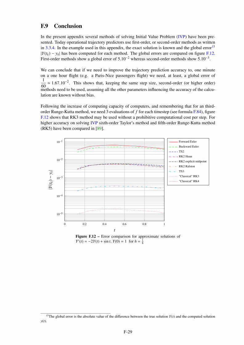
F.9 Conclusion

In the present appendix several methods of solving Initial Value Problem (IVP) have been pre-

sented. Today operational trajectory predictors use first-order, or second-order methods as written

in 3.3.4. In the example used in this appendix, the exact solution is known and the global error15

|Y(tk) − yk| has been computed for each method. The global errors are compared on figure F.12.

First-order methods show a global error of 5.10−2 whereas second-order methods show 5.10−3.

We can conclude that if we need to improve the trajectory prediction accuracy to, one minute

on a one hour flight (e.g. a Paris-Nice passengers flight) we need, at least, a global error of1

60≃ 1.67.10−2. This shows that, keeping the same step size, second-order (or higher order)

methods need to be used, assuming all the other parameters influencing the accuracy of the calcu-

lation are known without bias.

Following the increase of computing capacity of computers, and remembering that for an third-

order Runge-Kutta method, we need 3 evaluations of f for each timestep (see formula F.84), figure

F.12 shows that RK3 method may be used without a prohibitive computational cost per step. For

higher accuracy on solving IVP sixth-order Taylor’s method and fifth-order Runge-Kutta method

(RK5) have been compared in [89].

0 0.2 0.4 0.6 0.8 1

10−5

10−4

10−3

10−2

10−1

t

|Y(t

k)−

y k|

Forward Euler

Backward Euler

TS2

RK2 Heun

RK2 explicit midpoint

RK2 Ralston

TS3

"Classical" RK3

"Classical" RK4

Figure F.12 – Error comparison for approximate solutions of

Y ′(t) = −2Y(t) + sin t, Y(0) = 1 for h = 18

15The global error is the absolute value of the difference between the true solution Y(t) and the computed solution

y(t).

F-29

Appendix G

ICAO standard atmosphere

The goal of this appendix is to give a brief description of the ICAO standard atmosphere, giving

similar results than the International Standard Atmosphere (ISA) atmosphere below 32 km.

As the ICAO standard atmosphere is used to calibrate instruments, especially altimeters, com-

ments have been added to highlight the differences between the assumptions used by ICAO for

the standard atmosphere, and those used by mapping agencies, and by the World Geodetic System

1984 (WGS 84) system. The advent of GPS-based precision instrument approaches procedures

may be confronted with differences in heights measurement1.

G.1 Introduction

The physical properties of air partially determine, the aerodynamic forces (i.e. lift and drag) acting

on an aircraft, and the engines performances. They also affect the measurement of aircraft state el-

ements, such as airspeed and altitude. These properties are functions of altitude, time, geographic

location, sun activity, and more...

Layering based on temperature profiles gives a series of layers2. Moving upward from sea level,

these layers are named :

• The troposphere (0 to ≃ 11 km)

• The stratosphere3 (≃ 11 to 50 km)

• The mesosphere (50 to 85 km)

• The thermosphere (85 to a variable upper limit varying from 500 up to 1000 km)

• The exosphere (uppermost layer of the atmosphere, considered by some experts as the actual

"final frontier" of Earth’s gaseous envelope)

Commercial and business jets fly in the upper troposphere and in the lower stratosphere. The jet

streams (refer to section 6.1) flow near the border between the troposphere and the stratosphere.

Efforts have been devoted, since more than two centuries, to develop standard and reference atmo-

sphere models. The models of interest for the flight altitudes of the aircraft are :

1. The Committee on Space Research’s (COSPAR) CIRA4 1986 Model Atmosphere (0 to

120 km). The CIRA-86 data are zonally averaged monthly mean climatologies of several

1Today, most precision instrument approaches procedures are Instrument Landing System (ILS) procedures using

a radio altimeter able to accurately measure the height with reference to the ground surface.2The ionosphere is not considered as it is based on electrical properties.3Most of the ozone is contained in the stratosphere.4COSPAR International Reference Atmosphere (CIRA).

G-1

amospheric parameters including temperature, zonal wind and geopotential height. These

mean parameters are available on a 5 degree latitude by 0.25 log-pressure scale height grid.

2. The Committee on Extension to the Standard Atmosphere (COESA) 1976 model atmo-

sphere (0 to 86 km) known as the the U.S. Standard Atmosphere. Below 32 km this model

is identical with the Standard Atmosphere of the ICAO.

3. The ISO 2533-1975 Standard Atmosphere specifies a standard atmosphere that can be used

as a common basis for simulation, analysis and test (−2 to 50 km). Hypsometrical tables

have been added to the model in 1985. Extension to −5 km and standard atmosphere as a

function of altitude in feet have been added in 1997.

4. The ICAO standard atmosphere model - (0 to 80 km) - is described in ICAO Doc 7488/3.

The three last models are identical up to a height of 32 km, which corresponds to the Flight Levels

of commercial airplane operations5. Mathematical formula are available to calculate the atmo-

sphere parameters defined by the COESA 1976 and the ICAO atmosphere models.

G.2 Atmosphere, International Standard according to EASA

According to European Aviation Safety Agency (EASA) ED Decision 2003/11/RM 05/11/2003 -

on definitions and abbreviations used in certification specifications for products, parts and appli-

ances (“CS-Definitions”), “"Atmosphere, International Standard" means the atmosphere defined

in ICAO Document 7488/2. For the purposes of Certification Specifications the following is ac-

ceptable :

a. The air is a perfect dry gas ;

b. The temperature at sea-level is 15C ;

c. The pressure at sea-level is 1.013250 × 105 Pa (29.92 in Hg) (1013.2 mbar) ;

d. The temperature gradient from sea-level to the altitude at which the temperature becomes

−56.5C is 3.25C per 500 m (1.98C/1 000 ft) ;

e. The density at sea level ρ0, under the above conditions is 1.2250 kg/m3 (0.002378 slugs/ft3) ;

for the density at altitudes up to 15 000 m (50 000 ft).

ρ is the density appropriate to the altitude and ρ/ρ0 the relative density is indicated by σ.”.

G.3 The ICAO standard atmosphere

The ICAO atmosphere models of how the pressure, temperature, density and viscosity of the

Earth’s atmosphere change over the range of altitude from 0 to 80 km. The fundamental idea is a

defined variation of temperature with altitude, the other parameters will be deducted from it using

the perfect gas law.

As stated in [77] : “This international standard specifies the characteristics of an ICAO standard

atmosphere. It is intended for use in calculations in the design of aircraft, in presenting test results

of aircraft and their components under identical conditions, and to facilitate standardization in the

development and calibration of instruments. Its use is also recommended in the processing of data

from geophysical and meteorological observations.”.

5Even if some business jets fly up to FL550, they are still flying in the two lower regions of the atmosphere : the

troposphere and the lower stratosphere

G-2

G.3.1 Constants and characteristics

ICAO standard atmosphere assumes that the air is a perfect gas, free from moisture and dust.

Formula use the the following constants and characteristics :

g0 standard acceleration, at mean sea level, due to gravity, conforming with geographic

latitude ϕ = 4532′33” using Lambert’s equation of the acceleration :

g0,ϕ = g0(ϕ) = 9.80616(1 − 0.0026373 cos 2ϕ + 0.0000059 cos2 2ϕ) m.sec−2 (G.1)

M0 = 28.964420 k.kmol−1, sea level mean molar mass

NA = 602.257 × 10−4 kmol−1, Avogadro constant

P0 = 1013.250 hPa, sea level atmospheric pressure

R∗ = 8314.32 J.K−1.kmol−1, universal gas constant

R =R∗

M0= 287.05287 J.K−1.kg−1, specific gas constant

T0 = 288.15 K, sea level temperature

t0 = 15.00 C, Celsius sea level temperature

κ =Cp

Cv

= 1.4, adiabatic index, the ratio of the specific heat of air at constant pressure to its

specific heat at constant volume

ρ0 = 1.225 kg.m−3, sea level atmospheric density

G.3.2 The hydrostatic equation and the perfect gas law

The hydrostatic equation

Air pressure at any altitude in the atmosphere is due to the force per unit area exerted by the weight

of all of the air lying above that altitude. Thus, atmospheric pressure decreases with increasing

altitude above the ground.

If we consider the horizontal cylindrical fluid section of area A and geometric height dh, depicted

on figure G.1, the net upward force acting on it due to the decrease in atmospheric pressure with

height. That net upward force is generally very closely compensated by the downward force due

to gravitational attraction acting on the horizontal cylindrical fluid section.

When net upward pressure force on the horizontal cylindrical fluid section equals the downward

force of gravity on the horizontal cylindrical fluid section, the fluid is said to be in hydrostatic

equilibrium. Taking the fluid as the atmosphere, we can then derive the hydrostatic equation of the

atmosphere.

dhρA dh−→g

−−−−−−−−→A(p + dp)

−→Ap

Figure G.1 – Vertical forces in an atmosphere in hydrostatic equilibrium

G-3

The mass of air between geometric heights h and h + dh in the column of air is ρA dh. The

downward gravitational force acting on it is ρA dh−→g . The equilibrium of forces on figure G.1

gives :

−−−−−−−−→A(p + dp) + ρA dh−→g = −→Ap (G.2)

leading to :

dp + ρ dhg = 0 (G.3)

and

− dp = ρg dh (G.4)

known as the the hydrostatic equation, where ρ, p, and g depend on the geometric height h6.

The perfect gas law

The ideal (i.e. perfect) gas equation may be written as :

pV = mRT (G.5)

where p,V,m,R,T are respectively the pressure (Pa), the volume (m3), the mass (kg), a constant

for 1 kg of gas, and the temperature (K).

If we introduce the density of the gas ρ =m

V, equation can be written as :

p = ρRT (G.6)

Let’s M be the gram-molecular mass, i.e. a mole (mol) as the molecular mass of a substance

expressed in grams. The number of moles n in a mass m is then given by:

n =m

M(G.7)

The number of molecules in one mole is a universal constant named Avogadro’s number

NA = 6.02214076 × 1023 mol−1 [18]. Avogadro’s hypothesis tells us that gases containing the

same number of molecules, at a given temperature and a given pressure, occupy the same volume.

As one mole of a gas contains the same number of molecules than one mole of any other gas, the

constant R in equation G.5 should be the same for one mole of any gas. Thus for one mole of gas

we have :

pV = R∗T (G.8)

For n moles we have :

pV = nR∗T (G.9)

Comparing equations G.5 and G.9 we get :

nR∗T = mRT ⇔ nR∗ = mR⇔ R∗

m

n

= R⇔ R =R∗

M(G.10)

For one molecule of any gas, the gas constant is a universal constant named the Boltzmann constant

k = 1.380649 × 10−23J.K−1 [18] with :

R∗ = NA × k = 6.02214076 × 1023 × 1.380649 × 10−23 = 8, 314462 J.K−1.mol−1 (G.11)

6Strictly speaking, the equation should be written using partial derivatives. In the present case, total derivative is

used as we assume that the pressure does not change either horizontally or over time.

G-4

G.3.3 Geopotential and geometric heights

The geopotential7 Φ, at any point in the Earth’s atmosphere, is defined as the work that must be

done to raise a mass of 1 kg from sea level to that point, taking into account the Earth’s gravi-

tational field. It is the gravitational potential energy per unit mass, it characterizes the potential

energy of an air particle at a given point. SI units of geopotential are J.kg−1 or m2.s−2.

At a given time t0, a single value of geopentential Φ(x, y, z, t0) can be associated to any point of

coordinates (x, y, z) or Φ(ϕ, λ, h) in the ECEF frame (see A.2.3). An iso geopotential surface is

defined by the equation :

Φ(x, y, z, t0) = constant⇔ Φ(ϕ, λ, h, t0) = constant (G.12)

The work to shift a unit mass when moving, along the external normal, from any point on the

surface Φ1, to the infinitely close point where the value of the geopotential is Φ2 = Φ1 + dΦ, is

given by8 :

dΦ(ϕ, λ, h, t) = g(ϕ, λ, h, t) dh (G.13)

or

Φ(ϕ, λ, h, t) =

∫ h

0

g(ϕ, λ, h, t) dh (G.14)

where g(h) is the acceleration due to gravity at the geometric height h9. g is a function of latitude

ϕ, longitude λ, geometric elevation from sea level h, and time t. In the following, we will assume

that acceleration due to gravity does not change over time (no tidal effects, no non-tidal temporal

gravity variations due to mass redistribution), thus g(ϕ, λ, h, t) = g(ϕ, λ, h). This is also the as-

sumption adopted by the ICAO for the standard atmosphere.

Dividing both members of equation G.14 by standard acceleration due to gravity g0 (see G.3.1),

we get :

H(ϕ, λ, h) =Φ(ϕ, λ, h)

g0=

1

g0

∫ h

0

g(ϕ, λ, h) dh (G.15)

g0 = 9.80665 m.sec−2 is the WMO value for the normal acceleration of gravity. This value agrees

with that recommended by the International Committee of Weights and Measures (1901, 1948). It

is also the most representative of the acceleration of gravity, at sea level at latitude 45N (opinion

of the International Association of Geodesy - 1950).

H(ϕ, λ, h) has a length dimension. Expressed in meters, H(ϕ, λ, h) equals the geopotential height10

at latitude ϕ and longitude λ, measured in standard geopotential meters, in meteorology11.

Geopotential height is used as the vertical coordinate in Numerical Weather Prediction (NWP)

applications, in which energy plays an important role. Geometric height relative to the WGS84

ellipsoid are today used by the providers of GPS derived atmospheric profiles, but they are not

yet used by airplane as the altitude is defined as a barometric altitude. This barometric altitude is

referred as :

7Also known as gravity potential.8As gravity is conservative, the specific work performed during a cyclic displacement of mass through the Earth’s

gravitational field equals zero. This is is a necessary and sufficient condition for the existence of an exact differential9We consider the geometric height which is the Mean Sea Level altitude or orthometric height. Its corresponds to

elevation, measured along a plumb line from the geoid to a point on Earth’s surface. The geoid, reflects Earth’s irregular

shape and distribution of mass. It is the true zero surface for measuring elevations.10The Mean Sea Level (MSL) surface is the reference 0 for both geopotential and geometric heights. It is in a state

of gravitational equilibrium, it can be regarded as extending under the continents and it is a close approximation of the

Earth’s geoid.11Geopotential heights are known in geodesy as dynamic heights.

G-5

• Above Ground Level (AGL) - Atmospheric pressure (Q) at Field (aerodrome) Elevation (or

at runway threshold) (QFE) altimeter setting

• Above Mean Sea Level (AMSL) - Atmospheric pressure (Q) at Nautical Height (QNH)

altimeter setting

• Flight Level (FL) - standard altimeter setting (29.92 in Hg, 1013.2 mbar)

Remark G.1. As stated in [150], QNH altimeter setting is defined as barometric pressure adjusted

to sea level. It is a pressure setting used by pilots, ATC and low frequency weather beacons to

refer to the barometric setting which, when set on an aircraft’s altimeter, will cause the altimeter

to read altitude above mean sea level within a certain defined region.

In the sequel we consider the standard atmosphere, i.e. the atmosphere during a standard day, the

altitude read on the altimeter by the QNH and standard setting are the same. We will assume that

it equals the geometric height.

As for take-off performance calculations, SIDs, STARs and instruments approaches, terrain charts

are given in altitude above mean sea level, we need to relate geopotential and geometric height.

This can be done from equation G.15, with a relation between acceleration due to gravity and

geometric height h.

G.3.4 Gravity and geopotential height

The acceleration of gravity does not act purely in the vertical plan, and has three basic contributions

in the Earth-Center, Earth-Fixed (ECEF) frame :

1. The radial gravitation by the Earth’s mass

2. The centrifugal acceleration due to the rotation of the ECEF frame

3. Anisotropic contributions

the radial gravitation being the dominant contribution.

These three contributions determine the effective gravity which can be expressed as [117] :

g(ϕ, λ, h) =(

r

r + h

)2

g0,ϕ−→k + ω2(r + h) cosϕ−→er +

−→ε (ϕ, λ, h) (G.16)

where r is the mean radius of the Earth, go,ϕ is the radial (i.e. normal) gravitation at Mean Sea

Level (MSL) and latitude ϕ,−→k is the local upward unit normal vector, ω is the Earth’s angular

velocity, ϕ is the latitude, λ is the longitude, −→er is a unit vector directed outward from the ECEF

axis of rotation, and −→ε (ϕ, λ, h) represents all anisotropic contributions.

Formula G.15 and G.16 show a dependency in longitude λ for the gravity. It is possible to find

two points on the Earth’s surface of the same latitude and altitude (relative to mean sea level) for

which the value of the gravity field differs. However, today the Earth is modeled by an ellipsoid

of revolution, and as Walter D. Lambert wrote in his 1945 article [92] : “A longitude term in

the gravity formula is incompatible with the fundamental concept of the International Gravity

Formula, namely, a formula corresponding to a predetermined ellipsoid of revolution.”. Because

of this modeling, we can reduce the gravity to a function of two variables the latitude ϕ and the

geometric height h :

g(ϕ, λ, h) = g(ϕ, h) (G.17)

The acceleration of gravity at a point P is the vectorial sum of the gravitational attraction and the

centrifugal force due to Earth’s rotation. It is a function of the latitude ϕP and the radial distance

G-6

between P and the Earth’s center. For the standard atmosphere, ICAO neglects the centrifugal

force, and limit the gravity acceleration to Newton’s gravitational force. Therefore,

g(ϕ, h) = g0(ϕ)(

r

r + h

)2

(G.18)

where g0(ϕ) is the acceleration of gravity at mean sea-level for the latitude ϕ, r is the length of the

Earth’s radius at the given latitude, and h the geometric height.

Integration of equation G.15 with substitution of g(ϕ, h) from G.18 gives :

H(ϕ, h) =Φ

g0=

1

g0

∫ h

0

g(ϕ, h) dh =1

g0g0(ϕ)

∫ h

0

(r

r + h

)2

dh

=g0(ϕ)

g0r2

∫ h

0

(

1

r + h

)2

dh =g0(ϕ)

g0

[

− r

r + h

]h

0dh

=g0(ϕ)

g0r2

( −1

r + h+

1

r

)

=g0(ϕ)

g0

rh

r + h

(G.19)

We now have a formula for the geopotential height :

H(ϕ, h) =g0(ϕ)

g0

rh

r + h(G.20)

showing that the geopotential height depends on the latitude ϕ through g0(ϕ), and through the

Earth’s radius r (r = r(ϕ) due to the Earth’s geoid ellipsoid model).

For the definition of the ICAO standard atmosphere, two simplifying assumptions are made :

1. g0(ϕ) does not depend on latitude, and an arbitrary reference value is taken for the accel-

eration of gravity. Thus g0(ϕ) = g0(4532′33”) = g0(45.5425) giving from equation G.1

g0 = 9.80664973151875 ≈ 9.8066512.

2. r does not depend on latitude, and a arbitrary value of r = 6356766 m is taken as the nominal

Earth’s radius (see Remark G.3).

These simplifying assumptions make geopotential height independent of latitude and we have :

H =rh

r + h(G.21)

and

h =rH

r − H(G.22)

Remark G.2. Gravity formulas

The ICAO gravity formula G.1 expressed in terms on sinϕ gives [149] :

gϕ = 9.780356(1 + 0.0052885 sin2 ϕ − 0.0000059 sin2 2ϕ) m.sec−2 (G.23)

The formulas G.1 and G.23 use the ellipsoidal latitude on the ellipsoid (i.e. geodetic latitude,

geographic latitude), and are based on :

• The International Ellipsoid of Reference (semi-major axis a = 6378388.000 m and flat-

tening f = 1/297.000 (adopted by the International Association of Geodesy - Madrid,

1924 - based on Hayford’s Spheroid of 1909).

• The value 9.80616 m.sec−2 chosen as the most representative of the acceleration of gravity at

sea level and latitude ϕ = 45N (opinion of the International Association of Geodesy (IAG)

in 1950).

It should be noted that the ICAO gravity formula at sea level differs from those of :

12Formula G.1 gives g0(0) = 9.780356070576 and g0(90) = 9.832079642, thus g0 = 9.806217856344.

G-7

• The IAG gravity formula adopted in Stockholm in 1930

g0,ϕ = 9.780490(1 + 0.0052884 sin2 ϕ − 0.0000059 sin2 2ϕ) m.sec−2 (G.24)

based on the acceleration of gravity at sea level of 9.780490 m.sec−2 on the equator or

9.80629 m.sec−2 at latitude ϕ = 45. These two values are based on the Potsdam system

with an acceleration of gravity of 9.81274 m.sec−2, measured at Potsdam in 1906.

• The International Union of Geodesy and Geophysics (IUGG) Geodetic Reference System

1980 (GRS 80)13 gravity formula (adopted in Canberra, Australia, 1979)

g0,ϕ = 9.780327(1 + 0.0053024 sin2 ϕ − 0.0000058 sin2 2ϕ) m.sec−2 (G.25)

where ϕ is the geodetic latitude. The formula G.25 is based on the acceleration of gravity

at sea level of 9.780327 m.sec−2 adopted by the GRS 80.

• The WGS84 gravity formula, that comes from the improved Earth Gravitational Model 2008

(EGM2008). It uses the closed formula of Somigliana, for the theoretical Normal Gravity

at latitude φ :

γφ = γe

1 + k sin2 φ√

1 − e2 sin2 φ

with k =bγp

aγe

− 1 (G.26)

where, using WGS 84 notations [99] :

a = 6378137.00m is the semi-major axis of the WGS 84 ellipsoid

b = 6356752.3142m is the semi-minor axis of the WGS 84 ellipsoid (Polar Radius of

the Earth)

γp = 9.8321849379 m.sec−2 Normal Gravity at the Pole (on the Ellipsoid)

γe = 9.7803253359 m.sec−2 Normal Gravity at the Equator (on the Ellipsoid)

k = 1.931852652458 × 10−3 Somigliana’s Formula - Normal Gravity Formula Con-

stant

e2 = 6.694379990141 × 10−3 is the first eccentricity squared

φ is the geodetic latitude

Formula G.26 closed form is given by :

γφ = 9.78032533591 + 1.931852652458 × 10−3 sin2 φ√

1 − 6.694379990141 × 10−3 sin2 φ

(G.27)

Remark G.3. ICAO Earth’s radius

The radius r = 6356766 m is obtained by interpolating [149, Table 3.1.1 - Factors for comput-

ing the relation between geopotential and geometric height], for ϕ = 4532′33” (45.5425) as

follows :

for ϕ = 45 r = 6356360 m

for ϕ = 46 r = 6357108 m

leading to 6356360 + [(6357108 − 6356360) × (45.5425 − 45)] = 6356765.79 ≃ 6356766.

The value of r = 6356766 m seems to be based on 1924 International Ellipsoid of Reference.

13The GRS 80 reference system was originally used by the WGS 84.

G-8

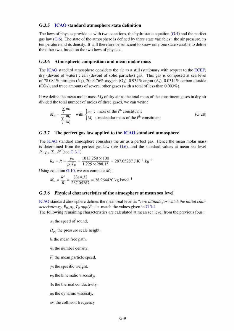
G.3.5 ICAO standard atmosphere state definition

The laws of physics provide us with two equations, the hydrostatic equation (G.4) and the perfect

gas law (G.6). The state of the atmosphere is defined by three state variables : the air pressure, its

temperature and its density. It will therefore be sufficient to know only one state variable to define

the other two, based on the two laws of physics.

G.3.6 Atmospheric composition and mean molar mass

The ICAO standard atmosphere considers the air as a still (stationary with respect to the ECEF)

dry (devoid of water) clean (devoid of solid particles) gas. This gas is composed at sea level

of 78.084% nitrogen (N2), 20.9476% oxygen (O2), 0.934% argon (Ar), 0.0314% carbon dioxide

(CO2), and trace amounts of several other gases (with a total of less than 0.003%).

If we define the mean molar mass Md of dry air as the total mass of the constituent gases in dry air

divided the total number of moles of these gases, we can write :

Md =

∑

i

mi

∑

i

mi

Mi

with

mi : mass of the ith constituant

Mi : molecular mass of the ith constituant(G.28)

G.3.7 The perfect gas law applied to the ICAO standard atmosphere

The ICAO standard atmosphere considers the air as a perfect gas. Hence the mean molar mass

is determined from the perfect gas law (see G.6), and the standard values at mean sea level

P0, ρ0,T0,R∗ (see G.3.1).

Rd = R =p0

ρ0T0=

1013.250 × 100

1.225 × 288.15= 287.05287 J.K−1.kg−1

Using equation G.10, we can compute M0 :

M0 =R∗

R=

8314.32

287.05287= 28.964420 kg.kmol−1

G.3.8 Physical characteristics of the atmosphere at mean sea level

ICAO standard atmosphere defines the mean seal level as “zero altitude for which the initial char-

acteristics g0, P0, ρ0,T0 apply”, i.e. match the values given in G.3.1.

The following remaining characteristics are calculated at mean sea level from the previous four :

a0 the speed of sound,

Hp0the pressure scale height,

l0 the mean free path,

n0 the number density,

ν0 the mean particle speed,

γ0 the specific weight,

υ0 the kinematic viscosity,

λ0 the thermal conductivity,

µ0 the dynamic viscosity,

ω0 the collision frequency

G-9

Remark G.4. From the above, we can conclude that the definition of mean sea level differs be-

tween the World Meteorological Organization and the International Civil Aviation Organization.

Meteorologists define mean sea level by [151] “The fixed reference level of MSL should be a well-

defined geoid, like the WGS-84 Earth Geodetic Model 1996 (EGM96) [Geoid : the equipotential

surface of the Earth’s gravity field which best fits, in a least squares sense, global MSL].”. Accord-

ing to WMO it is based on a geoid, whereas according to ICAO, it is based on three atmosphere

state variables and a constant gravity g0.

G.3.9 Temperature and vertical temperature gradient (lapse rate)

The temperatures are referred to the temperature of the ice point under a pressure of 1013.25 hPa

taken as Ti = 273.15 K. Temperatures are expressed in Kelvin using the following formula :

T = Ti + t (G.29)

where t is the Celsius temperature, expressed in C.

Observations showed that according to the temperature variations, the atmosphere could be divided

in layers (see G.1). This is the assumption used by the ICAO standard atmosphere. The transitional

zones between the layers are the tropopause, the stratopause and the mesopause. The temperature

in each layer is assumed to be a linear function of the geopotential altitude14, that can be written

in the form :

T = Tb + β(H − Hb) (G.30)

where :

Tb is the temperature of the lower limit of the concerned layer,

Hb is the geopotential altitude of the lower limit of the concerned layer,

β is the concerned layer vertical temperature gradientd T

d Hgiven in table G.1. Figure G.2

show the temperature variation between 0 and 32 km geometric height, according to ICAO

atmosphere model.

Table G.1 – ICAO standard atmosphere - Temperatures and vertical temperature gradients

Geopotential altitude H (km) Temperature T (K) Temperature gradient β (K.km−1)−5.00 320.65

−6.500.00 288.15

-6.5011.00 216.65

0.0020.00 216.65

+1.0032.00 228.65

+2.8047.00 270.65

0.0051.00 270.65

-2.8071.00 214.65

-2.0080.00 196.65

14Remembering that H =rh

r + h, this definition shows that the temperature is not a linear function of the altitude

(i.e., geometric height).

G-10

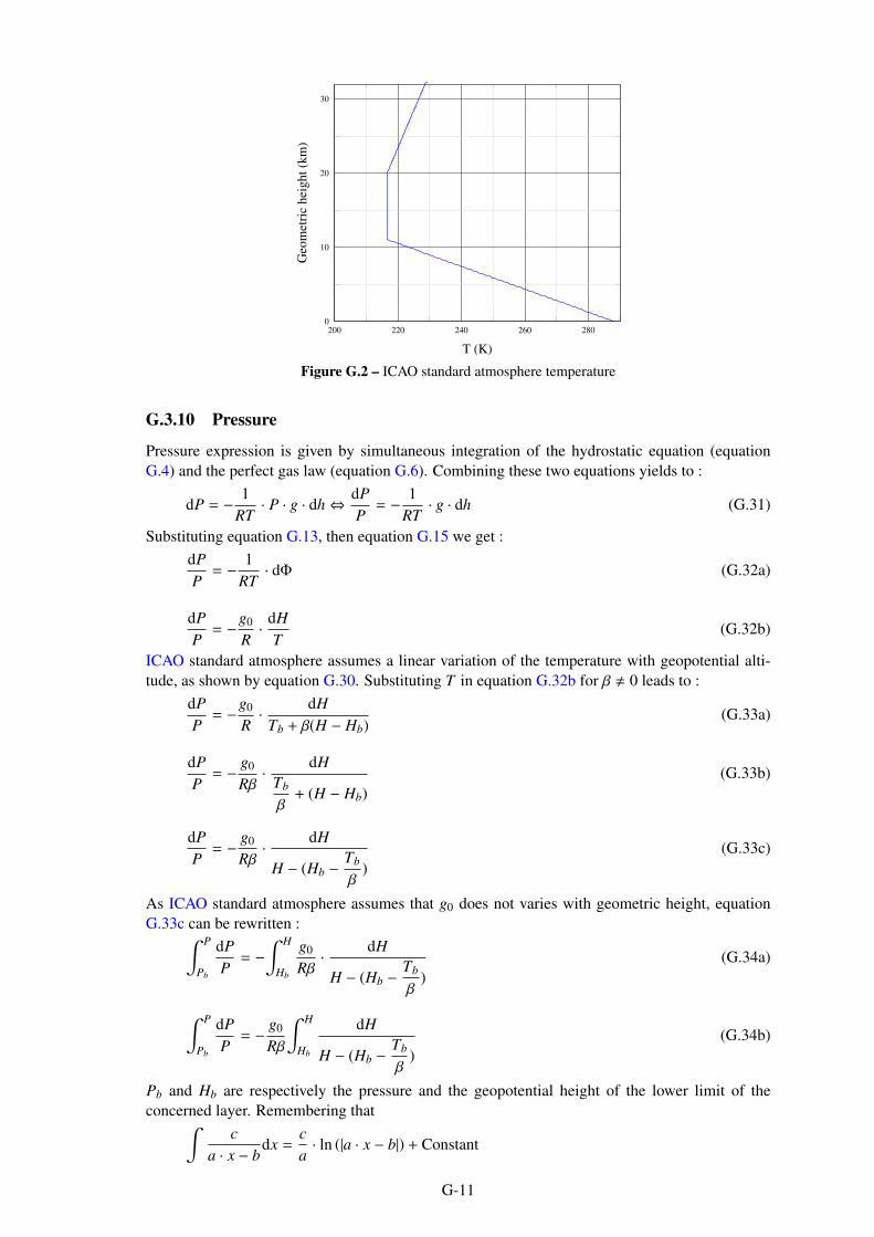
200 220 240 260 2800

10

20

30

T (K)

Geo

met

ric

hei

gh

t(k

m)

Figure G.2 – ICAO standard atmosphere temperature

G.3.10 Pressure

Pressure expression is given by simultaneous integration of the hydrostatic equation (equation

G.4) and the perfect gas law (equation G.6). Combining these two equations yields to :

dP = − 1

RT· P · g · dh⇔ dP

P= − 1

RT· g · dh (G.31)

Substituting equation G.13, then equation G.15 we get :

dP

P= − 1

RT· dΦ (G.32a)

dP

P= −g0

R· dH

T(G.32b)

ICAO standard atmosphere assumes a linear variation of the temperature with geopotential alti-

tude, as shown by equation G.30. Substituting T in equation G.32b for β , 0 leads to :

dP

P= −g0

R· dH

Tb + β(H − Hb)(G.33a)

dP

P= − g0

Rβ· dH

Tb

β+ (H − Hb)

(G.33b)

dP

P= − g0

Rβ· dH

H − (Hb −Tb

β)

(G.33c)

As ICAO standard atmosphere assumes that g0 does not varies with geometric height, equation

G.33c can be rewritten :∫ P

Pb

dP

P= −

∫ H

Hb

g0

Rβ· dH

H − (Hb −Tb

β)

(G.34a)

∫ P

Pb

dP

P= − g0

Rβ

∫ H

Hb

dH

H − (Hb −Tb

β)

(G.34b)

Pb and Hb are respectively the pressure and the geopotential height of the lower limit of the

concerned layer. Remembering that∫

c

a · x − bdx =

c

a· ln (|a · x − b|) + Constant

G-11

we can solve equation G.34b :

[ln (|P|)]PPb= − g0

Rβ

[

ln

(∣∣∣∣∣H − (Hb −

Tb

β)

∣∣∣∣∣

)]H

Hb

= − g0

Rβ

(

ln

(∣∣∣∣∣H − (Hb −

Tb

β)

∣∣∣∣∣

)

− ln

(∣∣∣∣∣Hb − (Hb −

Tb

β)

∣∣∣∣∣

))

= − g0

Rβ

(

ln

(∣∣∣∣∣

Tb + β(H − Hb)

β

∣∣∣∣∣

)

− ln

(∣∣∣∣∣

Tb

β

∣∣∣∣∣

))

= − g0

Rβ· ln

(∣∣∣∣∣

Tb + β(H − Hb)

Tb

∣∣∣∣∣

)

(G.35)

As P, Pb,Tb + β(H − Hb)

Tb

are all positive, we can write :

ln (P) = ln (Pb) − g0

Rβln

(

1 +β(H − Hb)

Tb

)

(G.36)

and finally :

P = Pb

(

1 +β(H − Hb)

Tb

)−g0

Rβ(G.37)

When β = 0, equation G.33a becomes :

dP

P= −g0

R· dH

Tb

(G.38)

leading to :∫ P

Pb

dP

P= −

∫ H

Hb

g0

R· dH

T⇔ ln (P) = ln (Pb) − g0

RT(H − Hb) (G.39)

where T and pb are respectively the temperature and the pressure of the lower limit of the con-

cerned (assumed isotherm) layer. Thus :

P = Pb exp(−g0

RT(H − Hb)

)

for β = 0 (G.40)

Figure G.3 show the pressure variation between 0 and 32 km geometric height, according to ICAO

atmosphere model.

200 400 600 800 1,0000

10

20

30

P (HPa)

Geo

met

ric

hei

gh

t(k

m)

Figure G.3 – ICAO standard atmosphere pressure

G.3.11 Density and specific weight

Once the temperature and the pressure have been computed using formula G.30, G.37 and G.40

the density is given by :

ρ =P

RT(G.41)

G-12

The specific weight γ is the weight per unit volume of air and is given by :

γ = ρg (G.42)

G.3.12 Speed of sound

The speed of sound a is given by the expression :

a =√κRT = 20.046796

√T with κ =

Cp

Cv

= 1.4 the adiabatic index (G.43)

G.4 Off-standard atmospheric models

As the Earth’s atmosphere is a dynamic changing environment, off-standard atmospheric models

are used to compute aircraft performance and flight parameters (e.g. altitude). These off-standard

atmospheric models use a single change, to an ICAO standard atmosphere constant or a charac-

teristic (see G.3.1). Most of the time temperature offsetting is used, i.e. the MSL temperature is

increased or decreased, but the lapse rate remains unchanged (see table G.1). The atmosphere is

said to be ISA +∆T , when the actual MSL temperature is above T0 = 288.15 K, and or ISA −∆T ,

when the actual MSL is below T0 = 288.15 K, with ∆T = |T − T0|15.

G.5 Matlab R© and Simulink R© implementations

Matlab R© and Simulink R© both implement atmosphere models.

The Aerospace BlocksetTM

provides Simulink R© with the following blocks :

1. The CIRA-86 Atmosphere Model (implementation of the mathematical representation of

1986 CIRA atmosphere).

2. The COESA Atmosphere Model (implementation of the 1976 COESA lower atmosphere).

3. The ISA Atmosphere Model (implementation of the International Standard Atmosphere16).

4. The Lapse Rate Model (implementation of the lapse rate model for the atmosphere).

In Matlab R© the Aerospace Toolbox provides :

1. The atmosisa function (implements the mathematical representation of the International

Standard Atmosphere17 values for ambient temperature, pressure, density, and speed of

sound for the input geopotential altitude). It assumes that temperature and pressure values

are held constant below the geopotential altitude of 0 km and above the geopotential altitude

of the tropopause (at 20 km).

2. The atmoscira function (implements the mathematical representation of the COmmittee

on SPAce Research (COSPAR) International Reference Atmosphere (CIRA) from 1986

model).

3. The atmoscoesa function (implements the mathematical representation of the 1976 COESA

United States standard lower atmospheric values - identical to ICAO standard atmosphere

for geopotential heights between 0 and 32 km).

15It should be noted that the 2010 BADA new atmosphere model [108] uses both temperature differential (∆T ) and

pressure differential (∆P) at mean sea level.16Not the ICAO standard atmosphere, as below the geopotential altitude of 0 km and above the geopotential altitude

of the tropopause, temperature and pressure values are held, whereas ICAO defines a lapse rate below 0 km geopotential

height.17Not the ICAO standard atmosphere

G-13

4. The atmoslapse function (implements the mathematical representation of the lapse rate at-

mospheric equations for ambient temperature, pressure, density, and speed of sound for the

input geopotential altitude). This function may be used to customize the atmospheric model.

G.6 Conclusion

The ICAO standard atmosphere can be seen as a linear approximation of the mean meteorological

conditions in the northern hemisphere around 45N latitude. It is used for airplane performance

analysis (e.g. rate of climb), airplane operations (e.g. Driftdown escape route18 planning) and

calibration of instruments.

With the advent of new GNSS-based instrument approach procedures, it should be kept in mind

that altimeters are calibrated for a standard atmosphere. The LNAV/Baro-VNAV approaches uses

barometric altitude information from the aircraft’s pitot-static system and the ADC19, to compute

vertical guidance for the pilot. Generally, temperature limitations are published on the approach

chart which may result in approach restrictions (unless navigation system has temperature com-

pensation function)20.

The gravity model used by the ICAO standard atmosphere differs from those used by the WMO

and the World Geodetic System 1984 (WGS-84) models. Care must be taken when processing

airplane meteorological observations.

During a standard day (i.e. P = P0, ρ = ρ0, T = T0), care must also be taken when flying the

same GNSS approach with vertical guidance. Depending on whether the approach is flown with

Baro-VNAV, or Satellite-Based Augmentation System (SBAS)-VNAV21, the vertical profiles may

differ. Instrument approach charts normally give different minima for Baro-VNAV (LNAV/VNAV

minima) and SBAS-VNAV (Localiser Performance with Vertical guidance (LPV) minima).

18A passengers jet optimum cruising altitude generally exceeds the OEI service ceiling. Thus in case of an engine

failure a descent and in most cases a driftdown procedure are needed.19Pilots must keep in mind the limitations of the altimeter calibration, specially when using baro-aided GPS units,

as the temptation to fly the procedure like an ILS may be great.20Cold temperatures reduce actual glide-path angle, whereas high temperatures increase actual glide-path angle.21The Airbus A350 XWB is the first wide-body aircraft providing a SBAS navigation solution in its design, through

its Airbus Satellite Landing System (SLS).

G-14

Bibliography

[1] 108th Congress. Public Law 108 - 176 - Vision 100–Century of Aviation Reauthorization

Act. Dec. 12, 2003.

[2] 1278.1-2012 - IEEE Standard for Distributed Interactive Simulation - Application Proto-

cols. IEEE, 2012.

[3] Malcolm J. Abzug. Computational Flight Dynamics. American Institute of Aeronautics

and Astronautics, 1998.

[4] European Aviation Safety Agency. Airworthiness Directive - Airspeed Pitot Probes Re-

placement. Aug. 2009.

[5] AIAA R-004 - Atmospheric and Space Flight Vehicle Coordinate Systems. AIAA, Jan.

1992.

[6] David Allerton. Principles of Flight Simulation. John Wiley & Sons, Ltd, 2009.

[7] Ken Alton. ‘Dijkstra-like Ordered Upwind Methods for Solving Static Hamilton-Jacobi

Equations’. PhD thesis. The University of British Columbia, 2010.

[8] Luca Amodei and Mohamed-Najib Benbourhim. ‘A vector spline approximation’. In:

Journal of Approximation Theory 67.1 (1991), pages 51–79.

[9] John D. Anderson Jr. Fundamentals of Aerodynamics. McGraw-Hill series in aeronautical

and aerospace engineering. McGraw-Hill, 2011.

[10] Boris Aronov, Sariel Har-Peled, Christian Knauer, Yusu Wang, and Carola Wenk. ‘Fréchet

Distance for Curves, Revisited’. In: Algorithms – ESA 2006. Edited by Yossi Azar and

Thomas Erlebach. Berlin, Heidelberg: Springer Berlin Heidelberg, 2006, pages 52–63.

[11] A. Arribas, K.B. Robertson, and K.R. Mylne. ‘Test of a poor Man’s ensemble predic-

tion system for short-range probability forecastingEnsemble experiments on numerical

weather prediction error and uncertainty for a North Pacific forecast failure’. In: Monthly

Weather Review 133.7 (2005), pages 1825–1839.

[12] Air Line Pilots Association. Aircraft accident report on Tenerife accident.

[13] International Air Transport Association. Controlled Flight Into Terrain accident analysis

report - 2014-2014. 2015.

[14] T. Baklacioglu and M. Cavcar. ‘Aero-propulsive modelling for climb and descent trajec-

tory prediction of transport aircraft using genetic algorithms’. In: The Aeronautical Jour-

nal 118.1199 (2014), pages 65–79.

[15] John Barrer, Peter Kuzminski, and William Swedish. ‘Analyzing the Runway Capacity of

Complex Airports’. In: AIAA 5th ATIO and 16th Lighter-Than-Air Sys Tech. and Balloon

Systems Conferences. Sept. 2005.

[16] Ben Musialek, Carmen F. Munafo, Hollis Ryan, and Mike Paglione. Literature Survey of

Trajectory Predictor Technology. Technical report. FAA, Nov. 2010.

[17] Stanley G. Benjamin, Barry E. Schwartz, and Rodney E. Cole. ‘Weather and forecasting’.

In: American Meteorological Society 14.6 (Dec. 1999), pages 1032–1038.

[18] BIPM. Le Système international d’unités / The International System of Units. 9th edition.

Bureau international des poids et mesures, 2019.

BiB – 1

[19] Jean-Luc Boiffier. The Dynamics of Flight, The Equations (Vol 1). Edited by Wiley. 1998.

[20] Bill Bulfer. FMC’s user guide - B737. Leading Edge Publishing, Apr. 2003.

[21] Robert Burtch. A comparaison of methods used in rectangular to geodetic coordinate

transformations. 2006.

[22] Civil Aviation Bureau Of Japan. The Long-Term Vision of Future Air Traffic Systems in

Japan - CARATS. Nov. 10, 2010.

[23] Neculai Cojocariu and Razvan Bbucuroiu. Operational Use of Downlink Airborne Param-

eters. Technical report. Eurocontrol, Nov. 2012.

[24] Rodney E. Cole, Steve M. Green, Matt R. Jardin, Barry E. Schwartz, and Stanley G. Ben-

jamin. ‘Wind Prediction Accuracy for Air Traffic Management Decision Support Tools’.

In: Proceedings of 3th USA-Europe ATM Seminar. FAA/Eurocontrol. 2000.

[25] Commission Of The European Communities. Communication from the Comission to the

Council and the European Parliament - The creation of the single European sky. Dec.

1999.

[26] 4DCo-GC Consortium. 4DCo-GC Report Summary. Oct. 2014.

[27] Daniel Delahaye. ‘Wind Field Update using Radar Track Data’. Master’s thesis. Ecole

Nationale de l’Aviation Civile, 1992.

[28] Daniel Delahaye and Stéphane Puechmorel. ‘Air traffic complexity based on dynami-

cal systems’. In: 49th IEEE Conference on Decision and Control (CDC). Dec. 2010,

pages 2069–2074.

[29] Daniel Delahaye, Stéphane Puechmorel, Sameer Alam, and Eric Féron. ‘Trajectory Math-

ematical Distance Applied to Airspace Major Flows Extraction’. In: EIWAC 2017 The

5th ENRI International Workshop on ATM/CNS. Volume Lecture Notes in Electrical En-

gineering. Air Traffic Management and Systems III. ENRI. Tokyo, Japan: Springer, Nov.

2017.

[30] Daniel Delahaye, Stéphane Puechmorel, Panagiotis Tsiotras, and Eric Féron. ‘Mathemat-

ical Models for Aircraft Trajectory Design: A Survey’. In: Air Traffic Management and

Systems : Selected Papers of the 3rd ENRI International Workshop on ATM/CNS (EI-

WAC2013). Tokyo: Springer Japan, 2014, pages 205–247.

[31] E. W. Dijkstra. ‘A note on two problems in connexion with graph’. In: Numerische Math-

ematlk 1 (1959), pages 269–271.

[32] Dominic J. Diston. Computational Modelling and Simulation of Aircraft and the Environ-

ment: Volume 1: Platform Kinematics and Synthetic Environment. Wiley & Sons, May 11,

2009.

[33] Wayne Durham. Aircraft Flight Dynamics and Control. JOHN WILEY & SONS INC,

Oct. 7, 2013. 306 pages.

[34] Daniel Dvorak. ‘NASA Study on Flight Software Complexity’. In: (Apr. 2009).

[35] Gabriele Enea and Marco Porretta. ‘A comparison of 4d-trajectory operations envisioned

for nextgen and sesar, some preliminary findings’. In: International Council of the Aero-

nautical Science. Sept. 2012.

[36] M. Enriquez. ‘Identifying Temporally Persistent Flows in the Terminal Airspace via Spec-

tral Clustering’. In: ATM Seminar 10. Edited by FAA/Eurocontrol. June 2013.

[37] Bernard Etkin and Reid Lloyd Duff. Dynamics of Flight: Stability and Control. Nov. 1996.

[38] Eurocontrol. Eurocontrol Specification for Trajectory Prediction. Mar. 2017.

[39] Eurocontrol and Institute of Geodesy and Navigation (IfEN). WGS 84 Implementation

Manual. ICAO, 1998.

BiB – 2

[40] Eurocontrol/FAA. ACTION PLAN 16 : Common Trajectory Prediction Capability - TP

Requirements Engineering Methodology paper. Sept. 2004.

[41] Eurocontrol/FAA. ACTION PLAN 17 : Future Communications Study - Final Conclusions

and Recommendations Report. Nov. 2007.

[42] Eurocontrol/FAA. SESAR-NextGen Aligned TP Structure and Terminology - AP16 White

Paper. Jan. 2010.

[43] European Commission. Official Journal of the European Union, Commission Regulation

(EU) No 965/2012. Official Journal of the European Union. European Union, Oct. 2012.

[44] FAA/Eurocontrol. White Paper : Common TP Structure and Terminology in support of

SESAR & NextGen. Jan. 2010.

[45] Yann Le Fablec and Jean Marc Alliot. ‘Using Neural Networks to predict aircraft trajecto-

ries’. In: Proceedings of the International Conference on Artificial Intelligence. 1999.

[46] A. C. Fang and B. G. Zimmerman. Digital Simulation of Rotational Kinematicss. Techni-

cal report NASA/TN-D-5302. NASA, Oct. 1969.

[47] Federal Aviation Administration. Advisory Circular : Aircraft Operations at Altitudes

Above 25,000 Feet Mean Sea Level or Mach Numbers Greater Than .75. Sept. 2015.

[48] Federal Aviation Administration. Special Conditions: Boeing Model 777-200, -300, and

-300ER Series Airplanes; Aircraft Electronic System Security Protection From Unautho-

rized Internal Access. Nov. 2013.

[49] Roberto Felix Patron and Ruxandra Botez. ‘Flight Trajectory Optimization Through Ge-

netic Algorithms for LNAV and VNAV Integrated Paths’. In: Journal of Aerospace Infor-

mation Systems 12 (Sept. 2015).

[50] F. Ferraty and P. Vieu. Nonparametric Functional Data Analysis: Theory and Practice.

Springer Series in Statistics. Springer, 2006.

[51] Antonio Filippone. Advanced aircraft flight performance. Cambridge University Press,

2013.

[52] David Flanagan and Evans Benjamin J. Java in a Nutshell, 6th Edition. O’Reilly Media,

Inc., Oct. 2014.

[53] Flight dynamics - Concepts, quantities and symbols - Part 1 : Aircraft motion relative to

the air. International Organization for Standardization, 1988.

[54] Flight Dynamics Model Exchange Standard (ANSI/AIAA S-119-2011(2016)). AIAA, 2011.

[55] Flight Operations Engineering Boeing Commercial Airplane Group. Flight planning and

performance manual. Technical report. The Boeing Company, Nov. 2005.

[56] A. Gelb and Analytic Sciences Corporation Technical Staff. Applied Optimal Estimation.

Applied Optimal Estimation. MIT Press, 1974.

[57] Mohinder S. Grewal, Lawrence R. Weill, and Angus P. Andrews. Global Positioning Sys-

tems, Inertial Navigation, and Integration. Wiley-Interscience, 2007.

[58] J. P. Hacker, E. S. Krayenhoff, and R. B. Stull. ‘Ensemble experiments on numerical

weather prediction error and uncertainty for a North Pacific forecast failure. A note on two

problems in connexion with graph’. In: Weather and Forecasting 18.1 (2003), pages 219–

260.

[59] P. E. Hart, N. J. Nilsson, and B. Raphael. ‘A Formal Basis for the Heuristic Determination

of Minimum Cost Paths’. In: IEEE Transactions on Systems Science and Cybernetics 4.2

(July 1968), pages 100–107.

[60] Jochen Hinkelbein, Christopher Neuhaus, Lennert Böhm, Steffen Kalina, and Stefan Brau-

necker. ‘In-flight medical emergencies during airline operations: a survey of physicians

on the incidence, nature, and available medical equipment’. In: Open Access Emergency

Medicine : OAEM 9 (2017), pages 31–5.

BiB – 3

[61] David G. Hoag. Apollo Guidance and Navigation : Considerations of Apollo IMU Gimbal

Lock. Technical report E-1344. MIT Instrumentation Laboratory, Apr. 1963.

[62] David G. Hoag. Apollo Navigation, Guidance, and Control Systems : A Progress Report.

Technical report E-2411. MIT Instrumentation Laboratory, Feb. 1969.

[63] Walter M. Hollister, Ethan R. Bradford, and Jerry D. Welch. ‘Using Aircraft Radar Tracks

to Estimate Winds Aloft’. In: The Lincoln Laboratory Journal 2 (1989).

[64] David G. Hull. Fundamentals of Airplane Flight Mechanics. 1st edition. Springer-Verlag

GmbH, Feb. 5, 2007.

[65] ICAO. 2013-2028 Global Air Navigation Plan - Doc 9750-AN/963. 4th edition. ISBN

978-92-9249-365-3. International Civil Aviation Organization, 2013.

[66] ICAO. Aircraft Operations - Doc 8168-OPS/611. International Civil Aviation Organiza-

tion, 2006.

[67] ICAO. Annex 10 to the Convention on International Civil Aviation - Aeronautical telecom-

munications - (Part I - Digital Data Communication Systems, Part II - Voice Communi-

cation Systems). 2nd edition. Volume II. July 2007.

[68] ICAO. Annex 10 to the Convention on International Civil Aviation - Aeronautical telecom-

munications - (Surveillance and Collision Avoidance Systems). 5th edition. Volume IV.

July 2014.

[69] ICAO. Annex 11 to the Convention on International Civil Aviation - Air Traffic Services.

14th edition. July 2016.

[70] ICAO. Annex 3 to the Convention on International Civil Aviation - Meteorological Service

for International Air Navigation. 19th edition. July 2016.

[71] ICAO. Annex 6 to the Convention on International Civil Aviation - Operation of Aircraft -

Part I - International Commercial Air Transport - Aeroplanes. 10th edition. July 2016.

[72] ICAO. Continuous Descent Operations (CDO) Manual - Doc 9931 AN/476. 1st edition.

ISBN 92-9194-554-4. International Civil Aviation Organization, 2010.

[73] ICAO. Doc 4444 ATM/501 - Procedures for Air Navigation Services - Air Traffic Manage-

ment. 15th edition. 2007.

[74] ICAO. Global Air Traffic Management Operational Concept - Doc 9854-AN/458. 1st edi-

tion. International Civil Aviation Organization, 2005.

[75] ICAO. Global Operational Data Link Document (GOLD). Apr. 2013.

[76] ICAO. Information Paper : Joint demo flights of manned and unmanned aircraft in Russian

Federation in non-segregated controlled airspace under RLOS and under existing ICAO,

EUROCAE and ETSI standards. Dec. 2015.

[77] ICAO. Manual of the ICAO standard atmosphere extended to 80 kilometres (262 500 feet)

- 3rd Edition. 1993.

[78] ICAO. Manual on system wide information management (SWIM) concept. Interim advance

edition. ICAO, 2015.

[79] ICAO. Technical Provisions for Mode S Services and Extended Squitter. 1st edition. 2008.

[80] ICAO European and North Atlantic Office. North Atlantic Operations and Airspace Man-

ual. International Civil Aviation Organization, 2018.

[81] ISO/IEC 18026 : Information technology - Spatial Reference Model (SRM). International

Standards Organization, July 2009.

[82] Mike Jackson. ‘Standards for Air Traffic Data. Communication Services. An Overview for

E-Operations Workshop’. In: RTCA Special Committee 214. 2007.

[83] Li Jin, Yi Cao, and Dengfeng Sun. ‘Investigation of Potential Fuel Savings Due to Continuous-

Descent Approach’. In: Journal Of Aircraft 50.3 (May 2013–June 2013), pages 807–816.

BiB – 4

[84] Joint Planning and Development Office JPDO. Concept of Operations for the Next Gener-

ation Air Transportation System. July 2006.

[85] Joint Planning and Development Office JPDO, Next Generation Air Transportation System

(NextGen). Concept of Operations for the Next Generation Air Transportation System.

Version 3.2. 2011.

[86] Ashish Kapoor, Zachary Horvitz, Spencer Laube, and Eric Horvitz. ‘Airplanes Aloft As

a Sensor Network for Wind Forecasting’. In: Proceedings of the 13th International Sym-

posium on Information Processing in Sensor Networks. IPSN ’14. Berlin, Germany: IEEE

Press, 2014, pages 25–34.

[87] David A. Karr, Robert A. Vivona, Sharon Woods, and David J. Wing. ‘Point-Mass Air-

craft Trajectory Prediction Using a Hierarchical, Highly-Adaptable Software Design’. In:

AIAA Aviation Forum. American Institute of Aeronautics and Astronautics, June 2017.

[88] David G. Kendall. ‘Shape Manifolds, Procrustean Metrics, and Complex Projective Spaces’.

In: Bulletin of the London Mathematical Society 16.2 (1984), pages 81–121.

[89] Gashu Kiltu and Habtamu Garoma. ‘Comparison of Higher Order Taylor’s Method and

Runge- Kutta Methods for Solving First Order Ordinary Differential Equations’. In: Jour-

nal of Computer and Mathematical Sciences 8 (Jan. 2017), pages 12–23.

[90] Jack B. Kuipers. Quaternions and Rotation Sequences : A Primer with Applications to

Orbits, Aerospace and Virtual Reality. Princeton University Press, 2002.

[91] Wu Kun and Pan Wei. ‘A 4-D trajectory prediction model based on radar data’. In: 2008

27th Chinese Control Conference. July 2008, pages 591–594.

[92] Walter D. Lambert and U.S. Coast and Geodetic Survey. ‘The international gravity for-

mula’. In: American Journal of Science 243-A (1945), pages 360–392.

[93] A. M. P. de Leege. ‘Enabling Continuous Descent Operations in High-Density Traffic’.

Master’s thesis. Technische Universiteit Delft, 2013.

[94] T. Warren Liao. ‘Clustering of time series data - a survey’. In: Pattern Recognition 38

(2005), pages 1857–1874.

[95] Chungu Lu, Huiling Yuan, Barry E. Schwartz, and Stanley G. Benjamin. ‘Short-range

numerical weather prediction using time-lagged ensembles’. In: Weather and Forecasting

22.3 (2007), pages 580–595.

[96] Stéphane Mondoloni. Aircraft trajectory prediction errors. Technical report Version 0.2.

July 2006.

[97] Stéphane Mondoloni and Diana Liang. ‘Improving Trajectory Forecasting Through Adap-

tive Filtering Technique’. In: Proceedings of 5th USA-Europe ATM Seminar. FAA/Euro-

control. 2003.

[98] NASA. NASA & the next generation air transportation system. June 2007.

[99] National Imagery and Mapping Agency. Department of Defense World Geodetic Sys-

tem 1984: its definition and relationships with local geodetic systems. Technical report

TR8350.2. St. Louis, MO, USA: National Imagery and Mapping Agency, Jan. 2000.

[100] C. Needham and R. Boyle. ‘Performance Evaluation Metrics and Statistics for Positional

Tracker Evaluation’. In: Proceedings of ICVS, Graz, Austria. Apr. 2003, pages 278–289.

[101] Robert C. Nelson. Flight Stability and Automatic Control. McGraw-Hill, 1989.

[102] Angela Nuic. User Manual For The Base of Aircraft DAta (BADA) Revision 3.12. Techni-

cal report. Eurocontrol, Aug. 2014.

[103] Erwan Page. Airport Collaborative Decision-Making Update presentation - CDM DSNA

seminar. Ministère de l’Ecologie, du Développement durable, et de l’Energie - Direction

Générale de l’Aviation Civile, Nov. 2015.

BiB – 5

[104] Drew C. Peterson, Christian Martin-Gill, Francis X. Guyette, Adam Z. Tobias, Catherine

E. McCarthy, Scott T. Harrington, Theodore R. Delbridge, and Donald M. Yealy. ‘Out-

comes of Medical Emergencies on Commercial Airline Flights’. In: New England Journal

of Medicine 368.22 (2013). PMID: 23718164, pages 2075–2083.

[105] Gerard Petit and Brian Luzum. IERS Conventions (2010). Technical report. International

Earth Rotation and Reference Systems Service (IERS), 2010.

[106] C. Petres, Y. Pailhas, P. Patron, Y. Petillot, J. Evans, and D. Lane. ‘Path Planning for

Autonomous Underwater Vehicles’. In: IEEE Transactions on Robotics 23.2 (Apr. 2007),

pages 331–341.

[107] Damir Poles. Base of Aircraft DAta (BADA) aircraft performance modelling report. Tech-

nical report. Eurocontrol, Mar. 2009.

[108] Damir Poles. EEC Technical Report No. 2010-001 : revision of atmosphere model in BADA

aircraft performance model. Technical report. Eurocontrol, Feb. 2010.

[109] International Association Of Gas & Oil Producers. Geomatics Guidance Note Number

7, part 2 - Coordinate Conversions and Transformations including Formulas. Technical

report. Apr. 2015.

[110] Stéphane Puechmorel. ‘Geometry of curves with application to aircraft trajectories anal-

ysis’. In: Annales de la Faculté des Sciences de Toulouse. Mathématiques. Série 6 (July

2015).

[111] J. Ramsay and B.W. Silverman. Functional Data Analysis. Springer Series in Statistics.

Springer New York, 2006.

[112] J. O. Ramsay and Xiaochun Li. ‘Curve registration’. In: Journal of the Royal Statistical

Society: Series B (Statistical Methodology) 60.2 (1998), pages 351–363.

[113] Sangeeta Rani and Geeta Sikka. ‘Recent Techniques of Clustering of Time Series Data: A

Survey’. In: International Journal of Computer Applications 52.15 (Aug. 2012). Full text

available, pages 1–9.

[114] C. M. Rekkas, C. C. Lefas, and N. J. Krikelis. ‘Three Dimensional Tracking Using On-

Board Measurements.’ In: IEEE Transactions on Aerospace and Electronic Systems 27.4

(1991), pages 617–624.

[115] Olga Rodionova, Daniel Delahaye, Mohammed Sbihi, and Marcel Mongeau. ‘Aircraft

trajectory prediction in North Atlantic Oceanic Airspace by Wind Networking’. In: DASC

2014, 33rd Digital Avionics Systems Conference. Best Paper of Session & 2nd Place Best

Graduate Student Paper. Colorado Springs, United States, Oct. 2014.

[116] Leiba Rodman. Topics in Quaternion Linear Algebra. Princeton University Press, 2014.

[117] Murry Salby. Fundamentals of Atmospheric Physics. Academic Press, 1996.

[118] Saulo Da Silva. Trajectory-Based Operations (TBO). ICAO Workshop on preparations for

ANConf/12 - ASBU methodology - Bangkok. May 14, 2012–May 18, 2012.

[119] Michelle Schatzman. Numerical Analysis - A Mathematical Introduction. Edited by Ox-

ford University Press. Clarendon Press, Oct. 2002.

[120] Barry E. Schwartz, Stanley G. Benjamin, Steven Martin Green, and Matt R. Jardin. ‘Weather

and Forecasting’. In: American Meteorological Society 15.3 (June 2000), pages 313–326.

[121] Consortium SESAR. SESAR Master Plan. Technical report. Apr. 2008.

[122] SESAR Joint Undertaking. European Air Traffic Management Master Plan - Ed2. Oct. 25,

2012.

[123] SESAR Joint Undertaking. European Air Traffic Management Master Plan - Ed3. Dec.

2015.

[124] SESAR Joint Undertaking. European Air Traffic Management Master Plan - First edition.

Mar. 30, 2009.

BiB – 6

[125] SESAR Joint Undertaking. Evolution of the Surveillance Infrastructure. Oct. 19, 2012.

[126] SESAR Joint Undertaking. SESAR factsheet 01/2011 : System Wide Information Manage-

ment (SWIM). 2011.

[127] SESAR Joint Undertaking. SESAR factsheet 02/2010 : Business Trajectory / ’4D’ Trajec-

tory. 2010.

[128] J.A. Sethian. Level Set Methods and Fast Marching Methods: evolving interfaces in com-

putational geometry, fluid mechanics, computer vision, and materials science. Cambridge

University Press, 1999.

[129] Donald Shepard. ‘A two-dimensional interpolation function for irregularly-spaced data’.

In: ACM ’68 Proceedings of the 1968 23rd ACM national conference. Association for

Computing Machinery. ACM New York, NY, USA, 1968, pages 517–524.

[130] Gary Slater. ‘Study on variations in vertical profile for CDA descents’. In: 9th AIAA Avia-

tion Technology, Integration, and Operations Conference (ATIO). Sept. 21, 2009–Sept. 23,

2009.

[131] R. Sopjes, P. M. A. de Jong, C. Borst, M. M. van Paassen, and M. Mulder. ‘Continuous

Descent Approaches with Variable Flight-Path Angles under Time Constraints’. In: AIAA

Guidance, Navigation, and Control Conference. Aug. 8, 2011–Aug. 11, 2011.

[132] Laurel Stell. ‘Prediction of Top of Descent Location for Idle-thrust Descents’. In: Ninth

USA/Europe Air Traffic Management Research and Development Seminar (ATM2011).

2011.

[133] Robert F. Stengel. Flight Dynamics. Princeton University Press, Sept. 27, 2004. 864 pages.

[134] Brian L. Stevens and Frank L. Lewis. Aircraft Control and Simulation. Wiley-Interscience,

2003.

[135] Brian L. Stevens, Frank L. Lewis, and Eric N. Johnson. Aircraft Control and Simulation:

Dynamics, Controls Design, and Autonomous Systems, 3rd Edition. Wiley-Blackwell, 2016.

[136] Study Group for the Future Air Traffic Systems. CARATS Long-term Vision for the Future

Air Traffic Systems - Changes toIntelligentAir Traffic Systems. 2010.

[137] Kairat Tastambekov, Stéphane Puechmorel, Daniel Delahaye, and Chistophe Rabut. ‘Air-

craft trajectory forecasting using local functional regression in Sobolev space’. In: Trans-

portation Research Part C : Emerging Technologies 39 (Feb. 2014), pages 1–22.

[138] ‘Tokyo Capacity: Japan Air Navigation Service is exploring every opportunity to increase

flight capacity in the congested skies above Tokyo.’ In: Airspace Issue (2016), pages 26–

29.

[139] Ralph M. Toms. An Improved Algorithm for Geocentric to Geodetic Coordinate Conver-

sion. 14 th Workshop on Standards for Distributed Interactive Simulations. Mar. 1996.

[140] Egbert Torenbeek and H. Wittenberg. Flight Physics. Springer Netherlands, 2009.

[141] United States Government Accountability Office. Next Generation Air Transportation Sys-

tem. July 2015.

[142] US House of Representatives - Commitee on Transportation and Infrastructure. FAA Reau-

thorization : Issues in Modernizing and Operating the Nation’s Airspace. Nov. 14, 2014.

[143] John Vince. Quaternions for Computer Graphics. Springer-Verlag London, 2011.

[144] Robert A. Vivona, Karen T. Cate, and Steven M. Green. ‘Comparison of Aircraft Tra-

jectory Predictor Capabilities and Their Impacts on Air Traffic Management Automation

Interoperability’. In: American Institute of Aeronautics and Astronautics (2011).

[145] Randy Walter. The Avionics Handbook - Flight Management Systems. Edited by Cary R.

Cary R. Spitzer. CRC, 2001.

BiB – 7

[146] Andreas Wieland and Carl Marcus Wallenburg. ‘Dealing with Supply Chain Risks: Link-

ing Risk Management Practices and Strategies to Performance’. In: International Journal

of Physical Distribution & Logistics Management 42.10 (2012), pages 887–905.

[147] World Meteorological Organization (WMO). Final Report - Inaugural Meeting of the AM-

DAR Panel. Mar. 1998.

[148] World Meteorological Organization (WMO). WMO AMDAR Observing System Newslet-

ter. Apr. 2016.

[149] World Meteorological Organization (WMO). WMO-No. 188 International Meteorological

Tables. 1966.

[150] World Meteorological Organization (WMO). WMO-No. 306 Manual on Codes. Volume I.3.

2015. 2017 revised edition.

[151] World Meteorological Organization (WMO). WMO-No. 8 : Guide to Meteorological In-

struments and Methods of Observation. 7th edition. 2008.

[152] Thomas R. Yechout, Steven L. Morris, David E. Bossert, and Wayne F. Hallgren. Introduc-

tion to Aircraft Flight Mechanics : Performance, Static Stability, Dynamic Stability, and

Classical Feedback Control. American Institute of Aeronautics and Astronautics, 2003.

[153] Yutaka Fukuda. 10th USA/Europe ATM R&D Seminar - ATM Research in Japan Presen-

tation. June 13, 2013.

[154] Peter. H. Zipfel. Modeling and Simulation of Aerospace Vehicle Dynamics, Second Edi-

tion. AIAA, 2007.

[155] Peter. H. Zipfel. ‘Perturbation Methods in Atmospheric Flight Mechanics’. In: AIAA Jour-

nal 11.9 (Sept. 1973), pages 1247–1251.

BiB – 8

Index

1-2-3 rotation sequence, C-2

1.3g flight envelope, 5-1

1090ES, 2-17

1090 MHz ADS-B Extended Squitter

(1090ES), 2-17

120-minutes ETOPS rule, 7-2

2-stage Runge-Kutta method, F-18, F-19

2D grid, 4-6

3-stage Runge-Kutta method, F-24

3D box, 5-12

3D trajectory, 6-11

3DOF equations of motion, 3-5, 3-41

3DOF models, A-1

3DOF point-mass model, 6-3

4 dimensional continuum flight path, 2-10

4 dimensions space, 4-5, 4-11

4-Dimensional Trajectory operation, 2-11

4-stage Runge-Kutta method, F-26

4D Trajectory Based Operations, 4-27

4D control, 2-4

4D grid, 4-6, 4-11, 4-12, 5-11, 5-12

4D grid point, 4-6

4D neighborhood, 4-6, 5-12

4D trajectory, 2-7

4D trajectory management, 2-4

4D trajectory negotiation, 5-9

4D vicinity, 4-5

6DOF, 3-3

6DOF equations of motion, 3-5

6DOF equations of motion model, 3-41

6DOF models, A-1

Earth’s equatorial plane, A-2

SADIS 2G, 7-7

A

A* algorithm, 6-2

A/T, 3-6

Absolute ceiling, 5-8

Acceleration due to gravity, 5-6, G-5

Acceleration of gravity, G-6

Acceleration of gravity at mean sea-level,

G-7

Accelerometer, 3-28, 3-29

Accuracy, 7-1

Accurate ETA, 5-9

Accurate ETE, 5-9

Actual sensed temperature, 5-10

Actual sensed wind, 5-10

Actual trajectory, 5-1

Actual weather conditions, 7-4

Adaptive clustering algorithm, 6-15

ADC, 4-2, 4-7

Adequate airport, 7-2

Adiabatic index, 5-3, 5-7, G-3

ADS-B, 2-15, 2-17, 2-19, 4-1

ADS-B OUT, 2-16

ADS-B report, 7-7

ADS-B VHF Data Link Mode 4 (VDL-M4),

2-17

ADS-B-StateVector, 2-19

ADS-C, 2-18

ADS-C report, 5-9

ADS-R, 2-17, 2-18

Adverse weather, 2-5

Aerobatics maneuver, 3-32

Aerodrome capacity, 2-3

Aerodrome Operations (AO), 2-3

Aerodynamic angle of attack, 3-37, A-7,

A-17

Aerodynamic azimuth angle, A-16

Aerodynamic bank angle, A-16

Aerodynamic ceiling, 5-6–5-8

Aerodynamic climb angle, A-16

Aerodynamic configuration, 5-6

Aerodynamic forces, 3-5, 3-33

Aerodynamic frame, 3-38, A-6, A-16–A-18

Aerodynamic model, 3-29

Aerodynamic sideslip angle, A-17

aerodynamic sideslip angle, A-7

Aerodynamic velocity, A-16, A-17

aerodynamic velocity vector, A-6

AF leg, 3-15, D-4

AFDS, 3-6

Ind - 1

Affine registration, 6-13

Ailerons, 3-29

Air Data Computer, 4-2

Air density, 5-6, G-9, G-12

Air distance, 6-3

Air navigation database providers, 3-26

Air pressure, 5-3, 5-7, 5-9, G-9

Air specific gas constant, 5-3

Air temperature, 5-7, 5-9, G-9

Air Traffic Management Operational

Concept Panel (ATMCP), 2-2

Air-path frame, A-6

AIRAC cyle, 3-7

Airborne Collision Avoidance System

(ACAS), 2-4

Airborne trajectory predictors, 3-42

Aircraft attitude, 1-3, 3-1, 3-2, 3-17, 3-28,

3-29, 3-39, C-3

Aircraft attitude representation, E-1

Aircraft body-fixed reference frame, 3-28

Aircraft center of mass, A-5–A-7

Aircraft density, 5-17

Aircraft elevation, C-4

Aircraft flow control, 5-10

Aircraft flows management, 7-1

Aircraft future 4D position, 3-26

Aircraft instantaneous plane of motion, A-7

Aircraft mass, 5-7

Aircraft motion relative to the atmosphere,

3-27

Aircraft orientation, 3-30, C-3

Aircraft path, 6-9

Aircraft performance, 3-4, 3-19, G-13

Aircraft Performance Database, 3-41

Aircraft Performance Model, 3-21, 3-33

Aircraft performance tables, 3-41

Aircraft performances characteristics, 2-5

Aircraft position, 4-10

Aircraft positional information, 6-11

Aircraft separation, 2-5, 5-2

Aircraft speed, 4-10

Aircraft state, 3-41, 3-43

Aircraft state vector, 3-1

Aircraft thrust knowledge, 3-21

Aircraft to aircraft data link, 4-4

Aircraft to ground data link, 4-4

Aircraft trajectory, 5-16, 6-11

Aircraft Trajectory Model, 4-1

Aircraft/aircraft wind information sharing,

4-5

Aircraft/aircraft wind/temp information

sharing, 5-11

Aircraft/ground wind information sharing,

4-5

Aircraft/ground wind/temp information

sharing, 5-11

Airplane configuration, 3-40

Airplane initial lateral maneuvers, 3-6

Airplane initial vertical maneuvers, 3-6

Airplane intends, 3-6

Airplane mass, 5-6

Airplane operational condition, 3-7

Airplane orientation, 3-1

Airplane performance, G-14

Airplane position, 3-1

Airplane position and orientation, 3-28

Airplane track, 3-14

Airport-Collaborative Decision Making

(A-CDM), 2-6

Airports congestion, 7-1

Airspace capacity, 2-3

Airspace Organization and Management

(AOM), 2-3

Airspace resources, 2-3

Airspace User Operations (AUO), 2-4

Algorithm, 5-11

Algorithm implementation, 4-2, 4-12, 5-13

Algorithm validation, 4-10

All weather operations, 2-3

Along-track error source, 5-1

Altimeter calibration, G-14

Altimeter setting, A-13

Altitude, 5-9, 6-11

Altitude z, 6-4

Altitude above mean sea level, G-6

Altitude capability, 5-2

Altitudes restrictions, 3-12

Angle of attack, 5-6, 5-7

Angle-axis rotation, 3-30

angle2dcm Matlab function, C-8

Angular acceleration, 3-34

Angular momentum, 3-36

Anisotropic contributions, G-6

ANSI/AIAA R-004-1992, 3-27

ANSI/AIAA S-119-2011, 3-27

Anti-ice, 3-19

Anti-icing, 3-19

APM, 3-21, 3-33

Apparent sun, A-19

Approach, 3-17

Approach phase, 4-5, 5-11

Approximation of derivatives, F-3

Arc to point segments, 3-24

Arc-length, 6-12, 6-13

Arc-length warping, 6-13

Arcs of circle, 3-20, 3-22

Ind - 2

Area distance, 6-10

ARINC, 7-7

ARINC 424, 3-2, 3-9, 3-24–3-26

ARINC 424 leg, 3-2

ARINC 424 Legs, D-1

ARINC 424 trajectories, 3-25

ARINC 702A Supplement 3, 3-29

Aspect Ratio, 3-39

Assumed TAS, 3-20

Assumed winds, 3-20

Asymmetric protocol, 7-7

ATM community axis orientation, 3-38

ATM operation, 2-11

ATM safety management, 2-4

ATM Service Delivery Management (SDM),

2-4

atmoscira Matlab function, G-13

atmoscoesa Matlab function, G-13

atmosisa Matlab function, G-13

atmoslapse Matlab function, G-14

Atmospheric data, 4-2

Atmospheric pressure, G-3

Atmospheric reference frame, 3-28

Atmospheric vehicle coordinate systems,

3-27

Attitude, 3-28–3-32, 3-34, B-3, B-4

Attitude calculation, E-1

Attitude dynamics, 3-33

Attitude equations, 3-33

Attitude motion, 3-33

Attitude representation, E-1

Auto-throttle, 5-2

Automatic Dependent

Surveillance - Contract (ADS-C), 2-18

Automatic Dependent

Surveillance - Rebroadcast, 2-18

Autopilot, 5-2

Autopilot Flight Director System, 3-6

AutoThrottle, 3-6, 5-11

Aviation System Block Upgrade (ASBU),

2-2

Avionics providers, 3-26

Avogadro’s hypothesis, G-4

Avogadro’s number, G-4

Axis of rotation, B-3

Axis systems, 3-27

Azimuth, A-18

Azimuth angle, A-16

B

Bézier Approximation Curve, 3-25

Back propagation process, 6-8

Backward difference approximation, F-4,

F-7

Backward Euler’s method, 3-20, F-7–F-9

BADA, 3-29, 5-9

BADA 3, 3-37

BADA data base, 5-16

BADA model, 3-41

Balanced flight, 3-37

Bank angle, 3-29, 3-39, A-16, C-4, C-5

Barometric altitude, 2-17, 3-29, G-5, G-14

Barometric altitude rate, 3-30

Barometric pressure adjusted to sea level,

G-6

BDS code 4,0, 3-30

BDS code 5,0, 3-30

BDS code 6,0, 3-30

Behavior model, 3-4, 3-5, 3-15

Bellman algorithm, 6-3, 6-4, 6-15, 6-16

Bellman-Ford’s algorithm, 6-7

BIH Zero Meridian, A-4

Bisection method, F-8

Body Axis System, 3-28

Body Coordinate System, 3-28

Body fixed coordinates, C-1

Body frame, 3-28, 3-37, A-5, A-7, A-16,

A-17

Body-fixed reference frames, 3-28

Boltzmann constant, G-4

Boundary conditions, 7-3

Buffet margin, 5-6

Buffet-onset boundary safety margins, 5-7

BUFR message, 7-3

Business trajectory, 2-7

Butcher tableau, F-17–F-21, F-23, F-25,

F-26

C

CA leg, 3-15, D-3

Calibrated Air Speed, 5-10

Calibrated AirSpeed, 5-2

CARATS, 1-1, 2-1, 2-10

Cardano angles, C-5

Cartesian coordinates, 6-5

Cartesian coordinates system, 6-8

Cartesian distance, 6-9

Cartesian tensors, 3-35

CAS, 5-2

CAT, 5-7

CD leg, 3-16, D-4

CDA, 4-5

CDTI, 2-17

Center of mass, 3-33, 3-37, 3-38

Center of pressure, 3-37, 3-38

Central difference approximation, F-5, F-10

Centrifugal acceleration, G-6

Centrifugal force, G-6

Ind - 3

CF Leg, D-2

CF leg, 3-15

CI leg, 3-16, D-4

CIRA 1986 Atmosphere Model, G-1, G-13

Classical RK3, F-25

Classical RK4, F-27

Clear air turbulence, 5-7

Climb, 3-17

Climb phase, 3-37, 5-10, 5-18, 6-3

Climb profile, 3-42

Climb thrust, 5-9

Climb thrust reduction point, 3-17

Climb wind, 4-5

Cluster, 6-16, 6-18, 6-19

Cluster centroid, 6-15, 6-16

Cluster dispersion, 6-16

Clustering algorithm, 6-2, 6-15

Clustering procedure, 6-12

Cockpit Display Traffic Information(CDTI),

2-17

COESA 1976 Atmosphere Model, G-2

COESA Atmosphere Model, G-13

Collaborative Decision Making (CDM), 2-6

Collision avoidance stage, 2-4

Combined rotation, C-2

Comm-B Data Selector, 3-30

Compactly supported mapping, 6-10

Component presentation, 3-35

Computation block, 3-4

Computer graphics, 3-32

Computer programming, 3-35

Conflict, 1-2

Conflict alert, 3-1

Conflict detection, 1-3, 3-2, 3-42

Conflict horizon, 2-4

Conflict Management (CM), 2-4

Constant altitude equations, 3-21

Constant flight level, 6-3

Constant FPA, 3-21

Constant horizontal speed, 3-21

Constant Mach number, 3-41, 5-2, 5-4, 5-11,

5-13, 5-16, 5-18

Constant vertical speed, 3-21

Constraints handled, 3-5, 3-8

Continuous climb, 2-7

Continuous descent, 2-7

Continuous Descent Approach, 4-5

Control surfaces, 3-5

Control theory, 3-32

Coordinate system, 3-26, 3-35, 3-43, A-1

Coordinates synchronization, 6-9

Coordinates transformation, E-1

Cost index, 6-2

Course, A-18

CR leg, D-4

Crew entered weather data, 6-2

Cross-track, 3-20

Cross-track error, 3-22

Crossover altitude, 5-2

Cruise, 3-17

Cruise phase, 3-37, 6-3

Cruise wind field, 4-5

Cubic splines interpolation, 3-25

Current ETA, 5-13

Current outside air temperature, 5-10

Current winds, 3-20

D

DAEs, 3-20

Data link functions, 4-3

Data network node, 3-6

Data perspective, 3-3

Data sharing requirements, 2-10

Data structures, 4-12, 5-13, 5-16

Data-linked clearance, 5-10

DCM, 3-30, B-2

DCM inverse matrix, B-2

DCM transpose matrix, B-2

Decoupling rotational equations, 3-5

Decoupling translational equations, 3-5

Deformation energy, 6-14

Delegated separation, 2-15, 2-18

Demand and Capacity Balancing (DCB), 2-3

Density, G-2

Density altitude, 5-8

Depressurization, 7-3

Descend phase, 5-11

Descent, 3-17

Descent phase, 3-37, 4-5, 6-3

Descent thrust for approach, 3-40

Descent thrust for high altitude, 3-40

Descent thrust for landing, 3-40

Descent thrust for low altitude, 3-40

Destination node, 6-5, 6-8

Detection of conflict, 2-4

Deterministic approach, 3-3

Deterministic forecasts, 6-2

Deterministic methods, 3-43

Deterministic model, A-1

DF Leg, D-2

Differential and algebraic equations, 3-20

Digital backbone, 2-10

Dijkstra algorithm, 6-2, 6-7

Direct Cosine Matrix, E-1

Direct ransformation matrix, A-12

Direct transformation matrix, A-13

Ind - 4

Direction Cosine Matrix, 1-4, 3-29–3-31,

B-1, B-2

Displacement vector, 3-35

Distance between trajectories, 6-15

Distortions in time, 6-9, 6-11

Distributed Decision Making, 2-9

Distributed weather information, 5-1

Divergence operator, 4-9

Diversion route, 5-5

Diversion time, 7-2

Divided differences, F-3

Drag, 3-5, 3-12, 3-37–3-39, 5-6, 5-7

Drag coefficient, 3-39, 5-6

Drag multiplication factor, 3-40

Drag polar, 3-39

Drag polar coefficients, 3-40

Drift angle, A-18

Driftdown, 5-4, 5-5, 7-4, G-14

Driftdown procedure, 7-4

Duration, 6-9

DVB satellite, 7-7

Dynamic airspace organization, 2-3

Dynamic equations, 3-5

Dynamic height, G-5

Dynamic time warping, 6-13

E

Earth Axis System, 3-28

Earth Orientation Parameters, A-19

Earth’s angular velocity, A-19, G-6

Earth’s center of gravity, A-2

Earth’s equatorial plane, A-3

Earth’s geoid, A-4, G-5

Earth’s geoid ellipsoid model, G-7

Earth’s gravitational field, G-5

Earth’s radius, G-7

Earth’s Rotation Angle, A-15

Earth’s rotation axis, A-2

Earth’s rotation matrix, A-14

Earth-centered reference frame, 3-28

Earth-Centred Axis Systems, 3-28

Earth-fixed reference frame, 3-28

East wind component WE , 6-4

East-West routes, 6-1

ECEF axis of rotation, G-6

ECEF frame, 3-31, 3-33, 3-35, 3-43, 4-6,

A-2

ECI Frame, A-2

ECI frame, 3-33

Edge, 6-4

Effective gravity, G-6

Effective wind, 4-20

Efficient trajectory, 6-2

Eigenvalues, B-3

Eigenvector, B-3

Elapsed time, 3-41

Elemental rotations composition, A-11

Elementary rotation, A-9

Elevators, 3-29

Ellipsoid normal, A-5

Ellipsoidal latitude, G-7

En route conflict probe, 3-1

En Route operations, 3-3

En route wind, 5-10

En-route diversion, 7-5

En-route wind profile, 6-1

Energy, 3-2

Energy balance equations, 3-11

Energy formalism, 3-24

Energy Share Factor, 3-40

Engine bleed air, 3-19

Engine diameter, 5-9

Engine model, 3-29

Engine output power, 5-2

Engine performance, 3-42, 5-2, 5-8, 5-18,

7-4

Engine type, 3-40

Engines database, 5-9

Enhanced local wind/temperature map, 1-3

Enhanced weather information, 5-2

Ensemble Prediction, 6-2

Entity Coordinates System, 3-28

Environmental awareness, 6-1

Environmental constraints, 6-2

Equations decoupling, 3-33

Equations of motion, 3-11, A-1

Equatorial plane, A-19

Equitable access, 2-3

Erroneous fuel consumption prediction, 4-5

Erroneous winds, 4-5

Escape maneuver, 7-4

ESF, 3-40

Estimated Time En route, 4-20

Estimated Time of Arrival, 4-5

Estimation problem, 3-1

ETA, 4-5

ETA prediction, 4-25

ETE calculations, 5-13

ETE prediction error, 5-1

ETOP approval, 7-2

ETOPS, 5-1, 5-18, 7-3

ETOPS 330 min capability, 7-2

ETOPS approval category, 7-2

Euclidean distance, 6-8

Euclidean norm, 4-9

eul2rotm Matlab function, C-7

Euler angles, 3-30, 3-31, C-1, E-1

Ind - 5

Euler angles (1-2-3) rotation convention,

C-2

Euler angles (3-2-1) orientation convention,

C-3

Euler angles convention, C-1

Euler angles conversion to rotation matrix,

C-5

Euler angles sequences, C-1

Euler integration methods, 1-5, 3-41

Euler’s law, 3-33

Euler’s methods, F-1

Euler’s methods variants, F-9

Euler’s rotation theorem, B-3, E-1

Exosphere, G-1

Explicit method, F-8, F-10, F-17, F-18

Explicit midpoint method, F-21

Explicit RK methods, F-17

Extended situational awareness, 2-18

External force vector, 3-36

External normal, G-5

Externally applied moment, 3-36

F

FA Leg, D-3

FA leg, 3-15

False trajectory conflict alert, 3-1

FC leg, D-3

FD leg, D-3

Filed flight PLan (FPL), 2-14, 3-6

Filtering, 3-1

Final attitude, C-5

Final base, C-6

Final orientation, C-5

First order differential equations system,

3-41

First-order approximation, F-3, F-4

First-order differential equation, F-5

First-order tensors, 3-36

FIS-B, 2-18

Fitting, 4-8

Fixed ENU frame, A-4

Fixed geographical point, 3-20

FLight AlaRM (FLARM), 2-4

Flight dynamics Euler angles convention,

C-2

Flight dynamics model, 3-29

Flight envelope, 3-12, 5-6

Flight Information Service Broadcast, 2-18

Flight load factor, 5-6

Flight Management Computer, 3-6, 4-2

Flight parameters, G-13

Flight path, 6-12, A-7

Flight Path Angle, 3-14, 3-23, 3-37

Flight path azimuth, A-18

Flight path climb angle, A-18

Flight Path Director, 3-14

Flight path inclination angle, A-18

Flight path track angle, A-18

Flight Path Vector, 3-14

Flight performance, 6-1

Flight planning, 5-10

Flight procedure, 3-24

Flight safety, 3-43

Flight state, 3-7

Flight time, 6-1

Flight-path bank angle, A-18

Flight-path frame, A-7

Floating geographical point, 3-20

Fly dynamics equations, 3-36

Fly-by waypoint, 3-16

Fly-over waypoint, 3-16

FM leg, 3-15, D-3

FMC, 1-1, 3-6, 4-2

FMC weather update, 4-4

FMS, 1-1

FMS performance predictions, 5-10

FMS temperature linear interpolation, 5-10

FMS wind linear interpolation, 5-10

Forecast wind, 3-20, 4-5, 4-16

Forecast wind data, 3-19

Forward difference approximation, F-4, F-5

Forward Euler’s method, 3-20, F-5, F-6,

F-8, F-18

FPA, 3-14

FPD, 3-14

FPL, 3-6

FPV, 3-14

Frame, 3-35

Frame alignment, C-4

Frame of Reference, 3-26

Frame systems, 3-26

Front propagation method, 6-2

Fréchet distance, 6-13

Fuel balance, 4-5

Fuel consumption, 6-1

Fuel consumption estimation, 5-11

Fuel cost, 6-1

Fuel estimation, 5-1

Fuel fees, 6-1

Fuel flow, 5-9

Fuel freezing, 5-9

Fuel mandatory reserves, 7-5

Full-separation, 2-4

Functional data statistics, 6-12

Future Air Navigation System (FANS), 2-2

Future ATM concept, 4-27

Future position, 5-17

Ind - 6

Future trajectory, 4-23

G

Gas density, G-4

Gate assignment, 4-27

Gate to gate trajectory, 2-5

Gates assignment, 4-25

Genetic algorithm, 3-43

Geocentric Cartesian Coordinate System,

3-28

Geocentric coordinates, 3-27

Geocentric Earth-Fixed Coordinate System,

3-28

Geodetic altitude, 3-38, 3-40

Geodetic coordinate system, A-7

Geodetic coordinate to ECEF coordinate,

A-13

Geodetic East, A-4, A-5

Geodetic latitude, A-7, A-8, A-15, G-7

Geodetic North, A-4, A-5

Geodetic reference datum, 3-27

Geodetic to geocentric transformation, A-13

Geographic latitude, G-7

Geographic reference frame, C-4

Geographical North, A-18

Geometric algorithms, 3-20

Geometric approximation, 3-20

Geometric elevation, G-5

Geometric height, G-3–G-7, G-10

Geopotential, G-5

Geopotential altitude, 3-38, G-10, G-11

Geopotential height, G-5–G-7, G-11

Geopotential meter, G-5

Geopotential pressure altitude, 5-9

Gibbs vector mechanics, 3-35

Gimbal, 3-28

Gimbal lock, 3-31

Global Air Traffic Management Operational

Concept (GATMOC), 2-2

Global characteristics, 6-12

Global Positioning System, 3-6

glRotatef OpenGL function, C-9

Go-Around, 3-17

GPS, 3-6

GPS speed, 5-4

Gram-molecular mass, G-4

Graph, 6-4

Graphics libraries, 3-31

Gravitational attraction, A-4, A-5, G-3, G-6

Gravitational force, 3-5, G-4

Gravitational potential energy, G-5

Gravity, 3-33

Gravity model, G-14

Gravity vector, A-7

Gravity-related height, A-13

Great circle navigation, A-3

Greenwich meridian, A-19

Greenwich Sideral Time, A-19

GRIB2 message, 7-3

Grid coordinates, 5-11

Grid network, 6-20

Ground Axis System, 3-28

Ground predictors, 3-2, 3-7, 3-9, 3-15–3-17,

3-19–3-23, 3-42

Ground Proximity Warning System

(GPWS), 2-4

Ground Speed, 3-30

Ground speed, 2-14

Ground track, 2-14

GRS 80 gravity formula, G-8

GS bias, 5-11

GS calculation, 3-22

GST, A-19

Gyroscope, 3-28, 3-29

H

HA leg, D-6

Head wind, 5-9

Heading, C-4

Heading and speed report, 3-30

Heading change, 3-1

Heat capacity ratio, 5-3

Height, A-13, A-15

Height above the ellipsoid, A-13

Hermite interpolation polynomials, 3-25

Heun’s method, F-11, F-19, F-20

HF leg, D-6

Hierarchical clustering, 6-12

Hierarchical clustering algorithm, 6-20

High traffic density area, 4-22

High-pressure rotor rpm, 5-9

High-speed buffet, 5-6

HM leg, D-7

Hold, 1-1

Holding pattern, 3-9, 3-29

Homotopic distance, 6-12

Homotopy, 6-13, 6-14

Horizon time, 4-24, 5-1, 5-13, 5-17

Hour angle, A-19

Hub-and-spoke system, 4-25

Hybrid kinetic methods, 3-29

Hydrostatic equation, G-3, G-4, G-9, G-11

Hydrostatic equilibrium, G-3

I

IAG gravity formula, G-8

IAS, 3-30

IAS deviation, 5-9

Ind - 7

ICAO ATM concept, 2-1

ICAO ATM concept components, 2-2

ICAO Global Air Navigation Plan, 2-2

ICAO Global ATM Operational Concept,

2-1

ICAO gravity formula, G-7

ICAO Standard Atmosphere, 1-5, 5-2, 5-16,

G-1, G-2

Icing, 2-9

Idle throttle descent, 3-18

Idle thrust, 3-42

Idle thrust behavior, 3-19

Idle thrust descent, 4-5, 5-11

IEEE 1278 DIS, 3-27, 3-28

IERS, A-14

IERS Reference Meridian, A-4

IERS Reference Pole, A-3

IF Leg, D-1

Implicit method, F-8, F-11

Inclination angle, A-16

Independent variable, 3-41, 3-42, F-5, F-11,

F-18, F-25

Induced drag coefficient, 3-39

Inertial coordinate systems, 3-33

Inertial reference frame, 3-5, 3-28, 3-38, A-2

Inertial Reference System, 3-6

Inertial speed, 5-4

Inertial vertical velocity, 3-30

Information overload, 2-5

Information Services, 2-5

Information sharing, 2-5, 3-6

Initial base, C-6

Initial climb phase, 3-21

Initial conditions, 4-1, 6-2, 7-3

Initial frame, C-5

Initial heading, 3-29

Initial position, 3-6, 3-7, 3-29

Initial state data, 3-17

Initial value, F-5

Initial value condition, F-5

INMARSAT, 7-3

Input state data, 3-5, 3-6, 3-22

Input state data comparison, 3-8

Integral curves, 4-8

INTELSAT, 7-7

Intermediate frame, A-11, C-5

International Atomic Time, A-19

International Atomic Time scale, A-19

Interoperability, 3-28, 3-43

Interpolate wind/temp measurements, 5-12

Interpolation, 6-4

Interpolation criterion, 4-8

Invariant tensor form, 3-35

Inverse linear operation, C-7

Inverse transformation matrix, A-9

IRS, 3-6

ISA deviation, 5-4, 5-10

ISO 1151, 3-27

ISO 2533-1975 Standard Atmosphere, G-2,

G-13

Iso geopotential surface, G-5

ISO/IEC 18026:2009(E) Spatial Reference

Model, 3-28

Isolated aerodrome, 7-6

Isolated destination, 7-5

J

J2000.0, A-19

Joint Planning and Development Office

(JPDO), 2-8

Julian, A-15

K

Kinematic angle of attack, A-7, A-17

Kinematic angular velocity, 3-34

Kinematic azimuth, A-18

Kinematic azimuth angle, A-18

Kinematic bank angle, A-18

Kinematic climb angle, A-18

Kinematic equations, 3-5

Kinematic equations of motion, 3-21

Kinematic frame, A-7, A-17, A-18

Kinematic sideslip angle, A-7, A-17

Kinematic speed vector, 3-35

Kinematic velocity, 3-34, A-7, A-17

Kinematics methods, 3-29

Kinematics model, 3-21, 3-33

Kinematics models, 3-23

Kinetic energy, 3-38

Kinetic equations of motion, 3-21

Kinetic model, 3-23, 3-33

Kinetics model, 3-21

L

Lack of neighboring aircraft, 4-21

Lagrange interpolation polynomials, 3-25

Landau notation O( ), F-3

Landing time estimation, 3-12

Landmarks, 6-12, 6-13

Late descent, 3-42

Lateral behavior models, 3-15

Lateral constraints, 3-9

Lateral Math Models, 3-21

Lateral NAVigation, 3-2

Lateral navigation, 3-24

Lateral path, 3-22

Latitude, 6-11, A-13, G-5–G-7

Ind - 8

Latitude φ, 6-4

Leapfrog method, F-10

Least Squares Minimization method, 4-8,

4-9, 5-12

Level D simulator, 3-5

Level flight, 5-7

Level off altitude, 5-5, 7-4

Lift, 3-5, 3-12, 3-37

Lift coefficient, 3-39, 5-6

Lift coefficient formula, 3-39

Lift induced drag, 3-39, 5-7

Lift limit, 5-7

Lifting surfaces, 5-6

Line to point, 3-24

Linear acceleration, 3-34

Linear approximation, G-14

Linear dynamical system modeling, 4-9

Linear functional regression, 3-3

Linear homotopy, 6-14

Linear interpolation, 5-10

Linear momentum vector, 3-36

Linear transformation, B-3

Link, 6-4, 6-5

Link bearing, 6-6

Link cost, 6-7

LNAV, 3-2

Load factor, 5-6

Local meteorological conditions, 3-7

Local neighbor, 5-11

Local normal, A-8

Local shock waves, 5-6

Local upward unit normal vector, G-6

Local vertical, 3-29, A-8

Local wind field, 4-7

Local wind/temp field, 5-12

Local wind/temperature map, 5-2

Local-horizontal reference frame, 3-28

Longitude, 6-11, A-8, A-13, A-15, G-5, G-6

Longitude λ, 6-4

Longitudinal equations of motion, 3-20

Longitudinal error source, 5-1

Longitudinal separation, 5-2

Look-ahead time, 1-2, 5-1

Low speed buffet, 5-6

Low subsonic polar, 5-6

Low traffic density area, 4-22

Low visibility operations, 2-5

Low-pressure rotor rpm, 5-9

LSM method, 4-8

M

Mach number, 3-1, 3-13, 3-30, 3-40, 3-41,

5-3, 5-6, 5-9, 5-10

Mach number definition, 5-3

Mach Number Technique, 5-2, 6-3

Machine learning technique, 3-3

Maclaurin series, F-2

Macroscopic model, 3-3

Magnetic heading, 3-30

Maintain a target descent speed, 3-19

Maintain a vertical path, 3-19

Maneuvering capabilities, 5-7

Mapping, 6-11

mapping, 6-11

Mass versus time, 3-5

Mathematical computation, 4-18

Mathematical distance, 6-8, 6-20

Mathematical distance between trajectories,

6-2, 6-8

Mathematical models, 3-5, 3-20

Matrix algebra, E-3

Matrix multiplication, B-1

Matrix multiplication order, A-13

Matrix of transformation between frames,

A-9

Maximum climb thrust, 3-40

Maximum cruise thrust, 3-40

Maximum Diversion Time concept, 7-2

Maximum rate of climb, 5-7

Mean error, 6-11

Mean meteorological conditions, G-14

Mean solar day, A-19

Measurement errors, 4-1

Median distance, 6-9

Merging, 4-27

Mesosphere, G-1

Meteorological conditions inputs, 3-3

Meteorological data, 3-4, 4-3, 5-9, 7-7

Meteorological data sharing, 7-6

Meteorological information, 2-5, 2-18

Meteorological model equations, 6-2

Meteorological model parameters, 6-2

Meteorological predictions, 6-2

Midpoint method, F-10

Military flight simulator, 3-32

Minimum error, 5-12

Minimum time path algorithm, 6-8

Mode S Enhanced Surveillance (EHS), 3-29

Model parameters, 4-1

Modeling error, 4-1

Modified Euler’s method, F-11

Moisture, G-3

Monotonic polynomial approximation, 6-13

Most favorable route, 4-3

Multicast group, 7-7

N

N-uple, 6-9

Ind - 9

Nabla operator, 4-9

NASA’s Traffic Aware Planner, 3-42

NAT-OTS, 3-25, 5-9, 6-5

Nautical Air Miles, 6-3

Nautical angles, C-5

Navigation data, 3-6

Navigational Axis System, 3-28

NED Earth fixed frame, A-4

NED Frame, 3-28, 3-31, 3-34, 3-35, 3-37,

3-38

Neighbor, 6-5

Neighbor aircraft, 5-16

Neighborhood of an aircraft, 4-7

Neighboring 4D boxes, 4-6

Neighboring aircraft, 4-5, 4-20, 5-13

Neighboring nodes, 6-8

Net-Centric Operations (NCO), 2-9

Neural networks, 3-3

Newton’s gravitational force, G-7

Newton’s method, F-8

Newton’s second law, 3-33, 3-34, 3-38, B-1

NextGen, 1-1, 2-1, 2-8

Node, 6-4, 6-5

Nominal Earth’s radius, G-7

Non linear dynamical system, 5-12

Non-linear dynamic system, 4-9

Non-linear dynamical system, 4-8

Non-linear dynamical system modeling, 4-7,

5-12

Non-standard temperature lapse rate, 5-10

North ATlantic Organized Track System,

3-25

North Atlantic tracks, 6-4

North polar axis, A-2

North wind component WN , 6-4

Number of observations, 4-8

Numerical solution, 3-35

Numerical Weather Prediction, G-5

O

Object-oriented programming, 4-12

Obstacles clearance, 5-5

ODE Integration Methods, F-1

ODEs, 3-20

OEI, 5-1, 7-4

OEI cruising speed, 7-2

OEI level off altitude, 5-1, 5-4

OEI level off performances, 5-5

Off-standard atmospheric model, G-13

On-time performance, 6-1

One-stage Runge-Kutta Method, F-18

One-step method, F-17

Operational error, 7-1

Optimal flight level, 4-5, 5-11

Optimal long-haul route, 6-2

Optimal path, 6-2

Optimal trajectory, 6-2

Optimize flight trajectory planning, 2-5

Optimize flight trajectory prediction, 2-5

Optimum altitude, 4-27, 5-2

Optimum flight level, 2-7

Order of the method, F-18

Order-p Taylor Serie method TS(p), F-16

Order-three Taylor Serie method TS(3),

F-14, F-15

Order-two Taylor Serie method TS(2), F-11

Ordinary differential equations, 3-20

Orientation, 3-1, 3-27–3-34, B-3, B-4, C-1,

E-5

Orientation of the axis directions, 3-28

Orientation operator, C-3

Origin node, 6-5

Origin of time, 6-11

Original axe, C-1, C-2

Orthometric height, A-8

Orthonormal transformation matrix, A-9

Oswald efficiency factor, 3-39

Output trajectory data, 3-5, 3-22

Over-registration phenomenon, 6-13

Overload detection, 4-27

P

PANS-OPS, 3-25

Parameter vector, 4-9

Parameterized shape, 6-11

Parametrization invariance, 6-12

Parasite drag, 5-7

Parasite drag coefficient, 3-39

Partial throttle descent, 3-19

Past data, 4-5

Path, 6-11

Path and terminator concept, 3-25

Path stretching method, 3-16

Path/terminator, 3-25

PBN, 3-5

PCA, 3-25

Perfect gas, G-3

Perfect gas equation, G-4

Perfect gas law, G-2, G-9, G-11

Performance analysis, 4-20, 5-16

Performance Based Navigation, 3-5

Performance calculation, G-6

Performance database, 3-29

PET, 7-4, 7-5

PFD, 3-14

PI leg, 3-15, D-6

Piecewise cubic interpolation, 3-25

Piecewise linear interpolation, 3-25

Ind - 10

Pilot-entered information, 5-10

Pitch, 3-17, 3-19, 3-22, 3-29, 3-31, 3-32,

3-34, A-5, C-4

Pitch angle, 3-8, 3-19, 3-29, 3-37, C-5

Pitch attitude, E-1

Pitch control, 3-18, 3-19

Pitch rate, 3-34

Pitot tube, 5-3

Platform Axis System, 3-28

PNR, 7-5

Point mass model, 1-3, 3-3, 3-42, A-1

Point merge sequencing, 3-16

Point of Equal Time, 7-4

Point of No Return, 7-5, 7-6

Point-Mass models, 3-23

Polar, 5-6

Polar motion, A-15, A-19

Polar motion matrix, A-14

Polar operations, 5-18

Polar regions, A-14

Polynomial equations, 3-21

Position, 3-27, 3-34

Position error, 5-4

Position vector, 3-35

Potential energy, 3-38

Power required, 5-7

Pre-tactical stage, 2-3

Precession-nutation, A-15

Precession-nutation matrix, A-14

Pred-Temp, 5-16

Pred-Wind, 5-16

Predicted ETA, 5-13

Predicted temperature, 5-10, 5-11, 5-17

Predicted Time, 4-23, 5-17

Predicted Time Error, 4-24, 5-17

Predicted trajectory, 5-1, 6-2

Predicted Wind, 4-7

Predicted wind, 4-5, 4-6, 4-20, 5-10, 5-11,

5-17

Predicted wind map, 4-20

Predicted Wind/Temp, 5-12, 5-16

Predicted Winds/Temp, 5-12

Predicted winds/temps, 5-13

PredTempError, 5-16

Pressure, G-2, G-4, G-11

Pressure altitude, 5-7

Pressure ratio, 5-9

Pressure variation, G-12

Primary control surfaces, 3-29

Primary Flight Display, 3-14

Primary independent variable, 3-41

Prime meridian, A-3

Principal Component Analysis, 3-25

Principal rotation, C-1

Principal rotations, 3-31

Probabilistic approach, 3-3

Procedural programming, 4-12

Process perspective, 3-3

Projection, 3-31

Propulsive force, 3-5

Propulsive forces, 3-33

Proximity between trajectories, 6-12

Pseudo circles, 3-21

Pseudo kinetic aircraft model, 3-37

Pure quaternion, E-5

Q

QFE, G-6

QFE altimeter setting, G-6

QNH, A-13, G-6

QNH Altimeter setting, G-6

QNH altimeter setting, G-6

Quaternion addition, E-2

Quaternion algebra, E-2

Quaternion as rotation operator, E-8

Quaternion associated angle, E-7

Quaternion calculation, E-1

Quaternion complex conjugate, E-4

Quaternion equality, E-2

Quaternion inverse, E-4

Quaternion multiplication, E-2

Quaternion norm, E-4

Quaternion operation, E-1

Quaternion triple product, E-5

Quaternions, 1-5, 3-30, 3-32, E-1

Quaternions definition, E-2

Quaternions product matrix algebra, E-3

Quaternions product matrix notation, E-3

R

Radar vectored flight path, 3-12

Radial gravitation, G-6

Ralston’s method, F-23

Rate of descent, 3-42

Re-parametrization invariance, 6-12

Re-sampling procedure, 6-12

Reduced climb thrust, 3-40

Reduced Lateral separation, 3-25

Reduced separation, 2-10, 2-15

Reference frame, 3-26, 3-43, A-1

Reference trajectory, 2-7, 5-16

Registration problem, 6-12

Regression, 4-9

Regular field, 4-9

Regularity criterion, 4-9

Reliability, 7-1

Reliable temperature, 5-9

Ind - 11

Reliable wind, 5-9

Remotely Piloted Aerial Vehicle (RPAV),

2-4, 3-43

Required thrust, 5-7

RF Leg, D-2

RF leg, 3-9, 3-15

Rhumb line navigation, A-3

Riemanian manifold, 6-12

Rigid body, 3-5

RK1 method, F-18

RK2 method, F-19, F-20, F-23

RK3 method, F-25

RK4 method, F-27

RLat, 3-25

Robust, 6-18

Robust trajectory planning, 6-2

Robust wind optimal trajectories, 6-3, 6-18,

6-20

Robustness, 6-18

Rodrigues’ rotation formula, 3-32

Rodrigues? rotation formula, E-9

Roll, 3-22, 3-25, 3-29, 3-31, 3-34

Roll angle, 3-8, 3-29, 3-30, 3-43, C-5

Roll rate, 3-1, 3-34

Rotated axis, C-1, C-2

Rotating airplane, 3-31

Rotation, 3-31, B-3, B-4, C-1, E-5

Rotation matrix, C-7

Rotation of the coordinate axes, A-2

Rotation of the Earth, 3-33

Rotation operation, B-3

Rotation operator, B-3, E-5, E-9

Rotation rate, 3-5

Rotation sequence, C-5

Rotational operator, 4-9

Rotational time derivative, 3-35, 3-36

Rotations order, C-2

Route interception maneuver, 3-16

RPAV, 3-43

Rudder, 3-29

Runge-Kutta 2nd order method, 3-20

Runge-Kutta integration methods, 3-41

Runge-Kutta methods, 1-5, F-1

Runge-Kutta nodes, F-17

Runge-Kutta RK1, F-18




Runge-Kutta weights, F-17

Runway occupancy time, 2-3

Runway System Capacity, 4-25, 4-27

Runway throughput, 2-4, 7-1

Runway throughput reduction, 2-5

S

S-stage Runge-Kutta methods, F-17

Safe endurance, 7-5

Safety issues, 5-2

Sample wind data, 4-3

SATCOM, 7-7

Satellite-based broadcast system, 7-3

Scaling ability, 6-12

Sea level atmospheric density, G-3

Sea level atmospheric pressure, G-3

Sea level temperature, G-3

Secant method, F-8

Second-order approximation, F-4, F-5

Second-order tensors, 3-36

Selected vertical intention, 3-30

Self-separation, 2-4, 2-18

Semi-distance between trajectories, 6-12

Sensed temperature, 5-10, 5-11, 5-18, 7-4

Separation management, 3-1

Separation provision stage, 2-4

Separator, 2-4

Sequence of rotation, C-1

Sequencing, 4-27

Sequencing maneuver, 3-16

Sequential rotation, A-16, A-18, C-2

Sequential transformation matrix, A-17

Sequential transformations, A-11

Service ceiling, 5-7–5-9

SESAR, 1-1, 2-1, 2-5

shape homotopy, 6-14

Shape manifold, 6-12

Shape of the trajectory, 6-12

Shepard’s Method, 6-4

Shortest path computation, 6-7

SID, 3-2

Sideral time, A-19

Sideslip angle, 3-37

SIGWX charts, 7-3

Single metric, 6-12

Single-step method, F-10, F-12, F-15, F-17

Situational awareness, 2-17

Six degree-of-freedom model, 3-3

Slot, 1-1

Smooth curve, 6-12

Smoothing, 3-1

Somigliana formula, G-8

Sound speed, 5-3, 5-6

Source node, 6-8

Sovereignty on airspace, 2-3

Space fixed coordinates, C-1

Space flight vehicle coordinate systems,

3-27

Space-fixed principal axes, C-2

Ind - 12

Spacing applications, 2-18

Spatial evolution function, 4-8

Specific gas constant, 5-7, G-3

Specific gas ratio constant, 5-3

Specific heat, 5-7

Speed, 3-34, 3-38

Speed of sound, 5-3, G-13

Speed restrictions, 3-12, 3-13

Speed schedule, 3-41

Speedbrakes, 3-42

Speedbrakes usage, 3-40

Stability-axes coordinate system, 3-38

Stall, 5-7

Standard acceleration due to gravity, G-5

Standard altimeter setting, G-6

Standard constant gravity field, 3-38

Standardization of coordinate systems, 3-27

STAR, 3-2

Start point, 3-24

State variable, G-9

State vector, 5-12

State vector of the system, 4-8

Static air temperature, 5-3

Static pressure, 5-3

Step climb, 3-18

Step descend, 3-18

Step size, F-4, F-11, F-27, F-29

Still air, G-9

Straight segments, 3-20–3-22

Strapdown, 3-28

Strategic conflict management stage, 2-4

Strategic stage, 2-3

Stratosphere, G-1

Successive frame rotations, A-13

Successive matrix multiplications, A-12,

A-13

Successive rotations, A-11

Sum of external forces, 3-34

Sum of the moments of the external forces,

3-34

Supremum norm, 6-9

Surface’s outward normal, A-4

Surveillance based control, 2-10

SWIM concept, 2-7

Synoptic data, 7-3

System Wide Information Management

(SWIM), 2-6, 2-12, 2-13

T

T/P Leg types, D-1

Tactical stage, 2-3

TAI, A-19

Tail wind, 5-4

Tait-Bryan angles, 3-31, C-5

Take Off, 3-17

Take-off phase, 3-21

Take-off profile, 3-42

TAS, 3-30

TAS temperature correction, 5-13

Taylor series methods, F-1, F-11

Taylor’s theorem, F-1–F-3, F-14

Taylor’s development, F-18

TBO philosophy, 2-14

TCAS resolution maneuver, 2-9

Telecommunications architecture, 7-1

Temp Networking, 5-17

Temperature, G-2, G-4

Temperature corrections, 5-13

Temperature data, 5-9

Temperature effect, 3-42

Temperature error, 4-1, 5-16, 7-1

Temperature field, 5-12

Temperature forecast, 5-10

Temperature lapse rate, G-10, G-13

Temperature networking, 5-18

Temperature offsetting, G-13

Temperature ratio, 5-9

Temperature standard deviation error, 2-13

Temperature standard lapse rate, 5-11

Temperature statistics, 7-4

Temporal gravity variations, G-5

Tensor, 3-35

Tensor Flight Dynamics, 3-2, 3-24, 3-35,

3-36

Terminal Area operations, 3-3

TERPS, 3-25

Terrestrial Reference System, A-3

TF Leg, 3-25, D-1

TFD, 3-36

Thrust, 3-5, 3-12, 3-37, 3-38, 5-7, 5-8

Thrust approximation, 5-9

Thrust formula, 5-9

Thrust limit, 4-1

Thrust limited, 5-2

Thrust models, 3-21

Tidal effects, G-5

Time accuracy, 7-7

Time difference between trajectories, 6-12

Time Error, 4-24

Time horizon, 1-2, 4-1

Time landmarks, 6-13

Time parametrization, 6-12

Time regularization, 6-13

Time sampling rate, 6-9

Time sequence of coordinates, 6-9

Time serie, 6-11, 6-12

Time shift, 6-12

Ind - 13

Time validity period, 4-6

TIS-B, 2-17, 2-18

TOD estimation, 4-5, 5-11

Top of climb calculation, 3-42

Top of climb wind, 4-5

Top of descent calculation, 3-42

Total aerodynamic force, 3-37

Total air temperature, 5-3

Total drag, 5-7

Total energy rate equation, 3-38

Total pressure, 5-3

Track and turn report, 3-30

Track angle error, 3-20

Track angle rate, 3-30, 3-43

Traffic Alert and Collision Avoidance

System (TCAS), 2-4

Traffic Information System - Broadcast,

2-18

Traffic Information System - Broadcast

(TIS-B), 2-17

Traffic ordering, 2-4

Traffic Synchronization, 4-27

Traffic Synchronization (TS), 2-4

Trajectories comparison, 6-11

Trajectories modification, 2-3

Trajectories scheduling, 2-3

Trajectory based control, 2-10

Trajectory Based Operations (TBO), 2-7,

2-10–2-12, 2-14, 3-2

Trajectory clustering, 6-8

Trajectory computation, 3-4

Trajectory description, 3-6

Trajectory Engine, 3-4

Trajectory entanglement, 6-11

Trajectory initial conditions, 3-6

Trajectory optimization, 7-8

Trajectory prediction, 1-2, 4-1, 4-10, 4-20,

5-9, 5-11, 5-16, 7-1

Trajectory prediction accuracy, 7-1

Trajectory prediction function, 5-10

Trajectory prediction performance, 4-20,

4-23, 5-16

Trajectory prediction performances, 5-2

Trajectory prediction uncertainty, 5-1

Trajectory predictor standard, 3-2

Trajectory predictors comparisons, 3-5

Trajectory registration, 6-12

Trajectory registration procedure, 6-13

Trajectory robustness, 6-2

Trajectory segment, 3-6

Trajectory segments characteristics, 3-26

Trajectory shape approach, 6-11

Trajectory time continuity, 6-11

Trajectory time shift, 6-11

Trajectory time/position approach, 6-11

Transformation, E-5

Transformation matrices between frames,

1-4

Transformation matrix, A-9–A-12, A-15,

A-16, A-18

Transformation matrix determinant, A-9

Transition altitude, 3-1

Translation of the origin, A-2

Translational degrees of freedom, 3-33

Translational equations, 3-33

Translational motion, 3-33

Transonic speed range, 5-6

Transpose transformation matrix, A-9

Trapezoidal method, F-10

TreeMap, 4-18

Triple product quaternions operator, E-6

Troposphere, G-1

True Air Speed, 2-14, 2-17, 3-38, 3-39,

3-42, 5-6, 5-7, 5-9, 5-10, 6-7, 7-5

True course, A-18

True temperature, 5-16, 5-17

True Time, 4-23, 5-17

True track angle, 3-30

True Wind, 4-7

True wind, 4-6, 5-16, 5-17

True wind map, 4-20

True Wind/Temp, 5-12, 5-16

True winds/temps, 5-12, 5-13

TS(2) method, F-11, F-14

TS(3) method, F-14

TS(p) method, F-16

Turboprop aircraft particular case, 5-16

U

UAT, 2-17

UDP multicast, 7-7

Uncertain factors, 1-3, 4-1

Uncertainty, 6-2

Uniform B-Splines, 3-25

Universal Access Transceiver 978 MHz

(UAT), 2-17

Universal gas constant, G-3

Universal Time, A-19

Universal Time corrected for the polar

motion, A-19

Unmanned Aerial Vehicle (UAV), 2-3

Update rate, 4-3

Updated temp, 5-16

Updated temperature field, 5-2

Updated temperature information, 3-20

Updated Time, 4-23, 5-17

Updated Time Error, 4-24, 5-17

Ind - 14

Updated trajectory, 4-20

Updated Wind, 4-7

Updated wind, 4-20, 5-16

Updated wind computation, 4-7

Updated wind error, 4-21

Updated wind information, 3-20

Updated Wind/Temp, 5-12, 5-16

Updated wind/temp fields, 1-3, 5-2

UpdatedTempError, 5-16

User focus, 2-8

User preferences, 2-3

UT1, A-19

V

VA leg, 3-15, D-5

Valid time, 4-3

Valid trajectory conflict alert, 3-1

Variable-mass body, 3-5

Variance distance, 6-9

VD leg, D-5

VDL-M4, 2-17

Vector rotation, E-1, E-10

Vector transformation, E-1

Vectors classical dynamics, 3-33

Vectors classical flight dynamics, 3-2

Vectors field, 4-8

Vectors formalism flight dynamics, 3-24

Vehicle carried NED frame, A-5

Vehicle dynamics, 3-35

Vernal equinox, A-2, A-19

Vertex, 6-4

Vertical acceleration, 3-38

Vertical bearing direct, 3-23

Vertical behavior models, 3-17

Vertical constraints, 3-11, 3-13

Vertical Descent Path Deviation, 3-23

Vertical equations of motion, 3-20

Vertical Math Models, 3-21

Vertical NAVigation, 3-2

Vertical navigation, 3-24

Vertical speed, 3-23

Vertical temperature gradient, G-10

VI leg, 3-15, D-5

Visible moisture, 5-5

VM leg, 3-15, D-5

VNAV, 3-2

Volume, G-4

VR leg, D-6

W

Warping function, 6-13

Wavelet decomposition, 3-3

WayPoinT, 3-8

Weak stable, F-10

Weather conditions, 6-2

Weather data, 6-2, 7-3

Weather forecasts, 6-2, 7-2

Weather information, 5-10

Weight, 3-5, 3-37

Weighted average, 6-4, F-17

WGS84, 3-6, 3-27, 3-43

WGS84 ellipsoid, G-5

WGS84 geodetic reference system, 3-28

WGS84 gravity formula, G-8

WGS84 notations, G-8

WGS84 pseudo circles, 3-21

Wide Area Multilateration (WAM), 2-15

Wind along the future trajectory, 4-27

Wind along-Track component, 7-5

Wind along-track component, 6-7, 6-20

Wind and Temperature charts, 7-3

Wind and Temperature Networking, 2-13,

2-15, 3-20, 5-1, 7-1, 7-3, 7-7

Wind and temperature update, 3-3

Wind angle of attack, A-17

Wind axes system, A-7

Wind bank angle, A-18

Wind bearing θW , 6-5

Wind data, 5-9, 7-3

Wind data information, 6-3

Wind data sharing, 4-16

Wind dispersion data, 6-17

Wind error, 4-22, 7-1

Wind estimate, 4-7, 4-20, 4-22

Wind estimation, 4-2

Wind field, 4-7, 4-8, 5-12

Wind field interpolation, 4-8

Wind forecast, 5-10

Wind grid, 6-3, 6-4

Wind interpolation algorithm, 4-7

Wind interpolations, 4-9

Wind maps, 4-6

Wind measurement, 4-5, 4-6

Wind Networking, 4-2, 5-17

Wind Networking benefit, 4-20

Wind Networking concept, 4-2, 4-5, 4-12,

4-27, 5-17

Wind Networking improvement, 4-22

Wind optimal route, 6-18

Wind optimal trajectory, 6-2, 6-7, 6-8

Wind prediction error, 4-21

Wind prediction improvement, 4-5

Wind predictions, 4-10

Wind sideslip angle, A-18

Wind speed error, 4-20

Wind standard deviation error, 2-13

Wind Temp Networking, 5-13

Ind - 15

Wind Temp Networking benefit, 5-16

Wind Temp Networking performance, 5-17

Wind uncertainty, 4-1

Wind updating, 4-2, 4-16

Wind-axis system, 3-28

Wind/temp error, 5-16

Wind/temp error statistics, 5-17

Wind/temp estimate, 5-12, 5-16

Wind/temp interpolation, 5-13

Wind/temp interpolation algorithm, 5-12

Wind/temp map, 5-16

Wind/Temp Networking, 1-3, 5-2

Wind/temperature measurements, 5-1

Winds Aloft forecasts, 2-14

Wing reference area, 3-39

Wing span, 3-39

Wings area, 5-6

WINTEM chart, 4-3, 4-20, 7-3

World Area Forecast Center, 7-3

WPT, 3-8

WTN, 1-3, 3-20

Y

Yaw, 3-22, 3-29, 3-31, 3-34, A-5

Yaw angle, 3-8, C-5

Yaw rate, 3-34

Z

Zeroth-order tensor, 3-36

Ind - 16

Correction and Optimization of 4D aircraft trajectories by ...

Documents

Transcript of Correction and Optimization of 4D aircraft trajectories by ...