
Novel Methods for Modelling, Design and Control of ... - CORE
283
Novel Methods for Modelling, Design and Control of Advanced Well Completion Performance Bona Prakasa Submitted for the degree of Doctor of Philosophy Heriot-Watt University School of Energy Geoscience Infrastructure and Society Institute of Petroleum Engineering August, 2018 The copyright in this thesis is owned by the author. Any quotation from the thesis or use of any of the information contained in it must acknowledge this thesis as the source of the quotation or information.
-
Upload
khangminh22 -
Category
Documents
-
view
3 -
download
0
Transcript of Novel Methods for Modelling, Design and Control of ... - CORE

Novel Methods for Modelling, Design and Control of Advanced Well
Completion Performance
Bona Prakasa
Submitted for the degree of Doctor of Philosophy
Heriot-Watt University
School of Energy Geoscience Infrastructure and Society
Institute of Petroleum Engineering
August, 2018
The copyright in this thesis is owned by the author. Any quotation from the
thesis or use of any of the information contained in it must acknowledge
this thesis as the source of the quotation or information.
Abstract
This thesis presents new approaches to modelling of reservoir and well flow performance
when the wells are completed with Advanced Well Completions (AWC). The particular
focus of this research is modelling fluid flow in the reservoir-AWC-well systems using
simple, reduced-physics models that do not necessarily require detailed reservoir
description yet are comprehensive enough to capture the major trends in the system to
achieve the AWC performance evaluation and design objectives. This allows rapid
screening and design of the AWC technology that is at the same time less subject to the
reservoir uncertainty due to less input on the reservoir geology required. Such models can
also complement, e.g. in order to steer or speed-up, the existing AWC modelling and
design workflows that involve full reservoir simulation. The outcome aids reliable
investigation of expected AWC and reservoir performance derived from the available
data in order to perform quick scoping of reservoir management concepts and options
prior, or in addition, to detailed modelling. This is particularly important in real field
models where the numerical reservoir simulation is often uncertain and computationally
expensive, especially when coupled with AWC wellbore models.
The study first introduces three main classes of flow control technologies used in AWCs:
passive (realised with Inflow Control Devices - ICDs), the recently introduced
autonomous (Autonomous Flow Control Devices - AFCDs) and active (Inflow Control
Valves - ICVs). The traditional workflows for AWC performance modelling and design
using commercial numerical reservoir simulation for each AWC class are discussed and
evaluated. Finally, the novel, rapid AWC modelling methods are developed that can
reliably inform reservoir development and management decisions.
The thesis develops the following approaches and modelling methods aimed at analysis
and design of AWC flow performance:
1. The model describing the trade-off between the well productivity loss and the
improved inflow equalisation in AWCs in well with heel-toe effect and
heterogeneous reservoir
2. The technique to estimate the additional, long-term value derived by controlling
zonal flow rate (AWC’s well) in pistonlike and non-pistonlike displacement.
3. The concept relating the various short-term, AWC design methods and their long-
term outcomes.

4. Characterisation of inter-well and inter-layer connectivity for waterflooded
reservoirs developed with wells completed with zonal gauges and ICV
completions.
5. Consequently, the framework for optimal ICV control when the inter-well
connectivities are estimated.
This work enables application of rapid AWC design and optimisation. Moreover,
integration with the reservoir waterflood monitoring results in a better understanding of
the reservoir performance. Practical utility of the proposed methods is illustrated in case
studies.

ACADEMIC REGISTRY Research Thesis Submission
Name: Bona Prakasa
School: Energy Geoscience Infrastructure and Society
Version: (i.e. First,
Resubmission, Final) First Degree Sought: PhD in Petroleum Engineering
Declaration In accordance with the appropriate regulations I hereby submit my thesis and I declare that:
1) the thesis embodies the results of my own work and has been composed by myself 2) where appropriate, I have made acknowledgement of the work of others and have made
reference to work carried out in collaboration with other persons 3) the thesis is the correct version of the thesis for submission and is the same version as
any electronic versions submitted*. 4) my thesis for the award referred to, deposited in the Heriot-Watt University Library, should
be made available for loan or photocopying and be available via the Institutional Repository, subject to such conditions as the Librarian may require
5) I understand that as a student of the University I am required to abide by the Regulations of the University and to conform to its discipline.
6) I confirm that the thesis has been verified against plagiarism via an approved plagiarism detection application e.g. Turnitin.
* Please note that it is the responsibility of the candidate to ensure that the correct version
of the thesis is submitted.
Signature of Candidate: Date:
Submission
Submitted By (name in capitals):
Signature of Individual Submitting:
Date Submitted:
For Completion in the Student Service Centre (SSC)
Received in the SSC by (name in
capitals):
Method of Submission
(Handed in to SSC; posted through internal/external mail):
E-thesis Submitted (mandatory
for final theses)
Signature:
Date:
v
Table of Contents
Table of Contents Method of Submission ................................................................................................................ 4 E-thesis Submitted (mandatory for final theses) ......................................................................... 4
Table of Contents ......................................................................................................................................... v
List of Figures ............................................................................................................................................ vii
List of Tables ............................................................................................................................................. xii
List of Publications and Presentations by the Candidate ........................................................................... xiii
Chapter 1 – Introduction .............................................................................................................................. 1
Thesis Motivation ........................................................................................................................ 2 Thesis Outline ............................................................................................................................. 2
Chapter 2 – Introduction to Advanced Well Completion ............................................................................. 5
Introduction ................................................................................................................................. 5 The major components of AWCs can be split into: ..................................................................... 5
Flow control devices (FCD) ........................................................................................................ 8 Inflow Control Devices ............................................................................................................... 8 Inflow Control Valves ............................................................................................................... 11 Autonomous flow control devices ............................................................................................. 14
Modelling of Advanced Wells .................................................................................................. 16 Models for specific flow control devices ....................................................................... 19
Problems with MRC wells reduced by ICD and AFCD installation ......................................... 23 Problems with AWCs completed with monitoring system and ICVs ....................................... 26 The needs for simple AWC modelling ...................................................................................... 28
Chapter 3 - Design of Flow Control Completion in Static Condition ........................................................ 31
Brief Introduction of horizontal well ......................................................................................... 31 Development of Horizontal Wells Modelling ........................................................................... 33
Infinite Conductivity Wellbore Models ......................................................................... 34 Finite Conductivity Wellbore Model ............................................................................. 39
Horizontal Well flow performance in heterogeneous reservoirs ............................................... 44 Geological structures and horizontal wells in heterogeneous reservoirs ................................... 44
Measures of reservoir heterogeneity .............................................................................. 46 Model of flow in a horizontal well in a heterogeneous reservoir ................................... 49
Role of ICDs in Horizontal Wells ............................................................................................. 49 ICD completion in wells with dominating heel-toe effect ......................................................... 49
ICD completion in heterogeneous reservoirs ................................................................. 51 ICD design objectives and options ............................................................................................ 52 Analytical Modelling of Flow in Wells with ICDs ................................................................... 60 Proposed method for ICD completion design in a homogenous reservoir ................................ 63 Proposed method for ICD completion design in heterogeneous reservoirs ............................... 73 The type-curve based ICD design workflow ............................................................................. 83
Case Studies .............................................................................................................................. 86 Homogenous reservoir scenario ..................................................................................... 87 Heterogeneous reservoir case study ............................................................................... 93
Discussion & Conclusion .......................................................................................................... 98 Summary ................................................................................................................................. 100 Nomenclature .......................................................................................................................... 101
Subscripts ..................................................................................................................... 102 Abbreviations ............................................................................................................... 102
Chapter 4 – Rigorous Design of Flow Control Completion for Long-term Production Objectives ......... 104
Brief Introduction to Coupled Wellbore-Reservoir Modelling ............................................... 104 Simplified Methods for Waterflood Analysis ......................................................................... 108 Modelling the performance of a waterflood with vertical AWC wells using modified DP
method ..................................................................................................................................... 111 DP method for a non-communicating, layered reservoir with piston-like displacement
..................................................................................................................................... 111 Extension of the DP method to the case of wells with AWC ....................................... 116 Workflow AWC with piston like displacement in vertical well .................................. 118
vi
Model Verification and Example Applications ............................................................ 122 Modelling performance of waterflood by vertical wells with AWCs using modified BL method
................................................................................................................................................ 130 BL method and non-piston like displacement ......................................................................... 131
Predicting front saturation and average saturation behind front................................... 134 Extension of the BL method to the case of wells with AWC ....................................... 137 Workflow for the modified BL method with an AWC ................................................ 138 Verification and Example Applications for the modified BL model with an AWC .... 142
Modelling a horizontal well’s AWC in a heterogeneous reservoir ......................................... 159 AWC rapid modelling in a horizontal well for a heterogeneous reservoir with a large,
active aquifer ................................................................................................................ 159 Verification of the horizontal well model in a heterogeneous, box-shaped reservoir
model ........................................................................................................................... 161 Discussion and conclusion ...................................................................................................... 168 Summary ................................................................................................................................. 170 Nomenclature .......................................................................................................................... 173
Subscripts ..................................................................................................................... 173 Superscripts .................................................................................................................. 174 Abbreviations ............................................................................................................... 174
Chapter 5 – Reservoir Characterisation and Production Optimisation of Advanced Well completion using
Capacitance-Resistance Model ................................................................................................................ 175
Introduction ............................................................................................................................. 175 Capacitance-Resistance Model ................................................................................................ 176 Available CRM solutions ........................................................................................................ 178
CRM for a given Producer (CRMP) ............................................................................ 178 CRM for a given pair of Producer-Injector (CRMIP) .................................................. 179 CRM for a given Producer - Multi-Layered reservoir, no cross-flow (CRMP-ML) .... 180 CRM for a given Producer - Multi-Layered reservoir with Crossflow (CRMP-MLCr)
..................................................................................................................................... 181 Data Processing ............................................................................................................ 182
CRM for a field with dynamic well control or changing permeability (fracture) with time. .. 184 Case history for reservoir with Thermal Induced Fractures ......................................... 188
CRM for a Field with AWC completions ................................................................................ 192 New analytical solution for CRM in wells with AWC................................................. 193 CRM-AWC in a single-layer reservoir ........................................................................ 196 CRM-AWC in a multi-layer reservoir ......................................................................... 198
Proactive optimisation in AWC using CRM ........................................................................... 207 F- 𝝓 graph .................................................................................................................... 210 The workflow for closed-loop production optimisation of AWC wells using CRM-
AWC and a modified 𝑭 − 𝝓 graph ............................................................................. 213 CRM-AWC Case study ................................................................................................ 214
Discussion and conclusion ...................................................................................................... 233 Summary ................................................................................................................................. 236 Nomenclature .......................................................................................................................... 237
Subscripts and superscripts .......................................................................................... 237 Abbreviations ............................................................................................................... 237
Chapter 6 – Conclusions and Future Work .............................................................................................. 239
Discussion ............................................................................................................................... 239 Conclusion............................................................................................................................... 242 Future work ............................................................................................................................. 243
Bibliography ............................................................................................................................................. 247
Appendix A .............................................................................................................................................. 259
Appendix B .............................................................................................................................................. 261
Appendix C .............................................................................................................................................. 263
vii
List of Figures
Figure 2-1. AWC main components for flow control .................................................................................. 6 Figure 2-2. AWC main components for downhole monitoring (Da Silva, et al., 2012) .............................. 6 Figure 2-3. Typical external casing packer (Gavioli et al., 2012) ................................................................ 7 Figure 2-4. AWC completion in a horizontal well with ICDs installed between packers (Henriksen et al.,
2006) ............................................................................................................................................................ 8 Figure 2-5b (right). Combination of ICD, AFCD, ICV, multiple packers, and monitoring devices installed
in a multi-lateral well (Da Silva, et al., 2012). ............................................................................................. 8 Figure 2-6. Comparison of inflow variation with (right) and without (left) ICDs in a heterogeneous
reservoir (Courtesy of WellDynamics). ....................................................................................................... 9 Figure 2-7. Original ICD concept (Courtesy of Inventech) ........................................................................ 10 Figure 2-8. The fluid’s flow path from reservoir to tubing (courtesy of Weatherford) .............................. 10 Figure 2-9a. (upper). Permeability map for Troll Field around well P-13. ................................................ 15 Figure 2-10. Illustration of flow path from the reservoir to the tubing in AWCs ....................................... 17 Figure 2-11. Schematic of the multi-segment well model .......................................................................... 18 Figure 2-12. Example of flow performance of adjustable slot-type ICDs (Al-Khelaiwi, 2013) ................ 20 Figure 2-13. Example of flow performance of discrete position ICV (Al-Khelaiwi, 2013) ....................... 20 Figure 2-14. Example of flow performance of a single-phase AFCD (Eltaher, 2017) ............................... 21 Figure 2-15. An AWC completion in a vertical well illustrating different water propagation in different
layers due to reservoir heterogeneity. ......................................................................................................... 24 Figure 2-16. AWC completion in horizontal well with flow variation. ..................................................... 25 Figure 2-17. An AWC completion in horizontal well illustrating the heel-to-toe effect. ........................... 25 Figure 2-18. An AWC completion in horizontal well in a compartmentalised reservoir. .......................... 25 Figure 2-19. The cycle of closed-loop reservoir optimisation .................................................................... 26 Figure 2-20. Decision focus by a top-down approach. The scope of this thesis covers the spreadsheet, the
energy and connections, and the coarse model .......................................................................................... 30 Figure 3-1. Schematic of Horizontal well (courtesy of RigZone) .............................................................. 31 Figure 3-2. Increasing trend of horizontal wells (Davies, 2012) ................................................................ 32 Figure 3-3. Count of oil wells in US, producing at least 400 boe/day between 2000-2015. (U.S Energy
Information Administration, 2016) ............................................................................................................ 32 Figure 3-4. Horizontal well nomenclature (Davies, 2012) ......................................................................... 33 Figure 3-5. Productivity and PIF for different analytical solutions ............................................................ 37 Figure 3-6. Pressure loss models in the horizontal well section ................................................................. 39 Figure 3-7. Simple horizontal well flow model with Js (Cho and Shah, 2002) .......................................... 40 Figure 3-8. Horizontal well Type-Curve for rate constrained case ............................................................ 43 Figure 3-9. Horizontal well Type-Curve for pressure constrained case ..................................................... 44 Figure 3-10. A Horizontal (or highly deviated) well in channel sands....................................................... 45 Figure 3-11. Horizontal well in fracture system ......................................................................................... 46 Figure 3-12. Illustration of measuring heterogeneity using Dykstra-Parson coefficient (Corbett, 2012) .. 47 Figure 3-13. Illustration of measuring heterogeneity using Lorenz Plot .................................................... 49 Figure 3-14. Homogeneous reservoir flow affected by strong Heel-Toe Effect (Vela et al., 2011). .......... 50 Figure 3-15. Comparison of inflow variation with and without ICDs in a homogeneous reservoir in a well
with a strong heel-toe effect. (Courtesy of WellDynamics). ...................................................................... 50 Figure 3-16. Heterogeneous reservoir flow affected by the inflow variation in the well (Vela et al., 2011).
.................................................................................................................................................................... 51 Figure 3-17 (left). Required additional pressure to create a uniform inflow profile in a well with a
dominating heel-toe effect. The HTE is translated to pressure drop required across the ICDs. Figure 3-18
(right). Heel-Toe inflow profile (orange) is evened with this ICD completion (blue). .............................. 53 Figure 3-18 (left). Required additional pressure to create a U-low profile in well is translated to pressure
drop required across the ICDs. Figure 3-18 (right). U-flow inflow profile (orange) is reduced (controlled)
with the ICD completion (blue). ................................................................................................................ 54 Figure 3-19. Illustration of constant ICD size completion ......................................................................... 55 Figure 3-20. Illustration of the variable ICD size in all segments. ............................................................. 55 Figure 3-21. Workflow to achieve uniform inflow with variable strength ICDs ....................................... 57 Figure 3-22. Workflow to achieve a more uniform flow with constant strength ICDs .............................. 58 Figure 3-23. Nodal pressure analysis for a standard well (left) and an ICD well completion
(right). The ICD’s pressure drop is not linearly related to the flow velocity .............................. 60 Figure 3-24. Case 1. Short–big bore completion in a low permeability reservoir. Hp = 0.75 .................... 67 Figure 3-25. Case 2. Long–small bore completion in low permeability reservoir. Hp = 8.8 ..................... 67 Figure 3-26. Case 3. Short–big bore completion in high permeability reservoir. Hp = 23.9 ..................... 67 Figure 3-27. Case 4. Long–small bore completion in high permeability reservoir. Hp = 75 ..................... 67
viii
Figure 3-28. Comparison for different cases of ICD completion performance in homogeneous reservoirs,
covering the range low HTE to high HTE. The solid lines show Ep for various cases. ............................. 68 Figure 3-29. Type Curves of ICD completion performance for a pressure constrained well in a
homogeneous reservoir. ............................................................................................................................. 69 Figure 3-30. Type Curves of ICD completion performance fora production rate constrained well in a
homogeneous reservoir .............................................................................................................................. 69 Figure 3-31. Illustration of Inflow Variation (IV) and Inflow equalisation (IE) Birchenko et al. (2010) .. 75 Figure 3-32. The reservoir is heterogeneous (top), resulting in early breakthrough in several layers leaving
the other layers unswept (bottom). ............................................................................................................. 76 Figure 3-33. Highly homogenous Reservoir. CvOH = 0.13; IVOH = 0.12.................................................... 76 Figure 3-34. Homogenous Reservoir. CvOH = 0.36; IVOH = 0.34 ............................................................... 76 Figure 3-35. Heterogeneous Reservoir. CvOH = 0.74; IVOH = 0.48 ............................................................ 76 Figure 3-36. Highly heterogeneous reservoir. CvOH = 1.26; IVOH = 0.72................................................... 77 Figure 3-37. Definition of reservoir heterogeneity (Corbett, 2012). .......................................................... 77 Figure 3-38. Universal type curves of Inflow Equalisation and well Productivity Error for various
heterogeneity scenarios represented by the Dykstra-Parsons coefficient ................................................... 78 Figure 3-39. Type Curve for an ICD completion performance in a heterogeneous reservoir .................... 79 Figure 3-40. ICD completion performance in a highly heterogeneous reservoir. IVOH = 0.72. ................. 81 Figure 3-41. ICD completion performance in a medium-low heterogeneous reservoir. IVOH = 0.34 ........ 81 Figure 3-42. ICD completion performance in a medium-high heterogeneity reservoir. IVOH = 0.48 ........ 82 Figure 3-43. ICD completion performance in a low heterogeneity reservoir. IVOH = 0.12 ........................ 82 Figure 3-44. Workflow for ICD completion design in homogenous reservoirs. ........................................ 85 Figure 3-45. Workflow for ICD completion design in heterogeneous reservoirs. ..................................... 86 Figure 3-46. The reservoir is homogeneous (top). When producing the water influx is higher in the heel
section leaving most of the layer unswept (bottom). .................................................................................. 88 Figure 3-47. Flow profile of case 1a. Comparison between analytical & numerical results. ..................... 89 Figure 3-48. Well’s rate in case 1a. Comparison between analytical & numerical result .......................... 89 Figure 3-49. Cumulative production of case 1a after 10 years of production. ........................................... 90 Figure 3-50. Illustration of case 1a design options plotted as points on the type curves. ........................... 90 Figure 3-51. Flow profile in case 1b. Comparison between analytical & numerical results. ..................... 92 Figure 3-52. Well’s rate in case 1b. Comparison between analytical & numerical result .......................... 92 Figure 3-53. Cumulative production of case 1b after 10 years of production. ........................................... 92 Figure 3-54. Illustration of case 1b design options plotted as points on the type curves. .......................... 93 Figure 3-55. Shorter (500m instead of 1000 m) horizontal length (right) after the originally planned 1000
m horizontal length length) was cut short due to drilling problems. .......................................................... 95 Figure 3-56. Well’s rate in case 2a. Comparison between analytical & numerical results for three different
options in this scenario. .............................................................................................................................. 96 Figure 3-57. Type curves for case 2a: ICD completion designs for the expected and the actual inflow rate
distributions. ............................................................................................................................................... 96 Figure 3-58. Expected and actual permeability distribution of the case 2 horizontal completion. ............. 97 Figure 3-59. Flow rate forecasts in Case 2. ................................................................................................ 98 Figure 3-60. Type curves for case 2b: ICD completion designs for the expected and the actual inflow rate
distributions. ............................................................................................................................................... 98 Figure 4-1. Workflow coupling wellbore and reservoir simulators when optimising advanced well
completions .............................................................................................................................................. 105 Figure 4-2. Empower workflow model (Wan et al., 2008) .......................................................................... 106 Figure 4-3. Workflow for coupling wellbore and reservoir simulators (Grubert et al., 2009) ................. 107 Figure 4-4. Simulation time for a viscous oil field runs ........................................................................... 108 Figure 4-5. Schematic view of oil displacement from an injector to a producer at some time in a
heterogeneous reservoir............................................................................................................................ 112 Figure 4-6. Saturation profile in Layer j ................................................................................................... 113 Figure 4-7. Numerical simulation (“num sim”) and AWC-extended Dykstra-Parsons (exDP) model
prediction results ...................................................................................................................................... 124 Figure 4-8.Water Saturation after 4 months, case “a* 0 0”. Injection is from left to right. ...................... 124 Figure 4-9. Water saturation after 4 months, case “a* 0.016 0.016”. Injection is from left to right. ....... 124 Figure 4-10. Inflow rate from each layer at the start of production ......................................................... 125 Figure 4-11. Fractional flow rate (i.e. watercut at bottomhole conditions) vs WI for several FCC strength
options calculated by the extended DP method ........................................................................................ 126 Figure 4-12. The ‘Static’ Lorenz plot illustrates how the stronger FCC balances the inflow (i.e. the curves
move closer to the ‘ideal’ straight line). ................................................................................................... 127 Figure 4-13. The Dynamic’ Lorenz plot illustrating how the stronger FCC balances the inflow profile, i.e.
the curves move closer to the ‘ideal’ straight line. ................................................................................... 127 Figure 4-14. RE vs time for several FCC strength options ...................................................................... 128
ix
Figure 4-15. Fractional flow vs time for several FCC strength options ................................................... 128 Figure 4-16. RE vs time for an AFCD completion compared with previous ICD completions ............... 129 Figure 4-17. Fractional flow vs time for an AFCD completion compared with previous ICD completions
.................................................................................................................................................................. 130 Figure 4-18. Mass flow through core (1D displacement) (Todd, 2012) ................................................... 131 Figure 4-19. Displacement of oil by water for a concave upwards fractional flow curves (light oil
displacement) (Todd, 2012) ..................................................................................................................... 132 Figure 4-20. Displacement of a medium viscosity oil by water with an S-shaped fractional flow curve.
(Todd, 2012) ............................................................................................................................................. 133 Figure 4-21. Displacement of a viscous oil by water (heavy oil displacement) (Todd, 2012) ................. 134 Figure 4-22. Fractional flow curve ........................................................................................................... 135 Figure 4-23. Welge’s graphical determination of average water saturation. 𝑆𝑤 after breakthrough. ...... 135 Figure 4-24. Dividing the formation water behind the front into blocks .................................................. 136 Figure 4-25. Behind the water front, there may be assumed several blocks with different relative
permeability. ............................................................................................................................................ 137 Figure 4-26. Corey type relative permeability curves for Layer 1 ........................................................... 143 Figure 4-27. Water flood behaviour for different oils. Colours are representing saturation: red – oil,
yellow – two-phase (oil and water), blue – water. Medium viscosity oil displacement (top). Heavy oil
displacement (bottom). ............................................................................................................................. 144 Figure 4-28. Fractional flow analysis for the medium oil displacement. ................................................. 145 Figure 4-29. Fractional flow analysis for the heavy oil displacement. ..................................................... 145 Figure 4-30. Water and oil production rates for medium oil displacement. ............................................. 146 Figure 4-31. Water and oil production rates for heavy oil displacement. ................................................ 146 Figure 4-32. The layer front position vs time for each layer calculated with the analytical BL model .... 148 Figure 4-33. Displacement at xR = 0.4 ...................................................................................................... 148 Figure 4-34. Displacement at xR = 0.8 ...................................................................................................... 148 Figure 4-35. Water saturation as a function of distance ........................................................................... 149 Figure 4-36. Layer’s flow rate prediction over time ................................................................................ 149 Figure 4-37. Numerical and analytical prediction of oil & water production rates .................................. 150 Figure 4-38. Numerical and analytical prediction of the cumulative oil and water production. .............. 150 Figure 4-39. Comparison of oil production for scenario 1 - 16 ................................................................ 152 Figure 4-40. Comparison of water production for scenario 1 – 16 .......................................................... 153 Figure 4-41. Comparison of fw vs. WI* results for scenario 1 - 16 .......................................................... 153 Figure 4-42. Comparison of RE vs. WI* results for scenario 1 - 16 ........................................................ 154 Figure 4-43. Comparison of WI* vs. time results for scenario 1 - 16 ...................................................... 154 Figure 4-44. Comparison of FOPT results for scenarios 1 - 16................................................................ 155 Figure 4-45. Comparison of FWPT results for scenarios 1 - 16 ............................................................... 155 Figure 4-46. Comparison of NPV results for scenario 1 - 16 ................................................................... 157 Figure 4-47. Comparison of NPV over time for scenario 1-16 ................................................................ 158 Figure 4-48. Comparison of maximum at different time for scenario 1-16 ............................................ 158 Figure 4-49. Illustration of vertical displacement around a horizontal well (Vela, 2011) ........................ 159 Figure 4-50. 1D column vertical layer displacement ............................................................................... 161 Figure 4-51. Illustration of horizontal well swept by vertical water displacement from the aquifer. Top-
figure is the permeability distribution and bottom-figure is the water saturation distribution. Each layer is
treated as an individual system and analysed with the modified BL method for an AWC completion. .. 163 Figure 4-52. Comparison of horizontal well’s cumulative oil production for the screen, ICD, and AFCD
completion. ............................................................................................................................................... 164 Figure 4-53. Comparison of horizontal well’s cumulative water production for screen, ICD, and AFCD
completion. ............................................................................................................................................... 164 Figure 4-54. Comparison of NPV after 500 days for screen, ICD, and AFCD completion. .................... 165 Figure 4-55. NPV over time for screen, ICD, and AFCD completion. .................................................... 166 Figure 4-56. NPV comparisons for different completions. ...................................................................... 166 Figure 4-57. Type-Curve method for the heterogeneous reservoir, coupled with the modified BL method
for AWC modelling. The economic sensitivity check is attached to the corresponding IVICD result. ... 168 Figure 5-1. Control Schematic of volume of producer j in a single-layer reservoir, CRMP (Sayarpour,
2009). The green circle depicts the drainage volume of producer j, while the arrows depict the inter-well
interactions between injector i and producer j. ......................................................................................... 179 Figure 5-2. CRMIP Model of Flow between an Injection and a Production Well ................................... 180 Figure 5-3. Control volume of producer j in a non-communicating multi-layer reservoir, CRMP-ML
(Mamghaderi, 2012) ................................................................................................................................. 181 Figure 5-4. Control volume of producer j in a communicating multi-layer reservoir, CRMP-MLCr
(Mamghaderi and Pourafshary, 2013) ...................................................................................................... 182 Figure 5-5. Workflow for CRM application in I-Wells............................................................................ 183

x
Figure 5-6. Illustration of CRM Workflow .............................................................................................. 183 Figure 5-7. A simple reservoir model with 1 Injector supporting 2 Producers. Located in reservoir blocks
with different permeabilities. ................................................................................................................... 185 Figure 5-8. Streamline map (Case 1)........................................................................................................ 186 Figure 5-9. Connectivity map of reservoir (Case 1) ................................................................................. 186 Figure 5-10. Comparison between the case 1 CRM results (Est.) against the production history data in P1
(Obs.) ....................................................................................................................................................... 186 Figure 5-11. Comparison between the case 1 CRM results (Est.) against the production history data in P2
(Obs.) ....................................................................................................................................................... 186 Figure 5-12. Field saturation map (Case 1) .............................................................................................. 187 Figure 5-13. Streamline map (Case 2) ...................................................................................................... 187 Figure 5-14. Connectivity map of reservoir (Case 2) ............................................................................... 187 Figure 5-15. Field saturation map (Case 2) .............................................................................................. 188 Figure 5-16. The case 1 and 2 comparison of cumulative oil and water .................................................. 188 Figure 5-17. Comparison between the case 2 CRM results (Est.) against the production history data in P1
(Obs.) ....................................................................................................................................................... 188 Figure 5-18. Comparison between the case 2 CRM results (Est.) against the production history data in P1
(Obs.) ....................................................................................................................................................... 188 Figure 5-19. CRM and Streamline connectivities compared.................................................................... 188 Figure 5-20. Illustration of TIF in N-field. (Left: connectivity pre-TIF); (right: connectivity post-TIF) . 189 Figure 5-21. Comparison of CRM estimated flow rate and observed rate for NP4 production well for pre-
TIF. ........................................................................................................................................................... 190 Figure 5-22. Comparison of CRM estimated flow rate and observed rate for NP4 production well for
Post-TIF. .................................................................................................................................................. 190 Figure 5-23. Pre- and Post-TIF Connectivity of Well NP4 with NI6 and NI5 ......................................... 190 Figure 5-24. History data for injection well NI6 and production well NP4 ............................................. 191 Figure 5-25 (left). Connectivity pre-TIF; (right). Connectivity post-TIF. The size of white arrows
represent degree of connectivity between wells (red lines). ..................................................................... 191 Figure 5-26. Schematic view of a well with Intelligent Well Completion ............................................... 192 Figure 5-27. Nodal pressure analysis for a standard well (left) and an intelligent well completion (right).
The FCD’s pressure drop is not linearly related to the flow velocity ....................................................... 193 Figure 5-28. Scenario 1 comparison between CRM results against the history data for P1 and P2 ......... 197 Figure 5-29. Scenario 1 connectivity map of single-layer reservoir ........................................................ 197 Figure 5-30. Scenario 2 comparison between CRM results against the history data in P1 and P2 .......... 197 Figure 5-31. Scenario 2 connectivity map of reservoir ............................................................................ 197 Figure 5-32. Scenario 3 comparison between CRM results against the history data in P1 and P2 .......... 198 Figure 5-33. Scenario 3 connectivity map of reservoir ............................................................................ 198 Figure 5-34. Schematic of the simple reservoir case, completed with one injector and two producers
(testing-bed for CRM for AWC). ............................................................................................................. 198 Figure 5-35. Aerial view of the permeability map of the top and bottom reservoir layers in Figure 5-32199 Figure 5-36. Water saturation map after 120 days for top layer (left) and bottom layer (right). Blue =
water; red = oil ......................................................................................................................................... 200 Figure 5-37. Connectivity map (stage 1) after 120 days. ......................................................................... 200 Figure 5-38. Comparison of CRM estimated flow rate and observed rate for P1 and P2 top layers ........ 200 Figure 5-39. Comparison of CRM estimated rate and observed rate for bottom P1 and P2 bottom layers
.................................................................................................................................................................. 201 Figure 5-40. Connectivity map (stage 2) after 245 days .......................................................................... 201 Figure 5-41. Comparison of CRM estimated flow rate and observed rate for P1 and P2 top layers between
120 and 365 days ...................................................................................................................................... 202 Figure 5-42. Comparison of RM estimated flow rate and observed rate for P1 and P2 bottom layers
between 120 and 365 days. ...................................................................................................................... 202 Figure 5-43. Connectivity map (stage 2) after 370 days. ......................................................................... 203 Figure 5-44. Comparison of the CRM estimated flow rate and the observed rate for the P1 and P2 top
layer from 365 to 800 days production .................................................................................................... 203 Figure 5-45 Comparison of CRM estimated flow rate and the observed rates for the P2 and P2 bottom
layers after 365 to 800 days of production ............................................................................................... 204 Figure 5-46. CRM estimated rate for the P1 (red line) and P2 (purple line) top layers from 0 to 800 days
.................................................................................................................................................................. 204 Figure 5-47. CRM estimated flow rate for the P1 (black line) and P2 (blue line) bottom layers from 0 to
800 days ................................................................................................................................................... 204 Figure 5-48. Comparison of the connectivity values from CRM and Streamline simulation for stage 1 to
stage 3 ...................................................................................................................................................... 205 Figure 5-49. Well flow and Annulus pressure of the top & bottom layer in Producer 1 .......................... 206
xi
Figure 5-50. ICV restriction change the allocated injection water of the I’s top and bottom layers ........ 206 Figure 5-51. Comparison between the conventional reservoir simulator (ECLIPSE) and
Streamline simulator (Streamline) for the top layer ....................................................................... 207 Figure 5-52. Comparison between the conventional reservoir simulator (ECLIPSE) and Streamline
simulator (Streamline) for the bottom layer ............................................................................................. 207 Figure 5-53. F- ϕ graph for injector LI1 & LI2 (Izgec, 2012) .................................................................. 209 Figure 5-54. Static permeability map for area nearby well LI1(left) and LI2 (right) (Izgec, 2012). This
map is compared to dynamic heterogeneity captured by figure 5-53 ....................................................... 209 Figure 5-55. Modified F − ϕ curve for stage 1 to stage 3 for the reservoir depicted in Figure 5-34 ...... 211 Figure 5-56. Modified 𝐹𝜙 for each producer at different stages for the reservoir depicted in Figure 5-34.
.................................................................................................................................................................. 212 Figure 5-57. Lorenz coefficient for stages 1, 2 and 3 for the reservoir depicted in Figure 5-34. ............. 213 Figure 5-58. Workflow for production monitoring and optimisation using CRM-AWC and modified 𝐹 − ϕ .............................................................................................................................................................. 214 Figure 5-59. Synthetic field permeability map (multi-layer reservoir with non-communicating layer in
between) ................................................................................................................................................... 215 Figure 5-60. Top layer permeability map, with five injectors and four producers. .................................. 216 Figure 5-61. Bottom layer permeability map with five injectors and four producers. ............................. 216 Figure 5-62. Connectivity network between injectors and producers for stage 1 .................................... 218 Figure 5-63. Comparison of the CRM-AWC estimated rate and the observed rate for the top and bottom
layer from the start to 10 years. OBSPx is observed production rates, CRMPx is CRM calculated rates 218 Figure 5-64. Modified 𝐹 − ϕ graph of stage 1 ........................................................................................ 219 Figure 5-65. 𝐹 ϕ histogram of stage 1 ..................................................................................................... 219 Figure 5-66. Connectivity network between injectors and producers for stage 2. ................................... 220 Figure 5-67. Comparison of estimated CRM-AWC rate and observed rate for top and bottom layers
between 100-200 days. OBSPx is observed production rates, CRMPx is CRM calculated rates ............ 221 Figure 5-68. Modified 𝐹 − ϕ graph for stage 1 and 2 ............................................................................. 222 Figure 5-69. 𝐹 ϕ histogram for stage 1 and stage 2 ................................................................................. 222 Figure 5-70. Stage 1 and 2 field oil cumulative production from the start until 10 years ........................ 223 Figure 5-71. Stage 1 and 2 field water cumulative production from the start until 10 years .................... 223 Figure 5-72. Connectivity network for stage 3 ................................................................................ 223 Figure 5-73. Comparison of estimated rate from CRM-AWC and observed rate for top and bottom layers
between 200-300 days. ............................................................................................................................. 224 Figure 5-74. Modified 𝐹 − ϕ graph of stage1, 2 and 3 ….. ........................................................... 225
Figure 5-75. 𝐹 ϕ Histogram for stage 1, 2 and 3 ............................................................................. 225 Figure 5-76. Stage 1, 2 and 3 field oil cumulative production from the start until 10 years
Figure 5-77. Stage 1, 2 and 3 field water cumulative production from the start until 10 years
.................................................................................................................................................................. 225 Figure 5-78. Connectivity network of stage 4 ................................................................................. 226 Figure 5-79. Comparison of the CRM-AWC estimated rate and the observed rate for the top and bottom
layers between 300-400 days. OBSPx is observed production rates, CRMPx is CRM calculated rates .. 227 Figure 5-80. Modified 𝐹 − ϕ graph for stage 1, 2, 3, and 4 .................................................................... 228 Figure 5-81. 𝐹 ϕ histogram of stage 1, 2, 3, and 4 ................................................................................... 228 Figure 5-82. Stage 1, 2,3 and 4 field oil cumulative production from the start until 10 years ................. 228 Figure 5-83. Stage 1, 2,3 and 4 field water cumulative production from the start until 10 years ............. 228 Figure 5-84. Connectivity network for stage 5 ......................................................................................... 229 Figure 5-85. Comparison of estimated rate from CRM-AWC and observed rate for top and bottom layers
between 400-500 days. OBSPx is observed production rates, CRMPx is CRM calculated rates ............ 230 Figure 5-86. Modified 𝐹 − ϕ graph of stage 1, 2, 3, 4 and 5 .................................................................. 230 Figure 5-87. 𝐹 ϕ Histogram of stage 1, 2, 3, 4 and 5 ............................................................................... 230 Figure 5-88. Stage 1, 2, 3, 4 and 5 field oil cumulative production from the start until 10 years ............ 230 Figure 5-89. Stage 1, 2, 3, 4 and 5 field water cumulative production from the start until 10 years ........ 230 Figure 5-90. Cross-plot of oil and water production cumulative against the modified Lorenz coefficient
.................................................................................................................................................................. 233 Figure 6-1. Hierarchy of reservoir modelling tools .................................................................................. 241 Figure C-1. Schematic representation of the impact of an injection rate signal on total production response
for an arbitrary reservoir control volume in CRM (Kim, Lake and Edgar, 2012) .................................... 263 Figure C-2. Stepwise change of injection rate schedule from time t0 to tn (Sayarpour et al., 2009). ........ 266 Figure C-3. Piecewise linear producer bottom hole pressure change schedule from time t0 to tn (Sayarpour
et al., 2009) ............................................................................................................................................... 266

xii
List of Tables
Table 2-1. Comparison of commerical ICD types ...................................................................................... 11 Table 3-1. Comparison of the early horizontal well inflow analytical equations ....................................... 35 Table 3-2. Well data used by (Joshi, 1991), example 3-1 .......................................................................... 37 Table 3-3. Summary of the solutions for ICD performance in wells with dominating heel-to effect. ....... 61 Table 3-4. Homogeneous reservoir properties for validation ..................................................................... 66 Table 3-5. Summary of parameters informed by type-curve analysis to design ICD completion
performance in wells with the dominating heel-toe effect such that Hp or Hq >5. .................................... 70 Table 3-6. Summary of parameters used in type-curve- informed ICD completion performance design in
heterogeneous reservoirs. ........................................................................................................................... 82 Table 3-7. Reservoir oil column data properties (Birchenko, Muradov and Davies, 2010). ...................... 88 Table 3-8. Heterogeneous reservoir properties (Birchenko, Muradov and Davies, 2010) ......................... 93 Table 4-1. Layer properties in the test reservoir ....................................................................................... 122 Table 4-2. Well completion options modelled in the test case ................................................................. 123 Table 4-3. Well completion options modelled in the test case ................................................................. 142 Table 4-4. The difference of Kr average between using the harmonic average method and using relative
permeability table for Swavg Welge method. ............................................................................................ 145 Table 4-5. Properties of the reservoir with medium oil displacement. ..................................................... 147 Table 4-6. Properties of the AFCD completion ........................................................................................ 147 Table 4-7. AFCD completion scenarios ................................................................................................... 151 Table 4-8.Assumptions for economic calculation .................................................................................... 156 Table 4-9. Reservoir properties along the horizontal well completion..................................................... 162 Table 4-10. Completion properties for the box-shaped model, for non-pistonlike displacement............. 163 Table 4-11. The properties of the horizontal well in Figure 4-51, and Table 4-9. ................................... 167 Table 5-1. Properties for the fig. 5-7 production system (Case 1). .......................................................... 185 Table 5-2. ICV strength and the associated ICV flow area of scenario 1-3 ............................................. 196 Table 5-3. Properties of reservoir illustrated in Figure 5-35 .................................................................... 199 Table 5-4. List of reservoir properties illustrated in Figure 5-59 ............................................................. 217 Table 5-5. ICV strength for different stage .............................................................................................. 231 Table 5-6. CRM vs. Streamline results, comparison of connectivity and allocation factors .................... 232

xiii
List of Publications and Presentations by the Candidate
Prakasa, B., Muradov, K., Davies, D. Rapid Design of an Inflow Control Device
Completion in Heterogeneous Clastic Reservoirs Using Type Curves, SPE Offshore
Europe, Aberdeen 2015.
Haghighat, M., Prakasa, B., Khalid, E., Davies, D. Guidelines for Flow Control
Completion Modelling and Design, Inflow Control Technology Forum, Houston 2015.
Almarri, M., Prakasa, B., Muradov, K., & Davies, D. Identification and Characterization
of Thermally Induced Fractures Using Modern Analytical Techniques, SPE Kingdom of
Saudi Arabia, Dammam 2017.
Prakasa, B., Shi, Xiang., Muradov, K., Davies, D. Novel Application of Capacitance-
Resistance Model for Reservoir characterization of and Zonal, Intelligent Well Control,
SPE Asia Pacific, Jakarta 2017.
Muradov, K., Prakasa, B., Davies, D. Analytical Performance of Waterflooding of Non-
Communicating Layers by Advanced Wells, Journal of Society of Petroleum Engineering
(SPE REE).

I was early taught to work as well as play
My life has been one long, happy holiday
Full of work, and full of play
I dropped the worry on the way
And God was good to me every day.
- J. D. Rockefeller
In the midst of winter, I found there was, within me, an
Invincible summer
- Albert Camus

Acknowledgement
I owe a special gratitude to my supervisors Dr. Khafiz Muradov and Prof. David Davies
who provided a great support and invaluable help during the period of my PhD study.
A big thank you to Dr. Karl Stephen and Prof. Matthew Jackson for agreeing to be my
examiners and spending their valuable time in reading this thesis.
I would like to thank all sponsors of VAWE project for the financial support and data
provided for my study, as well as valuable discussions and suggestions during the JIP
meetings. I am also thankful to Schlumberger, Landmark, Weatherford, and MathWorks
for allowing access to their software.
My colleagues in the office: Morteza Highighat, Akindola Dada, Eltazy Khalid, Misfer
Almari, Ehsan Nikjoo, Victor Guiterrez and Mojtaba Moradi (Thank you all).
Special thanks to Dr. Junko Hutahaean, (soon-to-be) Dr. Jackson Pola, You both are great
buddies!!
Thanks to Edinburgh for being such a great city. I have met and spent times with so many
people in this city which I cannot enumerate them. Thank you all.
Finally, most deeply and most patiently, I sincerely thank my mother (Margeretha
Nababan), father (Marthin Ritonga), for their relentless prayers. I cannot imagine the
world without your love and guidance.
More than academics, I learnt a lot about life in this period, I am a lucky man!!

1
Chapter 1 – Introduction
Ongoing improvements in drilling and completion technology have moved maximum
reservoir contact (MRC) wells (horizontal wells, multilateral wells) from being part of
the area of specific expertise to being a standard operation for exploiting hydrocarbons.
MRC wells may increase the profitability per dollar invested in well and field
developments by maximising the reservoir-well contact, allowing access to otherwise
inaccessible reservoir areas/layers, increasing the recovery factor as well as the well flow
rates. By doing so, the MRC wells improve well productivity. The extended well length
and rock heterogeneity encountered by an MRC well, however, result in a higher variation
of the local inflow/outflow rates along the well completion. High flow rates often invite
unwanted fluids, for example water and gas to arrive early, thus increasing water cut and
reducing recovery. These issues are detrimental to production, and if not mitigated, can
turn an initially high-profile MRC well into an uneconomical well after a short period of
well production.
Advanced well completion (AWC), a mature and proven technology employs downhole
flow control such as inflow control devices (ICDs), interval control valves (ICVs),
autonomous flow control devices (AFCDs), and downhole monitoring, such as pressure
and temperature gauges (PT gauges). They provide solutions to the production constraints
encountered in MRC wells. AWC enables a better-distributed commingled
production/injection from/into different reservoir zones/layers by adding a downhole
restriction to each device. AWC technology thus addresses the shortcomings of MRC
wells and maintains the wells’ profitability. There are many examples of AWC
technology enabling more efficient field development by improving sweeping efficiency
and reducing the number of production/injection wells.
Modelling the AWCs interaction with the reservoir is therefore critical. This is done by
coupling the wellbore model, which includes various components of AWC, to the
reservoir model. The modelling technique, a grid-based, numerical well/reservoir
simulation is highly specialised and computationally expensive. Moreover, the
resources/data to feed such model are often not available. Many operators are not aware
of this, and instead design and optimise AWC wells using standard, grid-based numerical
simulation, techniques that were developed for conventional wells.
2
Thesis Motivation
This thesis presents a new approach to model reservoirs with AWC that enables fast
design of AWC and complements the operators’ existing workflows. The fluid flow
through the reservoir-AWC-well system is characterised as a much simpler proxy model
(reduced-physics model), that is still comprehensive enough to capture the main
characteristic of the reservoir system. It provides a simple model, that is appropriate to
the available data, while hence allowing a quick scoping of concepts and options prior,
or in addition, to detailed reservoir modelling. Such workflows meet the oil and gas
business’s preferences for simpler and faster processes.
This thesis provides the first rapid design and optimisation workflow for advanced well
technology. A simple, portable toolbox is coded to determine the optimal
ICD/AFCD/ICV completion response in various field/fluid conditions within the short
time that is available when making a decision. Furthermore, the proposed proxy models
could be enrolled as a fast initiation (or quick scoping) prior, or in addition, to detailed
modelling enabling a faster work cycle.
Thesis Outline
Chapter 2 starts by introducing three main categories of AWC: the passive (employing
ICDs), the recently introduced autonomous (employing AFCDs), and the active
(employing ICVs) completion. Standard modelling techniques for AWC are presented,
and their complexity is discussed. The chapter will discuss the definition of the
‘restriction strength’ provided by the AWC devices that will appear in the subsequent
chapters. The primary focus of this chapter is to introduce the need for ‘simple’ modelling
for AWC when making a decision.
Chapter 3 focuses on developing an analytical model for production issues that are
mainly encountered when completing the well with ICD completion (uneven flow in the
event of the heel-toe effect and a heterogeneous reservoir). The chapter starts with the
history of horizontal wells and a literature review of various horizontal wells (with or
without incorporating the wellbore friction effect) in homogeneous and heterogeneous
reservoirs.
An in-depth explanation of the role of ICDs in mitigating the problems that are mainly
encountered in horizontal wells (uneven production/injection due to the heel-toe effect or
3
a heterogeneous reservoir) is then provided, including the design methodology and the
workflow. Then, an analytical model of ICD-completion flow performance is described
along with its assumptions. It should be noted that the proposed model in this chapter is
an extension of the analytical model of previous studies. The mathematical models are
then visualised (or translated into an intuitive graph) as a type-curve that allows the
complicated maths to be communicated simply. The practical utility of the proposed
model is illustrated through four case studies. The results from the proposed models were
verified by conventional, grid-based, numerical simulation for each of the case studies.
Chapter 4 aims to develop a framework that enables to design ICD and AFCD
completion for long-term optimisation, i.e. in the ‘dynamic’ reservoir flow condition. The
chapter starts by providing the advantage of having a long-term strategy/outlook when
designing the flow control completion. The feasibility of AWC is mainly influenced by
the economic parameters, which can only be obtained once we have an outlook on the
long-term results from installing the AWC. The developed model is constructed from the
combination of classical waterflood displacement equations with a recently developed
analytical model of a flow control completion. The idea is then extended for light-oil
displacement, which replicates piston-like displacement (an extension of Dykstra-Parsons
solution to AWC wells) and medium/heavy-oil displacement, which replicate non-piston
like displacement (an extension of Buckley-Leverett & Welge solution to AWC wells).
The model was successfully tested and verified using numerical reservoir simulation. The
modification of the proposed models is then also made for a horizontal well scenario
where the displacement of water is vertical. The resulting workflow is nearly identical to
that for a vertical well. The coupling between the type-curve model described in chapter
3 and the proposed models described in this chapter can be used to simplify the decision
when designing an AWC.
Chapter 5 explains the novel analytical solution for the capacitance-resistance model
(CRM) in the presence of AWC. The new solution is extended for single- and multi-layer
reservoirs. The CRM technique, being a data-driven method requires only basic data, such
as the production history. It simplifies the complexity of the reservoir model and reduces
the required computational time. The CRM derived model is a proxy of the real reservoirs,
and can suggest, within a short time period, several critical observations, such as whether
there are sealing zones between injector-producer wells or whether there is a significant
fracture that could potentially be the source of water breakthrough.

4
The chapter also discusses the importance of considering the CRM’s properties
(connectivity and time-storage) as dynamic properties. We investigate a real field case of
a thermal-induced-fracture (TIF) reservoir using the principle of a dynamic CRM to
estimate the likely TIF growth. When dealing with AWC, the ICV action (closing and
opening the valve) would alter the well/zone drainage control. Thus, this provides an
opportunity to optimise the waterflood operations, such as reallocating the injection rate
by choking ICVs.
The chapter concludes by proposing a new way to optimise the ICV before water
breakthrough (proactive optimisation) using the CRM derived parameters “connectivity”
and “time-storage”. The proposed technique adopts the ideas behind the classic Lorenz
plot and translates them into waterflood operations. These new ideas are employed as an
intuitive, simple method to design and optimise the AWC.
Chapter 6 summarises the conclusion of this thesis and makes recommendations for
future research studies.

5
Chapter 2 – Introduction to Advanced Well Completion
Introduction
Advanced well completions (AWCs), also known as intelligent wells systems (IWS), are
capable (to some extent) of downhole surveillance and/or providing flexible control of
inflow and/or outflow from different zones (Robinson, 2003). This well, in essence,
should be capable of doing one of the following:
1. Monitoring and transmitting data to surface the properties of the fluid flowing into
and out of the wellbore.
2. Remote action to control the reservoir, zones, and production process.
AWCs enhance the performance of maximum reservoir contact (MRC) wells that would
otherwise not produce to the full potential due to the effects like a skewed flow profile
due to the heel-toe effect, uneven inflows due to reservoir heterogeneity, or cross-flow
between producing zones or sand problems due to resulting water influx. The AWC wells
are primarily installed to enhance the delivery of MRC wells (Sefat, 2016) and their aims
are to:
1. Reduce the number of wells to be drilled and deliver cost-effective field
development.
2. Add value by allowing improved reservoir management and increased
hydrocarbon recovery.
3. Increase well profitability and lower operational/maintenance costs by decreasing
the required number of well interventions.
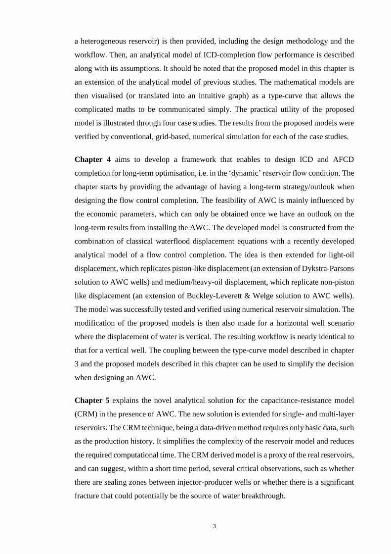
The major components of AWCs can be split into:
1) Flow control devices (FCD)
These devices allow on/off or variable control of production or injection of reservoir
intervals/layers. There are three types of FCDs: passive, control with inflow control
devices (ICDs), active control with inflow control valves (ICVs), and the recently
introduced autonomous flow control devices (AFCDs). Section 2.2 explains the
characteristics and operation principles of each device.
6
Figure 2-1. AWC main components for flow control
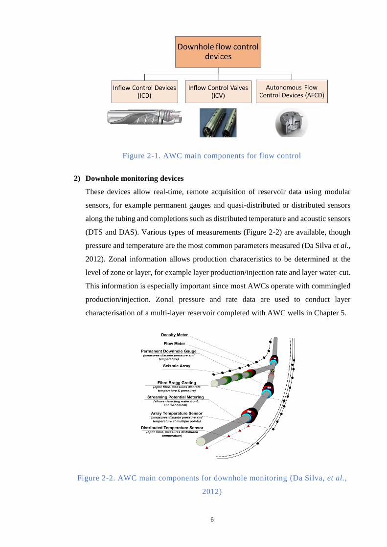
2) Downhole monitoring devices
These devices allow real-time, remote acquisition of reservoir data using modular
sensors, for example permanent gauges and quasi-distributed or distributed sensors
along the tubing and completions such as distributed temperature and acoustic sensors
(DTS and DAS). Various types of measurements (Figure 2-2) are available, though
pressure and temperature are the most common parameters measured (Da Silva et al.,
2012). Zonal information allows production characeristics to be determined at the
level of zone or layer, for example layer production/injection rate and layer water-cut.
This information is especially important since most AWCs operate with commingled
production/injection. Zonal pressure and rate data are used to conduct layer
characterisation of a multi-layer reservoir completed with AWC wells in Chapter 5.
Figure 2-2. AWC main components for downhole monitoring (Da Silva, et al.,
2012)

7
3) Annular flow isolation (AFI) devices
These devices isolate and prevent unwanted fluid flow in the annular space (annular
flow) between the tubing and the sand face or cemented/perforated casing. The design
of AFI is an important aspect since AWCs often encounter high annular flows rates
(Moradidowlatabad et al., 2014), for example, in commingled heterogeneous multi-
zones. Furthermore, the performance efficiency of FCD (ICDs, ICVs, and AFCDs)
are closely related to the compartmentalisation along the AWC’s zones. AFI can be
achieved by many types of packers (e.g. Figure 2-3) and by a gravel pack completion
in the case of sand-prone wells. Faisal Al-Khelaiwi (2013) detailed the various types
of packers used in AWCs. The completion design engineers have to determine the
optimum number and placement of packers. Studies for packer placement
optimisation have been conducted by Gavioli et al. (2012), Moradidowlatabad et al.
(2014), and Dowlatabad (2015). This thesis will assume that sufficient AFI is installed
to ensure negligible annular flow along the length of the wells.
Figure 2-3. Typical external casing packer (Gavioli et al., 2012)
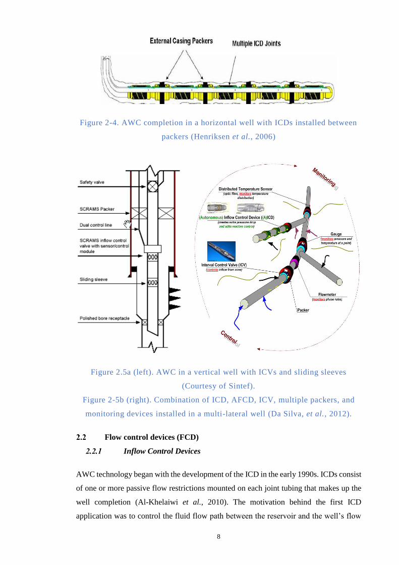
The design of an AWC is dependent on the specific well and geological environment.
Examples of an AWCs are an ICD completion in a horizontal well (Figure 2-4), an ICV
completion in a vertical well Figure 2.5a (left). AWC in a vertical well with ICVs and
sliding sleeves. Figure 2-5a, and a combination of multiple downhole control devices
installed in a multi-lateral well Figure 2.5a (left). AWC in a vertical well with ICVs and
sliding sleeves. Figure 2-5b. Further information on the applications of the AWCs can
be found in Faisal Al-Khelaiwi (2013).
8
Figure 2-4. AWC completion in a horizontal well with ICDs installed between
packers (Henriksen et al., 2006)
Figure 2.5a (left). AWC in a vertical well with ICVs and sliding sleeves
(Courtesy of Sintef).
Figure 2-5b (right). Combination of ICD, AFCD, ICV, multiple packers, and
monitoring devices installed in a multi-lateral well (Da Silva, et al., 2012).
Flow control devices (FCD)
Inflow Control Devices
AWC technology began with the development of the ICD in the early 1990s. ICDs consist
of one or more passive flow restrictions mounted on each joint tubing that makes up the
well completion (Al-Khelaiwi et al., 2010). The motivation behind the first ICD
application was to control the fluid flow path between the reservoir and the well’s flow
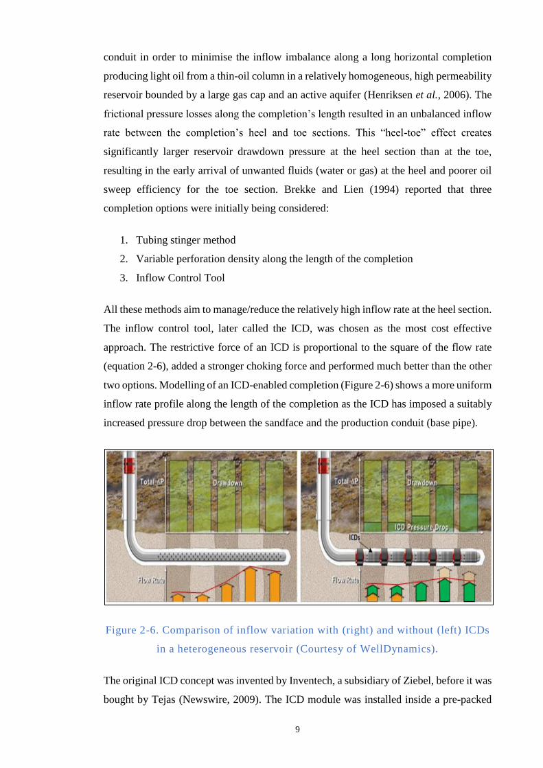
9
conduit in order to minimise the inflow imbalance along a long horizontal completion
producing light oil from a thin-oil column in a relatively homogeneous, high permeability
reservoir bounded by a large gas cap and an active aquifer (Henriksen et al., 2006). The
frictional pressure losses along the completion’s length resulted in an unbalanced inflow
rate between the completion’s heel and toe sections. This “heel-toe” effect creates
significantly larger reservoir drawdown pressure at the heel section than at the toe,
resulting in the early arrival of unwanted fluids (water or gas) at the heel and poorer oil
sweep efficiency for the toe section. Brekke and Lien (1994) reported that three
completion options were initially being considered:
1. Tubing stinger method
2. Variable perforation density along the length of the completion
3. Inflow Control Tool
All these methods aim to manage/reduce the relatively high inflow rate at the heel section.
The inflow control tool, later called the ICD, was chosen as the most cost effective
approach. The restrictive force of an ICD is proportional to the square of the flow rate
(equation 2-6), added a stronger choking force and performed much better than the other
two options. Modelling of an ICD-enabled completion (Figure 2-6) shows a more uniform
inflow rate profile along the length of the completion as the ICD has imposed a suitably
increased pressure drop between the sandface and the production conduit (base pipe).
Figure 2-6. Comparison of inflow variation with (right) and without (left) ICDs
in a heterogeneous reservoir (Courtesy of WellDynamics).
The original ICD concept was invented by Inventech, a subsidiary of Ziebel, before it was
bought by Tejas (Newswire, 2009). The ICD module was installed inside a pre-packed
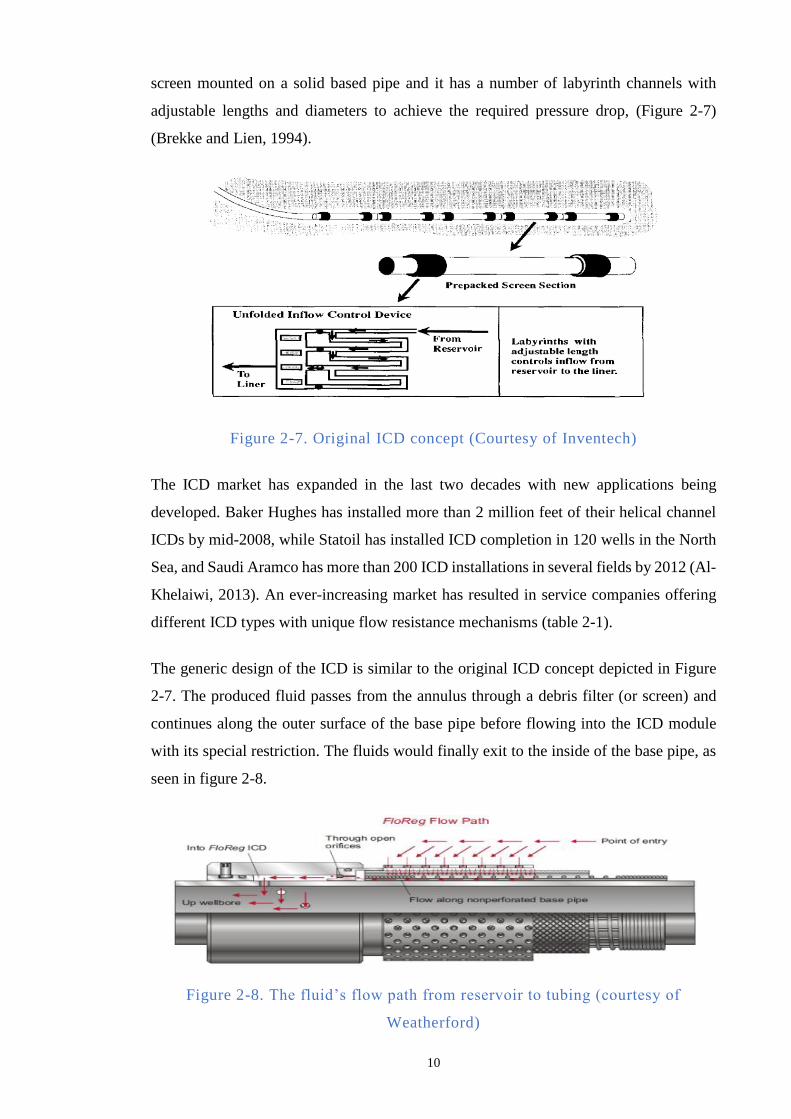
10
screen mounted on a solid based pipe and it has a number of labyrinth channels with
adjustable lengths and diameters to achieve the required pressure drop, (Figure 2-7)
(Brekke and Lien, 1994).
Figure 2-7. Original ICD concept (Courtesy of Inventech)
The ICD market has expanded in the last two decades with new applications being
developed. Baker Hughes has installed more than 2 million feet of their helical channel
ICDs by mid-2008, while Statoil has installed ICD completion in 120 wells in the North
Sea, and Saudi Aramco has more than 200 ICD installations in several fields by 2012 (Al-
Khelaiwi, 2013). An ever-increasing market has resulted in service companies offering
different ICD types with unique flow resistance mechanisms (table 2-1).
The generic design of the ICD is similar to the original ICD concept depicted in Figure
2-7. The produced fluid passes from the annulus through a debris filter (or screen) and
continues along the outer surface of the base pipe before flowing into the ICD module
with its special restriction. The fluids would finally exit to the inside of the base pipe, as
seen in figure 2-8.
Figure 2-8. The fluid’s flow path from reservoir to tubing (courtesy of
Weatherford)
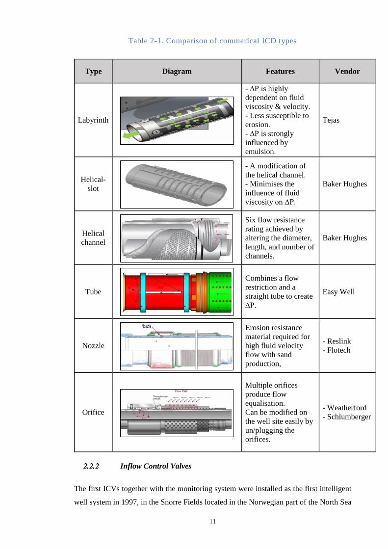
11
Table 2-1. Comparison of commerical ICD types
Type Diagram Features Vendor
Labyrinth
- ∆P is highly
dependent on fluid
viscosity & velocity.
- Less susceptible to
erosion.
- ∆P is strongly
influenced by
emulsion.
Tejas
Helical-
slot
- A modification of
the helical channel.
- Minimises the
influence of fluid
viscosity on ∆P.
Baker Hughes
Helical
channel
Six flow resistance
rating achieved by
altering the diameter,
length, and number of
channels.
Baker Hughes
Tube
Combines a flow
restriction and a
straight tube to create
∆P.
Easy Well
Nozzle
Erosion resistance
material required for
high fluid velocity
flow with sand
production,
- Reslink
- Flotech
Orifice
Multiple orifices
produce flow
equalisation.
Can be modified on
the well site easily by
un/plugging the
orifices.
- Weatherford
- Schlumberger
Inflow Control Valves
The first ICVs together with the monitoring system were installed as the first intelligent
well system in 1997, in the Snorre Fields located in the Norwegian part of the North Sea
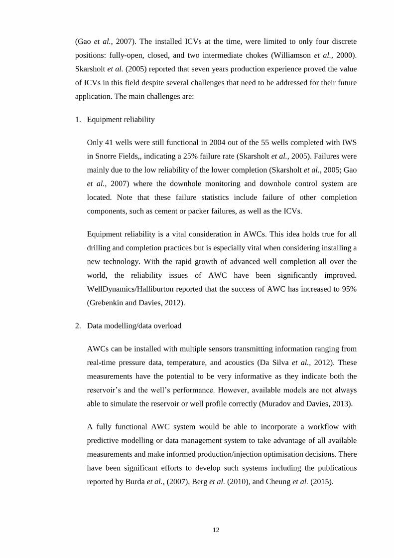
12
(Gao et al., 2007). The installed ICVs at the time, were limited to only four discrete
positions: fully-open, closed, and two intermediate chokes (Williamson et al., 2000).
Skarsholt et al. (2005) reported that seven years production experience proved the value
of ICVs in this field despite several challenges that need to be addressed for their future
application. The main challenges are:
1. Equipment reliability
Only 41 wells were still functional in 2004 out of the 55 wells completed with IWS
in Snorre Fields,, indicating a 25% failure rate (Skarsholt et al., 2005). Failures were
mainly due to the low reliability of the lower completion (Skarsholt et al., 2005; Gao
et al., 2007) where the downhole monitoring and downhole control system are
located. Note that these failure statistics include failure of other completion
components, such as cement or packer failures, as well as the ICVs.
Equipment reliability is a vital consideration in AWCs. This idea holds true for all
drilling and completion practices but is especially vital when considering installing a
new technology. With the rapid growth of advanced well completion all over the
world, the reliability issues of AWC have been significantly improved.
WellDynamics/Halliburton reported that the success of AWC has increased to 95%
(Grebenkin and Davies, 2012).
2. Data modelling/data overload
AWCs can be installed with multiple sensors transmitting information ranging from
real-time pressure data, temperature, and acoustics (Da Silva et al., 2012). These
measurements have the potential to be very informative as they indicate both the
reservoir’s and the well’s performance. However, available models are not always
able to simulate the reservoir or well profile correctly (Muradov and Davies, 2013).
A fully functional AWC system would be able to incorporate a workflow with
predictive modelling or data management system to take advantage of all available
measurements and make informed production/injection optimisation decisions. There
have been significant efforts to develop such systems including the publications
reported by Burda et al., (2007), Berg et al. (2010), and Cheung et al. (2015).

13
The first deployment of ICVs with only four-positions were considered inadequate to
cover all the desirable control positions (each position represents a different flow area
that is chosen based on desired flow rate and pressure drop). Since then, ICVs have been
developed, and now ICVs can be put into three categories based on control position (or
flow area) options. The complexity of the application became the criteria for choosing the
level of control flexibility for the ICV. ICV type 1 is the simplest while type 3 is the most
complex.
1. On/Off ICV. The ICV is either a fully-open or fully-closed.
2. Discrete ICV. The ICV has a limited number of positions (typically up to 10, including
the fully-open and fully-closed positions).
3. Infinitely Variable ICVs: Provides continuous control between the fully-open and
fully-closed positions.
Their control-line connects the downhole valve to the surface, and ICVs can also be
categorised based on how they are powered and controlled. Potiani, Eduardo, and Hughes
(2014) compared the hydraulics system, electric-hydraulics, and the all-electric system.
1. Hydraulic systems
The valves in ICV are actuated by a hydraulic line. This ICV type would require feed-
through packers and a feed-through wellhead for the hydraulics lines to go through.
Being the oldest, most widely used control system for downhole equipment, it has the
advantage of familiarity and reliability. However, each valve requires a dedicated
control line to operate. This system is constrained to wellhead feed-through capability
the maximum number of hydraulic lines that can be installed in a standard well is 5,
(Al-Khelaiwi et al., 2010). n+1 control lines are required for n valves. This would
limit the segments/zonation length of the completed interval and the ICV
performance. The summary of concerns are:
Installation depth of the ICV
Operating pressure of the ICV
Limited number of penetrations possible in subsea wellheads.
Control line fluid degradations/contamination
Control line damage when running through the Multi-Lateral (ML) junction
or the horizontal sections.
2. Electric-hydraulics systems (2 hydraulic lines, and 1 electrical cable)

14
This ICV type uses electrical measurement and transmission of data to the surface
while hydraulic power operates the valves. This reduces the number of control lines
(hydraulics and electrics) since two control lines can operate several valves. The
concerns for this ICV type is the same with those for type 1 ICVs.
3. All-electric systems
The developments in ICVs enabled a single electric downhole cable to control up to
20 valves. This type practically eliminates many of the concerns mentioned in other
ICV types. Potiani, Eduardo, and Hughes (2014) concluded that all-electric systems
are as reliable as the other two with some all-electric system have been still fully
functional 10 years after installations.
Autonomous flow control devices
The recently introduced autonomous inflow control device (AICD) and autonomous
inflow control valve (AICV) react to unwanted fluid phases, such as free gas and water,
by restricting the in-situ flow rate and hopefully improving oil recovery. For simplicity,
we will combine AICDs and AICVs as AFCDs where their distinction is not explicitly
required in this thesis. AFCDs are the latest versions of ICDs since they replace the
passive or fixed restriction with a self-adjusting restriction. This feature is advantageous
in a reservoir with high uncertainty, where the location of producing layers that will
experience early breakthrough is unknown.
The first reported installation of AFCD technology was in 2008, in Troll Field (Halvorsen,
et al., 2012). The AFCD was deployed to control gas production in a multi-lateral well.
The well had two laterals completed with different downhole control devices, lateral 1
was an ICD completion, and lateral 2 was an AFCD completion. These two laterals were
completed in similar geology and they were drilled parallel with a spacing of only 191
metres (fig. 2.9a and 2.9b), hence allowing a realistic, real-field comparison between ICD
and AFCD completion performance.
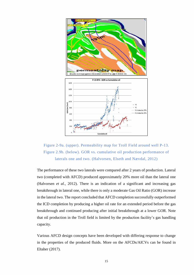
15
Figure 2-9a. (upper). Permeability map for Troll Field around well P-13.
Figure 2.9b. (below). GOR vs. cumulative oil production performance of
laterals one and two. (Halvorsen, Elseth and Nævdal, 2012)
The performance of these two laterals were compared after 2 years of production. Lateral
two (completed with AFCD) produced approximately 20% more oil than the lateral one
(Halvorsen et al., 2012). There is an indication of a significant and increasing gas
breakthrough in lateral one, while there is only a moderate Gas Oil Ratio (GOR) increase
in the lateral two. The report concluded that AFCD completion successfully outperformed
the ICD completion by producing a higher oil rate for an extended period before the gas
breakthrough and continued producing after initial breakthrough at a lower GOR. Note
that oil production in the Troll field is limited by the production facility’s gas handling
capacity.
Various AFCD design concepts have been developed with differing response to change
in the properties of the produced fluids. More on the AFCDs/AICVs can be found in
Eltaher (2017).

16
Modelling of Advanced Wells
Modelling of an AWC completion requires incorporation of the various components to
its completion system. These vary the pressure losses along the well completion; a
parameter that was considered constant in a standard well completion. The complexity is
exacerbated by the need of the new approach to also account for the connection between
the well components and reservoir grid, as well as capturing the essential physics of fluid
flow through the annulus and new FCDs.
In general an AWC consists of five, main flow paths. Eltaher (2017) illustrated the
production flow paths (Figure 2-10). Note that the flow path for an injector well will be
reversed.
1. Flow from the reservoir towards the well’s sandface
E.g. in the case of liquid flow there may be assumed a linear relationship between the
flow velocity and the pressure drop (Darcy’s law).
2. Flow along the annulus
Annular flow along the area between the tubing’s outer diameter and the formation
sandface (for AWCs completed in open-hole). Such modelling must account for the
friction and any turbulence flow along the annulus. The study in this thesis, however,
assumes perfect AFI, i.e. annular flow losses are sufficiently small that that do not
affect the findings in this thesis.
3. Flow across the FCD
Flow across the FCD is characterised by a flow regime within a non-linear
velocity/pressure drop relationship. Characterisation of the flow relationship of each
device is typically evaluated in flow- testing, with the results of flow rate versus
pressure drop performance data curves for single-phase oil, water, and occasionally
gas flow. The performance data is then expressed as a mathematical correlation or as
tables based on this empirical data.
4. Flow along the production tubing
The flowing wellbore pressure is generally defined as the pressure at the mid-point of
the completion interval. It is assumed to be constant over the entire interval. This
approach is no longer valid for many MRC well since pressure losses occur along the
wellbore length (due to friction, acceleration, hydrostatics, and phase changes).
Chapter 3 of this thesis discusses this topic in more detail.
5. Flow along the downstream completion
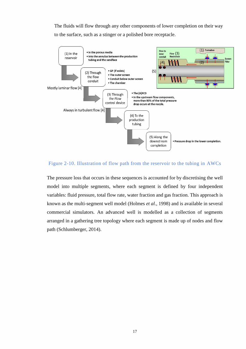
17
The fluids will flow through any other components of lower completion on their way
to the surface, such as a stinger or a polished bore receptacle.
Figure 2-10. Illustration of flow path from the reservoir to the tubing in AWCs
The pressure loss that occurs in these sequences is accounted for by discretising the well
model into multiple segments, where each segment is defined by four independent
variables: fluid pressure, total flow rate, water fraction and gas fraction. This approach is
known as the multi-segment well model (Holmes et al., 1998) and is available in several
commercial simulators. An advanced well is modelled as a collection of segments
arranged in a gathering tree topology where each segment is made up of nodes and flow
path (Schlumberger, 2014).
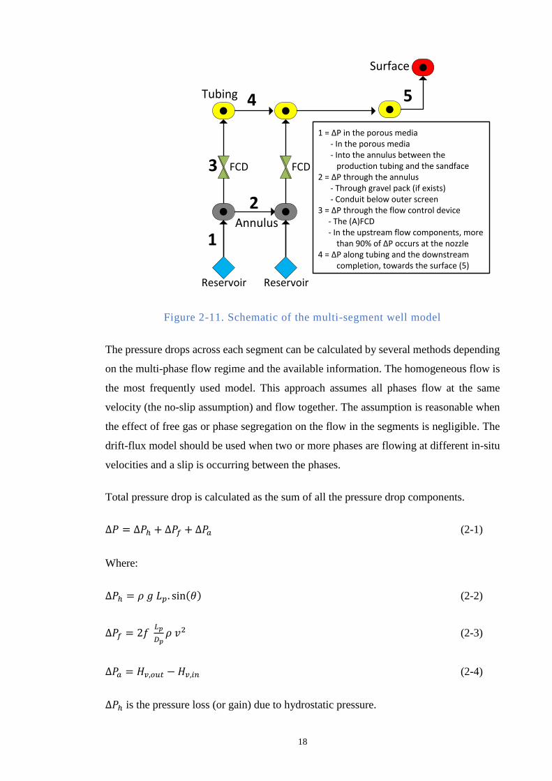
18
Reservoir
FCD
Annulus
Tubing
1
3
2
4
Reservoir
FCD
5
1 = ∆P in the porous media - In the porous media - Into the annulus between the
production tubing and the sandface2 = ∆P through the annulus - Through gravel pack (if exists) - Conduit below outer screen 3 = ∆P through the flow control device - The (A)FCD - In the upstream flow components, more
than 90% of ∆P occurs at the nozzle4 = ∆P along tubing and the downstream
completion, towards the surface (5)
Surface
Figure 2-11. Schematic of the multi-segment well model
The pressure drops across each segment can be calculated by several methods depending
on the multi-phase flow regime and the available information. The homogeneous flow is
the most frequently used model. This approach assumes all phases flow at the same
velocity (the no-slip assumption) and flow together. The assumption is reasonable when
the effect of free gas or phase segregation on the flow in the segments is negligible. The
drift-flux model should be used when two or more phases are flowing at different in-situ
velocities and a slip is occurring between the phases.
Total pressure drop is calculated as the sum of all the pressure drop components.
∆𝑃 = ∆𝑃ℎ + ∆𝑃𝑓 + ∆𝑃𝑎 (2-1)
Where:
∆𝑃ℎ = 𝜌 𝑔 𝐿𝑝. sin(𝜃) (2-2)
∆𝑃𝑓 = 2𝑓 𝐿𝑝
𝐷𝑝𝜌 𝑣2 (2-3)
∆𝑃𝑎 = 𝐻𝑣,𝑜𝑢𝑡 − 𝐻𝑣,𝑖𝑛 (2-4)
∆𝑃ℎ is the pressure loss (or gain) due to hydrostatic pressure.
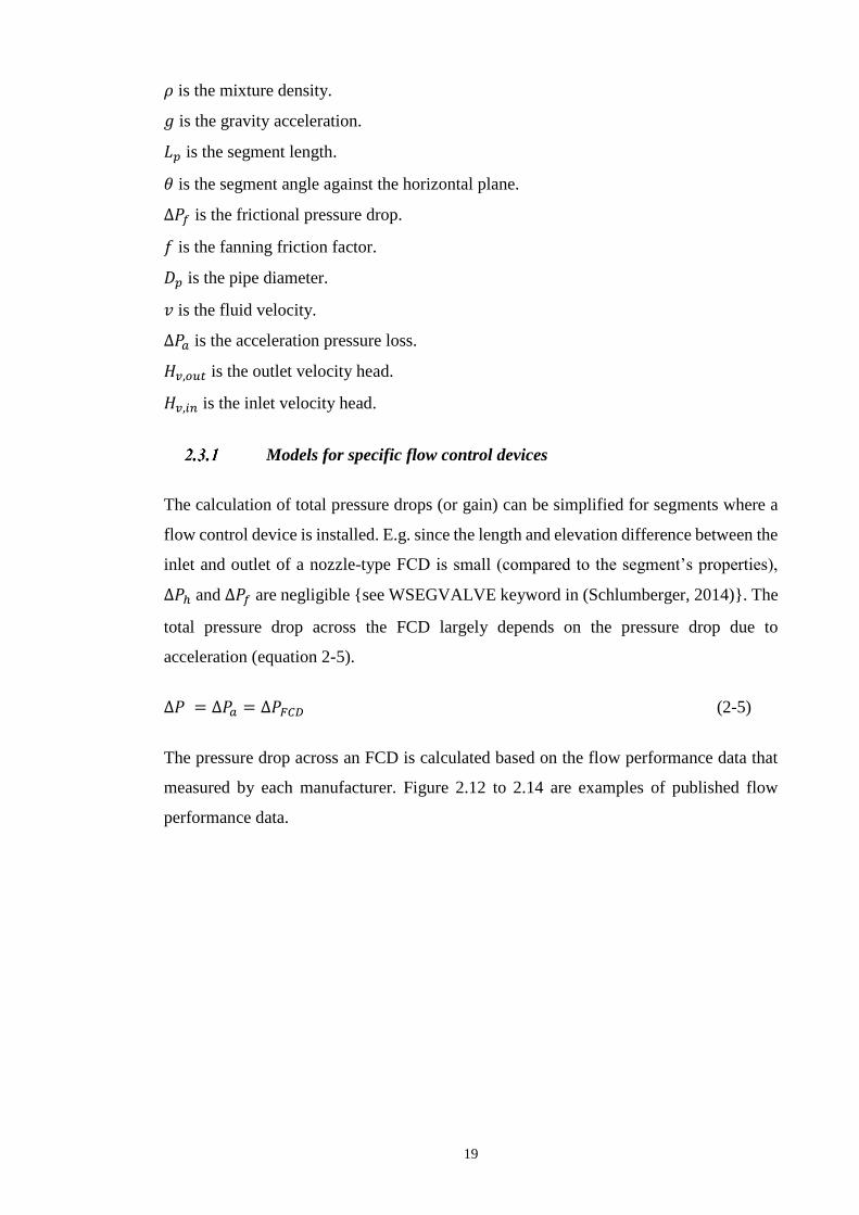
19
𝜌 is the mixture density.
𝑔 is the gravity acceleration.
𝐿𝑝 is the segment length.
𝜃 is the segment angle against the horizontal plane.
∆𝑃𝑓 is the frictional pressure drop.
𝑓 is the fanning friction factor.
𝐷𝑝 is the pipe diameter.
𝑣 is the fluid velocity.
∆𝑃𝑎 is the acceleration pressure loss.
𝐻𝑣,𝑜𝑢𝑡 is the outlet velocity head.
𝐻𝑣,𝑖𝑛 is the inlet velocity head.
Models for specific flow control devices
The calculation of total pressure drops (or gain) can be simplified for segments where a
flow control device is installed. E.g. since the length and elevation difference between the
inlet and outlet of a nozzle-type FCD is small (compared to the segment’s properties),
∆𝑃ℎ and ∆𝑃𝑓 are negligible see WSEGVALVE keyword in (Schlumberger, 2014). The
total pressure drop across the FCD largely depends on the pressure drop due to
acceleration (equation 2-5).
∆𝑃 = ∆𝑃𝑎 = ∆𝑃𝐹𝐶𝐷 (2-5)
The pressure drop across an FCD is calculated based on the flow performance data that
measured by each manufacturer. Figure 2.12 to 2.14 are examples of published flow
performance data.
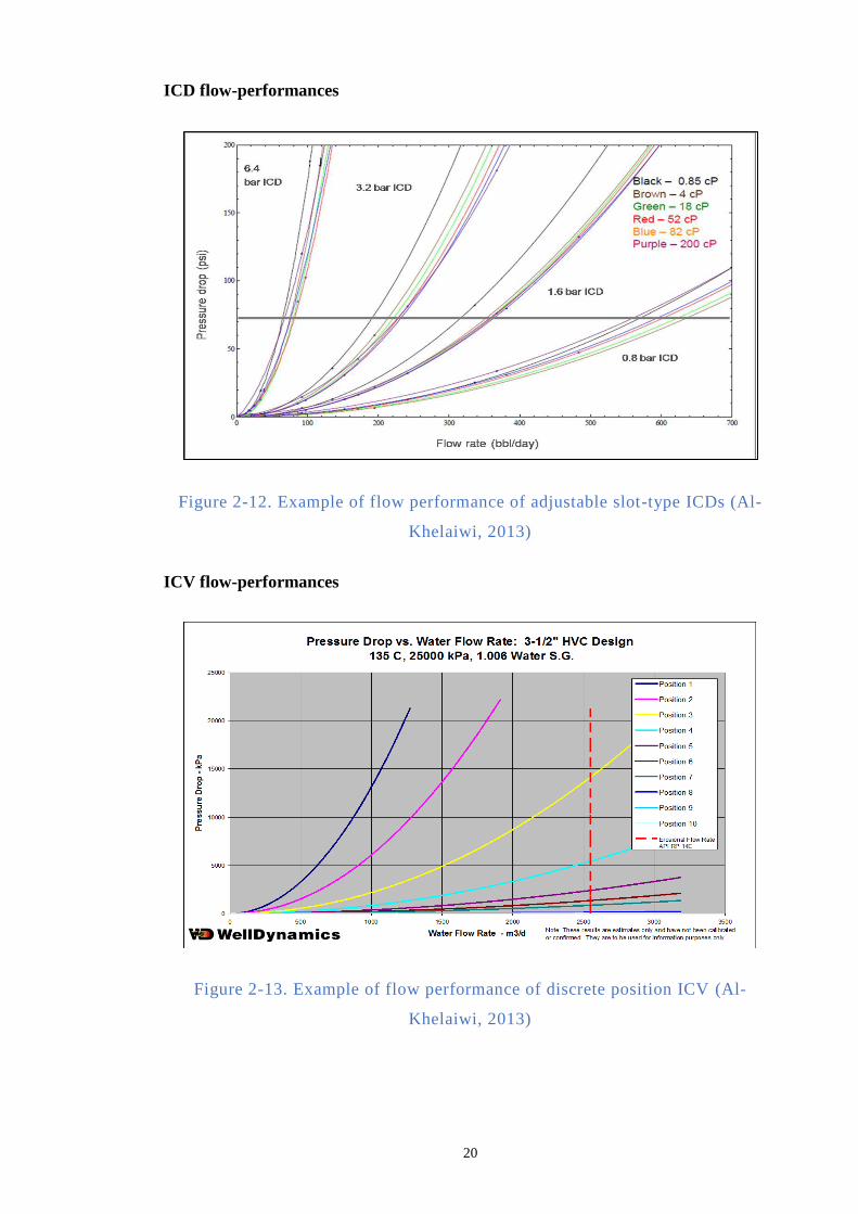
20
ICD flow-performances
Figure 2-12. Example of flow performance of adjustable slot-type ICDs (Al-
Khelaiwi, 2013)
ICV flow-performances
Figure 2-13. Example of flow performance of discrete position ICV (Al-
Khelaiwi, 2013)
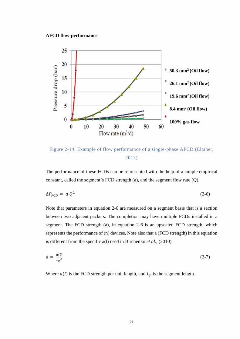
21
AFCD flow-performance
Figure 2-14. Example of flow performance of a single-phase AFCD (Eltaher,
2017)
The performance of these FCDs can be represented with the help of a simple empirical
constant, called the segment’s FCD strength (a), and the segment flow rate (Q).
∆𝑃𝐹𝐶𝐷 = 𝑎 𝑄2 (2-6)
Note that parameters in equation 2-6 are measured on a segment basis that is a section
between two adjacent packers. The completion may have multiple FCDs installed in a
segment. The FCD strength (a), in equation 2-6 is an upscaled FCD strength, which
represents the performance of (n) devices. Note also that a (FCD strength) in this equation
is different from the specific a(l) used in Birchenko et al., (2010).
𝑎 = 𝑎(𝑙)
𝐿𝑝2 (2-7)
Where 𝑎(𝑙) is the FCD strength per unit length, and 𝐿𝑝 is the segment length.
50.3 mm2 (Oil flow)
26.1 mm2 (Oil flow)
19.6 mm2 (Oil flow)
8.4 mm2 (Oil flow)
100% gas flow
22
The way this generated pressure drop is independent on the device’s manufacturer:
1) ICD
a. An ICD that uses frictional pressure drop developed by flow through one or
more small conduits. The restriction strength can be calculated from
Poiseuille’s law (equation 2-8) to describe the (frictional) performance of this
type of ICD. Examples are: the helical channel design that uses one or more
flow channels wrapped around a base pipe and the labyrinth design using a
tortuous pathway to impose abrupt alterations in the fluid’s flow direction.
Unfortunately, this type of ICD, being relatively viscosity dependent,
encourages (less viscous) water production after water breakthrough.
𝑎 = 𝐶𝑢𝜌𝐵
2
𝐶𝑑2𝑑4
(2-8)
b. An ICD that works as a local restriction. Strength derived from Bernoulli’s
law (equation 2-9) estimates the pressure loss across the nozzles and orifices
of this type of ICD restriction, though the design does make it more sensitive
to abrasion and plugging.
𝑎 =(𝜌𝑐𝑎𝑙 𝜇)
(𝜌 𝜇𝑐𝑎𝑙)
1
4 𝜌
𝜌𝑐𝑎𝑙𝐵2 𝑎𝑐ℎ𝑎𝑛𝑛𝑒𝑙 (2-9)
Where a is the restriction strength of a single ICD device, 𝜌𝑐𝑎𝑙 is the density
of the calibration fluids, 𝜌 is the density of mixed fluids, 𝜇𝑐𝑎𝑙 is the viscosity
of the calibration fluids, 𝜇 is the viscosity of mixed fluids. B is the formation
volume factor, 𝑎𝑐ℎ𝑎𝑛𝑛𝑒𝑙 is the channel ICD strength, d is the ICD nozzle
diameter, 𝐶𝑑 is the discharge coefficient for the nozzle or orifice, and 𝐶𝑢 is a
unit conversion factors: 8/π2 for SI units, 1.0858.10−15 for metric units, and
7.3668.10−13 in field units.
2) AFCD
AFCD adds an extra restriction to the flow of unwanted fluids by autonomously
reacting when there is an unwanted change in fluid properties by altering the flow
geometry within the device. The AICD/AICV performance (Figure 2-14) is described
separately for single-phase oil flow and for single-phase water or gas flow since the
23
performance curves differ significantly. However, in both cases their single-phase
flow performance can be acceptably matched by equation 2-10. The AICD/AICV
multiphase flow performance is difficult to model accurately and frequently only
single-phase flow performance data is available. Modelling techniques for AFCDs
are thoroughly discussed in Eltaher (2017). Commercial reservoir simulators
(Halliburton, 2012; Schlumberger, 2014) use the empirically fitted equations
formulated by Halvorsen et al., 2012; Mathiesen et al., 2014:
𝑎 = (𝜌𝑚𝑖𝑥2
𝜌𝑐𝑎𝑙) (
µ𝑐𝑎𝑙
µ𝑚𝑖𝑥)𝑦
𝑎𝑎𝑖𝑐𝑑 (2-10)
𝜌𝑐𝑎𝑙 is the density of the calibration fluids, 𝜌mix is the density of mixed fluids, 𝜇𝑐𝑎𝑙 is
the viscosity of the calibration fluids, 𝜇mix is the viscosity of mixed fluids. aaicd is the
device strength parameter, and y is a fitting input constant.
3) ICV
Flow through the ICV is sub-critical for most ICV applications. It can be modelled
using a simpler version of surface chokes flow performance, where flow through the
ICV is sub-critical. Commercial simulators (Halliburton, 2012; Schlumberger, 2014)
model the choke strength of ICV (Figure 2-13) as :
𝑎 = 8𝐶𝑢𝜌𝑚𝑖𝑥
𝜋𝐶𝑑2𝑑𝑉
4 (2-11)
Cu is a unit conversion factors: 8/π2 for SI units, 1.0858.10−15 for metric units, and
7.3668. 10−13 in field units, ρmix is the density of mixed fluids, Cd is a
(dimensionless) discharge coefficient based on the valve position, and dV is the ICV
restriction diameter.
Problems with MRC wells reduced by ICD and AFCD installation
Ongoing improvements in drilling technology have maximised the reservoir contact with
horizontal well designs becoming more sophisticated (multi-lateral, snake-wells). An
MRC well, with higher productivity index, enables a lower drawdown to achieve the
target production rate compared to a conventional well. However, greater reservoir
contact results in higher inflow variation for more heterogeneous reservoirs encountered
along the length of the completion (Figure 2-15 and Figure 2-16). The details of the
magnitude of the observed changes in hydrocarbon saturation, formation permeability,
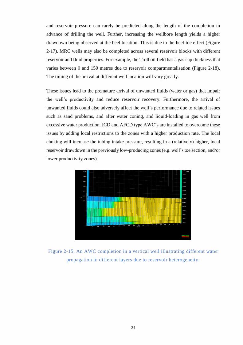
24
and reservoir pressure can rarely be predicted along the length of the completion in
advance of drilling the well. Further, increasing the wellbore length yields a higher
drawdown being observed at the heel location. This is due to the heel-toe effect (Figure
2-17). MRC wells may also be completed across several reservoir blocks with different
reservoir and fluid properties. For example, the Troll oil field has a gas cap thickness that
varies between 0 and 150 metres due to reservoir compartmentalisation (Figure 2-18).
The timing of the arrival at different well location will vary greatly.
These issues lead to the premature arrival of unwanted fluids (water or gas) that impair
the well’s productivity and reduce reservoir recovery. Furthermore, the arrival of
unwanted fluids could also adversely affect the well’s performance due to related issues
such as sand problems, and after water coning, and liquid-loading in gas well from
excessive water production. ICD and AFCD type AWC’s are installed to overcome these
issues by adding local restrictions to the zones with a higher production rate. The local
choking will increase the tubing intake pressure, resulting in a (relatively) higher, local
reservoir drawdown in the previously low-producing zones (e.g. well’s toe section, and/or
lower productivity zones).
Figure 2-15. An AWC completion in a vertical well illustrating different water
propagation in different layers due to reservoir heterogeneity.
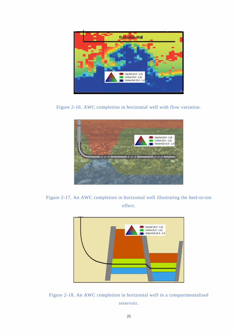
25
Figure 2-16. AWC completion in horizontal well with flow variation.
Figure 2-17. An AWC completion in horizontal well illustrating the heel-to-toe
effect.
Figure 2-18. An AWC completion in horizontal well in a compartmentalised
reservoir.
Green color is oil
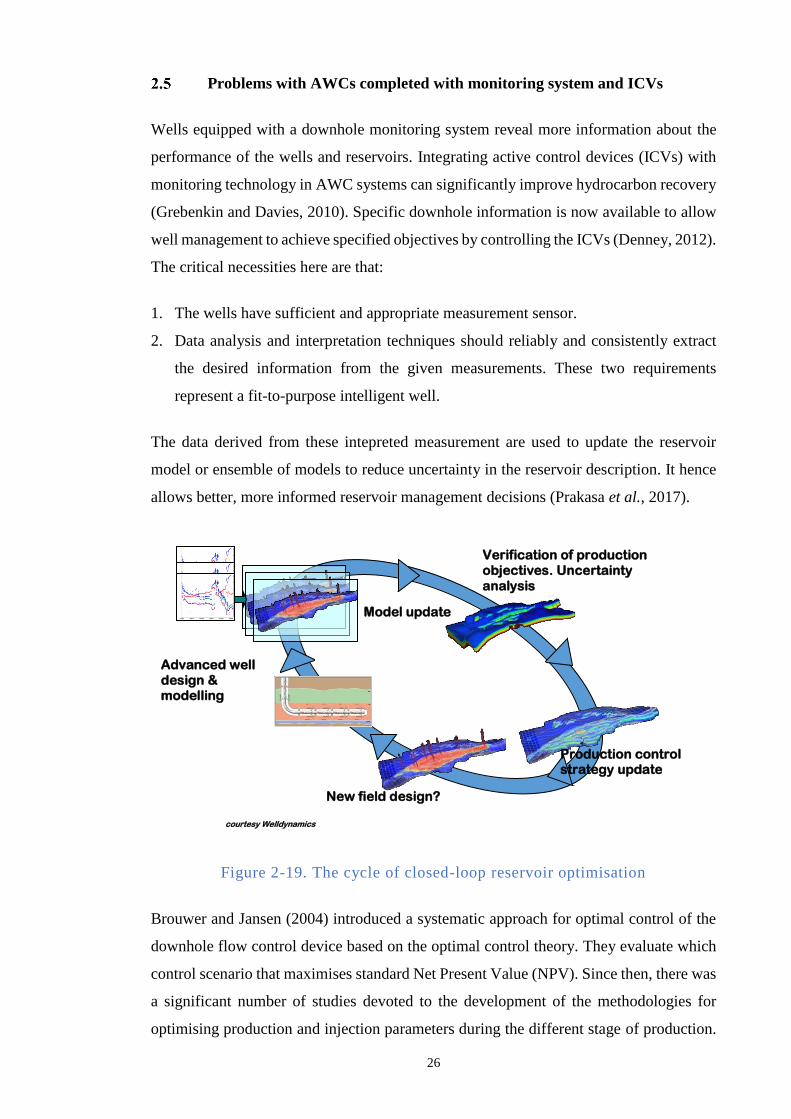
26
Problems with AWCs completed with monitoring system and ICVs
Wells equipped with a downhole monitoring system reveal more information about the
performance of the wells and reservoirs. Integrating active control devices (ICVs) with
monitoring technology in AWC systems can significantly improve hydrocarbon recovery
(Grebenkin and Davies, 2010). Specific downhole information is now available to allow
well management to achieve specified objectives by controlling the ICVs (Denney, 2012).
The critical necessities here are that:
1. The wells have sufficient and appropriate measurement sensor.
2. Data analysis and interpretation techniques should reliably and consistently extract
the desired information from the given measurements. These two requirements
represent a fit-to-purpose intelligent well.
The data derived from these intepreted measurement are used to update the reservoir
model or ensemble of models to reduce uncertainty in the reservoir description. It hence
allows better, more informed reservoir management decisions (Prakasa et al., 2017).
Figure 2-19. The cycle of closed-loop reservoir optimisation
Brouwer and Jansen (2004) introduced a systematic approach for optimal control of the
downhole flow control device based on the optimal control theory. They evaluate which
control scenario that maximises standard Net Present Value (NPV). Since then, there was
a significant number of studies devoted to the development of the methodologies for
optimising production and injection parameters during the different stage of production.
Verification of production objectives. Uncertainty analysis
New field design?
Model update
Production control strategy update
Advanced well design & modelling
courtesy Welldynamics
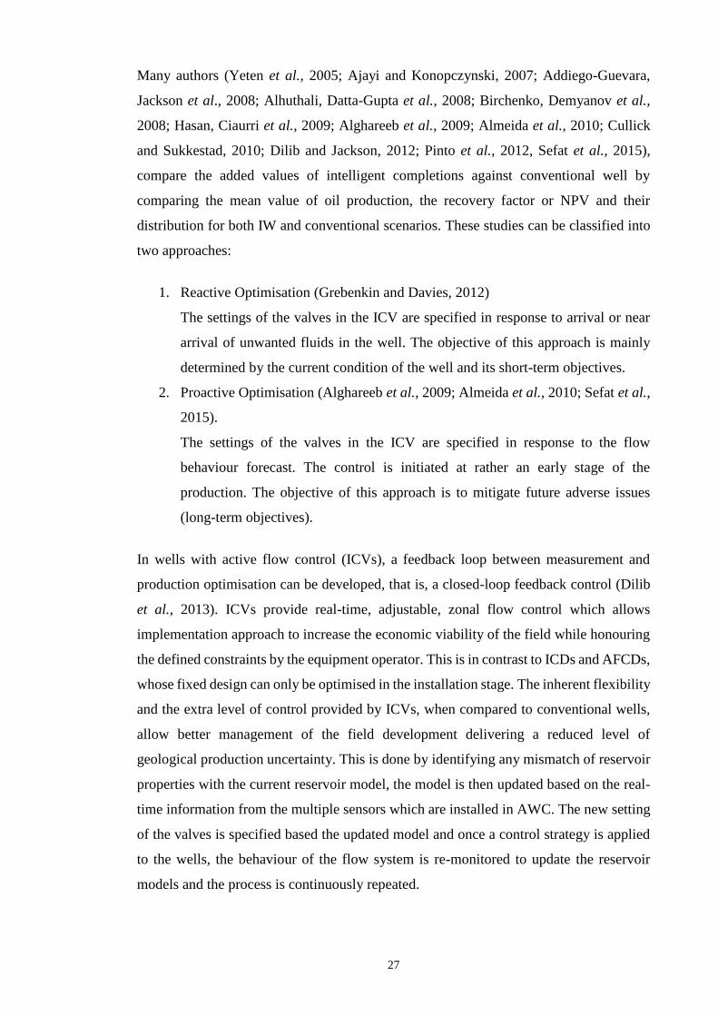
27
Many authors (Yeten et al., 2005; Ajayi and Konopczynski, 2007; Addiego-Guevara,
Jackson et al., 2008; Alhuthali, Datta-Gupta et al., 2008; Birchenko, Demyanov et al.,
2008; Hasan, Ciaurri et al., 2009; Alghareeb et al., 2009; Almeida et al., 2010; Cullick
and Sukkestad, 2010; Dilib and Jackson, 2012; Pinto et al., 2012, Sefat et al., 2015),
compare the added values of intelligent completions against conventional well by
comparing the mean value of oil production, the recovery factor or NPV and their
distribution for both IW and conventional scenarios. These studies can be classified into
two approaches:
1. Reactive Optimisation (Grebenkin and Davies, 2012)
The settings of the valves in the ICV are specified in response to arrival or near
arrival of unwanted fluids in the well. The objective of this approach is mainly
determined by the current condition of the well and its short-term objectives.
2. Proactive Optimisation (Alghareeb et al., 2009; Almeida et al., 2010; Sefat et al.,
2015).
The settings of the valves in the ICV are specified in response to the flow
behaviour forecast. The control is initiated at rather an early stage of the
production. The objective of this approach is to mitigate future adverse issues
(long-term objectives).
In wells with active flow control (ICVs), a feedback loop between measurement and
production optimisation can be developed, that is, a closed-loop feedback control (Dilib
et al., 2013). ICVs provide real-time, adjustable, zonal flow control which allows
implementation approach to increase the economic viability of the field while honouring
the defined constraints by the equipment operator. This is in contrast to ICDs and AFCDs,
whose fixed design can only be optimised in the installation stage. The inherent flexibility
and the extra level of control provided by ICVs, when compared to conventional wells,
allow better management of the field development delivering a reduced level of
geological production uncertainty. This is done by identifying any mismatch of reservoir
properties with the current reservoir model, the model is then updated based on the real-
time information from the multiple sensors which are installed in AWC. The new setting
of the valves is specified based the updated model and once a control strategy is applied
to the wells, the behaviour of the flow system is re-monitored to update the reservoir
models and the process is continuously repeated.
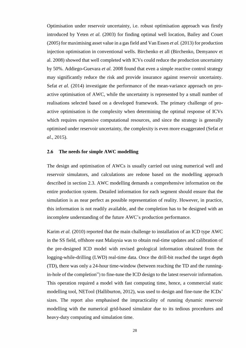
28
Optimisation under reservoir uncertainty, i.e. robust optimisation approach was firstly
introduced by Yeten et al. (2003) for finding optimal well location, Bailey and Couet
(2005) for maximising asset value in a gas field and Van Essen et al. (2013) for production
injection optimisation in conventional wells. Birchenko et all (Birchenko, Demyanov et
al. 2008) showed that well completed with ICVs could reduce the production uncertainty
by 50%. Addiego-Guevara et al. 2008 found that even a simple reactive control strategy
may significantly reduce the risk and provide insurance against reservoir uncertainty.
Sefat et al. (2014) investigate the performance of the mean-variance approach on pro-
active optimisation of AWC, while the uncertainty is represented by a small number of
realisations selected based on a developed framework. The primary challenge of pro-
active optimisation is the complexity when determining the optimal response of ICVs
which requires expensive computational resources, and since the strategy is generally
optimised under reservoir uncertainty, the complexity is even more exaggerated (Sefat et
al., 2015).
The needs for simple AWC modelling
The design and optimisation of AWCs is usually carried out using numerical well and
reservoir simulators, and calculations are redone based on the modelling approach
described in section 2.3. AWC modelling demands a comprehensive information on the
entire production system. Detailed information for each segment should ensure that the
simulation is as near perfect as possible representation of reality. However, in practice,
this information is not readily available, and the completion has to be designed with an
incomplete understanding of the future AWC’s production performance.
Karim et al. (2010) reported that the main challenge to installation of an ICD type AWC
in the SS field, offshore east Malaysia was to obtain real-time updates and calibration of
the pre-designed ICD model with revised geological information obtained from the
logging-while-drilling (LWD) real-time data. Once the drill-bit reached the target depth
(TD), there was only a 24-hour time-window (between reaching the TD and the running-
in-hole of the completion”) to fine-tune the ICD design to the latest reservoir information.
This operation required a model with fast computing time, hence, a commercial static
modelling tool, NETool (Halliburton, 2012), was used to design and fine-tune the ICDs’
sizes. The report also emphasised the impracticality of running dynamic reservoir
modelling with the numerical grid-based simulator due to its tedious procedures and
heavy-duty computing and simulation time.

29
NETool is the most widely used simulator when designing an AWC completion. It is a
static modelling tool that allows quick multiple sensitivities of various parameters. This
platform, however, still requires the output of a reservoir simulator to provide a snapshot
of the reservoir performance, where the completion is designed. When the latest
information from the open-hole log’s latest information is used to update the accurate
workflow (with revised reservoir properties) and run a new base-case dynamic numerical
reservoir simulator before engineers run any sensitivities in NETool. This sequence is the
ideal standard practice. However, it is often not followed due to operational constraints
(Karim et al., 2010), resulting in the design of the FCD completion not being based on
the latest information.
The challenge when designing AWCs is to find the right balance (or trade-off) between
well productivity loss (due to added restrictions) and improved added values, obtained by
re-distributing/balancing the flow variation (Birchenko et al., 2011; Al-Khelaiwi, 2013).
The static modelling tool, being very simple, is only able to capture the short-term added
value of the candidate well’s inflow performance immediately after installing the AWC
completion based on a “snapshot” in time of the well’s performance. Such short-term
evaluation, being simple and intuitive; has been widely used by production and
completion engineers. However, it cannot capture future reservoir behaviour and ultimate
project economics of such a completion. The long-term evaluation task is appropriate for
a grid-based numerical simulator. However, using this approach is labour intensive and
requires extensive reservoir simulation skills.
The computational power available to solve complex numerical simulations has increased
over the years. However, the industry still lacks a model that has the capability to evaluate
AWC performance in various scenarios (short-term and long-term evaluations) without
adding too much complexity. Therefore, a simple analytical design tool capturing the
important physics of the wellbore and reservoir will allow engineers to perform
(Birchenko et al., 2011):
Quick assessments of the AWC’s performance (screening AWC candidates).
Verification of numerical simulation results.
Communicating best practice in a non-product specific manner.
Moreover, due to with the uncertainty inherent in the many assumptions made for the
geological, petrophysical, and fluid properties, the results of detailed full-physics
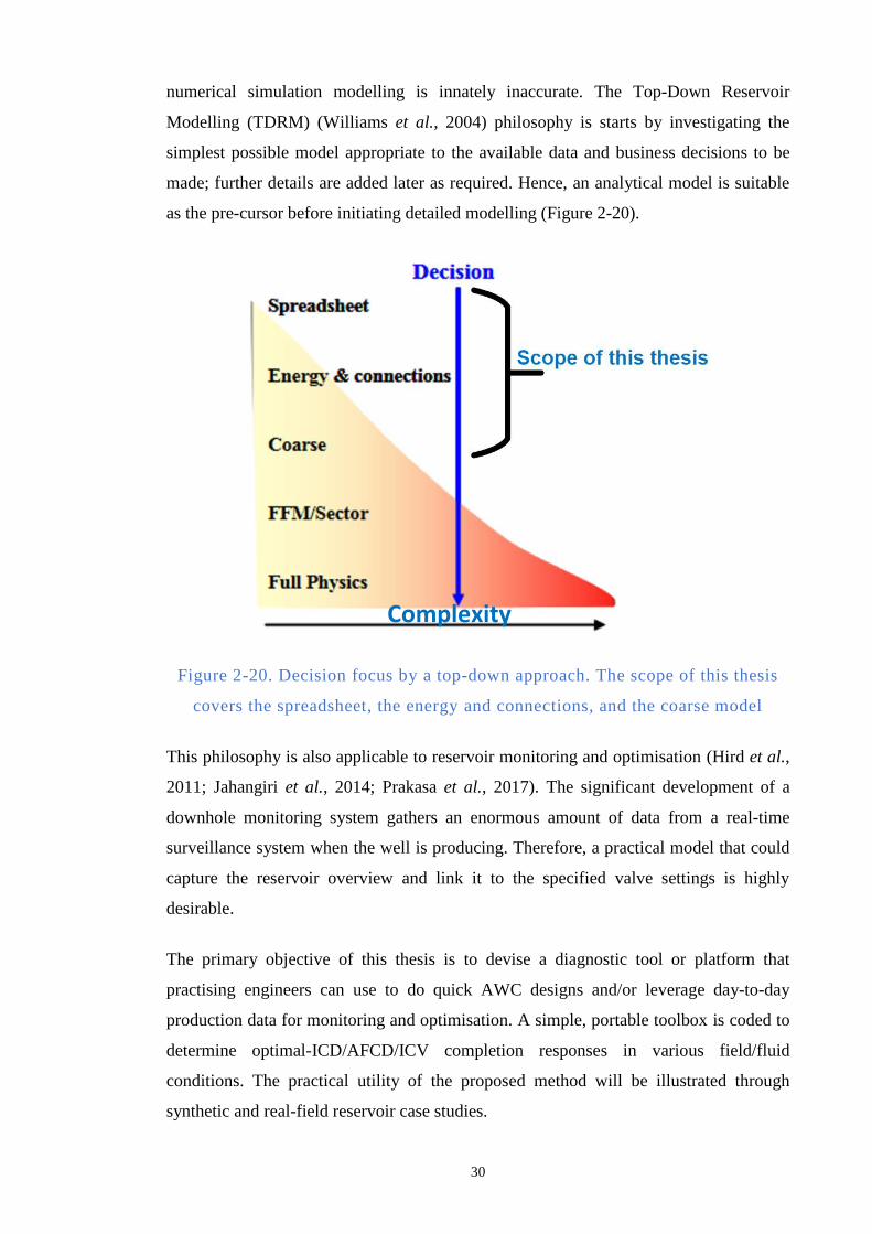
30
numerical simulation modelling is innately inaccurate. The Top-Down Reservoir
Modelling (TDRM) (Williams et al., 2004) philosophy is starts by investigating the
simplest possible model appropriate to the available data and business decisions to be
made; further details are added later as required. Hence, an analytical model is suitable
as the pre-cursor before initiating detailed modelling (Figure 2-20).
Figure 2-20. Decision focus by a top-down approach. The scope of this thesis
covers the spreadsheet, the energy and connections, and the coarse model
This philosophy is also applicable to reservoir monitoring and optimisation (Hird et al.,
2011; Jahangiri et al., 2014; Prakasa et al., 2017). The significant development of a
downhole monitoring system gathers an enormous amount of data from a real-time
surveillance system when the well is producing. Therefore, a practical model that could
capture the reservoir overview and link it to the specified valve settings is highly
desirable.
The primary objective of this thesis is to devise a diagnostic tool or platform that
practising engineers can use to do quick AWC designs and/or leverage day-to-day
production data for monitoring and optimisation. A simple, portable toolbox is coded to
determine optimal-ICD/AFCD/ICV completion responses in various field/fluid
conditions. The practical utility of the proposed method will be illustrated through
synthetic and real-field reservoir case studies.
Complexity
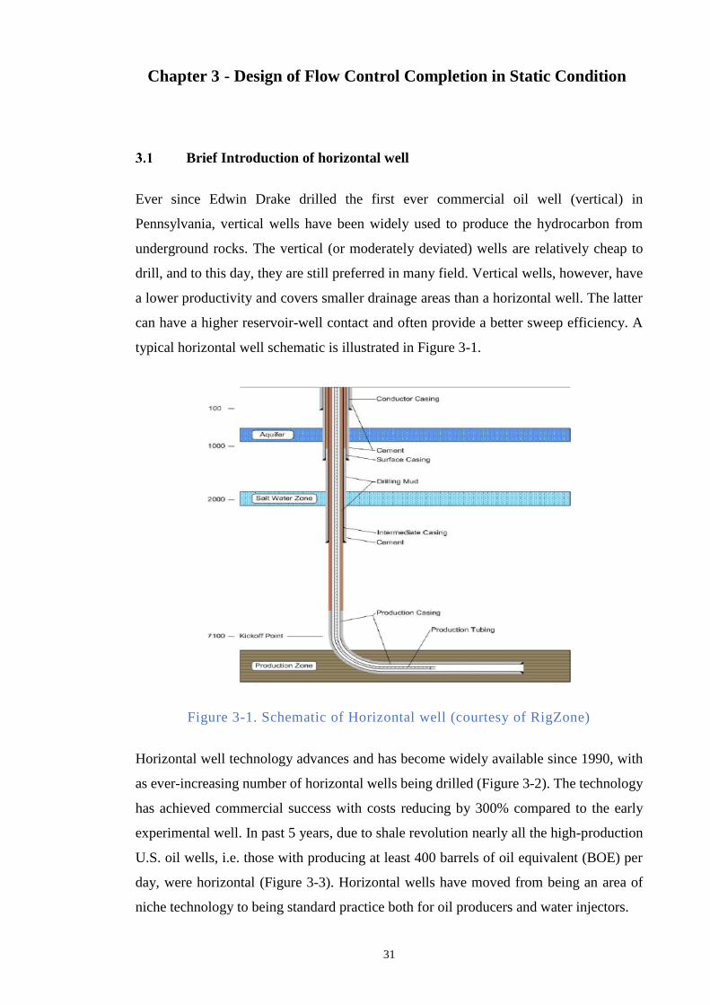
31
Chapter 3 - Design of Flow Control Completion in Static Condition
Brief Introduction of horizontal well
Ever since Edwin Drake drilled the first ever commercial oil well (vertical) in
Pennsylvania, vertical wells have been widely used to produce the hydrocarbon from
underground rocks. The vertical (or moderately deviated) wells are relatively cheap to
drill, and to this day, they are still preferred in many field. Vertical wells, however, have
a lower productivity and covers smaller drainage areas than a horizontal well. The latter
can have a higher reservoir-well contact and often provide a better sweep efficiency. A
typical horizontal well schematic is illustrated in Figure 3-1.
Figure 3-1. Schematic of Horizontal well (courtesy of RigZone)
Horizontal well technology advances and has become widely available since 1990, with
as ever-increasing number of horizontal wells being drilled (Figure 3-2). The technology
has achieved commercial success with costs reducing by 300% compared to the early
experimental well. In past 5 years, due to shale revolution nearly all the high-production
U.S. oil wells, i.e. those with producing at least 400 barrels of oil equivalent (BOE) per
day, were horizontal (Figure 3-3). Horizontal wells have moved from being an area of
niche technology to being standard practice both for oil producers and water injectors.
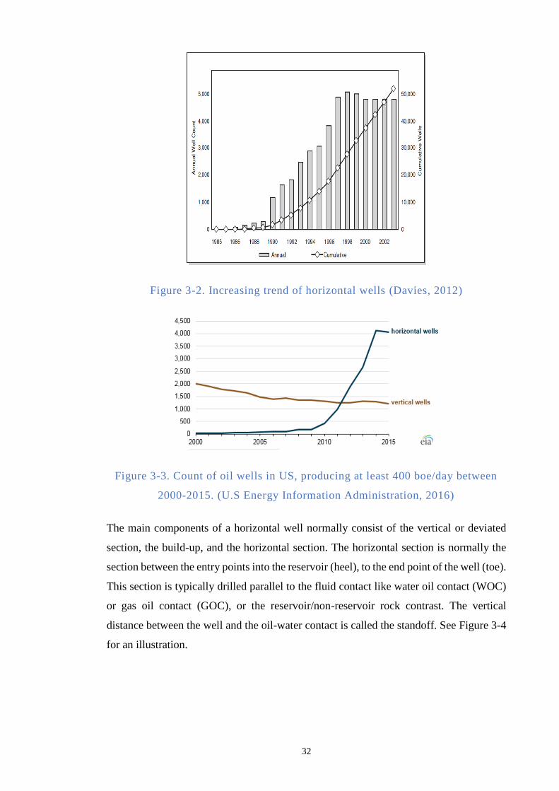
32
Figure 3-2. Increasing trend of horizontal wells (Davies, 2012)
Figure 3-3. Count of oil wells in US, producing at least 400 boe/day between
2000-2015. (U.S Energy Information Administration, 2016)
The main components of a horizontal well normally consist of the vertical or deviated
section, the build-up, and the horizontal section. The horizontal section is normally the
section between the entry points into the reservoir (heel), to the end point of the well (toe).
This section is typically drilled parallel to the fluid contact like water oil contact (WOC)
or gas oil contact (GOC), or the reservoir/non-reservoir rock contrast. The vertical
distance between the well and the oil-water contact is called the standoff. See Figure 3-4
for an illustration.

33
Figure 3-4. Horizontal well nomenclature (Davies, 2012)
Many operators may now drill wells with more than 6,000 ft of horizontal section. One
of the longest horizontal section ever recorded, measuring 35,770 ft. MDRT was
completed in May 2008 by Maersk Oil and Qatar Petroleum. The longest total horizontal
well was measuring 15,000-m, drilled by ExxonMobil in November 2017 in the Sea of
Okhotsk.
This work investigates the impact of flow control completions on horizontal well
performance, so at first, we will dedicate several sections to generally describing the
horizontal well technology and its widespread modelling routines. We will also briefly
cover the well and reservoir flow description concepts and statistical terms as they will
be used in our novel methods described later.
Development of Horizontal Wells Modelling
The initial studies (Borisov, 1984; Giger, 1984; Joshi, 1988; Renard et al., 1991) derived
different mathematical solutions, depending on the boundary conditions (Table 3-1), to
calculate the well Productivity Index (PI) or J (terms used by production engineers and
reservoir engineers respectively). This parameter is a commonly measured well property,
defining the well potential or the ability to produce per given drawdown pressure.
34
𝐽 =𝑄𝑤
(𝑃𝑎𝑣𝑔−𝑃𝑤𝑓) (3-1)
Where Q is the hydrocarbon Production rate at standard conditions, Pavg is the average
reservoir pressure (sometimes can be Pe or external pressure) and Pwf is the bottom-hole
flowing pressure.
Drilling a horizontal well is significantly costlier than drilling a conventional vertical
well. On top of that, a horizontal well is technically more challenging and prone to
potential drilling failures. All this prompts the question: What is the benefit of drilling
such well?
There are various parameters used to justify drilling a horizontal well. The most
informative way, according to (Levitan et al., 2001) is to evaluate the performance of a
well with the Productivity Improvement Factor (PIF) or the ratio of horizontal well’s PI
to vertical well’s PI, equation 3-2
𝑃𝐼𝐹 =𝐽𝐻
𝐽𝑉 (3-2)
Where PIF describes the Productivity Improvement Factor, 𝐽𝐻 is the horizontal well’s PI
and 𝐽𝑉 describes the vertical well's PI.
The term Productivity Index (PI) or J was used because other parameters such as rate or
drawdown pressure are interrelated, i.e. rate depends on the pressure drawdown and vice
versa (Beliveau, 1995).
Infinite Conductivity Wellbore Models
Numerous solutions for Jh have been published in the literature. The model for reservoir
operating under steady-state (SS) condition was the subject of the earlier publications due
to its simplicity and yielded the most widely used solutions. In this chapter, only the SS
solutions that have been verified in real case studies are going to be discussed. The first
ever published solution was from (Borisov, 1984), where the analytical solution is derived
for single-phase incompressible fluids in a homogenous reservoir. The model assumes
that the well is placed in the centre of the formation with elliptical drainage area. The
analytical model assumed that the horizontal well is acting like fracture with infinite
conductivity, i.e. there is constant wellbore pressure along the well. In the same year
(Giger, 1984) also developed the analytical solution for single-phase, slightly
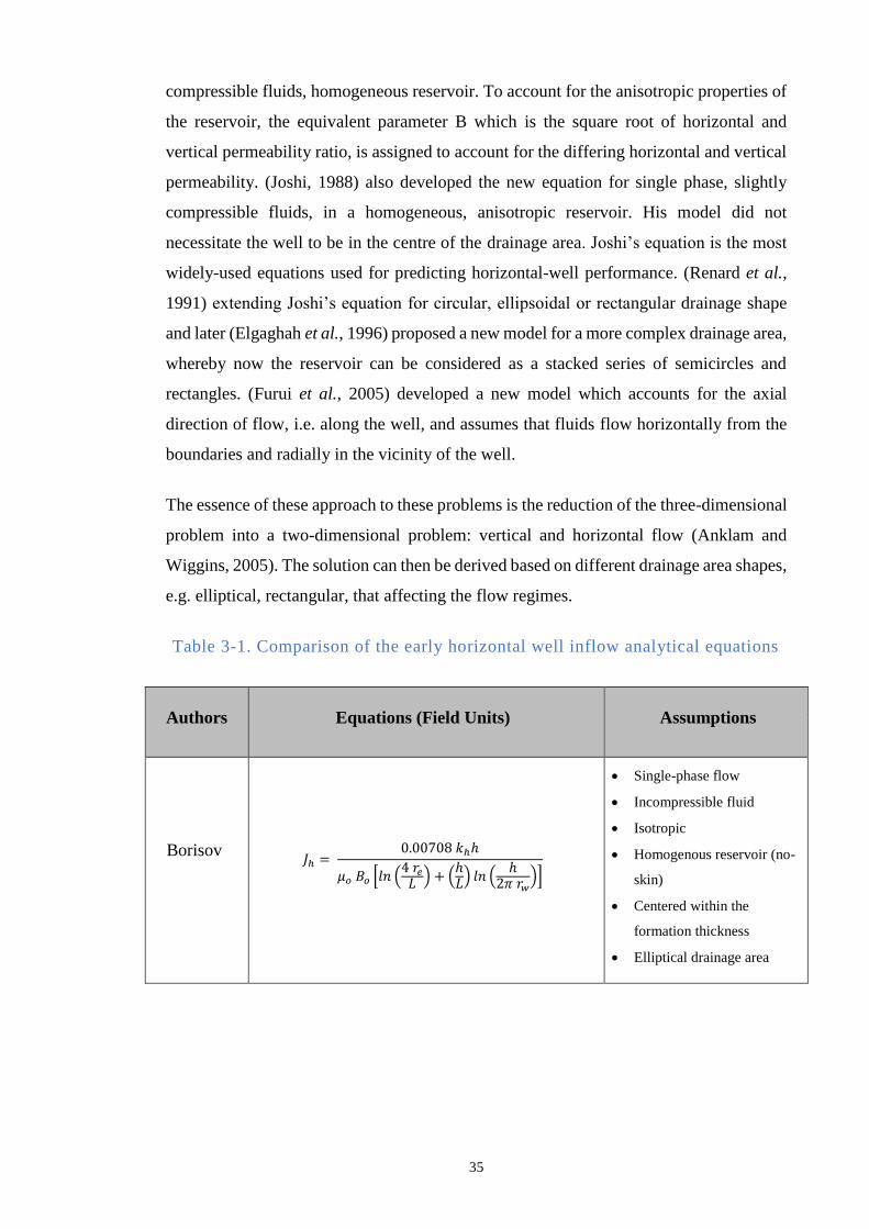
35
compressible fluids, homogeneous reservoir. To account for the anisotropic properties of
the reservoir, the equivalent parameter B which is the square root of horizontal and
vertical permeability ratio, is assigned to account for the differing horizontal and vertical
permeability. (Joshi, 1988) also developed the new equation for single phase, slightly
compressible fluids, in a homogeneous, anisotropic reservoir. His model did not
necessitate the well to be in the centre of the drainage area. Joshi’s equation is the most
widely-used equations used for predicting horizontal-well performance. (Renard et al.,
1991) extending Joshi’s equation for circular, ellipsoidal or rectangular drainage shape
and later (Elgaghah et al., 1996) proposed a new model for a more complex drainage area,
whereby now the reservoir can be considered as a stacked series of semicircles and
rectangles. (Furui et al., 2005) developed a new model which accounts for the axial
direction of flow, i.e. along the well, and assumes that fluids flow horizontally from the
boundaries and radially in the vicinity of the well.
The essence of these approach to these problems is the reduction of the three-dimensional
problem into a two-dimensional problem: vertical and horizontal flow (Anklam and
Wiggins, 2005). The solution can then be derived based on different drainage area shapes,
e.g. elliptical, rectangular, that affecting the flow regimes.
Table 3-1. Comparison of the early horizontal well inflow analytical equations
Authors Equations (Field Units) Assumptions
Borisov
𝐽ℎ = 0.00708 𝑘ℎℎ
𝜇𝑜 𝐵𝑜 [𝑙𝑛 (4 𝑟𝑒𝐿) + (
ℎ𝐿) 𝑙𝑛 (
ℎ2𝜋 𝑟𝑤
)]
Single-phase flow
Incompressible fluid
Isotropic
Homogenous reservoir (no-
skin)
Centered within the
formation thickness
Elliptical drainage area
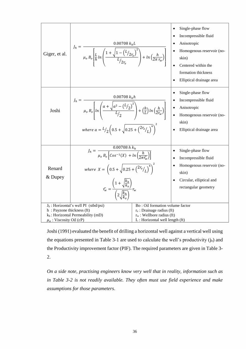
36
Giger, et al.
𝐽ℎ = 0.00708 𝑘ℎ𝐿
𝜇𝑜 𝐵𝑜
[ 𝐿ℎ𝑙𝑛
(
1 + √1 − (𝐿 2𝑟𝑒
⁄ )2
𝐿2𝑟𝑒⁄
)
+ 𝑙𝑛 (ℎ
2𝜋 𝑟𝑤)
]
Single-phase flow
Incompressible fluid
Anisotropic
Homogenous reservoir (no-
skin)
Centered within the
formation thickness
Elliptical drainage area
Joshi
𝐽ℎ = 0.00708 𝑘ℎℎ
𝜇𝑜 𝐵𝑜
[
𝑙𝑛
(
𝑎 + √𝑎2 − (𝐿 2⁄ )
2
𝐿2⁄
)
+ (ℎ𝐿) 𝑙𝑛 (
ℎ2𝑟𝑤
)
]
𝑤ℎ𝑒𝑟𝑒 𝑎 = 𝐿 2⁄ (0.5 + √0.25 + (2𝑟𝑒
𝐿⁄ )4
)
2
Single-phase flow
Incompressible fluid
Anisotropic
Homogenous reservoir (no-
skin)
Elliptical drainage area
Renard
& Dupey
𝐽ℎ = 0.00708 ℎ 𝑘ℎ
𝜇𝑜 𝐵𝑜 [𝐶𝑜𝑠−1(𝑋) + 𝑙𝑛 (
ℎ2𝜋𝑟
)]
𝑤ℎ𝑒𝑟𝑒 𝑋 = (0.5 + √0.25 + (2𝑟𝑒
𝐿⁄ )4
)
2
𝑟 =
(1 + √𝑘ℎ𝑘𝑣)
(2√𝑘ℎ𝑘𝑣)
𝑟𝑤
Single-phase flow
Incompressible fluid
Homogenous reservoir (no-
skin)
Circular, elliptical and
rectangular geometry
Jh : Horizontal’s well PI (stbd/psi)
h : Payzone thickness (ft)
kh : Horizontal Permeability (mD)
𝜇𝑜 : Viscosity Oil (cP)
Bo : Oil formation volume factor
re : Drainage radius (ft)
rw : Wellbore radius (ft)
L : Horizontal well length (ft)
Joshi (1991) evaluated the benefit of drilling a horizontal well against a vertical well using
the equations presented in Table 3-1 are used to calculate the well’s productivity (jh) and
the Productivity improvement factor (PIF). The required parameters are given in Table 3-
2.
On a side note, practising engineers know very well that in reality, information such as
in Table 3-2 is not readily available. They often must use field experience and make
assumptions for those parameters.
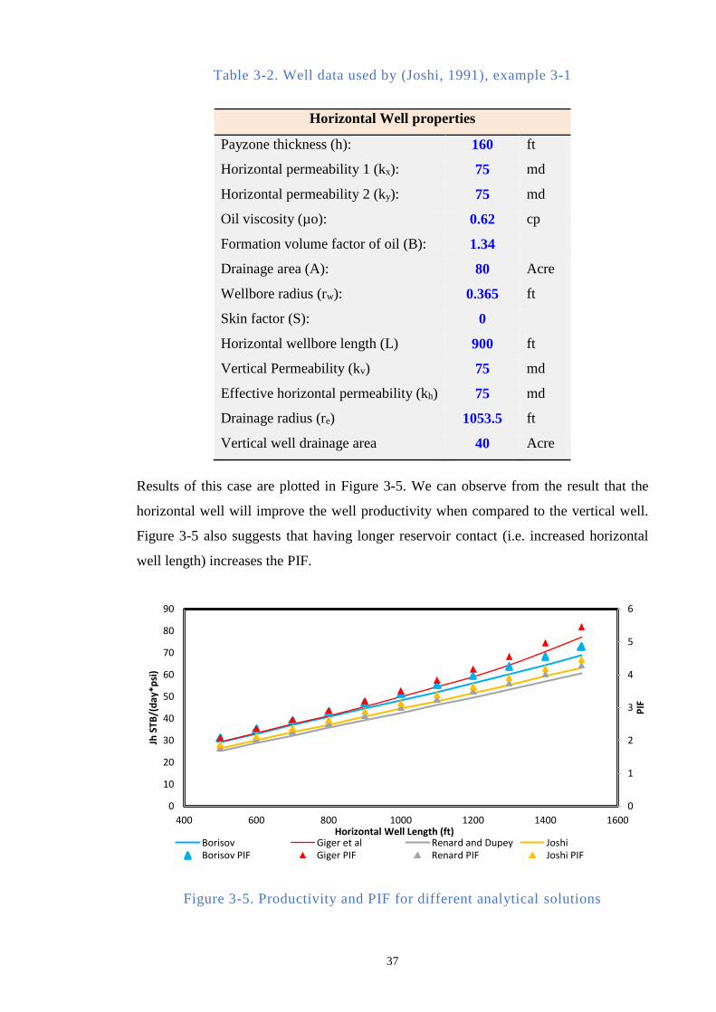
37
Table 3-2. Well data used by (Joshi, 1991), example 3-1
Horizontal Well properties
Payzone thickness (h): 160 ft
Horizontal permeability 1 (kx): 75 md
Horizontal permeability 2 (ky): 75 md
Oil viscosity (µo): 0.62 cp
Formation volume factor of oil (B): 1.34
Drainage area (A): 80 Acre
Wellbore radius (rw): 0.365 ft
Skin factor (S): 0
Horizontal wellbore length (L) 900 ft
Vertical Permeability (kv) 75 md
Effective horizontal permeability (kh) 75 md
Drainage radius (re) 1053.5 ft
Vertical well drainage area 40 Acre
Results of this case are plotted in Figure 3-5. We can observe from the result that the
horizontal well will improve the well productivity when compared to the vertical well.
Figure 3-5 also suggests that having longer reservoir contact (i.e. increased horizontal
well length) increases the PIF.
Figure 3-5. Productivity and PIF for different analytical solutions
0
1
2
3
4
5
6
0
10
20
30
40
50
60
70
80
90
400 600 800 1000 1200 1400 1600
PIF
Jh S
TB/(
day
*psi
)
Horizontal Well Length (ft)Borisov Giger et al Renard and Dupey JoshiBorisov PIF Giger PIF Renard PIF Joshi PIF

38
One conclusion from this result could be that the maximum horizontal well length will
always show maximum gain. This is practically not true with many field histories
reporting poor performance of long horizontal wells. Surveys in the 1990s (Levitan et al.,
2001) reported project with proper implementation of drilling technique ensuring the
success ratio of drilling a horizontal well of 95%. The objective of drilling long horizontal
wells without operational problems was achieved, but it came with an ever-increasing
cost per feet with longer horizontal sections. An increased production rate (from having
greater reservoir contact) were expected to offset this cost. However this was not the case.
It was reported only about 50% of horizontal wells that were economically justified.
The reported case indicated an essential element was not being accounted for by the
equations in Table 3-1. This element is the frictional pressure loss in the wellbore. The
above solutions (and many other equations) assumed pressure drop along the well length
is negligible, i.e. an infinitely-conductive well. This is an acceptable assumption for a
short horizontal well with small flow rate. However, many wells today have an extensive
horizontal section and operates with large flowing rate. For those wells, the effect of
friction pressure along the well is no longer trivial, and a single value of pressure is
insufficient to represent the whole horizontal section. (Babu and Odeh, 1989) are ones of
the first initiators of horizontal well modelling, looked into this problem. Their model still
assumed a uniform flux with infinite conductivity, but they did point out the inaccuracy
of assuming constant pressure along the entire length of the horizontal section.
This issue is illustrated in Figure 3-6. Continuous fluid flow along the horizontal well
requires a certain amount of pressure drop between the toe and heel section, or PToe - PHeel
(∆PHT) > 0. The heel-toe effect reduces the potential drawdown, particularly at the toe
section. The drawdown for this section is overestimated by traditional models, resulting
in the predicted well rates also being overestimated. The extra pressure drop depreciated
by tubing outflow due, for example, to the well being completed with a too small diameter
of tubing, will have a similar effect on the rate predictions as the heel-toe effect. Note that
the analysis of this chapter assumes a perfectly horizontal well where the pressure loss
between heel and toe is dominated by the friction effect, and hydrostatic head differences
are (relatively) negligible.
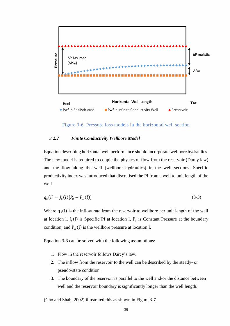
39
Figure 3-6. Pressure loss models in the horizontal well section
Finite Conductivity Wellbore Model
Equation describing horizontal well performance should incorporate wellbore hydraulics.
The new model is required to couple the physics of flow from the reservoir (Darcy law)
and the flow along the well (wellbore hydraulics) in the well sections. Specific
productivity index was introduced that discretised the PI from a well to unit length of the
well.
𝑞𝑠(𝑙) = 𝐽𝑠(𝑙)[𝑃𝑒 − 𝑃𝑤(𝑙)] (3-3)
Where qs(l) is the inflow rate from the reservoir to wellbore per unit length of the well
at location l, Js(l) is Specific PI at location l, Pe is Constant Pressure at the boundary
condition, and Pw(l) is the wellbore pressure at location l.
Equation 3-3 can be solved with the following assumptions:
1. Flow in the reservoir follows Darcy’s law.
2. The inflow from the reservoir to the well can be described by the steady- or
pseudo-state condition.
3. The boundary of the reservoir is parallel to the well and/or the distance between
well and the reservoir boundary is significantly longer than the well length.
(Cho and Shah, 2002) illustrated this as shown in Figure 3-7.
Pre
ssu
re
Horizontal Well Length
Pwf in Realistic case Pwf in Infinite Conductivity Well Preservoir
Heel Toe
∆P realistic ∆P Assumed
(∆Pres)
∆PHT
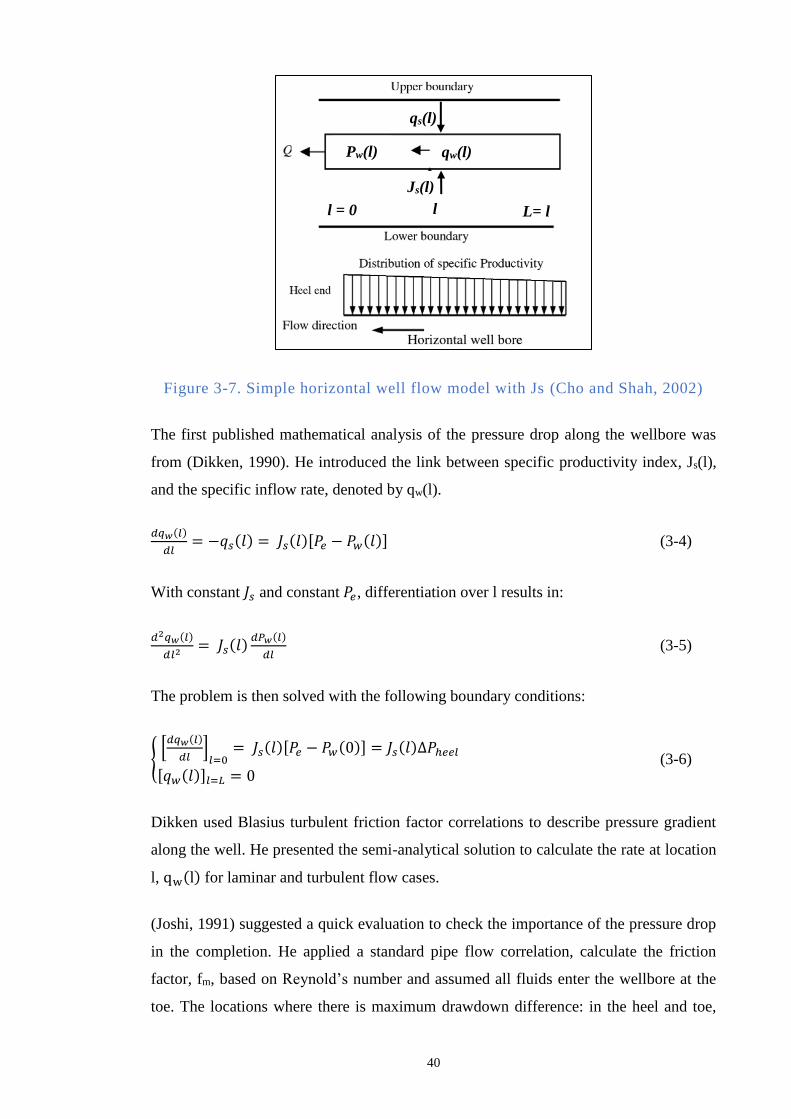
40
Figure 3-7. Simple horizontal well flow model with Js (Cho and Shah, 2002)
The first published mathematical analysis of the pressure drop along the wellbore was
from (Dikken, 1990). He introduced the link between specific productivity index, Js(l),
and the specific inflow rate, denoted by qw(l).
𝑑𝑞𝑤(𝑙)
𝑑𝑙= −𝑞𝑠(𝑙) = 𝐽𝑠(𝑙)[𝑃𝑒 − 𝑃𝑤(𝑙)] (3-4)
With constant 𝐽𝑠 and constant 𝑃𝑒, differentiation over l results in:
𝑑2𝑞𝑤(𝑙)
𝑑𝑙2= 𝐽𝑠(𝑙)
𝑑𝑃𝑤(𝑙)
𝑑𝑙 (3-5)
The problem is then solved with the following boundary conditions:
[𝑑𝑞𝑤(𝑙)
𝑑𝑙]𝑙=0
= 𝐽𝑠(𝑙)[𝑃𝑒 − 𝑃𝑤(0)] = 𝐽𝑠(𝑙)∆𝑃ℎ𝑒𝑒𝑙
[𝑞𝑤(𝑙)]𝑙=𝐿 = 0 (3-6)
Dikken used Blasius turbulent friction factor correlations to describe pressure gradient
along the well. He presented the semi-analytical solution to calculate the rate at location
l, qw(l) for laminar and turbulent flow cases.
(Joshi, 1991) suggested a quick evaluation to check the importance of the pressure drop
in the completion. He applied a standard pipe flow correlation, calculate the friction
factor, fm, based on Reynold’s number and assumed all fluids enter the wellbore at the
toe. The locations where there is maximum drawdown difference: in the heel and toe,
qs(l)
Js(l)
qw(l) Pw(l)
l = 0 l L= l
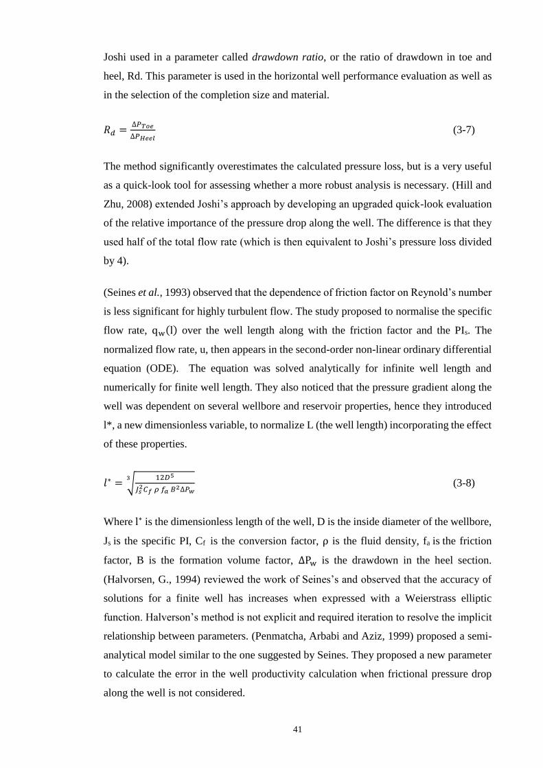
41
Joshi used in a parameter called drawdown ratio, or the ratio of drawdown in toe and
heel, Rd. This parameter is used in the horizontal well performance evaluation as well as
in the selection of the completion size and material.
𝑅𝑑 =∆𝑃𝑇𝑜𝑒
∆𝑃𝐻𝑒𝑒𝑙 (3-7)
The method significantly overestimates the calculated pressure loss, but is a very useful
as a quick-look tool for assessing whether a more robust analysis is necessary. (Hill and
Zhu, 2008) extended Joshi’s approach by developing an upgraded quick-look evaluation
of the relative importance of the pressure drop along the well. The difference is that they
used half of the total flow rate (which is then equivalent to Joshi’s pressure loss divided
by 4).
(Seines et al., 1993) observed that the dependence of friction factor on Reynold’s number
is less significant for highly turbulent flow. The study proposed to normalise the specific
flow rate, qw(l) over the well length along with the friction factor and the PIs. The
normalized flow rate, u, then appears in the second-order non-linear ordinary differential
equation (ODE). The equation was solved analytically for infinite well length and
numerically for finite well length. They also noticed that the pressure gradient along the
well was dependent on several wellbore and reservoir properties, hence they introduced
l*, a new dimensionless variable, to normalize L (the well length) incorporating the effect
of these properties.
𝑙∗ = √12𝐷5
𝐽𝑠2𝐶𝑓 𝜌 𝑓𝑎 𝐵
2∆𝑃𝑤
3 (3-8)
Where l∗ is the dimensionless length of the well, D is the inside diameter of the wellbore,
Js is the specific PI, Cf is the conversion factor, ρ is the fluid density, fa is the friction
factor, B is the formation volume factor, ∆Pw is the drawdown in the heel section.
(Halvorsen, G., 1994) reviewed the work of Seines’s and observed that the accuracy of
solutions for a finite well has increases when expressed with a Weierstrass elliptic
function. Halverson’s method is not explicit and required iteration to resolve the implicit
relationship between parameters. (Penmatcha, Arbabi and Aziz, 1999) proposed a semi-
analytical model similar to the one suggested by Seines. They proposed a new parameter
to calculate the error in the well productivity calculation when frictional pressure drop
along the well is not considered.
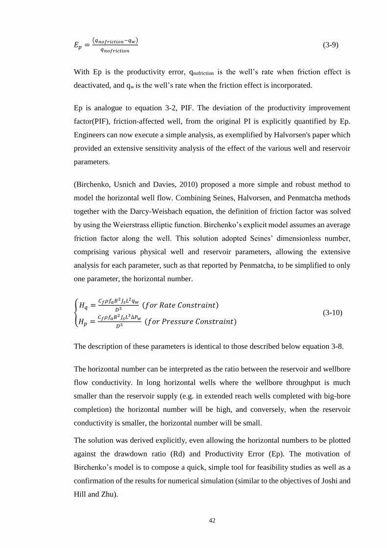
42
𝐸𝑝 =(𝑞𝑛𝑜𝑓𝑟𝑖𝑐𝑡𝑖𝑜𝑛−𝑞𝑤)
𝑞𝑛𝑜𝑓𝑟𝑖𝑐𝑡𝑖𝑜𝑛 (3-9)
With Ep is the productivity error, qnofriction is the well’s rate when friction effect is
deactivated, and qw is the well’s rate when the friction effect is incorporated.
Ep is analogue to equation 3-2, PIF. The deviation of the productivity improvement
factor(PIF), friction-affected well, from the original PI is explicitly quantified by Ep.
Engineers can now execute a simple analysis, as exemplified by Halvorsen's paper which
provided an extensive sensitivity analysis of the effect of the various well and reservoir
parameters.
(Birchenko, Usnich and Davies, 2010) proposed a more simple and robust method to
model the horizontal well flow. Combining Seines, Halvorsen, and Penmatcha methods
together with the Darcy-Weisbach equation, the definition of friction factor was solved
by using the Weierstrass elliptic function. Birchenko’s explicit model assumes an average
friction factor along the well. This solution adopted Seines’ dimensionless number,
comprising various physical well and reservoir parameters, allowing the extensive
analysis for each parameter, such as that reported by Penmatcha, to be simplified to only
one parameter, the horizontal number.
𝐻𝑞 =
𝐶𝑓𝜌𝑓𝑎𝐵2𝐽𝑠𝐿
2𝑞𝑤
𝐷5 (𝑓𝑜𝑟 𝑅𝑎𝑡𝑒 𝐶𝑜𝑛𝑠𝑡𝑟𝑎𝑖𝑛𝑡)
𝐻𝑝 =𝐶𝑓𝜌𝑓𝑎𝐵
2𝐽𝑠𝐿3∆𝑃𝑤
𝐷5 (𝑓𝑜𝑟 𝑃𝑟𝑒𝑠𝑠𝑢𝑟𝑒 𝐶𝑜𝑛𝑠𝑡𝑟𝑎𝑖𝑛𝑡)
(3-10)
The description of these parameters is identical to those described below equation 3-8.
The horizontal number can be interpreted as the ratio between the reservoir and wellbore
flow conductivity. In long horizontal wells where the wellbore throughput is much
smaller than the reservoir supply (e.g. in extended reach wells completed with big-bore
completion) the horizontal number will be high, and conversely, when the reservoir
conductivity is smaller, the horizontal number will be small.
The solution was derived explicitly, even allowing the horizontal numbers to be plotted
against the drawdown ratio (Rd) and Productivity Error (Ep). The motivation of
Birchenko’s model is to compose a quick, simple tool for feasibility studies as well as a
confirmation of the results for numerical simulation (similar to the objectives of Joshi and
Hill and Zhu).
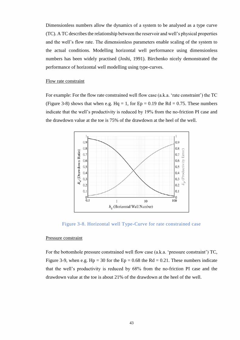
43
Dimensionless numbers allow the dynamics of a system to be analysed as a type curve
(TC). A TC describes the relationship between the reservoir and well’s physical properties
and the well’s flow rate. The dimensionless parameters enable scaling of the system to
the actual conditions. Modelling horizontal well performance using dimensionless
numbers has been widely practised (Joshi, 1991). Birchenko nicely demonstrated the
performance of horizontal well modelling using type-curves.
Flow rate constraint
For example: For the flow rate constrained well flow case (a.k.a. ‘rate constraint’) the TC
(Figure 3-8) shows that when e.g. Hq = 1, for Ep = 0.19 the Rd = 0.75. These numbers
indicate that the well’s productivity is reduced by 19% from the no-friction PI case and
the drawdown value at the toe is 75% of the drawdown at the heel of the well.
Figure 3-8. Horizontal well Type-Curve for rate constrained case
Pressure constraint
For the bottomhole pressure constrained well flow case (a.k.a. ‘pressure constraint’) TC,
Figure 3-9, when e.g. Hp = 30 for the Ep = 0.68 the Rd = 0.21. These numbers indicate
that the well’s productivity is reduced by 68% from the no-friction PI case and the
drawdown value at the toe is about 21% of the drawdown at the heel of the well.
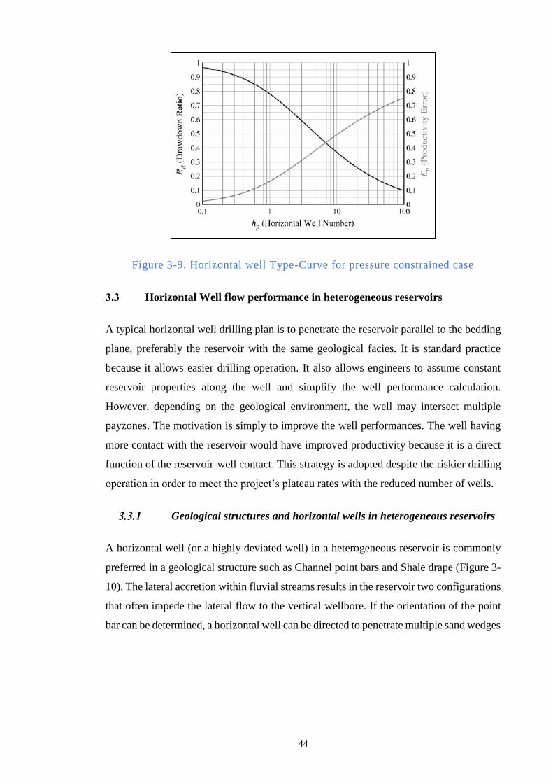
44
Figure 3-9. Horizontal well Type-Curve for pressure constrained case
Horizontal Well flow performance in heterogeneous reservoirs
A typical horizontal well drilling plan is to penetrate the reservoir parallel to the bedding
plane, preferably the reservoir with the same geological facies. It is standard practice
because it allows easier drilling operation. It also allows engineers to assume constant
reservoir properties along the well and simplify the well performance calculation.
However, depending on the geological environment, the well may intersect multiple
payzones. The motivation is simply to improve the well performances. The well having
more contact with the reservoir would have improved productivity because it is a direct
function of the reservoir-well contact. This strategy is adopted despite the riskier drilling
operation in order to meet the project’s plateau rates with the reduced number of wells.
Geological structures and horizontal wells in heterogeneous reservoirs
A horizontal well (or a highly deviated well) in a heterogeneous reservoir is commonly
preferred in a geological structure such as Channel point bars and Shale drape (Figure 3-
10). The lateral accretion within fluvial streams results in the reservoir two configurations
that often impede the lateral flow to the vertical wellbore. If the orientation of the point
bar can be determined, a horizontal well can be directed to penetrate multiple sand wedges
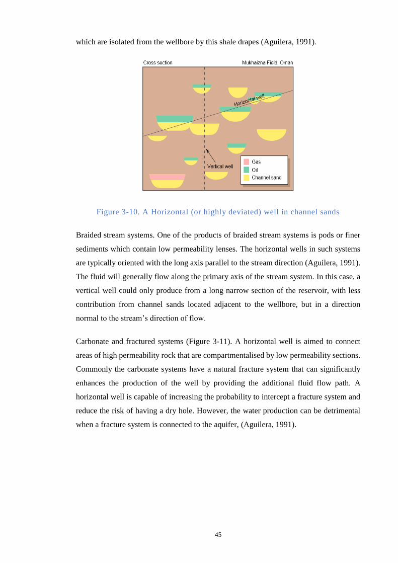
45
which are isolated from the wellbore by this shale drapes (Aguilera, 1991).
Figure 3-10. A Horizontal (or highly deviated) well in channel sands
Braided stream systems. One of the products of braided stream systems is pods or finer
sediments which contain low permeability lenses. The horizontal wells in such systems
are typically oriented with the long axis parallel to the stream direction (Aguilera, 1991).
The fluid will generally flow along the primary axis of the stream system. In this case, a
vertical well could only produce from a long narrow section of the reservoir, with less
contribution from channel sands located adjacent to the wellbore, but in a direction
normal to the stream’s direction of flow.
Carbonate and fractured systems (Figure 3-11). A horizontal well is aimed to connect
areas of high permeability rock that are compartmentalised by low permeability sections.
Commonly the carbonate systems have a natural fracture system that can significantly
enhances the production of the well by providing the additional fluid flow path. A
horizontal well is capable of increasing the probability to intercept a fracture system and
reduce the risk of having a dry hole. However, the water production can be detrimental
when a fracture system is connected to the aquifer, (Aguilera, 1991).
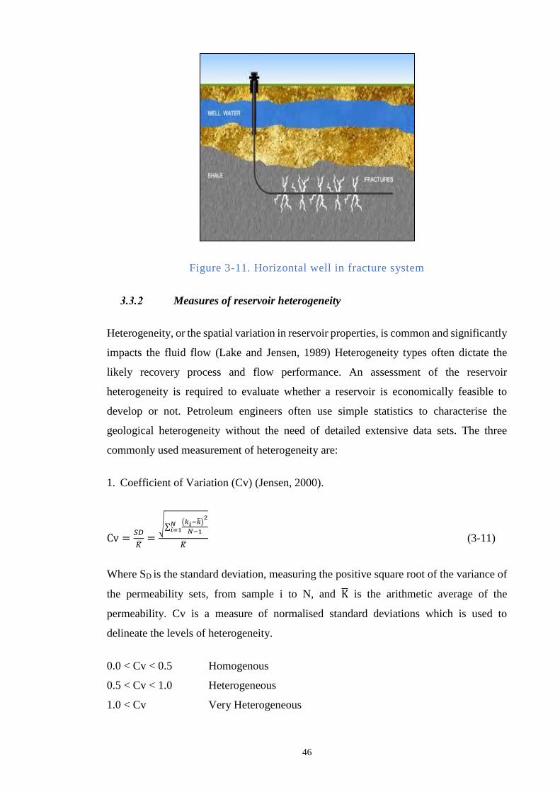
46
Figure 3-11. Horizontal well in fracture system
Measures of reservoir heterogeneity
Heterogeneity, or the spatial variation in reservoir properties, is common and significantly
impacts the fluid flow (Lake and Jensen, 1989) Heterogeneity types often dictate the
likely recovery process and flow performance. An assessment of the reservoir
heterogeneity is required to evaluate whether a reservoir is economically feasible to
develop or not. Petroleum engineers often use simple statistics to characterise the
geological heterogeneity without the need of detailed extensive data sets. The three
commonly used measurement of heterogeneity are:
1. Coefficient of Variation (Cv) (Jensen, 2000).
Cv =𝑆𝐷
=
√∑(𝑘𝑖−)
2
𝑁−1𝑁𝑖=1
(3-11)
Where SD is the standard deviation, measuring the positive square root of the variance of
the permeability sets, from sample i to N, and K is the arithmetic average of the
permeability. Cv is a measure of normalised standard deviations which is used to
delineate the levels of heterogeneity.
0.0 < Cv < 0.5 Homogenous
0.5 < Cv < 1.0 Heterogeneous
1.0 < Cv Very Heterogeneous
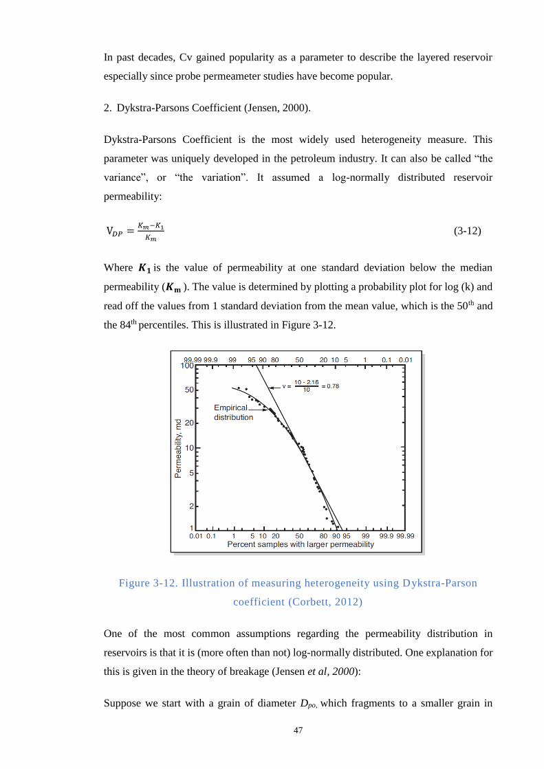
47
In past decades, Cv gained popularity as a parameter to describe the layered reservoir
especially since probe permeameter studies have become popular.
2. Dykstra-Parsons Coefficient (Jensen, 2000).
Dykstra-Parsons Coefficient is the most widely used heterogeneity measure. This
parameter was uniquely developed in the petroleum industry. It can also be called “the
variance”, or “the variation”. It assumed a log-normally distributed reservoir
permeability:
V𝐷𝑃 =𝐾𝑚−𝐾1
𝐾𝑚 (3-12)
Where 𝑲𝟏 is the value of permeability at one standard deviation below the median
permeability (𝑲𝐦 ). The value is determined by plotting a probability plot for log (k) and
read off the values from 1 standard deviation from the mean value, which is the 50th and
the 84th percentiles. This is illustrated in Figure 3-12.
Figure 3-12. Illustration of measuring heterogeneity using Dykstra-Parson
coefficient (Corbett, 2012)
One of the most common assumptions regarding the permeability distribution in
reservoirs is that it is (more often than not) log-normally distributed. One explanation for
this is given in the theory of breakage (Jensen et al, 2000):
Suppose we start with a grain of diameter Dpo, which fragments to a smaller grain in

48
proportion f0 yield a grain of Dp1. Repeating this process obviously leads to an immense
tree of possibility for the ultimate grain diameter. However, if we follow one branch of
this tree, its grain diameter Dp1 will yields an additive process upon taking a logarithm.
Therefore, we should expect ln Dp1 to be normally distributed from the Central Limit
Theorem. Since permeability is proportional to the grain size squared (e.g. in Kozeny-
Carman equation), it is also log-normally distributed.
The main advantage of using this parameter, VDP, is that it has been the subject of
numerous studies in the petroleum industry. Different correlations have been built relating
the VDP to the other parameters such as recovery factor, injection volume, water cut,
dimensionless time, etc (Johnson, 1956; Jensen and Currie, 1990; El-khatib, 2011).
3. Lorenz coefficient (Lake and Jensen, 1989)
The Lorenz Coefficient (Lc) (Or Gini Index) is the particular area within Lorenz Plot, a
plot which illustrated the relationship between total reservoir porosity and permeability.
The Lorenz plot constitutes two parameters:
F𝐽 =∑ 𝑘jℎj𝐽𝑗=1
∑ 𝑘jℎj𝐼𝑖=1
C𝐽 =∑ Φjℎj𝐽𝑗=1
∑ Φjℎj𝐼𝑖=1
(3-13)
Where J is the index of data points, with maximum I. FJ, is the flow capacity and Cj is the
storage capacity (Figure 3-13.). These capacities, ordered from smallest to largest, are
plotted on a linear plot (red line). The Lorenz Coefficient is the ration between the (grey)
area bounded by the line of equality (Y = X line, black line in Figure 3-13.) and the Lorenz
curve (red line in Figure 3-13.), and the triangle (blue) area between the line of equality
and the Cartesian plot (blue line if Figure 3-13.). Since the triangle area is always 0.5,
hence the Lorenz coefficient (Lc) can be calculated as twice the shaded area and is in the
range from 0 to 1. As a reference, the full uniformity or homogeneity is identified by the
black diagonal line and it has Lc = 0. More about the Lorenz coefficient will be discussed
in chapter 5.
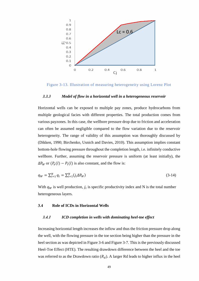
49
Figure 3-13. Illustration of measuring heterogeneity using Lorenz Plot
Model of flow in a horizontal well in a heterogeneous reservoir
Horizontal wells can be exposed to multiple pay zones, produce hydrocarbons from
multiple geological facies with different properties. The total production comes from
various payzones. In this case, the wellbore pressure drop due to friction and acceleration
can often be assumed negligible compared to the flow variation due to the reservoir
heterogeneity. The range of validity of this assumption was thoroughly discussed by
(Dikken, 1990; Birchenko, Usnich and Davies, 2010). This assumption implies constant
bottom-hole flowing pressure throughout the completion length, i.e. infinitely conductive
wellbore. Further, assuming the reservoir pressure is uniform (at least initially), the
∆P𝑊 or (𝑃𝑒(𝑙) − 𝑃𝑙(𝑙) is also constant, and the flow is:
𝑞𝑊 = ∑ 𝑞𝑖𝑁𝑖=1 = ∑ (𝑗𝑖∆P𝑊)
𝑁𝑖=1 (3-14)
With 𝑞𝑊 is well production, 𝑗𝑖 is specific productivity index and N is the total number
heterogeneous layers.
Role of ICDs in Horizontal Wells
ICD completion in wells with dominating heel-toe effect
Increasing horizontal length increases the inflow and thus the friction pressure drop along
the well, with the flowing pressure in the toe section being higher than the pressure in the
heel section as was depicted in Figure 3-6 and Figure 3-7. This is the previously discussed
Heel-Toe Effect (HTE). The resulting drawdown difference between the heel and the toe
was referred to as the Drawdown ratio (𝑅𝑑). A larger Rd leads to higher influx in the heel
Lc = 0.6
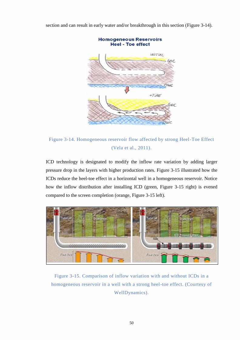
50
section and can result in early water and/or breakthrough in this section (Figure 3-14).
Figure 3-14. Homogeneous reservoir flow affected by strong Heel -Toe Effect
(Vela et al., 2011).
ICD technology is designated to modify the inflow rate variation by adding larger
pressure drop in the layers with higher production rates. Figure 3-15 illustrated how the
ICDs reduce the heel-toe effect in a horizontal well in a homogeneous reservoir. Notice
how the inflow distribution after installing ICD (green, Figure 3-15 right) is evened
compared to the screen completion (orange, Figure 3-15 left).
Figure 3-15. Comparison of inflow variation with and without ICDs in a
homogeneous reservoir in a well with a strong heel -toe effect. (Courtesy of
WellDynamics).
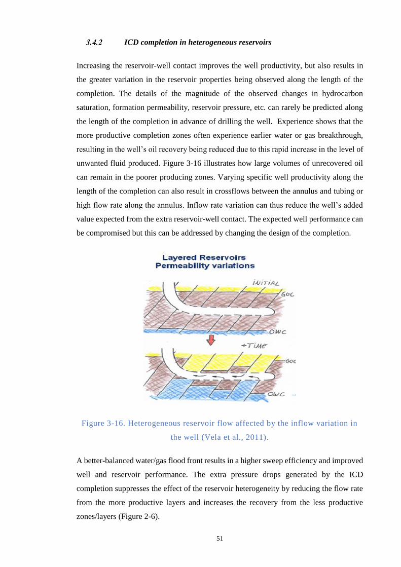
51
ICD completion in heterogeneous reservoirs
Increasing the reservoir-well contact improves the well productivity, but also results in
the greater variation in the reservoir properties being observed along the length of the
completion. The details of the magnitude of the observed changes in hydrocarbon
saturation, formation permeability, reservoir pressure, etc. can rarely be predicted along
the length of the completion in advance of drilling the well. Experience shows that the
more productive completion zones often experience earlier water or gas breakthrough,
resulting in the well’s oil recovery being reduced due to this rapid increase in the level of
unwanted fluid produced. Figure 3-16 illustrates how large volumes of unrecovered oil
can remain in the poorer producing zones. Varying specific well productivity along the
length of the completion can also result in crossflows between the annulus and tubing or
high flow rate along the annulus. Inflow rate variation can thus reduce the well’s added
value expected from the extra reservoir-well contact. The expected well performance can
be compromised but this can be addressed by changing the design of the completion.
Figure 3-16. Heterogeneous reservoir flow affected by the inflow variation in
the well (Vela et al., 2011).
A better-balanced water/gas flood front results in a higher sweep efficiency and improved
well and reservoir performance. The extra pressure drops generated by the ICD
completion suppresses the effect of the reservoir heterogeneity by reducing the flow rate
from the more productive layers and increases the recovery from the less productive
zones/layers (Figure 2-6).

52
An ICD completion can have the additional advantage (F. Al-Khelaiwi et al., 2010b) of
being more effective than Inflow Control Valves when rapid changes in the local inflow
rate are observed along the length of the completion due to the potentially finer
discretisation of the flow control zones by installing more ICDs and annular flow isolation
(packers).
ICD design objectives and options
ICD design aims to redistribute inflow/outflow along the well length, i.e. inflow profile
alteration (Al-Khelaiwi et al., 2010a). The idea is to regulate the flow, to some extent, to
obtain the flow profile which will give desirable results, e.g. higher recovery, lower water
cut, etc., (Daneshy et al., 2012). The problem is to guess what kind of flow profile that
should be. The two ideal (though rarely achievable), expected profiles reported are the
flat (uniform inflow) profile and the U-flow (U-shaped, uniform coning) profile. This
section will describe the profile selection methods for the heel-toe dominated profile case.
Similar approaches can be applied to a well with inflow variation due to a heterogeneous
reservoir.
1. Uniform Flow (U-Flow) design objective
The objective is to achieve a uniform inflow along the well, by modifying drawdown
with additional, completion pressure selectively along the well, at least at the start of
the production. This approach is intuitive, reliable and currently the most popular ICD
design method when the varying ICD size along the completion is allowed which is
less common compared to the constant size (or ‘strength’) ICD designs. The idea is
that every part of the well should give an equal flow contribution. For example, in a
well with HTE problem, the heel section that is exposed to larger drawdown is
completed with ICDs having stronger restriction, while the toe section is completed
with weaker ICDs (figure 3-17 left). The flow distribution when well is completed
with such designed ICD completion should look like a flat line as if the well has no
heel-toe effect (figure 3-17 right). This method is reported in various publications
(Garcia et al., 2009; Marzooqi et al., 2010; Zadeh et al., 2012; Akbari et al., 2014).
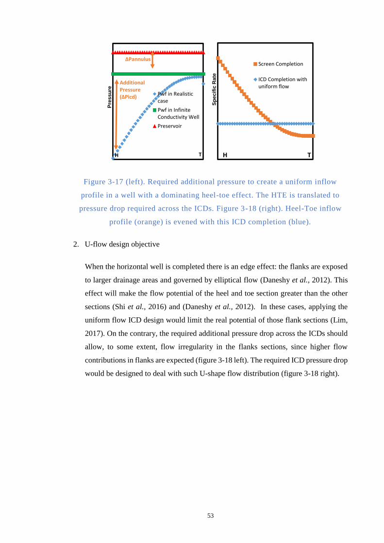
53
Figure 3-17 (left). Required additional pressure to create a uniform inflow
profile in a well with a dominating heel-toe effect. The HTE is translated to
pressure drop required across the ICDs. Figure 3-18 (right). Heel-Toe inflow
profile (orange) is evened with this ICD completion (blue).
2. U-flow design objective
When the horizontal well is completed there is an edge effect: the flanks are exposed
to larger drainage areas and governed by elliptical flow (Daneshy et al., 2012). This
effect will make the flow potential of the heel and toe section greater than the other
sections (Shi et al., 2016) and (Daneshy et al., 2012). In these cases, applying the
uniform flow ICD design would limit the real potential of those flank sections (Lim,
2017). On the contrary, the required additional pressure drop across the ICDs should
allow, to some extent, flow irregularity in the flanks sections, since higher flow
contributions in flanks are expected (figure 3-18 left). The required ICD pressure drop
would be designed to deal with such U-shape flow distribution (figure 3-18 right).
Sp
ecif
ic R
ate
Screen Completion
ICD Completion withuniform flow
H T
Pre
ssu
re
Pwf in Realisticcase
Pwf in InfiniteConductivity Well
Preservoir
∆Pannulus
Additional Pressure (∆Picd)
H T
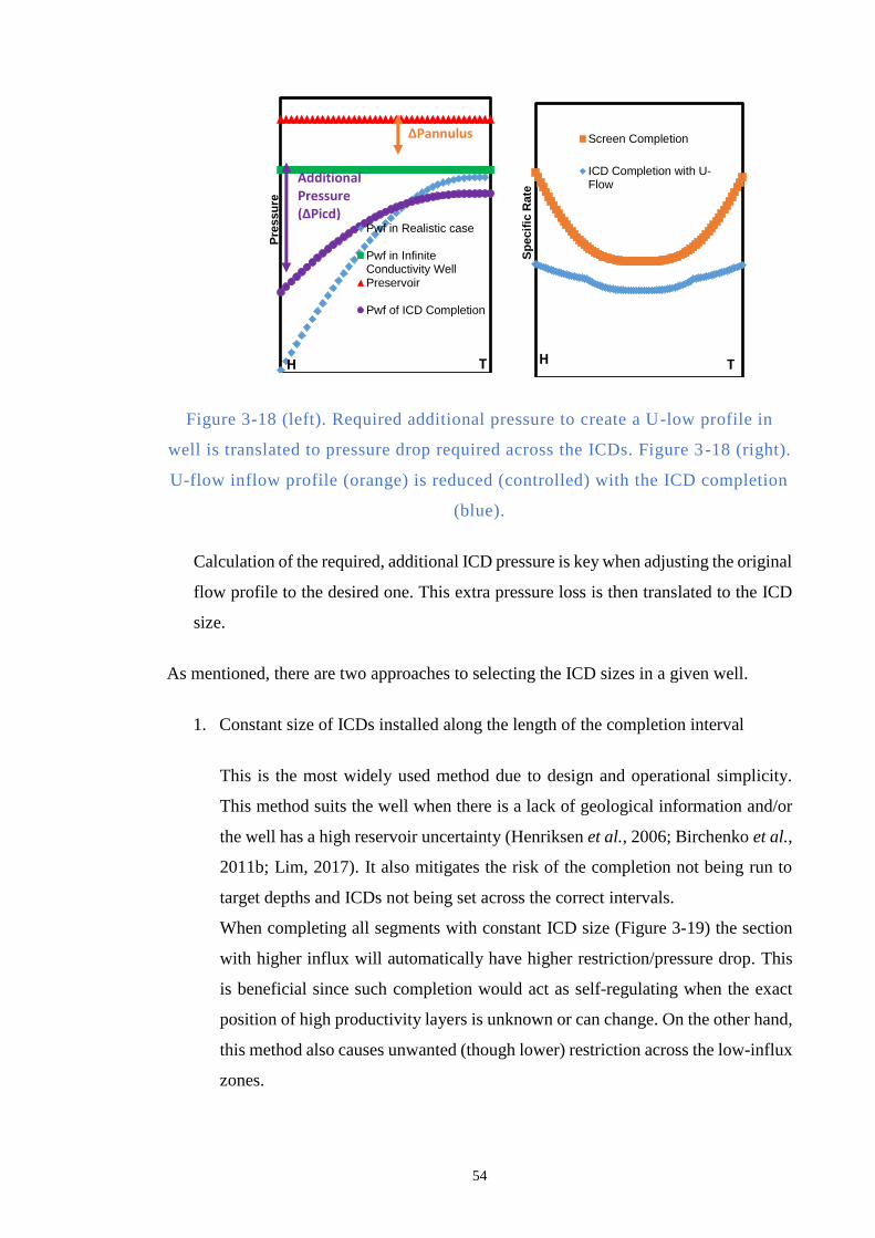
54
Figure 3-18 (left). Required additional pressure to create a U-low profile in
well is translated to pressure drop required across the ICDs. Figure 3 -18 (right).
U-flow inflow profile (orange) is reduced (controlled) with the ICD completion
(blue).
Calculation of the required, additional ICD pressure is key when adjusting the original
flow profile to the desired one. This extra pressure loss is then translated to the ICD
size.
As mentioned, there are two approaches to selecting the ICD sizes in a given well.
1. Constant size of ICDs installed along the length of the completion interval
This is the most widely used method due to design and operational simplicity.
This method suits the well when there is a lack of geological information and/or
the well has a high reservoir uncertainty (Henriksen et al., 2006; Birchenko et al.,
2011b; Lim, 2017). It also mitigates the risk of the completion not being run to
target depths and ICDs not being set across the correct intervals.
When completing all segments with constant ICD size (Figure 3-19) the section
with higher influx will automatically have higher restriction/pressure drop. This
is beneficial since such completion would act as self-regulating when the exact
position of high productivity layers is unknown or can change. On the other hand,
this method also causes unwanted (though lower) restriction across the low-influx
zones.
Sp
ecif
ic R
ate
Screen Completion
ICD Completion with U-Flow
H T
Pre
ssu
re
Pwf in Realistic case
Pwf in InfiniteConductivity WellPreservoir
Pwf of ICD Completion
∆Pannulus
Additional Pressure (∆Picd)
He
To
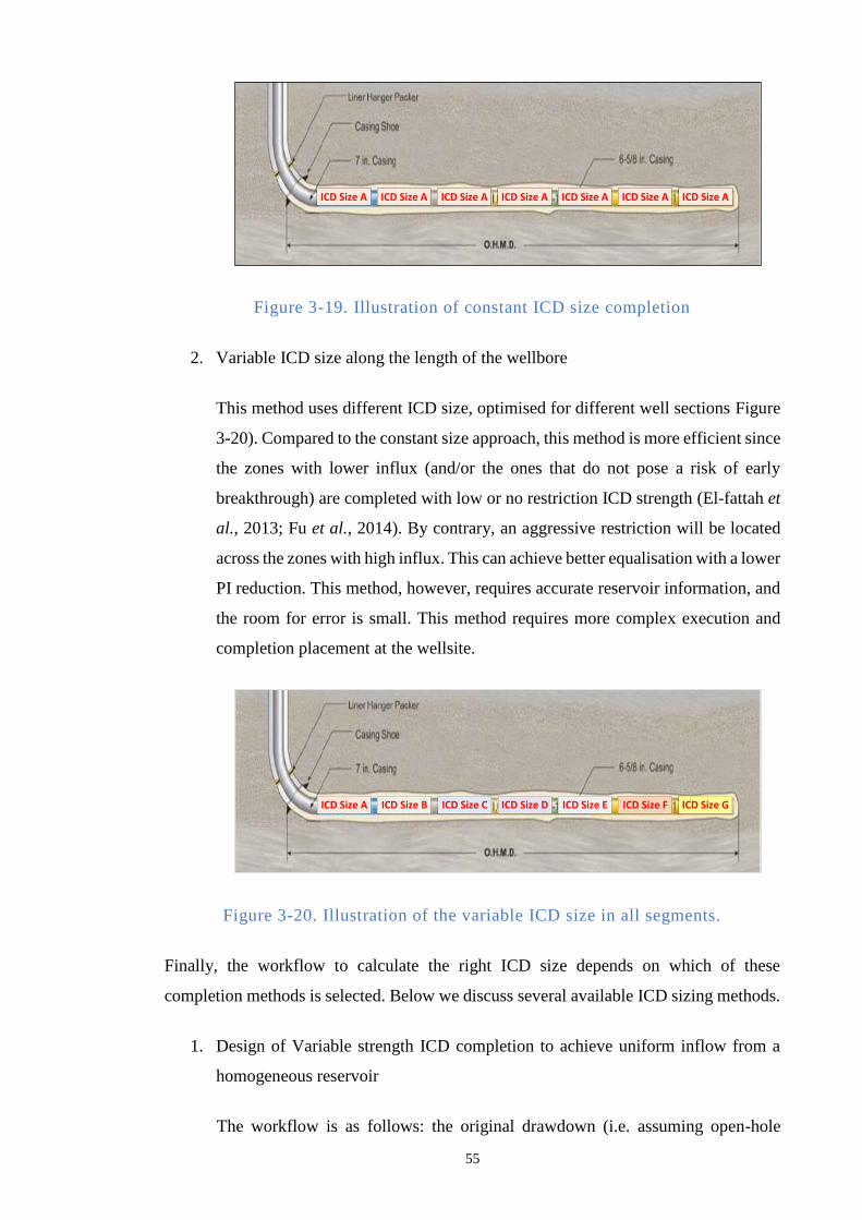
55
ICD Size A ICD Size A ICD Size A ICD Size A ICD Size A ICD Size A ICD Size A
Figure 3-19. Illustration of constant ICD size completion
2. Variable ICD size along the length of the wellbore
This method uses different ICD size, optimised for different well sections Figure
3-20). Compared to the constant size approach, this method is more efficient since
the zones with lower influx (and/or the ones that do not pose a risk of early
breakthrough) are completed with low or no restriction ICD strength (El-fattah et
al., 2013; Fu et al., 2014). By contrary, an aggressive restriction will be located
across the zones with high influx. This can achieve better equalisation with a lower
PI reduction. This method, however, requires accurate reservoir information, and
the room for error is small. This method requires more complex execution and
completion placement at the wellsite.
ICD Size A ICD Size B ICD Size C ICD Size D ICD Size E ICD Size F ICD Size G
Figure 3-20. Illustration of the variable ICD size in all segments.
Finally, the workflow to calculate the right ICD size depends on which of these
completion methods is selected. Below we discuss several available ICD sizing methods.
1. Design of Variable strength ICD completion to achieve uniform inflow from a
homogeneous reservoir
The workflow is as follows: the original drawdown (i.e. assuming open-hole
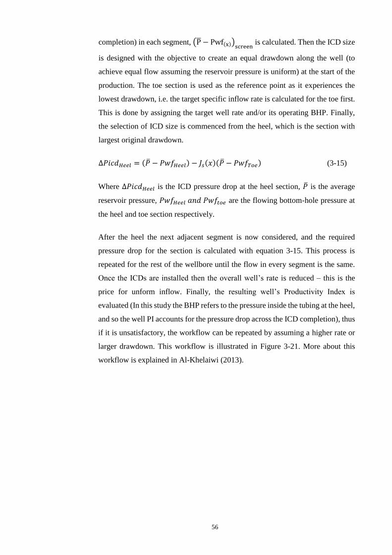
56
completion) in each segment, (P − Pwf(x))screen is calculated. Then the ICD size
is designed with the objective to create an equal drawdown along the well (to
achieve equal flow assuming the reservoir pressure is uniform) at the start of the
production. The toe section is used as the reference point as it experiences the
lowest drawdown, i.e. the target specific inflow rate is calculated for the toe first.
This is done by assigning the target well rate and/or its operating BHP. Finally,
the selection of ICD size is commenced from the heel, which is the section with
largest original drawdown.
∆𝑃𝑖𝑐𝑑𝐻𝑒𝑒𝑙 = ( − 𝑃𝑤𝑓𝐻𝑒𝑒𝑙) − 𝐽𝑠(𝑥)( − 𝑃𝑤𝑓𝑇𝑜𝑒) (3-15)
Where ∆𝑃𝑖𝑐𝑑𝐻𝑒𝑒𝑙 is the ICD pressure drop at the heel section, is the average
reservoir pressure, 𝑃𝑤𝑓𝐻𝑒𝑒𝑙 𝑎𝑛𝑑 𝑃𝑤𝑓𝑡𝑜𝑒 are the flowing bottom-hole pressure at
the heel and toe section respectively.
After the heel the next adjacent segment is now considered, and the required
pressure drop for the section is calculated with equation 3-15. This process is
repeated for the rest of the wellbore until the flow in every segment is the same.
Once the ICDs are installed then the overall well’s rate is reduced – this is the
price for unform inflow. Finally, the resulting well’s Productivity Index is
evaluated (In this study the BHP refers to the pressure inside the tubing at the heel,
and so the well PI accounts for the pressure drop across the ICD completion), thus
if it is unsatisfactory, the workflow can be repeated by assuming a higher rate or
larger drawdown. This workflow is illustrated in Figure 3-21. More about this
workflow is explained in Al-Khelaiwi (2013).
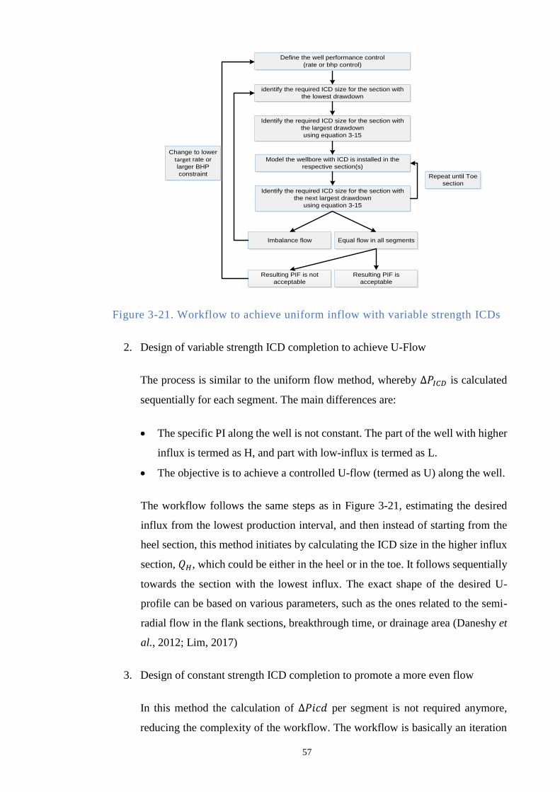
57
Identify the required ICD size for the section with
the largest drawdown
using equation 3-15
Repeat until Toe
section
Model the wellbore with ICD is installed in the
respective section(s)
Define the well performance control
(rate or bhp control)
identify the required ICD size for the section with
the lowest drawdown
Identify the required ICD size for the section with
the next largest drawdown
using equation 3-15
Imbalance flow Equal flow in all segments
Resulting PIF is not
acceptable
Resulting PIF is
acceptable
Change to lower
target rate or
larger BHP
constraint
Figure 3-21. Workflow to achieve uniform inflow with variable strength ICDs
2. Design of variable strength ICD completion to achieve U-Flow
The process is similar to the uniform flow method, whereby ∆𝑃𝐼𝐶𝐷 is calculated
sequentially for each segment. The main differences are:
The specific PI along the well is not constant. The part of the well with higher
influx is termed as H, and part with low-influx is termed as L.
The objective is to achieve a controlled U-flow (termed as U) along the well.
The workflow follows the same steps as in Figure 3-21, estimating the desired
influx from the lowest production interval, and then instead of starting from the
heel section, this method initiates by calculating the ICD size in the higher influx
section, 𝑄𝐻, which could be either in the heel or in the toe. It follows sequentially
towards the section with the lowest influx. The exact shape of the desired U-
profile can be based on various parameters, such as the ones related to the semi-
radial flow in the flank sections, breakthrough time, or drainage area (Daneshy et
al., 2012; Lim, 2017)
3. Design of constant strength ICD completion to promote a more even flow
In this method the calculation of ∆𝑃𝑖𝑐𝑑 per segment is not required anymore,
reducing the complexity of the workflow. The workflow is basically an iteration
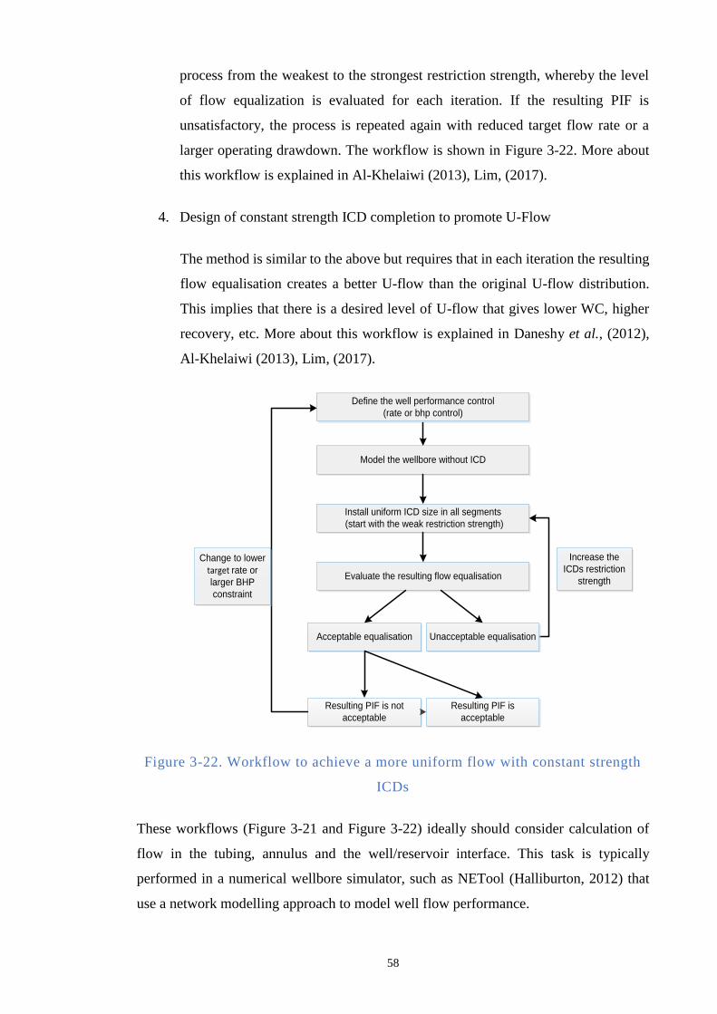
58
process from the weakest to the strongest restriction strength, whereby the level
of flow equalization is evaluated for each iteration. If the resulting PIF is
unsatisfactory, the process is repeated again with reduced target flow rate or a
larger operating drawdown. The workflow is shown in Figure 3-22. More about
this workflow is explained in Al-Khelaiwi (2013), Lim, (2017).
4. Design of constant strength ICD completion to promote U-Flow
The method is similar to the above but requires that in each iteration the resulting
flow equalisation creates a better U-flow than the original U-flow distribution.
This implies that there is a desired level of U-flow that gives lower WC, higher
recovery, etc. More about this workflow is explained in Daneshy et al., (2012),
Al-Khelaiwi (2013), Lim, (2017).
Install uniform ICD size in all segments
(start with the weak restriction strength)
Increase the
ICDs restriction
strength Evaluate the resulting flow equalisation
Define the well performance control
(rate or bhp control)
Model the wellbore without ICD
Acceptable equalisation Unacceptable equalisation
Resulting PIF is not
acceptable
Resulting PIF is
acceptable
Change to lower
target rate or
larger BHP
constraint
Figure 3-22. Workflow to achieve a more uniform flow with constant strength
ICDs
These workflows (Figure 3-21 and Figure 3-22) ideally should consider calculation of
flow in the tubing, annulus and the well/reservoir interface. This task is typically
performed in a numerical wellbore simulator, such as NETool (Halliburton, 2012) that
use a network modelling approach to model well flow performance.

59
An ICD design workflow should find a compromise between the benefits and the
drawbacks of an ICD completion. On one hand, the ICD completion improves the inflow
rate distribution, but on the other it reduces the well’s Productivity Index (PI) by adding
an extra pressure drop. The design’s challenge is to manage this additional pressure drop
without excessively reducing the well’s PI. This relationship requires a reliable method
of estimation. It also needs to be able to answer questions like:
When can the ICD completion add value or is feasibility?
What is the performance forecast of the ICD completed well?
Is there a quick tool or simple rules available for completion redesign to
accommodate for potential operational issues, such as alternative design if the
logging tool revealed a different reservoir permeability or severe loss of
circulation in an interval, etc.?
How to perform verification of numerical simulation results?
How to produce an initial guess design before going to a more details analysis?
Below in this chapter we present an integration of analytical modelling of wells with ICDs
and the type-curve methodology that can be used to design and optimise the ICD
completion. This workflow is simple, requires minimum computational power to analyse
and make the necessary ICD size adjustment based on the latest, more accurate
information from the open-hole logging. The objective follows those suggested by
previous studies (Joshi, 1991; Hill and Zhu, 2008; Birchenko, Usnich and Davies, 2010)
suggested to compose a quick-look analysis of an ICD completion performance.
The proposed methodology will be further evaluated by the wellbore numerical simulator,
NETool, the most widely used platform in the industry for wellbore modelling of an ICD
completed well (Halliburton, 2017). The presented methods will be thoroughly explained
and summarised in a workflow that provides a rapid decision-making tool. The
application of the workflow will be illustrated on a synthetic oil-rim reservoir mimicking
a larger North-Sea oil field. Several scenarios illustrate the range of studies that can be
possible carried out without running a reservoir simulator. A comparison will be made
between the proposed simplified design workflow and the comprehensive results from a
NETool numerical simulation to support this new workflow.
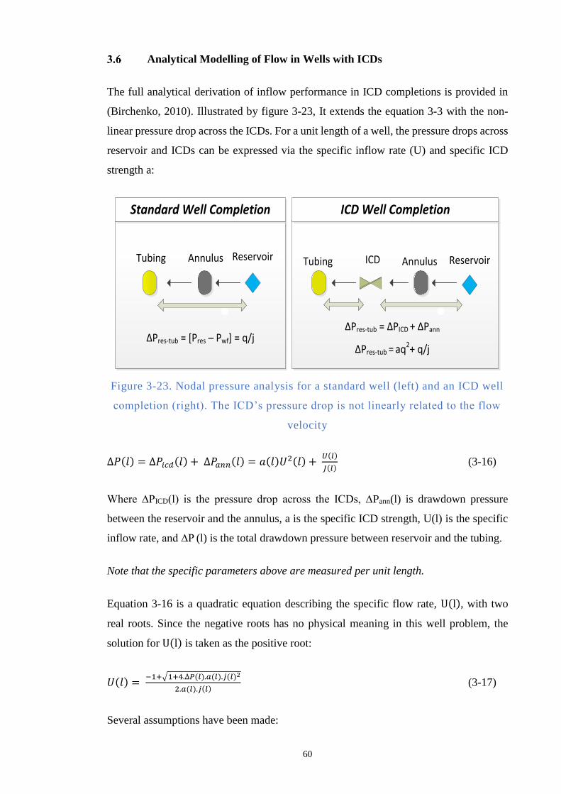
60
Analytical Modelling of Flow in Wells with ICDs
The full analytical derivation of inflow performance in ICD completions is provided in
(Birchenko, 2010). Illustrated by figure 3-23, It extends the equation 3-3 with the non-
linear pressure drop across the ICDs. For a unit length of a well, the pressure drops across
reservoir and ICDs can be expressed via the specific inflow rate (U) and specific ICD
strength a:
ReservoirICDTubingReservoirTubing
Standard Well Completion ICD Well Completion
Annulus Annulus
∆Pres-tub = [Pres – Pwf] = q/j∆Pres-tub = ∆PICD + ∆Pann
∆Pres-tub = aq2+ q/j
Figure 3-23. Nodal pressure analysis for a standard well (left) and an ICD well
completion (right). The ICD’s pressure drop is not linearly related to the flow
velocity
∆𝑃(𝑙) = ∆𝑃𝑖𝑐𝑑(𝑙) + ∆𝑃𝑎𝑛𝑛(𝑙) = 𝑎(𝑙)𝑈2(𝑙) + 𝑈(𝑙)
𝐽(𝑙) (3-16)
Where ∆PICD(l) is the pressure drop across the ICDs, ∆Pann(l) is drawdown pressure
between the reservoir and the annulus, a is the specific ICD strength, U(l) is the specific
inflow rate, and ∆P (l) is the total drawdown pressure between reservoir and the tubing.
Note that the specific parameters above are measured per unit length.
Equation 3-16 is a quadratic equation describing the specific flow rate, U(l), with two
real roots. Since the negative roots has no physical meaning in this well problem, the
solution for U(l) is taken as the positive root:
𝑈(𝑙) = −1+√1+4.∆𝑃(𝑙).𝑎(𝑙).𝑗(𝑙)2
2.𝑎(𝑙).𝑗(𝑙) (3-17)
Several assumptions have been made:
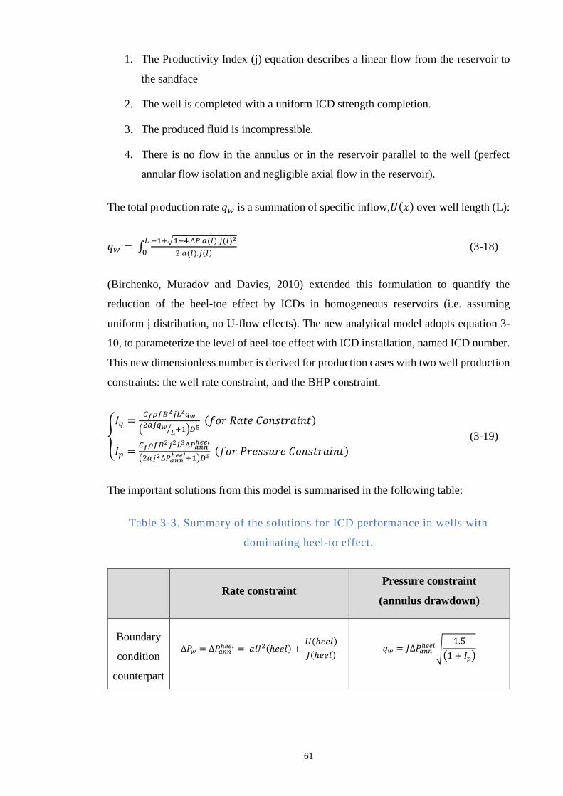
61
1. The Productivity Index (j) equation describes a linear flow from the reservoir to
the sandface
2. The well is completed with a uniform ICD strength completion.
3. The produced fluid is incompressible.
4. There is no flow in the annulus or in the reservoir parallel to the well (perfect
annular flow isolation and negligible axial flow in the reservoir).
The total production rate 𝑞𝑤 is a summation of specific inflow,𝑈(𝑥) over well length (L):
𝑞𝑤 = ∫−1+√1+4.∆𝑃.𝑎(𝑙).𝑗(𝑙)2
2.𝑎(𝑙).𝑗(𝑙)
𝐿
0 (3-18)
(Birchenko, Muradov and Davies, 2010) extended this formulation to quantify the
reduction of the heel-toe effect by ICDs in homogeneous reservoirs (i.e. assuming
uniform j distribution, no U-flow effects). The new analytical model adopts equation 3-
10, to parameterize the level of heel-toe effect with ICD installation, named ICD number.
This new dimensionless number is derived for production cases with two well production
constraints: the well rate constraint, and the BHP constraint.
𝐼𝑞 =𝐶𝑓𝜌𝑓𝐵
2𝑗𝐿2𝑞𝑤
(2𝑎𝑗𝑞𝑤
𝐿⁄ +1)𝐷5 (𝑓𝑜𝑟 𝑅𝑎𝑡𝑒 𝐶𝑜𝑛𝑠𝑡𝑟𝑎𝑖𝑛𝑡)
𝐼𝑝 =𝐶𝑓𝜌𝑓𝐵
2𝑗2𝐿3∆𝑃𝑎𝑛𝑛ℎ𝑒𝑒𝑙
(2𝑎𝑗2∆𝑃𝑎𝑛𝑛ℎ𝑒𝑒𝑙+1)𝐷5
(𝑓𝑜𝑟 𝑃𝑟𝑒𝑠𝑠𝑢𝑟𝑒 𝐶𝑜𝑛𝑠𝑡𝑟𝑎𝑖𝑛𝑡)
(3-19)
The important solutions from this model is summarised in the following table:
Table 3-3. Summary of the solutions for ICD performance in wells with
dominating heel-to effect.
Rate constraint Pressure constraint
(annulus drawdown)
Boundary
condition
counterpart
∆𝑃𝑤 = ∆𝑃𝑎𝑛𝑛ℎ𝑒𝑒𝑙 = 𝑎𝑈2(ℎ𝑒𝑒𝑙) +
𝑈(ℎ𝑒𝑒𝑙)
𝐽(ℎ𝑒𝑒𝑙) 𝑞𝑤 = 𝐽∆𝑃𝑎𝑛𝑛
ℎ𝑒𝑒𝑙√1.5
(1 + 𝐼𝑝)
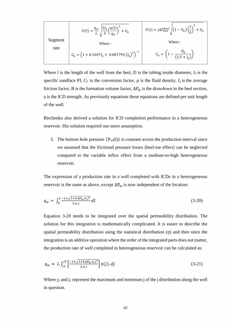
62
Segment
rate
𝑈(𝑙) =𝑞𝑤𝐿√2𝐼𝑞
3(𝑞(𝑙)
𝑞𝑤)
3
+ 𝐺𝑞
Where :
𝐺𝑞 ≈ (1 + 0.1647𝐼𝑞 + 0.001793 (𝐼𝑞)2)−1
𝑈(𝑙) = 𝑗∆𝑃𝑎𝑛𝑛ℎ𝑒𝑒𝑙√(1 − 𝐺𝑝) (
𝑙
𝐿)3
+ 𝐺𝑝
Where :
𝐶𝑞 ≈ (1 − 𝐻𝑝
(1.5 + 𝐼𝑝))
Where l is the length of the well from the heel, D is the tubing inside diameter, Js is the
specific sandface PI, Cf is the conversion factor, ρ is the fluid density, fa is the average
friction factor, B is the formation volume factor, ∆Pw is the drawdown in the heel section,
a is the ICD strength. As previously equations these equations are defined per unit length
of the well.
Birchenko also derived a solution for ICD completion performance in a heterogeneous
reservoir. His solution required one more assumption.
5. The bottom hole pressure Pwf(l) is constant across the production interval since
we assumed that the frictional pressure losses (heel-toe effect) can be neglected
compared to the variable influx effect from a medium-to-high heterogeneous
reservoir.
The expression of a production rate in a well completed with ICDs in a heterogeneous
reservoir is the same as above, except ∆Pw is now independent of the location:
𝑞𝑤 = ∫−1+√1+4.∆𝑃𝑤.𝑎.𝑗2
2.𝑎.𝑗𝑑𝑙
𝐿
0 (3-20)
Equation 3-20 needs to be integrated over the spatial permeability distribution. The
solution for this integration is mathematically complicated. It is easier to describe the
spatial permeability distribution using the statistical distribution (𝜂) and then since the
integration is an additive operation where the order of the integrated parts does not matter,
the production rate of well completed in heterogeneous reservoir can be calculated as:
𝑞𝑤 = 𝐿 ∫ −1+√1+4.∆𝑃𝑤.𝑎.𝑗2
2.𝑎.𝑗 𝜂(𝑗). 𝑑𝑗
𝑗2
𝑗1 (3-21)
Where j2 and j1 represent the maximum and minimum j of the j distribution along the well
in question.
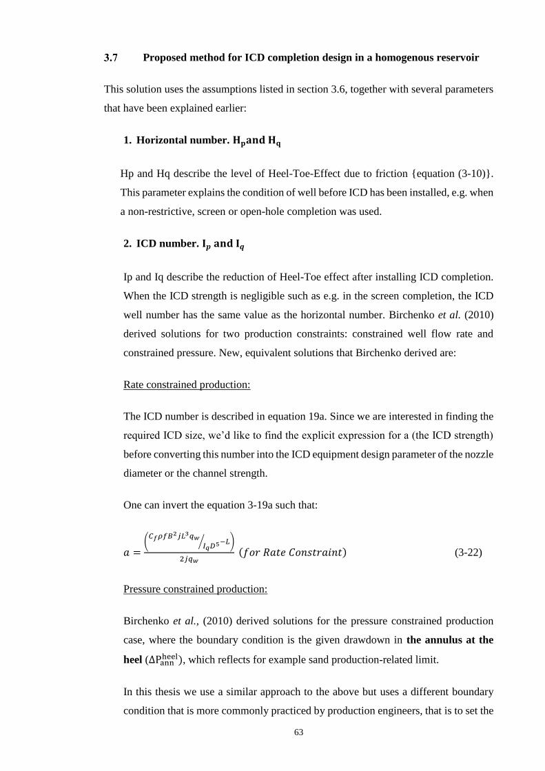
63
Proposed method for ICD completion design in a homogenous reservoir
This solution uses the assumptions listed in section 3.6, together with several parameters
that have been explained earlier:
1. Horizontal number. 𝐇𝐩𝐚𝐧𝐝 𝐇𝐪
Hp and Hq describe the level of Heel-Toe-Effect due to friction equation (3-10).
This parameter explains the condition of well before ICD has been installed, e.g. when
a non-restrictive, screen or open-hole completion was used.
2. ICD number. 𝐈𝒑 𝐚𝐧𝐝 𝐈𝒒
Ip and Iq describe the reduction of Heel-Toe effect after installing ICD completion.
When the ICD strength is negligible such as e.g. in the screen completion, the ICD
well number has the same value as the horizontal number. Birchenko et al. (2010)
derived solutions for two production constraints: constrained well flow rate and
constrained pressure. New, equivalent solutions that Birchenko derived are:
Rate constrained production:
The ICD number is described in equation 19a. Since we are interested in finding the
required ICD size, we’d like to find the explicit expression for a (the ICD strength)
before converting this number into the ICD equipment design parameter of the nozzle
diameter or the channel strength.
One can invert the equation 3-19a such that:
𝑎 =(𝐶𝑓𝜌𝑓𝐵
2𝑗𝐿3𝑞𝑤𝐼𝑞𝐷5⁄ −𝐿)
2𝑗𝑞𝑤 (𝑓𝑜𝑟 𝑅𝑎𝑡𝑒 𝐶𝑜𝑛𝑠𝑡𝑟𝑎𝑖𝑛𝑡) (3-22)
Pressure constrained production:
Birchenko et al., (2010) derived solutions for the pressure constrained production
case, where the boundary condition is the given drawdown in the annulus at the
heel (∆Pannheel), which reflects for example sand production-related limit.
In this thesis we use a similar approach to the above but uses a different boundary
condition that is more commonly practiced by production engineers, that is to set the

64
minimum wellbore flowing pressure in the tubing (Pwf) at the heel as the boundary
condition. For example, this is needed in order to be able to lift the fluids to surface.
One novelty of this chapter is that the well will now be constrained by the total
drawdown between the reservoir pressure and the tubing flowing pressure, ∆𝐏𝐰.
A solution for this condition is derived as follows:
- Recall the ICD number for pressure constrained well described in equation 19b
- Substitute ∆Pannheel with equation 3-16 & 3-17:
∆𝑃𝑎𝑛𝑛ℎ𝑒𝑒𝑙 = ∆𝑃𝑤 −
(√1+𝛼∆𝑃𝑤−1)2
𝛼 (3-23)
We can now write the new ICD number for the tubing pressure constrained well:
𝐼𝑝 = 𝐶𝑓𝜌𝑓𝐵
2𝑗2𝐿3(∆𝑃𝑤−(√1+𝛼∆𝑃𝑤−1)
2
𝛼)
√1+𝛼∆𝑃𝑤 𝐷5 (3-24)
Where 𝛼 = 4𝑎𝑗2
The relationship between the ICD strength (a) and ICD number in the pressure
constraint scenario (Ip) is non-linear and requires simplification. This was not
required for the rate constrained solutions.
Equation 3-19b can be modified such that∶
𝛽 ≡ 2(𝑎 +1
2𝑗2∆𝑃𝑎𝑛𝑛ℎ𝑒𝑒𝑙)
Where the 𝛽 =𝐶𝑓𝜌𝑓𝐵
2𝐿3
𝐼𝑝𝐷5
We can now write equation 3-19b as:
𝛽 ≡2𝑎√1 + 4𝑎𝑗2∆𝑃𝑤
(√1 + 4𝑎𝑗2∆𝑃𝑤 − 1)
The solution can be simplified and formed as a cubic equation:
(16𝑗2∆𝑃𝑤)𝑎3 + (4 − 16𝑗2∆𝑃𝑤𝛽)𝑎
2 + (4𝑗2∆𝑃𝑤𝛼2 − 4𝛽)𝑎 = 0
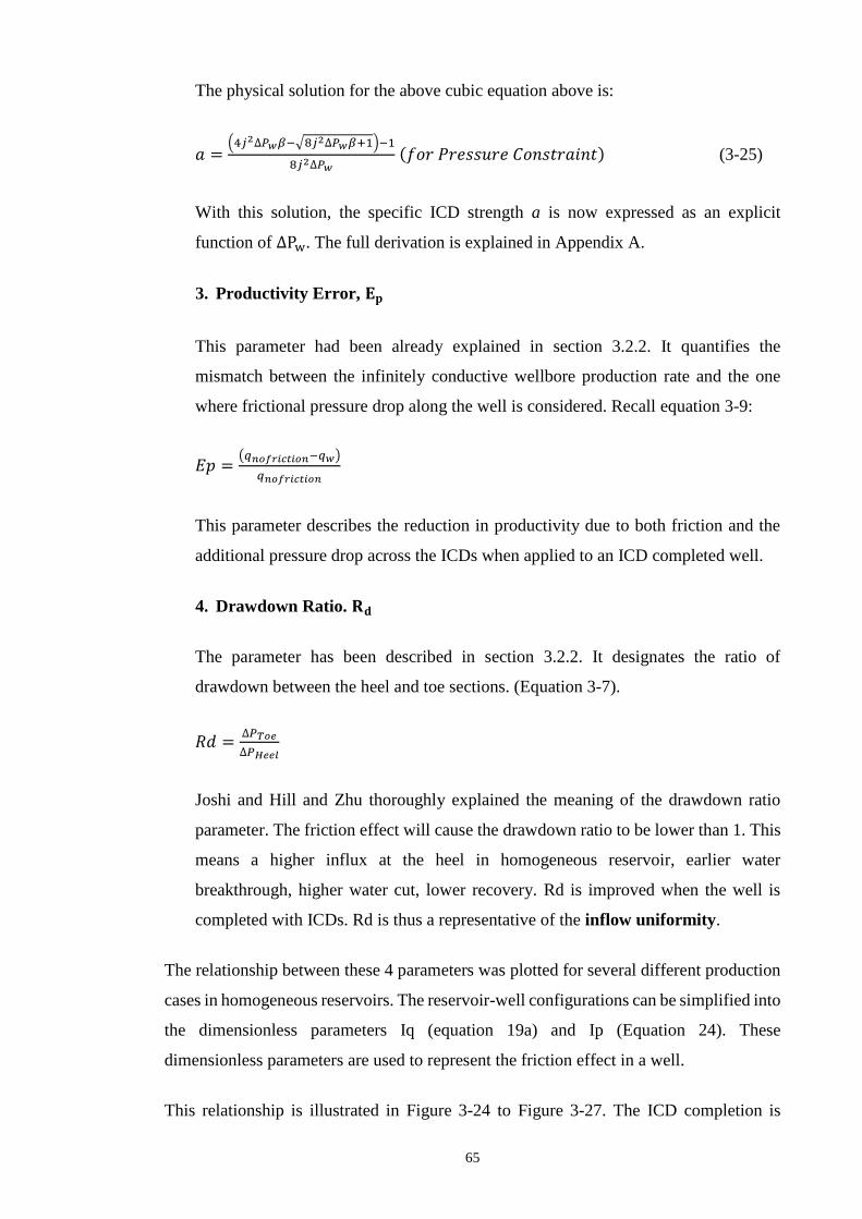
65
The physical solution for the above cubic equation above is:
𝑎 =(4𝑗2∆𝑃𝑤𝛽−√8𝑗2∆𝑃𝑤𝛽+1)−1
8𝑗2∆𝑃𝑤 (𝑓𝑜𝑟 𝑃𝑟𝑒𝑠𝑠𝑢𝑟𝑒 𝐶𝑜𝑛𝑠𝑡𝑟𝑎𝑖𝑛𝑡) (3-25)
With this solution, the specific ICD strength a is now expressed as an explicit
function of ∆Pw. The full derivation is explained in Appendix A.
3. Productivity Error, 𝐄𝐩
This parameter had been already explained in section 3.2.2. It quantifies the
mismatch between the infinitely conductive wellbore production rate and the one
where frictional pressure drop along the well is considered. Recall equation 3-9:
𝐸𝑝 =(𝑞𝑛𝑜𝑓𝑟𝑖𝑐𝑡𝑖𝑜𝑛−𝑞𝑤)
𝑞𝑛𝑜𝑓𝑟𝑖𝑐𝑡𝑖𝑜𝑛
This parameter describes the reduction in productivity due to both friction and the
additional pressure drop across the ICDs when applied to an ICD completed well.
4. Drawdown Ratio. 𝐑𝐝
The parameter has been described in section 3.2.2. It designates the ratio of
drawdown between the heel and toe sections. (Equation 3-7).
𝑅𝑑 =∆𝑃𝑇𝑜𝑒
∆𝑃𝐻𝑒𝑒𝑙
Joshi and Hill and Zhu thoroughly explained the meaning of the drawdown ratio
parameter. The friction effect will cause the drawdown ratio to be lower than 1. This
means a higher influx at the heel in homogeneous reservoir, earlier water
breakthrough, higher water cut, lower recovery. Rd is improved when the well is
completed with ICDs. Rd is thus a representative of the inflow uniformity.
The relationship between these 4 parameters was plotted for several different production
cases in homogeneous reservoirs. The reservoir-well configurations can be simplified into
the dimensionless parameters Iq (equation 19a) and Ip (Equation 24). These
dimensionless parameters are used to represent the friction effect in a well.
This relationship is illustrated in Figure 3-24 to Figure 3-27. The ICD completion is
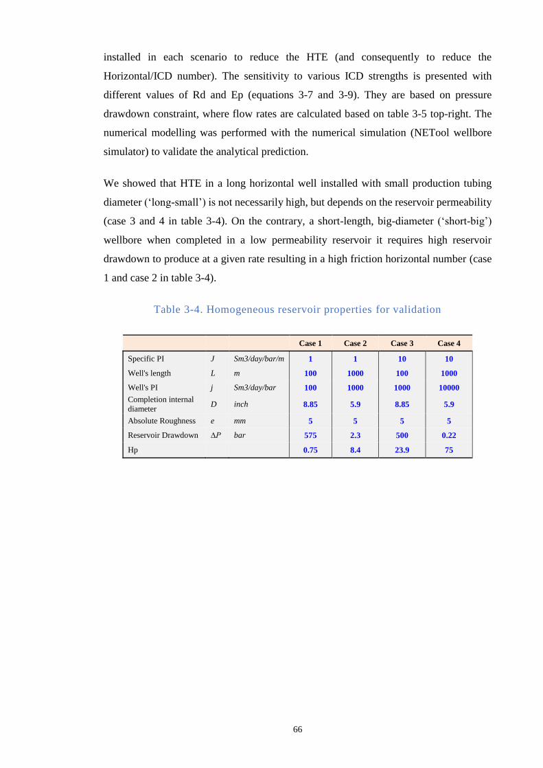
66
installed in each scenario to reduce the HTE (and consequently to reduce the
Horizontal/ICD number). The sensitivity to various ICD strengths is presented with
different values of Rd and Ep (equations 3-7 and 3-9). They are based on pressure
drawdown constraint, where flow rates are calculated based on table 3-5 top-right. The
numerical modelling was performed with the numerical simulation (NETool wellbore
simulator) to validate the analytical prediction.
We showed that HTE in a long horizontal well installed with small production tubing
diameter (‘long-small’) is not necessarily high, but depends on the reservoir permeability
(case 3 and 4 in table 3-4). On the contrary, a short-length, big-diameter (‘short-big’)
wellbore when completed in a low permeability reservoir it requires high reservoir
drawdown to produce at a given rate resulting in a high friction horizontal number (case
1 and case 2 in table 3-4).
Table 3-4. Homogeneous reservoir properties for validation
Case 1 Case 2 Case 3 Case 4
Specific PI J Sm3/day/bar/m 1 1 10 10
Well's length L m 100 1000 100 1000
Well's PI j Sm3/day/bar 100 1000 1000 10000
Completion internal
diameter D inch 8.85 5.9 8.85 5.9
Absolute Roughness e mm 5 5 5 5
Reservoir Drawdown ∆P bar 575 2.3 500 0.22
Hp 0.75 8.4 23.9 75
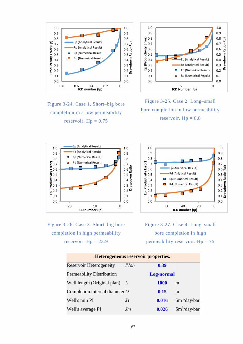
67
Figure 3-24. Case 1. Short–big bore
completion in a low permeability
reservoir. Hp = 0.75
Figure 3-25. Case 2. Long–small
bore completion in low permeability
reservoir. Hp = 8.8
Figure 3-26. Case 3. Short–big bore
completion in high permeability
reservoir. Hp = 23.9
Figure 3-27. Case 4. Long–small
bore completion in high
permeability reservoir. Hp = 75
Heterogeneous reservoir properties.
Reservoir Heterogeneity IVoh 0.39
Permeability Distribution
Log-normal
Well length (Original plan) L 1000 m
Completion internal diameter D 0.15 m
Well's min PI J1 0.016 Sm3/day/bar
Well's average PI Jm 0.026 Sm3/day/bar
0.0
0.1
0.2
0.3
0.4
0.5
0.6
0.7
0.8
0.9
1.0
0.0
0.1
0.2
0.3
0.4
0.5
0.6
0.7
0.8
0.9
1.0
00.20.40.60.8
Dra
wd
ow
n R
atio
(R
d)
Pro
du
ctiv
ity
Erro
r (E
p)
ICD number (Ip)
Ep (Analytical Result)
Rd (Analytical Result)
Ep (Numerical Result)
Rd (Numerical Result)
0.0
0.1
0.2
0.3
0.4
0.5
0.6
0.7
0.8
0.9
1.0
0.0
0.1
0.2
0.3
0.4
0.5
0.6
0.7
0.8
0.9
1.0
05
Dra
wd
ow
n R
atio
(R
d)
Ep (
Pro
du
ctiv
ity
Erro
r)
ICD Number (Ip)
Ep (Analytical Result)
Rd (Analytical Result)
Ep (Numerical Result)
Rd (Numerical Result)
0.0
0.1
0.2
0.3
0.4
0.5
0.6
0.7
0.8
0.9
1.0
0.0
0.1
0.2
0.3
0.4
0.5
0.6
0.7
0.8
0.9
1.0
01020
Dra
wd
ow
n R
atio
Ep (
Pro
du
ctiv
ity
Erro
r)
ICD number (Ip)
Ep (Analytical Result)
Rd (Analytical Result)
Ep (Numerical Result)
Rd (Numerical Result)
0.0
0.1
0.2
0.3
0.4
0.5
0.6
0.7
0.8
0.9
1.0
0.0
0.1
0.2
0.3
0.4
0.5
0.6
0.7
0.8
0.9
1.0
0204060
Dra
wd
ow
n R
atio
(R
d)
Ep (
Pro
du
ctiv
ity
Erro
r)
ICD number (Ip)
Ep (Analytical Result)
Rd (Anlytical Result)
Ep (Numerical Result)
Rd (Numerical Result)
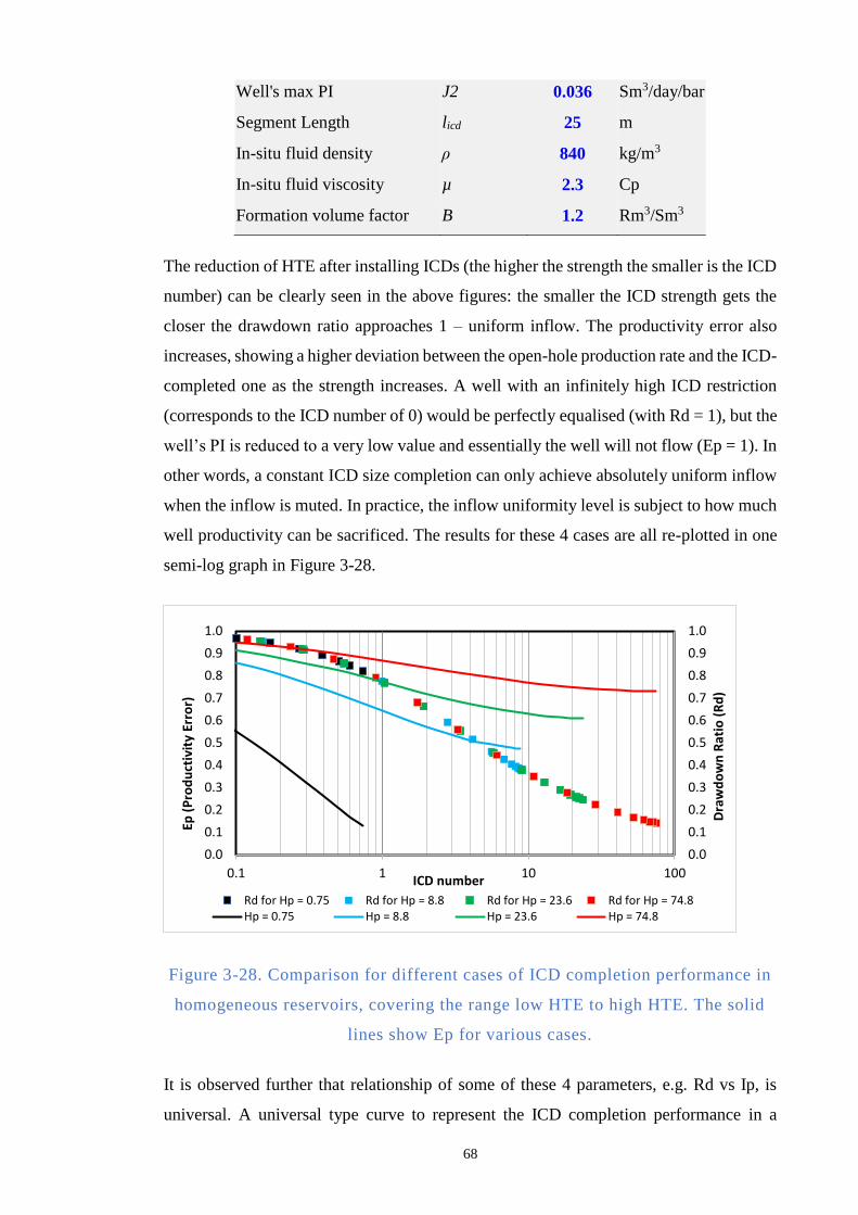
68
Well's max PI J2 0.036 Sm3/day/bar
Segment Length licd 25 m
In-situ fluid density ρ 840 kg/m3
In-situ fluid viscosity µ 2.3 Cp
Formation volume factor B 1.2 Rm3/Sm3
The reduction of HTE after installing ICDs (the higher the strength the smaller is the ICD
number) can be clearly seen in the above figures: the smaller the ICD strength gets the
closer the drawdown ratio approaches 1 – uniform inflow. The productivity error also
increases, showing a higher deviation between the open-hole production rate and the ICD-
completed one as the strength increases. A well with an infinitely high ICD restriction
(corresponds to the ICD number of 0) would be perfectly equalised (with Rd = 1), but the
well’s PI is reduced to a very low value and essentially the well will not flow (Ep = 1). In
other words, a constant ICD size completion can only achieve absolutely uniform inflow
when the inflow is muted. In practice, the inflow uniformity level is subject to how much
well productivity can be sacrificed. The results for these 4 cases are all re-plotted in one
semi-log graph in Figure 3-28.
Figure 3-28. Comparison for different cases of ICD completion performance in
homogeneous reservoirs, covering the range low HTE to high HTE. The solid
lines show Ep for various cases.
It is observed further that relationship of some of these 4 parameters, e.g. Rd vs Ip, is
universal. A universal type curve to represent the ICD completion performance in a
0.0
0.1
0.2
0.3
0.4
0.5
0.6
0.7
0.8
0.9
1.0
0.0
0.1
0.2
0.3
0.4
0.5
0.6
0.7
0.8
0.9
1.0
0.1 1 10 100
Dra
wd
ow
n R
atio
(R
d)
Ep (
Pro
du
ctiv
ity
Erro
r)
ICD number
Rd for Hp = 0.75 Rd for Hp = 8.8 Rd for Hp = 23.6 Rd for Hp = 74.8Hp = 0.75 Hp = 8.8 Hp = 23.6 Hp = 74.8
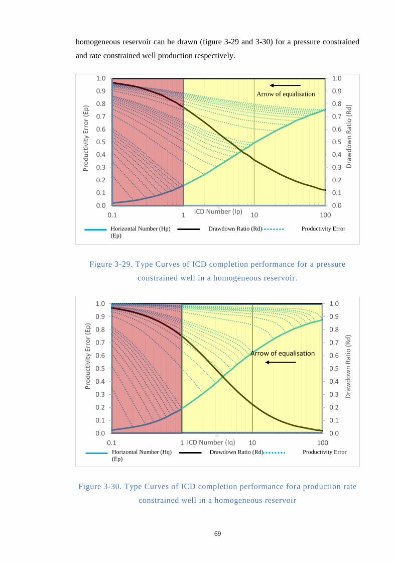
69
homogeneous reservoir can be drawn (figure 3-29 and 3-30) for a pressure constrained
and rate constrained well production respectively.
Figure 3-29. Type Curves of ICD completion performance for a pressure
constrained well in a homogeneous reservoir.
Figure 3-30. Type Curves of ICD completion performance fora production rate
constrained well in a homogeneous reservoir
0.0
0.1
0.2
0.3
0.4
0.5
0.6
0.7
0.8
0.9
1.0
0.0
0.1
0.2
0.3
0.4
0.5
0.6
0.7
0.8
0.9
1.0
0.1 1 10 100
Dra
wd
ow
n R
atio
(R
d)
Pro
du
ctiv
ity
Erro
r (E
p)
ICD Number (Ip)
0.0
0.1
0.2
0.3
0.4
0.5
0.6
0.7
0.8
0.9
1.0
0.0
0.1
0.2
0.3
0.4
0.5
0.6
0.7
0.8
0.9
1.0
0.1 1 10 100
Dra
wd
ow
n R
atio
(R
d)
Pro
du
ctiv
ity
Erro
r (E
p)
ICD Number (Iq)
Horizontal Number (Hp) Drawdown Ratio (Rd) Productivity Error
(Ep)
Horizontal Number (Hq) Drawdown Ratio (Rd) Productivity Error
(Ep)
Arrow of equalisation
Arrow of equalisation
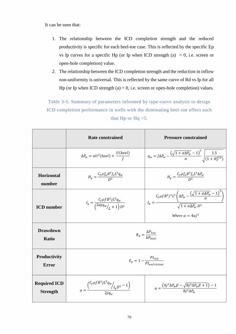
70
It can be seen that:
1. The relationship between the ICD completion strength and the reduced
productivity is specific for each heel-toe case. This is reflected by the specific Ep
vs Ip curves for a specific Hp (or Ip when ICD strength (a) = 0, i.e. screen or
open-hole completion) value.
2. The relationship between the ICD completion strength and the reduction in inflow
non-uniformity is universal. This is reflected by the same curve of Rd vs Ip for all
Hp (or Ip when ICD strength (a) = 0, i.e. screen or open-hole completion) values.
Table 3-5. Summary of parameters informed by type-curve analysis to design
ICD completion performance in wells with the dominating heel -toe effect such
that Hp or Hq >5.
Rate constrained Pressure constrained
∆𝑃𝑤 = 𝑎𝑈2(ℎ𝑒𝑒𝑙) +
𝑈(ℎ𝑒𝑒𝑙)
𝐽 𝑞𝑤 = 𝐽∆𝑃𝑤 −
(√1 + 𝛼∆𝑃𝑤 − 1)2
𝛼√
1.5
(1 + 𝐻𝑃𝐼𝐶𝐷)
Horizontal
number
𝐻𝑞 =𝐶𝑓𝜌𝑓𝑎𝐵
2𝐽𝑠𝐿2𝑞𝑤
𝐷5 𝐻𝑝 =
𝐶𝑓𝜌𝑓𝑎𝐵2𝐽𝑠𝐿
3∆𝑃𝑤
𝐷5
ICD number 𝐼𝑞 =
𝐶𝑓𝜌𝑓𝐵2𝑗𝐿2𝑞𝑤
(2𝑎𝑗𝑞𝑤
𝐿⁄ + 1)𝐷5 𝐼𝑝 =
𝐶𝑓𝜌𝑓𝐵2𝑗2𝐿3 (∆𝑃𝑤 −
(√1 + 𝛼∆𝑃𝑤 − 1)2
𝛼)
√1 + 𝛼∆𝑃𝑤 𝐷5
Where 𝛼 = 4𝑎𝑗2
Drawdown
Ratio 𝑅𝑑 =
∆𝑃𝑇𝑜𝑒∆𝑃𝐻𝑒𝑒𝑙
Productivity
Error 𝐸𝑝 = 1 −
𝑃𝐼𝐼𝐶𝐷𝑃𝐼𝑛𝑜𝑓𝑟𝑖𝑐𝑡𝑖𝑜𝑛
Required ICD
Strength 𝑎 =
(𝐶𝑓𝜌𝑓𝐵
2𝑗𝐿3𝑞𝑤𝐼𝑞𝐷
5⁄ − 𝐿)
2𝑗𝑞𝑤 𝑎 =
(4𝑗2∆𝑃𝑤𝛽 − √8𝑗2∆𝑃𝑤𝛽 + 1) − 1
8𝑗2∆𝑃𝑤
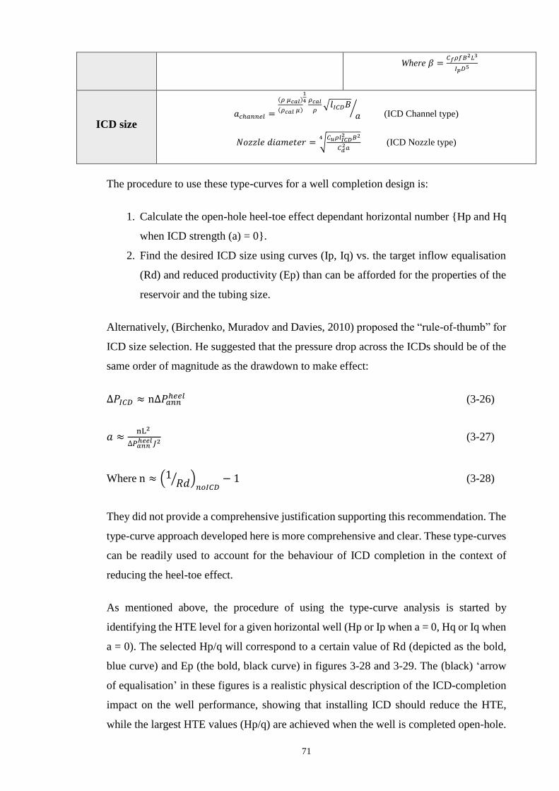
71
Where 𝛽 =𝐶𝑓𝜌𝑓𝐵
2𝐿3
𝐼𝑝𝐷5
ICD size 𝑎𝑐ℎ𝑎𝑛𝑛𝑒𝑙 =
(𝜌 𝜇𝑐𝑎𝑙)
(𝜌𝑐𝑎𝑙 𝜇)
1
4 𝜌𝑐𝑎𝑙
𝜌√𝑙𝐼𝐶𝐷𝐵
𝑎⁄
(ICD Channel type)
𝑁𝑜𝑧𝑧𝑙𝑒 𝑑𝑖𝑎𝑚𝑒𝑡𝑒𝑟 = √𝐶𝑢𝜌𝑙𝐼𝐶𝐷
2 𝐵2
𝐶𝑑2𝑎
4 (ICD Nozzle type)
The procedure to use these type-curves for a well completion design is:
1. Calculate the open-hole heel-toe effect dependant horizontal number Hp and Hq
when ICD strength (a) = 0.
2. Find the desired ICD size using curves (Ip, Iq) vs. the target inflow equalisation
(Rd) and reduced productivity (Ep) than can be afforded for the properties of the
reservoir and the tubing size.
Alternatively, (Birchenko, Muradov and Davies, 2010) proposed the “rule-of-thumb” for
ICD size selection. He suggested that the pressure drop across the ICDs should be of the
same order of magnitude as the drawdown to make effect:
∆𝑃𝐼𝐶𝐷 ≈ n∆𝑃𝑎𝑛𝑛ℎ𝑒𝑒𝑙 (3-26)
𝑎 ≈nL2
∆𝑃𝑎𝑛𝑛ℎ𝑒𝑒𝑙𝐽2
(3-27)
Where n ≈ (1 𝑅𝑑⁄ )𝑛𝑜𝐼𝐶𝐷
− 1 (3-28)
They did not provide a comprehensive justification supporting this recommendation. The
type-curve approach developed here is more comprehensive and clear. These type-curves
can be readily used to account for the behaviour of ICD completion in the context of
reducing the heel-toe effect.
As mentioned above, the procedure of using the type-curve analysis is started by
identifying the HTE level for a given horizontal well (Hp or Ip when a = 0, Hq or Iq when
a = 0). The selected Hp/q will correspond to a certain value of Rd (depicted as the bold,
blue curve) and Ep (the bold, black curve) in figures 3-28 and 3-29. The (black) ‘arrow
of equalisation’ in these figures is a realistic physical description of the ICD-completion
impact on the well performance, showing that installing ICD should reduce the HTE,
while the largest HTE values (Hp/q) are achieved when the well is completed open-hole.

72
Once the Rd and Ep intersection points have been established, one should follow the curve
of Rd and dashed blue curve of Ep for the given Hp/q to evaluate the trade-off between
the inflow equalisation and the reduction in the well’s PI due to installing ICDs. Note that
the dashed-blue curves of Ep are unique for different Hp/q values (every Hp/q has its
signature Ep curve) while the bold-black curve of Rd is universal for all Hp/q values.
This type-curve allows one to perform analysis needed for ICD completion design
optimisation.
Take a look at the yellow region in figure 3-28:
Take the slope of Rd curve, that is Rd value after installing ICD (RdICD), or the
intersection point of the Rd (bolded-black) curve against the ICD number (Ip/q)
minus the original Rd value in the open-hole well (RdOH) or the intersection point
of the Rd (bolded-black) curve against the Horizontal number (Hp/q), or ICD
number when a = 0.
Take the slope of Ep curve, that is Ep value after installing ICD (EpICD) or the
intersection point of the EpICD (dashed-blue Curve) against the ICD number
(Ip/q) minus the original Ep value in the open-hole well (EpOH) the intersection
point of the bolded-blue curve (Ep Curve) against the Horizontal number or ICD
number when a = 0 (Hp/q).
We define that efficient flow equalisation is when the long-term gain, indicated
by the flow distribution improvement represented by an increasing Rd, can offset
its short-term cost, indicated by the reduction of well’s PI represented by an
increased Ep. That is: (𝑅𝑑𝐼𝐶𝐷 − 𝑅𝑑𝑂𝐻) ≥ (𝐸𝑝𝐼𝐶𝐷 − 𝐸𝑝𝑂𝐻). Efficient equalisation
is covered within this yellow-shaded area.
Take a look at the red region in figure 3-28:
In this region, the slope of Rd curve is (generally) smaller than the slope of the Ep
curve. In other words, the long-term gain indicated by the reduction of Ep is
obtained in the expense of larger reduction of well’s PI (or increased Ep).
(𝑅𝑑𝐼𝐶𝐷 − 𝑅𝑑𝑂𝐻) < (𝐸𝑝𝐼𝐶𝐷 − 𝐸𝑝𝑂𝐻). Inefficient equalisation region is shown by
this red-shaded area.
Note that the threshold value for (In)efficient equalisation, Ip = 1 is chosen as a
practical purpose to ease the use of this type-curve. More accurate calculation can
be obtained by solving the mathematical models presented in appendix A.
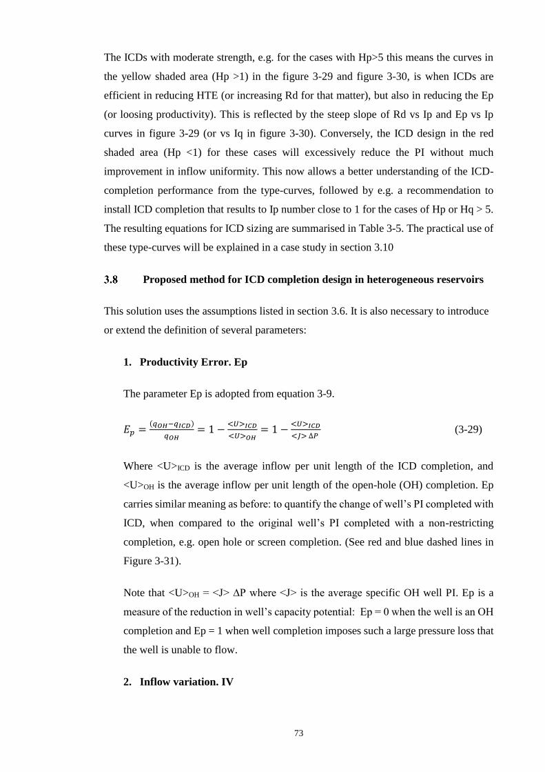
73
The ICDs with moderate strength, e.g. for the cases with Hp>5 this means the curves in
the yellow shaded area (Hp >1) in the figure 3-29 and figure 3-30, is when ICDs are
efficient in reducing HTE (or increasing Rd for that matter), but also in reducing the Ep
(or loosing productivity). This is reflected by the steep slope of Rd vs Ip and Ep vs Ip
curves in figure 3-29 (or vs Iq in figure 3-30). Conversely, the ICD design in the red
shaded area (Hp <1) for these cases will excessively reduce the PI without much
improvement in inflow uniformity. This now allows a better understanding of the ICD-
completion performance from the type-curves, followed by e.g. a recommendation to
install ICD completion that results to Ip number close to 1 for the cases of Hp or Hq > 5.
The resulting equations for ICD sizing are summarised in Table 3-5. The practical use of
these type-curves will be explained in a case study in section 3.10
Proposed method for ICD completion design in heterogeneous reservoirs
This solution uses the assumptions listed in section 3.6. It is also necessary to introduce
or extend the definition of several parameters:
1. Productivity Error. Ep
The parameter Ep is adopted from equation 3-9.
𝐸𝑝 =(𝑞𝑂𝐻−𝑞𝐼𝐶𝐷)
𝑞𝑂𝐻= 1 −
<𝑈>𝐼𝐶𝐷
<𝑈>𝑂𝐻= 1 −
<𝑈>𝐼𝐶𝐷
<𝐽> ∆𝑃 (3-29)
Where <U>ICD is the average inflow per unit length of the ICD completion, and
<U>OH is the average inflow per unit length of the open-hole (OH) completion. Ep
carries similar meaning as before: to quantify the change of well’s PI completed with
ICD, when compared to the original well’s PI completed with a non-restricting
completion, e.g. open hole or screen completion. (See red and blue dashed lines in
Figure 3-31).
Note that <U>OH = <J> ∆P where <J> is the average specific OH well PI. Ep is a
measure of the reduction in well’s capacity potential: Ep = 0 when the well is an OH
completion and Ep = 1 when well completion imposes such a large pressure loss that
the well is unable to flow.
2. Inflow variation. IV
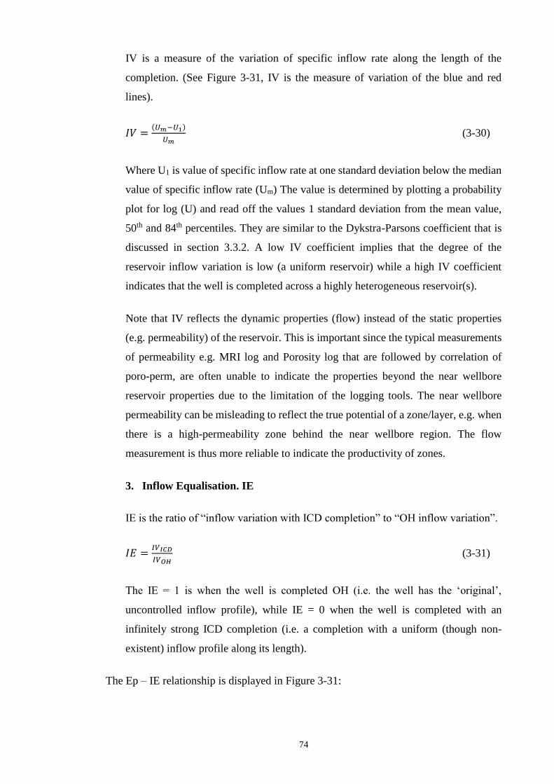
74
IV is a measure of the variation of specific inflow rate along the length of the
completion. (See Figure 3-31, IV is the measure of variation of the blue and red
lines).
𝐼𝑉 =(𝑈𝑚−𝑈1)
𝑈𝑚 (3-30)
Where U1 is value of specific inflow rate at one standard deviation below the median
value of specific inflow rate (Um) The value is determined by plotting a probability
plot for log (U) and read off the values 1 standard deviation from the mean value,
50th and 84th percentiles. They are similar to the Dykstra-Parsons coefficient that is
discussed in section 3.3.2. A low IV coefficient implies that the degree of the
reservoir inflow variation is low (a uniform reservoir) while a high IV coefficient
indicates that the well is completed across a highly heterogeneous reservoir(s).
Note that IV reflects the dynamic properties (flow) instead of the static properties
(e.g. permeability) of the reservoir. This is important since the typical measurements
of permeability e.g. MRI log and Porosity log that are followed by correlation of
poro-perm, are often unable to indicate the properties beyond the near wellbore
reservoir properties due to the limitation of the logging tools. The near wellbore
permeability can be misleading to reflect the true potential of a zone/layer, e.g. when
there is a high-permeability zone behind the near wellbore region. The flow
measurement is thus more reliable to indicate the productivity of zones.
3. Inflow Equalisation. IE
IE is the ratio of “inflow variation with ICD completion” to “OH inflow variation”.
𝐼𝐸 =𝐼𝑉𝐼𝐶𝐷
𝐼𝑉𝑂𝐻 (3-31)
The IE = 1 is when the well is completed OH (i.e. the well has the ‘original’,
uncontrolled inflow profile), while IE = 0 when the well is completed with an
infinitely strong ICD completion (i.e. a completion with a uniform (though non-
existent) inflow profile along its length).
The Ep – IE relationship is displayed in Figure 3-31:
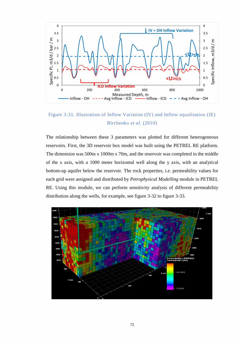
75
Figure 3-31. Illustration of Inflow Variation (IV) and Inflow equalisation (IE)
Birchenko et al. (2010)
The relationship between these 3 parameters was plotted for different heterogeneous
reservoirs. First, the 3D reservoir box model was built using the PETREL RE platform.
The dimension was 500m x 1000m x 70m, and the reservoir was completed in the middle
of the x axis, with a 1000 meter horizontal well along the y axis, with an analytical
bottom-up aquifer below the reservoir. The rock properties, i.e. permeability values for
each grid were assigned and distributed by Petrophysical Modelling module in PETREL
RE. Using this module, we can perform sensitivity analysis of different permeability
distribution along the wells, for example, see figure 3-32 to figure 3-33.
0
0.5
1
1.5
2
2.5
3
3.5
4
0
0.5
1
1.5
2
2.5
3
3.5
4
0 200 400 600 800 1000
Spec
ific
Infl
ow
, m3
/d /
m
Spec
ific
PI,
m3
/d /
bar
/ m
Measured Depth, mInflow - OH Avg Inflow - ICD Inflow - ICD Avg Inflow - OH
d
IV = OH Inflow Variation
ICD Inflow Variation
<U>OH
<U>ICD
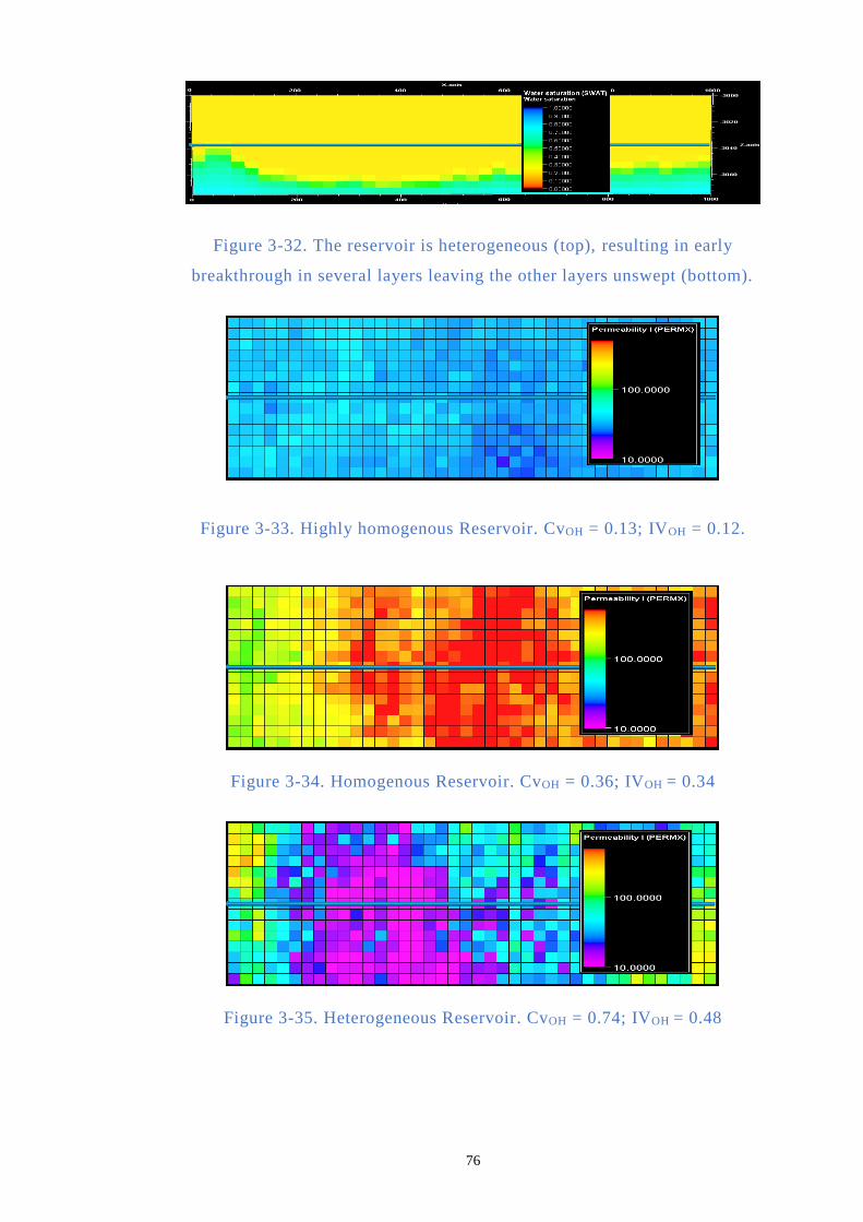
76
Figure 3-32. The reservoir is heterogeneous (top), resulting in early
breakthrough in several layers leaving the other layers unswept (bottom).
Figure 3-33. Highly homogenous Reservoir. CvOH = 0.13; IVOH = 0.12.
Figure 3-34. Homogenous Reservoir. CvOH = 0.36; IVOH = 0.34
Figure 3-35. Heterogeneous Reservoir. CvOH = 0.74; IVOH = 0.48

77
Figure 3-36. Highly heterogeneous reservoir. CvOH = 1.26; IVOH = 0.72
Coefficient of Variation (Cv) is widely used when comparing geological heterogeneities
(Corbett, 2012). Conventionally, a homogeneous reservoir is defined by Cv < 0.5; a
heterogeneous reservoir is defined as the reservoir with Cv value is between 0.5 to 1.0
(0.5 < Cv < 1.0); and a highly heterogeneous reservoir has Cv above 1.0 (Cv >1.0). The
Cv is calculated from the permeability distribution. Analogous to the comparison between
the Inflow Variation and the Dykstra-parson explained in the above sections, the dynamic
(inflow) parameter is preferred in this work. We use the inflow-distribution based CoV
instead of the static (permeability-based) CoV. The examples in figures 3-32 to 3-35
represent cases of increasing reservoir heterogeneity (up to figure 3-35). Each example is
also translated to the Inflow Variation (IV) terms since in this thesis we are interested to
build a model using IV. Note that CoV is subscripted with OH, to emphasize that this
(dynamic) flow distribution was measured in the open-hole completion, and once
completion is equipped with ICDs, the CoVICD value will be reduced.
Figure 3-37. Definition of reservoir heterogeneity (Corbett, 2012).
Our workflow is based on the existence of a series of universal curves of IE versus Ep for
each case of the OH reservoir heterogeneity quantified by the IV coefficient. These
universal curves were developed after analyzing modelling results from reservoir
illustrated by figure 3-33 to 3-36. These reservoirs represent different spatial permeability
variation level from homogeneous to very heterogeneous (figure 3-35). We build
relationship between Ep – IE as displayed in Figure 3-31. The analytical results are
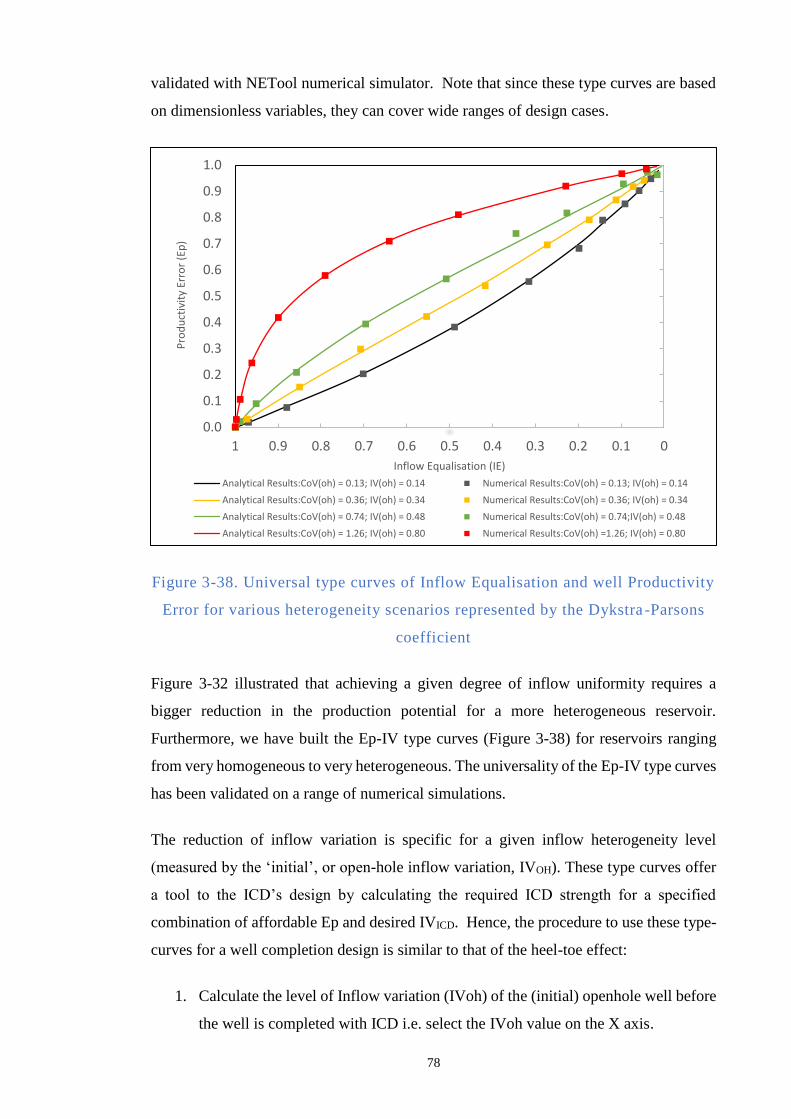
78
validated with NETool numerical simulator. Note that since these type curves are based
on dimensionless variables, they can cover wide ranges of design cases.
Figure 3-38. Universal type curves of Inflow Equalisation and well Productivity
Error for various heterogeneity scenarios represented by the Dykstra -Parsons
coefficient
Figure 3-32 illustrated that achieving a given degree of inflow uniformity requires a
bigger reduction in the production potential for a more heterogeneous reservoir.
Furthermore, we have built the Ep-IV type curves (Figure 3-38) for reservoirs ranging
from very homogeneous to very heterogeneous. The universality of the Ep-IV type curves
has been validated on a range of numerical simulations.
The reduction of inflow variation is specific for a given inflow heterogeneity level
(measured by the ‘initial’, or open-hole inflow variation, IVOH). These type curves offer
a tool to the ICD’s design by calculating the required ICD strength for a specified
combination of affordable Ep and desired IVICD. Hence, the procedure to use these type-
curves for a well completion design is similar to that of the heel-toe effect:
1. Calculate the level of Inflow variation (IVoh) of the (initial) openhole well before
the well is completed with ICD i.e. select the IVoh value on the X axis.
0.0
0.1
0.2
0.3
0.4
0.5
0.6
0.7
0.8
0.9
1.0
00.10.20.30.40.50.60.70.80.91
Pro
du
ctiv
ity
Erro
r (E
p)
Inflow Equalisation (IE)
Analytical Results:CoV(oh) = 0.13; IV(oh) = 0.14 Numerical Results:CoV(oh) = 0.13; IV(oh) = 0.14
Analytical Results:CoV(oh) = 0.36; IV(oh) = 0.34 Numerical Results:CoV(oh) = 0.36; IV(oh) = 0.34
Analytical Results:CoV(oh) = 0.74; IV(oh) = 0.48 Numerical Results:CoV(oh) = 0.74;IV(oh) = 0.48
Analytical Results:CoV(oh) = 1.26; IV(oh) = 0.80 Numerical Results:CoV(oh) =1.26; IV(oh) = 0.80
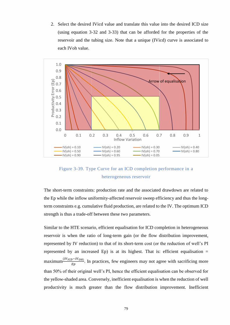
79
2. Select the desired IVicd value and translate this value into the desired ICD size
(using equation 3-32 and 3-33) that can be afforded for the properties of the
reservoir and the tubing size. Note that a unique (IVicd) curve is associated to
each IVoh value.
Figure 3-39. Type Curve for an ICD completion performance in a
heterogeneous reservoir
The short-term constraints: production rate and the associated drawdown are related to
the Ep while the inflow uniformity-affected reservoir sweep efficiency and thus the long-
term constraints e.g. cumulative fluid production, are related to the IV. The optimum ICD
strength is thus a trade-off between these two parameters.
Similar to the HTE scenario, efficient equalisation for ICD completion in heterogeneous
reservoir is when the ratio of long-term gain (or the flow distribution improvement,
represented by IV reduction) to that of its short-term cost (or the reduction of well’s PI
represented by an increased Ep) is at its highest. That is: efficient equalisation =
maximum(𝐼𝑉𝐼𝐶𝐷−𝐼𝑉𝑂𝐻)
𝐸𝑝. In practices, few engineers may not agree with sacrificing more
than 50% of their original well’s PI, hence the efficient equalisation can be observed for
the yellow-shaded area. Conversely, inefficient equalisation is when the reduction of well
productivity is much greater than the flow distribution improvement. Inefficient
0.0
0.1
0.2
0.3
0.4
0.5
0.6
0.7
0.8
0.9
1.0
0 0.1 0.2 0.3 0.4 0.5 0.6 0.7 0.8 0.9 1
Pro
du
ctiv
ity
Erro
r (E
p)
Inflow Variation
IV(oh) = 0.10 IV(oh) = 0.20 IV(oh) = 0.30 IV(oh) = 0.40IV(oh) = 0.50 IV(oh) = 0.60 IV(oh) = 0.70 IV(oh) = 0.80IV(oh) = 0.90 IV(oh) = 0.95 IV(oh) = 0.05
Arrow of equalisation

80
equalisation is represented by the red-shaded area where the slope of the Rd curve is much
smaller than the slope of the Ep curve.
For a given range of heterogeneity representative IVOH values, the corresponding type
curve plot can be divided into two areas. E.g. for wells with IVOH values of 0.6-0.7 (very
heterogeneous inflow) the yellow shaded area in Figure 3-39 is when the ICD completion
is considered to perform efficiently, that is when the reduction of inflow variation is steep
while the well’s productivity’s loss is slow. The red shaded area below IVICD = 0.2 is
when the reduction of inflow variation results in excessive productivity reduction. The
red shaded area above IV = 0.7 shows the ICD completion performance rapidly reducing
the well productivity but not yet affecting the inflow uniformity much.
Note that as far as the highly heterogeneous reservoirs are concerned (high IVOH
number), the modelled reservoir’s very permeable layers (or fractures, channels) that,
though present in small numbers, have a significant effect on the total well inflow
performance. A more logical method would be to install varying-size ICDs with a very
aggressive restriction across the highly permeable layers, or if required, to fully shut
those prominent layers with blank pipe, while installing lower strength ICDs across the
layers with lower permeability.
The procedure to use this type-curves analysis is similar to the one developed for
homogeneous reservoirs. The first step is to calculate the level of open-hole inflow
variation, (IVOH). The next step is the selection of the desired ICD inflow variation
(IVICD), against the reduced well’s PI (Ep), or vice versa.
Further, the found IVICD value actually depends on a unique combination of the
drawdown ∆Pw (for pressure constrained production) or rate Q (for rate constrained
production) values, as well as on the specific ICD strength (a) in a given case. We thus
need to find the formula that relates the specific a (ICD strength) to IVICD (Inflow
Variation ICD) in a given case.
The resulting ICD strength for pressure constrained production is:
𝑎 =((Ω.𝐽𝑚2−𝐽12)
(Ω−1)−𝐽𝑚2)
((𝐽12−Ω2.𝐽𝑚2)
Ω(Ω−1))2
∆𝑃𝑤
(3-32)
Or for a rate constrained well:
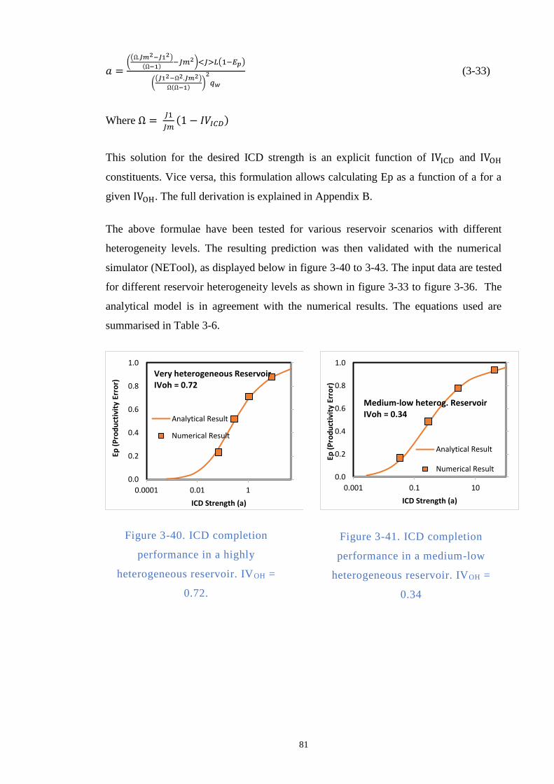
81
𝑎 =((Ω.𝐽𝑚2−𝐽12)
(Ω−1)−𝐽𝑚2)<𝐽>𝐿(1−𝐸𝑝)
((𝐽12−Ω2.𝐽𝑚2)
Ω(Ω−1))2
𝑞𝑤
(3-33)
Where Ω = 𝐽1
𝐽𝑚(1 − 𝐼𝑉𝐼𝐶𝐷)
This solution for the desired ICD strength is an explicit function of IVICD and IVOH
constituents. Vice versa, this formulation allows calculating Ep as a function of a for a
given IVOH. The full derivation is explained in Appendix B.
The above formulae have been tested for various reservoir scenarios with different
heterogeneity levels. The resulting prediction was then validated with the numerical
simulator (NETool), as displayed below in figure 3-40 to 3-43. The input data are tested
for different reservoir heterogeneity levels as shown in figure 3-33 to figure 3-36. The
analytical model is in agreement with the numerical results. The equations used are
summarised in Table 3-6.
Figure 3-40. ICD completion
performance in a highly
heterogeneous reservoir. IVOH =
0.72.
Figure 3-41. ICD completion
performance in a medium-low
heterogeneous reservoir. IVOH =
0.34
0.0
0.2
0.4
0.6
0.8
1.0
0.0001 0.01 1
Ep (
Pro
du
ctiv
ity
Erro
r)
ICD Strength (a)
Very heterogeneous ReservoirIVoh = 0.72
Analytical Result
Numerical Result
0.0
0.2
0.4
0.6
0.8
1.0
0.001 0.1 10
Ep (
Pro
du
ctiv
ity
Erro
r)
ICD Strength (a)
Medium-low heterog. Reservoir IVoh = 0.34
Analytical Result
Numerical Result
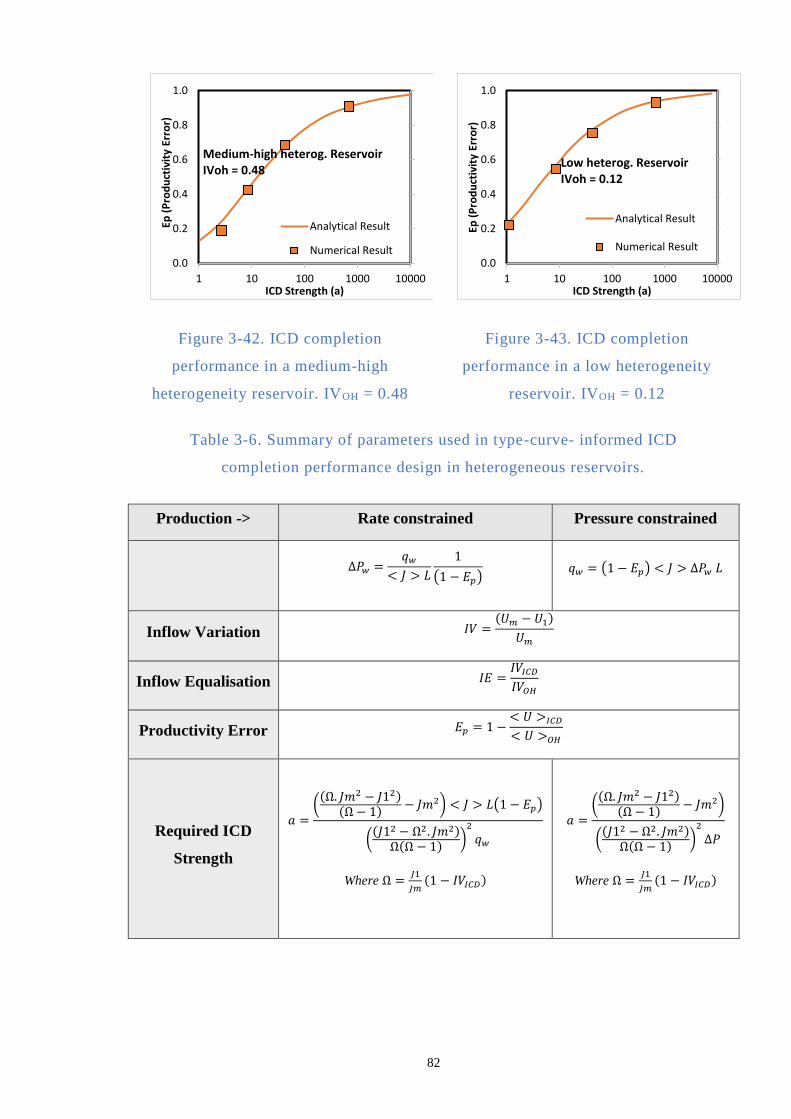
82
Figure 3-42. ICD completion
performance in a medium-high
heterogeneity reservoir. IVOH = 0.48
Figure 3-43. ICD completion
performance in a low heterogeneity
reservoir. IVOH = 0.12
Table 3-6. Summary of parameters used in type-curve- informed ICD
completion performance design in heterogeneous reservoirs.
Production -> Rate constrained Pressure constrained
∆𝑃𝑤 =𝑞𝑤
< 𝐽 > 𝐿
1
(1 − 𝐸𝑝) 𝑞𝑤 = (1 − 𝐸𝑝) < 𝐽 > ∆𝑃𝑤 𝐿
Inflow Variation 𝐼𝑉 =(𝑈𝑚 − 𝑈1)
𝑈𝑚
Inflow Equalisation 𝐼𝐸 =𝐼𝑉𝐼𝐶𝐷𝐼𝑉𝑂𝐻
Productivity Error 𝐸𝑝 = 1 −< 𝑈 >𝐼𝐶𝐷< 𝑈 >𝑂𝐻
Required ICD
Strength
𝑎 =((Ω. 𝐽𝑚2 − 𝐽12)
(Ω − 1)− 𝐽𝑚2) < 𝐽 > 𝐿(1 − 𝐸𝑝)
((𝐽12 − Ω2. 𝐽𝑚2)Ω(Ω − 1)
)2
𝑞𝑤
Where Ω =𝐽1
𝐽𝑚(1 − 𝐼𝑉𝐼𝐶𝐷)
𝑎 =((Ω. 𝐽𝑚2 − 𝐽12)
(Ω − 1)− 𝐽𝑚2)
((𝐽12 − Ω2. 𝐽𝑚2)Ω(Ω − 1)
)2
∆𝑃
Where Ω =𝐽1
𝐽𝑚(1 − 𝐼𝑉𝐼𝐶𝐷)
0.0
0.2
0.4
0.6
0.8
1.0
1 10 100 1000 10000
Ep (
Pro
du
ctiv
ity
Erro
r)
ICD Strength (a)
Medium-high heterog. Reservoir IVoh = 0.48
Analytical Result
Numerical Result0.0
0.2
0.4
0.6
0.8
1.0
1 10 100 1000 10000
Ep (
Pro
du
ctiv
ity
Erro
r)
ICD Strength (a)
Low heterog. Reservoir IVoh = 0.12
Analytical Result
Numerical Result

83
ICD size – strength
relationship
𝑎𝑐ℎ𝑎𝑛𝑛𝑒𝑙 =
(𝜌 𝜇𝑐𝑎𝑙)
(𝜌𝑐𝑎𝑙 𝜇)
1
4 𝜌𝑐𝑎𝑙
𝜌√𝑙𝐼𝐶𝐷𝐵
𝑎⁄
(ICD Channel type)
𝑁𝑜𝑧𝑧𝑙𝑒 𝑑𝑖𝑎𝑚𝑒𝑡𝑒𝑟 = √𝐶𝑢𝜌𝑙𝐼𝐶𝐷
2 𝐵2
𝐶𝑑2𝑎
4 (ICD Nozzle type)
The type-curve based ICD design workflow
The above type-curves can form the basis of a fast workflow to design a uniform-strength
ICD completion. They provide the insight to the ICD’s design parameters and aid
calculating the required ICD strength for a specified combination of either Hp, Ip, Ep,
and Rd (for homogeneous reservoirs); or IVICD, IVOH, and Ep (for heterogeneous
reservoirs).
An ICD completion design can be driven by long-term objectives (increased cumulative
oil, delayed breakthrough time, improved sweep efficiency, etc.). These parameters are
related to the inflow uniformity represented by Rd or IVICD. A more uniform inflow rate
distribution along the length of the completion is likely to enhance these long-term
objectives (e.g. El-Khatib, 2012 showed that the breakthrough time, fractional recovery
and water cut of a heterogeneous reservoir are all a function of the IV value of an OH
well.).
An ICD completion design can also be driven by short-term objectives (increased
production rate and/or drawdown at a specific time). The production rate and the
associated well drawdown (i.e. the short-term objectives) are related to the Ep. The ICD
strength required to achieve the objectives selected from the type curves is calculated
using the analytical solutions as was shown above. Figure 3-44 and Figure 3-45 show the
ICD design workflow that was coded into a standard Engineering worksheet in Excel with
the results further validated by comparison with numerical simulation software
(NEToolTM, 2012).
The ICD completion’s design varies depending on whether the design objective is a:
Long-term production strategy
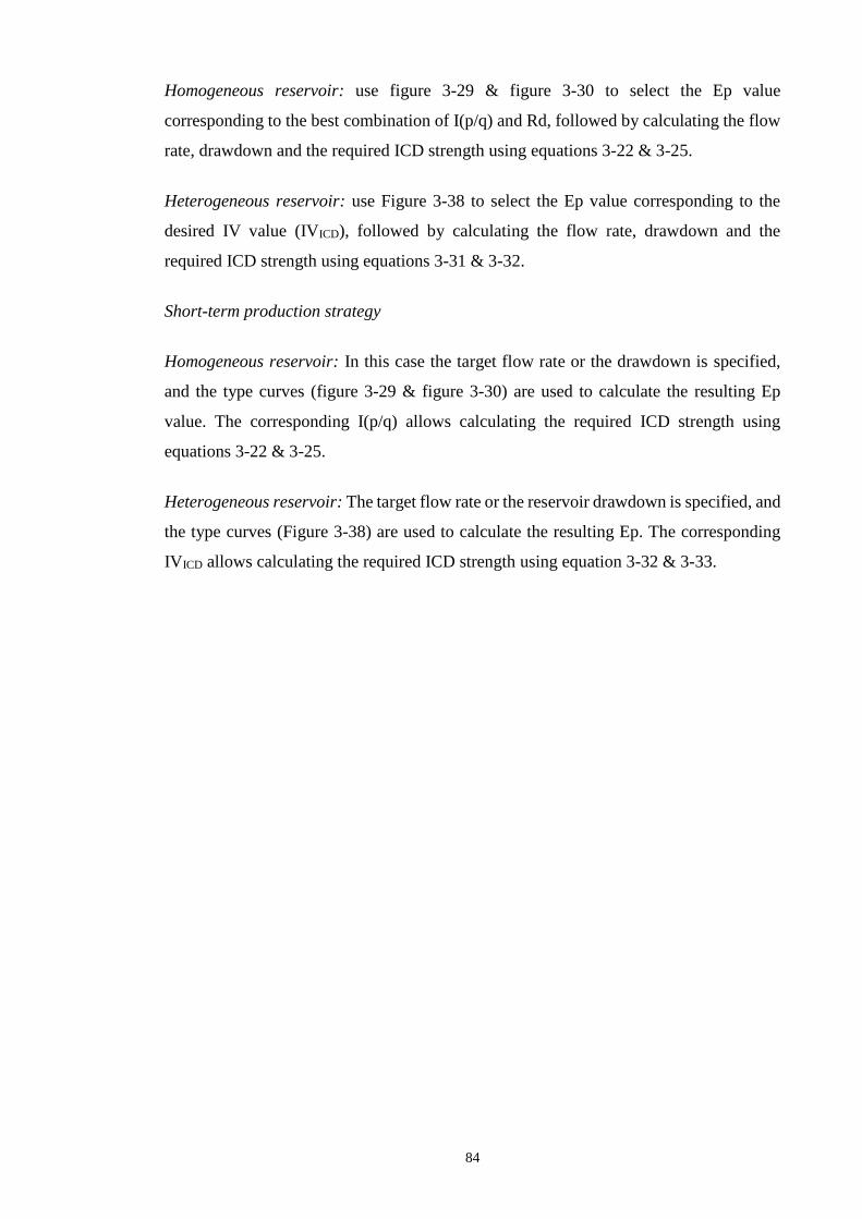
84
Homogeneous reservoir: use figure 3-29 & figure 3-30 to select the Ep value
corresponding to the best combination of I(p/q) and Rd, followed by calculating the flow
rate, drawdown and the required ICD strength using equations 3-22 & 3-25.
Heterogeneous reservoir: use Figure 3-38 to select the Ep value corresponding to the
desired IV value (IVICD), followed by calculating the flow rate, drawdown and the
required ICD strength using equations 3-31 & 3-32.
Short-term production strategy
Homogeneous reservoir: In this case the target flow rate or the drawdown is specified,
and the type curves (figure 3-29 & figure 3-30) are used to calculate the resulting Ep
value. The corresponding I(p/q) allows calculating the required ICD strength using
equations 3-22 & 3-25.
Heterogeneous reservoir: The target flow rate or the reservoir drawdown is specified, and
the type curves (Figure 3-38) are used to calculate the resulting Ep. The corresponding
IVICD allows calculating the required ICD strength using equation 3-32 & 3-33.
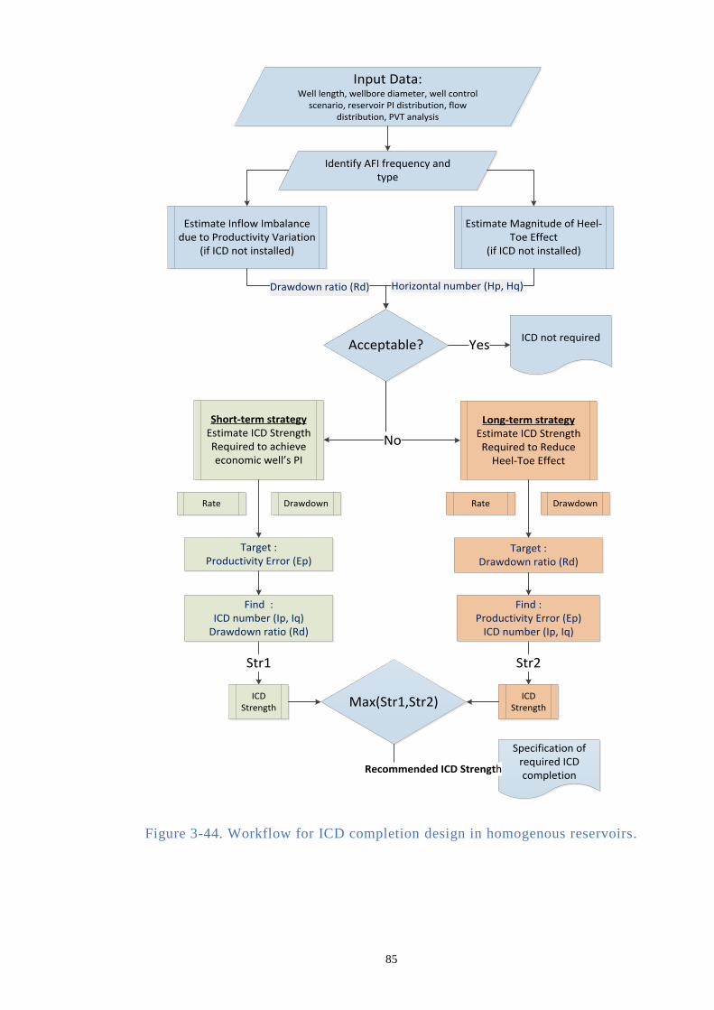
85
Identify AFI frequency and type
Estimate Inflow Imbalance due to Productivity Variation
(if ICD not installed)
Estimate Magnitude of Heel-Toe Effect
(if ICD not installed)
Acceptable?ICD not required
Drawdown ratio (Rd) Horizontal number (Hp, Hq)
Yes
Short-term strategyEstimate ICD Strength Required to achieve economic well’s PI
Long-term strategyEstimate ICD Strength Required to Reduce
Heel-Toe Effect
No
Max(Str1,Str2)
Str1 Str2
Specification of required ICD completion
Recommended ICD Strength
Input Data:Well length, wellbore diameter, well control
scenario, reservoir PI distribution, flow distribution, PVT analysis
Target :Drawdown ratio (Rd)
Find :Productivity Error (Ep)
ICD number (Ip, Iq)
Rate
ICD Strength
Drawdown
Target :Productivity Error (Ep)
Rate Drawdown
Find :ICD number (Ip, Iq)
Drawdown ratio (Rd)
ICD Strength
Figure 3-44. Workflow for ICD completion design in homogenous reservoirs.
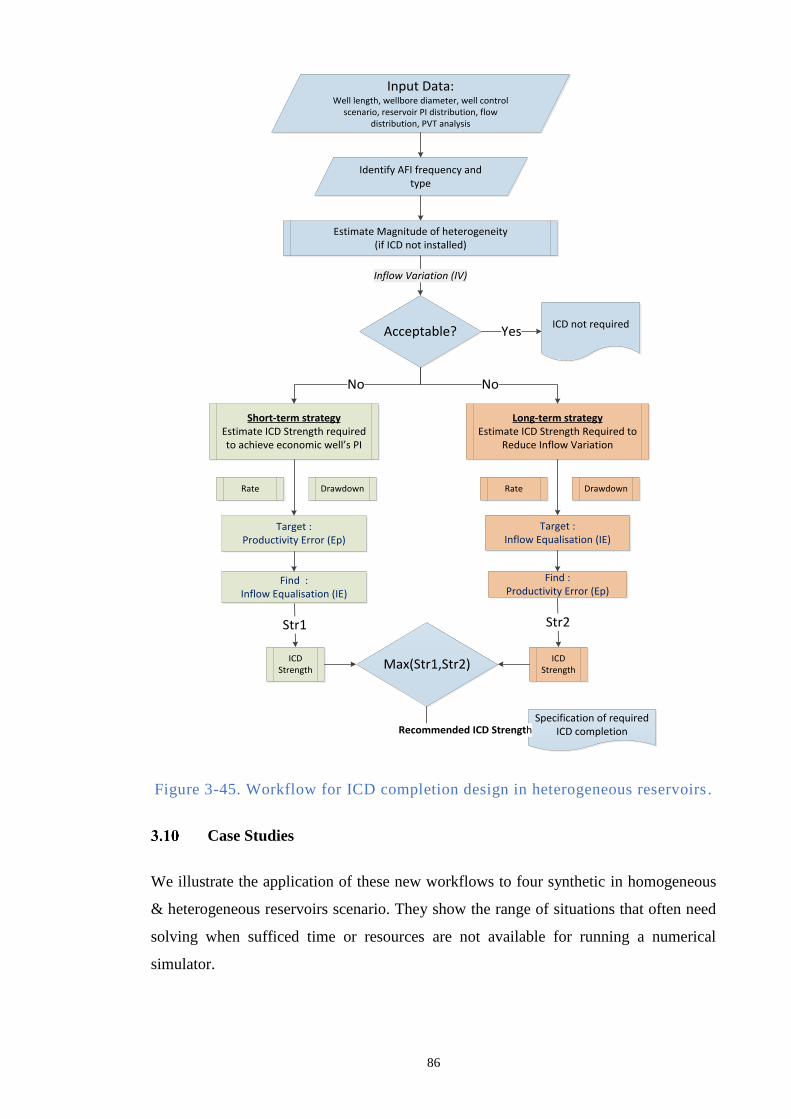
86
Identify AFI frequency and type
Estimate Magnitude of heterogeneity (if ICD not installed)
Acceptable?ICD not required
Inflow Variation (IV)
Yes
Short-term strategyEstimate ICD Strength required to achieve economic well’s PI
No
Long-term strategyEstimate ICD Strength Required to
Reduce Inflow Variation
No
Max(Str1,Str2)
Str1 Str2
Specification of required ICD completionRecommended ICD Strength
Input Data:Well length, wellbore diameter, well control
scenario, reservoir PI distribution, flow distribution, PVT analysis
Target :Inflow Equalisation (IE)
Find :Productivity Error (Ep)
Rate
ICD Strength
Drawdown
Target :Productivity Error (Ep)
Rate Drawdown
Find :Inflow Equalisation (IE)
ICD Strength
Figure 3-45. Workflow for ICD completion design in heterogeneous reservoirs .
Case Studies
We illustrate the application of these new workflows to four synthetic in homogeneous
& heterogeneous reservoirs scenario. They show the range of situations that often need
solving when sufficed time or resources are not available for running a numerical
simulator.
87
Homogenous reservoir scenario
Case 1a evaluates the ICD size that was recommended by (Birchenko, et al. 2010) and
(Henriksen, Gule and Augustine, 2006) for a well in an oil-rim reservoir (Figure 3-46), a
permeable homogenous sandstone with the initial reservoir pressure close to the bubble
point pressure (Table 3-7). The 3D reservoir box model was built using the PETREL RE
platform. The dimension was 750m x 2500m x 15m, and the reservoir was completed in
the middle of the x axis, with 2500 meter horizontal well along the y axis, with an
analytical bottom-up aquifer below the reservoir.
The production is constrained by the allowable drawdown. The recommendation by both
studies was to assign ICD pressure drop with the n times magnitude of the annulus
drawdown at the heel, ∆𝑃𝑎𝑛𝑛ℎ𝑒𝑒𝑙. The type-curve method is now used in this thesis to
evaluate Birchenko’s method in the context of reduction of inflow inequality against the
well’s performance. Our workflow is tested and compared to Birchenko’s
recommendations.
Case 1b also used the data outlined in table 3-6, however, in this case, the pre-completion
ICD design should be revised at the well site against the new geological information (it
appears the reservoir has lower permeability than expected) obtained after drilling the
well (e.g. open-hole well log), prior to completion. This case study exemplifies the
usefulness of rapid workflow to evaluate the various combinations of well completion
selection with a limited time for analysis.
Horizontal well
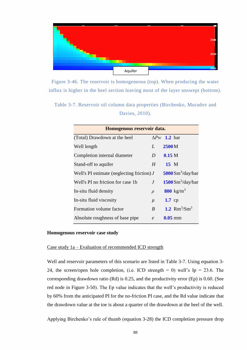
88
Figure 3-46. The reservoir is homogeneous (top). When producing the water
influx is higher in the heel section leaving most of the layer unswept (bottom).
Table 3-7. Reservoir oil column data properties (Birchenko, Muradov and
Davies, 2010).
Homogenous reservoir data.
(Total) Drawdown at the heel ∆Pw 1.2 bar
Well length L 2500 M
Completion internal diameter D 0.15 M
Stand-off to aquifer H 15 M
Well's PI estimate (neglecting friction) J 5000 Sm3/day/bar
Well's PI no friction for case 1b J 1500 Sm3/day/bar
In-situ fluid density ρ 800 kg/m3
In-situ fluid viscosity µ 1.7 cp
Formation volume factor B 1.2 Rm3/Sm3
Absolute roughness of base pipe e 0.05 mm
Homogenous reservoir case study
Case study 1a – Evaluation of recommended ICD strength
Well and reservoir parameters of this scenario are listed in Table 3-7. Using equation 3-
24, the screen/open hole completion, (i.e. ICD strength = 0) well’s Ip = 23.6. The
corresponding drawdown ratio (Rd) is 0.25, and the productivity error (Ep) is 0.60. (See
red node in Figure 3-50). The Ep value indicates that the well’s productivity is reduced
by 60% from the anticipated PI for the no-friction PI case, and the Rd value indicate that
the drawdown value at the toe is about a quarter of the drawdown at the heel of the well.
Applying Birchenko’s rule of thumb (equation 3-28) the ICD completion pressure drop
Aquifer
2505
2510
2515
2515
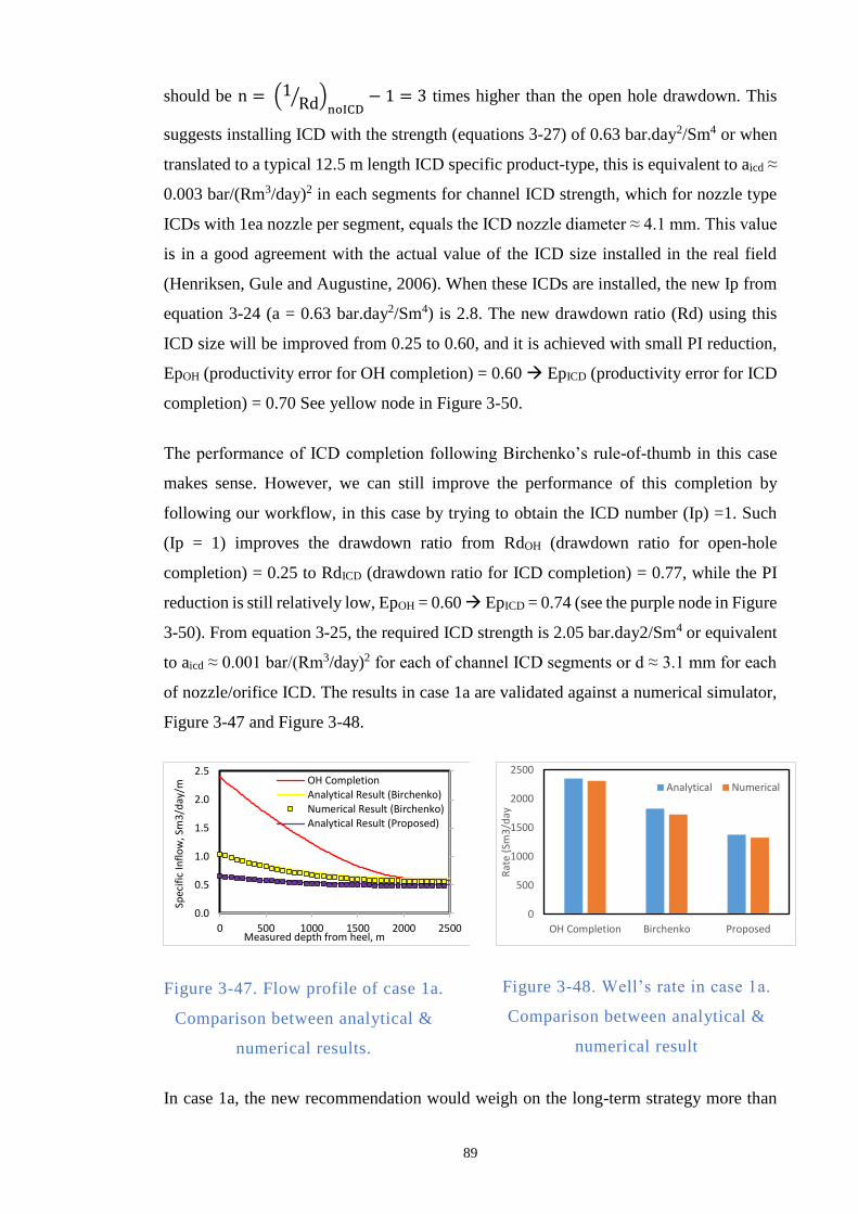
89
should be n = (1 Rd⁄ )noICD
− 1 = 3 times higher than the open hole drawdown. This
suggests installing ICD with the strength (equations 3-27) of 0.63 bar.day2/Sm4 or when
translated to a typical 12.5 m length ICD specific product-type, this is equivalent to aicd ≈
0.003 bar/(Rm3/day)2 in each segments for channel ICD strength, which for nozzle type
ICDs with 1ea nozzle per segment, equals the ICD nozzle diameter ≈ 4.1 mm. This value
is in a good agreement with the actual value of the ICD size installed in the real field
(Henriksen, Gule and Augustine, 2006). When these ICDs are installed, the new Ip from
equation 3-24 (a = 0.63 bar.day2/Sm4) is 2.8. The new drawdown ratio (Rd) using this
ICD size will be improved from 0.25 to 0.60, and it is achieved with small PI reduction,
EpOH (productivity error for OH completion) = 0.60 EpICD (productivity error for ICD
completion) = 0.70 See yellow node in Figure 3-50.
The performance of ICD completion following Birchenko’s rule-of-thumb in this case
makes sense. However, we can still improve the performance of this completion by
following our workflow, in this case by trying to obtain the ICD number (Ip) =1. Such
(Ip = 1) improves the drawdown ratio from RdOH (drawdown ratio for open-hole
completion) = 0.25 to RdICD (drawdown ratio for ICD completion) = 0.77, while the PI
reduction is still relatively low, EpOH = 0.60 EpICD = 0.74 (see the purple node in Figure
3-50). From equation 3-25, the required ICD strength is 2.05 bar.day2/Sm4 or equivalent
to aicd ≈ 0.001 bar/(Rm3/day)2 for each of channel ICD segments or d ≈ 3.1 mm for each
of nozzle/orifice ICD. The results in case 1a are validated against a numerical simulator,
Figure 3-47 and Figure 3-48.
Figure 3-47. Flow profile of case 1a.
Comparison between analytical &
numerical results.
Figure 3-48. Well’s rate in case 1a.
Comparison between analytical &
numerical result
In case 1a, the new recommendation would weigh on the long-term strategy more than
0.0
0.5
1.0
1.5
2.0
2.5
0 500 1000 1500 2000 2500
Spec
ific
Infl
ow
, Sm
3/d
ay/m
Measured depth from heel, m
OH CompletionAnalytical Result (Birchenko)Numerical Result (Birchenko)Analytical Result (Proposed)
0
500
1000
1500
2000
2500
OH Completion Birchenko Proposed
Rat
e (S
m3
/day
Analytical Numerical
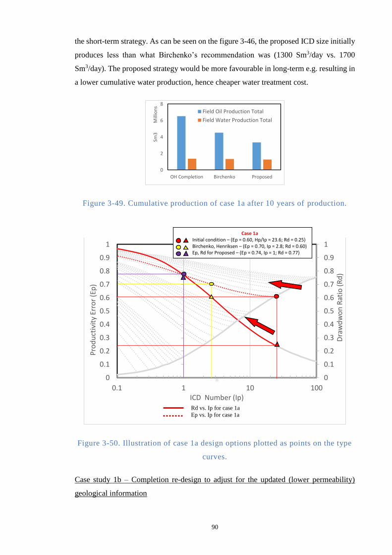
90
the short-term strategy. As can be seen on the figure 3-46, the proposed ICD size initially
produces less than what Birchenko’s recommendation was (1300 Sm3/day vs. 1700
Sm3/day). The proposed strategy would be more favourable in long-term e.g. resulting in
a lower cumulative water production, hence cheaper water treatment cost.
Figure 3-49. Cumulative production of case 1a after 10 years of production.
Figure 3-50. Illustration of case 1a design options plotted as points on the type
curves.
Case study 1b – Completion re-design to adjust for the updated (lower permeability)
geological information
0
2
4
6
8
OH Completion Birchenko Proposed
Sm3
Mill
ion
s
Field Oil Production Total
Field Water Production Total
0
0.1
0.2
0.3
0.4
0.5
0.6
0.7
0.8
0.9
1
0
0.1
0.2
0.3
0.4
0.5
0.6
0.7
0.8
0.9
1
0.1 1 10 100
Dra
wd
wo
n R
atio
(R
d)
Pro
du
ctiv
ity
Erro
r (E
p)
ICD Number (Ip)Rd vs. Ip for case 1a
Ep vs. Ip for case 1a
Case 1a Initial condition – (Ep = 0.60, Hp/Ip = 23.6; Rd = 0.25) Birchenko, Henriksen – (Ep = 0.70, Ip = 2.8; Rd = 0.60) Ep, Rd for Proposed – (Ep = 0.74, Ip = 1; Rd = 0.77)

91
The open-hole well log run after drilling the well reveals the reservoir is less permeable
than what was expected. The actual well’s PI is 1500 Sm3/day/bar. Consequently, this
well will also have different heel-toe effect. A quick calculation is needed to find the new
ICD configuration and adjust it on site. Given the limited time between logging and
running the completion string.
First, we can directly quantify the new heel-toe effect using equation 3-24. New Ip will
be 2.3, and from the type-curve, the corresponding Rd = 0.62. Ep= 0.26 (see blue node in
Figure 3-54). If we were to follow the Birchenko’s rule-of-thumb, the new ICD strength
(equations 3-27 and 3-28) a ≈ 9.0 bar.day2/Sm4 or when translated to a typical 12.5 m
length ICD specific product-type, this is equivalent to aicd ≈ 0.033 bar/(Rm3/day)2 in each
segments for channel ICD strength, which for nozzle type ICDs with 1ea nozzle per
segment, equals the ICD nozzle diameter ≈ 2.16 mm. The new completion configuration
is Hp = 0.23, Rd = 0.93. Ep= 0.62 (see green node in Figure 3-54).
Unlike the scenario in case 1a, following Birchenko’s rule-of-thumb case 1b will result
in poor ICD performance. The improvement of drawdown ratio, from RdOH = 0.62
RdICD = 0.92, is penalized with severed well’s productivity loss, from EpOH = 0.26
EpICD = 0.62. With this configuration: (RdICD - RdOH) < (EpICD - EpOH) hence the reduction
of well’s PI with this rule-of-thumb is not worth it.
Earlier it was suggested that for a certain range of Hp values the reduction of heel-toe
effect is efficient until ICD number, Ip = 1 (See brown node in Figure 3-54). This is
obtained by installing ICDs with the strength (equations 3-27) of 1.60 bar.day2/Sm4 or
when translated to a typical 12.5 m length ICD specific product-type, this is equivalent to
aicd ≈ 0.006 bar/(Rm3/day)2 in each segments for channel ICD strength, which for nozzle
type ICDs with 1ea nozzle per segment, equals the ICD nozzle diameter ≈ 3.32 mm. This
way the drawdown ratio will be improved, RdOH = 0.62 RdICD = 0.77 with lower PI’s
reduction, EpOH = 0.26 EpICD = 0.38. i.e. (RdICD - RdOH) > (EpICD - EpOH). The results
of this case are validated by the numerical simulator as depicted in Figure 3-51 &Figure
3-52.
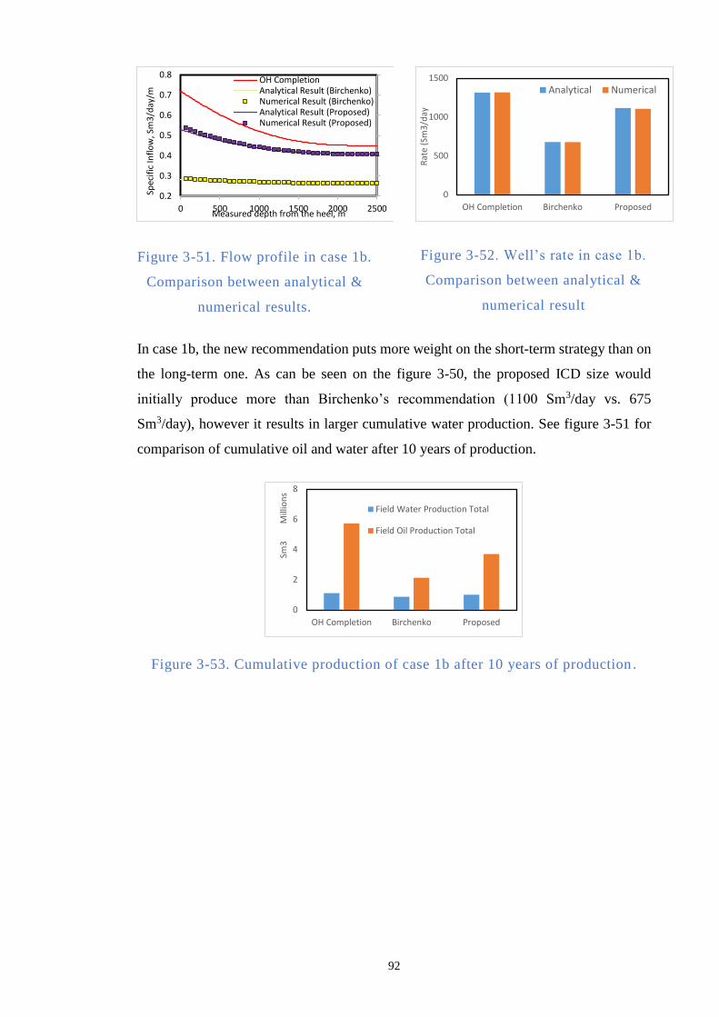
92
Figure 3-51. Flow profile in case 1b.
Comparison between analytical &
numerical results.
Figure 3-52. Well’s rate in case 1b.
Comparison between analytical &
numerical result
In case 1b, the new recommendation puts more weight on the short-term strategy than on
the long-term one. As can be seen on the figure 3-50, the proposed ICD size would
initially produce more than Birchenko’s recommendation (1100 Sm3/day vs. 675
Sm3/day), however it results in larger cumulative water production. See figure 3-51 for
comparison of cumulative oil and water after 10 years of production.
Figure 3-53. Cumulative production of case 1b after 10 years of production .
0.2
0.3
0.4
0.5
0.6
0.7
0.8
0 500 1000 1500 2000 2500
Spec
ific
Infl
ow
, Sm
3/d
ay/m
Measured depth from the heel, m
OH CompletionAnalytical Result (Birchenko)Numerical Result (Birchenko)Analytical Result (Proposed)Numerical Result (Proposed)
0
500
1000
1500
OH Completion Birchenko Proposed
Rat
e (S
m3
/day
Analytical Numerical
0
2
4
6
8
OH Completion Birchenko Proposed
Sm3
Mill
ion
s
Field Water Production Total
Field Oil Production Total
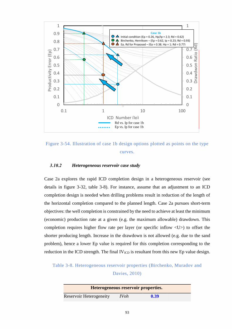
93
Figure 3-54. Illustration of case 1b design options plotted as points on the type
curves.
Heterogeneous reservoir case study
Case 2a explores the rapid ICD completion design in a heterogeneous reservoir (see
details in figure 3-32, table 3-8). For instance, assume that an adjustment to an ICD
completion design is needed when drilling problems result in reduction of the length of
the horizontal completion compared to the planned length. Case 2a pursues short-term
objectives: the well completion is constrained by the need to achieve at least the minimum
(economic) production rate at a given (e.g. the maximum allowable) drawdown. This
completion requires higher flow rate per layer (or specific inflow <U>) to offset the
shorter producing length. Increase in the drawdown is not allowed (e.g. due to the sand
problem), hence a lower Ep value is required for this completion corresponding to the
reduction in the ICD strength. The final IVICD is resultant from this new Ep value design.
Table 3-8. Heterogeneous reservoir properties (Birchenko, Muradov and
Davies, 2010)
Heterogeneous reservoir properties.
Reservoir Heterogeneity IVoh 0.39
0
0.1
0.2
0.3
0.4
0.5
0.6
0.7
0.8
0.9
1
0
0.1
0.2
0.3
0.4
0.5
0.6
0.7
0.8
0.9
1
0.1 1 10 100
Dra
wd
wo
n R
atio
(R
d)
Pro
du
ctiv
ity
Erro
r (E
p)
ICD Number (Ip)Rd vs. Ip for case 1b
Ep vs. Ip for case 1b
Case 1b Initial condition (Ep = 0.26, Hp/Ip = 2.3; Rd = 0.62) Birchenko, Henriksen – (Ep = 0.62, Ip = 0.23; Rd = 0.93) Ep, Rd for Proposed – (Ep = 0.38, Hp = 1; Rd = 0.77)
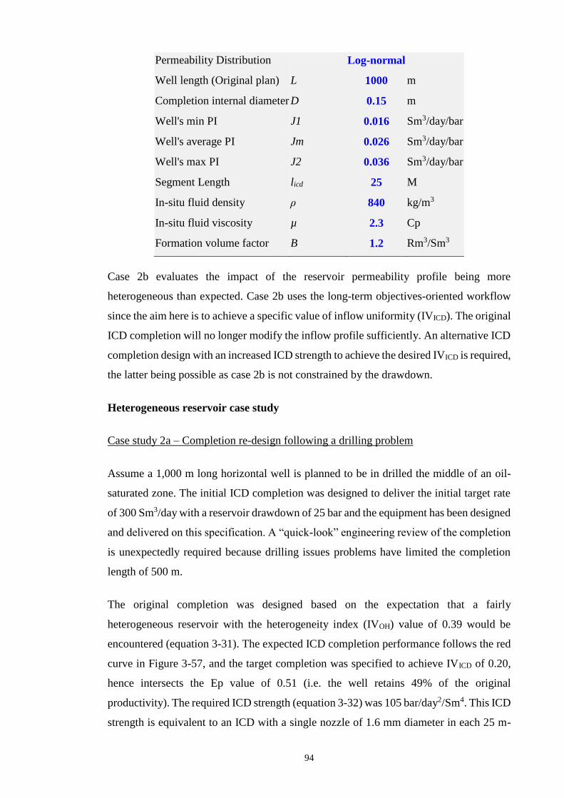
94
Permeability Distribution
Log-normal
Well length (Original plan) L 1000 m
Completion internal diameter D 0.15 m
Well's min PI J1 0.016 Sm3/day/bar
Well's average PI Jm 0.026 Sm3/day/bar
Well's max PI J2 0.036 Sm3/day/bar
Segment Length licd 25 M
In-situ fluid density ρ 840 kg/m3
In-situ fluid viscosity µ 2.3 Cp
Formation volume factor B 1.2 Rm3/Sm3
Case 2b evaluates the impact of the reservoir permeability profile being more
heterogeneous than expected. Case 2b uses the long-term objectives-oriented workflow
since the aim here is to achieve a specific value of inflow uniformity (IVICD). The original
ICD completion will no longer modify the inflow profile sufficiently. An alternative ICD
completion design with an increased ICD strength to achieve the desired IVICD is required,
the latter being possible as case 2b is not constrained by the drawdown.
Heterogeneous reservoir case study
Case study 2a – Completion re-design following a drilling problem
Assume a 1,000 m long horizontal well is planned to be in drilled the middle of an oil-
saturated zone. The initial ICD completion was designed to deliver the initial target rate
of 300 Sm3/day with a reservoir drawdown of 25 bar and the equipment has been designed
and delivered on this specification. A “quick-look” engineering review of the completion
is unexpectedly required because drilling issues problems have limited the completion
length of 500 m.
The original completion was designed based on the expectation that a fairly
heterogeneous reservoir with the heterogeneity index (IVOH) value of 0.39 would be
encountered (equation 3-31). The expected ICD completion performance follows the red
curve in Figure 3-57, and the target completion was specified to achieve IVICD of 0.20,
hence intersects the Ep value of 0.51 (i.e. the well retains 49% of the original
productivity). The required ICD strength (equation 3-32) was 105 bar/day2/Sm4. This ICD
strength is equivalent to an ICD with a single nozzle of 1.6 mm diameter in each 25 m-
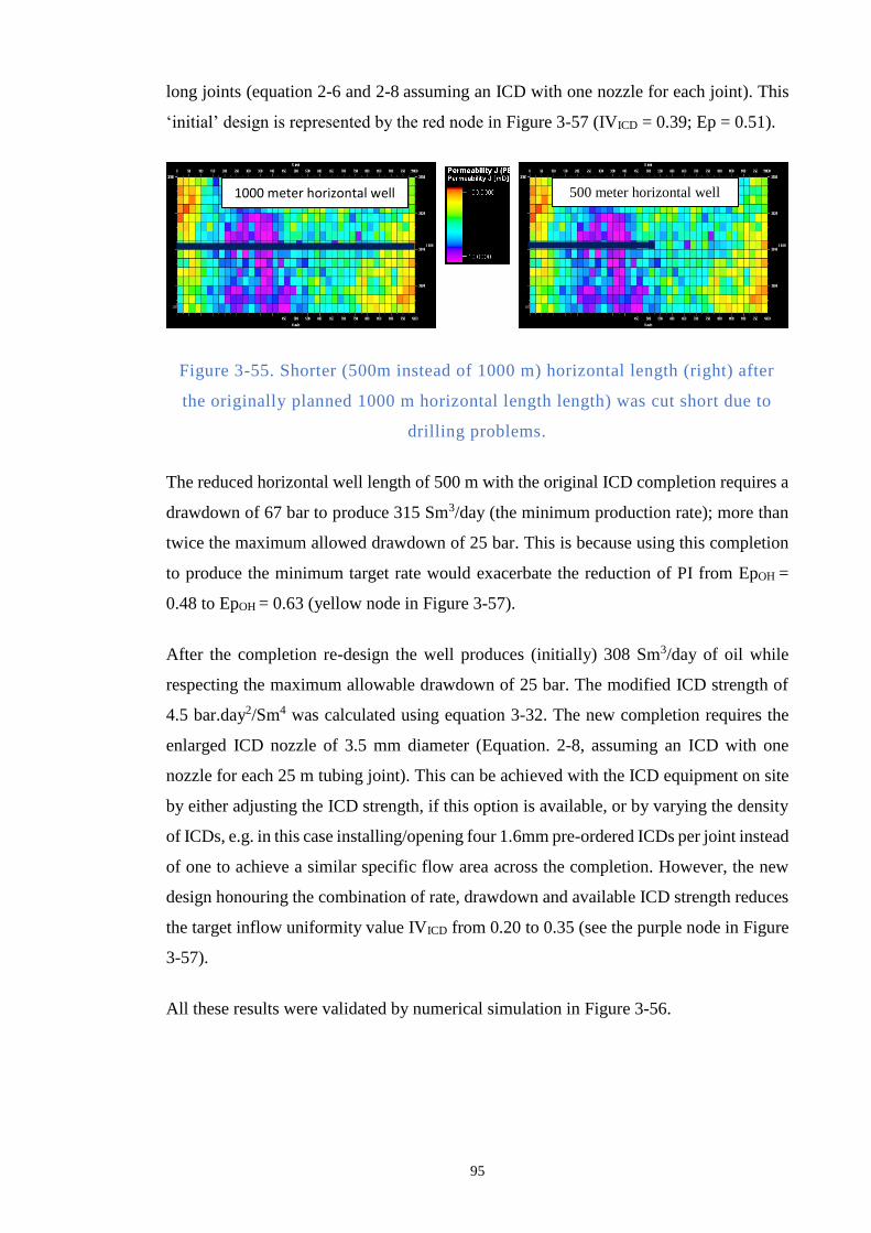
95
long joints (equation 2-6 and 2-8 assuming an ICD with one nozzle for each joint). This
‘initial’ design is represented by the red node in Figure 3-57 (IVICD = 0.39; Ep = 0.51).
Figure 3-55. Shorter (500m instead of 1000 m) horizontal length (right) after
the originally planned 1000 m horizontal length length) was cut short due to
drilling problems.
The reduced horizontal well length of 500 m with the original ICD completion requires a
drawdown of 67 bar to produce 315 Sm3/day (the minimum production rate); more than
twice the maximum allowed drawdown of 25 bar. This is because using this completion
to produce the minimum target rate would exacerbate the reduction of PI from EpOH =
0.48 to EpOH = 0.63 (yellow node in Figure 3-57).
After the completion re-design the well produces (initially) 308 Sm3/day of oil while
respecting the maximum allowable drawdown of 25 bar. The modified ICD strength of
4.5 bar.day2/Sm4 was calculated using equation 3-32. The new completion requires the
enlarged ICD nozzle of 3.5 mm diameter (Equation. 2-8, assuming an ICD with one
nozzle for each 25 m tubing joint). This can be achieved with the ICD equipment on site
by either adjusting the ICD strength, if this option is available, or by varying the density
of ICDs, e.g. in this case installing/opening four 1.6mm pre-ordered ICDs per joint instead
of one to achieve a similar specific flow area across the completion. However, the new
design honouring the combination of rate, drawdown and available ICD strength reduces
the target inflow uniformity value IVICD from 0.20 to 0.35 (see the purple node in Figure
3-57).
All these results were validated by numerical simulation in Figure 3-56.
1000 meter horizontal well 500 meter horizontal well
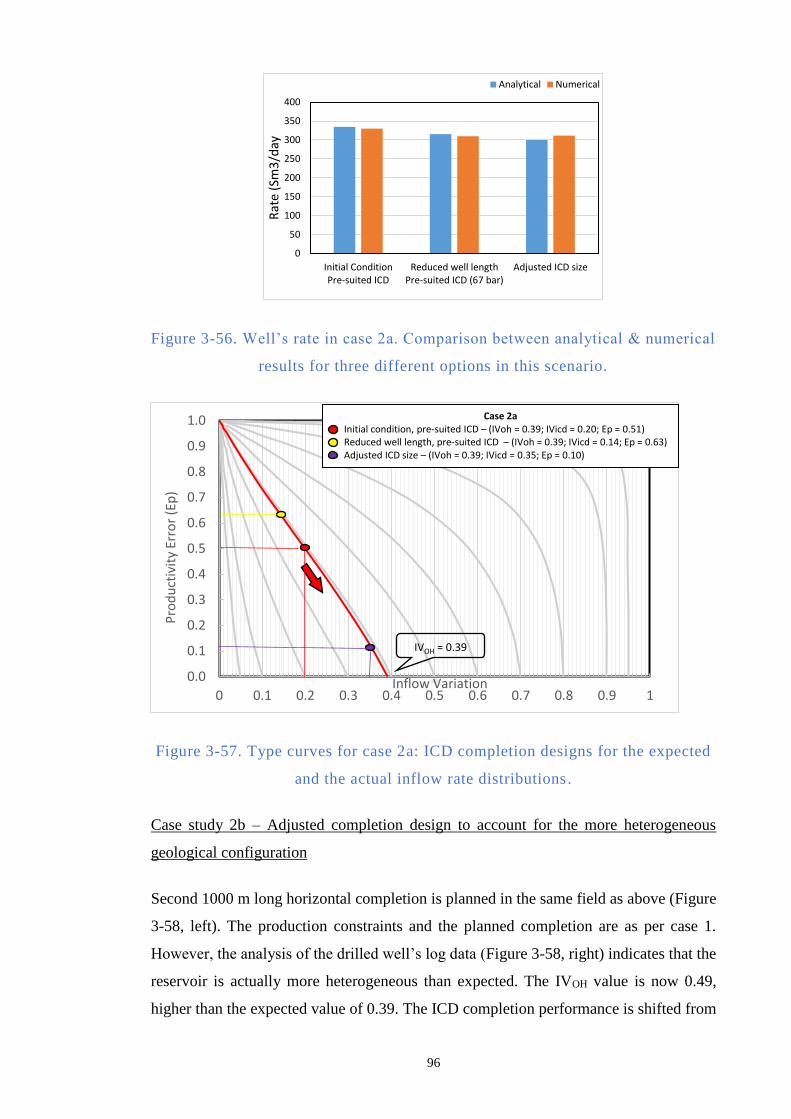
96
Figure 3-56. Well’s rate in case 2a. Comparison between analytical & numerical
results for three different options in this scenario.
Figure 3-57. Type curves for case 2a: ICD completion designs for the expected
and the actual inflow rate distributions.
Case study 2b – Adjusted completion design to account for the more heterogeneous
geological configuration
Second 1000 m long horizontal completion is planned in the same field as above (Figure
3-58, left). The production constraints and the planned completion are as per case 1.
However, the analysis of the drilled well’s log data (Figure 3-58, right) indicates that the
reservoir is actually more heterogeneous than expected. The IVOH value is now 0.49,
higher than the expected value of 0.39. The ICD completion performance is shifted from
0
50
100
150
200
250
300
350
400
Initial ConditionPre-suited ICD
Reduced well lengthPre-suited ICD (67 bar)
Adjusted ICD sizeR
ate
(Sm
3/d
ay
Analytical Numerical
0.0
0.1
0.2
0.3
0.4
0.5
0.6
0.7
0.8
0.9
1.0
0 0.1 0.2 0.3 0.4 0.5 0.6 0.7 0.8 0.9 1
Pro
du
ctiv
ity
Erro
r (E
p)
Inflow Variation
Case 2aInitial condition, pre-suited ICD – (IVoh = 0.39; IVicd = 0.20; Ep = 0.51)Reduced well length, pre-suited ICD – (IVoh = 0.39; IVicd = 0.14; Ep = 0.63)Adjusted ICD size – (IVoh = 0.39; IVicd = 0.35; Ep = 0.10)
IVOH = 0.39
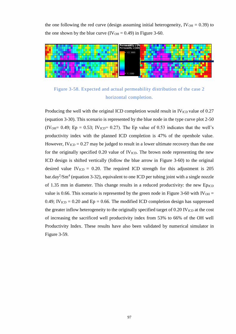
97
the one following the red curve (design assuming initial heterogeneity, IVOH = 0.39) to
the one shown by the blue curve (IVOH = 0.49) in Figure 3-60.
Figure 3-58. Expected and actual permeability distribution of the case 2
horizontal completion.
Producing the well with the original ICD completion would result in IVICD value of 0.27
(equation 3-30). This scenario is represented by the blue node in the type curve plot 2-50
(IVOH= 0.49; Ep = 0.53; IVICD= 0.27). The Ep value of 0.53 indicates that the well’s
productivity index with the planned ICD completion is 47% of the openhole value.
However, IVICD = 0.27 may be judged to result in a lower ultimate recovery than the one
for the originally specified 0.20 value of IVICD. The brown node representing the new
ICD design is shifted vertically (follow the blue arrow in Figure 3-60) to the original
desired value IVICD = 0.20. The required ICD strength for this adjustment is 205
bar.day2/Sm4 (equation 3-32), equivalent to one ICD per tubing joint with a single nozzle
of 1.35 mm in diameter. This change results in a reduced productivity: the new EpICD
value is 0.66. This scenario is represented by the green node in Figure 3-60 with IVOH =
0.49; IVICD = 0.20 and Ep = 0.66. The modified ICD completion design has suppressed
the greater inflow heterogeneity to the originally specified target of 0.20 IVICD at the cost
of increasing the sacrificed well productivity index from 53% to 66% of the OH well
Productivity Index. These results have also been validated by numerical simulator in
Figure 3-59.
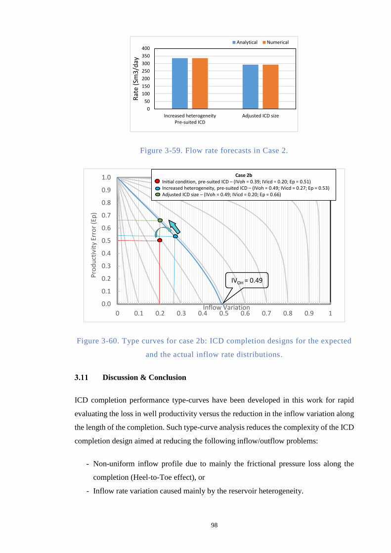
98
Figure 3-59. Flow rate forecasts in Case 2.
Figure 3-60. Type curves for case 2b: ICD completion designs for the expected
and the actual inflow rate distributions.
Discussion & Conclusion
ICD completion performance type-curves have been developed in this work for rapid
evaluating the loss in well productivity versus the reduction in the inflow variation along
the length of the completion. Such type-curve analysis reduces the complexity of the ICD
completion design aimed at reducing the following inflow/outflow problems:
- Non-uniform inflow profile due to mainly the frictional pressure loss along the
completion (Heel-to-Toe effect), or
- Inflow rate variation caused mainly by the reservoir heterogeneity.
0
50
100
150
200
250
300
350
400
Increased heterogeneityPre-suited ICD
Adjusted ICD size
Rat
e (
Sm3
/day
Analytical Numerical
0.0
0.1
0.2
0.3
0.4
0.5
0.6
0.7
0.8
0.9
1.0
0 0.1 0.2 0.3 0.4 0.5 0.6 0.7 0.8 0.9 1
Pro
du
ctiv
ity
Erro
r (E
p)
Inflow Variation
Case 2bInitial condition, pre-suited ICD – (IVoh = 0.39; IVicd = 0.20; Ep = 0.51)Increased heterogeneity, pre-suited ICD – (IVoh = 0.49; IVicd = 0.27; Ep = 0.53)Adjusted ICD size – (IVoh = 0.49; IVicd = 0.20; Ep = 0.66)
IVOH = 0.49

99
This study extends the available, analytical, ICD completion modelling and design
methods by proposing a visual, type-curve based approach to select completion nearest
ICD strength that meets the well’s objectives. This method provides immediate insight
into the relationship between the long-term and short-term objectives-related aspects of
such completion. The type curves based on dimensionless variables can be employed to
analyse a broad range of ICD completion design cases.
Explicit formulae to calculate the required ICD strength and size for the selected “inflow
rate variation” / “loss in well productivity trade-off” scenario are also derived. Finally,
the type curves’ accuracy has been verified by a commercially simulator in a broad range
of reservoir and well models.
The type curves can also be treated to aid the selection of the initial design of the
completion, before optimising it further with numerical simulation, e.g. with the full
numerical reservoir modelling. The benefit is particularly useful when optimising the
required ICD size against the desired well performance in order to e.g. reduce the “search
space” of the reservoir optimisation workflow.
The workflow was tested by coding it as MS Excel spreadsheet. It is a portable, rapid
calculation tool to aid real-time well completion decisions. This allows wellsite crew to
take advantage of the latest advance in ICD technology by simply changing the ICD
installation density or size of the built-in adjustable restriction, the completion specialist
can thus modify the completion designs using the most recent reservoir information. Such
real-time decision making can improve the well’s performance, as well as reduce the
uncertainty, being based on the latest, more accurate reservoir measurements. Our
workflow has been illustrated by four scenarios which consider typical field situations.
The results were confirmed via comparative, commercial simulator studies.
It is important to recognise that the overall well performance model in this study is
developed for “initial or before breakthrough” condition. This does limit the applicability
of the proposed methods as far as the long-term production objectives are concerned, as
was explained. Strictly speaking, the flow profile modification referred in this study can
be considered as the “near-wellbore” one. The long-term objectives-related parameters
used in this study rather refer to the inflow heterogeneity or Inflow Variation, with
measures developed by petroleum geologist. These parameters are assumed to be related
to the ultimate reservoir recovery or water breakthrough time. The solid link between the

100
instantaneous production optimisation and the long-term production objectives will be
additionally developed in the subsequent chapter of this thesis.
At this moment, choking or reducing the layer’s or zonal flow is the one and only
available control action. For instance, equalising inflow can be achieved by the means of
reducing inflow in all layers until it is the same as the worst flowing layer. This is shown
in our type-curve to cause excess loss of productivity (curve shapes in Fig 3-37). In the
future, efforts should be pursued to develop an AWC system that can improve the
productivity/permeability of each layer being completed, e.g. creating local layer’s
stimulation, or performing layer’s fracturing.
Summary
The focus of this chapter is investigating the benefit of ICD completion to the “cost” of
achieving a more uniform inflow profile caused by either a dominant heel-toe effect (in
homogeneous reservoirs) or by reservoir heterogeneity. The case histories illustrate how
the solution between these two, that is the between the better inflow profile and the loss
in productivity, is not an either-or option, instead it is a compromise to find results that
are acceptable. The process of finding this optimum solution is normally done using a
numerical simulator. We have presented a new approach to design such advanced well
completion by combining analytical solutions and graphical plots. Complex effects like
HTE or reservoir heterogeneity are presented as simple, dimensionless parameters. The
other key element here is that the workflow communicates the modelled results clearly,
so that the ICD completion performance and impact can be immediately, intuitively
understood by looking at the graphs. The goal is to draw a mental picture of the ICD
completion performance when reducing inflow variation.
This chapter has presented:
An overview of the horizontal well technology.
A review of several horizontal well completion design analytical solutions and the
importance of THE in them.
A review of horizontal well technology application to heterogeneous reservoirs and
measures used to quantify reservoir heterogeneity.
The role of ICD completion in HTE control and heterogeneous reservoir inflow
control.
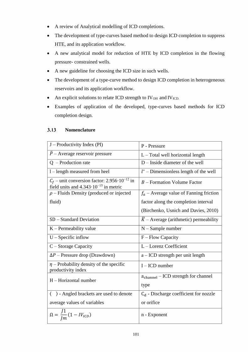
101
A review of Analytical modelling of ICD completions.
The development of type-curves based method to design ICD completion to suppress
HTE, and its application workflow.
A new analytical model for reduction of HTE by ICD completion in the flowing
pressure- constrained wells.
A new guideline for choosing the ICD size in such wells.
The development of a type-curve method to design ICD completion in heterogeneous
reservoirs and its application workflow.
An explicit solutions to relate ICD strength to IVOH and IVICD.
Examples of application of the developed, type-curves based methods for ICD
completion design.
Nomenclature
J – Productivity Index (PI) P - Pressure
– Average reservoir pressure L – Total well horizontal length
Q – Production rate D – Inside diameter of the well
l – length measured from heel 𝑙∗ – Dimensionless length of the well
𝐶𝑓 – unit conversion factor: 2.956·10−12 in
field units and 4.343·10−15 in metric 𝐵 – Formation Volume Factor
𝜌 – Fluids Density (produced or injected
fluid)
𝑓𝑎 – Average value of Fanning friction
factor along the completion interval
(Birchenko, Usnich and Davies, 2010)
SD – Standard Deviation – Average (arithmetic) permeability
K – Permeability value N – Sample number
U – Specific inflow F – Flow Capacity
C – Storage Capacity L – Lorenz Coefficient
∆𝑃 – Pressure drop (Drawdown) a – ICD strength per unit length
𝜂 – Probability density of the specific
productivity index I – ICD number
H – Horizontal number achannel – ICD strength for channel
type
⟨ ⟩ - Angled brackets are used to denote
average values of variables
Cd - Discharge coefficient for nozzle
or orifice
Ω = 𝐽1
𝐽𝑚(1 − 𝐼𝑉𝐼𝐶𝐷) n - Exponent
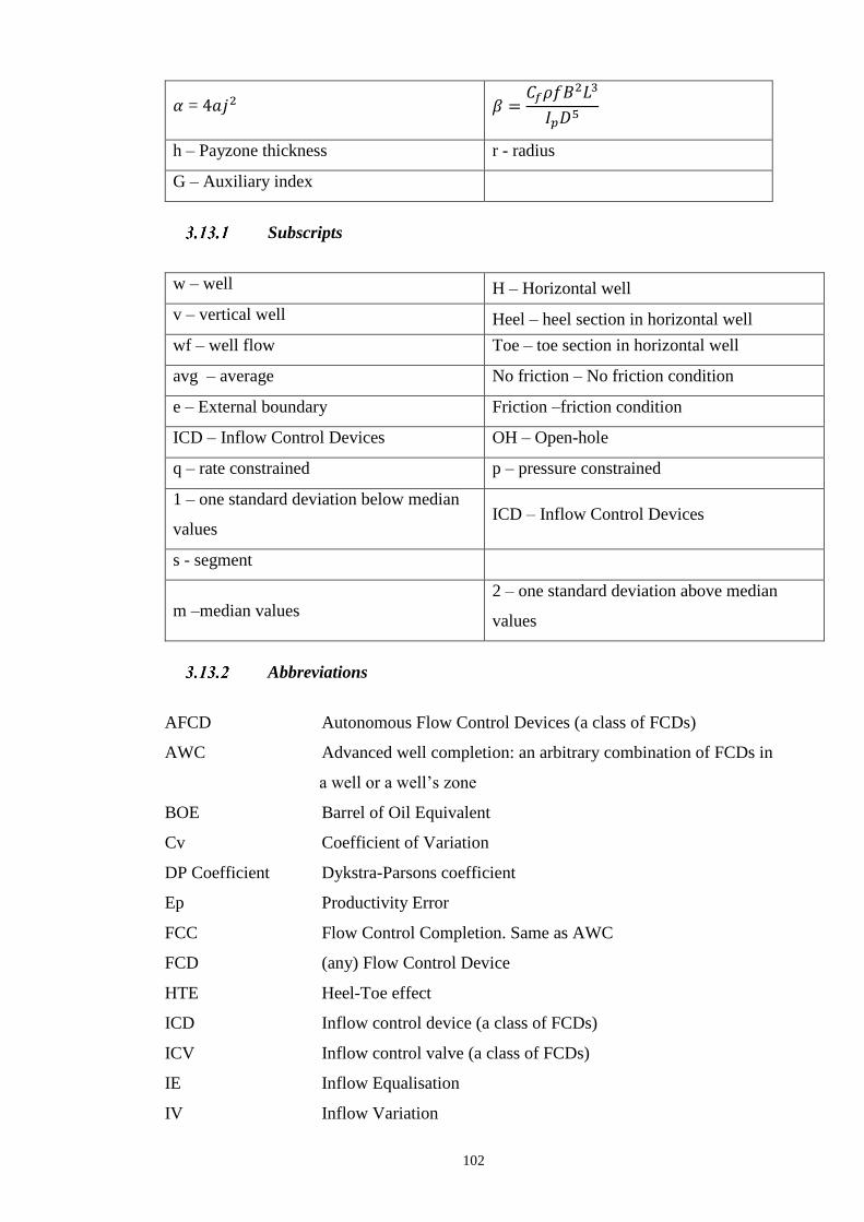
102
𝛼 = 4𝑎𝑗2 𝛽 =𝐶𝑓𝜌𝑓𝐵
2𝐿3
𝐼𝑝𝐷5
h – Payzone thickness r - radius
G – Auxiliary index
Subscripts
w – well H – Horizontal well
v – vertical well Heel – heel section in horizontal well
wf – well flow Toe – toe section in horizontal well
avg – average No friction – No friction condition
e – External boundary Friction –friction condition
ICD – Inflow Control Devices OH – Open-hole
q – rate constrained p – pressure constrained
1 – one standard deviation below median
values ICD – Inflow Control Devices
s - segment
m –median values
2 – one standard deviation above median
values
Abbreviations
AFCD Autonomous Flow Control Devices (a class of FCDs)
AWC Advanced well completion: an arbitrary combination of FCDs in
a well or a well’s zone
BOE Barrel of Oil Equivalent
Cv Coefficient of Variation
DP Coefficient Dykstra-Parsons coefficient
Ep Productivity Error
FCC Flow Control Completion. Same as AWC
FCD (any) Flow Control Device
HTE Heel-Toe effect
ICD Inflow control device (a class of FCDs)
ICV Inflow control valve (a class of FCDs)
IE Inflow Equalisation
IV Inflow Variation

103
MDRT Measured Depth from Rotary Table
Rd Drawdown Ratio
PI Productivity Index
PIF Productivity Improvement Factor
WOC Water Oil Contact
GOC Gas Oil Contact
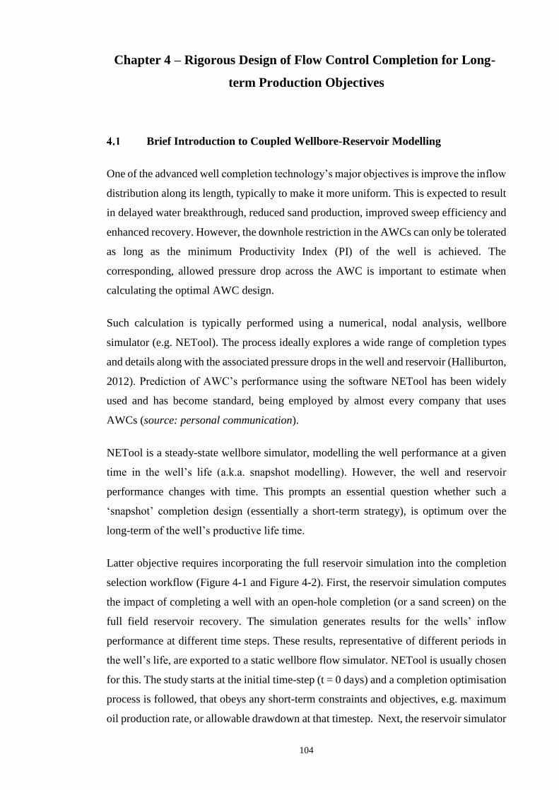
104
Chapter 4 – Rigorous Design of Flow Control Completion for Long-
term Production Objectives
Brief Introduction to Coupled Wellbore-Reservoir Modelling
One of the advanced well completion technology’s major objectives is improve the inflow
distribution along its length, typically to make it more uniform. This is expected to result
in delayed water breakthrough, reduced sand production, improved sweep efficiency and
enhanced recovery. However, the downhole restriction in the AWCs can only be tolerated
as long as the minimum Productivity Index (PI) of the well is achieved. The
corresponding, allowed pressure drop across the AWC is important to estimate when
calculating the optimal AWC design.
Such calculation is typically performed using a numerical, nodal analysis, wellbore
simulator (e.g. NETool). The process ideally explores a wide range of completion types
and details along with the associated pressure drops in the well and reservoir (Halliburton,
2012). Prediction of AWC’s performance using the software NETool has been widely
used and has become standard, being employed by almost every company that uses
AWCs (source: personal communication).
NETool is a steady-state wellbore simulator, modelling the well performance at a given
time in the well’s life (a.k.a. snapshot modelling). However, the well and reservoir
performance changes with time. This prompts an essential question whether such a
‘snapshot’ completion design (essentially a short-term strategy), is optimum over the
long-term of the well’s productive life time.
Latter objective requires incorporating the full reservoir simulation into the completion
selection workflow (Figure 4-1 and Figure 4-2). First, the reservoir simulation computes
the impact of completing a well with an open-hole completion (or a sand screen) on the
full field reservoir recovery. The simulation generates results for the wells’ inflow
performance at different time steps. These results, representative of different periods in
the well’s life, are exported to a static wellbore flow simulator. NETool is usually chosen
for this. The study starts at the initial time-step (t = 0 days) and a completion optimisation
process is followed, that obeys any short-term constraints and objectives, e.g. maximum
oil production rate, or allowable drawdown at that timestep. Next, the reservoir simulator
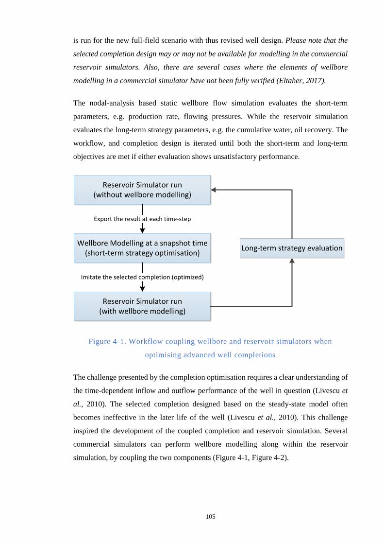
105
is run for the new full-field scenario with thus revised well design. Please note that the
selected completion design may or may not be available for modelling in the commercial
reservoir simulators. Also, there are several cases where the elements of wellbore
modelling in a commercial simulator have not been fully verified (Eltaher, 2017).
The nodal-analysis based static wellbore flow simulation evaluates the short-term
parameters, e.g. production rate, flowing pressures. While the reservoir simulation
evaluates the long-term strategy parameters, e.g. the cumulative water, oil recovery. The
workflow, and completion design is iterated until both the short-term and long-term
objectives are met if either evaluation shows unsatisfactory performance.
Reservoir Simulator run(without wellbore modelling)
Wellbore Modelling at a snapshot time(short-term strategy optimisation)
Export the result at each time-step
Long-term strategy evaluation
Reservoir Simulator run(with wellbore modelling)
Imitate the selected completion (optimized)
Figure 4-1. Workflow coupling wellbore and reservoir simulators when
optimising advanced well completions
The challenge presented by the completion optimisation requires a clear understanding of
the time-dependent inflow and outflow performance of the well in question (Livescu et
al., 2010). The selected completion designed based on the steady-state model often
becomes ineffective in the later life of the well (Livescu et al., 2010). This challenge
inspired the development of the coupled completion and reservoir simulation. Several
commercial simulators can perform wellbore modelling along within the reservoir
simulation, by coupling the two components (Figure 4-1, Figure 4-2).
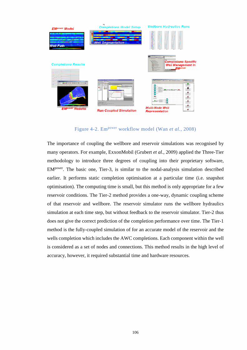
106
Figure 4-2. Empower workflow model (Wan et al., 2008)
The importance of coupling the wellbore and reservoir simulations was recognised by
many operators. For example, ExxonMobil (Grubert et al., 2009) applied the Three-Tier
methodology to introduce three degrees of coupling into their proprietary software,
EMpower. The basic one, Tier-3, is similar to the nodal-analysis simulation described
earlier. It performs static completion optimisation at a particular time (i.e. snapshot
optimisation). The computing time is small, but this method is only appropriate for a few
reservoir conditions. The Tier-2 method provides a one-way, dynamic coupling scheme
of that reservoir and wellbore. The reservoir simulator runs the wellbore hydraulics
simulation at each time step, but without feedback to the reservoir simulator. Tier-2 thus
does not give the correct prediction of the completion performance over time. The Tier-1
method is the fully-coupled simulation of for an accurate model of the reservoir and the
wells completion which includes the AWC completions. Each component within the well
is considered as a set of nodes and connections. This method results in the high level of
accuracy, however, it required substantial time and hardware resources.
107
Figure 4-3. Workflow for coupling wellbore and reservoir simulators (Grubert
et al., 2009)
The fully coupled approach requires more computing power and engineering time. This
however, is often not the case; plus sufficient input information, such a detailed geological
model is also often not available (Williams et al., 2004). Modelling an Advanced Well
Completion (AWC) adds complexity to the wellbore model, increasing even more the
required computing time and resources compared to a typical reservoir simulation. The
complex physics of the flow devices necessitates multiple model iterations, while and the
simulation may require even more resources for the new generation of flow control
devices (AICV, AFCD).
As an example, Heriot-Watt’s Joint Industry Project (JIP) did an early, full-field
feasibility study of wells with autonomous flow control devices for an offshore, viscous
oil field (Haghighat, et al 2015). The objective of the study was to find the best
completion (type and size) for the oil reservoir completed with 3 multi-lateral wells in the
presence of a large aquifer. The primary challenge of the study was that the full-field
simulation time exceeded 24 hours for completing a single run (Figure 4-4). The
simulation time almost doubled when flow control devices were introduced into the well
models (the green and red lines in Figure 4-4). More than 500 sensitivity runs were
required to find the optimum completion design. A method to reduce computing time is
thus much needed.
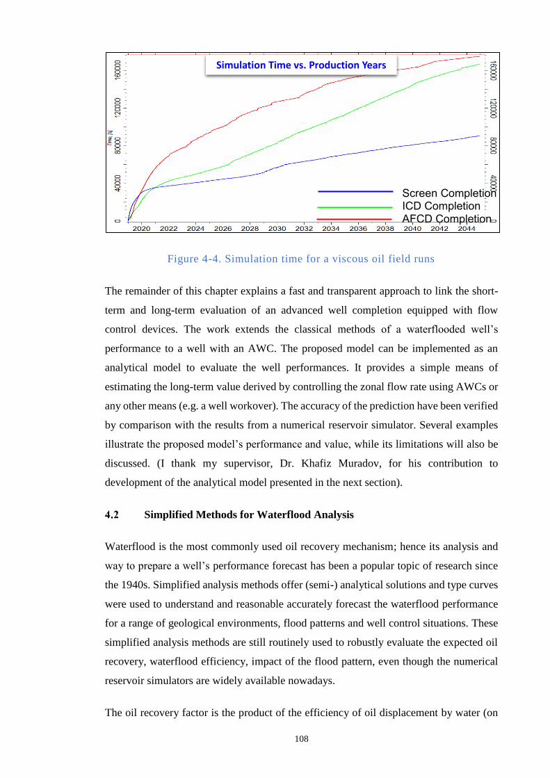
108
Figure 4-4. Simulation time for a viscous oil field runs
The remainder of this chapter explains a fast and transparent approach to link the short-
term and long-term evaluation of an advanced well completion equipped with flow
control devices. The work extends the classical methods of a waterflooded well’s
performance to a well with an AWC. The proposed model can be implemented as an
analytical model to evaluate the well performances. It provides a simple means of
estimating the long-term value derived by controlling the zonal flow rate using AWCs or
any other means (e.g. a well workover). The accuracy of the prediction have been verified
by comparison with the results from a numerical reservoir simulator. Several examples
illustrate the proposed model’s performance and value, while its limitations will also be
discussed. (I thank my supervisor, Dr. Khafiz Muradov, for his contribution to
development of the analytical model presented in the next section).
Simplified Methods for Waterflood Analysis
Waterflood is the most commonly used oil recovery mechanism; hence its analysis and
way to prepare a well’s performance forecast has been a popular topic of research since
the 1940s. Simplified analysis methods offer (semi-) analytical solutions and type curves
were used to understand and reasonable accurately forecast the waterflood performance
for a range of geological environments, flood patterns and well control situations. These
simplified analysis methods are still routinely used to robustly evaluate the expected oil
recovery, waterflood efficiency, impact of the flood pattern, even though the numerical
reservoir simulators are widely available nowadays.
The oil recovery factor is the product of the efficiency of oil displacement by water (on
Screen Completion
ICD Completion
AFCD Completion
Simulation Time vs. Production Years

109
the pore level) and the volumetric sweep efficiency (the extent of the water front on the
reservoir level). The latter is the product of the areal and vertical sweep efficiencies. The
areal sweep efficiency is very much the function of the flood pattern, geological
discontinuities, mobility ratio, etc. The vertical sweep efficiency at any given time is the
fraction of the cross-section between e.g. an injection and a production well that is flooded
by water. This efficiency, inter alia, strongly depends on the reservoir heterogeneity: more
permeable layers are flooded faster distorting the water front.
Prediction and analysis of the vertical sweep (or horizontal sweep for horizontal well)
efficiency will be the main topic of this chapter since generally the AWCs are designed
to deal with the non-even flood front propagation in heterogeneous reservoirs. The areal
sweep efficiency and oil displacement efficiency can be found by other means:
mathematical models, e.g. Dyes et al., 1954 or core flooding experiments respectively.
Analytical solutions for vertical sweep efficiency in heterogeneous reservoirs require
number of assumptions, such as the level of inter-layer communication. Two situations
must be assumed: the layers can either be non-communicating or are perfectly
communicating (i.e. instantaneous, vertical, pressure equilibrium).
The case of non-communicating layers with arbitrary properties was well analysed by
Dykstra and Parsons, 1950. They derived analytical solutions (called here the “DP
method”) which applied when on a layer-by-layer basis, provide estimates of the recovery
efficiency, the fractional flow curve, with regard to the injected water volume. They also
used these analytical solutions to derive general formulae and type curves for a reservoir
with a vertical, log-normal, permeability distribution. Later, major contributions in this
area include the works by Muscat, 1950, who derived expressions for other types of
permeability distribution; while the situations with other-than-one water-oil ratios were
analysed by Johnson, 1956. The model prediction w.r.t injected volumes were translated
into the time domain by Reznik et al., 1984, and El-Khatib, 1985. Osman and Tiab, 1981,
extended the model to the case of composite layers (i.e. were permeability vary laterally).
The frontal displacement theory describing the two-phase, immiscible displacement in
linear system was developed by Buckley and Leverett, 1942. This solution will be called
the BL method. Frontal displacement theory establishes a relationship between the
average water saturation as a function of either cumulative water injected, or of the
injection time. Welge, 1952, presented a new method to obtain the average saturation
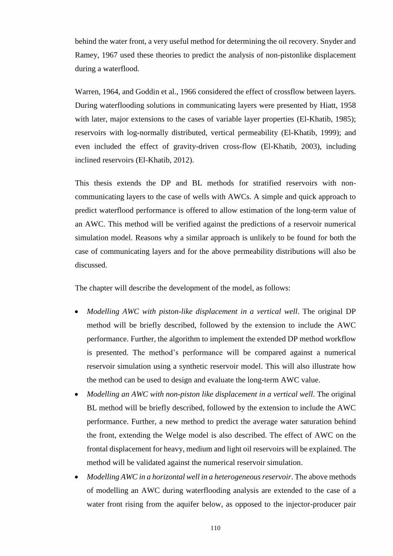
110
behind the water front, a very useful method for determining the oil recovery. Snyder and
Ramey, 1967 used these theories to predict the analysis of non-pistonlike displacement
during a waterflood.
Warren, 1964, and Goddin et al., 1966 considered the effect of crossflow between layers.
During waterflooding solutions in communicating layers were presented by Hiatt, 1958
with later, major extensions to the cases of variable layer properties (El-Khatib, 1985);
reservoirs with log-normally distributed, vertical permeability (El-Khatib, 1999); and
even included the effect of gravity-driven cross-flow (El-Khatib, 2003), including
inclined reservoirs (El-Khatib, 2012).
This thesis extends the DP and BL methods for stratified reservoirs with non-
communicating layers to the case of wells with AWCs. A simple and quick approach to
predict waterflood performance is offered to allow estimation of the long-term value of
an AWC. This method will be verified against the predictions of a reservoir numerical
simulation model. Reasons why a similar approach is unlikely to be found for both the
case of communicating layers and for the above permeability distributions will also be
discussed.
The chapter will describe the development of the model, as follows:
Modelling AWC with piston-like displacement in a vertical well. The original DP
method will be briefly described, followed by the extension to include the AWC
performance. Further, the algorithm to implement the extended DP method workflow
is presented. The method’s performance will be compared against a numerical
reservoir simulation using a synthetic reservoir model. This will also illustrate how
the method can be used to design and evaluate the long-term AWC value.
Modelling an AWC with non-piston like displacement in a vertical well. The original
BL method will be briefly described, followed by the extension to include the AWC
performance. Further, a new method to predict the average water saturation behind
the front, extending the Welge model is also described. The effect of AWC on the
frontal displacement for heavy, medium and light oil reservoirs will be explained. The
method will be validated against the numerical reservoir simulation.
Modelling AWC in a horizontal well in a heterogeneous reservoir. The above methods
of modelling an AWC during waterflooding analysis are extended to the case of a
water front rising from the aquifer below, as opposed to the injector-producer pair

111
dominated waterflood discussed above. The mathematical derivation will be
explained and its predictions validated against a numerical simulation. The results of
the cases studies with this model will be further coupled to the type-curve AWC
analysis described in chapter 2. This closes the loop for the rapid, of ICD completion
design workflow for wells in heterogeneous reservoirs.
Modelling the performance of a waterflood with vertical AWC wells using
modified DP method
DP method for a non-communicating, layered reservoir with piston-like
displacement
The DP method is traditionally used for vertical wells. It can also be used for predicting
the performance of a waterflood with deviated or horizontal wells (in the latter case the
layers must be tilted and/or contain channels), as long as the assumptions listed below are
satisfied. This justifies our extension of the method to AWCs that are not vertical. Note
that the equivalent methods for a communicating layered reservoir also exist. But since
they assume perfect vertical pressure equilibrium for all layers (i.e. the local pressure
derivative at a given distance from the well is the same for every layer), they are
impractical for wells with flow control completion whose sole purpose is to create
significantly different pressure drops across each layer.
The original DP method (Dykstra and Parsons, 1950) assumes non-communicating
layers. This is normally expressed by the stronger assumption kv = 0; stressing the fact
that the gravity forces’ layer-by-layer impact on the oil displacement front is minor
compared to the overall lateral flow. This holds true for numbers of heterogeneous
reservoirs. This method and its modifications are still extensively used for estimating
vertical sweep efficiency – an integral part of estimating the field’s recovery factor at its
design stage. A brief derivation of the original DP method for the conventional wells
provided below:
Figure 4-5 is an injector-producer pair, separated by distance L, in a heterogeneous
reservoir.
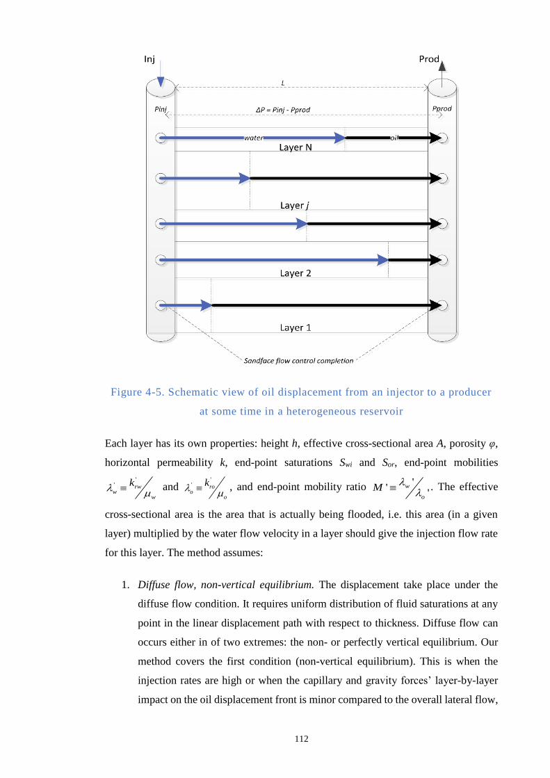
112
Figure 4-5. Schematic view of oil displacement from an injector to a producer
at some time in a heterogeneous reservoir
Each layer has its own properties: height h, effective cross-sectional area A, porosity φ,
horizontal permeability k, end-point saturations Swi and Sor, end-point mobilities
'' rww
w
k
and
'' roo
o
k
, and end-point mobility ratio '
''
w
o
M
. The effective
cross-sectional area is the area that is actually being flooded, i.e. this area (in a given
layer) multiplied by the water flow velocity in a layer should give the injection flow rate
for this layer. The method assumes:
1. Diffuse flow, non-vertical equilibrium. The displacement take place under the
diffuse flow condition. It requires uniform distribution of fluid saturations at any
point in the linear displacement path with respect to thickness. Diffuse flow can
occurs either in of two extremes: the non- or perfectly vertical equilibrium. Our
method covers the first condition (non-vertical equilibrium). This is when the
injection rates are high or when the capillary and gravity forces’ layer-by-layer
impact on the oil displacement front is minor compared to the overall lateral flow,
113
hence the communication between layers are minimal. This is normally expressed
by setting Pc = 0 and kv = 0.
2. Incompressible fluids. This implies our analysis is applicable to analysis of oil
displacement by water, or when the effect of gas compressibility is negligible on
the overall displacement efficiency.
3. Piston-like displacement in each given layer. This expresses the fact that the
lateral water front variation within a given layer is minor compared to the overall
front variation caused by the reservoir heterogeneity. This holds true for a vast
number of heterogeneous reservoirs.
4. The pressure drop between the injection and production wells is constant. More
specifically in this paper: the pressure drop between their sandface or bottom hole
pressures. This is reasonable since the injection and production wells are often
controlled by pressure for the most of their production life. Besides, 100% voidage
ratio is traditionally assumed in displacement models – the injection rate for each
layer matches its production rate and the liquids and rock are assumed to be
incompressible. Section 4.3.3 will show how the method can also be extended to
the constant production rate cases.
All the volumes and rates are discussed at reservoir conditions.
Consider layer j where water front has travelled to coordinate xj (Figure 4-6):
Figure 4-6. Saturation profile in Layer j
Darcy’s equation states that in oil and water regions the flow velocities are, respectively:
'
o oo
k Pu
L x
(4-1)
'
w ww
k Pu
x
(4-2)
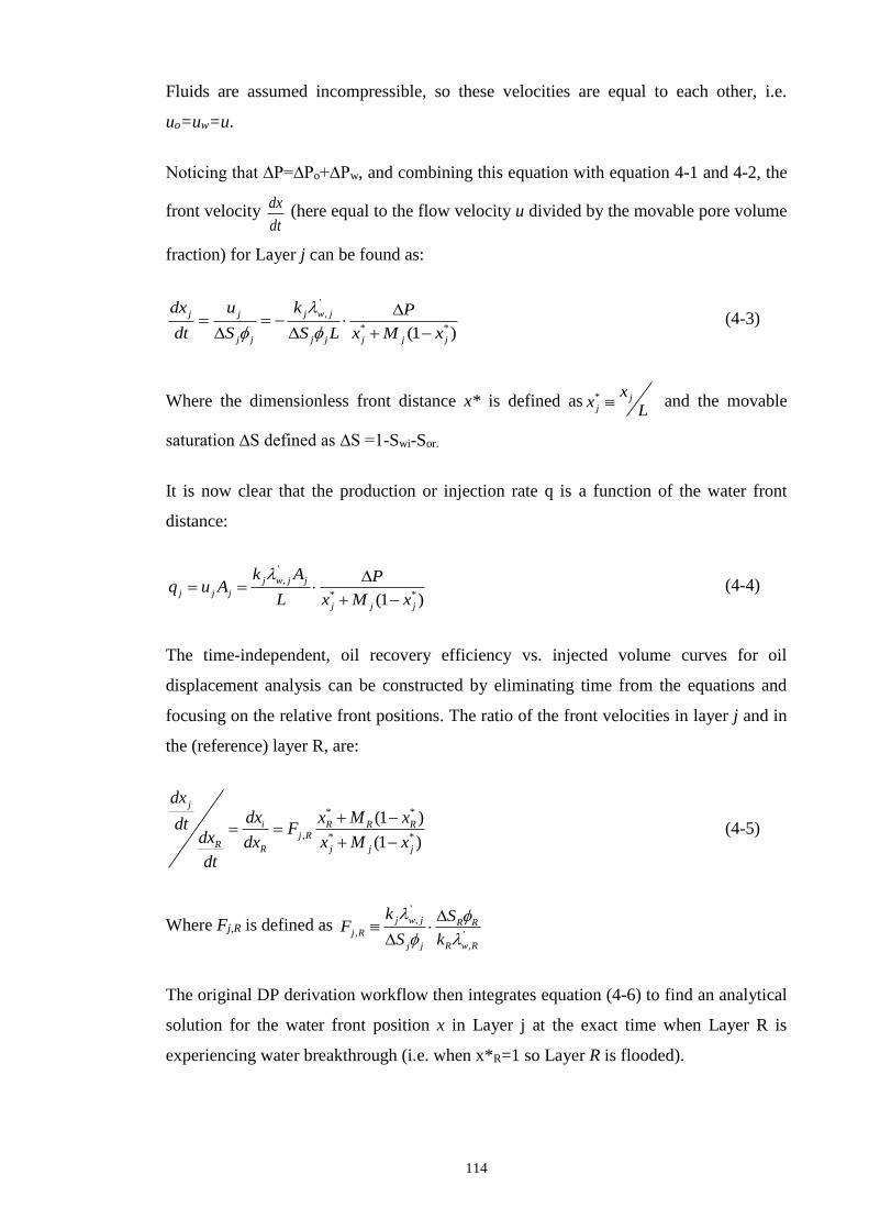
114
Fluids are assumed incompressible, so these velocities are equal to each other, i.e.
uo=uw=u.
Noticing that ∆P=∆Po+∆Pw, and combining this equation with equation 4-1 and 4-2, the
front velocity dx
dt (here equal to the flow velocity u divided by the movable pore volume
fraction) for Layer j can be found as:
'
,
* *(1 )
j j j w j
j j j j j j j
dx u k P
dt S S L x M x
(4-3)
Where the dimensionless front distance x* is defined as * jj
xx
L and the movable
saturation ∆S defined as ∆S =1-Swi-Sor.
It is now clear that the production or injection rate q is a function of the water front
distance:
'
,
* *(1 )
j w j j
j j j
j j j
k A Pq u A
L x M x
(4-4)
The time-independent, oil recovery efficiency vs. injected volume curves for oil
displacement analysis can be constructed by eliminating time from the equations and
focusing on the relative front positions. The ratio of the front velocities in layer j and in
the (reference) layer R, are:
* *
, * *
(1 )
(1 )
j
i R R Rj R
RR j j j
dxdx x M xdt F
dx dx x M xdt
(4-5)
Where Fj,R is defined as '
,
, '
,
j w j R Rj R
j j R w R
k SF
S k
The original DP derivation workflow then integrates equation (4-6) to find an analytical
solution for the water front position x in Layer j at the exact time when Layer R is
experiencing water breakthrough (i.e. when x*R=1 so Layer R is flooded).
115
*1
* * * * * *
,
0 0
(1 ) (1 )
jx
j j j j j R R R R Rx M x dx F x M x dx (4-6)
Further, the integral solution can then be expressed explicitly for xj as:
2
,*(1 )(1 )
1
j j j R j R
j
j
M M F M Mx
M
(4-7)
(Except for the case Mj=1 when the integral solution yields ,*
(1 )
2
j R R
j
F Mx
).
(It is also possible to find the imaginary distance (and hence the injected volume) of the
water front in a layer after it has been flooded by changing the integration limits.)
The front distances in the remaining layers are calculated by taking the first layer to
experience breakthrough as a reference layer. This allows calculation of both the overall
reservoir saturation and the injected volumes at this time. The production rates of oil and
(in the reference layer) water are calculated using equation 4-4. This allows calculation
of the production well’s fractional flow fw (or water cut WC).
The curve of reservoir water saturation or injected volume vs. WC is constructed by
repeating this this step for each subsequent layer in the order that they experience water
breakthrough. This allows analysing the waterflooding dynamics, efficiency and the
estimated recovery factor, hence the main objective of the method is achieved.
The formation permeabilities can be corrected if the layers are differentially depleted, as
proposed in Dake, 2001.
Time can be re-introduced into the model if required. This may be important when the
actual production/injection forecast is needed, e.g. for economic field evaluation. Time
can be introduced accurately by integrating the analytical solution for xj (Reznik et al.,
1984, El-Khatib, 1985). Alternatively, time can be approximately introduced by matching
the injection rates and injected volumes, i.e. *
,
1R
Rbt R
R at x
WIt
q
. This is an approximate
answer because the injection rate changes with time though not significantly until water
breaks through. Section 4.3.2 will follow the same workflow while introducing the
extended solutions that incorporates the impact of an arbitrary sandface, flow control

116
completion in wells.
Extension of the DP method to the case of wells with AWC
In general, a Flow Control Completion (FCC) imposes a pressure drop that is
quadratically proportional to the flow rate:
2
FCC flowing phaseP a q (4-8)
The coefficient a (FCC strength) is a function of the FCC strength, the number of FCDs
per zone in question, and the flowing fluid properties. Various formulae explaining how
to calculate it for a given FCC type or for a completion zone containing multiple FCCs
are presented in (Al-Khelaiwi, 2013). In this study for simplicity, we will refer to it simply
as aw for water flow and ao for oil flow. The total pressure drop across a layer is now a
function of both the reservoir and FCC pressure drops:
2 * 2
, ,FCC injector layer FCC producer inj prod layer layerP P P P a a q P a q P
(4-9)
Where *a for a given layer equals * *
, ,bbt w inj o proda a a a before water breaks through
this layer; and * *
, ,abt w inj w proda a a a after water breakthrough. It is possible to model
any arbitrary FCC performance or well workover action for any given layer by changing
the coefficients a for this layer. The following FCC examples illustrate what can be
modelled:
ICD, ICV, AFCD, AICV completion (with any arbitrary number of devices per
layer) when the a coefficients are selected to match the FCC’s number/layer and
the single phase flow performance curves
When a conventional completion is installed, i.e. when a = 0
Closure of the zone by e.g. an autonomous water shut-in response of the FCC, or
closure of an ICD/ICV, zonal isolation by a well workover, etc. by taking either
aw,prod = ∞ or simply qabt=0.
Any other arbitrary flow control action for each layer.
This allows modelling any FCC performance.
117
The original DP method is any valid for the reservoir-only flow, i.e. for an openhole
completion where the impact of FCC is absent, and the sandface pressures are calculated.
This sandface-to-sandface pressure drop (∆P) across any layer can be found by
rearranging equation 4-9 as:
* 2
layerP P a q (4-10)
Changing ∆P to ∆Player in equation 4-4 results in ' * 2
,
* *(1 )
j w j j j j
j
j j j
k A P a qq
L x M x
, and
expressing this quadratic equation for u=q/A yields:
2 * 2 2
* 2
4
2
j j j j j
j
j j j
B B a A C Pu
a A C
(4-11)
Where coefficients B and C are defined as:
* *(1 )j j j jB x M x (4-12)
'
,j w j
j
kC
L
(4-13)
Note that in the AWC case, the effective cross-sectional area is introduced immediately
since it affects the reservoir pressure drop. This differs from the original method where
this area only appears later in the method, when calculating the flow rates and watercuts.
This new approach demands that the effective cross-sectional area be reliably estimated,
by taking into account the areal sweep efficiency, flood patterns, faults, etc.
The integral (equation 4-14) is solved by following the same logic that led to equation 4-
6 in the original method:
* *
* *
0 0
j Rx x
j j R Rj R
j R
S Sdx dx
u u
(4-14)
The general analytic solution for integral 4-14 for arbitrary limits is:

118
*
*
*,min
*,min
2 * 2 2
*
* 2 2 2 * 2 2
4
4(1 ) 4 ln 4
j
j
j
j
x
xj j j j j j
j j j j
j
j j jxj j j j j j j j
x
B B a A C P BS Sdx
u M C P a A C P B a A C P B
(4-15)
Particular limits will be considered in Section 4.3.3, which describes the complete
application workflow.
Workflow AWC with piston like displacement in vertical well
Consider an injector-producer pair, separated by distance L, in a heterogeneous reservoir.
Each layer has its own height h, effective cross-sectional area A, porosity φ, horizontal
permeability k, end point saturation Swi and Sor, end-point mobilities '
' rww
w
k
and
'' roo
o
k
, and mobility ratio w
o
M
. One or both of the injector and producer
completion can have a FCC, the impact on each layer’s flow is described by the a*
coefficient defined by equation 4-8. Note that a* can vary, e.g. a*bbt before breakthrough
and a*abt after breakthrough.
The following steps, the original DP method, use the equations derived in Section 4.3.2,
that describe how the waterflood analysis can be carried out:
Step 1. Order the layers by breakthrough time, approximately estimated as the inter-well
distance divided by the front velocity calculated at the time when xj*=0.5, derived using
equations 4-11, 4-12, 4-13.
2* 2 2
, ,* 2
.
0.5
0.5 (1 0.5) 0.5 (1 0.5) 4( * 0.5) 2
j
j j j j
bt j j j j bbt j jj j j j bbt j j
x L
S L SLt L M M a A C P
dx u x a A C
dt
(4-16)
Step 2. Take the first layer to experience breakthrough as the reference layer. Find the
water front positions in the other layers when the reference layer experiences water
breakthrough (i.e. when x*R=1). This is done by equating the solutions described by
equation 4-15 as follows:
*1
* *
0 0
jx
j j R Rj R
j R
S Sdx dx
u u
119
Which yields:
2* * * * * 2 2 * * 2 * 2 2
, ,
2* * * 2 2 * *
,* 2 2
,2 * 2 2
,
(1 ) (1 ) 4 (1 ) 4
(1 ) 4 (1 )(1 )4 ln
4
j j j j j j j bbt j j j j j j j j bbt j j j
j j
j j j j bbt j j j j jj j
j bbt j j
j j bbt j j j
x M x x M x a A C P x M x M M a A C P M
S
x M x a A C P x M xM Ca A C P
M a A C P M
* 2 2 2 * 2 2
, ,
* 2 2
,* 2 2
,2 * 2 2
,
1 4 1 4
1 4 1(1 ) 4 ln4
R bbt j R R R R bbt R R R
R R
R bbt R RR R
R bbt R R
R R bbt R R R
a A C P M M a A C P M
Sa A C PM C a A C P
M a A C P M
(4-17)
The validity of the derivation can be tested by setting the FCC coefficients a in equation
4-17 to zero. The result should now match the original, (no-FCC) solution described by
equation 4-7
Note that xj can no longer be expressed explicitly as in the original method (equation 4-
7). It must be solved numerically. We solve such equation with gradient-based, non-linear
solver (available in MS Excel) in a fraction of a second.
Step 3. These front positions can be used to calculate the injected water volume in S.I
units (WI) or in reservoir pore volumes (WI*), as well as the reservoir oil recovery
efficiency (RE) as follows:
*
1
N
j j j j
j
WI A S x L
(4-18)
*
1*
1
N
j j j j
j
N
j j
j
A S x L
WI
A L
(4-19)
* *
*
,
1
,
1 1 1
(1 )
j j
N
j wi j j j
j
N
j j wi j
j if x then x
A S x L
RE
A L S
(4-20)
Note that xj in equation 4-20, equals 1 if xj>=1 for the layers that had previously
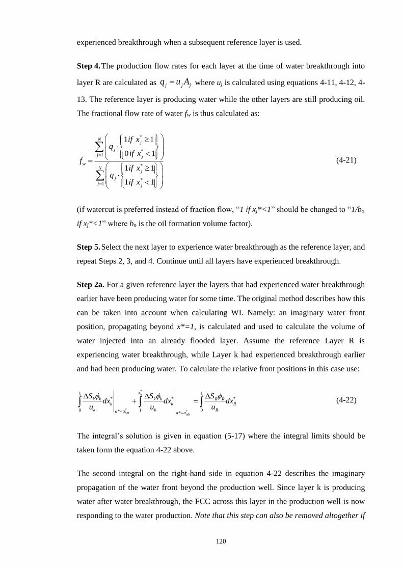
120
experienced breakthrough when a subsequent reference layer is used.
Step 4. The production flow rates for each layer at the time of water breakthrough into
layer R are calculated as j j jq u A where uj is calculated using equations 4-11, 4-12, 4-
13. The reference layer is producing water while the other layers are still producing oil.
The fractional flow rate of water fw is thus calculated as:
*
*1
*
*1
1 1
0 1
1 1
1 1
Nj
j
j j
wN
j
j
j j
if xq
if xf
if xq
if x
(4-21)
(if watercut is preferred instead of fraction flow, “1 if xj*<1” should be changed to “1/bo
if xj*<1” where bo is the oil formation volume factor).
Step 5. Select the next layer to experience water breakthrough as the reference layer, and
repeat Steps 2, 3, and 4. Continue until all layers have experienced breakthrough.
Step 2a. For a given reference layer the layers that had experienced water breakthrough
earlier have been producing water for some time. The original method describes how this
can be taken into account when calculating WI. Namely: an imaginary water front
position, propagating beyond x*=1, is calculated and used to calculate the volume of
water injected into an already flooded layer. Assume the reference Layer R is
experiencing water breakthrough, while Layer k had experienced breakthrough earlier
and had been producing water. To calculate the relative front positions in this case use:
*
**
1 1
* * *
0 1 0* *
k
bbtabt
x
k k k k R Rk k R
k k Ra a a a
S S Sdx dx dx
u u u
(4-22)
The integral’s solution is given in equation (5-17) where the integral limits should be
taken form the equation 4-22 above.
The second integral on the right-hand side in equation 4-22 describes the imaginary
propagation of the water front beyond the production well. Since layer k is producing
water after water breakthrough, the FCC across this layer in the production well is now
responding to the water production. Note that this step can also be removed altogether if
121
zonal water shut-in upon breakthrough is assumed by, e.g. ICV reactive control, water-
restrictive AFCD, ICD sliding sleeve closure, well workover operation, etc.
An example of the application of this workflow, and the excellent match of its results
with those of a comprehensive, numerical reservoir simulation model prediction, is shown
in the next section. This workflow was realized as an Excel spreadsheet and that is solved
using gradient-based, non-linear solver in Excel in a fraction of a second for arbitrary
boundary conditions and FCC set-ups
Finally, since time can be introduced into the production forecast, the method can be
modified to model a constant production rate case (as opposed to the constant pressure
drop case discussed in the calculations above):
A. Introducing time.
The traditional, accurate methods of translating the injected volume into time by
integrating the injection rate over front position x are not applicable here since there
is no explicit analytical solution for x. Instead, equation 4-16 is used to find the
approximate time of each breakthrough, allowing the calculation of the injected
volumes, oil recovery efficiency, fractional flow, etc. into the time domain. Naturally,
the flow velocity changes as the water front propagate within the layer (see e.g.
equation 4-1), but this change is not that significant, and so the velocity estimate at
x*=0.5 is reasonably good enough. The accuracy of this assumption will be confirmed
in section 4.3.4
B. Extending to the constant rate case.
The constant pressure drop workflow can be easily extended to the constant rate case.
The approximate layer rates are estimated by calculating the flow rates for an arbitrary
pressure drop at the time when xj*=0.5 using equations 4-11, 4-12, 4-13. Their sum
gives the total well rate. An optimizer is then used to find the pressure drop required
for this well production rate. This pressure drop is then used as usual in the workflow
described above. This extra step during the model set-up is included in our
spreadsheet. The extra operation takes a fraction of a second.
It is worth mentioning that, in point B above, the well’s approximate flow rate, used to
match the reservoir pressure drop, was estimated before water breakthrough. If there is a
significant post-breakthrough action (e.g. zonal isolation by an ICV), then the flow rate
will change significantly at the given pressure drop. The integration therefore has to be
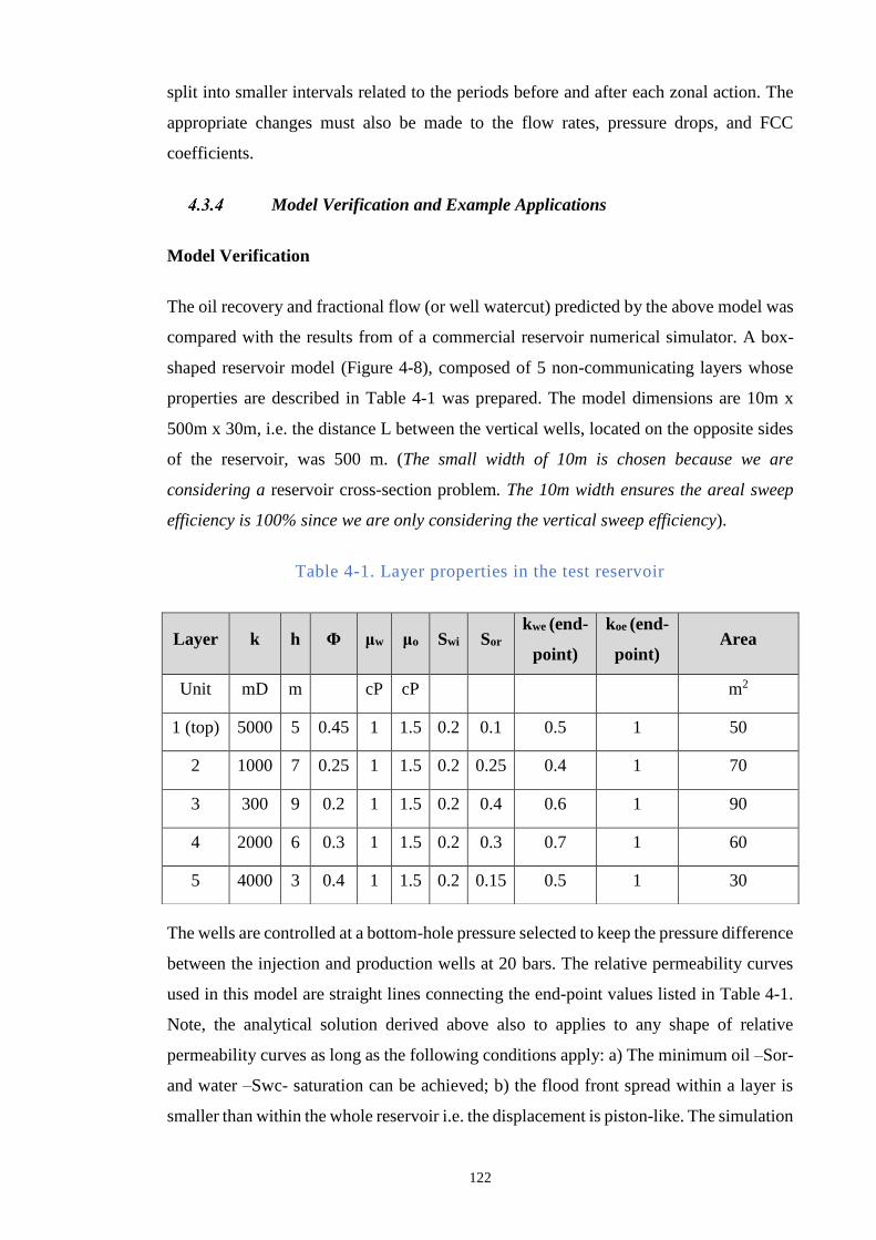
122
split into smaller intervals related to the periods before and after each zonal action. The
appropriate changes must also be made to the flow rates, pressure drops, and FCC
coefficients.
Model Verification and Example Applications
Model Verification
The oil recovery and fractional flow (or well watercut) predicted by the above model was
compared with the results from of a commercial reservoir numerical simulator. A box-
shaped reservoir model (Figure 4-8), composed of 5 non-communicating layers whose
properties are described in Table 4-1 was prepared. The model dimensions are 10m x
500m x 30m, i.e. the distance L between the vertical wells, located on the opposite sides
of the reservoir, was 500 m. (The small width of 10m is chosen because we are
considering a reservoir cross-section problem. The 10m width ensures the areal sweep
efficiency is 100% since we are only considering the vertical sweep efficiency).
Table 4-1. Layer properties in the test reservoir
The wells are controlled at a bottom-hole pressure selected to keep the pressure difference
between the injection and production wells at 20 bars. The relative permeability curves
used in this model are straight lines connecting the end-point values listed in Table 4-1.
Note, the analytical solution derived above also to applies to any shape of relative
permeability curves as long as the following conditions apply: a) The minimum oil –Sor-
and water –Swc- saturation can be achieved; b) the flood front spread within a layer is
smaller than within the whole reservoir i.e. the displacement is piston-like. The simulation
Layer k h Φ μw μo Swi Sor
kwe (end-
point)
koe (end-
point) Area
Unit mD m cP cP m2
1 (top) 5000 5 0.45 1 1.5 0.2 0.1 0.5 1 50
2 1000 7 0.25 1 1.5 0.2 0.25 0.4 1 70
3 300 9 0.2 1 1.5 0.2 0.4 0.6 1 90
4 2000 6 0.3 1 1.5 0.2 0.3 0.7 1 60
5 4000 3 0.4 1 1.5 0.2 0.15 0.5 1 30
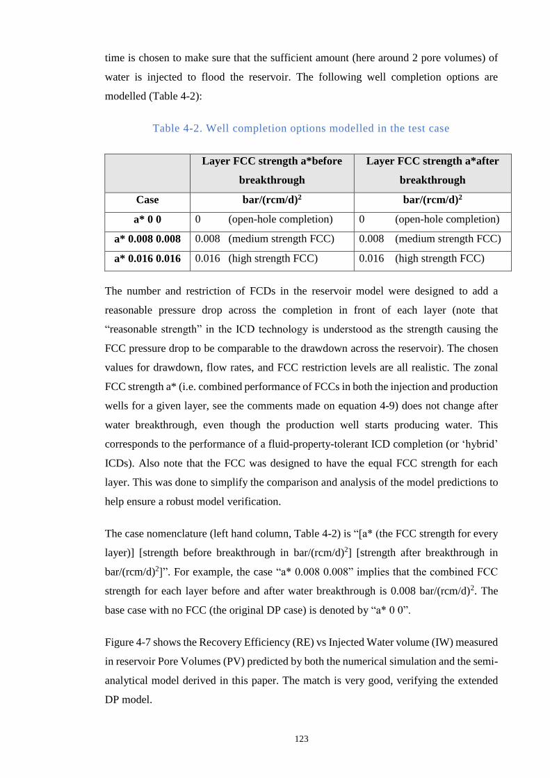
123
time is chosen to make sure that the sufficient amount (here around 2 pore volumes) of
water is injected to flood the reservoir. The following well completion options are
modelled (Table 4-2):
Table 4-2. Well completion options modelled in the test case
Layer FCC strength a*before
breakthrough
Layer FCC strength a*after
breakthrough
Case bar/(rcm/d)2 bar/(rcm/d)2
a* 0 0 0 (open-hole completion) 0 (open-hole completion)
a* 0.008 0.008 0.008 (medium strength FCC) 0.008 (medium strength FCC)
a* 0.016 0.016 0.016 (high strength FCC) 0.016 (high strength FCC)
The number and restriction of FCDs in the reservoir model were designed to add a
reasonable pressure drop across the completion in front of each layer (note that
“reasonable strength” in the ICD technology is understood as the strength causing the
FCC pressure drop to be comparable to the drawdown across the reservoir). The chosen
values for drawdown, flow rates, and FCC restriction levels are all realistic. The zonal
FCC strength a* (i.e. combined performance of FCCs in both the injection and production
wells for a given layer, see the comments made on equation 4-9) does not change after
water breakthrough, even though the production well starts producing water. This
corresponds to the performance of a fluid-property-tolerant ICD completion (or ‘hybrid’
ICDs). Also note that the FCC was designed to have the equal FCC strength for each
layer. This was done to simplify the comparison and analysis of the model predictions to
help ensure a robust model verification.
The case nomenclature (left hand column, Table 4-2) is “[a* (the FCC strength for every
layer)] [strength before breakthrough in bar/(rcm/d)2] [strength after breakthrough in
bar/(rcm/d)2]”. For example, the case “a* 0.008 0.008” implies that the combined FCC
strength for each layer before and after water breakthrough is 0.008 bar/(rcm/d)2. The
base case with no FCC (the original DP case) is denoted by “a* 0 0”.
Figure 4-7 shows the Recovery Efficiency (RE) vs Injected Water volume (IW) measured
in reservoir Pore Volumes (PV) predicted by both the numerical simulation and the semi-
analytical model derived in this paper. The match is very good, verifying the extended
DP model.
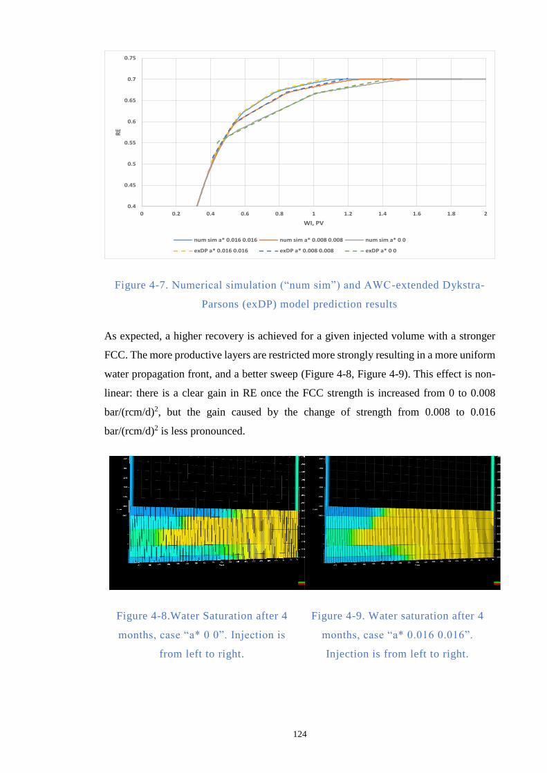
124
Figure 4-7. Numerical simulation (“num sim”) and AWC-extended Dykstra-
Parsons (exDP) model prediction results
As expected, a higher recovery is achieved for a given injected volume with a stronger
FCC. The more productive layers are restricted more strongly resulting in a more uniform
water propagation front, and a better sweep (Figure 4-8, Figure 4-9). This effect is non-
linear: there is a clear gain in RE once the FCC strength is increased from 0 to 0.008
bar/(rcm/d)2, but the gain caused by the change of strength from 0.008 to 0.016
bar/(rcm/d)2 is less pronounced.
Figure 4-8.Water Saturation after 4
months, case “a* 0 0”. Injection is
from left to right.
Figure 4-9. Water saturation after 4
months, case “a* 0.016 0.016”.
Injection is from left to right.
0.4
0.45
0.5
0.55
0.6
0.65
0.7
0.75
0 0.2 0.4 0.6 0.8 1 1.2 1.4 1.6 1.8 2
RE
WI, PV
num sim a* 0.016 0.016 num sim a* 0.008 0.008 num sim a* 0 0
exDP a* 0.016 0.016 exDP a* 0.008 0.008 exDP a* 0 0
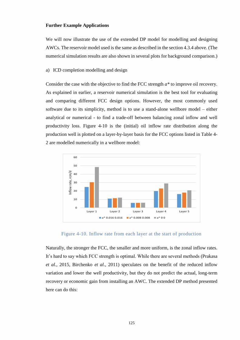
125
Further Example Applications
We will now illustrate the use of the extended DP model for modelling and designing
AWCs. The reservoir model used is the same as described in the section 4.3.4 above. (The
numerical simulation results are also shown in several plots for background comparison.)
a) ICD completion modelling and design
Consider the case with the objective to find the FCC strength a* to improve oil recovery.
As explained in earlier, a reservoir numerical simulation is the best tool for evaluating
and comparing different FCC design options. However, the most commonly used
software due to its simplicity, method is to use a stand-alone wellbore model – either
analytical or numerical - to find a trade-off between balancing zonal inflow and well
productivity loss. Figure 4-10 is the (initial) oil inflow rate distribution along the
production well is plotted on a layer-by-layer basis for the FCC options listed in Table 4-
2 are modelled numerically in a wellbore model:
Figure 4-10. Inflow rate from each layer at the start of production
Naturally, the stronger the FCC, the smaller and more uniform, is the zonal inflow rates.
It’s hard to say which FCC strength is optimal. While there are several methods (Prakasa
et al., 2015, Birchenko et al., 2011) speculates on the benefit of the reduced inflow
variation and lower the well productivity, but they do not predict the actual, long-term
recovery or economic gain from installing an AWC. The extended DP method presented
here can do this:
0
10
20
30
40
50
60
Layer 1 Layer 2 Layer 3 Layer 4 Layer 5
Inflo
w ra
te, r
cm/d
a* 0.016 0.016 a* 0.008 0.008 a* 0 0
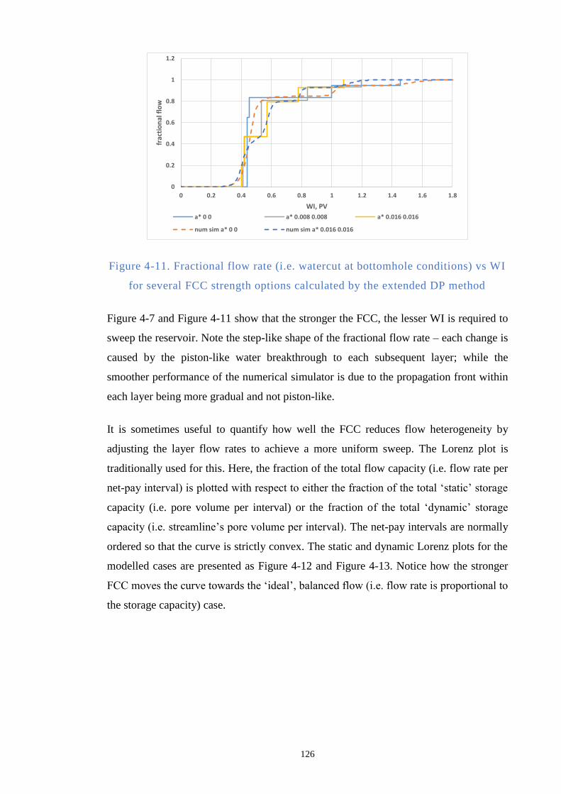
126
Figure 4-11. Fractional flow rate (i.e. watercut at bottomhole conditions) vs WI
for several FCC strength options calculated by the extended DP method
Figure 4-7 and Figure 4-11 show that the stronger the FCC, the lesser WI is required to
sweep the reservoir. Note the step-like shape of the fractional flow rate – each change is
caused by the piston-like water breakthrough to each subsequent layer; while the
smoother performance of the numerical simulator is due to the propagation front within
each layer being more gradual and not piston-like.
It is sometimes useful to quantify how well the FCC reduces flow heterogeneity by
adjusting the layer flow rates to achieve a more uniform sweep. The Lorenz plot is
traditionally used for this. Here, the fraction of the total flow capacity (i.e. flow rate per
net-pay interval) is plotted with respect to either the fraction of the total ‘static’ storage
capacity (i.e. pore volume per interval) or the fraction of the total ‘dynamic’ storage
capacity (i.e. streamline’s pore volume per interval). The net-pay intervals are normally
ordered so that the curve is strictly convex. The static and dynamic Lorenz plots for the
modelled cases are presented as Figure 4-12 and Figure 4-13. Notice how the stronger
FCC moves the curve towards the ‘ideal’, balanced flow (i.e. flow rate is proportional to
the storage capacity) case.
0
0.2
0.4
0.6
0.8
1
1.2
0 0.2 0.4 0.6 0.8 1 1.2 1.4 1.6 1.8
frac
tio
nal
flo
w
WI, PV
a* 0 0 a* 0.008 0.008 a* 0.016 0.016
num sim a* 0 0 num sim a* 0.016 0.016
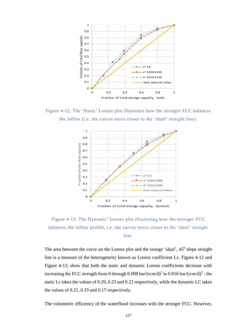
127
Figure 4-12. The ‘Static’ Lorenz plot illustrates how the stronger FCC balances
the inflow (i.e. the curves move closer to the ‘ideal’ straight line).
Figure 4-13. The Dynamic’ Lorenz plot illustrating how the stronger FCC
balances the inflow profile, i.e. the curves move closer to the ‘ideal’ straight
line.
The area between the curve on the Lorenz plot and the orange ‘ideal’, 450 slope straight
line is a measure of the heterogeneity known as Lorenz coefficient Lc. Figure 4-12 and
Figure 4-13, show that both the static and dynamic Lorenz coefficients decrease with
increasing the FCC strength from 0 through 0.008 bar/(rcm/d)2 to 0.016 bar/(rcm/d)2 : the
static Lc takes the values of 0.29, 0.23 and 0.22 respectively, while the dynamic LC takes
the values of 0.21, 0.19 and 0.17 respectively.
The volumetric efficiency of the waterflood increases with the stronger FCC. However,
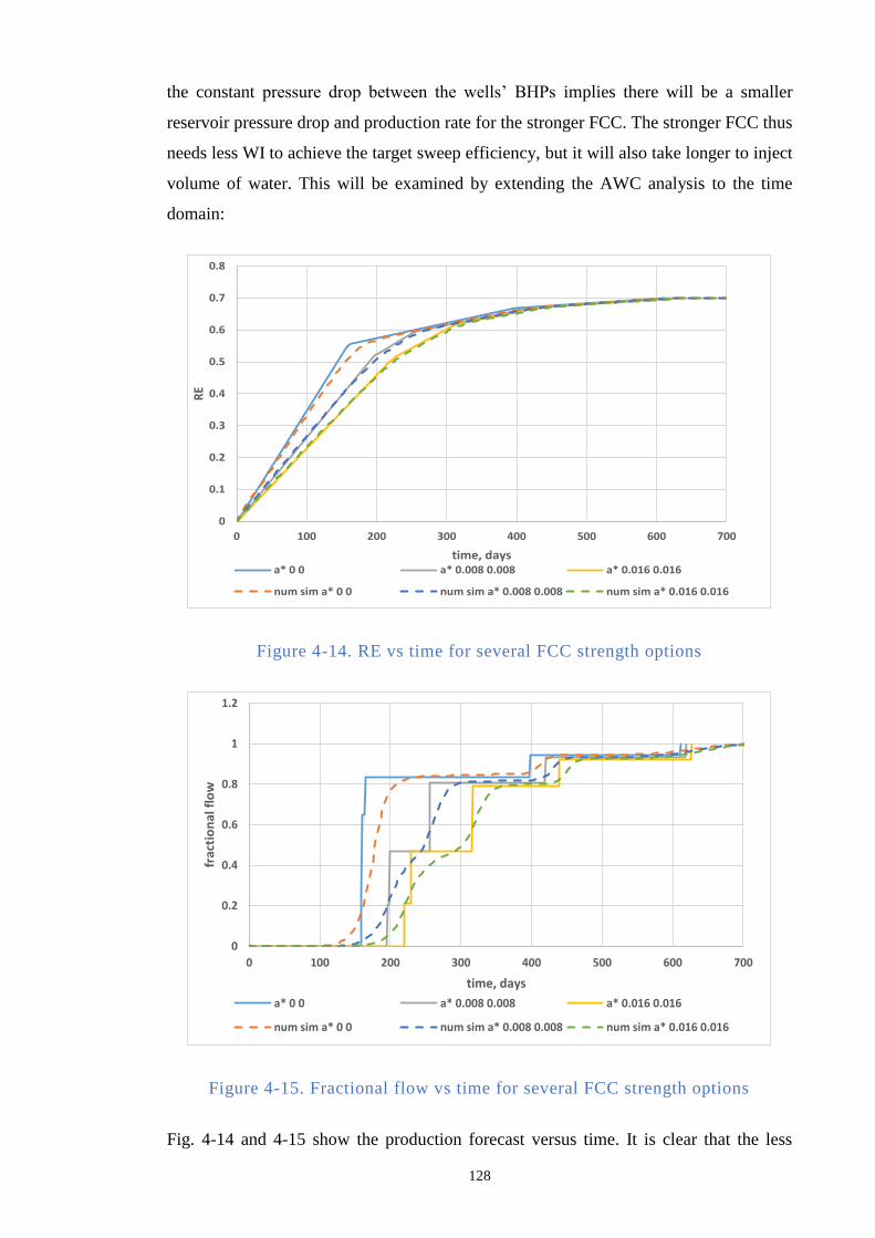
128
the constant pressure drop between the wells’ BHPs implies there will be a smaller
reservoir pressure drop and production rate for the stronger FCC. The stronger FCC thus
needs less WI to achieve the target sweep efficiency, but it will also take longer to inject
volume of water. This will be examined by extending the AWC analysis to the time
domain:
Figure 4-14. RE vs time for several FCC strength options
Figure 4-15. Fractional flow vs time for several FCC strength options
Fig. 4-14 and 4-15 show the production forecast versus time. It is clear that the less
0
0.1
0.2
0.3
0.4
0.5
0.6
0.7
0.8
0 100 200 300 400 500 600 700
RE
time, daysa* 0 0 a* 0.008 0.008 a* 0.016 0.016
num sim a* 0 0 num sim a* 0.008 0.008 num sim a* 0.016 0.016
0
0.2
0.4
0.6
0.8
1
1.2
0 100 200 300 400 500 600 700
fra
ctio
na
l flo
w
time, days
a* 0 0 a* 0.008 0.008 a* 0.016 0.016
num sim a* 0 0 num sim a* 0.008 0.008 num sim a* 0.016 0.016
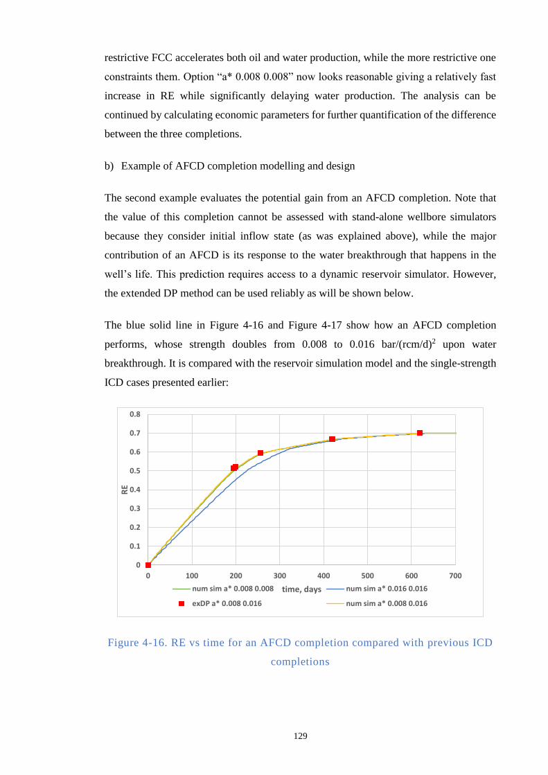
129
restrictive FCC accelerates both oil and water production, while the more restrictive one
constraints them. Option “a* 0.008 0.008” now looks reasonable giving a relatively fast
increase in RE while significantly delaying water production. The analysis can be
continued by calculating economic parameters for further quantification of the difference
between the three completions.
b) Example of AFCD completion modelling and design
The second example evaluates the potential gain from an AFCD completion. Note that
the value of this completion cannot be assessed with stand-alone wellbore simulators
because they consider initial inflow state (as was explained above), while the major
contribution of an AFCD is its response to the water breakthrough that happens in the
well’s life. This prediction requires access to a dynamic reservoir simulator. However,
the extended DP method can be used reliably as will be shown below.
The blue solid line in Figure 4-16 and Figure 4-17 show how an AFCD completion
performs, whose strength doubles from 0.008 to 0.016 bar/(rcm/d)2 upon water
breakthrough. It is compared with the reservoir simulation model and the single-strength
ICD cases presented earlier:
Figure 4-16. RE vs time for an AFCD completion compared with previous ICD
completions
0
0.1
0.2
0.3
0.4
0.5
0.6
0.7
0.8
0 100 200 300 400 500 600 700
RE
time, daysnum sim a* 0.008 0.008 num sim a* 0.016 0.016
exDP a* 0.008 0.016 num sim a* 0.008 0.016
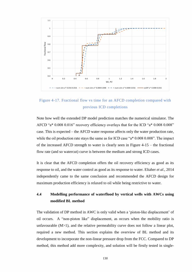
130
Figure 4-17. Fractional flow vs time for an AFCD completion compared with
previous ICD completions
Note how well the extended DP model prediction matches the numerical simulator. The
AFCD “a* 0.008 0.016” recovery efficiency overlays that for the ICD “a* 0.008 0.008”
case. This is expected – the AFCD water response affects only the water production rate,
while the oil production rate stays the same as for ICD case “a* 0.008 0.008”. The impact
of the increased AFCD strength to water is clearly seen in Figure 4-15 – the fractional
flow rate (and so watercut) curve is between the medium and strong ICD cases.
It is clear that the AFCD completion offers the oil recovery efficiency as good as its
response to oil, and the water control as good as its response to water. Eltaher et al., 2014
independently came to the same conclusion and recommended the AFCD design for
maximum production efficiency is relaxed to oil while being restrictive to water.
Modelling performance of waterflood by vertical wells with AWCs using
modified BL method
The validation of DP method in AWC is only valid when a ‘piston-like displacement’ of
oil occurs. A “non-piston like” displacement, as occurs when the mobility ratio is
unfavourable (M>1), and the relative permeability curve does not follow a linear plot,
required a new method. This section explains the overview of BL method and its
development to incorporate the non-linear pressure drop from the FCC. Compared to DP
method, this method add more complexity, and solution will be firstly tested in single-
0.4
0.5
0.6
0.7
0.8
0.9
1
1.1
0 0.2 0.4 0.6 0.8 1 1.2 1.4 1.6 1.8 2
frac
tio
nal
flo
w
WI, PV
num sim a* 0.016 0.016 num sim a* 0.008 0.008 num sim a* 0.008 0.016 exDP a* 0.008 0.016
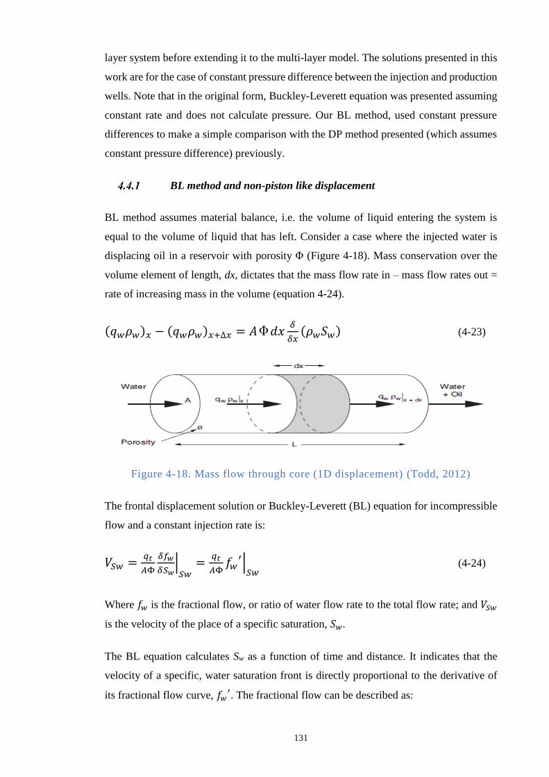
131
layer system before extending it to the multi-layer model. The solutions presented in this
work are for the case of constant pressure difference between the injection and production
wells. Note that in the original form, Buckley-Leverett equation was presented assuming
constant rate and does not calculate pressure. Our BL method, used constant pressure
differences to make a simple comparison with the DP method presented (which assumes
constant pressure difference) previously.
BL method and non-piston like displacement
BL method assumes material balance, i.e. the volume of liquid entering the system is
equal to the volume of liquid that has left. Consider a case where the injected water is
displacing oil in a reservoir with porosity Φ (Figure 4-18). Mass conservation over the
volume element of length, dx, dictates that the mass flow rate in – mass flow rates out =
rate of increasing mass in the volume (equation 4-24).
(𝑞𝑤𝜌𝑤)𝑥 − (𝑞𝑤𝜌𝑤)𝑥+∆𝑥 = 𝐴Φ𝑑𝑥𝛿
𝛿𝑥(𝜌𝑤𝑆𝑤) (4-23)
Figure 4-18. Mass flow through core (1D displacement) (Todd, 2012)
The frontal displacement solution or Buckley-Leverett (BL) equation for incompressible
flow and a constant injection rate is:
𝑉𝑆𝑤 =𝑞𝑡
𝐴Φ
𝛿𝑓𝑤
𝛿𝑆𝑤|𝑆𝑤=
𝑞𝑡
𝐴Φ𝑓𝑤
′|𝑆𝑤
(4-24)
Where 𝑓𝑤 is the fractional flow, or ratio of water flow rate to the total flow rate; and 𝑉𝑆𝑤
is the velocity of the place of a specific saturation, 𝑆𝑤.
The BL equation calculates Sw as a function of time and distance. It indicates that the
velocity of a specific, water saturation front is directly proportional to the derivative of
its fractional flow curve, 𝑓𝑤′. The fractional flow can be described as:
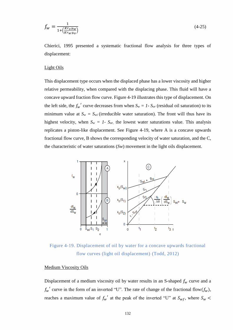
132
𝑓𝑤 =1
1+(𝐾𝑟𝑜𝐾𝑟𝑤
µ𝑤µ𝑜) (4-25)
Chierici, 1995 presented a systematic fractional flow analysis for three types of
displacement:
Light Oils
This displacement type occurs when the displaced phase has a lower viscosity and higher
relative permeability, when compared with the displacing phase. This fluid will have a
concave upward fraction flow curve. Figure 4-19 illustrates this type of displacement. On
the left side, the 𝑓𝑤′ curve decreases from when Sw = 1- Sor (residual oil saturation) to its
minimum value at Sw = Swi (irreducible water saturation). The front will thus have its
highest velocity, when Sw = 1- Sor, the lowest water saturations value. This analysis
replicates a piston-like displacement. See Figure 4-19, where A is a concave upwards
fractional flow curve, B shows the corresponding velocity of water saturation, and the C,
the characteristic of water saturations (Sw) movement in the light oils displacement.
Figure 4-19. Displacement of oil by water for a concave upwards fractional
flow curves (light oil displacement) (Todd, 2012)
Medium Viscosity Oils
Displacement of a medium viscosity oil by water results in an S-shaped 𝑓𝑤 curve and a
𝑓𝑤′ curve in the form of an inverted “U”. The rate of change of the fractional flow(𝑓𝑤),
reaches a maximum value of 𝑓𝑤′ at the peak of the inverted “U” at 𝑆𝑤𝑓, where 𝑆𝑤 <
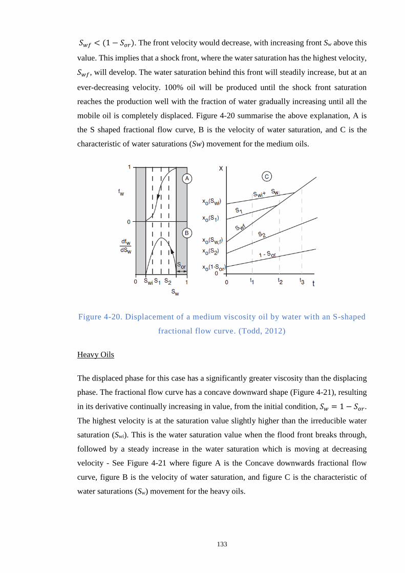
133
𝑆𝑤𝑓 < (1 − 𝑆𝑜𝑟). The front velocity would decrease, with increasing front Sw above this
value. This implies that a shock front, where the water saturation has the highest velocity,
𝑆𝑤𝑓, will develop. The water saturation behind this front will steadily increase, but at an
ever-decreasing velocity. 100% oil will be produced until the shock front saturation
reaches the production well with the fraction of water gradually increasing until all the
mobile oil is completely displaced. Figure 4-20 summarise the above explanation, A is
the S shaped fractional flow curve, B is the velocity of water saturation, and C is the
characteristic of water saturations (Sw) movement for the medium oils.
Figure 4-20. Displacement of a medium viscosity oil by water with an S-shaped
fractional flow curve. (Todd, 2012)
Heavy Oils
The displaced phase for this case has a significantly greater viscosity than the displacing
phase. The fractional flow curve has a concave downward shape (Figure 4-21), resulting
in its derivative continually increasing in value, from the initial condition, 𝑆𝑤 = 1 − 𝑆𝑜𝑟.
The highest velocity is at the saturation value slightly higher than the irreducible water
saturation (Swi). This is the water saturation value when the flood front breaks through,
followed by a steady increase in the water saturation which is moving at decreasing
velocity - See Figure 4-21 where figure A is the Concave downwards fractional flow
curve, figure B is the velocity of water saturation, and figure C is the characteristic of
water saturations (Sw) movement for the heavy oils.
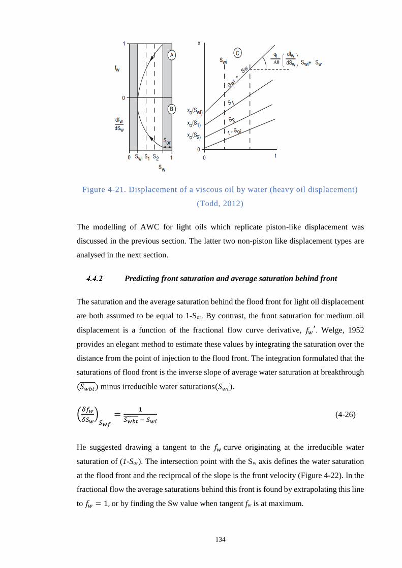
134
Figure 4-21. Displacement of a viscous oil by water (heavy oil displacement)
(Todd, 2012)
The modelling of AWC for light oils which replicate piston-like displacement was
discussed in the previous section. The latter two non-piston like displacement types are
analysed in the next section.
Predicting front saturation and average saturation behind front
The saturation and the average saturation behind the flood front for light oil displacement
are both assumed to be equal to 1-Sor. By contrast, the front saturation for medium oil
displacement is a function of the fractional flow curve derivative, 𝑓𝑤′. Welge, 1952
provides an elegant method to estimate these values by integrating the saturation over the
distance from the point of injection to the flood front. The integration formulated that the
saturations of flood front is the inverse slope of average water saturation at breakthrough
(𝑆𝑤𝑏𝑡 ) minus irreducible water saturations(𝑆𝑤𝑖).
(𝛿𝑓𝑤
𝛿𝑆𝑤)𝑆𝑤𝑓
=1
𝑆𝑤𝑏𝑡 − 𝑆𝑤𝑖 (4-26)
He suggested drawing a tangent to the 𝑓𝑤 curve originating at the irreducible water
saturation of (1-Sor). The intersection point with the Sw axis defines the water saturation
at the flood front and the reciprocal of the slope is the front velocity (Figure 4-22). In the
fractional flow the average saturations behind this front is found by extrapolating this line
to 𝑓𝑤 = 1, or by finding the Sw value when tangent fw is at maximum.
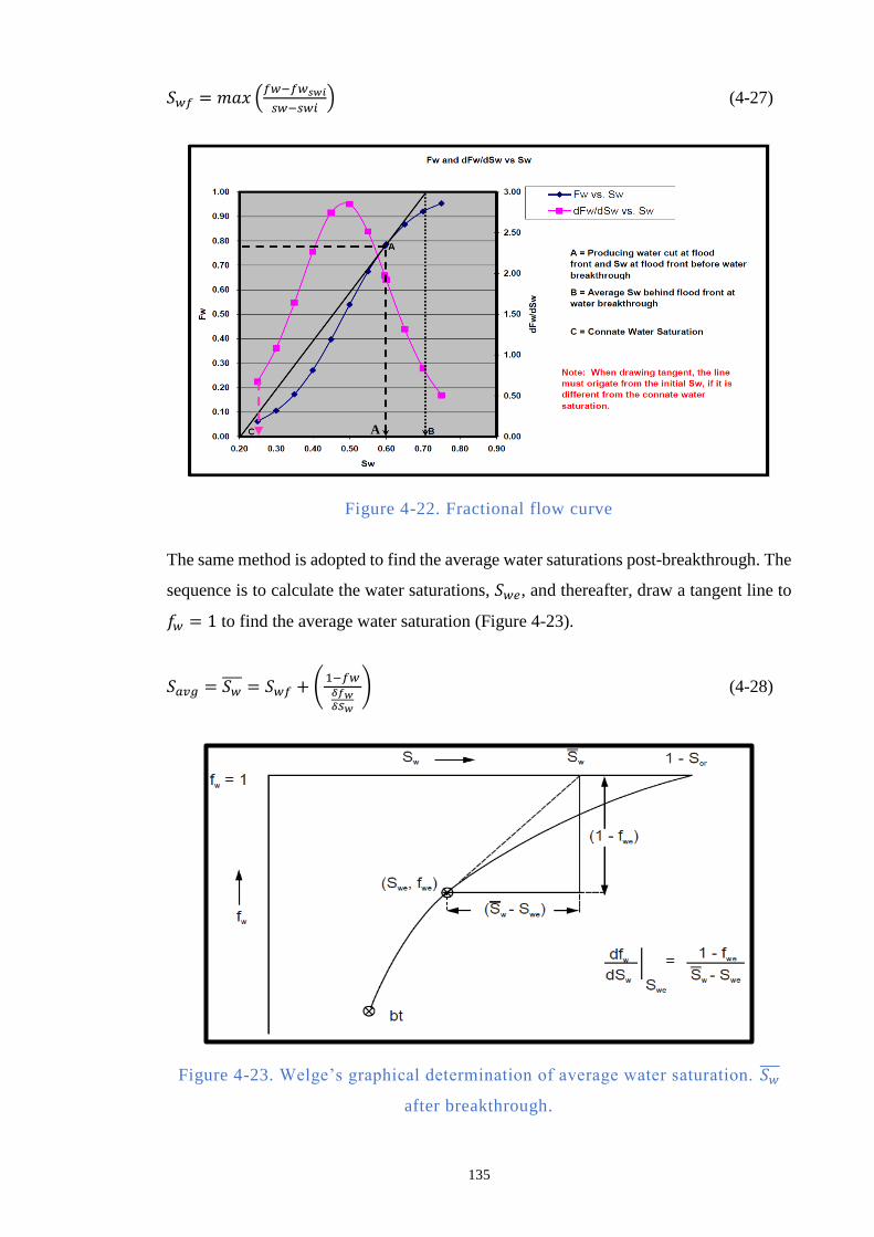
135
𝑆𝑤𝑓 = 𝑚𝑎𝑥 (𝑓𝑤−𝑓𝑤𝑠𝑤𝑖
𝑠𝑤−𝑠𝑤𝑖) (4-27)
Figure 4-22. Fractional flow curve
The same method is adopted to find the average water saturations post-breakthrough. The
sequence is to calculate the water saturations, 𝑆𝑤𝑒, and thereafter, draw a tangent line to
𝑓𝑤 = 1 to find the average water saturation (Figure 4-23).
𝑆𝑎𝑣𝑔 = 𝑆𝑤 = 𝑆𝑤𝑓 + (1−𝑓𝑤𝛿𝑓𝑤𝛿𝑆𝑤
) (4-28)
Figure 4-23. Welge’s graphical determination of average water saturation. 𝑆𝑤
after breakthrough.
A
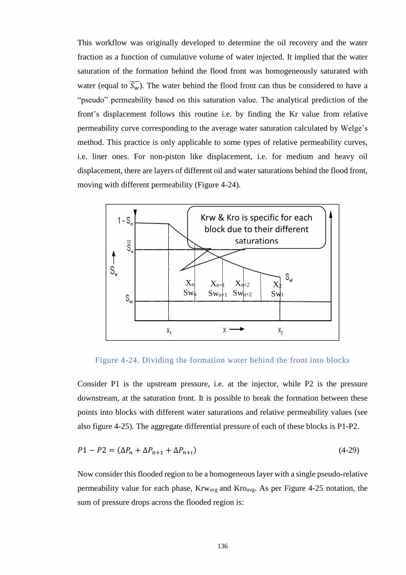
136
This workflow was originally developed to determine the oil recovery and the water
fraction as a function of cumulative volume of water injected. It implied that the water
saturation of the formation behind the flood front was homogeneously saturated with
water (equal to 𝑆𝑤 ). The water behind the flood front can thus be considered to have a
“pseudo” permeability based on this saturation value. The analytical prediction of the
front’s displacement follows this routine i.e. by finding the Kr value from relative
permeability curve corresponding to the average water saturation calculated by Welge’s
method. This practice is only applicable to some types of relative permeability curves,
i.e. liner ones. For non-piston like displacement, i.e. for medium and heavy oil
displacement, there are layers of different oil and water saturations behind the flood front,
moving with different permeability (Figure 4-24).
Figure 4-24. Dividing the formation water behind the front into blocks
Consider P1 is the upstream pressure, i.e. at the injector, while P2 is the pressure
downstream, at the saturation front. It is possible to break the formation between these
points into blocks with different water saturations and relative permeability values (see
also figure 4-25). The aggregate differential pressure of each of these blocks is P1-P2.
𝑃1 − 𝑃2 = (∆𝑃𝑛 + ∆𝑃𝑛+1 + ∆𝑃𝑛+𝑖) (4-29)
Now consider this flooded region to be a homogeneous layer with a single pseudo-relative
permeability value for each phase, Krwavg and Kroavg. As per Figure 4-25 notation, the
sum of pressure drops across the flooded region is:
Krw & Kro is specific for each block due to their different
saturations
Xn
Swn Xn+1
Swn+1
Xn+2
Swn+2 X2
Swf
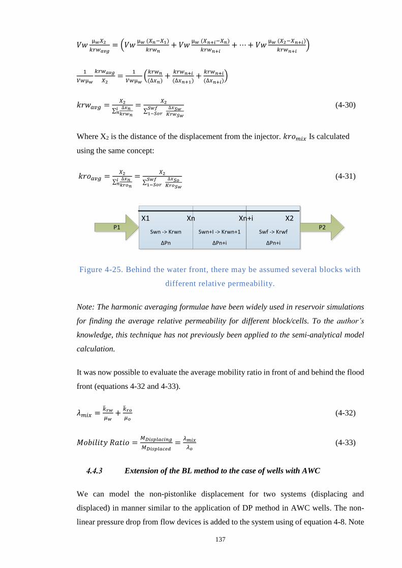
137
𝑉𝑤µ𝑤𝑋2
𝑘𝑟𝑤𝑎𝑣𝑔= (𝑉𝑤
µ𝑤 (𝑋𝑛−𝑋1)
𝑘𝑟𝑤𝑛+ 𝑉𝑤
µ𝑤 (𝑋𝑛+𝑖−𝑋𝑛)
𝑘𝑟𝑤𝑛+𝑖+⋯+ 𝑉𝑤
µ𝑤 (𝑋2−𝑋𝑛+𝑖)
𝑘𝑟𝑤𝑛+𝑖)
1
𝑉𝑤µ𝑤
𝑘𝑟𝑤𝑎𝑣𝑔
𝑋2=
1
𝑉𝑤µ𝑤(𝑘𝑟𝑤𝑛
(∆𝑥𝑛)+
𝑘𝑟𝑤𝑛+𝑖
(∆𝑥𝑛+1)+
𝑘𝑟𝑤𝑛+𝑖
(∆𝑥𝑛+𝑖))
𝑘𝑟𝑤𝑎𝑣𝑔 =𝑋2
∑∆𝑥𝑛𝑘𝑟𝑤𝑛
𝑖𝑛
=𝑋2
∑ ∆𝑥𝑆𝑤𝐾𝑟𝑤𝑆𝑤
𝑆𝑤𝑓1−𝑆𝑜𝑟
(4-30)
Where X2 is the distance of the displacement from the injector. 𝑘𝑟𝑜𝑚𝑖𝑥 Is calculated
using the same concept:
𝑘𝑟𝑜𝑎𝑣𝑔 =𝑋2
∑∆𝑥𝑛𝑘𝑟𝑜𝑛
𝑖𝑛
=𝑋2
∑ ∆𝑥𝑆𝑜𝐾𝑟𝑜𝑆𝑤
𝑆𝑤𝑓1−𝑆𝑜𝑟
(4-31)
P1Swn -> Krwn
∆Pn
Swn+I -> Krwn+1
∆Pn+i
Swf -> Krwf
∆Pn+i
P2
X1 Xn Xn+i X2
Figure 4-25. Behind the water front, there may be assumed several blocks with
different relative permeability.
Note: The harmonic averaging formulae have been widely used in reservoir simulations
for finding the average relative permeability for different block/cells. To the author’s
knowledge, this technique has not previously been applied to the semi-analytical model
calculation.
It was now possible to evaluate the average mobility ratio in front of and behind the flood
front (equations 4-32 and 4-33).
𝜆𝑚𝑖𝑥 =𝑟𝑤
𝜇𝑤+𝑟𝑜
𝜇𝑜 (4-32)
𝑀𝑜𝑏𝑖𝑙𝑖𝑡𝑦 𝑅𝑎𝑡𝑖𝑜 =𝑀𝐷𝑖𝑠𝑝𝑙𝑎𝑐𝑖𝑛𝑔
𝑀𝐷𝑖𝑠𝑝𝑙𝑎𝑐𝑒𝑑=
𝜆𝑚𝑖𝑥
𝜆𝑜 (4-33)
Extension of the BL method to the case of wells with AWC
We can model the non-pistonlike displacement for two systems (displacing and
displaced) in manner similar to the application of DP method in AWC wells. The non-
linear pressure drop from flow devices is added to the system using of equation 4-8. Note
138
that the modified BL method can work with either constraint of pressure difference or
well’s flow rate. To maintain consistency with the previously explained modified DP
method, we will explain in detail the displacement under the constraint of pressure
difference (as opposed to the flow rate constraint that the original BL method used). As a
consequence, the constant pressure drop would not give a constant production rates, and
the flow rates as well as the properties of the reservoir saturated with the displacing phase
are evaluated for different flood front positions and saturations (as will be described in
section 4.4.4).
𝐵𝑗 = (1 − 𝑀𝑚𝑖𝑥) + 𝑀𝑚𝑖𝑥 (4-34)
𝐶𝑗 =𝑘𝜆𝑎𝑣𝑔
𝐿 (4-35)
𝑄𝑖𝑛𝑗 =(−𝐵𝑗+√𝐵𝑗
2+4𝑎𝑗∗𝐴𝑗𝐶𝑗
2∆𝑃)∙𝐴𝑗
2𝑎𝑗∗𝐴𝑗2𝐶𝑗
(4-36)
Workflow for the modified BL method with an AWC
The following workflow has been designed:
Before Breakthrough
Step 1. Perform the fractional flow analysis using relative permeability values. Calculate
and draw the 𝑓𝑤 and 𝑓𝑤′ curves, find the value of flood front saturation and average water
saturation with equations 4-27 and 4-28. The saturation front (𝑆𝑤𝑓) and average water
saturation(𝑆) behind the front are constant prior to breakthrough. 𝐾𝑟𝑜𝑎𝑣𝑔 and 𝐾𝑟𝑤𝑎𝑣𝑔
of the displacing front will also be constant during this period.
Step 2. For each layer, divide the distance between producer and injector into n blocks
and evaluate displacement from every incremental of X, to Xn. Where X is the ratio of
the front distance from the injector to the total distance (L) between the injector and
producer wells. X0 is the initial condition and X0.2 is when the flood front has reached 0.2
L and X1 is when the water has arrived at the producer. The injection rate (𝑄𝑖𝑛𝑗) can be
calculated using equations 4-34, 4-35, and 4-36. The displacement efficiency (Ed) behind
this front is obtained using equation 4-37 before finding the total cumulative water
injection with equation 4-38.
139
𝐸𝑑 =𝑤−𝑆𝑤𝑖
1−𝑆𝑤𝑖∗ 𝑋 (4-37)
𝑊𝑖𝑛𝑗 = (1 − 𝑆𝑤𝑖) ∗ 𝐸𝑑 ∗ 𝑃𝑉 (4-38)
The cumulative water injection volume equals injection time * injected water rate: 𝑊𝑖𝑛𝑗 =
𝑡 ∗ 𝑄𝑖𝑛𝑗 , hence the required time for every evaluated X is calculated with equation 4-39:
𝑡 = ∑∆𝑡 = ∑𝑊𝑖𝑛𝑗
𝑄𝑖𝑛𝑗 (4-39)
The above is repeated for each of layers that make up the completion. The layers are
ordered in terms of increasing line to breakthrough. The first layer that experiences
breakthrough is the reference (layer R). The time required to saturate block in layer R, is
calculated. All other layers’ displacement properties, e.g. front position and velocity are
calculated at the total displacement time (t) to reach the injector. The front position in
these layers (layer j) is obtained from equation 4-33 as follows:
𝑡𝐽|𝑋𝑛= 𝑡𝑅 (4-40)
(𝑊𝑖𝑛𝑗,𝑋𝑛−𝑊𝑖𝑛𝑗,𝑋𝑛−1)𝐽
(𝑄𝑖𝑛𝑗,𝑛−𝑄𝑖𝑛𝑗,𝑛−1)𝐽
=(𝑊𝑖𝑛𝑗,𝑋𝑛−𝑊𝑖𝑛𝑗,𝑋𝑛−1
)𝑅
(𝑄𝑖𝑛𝑗−𝑄𝑖𝑛𝑗,𝑛−1)𝑅
(4-41)
((𝑤−𝑆𝑤𝑖)∗(𝑋𝑛−𝑋𝑛−1)∗𝑃𝑉)𝐽
(𝑄𝑖𝑛𝑗,𝑛−𝑄𝑖𝑛𝑗,𝑛−1)𝐽
=((𝑤−𝑆𝑤𝑖)∗(𝑋𝑛−𝑋𝑛−1)∗𝑃𝑉)𝑅
(𝑄𝑖𝑛𝑗,𝑛−𝑄𝑖𝑛𝑗,𝑛−1)𝑅
(4-42)
(𝑋𝑛−𝑋𝑛−1)𝑅
(𝑄𝑖𝑛𝑗,𝑛−𝑄𝑖𝑛𝑗,𝑛−1)𝑅
=1
((𝑤−𝑆𝑤𝑖)∗𝑃𝑉)𝑅
((𝑤−𝑆𝑤𝑖)∗(𝑋𝑛−𝑋𝑛−1)∗𝑃𝑉)𝐽
(𝑄𝑖𝑛𝑗,𝑛−𝑄𝑖𝑛𝑗,𝑛−1)𝐽
(4-43)
Note that 𝑄𝑖𝑛𝑗 𝑅
is a function of XR (equation 4-43), 𝑋𝑅 cannot therefore be expressed
explicitly, however using gradient-based, non-linear solver in Excel may be used to
obtain this value in a fraction of a second.
Step 3. Repeat the step 2 until layer j experiences breakthrough (i.e. xj = 1). Note that
𝑄𝑜 = 𝑄𝑖𝑛𝑗 at all time since flow into system equals flow out of it.
After the water breakthrough in layer j
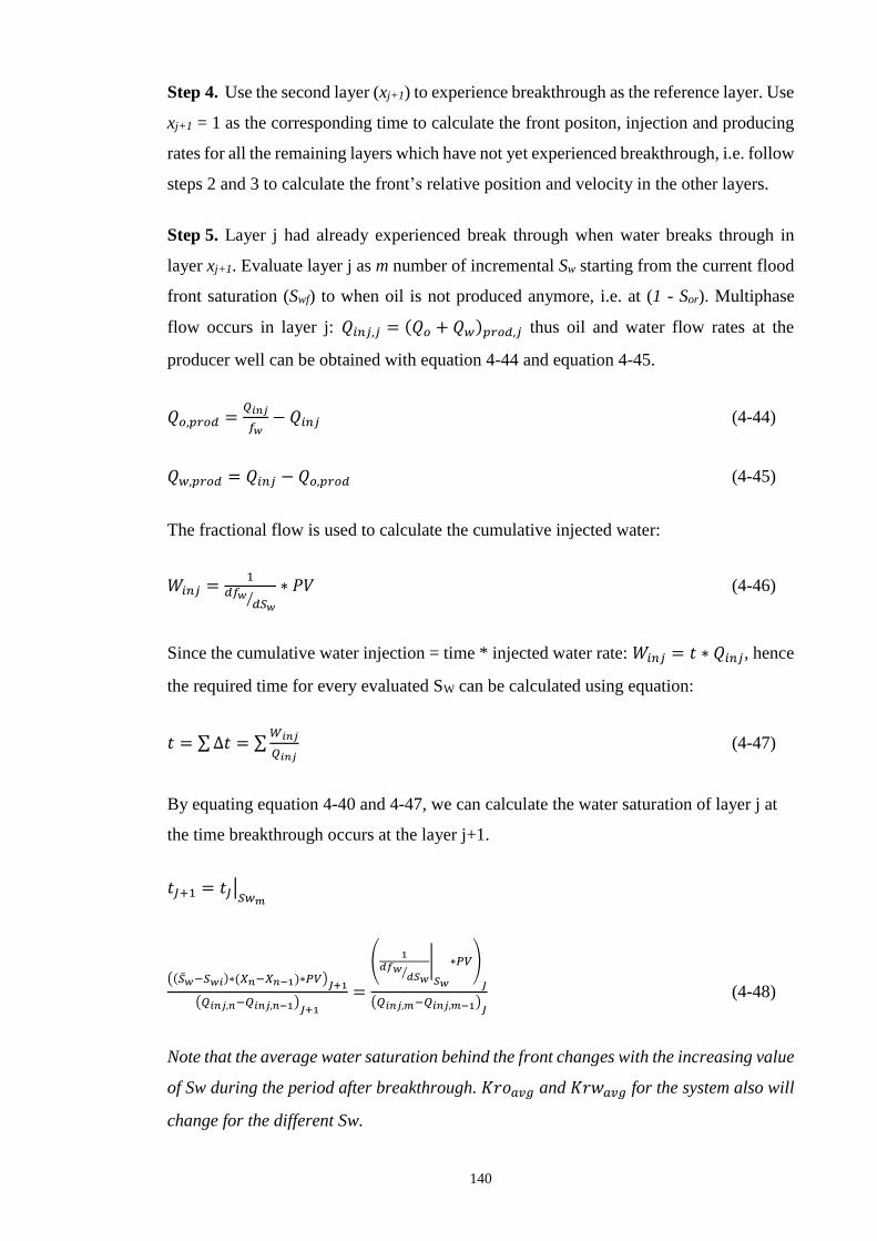
140
Step 4. Use the second layer (xj+1) to experience breakthrough as the reference layer. Use
xj+1 = 1 as the corresponding time to calculate the front positon, injection and producing
rates for all the remaining layers which have not yet experienced breakthrough, i.e. follow
steps 2 and 3 to calculate the front’s relative position and velocity in the other layers.
Step 5. Layer j had already experienced break through when water breaks through in
layer xj+1. Evaluate layer j as m number of incremental Sw starting from the current flood
front saturation (Swf) to when oil is not produced anymore, i.e. at (1 - Sor). Multiphase
flow occurs in layer j: 𝑄𝑖𝑛𝑗,𝑗 = (𝑄𝑜 + 𝑄𝑤)𝑝𝑟𝑜𝑑,𝑗 thus oil and water flow rates at the
producer well can be obtained with equation 4-44 and equation 4-45.
𝑄𝑜,𝑝𝑟𝑜𝑑 =𝑄𝑖𝑛𝑗
𝑓𝑤− 𝑄𝑖𝑛𝑗 (4-44)
𝑄𝑤,𝑝𝑟𝑜𝑑 = 𝑄𝑖𝑛𝑗 − 𝑄𝑜,𝑝𝑟𝑜𝑑 (4-45)
The fractional flow is used to calculate the cumulative injected water:
𝑊𝑖𝑛𝑗 =1
𝑑𝑓𝑤𝑑𝑆𝑤⁄
∗ 𝑃𝑉 (4-46)
Since the cumulative water injection = time * injected water rate: 𝑊𝑖𝑛𝑗 = 𝑡 ∗ 𝑄𝑖𝑛𝑗, hence
the required time for every evaluated SW can be calculated using equation:
𝑡 = ∑∆𝑡 = ∑𝑊𝑖𝑛𝑗
𝑄𝑖𝑛𝑗 (4-47)
By equating equation 4-40 and 4-47, we can calculate the water saturation of layer j at
the time breakthrough occurs at the layer j+1.
𝑡𝐽+1 = 𝑡𝐽|𝑆𝑤𝑚
((𝑤−𝑆𝑤𝑖)∗(𝑋𝑛−𝑋𝑛−1)∗𝑃𝑉)𝐽+1
(𝑄𝑖𝑛𝑗,𝑛−𝑄𝑖𝑛𝑗,𝑛−1)𝐽+1
=
(1
𝑑𝑓𝑤𝑑𝑆𝑤⁄
|
𝑆𝑤
∗𝑃𝑉)
𝐽
(𝑄𝑖𝑛𝑗,𝑚−𝑄𝑖𝑛𝑗,𝑚−1)𝐽
(4-48)
Note that the average water saturation behind the front changes with the increasing value
of Sw during the period after breakthrough. 𝐾𝑟𝑜𝑎𝑣𝑔 and 𝐾𝑟𝑤𝑎𝑣𝑔 for the system also will
change for the different Sw.
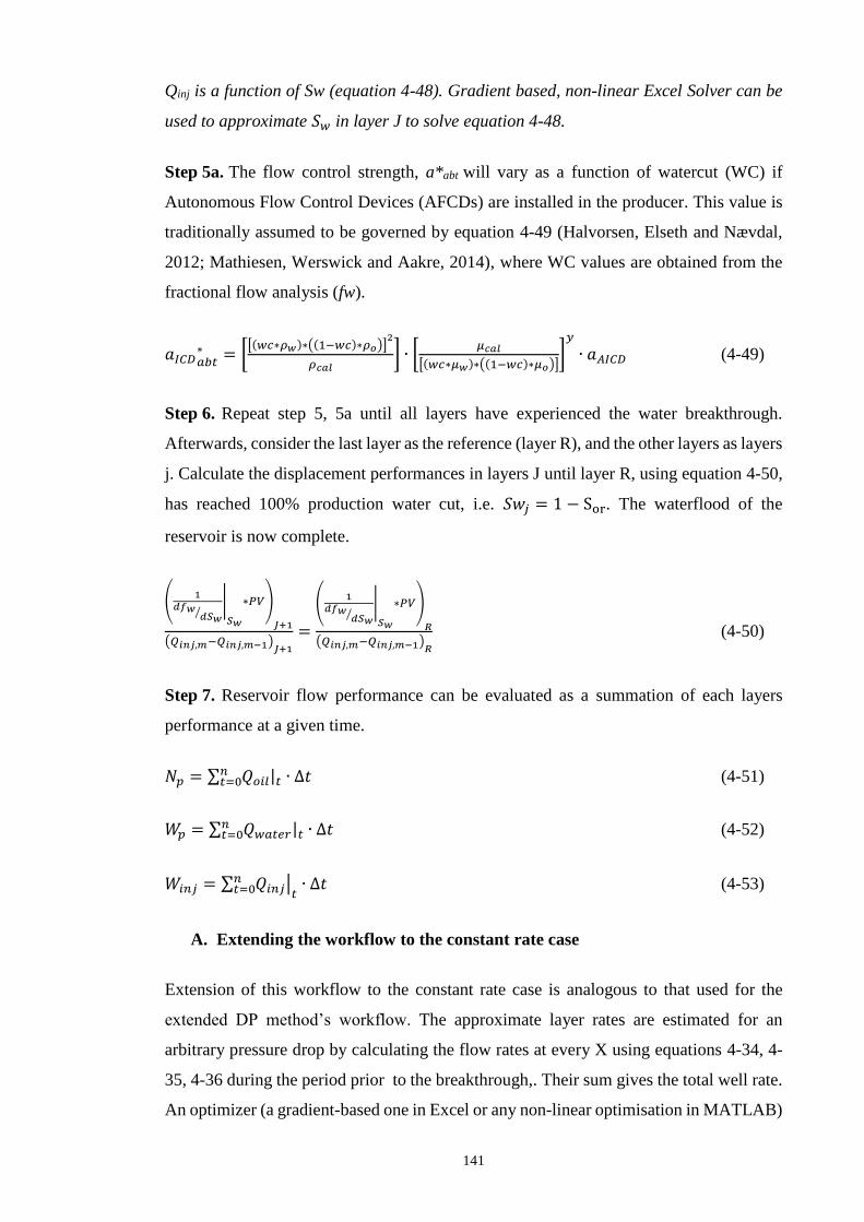
141
Qinj is a function of Sw (equation 4-48). Gradient based, non-linear Excel Solver can be
used to approximate 𝑆𝑤 in layer J to solve equation 4-48.
Step 5a. The flow control strength, a*abt will vary as a function of watercut (WC) if
Autonomous Flow Control Devices (AFCDs) are installed in the producer. This value is
traditionally assumed to be governed by equation 4-49 (Halvorsen, Elseth and Nævdal,
2012; Mathiesen, Werswick and Aakre, 2014), where WC values are obtained from the
fractional flow analysis (fw).
𝑎𝐼𝐶𝐷𝑎𝑏𝑡∗ = [
[(𝑤𝑐∗𝜌𝑤)∗((1−𝑤𝑐)∗𝜌𝑜)]2
𝜌𝑐𝑎𝑙] ∙ [
𝜇𝑐𝑎𝑙
[(𝑤𝑐∗𝜇𝑤)∗((1−𝑤𝑐)∗𝜇𝑜)]]𝑦
∙ 𝑎𝐴𝐼𝐶𝐷 (4-49)
Step 6. Repeat step 5, 5a until all layers have experienced the water breakthrough.
Afterwards, consider the last layer as the reference (layer R), and the other layers as layers
j. Calculate the displacement performances in layers J until layer R, using equation 4-50,
has reached 100% production water cut, i.e. 𝑆𝑤𝑗 = 1 − Sor. The waterflood of the
reservoir is now complete.
(1
𝑑𝑓𝑤𝑑𝑆𝑤⁄
|
𝑆𝑤
∗𝑃𝑉)
𝐽+1
(𝑄𝑖𝑛𝑗,𝑚−𝑄𝑖𝑛𝑗,𝑚−1)𝐽+1
=
(1
𝑑𝑓𝑤𝑑𝑆𝑤⁄
|
𝑆𝑤
∗𝑃𝑉)
𝑅
(𝑄𝑖𝑛𝑗,𝑚−𝑄𝑖𝑛𝑗,𝑚−1)𝑅
(4-50)
Step 7. Reservoir flow performance can be evaluated as a summation of each layers
performance at a given time.
𝑁𝑝 = ∑ 𝑄𝑜𝑖𝑙|𝑡 ∙ ∆𝑡𝑛𝑡=0 (4-51)
𝑊𝑝 = ∑ 𝑄𝑤𝑎𝑡𝑒𝑟|𝑡 ∙ ∆𝑡𝑛𝑡=0 (4-52)
𝑊𝑖𝑛𝑗 = ∑ 𝑄𝑖𝑛𝑗|𝑡 ∙ ∆𝑡𝑛𝑡=0 (4-53)
A. Extending the workflow to the constant rate case
Extension of this workflow to the constant rate case is analogous to that used for the
extended DP method’s workflow. The approximate layer rates are estimated for an
arbitrary pressure drop by calculating the flow rates at every X using equations 4-34, 4-
35, 4-36 during the period prior to the breakthrough,. Their sum gives the total well rate.
An optimizer (a gradient-based one in Excel or any non-linear optimisation in MATLAB)
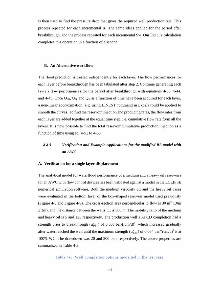
142
is then used to find the pressure drop that gives the required well production rate. This
process repeated for each incremental X. The same ideas applied for the period after
breakthrough, and the process repeated for each incremental Sw. Our Excel’s calculation
completes this operation in a fraction of a second.
B. An Alternative workflow
The flood prediction is treated independently for each layer. The flow performances for
each layer before breakthrough has been tabulated after step 2. Continue generating each
layer’s flow performances for the period after breakthrough with equations 4-36, 4-44,
and 4-45. Once Qinj, Qoil and Qw as a function of time have been acquired for each layer,
a non-linear approximation (e.g. using LINEST command in Excel) could be applied to
smooth the curves. To find the reservoir injection and producing rates, the flow rates from
each layer are added together at the equal time step, i.e. cumulative flow rate from all the
layers. It is now possible to find the total reservoir cumulative production/injection as a
function of time using eq. 4-51 to 4-53.
Verification and Example Applications for the modified BL model with
an AWC
A. Verification for a single layer displacement
The analytical model for waterflood performance of a medium and a heavy oil reservoirs
for an AWC with flow control devices has been validated against a model in the ECLIPSE
numerical simulation software. Both the medium viscosity oil and the heavy oil cases
were evaluated in the bottom layer of the box-shaped reservoir model used previously
(Figure 4-8 and Figure 4-9). The cross-section area perpendicular to flow is 30 m2 (10m
x 3m), and the distance between the wells, L, is 500 m. The mobility ratio of the medium
and heavy oil is 5 and 125 respectively. The production well’s AFCD completion had a
strength prior to breakthrough (𝑎𝑏𝑏𝑡∗ ) of 0.008 bar/(rcm/d)2, which increased gradually
after water reached the well until the maximum strength (𝑎𝑎𝑏𝑡∗ ) of 0.064 bar/(rcm/d)2 is at
100% WC. The drawdown was 20 and 200 bars respectively. The above properties are
summarised in Table 4-3.
Table 4-3. Well completion options modelled in the test case
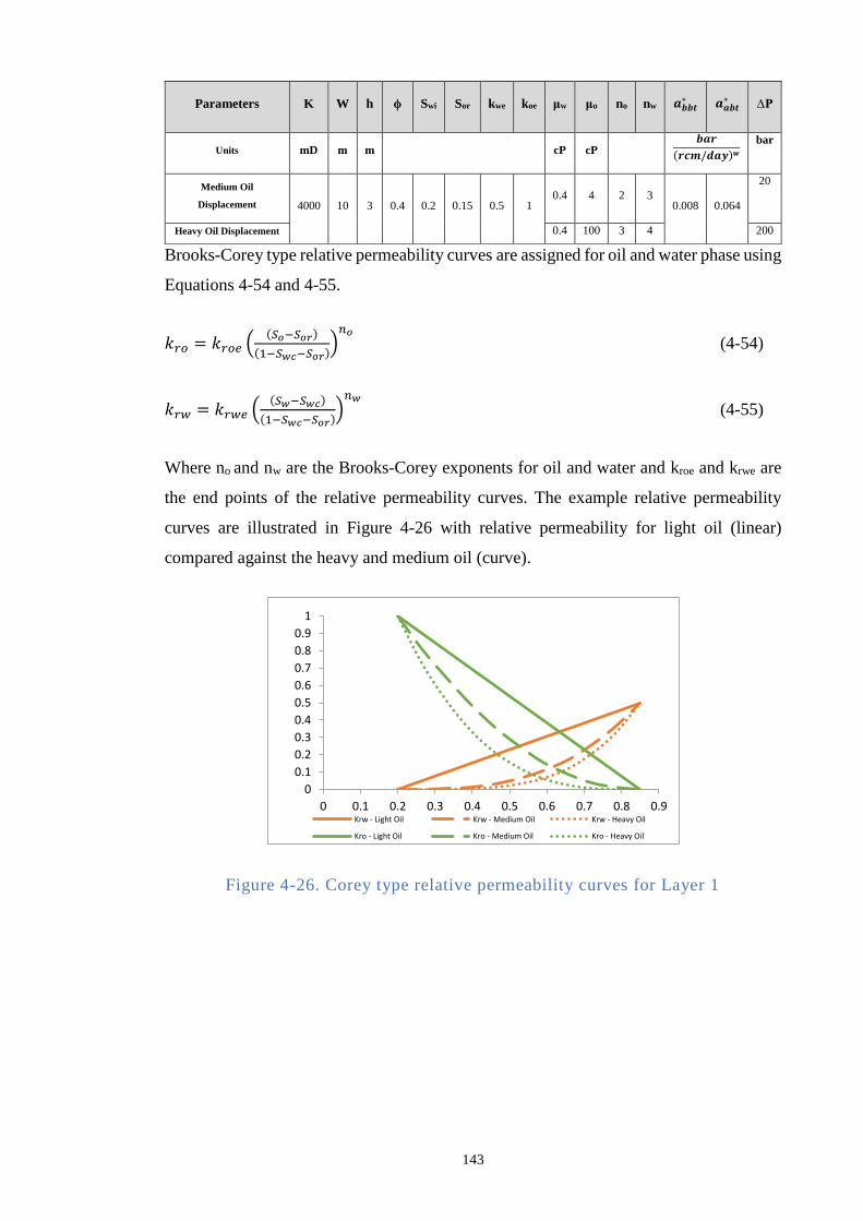
143
Brooks-Corey type relative permeability curves are assigned for oil and water phase using
Equations 4-54 and 4-55.
𝑘𝑟𝑜 = 𝑘𝑟𝑜𝑒 ((𝑆𝑜−𝑆𝑜𝑟)
(1−𝑆𝑤𝑐−𝑆𝑜𝑟))𝑛𝑜
(4-54)
𝑘𝑟𝑤 = 𝑘𝑟𝑤𝑒 ((𝑆𝑤−𝑆𝑤𝑐)
(1−𝑆𝑤𝑐−𝑆𝑜𝑟))𝑛𝑤
(4-55)
Where no and nw are the Brooks-Corey exponents for oil and water and kroe and krwe are
the end points of the relative permeability curves. The example relative permeability
curves are illustrated in Figure 4-26 with relative permeability for light oil (linear)
compared against the heavy and medium oil (curve).
Figure 4-26. Corey type relative permeability curves for Layer 1
0
0.1
0.2
0.3
0.4
0.5
0.6
0.7
0.8
0.9
1
0 0.1 0.2 0.3 0.4 0.5 0.6 0.7 0.8 0.9Krw - Light Oil Krw - Medium Oil Krw - Heavy Oil
Kro - Light Oil Kro - Medium Oil Kro - Heavy Oil
Parameters K W h ϕ Swi Sor kwe koe μw μo no nw 𝒂𝒃𝒃𝒕∗ 𝒂𝒂𝒃𝒕
∗ ∆P
Units mD m m cP cP 𝒃𝒂𝒓
(𝒓𝒄𝒎/𝒅𝒂𝒚)𝒘
bar
Medium Oil
Displacement 4000 10 3 0.4 0.2 0.15 0.5 1 0.4 4 2 3
0.008 0.064
20
Heavy Oil Displacement 0.4 100 3 4 200
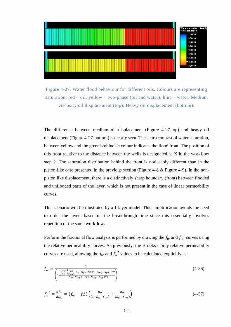
144
Figure 4-27. Water flood behaviour for different oils. Colours are representing
saturation: red – oil, yellow – two-phase (oil and water), blue – water. Medium
viscosity oil displacement (top). Heavy oil displacement (bottom).
The difference between medium oil displacement (Figure 4-27-top) and heavy oil
displacement (Figure 4-27-bottom) is clearly seen. The sharp contrast of water saturation,
between yellow and the greenish/blueish colour indicates the flood front. The position of
this front relative to the distance between the wells is designated as X in the workflow
step 2. The saturation distribution behind the front is noticeably different than in the
piston-like case presented in the previous section (Figure 4-8 & Figure 4-9). In the non-
piston like displacement, there is a distinctively sharp boundary (front) between flooded
and unflooded parts of the layer, which is not present in the case of linear permeability
curves.
This scenario will be illustrated by a 1 layer model. This simplification avoids the need
to order the layers based on the breakthrough time since this essentially involves
repetition of the same workflow.
Perform the fractional flow analysis is performed by drawing the 𝑓𝑤 and 𝑓𝑤′ curves using
the relative permeability curves. As previously, the Brooks-Corey relative permeability
curves are used, allowing the 𝑓𝑤 and 𝑓𝑤′ values to be calculated explicitly as:
𝑓𝑤 =1
(1+
𝜇𝑤𝜇𝑜
∙𝑘𝑟𝑜𝑒𝑘𝑟𝑤𝑒
∙(𝑆𝑜−𝑆𝑜𝑟)𝑛𝑜∙(1−𝑆𝑤𝑐−𝑆𝑜𝑟)
𝑛𝑤
(𝑆𝑤−𝑆𝑤𝑐)𝑛𝑤(1−𝑆𝑤𝑐−𝑆𝑜𝑟)
𝑛𝑜 )
(4-56)
𝑓𝑤′ =
𝑑𝑓𝑤
𝑑𝑆𝑤= (𝑓𝑤 − 𝑓𝑤
2) (𝑛𝑜
(1−𝑆𝑤−𝑆𝑜𝑟)+
𝑛𝑤
(𝑆𝑤−𝑆𝑤𝑐)) (4-57)
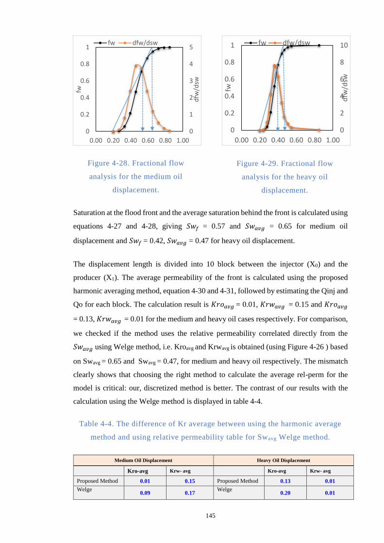
145
Figure 4-28. Fractional flow
analysis for the medium oil
displacement.
Figure 4-29. Fractional flow
analysis for the heavy oil
displacement.
Saturation at the flood front and the average saturation behind the front is calculated using
equations 4-27 and 4-28, giving 𝑆𝑤𝑓 = 0.57 and 𝑆𝑤𝑎𝑣𝑔 = 0.65 for medium oil
displacement and 𝑆𝑤𝑓 = 0.42, 𝑆𝑤𝑎𝑣𝑔 = 0.47 for heavy oil displacement.
The displacement length is divided into 10 block between the injector (X0) and the
producer (X1). The average permeability of the front is calculated using the proposed
harmonic averaging method, equation 4-30 and 4-31, followed by estimating the Qinj and
Qo for each block. The calculation result is 𝐾𝑟𝑜𝑎𝑣𝑔 = 0.01, 𝐾𝑟𝑤𝑎𝑣𝑔 = 0.15 and 𝐾𝑟𝑜𝑎𝑣𝑔
= 0.13, 𝐾𝑟𝑤𝑎𝑣𝑔 = 0.01 for the medium and heavy oil cases respectively. For comparison,
we checked if the method uses the relative permeability correlated directly from the
𝑆𝑤𝑎𝑣𝑔 using Welge method, i.e. Kroavg and Krwavg is obtained (using Figure 4-26 ) based
on Swavg = 0.65 and Swavg = 0.47, for medium and heavy oil respectively. The mismatch
clearly shows that choosing the right method to calculate the average rel-perm for the
model is critical: our, discretized method is better. The contrast of our results with the
calculation using the Welge method is displayed in table 4-4.
Table 4-4. The difference of Kr average between using the harmonic average
method and using relative permeability table for Swavg Welge method.
Medium Oil Displacement Heavy Oil Displacement
Kro-avg Krw- avg Kro-avg Krw- avg
Proposed Method 0.01 0.15 Proposed Method 0.13 0.01
Welge
0.09 0.17
Welge
0.20 0.01
0
1
2
3
4
5
0
0.2
0.4
0.6
0.8
1
0.00 0.20 0.40 0.60 0.80 1.00
dfw
/dsw
fw
fw dfw/dsw
0
2
4
6
8
10
0
0.2
0.4
0.6
0.8
1
0.00 0.20 0.40 0.60 0.80 1.00
dfw
/dsw
fw
fw dfw/dsw
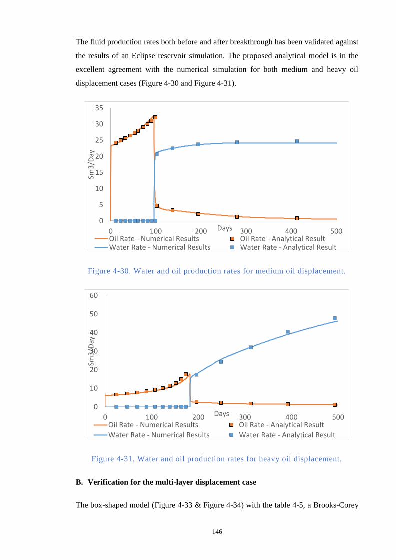
146
The fluid production rates both before and after breakthrough has been validated against
the results of an Eclipse reservoir simulation. The proposed analytical model is in the
excellent agreement with the numerical simulation for both medium and heavy oil
displacement cases (Figure 4-30 and Figure 4-31).
Figure 4-30. Water and oil production rates for medium oil displacement.
Figure 4-31. Water and oil production rates for heavy oil displacement.
B. Verification for the multi-layer displacement case
The box-shaped model (Figure 4-33 & Figure 4-34) with the table 4-5, a Brooks-Corey
0
5
10
15
20
25
30
35
0 100 200 300 400 500
Sm3
/Day
Days
Oil Rate - Numerical Results Oil Rate - Analytical ResultWater Rate - Numerical Results Water Rate - Analytical Result
0
10
20
30
40
50
60
0 100 200 300 400 500
Sm3
/Day
Days
Oil Rate - Numerical Results Oil Rate - Analytical Result
Water Rate - Numerical Results Water Rate - Analytical Result
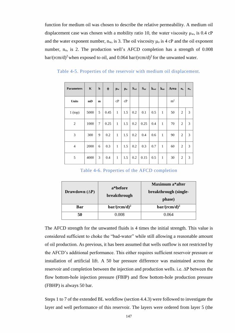
147
function for medium oil was chosen to describe the relative permeability. A medium oil
displacement case was chosen with a mobility ratio 10, the water viscosity μw, is 0.4 cP
and the water exponent number, nw, is 3. The oil viscosity μo is 4 cP and the oil exponent
number, no, is 2. The production well’s AFCD completion has a strength of 0.008
bar/(rcm/d)2 when exposed to oil, and 0.064 bar/(rcm/d)2 for the unwanted water.
Table 4-5. Properties of the reservoir with medium oil displacement.
Table 4-6. Properties of the AFCD completion
Drawdown (∆P) a*before
breakthrough
Maximum a*after
breakthrough (single-
phase)
Bar bar/(rcm/d)2 bar/(rcm/d)2
50 0.008 0.064
The AFCD strength for the unwanted fluids is 4 times the initial strength. This value is
considered sufficient to choke the “bad-water” while still allowing a reasonable amount
of oil production. As previous, it has been assumed that wells outflow is not restricted by
the AFCD’s additional performance. This either requires sufficient reservoir pressure or
installation of artificial lift. A 50 bar pressure difference was maintained across the
reservoir and completion between the injection and production wells. i.e. ∆P between the
flow bottom-hole injection pressure (FBIP) and flow bottom-hole production pressure
(FBHP) is always 50 bar.
Steps 1 to 7 of the extended BL workflow (section 4.4.3) were followed to investigate the
layer and well performance of this reservoir. The layers were ordered from layer 5 (the
Parameters K h ϕ μw μo Swi Sor kwe koe Area no nw
Units mD m cP cP m2
1 (top) 5000 5 0.45 1 1.5 0.2 0.1 0.5 1 50 2 3
2 1000 7 0.25 1 1.5 0.2 0.25 0.4 1 70 2 3
3 300 9 0.2 1 1.5 0.2 0.4 0.6 1 90 2 3
4 2000 6 0.3 1 1.5 0.2 0.3 0.7 1 60 2 3
5 4000 3 0.4 1 1.5 0.2 0.15 0.5 1 30 2 3
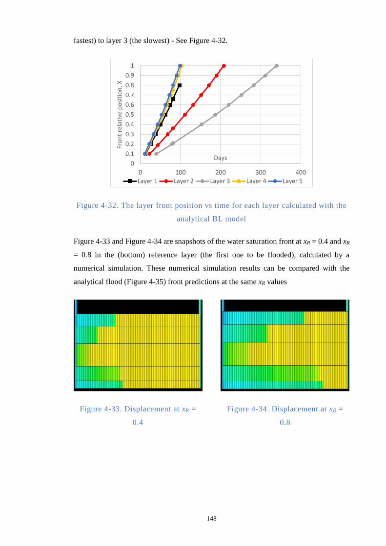
148
fastest) to layer 3 (the slowest) - See Figure 4-32.
Figure 4-32. The layer front position vs time for each layer calculated with the
analytical BL model
Figure 4-33 and Figure 4-34 are snapshots of the water saturation front at xR = 0.4 and xR
= 0.8 in the (bottom) reference layer (the first one to be flooded), calculated by a
numerical simulation. These numerical simulation results can be compared with the
analytical flood (Figure 4-35) front predictions at the same xR values
Figure 4-33. Displacement at xR =
0.4
Figure 4-34. Displacement at xR =
0.8
0
0.1
0.2
0.3
0.4
0.5
0.6
0.7
0.8
0.9
1
0 100 200 300 400
Fro
nt
rela
tive
po
siti
on
, X
Days
Layer 1 Layer 2 Layer 3 Layer 4 Layer 5
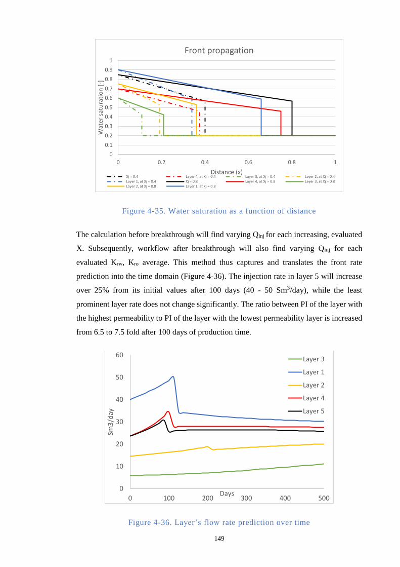
149
Figure 4-35. Water saturation as a function of distance
The calculation before breakthrough will find varying Qinj for each increasing, evaluated
X. Subsequently, workflow after breakthrough will also find varying Qinj for each
evaluated Krw, Kro average. This method thus captures and translates the front rate
prediction into the time domain (Figure 4-36). The injection rate in layer 5 will increase
over 25% from its initial values after 100 days (40 - 50 Sm3/day), while the least
prominent layer rate does not change significantly. The ratio between PI of the layer with
the highest permeability to PI of the layer with the lowest permeability layer is increased
from 6.5 to 7.5 fold after 100 days of production time.
Figure 4-36. Layer’s flow rate prediction over time
0
0.1
0.2
0.3
0.4
0.5
0.6
0.7
0.8
0.9
1
0 0.2 0.4 0.6 0.8 1
Wat
er s
atu
rati
on
[-]
Distance (x)
Front propagation
Xj = 0.4 Layer 4, at Xj = 0.4 Layer 3, at Xj = 0.4 Layer 2, at Xj = 0.4Layer 1, at Xj = 0.4 Xj = 0.8 Layer 4, at Xj = 0.8 Layer 3, at Xj = 0.8Layer 2, at Xj = 0.8 Layer 1, at Xj = 0.8
0
10
20
30
40
50
60
0 100 200 300 400 500
Sm3
/day
Days
Layer 3
Layer 1
Layer 2
Layer 4
Layer 5
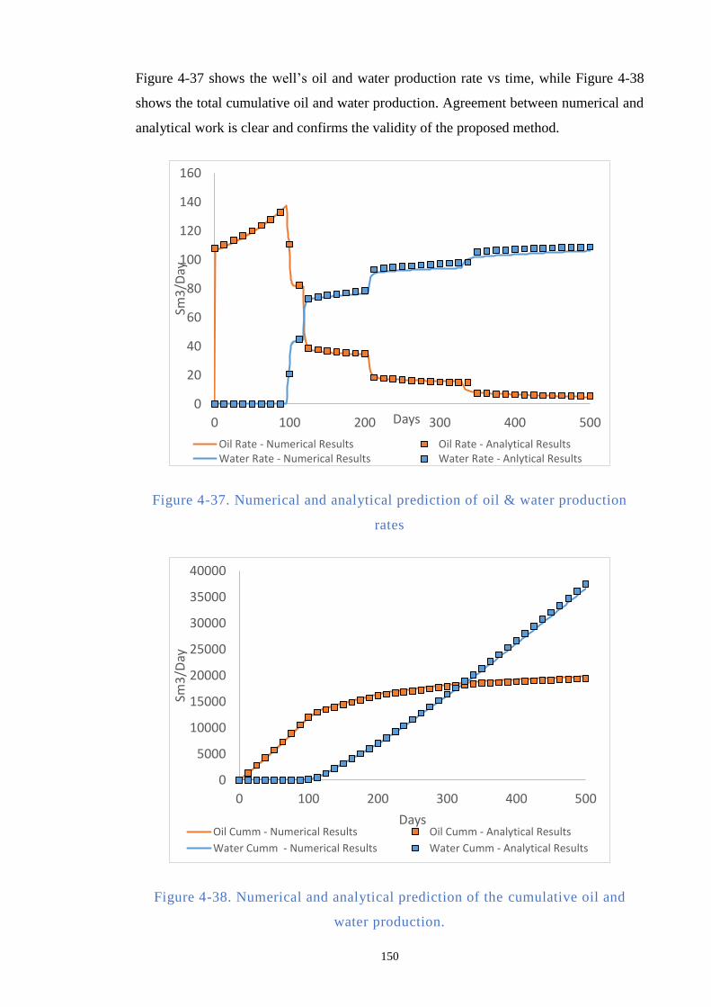
150
Figure 4-37 shows the well’s oil and water production rate vs time, while Figure 4-38
shows the total cumulative oil and water production. Agreement between numerical and
analytical work is clear and confirms the validity of the proposed method.
Figure 4-37. Numerical and analytical prediction of oil & water production
rates
Figure 4-38. Numerical and analytical prediction of the cumulative oil and
water production.
0
20
40
60
80
100
120
140
160
0 100 200 300 400 500
Sm3
/Day
Days
Oil Rate - Numerical Results Oil Rate - Analytical ResultsWater Rate - Numerical Results Water Rate - Anlytical Results
0
5000
10000
15000
20000
25000
30000
35000
40000
0 100 200 300 400 500
Sm3
/Day
DaysOil Cumm - Numerical Results Oil Cumm - Analytical Results
Water Cumm - Numerical Results Water Cumm - Analytical Results
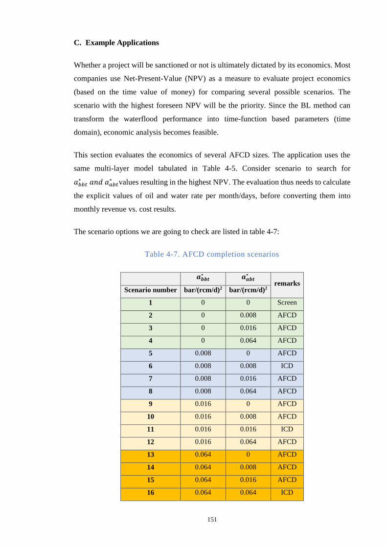
151
C. Example Applications
Whether a project will be sanctioned or not is ultimately dictated by its economics. Most
companies use Net-Present-Value (NPV) as a measure to evaluate project economics
(based on the time value of money) for comparing several possible scenarios. The
scenario with the highest foreseen NPV will be the priority. Since the BL method can
transform the waterflood performance into time-function based parameters (time
domain), economic analysis becomes feasible.
This section evaluates the economics of several AFCD sizes. The application uses the
same multi-layer model tabulated in Table 4-5. Consider scenario to search for
𝑎𝑏𝑏𝑡∗ 𝑎𝑛𝑑 𝑎𝑎𝑏𝑡
∗ values resulting in the highest NPV. The evaluation thus needs to calculate
the explicit values of oil and water rate per month/days, before converting them into
monthly revenue vs. cost results.
The scenario options we are going to check are listed in table 4-7:
Table 4-7. AFCD completion scenarios
𝒂𝒃𝒃𝒕∗ 𝒂𝒂𝒃𝒕
∗ remarks
Scenario number bar/(rcm/d)2 bar/(rcm/d)2
1 0 0 Screen
2 0 0.008 AFCD
3 0 0.016 AFCD
4 0 0.064 AFCD
5 0.008 0 AFCD
6 0.008 0.008 ICD
7 0.008 0.016 AFCD
8 0.008 0.064 AFCD
9 0.016 0 AFCD
10 0.016 0.008 AFCD
11 0.016 0.016 ICD
12 0.016 0.064 AFCD
13 0.064 0 AFCD
14 0.064 0.008 AFCD
15 0.064 0.016 AFCD
16 0.064 0.064 ICD
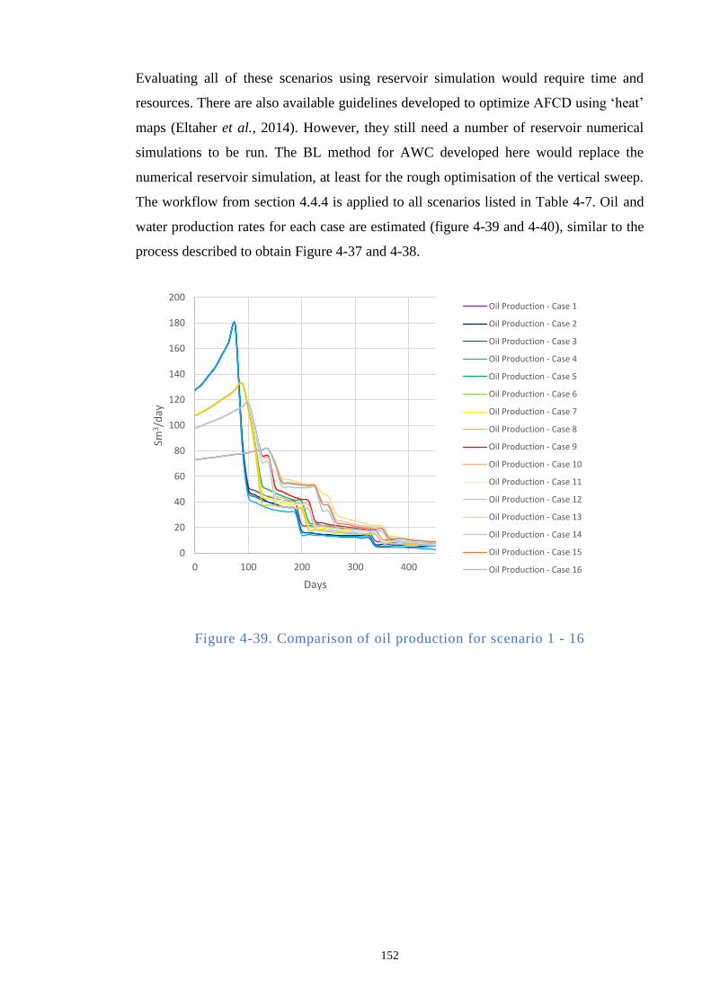
152
Evaluating all of these scenarios using reservoir simulation would require time and
resources. There are also available guidelines developed to optimize AFCD using ‘heat’
maps (Eltaher et al., 2014). However, they still need a number of reservoir numerical
simulations to be run. The BL method for AWC developed here would replace the
numerical reservoir simulation, at least for the rough optimisation of the vertical sweep.
The workflow from section 4.4.4 is applied to all scenarios listed in Table 4-7. Oil and
water production rates for each case are estimated (figure 4-39 and 4-40), similar to the
process described to obtain Figure 4-37 and 4-38.
Figure 4-39. Comparison of oil production for scenario 1 - 16
0
20
40
60
80
100
120
140
160
180
200
0 100 200 300 400
Sm3/d
ay
Days
Oil Production - Case 1
Oil Production - Case 2
Oil Production - Case 3
Oil Production - Case 4
Oil Production - Case 5
Oil Production - Case 6
Oil Production - Case 7
Oil Production - Case 8
Oil Production - Case 9
Oil Production - Case 10
Oil Production - Case 11
Oil Production - Case 12
Oil Production - Case 13
Oil Production - Case 14
Oil Production - Case 15
Oil Production - Case 16
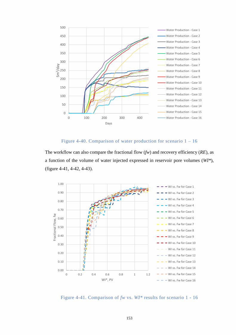
153
Figure 4-40. Comparison of water production for scenario 1 – 16
The workflow can also compare the fractional flow (fw) and recovery efficiency (RE), as
a function of the volume of water injected expressed in reservoir pore volumes (WI*),
(figure 4-41, 4-42, 4-43).
Figure 4-41. Comparison of fw vs. WI* results for scenario 1 - 16
0
50
100
150
200
250
300
350
400
450
500
0 100 200 300 400
Sm3 /
day
Days
Water Production - Case 1
Water Production - Case 2
Water Production - Case 3
Water Production - Case 4
Water Production - Case 5
Water Production - Case 6
Water Production - Case 7
Water Production - Case 8
Water Production - Case 9
Water Production - Case 10
Water Production - Case 11
Water Production - Case 12
Water Production - Case 13
Water Production - Case 14
Water Production - Case 15
Water Production - Case 16
0.00
0.10
0.20
0.30
0.40
0.50
0.60
0.70
0.80
0.90
1.00
0 0.2 0.4 0.6 0.8 1 1.2
Frac
tio
nal
Flo
w, f
w
WI*, PV
WI vs. Fw for Case 1
WI vs. Fw for Case 2
WI vs. Fw for Case 3
WI vs. Fw for Case 4
WI vs. Fw for Case 5
WI vs. Fw for Case 6
WI vs. Fw for Case 7
WI vs. Fw for Case 8
WI vs. Fw for Case 9
WI vs. Fw for Case 10
WI vs. Fw for Case 11
WI vs. Fw for Case 12
WI vs. Fw for Case 13
WI vs. Fw for Case 14
WI vs. Fw for Case 15
WI vs. Fw for Case 16
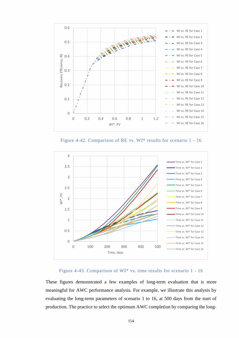
154
Figure 4-42. Comparison of RE vs. WI* results for scenario 1 - 16
Figure 4-43. Comparison of WI* vs. time results for scenario 1 - 16
These figures demonstrated a few examples of long-term evaluation that is more
meaningful for AWC performance analysis. For example, we illustrate this analysis by
evaluating the long-term parameters of scenario 1 to 16, at 500 days from the start of
production. The practice to select the optimum AWC completion by comparing the long-
0
0.1
0.2
0.3
0.4
0.5
0.6
0 0.2 0.4 0.6 0.8 1 1.2
Rec
ove
ry E
ffic
ien
cy, R
E
WI*, PV
WI vs. RE for Case 1
WI vs. RE for Case 2
WI vs. RE for Case 3
WI vs. RE for Case 4
WI vs. RE for Case 5
WI vs. RE for Case 6
WI vs. RE for Case 7
WI vs. RE for Case 8
WI vs. RE for Case 9
WI vs. RE for Case 10
WI vs. RE for Case 11
WI vs. RE for Case 12
WI vs. RE for Case 13
WI vs. RE for Case 14
WI vs. RE for Case 15
WI vs. RE for Case 16
0
0.5
1
1.5
2
2.5
3
3.5
4
0 100 200 300 400 500
WI*
, PV
Time, days
Time vs. WI* for Case 1
Time vs. WI* for Case 2
Time vs. WI* for Case 3
Time vs. WI* for Case 4
Time vs. WI* for Case 5
Time vs. WI* for Case 6
Time vs. WI* for Case 7
Time vs. WI* for Case 8
Time vs. WI* for Case 9
Time vs. WI* for Case 10
Time vs. WI* for Case 11
Time vs. WI* for Case 12
Time vs. WI* for Case 13
Time vs. WI* for Case 14
Time vs. WI* for Case 15
Time vs. WI* for Case 16
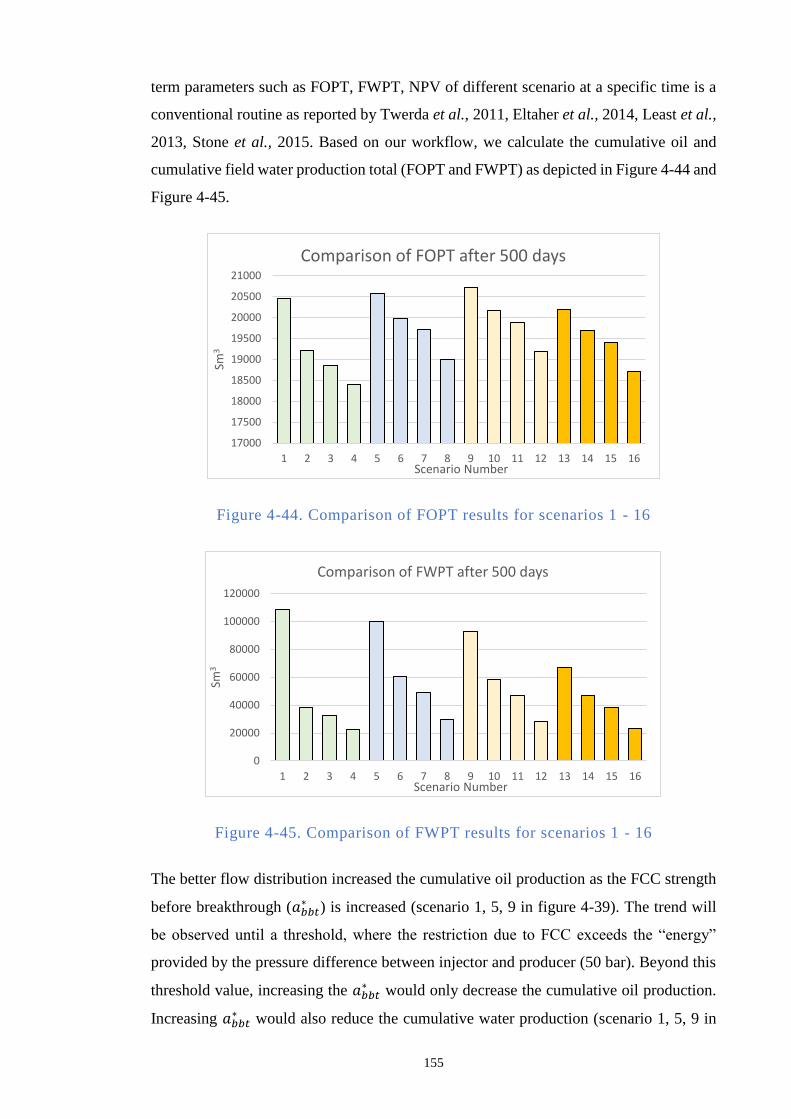
155
term parameters such as FOPT, FWPT, NPV of different scenario at a specific time is a
conventional routine as reported by Twerda et al., 2011, Eltaher et al., 2014, Least et al.,
2013, Stone et al., 2015. Based on our workflow, we calculate the cumulative oil and
cumulative field water production total (FOPT and FWPT) as depicted in Figure 4-44 and
Figure 4-45.
Figure 4-44. Comparison of FOPT results for scenarios 1 - 16
Figure 4-45. Comparison of FWPT results for scenarios 1 - 16
The better flow distribution increased the cumulative oil production as the FCC strength
before breakthrough (𝑎𝑏𝑏𝑡∗ ) is increased (scenario 1, 5, 9 in figure 4-39). The trend will
be observed until a threshold, where the restriction due to FCC exceeds the “energy”
provided by the pressure difference between injector and producer (50 bar). Beyond this
threshold value, increasing the 𝑎𝑏𝑏𝑡∗ would only decrease the cumulative oil production.
Increasing 𝑎𝑏𝑏𝑡∗ would also reduce the cumulative water production (scenario 1, 5, 9 in
17000
17500
18000
18500
19000
19500
20000
20500
21000
1 2 3 4 5 6 7 8 9 10 11 12 13 14 15 16
Sm3
Scenario Number
Comparison of FOPT after 500 days
0
20000
40000
60000
80000
100000
120000
1 2 3 4 5 6 7 8 9 10 11 12 13 14 15 16
Sm3
Scenario Number
Comparison of FWPT after 500 days
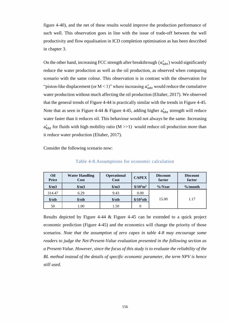
156
figure 4-40), and the net of these results would improve the production performance of
such well. This observation goes in line with the issue of trade-off between the well
productivity and flow equalisation in ICD completion optimisation as has been described
in chapter 3.
On the other hand, increasing FCC strength after breakthrough (𝑎𝑎𝑏𝑡∗ ) would significantly
reduce the water production as well as the oil production, as observed when comparing
scenario with the same colour. This observation is in contrast with the observation for
“piston-like displacement (or M < 1)” where increasing 𝑎𝑎𝑏𝑡∗ would reduce the cumulative
water production without much affecting the oil production (Eltaher, 2017). We observed
that the general trends of Figure 4-44 is practically similar with the trends in Figure 4-45.
Note that as seen in Figure 4-44 & Figure 4-45, adding higher abbt∗ strength will reduce
water faster than it reduces oil. This behaviour would not always be the same. Increasing
abbt∗ for fluids with high mobility ratio (M >>1) would reduce oil production more than
it reduce water production (Eltaher, 2017).
Consider the following scenario now:
Table 4-8.Assumptions for economic calculation
Oil
Price
Water Handling
Cost
Operational
Cost CAPEX
Discount
factor
Discount
factor
$/m3 $/m3 $/m3 $/103m3 %/Year %/month
314.47 6.29 9.43 0.00
15.00 1.17 $/stb $/stb $/stb $/103stb
50 1.00 1.50 0
Results depicted by Figure 4-44 & Figure 4-45 can be extended to a quick project
economic prediction (Figure 4-45) and the economics will change the priority of those
scenarios. Note that the assumption of zero capex in table 4-8 may encourage some
readers to judge the Net-Present-Value evaluation presented in the following section as
a Present-Value. However, since the focus of this study is to evaluate the reliability of the
BL method instead of the details of specific economic parameter, the term NPV is hence
still used.
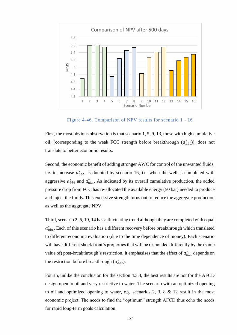
157
Figure 4-46. Comparison of NPV results for scenario 1 - 16
First, the most obvious observation is that scenario 1, 5, 9, 13, those with high cumulative
oil, (corresponding to the weak FCC strength before breakthrough (𝑎𝑏𝑏𝑡∗ )), does not
translate to better economic results.
Second, the economic benefit of adding stronger AWC for control of the unwanted fluids,
i.e. to increase 𝑎𝑏𝑏𝑡∗ , is doubted by scenario 16, i.e. when the well is completed with
aggressive 𝑎𝑏𝑏𝑡∗ and 𝑎𝑎𝑏𝑡
∗ . As indicated by its overall cumulative production, the added
pressure drop from FCC has re-allocated the available energy (50 bar) needed to produce
and inject the fluids. This excessive strength turns out to reduce the aggregate production
as well as the aggregate NPV.
Third, scenario 2, 6, 10, 14 has a fluctuating trend although they are completed with equal
𝑎𝑎𝑏𝑡∗ . Each of this scenario has a different recovery before breakthrough which translated
to different economic evaluation (due to the time dependence of money). Each scenario
will have different shock front’s properties that will be responded differently by the (same
value of) post-breakthrough’s restriction. It emphasises that the effect of 𝑎𝑎𝑏𝑡∗ depends on
the restriction before breakthrough (𝑎𝑏𝑏𝑡∗ ).
Fourth, unlike the conclusion for the section 4.3.4, the best results are not for the AFCD
design open to oil and very restrictive to water. The scenario with an optimized opening
to oil and optimized opening to water, e.g. scenarios 2, 3, 8 & 12 result in the most
economic project. The needs to find the “optimum” strength AFCD thus echo the needs
for rapid long-term goals calculation.
4.2
4.4
4.6
4.8
5
5.2
5.4
5.6
5.8
1 2 3 4 5 6 7 8 9 10 11 12 13 14 15 16
MM
$
Scenario Number
Comparison of NPV after 500 days
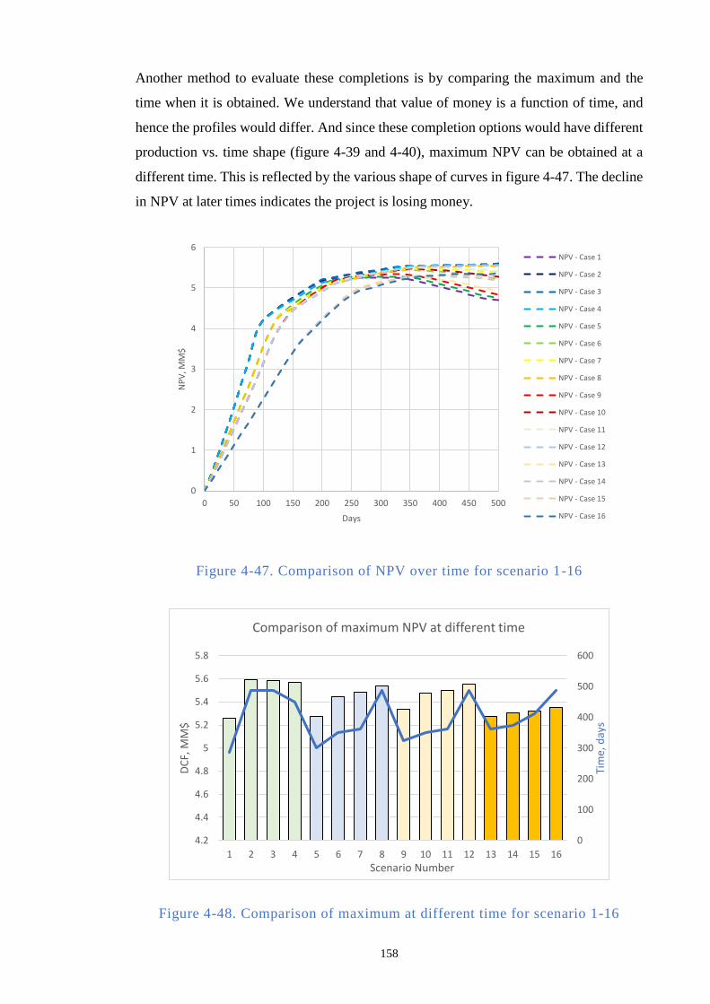
158
Another method to evaluate these completions is by comparing the maximum and the
time when it is obtained. We understand that value of money is a function of time, and
hence the profiles would differ. And since these completion options would have different
production vs. time shape (figure 4-39 and 4-40), maximum NPV can be obtained at a
different time. This is reflected by the various shape of curves in figure 4-47. The decline
in NPV at later times indicates the project is losing money.
Figure 4-47. Comparison of NPV over time for scenario 1-16
Figure 4-48. Comparison of maximum at different time for scenario 1-16
0
1
2
3
4
5
6
0 50 100 150 200 250 300 350 400 450 500
NP
V, M
M$
Days
NPV - Case 1
NPV - Case 2
NPV - Case 3
NPV - Case 4
NPV - Case 5
NPV - Case 6
NPV - Case 7
NPV - Case 8
NPV - Case 9
NPV - Case 10
NPV - Case 11
NPV - Case 12
NPV - Case 13
NPV - Case 14
NPV - Case 15
NPV - Case 16
0
100
200
300
400
500
600
4.2
4.4
4.6
4.8
5
5.2
5.4
5.6
5.8
1 2 3 4 5 6 7 8 9 10 11 12 13 14 15 16
Tim
e, d
ays
DC
F, M
M$
Scenario Number
Comparison of maximum NPV at different time
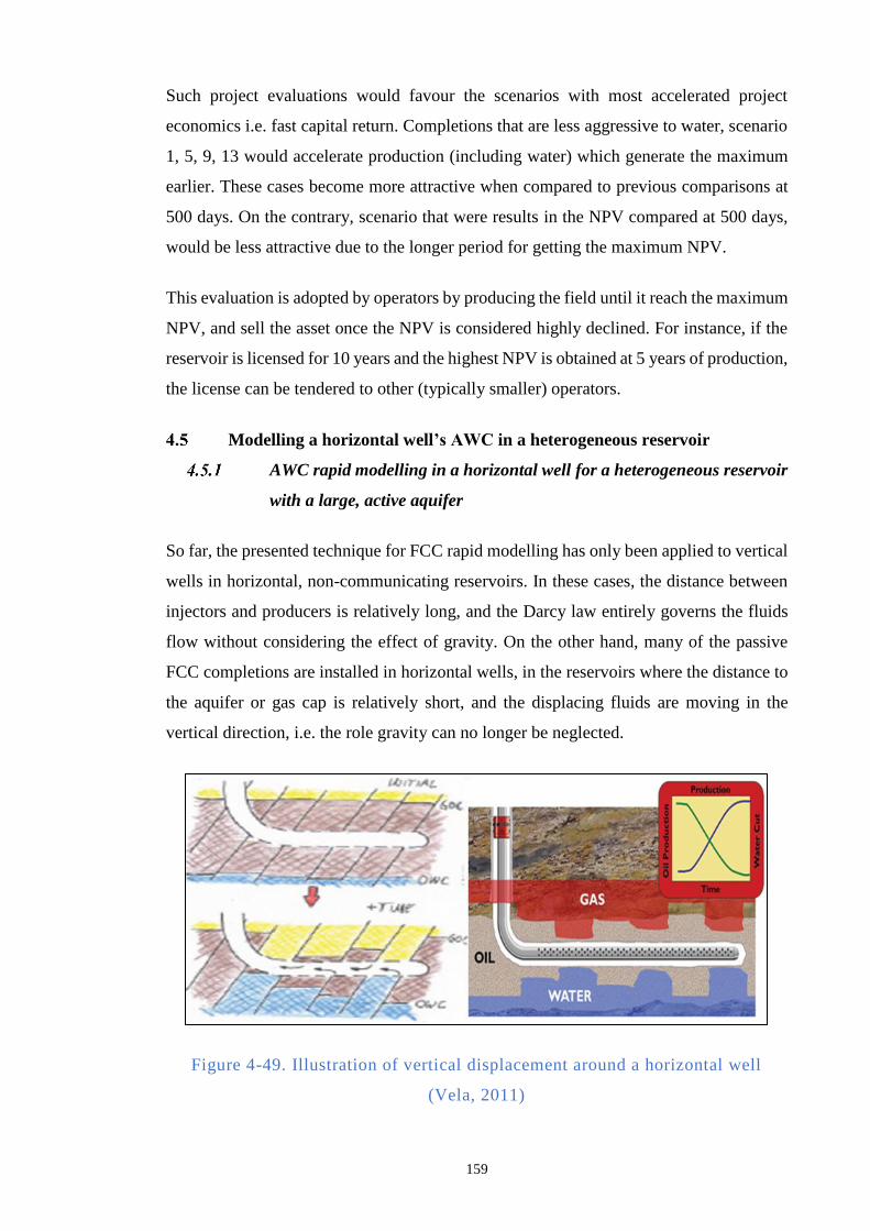
159
Such project evaluations would favour the scenarios with most accelerated project
economics i.e. fast capital return. Completions that are less aggressive to water, scenario
1, 5, 9, 13 would accelerate production (including water) which generate the maximum
earlier. These cases become more attractive when compared to previous comparisons at
500 days. On the contrary, scenario that were results in the NPV compared at 500 days,
would be less attractive due to the longer period for getting the maximum NPV.
This evaluation is adopted by operators by producing the field until it reach the maximum
NPV, and sell the asset once the NPV is considered highly declined. For instance, if the
reservoir is licensed for 10 years and the highest NPV is obtained at 5 years of production,
the license can be tendered to other (typically smaller) operators.
Modelling a horizontal well’s AWC in a heterogeneous reservoir
AWC rapid modelling in a horizontal well for a heterogeneous reservoir
with a large, active aquifer
So far, the presented technique for FCC rapid modelling has only been applied to vertical
wells in horizontal, non-communicating reservoirs. In these cases, the distance between
injectors and producers is relatively long, and the Darcy law entirely governs the fluids
flow without considering the effect of gravity. On the other hand, many of the passive
FCC completions are installed in horizontal wells, in the reservoirs where the distance to
the aquifer or gas cap is relatively short, and the displacing fluids are moving in the
vertical direction, i.e. the role gravity can no longer be neglected.
Figure 4-49. Illustration of vertical displacement around a horizontal well
(Vela, 2011)
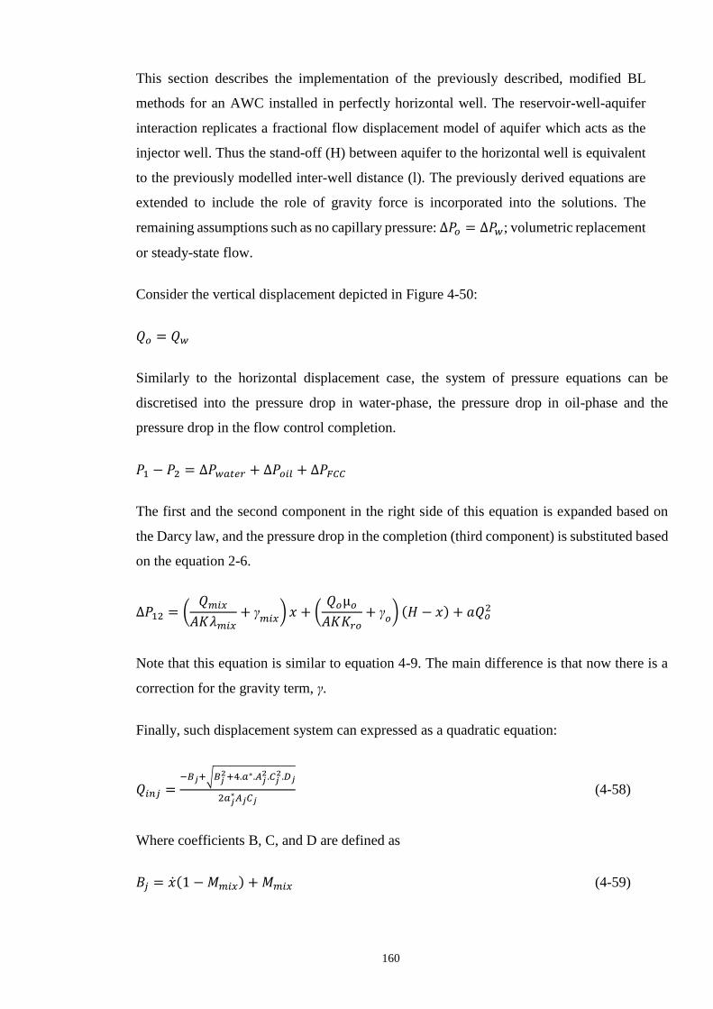
160
This section describes the implementation of the previously described, modified BL
methods for an AWC installed in perfectly horizontal well. The reservoir-well-aquifer
interaction replicates a fractional flow displacement model of aquifer which acts as the
injector well. Thus the stand-off (H) between aquifer to the horizontal well is equivalent
to the previously modelled inter-well distance (l). The previously derived equations are
extended to include the role of gravity force is incorporated into the solutions. The
remaining assumptions such as no capillary pressure: ∆𝑃𝑜 = ∆𝑃𝑤; volumetric replacement
or steady-state flow.
Consider the vertical displacement depicted in Figure 4-50:
𝑄𝑜 = 𝑄𝑤
Similarly to the horizontal displacement case, the system of pressure equations can be
discretised into the pressure drop in water-phase, the pressure drop in oil-phase and the
pressure drop in the flow control completion.
𝑃1 − 𝑃2 = ∆𝑃𝑤𝑎𝑡𝑒𝑟 + ∆𝑃𝑜𝑖𝑙 + ∆𝑃𝐹𝐶𝐶
The first and the second component in the right side of this equation is expanded based on
the Darcy law, and the pressure drop in the completion (third component) is substituted based
on the equation 2-6.
∆𝑃12 = (𝑄𝑚𝑖𝑥𝐴𝐾𝜆𝑚𝑖𝑥
+ γ𝑚𝑖𝑥
) 𝑥 + (𝑄𝑜µ𝑜𝐴𝐾𝐾𝑟𝑜
+ γ𝑜) (𝐻 − 𝑥) + 𝑎𝑄𝑜
2
Note that this equation is similar to equation 4-9. The main difference is that now there is a
correction for the gravity term, γ.
Finally, such displacement system can expressed as a quadratic equation:
𝑄𝑖𝑛𝑗 =−𝐵𝑗+√𝐵𝑗
2+4.𝑎∗.𝐴𝑗2.𝐶𝑗
2.𝐷𝑗
2𝑎𝑗∗𝐴𝑗𝐶𝑗
(4-58)
Where coefficients B, C, and D are defined as
𝐵𝑗 = (1 − 𝑀𝑚𝑖𝑥) + 𝑀𝑚𝑖𝑥 (4-59)
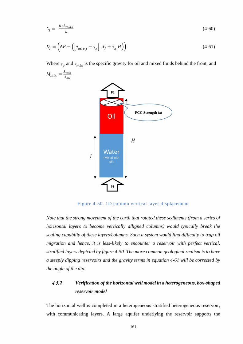
161
𝐶𝑗 = 𝐾𝑗.𝜆𝑚𝑖𝑥,𝑗
𝐿 (4-60)
𝐷𝑗 = (∆𝑃 − ([γ𝑚𝑖𝑥,𝑗
− γ𝑜] . 𝑗 + γ
𝑜 𝐻)) (4-61)
Where γ𝑜 and γ
𝑚𝑖𝑥 is the specific gravity for oil and mixed fluids behind the front, and
𝑀𝑚𝑖𝑥 =𝜆𝑚𝑖𝑥
𝜆𝑜𝑖𝑙
Figure 4-50. 1D column vertical layer displacement
Note that the strong movement of the earth that rotated these sediments (from a series of
horizontal layers to become vertically alligned columns) would typically break the
sealing capabiliy of these layers/columns. Such a system would find difficulty to trap oil
migration and hence, it is less-likely to encounter a reservoir with perfect vertical,
stratified layers depicted by figure 4-50. The more common geological realism is to have
a steeply dipping reservoirs and the gravity terms in equation 4-61 will be corrected by
the angle of the dip.
Verification of the horizontal well model in a heterogeneous, box-shaped
reservoir model
The horizontal well is completed in a heterogeneous stratified heterogeneous reservoir,
with communicating layers. A large aquifer underlying the reservoir supports the
Oil
Water (Mixed with
oil)
P1
P2
FCC Strength (a)
𝐻
l
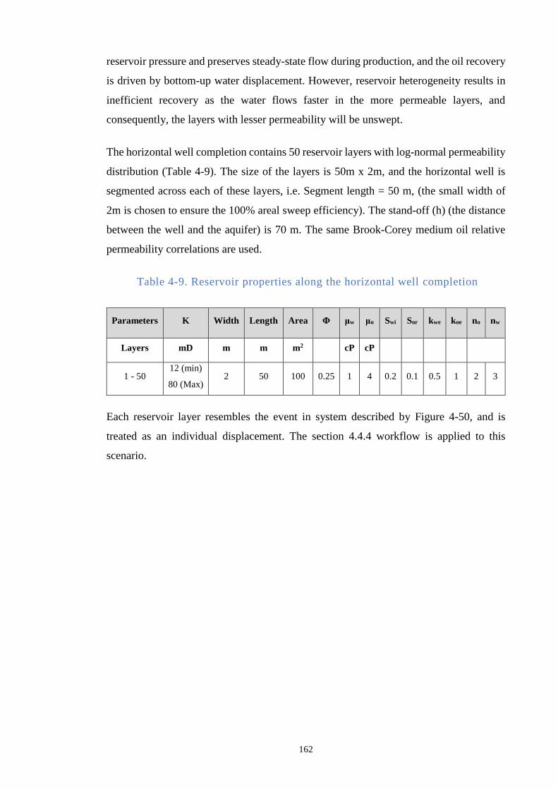
162
reservoir pressure and preserves steady-state flow during production, and the oil recovery
is driven by bottom-up water displacement. However, reservoir heterogeneity results in
inefficient recovery as the water flows faster in the more permeable layers, and
consequently, the layers with lesser permeability will be unswept.
The horizontal well completion contains 50 reservoir layers with log-normal permeability
distribution (Table 4-9). The size of the layers is 50m x 2m, and the horizontal well is
segmented across each of these layers, i.e. Segment length = 50 m, (the small width of
2m is chosen to ensure the 100% areal sweep efficiency). The stand-off (h) (the distance
between the well and the aquifer) is 70 m. The same Brook-Corey medium oil relative
permeability correlations are used.
Table 4-9. Reservoir properties along the horizontal well completion
Each reservoir layer resembles the event in system described by Figure 4-50, and is
treated as an individual displacement. The section 4.4.4 workflow is applied to this
scenario.
Parameters K Width Length Area Φ μw μo Swi Sor kwe koe no nw
Layers mD m m m2 cP cP
1 - 50 12 (min)
80 (Max) 2 50 100 0.25 1 4 0.2 0.1 0.5 1 2 3
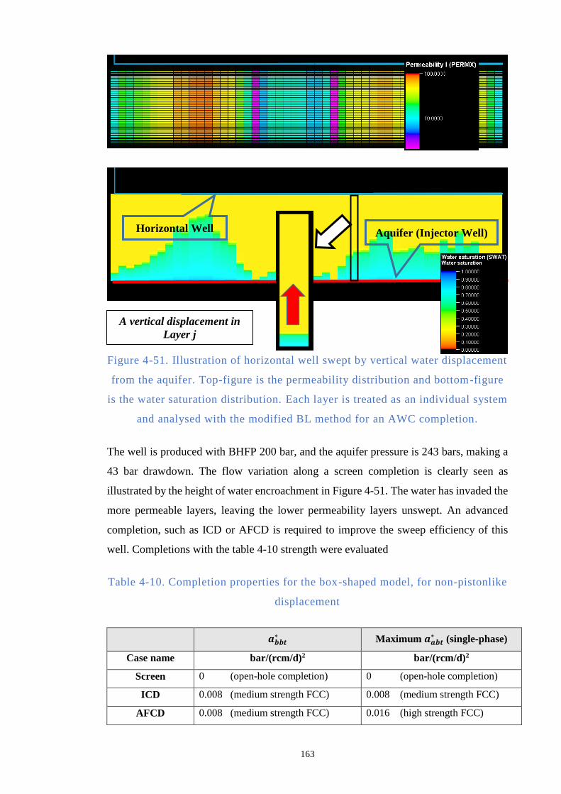
163
Figure 4-51. Illustration of horizontal well swept by vertical water displacement
from the aquifer. Top-figure is the permeability distribution and bottom-figure
is the water saturation distribution. Each layer is treated as an individual system
and analysed with the modified BL method for an AWC completion.
The well is produced with BHFP 200 bar, and the aquifer pressure is 243 bars, making a
43 bar drawdown. The flow variation along a screen completion is clearly seen as
illustrated by the height of water encroachment in Figure 4-51. The water has invaded the
more permeable layers, leaving the lower permeability layers unswept. An advanced
completion, such as ICD or AFCD is required to improve the sweep efficiency of this
well. Completions with the table 4-10 strength were evaluated
Table 4-10. Completion properties for the box-shaped model, for non-pistonlike
displacement
𝒂𝒃𝒃𝒕∗ Maximum 𝒂𝒂𝒃𝒕
∗ (single-phase)
Case name bar/(rcm/d)2 bar/(rcm/d)2
Screen 0 (open-hole completion) 0 (open-hole completion)
ICD 0.008 (medium strength FCC) 0.008 (medium strength FCC)
AFCD 0.008 (medium strength FCC) 0.016 (high strength FCC)
Horizontal Well Aquifer (Injector Well)
A vertical displacement in
Layer j
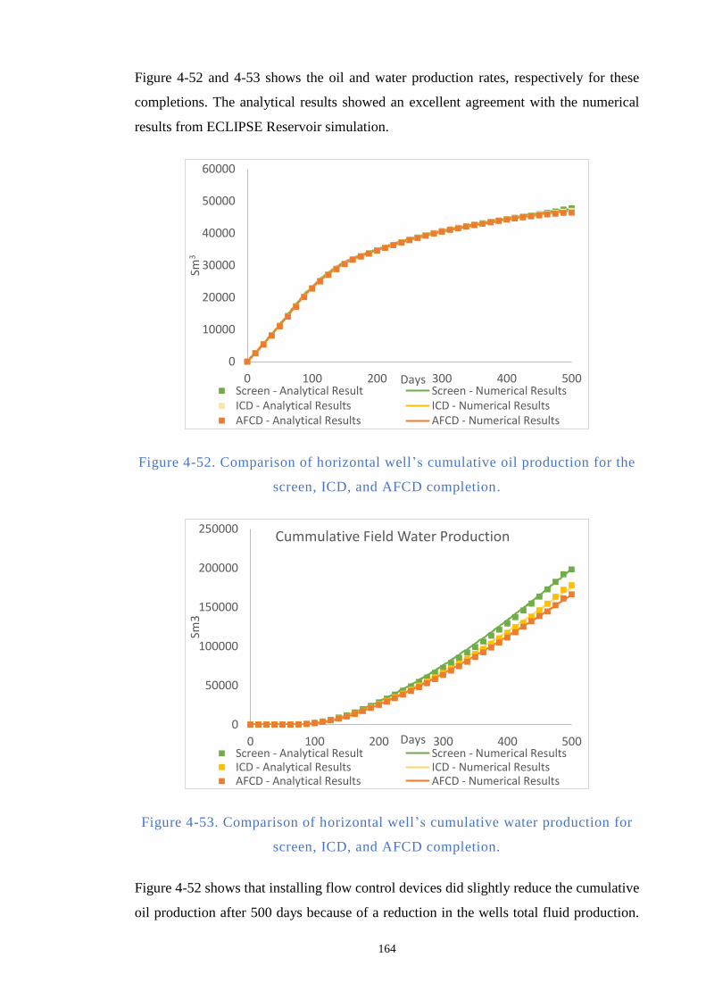
164
Figure 4-52 and 4-53 shows the oil and water production rates, respectively for these
completions. The analytical results showed an excellent agreement with the numerical
results from ECLIPSE Reservoir simulation.
Figure 4-52. Comparison of horizontal well’s cumulative oil production for the
screen, ICD, and AFCD completion.
Figure 4-53. Comparison of horizontal well’s cumulative water production for
screen, ICD, and AFCD completion.
Figure 4-52 shows that installing flow control devices did slightly reduce the cumulative
oil production after 500 days because of a reduction in the wells total fluid production.
0
10000
20000
30000
40000
50000
60000
0 100 200 300 400 500
Sm3
DaysScreen - Analytical Result Screen - Numerical ResultsICD - Analytical Results ICD - Numerical ResultsAFCD - Analytical Results AFCD - Numerical Results
0
50000
100000
150000
200000
250000
0 100 200 300 400 500
Sm3
Days
Cummulative Field Water Production
Screen - Analytical Result Screen - Numerical ResultsICD - Analytical Results ICD - Numerical ResultsAFCD - Analytical Results AFCD - Numerical Results
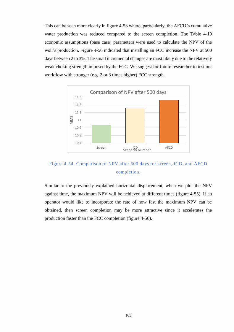
165
This can be seen more clearly in figure 4-53 where, particularly, the AFCD’s cumulative
water production was reduced compared to the screen completion. The Table 4-10
economic assumptions (base case) parameters were used to calculate the NPV of the
well’s production. Figure 4-56 indicated that installing an FCC increase the NPV at 500
days between 2 to 3%. The small incremental changes are most likely due to the relatively
weak choking strength imposed by the FCC. We suggest for future researcher to test our
workflow with stronger (e.g. 2 or 3 times higher) FCC strength.
Figure 4-54. Comparison of NPV after 500 days for screen, ICD, and AFCD
completion.
Similar to the previously explained horizontal displacement, when we plot the NPV
against time, the maximum NPV will be achieved at different times (figure 4-55). If an
operator would like to incorporate the rate of how fast the maximum NPV can be
obtained, then screen completion may be more attractive since it accelerates the
production faster than the FCC completion (figure 4-56).
10.7
10.8
10.9
11
11.1
11.2
11.3
Screen ICD AFCD
MM
$
Scenario Number
Comparison of NPV after 500 days
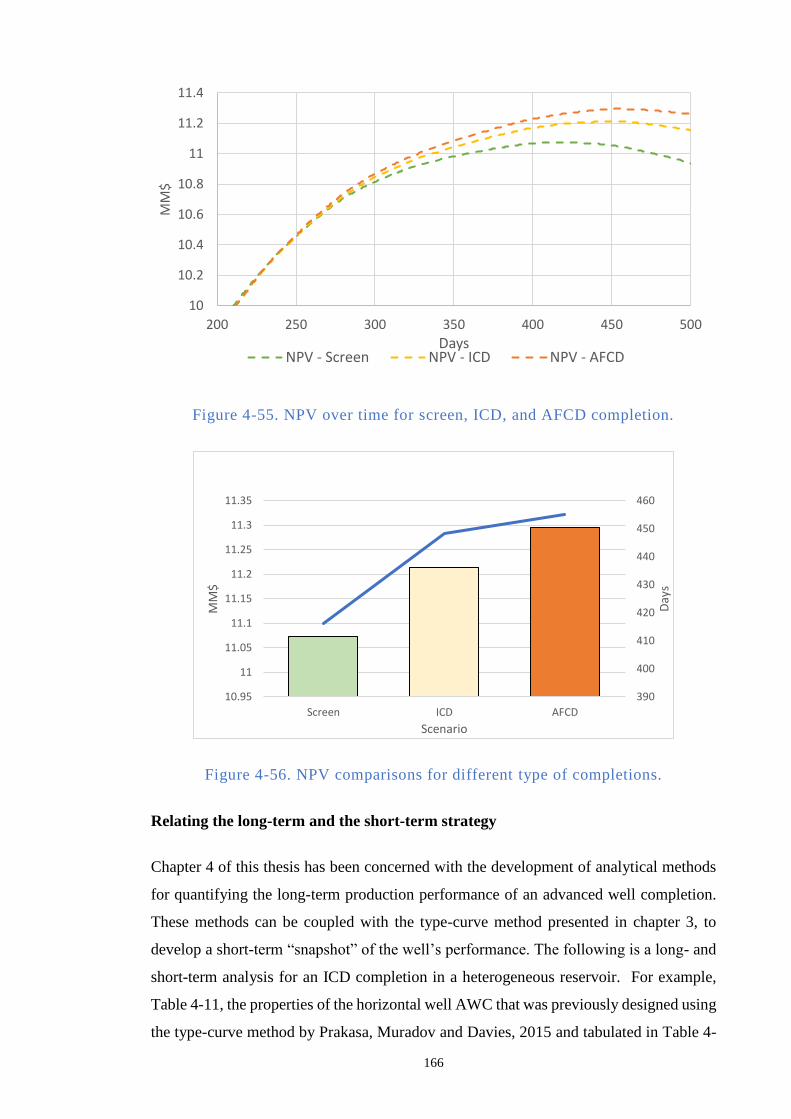
166
Figure 4-55. NPV over time for screen, ICD, and AFCD completion.
Figure 4-56. NPV comparisons for different type of completions.
Relating the long-term and the short-term strategy
Chapter 4 of this thesis has been concerned with the development of analytical methods
for quantifying the long-term production performance of an advanced well completion.
These methods can be coupled with the type-curve method presented in chapter 3, to
develop a short-term “snapshot” of the well’s performance. The following is a long- and
short-term analysis for an ICD completion in a heterogeneous reservoir. For example,
Table 4-11, the properties of the horizontal well AWC that was previously designed using
the type-curve method by Prakasa, Muradov and Davies, 2015 and tabulated in Table 4-
10
10.2
10.4
10.6
10.8
11
11.2
11.4
200 250 300 350 400 450 500
MM
$
DaysNPV - Screen NPV - ICD NPV - AFCD
390
400
410
420
430
440
450
460
10.95
11
11.05
11.1
11.15
11.2
11.25
11.3
11.35
Screen ICD AFCD
Day
s
MM
$
Scenario
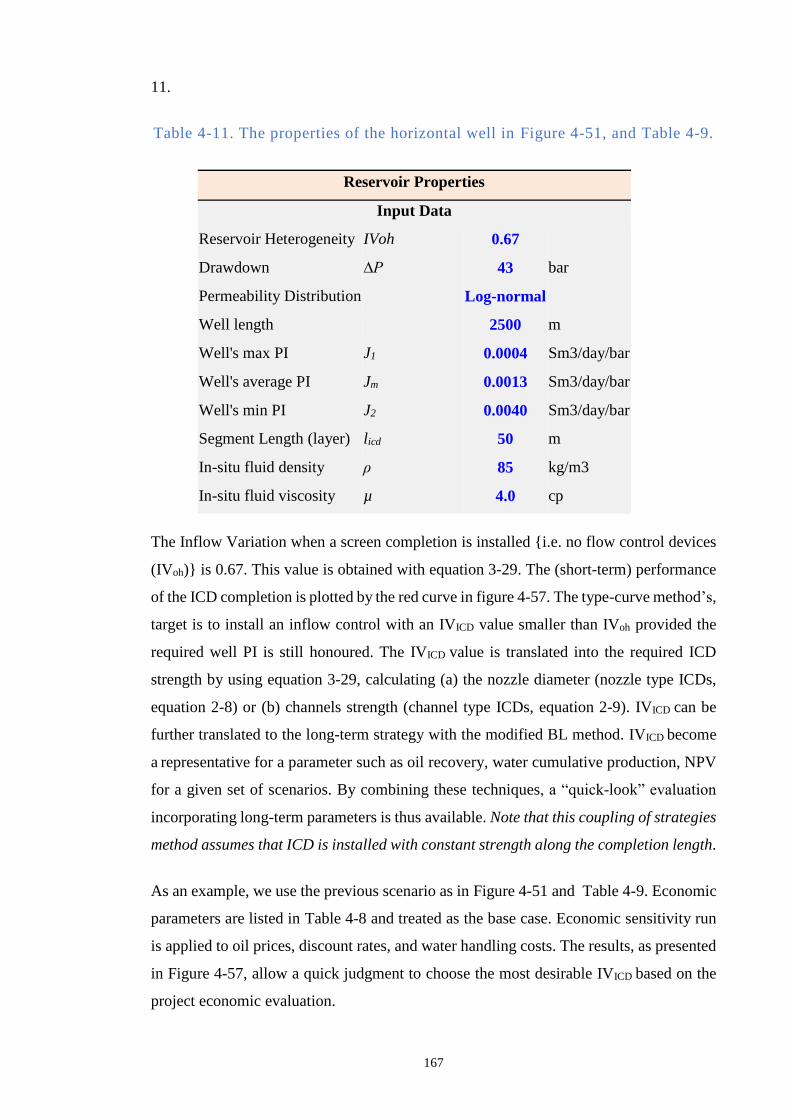
167
11.
Table 4-11. The properties of the horizontal well in Figure 4-51, and Table 4-9.
Reservoir Properties
Input Data
Reservoir Heterogeneity IVoh 0.67
Drawdown ∆P 43 bar
Permeability Distribution
Log-normal
Well length 2500 m
Well's max PI J1 0.0004 Sm3/day/bar
Well's average PI Jm 0.0013 Sm3/day/bar
Well's min PI J2 0.0040 Sm3/day/bar
Segment Length (layer) licd 50 m
In-situ fluid density ρ 85 kg/m3
In-situ fluid viscosity µ 4.0 cp
The Inflow Variation when a screen completion is installed i.e. no flow control devices
(IVoh) is 0.67. This value is obtained with equation 3-29. The (short-term) performance
of the ICD completion is plotted by the red curve in figure 4-57. The type-curve method’s,
target is to install an inflow control with an IVICD value smaller than IVoh provided the
required well PI is still honoured. The IVICD value is translated into the required ICD
strength by using equation 3-29, calculating (a) the nozzle diameter (nozzle type ICDs,
equation 2-8) or (b) channels strength (channel type ICDs, equation 2-9). IVICD can be
further translated to the long-term strategy with the modified BL method. IVICD become
a representative for a parameter such as oil recovery, water cumulative production, NPV
for a given set of scenarios. By combining these techniques, a “quick-look” evaluation
incorporating long-term parameters is thus available. Note that this coupling of strategies
method assumes that ICD is installed with constant strength along the completion length.
As an example, we use the previous scenario as in Figure 4-51 and Table 4-9. Economic
parameters are listed in Table 4-8 and treated as the base case. Economic sensitivity run
is applied to oil prices, discount rates, and water handling costs. The results, as presented
in Figure 4-57, allow a quick judgment to choose the most desirable IVICD based on the
project economic evaluation.
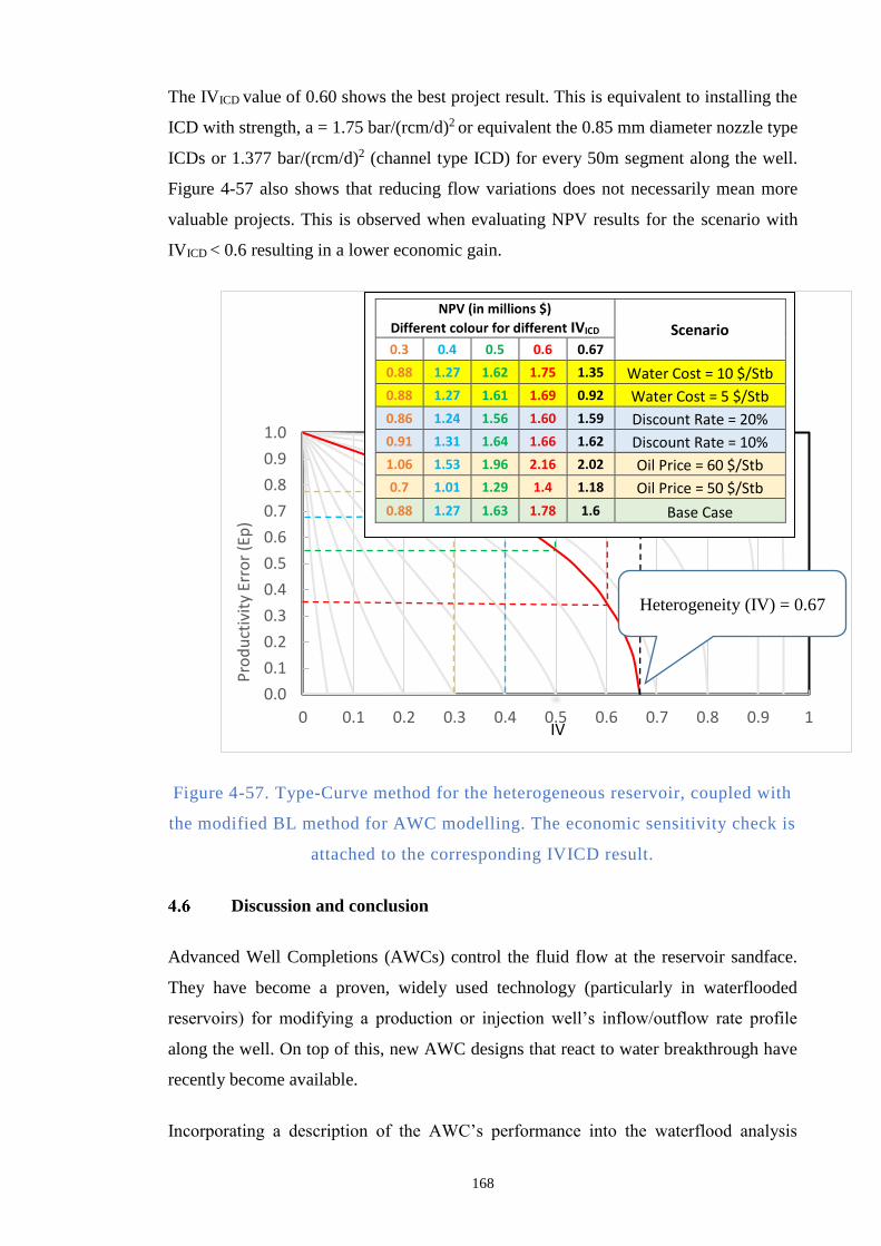
168
The IVICD value of 0.60 shows the best project result. This is equivalent to installing the
ICD with strength, a = 1.75 bar/(rcm/d)2 or equivalent the 0.85 mm diameter nozzle type
ICDs or 1.377 bar/(rcm/d)2 (channel type ICD) for every 50m segment along the well.
Figure 4-57 also shows that reducing flow variations does not necessarily mean more
valuable projects. This is observed when evaluating NPV results for the scenario with
IVICD < 0.6 resulting in a lower economic gain.
Figure 4-57. Type-Curve method for the heterogeneous reservoir, coupled with
the modified BL method for AWC modelling. The economic sensitivity check is
attached to the corresponding IVICD result.
Discussion and conclusion
Advanced Well Completions (AWCs) control the fluid flow at the reservoir sandface.
They have become a proven, widely used technology (particularly in waterflooded
reservoirs) for modifying a production or injection well’s inflow/outflow rate profile
along the well. On top of this, new AWC designs that react to water breakthrough have
recently become available.
Incorporating a description of the AWC’s performance into the waterflood analysis
0.0
0.1
0.2
0.3
0.4
0.5
0.6
0.7
0.8
0.9
1.0
0 0.1 0.2 0.3 0.4 0.5 0.6 0.7 0.8 0.9 1
Pro
du
ctiv
ity
Erro
r (E
p)
IV
NPV (in millions $)
Different colour for different IVICD Scenario 0.3 0.4 0.5 0.6 0.67
0.88 1.27 1.62 1.75 1.35 Water Cost = 10 $/Stb
0.88 1.27 1.61 1.69 0.92 Water Cost = 5 $/Stb
0.86 1.24 1.56 1.60 1.59 Discount Rate = 20%
0.91 1.31 1.64 1.66 1.62 Discount Rate = 10%
1.06 1.53 1.96 2.16 2.02 Oil Price = 60 $/Stb
0.7 1.01 1.29 1.4 1.18 Oil Price = 50 $/Stb
0.88 1.27 1.63 1.78 1.6 Base Case
Heterogeneity (IV) = 0.67

169
models allows fast forecasting of the production profile and oil recovery, as well as help
optimising the AWC configuration and control at the well design stage. The proposed
methods are particularly useful for predicting, analysing, and designing an advanced
well’s and/or controlling the well’s performance to maximize oil recovery or other means
e.g. of economic gain – a task that is rarely done in reality due to the complexity of the
existing modelling tools. The method’s transparency and ease of implementation of its
algorithms can make it a useful tool for well and reservoir engineers.
We built a tool to model and predict the long-term value added from AWC, and serve as
a bridge between simple inflow snapshot evaluation and full dynamic reservoir simulation
to enable quick screening of AWC. The tools will be realised in Excel spreadsheets
allowing their easy and widespread use. The reservoir sweep models forming the basis of
these tools have been recently, uniquely developed and successfully verified.
Preference will be for the tool to consider the drainage radius/area associated with a single
well to determine cumulate oil from area over time (i.e. as per pressure depletion).
Amongst others, the tool should be able to take following inputs into consideration:
• Permeability profile (e.g. md at depth)
• PVT information
• Saturation profile
• Reservoir Pressures
• Well/completion dimensions
• Typical boundary constrains, BHP, WHP, rate etc.
The engineers could be well served by a tool that can produce long-term parameters
associated with a completions type without always depending on complete reservoir
simulation tools, such as:
• Cumulative oil produced
• Cumulative water produced
• Cumulative gas produced
• Fluids distribution along horizontal segments
General observations from this chapter on extending the waterflood analyses to AWC
170
completions are:
The solutions presented in this work are for the case of constant pressure difference
between the injection and production wells. Note that in the original form, Buckley-
Leverett equation was presented assuming constant rate and does not calculate
pressure. Our BL method used constant pressure differences to make a simple
comparison with the DP method presented (which assumes constant pressure
difference) previously. The solution can be translated into the constant rate case. Note
that, if a strong response in the production well to water breakthrough (e.g. zonal shut-
in or increased AFCD strength) is observed, this results in a significant change in the
reservoir pressure drop. The equation 4-6 integrals now need to be split into parts.
Many publications emphasize in the impact of inflow uniformity, and its consequently
delayed breakthrough objectives for AWC design. This work has discussed how long-
term parameters such oil recovery, value creation, etc., should also be considered.
Remember also that the unhindered well outflow performance is also required.
It is also worth mentioning that the waterflood analysis methods for communicating
layers in vertical wells were briefly discussed in introduction. These methods assume
vertical pressure equilibrium for all layers, i.e. the local pressure derivative at a given
distance from the well is the same for every layer. They cannot be extended to the
AWC wells where a significantly different pressure drops is created across each layer.
The new models achieved a good match with the results of a numerical simulation. They
provide a simplified, fast, analysis of the impact of various well completion and control
options on the development of a waterflood and its efficiency. These models provide a
missing link between the various AWC design workflows available today and the long-
term value evaluation of an AWC when a commercial numerical simulation software is
either not available or is too time consuming.
Summary
The advantages and limitations of the extended of the classical waterflood analysis for
non-communicating layers to the situation when the reservoir is developed with an AWC
are:
a) The light oil displacement is being replicated by a sharp waterfront, resulting in a
“piston-like” displacement, modelled using Dykstra-Parsons method. The sandface,
171
flow control completion in an AWC well adds either a non-linear pressure drop across
each layer or the option of zonal closure. The resulting DP method could be modelled
analytically, though a numerical solution was required since the front position could
not be expressed explicitly. This extended DP method is thus applicable to waterflood
performance analysis for wells with arbitrary completion or control.
The important observations to note that:
The parameters related to the fractional flow rate of water (or watercut) in the
extended DP method have step-like performance. By contrast, an accurate
numerical simulation will predict a smoother change (see e.g. Figure 4-7, Figure
4-11).
This piston-like behaviour allows a fixed value of (A)FCD strength,
(𝒂𝒃𝒃𝒕∗ & 𝒂𝒂𝒃𝒕
∗ ), for each corresponding period. By contrast, these values for non-
piston like (varying WC) displacements will be a function of the average water-
cut (see below).
Equation 4-17. An explicit analytical expression for the waterfront x is not
possible for these extended DP methods. Modifications developed by various
researchers to the conventional, layer-by-layer DP method that can no longer be
applied to fields developed with AWCs. These include:
1) Introducing a statistical description of the reservoir permeability distribution
into the solution.
2) Accurate translation of the waterflood performance prediction into the time
domain by integrating the waterfront x over the layer. However, the alternative
approach presented here using the approximate injection rates was showing to
be acceptably accurate (e.g. Figure 4-14).
3) Osman and Tiab, 1981 presented a DP method for composite layers (i.e. layer
permeability changes laterally) with conventional production and injection
wells. Their solution has the same quadratic form as the DP model, so it may
well be possible to extend our AWC-DP model to composite layers. Further
investigation is required.
b) Medium or heavy oil displacement, is “non-pistonlike” and requires use of non-linear
or more realistic relative-permeability curves. This type of displacement follows the
two-phase front movement described by Buckley-Leverett. The modified DP method
172
alone is not suited to such fluids. The displacement system is best described by
splitting it into 3 different components.
1. The non-linear pressure drops across the installed flow control completion
2. The displaced phase as an oil with homogeneous properties
3. The displacing, mixed fluids: composed of oil and water. Its properties, e.g. make
up the mixture mobility, velocity, etc. are modelled as the average of the
individual fluid properties behind the front.
This averaging method follows the Welge method. Front saturation is predicted by
classical fractional flow analysis, and the displacing phase’s average properties are the
harmonic average for the multiple layers with different fluid saturations behind the front.
Tracking the front position in the time domain is possible since x is evaluated
simultaneously with the corresponding front velocity. This allows the time to be found
numerically using appropriate algorithms e.g. gradient based, non-linear Excel’s Solver
or any optimisation in MATLAB. The results were validated against a numerical
simulation (Figure 4-30, Figure 4-31, Figure 4-37, Figure 4-38). The importance of this
is outlined by:
Economic evaluation, requiring the time value of money, is now possible.
The step-like performance of the DP method is avoided and the predicted flow rates
show more realistic results.
The optimum AFCD design for a reservoir exhibiting piston-like displacement, is to
install an AFCD with low restriction to oil production and aggressive restriction to
water. This is not the case for reservoir with “non-pistonlike” displacement. There is
an optimum restriction for each that achieves the best results. Eltaher, 2017 introduced
the concept of “bad-water” and “good-water” production when designing an AFCD,
emphasizing further the importance of achieving the correct FCC strength.
It is also worth to note that the optimum FCC strength is intrinsically a function of WC.
Thus the ideal AFCD completion requires the FCC strength (𝑎𝑏𝑏𝑡∗ ) to vary during the post
breakthrough period. This is a consequence of multi-phase flow. Strictly speaking, the
𝑎𝑎𝑏𝑡∗ will progressively increase once breakthrough has occurred, until the maximum 𝑎𝑎𝑏𝑡
∗
value is reached, when WC = 100 % (equation 4-49). The produced WC can be predicted
using fractional flow analyses, hence the progressively increasing 𝑎𝑎𝑏𝑡∗ trajectory can be

173
calculated (see Figure 4-30, Figure 4-31, Figure 4-37, Figure 4-38). The BL method for
AWC can also be extended to horizontal wells with vertical displacement, a common
scenario for installing AWC. Gravity needs to be incorporated into equation 4-58, 4-59,
4-60, and 4-61. The workflow is otherwise identical to the workflow for vertical well.
Nomenclature
All values are in SI units and at reservoir conditions, unless otherwise stated.
A – effective area perpendicular to flow RE – oil recovery efficiency (recovery factor)
a – flow control completion strength
defined by eq. 4-8, 2-8, 2-9, 2-10, 2-11 S - saturation
t - time Sor – residual oil saturation
b – formation volume factor Swi – irreducible water saturation
φ - porosity u – fluid flow velocity
fw – fraction flow rate of water (watercut at
downhole conditions) WI – volume of Water Injected
F – constant defined below equation
* *
, * *
(1 )
(1 )
j
i R R Rj R
RR j j j
dxdx x M xdt F
dx dx x M xdt
𝑑𝑓𝑤
𝑑𝑆𝑤 = Fractional flow derivative
h – layer height x – lateral coordinate of the water front
k – horizontal permeability ΔP – pressure difference
L – distance between wells ΔS – movable saturation (1-Sor-Swi)
M – mobility ratio λ – fluid mobility (i.e. rel.perm./viscosity)
P - pressure μ – viscosity
n – exponent for modified Brooks-Corey
functions
H – height (standoff) between well and
aquifer
ρ - density γ – Specific Gravity
q – flow rate
Subscripts
abt – after breakthrough or – residual oil (saturation)
bbt – before breakthrough r – relative (permeability)
bt – breakthrough w – water
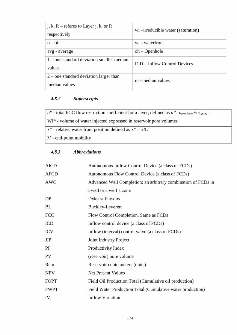
174
j, k, R – referes to Layer j, k, or R
respectively wi –irreducible water (saturation)
o – oil wf - waterfront
avg - average oh – Openhole
1 – one standard deviation smaller median
values ICD – Inflow Control Devices
2 – one standard deviation larger than
median values m –median values
Superscripts
a* - total FCC flow restriction coefficient for a layer, defined as a*=aproducer+ainjector
WI* - volume of water injected expressed in reservoir pore volumes
x* - relative water front position defined as x* = x/L
λ’ - end-point mobility
Abbreviations
AICD Autonomous Inflow Control Device (a class of FCDs)
AFCD Autonomous Flow Control Device (a class of FCDs)
AWC Advanced Well Completion: an arbitrary combination of FCDs in
a well or a well’s zone
DP Dykstra-Parsons
BL Buckley-Leverett
FCC Flow Control Completion. Same as FCDs
ICD Inflow control device (a class of FCDs)
ICV Inflow (interval) control valve (a class of FCDs)
JIP Joint Industry Project
PI Productivity Index
PV (reservoir) pore volume
Rcm Reservoir cubic meters (units)
NPV Net Present Values
FOPT Field Oil Production Total (Cumulative oil production)
FWPT Field Water Production Total (Cumulative water production)
IV Inflow Variation
175
Chapter 5 – Reservoir Characterisation and Production Optimisation
of Advanced Well completion using Capacitance-Resistance Model
Introduction
Numerical reservoir simulation is a valuable, though computationally expensive, tool for
the design, evaluation and operation of hydrocarbon fields. Such reservoir models are
complex, time consuming to build, yet uncertain; being based on limited information. The
use of alternative models based on the field’s production history data to reliably quantify
inter-well connectivity and support well control decisions is preferred. This chapter
extends their application to a field with Advanced Well Completions (AWCs) equipped
with downhole monitoring and flow control. A field with AWCs is a natural candidate
for closed-loop, reservoir model update and field optimisation.
The Capacitance-Resistance Model (CRM), one type of data-driven models, has proved
to be effective for making well production optimisation decisions in a single-layer,
mature, water flooded reservoirs. This study extends the application of CRMs to a
multiple-layer, heterogeneous reservoir being developed by AWCs. The optimisation
strategy was further extended to include both injection and production control at the level
of an AWC zone. The resulting, CRM-based, proactive optimisation strategy using zonal
production/injection history data proved to be capable of delaying water breakthrough
and increasing recovery.
This chapter proposed a new CRM solution which incorporates the non-linear pressure
drop of flow control devices (e.g. ICVs). The solution will be described in synthetic,
single- and multi-layer, reservoir models. CRM calculated inter-well, layer connectivity
and time-storage results can be used to suggest changes to the operation of one or more
AWC zone’s injection or production rate. The CRM can be updated once sufficient
further injection and production data has accumulated.
Furthermore, these calibrated parameters can be used to form a model of reservoir flow-
capacity storage (modified F − ϕ graph) which reveal the flooding (or drainage)
efficiency of each well/layer. The analysis of this graph provides data driven, feedback
control strategies, and lay out a new guideline for production optimisation based on the
degree of disparity of a well (or layer’s) flow-capacity compared to its associated drainage

176
volume. The Lorenz Coefficient is used to quantify the degree of disparity. Note that the
term disparity is used instead of heterogeneity, since disparity measure the relationship
between two different parameters (rate and drainage volume), while heterogeneity is
typically used for comparing the same parameter (e.g. permeability of layer j compared
to average permeability).
A comprehensive CRM-based, closed-loop workflow for data gathering, history
matching, and optimisation is described. The workflow, programmed as a spreadsheet, is
a complementary tool to numerical reservoir simulation. It provides insights into both
reservoir characterisation and production control for both intelligent and conventional
field developments.
Capacitance-Resistance Model
Numerical reservoir simulation is the standard approach for modelling fluid flow in the
reservoir. It provides the production forecast as well as informing reservoir management
decisions. It is a computationally-expensive process that requires large volumes of
frequently uncertain data that describes the reservoir’s properties. This paper discusses
an alternative approach that captures the reservoir-to-well system interactions with a
reduced-physics model. The Capacitance-Resistance Model (CRM) (Yousef, Lake and
Jensen, 2006) was chosen since it treats the pressure support from injection wells and/or
the aquifer as an input signal and the production rates as the output signal. CRM provides
an estimate of the values of the parameters controlling the relationship between the input-
output signals; i.e. the properties of the medium (reservoir rock and fluid saturations)
between the wells (the measurement points). CRM quantifies the inter-well connectivity
and the associated drainage volume similarly to the parameters that are equivalent to the
“resistance” and the “capacitance” of an electrical circuit. Further analysis of these
parameters gives an insight into some key reservoir information with much reduced-
computational time. It thus acts as a scoping tool, providing initial guidance prior to the
more complex calculation of numerical, reservoir simulation.
Case studies have confirmed the utility of CRMs to turn basic, production history data
(well production and injection rates and pressures) into field-performance information by
simple and quick calculations. Sayarpour, Kabir and Lake, 2009 reported CRMs provide
insights into the Reineke field’s waterflood overall performance and pattern-allocation
factors. The estimation of allocation water from each injectors and the time take for the

177
injection signal to reach a produces are the key elements in performance assessment.
Izgec et al., 2010 published a paper on how to use aquifer analytical model coupled with
CRMs to quantifying and discerning variable aquifer influx for individual producers.
Moreno and Garriz, 2014 reported a case study of channelling detection using CRMs in
Chiuido de la sierra Negra field. They also reported successful injection leakage detection
in this mature field using CRMs.
There many other cases where CRMs have been successfully applied to various fields,
reservoirs and production conditions (Sayarpour, Kabir and Lake, 2009; Nguyen et al.,
2011; Jahangiri et al., 2014; Kansao et al., 2017) with research continuing to extend their
application to even more complex cases. For example, BP applied the approach to
waterflood performance management for a North-Sea asset (Jahangiri et al., 2014). Their
“Top-Down Waterflood Diagnostics and Optimisation” workflow successfully combined
a CRM with their event-detection algorithms. The study emphasises the relative
simplicity of the method compared to numerical, reservoir simulation. It allows non-
specialist engineers to quickly identify the relative importance of all inter-well
connections; allowing “Top-Down Waterflood” calculations to provide valuable analysis
and understanding of the reservoir’s performance.
This study extends the application of CRMs to a multiple layer, heterogeneous reservoir
being developed by AWCs completed with zonal downhole sensors and flow-control
equipment. The optimisation strategy was further extended to include both injection and
production control at the level of an AWC zone. The rapid, production optimisation of an
AWC enabled field will be demonstrated with synthetic, reservoir history data.
Strictly speaking, CRM is a material balance, data-driven model that measures the
communication between wells in a waterflooded reservoir. The necessary reservoir
information is obtained from the analysis of the wells’ production and injection history
without the need for detailed geological information. CRM has received much attention
in the recent years since, unlike many other data-driven methods, it honours the
fundamental reservoir engineering concepts of material balance and fluid front
propagation. CRM characterises the reservoir as a ‘proxy’ model consisting of multiple,
inter-well, control units. Each unit is described by parameters related to its connectivity
and capacity; terms that represent the local, inter-well reservoir properties averaged over
space and time. “Connectivity”, analogous to ‘resistance’ in an electric circuit, represents
the formation’s conductivity to fluids flowing from an injector to a specific producer. The
178
drainage volume, or “capacitance”, is a measure of the fluid storage volume between the
wells.
CRM solutions have been developed for different levels of reservoir complexity. CRM
solutions for complex reservoirs, those with multiple layers and a large number of wells,
require a large number of fitting parameters and a corresponding increase in the volume
of production history data to calibrate the CRM. Non-linear, gradient-based solver in
Excel proved to be sufficiently powerful to perform the CRM calibration for a reservoir
completed with few wells. However, a more robust platform (e.g. MATLAB) is required
for a reservoir with multiple wells requiring calibration for numerous variables. We
describe the reservoir waterflood performance by estimating the connectivity between
injectors and producers using several CRM solutions in synthetic models of varying
complexity. The production history data was generated by numerical, reservoir
simulation. The inter-well connectivity calculations from the CRM were validated by
comparison with a streamline reservoir simulation. It was shown that CRM can be used
in this study to optimise the performance of AWC wells.
Available CRM solutions
CRM for a given Producer (CRMP)
This is the most widely used CRM (Sayarpour et al., 2009; Holanda et al., 2015) that
separately solves for the drainage volume for each production well and its surrounding
injectors Figure 5-1. The model investigates all the inter-well interactions between each
specific injector-producer well pair. There is one connectivity value (fij) for each
injector(i)-producer(j) pair and the total number of variables is kept relatively low by
having only one capacitance value for each producer (i.e. one characteristic time-constant
(τj) describing the time of water front propagation between wells). Equation 5-1 is the
solution for the case of constant productivity and injectivity indices with changing
injection rates (discretized into steps). It describes flow between Ni injectors Ii and the
producer Jj. fij is the connectivity between Injector i and Producer j while τj is the
capacitance value of producer j.
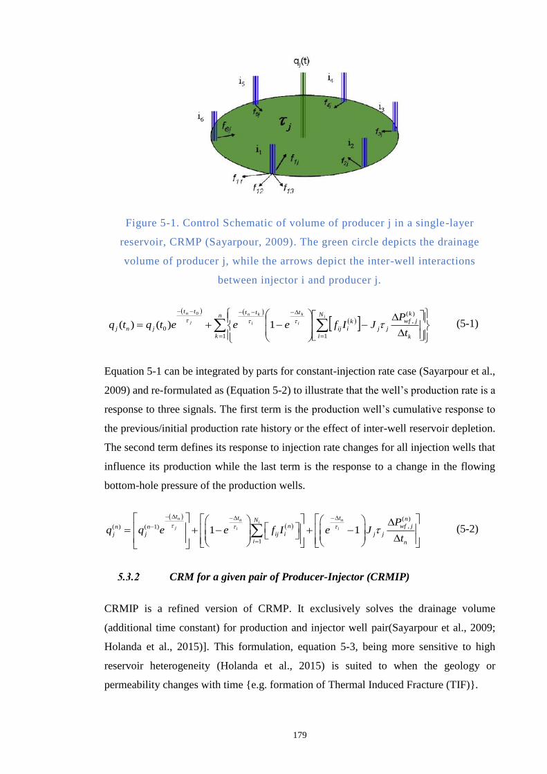
179
Figure 5-1. Control Schematic of volume of producer j in a single-layer
reservoir, CRMP (Sayarpour, 2009). The green circle depicts the drainage
volume of producer j, while the arrows depict the inter-well interactions
between injector i and producer j.
n
k
N
i k
k
jwf
jj
k
iij
ttttt
jnj
i
i
k
i
kn
j
n
t
PJIfeeetqtq
1 1
)(
,
0 1)()(
0
(5-1)
Equation 5-1 can be integrated by parts for constant-injection rate case (Sayarpour et al.,
2009) and re-formulated as (Equation 5-2) to illustrate that the well’s production rate is a
response to three signals. The first term is the production well’s cumulative response to
the previous/initial production rate history or the effect of inter-well reservoir depletion.
The second term defines its response to injection rate changes for all injection wells that
influence its production while the last term is the response to a change in the flowing
bottom-hole pressure of the production wells.
( )
,( ) ( 1)
1
1 1
n n ni
j i i
t t t nNn wf jn n
j j ij i j j
i n
Pq q e e f I e J
t
(5-2)
CRM for a given pair of Producer-Injector (CRMIP)
CRMIP is a refined version of CRMP. It exclusively solves the drainage volume
(additional time constant) for production and injector well pair(Sayarpour et al., 2009;
Holanda et al., 2015)]. This formulation, equation 5-3, being more sensitive to high
reservoir heterogeneity (Holanda et al., 2015) is suited to when the geology or
permeability changes with time e.g. formation of Thermal Induced Fracture (TIF).
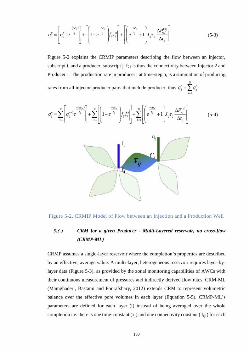
180
n
n
wf
ijij
t
n
iij
tt
n
ij
n
ijt
PJeIfeeqq ij
n
ij
n
ij
n )(
1 11
(5-3)
Figure 5-2 explains the CRMIP parameters describing the flow between an injector,
subscript i, and a producer, subscript j. f21 is thus the connectivity between Injector 2 and
Producer 1. The production rate in producer j at time-step n, is a summation of producing
rates from all injector-producer pairs that include producer, thus
N
i
n
ij
n
j qq1
.
N
i n
n
wf
ijij
tN
i
n
iij
tN
i
t
n
ij
n
jt
PJeIfeeqq ij
n
ij
n
ij
n
1
)(
11
1 11
(5-4)
Figure 5-2. CRMIP Model of Flow between an Injection and a Production Well
CRM for a given Producer - Multi-Layered reservoir, no cross-flow
(CRMP-ML)
CRMP assumes a single-layer reservoir where the completion’s properties are described
by an effective, average value. A multi-layer, heterogeneous reservoir requires layer-by-
layer data (Figure 5-3), as provided by the zonal monitoring capabilities of AWCs with
their continuous measurement of pressures and indirectly derived flow rates. CRM-ML
(Mamghaderi, Bastami and Pourafshary, 2012) extends CRM to represent volumetric
balance over the effective pore volumes in each layer (Equation 5-5). CRMP-ML’s
parameters are defined for each layer (l) instead of being averaged over the whole
completion i.e. there is one time-constant (τj) and one connectivity constant ( fijl) for each
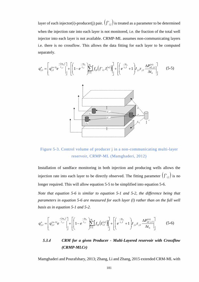
181
layer of each injector(i)-producer(j) pair. lif ,' is treated as a parameter to be determined
when the injection rate into each layer is not monitored, i.e. the fraction of the total well
injector into each layer is not available. CRMP-ML assumes non-communicating layers
i.e. there is no crossflow. This allows the data fitting for each layer to be computed
separately.
n
n
ljwf
ljlj
l
tN
i
n
iliijl
tt
n
lj
n
ljt
PJeIffeeqq i
ni
li
n
lj
n )(
,,
,,
,
1
,
)1(
,, 1'1 ,, (5-5)
Figure 5-3. Control volume of producer j in a non-communicating multi-layer
reservoir, CRMP-ML (Mamghaderi, 2012)
Installation of sandface monitoring in both injection and producing wells allows the
injection rate into each layer to be directly observed. The fitting parameter lif ,' is no
longer required. This will allow equation 5-5 to be simplified into equation 5-6.
Note that equation 5-6 is similar to equation 5-1 and 5-2, the difference being that
parameters in equation 5-6 are measured for each layer (l) rather than on the full well
basis as in equation 5-1 and 5-2.
n
n
ljwf
ljlj
l
tN
i
n
liijl
tt
n
lj
n
ljt
PJeIfeeqq i
ni
li
n
lj
n )(
,,
,,
,
1
,
)1(
,, 11 ,, (5-6)
CRM for a given Producer - Multi-Layered reservoir with Crossflow
(CRMP-MLCr)
Mamghaderi and Pourafshary, 2013; Zhang, Li and Zhang, 2015 extended CRM-ML with
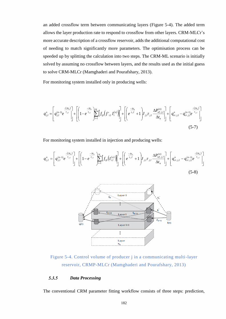
182
an added crossflow term between communicating layers (Figure 5-4). The added term
allows the layer production rate to respond to crossflow from other layers. CRM-MLCr’s
more accurate description of a crossflow reservoir, adds the additional computational cost
of needing to match significantly more parameters. The optimisation process can be
speeded up by splitting the calculation into two steps. The CRM-ML scenario is initially
solved by assuming no crossflow between layers, and the results used as the initial guess
to solve CRM-MLCr (Mamghaderi and Pourafshary, 2013).
For monitoring system installed only in producing wells:
lj
n
i
ni
li
n
lj
n t
n
ljcr
n
ljcr
n
n
ljwf
ljlj
l
tN
i
n
iliijl
tt
n
lj
n
lj eqqt
PJeIffeeqq ,,, )1(
,,,,
)(
,,
,,
,
1
,
)1(
,, 1'1
(5-7)
For monitoring system installed in injection and producing wells:
lj
n
i
ni
li
n
lj
n t
n
ljcr
n
ljcr
n
n
ljwf
ljlj
l
tN
i
n
liijl
tt
n
lj
n
lj eqqt
PJeIfeeqq ,,, )1(
,,,,
)(
,,
,,
,
1
,
)1(
,, 11
(5-8)
Figure 5-4. Control volume of producer j in a communicating multi -layer
reservoir, CRMP-MLCr (Mamghaderi and Pourafshary, 2013)
Data Processing
The conventional CRM parameter fitting workflow consists of three steps: prediction,
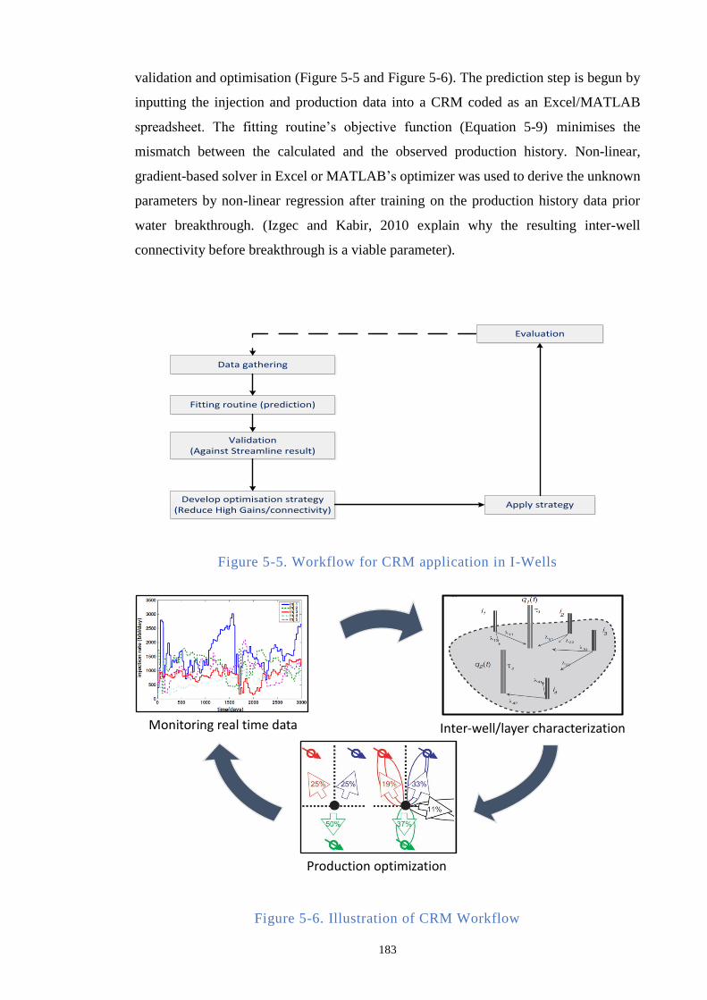
183
validation and optimisation (Figure 5-5 and Figure 5-6). The prediction step is begun by
inputting the injection and production data into a CRM coded as an Excel/MATLAB
spreadsheet. The fitting routine’s objective function (Equation 5-9) minimises the
mismatch between the calculated and the observed production history. Non-linear,
gradient-based solver in Excel or MATLAB’s optimizer was used to derive the unknown
parameters by non-linear regression after training on the production history data prior
water breakthrough. (Izgec and Kabir, 2010 explain why the resulting inter-well
connectivity before breakthrough is a viable parameter).
Data gathering
Apply strategy
Fitting routine (prediction)
Evaluation
Validation (Against Streamline result)
Develop optimisation strategy(Reduce High Gains/connectivity)
Figure 5-5. Workflow for CRM application in I-Wells
Figure 5-6. Illustration of CRM Workflow
Monitoring real time data Inter-well/layer characterization
Production optimization

184
The data-fitting process must also satisfy the equation 5-10 constraints that:
1. The water volume fraction flowing towards each layer (the injection fraction, f’il), the
time-constant, (τjl) and the connectivity constant (𝑓ijl) has to be a positive number or
zero.
2. The sum of all the connectivity constants (𝑓ijl) should be unity for a closed system
(voidage replacement), or it can be less than unity for an open system (i.e. a sector
model or a reservoir with a poorly described aquifer). The sum of water rate fractions
flowing towards each layer from an injector (f’il) has to be unity.
Objective function for nonlinear
regression:
nN
n
n
ljCRM
n
ljreal qqfunctionObj2
,,,,min.
(5-9)
Constraints for nonlinear regression:
, ,' , , 0i l ijl j lf f
iN
i
ijlf1
1 ;
LN
l
lif1
, 1'
(5-10)
The CRM fitting results were compared with the numerical reservoir model streamline
results in the validation step. A proxy, inter-well connectivity map that illustrates the
inter-well interactions was prepared from the CRM results and validated by comparison
with the results of the streamline simulation results (Izgec and Kabir, 2010; Jahangiri et
al., 2014). This validation step increases confidence in the CRM. Further, the connectivity
map can also be used to make informed production/injection optimisation decisions. This
is particularly valuable for I-wells where zonal flow control in real time is possible.
Note the above description is for a multilayer reservoir. The workflow for single-layer is
simpler with the parameters referring to the well instead of per layer basis. Subscript l is
no longer applied.
CRM for a field with dynamic well control or changing permeability
(fracture) with time.
Most publications on CRM assume the parameters are time-independent (Yousef, Lake
and Jensen, 2006; Liang et al., 2007; Sayarpour et al., 2009; Kim, Lake and Edgar, 2012;
Mamghaderi and Pourafshary, 2013). This can be inaccurate when analysing the
performance of AWC since a change in the control of one well will affect the drainage
area, and hence the inter-well connectivity, of all connected wells. Changing CRM
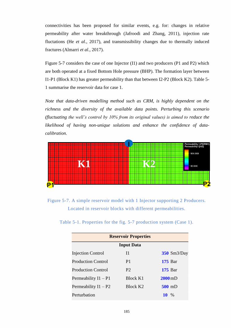
185
connectivities has been proposed for similar events, e.g. for: changes in relative
permeability after water breakthrough (Jafroodi and Zhang, 2011), injection rate
fluctations (He et al., 2017), and transmissibility changes due to thermally induced
fractures (Almarri et al., 2017).
Figure 5-7 considers the case of one Injector (I1) and two producers (P1 and P2) which
are both operated at a fixed Bottom Hole pressure (BHP). The formation layer between
I1-P1 (Block K1) has greater permeability than that between I2-P2 (Block K2). Table 5-
1 summarise the reservoir data for case 1.
Note that data-driven modelling method such as CRM, is highly dependent on the
richness and the diversity of the available data points. Perturbing this scenario
(fluctuating the well’s control by 10% from its original values) is aimed to reduce the
likelihood of having non-unique solutions and enhance the confidence of data-
calibration.
Figure 5-7. A simple reservoir model with 1 Injector supporting 2 Producers.
Located in reservoir blocks with different permeabilities.
Table 5-1. Properties for the fig. 5-7 production system (Case 1).
Reservoir Properties
Input Data
Injection Control I1 350 Sm3/Day
Production Control P1 175 Bar
Production Control P2 175 Bar
Permeability I1 – P1 Block K1 2000 mD
Permeability I1 – P2 Block K2 500 mD
Perturbation 10 %
P2 P1
I
K1 K2
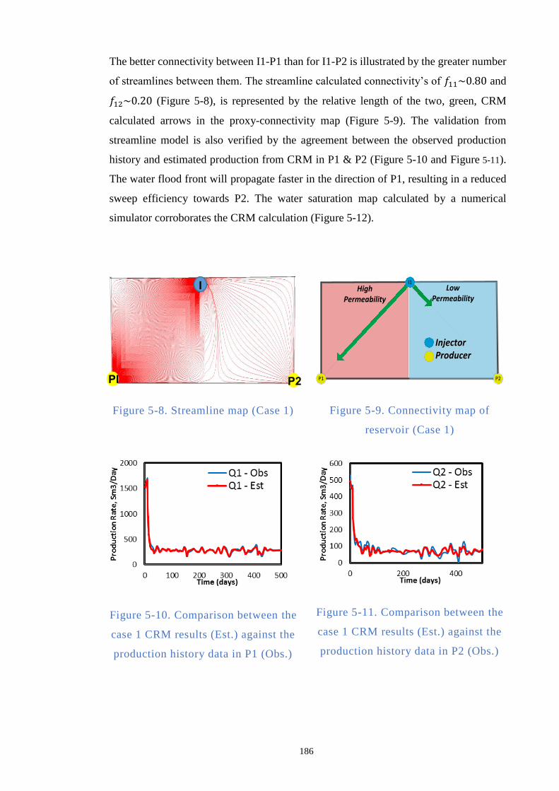
186
The better connectivity between I1-P1 than for I1-P2 is illustrated by the greater number
of streamlines between them. The streamline calculated connectivity’s of 𝑓11~0.80 and
𝑓12~0.20 (Figure 5-8), is represented by the relative length of the two, green, CRM
calculated arrows in the proxy-connectivity map (Figure 5-9). The validation from
streamline model is also verified by the agreement between the observed production
history and estimated production from CRM in P1 & P2 (Figure 5-10 and Figure 5-11).
The water flood front will propagate faster in the direction of P1, resulting in a reduced
sweep efficiency towards P2. The water saturation map calculated by a numerical
simulator corroborates the CRM calculation (Figure 5-12).
Figure 5-8. Streamline map (Case 1)
HighPermeability
P1
LowPermeability
InjectorProducerInjectorProducer
P2
I1
Figure 5-9. Connectivity map of
reservoir (Case 1)
Figure 5-10. Comparison between the
case 1 CRM results (Est.) against the
production history data in P1 (Obs.)
Figure 5-11. Comparison between the
case 1 CRM results (Est.) against the
production history data in P2 (Obs.)
I
PI P2
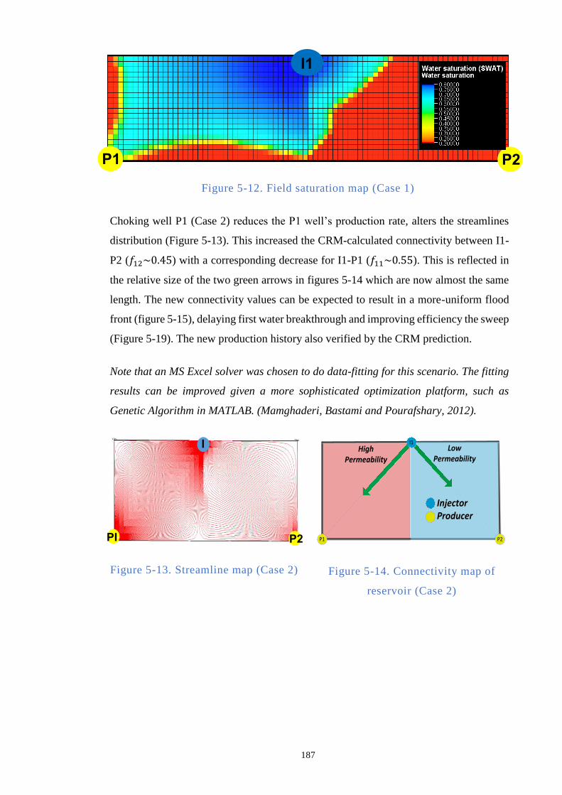
187
Figure 5-12. Field saturation map (Case 1)
Choking well P1 (Case 2) reduces the P1 well’s production rate, alters the streamlines
distribution (Figure 5-13). This increased the CRM-calculated connectivity between I1-
P2 (𝑓12~0.45) with a corresponding decrease for I1-P1 (𝑓11~0.55). This is reflected in
the relative size of the two green arrows in figures 5-14 which are now almost the same
length. The new connectivity values can be expected to result in a more-uniform flood
front (figure 5-15), delaying first water breakthrough and improving efficiency the sweep
(Figure 5-19). The new production history also verified by the CRM prediction.
Note that an MS Excel solver was chosen to do data-fitting for this scenario. The fitting
results can be improved given a more sophisticated optimization platform, such as
Genetic Algorithm in MATLAB. (Mamghaderi, Bastami and Pourafshary, 2012).
Figure 5-13. Streamline map (Case 2)
HighPermeability
P1
LowPermeability
InjectorProducerInjectorProducer
P2
I1
Figure 5-14. Connectivity map of
reservoir (Case 2)
P2 P1
I1
P
1
PI P2
I
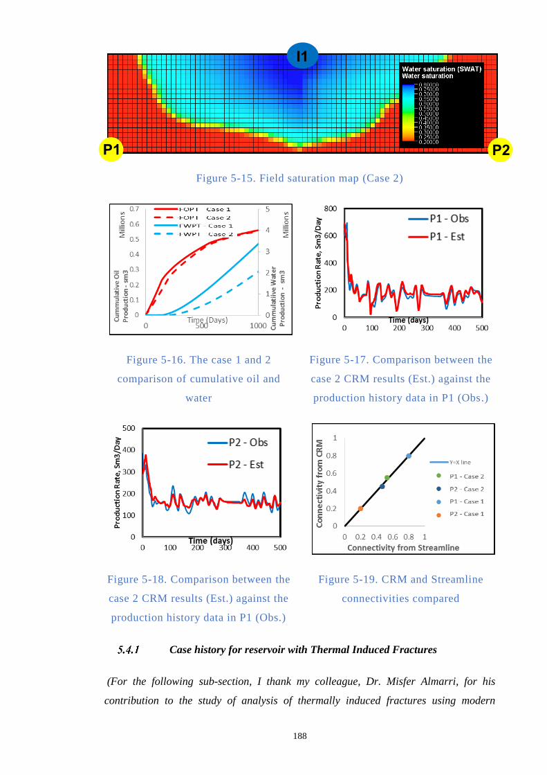
188
Figure 5-15. Field saturation map (Case 2)
Figure 5-16. The case 1 and 2
comparison of cumulative oil and
water
Figure 5-17. Comparison between the
case 2 CRM results (Est.) against the
production history data in P1 (Obs.)
Figure 5-18. Comparison between the
case 2 CRM results (Est.) against the
production history data in P1 (Obs.)
Figure 5-19. CRM and Streamline
connectivities compared
Case history for reservoir with Thermal Induced Fractures
(For the following sub-section, I thank my colleague, Dr. Misfer Almarri, for his
contribution to the study of analysis of thermally induced fractures using modern
P2 P1
I1
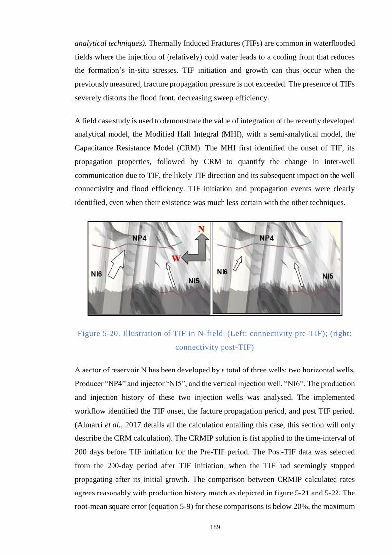
189
analytical techniques). Thermally Induced Fractures (TIFs) are common in waterflooded
fields where the injection of (relatively) cold water leads to a cooling front that reduces
the formation’s in-situ stresses. TIF initiation and growth can thus occur when the
previously measured, fracture propagation pressure is not exceeded. The presence of TIFs
severely distorts the flood front, decreasing sweep efficiency.
A field case study is used to demonstrate the value of integration of the recently developed
analytical model, the Modified Hall Integral (MHI), with a semi-analytical model, the
Capacitance Resistance Model (CRM). The MHI first identified the onset of TIF, its
propagation properties, followed by CRM to quantify the change in inter-well
communication due to TIF, the likely TIF direction and its subsequent impact on the well
connectivity and flood efficiency. TIF initiation and propagation events were clearly
identified, even when their existence was much less certain with the other techniques.
Figure 5-20. Illustration of TIF in N-field. (Left: connectivity pre-TIF); (right:
connectivity post-TIF)
A sector of reservoir N has been developed by a total of three wells: two horizontal wells,
Producer “NP4” and injector “NI5”, and the vertical injection well, “NI6”. The production
and injection history of these two injection wells was analysed. The implemented
workflow identified the TIF onset, the facture propagation period, and post TIF period.
(Almarri et al., 2017 details all the calculation entailing this case, this section will only
describe the CRM calculation). The CRMIP solution is fist applied to the time-interval of
200 days before TIF initiation for the Pre-TIF period. The Post-TIF data was selected
from the 200-day period after TIF initiation, when the TIF had seemingly stopped
propagating after its initial growth. The comparison between CRMIP calculated rates
agrees reasonably with production history match as depicted in figure 5-21 and 5-22. The
root-mean square error (equation 5-9) for these comparisons is below 20%, the maximum
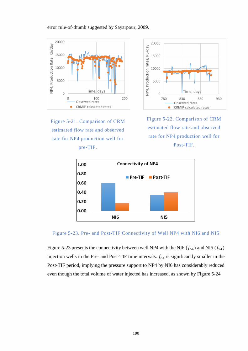
190
error rule-of-thumb suggested by Sayarpour, 2009.
Figure 5-21. Comparison of CRM
estimated flow rate and observed
rate for NP4 production well for
pre-TIF.
Figure 5-22. Comparison of CRM
estimated flow rate and observed
rate for NP4 production well for
Post-TIF.
Figure 5-23. Pre- and Post-TIF Connectivity of Well NP4 with NI6 and NI5
Figure 5-23 presents the connectivity between well NP4 with the NI6 (𝑓64) and NI5 (𝑓54)
injection wells in the Pre- and Post-TIF time intervals. 𝑓64 is significantly smaller in the
Post-TIF period, implying the pressure support to NP4 by NI6 has considerably reduced
even though the total volume of water injected has increased, as shown by Figure 5-24
0
5000
10000
15000
20000
0 100 200
NP
4, P
rod
uct
ion
Rat
e, R
b/d
ay
Time, days
Observed rates
CRMIP calculated rates
0
5000
10000
15000
20000
780 830 880 930
NP
4, P
rod
uct
ion
rat
es, R
B/d
ay
Time, days
Observed ratesCRMIP calculated rates
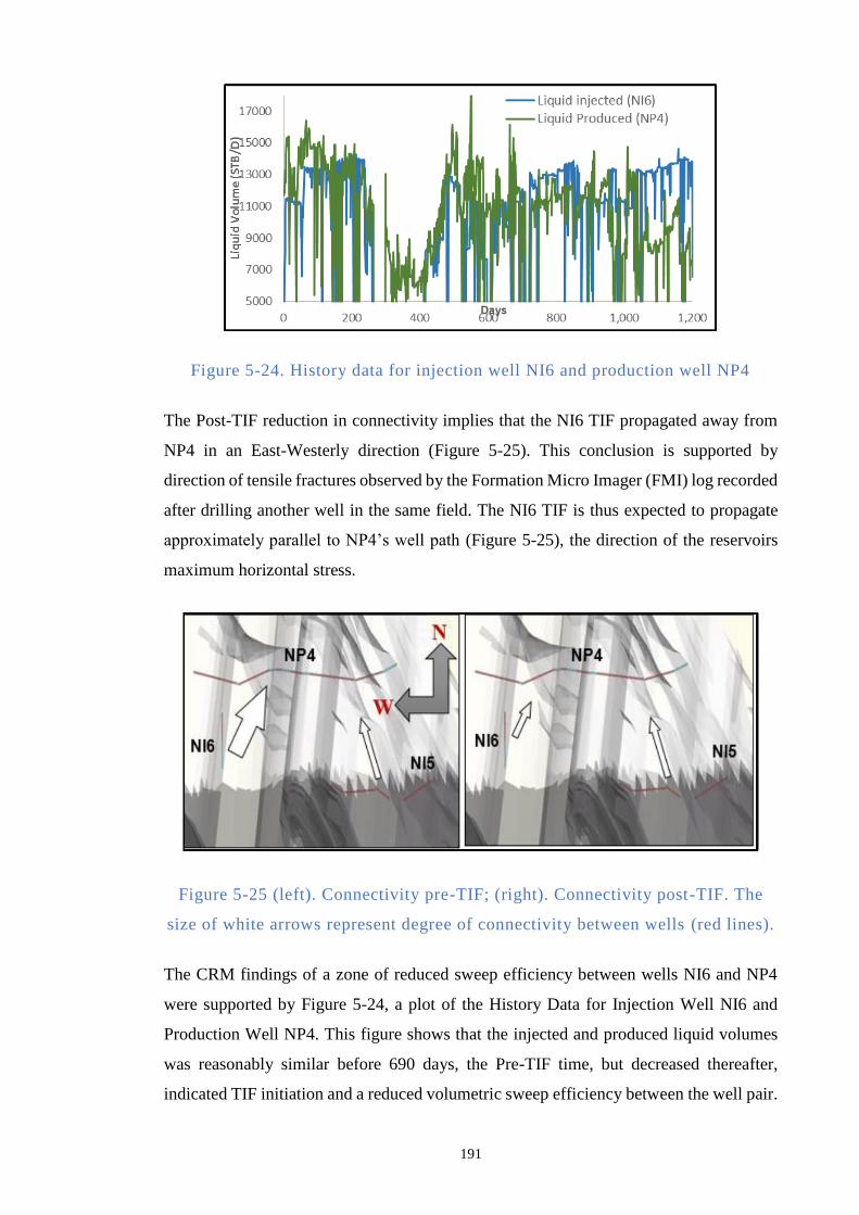
191
Figure 5-24. History data for injection well NI6 and production well NP4
The Post-TIF reduction in connectivity implies that the NI6 TIF propagated away from
NP4 in an East-Westerly direction (Figure 5-25). This conclusion is supported by
direction of tensile fractures observed by the Formation Micro Imager (FMI) log recorded
after drilling another well in the same field. The NI6 TIF is thus expected to propagate
approximately parallel to NP4’s well path (Figure 5-25), the direction of the reservoirs
maximum horizontal stress.
Figure 5-25 (left). Connectivity pre-TIF; (right). Connectivity post-TIF. The
size of white arrows represent degree of connectivity between wells (red lines).
The CRM findings of a zone of reduced sweep efficiency between wells NI6 and NP4
were supported by Figure 5-24, a plot of the History Data for Injection Well NI6 and
Production Well NP4. This figure shows that the injected and produced liquid volumes
was reasonably similar before 690 days, the Pre-TIF time, but decreased thereafter,
indicated TIF initiation and a reduced volumetric sweep efficiency between the well pair.
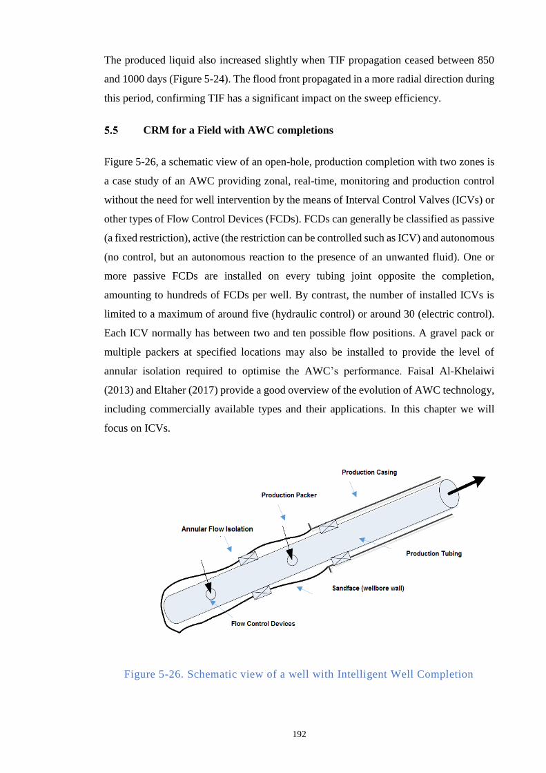
192
The produced liquid also increased slightly when TIF propagation ceased between 850
and 1000 days (Figure 5-24). The flood front propagated in a more radial direction during
this period, confirming TIF has a significant impact on the sweep efficiency.
CRM for a Field with AWC completions
Figure 5-26, a schematic view of an open-hole, production completion with two zones is
a case study of an AWC providing zonal, real-time, monitoring and production control
without the need for well intervention by the means of Interval Control Valves (ICVs) or
other types of Flow Control Devices (FCDs). FCDs can generally be classified as passive
(a fixed restriction), active (the restriction can be controlled such as ICV) and autonomous
(no control, but an autonomous reaction to the presence of an unwanted fluid). One or
more passive FCDs are installed on every tubing joint opposite the completion,
amounting to hundreds of FCDs per well. By contrast, the number of installed ICVs is
limited to a maximum of around five (hydraulic control) or around 30 (electric control).
Each ICV normally has between two and ten possible flow positions. A gravel pack or
multiple packers at specified locations may also be installed to provide the level of
annular isolation required to optimise the AWC’s performance. Faisal Al-Khelaiwi
(2013) and Eltaher (2017) provide a good overview of the evolution of AWC technology,
including commercially available types and their applications. In this chapter we will
focus on ICVs.
Figure 5-26. Schematic view of a well with Intelligent Well Completion
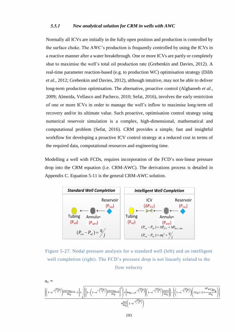
193
New analytical solution for CRM in wells with AWC
Normally all ICVs are initially in the fully open position and production is controlled by
the surface choke. The AWC’s production is frequently controlled by using the ICVs in
a reactive manner after a water breakthrough. One or more ICVs are partly or completely
shut to maximise the well’s total oil production rate (Grebenkin and Davies, 2012). A
real-time parameter reaction-based (e.g. to production WC) optimisation strategy (Dilib
et al., 2012; Grebenkin and Davies, 2012), although intuitive, may not be able to deliver
long-term production optimisation. The alternative, proactive control (Alghareeb et al.,
2009; Almeida, Vellasco and Pacheco, 2010; Sefat, 2016), involves the early restriction
of one or more ICVs in order to manage the well’s inflow to maximise long-term oil
recovery and/or its ultimate value. Such proactive, optimisation control strategy using
numerical reservoir simulation is a complex, high-dimensional, mathematical and
computational problem (Sefat, 2016). CRM provides a simple, fast and insightful
workflow for developing a proactive ICV control strategy at a reduced cost in terms of
the required data, computational resources and engineering time.
Modelling a well with FCDs, requires incorporation of the FCD’s non-linear pressure
drop into the CRM equation (i.e. CRM-AWC). The derivations process is detailed in
Appendix C. Equation 5-11 is the general CRM-AWC solution.
Reservoir(Pres)
Annulus(Pann)
ICV(∆PICV)
Tubing(Pwf)
jq
aqPP
PPPP
wfres
AnnsICVwfres
2
Re
)(
)(
Reservoir(Pres)
Annulus(Pann)
Tubing(Pwf)
jq
PP wfres )(
Standard Well Completion Intelligent Well Completion
Figure 5-27. Nodal pressure analysis for a standard well (left) and an intelligent
well completion (right). The FCD’s pressure drop is not linearly related to the
flow velocity
𝑞𝑛 =
[(1−𝑒−(∆𝑡𝑘τ )
)𝐽𝑎2τ𝑞𝑛−1
∆𝑡𝑘−1]+√[1−(1−𝑒
−(∆𝑡𝑘τ )
)𝐽𝑎2τ𝑞𝑛−1
∆𝑡𝑘]
2
+4𝑞𝑘−1𝑒−(∆𝑡𝑘τ )
[(1−𝑒−(∆𝑡𝑘τ )
)𝐽𝑎2τ
∆𝑡𝑘]−(1−𝑒
−(∆𝑡𝑘τ )
)(𝑖(𝑡𝑘)−J τ
∆𝑃𝑤𝑓∆𝑡𝑘∆𝑡𝑘
)
4𝐽𝑎τ
∆𝑡𝑘(1−𝑒
−(∆𝑡𝑘τ )
)
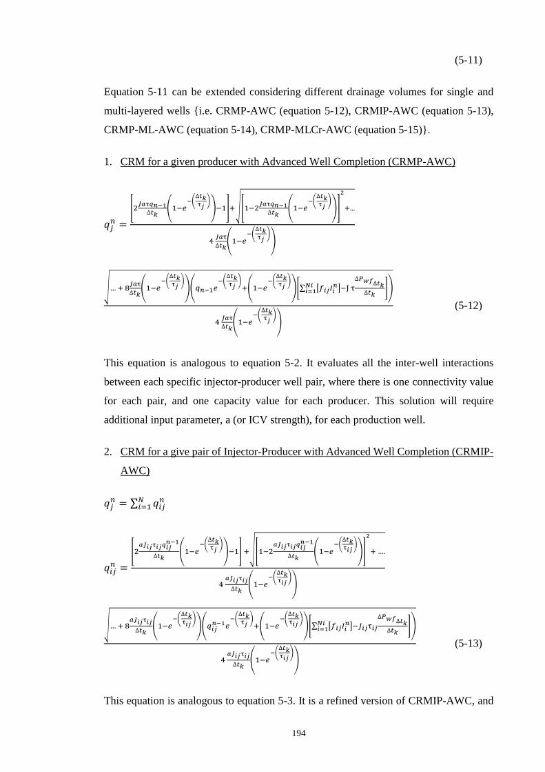
194
(5-11)
Equation 5-11 can be extended considering different drainage volumes for single and
multi-layered wells i.e. CRMP-AWC (equation 5-12), CRMIP-AWC (equation 5-13),
CRMP-ML-AWC (equation 5-14), CRMP-MLCr-AWC (equation 5-15).
1. CRM for a given producer with Advanced Well Completion (CRMP-AWC)
𝑞𝑗𝑛 =
[2𝐽𝑎τ𝑞𝑛−1
∆𝑡𝑘(1−𝑒
−(∆𝑡𝑘τ𝑗
))−1]+√[1−2
𝐽𝑎τ𝑞𝑛−1∆𝑡𝑘
(1−𝑒−(∆𝑡𝑘τ𝑗
))]
2
+...
4 𝐽𝑎τ
∆𝑡𝑘(1−𝑒
−(∆𝑡𝑘τ𝑗
))
√… + 8𝐽𝑎τ
∆𝑡𝑘(1−𝑒
−(∆𝑡𝑘τ𝑗
))(𝑞𝑛−1𝑒
−(∆𝑡𝑘τ𝑗
)+(1−𝑒
−(∆𝑡𝑘τ𝑗
))[∑ [𝑓𝑖𝑗𝐼𝑖
𝑛]−J τ
∆𝑃𝑤𝑓∆𝑡𝑘∆𝑡𝑘
𝑁𝑖𝑖=1 ])
4 𝐽𝑎τ
∆𝑡𝑘(1−𝑒
−(∆𝑡𝑘τ𝑗
))
(5-12)
This equation is analogous to equation 5-2. It evaluates all the inter-well interactions
between each specific injector-producer well pair, where there is one connectivity value
for each pair, and one capacity value for each producer. This solution will require
additional input parameter, a (or ICV strength), for each production well.
2. CRM for a give pair of Injector-Producer with Advanced Well Completion (CRMIP-
AWC)
𝑞𝑗𝑛 = ∑ 𝑞𝑖𝑗
𝑛𝑁𝑖=1
𝑞𝑖𝑗𝑛 =
[2𝑎𝐽𝑖𝑗τ𝑖𝑗𝑞𝑖𝑗
𝑛−1
∆𝑡𝑘(1−𝑒
−(∆𝑡𝑘τ𝑗
))−1] +√[1−2
𝑎𝐽𝑖𝑗τ𝑖𝑗𝑞𝑖𝑗𝑛−1
∆𝑡𝑘(1−𝑒
−(∆𝑡𝑘τ𝑖𝑗
))]
2
+ ….
4 𝑎𝐽𝑖𝑗τ𝑖𝑗
∆𝑡𝑘(1−𝑒
−(∆𝑡𝑘τ𝑖𝑗
))
√… + 8𝑎𝐽𝑖𝑗τ𝑖𝑗
∆𝑡𝑘(1−𝑒
−(∆𝑡𝑘τ𝑖𝑗
))(𝑞𝑖𝑗
𝑛−1𝑒−(∆𝑡𝑘τ𝑗
)+(1−𝑒
−(∆𝑡𝑘τ𝑖𝑗
))[∑ [𝑓𝑖𝑗𝐼𝑖
𝑛]−𝐽𝑖𝑗τ𝑖𝑗
∆𝑃𝑤𝑓∆𝑡𝑘∆𝑡𝑘
𝑁𝑖𝑖=1 ])
4 𝑎𝐽𝑖𝑗τ𝑖𝑗
∆𝑡𝑘(1−𝑒
−(∆𝑡𝑘τ𝑖𝑗
))
(5-13)
This equation is analogous to equation 5-3. It is a refined version of CRMIP-AWC, and
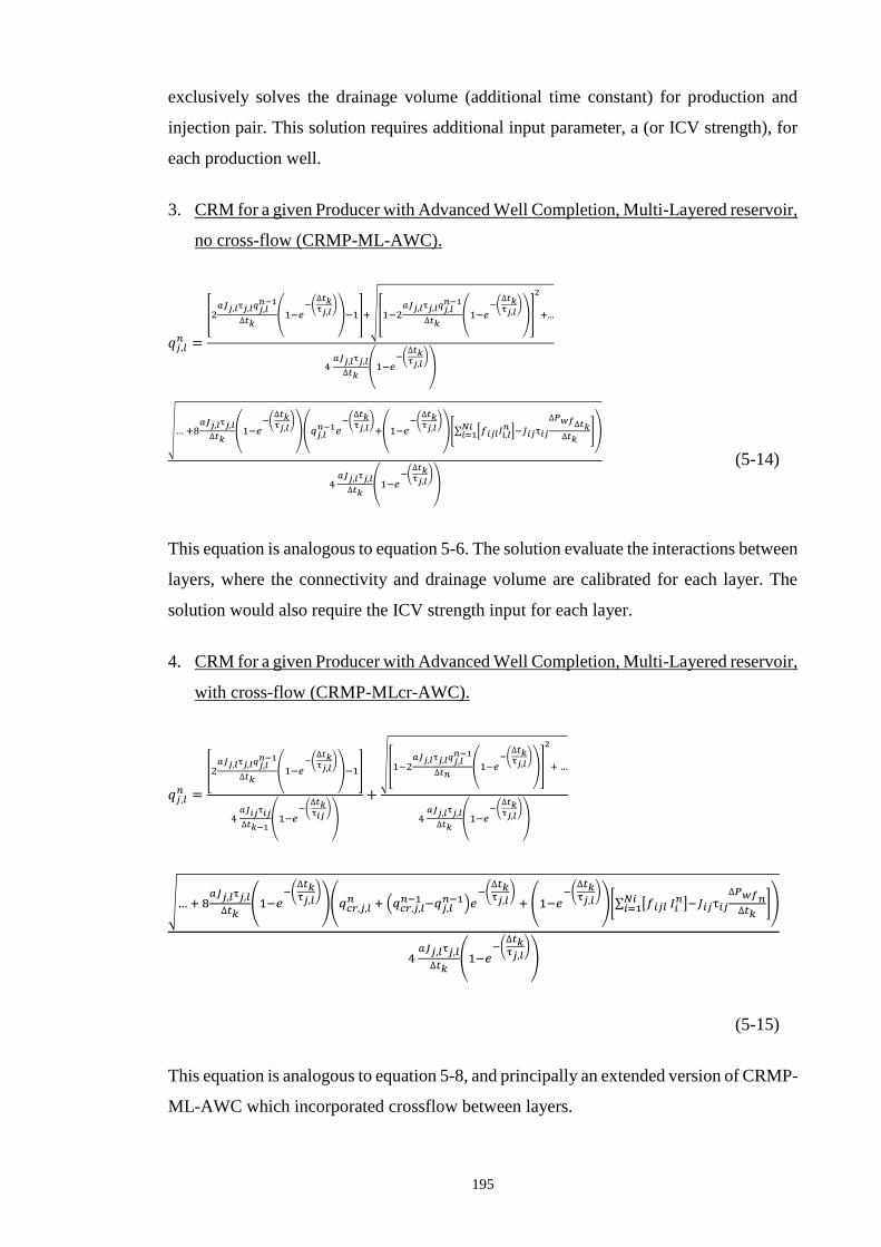
195
exclusively solves the drainage volume (additional time constant) for production and
injection pair. This solution requires additional input parameter, a (or ICV strength), for
each production well.
3. CRM for a given Producer with Advanced Well Completion, Multi-Layered reservoir,
no cross-flow (CRMP-ML-AWC).
𝑞𝑗,𝑙𝑛 =
[2𝑎𝐽𝑗,𝑙τ𝑗,𝑙𝑞𝑗,𝑙
𝑛−1
∆𝑡𝑘(1−𝑒
−(∆𝑡𝑘τ𝑗,𝑙
))−1]+√[1−2
𝑎𝐽𝑗,𝑙τ𝑗,𝑙𝑞𝑗,𝑙𝑛−1
∆𝑡𝑘(1−𝑒
−(∆𝑡𝑘τ𝑗,𝑙
))]
2
+...
4 𝑎𝐽𝑗,𝑙τ𝑗,𝑙
∆𝑡𝑘(1−𝑒
−(∆𝑡𝑘τ𝑗,𝑙
))
√… +8𝑎𝐽𝑗,𝑙τ𝑗,𝑙
∆𝑡𝑘(1−𝑒
−(∆𝑡𝑘τ𝑗,𝑙
))(𝑞𝑗,𝑙
𝑛−1𝑒−(∆𝑡𝑘τ𝑗,𝑙
)+(1−𝑒
−(∆𝑡𝑘τ𝑗,𝑙
))[∑ [𝑓𝑖𝑗𝑙𝐼𝑖,𝑙
𝑛 ]−𝐽𝑖𝑗τ𝑖𝑗
∆𝑃𝑤𝑓∆𝑡𝑘∆𝑡𝑘
𝑁𝑖𝑖=1 ])
4 𝑎𝐽𝑗,𝑙τ𝑗,𝑙
∆𝑡𝑘(1−𝑒
−(∆𝑡𝑘τ𝑗,𝑙
))
(5-14)
This equation is analogous to equation 5-6. The solution evaluate the interactions between
layers, where the connectivity and drainage volume are calibrated for each layer. The
solution would also require the ICV strength input for each layer.
4. CRM for a given Producer with Advanced Well Completion, Multi-Layered reservoir,
with cross-flow (CRMP-MLcr-AWC).
𝑞𝑗,𝑙𝑛 =
[2𝑎𝐽𝑗,𝑙τ𝑗,𝑙𝑞𝑗,𝑙
𝑛−1
∆𝑡𝑘(1−𝑒
−(∆𝑡𝑘τ𝑗,𝑙
))−1]
4 𝑎𝐽𝑖𝑗τ𝑖𝑗
∆𝑡𝑘−1(1−𝑒
−(∆𝑡𝑘τ𝑖𝑗
))
+
√[1−2𝑎𝐽𝑗,𝑙τ𝑗,𝑙𝑞𝑗,𝑙
𝑛−1
∆𝑡𝑛(1−𝑒
−(∆𝑡𝑘τ𝑗,𝑙
))]
2
+ …
4 𝑎𝐽𝑗,𝑙τ𝑗,𝑙
∆𝑡𝑘(1−𝑒
−(∆𝑡𝑘τ𝑗,𝑙
))
√… + 8𝑎𝐽𝑗,𝑙τ𝑗,𝑙
∆𝑡𝑘(1−𝑒
−(∆𝑡𝑘τ𝑗,𝑙
))(𝑞𝑐𝑟,𝑗,𝑙
𝑛 + (𝑞𝑐𝑟,𝑗,𝑙𝑛−1 −𝑞𝑗,𝑙
𝑛−1)𝑒−(∆𝑡𝑘τ𝑗,𝑙
) + (1−𝑒
−(∆𝑡𝑘τ𝑗,𝑙
))[∑ [𝑓𝑖𝑗𝑙 𝐼𝑖
𝑛]−𝐽𝑖𝑗τ𝑖𝑗∆𝑃𝑤𝑓𝑛∆𝑡𝑘
𝑁𝑖𝑖=1 ])
4 𝑎𝐽𝑗,𝑙τ𝑗,𝑙
∆𝑡𝑘(1−𝑒
−(∆𝑡𝑘τ𝑗,𝑙
))
(5-15)
This equation is analogous to equation 5-8, and principally an extended version of CRMP-
ML-AWC which incorporated crossflow between layers.
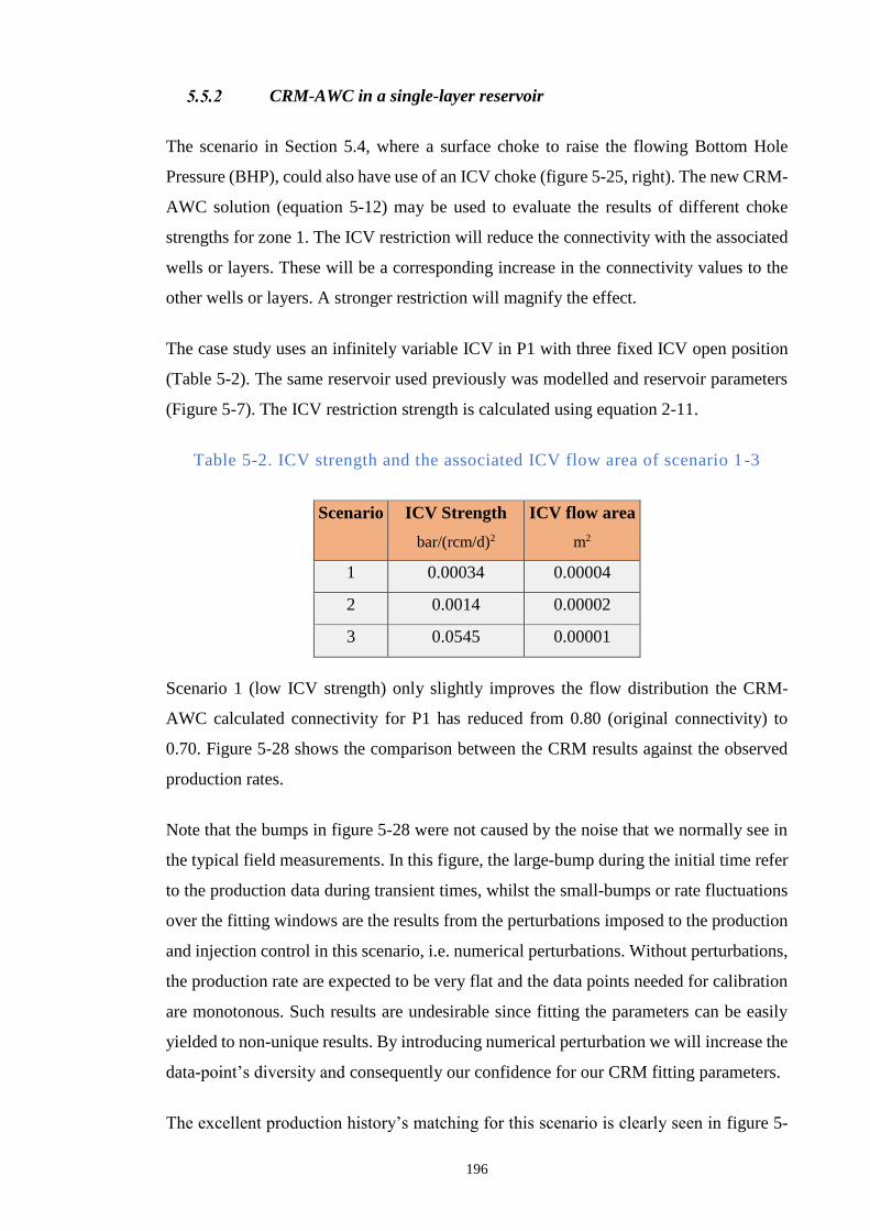
196
CRM-AWC in a single-layer reservoir
The scenario in Section 5.4, where a surface choke to raise the flowing Bottom Hole
Pressure (BHP), could also have use of an ICV choke (figure 5-25, right). The new CRM-
AWC solution (equation 5-12) may be used to evaluate the results of different choke
strengths for zone 1. The ICV restriction will reduce the connectivity with the associated
wells or layers. These will be a corresponding increase in the connectivity values to the
other wells or layers. A stronger restriction will magnify the effect.
The case study uses an infinitely variable ICV in P1 with three fixed ICV open position
(Table 5-2). The same reservoir used previously was modelled and reservoir parameters
(Figure 5-7). The ICV restriction strength is calculated using equation 2-11.
Table 5-2. ICV strength and the associated ICV flow area of scenario 1-3
Scenario ICV Strength
bar/(rcm/d)2
ICV flow area
m2
1 0.00034 0.00004
2 0.0014 0.00002
3 0.0545 0.00001
Scenario 1 (low ICV strength) only slightly improves the flow distribution the CRM-
AWC calculated connectivity for P1 has reduced from 0.80 (original connectivity) to
0.70. Figure 5-28 shows the comparison between the CRM results against the observed
production rates.
Note that the bumps in figure 5-28 were not caused by the noise that we normally see in
the typical field measurements. In this figure, the large-bump during the initial time refer
to the production data during transient times, whilst the small-bumps or rate fluctuations
over the fitting windows are the results from the perturbations imposed to the production
and injection control in this scenario, i.e. numerical perturbations. Without perturbations,
the production rate are expected to be very flat and the data points needed for calibration
are monotonous. Such results are undesirable since fitting the parameters can be easily
yielded to non-unique results. By introducing numerical perturbation we will increase the
data-point’s diversity and consequently our confidence for our CRM fitting parameters.
The excellent production history’s matching for this scenario is clearly seen in figure 5-
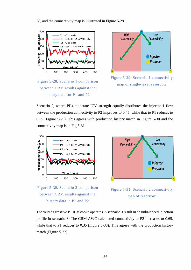
197
28, and the connectivity map is illustrated in Figure 5-29.
Figure 5-28. Scenario 1 comparison
between CRM results against the
history data for P1 and P2
HighPermeability
P1
LowPermeability
InjectorProducerInjectorProducer
P2
I1
Figure 5-29. Scenario 1 connectivity
map of single-layer reservoir
Scenario 2, where PI’s moderate ICV strength equally distributes the injector 1 flow
between the production connectivity to P2 improves to 0.45, while that to P1 reduces to
0.55 (Figure 5-29). This agrees with production history match in Figure 5-30 and the
connectivity map is in Fig 5-31.
Figure 5-30. Scenario 2 comparison
between CRM results against the
history data in P1 and P2
LowPermeability
HighPermeability
P1
InjectorProducerInjectorProducer
P2
I1
Figure 5-31. Scenario 2 connectivity
map of reservoir
The very aggressive P1 ICV choke operates in scenario 3 result in an unbalanced injection
profile in scenario 3. The CRM-AWC calculated connectivity to P2 increases to 0.65,
while that to P1 reduces to 0.35 (Figure 5-33). This agrees with the production history
match (Figure 5-32).
0
100
200
300
400
500
0 100 200 300 400 500
Pro
du
ctio
n R
ate
, Sm
3/D
ay
Time (days)
Q1 - Obs rate
Q1 - Est. CRM-AWC rate
Q2 - Obs Rate
Q2 - Est. CRM-AWC rate
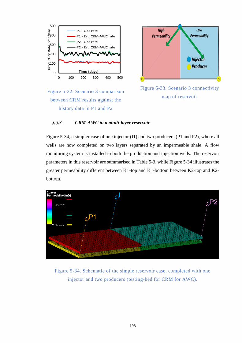
198
Figure 5-32. Scenario 3 comparison
between CRM results against the
history data in P1 and P2
LowPermeability
HighPermeability
P1
InjectorProducerInjectorProducer
P2
I1
Figure 5-33. Scenario 3 connectivity
map of reservoir
CRM-AWC in a multi-layer reservoir
Figure 5-34, a simpler case of one injector (I1) and two producers (P1 and P2), where all
wells are now completed on two layers separated by an impermeable shale. A flow
monitoring system is installed in both the production and injection wells. The reservoir
parameters in this reservoir are summarised in Table 5-3, while Figure 5-34 illustrates the
greater permeability different between K1-top and K1-bottom between K2-top and K2-
bottom.
Figure 5-34. Schematic of the simple reservoir case, completed with one
injector and two producers (testing-bed for CRM for AWC).
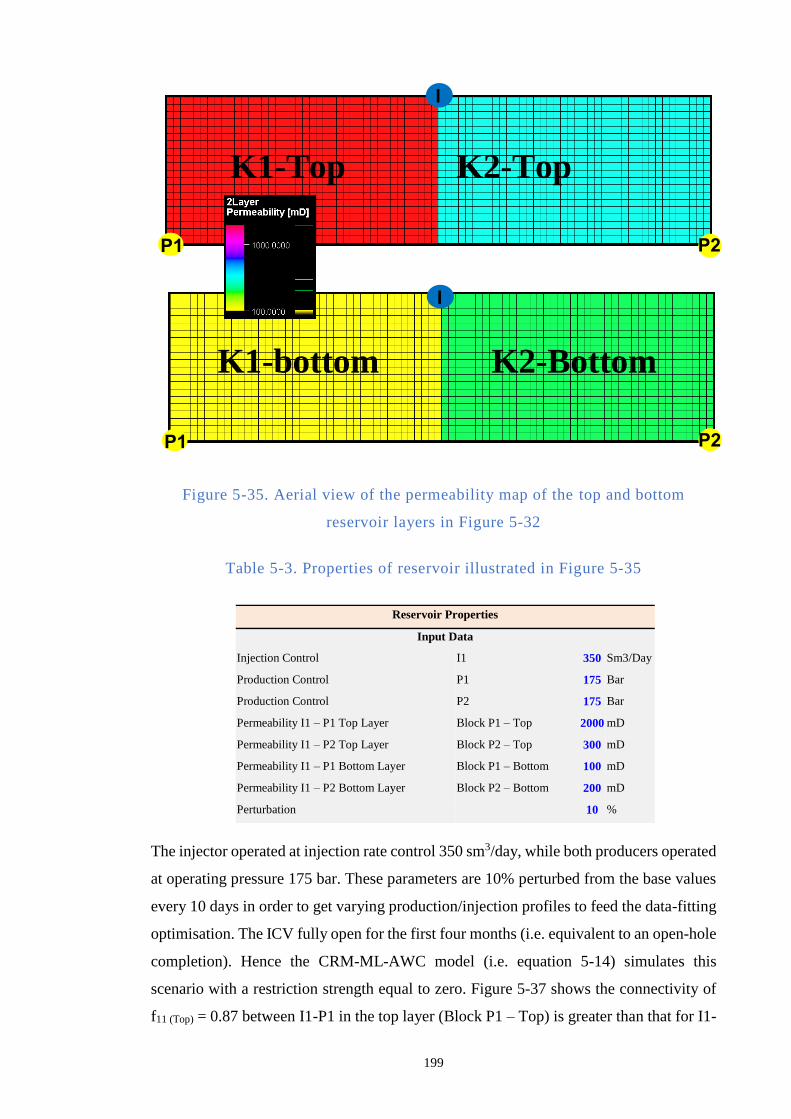
199
Figure 5-35. Aerial view of the permeability map of the top and bottom
reservoir layers in Figure 5-32
Table 5-3. Properties of reservoir illustrated in Figure 5-35
Reservoir Properties
Input Data
Injection Control I1 350 Sm3/Day
Production Control P1 175 Bar
Production Control P2 175 Bar
Permeability I1 – P1 Top Layer Block P1 – Top 2000 mD
Permeability I1 – P2 Top Layer Block P2 – Top 300 mD
Permeability I1 – P1 Bottom Layer Block P1 – Bottom 100 mD
Permeability I1 – P2 Bottom Layer Block P2 – Bottom 200 mD
Perturbation 10 %
The injector operated at injection rate control 350 sm3/day, while both producers operated
at operating pressure 175 bar. These parameters are 10% perturbed from the base values
every 10 days in order to get varying production/injection profiles to feed the data-fitting
optimisation. The ICV fully open for the first four months (i.e. equivalent to an open-hole
completion). Hence the CRM-ML-AWC model (i.e. equation 5-14) simulates this
scenario with a restriction strength equal to zero. Figure 5-37 shows the connectivity of
f11 (Top) = 0.87 between I1-P1 in the top layer (Block P1 – Top) is greater than that for I1-
P2 P1
I
K1-Top K2-Top
P2 P1
I
K1-bottom K2-Bottom
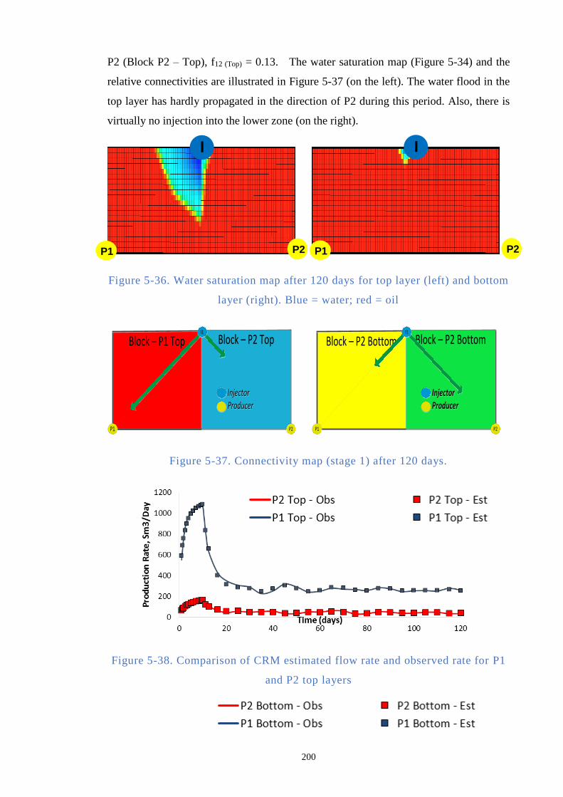
200
P2 (Block P2 – Top), f12 (Top) = 0.13. The water saturation map (Figure 5-34) and the
relative connectivities are illustrated in Figure 5-37 (on the left). The water flood in the
top layer has hardly propagated in the direction of P2 during this period. Also, there is
virtually no injection into the lower zone (on the right).
Figure 5-36. Water saturation map after 120 days for top layer (left) and bottom
layer (right). Blue = water; red = oil
Block – P1 Top
P1
Block – P2 Top
InjectorProducerInjectorProducer
P2
I1
Block – P2 Bottom
P1
Block – P2 Bottom
InjectorProducerInjectorProducer
P2
I1
Figure 5-37. Connectivity map (stage 1) after 120 days.
Figure 5-38. Comparison of CRM estimated flow rate and observed rate for P1
and P2 top layers
P2 P1
I
P2 P1
I
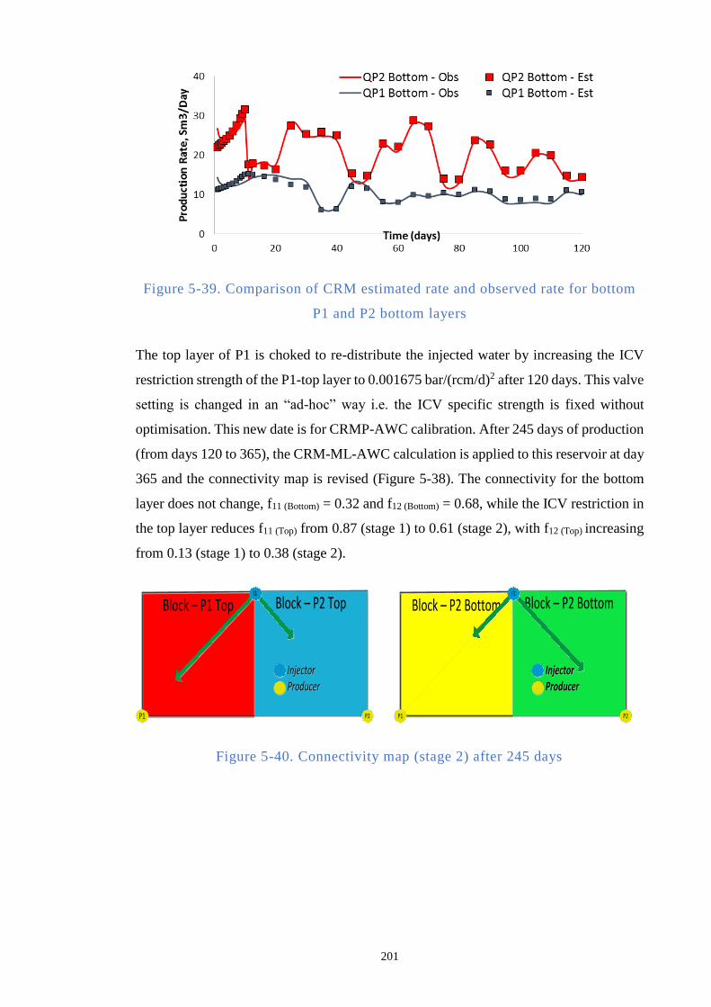
201
Figure 5-39. Comparison of CRM estimated rate and observed rate for bottom
P1 and P2 bottom layers
The top layer of P1 is choked to re-distribute the injected water by increasing the ICV
restriction strength of the P1-top layer to 0.001675 bar/(rcm/d)2 after 120 days. This valve
setting is changed in an “ad-hoc” way i.e. the ICV specific strength is fixed without
optimisation. This new date is for CRMP-AWC calibration. After 245 days of production
(from days 120 to 365), the CRM-ML-AWC calculation is applied to this reservoir at day
365 and the connectivity map is revised (Figure 5-38). The connectivity for the bottom
layer does not change, f11 (Bottom) = 0.32 and f12 (Bottom) = 0.68, while the ICV restriction in
the top layer reduces f11 (Top) from 0.87 (stage 1) to 0.61 (stage 2), with f12 (Top) increasing
from 0.13 (stage 1) to 0.38 (stage 2).
Block – P1 Top
P1
Block – P2 Top
InjectorProducerInjectorProducer
P2
I1
Block – P2 Bottom
P1
Block – P2 Bottom
InjectorProducerInjectorProducer
P2
I1
Figure 5-40. Connectivity map (stage 2) after 245 days
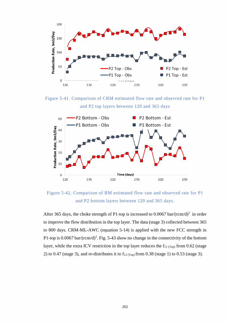
202
Figure 5-41. Comparison of CRM estimated flow rate and observed rate for P1
and P2 top layers between 120 and 365 days
Figure 5-42. Comparison of RM estimated flow rate and observed rate for P1
and P2 bottom layers between 120 and 365 days.
After 365 days, the choke strength of P1-top is increased to 0.0067 bar/(rcm/d)2 in order
to improve the flow distribution in the top layer. The data (stage 3) collected between 365
to 800 days. CRM-ML-AWC (equation 5-14) is applied with the new FCC strength in
P1-top is 0.0067 bar/(rcm/d)2. Fig. 5-43 show no change in the connectivity of the bottom
layer, while the extra ICV restriction in the top layer reduces the f11 (Top) from 0.62 (stage
2) to 0.47 (stage 3), and re-distributes it to f12 (Top) from 0.38 (stage 1) to 0.53 (stage 3).
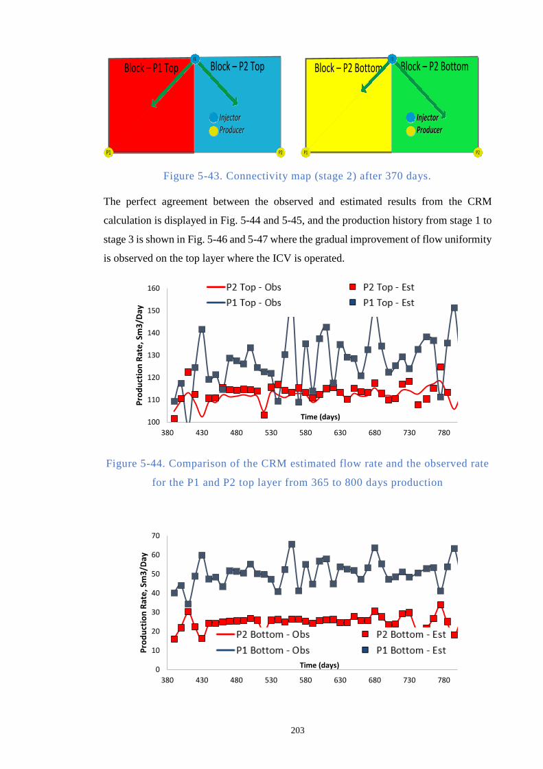
203
Block – P1 Top
P1
Block – P2 Top
InjectorProducerInjectorProducer
P2
I1
Block – P2 Bottom
P1
Block – P2 Bottom
InjectorProducerInjectorProducer
P2
I1
Figure 5-43. Connectivity map (stage 2) after 370 days.
The perfect agreement between the observed and estimated results from the CRM
calculation is displayed in Fig. 5-44 and 5-45, and the production history from stage 1 to
stage 3 is shown in Fig. 5-46 and 5-47 where the gradual improvement of flow uniformity
is observed on the top layer where the ICV is operated.
Figure 5-44. Comparison of the CRM estimated flow rate and the observed rate
for the P1 and P2 top layer from 365 to 800 days production
100
110
120
130
140
150
160
380 430 480 530 580 630 680 730 780
Pro
du
ctio
n R
ate
, Sm
3/D
ay
Time (days)
0
10
20
30
40
50
60
70
380 430 480 530 580 630 680 730 780
Pro
du
ctio
n R
ate
, Sm
3/D
ay
Time (days)
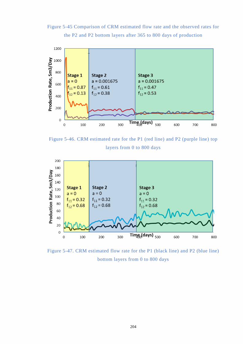
204
Figure 5-45 Comparison of CRM estimated flow rate and the observed rates for
the P2 and P2 bottom layers after 365 to 800 days of production
Figure 5-46. CRM estimated rate for the P1 (red line) and P2 (purple line) top
layers from 0 to 800 days
Figure 5-47. CRM estimated flow rate for the P1 (black line) and P2 (blue line)
bottom layers from 0 to 800 days
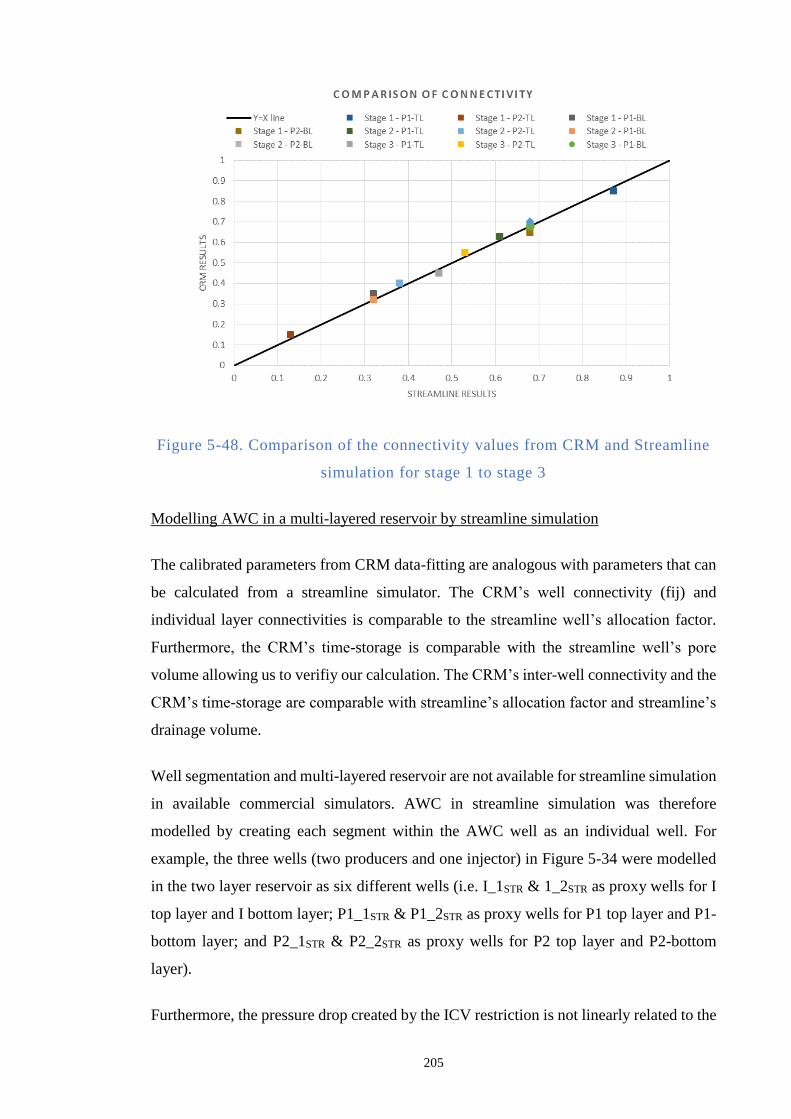
205
Figure 5-48. Comparison of the connectivity values from CRM and Streamline
simulation for stage 1 to stage 3
Modelling AWC in a multi-layered reservoir by streamline simulation
The calibrated parameters from CRM data-fitting are analogous with parameters that can
be calculated from a streamline simulator. The CRM’s well connectivity (fij) and
individual layer connectivities is comparable to the streamline well’s allocation factor.
Furthermore, the CRM’s time-storage is comparable with the streamline well’s pore
volume allowing us to verifiy our calculation. The CRM’s inter-well connectivity and the
CRM’s time-storage are comparable with streamline’s allocation factor and streamline’s
drainage volume.
Well segmentation and multi-layered reservoir are not available for streamline simulation
in available commercial simulators. AWC in streamline simulation was therefore
modelled by creating each segment within the AWC well as an individual well. For
example, the three wells (two producers and one injector) in Figure 5-34 were modelled
in the two layer reservoir as six different wells (i.e. I_1STR & 1_2STR as proxy wells for I
top layer and I bottom layer; P1_1STR & P1_2STR as proxy wells for P1 top layer and P1-
bottom layer; and P2_1STR & P2_2STR as proxy wells for P2 top layer and P2-bottom
layer).
Furthermore, the pressure drop created by the ICV restriction is not linearly related to the
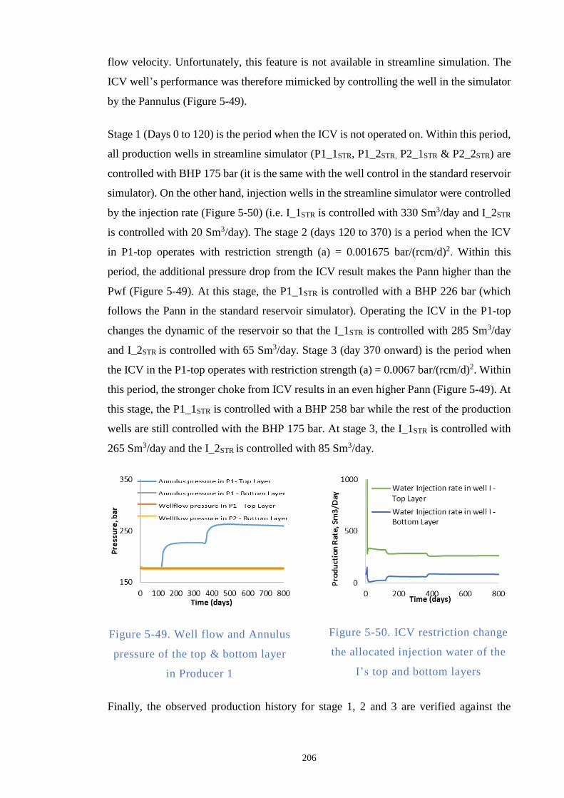
206
flow velocity. Unfortunately, this feature is not available in streamline simulation. The
ICV well’s performance was therefore mimicked by controlling the well in the simulator
by the Pannulus (Figure 5-49).
Stage 1 (Days 0 to 120) is the period when the ICV is not operated on. Within this period,
all production wells in streamline simulator (P1_1STR, P1_2STR, P2_1STR & P2_2STR) are
controlled with BHP 175 bar (it is the same with the well control in the standard reservoir
simulator). On the other hand, injection wells in the streamline simulator were controlled
by the injection rate (Figure 5-50) (i.e. I_1STR is controlled with 330 Sm3/day and I_2STR
is controlled with 20 Sm3/day). The stage 2 (days 120 to 370) is a period when the ICV
in P1-top operates with restriction strength (a) = 0.001675 bar/(rcm/d)2. Within this
period, the additional pressure drop from the ICV result makes the Pann higher than the
Pwf (Figure 5-49). At this stage, the P1_1STR is controlled with a BHP 226 bar (which
follows the Pann in the standard reservoir simulator). Operating the ICV in the P1-top
changes the dynamic of the reservoir so that the I_1STR is controlled with 285 Sm3/day
and I_2STR is controlled with 65 Sm3/day. Stage 3 (day 370 onward) is the period when
the ICV in the P1-top operates with restriction strength (a) = 0.0067 bar/(rcm/d)2. Within
this period, the stronger choke from ICV results in an even higher Pann (Figure 5-49). At
this stage, the P1_1STR is controlled with a BHP 258 bar while the rest of the production
wells are still controlled with the BHP 175 bar. At stage 3, the I_1STR is controlled with
265 Sm3/day and the I_2STR is controlled with 85 Sm3/day.
Figure 5-49. Well flow and Annulus
pressure of the top & bottom layer
in Producer 1
Figure 5-50. ICV restriction change
the allocated injection water of the
I’s top and bottom layers
Finally, the observed production history for stage 1, 2 and 3 are verified against the
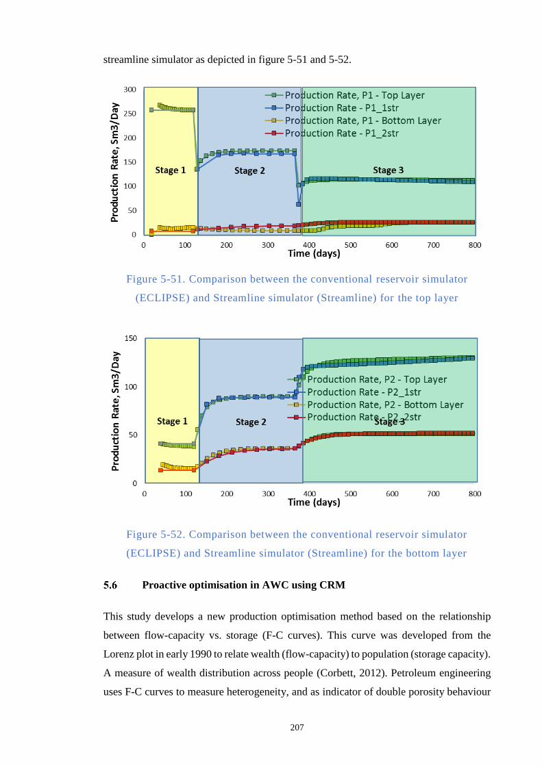
207
streamline simulator as depicted in figure 5-51 and 5-52.
Figure 5-51. Comparison between the conventional reservoir simulator
(ECLIPSE) and Streamline simulator (Streamline) for the top layer
Figure 5-52. Comparison between the conventional reservoir simulator
(ECLIPSE) and Streamline simulator (Streamline) for the bottom layer
Proactive optimisation in AWC using CRM
This study develops a new production optimisation method based on the relationship
between flow-capacity vs. storage (F-C curves). This curve was developed from the
Lorenz plot in early 1990 to relate wealth (flow-capacity) to population (storage capacity).
A measure of wealth distribution across people (Corbett, 2012). Petroleum engineering
uses F-C curves to measure heterogeneity, and as indicator of double porosity behaviour
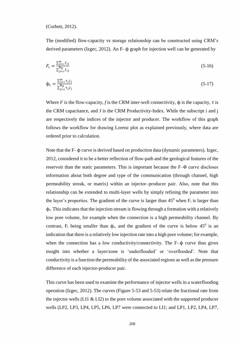
208
(Corbett, 2012).
The (modified) flow-capacity vs storage relationship can be constructed using CRM’s
derived parameters (Izgec, 2012). An F- ϕ graph for injection well can be generated by
𝐹𝑖 =∑ 𝑓𝑖𝑗𝑚𝑗=1
∑ 𝑓𝑖𝑗𝑁𝑝𝑗=1
(5-16)
ϕ𝑖 =∑ τ𝑗𝐽𝑗𝑚𝑗=1
∑ τ𝑗𝐽𝑗𝑁𝑝𝑗=1
(5-17)
Where F is the flow-capacity, f is the CRM inter-well connectivity, ϕ is the capacity, τ is
the CRM capacitance, and J is the CRM Productivity-Index. While the subscript i and j
are respectively the indices of the injector and producer. The workflow of this graph
follows the workflow for drawing Lorenz plot as explained previously, where data are
ordered prior to calculation.
Note that the F- ϕ curve is derived based on production data (dynamic parameters). Izgec,
2012, considered it to be a better reflection of flow-path and the geological features of the
reservoir than the static parameters. This is important because the F–Φ curve discloses
information about both degree and type of the communication (through channel, high
permeability streak, or matrix) within an injector–producer pair. Also, note that this
relationship can be extended to multi-layer wells by simply refining the parameter into
the layer’s properties. The gradient of the curve is larger than 450 when Fi is larger than
ϕi. This indicates that the injection stream is flowing through a formation with a relatively
low pore volume, for example when the connection is a high permeability channel. By
contrast, Fi being smaller than ϕi, and the gradient of the curve is below 450 is an
indication that there is a relatively low injection rate into a high pore volume; for example,
when the connection has a low conductivity/connectivity. The F- ϕ curve thus gives
insight into whether a layer/zone is ‘underflooded’ or ‘overflooded’. Note that
conductivity is a function the permeability of the associated regions as well as the pressure
difference of each injector-producer pair.
This curve has been used to examine the performance of injector wells in a waterflooding
operation (Izgec, 2012). The curves (Figure 5-53 and 5-53) relate the fractional rate from
the injector wells (LI1 & LI2) to the pore volume associated with the supported producer
wells (LP2, LP3, LP4, LP5, LP6, LP7 were connected to LI1; and LP1, LP2, LP4, LP7,
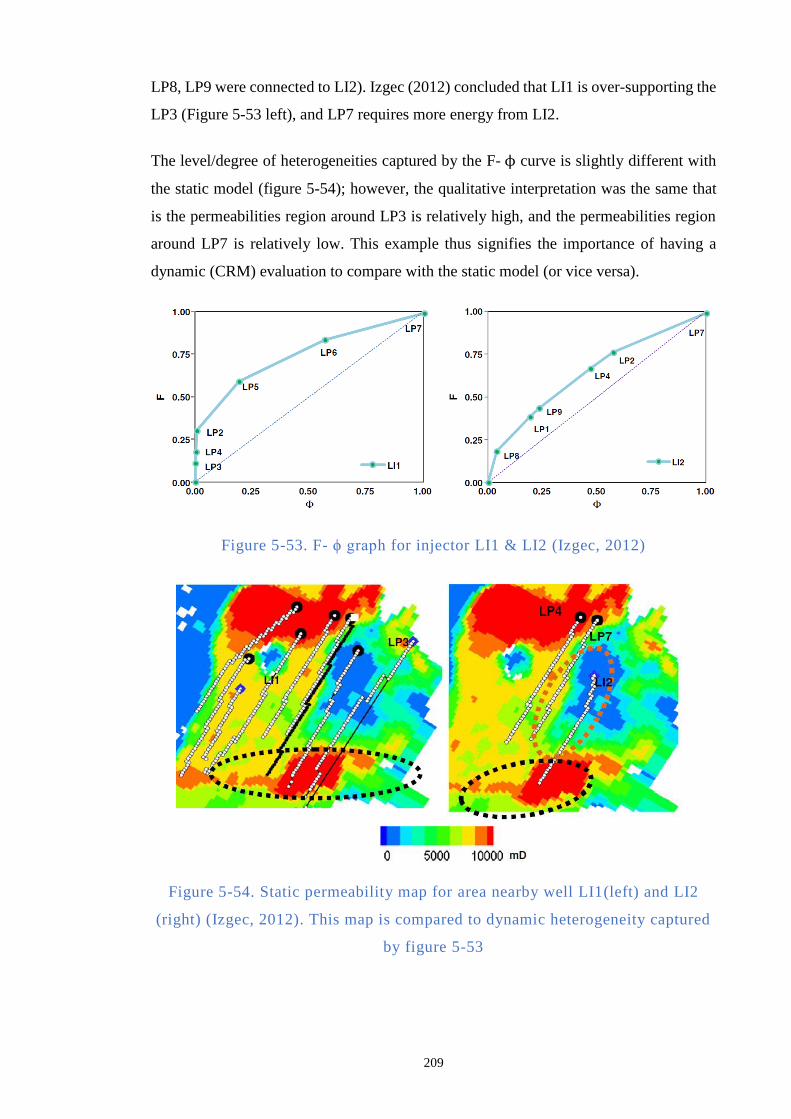
209
LP8, LP9 were connected to LI2). Izgec (2012) concluded that LI1 is over-supporting the
LP3 (Figure 5-53 left), and LP7 requires more energy from LI2.
The level/degree of heterogeneities captured by the F- ϕ curve is slightly different with
the static model (figure 5-54); however, the qualitative interpretation was the same that
is the permeabilities region around LP3 is relatively high, and the permeabilities region
around LP7 is relatively low. This example thus signifies the importance of having a
dynamic (CRM) evaluation to compare with the static model (or vice versa).
Figure 5-53. F- ϕ graph for injector LI1 & LI2 (Izgec, 2012)
Figure 5-54. Static permeability map for area nearby well LI1(left) and LI2
(right) (Izgec, 2012). This map is compared to dynamic heterogeneity captured
by figure 5-53

210
F- 𝝓 graph
A more refined layer (or well) performance evaluation can be formulated by normalising
the parameters (equations 5-18 and 5-19). The modified F- ϕ graph (F − ϕ) can provide
guidelines for ICV (or well) proactive optimisation, since the CRM parameters respond
to alterations in the well’s or layer’s control settings. A F − ϕ graph for a production
well completed in multi-layers can be generated by:
𝐹 =∑ ∑ 𝑗,𝑙
𝑛𝑙=1
𝑚𝑗=1
∑ 𝑗,𝑙𝑁𝑝𝑗=1
(5-18)
ϕ𝑗 =∑ ∑ τ𝑗,𝑙 𝐽𝑗,𝑙
𝑛𝑙=1
𝑚
∑ τ𝑗,𝑙𝐽𝑗,𝑙𝑁𝑝𝑗=1
(5-19)
The main difference with the original F- ϕ graph are :
1. Equation 5-18 and 5-19 are calibrated for multi-layers reservoir (the second sum
referred to layer, l = layer number).
2. Instead of comparing the connectivity values, the new graph directly evaluates
(average) production contribution for each layers
3. In the original F − ϕ graph, the connectivities were evaluated on well’s basis
while in the equation 5-18, each layer’s production rate is normalized against the
whole observed rate in the system. By doing so, we can have neutral comparison
to evaluate contribution of each layer’s.
Figure 5-55 is the modified F − ϕ curve for the reservoir illustrated in Figure 5-34. The
data were taken from table 5-3, and CRM calibration results illustrated in figure 5-46, 5-
47. The development of this was split into three stages. Stage 1 when the completion had
no restriction and stage 3 when an aggressive restriction was applied in the completion.
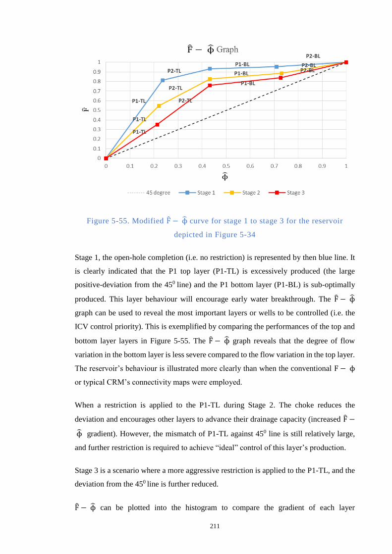
211
Figure 5-55. Modified F − ϕ curve for stage 1 to stage 3 for the reservoir
depicted in Figure 5-34
Stage 1, the open-hole completion (i.e. no restriction) is represented by then blue line. It
is clearly indicated that the P1 top layer (P1-TL) is excessively produced (the large
positive-deviation from the 450 line) and the P1 bottom layer (P1-BL) is sub-optimally
produced. This layer behaviour will encourage early water breakthrough. The F − ϕ
graph can be used to reveal the most important layers or wells to be controlled (i.e. the
ICV control priority). This is exemplified by comparing the performances of the top and
bottom layer layers in Figure 5-55. The F − ϕ graph reveals that the degree of flow
variation in the bottom layer is less severe compared to the flow variation in the top layer.
The reservoir’s behaviour is illustrated more clearly than when the conventional F − ϕ
or typical CRM’s connectivity maps were employed.
When a restriction is applied to the P1-TL during Stage 2. The choke reduces the
deviation and encourages other layers to advance their drainage capacity (increased F −
ϕ gradient). However, the mismatch of P1-TL against 450 line is still relatively large,
and further restriction is required to achieve “ideal” control of this layer’s production.
Stage 3 is a scenario where a more aggressive restriction is applied to the P1-TL, and the
deviation from the 450 line is further reduced.
F − ϕ can be plotted into the histogram to compare the gradient of each layer
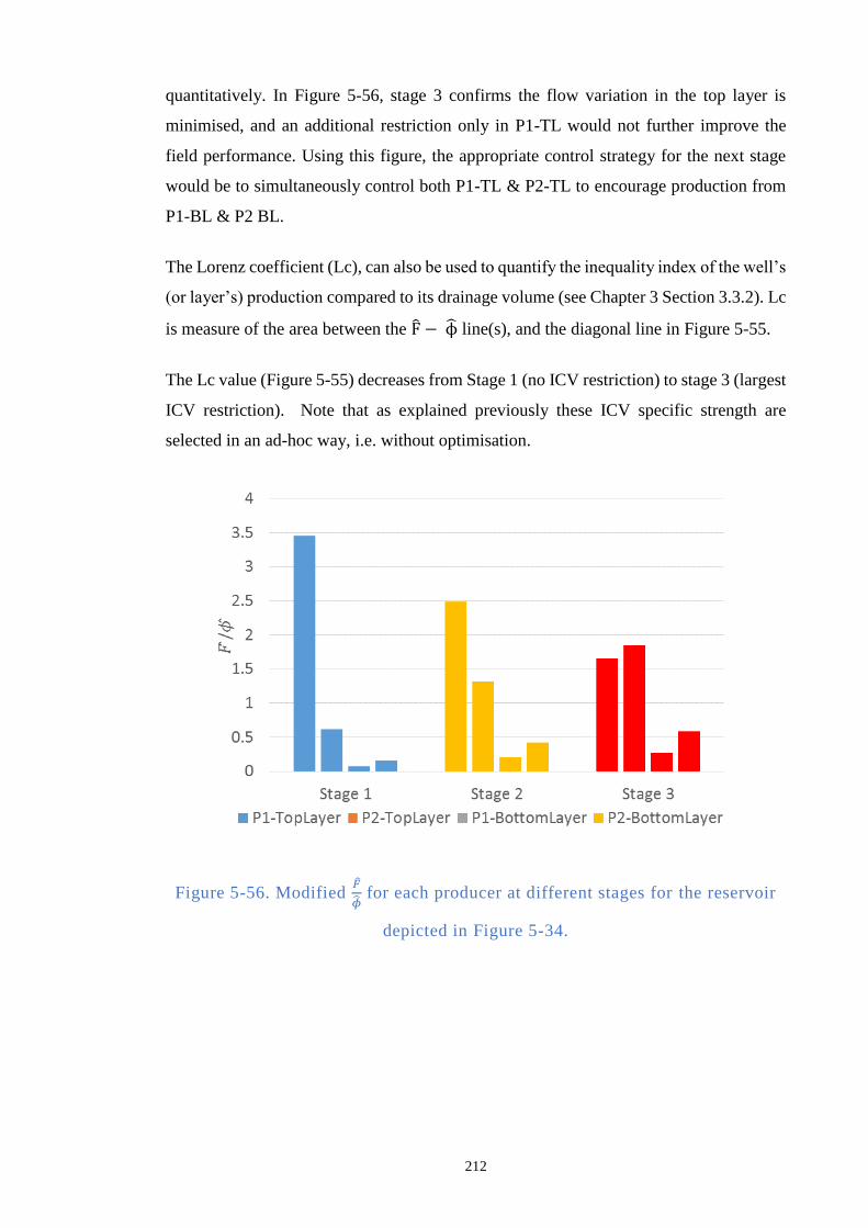
212
quantitatively. In Figure 5-56, stage 3 confirms the flow variation in the top layer is
minimised, and an additional restriction only in P1-TL would not further improve the
field performance. Using this figure, the appropriate control strategy for the next stage
would be to simultaneously control both P1-TL & P2-TL to encourage production from
P1-BL & P2 BL.
The Lorenz coefficient (Lc), can also be used to quantify the inequality index of the well’s
(or layer’s) production compared to its drainage volume (see Chapter 3 Section 3.3.2). Lc
is measure of the area between the F − ϕ line(s), and the diagonal line in Figure 5-55.
The Lc value (Figure 5-55) decreases from Stage 1 (no ICV restriction) to stage 3 (largest
ICV restriction). Note that as explained previously these ICV specific strength are
selected in an ad-hoc way, i.e. without optimisation.
Figure 5-56. Modified
for each producer at different stages for the reservoir
depicted in Figure 5-34.
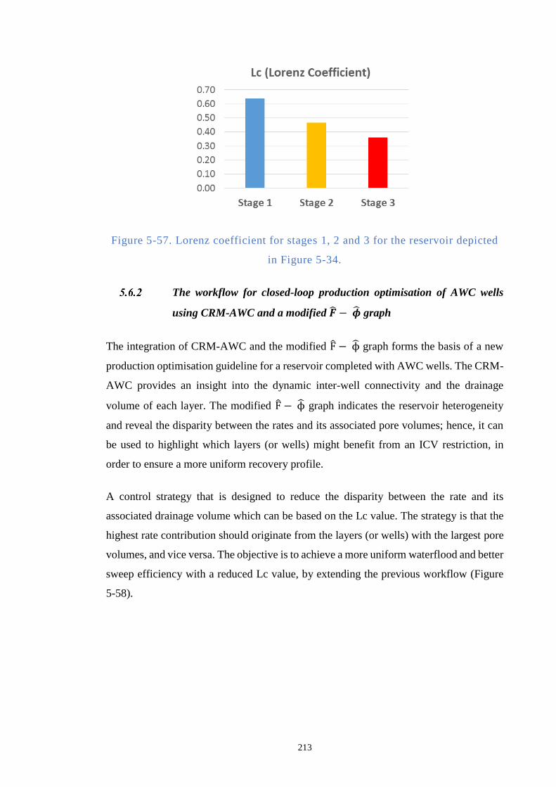
213
Figure 5-57. Lorenz coefficient for stages 1, 2 and 3 for the reservoir depicted
in Figure 5-34.
The workflow for closed-loop production optimisation of AWC wells
using CRM-AWC and a modified − graph
The integration of CRM-AWC and the modified F − ϕ graph forms the basis of a new
production optimisation guideline for a reservoir completed with AWC wells. The CRM-
AWC provides an insight into the dynamic inter-well connectivity and the drainage
volume of each layer. The modified F − ϕ graph indicates the reservoir heterogeneity
and reveal the disparity between the rates and its associated pore volumes; hence, it can
be used to highlight which layers (or wells) might benefit from an ICV restriction, in
order to ensure a more uniform recovery profile.
A control strategy that is designed to reduce the disparity between the rate and its
associated drainage volume which can be based on the Lc value. The strategy is that the
highest rate contribution should originate from the layers (or wells) with the largest pore
volumes, and vice versa. The objective is to achieve a more uniform waterflood and better
sweep efficiency with a reduced Lc value, by extending the previous workflow (Figure
5-58).
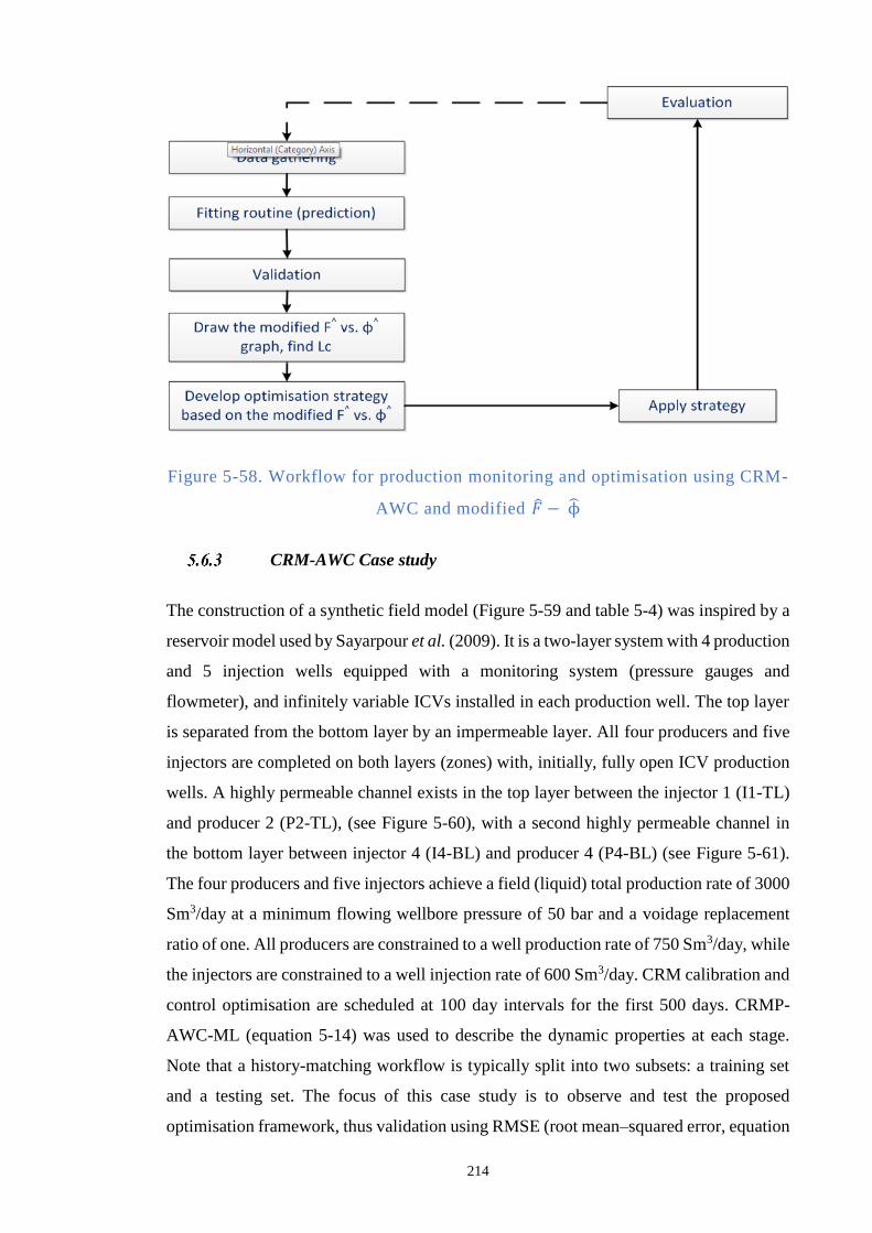
214
Figure 5-58. Workflow for production monitoring and optimisation using CRM-
AWC and modified − ϕ
CRM-AWC Case study
The construction of a synthetic field model (Figure 5-59 and table 5-4) was inspired by a
reservoir model used by Sayarpour et al. (2009). It is a two-layer system with 4 production
and 5 injection wells equipped with a monitoring system (pressure gauges and
flowmeter), and infinitely variable ICVs installed in each production well. The top layer
is separated from the bottom layer by an impermeable layer. All four producers and five
injectors are completed on both layers (zones) with, initially, fully open ICV production
wells. A highly permeable channel exists in the top layer between the injector 1 (I1-TL)
and producer 2 (P2-TL), (see Figure 5-60), with a second highly permeable channel in
the bottom layer between injector 4 (I4-BL) and producer 4 (P4-BL) (see Figure 5-61).
The four producers and five injectors achieve a field (liquid) total production rate of 3000
Sm3/day at a minimum flowing wellbore pressure of 50 bar and a voidage replacement
ratio of one. All producers are constrained to a well production rate of 750 Sm3/day, while
the injectors are constrained to a well injection rate of 600 Sm3/day. CRM calibration and
control optimisation are scheduled at 100 day intervals for the first 500 days. CRMP-
AWC-ML (equation 5-14) was used to describe the dynamic properties at each stage.
Note that a history-matching workflow is typically split into two subsets: a training set
and a testing set. The focus of this case study is to observe and test the proposed
optimisation framework, thus validation using RMSE (root mean–squared error, equation
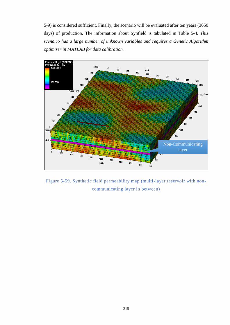
215
5-9) is considered sufficient. Finally, the scenario will be evaluated after ten years (3650
days) of production. The information about Synfield is tabulated in Table 5-4. This
scenario has a large number of unknown variables and requires a Genetic Algorithm
optimiser in MATLAB for data calibration.
Figure 5-59. Synthetic field permeability map (multi-layer reservoir with non-
communicating layer in between)
Non-Communicating
layer
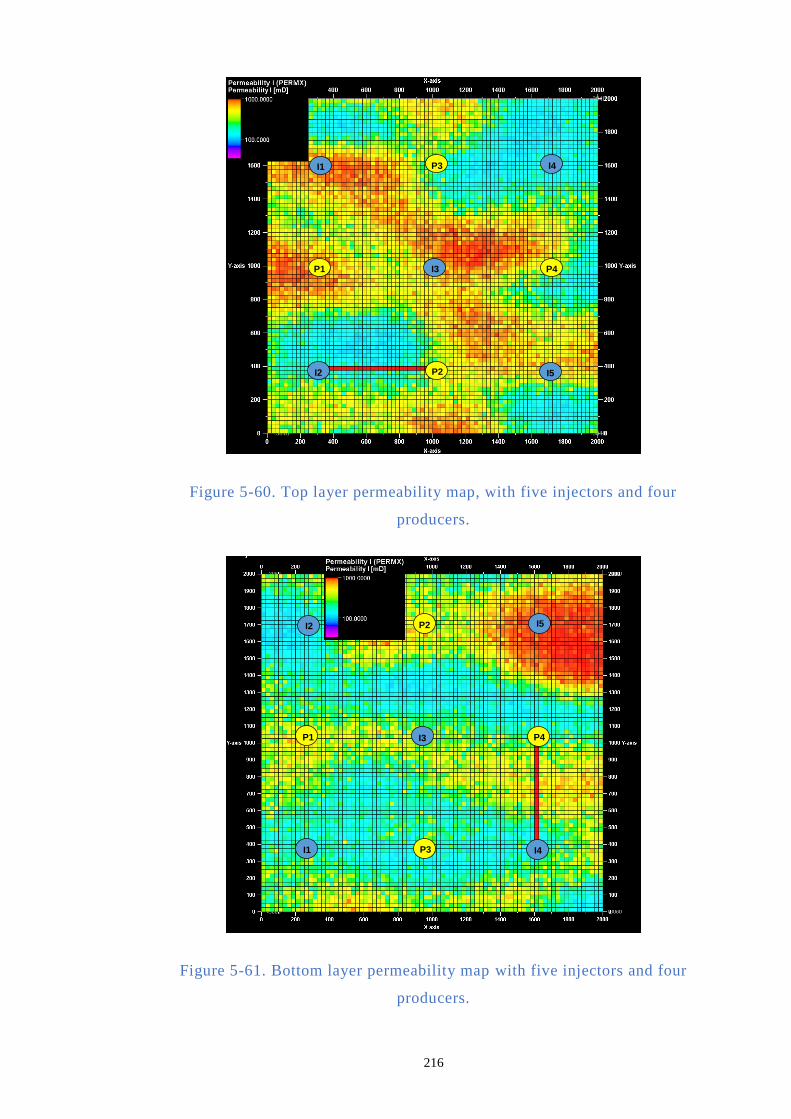
216
Figure 5-60. Top layer permeability map, with five injectors and four
producers.
Figure 5-61. Bottom layer permeability map with five injectors and four
producers.
I2 P2
I3 P1
I1 P3 I4
P4
I5
I1 P3
I3 P1
I2 P2 I5
P4
I4
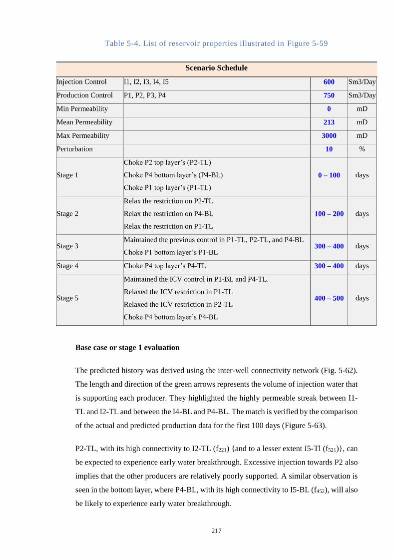
217
Table 5-4. List of reservoir properties illustrated in Figure 5-59
Scenario Schedule
Injection Control I1, I2, I3, I4, I5 600 Sm3/Day
Production Control P1, P2, P3, P4 750 Sm3/Day
Min Permeability 0 mD
Mean Permeability
213 mD
Max Permeability 3000 mD
Perturbation 10 %
Stage 1
Choke P2 top layer’s (P2-TL)
Choke P4 bottom layer’s (P4-BL)
Choke P1 top layer’s (P1-TL)
0 – 100 days
Stage 2
Relax the restriction on P2-TL
Relax the restriction on P4-BL
Relax the restriction on P1-TL
100 – 200 days
Stage 3 Maintained the previous control in P1-TL, P2-TL, and P4-BL
Choke P1 bottom layer’s P1-BL 300 – 400 days
Stage 4 Choke P4 top layer’s P4-TL 300 – 400 days
Stage 5
Maintained the ICV control in P1-BL and P4-TL.
Relaxed the ICV restriction in P1-TL
Relaxed the ICV restriction in P2-TL
Choke P4 bottom layer’s P4-BL
400 – 500 days
Base case or stage 1 evaluation
The predicted history was derived using the inter-well connectivity network (Fig. 5-62).
The length and direction of the green arrows represents the volume of injection water that
is supporting each producer. They highlighted the highly permeable streak between I1-
TL and I2-TL and between the I4-BL and P4-BL. The match is verified by the comparison
of the actual and predicted production data for the first 100 days (Figure 5-63).
P2-TL, with its high connectivity to I2-TL (f221) and to a lesser extent I5-Tl (f521), can
be expected to experience early water breakthrough. Excessive injection towards P2 also
implies that the other producers are relatively poorly supported. A similar observation is
seen in the bottom layer, where P4-BL, with its high connectivity to I5-BL (f452), will also
be likely to experience early water breakthrough.
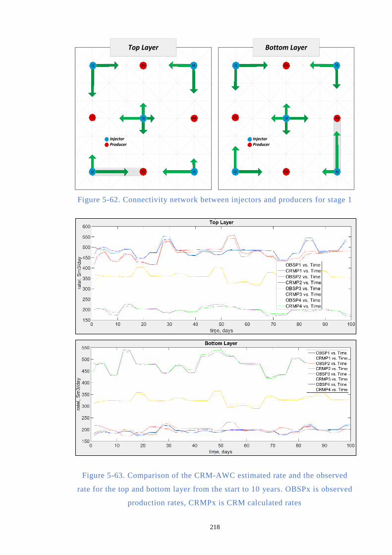
218
InjectorProducerInjectorProducer
P1
P3
P4
P2I2
I1
I3
Top Layer
InjectorProducerInjectorProducer
P1
P3
P2I2
I1
I3
Bottom Layer
P4
I4 I4
I5I5
Figure 5-62. Connectivity network between injectors and producers for stage 1
Figure 5-63. Comparison of the CRM-AWC estimated rate and the observed
rate for the top and bottom layer from the start to 10 years. OBSPx is observed
production rates, CRMPx is CRM calculated rates
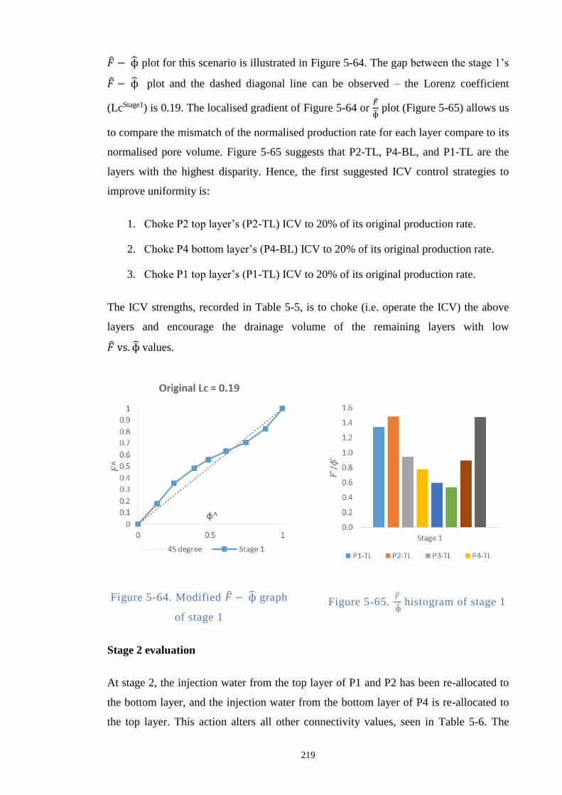
219
− ϕ plot for this scenario is illustrated in Figure 5-64. The gap between the stage 1’s
− ϕ plot and the dashed diagonal line can be observed – the Lorenz coefficient
(LcStage1) is 0.19. The localised gradient of Figure 5-64 or
ϕ plot (Figure 5-65) allows us
to compare the mismatch of the normalised production rate for each layer compare to its
normalised pore volume. Figure 5-65 suggests that P2-TL, P4-BL, and P1-TL are the
layers with the highest disparity. Hence, the first suggested ICV control strategies to
improve uniformity is:
1. Choke P2 top layer’s (P2-TL) ICV to 20% of its original production rate.
2. Choke P4 bottom layer’s (P4-BL) ICV to 20% of its original production rate.
3. Choke P1 top layer’s (P1-TL) ICV to 20% of its original production rate.
The ICV strengths, recorded in Table 5-5, is to choke (i.e. operate the ICV) the above
layers and encourage the drainage volume of the remaining layers with low
vs. ϕ values.
Figure 5-64. Modified − ϕ graph
of stage 1
Figure 5-65.
ϕ histogram of stage 1
Stage 2 evaluation
At stage 2, the injection water from the top layer of P1 and P2 has been re-allocated to
the bottom layer, and the injection water from the bottom layer of P4 is re-allocated to
the top layer. This action alters all other connectivity values, seen in Table 5-6. The
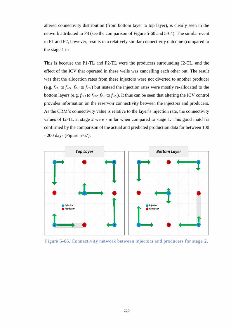
220
altered connectivity distribution (from bottom layer to top layer), is clearly seen in the
network attributed to P4 (see the comparison of Figure 5-60 and 5-64). The similar event
in P1 and P2, however, results in a relatively similar connectivity outcome (compared to
the stage 1 in
This is because the P1-TL and P2-TL were the producers surrounding I2-TL, and the
effect of the ICV that operated in these wells was cancelling each other out. The result
was that the allocation rates from these injectors were not diverted to another producer
(e.g. f211 to f221; f221 to f211) but instead the injection rates were mostly re-allocated to the
bottom layers (e.g. f211 to f212; f221 to f222). It thus can be seen that altering the ICV control
provides information on the reservoir connectivity between the injectors and producers.
As the CRM’s connectivity value is relative to the layer’s injection rate, the connectivity
values of I2-TL at stage 2 were similar when compared to stage 1. This good match is
confirmed by the comparison of the actual and predicted production data for between 100
- 200 days (Figure 5-67).
InjectorProducerInjectorProducer
P1
P3
P4
P2
I3
Top Layer
InjectorProducerInjectorProducer
P1
P3
P2I2
I1
I3
Bottom Layer
P4
I4 I4
I5I5
I1
I2
Figure 5-66. Connectivity network between injectors and producers for stage 2.
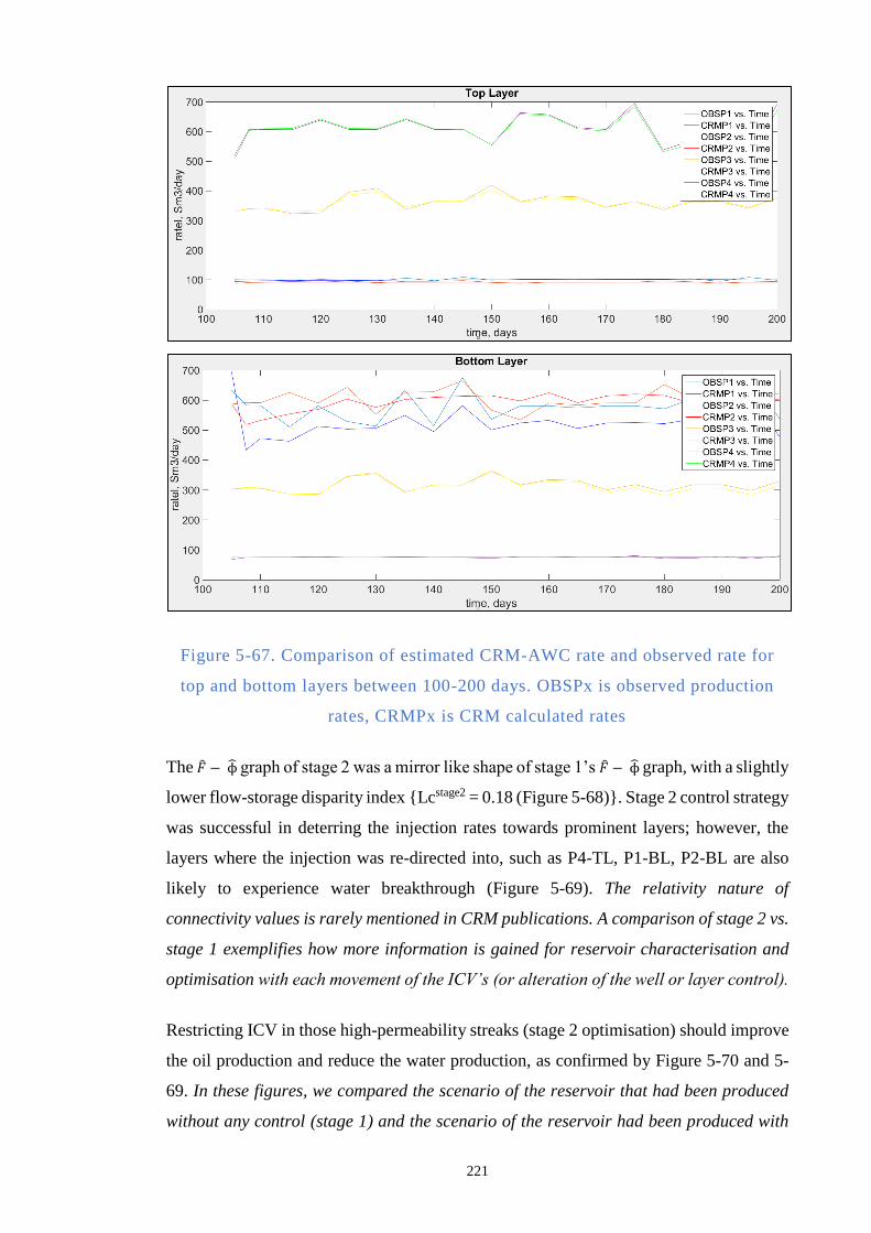
221
Figure 5-67. Comparison of estimated CRM-AWC rate and observed rate for
top and bottom layers between 100-200 days. OBSPx is observed production
rates, CRMPx is CRM calculated rates
The − ϕ graph of stage 2 was a mirror like shape of stage 1’s − ϕ graph, with a slightly
lower flow-storage disparity index Lcstage2 = 0.18 (Figure 5-68). Stage 2 control strategy
was successful in deterring the injection rates towards prominent layers; however, the
layers where the injection was re-directed into, such as P4-TL, P1-BL, P2-BL are also
likely to experience water breakthrough (Figure 5-69). The relativity nature of
connectivity values is rarely mentioned in CRM publications. A comparison of stage 2 vs.
stage 1 exemplifies how more information is gained for reservoir characterisation and
optimisation with each movement of the ICV’s (or alteration of the well or layer control).
Restricting ICV in those high-permeability streaks (stage 2 optimisation) should improve
the oil production and reduce the water production, as confirmed by Figure 5-70 and 5-
69. In these figures, we compared the scenario of the reservoir that had been produced
without any control (stage 1) and the scenario of the reservoir had been produced with
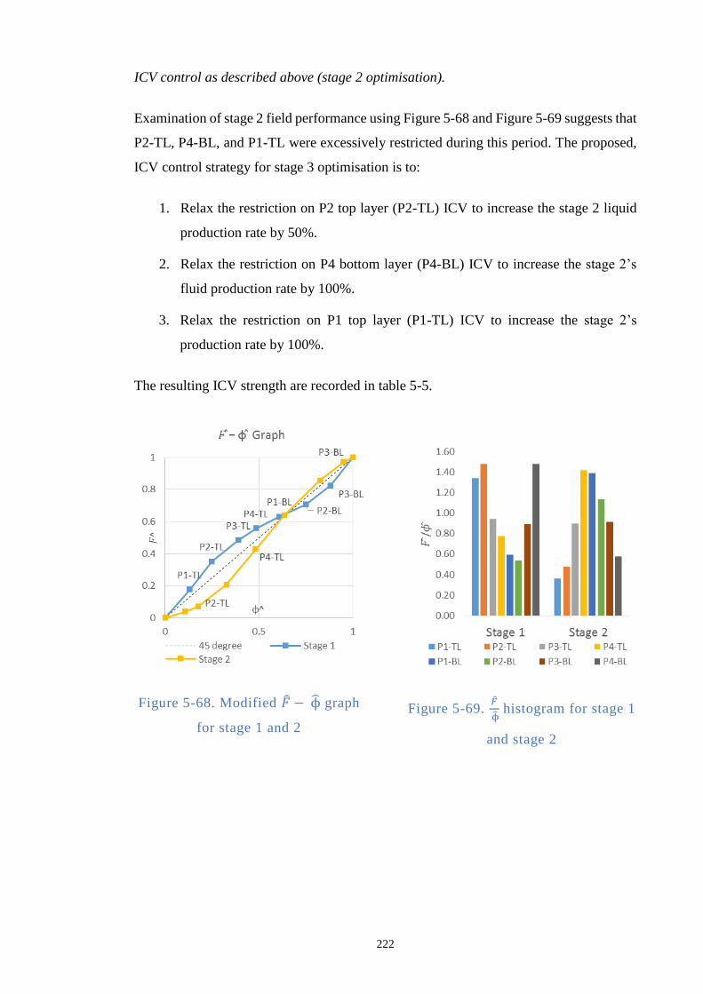
222
ICV control as described above (stage 2 optimisation).
Examination of stage 2 field performance using Figure 5-68 and Figure 5-69 suggests that
P2-TL, P4-BL, and P1-TL were excessively restricted during this period. The proposed,
ICV control strategy for stage 3 optimisation is to:
1. Relax the restriction on P2 top layer (P2-TL) ICV to increase the stage 2 liquid
production rate by 50%.
2. Relax the restriction on P4 bottom layer (P4-BL) ICV to increase the stage 2’s
fluid production rate by 100%.
3. Relax the restriction on P1 top layer (P1-TL) ICV to increase the stage 2’s
production rate by 100%.
The resulting ICV strength are recorded in table 5-5.
Figure 5-68. Modified − ϕ graph
for stage 1 and 2
Figure 5-69.
ϕ histogram for stage 1
and stage 2
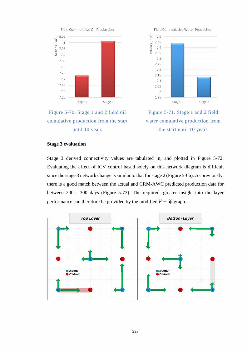
223
Figure 5-70. Stage 1 and 2 field oil
cumulative production from the start
until 10 years
Figure 5-71. Stage 1 and 2 field
water cumulative production from
the start until 10 years
Stage 3 evaluation
Stage 3 derived connectivity values are tabulated in, and plotted in Figure 5-72.
Evaluating the effect of ICV control based solely on this network diagram is difficult
since the stage 3 network change is similar to that for stage 2 (Figure 5-66). As previously,
there is a good match between the actual and CRM-AWC predicted production data for
between 200 - 300 days (Figure 5-73). The required, greater insight into the layer
performance can therefore be provided by the modified − ϕ graph.
InjectorProducerInjectorProducer
P1
P3
P4
P2
I3
Top Layer
InjectorProducerInjectorProducer
P1
P3
P2I2
I1
I3
Bottom Layer
P4
I4 I4
I5I5
I1
I2
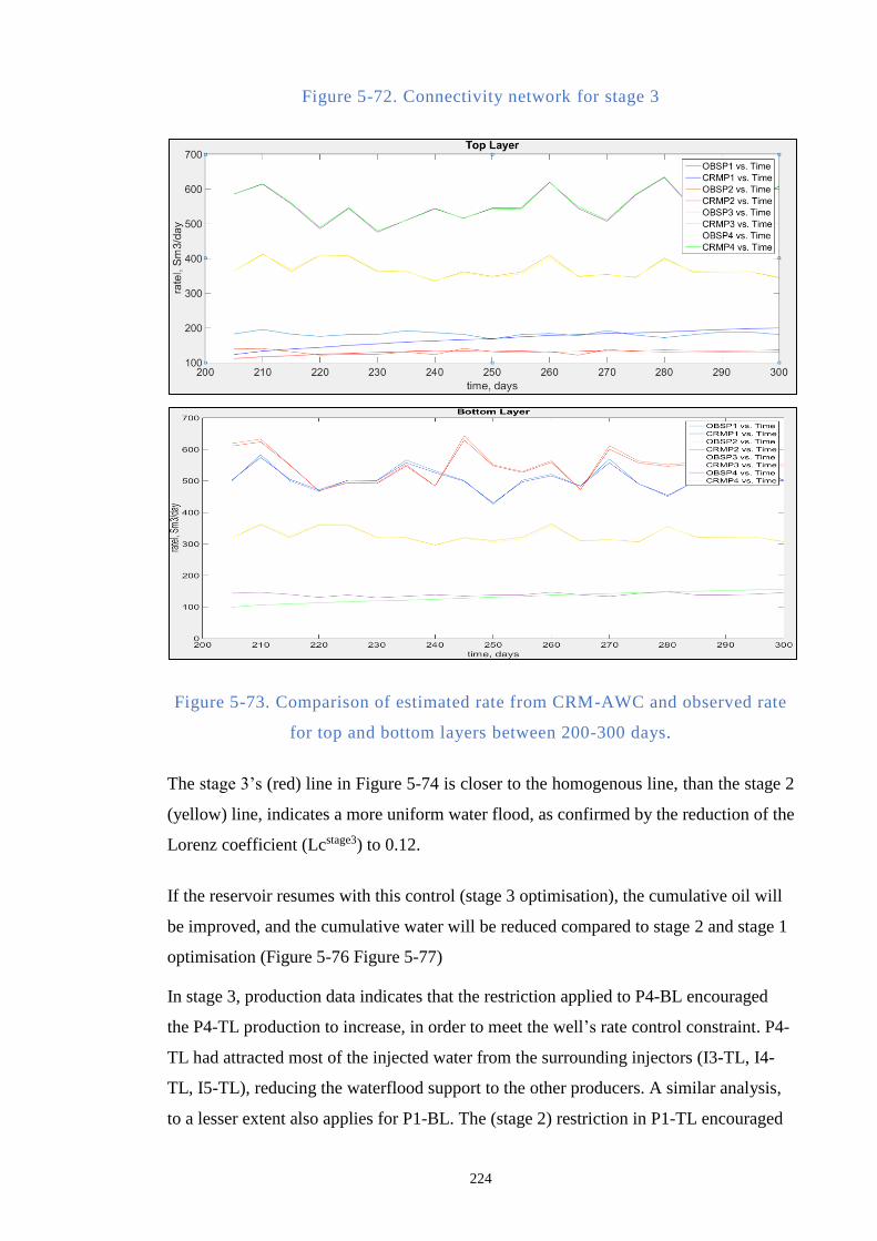
224
Figure 5-72. Connectivity network for stage 3
Figure 5-73. Comparison of estimated rate from CRM-AWC and observed rate
for top and bottom layers between 200-300 days.
The stage 3’s (red) line in Figure 5-74 is closer to the homogenous line, than the stage 2
(yellow) line, indicates a more uniform water flood, as confirmed by the reduction of the
Lorenz coefficient (Lcstage3) to 0.12.
If the reservoir resumes with this control (stage 3 optimisation), the cumulative oil will
be improved, and the cumulative water will be reduced compared to stage 2 and stage 1
optimisation (Figure 5-76 Figure 5-77)
In stage 3, production data indicates that the restriction applied to P4-BL encouraged
the P4-TL production to increase, in order to meet the well’s rate control constraint. P4-
TL had attracted most of the injected water from the surrounding injectors (I3-TL, I4-
TL, I5-TL), reducing the waterflood support to the other producers. A similar analysis,
to a lesser extent also applies for P1-BL. The (stage 2) restriction in P1-TL encouraged
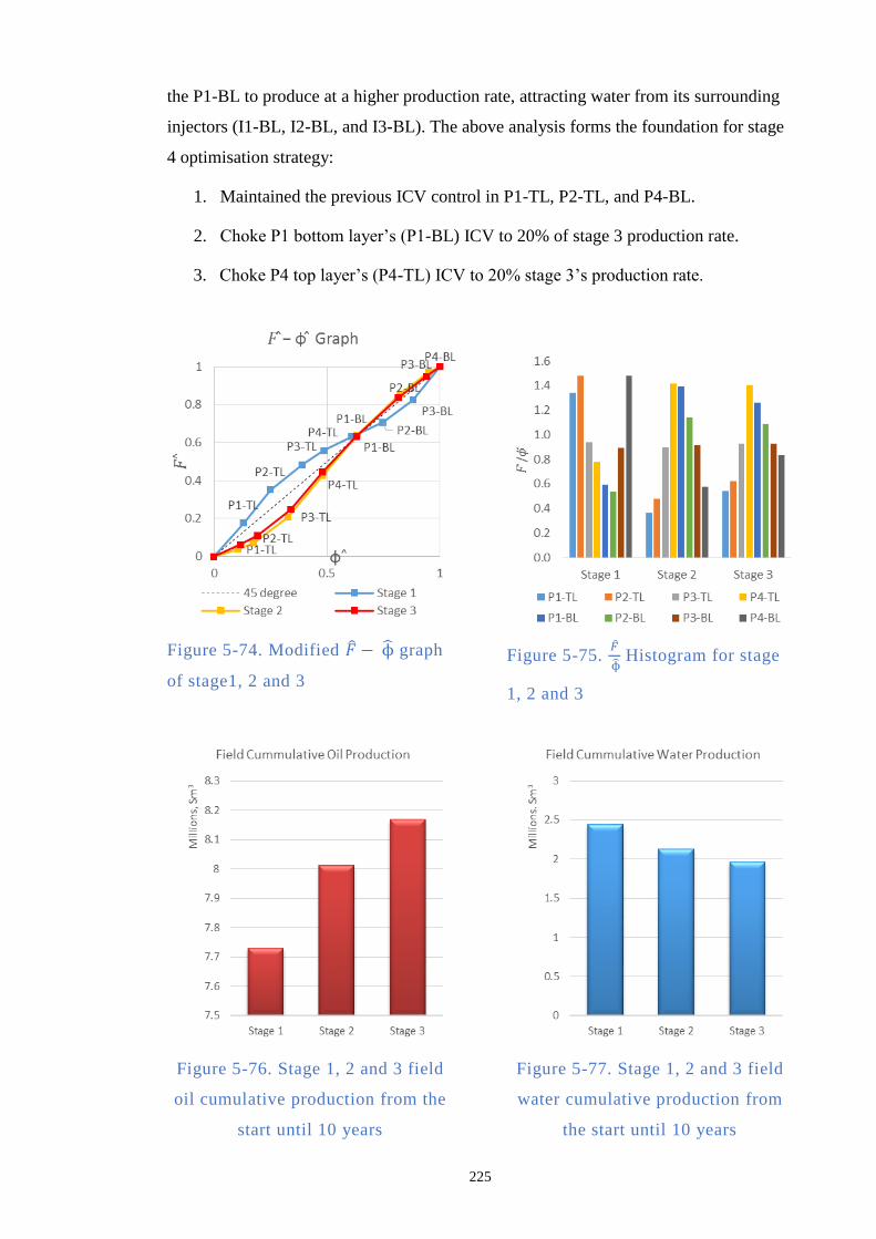
225
the P1-BL to produce at a higher production rate, attracting water from its surrounding
injectors (I1-BL, I2-BL, and I3-BL). The above analysis forms the foundation for stage
4 optimisation strategy:
1. Maintained the previous ICV control in P1-TL, P2-TL, and P4-BL.
2. Choke P1 bottom layer’s (P1-BL) ICV to 20% of stage 3 production rate.
3. Choke P4 top layer’s (P4-TL) ICV to 20% stage 3’s production rate.
Figure 5-74. Modified − ϕ graph
of stage1, 2 and 3
Figure 5-75.
ϕ Histogram for stage
1, 2 and 3
Figure 5-76. Stage 1, 2 and 3 field
oil cumulative production from the
start until 10 years
Figure 5-77. Stage 1, 2 and 3 field
water cumulative production from
the start until 10 years
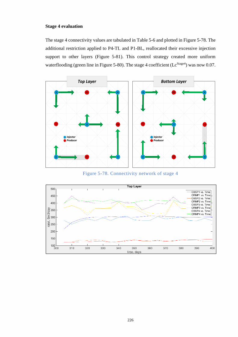
226
Stage 4 evaluation
The stage 4 connectivity values are tabulated in Table 5-6 and plotted in Figure 5-78. The
additional restriction applied to P4-TL and P1-BL, reallocated their excessive injection
support to other layers (Figure 5-81). This control strategy created more uniform
waterflooding (green line in Figure 5-80). The stage 4 coefficient (LcStage4) was now 0.07.
InjectorProducerInjectorProducer
P1
P3
P4
P2
I3
Top Layer
InjectorProducerInjectorProducer
P1
P3
P2I2
I1
I3
Bottom Layer
P4
I4 I4
I5I5
I1
I2
Figure 5-78. Connectivity network of stage 4
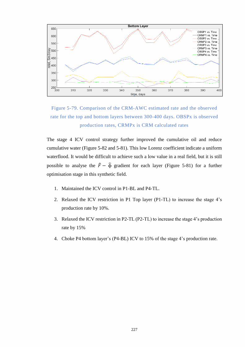
227
Figure 5-79. Comparison of the CRM-AWC estimated rate and the observed
rate for the top and bottom layers between 300-400 days. OBSPx is observed
production rates, CRMPx is CRM calculated rates
The stage 4 ICV control strategy further improved the cumulative oil and reduce
cumulative water (Figure 5-82 and 5-81). This low Lorenz coefficient indicate a uniform
waterflood. It would be difficult to achieve such a low value in a real field, but it is still
possible to analyse the − ϕ gradient for each layer (Figure 5-81) for a further
optimisation stage in this synthetic field.
1. Maintained the ICV control in P1-BL and P4-TL.
2. Relaxed the ICV restriction in P1 Top layer (P1-TL) to increase the stage 4’s
production rate by 10%.
3. Relaxed the ICV restriction in P2-TL (P2-TL) to increase the stage 4’s production
rate by 15%
4. Choke P4 bottom layer’s (P4-BL) ICV to 15% of the stage 4’s production rate.
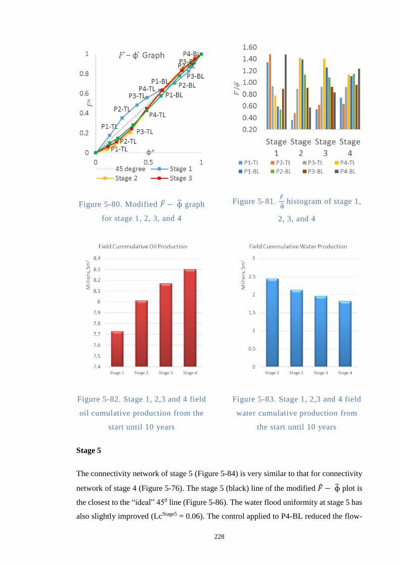
228
Figure 5-80. Modified − ϕ graph
for stage 1, 2, 3, and 4
Figure 5-81.
ϕ histogram of stage 1,
2, 3, and 4
Figure 5-82. Stage 1, 2,3 and 4 field
oil cumulative production from the
start until 10 years
Figure 5-83. Stage 1, 2,3 and 4 field
water cumulative production from
the start until 10 years
Stage 5
The connectivity network of stage 5 (Figure 5-84) is very similar to that for connectivity
network of stage 4 (Figure 5-76). The stage 5 (black) line of the modified − ϕ plot is
the closest to the “ideal” 450 line (Figure 5-86). The water flood uniformity at stage 5 has
also slightly improved (LcStage5 = 0.06). The control applied to P4-BL reduced the flow-
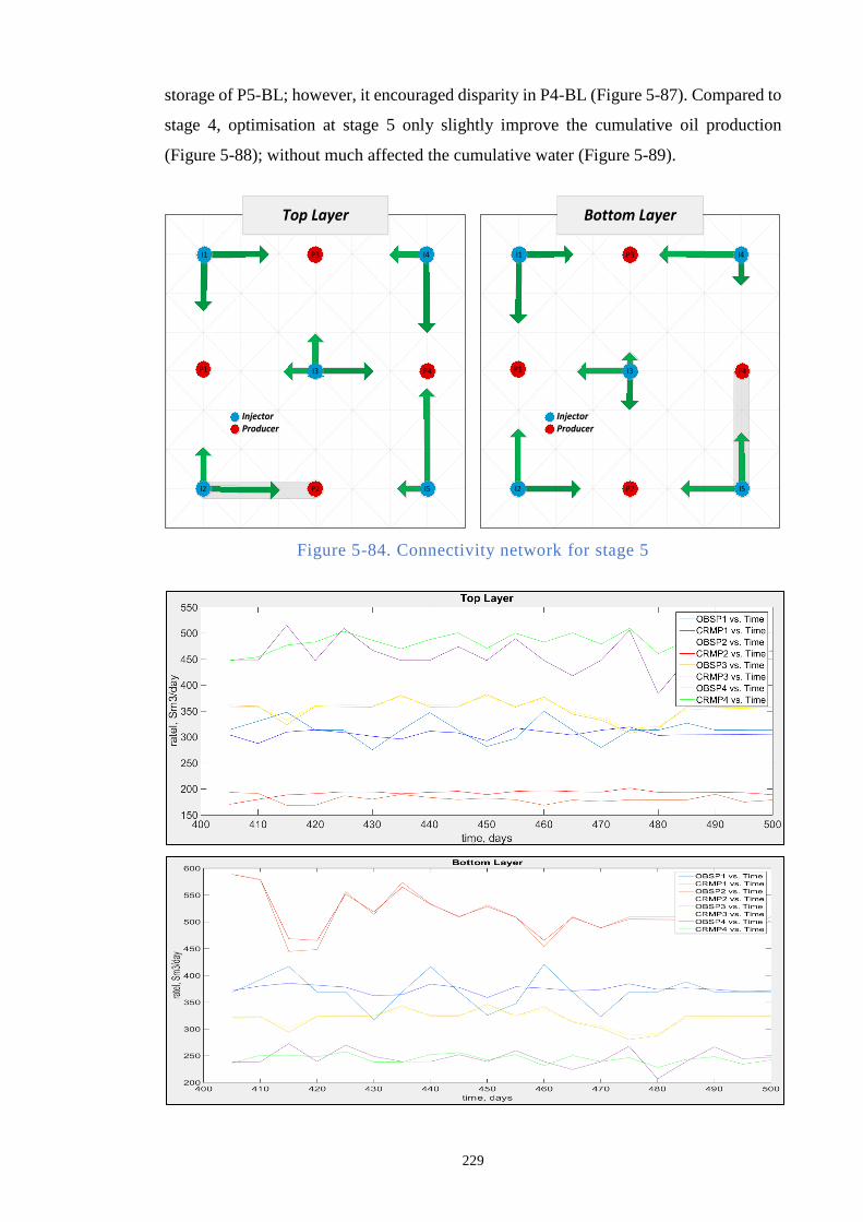
229
storage of P5-BL; however, it encouraged disparity in P4-BL (Figure 5-87). Compared to
stage 4, optimisation at stage 5 only slightly improve the cumulative oil production
(Figure 5-88); without much affected the cumulative water (Figure 5-89).
InjectorProducerInjectorProducer
P1
P3
P4
P2
I3
Top Layer
InjectorProducerInjectorProducer
P1
P3
P2I2
I1
I3
Bottom Layer
P4
I4 I4
I5I5
I1
I2
Figure 5-84. Connectivity network for stage 5
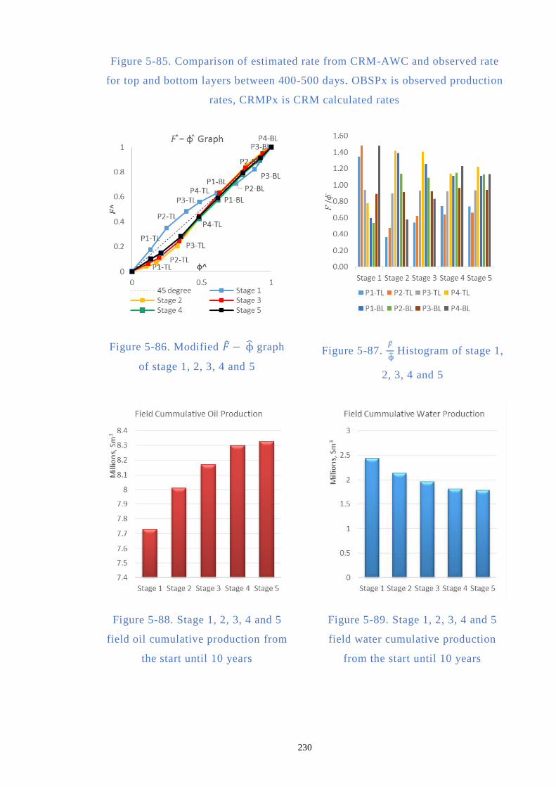
230
Figure 5-85. Comparison of estimated rate from CRM-AWC and observed rate
for top and bottom layers between 400-500 days. OBSPx is observed production
rates, CRMPx is CRM calculated rates
Figure 5-86. Modified − ϕ graph
of stage 1, 2, 3, 4 and 5
Figure 5-87.
ϕ Histogram of stage 1,
2, 3, 4 and 5
Figure 5-88. Stage 1, 2, 3, 4 and 5
field oil cumulative production from
the start until 10 years
Figure 5-89. Stage 1, 2, 3, 4 and 5
field water cumulative production
from the start until 10 years
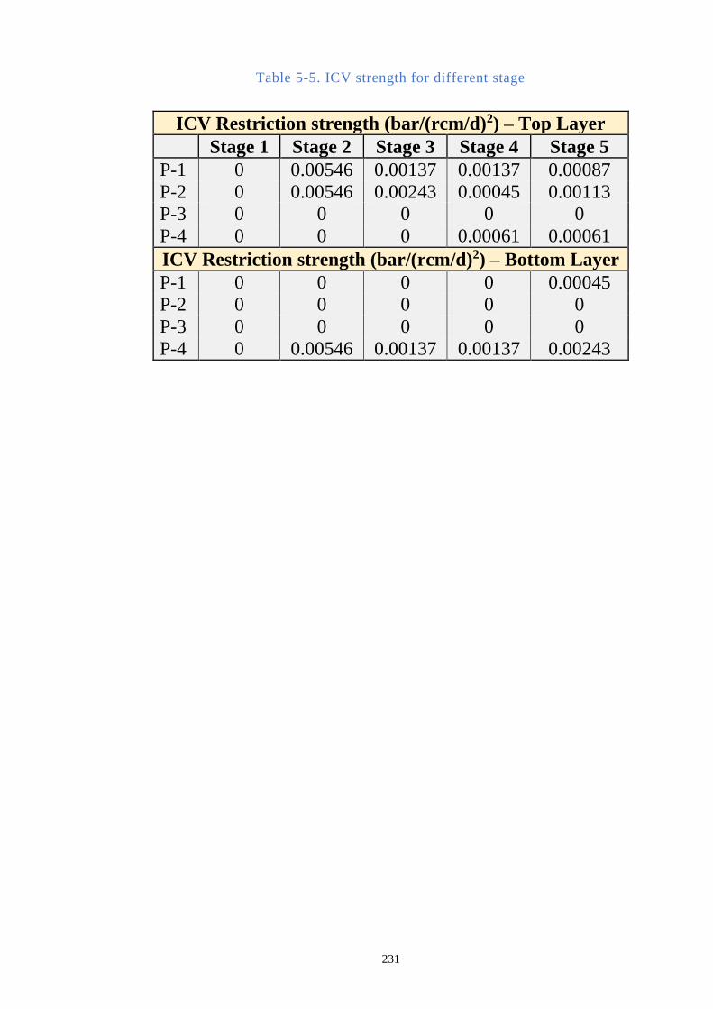
231
Table 5-5. ICV strength for different stage
ICV Restriction strength (bar/(rcm/d)2) – Top Layer
Stage 1 Stage 2 Stage 3 Stage 4 Stage 5
P-1 0 0.00546 0.00137 0.00137 0.00087
P-2 0 0.00546 0.00243 0.00045 0.00113
P-3 0 0 0 0 0
P-4 0 0 0 0.00061 0.00061
ICV Restriction strength (bar/(rcm/d)2) – Bottom Layer
P-1 0 0 0 0 0.00045
P-2 0 0 0 0 0
P-3 0 0 0 0 0
P-4 0 0.00546 0.00137 0.00137 0.00243
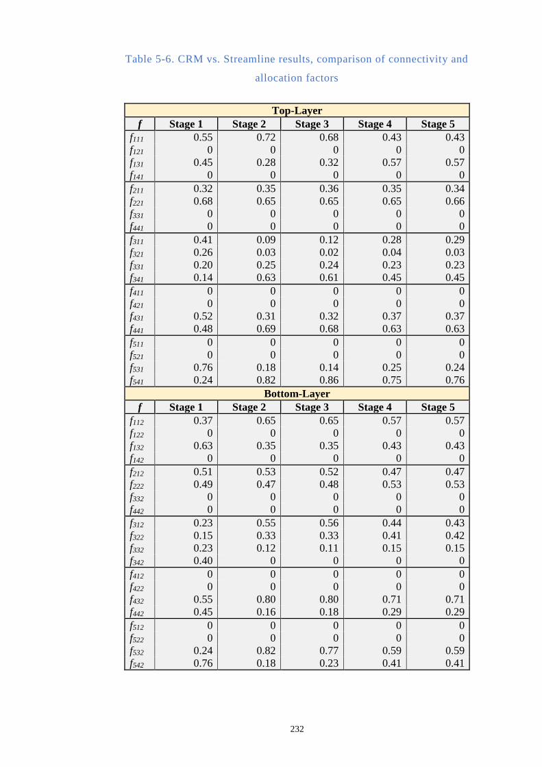
232
Table 5-6. CRM vs. Streamline results, comparison of connectivity and
allocation factors
Top-Layer
f Stage 1 Stage 2 Stage 3 Stage 4 Stage 5
f111 0.55 0.72 0.68 0.43 0.43
f121 0 0 0 0 0
f131 0.45 0.28 0.32 0.57 0.57
f141 0 0 0 0 0
f211 0.32 0.35 0.36 0.35 0.34
f221 0.68 0.65 0.65 0.65 0.66
f331 0 0 0 0 0
f441 0 0 0 0 0
f311 0.41 0.09 0.12 0.28 0.29
f321 0.26 0.03 0.02 0.04 0.03
f331 0.20 0.25 0.24 0.23 0.23
f341 0.14 0.63 0.61 0.45 0.45
f411 0 0 0 0 0
f421 0 0 0 0 0
f431 0.52 0.31 0.32 0.37 0.37
f441 0.48 0.69 0.68 0.63 0.63
f511 0 0 0 0 0
f521 0 0 0 0 0
f531 0.76 0.18 0.14 0.25 0.24
f541 0.24 0.82 0.86 0.75 0.76
Bottom-Layer
f Stage 1 Stage 2 Stage 3 Stage 4 Stage 5
f112 0.37 0.65 0.65 0.57 0.57
f122 0 0 0 0 0
f132 0.63 0.35 0.35 0.43 0.43
f142 0 0 0 0 0
f212 0.51 0.53 0.52 0.47 0.47
f222 0.49 0.47 0.48 0.53 0.53
f332 0 0 0 0 0
f442 0 0 0 0 0
f312 0.23 0.55 0.56 0.44 0.43
f322 0.15 0.33 0.33 0.41 0.42
f332 0.23 0.12 0.11 0.15 0.15
f342 0.40 0 0 0 0
f412 0 0 0 0 0
f422 0 0 0 0 0
f432 0.55 0.80 0.80 0.71 0.71
f442 0.45 0.16 0.18 0.29 0.29
f512 0 0 0 0 0
f522 0 0 0 0 0
f532 0.24 0.82 0.77 0.59 0.59
f542 0.76 0.18 0.23 0.41 0.41
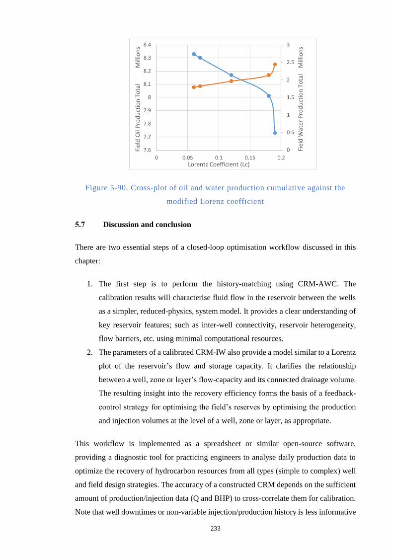
233
Figure 5-90. Cross-plot of oil and water production cumulative against the
modified Lorenz coefficient
Discussion and conclusion
There are two essential steps of a closed-loop optimisation workflow discussed in this
chapter:
1. The first step is to perform the history-matching using CRM-AWC. The
calibration results will characterise fluid flow in the reservoir between the wells
as a simpler, reduced-physics, system model. It provides a clear understanding of
key reservoir features; such as inter-well connectivity, reservoir heterogeneity,
flow barriers, etc. using minimal computational resources.
2. The parameters of a calibrated CRM-IW also provide a model similar to a Lorentz
plot of the reservoir’s flow and storage capacity. It clarifies the relationship
between a well, zone or layer’s flow-capacity and its connected drainage volume.
The resulting insight into the recovery efficiency forms the basis of a feedback-
control strategy for optimising the field’s reserves by optimising the production
and injection volumes at the level of a well, zone or layer, as appropriate.
This workflow is implemented as a spreadsheet or similar open-source software,
providing a diagnostic tool for practicing engineers to analyse daily production data to
optimize the recovery of hydrocarbon resources from all types (simple to complex) well
and field design strategies. The accuracy of a constructed CRM depends on the sufficient
amount of production/injection data (Q and BHP) to cross-correlate them for calibration.
Note that well downtimes or non-variable injection/production history is less informative
0
0.5
1
1.5
2
2.5
3
7.6
7.7
7.8
7.9
8
8.1
8.2
8.3
8.4
0 0.05 0.1 0.15 0.2
Fiel
d W
ater
Pro
du
ctio
n T
ota
lM
illio
ns
Fiel
d O
il P
rod
uct
ion
To
tal
Mill
ion
s
Lorentz Coefficient (Lc)
234
for CRM as they carry little (new) interaction events. An event/history should also be
long enough for the well rates/pressures to react to each other via their inter-well reservoir
volume.
There are several observations we can draw from this chapter:
The CRM workflow turns the routinely recorded data from production/injection
wells into a ‘proxy’ model quantifying the inter-well interactions and capturing the
major trends (or upscaled properties) of the reservoir system. The aim of the CRM
approach is not to replace numerical reservoir simulation, but to be a simple and
practical way of providing insights into the reservoir performance.
Theoretically, CRM could also be used to propose an injection strategy that would
enhance the information content of future production history data, specifically in
terms of a CRM update. In addition, integration of CRM prediction studies with data
from the injection of tracers, and the analysis of transient build-up tests provides
fundamental information on reservoir compartmentalization; this is information that
can be used to constrain the CRM calibration algorithm and improve its accuracy.
However, this will not always be a practical strategy due to the need to wait for weeks
or months before the reservoir’s reaction to well rate changes becomes clearly
interpretable.
The workflow of the new CRM-AWC follows a conventional CRM workflow apart
from the new parameter added to the model: the ICV restriction strength. The ICV
strength (a) was predicted in advance (using equation 2-11) and was treated as the
input parameter for the data calibration. In the scenario where the mechanical
position of the ICV is difficult to locate, and the value of ICV strength (a) becomes
arbitrary, such a procedure can be inverted and ICV strength (a) becomes one of the
CRM-calibrated parameters (along with connectivity and time-storage). This type of
inverse analysis is also applicable for cases where the prediction of ICV strength
using an explicit model (such as equation 2-11) is not recommended (e.g. eroded or
plugged valve).
This work used data generated by reservoir simulator and thus a noise free
experiment. In practical cases, the data required are measured in the field and may
be noisy due to measurement errors or fluctuations. Such noise must be reduced,
controlling the quality of the data used to model the reservoir. Cao, 2011; Weber,
235
2009; Kaviani et al, 2014; Holanda et al, 2015 suggest methods to deal with noise
and measurement errors to better evaluate the CRM model.
The modified flow-capacity storage ( − ϕ) graph reveals the rate-drainage
disparity and can be treated as a “guide” for selecting (or prioritising) which layer(s)
are most needed to be controlled. However, the graph does not specify the required
restriction for these layers. For example, in the case study of the 5I-4P synthetic field,
stage 3 control (whereby ICV valve is “fine-tuned” for a more appropriate restriction
strength) proved to be more effective than stage 2 control. Formulating the CRM-
AWC into a 1D system (Lerlertpakdee, and Jafarpour, 2014) and integrating it with
the Buckley-Leverett for the AWC solution, as explained in Chapter 3 might possibly
address this issue. The integration between CRM-AWC and Buckley-Leverett could
potentially translate the CRM’s conductivity/connectivity into permeability, or
parameters which practicing engineers commonly use. Such relationship is useful to
avoid calibrating the permeability values during history matching or avoiding any
inefficient history matching or optimisation tasks.
The disparity of the well’s (or layer’s) flow-capacity storage can be measured
quantitatively using the Lorenz coefficient (Lc). This parameter has a similar role
with the Inflow Variation (IV) parameter in Chapter 2; that is, it indicates the long-
term objectives of the reservoir management. Hence, the reduction of Lc becomes
the objective of each optimisation. In our case study, control action (i.e. task to reduce
the production and injection) for the otherwise inefficient layers is carried out without
lowering the total well’s productivity index. This can be done by maintaining the
production and injection rates control for each well, e.g. reduced production from
bottom-layer of a well will be compensated by its top layer.
Our hypotheses is there is a perfectly balanced well/layers contribution which yields
to optimal solution. We also showed in our case study that adjusting inflow to move
the modified Lorenz curve towards the 450 degree straight line suggested it will
improve the reservoir performance. However, without more robust testing such a
production varies significantly with small variations in Lorenz curve; also
diminishing its comparison to other optimisation method, etc. We hope to inspire
future researcher to do more work to test the assertion that the optimal solution
correlates with the modified Lorenz curve-based one.
In conclusion, this chapter has presented Capacitive Resistance Models in a new form for
236
reservoir characterisation and zonal, intelligent well control (i.e. CRM-AWC) that
includes the non-linear pressure drop from FCDs. The new CRM solution can be extended
to different levels of reservoir complexity such as single- or multi-layers with or without
cross-flow. Furthermore, the CRM-AWC calibration generates the parameters for a
production optimisation workflow based on the modified Lorenz plot. This chapter also
propose a new way to optimise the ICV before a water breakthrough (proactive
optimisation) using the CRM’s derived parameters (connectivity and time-storage). The
proposed technique adopted the ideas behind the classic Lorenz plot and translated it into
water flood operations. Unlike most production optimisation strategies that are based on
complex mathematical equations, this approach uses an engineering-based understanding
of a relationship between a well’s (or layer’s) flow-capacity against its associated
drainage volume. The workflow is employed as an intuitive, simple approach for AWC
production optimisation.
Summary
This chapter reports the application of a new analytical solution for the CRM in the
presence of AWC to manage the production and injection from a reservoir that provides
a continuous data stream of sand face pressure measurements. This chapter also discusses
the importance of considering the CRM’s properties (connectivity and time-storage) as
dynamic properties. We investigated a real field case of a thermal-induced-fracture (TIF)
reservoir using the principle of a dynamic CRM to estimate the likely TIF growth impact
and direction. When dealing with AWC, the ICV action (closing and opening the valve)
altered the well/zone drainage control. This provides an opportunity to optimise the
waterflood operations, such as reallocating the injection rate by choking ICVs.
In summary, we have presented:
A review of the CRM.
The application of a Capacitance-Resistance Model (CRM) to inform dynamic well
control.
A case history for a reservoir with Thermally Induced Fractures.
Development of the CRM to the case of wells with AWC (i.e. CRM-AWC).
Analytical solutions were presented for different form of CRMs.
Example application of the CRM-AWC in a single-layer reservoir. The examples
illustrated the method’s value and potential.
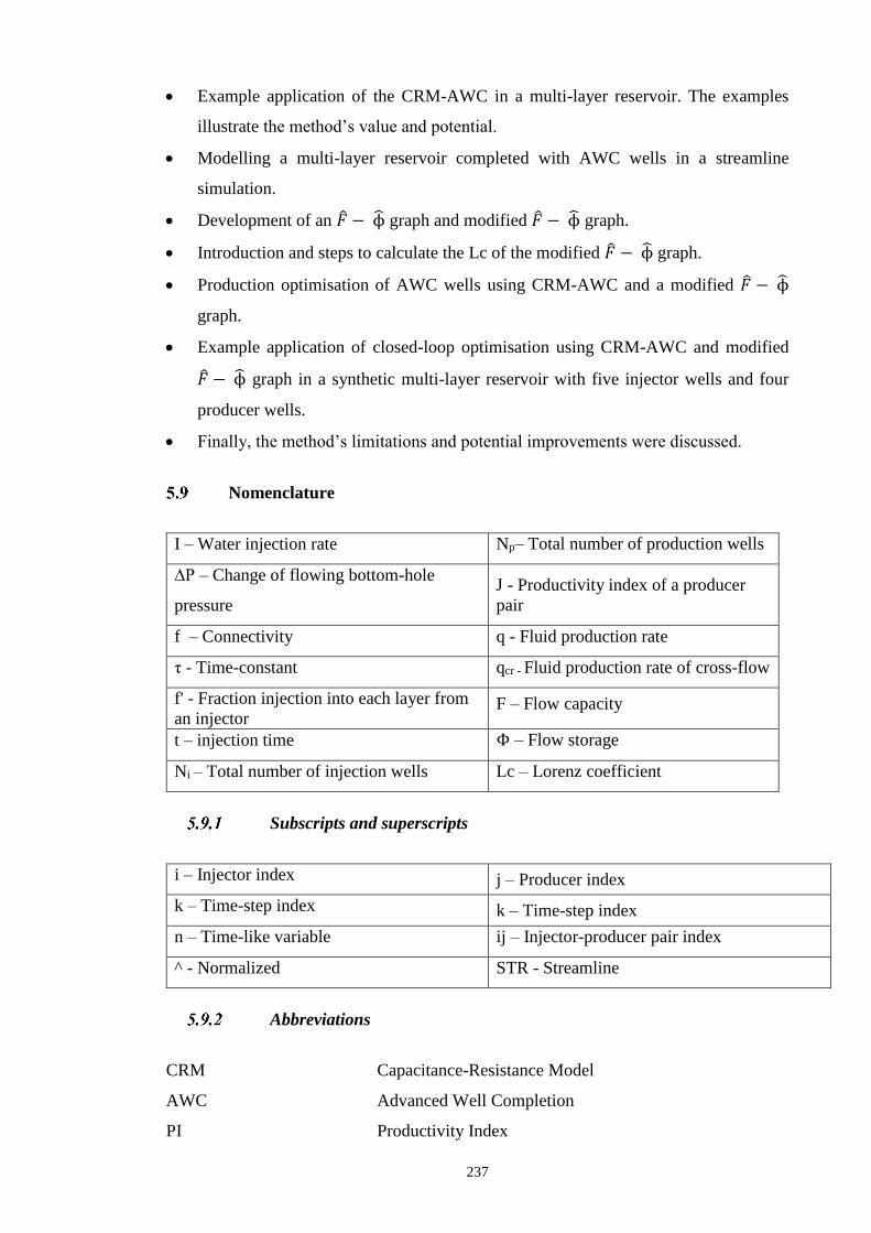
237
Example application of the CRM-AWC in a multi-layer reservoir. The examples
illustrate the method’s value and potential.
Modelling a multi-layer reservoir completed with AWC wells in a streamline
simulation.
Development of an − ϕ graph and modified − ϕ graph.
Introduction and steps to calculate the Lc of the modified − ϕ graph.
Production optimisation of AWC wells using CRM-AWC and a modified − ϕ
graph.
Example application of closed-loop optimisation using CRM-AWC and modified
− ϕ graph in a synthetic multi-layer reservoir with five injector wells and four
producer wells.
Finally, the method’s limitations and potential improvements were discussed.
Nomenclature
I – Water injection rate Np– Total number of production wells
∆P – Change of flowing bottom-hole
pressure
J - Productivity index of a producer
pair
f – Connectivity q - Fluid production rate
τ - Time-constant qcr - Fluid production rate of cross-flow
f' - Fraction injection into each layer from
an injector F – Flow capacity
t – injection time Φ – Flow storage
Ni – Total number of injection wells Lc – Lorenz coefficient
Subscripts and superscripts
i – Injector index j – Producer index
k – Time-step index k – Time-step index
n – Time-like variable ij – Injector-producer pair index
^ - Normalized STR - Streamline
Abbreviations
CRM Capacitance-Resistance Model
AWC Advanced Well Completion
PI Productivity Index

238
TIF Thermal Induced Fracture
CRMT CRM for single tank representation of a field
CRMP CRM for a given Producer
CRMIP CRM for a given pair of Producer-Injector
CRM-ML CRM for a given Producer - Multi-Layered reservoir, no
cross-flow
CRMP-MLCr CRM for a given Producer - Multi-Layered reservoir with
Crossflow
CRMP-AWC CRMP-ML for a given producer with Advanced Well
Completion
CRMP-ML-AWC CRMP-ML for a given producer with Advanced Well
Completion
CRMP-MLCr-AWC CRMP-MLCr for a given producer with Advanced Well
Completion
BHP Bottom Hole Pressure
MHI Modified Hall Integral
FMI Formation Micro Imager
ICV Interval Control Valves

239
Chapter 6 – Conclusions and Future Work
Discussion
The advancement of well technology has enabled us to build wells which would not only
intersect multiple reservoir layers (e.g. horizontal well, multi-lateral well), but also have
means of controlling and monitoring the production performance with the advent of
AWC. These completions typically incorporate permanent downhole sensors, active
surface-controlled downhole inflow flow control valves (ICV), or autonomous and non-
autonomous passive downhole inflow control devices ((A)ICD). These well’s
components will monitor, evaluate, and actively manage production (or injection) in real
time without any well interventions. Controlling the production performance has been
possible by installing the inflow control technology in the completion tubing to restrict
the amount of influx coming to the well. The gauges or sensors mounted in the completion
will measure the pressure and temperature of respected depth/layers which can be
processed further to be interpreted as flow rate, pressure, skin, and many other important
reservoir parameters.
There are three different topics in this thesis, dedicated to three main application areas of
AWC technologies.
1. ICD system. This is mainly covered in chapter 3.
2. AFCD system. This is mainly covered in chapter 4.
3. ICV and monitoring system. This is mainly covered in chapter 5.
We described the development of our models separately to illustrate how they solve issues
encountered by each system, such as: the lack of simple modelling to fine-tune the ICD
design; predicting long-term parameters of AFCD completion using an efficient model,
the necessity to extract meaningful information from pressure and rate data in the ICV
and monitoring system. Bear in mind that, each of above systems have their specific
operational differences, and thus it is important to evaluate the operational applicability
of equations we presented in this thesis. For example, ICD and AFCD completions are
modular that are typically installed with more than 20ea modules in a horizontal well.
ICD and AFCD completions are often not supported with full-monitoring system, e.g.
only one PT gauge is installed on the top of the lower completion. Due to these operational

240
limitations, CRM-ML-AWC may not be applicable for these systems. On the other hand,
there is a number of scenario with monitoring and AWC technologies installed on one
well. For example: a multi-lateral well with both ICV and monitoring system are operated
in the upper completion, while ICDs and AFCDs are installed in the lower completion.
This strategy is aimed to address multifaceted problems that require deeper analysis, and
engineers should employ combination of various models. We briefly introduced a case
where coupling of the type-curve design (chapter 3) and the extended BL-method for
AWC (chapter 4) can address the short-term vs. long-term evaluation of an AWC well.
In the future, more analysis can be done to test and analyse combination of all our
developed models.
This thesis focuses on the development of the methods to model and design AWC flow
performance, rather than using the conventional grid-based numerical simulation. The
proposed illustrate the advantage of the reduced-physics models to capture the main-
trends of the reservoir and access some key reservoir information with a much-reduced
computational time. Complex numerical simulation is often over-detailed and uncertain.
The methods developed in this thesis provide a good insight into the AWC’s performance
as well as being used to calibrate or verify a comprehensive numerical model if needed.
It has been recognised as good practice to employ many models of varying complexity
rather than depending only on a single model. The semi-analytical models developed are
simple, transparent, and allow engineers to perform AWC evaluations in an easily
understood form. The ideal workflow as suggested by (Hey, Tansley and Tolle, 2009) is
to use all available models including analytical, statistical (data intensive), and numerical
models to complement each other (Figure 6-1).
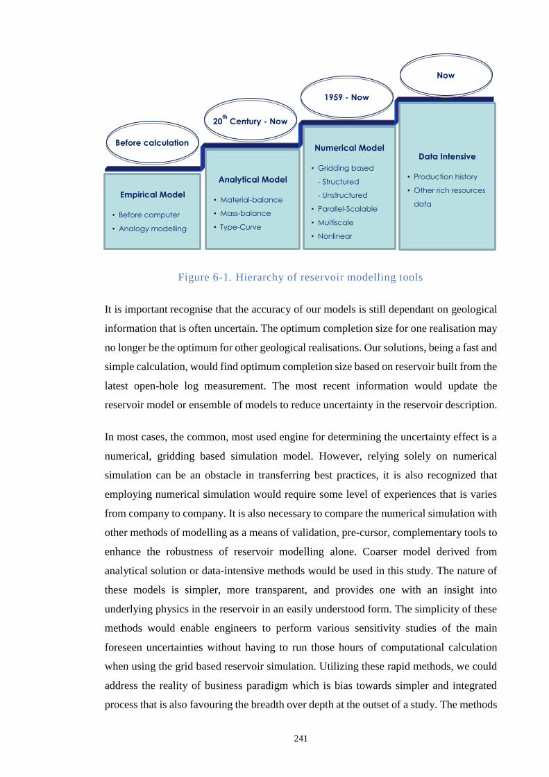
241
Figure 6-1. Hierarchy of reservoir modelling tools
It is important recognise that the accuracy of our models is still dependant on geological
information that is often uncertain. The optimum completion size for one realisation may
no longer be the optimum for other geological realisations. Our solutions, being a fast and
simple calculation, would find optimum completion size based on reservoir built from the
latest open-hole log measurement. The most recent information would update the
reservoir model or ensemble of models to reduce uncertainty in the reservoir description.
In most cases, the common, most used engine for determining the uncertainty effect is a
numerical, gridding based simulation model. However, relying solely on numerical
simulation can be an obstacle in transferring best practices, it is also recognized that
employing numerical simulation would require some level of experiences that is varies
from company to company. It is also necessary to compare the numerical simulation with
other methods of modelling as a means of validation, pre-cursor, complementary tools to
enhance the robustness of reservoir modelling alone. Coarser model derived from
analytical solution or data-intensive methods would be used in this study. The nature of
these models is simpler, more transparent, and provides one with an insight into
underlying physics in the reservoir in an easily understood form. The simplicity of these
methods would enable engineers to perform various sensitivity studies of the main
foreseen uncertainties without having to run those hours of computational calculation
when using the grid based reservoir simulation. Utilizing these rapid methods, we could
address the reality of business paradigm which is bias towards simpler and integrated
process that is also favouring the breadth over depth at the outset of a study. The methods
Before calculation
Empirical Model
• Before computer
• Analogy modelling
Analytical Model
• Material-balance
• Mass-balance
• Type-Curve
Numerical Model
• Gridding based
- Structured
- Unstructured
• Parallel-Scalable
• Multiscale
• Nonlinear
Data Intensive
• Production history
• Other rich resources
data
Now
1959 - Now
20th
Century - Now
242
introduced in this study are not an alternative for the established, common way or
predicting reservoir performance via gridding-based simulator, but as a rough-sketch or
blueprint of a reservoir model.
The new equations presented in this thesis to describe both the short- and long-term AWC
performance. They are made possible by the flow performance of a standard FCD being
described by a quadratic equation with the help of an empirical constant called FCD’s
strength (a). This parameter also allows approximating the published data from flow-loop
testing which presents the relationship between the FCD’s pressure drop and flow rate.
In the past few years however, a new generation of AFCDs shows a different rate vs.
pressure drop relationship. Hence, new AWC analytical equations that honour the type of
non-linear pressure drop of such FCDs may be required. The key approach to derive these
new equations is to incorporate the FCD’s pressure drop as an additional element in the
system of the equation, add together with other pressure drops in the specific observed
system, e.g. pressure drop of Darcy’s law, two-phase Buckley-Leverett’s pressure drop,
or CRM. We hope that future researchers will be inspired by our workflows to develop
AWC performance models for the new generations of AWCs.
Conclusion
In summary, the achievements of this work are the development of analytical models and
workflows that are able:
Chapter 3 examines the:
1. Short-term (a.k.a. ‘snapshot’) added values of installing AWCs in wells with
dominating heel-toe effect.
2. Short-term added values of installing AWCs in wells in heterogeneous reservoirs
with dominating inflow imbalance due to the heterogeneity.
Chapter 4 examines the:
3. Long-term AWC value derived by controlling the zonal flow rate in light oil
(when the piston-like displacement assumption is valid) waterflood scenarios.
4. Long-term AWC value derived by controlling the zonal flow rate in
medium/heavy oil (i.e. both piston and non-piston-like displacement) waterflood
scenarios.

243
Chapter 5 characterises the reservoir and inter-well connectivities to:
5. Assess the effectiveness of both conventional and the zonal, intelligent well
control.
6. Optimally control wells and/or ICVs for improved recovery.
Future work
The effort to advance the fast, transparent, data-driven modelling that capture (reduced)
physics involved in Advanced Well Completion is far from complete. Many areas for
research and improvements remain. Based on the work presented in this thesis, possible
extensions for the future work include:
Chapter 3:
1. A comprehensive evaluation tool can be developed advising how to make a choice
between installing constant or variable strength of flow control devices in an AWC.
The motivation for this research is to investigate the prevalent assumption that
installing constant size/strength AWC in wells is more robust against geological and
operational uncertainty, than installing a variable strength one. The studies would
review major aspects dictating the choice and quantify the value difference between
two different methodologies.
2. Develop an analytical model for the reduction of flow imbalance in a heterogeneous
reservoir in a long horizontal well when the heel-toe effect is no longer negligible.
The main assumption for analytical model of the ICD performance in heterogeneous
reservoir is that the pressure losses along the well are small compared to the reservoir
drawdown. We observed that there are cases where this is no longer the case and
adjustment for the new analytical formulation is needed.
Chapter 4:
1. Further investigation of the proposed methods in the presence of a strong gas-cap.
We have presented robust investigation about extending the fractional flow model to
include the response of non-linear pressure drop of the flow control devices. So far
244
the studies have been focused on the water-oil system, meanwhile there are many
AWC application in the presence of a gas-cap. The study could start by assuming an
immiscible gas-oil system, and then followed by the gas-water-oil system. The
outcome of such study would be the basis for future immiscible system.
2. Implement the proposed methods where the areal sweep efficiency (Ea) is not 100%.
Note that the oil recovery factor is the product of the efficiency of oil displacement
by water and the volumetric sweep efficiency (the extent of the water front on the
reservoir level). The latter is the product of the areal and vertical sweep efficiencies
(Ea). Chapter 4’s main assumption is that there is 100% Ea, while in reality this is
often not the case since Ea is the function of rock and fluids properties. The Ea value
can be found by other means, e.g. mathematical models of Dyes et al., 1954 or core
flooding experiments respectively.
3. The proposed workflows in this chapter assume strong water drive which enables a
perfect voidage replacement or steady-state conditions. Further model developments
for non-steady state conditions are desirable.
Such system would no longer follow the assumption of incompressible flow and this
study may have to consider the alternatives of fractional flow model.
4. Further investigation when there is pressure communication between layers.
Analytical solutions for vertical sweep efficiency in heterogeneous reservoirs require
two assumed situations: the layers can either be non-communicating or are perfectly
communicating (i.e. instantaneous, vertical, pressure equilibrium). The investigation
presented in chapter 4 deals with the non-communicating layers assumptions and
there is good opportunity to extend the findings for the situation where the layers have
good communication. This future work should start from the condition where there is
a perfect (instantaneous) equilibrium between layers. The available classical
waterflood method for a gravity dominated flow can be coupled to include the
advanced well completion.
5. Development of a semi-analytical model where the capillary pressure is non-trivial.
The analysis so far has been focussing around the displacement where diffuse flow
occurrs, and it is assumed that ahead of displacement interface, only oil is flowing
245
with water present at Swc. In reality, there would be a transition zone between these
two phases, associated with the imbibition capillary curve, i.e. Pc is no longer
negligible. Furthermore, this is especially important for AWC application where the
horizontal wells are completed in the transition zone, close to water-oil contact. It is
recommended to start this study from available studies of the classical waterflood
method where Buckley-Leverett was applied to the reservoirs with some degree of
capillary pressure. Such models can be extended to include the non-linear pressure
drop from flow control devices.
Chapter 5:
1. Automating the CRM event detection using the Integration of CRM-AWC with
ensemble Kalman-filter (EnKF).
Using CRM-AWC as the driving dynamical system describing the reservoir, a future
study can implement the ensemble EnKF procedure that estimates the CRM
parameters (interconnectivity, time lag, etc.) to obtain a time dependent estimate for
the parameters. These parameters can be automatically interpreted to detect events
such as well control or changed ICV strength, and change of reservoir properties, due
to a thermal induced fracture from cold water injectors. The uncertainty involved with
interwell connectivities and time lags can be systematically reduced with the EnKF
procedure (Jafroodi and Zhang, 2011).
2. Comparison between the optimal scenario based on − ϕ graph and optimal scenario
based on the proactive/reactive optimisation concepts by (Sefat, 2016) and
(Grebenkin, 2013).
Comparing the result from our proposed modified Lorenz plot – CRM-AWC with
common production optimisation strategies production such as Genetic Algorithm,
Simultaneous-Perturbation Stochastic Approximation (SPSA), etc. Additionally, this
study can do more robust testing such as production varies significantly with small
variations in Lorenz curve to test the assertion that the optimal solution correlates with
the modified Lorenz.
3. Implementing CRM-AWC as a forward predictive model.

246
The modified flow-capacity storage (F - ϕ ) graph does not specify the required
restriction for layers. Formulating the CRM-AWC into a 1D system (Lerlertpakdee,
and Jafarpour, 2014) and integrating it with the Buckley-Leverett for the AWC
solution, is possible to quantify the required specific restriction and can be used as a
forward predictive model. This solution may well possibly quantify the required
restriction to optimize the recovery of hydrocarbon resources.
247
Bibliography
Abd Elfattah, M., Al-Yateem, K., Qahtani, H., & Rajabian, B. (2013) ‘Variable Nozzle–
Based Inflow Control Device Completion: Inflow Distribution Comparison, Analysis,
and Evaluation’, International Petroleum Technology Conference. Beijing, China:
International Petroleum Technology Conference.
Addiego-Guevara, E., Jackson, M. D., & Giddins, M. A. (2008). Insurance Value of
Intelligent Well Technology against Reservoir Uncertainty. SPE/DOE Symposium on
Improved Oil Recovery, Tulsa, Oklahoma, USA, Society of Petroleum Engineers.
Aguilera, R. (1991). Horizontal wells : [formation evaluation, drilling, and production,
including heavy oil recovery], Contributions in petroleum geology & engineering. Gulf
Pub. Co.
Ajayi A. A. (2007) 'Theory and Application of Probabilistic Method of Designing
Customized Interval Control Valves Choke Trim for Multizone Intelligent Well Systems',
SPE Annual Technical Conference and Exhibition. California, U.S.A: Society of Petroleum
Engineers.
Akbari, M., Gonzalez, J. R. and Macklin, N. (2014) 'Considerations for Optimum Inflow
Control Devices (ICDs) Selection and Placement in Horizontal Sections', SPE Russian
Oil and Gas Exploration & Production Technical Conference and Exhibition. Moscow,
Russia: Society of Petroleum Engineers.
Al-Khelaiwi, F. T., Birchenko, V. M., Konopczynski, M. R., & Davies, D. (2010)
‘Advanced Wells: A Comprehensive Approach to the Selection Between Passive and
Active Inflow-Control Completions’, SPE Production & Operations. Society of
Petroleum Engineers, 25(3), pp. 305–326.
Alghareeb, Z., Horne, R. N., Yuen, B. B. W., & Shenawi, S. H. (2009) ‘Proactive
Optimization of Oil Recovery in Multilateral Wells Using Real Time Production Data’,
SPE Annual Technical Conference and Exhibition. New Orleans, Louisiana, U.S.A:
Society of Petroleum Engineers.
Alhuthali, A. H. H., Datta-Gupta, A., Yuen, B. B. W., & Fontanilla, J. P. (2008) ‘Optimal
Rate Control Under Geologic Uncertainty’, SPE/DOE Symposium on Improved Oil Recovery.
Tulsa, Oklahoma, U.S.A: Society of Petroleum Engineers.
248
Almarri, M., Prakasa, B., Muradov, K., & Davies, D. (2017) ‘Identification and
Characterization of Thermally Induced Fractures Using Modern Analytical Techniques’,
SPE Kingdom of Saudi Arabia Annual Technical Symposium and Exhibition. Dammam,
Saudi Arabia: Society of Petroleum Engineers.
Al Marzouqi, A. A. R., Helmy, H., Keshka, A. A.-S., Elasmar, M., & Shafia, S. (2010)
‘Wellbore Segmentation using Inflow Control Devices : Design and Optimisation
Process’. Abu Dhabi International Petroleum Exhibition and Conference. Abu Dhabi,
UAE: Society of Petroleum Engineers.
Almeida, L. F., Vellasco, M. M. B. R. and Pacheco, M. A. C. (2010) ‘Optimization system
for valve control in intelligent wells under uncertainties’, Journal of Petroleum Science
and Engineering. Elsevier B.V., 73(1–2), pp. 129–140.
Anklam, E. G. and Wiggins, M. L. (2005) ‘A Review of Horizontal-Wellbore Pressure
Equations’, SPE Production and Operations Symposium, p. 7.
Babu, D. K. and Odeh, A. S. (1989) ‘Productivity of a Horizontal Well’, SPE Reservoir
Engineering, 4(4), pp. 417–421.
Bailey, W. J. & Couet, B. 2005. ‘Field OptimisationTool for Maksimising asset Value’,
SPE Reservoir Evaluation & Engineering, 8, 7-21.
Beliveau, D. (1995) ‘Heterogeneity, Geostatistics, Horizontal Wells, and Blackjack
Poker’, SPE Journal.
Birchenko, V. M., Demyanov, V., Konopczynski, M. R., & Davies, D. R. (2008) ‘Impact
of Reservoir Uncertainty on Selection of Advanced Completion Type’ SPE Annual Technical
Conference and Exhibition, Denver, Colorado, U.S.A: Society of Petroleum Engineers.
Birchenko, V. (2010) ‘Analytical modelling of wells with inflow control devices’, PhD
Thesis, Heriot-Watt University.
Birchenko, V. M., Bejan, A. Lu., Usnich, A. V., Davies, D. R (2011a) ‘Application of
inflow control devices to heterogeneous reservoirs’, Journal of Petroleum Science and
Engineering, 78(2), pp. 534–541.
Birchenko, V. M., Muradov, K. M. and Davies, D. R. (2010) ‘Reduction of the horizontal
well’s heel-toe effect with inflow control devices’, Journal of Petroleum Science and
Engineering. Elsevier B.V., 75(1–2), pp. 244–250.
Birchenko, V. M., Usnich, A. V. and Davies, D. R. (2010) ‘Impact of frictional pressure
losses along the completion on well performance’, Journal of Petroleum Science and
249
Engineering. Elsevier B.V., 73(3–4), pp. 204–213.
Borisov, J. P. (1984) ‘Oil Production Using Horizontal and Multiple Deviation Wells’,
Translated into english by J. Strauss, edited by S. D. Joshi, Phillips Petroleum Co.
Brekke, K. and Lien, S. C. (1994) ‘New , Simple Completion Methods for’, SPE Drilling
& Completion, pp. 205–209.
Burda, B., Crompton, J., Sardoff, H. M., & Falconer, J. (2007) ‘Information Architecture
Strategy for the Digital Oil Field’, Digital Energy Conference and Exhibition, Houston,
Texas, U.S.A : Society of Petroleum Engineers.
Cheung, C. M., Goyal, P., Harris, G., Patri, O., Srivastava, A., Zhang, Y., … Prasanna,
V. K. (2015) ‘Rapid Data Integration and Analysis for Upstream Oil and Gas
Applications’, SPE Annual Technical Conference and Exhibition. Houston, Texas,
U.S.A: Society of Petroleum Engineers.
Chierici, G. l. (1995) Principles of Petroleum Engineering. Vol 2. Berlin: Springer
Verlag.
Cho, H. and Shah, S. N. (2002) ‘Optimization of well length for horizontal drilling’,
Journal of Canadian Petroleum Technology, 41(5), pp. 54–62.
Corbett, P. (2012) ‘Petroleum Geoscience', MSc. Petroleum Engineering Module, Heriot-
Watt University.
Cullick A. S. and Sukkestad T. (2010). ‘Smart Operations with Intelligent Well Systems.
SPE 126246, SPE Intelligent Energy Conference and Exhibition’, Society of Petroleum
Engineers. Utrecht, The Netherlands, Society of Petroleum Engineers.
Daneshy, A. A., Guo, B., Krasnov, V., & Zimin, S. (2012) ‘Inflow-Control-Device
Design: Revisiting Objectives and Techniques’, SPE Production & Operations, 27(1),
pp. 44–51.
Davies, D. (2012) 'Production Technology', MSc. Petroleum Engineering Module,
Heriot-Watt University.
Denney, D. (2012) ‘Intelligent-Well-Monitoring Systems: Review and Comparison’,
Journal of Petroleum Technology, 64(09), pp. 27–29.
Dikken, B. J. (1990) ‘Pressure drop in horizontal wells and its effect on production
performance’, SPE Journal, 42(11), pp. 1426–1433.
250
Dilib, F. A., Jackson, M. D., Mojaddam Zadeh, A., Aasheim, R., Årland, K., Gyllensten,
A. J., & Erlandsen, S. M (2013) ‘Closed-Loop Feedback Control for Production
Optimization of Intelligent Wells Under Uncertainty’, SPE Production & Operations,
28(4), pp. 345–357.
Dowlatabad, M. (2015) ‘Novel Integrated Approach Simultaneously Optimising AFI
Locations Plus Number and (A)ICD Sizes’, EUROPEC. Madrid, Spain: Society of
Petroleum Engineers.
El-khatib, N. A. F (2011) ‘The Modification of the Dykstra-Parsons Method for Inclined
Stratified Reservoirs’, SPE Middle East Oil and Gas Show and Conference. Manama,
Bahrain: Society of Petroleum Engineers.
Elgaghah, S. A., Osisanya, S. O. and Tiab, D. (1996) ‘A Simple Productivity Equation
for Horizontal Wells Based on Drainage Area Concept’, SPE Western Regional Meeting.
Anchorage, Alaska: Society of Petroleum Engineers.
Eltaher, E. (2017) ‘Modelling and Applications of Autonomous Flow Control Devices’,
PhD Thesis, Heriot-Watt University.
Eltaher, E. M. K., Sefat, M. H., Muradov, K., & Davies, D. (2014) ‘Performance of
Autonomous Inflow Control Completion in Heavy Oil Introduction to Advanced Well
Completions’, International Petroleum Technology Conference, Kuala Lumpur,
Malaysia: International Petroleum Technology Conference.
Faisal Al-Khelaiwi (2013) ‘A Comprehensive Approach to the Design of Advanced Well
Completions Faisal Turki Manee Al-Khelaiwi', PhD Thesis, Heriot-Watt University.
Fu, X., Li, G., Huang, Z., & Chi, H. (2014) ‘The Principle of Target Influx Selection and
the Optimization Process of Variable-ICD Completion Design for Heterogeneous
Reservoirs Reservoir model‘, SPE Deepwater Drilling and Completions Conference,
Texas, U.S.A: Society of Petroleum Engineers.
Furui, K., Zhu, D. and Hill, A. D. (2005) ‘A Comprehensive Skin-Factor Model of
Horizontal-Well Completion Performance’, SPE Production & Operations, 20(3), pp.
207–220.
Gao, C. H., Rajeswaran, R. T., & Nakagawa, E. Y. (2007) ‘A Literature Review on Smart-
Well Technology’, Production and Operations Symposium. Oklahoma City, Oklahoma,
U.S.A: Society of Petroleum Engineers.
Garcia, G. A., Coronado, M. P. and Gavioli, P. (2009) ‘Identifying Well Completion
Applications for Passive Inflow Control Devices’, SPE Annual Technical Conference and
251
Exhibition, New Orleans, Louisiana, U.S.A: Society of Petroleum Engineers.
Gavioli, P., Vicario, R. and Hughes, B. (2012) ‘The Evolution of the Role of Openhole
Packers in Advanced Horizontal Completions : From Novel Technology to a Critical Key
to Success’, SPE Asia Pacific Oil and Gas Conference and Exhibition. Brisbane,
Queensland, Australia: Society of Petroleum Engineers.
Giger, F. M. (1984) ‘The Reservoir Engineering Aspects of Horizontal Drilling’, SPE
Annual Technical Conference and Exhibition, Houston, Texas, U.S.A: Society of
Petroleum Engineers.
Grebenkin, I. and Davies, D. (2010) ‘Analysis of the Impact of an Intelligent Well
Completion on the Oil Production Uncertainty’, SPE Russian Oil and Gas Conference
and Exhibition. Moscow, Russia: Society of Petroleum Engineers.
Grebenkin, I. M. and Davies, D. R. (2012) ‘A Novel Optimisation Algorithm for Inflow
Control Valve Management’, SPE Europec/EAGE Annual Conference. Copenhagen,
Denmark: Society of Petroleum Engineers.
Grubert, M. A., Wan, J., Ghai, S. S., Livescu, S., Brown, W. B., & Long, T. A. (2009)
‘Coupled Completion and Reservoir Simulation Technology for Well Performance
Optimization’, SPE Annual Technical Conference and Exhibition. New Orleans,
Louisiana, U.S.A: Society of Petroleum Engineers.
Halliburton (2012), NETool Reference Manual. Halliburton
Halliburton (2017), NETool List of publications. Halliburton
Halvorsen, M., Elseth, G. and Nævdal, O. M. (2012) ‘Increased oil production at Troll by
autonomous inflow control with RCP valves’, SPE Annual Technical Conference and
Exhibition. San Antonio, Texas, U.S.A: Society of Petroleum Engineers.
Hasan, A. I., Echeverria-Ciaurri, D., Foss, B. A., & Kleppe, J. (2009) ‘Discrete Optimization
of Oil Production in Thin Oil Rim Reservoir under Geological Uncertainty’, SPE Asia
Pacific Oil and Gas Conference & Exhibition, Jakarta, Indonesia: Society of Petroleum
Engineers.
He, Y., Cheng, S., Li, L., Mu, G., Zhang, T., Xu, H., (2017) ‘Waterflood Direction and
Front Characterization With Four-Step Work Flow: A Case Study in Changqing Oil Field,
China’, SPE Reservoir Evaluation & Engineering, 20(3), pp. 708–725.
252
Henriksen, K., Augustine, J. and Wood, E., "Integration of New Open Hole Zonal
Isolation Technology Contributes to Improved Reserve Recovery and Revision in the
ndustri Best Practices", SPE International Improved Oil Recovery Conference in Asia
Pacific. Kuala Lumpur, Malaysia: Society of Petroleum Engineers.
Henriksen, K. H., Gule, E. I. and Augustine, J. R. (2006) ‘Case Study: The Application
of Inflow Control Devices in the Troll Oil Field’, SPE Europec/EAGE Annual Conference
and Exhibition. Vienna, Austria: Society of Petroleum Engineers.
Hill, A. and Zhu, D. (2008) ‘The Relative Importance of Wellbore Pressure Drop and
Formation Damage in Horizontal Wells’, SPE Production & Operations, 23(2).
Hird, K., Setiawan, A., & Petler, J. S. (2011) ‘Application of Real-Time Downhole
Pressure Data for Assessing Initial-Gas- In-Place Uncertainty’. SPE Asia Pacific Oil and
Gas Conference and Exhibition. Jakarta, Indonesia: Society of Petroleum Engineers.
Holanda, R. W. de, Gildin, E., & Jensen, J. L. (2015) ‘Improved Waterflood Analysis
Using the Capacitance-Resistance Model’, SPE Latin American and Carribbean
Petroleum Engineering Conference. Quito, Ecuador: Society of Petroleum Engineers.
Holmes, J., Barkve, T. and Lund, O. (1998) ‘Application of a multisegment well model
to simulate flow in advanced wells’, European Petroleum Conference. The Hague,
Netherlands: Society of Petroleum Engineers.
Izgec, O. (2012) ‘Understanding waterflood performance with modern analytical
techniques’, Journal of Petroleum Science and Engineering. Elsevier B.V., 81, pp. 100–
111.
Izgec, O., & Kabir, C. S. (2010) ‘Quantifying Nonuniform Aquifer Strength at Individual
Wells’, Direct, (August 2008), pp. 296–305.
Izgec, O., & Kabir, C. S. (2010) ‘Understanding reservoir connectivity in waterfloods
before breakthrough’, Journal of Petroleum Science and Engineering. Elsevier B.V.,
75(1–2), pp. 1–12.
Jackson, M. D. and Addiego-Guevara, E. A. (2008) ‘Insurance Value of Intelligent Well
Technology Against Reservoir Uncertainty’, SPE Symposium on Improved Oil Recovery.
Tulsa, Oklahoma, U.S.A: Society of Petroleum Engineers.
Jafroodi, N. and Zhang, D. (2011) ‘New method for reservoir characterization and
optimization using CRM-EnOpt approach’, Journal of Petroleum Science and
Engineering. Elsevier B.V., 77(2), pp. 155–171.
253
Jahangiri, H. R., Adler, C., Shirzadi, S., Bailey, R., Ziegel, E., Chesher, J., & White, M.
(2014) ‘A Data-Driven Approach Enhances Conventional Reservoir Surveillance
Methods for Waterflood Performance Management in the North Sea’, SPE Intelligent
Energy Conference & Exhibition. Utrecht, The Netherlands: Society of Petroleum
Engineers.
Jensen, J. and Currie, I. (1990) ‘A new method for estimating the Dykstra-Parsons
coefficient to characterize reservoir heterogeneity’, SPE Reservoir Engineering,
(August), pp. 369–374.
Jensen, J. L. (2000) ‘Statistics for petroleum engineers and geoscientists. Elsevier.
Johnson, C. E. (1956) ‘Prediction of Oil Recovery by Waterflood - A Simplified
Graphical Treatment of the Dykstra-Parsons Method’, Journal of Petroleum Technology,
8(11), pp. 55–56.
Joshi, S. D. (1988) ‘Augmentation of Well Productivity With Slant and Horizontal Wells
(includes associated papers 24547 and 25308 )’, Journal of Petroleum Technology, 40(6),
pp. 729–739.
Joshi, S. D. (1991) ‘Horizontal Well Technology‘. PennWell Corporation.
Junior, M. F. S., Muradov, K. M. and Davies, D. R. (2012) ‘SPE 150195 Review ,
Analysis and Comparison of Intelligent Well Monitoring Systems’, SPE Intelligent
Energy International, (March), pp. 27–29.
Kabir, C. S., Haftbaradaran, R., Asghari, R., & Sastre, J. P. (2015) ‘Understanding
Variable Well Performance in a Chalk Reservoir’, (September), pp. 8–11.
Kansao, R., Yrigoyen, A., Haris, Z., & Saputelli, L. (2017) ‘Waterflood Performance
Diagnosis and Optimization Using Data-Driven Predictive Analytical Techniques from
Capacitance Resistance Models CRM’. EUROPEC. Paris, France: Society of Petroleum
Engineers.
Karim, R. A., Goh, K. F. G., Nuriyadi, M. A., Ahmad, N. A., Leung, E., & Murison, J.
A. (2010) ‘Horizontal Well Optimization With Inflow Control Devices (ICDs)
Application in Heterogeneous and Dipping Gas-Capped Oil Reservoirs’, SPE Annual
Technical Conference and Exhibition. Florence, Italy: Society of Petroleum Engineers.
Kim, J. S., Lake, L. W. and Edgar, T. F. (2012) ‘Integrated capacitance-resistance model
for characterizing waterflooded reservoirs’, IFAC Proceedings Volumes (IFAC-
PapersOnline), 1(PART 1), pp. 19–24.

254
Lake, L. W. and Jensen, J. L. (1989) ‘A Review of Heterogeneity Measures Used in
Reservoir Characterization’.
Least, B., Bonner, A. J., Regulacion, R. E., Penaranda, R., Sampedro, T. F., & Coloma,
F. (2013). ‘Autonomous ICD Installation Success in Ecuador Heavy Oil: A Case Study‘,
SPE Annual Technical Conference and Exhibition. New Orleans, Louisiana, USA:
Society of Petroleum Engineers.
Lerlertpakdee, P., Jafarpour, B. and California, S. (2014) ‘Efficient Production
Optimization With Flow-Network Models’, SPE Journal, (2006), pp. 1–13.
Levitan, M. M., Clay, P. L. and Gilchrist, J. M. (2001) ‘How Good Are Your Horizontal
Wells ?’. SPE European Formation Damage Conference. Hague, Netherlands: Society of
Petroleum Engineers.
Liang, X., Lake, L. W., Edgar, T. F., Al-Yousef, A., Sayarpour, M., & Weber, D. (2007)
‘Optimization Of Oil Production Based On A Capacitance Model Of Production And
Injection Rates’, SPE Hydrocarbon Economics and Evaluation Symposium. Dallas,
Texas, U.S.A: Society of Petroleum Engineers.
Lim, M. (2017) ‘ICDs for Uncertainty and Heterogeneity Mitigation: Evaluation of Best
Practice Design Strategies for Inflow Control Devices’, SPE/IATMI Asia Pacific Oil &
Gas Conference and Exhibition. Jakarta, Indonesia: Society of Petroleum Engineers.
Livescu, S., Brown, W. P., Jain, R., Grubert, M., Ghai, S. S., Lee, L.-B. W., & Long, T.
(2010) ‘Application of a coupled wellbore/reservoir simulator to well performance
optimization’, SPE Annual Technical Conference and Exhibition. Florence, Italy: Society
of Petroleum Engineers.
Mamghaderi, A., Bastami, A. and Pourafshary, P. (2012) ‘Optimization of Waterflooding
Performance in a Layered Reservoir Using a Combination of Capacitance-Resistive
Model and Genetic Algorithm Method’, Journal of Energy Resources Technology,
135(1), p. 13102.
Mamghaderi, A. and Pourafshary, P. (2013) ‘Water flooding performance prediction in
layered reservoirs using improved capacitance-resistive model’, Journal of Petroleum
Science and Engineering. Elsevier, 108, pp. 107–117.
Mathiesen, V., Werswick, B. and Aakre, H. (2014) ‘The Next Generation Inflow Control,
the Next Step to Increase Oil Recovery on the Norwegian Continental Shelf’, SPE Bergen
One Day Seminar. Bergen, Norway: Society of Petroleum Engineers.

255
Moradidowlatabad, M., Muradov, K. and Davies, D. (2014) ‘Novel Workflow to
Optimise Annular Flow Isolation in Advanced Wells AFI Design and Annulus Pressure’,
SPE Offshore Europe Conference and Exhibition. Aberdeen, Scotland, UK: Society of
Petroleum Engineers.
Moreno, G. A. and Garriz, A. E. (2014) ‘Injection Leakage Detection in Mature Fields
Using Data-Driven Models’, SPE Latin America and Caribbean Petroleum Engineering
Conference. Maracaibo, Venezuela: Society of Petroleum Engineers.
Muradov, K. M. and Davies, D. R. (2013) ‘Prediction of Temperature Distribution in
Intelligent Wells’, SPE Russian Oil and Gas Technical Conference and Exhibition.
Moscow, Russia: Society of Petroleum Engineers.
Newswire, P. (2009) Tejas Completion Solutions Acquires the ICD Business of Ziebel
AS. Available at: https://www.prnewswire.com/news-releases/tejas-completion-
solutions-acquires-the-icd-business-of-ziebel-as-62118337.html (Accessed: 20
November 2017).
Nguyen, A. P., Lasdon, L., Lake, L. W., & Edgar, T. F. (2011) ‘Capacitance Resistive
Model Application to Optimize Waterflood in a West Texas Field’, SPE Annual
Technical Conference and Exhibition. Denver, Colorado, U.S.A: Society of Petroleum
Engineers.
Penmatcha, V., Arbabi, S. and Aziz, K. (1999) ‘Effects of Pressure Drop in Horizontal
Wells and Optimum Well Length’, SPE Journal, 4(3), pp. 215–223.
Pinto, M. A. S., Barreto, C. E., & Schiozer, D. J. (2012). ‘Optimization of Proactive
Control Valves of Producer and Injector Smart Wells under Economic Uncertainty’, SPE
Europec/EAGE Annual Conference, Copenhagen, Denmark: Society of Petroleum
Engineers.
Potiani, M., Eduardo, M. and Hughes, B. (2014) ‘A Review of IC Installations: Lessons
Learned from Electric-Hydraulic, Hydraulic and All-Electric Systems’, Offshore
Technology Conference. Houston, Texas, U.S.A: Society of Petroleum Engineers.
Prakasa, B., Shi, X., Muradov, K., & Davies, D. (2017) ‘Novel Application of
Capacitance-Resistance Model for Reservoir Characterisation and Zonal, Intelligent Well
Control’, SPE/IATMI Asia Pacific Oil & Gas Conference and Exhibition. Jakarta,
Indonesia: Society of Petroleum Engineers.

256
Prakasa, B., Muradov, K. and Davies, D. (2015) ‘Rapid design of an inflow control device
completion in heterogeneous clastic reservoirs using type curves’, SPE Offshore Europe
Conference and Exhibition. Aberdeen, Scotland, UK: Society of Petroleum Engineers.
Renard, G., Frangais, I. and Dupuy, J. M. (1991) ‘Formation Damage Effects on
Horizontal Well Flow Efficiency’, SPE, 2(19414).
Robinson, M. (2003) ‘Intelligent Well Completions’, SPE Journal of Petroleum
Technology, 55(8), pp. 57–59.
Sayarpour, M., Kabir, C. S., & Lake, L. W. (2009) ‘The use of capacitance-resistance
models for rapid estimation of waterflood performance and optimization’, Journal of
Petroleum Science and Engineering. Elsevier B.V., 69(3–4), pp. 227–238.
Sayarpour, M., Kabir, C. S. and Lake, L. (2009) ‘Field Applications of Capacitance-
Resistance Models in Waterfloods’, SPE Reservoir Evaluation & Engineering, 12(6), pp.
21–24.
Schlumberger (2014) ECLIPSE Reference Manual. Schlumberger.
Haghighat Sefat, M., Muradov, K. M., Elsheikh, A. H. & Davies, D. R. (2015) ‘Proactive
Optimisation of Intelligent Well Production Using Stochastic Gradient-Based
Algorithms, SPE Reservoir Evaluation & Engineering, 24(9), pp. 239–252.
Haghighat, M., Prakasa, B., Khalid, E., Davies, D. Guidelines for Flow Control
Completion Modelling and Design, Inflow Control Technology Forum, Houston 2015.
Sefat, M. H. (2016) ‘Proactive Optimisation of Intelligent Wells under Uncertainty’,
(October). PhD Thesis, Heriot-Watt University.
Seines, K., Aavatsmark, I., Lien, S. C., & Rushworth, P. (1993) ‘Considering Wellbore
Friction in Planning Horizontal Wells’, Journal of Petroleum Technology, 45(10), pp.
994–1000.
Shi, H., Zhou, H., Hu, Y., He, Y., Fu, R., & Ren, B. (2016) ‘A New Method to Design
and Optimize the ICD for Horizontal Wells’. Offshore Technology Conference. Houston,
Texas, U.S.A: Offshore Technology Conference.
Skarsholt, L. T., Mitchell, A. F., & Bjørnsgaard, A. H. (2005) ‘Use of Advanced
Completion Solutions to Maximise Reservoir Potential – Experiences in The Snorre
Field’, SPE/IADC Drilling Conference, Amsterdam Netherlands: Society of Petroleum
Engineers.
257
Stone, T. W., Moen, T., Edwards, D. A., Shadchnev, A., Rashid, K., Kvilaas, G. F., &
Christoffersen, K. (2015) ‘Optimized Design of Autonomous Inflow Control Devices for
Gas and Water Coning’, SPE Reservoir Simulation Symposium. Houston, Texas, U.S.A:
Society of Petroleum Engineers.
Todd, A. (2012) ‘Reservoir Engineering‘. MSc. Petroleum Engineering Module, Heriot-
Watt University.
Twerda, A., Nennie, E. D., Alberts, G., Leemhuis, A. P., & Widdershoven, C. (2011).
‘To ICD or not to ICD? A techno-economic analysis of different control strategies applied
to a thin oil rim field case’, SPE Middle East Oil and Gas Show and Conference. Manama,
Bahrain: Society of Petroleum Engineers.
U.S Energy Information Administration (2016) Oil Wells Drilled Horizontally Are
Among the Highest-Producing Wells, The Energy Collective. Available at:
http://www.theenergycollective.com/todayinenergy (Accessed: 8 November 2017).
Van Den Berg, F. G., Perrons, R. K., Moore, I., & Schut, G. (2010) ‘Business Value
From Intelligent Fields’, SPE Intelligent Energy Conference and Exhibition. Utrecht, The
Netherlands: Society of Petroleum Engineers.
Van Essen, G., Zandvliet, M., Van Den Hof, P., Bosgra, O. & Jansen, J.-D. 2013. Robust
Waterflooding Optimization of Multiple Geological Scenarios. SPE Journal, 14, 202-
210.
Vela, I., Viloria-gomez, L. A., Caicedo, R., & Porturas, F. (2011) ‘Well Production
Enhancement Results with Inflow Control Device (ICD) Completions in Horizontal
Wells in Ecuador’, SPE EUROPEC/EAGE Annual Conference and Exhibition. Vienna,
Austria: Society of Petroleum Engineers.
Wan, J., Dale, B. A., Ellison, T. K., Benish, T. G., & Grubert, M. (2008) ‘Coupled Well
and Reservoir Simulation Models to Optimize Completion Design and Operations for
Subsurface Control’, EUROPEC. Rome, Italy: Society of Petroleum Engineers.
Williams, G. J. J., Mansfield, M., MacDonald, D. G., & Bush, M. D. (2004) ‘Top-Down
Reservoir Modelling’, SPE Annual Technical Conference and Exhibition. Houston,
Texas: Society of Petroleum Engineers.
Williamson, J. R., Bouldin, B., & Purkis, D. (2000) ‘The Development of an Infinitely
Variable Choke for Intelligent Well Completions’, Offshore Technology Conference.
Houston, Texas: Offshore Technology Conference.

258
Yeten, B., Castellini, A., Guyaguler, B., & Chen, W. H. (2005). ‘A Comparison Study on
Experimental Design and Response Surface Methodologies’, SPE Reservoir Simulation
Symposium. Texas, U.S.A: Society of Petroleum Engineers.
Yousef, A. A., Lake, L. W. and Jensen, J. L. (2006) ‘A Capacitance Model To Infer
Interwell Connectivity From Production and Injection Rate Fluctuations’, SPE Annual
Technical Conference and Exhibition. Dallas, Texas: Society of Petroleum Engineers.
Zadeh, A., Slotte, P. A., Gyllensten, A. J., Aasheim, R., & Årland, K. (2012) ‘Optimal
Inflow Control Devices Configurations for Oil Rim Reservoirs’, Offshore Technology
Conference. Houston, Texas, U.S.A: Offshore Technology Conference.
Zhang, Z., Li, H. and Zhang, D. (2015) ‘Water flooding performance prediction by multi-
layer capacitance-resistive models combined with the ensemble Kalman filter’, Journal
of Petroleum Science and Engineering. Elsevier, 127, pp. 1–19.

259
Appendix A
Derivation to express ICD strength (a) as a function of the total drawdown (∆Pw)
for ICD completions in wellbores with dominating Heel-Toe Effect
The ICD number for a pressure constrained well is:
𝐼𝑝 =𝐶𝑓𝜌𝑓𝐵
2𝑗2𝐿3∆𝑃𝑎𝑛𝑛ℎ𝑒𝑒𝑙
(2𝑎𝑗2∆𝑃𝑎𝑛𝑛ℎ𝑒𝑒𝑙+1)𝐷5
(A-1)
This equation can also be instead written in a form of ICD strength (a) as a function of
the annulus drawdown in the heel (∆𝑃𝑎𝑛𝑛ℎ𝑒𝑒𝑙):
(2𝑎𝑗2∆𝑃𝑎𝑛𝑛ℎ𝑒𝑒𝑙 + 1) =
𝐶𝑓𝜌𝑓𝐵2𝑗2𝐿3∆𝑃𝑎𝑛𝑛
ℎ𝑒𝑒𝑙
𝐼𝑝 𝐷5 (A-2)
2𝑗2∆𝑃𝑎𝑛𝑛ℎ𝑒𝑒𝑙𝑎 =
𝐶𝑓𝜌𝑓𝐵2𝑗2𝐿3∆𝑃𝑎𝑛𝑛
ℎ𝑒𝑒𝑙
𝐼𝑝 𝐷5− 1 (A-3)
𝑎 =1
𝐼𝑝
𝐶𝑓𝜌𝑓𝐵2𝑗2𝐿3∆𝑃𝑎𝑛𝑛
ℎ𝑒𝑒𝑙
2𝑗2∆𝑃𝑎𝑛𝑛ℎ𝑒𝑒𝑙 𝐷5
−1
2𝑗2∆𝑃𝑎𝑛𝑛ℎ𝑒𝑒𝑙 (A-4)
Or
𝑎 +1
∆𝑃𝑎𝑛𝑛ℎ𝑒𝑒𝑙
1
2𝑗2=
1
𝐼𝑝
𝐶𝑓𝜌𝑓𝐵2𝐿3
2𝐷5 (A-5)
∆𝑃𝑎𝑛𝑛ℎ𝑒𝑒𝑙 can be described by the quadratic equation by (Birchenko, 2010):
∆𝑃𝑎𝑛𝑛ℎ𝑒𝑒𝑙 = ∆𝑃𝑤 − (
(√1+4𝑎𝑗2∆𝑃𝑤−1)2
4𝑎𝑗2) (A-6)
Hence A-6 can be expressed as:
𝑎 +1
∆𝑃𝑤−
(
(
√1+4𝑎𝑗2∆𝑃𝑤−1)
2
4𝑎𝑗2
)
1
2𝑗2=
𝐶𝑓𝜌𝑓𝐵2𝐿3
2𝐼𝑝𝐷5 (A-7)

260
This equation can be simplified into:
2𝑎√1+4𝑎𝑗2∆𝑃𝑤
(√1+4𝑎𝑗2∆𝑃𝑤−1)=
𝐶𝑓𝜌𝑓𝐵2𝐿3
𝐼𝑝𝐷5 (A-8)
The right-hand side term is now for simplicity named 𝛽, with equation A-8 reduced to:
(2𝑎√1 + 4𝑎𝑗2∆𝑃𝑤 − 𝛽√1 + 4𝑎𝑗2∆𝑃𝑤) = −𝛽 (A-9)
The quadratic form of equation A-9 is:
(1 + 4𝑎𝑗2∆𝑃𝑤)(4𝑎2 − 4𝑎𝛽 + 𝛼2) = 𝛽2 (A-10)
By simplifying A-10, the solution for a can be expressed as a cubic equation:
(16𝑗2∆𝑃𝑤)𝑎3 + (4 − 16𝑗2∆𝑃𝑤𝛽)𝑎
2 + (4𝑗2∆𝑃𝑤𝛽2 − 4𝛽)𝑎 = 0 (A-11)
Finally, the physical solution of A-11, applicable to our problem, is:
𝑎 =(4𝑗2∆𝑃𝑤𝛽−√8𝑗2∆𝑃𝑤𝛽+1)−1
8𝑗2∆𝑃𝑤 (A-12)
Where 𝛽 = 𝐶𝑓𝜌𝑓𝐵
2𝐿3
𝐼𝑝𝐷5

261
Appendix B
Derivation to express ICD strength (a) as a function of the total drawdown (∆Pw)
and the well’s production rate (Qw) for ICD completion in wellbores with a strong
inflow variation due for flow from a heterogeneous reservoir
The Inflow Equalisation (IE) is defined as:
𝐼𝐸 =𝐼𝑉𝐼𝐶𝐷
𝐼𝑉𝑂𝐻=
(𝑈𝑚−𝑈1)
𝑈𝑚(𝐽𝑚−𝐽1)
𝐽𝑚
(B-1)
Equation B-1 can be expressed as:
𝑈1 = [1 − ((𝐼𝐸 – 𝐼𝐸 𝐽1
𝐽𝑚))]𝑈𝑚 (B-2)
Following Birchenko, 2010, U1 and Um can be replaced by a solution of a quadratic
equation for specific inflow rate.
−1+√1+4∆𝑃𝑎𝐽12
2𝑎𝐽1= [1 − ((𝐼𝐸 – 𝐼𝐸
J1
Jm))]
−1+√1+4∆𝑃𝑎𝐽𝑚2
2𝑎𝐽𝑚 (B-3)
Equation B-3 can be simplified to:
√1 + 4∆𝑃𝑎𝐽12 = (−Ω + Ω√1 + 4∆𝑃𝑎𝐽𝑚2 ) + 1 (B-4)
Where:
Ω =𝐽1
𝐽𝑚(1 − 𝐼𝑉𝐼𝐶𝐷) (B-5)
The left and right hand sides of the equation B-4 are then squared and rearranged to
yield:
(√1 + 4∆𝑃𝑤𝑎𝐽𝑚2 ) = (1 −(4∆𝑃𝑤𝐽1
2−Ω24∆𝑃𝑤𝐽𝑚2 )
2Ω(Ω−1)𝑎) (B-6)
The left and right hand side terms of this equation are squared again and simplified as:

262
((2∆𝑃𝑤𝐽1
2−Ω22∆𝑃𝑤𝐽𝑚2 )
Ω(Ω−1))2
𝑎 =−(4∆𝑃𝑤𝐽1
2−4∆𝑃𝑤Ω2𝐽𝑚2 )
Ω(Ω−1)− 4∆𝑃𝑤(𝐽𝑚
2 ) (B-7)
Finally, the solution for strength for a pressure constrained well is:
𝑎 =((Ω𝐽𝑚
2 −𝐽12)
(Ω−1)−𝐽𝑚
2 )
((𝐽12−Ω2𝐽𝑚
2 )
Ω(Ω−1))
2
∆𝑃𝑤
(B-8)
And since ∆𝑃 =𝑞𝑤
<𝐽>𝐿
1
(1−𝐸𝑝) , the solution can be translated to the case of a rate
constrained well as:
𝑎 =(Ω𝐽𝑚2 −𝐽1
2
(Ω−1)−𝐽𝑚
2 )<𝐽>𝐿(1−𝐸𝑝)
((𝐽12−Ω2𝐽𝑚
2 )
Ω(Ω−1))
2
𝑞𝑤
(B-9)
Inverting equations B-8 and B-9 further allows calculating Ep as a function of ICD
strength (a) for a given IVOH.
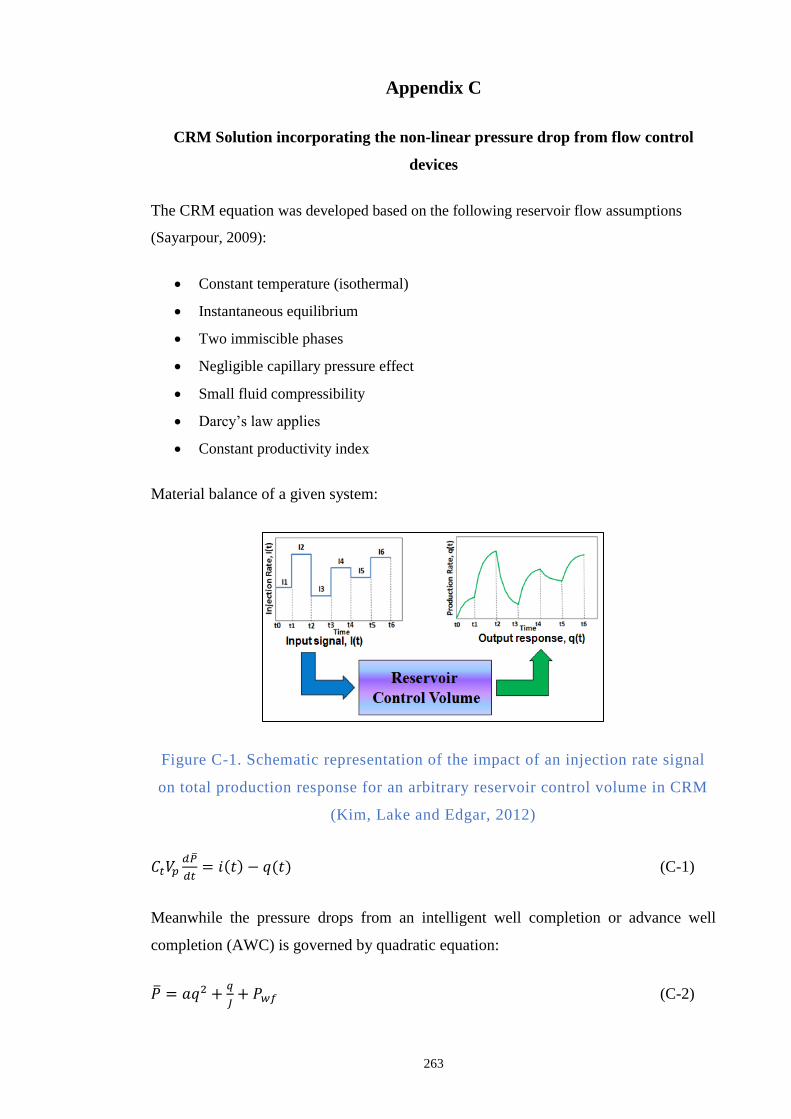
263
Appendix C
CRM Solution incorporating the non-linear pressure drop from flow control
devices
The CRM equation was developed based on the following reservoir flow assumptions
(Sayarpour, 2009):
Constant temperature (isothermal)
Instantaneous equilibrium
Two immiscible phases
Negligible capillary pressure effect
Small fluid compressibility
Darcy’s law applies
Constant productivity index
Material balance of a given system:
Figure C-1. Schematic representation of the impact of an injection rate signal
on total production response for an arbitrary reservoir control volume in CRM
(Kim, Lake and Edgar, 2012)
𝐶𝑡𝑉𝑝𝑑
𝑑𝑡= 𝑖(𝑡) − 𝑞(𝑡) (C-1)
Meanwhile the pressure drops from an intelligent well completion or advance well
completion (AWC) is governed by quadratic equation:
= 𝑎𝑞2 +𝑞
𝐽+ 𝑃𝑤𝑓 (C-2)

264
We can couple the equation C-3 with C-1 and describe the material balance of an AWC
system as:
𝐶𝑡𝑉𝑝𝑑(𝑎𝑞2+
𝑞
𝐽+𝑃𝑤𝑓)
𝑑𝑡= 𝑖(𝑡) − 𝑞(𝑡) (C-3)
Or
𝐶𝑡𝑉𝑝
𝐽
𝑑𝑞
𝑑𝑡+ 𝐶𝑡𝑉𝑝
𝑑𝑃𝑤𝑓
𝑑𝑡= 𝑖(𝑡) − 𝑞(𝑡) − 𝑎𝐶𝑡𝑉𝑝
𝑑𝑞2
𝑑𝑡 (C-4)
Where time-storage (τ) is defined as:
τ =𝐶𝑡𝑉𝑝
𝐽 (C-5)
Equation C-5 can be simplified as:
𝑑𝑞
𝑑𝑡+1
τ𝑞(𝑡) =
1
τ𝑖(𝑡) − J
𝑑𝑃𝑤𝑓
𝑑𝑡− J𝑎
𝑑𝑞2
𝑑𝑡 (C-6)
The right side of equation C-7 can be represented as the auxiliary parameter:
𝑔(𝑡) =1
τ𝑖(𝑡) − J
𝑑𝑃𝑤𝑓
𝑑𝑡− J𝑎
𝑑𝑞2
𝑑𝑡 (C-7)
Substituting equation C-7 into C-6 gives:
𝑑𝑞
𝑑𝑡+1
τ𝑞(𝑡) = 𝑔(𝑡) (C-8)
Multiplying both side of C-8 with 𝑒𝑡
τ gives:
𝑒𝑡
τ [𝑑𝑞
𝑑𝑡+1
τ𝑞(𝑡)] = 𝑒
𝑡
τ 𝑔(𝑡) (C-9)
Or:
𝑑[𝑒𝑡τ 𝑞]
𝑑𝑡= 𝑒
𝑡
τ 𝑔(𝑡) (C-10)
Integrate equation C-10 with respect to t:
𝑒𝑡
τ 𝑞 = 𝑐 + ∫𝑒𝑡
τ 𝑔(𝑡)𝑑𝑡 (C-11)
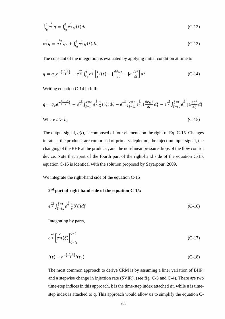
265
∫ 𝑒𝑡
τ 𝑞𝑡
𝑡0= ∫ 𝑒
𝑡
τ 𝑔(𝑡)𝑑𝑡𝑡
𝑡0 (C-12)
𝑒𝑡
τ 𝑞 = 𝑒𝑡0τ 𝑞𝑜 + ∫ 𝑒
𝑡
τ 𝑔(𝑡)𝑑𝑡𝑡
𝑡0 (C-13)
The constant of the integration is evaluated by applying initial condition at time t0,
𝑞 = 𝑞𝑜𝑒−(
𝑡−𝑡0τ) + 𝑒
−𝑡
τ ∫ 𝑒𝑡
τ [1
τ𝑖(𝑡) − J
𝑑𝑃𝑤𝑓
𝑑𝑡− J𝑎
𝑑𝑞2
𝑑𝑡] 𝑑𝑡
𝑡
𝑡0 (C-14)
Writing equation C-14 in full:
𝑞 = 𝑞𝑜𝑒−(
𝑡−𝑡0τ) + 𝑒
−𝑡
τ ∫ 𝑒𝜉
τ 1
τ𝑖(𝜉)𝑑𝜉
𝜉=𝑡
𝜉=𝑡0− 𝑒
−𝑡
τ ∫ 𝑒𝜉
τ J𝑑𝑃𝑤𝑓
𝑑𝜉𝑑𝜉
𝜉=𝑡
𝜉=𝑡0− 𝑒
−𝑡
τ ∫ 𝑒𝜉
τ Ja𝑑𝑞2
𝑑𝜉𝑑𝜉
𝜉=𝑡
𝜉=𝑡0
Where 𝑡 > 𝑡0 (C-15)
The output signal, q(t), is composed of four elements on the right of Eq. C-15. Changes
in rate at the producer are comprised of primary depletion, the injection input signal, the
changing of the BHP at the producer, and the non-linear pressure drops of the flow control
device. Note that apart of the fourth part of the right-hand side of the equation C-15,
equation C-16 is identical with the solution proposed by Sayarpour, 2009.
We integrate the right-hand side of the equation C-15
2nd part of right-hand side of the equation C-15:
𝑒−𝑡
τ ∫ 𝑒𝜉
τ 1
τ𝑖(𝜉)𝑑𝜉
𝜉=𝑡
𝜉=𝑡0 (C-16)
Integrating by parts,
𝑒−𝑡
τ [𝑒𝜉
τ𝑖(𝜉)]𝜉=𝑡0
𝜉=𝑡
(C-17)
𝑖(𝑡) − 𝑒−(𝑡−𝑡0τ)𝑖(𝑡0) (C-18)
The most common approach to derive CRM is by assuming a liner variation of BHP,
and a stepwise change in injection rate (SVIR), (see fig. C-3 and C-4). There are two
time-step indices in this approach, k is the time-step index attached ∆t, while n is time-
step index is attached to q. This approach would allow us to simplify the equation C-
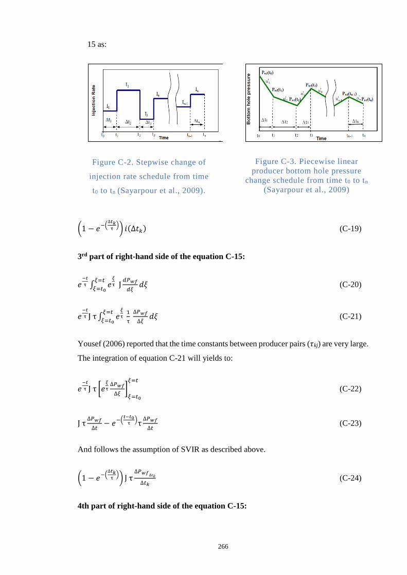
266
15 as:
Figure C-2. Stepwise change of
injection rate schedule from time
t0 to tn (Sayarpour et al., 2009).
Figure C-3. Piecewise linear
producer bottom hole pressure
change schedule from time t0 to tn
(Sayarpour et al., 2009)
(1 − 𝑒−(∆𝑡𝑘τ)) 𝑖(∆𝑡𝑘) (C-19)
3rd part of right-hand side of the equation C-15:
𝑒−𝑡
τ ∫ 𝑒𝜉
τ J𝑑𝑃𝑤𝑓
𝑑𝜉𝑑𝜉
𝜉=𝑡
𝜉=𝑡0 (C-20)
𝑒−𝑡
τ J τ ∫ 𝑒𝜉
τ 1
τ ∆𝑃𝑤𝑓
∆𝜉𝑑𝜉
𝜉=𝑡
𝜉=𝑡0 (C-21)
Yousef (2006) reported that the time constants between producer pairs (𝜏kj) are very large.
The integration of equation C-21 will yields to:
𝑒−𝑡
τ J τ [𝑒𝜉
τ∆𝑃𝑤𝑓
∆𝜉]𝜉=𝑡0
𝜉=𝑡
(C-22)
J τ∆𝑃𝑤𝑓
∆𝑡− 𝑒−(
𝑡−𝑡0τ)τ
∆𝑃𝑤𝑓
∆𝑡 (C-23)
And follows the assumption of SVIR as described above.
(1 − 𝑒−(∆𝑡𝑘τ)) J τ
∆𝑃𝑤𝑓∆𝑡𝑘
∆𝑡𝑘 (C-24)
4th part of right-hand side of the equation C-15:
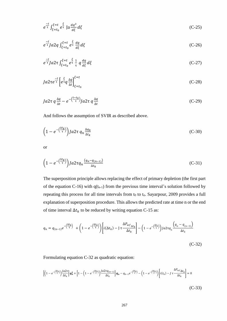
267
𝑒−𝑡
τ ∫ 𝑒𝜉
τ Ja𝑑𝑞2
𝑑𝜉𝑑𝜉
𝜉=𝑡
𝜉=𝑡0 (C-25)
𝑒−𝑡
τ 𝐽𝑎2𝑞 ∫ 𝑒𝜉
τ 𝑑𝑞
𝑑𝜉𝑑𝜉
𝜉=𝑡
𝜉=𝑡0 (C-26)
𝑒−𝑡
τ 𝐽𝑎2τ ∫ 𝑒𝜉
τ 1
τ 𝑞𝑑𝑞
𝑑𝜉𝑑𝜉
𝜉=𝑡
𝜉=𝑡0 (C-27)
𝐽𝑎2τ𝑒−𝑡
τ [𝑒𝜉
τ𝑞∆𝑞
∆𝑡]𝜉=𝑡0
𝜉=𝑡
(C-28)
𝐽𝑎2τ 𝑞∆𝑞
∆𝑡− 𝑒−(
𝑡−𝑡0τ)𝐽𝑎2τ 𝑞
∆𝑞
∆𝑡 (C-29)
And follows the assumption of SVIR as described above.
(1 − 𝑒−(∆𝑡𝑘τ)) 𝐽𝑎2τ 𝑞𝑛
∆𝑞𝑘
∆𝑡𝑘 (C-30)
or
(1 − 𝑒−(∆𝑡𝑘τ)) 𝐽𝑎2τ𝑞𝑛
(𝑞𝑛−𝑞(𝑛−1))
∆𝑡𝑘 (C-31)
The superposition principle allows replacing the effect of primary depletion (the first part
of the equation C-16) with q(tn-1) from the previous time interval’s solution followed by
repeating this process for all time intervals from t0 to tn. Sayarpour, 2009 provides a full
explanation of superposition procedure. This allows the predicted rate at time n or the end
of time interval ∆𝑡𝑘 to be reduced by writing equation C-15 as:
𝑞𝑛 = 𝑞(𝑛−1)𝑒−(∆𝑡𝑘τ) + (1 − 𝑒
−(∆𝑡𝑘τ)) [𝑖(∆𝑡𝑘) − J τ
∆𝑃𝑤𝑓∆𝑡𝑘∆𝑡𝑘
] − (1 − 𝑒−(∆𝑡𝑘τ)) 𝐽𝑎2τ𝑞
𝑛
(𝑞𝑛− 𝑞
(𝑛−1))
∆𝑡𝑘
(C-32)
Formulating equation C-32 as quadratic equation:
[(1 − 𝑒−(∆𝑡𝑘𝜏))𝐽𝑎2𝜏
∆𝑡𝑘] 𝒒𝒏
𝟐 + [1 − (1 − 𝑒−(∆𝑡𝑘𝜏))𝐽𝑎2𝜏𝑞(𝑛−1)
∆𝑡𝑘] 𝒒𝒏 − 𝑞𝑘−1𝑒
−(∆𝑡𝑘𝜏)− (1 − 𝑒−
(∆𝑡𝑘𝜏)) [𝑖(𝑡𝑘) − 𝐽 𝜏
∆𝑃𝑤𝑓∆𝑡𝑘∆𝑡𝑘
] = 0
(C-33)
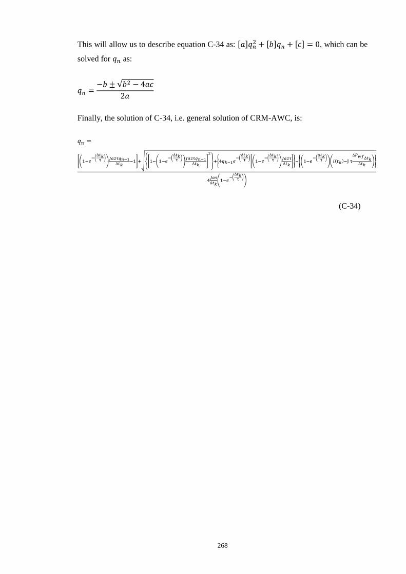
268
This will allow us to describe equation C-34 as: [𝑎]𝑞𝑛2 + [𝑏]𝑞𝑛 + [𝑐] = 0, which can be
solved for 𝑞𝑛 as:
𝑞𝑛 =−𝑏 ± √𝑏2 − 4𝑎𝑐
2𝑎
Finally, the solution of C-34, i.e. general solution of CRM-AWC, is:
𝑞𝑛 =
[(1−𝑒−(∆𝑡𝑘τ )
)𝐽𝑎2τ𝑞𝑛−1
∆𝑡𝑘−1]+√[1−(1−𝑒
−(∆𝑡𝑘τ )
)𝐽𝑎2τ𝑞𝑛−1
∆𝑡𝑘]
2
+4𝑞𝑘−1𝑒−(∆𝑡𝑘τ )
[(1−𝑒−(∆𝑡𝑘τ )
)𝐽𝑎2τ
∆𝑡𝑘]−(1−𝑒
−(∆𝑡𝑘τ )
)(𝑖(𝑡𝑘)−J τ
∆𝑃𝑤𝑓∆𝑡𝑘∆𝑡𝑘
)
4𝐽𝑎τ
∆𝑡𝑘(1−𝑒
−(∆𝑡𝑘τ )
)
(C-34)