Water Use Regulatory Method (WAT-RM-27) Modelling Methods for Groundwater Abstractions

Water Use

Regulatory Method (WAT-RM-27)

Modelling Methods for Groundwater Abstractions

Version: v3.0

Released: Apr 2013

2 of 26 Uncontrolled if printed v3.0 Apr 2013

Copyright and Legal Information

Copyright© 2013 Scottish Environment Protection Agency (SEPA).

All rights reserved. No part of this document may be reproduced in any form or by any means, electronic or mechanical, (including but not limited to) photocopying, recording or using any information storage and retrieval systems, without the express permission in writing of SEPA.

Disclaimer Whilst every effort has been made to ensure the accuracy of this document, SEPA cannot accept and hereby expressly excludes all or any liability and gives no warranty, covenant or undertaking (whether express or implied) in respect of the fitness for purpose of, or any error, omission or discrepancy in, this document and reliance on contents hereof is entirely at the user’s own risk.

Registered Trademarks All registered trademarks used in this document are used for reference purpose only.

Other brand and product names maybe registered trademarks or trademarks of their respective holders.

Update Summary

Version Description

v1.0 First issue for Water Use reference using approved content from the following documents:

GWABS_9_Modelling_in_Support_of_an Application_for_a_Groundwater_Abstraction_v1_9.doc

v2.0 Doc references revised.

v3.0 Expired CMS links reviewed and updated.

Notes

References: Linked references to other documents have been disabled in this web version of the document. See the References section for details of all referenced documents.

Printing the Document: This document is uncontrolled if printed and is only intended to be viewed online.

If you do need to print the document, the best results are achieved using Booklet printing or else double-sided, Duplex (2-on-1) A4 printing (both four pages per A4 sheet).

Always refer to the online document for accurate and up-to-date information.

v3.0 Apr 2013 Uncontrolled if printed 3 of 26

Table of Contents

1. Non-Technical Summary .................................................................................... 4

2. Introduction......................................................................................................... 5

2.1 Scope ....................................................................................................... 5

2.2 Purpose.................................................................................................... 5

3. The Modelling Process ....................................................................................... 6

4. The Conceptual Model........................................................................................ 7

4.1 Introduction .............................................................................................. 7

4.2 Developing a Conceptual Model .............................................................. 7

4.3 Conceptual Model Components ............................................................... 8

4.4 Component Description............................................................................ 9

4.5 Validating the Conceptual Model............................................................ 14

5. The Mathematical Model .................................................................................. 16

5.1 Analytical Models ................................................................................... 16

5.2 Numerical Models................................................................................... 16

6. Groundwater Flow Modelling ............................................................................ 19

6.1 Computer Modelling Code...................................................................... 19

6.2 Conceptual Model .................................................................................. 19

6.3 Model Construction ................................................................................ 19

6.4 Model Calibration ................................................................................... 19

6.5 Model Validation..................................................................................... 20

7. Reporting .......................................................................................................... 21

Appendix 1: Uncertainty........................................................................................ 22

Appendix 2: Glossary of Terms ............................................................................ 25

References ........................................................................................................... 26


1. Non-Technical Summary

The construction of conceptual models is fundamental to our understanding of the way in which systems are put together and work.

The Haynes Manuals for car repair are an example of a high level conceptual model. These are a schematic representation of a real car. They contain real data, diagrams and sources of information that allow us to understand how the car is put together and work. The builders’ sketch on the back of a fag packet is an example of a basic conceptual model. It contains a small amount of information that is crudely represented. They both have their place and both can be effective.

This guidance describes how to construct the equivalent of a groundwater Haynes Manual via the back of the fag packet.

Mathematical models are an extension and formalisation of conceptual models. They too may be simple or complex. Some mathematical models are so complex that they are best used to produce computer generated representations which aid interpretation of possible outcomes.

This guidance briefly describes the main types of mathematical models used for groundwater flow, how they may be constructed, calibrated and validated


2. Introduction

2.1 Scope

This document is designed to provide guidance to SEPA Hydrogeologists on the main factors to consider when constructing or assessing conceptual and mathematical models. It will also be of use to others, such as applicants for groundwater abstraction authorisation or their agent, who need to undertake conceptual or mathematical modelling in support of their application. For that reason it aims to set the standard for conceptual models constructed as part of further investigations submitted in support of an abstraction application.

SEPA strongly advises applicants for an abstraction licence that, where they lack the technical ability to be able to undertake the model construction, they seek the services of a competent person.

SEPA will undertake conceptual model construction for abstractions of less than 50 m3/day unless the applicant wishes to engage their own advisor. For abstractions of more than 50 m3/day it is the responsibility of the applicant or their agent to undertake conceptual modelling. For all abstractions, it is the responsibility of the applicant or their agent to produce and submit a numerical model when requested to do so by SEPA.

2.2 Purpose

Models will be used to assess the environmental sustainability of groundwater abstractions. They may be constructed to analyse the groundwater resource potential, to evaluate the impacts of the abstraction upon specific water features or to model the effects of intrusion of groundwater of a different quality. In all cases it is imperative that a rigorous approach is adopted so that the best possible model is constructed from the available data. It will be used by the SEPA Hydrogeologist when:

� Reviewing a failure of the initial impact assessment (the Level 1 assessment),

� Designing further investigations, and

� Assessing the results of the investigations


3. The Modelling Process

For groundwater impact assessment the modelling process consists of three distinct phases:

� Data collection

� Development of a conceptual model

� Development of a mathematical model

The three are interlinked, as is demonstrated in Figure 1, and the process should be one of interaction between data collection, conceptual and mathematical models with either or both models used to redefine data requirements. In some cases the mathematical component will not be required.

Figure 1 The Modelling Process


4. The Conceptual Model

4.1 Introduction

A conceptual model can be defined as a synthesis of how a real system behaves, based on qualitative and quantitative analysis of data. However complicated, it is always a simplification of reality. In spite of this the construction of a good conceptual model will enable realistic predictions to be made from mathematical models and increase the understanding of the groundwater system. In addition, the model does not necessarily have to be complex to fulfil the desired function.

For most systems there are a small number of crucial factors which must be examined in detail, and if any one of these is ignored the conclusions may be seriously flawed. Developing a good conceptual model will help in the identification of these factors. A good conceptual model reduces uncertainty and increases confidence in the decision making process.

The eventual complexity of the conceptual model will initially be suggested by the uncertainty associated with potential impacts. The greater the uncertainty the more detailed the investigation will need to be and the more complex the resulting model. The more complex the model the more time, effort and data is required and the higher the cost. There is always a trade off between reduction in uncertainty and cost and it may be difficult to determine the right balance. In some cases the use of long term monitoring should be considered as a substitute for further investigative work as, in addition to providing a direct indication of impacts, this will supply more data for the model.

A conceptual model has a number of important characteristics:

� It concentrates on the features that are important to the subject in hand

� It makes use of real data, i.e. it is based on evidence

� It must be written down. Maps, diagrams and tables are important components

� It must be verifiable, i.e. it needs to be tested using data

4.2 Developing a Conceptual Model

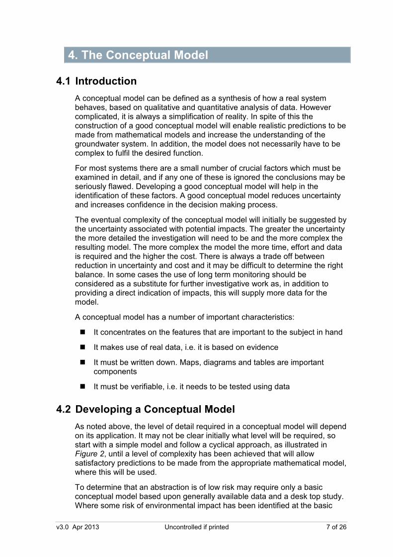
As noted above, the level of detail required in a conceptual model will depend on its application. It may not be clear initially what level will be required, so start with a simple model and follow a cyclical approach, as illustrated in Figure 2, until a level of complexity has been achieved that will allow satisfactory predictions to be made from the appropriate mathematical model, where this will be used.

To determine that an abstraction is of low risk may require only a basic conceptual model based upon generally available data and a desk top study. Where some risk of environmental impact has been identified at the basic



level then the model must be refined usually using some additional information from site specific sources, e.g. pumping test or monitoring data from which predictions can be made using analytical solutions.

Where the risk of potential impacts cannot be resolved with the intermediate level of conceptual model it will be necessary to collect further site specific data for a high level model, probably from custom made monitoring points, e.g. observation boreholes. This level of conceptual model should provide data of sufficient quality to construct a groundwater flow model.

Figure 2 Cyclic approach to conceptual modelling*

*After a number of Environment Agency documents

4.3 Conceptual Model Components

A basic conceptual model of an integrated groundwater/surface water system should contain the following components:

� A definition of the extent of the study area and its subdivision into appropriate zones (vertically and horizontally) based on the hydrogeology.

� A description of the hydrogeological conditions and flows at the boundaries of the area (including vertical boundaries such as changes in strata, e.g. faults, where the adjoining strata should be identified as aquitards, aquicludes, leaky aquifers etc). Recharge and discharge

The Conceptual Model


areas need to be defined as does the groundwater flow direction within the study area.

� Identification of all the water-dependent features in the area, such as rivers, ponds, wetlands, springs, seepages, estuaries, etc. Also, identification of all the quantitative pressures, e.g. abstractions and discharges.

� A description of the limitations of the current conceptual understanding, and the major sources of uncertainty.

As the model develops these components should be examined in a more detailed and scientific way.

This basic conceptual model will identify areas where further data is required for a better understanding. This data can be used to test and refine the model. As the model develops and becomes more complex the following components should be included:

� A description of the likely mechanisms and locations of interaction between groundwater and the surface water features.

� An estimate of all inflows to and outflows from the unit, and their variation in time, backed up by water balance calculations.

� An estimate of the plausible range of aquifer parameters in the unit.

� A description of the likely groundwater flow paths or flow patterns, both horizontal and vertical.

� Interpretation of available hydrochemical data, and identification of relevant water quality pressures on the unit, such as point source and diffuse pollution.

All conceptual models should be illustrated with appropriate maps, sketches, diagrams, graphs and geological cross-sections, bearing in mind that the level of detail should match the required level of confidence.

4.4 Component Description

The basic components of a conceptual model were listed in Section 4.3. Some of the main components will now be described briefly.

4.4.1 Study Area Extent

SEPA has described Groundwater Abstraction Management Units within groundwater bodies in Scotland. These will define the maximum area that will need to be examined when developing a regional conceptual groundwater flow model. The minimum area should be at least the radius of the Water Features Survey as defined in An applicants guide to water supply boreholes. In most cases the extent of the study area will lie between these extremes at the scale of the catchment within which the abstraction lies.



To help define the boundaries of the model more accurately, look for flow boundaries. These may be identified as:

� Places where there is no groundwater flow into or out of the area - this may be at a fault, the edge of the outcrop, or at a natural groundwater divide

� Discharge areas - generally where the flow discharges to a spring, a river, an estuary or to the sea

� Likely recharge areas of high relief

Reference to geological and topographic maps will help.

The depth and location of the abstraction will also be an important consideration. Where the borehole is deep, the abstraction will be from a longer groundwater flowpath and the effects may be felt at a greater distance than would be the case for a shallow abstraction of the same discharge volume. Large abstractions of any depth may impact upon both shallow and deep flowpaths.

4.4.2 Inflows

The most important component of inflow to groundwater comes from recharge, i.e. that amount of rainfall that infiltrates through overlying strata and reaches the water table.

For a basic conceptual model a good place to start modelling recharge is to use:

Recharge = Annual average rainfall – Evapotranspiration – Runoff

with mean annual values for rainfall and evapotranspiration, ideally expressed as volumes by multiplying the value per unit area by the total area of the groundwater abstraction unit.

� Annual average rainfall Totals can be obtained from rainfall contour maps, the UK Hydrometric Register, or software such as the Flood Estimation Handbook that gives average rainfalls for surface water catchments. This is also available as a layer on ArcGIS.

� Evapotranspiration Estimated from data obtained from MORECS (the Meteorological Office Rainfall and Evaporation Calculation System). This is also available as a layer on ArcGIS

� Mean annual runoff values Are given in the UK Hydrometric Register for gauged catchments.



These will include an element of baseflow* which is regarded as an outflow from a groundwater unit, and so should be subtracted.

If the outcrop area is small and there are no gauged river catchments thought to be representative of the outcrop area, it is possible to obtain approximate values of runoff. One approach is to multiply the rainfall by the standard percentage runoff (SPR), which is the proportion of rainfall that leads to quick runoff. The SPR can be estimated from soil type, and values are available for gauged and ungauged catchments from the Flood Estimation Handbook.

An assessment of the outcrop area is needed to determine the volume of recharge.

As the model is refined and developed then an intermediate level approach to recharge calculation would be to use the Excel spreadsheet model developed by The Scotland and Northern Ireland Forum For Environmental Research (SNIFFER) as part of the Water Framework research project and detailed in Derivation of a Methodology for Groundwater Recharge Assessment in Scotland and Northern Ireland. This provides an easy to use means of estimating groundwater recharge within a chosen area but it has limitations that need to be considered. These include:

� Recharge rates will vary over any given area depending on precipitation, topography, land use, soil type drift cover and aquifer permeability

� In Scotland, where many aquifers are of low permeability, the rate of recharge is limited by the ability of the aquifer to receive the recharge

Because of these limitations recharge is generally overestimated.

As the complexity of the model increases further, the following sources of inflows, or recharge, to the unit should be examined in detail:

� Recharge at outcrops and through superficial deposits and leakage from overlying deposits Care should be exercised if it is suspected that there is a perched water table, in which case the recharge will be to the perched water table and not to the main aquifer. Recharge to the main (lower) aquifer, if any, will occur due to flow through some intermediate low-permeability strata. This can be estimated using the head difference between the perched water table and the head in the lower aquifer, the hydraulic conductivity of the low-permeability strata, and Darcy’s equation. The hydraulic conductivity can be estimated from nearby pumping tests, or if no other local data are available, then published data for the aquifer type may be

* Baseflow can loosely be defined as the amount of flow in a river that is contributed by groundwater, as opposed to surface run-off. The baseflow index (BFI) is a measure of the baseflow as a proportion of the total flow. This can be derived from smoothing and separation of flow hydrographs, as explained in Low Flow Estimation in Scotland. Values of BFI are available for most gauged catchments.



used. If this approach is taken then some thought should be given to the effects of different values and calculations will need to be done using maxima and minima rather than average values.

� Recharge from losing reaches of canals traversing the unit Information on canal leakage may be available from British Waterways. Otherwise, it is very difficult to estimate, and usually depends on tests having been conducted where a length of canal is isolated and water losses measured (allowing for evaporation). If no data on canals are available, either a qualitative judgement will have to be made of the importance of canal - aquifer interaction, or an assessment will have to be made using the water budget (see the section below on validating the model).

� Recharge to groundwater from losing reaches of rivers or the contribution of baseflow to rivers from groundwater. This is difficult to assess, but possible sources of information include:

• Flow gauging data, usually spot-gauging surveys. If the gaugings have been done in appropriate locations, these can reveal which river reaches are gaining or losing water, after having allowed for abstractions, discharges, and tributaries. Reference to the Base Flow Index on the Flood Estimation Handbook gives a catchment scale value which might be adequate at the lowest level of conceptual model

• Low Flows can provide flow data and base flow index data for sub-catchments above a chosen assessment point. This might be adequate for an intermediate level conceptual model

• A higher level of model will need site specific data which might consist of groundwater heads measurements close to the river, comparison of the heads with the water level in the river (assuming the heads are being measured in an aquifer which is hydraulically connected to the river). Generally speaking, the magnitude of flow in either direction will depend on the head difference and permeability. However, note that if the groundwater head is below the river bed, and the groundwater is disconnected from the river, then the river will lose water by gravity drainage and the flux does not depend on the elevation of the groundwater head. Try to obtain estimates of the river bed permeability (as described in Calver). Normally these will take quite a wide range of possible values.

� Flow across boundaries from adjacent units, see section 4.4.3 Outflows.

� Release of water from storage in the aquifer If part or all of the aquifer is unconfined (or a confined aquifer has become dewatered), then abstraction may induce release of water from storage in the aquifer, which can supply considerable volumes of water, until the system has reached a new equilibrium.

� Recharge for karstic aquifers may be concentrated at surface features, e.g. dolines.



� Leakage from water pipes and sewers Leakage from water mains can be assessed using leakage data from the local water company. Leakage from sewers and contributions from discharges such as soakaways is more difficult to assess, although elevated nitrate or chloride concentrations in the groundwater nearby may provide evidence that it is happening.

� Artificial recharge from Aquifer Storage and Recovery (ASR) programmes.

4.4.3 Outflows

Similarly, the following outflows or discharges from the aquifer unit must be examined:

� Discharges to springs These are difficult to estimate as any gauging will normally take place a considerable distance downstream of the discharge. Some information on springs that are or have been used for abstraction may be found in the Springs Database, when available.

� Discharges to rivers This is the baseflow contribution to the total flow and can initially be assessed using the BFI (see section 4.4.2) and flow gauging data at a suitable gauging station. A more accurate estimation of groundwater contribution to baseflow can be obtained using Low Flows for the sub-catchment upstream of the chosen assessment point. For a high level model, comparison of head difference between river and aquifer and stream bed conductivity can be used in a similar but opposite way as recharge from rivers is calculated (see previous section)

� Flow across area boundaries For the basic level model an assumption of zero flow may be appropriate but the flow boundaries should be examined to confirm this assumption. For the higher level model cross boundary flow should be evaluated by consideration of groundwater levels or contours to determine whether a hydraulic gradient exists to drive the flow (perhaps seasonally), combined with estimates of the hydraulic conductivity or transmissivity of the boundary where appropriate, with Darcy’s equation, to establish the flow rate.

� Discharges to estuaries or the sea For the basic level model some assumptions may be made using the water balance but these should be examined to confirm that the estimates are realistic. For a higher level model an better estimate of flow may be derived from hydraulic gradients and aquifer hydraulic conductivities.

� Evapotranspiration This has already been taken into account when determining the recharge.



� Aquifer storage Rather than being directly discharged to the surface, water can be taken back into storage in unconfined aquifers (or dewatered confined aquifers) as water levels rise. The amount of recharge equivalent that this represents depends on the storage coefficient of the aquifer. Fractured aquifers usually have a storage coefficient of less than 5%. For granular aquifers the storage coefficient is usually greater than 5%. Many Scottish aquifers have predominantly fracture flow especially the hard rock aquifers of highlands, islands and the borders. There are many other aquifers in Scotland where the flow regime is comprised of both fracture and intergranular components such as the Devonian Sandstones. Aquifers having purely intergranular flow are generally restricted to unconsolidated sands and gravels and a few consolidated aquifers such as the sandstones of the Dumfries aquifer.

� Abstractions from the aquifer Data on licensed and actual abstraction quantities are available from regulatory staff. Abstractions from unlicensed sources (e.g. small domestic supplies of less than 10 m3/day ) should not be forgotten, as although usually small individually, they can add up to significant quantities in total.

4.5 Validating the Conceptual Model

There may be considerable uncertainty about the conceptual model, with many components being based on estimates. Therefore, it is very important to validate the model to some level, and this is best done using water balances. The overall aim is to build confidence in the model, and to understand its limitations. Detailed guidance on water balances can be found in the Framework for Groundwater Resources Conceptual and Numerical Modelling.

At the basic level of validation, mean annual fluxes are established for all inflows to and outflows from the area, as described above. These should be checked to see if they are plausible, and that there is an approximate annual water budget balance for the area. In other words, if there are no changes in storage over the period in question, the volume of inputs and outputs should be equivalent. Achieving this balance may require revisions to your conceptual model.

If there are several unknown terms in the water budget, plausible values can be assigned that ensure the overall balance is maintained. You should ensure that all terms are physically reasonable, and that they fit with data or experience from other areas. There are obviously many combinations that would still satisfy the water balance, and so the basic conceptual model cannot be considered validated: the solution you have proposed is simply a feasible combination of terms. However, in some cases this is the best that can be achieved at a basic level and it may be adequate to make a licensing decision.



At a higher level it may be necessary to calculate the water balance for critical periods, for example at periods of low and high recharge and discharge or, when greater detail is required, monthly.

An estimate should be produced of the range of uncertainty for the water balance, based on the uncertainties in all the individual components, bearing in mind the comments on combining uncertainties in Appendix 1. The uncertainty can be assessed by varying the terms in the water budget within their plausible ranges, and finding the resulting impact on the other terms (particularly terms which are most likely to be impacted by a new abstraction).


5. The Mathematical Model

There are a number of different mathematical modelling methods for describing groundwater flow, varying in complexity from deterministic, predictive equations for modelling drawdown, such as the Cooper-Jacob equation, to the groundwater body scale flow models of the USGS MODFLOW type. The type of mathematical model used must be chosen with care and is invariably a balance between effort (and therefore cost) and need. The type of model used should be agreed in prior consultation with SEPA. Amongst other things the choice of model depends upon:

� What is being modelled

� The risk of impact

High risk abstractions will require more complex models than low risk but it is unlikely that a groundwater body scale model will be needed to assess the risk of impacts from an abstraction of less than 50 m3/day.

No matter what the method chosen it must be based upon the appropriate conceptual model.

Within the context of cyclic model development the lowest level would be represented by an analytical model and the highest by a numerical model. There are no examples of intermediate mathematical models for groundwater abstraction assessment.

5.1 Analytical Models

These solve the mathematical equations describing groundwater flow exactly. This requires a simplification of the groundwater flow equations (see next section). In turn the conceptual model, and hence the groundwater flow regime, must be considerably simplified. For example, analytical models invariably assume a homogeneous aquifer of uniform thickness with an infinite extent. None of these assumptions are ever satisfied but some situations approximate these conditions.

Analytical models would normally be used to calculate aquifer parameters from pumping test data. These parameters can then be used to predict the lowering of the water table associated with a groundwater abstraction, at a specified distance from that abstraction after a particular time has elapsed (often several years). For guidance on the selection and use of analytical models for the determination of aquifer parameters refer to WAT-RM-26: Determination of Aquifer Properties.

5.2 Numerical Models

These are more powerful than analytical models and allow more realistic modelling to be undertaken. They also require a more complex conceptual model, which in turn means greater data input. Within Earth Sciences numerical models are used to investigate a number of processes including

The Mathematical Model


sedimentary basin development, erosion, glacial processes, coastal geomorphology and groundwater flow.

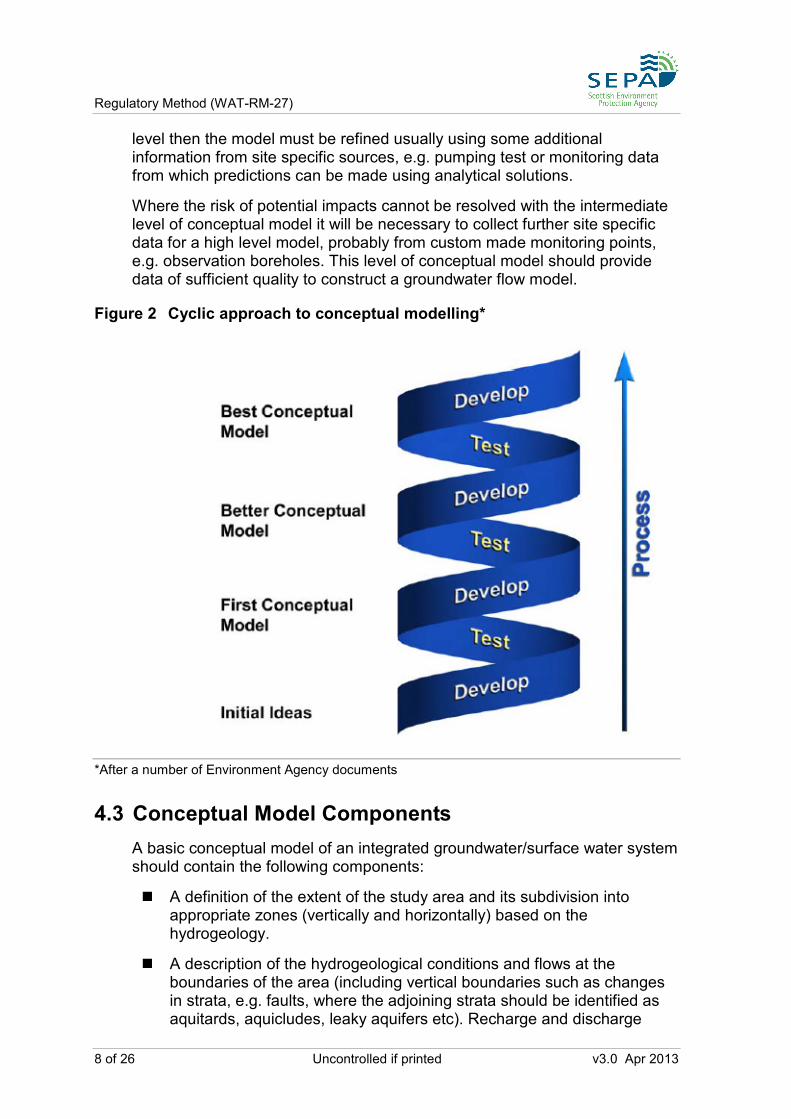
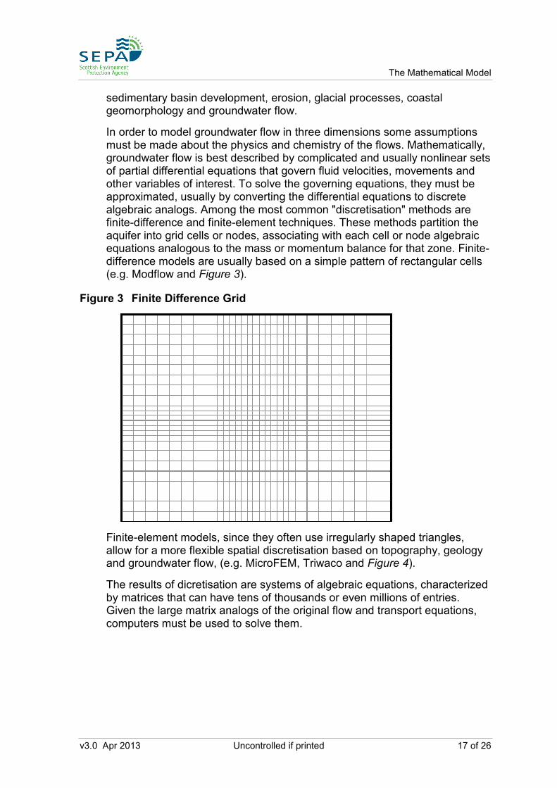
In order to model groundwater flow in three dimensions some assumptions must be made about the physics and chemistry of the flows. Mathematically, groundwater flow is best described by complicated and usually nonlinear sets of partial differential equations that govern fluid velocities, movements and other variables of interest. To solve the governing equations, they must be approximated, usually by converting the differential equations to discrete algebraic analogs. Among the most common "discretisation" methods are finite-difference and finite-element techniques. These methods partition the aquifer into grid cells or nodes, associating with each cell or node algebraic equations analogous to the mass or momentum balance for that zone. Finite-difference models are usually based on a simple pattern of rectangular cells (e.g. Modflow and Figure 3).

Figure 3 Finite Difference Grid

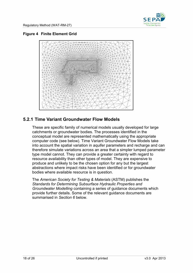
Finite-element models, since they often use irregularly shaped triangles, allow for a more flexible spatial discretisation based on topography, geology and groundwater flow, (e.g. MicroFEM, Triwaco and Figure 4).

The results of dicretisation are systems of algebraic equations, characterized by matrices that can have tens of thousands or even millions of entries. Given the large matrix analogs of the original flow and transport equations, computers must be used to solve them.



Figure 4 Finite Element Grid

5.2.1 Time Variant Groundwater Flow Models

These are specific family of numerical models usually developed for large catchments or groundwater bodies. The processes identified in the conceptual model are represented mathematically using the appropriate computer code (see below). Time Variant Groundwater Flow Models take into account the spatial variation in aquifer parameters and recharge and can therefore simulate variations across an area that a simpler lumped parameter type model cannot. They can provide a greater certainty with regard to resource availability than other types of model. They are expensive to produce and unlikely to be the chosen option for any but the largest abstractions where impact risks have been identified or for groundwater bodies where available resource is in question.

The American Society for Testing & Materials (ASTM) publishes the Standards for Determining Subsurface Hydraulic Properties and Groundwater Modelling containing a series of guidance documents which provide further details. Some of the relevant guidance documents are summarised in Section 6 below.


6. Groundwater Flow Modelling

6.1 Computer Modelling Code

There are a number of different modelling codes in use. The MODFLOW code developed by the USGS has been released into the public domain and subject to scrutiny by large number of individuals and organisations. Problems associated with the code are well understood. The reader is referred to the relevant manufacturer’s instruction manual for details on model construction.

6.2 Conceptual Model

A conceptual model should be constructed using geological (model area boundaries) and hydrological data (aquifer hydraulic properties, measurements of hydraulic head), boundary conditions of the area to be modelled (discharge, recharge and no flow boundaries) and sources and sinks (local abstractions, recharge) following the guidelines given above.

6.3 Model Construction

The conceptual model should be used to define input parameters for the groundwater flow model. In general, the more locations with data the better as more nodes can be populated which will give more accurate and reliable results. Where the number of input data locations is limited, it is still possible to increase the number of nodes within specific areas of interest but the model projections have a large degree of uncertainty associated with them as they are interpolations from the nearest data points. In such cases the objective should be to obtain more data from within the area of interest to validate and develop the model.

The modeller must decide if steady state or transient conditions will be appropriate. For reasons of size it may be necessary to create a boundary where none exists. Where such boundaries are a long way from the area of interest it is unlikely that this will have significant impact on model results. Nevertheless, all artificial boundaries should be tested to assess the sensitivity of the model to this condition.

Detailed information is available in the following ASTM guidance documents:

� ASTM D 5609–94: Defining boundary conditions

� ASTM D 5610–94: Defining initial conditions

6.4 Model Calibration

Model calibration consists of varying input parameters, within suitable ranges, until the model matches actual measurements. Parameter variation should be within the range appropriate to the conditions or determined from field measurement. Model calibration usually consists of trial and error



although there are other methods. The accuracy of the calibration is measured by use of ‘residuals’ i.e. the difference between the observed and modelled value at any one place, the object being to reduce residuals, and their standard deviation, to a minimum. Where calibration to an appropriate level proves impossible the modeller should examine the model and data to determine if changes are needed in the conceptual/numerical model or if better definition of certain input parameters would improve calibration. Sensitivity analysis identifies those parameters that are having the most effect and therefore need to be most accurately defined.

Further details are contained in the following ASTM guidance documents:

� ASTM D 5490–93: Model calibration

� ASTM D 5611–94: Sensitivity analysis

6.5 Model Validation

To increase confidence in modelling outputs, calibration should be undertaken for at least two separate sets of field data wherever possible, i.e. the model should be calibrated for one set of results and then used to predict another set of results for which there are field measurements, with the system under a different stress.


7. Reporting

It is imperative that all stages of the modelling process are documented so that reasons for the choice of conceptual model, numerical model and input parameters and any subsequent changes are reported. This will allow an assessment of model credibility to be made by an assessor. Any report produced should contain sufficient detail for the results to be independently repeated.


Appendix 1: Uncertainty

No matter how good the model it will never reproduce reality exactly because of the inherent uncertainties in the information that has been used in the model construction.

These uncertainties generally fall into two categories:

� Natural or environmental uncertainties: These arise as a result of the inherent variability of the natural environment, e.g. natural fluctuations in groundwater level and flow which occur due to variations in rainfall and evaporation.

� Knowledge uncertainties: This arises as a result of limited knowledge of the hydrogeological system, or inadequate scientific understanding of the processes involved. Knowledge uncertainty can be further subdivided into the following categories:

• Model uncertainty: Where models provide only an approximation of the real environment. Model uncertainty may have two components: (i) conceptual modelling uncertainty due to insufficient knowledge of the system and (ii) mathematical model uncertainty arising from the limitations of the model selected in accurately representing reality.

• Sample uncertainty: Where uncertainties arise from the accuracy of measurements or the validity of the sample.

• Data uncertainty: Where data are interpolated or extrapolated from other sources.

Natural uncertainty cannot be reduced, but knowledge uncertainty can be reduced by progressing through the tiers of conceptual modelling. All these types of uncertainty apply to the Impact Assessment process when making decisions about abstraction licences.

Examples

Consider the example of deriving aquifer parameters from pumping test results:

� Natural uncertainty: Everybody recognises that aquifers are heterogeneous in practice, and that aquifer parameters such as transmissivity and storage coefficient vary spatially. In addition, vertical and horizontal hydraulic conductivity can be different at each point (a condition known as anisotropy).

� Knowledge uncertainty: There are many key scientific areas where there is still only superficial knowledge and understanding of how real systems behave. Examples from hydrogeology include river-aquifer interaction, the influence of

Appendix 1: Uncertainty


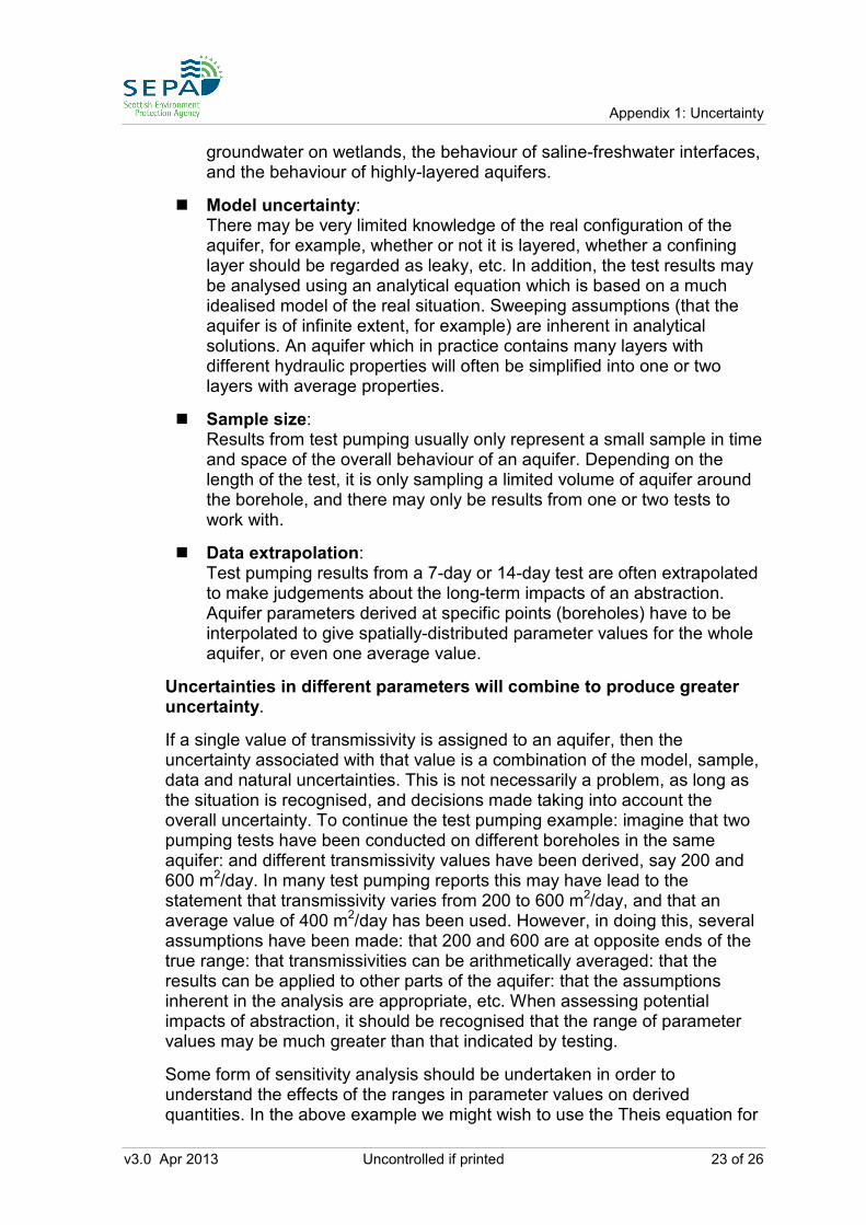
groundwater on wetlands, the behaviour of saline-freshwater interfaces, and the behaviour of highly-layered aquifers.

� Model uncertainty: There may be very limited knowledge of the real configuration of the aquifer, for example, whether or not it is layered, whether a confining layer should be regarded as leaky, etc. In addition, the test results may be analysed using an analytical equation which is based on a much idealised model of the real situation. Sweeping assumptions (that the aquifer is of infinite extent, for example) are inherent in analytical solutions. An aquifer which in practice contains many layers with different hydraulic properties will often be simplified into one or two layers with average properties.

� Sample size: Results from test pumping usually only represent a small sample in time and space of the overall behaviour of an aquifer. Depending on the length of the test, it is only sampling a limited volume of aquifer around the borehole, and there may only be results from one or two tests to work with.

� Data extrapolation: Test pumping results from a 7-day or 14-day test are often extrapolated to make judgements about the long-term impacts of an abstraction. Aquifer parameters derived at specific points (boreholes) have to be interpolated to give spatially-distributed parameter values for the whole aquifer, or even one average value.

Uncertainties in different parameters will combine to produce greater uncertainty.

If a single value of transmissivity is assigned to an aquifer, then the uncertainty associated with that value is a combination of the model, sample, data and natural uncertainties. This is not necessarily a problem, as long as the situation is recognised, and decisions made taking into account the overall uncertainty. To continue the test pumping example: imagine that two pumping tests have been conducted on different boreholes in the same aquifer: and different transmissivity values have been derived, say 200 and 600 m2/day. In many test pumping reports this may have lead to the statement that transmissivity varies from 200 to 600 m2/day, and that an average value of 400 m2/day has been used. However, in doing this, several assumptions have been made: that 200 and 600 are at opposite ends of the true range: that transmissivities can be arithmetically averaged: that the results can be applied to other parts of the aquifer: that the assumptions inherent in the analysis are appropriate, etc. When assessing potential impacts of abstraction, it should be recognised that the range of parameter values may be much greater than that indicated by testing.

Some form of sensitivity analysis should be undertaken in order to understand the effects of the ranges in parameter values on derived quantities. In the above example we might wish to use the Theis equation for



unsteady-state flow in confined aquifers to determine what effects the drawdown may have upon a sensitive wetland. To do this properly we must examine the effect of uncertainties in measurement of S and T, derived from the pump test, individually and in combination. Let us say that, in addition to the two Transmissivity values given above, the pump test gave values for Storativity of 5x10-5 and 5x10-4. Using an average value of S and the extremes for T gives a range for drawdown of 1.14 to 2.98 m. Using an average T and the extremes for S gives a range for drawdown of 1.31 to 1.77 m. However, combining the uncertainties (varying both T and S in the combinations which give the greatest extremes) results in a possible range for drawdown of 0.93 to 3.26 m. Which turns out to be the ‘true’ value could have dramatic implications for the wetland.

Some types of uncertainty are easier to reduce than others. For example, drilling another observation borehole for a pumping test will reduce the data uncertainty: conducting tests in several boreholes will reduce the sample uncertainty: using a radial flow model with layers (as opposed to an analytical equation) to analyse the results will reduce the model uncertainty. However, reducing knowledge uncertainty may require extended R&D and the need for uncertainty reduction must be closely linked to the risk of impact. Environmental or natural uncertainty is impossible to reduce, and must just be recognised.


Appendix 2: Glossary of Terms

Term Definition

Analytical Model An exact mathematical solution of the flow and/or transport equation for all points in time and space. In order to produce an exact solution, the flow/transport equations have to be considerably simplified (e.g. very limited, if any, representation of the spatial and temporal variation of the real system).

Conceptual Model A simplified representation or working description of how the real hydrogeological system is believed to behave. A quantitative conceptual model includes preliminary calculations, for example, of vertical and horizontal flows and of water balances.

Mathematical Model A mathematical expression(s) or governing equation(s) which approximate the observed relationships between the input parameters (recharge, abstractions, transmissivity etc.) and the outputs (groundwater head, river flows, etc.). These governing equations may be solved using analytical or numerical techniques.

Numerical Model A solution of the flow and/or transport equation using numerical approximations, i.e. inputs are specified at certain points in time and space which allows for a more realistic variation of parameters than in analytical models. However, outputs are also produced only at these same specified points in time and space.

Time Variant Groundwater Model

A specific type of numerical model, on the scale of a catchment, or larger, which simulates the behaviour of a hydrogeological system over a specified period of time (usually several decades). The parameters describing the system are varied according to their geographical and temporal distribution.


References

NOTE: Linked references to other documents have been disabled in this web version of the document. See the Water >Guidance pages of the SEPA website for Guidance and other documentation (www.sepa.org.uk/water/water_regulation/guidance.aspx). All references to external documents are listed on this page along with an indicative URL to help locate the document. The full path is not provided as SEPA can not guarantee its future location.

Key Documents

WAT-RM-11: Licensing Groundwater Abstractions including Dewatering

WAT-RM-26: Determination of Aquifer Properties

An applicants guide to water supply boreholes

External Documents

� ASTM (American Society for Testing & Materials) (www.astm.org/)

• Standards on Determining Subsurface Hydraulic Properties and Groundwater Modeling, ASTM, 1999

• Guidelines on Standards: ASTM D 5490–93: Model calibration ASTM D 5609–94: Defining boundary conditions ASTM D 5610–94: Defining initial conditions ASTM D 5611–94: Sensitivity analysis

� Riverbed Permeabilities: Information from Pooled Data Calver A, in Ground Water, Vol.39 No.4, pp546-553, July-August 2001.

� Derivation of a Methodology for Groundwater Recharge Assessment in Scotland and Northern Ireland, WFD12, SNIFFER (www.sniffer.org.uk)

� Flood Estimation Handbook Wallingford Hydro Solutions (www.hydrosolutions.co.uk/)

� Framework for Groundwater Resources Conceptual and Numerical Modelling, LIT 5348, EA Publications, (www.environment-agency.gov.uk/) See also: Groundwater Resources Modelling: Guidance Notes and Template Project Brief (Version 1). R&D Guidance Notes W213. Environment Agency, 2002

� Low Flows, Wallingford Hydro Solutions (www.hydrosolutions.co.uk)

� Low Flow Estimation in Scotland, IH Report 101, (www.ceh.ac.uk) Part of series of Low Flow Studies Reports (Institute of Hydrology 1980)

� Springs Database, British Geological Society (www.bgs.ac.uk/)

� UK Hydrometric Register, Centre for Ecology & Hydrology (www.ceh.ac.uk)

Water Use Regulatory Method (WAT-RM-27) Modelling Methods for Groundwater Abstractions

Documents

Transcript of Water Use Regulatory Method (WAT-RM-27) Modelling Methods for Groundwater Abstractions