HAL Id: tel-03275208https://tel.archives-ouvertes.fr/tel-03275208v2

Submitted on 30 Jun 2021

HAL is a multi-disciplinary open accessarchive for the deposit and dissemination of sci-entific research documents, whether they are pub-lished or not. The documents may come fromteaching and research institutions in France orabroad, or from public or private research centers.

L’archive ouverte pluridisciplinaire HAL, estdestinée au dépôt et à la diffusion de documentsscientifiques de niveau recherche, publiés ou non,émanant des établissements d’enseignement et derecherche français ou étrangers, des laboratoirespublics ou privés.

Abstractions of biochemical reaction networksAndreea Beica

To cite this version:Andreea Beica. Abstractions of biochemical reaction networks. Bioinformatics [q-bio.QM]. UniversitéParis sciences et lettres, 2019. English. NNT : 2019PSLEE071. tel-03275208v2

Préparée à l’École Normale Supérieure

Abstractions of Biochemical Reaction Networks

Soutenue par

Andreea BEICALe 12 juin 2019

École doctorale no386Sciences mathématiquesde Paris centre

SpécialitéInformatique

Composition du jury :

Mme. Anne SIEGELINRIA, CNRS & Univ. Rennes Présidente du jury,

Rapporteur

M. Gilles BERNOTCNRS & Univ. Nice-Sophia Antipolis Rapporteur

M. Jérôme FERETINRIA & ENS Examinateur

M. Wolfram LIEBERMEISTERInst. Nat. de la Recherche Agronomique Examinateur

Mme. Tatjana PETROVKonstanz University Examinateur

M. David SAFRANEKMasaryk University Examinateur

M. Vincent DANOSCNRS & ENS Directeur de thèse

Résumé

Cette thèse vise á étudier deux aspects liés á la modélisation des Réseaux de Réactions Biochim-iques.

Dans un premier temps, nous montrons comment la séparation des échelles de temps etde concentration dans les systèmes biologiques peut être utilisée pour la réduction de modèles.Nous proposons l’utilisation des modèles par régles de réécriture pour le prototypage de cir-cuits génétiques, puis nous exploitons le caractère multi-échelle de tels systèmes pour construireune méthode générale d’approximation de modèles. La réduction est effectuée via une anal-yse statique du système de règles. Notre heuristique de réduction repose sur des justificationsphysiques solides. Cependant, tout comme pour d’autres techniques de réduction de modèlesexploitant la séparation des échelles, on note la manque de méthodes précises pour quantifierl’erreur d’approximation, tout en évitant de résoudre le modèle original.

C’est pourquoi nous proposons ensuite une méthode d’approximation dans laquelle lesgaranties de réduction représentent l’exigence majeure. Cette seconde méthode combine ab-straction et approximation numérique, et vise á fournir une meilleure compréhension des méth-odes de réduction de modèles basées sur une séparation des échelles de temps et de concentration.

Dans la deuxième partie du manuscrit, nous proposons une nouvelle technique de reparamétri-sation pour les modèles d’équations différentielles des réseaux biochimiques, afin d’étudier l’effetdes stratégies de stockage de ressources intracellulaires sur la croissance, dans des modèles mé-canistiques d’auto-réplication cellulaire. Enfin, nous posons des bases pour la caractérisation dela croissance cellulaire en tant que propriété émergeante d’une nouvelle sémantique des réseauxde Petri modélisant des réseaux de réactions biochimiques.

i

ii

Abstract

This thesis aims at studying two aspects related to the modelling of Biochemical Reaction Net-works, in the context of Systems Biology.

In the first part, we analyse how scale-separation in biological systems can be exploitedfor model reduction. We first argue for the use of rule-based models for prototyping geneticcircuits, and then show how the inherent multi-scaleness of such systems can be used to devisea general model approximation method for rule-based models of genetic regulatory networks.The reduction proceeds via static analysis of the rule system.

Our method relies on solid physical justifications, however not unlike other scale-separationreduction techniques, it lacks precise methods for quantifying the approximation error, whileavoiding to solve the original model. Consequently, we next propose an approximation methodfor deterministic models of biochemical networks, in which reduction guarantees represent themajor requirement. This second method combines abstraction and numerical approximation,and aims at providing a better understanding of model reduction methods that are based ontime- and concentration- scale separation.

In the second part of the thesis, we introduce a new re-parametrisation technique fordifferential equation models of biochemical networks, in order to study the effect of intracellularresource storage strategies on growth, in self-replicating mechanistic models. Finally, we aimtowards the characterisation of cellular growth as an emergent property of a novel Petri Netmodel semantics of Biochemical Reaction Networks.

iii

iv

Acknowledgments

My first thanks go to Vincent Danos, for accepting to supervise my work during thesethree years. Thank you for advising me, and for cultivating a research environment based onfreedom of choice and scientific curiosity.

I would like to thank my reviewers Anne Siegel and Gilles Bernot, for accepting the timeconsuming task of reading this manuscript and writing reports. Thank you for your time andfor your valuable feedback. I also wish to express my gratitude towards the other members ofmy jury, for accepting to participate in my PhD defense.

My warmest thanks go to my co-authors, who provided me with invaluable help duringall stages of the research and writing process: Jérôme Feret, Cãlin Guet, Tanja Petrov andGuillaume Terradot. Thank you Jérôme for your availability and your sustained indispensablefeedback and help. Thank you Cãlin for the ever-stimulating discussions and for repeatedlywelcoming me into your lab. Thank you Tanja for your constant support, both scientificallyand personally. Thank you Guillaume for all the stimulating exchanges and for always beingwilling to share your impressive biological knowledge with me.

I am also thankful towards the rest of the permanent members of the Antique team: thankyou Xavier for sustainedly helping me navigate the meanders of administrative processes, thankyou Cezara for your much-needed advice and support. A warm thank you to the rest of theteam: Caterina, Ferdinanda, Gaëlle, Guillaume, Huisong, Ilias, Jiangchiao, Lý Kim, Marc,Nicolas, Patric, Pierre, Stan.

I am very grateful towards my circle of friends, for their constant and unconditional supportin my efforts towards this PhD: thank you Andreea, Alex, Coralie, Ioana, Ken, Laurent, Léa,Lola, Megumi, Raphaël. A special “thank you” goes to Kevin.

Most importantly, I would like to thank my parents, for giving me a taste for knowledgeand for science, and for their constant support and encouragement throughout these years.

This thesis is dedicated to my grandmother.

v

vi

Contents

Introduction 1Computer Science and Systems Biology . . . . . . . . . . . . . . . . . . . . . . . . . . 1Challenges . . . . . . . . . . . . . . . . . . . . . . . . . . . . . . . . . . . . . . . . . . . 6Outline and Contributions of the Thesis . . . . . . . . . . . . . . . . . . . . . . . . . . 11

I Biochemical Reaction Networks: A Review 17

1 Context and Motivation 191.1 Features of Dynamical Models in Systems

Biology . . . . . . . . . . . . . . . . . . . . . . . . . . . . . . . . . . . . . . . . . 191.2 Network models of biological systems . . . . . . . . . . . . . . . . . . . . . . . . . 20

2 Biochemical Reaction Networks: Syntax 23

3 Biochemical Reaction Networks: Semantics 293.1 Classical chemical kinetics . . . . . . . . . . . . . . . . . . . . . . . . . . . . . . . 293.2 Stochastic chemical kinetics . . . . . . . . . . . . . . . . . . . . . . . . . . . . . . 333.3 Stochastic vs deterministic models . . . . . . . . . . . . . . . . . . . . . . . . . . 41

4 Executable Biology: Computational models of Biochemical Reaction Net-works 534.1 Petri Nets . . . . . . . . . . . . . . . . . . . . . . . . . . . . . . . . . . . . . . . . 54

4.1.1 Motivation . . . . . . . . . . . . . . . . . . . . . . . . . . . . . . . . . . . 544.1.2 Qualitative Petri Nets . . . . . . . . . . . . . . . . . . . . . . . . . . . . . 554.1.3 Quantitative Petri nets . . . . . . . . . . . . . . . . . . . . . . . . . . . . . 60

4.2 Rule-based modeling and the Kappa language . . . . . . . . . . . . . . . . . . . . 614.2.1 Rule-based modeling . . . . . . . . . . . . . . . . . . . . . . . . . . . . . . 614.2.2 The Kappa language: Syntax and Operational Semantics . . . . . . . . . 634.2.3 The Kappa language: Stochastic Semantics . . . . . . . . . . . . . . . . . 67

II Model reduction 71

Motivation 73

vii

viii CONTENTS

5 Prototyping genetic circuits using rule-based models 775.1 Motivation . . . . . . . . . . . . . . . . . . . . . . . . . . . . . . . . . . . . . . . 775.2 A Kappa model of the λ-phage decision circuit . . . . . . . . . . . . . . . . . . . 79

5.2.1 Example: Kappa model of CI and CII production . . . . . . . . . . . . . . 835.3 Model Approximation using Michaelis-Menten-like reaction schemes . . . . . . . 85

5.3.1 Validity of the Michaelis-Menten enzymatic reduction in stochastic models 855.3.2 Generalized competitive enzymatic reduction . . . . . . . . . . . . . . . . 915.3.3 Operator site reduction . . . . . . . . . . . . . . . . . . . . . . . . . . . . 955.3.4 Fast dimerization reduction . . . . . . . . . . . . . . . . . . . . . . . . . . 995.3.5 Top-level reduction algorithm . . . . . . . . . . . . . . . . . . . . . . . . . 102

5.4 Results and Discussion . . . . . . . . . . . . . . . . . . . . . . . . . . . . . . . . . 1045.4.1 Results: reduction of the λ-phage decision circuit . . . . . . . . . . . . . . 1045.4.2 Conclusion and future work . . . . . . . . . . . . . . . . . . . . . . . . . . 106

6 Tropical Abstraction of Biochemical Reaction networks with guarantees 1096.1 Introduction . . . . . . . . . . . . . . . . . . . . . . . . . . . . . . . . . . . . . . . 1096.2 Definitions and Motivating Examples . . . . . . . . . . . . . . . . . . . . . . . . . 110

6.2.1 General Setting and Definitions . . . . . . . . . . . . . . . . . . . . . . . . 1106.2.2 Motivating example: Michaelis-Menten . . . . . . . . . . . . . . . . . . . . 1126.2.3 Motivating example: A DNA model . . . . . . . . . . . . . . . . . . . . . 121

6.3 Model reduction using conservative numerical approximations . . . . . . . . . . . 1216.4 Error estimates of tropicalized systems using conservative numerical approxima-

tions . . . . . . . . . . . . . . . . . . . . . . . . . . . . . . . . . . . . . . . . . . . 1316.4.1 Tyson’s Cell Cycle Model . . . . . . . . . . . . . . . . . . . . . . . . . . . 131

6.5 Comparison with existing methods . . . . . . . . . . . . . . . . . . . . . . . . . . 1366.6 Conclusion and outlook . . . . . . . . . . . . . . . . . . . . . . . . . . . . . . . . 138

III Modelling storage and growth 141

7 Effects of cellular resource storage on growth 1437.1 Introduction . . . . . . . . . . . . . . . . . . . . . . . . . . . . . . . . . . . . . . . 1437.2 Review of the Weisse cell model . . . . . . . . . . . . . . . . . . . . . . . . . . . . 145

7.2.1 Overview . . . . . . . . . . . . . . . . . . . . . . . . . . . . . . . . . . . . 1457.2.2 Nutrient Uptake and Metabolism . . . . . . . . . . . . . . . . . . . . . . . 1477.2.3 Transcription . . . . . . . . . . . . . . . . . . . . . . . . . . . . . . . . . . 1477.2.4 Competitive Binding . . . . . . . . . . . . . . . . . . . . . . . . . . . . . . 1497.2.5 Translation . . . . . . . . . . . . . . . . . . . . . . . . . . . . . . . . . . . 1497.2.6 Growth and cellular mass . . . . . . . . . . . . . . . . . . . . . . . . . . . 1507.2.7 Model parameters . . . . . . . . . . . . . . . . . . . . . . . . . . . . . . . 152

7.3 A scaling procedure for modelling nutrient storage in the cell . . . . . . . . . . . 1537.3.1 Motivation . . . . . . . . . . . . . . . . . . . . . . . . . . . . . . . . . . . 1537.3.2 Definition . . . . . . . . . . . . . . . . . . . . . . . . . . . . . . . . . . . . 1537.3.3 Examples . . . . . . . . . . . . . . . . . . . . . . . . . . . . . . . . . . . . 155

CONTENTS ix

7.3.4 Storage capacity in the Weisse model . . . . . . . . . . . . . . . . . . . . . 1577.4 The Growth Rate λ is an emergent property of the model . . . . . . . . . . . . . 1627.5 The Single Cell model . . . . . . . . . . . . . . . . . . . . . . . . . . . . . . . . . 164

7.5.1 The effects of metabolite storage on exponential growth rate . . . . . . . 1647.5.2 Metabolite storage and adaptation to environmental fluctuations . . . . . 1667.5.3 Environmental dynamics and resource storage strategies . . . . . . . . . . 172

7.6 The Ecological perspective . . . . . . . . . . . . . . . . . . . . . . . . . . . . . . . 1747.6.1 Motivation . . . . . . . . . . . . . . . . . . . . . . . . . . . . . . . . . . . 1747.6.2 Experiment setup: a mixed population model in a fluctuating environment1747.6.3 Results . . . . . . . . . . . . . . . . . . . . . . . . . . . . . . . . . . . . . 176

7.7 Conclusion . . . . . . . . . . . . . . . . . . . . . . . . . . . . . . . . . . . . . . . 185

8 Abstractions for cellular growth: towards a new Petri net semantics 1878.1 Motivation . . . . . . . . . . . . . . . . . . . . . . . . . . . . . . . . . . . . . . . 1878.2 Split-Burst: towards a piecewise-synchronous execution of Biochemical Reaction

Networks . . . . . . . . . . . . . . . . . . . . . . . . . . . . . . . . . . . . . . . . 1898.2.1 Max-parallel execution semantics of Petri Nets . . . . . . . . . . . . . . . 1898.2.2 Piecewise-synchronous execution semantics . . . . . . . . . . . . . . . . . 190

8.3 Linear Reaction Networks . . . . . . . . . . . . . . . . . . . . . . . . . . . . . . . 1928.3.1 Growth rate as an emergent property . . . . . . . . . . . . . . . . . . . . 1928.3.2 Synchronous execution . . . . . . . . . . . . . . . . . . . . . . . . . . . . . 193

8.4 Possible Applications . . . . . . . . . . . . . . . . . . . . . . . . . . . . . . . . . . 1958.4.1 Approximation of system dynamics . . . . . . . . . . . . . . . . . . . . . . 1958.4.2 Synchronous Balanced Analysis . . . . . . . . . . . . . . . . . . . . . . . . 195

8.5 Conclusion and future directions . . . . . . . . . . . . . . . . . . . . . . . . . . . 198

Conclusion 203

9 Conclusion and future directions 2039.1 Contributions . . . . . . . . . . . . . . . . . . . . . . . . . . . . . . . . . . . . . . 2039.2 Future works . . . . . . . . . . . . . . . . . . . . . . . . . . . . . . . . . . . . . . 205

Appendices 207

A Probability Theory 209

B A DNA model: equation for the derivative of the lower bound on theconcentration of x2 219

Bibliography 221

x CONTENTS

Introduction

Computer Science and Systems Biology

When delving into the history of Computer Science, one finds that the first design for amodern computer is widely accepted to be the Analytical Engine: a programmable mechanicalcalculator invented in 1837, by Charles Babbage. Its invention date considerably pre-dates thatof the modern digital computer, and hints at the initial goal of the field of study: creatingmechanical devices that automate mathematical calculations. The validity of this objective isreinforced by the consensus that the earliest foundations of Computer Science can be foundin ancient mechanical computation tools such as the abacus, the Antikythera mechanism, orthe mechanical analog computer devices of the medieval Islamic world. However, in the lastcentury, Computer Science has evolved from its initial calculation-related task of translatinga mathematical language model into a computer program simulating it, to become a centralcomponent of both a vast range of scientific areas and of mundane existence.

It can be argued that the main reason for which the field has become ubiquitous to modernlife lays in its evolution from being primarily a “science of calculation”, to also becoming a“science of models”. In this sense, one notes the recurring development of new domain-specificprogramming languages that are able to directly model a vast range of processes.

An indicator of the growing relevance of Computer Science in the area of scientific mod-elling is the emergence of interdisciplinary fields such as Systems Biology, computational biology,bioinformatics, computational linguistics, artificial intelligence, cognitive science, or computa-tional social science, to name a few.

The work presented in this thesis aims at developing new modeling and model analysistools for Systems Biology, in order to tackle two of the challenges specific to the field. Thefirst such issue deals with model reduction techniques and their guarantees, while the secondone addresses the mathematical modeling and analysis of specific biological behaviors such asdescribing cellular growth as an emergent system property, as well as how it is impacted bycellular resource storage strategies.

As the science that studies living systems, biology is concerned with their constituents atall scales: molecule, cell, tissue, organ, individual, organism, and ecosystem. As illustratedby existing biological classifications and taxonomies, the main activities of the discipline tra-ditionally had a prominent qualitative component. However, the advent of novel experimentaltechniques that allowed researchers to simultaneously observe the behaviours of large numbers

1

2 CONTENTS

of distinct molecular species, in the beginning of the 21st century, has triggered a shift towardthe quantitative side [36], and with it has seen the emergence of new approach to biology, inwhich Computer Science plays a key role. The resulting interdisciplinary research field, SystemsBiology, aims at building an integrated physiology of systems and a predictive understandingof the whole, by focusing on the data-centric quantitative modeling of biological processes andsystems [173]. In other words, intracellular processes are investigated as dynamic systems. Thisnew outlook on biology is made possible by recent technological advances that enable bothmolecular observations on far more inclusive scales than previously achievable, but also allowfor computational analysis of such observations.

Indeed, the last two decades have seen biological research become a data intensive science,due to the ever-increasing flow of data resulting from the ability to make comprehensive mea-surements on DNA sequence, gene expression profiles, or protein-protein interactions (to namea few). This, in turn, increases the role of computers and computer science in biology.

On the one hand, the considerable amount of vast information generated by new experimen-tal techniques such as DNA microarrays and genome sequencers1, as well as other large-scaletechnologies, exceeds human analysis capacity, and thus requires computation power for storing,processing, analyzing and understanding the data [98].

On the other hand, the rapidly growing amount of biological data in the public domainreinforces the importance of mathematical and computational models (as well as analysis tech-niques) of biological systems: measurements alone do not explain the underlying complex molec-ular mechanisms, therefore appropriate mechanistic theories are needed in order to understandthem. In other words, inferring physical or structural interactions in the system from func-tional data alone is impossible, meaning that dynamical modeling becomes a part of biologicalreasoning.

As such, the central philosophy of Systems Biology is that the traditional approach to bi-ological research, which consists in mapping out the physical components (and their individualinteractions) of a biological system, is unsatisfactory for the understanding of emergent proper-ties of a complex biological system, as the latter may be the result of the interplay of simpler,integrated parts of the network. Indeed, even though reductionism has been highly successfulin explaining macroscopic phenomena, purely in terms of the constituent parts, the underlyingassumptions (that there were few parts that interacted with each other in a simple manner,or that there were many parts but whose interactions could be neglected) are simply not truefor many systems of present interest. What’s more, the advent of computational techniqueshas revelead that even relatively small systems of interacting parts (e.g., the Lorenz system)could exhibit very complex behaviour. Biological systems, which are inherently complex, mustthus be modeled and studied using the prediction-control-understanding framework offered byexecutable mathematical models, which are also dubbed dynamical models.

Indeed, dynamical models prove to be a crucial component of the modern biologist’s tool-box, as via their simulation and predictive powers, they enable biological investigation in anumber of ways [99]:

1microarrays permit interrogation of more than one million single-nucleotide polymorphisms (SNPs) at thesame time

CONTENTS 3

1. Constructing such models demands a critical consideration of the underlying biologicalmechanisms, and can thus reveal inconsistencies or previously unnoticed gaps in knowl-edge.

2. They serve both as a recapitulation of system behavior, as well as a transparent, unequivocally-communicable description of the system.

3. They represent “working hypotheses”, which can be used to unambiguously investigatesystem behavior under conditions that are unachievable in a laboratory: model simulationscan be carried out quickly and with no real cost, with every aspect of model behavior beingobservable at all time points.

4. Model analysis yields insights into why a system behaves the way it does, thus providinglinks between network structure and behavior.

5. Through simulation, dynamical models allow for hypothesis generation and testing, en-abling one to rapidly analyze the effects of manipulating experimental conditions in silico.This iterative process leads to a continually improving understanding of the system, inwhat has been called a “virtuous cycle”.

6. Model-based design is also a central component of synthetic biology, as models of cellularnetworks are useful for guiding the choice of components and suggesting the most effectiveexperiments for testing system performance.

7. Other advantages of dynamical modeling include being able to model quantities that areexperimentally hidden, and being able to stretch or compress timescales.

What’s more, the very complexity of the living matter implies that biologists reason onmodels rather than on the objects themselves [36]. A “good” dynamical model should con-comitantly reflect known behavior of the studied system, contain hypotheses that need to beverified, and be able to predict the system’s behaviour in a precise, input-dependent manner.

All in all, Systems Biology aims at a system-level understanding and analysis of biologicalsystems, under the assumption that “the whole is greater than the sum of the parts”. As statedin [108], a system-level understanding “requires a set of principles and methodologies thatlinks the behaviors of molecules to system characteristics and functions” and ultimately aimsat describing and understanding living entities “at the system level grounded on a consistentframework of knowledge that is underpinned by the basic principles of physics”.

One of the recurring terms of the field is that of “network of networks”. It is a termthat provides meaningful insight into how the Systems Biology approach is different from, andmore predictive than, the traditional approach to biology, as it implies that biological systems(i.e., the bigger networks) are composed of many (smaller) networks that are integrated atand communicating on multiple scales. Under this “network of networks” framework, SystemsBiology seeks to formulate hypotheses for biological functions, as well as to provide spatial andtemporal insights into biological dynamics, by analyzing the component networks across scalesand by integrating their behavior at different levels[100].

4 CONTENTS

Indeed, by focusing on the study of single biomolecules and of the interactions betweenspecific pairs of proteins, the traditional reductionistic approach to molecular biology operateson a single scale, thus imparting a limited understanding of the system[100]. By contrast,instead of merely identifying individual genes, proteins and cells, and studying their specificfunctions, Systems Biology investigates the behavior and relationships of all of the elements ina particular biological system while it is functioning[98].

Consequently, when compared to the traditional reductionistic approach, a systems ap-proach towards biology enables the modeling of global biological mechanisms such as the cir-cadian clock, for example, that are a result of complex interactions between various agentsacting on heterogeneous time- and concentration- scales: genes, mRNAs, protein complexes,metabolites, tissues, organs, signalling networks, etc....

The philosophy of Systems Biology thus lays in the multiscale exploitation of the hugeamount of data yielded by the traditional approach, in order to study how the function of a bio-logical system arises from dynamic interactions between its parts (i.e., how low-level biologicaldata translates into functioning cells, tissues and organisms). In this way, it aims at creatinga consistent system of knowledge - and an understanding of biology at a system level- that isgrounded in the molecular level [108]. By integrating models at different scales and allowingflow of information between them, multiscale models describe a system in its entirety, and assuch, are intrinsic to the principles of Systems Biology[100].

The central tasks of Systems Biology can be divided into: [98] (a) comprehensively gath-ering information from each of the distinct levels of individual biological systems and (b) inte-grating the data to generate predictive mathematical models of the system.

According to [108], task (b) can be further partitioned into the following objectives:

1. System structure identification: identifying the system’s components, as well as theinteractions between them (i.e., the system topology) and the interaction parameters;

2. System behavior analysis: once the model’s structure is decided upon, its behaviorneeds to be understood, either by identifying the temporal evolution of the components’quantities (through simulation), or by using various analysis techniques to determinebehaviours (e.g., analyze the system’s sensitivity against external perturbations, and howquickly it returns to its normal state after the stimuli [108]);

3. System control: aims at applying the insights obtained by structure identification andsystem behavior analysis towards establishing a method to control the state of biologicalsystems, in order to address questions with immediate therapeutical benefits, such as:how to transform malfunctioning cells into functional ones, or how to drive cancer cells toapoptosis2, or how to control the differentiation status of a specific cell into a stem cell,and then control it to differentiate into the desired cell type;

4. System design/Synthetic Biology: ultimately design biological systems ab initio, thatexhibit a certain desired functionality.

2programmed cellular death

CONTENTS 5

As such, Systems Biology is a hypothesis-driven research field, which is characterized by asynergistic combination of experimentation, theory and computation. The idealized process ofSystems Biology research, as presented in [109] and illustrated in Fig.1, consists in a cycle thatbegins by selecting the contradictory issues of biological significance, and continues with themanual or automatic creation of a model representing the phenomenon. This model representsa computable set of assumptions and hypotheses that are to be tested experimentally, afterhaving previously been revelead as adequate through simulation. The in silico experimentsplay a key role in the research cycle: when provided with inadequate models, simulation revealsinconsistencies with established experimental facts, thus informing the researcher that the modelneeds to be either modified or rejected. Models that pass this test are then subjected to thoroughsystem analysis, where a number of predictions can be made. Among these, a set of predictionsthat are able to distinguish a correct model among competing models are selected for “wet”experiments - succesful experiments eliminate inadequate models. Models that survive thiscycle are deemed to be consistent with existing experimental evidence, and can therefore beused in Steps 3 and 4 mentioned above.

Figure 1: The idealized Systems Biology research cycle, according to [109]

In this manuscript, we address theoretical and computational issues in cellular modelling.More specifically, our contributions are in the areas of behavior analysis, model reduction, andthe computational modeling of specific biological behaviours of interest.

Our work consequently relates to the computation and analysis branches of the SystemsBiology research cycle of Figure 1, which aim at formulating data- and hypothesis-driven mod-

6 CONTENTS

els of and theories for biological mechanisms, as well as developing efficient algorithms, datastructures, visualization, data-analytical and communication tools for predictive computer mod-eling - a significant task of systems and mathematical biology. It involves the use of computersimulations of biological systems to both analyze and visualize the complex connections of theunderlying cellular processes, and its ultimate goal is to create accurate real-time models of asystem’s response to environmental and internal stimuli: e.g., a model of a cancer cell in orderto find weaknesses in its signalling pathways.

Notable previous efforts in Computational Systems Biology include helping sequence thehuman genome, and creating accurate models of the human brain [95].

Challenges

All in all, with Systems Biology, a paradigm shift occurs in biology, away from a descriptivescience, and toward a predictive one. Experimental observations cover a wide range of biolog-ical processes, that span from simple isolated enzymatic reactions, to complex systems suchas patterns of gene expression and regulation. As even simple dynamic systems can exhibit arange of complex behavior, which cannot be intuitively predicted from experiences, the systemsapproach requires quantitative mathematical and statistical modelling of biological system dy-namics [101]. Thus, modelling becomes a part of biological reasoning, however it turns out tobe a particularly challenging task.

The first challenge arising in model construction is that dynamical models need to addressthe specificities of biological systems, which are as follows [36]:

• Biological systems integrate multiple scales, both with respect to time, and withrespect to their constituent components. For example, chemical processes governing net-work dynamics span over many well separated timescales: while protein complex formationoccurs on the seconds scale, post-translational protein modification takes minutes, andchanging gene expression can take hours, or even days. As for the system components,multiscaleness applies both to the abundance of various species in biochemical networks(e.g., the DNA molecule has one to a few copies, while mRNA copy numbers can varyfrom a few to tens of thousands), and to the scale of the components themselves, whichcan range from molecule and cell, to tissue, organ, individual, organism, and ecosystem.

• Biological systems are governed by a mix of deterministic and probabilisticbehaviors: their behavior at the finest timescale is inherently stochastic, thus requiringprobabilistic models, while integrating across scales typically yields deterministic behav-iors.

• The complexity of biological systems warrants phenomenological models. Bio-logical systems have evolved under the dual mechanism of mutation and selection. Conse-quently, they have selected for robustness, which is often translated by the presence of re-dundant features. For example, consider the existence of alternative competing metabolicpathways that are related to the same function; indeed, such a redundant feature can beinterpreted as a backup strategy that renders the system robust to fluctuations in the

CONTENTS 7

environment. The presence of redundancy in biological systems sheds doubt on the exis-tence of simple laws governing the behavior of complex systems, which in turn partiallyexplains the apparent duality of biological modeling: one the one hand, models are de-rived from first principles, but on the other hand, the development of phenomenologicalmodels is based parameter correlation investigation, thus calling for machine learning andinferential modeling methods.

• The variability of biological systems calls for statistical assessments: thus, thereis a need for generic models that accommodate individual-specific variations, as well asfor a statistical assessment of the parameters used to single out specific properties.

Dynamical model construction also raises several central problems from a knowledge per-spective:

• finding an appropriate level of abstraction for a given analytic problem;

• finding a common basis to relate knowledge gained using different experimental techniqueson the same system, or conversely to relate knowledge gained from the same experimenton different model systems;

• incorporating knowledge incrementally as new data is analyzed.

Finally, any mathematical or algorithmic development for biological sciences requires ac-knowledging the existence of a number of specificities of the latter, that are not common practicein mathematics and computer science. Model and technique design should thus require recon-ciling these somewhat different perspectives. These specificities are [36]:

• an inherently system-centric development: while mathematics and computer scienceaim at exhibiting general properties and algorithms (which can be instantiated in a numberof settings), biology is often a system-centric activity that focuses on a specific cell, organ,or pathology.

• an interest towards ill-posed problems: while mathematics and computer sciencehave traditionally been concerned with well-posed problems, modeling in biology is asconcerned with designing models that serve to identify ill-posed problems, as it is withsolving well-posed ones.

• a need for validation: every biological model should eventually be evaluated againstexperimental results, in order to be confirmed or invalidated.

• models for complex biological systems are often multidisciplinary:

– biological knowledge/data serve as the starting point of the model, as well as pro-viding its semantics, by embedding it in a biological context

– mathematics enables the compromise between biological accuracy and conceptualsimplicity, by allowing information to be abstracted at different levels.

8 CONTENTS

– physics and chemistry are used to endow the abstract model with mechanical orelectrical properties

– computer science allows for automatizing tasks, performing analyses, and, most-importantly, running model simulations, that serve as numerical experiments fromwhich properties of the system can be inferred

• the dual contribution of mathematics and computer science in biology: firstly,the robustness and efficiency of existing methodological development can be improved bydevelopments in the two fields (e.g., by mastering the numerics of floating-point calcula-tions, improving the convergence properties of algorithms for optimization purposes, anddesigning algorithms with enhanced asymptotic properties, that scale better); secondly,concepts and algorithms from mathematics and computer science are used to lay thegroundwork for more advanced, more accurate models (e.g., stochastic modeling, inverseproblem solving, machine learning, statistical inference).

As mentioned above, the first question that arises when trying to construct models of bio-chemical networks deals with the level of abstraction to be employed. Dynamical models ofbiochemical networks, like all models, are abstractions of reality, which focus on certain aspectsof the subject, and abstract away other aspects. A wide variety of modelling techniques havebeen proposed, each of different complexity and abstraction, ranging from models representingregulatory relations between genes as simplified discrete circuits (e.g. gene regulatory networks),through models containing a detailed description of the low-level mechanistic interactions be-tween molecules (e.g. rule-based models), to models of spatio-temporal dynamics of processesconsidered at an individual particle level (e.g. stochastic models in which the diffusion, interac-tion with surfaces and participation in chemical reactions of each point-like particle is trackedindividually [6],[17]). In the absence of a universal modelling framework, each approach ab-stracts the biological processes being considered in a specific way, thus bringing along its ownset of assumptions as well as its own niche of validity. The overall challenge is related with theunderstanding of cellular processes and their modeling within the adequate level of abstraction.

After having settled on one of the available modelling frameworks, two issues await themodeler. The first challenge deals with identifying the structure of the system, a necessary steptowards the understanding of the biological system. The difficulty is that a biochemical networkcannot be inferred automatically from experimental data based on universal rules of principles,because biological systems evolve through stochastic processes and are not necessarily optimal[108]. What’s more, one must identify the true network, among multiple candidates that exhibitsimilar behavior to the desired one.

Once the structure of the system has been fixed, the modeler needs to identify the set ofcorresponding parameters (i.e., binding constant, transcription rate, translation rate, chemicalreaction rate, degradation rate, diffusion rate, etc...), as all computational results have to bematched and tested against actual experimental data. What’s more, simulation is needed in or-der to carry out a quantitative analysis of the system’s response and behavioral profile. Exceptfor certain well-studied cases, these constants are not readily available. Ideally, comprehensivemeasurements of major parameters should be carried out through wet-lab experiments, how-ever, rate constants often vary drastically in vivo[108]. Consequently, various in silico parameter

CONTENTS 9

optimization techniques can be used to find a set of parameters leading to simulation resultsconsistent with experimental data (e.g., brute force exhaustive search, genetic algorithms, sim-ulated annealing), however most of them are computationally expensive.

Computational cost turns out to be a bottleneck of Systems Biology: returning to thechallenge of choosing the modeling framework with the most adequate level of abstraction, onemight think that an increased level of details is desirable for model comprehensiveness. This,however, is not always true, as it can lead to a model whose complexity becomes prohibitive.For models of biological systems, the term “complexity” refers not only to non-linearity andemergent behavior, but also to (i) their inherent multiscaleness ( biochemical processes gov-erning network dynamics typically span over many well separated timescales, and abundanceof various chemical species can span over many well separated concentration scales) and to (ii)to the sheer size of the model (as measured by the number of components and the pattern ofinteractions among them). These complexity-inducing features make constructing an analyticalperspective w.r.t. biological models a challenging task. Moreover, as computational modelingcontinues to make significant progress, the issue of scalability of techniques to models of realis-tic size remains a major challenge, as the growth in complexity is often exponential and arisesindependently of the representation [165].

For example, in models of biochemical networks, the number of possible chemical species isoften subject to combinatorial explosion, due to the large number of species that may arise asa result of protein bindings and post-translational modifications [94]. As a consequence, mech-anistic models of signaling pathways easily become very combinatorial. What’s more, evenif compact ways of describing models prone to combinatorial explosion exist (i.e., rule-basedmodels), the curse of dimensionality once again rises when trying to compute the system be-havior. A strategy to cope with such complexity is model reduction, in which certain propertiesof biochemical models are exploited in order to obtain simpler versions of the original complexmodel; these simpler models should preserve the important behavioral aspects of the initial sys-tem. The major challenge with respect to model reduction techniques lies in providing explicitbounds on the accumulated reduction errors, or in other words, providing guarantees as to howthe solution of the reduced model relates to that of the original model, while avoiding to solvethe original model (whose size is often prohibitive).

Finally, the need for modeling biological systems, instead of biological mechanisms in iso-lation, has begotten the development of “whole-cell” computational models, which have beendescribed both as “the ultimate goal” of Systems Biology, and as “a grand challenge for the 21stcentury” ([35],[177]). These models aim to predict cellular phenotypes from genotype, by anexhaustive representation of the cellular machinery: all of the chemical reactions in a cell, all ofthe physical processes that influence their rates, the entire genome, the structure and concentra-tion of each molecular species, and the extracellular environment [105]. Given their potential ofunifying the understanding of cell biology and of enabling in silico experiments to be performedwith complete control, scope and detail ([143],[35],[177]), they are poised to have a dramaticimpact on Systems Biology, bioengineering and medicine [105]. The reasons for this lay in theirpotential to guide experiments in molecular biology, as well as enable computer-aided designand simulation in synthetic biology, and inform personalized treatment in medicine [122]. Todate, the most complete computational cell model is a mechanistic whole-cell model for the bac-

10 CONTENTS

terium Mycoplasma genitalium [104], in which diverse mathematical techniques from multiplefields are combined, in order to enable mechanistic modeling at multiple levels of abstraction 3,in an integrated simulation. [35]

Despite having being hailed as a future transformative force of Systems Biology, severalchallenges (still) prevent the wide-scale conception of whole-cell models. These challenges arerelated, among others, to incomplete and disparate biological knowledge, to the integrationof multiple scales from genotype to phenotype, to the exhaustive description of each moleculeand each interaction, and to the scalability of computational tools and methods. In [122], theauthors of the Mycoplasma genitalium model identified 7 areas containing the main challengesto building whole-cell models: experimental interrogation, data curation, model building andintegration, accelerated computation, analysis and visualization, model validation, and col-laboration and community development. However, Systems Biologists are leveraging recentprogress in measurement technology, bioinformatics, data sharing, rulebased modeling, andmulti-algorithmic simulation in order to construct whole-cell models, and it is anticipated thatongoing efforts towards developing whole-cell modeling tools “will enable dramatically morecomprehensive and more accurate models, including models of human cells”[143]. Beyond theexperimental and computational progress that is making whole-cell modeling possible, thereis nonetheless a need for several technological advances, that would help accelerate the frame-work, in the areas of: metabolome-wide and proteome-wide measurement technologies, kineticparameter measurement technologies, data aggregation tools, tools for collaboratively buildinglarge models directly from experimental data and for identifying gaps and inconsistencies inmodels, rule-based modelling languages that would support all of the biological processes thatmust be represented, scalable multi-algorithmic simulation, calibration and verification tools,and simulation analysis tools [143].

With all the challenges raised by whole-cell models that aim at exhaustively describing theentirety of the cell machinery, one can turn to a simpler class of models, dubbed “self-replicator”cellular models. Instead of accounting for all annotated gene functions of a cell, the “self-replicator” paradigm depicts minimal mechanistic models (i.e., that contain just a few classesof proteins, grouped according to their function) of the molecular regulatory mechanisms insidethe cell, and that are able to reproduce well-known experimental microbial growth laws. Thestrength of such models specifically lays in their ability to reproduce experimentally observedbehaviors, with a minimalistic, coarse-grained modelling approach. The most well-known suchmodel is presented in [130], where the authors construct a minimal model of a self-replicatingbacterial cell. The model consists of only 4 enzymes and a membrane, and is optimized forgrowth rate, under the assumption of competition for a limited amount of ribosomes. Theresults of such optimization display regulation of properties (like the ribosomal content and thesurface/volume ratio) similar to those observed in real cells.

In this manuscript, we will tackle such mechanistic self-replicator models (more specifically,the one presented in [182]), instead of whole-cell models in the classical sense, in order to addressthe issue of modelling intracellular resource storage strategies.

We note that by modeling an exhaustive range of cellular processes - albeit in a simplified

3thousands of heterogeneous experimental parameters are simultaneously included in the model, which cap-tures a wide range of cellular behaviors

CONTENTS 11

fashion-, from extracellular nutrient import and metabolization, to transcription, translationand degradation, such mechanistic models are indeed constructed in the spirit of Systems Biol-ogy.

Outline and Contributions of the Thesis

The works carried out during this thesis were precisely motivated by the challenges men-tioned previously. This manuscript is composed of four independent - but complementary -projects, each one tackling one of the existing challenges in Systems and Computational Biol-ogy. The four works can be grouped in two orthogonal groups: the first group tackles modelreduction heuristics and model reduction error estimation techniques that exploit the inherentmultiscaleness of biological systems, while in the second one, we study the formal modellingof relevant biological behaviours (i.e., intracellular resource storage and growth) in the deter-ministic modelling framework (i.e., through ordinary differential equations). We note that ourcontributions span both modelling frameworks: deterministic and stochastic. Furthermore, ourcase studies range from classical, well-understood and exhaustively-studied examples, such asthe E.coli’s λ-phage switch, to more recent models that fall under Systems’ Biology goal ofworking toward a system-level understanding of biological systems.As such, in Chapter 7, ourcase study builds upon a recent mechanistic cellular growth model that respects the universaltrade-offs that arise in cells due to resource limitations, and which quantitatively recovers thetypical behavior of both an individual growing cell, and of a population of cells.

The structure of the manuscript is the following.In Part I, Chapter 1, we introduce the notion of biochemical reaction network (BRN),

and present the state of the art with respect to its mathematical and computational modelling.As commonly done for programming languages, we differentiate between syntax and semantics.The former, presented in Chapter 2, is represented by a network structure that models thebiological system as set of species undergoing a series of chemical reactions. As for the semantics,we present the two major approaches to modeling the dynamics of a reaction network - thedeterministic and the stochastic dynamics - , as well as their respective associated simulationand analysis tools, in Chapter 3. Also in Chapter 3, we show how the deterministic andstochastic models are related via a scaling limit. In Chapter 4, we present two computationalmodels of Biochemical Reaction Networks, that will be addressed in this thesis: Petri Nets, inSection 4.1, and the the rule-based modeling language Kappa, in Section 4.2.

Part II of the manuscript is composed of two projects dealing with model reductiontechniques and reduction error estimate heuristics.

The first contribution, presented in Chapter 5, deals with the stochastic modelling ofgenetic circuits, in which the evolution dynamics of a BRN is modeled as a Continuous TimeMarkov Chain (CTMC). Herein, we argue for the use of rule-based models in prototypinggenetic circuits, and tackle the issue of multiscaleness-based model reduction in the context ofKappa, one of the existing rule-based modeling languages. As it will be explained in Part I,rule-based models allow, on the one hand, to circumvent the combinatorial explosion in thesize of the models, by using a set of rules to indirectly specify a mathematical model. On the

12 CONTENTS

other hand, rule-based modeling languages are designed to capture the mechanistic details ofthe protein-centric biological interactions, thus leading to transparent, modulable, extensibleand easily understandable models of biological networks. This latter aspect will be the focus ofour study; the complexity-reducing properties of using rules instead of reactions will a priorinot be exploited in this manuscript.

When designing genetic circuits, the typical primitives used in major existing modellingformalisms are gene interaction graphs. This framework operates on a high level of abstraction,by modelling the circuit as a graph whose nodes denote genes and whose edges denote activationor inhibition relations between genes. Gene interaction graphs contain no information withrespect to lower-level mechanistic details as to how such regulation relations are implemented.However, when designing experiments, it is important to be precise about this kind of details.

Fortunately, such protein-protein mechanistic interaction details can be modeled usingKappa - a rule-based language for modeling systems of interacting agents, which allows tounambiguously specify mechanistic details such as DNA binding sites, dimerisation of tran-scription factors, or co-operative interactions. Nonetheless, such a detailed description comeswith complexity, as well as computationally costly executions. Consequently, we propose a gen-eral reduction method of rule-based models of genetic circuits, in which each rule is a reaction,based on eliminating intermediate species and adjusting the rate constants accordingly.

Our method is an adaptation of an existing algorithm, which was designed for reducingreaction-based programs[112]; our version of the algorithm scans the rule-based Kappa model insearch for those interaction patterns known to be amenable to equilibrium approximations (e.g.Michaelis-Menten scheme, as well as a number of other stoichiometry-simplifying techniques).Additional checks are then performed in order to verify if the reduction is meaningful in thecontext of the full model. The reduced model is efficiently obtained by static inspection overthe rule-set. We test our tool on a detailed rule-based model of a λ-phage switch, which lists92 rules and 13 agents. The reduced model has 11 rules and 5 agents, and provides a dramaticreduction in simulation time of several orders of magnitude.

The Michaelis-Menten model of enzyme kinetics, which constitutes the basis of our re-duction algorithm, is arguably the best known example of an approximation that exploits themultiscaleness property of biochemical networks, with respect to both time-scales and speciesabundance. It is commonly used to represent enzyme-catalysed reactions in biochemical mod-els, and has been thoroughly studied in the context of traditional differential equation models[164]. Classically, ordinary differential equations represent an adequate approach to modellingbiochemical systems in which species appear in abundance. However, the presence of small-concentration species in biochemical systems encourages the conversion of the Michaelis-Mentenmechanism to a stochastic representation. It has been recently shown that this approximationis also applicable in discrete stochastic models, and that furthermore, its validity conditionsare the same as in the deterministic case [164]. More specifically, in the deterministic case,its derivation is based on the equilibrium approximation, which is valid if the substrate speciesreaches equilibrium on a much faster time-scale than product formation, or alternatively on thequasi steady-state approximation, which requires that enzyme concentration be much less thanthe substrate concentration.

Our method is an illustration of the fact that in general, the multi-scaleness of biochemical

CONTENTS 13

reaction networks represents a feature that can be exploited for model reduction purposes:it allows to approximate the complete mechanistic description with simpler rate expressions,retaining the essential features of the full problem on the time scale or in the concentrationrange of interest.

Nonetheless, providing guarantees as to how the solution of the reduced model relates to theoriginal one remains a challenge. To the best of our knowledge, there exist no precise methodsto quantify the error induced by time-scale separation approximations for biochemical reactionnetworks, while avoiding to solve the original model. The bottleneck lays in the complexity ofthe original system, whose behavior can be computationally costly to analyze - often times, itssize is prohibitive enough to allow even running a single simulation trace.

The correctness of our approach relies on the fact that the approximate model is equal tothe original one, in the artificial limit where certain reactions happen at a sufficiently largertime-scale than others, and they are seemingly equilibrated shortly upon the reactions initi-ation. However, not unlike other scale-separation reduction methods, our method relies on asolid physical justification, yet the numerical approximations lack both explicit bounds on theaccumulated errors, and proof of soundness.

This is the reason for which, in Chapter 6, we propose an approximation method fordeterministic models of biochemical networks, in which reduction guarantees represent the ma-jor requirement. Our method combines abstraction and numerical approximation, and aimsat providing a better evalutation of model reduction methods that are based on time- andconcentration- scale separation. The reduction guarantees of our method are a consequenceof a carefully designed symbolic propagation of dominance constraints: given an ODE modelof a BRN that exhibits time- and concentration- scale separation, we abstract the solution ofthe original system by a “box” that over-approximates the state of the original system andprovides lower and upper bounds for the value of each variable of the system in its currentstate. The simpler equations (which we call tropicalized) that define the hyperfaces of the boxare obtained by combining the dominance concept borrowed from tropical analysis [119] withsymbolic bounds propagation. Mass invariants of the initial system of ODEs are used to refinethe computed bounds, thus improving the accuracy of the method. The resulting (simplified)system provides a posteriori time-dependent lower and upper bounds for the concentrations ofthe initial model’s species, and thus bounds on numerical errors stemming from tropicalization.This means that no information on the original system’s trajectory is needed - the most im-portant advantage of our approach. By contrast, the main difficulty of applying the classicalQSS and QE reductions to biochemical models is that QE reactions and QSS species need tobe specified a priori, which implies that some knowledge about the initial system’s behavior isnecessary. This, in turn, means that significantly high-dimensional, non-linear systems cannotbenefit from these reductions, as their analysis can be prohibitive in practice.

Depending on the chosen granularity of mass-invariant-derived bounds, we show that ourmethod can either be used to reduce models of biochemical networks, or to quantify the ap-proximation error of tropicalization reduction methods that do not involve guarantees. As such,the guarantees of our method are obtained by formalizing the soundness relation between theoriginal system of equations and the abstract system of ordinary differential equations operatingon the coordinates of the hyper-faces of the box. The solution of a sound abstraction of an

14 CONTENTS

original system of differential equations, starting from a box that contains the initial state ofthe original system, defines a sound abstraction of the solution(s) of the original system. Weapply our method to several case studies (a simple DNA model constructed as an extensionof the classical Michaelis-Menten reaction scheme, and to the minimal cell cycle proposed byTyson [178], and finish by comparing it to existing interval numerical methods for enclosing thesolution of an initial value problem (IVP) between rigorous bounds.

The works presented in Part III deal with issues regarding the mathematical modeling ofbiological behaviors of particular interest, in the deterministic modelling framework. Namely, weaddress the modelling of intracellular resource storage strategies in self-replicating mechanisticmodels, as well as cellular growth as an emergent property of Petri Net model semantics ofBRNs.

As such, in Chapter 7 we address the issue of storage. Cells grow by fueling internalprocesses with resources taken from the outside. Depending on the responsiveness of thesebiosynthetic processes with respect to the availability of intracellular resources, cells can buildup different levels of resource storage. In this scenario, the questions we investigate are: howdoes storing resources impact cell growth? Namely, how much of these resources should a cellpile up internally, given the opportunity? And how does storage depend on resource availabilityand on other species competing for the same pool of resources?

To answer these questions, we introduce a new reparametrisation technique of ODE models,intended to model intracellular resource storage strategies. Our technique consists in defininga generic scaling transformation of BRNs that allows one to tune the concentration of certainchemical species, while preserving the network’s behaviour at steady state. Consequently, itenables one to symbolically navigate natural lines of iso-cost in parameter space, provided costfunctions only depend on steady-state constraints (and only on a subset of the model variables).In our specific case, this means that we can guarantee by construction that various storagestrategies preserve approximatively goodness-of-fit to the original growth data, and thereforecorrectly match growth conditions to sectorial resource allocations.

We acknowledge that storage has a concrete maintenance cost, because idle resources arediluted by growth, but also that higher storage levels improve the dynamics of reallocation ofresources among the various sectors of production (transporters, metabolism, translation) whensugar levels change sharply in the environment. This fundamental trade-off is best investigatedusing a mechanistic model of cellular growth, where costs are emergent and reflect architecturaltraits of the growth machinery. Consequently, we apply our method on such a recent “self-replicator” mathematical model of the coarse-grained mechanisms that drive cellular growth(i.e., the Weisse model [182]), in order to investigate the effects of cellular resource storage ongrowth. We carry out our analysis not only for a single-cell model, but also in a competitivecontext.

At the single cell level, we start by comparing storage strategies against different patternsof environmental changes. We investigate the impact of scaling (that we identify as storage) oncellular growth during shifts of the sugar yield, and are able to make a number of observations:(i) storage capacity can be modulated over several orders of magnitude without significantlyaffecting growth rate, (ii) in constant environments, excessive storage of the protein precursoris detrimental to growth rate, (iii) the cost of storage, in terms of reduced growth, is condition-

CONTENTS 15

dependent, and higher in rich growth conditions, (iv) storage results in smoother physiologicaltransitions during environmental up-shifts and increases biomass during such transitions, as re-source allocation is dependent on protein precursor concentration, and (v) evolutionary benefitsof storage increase with the frequency and magnitude of environmental fluctuations.

Our results thus suggest that there is a cost associated with high levels of storage, whichresults from the loss of stored resources through dilution. On the other hand, high levels ofstorage can benefit cells in variable environments, by increasing biomass production duringtransitions from one medium to another. A potential explanation for this behavior is that asuitable amount of storage can decrease the cost of resource reallocation caused by changes ingrowth conditions, as reflected by the Weisse model. Our results thus suggest that cells mayface trade-offs in their maintenance of resource storage based on the frequency of environmentalchange.

We continue by adopting an ecological perspective, in which we compare storage strategiesin competitive situations (i.e., in which species contend for the same resources). To do so, we testpopulations of low- and high-storage strategies against each other, in a variety of environmentsparametrized by the frequency of two superimposed probabilistic trains of high and low pulses ofsugar. Our experiments demonstrate the existence of a convex boundary separating a domainof “bursty” regimes, characterized by high and infrequent sugar pulses, from the rest. Inthis domain, the low-storage strategy, which is faster growing, wins. A surprising result isthat outside of this domain, the fast growers are driven to extinction by the high-storage, slowgrowers; lasting co-existence of the two storage strategies can only be observed on the boundary.

All in all, with our model in place, we are able to observe a rich interplay of storage levels,growth rates, growth yield (i.e., the amount of biomass produced per unit of growth medium),and resource variability. Our results indicate that the specificities of environmental changes playa decisive role in deciding which storage strategy is deemed the most beneficial (with respectto accumulating biomass over time). This is even more so the case when species content for thesame resource: the combined effect of storage strategies and competition lead to extracting lessbiomass out of the same amount of resources.

The last matter we address in this thesis deals with the modeling of cellular growth. InChapter 8, we work towards a characterization of cellular growth as an emergent propertyof a novel Petri net execution semantics. Consequently, we aim to substitute to a “growth”biochemical reaction network (BRN) (i.e., for which an exponential stationary phase exists)a piecewise-synchronous approximation of the deterministic dynamics. To achieve this, wepropose to model a BRN using a resource-allocation-centered Petri Net, with parallel maximal-step execution semantics. We argue that this semantics is better-suited for modeling biochemicalreaction networks, when compared to the classical interleaving semantics, as it takes into accountthe inherently concurrent nature of biological processes. In the case of unimolecular chemicalreactions, we prove the correctness of our method and show that it can be used either as anapproximation of the dynamics, or as a method of constraining the reaction rate constants (analternative to flux balance analysis, using an emergent formally defined notion of “growth rate”as the objective function), or a technique of refuting models.

16 CONTENTS

Part I

Biochemical Reaction Networks: AReview

17

Chapter 1Context and Motivation

1.1 Features of Dynamical Models in SystemsBiology

We have previously detailed the crucial role that quantitative mathematical (or dynamical)models plays in modern biological reasoning. Herein, we elaborate on their required components.

The primary components of a dynamical mathematical model of a biological system corre-spond to the molecular species present in the system.The abundance of each species is assignedto a state variable of the model, the collection of which represents the system state. The systemstate provides a complete description of the system’s condition at any given time, via its timecourse, as given by the model’s dynamic behavior.

Besides state variables, models of biological systems also include parameters, which charac-terize environmental effects and interactions among system components, and whose values arefixed - meaning that the distinction between model parameters and state variables is clear-cut.Example of common parameters include association constants, maximal expression rates, anddegradation rates. As a change in the value of a model parameter corresponds to a change inthe environmental conditions or in the system itself, model parameters are typically held con-stant during a simulation. Varying parameter values between rounds of simulation allows oneto explore system behavior under perturbations of the experimental conditions, or in alteredenvironments.

As the main feature of a dynamical model of a biological system is its ability to describethe temporal evolution of the system components’ quantities, building a model then involvestwo important choices: (i) how to represent the model structure (i.e., determine its species,parameters, and molecular interactions), which is akin to defining its syntax, and (ii) how to’interpret’, or execute, the model, which is akin to defining its semantics. These two stepsare indicative of a distinction that is commonly made when dealing with systems modeling:the qualitative approach, respectively the quantitative approach. While the latter essentiallyrelies on mathematical equations describing the performance of the system for a large set ofinput functions and initial states, the former requires no such formal mathematical formulation,instead relying on visual representations (e.g., diagrams) of the relationships between the systemcomponents, that is, it relies on the structural model.

19

20 Network models of biological systems

For a large class of biological systems, what one usually seeks to model are the interactionsbetween individual molecules which are only distinguishable by the class of species they belongto. Consequently, population models prove to be a well-suited, and popular, mathematicalmodelling framework for biological phenomena. Any population model can be described as a setof reactions operating on a set of biochemical species: this is what we will refer to as BiochemicalReaction Networks; they will represent the modeling framework of choice throughout this thesis.Below, we motivate our choice.

1.2 Network models of biological systems

While using mathematical models in the natural sciences (particularly in physics) is not anew idea1, the novelty lays in the use of such models in life sciences, most notably in biology andbiomedicine. As such, quantitative mathematical models have lain outside mainstream researchapproaches during the last decades of the purposely reductionist qualitative era of molecularbiology, which instead heavily employed qualitative models. Indeed, biologists have long usedthese type of models as abstractions of reality, be it in the familiar form of the ball-and-stickmodel of chemical structure, or more generally in the form of diagrams that illustrate a set ofcomponents and their interactions, and which play a central role in representing our knowledgeof cellular processes [99].

Figure 1.1: An interaction diagram, inspired from [99]. Species A and B bind reversibly,forming a complex that inhibits the rate at which species C is transformed into species D. Thegraphical conventions used are that the blunt arrows denote inhibition, normal arrows denoteactivation, while dashed lines denote regulatory interactions, i.e. the species is not consumedby the reaction.

Such interaction maps, also called networks, formalize the complex interactions betweenheterogeneous entities (within and between cells), which characterize biological systems. Forexample, Figure 1.1 shows molecular species A and B binding reversibly, to form a complexthat inhibits the rate at which species C is transformed into species D.

Generally speaking, such network-based modeling approaches help structure and formalizeexisting knowledge, as well as predict system behaviour, and have been widely used for describ-ing cellular regulation and metabolism [16]. Consequently, it makes sense that a quantitative

1 Instead, it can be traced back to ancient Greek scholars, if not even further in the past

Context and Motivation 21

modeling framework be developed using this widely-employed qualitative description of biologi-cal systems: enter Biochemical Reaction Networks (BRNs). The central argument that justifiesadding quantitative/mathematical information to simple interaction maps, in order to obtainquantitative BRN models, is that simple interaction diagrams leave ambiguities with respect tothe system’s behaviour: we know what components of the system interact with each other, butnot necessarily how. By employing a mathematical description of the system, this uncertaintycan be eliminated, at the cost of demanding a quantitative characterization of every interactiondepicted in the diagram [99].

For example, in order to quantify the interaction between molecular species A and B, inFigure 1.1, a numerical description of the process must be provided, under the form of the bind-ing and unbinding reaction rate constants. For cellular processes of which only a qualitativeunderstanding of the underlying molecular interactions is available, such a quantitative descrip-tion is not possible. However, for an important number of well-studied mechanisms, sufficientdata have been collected as to allow a quantitative characterization [99], that, when coupledwith the interaction diagram, can be used to formulate a mathematical model of the network’sdynamics, which typically involves the physical and chemical laws governing the mechanismsthat drive the observed behaviour (such models are dubbed mechanistic). Whenever the quan-titative information regarding molecular interactions is available, the result is a collection ofbiochemical reactions involving the system’s species. A species is a system entity that is quan-tifiable, and whose quantity is susceptible of evolving over time. A reaction is an elementaryaction of the system that consists of consuming (respectively producing) a finite and integerquantity of a finite subset of species, called reactants(respectively products).

For example, the reversible binding reaction between species A and B of the interactiondiagram in Figure 1.1 writes as:

A+Bκ1−−−−κ−1

A.B, (1.1)

where A.B denotes the resulting complex.We note that, at this level of modeling, the notation A.B for the complex species is simply

a name, and should not be considered as indicative of the reaction’s mechanistic details (i.e., Abinds B). In this sense, one could choose any other name for the complex species: e.g., reaction1.1 could be equivalently written as A+B

κ1−−−−κ−1

C.

The model parameters are the binding, respectively unbinding, reaction constants κ1 andκ−1. As we will see in this chapter, both the interpretation of the reaction constants and therepresentation of the system state will depend on the chemical kinetics assumed to govern thedynamics of the system.

Example 1.2.1A more biologically relevant example is the Michaelis-Menten mechanism, which consists of anenzyme, denoted E, that reversibly binds a substrate, S, to form a complex, E : S. The complexthen releases a product P , while preserving the enzyme. The associated reaction network writesas:

E + S κ1−−−−κ−1

E : S κ2−→ E + P (1.2)

22 Network models of biological systems

Biochemical Reaction Networks will be the modeling framework of choice throughout thisthesis. Consequently, in the next sections of this chapter we formally define both their syn-tax, as well as the two major applicable semantics: classical (deterministic) chemical kinetics,respectively stochastic chemical kinetics.

Before moving forward with the definition of BRNs, we note that a disadvantage of networkmodels is that as the number of components and interactions in a biological system grows, itbecomes increasingly difficult to maintain an intuitive understanding of the overall behaviour[99]. Thus, different levels of information abstraction can be employed when constructingnetwork models, according to the size of the system, the available data, and the research questionunder consideration. In their simplest form, the interaction maps only depict the possibility ofinteraction between genes or proteins (Figure 1.2, top) - and can therefore cover larger systems -,while at the other end of the scale one finds detailed models based on mathematical descriptions(Figure 1.2, bottom), which provide significantly more detailed insight into the dynamics, butare usually only used to describe small, well-studied subsystems. Figure 1.2 shows a hierarchyof different, widely-employed, network models, each one abstracting information on a differentlevel, and thus requiring different amounts of detail.

Figure 1.2: A hierarchy of network models for biological systems [16]. Existing net-work models of biological systems abstract information on different levels, depending on theavailable data and the biological questions under consideration. Top-down: depicted modeltypes are ranked in increasing detail level and data demand, and decreasing coverage power.Less detailed models cover larger systems (in number of genes/biomolecules), but do not allowfor true simulation of network dynamics - simulation is possible only for the most detailed cat-egory of models, dubbed “quantitative models”, that are labeled with kinetic rate constants.Intermediary models, i.e. causal and logical networks, allow at most for simulation of the eventsequence or gene activation order, but quantifying the speed of reactions is impossible underthese simplified frameworks.

Chapter 2Biochemical Reaction Networks: Syntax

Models of cellular phenomena often take the form of interaction diagrams, as in Fig.1.1. Forbiochemical and genetic networks, interaction diagrams depict the molecular species in thesystem - which could be ions, small molecules, macromolecules, or molecular complexes - asnodes, and the interactions between them as arrows. The arrows can represent a range ofprocesses: chemical binding or unbinding, reaction catalysis, or regulation of activity. Theprocesses result in the production, inter-conversion, transport, or consumption of the specieswithin the network.

A set of reactions constitutes a biochemical reaction network. The manner in which thebiochemical species interact is referred to as the network topology, and its organization is ap-parent if one rearranges the reactions in the form of an interaction graph. For example, theinteraction graph of the Michaelis-Menten mechanism of Ex.1.2.1 is shown in Fig.2.1.

In order to obtain a quantitative description, one needs to know the rates at which thereactions occur. In vivo, the rate of a reaction depends on its kinetic constant, on the con-centration of the reactants, and on physico-chemical conditions, such as temperature and pH.However, for in silico models, the physico-chemical conditions are fixed, such that rate laws canbe described solely in terms of reactant concentrations and the kinetic rate constants.

All in all, a biochemical reaction network can be defined as:

Definition 2.1(Biochemical Reaction Network) A biochemical reaction network (BRN) is a pair (S,R,α,β),

Figure 2.1: Interaction graph of the Michaelis-Menten enzymatic mechanism

23

24

such that:

(i) S = S1, S2, . . . ,Sn is a finite set of chemical species,

(ii) R = r1, r2, . . . , rm is a finite set of reactions. Each reaction is a triple rj ≡ (αj ,βj , κj) ∈Nn × Nn × R≥0, that writes as:

rj : αj1S1 + αj2S2 + . . .+ αjnSnκj−→ βj1S1 + βj2S2 + . . .+ βjnSn,

with vectors αj and βj being commonly referred to as the consumption, respectively theproduction vectors of reaction rj, and κj denoting the kinetic constant of rj,

(iii) α,β ∈ Rm×n denote the network’s consumption, respectively production, matrices; eachelement αji, respectively βji, denotes the quantity of species Si begin consumed, respectivelyproduced, by reaction rj.

Remark 2.1. The reaction network can be written compactly in matrix-vector form, asαS κ−→ βS, with S the species column vector, and κ the rates column vector.

Remark 2.2. The laws of thermodynamics state that all chemical reactions are re-versible. Nevertheless, under certain environmental conditions (temperature, pressure,the availability of an enzyme), the reverse reaction proceeds at a negligible rate: nearlyall of the reaction’s reactants are used to form products, which makes it very difficult,even under extreme conditions, to reverse the reaction. In this case, it is reasonableto describe the reaction as being irreversible: this is why, in Definition 2.1, we assumeelementary reactions to be irreversible. Reversible reactions will simply be representedby the couple of direct (forward) and reverse (backward) reactions, which we will note,for convenience, as:

αj1S1 + αj2S2 + . . .+ αjnSnk+j−−−−k−j

βjiS1 + βj2S2 + . . .+ βjnSn.

Definition 2.2(Reactants, products, modifiers) In a reaction rj, a species Si is said to be:

• a reactant, if αji > 0

• a product, if βji > 0.

Additionally, species Si is usually considered to be a modifier in rj if it participates inthe reaction both as a reactant and as a product, but is neither produced nor consumed by it:αji = βji > 0.

Biochemical Reaction Networks: Syntax 25

Definition 2.3(Stoichiometry matrix) The stoichiometric matrix of a BRN (S,R,α,β) is formed by thestoichiometric coefficients of the reactions that constitute the network, and is defined as them× n matrix ∇ = β −α.

Definition 2.4 (State-change vector)Let (S,R,α,β) be a biochemical reaction network. The jth line of the stoichiometry matrix ∇ iscalled the state-change vector of reaction rj ∈ R: νj ≡ (∇j1,∇j2, . . . ,∇jn). The state-changevector denotes the change in the molecular population caused by one occurence of reaction rj,i.e., if the system is in state x and one reaction rj occurs, the system immediately jumps tostate x+ νj.

Remark 2.3. We note that the process of converting a reaction network into a stoi-chiometry matrix is lossy. Otherwise said, a reaction scheme is not uniquely defined byits stoichiometry matrix, which means it is not always possible to recover the originalreaction scheme from a stoichiometry matrix. For example, while the reaction systemsX → ∅ and 2X → X have the same associated matrix, their dynamical behavior is clearlydifferent.

Example 2.1Consider once again the Michaelis-Menten system:E + S κ1−−−−

κ−1E : S

E : S κ2−→ E + P

Then S = S,E,E : S, P, R = r+1 , r−1 , r2, with

r+1 ≡ (

(1 1 0 0

),(0 0 1 0

), κ1)

r−1 ≡ ((0 0 1 0

),(1 1 0 0

), κ−1)

r2 ≡ ((0 0 1 0

),(0 1 0 1

), κ2),

meaning that α =

1 1 0 00 0 1 00 0 1 0

, β =

0 0 1 01 1 0 00 1 0 1

, and ∇ := β −α =

−1 −1 1 01 1 −1 00 1 −1 1

Biochemical reaction networks represent a quantitative description of the system, which

can be used to construct dynamical mathematical models. The dynamic behavior (kinetics) ofa biochemical reaction network describes the changes in system states over time. A system state

26

is described by a set of variables at a given point in time. One state should contain enoughinformation to predict all possible future behaviours. A state can be represented in differentways, and each model defines the contents of the system state, as well as the underlying processtype governing the system’s dynamics.

Generally speaking, the dynamics of a population model can be:

(i) either discrete, or continuous depending on whether the population quantity is modeled asdiscrete or continuous variable; discrete time is favored when the quantities of the modelvariables change only when specific events occur, while continuous time is favored whenmodel variables are in constant flux;

(ii) either deterministic, if the output trajectory is fully determined by the initial state ofthe system, or stochastic, if starting from a given initial state, different trajectories canemerge, each trajectory having an associated probability of happening.

The notion of determinism, which is akin to model behavior reproducibility, is a foundationfor much of scientific investigation. A model is called deterministic if its behavior is exactlyreproducible. Although the behavior of a model depends on a specified set of conditions, noother factors influence it, so that repeated simulations under the same conditions are always inperfect agreement (i.e., they are perfect replicates).

In contrast, stochastic models allow for randomness in the model behavior, which is in-fluenced both by specified conditions and by unpredictable forces/noise. Consequently, eachrepetition of a stochastic simulation, under identical environmental conditions, will yield adistinct sample of system behavior.

As an illustrative example, consider the simple monomolecular reaction:

Aκ−→ B (2.1)

The process underlying this reaction can be assumed to be either deterministic, or stochas-tic. According to both the level of abstraction and to the hypothesized nature of change in thesystem state in time, one further distinguishes between discrete and continuous deterministicmodels.

Deterministic processes with a discrete change of system state can be represented usingBoolean models, which approximate the dynamics of biological networks by considering eachmolecule (e.g., gene or protein) in the network as either active/expressed (1) or inactive/notexpressed (0). Under this representation, the questions that can asked about the system are ofa qualitative nature: for example, instead of inquiring about the exact quantities of the chemicalspecies present in the network, one is interested in their presence or absence. Despite their sim-plified underlying view of biological networks, and the fact that they introduce a coarse approx-imation by neglecting intermediate states, Boolean approaches give a meaningful insight intobiological knowledge, having proven useful in analyzing system dynamics and reasoning aboutthe stability and robustness of biological systems. For example, Boolean approaches enablethe detection of singleton attractors (i.e., fixed points), where the system is stable. Morevoer,Boolean networks have been successfully applied [180] in modeling gene regulatory and signal-ing networks in a variety of biological systems ([2],[73],[118],[133],[162],[163],[166],[181]), at bothcellular and population levels ([27],[116]).

Biochemical Reaction Networks: Syntax 27

However, in this thesis, we will not address discrete deterministic models such as Booleannetworks. Instead, we will focus on continuous deterministic models.

For deterministic models with continuous change in time, the state of the system no longertracks the activation state of species, but rather their concentrations. Each species in thediagram is assigned a single state variable, [Si](t), denoting its concentration at time t. Thecollection of values of all single state variables, [S1](t), [S2](t), [S3](t), . . ., at any point in timet, constitutes the state of the system. Then, to each molecular species, corresponds an ordinarydifferential equation (ODE) that describes how its concentration changes over time, due tointeractions with other species in the network. A reaction can have one of several effects onthe molecular species partaking in it: besides the obvious phenomena of species consumptionand production, there are also reactions that have a modifying effect on its reactants, suchas autocatalytic production, (de)phosphorylation, or (un)binding. All of these reaction arethought of as elementary: they are reactions with a single mechanistic step. A general rule forconstructing the differential equation of a species S, with respect to the type of reactions itparticipates in, is [43]:

d[S]dt

= synthesis− degradation− phosphorylation

+ dephosphorylation− binding + release, etc...(2.2)

Equation 2.2 indicates that each reaction in which species S is consumed or structurallychanged (e.g., phosphorylated, or bound to another species) contributes negatively to the evolu-tion of its concentration, while the reactions that either produce S, or revert structural changes,contribute positively to its evolution.

The rate of each reaction must be represented by a kinetic rate law, which will have one ormore kinetic rate constants associated with it. In the deterministic case, these rate constantsdenote the speed of the reaction: how frequently the reaction is expected to occur. As we willsee in the next section, biochemical reactions are assumed to operate under the law of massaction, which states that the rate of a chemical reaction is directly proportional to the productof the activities or concentrations of the reactants.

For example, under the law of mass action, the changes in concentration for species A andB in Example 2.1, in the time interval dt, are given by the following system of ODEs:

d[A]dt = −κ[A]d[B]dt = κ[A]

which states that species B is produced at the same rate at which species A is consumed, andthat that rate is proportional to both the concentration of the reaction’s reactant A, and to itskinetic rate constant κ.

The third modeling choice assumes that the underlying process is non-deterministic, i.e.,that it exhibits a random component. Then, one can employ stochastic models, in which thestate system is given by a vector of species’ molecule count (xS1(t), xS2(t), . . .) ∈ N≥0, insteadof concentrations, and whose dynamics is governed by the probability of a reaction occurring

28

in a small time interval (t, t + δt]. In this case, the rate constant of a reaction rj is no longerinterpreted as the reaction’s speed, but rather as an indicator of the probability that a tu-ple of molecules corresponding to rj ’s reactant species will react according to rj in the nextinfinitesimal time dt.

Then, the rate of reaction Aκ−→ B denotes the probability of a molecule A transforming

into a molecule B in a time interval dt:

P(xa(t+ dt) = xa(t)− 1, xb(t+ dt) = xb(t) + 1) = κxa(t),

with (xa(t), xb(t)) denoting the number of molecules of type A, respectively of type B, presentin the system at time t.

As the latter two frameworks constitute the modelling approaches used in this manuscript(i.e., we do not tackle Boolean models), we next formally elaborate on the concepts of stochasticand deterministic semantics of BRNs.

Chapter 3Biochemical Reaction Networks: Semantics

3.1 Classical chemical kinetics

Conventional chemical kinetics operate under a continuous deterministic modelling frame-work, which involves no randomness in the development of states. That is, if a deterministicsystem is known at one time, then it is known at all subsequent times. It serves as the traditionalway of representing the systems dynamic of complex biological systems that involve the interac-tion of many components: starting in the late 1970s, researchers began modeling cell physiologyprimarily using the continuous deterministic ODE approach, and creating increasingly detailedmodels over the next three decades.

Under this framework, the biochemical reaction network is modeled as a continuous systemwith continuous time dynamics. For a given BRN (S,R,α,β), the system state is representedby a n-vector (x1(t), x2(t), . . . , xn(t)) of continuous variables that keep track of reactant con-centrations, i.e., xi(t) denotes the concentration of species Si in the system at time t. Thechemical reactions/interactions are also represented by continuous processes, i.e., it is assumedthat reactions occur continuously and simultaneously.

Each process rj has an associated deterministic rate constants kj - whose value is identicalto that of the dimensionless constant κj introduced in Definition 2.1. It gives a measure ofhow frequently each type of reaction is expected to occur. The velocity of each reaction isspecified using a rate equation. Deterministic reaction rates are described under the followingassumptions:

(i) stochastic fluctuations in the system are negligible;

(ii) molecules are considered to be point-like entities;

(iii) the reaction volume border, as well as the resulting frontier effects, are neglected;

(iv) spatial homogeneity: the reaction volume is well stirred, i.e., the reactants are equallydistributed throughout the volume, meaning that the rate of each reaction is independentof the reactant position in space; the reaction rate can then be unambiguously referred toin the volume;

29

30 Classical chemical kinetics

(v) the continuum hypothesis: each species is present in the system in a large amount - molec-ular abundance can be then described in terms of their continuously varying concentration,as opposed to an integer-valued molecule count.

Then, in a fixed volume, and under the negligible stochastic fluctuation, spatial homo-geneity and continuum hypothesis, the reaction rate equations typically assume mass-actionkinetics - or an enzyme kinetic law based on mass-action, such as the Michaelis-Menten or Hillkinetics. The law of mass-action states that the rate of a chemical reaction is proportional tothe product of the reactants’ concentration.

Under these conditions, the dynamic evolution of the system state (represented as an ar-ray of species’ concentrations) can be described mathematically by a set of coupled ordinarydifferential equations, called the reaction-rate equation (RRE):

Definition 3.1.1 (Continuous deterministic model (RRE))Let (S,R,α,β) be a biochemical reaction system and x0 = (x1, x2, . . . , xn) ∈ Rn≥0 an initialstate of the system. Then, the continuous deterministic model is the solution of the set ofn coupled differential equations given by1:

dx(t)dt

= ∇T f(x(t)), (t ∈ R≥0) (3.1)

and satisfying the initial condition x0. The function f : Rn≥0 7→ Rm≥0 denotes the flux of eachreaction, in a given state. The flux fj of a reaction rj depends only on the concentrations ofrj’s reactants. Assuming mass-action kinetics, f is given by:

fj(x) ≡ κjn∏i=1

xαjii , (j ∈ R) (3.2)

which in turn means that dxdt is a multivariate polynomial of the species’ concentrations.

Example 3.1.1For the Michaelis-Menten mechanism, the mass-action reaction fluxes write as

fr1+ = κ1[E][S]fr1− = κ−1[E : S]fr2 = κ2[E : S]

and the ODE system describing the evolution of species’ concentrations is given by

1∇T denotes the transpose of the stoichiometry matrix ∇

Biochemical Reaction Networks: Semantics 31

dx

dt=

−1 1 0−1 1 11 −1 −10 0 1

κ1[E][S]κ−1[E : S]κ2[E : S]

=

=

−κ1[E][S] + κ−1[E : S]

−κ1[E][S] + κ−1[E : S] + κ2[E : S]κ1[E][S]− κ−1[E : S]− κ2[E : S]

κ2[E : S]

or, component-wise:

d[S]dt = κ−1[E : S]− κ1[E][S]d[E]dt = κ−1[E : S] + κ2[E : S]− κ1[E][S]d[E:S]dt = κ1[E][S]− κ−1[E : S]− κ2[E : S]

d[P ]dt = κ2[E : S]

(3.3)

Remark 3.1.1. As stated in Def.3.1.1, the deterministic model is the solution of theinitial value problem (IVP) of 6.5, which is guaranteed to uniquely exist under very weakconstraints regarding the smoothness of the reaction rate laws - constraints that are usu-ally satisfied by realistic models of reaction networks. However, finding the mathematicalexpression of this solution is not always easy. As very few nonlinear systems of ODEscan be solved explicitly, the analytically solvable class of ODE systems is reduced tolinear systems of equations, which unfortunately show very limited interesting dynam-ical behaviors, and cannot model complex reaction networks of interest (they can onlymodel unimolecular reactions). This means that only certain simple, but usually not bi-ologically realistic, systems of equations can be solved analytically, in order to obtain anexplicit formula describing the time course trajectory. In more complicated scenarios, thecommon practice is to solve a well-posed IVP numerically, using numerical integrationmethods (e.g., Euler, Runge-Kutta, etc. . .) that provide approximations of the solutionof the IVP [26].

32 Classical chemical kinetics

Challenges

Despite it being the traditional approach to biological modelling, continuous deterministicmodels fail to capture several important details of biological processes and their related exper-imental data. Besides the ubiquitous model scalability issue that stems from kinetic parameterestimation difficulties, the hypotheses needed for the continuous deterministic chemical kineticscan prove to be too constraining for biochemical systems.

For example, the spatial homogeneity assumption typically holds in stirred laboratoryreaction vessels, and can be a good approximation in the cell, where the rapid diffusion processenables the mixing of molecular components. However, biological systems in general can containa significant amount of spatial structure, meaning that in many cases the assumption of spatialhomogeneity does not hold.

As for the continuum hypothesis, it serves towards allowing discrete changes in moleculenumber to be approximated by continuous changes in concentration, as individual reactionevents cause infinitesimal changes in abundance. This assumption is valid when molar quantitiesof reactants are involved (recall that the number of Avogadro is 6.02 × 1023), and is thusappropriate for cellular species with molecular counts of at least thousands. However, if thesystem is small enough that the molecular populations of at least some of the reactants do notexceed a unitary order of magnitude, discreteness and stochasticity may play important roles, inwhich case Eq.6.5 does not accurately describe the system’s true behavior. As it turns out, it isoften the case that reactants are not abundant: a number of cellular processes are governed bysmall populations of molecules numbering dozens or even less. For example, many genes, RNAsand proteins are typically present in low copy numbers. Consequently, deterministic modelingcan prove to be inappropriate, as in some cases changes in molecule abundance should be treatedas discrete steps in population size.

What’s more, numerous wet-lab experiments enabled by recent advances in experimentalmethods have shown that stochastic effects generate phenotypic heterogeneity in cell behavior,and that even more important, cells can functionally exploit variability for increased fitness.They also demonstrate that the dynamics at the single cell (or even single molecule) levelare intrinsically stochastic, or “noisy”, and that that noise can have large implications for thequalitative dynamics - meaning that stochastic fluctuations are not negligible: biology seems tobe inherently stochastic.

Therefore, we next introduce the stochastic model of biochemical reaction networks, as analternative to continuous deterministic models.

Biochemical Reaction Networks: Semantics 33

3.2 Stochastic chemical kinetics

In the previous section, we argue that numerous experiments have revealed the inherentlystochastic nature of biological phenomena, which is explained by the fact that molecules exhibita certain degree of randomness in their dynamical behavior. Indeed, deterministic models ofbiochemical systems ignore the physical aspect involved in the dynamic behavior of biologicalsystems, by assuming that reactions occur continuously. However, in a typical biological system,reaction events do not occur at regular intervals, which is why, for example, molecular motioncan be represented as Brownian motion, even in a “well-mixed” solution. In the same way, bi-molecular reactions result from collisions of individual reactant molecules that approach closelyenough (and in the correct orientation). What’s more, most molecular collisions do not causereactions. All these factors mean that the timing of reaction events is stochastic rather thandeterministic: on a molecular scale, reactions are rare, hard-to-predict events. In many cellularprocesses, this randomness is averaged out over large numbers of reaction events, resulting inpredictable system behavior. Deterministic models take advantage of exactly this averagingphenomenon: a reaction network that comprises significant amounts of reactant molecules willinvolve many simultaneous reaction events, in which case the network behavior correspondsto the average over these events and will be accurately described by deterministic differentialequation models. However, models of processes that involve low-copy molecular species, suchas gene expression, should account for this random variance/stochasticity.

Stochastic chemical kinetics applies to models centred on individual reaction events, andaims to describe the time evolution of a well-stirred chemically reacting system in a way thatincorporates the system’s discreteness and stochasticity [79]. In a stochastic model of a BRN,the additional random element that determines the development of subsequent processes liesprecisely in the random manner in which collisions in a system of molecules take place - this inturn leads to a probability distribution of system states.

In the stochastic framework, for a given BRN (S,R,α,β) that is assumed to be confinedto a constant volume Ω and in thermal equilibrium, the abundance of each chemical species willbe described by the number of molecules in the reaction volume at time t, instead of using theirconcentrations. Thus, the system state is represented by a n-vector (X1(t), X2(t), . . . , Xn(t)) ofdiscrete variables that keep track of molecular count, i.e., Xi(t) denotes the number of moleculesof species Si in the system at time t. Chemical reactions are also assumed to occur discretely,instantaneously and at separate times.

Once again, changes in species populations are a consequence of the chemical reactionsof the network. Each reaction rj is mathematically characterized by two quantities: its state-change vector, as presented in Definition 2.4 and its propensity function.

The definition of the propensity function is regarded as the fundamental premise of stochas-tic chemical kinetics [79], as all the subsequent developments in stochastic chemical kineticstheory follow from it, via the laws of probability (a review of the basic definitions and conceptsof probability theory needed for definining the stochastic model can be found in Appendix A).

34 Stochastic chemical kinetics

Definition 3.2.1 (Propensity function)Let (S,R,α,β) be a biochemical reaction network modeling a well-stirred, constant-temperaturereaction system, which is considered in a finite volume Ω. The propensity of a reaction rj ∈ R,denoted aj, is defined such that:

aj(x)dt ≡ the probability that, given the state of the systemat time t, X(t) = x, one reaction rj occurs insideΩ in the next infinitesimal time interval [t, t+ dt).

(3.4)

From a formal point of view, the dynamic hypothesis behind the propensity function isthat the system trajectories are realizations of a continuous-time Markov chain (CTMC), whichleads us to the definition of the stochastic model of a biochemical reaction network:

Definition 3.2.2 (Stochastic model)Let (S,R,α,β) be a biochemical reaction network, and x0 = (X1, . . . , Xn) ∈ Nn an initialstate of the system. Then, the discrete, stochastic model is a continuous-time Markov chainX(t) with Markov graph (S,w, p0), such that:

(i) S = x | is reachable from x0 in R,

(ii) p0(x0) = 1,

(iii) w(x,y) =∑aj(x)1y=x+νj | j = 1, . . . ,m.

Equivalently, the stochastic semantics of the network is the homogeneous CTMC that is definedby its transition laws:

∀t ≥ 0,∀x ∈ Nn,∀1 ≤ j ≤ m s.t. x+ νj ∈ Rn

⇒

P(X(t+ dt) = x+ νj |X(t) = x) = aj(ν)dt,P(X(t+ dt) = x |X(t) = x) = 1− aj(ν)dt

Propensity functions are assumed to be of mass-action type: aj(x) = cjn∏i=1

(Xiαji

), where

cj is the stochastic kinetic rate constant - the existence of which is guaranteed by kinetic the-ory arguments and the well-stirred system hypothesis, and which is such that cjdt denotes theprobability that a random tuple of molecules of the reactant species will react according to rjin the next infinitesimal time dt. The binomial coefficient

(Xiαji

)indicates the total number of

possible tuples of reactant molecules, with the needed stoichiometry αji for each Si, amongst theXi available ones at time t.

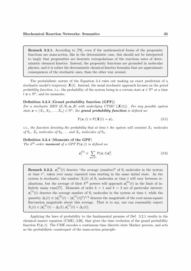
Biochemical Reaction Networks: Semantics 35

Remark 3.2.1. According to [79], even if the mathematical forms of the propensityfunctions are mass-action, like in the deterministic case, this should not be interpretedto imply that propensities are heuristic extrapolations of the reactions rates of deter-ministic chemical kinetics. Instead, the propensity functions are grounded in molecularphysics, and it is rather the deterministic chemical kinetics formulas that are approximateconsequences of the stochastic ones, than the other way around.

The probabilistic nature of the Equation 3.4 rules out making an exact prediction of astochastic model’s trajectory X(t). Instead, the usual stochastic approach focuses on the grandprobability function, i.e., the probability of the system being in a certain state x ∈ Nn at a timet x ∈ Nn, and its moments.

Definition 3.2.3 (Grand probability function (GPF))For a stochastic BRN (S,R,α,β) with underlying CTMC X(t). For any possible systemstate x = (X1, X2, . . . , Xn) ∈ Nn, the grand probability function is defined as:

P(x, t) ≡ P(X(t) = x), (3.5)

i.e., the function denoting the probability that at time t the system will containt X1 moleculesof S1, X2 molecules of S2, . . . and Xn molecules of Sn.

Definition 3.2.4 (Moments of the GPF)The kth-order moment of a GPF P(x, t) is defined as:

x(k)i ≡

∑x∈Nn

P(x, t)xki . (3.6)

Remark 3.2.2. x(k)i (t) denotes “the average (number)k of Si molecules in the system

at time t”, taken over many repeated runs starting in the same initial state. As thesystem is stochastic, the number Xi(t) of Si molecules at time t will vary between re-alizations, but the average of their kth powers will approach x(k)

i (t) in the limit of in-finitely many runs[77]. Moments of order k = 1 and k = 2 are of particular interest:x

(1)i (t) denotes the average number of Si molecules in the system at time t, while the

quantity ∆i(t) ≡ (x(2)i (t)− [x(1)

i (t)]2)1/2 denotes the magnitude of the root-mean-squarefluctuation magnitude about this average. That is to say, one can reasonably expectXi(t) ∈ [x(1)

i (t)−∆i(t),x(1)i (t) + ∆i(t)].

Applying the laws of probability to the fundamental premise of Def. 3.2.1 results in thechemical master equation (CME) [126], that gives the time evolution of the grand probabilityfunction P(x, t). The CME encodes a continuous time discrete state Markov process, and actsas the probabilistic counterpart of the mass-action principle:

36 Stochastic chemical kinetics

Definition 3.2.5 (The Chemical Master Equation)The probability law of the Markov chain X(t) of a biochemical reaction network(S,R,α,β) satisfies the equation:

∂P(x, t)∂t

=m∑j=1

[aj(x− νj)P(x− νj , t)− aj(x)P(x, t)

]. (3.7)

As it completely determines the function P(x, t), solving the CME means obtaining theprobability law of the system’s trajectory, as well as analytical formulas describing their firstand second order moments. However, the CME consists of a set of ODEs that has one equationfor every possible combination of reactant molecules. Consequently, analytical solutions of theCME for the probability density function of X(t) can only be obtained for a very few verysimple systems (e.g., for linear systems [102], or for systems consisting of one (irreversible orreversible) nonlinear reaction [114]). What’s more, even numerical solutions can prove to beprohibitively difficult in some cases [79].

As both the CME and the GPF moments prove to be virtually intractable, both analyticallyand numerically, the common practice is to construct numerical realizations of X(t) instead,i.e. to simulate the master equations’ stochastic realizations of the evolution of the state (its“paths”) via elementary reactions that occur with probabilities according to the CME. Theresulting method employs rigurously derived Monte Carlo techniques to numerically simulatethe very Markov process that the master equation describes analytically, meaning the simulationalgorithm is fully equivalent to the CME, even if the latter is never explicitly used [77].

In order to do so, instead of using the grand probability function P(x, t), a new functionis defined, called the reaction probability density:

p(τ, j | x, t)dτ ≡ the probability, given X(t) = x, that the nextreaction in the system to occur will be rj , andthat it will occur in the infinitesimal time interval[t+ τ, t+ τ + dt),

(3.8)

that describes the joint probability density function of two random variables: (i) the time tothe next reaction, τ , and (ii) the index of the next reaction, j.

The intuition behind employing these two random variables lies in the fact that changes inthe state of the underlying CTMC of a stochastic model occur at time instants 0 = t0 < t1 < . . .,where each ti corresponds to a reaction rj taking place.

Then, the a trajectory of the CTMC is entirely determined by the two quantities mentionedabove:

• the time elapsed between two consecutive reaction events, τk ≡ tk+1 − tk, for k ∈ N,

• the index (jk)k ∈ N∗ of the reaction taking place at time tk).

Biochemical Reaction Networks: Semantics 37

These two random variables enable the construction of a system trajectory, via the equation:

∀k ∈ N, X(tk+1) = X(tk) +∇ejk , (3.9)

with ei = (0, . . . , 0, 1(i), 0, . . . , 0)T the basis vectors of Rn.

By once again applying the laws of probability to the fundamental premise of 3.2.1, onecan derive 2 an exact formula for the reaction probability density function p(τ, j | x, t):

Theorem 3.2.1Given a stochastic model of a BRN (S,R,α,β), its reaction probability density function writesas:

p(τ, j | x, t) = aj(x)exp(−a0(x)τ), (3.10)

witha0(x) ≡

m∑j=1

aj(x),

which, as expected from a physical point of view, indicates that the probability of a par-ticular reaction occurring in the next time step is proportional to its propensity.

The reaction probability density function of 3.10 and Equation 3.9 are then used to con-struct a rigorous algorithm for simulating the temporal development of the stochastic chemicalsystem. Indeed, Equation 3.10 is the mathematical basis of the stochastic simulation, as itimplies that τ is an exponential random variable with mean and standard deviation 1

a0(x) , andthat j is a statistically independent integer random variable with point probabilities aj(x)

a0(x) [79].Samples of τ and j according to these distributions can be generated using Monte Carlo meth-ods, and then plugged into Equation 3.9 in order to generate an individual stochastic trajectoryof the system.

The simplest method of generating samples of τ and j is dubbed the direct method, in whichtwo random numbers n1 and n2 are drawn from the uniform distribution in the unit interval,and then used to construct [79] τ and j[79], as follows:

τ = 1a0(x) ln

1n1

j = the smallest integer satisfyingj∑

k=1ak(x) > n2a0(x).

(3.11)

Such a generating method (or a mathematically equivalent one) is then used in Gillespie’sstochastic simulation algorithm (SSA), in order to construct an exact numerical realization ofthe process X(t). The outline of the SSA algorithm is as follows. First, a maximal simulationtime tmax is set, and the initial state of the system is fixed. In Step 1, the algorithm proceeds bydrawing the reaction probabilities and the next reaction time from their respective distributions,after which the reaction to implement is chosen according to the fractional rates of 3.11. In Step

2for the exact derivation, the reader is refered to the original Gillespie paper [77]

38 Stochastic chemical kinetics

2, the time and system state are updated according to Equation 3.9. If the maximal simulationtime has been exceeded, the algorithm stops, otherwise it returns to Step 1.

Below is an implementation of the SSA algorithm, as described in ([79], [77]). The functiondraw_uniform is used to generate a random number from the uniform distribution in the unitinterval, and genτ (a0, n1) and genj(a, a0, n2) generate values for τ and j according to Equation3.11.

Algorithm 1: Gillespie’s SSA algorithm, direct versionInput: A BRN (S,R,α,β), with initial state x0, and a maximal simulation time tmaxOutput: An exact numerical realization (X(tk), tk)k∈N∗/* Step 0: initialize the time and the system state */

1 k ← 0;2 tk ← 0;3 X(tk)← x0;

/* Step 1: while the maximal simulation time has not been exceeded,simulate the trajectory one reaction at a time */

4 while tk < tmax do/* evaluate the propensity functions in the current state */

5 for j = 1 to m do6 aj ← cj

n∏i=1

(Xi(tk)αji

);

7 end/* evaluate a0 in the current state */

8 a0 ←m∑j=1

aj ;

/* draw n1 and n2 */9 n1 ← draw_uniform(0, 1);

10 n2 ← draw_uniform(0, 1);/* generate value for τ */

11 τk ← genτ (a0, n1);/* generate value for j */

12 jk ← genj(a, a0, n2);/* effect the next reaction by updating the time and the system state

according to Equation 3.9 */13 tk+1 ← tk + τk;

/* go back to Step 1 or finish simulation */14 k ← k + 1;15 end16 return (X(tk), tk)

Biochemical Reaction Networks: Semantics 39

Challenges

The validity of the hypotheses needed for continuous deterministic models remains an issueeven for discrete stochastic models. Indeed, in the stochastic modeling framework for BRNs onecontinues to operate under the spatial homogeneity and fixed volume hypotheses, as they allowthe system state to be described by specifiying only the molecular populations, while ignoringthe positions and velocities of the individual molecules, because the system is assumed to bewell-stirred.

When compared to the deterministic approach, stochastic models are often less tractable:the number of states of the underlying Markov chain can be prohibitively large (even infinite)when compared to the size of the network, which in turn makes solving the CME analytically(and even numerically) virtually impossible, save for a few simple cases. The Monte-Carloapproach, that is used in Gillespie’s algorithm, somewhat aleviates this issue, by generatingsystem trajectories that are correct w.r.t. the system’s stochastic semantics, and subsequentlyallowing to estimate its moments, by averaging a significant number of such trajectories. How-ever, difficulties also arise with respect to Gillespie’s algorithm. As the CME and SSA areboth derived exactly from the fundamental premise of Equation 3.4, they are equivalent to eachother. This means that the SSA imposes no approximations on the stochastic formulation ofchemical kinetics, thus taking full account of the inherent fluctuations ignored by the deter-ministic formulation. The SSA’s main advantage lays in its being a simple and compact wayof simulating exact trajectories for systems with an intractable CME. It can also be arguedthat the construction of the SSA exploits the fundamental premise (3.4) in a more direct waythan the CME. Indeed, Equation 3.4 describes the probability of the system being in a statex′′ at time t′′, knowing that it was in state x′ at time t′. While this step-like description ofthe dynamics is inherent to the SSA by construction, it cannot be expressed using the CME(unless one re-initializes time at each step, in order to consider (x′, t′) to be the initial state,i.e., (x0, 0)←− (x′, t′)).

However, the SSA is not without its flaws, the main one being that it is often slow, as itrelies on simulating every individual reaction event. This means that for realistic cellular system,which contain large quantities of molecular species, or for significant simulation durations, itsslowness becomes prohibitive. Consequently, a number of refinements of the SSA have beenproposed, aiming at reducing the simulation computational requirements. These refinementscan be split into two categories: exact variations and approximate methods.

Exact variations of SSA are essentially later elaborations on the most expensive computa-tion step of the original algorithm of ([77],[79]): locating the next reaction to fire, cf. Equation3.11. The classical SSA employed a linear search on the cumulative array of reaction propen-sities, in order to determine the next reaction event. Consequently, the first improvements tothe original algorithm included replacing the linear search by a binary-tree search ([117]), andsorting the cumulative array (either using a pre-simulation step [31], or on-the-fly [124]).

Other exact variation methods aimed at reducing the average number of operations requiredto obtain the index of the next reaction event, employed modifications such as reusing theunused reaction times computed during one SSA step [74], or using factored-out, partial reactionpropensities [156].

40 Stochastic chemical kinetics

Exact variation methods significantly increase the SSA’s speed for large networks (both interms of species and reactions), albeit they prove to be limited improvements of the originalSSA, as they still simulate reaction events one at a time.

On the other hand, approximate simulation strategies aim at finding a trade-off betweenthe exactness of SSA and simulation speed. Among these methods, we mention:

• The τ -leaping approximation algorithm ([76],[29],[30],[4],[39],[132]), which instead of tak-ing incremental steps in time, approximates the number of reaction events taking placein an interval of length τ , and performs all the reactions in that interval before updatingthe propensity functions. The value of τ is assumed to be small enough that there isno significant change in the value of the transition rates along during the time interval[t, t+ τ ];

• The conditional difference method [171], which approximates reversible processes by theircorresponding effective net reactions, before simulating the newly obtained system usingexisting stochastic procedures (such as the SSA).

Finally, we note that for stiff systems - evolving on both fast and slow timescales, with thefastes modes being stable -, because accuracy requires τ to be small on the fastest timescales,even the τ -leaping performs poorly in terms of speed. Consequently, accelerations procedureshave been developed for stiff systems: implicit τ -leaping ([159],[32]), which mirrors the implicitEuler method for systems of ODEs, and the slow-scale SSA (ssSSA) ([34],[33]), that directlysimulates the slow reactions (using specially modified propensity functions), while ignoring fastreactions.

Biochemical Reaction Networks: Semantics 41

3.3 Stochastic vs deterministic models

When comparing the deterministic and stochastic formulations of chemical kinetics, it iscommon practice to view the former as describing the average behavior of the latter, i.e., tointerpret the solution of the RRE as the mean of the species population size over a large numberof stochastic simulations. Consequently, one would expect equality between the solution of theRRE, χ and the expectation 3 of the GPF, E[X(t)]. However, in this section we will show thatthis equality holds only in one of two cases: in the thermodynamical limit ([80],[111]), or if allreactions in the network are unimolecular [126].

To do so, we derive the expectation of the marginal distribution of X(t), using the CME:

d

dtE[X(t)] = ∂

∂t

∑x

xP(x, t)

=∑x

m∑j=1

[aj(x− νj)P(x− νj , t)x− aj(x)P(x, t)x

]=∑x

m∑j=1

[aj(x− νj)P(x− νj , t)(x− νj)+

aj(x− νj)P(x− νj , t)νj−aj(x)P(x, t)x

]=

m∑j=1

∑x

[aj(x− νj)P(x− νj , t)(x− νj)+

aj(x− νj)P(x− νj , t)νj−aj(x)P(x, t)x

]=

m∑j=1

[E[aj(x)]x+ E[aj(x)]νj − E[aj(x)]x

]

, (3.12)

that is, one obtains that:dE[X(t)]

dt=

m∑j=1

E[aj(X(t))]νj . (3.13)

In order to compare dE[X(t)]dt to the corresponding deterministic expression for dχ

dt , we recallthat the relation between χ, the molecular concentration vector, and X, the molecular copynumber vector writes as χ ≡ X

Ω , where Ω denotes the volume.

Deterministic and stochastic rate constants

At this point, it is worth examining the relation between stochastic and deterministic reactionconstants. As previously mentioned, in the deterministic formulation of chemical kinetics, a

3For readability purposes, we will hereafter denote the first-order moment using the classical probabilitynotation for expectation, E[X(t)], instead of x(1).

42 Stochastic vs deterministic models

reaction constant kj is viewed as reaction rate/speed, whereas in the stochastic formulation,the constant cj is indicative of the reaction’s probability per unit of time [77]. Consequently,when switching between the stochastic and deterministic models, a conversion of rates must beperformed. Intuitively, this transformation is justified by the stochastic rate’s dependency onthe volume and the arity of the underlying reaction.

The recipe for this scaling procedure lies in the physical rationale of Definition 3.2.1, statingthat the propensity aj(x)dt, which in itself is a function of the stochastic kinetic rate cj , denotesthe probability of reaction rj taking place.

To start with, assume a unimolecular reaction

rj : S1 → . . . (3.14)

It denotes the spontaneous conversion of a molecule S1, and implies no molecular collision:consequently, its reaction rate is independent of the system volume Ω. This means that forunimolecular reactions, the stochastic kinetic constant cj is numerically equal to the reaction-rate constant kj of conventional deterministic chemical kinetics:

cj = kj (3.15)

On the other hand, for a bimolecular reaction

S1 + S2 → . . . , (3.16)

the stochastic rate cj will be inversely proportional to Ω, reflecting the fact that two reactantmolecules will have a harder time finding each other inside a larger volume. Indeed, if there arex1 molecules of S1 and x2 molecules of S2 inside a volume Ω, then there will be x1x2 distinctcombinations of reactant molecules in Ω, meaning that the probability that reaction rj willoccur somewhere inside Ω in the next infinitesimal time interval dt is given by x1x2cjdt. Fromthis, the average rate at which rj occurs inside Ω writes as

〈x1x2〉cj , (3.17)

where 〈〉 denotes the average taken over an ensemble of stochastically identical systems. Then,dividing by Ω, one obtains the average reaction rate per unit volume:

〈x1x2〉cjΩ , (3.18)

or, in terms of molecular concentrations, χi ≡ xiΩ :

〈χ1χ2〉 · Ω · cj (3.19)

The deterministic reaction constant kj is conventionally [77] defined as the average reactionrate per unit volume divided by the product of the average densities of the reactants:

kj = 〈χ1χ2〉 · Ω · cj〈χ1〉〈χ2〉

. (3.20)

Biochemical Reaction Networks: Semantics 43

However, in the deterministic formulation no distinction is made between the average ofa product and the product of the average, i.e., 〈χ1χ2〉 = 〈χ1〉〈χ2〉, which in turn leads to thesimplified expression relating the stochastic and deterministic reaction rate constants:

cj = kjΩ . (3.21)

Similarly, for a tri-molecular reaction, one would have the transformation:

cj = kjΩ2 . (3.22)

In general, for a reaction rj of arity p, in which all the reactants have stoichiometry one,the conversion rule is given by:

cj = kjΩp−1 . (3.23)

However, we note that for a bimolecular reaction involving the same species, S1 +S1 → . . .,the number of distinct possible reactant pairs would have been x1(x1−1)

2 ≈ x21, and we would

have obtained the relation:

cj = 2kjΩ (3.24)

instead of the expression of Equation 3.21.As it turns out, the conversion rule for any chemical reaction, no matter the reactant

stoichiometry, is given by:

kj

Ω

n∑i=1

αji−1= cj

n∏i=1

αji!(3.25)

Equation 3.25 is justified by the fact that in general, the conversion between the stochasticand deterministic rate constants is such that for any reaction rj , its stochastic rate functionapplied in a state X and the deterministic law of its conversion to a volume unit will relatethrough [78]:

fj(χ) = aj(X)Ω (3.26)

However, the quantities Ωfj(χ) and aj(X) write as:

Ωfj(χ) = Ω · kj ·n∏i=1

χαjii = kj · Ω

1−n∑i=1

αji·n∏i=1

Xαjii

aj(X) = cj ·n∏i=1

(Xi

αji

) (3.27)

44 Stochastic vs deterministic models

When all species in the system are abundant, i.e., if Xi →∞, the propensity function canbe approximated by:

aj(X) ≈ cjn∏i=1

αji!·n∏i=1

Xαjii (3.28)

By combining Equations 3.28 and 3.27, and applying the constraint of Equation 3.26, oneindeed obtains the general conversion rule of Equation 3.25.

The thermodynamic limit

When deriving the conversion rule of Equation 3.25, we hypothesized that all species areabundant, i.e., Xi →∞. It turns out that this hypothesis is linked to the first scenario in whichthe deterministic law of mass-action is valid w.r.t. to stochastic dynamics: the thermodynamiclimit [5].

The thermodynamic limit is defined as the limit in which both the species populations Xi,and the system volume Ω approach infinity, but in such a way that the species concentrations XiΩremain constant. Under this idealized state that provides a convenient approximation to macro-scopic systems, it was shown that the deterministic model represents a correct approximationof the stochastic one. Below, we sketch the proof presented in the original paper [5].

For a reaction rj , denote by Rj(t) the number of times rj occurs until time t. The value ofRj is a random variable described by the counting process satisfying:

Rj(t) = Yj(t∫

0

aj(X(s))ds), (3.29)

with Yj being independent unit Poisson processes.Then, the evolution of the state of the system satisfies:

X(t) = X(0) +m∑j=1

Rj(t)νj

= X(0) +m∑j=1

Yj(t∫

0

aj(X(s))ds)νj

(3.30)

If Ω denotes the size of the volume in which the reactions take place, one can introducethe scaled quantity denoting molecular concentration χ(t) ≡ X(t)

Ω . Using the scaling constraintfj(χ) = aj(X)

Ω of Equation 3.26, and the centered Poisson process Yj(t) = Yj(t) − t, one hasthat:

χ(t) = χ(0) +m∑j=1

Ω−1Yj(Ωt∫

0

fj(χ(s))ds)νj

= χ(0) +m∑j=1

Ω−1Yj(Ωt∫

0

fj(χ(s))ds)νj +m∑j=1νj

t∫0

fj(χ(s))ds

(3.31)

Biochemical Reaction Networks: Semantics 45

However, the law of large numbers for the Poisson process implies that Ω−1Yj(Ωu) ≈ 0,such that:

χ(t) ≈ χ(0) +m∑j=1νj

t∫0

fj(χ(s))ds), (3.32)

which, in the limit Ω → ∞, means that χ follows the classical deterministic law of massaction of Definition 3.1.1:

dχ(t)dt

=m∑j=1νjfj(χ(t)). (3.33)

Linear reaction networks

The second scenario in which classical chemical kinetics accurately describes the meanpopulation sizes is when the underlying reaction system is linear, i.e., when all of its reactionshave arity 0 (reactions of type ∅ → . . .) or 1 (unimolecular reactions).

Proposition 3.3.1Let (S,R,α,β) be a linear BRN. In its corresponding stochastic model, let X(t) be the stochas-tic process described by the CME, for an initial condition denoted by X0. Let χ(t) be thedeterministic time-evolution of species’ concentration described by the corresponding RRE, andstarting in initial state χ0 = X0

Ω . Then, for every time instant t, E[X(t)] = χ(t)Ω.

Proof. ([148]) The propensity of a 0-ary reaction is a constant, while the propensity of a unaryreaction is a linear function, meaning that E[aj(X)] = aj(E[X]). What’s more, according toEquation 3.25, stochastic and deterministic constants of linear reactions are identical, meaningthat aj = fj . Then, according to Equation 3.12, for every time point t, one has that:

d

dtE[X(t)/Ω] =

m∑j=1

E[aj(X(t)/Ω)]νj

=m∑j=1

fj(E[X(t)/Ω])νj, (3.34)

i.e., the expectation of X(t)/Ω evolves according to a differential equation that assumes theRRE law of mass action.

Examples

To illustrate the above-mentioned relation between stochastic and deterministic models, weproceed with the analysis of some simple reaction networks.

First, assume a linear reaction network, comprised of a single reversible reaction:

46 Stochastic vs deterministic models

Figure 3.1: Markov graph for the linear reaction network of (3.35), with initial condition x0 =(2, 0)

Ak1k−1

B, (3.35)

with initial condition x0 = (2, 0), i.e., there are initially 2 molecules of species A present in thesystem.

Its deterministic model is given by the ODE system:

d[A]dt = −k1[A] + k−1[B]d[B]dt = k1[A]− k−1[B]

(3.36)

.This system can be solved analytically; its solution is:A(t) = 2k−1+2k1e

−t(k1+k−1)

k1+k−1

B(t) = 2k1−2k1e−t(k1+k−1)

k1+k−1

(3.37)

The stochastic model of (3.35) is a CTMC X(t) with a Markov graph (S, ω, p0), suchthat:

• p0(x0) = 1;

• S = x0,x1,x2, with x1 = (1, 1), x2 = (0, 2);

• transition weights as depicted in Figure 3.1.

Using the notation P(x, t) ≡ P(X(t) = x) of Definition 3.2.3, the CME is represented bythe following system of equations:

dP(x0,t)dt = −2c1P(x0, t) + c−1P(x1, t)

dP(x1,t)dt = 2c1P(x0, t) + 2c−1P(x2, t)− c1P(x1, t)− c−1P(x1, 0)

dP(x2,t)dt = −2c−1P(x2, t) + c1P(x1, t)

(3.38)

with initial condition (x0,x1,x2) = (1, 0, 0).Applying the reaction rate scaling formula of Equation 3.25 for unimolecular reactions

means that the stochastic and deterministic constants have the same values: c1 = k1 andc−1 = k−1.

Biochemical Reaction Networks: Semantics 47

Figure 3.2: The deterministic solution and the stochastic mean population for species A inthe linear reaction network (3.35) coincide. The parameter values used for simulation arec1 = k1 = 1, c−1 = k−1 = 2.

The ODE system of Equation 3.38 contains only linear equations, meaning it can be solvedanalytically. The solution writes as:

P(x0, t) = c2−1+c2

1e−2t(c1+c−1)+2c1c−1e

−t(c1+c−1)

(c1+c−1)2

P(x1, t) = 2c1c−1−2c21e−2t(c1+c−1)+2c1e

−t(c1+c−1)(c1−c−1)(c1+c−1)2

P(x2, t) = c21+2c2

1e−t(c1+c−1)+c2

1e−2t(c1+c−1)

(c1+c−1)2

(3.39)

Then, the stochastic mean population of species A is indeed equal to the solution (3.37) ofthe deterministic model (3.36):

E[XA(t)] = 2 · P(x0, t) + 1 · P(x1, t) + 0 · P(x2, t)

= 2c−1 + 2c1e−t(c1+c−1)

c1 + c−1

= A(t)

(3.40)

In Figure 3.2 one can see that, as expected from Proposition 3.3.1, the stochastic meanpopulation of A coincides with the deterministic trajectory of its concentration, as obtained bynumerically simulating the mass-action equations of 3.36.

48 Stochastic vs deterministic models

Now consider the bimolecular reversible reaction:

A+Bk1k−1

C, (3.41)

with initial state x0 = (1, 3, 0), ODE system:d[A]dt = −k1[A][B] + k−1[C]d[B]dt = −k1[A][B] + k−1[C]d[C]dt = k1[A][B]− k−1[C]

(3.42)

and underlying CTMC as in Figure 3.3.

Figure 3.3: Markov graph for the bimolecular reaction network (3.41)

The resulting CME is given by the system of equations:dP(x0,t)

dt = −3c1P(x0, t) + c−1P(x1, t)dP(x1,t)

dt = 3c−1P(x0, t)− c−1P(x1, t)(3.43)

with initial condition (x0,x1) = (1, 0). Its solution is given by:

P(x0, t) = c−1

3c1+c−1+ 3c1e

−t(3c1+c−1)

3c1+c−1

P(x1, t) = 3c13c1+c−1

− 3c1e−t(3c1+c−1)

3c1+c−1

(3.44)

Consequently, the stochastic mean population of species A is given by:

E[XA(t)] = 1 · P(x0, t) + 0 · P(x1, t) (3.45)

We note that, as the forward reaction in 3.41 is bimolecular, the rate constants need tobe scaled according to the rules c1 = k1

Ω , c−1 = k−1. In order to compare the deterministicand stochastic models, the volume Ω is assumed to scale with the total molecule number. Weassume that one volume unit v corresponds to 4 molecules. Therefore, for an initial state of thestochastic model x0 = (1, 3, 0), the volume Ω = 4 would be equivalent one unit, while for aninitial state of x0 = (10, 30, 0), the volume Ω = 40 would take 10 units, i.e., Ω = 10v, and boththe bimolecular reaction rate constant and the trajectory of a resulting stochastic simulationwill be scaled by a factor of 10: c1 = k1

10 ,X(t)10 .

The results of Figure 3.4 confirm that for bimolecular reactions, the mean population sizedoes not coincide with the deterministic solution. However, as shown in Figure 3.5, as thesystem approaches the thermodynamical limit, the deterministic solution indeed approximatesthe mean population size.

Biochemical Reaction Networks: Semantics 49

Figure 3.4: As species A is a reactant of the bimolecular reaction (3.41), its mean populationsize does not coincide with its deterministic solution.

Conclusion

To summarize, in this chapter we have outlined the two fundamental formalisms for mod-eling biochemical reaction network dynamics: the classical framework, which is based on adeterministic chemical kinetics, and the stochastic framework, based on stochastic chemical ki-netics. The underlying assumptions and formalisms of the stochastic and deterministic modelsare listed for comparison in Table 3.1.

From a physical point of view, the stochastic formulation is superior to the deterministicone, as it captures and exploits the variability inherent to biological processes. The stochasticmodels are valid whenever the deterministic formulation is, but also when it is not.

However, from a mathematical point of view, the differential equations employed by thedeterministic formulation are far more tractable than its stochastic counterpart, the chemicalmaster equation. Nonetheless, when the modeled system involves large quantities of chemi-cal species and numerous reactions, neither formulation is tractable purely through analyticalmethods; instead, one resorts to numerical simulation methods in order to “solve” the model.

Finally, we have seen that, despite the fact that the deterministic formulation is consideredto model the average behavior of molecular populations, classical chemical kinetics faithfullydescribes this mean in only one of two cases: when all reactions are unimolecular, or when thesystem is in the thermodynamical limit.

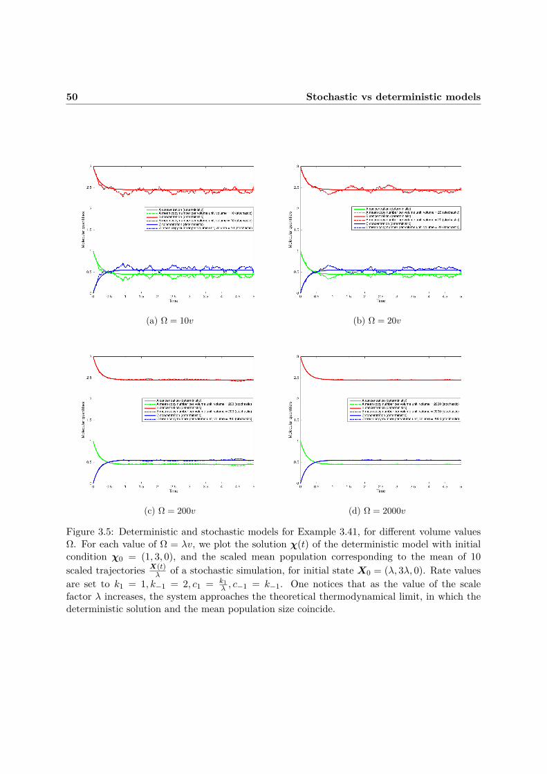
50 Stochastic vs deterministic models

(a) Ω = 10v (b) Ω = 20v

(c) Ω = 200v (d) Ω = 2000v

Figure 3.5: Deterministic and stochastic models for Example 3.41, for different volume valuesΩ. For each value of Ω = λv, we plot the solution χ(t) of the deterministic model with initialcondition χ0 = (1, 3, 0), and the scaled mean population corresponding to the mean of 10scaled trajectories X(t)

λ of a stochastic simulation, for initial state X0 = (λ, 3λ, 0). Rate valuesare set to k1 = 1, k−1 = 2, c1 = k1

λ , c−1 = k−1. One notices that as the value of the scalefactor λ increases, the system approaches the theoretical thermodynamical limit, in which thedeterministic solution and the mean population size coincide.

Biochemical Reaction Networks: Semantics 51

Mod

elDeterministic

Stocha

stic

Mathe

matical

form

alism

ODEs

CTMC

andCME

System

State

species’

conc

entration

numbe

rof

molecules

System

evolution

thefuture

stateof

thesystem

isun

ique

ly"predictab

le",givenpresentkn

owledg

einclud

esrand

omne

ss,e

very

simulationis

diffe

rent

Ana

lysistechniqu

eswiderang

eoftenrely

onsim

ulation

Validityassumptions

largepo

pulatio

nof

speciesis

involved

smalln

umbe

rsof

molecules

involved

Outpu

tda

tarepresents

popu

latio

naverag

epo

pulatio

nvaria

bility

Table 3.1: Comparison between deterministic and stochastic modelling of Biochemical ReactionNetworks

52 Stochastic vs deterministic models

Chapter 4Executable Biology: Computational modelsof Biochemical Reaction Networks

As previously stated, in order to benefit from the computational power and analysis tech-niques originating in Computer Science, Biochemical Reaction Networks need to be representedusing computational, or executable, models. The dichotomies between mathematical and com-putational models have recently been subject to debate ([64], [10]). Therein, the authors arguethat the differences between the two types of models stem from their primary semantics. Conse-quently, the primary semantics of mathematical models (such as ordinary differential equations)is considered to be denotational: such models describe the relationships between quantities ofthe system’s components in terms of equations, but these equations do not determine an algo-rithm for solving them; in general, there may be different solution algorithms. In contrast, theprimary semantics of computational models is operational: the model prescribes a sequence ofinstructions that can be executed on an abstract state machine, that can be implemented ona computer. Thus, they can be directly executed, as well as formally analyzed (e.g., by model-checking). Another advantage of computational models resides in their ability of offering botha quantitative and a qualitative modeling of biological systems. For comparison, mathematicalmodels generally represent quantitative relationships between entities.

For example, Boolean Networks are considered to be computational models, rather thanmathematical ones. Other examples include process algebras [128], interacting state machines[89], hybrid systems [3], spatio-temporal models (which can be compartment-based [160], agent-based [161], or lattice-based [141]), Petri nets [147], and rule-based systems ([18],[52], [53], [50]).The authors of [64] dub the approach of constructing computational models of biological systems“executable biology”.

In this sense, we next present two of these computational modeling approaches applicableto Biochemical Reaction Networks, which we will use throughout this manuscript: Petri nets,and the rule-based modeling language Kappa.

53

54 Petri Nets

4.1 Petri Nets

4.1.1 Motivation

By their very nature, Biochemical Reaction Networks have three distinctive characteristics [92]:

1. they have a bipartite structure: they consists of two different types of entities, species andtheir interactions

2. they are concurrent: several interactions can happen at the same time, independently;

3. they are stochastic: the timing behavior of the interactions is governed by stochastic laws.

Bipartiteness and concurrency are inherent characteristics of Petri Nets - a modelingmethodology especially tailored for representing and simulating concurrent dynamic systems,and as such stochastic Petri nets represent a natural choice for the modeling of biochemical reac-tion systems. Nonetheless, due to computational efforts required to analyse stochastic models,two other Petri net abstractions are more popular: qualitative models, and continuous models.While the choice of the latter abstraction is justified by the fact that continuous models arecommonly used to approximate stochastic behavior by a deterministic one, the former has theadvantage of abstracting away from any time dependencies.

All in all, the advantages of employing the Petri net formalism for biochemical networkmodeling are as follows [92]:

• they offer a formal modeling and analysis technique for systems that display behaviorssuch as parallelism, concurrency, synchronization and resource sharing - all of which areinherent to biological processes;

• they have an intuitive and executable modeling style;

• they dispose of both true concurrency (partial order) semantics, and interleaving semantics- which allows to simplify analysis;

• they have an exact mathematical definition of their execution semantics, and dispose ofwell-developed, mathematically founded qualitative and quantitative analysis techniquesbased on formal semantics;

• theoretical results concerning them are plentiful, and their properties have been and stillare extensively studied; most notably, they allow for coverage of both structural andbehavioral properties, as well as their relations;

• last, but not least, they dispose of reliable tool support.

Executable Biology: Computational models of Biochemical Reaction Networks 55

4.1.2 Qualitative Petri Nets

Qualitative Petri nets abstract away timed information: they are stoichiometric, or purelycausal, and are based on a graph-theoretical description of the underlying system’s topology.Consequently, the most abstract representation of a biochemical network is qualitative and isminimally described by its topology: herein, network structure represents static knowledgeabout interactions within a cell.

An ordinary Petri Net is a weighted directed bipartite graph, in which the nodes representeither places or transitions. The distinction between places and transitions reflects the differencebetween passive and active system components: while places are usually used to model passivecomponents such as conditions, transitions stand for active system components such as atomicactions. In the case of biochemical reaction networks, conditions are represented by chemicalcompounds (e.g. proteins, protein compounds) acting as precursors, products or enzymes, while(atomic) actions denote chemical reactions, for example (dis)association, (de)phosphorylation,or transforming precursors into products:

Definition 4.1.1 (Petri Net (QPN ), Syntax)A Petri Net is a quadruple N = (P, T, f,m0), where:

• P and T are disjoint finite sets: P ∪T 6= ∅, P ∩T = ∅; the elements of P are called places,and the elements of T are called transitions

• the function f : (P × T ) ∪ (T × P )→ N0 specifies the non-negative integer weights of thearcs connecting places to transitions and vice-versa

• m0 : P → N0 denotes the initial marking of the net; m(p) specifies the number of tokensin place p, for the marking m

The directed arcs connect precursors to reactions (incoming arcs), or reactions to prod-ucts (outgoing arcs). Arc weights are read as the multiplicity of the arc, and reflect knownstoichiometries. Thus, the arc weight 0 marks the absence of an arc, while arc weight 1 is thedefault value, and is usually omitted when drawing a Petri net.

To the original discrete Petri net model described in Def.4.1.1, David and Alla [55, 56]added a continuous model (CPN ), in which both the marking of a place and the weight ofan arc are no longer integers, but real positive numbers: f : ((P × T )

⋃(T × P )) → R+

0 ,m0 : P → R+

0 .By construction, in the case of Petri Nets modeling biochemical reaction networks, the

pre-places of a transitions correspond to the reaction’s precursors, and its post-places to thereaction’s products. For example, in Figure 4.1, we show the Petri nets modeling the reactionsA→ B (left), respectively A↔ B (right).

The following notations are used to formalize the notion of pre- and post-places:

Definition 4.1.2 (Pre- and post- set)For a node x ∈ P ∪ T :

• •x := y ∈ P ∪ T | f(y, x) 6= 0 is the pre-set of x

56 Petri Nets

Figure 4.1: Qualitative Petri nets modeling a simple reaction A → B (Left) and a reversiblereaction A↔ B (Right)

• x• := y ∈ P ∪ T | f(x, y) 6= 0 is the post-set of x

All in all, from the definition above, one can distinguish four types of sets:

• •t, the pre-places of a transition t, consisting in the underlying reaction’s precursors

• t•, the post-places of a transition t, consisting in the reaction’s products

• •p, the pre-transitions of a place p, consisting of all reactions producing this species

• p•, the post-transitions of a place p, consisting of all reactions consuming this species

In order to describe the dynamics of a Petri net, another object needs to be introduced -the token, denoted by a solid dot (•) inside the circles representing places. Tokens that inhabitthe system at a given time t constitute the marking of the net at t, and describe the state ofthe system at that time. In ordinary Petri nets, tokens are indistinguishable; their role is toindicate the presence (or absence) of a condition, resource or signal. For Petri nets that modelbiochemical systems, the quantity of tokens in a place may be interpreted according to the typeof net being used: in the case of a QPN , the integer number of tokens in a place is a proxy forthe discrete amount of the substance corresponding to that place, i.e. how many molecules ofthe substance are present in the system at the current time.

The behavior/semantics of a Petri net is defined by a firing rule, which consists of two parts:the precondition and the firing itself. The firing of a transition moves tokens from its pre-placesto its post-places, while possibly changing the number of tokens: it “consumes” tokens fromthe pre-places, and “produces” tokens in its post-places, just as a chemical reaction consumesreactants in order to create products.

In the case of qualitative Petri nets (QPN ), as presented in Def.4.1.1, the standard semanticdoes not associate a time with neither transitions nor with the sojourn of tokens at places.

Definition 4.1.3 ((QPN , Firing rule))Let N = (P, T, f,m0) be a Petri net. A transition t ∈ T is enabled in a marking m, written asm[t〉, if ∀p ∈• t,m(p) ≥ f(p, t). A transition t may (but is not forced to) fire in marking m, ifit is enabled. This firing yields a new marking m′, with ∀p ∈ P,m′(p) = m(p)− f(p, t) + f(t, p).For quantitative (untimed) Petri nets, the firing happens atomically/instantaneously: it doesnot consume any time.

Executable Biology: Computational models of Biochemical Reaction Networks 57

If the firing of (the enabled) transition t in markingm changes the system state into markingm′, it is common practice to write m t−→ m′. This notation is naturally extended to sequencesof transitions: one writes m t1t2...tn−−−−−→ m′ as an abbreviation of m t1−→ m1

t2−→ m2 . . .tn−→ m′.

The repeated firing of transitions establishes the behavior of the net. In the interleavingexecution semantics, only one transition fires at a time: in each step, one of the enabled transi-tions is selected non-deterministically, then fired. If there are no more enabled transitions, thenet deadlocks; otherwise, the procedure repeats. This semantics contains all possible interleav-ings of transitions, and as such describes the totally asynchronous behavior of the net. Theinterleaving semantics of Petri nets can be formally described a Kripke structure: a graph whosenodes represent the reachable states of the system, whose edges represent state transitions, andwhich is equipped with a labelling function mapping each node to a set of properties that holdin the corresponding state.

Definition 4.1.4 (Transition system/Kripke structure)A Kripke structure is a 6-tupleM = (S,Σ, T, I, AP, l), with:

• S a set of states (finite or infinite)

• Σ a set of actions

• T ⊆ S × Σ× S a set of transitions

• I ⊆ S a set of initial states

• AP a set of atomic propositions

• l : S → 2AP a labeling function

Definition 4.1.5 (Interleaving semantics)Let N = (P, T, f,m0) be a Petri net. We associate with it a transition systemM = (S,Σ,∆, I, AP, l),where:

• S = m | m : P → N0

• Σ = T

• ∆ = (m, t,m′) | ∀p ∈ P,m(p) ≥ f(p, t)∧m′(p) = m(p)− f(p, t) + f(t, p)

• I = m0

• AP = P

• l(m) = p ∈ P | m(p) > 0

When (m, t,m′) ∈ ∆, transition t is enabled in marking m, and its firing produces the markingm′. We also write m t−→ m′.

58 Petri Nets

The dynamic behavior of Petri nets can also be described (and completely analyzed) usingalgebraic equations - a feature which enables analysis techniques based on linear algebra.

The main idea is to represent the net structure by its incidence matrix, and then derivematrix equations that govern the dynamic behavior of concurrent systems modeled by Petrinets. We note that the solvability of the incidence matrix equations remains somewhat limited,partly because of the inherent non-deterministic nature of Petri nets, and partly because of thenon-negativity integer constraint imposed on the solutions.

Definition 4.1.6 (Incidence matrix)The incidence matrix of a Petri net N = (P, T, f,m0), with n transitions (i.e., | T |= n) andm places (i.e., | P |= m) is a m× n integer matrix ∇ : P × T → Z, whose entries are given by∇ij = f(j, i)− f(i, j).

We note that the incidence matrix of a Petri net that models a Biochemical ReactionNetwork is the same as the transpose of the stoichiometry matrix of the BRN.

Definition 4.1.7 (Parikh-vector of a sequence of transitions)Let N = (P, T, f,m0) be a net and t = t1t2 . . . tn a sequence of transitions. The Parikh-vectoris given by the function σt : T → N, which associates to each transition ti ∈ T , its number ofoccurences in t.

Definition 4.1.8 (State Equation)Consider a Petri net N = (P, T, f,m0), for which a marking is written as a P -vector. Then,the net marking/system state m obtained after firing an (enabled) transition sequence t =(t1t2 . . . tn) writes as:

m = m0 +∇ · σt,

with σt the Parikh-vector of transition sequence t.

Qualitative Analysis

The main advantage of using Petri nets to model biochemical networks resides in theirsupport for the qualitative analysis of many properties and problems commonly associatedwith concurrent systems. The available mathematically founded analysis techniques enable thedecision of an exhaustive range of properties, by relying (almost) exclusively on the topologyof the underlying net.

Such structural analysis enables identification of properties that are conserved during theexecution of the modeled system, such as:

1. Liveness: A Petri net is said to be live, if no matter what marking has been reachedfrom m0, it is possible to ultimately fire any transition of the net by firing some furthersequence. This means that a live Petri net is guaranteed to be deadlock-free, no matterwhat firing sequence is chosen.

2. Boundedness: Checking there is no infinite accumulation of tokens in a place.

Executable Biology: Computational models of Biochemical Reaction Networks 59

3. P-invariants: Identifying an ensemble of places in which the total amount of tokens isinvariant.

4. T-invariants: Identifying a set of transitions that have to fire from some initial markingm, to enable the Petri net to return to m.

5. Reachability: Deciding whether a certain marking is reachable from another marking.Reachability can be used to determine whether certain outcomes are possible for a givenPetri net and a given initial marking.

Such structural properties can provide meaningful insight to biologists[146]. The mostimmediate use of structural analysis is that it enables the identification of conflicting transitionsand concurrent processes. In addition, by checking for the structural properties listed above,one can answer an array of relevant questions the modeled biological system:

1. Checking the liveness property can answer questions related to the causality of biologicalreactions, e.g.,“Does inhibition of a reaction cause a state in which some other reactionscannot be executed?” [146].

2. By definition, reachability analysis allows the biologist to decide on whether a certain stateof the system is reachable from the initial state. It can also help answers w.r.t. the effectsof inhibiting certain activities: does inhibiting a certain activity render certain states ofthe system inaccessible, e.g., “If we block the immune system, can we still reach a statewhere the parasite is cleared from the blood system?” [146].

3. Verifying the boundedness of Petri nets can inform the biologist about the accumulationof metabolites at a toxic level.

4. Locating P-invariants can help identify parts of metabolic pathways, or sets of metabolitesthat are likely to be affected by the inhibition of a reaction (by locating P-invariantscontaining input/output places of the inhibited reaction).

5. Identifying T-invariants can help detect continuous operations and cycles in the BRN.

Since any real system behavior happens in time, qualitative Petri nets can be seen as asupplementary intermediate step that allows for model validation, “at least from the viewpointof the biochemist accustomed to quantitative modeling only”[92]. Generally, qualitative modelsprovide a complementary approach to the analysis of the system, when compared to the quan-titative ones: whereas the latter uses execution/simulation/“the token game” to experience andestablish confidence in (or dismiss) the model behavior, the former allows for formal exhaustiveanalysis and validation of the network. For example, in [75], the authors propose a discretequalitative Petri net model of the influence of the Raf Kinase Inhibitor Protein (RKIP) onthe Extracellular signal Regulated Kinase (ERK) signalling pathway, the analysis of which isthen used to derive the sets of initial concentrations required by the corresponding continuousordinary differential equation model.

We note that it is common practice to distinguish quantitative and qualitative models (andhandle them separately). As such, qualitative models are employed when kinetic parameters

60 Petri Nets

are either deficient or unavailable, and are widely accepted as an intermediary step for largermodels. Conversely, quantitative models become prevalent as soon as a substantial fraction ofthe necessary kinetic parameters is known - for example, kinetic reaction rate constants, species’concentrations and equilibrium constants. The remaining kinetic parameters are then usuallyeither estimated, or, if available, taken from the taxonomically nearest neighbour species. Thequantitative approach seems to be the favorite choice: the vast majority of published biochemicalmodels are quantitative.

In [150], the authors address the issue of bridging the gap between qualitative and quan-titative models, by demonstrating how to develop quantitative models of biochemical networksin a systematic manner, starting from the underlying qualitative ones. To do so, they exploitthe well-established structural Petri net analysis technique of transition invariants, which maybe interpreted as a characterization of the system’s steady state behaviour.

4.1.3 Quantitative Petri nets

Having succesfully validated a qualitative Petri net model, its quantitative counterpart can bederived, by adding timed information. This can be achieved in one of two ways: by assigningeither deterministic or exponentially distributed stochastic timings to the net’s transitions.

For biochemically interpreted continuous Petri nets, this amounts to assigning a firing ratefunction to each transition:

v : T 7→ H, with H =⋃t∈Tht | ht : R|•t| 7→ R,

the set of all firing rate functions, and v(t) = ht,∀t ∈ T .For biochemically interpreted stochastic Petri nets, H =

⋃t∈Tht | ht : N|

•t|0 7→ R+, and the

functions ht are dubbed stochastic transition rates.In both cases, the rate function of a transition depends on its underlying reaction’s rate

constant, and is defined according to mass-action kinetics:

• for continuous Petri nets: ht = kt∏p∈•t

m(p);

• for stochastic Petri nets: ht = ct∏p∈•t

(m(p)f(p,t)

).

Then, the execution semantics of stochastic Petri nets follows the standard firing ruleof the interleaving semantics of qualitative Petri nets, while that of continuous Petri nets isdefined by the system of ODEs imposed on the net by the firing rate function (i.e., dm(p)

t =∑t∈•p

f(t, p)v(t)−∑t∈p•

f(p, t)v(t)).

As such, these quantitative Petri nets are nothing more than a structured description ofeither the ODE system or the CTMC that describes the time evolution of the species’ quantities.

In Chapter 8, we will aim at defining a general piecewise-synchronous execution of Petrinets, in which the dynamic behaviour of a Biochemical Reaction Network is not simply imposedon the net (as is the case above), but is rather recreated by the execution semantics.

Executable Biology: Computational models of Biochemical Reaction Networks 61

4.2 Rule-based modeling and the Kappa language

4.2.1 Rule-based modeling

A second class of executable representations of Biochemical Reaction Networks that wewill use in this manuscript is given by rule-based models, which were originally developed toaddress the limitations of traditional approaches for modeling chemical kinetics in cell signalingsystems. Namely, that very large network models are needed in order to capture all possibleconsequences of the multiple molecular interactions that occur in such systems. In rule-basedmodels, this issue is circumvented by representing protein-centric interactions in terms of localrules.

Rule-based modeling languages borrow the concept of “rule” from chemistry: a rule rep-resents the mechanism of an interaction, and as such emphasizes the distinction between thetransformation of a structure fragment and the reaction instance that results when that frag-ment is transformed within the context of specific entities that contain it [149]. In other words,rules are context-free: there is no need to describe the whole state of the entities participatingin a rule in order to apply it; instead, only the partial information needed to trigger the rule isneeded.

Consequently, an advantage of using rules to concisely capture the dynamics of molecularinteractions, is that it avoids having to exhaustively enumerate the reachable chemical speciesof a system - a necessity in traditional modeling approaches.

As such, they enable reasoning on the behavior of systems that can suffer from a com-binatorially explosive complexity, as is the case for models of biochemical reaction networks.What’s more, their usefulness in biochemical modeling is accentuated by the fact that they area concise, transparent, and easily extensible modeling framework.

Remark 4.2.1. In this study, however, we choose to focus on the latter distinguishingfeature of rule-based models, instead of the former. In Chapter 5, we will argue for the useof rule-based models for prototyping genetic circuits, not due to the context-free propertyof rules, but rather due to the intuitive, chemical-like syntax of rule-based models, thatresults from reasoning in terms of protein-protein interactions, and which leads to theconstruction of transparent and easily understandable models of biochemical reactionnetworks.For example, consider once again the simple reaction of Example (1.1):

A+Bκ1−−−−κ−1

A.B,

We recall the observation made with respect to the notation of the complex species A.B,namely that in the classical modeling frameworks (both deterministic and stochastic),the notation A.B for the complex species is simply a name, and should not be consideredas indicative of the reaction’s mechanistic details (i.e., A binds B) - meaning that one

62 Rule-based modeling and the Kappa language

could choose any other name for the complex species: e.g., A+Bκ1−−−−κ−1

C.

However, in Kappa (the rule-based modeling language we will use in this manuscript),the same reaction writes as:

A(x), B(x) κ1−−−−κ−1

A(x[1]), B(x[1]),

where A and B are defined as two agents denoting their respective species, both contain-ing a site x, on which binding can occur.

The syntax of Kappa models mirrors the well-known manner of writing chemicalreactions, with the added advantage of including the mechanistic details of the interactionbetween proteins. Indeed, the Kappa notation for the product species is indicative of thereaction’s binding mechanism: A(x[1]), B(x[1]) indicates that there is bond between sitex of protein A and site x of protein B, which is denoted by its identifier, 1.

What’s more, the rule-based representation does not introduce a supplementary namefor the product species, a feature which proves to be essential when dealing with verylarge biological networks, which would otherwise demand the use of one notation peroccurring species, thus rendering the model opaque, non-intuitive and difficult to modifyor extend. By contrast, rule-based models of even large networks offer an intuitiveand easily understandable (and modifiable) representation of the underlying chemicalmechanisms.

The common feature of all rule-based modeling languages is that the structure of theircomposing entities is represented as a graph, and that rules consist in graph-rewriting directives.We next present the rule-based modeling language Kappa ([52],[53],[50]), which will be our rule-based language of choice throughout Chapter 5. It is a graph-rewrite language for representing,reasoning about, and simulating systems of interacting structured entities (graphs) [149], whichwe will use to specify biochemical reaction networks, by explicitly describing chemical speciesin form of site-graphs. Kappa was originally developed to reason about systems of protein-protein interaction: the “structured entities” mentioned above were meant to denote complexesof non-covalently bound proteins, as they arise in signaling and assembly processes.

However, in its most general definition, the Kappa language provides a versatile frame-work for thinking about the statistical dynamics induced by the mass-action of interactingheterogeneous agents, regardless of the chosen agent interpretation [149].

Executable Biology: Computational models of Biochemical Reaction Networks 63

4.2.2 The Kappa language: Syntax and Operational Semantics

At the heart of the Kappa language lies the conceptualization of proteins as agents withan interface of sites representing distinct interaction capabilities, such as binding and post-translational modifications. An agent can be thought of as an atomic entity: it can not bedecomposed into further agents. A complex is then a connected graph of agents. The analogybetween Kappa and chemistry then becomes clear: in chemistry, an atom would correspond toa Kappa agent, and a molecule, to a Kappa complex.

Formally, Kappa agents connect into site graphs via their sites. A site graph can be eitherfully specified, in terms of the interface and state of its agents, in which case it representsa molecular species, or partially specified - in which case it is considered a pattern. A ruler : E1 → E2 consists of two site graphs. The state of a system is given by a mixture: agraph consisting of an ensemble of disconnected graph sites, each representing an instance ofa molecular species. A rule r is applied to a mixture by embedding its left-hand side, E1, intothe mixture, i.e., by finding a match in the mixture of all agent types, site names and states(including binding states) mentioned in E1. Executing a rule r : E1 → E2 consists in replacingthe part of the mixture matched by E1 with E2.

We introduce the syntax and operational semantics of Kappa, in a process-like notation.We assume a finite set of agent names A, representing different kinds of proteins; a finite setof sites S, corresponding to protein domains; a finite set of internal states I, and Σι, Σβ twosignature maps from A to P(S), listing the domains of a protein which can bear an internalstate, respectively a binding state. We denote by Σ the signature map that associates to eachagent name A ∈ A the combined interface Σι(A) ∪ Σβ(A).

Definition 4.2.1 (Kappa agent)A Kappa agent A(σ) is defined by its type A ∈ A and its interface σ. In A(σ), the interface

σ is a sequence of sites s in Σ(A), with internal states (as subscript) and binding states (assuperscript). The internal state of the site s may be written as sε, which means that either itdoes not have internal states (when s ∈ Σ(A) \ Σι(A)), or that it is not specified. A site thatbears an internal state m ∈ I is written sm (in such a case s ∈ Σι(A)). The binding state ofa site s can be specified as sε, if it is free, otherwise it is bound (which is possible only whens ∈ Σβ(A)). There are several levels of information about the binding partner: we use a bindinglabel i ∈ N when we know the binding partner, or a wildcard bond − when we only know thatthe site is bound. The detailed description of the syntax of a Kappa agent is given by thefollowing grammar:

a ::= N(σ) (agent)N ::= A ∈ A (agent name)σ ::= ε | s, σ (interface)s ::= nλι (site)n ::= x ∈ S (site name)ι ::= ε | m ∈ I (internal state)λ ::= ε | − | i ∈ N (binding state)

The symbol ε is generally omitted.

64 Rule-based modeling and the Kappa language

Definition 4.2.2 (Kappa expression)A Kappa expression E is a set of agents A(σ) and fictitious agents ∅. Thus, the syntax of

a Kappa expression is defined as follows:

E ::= ε | a,E | ∅, E.

The structural equivalence ≡, defined as the smallest binary equivalence relation betweenexpressions that satisfies the rules:

E,A(σ, s, s′, σ′), E′ ≡ E,A(σ, s′, s, σ′), E′

E, a, a′, E′ ≡ E, a′, a, E′

E ≡ E, ∅

i, j ∈ N and i does not occur in EE[i/j] ≡ E

i ∈ N and i occurs only once in EE[ε/i] ≡ E

stipulates that neither the order of sites in interfaces, nor the order of agents in expressionsmatters, that a fictitious agent might as well not be there, that binding labels can be injectivelyrenamed and that dangling bonds can be removed.

Definition 4.2.3 (Kappa pattern, mixture and species)A Kappa pattern is a Kappa expression which satisfies the following five conditions: (i) no

site name occurs more than once in a given interface; (ii) each site name s in the interface ofthe agent A occurs in Σ(A); (iii) each site s which occurs in the interface of the agent A witha non empty internal state occurs in Σι(A); (iv) each site s which occurs in the interface ofthe agent A with a non empty binding state occurs in Σλ(A), and (v) each binding label i ∈ Noccurs exactly twice if it does at all — there are no dangling bonds.

A mixture is a pattern that is fully specified, meaning that each agent A documents its fullinterface Σ(A), that a site can only be free or tagged with a binding label i ∈ N, that a site inΣι(A) bears an internal state in I, and that no fictitious agent occurs.

A species is a connected mixture: for each two agents A0 and A, there is a finite sequenceof agents A1, . . . , Ak s.t. there is a bond between a site of Ak and a site of A, and for eachi = 0, 1, . . . , k − 1, there is bond between a site of agent Ai and a site of agent Ai+1. The stateof the system can then be considered as a multiset of species.

Definition 4.2.4 (Species occurring in a pattern)Given Kappa patterns Es and Ep, if Es defines a Kappa species, and Es is a substring of

Ep, we say that a species Es occurs in a pattern Ep.

Definition 4.2.5 (Kappa rule)A Kappa rule r is defined by two Kappa site-graphs (i.e., patterns or species) El and Er,

and a rate k ∈ R≥0, and is written: r = El → Er@k.

Executable Biology: Computational models of Biochemical Reaction Networks 65

Given a Kappa rule r = El → Er@k, we may assume without any loss of generality thatboth El and Er can be written as C1, . . . , Ck, respectively P1, . . . , Pj , where each Ci and eachPi is a connected pattern. Then, a species E occurs in the pattern El (respectively Er) of arule r if there is a Ci (respectively a Pi) sucht that Ci = E (respectively Pi = E).

A rule r is well-defined, if the expression Er is obtained from El by finite application ofthe following operations:

(i) creation: some fictitious agents ∅ are replaced with some fully defined agents of the formA(σ); moreover, σ documents all the sites occurring in Σ(A), and each site in Σι(A) bearsan internal state in I;

(ii) unbinding: some occurrences of the wild card and binding labels are removed;

(iii) deletion: some agents, bearing only free sites, are replaced with the fictitious agent ∅;

(iv) modification: some non-empty internal states are replaced with some non-empty internalstates;

(v) binding: some free sites are bound pair-wise by using binding labels in N.

In order to apply a rule r = El → Er@k to a mixture E, the structural equivalence ≡ isused in order to bring the participating agents to the front of E (with their sites in the sameorder as in El), to rename binding labels if necessary, and to introduce a fictitious agent foreach agent that is created by r.

The result is an equivalent expression E′ that matches the left hand side term El. Thematching relation writes as E |= El, and is defined inductively as follows:

E |= ε

a |= al ∧ E |= El ⇒ a,E |= al, El

∅ |= ∅σ |= σl ⇒ N(σ) |= N(σl)

σ |= ε

s |= sl ∧ σ |= σl ⇒ s, σ |= sl, σl

ι |= ιl ∧ λ |= λl ⇒ nλι |= nλlιlιl ∈ ε, ι ⇒ ι |= ιl

λl ∈ −, λ ∧ λ 6= ε⇒ λ |= λl

66 Rule-based modeling and the Kappa language

E′ is then replaced by E′[Er], which is defined as follows:

E[ε] = E

(a,E)[ar, Er] = a[ar], E[Er]∅[ar] = ar

ar[∅] = ∅N(σ)[N(σr)] = N(σ[σr])

σ[ε] = σ

(s, σ)[sr, σr] = s[sr], σ[σr]

nλι [nλrιr ] = nλ[λr]ι[ιr]

ιr ∈ I⇒ ι[ιr] = ιr

λr ∈ N ∪ ε ⇒ λ[λr] = λr

λ[−] = λ

Definition 4.2.6 (Kappa system)A Kappa system R = (x0,O, r1, . . . , rn) is given by an initial mixture x0, a set of Kappa

patterns O called observables, and a finite set of rules r1, . . . , rn.

We give below an equivalent definition of a Kappa system, that we will use to define thestochastic semantics in the next section:

Definition 4.2.7 (Kappa system)A Kappa system R = (πR0 , r1, . . . , rn) is given by a finite distribution over intial mixtures

πR0 : M01, . . . ,M0k 7→ [0, 1], and a finite set of rules r1, . . . , rn.

A simple example of a Kappa system is presented in Figure 4.2, while Figure 4.3 depicts arule being applied to a Kappa mixture. In the next section, we formally define the stochasticsemantics of Kappa.

Figure 4.2: An example of a rule-based model. The transcription factor T binds to the operator’ssite x via site a and, when bound, it initiates the production of protein P .

Executable Biology: Computational models of Biochemical Reaction Networks 67

Figure 4.3: In Kappa, rule application is akin to pattern rewriting: applying a certain rule iscarried out by finding an instance of the rule’s left-hand side pattern in the reaction mixture(pattern searching) and then replacing it with the rule’s right-hand side species (rewriting),according to the rule’s kinetic rate.

4.2.3 The Kappa language: Stochastic Semantics

We now present the stochastic semantics of a Kappa system, as given in [63]. This definitioninvolves observing the continuous time Markov chain (CTMC) generated by a weighted-labeledtransition system on a countable space. Intuitively, any rule-based system can be expandedto an equivalent reaction system, albeit with potentially infinitely many species and reactions.The stochastic semantics of a Kappa system is then the CTMC Xt assigned to that equivalentreaction system. We note that even though the semantics of a Kappa system is defined as thatof the equivalent reaction system, in practice, using Kappa models can be advantageous forseveral reasons: they are easy to read, write, edit or compose, they can compactly representpotentially infinite sets of reactions or species, and, perhaps most importantly, they can besymbolically executed.

4.2.3.1 Preliminaries

Definition 4.2.8 (Weighted-labeled transition system (WLTS))A weighted-labeled transition system is a tuple (X,L,w, π0), with:

• X a countable set of states (the state space);

• L a set of labels;

• w : X × L × X 7→ R+0 the weighing function, mapping two states and a label to a real

positive value;

• π0 : X 7→ [0, 1] an initial probability distribution

68 Rule-based modeling and the Kappa language

The assumptions made in Definition 4.2.8 are as follows:

– a label fully defines a transition: ∀x ∈ X, l ∈ L, there is at most one x′ ∈ X such thatw(x, l, x′) > 0;

– the system is finitely branching: the sets x ∈ X | π0 > 0 and Tx = (l, x′) ∈ L × X |w(x, l, x′) > 0 are finite, ∀x ∈ X.

Then, the activity of a state xi is defined as:

Definition 4.2.9 (State activity)The activity of a state xi ∈ X, denoted a : X 7→ R+

0 , is the sum of all weights originatingat xi:

a(xi) ≡∑

xj∈X,l∈Lw(xi, l, xj)

The WLTS definition implicitly defines a transition relation →⊆ X ×X, such that:

(xi, xj) ∈→ if and only if∑l∈L

w(xi, l, xj) > 0 (4.1)

One can differentiate the initial set of states I ⊆ X:

I = x ∈ X | π0(x) > 0

Definition 4.2.10 (Rate matrix of a WLTS)Given a WLTS W = (X,L,w, π0), one can assign it a CTMC matrix, R : X × X 7→ R,

defined by:R(xi, xj) ≡

∑l∈L

w(xi, l, xj)

We can now refer to the generated stochastic Markov process, written as a continuous-timerandom variable Xt over the countable state space X. If P(Xt = xi) denotes the probabilitythat the process takes the value xi at time t, then the following equalities hold:

P(X0 = xi) = π0(xi)P(Xt+dt = xj | Xt = xi) = R(xi, xj)dt, when i 6= j

P(Xt+dt = xi | Xt = xi) = 1−∑j 6=i

R(xi, xj)dt

For an execution of a WLTS, a trace denotes an observation of the sequence of visited states,of labels of the executed transitions, and of time points in which the transition happened:

Definition 4.2.11 (A trace of a WLTS)Assume a WLTS W = (X,L,w, π0), its CTMC, and a number k ∈ N. A trace of length k

is defined as τ ∈ (X × L× R+0 )k ×X,and writes as:

τ = x0l1,t1−−→ x1 . . . xk−1

lk,t1+...+tk−−−−−−−→ xk

If a trace τ is such that π0(x0) > 0, and ∀0 ≤ i ≤ k − 1, w(xi, li, xi+1) > 0, then τ is said tobelong to the set of traces of W ( τ ∈ T (W )).

Executable Biology: Computational models of Biochemical Reaction Networks 69

As we are dealing with continuous random variables, the probability of any single trace is0, meaning one cannot assign a probability distribution to the traces in T (W ). Consequently,the notion of cylinder set of traces over intervals of time is introduced:

Definition 4.2.12 (Cylinder set of traces)If IR is the set of all nonempty intervals in R+

0 , the cylinder set of traces τIR ∈ (X × L×IR)k ×X, is defined such that

τIR = x0l1,I1−−−→ x1 . . . xk−1

lk,Ik−−−→ xk (4.2)

denotes the set of all traces τ = x0l1,t1−−→ x1 . . . xk−1

lk,t1+...+tk−−−−−−−→ xk, such that t i ∈ Ii, 1 ≤ i ≤ k.If the cylinder of traces τIR is such that π0(x0) > 0, and ∀0 ≤ i ≤ k− 1, w(xi, li, xi+1) > 0,

then we say that τIR belongs to the cylinder set of traces of W (τIR ∈ TIR(W )).

With all this in place, we define a probability measure over Ω(TIR(W )), where Ω(TIR(W ))is the smallest Borel σ-algebra that contains all the cylinder sets of traces in TIR(W ):

Definition 4.2.13 (Trace density semantics over a WLTS)Given a WLTS W = (X,L,w, π0), and a number k ∈ N, the probability of the cylinder set

of traces τIR ∈ TIR(W ), specified as in (4.2), is given by:

π(τIR) = π(x0l1,I1−−−→ x1 . . . xk−1

lk,Ik−−−→ xk)

= π0(x0)k∏i=1

w(xi−1, li, xi)a(xi−1)

(e−a(x−1·inf(Ii)) − e−a(xi−1)·sup(Ii)

)We note that, since the probability density function of the residence time of xi−1 is equal to

a(xi−1)e−a(xi−1),∫Iia(xi−1)e−a(xi−1)·tdt = e−a(x−1·inf(Ii))−e−a(xi−1)·sup(Ii) denotes the probability

of exiting state xi−1 in a time interval Ii−1

4.2.3.2 Population-based stochastic semantics of Kappa

A correct definition of the system’s quantitative dynamics requires knowing the values ofreaction rate constants kj , but also a way of counting the number of times each rule can beapplied to a mixture - this is done using the notion of embedding between a mixture and anexpression:

Definition 4.2.14 (Embedding)Let Z = a1, . . . , am and Zl = c1, . . . , cn be two patterns with no occurrence of the fictitious

agent, and such that there exists a pattern Z ′ = b1, . . . , bm that satisfies both Z ≡ Z ′ andZ ′ |= Zl.

The agent permutations required while proving that Z ≡ Z ′ allow for the derivation of apermutation p such that ap(i) ≡ bi. Then, the restriction φ of p to the integers between 1 and nis called and embedding between Z and Zl, and writes as Zl /φ Z.

70 Rule-based modeling and the Kappa language

Remark 4.2.2. Several embeddings may exist between Zl and Z, for the same Z ′. If suchis the case, the relative weight of the reaction in the stochastic semantics is influenced.Let [Z,Z ′] denote the set of embeddings between Z and Z ′. The notion of embeddingcan be extended to patterns with fictitious agents, by defining Zl /φ Z if and only if(↓∅ Zl)/φ ↓∅ Z, where ↓∅ removes all occurrences of the fictitious agent in patterns.

We also note that if El is the left-hand-side term of a rule r = El → Er@k and Z is amixture such that El /φ Z, then the embedding φ between El and Z fully defines the action ofrule r on Z, up to structural equivalence. In order to define Kappa’s stochastic semantics wenote that computation steps have to occur over ≡-equivalent classes of mixtures. Consequently,an equivalence relation ≡L is defined over triples (r, E, φ), with φ an embedding of the left-hand-side of r into E:

(r1, φ1, E1) ≡L (r2, φ2, E2)⇔ r1 = r2 and ∃ an embedding Ψ ∈ [E1, E2] s.t. φ2 = Ψ φ1

The last notion needed in this section is that of the weight-labeled transition system asso-ciated to a given Kappa system:

Definition 4.2.15 (WLTS of a Kappa system)Let R = (πR0 , r1, . . . , rn) be a Kappa system. Then, its corresponding WLTSWR = (X,L,w, π0)consists of:

(i) X, the set of all ≡-equivalent classes of mixtures;

(ii) L, the set of of all ≡L-equivalence classes of triples (r, E, φ) such that φ is an embeddingbetween the left-hand-side of r and E;

(iii) w(x, l, x′) = k|[El,El]| , whenever there exists a rule r = El → Er@k, two mixtures E and E′,

and an embedding φ ∈ [El, E], such that x = [E]≡, l = [r, E, φ]≡L , and E′ is the result(up to ≡) of the application of r along φ to the mixture E; otherwise, w(x, l, x′) = 0;

(iv) π0(x) =∑

E′∈Dom(πR0 )∩xπR0 (E′).

It is assumed that the system state is an “agent soup”, i.e. the order of agents in themixture is irrelevant, or otherwise said the states of the system are the class of ≡-mixture.With all this in place, the stochastic semantics of a Kappa system R is defined as the tracedistribution semantics of its weighted-labeled transition system WR.

Part II

Model reduction

71

Motivation

As mentioned in the introduction of this thesis, one of the main challenges when modellingbiochemical reaction networks is related to the complexity of the resulting models. In particular,the number of possible chemical species of a model is often subject to combinatorial explosion,due to the large number of species that may arise as a result of protein bindings and post-translational modifications [94]. As a consequence, for example, mechanistic models of signalingpathways easily become very combinatorial.

More generally, when considering deterministic models of BRNs, this species’ numbers’combinatorial explosion caused by their rich pattern of interactions results in high-dimensional,non-linear systems of ODEs describing the evolution of said species’ concentrations. The analy-sis of such systems of equations is often computationally expensive and even prohibitive in prac-tice. What’s more, as we have previously shown, deterministic models generally offer an approx-imation of their stochastic counter-part [111]. Moreover, the differential equations themselvesdo not transparently reflect the underlying mechanisms. Addressing these latter issues, for-malisms allowing to write mechanistic hypothesis in form of discrete transition steps have beenproposed: Boolean networks[180], logical networks[185], Petri Nets[38], cellular automata[83],and rule-based languages[49], to name the most common. Languages such as Kappa[49, 53]and BNGL[18] provide compact ways of describing models prone to combinatorial explosion,of simulating them [50], and even transforming them into ODEs [18]. However, the curse ofdimensionality once again rises when trying to compute the system behavior.

A strategy to cope with such complexity is model reduction, in which certain propertiesof biochemical models are exploited in order to obtain simpler versions of the original complexmodel; these simpler models should preserve the important behavioral aspects of the initialsystem. An example of such a property is the multiscaleness of biochemical networks, withrespect to both time-scales and species’ abundance. In the case of the former, it is known thatbiochemical processes governing network dynamics span over many well separated timescales:while protein complex formation occurs on the seconds scale, post-translational protein modi-fication takes minutes, and changing gene expression can take hours, or even days. As for thelatter, multiscaleness also applies to the abundance of various species in biochemical networks:the DNA molecule has one to a few copies, while mRNA copy numbers can vary from a few totens of thousands. On the one hand, these widely different time- and concentration scales rep-resent challenges for the estimation of rate constants, for the measurement of low-concentrationspecies, and even for numerical integration. On the other hand, they represent a feature thatcan be exploited for model reduction purposes, allowing to approximate the complete mech-

73

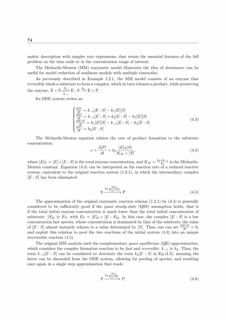
74

anistic description with simpler rate expressions, that retain the essential features of the fullproblem on the time scale or in the concentration range of interest.

The Michaelis-Menten (MM) enzymatic model illustrates the idea of dominance can beuseful for model reduction of nonlinear models with multiple timescales.

As previously described in Example 1.2.1, the MM model consists of an enzyme thatreversibly binds a substrate to form a complex, which in turn releases a product, while preservingthe enzyme, E + S k1−−−−

k−1E : S k2−→ E + P.

Its ODE system writes as:

d[S]dt = k−1[E : S]− k1[E][S]d[E]dt = k−1[E : S] + k2[E : S]− k1[E][S]d[E:S]dt = k1[E][S]− k−1[E : S]− k2[E : S]

d[P ]dt = k2[E : S]

(4.3)

The Michaelis-Menten equation relates the rate of product formation to the substrateconcentration:

v = d[P ]dt

= k2[E]T [S]KM + [S] , (4.4)

where [E]T = [E]+[E : S] is the total enzyme concentration, andKM = k2+k−1k1

is the Michaelis-Menten constant. Equation (4.4) can be interpreted as the reaction rate of a reduced reactivesystem, equivalent to the original reaction system (1.2.1), in which the intermediary complex[E : S] has been eliminated:

Sk2

[E]TKM+[S]−−−−−−→ P (4.5)

The approximation of the original enzymatic reaction scheme (1.2.1) by (4.4) is generallyconsidered to be sufficiently good if the quasi steady-state (QSS) assumption holds, that isif the total initial enzyme concentration is much lower than the total initial concentration ofsubstrate: [S]0 ET , with ET = [E]0 + [E : S]0. In this case, the complex [E : S] is a lowconcentration fast species, whose concentration is dominated by that of the substrate; the valueof [E : S] almost instantly relaxes to a value determined by [S]. Thus, one can set d[E:S]

dt = 0,and exploit this relation to pool the two reactions of the initial system (4.3) into an uniqueirreversible reaction (4.5).

The original MM analysis used the complementary quasi equilibrium (QE) approximation,which considers the complex formation reaction to be fast and reversible: k−1 k2. Thus, theterm k−1[E : S] can be considered to dominate the term k2[E : S] in Eq.(4.3), meaning thelatter can be discarded from the ODE system, allowing for pooling of species, and resultingonce again in a single step approximation that reads:

Sk2

[E]TKd+[S]−−−−−−→ P, (4.6)

75

with Kd = k−1k1

, if indeed [S] ET . We note that if the QE assumption is indeed valid, thenKM ≈ Kd.

The authors of [168] provide a similar validity criterion of the deterministic Michaelis–Menten approximation: [S]0 + KM ET . Whenever this condition holds, it is shown thata separation exists between a fast “pre-steady state” timescale and a slower “steady state”timescale. The solution of the Michaelis-Menten approximation closely tracks the solution ofthe initial enzymatic reaction system on the slow timescale.

This simple example illustrates how the dynamics of multiscale, large biochemical systemscan be reduced to those of simpler models, called dominant subsystems [138], which contain lessparameters and are easier to analyze. Dominant subsystems are chosen by comparing the time-scales of the large system. For example, the classical quasi steady-state (QSS) [23] and quasi-equilibrium (QE) approximations [127, 106] are conditions that lead to dominance, and representpopular methods for the computation of “first approximations” to the slow invariant manifold.Classical QSS is based on the small concentrations of highly reactive intermediate species (i.e.,atoms, ions, enzymes and substrate-enzyme complexes)[41], while in the QE approximation thereduction of the full mechanism is done based on the existence of fast and slow reactions.

The multiscaleness property of biochemical network is by definition closely linked to themathematical notion of dominance, captured in the framework of tropical analysis[9, 120].Recently, a class of semi-formal methods for reducing and hybridizing models of biochemicalnetworks has been developed, based on ideas from tropical analysis [138, 139, 154, 155]. Thesemethods exploit the multiscaleness of biochemical networks, in order to deduce dominancerelations among parameters and/or reaction rates, which can then be used to obtain a systemof truncated ODEs (by eliminating the dominated terms). One of the advantages of usingdominance relations in multi-scale networks is that it helps cope with parameter uncertainty:parameter values are replaced with their orders of magnitude, which are easier to determine.However, providing guarantees as to how the solution of the reduced model relates to the originalone, while avoiding to solve the latter, remains a challenge.

Consequently, the works presented in this first part of the manuscript deal with modelreduction techniques that exploit the multiscaleness property of biochemical reaction networks.

In Chapter 5, we investigate how the multiscaleness property can be exploited in the contextof rule-based models of genetic circuits. We argue that, while typical primitives for modellingsuch circuits are gene interaction networks, they fail to capture low-level mechanistic details ofgenetic interactions, which are necessary when designing in vivo experiments.

Rule-based modeling languages such as Kappa allow, by their nature, to unambiguouslyspecify mechanistic details such as DNA binding sites, dimerisation of transcription factors, orco-operative interactions. Nonetheless, such a detailed description comes with complexity andcomputationally costly executions. In order to tackle this issue, we propose a reduction methodfor rule-based programs, based on equilibrium approximations. Our algorithm is an adaptationof an existing algorithm, which was designed for reducing reaction-based programs; our versionof the algorithm scans the rule-based Kappa model (in which each rule operates exclusively onsite-graphs whose interfaces are fully specified, i.e., they are species), in search of interactionpatterns which are amenable to equilibrium approximations, such as the Michaelis-Mentenscheme. Additional checks are then performed, as to verify if the reduction is meaningful in the

76

context of the full model. The reduced model is efficiently obtained by static inspection overthe rule-set. Our tool is tested on a detailed rule-based model of a λ-phage switch, which lists92 rules and 13 agents. The reduced model has 11 rules and 5 agents, and provides a dramatic(several orders of magnitude) reduction in simulation time.

Our time-scale separation technique is justified by asymptotic convergence results; how-ever, for any concrete parameter values, one cannot obtain any information on the accuracy ofthe reduced model’s trajectories, without comparing them to those obtained by executing theoriginal model.

This is why, in Chapter 6, we design and test an approximation method for ODE models ofbiochemical reaction systems, in which the guarantees are our major requirement. Borrowingfrom tropical analysis techniques, we argue that the deterministic model of a multiscale BRN canbe simplified by exploiting the dominance relations among terms of each of its equations, in orderto determine the dominant subsystems that govern the evolution of each species’ concentration.As the dominant terms can change during a dynamic execution of the system, depending onwhich species dominate the others, several possible modes exist. Thus, simpler models consistingof only the dominant subsystems can be assembled into hybrid, piecewise smooth models, whichapproximate the behavior of the initial system. By combining the detection of dominatedterms with symbolic bounds propagation, we show how to approximate the original modelby an assembly of simpler models, consisting in ordinary differential equations that providetime-dependent lower and upper bounds for the concentrations of the initial model’s species.

The utility of our method is twofold. On the one hand, by the nature of its design, itprovides sound interval bounds for each species’ concentration, and can hence serve to evaluatethe accuracy of tropicalization reduction heuristics for ODE models of biochemical reductionsystems.

On the other hand, our method also provides a reduction heuristics that performs withoutany prior knowledge of the initial system’s behavior (i.e., no simulation of the initial system isneeded in order to reduce it).

Chapter 5Prototyping genetic circuits using rule-basedmodels

This chapter is based on the work published in the proceedings of the 4th HybridSystems Biology (HSB) workshop [13].

5.1 Motivation

As mentioned in the introductory section of this thesis, one of the goals of synthetic andsystems biology consists in the design and control of genetic circuits in an analogous way to howelectronic circuits are manipulated in human made computer systems. In this sense, one notesprevious successes in engineering simple genetic circuits that are encoded in DNA, and whichperform their function in the cellular environment [71], [87]. However, there remains a needfor rigorous quantitative characterization of such small circuits and their mutual compatibility[113], and an important ingredient towards such a characterization is having an appropriatemodeling language: one that is able to capture model requirements, to prototype circuits, andto predict their quantitative behavior before committing to time-intensive in vivo experiments.

As biomolecular systems are usually highly dimensional, stochastic, non-linear dynamicalsystems, their quantitative modeling is particularly challenging. Consequently, a common mod-eling practice consists in applying ad-hoc simplifications that neglect the mechanistic detailsof the underlying biological processes, but which allow to predict the system’s behaviour as afunction of time.

For example, the fact that “protein A activates protein P” is often modeled immediatelyin terms of a reaction A → A + P with the Hill kinetic coefficient (e.g. k[A]n

1+k[A]n ) - however,the actual biological protein activation mechanism includes the formation of a macromolecularcomplex and its binding to a molecular target.

While models that employ such simplifications are easier to execute, this type of simplifi-cation makes models hard to edit or refine. For example, the fact that several mechanistic stepsare merged into a single kinetic rate means that a new experimental insight about an interactionmechanism cannot be easily integrated into the model. Moreover, such abstract models do notprovide guidelines that are precise enough for circuit synthesis, and in some cases, only themore detailed models are able to explain certain behaviours (e.g., in [57], it is shown that only

77

78 Motivation

when incorporating the mRNA, the model explains certain experimentally observed facts).As detailed in Section 4.2, rule-based languages, such as Kappa [149] or BioNetGen [18],

are designed to naturally capture the protein-centric and concurrent nature of biochemicalsignalling: in a rule-based model, the internal protein structure is maintained in form of a site-graph, and interactions can occur by simply testing patterns, i.e., local contexts of molecularspecies. We have also shown in Section 4.2 that the executions of rule-based models are tracesof a continuous-time Markov chain (CTMC), defined according to the principles of chemicalkinetics.

In general, rule-based models can be considered as an improvement of classical biochemicalreaction models for two major reasons. First, the explicit graphical representation of molecularcomplexes makes models easy to read, write, edit or compose (by simply merging two collectionsof rules).

For example, the dimerization reaction between two CI molecules of the λ-phage [151]model is classically written as CI + CI→ CI2, where the convention is that CI represents a freemonomer, and CI2 represents a free dimer. On the other hand, the same reaction written inKappa amounts to:

where ci and or denote the binding sites of the protein CI, and CI(ci[1], or) indicates that theidentifier of the rule-based bond on the site ci, which accounts for the physical interactionbetween the two CI monomers, is 1. The left-handside of the rule states that dimerization canoccur only between two CI monomers that are free (unbound) on both the cri and the or sites.

Secondly, a rule set can be both executed, and subjected to formal static analysis: forexample, it provides efficient simulations [50], [96], but also automated answers about thereachability of a particular molecular complex [51], or about causal relations between ruleexecutions [49].

In this sense, in Section 5.2, we illustrate the advantages of using rule-based modelinglanguages to prototype genetic circuits, by building a detailed Kappa model of the λ-phagegenetic switch. When compared to traditional ODE modeling, and even to reaction-basedmodeling, using the chemically intuitive syntax/notations of Kappa results in a model thatcaptures the protein-centric mechanistic details of the underlying biochemical processes in away that can be easily understood and used by the biologist modeler, and which moreover isconcise, transparent, and easily extendable.

However, a downside to incorporating too many mechanistic details in the model is thatthey lead to computationally costly execution. For this reason, in Section 5.3, we propose andimplement an efficient method for automatically detecting and applying equilibrium approx-imations to the Kappa model. We note that in the specific Kappa models we build in thischapter, the kinetic rate constants of the chemical interactions are highly dependent on thefull interface of the reactant patterns. The consequence of this parameter sensitivity is thatreactions operating on similar left-handside patterns cannot be subsumed into a single rule.Hence, we assume that the left-handside of each rule is composed of patterns whose interface

Prototyping genetic circuits using rule-based models 79

is fully specified, i.e., each pattern is a species, and as such our algorithm provides a soundreduction of models in which each rule represents a reaction.

These approximations allow one to obtain a smaller model, in which some agents areeliminated, and the kinetic rates are appropriately adjusted. In this way, the experimentalistcan choose to obtain predictions more efficiently but less accurately, however without losingtrack of the underlying low-level mechanisms.

In related works [135] and [112], the authors propose an algorithm for reducing a reaction-based model, by searching for interaction schemes amenable to equilibrium approximations. Inthis paper, we adapt this algorithm to rule-based models of genetic circuits. We implement thealgorithm in OCaml, and test it on the detailed rule-based model of the λ-phage switch ([151],[152]) we construct in Section 5.2.

The results of this approximation are presented in Section 5.4.1: while the complete chemi-cal genetic circuit model contains 92 rules, 13 agents, and 61 species, the reduced model containsonly 11 rules and 5 agents, and is able to approximate the behavior of the original system. Weconclude this chapter by discussing the limitations of our reduction method, as well as futurework.

Related work. The principle of obtaining conclusions about system’s dynamics byanalysing their model description, originates from, and is exhaustively studied in thefield of formal program verification and model checking [45], [25], while it is recentlygaining recognition in the context of programs used for modeling biochemical networks.An example is the related work of detecting fragments for reducing the deterministicor stochastic rule-based models [62], [69], [63], detecting the information flow for ODEmodels of biochemical signaling [91], [20], or the reaction network theory [46].

5.2 A Kappa model of the λ-phage decision circuit

We start by building a Kappa model of the λ-phage decision circuit, using the reaction-based model presented in ([135], [112]). The λ-phage circuit is one of the most studied geneticcircuits in synthetic and systems biology. Over the years, much has been learned about thissimple genetic circuit, but even more than half a century after its discovery, new mechanismsare being discovered about its functioning.

The phage λ ([151],[152]) is a virus that infects E.coli cells, and replicates using one oftwo strategies: lysis or lysogeny. In the lysis strategy, phage λ uses the machinery of theE.coli cell to replicate itself and then lyses the cell wall, killing the cell and allowing the newlyformed viruses to escape and infect other cells. On the other hand, in the lysogeny scenario,the virus inserts its DNA into the host cell’s DNA and replicates through normal cell division,remaining in a latent state in the host cell (it can always revert to the lysis strategy). Thisswitch mechanism is illustrated in Figure 5.1.

The decision between lysis and lysogeny is known to be influenced by environmental pa-rameters, as well as the multiplicity of infection and variations in the average phage input [8].

80 A Kappa model of the λ-phage decision circuit

Figure 5.1: Phage λ developmental model (Figure taken from [135])

The key element controlling this decision process is the OR operator (shown in Figure (5.2)),which is composed of three operator sites (OR1, OR2, OR3) to which transcription factors canbind, in order to activate or repress the two promoters (PRM and PR) overlapping the operatorsites. When RNA polymerase (RNAP ) binds to PRM , it initiates transcription to the left, toproduce mRNA transcripts from the cI gene; RNAP bound to the PR promoter, on the otherhand, initiates transcription to the right, producing transcripts from the cro gene. The twopromoters form a genetic switch, since transcripts can only be produced in one direction at atime. This production mechanism is illustrated in Figure 5.2.

The cI gene codes for the CI protein, also known as the λ repressor : in its dimer form, itis attracted the the OR operator sites in the phage’s DNA, repressing the PR promoter from

(a) CI monomers are produced from the cIgene. Two CI monomers can bind together,and form a dimer that can in turn bind to oneof the OR operator sites.

(b) Cro monomers are produced from the crogene. Two Cro mononers can form a dimer,which can bind to one of the OR operator sites.

Figure 5.2: λ-phage switch: production of CI and Cro proteins. (Figure taken from [135])

Prototyping genetic circuits using rule-based models 81

which Cro production is initiated, and further activating CI production. Similarly, the cro genecodes for the Cro protein, which also dimerizes in order to bind to the OR operator sites andprevent production from PRM and its own production.

While CI2 and Cro2 can bind to any of the three operator sites at any time, they havea different affinity to each site. The CI2 has its strongest affinity to the OR1 operator site,next to the OR2 site, and finally to the OR3 site (in other words, CI2 first turns off PR , thenactivates PRM , and finally, represses its own production), while Cro2 has the reverse affinity(it first turns off CI production, then turns off its own production).

The effects of CI and Cro dimers binding to the operator sites are illustrated in Figure 5.3.

Figure 5.3: The effects of CI and Cro dimers binding to the operator sites. (Top row) A CIdimer bound to the site OR1 turns off the PR promoter. (Second row) A CI dimer bound to thesite OR2 activates the PRM promoter. (Third row) A CI dimer bound to the site OR3 turns offthe PRM promoter completely, while PR is activated.(Fourth row) When all operator sites arefree, promoter PR is active. (Fifth row) A Cro dimer bound to OR3 turns off PRM completely.(Bottom row) An additional binding of Cro dimers to OR1 and OR2 turns PR off completely.(Figure taken from [135])

82 A Kappa model of the λ-phage decision circuit

Remark 5.2.1. The specificities of the interactions described above, as illustrated inFigure 5.3, imply that the decision to execute a specific reaction in the model is takenby considering the full interface of the operator pattern OR: consider for example howin the fourth panel, PR is activated when all sites of OR are free. Similarly, in the lastpanel, PR is completely repressed when all sites of OR are bound to a Cro dimer.

This particularity of the λ-phage mechanism translates in the model by a high sen-sitivity of a reaction’s kinetic constant on its reactants’ full interface, e.g., each possibleconfiguration of the operator has a different binding affinity to the same given protein.The dependency of specific molecular interactions on the full reactant pattern interfacethus prevents the aggregation of different reactions describing similar mechanisms oper-ating on the same reactant species (e.g., the same protein binding some site of the sameoperator) into a single rule.

This restriction is perpetuated throughout the λ-phage model, which means that themajor advantage of rule-based modeling w.r.t. reaction based models (“a rule subsumesmany possible reactions”) could remain unexploited when constructing models of geneticcircuits. This feature motivates the “each-rule-is-a-reaction” constraint we will assumefor our reduction algorithm: we assume that a rule-based model is such that all left-handside and right-handside represent fully specified site-graphs (i.e., species), insteadof “don’t care, don’t write patterns”.

However, we argue that even under the above-mentioned restriction, rule-basedmodels are better suited for prototyping genetic circuits, when compared to reaction-based models. Indeed, the former benefit from an intuitive chemical syntax that thelatter lack, i.e., they enable the explicit representation of protein-protein interactions,which in itself is a strong enough reason to prefer rule-based models to reaction-basedmodels, when prototyping genetic circuits. All in all, we stress that in this chapter,we choose to employ rule-based models due to the chemical expressivity of their syntax,instead of their ability of avoiding combinatorially large model representations.

The feedback through the binding of the products as transcription factors coupled with theaffinities described makes the OR operator behave as a genetic bistable switch. In one state,the production of the Cro protein inhibits the production of CI. In this state, the cell followsthe lysis pathway, since genes downstream of Cro produce the proteins necessary to constructnew viruses and lyse the cell. In the other state, the production of CI prevents production ofCro, and the cell follows the lysogeny pathway, since proteins necessary to produce new virusesare not produced. Instead, the cell proceeds with the production of proteins that are used toinsert the DNA of the phage into the host cell.

We note that in the lysogeny state, the cell develops an immunity to further infection: thecro genes found on the DNA inserted by further infections of the virus are also shut off byCI2 molecules that are produced by the first virus to commit to lysogeny. Once a cell commitsto lysogeny, it becomes very stable and does not easily change over to the lysis pathway. Aninduction event is necessary to cause the transition from lysogeny to lysis. For example, lysogens(i.e., cells with phage DNA integrated within their own DNA) that are exposed to UV light endup following the lysis pathway.

Prototyping genetic circuits using rule-based models 83

5.2.1 Example: Kappa model of CI and CII production

To exemplify the advantages of rule-based models, consider the following sub-network ofthe λ-phage circuit, which describes a simplified mechanism for the production of CI from PRE ,and for the production of CII from PR.

Figure 5.4: CI and CII production from PR and PRE .(Figure taken from [135])

CII production is initiated from the PR promoter. Initially, CI production from promoterPRE proceeds at a low basal rate. As CII builds up, it binds to the OE operator site, activatingthe production of CI molecules from PRE . The CI molecules dimerize and bind to the ORoperator sites, further repressing production of CII. Over time CII degrades, reducing theproduction rate of CI. Finally, after CI degrades, the system returns to the initial state

For readability purposes, assume for the time being that we want to create a model for thenetwork of Figure 5.4, in which we abstract away the details regarding CI and CII binding tothe operators OE and OR, and focus solely on the regulatory effects of the interaction betweenthe proteins CI and CII and the promoters PR and PRE . More specifically, we want to create amodel in which protein CII activates CI production through the promoter PRE, and protein CIrepresses CII production through the promoter PR.

We create a Kappa model for this regulatory circuit, by assuming that proteins CI andCII can bind directly to their respective promoters PR and PRE . Among the different waysof modeling genetic regulatory networks, we use a systematic procedure that produces a fairlyreasonable model, and which can represent a guideline for prototyping genetic circuits in Kappa:

• create agents for RNAP (the RNA-polymerase), as well as for every protein and pro-moter/operator of the network under consideration;

• model the open complex formation for a promoter by a pair of rules: a reversible rule, inwhich the RNAP binds to the promoter, and an irreversible rule in which the resultingRNAP-promoter complex acts as a modifier for the production of the protein the promoterencodes for;

• model the repression of a promoter P by a repressor R through a reversible rule, in whichR binds to P , preventing the subsequent binding of P ’s activators;

• model the activation of a promoter P by an activator A by a pair of rules: a reversiblerule, in which A and RNAP both bind to P , followed by an irreversible reaction in which

84 A Kappa model of the λ-phage decision circuit

the A−RNAP − P complex acts as a modifier for the production of P ’s protein;

• add rule for modeling the remaining chemical behavior: protein degradation, dimerisation,etc...

Using these guidelines, the resulting Kappa model for the mechanism of Figure 5.4 writesas:

(i) degradation of CI and CII proteins, at the same rate kd:

(ii) basal-rate production of CI and CII:

(iii) CI dimerization:

(iv) CI dimers repress the activity of promoter PR, by binding to it:

(v) CII monomers activate the promoter PRE , by binding to it:

One notes that, when compared to the equivalent reaction-based model, the Kappa modelrepresents a significant improvement: no supplementary names need to be introduced for thecomplex species, which are instead denoted in an intuitive chemical style, that is indicativeof the underlying biological mechanisms. The result is a model that is more concise, moretransparent, easily readable, and easily extendible. The CI-CII Kappa model represents just anexample of the ease with which the Kappa language can be used to model biological interactionsnot only on a protein-protein level, but also at the genetic level - a feature that results in detailed

Prototyping genetic circuits using rule-based models 85

stochastic models that naturally account for transcriptional and translational resource usage[184]. What’s more, the existing visual representations of Kappa models mirror the intuitivelymodular nature of the modeling processes involved.

We also implement the full λ-phage circuit model, in which we include interactions withthe OR and OE operators, as well as the remaining reactions of the λ-phage circuit, the detaileddescription of the which can be found in [135].

The full Kappa model contains 96 rules, 16 proteins and 61 species. This model will serveas a case study for our reduction algorithm. Using available tools [149], we generate the model’scontact map, which we present in Figure 5.5.

Figure 5.5: The contact map of the full λ-phage model. The model consists of 96 rules, 16proteins and 61 species.

5.3 Model Approximation using Michaelis-Menten-like reactionschemes

In this section, we present the approximation algorithm, which comprises three reduc-tion schemes: competitive enzymatic reduction, operator-site reduction, and fast dimerizationreduction.

As all three schemes are based on the Michaelis-Menten (MM) enzymatic model, we startby providing some mathematical background for justifying the validity of the MM reductionscheme in the case of stochastic models.

We continue by detailing the three reductions, and conclude by presenting the top-levelalgorithm that employs them.

5.3.1 Validity of the Michaelis-Menten enzymatic reduction in stochasticmodels

As we will see in the next sections, our reduction algorithm will scan a Kappa model insearch for reaction patterns similar to the original Michaelis-Menten enzymatic mechanism(E + S ↔ E : S → P ), and then reduce them using MM-like approximations. We havepreviously seen that this approximation is generally considered to be sufficiently good under

86 Model Approximation using Michaelis-Menten-like reaction schemes

different assumptions, such as, for example, that the rate of dissociation of the complex to thesubstrate is much faster than its dissociation to the product (i.e. k1 k2), (the equilibriumapproximation). Even if the equilibrium condition is not satisfied, it can be compensated in asituation where the total amount of substrates is significantly larger than the enzyme quantity:[S]0 +Km ET (quasi-steady state assumption, or QSSA).

The informal terminology of being “significantly faster”, motivated the rigorous study of thelimitations of the approximations based on separating time scales. The enzymatic (Michaelis-Menten) approximation has been first introduced and subsequently studied in the context ofdeterministic models (e.g. [134]), and it had not been given much consideration in the context ofstochastic models, until relatively recently. However, this has changed, due to the computationaldemands of the stochastic simulation algorithm (SSA), which not only requires a potentiallylarge number of runs in order reasonably 1 estimate the system behavior, but more importantly,also requires every single reaction event to be simulated one at a time. In this sense, the QSSAapproximation not only reduces the dimensionality of the system, but it can also substantiallyreduce simulation time, by removing fast reactions such as complex formation and complexdissociation, which are commonly found in enzymatic models. Indeed, the propensities of suchvery fast reactions can be significantly larger than those of other reactions, and thus tendto dominate (and slow down) stochastic simulations. As a result, in order to facilitate moreefficient temporal behavior analysis, extended MM approximations, and more generally time-scale separation techniques, have recently started to be investigated in the stochastic context([157], [90], [47], [93], [164], [81]).

Moreover, mathematical justifications for the application of the QSSA within the stochasticchemical kinetic framework have been investigated to establish a theoretical basis to illustratehow the QSSA can be applied to stochastic simulation algorithms.

Notably, the following result from [54] (also shown as a special case of the multi scalestochastic analysis from [103]), shows that, under an appropriate scaling of species’ abundanceand reaction rates, the original model and the approximate model converge to the same process.

Theorem 5.3.1 ((Darden [54], Kang [103]))Consider the usual MM reaction network:

E + S k1−−−−k−1

E : S k2−→ E + P, (5.1)

and let XS(t), XE(t), XE:S(t) and XP (t) denote the respective species’ copy numbers, due tothe random-time change model (3.30). Write ET = XE:S(t) +XE(t) to denote the total enzymequantity, and let VE(t) =

∫ t0 N

−1XE(s)ds.Assuming that the amount of substrate is much larger than that of enzyme, the system

volume can be expressed as N = O(XS).Finally, let γ−1, γ1, γ2 be parameters of order 1.Then, under the scaling k−1 → γ−1, k1 → Nγ1, k2 → Nγ2, N → ∞, and XS(0)

N → xS(0),one has that:

1i.e., at a reasonable degree of statistical confidence

Prototyping genetic circuits using rule-based models 87

(XS(t)N

,VE(t))−→ (xS(t), vE(t)) ,

with: ddtvE(t) = ET

1+KxE(t)

ddtxS(t) = −ET γ2KxS(t)

1+KxS(t)

and K = γ−1γ1+γ2

.

The assumptions listed in the theorem capture the following: (i) XS and XP are scaled toconcentrations, while XE and XE:S remain in copy numbers; (ii) the stochastic reaction ratek−1 is an order of magnitude smaller than the rates k1 and k2.

A complete proof is provided in [103]. Herein, we outline the general idea.Let N > 0 be a natural number, and let ZS(t) = XS(t)/N , ZE(t) = XE(t), ZS:E(t) =

XS:E(t), ZP (t) = XP (t)/N . Writing out the scaled random time-change model for the substrategives:

ZS(t) = ZS(0)−N−1ξ1(N∫ t

0γ−1ZS(s)ZE(s)ds)

+N−1ξ2(N∫ t

0γ1ZS:E(s)ds),

Similarly, the scaled random time-change model for the complex E : S writes as:

ZE:S(t) = ZE:S(0) + ξ1(N∫ t

0γ−1ZS(s)ZE(s)ds)

− ξ2(N∫ t

0γ1ZS:E(s)ds)

− ξ3(N∫ t

0γ2ZS:E(s)ds).

After dividing the latter equation with N , and applying the law of large numbers, we obtainthe balance equations analogous to assuming that the complex is at equilibrium. This equationimplies the expression for d

dtvE(t).The equation for d

dtxS(t) follows from the model of ZS(t): we first use the conservation lawZS:E(s) = N−1ET − ZE(t) and then substitute the obtained value of d

dtvE(s).In order to confirm that the reduction is appropriate, our goal is now to show that the scaled

versions of the original enzymatic model (5.1) and the reduced model (4.5) are equivalent inthe limit when N →∞.

88 Model Approximation using Michaelis-Menten-like reaction schemes

Let ZP (t) := N−1XP (t) be the scaled random time change for the product in the originalmodel, and let ZP (t) := N−1XP (t), in the reduced model.

Notice that, from the balance equations, xPdt = −xSdt .

According to the reduced Michaelis-Meten system, the random time change for the productis given by

ZP (t) = ZP (0) +N−1ξ(∫ t

0

k2ETK

1 +KNZS(s)NZS(s)ds)

= ZP (0) +N−1ξ(∫ t

0N

γ2ET K

1 + KZS(s)ZS(s)ds).

Passing to the limit, we obtain the desired relation: zP (t)dt = zP (t)

dt .We note that Theorem (5.3.1) should not be interpreted as providing the means of com-

puting the approximation error, or even as an algorithm which suggests which difference intime-scales is good enough for an approximation to perform well.

Rather, this result shows that the enzymatic approximation is justified in the limit whenthe assumptions about the reaction rates and species’ abundance are met. In other words, whenN →∞, the scaled versions of the original and reduced models – e.g. ZP (t) = N−1XP (t) andZP = N−1XP – both converge to at the same, well-behaved process. This provides confidencethat the actual process XP is a good approximation of the process XP .

The observation that the enzymatic approximation is justified in the limit is in line withrecent works that study the robustness of classical enzyme kinetics in the context of cellularbiochemistry, i.e. in the in vivo context of small intracellular environments, where the largevolume, large species abundance, and negligible fluctuations assumptions do not hold. For ex-ample, in [85], the author shows that for a microscopic stochastic model of enzyme kinetics in asmall subcellular compartment, the intrinsic noise induces a breakdown of the Michaelis-Mentenequation, even if steady-state metabolic conditions are enforced, and that the deterministicrate equations can severely under-estimate steady-state intracellular substrate concentrations.Moreover, a formula is given for quantifying the deviations from the MM equations - the de-viations are substantial for small values of KM ; in this case, the bottleneck of the catalyticprocess (which resides in the decay of a complex, rather than the enzyme-substrate combina-tion) leads to correlations between successive binding events. The limitations of the stochasticquasi-steady-state approximation are also studied in [176], where a simple formula for the rel-ative error between the predictions of the two CMEs (original and reduced) for the simplestbiochemical circuit embedding the MM mechanism (i.e., the MM reaction plus a substrate inputreaction) is obtained. This formula predicts that the reduced approach can overestimate thevariance of the substrate fluctuations by as much as 30%, when the enzyme is half saturatedwith substrate, i.e., when xS = KM . However, for substrate concentrations much smaller orlarger than KM , this error becomes negligible. Other works from the same research group dealwith corrections to the classical enzyme kinetics models: in [175], the authors compute thefinite-volume/finite copy number corrections to the solutions of the rate equations of a systemcomposed of arbitrarily many enzyme-catalyzed reactions inside a small sub-cellular compart-ment, while in [84] the results of [85] are further explored, in order to derive novel stochastic

Prototyping genetic circuits using rule-based models 89

mesoscopic rate equations, replacing the conventional macroscopic deterministic equations, inthe case of subcellular (i.e., at micron and submicron scales) enzyme reaction networks; thesemesoscopic equations take into account the simultaneous influence of both intrinsic noise andsubstrate transport mode. Finally, in [86], the CME is used in order to obtain expressions forthe instantaneous and time averaged rate of product formation in an enzymatic MM scheme inwhich the conventional substrate abundance assumption is not imposed on the system. Notably,the authors show that (i) the relationship between the average rate of product formation andthe substrate concentration for a MM reaction with one enzyme molecule is (approximatively)given by a logarithmically corrected MM form, and that (ii) the relationship between the initialaverage product formation rate and the initial substrate concentration for an MM reaction withno reversible reaction and with any number of enzyme and substrate molecules is a sum of MMequations.

Several other analyses of the Michaelis-Menten reaction mechanism in the single-moleculecontext have been carried out. For example, for the case of only one enzyme molecule reactingwith one substrate molecule, differences of 20 − 30% between the average substrate concen-trations as given by the reduced ODE model and the stochastic CME model have been found[7]. In the case of a Michaelis-Menten reaction mechanism with substrate inflow catalysed byone enzyme molecule, it was shown [172] that the relationship between the mean steady-staterate of product formation is given not by the MM equation, but by a more complex expression,which nonetheless reduces to the usual MM equation in the limit KmΩ 1, with Ω denotingthe volume.

We argue for the relative accuracy of our method, as the conditions under which the MMapproximation is shown to be inaccurate in the above-mentioned studies do not hold for ourλ-phage stochastic model: the substrate abundant, KM 1, and the enzymes do not operatenear saturation.

Example 5.3.1To illustrate the meaning of Theorem 5.3.1, we compare the stochastic trajectories of the

product species P in the original and the reduced model, for different values of N .We start by plotting the mean protein level for the original and for the reduced model, for

a value of N = 1 (i.e., without scaling).Then, we scale up the parameters k1 and k2, as well as the initial concentration of substrate

T , in order to mimic the effect of choosing a larger N in 5.3.1.Figure 5.6 shows that, as expected, the distance between the original and reduced model

decreases in the scaled system (large N). This observation is consistent with those of [164],which state that the Michaelis–Menten approximation is applicable in discrete stochastic models,and that its validity conditions are the same as in the deterministic regime, as given in [168].Otherwise said, that a stochastic simulation of the reduced mechanism S → P with effectivepropensity function VmaxS

Km+S will closely approximate the solution of the full stochastic model ofthe Michaelis-Menten reaction set whenever S0 +Km ET . Indeed, scaling the MM system asin 5.3.1 widens the gap between these two quantities, as it implies increasing the values of bothS0 and Km (as Km = k1+k2

k−1), while keeping enzyme levels ET constant.

90 Model Approximation using Michaelis-Menten-like reaction schemes

Figure 5.6: (Top) We plot the mean protein expression for the MM enzymatic scheme, forone hundred sampled traces, before and after the enzymatic catalysis reduction. (Top Left)No scaling applied (N=1), initial species abundance given by xS(0) = 50, xE(0) = 1, andparameters k−1 = 1, k1 = 10, k2 = 10 b) Parameters k2, k3, and the initial number of substratesS are scaled up by a factor of 10 (N = 10). (Bottom) We consider the reduction error to begiven by the difference in mean protein copy numbers between the original and reduced model.As such, the reduction error is significantly smaller for the scaled models, cf. what is expectedfrom Theoerem 5.3.1

Prototyping genetic circuits using rule-based models 91

5.3.2 Generalized competitive enzymatic reduction

Generalized competitive enzymatic reduction

The Michaelis-Menten enzymatic approximation can be generalized to a situation in whichseveral substrates compete for binding to the same enzyme E. We will call such patterns ofrules competitive enzymatic rules.

Assume the multiple alternative substrate scheme, in which the same enzyme E can re-versibly bind one of n possible substrates Si, and in doing so, lead to production of Pi:

E + Sik−i−−−−k+i

E : Siki−→ E + Pi, i = 1 . . . n (5.2)

If the alternative substrate system i is taken as the leading substrate, the system containsn− 1 competitors. Under the assumption of a generalized quasi-steady state condition statingthat each complex E : Si reaches equilibrium fast enough, (i.e., dE:Si

dt ≈ 0), and taking intoaccount the conservation laws w.r.t. both the enzyme and the substrate amounts:

xE(t) +n∑i=1

xE:Si(t) = xE(0)

xSi(t) + xE:Si(t) + xPi(t) = xSi(0)

each such enzymatic scheme can be approximated by the following irreversible rule:

Si

kiKiETZ−−−−−→ Pi, (5.3)

meaning that Pi is produced at rate kiKixSiETZ , where

Z = 1 +∑

i∈1,...,nKixSi

ET = xE +∑

i∈1,...,pxE:Si

If the complex E : Si dissociates into E and Si much faster it is converted into the productPi, i.e. if k−i ki, the rapid equilibrium approximation can be applied, meaning that we canset Ki ≡

k−ik+i

, instead of the usual MM constant k−i +kik−i

. The rapid equilibrium approximationprovides a more aggressive reduction than the quasi-steady state approximation w.r.t. reducingthe complexity of the kinetic law, and, as such, whenever a model contains patterns that matchthe conditions for both methods, the rapid equilibrium approximation will have precedence inorder to reduce the complexity of the rule rate laws.

We adapt the algorithms of [112] to perform the reduction of Kappa models containingpatterns of multiple alternative substrate systems.

92 Model Approximation using Michaelis-Menten-like reaction schemes

In this sense, we adapt the following nomenclature:

Definition 5.3.1 (Kappa reactant, modifier, product)Given a rule (El, Er, k), a Kappa species s is called

• a reactant, if it is a species occuring in El (cf. Definition 4.2.4), but it is not a speciesoccuring in Er ,

• a modifier, if it occurs in both El and Er, and if the number of its occurrences in El equalsthe number of its occurrences in Er ,

• a product, if it does not occur in El, and it occurs in Er.

For the top-level competitive enzymatic reduction, Algorithm 2 scans the entire species set,in search for potential enzymes. For each such detected enzyme E, the system is transformedaccording to Eq. (5.3), and E is eliminated from the model.

Algorithm 2: Competitive enzymatic reductionInput : A Kappa model M over a set of species S and observables OOutput: The reduced Kappa model M ′ over a set of species S ′ and observables O

1 M ′ ←−M ;2 for s ∈ S do3 C ←− RapidEqCondition(M, s);4 if C 6= ∅ then5 M ′ ←− RapidEqTransform(M ′, s, C)6 end7 end8 return M ′

Checking if E is an enzyme is done via procedure RapidEqCondition, which ensures that2:

(i) E is not an observable in the Kappa model M ;

(ii) E is a reactant (cf. Definition 5.3.1) in at least one rule r : (El, Er, k) of M ;

(iii) each rule r : (El, Er, k) in which E is a reactant is a reversible rule, in which El containsonly two species, E and S, and in which Er is obtained by applying a binding transfor-mation on El, between species E and S;

(iv) for each such rule r, the right-handside species, which we denote E : Si for readability, isnot an observable, has an initial abundance 0, occurs as a reactant or product in exactlyone rule, and never occurs as a modifier;

(v) there exists an irreversible rule r2 : (El2 , Er2 , k2), with El2 = E : Si, and such that Er2

contains only the enzyme species E and a product species P : such a reaction convertsE : Si into a product and releases the enzyme;

2These tests are equivalent to those shown in [135] and [112].

Prototyping genetic circuits using rule-based models 93

(vi) either the quasi-steady state or the rapid equilibrium assumptions are verified, i.e., eitherSi(0) + k−i +ki

k+i

ET , or k−i ki.

Procedure RapidEqCondition(M,E)Input : A Kappa model M over a set of species S and observables O, and a species E

from its SOutput: Checks if E is an enzyme, and if so, returns the set of configurations

corresponding to all substrates E binds to1 C ←− ∅ ;2 if E ∈ O or E isn’t a reactant in any rule of M then3 return ∅;4 end5 for every rule r1 in which E is a reactant do6 if r1 6= E,Si ↔ E : Si@k+

i , k−i then

7 return ∅;8 end9 if xE:Si(0) 6= 0 or E : Si ∈ O then

10 return ∅;11 end12 if E : Si is a reactant in more than one rule, or a modifier in any rule, or a product

in any other rule than r then13 return ∅;14 end15 if @r2 = E : Si → E,Pi@ki then16 return ∅;17 else18 if ki

k−i> threshold then

19 if ETxSi (0)+(k−i +ki)/k+

i

>threshold then20 return ∅;21 else22 C ←− C ∪ (Si, E : Si,

k+i

k−i +ki, ki, r, r2);

23 end24 C ←− C ∪ (Si, E : Si,

k+i

k−i, ki, r, r2);

25 end26 end27 end28 return C;

94 Model Approximation using Michaelis-Menten-like reaction schemes

If species E satisfies these conditions, a set of configurations is formed; each configurationincludes a substrate Si to which the enzyme binds, the complex E : Si it forms by binding toSi, the equilibrium constant knew of the binding rule and the rate ki of the production rulecontaining E : Si as a reactant, as well as the names of the two rules.

This configuration set is then used by procedure RapidEqTransform to reduce the model:

(i) for an enzyme E, it loops through the set of configurations, to form Z - the expressionused in the denominator of each new rate law;

(ii) for each configuration (Si, E : Si, knew, ki, r1, r2), it makes the substrate Si a reactant forr2, and changes the rate constant of r2 accordingly;

(iii) finally E, E : Si and r1 are removed from the model.

Procedure RapidEqTransform(M,S,C)Input : A Kappa model M over a set of species S and observables O, an enzyme E and

its corresponding configuration set given by the RapidEqCondition procedureOutput: The model M , from which the enzyme E has been abstracted/* compute the new kinetic law expression */

1 Z ←− 1 +∑

(Si,E:Si,knew,r,r2)∈Cknew ∗ xSi ;

2 for (Si, E : Si, knew, ki, r, r2) ∈ C do3 add Si as a reactant in r2;4 rateconstant(r2) = k2∗xE(0)∗knew

Z ;5 remove E : Si from M ;6 remove rule r from M ;7 end8 remove E from M ;9 return M ;

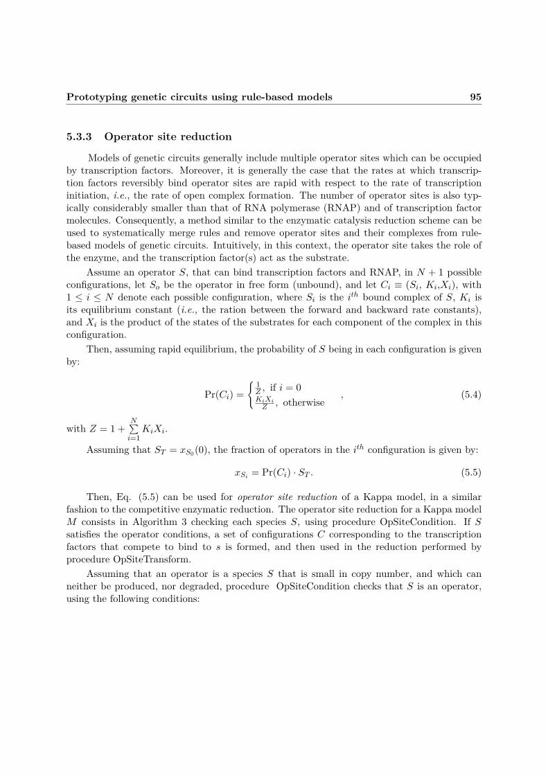
Prototyping genetic circuits using rule-based models 95

5.3.3 Operator site reduction

Models of genetic circuits generally include multiple operator sites which can be occupiedby transcription factors. Moreover, it is generally the case that the rates at which transcrip-tion factors reversibly bind operator sites are rapid with respect to the rate of transcriptioninitiation, i.e., the rate of open complex formation. The number of operator sites is also typ-ically considerably smaller than that of RNA polymerase (RNAP) and of transcription factormolecules. Consequently, a method similar to the enzymatic catalysis reduction scheme can beused to systematically merge rules and remove operator sites and their complexes from rule-based models of genetic circuits. Intuitively, in this context, the operator site takes the role ofthe enzyme, and the transcription factor(s) act as the substrate.

Assume an operator S, that can bind transcription factors and RNAP, in N + 1 possibleconfigurations, let So be the operator in free form (unbound), and let Ci ≡ (Si, Ki,Xi), with1 ≤ i ≤ N denote each possible configuration, where Si is the ith bound complex of S, Ki isits equilibrium constant (i.e., the ration between the forward and backward rate constants),and Xi is the product of the states of the substrates for each component of the complex in thisconfiguration.

Then, assuming rapid equilibrium, the probability of S being in each configuration is givenby:

Pr(Ci) = 1Z , if i = 0KiXiZ , otherwise

, (5.4)

with Z = 1 +N∑i=1

KiXi.

Assuming that ST = xS0(0), the fraction of operators in the ith configuration is given by:

xSi = Pr(Ci) · ST . (5.5)

Then, Eq. (5.5) can be used for operator site reduction of a Kappa model, in a similarfashion to the competitive enzymatic reduction. The operator site reduction for a Kappa modelM consists in Algorithm 3 checking each species S, using procedure OpSiteCondition. If Ssatisfies the operator conditions, a set of configurations C corresponding to the transcriptionfactors that compete to bind to s is formed, and then used in the reduction performed byprocedure OpSiteTransform.

Assuming that an operator is a species S that is small in copy number, and which canneither be produced, nor degraded, procedure OpSiteCondition checks that S is an operator,using the following conditions:

96 Model Approximation using Michaelis-Menten-like reaction schemes

Algorithm 3: Operator-site reductionInput : A Kappa model M over a set of species S and observables OOutput: The reduced Kappa model M ′ over a set of species S ′ and observables O

1 M ′ ←−M ;2 for s ∈ S do3 C ←− OpSiteCondition(M, s);4 if C 6= ∅ then5 M ′ ←− OpSiteTransform(M ′, s, C)6 end7 end8 returnM ′

(i) S’s initial copy number is not higher than a threshold;

(ii) S is not an observable, and is a reactant in at least one reversible rule, r : (El, Er, k),which in turn is a reversible complex formation rule: Er must be obtained by applyingthe binding operation between the species of El ;

(iii) the operator complex Er mentioned above is not an observable, it is uniquely producedby r and it is never a reactant in any rule of M ;

(iv) each rule r′ in which Er appears as a modifier is irreversible, has no reactants, no othermodifiers, and only one product;

(v) for each such rule r, a configuration (Er, xTi ,Ki, r) is created, with Er the product speciesS : T1 : . . . : Tj , Xi = k+

k−·∏

1≤k≤jxTk the product of copy numbers for reactants of r, except

S, Ki = k+/k−, the ratio between the forward and backward rates of r, and r the rulename;

(vi) finally, if all the above conditions are met, the set of all such configurations for S isreturned.

Procedure OpSiteTransform is then used to apply the reduction:

(i) for an operator S, it loops through the set of corresponding configurations to form Z, theexpression used in the denominator of each new rate;

(ii) it then considers every configuration (S : T1 : . . . : Tj ,K,r) of the set, and for every rule r′in which S : T1 : . . . : Tj appears as a modifier, it changes its rate constant accordingly,and adds T1, . . . , Tj as modifiers;

(iii) finally, S, sc, and r are removed.

Prototyping genetic circuits using rule-based models 97

Procedure OpSiteCondition(M,s)Input : A Kappa model M over a set of species S and observables O, and a species S

from its SOutput: Checks if S is an operator site, and if so, returns the set of configurations

corresponding to transcription factors bound to S1 C ←− ∅ ;2 if xS(0) > threshold then3 return ∅;4 end5 if S ∈ O or S is being produced by any rule of M then6 return ∅;7 end8 for every rule r in which S is a reactant do9 if r 6= S, T1, . . . , Tj ↔ S : T1 : . . . : Tj@k+, k− then

10 return ∅;11 else12 if S : T1 : . . . : Tj ∈ O, is produced by any other rule of M except r, or appears as

a reactant in any rule of M then13 return ∅;14 end15 for every rule r′ in which S : T1 : . . . : Ti appears as a modifier do16 if r′ 6= S : T1 : . . . : Tj → S : T1 : . . . : Tj , P@k2 then17 return ∅;18 end19 Ki ←− k+

k−;

20 Xi ←− k+k−

∏1≤k≤j

xTk ;

21 C ←− C ∪ (S : T1 : . . . : Tj , Xi,Ki, r);22 end23 end24 end25 return C;

98 Model Approximation using Michaelis-Menten-like reaction schemes

Procedure OpSiteTransform(M,S,C)Input : A Kappa model M over a set of species S and observables O, an operator site

S and its corresponding configuration set given by the OpSiteConditionprocedure

Output: The model M , from which the operator site S has been abstracted/* compute the new kinetic law expression */

1 Z ←− 1 +∑

(S:T1:...:Tj ,Xi,Ki,r)∈CXi;

2 for (S : T1 : . . . : Tj , Xi,Ki, r) ∈ C do3 for every rule r2 = S : T1 : . . . : Tj → S : T1 : . . . : Tj , P@k2 do4 add T1, . . . , Tj as modifiers in rule r2;5 rateconstant(r2)←− k2·Ki·xS(0)

Z

6 end7 remove S : T1 : . . . : Tj from M ;8 remove r from M ;9 end

10 remove S from M ;11 return M ;

Example 5.3.2We illustrate the operator-site transformation on a small subnetwork of the λ-phage model.The four rules presented below model the binding of the agent RNAP to the operator site ofthe agent PRE and subsequent production of protein CI. Agent PRE binds either only RNAP(at rate k1+ and k1−), or simultaneously with CII (at rate k2+ and k2−). The protein can beproduced whenever PRE and PRE are bound, but the rates will be different depending onwhether only RNAP is bound to the operator (rate ka), or, in addition, CII is bound to theoperator (rate kb):

PRE(cii[.], rnap[.]),RNAP(p1[.],p2[.])↔PRE(cii[.], rnap[1]),RNAP(p1[1], p2[.])@k1+, k1−

PRE(cii[.], rnap[.]),CII(pre[.]),RNAP(p1[.],p2[.])↔ PRE(cii[1], rnap[2]),CII(pre[1]),RNAP(p1[2],p2[.])@k2+, k2−

PRE(cii[.], rnap[1]),RNAP(p1[1],p2[.])→ PRE(cii[.], rnap[1]),RNAP(p1[1],p2[.]), 10CI(ci[.], or[.])@ka

PRE(cii[1], rnap[2]),CII(pre[1]),RNAP(p1[2], p2[.])→ PRE(cii[1], rnap[2]),CII(pre[1]),RNAP(p1[2],p2[.]), 10CI(ci[.], or[.])@kb

Prototyping genetic circuits using rule-based models 99

After the operator site reduction, the operator PRE is eliminated from each of the twocompeting enzymatic catalysis patterns. Consequently, the production of CI is modeled onlyas a function of RNAP and CII:

RNAP(p1[.],p2[.])→ RNAP(p1[.],p2[.]), 10CI(pr[.], ci[.])@ knew1

RNAP(p1[.],p2[.]),CII(pre[.])→ RNAP(p1[.],p2[.]),CII(pre[.]), 10CI(pr[.], ci[.])@ knew2,

where the rate constants are appropriately modified:

knew1 =ka ·

k+1k−1· PRE0

Z

knew2 =kb ·

k+2k−2· PRE0

Z

Z = 1 + k+1k−1· xRNAP + k+

2k−2· xRNAP · xCII

5.3.4 Fast dimerization reduction

Finally, a similar reduction reasoning can be applied to fast dimerization rules:

M +Mk−−−−−kM2

Under the assumption that both rates k and k− are fast compared to other rules involving Mor M2, it is common to also assume that the rule is equilibrated, that is:

kx2M − k−xM2 = 0,

where xM and xM2 denote the copy number (at time t, but for notation ease, we omit thetime in the notation), of monomers and dimers respectively. Such an assumption allows for areduction in which dimerization rules are removed, and the number of dimers is expressed interms of the total number of monomer molecules M .

The respective monomer and dimer copy numbers can be expressed as fractions of the totalquantity:

xM = 14K

(√8KMT (t) + 1− 1

),

xM2 = MT (t)2 − 1

2xM ,(5.6)

where K = kk− and MT (t) = xM + 2xM2 .

Our algorithm searches for such dimerization rules. Suppose that a pair of reversiblerules M,M ↔ M2 is detected, in which M2 is obtained by binding the two M reactants.

100 Model Approximation using Michaelis-Menten-like reaction schemes

Before proceeding to the reduction, we check whether an M dimer is produced elsewhere,or if the monomer is a modifier elsewhere. These checks are necessary because they preventfrom deviating from the assumed equilibrium. If all checks passed, the dimerization rule can beeliminated. Instead, a new species denoting the total quantity of momonmersMT is introduced.It used to replace both the monomer M or dimer M2 species in rules that previously involvedthem (the rates are adapted according to (5.6)).

Consequently, the dimerization reduction of a Kappa model M is done by looping throughM ’s rule set and reducing the dimerization rules as described above.

Algorithm 4 checks every rule r ∈M using procedure DimerCondition. If the dimerizationconditions are satisfied, a record Q of the monomer species, dimer species, and equilibriumconstant is created, and then used to perform the reduction using procedure DimerTransform.

Algorithm 4: Fast dimerization reductionInput : A Kappa model M over a set of species S and observables O, containing a set

of rules ROutput: The reduced Kappa model M ′ over a set of species S ′ and observables O

1 M ′ ←−M ;2 for r ∈ R do3 Q←− DimerCondition(M, r);4 if Q 6= ∅ then5 M ′ ←− DimerTransform(M ′, r, Q)6 end7 end8 return M ′

Cf. procedure DimerCondition, a rule r : (El, Er, k) is a dimerization rule that can bereduced, if it satisfies:

(i) r is a reversible rule;

(ii) El = M,M , i.e. the rule’s left-handside is comprised of two occurences of the same speciesM , and Er is obtained by adding a bond (or more) between the two Ms;

(iii) the monomer form (M) does not appear as a modifier in any rule;

(iv) the dimer form (Er) does not appear as a product in any other rule other than thedimerization rule r.

When a dimerization rule r is found, the model is abstracted as follows (cf. proce-dure DimerTransform):

(i) a new species, Mt, accounting for the total amount of speciesM is introduced, with initialabundance xAt(0) = xA(0) + 2xA2(0);

Prototyping genetic circuits using rule-based models 101

Procedure DimerCondition(M,r)Input : A Kappa rule rOutput: Checks if r is a dimerization rule

1 if r = A,A↔ A2@k+, k− then2 if A is never used as a modifier and A2 is only produced by rule r then3 Sm ←− A;4 Sd ←− A2;5 return < Sm, Sd, k+/k− >;6 else7 return ∅;8 end9 else

10 return ∅11 end

(ii) in all rules containing the monomer as a reactant, the monomer is replaced by Mt, andthe rates are updated accordingly;

(iii) for all rules containing the dimer as a modifier, the rates are adapted accordingly;

(iv) in all rules containing the dimer as a reactant, the dimer is replaced with by Mt, and therates are adapted accordingly ;

(v) in all rules containing the monomer as a product, the monomer is replaced by Mt;

(vi) the dimerization rule, the momoner and the dimer patterns are removed from the model.

102 Model Approximation using Michaelis-Menten-like reaction schemes

Procedure DimerTransform(M ′, r, < Sm, Sd,Ke >)Input : A dimerization rule r in a Kappa model M, alongside its record

< Sm, Sd, k+/k− >Output: The model M, from which the dimerization rule r has been reduced

1 add a new species, St to M;2 set xSt(0) = 2 ∗ xSd(0) + xSm(0);3 for every rule r′ in which Sm appears as a reactant do4 replace Sm with St in r′;5 replace xSm with 1

4 k+k−

(√

8k+k−xSt + 1− 1) in rate(r);

6 end7 for every rule r′ in which Sd appears as a reactant do8 replace Sd with 2St in r′;9 replace xSd with xSt

2 −1

8 k+k−

(√

8k+k−xSt + 1− 1)) in rate(r′)

10 end11 for every rule r′ in which Sd appears as a modifier do12 replace xSd with xSt

2 −1

8 k+k−

(√

8k+k−xSt + 1− 1)) in rate(r′)

13 end14 for every rule r in which Sm appears as a product do15 replace Sm with St in r16 end17 remove Sm, Sd, and r from M;18 return M;

5.3.5 Top-level reduction algorithm

Our top-level reduction algorithm is equivalent to that shown in [135] and [112], exceptfor the adaptations resulting from the fact that the data structure used to represent speciesin rule-based models are site-graphs, which are different from vectors of species’ multiplicitiesused in reaction-based models. Also, unlike in the original algorithm, there is no need to checkthe form of the reaction rate function, as in Kappa rule-based models one implicitly assumeschemical kinetics to follow the mass-action rule.

As mentioned previously, for reasons explained in Note 5.2.1, when designing the reductionalgorithm we assume that the rule-based model is such that all left-handside and right-handsideof a rule represent mixtures, that is, each rule is equivalent to one reaction. Hence, in our staticinspection of rules, we test species, i.e., fully defined connected mixtures). The extension to thecase where this assumption does not hold is subject to future work, and is discussed in moredetail in Section 5.4.2.

Our reduction of a Kappa system R = (x0,O, r1, . . . , rn) is performed by static analysisover the rule-set R, in search for one of the interaction patterns which are consequences of the

Prototyping genetic circuits using rule-based models 103

theory previously presented.A run of a complete reduction step starts by applying a modifier elimination procedure,

aimed at reducing complexity without losing accuracy. The modifier elimination abstractioncan be applied when a species only appears as a modifier throughout a model; such a specieswill never change its copy number throughout the dynamics, and therefore, its quantity will beconstant. In this case, the species can be eliminated from the reactions and each correspondingrate law will be multiplied by the initial copy number of this species.

We follow by sequentially applying the competitive enzymatic, operator site and fast dimer-ization reductions. The last operation consists in a similar reaction composition procedure,aimed at combining the structurally similar reactions that are often generated by the opera-tor model abstraction. In similar reaction composition, reactions that have the same reactants,modifiers and products are combined into a single reaction, by summing their rate laws. We notethat both modifier elimination and similar reaction composition are exact reductions: applyingthem does not change the semantics of the rule-based system.

The abstraction methods are applied in a loop, until they generate no more changes in themodel, as presented in the top-level algorithm shown in Alg. 5.

Algorithm 5: Top-level approximation algorithm.Input : A Kappa systemM = (x0,O, r1, . . . , rn) over a set of species S and

observables O.Output: A Kappa modelM′ over a set of species S ′ and observables O.

1 repeat2 M′ ←−M3 M←− Modifier elimination(M)4 M ←− Competitive enzymatic reduction(M)5 M ←− Operator-site reduction(M)6 M ←− Fast dimerization reduction(M)7 M ←− Similar reaction composition(M)8 until M ′ = M ;

104 Results and Discussion

5.4 Results and Discussion

5.4.1 Results: reduction of the λ-phage decision circuit

We test our reduction algorithm on the Kappa model of the λ-phage, as presented inSection 5.2.

Simulations were carried out on the complete chemical reaction genetic circuit model whichcontains 92 rules, 13 proteins and 61 species (the contact map of the original system is shownin Figure 5.5). After applying the reduction, the Kappa model is reduced to 11 rules and 5proteins.

In Figure 5.7, we plot the mean for the CI copy number obtained from 100 runs of theoriginal and of the reduced model, and the graphs show agreement.

Figure 5.7: Average trace of 100 simulations of the original full λ-phage model (solid) and thereduced model (thin) after the reduction, for initially 10 λ phage cells (multiplicities of infection– MOI’s). The simulation time for one simulation trace of the original model is ≈ 40 minutes ofCPU time, and of the reduced model is 5 seconds of CPU time. The initial number of proteinsCI, Cro, CII and CIII and N is set to 100.

In Figure 5.8, we compare the probability of lysogeny before and after the reduction ofthe model (lysogeny profile is detected if there are 328 molecules of CI before there are 133molecules of Cro). The graphs show overall agreement in predicting the lysogeny profile. Moreprecisely, for a value of MOI (multiplicity of infection) of at most 2, the probability of lysogenyis almost negligible. For an MOI of 3, both graphs show that lysogeny and lysis are equally

Prototyping genetic circuits using rule-based models 105

probable (the reduced model reports slightly larger probability), and for an MOI greater than4, both graphs show that lysogeny is highly probable. We note the considerable speedup insimulation: while one simulation of the original model takes about 40 mins, one simulation ofthe abstracted model takes about 5 seconds. A prototype of the tool is available for download[14].

Figure 5.8: Comparison of the probability of lysogeny before and after the reduction of the fullλ-phage model (lysogeny profile is detected if there are 328 molecules of CI before there are 133molecules of Cro). The profile was obtained by running 1000 simulations of the model for onecell cycle (2100 time units), for MOIs ranging from 1 to 10.

106 Results and Discussion

5.4.2 Conclusion and future work

In this chapter, we argue for the use of rule-based modeling language in prototying geneticcircuits, and show how the multi-scaleness of biological systems can be exploited for modelreduction in the stochastic case. As such, we construct a detailed rule-based Kappa model ofthe λ-phage decision circuit, and subsequently propose an model approximation method basedon variations of the Michaelis-Menten enzymatic scheme. Our method can be seen as a firststep towards a systematic time-scale separation of stochastic rule-based models. As such, it canbe extended in several directions.

From species to “don’t care, don’t write” patterns

When constructing our reduction method, besides the “every rule is a reaction” assumption, wealso assume the following:

(i) operator sites have no internal states;

(ii) the definition of dimer assumes binding between two identical monomers. This meansthat given a species M with a site that has two possible internal states M(x˜u˜p) (u forunphosphorylated, and p for phosphorylated), we consider that the reaction :

M(x˜u),M(x˜p)↔M(x˜u[1]),M(x˜p[1]),

in which an unphosphorylated M reversibly binds a phosphorylated M is not a dimeriza-tion reaction;

(iii) similarly, asymmetric dimerization (i.e., through binding on different sites of a monomerspecies) is not taken into consideration by our reduction method, as it can lead to polymerspecies; consequently, out method only searches for strict dimers, obtained via symmetricdimerization (i.e., binding on the same site);

We note that assumptions (iii) and (iv) amount to prohibiting hetero-dimers. Moreover,assumption (iii) ensures that no infinite species - such as polymers - occur in the model.

We argue that on the one hand that these restrictions are respected by models of geneticregulatory networks, and that on the other hand, they allow for sound model reduction, in linewith the original method presented in [112]. What’s more, we have seen that the specificities ofthe interaction mechanisms of the λ-phage decision circuit result in the creation of a rule-basedmodel in which all left-hand-side and all right-hand-side terms represent mixtures, i.e., eachrule is equivalent to one reaction. Consequently, our reduction algorithm is guaranteed to workwhen testing for species, i.e., fully defined connected mixtures.

However, our algorithm can be extended in order to guarantee a sound reduction of rulescontaining “don’t care, don’t write” patterns. Such an extension can be carried out by simplymodifying the way in which reduction conditions are tested.

More specifically, consider testing the condition on line 2 of procedure DimerCondition:

“the dimer A2 is produced only by rule r.” (5.7)

Prototyping genetic circuits using rule-based models 107

In the original algorithm of [112], A2 denotes the dimer species, so checking condition (5.7)amounts to searching for occurences of species A2 in the right-handside (rhs) (i.e., among theproducts) of other reactions.

However, in rule-based models, a rule generally subsumes many possible reactions, and apattern subsumes many possible species. If A2 is a “don’t care, don’t write” pattern (i.e., itcontain agents with partially specified interfaces), condition (5.7) is verified only if none of thespecies S that match the pattern A2 can be produced by any rule other than r, i.e., if none of thespecies that match A2 also match a pattern that appears in the rhs of any rule of the KappamodelM, except r:

∀r, r′ ∈M,

r = (El, Er, k)r′ = (E′l, E′r, k′)

⇒ @ species A2 s.t.A2 |= Er

A2 |= E′r

This latter condition can be checked using the notion of pattern compatibility. We nowthink about a pattern Z1 in terms of its extension Z1 , i.e., the set of species that match Z1, inorder to account for the ways in which any such species can match Z1.

Then, two patterns Z1 and Z2 are said to be compatible if the intersection of their extensionsis non-empty:

Z1 and Z2 are compatible ⇔ Z1 ∩ Z2 6= ∅

The fast dimerization reduction can then proceed if and only if pattern A2 is not compatiblewith any pattern that appears in the rhs of any other rule r′:

∀r′ : El′ → Er′ ∈M, r′ 6= r ⇒ @Pi ∈ Er′ s.t. A2 and Pi are compatible.

For example, consider a species A(x, y) with two sites, x and y, and two dimerization rules:

r1 : A(x[.]), A(x[.])↔ A(x[1]), A(x[1]) @ k1

r2 : A(y[.]), A(y[.])↔ A(y[1]), A(y[1]) @ k2

Denote A(x[1]), A(x[1]) with P1, and A(y[1]), A(y[1]) with P2.As the dimer species A(x[1], y[2]), A(x[1], y[2]) belongs to both P 1 and to P 2 , P1 and P2

are compatible, i.e., condition (5.7) is not satisfied, and thus the fast dimerization reductioncannot proceed.

Under the assumption of “no infinite species”, checking for pattern compatibility can beachieved, for example, by using the tool KaDe[28], which compiles Kappa models into reactionnetworks, in order to generate ODE models. As such, one of the features of KaDe deals withenumerating chemical species of the Kappa model, and one can consequently exploit this featureto check if the same species can be modeled by two different patterns, i.e., if two patterns arecompatible.

These extensions, as well as similar ones regarding operator site and fast enzymatic reduc-tions are currently under implementation.

108 Results and Discussion

Future directions

Other future directions worth exploring include investigating how the algorithm presented hereincan exploit the specificities of rule-based models to result in more efficient pattern recognition,as well as testing the applicability of the reduction algorithm on other case studies.

For example, one might consider how the set of approximation patterns can be extendedas to obtain good reductions for complex models of signaling pathways. More precisely, whileour tool is applicable to any rule-based model, the chosen set of approximation patterns aretailored for genetic regulatory networks, and may thus not provide significant reductions whenapplied to signaling pathways. To illustrate this, we analyze an EGF/insulin crosstalk model,and we observe that, unlike the λ-phage example, the number of dimerisation events does notrepresent a significant portion of the system’s total events (see Figure 5.9).

0

20000

40000

60000

80000

100000

120000

140000

0 500 1000 1500 2000

Simulation events (phage model)

Biological time

Total eventsDimerization events

0

1e+06

2e+06

3e+06

4e+06

5e+06

6e+06

0 500 1000 1500 2000

Simulation events (EGFR signaling)

Biological time

Total eventsEGFR dimerization events

Figure 5.9: a) The ratio of dimerisation events vs. total events in lambda phage model. Thenumber of dimerisation events takes roughly half of the total events over the whole cell cycle.b) The ratio of dimerisation events vs. total events in EGFR/insulin model. The number ofdimerisation events takes only a small fraction of the total events over the whole cell cycle.

To this end, more patterns could be included in our approximation, for the purpose ofreducing models of signaling pathways (e.g., approximating multiple phosphorylation events).

Finally, we note that the major issue of model reduction techniques is related to the quan-tification of the approximation error, without simulating the original system. In this sense, inthe next chapter we propose an approximation method of biochemical reaction networks thatexploits the multiscaleness of biochemical systems (a property also exploited by the Michaelis-Menten reduction scheme), in which the reduction guarantees are the major requirements.

Chapter 6Tropical Abstraction of Biochemical Reac-tion networks with guarantees

The work presented in this chapter has been presented at and accepted for publicationin the proceedings of the Static Analysis in Systems Biology (SASB) 2018 workshop(to appear) [12].

6.1 Introduction

The work presented in this chapter tackles the design of an approximation method forODE models of biochemical networks, in which reduction guarantees are the major require-ment. Our method combines abstraction and numerical approximation, and aims at providinga better understanding of tropical reduction methods. We abstract the solution of the originalsystem of ODEs by a “box” that over-approximates the state of the original system, providinglower and upper bounds for the value of each variable of the system in its current state. Thesimpler equations (which we call tropicalized) that define the hyperfaces of the box are obtainedby combining the dominance concept, borrowed from tropical analysis, with symbolic boundspropagation. Mass invariants of the initial system of ODEs are used to refine the computedbounds, thus improving the accuracy of the method. The resulting (simplified) system providesa posteriori time-dependent lower and upper bounds for the concentrations of the initial model’sspecies, and thus bounds on numerical errors stemming from tropicalization. This means thatno information on the original system’s trajectory is needed - the most important advantageof our approach. By contrast, the main difficulty of applying the classical QSS and QE reduc-tions to biochemical models is that QE reactions and QSS species need to be specified a priori,which implies that some knowledge about the initial system’s behavior is necessary. This, inturn, means that significantly high-dimensional, non-linear systems cannot benefit from thesereductions, as their analysis can be prohibitive in practice. An approach similar with respect toproviding a posteriori time-dependent lower and upper bounds has been proposed in [37], wherethe differential semantics of rule-based models with non-contracting dynamics and unboundedsets of variables are treated. Rather than using dominance relations between ODE terms, afinite set of patterns is used in order to bound the number of occurrences of each pattern.Further related works, similar in the sense that they provide automatizible reduction methods

109

110 Definitions and Motivating Examples

with strong reduction guarantees are described in [62, 63]. However, both of these works are de-signed specifically for rule-based models, where they exploit the site-graph encoding of species’structure, rather than the dominance regions.

Depending on the chosen granularity of mass-invariant-derived bounds, the method pre-sented in this paper can be used either to reduce models of biochemical networks, or to quantifythe approximation error of tropicalization-based reduction methods that do not involve guaran-tees. The guarantees of our method are obtained by formalizing the soundness relation betweenthe original system of equations and the abstract system of ordinary differential equations op-erating on the coordinates of the hyper-faces of the box. The solution of a sound abstraction ofan original system of differential equations, starting from a box that contains the initial stateof the original system, defines a sound abstraction of the solution(s) of the original system. Weapply our method to several case studies.

The rest of this chapter is organized as follows. In Section 6.2 we define the setting andconcepts used in our approach, as well as introduce motivating examples. We then formallypresent and justify the method for deriving the system of reduced ODEs over the lower and upperbounds of species’ concentrations in Section 6.3. In Section 6.4, we show that our method canbe used to quantify the approximation error of tropicalization-based reduction heuristics, whilein Section 6.5 we show that our approach outperforms (in terms of accuracy) several existinginterval numerical methods for the initial value problem (IVP). We discuss and conclude inSection 6.6.

6.2 Definitions and Motivating Examples

6.2.1 General Setting and Definitions

Herein, we focus on the deterministic model semantics of biochemical reaction networks,as presented in Definition 3.1.1 of Chapter 1. That is, the mass-action dynamics of a reactionsystem of the form:

rj :∑i

αjixikj−→∑i

βjixi, (6.1)

over a set of species S = x1, . . . , xs is described by a system of ODEs:

dx(t)dt

= ∇T f(x(t)), (6.2)

with

fj(x) = kj

n∏i=1

xαjii (6.3)

Then, the mass-action kinetics equation of the i-th species xi reads as a sum of monomials:

dxidt

=m∑j=1

(βji − αji)fj(x), (6.4)

Tropical Abstraction of Biochemical Reaction networks with guarantees 111

which can be split into production and consumption terms, according to the sign that precedestheir occurence in the equation:

dxidt

= P+i (x)− P−i (x), (6.5)

with P+/−i (x) Laurent polynomials with positive coefficients:

P+i (x) =

∑1≤j≤m

βji−αji>0

(βji − αji)fj(x)

P−i (x) =∑

1≤j≤mβji−αji<0

(αji − βji)fj(x)(6.6)

For convenience purposes, we will denote P+/−i (x) =

∑jM

+/−i,j (x), where M+/−

i,j (x) repre-

sent the production, respectively the consumption, monomials.The reduction heuristics that use ideas from tropical analysis exploit the concept of dom-

inance, which we borrow for our method. Let M1(x) = c1xα1 and M2(x) = c2x

α2 be two(positive) monomials. We define ε-dominance as the following partial order relation on the setof multivariate monomials defined on subsets of Rn+:Definition 6.2.1(ε-dominance) For an ε ∈ [0, 1], we say that M1 dominates M2 at a time point t, denoted byM1 ε M2, if ε ·M1(x(t)) ≥M2(x(t)).

In multiscale biochemical systems, the various monomials that compose the polynomialsP

+/−i have different magnitude orders, such that at any given time there is only one or a few

dominating monomials.Definition 6.2.2(Dominant monomial of a polynomial) For a given ε ∈ [0, 1], the dominant monomial ofa polynomial Pi(x) =

n∑j=1

Mi,j(x) is defined as Dom(Pi) = Mi,j | ∀1 ≤ k ≤ n, j 6= k,Mi,j ε

Mi,k.

By using the max-plus algebra idea that the sum of positive, well separated terms, can bereplaced by the maximum term, each of the two polynomials of (6.5) can be replaced by theirdominant monomials. The result is a reduced model, consisting of a piecewise smooth function.As the dominant monomials of the P+/−

i can change from one concentration domain to another,the reduced model is a piecewise-smooth hybrid model.Definition 6.2.3(Two-term tropicalization of the smooth ODE system) We call two-term tropicalizationof the smooth ODE system (4) the following piecewise-smooth system:

dxidt

= Dom(P+i (x))−Dom(P−i (x)) (6.7)

112 Definitions and Motivating Examples

We note that a one-term tropicalization of the smooth ODE system, Dom(dxidt ), is alsopossible, but choosing only one dominant momomial instead of the production-consumptionpair of dominant monomials leads to a less precise model reduction (as more information isdiscarded in the one-term tropicalization). Thus, in this paper, we choose to deal with thetwo-term method.

6.2.2 Motivating example: Michaelis-Menten

Previously, we mentioned that the classical QSS[23] and QE[106, 127] approximations rep-resent popular methods for the simplification of biochemical networks that operate on differenttime and concentration scales - that the Michaelis-Menten enzymatic reaction scheme being themost well-known example of such a simplification.

One of the main difficulties of applying the QSS and QE approximations to biochemicalmodels is that both the QE reactions and the QSS species need to be specified a priori. Thus,simulation of the original model is usually 1 needed in order to detect dominated species, whichare either QSS species, or participate in QE reactions [138]. For high-dimensional non-linearsystems, this requirement can represent an obstacle towards model reduction.

The issue regarding simulation of the initial system also arises when trying to quantifythe efficiency of model reduction methods: ideally, the approximation errors resulting from thereduction should be computed without executing the original system.

Thus, herein we propose an approximation method for biochemical networks, in whichno prior knowledge about the original system’s behavior is required. Our method combinesthe dominance concept with mass invariants of the original ODE system in order to computeinequality constraints on the species’ concentrations. These constraints are then combined withthe original system of equations, in order to obtain a reduced system of ODEs that providestime-dependent lower and upper bounds on the species’ concentrations. Depending on thecoarseness of detail we choose to incorporate in the mass invariant-generated inequalities, ourapproach can serve either as a reduction method, or to quantify the approximation errors oftropicalization reduction heuristics.

To achieve this, we abstract the original system by a box, the hyper-faces of which providelower and upper bounds for the concentrations of the species. The two equations of the hyper-faces of a species represent simplified versions of the original differential equation of the species,in which only the dominant positive and negative monomials are considered. We refer tothese equations as being tropicalized. Then, instead of interpreting the differential equationsover the state of the original system, we will lift this interpretation conservatively over eachhyper-face of the box. To do this, we will bound, for every hyper-face, the derivative of thecorresponding coordinate in the solution of the original differential equation over the wholehyper-face. Our method should allow for formal evaluation of tropicalization approaches, andas such the bounds are derived using the dominance relations between monomials of the original

1In [139], a formal method for the identification of QSS species and QE conditions is proposed, which followsfrom the calculation of the tropicalized system, and which does not require simulation of trajectories. Instead,QE reactions and QSS species are detected by checking a sliding mode condition on the tropical manifold. Thesliding mode condition is given in Theorem 2.5.1 in the original text [139].

Tropical Abstraction of Biochemical Reaction networks with guarantees 113

ODE. Mass invariants of the original system will then be used to refine the bounds, and thusincrease the accuracy of our method. By construction, the maximal solutions of the original,respectively tropicalized (i.e., abstracted) equations are related by the following soundnesscriterion: when both defined at time t, the state of the original system is within the hyper-boxof the abstract system.Example 6.2.1Let us consider the equations 4.3 of the Michaelis-Menten mechanism, under the assumptionthat k2 k−1, i.e. ε · k−2 ≥ k−1 ≥ 0, for an ε ∈ [0, 1]. From (6.2.1), it follows that one canwrite (by extension): k2 ε k−1. Then, we can deduce the following lower and upper bounds(that we call tropicalized) on the concentration of x2:

k−1[E : S]− k1[E][S] ≤ d[S]dt ≤ k−1[E : S]− k1[E][S]

k2[E : S]− k1[E][S] ≤ d[E]dt ≤ (1 + ε)k2[E : S]− k1[E][S]

k1[E][S]− (1 + ε)k2[E : S] ≤ d[E:S]dt ≤ k1[E][S]− k2[E : S]

k2[E : S] ≤ d[P ]dt ≤ k2[E : S]

(6.8)

For convenience purposes, we will use the notation x1, x2, x3, x4 for the species’ concentrations,[S], [E], [E : S], [P ]. We propose to approximate the state of the system by a box of R4. A boxof R4 is a set of the form (x1, x2, x3, x4) | xi ≤ xi ≤ xi, ∀1 ≤ i ≤ 4, where (xi, xi) are pairs ofnumbers satisfying xi ≤ xi, ∀1 ≤ i ≤ 4. Intuitively, the real number xi provides a lower boundto the value of the variable xi, and denotes the hyper-face (x1, x2, x3, x4) ∈ R4 | xi = xi, xj ≤xj ≤ xj ,∀1 ≤ j ≤ 4, i 6= j. We will denote this hyper-face as Fxi(x1, x1, x2, x2, x3, x3, x4, x4).The other hyper-faces are defined in the same way, and the same reasoning applies to xi, whichprovides an upper bound to the same variable. For ease of notation, we shall use (x,x) todenote the vector (x1, x1, x2, x2, x3, x3, x4, x4) .

Next, let us consider the following functions:

F#x1(x,x) = k−1x3 − k1x2x1

F#x1

(x,x) = k−1x3 − k1x2x1

F#x2(x,x) = k2x3 − k1x2x1

F#x2

(x,x) = (1 + ε)k2x3 − k1x2x1

F#x3(x,x) = k1x1x2 − (1 + ε)k2x3

F#x3

(x,x) = k1x1x2 − k2x3

F#x4(x,x) = k2x3

F#x4

(x,x) = k2x3

(6.9)

The abstraction of the concrete system of equations is then defined as:dxidt = F#

xi (x,x)dxidt = F#

xi(x,x)

, ∀1 ≤ i ≤ 4.

If we fix the same initial conditions for both the concrete and the abstracted system, xi(0) =xi(0) = xi(0),∀1 ≤ i ≤ 4, we can relate the solution of the abstract system to that of the original

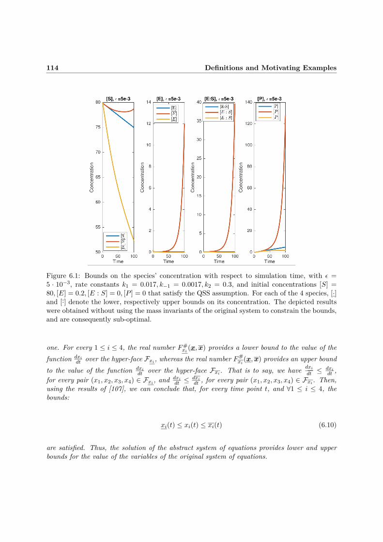
114 Definitions and Motivating Examples

Figure 6.1: Bounds on the species’ concentration with respect to simulation time, with ε =5 · 10−3, rate constants k1 = 0.017, k−1 = 0.0017, k2 = 0.3, and initial concentrations [S] =80, [E] = 0.2, [E : S] = 0, [P ] = 0 that satisfy the QSS assumption. For each of the 4 species, [·]and [·] denote the lower, respectively upper bounds on its concentration. The depicted resultswere obtained without using the mass invariants of the original system to constrain the bounds,and are consequently sub-optimal.

one. For every 1 ≤ i ≤ 4, the real number F#xi (x,x) provides a lower bound to the value of the

function dxidt over the hyper-face Fxi, whereas the real number F#

xi(x,x) provides an upper bound

to the value of the function dxidt over the hyper-face Fxi. That is to say, we have dxi

dt ≤dxidt ,

for every pair (x1, x2, x3, x4) ∈ Fxi, and dxidt ≤

dxidt , for every pair (x1, x2, x3, x4) ∈ Fxi. Then,

using the results of [107], we can conclude that, for every time point t, and ∀1 ≤ i ≤ 4, thebounds:

xi(t) ≤ xi(t) ≤ xi(t) (6.10)

are satisfied. Thus, the solution of the abstract system of equations provides lower and upperbounds for the value of the variables of the original system of equations.

Tropical Abstraction of Biochemical Reaction networks with guarantees 115

Remark 6.2.1. In the above example, in order to obtain safe lower/upper bounds onxi’s concentration, we make the variables range over the hyper-faces. One notices thatthe variable xi is treated specifically in the derivatives of the variables xi, xi - any of itsoccurences is replaced by the variable corresponding to the hyper-face we want to bound.By contrast, the other variables, xj , are replaced according to the sign of their occurence:

• in dxidt , xj is replaced with

xj , if xj occurs negatively,xj , if xj occurs positively.

• in dxidt , xj is replaced with

xj , if xj occurs positively,xj , if xj occurs negatively.

This comes from the fact that the derivative on xi is evaluated on the correspondinghyper-face, which allows for greatly reducing the loss of precision. For a formal proof ofthe soundness of this approach, the reader is referred to [107]. Intuitively, it is justifiedby the intermediate value theorem: given a family of functions fi over the real field, ifone function fi does not take the highest value at time t, whereas it is the case at timet′′ > t, then necessarily, there exists a time t′ such that t < t′ ≤ t′′ in which fi takes thehighest value while crossing another function of the family.

In Fig.6.1, we show the time-evolution of the bounds on the concentration of the 4 species inthe Michaelis-Menten system, for an arbitrarily chosen set of reaction rate constants and initialconcentrations that satisfy the QSS condition (i.e., k2 ε k−1, and [S] ε [E] + [E : S] at timet = 0). Nonetheless, our model reduction is sound no matter the value of initial concentrationsand reaction rate constants. The equations have been integrated using the solver ode15s ofMatlab[123]. Strictly speaking, numerical errors stemming from numerical integration mayaccumulate throughout the simulation, but herein we choose to ignore them.

In Fig.6.1, we notice that the bounds diverge at a fast rate from the original trajectory,despite the restriction of the derivative’s evaluation on the hyper-face of the box (as explained inRemark 6.2.1). A way to improve bound accuracy is to take into account the original system’smass invariants, when computing the bounds.

In general, a biochemical system can have several conservation laws/mass invariants, whichare linear functions b1(x), . . . , bm(x) of the concentrations, and are constant in time. Theseequality constraints can be used to refine the bounds on the initial system’s species’ concentra-tions, by (safely) restricting the evaluation of the derivative of each coordinate to the intersectionof the corresponding hyperface with the subspace delimited by the conservation laws containingthe variable itself. Because a variable can appear in more than one mass invariant, we chooseto keep the most optimistic bound that can be computed by intersecting the hyper-face withthe mass invariant subspace: the greatest lower bound, respectively the smallest upper bound.

116 Definitions and Motivating Examples

Example 6.2.2In the Michaelis-Menten system, the total number of enzymes is constant, and so is the overallnumber of substrates and product. The two conservation laws can be written as:

x2(t) + x3(t) = e0

x1(t) + x3(t) + x4(t) = s0

with e0 = x2(0) + x3(0), and s0 = x1(0) + x3(0) + x4(0).Assuming once more that k2 k−1, by substituting x3 by e0 − x2 or s0 − x1 − x4 into 6.8,

three equivalent tropicalized upper bounds on the concentration of x2 are obtained:

dx2dt ≤ (1 + ε)k2x3 − k1x2x1dx2dt ≤ (1 + ε)k2(e0 − x2)− k1x2x1dx2dt ≤ (1 + ε)k2(s0 − x1 − x4)− k1x2x1 ≤ (1 + ε)k2(s0 − x1)− k1x2x1

(6.11)

Lifting the interpretation of the differential equations over the hyper-face correspondingto x2 results in three different expressions for the upper bound on dx2

dt , of possibly differentaccuracies:

dx2,1dt = (1 + ε)k2x3 − k1x2x1

dx2,2dt = (1 + ε)k2(e0 − x2)− k1x2x1

dx2,3dt = (1 + ε)k2(s0 − x1)− k1x2x1

(6.12)

The most accurate sound upper bound on dx2dt then writes as:

min(dx2,1dt

,dx2,2dt

,dx2,3dt

) = (1 + ε) · k2 ·min(x3, e0 − x2, s0 − x1)− k1x2x1 (6.13)

Tropical Abstraction of Biochemical Reaction networks with guarantees 117

Remark 6.2.2. The choice to introduce min and max operations in the expressions ofthe computed bounds is accounted for by our initial motivation: because existing tropical-ization reduction heuristics are not justified by rigourous estimates, we aim to provide amethod for quantifying errors stemming from such tropicalization reduction approaches,at the same time creating a tropicalization approach with guarantees.We nonethelessstress that our goal is not to correct the faults of existing tropicalization-inspired re-duction methods, but rather quantify them by proposing a more rigorous tropicalizationapproach, in which the dominated monomials are bounded, rather than discarded fromthe ODEs. Consequently, we aim at computing error bounds that are as precise as possi-ble, hence the choice of using min and max operations for bound refinement, albeit withthe disadvantage of using functions that are not C1, thus introducing non-smooth vectorfields. The trade-off between smoothness and precision can be tuned according to thedesired goal: less precise bounds can be obtained by choosing to use smooth functions.Moreover, smoothness of vector fields is generally not guaranteed during the numericalsimulation of biochemical models: as the model variables represent biochemical species’concentrations, a good practice is to call the numerical solvers used to approximate thesystem’s behavior using with the ’Non-Negative’ option, which amounts to introducinga max operation into the equations (i.e., max(0, xi)), in order to prevent negative valuesof variables.

The same reasoning can be applied to all variables appearing in the expression of dx2dt , in

order to obtain the most accurate upper bound:

dx2dt

= (1 + ε) · k2 ·min(x3, e0 − x2, s0 − x1)− k1 ·max(x1, 0) ·max(x2, e0 − x3) (6.14)

Remark 6.2.3. In (6.11), when computing the third bound, instead of substituting x3by its conservation law expression, s0 − x1 − x4, we choose to bound its value by anexpression not containing x4. We do so in order to avoid introducing supplementaryvariables w.r.t. those present in the tropicalized original bound (i.e., x1, x2 and x3).This method, in which mass invariant partial refinement is introduced after the tropical-ized bounds have been computed, can be considered as a per se model reduction method,as no supplementary information/complexity is introduced by incorporating the conser-vation laws. By contrast, the approach in which all the information contained by theconservation laws is exploited in order to derive the most accurate bounds can constitutea method of error-estimation for tropicalization based reduction heuristics. We presentthe two different methods formally in Section 3.

The issue of specifying QSS species and QE reactions a priori, when performing modelreductions, is circumvented by our method. Instead, the notion of region is used in order toeliminate monomials from the species’ ODEs. Our method uses static inspection of each ODE,in order to partition the state space into different regions according to which production, respec-tively consumption terms dominate the others. Using this partitioning, simplified expressions

118 Definitions and Motivating Examples

Figure 6.2: Top: bounds on the concentration of P, obtained by simulating the ODE system inExample6.2.4, for different values of ε. Rate constants and initial concentration as in Fig.6.1:k1 = 0.017, k−1 = 0.0017, k2 = 0.3, [S] = 80, [E] = 0.2, [E : S] = 0, [P ] = 0. Bottom: Fordifferent values of ε, the accuracy of the resulting bounds is computed as the difference betweenthe upper and the lower bound.

Tropical Abstraction of Biochemical Reaction networks with guarantees 119

bounding the species concentrations are derived for each region of the state space, allowingsymbolic simplification and limiting numerical approximations.

Example 6.2.3In the case of the Michaelis-Menten mechanism, there are three possible dominance regions fordx2dt leading to three possible pairs of lower and upper bounds:

1. Region 1, if k−1 dominates k2:

εk−1 ≥ k2 ⇒ k−1x3 − k1x2x1 ≤ dx2dt ≤ (1 + ε)k−1x3 − k1x2x1

2. Region 2, if k2 dominates k−1:

εk2 ≥ k−1 ⇒ k2x3 − k1x2x1 ≤ dx2dt ≤ (1 + ε)k2x3 − k1x2x1

3. Region 3, if there is no dominant rate (i.e., k−1 and k2 are of comparable magnitude):εk−1 ≤ k2

εk2 ≤ k−1⇒ (k−1 + k2)x3 − k1x2x1 ≤ dx2

dt ≤ (k−1 + k2)x3 − k1x2x1

The complete system of equations obtained using mass invariants refinement of bounds, forall the possible dominance regions, can be found in Example 6.2.4. The improvement of boundaccuracy via mass invariants can be observed in Fig. 6.2. As expected, one can also observe inFig.6.2 that results become more precise as the value of ε increases, i.e. as k−1 and k2 becomemore separated.

Example 6.2.4For convenience purposes, denote the species concentrations, [S], [E], [E : S], [P ], using x1, x2, x3, x4.Then, the derivatives of the lower and upper bounds of the original system’s species’ concentra-tions write as:

dx1dt

= k−1 ·max(x3, e0 − x2)− k1 ·min(x1, s0 − x3) ·min(x2, e0 − x3)

dx1dt

= k−1 ·min(x3, e0 − x2, s0 − x1)− k1 ·min(x1, s0 − x3) ·max(x2, e0 − x3)

dx2dt

= c+ ·max(x3, e0 − x2)− k1 ·min(x1, s0 − x3) ·min(x2, e0 − x3),

with c+ =

k−1, if εk−1 ≥ k2

k2, if εk2 ≥ k−1

(k−1 + k2), otherwise

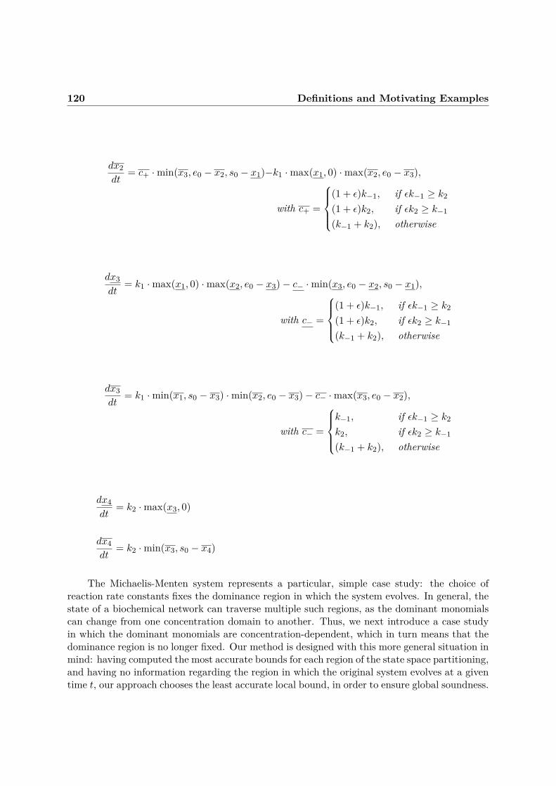
120 Definitions and Motivating Examples

dx2dt

= c+ ·min(x3, e0 − x2, s0 − x1)−k1 ·max(x1, 0) ·max(x2, e0 − x3),

with c+ =

(1 + ε)k−1, if εk−1 ≥ k2

(1 + ε)k2, if εk2 ≥ k−1

(k−1 + k2), otherwise

dx3dt

= k1 ·max(x1, 0) ·max(x2, e0 − x3)− c− ·min(x3, e0 − x2, s0 − x1),

with c− =

(1 + ε)k−1, if εk−1 ≥ k2

(1 + ε)k2, if εk2 ≥ k−1

(k−1 + k2), otherwise

dx3dt

= k1 ·min(x1, s0 − x3) ·min(x2, e0 − x3)− c− ·max(x3, e0 − x2),

with c− =

k−1, if εk−1 ≥ k2

k2, if εk2 ≥ k−1

(k−1 + k2), otherwise

dx4dt

= k2 ·max(x3, 0)

dx4dt

= k2 ·min(x3, s0 − x4)

The Michaelis-Menten system represents a particular, simple case study: the choice ofreaction rate constants fixes the dominance region in which the system evolves. In general, thestate of a biochemical network can traverse multiple such regions, as the dominant monomialscan change from one concentration domain to another. Thus, we next introduce a case studyin which the dominant monomials are concentration-dependent, which in turn means that thedominance region is no longer fixed. Our method is designed with this more general situation inmind: having computed the most accurate bounds for each region of the state space partitioning,and having no information regarding the region in which the original system evolves at a giventime t, our approach chooses the least accurate local bound, in order to ensure global soundness.

Tropical Abstraction of Biochemical Reaction networks with guarantees 121

6.2.3 Motivating example: A DNA model

We construct a simple extension of the Michaelis-Menten system, in which the product formationreaction is catalazyed by a dimer of an enzyme M . The reaction system is given by:

M +Mk1k−1

M2

M2 +DNAk2k−2

M2.DNA

M2.DNAk3−→ DNA+ P

and its ODE system2 writes as:

dx1dt = −2k1x

21 + 2k−1x2

dx2dt = −k−1x2 − k2x2x3 + k−2x4 + k1x

21

dx3dt = −k2x2x3 + k−2x4 + k3x4dx4dt = −k−2x4 − k3x4 + k2x2x3dx5dt = k3x4

(6.15)

The mass invariants are given by:x1 + 2x2 + 2x4 + 2x5 = M0

x3 + x4 = DNA0(6.16)

Dominance regions become concentration dependent: for example, the dominant positivemonomial in dx2

dt is determined by the dominance relations between both the concentrations ofx1 and x4, and between reaction rate constants k1 and k−2.

This DNA example will serve as a case study for the remainder of this chapter.

6.3 Model reduction using conservative numerical approxima-tions

The guarantees of our method are a consequence of a carefully designed symbolic propagationof inequality constraints on the species’ concentrations. Thus, symbolic transformations haveto be applied on numerical expressions, of which we introduce a syntax and semantics. We alsointroduce an alternative definition of a biochemical model to that presented in Sect. 2, whichis then used to define and justify our approximation method.

2once again, we denote the species M,M2, DNA,M2.DNA,P by x1, x2, x3, x4, x5

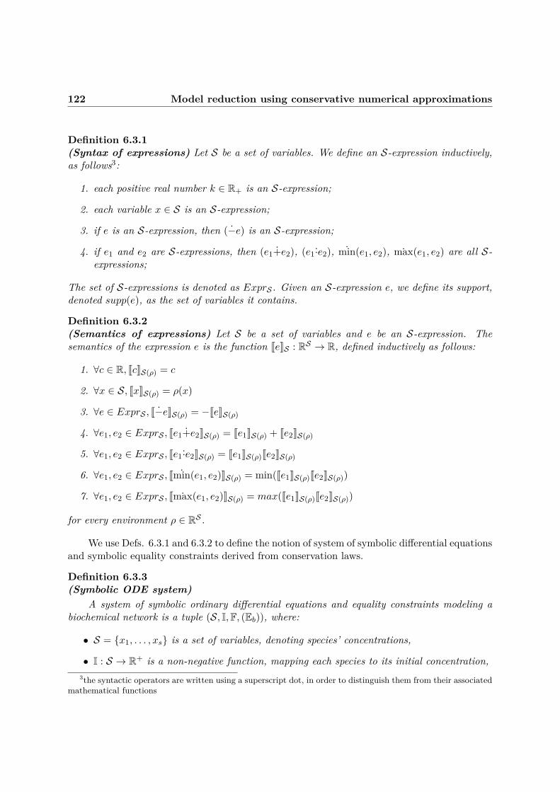
122 Model reduction using conservative numerical approximations

Definition 6.3.1(Syntax of expressions) Let S be a set of variables. We define an S-expression inductively,as follows3:

1. each positive real number k ∈ R+ is an S-expression;

2. each variable x ∈ S is an S-expression;

3. if e is an S-expression, then (−e) is an S-expression;

4. if e1 and e2 are S-expressions, then (e1+e2), (e1 ·e2), min(e1, e2), ˙max(e1, e2) are all S-expressions;

The set of S-expressions is denoted as ExprS . Given an S-expression e, we define its support,denoted supp(e), as the set of variables it contains.

Definition 6.3.2(Semantics of expressions) Let S be a set of variables and e be an S-expression. Thesemantics of the expression e is the function JeKS : RS → R, defined inductively as follows:

1. ∀c ∈ R, JcKS(ρ) = c

2. ∀x ∈ S, JxKS(ρ) = ρ(x)

3. ∀e ∈ ExprS , J−eKS(ρ) = −JeKS(ρ)

4. ∀e1, e2 ∈ ExprS , Je1+e2KS(ρ) = Je1KS(ρ) + Je2KS(ρ)

5. ∀e1, e2 ∈ ExprS , Je1 ·e2KS(ρ) = Je1KS(ρ)Je2KS(ρ)

6. ∀e1, e2 ∈ ExprS , Jmin(e1, e2)KS(ρ) = min(Je1KS(ρ)Je2KS(ρ))

7. ∀e1, e2 ∈ ExprS , J ˙max(e1, e2)KS(ρ) = max(Je1KS(ρ)Je2KS(ρ))

for every environment ρ ∈ RS .

We use Defs. 6.3.1 and 6.3.2 to define the notion of system of symbolic differential equationsand symbolic equality constraints derived from conservation laws.

Definition 6.3.3(Symbolic ODE system)

A system of symbolic ordinary differential equations and equality constraints modeling abiochemical network is a tuple (S, I,F, (Eb)), where:

• S = x1, . . . , xs is a set of variables, denoting species’ concentrations,

• I : S → R+ is a non-negative function, mapping each species to its initial concentration,3the syntactic operators are written using a superscript dot, in order to distinguish them from their associated

mathematical functions

Tropical Abstraction of Biochemical Reaction networks with guarantees 123

• F : S → ExprS is a function describing the evolution of species’ concentrations, as de-scribed in Eq.(6.5):

∀xi ∈ S,F(xi) = P+i (x)− P−i (x),

with P+/−i ∈ ExprS , Laurent polynomials with positive coefficients,

• Eb4 is a family of functions from the set S into the set ExprS , denoting equality con-straints derived from conservation laws, such that ∀f : S → RR+ satisfying

f(xi)(0) = I(0), ∀xi ∈ Sdf(xi)dt (t) = JF(xi)KS[xi 7→f(xi)(t)], ∀xi ∈ S and t ∈ R+

the constraintf(xi)(t) = JEb(xi)KS[xi 7→f(xi)(t)]

is satisfied for every function Eb of the family Eb, ∀xi ∈ S, and for every time t ∈ R+.

Example 6.3.1(A DNA example) In our running example, S = x1, x2, x3, x4, F is defined by the equationsof (6.15), and the equality constraints derived from the conservation laws of (6.16) write:

E1(x1) = M0 − 2x2 − 2x4 − 2x5; E2(x1) = M0 − 2DNA0 − 2x2 + 2x4 − 2x5

E1(x2) = M0−x12 − x4 − x5; E2(x2) = M0−x1

2 −DNA0 + x3 − x5

E1(x3) = DNA0 − x4; E2(x3) = DNA0 − M0−x12 + x2 + x5;

E1(x4) = DNA0 − x3; E2(x4) = M0−x12 − x2 − x5

E1(x5) = M0−x12 − x2 − x4; E2(x5) = M0−x1

2 −DNA0 + x3 − x2

(6.17)

We partition the state space of each ODE into regions, each one defined by the correspond-ing pair of dominant monomials, (Dom(P+

i (x)), Dom(P−i (x))). At any given time t, severalmonomials can be dominant, which can lead to an exponential number of possible regions. Tocircumvent this issue and obtain a linear number of regions, we choose to replace each regionthat has more than one dominant term with the unique region in which no term is dominant: if|Dom(P±i (x))| > 1, we choose to keep P±i (x) in the reduced ODE, instead of replacing it withDom(P±i (x)). The following definition formalizes these concepts.

Definition 6.3.4(State partitioning of a symbolic ODE) Let (S, I,F, Eb) be a symbolic ODE system,and ε ∈ [0, 1] a scale separation constant. Then, for every variable xi ∈ S, if P+

i =p∑j=1

M+j

and P−i =n∑j=1

M−j , its state space can be partitioned into (p + 1) × (n + 1) regions, each one

determined by the corresponding pair of dominant monomials4the number b indexes the different ways of expressing a species xi, by using the mass invariants in which it

appears

124 Model reduction using conservative numerical approximations

rk,li :=

(M+

k ,M−l ), if k ≤ p, l ≤ n,Dom(P+

i ) = M+k , Dom(P−i ) = M−l ,

(P+i ,M

−l ), if k = p+ 1, l ≤ n,Dom(P−i ) = M−l

(M+k , P

−i ), if k ≤ p, l = n+ 1, Dom(P+

i ) = M+k

(P+i , P

−i ), if k = p+ 1, l = n+ 1

(6.18)

Example 6.3.2(A DNA example) In Eq.(6.15), the state space of x2 can be partitioned in 9 regions, as itsODE contains 2 positive terms and 2 negative terms:

r1,12 = (k1x

21, k−1x2);

r2,12 = (k−2x4, k−1x2);r3,1

2 = (k1x21 + k−2x4, k−1x2);

r1,22 = (k1x

21, k2x2x3);

r2,22 = (k−2x4, k2x2x3);r3,2

2 = (k1x21 + k−2x4, k2x2x3);

r1,32 = (k1x

21, k−1x2 + k2x2x3);

r2,32 = (k−2x4, k−1x2 + k2x2x3);r3,3

2 = (k1x21 + k−2x4, k−1x2 + k2x2x3)

We next use the dominance relations that define each region, in order to obtain region-specific lower and upper bounds on the ODE being considered. The next definition formalizesthis procedure:

Definition 6.3.5(Region-specific tropicalized bounds) Given a symbolic ODE system (S, I,F, (Eb)), and theset of regions rk,li for each species xi, the dominance definition 6.2.1 can be used to define thefollowing functions, for every region rk,li :

Fk,l↓ (xi) :=

M+k −(1+(n−1)·ε)·M−l , if k ≤ p, l ≤ n,Dom(P+

i ) = M+k , Dom(P−i ) = M−l

P+i −(1+(n−1)·ε)·M−l , if k = p+ 1, l ≤ n,Dom(P−i ) = M−lM+k −P

−i , if k ≤ p, l = n+ 1, Dom(P+

i ) = M+k

P+i −Pi−, if k = p+ 1, l = n+ 1

Fk,l↑ (xi) :=

(1+(p−1)·ε)·M+

k −M−l , if k ≤ p, l ≤ n,Dom(P+

i ) = M+k , Dom(P−i ) = M−l

P+i −M

−l , if k = p+ 1, l ≤ n,Dom(P−i ) = M−l

(1+(p−1)·ε)·M+k −P

−i , if k ≤ p, l = n+ 1, Dom(P+

i ) = M+k

P+i −Pi−, if k = p+ 1, l = n+ 1

Tropical Abstraction of Biochemical Reaction networks with guarantees 125

Functions Fk,l↓ and Fk,l↑ provide symbolic tropicalized lower, resp. upper bounds for F(xi)on region rk,li .

Example 6.3.3(A DNA example) In our running example, in region r2,1

2 = (k−2x4, k−1x2), the dominantpositive (production) monomial is k−2x4, and the dominant negative (consumption) monomialis k−1x2. Formally, this writes as ε · k−2x4 ≥ k1x

21 ≥ 0, and ε · k−1x2 ≥ k2x2x3 ≥ 0.

Thus, the r2,12 specific tropicalized bounds write as:

F2,1↓ (x2) = k−2x4 − (1 + ε)k−1x2

F2,1↑ (x2) = (1 + ε)k−2x4 − k−1x2

,

which by construction satisfy F2,1↓ (x2) ≤ dx2

dt ≤ F2,1↑ (x2).

The bounds of Def. 6.3.5 can further be refined by using the mass invariants given by thefamily of functions Eb, as follows:

Definition 6.3.6(Region-specific refined tropicalized bounds) Given a symbolic ODE system (S, I,F, (Eb)),the set of regions rk,li and the symbolic tropicalized bounds Fk,l↓ (xi), Fk,l↑ (xi) for each species xi,we define the following bounds:

∀rk,li ,∀xj ∈ V,

Lk,li,b(xj) :=

Eb(xj), if V = Vb0, otherwise

Uk,li,b(xj) :=

Eb(xj), if V = VbJEb(xj)KVb\V[xj 7→bk,li (xj)]

, otherwise

with V = supp(Fk,l↓ (xi)) = supp(Fk,l↑ (xi)), Vb = supp(Eb(xj)), for each function Eb of the family(Eb) that applies to the variable xj, and bk,li (xj) ∈ ExprV is either 0, or a bound generated bythe dominating monomial inequality constraints.

Remark 6.3.1. The recipe of Definition 6.3.6 for defining bounds on the concentrationof a species xi is associated to the use of our method as a model reduction technique.

Consequently, when considering the refinement of bounds via mass invariants, weare careful as to not introduce supplementary variables w.r.t. those found in the sup-port of the dominant monomials - this explains why we choose to introduce a refiningbound Eb(xj) in its entirety, only if its support is identical to that of the correspondingtropicalized bound, i.e., if V = Vb.

126 Model reduction using conservative numerical approximations

Otherwise, we approximate the bound Eb by an expression that does not intro-duce supplementary variables: 0 for lower bounds, and an over-approximation E′b > Ebthat satisfies V ′b = V for upper bounds. This latter over-approximation is obtained byreplacing variables xj ∈ Vb \ V with either 0 (as variables xj appear in mass-invariant-derived constraints with negative polarity, replacing xj by 0 will yield an upper boundgreater than Eb), or with one of its bounds derived from dominating monomial inequalityconstraints.

In Section 6.4, however, one will be interested in using our method for estimating theapproximation error of tropicalization reduction techniques. Thus, we will trade modelsize for precision, and allow for introduction of supplementary variables. The definitionof region-specific tropicalized bounds will then simply be:

∀rk,li ,∀xj ∈ V,Lk,li,b(xj) := Eb(xj),Uk,li,b(xj) := Eb(xj)

Example 6.3.4(A DNA example)

When dealing with the tropicalized bounds of Ex.(6.3.3), one needs to refine the boundsof the variables in their support: V = x2, x4. We do so by using their respective equalityconstraints from (6.17): E1(x2),E2(x2),E1(x4), and E2(x4).

What’s more, the second dominance inequality of region r2,12 in Ex.(6.3.3)can be rewritten

as x3 ≤ εk−1k2

. This allows for a new upper bound on variable x3: b2,12 (x3) = εk−1k2∈ ExprV .

Using Def.6.3.6, the r2,12 -specific bounds on x2 and x4 write as:

L2,12,1(x2) = 0;

L2,12,2(x2) = 0;

L2,12,1(x4) = DNA0 − ε

k−1k2

;

L2,12,2(x4) = 0

U2,12,1(x2) = M0

2 − x4;

U2,12,2(x2) = M0

2 −DNA0 + εk−1k2

;

U2,12,1(x4) = DNA0;

U2,12,2(x4) = M0

2 − x2

Using mass invariants to compute the most optimistic bound is done inductively over theS expressions of the candidate bounds, by applying usual formulae of interval arithmetics 5 to

5the more complicated case is that of multiplication, in which every combination of lower/upper bounds

Tropical Abstraction of Biochemical Reaction networks with guarantees 127

propagate the min and ˙max operators. The resulting evaluation functions, which we call fminand f ˙max respectively, are defined by mutual induction over the syntax of the S-expressionsdenoting monomials:

1. ∀e1, e2, . . . , ek ∈ ExprS ,

• fmin(e1, e2, . . . , ek) ≡ min(e1, e2, . . . , ek)• f ˙max(e1, e2, . . . , ek) ≡ ˙max(e1, e2, . . . , ek)

2. ∀e1, e2 ∈ ExprS ,

• fmin(−e1, −e2) ≡ −(f ˙max(e1, e2))• f ˙max(−e1, −e2) ≡ −(fmin(e1, e2))

3. ∀e1, e2 ∈ ExprS ,∀c ∈ R,

• fmin(c·e1, c·e2) ≡c·fmin(e1, e2), if c ≥ 0c·f ˙max(e1, e2), if c < 0

• f ˙max(c·e1, c·e2) ≡c·f ˙max(e1, e2), if c ≥ 0c·fmin(e1, e2), if c < 0

4. ∀e, e1, e2 ∈ ExprS ,

• fmin(e1±e, e2±e) ≡ fmin(e1, e2)±e• f ˙max(e1±e, e2±e) ≡ f ˙max(e1, e2)±e

5. ∀e, e1, e2 ∈ ExprS ,

• fmin(e−e1, e−e2) ≡ e−f ˙max(e1, e2)• f ˙max(e−e1, e−e2) ≡ e−fmin(e1, e2)

may provide the lower or the upper bound of the multiplication result; in our case, this issue is nonethelesscircumvented, since variables denote concentrations, which are always positive

128 Model reduction using conservative numerical approximations

With all this in place, we can proceed to the definition of the reduced system.

Definition 6.3.7(Reduced system) Let A = (S, I,F, (Eb)) be a system of ordinary equations with equalityconstraints. The reduction of the system A is defined as the triple (S#, I#,F#), with:

1. S# = xi | xi ∈ S ∪ xi | xi ∈ S

2. I# : S# → R+ is defined by I#(xi) = I#(xi) = I(xi), ∀xi ∈ S h

3. F# : S# → ExprS#, defined as:F#(xi) = fmin([[F1,1

↓ (xi)]ρ↓1 ]ρ↓2, . . . , [[Fp+1,n+1

↓ (xi)]ρ↓1 ]ρ↓2

)F#(xi) = f ˙max([[F1,1

↑ (xi)]ρ↑1 ]ρ↑2, . . . , [[Fp+1,n+1

↑ (xi)]ρ↑1 ]ρ↑2

)

for every variable xi ∈ S ′, where:

• ρ↓1 =

xj 7→ ˙max(xj , ˙maxb

(Lk,li,b(xj))), if xj ∈ tk,l,i↓,+xj 7→ min(xj , min

b(Uk,li,b(xj))), if xj ∈ tk,l,i↓,−

• ρ↓2 =

xj 7→ xj , if xi = xj

xj 7→ xj , if xi 6= xj , for positive polarity/sign occurences of xjxj 7→ xj , if xi 6= xj , for negative polarity/sign occurences of xj

• ρ↑1 =

xj 7→ min(xj , minb

(Uk,li,b(xj))), if xj ∈ tk,l,i↑,+xj 7→ ˙max(xj , ˙max

b(Lk,li,b(xj))), if xj ∈ tk,l,i↑,−

• ρ↑2 =

xj 7→ xj , if xi = xj

xj 7→ xj , if xi 6= xj , for positive polarity/sign occurences of xjxj 7→ xj , if xi 6= xj , for negative polarity/sign occurences of xj

Intuitively, for each region (k, l) of species xi, the reduction method first replaces F(xi)by the pair of tropicalized lower and upper bounds, Fk,l↓ (xi) and Fk,l↑ (xi), that result directlyfrom the dominance inequalities that characterize the region. Then, Fk,l↓ (xi) and Fk,l↑ (xi) arerefined, using the bounds on variables that can be deduced from the conservation laws of theoriginal system. For example, replacing any occurence of a variable xj in Fk,l↓ (xi) with one ofits expressions Eb(xj) (or with its appropriate bound derived from Eb(xj)6) results in anothersafe upper bound for F(xi). By choosing the minimum such candidate bound, one obtains themost accurate, locally safe upper bound. The same reasoning applies to the computation oflower bounds, but the min operation is replaced with max.

In order to obtain safe (i.e., correct) global bounds, the least precise local bounds arechosen: the miminal lower, resp. the maximal upper bounds.

6Lk,li,b(xj) for the positive occurences of xj , and Uk,li,b(xj) for its negative occurences

Tropical Abstraction of Biochemical Reaction networks with guarantees 129

Finally, the interpretation of the variables is lifted over the hyper-faces. Any occurence ofxi is replaced with its analogue corresponding to the hyperface we want to bound, while theothers are replaced to their analogue given by the polarity of their occurence, as explained inNote 6.2.1.

Theorem 6.3.1Let A = (S, I,F, (Eb)) be a system of ordinary equations with equality constraints. Let (S#, I#,F#)be a reduction of the system A.

Let f be a function from the set S into the set RR+ s.t. for every variable xi ∈ S, we have:f(xi)(0) = I(xi)df(xi)dt (t) = F[xi 7→ f(xi)(t)]

and f# be a function from the set S# into the set RR+ s.t. for every abstract variablex#i ∈ S#, we have: f(x#

i )(0) = I#(x#i )

df#(x#i )

dt (t) = F#[x#i 7→ f#(x#

i )(t)]

Under these assumptions, we have that for every variable xi ∈ S and every time t ∈ R+:

f#(xi)(t)) ≤ f(xi)(t) ≤ f#(xi)(t),

i.e., the reduced system provides sound lower and upper bounds for the concentration of theoriginal system’s species.

Proof. The proof of this theorem essentially lays in the following result of [125].Assume the initial value problem:

dxdt = F(t,x)x(a) = xa

(6.19)

and x,x the solutions of the system of differential inequalities:dxdt ≤ F(t,x,x)dxdt ≥ F(t,x,x)

(6.20)

with F and F defined as:Fi(t,x,x) = inf

θFi(t, θ), when θi = xi, and xj ≥ θj ≤ xj ,∀j 6= i

Fi(t,x,x) = supθ

Fi(t, θ), when θi = xi, and xj ≥ θj ≤ xj , ∀j 6= i(6.21)

Then, ifx(a) ≤ x(a) ≤ x(a), (6.22)

130 Model reduction using conservative numerical approximations

the solutions of (6.20) provide lower and upper bounds on the solution of the initial valueproblem of (6.19) on the interval (a, b):

x(t) ≤ x(t) ≤ x(t),∀t ∈ (a, b). (6.23)

With this result in place (its detailed proof can be found in [125]), our proof is immediate.Indeed, it can be easily seen that the functions F# that define the reduced system of

Definition 6.3.7 verify conditions (6.20) and (6.21) by construction (remember that F#(xi) ≡fmin(. . .),F#(xi) ≡ f ˙max(. . .)), which in turn means that the inequalities of (6.23) hold for alltimes, i.e., the reduced system provides sound lower and upper bounds for the concentration ofthe original system’s species.

Example 6.3.5We apply our method on the DNA example constructed in Sect.6.2.3, for different values of thescale separating constant ε, and for arbitrarily chosen reaction rate constants k1 = k2 = k3 =0.1, k−1 = 0.01, k−2 = 0.00001 and initial concentrations [M ]0 = 1, [DNA]0 = 0.05. We showin Fig.6.3 the time evolution of the bounds on the concentration of the product species P , i.e.the variable x5. We notice once again that the results become more precise as ε decreases, i.e.as the monomials become more separated. As an example, in Appendix B we detail the equationfor the lower bound on the concentration of species M2 (i.e., x2).

Figure 6.3: Bounds on the concentration of P, in the DNA example, obtained by simulating theODE of tropicalized bounds for different values of the scale separation constant ε, rate constantsk1 = k2 = k3 = 0.1, k−1 = 0.01, k−2 = 0.00001 and initial concentrations [M ]0 = 1, [DNA]0 =0.05.

Tropical Abstraction of Biochemical Reaction networks with guarantees 131

6.4 Error estimates of tropicalized systems using conservativenumerical approximations

Our approach also serves as a heuristics for quantifying errors of tropicalization approaches forbiochemical model reduction, provided a slight modification is applied to Def.6.3.6. Instead ofcomputing bounds using only variables from the support of the tropicalized bounds, one can usethe equality constraints Eb, to refine the accuracy of bounds, cf. Remark 6.3.1. The resultingmodel presents a trade-off: it introduces new variables w.r.t. the support of the tropicalizedbounds, albeit exclusively in the form of conservation laws which are always linear functions,but gains in bound accuracy. Then, the approximation error/accuracy of a given reductionmethod can be assessed by checking if the reduced trajectory lies between the lower and upperbounds computed by our method.

Example 6.4.1It is well known that the Michaelis-Menten reduction is valid only under the QSS or QE as-sumptions. In Fig.6.4, we simulate the reduced Michaelis-Menten system (4.5), as well as ourmodified reduced system, as presented above, for a set of initial conditions that no longer satisfyneither the QSS, nor the QE assumptions, i.e. the total enzyme concentration is comparable tothe initial substrate concentration, and the complex dissociation reaction is significantly slowerthan product formation. As expected, the reduced Michaelis-Menten system no longer representsa good approximation of the initial enzymatic system (1.2.1); this is reflected by the fact thatthe trajectory of the reduced model does not lie between the lower and upper bounds computedby our approach.

6.4.1 Tyson’s Cell Cycle Model

The tropicalization heuristics can be difficult to justify by rigourous estimates, although this ispossible in some cases[138]. For example, the existence of tropical varieties - the set of pointsx ∈ Rn where at least two monomials of P−/+ are equal- can lead to sliding modes, whichin turn represent challenges in providing accuracy justifications for hybrid models obtainedusing tropical ideas. Sliding modes are well known phenomena in ODEs with discontinuousvector fields, in which the dynamics can follow discontinuity hyper-surfaces where the vectorfield is not defined; what’s more, the conditions for the existence of sliding modes are usuallyintricate. As noted in [139], sliding modes can have a nefarious effect on the behavior ofthe tropicalized system: tropical varieties (i.e. tropical curves) decompose the state space intosectors corresponding to the smooth modes of the hybrid tropicalized system, which passes fromone type of smooth dynamics to another intrinsically, when the trajectory attains the tropicalcurve. However, if certain conditions w.r.t. the sliding modes are fulfilled, the trajectorycan continue along some tropical curve instead of changing sector, which further deviates thereduced system’s trajectory from the original one (see Figure 1 in [139], for an example).

In [139], such phenomena become apparent when tropicalization is applied to the minimalcell cycle model proposed by Tyson[178], in order to obtain a reduced hybrid model. TheTyson model describes the interplay between cyclin and cyclin dependent kinase cdc2 during

132Error estimates of tropicalized systems using conservative numerical

approximations

Figure 6.4: Estimating the accuracy of the Michaelis-Menten approximation: bounds on theconcentration of [P], with respect to simulation time, for ε = 5 · 10−4, rate constants k1 =0.017, k−1 = 0.0017, k2 = 0.3, and initial concentrations that do not satisfy the QSS condition:[S] = 80, [E] = 40, [E : S] = 0, [P ] = 0. (left) Whereas the original system’s trajectory liesbetween the lower and upper bound given by our method, this is not the case for the classicalMichaelis-Menten approximation. Thus, as expected, one can conclude that if neither the QSSnor the QE conditions are met, the Michaelis-Menten approximation is inaccurate. (right)Zoomed in version, showing the enclosed original trajectory (in blue)

the progression of the cell cycle, and demonstrates the existence of three possible regimes, thatcan be associated to different phases in the cell life: the biochemical system can either functionas an oscillator, converge to a steady state, or behave as an excitable switch. The three possiblebehaviours can be associated to early embryos rapid division, arrest of unfertilised eggs andgrowth controlled division of somatic cells, respectively.

The dynamics of this non-linear model with rational reaction rates contains 6 species and9 reactions, and is described by the following system of polynomial differential equations:

dy1dt = k6y4 − k8y1 + k9y2dy2dt = −k3y2y5 + k8y1 − k9y2dy3dt = k3y2y5 − k′4y3 − k4y

24y3

dy4dt = k′4y3 + k4y

24y3 − k6y4

dy5dt = k1 − k3y2y5dy6dt = k6y4 − k7y6

, (6.24)

and has the conservation law y1(t) + y2(t) + y3(t) + y4(t) = 1, where the value 1 denoting thetotal initial concentration of kinase cdc2 (i.e. y1(0) + y2(0) + y3(0) + y4(0)) was chosen byconvenience. The values of the reaction rates constants are fixed as to have the model displaythe oscillatory behavior: k1 = 0.015, k3 = 200, k4 = 180, k′4 = 0.018, k6 = 1, k8 = 103, k9 = 106.

Tropical Abstraction of Biochemical Reaction networks with guarantees 133

The corresponding two-term tropicalized system writes as:

dy1dt = Dom(k6y4, k9y2)− k8y1dy2dt = k8y1 −Dom(k3y2y5, k9y2)dy3dt = k3y2y5 −Dom(k′4y3, k4y

24y3)

dy4dt = Dom(k′4y3, k4y

24y3)− k6y4

dy5dt = k1 − k3y2y5dy6dt = k6y4 − k7y6

, (6.25)

In [138, 139], a hybrid model of the Tyson cell cycle is obtained by detecting and elimi-nating QSS species of the original model, pruning dominated monomials, and then ultimatelytropicalizing the reduced-size model. The resulting model is a one-term tropicalization, de-scribed by the following two-variable ODE system (the remaining 4 species can be retrievedusing mass invariants and quasi-steady state equations):

dy3dt = Dom(−k′4y3,−k4y3y

24, k1)

dy4dt = Dom(k′4y3, k4y3y

24,−k6y4)

(6.26)

Figure 6.5 depicts the trajectories of the three ODE systems for the concentration of speciesy4, as well as the tropicalization approximation error, computed as the difference between theoriginal trajectory and each of the reduced models.

The equations for the lower and upper bounds on the concentration of y4 are:

dy3dt = fmin(t1,1↓ , t2,1↓ , t3,1↓ )dy4dt = f ˙max(t1,1↑ , t2,1↑ , t3,1↑ )

(6.27)

with

• t1,1↓ = k′4 ·max(x3, 1− x1 − x2 − x4)− k6 ·min(x4, 1− x1 − x2 − x3)

• t2,1↓ = k4 ·max(x4, 1−x1−x2−x3)2 ·max(x3, 1−x1−x2−x4)−k6 ·min(x4, 1−x1−x2−x3)

• t3,1↓ = k′4 ·max(x3, 1 − x1 − x2 − x4) + k4 ·max(x4, 1 − x1 − x2 − x3)2 ·max(x3, 1 − x1 −x2 − x4)− k6 ·min(x4, 1− x1 − x2 − x3)

• t1,1↑ = (1 + ε) · k′4 ·min(x3, 1− x1 − x2 − x4)− k6 ·max(x4, 1− x1 − x2 − x3)

• t2,1↑ = (1+ε) ·k4 ·min(x4, 1−x1−x2−x3)2 ·min(x3, 1−x1−x2−x4)/(12)−k6 ·max(x4, 1−x1 − x2 − x3)

• t3,1↑ = k′4 ·min(x3, 1−x1−x2−x4) + k4 ·min(x4, 1−x1−x2−x3)2 ·min(x3, 1−x1−x2−x4)− k6 ·max(x4, 1− x1 − x2 − x3)

134Error estimates of tropicalized systems using conservative numerical

approximations

Figure 6.5: Comparison of the original Tyson model with its tropicalized versions, for speciesy4. The two-term tropicalization of Definition 6.2.3 is dubbed “two-term tropicalization”, whilethe reduced model of [138] will be referred to as the “one-term tropicalized system”. (Top)Comparison of system trajectories. All three systems display oscillatory behavior, however ofdifferent periods and amplitudes. (Bottom) We plot the approximation errors of the two-termtropicalization (left) and the one-term tropicalization (right), as the difference in concentrationbetween the original system and the reduced one. As expected, the two-term tropicalization ismore a accurate approximation of the original system, however neither approximation is ableto faithfully recreate the original oscillatory behavior, from a quantitative point of view -they only do so qualitatively. An explanation for this can be given by the existence of slidingmodes in the tropical manifold [138].

Tropical Abstraction of Biochemical Reaction networks with guarantees 135

Besides having the inconvenient of analyzing trajectories of the original model in order todetect QSS species, the reduced model of [138] - which we dub the “one-term” sytems in thefigure captions - suffers from the sliding mode-related issues mentioned above: although both thesmooth (original) and the reduced system exhibit oscillating behavior and have stable periodictrajectory (i.e. limit cycle), the period of the tropicalized limit cycle is different with respect tothat of the smooth cycle, due to the tropicalized trajectory sliding along the tropical manifoldsinstead of changing sectors. Having different oscillation periods means in turn that assessingthe accuracy of the tropicalized reduced model is not a trivial question, as the distance betweenoriginal and tropicalized trajectories is variable from cycle to cycle (as can be seen in Figure6.6).What’s more, it can also provide an indication of the poor performance of tropicalization basedreduction methods when dealing with more complex systems, such oscillating systems.

Indeed, by applying our method to the original Tyson model, we are able to effectivelyprovide guarantees on the reduced model, albeit not very strong ones: this could be interpretedas an indication of the poor accuracy of the tropicalized Tyson model. In Figure 6.6, we plotthe bounds for the concentration of species y4 obtained using our method, in order to comparethe trajectory of the original model to the one of the hybrid one that can be found in [138].The lack of oscillating behavior in the computed bounds could intuitively be explained by thedifference in period of the original and reduced systems, that causes a shift at every cyclein the tropicalized trajectory w.r.t. the original behavior. Nonetheless, the obtained boundsaccurately capture the amplitude of the tropicalized model. One also notes that the time pointswhere the upper bound, respectively the tropicalized system, begin to diverge w.r.t. the originaltrajectory coincide.

Figure 6.6: Estimating the accuracy of the tropicalized Tyson model of [138]: bounds on theconcentration of [y4], with respect to simulation time, for ε = 10−3.

136 Comparison with existing methods

From a more practical point of view, we note that while simulation of the tropicalized Tysonmodel proposed in [139] was performed in 354.87 seconds, on a 2.2 GHz Intel Core i7 processorsimulating the model obtained via our method was carried out in 9.77 seconds using the samenumerical integration method (i.e. Matlab’s ode15s), thus providing a significant improvementin computation time.

We note that an alternative reduced model is obtained in [138], using tropical equilibra-tion, that circumvents the need to simulate the original system. We plan to include tropicalequilibration techniques in future work.

6.5 Comparison with existing methods

Wementioned previously that numerical errors stemming from numerical integration are ignoredherein. Indeed, numerical integration methods, while heavily used, only provide approximationsof the solution of the initial value problem (IVP) of ODE systems. Even when using variable-step size methods, there are no guarantees that the approximate solution computed by thechosen method is close to the actual solution. In order to solve the drawbacks associated totraditional ODE solvers/numerical solutions of IVP, interval numerical methods for IVP areused for computing validated enclosures of the solution of an IVP for an ODE. For example,the VNODE-LP[136] C++ solver proves that a unique solution to a problem exists, and thencomputes rigorous bounds that are guaranteed to contain it. Such bounds can then be usedto help prove theoretical results, check if a solution satisfied a condition in a safety-criticalcalculation, or simply to verify the results produced by a traditional ODE solver. Anotherexample of such software is the CAPD library [1]. Both represent well-established software forcomputing enclosures of generic ODE systems, and are integrated in various SMT solvers (e.g.,iSAT[68], dReal[70]). For a more comprehensive state of the art on such methods, the readeris refered to [137].

Interval methods for IVPs for ordinary differential equations are typically based on Taylorseries expansions, which require the computation of Taylor coefficients up to some order k.Given a final time point, the aim is to compute interval vectors that are guaranteed to containthe solution to a given IVP, at all intermediary points. In order to compute such intervalvectors, interval propagation methods are used to enclose roundoff and truncation errors in thecomputed bounds, and thus obtain rigorous bounds on the true solution of the ODE.

In our approach, instead of interpreting the differential equations over the state of the sys-tem, the interpretation is lifted conservatively over each hyper-face of the hyper-box abstractingthe system state (i.e., we over-approximate the derivatives only on the hyper-faces). When com-pared to our method, interval propagation methods over-approximate the partial derivatives ofthe function over the whole enclosing hyper-box, instead of doing so only on the hyper-faces.This in turn means that our approach computes tighter bounds than those computed by intervalmethods for IVPs.

We demonstrate our claim with the following example:

Tropical Abstraction of Biochemical Reaction networks with guarantees 137

Example 6.5.1Let us consider the following initial value problem :

dxdt = y · (2− cos(y))− x · (2− sin(y))dydt = x · (2− cos(y))− y · (2− sin(y))x(0) = y(0) = 1

As presented in Section 3, our framework can be decomposed in two independents parts:the first part consists in synthesizing bounds on the derivatives of the original system, and thesecond part deals with the propagation of said bounds, in order to obtain the enclosing system.

As our goal is to better understand and evaluate tropicalization approaches for biochemicalmodel reduction, so far we chose to focus on bounds obtained by using dominance relationsbetween monomials. The second part of our method simply represents an improved alternativeto existing ODE enclosure methods, as explained above, and as such can be used in such methodsin order to get better enclosure results.

For example, in order to compare the performance of our method to that of VNODE-LP andCAPD, instead of using dominance relations to derive inequality constraints on species’ con-centrations, we now use the Taylor Series expansion with k terms (k will serve as a parameter)for the functions sin and cos, in order to derive bounds on dx

dt and dydt :

sin(x) ≈ x− x3

3! + x5

5! −x7

7! + x9

9! − . . . =k−1∑n=0

(−1)n x2n+1

(2n+1)!

cos(x) ≈ 1− x2

2! + x4

4! −x6

6! + x8

8! − . . . =k−1∑n=0

(−1)n x2n

(2n)!

Then, for a fixed order k and an ε, instead of using dominance-related inequalities with ourmethod, one can use the following inequalities:

k−1∑n=0

(−1)n x2n+1

(2n+ 1)! − ε ≤ sin(x) ≤k−1∑n=0

(−1)n x2n+1

(2n+ 1)! + ε

k−1∑n=0

(−1)n x2n

(2n)! − ε ≤ cos(x) ≤k(−1∑n=0−1)n x2n

(2n)! + ε

,

where ε = (−1)2k+1 x2k+1

(2k+1)! cos(cx) for cx ∈ [0, x] is the residual for the Taylor expansion,

and can be bound by ε ≤ |x|2k+1

(2k+1)! , which in turn is ≤ (2k + 1)!−1 for x ∈ [−1, 1].Our method then proceeds as usual to the computation of ODEs for bounds on the concen-

trations of x and y.In Fig.6.7, we compare the accuracy of our method to that of VNODE-LP and CAPD, for

different values of the order k. The accuracy is given by the tightness of bounds, which can be

138 Conclusion and outlook

evaluated by computing the difference between the upper and lower bounds, during a simulation.The results indicate that, when compared to existing enclosure interval methods, our approachrepresents a consistent improvement of several orders of magnitude, across different values ofk.

6.6 Conclusion and outlook

In this section, we present an approximation method for biochemical networks, which can alsoserve as a technique for evaluating the accuracy of existing tropicalization reduction methodsthat do not involve guarantees. Our approach relies on the multiscaleness property of biochemi-cal systems. Tropical geometry offers a natural framework for studying such networks. Tropicalapproaches [154, 155] can guide model reduction of ODE systems, by using time- and concen-tration scales separation to identify and neglect equation terms whose values are significantlysmaller than those of other terms of the same equation. This leads to partitioning the statespace into different regions, according to which term dominates the others. A similar approachis employed in our method, but instead of neglecting the dominated terms, we propose to con-servatively bound their value using an amortizing scale separation constant and the value ofthe dominant terms. These bounds can be further refined by incorporating the conservationlaws of the initial system. The resulting approximated model is composed of two-term ODEs(which we call tropicalized), which by construction provide time-dependent lower and upperbounds for the concentration of the initial system’s species. As such, our approach can alsoserve to test the accuracy of other given reduction methods, while circumventing the executionof the original system: the suitability of a reduction will be confirmed if the reduced model’strajectory lies between the bounds provided by our abstraction.

We have tested our approach on the classical Michaelis-Menten system, a simple extensionof it, and Tyson’s cell cycle model. Our method can be easily automatized, either using staticanalysis, or existing symbolic math tools7 ; as such, Definitions 3.1-3.11 are written in anoperational-semantics style, as to describe the different procedures composing the algorithm thatimplements our method. Further work includes expanding the case studies to larger networks,possibly with no conservation laws.

7for example, Matlab’s Symbolic Math Toolbox

Tropical Abstraction of Biochemical Reaction networks with guarantees 139

Figure 6.7: Comparison of our method - which we denote by "T.A.G."- with existing ODEenclosure methods CAPD and VNODE-LP. For different values of the Taylor expansion order k,used to derive bounds on the system in Example 5.1, our method ultimately out-performs bothCAPD and VNODE-LP, in terms of accuracy; for k = 6, our method is initially outperformedby VNODE-LP on the studied example, but ultimately proves to be more efficient, for the timeframe t > 4. The exponent on the y-axis is an indicator of the decimal precision of the methods(i.e. a value of 10−15 means that the first 15 decimals of the computed lower and upper boundsare identical). We also note that both CAPD and VNODE-LP only allow values of k > 4.

140 Conclusion and outlook

Part III

Modelling storage and growth

141

Chapter 7Effects of cellular resource storage on growth

This chapter is based on a joint work with Guillaume Terradot, parts of which weresubject to a publication in [174].

7.1 Introduction

Growing cells have to perform concurrent tasks, each carried out by different groups of proteins.Said proteins, and their tasks, can be roughly classified into:

• enzymes, which take up extra-cellular resources and convert them into biosynthetic pre-cursors;

• biosynthetic proteins, the most important of which are ribosomes, which are responsiblefor protein production;

• and other housekeeping proteins.

In order to perform these task well, cells need to balance the uptake of extracellular re-sources with the intracellular demands of biosynthetic processes ([130],[167],[182]). Dependingon how they coordinate uptake and consumption, cells can adjust the buildup, or storage, ofintracellular resources. Cellular storage allows nutrients to be consumed some time after theyhave been internalized by a living cell [60]. By storing the gains of favourable environmentalperiods to survive unfavourable ones ([60],[158]), the “storage effect” has been proposed as anevolutionary tunable strategy of coping with variable environments. What’s more, it is saidto provide an explanation to behavioural diversity [40]: under the assumption that no singlestrategy can perform best in all environmental conditions, the storage effect explains the coex-istence of diverse responses in fluctuating environments, countering the competitive exclusionprinciple which states that two species exploiting the same set of resources cannot coexist in aclosed environment [88].

The careful exercise of balancing, allocating, and storing cellular resources will depend onthe growth conditions (growth media, competitors, antibiotics, etc...). Indeed, bacterial cells areknown to allocate their resources in a context-sensitive manner ([58],[97]). For example, one con-crete regulation by which this adaptation happens in bacteria is the ppGpp-dependent stringent

143

144 Introduction

response, which senses starvations in amino acids, i.e., protein precursors, and down-regulatesthe synthesis of catalysts of biosynthetic processes. What’s more, recent modeling work [82]seems to reinforce the idea that near-optimal control strategies w.r.t. cellular resource reallo-cation are triggered by sensing the concentration of immediate precursors to protein synthesis.Consequently, even if any internalized nutrient can a priori be considered an energy storagemolecule1, the study of cellular storage presented in this chapter focuses on resources that areimmediate precursors to protein synthesis.

We base our analysis on a recent model [182] that determines growth in terms of coarse-grained cellular mechanisms, and which reflects the adaptive behaviour previously mentioned,i.e., in which allocation of resources is modulated by the amount of protein precursors availablein the media. The mechanisms considered in the Weisse model comprise resource uptake andconversion into cellular precursors, as well as how the latter fuels protein biosynthesis, and thusgrowth. Most importantly, in the Weisse model the growth rate is emergent from the modeldynamics, instead of being obtained by optimization - this is different from the other modelswe have mentioned, such as [130] and [82], in which mechanisms for resource allocation are leftimplicit and the growth rate is maximized.This aspect will be key to our investigation, as in thesecond part of our investigation, we study the ability of the model in [182] to efficiently allocateits resources when the availability of the growth substrate changes stochastically, as well asstudy the impact of various storage strategies on the efficiency of such dynamic reallocations.As successful negotiation of changes in substrate availability is clearly the key to evolutionarysuccess of bacteria, finding out what the model of [182] can teach us about the most efficientresource storage strategies seems to be a worthwhile pursuit.

Our study of storage strategies is composed of two parts. In the preliminary sections, weinclude a brief review of the model, and introduce several modifications that aim at clarifyingsome underlying assumptions w.r.t. the definition of mass and growth (Section 7.2). Wecontinue by defining a generic scaling transformation of BRNs that acts as a proxy for thestorage phenomenon (Section 7.3), which we then apply to the growth model (Sections 7.3and 7.4). The first part of our storage strategy investigation is presented in Section 7.5, inwhich we use a single-cell model to investigate the impact of such strategies on cellular growthduring shifts of the sugar yield. The results of the numerical experiments enable a number ofobservations, that we summarize below:

• storage capacity can be modulated over several orders of magnitude, without significantlyaffecting the growth rate,

• however, excessive storage (i.e., of an order of magnitude that depasses those of theprevious point) of protein precursor is detrimental to growth,

• the cost of storage, in terms of reduced growth, is condition-dependent, and proves to behigher in rich growth conditions,

• storage results in smoother physiological transitions during environmental up-shifts andincreases biomass during such transitions, as resource allocation is dependent on protein

1by considering that the decision to use their contained energy has not yet been made, i.e. they can subse-quently be invested in building ribosomes, or transporters, or any other functions

Effects of cellular resource storage on growth 145

precursor concentration,

• the evolutionary benefits of storage increase with the frequency and magnitude of envi-ronmental fluctuations.

In Section 7.6 we perform a complementary series of experiments, in order to study howstorage strategies fare in a competitive context. To do so, we test populations of low- and high-storage strategies against each other, in a variety of environments parametrized by the frequencyof two superimposed probabilistic trains of high and low pulses of sugar. Our results suggestthat faster growing, low-storage cells perform better in environments with high infrequent sugarpulses, whereas outside this regime they are driven to extinction by the high-storage, slowgrowers.

Other observations enabled by this second series of numerical experiments are as follows:

• the results of the competition depends on the way an amount of sugar is delivered,

• “fat” cells are better at allocating their resources than “thin” cells,

• the amount of transporters of a cell seems to predict the outcome of the competition,

• during periods of nutrience abundance, fat cells are not the fittest.

7.2 Review of the Weisse cell model

7.2.1 Overview

In the spirit of Molenaar’s model of a self-replicating cell [130], the model introduced in [182] -and which will subsequently be referred to as the Weisse model, is a coarse-grained mechanisticcellular model built around the three universal2 cellular trade-offs that arise due to finite levelsof (i) cellular energy, (ii) ribosomes, and (iii) proteome/cell mass. These trade-offs prove tobe expressive enough as to recover the laws of microbial growth, as well as to enable the studyof evolutionary benefits of gene regulation, and to explain phenomena such as gene dosagecompensation or host effects on the performance of synthetic circuits [182].

The Weisse model describes the allocation of cellular resources to different functions indifferent growth media, and implements the trade-offs mentioned above by considering two corebiochemical processes: nutrient import and metabolism, and gene expression. Consequently,the model combines nutrient import and conversion to cellular energy with the biosyntheticprocesses of transcription and translation. It includes 14 variables, expressed as concentrations(number of molecules per a constant volume of 108 units3 of proteic mass), and accounting forfour classes of genes:

• ribosomes, r, which represent the only proteins capable of protein production, and arethus necessary in order to replicate the mass;

2In the sense that they are experienced by all living cells.3One unit of proteic mass corresponds to one amino-acid polymerized within a protein.

146 Review of the Weisse cell model

• transporter enzymes, et, for importing external sugar into the cell;

• metabolic enzymes, em, for processing the internalized sugar into protein precursors;

• non-ribosomal housekeeping proteins, q, the function of which is not represented in themodel, but which account for roughly half of the cell’s proteic mass across different growthconditions [167].

Each of the four classes of genes has an associated messenger RNA (mRNA), that conveysgenetic information from DNA to the ribosomes. mRNAs can appear either free (mx, x ∈r, q, em, et) or bound to a ribosome (cx, x ∈ r, q, em, et).

We note that, besides the finite energy, finite ribosomes and finite proteome trade-offs, thefollowing assumptions were used in elaborating the model:

1. Intracellular species are subject to first-order dilution, at a rate proportional to the growthrate;

2. There is no degradation of proteins, however mRNAs are subject to first-order degrada-tion;

3. The binding-unbinding reactions for mRNAs and free ribosomes are assumed to followmass-action kinetics;

4. Energy consumption from transcription is neglected; instead, energy consumption withinthe cell is assumed to stem from translation only.

The schematic of the biochemical processes contained in the model is shown in Fig. 7.1.The model consists in a deterministic system of ODEs, which reads:

dsidt

= νimp(et)− νcat(em)− λsi, (7.1)

da

dt= ns · νcat(em)−

∑x∈em,et,r,q

nxνx − λa, (7.2)

dr

dt= νr − λr +

∑x∈em,et,r,q

(νx − kbrmx + kucx), (7.3)

detdt

= νet − λet, (7.4)

demdt

= νem − λem, (7.5)

dq

dt= νq − λq, (7.6)

dmx

dt= ωx(a)− (λ+ dm)mx + νx − kbrmx + kucx, (7.7)

dcxdt

= −λcx + kbrmx − kucx − νx, ∀x ∈ r, em, et, q (7.8)

Effects of cellular resource storage on growth 147

Below, we detail the different reactions of the cell model, as well as their associated ratefunctions.

7.2.2 Nutrient Uptake and Metabolism

The transporter enzymes et import extracellular nutrients s into the cell. The metabolic en-zymes em transform the imported nutrients si into a metabolite a, with a stoichiometry ns. Theunderlying reactions are assumed to be enzymatically catalyzed, and saturable. Consequently,they follow the Michaelis-Menten kinetics with maximal rates vt and vm:

sνimp(et)−−−−−→ si, (r1)

siνcat(em)−−−−−→ ns · a, (r2)

with maximal rates given by

νimp = et ·vt s

Kt + s, (f1)

νcat = em ·vm siKm + si

. (f2)

The nutrient efficiency parameter ns represents the quality of the medium, i.e., the yieldof a from si. A biological interpretation of ns is that it is a measure of how many metabolicsteps or anabolic effort are/is needed by a cell to turn the nutrients present in the environmentinto protein precursors: the higher ns, the less metabolic work is needed. This translates in themodel into a higher yield of a from si for the same metabolic enzyme number.

7.2.3 Transcription

Transcription of mRNA has been estimated to cost ≈ 20 times less ATP (the main energycurrency for most cellular processes) than translation [121]. What’s more, in E.coli, the massfraction of RNA polymerases - which are the proteins responsible for transcription- is ten timessmaller than that of ribosomes [22]. Consequently, it is assumed in the model that in comparisonto translation, the cost of transcription is negligible, both in terms of proteic and energetic costs:(i) no proteins are needed to produce mRNA, and (ii) mRNA production does not consumethe metabolite a. However, transcription is assumed to be an energy-dependent4 process witheffective rates as follows:

ωx(a) = wxθxa

+ 1, ∀x ∈ t,m, r, (f3)

ωq(a) = wqθqa

+ 1· I(q), with I(q) = 1(

q

Kq

)αq+ 1

. (f4)

4transcription ceases when the cell runs out of energy

148 Review of the Weisse cell model

s

a

si

s

et

em

rq

+

uptake

transcription

translation

competitive binding

growth

Figure 7.1: Schematic of the Weisse cellular growth model (adapted from Ref. [182]). Four typesof proteins are considered: transporter enzymes (et), metabolic enzymes (em), ribosomes (r),and house-keeping proteins (q). External sugar s is imported into the cell by the transporterenzymes et (blue), after which the internalised sugar si is processed into protein precursor a bythe metabolic enzymes em (dark green) - see reactions (r1),(r2) for a quantitative descriptionof nutrient import and metabolism reactions. Messenger RNAs (mRNAs) are then producedthrough transcription, as described in reactions (r3),(r4)). Dashed arrows indicate that tran-scription rates depend on the concentration of metabolites a, but do not consume it. mRNAsmx compete for the same pool of ribosomes and reversibly bind them to form mRNA-Ribosomecomplexes cx (see reaction (r5)). mRNA-Ribosome complexes then incorporate a to producethe protein x (see reaction (r6)). Finally, the growth rate is defined as the rate at which cellsreproduce their own proteic mass (see reaction (r7)).

Effects of cellular resource storage on growth 149

We note the existence of a separate effective rate for the transcription of housekeepingproteins q; this is the case because q-proteins are assumed to be auto-regulated in order tosustain stable protein levels accross different growth conditions. What’s more, ribosomes andnon-ribosomal genes are assumed to have different transcriptional thresholds, θr 6= θnr, withθx = θnr,∀x ∈ em, et, q. In order to fit the experiments measuring the ribosomal mass fractionand the growth-rate in different growth-conditions from [167], the transcriptional threshold ofthe ribosomes θr must be such that θr θx, ∀x ∈ et, em, r. Consequently, for high values ofthe protein precursor a, the composition of the transcriptome shifts to one that accommodatesmore ribosomal mRNAs. This regulation mechanism ensures the balance between productionand consumption of a. Indeed, it promotes the consuming processes (ribosome-dependent) whenquantities of a a are high, and the production processes (metabolic/transporter-dependent)when quantities of a are low.

With all this in place, and assuming that mRNA degradation happens at a rate d, produc-tion and consumption of mRNA are described by the following reactions:

∅ ωx−→ mx (r3)

mxd−→ ∅ (r4)

7.2.4 Competitive Binding

Including the trade-off that results from the finite pool of intracellular ribosomes is achieved byexplicitly modeling the competition between mRNAs for binding free ribosomes. The differenttypes of mRNAs mx compete for the same pool of free ribosomes r, in order to form the mRNA-ribosome complex cx. We assume that the different mRNAs mx have the same binding constantfor the ribosomes, kb, and that cx have the same dissociation constant, ku:

r +mxkb←→ku

cx (r5)

7.2.5 Translation

A simplified mechanism of translation is assumed: first, the mRNA-ribosome complex cx re-versibly binds the “energy” metabolite a (the precursor for synthesizing new proteins), afterwhich the nascent peptide chain elongates by one amino acid, while consuming energy. Thetwo steps are repeated nx times, where nx is the length in amino acids of protein x. Finally,the ribosome, the mRNA and the newly synthesised protein are released, and the translationterminates.

This mechanism can be simply denoted by an irreversible reaction in which the mRNA-ribosome complex cx consumes a to produce the corresponding protein x, after which it disso-ciates into mx and r:

cx + nx · aνx−→ r + x+mx. (r6)

150 Review of the Weisse cell model

As previously mentioned, nx denotes the amount of a required to produce one protein x.The effective translation rate νx writes as:

νx = cx ·γ(a)nx

, with γ(a) = γmaxKγ

a+ 1

, (f6)

where γ(a) is the rate of elongation per translating ribosome (a incorporated per unit of timeper cx complex). We note that the trade-off resulting from the finite levels of cellular energy isimplemented through the energy dependence of Eq. (r6), and through the sum in Eq.(7.2).

For a more detailed derivation of reaction f6, the reader is referred to the original paper[182].

7.2.6 Growth and cellular mass

The growth-rate λ is defined as the time derivative of the mass5, relative to the currentconsidered mass:

λ = dM

dt· 1M

(7.9)

At stationary state, the original paper [182] gives the following definition for mass:

M =∑x

nx · x+ nr ·∑x

cx, (7.10)

i.e., the mass of the cell equals that of the proteic mass. As nx denotes the number of a perprotein x, this means that mass is counted in numbers of a, i.e., in number of amino-acids,meaning that the mass contribution of the two nutrients, si and a, is neglected. Indeed, in theoriginal model, the number of a and si do not exceed 150 a units, whereas the parametrizedproteic mass is taken to be 108 a.

At exponential growth, i.e., when intracellular variables are at steady state, the growthrate in the original model is proportional to the rate of protein synthesis, which agrees withother definitions of growth rate in the literature:

λ = γ(a)RtM

, (f8)

with Rt :=∑x cx denoting the number of translating ribosomes.

Equation f8 implements the finite proteome trade-off through its enforcement of Eq. 7.10,by specifying a value for M at steady-state: M = Ms, where Ms is approximately 108 amino-acids for E. coli.It is important to emphasize that the underlying assumption for fixing thevalueM = Ms in the original model is not that the cell mass is fixed, but rather that the modeldescribes the composition of a volume unit of a cell and that this volume unit, independentlyon the growth conditions, always contains an identical mass M = Ms = 108. Otherwise said,one should not understand it as a constant mass per cell, but rather as a fixed size of thecell volume we decide to observe. This volume may be set arbitrarily to any value, under the

5Or equivalently of the volume, under the assumption of constant density

Effects of cellular resource storage on growth 151

assumptions that: (i) the density (mass per volume) in a cell is constant (or invariant with thegrowth conditions, as it seems to be the case for protein per volume unit in several microbes[129]) and that (ii) the vector field describing the system’s dynamic is 1-homogeneous, as wewill later show.

However, in our analysis, we will employ a more general definition of the mass than theone given in Eq. 7.10, which includes the contributions of internal nutrients:

M = msi

ma· si + a+

∑x

nx · x+ nr ·∑x

cx, (7.11)

where msi and ma are respectively the mass (in mass units this time) of si and a, such thatmsi/ma is the mass of si counted in a equivalents. In this manuscript, the number of proteinprecursors a per cell at stationary state will be scaled over several order of magnitudes, suchthat its contribution to the mass cannot be neglected anymore. However, this will not be thecase for si, whose numbers won’t exceed 150 per cell. Neglecting si’s contribution to the massmay therefore be an option; we nevertheless choose to include it. The total mass of the the cellmodel is once again set arbitrarily to M = 108, as in [182].

Substituting the new definition of mass in Eq. (7.9), one obtains:

M · λ = ns ·dsidt

+ da

dt+∑x

nx ·dx

dt+ nr ·

∑x

dcxdt

(7.12)

where x denotes the amount of protein of type x in the cell, and ns is the mass of si, countedin amino-acids a. Substituting their respective time derivatives with the expressions of Eqs.(7.1)-(7.8), one obtains:

M · λ = ns · νimp = ns · et ·vt · siKt + si

(7.13)

which is equivalent to the Monod equation [131] for λmax = ns · et · vt.As we will see in Section 7.4, the growth rate λ is crucial for connecting cellular processes

and growth. More specifically, all intracellular species xi get diluted due to growth, at a rate λ:

xiλ−→ ∅. (r7)

which denotes a redistribution of cellular content between mother and daughter cells, andensures that the cell model, a 1-homogeneous vector field, reaches the steady state parametrizedmass. Indeed, when the mass defined in Eq. (7.11) has reached the parametrized value (in thiscase 108), the dilution pseudo-reactions will remove from the model exactly the same amountof mass that is being produced.

152 Review of the Weisse cell model

7.2.7 Model parameters

In our experiments, original parameter values from [182] are used, unless otherwise stated. Thesevalues are given in Table 7.1. Parameters that have ? left of their name have been obtained in[182] by fitting the model to data from [167]. We denote by aa the protein precursors, Aminoacids, or a in the growth model.

Parameter name Description Default value Units Amount of external nutrient 104 [molecules]dm mRNA-degradation rate 0.1 [min−1]ns Nutrient efficiency 0.5 nonenr Ribosome length 7459 [aa/protein]nx, x ∈ t,m, q Length of non-ribosomal proteins 300 [aa/protein]γmax max. Translation elongation rate 1260 [molecules/min]Kγ Translation elongation threshold 7 [molecules]vt Max. nutrient import rate 726 [molecules/min]Kt Nutrient import threshold 1000 [molecules]vm Max. enzymatic rate 5800 [molecules/min]Km Enzymatic threshold 1000 [molecules]wr ? Max. ribosome transcription rate 930 [molecules/min]we = wt = wm ? Max. enzyme transcription rate 4.14 [molecules/min]wq ? Max. q-transcription rate 948.93 [molecules/min]θr Ribosome transcription threshold 426.87 [molecules]θnr ? Non-ribosomal transcription threshold 4.38 [molecules]Kq ? q-autoinhibition threshold 152219 [molecules]hq q-autoinhibition Hill coefficient 4 nonekb mRNA-ribosome binding rate 1 [molecules−1/min]ku mRNA-ribosome unbinding rate 1 [min−1]M Total steady-state cell mass 108 [aa]kcm ? Chloramphenicol-binding rate 0.00599 [µM−1/min]

Table 7.1: Parameter values for the Weisse model

Effects of cellular resource storage on growth 153

7.3 A scaling procedure for modelling nutrient storage in thecell

7.3.1 Motivation

A key element of the Weisse model is the way the cell allocates its resources: what fractionof the mass is allocated for ribosomes vs for transporters and for metabolic enzymes. Themain feature of the regulation phenomenon - an example of the previously-mentioned factthat bacterial resource allocation strategies occur as a result of sensing protein precursors’concentration- that is needed to understand our investigation is that the amount of proteinprecursors a is positively correlated to the mass fraction of ribosomes, and negatively correlatedto that of transporter and metabolic enzymes. This prompts us to define the storage capacityin the Weisse model as a scaling factor of the protein precursor amount a at stationary state6.To do so, we define a generic scaling transformation of Biochemical Reaction Networks (BRNs)that allows us to tune the concentrations of certain chemical species, while preserving the BRNbehavior at steady state. In our specific case, this means that we can guarantee by constructionthat various storage strategies preserve approximatively goodness-of-fit to the original growthdata, and therefore correctly match growth conditions to sectorial resource allocations.

In this section, we proceed to define this scaling/reparametrisation procedure, and showhow to apply it to reactions with different types of kinetic rate functions: mass-action, Michaelis-Menten or Hill. We also elaborate on how the scaling is (partially) applied to the modifiedWeissemodel, in order to modulate the concentration of protein precursors.

7.3.2 Definition

Assume a biochemical reaction system A = (S,R,α,β), with a set of rate functions f =f1, . . . , fm that describe the deterministic chemical kinetics of its reactions. Each such func-tion fj is parametrized by κj , the set of reaction rate constants associated with reaction rj .That is, ∀rj ∈ R, we write fj(x;κj) to denote the kinetic law of reaction rj in state x ∈ Rn≥0(e.g., mass action, Michaelis-Menten, Hill, etc...)

We will write the deterministic dynamics of species Si in BRN A in state x as:

(dASidt| x)

=m∑j=1∇ijfj(x;κj) (7.14)

Definition 7.3.1 (Scalability)Let (A, f) be a BRN with reaction rate functions f , and Si ∈ S a species we want to scale.

Define dα,i : Rn≥0 → Rn≥0, the state expansion of species Si, as:

dα,i(x1, . . . , xi, . . . , xn) = (x1, . . . , αxi, . . . , xn).

Then (A, f) is said to be scalable along species Si, if the reaction kinetics allows rescaling,that is to say if for any rescaling factor α in R>0, and for any reaction rj in R, there exists κ′j

6We further elaborate on this choice in Section 7.3.4

154 A scaling procedure for modelling nutrient storage in the cell

such that:fj(x;κj) = fj(dα,i(x);κ′j).

We will denote a scalable couple (A, f), where A = (S,R,α,β), by using the tuple A ≡(S,R, f, κ).

The scalability condition ensures that the initial reaction fluxes can be retrieved throughthe scaling of the rates of reactions containing the species of interest (Si). Evidently, if Si isnot a reactant species of rj , there is no need for scaling, and one can simply take κ′j = κj .

We note that the scaling is parametrized by reactions, rather than reaction rates. In modelswhere a reaction rate name κ appears in several reactions, what is scaled is κ’s value in a certainreaction rj , rather than a scaling of its value across every reaction it appears in. In terms ofmodel variables, it can be interpreted as every κj being defined locally in reaction rj , ratherthan globally (i.e., across the whole model).

Definition 7.3.2 (Scaling of A along species Si)Let A = (S,R, f, κ) be a BRN that is scalable along species Si ∈ S. We define the scaling of Aalong species Si by a factor of α as follows:

(A, f) = (S,R, f, κ) α,Si−−→ (S,R, f, κ′) = B,

where each κ′j satisfies the condition of Def. 8.2.1.

A multi-species scaling of a CRN can be achieved by sequentially applying the transforma-tion described above, along different species.

Theorem 7.3.1Let A = (S,R, f, κ) be a CRN scalable along Si ∈ S, and let B be its scaling according to thetransformation of Def. 7.3.2: A α,Si−−→ B. Then:

∀x = (x1, . . . , xn) ∈ Rn≥0, ∀Si ∈ S :(dASidt| x)

=(dBSidt| dα,i(x)

)(7.15)

Proof of Theorem 7.3.1 is obtained directly via the definition of the network dynamics inDef.1, and the scalability condition.

Corollary 7.3.1If A is scalable along Si, A

α,Si−−→ B, and x is a steady state of A, then dα,i(x) is a steady stateof B.

We note that neither Theorem 7.3.1, nor its corollary should be interpreted as meaningtrajectory homothety, but rather as steady state equivalence, as can be observed in Fig. 7.2.

Effects of cellular resource storage on growth 155

0 2 4 6 8 100

2

4

6

8

10

12

14

16

18

20

Time (units)

Pro

tein

concen

tra

tion

Plot the evolution of proteins’ concentrations across time

[A] original model

[A] scaled model

[A] 2−homothety

[B] original model

[B] scaled model

Figure 7.2: Simulation of a simple BRN (A 1∗[A]−−−→ ∅;B 2∗[B]−−−→ ∅) and its scaling along species A,by a factor of 2. As stated by our theorem, the dynamics of species B remains unchanged. Thetrajectory of the scaled species is not homothetic to the original trajectory (homothety plottedin red, for comparison), but rather the two models (original and scaled) exhibit steady stateequivalence.

7.3.3 Examples

We now show how to apply the scaling transformation to common kinetic laws:

• if reaction rj has mass action kinetics:

fj(x;κj) = κj ·∏k

xαkjk ,

the reaction rate scales to κ′j = κjααij

, s.t. the reaction dynamics remains unchanged afterthe scaling: fj(x;κj) = fj(dα,i(x);κ′j)

• if reaction rj has Michaelis-Menten kinetics: fj(xi; vmax,KM ) = vmax·xiKM+xi , the reaction rates

scale to v′max = vmax and K ′M = αKM , s.t. the reaction dynamics remains unchangedafter the scaling: fj(xi; vmax,KM ) = fj(αxi; v′max,K ′M )

• if reaction rj has Hill kinetics: fj(xi; vmax, n,Kh) = vmax·xniKnh

+xni, the reaction rates scale to

n′ = n, v′max = vmax and K ′h = αKh, s.t. fj(xi; vmax, n,Kh) = fj(αxi; v′max, n′,K ′h). Aconcrete example of the results of scaling such a rate function is given in Fig. 7.3.

Example 7.3.1 (Mass-action kinetics)Consistent with the notations used in Theorem 7.3.1, consider a CRN

A = (A∗, B, r1, r2, f1, f2, k1, k2 >

156 A scaling procedure for modelling nutrient storage in the cell

with reactions:

r1 : ∅ f1(k1)−−−−→ A∗

r2 : A∗ f2(A∗;k2)−−−−−−→ B

and mass-action kinetics:

f1(k1) = k1

f2(A∗; k2) = k2 · [A∗]

meaning that: (dAA

∗

dt | (A∗, B)

)= f1 − f2 = k1 − k2 · [A∗](

dABdt | (A

∗, B))

= f2 = k2 · [A∗]

Construct A α,A∗−−−→ B =< A∗, B, r1, r2, f1, f2, k′1, k′2 > with:

r1 : ∅f1(k′1)−−−−→ A∗

r′2 : A∗f2(αA∗;k′2)−−−−−−−→ B

and mass-action kinetics.Then we can scale reaction rates as k′1 = k1, k′2 = k2

α , which satisfies Eq. (7.15) of Theorem7.3.1.

Example 7.3.2 (Michaelis-Menten kinetics)Consider the same two reactions as above, but where reaction r2 follows Michaelis-Mentenkinetics:

f2(A∗; v,KM ) = v · [A∗]KM + [A∗]

Again, one can easily verify that scaling the reaction rates using K ′M = αKM and v′ = v,satisfies Eq. (7.15) of Theorem 7.3.1.

Example 7.3.3 (Hill kinetics)To illustrate how our scaling procedure applies to Hill kinetics, we apply it to a model of thetoggle-switch, based on the model first published in [71].

Proteins A and B are produced at rates fA and fB:

BfA−→ A+B (r1)

AfB−−→ B +A (r2)

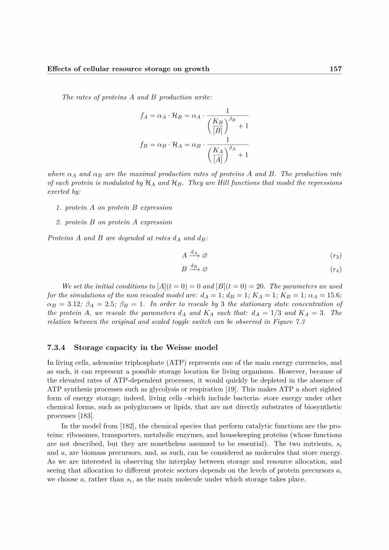
Effects of cellular resource storage on growth 157

The rates of proteins A and B production write:

fA = αA · HB = αA ·1(

KB

[B]

)βB+ 1

fB = αB · HA = αB ·1(

KA

[A]

)βA+ 1

where αA and αB are the maximal production rates of proteins A and B. The production rateof each protein is modulated by HA and HB. They are Hill functions that model the repressionsexerted by:

1. protein A on protein B expression

2. protein B on protein A expression

Proteins A and B are degraded at rates dA and dB:

AdA−→ ∅ (r3)

BdB−−→ ∅ (r4)

We set the initial conditions to [A](t = 0) = 0 and [B](t = 0) = 20. The parameters we usedfor the simulations of the non rescaled model are: dA = 1; dB = 1; KA = 1; KB = 1; αA = 15.6;αB = 3.12; βA = 2.5; βB = 1. In order to rescale by 3 the stationary state concentration ofthe protein A, we rescale the parameters dA and KA such that: dA = 1/3 and KA = 3. Therelation between the original and scaled toggle switch can be observed in Figure 7.3

7.3.4 Storage capacity in the Weisse model

In living cells, adenosine triphosphate (ATP) represents one of the main energy currencies, andas such, it can represent a possible storage location for living organisms. However, because ofthe elevated rates of ATP-dependent processes, it would quickly be depleted in the absence ofATP synthesis processes such as glycolysis or respiration [19]. This makes ATP a short sightedform of energy storage; indeed, living cells -which include bacteria- store energy under otherchemical forms, such as polyglucoses or lipids, that are not directly substrates of biosyntheticprocesses [183].

In the model from [182], the chemical species that perform catalytic functions are the pro-teins: ribosomes, transporters, metabolic enzymes, and housekeeping proteins (whose functionsare not described, but they are nonetheless assumed to be essential). The two nutrients, siand a, are biomass precursors, and, as such, can be considered as molecules that store energy.As we are interested in observing the interplay between storage and resource allocation, andseeing that allocation to different proteic sectors depends on the levels of protein precursors a,we choose a, rather than si, as the main molecule under which storage takes place.

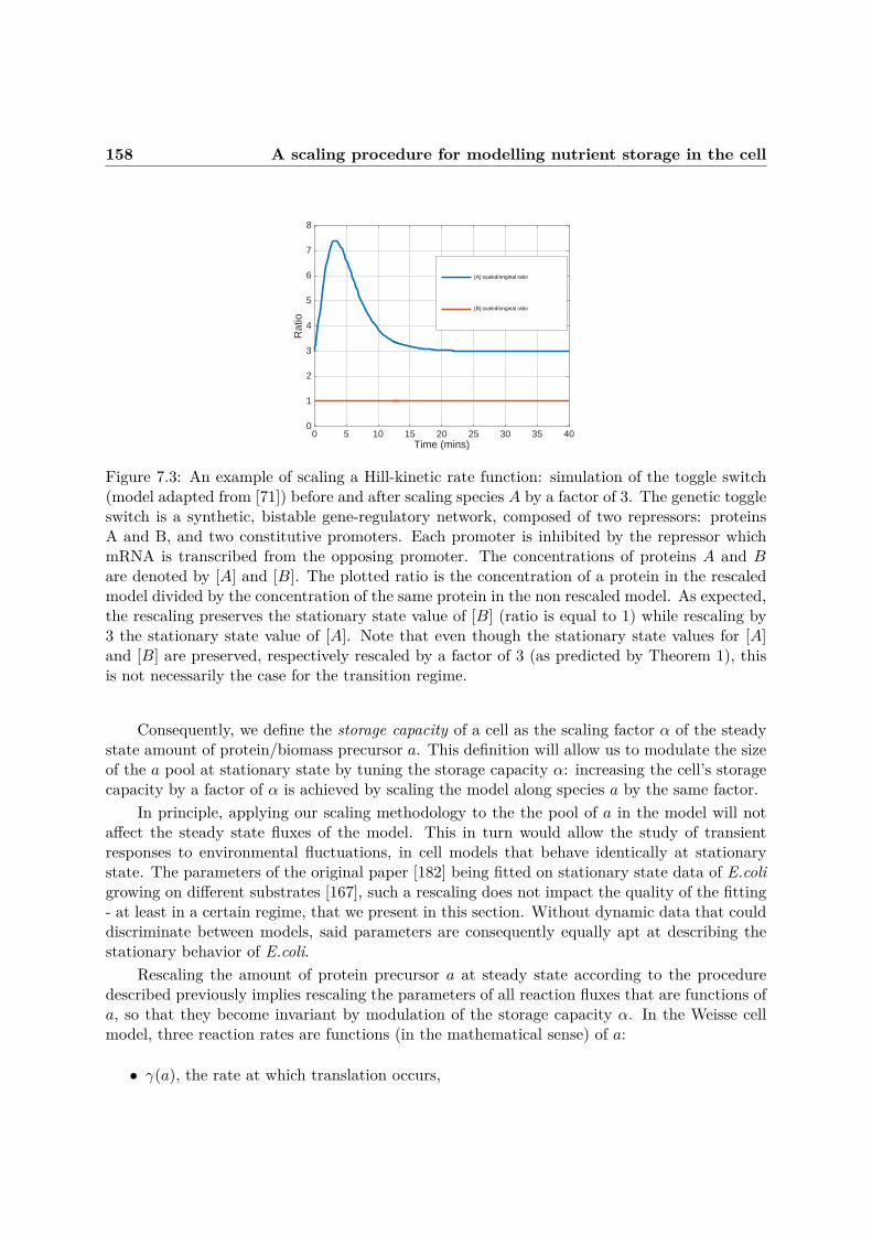
158 A scaling procedure for modelling nutrient storage in the cell

0 5 10 15 20 25 30 35 40Time (mins)

0

1

2

3

4

5

6

7

8

Rat

io

[A] scaled/original ratio

[B] scaled/original ratio

Figure 7.3: An example of scaling a Hill-kinetic rate function: simulation of the toggle switch(model adapted from [71]) before and after scaling species A by a factor of 3. The genetic toggleswitch is a synthetic, bistable gene-regulatory network, composed of two repressors: proteinsA and B, and two constitutive promoters. Each promoter is inhibited by the repressor whichmRNA is transcribed from the opposing promoter. The concentrations of proteins A and Bare denoted by [A] and [B]. The plotted ratio is the concentration of a protein in the rescaledmodel divided by the concentration of the same protein in the non rescaled model. As expected,the rescaling preserves the stationary state value of [B] (ratio is equal to 1) while rescaling by3 the stationary state value of [A]. Note that even though the stationary state values for [A]and [B] are preserved, respectively rescaled by a factor of 3 (as predicted by Theorem 1), thisis not necessarily the case for the transition regime.

Consequently, we define the storage capacity of a cell as the scaling factor α of the steadystate amount of protein/biomass precursor a. This definition will allow us to modulate the sizeof the a pool at stationary state by tuning the storage capacity α: increasing the cell’s storagecapacity by a factor of α is achieved by scaling the model along species a by the same factor.

In principle, applying our scaling methodology to the the pool of a in the model will notaffect the steady state fluxes of the model. This in turn would allow the study of transientresponses to environmental fluctuations, in cell models that behave identically at stationarystate. The parameters of the original paper [182] being fitted on stationary state data of E.coligrowing on different substrates [167], such a rescaling does not impact the quality of the fitting- at least in a certain regime, that we present in this section. Without dynamic data that coulddiscriminate between models, said parameters are consequently equally apt at describing thestationary behavior of E.coli.

Rescaling the amount of protein precursor a at steady state according to the proceduredescribed previously implies rescaling the parameters of all reaction fluxes that are functions ofa, so that they become invariant by modulation of the storage capacity α. In the Weisse cellmodel, three reaction rates are functions (in the mathematical sense) of a:

• γ(a), the rate at which translation occurs,

Effects of cellular resource storage on growth 159

• ωx(a), the transcription rates of each mRNA,

• λ(a), the dilution rate of a via growth7.

For convenience, when adjusting the stationary state concentration of a, we denote with ∗the reference parameters and concentrations, i.e., their values when α = 1.

7.3.4.1 Translation

For γ(a), we note that consumption of a through translation follows Michaelis-Menten kinetics,see rate (f6). According to Example r1, we scale the affinity of the ribosome for a∗ whentranslating proteins by a factor of α:

Kγ = α ·K∗γ (7.16)

We can check that this scaling of γ preserves the fluxes of all species’ concentrations, savefor a.

In other words, we verify that the consumption rate of the protein precursor a via transla-tion is independent of the storage capacity α.

If we denote the total amount of mRNA-Ribosome complexes by Rt =∑x cx, then the

consumption rate of a by translation is equal to Rt · γ(a; γmax,Kγ), where γ(a; γmax,Kγ) =γmaxKγ

a+ 1

is the rate of elongation per translating ribosome.

It then follows that:

∀α ∈ Rn≥0, Rt · γ(a∗; γ∗max,K∗γ) = Rt · γ(αa∗; γ∗max, α ·K∗γ) = Rt ·γ∗maxK∗γa∗

+ 1(7.17)

7.3.4.2 Transcription

In a similar fashion, the transcriptional rate ωx(a) also follows Michaelis-Menten kinetics, seerate (f4). Therefore, we scale the transcriptional thresholds by α:

θx = α · θ∗x (7.18)

Once again, we check that this scaling of θ preserves the fluxes of all species’ concentrations,save for a, or that the mRNA production rate for each gene x at exponential growth (i.e.,

7We note that in order to be coherent with the notations in the Definitions 8.2.1-7.3.2, the reaction fluxesneed to be written as a function of both the species concentrations and the parameters they depend on (i.e.write γ(a; γmax,Kγ) instead of simply γ(a)), but for concision purposes, the shorter notation is preferred in themanuscript, unless formal proofs using the definition notations are involved.

160 A scaling procedure for modelling nutrient storage in the cell

ωx(a) = wxθxa

+ 1) is invariant to the storage capacity α:

∀α ∈ Rn≥0, ωx(a∗;w∗x, θ∗x) = ωx(αa∗;w∗x, α · θ∗x) = w∗xθ∗xa∗

+ 1(7.19)

7.3.4.3 A discussion on dilution and growth

In order to scale the model according to the method of Definition 7.3.2, the dilution rate ofa by growth, i.e. λ(a) · a, should be scaled as well. Then Theorem 7.3.1 would ensure thepreservation of the scaled model’s behavior at steady state.

However, the scaling of the dilution reaction will result in either the coexistence of twodifferent growth rates (which contradicts the intuition behind the concept of growth rate itself,which is a unique property of the cell), or in a modified growth rate that would no longerpreserve the reaction fluxes.

The reason for the emergence of this contradictory behavior is that in order to scale thedilution reaction (i.e., a λ−→ ∅) by a factor of α, one would need to scale down λ∗ such that therescaled growth rate becomes λ(α) = λ∗

α . Indeed, at first glance, such a rescaling would keepthe rate of a dilution invariant with the rescaling, as λ∗

α · α · a∗ = λ∗ · a∗, where a = α · a∗.

However, since the growth rate is a unique property of the cell (a cell cannot have two growthrates simultaneously), rescaling the dilution reaction for a would also change the dilution rateof every other chemical species in the model, thereby breaking the preservation of the fluxes bythe rescaling of every chemical species other than a.

This interdiction to scale the dilution reactions stems from the observation that said dilutionreactions are nothing more than a practicality that allows the description of the growing cellmodel, whilst keeping its mass constant, and are thus artificial pseudo-reactions that are addedto the actual biological model. More specifically, when the model has reached the parametrizedmass (in this case 108), for each unit of total mass added by growth, the dilution reaction removesas much mass as was created, ensuring that the mass remains constant. The contribution ofeach chemical species to the mass may still vary, as the composition of the mass added bygrowth is not necessarily the same than the composition of the mass that is removed by thedilution pseudo-reaction (such is the case, if the model is not at stationary state).

Indeed, the growth rate and its associated dilution pseudo-reactions can be formally shownto be an emergent property of the growth model, instead of being sensu stricto chemical reac-tions (for the derivation, see Section 7.4), which justifies their unscalability.

However, this “partial” model scaling is sufficient to preserve the steady state model be-havior over a large range of values of the scaling parameter/storage capacity α. Indeed, wehave seen above that the scaling of γ and θ by definition preserve the fluxes of all species’ con-centrations, save for a. What’s more, we can numerically show that for a wide range of valuesof α, the dynamics of species a in the Weisse model remains virtually unchanged, despite thefact that we choose not to apply the scaling to its dilution reaction (which means that Theorem7.3.1 does not apply to a). For this, Figure 7.4 proves that, for values of α in the interval

Effects of cellular resource storage on growth 161

[1,≈ 105], the contribution of the dilution pseudo-reaction to the depletion of a is negligiblewhen compared to that from its consumption by translation:

Rt · γ(a) ≈ Rt · γ(a) + λ · a; (7.20)

0 1 2 3 4 5 6 7 8 9 10

log10α

-8

-7

-6

-5

-4

-3

-2

-1

0

Nu

trie

nt

dilu

tio

n t

erm

/ o

ve

rall

co

nsu

mp

tio

n,

at

ste

ad

y s

tate

(lo

g s

ca

le)

Figure 7.4: For values of the scaling parameter α ∈ [1,≈ 105], the contribution of the dilutionpseudo-reaction to the depletion of a is negligible when compared the consumption of a bytranslation.

For example, at α = 105, the dilution accounts for less than 0.3% of the total consumptionof a. Therefore, for α ∈ [1,≈ 105], the time derivative of a can neglect the contribution ofdilution:

da

dt= ns · νcat −Rt · γ(a)− λ · a ≈ ns · νcat −Rt · γ(a), (7.21)

which means its dynamics remains unchanged in the partially scaled model: da∗

dt = dαa∗

dt .This concludes the proof for the preservation of steady state behavior for all species involved

in the WS model, for small enough values of α. This statement will be reinforced by one of thenumerical observations of Section 7.5, namely that the growth rate does not change for α < 104,and only decreases by a few percents as long as α < 106.

162 The Growth Rate λ is an emergent property of the model

7.4 The Growth Rate λ is an emergent property of the model

In the Weisse model, cell division is modeled implicitly, by keeping the mass M at a constantvalue, and diluting all intracellular species at a rate λ (i.e., the growth rate, which connectscellular processes and growth). In this section, we show that the use of λ as a dilution term canbe explained by using the 1-homogeneity property of vector fields. More specifically, we showthat the growth rate λ, with the associated pseudo-reactions of dilution, are emergent behaviorswhen switching from an extensive, volume-independent description of a chemical system, to anintensive, volume-dependent one (i.e., when switching from describing the system using a vectorof species’ copy numbers to a description that uses species’ concentrations).

Let F : Rn 7→ Rn be a vector field.We say that F is 1-homogeneous, if:

∀α,X ∈ R, F (αX) = αF (X). (7.22)

In the case of chemical reaction networks, we suppose a 1-homogeneous vector field F : Rn 7→Rn describing the system’s dynamics.

We write X |= F , if X is a solution of F , and ϕFt (X0) to denote the value at t of X, theunique solution of the Initial Value Problem:

∀t, dX(t)dt = F (X(t))

X(0) = X0(7.23)

The intuition behind choosing the vectors X are that they denote vectors of species’ copynumbers. In order to switch to an intensive, concentration-based description of the system, letv ∈ Rn be a vector of the same dimension as the vectors X, that denotes the volume occupancyof each species.

Then define:x

def= X

〈v,X〉(7.24)

to be the description in terms of vectors of species concentrations, where 〈, 〉 denotes the scalarproduct of two vectors. This is the case, as 〈v,X〉 denotes the total mass of the system.

One can then compute the intensive form dynamics of the system:

dx

dt= d

dt

(X

〈v,X〉

)= (7.25)

= dX

dt· 1〈v,X〉

− X

〈v,X〉2· d〈v,X〉

dt= (7.26)

= F (X) · 1〈v,X〉

− X

〈v,X〉2· 〈v, dX

dt〉 = (7.27)

= F ( X

〈v,X〉)− X

〈v,X〉· 〈v, F (X)〉〈v,X〉

= (7.28)

= F (x)− 〈v, F (x)〉 · x (7.29)

Effects of cellular resource storage on growth 163

By defining λ(x) def= 〈v, F (x)〉, one observes that in the differential equation we obtain forx (i.e., dxdt = F (x)−x ·λ(x)), the species’ consumption (or "dilution") term is indeed denoted byλ. Thus, the dilution term (with its associated dilution pseudo-reactions) is indeed an emergentproperty of the intensive form, which is insensitive to division, through scaling by a constant v.

We remind the reader that in the general case, v is an arbitrary linear form, which wesuppose to be non-null along the trajectories (this is indeed the case if the vector field is givenby a mass action reaction network). For our purpose, the following interpretation of variablesholds: v denotes the volume occupancy of each species, X is the species’ copy number vector,〈v,X〉 (which we can note as V ) is the total volume of the system (or mass, if the density isconstant), and x = X

V - the species’ concentration vector. Using this interpretation, we haveshown that growth rate is an emergent property of the intensive vector field representation ofthe system.

We have also shown how, given the ODEs for the extensive form dXdt = F (X) of a chemical

system, as well as v its volume occupancy, one can derive the ODEs for its intensive form:dxdt = F (x)− 〈v, F (x)〉 · x, which we will note as Fv(x).

The reverse transformation (from intensive vector field to extensive vector field) is alsopossible. For that, suppose dx

dt = Fv(x), and fix X0 an initial species copy number vector,v the volume occupancy vector, and V0 = 〈v,X0〉. Then, if one defines the growth rate asλv = 〈v, F (x)〉, the volume as V (and note that its dynamics is described by the equationdVdt = λv · V ), and the extensive vector field as X = V · x, we show that:

dX

dt= dx

dt· V + x · dV

dt= (7.30)

= F (x) · V − x · 〈v, F (x)〉 · V + x · 〈v, F (x)〉 · V = (7.31)= F (V · x) = (7.32)= F (X) (7.33)

which is exactly the initial ODE for the extensive form.The above derivations show that, more generally, the following proposition (which relates

the solutions of the intensive and extensive forms of the system) holds.

Proposition 7.4.1If F is a 1-homogeneous vector field, and v a vector in the support of F , then:

∀t,∀X0, ϕFvt

(X0〈v,X0〉

)= ϕFt (X0)〈v,ϕFt (X0)〉

The proof of Prop. (7.4.1) is immediate, by using the constructions defined above.

164 The Single Cell model

7.5 The Single Cell model: Evolutionary Trade-offs in CellularResource Storage

Our first series of experiments aims at studying the impact of resource storage strategies oncellular growth, in the context of a single cell model. Consequently, in Section 7.5.1, we start byinvestigating the effect of different storage capacity strategies on the growth of a cell evolvingin a fixed environment (i.e., with a constant value of the nutritional capacity ns). We repeatthis experiment for three environments of different nutritional capacities ns, and find that, onthe one hand, storage capacity can be modulated over several orders of magnitude withoutsignificantly impacting growth, and that on the other hand, the negative impact of storage ongrowth is directly proportional to the environment’s nutritional richness.

In 7.5.2, we extend the analysis to fluctuating environments that result in quasi-instantaneouschanges of the sugar yield, in order to study the impact of storage strategies on the cell’s abilityto adapt to such changes in the environment. The results suggest that growth during envi-ronmental transitions is positively affected by an increased (up to a certain threshold) storagecapacity, and that low storage capacities come with high sensitivity of transcriptional regula-tion, which in turn result in overshoot regulation during transitions. We finish this first series ofexperiments by analyzing the trade-offs stemming from the two different types of experiments:on the one hand, the fact that increased storage capacities enable smoother transitions duringenvironmental up-shifts, and on the other hand, the detrimental impact of significantly highstorage strategies on the exponential growth rate.

7.5.1 The effects of metabolite storage on exponential growth rate

We start by defining the notion of storage cost, in terms of the fraction of protein precursora that, instead of being employed for biomass production, is diluted via the increase of cellvolume:

Definition 7.5.1 (Storage cost)Let AWeisse = (S,R, f, κ) denote the Weisse model as a scalable BRN along the protein precur-sor species ′a′, and let α denote a fixed scaling factor. The term “α-storage cost” refers tothe cost of scaling AWeisse along species ′a′ by a factor of α, and is defined as:

η(α) ≡ λ · [a]λ · [a] + γ ·Rt

(7.34)

≈ α · [a∗]M + α · [a∗] (7.35)

where λ denotes the growth rate, Rt =∑x cx denotes the total number of translating ribo-

somes, and [a] (respectively [a∗]) denotes the concentration of protein precursor in the scaled(respectively original) model.

We note that the approximation of (7.34) by (7.35) is justified by the steady-state equalityof (f8) and by Theorem 7.15.

Effects of cellular resource storage on growth 165

With all this in place, we can proceed with the numerical experiments in the single-cellcontext, the results of which allow us to make a number of observations.

The cost of storage depends on the richness of the environment.

Equation (7.35) of Definition 7.5.1 suggests that high storage capacities - which translate intohigher a concentrations - come with significant storage costs. The cost of high storage strategiescan also be explained intuitively, provided that the notion of “cost” is interpreted as opposingthat of “contribution to growth”: if one molecule of protein precursor a is invested into biomassproduction at time t0, its contribution to growth will be 1

M0, where M0 denotes the amount of

protein precursors that have to be invested in order to replicate the entire cell. However, if thesame a molecule is to be invested at a later time, t1 > t0, and if the growth rate is positive -i.e., the mass of cell at t1 is M1 > M0-, then its contribution to biomass growth will decrease:

1M1

< 1M0

. This suggests that the sooner after its production a molecule a is invested into massgrowth, the more it contributes to growth rate. As high storage capacities imply a longer timetime between the production and the consumption of protein precursors a, it becomes clearthat significant storage capacities have high costs.

4 5 6 7 8 9 100

0.1

0.2

0.3

0.4

0.5

0.6

0.7

0.8

0.9

1

log10

(α)

Rela

tive

gro

wth

rate

: λ /

λ0

ns = 0.08

ns = 0.20

ns = 0.50

Figure 7.5: The model is simulated for increasing storage capacities α, for three different en-vironments (ns = 0.08, 0.20 and 0.5). We denote by λ0 the growth rate obtained when thestorage capacity is α = 1, for any given ns. The relative growth rate λ/λ0 is defined as thegrowth rate obtained for a given storage capacity α, relative to the growth rate when α = 1.One observes that the relative growth rate decreases, as the storage capacity α increases. Thefaster a cell grows, the more storage is detrimental to growth.

What’s more, according to the Weisse model [182], the richer the medium, parameterised inthe model by the nutrient quality ns, the higher the concentration of metabolites a available fortranslation. This observation is experimentally validated, via an increase of tRNA concentration

166 The Single Cell model

[59], that in turn results in an increase of the ribosomal translation rate [22, 48, 187, 145, 66].Consequently, one expects that for cells evolving in nutrient-rich environments, high storagecapacities have a negative effect on cellular growth. The evolutionary pressure w.r.t. low storagecapacity in rich environments is confirmed by the numerical simulations of Fig. 7.5, in whichincreasing storage capacities are tested in environments of different nutritional richness. Figure7.5 also suggests that storage capacity can be modulated over several orders of magnitudewithout significantly affecting the exponential growth rate of our cell model. Consequently,cells may tune their storage capacity within that range, in order to maximize their biomassproduction in fluctuating environments, without impairing their ability to produce biomass inabsence of these fluctuations.

We next show how variations in storage capacity affect cell biomass production upon envi-ronmental fluctuations.

7.5.2 Metabolite storage and adaptation to environmental fluctuations

Cells adjust their resource allocation depending on which medium they grow in. In bacteriafor example, the ribosomal content increases as the medium gets more favourable to growth[58]. These adjustments are necessary in order to adapt biomass production in different growthconditions [167, 182]. However, the reallocation of cellular resources to different functions isnot instantaneous, as it is constrained by the cellular mechanisms that sense and regulate thedifferent processes; this has potential implications for biomass production during environmentaltransitions [44, 24]. A common assumption is that, on evolutionary time scales, cells seek tooptimize their mean biomass production over time, which means that they also seek to optimizethe dynamics of the transition between different physiological states, such that the biomassproduction over time is maximized.

Consequently, we analyze the behavior of growth rate during environmental transitions.To do so, we consider environmental up-shifts, which we model using an instantaneous changein ns, a parameter that is a proxy for the anabolic efficacy of the medium: i.e., how manymetabolic steps are necessary in order to convert the nutrients in the environment into proteinprecursors. The biological interpretation of shifting the medium abruptly to a higher value ofns is that nutrients that do not require a lot of metabolic processing before incorporation intobiomass (e.g., amino acids) are suddenly made available for the cell.

Storage capacity affects growth during environmental transitions

The results of our simulations, depicted in Fig. 7.6, show that higher storage capacities resultin smoother transitions from one physiological state to another.

To understand this behaviour we next look at the sensitivity of transcriptional regu-lation to levels of the resource a, which we define as:

σx(a) = dωxda

. (7.36)

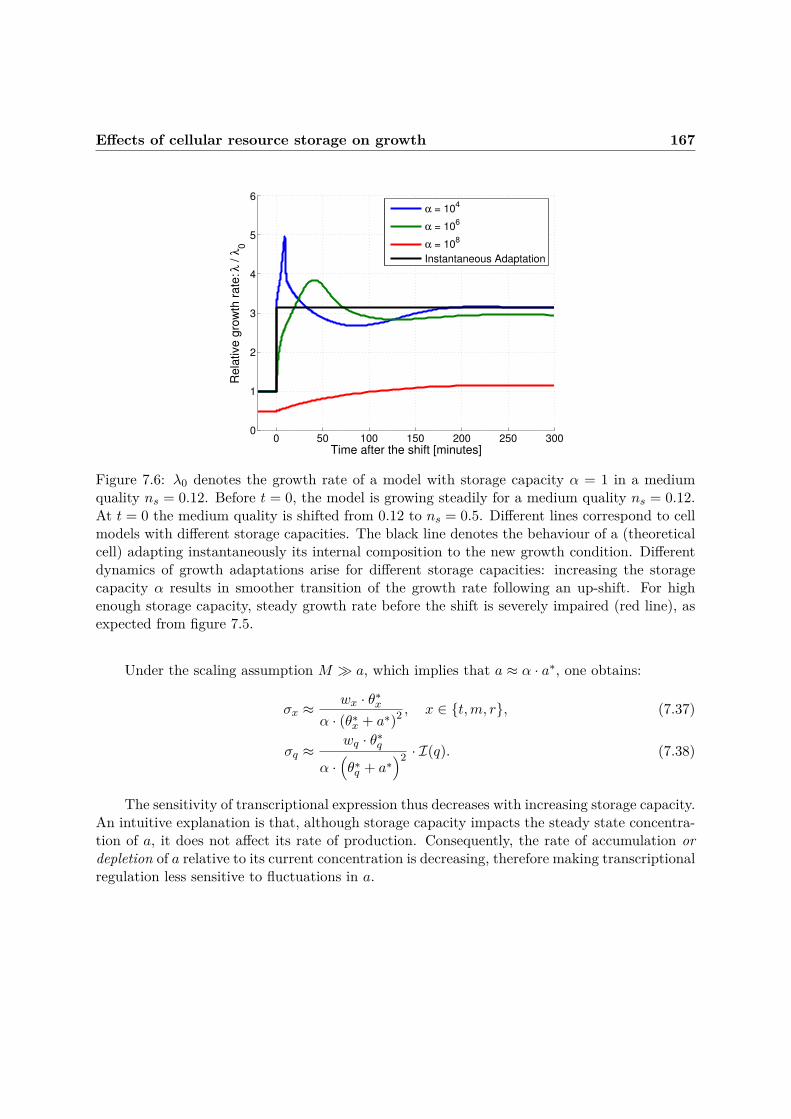
Effects of cellular resource storage on growth 167

0 50 100 150 200 250 3000

1

2

3

4

5

6

Time after the shift [minutes]

Rela

tive

gro

wth

ra

te: λ

/ λ

0

α = 104

α = 106

α = 108

Instantaneous Adaptation

Figure 7.6: λ0 denotes the growth rate of a model with storage capacity α = 1 in a mediumquality ns = 0.12. Before t = 0, the model is growing steadily for a medium quality ns = 0.12.At t = 0 the medium quality is shifted from 0.12 to ns = 0.5. Different lines correspond to cellmodels with different storage capacities. The black line denotes the behaviour of a (theoreticalcell) adapting instantaneously its internal composition to the new growth condition. Differentdynamics of growth adaptations arise for different storage capacities: increasing the storagecapacity α results in smoother transition of the growth rate following an up-shift. For highenough storage capacity, steady growth rate before the shift is severely impaired (red line), asexpected from figure 7.5.

Under the scaling assumption M a, which implies that a ≈ α · a∗, one obtains:

σx ≈wx · θ∗x

α · (θ∗x + a∗)2 , x ∈ t,m, r, (7.37)

σq ≈wq · θ∗q

α ·(θ∗q + a∗

)2 · I(q). (7.38)

The sensitivity of transcriptional expression thus decreases with increasing storage capacity.An intuitive explanation is that, although storage capacity impacts the steady state concentra-tion of a, it does not affect its rate of production. Consequently, the rate of accumulation ordepletion of a relative to its current concentration is decreasing, therefore making transcriptionalregulation less sensitive to fluctuations in a.

168 The Single Cell model

High sensitivity of transcriptional regulation results in overshoot regulation duringenvironmental up-shifts

With this in place, we analyze the reallocation dynamics of the Weisse model during an up-shift.The results depicted in Figure 7.8 suggest that high sensitivity of transcriptional regulation(achieved by low values of storage capacity α) results in a two-stage regulation:

1. Cellular resources are reallocated from metabolic enzymes to ribosomes.An increase in ns causes the net production of a to augment( Fig. 7.8C). This is a conse-quence of the linear increase of the production flux with nutrient quality, ns · νcat, whileconsumption by ribosomal mRNA complexes is saturated, which in turn causes the con-centration of a to increase (Fig. 7.8D). Consequently, reallocation of cellular resourcesfrom metabolic enzymes to ribosomes occurs: see the increase of ribosomal concentrationand decrease of metabolic enzymes concentration depicted in Fig. 7.8A and 7.8B.

2. Cellular resources are reallocated from ribosomes to metabolic enzymes.By the time the concentration of a decreases, ribosomal concentrations relative to those ofmetabolic enzymes are already high enough to create an imbalance between the productionand the consumption of a. The concentration of a decreases significantly, which results ina reallocation of resources from ribosomes to metabolic enzymes.

Thus, the transcriptional regulation of low-storage cells during an up-shift behaves like abang-bang control [170]: as described above, most of the available resources go to ribosomalproduction (relative to that of the exponential growth), which then leads to an excess in ri-bosomes, requiring to allocate most of the resources to metabolic enzymes. This behaviour ismade possible because:

• Reallocation of internal resources to different cellular functions is not instan-taneous.Indeed, allocation arises from competition for ribosomes, between different mRNAs. SincemRNAs have non-zero lifetimes, rewiring mRNA production to one cellular function doesnot result in a direct update of the mRNA repartitioning to different cellular functions.Additionally, the transcriptional regulation-induced stabilization of mRNA production tothe new desired steady state levels takes time, as seen in Figure 7.7. Both argumentsmotivate the use -in living systems- of post-transcriptional regulation mechanisms thatact directly at the translation level, instead of simply tuning transcription.

• Protein production is not instantaneous. The feedback coming from transcriptionalregulation of ribosomal or metabolic enzyme expression on a concentration also takestime, and can thus cause the overshoot in regulation.

Finally, we analyze the trade-off caused by high storage strategies: on the one hand, thesmoother transitions during up-shift, and on the other hand, their detrimental impact on theexponential growth rate.

Effects of cellular resource storage on growth 169

0 100 200 3000

0.1

0.2

0.3

0.4

0.5

0.6

0.7

0.8

0.9

1α = 1

Time after the shift [minutes]

Frac

tion

of to

tal m

RN

A pr

oduc

ed

t = m

r

0 100 200 3000

0.1

0.2

0.3

0.4

0.5

0.6

0.7

0.8

0.9

1α = 105

= 1

Time after the shift [minutes]

Figure 7.7: Before t = 0, the model is growing steadily for a medium quality ns = 0.12. Att = 0, the medium quality is shifted from 0.12 to ns = 0.5. The plot shows the fractionsof transporter-and-metabolic (green) and of ribosomal (blue) mRNA being produced for twodifferent storage capacity: (Left) α = 1 and (Right) α = 105. As the genetic regulation takesonly place at the transcriptional level in the model, it shows the genetic regulation overshoot asa result of fluctuations in a levels during the up shift, (see also figure 7.8. D.). This overshootis attenuated for higher storage capacity: high storage capacities and subsequent high steadystate levels of a, act as buffers for the genetic regulation.

170 The Single Cell model

0 50 100 150 200 250 3000

0.5

1

1.5

2

2.5

3

3.5

4

log 10

(Rel

ativ

e a

conc

entra

tion)

Time after the shift [minutes]

0 50 100 150 200 250 3000.5

0.6

0.7

0.8

0.9

1

1.1

1.2

Rel

ativ

e en

zym

e co

ncen

tratio

n

0 50 100 150 200 250 300−1

−0.5

0

0.5

1

1.5

2

2.5

3 x 106

[a] a

ccum

ulat

ion

0 50 100 150 200 250 3000.8

1

1.2

1.4

1.6

1.8

2

2.2

2.4

2.6

Rel

ativ

e rib

osom

e co

ncen

tratio

n α = 1e2α = 1e4α = 1e6α = 1e8

A B

C D

Figure 7.8: Before t = 0, the model is growing steadily for a medium quality ns = 0.12. At t = 0the medium quality is shifted from 0.12 to ns = 0.5. Different lines correspond to cell modelswith different storage capacities. (A) Ribosome concentration relative to its concentrationbefore the up-shift (B) Enzyme concentration relative to its concentration before the up-shift(C) Flux of a concentration: da

dt (D) log10 of a concentration relative to its concentration beforethe up-shift.

Effects of cellular resource storage on growth 171

Trade-offs between biomass production during transitions and during exponentialgrowth

For analysis purposes, let B(t0, T, α) denote the biomass production between two time pointst0 and T , for a storage capacity α, and let B0 denote the biomass at time t0.

Then:B(t0, T, α) = B0 · e

∫ Tt0λ(α)·dt

. (7.39)

The relative cumulative growth rate δ measures how much the mean growth rate with storagecapacity α deviates from the growth rate with the reference parameter (α = 1), between twotime points t0 and T . It is defined as:

δ = ln(B(t0, T, α))ln(B(t0, T, 1)) =

∫ Tt0λ(α) · dt∫ T

t0λ(1) · dt

(7.40)

The biomass production and the relative cumulative growth rate are then related through:

B(t0, T, 1)δ = B(t0, T, α). (7.41)

0 0.2 0.4 0.6 0.8 10

0.2

0.4

0.6

0.8

1T = 100 minutes

T = 1000 minutes

Incr

easin

g Sto

rage

Capac

ity

Rela

tive

Cu

mu

lati

ve G

row

th R

ate

Relative Exponential Growth Rate

Figure 7.9: Diamonds correspond to different up-shift experiments from ns = 0.12 to ns = 0.5for increasing the storage capacity α from 1 to 1010. The relative exponential growth rateis the ratio of the growth rate of the cell model when ns = 0.5 for one given value of thestorage capacity α over the growth rate of the cell model when ns = 0.5 and α = 1. Therelative cumulative growth rate defined in Equation (7.40) is computed for t0 = −20 minutesand T = 100 or T = 1000 minutes. Increasing the storage capacity α results in decrease ofthe relative exponential growth rate. The benefits from a smoother transition coming froman increased stock of metabolites result in a maximized relative cumulative growth rate atintermediary storage capacities.

172 The Single Cell model

Fig. 7.9 illustrates the trade-off between smoother transitions during an up-shift and thedetrimental impact of increased storage on the exponential growth rate (i.e., the growth rateonce the cell has reached the physiological state corresponding to the ns after the shift). Aslong as M a, the numerical results of Fig. 7.9 suggest that increasing the storage capacity inorder to maximize biomass production during the up-shifts is a convenient strategy. However,when the storage capacity gets too high, the exponential growth rate starts decreasing sharply,hence annihilating the gains coming from higher biomass production during the up-shift. Cellsmay thus tune their storage capacity as a result of this trade-off.

7.5.3 Environmental dynamics and resource storage strategies

So far, we have only considered one up-shift intensity. For the last series of experiments in thesingle-cell context, we will now consider several shift intensities: ns,1 − ns,0 where ns,0 and ns,1are respectively the quality of the medium before and after the shift. The results of this typeof experiment are as follows.

High storage strategies are favoured by sharper environmental shifts

In Fig. 7.10 (Left), we see that an increase in up-shift intensity results in an increase of theoptimal storage capacity α.

0 2 4 6 8 100

0.2

0.4

0.6

0.8

1

1.2

1.4

log10

(α)

Re

lative

Cu

mu

lative

Gro

wth

Ra

te

ns = 0.30

ns = 0.50

ns = 0.80

Maximal Biomass Production

0 2 4 6 8 100

0.2

0.4

0.6

0.8

1

1.2

1.4

log10

(α)

Re

lative

Cu

mu

lative

Gro

wth

Ra

te

τ = 300−1

[min−1]

τ = 600−1

[min−1]

τ = 2000−1

[min−1]

Maximal Biomass Production

Figure 7.10: (Left) The cumulative growth rate for one given storage capacity α relative tothat of when α = 1 is maximized for greater storage capacities when the up-shifts are sharper.∫ Tt0λ(α) · dt/

∫ Tt0λ(1) · dt is evaluated for t0 = −20 and T = 300 minutes. The model is shifted

from ns = 0.12 to ns = 0.30, ns = 0.50 and ns = 0.80. (Right) The cumulative growthrate for one given storage capacity α relative to that of when α = 1 is maximized for lowerstorage capacities when the frequency τ of up-shift occurrences decreases. The more frequentthe up-shifts, the higher the optimal storage capacity that maximises biomass production.

Effects of cellular resource storage on growth 173

Frequent environmental fluctuations favor high storage

We now consider environments that fluctuate repeatedly, and define the frequency of an envi-ronmental shift by τ = T−1. The results of Fig. 7.10 (Right) show that, for high frequencies,growth during transitions becomes non-negligible when compared to exponential steady stategrowth. Consequently, the optimal storage capacity, i.e., the one that maximizes cumulativegrowth, thus increases with the frequency of environmental change.

The final observation of the single-cell experiment section justifies our modelling approach,as it relates experimental data to the numerical predictions of our scaling method:

Experimentally observed E. coli ATP concentrations fall close to the predictedstorage capacity that maximizes biomass production

Living cells such as E. coli use ATP as their main energy currency. Because ATP is needed notonly for assembling molecules into amino acids (the main building block of proteins), but alsofor protein elongation during translation, it is considered one of the main protein precursors -as such, in the Weisse model, species a can be considered a proxy for ATP.

In a slow growing E. coli cell, which has a volume of approximatively 1 × 10−15 L [179],the average ATP concentration is 1.54× 10−3 mol.L−1 [186], and the number of amino acids -whether they are or not constitutive of proteins- is 5.6× 108 [22].

In the Weisse cell model, the mass (counted in amino acids) is 108 . Therefore, a slowgrowing E. coli model cell contains (1.54×10−3 ·1×10−15 ·NA)/5.6 ≈ 1.7×105 ATP moleculesper cell model mass, where NA = 6.02× 1023 is the Avogadro constant.

It is known that in E. coli, the average ATP cost per amino acid is approximatively 25ATP.aa−1 [121]. Therefore, the number of ATP per cell model mass, in amino acid cost equiv-alent, is (1.7× 105)/25 ≈ 7× 103.

This number falls close to the range of protein precursor a = α·a∗ which maximizes biomassproduction in fluctuating environments, as depicted by the results of Figure 7.10; therein, theoptimal range is given by 104 ·a∗ < α ·a∗ < 106 ·a∗, where a∗ ≈ 1 under slow growing conditions,and a∗ is the quantity of the protein precursor when the storage capacity is α = 1.

174 The Ecological perspective

7.6 The Ecological perspective: Storage Strategies for Compet-itive Growth

7.6.1 Motivation

The results of Section 7.5 allowed us to study the optimal storage strategy of a cell in differentenvironments, fluctuations of which are modeled as a quasi-instantaneous change in sugar yield(denoted by ns). Thus, changing the environment “quality” is achieved by varying ns. Moreprecisely, higher values of ns are proxies for environments more propitious to growth, as a highervalue of ns means that for an equivalent amount of transporter/metabolic enzymes more proteinprecursor will be produced per unit of time, which will in turn lead to an increased growth ratein the model.

As one can notice in Table 7.1, the numerical experiments of 7.5 were performed underthe assumption of a fuel-rich environment, such that the idealized cell experienced no sugarlimitations: s Kt, with s denoting the quantity of external nutrient (sugar), and Kt denotingthe half-saturate constant of transporters.

In this section, we perform a complementary series of experiments, in order to analyze howstorage strategies fare in a competitive context. Consequently, we will investigate the impactof storage strategies on the long term growth rate of a population of cells in fluctuating envi-ronments that (i) no longer dispose of unlimited amounts of external nutrient/sugar, and (ii)have constant sugar yields, i.e., constant values of ns. Fluctuating environments will no longerby modelled through a change in sugar yield, but will manifest as fluctuating sugar availabilityin the medium. We parametrize the sugar availability via the frequency of two superimposedprobabilistic series of high and low nutrient/sugar pulses. We test populations of low- and high-storage strategies against each other in such fluctuating environments. Our results indicate theexistence of a convex boundary separating a domain characterized by high infrequent pulses,inwhich the faster growing, low-storage strategies win, from the rest of the considered environ-ments, where the fast growers are driven to extinction by the slow growing, high-storage cells.Suprisingly, this boundary is the only place where lasting co-existence between slow and fastgrowers can be observed.

7.6.2 Experiment setup: a mixed population model in a fluctuating environ-ment

In this second series of experiments, we model a closed environment in which two types ofcompeting cell populations co-exist:

• “thin” cells, which have low storage capacity: α = 1;

• “fat” cells, which have high storage capacity: α = 2× 105.

Each of the two population has an associated death rate. We assume an identical deathrate for both cell populations, and we set its value to dN = 0.01min−1, meaning that 1% ofeach population is removed every minute.

Effects of cellular resource storage on growth 175

Remark 7.6.1. We stress the importance of constructing a mixed population experi-mental framework, in which both types of cells are present simultaneously. If one wereto study each type of cell model in isolation, like in the previous section 7.5, the two cellpopulations would have identical long-term growth rates: if thin and fat cells have thesame growth yield ns, as hypothesized above, and identical death rate, and what’s more,if the amount of sugar being delivered in a time interval δt is limiting, both types of cellwill have identical average growth rate during δt, for an identical amount of consumedsugar. However, in a mixed population setup, different amounts of sugar can be inter-nalized by the two populations, leading to faster overall growth of the cell type that isbetter at resource assimilation. All in all, it turns out that maximizing growth rate inisolation does not necessarily translate to maximizing growth when more than one typeof cells are competing for the same resources [67].

If Ni, with i ∈ 1, 2, denotes the population of thin, respectively fat cells, its growth isgiven by the ODE:

dNi

dt= Ni · (λi − di). (7.42)

The constant external sugar assumption of the initial Weisse model [182] is relaxed, in orderto assume that external sugar can be consumed proportionally to the size of the population andits import activity:

ds

dt= −

∑i

Ni · νimp,i, (7.43)

where νimp,i denotes the amount of sugar imported per cell of type i per unit of time, and dsdt is

the change in s quantities imputable to import by the cells.As mentioned above, the competitions are modeled in a closed environment, whose only

interference with the exterior world is the addition of medium (sugar). To model the fluctuatingavailability of sugar in the environment, we introduce two different random nutrient pulses:Every dt = 1 minutes, there is a probability p1 of adding a quantity Q1 of sugar, and aprobability p2 of adding a quantity Q2 of sugar. We consider Q1 to be a rare pulse, that yieldsa high amount of sugar, while Q2 is considered to be a more frequent, less sugar-rich pulse, thatyields I times less sugar than Q1: Q2 = Q1/I. Consequently, we refer to Q1 and Q2 as highintensity, respectively low intensity pulses.

We fix the expected number of cells in the environment: Ntot =∑iNi. Assuming that all

the added sugar contributes to cell growth (M α · a?), the average amount of cells producedper unit of time in a fix environment writes as:(

dNTot

dt

)P

=(d (∑iNi)dt

)P

=∑i

Ni · λi = ns · (p1 ·Q1 + p2 ·Q2)M

(7.44)

At steady state, one has that:

dNtot

dt=(dNTot

dt

)P−∑i

Ni · di = 0 (7.45)

176 The Ecological perspective

where (dNTot/dt)P is the growth term, and∑iNi · di is the death term.

Assuming identical death rates dN for every species i, we get that:∑i

Ni = NTot = ns · (p1 ·Q1 + p2 ·Q2)M · dN

(7.46)

For given values of the average number of cells in the environment (NTot), and of pulseprobabilities (p1, p2), the equation above constrains the choice of (Q1, Q2) to :

p1 ·Q1 + p2 ·Q2 = NTot ·M · dNns

(7.47)

By introducing the intensity ratio parameter constrain I = Q1/Q2 in Eq. (7.47), oneobtains the values of (Q1, Q2) required to get an average total number of cells NTot, for a fixedintensity ratio between the two pulses I and the frequencies associated to those pulses (p1, p2):Q2 = NTot ·M · dN

ns · (p1 · I + p2)Q1 = I ·Q2

(7.48)

For the numerical experiments, we take I = 100 and assume that the mean number of cellsthat can be supported by the environment, i.e., its carrying capacity, is given by NTot = 100.The choice of this last parameter is verified a posteriori in the in-silico experiments, as canbe observed in Figure 7.11. We consider a cell population to be extinct whenever its numberof cells is 10 times lower than that of its competitor. In experiments for which the extinctioncondition was not fulfilled by any of the two populations, after an hour (real-time) of simulation,the two populations were considered to co-exist, and the experiment was stopped.

7.6.3 Results

With all this in place, we carried out two types of experiments, which we detail below. In thefirst experiment, we simulated competition between thin and fat cells, in two environments thatdiffer only in their probability of low-intensity pulses. By setting the probability of high-intensitypulses to a low value, we are able to analyze how storage strategies fare during starvationperiods. In the second experiment, we carry out competitions in a range of environments thatdiffer through both high and low intensity pulse probability.

7.6.3.1 Experiment 1: Environments with different low-intensity pulse probabili-ties

We start by carrying out competitions in two different environments, which have an identicalprobability of type 1 pulses to occur (p1 = 10−3), and differ only by the probability of lowintensity pulses (p2 ≈ 0.11, respectively p2 ≈ 0.18).

From Eq. (7.48), it is apparent that each low intensity pulse with probability p2 ≈ 0.11will deliver ≈ 9.5× 108 sugar units, whereas if p2 ≈ 0.18, each pulse delivers ≈ 7.1× 108 sugarunits. As parametrized, the high intensity pulses Q1 deliver I = 100 times that amount.

Effects of cellular resource storage on growth 177

−3 −2.5 −2 −1.5 −1−2

−1.8

−1.6

−1.4

−1.2

−1

−0.8

−0.6

−0.4

−0.2

log10

(p1)

log

10(p

2)

Tim

e A

vera

ge T

ota

l Cell N

um

ber

80

85

90

95

100

105

110

115

120

Figure 7.11: Average of the total number of cells along the entire competition experiment. Asexpected from the constraint we imposed, the average total number of cells sits around 100.The high variability in the average number of cells that appears when decreasing p1 may bedue to the fact that the simulations didn’t last long enough so that the total number of cellsreaches wide sense stationarity. The time it takes to reach stationarity is indeed expected tobe longer as events that significantly impact the number of cells become rarer, as it is the casewhen the probability of pulse 1 decreases.

Remark 7.6.2. In order to make sense of these numbers, one should compare them tohow many sugar units are needed to build a new cell. Since the yield is set to ns = 0.5across all simulations, it means that 50% of the incorporated sugar will be convertedinto cell mass. For a cell weighing 108 mass units, this means that a low intensity pulsedelivers enough sugar to build ≈ 4.7, respectively ≈ 3.5 new cells (again, a high intensitypulse will build 100 times more cells).

Figure 7.12 depicts the results of this experiment. The first observation we were able tomake is that in absence of high-intensity pulses (what we refer to as the starvation period), thenutrient influx provided by low-intensity pulses of is most often insufficient for cells to growfaster than they die, hence the decrease in total number of cells. This decrease is particu-larly prominent following a high-intensity pulse, during which the total number of cells growssignificantly: after the sugar is exhausted, the large number of resulting cells are left to feedoff the limited amount of sugar provided by low-intensity pulses. This behavior is illustratedin Figure 7.12 (Middle Left) - where one can observe the total amount of cells, as well as inFigure 7.12 (Middle Right), which depicts the concomitant dynamics of sugar content. Sincethe death rate is linearly-dependent on the total number of cells, and since growth depends onsugar availability, it then becomes evident that the more a population grows following a sugardelivery, the faster it will become extinct when that supply is exhausted.

178 The Ecological perspective

The competition outcome depends on the frequency of low-intensity pulses

Our experiments indicate that for the time frame following a high-intensity pulse, survival ofcells that have a low storage capacity will be favored. Thus, in Fig. 7.12 (Top Right), oneobserves an increase in the fraction of α = 1 cells that immediately follows high-intensitypulses (which are visible in figure 7.12 (Middle Right) via the sugar spikes). The number oftransporters in the same time frame is shown for the two different cell populations, as well as forthe two different probabilities of low intensity pulses, in figure 7.12 (Bottom Left) and (BottomRight) (they correspond to p2 ≈ 0.11, respectively p2 ≈ 0.18). For the thin cells (low storagecapacity), the number of transporters fluctuates considerably less than it does for the fat ones,and this holds for the two different probabilities of low intensity pulses. Also, whereas duringstarvation periods (defined as time frames that do not follow a high intensity pulse, visible bythe sugar spikes in figure 7.12 (Middle Right)), fat cells have more transporters than thin ones,the situation is reversed during periods of nutrient abundance (defined as the time frame thatfollows a high intensity pulse).

Fat cells allocate their resources better than thin cells

Figure 7.13 shows the probability density plots of the number of transporters as a function ofthe sugar in the environment for low (Left) and high (Right) storage capacity cells, as well asfor p2 ≈ 0.11 (Top) and p2 ≈ 0.18. Colors indicate the density of data points: red regions maphigh probability density pairs of Number of transporter, Amount of sugar in the environment,whereas blue regions map low probability densities. In contrast with what is shown in figure7.12, we now consider not only data from a selected time frame, but rather across the entirecompetition (i.e., until one of the populations goes extinct).

There are three apparent regions. On the very left, one observes the time points at whichthe sugar was completely depleted from the environment. The second region, further on theright - around log10(sugar) = 9, corresponds to the data points that immediately follow theaddition of a low intensity pulse. The third region, even further on the right, consists of datapoints that follow a high intensity pulse. There is a consistent pattern, mostly visible for thefattest cell (see Fig. 7.13 (Right)), indicating that the amount of sugar in the environmentis inversely proportional to the amount of transporters. This is expected, since in nutrient-abundant environments, cells upregulate their internal allocation to biosynthetic functions,rather than to transport/metabolic functions [182, 167]. Nonetheless, this effect is hardly visiblefor the thinnest cell - see figure 7.13 (Left)- for which the amount of transporters is relativelyconstant with respect to variations in the amount of extracellular sugar.

Remark 7.6.3. The reason for which thin and fat cells allocate the resource differentlycan be understood by conducting the following thought experiment.

Thin cells have low storage capacity, and the amount of protein precursors in poormedium (low ns) can be as small as 1 per cell, whereas in rich medium (high ns), it canreach values between 10 and 20.

Consequently, following any kind of sugar pulse (low or high intensity), a thin cell

Effects of cellular resource storage on growth 179

0 20 40 60 80 1000

20

40

60

80

100

Time [days]

Fra

ction o

f α

= 1

cells

p1 = 10

−3

p2 = 0.11

p2 = 0.18

α = 1 goes extinct

α = 2 × 105 goes extinct

0 0.5 1 1.5 20.25

0.3

0.35

0.4

0.45

0.5

0.55

0.6

0.65

Time [days]

Fra

ction o

f α

= 1

Cells

p1 = 10

−3

0 0.5 1 1.5 20

100

200

300

400

500

600

Time [days]

Tota

l N

um

ber

of C

ells

p1 = 10

−3

0 0.5 1 1.5 2−2

0

2

4

6

8

10

12

14x 10

10

Time [days]

Am

ount of S

ubstr

ate

in the M

ediu

mp

1 = 10

−3

0 0.5 1 1.5 26500

7000

7500

8000

8500

9000

Time [days]

Num

ber

of tr

ansport

ers

[per

cell]

p1 = 10

−3, p

2 = 0.11

α = 1

α = 2 × 105

0 0.5 1 1.5 26500

7000

7500

8000

8500

9000

Time [days]

Num

ber

of tr

ansport

ers

[per

cell]

p1 = 10

−3, p

2 = 0.18

Figure 7.12: Modifying the way an equivalent amount of sugar is delivered in time can resultin the extinction of either the fattest or the thinnest cell models. (Top Left) Example of twocompetitions ran for p1 = 10−3. In the case where p2 ≈ 0.11 (probability of low intensitypulses), the fattest (α = 2 × 105) go extinct. When p2 ≈ 0.18, it is the opposite, and thethinnest (α = 1) go extinct. For the rest of the figures, the timed axis is a zoom in on the timeinterval [0, 2] days from the figure on the left. (Top Right) For this time interval, identicallyto the left figure, the fraction of α = 1 cells is displayed as a function of time. (Middle Left)Concomitant total number of cells as a function of time. (Middle Right) Corresponding amountof sugar as a function of time. (Bottom) Number of transporters in the same time interval forthe fattest, in red, and the thinnest, in black, in environments where the probability of type 2pulses is (Left) p2 ≈ 0.11 and (Right) p2 ≈ 0.18.

180 The Ecological perspective

will incorporate enough sugar for it to “sense” the environment as being abundant.Indeed, consider a low intensity pulse of Q2 ≈ 7 × 108 sugar units (for p1 = 10−3

and p2 ≈ 0.18), that is distributed uniformly between all cells; then, for a population of100 cells, each cell will get 7× 106 sugar units, and consequently build approximatively3.5× 106 protein precursors (as ns = 0.5). Because transporters and metabolic enzymesare already present in the cell models, prior to any kind of shift, the influx of a will befast, and, for the thin cells, will almost instantaneously reach the a > 10 cap that mapsto an allocation fit for rich environment, which in turn prioritizes biosynthetic processesover transporter/metabolic enzyme production.

One could argue that during starvation periods, thin cells could still shift theirallocation to make more transporters, but the almost-null amount of sugar availableduring this time, coupled with the cells’ lack of intracellular storage pools, makes thisvirtually impossible.

Therefore, we argue that thin cells only produce proteins when nutrients are presentin the environment; in this case, they react as if the environment were resource-abundant,and allocate a considerable amount of resources to biosynthetic processes over trans-porters.

In contrast to their competitors, fat cells are able to adapt their number of trans-porters to the amount of sugar present in the environment. By having a storage capacityof α = 2 × 105, they typically require the amount of protein precursors per cell to begreater than 106 (a considerably larger quantity than that demanded by thin cells), inorder to have an allocation status that prioritizes biosynthetic processes (e.g., productionof ribosomes).

Concretely, fat cells will pass through a continuum of allocation following a sugarpulse, that can be decomposed in three distinct phases: (i) for simplicity purposes,assume we start off an extracellular sugar amount equal to 0, as well as a null contentin protein precursors. A pulse occurs, and sugar is made available in the environment.The fattest takes up the sugar, but contrary to the thinnest, it will, during the firstphase of protein precursor accumulation (as long as it is schematically lower than 106),prioritize resource allocation towards transport/metabolic processes. (ii) If the supplyis large enough, the fattest may build up sufficient amount of protein precursors tostart allocating more resources to biosynthetic processes (schematically for amounts ofprotein precursors greater than 106). (iii) Once the sugar in the medium is depleted,the amount of protein precursors decreases, and when passing below 106, the fattest willagain prioritize synthesis of transporters/metabolic enzymes.

In environments in which the sugar supply varies, the fattest may therefore be ableto map its allocation status to a time average of the sugar supply, and avoid allocatingtoo much resources to biosynthetic processes in environments that frequently run dry ofnutrients.

Effects of cellular resource storage on growth 181

0 2 4 6 8 10 126800

7000

7200

7400

7600

7800

8000

log10

(Sugar)

Num

ber

of tr

ansport

ers

α = 1, p2 = 0.11

0 2 4 6 8 10 126800

7000

7200

7400

7600

7800

8000

log10

(Sugar)

Num

ber

of tr

ansport

ers

α = 2 × 105, p

2 = 0.11

0 2 4 6 8 10 126800

7000

7200

7400

7600

7800

8000

log10

(Sugar)

Num

ber

of tr

ansport

ers

α = 1, p2 = 0.18

0 2 4 6 8 10 126800

7000

7200

7400

7600

7800

8000

log10

(Sugar)

Num

ber

of tr

ansport

ers

α = 2 × 105, p

2 = 0.18

Figure 7.13: Fat cells have a larger dynamic range of their number of transporters. Colors indi-cate the density of the data points (how frequent a certain number of transporters occurs duringthe time interval the competition experiment lasts). All the figures correspond to competitionexperiments during which the probability of type 1 pulse (high intensity pulses) is p1 = 10−3.(Top) The probability of type 2 pulses is p2 ≈ 0.11; (Left) for the thinnest, α = 1, while (Right)the fattest has α = 2× 105. (Bottom) The probability of type 2 pulses is p2 ≈ 0.18, (Left) forthe thinnest and (Right) for the fattest. The pairs of probabilities (p1, p2) correspond to thoseused in Figure 7.12. Note that the region left of the plots seems to indicate that the extracel-lular sugar content is equal to 1 = (log10(10))−1. This is actually around 0 in the simulations.We set it to the arbitrary value of 1 for easier plotting, since log scale does not take as inputnegative values (between −1 and 0), that arise from small numerical errors of the integrator.

182 The Ecological perspective

7.6.3.2 Experiment 2: Environments with different low- and high-intensity pulseprobabilities

So far, we have restricted our analysis to two environments, which differ only through theirlow-intensity pulse probability. We now systematically observe the outcome of the competitionfor a 10 × 10 parameter grid, in which each component corresponds to a different pair of highand low intensity pulse probabilities (p1, p2).

A first observation is that thin cells have almost identical amounts of transporters in allstudied environments, see Fig. 7.15 (Bottom Left). On the contrary, fat cells have higheramounts of transporters for either high probabilities of low intensity pulses or, more surprisingly,for high probabilities of high intensity pulses, see Fig. 7.15 (Bottom Right).

However, by construction of pulse delivery, increasing the probability of high intensitypulses p1 means decreasing the amount of sugar delivered per high intensity pulse Q1, see Eq.(7.48) and Fig. 7.14. This reduces the amount of time during which extracellular sugar contentis enough for cells to grow without sugar limitation.

Indeed, if one fixes p1 = 0.1andp2 = 0.01, then by Eq. (7.48), the amount of sugar deliveredper high intensity pulse is Q1 ≈ 2 × 109, which is enough to build 10 new cells and is almostcomparable to a low intensity pulse when p1 = 10−3, p2 ≈ 0.11, where the amount of sugardelivered per low intensity pulse is Q2 ≈ 9.5× 107.

Thus, for high p1, the distribution of sugar in time is similar to that of an environmentbearing low p1 and high p2 (albeit, without the long spawned abundance periods).

−3 −2.5 −2 −1.5 −1−2

−1.8

−1.6

−1.4

−1.2

−1

−0.8

−0.6

−0.4

−0.2

log10

(p1)

log

10(p

2)

Su

ga

r per P

uls

e 2

[× 1

07]

1

3

10

30

100

Figure 7.14: Quantity of sugar added per pulse of type 1 as a function of (p1, p2), the two pulses’probabilities, upon the constraints that: (i) the average amount of sugar provided per minuteis kin = 2× 108 and (ii) that Q1 = I ·Q2, with I = 100.

Effects of cellular resource storage on growth 183

Transporter abundance predicts the competition outcome

A surprising observation is that the mean number of transporters of the fat cells, as depictedin Fig. 7.15 (Bottom Right), seems to entirely predict the outcome of the competition. Thiscan be observed in Fig. 7.15 (Top Right), for which the convention is as follows: in blue, thefattest wins, in red the thinnest wins, in green, the numerical experiments were interrupted dueto excessive computation time, and the two populations are assumed to co-exist.

Indeed, the simple rule of thumb: "whichever type of cell synthesizes the most transporterswins the competition in an environment where the nutrient supply is limiting", is verified em-pirically.

Although this seems to hold mathematically and experimentally at steady state - see 7.6.4-,it is not trivial to see why that should be the case in a fluctuating environment.

Remark 7.6.4. We note that the growth rate, as defined in Eq. (7.13), depends on theyield factor ns, the amount of sugar s, the number of transporters et, and the kineticproperties of the transporter (Kt and vt), at steady state.

Under the assumption that different types of cells, competing in the same environ-ment, have the same yield ns and the same type of transporters (identical Kt and vt),and given that the amount of sugar in the environment is the same for all cells, it thenfollows that their growth rate is actually parametrized by the amount of transportersthey express at steady state.

This implies that at steady state, in a competition between two cell models havingnegligible storage capacities, the one that allocates the most of its mass fraction totransporters will win the competition, in accordance with [67, 182].

It is important to emphasize that this does not mean that a cell should only expresstransporters, and not ribosomes. Indeed, if a cell were to do this, the sugar transportedinside the cell could not be consumed by biosynthetic processes (translation by ribosomes)at a sufficient rate, which would lead to an accumulation of metabolites until steady stateis reached, i.e., a state in which the rates of transport and biosynthetic processes balanceout.

This could paradoxically lead to a lower amount of transporters per mass unit, sincea higher fraction of the mass would be occupied by metabolites.

The fattest is the fittest in nutrient poor environments

Perhaps a good explanation for why storers outcompete fast growers in some conditions(i.e., nutrient poor environments) - see Figure 7.15 (Top Right), is that the latter run out ofresources suddenly and keep a frozen image (in their internal resource allocation) of an abundantpast which has ceased to exist - consequently expressing an insufficient amount of transporters.Storers, on the other hand, have a much more sensible picture of the conditions which areprevalent in their environment.

Considering two types of fluctuations of different intensities reveals an intricate competitivelandscape. Coexistence of the two species can be long, see figure 7.15 (Top Left), notably on

184 The Ecological perspective

the convex boundary, which is evocative of phenomena of critical slow downs near bifurcationsof dynamical systems. The result of the competition is quite different from what one wouldexpect by exclusively considering the growth of the two populations in isolation.

Indeed, for subtle reasons, the apparent competitive disadvantage of the fattest is com-pensated by mechanisms that appear to be orthogonal to the ones explored in Section 7.5 (i.e.higher growth rate during transitions from one growth medium to another), and sometimes leadto extinction of the low-storage fast growers.

Again, it is interesting to emphasize that the trade-offs between storage and growth areemergent properties that build up on well known biological mechanisms – which is different froma game theoretical approach that would consist in implementing this trade-off in an exogenousway.

For a more thorough numerical investigation, one would need to sample behaviors with afiner grain, as well as explore other temporal patterns for nutrient delivery.

−3 −2.5 −2 −1.5 −1−2

−1.8

−1.6

−1.4

−1.2

−1

−0.8

−0.6

−0.4

−0.2

log10

(p1)

log

10(p

2)

Tim

e u

ntil E

xtin

ctio

n [d

ays]

1

5

15

50

log10

(p1)

log

10(p

2)

−3 −2.5 −2 −1.5 −1−2

−1.8

−1.6

−1.4

−1.2

−1

−0.8

−0.6

−0.4

−0.2

log10

(p1)

log

10(p

2)

−3 −2.5 −2 −1.5 −1−2

−1.8

−1.6

−1.4

−1.2

−1

−0.8

−0.6

−0.4

−0.2 Mean T

ransporte

rs p

er C

ell [1

03]

7

7.2

7.4

7.6

7.8

8

log10

(p1)

log

10(p

2)

−3 −2.5 −2 −1.5 −1−2

−1.8

−1.6

−1.4

−1.2

−1

−0.8

−0.6

−0.4

−0.2 Mean T

ransporte

rs p

er C

ell [1

03]

7

7.2

7.4

7.6

7.8

8

Figure 7.15: The distributions of the low and high intensity pulses underly various differencesin the number of transporters between fat and thin cells. This difference in the number oftransporters predicts which of the fattest or the thinnest will win the competition. (Top Left)Time until one of the two population goes extinct. (Top Right) The red area depicts that thepopulation of the fattest (high storage capacity) goes extinct, whereas the blue area means thatthe thinnest (low storage capacity) goes extinct. The green area corresponds to environmentswherein, after 1 hour (real time) of simulations, no population was extinct. (Bottom) Numberof transporters across the different types of environments (characterized by the frequencies ofthe pulses 1 and 2) for (Left) the thinnest and (Right) the fattest.

Effects of cellular resource storage on growth 185

7.7 Conclusion

In the work presented in this chapter, we investigated the impact of different resource storagestrategies on cellular growth, using a recent mathematical model (the Weisse model) of thecoarse-grained mechanisms that drive cellular growth, which we modify slightly in order toclarify some assumptions relative to growth and cellular mass.

In order to model resource storage, we introduce a novel technique of reparametrizationof deterministic models of Biochemical Reaction Networks, which allows one to tune the con-centration of certain chemical species, while preserving the network’s behavior at steady state.This, in turn, allows one to symbolically navigate natural lines of iso-cost in parameter space,provided cost functions only depend on steady-state constraints. When applied to the Weissemodel, the scaling method guarantees by construction that various storage strategies preserveapproximatively goodness-of-fit to the original data, and therefore correctly match growth con-ditions to sectorial resource allocation.

In a first series of experiments, we analyze how the level of resource storage can impactcellular growth, and thus impose fitness costs or benefits on cells, for a single cell model. Wefirst test different storage strategies in different environments, parametrized by their respectivenutritional efficiency coefficient ns, and find that there is a cost associated with high levels ofstorage, resulting from the dilution-driven loss of stored resources. Our results also show thatthere is large window of concentrations for the universal precursor (considered as a conflationof all the various energy and carbon needs of the cell) in which the growth rate is essentiallyunchanged at steady state. This first experiment suggests that constant environments favourlow levels of resource storage, as no additional fitness can be obtained by storing.

In order to extend our analysis to fluctuating environments, we implement shifts in thesugar yield by modulating the nutritional coefficient parameter ns. We find that high levelsof storage can benefit cells in variable environments, by increasing biomass production duringtransitions from one medium to another. Consequently, fluctuating environments appear tofavour high levels of resource storage, i.e., additional fitness can be obtained by storing, withlittle detrimental effect on stationary growth.

These two results open up a significant possibility for selective pressure driving cells toa judicious choice of storage level, in order to extract the benefits during shifts in nutrientavailability and quality.

We also find that the cost of storage appears to increase as environments become morefavourable to growth. This can justify the use of regulatory systems that tune the storagecapacity according to growth conditions: in the case of E.coli, it has been shown that proteinsinvolved in glycogen (the main E.coli storage molecule) synthesis are up-regulated in poorgrowth conditions [61].

We follow up on the single cell model analysis by performing a series of complementaryexperiments, aimed at investigating how storage strategies fare in a competitive context as wellas on how the operational impact of intermittent energy sources may be mitigated by storage ofimmediate growth precursors. We argue that while most biologists focus on studying organismsin environments where nutrient supply is virtually infinite, and thus steady (e.g., during theexponential phase of a growth culture), these conditions do not reflect the environments most

186 Conclusion

living systems actually experience.In that sense, our rescaling technique allows us to generate a family of models that behave

differently when nutrient availability fluctuates - but which are nearly indistinguishable whenenvironmental conditions are steady. In this second series of experiments, fluctuations in theavailability of substrates fueling the biosynthetic process are entirely exogeneous to the cell, andare parametrized by two superimposed probabilistic trains of high, respectively low, pulses ofsugar 8. We test populations of low- and high- storage strategies against each other in a varietyof such fluctuating environments. Our results suggest the existence of a convex boundary thatseparates a domain of high and infrequent sugar pulses regimes - in which the fast growing, lowstorage cells survive-, from the rest of the environmental landscape - in which the fast growersare driven to extinction by the high-storage, slow growers.

Another, peculiarly interesting, yet completely unexpected behavior of the model is thatstorage seems to allow cells to “measure” the amount of resources in the environment on longertime scales. This behavior is reminiscent of the concept of memory and it provides a mechanisticexplanation of how storage could be used as a primitive source of information about the lifehistory of an organism: one could hypothesize that it may have provided an incentive for livingsystems to evolve to greater size over evolutionary time scales.

All in all, our analysis suggests that cells may face trade-offs in their maintenance ofresource storage, based on the frequency of environmental change. Quantitative models such asthe one we considered here could be used to reverse-engineer the ecology of cellular species —much of which we only know in laboratory conditions —, using existing data about metabolicresource concentrations [15].

Finally, although our analysis was performed on a model for unicellular growth, the mech-anisms described may be applicable to any system growing in an environment where resourcesare fluctuating and scarce.

8as opposed to the first series of experiments, where environmental fluctuations were modeled as variationsin the sugar yield, herein we use constant mean amounts of sugar per time unit

Chapter 8Abstractions for cellular growth: towards anew Petri net semantics

The work presented in this chapter has been published in the proceedings of the 5thHybrid Systems Biology (HSB) workshop [11].

8.1 Motivation

The previous discussion of Chapter 7 with respect to the incorporation of cellular growth inclassical models of Biochemical Reaction Networks motivates a deeper analysis of the subject.We are thus now interested in working towards a novel executable model of biochemical reactionnetworks, in which cellular growth can be characterized as an emergent property of the executionsemantics, thus circumventing the need of adding artificial constructs such as dilution reactionsto a growth model.

As seen in Section 4.1, Biochemical Reaction Networks can be represented using PetriNets, in a straightforward manner: place denote species, while transitions denote reactions.For general Petri nets, the execution of the net proceeds according to the usual interleavingsemantics: at each execution step, an enabled transition is selected non-deterministically, thenfired. The interleaving semantics describes totally asynchronous behavior, and consequently failsto capture the inherently concurrent nature of cellular behavior, in which multiple reactions canhappen in parallel. What’s more, intracellular processes rarely work in isolation, but rather incontinuous interaction with the rest of the cell. The cell has finite resources, so committingresources to one task reduces the amount of resources available to others. All cells experiencethese trade-offs, which potentially modify all cellular processes, but are often overlooked.

We have also seen that in the case of “biochemically interpreted” Petri nets, the usualchemical kinetics (be it stochastic or deterministic) is imposed as the execution semantics:transitions in stochastic Petri nets are executed according to the standard firing rule of theinterleaving semantics, while continuous Petri nets execution proceeds according to the systemof ODEs imposed on the net by the firing rate function. However, one could argue that theconstruction of these net dynamics demeans artificial, and limited in scope: with it in place,Petri nets are nothing more than a structured description of the biochemical reaction networksthey model. In this case, the existing structural Petri net analysis methods can be harnessed for

187

188 Motivation

biological purposes, but no supplementary information (with respect to the usual deterministicor stochastic model execution) about the biological system is gained via the execution semantics.

Consequently, in this chapter, we work towards defining a general Petri net executionsemantics that recreates the mass-action dynamics of deterministic BRNs models. More specif-ically, our method consists in a piecewise synchronous approximation of the dynamics of a“growth” 1 BRN: a resource-allocation-centered Petri net with maximal-step execution seman-tics. With our method in place, the trade-offs caused by finite resource allocation betweenreactions are put front stage, and the mass action run of the system can be rephrased as anoptimization problem: the inter-phase between synchronous runs defines an unknown, the re-source split, that can be exploited in order to find the best split (e.g., the one which minimizesparallel completion time, or maximizes growth rate).

For BRNs comprised exclusively of unimolecular reactions, we prove the correctness ofour method and show that it can be used either as an approximation of the dynamics, or as amethod of constraining the reaction rate constants or refuting models. Indeed, we show that forunimolecular reaction networks, the proposed PN execution semantics enables the definition of aformal notion of growth rate, which can serve as an improved “biomass objective function"[142]for a constraint method similar to flux balance analysis (FBA)[142].

Related work. While most intracellular growth processes are well characterized, themanner in which they are coordinated under the control of a scheduling policy is not wellunderstood. When fast replication is sought, a schedule that minimizes the completion time isnaturally desirable. But when resources are scarce, in the worst case it is computationally hardto find such a schedule [72],[169]. The scheduling problem of a self-replicating bacterial cell isstudied in [153].

The concept of maximally parallel execution already appears in the literature on P-systems[144], and in Levy’s family reductions [115], while in [110], the authors use it to develop aPetri Net execution semantics that resembles biology. The scheduling policy of cells is alsotackled in [65], where the notion of bounded asynchrony is introduced. In [148], the authorintroduces a constraint method that generalizes FBA to the stochastic case, allowing models tobe discriminated using second order moments.

This chapter is organised as follows. In the next section, we first define the max-parallelexecution of a PN, after which we introduce the piecewise synchronous execution semantics andshow it encompasses max-parallel execution. We then demonstrate that, at least in the caseof unimolecular reactions, our method recreates the usual ODE system dynamics, and that itcan be used either as an approximation of the dynamics, or as an alternative to flux balanceanalysis. The final section concludes with a summary and outlook regarding further work onthe subject.

1 we associate growth with the existence of an exponential stationary phase

Abstractions for cellular growth: towards a new Petri net semantics 189

8.2 Split-Burst: towards a piecewise-synchronous execution ofBiochemical Reaction Networks

From now on, assume a Petri net N = (P, T, f,m0) that models a given BRN A = (S,R,α,β)with initial species abundance given by the vector x0, i.e. the components of N verify theconditions:

(i) P = S;

(ii) T = R;

(iii) ∀(p, t) ∈ P × T, f(p, t) = αtp;

(iv) ∀(t, p) ∈ T × P, f(t, p) = βtp;

(v) m0 = x0.

The incidence matrix of N writes as:

∇ ≡ ∇+ −∇−,

with ∇+ ≡ βT , and ∇− ≡ αT .

8.2.1 Max-parallel execution semantics of Petri Nets

In [110], the authors introduce a Petri net execution semantics that accounts for the inherentconcurrency of biological systems, and as such, proves to be better suited for the modeling ofBRNs than the usual interleaving semantics: the max-parallel execution semantics, which canbe described informally as “execute greedily as many transitions as possible in one step"[110].

This description allows us to provide a formal definition of the max-parallel execution:

Definition 8.2.1 (Max-parallel execution step of a Petri net)A max-parallel execution step of the Petri net N at state m is a positive T-vector v such that:

1. v is compatible with m (i.e., there are enough tokens to do everything, in any order):

0 ≤m−∇−v

2. v is exhaustive (i.e., no reaction is enabled after firing):

∀j ∈ T,m−∇−v ∇−(:, j),

where ∇−(:, j) denotes the jth column of ∇−.

For example, Figure 8.1 depicts the Petri net of the BRN (we ignore the products):

3A+ 2B κ0−→ · · ·5B + 3C κ1−→ · · ·

Cκ2−→ · · ·

with initial marking m0 = (9, 9, 9), and its possible max-parallel strategies.

190Split-Burst: towards a piecewise-synchronous execution of Biochemical Reaction

Networks

A B C

t03

2

t15

3

t21

Figure 8.1: A network with exactly 2 possible maximally parallel steps: t0 × 3, t2 × 9 andt0 × 2, t1, t2 × 6

8.2.2 Piecewise-synchronous execution semantics

In order to deal with cellular resource allocation, we construct a Petri net execution semanticsthat is piecewise synchronous (and which includes the maximally parallel strategies): amongall traces of execution of a PN, we single out a subset of semi-synchronous ones.

Execution proceeds in an alternation of resource allocation (“split") and depletion (“burst").Between the depletion step and the next allocation, we add a phase of collection of products.

Allocation of tokens to their possible transitions is done via a |T |×|P | matrix αsplit, whereαsplitij denotes the fraction of resource j being allocated to reaction i, meaning that:

∀j ∈ P,∑i∈Tαsplitij ≤ 1 (8.1)

The “burst" phase consists of the execution of all transitions in parallel, until the availableinput are reduced to a small constant fraction of the initial amount (for reasons explainedbelow). This small constant remainder we impose on our semantics is both the reason forthe inequality sign in (8.1), and the reason our executions will be in the spirit of max-parallelexecutions, rather than max-parallel in the strict sense: whereas the max-parallel executionseeks to deplete all available resources, ours consumes them up to a fixed level (noted ε in thefollowing).

Resource allocation: relation to max-parallel execution

For a PN N , assume αsplit ∈ R|T |×|P |+ a resource allocation matrix defined as above,m ∈ R|P |×1

a marking of N (i.e., a resource array), and v ∈ R|T |×1 a (potentially max-parallel) reactionvector. We note that zero-order reactions (∅ → . . .) are not taken into account, as the questionof resource allocation does not apply to them.

We define the operation ? as:

Definition 8.2.2

(αsplit ?m)j ≡ mini∈P

( αji∇−ij·mi)

Then Theorem 8.2.1 states that our execution semantics encompasses the max-parallelstrategy (each max-parallel strategy is associated with a resource allocation matrix αsplit:

Abstractions for cellular growth: towards a new Petri net semantics 191

Theorem 8.2.1For every reaction vector v that is compatible with a resource vector m (and potentially max-parallel), there exists a resource allocation matrix αsplit such that:

v = αsplit ?m

Furthermore, if the BRN modeled by N , is unary, there is unicity of αsplit.

Proof. Given a resource arraym, the (potentially max-parallel) resource vector v is compatiblewith m iff

∇−v ≤m (8.2)

Then we can construct αsplit ∈ R|T |×|P |+ :

αsplitji ≡∇−ij · vjmi

(8.3)

s.t.

(αsplit ?m)j = mini∈P αji∇−ij·mi

= min∇−ij · vjmi

· mi

∇−ij| ∇−ij 6= 0

= vj

Furthermore, cf. (8.2),∀j ∈ P :∑i∈T α

splitij =

∑i∈T ∇

−ji·vi

mj≤ 1, i.e. αsplit is indeed a

resource-allocation matrix.If all reactions of the BRN are unimolecular, then :

∀j ∈ T, ∃!ij ∈ P s.t. ∇−ijj 6= 0 =⇒ ∀j ∈ T, (αsplit ?m)j =αjij∇−ijj

·mij (8.4)

hence the uniqueness of α.

For bimolecular reactions, αsplit defined as above is no longer the unique solution of v =αsplit?m; intuitively, for a bimolecular reaction rk : A+B → . . ., a different resource allocationmatrix α′ can be created by allocating to rk whatever amount of species A is not allocated inαsplit. The use of min in Def. 8.2.2 ensures that v = α′ ? m.

Example 8.2.1

Reconsider the BRN of Figure 8.1: m =

999

, ∇− =

3 0 02 5 00 3 1

, and v =

216

, and one of the

2 possible maximally parallel steps: t0 × 2, t1, t2 × 6.

192 Linear Reaction Networks

Then, ∃αsplit =

69

49 0

0 59

39

0 0 69

, defined as in (8.3), s.t.

αsplit ?m =

69 · 9 ·

13 ∧

49 · 9 ·

12 ∧∞

∞∧ 59 · 9 ·

15 ∧

39 · 9 ·

13

∞∧∞∧ 69 · 9 ·

11

=

216

= v.

By re-allocating the excess of species A to the first reaction, we get α′ =

1 49 0

0 59

39

0 0 69

,a resource-allocation matrix that also verifies

α′ ?m =

1 · 9 · 13 ∧

49 · 9 ·

12 ∧∞

∞∧ 59 · 9 ·

15 ∧

39 · 9 ·

13

∞∧∞∧ 69 · 9 ·

11

=

216

= v,

hence the non-uniqueness of αsplit in the bimolecular case.

8.3 Linear Reaction Networks

8.3.1 Growth rate as an emergent property

Consider a BRN comprised exclusively of unimolecular reactions. Then, form an initial mark-ing, ∇ the composite change matrix, and αsplit a resource allocation matrix, the state of thesystem after one execution with the αsplit split is given by the matrix(I +∇ ·αsplit) ·m, with I the identity matrix.

More generally, after k iterations of the “split-burst” execution with the same split αsplit,the state of the system is:

Dkα ·m, with Dα = I +∇ ·αsplit (8.5)

Let λ1 > λ2 > · · · , the eigenvalues of Dα, and E(λi) the eigenspace associated to each λi.If the initial marking vector can be decomposed as m =

∑imi, with mi ∈ E(λi), then we can

rewrite:

Dkα ·m = λk1 · [m1 +

∑i≥2

(λiλ1

)k ·mi] (8.6)

If λ1 < 1, given (8.6), the system will eventually go extinct. Also, if m1 ∈ E(λ1) isnot unique, one has redundancy of growth (i.e., growth on multiple species/sources). We thusassume that λ1 > 1, alongside uniqueness of m1 and unidimensionality of eigenspaces.

Under these assumptions, as λiλ1

< 1, for a big-enough k, the state of the system willconverge to λk1 ·m1, meaning that the growth rate of the system is given by λ1, the biggesteigenvalue of Dα.

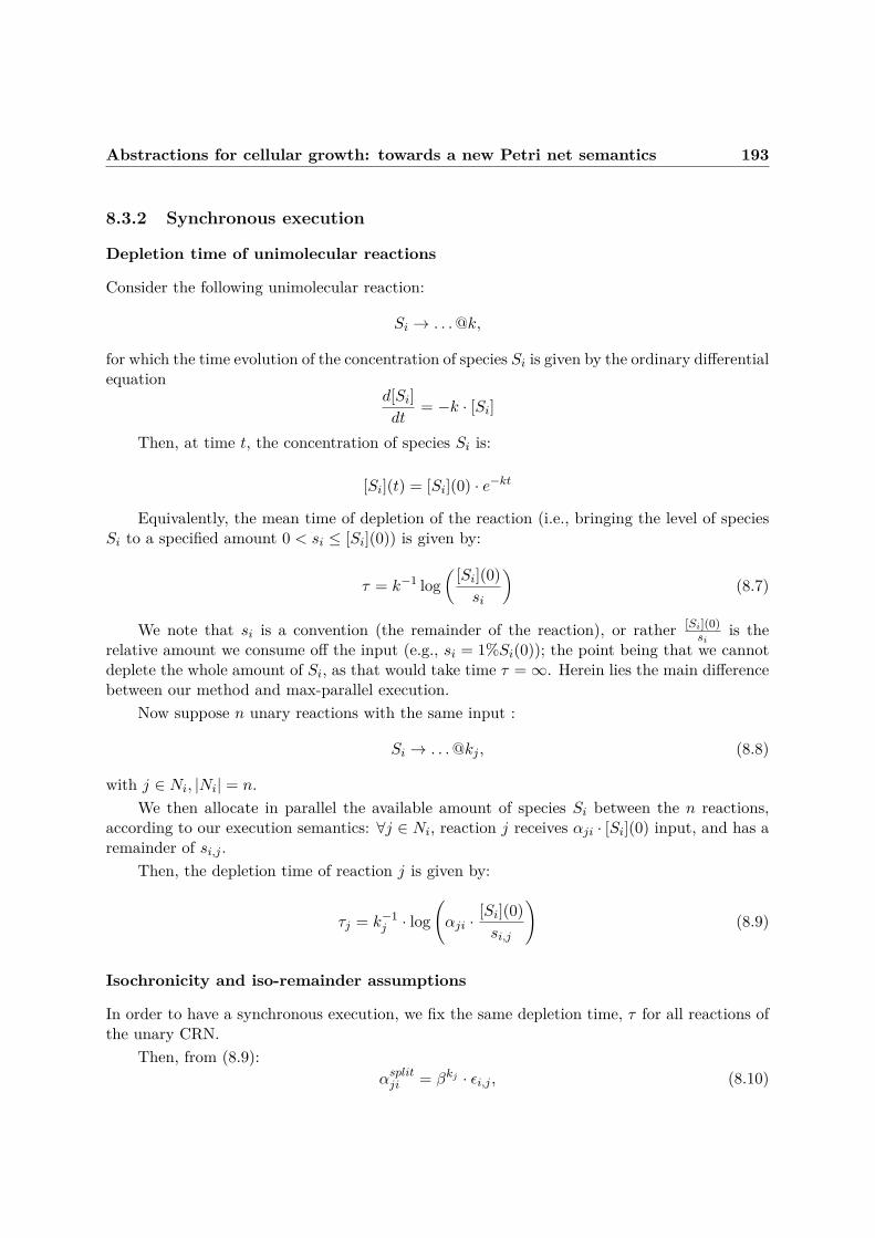
Abstractions for cellular growth: towards a new Petri net semantics 193

8.3.2 Synchronous execution

Depletion time of unimolecular reactions

Consider the following unimolecular reaction:

Si → . . .@k,

for which the time evolution of the concentration of species Si is given by the ordinary differentialequation

d[Si]dt

= −k · [Si]

Then, at time t, the concentration of species Si is:

[Si](t) = [Si](0) · e−kt

Equivalently, the mean time of depletion of the reaction (i.e., bringing the level of speciesSi to a specified amount 0 < si ≤ [Si](0)) is given by:

τ = k−1 log( [Si](0)

si

)(8.7)

We note that si is a convention (the remainder of the reaction), or rather [Si](0)si

is therelative amount we consume off the input (e.g., si = 1%Si(0)); the point being that we cannotdeplete the whole amount of Si, as that would take time τ =∞. Herein lies the main differencebetween our method and max-parallel execution.

Now suppose n unary reactions with the same input :

Si → . . .@kj , (8.8)

with j ∈ Ni, |Ni| = n.We then allocate in parallel the available amount of species Si between the n reactions,

according to our execution semantics: ∀j ∈ Ni, reaction j receives αji · [Si](0) input, and has aremainder of si,j .

Then, the depletion time of reaction j is given by:

τj = k−1j · log

(αji ·

[Si](0)si,j

)(8.9)

Isochronicity and iso-remainder assumptions

In order to have a synchronous execution, we fix the same depletion time, τ for all reactions ofthe unary CRN.

Then, from (8.9):αsplitji = βkj · εi,j , (8.10)

194 Linear Reaction Networks

where β = eτ and εi,j = si,j[Si](0) .

In this notation, εi,j is the remaining percentage (relative amount) of the total amount ofSi available in the beginning of the split round (i.e., [Si](0)), after reaction j is executed.

Furthermore, if we assume the same relative amount, si, remains after executing all nreactions, we have that:

∀j ∈ Ni, αsplitji = εi · βkj , (8.11)

with εi = siSi(0) .

Under these assumptions, the dynamics of the system in state m, for species Si, is givenby:

∆m(τ) ≡ ∇ · (αsplit_i − ε_i) ·m, (8.12)

where αsplit_i denotes the ith column of the resource allocation matrix αsplit:

∀j ∈ T, αji =εi · βkj , if j ∈ Ni

0, otherwise,

and

∀j ∈ T, εji =εi, if j ∈ Ni

0, otherwise.

Then, from (8.1) 2 and (8.11), we have that:

εi = 1∑j∈Ni

1 + βkj,

and we can define:

αSi(τ, kSi) ≡[α_i − ε_i

]=[ eτ ·kj − 1∑

j 1 + eτ ·kj

] (8.13)

with[

eτ ·kj−1∑j

1+eτ ·kj]denoting the T-vector that has 0 in the components representing reactions

j /∈ Ni.Then, by injecting equation (8.13) into equation (8.12), and by using the fact that when

x → 0, ex ≈ 1 + x, one can easily observe that when τ → 0, ∆m(τ) recreates the usual ODEdynamics for unimolecular BRNs:

2the inequality of (8.1) is here explicitly expressed via the remainder ε :∑

i∈T αij ≤ 1 is the same as∑i∈T (αij + εj) = 1

Abstractions for cellular growth: towards a new Petri net semantics 195

∆mτ≈ ∇ · k ·m (8.14)

8.4 Possible Applications

Based on formulae given in (8.6) and (8.14), our method can be interpreted either as an approx-imation of the real system’s dynamics (and be used for simulation purposes), or in an abstractway, as an alternative to flux balance analysis.

8.4.1 Approximation of system dynamics

As an approximation of the dynamics, under the unary/isochronous/iso-remainder assumptions,ours is a temporised discrete execution dynamics, that, when τ → 0, recreates the usual ODEdynamics. If we fix τ the execution time-step, and k the reaction rate vector, we can determineαsplit, the resource allocation matrix, and ε, the remainder percentage (cf. (8.13)).

We note that the “iso-” assumptions represent a way of decoupling production and con-sumption in the biochemical network, in the spirit of Karr’s modular systems [104]; intuitively,it can be interpreted as: “in a parallel execution of a reaction set, there is no waiting for theslowest reaction to complete”.

As a simulation method, it can be viewed as a big-step approximation of an integrator,resembling a deterministic τ -leaping [76].

8.4.2 Synchronous Balanced Analysis

Conversely, if the resource allocation matrix α is fixed, our execution semantics can be in-terpreted as an alternative to Flux Balance Analysis (FBA)[142], in order to determine thelimitations of a metabolic system. This is a second possible utility of the “split-burst” Petri netexecution semantics, and arguably the most important application of our method.

Flux Balance Analysis is a widely used constraint-based mathematical approach for analyz-ing the flow of metabolites through a metabolic network, thereby making it possible to predictthe growth rate of the system. The constraints lying at the heart of FBA come from two sources.Firstly, the system is assumed to be at steady state, a condition which is translated into flux (ormass) balance constraints imposed on the system by its stoichiometry matrix. Secondly, one as-sumes inequalities that impose bounds on the system; these inequalities translate the possibilityof definining minimum and maximum allowable reaction fluxes. These two types of constraints(balances and bounds) define the space of allowable flux distributions of a system, i.e., the ratesat which every metabolite/species is consumed or produce by each reaction [142]. In FBA,this allowable space is then further reduced via optimization of the sytem phenotype. This isachieved by defining a biological objective relevant to the system in question, and then translat-ing it into a mathematical objective function that indicates how much each reaction contributesto the phenotype, and which is to be maximized. Together, the mathematical representationsof the constraints and of the phenotype define a system of linear equations, which are solved

196 Possible Applications

in FBA using linear programming. In the case of predicting growth, the objective is biomassproduction: the rate at which metabolic compounds are converted into biomass constituents.For this, a biomass reaction is constructed by the modeler and then artificially introduced in themetabolic reaction system. The biomass reaction drains precursor metabolites from the systemat their relative stoichiometries, in order to simulate biomass production [142]. This reaction isthen scaled such that its flux be equal to the exponential growth rate (λ) of the organism.

A mathematical presentation of FBA, taken from [142], is given below.

Flux Balance Analysis:Assume a metabolic reaction network given by M = (S,R,α,β), with stoichiometrymatrix ∇ = β − α ∈ Rm×n, where | S |= n, | R |= m. As usually for BRNs, the fluxthrough all of the network’s reactions is represented by a vector f ∈ Rm, while the systemstate is given by the vector of metabolite concentrations x ∈ Rn.FBA assumes the system to be at steady state, which writes as:

dx

dt= ∇Tf = 0 (8.15)

Supplementary constraints on the system can be introduced by defining minimum andmaximum allowable reaction fluxes:

fmini ≤ fi ≤ fmax

i , 1 ≤ i ≤ m (8.16)

The FBA objective function can be defined as any linear combination of fluxes:

Z = cTf , (8.17)

where c is a vector of weights that indicates how much each reaction contributes to theobjective function.In the case of growth simulation, only the biomass reaction is desired for maximization,

i.e., c is a vector of zeros, except for the element corresponding to the biomass reaction,which is set to a value of one.Then, FBA proceeds by using linear programming techniques to identify a particular

flux distribution fFBA that maximizes the objective function of Equation (8.17), whileobserving the constraints imposed by the flux balance equations of (8.15) and the reactionbound equations of (8.16). Seeing how in the case of growth simulation, the objectivefunction is given by the biomass reaction (whose flux in turn is given by the exponentialgrowth rate), we see that FBA enables prediction (and maximization) of the growth rateof an organism.

Abstractions for cellular growth: towards a new Petri net semantics 197

Figure 8.2: Flux Balance Analysis versus “Synchronous Balanced Analysis”(Right: Flux Balance Analysis) A workflow for FBA, as taken from [142]. When applied togrowth maximization, the biomass objective function is defined by adding an artifical “biomass”reaction into the reaction network, the flux of which is set to be equal to the exponentialgrowth rate λ. Thus, growth optimization using FBA is achieved by maximizing the flux of this“biomass reaction”. (Left:“Synchronous Balance Analysis”) For BRNs comprised exclusively ofunimolecular reactions, our Petri net execution semantics enables the mathematical character-ization of the system’s growth rate, which in turn avoids any artificial addition to the model:maximizing the growth rate becomes akin to finding the matrix Dα with the maximal biggesteigenvalue. Our method can also be used to constrain reaction rates and/or refute models,based on their parameter values.

The FBA method’s main advantage lies in the fact that it does not require kinetic param-eters. Morevoer, it can be computed quickly even for large reaction networks.

However, its lack of information on kinetic parameters means that FBA is not able topredict metabolite concentrations. Another important limitation consists in its ability of deter-mining fluxes exclusively at at steady state.

We argue that our execution semantics can offer an alternative to FBA, that circumventsthese issues. Indeed, through our method, the emergent definition of the growth rate λ canbe used as an objective function. According to (8.6), maximizing λ is achieved by finding theresource allocation matrix α with the biggest eigenvalue. Once this αsplit is fixed, Equation(8.13) can be used in order to constrain the reaction rate constants k, as well as the time-step

198 Conclusion and future directions

τ and the remainder ε. By constraining the reaction rate constants, our method could be usedas a technique of refuting models.

The advantages, when compared to FBA, are twofold. Firstly, our method can be appliedto growth systems: unlike FBA, the system is not considered to be at steady-state. This inturn means that it accounts for the real system kinetcs. Secondly, our approach preserves theides of biomass maximization, but the artificial creation of an objective biomass function is nolonger needed. Instead, the growth rate emerges directly from our method. The downside ofour approach however lies in maximizing the biggest eigenvalue of matrix Dα.

8.5 Conclusion and future directions

In this chapter, we propose a piecewise synchronous approximation of the dynamics of a (growth)chemical reaction network: a parallel execution semantics of Petri Nets, based on resourceallocation. For BRNs composed exclusively of unimolecular reactions, we show that our methodcan be interpreted either as an approximation of the real system’s dynamics, or as a constraintmethod similar to Flux Balance Analysis. The main advantage of our approach resides inits ability of characterizing the behavior of a cell using only one construction: the resourceallocation matrix αsplit. Consequently, one can eliminate the mechanistic details that dealwith resource allocation, and replace them by an abstract vector (αsplit). Furthermore, whencompared to flux balance analysis, our method is applicable to growth systems.

Future work

Our method can be extended into several directions, the most important of which deals withencompassing binary reactions into our execution semantics. Overcoming this obstacle willallow for the construction of untrivial examples based on real-life BRNs, in order to investigatehow our method can be used to determine correlations between growth rate and different modelparameters (such as reaction rate constants). Once the issue of bi-molecular reactions solved,the two possible interpretations of our approach, as presented in Section 8.4, imply that thequality of our “split-burst” PN semantics could be assessed by comparing it to other existingBRN simulation approaches, such as τ -leaping, or by comparing it to more biologically-inspired,constraint-based heuristics, such as the allocation method proposed by Karr [104] (in whichregulation of metabolic protein is carried out via Flux Balance Analysis).

Consider a BRN that contains a bimolecular reaction:

r1 : A+B → C

and assume a resource allocation (via a matrix αsplit) that reserves 3 molecules of A and2 molecules of B for consumption by r1. Naturally, the number of times a reaction can beexecuted in a max-parallel execution step wil be constrained by the quantity of the least-abundant reactant species, as given by the resource allocation. For example, for the allocationgiven above, speciesA represents the “limiting species”: r1 can be executed at most min(2, 3) = 2times in a max-parallel execution step. Thus, the evolution of the system state is no longer

Abstractions for cellular growth: towards a new Petri net semantics 199

given by Equation 8.5. A similar equation for describing the evolution of a system containingbimolecular reactions should incorporate the computation of the limiting species’ quantities,using the min operator.

The solution to this problem could reside in the use of tropical mathematics, (more specif-ically max-plus or min-plus algebras or semi-rings). Therein, matrix multiplication over thering of real numbers (R,+,×) is replaced with matrix multiplication over the idempotent semi-ring (R∪ −∞∪ ∞,

⊕,⊗

), with⊕

denoting either the max (for (max,+)) or the min (for(min,+)) operation, and

⊗denoting the usual addition. Much of the initial interest in (max,+),

(min,+) and other idempotent semiring structures was in connection with the modeling of dis-crete event systems typically arising in areas involving allocation of resources, scheduling andqueuing theory [9]. The development of tropical analogues of several ideas from classical linearalgebra (e.g., spectral theory, linear independence) resulted in a wealth of results w.r.t. thedynamics of discrete event systems, including descriptions of periodic regimes, and asymptoticbehaviors. The question arising in our case refers to how these results can be extended to thecase of models of BRNs.

Indeed, (timed) Petri nets represent a common tool to describe discrete event systems(DES). It is known that conventional linear systems have “modes” related to their eigenstruc-tures, which are reached asymptotically when said systems are stable. The (max,+) and(min,+) approaches enable the definition of similar notions for a subclass of Petri nets: ina nutshell, they enable a structural description of the net’s throughput λ, which is shown tobe equal to the largest average weight of a directed circuit of the net. The throughput λ isassociated with the cycle time of the underlying system: if such a λ exists, then each transitionof the network becomes active every λ units of time. Consequently, the notion of throughputcan be used as a proxy of the net’s growth rate.

The main issue with the tropical approach is related to the restrictions imposed on the netstructure: the class of timed Petri nets which can be described by linear max-plus or min-plusequations is given by Timed Event Graphs (TEGs). TEGs enable modeling of synchronization,but not of conflicts: in a TEG, each place has exactly one upstream transition, and exactlyone downstream transition. Whereas the latter restriction can be solved by splitting resourcesaccording to the resource allocation matrix αsplit, the “exactly one upstream transition” con-dition appears to be too restrictive for most models of BRNs (as it translates into “each speciescan be produced by exactly one reaction”). Relaxing this restriction leads to weaker results [42]w.r.t. the existence of the throughput (i.e. growth rate in our case). What’s more, the resultsw.r.t. the throughput of a TEG assume the net to be autonomous and strongly connected.

Another issue is related to the timing aspect: in the case of Petri nets that model discreteevent systems, a constant “duration” is associated to each place, in order to denote the minimumsojourn time of a token in a place. In order to apply the (min,+)-algebra analysis to models ofBRNs, the relation between chemical reaction rate constants and such sojourn times needs toformally established.

Despite these restrictions, the tropical approach has proven to be useful in the analysisof certain biological systems. For example, in [21], a (max,+) model for the dynamics ofmRNA translation is proposed, which allows one to predict protein production rates and codonoccupation densities. The results of [21] give an indication of how, under a suitable level of

200 Conclusion and future directions

abstraction, the results obtained via (max,+)-algebra analysis can be harnessed for biologicalpurposes. This suitable level of abstraction seems to consist in modeling a BRN using a Petrinet in which each transition models a biological event in an abstract way, instead of the usualdirect transition-to-reaction correspondence between PNs and BRNs. For example, in [21], theauthors perform the (max,+) analysis on a TEG in which the firing of a transition models theevent consisting in “a ribosome moving from codon i to codon i+1”, without describing themechanistic details behind this event. Consequently, future work includes studying the trade-off between the level of abstraction in DES models of BRNs and results obtained via tropicalmathematics analysis.

Another way to potentially relieve the issue of biomolecular reactions is by assuming thatno significant change in the concentration of one of the two reactants is being caused by anyother reaction during one execution step. In this sense, Michaelis-Menten like reduction schemescould be considered.

Conclusion

201

Chapter 9Conclusion and future directions

9.1 Contributions

In this thesis, we propose several contributions related to the modeling and analysis ofBiochemical Reaction Networks. In the first part, we study how the inherent multi-scalenessof biological systems can be exploited for both model reduction heuristics, and model reduc-tion error estimation techniques. The first work deals with the use of rule-based modeling forprototyping genetic regulatory networks: we argue that because of their capacity to unam-biguously specify protein-protein interactions in general, and consequently mechanistic detailssuch as DNA binding sites, dimerisation of transcription factors, or co-operative interactions,rule-based modeling languages are more appropriate for designing genetic circuits in a modular,transparent and easily modifiable fashion than reaction based languages.

Nonetheless, such a detailed description comes with complexity, as well as computationallycostly executions. Consequently, we next propose a general reduction method for a subsetof rule-based models, aimed at modeling genetic circuits, which exploits concentration andtime-scale separation. The method is an adaptation of an existing algorithm [112], designedfor reaction based models. Our version of the algorithm proceeds by static inspection of therule-set: it scans the Kappa model in search for interaction patterns known to be amenableto equilibrium approximations (e.g. Michaelis-Menten scheme, as well as a number of otherstoichiometry-simplifying techniques), and after performing additional checks in order to verifyif the reduction is meaningful in the context of the full model, it proceeds with the eliminationof intermediate species and with the adjustment of the rule rates. When tested on a detailedrule-based model of a λ-phage switch, our tool provides a dramatic reduction in simulation timeof several orders of magnitude. Our method is an illustration of the fact that in general, themultiscaleness of biochemical reaction networks represents a feature that can be exploited formodel reduction purposes.

The correctness of our approach relies on the fact that the approximate model is equal to theoriginal one, in the artificial limit where certain reactions happen at a sufficiently larger time-scale than others, and they are seemingly equilibrated shortly upon the reactions’ initiation.However, not unlike other scale-separation reduction methods, our method relies on a solidphysical justification, yet (to the best of our knowledge) there is no precise method to quantifythe error induced by time-scale separation approximations for biochemical reaction networks,

203

204 Contributions

while avoiding to solve the original model.This is why, we next propose an approximation method in the deterministic modeling

framework that exploits the multiscaleness property, in which reduction guarantees representthe major requirement. Our method combines abstraction and numerical approximation, andaims at providing a better evaluation of model reduction methods that are based on time- andconcentration- scale separation. The reduction guarantees of our method are a consequenceof a carefully designed symbolic propagation of dominance constraints: given an ODE modelof a BRN that exhibits time- and concentration- scale separation, we abstract the solution ofthe original system by a “box” that over-approximates the state of the original system andprovides lower and upper bounds for the value of each variable of the system in its currentstate. The simpler equations (which we call tropicalized) that define the hyperfaces of the boxare obtained by combining the dominance concept borrowed from tropical analysis [119] withsymbolic bounds propagation. Mass invariants of the initial system of differential equationsare used to refine the computed bounds, thus improving the accuracy of the method. Theresulting (simplified) system provides a posteriori time- dependent lower and upper bounds forthe concentrations of the initial model’s species, and thus bounds on numerical errors stemmingfrom tropicalization. This means that no information on the original system’s trajectory isneeded - the most important advantage of our approach.

In the second part of this manuscript, we address the formal modelling of relevant biologicalbehaviours, such as intracellular resource storage and cellular growth, in the deterministic mod-eling framework of biochemical reaction networks. We first introduce a new reparametrisationtechnique of ordinary differential equations models, intended to model intracellular resourcestorage strategies. Our technique consists in defining a generic scaling transformation of bio-chemical reaction networks that allows one to tune the concentration of certain chemical species,while preserving the network’s behaviour at steady state. We then employ this technique tostudy the effect of different storage strategies on cellular growth. This fundamental trade-off isbest investigated using a mechanistic model of cellular growth, where costs are emergent andreflect architectural traits of the growth machinery. Consequently, we apply our method onsuch a recent “self-replicator” mathematical model [182] of the coarse-grained mechanisms thatdrive cellular growth. Our analysis is carried out first for a single-cell model, and afterwardsin a competitive context. In the single-cell experiments, we compare storage strategies againstdifferent patterns of environmental changes. Our results suggest that on the one hand thereis a cost associated with high levels of storage, which results from the loss of stored resourcesthrough dilution, and that on the other hand, high levels of storage can benefit cells in variableenvironments, by increasing biomass production during transitions from one medium to another.In the competitive experiments, we test populations of low- and high-storage strategies againsteach other, in a variety of environments parametrized by the frequency of two superimposedprobabilistic trains of high and low pulses of sugar. All in all, we are able to observe a rich inter-play of storage levels, growth rates, growth yield, and resource variability. Our results indicatethat the specificities of environmental changes play a decisive role in deciding which storagestrategy is deemed the most beneficial (with respect to accumulating biomass over time). Thisis even more so the case when species content for the same resource: the combined effect ofstorage strategies and competition lead to extracting less biomass out of the same amount of

Conclusion and future directions 205

resources.In the final work of this manuscript, we work towards a characterization of cellular growth

as an emergent property of model execution semantics. In this sense, we work towards a novelPetri net execution semantics representing a piecewise-synchronous approximation of the de-terministic dynamics. To achieve this, we propose to model a biochemical reaction networkusing a resource-allocation-centered Petri net, with parallel maximal-step execution semantics.We argue that this semantics is better-suited for modeling biochemical reaction networks, whencompared to the classical interleaving semantics, as it takes into account the inherently con-current nature of biological processes. In the case of unimolecular chemical reactions, we provethe correctness of our method and show that it can be used either as an approximation of thedynamics, as a technique of refuting models, or as a method of constraining the reaction rateconstants - consequently, as an alternative to flux balance analysis, using an emergent formallydefined notion of “growth rate” as the objective function.

9.2 Future works

The works presented in this manuscript can be extended in several directions. The detaileddescription of each considered extension is contained in the chapters corresponding to eachproject. We give a final brief summary of the planned extensions below.

• “Prototyping genetic circuits using rule-based models”:

– the reduction algorithm is currently being extended in order to ensure a sound re-duction in the case of “don’t care don’t write” Kappa patterns;

– we also plan on studying how the set of approximation patterns can be extended inorder to obtain good reductions for complex models of signaling pathways.

• “Tropical Abstraction of BRNs with guarantees”: we plan on extending ourmethod as to take into account reaction networks with no mass conservation laws. Inthis sense, we plan on looking into tropical equilibrations and the permanency concept[140].

• “Abstractions for cellular growth”: we plan on analyzing how our piecewise-synchronousPetri net execution semantics can be extended to bimolecular reaction networks, eitherby using the (max,+)-algebra approach, or by using Michaelis-Menten like reductionschemes. We also plan on comparing our method to the τ -leaping simulation method,and to the allocation method propsed by Karr [104].

206 Future works

Appendices

207

Chapter AProbability Theory

Herein, we review the basic definitions and concepts of elementary probability theory, whichare required for defining the stochastic model semantics of biochemical reaction networks.

The usual notations from set theory are used. For subsets A,Ak, B, . . . of some abstractspace Ω, the set union writes as A∪B or

⋃kAk, intersection writes as A∩B or

⋂kAk, complement

writes as AC , and difference writes as A \B = A∪BC . We denote by P(Ω) ≡ A | A ∈ Ω theset of all subsets of Ω (i.e., the power-set), by |Ω| the number of elements in Ω, and by R(f)the range of values taken by a function f : A 7→ B.

Basic notions of measure theory

We start by presenting the basic notions and results of measure theory, for which a simpledefinition is that it is a theory about the distribution of mass over a set S. If the mass isuniformly distributed and S is an Euclidean space Rk, it is the theory of Lebesgue measure onRk (i.e., length in R, area in R2, volume in R3, etc.). Probability theory is concerned with thecase when S is the sample space of a random experiment and the total mass equals one. Thus,measure theory notions will be useful in defining concepts from probability theory.

Definition A.1 (σ-algebra)Let Ω be a set. A collection of sets F ∈ P(Ω) is called a σ-algebra on Ω if it is nonempty andclosed under countable set operations:

(i) ∅ ∈ F ,

(ii) A ∈ F ⇒ AC ∈ F ,

(iii) An ∈ F for n ≥ 1⇒⋂n≥1

An ∈ F ,⋃n≥1

An ∈ F .

Example A.1Let A be any class of subsets of a set Ω. The set of all subsets of Ω is a σ-algebra containingA. The intersection of any collection of σ-algebras is again a σ-algebra. The collection of σ-algebras containing A is therefore non-empty and its intersection is a σ-algebra σ〈A〉, which iscalled the σ-algebra generated by A:

209

210

σ〈A〉 =⋂

F∈I(A)F ,

where I(A) ≡ F | A ⊂ F and F is a σ-algebra on Ω is the collection of σ-algebras containingA.

A particularly useful class of σ-algebras are those generated by open sets of a topologicalspace. These are called Borel σ-algebras. We recall that a topological space is a pair (S, T ),where S is a nonempty set and T is a collection of subsets of S such that (i)S ∈ T , (ii)O1,O2 ∈T ⇒ O1 ∩ O2 ∈ T , and (iii)Oα | α ∈ I ⊂ T ⇒

⋃α∈IOα ∈ T . Elements of T are called open

sets.Similarly, a metric space is a pair (S, d), where S is a nonempty set and d is a function

d : S × S 7→ R+ satisfying (i) d(x, y) = d(y, x),∀x, y ∈ S, (ii) d(x, y) = 0 iff x = y, and (iii)d(x, z) ≤ d(x, y) + d(y, z), ∀x, y, z ∈ S. The function d is called a metric on S.

Definition A.2 (Borel σ-algebra)The Borel σ-algebra on a topological space S (in particular, on a metric space or an Euclideanspace) is defined as the σ-algebra generated by the collection of open sets in S.

A set function is an extended real valued function defined on a class of subsets of a setΩ. Measures are nonnegative set functions that, intuitively speaking, measure the content ofa subset of Ω. Consequently, they have to satisfy certain natural requirements, such as “themeasure of the union of a countable collection of disjoint sets is the sum of the measures of theindividual sets”:

Definition A.3 (Measure space)Let Ω be a nonempty set and F a σ-algebra on Ω. The pair (Ω,F) is called a measurablespace, and each A ∈ F is called a measurable set. A measure µ on (Ω,F) is a functionµ : F 7→ [0,∞) which satisfies the countable additivity property:

(i) µ(∅) = 0,

(ii) A1, A2, . . . ∈ F a sequence of disjoint sets ⇒ µ(⋃k≥1

Ak) =∑k≥1

µ(Ak).

The triple (Ω,F , µ) is called a measure space.

A measure µ is said to be finite if µ(Ω) < ∞, respectively infinite if µ(Ω) = ∞. Afinite measure with µ(Ω) = 1 is called a probability measure. A measure µ on a σ-algebraF is called σ-finite if there exist a countable collection of sets A1, A2, . . . ∈ F such that (a)⋃n≥1

An = Ω and (b) µ(An) <∞, ∀n ≥ 1.

Armed with the definition of a measure space, one can proceed to define a basic probabilityspace, a notion that provides the basic apparatus for modelling randomness:

Definition A.4 (Probability space)A probability space is a measure space (Ω,F , P ), with P a probability measure (i.e., P (Ω) =

Probability Theory 211

1). A probability space provides a model for an experiment whose outcome is subject to chance.In the probabilistic context, the interpretation of the underlying measure space components areas follows:

(i) Ω is the set of possible outcomes of the experiment, called samples;

(ii) F is a set of observable sets of outcomes, and sets A ∈ F are called events;

(iii) and P (A) is called the probability of event A ∈ F .

Other useful examples of measures are:

Example A.2 (The counting measure)When Ω is a finite countable set, the measure on (Ω,P(Ω)) that assigns to each measurable setA the number of elements it contains, i.e. m(A) = |A|, is called the counting measure on Ω. IfΩ is not countable, one works instead with Borel sets.

Example A.3 (The Lebesgue measure)Given a set Ω, the Borel σ-algebra of Ω (i.e., the σ-algebra generated by the set of open sets inΩ) writes as B(Ω). The elements of B(Ω) are called Borel sets. If Ω = R, and A = (a, b) |a, b ∈ R, a < b, then B denotes the Borel σ-algebra on R. It can be shown that there is aunique measure µ on (R,B) such that:

µ(a, b) = a− b, ∀a, b.

This measure µ is called the Lebesgue measure.

Example A.4 (Discrete probability measures)Let ω1, ω2, . . . ∈ Ω, and p1, p2, . . . ∈ [0, 1], such that

∑i≥1

pi = 1. Define for any A ∈ Ω:

P(A) =∑i≥1

pi1A(ωi),

with 1A the indicator function of a set A, as defined in Example A.5. For any disjointcollection of sets A1, A2, . . . ∈ P(Ω),

P(⋃i≥1

Ai) =∑j≥1

pjI⋃i≥1

Ai(ωj)

=∑j≥1

pj(∑i≥1

IAi(ωj))

=∑i≥1

(∑j≥1

pjIAi(ωj))

=∑i≥1

P(Ai),

which shows that P is a probability measure on P(Ω).

212

Oftentimes, when dealing with probabilities, one is not interested in the full details of ameasure space (Ω,F , µ), but only on certain functions defined on Ω: if Ω represents the outcomeof 10 tosses of a fair coin, one may only be interested in knowing the number of heads in the10 tosses. As it turns out, in order to assign measures (probabilities) to sets (events) involvingsuch functions, one can only allow certain functions, called measurable functions:

Definition A.5 (〈F ,B〉-measurable function)Let (Ω,F) be a measurable space. A function f : Ω 7→ R is said to be 〈F ,B〉-measurable, orsimply F-measurable, if for each a ∈ R:

f−1((−∞, a]) ≡ ω | f(ω) ≤ a ∈ F

This definition can be generalized to maps between any two measurable spaces:

Definition A.6 (Measurable function)Let (Ω1,F1) and (Ω2,F2) be two measurable spaces. A function f : Ω1 7→ Ω2 is 〈F∞,F∈〉-measurable if the inverse image of any A ∈ F2 lies in F1:

∀A ∈ F2, f−1(A) ∈ F1, with f−1(A) := a ∈ Ω1 | f(a) ∈ A.

A measurable function is often called a measurement on (Ω1,A1). A measurable functionon a Borel σ-algebra is called a Borel function.

Example A.5A measurement on (Ω,A) is the indicator function of the set A ∈ A, given by :

1A(a) =

1, if a ∈ A0, otherwise

.

Then, a random variable on a probability space (Ω,F ,P) may be defined as an 〈F ,B〉-measurable function on Ω, and is interpreted as reducing the probability space to the subset ofobservations of interest:

Definition A.7 (Random variable)Let (Ω,F ,P) be a probability space. Then a function X : Ω 7→ R is called a random variable,if the event1

X−1((−∞, a]) ≡ ω | X(ω) ≤ a ∈ F

for each a ∈ R, i.e., a random variable is a real valued 〈F ,B〉-measurable function on a proba-bility space (Ω,F ,P).

A random variable X can be either discrete, if R(X) is a countable set, or continuous,otherwise.

Definition A.8A random variable X is called:

1or equivalently if X−1(A) ∈ F , ∀A ∈ B(R)

Probability Theory 213

• discrete, if there exists a countable set A ∈ R such that P(X ∈ A) = 1,

• continuous, if P(X = x) = 0,∀x ∈ R.

If X is a random variable defined on a probability space (Ω,F ,P), then P governs theprobabilities assigned to events such as X−1([a, b]),−∞ < a < b < ∞. Since X takes valuesin the real line, one would like to express such probabilities only as a function of the set [a, b].Since X is 〈F ,B〉-measurable, X−1(A) ∈ F , ∀A ∈ B(R), and the function:

PX(A) ≡ P(X−1(A))

is a set function defined on B(R).

Proposition A.1Let (Ω1,F1) and (Ω2,F2) be two measurable spaces, and let T : Ω1 7→ Ω2 be a 〈F∞,F2〉-measurable function. Then, for any measure µ on (Ω1,F1), the set function µT−1, definedby

µT−1(A) ≡ µ(T−1(A)), A ∈ F2

is a measure on F2.

Definition A.9The measure µT−1 is called the measure induced by T (or the induced measure of T) on F2.

In particular, if µ(Ω1) = 1, then µT−1(Ω2) = 1.The, PX turns out to be a probability measure on B(R), called the probability distribution

of X:

Definition A.10 (Probability distribution)For a random variable X defined on a probability space (Ω,F ,P), the probability distributionof X (or law of X) is given by the induced measure of X under P on R, i.e., PX ≡ PX−1.

We note that when defining probabilities of events like ‘X ∈ [a, b]‘, it is common practiceto use the probability mass function when dealing with discrete random variables and theprobability density function for continuous random variables. The measure-theoretic defi-nition above allows one to treat both these cases, as well as the case of “mixed” distributions,under a unified framework.

Definition A.11 (Cumulative distribution function)The cumulative distribution function (or cdf in short) of a random variable X is defined as:

FX(x) ≡ PX((−∞, x])≡ P(ω | X(ω) ≤ x), x ∈ R.

214

Integral of a measurable function

Let (Ω,F , µ) be a measure space and f : Ω 7→ R be an arbitrary measurable function. Onewants to define the integral of f with respect to the measure µ, which will be used to define theexpectancy of a random variable.

If (Ω,F) is a measurable space, denote by mF the set of measurable functions f : Ω 7→ R.Then, mF is a vector space. Let mF+ denote the set of non-negative measurable functionsf : Ω 7→ [0,∞], where one takes on [0,∞] the σ-algebra generated by the open intervals (a, b).Then, mF+ is a cone:

(f, g ∈ mF+, α, β ≥ 0)⇒ αf + βg ∈ mF+,

which is closed under countable suprema:

(fi ∈ mF+, i ∈ I)⇒ supifi ∈ mF+.

It follows that, for a sequence of functions fn ∈ mF+, both lim supn fn and lim infn fnlie in mF+ (so does limn fn, when it exists). It can be shown that there is a unique mapµ : mF+ 7→ [0,∞], such that:

(i) µ(1A) = µ(A),∀A ∈ F ;

(ii) µ(αf + βg) = αµ(f) + βµ(g), ∀f, g ∈ mF+, α, β ≥ 0;

(iii) (fn ∈ mF+, n ∈ N)⇒ µ(∑nfn) =

∑nµ(fn).

For f ∈ mF , let f+ = max f, 0 and f− = max−f, 0. Then, f+, f− ∈ mF+, f = f+ − f−,and |f | = f+ + f−. If µ(|f |) <∞, then f is to be integrable, and one can set:

µ(f) = µ(f+)− µ(f−).

We call µ(f) the integral of f , but by convention, this notation can be replaced by oneof the alternatives:

µ(f) =∫

Ω fdµ =∫x∈Ω f(x)µ(dx).

In the case of the Lebesgue measure µ, one simply writes∫x∈R f(x)dx.

Definition A.12 (Expected value)Let X be a random variable on a probability space (Ω,F ,P). The expected value (or mean),or expectation of X, denoted by E[X], is defined as:

E[X] ≡∫

ΩXdP,

Definition A.13 (Variance)The variance of a random variable X is defined as:

Probability Theory 215

Var(X) ≡ E[(X − E[X])2].

Example A.6 (Bernoulli random variable)The simplest example of a discrete random variable is the Bernoulli random variable,Xp : Ω 7→ 0, 1, which models an experiment with only two possible outcomes (denoted by 0or 1), which occur with probabilities PXp(1) = p, and PXp(0) = 1− p. The mean of a Bernoullivariable is E[Xp] = p, and its variance is Var(X + p) = p(1− p).

Example A.7 (Exponential, Poisson random variables)The two most important random variables for constructing a continuous Markov chain are:

(i) the exponential random variable, Expλ : Ω 7→ [0,∞), with probability density functionfExpλ(x) = λe−λx, mean E[Expλ] = 1

λ , and variance Var(Expλ) = 1λ2

(ii) the Poisson random variable, Poissonλ : Ω 7→ 0, 1, 2, . . ., with probability mass func-tion P(Poissonλ = k) = λke−k

k! , mean E[Poissonλ] = λ, and variance Var(Poissonλ) = λ.

Definition A.14 (Memoryless property)For x, y ∈ R(X), X : Ω 7→ R is said to have the memoryless property, if

PX >x+ y | X >x = PX >x

.The only continuous random variables to satisfy the memoryless property are exponential

random variables.

Markov chains

Definition A.15 (Stochastic process)A stochastic process, or random process, with state space S and parameter set T is acollection of random variables Xt, t ∈ T, defined on a common probability space (Ω,A,P).The process is said to be “discrete” if T is countable, and “continuous”, otherwise.

Usually, t is to be interpreted as an indicator of time, in which case Xt represent thestate of the process at time t. For every fixed ω ∈ Ω, the mapping t 7→ Xt(ω) defines atrace/trajectory/realization/sample path of the process.

In order to facilitate analysis, additional properties are assumed on a stochastic model:

Definition A.16 (Markov property, time-homogeneity)For a given stochastic process Xt on a countable state space S, let HX(t) denote all theinformation about the process until time t ∈ T . Then, the process Xt is said to satisfy theMarkov property, if the conditional (on both past and present states) probability distributionof future states of the process depends only upon the present state, not on the sequence of eventsthat preceded it. That is, if for all states s, s′ ∈ S, and for all times t+ h > t, one has that:

PXt+h = s′ | HXt = PXt+h = s′ | Xt.

216

The process is said to be time-homogeneous if the transition probability between any two statevalues at two given times depends only on the difference between those state values:

PXt+h = s′ | Xt = s = PXh = s′ | X0 = s

.

Definition A.17 (Transition probability matrix)For a stochastic process with a finite state space S, for some ordering of the elements of S,the transition probability matrix for step t is defined as P(t), a S × S-matrix with entriesP(t)(s, s′) = PXt = s′ | X0 = s.

Then, any Markov time-homogeneous process satisfies the Chapman-Kolmogorov equations:

P(t+h) = P(t)P(h),∀t, h ∈ T

.

Then, a discrete (respectively continuous) time Markov chain is defined as a discrete (re-spectively continuous) time random process Xnn∈N (respectively Xtt∈R≥0 that satisfies theMarkov and time-homogeneity properties.

Another definition of Markov chains consists in assigning a Markov process to a Markovgraph:

Definition A.18 (Markov graph)A Markov graph is a triple (S,w, p0), with:

(i) S a countable state space,

(ii) w : S × S 7→ R, the transition weight function

(iii) p0 : S 7→ [0, 1] such that∑sip0(si) = 1.

Definition A.19 (Discrete-time Markov Chain (DTMC))A discrete-time Markov graph M = (S,w, p0) is such that ∀s ∈ S,w(s, :) is a probability. Then,a process Xt assigned to M is called a discrete-time Markov chain (DTMC), and issuch that ∀s, s′ ∈ S, the following conditions are satisfied:

(i) P(X0 = s) = p0(s),

(ii) P(X1 = s′ | X0 = s) = w(s, s′).

Reasoning about continuous-time Markov chains proves to be a bit more subtle: the pa-rameter set T is uncountable, and one cannot assign a probability to an uncountable union ofmarginal distributions. Instead, the probability of transitions will be defined in a small interval[0, h). In this case, one talks about a restriction to right-continuous processes: ∀w ∈ Ω,∀t ≥0, ∃ε > 0 such that Xs(w) = Xt(w), for s ∈ [t, t+ ε].

Probability Theory 217

Definition A.20 (Continuous-time Markov Chain (CTMC))A continuous-time Markov graph M = (S,w, p0) is such that ∀s ∈ S, s 6= s′ ⇒ w(s, s′) ≥ 0,where w is also called the rate function. For any state s ∈ S, the activity of state s can be definedas a(s) =

∑s′∈S

w(s, s′). Also, for each state s ∈ S, the rate function is set to w(s, s) = a(s). A

process Xt assigned to M is called a continuous-time Markov chain (CTMC), and issuch that ∀s, s′ ∈ S, and ∀t ≥ 0 the following conditions are satisfied:

(i) P(X0 = s) = p0(s),

(ii) P(Xt+h = s′ | Xt = s) =w(s, s′)h+ o(h), if s 6= s′

1− a(s)h+ o(h), otherwise, with f ∈ o(h) if lim

h→0f(h)h =

0.

Another definition of a CTMC, which can prove more useful for its simulation, can be givenby associating each right-continuous process with the random variables:

(i) ξ0, ξ1, . . . ∈ R≥0, the jump times of Xt, defined as the (absolute) time instances at whichjumps occur 2:

ξ0 = 0ξn+1 = inft > ξn | Xt 6= Xξn

(ii) τ0, τ1, . . . ∈ R≥0, the waiting times relative to the last jump: τi = ξi+1 − ξi

(iii) Z0, Z1, . . . ∈ S the sequence of states visited by jumps (Zi = Xξi) which defines theembedded discrete process.

Then, a CTMC Xt is such that:

(i) P(X0 = s) = p0(s),∀s ∈ S,

(ii) P(ξi < t | Z0 = s) = 1− e−a(s)t,∀s, s′ ∈ S,

(iii) P(Z1 = s′|Z0 = s) = w(s,s′)a(s) ,∀s, s′ ∈ S.

2We are working under the assumption of non-explosive processes, i.e. in all finite intervals [0, t) only finitelymany jumps can occur. Stochastic models of BRNs are trivially non-explosive.

218

Chapter BA DNA model: equation for the derivativeof the lower bound on the concentration ofx2

According to Def.6.3.7, the derivative of the lower bound on the concentration of x2 is computedby selecting the minimum region-dependent (i.e., local) lower bound, out of the 9 possible cases:

dx2dt

= min(t1,1↓ , t1,2↓ , t1,3↓ , t2,1↓ , t2,2↓ , t2,3↓ , t3,1↓ , t3,2↓ , t3,3↓ )

with

t1,1↓ = max(k1x12, k−2(DNA0

ε− k−1

k2))−

(1 + ε)k−1 ·min(x2,M0 − x1

2 ,M02 −DNA0 −

x12 − ε

k−1k2

);

t1,2↓ = max(k1x12, k−2

DNA0 − x3u

ε)−

(1 + ε)k2 ·min(x2,M0 − x1

2 ,M0 − 2DNA0 − x1 + 2x3

2 )·

·min(x3, DNA0)

t1,3↓ = max(k1x12, (k−2

ε(DNA0 −

k−1εk2

), k−2ε

(DNA0 − x3))−

min(x2,M0 − x1

2 + min(x3 −DNA0,k2εk−1

−DNA0)))·

(k2 ·min(x3, DNA0) + k−1);

219

220

t2,1↓ =k−2 ·max(x4, DNA0 −εk−1k2

)−

(1 + ε)k−1 ·min(x2,M02 −max(x4, DNA0 − ε

k−1k2

))

t2,2↓ =k−2 ·max(x4, DNA0 − x3)−

(1 + ε)k2 ·min(x2,M02 − x4,

M02 −DNA0 + x3)·

min(x3, DNA0 − x4)

t2,3↓ =k−2 ·max(x4, DNA0 − x3, DNA0 −k−1εk2

))−

min(x2,M02 −max(x4, DNA0 − x3, DNA0 −

k−1εk2

))

(k−1 + k2 ·min(x3, DNA0 − x4));

t3,1↓ = max(εk−2x4, k1x12) + max(εk1x1

2, k−2 · (DNA0 − εk−1x2k2

))−

(1 + ε)k−1 ·min(x2,M0 − x1

2 − εk1 · x12k−2);

t3,2↓ = max(k1x12, εk−2x4, εk−2(DNA0 − x3)) + k−2 ·max(x4, DNA0 − x3, εk1

x12

k−2)

−(1 + ε)k2 ·min(x2,M0 − x1

2 −max(x4, εk1x1

2

k−2, DNA0 − x3)))·

min(x3, DNA0 −max(x4, εk1x1

2

k−2));

A DNA model: equation for the derivative of the lower bound on theconcentration of x2 221

t3,3↓ =k1x12 + k−2 ·max(x4, DNA0 − x3)−

k2 ·min(x2,M0 − x1

2 −max(x4, DNA0 − x3)) ·min(x3, DNA0 − x4)−

k−1 ·min(x2,M0 − x1 − 2 · x4

2 );

222

Bibliography

[1] Computer assisted proofs in dynamics (capd) library. http://capd.ii.uj.edu.pl. [On-line; accessed 14-January-2019].

[2] R. Albert and H. G. Othmer. The topology of the regulatory interactions predicts theexpression pattern of the segment polarity genes in drosophila melanogaster. Journal ofTheoretical Biology, 223(1):1 – 18, 2003.

[3] R. Alur, C. Courcoubetis, T. A. Henzinger, and P.-H. Ho. Hybrid automata: An algorith-mic approach to the specification and verification of hybrid systems. In Hybrid systems,pages 209–229. Springer, 1993.

[4] D. F. Anderson. Incorporating postleap checks in tau-leaping. The Journal of ChemicalPhysics, 128(5), 2008.

[5] D. F. Anderson and T. G. Kurtz. Continuous time markov chain models for chemicalreaction networks. In Design and analysis of biomolecular circuits, pages 3–42. Springer,2011.

[6] S. Andrews. Spatial and stochastic cellular modeling with the smoldyn simulator. Methodsin molecular biology (Clifton, N.J.), 804:519–42, 10 2012.

[7] P. Arányi and J. Tóth. A full stochastic description of the michaelis-menten reactionfor small systems. Acta biochimica et biophysica; Academiae Scientiarum Hungaricae,12(4):375–388, 1977.

[8] A. Arkin, J. Ross, and H. H. McAdams. Stochastic kinetic analysis of developmentalpathway bifurcation in phage λ-infected escherichia coli cells. Genetics, 149(4):1633–1648,1998.

[9] F. Baccelli, G. Cohen, G. J. Olsder, and J.-P. Quadrat. Synchronization and linearity:an algebra for discrete event systems. 1992.

[10] E. Bartocci and P. Lió. Computational Modeling, Formal Analysis, and Tools for SystemsBiology. PLOS Computational Biology, 12(1):1–22, 01 2016.

[11] A. Beica and V. Danos. Synchronous balanced analysis. In E. Cinquemani and A. Donzé,editors, Hybrid Systems Biology, pages 85–94, Cham, 2016. Springer International Pub-lishing.

223

224 BIBLIOGRAPHY

[12] A. Beica, J. Feret, and T. Petrov. Tropical abstraction of biochemical reaction networkswith guarantees. arXiv preprint arXiv:1812.11405, 2018.

[13] A. Beica, C. C. Guet, and T. Petrov. Efficient reduction of kappa models by staticinspection of the rule-set. In International Workshop on Hybrid Systems Biology, pages173–191. Springer, 2015.

[14] A. Beica and T. Petrov. Kared, 2014. https://github.com/andreeabeica/KappaRed.

[15] B. Bennett. Absolute metabolite concentrations and implied enzyme active site occupancyin escherichia coli. Nature Chemical Biology, 2009.

[16] A. Beyer. Network-Based Models in Molecular Biology, pages 35–56. Birkhauser, 02 2009.

[17] A. T. Bittig and A. M. Uhrmacher. Ml-space: Hybrid spatial gillespie and particle sim-ulation of multi-level rule-based models in cell biology. IEEE/ACM Transactions onComputational Biology and Bioinformatics, 14(6):1339–1349, Nov 2017.

[18] M. L. Blinov, J. R. Faeder, B. Goldstein, and W. S. Hlavacek. Bionetgen: software forrule-based modeling of signal transduction based on the interactions of molecular domains.Bioinformatics, 20(17):3289–3291, 2004.

[19] M. Bonora, S. Patergnani, A. Rimessi, E. De Marchi, J. M. Suski, A. Bononi, C. Giorgi,S. Marchi, S. Missiroli, F. Poletti, M. R. Wieckowski, and P. Pinton. Atp synthesis andstorage. Purinergic Signalling, 8(3):343–357, Sep 2012.

[20] N. M. Borisov, N. I. Markevich, J. B. Hoek, and B. N. Kholodenko. Signaling throughreceptors and scaffolds: independent interactions reduce combinatorial complexity. Bio-physical journal, 89(2):951–966, 2005.

[21] C. A. Brackley, D. S. Broomhead, M. C. Romano, and M. Thiel. A max-plus model ofribosome dynamics during mrna translation. Journal of Theoretical Biology, 303:128–140,2012.

[22] H. Bremer, P. P. Dennis, et al. Modulation of chemical composition and other parametersof the cell by growth rate. E Coli Salmonella Cell Mol Biol 01, 1996.

[23] G. E. Briggs and J. B. S. Haldane. A note on the kinetics of enzyme action. Biochemicaljournal, 19(2):338, 1925.

[24] H. Brunschede, T. Dove, and H. Bremer. Establishment of exponential growth after anutritional shift-up in escherichia coli b/r: accumulation of deoxyribonucleic acid, ribonu-cleic acid, and protein. Journal of bacteriology, 129(2):1020–1033, 1977.

[25] J. R. Burch, E. M. Clarke, K. L. McMillan, D. L. Dill, and L.-J. Hwang. Symbolic modelchecking: 1020 states and beyond. Information and computation, 98(2):142–170, 1992.

[26] J. Butcher. Numerical methods for differential equations and applications, 1997.

BIBLIOGRAPHY 225

[27] C. Campbell, S. Yang, R. Albert, and K. Shea. A network model for plant–pollinatorcommunity assembly. Proceedings of the National Academy of Sciences, 108(1):197–202,2011.

[28] F. Camporesi, J. Feret, and K. Q. Ly. K a de: A tool to compile kappa rules into (reduced)ode models. In International Conference on Computational Methods in Systems Biology,pages 291–299. Springer, 2017.

[29] Y. Cao, D. T. Gillespie, and L. R. Petzold. Avoiding negative populations in explicitpoisson tau-leaping. The Journal of chemical physics, 123(5):054104, 2005.

[30] Y. Cao, D. T. Gillespie, and L. R. Petzold. Efficient step size selection for the tau-leapingsimulation method. The Journal of Chemical Physics, 124(4):044109, 2006.

[31] Y. Cao, H. Li, and L. Petzold. Efficient formulation of the stochastic simulation algorithmfor chemically reacting systems. The Journal of Chemical Physics, 121(9):4059–4067,2004.

[32] Y. Cao and L. Petzold. Trapezoidal tau-leaping formula for the stochastic simulationof biochemical systems. Proceedings of Foundations of Systems Biology in Engineering(FOSBE 2005), pages 149–152, 01 2005.

[33] Y. Cao, D. T Gillespie, and L. Petzold. Accelerated stochastic simulation of the stiffenzyme-substrate reaction. The Journal of chemical physics, 123:144917, 11 2005.

[34] Y. Cao, D. T Gillespie, and L. Petzold. The slow-scale stochastic simulation algorithm.The Journal of chemical physics, 122:14116, 02 2005.

[35] J. Carrera and M. W Covert. Why build whole-cell models? Trends in cell biology, 25,10 2015.

[36] F. Cazals and P. Kornprobst. Modeling in computational biology and biomedicine. Amultidisciplinary endeavor. Springer, 03 2013.

[37] K. Chanseau Saint-Germain and J. Feret. Conservative numerical approximations of thedifferential semantics in biological rule-based models, 2016.

[38] C. Chaouiya. Petri net modelling of biological networks. Briefings in bioinformatics,8(4):210–219, 2007.

[39] A. Chatterjee, D. G. Vlachos, and M. A. Katsoulakis. Binomial distribution based τ -leapaccelerated stochastic simulation. The Journal of Chemical Physics, 122(2), 2005.

[40] P. Chesson. Multispecies competition in variable environments. Theoretical PopulationBiology, 45(3):227 – 276, 1994.

[41] B. Choi, G. A. Rempala, and J. K. Kim. Beyond the Michaelis-Menten equation: Accurateand efficient estimation of enzyme kinetic parameters. Scientific reports, 7(1):17018, 2017.

226 BIBLIOGRAPHY

[42] G. Cohen, S. Gaubert, and J.-P. Quadrat. Algebraic system analysis of timed Petri nets.Idempotency, Collection of the Isaac Newton Institute, Cambridge, University Press, 1998.

[43] E. Conrad and J. Tyson. Modeling Molecular Interaction Networks with Nonlinear Ordi-nary Differential Equations, chapter 6, pages 97–123. MITP, 2006.

[44] S. Cooper. Cell division and dna replication following a shift to a richer medium. Journalof molecular biology, 43(1):1–11, 1969.

[45] P. Cousot. Abstract interpretation based formal methods and future challenges. In Infor-matics - 10 Years Back. 10 Years Ahead., pages 138–156, London, UK, 2001. Springer-Verlag.

[46] G. Craciun and M. Feinberg. Multiple equilibria in complex chemical reaction networks:Ii. the species-reaction graph. SIAM Journal on Applied Mathematics, 66(4):1321–1338,2006.

[47] A. Crudu, A. Debussche, and O. Radulescu. Hybrid stochastic simplifications for multi-scale gene networks. BMC systems biology, 3(1):89, 2009.

[48] D. G. Dalbow and R. Young. Synthesis time of β-galactosidase in escherichia coli b/r asa function of growth rate. Biochemical Journal, 150(1):13–20, 1975.

[49] V. Danos, J. Feret, W. Fontana, R. Harmer, and J. Krivine. Rule-based modelling of cellu-lar signalling, invited paper. In Proceedings of the Eighteenth International Conference onConcurrency Theory, CONCUR ’2007, Lisbon, Portugal, volume 4703 of Lecture Notes inComputer Science, pages 17–41, Lisbon, Portugal, 3–8 September 2007. Springer, Berlin,Germany.

[50] V. Danos, J. Feret, W. Fontana, and J. Krivine. Scalable simulation of cellular signalingnetworks. In Asian Symposium on Programming Languages and Systems, pages 139–157.Springer, 2007.

[51] V. Danos, J. Feret, W. Fontana, and J. Krivine. Abstract interpretation of reachablecomplexes in biological signalling networks. In Proceedings of the 9th International Con-ference on Verification, Model Checking and Abstract Interpretation (VMCAI’08), volume4905, pages 42–58, 2008.

[52] V. Danos and C. Laneve. Core formal molecular biology. Theoretical Computer Science,325:69–110, 2003.

[53] V. Danos and C. Laneve. Formal molecular biology. Theoretical Computer Science,325(1):69–110, 2004.

[54] T. A. Darden. A pseudo-steady-state approximation for stochastic chemical kinetics. PhDthesis, University of California, Berkeley, 1979.

[55] R. David and H. Alla. Continuous Petri Nets. Proc. 8th Int. Work. on Applications andTheory of Petri Nets, pages 275–294, 1987.

BIBLIOGRAPHY 227

[56] R. David and H. Alla. Continuous and Hybrid Petri Nets. Journal of Circuits, Systems,and Computers, 8:159–188, 1998.

[57] D. Del Vecchio. Design and analysis of an activator-repressor clock in e. coli. In AmericanControl Conference, 2007. ACC’07, pages 1589–1594. IEEE, 2007.

[58] P. P. Dennis and H. Bremer. Macromolecular composition during steady-state growth ofescherichia coli b/r. Journal of bacteriology, 119(1):270–281, 1974.

[59] H. Dong, L. Nilsson, and C. G. Kurland. Co-variation of trna abundance and codon usageinescherichia coliat different growth rates. Journal of molecular biology, 260(5):649–663,1996.

[60] M. R. Droop. Vitamin b12 and marine ecology. iv. the kinetics of uptake, growth andinhibition in monochrysis lutheri. Journal of the Marine Biological Association of theUnited Kingdom, 48(3):689–733, 1968.

[61] A. N. Edwards, L. M. Patterson-Fortin, C. A. Vakulskas, J. W. Mercante, K. Potrykus,D. Vinella, M. I. Camacho, J. A. Fields, S. A. Thompson, D. Georgellis, et al. Circuitrylinking the csr and stringent response global regulatory systems. Molecular microbiology,80(6):1561–1580, 2011.

[62] J. Feret, V. Danos, J. Krivine, R. Harmer, and W. Fontana. Internal coarse-graining ofmolecular systems. Proceedings of the National Academy of Sciences, 106(16):6453–6458,April 2009.

[63] J. Feret, T. Henzinger, H. Koeppl, and T. Petrov. Lumpability abstractions of rule-basedsystems. Theor. Comput. Sci., 431:137–164, May 2012.

[64] J. Fisher and T. A. Henzinger. Executable cell biology. Nature biotechnology, 25(11):1239,2007.

[65] J. Fisher, T. A. Henzinger, M. Mateescu, and N. Piterman. Bounded asynchrony: Concur-rency for modeling cell-cell interactions. In International Workshop on Formal Methodsin Systems Biology, pages 17–32. Springer, 2008.

[66] J. Forchhammer and L. Lindahl. Growth rate of polypeptide chains as a function ofthe cell growth rate in a mutant of escherichia coli 15. Journal of molecular biology,55(3):563–568, 1971.

[67] S. A. Frank. The trade-off between rate and yield in the design of microbial metabolism.Journal of Evolutionary Biology, 23(3):609–613, 2010.

[68] M. Franzle, C. Herde, T. Teige, S. Ratschan, and T. Schubert. Efficient solving of largenon-linear arithmetic constraint systems with complex boolean structure. Journal onSatisfiability, Boolean Modeling and Computation, 1:209–236, 2007.

[69] A. Ganguly, T. Petrov, and H. Koeppl. Markov chain aggregation and its applications tocombinatorial reaction networks. Journal of mathematical biology, November 2013.

228 BIBLIOGRAPHY

[70] S. Gao, S. Kong, and E. M. Clarke. dReal: An SMT solver for nonlinear theories overthe reals. In International conference on automated deduction, pages 208–214. Springer,2013.

[71] T. S. Gardner, C. R. Cantor, and J. J. Collins. Construction of a genetic toggle switchin Escherichia coli. Nature, 403(6767):339–342, Jan 2000.

[72] M. R. Garey, D. S. Johnson, and R. Sethi. The complexity of flowshop and jobshopscheduling. Mathematics of operations research, 1(2):117–129, 1976.

[73] C. E. Giacomantonio and G. J. Goodhill. A boolean model of the gene regulatory networkunderlying mammalian cortical area development. PLOS Computational Biology, 6(9):1–13, 09 2010.

[74] M. A. Gibson and J. Bruck. Efficient exact stochastic simulation of chemical systems withmany species and many channels. The Journal of Physical Chemistry A, 104(9):1876–1889,2000.

[75] D. Gilbert and M. Heiner. From Petri nets to differential equations - An integrative ap-proach for biochemical network analysis. Lecture Notes in Computer Science, Conference:27th International Conference on Applications and Theory of Petri Nets, pages 181–200,01 2006.

[76] D. Gillespie. Approximate accelerated stochastic simulation of chemically reacting sys-tems. The Journal of Chemical Physics, 115:1716–1733, 2001.

[77] D. T. Gillespie. A general method of numerically simulating the stochastic time evolutionof coupled chemical reactions. Journal of Computational Physics, 22:403–434, 12 1976.

[78] D. T. Gillespie. Markov Processes: An Introduction for Physical Scientists. AcademicPress, San Diego, 1992.

[79] D. T. Gillespie. Stochastic simulation of chemical kinetics. Annual Review of PhysicalChemistry, 58(1):35–55, 2007. PMID: 17037977.

[80] D. T. Gillespie. Deterministic limit of stochastic chemical kinetics. The Journal of PhysicalChemistry B, 113(6):1640–1644, 2009. PMID: 19159264.

[81] D. T. Gillespie, Y. Cao, K. R. Sanft, and L. R. Petzold. The subtle business of modelreduction for stochastic chemical kinetics. The Journal of chemical physics, 130(6):064103,2009.

[82] N. Giordano, F. Mairet, J.-L. Gouzé, J. Geiselmann, and H. de Jong. Dynamical allocationof cellular resources as an optimal control problem: Novel insights into microbial growthstrategies. PLOS Computational Biology, 12(3):1–28, 03 2016.

[83] D. Green. Cellular automata models in biology. Mathematical and Computer Modelling,13(6):69–74, 1990.

BIBLIOGRAPHY 229

[84] R. Grima. Investigating the robustness of the classical enzyme kinetic equations in smallintracellular compartments. BMC systems biology, 3(1):101, 2009.

[85] R. Grima. Noise-induced breakdown of the michaelis-menten equation in steady-stateconditions. Physical review letters, 102(21):218103, 2009.

[86] R. Grima and A. Leier. Exact product formation rates for stochastic enzyme kinetics.The Journal of Physical Chemistry B, 121(1):13–23, 2016.

[87] C. C. Guet, M. B. Elowitz, W. Hsing, and S. Leibler. Combinatorial synthesis of geneticnetworks. Science, 296(5572):1466–1470, 2002.

[88] G. Hardin. The competitive exclusion principle. Science, 131(3409):1292–1297, 1960.

[89] D. Harel. Statecharts: A visual formalism for complex systems. Science of computerprogramming, 8(3):231–274, 1987.

[90] E. L. Haseltine and J. B. Rawlings. Approximate simulation of coupled fast and slowreactions for stochastic chemical kinetics. The Journal of chemical physics, 117(15):6959–6969, 2002.

[91] H.Conzelmann, J.Saez-Rodriguez, T.Sauter, B.N.Kholodenko, and E. Gilles. A domain-oriented approach to the reduction of combinatorial complexity in signal transductionnetworks. BMC Bioinformatics, 7, 2006.

[92] M. Heiner, D. Gilbert, and R. Donaldson. Petri Nets for Systems and Synthetic Biology.Formal Methods for Computational Systems Biology, pages 215–264, 2008.

[93] B. Hepp, A. Gupta, and M. Khammash. Adaptive hybrid simulations for multiscalestochastic reaction networks. arXiv preprint arXiv:1402.3523, 2014.

[94] W. Hlavacek, J. Faeder, M. L Blinov, A. Perelson, and B. Goldstein. The complexity ofcomplexes in signal transduction. Biotechnology and bioengineering, 84:783–94, 12 2003.

[95] P. Hogeweg. The roots of bioinformatics in theoretical biology. PLOS ComputationalBiology, 7(3):1–5, 03 2011.

[96] J. S. Hogg, L. A. Harris, L. J. Stover, N. S. Nair, and J. R. Faeder. Exact hybridparticle/population simulation of rule-based models of biochemical systems. PLoS com-putational biology, 10(4):e1003544, 2014.

[97] S. Hui, J. M. Silverman, S. S. Chen, D. W. Erickson, M. Basan, J. Wang, T. Hwa, andJ. R. Williamson. Quantitative proteomic analysis reveals a simple strategy of globalresource allocation in bacteria. Molecular Systems Biology, 11(2), 2015.

[98] T. Ideker, T. Galitski, and L. Hood. A new approach to decoding life: Systems biology.Annual review of genomics and human genetics, 2:343–72, 02 2001.

[99] B. Ingalls. Mathematical Modelling in Systems Biology: An Introduction. MIT Press, 012013.

230 BIBLIOGRAPHY

[100] ISB. https://systemsbiology.org/about/what-is-systems-biology/. [Online; ac-cessed 14-January-2019].

[101] D. J Wilkinson. Stochastic modelling for quantitative description of heterogeneous bio-logical systems. Nature reviews. Genetics, 10:122–33, 02 2009.

[102] T. Jahnke and W. Huisinga. Solving the chemical master equation for monomolecularreaction systems analytically. Journal of Mathematical Biology, 54(1):1–26, Jan 2007.

[103] H.-W. Kang and T. G. Kurtz. Separation of time-scales and model reduction for stochasticreaction networks. The Annals of Applied Probability, 23(2):529–583, 2013.

[104] J. R. Karr, J. C. Sanghvi, D. N. Macklin, M. V. Gutschow, J. M. Jacobs, B. Bolival,N. Assad-Garcia, J. I. Glass, and M. W. Covert. A whole-cell computational modelpredicts phenotype from genotype. Cell, 150(2):389 – 401, 2012.

[105] J. R. Karr, K. Takahashi, and A. Funahashi. The principles of whole-cell modeling.Current opinion in microbiology, 27:18–24, 06 2015.

[106] J. Keener and J. Sneyd. Mathematical Phsiology I: Cellular Physiology, volume 2.Springer, 2009.

[107] M. Kirkilionis and S. Walcher. On comparison systems for ordinary differential equations.Journal of mathematical analysis and applications, 299(1):157–173, 2004.

[108] H. Kitano. Foundations of Systems Biology. MIT Press, 01 2001.

[109] H. Kitano. Systems biology: A brief overview. Science, 295(5560):1662–1664, 2002.

[110] E. Krepska, N. Bonzanni, A. Feenstra, W. Fokkink, T. Kielmann, H. Bal, and J. Heringa.Design issues for qualitative modelling of biological cells with petri nets. In FormalMethods in Systems Biology, pages 48–62. Springer, 2008.

[111] T. G. Kurtz. Solutions of ordinary differential equations as limits of pure jump markovprocesses. Journal of applied Probability, 7(1):49–58, 1970.

[112] H. Kuwahara, C. J. Myers, M. S. Samoilov, N. A. Barker, and A. P. Arkin. Automatedabstraction methodology for genetic regulatory networks. In C. Priami and G. Plotkin,editors, Transactions on Computational Systems Biology VI, pages 150–175, Berlin, Hei-delberg, 2006. Springer Berlin Heidelberg.

[113] R. Kwok. Five hard truths for synthetic biology. Nature, 463(7279):288–290, 2010.

[114] C. H. Lee and P. Kim. An analytical approach to solutions of master equations forstochastic nonlinear reactions. Journal of Mathematical Chemistry, 50(6):1550–1569, Jun2012.

[115] J.-J. Lévy. Réductions correctes et optimales dans le lambda-calcul. 1978. Reproductionde Thèse d’Etat Mathématiques. Informatique algébrique Paris 7 1978.

BIBLIOGRAPHY 231

[116] F. Li, T. Long, Y. Lu, Q. Ouyang, and C. Tang. The yeast cell-cycle network is robustlydesigned. Proceedings of the National Academy of Sciences, 101(14):4781–4786, 2004.

[117] H. Li and L. Petzold. Logarithmic direct method for discrete stochastic simulation ofchemically reacting systems. The Journal of Chemical Physics, 2006.

[118] S. Li, S. M. Assmann, and R. Albert. Predicting essential components of signal trans-duction networks: A dynamic model of guard cell abscisic acid signaling. PLOS Biology,4(10):1–17, 09 2006.

[119] G. L. Litvinov. Maslov dequantization, idempotent and tropical mathematics: A briefintroduction. Journal of Mathematical Sciences, 140(3):426–444, 2007.

[120] G. L. Litvinov. Tropical mathematics, idempotent analysis, classical mechanics and ge-ometry. 2011.

[121] M. Lynch and G. K. Marinov. The bioenergetic costs of a gene. Proceedings of the NationalAcademy of Sciences, 112(51):15690–15695, 2015.

[122] D. N. Macklin, N. A. Ruggero, and M. W. Covert. The future of whole-cell modeling.Current Opinion in Biotechnology, 28:111 – 115, 2014. Nanobiotechnology • Systemsbiology.

[123] MATLAB. version R2015b. The MathWorks Inc., Natick, Massachusetts, 2015.

[124] J. M. McCollum, G. D. Peterson, C. D. Cox, M. L. Simpson, and N. F. Samatova.The sorting direct method for stochastic simulation of biochemical systems with varyingreaction execution behavior. Computational Biology and Chemistry, 30(1):39 – 49, 2006.

[125] A. McNabb. Comparison theorems for differential equations. Journal of mathematicalanalysis and applications, 119(1-2):417–428, 1986.

[126] D. A. McQuarrie. Stochastic approach to chemical kinetics. Journal of Applied Probability,4(3):413–478, 1967.

[127] L. Michaelis and M. L. Menten. Die kinetik der invertinwirkung.

[128] R. Milner. Communicating and mobile systems: the pi calculus. Cambridge universitypress, 1999.

[129] R. Milo. What is the total number of protein molecules per cell volume? a call to rethinksome published values. BioEssays, 35(12):1050–1055, 2013.

[130] D. Molenaar, R. van Berlo, D. de Ridder, and B. Teusink. Shifts in growth strategiesreflect tradeoffs in cellular economics. Molecular Systems Biology, 5(1), 2009.

[131] J. Monod. The growth of bacterial cultures. Annual Review of Microbiology, 3(1):371–394,1949.

232 BIBLIOGRAPHY

[132] A. Moraes, R. Tempone, and P. Vilanova. Hybrid chernoff tau-leap. Multiscale Modeling& Simulation, 12(2):581–615, 2014.

[133] M. K. Morris, J. Saez-Rodriguez, P. K. Sorger, and D. A. Lauffenburger. Logic-basedmodels for the analysis of cell signaling networks. Biochemistry, 49(15):3216–3224, 2010.

[134] J. D. Murray. Mathematical biology i: An introduction, vol. 17 of interdisciplinary appliedmathematics, 2002.

[135] C. J. Myers. Engineering genetic circuits. CRC Press, 2011.

[136] N. Nedialkov. Vnode-lp: A validated solver for initial value problems in ordinary differ-ential equations. 2006.

[137] N. S. Nedialkov. Interval tools for odes and daes. In 12th GAMM-IMACS Interna-tional Symposium on Scientific Computing, Computer Arithmetic and Validated Numerics(SCAN 2006), pages 4–4. IEEE, 2006.

[138] V. Noël. Modèles réduits et hybrides de réseaux de réactions biochimiques : applicationsà la modélisation du cycle cellulaire. PhD Thesis, 2012.

[139] V. Noel, D. Grigoriev, S. Vakulenko, and O. Radulescu. Tropical geometries and dynamicsof biochemical networks application to hybrid cell cycle models. Electronic Notes inTheoretical Computer Science, 284:75–91, 2012.

[140] V. Noel, D. Grigoriev, S. Vakulenko, and O. Radulescu. Tropicalization and tropical equi-libration of chemical reactions. Tropical and Idempotent Mathematics and Applications,616:261–277, 2014.

[141] M. J. North, N. T. Collier, and J. R. Vos. Experiences creating three implementationsof the repast agent modeling toolkit. ACM Transactions on Modeling and ComputerSimulation (TOMACS), 16(1):1–25, 2006.

[142] J. D. Orth, I. Thiele, and B. Ø. Palsson. What is flux balance analysis? Nature biotech-nology, 28(3):245, 2010.

[143] A. P. Goldberg, B. Szigeti, Y. H. Chew, J. Sekar, Y. Roth, and J. Karr. Emergingwhole-cell modeling principles and methods. Current opinion in biotechnology, 51, 102017.

[144] G. Păun and G. Rozenberg. A guide to membrane computing. Theoretical ComputerScience, 287(1):73–100, 2002.

[145] S. Pedersen. Escherichia coli ribosomes translate in vivo with variable rate. The EMBOjournal, 3(12):2895–2898, 1984.

[146] M. Peleg, D. Rubin, and R. B. Altman. Using petri net tools to study properties anddynamics of biological systems. Journal of the American Medical Informatics Association,12(2):181–199, 2005.

BIBLIOGRAPHY 233

[147] C. Petri. Kommunikation mit Automaten. Bonn: Institut fur Instrumentelle Mathematik,Schriften des IIM, 2, 1962.

[148] V. Picard. Réseaux de réactions: de l’analyse probabiliste à la réfutation. PhD thesis,Université Rennes 1, 2015.

[149] J. K. Pierre Boutillier, Jérôme Feret and W. Fontana. The kappa language and kappatools: A user manual and guide, 2008-2018. http://www.kappalanguage.org.

[150] L. Popova-Zeugmann, M. Heiner, and I. Koch. Time Petri Nets for Modelling and Analysisof Biochemical Networks. Fundamenta Informaticae, 67:149–162, 2005.

[151] M. Ptashne. A genetic switch: Gene control and phage lambda. 1986.

[152] M. A. Ptashne. Genes & signals. 2001.

[153] R. Pugatch. Greedy scheduling of cellular self-replication leads to optimal doublingtimes with a log-frechet distribution. Proceedings of the National Academy of Sciences,112(8):2611–2616, 2015.

[154] O. Radulescu, A. N. Gorban, A. Zinovyev, and V. Noel. Reduction of dynamical bio-chemical reactions networks in computational biology. Frontiers in genetics, 3:131, 2012.

[155] O. Radulescu, S. Vakulenko, and D. Grigoriev. Model reduction of biochemical reactionsnetworks by tropical analysis methods. Mathematical Modelling of Natural Phenomena,10(3):124–138, 2015.

[156] R. Ramaswamy and I. F. Sbalzarini. A partial-propensity variant of the composition-rejection stochastic simulation algorithm for chemical reaction networks. The Journal ofChemical Physics, 132(4):044102, 2010.

[157] C. V. Rao and A. P. Arkin. Stochastic chemical kinetics and the quasi-steady-stateassumption: Application to the gillespie algorithm. Journal of Chemical Physics,118(11):4999–5010, 2003.

[158] W. C. Ratcliff and R. F. Denison. Individual-level bet hedging in the bacterium sinorhi-zobium meliloti. Current Biology, 20(19):1740 – 1744, 2010.

[159] M. Rathinam, L. R. Petzold, Y. Cao, and D. T. Gillespie. Stiffness in stochastic chemicallyreacting systems: The implicit tau-leaping method. The Journal of Chemical Physics,119(24):12784–12794, 2003.

[160] A. Regev, E. M. Panina, W. Silverman, L. Cardelli, and E. Shapiro. Bioambients: anabstraction for biological compartments. Theoretical Computer Science, 325(1):141–167,2004.

[161] P. Richmond, D. Walker, S. Coakley, and D. Romano. High performance cellular levelagent-based simulation with flame for the gpu. Briefings in bioinformatics, 11(3):334–347,2010.

234 BIBLIOGRAPHY

[162] J. Saez-Rodriguez, L. Simeoni, J. A. Lindquist, R. Hemenway, U. Bommhardt, B. Arndt,U.-U. Haus, R. Weismantel, E. D. Gilles, S. Klamt, and B. Schraven. A logical modelprovides insights into t cell receptor signaling. PLOS Computational Biology, 3(8):1–11,08 2007.

[163] R. Samaga, J. Saez-Rodriguez, L. G. Alexopoulos, P. K. Sorger, and S. Klamt. Thelogic of egfr/erbb signaling: Theoretical properties and analysis of high-throughput data.PLOS Computational Biology, 5(8):1–19, 08 2009.

[164] K. Sanft, D. Gillespie, and L. Petzold. Legitimacy of the stochastic michaelis-mentenapproximation. Systems Biology, IET, 5:58 – 69, 02 2011.

[165] H. Sauro, D. Harel, M. Z. Kwiatkowska, C. Shaffer, A. Uhrmacher, M. Hucka, P. Mendes,L. Strömbäck, and J. J. Tyson. Challenges for modeling and simulation methods insystems biology. Proceedings - Winter Simulation Conference, pages 1720–1730, 12 2006.

[166] R. Schlatter, K. Schmich, I. Avalos Vizcarra, P. Scheurich, T. Sauter, C. Borner, M. Ed-erer, I. Merfort, and O. Sawodny. On/off and beyond - a boolean model of apoptosis.PLOS Computational Biology, 5(12):1–13, 12 2009.

[167] M. Scott, C. W. Gunderson, E. M. Mateescu, Z. Zhang, and T. Hwa. Interdependence ofcell growth and gene expression: origins and consequences. Science, 330(6007):1099–1102,2010.

[168] L. A. Segel and M. Slemrod. The quasi-steady-state assumption: a case study in pertur-bation. SIAM review, 31(3):446–477, 1989.

[169] O. Sinnen. Task scheduling for parallel systems, volume 60. John Wiley & Sons, 2007.

[170] L. Sonneborn and F. Van Vleck. The bang-bang principle for linear control systems. Jour-nal of the Society for Industrial and Applied Mathematics, Series A: Control, 2(2):151–159,1964.

[171] F. Spill, P. K. Maini, and H. M. Byrne. Optimisation of simulations of stochastic processesby removal of opposing reactions. The Journal of Chemical Physics, 144(8):084105, 2016.

[172] M. O. Stéfanini, A. J. McKane, and T. J. Newman. Single enzyme pathways and substratefluctuations. Nonlinearity, 18(4):1575, 2005.

[173] J. Stelling. System Modeling in Cellular Biology : From Concepts to Nuts and Bolts.Cambridge: MIT Press, 2006.

[174] G. Terradot, A. Beica, A. Weiße, and V. Danos. Survival of the fattest: Evolutionarytrade-offs in cellular resource storage. Electr. Notes Theor. Comput. Sci., 335:91–112,2018.

[175] P. Thomas, A. V. Straube, and R. Grima. Stochastic theory of large-scale enzyme-reaction networks: Finite copy number corrections to rate equation models. The Journalof chemical physics, 133(19):11B607, 2010.

BIBLIOGRAPHY 235

[176] P. Thomas, A. V. Straube, and R. Grima. Communication: limitations of the stochasticquasi-steady-state approximation in open biochemical reaction networks, 2011.

[177] M. Tomita. Whole-cell simulation: A grand challenge of the 21st century. Trends inbiotechnology, 19:205–10, 07 2001.

[178] J. J. Tyson. Modeling the cell division cycle: cdc2 and cyclin interactions. Proceedings ofthe National Academy of Sciences, 88(16):7328–7332, 1991.

[179] B. Volkmer and M. Heinemann. Condition-dependent cell volume and concentration ofescherichia coli to facilitate data conversion for systems biology modeling. PloS one,6(7):e23126, 2011.

[180] R.-S. Wang, A. Saadatpour, and R. Albert. Boolean modeling in systems biology: anoverview of methodology and applications. Physical Biology, 9(5):055001, sep 2012.

[181] S. Watterson, S. Marshall, and P. Ghazal. Logic models of pathway biology. Drug Dis-covery Today, 13(9):447 – 456, 2008.

[182] A. Weisse, D. Oyarzún, V. Danos, and P. S. Swain. Mechanistic links between cellulartrade-offs, gene expression, and growth. PNAS, 112, 02 2015.

[183] J. F. Wilkinson. Carbon and energy storage in bacteria. Microbiology, 32(2):171–176,1963.

[184] J. Wilson-Kanamori, V. Danos, T. Thomson, and R. Honorato-Zimmer. Kappa rule-based modeling in synthetic biology. In Computational Methods in Synthetic Biology,pages 105–135. Springer, 2015.

[185] M. L. Wynn, N. Consul, S. D. Merajver, and S. Schnell. Logic-based models in systemsbiology: a predictive and parameter-free network analysis method. Integrative biology,4(11):1323–1337, 2012.

[186] H. Yaginuma. Diversity in ATP concentrations in a single bacterial cell population re-vealed by quantitative single-cell imaging. Scientific Reports, 2014.

[187] R. Young and H. Bremer. Polypeptide-chain-elongation rate in Escherichia coli B/r as afunction of growth rate. Biochemical Journal, 160(2):185–194, 1976.

236 BIBLIOGRAPHY

List of Figures

1 The idealized Systems Biology research cycle . . . . . . . . . . . . . . . . . . . . 5

1.1 An interaction diagram: species A and B bind reversible, forming a complex thatinhibits the rate at which species C is transformed into species D. . . . . . . . . 20

1.2 A hierarchy of network models for biological systems. . . . . . . . . . . . . . . . . 22

2.1 Interaction graph of the Michaelis-Menten enzymatic mechanism . . . . . . . . . 23

3.1 Markov graph for the linear reaction network of (3.35) . . . . . . . . . . . . . . . 463.2 The deterministic solution and the stochastic mean population for species A in

the linear reaction network (3.35) coincide . . . . . . . . . . . . . . . . . . . . . . 473.3 Markov graph for the bimolecular reaction network (3.41) . . . . . . . . . . . . . 483.4 As species A is a reactant of the bimolecular reaction (3.41), its mean population

size does not coincide with its deterministic solution. . . . . . . . . . . . . . . . . 493.5 Deterministic and stochastic models for Example 3.41, for different volume values Ω 50

4.1 Qualitative Petri nets modeling a simple reaction A→ B (Left) and a reversiblereaction A↔ B (Right) . . . . . . . . . . . . . . . . . . . . . . . . . . . . . . . . 56

4.2 An example of a rule-based model . . . . . . . . . . . . . . . . . . . . . . . . . . 664.3 Kappa rule application . . . . . . . . . . . . . . . . . . . . . . . . . . . . . . . . . 67

5.1 Phage λ developmental model (Figure taken from [135]) . . . . . . . . . . . . . . 805.2 λ-phage switch: production of CI and Cro proteins. (Figure taken from [135]) . 805.3 The effects of CI and Cro dimers binding to the operator sites. . . . . . . . . . . 815.4 CI and CII production . . . . . . . . . . . . . . . . . . . . . . . . . . . . . . . . . 835.5 Contact map of the full λ-phage model . . . . . . . . . . . . . . . . . . . . . . . . 855.6 Stochastic Michaelis-Menten reduction . . . . . . . . . . . . . . . . . . . . . . . . 905.7 Comparison of the full and reduced λ-phage models: CI . . . . . . . . . . . . . . 1045.8 Comparison of the full and reduced λ-phage models: lysogeny probability . . . . 1055.9 The ratio of dimerisation events vs. total events, in the λ-phage model, and in

the EGFR/insulin model . . . . . . . . . . . . . . . . . . . . . . . . . . . . . . . . 108

6.1 Michaelis-Menten case study: bounds on the species’ concentrations . . . . . . . 1146.2 Michaelis-Menten case study: including mass invariant-derived constraints results

in better accuracy of computed bounds . . . . . . . . . . . . . . . . . . . . . . . . 1186.3 A DNA example: bounds on the concentration of the product species P . . . . . 130

237

238 LIST OF FIGURES

6.4 Estimating the accuracy of the Michaelis-Menten approximation . . . . . . . . . 1326.5 Comparison of the original Tyson model with its tropicalized versions . . . . . . 1346.6 Estimating the accuracy of the tropicalized Tyson model of [138] . . . . . . . . . 1356.7 Comparison of our method with existing ODE enclosure methods CAPD and

VNODE-LP . . . . . . . . . . . . . . . . . . . . . . . . . . . . . . . . . . . . . . . 139

7.1 Schematic of the Weisse cellular growth model . . . . . . . . . . . . . . . . . . . 1487.2 Simulation of a simple BRN (A 1∗[A]−−−→ ∅;B 2∗[B]−−−→ ∅) and its scaling along species

A, by a factor of 2 . . . . . . . . . . . . . . . . . . . . . . . . . . . . . . . . . . . 1557.3 An example of scaling a Hill-kinetic rate function: simulation of the toggle switch

(model adapted from [71]) before and after scaling species A by a factor of 3. . . 1587.4 For values of the scaling parameter α ∈ [1,≈ 105], the contribution of the di-

lution pseudo-reaction to the depletion of a is negligible when compared theconsumption of a by translation. . . . . . . . . . . . . . . . . . . . . . . . . . . . 161

7.5 The effects of metabolite storage on exponential growth rate, in the single cellmodel . . . . . . . . . . . . . . . . . . . . . . . . . . . . . . . . . . . . . . . . . . 165

7.6 Metabolite storage affects growth during environmental transitions . . . . . . . . 1677.7 Genetic regulation overshoot is a result of fluctuations in protein precursors dur-

ing up-shifts . . . . . . . . . . . . . . . . . . . . . . . . . . . . . . . . . . . . . . . 1697.8 High sensitivity of transcriptional regulation results in overshoot regulation dur-

ing environmental up-shifts . . . . . . . . . . . . . . . . . . . . . . . . . . . . . . 1707.9 Trade-offs between biomass production during transitions and during exponential

growth . . . . . . . . . . . . . . . . . . . . . . . . . . . . . . . . . . . . . . . . . . 1717.10 Sharper environmental up-shifts and frequent environmental fluctuations favor

high storage strategies . . . . . . . . . . . . . . . . . . . . . . . . . . . . . . . . . 1727.11 Average of the total number of cells along the entire competition experiment . . . 1777.12 Modifying the way an equivalent amount of sugar is delivered in time can result

in the extinction of either the fattest or the thinnest cell models . . . . . . . . . . 1797.13 Fat cells have a larger dynamic range of their number of transporters . . . . . . . 1817.14 Quantity of sugar added per pulse of type 1 as a function of the probabilities of

the two pulses . . . . . . . . . . . . . . . . . . . . . . . . . . . . . . . . . . . . . . 1827.15 The distributions of the low and high intensity pulses underly various differences

in the number of transporters between fat and thin cells . . . . . . . . . . . . . . 184

8.1 A network with exactly 2 possible maximally parallel steps . . . . . . . . . . . . 1908.2 Flux Balance Analysis versus “Synchronous Balanced Analysis” . . . . . . . . . . 197

List of Tables

3.1 Comparison between deterministic and stochastic modelling of Biochemical Re-action Networks . . . . . . . . . . . . . . . . . . . . . . . . . . . . . . . . . . . . . 51

7.1 Parameter values for the Weisse model . . . . . . . . . . . . . . . . . . . . . . . . 152

239

RÉSUMÉ

Cette thèse vise á étudier deux aspects liés á la modélisation des Réseaux de Réactions Biochimiques.

Dans un premier temps, nous montrons comment la séparation des échelles de temps et de concentration dans lessystèmes biologiques peut être utilisée pour la réduction de modèles. Nous proposons l’utilisation des modèles parrégles de réécriture pour le prototypage de circuits génétiques, puis nous exploitons le caractère multi-échelle de telssystèmes pour construire une méthode générale d’approximation de modèles. La réduction est effectuée via uneanalyse statique du système de règles. Notre heuristique de réduction repose sur des justifications physiques solides.Cependant, tout comme pour d’autres techniques de réduction de modèles exploitant la séparation des échelles, on notela manque de méthodes précises pour quantifier l’erreur d’approximation, tout en évitant de résoudre le modèle original.

C’est pourquoi nous proposons ensuite une méthode d’approximation dans laquelle les garanties de réduction représen-tent l’exigence majeure. Cette seconde méthode combine abstraction et approximation numérique, et vise á fournir unemeilleure compréhension des méthodes de réduction de modèles basées sur une séparation des échelles de temps etde concentration.

Dans la deuxième partie du manuscrit, nous proposons une nouvelle technique de reparamétrisation pour les modèlesd’équations différentielles des réseaux biochimiques, afin d’étudier l’effet des stratégies de stockage de ressources in-tracellulaires sur la croissance, dans des modèles mécanistiques d’auto-réplication cellulaire. Enfin, nous posons desbases pour la caractérisation de la croissance cellulaire en tant que propriété émergeante d’une nouvelle sémantiquedes réseaux de Petri modélisant des réseaux de réactions biochimiques.

MOTS CLÉS

réseaux de réactions biochimiques, séparation des échelles temps et concentration, réduction de modèles,croissance cellulaire, stockage de resources cellulaires, modèles mécanistiques de réplication cellulaire

ABSTRACT

This thesis aims at studying two aspects related to the modelling of Biochemical Reaction Networks, in the context ofSystems Biology.

In the first part, we analyse how scale-separation in biological systems can be exploited for model reduction. We firstargue for the use of rule-based models for prototyping genetic circuits, and then show how the inherent multi-scaleness ofsuch systems can be used to devise a general model approximation method for rule-based models of genetic regulatorynetworks. The reduction proceeds via static analysis of the rule system.

Our method relies on solid physical justifications, however not unlike other scale-separation reduction techniques, it lacksprecise methods for quantifying the approximation error, while avoiding to solve the original model. Consequently, wenext propose an approximation method for deterministic models of biochemical networks, in which reduction guaranteesrepresent the major requirement. This second method combines abstraction and numerical approximation, and aims atproviding a better understanding of model reduction methods that are based on time- and concentration- scale separation.

In the second part of the thesis, we introduce a new re-parametrisation technique for differential equation models ofbiochemical networks, in order to study the effect of intracellular resource storage strategies on growth, in self-replicatingmechanistic models. Finally, we aim towards the characterisation of cellular growth as an emergent property of a novelPetri Net model semantics of Biochemical Reaction Networks.

KEYWORDS

Biochemical Reaction Networks, multiscaleness, model reduction, cellular growth, cellular resource storage,mechanistic self-replicating cellular models