
Inductorless Chua's Circuit: Experimental Time Series Analysis
Upload
khangminh22Category
view
1download
0

NONLINEAR TIME SERIESANALYSIS

WILEY SERIES IN PROBABILITY AND STATISTICSEstablished by Walter A. Shewhart and Samuel S. Wilks
Editors: David J. Balding, Noel A. C. Cressie, Garrett M. Fitzmaurice,Geof H. Givens, Harvey Goldstein, Geert Molenberghs, David W. Scott,Adrian F. M. Smith, Ruey S. Tsay
Editors Emeriti: J. Stuart Hunter, Iain M. Johnstone, Joseph B. Kadane,Jozef L. Teugels
The Wiley Series in Probability and Statistics is well established andauthoritative. It covers many topics of current research interest in bothpure and applied statistics and probability theory. Written by leadingstatisticians and institutions, the titles span both state-of-the-artdevelopments in the field and classical methods.
Reflecting the wide range of current research in statistics, the seriesencompasses applied, methodological and theoretical statistics, rangingfrom applications and new techniques made possible by advances incomputerized practice to rigorous treatment of theoretical approaches.This series provides essential and invaluable reading for all statisticians,whether in academia, industry, government, or research.

NONLINEAR TIMESERIES ANALYSIS
Ruey S. TsayUniversity of Chicago, Chicago, Illinois, United States
Rong ChenRutgers, The State University of New Jersey,New Jersey, United States

This edition first published 2019© 2019 John Wiley & Sons, Inc.
All rights reserved. No part of this publication may be reproduced, stored in a retrieval system, ortransmitted, in any form or by any means, electronic, mechanical, photocopying, recording orotherwise, except as permitted by law. Advice on how to obtain permission to reuse material fromthis title is available at http://www.wiley.com/go/permissions.
The right of Ruey S. Tsay and Rong Chen to be identified as the authors of this work has beenasserted in accordance with law.
Registered OfficeJohn Wiley & Sons, Inc., 111 River Street, Hoboken, NJ 07030, USA
Editorial OfficeJohn Wiley & Sons, Inc., 111 River Street, Hoboken, NJ 07030, USA
For details of our global editorial offices, customer services, and more information about Wileyproducts visit us at www.wiley.com.
Wiley also publishes its books in a variety of electronic formats and by print-on-demand. Somecontent that appears in standard print versions of this book may not be available in other formats.
Limit of Liability/Disclaimer of WarrantyWhile the publisher and authors have used their best efforts in preparing this work, they make norepresentations or warranties with respect to the accuracy or completeness of the contents of thiswork and specifically disclaim all warranties, including without limitation any implied warranties ofmerchantability or fitness for a particular purpose. No warranty may be created or extended by salesrepresentatives, written sales materials or promotional statements for this work. The fact that anorganization, website, or product is referred to in this work as a citation and/or potential source offurther information does not mean that the publisher and authors endorse the information or servicesthe organization, website, or product may provide or recommendations it may make. This work issold with the understanding that the publisher is not engaged in rendering professional services. Theadvice and strategies contained herein may not be suitable for your situation. You should consult witha specialist where appropriate. Further, readers should be aware that websites listed in this work mayhave changed or disappeared between when this work was written and when it is read. Neither thepublisher nor authors shall be liable for any loss of profit or any other commercial damages,including but not limited to special, incidental, consequential, or other damages.
Library of Congress Cataloging-in-Publication DataNames: Tsay, Ruey S., 1951- author. | Chen, Rong, 1963- author.Title: Nonlinear time series analysis / by Ruey S. Tsay and Rong Chen.Description: Hoboken, NJ : John Wiley & Sons, 2019. | Series: Wiley series in
probability and statistics | Includes index. |Identifiers: LCCN 2018009385 (print) | LCCN 2018031564 (ebook) |
ISBN 9781119264064 (pdf) | ISBN 9781119264071 (epub) | ISBN 9781119264057 (cloth)Subjects: LCSH: Time-series analysis. | Nonlinear theories.Classification: LCC QA280 (ebook) | LCC QA280 .T733 2019 (print) | DDC 519.5/5–dc23LC record available at https://lccn.loc.gov/2018009385
Cover Design: WileyCover Image: Background: © gremlin/iStockphoto;Graphs: Courtesy of the author Ruey S. Tsay and Rong Chen
Set in 10/12.5pt TimesLTStd by Aptara Inc., New Delhi, India
10 9 8 7 6 5 4 3 2 1

To Teresa, Julie, Richard, and Victoria (RST)To Danping, Anthony, and Angelina (RC)

CONTENTS
Preface xiii
1 Why Should We Care About Nonlinearity? 1
1.1 Some Basic Concepts 2
1.2 Linear Time Series 3
1.3 Examples of Nonlinear Time Series 3
1.4 Nonlinearity Tests 20
1.4.1 Nonparametric Tests 21
1.4.2 Parametric Tests 31
1.5 Exercises 38
39References
2 Univariate Parametric Nonlinear Models 41
2.1 A General Formulation 41
2.1.1 Probability Structure 42
vii

viii CONTENTS
2.2 Threshold Autoregressive Models 43
2.2.1 A Two-regime TAR Model 44
2.2.2 Properties of Two-regime TAR(1) Models 45
2.2.3 Multiple-regime TAR Models 48
2.2.4 Estimation of TAR Models 50
2.2.5 TAR Modeling 52
2.2.6 Examples 55
2.2.7 Predictions of TAR Models 62
2.3 Markov Switching Models 63
2.3.1 Properties of Markov Switching Models 66
2.3.2 Statistical Inference of the State Variable 66
2.3.3 Estimation of Markov Switching Models 69
2.3.4 Selecting the Number of States 75
2.3.5 Prediction of Markov Switching Models 75
2.3.6 Examples 76
2.4 Smooth Transition Autoregressive Models 92
2.5 Time-varying Coefficient Models 99
2.5.1 Functional Coefficient AR Models 99
2.5.2 Time-varying Coefficient AR Models 104
2.6 Appendix: Markov Chains 111
2.7 Exercises 114
References 116
3 Univariate Nonparametric Models 119
3.1 Kernel Smoothing 119
3.2 Local Conditional Mean 125
3.3 Local Polynomial Fitting 129
3.4 Splines 134
3.4.1 Cubic and B-Splines 138
3.4.2 Smoothing Splines 141
3.5 Wavelet Smoothing 145
3.5.1 Wavelets 145
3.5.2 The Wavelet Transform 147
3.5.3 Thresholding and Smoothing 150
3.6 Nonlinear Additive Models 158

CONTENTS ix
3.7 Index Model and Sliced Inverse Regression 164
3.8 Exercises 169
References 170
4 Neural Networks, Deep Learning, and Tree-basedMethods 173
4.1 Neural Networks 173
4.1.1 Estimation or Training of Neural Networks 176
4.1.2 An Example 179
4.2 Deep Learning 181
4.2.1 Deep Belief Nets 182
4.2.2 Demonstration 184
4.3 Tree-based Methods 195
4.3.1 Decision Trees 195
4.3.2 Random Forests 212
4.4 Exercises 214
References 215
5 Analysis of Non-Gaussian Time Series 217
5.1 Generalized Linear Time Series Models 218
5.1.1 Count Data and GLARMA Models 220
5.2 Autoregressive Conditional Mean Models 229
5.3 Martingalized GARMA Models 232
5.4 Volatility Models 234
5.5 Functional Time Series 245
5.5.1 Convolution FAR models 248
5.5.2 Estimation of CFAR Models 251
5.5.3 Fitted Values and Approximate Residuals 253
5.5.4 Prediction 253
5.5.5 Asymptotic Properties 254
5.5.6 Application 254
Appendix: Discrete Distributions for Count Data 260
5.6 Exercises 261
References 263

x CONTENTS
6 State Space Models 265
6.1 A General Model and Statistical Inference 266
6.2 Selected Examples 269
6.2.1 Linear Time Series Models 269
6.2.2 Time Series With Observational Noises 271
6.2.3 Time-varying Coefficient Models 272
6.2.4 Target Tracking 273
6.2.5 Signal Processing in Communications 279
6.2.6 Dynamic Factor Models 283
6.2.7 Functional and Distributional Time Series 284
6.2.8 Markov Regime Switching Models 289
6.2.9 Stochastic Volatility Models 290
6.2.10 Non-Gaussian Time Series 291
6.2.11 Mixed Frequency Models 291
6.2.12 Other Applications 292
6.3 Linear Gaussian State Space Models 293
6.3.1 Filtering and the Kalman Filter 293
6.3.2 Evaluating the likelihood function 295
6.3.3 Smoothing 297
6.3.4 Prediction and Missing Data 299
6.3.5 Sequential Processing 300
6.3.6 Examples and R Demonstrations 300
6.4 Exercises 325
References 327
7 Nonlinear State Space Models 335
7.1 Linear and Gaussian Approximations 335
7.1.1 Kalman Filter for Linear Non-GaussianSystems 336
7.1.2 Extended Kalman Filters for NonlinearSystems 336
7.1.3 Gaussian Sum Filters 338
7.1.4 The Unscented Kalman Filter 339
7.1.5 Ensemble Kalman Filters 341
7.1.6 Examples and R implementations 342

CONTENTS xi
7.2 Hidden Markov Models 351
7.2.1 Filtering 351
7.2.2 Smoothing 352
7.2.3 The Most Likely State Path: the Viterbi Algorithm 355
7.2.4 Parameter Estimation: the Baum–Welch Algorithm 356
7.2.5 HMM Examples and R Implementation 358
7.3 Exercises 371
References 372
8 Sequential Monte Carlo 375
8.1 A Brief Overview of Monte Carlo Methods 376
8.1.1 General Methods of Generating Random Samples 378
8.1.2 Variance Reduction Methods 384
8.1.3 Importance Sampling 387
8.1.4 Markov Chain Monte Carlo 398
8.2 The SMC Framework 402
8.3 Design Issue I: Propagation 410
8.3.1 Proposal Distributions 411
8.3.2 Delay Strategy (Lookahead) 415
8.4 Design Issue II: Resampling 421
8.4.1 The Priority Score 422
8.4.2 Choice of Sampling Methods in Resampling 423
8.4.3 Resampling Schedule 425
8.4.4 Benefits of Resampling 426
8.5 Design Issue III: Inference 428
8.6 Design Issue IV: Marginalization and the Mixture KalmanFilter 429
8.6.1 Conditional Dynamic Linear Models 429
8.6.2 Mixture Kalman Filters 430
8.7 Smoothing with SMC 433
8.7.1 Simple Weighting Approach 433
8.7.2 Weight Marginalization Approach 434
8.7.3 Two-filter Sampling 436
8.8 Parameter Estimation with SMC 438
8.8.1 Maximum Likelihood Estimation 438

xii CONTENTS
8.8.2 Bayesian Parameter Estimation 441
8.8.3 Varying Parameter Approach 441
8.9 Implementation Considerations 442
8.10 Examples and R Implementation 444
8.10.1 R Implementation of SMC: Generic SMC andResampling Methods 444
8.10.2 Tracking in a Clutter Environment 449
8.10.3 Bearing-only Tracking with Passive Sonar 466
8.10.4 Stochastic Volatility Models 471
8.10.5 Fading Channels as Conditional Dynamic LinearModels 478
8.11 Exercises 486
References 487
Index 493

PREFACE
Time series analysis is concerned with understanding the dynamic dependenceof real-world phenomena and has a long history. Much of the work in time seriesanalysis focuses on linear models, even though the real world is not linear. Onemay argue that linear models can provide good approximations in many applica-tions, but there are cases in which a nonlinear model can shed light far beyondwhere linear models can. The goal of this book is to introduce some simple yetuseful nonlinear models, to consider situations in which nonlinear models canmake significant contributions, to study basic properties of nonlinear models,and to demonstrate the use of nonlinear models in practice. Real examples fromvarious scientific fields are used throughout the book for demonstration.
The literature on nonlinear time series analysis is enormous. It is too muchto expect that a single book can cover all the topics and all recent developments.The topics and models discussed in this book reflect our preferences and per-sonal experience. For the topics discussed, we try to provide a comprehensivetreatment. Our emphasis is on application, but important theoretical justificationsare also provided. All the demonstrations are carried out using R packages anda companion NTS package for the book has also been developed to facilitatedata analysis. In some cases, a command in the NTS package simply provides
xiii

xiv PREFACE
an interface between the users and a function in another R package. In othercases, we developed commands that make analysis discussed in the book moreuser friendly. All data sets used in this book are either in the public domain oravailable from the book’s web page.
The book starts with some examples demonstrating the use of nonlinear timeseries models and the contributions a nonlinear model can provide. Chapter 1 alsodiscusses various statistics for detecting nonlinearity in an observed time series.We hope that the chapter can convince readers that it is worthwhile pursuingnonlinear modeling in analyzing time series data when nonlinearity is detected. InChapter 2 we introduce some well-known nonlinear time series models availablein the literature. The models discussed include the threshold autoregressivemodels, the Markov switching models, the smooth transition autoregressivemodels, and time-varying coefficient models. The process of building thosenonlinear models is also addressed. Real examples are used to show the featuresand applicability of the models introduced. In Chapter 3 we introduce somenonparametric methods and discuss their applications in modeling nonlineartime series. The methods discussed include kernel smoothing, local polynomials,splines, and wavelets. We then consider nonlinear additive models, index models,and sliced inverse regression. Chapter 4 describes neural networks, deep learning,tree-based methods, and random forests. These topics are highly relevant in thecurrent big-data environment, and we illustrate applications of these methodswith real examples. In Chapter 5 we discuss methods and models for modelingnon-Gaussian time series such as time series of count data, volatility models, andfunctional time series analysis. Poisson, negative binomial, and double Poissondistributions are used for count data. The chapter extends the idea of generalizedlinear models to generalized linear autoregressive and moving-average models.For functional time series, we focus on the class of convolution functionalautoregressive models and employ sieve estimation with B-splines basis functionsto approximate the true underlying convolution functions.
The book then turns to general (nonlinear) state space models (SSMs) inChapter 6. Several models discussed in the previous chapters become specialcases of this general SSM. In addition, some new nonlinear models are introducedunder the SSM framework, including targeting tracking, among others. We thendiscuss methods for filtering, smoothing, prediction, and maximum likelihoodestimation of the linear and Gaussian SSM via the Kalman filter. Special attentionis paid to the linear Gaussian SSM as it is the foundation for further developmentsand the model can provide good approximations in many applications. Again,real examples are used to demonstrate various applications of SSMs. Chapter 7is a continuation of Chapter 6. It introduces various extensions of the Kalmanfilter, including extended, unscented, and ensemble Kalman filters. The chapterthen focuses on hidden Markov models (HMMs) to which the Markov switching

PREFACE xv
model belongs. Filtering and estimation of HMMs are discussed in detail and realexamples are used to demonstrate the applications. In Chapter 8 we introduce ageneral framework of sequential Monte Carlo methods that is designed to analyzenonlinear and non-Gaussian SSM. Some of the methods discussed are alsoreferred to as particle filters in the literature. Implementation issues are discussedin detail and several applications are used for demonstration. We do not discussmultivariate nonlinear time series, even though many of the models and methodsdiscussed can be generalized.
Some exercises are given in each chapter so that readers can practice empiricalanalysis and learn applications of the models and methods discussed in the book.Most of the exercises use real data so that there exist no true models, but goodapproximate models can always be found by using the methods discussed in thechapter.
Finally, we would like to express our sincere thanks to our friends, colleagues,and students who helped us in various ways during our research in nonlinearmodels and in preparing this book. In particular, Xialu Liu provided R code andvaluable help in the analysis of convolution functional time series and ChenchengCai provided R code of optimized parallel implementation of likelihood functionevaluation. Daniel Pena provided valuable comments on the original draft.William Gonzalo Rojas and Yimeng Shi read over multiple draft chapters andpointed out various typos. Howell Tong encouraged us in pursuing research innonlinear time series and K.S. Chan engaged in various discussions over the years.Last but not least, we would like to thank our families for their unconditionalsupport throughout our careers. Their love and encouragement are the mainsource of our energy and motivation. The book would not have been writtenwithout all the support we have received.
The web page of the book is http://faculty.chicagobooth.edu/ruey.tsay/teaching/nts (for data sets) and www.wiley.com/go/tsay/nonlineartimeseries (forinstructors).
R.S.T. Chicago, ILR.C. Princeton, NJ
November 2017

CHAPTER 1
WHY SHOULD WE CARE ABOUTNONLINEARITY?
Linear processes and linear models dominate research and applications of timeseries analysis. They are often adequate in making statistical inference in practice.Why should we care about nonlinearity then? This is the first question that cameto our minds when we thought about writing this book. After all, linear models areeasier to use and can provide good approximations in many applications. Empir-ical time series, on the other hand, are likely to be nonlinear. As such, nonlinearmodels can certainly make significant contributions, at least in some applications.The goal of this book is to introduce some nonlinear time series models, to discusssituations under which nonlinear models can make contributions, to demonstratethe value and power of nonlinear time series analysis, and to explore the nonlin-ear world. In many applications, the observed time series are indirect (possiblymultidimensional) observations of an unobservable underlying dynamic processthat is nonlinear. In this book we also discuss approaches of using nonlinear andnon-Gaussian state space models for analyzing such data.
Nonlinear Time Series Analysis, First Edition. Ruey S. Tsay and Rong Chen.© 2019 John Wiley & Sons, Inc. Published 2019 by John Wiley & Sons, Inc.Companion website: www.wiley.com/go/tsay/nonlineartimeseries
1
2 1. WHY SHOULD WE CARE ABOUT NONLINEARITY?
To achieve our objectives, we focus on certain classes of nonlinear time seriesmodels that, in our view, are widely applicable and easy to understand. It is notour intention to cover all nonlinear models available in the literature. Readers arereferred to Tong (1990), Fan and Yao (2003), Douc et al. (2014), and De Gooijer(2017) for other nonlinear time series models. The book, thus, shows our prefer-ence in exploring the nonlinear world. Efforts are made throughout the book tokeep applications in mind so that real examples are used whenever possible. Wealso provide the theory and justifications for the methods and models consideredin the book so that readers can have a comprehensive treatment of nonlinear timeseries analysis. As always, we start with simple models and gradually move towardmore complicated ones.
1.1 SOME BASIC CONCEPTS
A scalar process xt is a discrete-time time series if xt is a random variable and thetime index t is countable. Typically, we assume the time index t is equally spacedand denote the series by {xt}. In applications, we consider mainly the case of xtwith t ≥ 1. An observed series (also denoted by xt for simplicity) is a realizationof the underlying stochastic process.
A time series xt is strictly stationary if its distribution is time invariant. Math-ematically speaking, xt is strictly stationary if for any arbitrary time indices{t1,… , tm}, where m > 0, and any fixed integer k such that the joint distributionfunction of (xt1
,… , xtm) is the same as that of (xt1+k,… , xtm+k). In other words,
the shift of k time units does not affect the joint distribution of the series. A timeseries xt is weakly stationary if the first two moments of xt exist and are timeinvariant. In statistical terms, this means E(xt) = 𝜇 and Cov(xt, xt+𝓁) = 𝛾𝓁 , whereE is the expectation, Cov denotes covariance, 𝜇 is a constant, and 𝛾𝓁 is a functionof 𝓁. Here both 𝜇 and 𝛾𝓁 are independent of the time index t, and 𝛾𝓁 is calledthe lag-𝓁 autocovariance function of xt. A sequence of independent and identi-cally distributed (iid) random variates is strictly stationary. A martingale differ-ence sequence xt satisfying E(xt ∣ xt−1, xt−2,…) = 0 and Var(xt ∣ xt−1, xt−2,…) =𝜎2 > 0 is weakly stationary. A weakly stationary sequence is also referred to as acovariance-stationary time series. An iid sequence of Cauchy random variables isstrictly stationary, but not weakly stationary, because there exist no moments. Letxt = 𝜎t𝜖t, where 𝜖t ∼𝑖𝑖d N(0, 1) and 𝜎2
t = 0.1 + 0.2x2t−1. Then xt is weakly station-
ary, but not strictly stationary.Time series analysis is used to explore the dynamic dependence of the series.
For a weakly stationary series xt, a widely used measure of serial dependencebetween xt and xt−𝓁 is the lag-𝓁 autocorrelation function (ACF) defined by
𝜌𝓁 =Cov(xt, xt−𝓁)
Var(xt)≡𝛾𝓁𝛾0
, (1.1)

1.3 EXAMPLES OF NONLINEAR TIME SERIES 3
where 𝓁 is an integer. It is easily seen that 𝜌0 = 1 and 𝜌𝓁 = 𝜌−𝓁 so that we focuson 𝜌𝓁 for 𝓁 > 0. The ACF defined in Equation (1.1) is based on the Pearson’scorrelation coefficient. In some applications we may employ the autocorrelationfunction using the concept of Spearman’s rank correlation coefficient.
1.2 LINEAR TIME SERIES
A scalar process xt is a linear time series if it can be written as
xt = 𝜇 +∞∑
𝑖=−∞𝜓𝑖at−𝑖, (1.2)
where 𝜇 and 𝜓𝑖 are real numbers with 𝜓0 = 1,∑∞𝑖=−∞ |𝜓𝑖| <∞, and {at} is a
sequence of iid random variables with mean zero and a well-defined density func-tion. In practice, we focus on the one-sided linear time series
xt = 𝜇 +∞∑𝑖=0
𝜓𝑖at−𝑖, (1.3)
where𝜓0 = 1 and∑∞𝑖=0 |𝜓𝑖| < ∞. The linear time series in Equation (1.3) is called
a causal time series. In Equation (1.2), if 𝜓j ≠ 0 for some j < 0, then xt becomes anon-causal time series. The linear time series in Equation (1.3) is weakly station-ary if we further assume that Var(at) = 𝜎2
a < ∞. In this case, we have E(xt) = 𝜇,Var(xt) = 𝜎2
a
∑∞𝑖=0 𝜓
2𝑖
, and 𝛾𝓁 = 𝜎2a
∑∞𝑖=0 𝜓𝑖𝜓𝑖+𝓁 .
The well-known autoregressive moving-average (ARMA) models of Box andJenkins (see Box et al., 2015) are (causal) linear time series. Any deviation fromthe linear process in Equation (1.3) results in a nonlinear time series. Therefore,the nonlinear world is huge and certain restrictions are needed in our exploration.Imposing different restrictions leads to different approaches in tackling the non-linear world which, in turn, results in emphasizing different classes of nonlin-ear models. This book is no exception. We start with some real examples thatexhibit clearly some nonlinear characteristics and employ simple nonlinear mod-els to illustrate the advantages of studying nonlinearity.
1.3 EXAMPLES OF NONLINEAR TIME SERIES
To motivate, we analyze some real-world time series for which nonlinear modelscan make a contribution.

4 1. WHY SHOULD WE CARE ABOUT NONLINEARITY?
Example 1.1 Consider the US quarterly civilian unemployment rates from1948.I to 2015.II for 270 observations. The quarterly rate is obtained by averagingthe monthly rates, which were obtained from the Federal Reserve Economic Data(FRED) of the Federal Reserve Bank of St. Louis and were seasonally adjusted.Figure 1.1 shows the time plot of the quarterly unemployment rates. From theplot, it is seen that (a) the unemployment rate seems to be increasing over time,(b) the unemployment rate exhibits a cyclical pattern reflecting the business cyclesof the US economy, and (c) more importantly, the rate rises quickly and decaysslowly over a business cycle. As usual in time series analysis, the increasing trendcan be handled by differencing. Let rt be the quarterly unemployment rate andxt = rt − rt−1 be the change series of rt. Figure 1.2 shows the time plot of xt. Asexpected, the mean of xt appears to be stable over time. However, the asymmet-ric pattern in rise and decay of the unemployment rates in a business cycle showsthat the rate is not time-reversible, which in turn suggests that the unemploymentrates are nonlinear. Indeed, several nonlinear tests discussed later confirm that xtis indeed nonlinear.
If a linear autoregressive (AR) model is used, the Akaike information criterion(AIC) of Akaike (1974) selects an AR(12) model for xt. Several coefficients of the
****
*
*
**
*
*
*
*
*
******
****
*
*
**
*
***********
*
*
**
*
*
***
***
*
***
*
***********************
*******
**
*
*
*
*********
****
**
*
*
*
*
**
*****
********
****
******
*
*
*
*
***
*
*
*
***********
***********
***
*
*
*************
**
*******
*************
*******
*
***************************
*
*
*
*******
***
*
*********
**
***
2010200019901980197019601950
108
64
Year
Rat
e
Figure 1.1 Time plot of US quarterly civilian unemployment rates, seasonally adjusted,from 1948.I to 2015.II.

1.3 EXAMPLES OF NONLINEAR TIME SERIES 5
*
**
*
*
*
*
*
**
*
*
*
*
*
*
*
*
*
**
*
*
*
*
*
**
**
*
*
*
**
*
**
*
*
*
*
*
*
*
*
*
*
*
*
*
*
*
*
**
*
**
*
*
*
*
*
**
**
****
***
*
**
*
**
**
***
*
**
*
*
*
*
*
*****
*
*
**
*
*
*
*
*
*
*
*
*
*
*
*
**
****
*
**
*
**
*
*
*
*
***
*
**
*
*
**
**
*
*
*
**
*
**
*
*
********
*
**
**
*
**
***
*
*
***
*
**
*
***
*
*
*
*
*
****
*
*
*
***
*
*
*
****
*
**
*
*
*
*
*
*
**
*
*
*
*
*
*
***
*
***
*
*
**
*
**
***
*
*
*
*
*
**
***
*
*
**
**
*
**
*
*****
*
*
**
2010200019901980197019601950
1.5
1.0
0.5
0.0
−0.
5−
1.0
Year
Cha
nge
in r
ate
Figure 1.2 Time plot of the changes in US quarterly civilian unemployment rates, sea-sonally adjusted, from 1948.I to 2015.II.
fitted AR(12) model are not statistically significant so that the model is refined.This leads to a simplified AR(12) model as
xt = 0.68xt−1 − 0.26xt−4 + 0.18xt−6 − 0.33xt−8 + 0.19xt−9 − 0.17xt−12 + at, (1.4)
where the variance of at is 𝜎2a = 0.073 and all coefficient estimates are statistically
significant at the usual 5% level. Figure 1.3 shows the results of model checking,which consists of the time plot of standardized residuals, sample autocorrelationfunction (ACF), and the p values of the Ljung–Box statistics Q(m) of the residuals.These p values do not adjust the degrees of freedom for the fitted parameters, butthey are sufficient in indicating that the fitted AR(12) model in Equation (1.4)is adequate.
On the other hand, one can use the self-exciting threshold autoregressive (TAR)models of Tong (1978, 1990) and Tong and Lim (1980) to describe the nonlinearcharacteristics of the data. The TAR model is one of the commonly used nonlineartime series models to be discussed in Chapter 2. Using the TSA package of R (RDevelopment Core Team, 2015), we obtain the following two-regime TAR model
xt = 0.47xt−1 + 0.15xt−2 − 0.02xt−3 − 0.17xt−4 + a1t, if xt−1 ≤ 𝛿 (1.5)
= 0.85xt−1 − 0.08xt−2 − 0.22xt−3 − 0.29xt−4 + 0.23xt−5 + 0.36xt−6 − 0.14xt−7
− 0.51xt−8 + 0.37xt−9 + 0.17xt−10 − 0.23xt−11 − 0.21xt−12 + a2t, if xt−1 > 𝛿,

6 1. WHY SHOULD WE CARE ABOUT NONLINEARITY?
Standardized residuals
Time250200150100500
(a)
(b)
(c)
31
−1
−3
20151050
0.8
0.4
0.0
Lag
AC
F
ACF of residuals
2015105
0.8
0.4
0.0
p values for Ljung−Box statistic
Lag
p v
alue
Figure 1.3 Model checking of the fitted AR(12) model of Equation (1.4) for the changeseries of US quarterly unemployment rates from 1948.II to 2015.II: (a) standardized resid-uals, (b) ACF of residuals, and (c) p values for Ljung–Box statistics.
where the threshold 𝛿 = −0.066666 and the standard errors of a1t and a2t are 0.181and 0.309, respectively. Some of the coefficient estimates are not statistically sig-nificant at the 5% level, but, for simplicity, we do not seek any further refinement ofthe model. Model checking shows that the fitted TAR model is adequate. Figure 1.4shows the time plot of standardized residuals of model (1.5) and the sample auto-correlations of the standardized residuals. The Ljung–Box statistics of the stan-dardized residuals show Q(12) = 6.91 (0.86) and Q(24) = 18.28(0.79), where thenumber in parentheses denotes the asymptotic p value. In this particular instance,xt−1 is the threshold variable and the fitted model shows that when the quarterlyunemployment rate decreased by −0.07% or more, the dynamic dependence of theunemployment rates appears to be simpler than when the rate was increasing orchanged mildly. In other words, the model implies that the dynamic dependence

1.3 EXAMPLES OF NONLINEAR TIME SERIES 7
Time
Sta
ndar
dize
d re
sidu
als
250200150100500
3(a)
(b)
1−
1−
3
2015105
0.10
0.00
−0.
15
Standardized residuals−TAR
Lag
AC
F
Figure 1.4 Model checking of the fitted TAR(4,12) model of Equation (1.5) for thechange series of US quarterly unemployment rates from 1948.II to 2015.II. (a) The timeplot of standardized residuals of model (1.5) and (b) the sample autocorrelations of thestandardized residuals.
of the US quarterly unemployment rates depends on the status of the US economy.When the economy is improving, i.e. the unemployment rate decreased substan-tially, the unemployment rate dynamic dependence became relatively simple.
To compare the AR and TAR models in Equations (1.4) and (1.5) for theunemployment rate series, we consider model goodness-of-fit and out-of-samplepredictions. For goodness of fit, Figure 1.5 shows the density functions of thestandardized residuals of both fitted models. The solid line is for the TARmodel whereas the dashed line is for the linear AR(12) model. From the densityfunctions, it is seen that the standardized residuals of the TAR model are closerto the normality assumption. Specifically, the residuals of the TAR model are lessskewed and have lower excess kurtosis. In this particular instance, the skewnessand excess kurtosis of the standardized residuals of the linear AR(12) model are0.318 and 1.323, respectively, whereas those of the TAR model are 0.271 and0.256, respectively. Under the assumption that the standardized residuals are

8 1. WHY SHOULD WE CARE ABOUT NONLINEARITY?
420−2−4
0.5
0.4
0.3
0.2
0.1
0.0
Standardized residuals
Den
sity
Figure 1.5 Density functions of standardized residuals of the linear AR(12) model inEquation (1.4) and the TAR(4,12) model of Equation (1.5) for the change series of USquarterly unemployment rates from 1948.II to 2015.II. The solid line is for the TAR model.
independent and identically distributed, the t ratios for excess kurtosis are 4.33and 0.84, respectively, for the fitted AR(12) and the TAR model. Similarly, the tratios for the skewness are 2.08 and 1.77, respectively, for AR(12) and the TARmodel. If the 5% critical value of 1.96 is used, then one cannot reject the hypothe-ses that the standardized residuals of the fitted TAR model in Equation (1.5)are symmetric and do not have heavy tails. On the other hand, the standardizedresiduals of the linear AR(12) model are skewed and have heavy tails.
We also use rolling one-step ahead out-of-sample forecasts, i.e. back-testing,to compare the two fitted models. The starting forecast origin is t = 200 so that wehave 69 one-step ahead predictions for both models. The forecasting procedure isas follows. Let n be the starting forecast origin. For a given model, we fit the modelusing the data from t = 1 to t = n; use the fitted model to produce a prediction fort = n + 1 and compute the forecasting error. We then advance the forecast originby 1 and repeat the estimation–prediction process. We use root mean squared error(RMSE), mean absolute error (MAE) and (average) bias of predictions to quantifythe performance of back-testing. In addition, we also classify the predictions basedon the regime of the forecast origin. The results are given in Table 1.1. From thetable, it is seen that while the nonlinear TAR model shows some improvement in

1.3 EXAMPLES OF NONLINEAR TIME SERIES 9
(a) Linear AR(12) model
Criterion Overall Origins in Regime 1 Origins in Regime 2
RMSE 0.2166 0.1761 0.2536MAE 0.1633 0.1373 0.1916Bias 0.0158 0.0088 0.0235
(b) Threshold AR model
RMSE 0.2147 0.1660 0.2576MAE 0.1641 0.1397 0.1906Bias −0.0060 −0.1003 0.0968
Table 1.1 Performance of out-of-sample forecasts of the linear AR(12) model inEquation (1.4) and the threshold AR model in Equation (1.5) for the US quarterlyunemployment rates from 1948.II to 2015.II. The starting forecast origin is 200, and thereare 69 one-step ahead predictions.
out-of-sample predictions, the improvement is rather minor and seems to comefrom those associated with forecast origins in Regime 1.
In this example, a simple nonlinear model can help in prediction and, moreimportantly, the nonlinear model improves the model goodness of fit as shown bythe properties of the residuals.
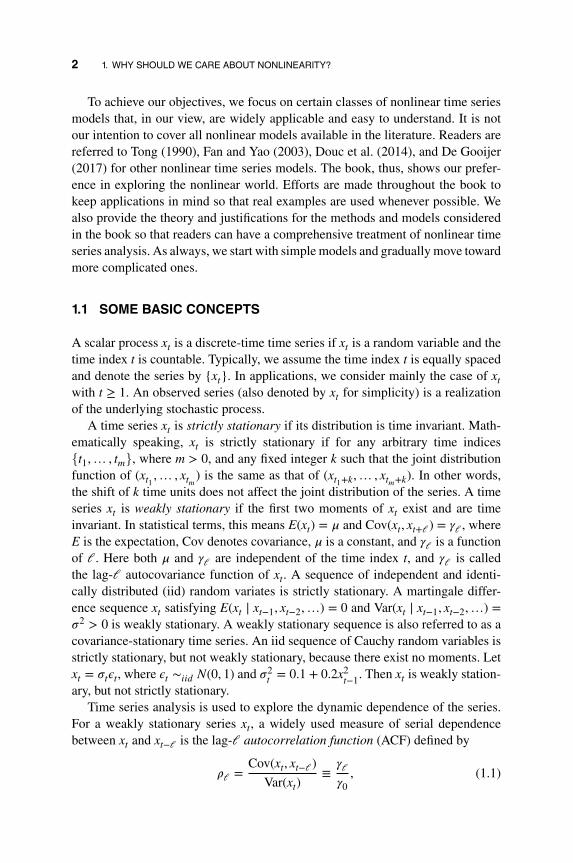
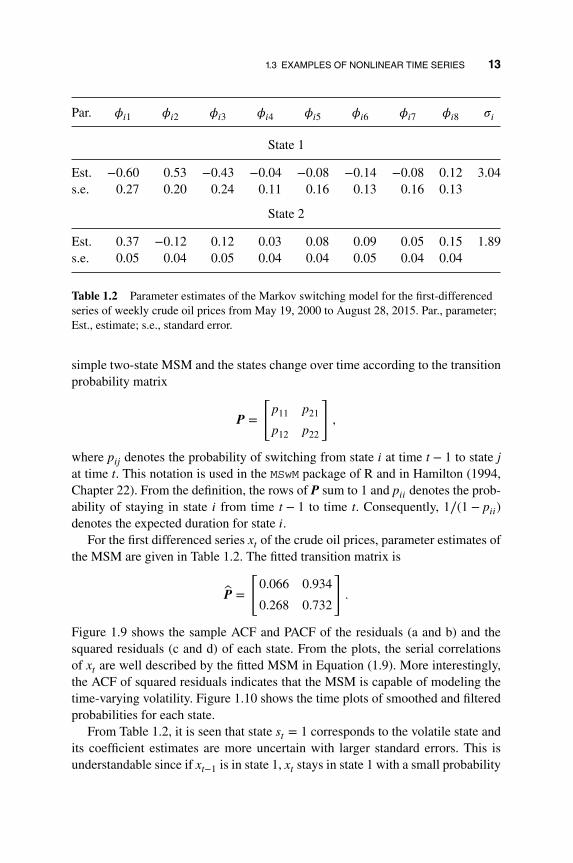
Example 1.2 As a second example, we consider the weekly crude oil pricesfrom May 12, 2000 to August 28, 2015. The data used are part of the commodityprices available from Federal Reserve Bank of St. Louis and they are the crude oilprices, West Texas Intermediate, Cushing, Oklahoma. Figure 1.6 shows the timeplot of the original crude oil prices and the first differenced series of the prices.The differenced series is used in our analysis as the oil prices exhibit strong serialdependence, i.e. unit-root nonstationarity. From the plots, it is seen that the vari-ability of the time series varies over time. Let xt = pt − pt−1, where pt denotes theobserved weekly crude oil price at week t. If scalar AR models are employed, anAR(8) model is selected by AIC and the fitted model, after removing insignificantparameters, is
xt = 0.197xt−1 + 0.153xt−8 + at, 𝜎2a = 6.43, (1.6)
where the standard errors of both AR coefficients are around 0.034. This sim-ple AR model adequately describes the dynamic correlations of xt, but it failsto address the time-varying variability. Figure 1.7 shows the sample ACF of the
10 1. WHY SHOULD WE CARE ABOUT NONLINEARITY?
2000
2005
2010
2015
140
100
6020
Year
2000
2005
2010
2015
Year
Pric
e
155
−5
−15
Cha
nge
(a)
(b)
Figure 1.6 Time plot of weekly crude oil prices from May 12, 2000 to August 28, 2015:(a) oil prices and (b) the first differenced series. The prices are West Texas Intermediate,Cushing, Oklahoma, and obtained from FRED of Federal Reserve Bank, St. Louis
residuals and those of the squared residuals. From the plots, the residuals have nosignificant serial correlations, but the squared residuals have strong serial depen-dence. In finance, such a phenomenon is referred to as time-varying volatility orconditional heteroscedasticity.
One approach to improve the linear AR(8) model in Equation (1.6) is to usethe generalized autoregressive conditional heteroscedastic (GARCH) model ofBollerslev (1986). GARCH models are nonlinear based on the linearity defini-tion of Equation (1.2). In this particular instance, the fitted AR-GARCH modelwith Student-t innovations is
xt ≈ 0.227xt−1 + 0.117xt−8 + at, (1.7)
at = 𝜎t𝜖t, 𝜖t ∼𝑖𝑖d t∗7.91,
𝜎2t = 0.031 + 0.072a2
t−1 + 0.927𝜎2t−1, (1.8)

1.3 EXAMPLES OF NONLINEAR TIME SERIES 11
0 5 10 15 20 25 30
0.8
0.4
0.0
Lag
AC
FStandardized residuals
0 5 10 15 20 25 30
0.8
0.4
0.0
Lag
AC
F
Standardized residuals^2
(a)
(b)
Figure 1.7 Sample autocorrelation functions of (a) the residuals of the AR(8) model inEquation (1.6) for the first differenced series of weekly crude oil prices and (b) the squaredresiduals.
where t∗v denotes standardized Student-t distribution with v degrees of freedom.In Equation (1.7) we use the approximation ≈, since we omitted the insignificantparameters at the 5% level for simplicity. In Equation (1.8), the standard errorsof the parameters are 0.024, 0.016, and 0.016, respectively. This volatility modelindicates the high persistence in the volatility. For further details about volatilitymodels, see Chapter 5 and Tsay (2010, Chapter 3). Model checking indicates thatthe fitted AR-GARCH model is adequate. For instance, we have Q(20) = 14.38(0.81) and 9.89(0.97) for the standardized residuals and the squared standardizedresiduals, respectively, of the model, where the number in parentheses denotes thep value. Figure 1.8(a) shows the time plot of xt along with point-wise two-standarderrors limits, which further confirms that the model fits the data well. Figure 1.8(b)shows the quantile-to-quantile (QQ) plot of the standardized residuals versus theStudent-t distribution with 7.91 degrees of freedom. The plot shows that it is rea-sonable to employ the Student-t innovations.
Compared with the linear AR(8) model in Equation (1.6), the fittedAR-GARCH model does not alter the serial dependence in the xt series

12 1. WHY SHOULD WE CARE ABOUT NONLINEARITY?
0
200
400
600
800
155
−5
−15
Series with 2 conditional SD superimposed
Index
x
−4
−2 0 2 4
42
0−
4
qstd − QQ plot
Theoretical quantiles
Sam
ple
quan
tiles
(a)
(b)
Figure 1.8 (a) The time plot of the first-differenced crude oil prices and point-wise twostandard error limits of the model in Equations (1.7) and (1.8). (b) The quantile-to-quantileplot for the Student-t innovations.
because Equation (1.7) is relatively close to Equation (1.6). What the GARCHmodel does is to handle the time-varying volatility so that proper inference,such as interval predictions, can be made concerning the crude oil prices. Insome finance applications volatility plays a key role and the fitted AR-GARCHnonlinear model can be used.
Alternatively, one can use the Markov switching model (MSM) to improve thelinear AR(8) model. Details of the MSM are given in Chapters 2 and 7. In thisparticular application, the model used is
xt =
{𝜙11xt−1 + 𝜙12xt−2 +⋯ + 𝜙18xt−8 + 𝜎1𝜖t, if st = 1,
𝜙21xt−1 + 𝜙22xt−2 +⋯ + 𝜙28xt−8 + 𝜎2𝜖t, if st = 2,(1.9)
where 𝜙𝑖,j denotes the coefficient of state 𝑖 at lag-j, 𝜖t are independent and identi-cally distributed random variables with mean zero and variance 1, 𝜎𝑖 is the innova-tion standard error of state 𝑖, and st denotes the status of the state at time t. This is a
1.3 EXAMPLES OF NONLINEAR TIME SERIES 13
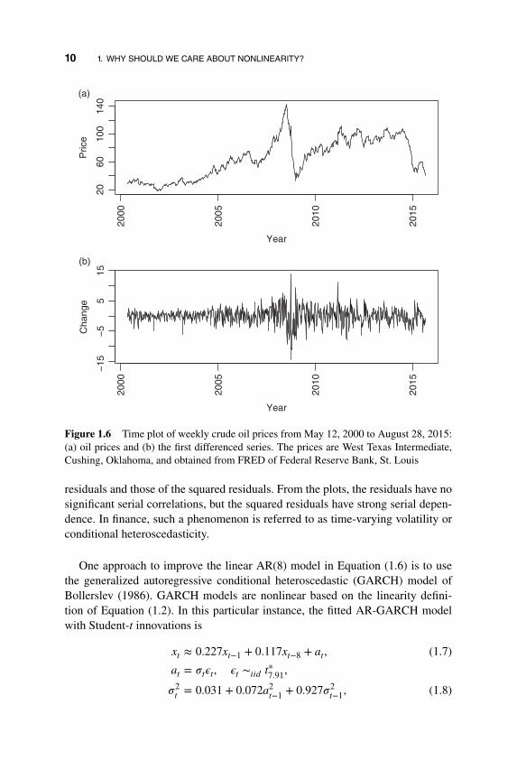
Par. 𝜙𝑖1 𝜙𝑖2 𝜙𝑖3 𝜙𝑖4 𝜙𝑖5 𝜙𝑖6 𝜙𝑖7 𝜙𝑖8 𝜎𝑖
State 1
Est. −0.60 0.53 −0.43 −0.04 −0.08 −0.14 −0.08 0.12 3.04s.e. 0.27 0.20 0.24 0.11 0.16 0.13 0.16 0.13
State 2
Est. 0.37 −0.12 0.12 0.03 0.08 0.09 0.05 0.15 1.89s.e. 0.05 0.04 0.05 0.04 0.04 0.05 0.04 0.04
Table 1.2 Parameter estimates of the Markov switching model for the first-differencedseries of weekly crude oil prices from May 19, 2000 to August 28, 2015. Par., parameter;Est., estimate; s.e., standard error.
simple two-state MSM and the states change over time according to the transitionprobability matrix
P =
[p11 p21
p12 p22
],
where p𝑖j denotes the probability of switching from state 𝑖 at time t − 1 to state jat time t. This notation is used in the MSwM package of R and in Hamilton (1994,Chapter 22). From the definition, the rows of P sum to 1 and p𝑖𝑖 denotes the prob-ability of staying in state 𝑖 from time t − 1 to time t. Consequently, 1∕(1 − p𝑖𝑖)denotes the expected duration for state 𝑖.
For the first differenced series xt of the crude oil prices, parameter estimates ofthe MSM are given in Table 1.2. The fitted transition matrix is
P =
[0.066 0.934
0.268 0.732
].
Figure 1.9 shows the sample ACF and PACF of the residuals (a and b) and thesquared residuals (c and d) of each state. From the plots, the serial correlationsof xt are well described by the fitted MSM in Equation (1.9). More interestingly,the ACF of squared residuals indicates that the MSM is capable of modeling thetime-varying volatility. Figure 1.10 shows the time plots of smoothed and filteredprobabilities for each state.
From Table 1.2, it is seen that state st = 1 corresponds to the volatile state andits coefficient estimates are more uncertain with larger standard errors. This isunderstandable since if xt−1 is in state 1, xt stays in state 1 with a small probability

14 1. WHY SHOULD WE CARE ABOUT NONLINEARITY?
2520151050
1.0
0.5
0.0
−0.
5−
1.0
1.0
0.5
0.0
−0.
5−
1.0
1.0
0.5
0.0
−0.
5−
1.0
1.0
0.5
0.0
−0.
5−
1.0
Lag
AC
F
ACF of residuals(a) (b)
(c) (d)
2520151050
Lag
2520151050
Lag
2520151050
Lag
Par
tial A
CF
PACF of residuals
AC
F
ACF of square residualsP
artia
l AC
FPACF of square residuals
Figure 1.9 The sample autocorrelation functions of the residuals (a and b) and squaredresiduals (c and d), by state, for the Markov switching model of Equation (1.9) fitted to thefirst-differenced series of weekly crude oil prices from May 19, 2000 to August 28, 2015.
0.066 and it switches to state 2 about 93% of the time. The marginal probabilitythat xt is in state 1 is 0.223. The table also shows that the serial dependence of xtdepends on the state; the serial dependence can be modeled by an AR(3) model instate 1, but it requires an AR(8) model in state 2. Figure 1.10 confirms that xt staysin state 2 often, implying that during the data span the crude oil prices encounteredsome volatile periods, but the high volatility periods are short-lived.
In this example, we show that nonlinear models can provide a deeper under-standing of the dynamic dependence of a time series. In addition, various nonlinearmodels can be used to improve the fitting of a linear model. The Markov switchingmodel allows the dynamic dependence of a time series to change according to thestate it belongs to. It is also capable of handling time-varying volatility.
1.3 EXAMPLES OF NONLINEAR TIME SERIES 15
0.0
0.4
0.8
0.0
0.4
0.8
Pro
babi
lity
Pro
babi
lity
(a)
(b)
0
200
400
600
800
Filtered probability regime 1
Time
0
200
400
600
800
Smoothed probability regime 1
Time
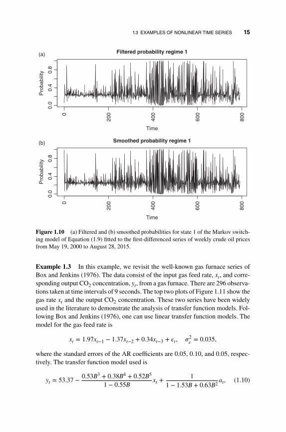
Figure 1.10 (a) Filtered and (b) smoothed probabilities for state 1 of the Markov switch-ing model of Equation (1.9) fitted to the first-differenced series of weekly crude oil pricesfrom May 19, 2000 to August 28, 2015.
Example 1.3 In this example, we revisit the well-known gas furnace series ofBox and Jenkins (1976). The data consist of the input gas feed rate, xt, and corre-sponding output CO2 concentration, yt, from a gas furnace. There are 296 observa-tions taken at time intervals of 9 seconds. The top two plots of Figure 1.11 show thegas rate xt and the output CO2 concentration. These two series have been widelyused in the literature to demonstrate the analysis of transfer function models. Fol-lowing Box and Jenkins (1976), one can use linear transfer function models. Themodel for the gas feed rate is
xt = 1.97xt−1 − 1.37xt−2 + 0.34xt−3 + 𝜖t, 𝜎2𝜖 = 0.035,
where the standard errors of the AR coefficients are 0.05, 0.10, and 0.05, respec-tively. The transfer function model used is
yt = 53.37 − 0.53B3 + 0.38B4 + 0.52B5
1 − 0.55Bxt +
11 − 1.53B + 0.63B2
at, (1.10)

16 1. WHY SHOULD WE CARE ABOUT NONLINEARITY?
Time
300250200150100500
Time
300250200150100500
Time
300250200150100500
CO
2
6055
50
Gas
32
10
−2
Sta
ndar
d
21
−1
−3
(a)
(b)
(c)
Figure 1.11 Time plots of the gas furnace data: (a) input gas feed rates, (b) output CO2
concentrations, and (c) gas rates weighted by time trend st = 2t∕296.
where B denotes the back-shift (or lag) operator such that Bxt = xt−1, the varianceof at is 0.0576, and all parameter estimates are statistically significant at the usual5% level. Residual analysis shows that the model in Equation (1.10) is adequate.For instance, the Ljung–Box statistics of the residuals gives Q(12) = 15.51 with pvalue 0.21.
On the other hand, nonlinear transfer function models have also been pro-posed in the literature, e.g. Chen and Tsay (1996). In this example, we followthe approach of Tsay and Wu (2003) by allowing the coefficients of the transferfunction model to depend on a state variable st. In this particular instance, thestate variable used is st = 2t∕296, which simply represents the time sequence ofthe observations. The corresponding transfer function model would become
yt = c0 +𝜔3(st)B
3 + 𝜔4(st)B4 + 𝜔5(st)B
5
1 − 𝛿(st)Bxt +
11 − 𝜙1B − 𝜙2B2
at,

1.3 EXAMPLES OF NONLINEAR TIME SERIES 17
where 𝜔𝑖(st) and 𝛿(st) are smooth functions of the state variable st, c0 and 𝜙𝑖are constant. This is a special case of the functional-coefficient models of Chenand Tsay (1993). To simplify the model, Tsay and Wu (2003) used the first-orderTaylor series approximations of the functional coefficients
𝜔𝑖(st) ≈ 𝜔𝑖0 + 𝜔𝑖1st, 𝛿(st) ≈ 𝛿0 + 𝛿1st,
where𝜔𝑖j and 𝛿j are constant, and simplified the model further to obtain the transferfunction model
yt = 52.65 − 1.22B3
1 − 0.61Bxt + 0.73st +
0.99B3 − 0.99B4
1 − 0.65B(stxt) (1.11)
+ 11 − 1.42B + 0.49B2
at,
where the residual variance is 𝜎2a = 0.0461 and all coefficient estimates are
statistically significant at the 5% level. The Ljung–Box statistics of the resultsgives Q(12) = 9.71 with p value 0.64. This model improves the in-sample fit asthe residual variance drops from 0.0576 to 0.0431. Figure 1.11(c) shows the timeplot of stxt, from which the new variable stxt seems to emphasize the latter partof the xt series.
Table 1.3 shows the results of out-of-sample forecasts of the two transfer func-tion models in Equations (1.10) and (1.11). These summary statistics are based on96 one-step ahead forecasts starting with initial forecast origin t = 200. As before,the models were re-estimated before prediction once a new observation was avail-able. From the table it is easily seen that the model in Equation (1.11) outper-forms the traditional transfer function model in all three measurements of out-of-sample prediction. The improvement in the root mean squared error (RMSE) is(0.3674 − 0.3311)∕0.3311= 10.96%. This is a substantial improvement given thatthe model in Equation (1.10) has been regarded as a gold standard for the data set.
In this example we show that the functional-coefficient models can be usefulin improving the accuracy of forecast. It is true that the model in Equation (1.11)
Model Bias RMSE MAE
Equation (1.10) 0.0772 0.3674 0.2655Equation (1.11) 0.0300 0.3311 0.2477
Table 1.3 Summary statistics of out-of-sample forecasts for the models in Equations(1.10) and (1.11). The initial forecast origin is 200 and the results are based on 96one-step ahead predictions.

18 1. WHY SHOULD WE CARE ABOUT NONLINEARITY?
ooo
o
o
o
o
o
o
o
o
o
oo
o
o
o
oo
o
o
oo
o
o
oo
o
oo
o
o
o
o
o
oo
o
o
o
o
o
o
o
oo
o
o
oo
o
oo
oo
o
o
o
oo
o
o
ooooo
o
oo
o
oo
oo
oo
o
o
o
oo
o
o
oo
o
o
o
o
o
o
o
o
o
o
o
o
o
o
o
o
o
o
o
o
oo
o
o
o
o
o
o
o
o
o
o
o
o
oo
oo
o
o
o
o
oo
o
o
o
o
o
oo
o
o
o
200019981996199419921990
5040
3020
100
Year
Cas
es
Figure 1.12 Time plot of the number of cases of Campylobacterosis infections in north-ern Quebec, Canada, in 4-week intervals from January 1990 to October 2000 for 140observations.
remains linear because the added variable stxt can be treated as a new input vari-able. However, the model was derived by using the idea of functional-coefficientmodels, a class of nonlinear models discussed in Chapter 2.
Example 1.4 Another important class of nonlinear models is the generalizedlinear model. For time series analysis, generalized linear models can be used toanalyze count data. Figure 1.12 shows the number of cases of Campylobactero-sis infections in the north of the province Quebec, Canada, in 4-week intervalsfrom January 1990 to the end of October 2000. The series has 13 observations peryear and 140 observations in total. See Ferland et al. (2006) for more information.The data are available from the R package tscount by Liboschik et al. (2015).Campylobacterosis in an acute bacterial infectious disease attacking the digestivesystem. As expected, the plot of Figure 1.12 shows some seasonal pattern.
This is an example of time series of count data, which occur in many scientificfields, but have received relatively less attention in the time series literature. Sim-ilar to the case of independent data, Poisson or negative binomial distribution isoften used to model time series of count data. Here one postulates that the time
1.3 EXAMPLES OF NONLINEAR TIME SERIES 19
2.01.51.00.50.0
1.0
0.8
0.6
0.4
0.2
0.0
−0.
2
Lag
AC
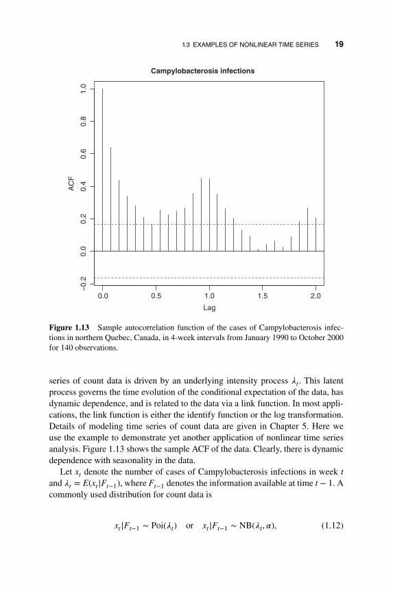
FCampylobacterosis infections
Figure 1.13 Sample autocorrelation function of the cases of Campylobacterosis infec-tions in northern Quebec, Canada, in 4-week intervals from January 1990 to October 2000for 140 observations.
series of count data is driven by an underlying intensity process 𝜆t. This latentprocess governs the time evolution of the conditional expectation of the data, hasdynamic dependence, and is related to the data via a link function. In most appli-cations, the link function is either the identify function or the log transformation.Details of modeling time series of count data are given in Chapter 5. Here weuse the example to demonstrate yet another application of nonlinear time seriesanalysis. Figure 1.13 shows the sample ACF of the data. Clearly, there is dynamicdependence with seasonality in the data.
Let xt denote the number of cases of Campylobacterosis infections in week tand 𝜆t = E(xt|Ft−1), where Ft−1 denotes the information available at time t − 1. Acommonly used distribution for count data is
xt|Ft−1 ∼ Poi(𝜆t) or xt|Ft−1 ∼ NB(𝜆t, 𝛼), (1.12)

20 1. WHY SHOULD WE CARE ABOUT NONLINEARITY?
where Poi(𝜆t) and NB(𝜆t, 𝛼) denote, respectively, a Poisson distribution with mean𝜆t and a negative binomial distribution with mean 𝜆t and dispersion parameter𝛼 > 0. Specifically, for the Poisson distribution we have
P(xt = k|𝜆t) =1k!
e−𝜆t𝜆kt , k = 0, 1,… .
For the negative binomial distribution, there are several parameterizations avail-able in the literature. We use the probability mass function
P(xt = k|𝜆t, 𝛼) = Γ(𝛼 + k)Γ(𝛼)Γ(k + 1)
(𝛼
𝛼 + k
)𝛼 ( 𝜆t
𝛼 + 𝜆t
)k
, k = 0, 1,… .
Under this parameterization, we have E(xt|Ft−1) = 𝜆t and Var(xt|Ft−1) =𝜆t + 𝜆2
t ∕𝛼. Here 𝛼 ∈ (0,∞) is the dispersion parameter and the negative binomialdistribution approaches the Poisson distribution as 𝛼 → ∞.
For the time series in Figure 1.12, one can introduce the dynamic dependencefor the data by using the model
𝜆t = 𝛾0 + 𝛾1xt−1 + 𝛿13𝜆t−13, (1.13)
where 𝜆t−13 is used to describe the seasonality of the data. This model is similar tothe GARCH model of Bollerslev (1986) for the volatility model and belongs to theclass of observation-driven models in generalized linear models. See Ferland et al.(2006), among others. Using Equation (1.13) with negative binomial distribution,the quasi maximum likelihood estimation gives
𝜆t = 2.43 + 0.594xt−1 + 0.188𝜆t−13,
where the dispersion parameter is 0.109 and the standard deviations of the coeffi-cient estimates are 1.085, 0.092, and 0.123, respectively. Figure 1.14 shows vari-ous plots of model checking for the fitted model in Equation (1.13). From the timeplot of Pearson residuals, it is seen that certain outlying observations exist so thatthe model can be refined. Comparing the autocorrelations of the data in Figure1.13 and the residual autocorrelations in Figure 1.14, the simple model in Equa-tion (1.13) does a decent job in describing the dynamic dependence of the countdata. Details of model checking and refinement of the generalized linear modelsfor time series of count data will be given in Chapter 5. The analysis can also behandled by the state space model of Chapter 6.
In this example, we demonstrate that the generalized linear models, which arenonlinear, can be used to analyze time series of count data.
1.4 NONLINEARITY TESTS
The flexibility of nonlinear models in data fitting may encounter the problem offinding spurious structure in a given time series. It is, therefore, of importance
1.4 NONLINEARITY TESTS 21
1.51.00.50.0
1.0
0.6
0.2
−0.
2
Lag
AC
F
ACF of pearson residuals
Pearson residuals over time
Time
Res
idua
ls
200019981996199419921990
3010
−10
6543210
0.8
0.4
0.0
Cumulative periodogram of pearson residuals
Frequency
Non−randomized PIT histogram
Probability integral transform
Den
sity
1.00.80.60.40.20.0
1.2
0.8
0.4
0.0
50403020100
0.03
0.00
−0.
03
Marginal calibration plot
Threshold value
Diff
. of p
red.
and
em
p. c
.d.f
(a) (b)
(c)
(e)
(d)
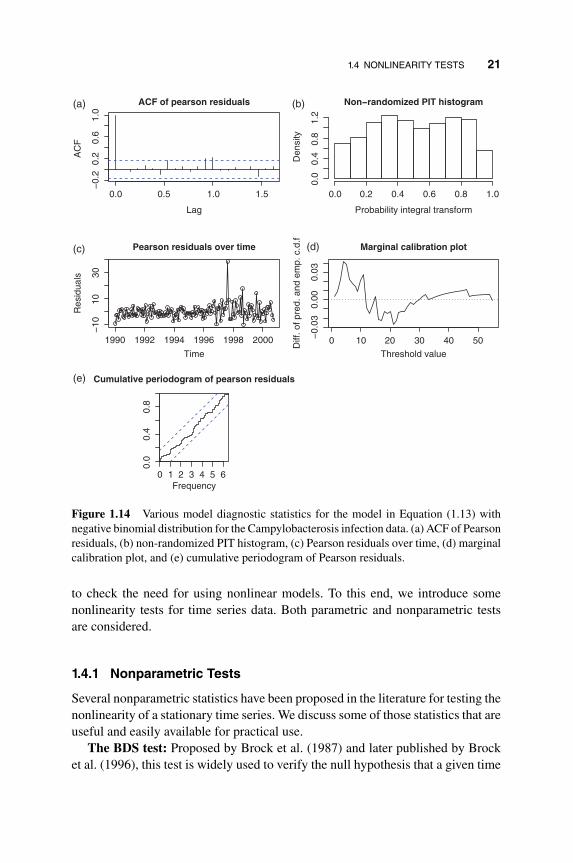
Figure 1.14 Various model diagnostic statistics for the model in Equation (1.13) withnegative binomial distribution for the Campylobacterosis infection data. (a) ACF of Pearsonresiduals, (b) non-randomized PIT histogram, (c) Pearson residuals over time, (d) marginalcalibration plot, and (e) cumulative periodogram of Pearson residuals.
to check the need for using nonlinear models. To this end, we introduce somenonlinearity tests for time series data. Both parametric and nonparametric testsare considered.
1.4.1 Nonparametric Tests
Several nonparametric statistics have been proposed in the literature for testing thenonlinearity of a stationary time series. We discuss some of those statistics that areuseful and easily available for practical use.
The BDS test: Proposed by Brock et al. (1987) and later published by Brocket al. (1996), this test is widely used to verify the null hypothesis that a given time

22 1. WHY SHOULD WE CARE ABOUT NONLINEARITY?
series consists of independent and identically distributed (iid) random variables.The test uses the idea of correlation integral popular in chaotic time series analysis.Roughly speaking, a correlation integral is a measure of the frequency with whichtemporal patterns repeat themselves in a data set. Consider a time series {xt|t =1,… , T}, where T denotes the sample size. Let m be a given positive integer.Define an m-history of the series as xm
t = (xt, xt−1,… , xt−m+1) for t = m,… , T .Define the correlation integral at the embedding dimension m as
C(m, 𝜖) = limTm→∞
2Tm(Tm − 1)
∑ ∑m≤s<t≤T
I(xmt , xm
s |𝜖) (1.14)
where Tm = T − m + 1 is the number of constructed m-histories, 𝜖 is a givenpositive real number, and I(u, v|𝜖) is an indicator variable that equals to one if‖u − v‖ < 𝜖 and zero otherwise, where ‖ ⋅ ‖ denotes the sup-norm of two vectors.For the m-histories, we have I(u, v|𝜖) = 1 if |u𝑖 − v𝑖| < 𝜖 for 𝑖 = 1,… , m and =0 otherwise. For a given 𝜖, Equation (1.14) simply measures the probability ofm-histories being within a distance 𝜖 of each other.
For testing purpose, the magnitude of the correlation integral in Equation (1.14)needs to be judged. To this end, the BDS test compares C(m, 𝜖) with C(1, 𝜖) underthe null hypothesis. Intuitively, if {xt} are iid, then there exist no patterns in the dataso that a probability of the m-history is simply the mth power of the correspondingprobability of the 1-history. This is so because under independence Pr(A ∩ B) =Pr(A) × Pr(B). In other words, under the iid assumption, we expect that C(m, 𝜖) =C(1, 𝜖)m. The BDS test is then defined as
D(m, 𝜖) =√
T[C(m, 𝜖) − {C(1, 𝜖)}m]s(m, 𝜖)
(1.15)
where C(k, 𝜖) is given by
C(k, 𝜖) = 2Tk(Tk − 1)
∑ ∑k≤s<t≤T
I(xkt , xk
s |𝜖), k = 1, m,
and s(m, 𝜖) denotes the standard error of C(m, 𝜖) − {C(1, 𝜖)}m, which can be con-sistently estimated from the data under the null hypothesis. For details, readersmay consult Brock et al. (1996) or Tsay (2010, Chapter 4). In practice, one needsto select the embedding dimension m and the distance 𝜖.
The BDS test is available in the fNonlinear package of R under the commandbdsTest. The user has the option to select the maximum embedding dimensionm and the distance 𝜖. The default maximum dimension is m = 3, which means theembedding dimensions used in the test are 2 and 3. The default choices of 𝜖 are(0.5, 1, 1.5, 2)��x, where ��x denotes the sample standard error of xt. To demonstrate,we consider a simulation of iid random variables from N(0, 1) and a daily log return

1.4 NONLINEARITY TESTS 23
series of the stock of International Business Machines (IBM) Corporation. Detailsare given below with output edited for simplicity.
R demonstration: BDS test using the package fNonlinear.
> require(fNonlinear)> set.seed(1)> x < rnorm(300)> bdsTest(x)Title: BDS Test
Test Results:PARAMETER:Max Embedding Dimension: 3eps[1]: 0.482; eps[2]: 0.964eps[3]: 1.446; eps[4]: 1.927
STATISTIC:eps[1] m=2: 1.1256; eps[1] m=3: 1.4948eps[2] m=2: 0.7145; eps[2] m=3: 1.1214eps[3] m=2: 0.6313; eps[3] m=3: 0.8081eps[4] m=2: 0.7923; eps[4] m=3: 1.2099
P VALUE:eps[1] m=2: 0.2604; eps[1] m=3: 0.135eps[2] m=2: 0.4749; eps[2] m=3: 0.2621eps[3] m=2: 0.5278; eps[3] m=3: 0.419eps[4] m=2: 0.4282; eps[4] m=3: 0.2263
> require("quantmod")> getSymbols("IBM",from="20100102",to="20150930")> head(IBM)
IBM.Open IBM.High IBM.Low IBM.Close IBM.Volume IBM.Adjusted20100104 131.18 132.97 130.85 132.45 6155300 117.658020100105 131.68 131.85 130.10 130.85 6841400 116.2367> rtn < diff(log(as.numeric(IBM[,6])))> ts.plot(rtn) # not shown> Box.test(rtn,type="Ljung",lag=10)
BoxLjung testdata: rtnXsquared = 15.685, df = 10, pvalue = 0.109 # No serial correlations> bdsTest(rtn)Title: BDS Test
Test Results:PARAMETER:Max Embedding Dimension: 3eps[1]: 0.006; eps[2]: 0.012eps[3]: 0.018; eps[4]: 0.024
STATISTIC:eps[1] m=2: 4.4058; eps[1] m=3: 5.3905
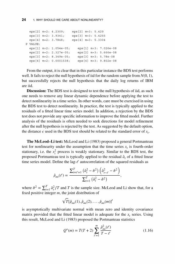
24 1. WHY SHOULD WE CARE ABOUT NONLINEARITY?
eps[2] m=2: 4.2309; eps[2] m=3: 5.429eps[3] m=2: 3.9341; eps[3] m=3: 5.4255eps[4] m=2: 3.7848; eps[4] m=3: 5.3304
P VALUE:eps[1] m=2: 1.054e05; eps[1] m=3: 7.026e08eps[2] m=2: 2.327e05; eps[2] m=3: 5.666e08eps[3] m=2: 8.349e05; eps[3] m=3: 5.78e08eps[4] m=2: 0.0001538; eps[4] m=3: 9.802e08
From the output, it is clear that in this particular instance the BDS test performswell. It fails to reject the null hypothesis of iid for the random sample from N(0, 1),but successfully rejects the null hypothesis that the daily log returns of IBMare iid.
Discussion: The BDS test is designed to test the null hypothesis of iid, as suchone needs to remove any linear dynamic dependence before applying the test todetect nonlinearity in a time series. In other words, care must be exercised in usingthe BDS test to detect nonlinearity. In practice, the test is typically applied to theresiduals of a fitted linear time series model. In addition, a rejection by the BDStest does not provide any specific information to improve the fitted model. Furtheranalysis of the residuals is often needed to seek directions for model refinementafter the null hypothesis is rejected by the test. As suggested by the default option,the distance 𝜖 used in the BDS test should be related to the standard error of xt.
The McLeod–Li test: McLeod and Li (1983) proposed a general Portmanteautest for nonlinearity under the assumption that the time series xt is fourth-orderstationary, i.e. the x2
t process is weakly stationary. Similar to the BDS test, theproposed Portmanteau test is typically applied to the residual at of a fitted lineartime series model. Define the lag-𝓁 autocorrelation of the squared residuals as
��aa(𝓁) =
∑Tt=𝓁+1
(a2
t − ��2) (
a2t−𝓁 − ��2
)∑T
t=1
(a2
t − ��2) ,
where ��2 =∑T
t=1 a2t ∕T and T is the sample size. McLeod and Li show that, for a
fixed positive integer m, the joint distribution of√T[��aa(1), ��aa(2),… , ��aa(m)]′
is asymptotically multivariate normal with mean zero and identity covariancematrix provided that the fitted linear model is adequate for the xt series. Usingthis result, McLeod and Li (1983) proposed the Portmanteau statistics
Q∗(m) = T(T + 2)m∑
𝓁=1
��2aa(𝓁)
T − 𝓁(1.16)

1.4 NONLINEARITY TESTS 25
to detect nonlinearity in xt. Under the assumption that xt is fourth-order stationaryand the fitted linear model is adequate, Q∗(m) is asymptotically distributed as 𝜒2
m.This is essentially a Ljung–Box test on the x2
t series.In the literature, the Portmanteau statistics of Equation (1.16) is often used to
check for conditional heteroscedasticity. As a matter of fact, the test is asymptoti-cally equivalent to the Lagrange multiplier test of Engle (1982) for the autoregres-sive conditional heteroscedastic (ARCH) model. To test for ARCH effects, Engle(1982) uses the AR(m) model
a2t = 𝛽0 + 𝛽1a2
t−1 +⋯ + 𝛽ma2t−m + 𝜖t, (1.17)
where 𝜖t denotes the error term, and considers the null hypothesis H0 : 𝛽1 = 𝛽2 =⋯ = 𝛽m = 0 versus the alternative hypothesis Ha : 𝛽𝑖 ≠ 0 for some 𝑖 ∈ {1,… , m}.The F-statistic of the linear regression in Equation (1.17) can be used to performthe test. Alternatively, one can use mF as a test statistic. Under the same conditionsas those of McLeod and Li (1983), mF is asymptotically distributed as 𝜒2
m. TheQ∗(m) statistics of Equation (1.16) can be easily computed. We demonstrate thisbelow.
R demonstration: McLeod–Li and Engle tests for nonlinearity.
> set.seed(15)> xt < rnorm(300)> Box.test(xt,lag=10,type='Ljung')
BoxLjung testdata: xtXsquared = 11.095, df = 10, pvalue = 0.3502 # No serial correlations> Box.test(xtˆ2,lag=10,type='Ljung')
BoxLjung testdata: xtˆ2Xsquared = 8.4539, df = 10, pvalue = 0.5846 # Qstar test
> require(quantmod)> getSymbols("MSFT",from="20090102",to="20151015",src="google")> msft < diff(log(as.numeric(MSFT$MSFT.Close))) #log returns> Box.test(msft,lag=10,type='Ljung')
BoxLjung testdata: msftXsquared = 17.122, df = 10, pvalue = 0.0717 # No serial correlations> Box.test(msftˆ2,lag=10,type='Ljung')
BoxLjung testdata: msftˆ2Xsquared = 70.54, df = 10, pvalue = 3.487e11 ## Nonlinearity### Engle's test with m = 10.> nT < length(msft)> y < msft[11:nT]ˆ2

26 1. WHY SHOULD WE CARE ABOUT NONLINEARITY?
> X < NULL> for (i in 1:10)+ X < cbind(X,msft[(11i):(nTi)]ˆ2)+ }> m2 < lm(y ˜X) ## Linear regression> anova(m2)Analysis of Variance TableResponse: y
Df Sum Sq Mean Sq F value Pr(>F)X 10 0.00003036 3.0358e06 4.65 1.447e06 ***Residuals 1687 0.00110138 6.5286e07> qstar = 4.64*10> pv = 1 pchisq(qstar,10)> print(c(qstar,pv))[1] 4.65e+01 1.162495e06 ### ARCH effect exists
From the output, the traditional Ljung–Box statistics confirm that both theseries of iid N(0, 1) random variables and the daily log returns of Microsoft(MSFT) stock from January 2010 to October 15, 2015 have no serial correlations.On the other hand, the McLeod–Li test statistic of (1.16) cannot reject the nullhypothesis of linear time series for the N(0, 1) iid random sample, but it clearlyrejects linearity for the daily log returns of MSFT stock. The ARCH effect is alsoconfirmed by the Lagrange multiplier test of Engle (1982).
Rank-based Portmanteau test: The McLeod–Li test requires the existence ofthe fourth moment of the underlying time series xt. In some applications, empir-ical data may exhibit high excess kurtosis. In this situation, the performance ofthe McLeod–Li test may deteriorate. To overcome the impact of heavy-tails onthe McLeod–Li test, one can apply the rank-based Ljung–Box statistics. See, forinstance, Dufour and Roy (1986) and Tsay (2014, Chapter 7) and the referencestherein. Let R𝑖 be the rank of a2
𝑖in the squared residuals {a2
t }. The lag-𝓁 rank-based serial correlation is defined as
��𝓁 =∑T
t=𝓁+1(Rt − R)(Rt−𝓁 − R)∑Tt=1(Rt − R)2
, 𝓁 = 1, 2,…
where it can be shown that
R =T∑
t=1
Rt∕T = (T + 1)∕2
T∑t=1
(Rt − R)2 = T(T2 − 1)∕12.
1.4 NONLINEARITY TESTS 27
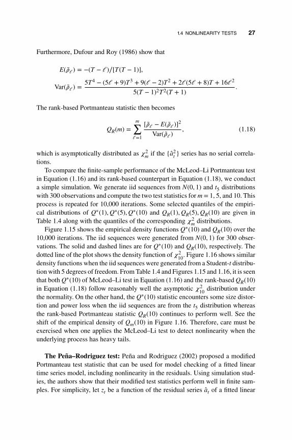
Furthermore, Dufour and Roy (1986) show that
E(��𝓁) = −(T − 𝓁)∕[T(T − 1)],
Var(��𝓁) = 5T4 − (5𝓁 + 9)T3 + 9(𝓁 − 2)T2 + 2𝓁(5𝓁 + 8)T + 16𝓁2
5(T − 1)2T2(T + 1).
The rank-based Portmanteau statistic then becomes
QR(m) =m∑
𝓁=1
[��𝓁 − E(��𝓁)]2
Var(��𝓁), (1.18)
which is asymptotically distributed as 𝜒2m if the {a2
t } series has no serial correla-tions.
To compare the finite-sample performance of the McLeod–Li Portmanteau testin Equation (1.16) and its rank-based counterpart in Equation (1.18), we conducta simple simulation. We generate iid sequences from N(0, 1) and t5 distributionswith 300 observations and compute the two test statistics for m = 1, 5, and 10. Thisprocess is repeated for 10,000 iterations. Some selected quantiles of the empiri-cal distributions of Q∗(1), Q∗(5), Q∗(10) and QR(1), QR(5), QR(10) are given inTable 1.4 along with the quantiles of the corresponding 𝜒2
m distributions.Figure 1.15 shows the empirical density functions Q∗(10) and QR(10) over the
10,000 iterations. The iid sequences were generated from N(0, 1) for 300 obser-vations. The solid and dashed lines are for Q∗(10) and QR(10), respectively. Thedotted line of the plot shows the density function of 𝜒2
10. Figure 1.16 shows similardensity functions when the iid sequences were generated from a Student-t distribu-tion with 5 degrees of freedom. From Table 1.4 and Figures 1.15 and 1.16, it is seenthat both Q∗(10) of McLeod–Li test in Equation (1.16) and the rank-based QR(10)in Equation (1.18) follow reasonably well the asymptotic 𝜒2
10 distribution underthe normality. On the other hand, the Q∗(10) statistic encounters some size distor-tion and power loss when the iid sequences are from the t5 distribution whereasthe rank-based Portmanteau statistic QR(10) continues to perform well. See theshift of the empirical density of Qm(10) in Figure 1.16. Therefore, care must beexercised when one applies the McLeod–Li test to detect nonlinearity when theunderlying process has heavy tails.
The Pena–Rodriguez test: Pena and Rodriguez (2002) proposed a modifiedPortmanteau test statistic that can be used for model checking of a fitted lineartime series model, including nonlinearity in the residuals. Using simulation stud-ies, the authors show that their modified test statistics perform well in finite sam-ples. For simplicity, let zt be a function of the residual series at of a fitted linear

28 1. WHY SHOULD WE CARE ABOUT NONLINEARITY?
Distribution Statistics 0.025 0.05 0.5 0.95 0.975
𝜒21 0.00098 0.00393 0.455 3.842 5.024
N(0, 1) Q∗(1) 0.00096 0.00372 0.451 3.744 4.901QR(1) 0.00088 0.00392 0.463 3.762 5.056
t5 Q∗(1) 0.00074 0.00259 0.288 2.936 4.677QR(1) 0.00098 0.00367 0.441 3.716 4.856
𝜒25 0.8312 1.1455 4.351 11.070 12.833
N(0, 1) Q∗(5) 0.7903 1.0987 4.129 11.045 13.131QR(5) 0.7884 1.1193 4.263 11.042 12.792
t5 Q∗(5) 0.3634 0.5575 2.909 10.992 15.047QR(5) 0.8393 1.1287 4.254 11.123 13.002
𝜒210 3.2470 3.9403 9.342 18.307 20.483
N(0, 1) Q∗(10) 3.1077 3.7532 8.870 12.286 21.122QR(10) 3.1737 3.8524 9.184 18.163 20.516
t5 Q∗(10) 1.1347 1.6916 6.685 19.045 23.543QR(10) 3.2115 3.8265 9.216 18.495 20.786
Table 1.4 Empirical quantiles of McLeod–Li Portmanteau statistics and the rank-basedPortmanteau statistics for random samples of 300 observations. The realizations aregenerated from N(0, 1) and Student-t distribution with 5 degrees of freedom. The resultsare based on 10,000 iterations.
model. For instance, zt = a2t or zt = |at|. The lag-𝓁 sample autocorrelation of zt is
defined as
��𝓁 =∑T
t=𝓁+1(zt−𝓁 − z)(zt − z)∑Tt=1(zt − z)2
, (1.19)
where, as before, T is the sample size and z =∑
t zt∕T is the sample mean of zt. Asusual, ��𝓁 is a consistent estimate of the lag-𝓁 autocorrelation 𝜌𝓁 of zt under someregularity conditions. For a given positive integer m, the Pena and Rodriguez teststatistic for testing the null hypothesis of H0 : 𝜌1 = ⋯ = 𝜌m = 0 is
Dm = T[1 − |Rm|1∕m], (1.20)

1.4 NONLINEARITY TESTS 29
403020100
0.10
0.08
0.06
0.04
0.02
0.00
x
Den
sity
Figure 1.15 Empirical density functions of Q∗(10) in Equation (1.16) (solid line) andQR(10) in Equation (1.18) (dashed line) when the iid sequences are generated from N(0, 1).The results are for sample size 300 and 10,000 iterations. The dotted line denotes the densityfunction of 𝜒2
10.
where the (m + 1) by (m + 1) matrix Rm is defined below:
Rm =
⎡⎢⎢⎢⎢⎢⎣
1 ��1 ⋯ ��m
��1 1 ⋯ ��m−1
⋮ ⋮ ⋱ ⋮
��m ��m−1 ⋯ 1
⎤⎥⎥⎥⎥⎥⎦. (1.21)
Using the idea of pseudo-likelihood, Pena and Rodriguez (2006) further modifiedthe test statistic in Equation (1.20) to
D∗m = − T
m + 1log(|Rm|), (1.22)
where the denominator m + 1 is the dimension of Rm. Under the assumption thatthe fitted ARMA(p, q) model is correctly specified, Pena and Rodriguez (2006)

30 1. WHY SHOULD WE CARE ABOUT NONLINEARITY?
806040200
0.10
0.08
0.06
0.04
0.02
0.00
x
Den
sity
Figure 1.16 Empirical density functions of Q∗(10) in Equation (1.16) (solid line) andQR(10) in Equation (1.18) (dashed line) when the iid sequences are generated from aStudent-t distribution with 5 degrees of freedom. The results are for sample size 300 and10,000 iterations. The dotted line denotes the density function of 𝜒2
10.
show that the test statistic D∗m of Equation (1.22) is asymptotically distributed
as a mixture of m independent 𝜒21 random variates. The weights of the mixture
are rather complicated. However, the authors derived two approximations to sim-plify the calculation. The first approximation of D∗
m is denoted by GD∗m, which is
approximately distributed as a gamma random variate, Γ(𝛼, 𝛽), where
𝛼 =3(m + 1)[m − 2(p + q)]2
2[2m(2m + 1) − 12(m + 1)(p + q)],
𝛽 =3(m + 1)[m − 2(p + q)]
2m(2m + 1) − 12(m + 1)(p + q).
The second approximation is
ND∗m = (𝛼∕𝛽)−1∕𝜆(𝜆∕
√𝛼)[(D∗
m)1∕𝜆 − (𝛼∕𝛽)1∕𝜆(
1 − 𝜆 − 12𝛼𝜆2
)], (1.23)

1.4 NONLINEARITY TESTS 31
where 𝛼 and 𝛽 are defined as before, and
𝜆 =[
1 −2(m∕2 − (p + q))(m2∕(4(m + 1)) − (p + q))
3(m(2m + 1)∕(6(m + 1)) − (p + q))2
]−1
.
Asymptotically, ND∗n is distributed as N(0, 1). For large m, 𝜆 ≈ 4. In practice, the
authors recommend replacing ��𝓁 by ��𝓁 = (T + 2)��𝓁∕(T − 𝓁) in the Rm matrix ofEquation (1.21) for better performance in finite samples, especially when T issmall.
To demonstrate the ND∗m statistic of Equation (1.23), we consider the daily log
returns of Microsoft stock from January 2, 2009 to October 15, 2015. The sameseries was used before in demonstrating the McLeod–Li test. The sample size isT = 1708 so that we select m = ⌊log(T)⌋ + 1 = 8. The test, denoted by PRnd, isavailable in the package NTS.
R demonstration: Pena–Rodriguez test.
> require(quantmod); require(NTS)> getSymbols("MSFT",from="20090102",to="20151015",src="google")> msft < diff(log(as.numeric(MSFT$MSFT.Close))) # log returns> log(length(msft))[1] 7.443078> PRnd(msft,m=8)NDstat & pvalue 0.1828238 0.8549363> PRnd(abs(msft),m=8)NDstat & pvalue 2.302991 0.02127936
From the output, the daily log returns have no significant serial correlations,but their absolute values have serial correlations. Again, the results confirm thenonlinearity in the daily MSFT log returns.
1.4.2 Parametric Tests
Most parametric tests for nonlinearity are developed under the assumption of cer-tain nonlinear models as the alternative. Roughly speaking, a well-behaved zero-mean stationary time series xt can be written as a Volterra series
xt =t−1∑𝑖=1
𝜓𝑖xt−𝑖 +t−1∑𝑖=1
t−1∑j=1
𝜓𝑖jxt−𝑖xt−j +∑𝑖
∑j
∑k
𝜙𝑖jkxt−𝑖xt−jxt−k +⋯ + 𝜖t, (1.24)
where 𝜖t denotes the noise term and the 𝜓s are real numbers. For a linear timeseries xt, we have 𝜓𝑖j = 𝜓𝑖jk = ⋯ = 0. Therefore, some of the higher-order coef-ficients are non-zero if xt is nonlinear. If the third order and higher coefficients arezero, but 𝜓𝑖j ≠ 0 for some 𝑖 and j, then xt becomes a bilinear process. Parametric

32 1. WHY SHOULD WE CARE ABOUT NONLINEARITY?
tests for nonlinearity of xt are statistics that exploit certain features of the Volterraseries in Equation (1.24). We discuss some of the parametric tests in this section.
The RESET test: Ramsey (1969) proposed a specification test for linear leastsquares regression analysis. The test is referred to as a RESET test and is readilyapplicable to linear AR models. Consider the linear AR(p) model
xt = X′t−1𝝓 + at, (1.25)
where Xt−1 = (1, xt−1,… , xt−p)′ and 𝝓 = (𝜙0,𝜙1,… ,𝜙p)′. The first step of the
RESET test is to obtain the least squares estimate �� of Equation (1.25) and com-pute the fitted value xt = X′
t−1��, the residual at = xt − xt, and the sum of squared
residuals SSR0 =∑T
t=p+1 a2t , where T is the sample size. In the second step, con-
sider the linear regression
at = X′t−1𝜶1 + M′
t−1𝜶2 + vt, (1.26)
where Mt−1 = (x2t ,… , xs+1
t )′ for some s ≥ 1, and compute the least squaresresiduals
vt = at − X′t−1��1 − M′
t−1��2
and the sum of squared residuals SSR1 =∑T
t=p+1 v2t of the regression. The basic
idea of the RESET test is that if the linear AR(p) model in Equation (1.25) isadequate, then 𝜶1 and 𝜶2 of Equation (1.26) should be zero. This can be tested bythe usual F statistic of Equation (1.26) given by
F =(SSR0 − SSR1)∕g
SSR1∕(T − p − g)with g = s + p + 1, (1.27)
which, under the linearity and normality assumption, has an F distribution withdegrees of freedom g and T − p − g.
Remark: Because the variables xkt for k = 2,… , s + 1 tend to be highly corre-
lated with Xt−1 and among themselves, principal components of Mt−1 that are notco-linear with Xt−1 are often used in fitting Equation (1.26).
Keenan (1985) proposed a nonlinearity test for time series that uses x2t only and
modifies the second step of the RESET test to avoid multicollinearity between x2t
and Xt−1. Specifically, the linear regression (1.26) is divided into two steps. In step2(a), one removes linear dependence of x2
t on Xt−1 by fitting the regression
x2t = X′
t−1𝜷 + ut

1.4 NONLINEARITY TESTS 33
and obtaining the residual ut = x2t − Xt−1𝜷. In step 2(b), consider the linear
regression
at = ut𝛼 + vt,
and obtain the sum of squared residuals SSR1 =∑T
t=p+1(at − ut��)2 =∑T
t=p+1 v2t
to test the null hypothesis 𝛼 = 0.
The F-test: To improve the power of Keenan’s and RESET tests, Tsay (1986)used a different choice of the regressor Mt−1. Specifically, he suggested usingMt−1 = vech(Xt−1X′
t−1), where vech(A) denotes the half-stacking vector of thematrix A using elements on and below the diagonal only. For example, if p =2, then Mt−1 = (x2
t−1, xt−1xt−2, x2t−2)′. The dimension of Mt−1 is p(p + 1)∕2 for an
AR(p) model. In practice, the test is simply the usual partial F statistic for testing𝜶 = 0 in the linear least squares regression
xt = X′t−1𝝓 + M′
t−1𝜶 + et,
where et denotes the error term. Under the assumption that xt is a linear AR(p)process, the partial F statistic follows an F distribution with degrees of freedomg and T − p − g − 1, where g = p(p + 1)∕2. We refer to this F test as the F-test.Luukkonen et al. (1988) further extended the test by augmenting Mt−1 with cubicterms x3
t−𝑖 for 𝑖 = 1,… , p.
To demonstrate nonlinearity tests, consider the US quarterly unemploymentrates of Example 1.1. In this particular instance, both Keenan test and F-test con-firm that the series is nonlinear. The F-test is referred to as the Tsay.test in theTSA package.
R demonstration: Parametric tests.
> require(TSA)> da=read.table("qunrate.txt",header=T)> rate < da$rate> Keenan.test(unrate)$test.stat[1] 7.428776$p.value[1] 0.006858382$order[1] 5> Tsay.test(unrate)$test.stat[1] 2.626$p.value

34 1. WHY SHOULD WE CARE ABOUT NONLINEARITY?
[1] 0.00108$order[1] 5
Remark: The dimension of Mt−1 used in the F-test is p(p + 1)∕2, which canbe high when the order p is not small compared with the sample size T . In thissituation, the F-test might have low power in detecting nonlinearity. To improvethe F-test, one can use the idea of thresholding. Specifically, one constructsMt−1 using only those lagged variables in Xt−1 with t-ratio greater than somethreshold in modulus. To illustrate, consider the well-known Canadian Lynx data,which is available in the TSA package. The series has 114 observations. Withlog-transformation, an AR(11) is selected by the Keenan.test and Tsay.test
of the TSA package. In this particular case, the Keenan test shows that the logseries is nonlinear, but the F-test fails. This is not surprising because the F-testfits 11(12)∕2 = 66 additional parameters whereas the effective sample size isonly 114 − 11 = 103. On the other hand, with threshold 1.645, the F-test alsoconfirms that the log series is nonlinear. Here the threshold 1.645 selects fivelagged variables to construct Mt−1 in the F-test.
R demonstration:
> require(TSA)> data(lynx)> y < log10(lynx)> Keenan.test(y)$test.stat[1] 11.66997$p.value[1] 0.0009550016$order[1] 11> Tsay.test(y)$test.stat[1] 1.316$p.value[1] 0.2256$order[1] 11> require(NTS)> F.test(y,thres=1.645)$test.stat[1] 1.971$p.value

1.4 NONLINEARITY TESTS 35
[1] 0.02858$order[1] 11
Threshold test: If the alternative model under study is the self-exciting thresh-old autoregressive (TAR) model shown in Example 1.1, one can derive specifictest statistics to increase the power of detecting nonlinearity. One of the specifictests is the likelihood ratio statistic studied by Chan and Tong (1990) and Chan(1990, 1991). The TAR(p) model considered can be written as
xt = 𝜙0 +p∑𝑖=1
𝜙𝑖xt−𝑖 + I(xt−d > r)
(𝛽0 +
p∑𝑖=1
𝛽𝑖xt−𝑖
)+ at, (1.28)
where at is a sequence of independent and identically distributed Gaussian randomvariables with mean zero and variance 𝜎2, 𝜙𝑖 and 𝛽j are real valued parameters,d > 0 with xt−d being the threshold variable, r is the threshold, and I(xt−d > r) isan indicator variable such that I(xt−d > r) = 1 if xt−d > r and = 0 otherwise. Thenull hypothesis is H0 : 𝛽𝑖 = 0 for 𝑖 ∈ {0,… , p} and the alternative hypothesis isHa : 𝛽𝑖 ≠ 0 for some 𝑖. In Equation (1.28), we assume that the threshold r liesinside a known bounded closed interval R ⊆ R. For simplicity, we further assumethat d ≤ p. The likelihood ratio test statistic is then
𝜆 =n(��2
0 − ��2)
��2, (1.29)
where n = T − p + 1 with T being the sample size,
��2 = minr∈R,𝜃,𝜙
⎡⎢⎢⎣T∑
t=p+1
{xt − 𝜙0 −
p∑𝑖=1
𝜙𝑖xt−𝑖 − I(xt−d > r)
(𝛽0 +
p∑𝑖=1
𝛽𝑖xt−𝑖
)}2⎤⎥⎥⎦ ,
��20 = min
𝜙
⎧⎪⎨⎪⎩T∑
t=p+1
(xt − 𝜙0 −
p∑𝑖=1
𝜙𝑖xt−𝑖
)2⎫⎪⎬⎪⎭ .The null hypothesis is rejected if and only if 𝜆 of Equation (1.29) is large. The lim-iting properties of the test statistic 𝜆, however, are non-standard and more involvedbecause the threshold r is undefined under the null hypothesis H0. This is an issueof nuisance parameter under the null hypothesis. Interested readers are referredto Chan and Tong (1990). The percentage points of 𝜆 under the null hypothesishave been investigated by Chan (1990). In the literature, it is common to assumethat R = [v, u], where v and u are pre-specified real numbers with v < u. See, forinstance, Davis (1987) and Andrews and Ploberger (1994).

36 1. WHY SHOULD WE CARE ABOUT NONLINEARITY?
Another specific threshold nonlinearity test is to transform the testing prob-lem into a change point detection problem. The transformation is carried out viathe arranged autoregression. See Tsay (1989, 1998) and the references therein.Specifically, the arranged autoregression transfers the TAR model under the alter-native hypothesis Ha into a model-change problem with the threshold r being thechange point. To see this, the TAR model in Equation (1.28) says that xt followsessentially two linear models depending on whether xt−d < r or xt−d ≥ r. For arealization of T data points, say {xt}
Tt=1, the threshold variable xt−d can assume
values {x1,… , xT−d}. Let x(1) ≤ x(2) ≤ ⋯ ≤ x(T−d) be the ordered statistics of{xt}
T−dt=1 . The TAR model can then be written as
x(j)+d = 𝜃0 +p∑𝑖=1
𝜃𝑖x(j)+d−𝑖 + a(j)+d, j = 1,… , T − d, (1.30)
where 𝜃𝑖 = 𝜙𝑖 if x(j) ≤ r, and 𝜃𝑖 = 𝜙𝑖 + 𝛽𝑖 if x(j) > r, for 𝑖 = 0,… , p. Conse-quently, the threshold r is a change point for the linear regression in Equation(1.30), and we refer to Equation (1.30) as an arranged autoregression (in increas-ing order of the threshold variable xt−d). Note that the arranged autoregression inEquation (1.30) does not alter the dynamic dependence of xt on xt−𝑖 for 𝑖 = 1,… , pbecause x(j)+d still depends on x(j)+d−𝑖 for 𝑖 = 1,… , p. What is done is simply topresent the TAR model in the threshold space instead of in the time space. Thatis, the equation with a smaller xt−d appears before that with a larger xt−d. Thethreshold test of Tsay (1989) is obtained as follows.
� Step 1: Fit Equation (1.30) using j = 1,… , m, where m is a pre-specifiedpositive integer (e.g., 30). Denote the least squares estimates of 𝜃𝑖 by ��𝑖,m,where m denotes the number of data points used in estimation.
� Step 2: Compute the predictive residual
a(m+1)+d = x(m+1)+d − ��0,m −p∑𝑖=1
��𝑖,mx(m+1)+d−𝑖
and its standard error. Let e(m+1)+d be the standardized predictive residual.
� Step 3: Use the recursive least squares method to update the least squaresestimates to ��𝑖,m+1 by incorporating the new data point x(m+1)+d.
� Step 4: Repeat Steps 2 and 3 until all data points are processed.
� Step 5: Consider the linear regression of the standardized predictive residual
e(m+j)+d = 𝛼0 +p∑𝑖=1
𝛼𝑖x(m+j)+d−𝑖 + vt, j = 1,… , T − d − m (1.31)

1.4 NONLINEARITY TESTS 37
and compute the usual F statistic for testing 𝛼𝑖 = 0 in Equation (1.31) for𝑖 = 0,… , p. Under the null hypothesis that xt follows a linear AR(p) model,the F ratio has a limiting F distribution with degrees of freedom p + 1 andT − d − m − p.
We refer to the resulting F test as a Tar-F test. The idea behind the test is thatunder the null hypothesis there is no model change in the arranged autoregressionin Equation (1.30) so that the standardized predictive residuals should be close toiid with mean zero and variance 1. In this case, they should have no correlationswith the regressors x(m+j)+d−𝑖. For further details, including formulas for a recur-sive least squares method and some simulation study on performance of the Tar-Ftest, see Tsay (1989). The Tar-F test avoids the problem of nuisance parametersencountered by the likelihood ratio test. It does not require knowing the thresholdr. It simply tests that the predictive residuals have no correlations with regressorsif the null hypothesis holds. Therefore, the test does not depend on knowing thenumber of regimes in the alternative model. Yet the Tar-F test is not as powerful asthe likelihood ratio test if the true model is indeed a two-regime TAR model withGaussian innovations.
The likelihood ratio test for a two-regime Gaussian TAR model is available viathe command tlrt of the TSA package, whereas the Tar-F test is available via thecommand thr.test of the NTS package. For the US quarterly unemploymentrates of Example 1.1, both tests detect nonlinearity with p = 5 and d = 5 anddefault options. Details are given below.
R demonstration: Threshold tests.
> da < read.table("qunrate.txt",header=T)> unrate < da$rate> require(NTS)> require(TSA)> thr.test(unrate,p=5,d=5)SETAR model is entertainedThreshold nonlinearity test for (p,d): 5 5Fratio and pvalue: 2.849921 0.01081263> tlrt(unrate,p=5,d=5)$percentiles[1] 24.9 75.1$test.statistic
33.028$p.value
0.0003066953

38 1. WHY SHOULD WE CARE ABOUT NONLINEARITY?
1.5 EXERCISES
1.1 Consider the global land and ocean temperature anomalies from January1880 to May 2017. The monthly data are available from the National Oceanicand Atmospheric Administration (NOAA) at www.ncdc.noaa.gov and are inthe file globaltemp18802017.csv. The data are in degrees Celsius andthe base period is 1901–2000. The temperature anomalies show an upwardtrend so consider the change series, i.e. the first difference. Is the differencedseries nonlinear? Perform some tests and draw a conclusion. Does the seriesshow threshold nonlinearity? Why?
1.2 Consider the daily log returns of the exchange-traded fund for the S&P 500index with tick symbol SPY from January 3, 2007 to June 30, 2017. Dailylog returns denote the first difference of log daily closing prices. The firstcolumn of the file SPY0717.txt contains the log return. Is the return seriesnonlinear? Perform some tests, including the BDS test to draw a conclusion.
1.3 Asset return series tend to exhibit conditional heteroscedasticity. TheGARCH models are often used to handle conditional heteroscedasticity.Consider the SPY daily log returns of previous problem. The second col-umn of the file SPY0717.txt shows the standardized residuals of a fittedAR(1)-GARCH(1,1) model with standardized Student-t innovations. Doesthe standardized residual series consist of independent and identically dis-tributed random variables? Why?
1.4 Consider the grow rate series (first difference of the log index) of the USmonthly producer price index from February 1913 to August 2017. Thedata can be obtained from FRED (PPIACO, 1982 index=100, not season-ally adjusted). The data are also in the file PPIACO.csv. Is the growth rateseries linear? Perform some nonlinearity tests to draw a conclusion.
1.5 Consider again the growth rate series of the US monthly producer price indexof the prior problem. Let xt be the growth rate series. Use the fGarch pack-age to fit the model:
require(fGarch)m1 < garchFit( arma(3,2)+garch(1,1),data=x_t,trace=F,
cond.dist="std")rt < residuals(m1,standardize=T)
The rt denotes the standardized residuals. Apply the McLeod–Li test todetect any nonlinearity in the rt series and apply the BDS test to checkwhether the rt series consists of iid random variables.
REFERENCES 39
REFERENCES
Akaike, H. (1974). A new look at the statistical model identification. IEEE Transactions onAutomatic Control AC-19: 716–723.
Andrews, D. W. K. and Ploberger, W. (1994). Optimal tests when a nuisance parameter ispresent only under the alternative. Econometrica 62: 1383–1414.
Bollerslev, T. (1986). Generalized autoregressive conditional heteroskedasticity. Journal ofEconometrics 31: 307–327.
Box, G. E. P. and Jenkins, G. M. (1976). Time Series Analysis: Forecasting and Control,revised ed. Holden-Day, San Francisco.
Box, G. E. P., Jenkins, G. M., Reinsel, G. C., and Ljung, G. M. (2015). Time Series Analysis:Forecasting and Control, 5th edition. Wiley, Hoboken, NJ.
Brock, W., Dechert, W.D., and Scheinkman, J. (1987). A test for independence based onthe correlation dimension. Working paper, Department of Economics, University ofWisconsin-Madison.
Brock, W., Dechert, W. D., Scheinkman, J., and LeBaron, B. (1996). A test for indepen-dence based on the correlation dimension. Econometric Reviews 15: 197–235.
Chan, K. S. (1990). Percentage points of likelihood ratio tests for threshold autoregression.Journal of the Royal Statistical Society, Series B 53: 691–696.
Chan, K. S. (1991). Percentage points of likelihood ratio tests for threshold autoregression.Journal of the Royal Statistical Society Series B 53: 691–696.
Chan, K. S. and Tong, H. (1990). On likelihood ratio tests for threshold autoregression.Journal of the Royal Statistical Society, Series B 52: 469–476.
Chen, R. and Tsay, R. S. (1993). Functional-coefficient autoregressive models. Journal ofthe American Statistical Association 88: 298-308.
Chen, R. and Tsay, R. S. (1996). Nonlinear transfer function. Journal of NonparametricStatistics 6: 193–204.
Davis, R. B. (1987). Hypothesis testing when a nuisance parameter is present only underthe alternative. Biometrika 74: 33–43.
De Gooijer, J. G. (2017). Elements of Nonlinear Time Series Analysis and Forecasting.Springer, Cham, Switzerland.
Douc, R., Moulines, E., and Stoffer, D. S. (2014). Nonlinear Time Series: Theory, Methods,and Applications with R Examples. CRC Press, Boca Raton, FL.
Dufour, J. M. and Roy, R. (1986). Generalized portmanteau statistics and tests of random-ness. Communications in Statistics – Theory and Methods 15: 2953–2972,
Engle, R. F. (1982). Autoregressive conditional heteroscedasticity with estimates of thevariance of United Kingdom inflations. Econometrica 50: 987–1007.
Fan, J. and Yao, Q. (2003). Nonlinear Time Series: Nonparametric and Parametric Meth-ods. Springer, New York.
Ferland, R., Latour, A. and Oraichi, D. (2006). Integer-valued GARCH process. Journal ofTime Series Analysis 27: 923–942.

40 1. WHY SHOULD WE CARE ABOUT NONLINEARITY?
Hamilton, J. D. (1994). Time Series Analysis. Princeton University Press, Princeton, NJ.
Keenan, D. M. (1985). A Tukey non-additivity-type test for time series nonlinearity.Biometrika 72: 39–44.
Liboschik, T., Fried, R., Fokianos, K., Probst, P., and Rathjens, J. (2015). Analysis of CountTime Series, R Package, http://tscount.r-forge.r-project.org.
Luukkonen, R., Saikkonen, P., and Terasvirta (1988). Testing linearity against smooth tran-sition autoregressive models. Biometrika 75: 491–499.
McLeod, A. I. and Li, W. K. (1983). Diagnostic checking ARMA time series models usingsquared-residual autocorrelations. Journal of Time Series Analysis 4: 269–273.
Pena, D. and Rodriguez, J. (2002). A powerful Portmanteau test of lack of fit for time series.Journal of the American Statistical Association 97: 601–610.
Pena, D. and Rodriguez, J. (2006). The log of the determinant of the autocorrelation matrixfor testing goodness of fit in time series. Journal of Statistical Planning and Inference136: 2706–2718.
R Development Core Team (2015). R: A Language and Environment for Statistical Com-puting. R Foundation for Statistical Computing, Vienna, Austria. ISBN 3-900051-07-0.http://www.R-project.org.
Ramsey, J. B. (1969). Tests for specification errors in classical linear least squares regressionanalysis. Journal of the Royal Statistical Society Series B 31: 350–371.
Tong, H. (1978). On a threshold model. In C.H. Chen (ed.), Pattern Recognition and SignalProcessing. Sijhoff & Noordhoff, Amsterdam.
Tong, H. (1990). Non-Linear Time Series: A Dynamical System Approach. Oxford Univer-sity Press, Oxford.
Tong, H. and Lim, K. S. (1980). Threshold autoregression,limit cycles and cyclical data(with discussion). Journal of the Royal Statistical Society, Series B 42: 245–292.
Tsay, R. S. (1986). Nonlinearity tests for time series. Biometrika 73: 461–466.
Tsay, R. S. (1989). Testing and modeling threshold autoregressive processes. Journal of theAmerican Statistical Association 84: 231–240.
Tsay, R. S. (1998). Testing and modeling multivariate threshold models. Journal of theAmerican Statistical Association 93: 1188–1202.
Tsay, R. S. (2010). Analysis of Financial Time Series, 3rd edition. John Wiley,Hoboken, NJ.
Tsay, R. S. (2014). Multivariate Time Series Analysis with R and Financial Applications,John Wiley, Hoboken, NJ.
Tsay, R. S. and Wu, C. S. (2003). Forecasting with leading indicators revisited. Journal ofForecasting 22: 603–617.

CHAPTER 2
UNIVARIATE PARAMETRICNONLINEAR MODELS
In this chapter we introduce some univariate nonlinear time series models, discusstheir properties, and demonstrate their applications. We also address the pros andcons of the models using real examples. The models introduced include thresholdautoregressive (TAR) models, Markov switching models (MSM), smooth thresh-old autoregressive (STAR) models, and time-varying parameter models. We beginwith some general setup for a dynamic system and the basic probability structureunderling the system, hoping to provide readers with a deeper understanding ofthe models introduced.
2.1 A GENERAL FORMULATION
The goal of analyzing a time series xt is to explore its dynamic dependence, and ageneral model for xt is
xt = f (xt−1, xt−2, … , at), (2.1)
Nonlinear Time Series Analysis, First Edition. Ruey S. Tsay and Rong Chen.© 2019 John Wiley & Sons, Inc. Published 2019 by John Wiley & Sons, Inc.Companion website: www.wiley.com/go/tsay/nonlineartimeseries
41

42 2. UNIVARIATE PARAMETRIC NONLINEAR MODELS
where f (⋅) is a well-defined real-valued function and at is an iid sequence ofrandom variables with mean zero and variance 𝜎2
a . We often refer to at as theinnovation of the system at time t and assume 0 < 𝜎2
a <∞. For example, iff (⋅) = 𝜙0 + 𝜙1xt−1 + at, then xt is an AR(1) time series. If f (⋅) is a nonlinear func-tion, then xt follows a nonlinear time series model. For many applications, thedynamic system f (⋅) only depends on a finite number of past values, and it can bewritten as f (⋅) = f (xt−1,… , xt−p, at), where p is a positive integer.
To understand the properties of the dynamic system in Equation (2.1), it isoften helpful to study the function f (⋅) recursively by dropping the innovation at.For instance, consider the AR(1) time series xt with 𝜙0 = 0. The f (⋅) functionbecomes f (xt−1) = 𝜙1xt−1. This is referred to as the skeleton of the system in Tong(1990). By recursive substitutions, we have f t(x0) = f (f t−1(x0)) = 𝜙t
1x0, wherex0 denotes the initial value of the system. Since x0 can assume any real value,for f t(x0) = 𝜙t
1x0 to be meaningful as t increases we need |𝜙1| < 1. This leads tolimt→∞ f t(x0) = 0, which is the mean of the underlying AR(1) series. It is well-known that the condition |𝜙1| < 1 is the necessary and sufficient condition for theweak stationarity of the AR(1) time series provided that 𝜎2
a <∞. The case fornonlinear models is much more involved, but the recursive substitutions of f (⋅)remain informative in studying the properties of time series xt.
2.1.1 Probability Structure
For a given time index t, xt is a random variable. We can study the propertiesof xt by drawing random variates from its probability distribution function. Let{x(1)
t , x(2)t ,… , x(m)
t } be a random sample of xt, where m denotes the sample size.
Then the mean value of xt can be estimated by ��t =1m
∑m𝑖=1 x(𝑖)
t , provided that themean E(xt) = 𝜇t exists. Next, fixing the superscript and drawing a temporal series,we have a sample time series {x(1)
1 , x(1)2 , x(1)
3 ,…}, denoted by {x(1)t }. This is called
a realization of the time series {xt}. By considering the m realizations jointly,we have an ensemble {x(𝑖)
t |t = 1,… ; 𝑖 = 1,… , m} of the time series xt. Such anensemble can be used to study properties of the series.
However, we do not have the luxury of owning an ensemble of a time series inreal applications. What we have is just an observed realization {xt|t = 1,… , T},where T denotes the length of the realization. How can we study the propertiesof xt based on such a single realization? To this end, some additional conceptsare needed. Suppose that the time series xt is weakly stationary. Then, we haveE(xt) = 𝜇, which does not depend on t. Therefore, each data point xt can be thoughtof as an estimate of the mean 𝜇, and we can combine the estimates together to forma pooled estimate of 𝜇, say �� = 1
T
∑Tt=1 xt, which is a time average. The statisti-
cal theory that provides justifications for pooling estimates over time is called the
2.2 THRESHOLD AUTOREGRESSIVE MODELS 43
ergodic theorem. Ergodicity basically ensures that the law of large numbers con-tinues to hold for the dependent time series data under certain conditions.
A weakly stationary time series xt is said to be ergodic in the mean if the timeaverage �� = 1
T
∑Tt=1 xt converges in probability to E(xt) as T → ∞. It can be shown
that if the following condition holds
∞∑𝑖=0
|𝛾𝑖| < ∞, (2.2)
where 𝛾𝑖 is the lag-𝑖 autocovariance of xt, then xt is ergodic in the mean. See, forinstance, Hamilton (1994, Chapter 7). A weakly stationary time series xt is said tobe ergodic in the second moment if
1T − j
T∑t=j+1
(xt − 𝜇)(xt−j − 𝜇) →p Cov(xt, xt−j), T → ∞,
where →p denotes convergence in probability. For a stationary (causal) linear timeseries xt defined in Chapter 1, the condition in Equation (2.2) and the assumptionthat E|at|r <∞ for some r > 2 are sufficient for it to be ergodic in the secondmoment. If one further assumes that xt is Gaussian, then the condition in Equation(2.2) implies that xt is ergodic in all moments.
For nonlinear time series xt, the condition for ergodicity is much harder to estab-lish. The conditions tend to be model specific, but they can often be derived usingthe Markov chain theory as most nonlinear models considered have Markov prop-erties. The appendix to this chapter gives some basic concepts of Markov chains.A good reference for studying the ergodicity and stability of a Markov chain isMeyn and Tweedie (2009). We make use of their results in this book, and shallrevisit ergodicity briefly in Chapter 8 when we discuss the Markov chain MonteCarlo method.
2.2 THRESHOLD AUTOREGRESSIVE MODELS
The self-exciting TAR model is arguably the most widely used scalar nonlineartime series model. It is an extension of the piecewise linear regression model(or segmented linear regression model) with structural changes occurring in thethreshold space. In the time series literature, the TAR model was proposed byTong (1978) and has been widely used since the publication of Tong and Lim(1980). We start with the simple two-regime TAR model and discuss multiple-regime TAR models later.

44 2. UNIVARIATE PARAMETRIC NONLINEAR MODELS
2.2.1 A Two-regime TAR Model
A time series xt follows a two-regime TAR model of order p with threshold variablext−d if it satisfies
xt =
{𝜙0 +
∑p𝑖=1 𝜙𝑖xt−𝑖 + 𝜎1𝜖t, if xt−d ≤ r,
𝜃0 +∑p𝑖=1 𝜃𝑖xt−𝑖 + 𝜎2𝜖t, if xt−d > r,
(2.3)
where 𝜖t is a sequence of iid random variables with mean zero and unit variance,𝜃𝑖 and 𝜙j are real-valued parameters such that 𝜃𝑖 ≠ 𝜙𝑖 for some 𝑖, d is a positiveinteger denoting the delay, and r is the threshold. Often, we further assume that𝜖t follows N(0, 1). We use the same order p for both regimes. This is purely forsimplicity as different orders can easily be used.
The TAR model in Equation (2.3) can also be written as
xt = 𝜙0 +p∑𝑖=1
𝜙𝑖xt−𝑖 + 𝜎1𝜖t + I(xt−d > r)(𝛽0 +p∑𝑖=1
𝛽𝑖xt−𝑖 + 𝛾𝜖t), (2.4)
where I(xt−d > r) = 1 if xt−d > r and = 0 otherwise, 𝛽𝑖 = 𝜃𝑖 − 𝜙𝑖 for 𝑖 = 0,… , pand 𝛾 = 𝜎2 − 𝜎1. In this way, the structural change of the model at xt−d = rbecomes apparent with 𝛽𝑖 denoting the change in the 𝑖th coefficient. This type ofmodel occurs often in many scientific fields. For instance, let xt denote the weightof a health-conscientious individual in week t. The person is likely to take certainaction to reduce his weight when xt exceeds some threshold. However, it takes timefor his action to show its effect, resulting in a delay of d weeks to see changes inhis weight. Consequently, a threshold model appears to be sensible for describingthe time evolution of his weight.
To contrast the TAR models with the linear time series model, Figure 2.1 showsthe time plot of a realization of the following two-regime TAR model
xt =
{−1.5xt−1 + 𝜖t, if xt−1 ≤ 0,
0.6xt−1 + 𝜖t, if xt−1 > 0,(2.5)
with 400 observations, where 𝜖t are iid standard Gaussian random variates. Thehorizontal line of the plot denotes zero. This simulated example shows clearlyseveral features of nonlinear models. First, the plot shows that the model inEquation (2.5) is weakly stationary, yet one of the lag-1 coefficients is greaterthan 1 in modulus. Second, the plot shows that the mean of the series is positive,yet the model has no constant term in either regime. Third, there are more positiverealizations than negative ones. In other words, the time series xt cannot stay longin the negative region. Why? To understand these features, we need to investigatethe properties of the TAR models.

2.2 THRESHOLD AUTOREGRESSIVE MODELS 45
Time
x t
4003002001000
43
21
0−
1−
2
Figure 2.1 A simulated realization with 400 observations from the model in Equation(2.5). The horizontal line denotes zero.
2.2.2 Properties of Two-regime TAR(1) Models
Consider the simplest two-regime TAR(1) model
xt =
{𝜙1xt−1 + 𝜎1𝜖t, if xt−1 ≤ 0,
𝜃1xt−1 + 𝜎2𝜖t, if xt−1 > 0,(2.6)
where the delay is d = 1, threshold is zero, and 𝜖t is an iid sequence of continuousrandom variables with mean zero, variance 1, and a positive probability densityfunction. The skeleton of this simple model is
f (xt−1) =
{𝜙1xt−1, if xt−1 ≤ 0,
𝜃1xt−1, if xt−1 > 0.(2.7)
Since x0 can assume any real number, it is easily seen that for the series xt tobe well-defined, we need 𝜙1 < 1 and 𝜃1 < 1. Otherwise, we can find some x0for which recursive substitutions of f (⋅) lead to explosive values. This is not sur-prising as the stationary region for a linear AR(1) model is −1 < 𝜙1 < 1. On theother hand, the switching between the two regimes creates a new opportunity forTAR models. It turns out that the (geometrically) ergodic region of the two-regime

46 2. UNIVARIATE PARAMETRIC NONLINEAR MODELS
−4
(a) (b)
−2 0 2 4
−4
−2
02
4
φ
ϑ
−4 −2 0 2 4
−4
−2
02
4
φϑ
Figure 2.2 Ergodic region of a two-regime TAR(1) model: (a) model with delay d = 1and (b) model with delay d = 2.
TAR(1) model in Equation (2.6) is given by the conditions that (a) 𝜙1 < 1, (b)𝜃1 < 1, and (c) 𝜙1𝜃1 < 1. The condition (c) ensures that the corresponding skele-ton of the model in Equation (2.7) remains stable for any arbitrary starting value.For illustration, consider the simulated TAR model in Equation (2.5) for which thethree ergodicity conditions hold. In this particular instance it is true that the modelin Regime 1 is explosive with coefficient satisfying |𝜙1| = |−1.5| > 1. However,in this regime, we have xt−1 ≤ 0 so that −1.5xt−1 > 0 provided that xt−1 ≠ 0. Con-sequently, we have P(xt > 0) > P(xt ≤ 0), implying that with high probability thesystem would switch to Regime 2. Once xt is in Regime 2, it follows a stationaryAR(1) model with coefficient 0.6. In this way, the explosive nature of the systemin Regime 1 would not lead to any issue of non-stability for xt. In other words,for the model in Equation (2.5), the dynamic dependence in Regime 2 would pullback any explosive value of xt created by Regime 1. This expanding and pullingphenomenon makes the nonlinear TAR model interesting. Figure 2.2(a) shows thegeometrically ergodic region of the TAR model in Equation (2.6). This result wasshown in Petruccelli and Woolford (1984).
The skeleton of a two-regime TAR model also depends on the delay parameterd. Consider the general two-regime TAR(1) model
xt =
{𝜙1xt−1 + 𝜎1𝜖t, if xt−d ≤ 0,
𝜃1xt−1 + 𝜎2𝜖t, if xt−d > 0,(2.8)
where d > 1. For this particular model, Chen and Tsay (1991) show that thegeometrically ergodic conditions of the model are (a) 𝜙1 < 1, (b) 𝜃1 < 1, and

2.2 THRESHOLD AUTOREGRESSIVE MODELS 47
Size Mean Med. Var. Range Prob. ��1 ��2 ��22
400 0.84 0.88 1.20 (−2.01,3.80) 0.23 0.04 −0.02 −0.024000 0.81 0.78 1.43 (−3.94,6.80) 0.25 0.14 −0.01 −0.03
40000 0.83 0.80 1.38 (−3.53,6.44) 0.24 0.14 0.01 −0.01400000 0.83 0.80 1.38 (−4.35,7.83) 0.24 0.14 0.01 −0.01
Table 2.1 Summary statistics of the two-regime TAR(1,1) model in Equation (2.5) withdifferent sample sizes, where “Prob.” denotes P(xt ≤ 0), ��𝑖 denotes Lag-𝑖 sampleautocorrelation and ��22 Lag-2 sample partial autocorrelation.
(c) 𝜙s(d)1 𝜃
t(d)1 < 1 and 𝜙t(d)
1 𝜃s(d)1 < 1, where s(d) and t(d) are functions of the delay
parameter d. For instance, we have s(d) = t(d) = 1 if d = 1 and s(d) = 1, t(d) = 2for d = 2. The ergodicity regime of the model in Equation (2.8) with d = 2 isshown in Figure 2.2(b). In general, the ergodicity conditions for a TAR modelare hard to obtain. On the other hand, the skeleton of a given TAR model can beobtained easily by recursive substitutions.
Statistical properties of stationary TAR models are hard to obtain, even for thesimple model in Equation (2.6). However, one can use simulations to gain someinsights. To demonstrate, Table 2.1 provides some empirical summary statisticsfor the TAR model in Equation (2.5). From the table, it is seen that the sum-mary statistics, except the range, become stable when the sample size is suf-ficiently large. Figure 2.3 shows the empirical density functions of xt for therealizations given in Table 2.1, where the black line is for sample size 400,the dashed line is for sample size 4000, and the dotted line is for sample size40,000. From the plots, the marginal density functions of xt are almost identi-cal for the sample sizes 4000 and 40,000, confirming the weak stationarity of themodel.
The nonlinear characteristics of the realizations shown in Table 2.1 are easy tosee even for the case of sample size 400. Figure 2.4 shows the scatter plot of xt ver-sus xt−1. The solid line of the plot corresponds to the fitted line by a local smooth-ing technique, via the command loess in R. See Chapter 3 for local smoothing.From the scatter plot and the fitted line, it is clear that the dependence of xt onxt−1 is nonlinear. As a matter of fact, the fitted line shows a V-shape function,which is indicative of the two different slopes of the two-regime TAR(1) model ofEquation (2.5).
Remark: The simulations of the TAR models used are obtained by the commanduTAR.sim of the NTS package.

48 2. UNIVARIATE PARAMETRIC NONLINEAR MODELS
86420−2−4
0.3
0.2
0.1
0.0
x
Den
sity
Figure 2.3 Empirical (marginal) density functions for the TAR model of Equation (2.5)with sample sizes given in Table 2.1. The solid line is for sample size 400, the dashed lineis for sample size 4000, and the dotted line is for sample size 40,000.
2.2.3 Multiple-regime TAR Models
The generalization of two-regime TAR models to multiple regimes is straightfor-ward. For a positive finite integer m > 1, let {r𝑖|𝑖 = 0,… , m} be a sequence of realnumbers satisfying
r0 = −∞ < r1 < r2 < ⋯ < rm−1 < rm = ∞,
where, for simplicity, we treat −∞ and ∞ as real numbers. A time series xt fol-lows an m-regime self-exciting TAR(p) model with threshold variable xt−d, whered > 0, if it satisfies
xt =
⎧⎪⎪⎨⎪⎪⎩
𝜙0,1 +∑p𝑖=1 𝜙𝑖,1xt−𝑖 + 𝜎1𝜖t, if xt−d ≤ r1,
𝜙0,2 +∑p𝑖=1 𝜙𝑖,2xt−𝑖 + 𝜎2𝜖t, if r1 < xt−d ≤ r2,
⋯
𝜙0,m +∑p𝑖=1 𝜙𝑖,mxt−𝑖 + 𝜎m𝜖t, if rm−1 < xt−d,
(2.9)
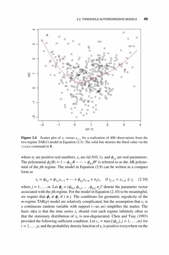
2.2 THRESHOLD AUTOREGRESSIVE MODELS 49
43210−1−2
43
21
0−
1−
2
x(t−1)
x(t)
Figure 2.4 Scatter plot of xt versus xt−1 for a realization of 400 observations from thetwo-regime TAR(1) model in Equation (2.5). The solid line denotes the fitted value via theloess command in R.
where 𝜎𝑖 are positive real numbers, 𝜖t are iid N(0, 1), and 𝜙𝑖,j are real parameters.The polynomial 𝜙j(B) = 1 − 𝜙1,jB −⋯ − 𝜙p,jB
p is referred to as the AR polyno-mial of the jth regime. The model in Equation (2.9) can be written in a compactform as
xt = 𝜙0,j + 𝜙1,jxt−1 +⋯ + 𝜙p,jxt−p + 𝜎j𝜖t, if rj−1 < xt−d ≤ rj (2.10)
where j = 1,… , m. Let 𝝓j = (𝜙0,j,𝜙1,j,… ,𝜙p,j, 𝜎j)′ denote the parameter vector
associated with the jth regime. For the model in Equation (2.10) to be meaningful,we require that 𝝓𝑖 ≠ 𝝓j if 𝑖 ≠ j. The conditions for geometric ergodicity of them-regime TAR(p) model are relatively complicated, but the assumption that 𝜖t isa continuous random variable with support (−∞,∞) simplifies the matter. Thebasic idea is that the time series xt should visit each regime infinitely often sothat the stationary distribution of xt is non-degenerated. Chen and Tsay (1993)provided the following sufficient condition. Let c𝑖 = max{|𝜙𝑖,j|, j = 1,… , m} for𝑖 = 1,… , p, and the probability density function of 𝜖t is positive everywhere on the

50 2. UNIVARIATE PARAMETRIC NONLINEAR MODELS
real line R1, then the TAR process xt in Equation (2.10) is geometrically ergodicprovided that all the roots of the characteristic function
𝜆p − c1𝜆p−1 −⋯ − cp−1𝜆 − cp = 0
are inside the unit circle (see Section 2.5). Most of the applications of TAR modelsfocus on m = 2 or m = 3, however.
2.2.4 Estimation of TAR Models
Estimation of TAR models is often carried out by the nonlinear least squaresmethod. Properties of the resulting estimators are hard to establish, however. As amatter of fact, limiting properties of the least squares estimates are only availablefor the two-regime TAR(p) model. It is believed that similar results can be shownfor multi-regime TAR models.
Chan (1993) considered the estimation of the two-regime TAR(p) model ofEquation (2.3). Let 𝝓 = (𝜙0,𝜙1,… ,𝜙p)′ and 𝜽 = (𝜃0, 𝜃1,… , 𝜃p)′ be the parame-ter vectors of the two regimes, respectively. Let 𝚯 = (𝝓′,𝜽, r, d)′ be the coefficientvector of the model in Equation (2.3) and 𝚯0 be the true coefficient vector. Sup-pose that the realizations {x1,… , xT} are available, where T denotes the samplesize. Let EΘ(xt ∣ t−1) be the conditional expectation of the model given coeffi-cient vector 𝚯 and the past observations t−1 = (xt−1, xt−2,… , x1). The objectivefunction of the conditional least squares estimation is
LT (𝚯) =T∑
t=p+1
[xt − EΘ(xt ∣ t−1)]2.
In practice, the objective function LT (𝚯) is minimized by minimizing S(r, d),where S(r, d) is the minimum residual sum of squares of the model given fixedthreshold r and delay d. S(r, d) can be obtained by minimizing the sum of squaresof residuals using data in each regime. Specifically, given r and d, we let S1 = {t ∣xt−d ≤ r} and S2 = {t ∣ xt−d > r} be the collections of time indexes for Regimes1 and 2, respectively. Then, 𝝓 is estimated by the ordinary least-squares linearregression
xt = 𝜙0 +p∑𝑖=1
𝜙𝑖xt−𝑖 + et, t ∈ S1,
and 𝜽 by the ordinary least-squares linear regression
xt = 𝜃0 +p∑𝑖=1
𝜃𝑖xt−𝑖 + et, t ∈ S2,

2.2 THRESHOLD AUTOREGRESSIVE MODELS 51
where et denotes the error term. The variances 𝜎21 and 𝜎2
2 are then estimated bythe residual mean squared errors of the prior two linear regressions, respectively.Then the objective function LT (𝚯) can be minimized by minimizing S(r, d).
Since any r between two consecutive ordered observations (x(𝑖), x(𝑖+1)) yieldsthe same value of the conditional least squares criterion LT (𝚯), where x(𝑖) is the𝑖th order statistic of the sample, it is often assumed that r only takes finite possiblevalues. Chan (1993) assumed that r = x(n), where n is within a pre-specified range,e.g. 0.05T ≤ n ≤ 0.95T . In addition, d is also assumed to be in a finite set, e.g.d ∈ {1,… , p}. Therefore, minimizing S(r, d) is carried out in finite steps.
Let �� be the resulting least squares estimate of 𝚯. Suppose that the two-regimeTAR(p) model of Equation (2.3) is stationary and ergodic, having finite secondmoments and 1 ≤ d ≤ p, and that the density function of the stationary distribu-tion of (x1,… , xp)′ is positive everywhere. Chan (1993) showed that �� is strongly
consistent as T → ∞. That is, �� → 𝚯0 almost surely as T → ∞. In addition, ��2𝑖
(𝑖 = 1, 2) are also strongly consistent.To obtain the limiting distribution of ��, Chan (1993) used properties of the
Markov chain. Let xt = (xt, xt−1,… , xt−p+1)′. It is easy to see that {xt} is a Markov
chain. Denote the 𝓁-step transition probability of xt by P𝓁(x, A) = P(xt+𝓁 ∈ A ∣xt = x), where x ∈ Rp (the p-dimensional Euclidean space) and A is a Borel set.The following four conditions are needed:
C1: xt has a unique invariant measure 𝜋(⋅) such that there exist positive real val-ues K and 𝜌 < 1 such that for every x ∈ Rp and every positive integer n,‖Pn(x, ⋅) − 𝜋(⋅)‖ ≤ K(1 + |x|)𝜌n, where ‖ ⋅ ‖ and | ⋅ | denote the total vari-ation norm and the Euclidean norm, respectively.
C2: 𝜖t is absolutely continuous with a uniformly continuous and positive proba-bility density function (pdf). In addition, E(𝜖4
t ) < ∞.
C3: xt is stationary with marginal pdf 𝜂(⋅) and E(x4t ) < ∞.
C4: The autoregressive function is discontinuous, that is, there exists X∗ =(1, xp−1, xp−2,… , x0)′ such that (𝝓 − 𝜽) ⋅ X∗ ≠ 0 and xp−d = r.
Assume that Conditions C1 to C4 hold. Chan (1993) showed that T(r − r) con-verges in distribution to a random quantity M, which is determined by a compoundPoisson process, where r is the least squares estimate of the threshold r. Further-
more, T(r − r) is asymptotically independent of√
T(�� − 𝝓, �� − 𝜽) and the latteris asymptotically normal with a distribution the same as that for the case when ris known.
The convergence rate of the threshold estimate r is T , implying that the thresh-old estimate is super consistent. This is not surprising under Condition C4, which

52 2. UNIVARIATE PARAMETRIC NONLINEAR MODELS
says that the threshold r corresponds to a jump in the autoregressive function. Inpractice, time series data of continuous variables tend to be informative about thelocations of jumps. Chan and Tsay (1998) studied the case under which ConditionC4 fails, i.e. the autoregressive function of the TAR model is smooth. The estimate
r of the threshold then is only√
T consistent.
2.2.5 TAR Modeling
TAR modeling has been extensively studied in the literature. See, for instance,Tsay (1989) and the reference therein. For two-regime TAR models, one oftenstarts the model selection procedure by postulating an order for the autoregression,say p, and assumes that the delay d satisfies 1 ≤ d ≤ p. Furthermore, one alsoassumes that the threshold r assumes certain value of the ordered statistics of thedata. Denote the order statistics of the data by
x(1) ≤ x(2) ≤ ⋯ ≤ x(n) ≤ x(n+1) ≤ ⋯ ≤ x(T).
One assumes that r ∈ {x(l), x(l+1),… , x(u)}, where l = ⌊𝛼T⌋ and u = ⌊(1 − 𝛼)T⌋with 0 < 𝛼 < 0.3 and ⌊z⌋ denoting the integer part of the real number z. The defaultchoice of 𝛼 for the TAR modeling in the TSA package of R is 𝛼 = 0.05. The choiceof 𝛼 may also depend on balancing the number of observations in each regime.
With pre-specified maximum AR order p and 𝛼, one can select the delay d, thethreshold r, the AR order p𝑖 in each regime, and the autoregressive coefficientsby using information criterion, e.g. the Akaike information criterion (AIC), offitted candidate models. See Akaike (1974). The computation involved might beintensive, but can be done relatively easily with certain recursive procedures. LetT𝑖 be the number of data points in Regime S𝑖, where 𝑖 = 1 and 2. Under normality,the maximum likelihood estimate of the innovation variance is
��2𝑖 = 1
T𝑖
∑t∈S𝑖
(xt − ��0,𝑖 −p𝑖∑
j=1
��j,𝑖xt−j)2,
where p𝑖 is the AR order of Regime 𝑖, ��j,𝑖 is the least squares estimate of 𝜙j,𝑖, andit is understood that 𝜙0,𝑖 can be dropped if no constant term is needed in Regime 𝑖.Then, the overall AIC for the fitted two-regime TAR model is
AIC = T1 ln(��2
1
)+ T2 ln
(��2
2
)+ T[1 + ln(2𝜋)] + 2np,
where np denotes the number of parameters used in the model. For instance, np =(p1 + 1) + (p2 + 1) + 1 if both regimes contain the constant term.
On the other hand, building multi-regime TAR models could become difficult.For a given data set, care must be exercised because there exists a trade offbetween the number of regimes and the autoregressive model of each regime.Intuitively, the more the number of regimes, the lower the autoregressive order

2.2 THRESHOLD AUTOREGRESSIVE MODELS 53
of individual regime. In practice, the number of regimes is often assumed tobe small such as m ≤ 3. If a three-regime model becomes plausible, one canuse various tools of explanatory data analysis to seek possible locations of thethresholds. For instance, Tsay (1989) uses the recursive least squares method toestimate arranged autoregression and plots the resulting autoregressive coefficientestimates to locate possible threshold values. The basic idea of such a method isthat thresholds are locations of model changes under the arranged autoregression.An alternative approach is to apply some nonparametric method, such as the localpolynomial fitting, to xt versus the threshold variable xt−d. Ideally, the thresholdscorrespond to change points of the fitted model.
To illustrate, we consider the annual copper prices from 1800 to 1996. Thedata are from Hyndman (2016) and the prices are adjusted prices after remov-ing a long-term trend. Figure 2.5 shows the time plot of the price series and itssample autocorrelation function. As expected, the price evolves over time and hasstrong serial dependence. Let xt denote the copper price of the tth year in the data.Figure 2.6 shows the scatter plot of xt versus xt−1. The solid line denotes the fit-ted value by the local smoothing method loess of R. From the plot and local fit,the dependence of xt on xt−1 appears to be nonlinear. In particular, the slope ofthe fitted line seems to change when xt−1 is slightly less than 1.0. From the plot,
1800 1850 1900 1950 2000
−2
02
4
Year
Pric
e
5 10 15 20
−0.
20.
20.
6
Series copper
Lag
AC
F
(a)
(b)
Figure 2.5 (a) The time plot of the annual copper prices from 1800 to 1996. The price isthe adjusted price after removing a long-term trend. (b) The sample autocorrelation functionof the copper price series.

54 2. UNIVARIATE PARAMETRIC NONLINEAR MODELS
−2 0 2 4
42
0−
2
x(t−1)
x(t)
Figure 2.6 The scatter plot of copper price versus its lagged value. The solid line is thefitted value via the local smoothing method loess of R.
it seems that a two-regime TAR model might be suitable for the series of annualcopper prices.
R commands used: Annual copper prices.
> copper < scan(file="copper1800t1996.txt") # load data into R> tdx < c(1800:1996) # years> par(mfcol=c(2,1))> plot(tdx,copper,xlab='year',ylab='price',type='l')> acf(copper)> y < copper[2:197]; x < copper[1:196]> m1 < loess(y˜x) ## local smoothing> sx < sort(x,index=T) ## sorting the threshold variable> par(mfcol=c(1,1))> ix < sx$ix ## index for orderstatistics> plot(x,y,xlab='x(t1)',ylab='x(t)')> lines(x[ix],m1$fitted[ix],col="red")

2.2 THRESHOLD AUTOREGRESSIVE MODELS 55
2.2.6 Examples
We demonstrate TAR modeling by considering two examples. The data used arerelatively easy to analyze, but they show the procedure we use to build TAR modelsin practice.
Example 2.1 Consider again the annual adjusted copper prices of Figure 2.5. Ifa linear time series model is used, an AR(12) model is selected by the AIC. Afterrefinements, the fitted model is
xt = 0.90xt−1 − 0.16xt−2 + 0.16xt−6 + 0.17xt−11 − 0.22xt−12 + at, (2.11)
where ��2a = 0.57. The AIC of the model is 461.13 and the model fits the data
reasonably well with Ljung–Box statistics of the residuals showing Q(10) = 5.33,which corresponds to a p value of 0.38 based on the 𝜒2
5 reference distribution. Allcoefficient estimates of Equation (2.11) are statistically significant at the 5% level.An alternative linear model for the series is an ARMA(3,2) model
xt = −0.59xt−1 + 0.31xt−2 + 0.66xt−3 + at + 1.57at−1 + 0.96at−2, (2.12)
where ��2a = 0.58 and the AIC of the model is 465.48. This model also fits the data
well with Q(10) = 9.53, which gives a p value of 0.09 compared with 𝜒25 .
Following the indication of Figure 2.6, we use a two-regime TAR model. Thetar command of the TSA package can automatically remove insignificant autore-gressive coefficients and selects the model
xt =
{0.08 + 0.93xt−1 + 𝜎1𝜖t if xt−1 ≤ 0.946,
0.73 + 0.73xt−1 − 0.29xt−2 + 𝜎2𝜖t if xt−1 > 0.946,(2.13)
where ��21 = 0.36 and ��2
2 = 1.30. This model fits the data well with Q(10) = 9.47,which gives a p value of 0.09 based on the 𝜒2
5 distribution. The sample sizes forthe two regimes are 144 and 51, respectively. The overall AIC of model (2.13) is427.8. For this nonlinear model, the constant term 0.08 of the first regime is notsignificant at the 5% level, but we keep it for simplicity.
Discussion: It is interesting to compare the fitted models for the series of annualcopper prices. First, between the two linear models, the AR(12) model in Equation(2.11) is slightly preferred because its AIC and ��2
a are lower. Second, the AIC ofthe TAR model appears to be lower than those of the linear models. However, caremust be exercised because different sample sizes are used in calculating the AICvalues. In this particular instance, the linear models use T = 197 observations,but the TAR model uses T = 195 observations because the maximum autoregres-sive order is 2 and the delay is 1. It is important to adjust for the effective sam-ple size used in calculating information criteria when different classes of modelsare used. For the copper price series, the AIC for the TAR model would become

56 2. UNIVARIATE PARAMETRIC NONLINEAR MODELS
427.8 × 197∕195 = 432.2, which remains lower than those of the linear models.Third, part of the contribution of the TAR model in this particular instance arisesfrom the fact that the residual variances of the two regimes are rather different.This phenomenon can also be seen from the scatter plot of Figure 2.6.
R demonstration: The copper price series. Output shortened.
> copper <- scan("copper1800t1996.txt")
> m0 <- ar(copper,method="mle")
> m0$order
[1] 12
> m1 <- arima(copper,order=c(12,0,0))
> m1
Call: arima(x = copper, order = c(12, 0, 0))
Coefficients:
ar1 ar2 ar3 ar4 ar5 ar6 ar7 ar8
0.8999 -0.1981 0.0399 0.0459 -0.0855 0.1931 -0.0691 0.1418
s.e. 0.0689 0.0930 0.0938 0.0936 0.0936 0.0945 0.0948 0.0949
ar9 ar10 ar11 ar12 intercept
-0.0416 -0.0518 0.2037 -0.2324 0.1695
s.e. 0.0950 0.0954 0.0963 0.0706 0.3360
sigmaˆ2 estimated as 0.5542: log likelihood = -222.47, aic = 472.94
> c1 <- c(NA,NA,0,0,0,NA,0,0,0,0,NA,NA,0)
> m1a <- arima(copper,order=c(12,0,0),fixed=c1)
> m1a
Call: arima(x = copper, order = c(12, 0, 0), fixed = c1)
Coefficients:
ar1 ar2 ar3 ar4 ar5 ar6 ar7 ar8 ar9 ar10 ar11
0.8984 -0.1596 0 0 0 0.1559 0 0 0 0 0.1671
s.e. 0.0674 0.0696 0 0 0 0.0456 0 0 0 0 0.0704
ar12 intercept
-0.2166 0
s.e. 0.0696 0
sigmaˆ2 estimated as 0.5666: log likelihood = -224.57, aic = 461.13
> require(forecast) ### For automatic selection of ARIMA models.
> auto.arima(copper)
Series: copper
ARIMA(3,0,2) with zero mean
Coefficients:
ar1 ar2 ar3 ma1 ma2
-0.5852 0.3070 0.6622 1.5709 0.9630
s.e. 0.0710 0.0962 0.0850 0.0564 0.0265

2.2 THRESHOLD AUTOREGRESSIVE MODELS 57
sigmaˆ2 estimated as 0.5769: log likelihood=-226.74
AIC=465.48 AICc=465.92 BIC=485.18
> m2 <- arima(copper,order=c(3,0,2),include.mean=F)
> m2
Call: arima(x = copper, order = c(3, 0, 2), include.mean = F)
Coefficients:
ar1 ar2 ar3 ma1 ma2
-0.5852 0.3070 0.6622 1.5709 0.9630
s.e. 0.0710 0.0962 0.0850 0.0564 0.0265
sigmaˆ2 estimated as 0.5769: log likelihood = -226.74, aic = 465.48
> Box.test(m2$residuals,lag=10,type='Ljung')
Box-Ljung test
data: m2$residuals
X-squared = 9.5266, df = 10, p-value = 0.483
> Box.test(m1a$residuals,lag=10,type='Ljung')
Box-Ljung test
data: m1a$residuals
X-squared = 5.334, df = 10, p-value = 0.8678
> pv <- 1-pchisq(5.334,5) ## Compute p-value, adjusting df.
> pv
[1] 0.3764918
> pv <- 1-pchisq(9.53,5)
> pv
[1] 0.08970192
> require(TSA) # Load TSA package
> m3 <- tar(copper,12,12,1)
> m3$thd
0.9459653
> m3$qr1$coefficients
intercept-copper lag1-copper
0.0809485 0.9519411
> m3$qr2$coefficients
intercept-copper lag1-copper lag2-copper
0.8258597 0.7184221 -0.3023816
> m4 <- tar(copper,2,2,1) ### Lower the AR orders to 2.
> m4$thd
0.9459653
> m4$qr1$coefficients
intercept-copper lag1-copper
0.07536253 0.92867483
> m4$qr2$coefficients
intercept-copper lag1-copper lag2-copper
0.7303377 0.7336741 -0.2881161

58 2. UNIVARIATE PARAMETRIC NONLINEAR MODELS
> m4$AIC
427.8
> m4$rms1
0.3628672
> m4$rms2
1.303754
> Box.test(m4$residuals,lag=10,type='Ljung')
Box-Ljung test
data: m4$residuals
X-squared = 9.4695, df = 10, p-value = 0.4882
> pv <- 1 - pchisq(9.47,5)
> pv
[1] 0.09172323
Example 2.2 In this example, we consider the monthly precipitation (in mm) ofLondon, United Kingdom, from January 1983 to April 1994 for 136 observations.Again, the data are downloaded from Hyndman (2016). Figure 2.7(a) shows thetime plot of the data whereas Figure 2.7(b) gives the sample partial autocorrelationfunction (PACF). From the plots, the series appears to be weakly stationary with
1984 1986 1988 1990 1992 1994
5015
0
Year
Pre
cipi
tatio
n(m
m)
xxx
x
x
xxxxx
xx
x
xxx
x
x
xx
x
x
x
xx
xx
x
xxx
x
x
xx
x
x
xxxx
xx
x
x
x
x
x
x
x
xxxxx
x
xx
xx
x
xxxx
x
xx
x
xx
xxxxx
xx
x
xxx
x
xx
x
xx
xx
xxx
xx
x
xx
x
xxxx
xx
xxxx
xx
x
xx
x
xx
x
x
xx
xx
x
x
xx
x
x
xxx
x
xx
x
5 10 15 20
−0.
20.
00.
1
Lag
Par
tial A
CF
Series pr
(a)
(b)
Figure 2.7 (a) The time plot of the monthly precipitation (in mm) of London, UnitedKingdom, from January 1983 to April 1993. (b) The sample partial autocorrelation functionof the precipitation series.

2.2 THRESHOLD AUTOREGRESSIVE MODELS 59
some minor serial dependence. The PACF indicates that an AR(4) model mightbe suitable for the series. The fitted model, after removing some insignificantparameters, is
xt = 71.87 + 0.16xt−1 + 0.20xt−3 − 0.20xt−4 + at, (2.14)
where xt is the monthly precipitation and ��2a = 1280. This simple model fits the
data well, as shown by the model checking statistics in Figure 2.8.On the other hand, with p = 4, the Keenan test of Chapter 1 strongly rejects the
null hypothesis of linearity. The test statistic is 29.23 with p value close to zero.Next, we use TAR models. With p= 4 and the delay d ∈ {1, 2, 3, 4}, we applied thethreshold nonlinearity test of Tsay (1989). The test statistics and their p values (inparentheses) are 0.36(0.87), 1.37(0.24), 0.37(0.87), and 2.09(0.07), respectively,for d = 1,… , 4. The threshold nonlinearity is only marginally supported whend = 4. Consequently, we use d = 4 for the delay. Figure 2.9 shows the scatter plotof xt versus xt−4 for the precipitation series. The solid line is the fitted value using
Sta
ndar
dize
d re
sidu
als
140120100806040200
12108642
AC
F o
f res
idua
ls
12108642
43
21
0−
20.
100.
00−
0.15
0.8
0.4
0.0
p v
alue
s
Figure 2.8 Model checking of the fitted AR(4) model for the monthly precipitation seriesof London, United Kingdom, from January 1983 to April 1993.

60 2. UNIVARIATE PARAMETRIC NONLINEAR MODELS
50 100 150 200
5010
015
020
0
x(t−1)
x(t)
Figure 2.9 The scatter plot of monthly precipitation versus its lag-4 value. The solid lineis the fitted value via the local smoothing method loess.
the local smoothing method loess. The fitted line provides some justification forusing a two-regime TAR model with a threshold around 75.0 mm.
The fitted TAR model is
xt =
{98.39 + 𝜎1𝜖t, if xt−4 ≤ 71.5,
41.27 + 0.19xt−1 − 0.05xt−2 + 0.26xt−3 + 𝜎2𝜖t, if xt−4 > 71.5,
(2.15)
where ��21 = 1826.6 and ��2
2 = 823.4. The overall AIC of the model is 1313. The sam-ple sizes for the two regimes are 57 and 75, respectively. The Ljung–Box statisticsshow that the residuals of the fitted TAR model have no serial correlations. Forinstance, Q(12) = 3.18, which corresponds to a p value of 0.67 compared withthe 𝜒2
7 distribution. Finally, for this particular instance, AIC for the linear AR(4)model in Equation (2.14) is 1369.25 whereas that of the TAR model in Equation(2.15) is 1313.

2.2 THRESHOLD AUTOREGRESSIVE MODELS 61
Discussion: The limiting properties of the parameter estimates for the TAR modelin Equation (2.15) are, strictly speaking, unknown, because the delay d = 4 isgreater than the maximum AR order of the model. The fitted TAR model confirmsthat the serial dependence in the precipitation is weak. In particular, the precipita-tion was not serially correlated when xt−4 ≤ 71.5 mm.
R demonstration: Precipitation series of London. Output abridged.
> pr <- scan(file="m-precipitationLondon.txt")
> Keenan.test(pr,4)
$test.stat
[1] 29.23289
$p.value
[1] 3.099153e-07
> require(NTS)
> thr.test(pr,4,d=1)
SETAR model is entertained
Threshold nonlinearity test for (p,d): 4 1
F-ratio and p-value: 0.3664116 0.8702775
....
> thr.test(pr,4,d=4)
SETAR model is entertained
Threshold nonlinearity test for (p,d): 4 4
F-ratio and p-value: 2.091034 0.07409199
> ### TAR modeling
> m5 <- tar(pr,4,4,d=4)
> names(m5)
[1] "dxy1" "dxy2" "p1" "q1" "d"
[6] "qr1" "qr2" "x.regime1" "y.regime1" "x.regime2"
[11] "y.regime2" "thd" "thdindex" "qr1" "qr2"
[16] "i1" "i2" "x" "m" "rss1"
[21] "rss2" "n1" "n2" "std.res" "p1"
[26] "p2" "rms1" "rms2" "is.constant1" "is.constant2"
[31] "residuals" "AIC" "aic.no.thd" "y" "like"
[36] "method"
> m5$thd
71.5
> m5$qr1$coefficients
intercept-pr
98.39298
> m5$qr2$coefficients
intercept-pr lag1-pr lag2-pr lag3-pr
41.27491106 0.19071082 -0.04809674 0.26076648
> m5$rms1; m5$rms2

62 2. UNIVARIATE PARAMETRIC NONLINEAR MODELS
1826.553; 823.3881
> m5$AIC
1313
> m5$n1
[1] 57
> m5$n2
[1] 75
> Box.test(m5$residuals,lag=12,type='Ljung')
Box-Ljung test
data: m5$residuals
X-squared = 3.1796, df = 12, p-value = 0.9941
2.2.7 Predictions of TAR Models
Predictions of a TAR model can be obtained by simulation. We use the two-regimeTAR model in Equation (2.3) in our discussion. Let n be the forecast origin. Typi-cally, n = T is the sample size. Let 𝓁 be the forecast horizon, i.e. we are interestedin predicting xn+𝓁 given the model and the data {xn, xn−1,…}. Let xn(𝓁) denotethe point forecast of xn+𝓁 and en(𝓁) the associated forecast error. For simplicity,we ignore the model and parameter uncertainty in our discussion and use the min-imum mean squared errors criterion to obtain the forecasts. Other loss functionscan be used if needed.
One-step ahead prediction: Given that d ≥ 1, the one-step ahead predictionof a TAR model is straightforward to compute. This is so because the value of thethreshold variable xt+1−d is observed. If xt+1−d ≤ r, then we have
xn(1) = 𝜙0 +p∑𝑖=1
𝜙𝑖xn+1−𝑖, en(1) = 𝜎1𝜖n+1.
Under normality, a 95% interval prediction of xn+1 is xn(1) ± 1.96𝜎1. On the otherhand, if xn+1−d > r, then we have
xn(1) = 𝜃0 +p∑𝑖=1
𝜃𝑖xn+1−𝑖, en(1) = 𝜎2𝜖n+1,
and a 95% interval prediction of xn+1 is xn(1) ± 1.96𝜎2.Multi-step ahead prediction: Consider a two-step ahead prediction. If the
threshold value xn+2−d is observed and xn+2−d ≤ r, then
xn(2) = 𝜙0 + 𝜙1xn(1) +p∑𝑖=2
𝜙𝑖xn+2−𝑖, en(2) = 𝜙1en(1) + 𝜎1𝜖n+2.

2.3 MARKOV SWITCHING MODELS 63
If xn+2−d > r, then we have
xn(2) = 𝜃0 + 𝜃1xn(1) +p∑𝑖=2
𝜃𝑖xn+2−𝑖, en(2) = 𝜃1en(1) + 𝜎2𝜖n+2.
On the other hand, if xn+2−d is not observed, then simulation is needed to computethe forecasts.
In general, it is more convenient to use simulation to compute forecasts of aTAR model. Multiple iterations are often needed to obtain reliable forecasts. Theprocedure is as follows.
Forecasting procedure: Let m be the number of iterations. For j = 1,… , m
1. Draw 𝓁 random variates from the distribution of 𝜖t. Typically, we assume𝜖t ∼ N(0, 1). Denote the random variates by 𝜖(j)
n+1,… , 𝜖(j)n+𝓁 .
2. For t = n + 1,… , n + 𝓁, use the TAR model and {𝜖(j)n+𝑖} to generate realiza-
tions x(j)n+1,… , x(j)
n+𝓁 of the jth iteration.
Finally, compute the point forecasts and associated variances for 𝑖 = 1,… ,𝓁 by
xn(𝑖) = 1m
m∑j=1
x(j)n+𝑖, Var[en(𝑖)] = 1
m − 1
m∑j=1
[x(j)n+𝑖 − xn(𝑖)]2.
Self-exciting TAR models can be extended to the multivariate case. See, forinstance, Tsay (1998). Threshold moving-average models have been studied byLing and Tong (2005) and the references therein.
2.3 MARKOV SWITCHING MODELS
Another class of nonlinear models widely used in econometrics is the Markovswitching (MS) model. The idea of Markov switching has a long history in theliterature. See, for instance, Tong (1978) and Neftci (1984). The model attractedmuch attention in econometrics after the publication of Hamilton (1989).
Consider a time series xt. Let St denote the state of the process at time t. For atwo-state Markov switching model (MSM), St assumes two possible values, saySt = 1 or St = 2. For example, if xt is the growth rate of US quarterly domesticgross product (GDP), then St may represent the status of the US economy at timet with St = 1 representing expansion and St = 2 contraction. The series xt followsa two-state autoregressive MSM if it satisfies
xt =
{𝜙0,1 + 𝜙1,1xt−1 +⋯ + 𝜙p,1xt−p + 𝜎1𝜖t if St = 1,
𝜙0,2 + 𝜙1,2xt−1 +⋯ + 𝜙p,2xt−p + 𝜎2𝜖t if St = 2,(2.16)

64 2. UNIVARIATE PARAMETRIC NONLINEAR MODELS
where 𝜙𝑖,j are real numbers, 𝜎𝑖 > 0, and {𝜖t} is a sequence of iid random vari-ables with mean zero and variance 1.0. Let 𝜙j(B) = 1 − 𝜙1,jB −⋯ − 𝜙p,jB
j bethe autoregressive polynomial of the j state. We often require that the roots of𝜙j(B) = 0 are outside the unit circle for j = 1 and 2. The state transition of themodel is governed by the transition probabilities
P(St = 2 ∣ St−1 = 1) = 𝜂1, P(St = 1 ∣ St−2 = 2) = 𝜂2,
where 0 < 𝜂j < 1. In matrix form, we have the transition probability matrix
P =
[1 − 𝜂1 𝜂1
𝜂2 1 − 𝜂2
].
Let 𝝓j = (𝜙0,j,𝜙1,j,… ,𝜙p,j)′ be the coefficient vector of state j. For the autore-
gressive MSM in Equation (2.16) to be meaningful, we require either 𝝓1 ≠ 𝝓2 or𝜎1 ≠ 𝜎2 or both. This model was used in McCulloch and Tsay (1994), who alsoconsidered a logistic function for 𝜂𝑖.
From the definition, a two-state MSM is similar to a two-regime TAR model.The main difference lies in the switching between the two autoregressive models.For the TAR model, the switching is governed by the threshold variable whereasthe switching is based on transition probabilities in the MSM. In some sense, onecan say that the switching between regimes of a TAR model is “deterministic” asthe regime is determined once the value of the threshold variable xt−d is known.On the other hand, the switching is “stochastic” for an MSM because it is governedby a probability law. This difference becomes apparent in applications because theactual value of the state St is rarely certain for a given MSM. What one can inferis the probability of being in a given state, such as P(St = 1 ∣ data, model). In fact,an attractive feature of using MSM is that it enables users to estimate both fil-tered and smoothed state probabilities. However, predictions using MSM dependsolely on the transition probability matrix without the aid of an observed thresh-old variable, hence they tend to have higher uncertainty. Wu and Chen (2007)considered a hybrid model between TAR and MSM by assuming the transitionis stochastic but based on a “strength” of the threshold variable. Specifically, itis assumed that P(St = 1) = exp{a + b(xt−d − r)}∕(1 + exp{a + b(xt−d − r)}) forb > 0, so that when |xt−d − r| is large, the regime can be identified with high cer-tainty, but when xt−d is close to the threshold value r, the regime identity becomeshighly uncertain. The model is closely related to the smooth transition autoregres-sive model of Section 2.4. McCulloch and Tsay (1994) used a logistic regressionto model the transition probabilities.

2.3 MARKOV SWITCHING MODELS 65
Some discussions of MSM are in order. First, it is straightforward to generalizethe model to have more than two states. Let S = {1,… , k} denote the possiblevalues of state variable St. A k-state Markov switching autoregressive model canbe written as
xt = 𝜙0,St+ 𝜙1,St
xt−1 +⋯ + 𝜙p,Stxt−p + 𝜎St
𝜖t, St ∈ {1,… , k}, (2.17)
where 𝜖t is a sequence of iid random variables with mean zero and variance 1, 𝜙𝑖,jare real numbers, 𝜎𝑖 > 0, and the state transition is governed by a k × k transitionmatrix P = [p𝑖j] such that P(St = j ∣ St−1 = 𝑖) = p𝑖j. The Markovian property isused here so that P(St = j ∣ St−1 = 𝑖, St−2,… , S0) = P(St = j ∣ St−1 = 𝑖). For fur-ther information on the Markov chain, see the appendix to this chapter. Similarto the multi-regime TAR models, multi-state Markov switching models are hardto handle in applications. Our discussions focus mainly on the two-state mod-els. Second, MSM has an inherent labeling issue. Consider the model in Equa-tion (2.16). The labeling of a state is rather arbitrary. As a matter of fact, onecan easily switch the labels between state 1 and state 2 and obtain the samemodel. For instance, consider the US quarterly GDP growth rates. State 1 canbe used to represent either “expansion” or “contraction”. This type of modelidentifiability is harmless provided that proper care is exercised in estimationto uniquely identify the model. For the GDP example, it is natural to requirethat the conditional mean of the growth rate is higher in the expansion state.The labeling issue becomes more complex as the number of states increases.
For a k-state MSM, there are k! equivalent representations induced by labeling.Third, the autoregressive model of a given state can be expanded to include someexplanatory variables. The resulting model is flexible and can be useful in manyapplications. Fourth, since state St is not directly observable, it is a latent vari-able. Thus, MSM belongs to the statistical family of latent variables as such itrequires heavier computation in estimation. Finally, the Markov switching modelis a special case of the hidden Markov model of Chapter 7 and can be estimatedaccordingly.
Remark: The Markov switching model in Equation (2.16) is rather general. Themodel can also be written as
xt − 𝜇St= 𝜙1,St
(xt−1 − 𝜇St−1) +⋯ + 𝜙p,St
(xt−p − 𝜇St−p) + 𝜎St
𝜖t, (2.18)
where {Sv} is the sequence of state variables, which assume the value 1 or 2. Thismodel representation highlights the flexibility of MSM. It shows that the modelcan have different expectations as well as different dynamic structures for differ-ent states. Some special cases of the model (2.18) have been widely used in the

66 2. UNIVARIATE PARAMETRIC NONLINEAR MODELS
literature. For instance, Hamilton (1989) used the special case of 𝜙𝑖,1 = 𝜙𝑖,2 for𝑖 = 1,… , p but𝜙0,1 ≠ 𝜙0,2 to study the business cycle dynamic of US GDP growthrates. For further references, see Fruhwirth-Schnatter (2006, Chapter 12).
2.3.1 Properties of Markov Switching Models
The conditions for strict stationarity and existence of high-order moments of anMSM are rather complicated. Interested readers are referred to Holst et al. (1994),Krolzig (1997), Yao and Attali (2000), and Francq and Zakoian (2001). For sta-tionary Markov switching autoregressive processes, Timmermann (2000) derivedcertain moments and proposed ways to compute those moments. In general, anMSM can introduce dynamic dependence from either the autoregressive structureor the hidden Markov process, or both.
2.3.2 Statistical Inference of the State Variable
An important application of MSM is to make inference about state St given the dataand the model. Let xt = (x1,… , xt) denote the observations available at time t andmodel M. Two types of statistical inference of St are of interest in practice. Thefirst type is concerned with the probability P(St = 𝑖 ∣ xt, M) and is called filteredstate probability, where 𝑖 = 1,… , k for a k-state MSM. It assesses the probabil-ity of St being in a given state based on the model and currently available data.For instance, an economist might be interested in the probability that an econ-omy is in recession given the currently available data and the proposed model.The second type of inference is concerned with the probability P(St = 𝑖 ∣ xT , M)and is referred to as the smoothed state probability, where T is the sample sizeand T > t. The issue here is to make inference about the state at time t whenmore data become available. For instance, the exact date of an economy drop-ping into recession is often made after more quarterly economic data becomeavailable.
For MSM, various algorithms have been developed in the literature for filter-ing and smoothing the state probability. See, for instance, Fruhwirth-Schnatter(2006, Chapter 11). The algorithms are discrete versions of the general filteringand smoothing methods in state space models with the Kalman filter, as discussedin Chapters 6 and 7 and in Tsay (2010, Chapter 11). We introduce some algorithmsbelow that can be derived by using the Bayes theorem or conditional distributionsof normal random variables in statistics.
2.3.2.1 Filtering State Probabilities Filtered state probabilities can beobtained sequentially by the following steps for t = 1,… , T .

2.3 MARKOV SWITCHING MODELS 67
1. One-step ahead prediction probability: for j = 1,… , k,
P(St = j ∣ xt−1, M)
=k∑𝑖=1
P(St = j ∣ St−1 = 𝑖, xt−1, M)P(St−1 = 𝑖 ∣ xt−1, M)
=k∑
j=1
p𝑖jP(St−1 = 𝑖 ∣ xt−1, M), (2.19)
where the second equality holds because the Markov chain of the MSM usedis homogeneous with time-invariant transition probability matrix P = [p𝑖j].
2. Filtering state probability:
P(St = j ∣ xt, M) =p(xt ∣ St = j, xt−1, M)P(St = j ∣ xt−1, M)
p(xt ∣ xt−1, M), (2.20)
where p(xt ∣ St = j, xt−1, M) denotes the probability density function of xtgiven state j, data xt−1, and the model M, and
P(xt ∣ xt−1, M) =k∑𝑖=1
p(xt ∣ St = 𝑖, xt−1, M)P(St = 𝑖|xt−1, M). (2.21)
At time t = 1, the filter starts with some initial distribution P(S0 = 𝑖 ∣ P), e.g. theinvariant state distribution if exists, so that
P(S1 = j ∣ x0, M) =k∑𝑖=1
p𝑖jP(S0 = 𝑖 ∣ P).
With the initial values P(S0 = 𝑖 ∣ P), where 𝑖 = 1,… , k, the prior algorithm is sim-ply an adaptive procedure for updating information when new data xt becomesavailable. Given the data xt−1 and the model M, Equation (2.19) acts as a prior thatsummarizes information about state St. Once the new data xt is available, Equation(2.20) updates the information about state St via the posterior distribution.
Equation (2.19) follows the concept of total probability whereas Equation(2.20) can be obtained by Bayes’ theorem. More specifically, writing xt =(xt, xt−1), one can apply Bayes’ theorem, P(A ∣ B) = P(B ∣ A)P(A)∕P(B) with A ={St = j ∣ xt−1, M} and B = {xt ∣ xt−1, M}, to obtain Equation (2.20).
Turn to the smoothed state probabilities. Several algorithms have also beenproposed in the literature. See, for instance, Chib (1996).
2.3.2.2 Smoothing State Probabilities To begin, one applies the algorithmof filtering state probabilities so that the filtered probabilities P(St = j ∣ xt, M) are

68 2. UNIVARIATE PARAMETRIC NONLINEAR MODELS
available for j = 1,… , k and t = 1,… , T . Then, the following backward algorithmis carried out sequentially for t = T , T − 1,… , 0.
1. Starting values: P(ST = j ∣ xT , M), where j = 1,… , k.
2. Smoothed probabilities: for t = T − 1, T − 2,⋯,
P(St = j ∣ xT , M) =k∑𝑖=1
pj𝑖(t)P(St = j ∣ xt, M)P(St+1 = 𝑖 ∣ xT , M)∑kv=1 pv𝑖(t)P(St = v ∣ xt, M)
=k∑𝑖=1
pj𝑖P(St = j ∣ xt, M)P(St+1 = 𝑖 ∣ xT , M)∑kv=1 pv𝑖P(St = v ∣ xt, M)
(2.22)
where pj𝑖(t) = P(St+1 = 𝑖 ∣ St = j, xt, M), which reduces to pj𝑖 for the MSMwith time-invariant transition probability matrix P = [p𝑖j].
From Equation (2.22), it is seen that to obtain the smoothed probabilities P(St =j ∣ xT , M) one needs to know the filtered probabilities P(St = 𝑖 ∣ xt, M) at time tand the smoothed probabilities P(St+1 = v ∣ xT , M) at time t + 1. When t = T − 1,the required probabilities are available from the filtering algorithm discussed inSection 2.3.2.1. Consequently, the smoothed state probabilities are obtained byalgorithms of forward filtering and backward smoothing.
It remains to verify Equation (2.22). To this end, by total probability, we have
P(St = j ∣ xT , M) =k∑𝑖=1
P(St = j, St+1 = 𝑖 ∣ xT , M) (2.23)
=k∑𝑖=1
P(St = j ∣ St+1 = 𝑖, xT , M)P(St+1 = 𝑖 ∣ xT , M)
Next, by Bayes’ theorem P(A ∣ B) ∝ P(B ∣ A)P(A), we have
P(St = j ∣ St+1 = 𝑖, xT , M)
∝ p(xt+1,… , xT |St = j, St+1 = 𝑖, xt,M)P(St = j|St+1 = 𝑖, xt,M). (2.24)
Note that, under the MSM, the joint distribution of (xt+1,… , xT ) is independentof St when St+1 is given. Consequently, Equation (2.24) reduces to
P(St = j ∣ St+1 = 𝑖, xT , M) ∝ P(St = j ∣ St+1 = 𝑖, xt, M).
Next, applying Bayes’ theorem once more we have
P(St = j ∣ St+1 = 𝑖, xt, M) ∝ P(St+1 = 𝑖 ∣ St = j, xt, M)P(St = j ∣ xt, M)
= pj𝑖P(St = j ∣ xt, M). (2.25)

2.3 MARKOV SWITCHING MODELS 69
Since Equation (2.25) must be normalized so that the total probability is 1, weobtain
P(St = j ∣ St+1 = 𝑖, xT , M) =pj𝑖P(St = j ∣ xt, M)∑k
v=1 pv𝑖P(St = v ∣ xt, M). (2.26)
Combining Equations (2.23) and (2.26), we obtain the smoothing Equation (2.22).
2.3.3 Estimation of Markov Switching Models
We divide the estimation of MSMs into two main steps. In the first step, we assumethat the states are observable, i.e. S = (S0, S1,… , ST )′ is known, where S0 is theinitial state. In practice, S is, of course, unobservable, but the division simplifiesthe discussion and the results obtained will be used later in iterative estimationprocedures.
Suppose that xt follows a k-state MSM with transition probability matrix P =[p𝑖j] and a realization xT = (x1,… , xT )′ is available. For ease in notation, we writex = xT in the rest of this section. The autoregressive order p and the number ofstates k of the model are given. Let 𝝓j = (𝜙0,j,𝜙1,j,… ,𝜙p,j)
′ be the AR parametervector of state j, where j = 1,… , k. Let 𝝑 be the collection of all parameters of themodel, i.e. 𝝑 = (𝝓1,… ,𝝓k, 𝜎1,… , 𝜎k, P).
2.3.3.1 The States are Known Given the data x and the states S, the likeli-hood function of the model can be written as
L(x, S ∣ 𝝑) = p(x ∣ S,𝝑)P(S ∣ 𝝑), (2.27)
where p(x ∣ S,𝝑) is the joint probability density function of the data given thestates S and P(S ∣ 𝝑) is the joint probability density of the states. Equation (2.27)is referred to as the complete-data likelihood in the literature. For the MSM used,P(S ∣ 𝝑) only depends on the transition matrix P. Specifically, we have
P(S ∣ 𝝑) = P(S ∣ P) =
[T∏
t=1
P(St ∣ St−1, P)
]P(S0 ∣ P)
=
[T∏
t=1
pSt−1,St
]P(S0 ∣ P)
= P(S0 ∣ P)k∏𝑖=1
k∏j=1
pn𝑖j𝑖j , (2.28)
where n𝑖j denotes the number of transitions from state 𝑖 to state j in S, i.e.
n𝑖j = #{t ∣ St−1 = 𝑖, St = j}, 1 ≤ 𝑖, j ≤ k.

70 2. UNIVARIATE PARAMETRIC NONLINEAR MODELS
For the MSM used, we also have
p(x ∣ S,𝝑) =T∏
t=1
p(xt ∣ St, xt−1,𝝑). (2.29)
For the MSM, the probability density function of xt is known once St is given.Equation (2.29), thus, can be written, under normality, as
p(x ∣ S,𝝑) =k∏
j=1
∏t:St=j
p(xt ∣ 𝝓j, 𝜎j, xt−1)
=k∏
j=1
∏t:St=j
1√2𝜋𝜎j
exp
[−1
2𝜎2j
(xt − 𝜙0,j −p∑𝑖=1
𝜙𝑖,jxt−𝑖)2
](2.30)
where∏
t:St=j denotes the product over t satisfying p + 1 ≤ t ≤ T and St = j. UsingEquations (2.27), (2.28), and (2.30), one can easily obtain the maximum likelihoodestimates of the MSM under the complete data setting. For instance, we have p𝑖j =n𝑖j∕T and ��j and ��2
j are the same as those of the usual AR estimation using datawith St = j only.
Bayesian estimates under conjugate priors: For Bayesian estimation, wehave
p(𝝑 ∣ x, S) ∝ L(x, S ∣ 𝝑)p(𝝑),
where p(𝝑) denotes the prior distribution. Often one uses product priors such that
p(𝝑) =k∏
j=1
p(𝝓j, 𝜎j)p(P). (2.31)
For instance, p(𝝓j, 𝜎j) = p(𝝓j)p(𝜎j), where the usual conjugate priors of autore-gressions can be used. Keep in mind that the parameters in P satisfy the conditionsthat
∑kj=1 p𝑖j = 1 for 𝑖 = 1,… , k.
In what follows, we provide Bayesian estimates of MSM parameters under thecomplete-data setting with conjugate priors. The results are widely available in theliterature. See, for instance, Tsay (2010, Chapter 12).
Assume that the priors for 𝝓j and 𝜎2j are
𝝓j ∼ N(𝝓j,o,𝚺j,o),vj𝜆j
𝜎2j
∼ 𝜒2vj
,

2.3 MARKOV SWITCHING MODELS 71
where 𝝓j,o, 𝚺j,o, vj, and 𝜆j are hyper-parameters for state j. From Equation (2.30),the sample estimates of 𝝓j and 𝜎2
j are
��j =
(∑t:St=j
XtX′t
)−1 (∑t:St=j
Xtxt
), ��2
j = 1Tj
∑t:St=j
(xt − X′t��j)
2,
where Xt = (1, xt−1,… , xt−p)′ and Tj = #{t ∣ St = j, p + 1 ≤ t ≤ T}. It is under-stood that Tj > p for the estimates to exist. The posterior estimates are
��j ∼ N(𝝓j,∗,𝚺j,∗),vj𝜆j +
∑t:St=j(xt − X′
t��j)2
��2j
∼ 𝜒2vj+Tj−p−1, (2.32)
where
𝚺−1j,∗ =
∑t:St=j XtX
′t
��2j
+ 𝚺−1j,o , ��j,∗ = 𝚺j,∗
(∑t:St=j XtX
′t
��2j
��j + 𝚺−1j,o𝝓j,o
).
Let P𝑖. denote the 𝑖th row of the transition matrix P. We assume that the priors forP𝑖. are independent for different 𝑖 (i.e., row independent). Since each row sums to1, we assume that
P𝑖. ∼ D(e𝑖1,… , e𝑖k), 𝑖 = 1,… , k,
where D(⋅) denotes a Dirichlet distribution with hyper parameters e𝑖j. Using Equa-tion (2.28), the posterior distribution of P𝑖. is also independent for different 𝑖, andis given by
P𝑖. ∣ S ∼ D(e𝑖1 + n𝑖1,… , e𝑖k + n𝑖k), (2.33)
where n𝑖j denotes the number of transition from state 𝑖 to state j. For k = 2, theprior posterior distribution reduces to the beta distribution.
2.3.3.2 The States are Unknown For simplicity, we assume for now thatthe number of states k is known. The selection of k will be discussed later. Withk fixed, there are kT+1 possible configurations for the states S = (S0, S1,… , ST )′.Let ℧ be the collection of all kT+1 possible state configurations. The likelihoodfunction of the data then becomes a finite mixture of the complete-data likelihoodfunction of Equation (2.27), that is,
L(x ∣ 𝝑) =∑S∈℧
p(x ∣ S,𝝑)P(S ∣ P)
=∑S∈℧
T∏t=p+1
p(xt ∣ xt−1,𝝓St, 𝜎St
)k∏𝑖=1
k∏j=1
pn𝑖j(S)
𝑖j P(S0 ∣ P), (2.34)

72 2. UNIVARIATE PARAMETRIC NONLINEAR MODELS
where n𝑖j(S) denotes the number of transitions from state 𝑖 to state j for the givenstate configuration S, and p is the AR order of the model. Strictly speaking, this isa conditional likelihood function as we treat x1,… , xp as fixed.
Maximizing the likelihood function of Equation (2.34) is non-trivial becausekT+1 could be very large, even for k = 2. In the literature, two general approacheshave been proposed to obtain the maximum likelihood estimates, especially underthe normality assumption. Both approaches use the idea of data augmentation andrequire many iterations to achieve convergence in estimation. The first methoduses the EM algorithm. See, for instance, Hamilton (1990). We briefly describethe estimation via EM algorithm later. Asymptotic properties of the maximumlikelihood estimators of MSM can be found in Cappe et al. (2005). The sec-ond approach is to use Markov chain Monte Carlo (MCMC) methods such asthose discussed in McCulloch and Tsay (1994) and Fruhwirth-Schnatter (2006,Chapter 11).
Remark: Note that the likelihood function in Equation (2.34) is invariant underpermutations of the label of states. There are ways to deal with this issue. See,for instance, the discussion in Fruhwirth-Schnatter (2006). For the autoregressiveMSM discussed in this book, one can apply certain constraints to uniquely identifythe states. For instance, McCulloch and Tsay (1994) required that the mean of theAR model in state 1 is higher than that in state 2 when a two-state MSM is appliedto the growth rates of US quarterly GDP. In this case, state 1 represents the casewhere the US economy is growing.
MCMC estimation: This estimation method also involves two main steps toobtain Bayesian estimates of the MSM using Equation (2.34). It starts with someprior specification for the parameters in 𝝑, such as the independent priors of Equa-tion (2.31). Furthermore, conjugate priors are used to simplify the random drawsfrom the conditional posterior distributions. The first main step is to draw randomvariates from the conditional posterior distributions of 𝝑 under the assumption thatstate S is known. For instance, one can use the posterior distributions discussedin Section 2.3.3.1. The second main step is to draw state S conditioned on theparameters drawn in the first step.
There are two general approaches available to draw state S. The first approach isto draw a single state St conditioned on 𝝑, x, and other states, i.e. S−t, where S−t =(S0,… , St−1, St+1,… , ST )′. This approach is referred to as a single-move samplingapproach and is used in McCulloch and Tsay (1994). The second approach is todraw S jointly conditioned on 𝝑 and x. This approach is referred to as a multi-move sampling approach. See, for instance, Chib (1996) and Krolzig (1997). Ingeneral, the multi-move sampling approach is preferred, especially when the state

2.3 MARKOV SWITCHING MODELS 73
transition is sticky (or persistent). On the other hand, the single-move samplingapproach is easier to understand and implement.
Single-move SamplingThe conditional posterior probability distribution P(St = j ∣ S−t, x,𝝑) of state
St can be obtained by Bayes’ theorem,
P(St ∣ S−t, x,𝝑) ∝ P(x ∣ S,𝝑)P(S ∣ P) (2.35)
∝T∏
t=1
p(xt ∣ xt−1, St,𝝑)T∏
t=1
P(St ∣ St−1, xt−1,𝝑)P(S0 ∣ P),
where St = (S0, S1,… , St)′. By Markov properties, St only depends on St−1 and
St+1, and we can drop terms that are independent of St to obtain that, for 1 ≤ t ≤T − 1,
P(St = j ∣ S−t, x,𝝑) ∝ p(xt ∣ xt−1, St−1, St = j,𝝑)pSt−1,jpj,St+1,
where it is understood that the state transition is homogeneous. For the two extremetime points, we have
P(S0 = j ∣ S−0, x,𝝑) ∝ pj,S1P(S0 = j ∣ P),
P(ST = j ∣ ST−1, x,𝝑) ∝ p(xT ∣ xT−1, ST−1, ST = j,𝝑)pST−1,j.
Since St ∈ {1,… , k}, the above formulas of the conditional posterior probabilitysum to 1 so that one can draw random variates of St easily using the correspondingmultinomial distribution.
Multi-move samplingThe joint posterior distribution P(S ∣ x,𝝑) can be written as
P(S ∣ x,𝝑) =
[T−1∏t=0
P(St ∣ St+1,… , ST , x,𝝑)
]P(ST ∣ x,𝝑), (2.36)
where P(ST ∣ x,𝝑) is the filtered probability distribution at t = T . Furthermore, theconditional probability distribution P(St ∣ St+1,… , ST , x,𝝑) = P(St ∣ St+1, x,𝝑),which is given in Equation (2.26). To summarize, we outline the procedure ofmulti-move sampling of the states below.
Multi-move sampling procedure of the states: To sample the state path S(v) forthe vth iteration of MCMC estimation, we perform the following:
(a) Apply the algorithm of filtered state probabilities to obtain P(St = j ∣ xt,𝝑)for j = 1,… , k and t = 1,… , T .

74 2. UNIVARIATE PARAMETRIC NONLINEAR MODELS
(b) Sample S(v)T from the filtered state probability distribution P(ST = j ∣ x,𝝑).
(c) For t = T − 1, T − 2,… , 0, sample S(v)t from the conditional probability
distribution
P(St = j ∣ S(v)t+1 = m, xt,𝝑) =
pjmP(St = j ∣ xt,𝝑)∑k𝑖=1 p𝑖mP(St = 𝑖 ∣ xt,𝝑)
.
From the steps, it is clear that for each time t, P(St = j ∣ S(v)t+1 = m, xt,𝝑) must be
computed for j = 1,… , k. This, in turn, requires the filtered state probabilitiesP(St = 𝑖 ∣ xt,𝝑) for 𝑖 = 1,… , k, but those probabilities are available in step (a).
EM algorithm estimation: Hamilton (1990) provides details of estimating MSMsvia the EM algorithm. To simplify the estimation, he considers the conditionallikelihood function assuming that x1,… , xp are fixed. In addition, he assumes thatthe conditional probability distribution of (S1,… , Sp) satisfies
p(Sp = 𝑖p, Sp−1 = 𝑖p−1,… , S1 = 𝑖1 ∣ xp) = 𝜉𝑖p,𝑖p−1,…,𝑖1,
which is independent of 𝝑. These new probabilities sum to 1 and are parametersto be estimated jointly with 𝝑. If the probability 𝜉𝑖p,𝑖p−1,…,𝑖1
is dependent of thetransition matrix P, the estimation becomes more complicated. See the next sectionfor details.
Under Hamilton’s setting, the parameters are (𝝑, 𝝃), where 𝝃 = {𝜉𝑖p,𝑖p−1,…,𝑖1}
and 𝝃 has kp possible values that sum to 1. Also, with the assumption on the firstp states, the initial state S0 is not needed. The likelihood function then becomes
L(x ∣ 𝝑, 𝝃) =∑S
p(x ∣ S,𝝑, 𝝃)P(S ∣ P, 𝝃), (2.37)
where S = (S1,… , ST )′. The idea of the EM algorithm is to evaluate the log like-lihood function of Equation (2.37) by replacing P(S ∣ P, 𝝃) by its value given thedata and the parameters of the previous iteration. In other words, the algorithmreplaces P(S ∣ P, 𝝃) by its expected value given the data and previous parameterestimates. Let 𝚯 = (𝝑, 𝝃) be the collection of parameters and 𝚯(v) be the param-eter estimates of the vth iteration. Then, the EM algorithm updates the estimates𝚯(v+1) via
p(v+1)𝑖j =
∑t=p+1 p(St = j, St−1 = j ∣ x,𝚯(v))∑
t=p+1 p(St−1 = 𝑖 ∣ x,𝚯(v)), 𝑖, j = 1,… , k. (2.38)

2.3 MARKOV SWITCHING MODELS 75
Obtain 𝝑(v+1) by solving
T∑t=p+1
k∑St=1
⋯k∑
t−p=1
𝜕 log p(xt ∣ St,𝚯)
𝜕𝝑|𝝑=𝝑(v+1) × P(St,… , St−p ∣ x,𝚯(v)) = 0.
(2.39)
Finally, the initial probabilities are
𝜉𝑖p,𝑖p−1,⋯,𝑖1= P(Sp = 𝑖p,… , S1 = 𝑖1 ∣ x,𝚯(v)), 𝑖1,… , 𝑖m = 1,… , k. (2.40)
In Equations (2.38) to (2.40), the state probabilities needed are smoothed stateprobabilities that can be computed recursively, as discussed in Section 2.3.2.2,and the algorithm starts with some arbitrary initial parameter values.
2.3.3.3 Sampling the Unknown Transition Matrix It remains to considerthe role played by P(S0 ∣ P) in the estimation. It turns out that the assumption madeconcerning the distribution of S0 affects the way random draws of P are taken. Ifthe distribution of S0 is independent of the transition matrix P, then the traditionalGibbs sampling can be used to draw rows of P, as discussed in Equation (2.33).On the other hand, if S0 follows the invariant distribution associated with P, thenposterior distributions of the rows of P are no longer independent. In this case, oneneeds to use the Metropolis–Hastings algorithm to draw random variates of rowsof P. Often one can use certain Dirichlet distribution as a proposal density. Seealso Chapter 7.
2.3.4 Selecting the Number of States
When the number of states k is unknown, one can use multiple possible values for kand use marginal likelihoods to select k. For instance, assume k ∈ {1,… , K} with,K being a pre-determined positive integer. The marginal likelihoods of interestare log p(x ∣ k = 𝑖) for 𝑖 = 0,… , K, where k = 0 denotes model without Markovswitching. One selects k that corresponds to the maximum marginal likelihood.Several methods have been proposed in the literature to compute the marginallikelihood, especially when MCMC methods are used in estimation. For details,readers are referred to Fruhwirth–Schnatter (2006, Chapter 5). In applications,meaningful interpretations of the states can also play a role in selecting the numberof states k.
2.3.5 Prediction of Markov Switching Models
A simple way to obtain predictions of a given MSM is via simulation. Assume thatthe forecast origin is T and the forecast horizon is h. That is, we are interested in

76 2. UNIVARIATE PARAMETRIC NONLINEAR MODELS
forecasting xT+1,… , xT+h given the model and the data xT . If explanatory variablezt is also used, then we assume that zT+1,… , zT+h are also available. In some cases,a time series model for zt can be built to obtain predictions of zT+1,… , zT+h.
From the given model M, which includes the transition matrix P, and the dataxT , one can apply the filtering procedure of Section 2.3.2.1 to obtain the filteredstate probability P(ST = j ∣ xT , M) for j = 1,… , k. Let N be the number of iter-ations used in the simulation. For the 𝓁th iteration (𝓁 = 1,… , N), perform thefollowing procedure:
Simulation procedure
1. Draw h random variates from the distribution of 𝜖t. Denote these randomdraws by {𝜖(𝓁)
T+1,… , 𝜖(𝓁)T+h}.
2. Draw the state ST using the filtered state probability P(ST = j ∣ xT , M).Denote the random state as ST = v.
3. Given ST = v, do the following for 𝑖 = 1,… , h:
(a) Conditioned on ST+𝑖−1, draw the state ST+𝑖 using the transition proba-bility matrix P.
(b) Compute xT+𝑖 based on the model M, the data xT , and available predic-tions, say {xT+1,… , xT+𝑖−1}.
4. Denote the resulting predictions by x(𝓁)T+1,… , x(𝓁)
T+h.
The above procedure gives N sets of predictions, namely {x(𝓁)T+1,… , x(𝓁)
T+h ∣ 𝓁 =1,… , N}. One can use these predictions to obtain point and interval forecasts.Specifically, the point forecasts are the averages,
xT (1) = 1N
N∑𝓁=1
x(𝓁)T+1,… , xT (h) = 1
N
N∑𝓁=1
x(𝓁)T+h,
where xT (𝑖) denotes the 𝑖-step ahead prediction of xT+𝑖 at the forecast origin t = T .
The sample variance of {x(𝓁)T+𝑖|𝓁 = 1,… , N} can be used as the variance of the 𝑖-
step ahead forecast errors. In practice, N should be sufficiently large.
2.3.6 Examples
We demonstrate MSMs by considering some examples. In this section, we usethe MSwM package of R, which uses the EM algorithm of Hamilton (1990) to per-form estimation. In Chapter 7, we use the package HiddenMarkov to estimate theMarkov switching models.

2.3 MARKOV SWITCHING MODELS 77
Time
x t
0 50 100 150 200 250 300
−10
05
15
Time
St
0 50 100 150 200 250 300
1.0
1.4
1.8
Figure 2.10 Time plots of (a) the simulated time series xt and (b) the associated statevariable St. The data are generated from the model in Equation (2.41).
Example 2.3 To introduce the MSwM package and MSMs, we start with a simplesimulated example. We generated 300 observations from the following model
xt =
{2.0 + 0.8xt−1 + 1.5𝜖t if St = 1,
−2.0 + 0.6zt − 0.8xt−1 + 𝜖t if St = 2,(2.41)
where 𝜖t are iid N(0, 1) and zt are iid U[0, 1]. State St is given below
St =
{1 if t ∈ [1 : 50; 71 : 100; 131 : 200; 211 : 250; 271 : 300]
2 if t ∈ [51 : 70; 101 : 130; 201 : 210; 251 : 270].
Figure 2.10 shows the time plot of xt and the state variable St. In this example, theexogenous variable zt affects xt in state 2. The two-state feature of the model isclearly seen from the time plot of xt.
For this particular instance, the sample correlation between xt and zt is −0.03,which is not significant at the 5% level. This is not surprising as zt only appears instate 2, which has a smaller sample size. The fitted linear regression model is
xt = 6.76 − 0.51zt + et, ��e = 5.79.
Assuming that p = 1 and k = 2 are known, we can write the model as
xt = 𝛽0,St+ 𝛽1,St
zt + 𝜙Stxt−1 + 𝜎St
𝜖t,
78 2. UNIVARIATE PARAMETRIC NONLINEAR MODELS
where Sv = 1 or 2. This formulation is used in the MSwM package and the four-statedependent parameters are (𝛽0,St
, 𝛽1,St,𝜙St
, 𝜎St)′, which will be used to demonstrate
the flexibility of the package. More specifically, the package allows users to selectwhich parameters may switch from one state to another and which parametersremain constant across states. In this particular case, all four parameters are state-dependent so that we use the subcommand sw = (T,T,T,T) with “T” denoting state-dependent and “F” state-invariant. See the subcommand sw in the R output belowwhere we allow all four parameters to switch.
The fitted MSM is
xt =
{2.0 − 0.40zt + 0.83xt−1 + 1.54𝜖t, if St = 1,
−1.75 + 0.34zt − 0.80xt−1 + 0.91𝜖t, if St = 2,(2.42)
where the standard errors of the coefficient estimates are 0.34, 0.36, and 0.03for state 1 and 0.20, 0.35, and 0.02 for state 2. The fitted transition probabilitymatrix is
P =
[0.982 0.018
0.052 0.948
].
From the results, it is seen that the parameter estimates are reasonable except thecoefficient of zt. The estimated switching probabilities are P(St = 2 ∣ St−1 = 1) =0.018 and P(St = 1 ∣ St−1 = 2) = 0.052. These low probabilities are also reason-able as there is only a small number of switches in the data-generating model.
We now turn to model checking. Figure 2.11 shows the ACF and PACF ofthe residuals and their squares of the fitted model in Equation (2.42). There existno serial correlations in either the residuals or the squared residuals. Figure 2.12shows the Q–Q plot and time plot of the residuals. Both plots fail to indicate anymajor model discrepancy. Thus, the model fits the data well. Finally, Figure 2.13shows the filtered (a) and smoothed (b) probabilities for state 1 of the fitted model.It is interesting to compare the smoothed state probabilities with the actual statesshown in Figure 2.10. The classification of states works nicely in this simpleexample.
R demonstration: Markov switching model and the MSwM package.
#### Generating MS process x(t) and explanatory variable z(t)
set.seed(51)
n <- 300; np1 <- n+1
St <- c(rep(1,51),rep(2,20),rep(1,30),rep(2,30),rep(1,70),rep(2,10),
rep(1,50),rep(2,20),rep(1,20))
zt <- runif(np1,min=0,max=1) ## regressor
at <- rnorm(np1) ## epsilon(t)

2.3 MARKOV SWITCHING MODELS 79
20151050Lag
AC
F
ACF of residuals
2015105
1.0
0.5
0.0
−0.
5−
1.0
1.0
0.5
0.0
−0.
5−
1.0
1.0
0.5
0.0
−0.
5−
1.0
1.0
0.5
0.0
−0.
5−
1.0
Lag
Par
tial A
CF
PACF of residuals
20151050Lag
AC
F
ACF of square residuals
2015105Lag
Par
tial A
CF
PACF of square residuals
(a)
(c)
(b)
(d)
Figure 2.11 Autocorrelation function and partial autocorrelation function of the residuals(a and b) and squared residuals (c and d) of the fitted Markov switching model in Equation(2.42).
x <- at[1] ### set initial value
for (i in 2:np1){
tmp = 0
if(St[i]==1){
tmp = 2.0 + 0.8*x[i-1] + 1.5*at[i]
}
else{
tmp = -2.0+0.6*zt[i]-0.8*x[i-1]+at[i]
}
x <- c(x,tmp)
}
xt <- x[-1]; zt <- zt[-1]; St <- St[-1] ## Remove the initial value
> x <- cbind(xt,rep(1,300),zt) # Start model fitting
> colnames(x) <- c("xt","cnst","zt")

80 2. UNIVARIATE PARAMETRIC NONLINEAR MODELS
Pooled residuals
Time
Res
idua
ls p
oole
d
0 50 100 150 200 250 300
−4
02
4
−3 −2 −1 0 1 2 3
−4
02
4
Normal Q−Q plot pooled residuals
Theoretical quantiles
Sam
ple
quan
tiles
(a)
(b)
Figure 2.12 (a) Time plot and (b) normal probability plot of the residuals of the fittedMarkov switching model in Equation (2.42).
0 50 100
150
200
250
300
0.0
0.6
Filtered probability regime 1
Time
Pro
babi
lity
0 50 100
150
200
250
300
0.0
0.6
Smoothed probability regime 1
Time
Pro
babi
lity
(a)
(b)
Figure 2.13 (a) Filtered and (b) smoothed state probabilities for Regime 1 of the fittedMarkov switching model in Equation (2.42).

2.3 MARKOV SWITCHING MODELS 81
> X <- data.frame(x)
> m1 <- lm(xt˜-1+cnst+zt,data=X)
> summary(m1)
Call: lm(formula = xt ˜ -1 + cnst + zt, data = X)
Coefficients:
Estimate Std. Error t value Pr(>|t|)
cnst 6.7610 0.6269 10.784 <2e-16 ***
zt -0.5134 1.1343 -0.453 0.651
Signif. codes: 0 *** 0.001 ** 0.01 * 0.05 . 0.1 1
Residual standard error: 5.785 on 298 degrees of freedom
> require(MSwM) # Load the package
> m2 <- msmFit(m1,k=2,p=1,sw=c(T,T,T,T))
> summary(m2)
Markov Switching Model
Call: msmFit(object = m1, k = 2, sw = c(T, T, T, T), p = 1)
AIC BIC logLik
1101.089 1157.494 -544.5443
Coefficients:
Regime 1
Estimate Std. Error t value Pr(>|t|)
cnst(S) 2.0030 0.3374 5.9366 2.91e-09 ***
zt(S) -0.4008 0.3574 -1.1214 0.2621
xt_1(S) 0.8265 0.0300 27.5500 < 2.2e-16 ***
Residual standard error: 1.542166
Regime 2
Estimate Std. Error t value Pr(>|t|)
cnst(S) -1.7467 0.1953 -8.9437 <2e-16 ***
zt(S) 0.3449 0.3454 0.9986 0.318
xt_1(S) -0.8043 0.0215 -37.4093 <2e-16 ***
Residual standard error: 0.9059516
Transition probabilities:
Regime 1 Regime 2
Regime 1 0.98171408 0.0517276
Regime 2 0.01828592 0.9482724
> plotDiag(m2) # Residual ACF and PACF
> par(mfcol=c(2,1))

82 2. UNIVARIATE PARAMETRIC NONLINEAR MODELS
> plotDiag(m2,which=1) # Residual plot
> plotDiag(m2,which=2) # Q-Q plot of residuals
> slotNames(m2)
> slotNames(m2@Fit)
> dim(m2@Fit@filtProb)
> par(mfrow=c(2,1))
> plot(m2@Fit@filtProb[,1],type='l',main='Filtered Probability Regime 1',
ylab='prob',xlab='time')
> plot(m2@Fit@smoProb[,1],type='l',main='Smoothed Probability Regime 1',
ylab='prob',xlab='time')
# Figure 2.13
Example 2.4 Consider the quarterly growth rates of US real gross domesticproduct (GDP) from the second quarter of 1947 to the second quarter of 2015.The growth rate is defined as xt = ln(Xt) − ln(Xt−1), where Xt is the quarterly USGDP in billions of 2009 chained dollars. The data are obtained from FRED of theFederal Reserve Bank of St. Louis. This series (or its subsets) has been widelyused to demonstrate Markov switching models. Figure 2.14 shows the time plotof the growth rates. The apparent change in volatility of the series after the 1980sis referred to as the Great Moderation in the literature.
The AIC selects an AR(3) model for the series xt of growth rates. Therefore,we start the analysis with a two-state AR(3) MSM and obtain the fitted model
xt = 𝜙0,St+ 𝜙1,St
xt−1 + 𝜙2,Stxt−2 + 𝜙3,St
xt−3 + 𝜎St𝜖t, St = 1 or 2, (2.43)
where the parameter estimates and their standard errors (in parentheses) are
State 𝜙0 𝜙1 𝜙2 𝜙3 𝜎
1 0.0052(0.0013) 0.37(0.08) 0.09(0.09) −0.09(0.08) 0.01102 0.0044(0.0009) 0.20(0.10) 0.29(0.09) −0.10(0.08) 0.0046
and the transition probability matrix is
P =
[0.9904 0.0096
0.0199 0.9801
].
Figure 2.15 shows the autocorrelation and partial autocorrelation functions of theresiduals and squared residuals of model (2.43). The model seems to fit the datareasonably well as there exists no significant serial dependence in the residuals.Figure 2.16 shows the filtered and smoothed state probabilities for Regime 1 of thefitted model. From the probability plot, it is seen that the fitted model essentiallycaptures the dominating feature of the GDP growth rates, namely the change in

2.3 MARKOV SWITCHING MODELS 83
1950 1960 1970 1980 1990 2000 2010
−0.
02−
0.01
0.00
0.01
0.02
0.03
0.04
Year
GD
P g
row
th
Figure 2.14 Time plot of the quarterly growth rates of US real gross domestic productfrom the second quarter of 1947 to the second quarter of 2015.
volatility after the 1980s. While it is reassuring to see that the Markov switchingmodel can describe the main feature of the data, it remains unsatisfactory to seethat the model fails to show other characteristics of the data.
There are ways to improve the fitted model in Equation (2.43). One can dividethe series into two subseries based on the Great Moderation and analyze the sub-series separately. One can also increase the flexibility of the fitted model. We adoptthe latter approach by increasing the number of states to three, illustrating that thecharacteristics of the data may help to select the number of states.
The fitted three-state MSM is in the same form as that of Equation (2.43) exceptthat St now assumes three values denoted by {1, 2, 3}. The parameter estimates andtheir standard errors (in parentheses) are given below:
State 𝜙0 𝜙1 𝜙2 𝜙3 𝜎
1 0.0052(0.0013) 0.32(0.09) 0.09(0.09) −0.07(0.09) 0.01112 0.0081(0.0007) 0.57(0.09) −0.01(0.06) −0.08(0.07) 0.00253 0.0002(0.0008) 0.62(0.09) 0.30(0.07) −0.26(0.06) 0.0033

84 2. UNIVARIATE PARAMETRIC NONLINEAR MODELS
20151050
1.0
0.5
0.0
−0.
5−
1.0
1.0
0.5
0.0
−0.
5−
1.0
1.0
0.5
0.0
−0.
5−
1.0
1.0
0.5
0.0
−0.
5−
1.0
Lag
AC
F
ACF of residuals
2015105Lag
Par
tial A
CF
PACF of residuals
20151050Lag
AC
F
ACF of square residuals
2015105Lag
Par
tial A
CF
PACF of square residuals
(a) (b)
(c) (d)
Figure 2.15 Autocorrelations and partial autocorrelations of residuals (a and b) andsquared residuals (c and d) of the two-state AR(3) model in Equation (2.43) for the growthrates of US quarterly real GDP.
0 50 100
150
200
250
0.0
0.6
Filtered probability regime 1
Time
Pro
babi
lity
0 50 100
150
200
250
0.0
0.6
Smoothed probability regime 1
Time
Pro
babi
lity
(a)
(b)
Figure 2.16 (a) Filtered and (b) smoothed state probabilities of Regime 1 of the fittedtwo-state AR(3) Markov switching model in Equation (2.43) for the growth rates of USreal quarterly GDP from the second quarter of 1947 to the second quarter of 2015.

2.3 MARKOV SWITCHING MODELS 85
and the transition probability matrix is
P =⎡⎢⎢⎢⎣
0.951 0.030 0.019
0.086 0.008 0.906
0.033 0.563 0.404
⎤⎥⎥⎥⎦ .Figures 2.17 and 2.18 show the model checking for the fitted three-state AR(3)MSM. As expected, the residuals of the fitted model do not have strong serialdependence, and the residual plot shows no surprise in view of the Great Moder-ation. On the other hand, the Q–Q plot indicates that the normality assumption isquestionable for the series.
Some discussions of the fitted three-state AR(3) MSM are in order. First, themodel of state 3 differ markedly from those of the other two states. In particular, theexpected GDP growth rate of state 3 is essentially zero, whereas the expected GDPgrowths are positive in states 1 and 2. Using 𝜇 = 4 × 𝜙0∕(1 − 𝜙1 − 𝜙2 − 𝜙3), we
20151050
1.0
0.5
0.0
−0.
5−
1.0
1.0
0.5
0.0
−0.
5−
1.0
1.0
0.5
0.0
−0.
5−
1.0
1.0
0.5
0.0
−0.
5−
1.0
Lag
AC
F
ACF of residuals
2015105Lag
Par
tial A
CF
PACF of residuals
20151050Lag
AC
F
ACF of square residuals
2015105Lag
Par
tial A
CF
PACF of square residuals
(a) (b)
(c) (d)
Figure 2.17 Autocorrelations and partial autocorrelations of residuals (a and b) andsquared residuals (c and d) of the fitted three-state AR(3) model for the growth rates ofUS quarterly real GDP.

86 2. UNIVARIATE PARAMETRIC NONLINEAR MODELS
Pooled residuals
Time
Res
idua
ls p
oole
d
250200150100500
0.03
0.00
−0.
030.
030.
00−
0.03
3210−1−2−3
Normal Q−Q plot pooled residuals
Theoretical quantiles
Sam
ple
quan
tiles
(b)
(a)
Figure 2.18 (a) Time plot and (b) normal probability plot of the residuals of the fittedthree-state AR(3) model for the growth rates of US quarterly real GDP.
obtain that the annualized expected growth rates are approximately 3.2%, 6.2%,and 0.2%, respectively, for state 1 to state 3. Based on these expected values, thethree states can be classified as representing the “moderate”, “high”, and “zero””growth periods of the US economy. Second, the fitted AR models of states 1 and2 are basically an AR(1) model with a small or moderate coefficient, indicatingthat the GDP growth rate reverts to its mean quickly in these two states. On theother hand, for state 3, all three AR coefficients are significantly different fromzero at the usual 5% level. In addition, the fitted AR polynomial is approximately𝜙(B) = 1 − 0.6197B − 0.3003B2 + 0.2649B3, which has one real and two com-plex roots. A simple calculation shows that the complex conjugate roots give riseto an average period of 15.99 quarters for business cycles. For discussion of ARpolynomial roots, see, for instance, Tsay (2010, Chapter 2). Thus, in addition tostate switching, the fitted MSM also supports the pattern of business cycles ofthe US economy. Third, the fitted transition matrix also reveals some interestingcharacteristics of the model:
1. The probability of staying in state 1 is high at 95.1%. In addition, when theUS economy grew at a moderate rate, it had a slightly higher probability tojump into the high-growth than zero-growth state (3% versus 1.9%).

2.3 MARKOV SWITCHING MODELS 87
2. When the US economy grew rapidly, it was almost certain to contract intothe zero-growth state. The probability is about 90.6%.
3. When the US economy was in trouble (in the zero-growth state), it eitherjumped out with a rapid growth or remained in the zero growth. The proba-bilities are approximately 56% and 40%, respectively.
Fourth, the probabilities of switching to other states are 0.049, 0.992, and 0.596,respectively, for state 1 to state 3. Consequently, the expected durations for thestates are 20.4, 1.0, and 1.7 quarters, respectively, implying that the rapid-growthand zero-growth periods of the US economy were rather short on average. This isnot surprising.
Fifth, Figure 2.19 shows the filtered and smoothed state probabilities of thefitted three-state model. From the plots, it is seen that, as expected, the US econ-omy was most often in the moderate-growth state (state 1). However, the transi-tions among the states increased markedly during the Great Moderation era. Thisimplies that, with reduced volatility in the GDP growth rates, the status of USeconomy seems to change quickly.
Finally, the R output for the three-state MSM model is given below.
R commands and output for three-state AR(3) MSM: The MSwM package.
> da=read.table("GDPC1.txt",header=T)
> gdp=diff(log(da[,4]))
> length(gdp)
[1] 273
> x <- cbind(gdp,rep(1,length(gdp)))
> colnames(x) <- c("gdp","cnst")
> X <- data.frame(x)
> m1 <- lm(gdp˜-1+cnst,data=X) # Basic model for the expected growth
> summary(m1)
Call: lm(formula = gdp ˜ -1 + cnst, data = X)
Coefficients:
Estimate Std. Error t value Pr(>|t|)
cnst 0.0078125 0.0005784 13.51 <2e-16 ***
> require(MSwM)
> m2 <- msmFit(m1,k=3,p=3,sw=c(T,T,T,T,T))
> summary(m2)
Markov Switching Model
Call: msmFit(object = m1, k = 3, sw = c(T, T, T, T, T), p = 3)
AIC BIC logLik
-1839.701 -1729.339 931.8506
Coefficients:

88 2. UNIVARIATE PARAMETRIC NONLINEAR MODELS
0 50 100
150
200
250
0.0
0.6
Filtered probability regime 1
Time
Pro
babi
lity
0 50 100
150
200
250
0.0
0.6
Filtered probability regime 2
Time
Pro
babi
lity
0 50 100
150
200
250
0.0
0.6
Filtered probability regime 3
Time
Pro
babi
lity
0 50 100
150
200
250
0.0
0.6
Smoothed probability regime 1
Time
Pro
babi
lity
0 50 100
150
200
250
0.0
0.6
Smoothed probability regime 2
Time
Pro
babi
lity
0 50 100
150
200
250
0.0
0.6
Smoothed probability regime 3
Time
Pro
babi
lity
(a)
(b)
(c)
(d)
(e)
(f)
Figure 2.19 Filtered (a–c) and smoothed (d–f) state probabilities of the fitted three-stateAR(3) MSM for the growth rates of US real quarterly GDP from the second quarter of 1947to the second quarter of 2015.

2.3 MARKOV SWITCHING MODELS 89
Regime 1
Estimate Std. Error t value Pr(>|t|)
cnst(S) 0.0052 0.0013 4.0000 6.334e-05 ***
gdp_1(S) 0.3176 0.0873 3.6380 0.0002748 ***
gdp_2(S) 0.0908 0.0940 0.9660 0.3340442
gdp_3(S) -0.0691 0.0934 -0.7398 0.4594214
Signif. codes: 0 *** 0.001 ** 0.01 * 0.05 . 0.1 1
Residual standard error: 0.011107
Regime 2
Estimate Std. Error t value Pr(>|t|)
cnst(S) 0.0081 0.0008 10.1250 < 2.2e-16 ***
gdp_1(S) 0.5686 0.0899 6.3248 2.536e-10 ***
gdp_2(S) -0.0096 0.0594 -0.1616 0.8716
gdp_3(S) -0.0825 0.0652 -1.2653 0.2058
Residual standard error: 0.002533775
Regime 3
Estimate Std. Error t value Pr(>|t|)
cnst(S) 0.0002 0.0008 0.2500 0.8026
gdp_1(S) 0.6197 0.0937 6.6137 3.748e-11 ***
gdp_2(S) 0.3003 0.0687 4.3712 1.236e-05 ***
gdp_3(S) -0.2649 0.0607 -4.3641 1.276e-05 ***
Residual standard error: 0.003278711
Transition probabilities:
Regime 1 Regime 2 Regime 3
Regime 1 0.95122395 0.086451577 0.03303734
Regime 2 0.02950221 0.007717656 0.56273477
Regime 3 0.01927384 0.905830767 0.40422789
> plotDiag(m2) ## Residual ACF and PACF
> par(mfcol=c(2,1))
> plotDiag(m2,which=1) # Residual plot
> plotDiag(m2,which=2) # Residual Q-Q plot
> plotProb(m2,which=1) # State probabilities (Not shown)
> plotProb(m2,which=2) # State-1 probabilities (Not shown)
> plotProb(m2,which=4) # State-3 probabilities (No shown)
> par(mfrow=c(3,1))

90 2. UNIVARIATE PARAMETRIC NONLINEAR MODELS
> plot(m2@Fit@filtProb[,1],type='l',main='Filtered Probability Regime 1',
ylab='prob',xlab='time')
> plot(m2@Fit@filtProb[,2],type='l',main='Filtered Probability Regime 2',
ylab='prob',xlab='time')
> plot(m2@Fit@filtProb[,3],type='l',main='Filtered Probability Regime 3',
ylab='prob',xlab='time')
# Figure 2.19 upper three
> plot(m2@Fit@smoProb[,1],type='l',main='Smoothed Probability Regime 1',
ylab='prob',xlab='time')
> plot(m2@Fit@smoProb[,2],type='l',main='Smoothed Probability Regime 2',
ylab='prob',xlab='time')
> plot(m2@Fit@smoProb[,3],type='l',main='Smoothed Probability Regime 3',
ylab='prob',xlab='time')
# Figure 2.19 lower three
> p1 = c(1, -0.6197, -.3003, .2649)
> s1 <- polyroot(p1)
> s1
[1] 1.394760+0.57827i -1.655885-0.00000i 1.394760-0.57827i
> Mod(s1)
[1] 1.509885 1.655885 1.509885
> kk=2*pi/acos(1.3948/1.5099)
> kk
[1] 15.98833
Remark: One can also use the switching regression format to fit the autoregres-sive MSM in the MSwM package. We illustrate the commands and output below. Asexpected, except for changes in label, the results are essentially the same.
R demonstration: An alternative representation of MSM.
> X <- cbind(gdp[4:273],rep(1,270),gdp[3:272],gdp[2:271],gdp[1:270])
> colnames(X) <- c("gdp","cnst","gdpl1","gdpl2","gdpl3")
> X <- data.frame(X)
> m1 <- lm(gdp˜-1+.,data=X) ## Linear AR(3) fit
> summary(m1)
Call: lm(formula = gdp ˜ -1 + ., data = X)
Coefficients:
Estimate Std. Error t value Pr(>|t|)
cnst 0.0048627 0.0008053 6.038 5.22e-09 ***
gdpl1 0.3465507 0.0608520 5.695 3.26e-08 ***
gdpl2 0.1284203 0.0639292 2.009 0.0456 *
gdpl3 -0.0958892 0.0607570 -1.578 0.1157
Residual standard error: 0.008842 on 266 degrees of freedom

2.3 MARKOV SWITCHING MODELS 91
> m2 <- msmFit(m1,k=3,sw=c(T,T,T,T,T))
> summary(m2)
Markov Switching Model
Call: msmFit(object = m1, k = 3, sw = c(T, T, T, T, T))
AIC BIC logLik
-1840.463 -1730.101 932.2315
Coefficients:
Regime 1
Estimate Std. Error t value Pr(>|t|)
cnst(S) 0.0082 0.0008 10.2500 < 2.2e-16 ***
gdpl1(S) 0.5855 0.1283 4.5635 5.031e-06 ***
gdpl2(S) 0.0068 0.0862 0.0789 0.9371
gdpl3(S) -0.1048 0.1129 -0.9283 0.3533
Residual standard error: 0.002392347
Regime 2
Estimate Std. Error t value Pr(>|t|)
cnst(S) 0.0052 0.0013 4.0000 6.334e-05 ***
gdpl1(S) 0.3272 0.0866 3.7783 0.0001579 ***
gdpl2(S) 0.0951 0.0909 1.0462 0.2954687
gdpl3(S) -0.0749 0.0886 -0.8454 0.3978875
Residual standard error: 0.01110063
Regime 3
Estimate Std. Error t value Pr(>|t|)
cnst(S) 0.0002 0.0009 0.2222 0.82416
gdpl1(S) 0.6197 0.0860 7.2058 5.771e-13 ***
gdpl2(S) 0.2634 0.1303 2.0215 0.04323 *
gdpl3(S) -0.2378 0.0934 -2.5460 0.01090 *
Residual standard error: 0.003247124
Transition probabilities:
Regime 1 Regime 2 Regime 3
Regime 1 0.003303693 0.02108811 0.53566037
Regime 2 0.064955893 0.95537940 0.04115438
Regime 3 0.931740414 0.02353249 0.42318526

92 2. UNIVARIATE PARAMETRIC NONLINEAR MODELS
2.4 SMOOTH TRANSITION AUTOREGRESSIVE MODELS
Another class of nonlinear time series models is smooth transition autoregressive(STAR) models. See Tong (1990, p. 107), Terasvirta (1994), and the survey articleof Van Dijk, Terasvirta, and Frances (2002). The STAR model is similar to thethreshold autoregressive model. The main difference between these two modelsis the mechanism governing the transition between regimes. We use a two-regimemodel in our discussion. The concept can be extended to the case with more thantwo regimes. To make the connection between different classes of nonlinear modelclear, the two-regime TAR(p) model discussed in Section 2.2 can be rewritten as
xt = (𝜙0,1 + 𝜙1,1xt−1 +⋯ + 𝜙p,1xt−p + 𝜎1𝜖t)[1 − I(xt−d > r)]
+ (𝜙0,2 + 𝜙1,2xt−1 +⋯ + 𝜙p,2xt−p + 𝜎2𝜖t)I(xt−d > r),
where I(y) denotes the indicator variable such that I(y) = 1 if y holds and = 0 oth-erwise. Here the transition of the model from one regime to another is governedby the step function I(xt−d > r), where d is the delay, xt−d is the threshold vari-able, and r is the threshold. The STAR model, on the other hand, uses a smooth(continuous) transition function with range between 0 and 1.
Consider a time series xt. Let st be the threshold variable. For instance, st = xt−dfor some d > 0. The series xt follows a two-regime STAR model with transitionfunction G(st ∣ 𝛾 , c) if it satisfies
xt = (𝜙0,1 + 𝜙1,1xt−1 +⋯ + 𝜙p,1xt−p)[1 − G(st ∣ 𝛾 , c)]
+ (𝜙0,2 + 𝜙1,2xt−1 +⋯ + 𝜙p,2xt−p)G(st ∣ 𝛾 , c) + at (2.44)
where at is an iid sequence of random noises with mean zero and variance 𝜎2a > 0.
In this model, we have 0 ≤ G(st ∣ 𝛾 , c) ≤ 1, where 𝛾 and c are referred to asthe scale and location parameters of the transition function. The two AR mod-els are assumed to satisfy the usual conditions for weak stationarity. From thedefinition, the STAR series xt follows the AR(p) model with AR polynomial𝜙1(B) = 1 − 𝜙1,1B −⋯ − 𝜙p,1Bp if G(st ∣ 𝛾 , c) = 0. On the other extreme, it fol-lows another AR(p) model with AR polynomial 𝜙2(B) = 1 − 𝜙1,2B −⋯ − 𝜙p,2Bp
if G(st ∣ 𝛾 , c) = 1. For 0 < G(st ∣ 𝛾 , c) < 1, xt is a weighted average between twoAR models with weights governed by G(st ∣ 𝛾 , c). Clearly, the parameters 𝛾 and care only defined when the two AR polynomials are different. It is easy to extend theSTAR model in Equation (2.44) to have different innovation variances. However,a common variance is often used in the literature.
Different choices of the transition function G(st ∣ 𝛾 , c) result in different typesof STAR models. For instance, one can use G(st ∣ 𝛾 , c) = Φ[(st − c)∕𝛾], where

2.4 SMOOTH TRANSITION AUTOREGRESSIVE MODELS 93
Φ(z) is the cumulative distribution function of the standard Gaussian random vari-able. In the literature, two transition functions are commonly used. They are thelogistic and exponential functions. The logistic function is defined as
G(st ∣ 𝛾 , c) = 11 + exp[−𝛾(st − c)]
, (2.45)
and the resulting model is referred to as a logistic STAR (or LSTAR) model. Theexponential function is defined as
G(st ∣ 𝛾 , c) = 1 − exp[−𝛾(st − c)2], 𝛾 > 0, (2.46)
and the resulting model is called an exponential STAR (ESTAR) model. The dif-ference between LSTAR and ESTAR models is that the exponential function inEquation (2.46) approaches 1 when st → ±∞. On the other hand, the logistic func-tion in Equation (2.45) approaches 1 only when 𝛾(st − c) → ∞.
Figure 2.20 shows three logistic transition functions G(x ∣ 𝛾 , 0) for 𝛾 = 0.5, 1,and 2. The solid line is for 𝛾 = 1, the dashed line for 𝛾 = 0.5, and the dotted line
−10 −5 0 5 10
1.0
0.8
0.6
0.4
0.2
0.0
x
Logi
stic
Figure 2.20 Logistic transition functions for c = 0 and 𝛾 = 0.5 (dashed), 1.0 (solid), and2.0 (dotted), respectively.

94 2. UNIVARIATE PARAMETRIC NONLINEAR MODELS
−10 −5 0 5 10
0.0
0.2
0.4
0.6
0.8
1.0
x
Exp
onen
tial
Figure 2.21 Exponential transition functions for c = 0 and 𝛾 = 0.5 (dashed), 1.0 (solid),and 2.0 (dotted), respectively.
for 𝛾 = 2. From the plots, it is seen that the transition approaches the step functionused in the TAR model when 𝛾 → ∞. Figure 2.21 shows the three correspond-ing exponential transition functions. From the plots, the transition approaches an(inverted) singular function at x = 0 when 𝛾 → ∞.
The idea of smooth transition is appealing as abrupt changes in the dynamicdependence of a time series are relatively rare in application. Changes are likelyto evolve gradually over time. However, the STAR model often encounters somedifficulties in estimating the transition parameters 𝛾 and c, regardless of the choiceof transition function. See, for instance, the examples used in this section and inVan Dijk et al. (2002). This is so because one seldom has a sufficient numberof observations to provide accurate estimates of the transition parameters in realapplications. To avoid this difficulty, one may fix a priori one of the transitionparameters, e.g. 𝛾 .
Example 2.5 Consider the US monthly industrial production (IP) index fromJanuary 1919 to February 2016. The data are available from FRED and are
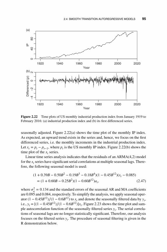
2.4 SMOOTH TRANSITION AUTOREGRESSIVE MODELS 95
1920 1940 1960 1980 2000 2020
040
80
Year
IP
1920 1940 1960 1980 2000 2020
−4
−2
02
Year
Diff
eren
ced
(p)
(a)
(b)
Figure 2.22 Time plots of US monthly industrial production index from January 1919 toFebruary 2016: (a) industrial production index and (b) its first differenced series.
seasonally adjusted. Figure 2.22(a) shows the time plot of the monthly IP index.As expected, an upward trend exists in the series and, hence, we focus on the firstdifferenced series, i.e. the monthly increments in the industrial production index.Let xt = pt − pt−1, where pt is the US monthly IP index. Figure 2.22(b) shows thetime plot of the xt series.
Linear time series analysis indicates that the residuals of an ARMA(4,2) modelfor the xt series have significant serial correlations at multiple seasonal lags. There-fore, the following seasonal model is used:
(1 + 0.39B − 0.50B2 − 0.19B3 − 0.18B4)(1 − 0.45B12)(xt − 0.085)
= (1 + 0.60B − 0.25B2)(1 − 0.60B12)at, (2.47)
where 𝜎2a = 0.134 and the standard errors of the seasonal AR and MA coefficients
are 0.095 and 0.084, respectively. To simplify the analysis, we apply seasonal oper-ator (1 − 0.45B12)∕(1 − 0.6B12) to xt and denote the seasonally filtered data by yt,i.e., yt = [(1 − 0.45B12)∕(1 − 0.6B12)]xt. Figure 2.23 shows the time plot and sam-ple autocorrelation function of the seasonally filtered series yt. The serial correla-tions of seasonal lags are no longer statistically significant. Therefore, our analysisfocuses on the filtered series yt. The procedure of seasonal filtering is given in theR demonstration below.
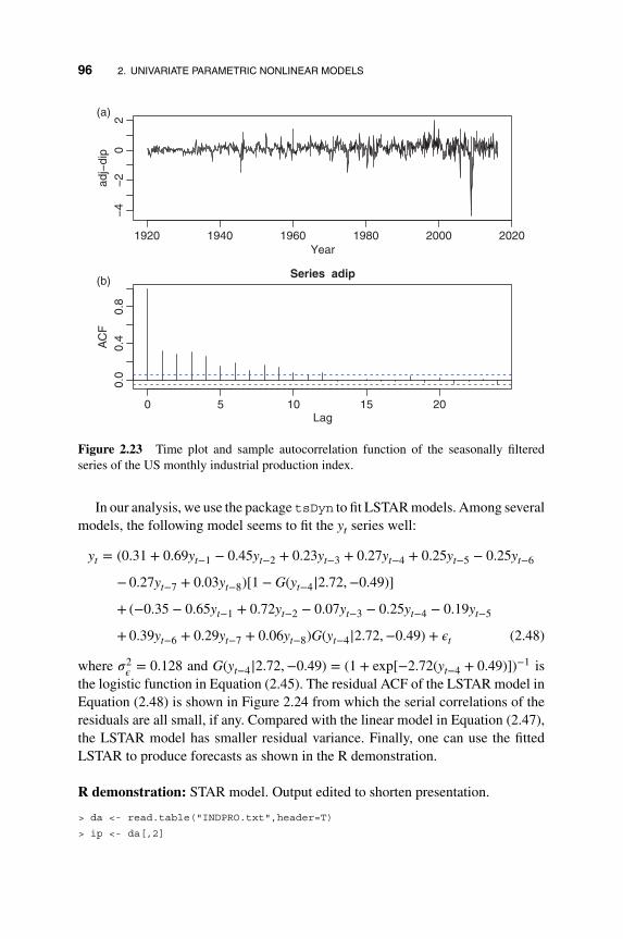
96 2. UNIVARIATE PARAMETRIC NONLINEAR MODELS
1920 1940 1960 1980 2000 2020
−4
−2
02
Year
adj−
dip
0 5 10 15 20
0.0
0.4
0.8
Lag
AC
F
Series adip
(a)
(b)
Figure 2.23 Time plot and sample autocorrelation function of the seasonally filteredseries of the US monthly industrial production index.
In our analysis, we use the package tsDyn to fit LSTAR models. Among severalmodels, the following model seems to fit the yt series well:
yt = (0.31 + 0.69yt−1 − 0.45yt−2 + 0.23yt−3 + 0.27yt−4 + 0.25yt−5 − 0.25yt−6
− 0.27yt−7 + 0.03yt−8)[1 − G(yt−4|2.72,−0.49)]
+ (−0.35 − 0.65yt−1 + 0.72yt−2 − 0.07yt−3 − 0.25yt−4 − 0.19yt−5
+ 0.39yt−6 + 0.29yt−7 + 0.06yt−8)G(yt−4|2.72,−0.49) + 𝜖t (2.48)
where 𝜎2𝜖 = 0.128 and G(yt−4|2.72,−0.49) = (1 + exp[−2.72(yt−4 + 0.49)])−1 is
the logistic function in Equation (2.45). The residual ACF of the LSTAR model inEquation (2.48) is shown in Figure 2.24 from which the serial correlations of theresiduals are all small, if any. Compared with the linear model in Equation (2.47),the LSTAR model has smaller residual variance. Finally, one can use the fittedLSTAR to produce forecasts as shown in the R demonstration.
R demonstration: STAR model. Output edited to shorten presentation.
> da <- read.table("INDPRO.txt",header=T)
> ip <- da[,2]

2.4 SMOOTH TRANSITION AUTOREGRESSIVE MODELS 97
0 5 10 15 20 25 30
0.0
0.2
0.4
0.6
0.8
1.0
Lag
AC
FLSTAR
Figure 2.24 Residual autocorrelation function of the LSTAR model in Equation (2.48)for the seasonally filtered series of the US monthly industrial production index.
> dip <- diff(ip)
> tdx <- c(1:nrow(da))/12+1919
> par(mfcol=c(2,1))
> plot(tdx,ip,xlab="year",ylab='ip',type='l')
> plot(tdx[-1],dip,xlab="year",ylab='diff(ip)',type='l')
> m4<- arima(dip,order=c(4,0,2),seasonal=list(order=c(1,0,1),period=12))
> m4
Call:arima(x=dip,order=c(4,0,2),seasonal=list(order=c(1,0,1),period=12))
Coefficients:
ar1 ar2 ar3 ar4 ma1 ma2 sar1 sma1
-0.3982 0.4951 0.1925 0.1813 0.6016 -0.2501 0.4517 -0.6033
s.e. 0.1210 0.1040 0.0625 0.0420 0.1228 0.1251 0.0949 0.0836
intercept
0.0848
s.e. 0.0199
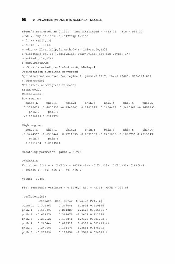
98 2. UNIVARIATE PARAMETRIC NONLINEAR MODELS
sigmaˆ2 estimated as 0.1341: log likelihood = -483.16, aic = 986.32
> wt <- dip[13:1165]-0.4517*dip[1:1153]
> f1 <- rep(0,12)
> f1[12] <- .6033
> adip <- filter(adip,f1,method="r",ini=rep(0,12))
> plot(tdx[-c(1:13)],adip,xlab='year',ylab='adj-dip',type='l')
> acf(adip,lag=24)
> require(tsDyn)
> n5 <- lstar(adip,m=8,mL=8,mH=8,thDelay=4)
Optimization algorithm converged
Optimized values fixed for regime 2: gamma=2.7217, th=-0.48605; SSE=147.069
> summary(n5)
Non linear autoregressive model
LSTAR model
Coefficients:
Low regime:
const.L phiL.1 phiL.2 phiL.3 phiL.4 phiL.5 phiL.6
0.3115624 0.6870931 -0.4545742 0.2301197 0.2654436 0.2460963 -0.2653893
phiL.7 phiL.8
-0.2528939 0.0281774
High regime:
const.H phiH.1 phiH.2 phiH.3 phiH.4 phiH.5 phiH.6
-0.3474566 -0.6539442 0.7211033 -0.0691959 -0.2485699 -0.1878756 0.2913649
phiH.7 phiH.8
0.3911484 0.0579544
Smoothing parameter: gamma = 2.722
Threshold
Variable: Z(t) = + (0)X(t) + (0)X(t-1)+ (0)X(t-2)+ (0)X(t-3)+ (1)X(t-4)
+ (0)X(t-5)+ (0) X(t-6)+ (0) X(t-7)
Value: -0.486
Fit: residuals variance = 0.1276, AIC = -2334, MAPE = 339.8%
Coefficient(s):
Estimate Std. Error t value Pr(>|z|)
const.L 0.311562 0.249085 1.2508 0.210996
phiL.1 0.687093 0.284827 2.4123 0.015851 *
phiL.2 -0.454574 0.364479 -1.2472 0.212328
phiL.3 0.230120 0.132841 1.7323 0.083222 .
phiL.4 0.265444 0.087511 3.0333 0.002419 **
phiL.5 0.246096 0.181475 1.3561 0.175072
phiL.6 -0.252894 0.112054 -2.2569 0.024015 *

2.5 TIME-VARYING COEFFICIENT MODELS 99
phiL.7 -0.265389 0.117760 -2.2536 0.024219 *
phiL.8 0.028177 0.082941 0.3397 0.734060
const.H -0.347457 0.312239 -1.1128 0.265799
phiH.1 -0.653944 0.330864 -1.9765 0.048101 *
phiH.2 0.721103 0.396752 1.8175 0.069138 .
phiH.3 -0.069196 0.163429 -0.4234 0.672003
phiH.4 -0.248570 0.136231 -1.8246 0.068058 .
phiH.5 -0.187876 0.185756 -1.0114 0.311820
phiH.6 0.391148 0.131696 2.9701 0.002977 **
phiH.7 0.291365 0.129243 2.2544 0.024171 *
phiH.8 0.057954 0.110205 0.5259 0.598974
gamma 2.721685 1.622500 1.6775 0.093452 .
th -0.486046 0.306333 -1.5867 0.112590
Non-linearity test of full-order LSTAR model against full-order AR model
F = 6.8874 ; p-value = 7.0957e-09
> predict(n5,n.ahead=5)
Time Series:
Start = 1166
End = 1170
Frequency = 1
[1] 0.030077216 0.014749998 0.113773221 0.003575012 0.139365484
2.5 TIME-VARYING COEFFICIENT MODELS
Time-varying coefficient (TVC) models are perhaps the most commonly usedmodels when weak stationarity conditions or linearity conditions become ques-tionable. They are nonlinear and flexible. As a matter of fact, the way in whichthe coefficients evolve over time plays a critical role in determining properties ofTVC models. In this section we introduce some simple TVC models, discuss theirproperties, and demonstrate their applications.
2.5.1 Functional Coefficient AR Models
Let St denote a random vector observable at time t. In practice, St is expected to berelated to xt and often includes lagged values of xt. A general functional coefficientautoregressive (FAR) model can be written as
xt = 𝜙0(St) +p∑𝑖=1
𝜙𝑖(St)xt−𝑖 + 𝜖t, (2.49)
where 𝜙𝑖(St) is a smooth function of St for 𝑖 = 0, 1,… , p and {𝜖t} is a sequence ofiid random variables with mean zero and variance 𝜎2. See Chen and Tsay (1993).

100 2. UNIVARIATE PARAMETRIC NONLINEAR MODELS
This model contains several nonlinear models available in the literature as specialcases. For instance, if 𝜙𝑖(St) = a𝑖 + b𝑖 exp(−c𝑖x
2t−d), then the model becomes the
exponential autoregressive model of Haggan and Ozaki (1981), where a𝑖, b𝑖 andc𝑖 are constants. In addition, if 𝜙𝑖(St) = 𝜙𝑖,1I(xt−d ≤ c) + 𝜙𝑖,2I(xt−d > c), then themodel reduces to a TAR model, where I(s) denotes the indicator variable for thestatement s. The model itself is a special case of the state-dependent models ofPriestley (1980), in which St is the state vector at time t.
Some probabilistic properties of the FAR models in Equation (2.49) have beenstudied by Chen and Tsay (1993). For instance, if |𝜙𝑖(St)| ≤ c𝑖 for 𝑖 = 0,… , p,where c𝑖 is a constant, and the probability density function of 𝜖t is positive every-where on the real line R1, then the FAR process xt in Equation (2.49) is geometri-cally ergodic provided that all the roots of the characteristic function
𝜆p − c1𝜆p−1 −⋯ − cp−1𝜆 − cp = 0
are inside the unit circle. Furthermore, if 𝜙𝑖(St) = g𝑖(St) + h𝑖(St) such that bothg𝑖(⋅) and h𝑖(⋅) are bounded functions with |g𝑖(⋅)| < c𝑖 and h𝑖(St)x𝑖 is uniformlybounded, then the aforementioned conditions also imply the geometric ergodicityof the FAR process in Equation (2.49). See Theorems 1.1 and 1.2 of Chen andTsay (1993). Cai et al. (2000) studied functional-coefficient regression models fornonlinear time series.
FAR are flexible, and the final model used often depends on the domain knowl-edge of the series under study or prior experience of the analyst. Example 1.3 ofChapter 1 shows that a simple FAR model fares better in transfer function mod-eling. In this section, we use the filtered monthly industrial production index ofExample 2.5 to demonstrate the applicability of FAR models.
Example 2.6 Consider again the monthly US industrial production index fromJanuary 1919 to February 2016. Similar to Example 2.5, we use the seasonallyfiltered series yt to remove the seasonality remaining in the data. In this particularinstance of FAR modeling, we use two possible choices of St. In the first case, weuse St = yt−1 and assume that
𝜙𝑖(St) = 𝜙𝑖(yt−1) = 𝛽𝑖 + 𝛾𝑖yt−1,
where 𝛽𝑖 and 𝛾𝑖 are constant parameters. The AIC criterion selects an AR(9) modelfor yt, and, hence, our modeling begins with a FAR model of order 9. However,estimation results show that the parameter estimates associated with yt−9 are sta-tistically insignificant and we arrive at the model
yt = 0.05 + 0.22yt−1 + (0.12 + 0.09yt−1)yt−2 + (0.18 − 0.12yt−1)yt−3
+ (0.04 − 0.16yt−1)yt−4 + (0.07 + 0.06yt−1)yt−6 − (0.07 − 0.16yt−1)yt−7
+ (0.08 − 0.20yt−1)yt−8 + 𝜖t (2.50)

2.5 TIME-VARYING COEFFICIENT MODELS 101
Residuals of FAR model
Time
Res
idua
ls
0 200 400 600 800 1000
−4
−2
01
2
0 5 10 15 20 25 30
0.0
0.4
0.8
Lag
AC
F
ACF
(a)
(b)
Figure 2.25 Time plot and sample autocorrelation function of the residuals of thefunctional-coefficient model in Equation (2.50).
where �� = 0.3613 and all coefficient estimates, but 0.04 of yt−4 and 0.06 ofyt−1yt−6, are statistically significant at the 5% level. Figure 2.25 shows thetime plot and sample autocorrelation function of the residuals of the model inEquation (2.50). From the plot, the residuals have no significant serial correlations.In fact, the Ljung–Box statistics show Q(24) = 31.02 with p value approximately0.15.
In the second case, we use St = yt−4 as suggested by the LSTAR model of theprior section and assume that
𝜙𝑖(St) = 𝜙𝑖(yt−4) = 𝛽𝑖 + 𝛾𝑖yt−4.
After removing insignificant parameter estimates, we obtain the model
yt = 0.05 + (0.18 − 0.24yt−4)yt−1 + (0.13 + 0.16yt−4)yt−2
+ (0.16 − 0.12yt−4)yt−3 + 0.07yt−4 + 0.06yt−6 − (0.05 − 0.12yt−4)yt−7
+ 0.06yt−8 + 𝜖t (2.51)
where �� = 0.3618 and all coefficients are statistically significant at the 5% levelexcept for the coefficient −0.05 of yt−7, which has a p value of 0.072. Residualseries of the model in Equation (2.51) are similar to those of the model in Equation

102 2. UNIVARIATE PARAMETRIC NONLINEAR MODELS
(2.50) and have no serial correlations. For instance, the Ljung–Box statistics showQ(24) = 29.08 with p value 0.22.
The fitted FAR models in Equations (2.50) and (2.51) belong to bilinear autore-gressive models or quadratic AR models. They can be fitted by the command lm
of the linear model in R provided that the regressors are properly formed. Detailsare given in the R demonstration. The two fitted FAR models are close to eachother. They demonstrate the flexibility of FAR models. To compare the two fittedmodels, we can use cross-validation because the models can be casted in the linearmodel framework. For a given model and iteration, the cross-validation procedureis as follows:
1. Select a random subsample from the design matrix, without replacement.
2. Refit the model using the selected subsample.
3. Use the fitted model to predict the remaining data and compute the forecasterrors.
4. Compute the root mean squares of forecast errors (RMSE) and the meanabsolute forecast errors (MAE).
Repeat the prior procedure for many iterations, and compute the averages ofRMSE and MAE over the iterations for model comparison.
For the monthly industrial production data, the cross-validation slightly prefersthe FAR model in Equation (2.50). Details are given in the R demonstration.
R demonstration: FAR models. Output edited.
da=read.table("INDPRO.txt",header=T)
xt <- diff(da$VALUE)
wt <- xt[13:length(xt)]-0.4517*xt[1:(length(xt)-12)]
f1 <- rep(0,12); f1[12]=0.6033
yt <- filter(wt,f1,method="r",ini=rep(0,12))
ist <- 9; nT <- length(yt)
y <- yt[ist:nT]; X <- NULL
for (i in 1:8){
X <- cbind(X,yt[(ist-i):(nT-i)])}
colnames(X) <- paste(“lag'',1:8,sep=“'')
Z <- model.matrix(y˜lag1*(lag2+lag3+lag4+lag6+lag7+lag8),data=data.frame(X))
m1 <- lm(y˜-1+Z)
summary(m1)
Call: lm(formula = y ˜ -1 + Z)
Coefficients:
Estimate Std. Error t value Pr(>|t|)
Z(Intercept) 0.05058 0.01258 4.021 6.18e-05 ***
Zlag1 0.22153 0.03157 7.016 3.92e-12 ***

2.5 TIME-VARYING COEFFICIENT MODELS 103
Zlag2 0.11574 0.03137 3.689 0.000236 ***
Zlag3 0.18077 0.02997 6.032 2.19e-09 ***
Zlag4 0.04270 0.03127 1.366 0.172360
Zlag6 0.06628 0.03021 2.193 0.028476 *
Zlag7 -0.07221 0.02979 -2.424 0.015520 *
Zlag8 0.08205 0.02975 2.758 0.005917 **
Zlag1:lag2 0.09464 0.03879 2.440 0.014856 *
Zlag1:lag3 -0.12200 0.04488 -2.719 0.006658 **
Zlag1:lag4 -0.15602 0.03090 -5.050 5.15e-07 ***
Zlag1:lag6 0.05693 0.05841 0.975 0.329944
Zlag1:lag7 0.15932 0.04988 3.194 0.001441 **
Zlag1:lag8 -0.19915 0.05522 -3.607 0.000324 ***
Residual standard error: 0.3613 on 1131 degrees of freedom
Multiple R-squared: 0.2855, Adjusted R-squared: 0.2767
F-statistic: 32.28 on 14 and 1131 DF, p-value: < 2.2e-16
Box.test(m1$residuals,lag=24,type="Ljung")
Box-Ljung test
data: m1$residuals
X-squared = 31.201, df = 24, p-value = 0.1481
### Model comparison
> m1f <- cvlm(y,Z,subsize=1000,iter=300)
Average RMSE: 0.1405556 Average MAE: 0.2469571
> m1f <- cvlm(y,Z,subsize=1000,iter=500)
Average RMSE: 0.1389267 Average MAE: 0.2464725
> m1f <- cvlm(y,Z,subsize=1000,iter=1000)
Average RMSE: 0.1386875 Average MAE: 0.2470499
##
Z<-model.matrix(y˜lag6+lag8+lag4*(lag1+lag2+lag3+lag7),data=data.frame(X))
m2 <- lm(y˜-1+Z)
summary(m2)
Call: lm(formula = y ˜ -1 + Z)
Coefficients:
Estimate Std. Error t value Pr(>|t|)
Z(Intercept) 0.05250 0.01259 4.170 3.28e-05 ***
Zlag6 0.06115 0.02981 2.052 0.040421 *
Zlag8 0.05909 0.02902 2.036 0.041960 *
Zlag4 0.06998 0.03162 2.213 0.027104 *
Zlag1 0.17990 0.02899 6.206 7.62e-10 ***
Zlag2 0.12606 0.02940 4.287 1.96e-05 ***
Zlag3 0.16464 0.03155 5.218 2.15e-07 ***
Zlag7 -0.05460 0.03031 -1.801 0.071906 .
Zlag4:lag1 -0.24395 0.03566 -6.841 1.29e-11 ***
Zlag4:lag2 0.15998 0.04772 3.353 0.000827 ***
Zlag4:lag3 -0.11864 0.03743 -3.169 0.001569 **
Zlag4:lag7 0.12208 0.03289 3.712 0.000216 ***

104 2. UNIVARIATE PARAMETRIC NONLINEAR MODELS
Residual standard error: 0.3618 on 1133 degrees of freedom
Multiple R-squared: 0.2821, Adjusted R-squared: 0.2745
Box.test(m2$residuals,lag=24,type="Ljung")
Box-Ljung test
data: m2$residuals
X-squared = 29.079, df = 24, p-value = 0.2172
> m2f <- cvlm(y,Z,subsize=1000,iter=300)
Average RMSE: 0.145679 Average MAE: 0.2506342
> m2f <- cvlm(y,Z,subsize=1000,iter=500)
Average RMSE: 0.1438586 Average MAE: 0.2492642
> m2f <- cvlm(y,Z,subsize=1000,iter=1000)
Average RMSE: 0.1423353 Average MAE: 0.2491681
2.5.2 Time-varying Coefficient AR Models
A time-varying coefficient AR (tvAR) model can be written as
xt = 𝜙0,t +p∑𝑖=1
𝜙𝑖,txt−𝑖 + 𝜖t, (2.52)
where 𝜙j,t, for j = 0,… , p, are random variables and {𝜖t} is a sequence of iidrandom variables with mean zero and variance 𝜎2, and {𝜙j,t} are independent of𝜖t. There are many ways to specify the time evolution of the random coefficients𝜙j,t, resulting in various tvAR models. In this section we assume that each {𝜙j,t}process follows a random-walk model and {𝜙j,t} and {𝜙k,t} are mutually indepen-dent if j ≠ k. The independence assumption between 𝜙𝑖t is for simplicity. It can berelaxed at the expense of increased complexity in estimation.
A simple way to understand the tvAR model is to cast it in a state space model.Specifically, let 𝝓t = (𝜙0,t,𝜙1t,… ,𝜙pt)
′ be the (p + 1)-dimensional vector of ran-dom coefficients at time t, and Ft = (1, xt−1,… , xt−p) be a (p + 1)-dimensionalrow vector of regressors. Then, we have
xt = Ft𝝓t + 𝜖t, (2.53)
𝝓t = G𝝓t−1 + wt, (2.54)
where G is the (p + 1)-dimensional identify matrix, {𝜖t} are iid N(0, 𝜎2), wt =(w0t, w1t,… , wpt)
′ is a (p + 1)-dimensional random vector such that {wt} formsa sequence of iid Gaussian random vectors with E(wt) = 0 and cov(wt) = W =diag{𝜎2
𝑖𝑖|𝑖 = 0,… , p}, a diagonal matrix. Clearly, the variance 𝜎2
𝑖𝑖controls the
variability of the coefficient 𝜙𝑖t. In particular, 𝜙𝑖t reduces to a constant if 𝜎𝑖𝑖 = 0.Kitagawa (2010, Chapter 13) provides a good introduction of the tvAR models viathe state space model representation.

2.5 TIME-VARYING COEFFICIENT MODELS 105
Equation (2.53) is refereed to as the observation equation and Equation (2.54)is the state transition equation with 𝝓t being the state vector. The noise 𝜖t becomesthe observational noise and wt is the state transition noise. The initial state 𝝓0 isa random vector with mean 𝝓∗ and covariance matrix 𝚺𝜙. Both 𝝓∗ and 𝚺𝜙 areassumed to be known. In this section, we let 𝝓∗ be the least squares estimates ofthe coefficients of a linear AR(p) model and 𝚺𝜙 an arbitrary diagonal matrix. Theunknown parameters of the state space model in Equations (2.53) and (2.54) are 𝜎2
and the diagonal elements of W. In application, these parameters can be estimatedby the maximum likelihood method. Inference concerning the time-varying coef-ficients 𝝓t can be obtained by filtering and smoothing of state space model. Morespecifically, inference of the model can be obtained via the well-known Kalmanfilter. For further information on the state space model, see Tsay (2010, Chapter11) and Chapter 6.
A useful special case of the tvAR model is the local level model given by
xt = 𝜙t + 𝜖t, 𝜖t ∼𝑖𝑖d N(0, 𝜎2𝜖 ) (2.55)
𝜙t = 𝜙t−1 + wt, wt ∼𝑖𝑖d N(0, 𝜎2w). (2.56)
Here Ft = 1 and G = 1, and we have E(xt ∣ t−1) = 𝜙t−1, where t−1 denotesthe information available at time t − 1. Therefore, the conditional mean of xt fol-lows a random walk. The model is also known as an exponential smoothing modelbecause xt follows an autoregressive integrated moving-average of order (0,1,1)model, i.e. ARIMA(0,1,1). See Tsay (2010, Chapter 11).
Remark: The R package dlm can be used to estimate the tvAR model discussedin this section. The command tvAR of the NTS package makes use of functions ofthe dlm package to perform parameter estimation of the tvAR model. The com-mand tvARFiSm also uses the dlm package to perform filtering and smoothing ofthe state variables. In the tvAR command, variance parameters are parameterizedin log scale.
Example 2.7 Consider the daily realized volatility of Alcoa stock from January2, 2003 to May 7, 2004 for 340 observations. The realized volatility is obtainedby using intraday 10-minute log returns, and the data have been used in Example11.1 of Tsay (2010). Let xt denote the logarithm of the realized volatility. Figure2.26 shows the time plot of xt (most variable line). In this particular instance, theinitial state𝜙0 is assumed to have E(𝜙0) = 𝜇 and cov(𝜙0) = exp(1). The maximumlikelihood estimates of 𝜎𝜖 and 𝜎w are 0.48 and 0.074, respectively. As expected,these estimates are close to the values shown in Example 11.1 of Tsay (2010,Chapter11). Figure 2.26 also shows the filtered and smoothed state 𝜙t of the fitted

106 2. UNIVARIATE PARAMETRIC NONLINEAR MODELS
0 50 100 150 200 250 300 350
−1
01
23
Time
log(
rv)
Figure 2.26 Time plot, filtered (medium variability), and smoothed (smooth line) statesof the realized volatility of Alcoa stock.
model. From the plots, the tvAR model describes adequately the movement of therealized volatility.
Example 2.8 Consider again the filtered series of the US monthly industrialproduction index (see Example 2.6). For simplicity, we use a tvAR(4) model inEquation (2.52) for the series yt. Here 𝝓t is a five-dimensional state vector andFt = (1, yt−1,… , yt−4); see the state space model in Equations (2.53) and (2.54).Here the mean of the initial state 𝝓0 consists of the coefficient estimates of theAR(4) model and the covariance matrix of 𝝓0 is a diagonal matrix with elementsexp(1). The parameter estimates are �� = 0.298 and ��𝑖𝑖 = 0.025, 0.249, 0.005,0.006, and 0.042, respectively, for 𝑖 = 0,… , 4. From the estimates, it is seen thatthe coefficient of xt−1 varies markedly over time. Figure 2.27 shows the time plotsof the filtered states whereas Figure 2.28 shows the time plots of the smoothed statevariables. In both plots, the upper panel shows 𝜙0t and 𝜙1t of the states whereasthe lower panel shows 𝜙2t to 𝜙4t of the states. Figure 2.29 shows the time plot ofthe one-step ahead predicted residuals of the fitted tvAR(4) model. Except for alarge outlying value, the predicted residuals look reasonable.

2.5 TIME-VARYING COEFFICIENT MODELS 107
**********************************************************************************************************************************************************************************************************************************************************************************************************************************************************************************************************************************************************************************************************************************************************************************************************************************************************************************************************************************************************************************************************************************************************************************************************************************************************************************************************************************************************************************************
************************************************************************************************************
1920 1940 1960 1980 2000 2020
−1
01
2
Year
Coe
ffici
ents
****************************************************************************************************************************************************************************************************************************************************************************************************
*********************************************************************************************************************************************************************************************************************************************************************************************************************************************************************************************************************************************************************************************************************************************************************************************************************************************************
*********************************************************************************************************************************************************************************************************************************************
1920 1940 1960 1980 2000 2020
−1
01
2
Year
Coe
ffici
ents
(a)
(b)
Figure 2.27 Filtered state variables of a tvAR(4) model for the filtered US monthly indus-trial production index. (a) 𝜙0t (bold) and 𝜙1t, and (b) 𝜙2t (bold), 𝜙3t (line), and 𝜙4t.
**********************************************************************************************************************************************************************************************************************************************************************************************************************************************************************************************************************************************************************************************************************************************************************************************************************************************************************************************************************************************************************************************************************************************************************************************************************************************************************************************************************************************************************************************************************************************************************************************************
1920 1940 1960 1980 2000 2020
−0.
50.
51.
5
Year
Coe
ffici
ents
(a)
(b)
Figure 2.28 Smoothed state variables of a tvAR(4) model for the filtered US monthlyindustrial production index. (a) 𝜙0t (bold) and 𝜙1t, and (b) 𝜙2t (bold), 𝜙3t (line), and 𝜙4t.

108 2. UNIVARIATE PARAMETRIC NONLINEAR MODELS
1920 1940 1960 1980 2000
05
10
Year
Pre
dict
ed r
esid
uals
Figure 2.29 Time plot of filtered residuals of a tvAR(4) model for the US monthly indus-trial production index.
R demonstration: Time-varying AR models. Output edited.
> require(NTS); require(dlm)
> da <- read.table("aa-3rv.txt") ## Example 7
> xt <- log(da[,2])
> m1 <- tvAR(xt,lags=NULL)
par: -1.467084 -5.219068
> sqrt(exp(m1$par))
[1] 0.48020505 0.07356883
> m1k <- tvARFiSm(xt,lags=NULL,par=m1$par)
> fil <- m1k$filter; sm <- m1k$smooth
> plot(xt,xlab='time',ylab='log(rv)',type='l')
> lines(fil$m,col="blue"); lines(sm$s,col="red")
###
> adip <- scan("m-adip.txt")
> mk <- tvAR(adip,lags=c(1:4))
par: -2.419878 -7.369506 -2.779889 -10.71095 -10.26296 -6.325027

2.5 TIME-VARYING COEFFICIENT MODELS 109
> sqrt(exp(mk$par))
[1] 0.298215 0.025103 0.24909 0.00472 0.00591 0.04232
> mkk <- tvARFiSm(adip,lags=c(1:4),par=mk$par)
> names(mkk)
[1] "filter" "smooth"
> filter <- mkk$filter; smooth <- mkk$smooth
> names(filter)
[1] "y" "mod" "m" "U.C" "D.C" "a" "U.R" "D.R" "f"
> resi <- adip[5:1153]-filter$f
> m <- filter$m; s <- smooth$s
> range(m)
[1] -1.265166 2.750762
> range(s)
[1] -0.7726883 1.5985201
> tdx <- c(2:1154)/12+1919
> tdx <- tdx[-c(1:3)]
> par(mfcol=c(2,1))
> plot(tdx,m[,1],xlab='year',ylab='coefs',ylim=c(-1.3,2.8),pch="*",cex=0.5)
> lines(tdx,m[,2],lty=1)
> plot(tdx,m[,3],xlab='year',ylab='coefs',ylim=c(-1.3,2.8),pch="*",cex=0.5)
> lines(tdx,m[,4])
> lines(tdx,m[,5],lty=2)
> plot(tdx,s[,1],xlab='year',ylab='coefs',ylim=c(-0.8,1.61),pch="*",cex=0.5)
> lines(tdx,s[,2],lty=1)
> plot(tdx,s[,3],xlab='year',ylab='coefs',ylim=c(-0.8,1.61),pch="*",cex=0.5)
> lines(tdx,s[,4])
> lines(tdx,s[,5],lty=2)
Remark: Consider the tvAR model in Equation (2.52). For simplicity, we assume𝜙0t = 0 for all t, that is, xt is mean-adjusted. If one assumes that each AR coeffi-cient 𝜙𝑖t follows a random distribution, e.g. 𝜙𝑖t ∼ N(𝜙𝑖, 𝜎
2𝑖𝑖
), and the distributionsare mutually independent, then the tvAR model reduces to a random-coefficientAR (RCA) model. In this particular case, let 𝜂𝑖t = 𝜙𝑖t − 𝜙𝑖 for 𝑖 = 1,… , p, thenthe model becomes
xt =p∑𝑖=1
𝜙𝑖xt−𝑖 + (xt−1,… , xt−p)𝜼t + 𝜖t,
where 𝜼t = (𝜂1t,… , 𝜂pt)′ is a random vector satisfying E(𝜼t) = 0 and cov(𝜼t) =
diag{𝜎2𝑖𝑖|𝑖 = 1,… , p}. Let t−1 denote the information available at time t − 1,
then we
E(xt ∣ t−1) =p∑𝑖=1
𝜙𝑖xt−𝑖, cov(xt ∣ t−1) = 𝜎2 +p∑𝑖=1
x2t−𝑖𝜎
2𝑖𝑖.
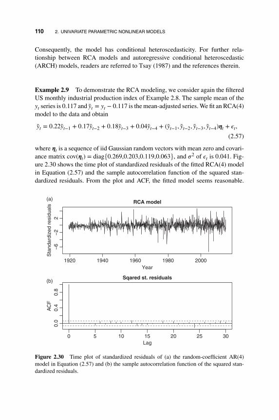
110 2. UNIVARIATE PARAMETRIC NONLINEAR MODELS
Consequently, the model has conditional heteroscedasticity. For further rela-tionship between RCA models and autoregressive conditional heteroscedastic(ARCH) models, readers are referred to Tsay (1987) and the references therein.
Example 2.9 To demonstrate the RCA modeling, we consider again the filteredUS monthly industrial production index of Example 2.8. The sample mean of theyt series is 0.117 and yt = yt − 0.117 is the mean-adjusted series. We fit an RCA(4)model to the data and obtain
yt = 0.22yt−1 + 0.17yt−2 + 0.18yt−3 + 0.04yt−4 + (yt−1, yt−2, yt−3, yt−4)𝜼t + 𝜖t,
(2.57)
where 𝜼t is a sequence of iid Gaussian random vectors with mean zero and covari-ance matrix cov(𝜼t) = diag{0.269,0.203,0.119,0.063}, and 𝜎2 of 𝜖t is 0.041. Fig-ure 2.30 shows the time plot of standardized residuals of the fitted RCA(4) modelin Equation (2.57) and the sample autocorrelation function of the squared stan-dardized residuals. From the plot and ACF, the fitted model seems reasonable.
1920 1940 1960 1980 2000
−6
−2
2
RCA model
Year
Sta
ndar
dize
d re
sidu
als
0 5 10 15 20 25 30
0.0
0.4
0.8
Lag
AC
F
Sqared st. residuals
(a)
(b)
Figure 2.30 Time plot of standardized residuals of (a) the random-coefficient AR(4)model in Equation (2.57) and (b) the sample autocorrelation function of the squared stan-dardized residuals.

2.6 APPENDIX: MARKOV CHAINS 111
In fact, the conditional heteroscedasticity is well modeled by the RCA(4) model.For instance, the Ljung–Box statistics of the squared standardized residuals showQ(12) = 6.61 with p value 0.88.
R demonstration: RCA model. Output edited.
> mm <- rcAR(adip,lags=c(1:4)) # NTS packageSample mean: 0.1166405Estimates:
est se.est tratioX1 0.2216 0.0379 5.8515X2 0.1653 0.0377 4.3801X3 0.1811 0.0354 5.1228X4 0.0441 0.0327 1.3476
-1.3136 0.1563 -8.4028-1.5962 0.2426 -6.5794-2.1289 0.3376 -6.3050-2.7627 0.4419 -6.2512-3.1882 0.1098 -29.0300
> names(mm)[1] "par" "se.est" "residuals" "sresiduals"> exp(mm$par[5:9])0.26885490 0.20265937 0.11896990 0.06312199 0.04124666> Box.test(mm$sresidualsˆ2,lag=12,type='Ljung')
Box-Ljung testdata: mm$sresidualsˆ2X-squared = 6.616, df = 12, p-value = 0.8819
2.6 APPENDIX: MARKOV CHAINS
In this appendix we briefly introduce some important concepts of Markov chains.The discussion is restricted to finite-state Markov chains {St, t = 1,…}, whereSt assumes values in a finite set. The concepts can easily be extended to generalspaces.
Let S = {s1, s2,… , sk} be a collection of k possible values. We refer to S as thestate space, and each element s𝑖 of S is called a state. Let P be a k × k real-valuedmatrix defined by
P =
⎡⎢⎢⎢⎢⎣p11 p12 p13 ⋯ p1k
p21 p22 p23 ⋯ p2k
⋮ ⋮ ⋮ ⋱ ⋮
pk1 pk2 pk3 ⋯ pkk
⎤⎥⎥⎥⎥⎦,

112 2. UNIVARIATE PARAMETRIC NONLINEAR MODELS
where p𝑖j ≥ 0 and∑k
j=1 p𝑖j = 1 for a fixed 𝑖. Consider a sequence of random vari-ables {S0, S1,…}, where S𝑖 assumes a value in the state space S with S0 being theinitial state. This sequence forms a Markov chain if the value of St+1 is determinedby the following transition equation
P(St+1 = sj ∣ S0 = 𝑖0,… , St−1 = 𝑖t−1, St = s𝑖) = P(St+1 = sj ∣ St = s𝑖) = p𝑖j,
where 𝑖j ∈ S for j = 0,… , t − 1. More precisely, such a sequence {St} is calleda (time-homogeneous) Markov chain with transition probability P on the statespace S. If k is finite, we have a finite-state Markov chain. From the definition,St+1 assumes a value in S according to the transition probability P and the value ofSt. The history {S0,… , St−1} plays no role in determining St+1 once St is given.This feature is referred to as the memorylessness of Markov chains. Since P isfixed, we have
P(St+2 = sj ∣ St = s𝑖) =k∑
v=1
P(St+1 = sv ∣ St = s𝑖)P(St+2 = sj ∣ St+1 = sv)
=k∑
v=1
p𝑖vpvj,
which is the (𝑖, j)th element of the matrix P2. This feature applies to any power ofthe matrix P with P0 = I, the k × k identity matrix. Following the literature, weuse th notation p(n)
𝑖j to denote the (𝑖, j)th element of Pn. Properties of the Markovchain are thus determined by the transition probability matrix P. For instance, weare often interested in knowing the stationary distribution of St as t → ∞ for agiven P.
Two important properties of Markov chains are irreducibility and aperiodicity.The key result is that an aperiodic and irreducible Markov chain has a stationarydistribution. See below for further details. The state sj is said to be accessiblefrom state s𝑖 if the chain started in state s𝑖 can transition into state sj in finite steps.Mathematically, state sj is accessible from state s𝑖 if there exists a nonnegativeinteger n, which may depend on s𝑖 and sj, such that
P(Sn = sj ∣ S0 = s𝑖) = p(n)𝑖j > 0.
We use the notation s𝑖 → sj to denote that sj is accessible from s𝑖. If s𝑖 → sj andsj → s𝑖 hold simultaneously, then s𝑖 and sj communicate with each other (denotedby s𝑖 ↔ sj). A subset C of S is a communicating class if every pair of states in Ccommunicates with each other. A communicating class C is said to be close if theprobability of leaving the class is zero. In other words, if C is close and s𝑖 ∈ C, butsj ∉ C, then sj is not accessible from s𝑖. A Markov chain is said to be irreducible if

2.6 APPENDIX: MARKOV CHAINS 113
its state space S forms a single communicating class. In other words, the Markovchain is irreducible if it is possible to get to any state sj from any state s𝑖.
The period 𝓁𝑖 of state s𝑖 of a Markov chain is defined as
𝓁𝑖 = gcd{n > 0 s.t. P(Sn = s𝑖 ∣ S0 = s𝑖) > 0}, (2.58)
where “gcd” stands for the greatest common divisor, provided that the set is notempty. The period 𝓁𝑖 is undefined if the set in Equation (2.58) is empty. Sincethe period 𝓁𝑖 is defined in term of gcd, state s𝑖 may not be reached in 𝓁𝑖 steps.For example, if s𝑖 appears in steps {4, 6, 8, 10, 12, 14, ⋯}, then we have 𝓁𝑖 = 2,but S2 did not assume the value s𝑖. The state s𝑖 is said to be aperiodic if 𝓁𝑖 = 1.A Markov chain is aperiodic if every state is aperiodic. An irreducible Markovchain only needs one state to be aperiodic to imply that it is aperiodic.
A state s𝑖 of a Markov chain is said to be an absorbing state if it is not possibleto leave s𝑖. Mathematically, we have p𝑖𝑖 = 1 and p𝑖j = 0 for 𝑖 ≠ j. If every state canreach an absorbing state, then the Markov chain is an absorbing chain.
A state s𝑖 is said to be transient if, given that the chain starts in state s𝑖, thereis a non-zero probability that the chain will never return to s𝑖. To be more precise,define the random variable
T𝑖 = inf{n ≥ 1 : Sn = s𝑖|S0 = s𝑖}
which is called the hitting time of state s𝑖. The quantity
h(n)𝑖𝑖
= P(T𝑖 = n)
is the probability that the chain returns to state s𝑖 for the first time after n steps.Then, state s𝑖 is transient if
P(T𝑖 < ∞) =∞∑
n=1
h(n)𝑖𝑖< 1.
A state s𝑖 is recurrent if it is not transient. If s𝑖 is recurrent, then P(T𝑖 < ∞) = 1so that it has a finite hitting time with probability 1. It can be shown that state s𝑖 isrecurrent if and only if
∞∑n=0
p(n)𝑖𝑖
= ∞.
Both transience and recurrence are class properties in the sense that every state ina communicating class either holds that property or does not hold that property.
The mean recurrence time of state s𝑖 is defined as
M𝑖 = E(T𝑖) =∞∑
n=1
nh(n)𝑖𝑖.
114 2. UNIVARIATE PARAMETRIC NONLINEAR MODELS
State s𝑖 is positive recurrent if M𝑖 is finite. Otherwise, s𝑖 is null recurrent.A state s𝑖 of a Markov chain is said to be ergodic if it is aperiodic and positive
recurrent. In other words, s𝑖 is ergodic if it is recurrent, has a period of 1, andhas a finite mean recurrence time. If all states in an irreducible Markov chain areergodic, then the chain is ergodic. It can be shown that a finite-state irreducibleMarkov chain is ergodic if it has an aperiodic state.
Consider a probability distribution 𝝅 = (𝜋1,… ,𝜋k) over the state space S.This distribution is called a stationary distribution of a Markov chain with time-invariant transition probability matrix P = [p𝑖j], if (a) 𝜋𝑖 ≥ 0, (b)
∑k𝑖=1 𝜋𝑖 = 1,
and (c)
𝜋j =k∑𝑖=1
𝜋𝑖p𝑖j, j = 1,… , k.
Treating 𝝅 as a row vector, the prior condition can be written as 𝝅 = 𝝅P. Thismeans that the stationary distribution of a Markov chain, if it exists, is a normalizedleft-eigenvector of the transition matrix P associated with eigenvalue 1. Of course,one can use
P′𝝅′ = 𝝅′
so that 𝝅′ is an eigenvector of the matrix P′ associated with unit eigenvalue.An irreducible Markov chain has a stationary distribution if and only if all of
its states are positive recurrent. In this case, 𝝅 is unique and is related to the meanexpected return time M𝑖 via
𝜋𝑖 =CM𝑖
,
where C is a normalization constant. Furthermore, if the positive recurrent chainis both irreducible and aperiodic, then it has a limiting distribution
limn→∞
p(n)v𝑖 = C
M𝑖
,
for any states s𝑖 and sj. For further information on Markov chains, see Karlin andTaylor (1975).
2.7 EXERCISES
Again, all tests use the 5% type-I error.
2.1 Use the following commands to simulate a two-regime TAR(1) model with400 observations.

EXERCISES 115
require(NTS)set.seed(1)phi < matrix(c(0.8,0.7),2,1)m1 < uTAR.sim(400,c(1,1),phi)xt < m1$series
(a) Obtain a time plot for the data and its sample autocorrelation functionwith 12 lags.
(b) Obtain a scatter plot of xt versus xt−1 and draw a smooth line on theplot using the loess local smoothing.
(c) Apply the threshold tests of Chapter 1 to confirm the threshold nonlin-earity of the time series.
(d) Finally, build a two-regime TAR model for the series and write downthe fitted model.
2.2 Consider the monthly mean duration of unemployment in the USA. The datawere seasonally adjusted from January 1948 to August 2017. They are avail-able from FRED and are also in the file Unempduration.csv. The meanduration shows an upward trend so let xt be the first difference of the originaldata.
(a) Build a linear AR model for xt. Write down the fitted model and performmodel checking.
(b) Perform the threshold tests of Chapter 1 to confirm that xt exhibitsthreshold nonlinearity.
(c) Use p = 5 and d ∈ {1,… , 5}, where d denotes the delay, to select thethreshold variable xt−d. You may use the p value of the threshold testto select d.
(d) Build a two-regime TAR(5) model for xt. Perform model checking andwrite down the fitted model.
(e) Compare the linear AR model and the TAR model.
2.3 Consider the monthly value-weighted SMALL-LoBM portfo-lio returns of Fama-French data, denoted by xt. See the web:mba.tuck.dartmonth.edu/pages/faculty/ken.french/data_library.html. Also,consider the monthly Fama-French three factors, also available from thesame web. Denote the factors by Mrk.RF, SMB, and HML, respectively.The data span is from July 1926 to July 2017 for 1903 observations. Seealso the files FF_Factors.csv and FF_6_Portfolios.csv.

116 2. UNIVARIATE PARAMETRIC NONLINEAR MODELS
(a) Fit the linear regression model:
xt = 𝛽0 + 𝛽1Mrk.RFt + 𝛽2SMBt + 𝛽3HMLt + 𝜖t.
Write down the model and perform model checking.
(b) Fit a two-state Markov switching model to the data and write down thefitted model.
(c) Compare the two fitted models in (a) and (b).
2.4 Again, consider the change series of the US monthly unemployment dura-tion from February 1948 to August 2017. Fit a two-state Markov switchingautoregressive model to the series. Perform model checking and write downthe fitted model. Compare the Markov switching model with the thresholdmodel built previously. Comment on the two models.
2.5 Again, consider the change series of the US monthly unemployment durationfrom February 1948 to August 2017. Fit a LSTAR model to the series. Per-form model checking and write down the fitted model. Use the fitted modelto produce one-step to five-step ahead predictions for xt at the forecast originAugust 2017.
2.6 Again, consider the change series of the US monthly unemployment durationfrom February 1948 to August 2017. Fit a time-varying coefficient AR modelto the data. Perform model checking and write down the fitted model. Plotthe filtered and smooth state variables.
REFERENCES
Akaike, H. (1974). A new look at the statistical model identification. IEEE Transactions onAutomatic Control AC-19: 716–723.
Cai, Z., Fan, J., and Yao, Q. (2000). Functional-coefficient regression models for nonlineartime series. Journal of the American Statistical Association 95: 941–956.
Cappe, Q., Moulines, E., and Ryden, T. (2005). Inference in Hidden Markov Models.Springer Series in Statistics. Springer, New York.
Chan, K. S. (1993). Consistency and limiting distribution of the least squares estimator ofa threshold autoregressive model. The Annals of Statistics 21: 520–533.
Chan, K. S. and Tsay, R. S. (1998). Limiting properties of the conditional least squaresestimator of a continuous TAR model. Biometrika 85: 413–426.
Chen, R. and Tsay, R. S. (1991). On the ergodicity of TAR(1) processes. Annals of AppliedProbability 1: 613–634.
Chen, R. and Tsay, R. S. (1993). Functional-coefficient autoregressive models. Journal ofthe American Statistical Association 88: 298–308.

REFERENCES 117
Chib, S. (1996). Calculating posterior distributions and modal estimates in Markov mixturemodels. Journal of Econometrics 75: 79–97.
Francq, C. and Zakoian, J. (2001). Stationarity of multivariate Markov switching ARMAmodels. Journal of Econometrics 102: 339–364.
Fruhwirth-Schnatter, S. (2006). Finite Mixture and Markov Switching Models. Springer,New York.
Haggan, V. and Ozaki, T. (1981). Modeling nonlinear vibrations using an amplitude-dependent autoregressive time series model. Biometrika 68: 189–196.
Hamilton, J. D. (1989). A new approach to the economic analysis of nonstationary timeseries and the business cycle. Econometrica 57: 357–384.
Hamilton, J. D. (1990). Analysis of time series subject to changes in regime. Journal ofEconometrics 45: 39–70.
Hamilton, J. D. (1994). Time Series Analysis. Princeton University Press, Princeton, NJ.
Holst, U., Lindgren, G., Holst, J., and Thuvesholmen, M. (1994). Recursive estimation inswitching autoregressions with a Markov regime. Journal of Time Series Analysis 15:489–506.
Hyndman, R. J. (2016). Time Series Data Library. http://data.is/TSDLdemo. AccessedMarch, 2016.
Karlin, S. and Taylor, H. M. (1975). A First Course in Stochastic Processes, 2nd edition.Academic Press, San Diego.
Kitagawa, G. (2010). Introduction to Time Series Modeling. CRC Press, Chapman and Hall,Boca Raton, FL.
Krolzig, H. M. (1997). Markov Switching Vector Autoregressions: Modeling, StatisticalInference, and Applications to Business Cycle Analysis. Lecture Notes in Economicsand Mathematical Systems. Springer, New York.
Ling, S. and Tong, H. (2005). Testing for a linear MA model against threshold MA models.Annals of Statistics 33: 2529–2552.
McCulloch, R. E. and Tsay, R. S. (1994). Statistical inference of macroeconomic time seriesvia Markov switching models. Journal of Time Series Analysis 15: 523–539.
Meyn, S. and Tweedie, R. (2009). Markov Chains and Stochastic Stability, 2nd edition.Cambridge University Press, Cambridge.
Neftci, S. N. (1984). Are economic time series asymmetric over the business cycles? Jour-nal of Political Economy 92: 307–328.
Petruccelli, J. and Woolford, S. W. (1984). A threshold AR(1) model. Journal of AppliedProbability 21: 270–286.
Priestley, M. B. (1980). State-dependent models: a general approach to nonlinear time seriesanalysis. Journal of Time Series Analysis 1: 47–71.
Terasvirta, T. (1994). Specification, estimation, and evaluation of smooth transition autore-gressive models. Journal of the American Statistical Association 89: 208–218.
Timmermann, A. (2000). Moments of Markov switching models. Journal of Economet-rics 96: 75–111.

118 2. UNIVARIATE PARAMETRIC NONLINEAR MODELS
Tong, H. (1978). On a threshold model. In C.H. Chen (ed.), Pattern Recognition and SignalProcessing. Sijhoff & Noordhoff, Amsterdam.
Tong, H. (1990). Non-Linear Time Series: A Dynamical System Approach. Oxford Univer-sity Press, Oxford.
Tong, H. and Lim, K. S. (1980). Threshold autoregression,limit cycles and cyclical data(with discussion). Journal of the Royal Statistical Society, Series B 42: 245–292.
Tsay, R. S. (1987). Conditional heteroscedastic time series models. Processes. Journal ofthe American Statistical Association 82: 590–604.
Tsay, R. S. (1989). Testing and modeling threshold autoregressive processes. Journal of theAmerican Statistical Association 84: 231–240.
Tsay, R. S. (1998). Testing and modeling multivariate threshold models. Journal of theAmerican Statistical Association 93: 1188–1202.
Tsay, R. S. (2010). Analysis of Financial Time Series, 3rd edition. John Wiley, Hoboken,NJ.
Van Dijk, D., Terasvirta, T., and Frances, F. P. (2002). Smooth transition autoregressivemodels: a survey of recent developments. Econometric Reviews 21: 1–47.
Wu, S. and Chen, R. (2007) Threshold variable selection and threshold variable drivenswitching autoregressive models. Statistica Sinica 17: 241–264.
Yao, J. and Attali, J. (2000). On stability of nonlinear AR processes with Markov switching.Advances in Applied Probabilities 32: 394–407.

CHAPTER 3
UNIVARIATE NONPARAMETRICMODELS
In this chapter we introduce nonparametric modeling of univariate time series. Westart with kernel smoothing, local polynomial methods, B-splines, and smoothingsplines, and use the methods discussed to explore nonlinearity in a time series andto introduce nonlinear additive autoregressive (NAAR) models. The nonparamet-ric approach to time series analysis increases the flexibility in modeling nonlin-earity embedded in the data. We also introduce some wavelet methods, includingthresholding, and discuss their applications in time series analysis. Finally, weconsider index models and sliced inverse regression for time series analysis. For areview of nonparametric time series analysis, see Hardle et al. (1997). Several Rpackages are used in this chapter in empirical analysis.
3.1 KERNEL SMOOTHING
The kernel method has a long history in statistics, dating back to Nadaraya (1964)and Watson (1964). Consider a dependent variable Y of interest and an independent
Nonlinear Time Series Analysis, First Edition. Ruey S. Tsay and Rong Chen.© 2019 John Wiley & Sons, Inc. Published 2019 by John Wiley & Sons, Inc.Companion website: www.wiley.com/go/tsay/nonlineartimeseries
119

120 3. UNIVARIATE NONPARAMETRIC MODELS
variable X. The model is Y = m(X) + 𝜖, where 𝜖 is the error term with zero meanand a variance that may depend on X. Denote the conditional mean and varianceof Y given X = x as
E(Y ∣ X = x) = m(x), Var(Y ∣ X = x) = 𝜎2(x). (3.1)
Many statistical applications are concerned with estimating the mean functionm(x) and the variance function 𝜎2(x) under some regularity conditions. Assumethat a random sample {(y1, x1),… , (yn, xn)} of n observations is available. Thewell-known Nadaraya–Watson estimator of the mean function m(x) is given by
mh(x) =∑n𝑖=1 Kh(x𝑖 − x)y𝑖∑n𝑖=1 Kh(x𝑖 − x)
≡
n∑𝑖=1
w𝑖(x)y𝑖 (3.2)
where Kh(⋅) = K(.∕h)∕h, K(⋅) is a kernel function, which is usually a symmet-ric probability density, h is the bandwidth (or smoothing parameter), which isa nonnegative real number controlling the size of the local neighborhood of x.The denominator of Equation (3.2) is used for normalization purpose so that theweights w𝑖(x) sum to one. Since the kernel K(⋅) is a density function, we haveK(x) ≥ 0 and ∫ K(z)dz = 1. In Equation (3.2), we have
w𝑖(x) =Kh(x𝑖 − x)∑n𝑖=1 Kh(x𝑖 − x)
. (3.3)
Thus, the Nadaraya–Watson estimator is a linear estimator and uses a weightedaverage of y𝑖 to estimate the conditional mean function at X = x with more weightsgiven to y𝑖 if x𝑖 is closer to x.
The commonly used kernels include the Gaussian kernel K(z) = exp(−z2∕2)√2𝜋
andthe symmetric Beta family,
K(z) = 1Beta(1∕2, 𝛾 + 1)
(1 − z2)𝛾+, 𝛾 = 0, 1, 2,… (3.4)
where (⋅)+ denotes the positive part of the given function. The choices of 𝛾 = 0, 1,2, and 3 result in using the uniform, the Epanechnikov (Epanechnikov, 1969), thebi-weight and the tri-weight kernel functions, respectively. Note that Beta(0.5,𝛾 +1) = 2, 4/3, 16/15, 32/35 for 𝛾 = 0,… , 3, respectively. Figure 3.1 shows the plotsof Gaussian kernel (dashed), uniform kernel (horizontal), Epanechnikov kernel(dotted), bi-weight kernel, and tri-weight kernel (solid), respectively. The Gaus-sian kernel is not re-scaled to the domain [−1, 1]. If one re-scales the domain to[−1, 1], then the Gaussian kernel becomes the limiting curve of the symmetricBeta family in Equation (3.4) as 𝛾 → ∞.
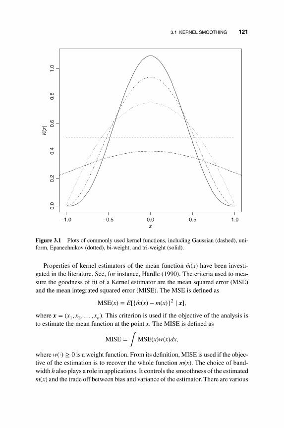
3.1 KERNEL SMOOTHING 121
1.00.50.0−0.5−1.0
0.0
0.2
0.4
0.6
0.8
1.0
z
K(z
)
Figure 3.1 Plots of commonly used kernel functions, including Gaussian (dashed), uni-form, Epanechnikov (dotted), bi-weight, and tri-weight (solid).
Properties of kernel estimators of the mean function m(x) have been investi-gated in the literature. See, for instance, Hardle (1990). The criteria used to mea-sure the goodness of fit of a Kernel estimator are the mean squared error (MSE)and the mean integrated squared error (MISE). The MSE is defined as
MSE(x) = E[{m(x) − m(x)}2 ∣ x],
where x = (x1, x2,… , xn). This criterion is used if the objective of the analysis isto estimate the mean function at the point x. The MISE is defined as
MISE =∫
MSE(x)w(x)dx,
where w(⋅) ≥ 0 is a weight function. From its definition, MISE is used if the objec-tive of the estimation is to recover the whole function m(x). The choice of band-width h also plays a role in applications. It controls the smoothness of the estimatedm(x) and the trade off between bias and variance of the estimator. There are various

122 3. UNIVARIATE NONPARAMETRIC MODELS
proposals available in the literature to choose the bandwidth for a given randomsample, including the plug-in method and cross-validation. The most commonlyused cross-validation method is the leave-one-out procedure. The criterion is
CV(h) = 1n
n∑j=1
[y𝑖 − mh(j)(xj)]2,
where the subscript ( j) indicates that the jth data point (xj, yj) is left out of thefitting. One selects the h that minimizes this CV(h) criterion. For simplicity, weoften use the default options in R packages to select the bandwidth and the kernelfunction.
It is computationally expensive to calculate CV(h) on a dense grid of h. Oftenthe generalized cross-valuation (GCV) criterion is used. Specifically,
GCV(h) =
∑nj=1[yj − mh(xj)]
2
n[1 − tr(S(h))∕n]2,
where S(h) is an n × n matrix with the (𝑖, j)th element being wj(x𝑖, h) defined inEquation (3.3), mh(xj) denotes the fitted value of the function m(xj) using band-width h. This is computationally much faster since mh(⋅) and tr(S(h)) are evaluatedusing all observations.
Another kernel estimator available is the Gasser–Muller estimator, defined as
mh(x) =n∑𝑖=1
[∫
s𝑖
s𝑖−1
Kh(u − x)du
]y𝑖, (3.5)
where s𝑖 = (x𝑖 + x𝑖+1)∕2, x0 = −∞, and xn+1 = ∞. A special feature of this esti-mator is that the weights are summed to one and, hence, no denominator is needed.The estimator is a modification of the one proposed by Priestley and Chao (1972).Properties of the Gasser–Muller estimator are studied in Muller (1988). From thedefinitions, the weights of the kernel estimator in Equation (3.2) are proportionalto the heights of re-scaled kernel whereas those of Gasser–Muller estimator inEquation (3.5) are determined by the areas under the kernel function and boundedby the mid-points of x𝑖 close to x.
Remark: One can use the command ksmooth in R to obtain theNadaraya–Watson estimator. However, the kernel functions available are uniformand Gaussian only. The command hcv of the package sm uses cross-validation toselect bandwidth.
Example 3.1 A widely used example in the statistical literature for nonparamet-ric analysis is the Old Faithful data from Yellowstone National Park. The data setis available from R and consists of two variables, namely the waiting time (Y) and
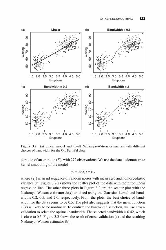
3.1 KERNEL SMOOTHING 123
*
*
*
*
*
*
**
*
*
*
**
*
*
*
*
*
*
*
**
*
**
*
*
** **
*
*
**
**
*
*
*
*
*
*
*
*
*
*
*
*
*
*
*
*
*
*
*
*
*
**
*
*
*
*
*
*
* *
*
*
*
*
*
*
*
*
*
**
*
*
*
**
*
*
**
*
*
*
*
*
*
*
*
*
*
*
*
*
*
*
**
*
*
*
**
*
*
*
*
*
*
*
*
*
*
*
*
*
*
*
*
*
*
*
*
*
*
*
*
*
*
*
*
*
* *
*
***
*
*
*
*
*
**
*
*
* *
*
*
*
*
*
*
*
*
*
*
*
*
*
*
*
*
*
*
* *
*
*
*
*
*
***
*
**
*
*
*
*
*
*
*
**
*
*
*
*
*
*
*
*
*
*
*
*
*
*
*
*
*
*
*
*
*
*
*
*
*
*
*
** ** *
*
*
*
*
*
*
*
**
**
*
*
*
*
*
**
*
*
*
*
*
*
* *
*
*
*
*
*
* **
*
*
*
*
**
*
*
*
*
5.04.54.03.53.02.52.01.5
Linear
Eruptions
Wai
ting
*
*
*
*
*
*
**
*
*
*
**
*
*
*
*
*
*
*
**
*
**
*
*
** **
*
*
**
**
*
*
*
*
*
*
*
*
*
*
*
*
*
*
*
*
*
*
*
*
*
**
*
*
*
*
*
*
* *
*
*
*
*
*
*
*
*
*
**
*
*
*
**
*
*
**
*
*
*
*
*
*
*
*
*
*
*
*
*
*
*
**
*
*
*
**
*
*
*
*
*
*
*
*
*
*
*
*
*
*
*
*
*
*
*
*
*
*
*
*
*
*
*
*
*
* *
*
***
*
*
*
*
*
**
*
*
* *
*
*
*
*
*
*
*
*
*
*
*
*
*
*
*
*
*
*
* *
*
*
*
*
*
***
*
**
*
*
*
*
*
*
*
**
*
*
*
*
*
*
*
*
*
*
*
*
*
*
*
*
*
*
*
*
*
*
*
*
*
*
*
** ** *
*
*
*
*
*
*
*
**
**
*
*
*
*
*
**
*
*
*
*
*
*
* *
*
*
*
*
*
* **
*
*
*
*
**
*
*
*
*
5.04.54.03.53.02.52.01.5
Bandwidth = 0.2
Eruptions
Wai
ting
*
*
*
*
*
*
**
*
*
*
**
*
*
*
*
*
*
*
**
*
**
*
*
** **
*
*
**
**
*
*
*
*
*
*
*
*
*
*
*
*
*
*
*
*
*
*
*
*
*
**
*
*
*
*
*
*
* *
*
*
*
*
*
*
*
*
*
**
*
*
*
**
*
*
**
*
*
*
*
*
*
*
*
*
*
*
*
*
*
*
**
*
*
*
**
*
*
*
*
*
*
*
*
*
*
*
*
*
*
*
*
*
*
*
*
*
*
*
*
*
*
*
*
*
* *
*
***
*
*
*
*
*
**
*
*
* *
*
*
*
*
*
*
*
*
*
*
*
*
*
*
*
*
*
*
* *
*
*
*
*
*
***
*
**
*
*
*
*
*
*
*
**
*
*
*
*
*
*
*
*
*
*
*
*
*
*
*
*
*
*
*
*
*
*
*
*
*
*
*
** ** *
*
*
*
*
*
*
*
**
**
*
*
*
*
*
**
*
*
*
*
*
*
* *
*
*
*
*
*
* **
*
*
*
*
**
*
*
*
*
5.04.54.03.53.02.52.01.5
9080
7060
50
9080
7060
5090
8070
6050
9080
7060
50
Bandwidth = 0.5
Eruptions
Wai
ting
*
*
*
*
*
*
**
*
*
*
**
*
*
*
*
*
*
*
**
*
**
*
*
** **
*
*
**
**
*
*
*
*
*
*
*
*
*
*
*
*
*
*
*
*
*
*
*
*
*
**
*
*
*
*
*
*
* *
*
*
*
*
*
*
*
*
*
**
*
*
*
**
*
*
**
*
*
*
*
*
*
*
*
*
*
*
*
*
*
*
**
*
*
*
**
*
*
*
*
*
*
*
*
*
*
*
*
*
*
*
*
*
*
*
*
*
*
*
*
*
*
*
*
*
* *
*
***
*
*
*
*
*
**
*
*
* *
*
*
*
*
*
*
*
*
*
*
*
*
*
*
*
*
*
*
* *
*
*
*
*
*
***
*
**
*
*
*
*
*
*
*
**
*
*
*
*
*
*
*
*
*
*
*
*
*
*
*
*
*
*
*
*
*
*
*
*
*
*
*
** ** *
*
*
*
*
*
*
*
**
**
*
*
*
*
*
**
*
*
*
*
*
*
* *
*
*
*
*
*
* **
*
*
*
*
**
*
*
*
*
5.04.54.03.53.02.52.01.5
Bandwidth = 2
Eruptions
Wai
ting
(a) (b)
(c) (d)
Figure 3.2 (a) Linear model and (b–d) Nadaraya–Watson estimators with differentchoices of bandwidth for the Old Faithful data.
duration of an eruption (X), with 272 observations. We use the data to demonstratekernel smoothing of the model
y𝑖 = m(x𝑖) + 𝜖𝑖,
where {𝜖𝑖} is an iid sequence of random noises with mean zero and homoscedasticvariance 𝜎2. Figure 3.2(a) shows the scatter plot of the data with the fitted linearregression line. The other three plots in Figure 3.2 are the scatter plot with theNadaraya–Watson estimator m(x) obtained using the Gaussian kernel and band-widths 0.2, 0.5, and 2.0, respectively. From the plots, the best choice of band-width for the data seems to be 0.5. The plot also suggests that the mean functionm(x) is likely to be nonlinear. To confirm the bandwidth selection, we use cross-validation to select the optimal bandwidth. The selected bandwidth is 0.42, whichis close to 0.5. Figure 3.3 shows the result of cross-validation (a) and the resultingNadaraya–Watson estimator (b).

124 3. UNIVARIATE NONPARAMETRIC MODELS
0.2 0.4 0.6 0.8
9000
1000
011
000
1200
013
000
1400
015
000
h
CV
1.5 2.5 3.5 4.5
5060
7080
90
Eruptions
Wai
ting
(a) (b)
Figure 3.3 Result of (a) cross-validation and (b) the associated Nadaraya–Watson esti-mator for the Old Faithful data.
R demonstration: Kernel smoothing.
> data(faithful)> dim(faithful)[1] 272 2> par(mfcol=c(2,2))> plot(waiting˜ eruptions,data=faithful,main="linear",pch="*")> m1 < lm(waiting˜ eruptions,data=faithful)> lines(faithful$eruptions,m1$fitted.values)> plot(waiting˜ eruptions,data=faithful,main="bandwidth=0.2",pch="*")> lines(ksmooth(faithful$eruptions,faithful$waiting,"normal",0.2))> plot(waiting˜ eruptions,data=faithful,main="bandwidth=0.5",pch="*")> lines(ksmooth(faithful$eruptions,faithful$waiting,"normal",0.5))> plot(waiting˜ eruptions,data=faithful,main="bandwidth=2",pch="*")> lines(ksmooth(faithful$eruptions,faithful$waiting,"normal",2))> par(mfcol=c(1,2))> require(sm)> h < hcv(faithful$eruptions,faithful$waiting,display="lines")> h

3.2 LOCAL CONDITIONAL MEAN 125
[1] 0.4243375> sm.regression(faithful$eruptions,faithful$waiting,h=h,xlab="eruptions",ylab="waiting")
3.2 LOCAL CONDITIONAL MEAN
A direct application of kernel methods in nonlinear time series analysis is to esti-mate the conditional mean function of the general nonlinear autoregressive model
xt = f (xt−1,… , xt−p) + 𝜖t, (3.6)
where p is a positive integer and 𝜖t is an iid sequence of random variates with meanzero and variance 0 < 𝜎2 < ∞. Let Xt−1 = (xt−1,… , xt−p)′ be the vector of past plagged values. Let y = (y1,… , yp)′ be a p-dimensional vector on which the condi-tional mean of xt, i.e. E(xt ∣ Xt−1 = y) = f (y1,… , yp), is of interest. Suppose theavailable sample is {x1,… , xT}. A simple approach to estimate the conditionalmean via nonparametric kernel methods is as follows. Let N𝑖(y) = {t ∣ ‖Xt−1 −y‖ < 𝛿𝑖, t = p,… , T}, where 𝛿𝑖 is a given positive real number and ‖ ⋅ ‖ denotesthe Euclidean norm. In other words, N𝑖(y) consists of the past p-dimensional vec-tors Xt−1 that are in the 𝛿𝑖-neighborhood of y. The simple estimator is then
f (y1,… , yp) = 1#N𝑖(y)
∑t∈N𝑖(y)
xt, (3.7)
where #N𝑖(y) denotes the number of the p-dimensional vectors in N𝑖(y). Inother words, one simply uses the average of all xt for which Xt−1 is in the 𝛿𝑖-neighborhood of y. This estimator can be thought of a kernel estimate using theuniform kernel. Truong (1993) proved strong consistency and asymptotic normal-ity of f (x) in Equation (3.7) and derived the optimal rate of convergence for suitablesequences 𝛿𝑖 → 0.
Many authors used the Nadaraya–Watson estimator with product kernels toestimate the conditional mean f (x1,… , xp) of the general nonlinear AR modelin Equation (3.6). See Hardle et al. (1997) and the references therein. Theestimator is
f (y1,… , yp) =
∑Tt=p+1
∏p𝑖=1 K[(y𝑖 − xt−𝑖)∕h𝑖]xt∑T
t=p+1
∏p𝑖=1 K[(y𝑖 − xt−𝑖)∕h𝑖]
, (3.8)
where K(⋅) is a chosen kernel and h𝑖 is the bandwidth for the 𝑖th lagged vari-able. Here the effective sample size is n = T − p. Limiting properties of the kernelestimator in Equation (3.8) have been derived by several authors under certainmixing conditions that govern the dynamic dependence of the xt series. Robinson(1983) and Masry and Tj𝜙stheim (1995) proved strong consistency and asymptotic

126 3. UNIVARIATE NONPARAMETRIC MODELS
normality for 𝛼-mixing series xt. Bierens (1983, 1987) and Collomb and Hardle(1986) showed the uniform consistency of the estimator for𝜙-mixing series xt. Theasymptotic results of kernel smoothing for time series data are almost the same asthose for independent observations (e.g., nonparametric regression), due to thewhitening by window phenomenon. It is noticed that under the mixing conditions,the observations within a small window in the space of Xt−1 (for which we takeaverages) are almost independent, since the time gaps among these observationstend to be large though they are close in space.
Mixing conditions are often used in the time series literature to control thedependence between xt and xt−j as the time distance between the two variables jincreases. Specifically, xt is said to be 𝛼-mixing if
supA∈ n
1,B∈∞n+k
|P(A ∩ B) − P(A)P(B)| ≤ 𝛼k, (3.9)
where 𝛼k → 0 as k → ∞ and j𝑖
is the 𝜎-field generated by {x𝑖, x𝑖+1,… , xj}. SeeRobinson (1983). The series xt is said to be 𝜙-mixing if|P(A ∩ B) − P(A)P(B)| ≤ 𝜙kP(A), (3.10)
for any A ∈ n1 and B ∈
∞n+k and𝜙k → 0 as k → ∞. The𝜙-mixing is stronger and
is also known as uniformly mixing. The rate at which 𝛼k and 𝜙k go to zero playsan important role in deriving the asymptotic properties of the kernel estimators.In practice, mixing conditions are hard to check, but some commonly used timeseries models are known to satisfy these conditions. See Tweedie (1975).
Example 3.2 Consider the quarterly unemployment durations of the USA from1948.I to 2017.II. The original data are obtained from FRED and are monthly andseasonally adjusted. We compute the quarterly series by taking the mean of thethree monthly durations. Figure 3.4(a) shows the time plot of the quarterly unem-ployment duration, which exhibits an upward trend. Figure 3.4(b) shows the firstdifferenced series of the quarterly durations. The monthly unemployment durationseries has been analyzed in the Exercises of Chapter 2.
Let xt be the first differenced series of the quarterly unemployment durations.If linear models are used, an AR(1) model provides a decent fit. The model isxt = 0.52xt−1 + at, with ��2
a = 0.566. However, the threshold nonlinear test showsthat xt is nonlinear with test statistic 4.88 and p value 0.008. Therefore, we applythe local conditional mean estimator of Equation (3.8) with p = 1 to the series. Theconditional means are estimated at observed xt−1. Figure 3.5 shows the scatterplot of xt versus xt−1 and the fitted conditional mean function (solid line). Theestimation is carried by a Gaussian kernel with bandwidth 0.416. From the plot,it is seen that the dependence of xt on xt−1 is indeed nonlinear. For comparison,

3.2 LOCAL CONDITIONAL MEAN 127
1950 1960 1970 1980 1990 2000 2010 2020
1020
3040
Year
Qua
rter
ly u
nem
ploy
men
tdu
ratio
n
1950 1960 1970 1980 1990 2000 2010 2020
−2
01
23
Year
Firs
t diff
eren
ced
serie
s
(a)
(b)
Figure 3.4 Time plots of US quarterly unemployment durations from 1948.I to 2017.II.(a) Quarterly unemployment durations and (b) the first differenced series.
the dashed line of Figure 3.5 shows the fitted line via the lowess procedure of R.See the discussion in the next section for the method. The dashed line also showscertain nonlinearity.
Remark: For the local conditional mean estimation, we used the package np ofR. The bandwidth was selected automatically by the command npreg.
R demonstration: The np package of R.
> da < read.table("qunempdur.txt",header=T)> y < da[,2]> dy < diff(y)> ts.plot(dy)> m1 < arima(dy,order=c(1,0,0),include.mean=F)> m1Call:arima(x = dy, order = c(1, 0, 0), include.mean = F)Coefficients:
ar10.5238
s.e. 0.0510
sigmaˆ2 estimated as 0.566: log likelihood = 314.38, aic = 632.77> k1 < lowess(dy[2:277]˜ dy[1:276]) # lowess fitting

128 3. UNIVARIATE NONPARAMETRIC MODELS
3210−1−2
32
10
−1
−2
Lag−1
Firs
t diff
eren
ced
serie
s
Figure 3.5 Scatter plot of the first differenced series of US quarterly unemployment dura-tion versus its lagged values. The solid line is the local conditional mean fit via Gaussiankernel and the dashed line shows the lowess fit. The sample period is from 1948.II to2017.II.
> require(np)> Y < dy[2:277]> X < matrix(dy[1:276],276,1)> m2 < npreg(txdat=X,tydat=Y,residuals=T)> names(m2)[1] "bw" "bws" "pregtype" "xnames" "ynames"[6] "nobs" "ndim" "nord" "nuno" "ncon"
[11] "pscaling" "ptype" "pckertype" "pukertype" "pokertype"
[16] "eval" "mean" "merr" "grad" "gerr"[21] "resid" "ntrain" "trainiseval" "gradients" "residuals"[26] "R2" "MSE" "MAE" "MAPE" "CORR"[31] "SIGN" "rows.omit" "nobs.omit" "call"> m2$bw[1] 0.4163248> m2$pckertype
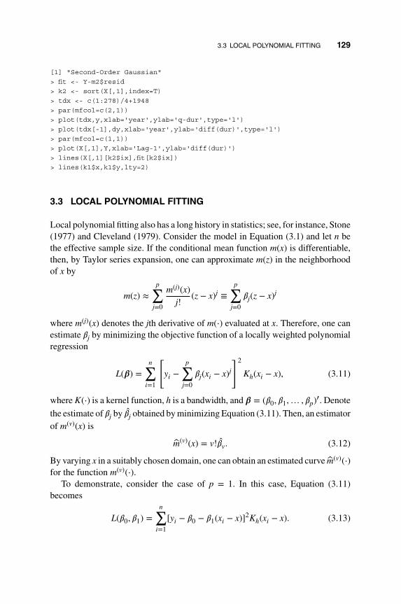
3.3 LOCAL POLYNOMIAL FITTING 129
[1] "SecondOrder Gaussian"> fit < Ym2$resid> k2 < sort(X[,1],index=T)> tdx < c(1:278)/4+1948> par(mfcol=c(2,1))> plot(tdx,y,xlab='year',ylab='qdur',type='l')> plot(tdx[1],dy,xlab='year',ylab='diff(dur)',type='l')> par(mfcol=c(1,1))> plot(X[,1],Y,xlab='Lag1',ylab='diff(dur)')> lines(X[,1][k2$ix],fit[k2$ix])> lines(k1$x,k1$y,lty=2)
3.3 LOCAL POLYNOMIAL FITTING
Local polynomial fitting also has a long history in statistics; see, for instance, Stone(1977) and Cleveland (1979). Consider the model in Equation (3.1) and let n bethe effective sample size. If the conditional mean function m(x) is differentiable,then, by Taylor series expansion, one can approximate m(z) in the neighborhoodof x by
m(z) ≈p∑
j=0
m(j)(x)j!
(z − x)j ≡
p∑j=0
𝛽j(z − x)j
where m(j)(x) denotes the jth derivative of m(⋅) evaluated at x. Therefore, one canestimate 𝛽j by minimizing the objective function of a locally weighted polynomialregression
L(𝜷) =n∑𝑖=1
[y𝑖 −
p∑j=0
𝛽j(x𝑖 − x)j
]2
Kh(x𝑖 − x), (3.11)
where K(⋅) is a kernel function, h is a bandwidth, and 𝜷 = (𝛽0, 𝛽1,… , 𝛽p)′. Denote
the estimate of 𝛽j by 𝛽j obtained by minimizing Equation (3.11). Then, an estimatorof m(v)(x) is
m(v)(x) = v!𝛽v. (3.12)
By varying x in a suitably chosen domain, one can obtain an estimated curve m(v)(⋅)for the function m(v)(⋅).
To demonstrate, consider the case of p = 1. In this case, Equation (3.11)becomes
L(𝛽0, 𝛽1) =n∑𝑖=1
[y𝑖 − 𝛽0 − 𝛽1(x𝑖 − x)]2Kh(x𝑖 − x). (3.13)

130 3. UNIVARIATE NONPARAMETRIC MODELS
Taking partial derivatives of L(𝛽0, 𝛽1) with respect to 𝛽j, equating the derivativesto zero, and letting W𝑖(x) = Kh(x𝑖 − x), we obtain the first-order equations
n∑𝑖=1
W𝑖(x)y𝑖 = 𝛽0
n∑𝑖=1
W𝑖(x) + 𝛽1
n∑𝑖=1
(x𝑖 − x)W𝑖(x)
n∑𝑖=1
y𝑖(x𝑖 − x)W𝑖(x) = 𝛽0
n∑𝑖=1
(x𝑖 − x)W𝑖(x) + 𝛽1
n∑𝑖=1
(x𝑖 − x)2W𝑖(x).
Next, define
Sn, j =n∑𝑖=1
W𝑖(x)(x𝑖 − x)j, j = 0, 1, 2.
The first-order equations become[Sn,0 Sn,1Sn,1 Sn,2
] [𝛽0𝛽1
]=[ ∑n
𝑖=1 W𝑖(x)y𝑖∑n𝑖=1 W𝑖(x)(x𝑖 − x)y𝑖
].
Consequently, we have
𝛽0 =Sn,2
∑n𝑖=1 W𝑖(x)y𝑖 − Sn,1
∑n𝑖=1(x𝑖 − x)W𝑖(x)y𝑖
Sn,0Sn,2 − S2n,1
,
which is an estimate of the conditional mean function m(x). Some algebraic cal-culations show that
𝛽0 =∑n𝑖=1{W𝑖(x)[Sn,2 − (x𝑖 − x)Sn,1]}y𝑖∑n𝑖=1 W𝑖(x)[Sn,2 − (x𝑖 − x)Sn,1]
≡
∑n𝑖=1 w𝑖y𝑖∑n𝑖=1 w𝑖
(3.14)
where the weight is now given by w𝑖 = W𝑖(x)[Sn,2 − (x𝑖 − x)Sn,1]. Thus, the localpolynomial estimate of m(x) with p = 1 is also a weighted average of y𝑖. Theweights, however, depend on the choice of the order p. A nice feature of the esti-mate in Equation (3.14) is that
n∑𝑖=1
(x𝑖 − x)w𝑖 = Sn,2Sn,1 − Sn,1Sn,2 = 0.
Also, if one uses p = 0 in Equation (3.11), then the local polynomial estimate ofm(x) reduces to the Nadaraya–Watson estimator in Equation (3.2). To avoid thenumerical difficulty of zero denominator in Equation (3.14), one often uses themodified version
m(x) =∑n𝑖=1 w𝑖y𝑖
1∕n +∑n𝑖=1 w𝑖
.
For further information on local polynomial fitting, see Fan and Gijbels (1996).

3.3 LOCAL POLYNOMIAL FITTING 131
Remark: Under the assumption that the underlying m(x) function is continu-ously differentiable to the pth order, the local polynomial estimator is superior tothe kernel estimator, with smaller bias, faster convergence rate, and smaller mini-max risk. It also performs better on the boundary of the observed data. However,in practice one is never sure about the degrees of smoothness of the underlyingfunction. Often a local linear estimator is used. See Fan and Yao (2003).
Cleveland (1979) proposes a robust version of locally weighted least squaresmethod called LOcally Weighted Scatterplot Smoothing (LOWESS). Instead offixing bandwidth, LOWESS uses a fixed number of nearest neighbors for smooth-ing. The kernel function used by LOWESS is
K(z) = 7081
(1 − |z|3)3I[−1,1](z), (3.15)
where IA(z) is the indicator variable of the interval A, e.g, I[−1,1](z) = 1 if andonly if z ∈ [−1, 1]. The basic idea of LOWESS is to start the fitting with a localpolynomial estimate using a fixed number of nearest neighbors, and uses the fittedvalues to compute residuals. Then, assign weights to the residuals based on theirmagnitudes with large residuals receiving lower weights. One can then repeat thelocal polynomial fitting with new weights that are the products of the weights ofthe original local fitting and the residual weights. By so doing, large residualsare down-weighted to reduce their impacts on the model fitting. The procedure isiterated for several iterations to obtain robust local polynomial fitting.
In what follows, we briefly describe the LOWESS procedure as the estimator isoften used in applications. Consider, again, the random sample with n observations{(x1, y1),… , (xn, yn)}. Let v be a selected integer satisfying v ∈ (0, n]. Focus onthe observation (xk, yk). Select a bandwidth hk so that there are exactly v nearestneighbors in the window [xk − hk, xk + hk]. For a selected kernel function K(⋅) andthe bandwidth hk, we can obtain a local polynomial estimate for m(xk) by assigningweight
Khk(x𝑖 − xk) = h−1
k K[h−1k (x𝑖 − xk)], 𝑖 = 1,… , n.
For a given order p, one can obtain a local estimate 𝛽0 by using Equation (3.11).Denote the resulting estimate by
yk = 𝛽0 =n∑𝑖=1
w𝑖(xk)y𝑖,
where w𝑖(xk) is the weight assigned to the data point (x𝑖, y𝑖). This estimate is carriedout for each xk, k = 1,… , n. Also, define the residual
rk = yk − yk, k = 1,… , n. (3.16)

132 3. UNIVARIATE NONPARAMETRIC MODELS
Next, let M be the median of the absolute residuals, i.e. M =median{|r1|,… , |rn|}. One defines the robustness weight by
𝜂𝑖 = B(r𝑖∕(6M)), 𝑖 = 1,… , n,
where
B(z) = (1 − |z|2)2I[−1,1](z)
is the bi-weight kernel of Equation (3.4) with 𝛾 = 2. Now, one can repeat the localpth order polynomial fitting using the product weights 𝜂𝑖Khk
(x𝑖 − xk). The addi-tional weight 𝜂𝑖 takes into account the heteroscedasticity in the noise variance, sim-ilar to the weighted least squares approach. For example, if r𝑖 > 6M, then 𝜂𝑖 = 0.That is, (x𝑖, y𝑖) is considered as an outlier, hence it is assigned a zero weight and isnot included in the analysis. Larger r𝑖 indicates larger variance of 𝜀𝑖, hence receiv-ing smaller weight.
The procedure is iterated multiple times to obtain stable estimates.
Example 3.3 Consider the annual mean sunspot numbers from 1700 to 2006.The data are downloaded from WDC-SILSO, Royal Observatory of Belgium,Brussels. Figure 3.6 shows the time plot of the series. The sunspot data havebeen widely used in the literature as an example of nonlinear time series. See,
2000195019001850180017501700
250
200
150
100
500
Year
Sun
spot
***
*
*
*
*
*
******
*
*
*
**
*
***
*
*
*
*
*
*
*
*
*
**
*
*
*
*
*
*
*
*
**
**
*
*
*
**
**
*
***
*
*
*
*
*
*
*
*
*
*
*
*
**
*
*
**
*
*
*
*
*
*
*
*
*
*
*
*
**
*
*
*
*
**
**
***
*
*
****
*
******
**
*
**
*
*
*
****
*
*
*
***
*
*
**
*
*
*
*
*
*
*
*
**
*
*
*
*
*
**
*
*
*
**
*
*
**
*
*
**
*
*
*
*
*
*
*
*
*
*
***
**
*
****
*
*
*
***
*
*
*
*
*
*
**
**
**
*
*
*
*
*
**
*
***
*
*
*
*
*
*
*
*
*
*
*
*
**
*
*
*
*
***
*
*
**
*
*
*
*
*
*
*
*
*
**
*
*
*
*
*
*
*
**
*
*
*
*
*
**
*
*
***
**
**
**
*
*
**
*
*
*
*
**
*
*
*
*
*
*
*
*
*
*
*
*
*
***
*
*
*
*
***
*
***
*
*
Figure 3.6 Time plot of annual mean sunspot numbers from 1700 to 2006.

3.3 LOCAL POLYNOMIAL FITTING 133
0 50 100 150 200 250
050
100
200
Lowess
x(t−2)
x(t)
0 50 100 150 200 250
050
100
200
Local−polynomial, degree 0
x(t−2)
x(t)
0 50 100 150 200 250
050
100
200
Local−polynomial, degree 1
x(t−2)
x(t)
0 50 100 150 200 250
050
100
200
Local−polynomial, degree 2
x(t−2)
x(t)
(a)
(b) (d)
(c)
Figure 3.7 Scatter plot of xt versus xt−2 of the annual sunspot numbers: (a) the LOWESSline and (b)–(d) local polynomial fits of degrees 0, 1, and 2, respectively. The bandwidth oflocal polynomial fitting is 50% of the sample standard deviation of the data.
for instance, Tong (1990) and the references therein. In this example, we focus onthe relationship between xt and xt−2, where xt denotes the annual sunspot num-ber of year t + 1699. In other words, we consider xt = m(xt−2) + 𝜖t, where 𝜖t isa sequence of random noises. Figure 3.7 shows the scatter plot of xt versus xt−2and several estimates of m(xt−2). The line in part (a) is obtained via LOWESSwith default options, namely v = 2∕3 and three iterations. The lines in parts (b)to (d) are from the local polynomial fitting with degrees 0, 1, and 2, respectively.The bandwidth is h = 31, which is approximately 0.5��, with �� being the samplestandard deviation of xt. Thus, part (b) shows the traditional Nadaraya–Watsonestimate. From the plots, the degree used in local polynomial fitting may affectthe boundaries of the fit. The robustness of the LOWESS procedure is clearly seenwhen xt−2 is approximately 50.

134 3. UNIVARIATE NONPARAMETRIC MODELS
R demonstration: Local polynomial fitting via the KernSmooth package.
da < read.table("SN_y_tot_V2.0.txt",header=T)sn < da[,2]; n < length(sn)s < sqrt(var(sn))y < sn[3:n]; x < sn[1:(n2)]require(KernSmooth)par(mfcol=c(2,2))plot(x,y,xlab="x(t2)",ylab="x(t)",main="(a) Lowess")lines(lowess(x,y),col="red")m3 < locpoly(x,y,degree=0,bandwidth=0.5*s)plot(x,y,xlab="x(t2)",ylab="x(t)",main="(b) Local polynomial, degree 0")lines(m3$x,m3$y,col="red")m4 < locpoly(x,y,degree=1,bandwidth=0.5*s)plot(x,y,xlab="x(t2)",ylab="x(t)",main="(c) Local polynomial, degree 1")lines(m4$x,m4$y,col="red")m5 < locpoly(x,y,degree=2,bandwidth=0.5*s)plot(x,y,xlab="x(t2)",ylab="x(t)",main="(d) Local polynomial, degree 2")lines(m5$x,m5$y,col="red")
3.4 SPLINES
The local polynomial fitting of Section 3.3 is motivated by Taylor series expan-sion. By increasing the degree of the polynomial used, we increase the flexibilityin model fitting. However, the method is still treating the domain of the X variablelocally, as the function is estimated at each point individually using a local windowcentering around it. An alternative approach is to estimate the function globallyusing an increasingly larger set of basis functions to approximate the underlyingfunction. The entire function is then estimated in one step under a global opti-mization criterion. Global basis functions such as polynomials are not stable andinflexible. Using local basis functions such as piecewise polynomials increasesflexibility. Consider the simple case in which the dependent variable Y is a func-tion of a scalar variable X,
Y = f (X) + 𝜖,where 𝜖 denotes the noise term. One can divide the domain of X into contigu-ous intervals and approximate f (X) by a separate polynomial in each interval. Todemonstrate, we use the smooth function f (X) = 2 sin(2𝜋X), and let {x𝑖} be the 51equally spaced points in [0,1]. The observed dependent variable is y𝑖 = f (x𝑖) + 𝜖𝑖,where 𝜖𝑖 are iid N(0, 1). We divide the range of x𝑖 into three non-overlapping con-tiguous intervals, namely
I1 = [0, 0.32), I2 = [0.32, 0.66), I3 = [0.66, 1].
These intervals are defined by the points 𝜉0 = 0, 𝜉1 = 0.32, 𝜉2 = 0.66, and 𝜉4 = 1.In the literature, these {𝜉𝑖} are called knots. The data and the true function f (x)
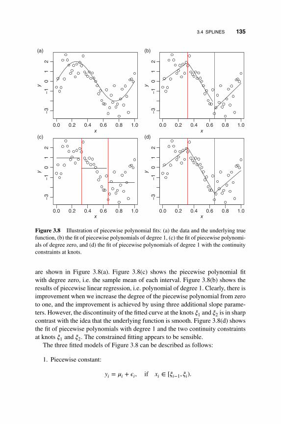
3.4 SPLINES 135
0.0 0.2 0.4 0.6 0.8 1.0
−3
−1
01
2
x
y
0.0 0.2 0.4 0.6 0.8 1.0
−3
−1
01
2
x
y
0.0 0.2 0.4 0.6 0.8 1.0
−3
−1
01
2
x
y
0.0 0.2 0.4 0.6 0.8 1.0
−3
−1
01
2
x
y
(a) (b)
(c) (d)
Figure 3.8 Illustration of piecewise polynomial fits: (a) the data and the underlying truefunction, (b) the fit of piecewise polynomials of degree 1, (c) the fit of piecewise polynomi-als of degree zero, and (d) the fit of piecewise polynomials of degree 1 with the continuityconstraints at knots.
are shown in Figure 3.8(a). Figure 3.8(c) shows the piecewise polynomial fitwith degree zero, i.e. the sample mean of each interval. Figure 3.8(b) shows theresults of piecewise linear regression, i.e. polynomial of degree 1. Clearly, there isimprovement when we increase the degree of the piecewise polynomial from zeroto one, and the improvement is achieved by using three additional slope parame-ters. However, the discontinuity of the fitted curve at the knots 𝜉1 and 𝜉2 is in sharpcontrast with the idea that the underlying function is smooth. Figure 3.8(d) showsthe fit of piecewise polynomials with degree 1 and the two continuity constraintsat knots 𝜉1 and 𝜉2. The constrained fitting appears to be sensible.
The three fitted models of Figure 3.8 can be described as follows:
1. Piecewise constant:
y𝑖 = 𝜇𝑖 + 𝜖𝑖, if x𝑖 ∈ [𝜉𝑖−1, 𝜉𝑖).

136 3. UNIVARIATE NONPARAMETRIC MODELS
2. Piecewise linear regression:
y𝑖 = 𝛼𝑖 + 𝛽𝑖x𝑖 + 𝜖𝑖, if x𝑖 ∈ [𝜉𝑖−1, 𝜉𝑖).
3. Piecewise linear regression with continuity constraints: The same model asCase 2 with the constraints
𝛼1 + 𝛽1𝜉1 = 𝛼2 + 𝛽2𝜉1 and 𝛼2 + 𝛽2𝜉2 = 𝛼3 + 𝛽3𝜉2.
The numbers of coefficients of the three models are 3, 6, and 4, respectively. Amore direct way to describe the three models is to think that we are constructingcertain functions of the X variable to approximate the function f (X). The piecewiseconstant model is achieved by creating three indicator functions
b1(X) = I[X < 𝜉1], b2(X) = I[𝜉1 ≤ X < 𝜉2], b3(X) = I[𝜉2 ≤ X],
and we simply fit the model
y𝑖 = 𝜇1b1(x𝑖) + 𝜇2b2(x𝑖) + 𝜇3b3(x𝑖) + 𝜖𝑖.
The piecewise linear regression is achieved by adding three more functions
b4(X) = Xb1(X), b5(X) = Xb2(X), b6(X) = Xb3(X),
and approximating f (X) by a linear combination of {bj(X)| j = 1,… , 6}. Finally,the constrained linear regression is achieved by using
b1(X) = 1, b2(X) = X, b3(X) = (X − 𝜉1)+, b4(X) = (X − 𝜉2)+,
where (z)+ = max(0, z) is the positive part of z. Here b3(X) and b4(X) are simplyramp functions.
While the piecewise linear regression (polynomial of order 1) with continuityconstraints provides a continuous fitted function, the resulting curve is not smooth.The curve is not differentiable at the knots. On the other hand, we often prefersmooth functions in applications. This can be achieved by increasing the degree thepiecewise polynomial used and requiring smoothness in certain derivatives of thefitted function. Figure 3.9 shows the fits of some smooth splines to the illustrativedata set. The four plots differ in the degrees of freedom used. Figure 3.9(d) showsa reasonable fit in this particular instance.
R demonstration: Smoothing spline in Figure 3.9.
> x < seq(0,1,0.02); f < 2*sin(2*pi*x)> set.seed(11)> y < f + rnorm(51)

3.4 SPLINES 137
0.0 0.2 0.4 0.6 0.8 1.0
−3
−2
−1
01
2
x
y
0.0 0.2 0.4 0.6 0.8 1.0
−3
−2
−1
01
2
x
y
0.0 0.2 0.4 0.6 0.8 1.0
−3
−2
−1
01
2
x
y
0.0 0.2 0.4 0.6 0.8 1.0
−3
−2
−1
01
2
x
y
(a) (b)
(c) (d)
Figure 3.9 Illustration of smooth splines. The data used are the same as those ofFigure 3.8. (a), (c) and (b) and (d) have degrees of freedom 2, 3, 4 and 5, respectively.
> require(stats)> par(mfcol=c(2,2))> xi < c(0.32,0.66) # equallyspaced knots> plot(x,y); abline(v=xi,col="red")> m1 < smooth.spline(x,y,df=2)> lines(m1)> plot(x,y); abline(v=xi,col="red")> m2 < smooth.spline(x,y,df=3)> lines(m2)> plot(x,y); abline(v=xi,col="red")> m3 < smooth.spline(x,y,df=4)> lines(m3)> plot(x,y); abline(v=xi,col="red")> m4 < smooth.spline(x,y,df=5)> lines(m4)

138 3. UNIVARIATE NONPARAMETRIC MODELS
3.4.1 Cubic and B-Splines
For a given set of knots {𝜉𝑖|𝑖 = 1,… , K}, a flexible spline function is the naturalcubic spline. It consists of cubic splines within intervals between knots and theadditional constraints that the function is linear beyond the boundary knots. Theadditional constraints are achieved by requiring that the second and third deriva-tives of f (⋅) are zero at the boundary. Mathematically, the resulting smooth functioncan be written as
f (x) = 𝛽0 + 𝛽1x + 𝛽2x2 + 𝛽3x3 +K∑
j=1
𝛾j(x − 𝜉j)3+ (3.17)
where, again, (z)+ = max(0, z). However, the model in Equation (3.17) is not effi-cient in computing. It requires evaluation of the regressors at all points to the rightof its knot. A more convenient form for estimation is to express the model usingcertain basis functions, each of which only requires evaluation in a small numberof intervals. A well-known class of basis functions is the B-splines. de Boor (1978)discusses splines and B-splines in detail.
Also, for computational reason, we need to augment the knot sequence 𝜉1 <
𝜉2 < ⋯ < 𝜉K . Let 𝜉0 < 𝜉1 and 𝜉K < 𝜉K+1 be the two boundary knots. Typically,[𝜉0, 𝜉K+1] denotes the domain over which the spline is evaluated. Let M be theorder of the spline function. Following Hastie, Tibshirani and Friedman (2001),we create an augmented knot sequence {𝜏j} such that
� 𝜏1 ≤ 𝜏2 ≤ ⋯ ≤ 𝜏M ≤ 𝜉0;
� 𝜏𝑖+M = 𝜉𝑖, for 𝑖 = 1,… , K;
� 𝜏K+1 ≤ 𝜏K+2 ≤ ⋯ ≤ 𝜏K+2M .
The actual values of the newly added knots are arbitrary and they may assume thesame values as the boundary knots 𝜉0 and 𝜉K+1, respectively. Let B𝑖,m(x) be the𝑖th B-spline basis function of order m for the knot sequence 𝜏, where m ≤ M. Onecan define the basis functions recursively starting with the Haar basis functions:
B𝑖,1(x) ={
1 if 𝜏𝑖 ≤ x < 𝜏𝑖+10 otherwise
(3.18)
where 𝑖 = 1,… , K + 2M − 1. Then,
B𝑖,m(x) =x − 𝜏𝑖
𝜏𝑖+m−1 − 𝜏𝑖B𝑖,m−1(x) +
𝜏𝑖+m − x
𝜏𝑖+m − 𝜏𝑖+1B𝑖+1,m−1(x) (3.19)
where 𝑖 = 1,… , K + 2M − m. This recursion is referred to as the Cox–de Boorrecursion. In practice, it is the convention to adopt B𝑖,1 = 0 if 𝜏𝑖 = 𝜏𝑖+1. By induc-tion, we then have B𝑖,m = 0 if 𝜏𝑖 = 𝜏𝑖+1 = ⋯ = 𝜏𝑖+m.
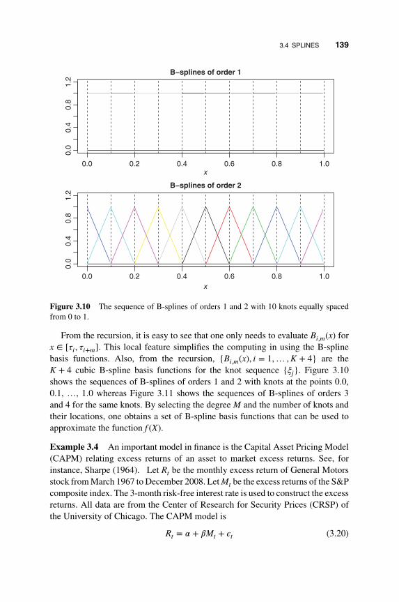
3.4 SPLINES 139
0.0 0.2 0.4 0.6 0.8 1.0
0.0
0.4
0.8
1.2
x
B−splines of order 1
0.0 0.2 0.4 0.6 0.8 1.0
0.0
0.4
0.8
1.2
x
B−splines of order 2
Figure 3.10 The sequence of B-splines of orders 1 and 2 with 10 knots equally spacedfrom 0 to 1.
From the recursion, it is easy to see that one only needs to evaluate B𝑖,m(x) forx ∈ [𝜏𝑖, 𝜏𝑖+m]. This local feature simplifies the computing in using the B-splinebasis functions. Also, from the recursion, {B𝑖,m(x), 𝑖 = 1,… , K + 4} are theK + 4 cubic B-spline basis functions for the knot sequence {𝜉j}. Figure 3.10shows the sequences of B-splines of orders 1 and 2 with knots at the points 0.0,0.1, …, 1.0 whereas Figure 3.11 shows the sequences of B-splines of orders 3and 4 for the same knots. By selecting the degree M and the number of knots andtheir locations, one obtains a set of B-spline basis functions that can be used toapproximate the function f (X).
Example 3.4 An important model in finance is the Capital Asset Pricing Model(CAPM) relating excess returns of an asset to market excess returns. See, forinstance, Sharpe (1964). Let Rt be the monthly excess return of General Motorsstock from March 1967 to December 2008. Let Mt be the excess returns of the S&Pcomposite index. The 3-month risk-free interest rate is used to construct the excessreturns. All data are from the Center of Research for Security Prices (CRSP) ofthe University of Chicago. The CAPM model is
Rt = 𝛼 + 𝛽Mt + 𝜖t (3.20)

140 3. UNIVARIATE NONPARAMETRIC MODELS
0.0 0.2 0.4 0.6 0.8 1.0
0.0
0.4
0.8
1.2
x
B−splines of order 3
0.0 0.2 0.4 0.6 0.8 1.0
0.0
0.4
0.8
1.2
x
B−splines of order 4
Figure 3.11 The sequence of B-splines of orders 3 and 4 with 10 knots equally spacedfrom 0 to 1.
and the coefficients are estimated by the ordinary least squares method.Figure 3.12 shows the scatter plot of Rt versus Mt and the fitted linear regressionline (straight). Also shown in Figure 3.12 is a B-spline fit, the curve. The B-splinesare degree 3 and default knot options. From the plot, the spline fit seems to farebetter in this particular instance.
R demonstration: B-splines via the package splines.
> require(stats); require(splines)> da < read.table("mgmsp6708.txt",header=T)> da1 < read.table("mriskfree3m6708.txt",header=T)> rf < da1[,4]/(100*12)> gm < da$GMrf; sp < da$SPrf> plot(sp,gm,xlab="Market excess returns",ylab='GM excess returns')> m1 < lm(gm˜ sp)> lines(sp,m1$fitted.values)> m2 < bs(sp,degree=3) ### Bsplines of degree 3.> m3 < lm(gm˜ m2)> xx < sort(sp,index=T)> lines(sp[xx$ix],m3$fitted.values[xx$ix],col=2)

3.4 SPLINES 141
−0.2 −0.1 0.0 0.1
−0.
4−
0.3
−0.
2−
0.1
0.0
0.1
0.2
Market excess returns
GM
exc
ess
retu
rns
Figure 3.12 Scatter plot of monthly excess returns of General Motors stock versus theexcess returns of the S&P market index from March 1967 to December 2008. The straightline and curve represent the linear regression and B-spline fit, respectively.
3.4.2 Smoothing Splines
In the discussion of spline functions, we simply use equally spaced knots over thedomain of the X variable. In real applications, one needs to specify both the numberof knots and their exact locations. Even though there are methods available in theliterature to perform such selection, we shall not address them in this chapter.To mitigate this selection problem, we introduce the smoothing-spline method,which uses a maximal set of knots, but controls the complexity of the fit by certainregularization.
Consider all functions f (x) with first two continuous derivatives. Smoothingspline method finds the one that minimizes the penalized residual sum of squares
RSS(f , 𝜆) =n∑𝑖=1
[y𝑖 − f (x𝑖)]2 + 𝜆
∫f ′′(s)ds, (3.21)
where 𝜆 ≥ 0 is the smoothing parameter and n denotes the sample size. The firstterm of Equation (3.21) measures the goodness of fit whereas the second term
142 3. UNIVARIATE NONPARAMETRIC MODELS
penalizes curvature in the function. If 𝜆 = 0, there is no penalty and any f (x) thatinterpolates the data will suffice. If 𝜆 = ∞, then no second derivative is allowedand f (x) is simply the least squares line. The idea of smoothing spline is to finda suitable penalty 𝜆 ∈ (0,∞) such that the resulting estimate f (x) works well inpractice.
At first glance, Equation (3.21) involves functional space and seems hard tominimize. It turns out that it has a unique minimizer, which is a natural cubic splinewith knots at the observed values {x𝑖|𝑖 = 1,… , n}. The penalty term effectivelyputs constraints on the spline coefficients to reduce the degrees of freedom. See,for instance, Hastie et al. (2001, Chapter 5). Let {𝜉𝑖|𝑖 = 1,… , n} be the knots (inincreasing order). Define
N1(x) = 1, N2(x) = x, Nk+2(x) = dk(x) − dk−1(x), (3.22)
where
dk(x) =(x − 𝜉k)+ − (x − xn)+
𝜉n − 𝜉k.
Then,
f (x) =n∑
k=1
Nk(x)𝛽k,
and we have
RSS(f , 𝜆) = (y − N𝜷)′(y − N𝜷) + 𝜆𝜷′𝛀n𝜷, (3.23)
where y is the observed values of the y variable, 𝜷 denotes the parameter vector,N = [N𝑖j] with N𝑖j = Nj(x𝑖), and 𝛀n = [Ω𝑖j] with Ω𝑖j = ∫ N′′
𝑖(s)N′′
j (s)ds. Equation(3.23) is in the form of the well-known ridge regression. Its solution is
𝜷 = (N′N + 𝜆𝛀n)−1N′y (3.24)
and the fitted smoothing spline is
f (x) =n∑𝑖=1
N𝑖(x)𝛽𝑖.
Let S𝜆 = N(N′N + 𝜆𝛀n)−1N′, which can be thought of as a generalized Hat-matrix of the linear least squares regression. We have f = S𝜆y. The smoothingspline estimator is thus a linear estimator, i.e. a weighted linear combination of y.The effective degrees of freedom (df) of the smoothing spline is defined as
df𝜆 = tr(S𝜆), (3.25)

3.4 SPLINES 143
which is the sum of the diagonal elements of S𝜆. The concept of degrees of free-dom is useful and a widely used approach to parameterize the smoothing spline.Specifically, since df𝜆 is monotone in 𝜆, one can fix 𝜆 by specifying df𝜆.
In applications, the smoothing parameter 𝜆, or equivalently the degrees offreedom df𝜆, can be selected by cross-validation. When the sample size n isnot too large, one can use the leave-one-out cross-validation. Here the criterionfunction is
CV(f𝜆) =n∑𝑖=1
[y𝑖 − f (−𝑖)𝜆
(x𝑖)]2 =
n∑𝑖=1
(y𝑖 − f𝜆(x𝑖)
1 − S𝜆(𝑖, 𝑖)
)2
(3.26)
where f (−𝑖)𝜆
(x𝑖) denotes the smoothing-spline fit with the 𝑖th observation omittedand S𝜆(𝑖, 𝑖) is the (𝑖, 𝑖)th element of S𝜆. The second equality of Equation (3.26)shows that, for a given 𝜆, the CV can be computed using the original fitted values.There is no need to re-fit the model in computing the criterion. This is a nice result.One chooses the value of 𝜆 by the minimum value of CV(f𝜆).
Example 3.5 Consider the growth rates of US quarterly real gross domesticproduct (GDP) from the second quarter of 1947 to second quarter of 2015 for 273observations. Let xt denote the GDP growth rate. The data are available fromFRED. As discussed in Chapter 2, the xt series exhibits certain nonlinear charac-teristics. Figure 3.13 shows the scatter plot of xt versus xt−2. Also shown are threefitted models via the smoothing spline method. The solid line denotes the fit withthe smoothing parameter 𝜆 selected by the CV criterion in Equation (3.26). In thisparticular instance, the selected 𝜆 is around 1.34. The dashed line of Figure 3.13is the fit with df𝜆 = 5, which corresponds to 𝜆 = 1.18. The dotted line, on the otherhand, is the fit with df𝜆 = 15, which corresponds to 𝜆 = 0.87. From the plots, wesee that the choice of df𝜆 = 15 is too large, resulting in a wiggly fit. Overall, thefits seem to confirm that some nonlinearity exists in the data.
R demonstration: Smoothing spline via the package splines.
da < read.table("GDPC1.txt",header=T)gdp < diff(log(da$rgdp)); n < length(gdp)x < gdp[1:(n2)]; y < gdp[3:n]plot(x,y,xlab='gdp(t2)',ylab='gdp(t)')require(splines)m1 < smooth.spline(x,y,cv=T) ## crossvalidationlines(m1)names(m1)[1] "x" "y" "w" "yin" "data" "lev"[7] "cv.crit" "pen.crit" "crit" "df" "spar" "lambda"
[13] "iparms" "fit" "call"

144 3. UNIVARIATE NONPARAMETRIC MODELS
−0.02 −0.01 0.00 0.01 0.02 0.03 0.04
−0.
02−
0.01
0.00
0.01
0.02
0.03
0.04
gdp(t−2)
gdp(
t)
Figure 3.13 Scatter plot of US quarterly real GDP growth rate versus its lag-2 value. Thelines denote fits via smoothing splines with different smoothing parameters 𝜆. The solidline corresponds to 𝜆 = 1.34 selected by cross-validation in Equation (3.26). The dashedand dotted lines are for degrees of freedom 5 and 15, respectively. The corresponding 𝜆 are1.18 and 0.87, respectively.
m1$spar[1] 1.338832m2 < smooth.spline(x,y,df=5)lines(m2,lty=2, lwd=2) #col="red")m2$spar[1] 1.179196m3 < smooth.spline(x,y,df=15)lines(m3,lty=3, lwd=2) #col="blue")m3$spar[1] 0.8719036

3.5 WAVELET SMOOTHING 145
Remark: There are other spline-based methods available in the literature. In par-ticular, the thin plate splines of Wood (2003) have been widely used in fitting non-linear regression models.
3.5 WAVELET SMOOTHING
In this section we consider another approach of using basis functions in time seriesanalysis and smoothing. The tools are the wavelets and the approach is referred toas wavelet smoothing. There are several books that apply wavelet methods to timeseries analysis. See, for instance, Percival and Waldem (2000) and Nason (2008).Our discussion focuses on the approach of discrete wavelet transform.
3.5.1 Wavelets
Wavelet methods typically start with the selection of a scaling function, which iscalled father wavelet. Corresponding to the father wavelet, there is a basic waveletfunction, which is used to generate a set of orthonormal basis functions. The basicwavelet is called the mother wavelet and the orthonormal basis functions are gen-erated by translations and dilations of the mother wavelet. Mother wavelets mustsatisfy certain conditions such as absolute and square integrable and having van-ishing moments. There are many choices available for the mother wavelet. See,for instance, Daubechies (1992). With a given set of wavelet basis functions, onecan approximate the underlying true function via a linear combination of the basisfunctions. The main idea behind this is that any square-integrable function canbe well approximated by wavelet basis functions. Data analysis can then be per-formed by processing the coefficients of the linear combination. In a nutshell, theprocess of wavelet data analysis can be shown as
Raw data ⇒ Wavelet decomposition ⇒ Thresholding⇒ Wavelet reconstruction ⇒ Processed data
Thus, the idea of wavelet analysis is similar to that of Fourier analysis. How-ever, there are some important differences between Fourier analysis and wavelets.Fourier basis functions are localized in frequency but not in time. A small fre-quency change in Fourier transform will result in changes throughout the timedomain. Wavelets are local in both frequency and time, and this difference pro-vides advantages for wavelets in many applications. Another difference is thatwavelets can provide a more compact way to approximate the underlying functionby choosing a proper mother wavelet. On the other hand, Fourier analysis enjoyssome advantages in estimating derivatives of the underlying function.

146 3. UNIVARIATE NONPARAMETRIC MODELS
0.0 0.2 0.4 0.6 0.8 1.0
−1.
0−
0.5
0.0
0.5
1.0
x
psi(x
)
Figure 3.14 The Haar function.
To demonstrate wavelet analysis, we use the simplest Haar wavelet, definedby
𝜓(x) ={
1 if 0 ≤ x < 0.5,−1 if 0.5 ≤ x < 1.
(3.27)
Figure 3.14 shows the Haar function. To generate basis functions from the Haarwavelet, we use translations and dilations given by
𝜓j,k(x) = 2j∕2𝜓(2jx − k) (3.28)
where k and j are integers. The translation is achieved by k and the dilation bypowers of j. The constant 2j∕2 is used so that the square-integral of 𝜓j,k(x) is 1.Figure 3.15 shows the plots of {𝜓1,0(x),𝜓1,1(x),𝜓20,(x),𝜓2,1(x),𝜓2,2(x),𝜓2,3(x)}over the interval [0,1]. It is easy to see that the basis functions satisfy
∫
1
0𝜓2
j,k(x)dx = 1,∫
1
0𝜓j,k(x)𝜓u,v(x)dx = 0
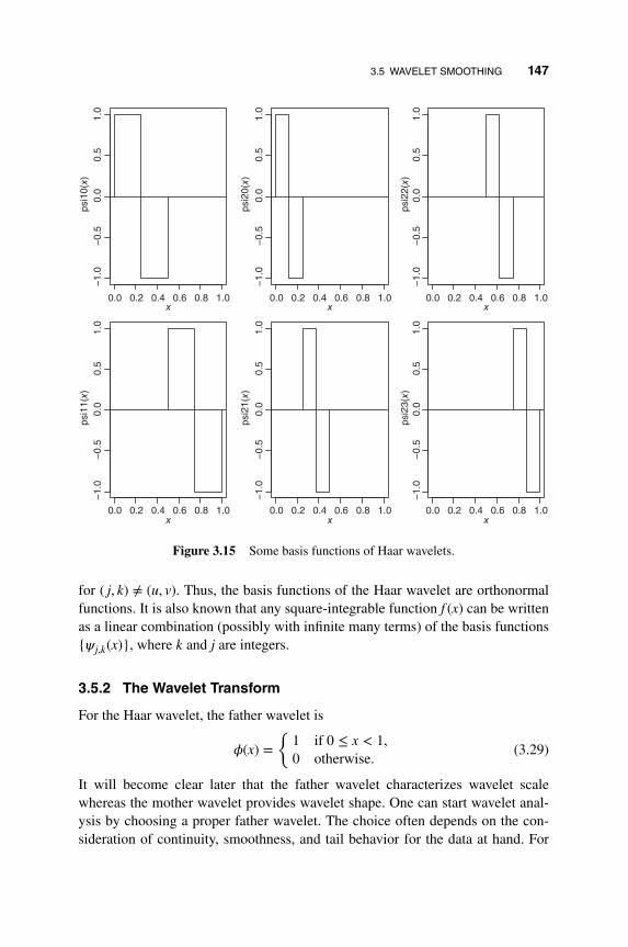
3.5 WAVELET SMOOTHING 147
1.00.80.60.40.20.0
1.0
0.5
0.0
−0.
5−
1.0
1.0
0.5
0.0
−0.
5−
1.0
1.0
0.5
0.0
−0.
5−
1.0
1.0
0.5
0.0
−0.
5−
1.0
1.0
0.5
0.0
−0.
5−
1.0
1.0
0.5
0.0
−0.
5−
1.0
x
psi1
0(x)
1.00.80.60.40.20.0x
psi1
1(x)
1.00.80.60.40.20.0x
psi2
0(x)
1.00.80.60.40.20.0x
psi2
1(x)
1.00.80.60.40.20.0x
psi2
2(x)
1.00.80.60.40.20.0x
psi2
3(x)
Figure 3.15 Some basis functions of Haar wavelets.
for ( j, k) ≠ (u, v). Thus, the basis functions of the Haar wavelet are orthonormalfunctions. It is also known that any square-integrable function f (x) can be writtenas a linear combination (possibly with infinite many terms) of the basis functions{𝜓j,k(x)}, where k and j are integers.
3.5.2 The Wavelet Transform
For the Haar wavelet, the father wavelet is
𝜙(x) ={
1 if 0 ≤ x < 1,0 otherwise.
(3.29)
It will become clear later that the father wavelet characterizes wavelet scalewhereas the mother wavelet provides wavelet shape. One can start wavelet anal-ysis by choosing a proper father wavelet. The choice often depends on the con-sideration of continuity, smoothness, and tail behavior for the data at hand. For

148 3. UNIVARIATE NONPARAMETRIC MODELS
a chosen father wavelet 𝜙(x), the translation functions {𝜙0,k(x) = 𝜙(x − k)|k =0,±1,±2,⋯} form an orthonormal basis for a reference space V0 ⊂ I2(R), whereI2(R) consists of all square-integrable functions on R. For the Haar wavelet 𝜙(x),V0 is formed by all piecewise constant functions with jumps at integers. Next,
consider the dilations 𝜙1,k(x) =√
2𝜙(2x − k), where k is an integer. It is easy tosee that {𝜙1,k(x)} form an orthonormal basis for a space V1 ⊃ V0. For the Haarwavelet, V1 consists of piecewise constant functions on intervals of length 0.5.In fact, we have a sequence of spaces ⋯ ⊃ V2 ⊃ V1 ⊃ V0 ⊃ V−1 ⊃ ⋯, where Vj isspanned by 𝜙j,k(x) = 2j∕2𝜙(2jx − k), where k is an integer. Mathematically, {Vj} isdense in I2(R) and the intersection ∩jVj = ∅. Also, if f (x) ∈ Vj, then f (2x) ∈ Vj+1.
Next, we introduce the role played by the mother wavelet and its offspring.Since V0 ⊂ V1, any function in V0 can be written as a linear combination of thebasis of V1. In particular, since the father wavelet (scaling function) is in V0, wehave
𝜙(x) =∑
k
hk𝜙1,k(x) =∑
k
hk
√2𝜙(2x − k), (3.30)
where the coefficient hk is the inner product hk =< 𝜙(x),√
2𝜙(2x − k) >. For theHaar scaling function, simple calculation shows
𝜙(x) =√
22𝜙1,0(x) +
√2
2𝜙1,1(x) =
√2
2[√
2𝜙(2x)] +√
22
[√
2𝜙(2x − 1)].
Now, define
𝜓(x) =∑
k
(−1)kh−k+1𝜙1,k(x) =∑
k
(−1)kh−k+1
√2𝜙(2x − k). (3.31)
Readers will see immediately that we use the notation of the mother wavelet. Thisis indeed true. For the Haar wavelet, direct calculation shows that𝜓(x) of Equation(3.31) turns out to be precisely the mother wavelet of Equation (3.27), that is,
𝜓(x) = h1𝜙1,0(x) + h0𝜙1,1(x) =√
22
[√
2𝜙(2x)] −√
22
[√
2𝜙(2x − 1)]
= 𝜙(2x) − 𝜙(2x − 1).
Let W0 be the orthogonal complement of V0 to V1. Then, we can express V1 asV1 = V0 ⊗W0. It is easy to see that the functions {𝜓(x − k)}, where k is an integer,form an orthonormal basis for W0. In general, let Wj be the orthogonal complementof Vj to Vj+1. We have Vj+1 = Vj ⊗Wj and {𝜓j,k(x) = 2j∕2𝜓(2x − k)} form a basisfor Wj. From ∪jVj = ∪jWj, we see that {Wj} is also dense in I2(R) and the family{𝜓j,k(x)}, where both j and k are integers, is a basis for I2(R).

3.5 WAVELET SMOOTHING 149
Suppose that f (x) is a function in VJ . By the recursion Vj+1 = Vj ⊗Wj, we have
VJ = VJ−1 ⊗WJ−1 = VJ−2 ⊗WJ−2 ⊗WJ−1 = V0 ⊗W0 ⊗W1 ⊗⋯⊗WJ−1.
Consequently, f (x) can be written as
f (x) = f0(x) +J−1∑𝑖=0
g𝑖(x),
where f0(x) ∈ V0 and gj(x) ∈ Wj. In an application with T data points such thatT = 2J for some integer J, VJ is as far as we can go. There are 2j basis elementsat the level j (j = 1,… , J − 1) and, adding up, we have a total of 2J − 1 elementsin the spaces Wj and one in V0. Since all spaces involved are orthogonal, all thebasis functions are orthonormal. This type of structured orthonormal basis allowsfor an efficient multiresolution analysis.
The Haar wavelet is easy to understand, but is discontinuous and is too coarsefor some applications. Many other wavelet functions have been proposed in theliterature. Figure 3.16 shows examples of symmlet (symmlet-8) and Daubechies(d16) wavelets. These wavelets have certain nice features. For instance, asymmlet-p family has a support of 2p − 1 consecutive intervals. The wider thesupport, the longer the wavelet has to go to zero. This in turn enables the waveletto achieve additional smoothness. Also, the scaling function 𝜙(x) of a symmlet-pwavelet has p vanishing moments, namely
∫𝜙(x)xjdx = 0, j = 1,… , p.
Consequently, any degree-p polynomial over the T = 2J time points can be repro-duced exactly in the space V0. This is an improvement over the Haar wavelet,which can only reproduce any constants in its V0.
In general, for a given father wavelet 𝜙(x), the transform operations are similarto those of the Haar basis:
1. If V0 is spanned by translations 𝜙(x − k), then V1 ⊃ V0 is spanned by
𝜙1,k(x) =√
2𝜙(2x − k) and 𝜙(x) =∑
k hk𝜙1,k(x), where hk are filter coeffi-cients. For instance, for Daubechies wavelet with parameter 2 (d2), we have
h0 =1 +
√3
4√
2, h1 =
3 +√
3
4√
2, h2 =
3 −√
3
4√
2, h3 =
1 −√
3
4√
2.
2. W0 is spanned by 𝜓(x) =∑
k gk𝜙1,k(x), where the coefficients are gk =(−1)kh1−k.
The sequence {hk} is called the low pass or low band filter whereas {gk} is thehigh pass or high band filter in the signal processing literature. The low-pass filter
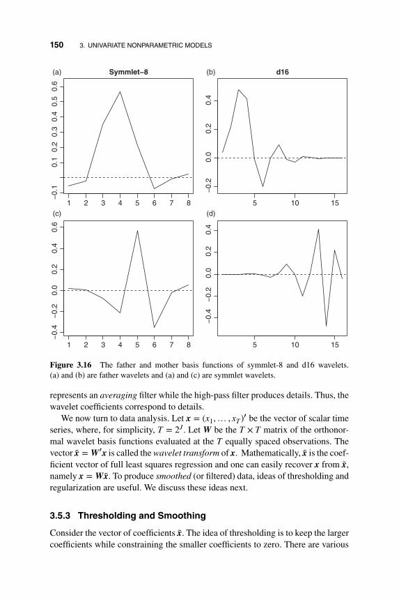
150 3. UNIVARIATE NONPARAMETRIC MODELS
87654321
0.6
0.5
0.4
0.3
0.2
0.1
−0.
1
Symmlet−8
87654321
0.6
0.4
0.2
0.0
−0.
2−
0.4
151050.
40.
20.
0−
0.2
d16
15105
0.4
0.2
0.0
−0.
2−
0.4
(a) (b)
(c) (d)
Figure 3.16 The father and mother basis functions of symmlet-8 and d16 wavelets.(a) and (b) are father wavelets and (a) and (c) are symmlet wavelets.
represents an averaging filter while the high-pass filter produces details. Thus, thewavelet coefficients correspond to details.
We now turn to data analysis. Let x = (x1,… , xT )′ be the vector of scalar timeseries, where, for simplicity, T = 2J . Let W be the T × T matrix of the orthonor-mal wavelet basis functions evaluated at the T equally spaced observations. Thevector x = W′x is called the wavelet transform of x. Mathematically, x is the coef-ficient vector of full least squares regression and one can easily recover x from x,namely x = Wx. To produce smoothed (or filtered) data, ideas of thresholding andregularization are useful. We discuss these ideas next.
3.5.3 Thresholding and Smoothing
Consider the vector of coefficients x. The idea of thresholding is to keep the largercoefficients while constraining the smaller coefficients to zero. There are various
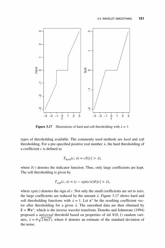
3.5 WAVELET SMOOTHING 151
3210−1−2−3
32
10
−1
−2
−3
c
Har
d
3210−1−2−3
21
0−
1−
2
x
Sof
t
Figure 3.17 Illustrations of hard and soft thresholding with 𝜆 = 1.
types of thresholding available. The commonly used methods are hard and softthresholding. For a pre-specified positive real number 𝜆, the hard thresholding ofa coefficient c is defined as
Thard(c, 𝜆) = cI(|c| > 𝜆),
where I(⋅) denotes the indicator function. Thus, only large coefficients are kept.The soft thresholding is given by
Tsoft(c, 𝜆) = (c − sgn(c)𝜆)I(|c| > 𝜆),
where sgn(c) denotes the sign of c. Not only the small coefficients are set to zero,the large coefficients are reduced by the amount 𝜆. Figure 3.17 shows hard andsoft thresholding functions with 𝜆 = 1. Let x∗ be the resulting coefficient vec-tor after thresholding for a given 𝜆. The smoothed data are then obtained byx = Wx∗, which is the inverse wavelet transform. Donoho and Johnstone (1994)proposed a universal threshold based on properties of iid N(0, 1) random vari-ates, 𝜆 = ��
√2 ln(T), where �� denotes an estimate of the standard deviation of
the noise.

152 3. UNIVARIATE NONPARAMETRIC MODELS
1086420
1.5
1.0
0.5
0.0
−0.
5−
1.0
−1.
5
Seconds
mV
ECG
Figure 3.18 The electrocardiogram of a patient, taking 180 samplers per second for 2048observations. The data are from the wmtsa package of R. See Percival and Walden (2000)for a description.
Another approach to obtain smoothed data is to apply regularization. Donohoand Johnstone (1994) considered a Stein unbiased risk estimation (SUREshrinkage):
min𝜷
‖x − W𝜷‖2 + 2𝜆‖𝜷‖1, (3.32)
which is the same as the well-known LASSO criterion for linear regression. SinceW is orthonormal, a simple solution is
𝛽j = sgn(xj)(|xj| − 𝜆)+, (3.33)
where 𝛽j is the jth element of 𝜷 and xj is the jth element of the wavelet transform
x. The inverse wavelet transform is then given by x = W𝜷.
Example 3.6 Figure 3.18 plots the electrocardiogram (ECG) data in the wmtsapackage of R. Details of the data are given in Percival and Walden (2000,Section 4.10). The data consist of 2048 observations of electrocardiogram (ECG)
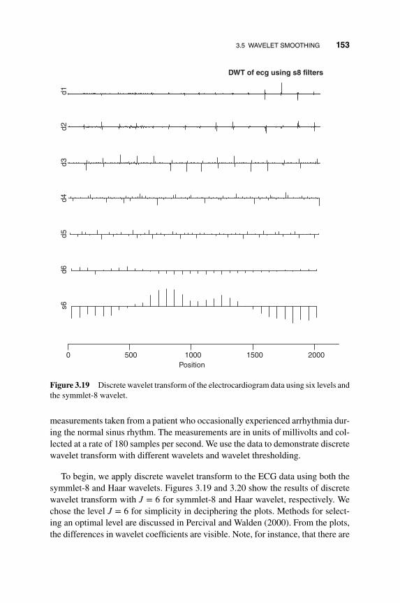
3.5 WAVELET SMOOTHING 153
2000150010005000
d1d2
d3d4
d5d6
s6DWT of ecg using s8 filters
Position
Figure 3.19 Discrete wavelet transform of the electrocardiogram data using six levels andthe symmlet-8 wavelet.
measurements taken from a patient who occasionally experienced arrhythmia dur-ing the normal sinus rhythm. The measurements are in units of millivolts and col-lected at a rate of 180 samples per second. We use the data to demonstrate discretewavelet transform with different wavelets and wavelet thresholding.
To begin, we apply discrete wavelet transform to the ECG data using both thesymmlet-8 and Haar wavelets. Figures 3.19 and 3.20 show the results of discretewavelet transform with J = 6 for symmlet-8 and Haar wavelet, respectively. Wechose the level J = 6 for simplicity in deciphering the plots. Methods for select-ing an optimal level are discussed in Percival and Walden (2000). From the plots,the differences in wavelet coefficients are visible. Note, for instance, that there are

154 3. UNIVARIATE NONPARAMETRIC MODELS
2000150010005000
d1d2
d3d4
d5d6
s6DWT of ecg using haar filters
Position
Figure 3.20 Discrete wavelet transform of the electrocardiogram data using six levels andthe Haar wavelet.
more larger values in the d1 plot of Figure 3.20. Figures 3.21 and 3.22 show theextended data analysis of the two discrete wavelet transforms of the ECG data.Extended data analysis is a graphical tool used to visually summarize the salientfeatures of the discrete wavelet transform. The upper right plots of these two fig-ures are the same as those of Figures 3.19 and 3.20. From the energy distributionof the two figures we see that the two wavelets work similarly, but also have somedifferences.
Next, we demonstrate the wavelet thresholding by applying both hard and softthresholding with universal threshold to the d1 coefficients of the discrete wavelettransform of the electrocardiogram data with symmlet-8 wavelet. Figure 3.23shows the plots of empirical d1 and results of thresholding using the universal
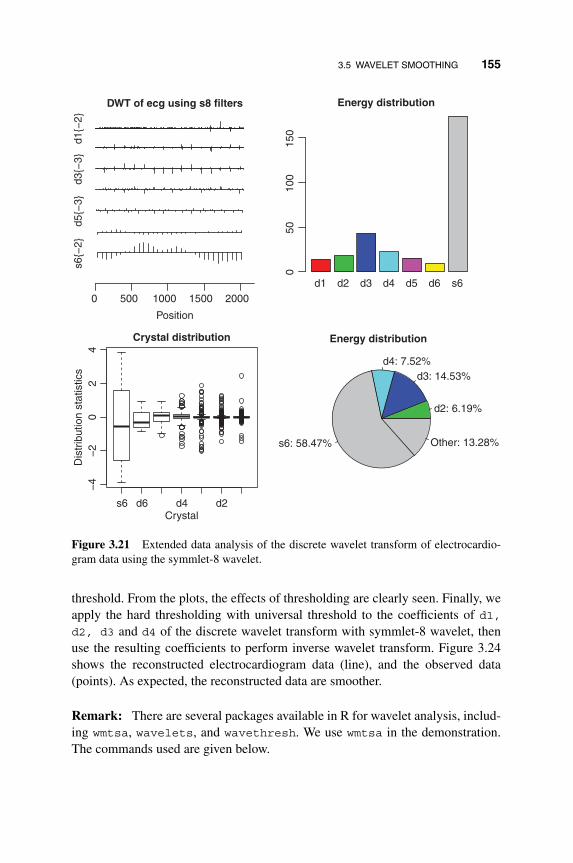
3.5 WAVELET SMOOTHING 155
2000150010005000
d1{−
2}d3
{−3}
d5{−
3}s6
{−2}
DWT of ecg using s8 filters
Position
s6d6d5d4d3d2d115
010
050
0
Energy distribution
d2d4d6s6
42
0−
2−
4
Crystal
Dis
trib
utio
n st
atis
tics
Crystal distribution
d2: 6.19%
d3: 14.53%d4: 7.52%
s6: 58.47% Other: 13.28%
Energy distribution
Figure 3.21 Extended data analysis of the discrete wavelet transform of electrocardio-gram data using the symmlet-8 wavelet.
threshold. From the plots, the effects of thresholding are clearly seen. Finally, weapply the hard thresholding with universal threshold to the coefficients of d1,d2, d3 and d4 of the discrete wavelet transform with symmlet-8 wavelet, thenuse the resulting coefficients to perform inverse wavelet transform. Figure 3.24shows the reconstructed electrocardiogram data (line), and the observed data(points). As expected, the reconstructed data are smoother.
Remark: There are several packages available in R for wavelet analysis, includ-ing wmtsa, wavelets, and wavethresh. We use wmtsa in the demonstration.The commands used are given below.

156 3. UNIVARIATE NONPARAMETRIC MODELS
2000150010005000
DWT of ecg using haar filters
Position
s6d6d5d4d3d2d1
Energy distribution
d2d4d6s6
d1{0
}d3
{0}
d5{0
}s6
{0}
150
100
500
42
0−
2
Crystal
Dis
trib
utio
n st
atis
tics
Crystal distribution
d2: 9.53%
d3: 12.54%d4: 6.63%
s6: 57.13% Other: 14.17%
Energy distribution
Figure 3.22 Extended data analysis of the discrete wavelet transform of electrocardio-gram data using the Haar wavelet.
R demonstration: Wavelet transform via the wmtsa package.
> require(wmtsa)> plot(ecg)> m1 < wavDWT(ecg,n.level=6)> names(m1)[1] "data" "scales" "series" "dictionary" "shifted"[6] "xform"> plot(m1)> eda.plot(m1)> m2 < wavDWT(ecg,n.level=6,wavelet="haar")> plot(m2)> eda.plot(m2)

3.5 WAVELET SMOOTHING 157
10008006004002000
21
0−
12
10
−1
Index
d1 c
oeffi
cien
ts
10008006004002000Index
Har
d
10008006004002000
1.5
0.5
−1.
0
Index
Sof
t
Figure 3.23 Hard and soft thresholding with universal threshold for the d1 coefficientsof the discrete wavelet transform of the electrocardiogram data with symmlet-8 wavelet.
# Thresholding with "universal" threshold function> d1 < wavShrink(m1$data$d1) ## hard threshold> d1a < wavShrink(m1$data$d1,shrink.fun="soft")> par(mfcol=c(3,1))> plot(m1$data$d1,type="h",ylab="d1 coefficients")> plot(d1,type="h",ylab='hard')> plot(d1a,type="h",ylab='soft')### Reconstruction> d1 < wavShrink(m1$data$d1) ## Hard thresholding> d2 < wavShrink(m1$data$d2)> d3 < wavShrink(m1$data$d3)> d4 < wavShrink(m1$data$d4)> m1copy < m1> m1copy$data$d1 < d1> m1copy$data$d2 < d2> m1copy$data$d3 < d3> m1copy$data$d4 < d4> ecg1 < reconstruct(m1copy)> ts.plot(ecg1,ylab='ecg',col="red")> points(1:2048,as.numeric(ecg),cex=0.4)

158 3. UNIVARIATE NONPARAMETRIC MODELS
Time
EC
G
2000150010005000
1.5
1.0
0.5
0.0
−0.
5−
1.0
−1.
5
Figure 3.24 Observations and reconstructed values of electrocardiogram data. The recon-struction is done by the inverse wavelet transform after hard thresholding some of the coef-ficients of discrete wavelet transform of the observed data with the symmlet-8 wavelet.
3.6 NONLINEAR ADDITIVE MODELS
A zero-mean time series xt follows a nonlinear additive autoregressive (NAAR)model of order p if it satisfies
xt =p∑𝑖=1
f𝑖(xt−𝑖) + at, (3.34)
where f𝑖(xt−𝑖) is a smooth zero-mean function of xt−𝑖 and {at} is a sequence ofindependent and identically distributed random variables with mean zero and vari-ance 0 < 𝜎2
a <∞. This model was introduced by Chen and Tsay (1993). It is aspecial case of the general nonlinear AR(p) model xt = 𝜇 + f (xt−1,… , xt−p) + at.See Equation (3.6). Except for the dynamic dependence, the model also belongsto the generalized additive models of Hastie and Tibshirani (1990).
For a given NAAR model, Chen and Tsay (1993) discussed two backfittingmethods for model fitting. The two methods are the alternating conditionalexpectation (ACE) algorithm of Breiman and Friedman (1985) and the BRUTOalgorithm of Hastie and Tibshirani (1990). These two algorithms are iterative,

3.6 NONLINEAR ADDITIVE MODELS 159
use nonparametric smoothing methods, and apply generalized cross-validationto select the smoothing parameters. They are called backfitting procedures sincethey are based on the fact that
f𝑖(xt−𝑖) = E
[xt −
p∑k≠𝑖
fk(xt−k)
].
The smoothing methods used include smoothing splines, local polynomials, andthe LOWESS procedures discussed in Section 3.3. Roughly speaking, for theNAAR model in Equation (3.34), one starts with some initial estimate f (0)
𝑖(xt−𝑖)
for each function f𝑖(xt−𝑖). To obtain the jth refined estimate of f𝑖(xt−𝑖), oneconsiders the smoother
f (j)𝑖
(xt−𝑖) = S𝑖
[xt −
p∑k≠𝑖
f (j−1)k (xt−k)
|||||| xt−𝑖
],
where S𝑖(⋅) is smoother and the superscript ( j) denotes the jth iteration. Thesmoother S𝑖(⋅) is typically represented by a symmetric matrix, as given in Section3.4.2. The iteration cycles through 𝑖 = 1,… , p for the jth iteration and continuesuntil all individual fitted functions do not change. Basically, nonparametricestimation of the NAAR model in (3.34) involves the selection of p smoothingparameters via the generalized cross-validation, which is defined as
GCV(𝜆1,… , 𝜆p) =∑n
t=1[xt −∑p𝑖=1 f𝑖,𝜆𝑖(xt−𝑖)]
2
n[1 − trR(𝜆1,… , 𝜆p)∕n]2, (3.35)
where R(𝜆1,… , 𝜆p) is the additive-fit operator for the given smoothing parameters
𝜆1,… , 𝜆p and f𝑖,𝜆𝑖(xt−𝑖) denotes the fitted value of the function f𝑖(xt−𝑖). In practice,evaluating the denominator of Equation (3.35) requires intensive computation inorder to optimize the p bandwidths simultaneously. See, for instance, the Newtonmethod described in Gu and Wahba (1991).
To ease the computational burden, the BRUTO algorithm attempts to minimizethe statistic
GCVB(𝜆1,… , 𝜆p) =1n
∑nt=1[xt −
∑p𝑖=1 f𝑖,𝜆𝑖(xt−𝑖)]
2
{1 − [1 +∑p𝑖=1(trS𝑖(𝜆𝑖) − 1)]∕n}2
. (3.36)
The use of 1 +∑p𝑖=1[trS𝑖(𝜆𝑖) − 1] in place of trR(𝜆1,… , 𝜆p) reduces the compu-
tation from O(n3) to O(n). Details and convergence of the BRUTO algorithm canbe found in Hastie and Tibshirani (1990) and the references therein. A special fea-ture of the criterion in Equation (3.36) is that the minimization is carried out oneparameter at a time yet the objective function is global.

160 3. UNIVARIATE NONPARAMETRIC MODELS
The ACE algorithm attempts to estimate nonparametric models and a suitabletransformation of the dependent variable jointly. Specifically, the working modelcorresponding to the NAAR model in Equation (3.34) is
𝜃(xt) =p∑𝑖=1
f𝑖(xt−𝑖) + at, (3.37)
where 𝜃(xt) denotes a link function between the conditional expectation of xtgiven the predictor
∑p𝑖=1 f𝑖(xt−𝑖) and the initial values x1,… , xp. The link function
is assumed to be monotone, zero mean and unit variance for identifiablity. Forthe NAAR models, 𝜃(xt) is simply the identity function. The ACE algorithm forestimating the model in Equation (3.37) is as follows:
(i) Initialize: Let 𝜃(xt) = [xt − E(xt)]∕var(xt)1∕2.
(ii) Fit an additive model to 𝜃(xt) to update the functions f1(xt−1),… , fp(xt−p).
(iii) Compute the expectation ��(xt) = E[∑p𝑖=1 f𝑖(xt−𝑖)|xt] and standardize to
obtain a new estimate 𝜃(xt) = ��(xt)∕{var[��(xt)]}1∕2.
(iv) Alternate steps (ii) and (iii) until E[𝜃(xt) −∑p𝑖=1 f𝑖(xt−𝑖)]
2 does not change.
The NAAR model in Equation (3.34) can easily be extended to include someexplanatory variables. For instance, let zt denote an explanatory variable that mightbe helpful in understanding or predicting the time series xt. A generalized nonlin-ear additive model then becomes
xt = 𝜇 +p∑𝑖=1
f𝑖(xt−𝑖) +s∑
j=0
gj(zt−j) + at, (3.38)
where s is a nonnegative integer and gj(⋅) are smooth functions similar to f𝑖(⋅).The estimation methods for NAAR models continue to apply to the model inEquation (3.38).
Example 3.7 Consider the weekly US regular gasoline prices, dollars per gallon,from January 7, 2008 to March 20, 2017 for 481 observations. It is known that theprice of gasoline depends on the crude oil price so we also consider the weeklycrude oil prices, dollars per barrel of West Texas Intermediate (WTI). The twoprice series are shown in Figure 3.25. In this analysis, we use the first-differencedprice series, that is, we analyze the price changes. The sample size used is thenT = 480. Let xt be the weekly change series of the regular gasoline price and ztbe the change series of crude oil price. Figure 3.26 shows some scatter plots ofxt against lagged values of xt and zt. As expected, the plots exhibit dependencebetween xt and the selected lagged variables.
If univariate time series models with exogenous variables are used, we obtainthe model
xt = 0.366xt−1 + 0.078xt−2 + 0.0094zt + 0.0021zt−1 + et, ��e = 0.0419, (3.39)

3.6 NONLINEAR ADDITIVE MODELS 161
2008 2010 2012 2014 2016
4080
120
Time
Oil
2008 2010 2012 2014 2016
1.5
2.5
3.5
Time
Gas
Figure 3.25 Time plots of weekly US regular gasoline prices and crude oil prices fromJanuary 7, 2008 to March 20, 2017.
where all coefficient estimates are statistically significant at the 5% level. Modelchecking indicates that this model fits the data reasonably well. On the other hand,the upper-right plot of Figure 3.26 shows some nonlinear relationship between xtand zt. This is understandable as the gasoline price tends to increase immediatelyfollowing a jump in the crude oil price, but decline slowly after a drop in theoil price.
To explore the nonlinear relationship, we use a nonlinear additive model withexplanatory variables xt−1, xt−2, zt, and zt−1. The estimation is carried out via thegam package of R by using smoothing splines with 4 degrees of freedom for eachexplanatory variable. The nonlinear additive model improves the fit. However,the associated analysis of variance for the nonparametric effects indicates that theexplanatory variable xt−2 does not contribute significantly to the model. See below:
Anova for Nonparametric EffectsNpar Df Npar F Pr(F)
s(pcgasm1, 4) 3 11.1235 4.623e07 ***s(pcgasm2, 4) 3 1.4769 0.2200580s(pcoil, 4) 3 6.8333 0.0001634 ***s(pcoilm1, 4) 3 4.4194 0.0044548 **
To simplify the model, we remove xt−2 and re-fit the nonlinear additive model. Allthree explanatory variables are now statistically significant at the usual 5% level.

162 3. UNIVARIATE NONPARAMETRIC MODELS
0.20.10.0−0.1−0.2−0.3−0.4pcgasm1
pcga
s
0.20.10.0−0.1−0.2−0.3−0.4pcgasm2
pcga
s
151050−5−10−15
0.2
0.0
−0.
2−
0.4
0.2
0.0
−0.
2−
0.4
0.2
0.0
−0.
2−
0.4
0.2
0.0
−0.
2−
0.4
pcoil
151050−5−10−15pcoilm1
pcga
s
Figure 3.26 Selected scatter plots of price changes of regular gasoline and their laggedvariables. The data are from January 7, 2008 to March 20, 2017.
For comparison, the residual standard error of the linear ARX model of Equation(3.39) is 0.0419 whereas that of the nonlinear additive model is 0.0390. Note thatcaution should be exercised when comparing residual sum of squares obtainedfrom a nonparametric method, since it depends on the bandwidth. A small band-width often results in a small residual sum of squares. Comparing cross-validationcriterion is often preferred. Figure 3.27 shows the smooth functions used in thenonlinear additive model. The plots also include the point-wise 95% confidenceintervals of the smooth functions. From the plots, the nonlinear feature of the rela-tionship is seen. Furthermore, we also use the analysis of variance to compare thelinear model of Equation (3.39) with the fitted nonlinear additive model. The resultis given below:
> anova(m2.lm,m2.gam)Analysis of Variance Table
Model 1: pcgas ˜ 1 + pcgasm1 + pcgasm2 + pcoil + pcoilm1Model 2: pcgas ˜ 1 + s(pcgasm1, 4) + s(pcoil, 4) + s(pcoilm1, 4)

3.6 NONLINEAR ADDITIVE MODELS 163
0.20.10.0−0.1−0.2−0.3−0.4
0.05
−0.
05−
0.15
−0.
25
pcgasm1
s(pc
gasm
1, 4
)
151050−5−10−15
0.15
0.05
−0.
05−
0.15
pcoil
s(pc
oil,
4)
151050−5−10−15
0.05
−0.
05−
0.15
pcoilm1
s(pc
oilm
1, 4
)
Figure 3.27 Smooth functions of explanatory variables resulted from fitting an additivemodel to the price change of the US weekly regular gasoline price. The dashed lines indicatepoint-wise 95% confidence intervals. The data are from January 7, 2008 to March 20, 2017.
Res.Df RSS Df Sum of Sq F Pr(>F)1 474 0.832182 466 0.72499 8.0001 0.10719 8.6123 5.619e11 ***
Clearly, the nonlinear model shows significant improvements over the linear ARXmodel. Finally, we use the bruto command of the mda package in R to confirmthe fitted nonlinear additive model. The result of BTUTO fit is
> require(mda)> m3.bruto < bruto(X[,1],X[,1])> m3.bruto$typepcgasm1 pcgasm2 pcoil pcoilm1smooth excluded smooth linear
Levels: excluded linear smooth

164 3. UNIVARIATE NONPARAMETRIC MODELS
The result confirms the removal of xt−2 and using smooth spline functions ofxt−1 and zt (pcoil).
R commands used in fitting the NAAR model via the gam package.
require(gam)
da < read.csv("wgasoilpc.csv")
X < data.frame(da[,1])
m2.lm < lm(pcgas˜ 1+pcgasm1+pcgasm2+pcoil+pcoilm1,data=X)
m2 < gam(pcgas˜ 1+s(pcgasm1,4)+s(pcgasm2,4)+s(pcoil,4)+s(pcoilm1,4),data=X)
summary(m2)
m2.gam < gam(pcgas˜ 1+s(pcgasm1,4)+s(pcoil,4)+s(pcoilm1,4),data=X)
par(mfcol=c(2,2))
plot(m2.gas)
par(mfcol=c(1,1))
anova(m2.lm,m2.gam)
require(mda)
m3.bruto < bruto(X[,1],X[,1])
m3.bruto$type
3.7 INDEX MODEL AND SLICED INVERSE REGRESSION
Another class of nonlinear models useful in many scientific areas is the indexmodels, especially the single index model. This model is closely related to dimen-sion reduction and projection pursue in the statistical literature. Let xt be the timeseries of interest and zt = (z1t,… , zkt)
′ be a k-dimensional vector of explanatoryvariables, the components of which may include lagged variables of xt. A generalindex model can be written as
xt = f (𝜷′zt) + at, (3.40)
where {at} is a white noise series and independent of 𝜷′zt, 𝜷 is a k × m full-rankmatrix of real numbers with m > 0, and f (⋅) denotes a smooth function. Typically,we have m ≪ k so that xt depends on m linear combinations of zt rather than the kexplanatory variables directly. The integer m is referred to as the effective dimen-sion of the model or the number of indices, and the function f (⋅) is m-dimensional.In particular, if m = 1, then xt depends on vt = 𝜷′zt, which is a scalar, and the func-tion f (⋅) is one-dimensional. The resulting model is called the single index model.
Strictly speaking, the 𝜷 matrix of Equation (3.40) is not uniquely definedbecause f (⋅) is not precisely specified. This type of non-uniqueness does not causeany problems in applications because we can require that columns of 𝜷 are nor-malized and orthogonal to each other so that 𝜷′𝜷 = Im, the m × m identity matrix.Since both f (⋅) and 𝜷 are unknown, we need certain conditions to obtain consistentestimates of 𝜷. To this end, many methods have been proposed in the literature, andone of these methods is the sliced inverse regression of Li (1991). A key concept
3.7 INDEX MODEL AND SLICED INVERSE REGRESSION 165
of the index model is that the conditional distribution of xt given zt is the same asthat of xt given 𝜷′zt. Therefore, the subspace expanded by 𝜷′zt is referred to as thecentral subspace, which is of dimension m, not k. Since this subspace of zt is in thepredictor space, it is referred to as an inverse subspace. Hence, the name inverseregression is used. A sufficient condition for the existence of a lower dimensionalcentral inverse subspace is as follows. For any arbitrary non-zero vector b ∈ Rk,there exists a constant c0 and an m-dimensional constant vector c = (c1,… , cm)′
such that
E(b′zt|𝜷′zt) = c0 + c′(𝜷′zt). (3.41)
This condition essentially states that given 𝜷′zt, the expectation of any non-zerolinear combination of zt is in the subspace generated by 𝜷′zt. Under this conditionLi (1991) established the following theorem.
Theorem 3.1 Consider the index model of Equation (3.40) and assume thatthe condition (3.41) holds. Then, the centered inverse regression curve E(zt ∣xt) − E(zt) is contained in the linear subspace spanned by 𝚺z𝜷, where 𝚺z is thecovariance matrix of zt.
To make use of Theorem 3.1, one needs to estimate 𝚺z and the covariancematrix of E(zt ∣ xt). The former is estimated by the sample covariance matrix ofzt. The latter, on the other hand, requires some creative thinking. Li (1991) pro-vided a crude, but effective, estimate based on slices of zt given xt. This leads tothe procedure of sliced inverse regression. To describe the procedure, we expressthe data as (X, Z), where X = (x1,… , xT )′ and Z is a T × k design matrix such thatthe tth row is z′t .
SIR procedure: Let H be a positive integer.1. Sort the data (X, Z) by xt (in increasing order).
2. Divide the data set into H non-overlapping slices as equally as possible.Denote the slices by (X(𝑖), Z(𝑖)), 𝑖 = 1,… , H.
3. For each slice, compute the sample mean of Z(𝑖). That is, compute the meanvector of the regressors of each slice.Let Z(𝑖) =
1n𝑖
∑n𝑖j=1 z(𝑖),j, where n𝑖 is the number of data points in the 𝑖th slice
and z(𝑖),j is the jth data point of the 𝑖th slice.
4. Compute the covariance matrix of the slice means of Z weighted by the sizeof the slice.
��s =1T
H∑𝑖=1
n𝑖(Z(𝑖) − Z)(Z(𝑖) − Z)′,

166 3. UNIVARIATE NONPARAMETRIC MODELS
where T is the sample size, Z is the sample mean of Z, and the subscript s isused to signify that 𝚺s is formed using slices.
5. Find the SIR directions by performing the eigenvalue–eigenvector analysis
of ��−1
z ��s, where ��z is the sample covariance matrix of zt. That is, obtain
��s𝜷 𝑖 = 𝜆𝑖𝚺z𝜷 𝑖, 𝑖 = 1,… , k,
where 𝜆1 ≥ 𝜆2 ≥ ⋯ ≥ 𝜆k. 𝜷 𝑖 is called the 𝑖th SIR direction.
6. Use each SIR direction to form a linear combination of zt.
7. Estimate f (⋅) by smoothing xt against 𝜷′𝑖zt.
The statistic ��s is used to estimate the covariance matrix of E(zt ∣ xt), and the laststep can be done by one of the smoothing methods discussed in the chapter.
The eigenvalues 𝜆𝑖 of the SIR procedure can be used to find the dimension mof the central inverse subspace. Li (1991) also showed that, under the assumptionthat zt are normally distributed, then T(k − j)��k−j follows a chi-square distributionwith (k − j)(H − j − 1) degrees of freedom, where ��k−j is the average of the (k − j)smallest eigenvalues.
The number of slices H does not need to be large for the sliced inverse regres-sion to perform well. Furthermore, there exist several extensions of the SIRmethod, including the principal Hessian directions of Li (1992) and Cook (1998),an adaptive approach by Xia et al. (2002), and the sliced average variance esti-mation (SAVE) of Shao et al. (2007). In applications, the dr package of R can beused to perform the SIR method and its extensions for dimension reduction.
Example 3.8 Consider again the weekly US regular gasoline prices and thecrude oil prices of Example 3.7. Here we also use the price change series xt andzt, and our goal is to demonstrate the application of sliced inverse regression inexploring the dependence of xt on its lagged values xt−1 and xt−2, and on zt andzt−1. To this end, we have zt = (xt−1, xt−2, zt, zt−1)′.
Applying the dr command in the dr package, we obtain the following result:
> require(dr)> da < read.csv("wgasoilpc.csv")> head(da)N pcgas pcgasm1 pcgasm2 pcoil pcoilm1
1 1 0.038 0.050 0.047 2.10 3.25....> X < da[,1]

3.7 INDEX MODEL AND SLICED INVERSE REGRESSION 167
> m1 < dr(pcgas˜ .,data=data.frame(X))> summary(m1)Call: dr(formula = pcgas ˜ ., data = data.frame(X))
Method: sir with 8 slices, n = 478.Slice Sizes:59 59 59 60 61 59 61 60
Estimated Basis Vectors for Central Subspace:Dir1 Dir2 Dir3 Dir4
pcgasm1 0.996244 0.037141 0.65816 0.902187pcgasm2 0.083244 0.999245 0.75199 0.431118pcoil 0.023252 0.011099 0.02416 0.002282pcoilm1 0.005176 0.002633 0.02744 0.013846
Dir1 Dir2 Dir3 Dir4Eigenvalues 0.4983 0.03988 0.004562 0.001055Rˆ2(OLS|dr) 0.9975 0.99855 0.999395 1.000000
Largesample Marginal Dimension Tests:Stat df p.value
0D vs >= 1D 259.9249 28 0.00001D vs >= 2D 21.7489 18 0.24332D vs >= 3D 2.6851 10 0.98793D vs >= 4D 0.5043 4 0.9731
The default option of the dr command uses eight slices each with size approxi-mately 60. The large-sample test indicates that the dimension of the effective cen-tral subspace is 1. The null hypothesis of zero dimension is clearly rejected withthe p value being zero whereas that of one dimension cannot be rejected with pvalue 0.24. This conclusion can also be seen as the largest eigenvalue is 0.49,which explains about 99.75% of the variability. The second largest eigenvalue isonly 0.040.
Let rt denote the transformed data of the first principal direction shown bydirection 1 of the SIR method. Figure 3.28 shows the scatter plot of xt versus rt.The solid line of the plot denotes the fitted values via the local smoothing methodlowess. From the plot it is seen that there exists some minor nonlinearity betweenxt and rt. More importantly, the local smoothing suggests a slope change aroundrt ≈ −0.2. Therefore, we used a simple threshold model and obtained
xt =
{0.366rt + 𝜖t, if rt ≥ −0.2,
0.462rt + 𝜖t, if rt < −0.2,(3.42)

168 3. UNIVARIATE NONPARAMETRIC MODELS
0.40.20.0−0.2−0.4−0.6
0.2
0.1
0.0
−0.
1−
0.2
−0.
3−
0.4
Direction 1
Gas
olin
e pr
ice
Figure 3.28 Scatter plot of changes in weekly regular gasoline price versus the first prin-cipal direction of the sliced inverse regression. The solid line denotes the local smoothingfit via lowess.
where the residual standard error is 0.042 and the two coefficient estimates arestatistically significant at the 1% level. The Ljung–Box statistics of the residualsindicate that there exist no significant serial correlations in the residuals. Specifi-cally, we have Q(12) = 10.35 with p value 0.59.
### Further Analysis> TZ < as.matrix(X[,1])%*%m1$evectors> idx < c(1:478)[TZ[,1] < 0.2]> R1 < rep(0,478)> R1[idx] < 1> LTZ < TZ[,1]*R1> m2 < lm(X$pcgas˜ 1+TZ[,1]+LTZ)> summary(m2)
Call: lm(formula = X$pcgas ˜ 1 + TZ[, 1] + LTZ)

EXERCISES 169
Coefficients:Estimate Std. Error t value Pr(>|t|)
TZ[, 1] 0.36633 0.02017 18.165 < 2e16 ***LTZ 0.09613 0.03345 2.874 0.00424 **Residual standard error: 0.04152 on 476 degrees of freedomMultiple Rsquared: 0.5697, Adjusted Rsquared: 0.5679
> Box.test(m2$residuals,lag=12,type='Ljung')BoxLjung test
data: m2$residualsXsquared = 10.353, df = 12, pvalue = 0.585
3.8 EXERCISES
3.1 Consider the half-hourly electricity demands of Mondays in Adelaide, Aus-tralia, from July 6, 1997 to March 31, 2007. The data are available from thefds package of R. See Hyndman (2016). There are 48 observations in a dayand 508 weeks. The original data consist of demands from Sunday to Satur-day, but we focus here on Monday only. Since the demands have an upwardtrend so we focus on xt = (1 − B48)dt with dt denoting the demand. Use thecommands below to obtain the xt series.
require(fds)data(mondaydemand)de < c(mondaydemand$y)xt < diff(de,48)
(a) Perform discrete wavelet transform of xt using six levels and thesymmlet-8 wavelet. Show the plot and eda.plot, as in Example 3.6.
(b) Repeat part (a) using the Haar wavelet.
(c) Perform a reconstruction using hard thresholding, as in Example 3.6.
3.2 Consider the US monthly leading index from January 1982 to July 2017.The data can be obtained from FRED (code: USSLIND) and are season-ally adjusted. Let xt denote the monthly leading index. Use lowess and localpolynomials with degrees 0, 1, and 2 to explore the dependence of xt onxt−6. Show a scatter plot of xt versus xt−6 with fitted lines of lowess and localpolynomials. Is the relationship nonlinear? Why?
3.3 Consider again the US monthly leading index of question 2. This time useB-splines and smooth splines to explore the dependence of xt on xt−6. Show

170 3. UNIVARIATE NONPARAMETRIC MODELS
the scatter plot of xt versus xt−6 with fitted lines via B-splines and smoothsplines. Is the relationship nonlinear? Why?
3.4 Consider again the US monthly leading index of question 2.
(a) Fit a linear AR(6) model to xt and refine the model by removing the esti-mates that are not statistically significant at the usual 5% level. Writedown the fitted model.
(b) Fit a NAAR model
xt = c0 + f1(xt−1) + f3(xt−3) + f4(xt−4) + f6(xt−6) + 𝜖t,
to the data, where f𝑖(xt−𝑖) is a spline function. You may use the gam
package.
(c) Perform an analysis of variance to confirm that the NAAR model issignificantly different from the linear AR(6) model.
3.5 Consider the US quarterly index of manufacturing real output from 1987.Ito 2017.II. The data can be obtained from FRED (code: OUTMS). Let xt =ln(Ot) − ln(Ot−1), where Ot is the real output index (2009=100).
(a) Build a linear AR model for xt. Perform model checking and write downthe fitted model.
(b) Fit the NAAR model
xt = c0 + f1(xt−1) + f2(xt−2) + 𝜖t,
using the gam package. What are the estimates of the coefficients? Per-form model checking. Is the model adequate? Why?
(c) Perform analysis of variance to confirm that the NAAR model con-tributes significantly over the linear AR model of part (a).
(d) Obtain the residual plots of the two fitted models in parts (a) and (b).Comments on the fit of the models.
REFERENCES
Bierens, H. J. (1983). Uniform consistency of kernel estimators of a regression func-tion under generalized conditions. Journal of the American Statistical Association 78:699–707.
Bierens, H. J. (1987). Kernel estimators of regression functions in Advances on Econo-metrics: Fifth World Congress, ed. T. F. Bewley. Cambridge University Press,Cambridge.

REFERENCES 171
Breiman, L. and Friedman, J. H. (1985). Estimating optimal transformation for multipleregression and correlation (with discussion). Journal of the American Statistical Asso-ciation 80: 580–619.
Chen, R. and Tsay, R. S. (1993). Nonlinear additive ARX models. Journal of the AmericanStatistical Association 88: 955–967.
Cleveland, W. S. (1979). Robust locally weighted regression and smoothing scatterplots.Journal of the American Statistical Association 74: 829–836.
Collomb, G. and Hardle, W. (1986). Strong uniform convergence rates in robust nonpara-metric time series analysis and prediction: Kernel regression estimation from dependentobservations. Stochastic Processes and Their Applications 23: 77–89.
Cook, R. D. (1998). Principal Hessian directions revisited (with discussion). Journal of theAmerican Statistical Association 93: 84–100.
Daubechies, B. (1992). Ten Lectures in Wavelets. Society for Industrial and Applied Math-ematics, Philadelphia.
de Boor, C. (1978). A Practical Guide to Splines. Springer-Verlag, New York.
Donoho, D. and Johnstone, I. (1994). Ideal spatial adaptation by wavelet shrinkage.Biometrika 81: 425–455.
Epanechnikov, V. (1969). Nonparametric estimates of a multivariate probability density.Theory of Probability and Its Applications 14: 153–158.
Fan, J. and Gijbels, I. (1996). Local Polynomial Modeling and Its Applications. Chapmanand Hall, London.
Fan, J. and Yao, Q. (2003). Nonlinear Time Series: Nonparametric and Parametric Meth-ods. Springer-Verlag, New York.
Gu, C. and Wahba, G. (1991). Minimizing GCV/GML scores with multiple smoothingparameters via the Newton method. SIAM Journal of Scientific and Statistical Comput-ing 12: 383–398.
Hardle, W. (1990). Applied Nonparametric Regression. Cambridge University Press, NewYork.
Hardle, W., Lutkepohl, H., and Chen, C. (1997). A review of nonparametric time seriesanalysis. International Statistical Review 65: 49–72.
Hastie, T. J. and Tibshirani, R. J. (1990). Generalized Additive Models. Chapmand and Hall,New York.
Hastie, T., Tibshirani, R. and Friedman, J. (2001). The Elements of Statistical Learning:Data Mining, Inference, and Prediction. Springer, New York.
Hyndman, R. J. (2016). Time Series Data Library. http://data.is/TSDLdemo. AccessedMarch, 2016.
Li, K. C. (1991). Sliced inverse regression for dimension reduction (with discussion). Jour-nal of the American Statistical Association 86: 316–342.
Li, K. C. (1992). On principal Hessian directions for data visualization and dimensionreduction: Another application of Stein’s lemma. Journal of the American StatisticalAssociation 87: 1025–1039.

172 3. UNIVARIATE NONPARAMETRIC MODELS
Masry, E. and Tj𝜙stheim, D. (1995). Nonparametric estimation and identification of non-linear ARCH time series: Strong consistency and asymptotic normality. EconometricTheory 11: 258–289.
Muller, H. G. (1988). Nonparametric Regression Analysis of Longitudinal Data. LectureNotes in Statistics, 46. Springer-Verlag, Berlin.
Nadaraya, E. A. (1964). On estimating regression. Theory of Probability and its Applica-tions 9: 141–142.
Nason, G. P. (2008). Wavelet Methods in Statistics with R. Springer, New York.
Percival, D. B. and Walden, A. T. (2000). Wavelet Methods for Time Series Analysis. Cam-bridge University Press, Cambridge.
Priestley, M. B. and Chao, M. T. (1972). Nonparametric function fitting. Journal of theRoyal Statistical Society Series B 34: 384–392.
Robinson, P. (1983). Nonparametric estimation for time series models. Journal of TimeSeries Analysis 4: 185–208.
Shao, Y., Cook, R. D. and Weisberg, S. (2007). Marginal tests with sliced average varianceestimation. Biometrika 94: 285–296.
Sharpe, W. (1964). Capital asset prices: A theory of market equilibrium under conditionalrisk. Journal of Finance 19: 425–442.
Stone, C. J. (1977). Consistent nonparametric regression. Annals of Statistics 5: 595–645.
Tong, H. (1990). Non-Linear Time Series: A Dynamical System Approach. Oxford Univer-sity Press, Oxford.
Truong, Y. K. (1993). A nonparametric framework for time series analysis in New Direc-tions in Time Series Analysis. Springer, New York.
Tweedie, R. L. (1975). Sufficient conditions for ergodicity and recurrence of Markov chainon a general state space. Stochastic Processes and Their Applications 3: 385–403.
Watson, G. S. (1964). Smooth regression analysis. Sankhya Series A 26: 359–372.
Wood, S. N. (2003). Thin plate regression splines. Journal of the Royal Statistical Society,Series B 65: 95–114.
Xia, Y., Tong, H., Li, W.K., and Zhu, L. (2002). An adaptive estimation of dimensionreduction space (with discussion). Journal of the Royal Statistical Society, Series B 64:363–410.

CHAPTER 4
NEURAL NETWORKS, DEEPLEARNING, AND TREE-BASEDMETHODS
In this chapter we introduce some recent developments in high-dimensional sta-tistical analysis that are useful in time series analysis. The methods discussedinclude neural networks, deep learning, and regression trees. Our discussions focuson analysis of dynamically dependent data and their applications. Deep learn-ing and neural networks have a long history with many successful applicationsand continue to attract lots of research interest. Readers are referred toSchmidhuber (2015) for an overview and to the online free book by M. Nielsen(2017) for detailed descriptions and computing codes.
4.1 NEURAL NETWORKS
Neural networks are semi-parametric statistical procedures that have evolved overtime with the advancement in computational power and algorithms. They canbe used in prediction or in classification. In this section, we shall only describe
Nonlinear Time Series Analysis, First Edition. Ruey S. Tsay and Rong Chen.© 2019 John Wiley & Sons, Inc. Published 2019 by John Wiley & Sons, Inc.Companion website: www.wiley.com/go/tsay/nonlineartimeseries
173

174 4. NEURAL NETWORKS, DEEP LEARNING, AND TREE-BASED METHODS
Figure 4.1 Schematic of a 3-4-2 feedforward neural network. The x nodes are input, theh nodes represent the hidden layer, and the y nodes are output.
the widely used vanilla feedforward networks. For general networks, readers arereferred to textbooks on the topic. See, for instance, Hassoun (2003).
The concept of neural networks originates from models for the human brain, butit has evolved into a powerful statistical method for information processing. Someterminologies of the brain remain in use. Figure 4.1 shows a network diagramfor a feedforward 3-4-2 network. The circles in the diagram are referred to asnodes or neurons, and the arrows signify the direction of information flow andthe connection between nodes. In this particular network, there are three inputvariables, denoted by Xs, and two output variables, denoted by Ys. The networkhas a single hidden layer that has four nodes, denoted by hs. Each input variableis connected to every hidden node, which in turn is connected to every outputvariable. The name 3-4-2 is used to represent the structure of the network. Theoutput variables Ys can be continuous or discrete. In classification applications,Y is discrete with y𝑖 being the probability that the output belongs to the 𝑖th class.In real applications, multiple hidden layers may exist in a network. For simplicity,we only describe the case of a single hidden layer in our discussion. The sameidea, however, applies to the general networks.
Suppose that X = (X1,… , Xp)′ is the vector of p input variables, H =(H1,… , Hm)′ is the vector of m hidden nodes, and Y = (Y1,… , Yk)′ is the vec-tor of k output variables. Thus, we consider a p − m − k feedforward network. Animportant feature of a given neural network is the way in which the information isprocessed from input nodes to the hidden nodes, then to the output nodes. Underthe statistical framework used, we can write the network as
H𝑖 = h(𝛼0𝑖 + 𝜶′𝑖X), 𝑖 = 1,… , m, (4.1)
Lj = 𝛽0j + 𝜷′jH, j = 1,… , k, (4.2)
Yj(X) = gj(L), j = 1,… , k, (4.3)
where h(⋅) and gj(⋅) are activation functions, 𝛼0𝑖 and 𝛽0j are real parame-ters, 𝜶𝑖 = (𝛼1𝑖,… , 𝛼p𝑖)
′ is a p-dimensional real vector, 𝜷 j = (𝛽1j,… , 𝛽mj)′ is an

4.1 NEURAL NETWORKS 175
m-dimensional real vector, and L = (L1,… , Lk)′. The linear functions Lj are usedas an intermediate step. The activation function h(⋅) is often chosen to be thesigmoid function (inverse of the logit function)
h(v) = 11 + e−v
. (4.4)
The choice of activation function gj(⋅) depends on the output variables. If the out-put variables Y are continuous, then gj(L) = Lj, which is simply the identity func-tion of the jth element of L. On the other hand, if Y represents classification, then
gj(L) = eLj∑kv=1 eLv
, (4.5)
which is the softmax function satisfying 0 ≤ gj(⋅) ≤ 1 and∑k
j=1 gj(L) = 1, thatis, it is a multinomial model. In statistics, 𝛼𝑖j and 𝛽𝑖j of Equations (4.1)–(4.3) areunknown parameters. In neural networks, they are referred to as weights. For agiven network, neural network modeling reduces to estimation of the unknownparameters provided that the activation functions are chosen. In this sense, neuralnetworks belong to semi-parametric statistical models. In the special case thatk = 1 and Y is binary, the activation function in (4.5) may reduce the heavisidefunction,
g(x) =
{0 if x < 0,
1 if x ≥ 0.
The resulting simple feedforward neural network is referred to as a perceptron inthe literature.
Figure 4.2 shows the sigmoid function h(⋅) and two of its scaled versions h(sv)with s = 0.5 and s = 5, respectively. From the plots, it is seen that for small v, h(v)is approximately linear and h(sv) approaches the 0-1 step function as s → ∞. Inapplications, one can use h(s(v − v0)) to shift the activation threshold from 0 to v0.
Another common choice for the activation function is the hyperbolic tangent,
tanh(x) = sinh(x)cosh(x)
= ex − e−x
ex + e−x. (4.6)
Figure 4.3 shows the tanh function. A nice property of tanh function is 𝜕tanh(x)𝜕x
=sech2(x). In addition, the function has a nice Taylor series expansion and can bewritten as the fraction given below:
tanh(x) = x − 13
x2 + 215
x5 − 17315
x7 + 622835
x9 −⋯
= x
1 + x2
3+ x2
5+⋯

176 4. NEURAL NETWORKS, DEEP LEARNING, AND TREE-BASED METHODS
−10 −5 0 5 10
0.0
0.2
0.4
0.6
0.8
1.0
v
h(v)
Figure 4.2 The activation function h(v) of Equation (4.4): the solid line is h(v), the dashedline is h(0.5v), and the dotted line is h(5v).
4.1.1 Estimation or Training of Neural Networks
Application of neural networks often divides the data into training and forecastingsubsamples. The parameters (or weights) are estimated using data in the trainingsubsample. The fitting is typically carried out by the back propagation method,which is a gradient descent procedure. For a given p − m − k network, the weightsconsist of {𝛼0𝑖,𝜶𝑖|𝑖 = 1,… , m} with m(p + 1) elements and {𝛽0j,𝜷 j|j = 1,… , k}with k(m + 1) elements. For ease in notation, we incorporate 𝛼0𝑖 and 𝛽0j into 𝜶𝑖and 𝜷 j, respectively, and define ht = (h0t, h1t,… , hmt)
′, where h0t = 1 and h𝑖t =h(𝜶′
𝑖xt) for 𝑖 > 0, with the understanding that xt includes 1 as its first element.
Let 𝜽 be the collection of all weights. For continuous output variables, theobjective function of model fitting is the sum of squared errors
𝓁(𝜽) =k∑
j=1
N∑t=1
[yjt − Yj(xt)]2 (4.7)

4.1 NEURAL NETWORKS 177
−3 −2 −1 0 1 2 3
−1.
0−
0.5
0.0
0.5
1.0
x
tanh
(x)
Figure 4.3 The hyperbolic tangent function.
where yjt is the tth observation of the jth output variable, xt denotes the tth observa-tion of the input vector (including 1), and N denotes the sample size of the trainingsubsample. For classification problems, we use the cross-entropy (or deviance) asthe objective function,
𝓁(𝜽) = −k∑
j=1
N∑t=1
yjt log Yj(xt), (4.8)
and the classification rule is argmaxjYj(xt).In the following, we use the objective function in Equation (4.7) to describe the
back propagation method. Rewrite the objective function as
𝓁(𝜽) =N∑
t=1
𝓁t, with 𝓁t =k∑
j=1
[yjt − Yj(xt)]2.
178 4. NEURAL NETWORKS, DEEP LEARNING, AND TREE-BASED METHODS
Taking partial derivatives and using the chain rule, we have
𝜕𝓁t
𝜕𝛽𝑖j= −2[yjt − Yj(xt)]g
′j(𝜷
′jht)h𝑖t, 𝑖 = 0,… , m; j = 1,… , k, (4.9)
𝜕𝓁t
𝜕𝛼𝑖v= −
k∑j=1
2[yjt − Yj(xt)]g′j(𝜷
′jht)𝛽vjh
′(𝜶′vxt)x𝑖t. (4.10)
From Equations (4.9) and (4.10), a gradient decent update from the uth to the(u + 1)th iteration assumes the form
𝛽(u+1)𝑖j = 𝛽
(u)𝑖j − 𝛿u
N∑t=1
𝜕𝓁t
𝜕𝛽(u)𝑖j
(4.11)
𝛼(u+1)𝑖v = 𝛼
(u)𝑖v − 𝛿u
N∑t=1
𝜕𝓁t
𝜕𝛼(u)𝑖v
, (4.12)
where 𝛿u is the learning rate, which is usually taken to be a constant and, if nec-essary, can also be optimized by a line search that minimizes the error functionat each update. On the other hand, 𝛿u should approach zero as u → ∞ for onlinelearning.
Rewrite Equations (4.9) and (4.10) as
𝜕𝓁t
𝜕𝛽𝑖j= djth𝑖t (4.13)
𝜕𝓁t
𝜕𝛼𝑖v= svtx𝑖t. (4.14)
The quantities djt and svt can be regarded as errors from the current model at theoutput and hidden layer nodes, respectively. From their definitions, these errorssatisfy
svt = h′(𝜶′vxt)
k∑j=1
𝛽vjdjt, (4.15)
which are the back-propagation equations from which the updates in Equations(4.11) and (4.12) can be carried out by a two-pass algorithm. Specifically, in theforward pass, the current weights are given and the predicted values Yj(xt) arecomputed from the model in Equations (4.1)–(4.3). In the backward pass, theerrors djt are computed and then back-propagated via Equation (4.15) to give theerrors svt. The two sets of errors are then used to compute the gradients for theupdates in Equations (4.11) and (4.12). The back-propagation is relatively sim-ple, but it may converge slowly in an application. In addition, some cares must beexercised in training neural networks. Readers are referred to Hastie et al. (2001,Chapter 11) for further discussions and examples of application.

4.1 NEURAL NETWORKS 179
The gradient decent updates in Equations (4.11) and (4.12) can be modifiedby adding a random disturbance term to overcome some difficulties or to improveefficiency in network training.
4.1.2 An Example
To demonstrate the application of neural networks, we consider the US weeklycrude oil prices from January 3, 1986 to August 28, 2015 for 1548 observations.The data are available from the FRED (Federal Reserve Bank of St. Louis) andare the West Texas Intermediate prices, Cushing, Oklahoma. Let xt denotes theweekly crude oil price at time index t. The time plot shows that xt has an upwardtrend during the sample period so we employ the change series yt = xt − xt−1with sample size T = 1547. Figure 4.4 shows the time plot of yt with the verticalline denoting the separation between modeling and forecasting subsamples.
1985 1990 1995 2000 2005 2010 2015
−15
−10
−5
05
1015
Year
Diff
(coi
l)
Figure 4.4 Time plot of the change series of weekly US crude oil prices, West TexasIntermediate, Cushing, Oklahoma, from January 1986 to August 2015. The vertical lineseparates the modeling and forecasting subsamples.

180 4. NEURAL NETWORKS, DEEP LEARNING, AND TREE-BASED METHODS
Model RMSE MAE
AR(0) 5.3331 1.7968AR(8) 4.8930 1.7066AR(13) 4.8658 1.699513-1-1 nnet 5.0744 1.760313-1-1 nnet 4.8488 1.699013-1-1 nnet 4.9945 1.72458-3-1 nnet 5.0210 1.7246
Table 4.1 Out-of-sample predictions of various models forthe change series of US weekly crude oil prices from January1986 to August 2015. The last 200 observations are used asthe forecasting subsample. RMSE, root mean squared error;MAE, mean absolute errors; AR(0), sample mean of themodeling subsample used as prediction.
The forecasting subsample consists of the last 200 observations. From the plot, itis clear that the variability of the price changes yt increased markedly after 2008.
For comparison, we use the root mean squared forecast errors (RMSE) andmean absolute forecast errors (MAE) to measure the performance of the modelused in out-of-sample prediction. In addition, we use a linear AR(0) model (e.g.,a white noise model) as a benchmark, and use two additional linear AR models.An AR(8) or AR(13) model fits the training data well. For the neural networks, weuse the R package nnet in this example and employ yt−1,… , yt−13 as the inputvariables. Different numbers of nodes in the hidden layer are tried. Furthermore,we trained a given neural network multiple times to better understand its perfor-mance. Table 4.1 summarizes the out-of-sample performance of various models.From the table, the neural networks, in this particular case, produce similar fore-casts as the linear AR models. As expected, the models used fare better than thebenchmark AR(0).
R demonstration: Some commands used. The R command NNsetting of theNTS package is used to set up the input matrix and the output variable in both thetraining and forecasting subsamples for a time series.
da < read.table('wcoilwti.txt',header=T)yt < diff(da[,4])require(NTS)m1 < NNsetting(yt,nfore=200,lags=c(1:13))names(m1)X < m1$X; y < m1$y; predX < m1$predX; predY < m1$predYm2 < lm(y˜1+X)yhat < predY < predX%*%matrix(m2$coefficients,13,1)

4.2 DEEP LEARNING 181
er1 < yhatpredYmean(er1ˆ2); mean(abs(er1))require(nnet)m3 < nnet(X,y,size=1,skip=T,linout=T,maxit=1000)pm3 < predict(m3,newdata=predX)er2 < pm3predYmean(er2ˆ2); mean(abs(er2))
4.2 DEEP LEARNING
Deep learning is a large multilayer neural network. It makes use of the advances inoptimization algorithms and computing power, and has become popular in recentyears because we now have access to huge amounts of data and the computationpower to train complicated neural networks. The word deep is often used to referto the number of layers in a network. Thus, deep learning can be thought of asa multilayer perceptron network. To handle the complexity in data, neural net-works have also been extended to include loops, adding feedback and memory tothe networks over time. Such networks are called recurrent neural networks. Thefeedback and memory allow recurrent networks to learn and generalize acrosssequences of inputs. This in turn improves the power of neural networks. There-fore, deep learning can also be considered as a convolution neural network or longshort-term memory recurrent neural network. Details are given below. In the lit-erature, deep learning has been found useful in many applications, but, due tocomputational intensity, most of the current applications of deep learning are forclassification (or labeled data). Interested readers are referred to Goodfellow et al.(2016) and Geron (2017) for further information.
The feedforward neural network discussed in Section 4.1 often encounters twomain difficulties in application, namely overfitting and computing time. Overfittingcan occur when we do not have enough data to train a complicated network. Withrecent developments in optimization methods, overfitting can be mitigated by thefollowing techniques: (a) pruning or dropout, which randomly omits nodes fromhidden layers during training, (b) weight decay, which uses 𝓁2 regularization to theparameters, and (c) sparsity, which applies 𝓁1 regularization to reduce the numberof parameters. The pruning can reduce the correlations between the weights (i.e.parameters) of a network whereas 𝓁1 penalty is widely used in high-dimensionalstatistical inference.
The back-propagation procedure continues to apply in training deep learningnetworks. However, when the number of hidden layers is large and the network isrecurrent, the gradient decent updates in Equations (4.11) and (4.12) can becomeinefficient. Consider, for example, the hyperbolic tangent activation function.The gradient is between −1 and 1 for each parameter. When the network is

182 4. NEURAL NETWORKS, DEEP LEARNING, AND TREE-BASED METHODS
complicated, products of many small gradients can easily be close to zero,making the updating ineffective. This is referred to as the vanishing gradientproblem. Hochreiter and Schmidhuber (1997) proposed the long short-term mem-ory (LSTM) method to overcome this difficulty in network training. Specifically,the LSTM method augments the network with certain forget gates to preventbackpropagated errors from vanishing or exploding. Let xt be the input vectorand yt be the output vector. In addition, let st be a state vector and f t, 𝒊t, and ut bethree gate vectors. Starting with y0 = 0 and s0 = 0 a traditional LSTM networkcan be written as
f t = Ag(𝜷 f xt + 𝜹f yt−1 + bf )
𝒊t = Ag(𝜷 𝑖xt + 𝜹𝑖yt−1 + b𝑖) (4.16)
ut = Ag(𝜷uxt + 𝜹uyt−1 + bu)
st = f t◦st−1 + 𝒊t◦As(𝜷sxt + 𝜹syt−1 + bs) (4.17)
yt = ut◦Ay(st) (4.18)
where ◦ denotes the Hadamard product (element-wise product), 𝜷 j and 𝜹j areparameter matrices for j = f , 𝑖, u and s, and bj are the associated parametervectors. In the network, Aj(⋅) are activation functions for j = g, s and y with Ag(⋅)being the sigmoid function, As(⋅) the hyperbolic tangent function, and Ay(⋅) eitherthe hyperbolic tangent or the identity function.
A nice feature of the LSTM network is that it avoids the difficulty of vanishinggradient in network training. This is so because when the error values are back-propagated from the output, the error becomes trapped in the memory portionof the network. Thus, back-propagation can be used to train an LSTM networkeffectively.
4.2.1 Deep Belief Nets
In this section, we introduce the deep belief nets (DBN) to gain further insightconcerning deep learning. In the 1980s, Boltzmann machines were introducedto learn arbitrary probability distributions over binary vectors. See, for instance,Hinton and Sejnowski (1986), among others. Let X = (x1,… , xn)′ denote a set ofn nodes (or neurons), where each x𝑖 is a binary variable. In a Boltzmann machine,all neurons are connected to each other. The probability that the 𝑖th neuron willassume the output 1 in the next step is given by
P(x(1)𝑖
= 1) = h
(∑nj=1 w𝑖jxj + b𝑖
T
), (4.19)
where the superscript (1) denotes the next step, b𝑖 is the bias term (a constant termin statistics), h(x) is the logistic activation function, w𝑖j is the connection weight

4.2 DEEP LEARNING 183
between neurons 𝑖 and j with w𝑖𝑖 = 0, and T denotes the temperature; the higherthe temperature, the more random the output is, i.e. P(x(1)
𝑖= 1) → 0.5 as T → ∞.
The nodes are divided into two groups, namely visible nodes and hidden nodes,with visible nodes consisting of input and output. The probability distribution isobtained when the machine is iterated many iterations until the probabilities nolonger depend on the initial state, i.e. the probability distribution is a functionof the weights and biases only. This is often achieved with the help of gradu-ally decreasing the temperature T during the iterations. Clearly, the training of aBoltzmann machine can become difficult when the number of nodes n is large.
A restricted Boltzmann machine (RBM) is a Boltzmann machine in which thereare no connections between visible nodes or between hidden nodes. The connec-tions are between visible and hidden nodes. RBM is also known as harmonium.The restriction dramatically simplifies the computation or training of the machine.Let v and h denote the visible and hidden nodes of a Boltzmann machine, respec-tively. Using the idea of Gibbs sampling, the joint distribution of the nodes can beobtained by using the conditional distributions p(h|v) and p(v ∣ h). The connec-tions of RBM further imply that
p(h ∣ v) =∏𝑖
p(h𝑖 ∣ v) and p(v ∣ h) =∏
j
p(vj ∣ h).
Consequently, efficient block Gibbs sampling is possible, which alternatesbetween sampling all of h simultaneously and sampling all of v simultaneously.For an introduction to Gibbs sampling, interested readers are referred to textbooksthat contain Markov chain Monte Carlo methods. See, for instance, Tsay (2010,Chapter 12) and Robert and Casella (2004). We also include a short introductionin Chapter 8.
An efficient training algorithm was introduced by Carriera–Perpinan andHinton (2005) that marks a significant improvement. The algorithm is called con-trastive divergence. In the literature of Boltzmann machine, the activation func-tion is referred to as the energy function. With the separation of visible and hiddennodes, the energy function can be written as
p(h ∣ v) ∝ exp[−E(v, h)], (4.20)
where
E(v, h) = −b′v − c′h − v′Wh,
where b and c denote the vector of biases associated with v and h, respectively,and W = [w𝑖j] is the weight matrix. This energy is linear so that we have
𝜕
𝜕w𝑖jE(v, h) = −v𝑖hj, (4.21)

184 4. NEURAL NETWORKS, DEEP LEARNING, AND TREE-BASED METHODS
where v𝑖 is the 𝑖th node of v and hj is the jth node of h. The contrasive divergenceworks as follows. For a training v, the algorithm starts by feeding it to the networkso that the state of the hidden nodes can be computed by the activation functionin Equation (4.19). With a given h, one can also compute the state of the visiblenodes by the same activation function (4.19). This results in a new vector v. Next,one computes again the hidden nodes, resulting in a new vector h. Making useof the derivative in Equation (4.21), the contrasive divergence weight updatingbecomes
w(1)𝑖j = w𝑖j + 𝜂(v′h − v′h), (4.22)
where 𝜂 is the learning rate and again the superscript (1) denotes the next step in thetraining. A nice feature of this algorithm is that it simply goes forward, backward,and forward of the network. There is no need to wait for the network to reach anequilibrium in the iteration.
Several layers of RBMs can be stacked such that the hidden nodes of the first-layer RBM serves as the visible nodes of the second-layer RBM, and so on. Sucha multilayer RBM network is called a deep belief net (DBN). The DBN becomesfeasible because it is possible to train one layer of the network at a time using thecontrasive divergence algorithm, starting with the first layer and then graduallymoving up to the last layer. See Hinton et al. (2006).
4.2.2 Demonstration
There are several deep learning packages available in R. In this book, we use thepackages darch by Drees et al. (2016) and deepnet by Xiao (2014). Detailsof the two packages can be found from their reference manuals available from Rweb page at https://www.r-project.org. These two packages apply deep learning toclassification, and they are based on the RBM and DBN methodology. We considertwo applications in this subsection.
Example 4.1 In this simple example, we use deep learning to model and predictthe direction of the daily price movement of Amazon stock. The data period usedis from January 3, 2007 to April 28, 2017. Let rt be the daily log return of theAmazon stock, i.e. the first difference of its log prices. We define the direction ofprice movement as
yt =
{1 if rt ≥ 0,
0 if rt < 0.(4.23)
Since the Amazon price movement is likely to be affected by the movement of thefinancial market, we use the daily log returns of the S&P 500 index (tick symbol
4.2 DEEP LEARNING 185
GSPC) as an explanatory variable. We use the first 2000 data points as the trainingsubsample and the remaining 598 observations as the forecasting subsample.
Let mt be the daily log return of the S&P 500 index and dt be the direction ofS&P price movement. In this study, we use 12 input variables defined as
xt = (yt−1, dt−1, rt−1, mt−1, yt−2, dt−2, rt−2, mt−2, yt−3, dt−3, rt−3, mt−3)′.
In other words, we use lags 1 to 3 of the past directions and past log returns asthe input variables. As a benchmark for comparison, we use the logistic linearregression. Let pt = P(yt = 1|Ft−1) with Ft−1 being the available information. Thefitted logistic model in the training subsample is
logit(pt) = 0.06 − 0.26yt−1 + 0.16dt−1 + 0.80rt−1 − 9.06mt−1 + 0.07yt−2
+ 0.09dt−2 − 6.99rt−2 + 2.97mt−2 − 0.05yt−3 − 0.08dt−3
+ 2.21rt−3 − 2.64mt−3 (4.24)
where the coefficients of yt−1 and yt−2 are significant at the 5% level and that ofmt−1 at the 10% level. If we classify the predicted price movement using the sameprocedure as Equation (4.23), then the prediction result of the fitted logistic linearregression is
Observed yt Predicted yt
0 10 135 1381 153 172
Therefore, the probability of correct prediction is (135 + 172)∕598 = 0.513,which is slightly better than the random walk model.
Using the same input variables, we use deepnet to train several neural net-works and use the fitted model to predict the price movement of Amazon stock.Figure 4.5 shows the time plot of the predicted probabilities of a 12-10-1 network.The plot looks reasonable. On the other hand, Figure 4.6 shows the predicted prob-abilities of a 12-5-5-1 network. The predicted probabilities are not centered around0.5 so we modify the classification rule as
yt =
{1 if pt ≤ p
0 if pt < p,
where pt denotes the fitted value of a neural network and p denotes the samplemean of pt.
We also apply the darch package using the same input variables. Figure 4.7shows the time plot of the predicted values of a 12-10-1 network via darch. The

186 4. NEURAL NETWORKS, DEEP LEARNING, AND TREE-BASED METHODS
Time
pn1
0 100 200 300 400 500 600
0.49
80.
499
0.50
00.
501
0.50
2
Figure 4.5 Time plot of the predicted values of a 12-10-1 neural network via deepnet.
mean of the predicted values is close to 0.5 so we used the classification procedureof Equation (4.23) to assess the prediction performance of the darch package.
Table 4.2 shows the prediction results of various neural networks using the deeplearning packages. From the table it is seen that the deep learning methods performsimilarly to the logistic linear regression in this simple example.
R demonstration: Deep learning with deepnet and darch packages.
> amzn <- read.csv("Amzn.csv")
> gspc <- read.csv("GSPC.csv")
> dim(amzn)
[1] 2599 7
> Gspc <- diff(log(as.numeric(gspc$Adj.Close)))
> damzn <- ifelse(Amzn >= 0,1,0)
> dgspc <- ifelse(Gspc >= 0,1,0)
> rtn <- cbind(Amzn,Gspc)
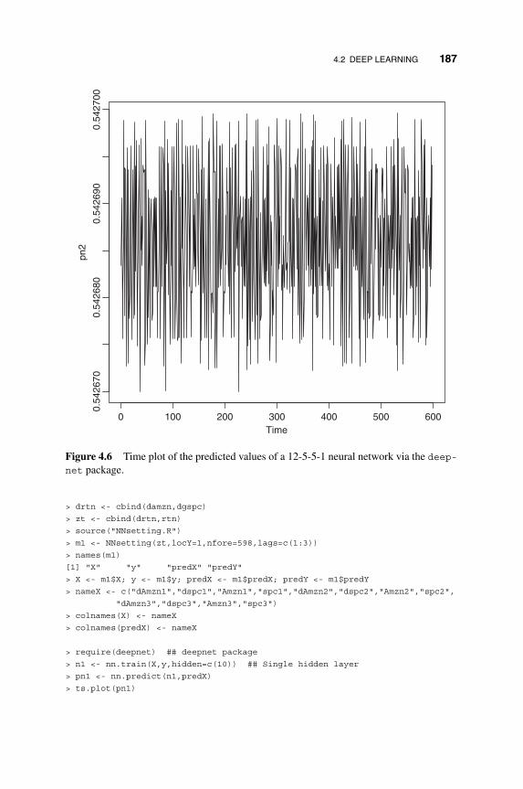
4.2 DEEP LEARNING 187
Time
pn2
0 100 200 300 400 500 600
0.54
2670
0.54
2680
0.54
2690
0.54
2700
Figure 4.6 Time plot of the predicted values of a 12-5-5-1 neural network via the deep-net package.
> drtn <- cbind(damzn,dgspc)
> zt <- cbind(drtn,rtn)
> source("NNsetting.R")
> m1 <- NNsetting(zt,locY=1,nfore=598,lags=c(1:3))
> names(m1)
[1] "X" "y" "predX" "predY"
> X <- m1$X; y <- m1$y; predX <- m1$predX; predY <- m1$predY
> nameX <- c("dAmzn1","dspc1","Amzn1","spc1","dAmzn2","dspc2","Amzn2","spc2",
"dAmzn3","dspc3","Amzn3","spc3")
> colnames(X) <- nameX
> colnames(predX) <- nameX
> require(deepnet) ## deepnet package
> n1 <- nn.train(X,y,hidden=c(10)) ## Single hidden layer
> pn1 <- nn.predict(n1,predX)
> ts.plot(pn1)

188 4. NEURAL NETWORKS, DEEP LEARNING, AND TREE-BASED METHODS
Time
pk1
0 100 200 300 400 500 600
0.4
0.5
0.6
0.7
Figure 4.7 Time plot of the predicted values of a 12-10-1 neural network via the darchpackage.
> dpn1 <- ifelse(pn1 >= 0.5,1,0)
> table(predY,dpn1)
dpn1
predY 0 1
0 150 123
1 160 165
#### the same result if mean is used.
> dpn1 <- ifelse(pn1 >= mean(pn1), 1,0)
> table(predY,dpn1)
dpn1
predY 0 1
0 150 123
1 160 165
> n2 <- nn.train(X,y,hidden=c(5,5)) ## two hidden layers
> require(darch) ## darch package
> d1 <- darch(X,y,layers=10) ## Single hidden layer
> pk1 <- predict(d1,newdata=predX)

4.2 DEEP LEARNING 189
Methods Two-way tableProbability of correct
prediction
Logistic linear regression 135 138 (135+172)/598 = 0.513153 172
deepnet 12-10-1 150 123 0.527160 165
deepnet 12-100-1 154 119 0.518169 156
deepnet 12-10-10-1 131 142 0.493161 164
deepnet 12-10-10-10-1 137 136 0.492168 157
darch 12-10-1 180 93 0.509201 124
darch 12-100-1 198 75 0.503222 103
darch 12-5-5-1 193 80 0.5219 106
Table 4.2 Comparison of selected deep networks with logistic linear regression inpredicting the direction of daily price movement of Amazon stock. The training sample isfrom January 3, 2007 to December 11, 2014 whereas the forecasting sample is fromDecember 12, 2014 to April 28, 2017.
> ts.plot(pk1)
> pp1 <- ifelse(pk1 >= 0.5,1,0)
> table(predY,pp1)
pp1
predY 0 1
0 180 93
1 201 124
> d3 <- darch(X,y,layers=c(12,5,5,1)) ## Two hidden layers of sizes 5 and 5.
Example 4.2 Modeling the trade-by-trade price changes is of particular interestin high-frequency financial data analysis. Many methods have been proposed inthe literature, including the decomposition approach of Rydberg and Shephard(2003) and the ordered probit model of Hauseman et al. (1992). See Tsay (2013)for application of these methods. In this example, we apply deep learning as amodern approach to modeling the intraday price movements of a stock.
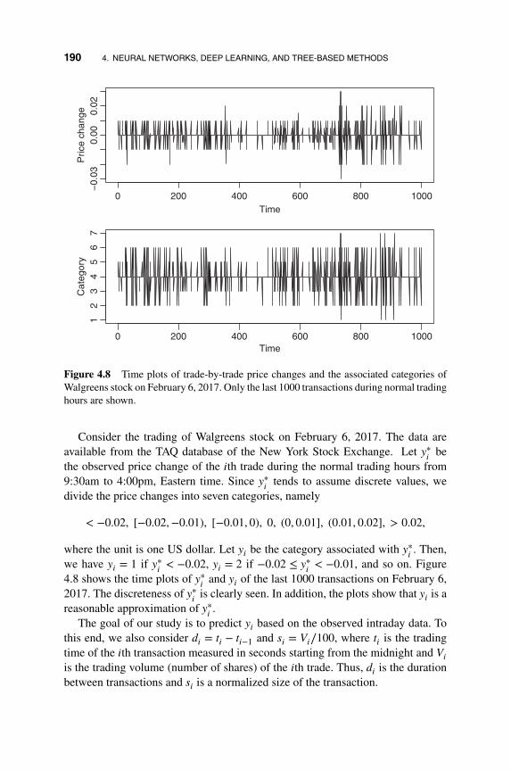
190 4. NEURAL NETWORKS, DEEP LEARNING, AND TREE-BASED METHODS
Time
Pric
e ch
ange
0 200 400 600 800 1000
−0.
030.
000.
02
Time
Cat
egor
y
0 200 400 600 800 1000
12
34
56
7
Figure 4.8 Time plots of trade-by-trade price changes and the associated categories ofWalgreens stock on February 6, 2017. Only the last 1000 transactions during normal tradinghours are shown.
Consider the trading of Walgreens stock on February 6, 2017. The data areavailable from the TAQ database of the New York Stock Exchange. Let y∗
𝑖be
the observed price change of the 𝑖th trade during the normal trading hours from9:30am to 4:00pm, Eastern time. Since y∗
𝑖tends to assume discrete values, we
divide the price changes into seven categories, namely
< −0.02, [−0.02,−0.01), [−0.01, 0), 0, (0, 0.01], (0.01, 0.02], > 0.02,
where the unit is one US dollar. Let y𝑖 be the category associated with y∗𝑖. Then,
we have y𝑖 = 1 if y∗𝑖< −0.02, y𝑖 = 2 if −0.02 ≤ y∗
𝑖< −0.01, and so on. Figure
4.8 shows the time plots of y∗𝑖
and y𝑖 of the last 1000 transactions on February 6,2017. The discreteness of y∗
𝑖is clearly seen. In addition, the plots show that y𝑖 is a
reasonable approximation of y∗𝑖.
The goal of our study is to predict y𝑖 based on the observed intraday data. Tothis end, we also consider d𝑖 = t𝑖 − t𝑖−1 and s𝑖 = V𝑖∕100, where t𝑖 is the tradingtime of the 𝑖th transaction measured in seconds starting from the midnight and V𝑖is the trading volume (number of shares) of the 𝑖th trade. Thus, d𝑖 is the durationbetween transactions and s𝑖 is a normalized size of the transaction.

4.2 DEEP LEARNING 191
With seven categories, we define six dummy variables for the price change.Specifically, let
x𝑖,j =
{1 if y𝑖 = j,
0 if y𝑖 ≠ j,j = 2,… , 7. (4.25)
Let x𝑖 = (x𝑖,2, x𝑖,3,… , x𝑖,7)′ be the six-dimensional indicator variable of pricechange for the 𝑖-trade. In particular, x𝑖 = 0 implies that y𝑖 = 1.
In our demonstration, we use the following 27 input variables
X𝑖 ≡ {x𝑖−j, y∗𝑖−j, d𝑖−j, s𝑖−j| j = 1, 2, 3},
and our goal is to obtain P(y𝑖 = j ∣ X𝑖). In other words, we like to predict y𝑖 usingselected prior transactions data.
On February 6, 2017, there were 29275 transactions available for the Walgreensstock. We use the first 27275 observations as the training subsample and reservethe last 2000 observations for out-of-sample prediction to perform model compar-ison. Besides several network models, we also used the ordered probit model asa benchmark. The fitted ordered probit model is shown in the R output below. Inthis particular instance, the ordered probit model does not fare well in prediction.As a matter of fact, the model predicts no price change for all of the last 2000transactions. See the forecast tabulation in the R demonstration below.
For deep learning, we use the darch package and employ three models. Theyare 27-5-1, 27-10-1, and 27-10-5-1 networks. Figure 4.9 shows the training resultsof the 27-5-1 network. With default of 100 epochs, the best iteration appears to be84. The predictions of the three networks for the last 2000 transactions are alsoshown in the R demonstration. In this particular instance, the 27-10-1 networkappears to perform the best. In particular, it was able to correctly predict 3, 47,1389, and 11 times for Categories 1, 3, 4, and 5, respectively.
In this example, we demonstrated that deep learning can be helpful in modelingtrade-by-trade price changes of Walgreens stock. This is encouraging. On the otherhand, we did not attempt to find the best deep learning model for the given data.This important question deserves careful investigation.
R demonstration: Ordered probit model and deep learning.
> da < read.table("taqwbacpchfeb062017.txt",header=T)> dim(da)[1] 29275 4### create dummy variables> c2 < c3 < c4 < c5 < c6 < c7 < rep(0,29275)> nT < nrow(da)> idx < c(1:nT)[da[,1]==2]

192 4. NEURAL NETWORKS, DEEP LEARNING, AND TREE-BASED METHODS
1.52
1.56
1.60
1.64
0 25 50 75 100
Epoch
Cro
ss e
ntro
py e
rror
DatasetTraining
Network errorbest iteration = 84, train error = 1.538
Figure 4.9 Fitting results of a 27-5-1 network via the darch package for the trade-by-trade price changes of Walgreens transactions data for February 6, 2017.
> c2[idx] <1> idx < c(1:nT)[da[,1]==3]> c3[idx] <1> idx < c(1:nT)[da[,1]==4]> c4[idx] < 1> idx < c(1:nT)[da[,1]==5]> c5[idx] < 1> idx < c(1:nT)[da[,1]==6]> c6[idx] < 1> idx < c(1:nT)[da[,1]==7]> c7[idx] < 1> Z < cbind(da,c2,c3,c4,c5,c6,c7)> source("NNsetting.R")> n1 < NNsetting(Z,nfore=2000,lags=c(1:3),include.lagY=F)> X < n1$X; y < n1$y; predX < n1$predX; predY < n1$predY> na < c("pr","dur","size","c2","c3","c4","c5","c6","c7")> na1 < paste(na,"l1",sep=""); na2 < paste(na,"l2",sep="")> na3 <paste(na,"l3",sep="")

4.2 DEEP LEARNING 193
> name < c(na1,na2,na3)> colnames(X) < colnames(predX) < name> require(MASS)> y < as.factor(y)> m1 < polr(y˜.,data=data.frame(X),method="probit")> summary(m1)Call: polr(formula = y ˜ ., data = data.frame(X), method = "probit")Coefficients:
Value Std. Error t valueprl1 1.901e+01 2.004434 9.4855durl1 1.284e02 0.002678 4.7971sizel1 2.194e03 0.001322 1.6596c2l1 2.955e01 0.101196 2.9200c3l1 6.422e01 0.106859 6.0097c4l1 1.005e+00 0.112055 8.9728c5l1 1.300e+00 0.122176 10.6376c6l1 1.610e+00 0.133076 12.0973c7l1 1.759e+00 0.188524 9.3279prl2 9.389e+00 1.999849 4.6951durl2 5.934e03 0.002753 2.1552sizel2 2.265e03 0.001336 1.6956c2l2 3.550e01 0.102485 3.4640c3l2 4.644e01 0.108436 4.2830c4l2 6.333e01 0.113046 5.6022c5l2 6.913e01 0.123311 5.6063c6l2 9.001e01 0.133976 6.7186c7l2 1.218e+00 0.189065 6.4434prl3 4.302e+00 1.847475 2.3286durl3 8.912e04 0.002770 0.3218sizel3 3.752e04 0.001043 0.3597c2l3 2.086e02 0.100412 0.2077c3l3 9.264e02 0.105887 0.8749c4l3 1.311e01 0.110385 1.1876c5l3 1.790e01 0.120459 1.4858c6l3 2.369e01 0.130089 1.8208c7l3 3.802e01 0.184299 2.0629
Intercepts:Value Std. Error t value
1|2 4.3392 0.2111 20.55862|3 3.3606 0.2100 16.00443|4 2.8530 0.2098 13.59714|5 0.5979 0.2094 2.85495|6 0.0710 0.2093 0.33916|7 0.8207 0.2091 3.9243
Residual Deviance: 54018.88

194 4. NEURAL NETWORKS, DEEP LEARNING, AND TREE-BASED METHODS
> pm1 < predict(m1,newdata=predX,type="class") ## prediction> table(predY,pm1)
pm1predY 1 2 3 4 5 6 7
1 0 0 0 4 0 0 02 0 0 0 100 0 0 03 0 0 0 180 0 0 04 0 0 0 1437 0 0 05 0 0 0 174 0 0 06 0 0 0 100 0 0 07 0 0 0 5 0 0 0
### Deep learning> require(darch)> y1 < as.factor(y)> nn1 < darch(X,y1,layers=5)> pnn1 < predict(nn1,newdata=predX,type="raw")> dim(pnn1)[1] 2000 7> x1 < apply(pnn1,1,which.max)> table(predY,x1)
x1predY 4 5
1 4 02 99 13 171 94 1420 175 156 186 99 17 5 0
>> nn2 < darch(X,y1,layers=10)> pnn2 < predict(nn2,newdata=predX)> x1 < apply(pnn2,1,which.max)> table(predY,x1)
x1predY 1 3 4 5
1 3 0 1 02 0 2 98 03 0 47 129 44 2 38 1389 85 0 11 152 116 0 5 95 07 0 0 5 0
>> nn3 < darch(X,y1,layers=c(27,10,5,1))> pnn3 < predict(nn3,newdata=predX)> x3 < apply(pnn3,1,which.max)

4.3 TREE-BASED METHODS 195
> table(predY,x3)x3
predY 3 4 51 0 4 02 2 98 03 46 123 114 43 1367 275 8 141 256 3 95 27 0 5 0
4.3 TREE-BASED METHODS
Tree-based methods have been widely used in the literature for prediction andclassification, especially for independent observations. See, for instance, Jameset al. (2013). The methods include regression tree, classification tree, bagging,random forests, and boosting. The basic idea of tree-based statistical methods isstratifying or segmentation of the predictor space into multiple subregions, eachof which contains relatively more homogeneous observations so that simple mod-els can be used in these subregions. These methods are useful in understandingthe basic structure embedded in the data and in interpretation. Although muchof research into tree-based methods assumes independent data, the basic idea ofthe methods remains highly relevant for analysis of time series data. With somemodifications on the procedure to account for the serial dependence in time series,tree-based methods can also be useful in nonlinear time series analysis. The goal ofthis section is to introduce some tree-based methods and to consider modificationsto these methods in the presence of serial dependence. We shall also demonstratethe applications of tree-based methods in prediction.
4.3.1 Decision Trees
Binary trees are the building block of most tree-based statistical methods. Bybinary, we mean that each branch of the tree can only be divided into two sub-branches. These trees are commonly referred to as decision trees.
4.3.1.1 Regression Tree We begin our discussion of decision trees with asimple example of the regression tree. Consider the quarterly growth rates, inpercentages, of US real gross domestic product (GDP) from 1947.II to 2015.II for273 observations. Figure 4.10 shows the time plot of the GDP growth rates. For aclear display of a fitted tree, we round the GDP growth rates to two decimal points.

196 4. NEURAL NETWORKS, DEEP LEARNING, AND TREE-BASED METHODS
1950 1960 1970 1980 1990 2000 2010
−0.
02−
0.01
0.00
0.01
0.02
0.03
0.04
Year
GD
P−
rate
Figure 4.10 Time plot of the quarterly growth rates of US real gross domestic productfrom 1947.II to 2015.II.
Our goal is to predict the GDP growth rate using its own past three lagged values.Mathematically, one can think of the underlying model as
yt = g(yt−1, yt−2, yt−3) + at,
where yt is the GDP growth rate at time t, at denotes the error term, and g(⋅) is asmooth function from R3 to R. The decision tree represents a piecewise nonlinearapproximation for g(⋅).
Figure 4.11 shows the output of a fitted regression tree for the GDP growthrates. From the plot, the tree is drawn upside down in the sense that the leaves areat the bottom of the tree. In this particular instance, the tree has 11 leaves, shownby the numerical values in the plot, i.e. −0.2450, 0.6529, 1.239, etc. Starting fromthe root at the top of the plot, the first split of the tree is determined by the lag-1variable yt−1, denoted by GDP1 in the plot. The left branch is for yt−1 < 1.15. Theright branch (for yt−1 ≥ 1.15) further splits into two subbranches determined by

4.3 TREE-BASED METHODS 197
|GDP1 < 1.15
GDP1 < −0.395
GDP2 < 0.685GDP2 < 0.83
GDP2 < −1.025
GDP2 < −0.205
GDP2 < 0.04GDP3 < 0.635
GDP1 < 0.665
GDP3 < −0.275
−0.2450
1.2390
0.2440 1.6260
0.2385
0.8120
2.2320
0.7672
−0.6950
0.6529
1.2090
Figure 4.11 A regression tree for the quarterly growth rate of US real gross domesticproduct using three lagged values as explanatory variables. The data are from 1947.II to2015.II.
the lagged variable yt−3, denoted by GDP3 in the plot. The new left subbranch isfor yt−3 < −0.275. The plot then shows two leaves, namely 2.232 and 1.209.
The first left branch of the tree is further divided into two subbranches by thelag-1 variable yt−1 with the new left subbranch satisfying yt−1 < −0.395. This newsubbranch is further divided into two new sub-subbranches by the lag-2 variableyt−2 with the criterion yt−2 < 0.83, resulting in two leaves with values −0.2450and 0.6529. The rest of the tree can be considered in a similar manner.
The tree in Figure 4.11 can be used in prediction. For instance, suppose thatwe have (yn, yn−1, yn−2) = (0.51,1.05,1.12) at the forecast origin t = n and wantto predict yn+1. From the fitted tree, we see that the prediction is 0.812. Since thelag-1 value for t = n + 1 is yn = 0.51, which is less than 1.15, so that yn+1 belongsto the left branch of the first split. Since yn ≥ −0.395, yn+1 then belongs to theright subbranch of the second split. Finally, the lag-2 value of yn+1 is yn−1 = 1.05,which is greater than 0.685, so that yn+1 belongs to the right subbranch at the thirdsplit. The prediction (or leaf) 0.812 is the sample mean for all data in the samesubregion as yn+1.

198 4. NEURAL NETWORKS, DEEP LEARNING, AND TREE-BASED METHODS
The tree in Figure 4.11 can be interpreted as follows. Among the three explana-tory variables, the lag-1 GDP growth rate is the most important one in determiningthe GDP growth rate. This is not surprising given the dynamic dependence of thedata. When the last quarter’s growth rate is greater than or equal to 1.15%, thenthe lag-2 variable becomes irrelevant. The growth rate is then determined by thelag-3 variable. If yt−3 < −0.275, meaning that the US economy was in deep con-traction, then the US economy was expected to grow faster at the rate of 2.23%.This phenomenon seems reasonable. It is well-known that consecutive negativeGDP growths are rare. When the economy was in deep contraction at yt−3, cer-tain interventions were likely to take place resulting in a turn around in yt−1. Theeffect of the intervention was likely to continue so that the growth rate yt shouldbe greater. Other branches of the tree might also have some nice interpretation.
As illustrated by the example of GDP growth rate, the regression tree dividesthe predictor space into non-overlapping subregions and uses the sample averageof each subregion to produce prediction. Figure 4.12 shows the scatter plot of
−2 −1 0 1 2 3 4
−2
−1
01
23
4
GDP1
GD
P
Figure 4.12 The scatter plot of US quarterly GDP growth rate versus the past quarter’sgrowth rate. The vertical line is 1.15, and the data are from 1947.II to 2015.II.
4.3 TREE-BASED METHODS 199
yt versus yt−1 of the GDP growth rates. The vertical line of the plot shows thedivision of yt into two groups based on the values of yt−1 with the threshold 1.15.This threshold is determined by the following method. Let c be a real number,and let R1 = {t ∣ yt−1 < c} and R2 = {t ∣ yt−1 ≥ c}. Furthermore, let y1,c and y2,cbe the sample means of yt in R1 and R2, respectively. The sum of squared errors(SSE) corresponding to this given c is
SSE1(c) =∑t∈R1
(yt − y1,c)2 +∑t∈R2
(yt − y2,c)2, (4.26)
which is a function of c. The threshold 1.15 is then obtained by
1.15 = argmincSSE1(c).
The choice of threshold 1.15 can be seen clearly from Figure 4.12. Of course, oneperforms such a division because
SSE1(1.15) < SSE0 ≡
T∑t=4
(yt − y)2,
where T = 273 is the sample size and y is the sample mean of yt for t = 4,… , T .The summation starts with t = 4 because we used yt−1, yt−2, and yt−3 as theexplanatory variables.
In this particular example, we have three explanatory variables. The use of yt−1to perform the first tree split actually involves variable selection. In theory, we alsoconsider yt−2 and yt−3 to form two regions using the method stated in Equation(4.26). However, yt−1 is chosen because the resulting SSE1(1.15) is smaller thanany binary partition based on either yt−2 or yt−3.
Next, to grow the tree, we can consider R1 and R2 separately. Focus on theregion R2, which is the right branch of the first split. One can treat observa-tions in R2 as a new sample and apply the tree-growing process by selectingthe best explanatory variable and the best threshold to form a new split. For theGDP growth rate example, R2 is divided into R21 = {t ∣ (yt−1 ≥ 1.15) ∩ (yt−3 <
−0.275)} and R22 = {t ∣ (yt−1 ≥ 1.15) ∩ (yt−3 ≥ −0.275)}. Turn to the region R1,which is the left branch of the first split. One can also apply the tree-growing pro-cess. The decision to first split R1 or R2 is determined by the resulting sum ofsquared errors. One selects the second split so that the resulting tree, which hasthree branches, has the smallest sum of squared errors.
In theory, using the sum of squared errors as the objective function, one cancontinue to grow a binary tree by repeating the process of selecting the best pre-dictor and the best threshold for splitting so as to minimize the objective function.However, a tree with many leaves often results in over-fitting, which in turn leadsto suboptimal prediction. Some pruning is needed.
200 4. NEURAL NETWORKS, DEEP LEARNING, AND TREE-BASED METHODS
4.3.1.2 Tree Pruning Let be a tree with | | leaves. Let R𝑖 be the 𝑖th regionof the tree for 𝑖 = 1,… , | |. Furthermore, let yt be the tth observation of the depen-dent variable and xt be the corresponding vector of predictors. Let yR𝑖
be the sam-ple mean of the dependent variable in region R𝑖, i.e.
yR𝑖= 1|R𝑖| ∑t
ytI(xt ∈ R𝑖),
where |R𝑖| denotes the number of data points in region R𝑖. The idea of tree pruningis to apply a penalty to a tree based on its complexity. Here the complexity of atree is measured by the number of its leaves.
Suppose that the sample size is T so that the data are (yt, xt) for t = 1,… , T .Similar to the selection of other statistical models discussed in the book, weuse out-of-sample prediction to select a binary tree for the data. To this end, wedivide the data into training and forecasting subsamples. Typically, for time seriesdata the training sample consists of the first N data points and the forecasting sub-sample the last T − N data points.
Use the training sample to grow a large tree, say 0, which is often determinedby setting an upper bound for |R𝑖|, the number of data points in region R𝑖. For agiven penalty 𝛼, there exists a subtree ⊂ 0 such that
| |∑𝑖=1
∑t, xt∈R𝑖
(yt − yR𝑖)2 + 𝛼| |, (4.27)
is as small as possible. Clearly, Equation (4.27) shows that the penalty parameter𝛼 controls a trade-off between the complexity and goodness of fit of the subtree . Denote the subtree by 𝛼 .
We then apply the selected subtree 𝛼 to produce predictions in the forecastingsubsample and compute the mean squared forecast errors, which is also a functionof 𝛼. Let 𝛼0 be the value of 𝛼 that gives the minimum mean squared forecast errors.Finally, we choose 𝛼0
as the selected tree for yt.In the literature, cross-validation is often used to select the penalty parameter 𝛼
in tree pruning. Such a procedure can still be used if yt is assumed to be a linear ARprocess. Also, there is substantial research on Bayesian classification and regres-sion tree (BCART) in the literature. See, for instance, Chipman et al. (1998). In theBayesian framework, prior information is used to grow and prune a tree. Instead ofusing sample mean of the response variable in each subregion (leaf), linear regres-sion models or other predictive models can also be used, similar to the piecewiselinear approximations discussed in Chapter 3.

4.3 TREE-BASED METHODS 201
R demonstration: Regression tree.
> da < read.table("GDPC1.txt",header=T)> gdp < diff(log(da$rgdp))> tdx < da$year + (da$mon/12)> tdx < tdx[1]> plot(tdx,gdp,xlab='year',ylab='gdprate',type='l')> length(gdp)[1] 273> gdp < round(gdp*100,2)#> X < cbind(gdp[4:273],gdp[3:272],gdp[2:271],gdp[1:270])> colnames(X) < c("gdp","gdp1","gdp2","gdp3")> require(tree)> t1 < tree(gdp˜.,data=data.frame(X))> summary(t1)Regression tree:tree(formula = gdp ˜ ., data = data.frame(X))Number of terminal nodes: 11Residual mean deviance: 0.6654 = 172.3 / 259Distribution of residuals:
Min. 1st Qu. Median Mean 3rd Qu. Max.3.27300 0.46200 0.03298 0.00000 0.51020 3.25700> plot(t1)> text(t1,pretty=0)
4.3.1.3 Classification Tree A classification tree is very similar to a regres-sion tree, but it deals with a qualitative response variable instead of a quantita-tive one. As such, the same tree-building algorithm continues to apply. However,the categorical nature of the response variable requires using a different objectivefunction. Suppose that the response variable yt may assume K possible values, say{1, 2,… , K}. Denote the corresponding vector of explanatory variables by xt. LetR𝑖 be the 𝑖th leaf (or region) of a tree. One can then estimate the probability of ytbelonging to Category k in R𝑖 by
p𝑖k =|R𝑖k||R𝑖| , k = 1,… , K,
where R𝑖k = {j|(yj = k) ∩ (xj ∈ R𝑖)} in the training sample and |R𝑖| is the numberof data points in R𝑖. For prediction, one may apply the simple majority rule, knownas the most commonly occurring class, so that, given xt ∈ R𝑖
yt = k0, k0 = argmaxk{p𝑖k}.

202 4. NEURAL NETWORKS, DEEP LEARNING, AND TREE-BASED METHODS
The resulting classification error rate for yt is then et = 1 − p𝑖,k0provided that xt ∈
R𝑖. Experience shows that the classification error rate is not sufficiently sensitivefor growing a classification tree. Two alternative measures are often used. Theyare the Gini index and the cross-entropy.
The Gini index is defined by
gt =K∑
k=1
p𝑖k(1 − p𝑖k), (4.28)
which measures the total variance of the K categories. The Gini index takes asmall positive value if all p𝑖k are close to either 0 or 1. Consequently, a small Giniindex implies that R𝑖 contains predominantly observations from a single category.In Equation (4.28), it is understood that p𝑖k depends on xt.
The second alternative measure is the cross-entropy defined by
ct = −K∑
k=1
p𝑖k log(p𝑖k). (4.29)
It is not hard to see that the cross-entropy ct ≥ 0 and it will take a small value if allprobabilities p𝑖k are close to either 0 or 1. The latter property of the cross-entropyis similar to that of the Gini index. In applications, one may experiment with allthree measurements to obtain a classification tree for prediction.
Example 4.3 Consider the daily measurement of PM2.5 (fine particular matterwith diameter less than 2.5 mm) of Shanghai, China, from January 1, 2013 toMay 31, 2017. The original data are hourly, measured in units (𝜇g/m3), and canbe downloaded from www.stateair.net, which is part of US Department of State airquality monitoring program. There were missing values in the hourly observationsand we filled in those missing values by the previously available measurement. Wethen take the average of hourly data as the measurement of PM2.5 for a given day.For simplicity in analysis, we removed the observation for February 29, 2016 sothat each year has the same number of observations. Figure 4.13(a) shows the timeplot of the PM2.5 series whereas Figure 4.13(b) gives the sample autocorrelationsof the series. From the plot and sample ACF, as expected, the series has an annualcycle.
Our goal here is to demonstrate the application of tree methods in predictionand to compare the results with other commonly used linear models. To this end,we reserve the last 365 observations as the forecasting subsample. Thus, there

4.3 TREE-BASED METHODS 203
2013 2014 2015 2016 2017
010
030
0
Year
PM
2.5
0 200 400 600 800
−0.
20.
20.
61.
0
Lag
(a)
(b)
AC
F
Series PM2.5
Figure 4.13 Time series of daily PM2.5 of Shanghai, China, from January 1, 2013 toMay 31, 2017: (a) the time plot of the series and (b) the sample autocorrelations of the data.The daily data are the average of hourly measurements.
are 1246 observations for training. Because of the annual cycle, we use the linearmodel
yt = 𝛽0 +10∑𝑖=1
𝛽𝑖yt−𝑖 +370∑
j=365
𝛽jyt−j + et, t = 371,… , 1246, (4.30)
as the benchmark model, where yt denotes the PM2.5 at time t, and et denotesthe error term. This is a special AR(370) model. The fitted model is given in theR demonstration shown below. The R2 of the model is 34.43%, and the modelfits the series reasonably well. The Ljung–Box statistics of the residuals showQ(400) = 370.16 with p value 0.86. The p value would remain high even afteradjusting the degrees of freedom of the chi-square distribution due to estimation.Thus, the residuals have no significant serial correlations.
Using the same explanatory variables, we apply the regression tree to thedata. The resulting tree is shown in Figure 4.14. From the tree, it is seen thatlag-1 variable yt−1 is the most important explanatory variable, and the seasonallagged variables yt−370 and yt−367 are also important. But the residuals of the fit-ted tree show some minor serial correlations both at the regular and seasonal lags.

204 4. NEURAL NETWORKS, DEEP LEARNING, AND TREE-BASED METHODS
|L1 < 53.5
L1 < 34.0208
L367 < 168L1 < 19.75
L370 < 130.375
L8 < 172.333
L1 < 138.979
L4 < 130.146L369 < 134.271
L1 < 172.333
L367 < 60.7292
22.28 36.00 47.18 88.56
62.07 91.54104.70
145.10 65.52
134.20125.00 85.39
Figure 4.14 Regression tree for the daily PM2.5 of Shanghai, China. The tree was builtusing the first 1246 observations as the training subsample.
The Ljung–Box statistics of the residuals give Q(400) = 566.59 with p value closeto zero. This is not surprising as the fitted tree has 12 leaves, indicating that it onlyuses 12 values in prediction.
Turn to out-of-sample prediction. The linear AR(370) model in Equation (4.30)gives (MAE, RMSE) = (15.45, 20.19) whereas the fitted tree provides (MAE,RMSE) = (16.38, 22.27), where MAE and RMSE denote mean absolute error androot mean squared error, respectively. For the same reason as that stated in modelchecking, the performance of the regression tree in forecasting is not surprisingeither.
To demonstrate pruning, we apply the traditional cross-validation to the fittedtree. This can be justified as the model fitted is of the autoregressive type. Figure4.15 shows the results of cross-validation. In this particular instance, the best treeseems to be of size 4. Figure 4.16 shows the prune tree for the Shanghai PM2.5during the training sample. Only the lag-1 and lag-370 variables are used in thissimplified tree. Using the prune tree to perform out-of-sample prediction, wehave (MAE,RMSE) = (17.12, 22.03).

4.3 TREE-BASED METHODS 205
2 4 6 8 10 12
6500
0070
0000
7500
0080
0000
cv.t1$size
cv.t1
$dev
Figure 4.15 Results of cross-validation of regression tree for the daily PM2.5 of Shanghai,China. The tree was built using the first 1246 observations as the training subsample.
R demonstration: Tree.
> PM2.5 < scan(file="dShanghai1317.txt")> tdx < c(1:length(PM2.5))/365+2013> par(mfcol=c(2,1))> plot(tdx,PM2.5,xlab='year',ylab='PM2.5',type='l')> acf(PM2.5,lag=800)> m1 < NNsetting(PM2.5,nfore=365,lags=c(1:10,365:370))> names(m1)[1] "X" "y" "predX" "predY"> X < m1$X; y < m1$y; predX < m1$predX; predY < m1$predY> n1 < paste("L",1:10,sep="")> n2 < paste("L",365:370,sep="")> colnames(X) < colnames(predX) < c(n1,n2)> m2 < lm(y˜.,data=data.frame(X))> summary(m2)Call: lm(formula = y ˜ ., data = data.frame(X))

206 4. NEURAL NETWORKS, DEEP LEARNING, AND TREE-BASED METHODS
|L1 < 53.5
L370 < 130.375L1 < 34.0208
47.91 32.50 102.40 67.56
Figure 4.16 Prune regression tree for the daily PM2.5 of Shanghai, China. The treewas built using the first 1246 observations as the training subsample and prune by cross-validation.
Coefficients:Estimate Std. Error t value Pr(>|t|)
(Intercept) 11.330124 2.605231 4.349 1.53e05 ***L1 0.487490 0.033792 14.426 < 2e16 ***L2 0.046739 0.037458 1.248 0.21246L3 0.062058 0.037249 1.666 0.09607 .L4 0.026367 0.037273 0.707 0.47951L5 0.082690 0.037183 2.224 0.02641 *L6 0.006062 0.037240 0.163 0.87074L7 0.005810 0.037323 0.156 0.87632L8 0.106191 0.037370 2.842 0.00459 **L9 0.107141 0.037513 2.856 0.00439 **L10 0.110018 0.033664 3.268 0.00113 **L365 0.019086 0.029047 0.657 0.51131L366 0.035823 0.032708 1.095 0.27372L367 0.051650 0.032712 1.579 0.11472L368 0.011674 0.032646 0.358 0.72074L369 0.051792 0.032573 1.590 0.11219L370 0.058908 0.028975 2.033 0.04236 *

4.3 TREE-BASED METHODS 207
–––Residual standard error: 25.01 on 859 degrees of freedomMultiple Rsquared: 0.3443, Adjusted Rsquared: 0.3321Fstatistic: 28.19 on 16 and 859 DF, pvalue: < 2.2e16> acf(m2$residuals,lag=400)> Box.test(m2$residuals,lag=400,type="Ljung")
BoxLjung testdata: m2$residualsXsquared = 370.16, df = 400, pvalue = 0.8552> pm2 < predict(m2,newdata=data.frame(predX))> er < predYpm2> mean(abs(er))[1] 15.44751> sqrt(mean(erˆ2))[1] 20.18687
> require(tree)> t1 < tree(y˜.,data=data.frame(X))> par(mfcol=c(1,1))> plot(t1)> text(t1,pretty=0)> pt1 < predict(t1,newdata=data.frame(predX))> er3 < pt1predY> mean(abs(er3))[1] 16.3767> sqrt(mean(er3ˆ2))[1] 22.2729### Compute residuals for model checking> pp1 < predict(t1,newdata=data.frame(X))> resi < ypp1> Box.test(resi,lag=400,type="Ljung")
BoxLjung testdata: resiXsquared = 566.59, df = 400, pvalue = 7.614e08### Pruning tree> cv.t1 < cv.tree(t1)> plot(cv.t1$size,cv.t1$dev,type="b")> prune.t1 < prune.tree(t1,best=4)> plot(prune.t1)> text(prune.t1,pretty=0)> prun < predict(prune.t1,newdata=data.frame(predX))> per < predYprun> mean(abs(per))[1] 17.11805> sqrt(mean(perˆ2))[1] 22.03309

208 4. NEURAL NETWORKS, DEEP LEARNING, AND TREE-BASED METHODS
Example 4.4 Consider again the daily PM2.5 of Shanghai, but classify the mea-surements into four categories as
(0, 50], (50, 100], (100, 150], (150,∞].
The classification is similar to that used in Stateair.net and the categories arereferred to as good, moderate, sensitive, and unhealthy, respectively. On theStateair.net, the unhealthy category is further divided into four classes, but themaximum of the dependent variable during the sample period is only about 221so it suffices to use four categories.
We use the same explanatory variables as those of Equation (4.30). Figure 4.17shows the fitted tree for the PM2.5 series in the training sample. Again, the lag-1variable remains the most important determining factor in predicting PM2.5, butsome seasonal lagged variables are also relevant. Applying the fitted tree in Figure4.17 to the forecasting subsample, we see that the success rate is approximately71.8%, but the model fails to predict the occurrence of Categories 3 and 4.
|L1 < 43.6042
L1 < 34.125
L367 < 75.125
L1 < 69.4583
L10 < 129.917
L2 < 85.75
L9 < 21.1667
L7 < 32.7292
L370 < 121.27111
1
21
1
1 2
2 3
Figure 4.17 Classification tree for the daily PM2.5 of Shanghai, China. The tree was builtusing the first 1246 observations as the training subsample. The PM2.5 was divided into fourcategories, namely (0,50], (50,100], (100,150], (150,∞].
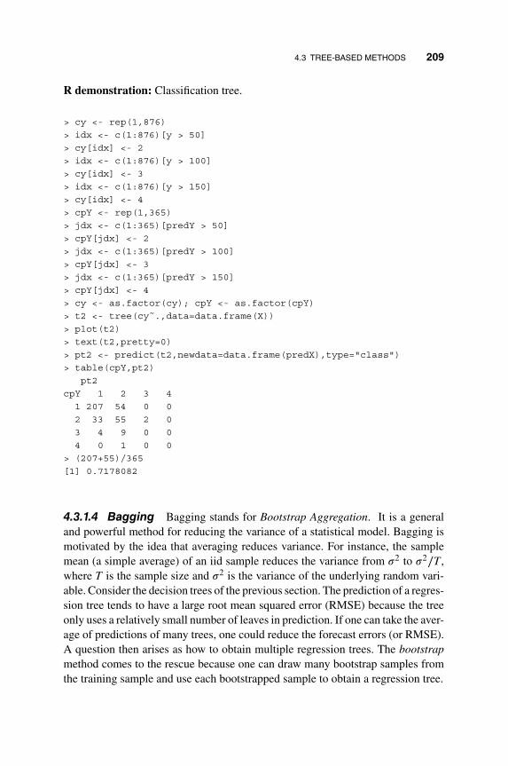
4.3 TREE-BASED METHODS 209
R demonstration: Classification tree.
> cy < rep(1,876)> idx < c(1:876)[y > 50]> cy[idx] < 2> idx < c(1:876)[y > 100]> cy[idx] < 3> idx < c(1:876)[y > 150]> cy[idx] < 4> cpY < rep(1,365)> jdx < c(1:365)[predY > 50]> cpY[jdx] < 2> jdx < c(1:365)[predY > 100]> cpY[jdx] < 3> jdx < c(1:365)[predY > 150]> cpY[jdx] < 4> cy < as.factor(cy); cpY < as.factor(cpY)> t2 < tree(cy˜.,data=data.frame(X))> plot(t2)> text(t2,pretty=0)> pt2 < predict(t2,newdata=data.frame(predX),type="class")> table(cpY,pt2)
pt2cpY 1 2 3 41 207 54 0 02 33 55 2 03 4 9 0 04 0 1 0 0
> (207+55)/365[1] 0.7178082
4.3.1.4 Bagging Bagging stands for Bootstrap Aggregation. It is a generaland powerful method for reducing the variance of a statistical model. Bagging ismotivated by the idea that averaging reduces variance. For instance, the samplemean (a simple average) of an iid sample reduces the variance from 𝜎2 to 𝜎2∕T ,where T is the sample size and 𝜎2 is the variance of the underlying random vari-able. Consider the decision trees of the previous section. The prediction of a regres-sion tree tends to have a large root mean squared error (RMSE) because the treeonly uses a relatively small number of leaves in prediction. If one can take the aver-age of predictions of many trees, one could reduce the forecast errors (or RMSE).A question then arises as how to obtain multiple regression trees. The bootstrapmethod comes to the rescue because one can draw many bootstrap samples fromthe training sample and use each bootstrapped sample to obtain a regression tree.

210 4. NEURAL NETWORKS, DEEP LEARNING, AND TREE-BASED METHODS
Consider the simple one-step ahead prediction at the forecast origin t = n.Let yn+1,m be the prediction obtained from the mth bootstrapped sample, wherem = 1,… , M, with M being a sufficiently large positive integer. Then, the simpleaverage
yn+1,bag = 1M
M∑m=1
yn+1,m
is called the bagged prediction. This process is referred to as bagging. For theclassification tree, one can replace the averaging by the majority votes among theM bootstrapped predictions to achieve the effect of bagging.
In practice, the trees of the bootstrapped samples are grown deep and are notpruned. The idea here is to keep the bias of an individual tree small. Of course, fortime series data, one needs to apply proper methods to draw the bootstrap samples.There are many methods available in the literature, including block bootstrap, wildbootstrap, and frequency domain bootstrap. See, for instance, Lahiri (2003) andthe references therein. For an autoregressive-type of time series, one can applysimple random sampling with replacement to the rows of the predictor matrix toobtain bootstrap samples. While this approach may not be ideal to draw a bootstrapsample, the independence of the error terms and the simplicity of the procedureprovide some justifications.
A byproduct of bagging is the out-of-bag error estimation. As mentionedbefore, bagging fits trees to the bootstrapped samples. For the linear regressionsetup, the default setting is to use approximately two-thirds of the observationsin the training sample. The remaining observations not used to fit a given baggedtree are referred to as the out-of-bag (OOB) observations. We can use the fittedtree to predict the response variable of every OOB observation. This will yieldroughly M∕3 predictions for each observation in the training sample. Using a sim-ple average of those predictions to obtain a single prediction, one can computethe OOB mean squared error for the bagged model. For time series data, one canuse the OOB predictions to compute the (pseudo predictive) residuals of a baggedtree. The residuals can then be used for model checking. Strictly speaking, the fit-ted values are averages of out-of-sample predictions over many bagged trees, sopseudo predictive residuals might be a more appropriate term.
Example 4.5 Again, consider the daily PM2.5 of Shanghai used in Example 4.3.We now apply bagging to the series. For illustrative purposes, we use M = 500and 1000 bootstrap iterations. Once a bagged tree is built, we applied it to obtainout-of-sample predictions of the 365 observations in the forecasting sample. Theresulting (MAE, RMSE) are (15.72, 20.37) and (15.69, 20.32), respectively, forM = 500 and 1000. As expected, the results show improvements over the singletree of Example 4.3. They also indicate that the number of bootstrap iterations is

4.3 TREE-BASED METHODS 211
not critical so long as it is sufficiently large. In our application, the improvementsfrom 500 iterations to 1000 iterations are relatively small. Finally, the results ofbagging are close to those of the linear model in Equation (4.30). To check thebagged trees, we use the average of the fitted values of the tree with 1000 iter-ations to compute the residuals. The Ljung–Box statistics of the residuals givesQ(400) = 397.21 with p value 0.53, indicating that the bagged tree describes thedynamic dependence of Shanghai PM2.5 reasonably well. Details of using baggingare given in the R demonstration.
R demonstration: Bagging is a special case of random forests with the subcom-mand mtry being the number of explanatory variables. The R package random-Forest is used in the demonstration.
> require(randomForest)
> dim(X)
[1] 876 16
> bag1 <- randomForest(y˜.,data=data.frame(X),mtry=16,importance=TRUE)
> bag1
Call: randomForest(formula = y˜.,data=data.frame(X), mtry=16,importance=TRUE)
Type of random forest: regression
Number of trees: 500
No. of variables tried at each split: 16
Mean of squared residuals: 655.6926
% Var explained: 29.93
> pbag1 <- predict(bag1,newdata=data.frame(predX))
> er <- pbag1-predY
> mean(abs(er))
[1] 15.72161
> sqrt(mean(erˆ2))
[1] 20.36633
>
> set.seed(1)
> bag2 <- randomForest(y˜.,data=data.frame(X),mtry=16,ntree=1000)
> bag2
Call: randomForest(formula=y ˜ ., data=data.frame(X),mtry=16,ntree=1000)
Type of random forest: regression
Number of trees: 1000
No. of variables tried at each split: 16
Mean of squared residuals: 649.4435
% Var explained: 30.6
> pbag2 <- predict(bag2,newdata=data.frame(predX))
> er2 <- pbag2-predY
> mean(abs(er2))
[1] 15.688
> sqrt(mean(er2ˆ2))
[1] 20.32263
> names(bag2)

212 4. NEURAL NETWORKS, DEEP LEARNING, AND TREE-BASED METHODS
[1] "call" "type" "predicted" "mse"
[5] "rsq" "oob.times" "importance" "importanceSD"
[9] "localImportance" "proximity" "ntree" "mtry"
[13] "forest" "coefs" "y" "test"
[17] "inbag" "terms"
> resi <- y - bag2$predicted
> ts.plot(resi)
> acf(resi,lag=400)
> Box.test(resi,lag=400,type="Ljung")
Box-Ljung test
data: resi
X-squared = 397.21, df = 400, p-value = 0.53
4.3.2 Random Forests
Random forests are bagging with a small tweak to reduce the correlations betweentrees. Like bagging, random forests also build many trees from the bootstrappedtraining samples, but they modify the tree-building process. Suppose that there arep explanatory variables with p being large. Let m ≤ p be a positive integer. Typi-cally, m < p such that m ≈
√p. To build a decision tree for a given bootstrapped
training sample in random forecasts, at each time a split is considered, a randomsample of m predictors is chosen from the p explanatory variables to serve as splitcandidates. Thus, the split is only allowed to use one of those selected m predictors.A fresh random sample of m predictors is drawn at each split.
Consequently, in a random forecast, trees are built using a randomly chosenset of predictors as split candidates at each split. The rationale for using such atree-building process is to avoid the possibility that all trees in a random forestare dominated by a single strong predictor. Consider the special case in which onepredictor is very strong and other predictors are moderate, then the strong predictorwill be chosen to perform the first split for all trees in the forest under bagging.The predictions of the resulting trees are likely to be highly correlated. The highcorrelations, in turn, reduce the number of effective bootstrap iterations, whichseems to be in contradiction with the fundamental concept of bagging.
A word of caution is in order for applying random forests to time series data.Due to the dynamic dependence, strong predictors are likely to occur in a timeseries, and one often needs those predictors in a model for it to provide good fit.Consider, for example, the daily PM2.5 series of Shanghai used in Section 4.3.1.4.The lag-1 and lag-370 values are strong explanatory variables as the series hasregular and seasonal dependence. It seems important to include these two explana-tory variables in a decision tree. This consideration seems to go against the ideaof random forests. A careful study of applying random forests to time series datais needed. This is particularly so when the time series involved has strong serialdependence.
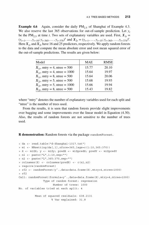
4.3 TREE-BASED METHODS 213
Example 4.6 Again, consider the daily PM2.5 of Shanghai of Example 4.3.We also reserve the last 365 observations for out-of-sample prediction. Let ytbe the PM2.5 at time t. Two sets of explanatory variables are used. First, X1t =(yt−1,… , yt−10; yt−365,… , yt−370)′ and X2t = (yt−1,… , yt−15; yt−365,… , yt−374)′.Here X1t and X2t have 16 and 25 predictors, respectively. We apply random foreststo the data and compute the mean absolute error and root mean squared error ofthe out-of-sample predictions. The results are given below:
Model MAE RMSE
X1t, mtry = 4, ntree = 500 15.77 20.10X1t, mtry = 4, ntree = 1000 15.64 19.97X1t, mtry = 8, ntree = 500 15.64 20.06X2t, mtry = 5, ntree = 500 15.68 19.93X2t, mtry = 5, ntree = 1000 15.66 19.94X2t, mtry = 8, ntree = 500 15.43 19.82
where “mtry” denotes the number of explanatory variables used for each split and“ntree” is the number of trees used.
From the results, it is seen that random forests provide slight improvementsover bagging and some improvements over the linear model in Equation (4.30).Also, the results of random forests are not sensitive to the number of treesused.
R demonstration: Random forests via the package randomForest.
> da <- read.table("d-Shanghai-1317.txt")> m1 <- NNsetting(da[,1],nfore=365,lags=c(1:10,365:370))> X <- m1$X; y <- m1$y; predX <- m1$predX; predY <- m1$predY> n1 <- paste("L",1:10,sep="")> n2 <- paste("L",365:370,sep="")> colnames(X) <- colnames(predX) <- c(n1,n2)> require(randomForest)> rf2 <- randomForest(y˜.,data=data.frame(X),mtry=4,ntree=1000)> rf2Call: randomForest(formula=y˜.,data=data.frame(X),mtry=4,ntree=1000)
Type of random forest: regressionNumber of trees: 1000
No. of variables tried at each split: 4
Mean of squared residuals: 638.2131% Var explained: 31.8

214 4. NEURAL NETWORKS, DEEP LEARNING, AND TREE-BASED METHODS
> prf2 <- predict(rf2,newdata=data.frame(predX))> er2 <- prf2-predY> mean(abs(er2))[1] 15.64032> sqrt(mean(er2ˆ2))[1] 19.97458######## add more predictors> m2 <- NNsetting(da[,1],nfore=365,lags=c(1:15,365:374))> X <- m2$X; y <- m2$y; predX <- m2$predX; predY <- m2$predY> n1 <- paste("L",1:15,sep="")> n2 <- paste("L",365:374,sep="")> colnames(X) <- colnames(predX) <- c(n1,n2)> dim(X)[1] 872 25> rf4 <- randomForest(y˜.,data=data.frame(X),mtry=5)> rf4Call: randomForest(formula = y ˜ ., data = data.frame(X), mtry= 5)
Type of random forest: regressionNumber of trees: 500
No. of variables tried at each split: 5
Mean of squared residuals: 634.4673% Var explained: 32.42
> prf4 <- predict(rf4,newdata=data.frame(predX))> er4 <- prf4-predY> mean(abs(er4))[1] 15.68707> sqrt(mean(er4ˆ2))[1] 19.93318
4.4 EXERCISES
4.1 Consider the transactions data of Walgreens stock on February 6, 2017.Apply the classification tree to the data to model the price movement usingthe same training and forecasting subsamples as those of Example 4.2 of thechapter. Compare the prediction accuracy with that of deep learning.
4.2 Use the methods of neural network, deep learning, and classification tree topredict the PM2.5 series of Beijing. You may use the same lagged explanatoryvariables as those of the Shanghai data in Example 4.3. For deep learning,classify the PM2.5 into six categories, namely
(0, 50], (50, 100], (100, 150], (150, 200], (200, 300], (300,∞].
Use the last 365 observations as the forecasting subsample.
REFERENCES 215
4.3 Consider again the Beijing data. Use bagging with 300 bootstrap iterationsto predict the PM2.5 of Beijing. Again, reserve the last 365 observations asthe forecasting subsample. Repeat the bagging analysis with 600 bootstrapiterations. Are there serial correlations in the residuals of the bagged treewith 600 iterations? Why?
4.4 Consider again the daily PM2.5 series of Beijing. Reserve the last 365 obser-vations for out-of-sample prediction. Apply random forests to obtain predic-tions. Use the same lagged values as in Example 4.6 as the predictors. Tryseveral random forests and comment on their performance.
4.5 Consider the US monthly unemployment rates from January 1948 forSeptember 2017 for 837 observations. The data can be downloaded fromFRED (code: UNRATE) and are seasonally adjusted. The series has strongserial correlations. The goal of this exercise is to explore the effect of strongserial dependence on the performance of bagging and random forests. Tothis end, use the first 700 observations as the modeling subsample andreserve the last 137 observations as the forecasting subsample. Let Xt =(xt−1,… , xt−24)′ be the predictors, where xt is the unemployment rate attime t.
(a) Apply bagging with 1000 bootstrap iterations to the modeling subsam-ple and compute the mean absolute forecast error and the root meansquared forecast errors of the out-of-sample predictions.
(b) Apply random forests with mtry = 5 and ntree=500 and computethe out-of-sample prediction measures as part (a).
(c) Repeat part (b) with mtry = 8 and btree=500.
(d) Compare and comment on the forecasting accuracy of parts (a) to (c).In particular, what is the effect of strong serial correlations on baggingand random forests, if any?
REFERENCES
Carreira-Perpinan, M. A. and Hinton, G. E. (2005). On contrastive divergence learning. InProceedings of the Tenth International Workshop on Artificial Intelligence and Statistics(AISTATS’05), eds. R. G. Cowell and Z. Ghahramani, pp. 30–40. Society for ArtificialIntelligence and Statistics.
Chipman, H. A., George, E. I., and McCulloch, R. E. (1998). Bayesian CART model search(with discussion). Journal of the American Statistical Association 93: 935–960.
Drees, M., J. Rueckert, C. M. Friedrich, G. Hinton, R. Salakhutdinov, and C. E. Rasmussen(2016). darch: Deep Architures and Restricted Boltzmann Machines. R package.

216 4. NEURAL NETWORKS, DEEP LEARNING, AND TREE-BASED METHODS
Geron, A. (2017). Hands-on Machine Learning with SciKit learn and TensorFlow:Concepts, Tools, and Techniques to Build Intelligent Systems. O’Reilly Media,Sebastopol, CA.
Goodfellow, I., Dengio, Y. and Courville, A. (2016). Deep Learning. MIT Press, Boston.
Hassoun, M. H. (2003). Fundamentals of Artificial Neural Networks. A Bradford Book.MIT Press, Boston.
Hastie, T., Tibshirani, R. and Froedman, J. (2001). The Elements of Statistical Learning:Data Mining, Inference, and Prediction. Springer, New York.
Hauseman, J., Lo, A. and MacKinlay, C. (1992). An ordered probit analysis of transactionstock prices. Journal of Financial Economics 31: 319–379.
Hinton, G. E. and Sejnowski, T. J. (1986). Learning and relearning in Boltzmann machines.In Parallel Distributed Processing, eds. D. E. Rumelhart and J. L. McClelland, Vol. 1,Chapter 7, pp. 282–317. MIT Press, Cambridge, MA.
Hinton, G. E., Osindero, S., and Teh, Y. (2006). A fast learning algorithm for deep beliefnets. Neural Computation, 18: 1527–1154.
Hochreiter, S. and Schmidhuber, J. (1997). Long short-term memory. Neural Computation9: 1735–1780.
James, G., Witten, D., Hastie, T., and Tibshirani, R. (2013). An Introduction to StatisticalLearning with Applications in R. Springer, New York.
Lahiri, S. N. (2003). Resampling Methods for Dependent Data. Springer, New York.
Nielsen, M. (2017). Neural Networks and Deep Learning. A free online book athttp://neuralnetworksanddeeplearning.com.
Robert, C. P. and Casella, G. (2004). Monte Carlo Statistical Methods, 2nd edition.Springer, New York.
Rydberg, T. H. and Shephard, N. (2003). Dynamics of trade-by-trade price movementsdecomposition and models. Journal of Financial Econometrics 1: 2–25.
Schmdhuber, J. (2015). Deep learning in neural networks: An overview. Neural Networks,61: 85–117.
Tsay, R. S. (2010). Analysis of Financial Time Series, 3rd edition. John Wiley, Hoboken,NJ.
Tsay, R. S. (2013). An Introduction to Analysis of Financial Data with R. John Wiley,Hoboken, NJ.
Xiao, R. (2014). deepnet: Deep learning toolkit in R. R package.

CHAPTER 5
ANALYSIS OF NON-GAUSSIANTIME SERIES
In this chapter we study the analysis of non-Gaussian time series. The seriesconsidered consist of discrete-valued data, functional data, and financial data,with the latter being serially uncorrelated but dependent. We focus on parametricmodels except for functional data. For discrete-valued time series, we discusstwo modeling approaches. The first modeling approach employs the generalizedautoregressive moving-average (GARMA) models and can be thought of as anextension of the generalized linear models (GLM) of McCullagh and Nelder(1989) to serially dependent data. This general class of models was consideredby Benjamin et al. (2003). For empirical analysis, we use the R package glarmaof Dunsmuir et al. (2015), where GLARMA stands for the generalized linearautoregressive moving-average models. We also introduce a recent extensionof the model by Zheng et al. (2015), the martingalized GARMA (M-GARMA)model, which addresses some of the shortcomings of the GARMA models. Thesecond modeling approach employs the autoregressive conditional mean models,which are closely related to the autoregressive conditional duration (ACD)
Nonlinear Time Series Analysis, First Edition. Ruey S. Tsay and Rong Chen.© 2019 John Wiley & Sons, Inc. Published 2019 by John Wiley & Sons, Inc.Companion website: www.wiley.com/go/tsay/nonlineartimeseries
217

218 5. ANALYSIS OF NON-GAUSSIAN TIME SERIES
models of Engle and Russell (1998). See Heinen (2003) for the autoregressiveconditional Poisson (ACP) model and Hautsch (2012) for applications of themodel in financial econometrics. There are other approaches to modeling timeseries of counts. See Jung and Tremayne (2011) for a comprehensive review.
For financial data, we introduce some commonly used volatility models. Ourdiscussion is brief, and we refer interested readers to books on analysis of finan-cial time series, e.g. Tsay (2010) and Ruppert and Matteson (2015, Chapter 14).The R packages fGarch and rugarch are useful for analyzing asset return series.Finally, for functional data, we discuss some simple autoregressive models, includ-ing convolution models, for modeling and prediction. Nonparametric spline meth-ods are used in estimation.
5.1 GENERALIZED LINEAR TIME SERIES MODELS
Non-Gaussian time series analysis has a long history, especially for count data.See the references in Jung and Tremayne (2011), Dunsmuir and Scott (2015), andWeiss (2017). Following Cox (1981), statistical models for discrete-valued timeseries are classified into observation-driven and parameter-driven models. It turnsout that the observation-driven models are often easier to estimate and we shallfocus on such models in this section.
Benjamin et al. (2003) proposed a broad class of generalized autoregressivemoving-average (GARMA) models for modeling non-Gaussian time series. Manyexisting models in the literature are special cases of the GARMA models. Let yt bea (non-Gaussian) time series and xt be a finite-dimensional vector of explanatoryvariables. Denote by t = 𝜎{yt−1, yt−2,… ; xt, xt−1,…} the 𝜎-field generated bythe past values of yt and the current and past values of xt. The GARMA(p, q)model of Benjamin et al. (2003) postulates that the conditional distribution of ytgiven t is a member of the exponential family distributions via some link functionsimilar to those of the generalized linear models of McCullagh and Nelder (1989).Specifically, the conditional density function of yt given t is
f (yt ∣ t) = exp{
yt𝜗t − b(𝜗t)
𝜑+ a(yt,𝜑)
}, (5.1)
where 𝜗t and 𝜑 are the canonical and scale parameters and the functions b(⋅) anda(⋅) define the specific member of the exponential family of interest. The condi-tional expectation and variance of yt given t are, respectively,
E(yt ∣ t−1) = 𝜇t = b′(𝜗t), Var(yt ∣ t−1) = 𝜑b′′(𝜗t),
where b′(𝜗t) and b′′(𝜗t) denote the first and second derivatives of b(⋅) withrespect to its argument. Furthermore, a link function g(⋅) is used to relate the

5.1 GENERALIZED LINEAR TIME SERIES MODELS 219
conditional expectation 𝜇t to the canonical parameter so that g(𝜇t) = 𝜗t. For sim-plicity, Benjamin et al. (2003) and Dunsmuir and Scott (2015) use the form
𝜗t = x′t𝜷 + wt, (5.2)
where wt is a dynamically dependent variable and 𝜷 denotes the coefficient vectorof explanatory variables. If wt = 0 in Equation (5.2), then the model reduces tothe conventional GLM of McCullagh and Nelder (1989) and the time series yt isconditionally uncorrelated given xt.
Benjamin et al. (2003) consider a general form for wt as
wt ≡ g(𝜇t) =p∑
j=1
𝜙jA(yt−j, xt−j,𝜷) +q∑
j=1
𝛿jM(yt−j,𝜇t−j), (5.3)
where p and q are non-negative integers, 𝝓 = (𝜙1,… ,𝜙p)′ and 𝜹 = (𝛿1,⋯ , 𝛿q)′
are the autoregressive and moving-average parameters, and A(⋅) and M(⋅) areautoregressive and moving-average components. The authors suggest several pos-sibilities for the choice of M(⋅), including deviance residuals, Pearson residu-als, residuals on the original scale yt − 𝜇t, and residuals on the predictor scaleg(yt) − 𝜗t.
The ARMA formulation of Equation (5.3) is too general for practical use.Benjamin et al. (2003) focus on the simple form
𝜗t = x′t𝜷 +p∑
j=1
[g(yt−j) − x′t−j𝜷] +q∑
j=1
𝜃j[g(yt−j) − 𝜗t−j]. (5.4)
Let 𝜖t = g(yt) − 𝜗t = g(yt) − g(𝜇t) be the deviation of g(yt) from g(𝜇t). By addingg(yt) − 𝜗t to both sides of Equation (5.4), we obtain
g(yt) = x′t𝜷 +p∑
j=1
[g(yt−j) − x′t−j𝜷] + 𝜖t +q∑
j=1
𝜃j𝜖t−j. (5.5)
Thus, under the GARMA framework, the transformed series g(yt) assumes theformulation of an ARMAX model commonly used in time series analysis. In thissense, GARMA models are models on the predictor scale, not the original scale.
However, there is a key difference between the ARMA and GARMA models.The error 𝜖t of the GARMA model in Equation (5.5) is not necessarily a whitenoise series. In particular, for a nonlinear function g(⋅), E(𝜖t ∣ t−1) might be non-zero. If the link function g(⋅) is the identity function, then it is easy to show, via iter-ated expectations, that {𝜖t} consists of a sequence of zero-mean and serially uncor-related random variates. The distributions of 𝜖t, however, might be time dependent.The martingalized GARMA models discussed in the next section are proposed toovercome this difficulty.
220 5. ANALYSIS OF NON-GAUSSIAN TIME SERIES
The ARMAX formulation of Equation (5.5) is helpful in understanding theGARMA models. On the other hand, because the observed response yt entersthe equation after the transformation by the link function, care must be exer-cised in some applications. In fact, an arbitrary threshold for observations is oftenneeded for the model to work. Consider, for instance, the Poisson response withlog link, i.e. g(yt) = log(yt). Then, g(yt) is not defined when yt = 0. In many appli-cations of count data, yt = 0 is common. One may even encounter zero-inflatedcount data.
Remark: The acronym GARMA is also used by Woodward et al. (2016) todenote the Gegenbauer ARMA process, which involves a (1 − 2uB + B2) factorin the autoregressive polynomial, where |u| < 1 and B is the backshift operator.The R package tswge associated with Woodward et al. (2016) can be used to esti-mate Gegenbauer ARMA models, but not the GARMA models discussed here.
5.1.1 Count Data and GLARMA Models
Count data are perhaps the most commonly encountered non-Gaussian data in timeseries analysis. See, for example, Davis et al. (2003) and Davis and Wu (2009),among others. Dunsmuir et al. (2015) and Dunsmuir and Scott (2015) consider thegeneralized linear autoregressive moving-average (GLARMA) models for countdata. These models are special cases of the GARMA models with some simplify-ing assumptions. The conditional distribution of GLARMA models is
f (yt ∣ t) = exp{
yt𝜗t − gtb(𝜗t) + ct
}, (5.6)
where gt and ct are sequences of constants possibly depending on the observationsyt. Compared with Equation (5.1), the scale parameter 𝜑 = 1 under the GLARMAmodel, but the function b(⋅) is scaled by a factor gt. This is a restricted form of theexponential family. The conditional means and variances of the responses of Equa-tion (5.6) are 𝜇t ≡ E(yt ∣ t) = gtb
′(𝜗t) and 𝜎2t ≡ Var(yt ∣ t) = gtb
′′(𝜗t). Notethat the negative binomial distribution is not a member of the exponential fam-ily when the scale parameter is not fixed. The canonical parameter employed bythe glarma package of Dunsmuir et al. (2015) is defined as
𝜗t = x′t𝜷 + Ot + wt, (5.7)
where Ot is an offset term, which provides an added flexibility for parameter inter-pretation. For example, for Poisson data such as disease counts, Ot is the logarithmof population, which results in a model for the incidence per unit of population.There is no coefficient parameter associated with Ot.

5.1 GENERALIZED LINEAR TIME SERIES MODELS 221
Function Poisson Binomial Negative binomial
f (yt ∣ t)𝜇
ytt e−𝜇t
yt!
(mt
yt
)𝜋
ytt (1 − 𝜋t)
mt−yt Equation (5.8)
at 1 mt –
ct − log(yt!) log
(mt
yt
)–
b(𝜗t) e𝜗t log(1 + e𝜗t ) –𝜇t e𝜗t mt𝜋t e𝜗t
𝜎2t 𝜇t mt𝜋t(1 − 𝜋t) 𝜇t + (𝜇2
t ∕𝛼2)
Link log logit log
Table 5.1 Distributions and the associated link functions supported by the glarmapackage.
The response distributions used in the glarma package are Poisson and bino-mial, both of which can be put in the form of Equation (5.6), and the negativebinomial distribution with density function given by
f (yt ∣ t, 𝛼) =Γ(𝛼 + yt)
Γ(𝛼)Γ(yt + 1)
[𝛼
𝛼 + 𝜇t
]𝛼 [ 𝜇t
𝛼 + 𝜇t
]yt
, (5.8)
where 𝜇t = exp(𝜗t). This cannot be put into the one parameter exponential familyform when 𝛼 is unknown. In practice, negative binomial distribution is useful in thepresence of over-dispersion. Clearly, negative binomial density converges to thePoisson density as 𝛼 → ∞. Table 5.1 provides a summary of the conditional distri-butions and associated link functions employed by the glarma package. Furtherdetails of the discrete distributions used for count data are given in the appendixto this chapter, including the double Poisson distribution of Efron (1986).
With Equation (5.2), the serial dependence of GLARMA models is governedby
wt =p∑𝑖=1
𝜙𝑖(wt−𝑖 + et−𝑖) +q∑
j=1
𝜃jet−j (5.9)
where et = (yt − 𝜇t)∕vt for some scaling sequence {vt}. Three specifications of vtare supported by the glarma package:
� vt = 𝜎t, the standard deviation of the predictive distribution given inTable 5.1. The resulting et is called the Pearson residual.
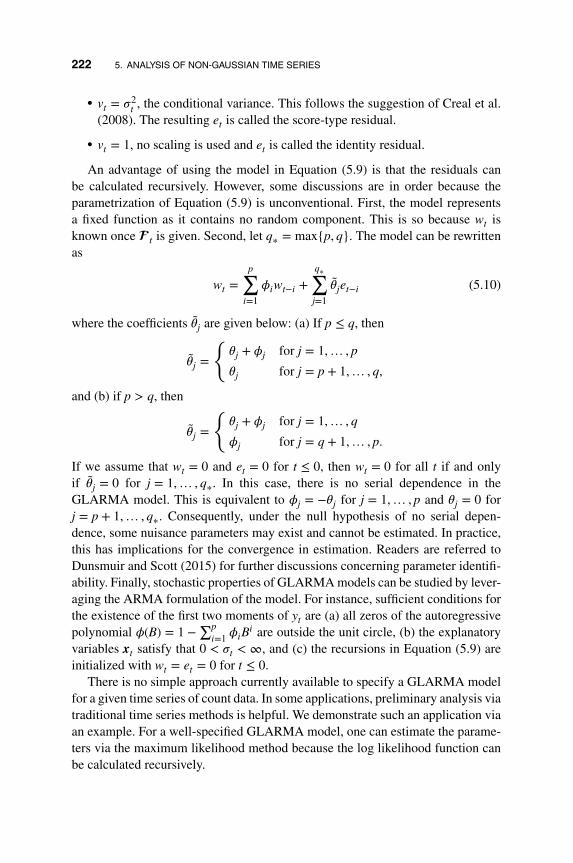
222 5. ANALYSIS OF NON-GAUSSIAN TIME SERIES
� vt = 𝜎2t , the conditional variance. This follows the suggestion of Creal et al.
(2008). The resulting et is called the score-type residual.
� vt = 1, no scaling is used and et is called the identity residual.
An advantage of using the model in Equation (5.9) is that the residuals canbe calculated recursively. However, some discussions are in order because theparametrization of Equation (5.9) is unconventional. First, the model representsa fixed function as it contains no random component. This is so because wt isknown once t is given. Second, let q∗ = max{p, q}. The model can be rewrittenas
wt =p∑𝑖=1
𝜙𝑖wt−𝑖 +q∗∑j=1
𝜃jet−𝑖 (5.10)
where the coefficients 𝜃j are given below: (a) If p ≤ q, then
𝜃j =
{𝜃j + 𝜙j for j = 1,… , p
𝜃j for j = p + 1,… , q,
and (b) if p > q, then
𝜃j =
{𝜃j + 𝜙j for j = 1,… , q
𝜙j for j = q + 1,… , p.
If we assume that wt = 0 and et = 0 for t ≤ 0, then wt = 0 for all t if and onlyif 𝜃j = 0 for j = 1,… , q∗. In this case, there is no serial dependence in theGLARMA model. This is equivalent to 𝜙j = −𝜃j for j = 1,… , p and 𝜃j = 0 forj = p + 1,… , q∗. Consequently, under the null hypothesis of no serial depen-dence, some nuisance parameters may exist and cannot be estimated. In practice,this has implications for the convergence in estimation. Readers are referred toDunsmuir and Scott (2015) for further discussions concerning parameter identifi-ability. Finally, stochastic properties of GLARMA models can be studied by lever-aging the ARMA formulation of the model. For instance, sufficient conditions forthe existence of the first two moments of yt are (a) all zeros of the autoregressivepolynomial 𝜙(B) = 1 −
∑p𝑖=1 𝜙𝑖B
𝑖 are outside the unit circle, (b) the explanatoryvariables xt satisfy that 0 < 𝜎t < ∞, and (c) the recursions in Equation (5.9) areinitialized with wt = et = 0 for t ≤ 0.
There is no simple approach currently available to specify a GLARMA modelfor a given time series of count data. In some applications, preliminary analysis viatraditional time series methods is helpful. We demonstrate such an application viaan example. For a well-specified GLARMA model, one can estimate the parame-ters via the maximum likelihood method because the log likelihood function canbe calculated recursively.

5.1 GENERALIZED LINEAR TIME SERIES MODELS 223
Column Variable Description
1 Count Daily asthma counts2 Intercept Vector of 1s3 Sunday Dummy variable for Sundays4 Monday Dummy variable for Mondays5 CosAnnual cos(2𝜋t∕365), annual cosine function6 SinAnnual sin(2𝜋t∕365), annual sine function7 H7 Scaled, lagged, and smoothed humidity8 NO2max Maximum daily nitrogen oxide9-16 T1.1990–T2.1993 Smooth curves for school terms in each year
Table 5.2 Variables used in the asthma studies.
Example 5.1 Consider the asthma data of Davis et al. (2003), which are availablefrom the glarma package. Let yt be the daily number of asthma cases presentingat the emergency department of a hospital in the south west region of Sydney,Australia. The data are part of a study concerning the relationship between atmo-spheric pollution and asthma cases. Table 5.2 provides a description of the vari-ables in the data set. There are 16 variables (including the intercept) and 1461observations. Figure 5.1 shows the time-plot of the daily asthma counts.
We start with some preliminary analyses to gain insights into the data. Letzt =
√yt and treat zt as a real-valued series. The goal of the project is to seek
the relationship between atmospheric pollution and asthma cases so we start witha linear regression model and obtain the result below:
>require(glarma)> data("Asthma",package="glarma")> y <- Asthma[,1]> X <- as.matrix(Asthma[,-1])> z <- sqrt(y)> m1 <- lm(z˜-1+.,data=data.frame(X))> summary(m1)Call: lm(formula = z ˜ -1 + ., data = data.frame(X))
Coefficients:Estimate Std. Error t value Pr(>|t|)
Intercept 1.19440 0.05177 23.072 < 2e-16 ***Sunday 0.12873 0.04855 2.652 0.008095 **Monday 0.18631 0.04776 3.901 0.000100 ***CosAnnual -0.16244 0.03022 -5.376 8.88e-08 ***

224 5. ANALYSIS OF NON-GAUSSIAN TIME SERIES
1990 1991 1992 1993 1994
02
46
810
1214
Year
Cou
nts
Figure 5.1 Time plot of the daily asthma counts in a hospital in the south west region ofSydney, Australia from 1990 to 1993.
SinAnnual 0.13169 0.03272 4.025 5.99e-05 ***H7 0.10311 0.04667 2.210 0.027292 *NO2max -0.08138 0.02761 -2.947 0.003256 **T1.1990 0.20539 0.05374 3.822 0.000138 ***T2.1990 0.11551 0.05321 2.171 0.030124 *T1.1991 0.05616 0.05481 1.025 0.305715T2.1991 0.15497 0.05457 2.840 0.004579 **T1.1992 0.21848 0.05383 4.059 5.19e-05 ***T2.1992 0.28513 0.05315 5.364 9.46e-08 ***T1.1993 0.37351 0.05393 6.926 6.48e-12 ***T2.1993 0.06352 0.05461 1.163 0.244928Residual standard error: 0.6296 on 1446 degrees of freedomMultiple R-squared: 0.7977, Adjusted R-squared: 0.7956F-statistic: 380 on 15 and 1446 DF, p-value: < 2.2e-16

5.1 GENERALIZED LINEAR TIME SERIES MODELS 225
0 5 10 15 20 25 30
0.0
0.2
0.4
0.6
0.8
1.0
Lag
AC
F
Series m1$residuals
Figure 5.2 Residual autocorrelation function of a linear regression model for the squareroot series of asthma counts.
The regression result shows that all explanatory variables but T1.1991 andT2.1993 are statistically significant at the 5% level, indicating that air pollutionvariables are indeed affecting asthma counts. Figure 5.2 shows the sample auto-correlations of the residuals of the linear regression model. From the plot, it seemsthat there exists some minor serial correlation at lag-7. This is not surprising aspeople tend to have different activities on weekdays and weekends.
To refine the model, we employ a linear regression model with time serieserrors. See Tsay (2010). The result becomes
> m2 <-arima(z,seasonal=list(order=c(0,0,1),period=7),xreg=X,include.mean=F)
> m2
Call:arima(x=z,seasonal=list(order=c(0,0,1),period=7),xreg=X,include.mean=F)
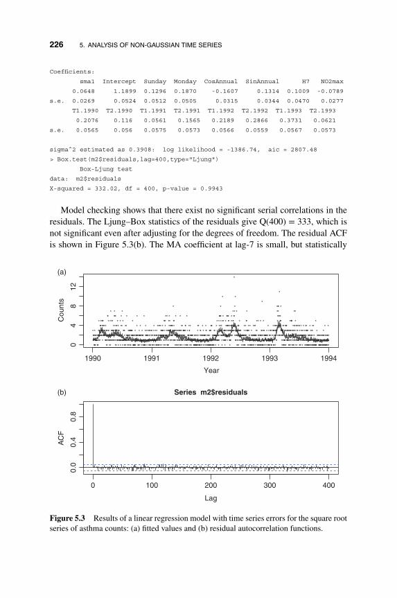
226 5. ANALYSIS OF NON-GAUSSIAN TIME SERIES
Coefficients:
sma1 Intercept Sunday Monday CosAnnual SinAnnual H7 NO2max
0.0648 1.1899 0.1296 0.1870 -0.1607 0.1314 0.1009 -0.0789
s.e. 0.0269 0.0524 0.0512 0.0505 0.0315 0.0344 0.0470 0.0277
T1.1990 T2.1990 T1.1991 T2.1991 T1.1992 T2.1992 T1.1993 T2.1993
0.2076 0.116 0.0561 0.1565 0.2189 0.2866 0.3731 0.0621
s.e. 0.0565 0.056 0.0575 0.0573 0.0566 0.0559 0.0567 0.0573
sigmaˆ2 estimated as 0.3908: log likelihood = -1386.74, aic = 2807.48
> Box.test(m2$residuals,lag=400,type="Ljung")
Box-Ljung test
data: m2$residuals
X-squared = 332.02, df = 400, p-value = 0.9943
Model checking shows that there exist no significant serial correlations in theresiduals. The Ljung–Box statistics of the residuals give Q(400) = 333, which isnot significant even after adjusting for the degrees of freedom. The residual ACFis shown in Figure 5.3(b). The MA coefficient at lag-7 is small, but statistically
*
******
***
**
***
*************
****
****
*
*
*
*****
***
*
**
******
**
**
***
***
*
*****
*******
*
**
**
*
***
***
**
***
*
*
*****
****
*
**
*
***
*
*
*
*
*
*
*
***
*
**
*
***
*
**
*
*
*
*
*
*
*
**
**
***
**
**
*
***
*
*
**
*
********
*
****
*
*
***
*
*
*
***
*
**
*
***
*
**
******
*
****
*
**
*
********
*
*
*****
**
***
***
*
*
**********
*
**
**
*
****
*
**
***
*
**********
*
*
*****
****
***
***
*
***
*
*******
***
*****
*
******
*
******
*
*
*
*
****
***
*
****
********
**
******
*
*****
***
**
**********
**
**
******
*
*****
****
****
*
***
*
*
*
*
**
**
*
****
*
*
**
****
*
*****
*******
*
*
*
*
*
*
*
*
**
**
*
*
***
***
*
**
****
*
**
*
*
**
*
**
*
*
*
**
**
*
****
**
***
*
****
*
*
*
*
**
*
**
*
*
****
*
**
**
***
***
*
****
*****
****
**
*
*
*
**
****
*
**
*
*
*
****
******
*
*
***
*
*
***
*******
*
**
*
**
*******
*
***
****
*
*****
*********************
******
*
*******
**
***
**
***
*
*********
**
*
*
**
*
********
*
****
*
****
**********
**
**
*
********
***
*******
**
*
*
**
*
*
**
***
**
****
*******
**
***********
****
*
***
*
*
*******
***
*
*
*
***
*
*
*
*
*
**
**
*
****
**
*
*
*
**
****
*
***
*
*
****
*
**
****
*
**
*
***
*
**
*******
*
**
*
*
*
**
**
**
**
*
**
****
*
*
**
**
*
*
*
**
*
*
**
*
****
***
*
*
*
*
***
*
*
*
**
*
*
***
*
*
**
*****
*****
*******
*
******
**
**
**
**
**
*
**
**
*
*
*
*
*
**
**
***
*
*
*
*
*
******
*
*******************
*
*
**
****
*
***
*
**
*
**
****
*
*
******
*
*
*
*
***
******
**
*
*
**
*
***
**
*
*
*
*
*
*
*
*
*
**
**
***
*
**
**********
********
*
****
*
**
**
******
*
**
**********
*****
***
*
*
***
**
*
*
**
*****
***
**
*
*
*
*
***
*
*
**
*
*
*
**
*****
*
*******
******
**
*
*
*****
*
***
**
**
***
**
***
*
*
**
******
*
*
*
*
****
*
**
****
***
*
*
*
*
**
**
**
**
****
*
**
*
**
*
*
**
****
**
*
*
*****
*******
**
*
**
*
*****
*
*******
***
***
**
*
******
**
*
****
**
**
*
*
**
*
*
***
*
**
***
*
*
**
***
*
****
*
*
******
**
**
*****
*
*************
*
******
*
*************
*
***
*
****
******
**********
**
*
*
*******
*
***
*
*
*******
*****
**
*
**
**
1990 1991 1992 1993 1994
(a)
(b)
04
812
Year
Cou
nts
0 100 200 300 400
0.0
0.4
0.8
Lag
AC
F
Series m2$residuals
Figure 5.3 Results of a linear regression model with time series errors for the square rootseries of asthma counts: (a) fitted values and (b) residual autocorrelation functions.
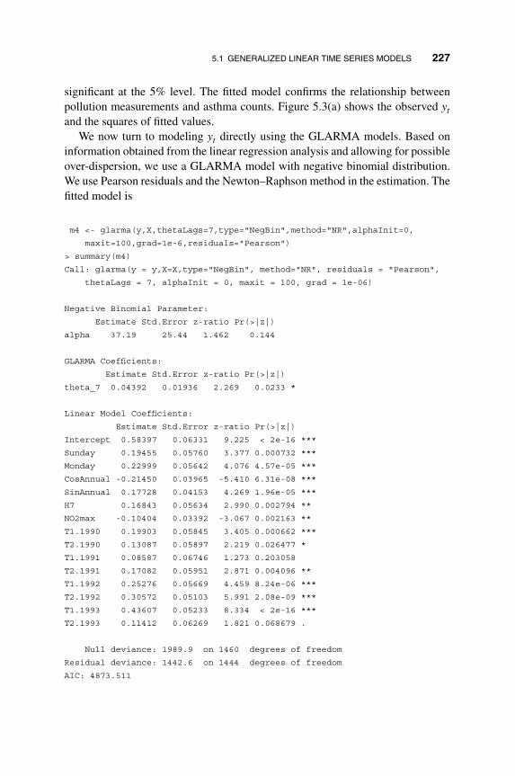
5.1 GENERALIZED LINEAR TIME SERIES MODELS 227
significant at the 5% level. The fitted model confirms the relationship betweenpollution measurements and asthma counts. Figure 5.3(a) shows the observed ytand the squares of fitted values.
We now turn to modeling yt directly using the GLARMA models. Based oninformation obtained from the linear regression analysis and allowing for possibleover-dispersion, we use a GLARMA model with negative binomial distribution.We use Pearson residuals and the Newton–Raphson method in the estimation. Thefitted model is
m4 <- glarma(y,X,thetaLags=7,type="NegBin",method="NR",alphaInit=0,
maxit=100,grad=1e-6,residuals="Pearson")
> summary(m4)
Call: glarma(y = y,X=X,type="NegBin", method="NR", residuals = "Pearson",
thetaLags = 7, alphaInit = 0, maxit = 100, grad = 1e-06)
Negative Binomial Parameter:
Estimate Std.Error z-ratio Pr(>|z|)
alpha 37.19 25.44 1.462 0.144
GLARMA Coefficients:
Estimate Std.Error z-ratio Pr(>|z|)
theta_7 0.04392 0.01936 2.269 0.0233 *
Linear Model Coefficients:
Estimate Std.Error z-ratio Pr(>|z|)
Intercept 0.58397 0.06331 9.225 < 2e-16 ***
Sunday 0.19455 0.05760 3.377 0.000732 ***
Monday 0.22999 0.05642 4.076 4.57e-05 ***
CosAnnual -0.21450 0.03965 -5.410 6.31e-08 ***
SinAnnual 0.17728 0.04153 4.269 1.96e-05 ***
H7 0.16843 0.05634 2.990 0.002794 **
NO2max -0.10404 0.03392 -3.067 0.002163 **
T1.1990 0.19903 0.05845 3.405 0.000662 ***
T2.1990 0.13087 0.05897 2.219 0.026477 *
T1.1991 0.08587 0.06746 1.273 0.203058
T2.1991 0.17082 0.05951 2.871 0.004096 **
T1.1992 0.25276 0.05669 4.459 8.24e-06 ***
T2.1992 0.30572 0.05103 5.991 2.08e-09 ***
T1.1993 0.43607 0.05233 8.334 < 2e-16 ***
T2.1993 0.11412 0.06269 1.821 0.068679 .
Null deviance: 1989.9 on 1460 degrees of freedom
Residual deviance: 1442.6 on 1444 degrees of freedom
AIC: 4873.511

228 5. ANALYSIS OF NON-GAUSSIAN TIME SERIES
Number of Newton Raphson iterations: 6
LRT and Wald Test:
Alternative hypothesis: model is a GLARMA process
Null hypothesis: model is a GLM with the same regression structure
Statistic p-value
LR Test 7.047 0.00794 **
Wald Test 5.147 0.02329 *
> par(mfcol=c(2,2))
> plot(m4,which=c(1,2,3,5),titles=c("","","","PIT for glarma(NegBin)"))
From the output, the MA coefficient is small, but statistically significant. The esti-mate of 𝛼 is relatively large, indicating that a Poisson distribution might be suffi-cient. The likelihood ratio test and the Wald test indicate that a GLARMA modelis needed. Figure 5.4 shows the model checking of the fitted GLARMA model.
Time
(a)
(b)
(c)
(d)
Cou
nts
0 500 1000 1500
02
46
810
14
glarmafixedobs
0 5 10 15 20 25 30
0.0
0.2
0.4
0.6
0.8
1.0
Lag
AC
F
Time
Res
idua
ls
0 500 1000 1500
−2
02
46
PIT for glarma(NegBin)
Probability integral transform
Rel
ativ
e fr
eque
ncy
0.0
0.5
1.0
1.5
2.0
0.0 0.2 0.4 0.6 0.8 1.0
Figure 5.4 Model checking of a fitted GLARMA model for the asthma counts: (a) thefitted values, (b) the residual autocorrelations, (c) the residual plot, and (d) the probabilityintegral transformation.

5.2 AUTOREGRESSIVE CONDITIONAL MEAN MODELS 229
The plots indicate that the model is adequate. Overall, the model also confirms theeffect of pollution measurements on the asthma counts.
Remark: There are other R packages that can fit GARMA models. See, forinstance, VGAM and gamlss.util. Also, the package tscount of R can handletime series of count data.
5.2 AUTOREGRESSIVE CONDITIONAL MEAN MODELS
A highly related class of models for time series of count data is the autoregres-sive conditional mean (ACM) models. Motivated by the autoregressive conditionalduration (ACD) models of Engle and Russell (1998), Heinen (2003) proposes theautoregressive conditional Poisson (ACP) models. Since then, various extensionsof ACM models have been developed. Again, let yt be the time series of interestand t = 𝜎{yt−1, yt−2,… ; xt, xt−1,…}. The conditional mean models postulate
E(yt ∣ t) = exp(x′t𝜷)𝜆t, (5.11)
and 𝜆t follows the model
𝜆t = 𝜔 +p∑𝑖=1
𝛼𝑖
[yt−𝑖
exp(x′t−𝑖𝜷)
]+
q∑j=1
𝛾j𝜆t−j, (5.12)
where p and q are nonnegative integers,𝜔 > 0, and 𝛼𝑖 and 𝛾j are parameters satisfy-ing certain conditions so that 𝜆t is positive and finite. The conditional distributionp(yt ∣ t) is Poisson, negative binomial or double Poisson. Descriptions of thesethree distributions are given in the appendix. The negative binomial distributionallows for over-dispersion whereas the double Poisson can handle both over- andunder-dispersion.
Properties of the conditional mean models have been derived in the literature.For example, assuming that there exist no explanatory variables, Heinen (2003)showed that the ACP process with 𝜆t in Equation (5.12) is stationary if 𝜔 > 0 and0 ≤
∑p𝑖=1 𝛼𝑖 +
∑qj=1 𝛾j < 1. The unconditional mean of the process is given by
E(yt) ≡ 𝜇 = 𝜔
1 −∑p𝑖=1 𝛼𝑖 −
∑qj=1 𝛾j
.
In addition, for the ACP(1,1) model, the unconditional covariance function is givenby
Cov(yt, yt−h) =⎧⎪⎨⎪⎩
[1−(𝛼1+𝛾1)2+𝛼21]𝜇
1−(𝛼1+𝛾1)2 , h = 0
𝛼1[1−𝛾1(𝛼1+𝛾1)](𝛼1+𝛾1)h−1𝜇
1−(𝛼1+𝛾1)2 , h ≥ 1.(5.13)
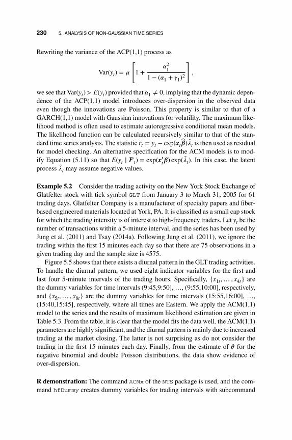
230 5. ANALYSIS OF NON-GAUSSIAN TIME SERIES
Rewriting the variance of the ACP(1,1) process as
Var(yt) = 𝜇
[1 +
𝛼21
1 − (𝛼1 + 𝛾1)2
],
we see that Var(yt)> E(yt) provided that 𝛼1 ≠ 0, implying that the dynamic depen-dence of the ACP(1,1) model introduces over-dispersion in the observed dataeven though the innovations are Poisson. This property is similar to that of aGARCH(1,1) model with Gaussian innovations for volatility. The maximum like-lihood method is often used to estimate autoregressive conditional mean models.The likelihood function can be calculated recursively similar to that of the stan-dard time series analysis. The statistic rt = yt − exp(xt𝜷)��t is then used as residualfor model checking. An alternative specification for the ACM models is to mod-ify Equation (5.11) so that E(yt ∣ t) = exp(x′t𝜷) exp(��t). In this case, the latentprocess ��t may assume negative values.
Example 5.2 Consider the trading activity on the New York Stock Exchange ofGlatfelter stock with tick symbol GLT from January 3 to March 31, 2005 for 61trading days. Glatfelter Company is a manufacturer of specialty papers and fiber-based engineered materials located at York, PA. It is classified as a small cap stockfor which the trading intensity is of interest to high-frequency traders. Let yt be thenumber of transactions within a 5-minute interval, and the series has been used byJung et al. (2011) and Tsay (2014a). Following Jung et al. (2011), we ignore thetrading within the first 15 minutes each day so that there are 75 observations in agiven trading day and the sample size is 4575.
Figure 5.5 shows that there exists a diurnal pattern in the GLT trading activities.To handle the diurnal pattern, we used eight indicator variables for the first andlast four 5-minute intervals of the trading hours. Specifically, {x1t,… , x4t} arethe dummy variables for time intervals (9:45,9:50], …, (9:55,10:00], respectively,and {x5t,… , x8t} are the dummy variables for time intervals (15:55,16:00], …,(15:40,15:45], respectively, where all times are Eastern. We apply the ACM(1,1)model to the series and the results of maximum likelihood estimation are given inTable 5.3. From the table, it is clear that the model fits the data well, the ACM(1,1)parameters are highly significant, and the diurnal pattern is mainly due to increasedtrading at the market closing. The latter is not surprising as do not consider thetrading in the first 15 minutes each day. Finally, from the estimate of 𝜃 for thenegative binomial and double Poisson distributions, the data show evidence ofover-dispersion.
R demonstration: The command ACMx of the NTS package is used, and the com-mand hfDummy creates dummy variables for trading intervals with subcommand
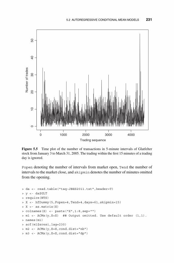
5.2 AUTOREGRESSIVE CONDITIONAL MEAN MODELS 231
0 1000 2000 3000 4000
010
2030
4050
Trading sequence
Num
ber
of tr
ades
Figure 5.5 Time plot of the number of transactions in 5-minute intervals of Glatfelterstock from January 3 to March 31, 2005. The trading within the first 15 minutes of a tradingday is ignored.
Fopen denoting the number of intervals from market open, Tend the number ofintervals to the market close, and skipmin denotes the number of minutes omittedfrom the opening.
> da <- read.table("taq-JBES2011.txt",header=T)> y <- da$GLT> require(NTS)> X <- hfDummy(5,Fopen=4,Tend=4,days=61,skipmin=15)> X <- as.matrix(X)> colnames(X) <- paste("X",1:8,sep="")> m1 <- ACMx(y,X=X) ## Output omitted. Use default order (1,1).> names(m1)> acf(m1$sresi,lag=230)> m2 <- ACMx(y,X=X,cond.dist="nb")> m3 <- ACMx(y,X=X,cond.dist="dp")

232 5. ANALYSIS OF NON-GAUSSIAN TIME SERIES
Parameter Poisson Neg-binomial Double Poisson
𝛽1 −0.020(0.049) 0.006(0.077) −0.020(0.069)𝛽2 −0.033(0.049) −0.018(0.077) −0.034(0.070)𝛽3 −0.109(0.052) −0.112(0.078) −0.107(0.073)𝛽4 0.110(0.048) 0.103(0.076) 0.107(0.067)𝛽5 0.599(0.038) 0.609(0.070) 0.594(0.054)𝛽6 0.169(0.047) 0.186(0.075) 0.165(0.066)𝛽7 0.138(0.048) 0.143(0.076) 0.134(0.068)𝛽8 0.128(0.049) 0.126(0.076) 0.128(0.068)𝜔 0.503(0.048) 0.483(0.068) 0.535(0.071)𝛼1 0.173(0.009) 0.171(0.013) 0.171(0.012)𝛾1 0.735(0.015) 0.741(0.022) 0.735(0.022)𝜃 4.913(0.198) 0.497(0.009)Q(230) 92.15(0.09) 91.45(0.10) 93.62(0.07)
Table 5.3 Maximum likelihood estimates of an autoregressive conditional mean modelof order (1,1) for the number of trades in 5-minute intervals of Glatfelter stock fromJanuary 1 to March 31, 2005. The sample size is 4575. The numbers in parentheses for theestimates are standard errors and that for Q(m) statistics is p value.
5.3 MARTINGALIZED GARMA MODELS
Zheng et al. (2015) proposed the martingalized GARMA models to mitigate someshortcomings of Equation (5.5). Specifically, the authors introduce an additionaltransformation of the time series yt so that the error terms of the ARMAX formu-lation of a GARMA model become a martingale difference sequence. The newmodel is called a martingalized GARMA model or M-GARMA model for short.To this end, Zheng et al. (2015) assumed that the conditional probability massfunction of yt given t can be parameterized as
p(yt ∣ t) = f (yt ∣ 𝜇t,𝝋) (5.14)
where 𝝋 denotes the collection of all time-invariant parameters. This assumptionsays that all past information concerning yt is summarized in𝜇t. Furthermore, thereexist a function h(yt) and the link function g𝜑(𝜇t) = E[h(yt) ∣ t] so that Equation(5.4) becomes
g𝜑(𝜇t) = x′t𝜷 +p∑𝑖=1
𝜙𝑖[h(yt−𝑖) − x′t−𝑖𝜷] +q∑
j=1
𝜃j[h(yt−j) − g𝜑(𝜇t−j)]. (5.15)

5.3 MARTINGALIZED GARMA MODELS 233
Distribution Density E(yt ∣ t−1) Var(yt ∣ t−1)
Lognormal logN(log(𝜇t) − 𝜎2∕2, 𝜎2) 𝜇t (e𝜎2 − 1)𝜇2
tGamma Γ(c𝜇d
t , c𝜇d−1t ) 𝜇t 𝜇2−d
t ∕cInv-gamma Inv-Γ(c𝜇d
t + 1, c𝜇dt ) 𝜇t c𝜇1+d
t ∕(c𝜇d−1t − 1)
Weibull Weibull(k,𝜇t∕Γ(1 + k−1)) 𝜇t 𝜇2t
[Γ(1+2k−1)Γ2(1+k−1)
− 1]
Beta Beta(𝜏𝜇t, 𝜏(1 − 𝜇t)) 𝜇t𝜇t(1−𝜇t)
1+𝜏Poisson Poisson(𝜇t) 𝜇t 𝜇t
g𝜑(𝜇t) h(yt) Var[h(yt) ∣ t−1]
Lognormal log(𝜇t) −𝜎2
2log(yt) 𝜎2
Gamma 𝜓(c𝜇dt ) − log(𝜇d−1
t ) − log(c) log(yt) 𝜓1(c𝜇2t )
Inv-gamma log(c𝜇dt ) − 𝜓(c𝜇d−1
t + 1) log(yt) 𝜓1(c𝜇d−1t + 1)
Weibull ≈ log(𝜇t) −12
[Γ(1+2k−1)Γ2(1+k−1)
− 1]
log(yt) ≈ Γ(1+2k−1)Γ2(1+k−1)
− 1
Beta 𝜓(𝜏𝜇t) − 𝜓(𝜏(1 − 𝜇t)) log(
yt
1−yt
)𝜓1(𝜏𝜇t) + 𝜓1(𝜏(1 − 𝜇t))
Poisson ≈√𝜇t
√yt ≈ 1
4
Table 5.4 Some commonly used conditional distributions, their recommended y-linkfunctions, the corresponding link functions, and the first two moments, where t−1
denotes the lagged values of yt. 𝜓(⋅) and 𝜓1(⋅) denote the gigamma and trigammafunctions, respectively. See Zheng et al. (2015).
By adding h(yt) − g𝜑(𝜇t) to both sides of Equation (5.15), we have
h(yt) = x′t𝜷 +p∑𝑖=1
𝜙𝑖[h(yt−𝑖) − x′t−𝑖𝜷] + 𝜖t +q∑
j=1
𝜃j𝜖t−j, (5.16)
where 𝜖t = h(yt) − g𝜑(𝜇t). By the construction of h(⋅) and g𝜑(⋅), it is easy to show,via iterated expectations, that (a) E(𝜖t) = E[E(h(yt) − g𝜑(𝜇t) ∣ t)] = 0 and (b)E(𝜖t𝜖t−j) = E[𝜖t−jE(𝜖t ∣ t)] = 0 for j > 0. Therefore, {𝜖t} is a martingale differ-ence sequence. The function h(⋅) is referred to as the y-link function and g𝜑(⋅) isthe link function.
From the discussion, it is seen that the link function h(⋅) is used to transformthe yt series into a linear process. Zheng et al. (2015) recommended that one usesa y-link function that does not involve any unknown parameter. In this case, theorders p and q and the ARMA parameters of Equation (5.16) can be obtained bystudying h(yt). The link function g𝜑(⋅), on the other hand, may contain unknownparameters. The authors also suggested ways to select a proper transformationh(⋅). Table 5.4 provides some commonly used conditional distributions and theirrecommended y-link functions; see Zheng et al. (2015).

234 5. ANALYSIS OF NON-GAUSSIAN TIME SERIES
To gain insights into the M-GARMA model, we rewrite Equation (5.15) as
𝜂t = v(xt,𝜷) +m∑𝑖=1
��𝑖h(yt−𝑖) +m∑
j=1
𝜃j𝜂t−j, (5.17)
where 𝜂t = g𝜑(𝜇t), v(xt,𝜷) is a function of t and 𝜷 in the presence of xt andis a constant otherwise, m = max{p, q}, ��𝑖 = 𝜙𝑖 + 𝜃𝑖 for 𝑖 = 1,… , m, 𝜃j = −𝜃jfor j = 1,… , q with 𝜙𝑖 = 0 for 𝑖 > p and 𝜃j = 0 for 𝑖 > q. Equation (5.17) showsthat 𝜂t is a linear predictor of h(yt), which is a linear combination of past trans-formed responses h(yt−1),… , h(yt−p) and the past predictors 𝜂t−1,… , 𝜂t−q. Thisfixed function framework is similar to that of the generalized autoregressive con-ditional heteroscedastic (GARCH) models for volatility to be discussed in the nextsection.
Some stochastic properties of M-GARMA models are derived in Zheng et al.(2015) using the geometric drift condition of Meyn and Tweedie (2009). Theauthors consider two estimation methods for the model. The first method usesGaussian pseudo likelihood and the second method is the maximum likelihoodestimation. Finally, they also demonstrate two applications of the M-GARMAmodels.
5.4 VOLATILITY MODELS
Let yt be the return (or log return) of an asset at time t. The volatility of theasset is defined as the conditional standard deviation of yt given the information t−1 = 𝜎{yt−1, yt−2,… , }. In finance, volatility plays an important role becauseit serves as a measurement of risk and is widely used in asset pricing. Figure 5.6shows the daily log returns of the SPDR S&P 500 ETF (SPY) from January 3,2007 to December 31, 2016. This exchange traded fund (ETF) follows the S&P500 index, which is commonly used to represent the US financial market. From theplot, it is seen that the returns exhibit periods of high variability. This phenomenonis called volatility clustering in finance. Selected summary statistics of the SPYlog returns are
Mean Standard error Median Skewness Excess kurtosis0.0003 0.0131 0.0006 −0.099 12.93
Clearly, the log returns have high excess kurtosis and center around zero. Theplot and summary statistics show the stylized characteristics of asset returns,namely zero mean, heavy tails, and volatility clustering.
The goal of volatility modeling is then to consider statistical models that canadequately describe the observed characteristics of asset returns. Two general
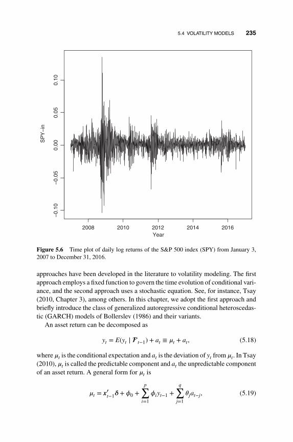
5.4 VOLATILITY MODELS 235
2008 2010 2012 2014 2016
−0.
10−
0.05
0.00
0.05
0.10
Year
SP
Y−
in
Figure 5.6 Time plot of daily log returns of the S&P 500 index (SPY) from January 3,2007 to December 31, 2016.
approaches have been developed in the literature to volatility modeling. The firstapproach employs a fixed function to govern the time evolution of conditional vari-ance, and the second approach uses a stochastic equation. See, for instance, Tsay(2010, Chapter 3), among others. In this chapter, we adopt the first approach andbriefly introduce the class of generalized autoregressive conditional heteroscedas-tic (GARCH) models of Bollerslev (1986) and their variants.
An asset return can be decomposed as
yt = E(yt ∣ t−1) + at ≡ 𝜇t + at, (5.18)
where 𝜇t is the conditional expectation and at is the deviation of yt from 𝜇t. In Tsay(2010), 𝜇t is called the predictable component and at the unpredictable componentof an asset return. A general form for 𝜇t is
𝜇t = x′t−1𝜹 + 𝜙0 +p∑𝑖=1
𝜙𝑖yt−1 +q∑
j=1
𝜃jat−j, (5.19)

236 5. ANALYSIS OF NON-GAUSSIAN TIME SERIES
where xt−1 denotes a vector of available explanatory variables, 𝜹 is the coefficientvector, 𝜙0 is a constant, and 𝜙𝑖 and 𝜃j are the usual autoregressive and moving-average parameters, respectively. In most applications, 𝜇t is simply a constant,especially for high-frequency returns. The unpredictable part of asset returns iswritten as
at = 𝜎t𝜖t, 𝜖t ∼𝑖𝑖d D(0, 1), (5.20)
where 𝜎2t = Var(yt ∣ t−1) = E[(yt − 𝜇t)
2 ∣ t−1] and 𝜖t is a sequence of inde-pendent and identically distributed random variates with mean zero and variance1, denoted by D(0, 1). The distribution of 𝜖t is Gaussian, standardized Student-twith v degrees of freedom, or the generalized error distribution. In some cases, 𝜖tassumes a skew distribution such as a skew normal or Student-t. Again, see Tsay(2010, Chapter 3) for further details, among others.
The most commonly used GARCH model is in the form
𝜎2t = 𝜔 + 𝛼a2
t−1 + 𝛽𝜎2t−1, (5.21)
where 𝜔 > 0, 0 ≤ 𝛼, 𝛽 < 1 and 𝛼 + 𝛽 < 1. The model in Equation (5.21) is calleda GARCH(1,1) model in the literature and has been widely studied. It is easy toshow that
E(a2t ) = Var(at) =
𝜔
1 − 𝛼 − 𝛽, if 𝛼 + 𝛽 < 1,
E(a4t )
[E(a2t )]2
= 3[1 − (𝛼 + 𝛽)2]
1 − (𝛼 + 𝛽)2 − 2𝛼2≥ 3, if 1 − 2𝛼2 − (𝛼 + 𝛽)2 > 0.
The second result was obtained assuming 𝜖t ∼ N(0, 1), and it implies that at hasheavy tails under the GARCH(1,1) model even though 𝜖t is Gaussian. The formulaalso shows that the heavy tails induced by the GARCH dynamics mainly comefrom the parameter 𝛼. Let 𝜂t = a2
t − 𝜎2t be the deviation of a2
t from its conditionalexpectation. The model in Equation (5.21) can be rewritten as
a2t = 𝜔 + (𝛼 + 𝛽)a2
t−1 − 𝛽𝜂t−1, (5.22)
which is in the form of an ARMA model. The statistic 𝜂t satisfies (a) E(𝜂t) = 0 and(b) Cov(𝜂t, 𝜂t−j)= 0 for j > 0. However, 𝜂t is not necessarily identically distributed.The ARMA formulation in Equation (5.22) is helpful in understanding propertiesof GARCH(1,1) models. For instance, for a GARCH(1,1) process to be weaklystationary, we need 0 < 𝛼 + 𝛽 < 1. Also, by leveraging the properties of an ARMAprocess, we have E(a2
t ) = 𝜔∕(1 − 𝛼 − 𝛽).From Equation (5.21), we see that a large 𝜎2
t−1 or a2t−1 leads to a large 𝜎2
t , imply-ing that a volatile period at t − 1 tends to be followed by another volatile period attime t. Therefore, the GARCH model is capable of producing volatility clusteringsobserved in practice.

5.4 VOLATILITY MODELS 237
0 5 10 15 20 25 30 35
(a)
(b)
0.0
0.4
0.8
Lag
AC
FSeries SPY
0 5 10 15 20 25 30 35
0.0
0.4
0.8
Lag
AC
F
Series SPY^2
Figure 5.7 Sample autocorrelation functions of the daily log returns of (a) SPY and (b)their squared series. The sample period is from January 3, 2007 to December 31, 2016. Theupper panel shows the ACF of the log return series.
GARCH models can be estimated by either the quasi maximum likelihoodmethod or the conditional maximum likelihood method. Asymptotic propertiesof the estimators have been established in the literature. See, for example, Tsay(2014b) and the references therein. There are several R packages available to esti-mate volatility models. For GARCH models and their variants, both fGarch andurgarch packages work well.
Example 5.3 Consider the daily log returns of SPY shown in Figure 5.6. Denotethe log return by yt. Similar to most asset return series, yt has weak serial corre-lations, but y2
t has strong serial dependence. See Figure 5.7 for the sample ACF ofyt and y2
t . Therefore, we employ the model
yt = 𝜇 + at, at = 𝜎t𝜖t (5.23)
𝜖t ∼ D(0, 1)
𝜎2t = 𝜔 + 𝛼a2
t−1 + 𝛽𝜎2t−1, (5.24)
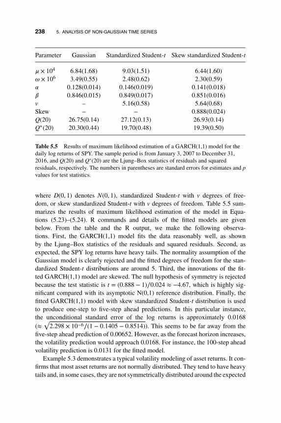
238 5. ANALYSIS OF NON-GAUSSIAN TIME SERIES
Parameter Gaussian Standardized Student-t Skew standardized Student-t
𝜇 × 104 6.84(1.68) 9.03(1.51) 6.44(1.60)𝜔 × 106 3.49(0.55) 2.48(0.62) 2.30(0.59)𝛼 0.128(0.014) 0.146(0.019) 0.141(0.018)𝛽 0.846(0.015) 0.849(0.017) 0.851(0.016)v – 5.16(0.58) 5.64(0.68)Skew – – 0.888(0.024)Q(20) 26.75(0.14) 27.12(0.13) 26.93(0.14)Q∗(20) 20.30(0.44) 19.70(0.48) 19.39(0.50)
Table 5.5 Results of maximum likelihood estimation of a GARCH(1,1) model for thedaily log returns of SPY. The sample period is from January 3, 2007 to December 31,2016, and Q(20) and Q∗(20) are the Ljung–Box statistics of residuals and squaredresiduals, respectively. The numbers in parentheses are standard errors for estimates and pvalues for test statistics.
where D(0, 1) denotes N(0, 1), standardized Student-t with v degrees of free-dom, or skew standardized Student-t with v degrees of freedom. Table 5.5 sum-marizes the results of maximum likelihood estimation of the model in Equa-tions (5.23)–(5.24). R commands and details of the fitted models are givenbelow. From the table and the R output, we make the following observa-tions. First, the GARCH(1,1) model fits the data reasonably well, as shownby the Ljung–Box statistics of the residuals and squared residuals. Second, asexpected, the SPY log returns have heavy tails. The normality assumption of theGaussian model is clearly rejected and the fitted degrees of freedom for the stan-dardized Student-t distributions are around 5. Third, the innovations of the fit-ted GARCH(1,1) model are skewed. The null hypothesis of symmetry is rejectedbecause the test statistic is t = (0.888 − 1)∕0.024 ≈ −4.67, which is highly sig-nificant compared with its asymptotic N(0,1) reference distribution. Finally, thefitted GARCH(1,1) model with skew standardized Student-t distribution is usedto produce one-step to five-step ahead predictions. In this particular instance,the unconditional standard error of the log returns is approximately 0.0168(≈
√2.298 × 10⁻⁶∕(1 − 0.1405 − 0.8514)). This seems to be far away from the
five-step ahead prediction of 0.00652. However, as the forecast horizon increases,the volatility prediction would approach 0.0168. For instance, the 100-step aheadvolatility prediction is 0.0131 for the fitted model.
Example 5.3 demonstrates a typical volatility modeling of asset returns. It con-firms that most asset returns are not normally distributed. They tend to have heavytails and, in some cases, they are not symmetrically distributed around the expected

5.4 VOLATILITY MODELS 239
0 500 1000 1500 2000 2500
−0.
10−
0.05
0.00
0.05
0.10
Series with 2 conditional SD superimposed
Index
x
Figure 5.8 Time plot of daily log returns and point-wise 95% confidence intervals for theSPY. The sample period is from January 3, 2007 to December 31, 2016. The volatilities areobtained from the GARCH(1,1) model with skew innovations of Table 5.5.
return. Figure 5.8 shows the log return series and the point-wise 95% confidenceband based on the fitted GARCH(1,1) model with Gaussian innovations. Similarplots can be obtained for other fitted models. Figure 5.9 shows the QQ-plots ofthe residuals of a fitted GARCH(1,1) model with standardized Student-t and skewstandardized Student-t. The QQ-plot of the model with skew innovations faresbetter than that with symmetric innovations.
R demonstration: GARCH modeling with various innovation distributions.
> require(fGarch)
> m1 <- garchFit(˜garch(1,1),data=spy,trace=F)
> summary(m1)
Title: GARCH Modelling

240 5. ANALYSIS OF NON-GAUSSIAN TIME SERIES
−6 −4 −2 0 2 4 6
(a)
(b)
−6
−2
02
qstd − QQ-plot
Theoretical quantiles
Sam
ple
quan
tiles
−6 −4 −2 0 2 4
−8
−4
02
qsstd − QQ-plot
Theoretical quantiles
Sam
ple
quan
tiles
Figure 5.9 QQ plots of fitted GARCH(1,1) models with (a) standardized Student-t and(b) skew standardized Student-t innovations. The models are given in Table 5.5.
Call: garchFit(formula = ˜garch(1, 1), data = spy, trace=F)
Conditional Distribution: norm
Error Analysis:
Estimate Std. Error t value Pr(>|t|)
mu 6.842e-04 1.681e-04 4.070 4.70e-05 ***
omega 3.494e-06 5.469e-07 6.388 1.68e-10 ***
alpha1 1.275e-01 1.403e-02 9.086 < 2e-16 ***
beta1 8.464e-01 1.463e-02 57.856 < 2e-16 ***
Standardised Residuals Tests:
Statistic p-Value
Jarque-Bera Test R Chiˆ2 557.7797 0
Ljung-Box Test R Q(10) 16.93149 0.07589384
Ljung-Box Test R Q(20) 26.75075 0.1424233
Ljung-Box Test Rˆ2 Q(10) 14.30636 0.1594707
Ljung-Box Test Rˆ2 Q(20) 20.29979 0.4393226
> plot(m1)

5.4 VOLATILITY MODELS 241
> m2 <- garchFit(˜garch(1,1),data=spy,cond.dist="std",trace=F)
> summary(m2)
Title: GARCH Modelling
Call: garchFit(formula=˜garch(1,1),data=spy,cond.dist="std",trace=F)
Conditional Distribution: std
Error Analysis:
Estimate Std. Error t value Pr(>|t|)
mu 9.031e-04 1.509e-04 5.986 2.16e-09 ***
omega 2.477e-06 6.248e-07 3.965 7.34e-05 ***
alpha1 1.456e-01 1.915e-02 7.601 2.95e-14 ***
beta1 8.490e-01 1.681e-02 50.499 < 2e-16 ***
shape 5.160e+00 5.813e-01 8.876 < 2e-16 ***
Standardised Residuals Tests:
Statistic p-Value
Ljung-Box Test R Q(10) 17.45736 0.06483688
Ljung-Box Test R Q(20) 27.11551 0.1320453
Ljung-Box Test Rˆ2 Q(10) 10.25488 0.4184234
Ljung-Box Test Rˆ2 Q(20) 19.70427 0.4765604
LM Arch Test R TRˆ2 11.08226 0.5218827
Information Criterion Statistics:
AIC BIC SIC HQIC
-6.430537 -6.418958 -6.430545 -6.426335
> m3 <- garchFit(˜garch(1,1),data=spy,cond.dist="sstd",trace=F)
> summary(m3)
Title: GARCH Modelling
Call:garchFit(formula=˜garch(1,1),data=spy,cond.dist="sstd",trace=F)
Conditional Distribution: sstd
Error Analysis:
Estimate Std. Error t value Pr(>|t|)
mu 6.441e-04 1.603e-04 4.017 5.90e-05 ***
omega 2.298e-06 5.858e-07 3.922 8.77e-05 ***
alpha1 1.405e-01 1.790e-02 7.848 4.22e-15 ***
beta1 8.514e-01 1.628e-02 52.310 < 2e-16 ***
skew 8.882e-01 2.352e-02 37.760 < 2e-16 ***
shape 5.637e+00 6.844e-01 8.236 2.22e-16 ***
Standardised Residuals Tests:
Statistic p-Value
Ljung-Box Test R Q(10) 17.46512 0.06468508
Ljung-Box Test R Q(20) 26.92805 0.1373005

242 5. ANALYSIS OF NON-GAUSSIAN TIME SERIES
Ljung-Box Test Rˆ2 Q(10) 9.8221 0.4562374
Ljung-Box Test Rˆ2 Q(20) 19.38767 0.4967704
Information Criterion Statistics:
AIC BIC SIC HQIC
-6.437849 -6.423954 -6.437861 -6.432807
> predict(m3,5)
meanForecast meanError standardDeviation
1 0.0006440697 0.005880318 0.005880318
2 0.0006440697 0.006049519 0.006049519
3 0.0006440697 0.006212803 0.006212803
4 0.0006440697 0.006370635 0.006370635
5 0.0006440697 0.006523421 0.006523421
A weakness of the GARCH models is that they do not distinguish past negativereturns from the positive ones. On the other hand, large past negative returns tendto have a greater impact on the volatility than their positive counterparts. Thisis known as the leverage effect in finance. To overcome this weakness, thresh-old GARCH (TGARCH) or GJR models have been proposed. See Glosten at al.(1993) and Zakoian (1994), among others. A TGARCH(1,1) volatility model canbe written as
𝜎2t = 𝜔 + (𝛼 + 𝛾Nt−1)a2
t−1 + 𝛽𝜎2t−1, (5.25)
where 𝜔 > 0, 0 ≤ 𝛼, 𝛽 < 1, 0 < 𝛼 + 𝛾 + 𝛽 < 1, and Nt−1 is given by
Nt−1 =
{0 if at−1 ≥ 0,
1 if at−1 < 0.
The parameter 𝛾 is referred to as the leverage effect and it is expected to be positive.Rewriting the model as
𝜎2t =
⎧⎪⎨⎪⎩𝜔 + 𝛼a2
t−1 + 𝛽𝜎2t−1 if at−1 ≥ 0,
𝜔 + (𝛼 + 𝛾)a2t−1 + 𝛽𝜎
2t−1 if at−1 < 0,
we see that the model is in the form of a threshold model discussed in Chapter 2with at−1 serving as the threshold variable and 0 being the threshold.
For the daily log returns of SPY of Example 5.3, the fitted TGARCH(1,1)model is
yt = 2.46 × 10⁻⁴ + at, at = 𝜎t𝜖t,
𝜖t ∼ t∗6.08(0.846),
𝜎2t = 2.89 × 10⁻⁶ + (0.07 + 1.0)a2
t−1 + 0.849𝜎2t−1,

5.4 VOLATILITY MODELS 243
where t∗v (𝜉) denotes a skew standardized Student-t distribution with v degrees offreedom and skew parameter 𝜉. Model checking shows that the model fits the datawell; see the R output below. The estimated leverage effect is statistically signif-icant at the 5% level, and the AIC of the model is lower than that without theleverage parameter in Table 5.5.
R demonstration: TGARCH model.
> m4 <- garchFit(˜garch(1,1),data=spy,leverage=T,trace=F,cond.dist="sstd")
> summary(m4)
Title: GARCH Modelling
Call: garchFit(formula=˜garch(1,1),data spy,cond.dist="sstd",leverage=T,trace=F)
Conditional Distribution: sstd
Error Analysis:
Estimate Std. Error t value Pr(>|t|)
mu 2.457e-04 1.571e-04 1.563 0.118
omega 2.890e-06 5.379e-07 5.372 7.80e-08 ***
alpha1 6.951e-02 1.646e-02 4.223 2.41e-05 ***
gamma1 1.000e+00 2.018e-01 4.956 7.21e-07 ***
beta1 8.492e-01 1.446e-02 58.713 < 2e-16 ***
skew 8.463e-01 2.330e-02 36.321 < 2e-16 ***
shape 6.083e+00 7.768e-01 7.831 4.88e-15 ***
Standardised Residuals Tests:
Statistic p-Value
Ljung-Box Test R Q(10) 14.5514 0.1492931
Ljung-Box Test R Q(20) 23.74802 0.2535727
Ljung-Box Test Rˆ2 Q(10) 13.71561 0.1863633
Ljung-Box Test Rˆ2 Q(20) 21.74093 0.3547326
LM Arch Test R TRˆ2 16.33507 0.1763667
Information Criterion Statistics:
AIC BIC SIC HQIC
-6.484754 -6.468543 -6.484769 -6.478871
Another commonly used volatility model with leverage effect is the exponentialGARCH (or EGARCH) model of Nelson (1991). The volatility equation of asimple EGARCH(1,1) model can be written as
log(𝜎2t ) = 𝜔 + 𝛼1𝜖t−1 + 𝛾1[|𝜖t−1| − E(|𝜖t−1|)] + 𝛽1 log(𝜎2
t−1), (5.26)
where 𝜖t−1 = at−1∕𝜎t−1 and
E(|𝜖t−1|) = ⎧⎪⎨⎪⎩√
2∕𝜋 for N(0, 1)
2Γ((v+1)∕2)√
v−2
Γ(v∕2)√𝜋
for t∗v .

244 5. ANALYSIS OF NON-GAUSSIAN TIME SERIES
From Equation (5.26), we see that the coefficients of 𝜖t−1 are (𝛼1 + 𝛾1) and (𝛼1 −𝛾1), respectively, for positive and negative 𝜖t−1. Taking into consideration the signof 𝜖t−1, 𝛼1 draws the difference between positive and negative 𝜖t−1. Therefore, 𝛼1of Equation (5.26) is called the leverage parameter. The EGARCH model can beestimated using the rugarch package. See the demonstration below for the SPYlog return series. As expected, the leverage effect is statistically significant.
R demonstration: EGARCH model via the rugarch package. Output edited.
> require(rugarch)
>spec4 <- ugarchspec(variance.model=list(model="eGARCH"),mean.model=
list(armaOrder=c(0,0)),distribution.model="sstd")
> m6 <- ugarchfit(data=spy,spec=spec4)
> m6
**
* GARCH Model Fit *
**
Conditional Variance Dynamics
GARCH Model : eGARCH(1,1)
Mean Model : ARFIMA(0,0,0)
Distribution : sstd
Optimal Parameters
Estimate Std. Error t value Pr(>|t|)
mu 0.000197 0.000295 0.66883 0.503602
omega -0.262853 0.054392 -4.83257 0.000001
alpha1 -0.214794 0.025768 -8.33573 0.000000
beta1 0.971598 0.004886 198.83937 0.000000
gamma1 0.141275 0.007465 18.92445 0.000000
skew 0.832645 0.013163 63.25713 0.000000
shape 6.198791 1.636482 3.78788 0.000152
Information Criteria
Akaike -6.4939, Bayes -6.4777
Shibata -6.4939, Hannan-Quinn -6.4880
Weighted Ljung-Box Test on Standardized Residuals
statistic p-value
Lag[1] 5.963 0.01461
Lag[2*(p+q)+(p+q)-1][2] 6.437 0.01683
Lag[4*(p+q)+(p+q)-1][5] 7.626 0.03647

5.5 FUNCTIONAL TIME SERIES 245
d.o.f=0
H0 : No serial correlation
Weighted Ljung-Box Test on Standardized Squared Residuals
statistic p-value
Lag[1] 4.246 0.03934
Lag[2*(p+q)+(p+q)-1][5] 5.234 0.13547
Lag[4*(p+q)+(p+q)-1][9] 6.351 0.25986
d.o.f=2
Finally, stochastic volatility models can be estimated by state space models (seeChapters 6 and 8).
5.5 FUNCTIONAL TIME SERIES
In recent years, functional data analysis has attracted much research interest; see,for example, Ramsay et al. (2009). In time series analysis, Bosq (2000) proposedthe functional autoregressive processes, and Liu et al. (2016) and Kowal et al.(2017) developed various functional autoregressive models. In applications, manydynamically dependent data can be treated as functional time series and handledaccordingly. Besse et al. (2000) studied forecasting functional climatic variationsand Chen and Li (2017) considered an adaptive functional autoregressive modelto predict electricity price curves. In this section, we briefly introduce some func-tional autoregressive models and discuss their properties.
To begin, we consider an example of functional time series. Figure 5.10 showsthe time series plots of electricity demand on Sundays in Adelaide, Australia, start-ing from July 6, 1997. Each line consists of 48 observations representing the elec-tricity demand of each 30-minute time interval starting from midnight. The plothas 508 lines and is not easy to comprehend. For ease of presentation, Figure 5.11shows the demand plots of the first 10 Sundays. In the figure, we added 50(𝑖 − 1)to the actual demands for the 𝑖th Sunday so that the lines show certain separation.The original data set has 3556 days from July 6, 1997 to March 31, 2007 organizedby days in a week. The data are obtained from Shang and Hyndman (2011) andhave been analyzed by several authors including Tsay (2016). Here we only showa small portion of the data and treat each plot as an electricity demand curve for agiven Sunday. Each curve consists of 48 observations and exhibits certain diurnalpattern caused by temperature and human activities. For instance, the electricitydemand was low around midnight when most people were sleeping and the tem-perature was low. In this particular instance, the goal of functional time seriesanalysis is to study the time evolution of the demand curves.

246 5. ANALYSIS OF NON-GAUSSIAN TIME SERIES
0 10 20 30 40
1000
1500
2000
2500
Half−hour
Ele
ctric
ity d
eman
d (m
egaw
atts
)
Figure 5.10 Time series plots of electricity demand on Sundays in Adelaide, Australia,starting from July 6, 1997. The demands are for 30-minute time intervals and there are 508Sundays.
As illustrated by the electricity demand curves, we focus on the scalar func-tional time series. Let D be a compact subset of the real line. For instance,D = [0, 1]. We consider the functional space L2(D,(D), 𝜆), where denotes theBorel 𝜎-field, 𝜆 is the Lebesgue measure, and L2(D) = {f : ∫D f 2(x)dx < ∞} isthe set of all continuous squared-integrable real-valued functions on D. Let Xt(s)be a functional time series at time t in L2(D), that is, yt(s) : D → R, where s ∈ Dand ∫D y2
t (s)ds <∞. Functional time series analysis is concerned with propertiesand time evolution of {yt(s)}. In applications, yt(s) is only observed at some finitediscrete points in D.
Most of the concepts of time series analysis continue to apply to the functionaltime series yt(s). For example, the series {yt(s)|s ∈ D, t = 1, 2,…} is weakly sta-tionary if (a) E[yt(s)] = 𝜇(s) and (b) Cov[yt+h(s1), ym+h(s2)] = Cov[yt(s1), ym(s2)]= 𝜔(|t − m|, |s1 − s2|), where h is an arbitrary integer, s𝑖 ∈ D, and 𝜔(., .) denotes

5.5 FUNCTIONAL TIME SERIES 247
0 10 20 30 40
1000
1500
2000
2500
Half−hour
Dem
and
(meg
awat
ts)
Figure 5.11 Time series plots of electricity demand on 10 Sundays in Adelaide,Australia, starting from July 6, 1997. The demands are for 30-minute time intervals. Inthe plot, 50(𝑖 − 1) were added to the actual demands for the 𝑖th Sunday to aid presentation.
a well-defined function of its arguments. In other words, yt(s) is weakly station-ary if its first two moments are time-invariant and space-invariant. The covariancefunction 𝜔(𝓁1,𝓁2) of a stationary functional time series only depends on the timelags that separate the series and the distance between the two positions in D. Ingeneral, 𝜔(𝓁1,𝓁2) → 0 sufficiently fast as 𝓁1 → ∞.
The most commonly used functional autoregressive (FAR) model for yt(s) isthe FAR model of order 1, i.e. FAR(1), which assumes the form
yt(s) − 𝜇(s) = Φ(yt−1 − 𝜇) + 𝜖t(s),
where 𝜇(s) is a time-invariant function in D, {𝜖t(s)} are independent white-noiseprocesses in D such as a sequence of independent Gaussian processes with meanzero and E(|𝜖t(s)|2) < ∞, and Φ(⋅) is a linear operator on L2(D). See Bosq (2000).

248 5. ANALYSIS OF NON-GAUSSIAN TIME SERIES
Often one further employs an integral function for Φ(⋅) and rewrites the FAR(1)model as
yt(s) − 𝜇(s) =∫𝜙(s, u)[yt−1(u) − 𝜇(u)]du + 𝜖t(s), s ∈ D (5.27)
where 𝜙(s, u) is a smooth squared-integrable function on R (or a subset of R deter-mined by the space D). In the literature, one often assumes that the employedsmooth function satisfies certain Lipschitz conditions.
5.5.1 Convolution FAR models
Following Liu et al. (2016), we assume D = [0, 1] and consider the convolutionFAR (CFAR) models. The smooth functions employed belong to the followingclasses:
Liph[−1, 1] = {f : [−1, 1] → R, |f (x + 𝛿) − f (x)| ≤ M𝛿h, M < ∞, 0 < h ≤ 1},
Lip𝜉2[−1, 1] = {f ∈ Cr[−1, 1] : f (r) ∈ Liph[−1, 1], 𝜉 > 1, r = ⌊𝜉⌋, h = 𝜉 − r}.
If f ∈ Lip𝜉2[−1, 1], then 𝜉 is called the moduli of smoothness of f (⋅). TheseLipschitz conditions are used to derive properties of the estimators of functionalAR models.
A zero-mean CFAR(1) model then becomes
yt(s) =∫
1
0𝜙1(s − u)yt−1(u)du + 𝜖t(s), s ∈ [0, 1], (5.28)
where 𝜙1 ∈ L2[−1, 1] is called the convolution function and {𝜖t} are independentand identically distributed Ornstein–Uhlenbeck (O-U) processes on [0,1] satis-fying the stochastic differential equation d𝜖t(s) = −𝜌𝜖t(s)ds + 𝜎dWs, with 𝜌 > 0,𝜎 > 0 and Ws being a Wiener process.
The use of O-U processes in Equation (5.28) is for simplicity as the processesare stationary with well-defined covariance structure. Specifically, we have
𝜖t(s1) ∼ N
(0,𝜎2
2𝜌
), corr(𝜖t(s1), 𝜖t(s2)) = e−𝜌|s1−s2|, s1, s2 ∈ [0, 1].
Other Gaussian processes can also be used. If 𝜙1(⋅) of Equation (5.28) is contin-uous, then yt(s) is continuous, but not differentiable. However, the deterministiccomponent
ft(s) =∫
1
0𝜙1(s − u)yt−1(u)du,
is differentiable.

5.5 FUNCTIONAL TIME SERIES 249
1.00.80.60.40.20.0
32
10
t=1
D[0,1]
cfar
1
1.00.80.60.40.20.0
−1
−2
−3
−4
−5
t=10
D[0,1]
cfar
1
1.00.80.60.40.20.0
21
0−
1−
2
21
0−
2
t=100
D[0,1]
cfar
1
1.00.80.60.40.20.0
1.0
0.0
−1.
0−
2.0
1.0
0.5
0.0
−1.
0
t=500
D[0,1]
cfar
1
1.00.80.60.40.20.0
t=800
D[0,1]
cfar
1
1.00.80.60.40.20.0
t=1000
D[0,1]
cfar
1
Figure 5.12 Selected time series plots of a simulated CFAR(1) process with 𝜌 = 2, 𝜎 = 1,T=1000, and N=500, where T is the sample size and N is the number of equally spacedpoints in [0,1]. The 𝜙1(⋅) function used is the probability density function of the standardGaussian distribution.
To demonstrate, we generate a CFAR(1) time series with 𝜌 = 2, 𝜎 = 1, T=1000,and N = 500, where T denotes the sample size and N is the number of equallyspaced points in [0,1]. The 𝜙1(⋅) function used is the probability density func-tion of the standard Gaussian distribution. Figure 5.12 shows the time plots ofselected {yt(s)}. With 𝜌 = 2 and N = 500, the variance and lag-1 serial corre-lations of the O-U processes used are 0.25 and 0.996, respectively. Thus, theinnovation processes used are stationary but close to the non-stationary bound-ary. It is then not surprising to see that the yt(s) series can vary markedly when tincreases.

250 5. ANALYSIS OF NON-GAUSSIAN TIME SERIES
Properties of CFAR(1) models have been studied by Liu et al. (2016). In par-ticular, a sufficient condition for the weak stationarity of yt(s) in Equation (5.28)is that
k = sup0≤s≤1
(∫
1
0𝜙2
1(s − u)du
)1∕2
< 1. (5.29)
Clearly, if ‖𝜙1‖22 < 1, then the stationarity condition in Equation (5.29) holds
and the resulting yt(s) process is weakly stationary. For a stationary yt(s), define𝜓1(s, u) = 𝜙1(s − u) and
𝜓𝓁(s, u) =∫
1
0𝜓𝓁−1(s, v)𝜙1(v − u)dv, 𝓁 ≥ 2.
Then, by repeated substitutions, we have
yt(s) = 𝜖t(s) +∞∑𝓁=1
∫
1
0𝜓𝓁(s, u)𝜖t−𝓁(u)du. (5.30)
This is a functional moving-average representation of a stationary CFAR(1) pro-cess of Equation (5.28).
Finally, the CFAR(1) model can be generalized easily to CFAR(p) models.Again, for simplicity, we assume the mean function of the process is zero. Thefunctional time series yt(s) on [0,1] is a (zero-mean) CFAR(p) process if
yt(s) =p∑𝑖=1
∫
1
0𝜙𝑖(s − u)yt−𝑖(u)du + 𝜖t(s), s ∈ [0, 1], (5.31)
where p is a positive integer, 𝜙𝑖 ∈ L2[−1, 1] is the lag-𝑖 convolution function, and𝜖t(s) is an O-U process as before. Let
k𝑖 = sup0≤s≤1
(∫
1
0𝜙2𝑖 (s − u)du
)1∕2
,
for 𝑖 = 1,… , p. Then, a sufficient condition for the weak stationarity of theCFAR(p) model in Equation (5.31) is that all the roots of the characteristicfunction
1 − k1z −⋯ − kpzp = 0
are outside the unit circle. This is a generalization of the scalar AR(p) time series.For a weakly stationary CFAR(p) process, define
𝜓1(s, u) = 𝜙1(s − u),
𝜓𝓁(s, u) =𝓁−1∑𝑖=1
∫
1
0𝜙𝑖(s − v)𝜓𝓁−𝑖(v, u)dv + 𝜙𝓁(s, u), 𝓁 = 2,… , p,

5.5 FUNCTIONAL TIME SERIES 251
𝜓𝓁(s, u) =p∑𝑖=1
∫
1
0𝜙𝑖(s − v)𝜓𝓁−𝑖(v, u)dv, 𝓁 = p + 1,… .
Then, the CFAR(p) process has an MA(∞) representation
yt(s) = 𝜖t(s) +∞∑𝓁=1
∫
1
0𝜓𝓁(s, u)𝜖t−𝓁(u)du.
5.5.2 Estimation of CFAR Models
Consider the CFAR(p) model in Equation (5.31). Under the smoothness assump-tion, one can use linear interpolation to evaluate yt(s) at any given point s1 ∈ [0, 1].This implies that for functional time series analysis the observed data can be irreg-ularly spaced and the series may have different numbers of observed values at dif-ferent time points. Assume that the sample size is T . For estimation, we consideryt(s) at sj = j∕N, where j = 0, 1,… , N and N is a pre-specified positive integer.Let s = (s0, s1,… , sN)′ be the grid points for yt(s). If yt(sj) is not observed andsn−1 ≤ sj ≤ sn, let
yt(sj) =(sn − sj)yt(sn−1) + (sj − sn−1)yt(sn)
1∕N.
We use yt(sj) as a proxy for yt(sj). Since the convolution functions 𝜙𝑖(⋅) areunknown, we use B-splines to provide approximations. Specifically, we employ
𝜙𝑖(⋅) ≈ ��k,𝑖 =k∑
j=1
𝛽k,𝑖,jBk,j(⋅), 𝑖 = 1,… , p, (5.32)
where {Bk,j(⋅)|j = 1,… , k} are uniform cubic B-spline basis functions with kdegrees of freedom. See Chapter 3 for some information concerning spline basisfunctions.
Using linearly interpolated values, if needed, and B-spline approximations, weobtain approximate residuals
𝜖t,n ≡ 𝜖t(sn) ≈ yt(sn) −p∑𝑖=1
k∑j=1
𝛽k,𝑖,j ∫
1
0Bk,j(sn − u)yt−𝑖(u)du. (5.33)
Let ��t = (𝜖t,0, 𝜖t,1,… , 𝜖t,N)′. We can put the approximate residuals in a matrixform
��t = yt(s) − Mt��k,

252 5. ANALYSIS OF NON-GAUSSIAN TIME SERIES
where Mt = (Mt,1,… , Mt,p), Mt,𝑖 is an (N + 1) × k matrix with entries
(Mt,𝑖)nj = ∫1
0 Bk,j(sn − u)yt−𝑖(u)du, and ��k is a pk × 1 vector with entries ��k =(��
′k,1,⋯ , ��
′k,p)′, and (𝜷k,𝑖)j = 𝛽k,𝑖,j. Here we use (A)𝑖j to denote the (𝑖, j)th element
of the matrix A and (b)j the jth element of the vector b.Since Bk,j(⋅) are known functions and fixed, Mt is known given the observations.
Furthermore, under the O-U process, the equally spaced grid points sn imply thatthe random process {𝜖t(sn)|0 ≤ n ≤ N} follows an AR(1) model with AR coef-ficient e−𝜌∕N and covariance matrix 𝚺 with (𝚺)𝑖j = e−𝜌|𝑖−j|∕N𝜎2∕(2𝜌). Therefore,the parameters 𝜷 = {𝛽𝑖j|𝑖 = 1,… , p; j = 1,… , k}, 𝜎2, and 𝜌 can be estimated bymaximizing the approximated log-likelihood function
Sk,T ,N(𝜷, 𝜎2, 𝜌) = −(N + 1)(T − p)
2ln(𝜋𝜎2
𝜌
)−
N(T − p)2
ln(
1 − 1e2𝜌∕N
)
− 12
T∑t=p+1
𝝐′𝛽,t𝚺
−1𝝐𝛽,t, (5.34)
where 𝝐𝛽,t = yt(s) − Mt𝜷. Let 𝜑 = e−𝜌∕N , 𝜔 = 𝜎2∕(2𝜌), 𝚺0 = 2𝜌𝚺∕𝜎2, and
e(𝜷,𝜑) =∑T
t=p+1 𝝐′𝛽,t𝚺
−10 𝝐𝛽,t, where 𝚺0 is the correlation matrix of 𝜖t(s). The
objective function of Equation (5.34) can be written as
Sk,T ,N(𝜷,𝜑,𝜔) = −(N + 1)(T − p)
2ln(2𝜋𝜔)
−N(T − p)
2ln(1 − 𝜑2) −
e(𝜷,𝜑)2𝜔
. (5.35)
Given 𝜷 and 𝜑, the maximizer of 𝜔 of Equation (5.35) is
�� =e(𝜷,𝜑)
(N + 1)(T − p). (5.36)
Hence, we have
max𝜷 ,𝜑,𝜔
Sk,T ,N(𝜷,𝜑,𝜔) = max𝜷 ,𝜑
[−
(N + 1)(T − p)2
ln e(𝜷,𝜑)
−N(T − p)
2ln(1 − 𝜑2) + c
]= max
𝜑
[−
(N + 1)(T − p)2
ln e(𝜷(𝜑),𝜑)
−N(T − p)
2ln(1 − 𝜑2) + c
], (5.37)

5.5 FUNCTIONAL TIME SERIES 253
where c is a constant and
𝜷(𝜑) = argmin𝜷
e(𝜷,𝜑)
=
(T∑
t=p+1
M′t𝚺
−1Mt
)−1 ( T∑t=p+1
M′t𝚺
−1yt(s)
). (5.38)
Equation (5.37) is a one-dimensional optimization problem and can be easilysolved to obtain ��. Consequently, via Equations (5.36) and (5.38), we can obtainestimates for the unknown parameters 𝜎2, 𝜌, and 𝜷. The convolution function 𝜙𝑖(⋅)can then be estimated by 𝜙k,𝑖(⋅) =
∑kj=1 𝛽k,𝑖,jBk,j(⋅).
5.5.3 Fitted Values and Approximate Residuals
With fitted convolution functions, one can obtain the fitted value and an updatedsmooth value of yt(s) for any given point s ∈ [0, 1]. Specifically, for s ∈ (sn, sn+1),let
ft(s) =p∑𝑖=1
∫
1
0𝜙k,𝑖(s − u)yt−𝑖(u)du, (5.39)
y∗t (s) = ft(s) + (e−��(v1), e−��(v2))��−1
0
[yt(sn) − ft(sn)
yt(sn+1) − ft(sn+1)
], (5.40)
where v1 = s − sn and v2 = sn+1 − s, and ��0 is the estimated correlation matrixbetween 𝜖t(sn) and 𝜖t(sn+1) with off-diagonal elements being e−��∕N . If s = sn, theny∗t (s) = yt(s), the observed value. For ease of reference, we refer to ft(s) as the fit-ted value of yt(s) and 𝜖t(sn) = yt(sn) − ft(sn) as an approximate residual. Equation(5.40) is similar to that of Kriging in the spatial statistics.
5.5.4 Prediction
Given a fitted CFAR(p) model and the data {yt(s)|t = 1,… , T}, one can obtain theminimum one-step ahead squared-error prediction as
yT+1(s) =p∑𝑖=1
∫
1
0𝜙k,𝑖(s − u)y∗T+1−𝑖(u)du, (5.41)
where y∗T+1−𝑖(⋅) is the fitted process of Equation (5.40).

254 5. ANALYSIS OF NON-GAUSSIAN TIME SERIES
5.5.5 Asymptotic Properties
Asymptotic properties of the estimators of CFAR models discussed in Section5.5.2 have been studied by Liu et al. (2016). The authors employ the sieve frame-work of Grenander (1981) and establish certain results as N (the number of pointsin [0,1]), T (the sample size), and k (the degrees of B-splines) go to infinity atcertain rates. In general, sieve methods are concerned with parameter estimationin an infinite-dimensional space 𝚯 for which optimization of the objective func-tion cannot be directly solved. Instead, one optimizes the objective function overan increasing sequence of subspaces {𝚯n, n = 1, 2,…}. The subspaces are calledsieve spaces and the associated sequence of estimators are called sieve estima-tors. Under certain conditions such as the sieve subspace 𝚯n converges to 𝚯 asn increases, sieve estimators are shown to be consistent. For further informationon sieve estimation, see Chen (2008) and Halberstam and Richert (2013). For theCFAR models, Liu et al. (2016) obtained the limiting distributions of the esti-mators of B-spline coefficients assuming that 𝜙𝑖(⋅) ∈ Lip𝜉2[−1, 1] with 𝜉 > 1 asT → ∞ and N2∕T → ∞, provided that 𝜎2 and 𝜌 are given. Interested readers arereferred to Liu et al. (2016) for details and proofs.
Finally, Liu et al. (2016) also proposed a method for determining the order k ofthe B-splines and a F-test for selecting the order of a CFAR model. Out-of-sampleprediction can also be used to select the CFAR order.
5.5.6 Application
To demonstrate analysis of functional time series, consider the electricity demandon Sundays shown in Figure 5.10. Also available are the half-hour temperaturedata at Adelaide Airport. See Shang and Hyndman (2011). Figure 5.13 shows thetime plots of the temperature series. From the plots, there exist some outlying ormissing values in the temperature series. Therefore, we used simple interpolationto fill in the 11 outlying observations. This is a very small portion of the data (11out of 24,384) and we do not expect the interpolation has any material effect onthe analysis. Since the effect of temperature on electricity demand is nonlinear, weuse the linear regression
Yt = 1255.9 + 0.924Tt + 68.12(Tt − 25)+ + yt, t = 1,… , 24384, (5.42)
where Yt denotes the observed electricity demand, Tt is the temperature(Tt − 25)+ = max{0, Tt − 25}, and yt is the error term. The coefficients are esti-mated by the ordinary least squares method and they are statistically significantlyat the 1% level. In what follows, we treat the residual series yt of Equation (5.42)as the electricity demand. Next, to simplify the modeling process, we remove the

5.5 FUNCTIONAL TIME SERIES 255
0 10 20 30 40
010
2030
40
Half−hour
Tem
pera
ture
Figure 5.13 Time series plots of temperature for Sundays at Adelaide Airport, Australia,starting from July 6, 1997. The temperatures (in ◦C) are for 30-minute time intervals andthere are 508 Sundays.
mean demand from the yt series. Specifically, for each half-hour interval, we esti-mate the mean 𝜇t = E(yt) using the sample mean over the 508 weeks. Figure 5.14shows the mean function.
Let yt = yt − ��t be the mean-adjusted electricity demand, where ��t denotes thesample mean of yt over the 508 weeks (with t fixed). Applying the F-test of Liuet al. (2015) to select the order of CFAR models with k = 6 for the B-splines, weobtain
Order 0 1 2 3 4 5 6
F-statistic 188.2 22.03 4.81 2.73 1.45 1.00 1.09p value 0 0 0 0.01 0.19 0.42 0.37
Therefore, a CFAR(4) model is chosen for the yt series. Figure 5.15 shows the plots

256 5. ANALYSIS OF NON-GAUSSIAN TIME SERIES
−20
0−
100
010
020
0Electricity pattern without temperature effect
Time
Ele
ctric
ity d
eman
d
00:00 3:00 6:00 9:00 12:00 15:00 18:00 21:00 24:00
Figure 5.14 The sample mean function of temperature-adjusted electricity demand onSundays.
of estimated coefficient functions. The estimated parameters of the O-U innovationprocess are �� = 2.08 and �� = 208.9. From Figure 5.15, the convolution function ofall four coefficient functions puts more weights around x = 0. This is reasonable.On the other hand, ��1 and ��3 have higher weights for negative x whereas ��2 and ��4have heavier weights for positive x. Model checking shows that the fitted CFAR(4)model provides a reasonable fit to yt. Finally, Figure 5.16 shows the one-step aheadprediction function for the electricity demand at the forecast origin t = 508. Thispredictive function is obtained by adding ��t to y508(1), where y508(1) denotes theone-step ahead prediction of the fitted CFAR(4) model.
R demonstration: Commands used in CFAR modeling.
require(fds)
data(sundaydemand)

5.5 FUNCTIONAL TIME SERIES 257
−1.0 −0.5 0.0 0.5 1.0
0.0
0.5
1.0
phi1
seq(−1, 1, by = 1/470)
est
−1.0 −0.5 0.0 0.5 1.0
−0.
40.
00.
40.
8
phi2
seq(−1, 1, by = 1/470)
est
−1.0 −0.5 0.0 0.5 1.0
0.0
0.2
0.4
0.6
phi3
seq(−1, 1, by = 1/470)
est
−1.0 −0.5 0.0 0.5 1.0
0.0
0.2
0.4
0.6
0.8
phi4
seq(−1, 1, by = 1/470)
est
Figure 5.15 The estimated coefficient functions of a CFAR(4) model for the temperature-adjusted electricity demand on Sundays.
electric <- sundaydemand$y
dim(electric) ## 48 by 508
ele=as.matrix(electric)
test=matrix(ele,48*508,1)
par(mfrow=c(1,1))
plot(test[1:(24*150)],type='l')
plot(test,type='l')
data(sundaytempairport)
temp=sundaytempairport$y
### fill in the missing values.
temp[1,90] <- (temp[1,89]+temp[1,91])/2
temp[12,6] <- (temp[12,5]+temp[12,7])/2
temp[14,269] <- (temp[14,268]+temp[14,270])/2

258 5. ANALYSIS OF NON-GAUSSIAN TIME SERIES
−10
00
100
200
Prediction of electricity demand
Time
Ele
ctric
ity d
eman
d
00:00 3:00 6:00 9:00 12:00 15:00 18:00 21:00 24:00
Figure 5.16 Time plot of the one-step ahead prediction for electricity demand onSundays. The forecast origin is T = 508.
temp[15,79] <- (temp[15,78]+temp[15,80])/2
temp[17,11] <- (temp[17,10]+temp[17,12])/2
temp[17,46] <- (temp[17,45]+temp[17,47])/2
temp[22,37] <- (temp[22,36]+temp[22,38])/2
temp[28,92] <- (temp[28,91]+temp[28,93])/2
temp[29,92] <- (temp[29,91]+temp[29,93])/2
temp[30,92] <- (temp[30,91]+temp[30,93])/2
temp[33,9] <- (temp[33,8]+temp[33,10])/2
n.row=dim(temp)[1]
n.col=dim(temp)[2]
dep=matrix(electric,n.row*n.col,1)
temp=as.matrix(temp)
indep=matrix(temp,n.row*n.col,1)

5.5 FUNCTIONAL TIME SERIES 259
indep2=indep
for(i in 1:(n.row*n.col)){
indep2[i]=max(0,indep[i]-25)
}
lm3=lm(dep˜indep+indep2)
summary(lm3)
data=t(matrix(lm3$residuals,n.row,n.col))
t=dim(data)[1]
mean=apply(data,2,mean)
plot(mean,type='l')
###############
### Average removed
data_re=data- matrix(rep(mean,each=t),t, dim(data)[2])
#pdf('plot.pdf')
par(mfrow=c(1,3))
plot(data[1,],type='l',ylim=c(min(data)*1.1,max(data)*1.1),
main='Original data',xlab='time',ylab='temperature',xaxt="n")
axis(1,at=seq(0,48,by=6),labels=c("00:00","3:00","6:00","9:00","12:00",
"15:00","18:00","21:00","24:00"))
for(i in 2:508){
points(data[i,],type='l',col=grey(i/508))
}
plot(mean,type='l',main='Temperature pattern',
xlab='time',ylab='temperature',xaxt="n")
axis(1,at=seq(0,48,by=6),labels=c("00:00","3:00","6:00","9:00","12:00",
"15:00","18:00","21:00","24:00"))
plot(data_re[1,],type='l',ylim=c(min(data_re)*1.1,max(data_re)*1.1),
main='Average removed',xlab='time',ylab='temperature',xaxt="n")
axis(1,at=seq(0,48,by=6),labels=c("00:00","3:00","6:00","9:00","12:00",
"15:00","18:00","21:00","24:00"))
for(i in 2:508){
points(data_re[i,],type='l',col=grey(i/508))
}
#dev.off()
par(mfrow=c(1,1))
#pdf('mean.pdf')
plot(mean,type='l',main='Electricity pattern without temperature effect',
xlab='time',ylab='Electricity demand',xaxt="n")
axis(1,at=seq(0,48,by=6),labels=c("00:00","3:00","6:00","9:00","12:00",
"15:00","18:00","21:00","24:00"))
#dev.off()

260 5. ANALYSIS OF NON-GAUSSIAN TIME SERIES
require(NTS)
grid=470
df_b=5
p.max=8
F_test(data_re,p.max,df_b,grid) ###CFAR(4)
#### Estimation
p=4
est=est_cfar(data_re,p,6,grid)
### end of addition
#pdf("phi.pdf")
par(mfrow=c(2,2))
plot(seq(-1,1,by=1/470),est$phi_func[1,],type='l',main='phi1',
xlab='x',ylab=",ylim=c(min(est$phi_func)*1.1,max(est$phi_func)*1.1))
plot(seq(-1,1,by=1/470),est$phi_func[2,],type='l',main='phi2',
xlab='x',ylab=",ylim=c(min(est$phi_func)*1.1,max(est$phi_func)*1.1))
plot(seq(-1,1,by=1/470),est$phi_func[3,],type='l',main='phi3',
xlab='x',ylab=",ylim=c(min(est$phi_func)*1.1,max(est$phi_func)*1.1))
plot(seq(-1,1,by=1/470),est$phi_func[4,],type='l',main='phi4',
xlab='x',ylab=",ylim=c(min(est$phi_func)*1.1,max(est$phi_func)*1.1))
#dev.off()
f=data_re
n=dim(f)[2]-1
t=dim(f)[1]
grid=470
index=seq(1,grid+1,by=grid/n)
pred=p_cfar(est,f,1)
pred_ele=pred[index]+mean
#pdf("prediction.pdf")
plot(pred_ele,type='l',main="Prediction of Electricity Demand",
xlab='Time', ylab='Electricity demand',xaxt="n")
axis(1,at=seq(0,48,by=6),labels=c("00:00","3:00","6:00","9:00","12:00",
"15:00","18:00","21:00","24:00"))
#dev.off()
APPENDIX: DISCRETE DISTRIBUTIONS FOR COUNT DATA
Four probability distributions are often used in modeling discrete-valued timeseries: the binomial distribution, the Poisson distribution, the negative binomialdistribution, and the double Poisson distribution. Let t−1 be the informationavailable at time t − 1. The probability mass functions (pmf) and the first twomoments of these distributions are given below.

EXERCISES 261
1. Binomial: yt ∣ t−1 ∼ B(mt, pt) with pmf
B(mt, pt) =
(mt
yt
)p
ytt (1 − pt)
mt−yt , 0 < pt < 1.
The mean and variance of the distribution are E(yt ∣ t−1) = mtpt andVar(yt ∣ t−1) = mtpt(1 − pt).
2. Poisson: yt ∣ t−1 ∼ Po(yt ∣ 𝜇t) with pmf
Po(yt ∣ 𝜇t) =exp(−𝜇t)𝜇
ytt
yt!, 𝜇t > 0.
The first two moments are E(yt ∣ t−1) = Var(yt ∣ t−1) = 𝜇t.
3. Negative binomial: yt ∣ t−1 ∼ NB(𝜃,𝜇t) with pmf
NB(yt ∣ 𝜃,𝜇t) =Γ(yt + 𝜃)
yt!Γ(𝜃)
(𝜃
𝜇t + 𝜃
)𝜃 ( 𝜇t
𝜇t + 𝜃
)yt
, 𝜃 > 0.
Here E(yt ∣ t−1) = 𝜇t and Var(yt ∣ t−1) = 𝜇t +𝜇2
t
𝜃. The distribution allows
for over-dispersion with 𝜃 > 0.
4. Double Poisson of Efron (1986) with pmf
DP(yt ∣ 𝜃,𝜇t) = c(𝜃,𝜇t)𝜃1∕2[Po(yt ∣ 𝜇t)]
𝜃[Po(yt ∣ yt)]1−𝜃
= c(𝜃,𝜇t)𝜃1∕2e−𝜃𝜇t
(e−yt y
ytt
yt!
)(e𝜇t
yt
)𝜃yt
, 𝜃 > 0,
where c(𝜃,𝜇t) serves as the normalization factor and can be approximatedby
1c(𝜃,𝜇t)
≈ 1 + 1 − 𝜃12𝜇t𝜃
(1 + 1
𝜇t𝜃
).
Here E(yt ∣ t−1) = 𝜇t and Var(yt ∣ t−1) ≈ 𝜇t∕𝜃, and the distributionallows for over- and under-dispersion.
5.6 EXERCISES
5.1 Consider the autoregressive conditional Poisson model of order (1,1).Assume that there exist no explanatory variables. Derive the result of Equa-tion (5.13).

262 5. ANALYSIS OF NON-GAUSSIAN TIME SERIES
5.2 Consider the number of transactions in 5-minute intervals for the WausauPaper Corporation (WPP) from January 3 to March 31, 2005. See Exam-ple 5.2 for further information on the data. The data are given in the filetaqJBES2011.txt. Fit an ACM(1,1) model to the series using Poisson,negative binomial, and double Poisson distributions. Write down the fittedmodels and perform model checking.
5.3 Consider the number of transactions in 5-minute intervals for the Empire Dis-trict Electric (EDE) stock from January 3 to March 31, 2005. See Example5.2 for further information on the high-frequency financial data. The dataand explanatory variables are in the file taqedeX.txt. Fit a GLARNAmodel with subcommand thetaLags=c(1:12) and negative binomial dis-tribution to the series. Perform model checking and write down the fittedmodel.
5.4 Consider the EDE transaction series of Problem 3. Delete the intercept
from the explanatory variables, then fit an ACM(1,1) model with nega-tive binomial distribution. Perform model checking and write down the fit-ted model. Compare the ACM and glarma models. Which model do youprefer? Why?
5.5 Consider the daily log returns of Amazon stock from January 3, 2007 toDecember 31, 2016. The simple returns of the stock obtained from the Cen-ter for Research in Security Prices, University of Chicago are in the filedamzn0716.txt. Find a GARCH model for the series. Perform modelchecking and write down the fitted model. Obtain one- to five-step aheadpredictions of the log return and its volatility.
5.6 Consider the daily log returns of Amazon stock in the prior question. Obtaina threshold GARCH model for the series. Perform model checking and writedown the fitted model. Is the leverage effect statistically significant at the 5%level? Why?
5.7 Consider the electricity demand and temperature on Saturdays in Adelaide,Australia from July 6, 1997 for 508 weeks. The data are available from theR package fds.
(a) Show the time plots of electricity demand and temperature for the half-hour intervals.
(b) Remove the effect of temperature on electricity demand using a similarlinear regression model to that of Equation (5.42).
(c) Let yt be the temperature-adjusted electricity demand. Obtain a timeplot of the mean demand function.

REFERENCES 263
(d) Let yt be the mean-adjusted series of yt. Build a CFAR model for yt.
(e) Obtain the one-step ahead prediction for the demand function at theforecast origin T = 508.
REFERENCES
Benjamin, M. A., Rigby, R. A., and Stasinopoulos, D. M. (2003). Generalized autore-gressive moving average models. Journal of the American Statistical Association 98:214–223.
Besse, P. C., Cardot, H. and Stephenson, D. B. (2000). Autoregressive forecasting of somefunctional climatic variations. Scandinavian Journal of Statistics, 27: 673-687.
Bollerslev, T. (1986). Generalized autoregressive conditional heterskedasticity. Journal ofEconometrics 31: 307–327.
Bosq, D. (2000). Linear Processes in Function Spaces: Theory and Applications. SpringerScience & Business Media, Berlin.
Chen, X. (2008). Large sample sieve estimation of semi-nonparametric models. In Hand-books of Econometrics, Volume 6B, pp. 5549–5632.
Chen, Y. and Li, B. (2017). An adaptive functional autoregressive forecast model to predictelectricity price curves. Journal of Business & Economic Statistics 35: 371–388.
Cox, D. (1981). Statistical analysis of time series: some recent developments. ScandinavianJournal of Statistics 8: 93–115.
Creal, D., Koopman, S., and Lucas, A. (2008). A general framework for observation-driventime-varying parameter models. Discussion paper, Tinbergen Institute.
Davis, R. A. and Wu, R. (2009). A negative binomial model for time series of counts.Biometrika 96: 735–749.
Davis, R. A., Dunsmuir, W. T. M., and Streett, S. B. (2003). Observation-driven models forPoisson counts. Biometrika 90: 777–790.
Dunsmuir, W. T. M. and Scott, D. J. (2015). The glarma package for observation-driventime series regression of counts. Journal of Statistical Software 67: 1–36.
Dunsmuir, W. T. M., Li, C., and Scott, D. J. (2015). glarma: Generalized Linear Autore-gressive Moving-Average Models. R package.
Efron, B. (1986). Double exponential families and their use in generalized linear models.Journal of the American Statistical Association 81: 709–721.
Engle, R. F. and Russell, J. R. (1998). Autoregressive conditional duration: a new modelfor irregularly spaced transaction data. Econometrica 66: 1127–1162.
Glosten, L. R., Jagannathan, R., and Runkle, D. E. (1993). On the relation betweenthe expected value and the volatility of nominal excess return on stocks. Journal ofFinance 48: 1779–1801.
Grenander, U. (1981). Abstract Inference. Wiley, New York.
Halberstam, H. and Richert, H. E. (2013). Sieve Methods. Dover Publications, New York.

264 5. ANALYSIS OF NON-GAUSSIAN TIME SERIES
Hautsch, N. (2012). Econometrics of Financial High-Frequency Data. Springer-Verlag,Berlin, Heidelberg.
Heinen, A. (2003). Modelling time series count data: an autoregressive condi-tional Poisson model. Available at SSRN: https://ssrn.com/abstract=1117187 orhttp://dx.doi.org/10.2139/ssrn.1117187.
Jung, R. C. and Tremayne, A. R. (2011). Useful models for time series of counts or simplywrong ones? Advances in Statistical Analysis 95: 59–91.
Jung, R. C., Liesenfeld, R., and Richard, J. F. (2011). Dynamic factor models for multi-variate count data: an application to stock-market trading activity. Journal of Business& Economic Statistics 29: 73–85.
Kowal, D. R., Matteson, D. S., and Ruppert, D. (in press). Functional autoregression forsparsely sampled data. Journal of Business & Economic Statistics.
Liu, X., Xiao, H., and Chen, R. (2016). Convolutional autoregressive models for functionaltime series. Journal of Econometrics 194: 263–282.
McCullagh, P. and Nelder, J. (1989). Generalized Linear Models. Chapman and Hall,London.
Meyn, S. and Tweedie, R. (2009). Markov Chains and Stochastic Stability, 2nd edition.Cambridge University Press, Cambridge.
Nelson, D. B. (1991). Conditional heteroscedasticity in asset returns: a new approach.Econometrika 59: 347–370.
Ramsay, J. B. (1969). Tests for specification errors in classical linear least squares regres-sion analysis. Journal of the Royal Statistical Society Series B 31: 350–371.
Ruppert, D. and Matteson, D. S. (2015). Statistics and Data Analysis for Financial Engi-neering with R examples, 2nd edition. Springer, New York.
Shang, H. L. and Hyndman, R. J. (2011). FDS: Functional Data Sets Package in R. RDevelopment Core Team, Vienna.
Tsay, R. S. (2010). Analysis of Financial Time Series, 3rd edition. John Wiley, Hoboken,NJ.
Tsay, R. S. (2014a). Dynamic models for multivariate time series of count data. Proceedingsof the Business & Economics Section. American Statistical Association.
Tsay, R. S. (2014b). Multivariate Time Series Analysis with R and Financial Applications.John Wiley, Hoboken, NJ.
Tsay, R. S. (2016). Some methods for analyzing big dependent data. Journal of Business &Economic Statistics 34: 673–688.
Weiss, C. (2017). An Introduction to Discrete-Valued Time Series. Wiley, Hoboken, NJ.
Woodward, W. A., Gray, H. L., and Elliott, A. C. (2016). Applied Time Series Analysis withR, 2nd edition. Chapman & Hall, CRC Press, Boca Raton, FL.
Zakoian, J. M. (1994). Threshold heteroscedastic models. Journal of Economic Dynamicsand Control 18: 931–955.
Zheng, T., Xiao, H., and Chen, R. (2015). Generalized ARMA models with martingaledifference errors. Journal of Econometrics 189: 492–506.

CHAPTER 6
STATE SPACE MODELS
State space models (SSMs) provide a general framework for studying stochas-tic processes, especially when the data might be contaminated by measurementerrors. Empirical time series often consist of indirect observations of an unob-served dynamic process that is of interest to the investigators. For example, theobserved location of an airplane on a radar screen is a noisy version of the truelocation of the plane, and is only part of the complex dynamics of the airplane’smovement, which includes the speed and acceleration of the plane in addition to itslocation. Cellphone signals are a modulated version of a sequence of digital signalssent through yet another dynamic process, the time-varying communication chan-nel, that is to be decoded. Observed economic indicators such as the gross domesticproduct (GDP), unemployment rate, and non-farm payroll are often noisy and indi-rect observations of the true underlying economic processes of an economy. Theseries of equity option prices at different strike prices and expiration dates reflectsindirectly the dynamics of volatility and risk neutral density of the asset. There are
Nonlinear Time Series Analysis, First Edition. Ruey S. Tsay and Rong Chen.© 2019 John Wiley & Sons, Inc. Published 2019 by John Wiley & Sons, Inc.Companion website: www.wiley.com/go/tsay/nonlineartimeseries
265

266 6. STATE SPACE MODELS
many more. We provide later a list of real examples to demonstrate the applica-tions of SSMs in Section 6.2. As a matter of fact, many of the models discussed inthe previous chapters are special cases of SSMs. In Section 6.3, we focus on linearGaussian models and briefly introduce the Kalman filter and Kalman smoothing.Four examples are given to demonstrate the applications of the linear Gaussianstate space model.
6.1 A GENERAL MODEL AND STATISTICAL INFERENCE
A generalized SSM is in the form
State equation: xt = ht(xt−1, 𝜀t) or xt ∼ qt(⋅ ∣ xt−1) (6.1)
Observation equation: yt = gt(xt, et) or yt ∼ ft(⋅ ∣ xt), (6.2)
where xt is the (unobservable) state variable, yt is the observation, and xj =(x1,… , xj)
′ denotes the entire history of the state xt before and at time j, a positiveinteger. Let yt = (y1,… , yt)
′ denote the entire past sequence of the observationsyt before and at time t. Both the state variable xt and the observation yt can bemulti-dimensional. The underlying states evolve (uncontrolled) through the func-tion ht(⋅) and the state innovation 𝜀t, with a known distribution. Equivalently, xtevolves through the conditional distribution qt(⋅). The function ht(⋅) and the dis-tribution of 𝜀t (or equivalently the conditional distribution qt(⋅)) are assumed tobe known, with possibly unknown parameters. On the other hand, the informationabout the underlying states is observed indirectly through yt via the function gt(⋅)and with observational noise et. Equivalently, yt depends on xt through the con-ditional distribution ft(⋅). Again, the function gt(⋅) and the distribution of et areassumed to be known, with possibly unknown parameters. It is often assumed thatthe state innovation 𝜀t and the observation noise et are independent. This indepen-dence condition can be relaxed, but care must be exercised in statistical inferencewhen the condition does not hold.
For the general SSM in Equations (6.1) and (6.2), the state transition is notnecessarily Markovian and the current state may depend on the entire history ofthe state trajectory, and in certain cases on the past observations as well. Similarly,the observation at time t may also depend on the entire state trajectory up to timet (inclusive).
A Markovian SSM assumes that ht(xt−1, 𝜀t) only depends on xt−1 and gt(xt, et)only depends on xt, that is,
State equation: xt = ht(xt−1, 𝜀t) or xt ∼ qt(⋅ ∣ xt−1) (6.3)
Observation equation: yt = gt(xt, et) or yt ∼ ft(⋅ ∣ xt). (6.4)

6.1 A GENERAL MODEL AND STATISTICAL INFERENCE 267
Hence xt forms a first-order Markov chain, and yt is directly related to the currentstate xt only, though indirectly yt is related to all the past values of xt.
Since a Markovian structure creates significant simplification in notation, mod-eling, and statistical inference, it is the preferred formulation whenever possible.For example, if ht(⋅) and gt(⋅) in Equations (6.1) and (6.2) only involve a finitenumber of lagged variables xt−1,… , xt−p, then one can expand the dimension ofthe state variable by letting x∗t = (xt, xt−1,… , xt−p+1) and reconfigure ht and gt sothat x∗t = h∗t (x∗t−1, 𝜀t) and yt = g∗t (x∗t , et). Then the system becomes a MarkovianSSM. Any input series is implicitly incorporated in the time-varying functionsht(⋅) and gt(⋅) in the above equations. In the following, unless specifically stated,we shall focus on the Markovian SSM.
Graphically, the following diagram depicts the structure of the Markovian SSMin Equations (6.3) and (6.4)
⋯ yt yt+1 ⋯↑ ↑
⋯ ⟶ xt → xt+1 ⟶ ⋯
At any given time t, statistical inference on the states x1,… , xt, given the obser-vations y1,… , yt up to time t, can be obtained through the posterior distribution
p(x1,… , xt ∣ yt) ∝ p(x1,… , xt, y1,… , yt)
∝t∏𝑖=1
p(y𝑖 ∣ x1,… , x𝑖, y1,… , y𝑖−1)p(x𝑖 ∣ x1,… , x𝑖−1, y1,… , y𝑖−1)
∝t∏𝑖=1
f𝑖(y𝑖 ∣ x𝑖)q𝑖(x𝑖 ∣ x𝑖−1). (6.5)
In practice, there are generally four main statistical inference objectives associatedwith such a system:
(i) Filtering: Obtain the marginal posterior distribution p(xt ∣ yt) of the cur-rent state xt given the observations up to time t, and estimate the currentstate (termed as a concurrent estimation)
E[𝜑(xt) ∣ yt],
for some integrable function𝜑(⋅), given the observations up to time t. Vari-ous functions𝜑(⋅) can be used for different problems, including the (condi-tional) mean (with 𝜑(s) = s), higher-order moments (with 𝜑(s) = sk), tailprobability (with 𝜙(s) = I(s > c)), expected shortfall (with 𝜑(s) = sI(s >c)), and many others.

268 6. STATE SPACE MODELS
(ii) Prediction: Obtain the marginal posterior distribution p(xt+1 ∣ y1,… , yt)of the future state xt+1 given the observations up to time t and make pre-diction
E[𝜑(xt+1) ∣ yt],
for some integrable function 𝜑(⋅).
(iii) Smoothing: Obtain the posterior distribution p(x1,… , xt−1 ∣ y1,… , yt) ofthe past states x1,… , xt−1 given the observations up to time t. A specialcase is the delayed estimation problem, making inference on xt−d at timet, given all the available observations y1,… , yt. Another special case ofinterest is to estimate the most likely path (state trajectory) x1,… , xt thatmaximizes p(x1,… , xt ∣ yt).
(iv) Likelihood and parameter estimation: Let 𝜃 be the collection of allunknown parameters in the model, including the parameters in the func-tions ht(⋅) and gt(⋅) and the parameters associated with the distributionsof the state innovation 𝜀t and the observational noise et. The likelihoodfunction, given all observations yT = {yt, t = 1,… , T} is
L(𝜃) = p(yT ∣ 𝜃) =∫
p(y1,… , yT , x1,… , xT ∣ 𝜃)dx1 … dxT . (6.6)
Here L(𝜃) can also be viewed as the normalizing constant ofEquation (6.5).
A different formulation is
L(𝜃) = p(y1,… , yT ∣ 𝜃) =T∏
t=1
p(yt ∣ yt−1, 𝜃), (6.7)
where
p(yt ∣ yt−1, 𝜃) =∫
p(yt ∣ xt, yt−1, 𝜃)p(xt ∣ yt−1, 𝜃)dxt
=∫
p(yt ∣ xt, 𝜃)p(xt ∣ yt−1, 𝜃)dxt
=∫
ft(yt ∣ xt, 𝜃)p(xt ∣ yt−1, 𝜃)dxt.
If we can obtain p(xt ∣ yt−1, 𝜃), the predictive density, recursively and areable to evaluate the integral, then the likelihood function can be evaluated.We shall introduce some approaches to achieve this objective for both thelinear Gaussian case and the nonlinear non-Gaussian case.
Maximum likelihood estimation of 𝜃 can then be carried out by maxi-mizing Equations (6.6) or (6.7).
6.2 SELECTED EXAMPLES 269
In some engineering applications such as target tracking and wireless commu-nication, Objectives (i) and (ii) are often carried out on-line in real time, with asystem without unknown parameters. In such applications, it is standard to useiterative procedures that can quickly update the system when a new observationbecomes available. A special case of Objective (iii), the delayed estimation ofE[𝜑(xt−d) ∣ y1,… , yt], is also often carried out on-line.
Objectives (iii) and (iv) are often encountered in time series applicationsin which the entire observed sequence y1,… , yT is available and one is inter-ested in estimating the underlying state xT and the unknown parameters 𝜃 basedon all available data. Signal extraction and seasonal adjustment are two suchapplications.
6.2 SELECTED EXAMPLES
SSMs have been widely used in many scientific areas. In this section we presenta small fraction of potential applications of the model. These examples demon-strate, in detail, how SSMs can be used. They also provide various approachesto formulating a specific problem into a Markovian SSM. Here we concen-trate on the construction of an SSM for a given problem. Analysis of the mod-els, including filtering, prediction, and estimation, will be discussed in lattersections. Some of the examples considered have been studied in the previouschapters.
6.2.1 Linear Time Series Models
The classical ARIMA model of Box and Jenkins (1976) is widely used in lin-ear time series analysis. It can be represented by a linear and Gaussian SSM. Infact, the SSM formulation is the most convenient and efficient representation ofARIMA models for the maximum likelihood estimation of the parameters. Specif-ically, a zero-mean ARMA(p, q) model assumes the form
yt = 𝜙1yt−1 +…+ 𝜙pyt−p + 𝜀t + 𝜃1𝜀t−1 +…+ 𝜃q𝜀t−q, (6.8)
where 𝜀t ∼𝑖𝑖d N(0, 𝜎2) and p and q are nonnegative integers. Using the back-shiftoperator B such that Byt = yt−1, the model can be rewritten as
𝜙(B)yt = 𝜃(B)𝜀t,
where 𝜙(B) = 1 − 𝜙1B −…− 𝜙pBp and 𝜃(B) = 1 + 𝜃1B +…+ 𝜃qBq are the ARand MA polynomials, respectively. Let zt be a process satisfying 𝜙(B)zt = 𝜀t, thenyt = 𝜙−1(B)𝜃(B)𝜀t = 𝜃(B)zt. If we treat xt = (zt,… , zt−p+1)′ as the unobservedstate variable, and assume that q < p, then the ARMA model (6.8) can be rewritten

270 6. STATE SPACE MODELS
as an SSM:
State equation xt = Hxt−1 + W𝜀t,
Observation equation yt = Gxt,
where
H =
⎡⎢⎢⎢⎢⎢⎣
𝜙1 𝜙2 ⋯ 𝜙p−1 𝜙p1 0 ⋯ 0 00 1 ⋯ 0 0⋮ ⋮ ⋱ ⋮ ⋮0 0 ⋯ 1 0
⎤⎥⎥⎥⎥⎥⎦, (6.9)
and W = (1, 0,… , 0)′ and G = (1, 𝜃1, 𝜃2,… , 𝜃p−1) are p-dimensional vectorswith 𝜃j = 0 for j > q, and 𝜀t ∼ N(0, 𝜎2). In this setting there is no observationnoise. Occasionally this may cause certain instability in the inference procedures(filtering and smoothing in Sections 6.3.1 and 6.3.3) since zero observational noiseremoves a guarantee of the invertibility of a matrix that needs to be inverted in(6.29).
Shumway and Stoffer (2006) proposed an alternative representation. Assumep ≥ q with 𝜃j = 0 for j > q. They rewrite model (6.8) in the following form.
State equation xt+1 = Hxt + W𝜀t,
Observation equation yt = Gxt + V𝜀t,
where
H =
⎡⎢⎢⎢⎢⎢⎣
𝜙1 1 0 ⋯ 0𝜙2 0 1 ⋯ 0⋮ ⋮ ⋮ ⋱ ⋮
𝜙p−1 0 0 ⋯ 1𝜙p 0 0 ⋯ 0
⎤⎥⎥⎥⎥⎥⎦, W =
⎡⎢⎢⎢⎢⎢⎢⎣
𝜃1 + 𝜙1⋮
𝜃q + 𝜙q𝜙q+1⋅𝜙p
⎤⎥⎥⎥⎥⎥⎥⎦,
and G = (1, 0,… , 0) and V = 1. Note that in this representation, the innovation𝜀t appears in both the state and observation equations. Additional care is neededin its inference procedures. Also, in this format the elements of the state vector xtcan be obtained iteratively as
x𝑖,t =p∑
j=𝑖𝜙jyt+𝑖−1−j +
p∑j=𝑖𝜃j𝜖t+𝑖−1−j, 𝑖 = 1,… , p. (6.10)
There are other ways to represent an ARMA model as an SSM, including thosein Harvey (1993), Aoki (2013), and Akaike (1975). See Tsay (2010, Chapter 11)for further details.

6.2 SELECTED EXAMPLES 271
6.2.2 Time Series With Observational Noises
Traditional time series analysis often assumes that the process is observed accu-rately. However, in practice this is seldom the case. For example, all economicindicators are observed with errors due to imperfect sampling and survey, andall physical measurements, such as level of river flow, pollution indexes and oth-ers, are also observed with errors due to the limited precision of the measuringinstruments and the random noise in the environment. One should then treat theunderlying true process as the unobserved state, and the observations are its noisyrealizations. A linear AR(p) process zt with observational noises can be written asan SSM:
State equation xt = Hxt−1 + W𝜀t,
Observation equation yt = Gxt + et,
where the state variable is xt = (zt, zt−1,… , zt−p+1)′, H is given in (6.9), W′ =G = (1, 0,… , 0), and et denotes the measurement error. Here zt follows an AR(p)model and yt = zt + et is its noisy observation.
In fact, most of the parametric time series models with observed noises can bewritten as SSMs. For example, an exponential AR model of order 1 with observa-tional noises can be written as an SSM:
xt = exp{a + b|xt−1 − c|}xt−1 + 𝜀t,
yt = xt + et.
See Haggan and Ozaki (1981) and Tong (1990) for exponential AR models.A special SSM that has been widely used is the local level structural model.
This model assumes that the underlying state follows a simple random walk andthe observation is a noisy version of the state. Specifically,
State equation xt = xt−1 + 𝜀t,
Observation equation yt = xt + et.
One can also include (random) acceleration terms to create a local trend com-ponent. For example,
State equation ct = ct−1 + ut + 𝜀1t,
ut = ut−1 + 𝜀2t,
Observation equation yt = ct + et.
Here xt = (ct, ut) is the state variable.The model can be further extended to include seasonal effects (local trend and
seasonal model) in the form of
ct = ct−1 + 𝜀1t; ut = ut−1 + 𝜀2t; st = st−d + 𝜀3t,

272 6. STATE SPACE MODELS
with the observation yt = ct + ut + st + et. Here d denotes the seasonality (or sea-sonal period) of yt, e.g. 12 for monthly data and 4 for quarterly series. The threenoise series 𝜀𝑖t are often assumed to be mutually independent. To write this sea-sonal model into a Markovian state space representation, let the state variable bext = (ct, ut, st,… , st−(d−1)). Then we have
State equation xt = Hxt−1 + Wwt,
Observation equation yt = Gxt + Vvt,
where H and W are (d + 2) × (d + 2) and (d + 2) × 3 matrices given by
H =
⎡⎢⎢⎢⎢⎢⎢⎢⎣
1 0 0 0 0 ⋯ 0 00 1 0 0 0 ⋯ 0 00 0 0 0 0 ⋯ 0 10 0 1 0 0 ⋯ 0 00 0 0 1 0 ⋯ 0 0⋮ ⋮ ⋮ ⋮ ⋮ ⋱ ⋮ ⋮0 0 0 0 0 ⋯ 1 0
⎤⎥⎥⎥⎥⎥⎥⎥⎦, W =
⎡⎢⎢⎢⎢⎢⎢⎢⎣
𝜎1 0 00 𝜎2 00 0 𝜎30 0 0⋮ ⋮ ⋮0 0 00 0 0
⎤⎥⎥⎥⎥⎥⎥⎥⎦,
G = [1, 1, 1, 0,… , 0], and V = 𝜎e. The noises are wt ∼ N(0, I3×3) and vt ∼N(0, 1). The noises are assumed to be independent.
Such local structural models have been widely used in analyzing economic timeseries. See Harvey (1989), West and Harrison (1989), and Durbin and Koopman(2001). Tsay (2005, Chapter 11) used the local trend model to analyze realizedvolatility (the observation) while assuming that the underlying true volatility fol-lows a random walk.
6.2.3 Time-varying Coefficient Models
In addition to the time series yt, suppose that there exists a set of observed pre-dictors {u1t,… , udt}. Assume that yt depends on the predictors linearly but withtime-varying coefficients. See, for example, the time-varying coefficient modelsin Chapter 2. In this case, a useful approach is to employ an SSM and treat thecoefficients as the underlying state, with a certain structure. For example, if
yt =d∑𝑖=1
𝛽𝑖tu𝑖t + et, 𝛽𝑖t = 𝛽𝑖,t−1 + 𝜖𝑖t, 𝑖 = 1,… , d,
then we have
State equation xt = xt−1 + 𝜀t, 𝑖 = 1,… , d,
Observation equation yt = Gtxt + et,

6.2 SELECTED EXAMPLES 273
where Gt = (u1t,… , udt) and xt = (𝛽1t,… , 𝛽dt)′. The state equation can be
extended to include other time series models if needed.The time-varying coefficient model is flexible and widely applicable. For exam-
ple, it has been used to model the time-varying behavior of the capital asset pricingmodel (CAPM). The CAPM of Sharpe (1964) and Fama (1970) is one of the fun-damental models of asset pricing in finance. It assumes that
yt = 𝛼 + 𝛽Mt + et,
where yt is the excess return (over the risk-free interest rate) of an asset (stock,stock portfolio, or other type of assets) and Mt is the excess return of the“market”, often represented by a stock index (such as the S&P 500 index). Sincethe characteristics of the underlying asset change over time, the model can beextended to allow the coefficients (𝛼, 𝛽) to evolve slowly, resulting in the follow-ing SSM:
State equation 𝛼t = 𝛼t−1 + 𝜀0,t,
𝛽t = 𝛽t−1 + 𝜀1,t,
Observation equation yt = 𝛼t + 𝛽tMt + et,
where the state variable xt = (𝛼t, 𝛽t)′.
The model has also been extended to include the Fama–French factor model,
State equation xt = xt−1 + 𝜀t
Observation equation yt = Ftxt + et,
where Ft is a 1 × k matrix consisting of the Fama–French factors (such as mar-ket, size factor, book-to-equity ratio factor, and momentum factor). See Famaand French (1993, 1996). A variety of the time-varying coefficient CAPM andFama–French factor models have been studied by Adrian and Franzoni (2009),Faff et al. (2000), and Gonzalez-Rivera (1997). We show an example of buildingand estimating such a model in Section 6.3.6.
Note that if one includes the lagged variables yt−j (j > 0) as part of the covari-ates series (u1,t,… , ud,t), the model becomes the time-varying autoregressivemodel discussed in Chapter 2.
6.2.4 Target Tracking
Designing a sophisticated target tracking algorithm is an important task for bothcivilian and military surveillance systems, particularly when a radar, sonar, oroptical, chemical, or nuclear material sensor is operated in a cluttered and noisyenvironment, or sensors produce unconventional observations, or innovations arenon-Gaussian. See Bar-Shalom and Fortmann (1988). SSMs are often used for

274 6. STATE SPACE MODELS
tracking problems since the characteristics of the target (location, speed, motionstatus, etc.) are often unobserved and change when the target moves. The motioncharacteristics can be summarized as the state variable and a motion model isoften available as the state equation in an SSM. Observations from sensors arethen linked to the underlying state in an observation equation, under certainassumptions on the sensors and observational noises. We briefly describe someof the tracking applications.
1. Single target in a clean environment: Consider a single target moving in astraight line with random (Gaussian) acceleration. One observes only the locationof the target with a Gaussian observational error et ∼ N(0, r2). The unobservedstate variable is xt = (dt, st)
′, where dt is the true location (or distance to a fixedpoint) at time t and st is the speed at time t. Let ΔT be the time duration betweentwo consecutive observations and we assume that the target maintains a randombut constant acceleration between two consecutive observations, i.e. at = wt∕ΔT ,where wt is the total acceleration within the period and is assumed to be N(0, q2).Hence the motion model consists of
dt = dt−1 + st−1ΔT + 0.5ΔTwt, wt ∼ N(0, q2),
st = st−1 + wt.
Using xt = (dt, st)′ as the state variable, the system can be written as
State equation xt = Hxt−1 + W𝜀t
Observation equation yt = Gxt + et,
where
H =[
1 ΔT0 1
], W =
[0.5ΔTq
1
],
and G = [1, 0], 𝜀t ∼ N(0, 1) and et ∼ N(0, r2). This tracking system is linear andGaussian. The objective of tracking is to estimate the true location and speedxt based on all the observations up to time t, that is, we are interested in p(xt ∣y1,… , yt).
The model can easily be extended to track a target moving in a three-dimensional space such as an airplane or missile based on observations receivedfrom a radar system by expanding the dimensions.
2. Tracking a one-dimensional target in clutter: Here we continue with the priorone-dimensional target tracking example. Suppose at time t we observe total mtsignals yt = (yt1,… , ytmt
), where
mt ∼ Bernoulli(pd) + Poisson(𝜆)

6.2 SELECTED EXAMPLES 275
Among the mt signals, the true signal dt + et has probability pd to be observedand the rest are all false signals, such as deceiving objects, electro-magnetic inter-ferences, and others. These false signals are distributed uniformly and indepen-dently in the detection region Ω. To set up an SSM for the problem, we includean indicator It in the state variable. This indicator shows which of the signals isthe true signal dt + et, that is, It = 𝑖 if the 𝑖th observation is the true signal andIt = 0 if the true signal is not received at time t. Hence the state variable becomesxt = (dt, st, It). We have:State equations (motion model)
dt = dt−1 + st−1ΔT + 0.5ΔTwt,
st = st−1 + wt,
P(It = 0) = 1 − pd, and P(It = 𝑖) = pd∕mt, 𝑖 = 1,… , mt.
Observation equations
yt𝑖 = dt + et, if 𝑖 = It,
yt𝑖 ∼ Unif[Ω] if 𝑖 ≠ It.
Figure 6.1 shows the observed signals through time, from a simulation of the abovesystem with ΔT = 1, pd = 0.95, Var(wt) = 0.12, Var(et) = 0.52, and a fixed num-ber signals mt = 50 in the detection range [−80, 80]. The horizontal axis is thetime. Each column of dots represents the observed signals at time t on a one-dimensional line (in the y axis).
3. Tracking a maneuvering target in a clean environment: Consider a singletarget moving in a space with random (Gaussian) acceleration and unknownmaneuvering. For simplicity, we discuss the case where the target is moving in aone-dimensional space. Extension to the three-dimensional setting is trivial.
If one assumes that there are three possible modes of maneuvering (fast, slow,and no maneuvering), each corresponding to an additional random accelerationwith large, small, and zero variances, respectively, then we can build the follow-ing SSM using a maneuvering indicator It ∈ {2, 1, 0}. Let ut be the maneuveringacceleration, ut ∼ N(0, 𝜎2
𝑖) if It = 𝑖, 𝑖 = 0, 1, 2, where 𝜎2 > 𝜎1 and 𝜎0 = 0. Let the
state variable be Xt = (dt, st, It) ≡ (x′t , It), where dt and st are the one-dimensionallocation and speed, respectively. Let yt be the one-dimensional location observa-tion with noise. Assuming It follows a Markov chain with transition probabilitymatrix Q(𝑖, j), we have
xt = Hxt−1 + WIt𝜖t
P(It ∣ It−1) = Q(It−1, It)
yt = Gxt + et,

276 6. STATE SPACE MODELS
0 20 40 60 80 100
−50
050
Time
Sig
nal
Figure 6.1 Observations of single target in a cluttered environment.
where H and G are defined as before in Case 1,
W𝑖 =⎡⎢⎢⎣
0.5ΔT√
q2 + 𝜎2𝑖√
q2 + 𝜎2𝑖
⎤⎥⎥⎦,
for 𝑖 = 0, 1, 2, 𝜖t ∼ N(0, 1) and et ∼ N(0, r2).
4. Passive sonar: Tracking an airplane with a radar or tracking a ship or subma-rine with a sonar is based on emitting a radio or sound signal and receiving itsreflection from the target. By timing the round trip of the signal, the distance ofthe target can be measured. However, the emitted signals can be detected by thetarget being tracked, hence revealing the existence of the tracking unit. For con-cealment of a submarine but maintaining the tracking capability, passive sonar isoften used. Without emitting any sound wave, a passive sonar quietly detects anysound signals generated by the motion of the target ship or submarine. However,without emitting an active signal, there is no reflection, hence the distance of the

6.2 SELECTED EXAMPLES 277
source cannot be directly observed. In this case, only the direction (or bearing) ofthe target (related to the detector) is observed, with error. With multiple detectors(e.g., multiple ships equipped with passive sonar devices and with constant com-munications, or multiple passive sonar devices installed on different locations ona single ship, or if the detector is moving (and hopefully without being detectedby the target), the location of the target can be tracked, similar to the triangulationalgorithm. However, such a problem becomes highly nonlinear.
Suppose the target is moving in a two-dimensional plane and there are twostationary detectors located on the same plane at 𝜂𝑖 = (𝜂𝑖1, 𝜂𝑖2) (𝑖 = 1, 2) corre-sponding to a Cartesian coordinate. At each time t the observations consist of twoangles (bearings) 𝜙𝑖t (𝑖 = 1, 2) of the target related to the detectors, with noise.Suppose the target is moving with random acceleration as previously discussed.The state variable is then xt = (d1t, d2t, s1t, s2t)
′, with the same state equations (intwo dimensions) as above. The observation equation can be written as
𝜙𝑖t = arc tan
(d2t − 𝜂𝑖2d1t − 𝜂𝑖1
)+ e𝑖t for 𝑖 = 1, 2.
We restrict 𝜙𝑖t in [−𝜋∕2,𝜋∕2].Figure 6.2 depicts the observations in relation to the detectors and the target.
This is a highly nonlinear SSM and has been studied in the literature by Kronhamn(1998), Arulampalam et al. (2004), and Peach (1995) among many others. Weshow an implementation of the tracking with bearing-only signals in Example 7.1.
5. Mobile network for nuclear material surveillance: In Grelaud et al. (2018),a mobile sensor network is proposed to detect nuclear material in large citiesto prevent terrorist attacks using dirty bombs or portable nuclear weapons. Amobile sensor network is formed by installing inexpensive nuclear sensors on
ϕ1
ϕ2
Figure 6.2 Illustration of passive sonar observation.

278 6. STATE SPACE MODELS
many constantly moving taxi cabs and police vehicles equipped with a globalpositioning system (GPS). The sensors would send binary signals (positive ornegative) to a command center for on-line surveillance and detection in real time.This is of relatively lower cost than a fixed sensor network because inexpensiveand less accurate sensors can be used due to the mobility of the sensors. It is alsodifficult to be tempered, while a fixed sensor network can easily be tempered tocreate blind spots in the network.
The problem is slightly different from the standard tracking problem due tothe large number of binary signals received, with both false positive and falsenegative errors. Also the motion model needs to be adjusted since the target ismoving within a road system in a large city.
Suppose a sensor has a detection range r for a specific source (target). Thisrange is an unknown parameter as it depends on the source energy. Given r, denoteS as the distance indicator, S = 1 if d < r and S = 0, otherwise. This serves as thetrue signal if a perfect sensor is a distance d away from the source.
We assume that the sensors have detection errors, with sensor false-positiverate 𝛾 = P(D = 1 ∣ S = 0) and false-negative rate 𝛿 = P(D = 0 ∣ S = 1), where Dis the binary signal the sensor sends to the control center. Let xt = (𝜂t, st)
′ be thestate variable that consists of the motion characteristics of the target (location andspeed). The state equation is then a motion model for the source, possibly based ona city map. The observations at time t include the locations and the emitted signalsof the n mobile sensors deployed at time t, {(y𝑖t, D𝑖t), 𝑖 = 1,… , n}. Let d𝑖t = ||y𝑖t −𝜂t|| be the distance between the 𝑖th mobile sensor and the current source location𝜂t and let S𝑖t = I(d𝑖t < r). Then the observation equation is the likelihood
p(y1t,… , ynt, D1t,… , Dnt ∣ st) = (1 − 𝛿)n1t𝛿n2t𝛾n3t (1 − 𝛾)n4t ,
where n1t =∑n𝑖=1 D𝑖tS𝑖t is the number of true positives, n2t =
∑n𝑖=1(1 − D𝑖t)(1 −
S𝑖t) is the number of true negatives, n3t =∑n𝑖=1 D𝑖t(1 − S𝑖t) is the number of false
positives, and n4t =∑n𝑖=1(1 − D𝑖t)S𝑖t is the number of false negatives, given the
source location is at 𝜂t. They can be calculated based on the observations and xt.Figure 6.3 depicts a set of observations, assuming all vehicles are on the streets,
mapped by the grid. The shaded area is the detection area surrounding the target.The open circles are the locations of the sensors sending negative signals (thosein the shaded area are false-negative signals). The black circles are the locationsof the sensors sending positive signals (those outside the shaded area are false-positive signals).
Other tracking problems: Other tracking problems formulated as SSMs includestracking multiple targets in Shumway and Stoffer (1991), Avitzour (1995), Hueet al. (2002), and Orton and Fitzgerald (2002); tracking and discriminating multi-ple targets in Srivastava et al. (2001); two-dimensional tracking (tanks, cars) with

6.2 SELECTED EXAMPLES 279
Figure 6.3 Illustration of mobile sensor observations.
radar in Irwin et al. (2002); two-dimensional tracking (cars, cellular phones) ina cellular network, with or without the assistance of a map in Liu et al. (1998);tracking and guidance of Salmond and Gordon (2001); two-dimensional track-ing with GPS in Gustaffson et al. (2002); tracking with passive sonar in Paris andJauffret (2004); tracking with a sequence of images (computer vision) in Isard andBlake (1996), Blake et al. (1998, 2001), Torma and Szepesvari (2003), Bruno et al.(2007), and Bruno and Moura (2000); audio tracking in Nickel et al. (2007) andItohara et al (2011); mobile robot localization in Dellaert et al. (1999) and Fox et al.(1999, 2001). Tutorials and overviews of applications of SSM in target trackingcan be found in Arulamapalam et al. (2002), Ristic et al. (2004), and Haug (2012).
6.2.5 Signal Processing in Communications
Signal processing is one of the major scientific areas in which SSM is commonlyused. A sequence of information signals (along with other information) sent froma sender must be extracted by the receiver from a sequence of observations thathave been coded, modulated, and transmitted through the transmission media andobserved with noises. There is a vast amount of literature on using SSMs for signal
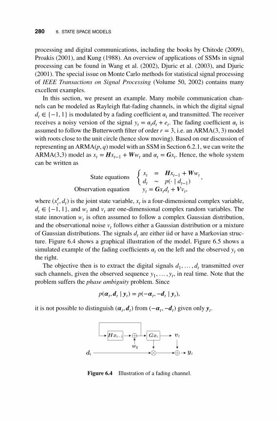
280 6. STATE SPACE MODELS
processing and digital communications, including the books by Chitode (2009),Proakis (2001), and Kung (1988). An overview of applications of SSMs in signalprocessing can be found in Wang et al. (2002), Djuric et al. (2003), and Djuric(2001). The special issue on Monte Carlo methods for statistical signal processingof IEEE Transactions on Signal Processing (Volume 50, 2002) contains manyexcellent examples.
In this section, we present an example. Many mobile communication chan-nels can be modeled as Rayleigh flat-fading channels, in which the digital signaldt ∈ {−1, 1} is modulated by a fading coefficient 𝛼t and transmitted. The receiverreceives a noisy version of the signal yt = 𝛼tdt + et. The fading coefficient 𝛼t isassumed to follow the Butterworth filter of order r = 3, i.e. an ARMA(3, 3) modelwith roots close to the unit circle (hence slow moving). Based on our discussion ofrepresenting an ARMA(p, q) model with an SSM in Section 6.2.1, we can write theARMA(3,3) model as xt = Hxt−1 + Wwt and 𝛼t = Gxt. Hence, the whole systemcan be written as
State equations
{xt = Hxt−1 + Wwtdt ∼ p(⋅ ∣ dt−1)
,
Observation equation yt = Gxtdt + Vvt,
where (x′t , dt) is the joint state variable, xt is a four-dimensional complex variable,dt ∈ {−1, 1}, and wt and vt are one-dimensional complex random variables. Thestate innovation wt is often assumed to follow a complex Gaussian distribution,and the observational noise vt follows either a Gaussian distribution or a mixtureof Gaussian distributions. The signals dt are either iid or have a Markovian struc-ture. Figure 6.4 shows a graphical illustration of the model. Figure 6.5 shows asimulated example of the fading coefficients 𝛼t on the left and the observed yt onthe right.
The objective then is to extract the digital signals d1,… , dt transmitted oversuch channels, given the observed sequence y1,… , yt, in real time. Note that theproblem suffers the phase ambiguity problem. Since
p(𝜶t, dt ∣ yt) = p(−𝜶t,−dt ∣ yt),
it is not possible to distinguish (𝜶t, dt) from (−𝜶t,−dt) given only yt.
dt ⊗ ⊕ yt
vtGxt⊕wt
Hxt−1
Figure 6.4 Illustration of a fading channel.

6.2 SELECTED EXAMPLES 281
0 20 40 60 80 100 120 140 160 180 200−3
−2.5
−2
−1.5
−1
−0.5
0
0.5
1
1.5
2
0 20 40 60 80 100 120 140 160 180 200−3
−2
−1
0
1
2
3
Figure 6.5 Example of fading channel signals.
To resolve the phase ambiguity, differential coding is often utilized. Specifi-cally, if the information sequence is d1,… , dt, then one transmits the sequenced∗1 ,… , d∗t , where d∗t−1d∗t = dt, d∗0 = 1. Hence, on the receiver side, it is onlyrequired to estimate dt = d∗t−1d∗t , which does not have phase ambiguity.
A standard detector is the differential detector:
dt = sign(ytyt−1) = sign(𝛼t𝛼t−1dt + 𝛼td∗t et−1 + 𝛼t−1d∗t−1et + et−1et).
When 𝛼t changes slowly without altering its sign often, 𝛼t𝛼t−1 is positive mostof the time. When the noise is small, dt should be accurate for most time points.However, whenever 𝛼t changes its sign, the detector tends to make an error, nomatter how small the noise et is. This results in an error floor. As the signal to noiseratio goes to ∞, the probability of making a wrong detection goes to the frequencyat which 𝛼t changes its sign. This frequency is a property of the channel and doesnot vanish even if the observational noise et vanishes. Figure 6.6 shows the bit-error rate of the differential decoder in a simulated example. It flats out as the signalto noise ratio increases. In the figure the known channel bound is the bit-error rateif the fading coefficient 𝛼t is given and known. The “genie-bound” is the bit-errorrate using a genie-assisted estimated sequence of fading coefficients ��t, which isobtained as if a known information sequence d∗∗t is transmitted through the exactchannel, being modulated with the exact sequence 𝛼t, and its corresponding y∗∗twere received and used to estimate 𝛼t. An objective is to construct a procedurethat is able to break the error floor of the differential decoder and hopefully withperformance approaching the genie-bound. Chen et al. (2000) and Wang et al.(2002) used an SSM approach for this problem and were able to design a procedurewith performance close to the genie-bound, shown in Figure 6.6. The solid linewith circles is the bit-error rate using a concurrent estimator: using the receivedobservations up to time t to estimate the transmitted bit dt at time t. The procedure

282 6. STATE SPACE MODELS
10 15 20 25 30 35 40
10–1
10–2
10–3
10–4
Eb/No (dB)
Bit
Err
or R
ate
(BE
R)
Δ=0
Δ=1
Δ=2
Known channel bound
Genie−bound
Diff. detection
Figure 6.6 Bit-error rate of the illustrative example of fading channel signals.
is able to outperform the differential decoder. The Δ = 1 and Δ = 2 lines are theperformance using the same SSM approach, except allowing a slight time delayof 1 and 2 periods, respectively, that is, we estimate dt at time t + 1 (or t + 2),with observations up to time t + 1 (t + 2). The delay method is discussed later inSection 8.3.

6.2 SELECTED EXAMPLES 283
6.2.6 Dynamic Factor Models
Let {y𝑖t}, 𝑖 = 1,… , N and t = 1,…T be a set of N time series with length T . Alinear dynamic factor model (DFM) for {y𝑖t } assumes the form
y𝑖t = 𝝀𝑖0𝜼t + 𝝀𝑖1𝜼t−1 +⋯ + 𝝀𝑖q𝜼t−q + 𝜀𝑖t, 𝑖 = 1,… , N, (6.11)
𝜼t =p∑
k=1
𝚽k𝜼t−k + et, (6.12)
where q is a nonnegative integer and 𝜼t = (𝜂1t,… , 𝜂rt)′ is a r-dimensional time
series of unobserved factors satisfying r ≪ N. The row vector 𝝀𝑖j is called factorloading of the 𝑖th series on the jth lagged values of the factors. The collection of{𝝀𝑖j|𝑖 = 1,… , N; j = 1,… , q} is called the loading matrix.
The idiosyncratic noise 𝜀𝑖t is assumed to be uncorrelated with the factors 𝜼t inall leads and lags. In addition, 𝜀𝑖t is also assumed to be uncorrelated with eachother in all leads and lags, though it may possess some autocorrelations. Someresearch allows for weak cross-correlations between 𝜀𝑖t values. See Chamberlain(1983) and Chamberlain and Rothschild (1983). Equation (6.12) assumes that thefactor follows a r-dimensional linear vector AR(p) model, with coefficient matri-ces {𝚽k, k = 1,… , p}. The noise process et is assumed to be a white noise seriesand uncorrelated with 𝜀𝑖t.
To see the model more clearly, consider the simplest DFM:
y𝑖t = 𝜆𝑖𝜂t + 𝜀𝑖t, 𝑖 = 1,… , N,
𝜂t = 𝜙𝜂t−1 + et.
Here all co-movements of the time series y𝑖t are driven by the common factor 𝜂t,a latent process following an AR(1) model. The factor loading 𝜆𝑖 provides a linkbetween the common factor and the 𝑖th series y𝑖t. Clearly, this is an SSM with 𝜂tbeing the unobserved state variable.
The DFM was first proposed by Geweke (1977). It gained popularity withSargent and Sims (1977), who showed that two dynamic factors could explaina large fraction of the variance of many important US quarterly macroeconomicvariables. In Forni et al. (2002), the DFM is extended to the generalized DFMthat allows infinite order dynamics and nonorthogonal idiosyncratic components.Extensive surveys on the theory, methods, and applications of the DFM can befound in Stock and Watson (2006, 2012) and Bai and Ng (2008).
A typical analysis using the DFM starts with the estimation of the common fac-tors (or more precisely the space spanned by the common factors) and the deter-mination of the number of factors r. See Bai and Ng (2002), and Hallin and Liska(2007), among others. The order of the vector AR (VAR) model for the commonfactors needs to be determined. When the dimension N is small and the noise

284 6. STATE SPACE MODELS
is assumed to be Gaussian, maximum likelihood estimators, along with a modelselection criterion for determining the number of common factors r in (6.11) andthe VAR order p in (6.12), can be obtained.
However, this approach encounters some difficulties when the number of timeseries N becomes large, for there are many parameters to estimate and the relation-ship between the variables becomes complex. If N is large, principle componentanalysis (PCA) and its variants are often used to estimate the common factors.The least squares method is then used to estimate the loading matrix and the VARmodel. One can then use the SSM representation of the DFM to refine the esti-mates of common factors by treating the estimated parameters of the second stepsas given. See, for instance, Forni et al. (2009) and Doz (2007). We consider anexample of estimating the DFM in Example 6.4.
6.2.7 Functional and Distributional Time Series
Analysis of functional time series was discussed in Chapter 5 using nonparametricapproaches. In this chapter we consider a different approach via a structural modelformulation under the SSM framework. Let D be the domain of a functional timeseries yt(⋅), i.e. yt(s) : D → R for every time point t. The time series {yt(⋅), t =1,… , } is said to be driven by a dynamic process if, for any fixed t, the functionyt(⋅) can be written as
yt(s) = ft(s; 𝜃t) + 𝜀t(s), s ∈ D, (6.13)
where the function ft(⋅) is known up to some parameter 𝜃t, 𝜃t follows a dynamicprocess over time, and 𝜀t(s) is a noise process defined on D with E[𝜀t(s)] = 0 forall s ∈ D. Often it is further assumed that 𝜀t1
(⋅) and 𝜀t2(⋅) are independent for
t1 ≠ t2, but some dependence between 𝜀t(s1) and 𝜀t(s2) is allowed for s1, s2 ∈ D.In model (6.13), the dependence of the process yt(⋅) is completely characterizedby the parameter process 𝜃t and the noise process 𝜀t(⋅). The process {𝜃t} is calledthe driving process. This is similar to the parameter driving models in modelingnon-Gaussian time series of Chapter 5. In most applications, yt(⋅) is only observedat a finite number of locations in D. In the following, we assume that for eachtime t, a set of observations {yt(st𝑖), 𝑖 = 1,… , mt} is available and they satisfyyt(st𝑖) = ft(st𝑖, 𝜃t) + 𝜀t(st𝑖).
The model can be written as an SSM:
𝜃t = h(𝜃t−1,… , 𝜃t−p, et,… , et−q,𝜷), (6.14)
yt(st𝑖) = f (st𝑖, 𝜃t) + 𝜀t(st𝑖), 𝑖 = 1,… , mt, (6.15)
where h(⋅) is a known function with unknown parameters 𝜷, p and q are non-negative integers, and et is a sequence of scalar or vector white noises. For exam-ple, one can use a VAR(p) model for (6.14).

6.2 SELECTED EXAMPLES 285
When the functional time series {yt} is driven by a finite dimensional process 𝜃t,it in fact assumes a hierarchical model with functional observations and dynamiclatent processes. This is similar to the DFM, with a nonlinear loading relation-ship and the driving process as the dynamic factors. The difference is that theloading relationship is completely specified here whereas the loading matrices areunknown in a DFM.
For distributional time series, let 𝜋t(⋅) be a sequence of distributions, indexedby time t. An objective of analyzing such time series is to study the dependencebetween the distributions and to make predictions of future distributions. Supposeat time t we observe independent data yt𝑖 ∼ 𝜋t, 𝑖 = 1,… , mt. Similar to the case offunctional time series, if the distributions 𝜋t belong to a parametric family 𝜋t(y) =𝜋(y; 𝜃t) and 𝜃t forms a dynamic process, then the distributional time series {𝜋t} isdriven by a dynamic process.
For distributional time series, similar to Equations (6.14) and (6.15), we have
𝜃t = h(𝜃t−1,… , 𝜃t−p, et,… , et−q,𝜷),
yt𝑖 ∼ 𝜋( ⋅ ; 𝜃t), 𝑖 = 1,… , mt, (6.16)
where h(⋅) presents a time series model with unknown parameters 𝜷 and et is ascalar or vector white noise series. Distributional time series have many appli-cations. For example, the simplest version of the popular stochastic volatilitymodel in finance of Hull and White (1987) and Jacquier et al. (1994) takes theform yt ∼ N(0, 𝜎2
t ), where log(𝜎2t ) = 𝛽0 + 𝛽1 log(𝜎2
t−1) + et. This is a restrictedcase of model (6.16), with one observation per time period. As another example,assume that an underlying time series 𝜂t is observed multiple times with noises,e.g. yt𝑖 ∼ N(𝜂t, 𝜎
2t ). Here we have the flexibility of adding certain structure for 𝜎2
tsuch as that in the stochastic volatility models, or heteroscedasticity in the form𝜎2
t = 𝜎2𝜂2t .
In what follows we consider two specific examples.
Example A: Yield curve of interest rates. An important topic in finance isthe dynamic behavior of the term structure of interest rates (yield curve) ofgovernment bonds. The yield curve is the functional relationship between interestrate and its time to maturity. It plays a crucial role in fixed-income portfoliomanagement, risk management, and many other finance and economic decisions.Modeling yield curves has been studied extensively in finance and economics. See,for instance, Vasicek (1977), Cox et al. (1985), Hull and White (1990), Heath et al.(1992), and Duffie and Kan (1998). However, most of the research papers focus onestimating the yield curve at a fixed time point instead of considering the dynam-ical evolution of the curve over time. These studies do not address the importantissue of prediction, which is important for both derivative pricing and risk
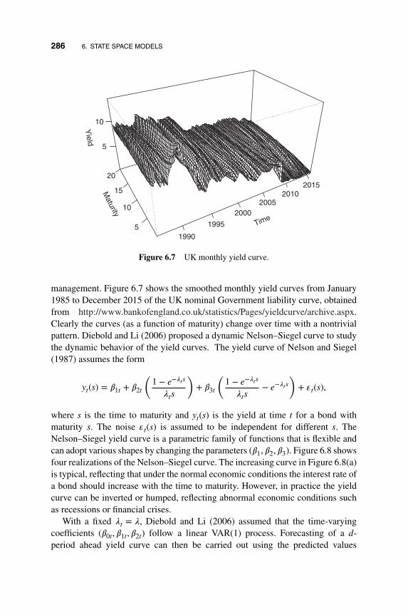
286 6. STATE SPACE MODELS
Time
1990
1995
20002005
20102015
Maturity
5
10
15
20
Yield
5
10
Figure 6.7 UK monthly yield curve.
management. Figure 6.7 shows the smoothed monthly yield curves from January1985 to December 2015 of the UK nominal Government liability curve, obtainedfrom http://www.bankofengland.co.uk/statistics/Pages/yieldcurve/archive.aspx.Clearly the curves (as a function of maturity) change over time with a nontrivialpattern. Diebold and Li (2006) proposed a dynamic Nelson–Siegel curve to studythe dynamic behavior of the yield curves. The yield curve of Nelson and Siegel(1987) assumes the form
yt(s) = 𝛽1t + 𝛽2t
(1 − e−𝜆ts
𝜆ts
)+ 𝛽3t
(1 − e−𝜆ts
𝜆ts− e−𝜆ts
)+ 𝜀t(s),
where s is the time to maturity and yt(s) is the yield at time t for a bond withmaturity s. The noise 𝜀t(s) is assumed to be independent for different s. TheNelson–Siegel yield curve is a parametric family of functions that is flexible andcan adopt various shapes by changing the parameters (𝛽1, 𝛽2, 𝛽3). Figure 6.8 showsfour realizations of the Nelson–Siegel curve. The increasing curve in Figure 6.8(a)is typical, reflecting that under the normal economic conditions the interest rate ofa bond should increase with the time to maturity. However, in practice the yieldcurve can be inverted or humped, reflecting abnormal economic conditions suchas recessions or financial crises.
With a fixed 𝜆t = 𝜆, Diebold and Li (2006) assumed that the time-varyingcoefficients (𝛽0t, 𝛽1t, 𝛽2t) follow a linear VAR(1) process. Forecasting of a d-period ahead yield curve can then be carried out using the predicted values

6.2 SELECTED EXAMPLES 287(b
)(a
)
(d)
(c)
tau
Rate
Var
ying
lam
bda
Fix
ed la
mbd
a
Var
ying
lam
bda
Fix
ed la
mbd
a
Typ
e 1
(no
rmal
) yi
eld
cu
rve:
2/2
7/70
tau
Rate
Var
ying
lam
bda
Fix
ed la
mbd
a
Typ
e 2
(in
vert
ed)
yiel
d c
urv
e: 5
/29/
81
tau
Rate
Typ
e 3
(do
wn
−th
en−u
p)
yiel
d c
urv
e: 7
/31/
89
020
4060
8010
012
0
3.54.04.55.05.5
020
4060
8010
012
0
12.513.013.514.014.515.015.516.00
2040
6080
1012
0
7.47.57.67.77.87.9
020
4060
8010
012
05.65.86.06.26.46.6
tau
Rate
Typ
e 4
(up
−th
em−d
ow
n)
yiel
d c
urv
e: 5
/29/
81
Fig
ure
6.8
Four
real
izat
ions
ofth
eN
elso
n–Si
egel
curv
e.
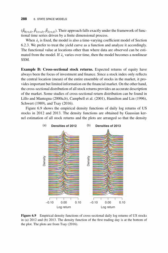
288 6. STATE SPACE MODELS
(𝛽0(t+d), 𝛽1(t+d), 𝛽2(t+d)). Their approach falls exactly under the framework of func-tional time series driven by a finite dimensional process.
When 𝜆t is fixed, the model is also a time-varying coefficient model of Section6.2.3. We prefer to treat the yield curve as a function and analyze it accordingly.The functional value at locations other than where data are observed can be esti-mated from the model. If 𝜆t varies over time, then the model becomes a nonlinearSSM.
Example B: Cross-sectional stock returns. Expected returns of equity havealways been the focus of investment and finance. Since a stock index only reflectsthe central location (mean) of the entire ensemble of stocks in the market, it pro-vides important but limited information on the financial market. On the other hand,the cross-sectional distribution of all stock returns provides an accurate descriptionof the market. Some studies of cross-sectional return distribution can be found inLillo and Mantegna (2000a,b), Campbell et al. (2001), Hamilton and Lin (1996),Schwert (1989), and Tsay (2016).
Figure 6.9 shows the empirical density functions of daily log returns of USstocks in 2012 and 2013. The density functions are obtained by Gaussian ker-nel estimation of all stock returns and the plots are arranged so that the density
−0.10 0.00 0.10
Densities of 2012
Log return
Den
sity
−0.10 0.00 0.10
Densities of 2013
Log return
Den
sity
(b)(a)
Figure 6.9 Empirical density functions of cross-sectional daily log returns of US stocksin (a) 2012 and (b) 2013. The density function of the first trading day is at the bottom ofthe plot. The plots are from Tsay (2016).

6.2 SELECTED EXAMPLES 289
function of the first trading day of a given year is at the bottom of the plot. For easein presentation, the density functions are only shown in the range D = [−0.1, 0.1].See Tsay (2016) for further details. From the plots, it is clear that the behavior ofcross-sectional stock returns evolves over time and the return distributions can betreated as functional time series. Alternatively, one can model the time evolution ofthe quantiles of cross-sectional stock returns using distributional time series. Linand Chen (2017) used distributional time series to study the dynamics of cross-section stock returns. They modeled the cross-sectional distribution by a skewedt-distribution with four parameters 𝜽t = (𝜇t, 𝜎t, 𝜈t, 𝜆t), the location, scale, skew-ness, and degrees of freedom parameters, respectively, and established an SSM asin (6.16), where the 𝜽t is serving as the dynamic driving process and is assumedto follow a VAR model.
6.2.8 Markov Regime Switching Models
The regime switching mechanism, similar to threshold crossing, provides a pow-erful tool for modeling nonlinear dynamics. It often serves as a first-step depar-ture from the linearity. The Markov switching autoregressive models of Section2.3 belong to a larger class of Markovian regime switching models. Model (2.16)can be viewed as an SSM in which St is the unobserved state variable, with thestate equation specifying the transition probability structure P(St = 𝑖 ∣ St−1 = j)for 𝑖, j = 1, 2. The observation equation specifies the conditional distribution of xtgiven the state St. When the state variable follows a Markov chain and takes valuein a finite set, the corresponding SSM is also referred to as a hidden Markov model(HMM).
The Markov switching autoregressive model in Equation (2.16) can beextended so that the regime switching mechanism is enforced on a general SSM.Specifically, a Markov regime-switching SSM assumes the form
State equation xt = hSt(xt−1, 𝜀t),
P(St = 𝑖 ∣ St−1 = j) = p𝑖j,
Observation equation yt = gSt(xt, et), (6.17)
where St ∈ {1,… , k} and the functions h𝑖(⋅) and g𝑖(⋅) belong to a finite family ofk functions, where k is the number of regimes. In this case, the state variable isactually (xt, St). We stress the regime indicator St for its important interpretation,but also for technical conveniences.
The model in Equation (6.17) is useful in many situations. For example, aMarkov switching ARMA model can be written as a Markov regime switchingSSM by rewriting the ARMA model in each regime in a state space form, as in Sec-tion 6.2.1. Tracking a maneuvering target problem in Section 6.2.4 can be viewedas a Markov regime switching SSM, in which the maneuvering status is treated as

290 6. STATE SPACE MODELS
the regime. The time-varying coefficient linear models in Section 6.2.3, in whichthe coefficients may vary under a regime switching mechanism, can be extended.
The varying coefficient Fama–French model can be extended so that the coef-ficients follow a Markov switching autoregressive (MSA) model, since the coef-ficients may assume different dynamics when the market conditions change. Wecan write the model as
State equation xt = cst+ Hst
xt−1 + 𝜀t,
P(st = 𝑖 ∣ st−1 = j) = p𝑖j, 𝑖, j = 1, 2
Observation equation yt = Ftxt + et,
where Ft is a 1 × k matrix consisting of the Fama–French factors at time t.Note that model (6.17) is different from the HMM model in that the state vari-
able is a hybrid of continuous and discrete variables. Inference for such a modelis much more challenging than that of the standard HMM model, but the Markovswitching SSM has a wider range of applications than the traditional HMM.
6.2.9 Stochastic Volatility Models
Stochastic volatility (SV) models are an alternative to modeling conditional het-eroscedasticity, discussed in Section 5.4, and they are often referred to as an exten-sion of the volatility models by allowing the variance (volatility) component of anasset return to vary according to a stochastic diffusion process. See, for instance,Hull and White (1987), Jacquier et al. (1994), Shephard and Pitt (1997), Aıt-Sahalia and Jacod (2014), and Fouque et al. (2000, 2011). The models have beenconsidered in both continuous time and discrete time.
In the ARCH and GARCH models of Section 5.4, the volatility changes deter-ministically, conditional on the past information. An alternative approach is toemploy a stochastic process to govern the random propagation of volatility, result-ing in a discrete-time stochastic volatility model. See Ghysels et al. (1996) andShephard (1996).
We discuss a simple SV model here. Let yt be the observed return of an asset attime t. Pitt and Shephard (1999) and Harvey et al. (1994) assumed that yt followsa normal distribution with mean zero and variance 𝜎2
t . The time-varying volatility𝜎t is an unobservable state variable, following an AR(1) process. To enforce thepositivity of conditional variance, one can use the parametrization 𝜎t = exp(xt),and form the following SSM:
xt = 𝜙0 + 𝜙xt−1 + 𝜂t,
yt = exp(xt)vt,
where 𝜂t ∼ N(0, 𝜎2), vt ∼ N(0, 1). This is a nonlinear SSM.

6.2 SELECTED EXAMPLES 291
Another form is to replace the observation equation by ln(y2t ) = 𝛽∗ + xt + vt
where vt = ln(e2t ), et ∼ N(0, 1). This is a linear but non-Gaussian SSM.
6.2.10 Non-Gaussian Time Series
Several of the non-Gaussian time series models of Chapter 5 can be casted intoa SSM by carefully defining a proper state variable. For example, consider thePoisson count data yt ∼ Po𝑖(𝜆t). We can define xt = ln(𝜆t) as a state variable andemploy an ARMA model for xt.
As another example, consider a proportional time series yt ∈ (0, 1). Forinstance, yt may denote the market share of a product at time t. Here we canassume
xt ∼ ARMA(p, q),
yt ∼ Beta(𝜏𝜇t, 𝜏(1 − 𝜇t)),
where xt = ln(𝜇t∕(1 − 𝜇t)) is the logit transformation of the conditional mean 𝜇t.Note that this model is different from a direct transformation zt = ln(yt∕(1 − yt))and fitting an ARMA model to zt.
The model can be extended to the compositional time series, where yt =(st1,… , std) is the observed compositions such as the monthly household expen-diture among different categories, import/export proportions of different prod-uct categories, or word count (in percentage) in a document. Since st𝑖 > 0 and∑d𝑖=1 st𝑖 = 1, we may assume
xt ∼ ARMA(p, q),
yt ∼ Dirichelet(𝜏, pt1,… , ptd),
where xt = (𝜂t1,… , 𝜂t(d−1)), 𝜏 =∑d𝑖=1 pt𝑖, and 𝜂t𝑖 = ln(pt𝑖∕ptd). For analysis of
compositional time series, see Zheng and Chen (2017).
6.2.11 Mixed Frequency Models
Economic time series are often reported at different frequencies. For example,real GDP growth is reported quarterly, while inflation index is reported monthly.When these time series are modeled jointly, or one series is used as a covariateof the other, the analysis is called a mixed frequency data analysis. It is easy toconvert high-frequency series to the lower-frequency ones, but such a convertingprocedure does not utilize fully the available information. In recent years, there hasbeen substantial research interest in mixed-frequency data analysis (MIDAS). See,for instance, Ghysels et al. (2007), Gagliardini et al. (2017), and Ghysels (2016),among others.

292 6. STATE SPACE MODELS
Here we demonstrate, via a simple example, that the SSM approach can be usedto analyze mixed-frequency data. Consider a mixed-frequency VAR(1) model withtwo components. The setting can easily be extended to a VAR(p) model with mul-tiple components. Suppose yt is an observed monthly series and zt is an unobservedmonthly series for which only the quarterly total s3s = z3s + z3s−1 + z3s−2 is avail-able. Suppose (yt, zt) jointly follows a VAR(1) model,(
ztyt
)=[𝜙11 𝜙12𝜙21 𝜙22
](zt−1yt−1
)+(
wtvt
).
We can rewrite the model as:
zt = 𝜙11zt−1 + 𝜙12yt−1 + wt where wt ∼ N(0, 𝜎2),zt−1 = zt−1,zt−2 = zt−2,yt = 𝜙21zt−1 + 𝜙22yt−1 + vt, where vt ∼ N
(0, 𝜎2
v
),
st = zt + zt−1 + zt−2, if t = 3s.
Let xt = (yt, zt, zt−1, zt−2) be the underlying state variable, then the model can berewritten in an SSM. We analyze a mixed-frequency series in Example 6.3 undera slightly different setting.
6.2.12 Other Applications
SSMs, especially nonlinear and non-Gaussian SSMs, have been successfullydesigned for many other important applications, including speech recognition(Rabiner, 1989), sensor collaborations (Guo and Wang, 2004), movement intentinference (Ahmad et al., 2016), brain source localization (Chen et al., 2015),combinatorial optimizations (Wong and Liang, 1997), genetics (Irwing et al.,1994), DNA, RNA and protein sequence analysis (Churchill, 1989; Krough et al.,1994; Liu et al., 1999; Liang et al., 2002; Zhang et al., 2003, 2009), probabilisticexpert systems (Kong et al., 1994; Spiegelhalter and Lauritzen, 1990; Berzuiniet al., 1997), target recognition (Srivastava et al., 2001), freeway traffic vision (forvehicle control) (Huang et al., 1994), dynamic Bayesian networks (Koller andLerner, 2001; Murphy and Russell, 2001; Naesseth et al., 2014; Bouchard-Coteet al., 2012), infectious disease dynamics (Smith et al., 2017), copula models(Creal and Tsay, 2015), on-line control of industrial production (Marrs, 2001),diffusion bridges (Lin et al., 2010), audio signal enhancing (Fong et al., 2002),data network analysis (Coates and Nowak, 2002), neural networks (Andrieu et al.,1999; de Freitas et al., 2000), and financial applications (Lopes and Tsay, 2011),among many others.
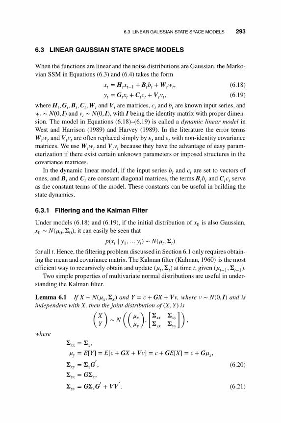
6.3 LINEAR GAUSSIAN STATE SPACE MODELS 293
6.3 LINEAR GAUSSIAN STATE SPACE MODELS
When the functions are linear and the noise distributions are Gaussian, the Marko-vian SSM in Equations (6.3) and (6.4) takes the form
xt = Htxt−1 + Btbt + Wtwt, (6.18)
yt = Gtxt + Ctct + Vtvt, (6.19)
where Ht, Gt, Bt, Ct, Wt and Vt are matrices, ct and bt are known input series, andwt ∼ N(0, I) and vt ∼ N(0, I), with I being the identity matrix with proper dimen-sion. The model in Equations (6.18)–(6.19) is called a dynamic linear model inWest and Harrison (1989) and Harvey (1989). In the literature the error termsWtwt and Vtvt are often replaced simply by 𝜀t and et with non-identity covariancematrices. We use Wtwt and Vtvt because they have the advantage of easy param-eterization if there exist certain unknown parameters or imposed structures in thecovariance matrices.
In the dynamic linear model, if the input series bt and ct are set to vectors ofones, and Bt and Ct are constant diagonal matrices, the terms Btbt and Ctct serveas the constant terms of the model. These constants can be useful in building thestate dynamics.
6.3.1 Filtering and the Kalman Filter
Under models (6.18) and (6.19), if the initial distribution of x0 is also Gaussian,x0 ∼ N(𝜇0,𝚺0), it can easily be seen that
p(xt ∣ y1,… yt) ∼ N(𝜇t,𝚺t)
for all t. Hence, the filtering problem discussed in Section 6.1 only requires obtain-ing the mean and covariance matrix. The Kalman filter (Kalman, 1960) is the mostefficient way to recursively obtain and update (𝜇t,𝚺t) at time t, given (𝜇t−1,𝚺t−1).
Two simple properties of multivariate normal distributions are useful in under-standing the Kalman filter.
Lemma 6.1 If X ∼ N(𝜇x,𝚺x) and Y = c + GX + Vv, where v ∼ N(0, I) and isindependent with X, then the joint distribution of (X, Y) is(
XY
)∼ N
((𝜇x𝜇y
),
[𝚺xx 𝚺xy𝚺yx 𝚺yy
]),
where
𝚺xx = 𝚺x,
𝜇y = E[Y] = E[c + GX + Vv] = c + GE[X] = c + G𝜇x,
𝚺xy = 𝚺xG′, (6.20)
𝚺yx = G𝚺x,
𝚺yy = G𝚺xG′ + VV
′. (6.21)

294 6. STATE SPACE MODELS
Equation (6.20) holds because
𝚺xy = E[(X − 𝜇x)(Y − 𝜇y)′] = E[(X − 𝜇x)((X − 𝜇x)
′G
′ + v′V
′)] = 𝚺xG
′,
and Equation (6.21) follows from
𝚺yy = E[(Y − 𝜇y)(Y − 𝜇y)′] = E[G(X − 𝜇x)(X − 𝜇x)
′G
′ + Vvv′V
′]
= G𝚺xG′ + VV
′.
Lemma 6.2 If (XY
)∼ N
((𝜇x𝜇y
),
[𝚺xx 𝚺xy𝚺yx 𝚺yy
]),
and we assume that 𝚺−1yy exists, then
E(X ∣ Y = y) = 𝜇x − 𝚺xy𝚺−1yy (y − 𝜇y),
Var(X ∣ Y = y) = 𝚺xx − 𝚺xy𝚺−1yy 𝚺yx.
The Kalman filter uses these two properties to obtain the distribution of p(xt ∣yt) recursively, where yt = (y1,… , yt). Suppose at time t − 1 we have obtained𝜇t−1 and 𝚺t−1, that is,
p(xt−1 ∣ yt−1) ∼ N(𝜇t−1,𝚺t−1).
Before we observe yt, we can use the state equation to predict xt. Since
xt = Htxt−1 + Btbt + Wtwt,
and both p(xt−1 ∣ yt−1) and wt are normal, p(xt ∣ yt−1) is normal. Denoting
p(xt ∣ yt−1) ∼ N(𝜇t∣t−1,𝚺t∣t−1), (6.22)
we have
𝜇t∣t−1 = E(Htxt−1 + Btbt + Wtwt ∣ yt−1)
= HtE(xt−1 ∣ yt−1) + Btbt
= Ht𝜇t−1 + Btbt, (6.23)
𝚺t∣t−1 = Var(Htxt−1 + Btbt + Wtwt ∣ yt−1)
= Var(Htxt−1 ∣ yt−1) + WtW′t
= Ht𝚺t−1H′
t + WtW′
t . (6.24)
Now consider the new observation yt. Using (6.23), (6.24) and the obser-vation equation yt = Gtxt + Ctct + Vtvt, Lemma 6.1 provides the joint distribu-tion p(xt, yt ∣ y1,… , yt−1). Then using Lemma 6.2, we get p(xt ∣ y1,… , yt−1, yt).Putting everything together, we have

6.3 LINEAR GAUSSIAN STATE SPACE MODELS 295
Algorithm 6.1: Kalman Filter
𝜇t∣t−1 = Ht𝜇t−1 + Btbt, (6.25)
𝚺t∣t−1 = Ht𝚺t−1H′
t + WtW′
t , (6.26)
𝜇t = 𝜇t∣t−1 + Kt(yt − Ctct − Gt𝜇t∣t−1), (6.27)
𝚺t = 𝚺t∣t−1 − KtGt𝚺t∣t−1, (6.28)
where
Kt = 𝚺t∣t−1G′
t[Gt𝚺t∣t−1G′t + V
′
tVt]−1. (6.29)
The matrix Kt is often called the Kalman gain matrix.
Another way of understanding the Kalman filter is via the Bayes theorem.Before the arrival of yt, the predictive distribution p(xt ∣ y1,… , yt−1) in Equation(6.22) can be thought as the prior distribution of xt. The new observation yt pro-vides additional information about xt, or correction to the prediction. Based onBayes theorem
p(xt ∣ y1,… , yt−1, yt) ∝ p(yt ∣ xt, y1,… , yt−1)p(xt ∣ y1,… , yt−1)
= p(yt ∣ xt)p(xt ∣ y1,… , yt−1).
The Kalman filter can be obtained by a detailed calculation of the above equation.Intuitively, Equation (6.25) provides a one-step ahead prediction of xt before
the observation yt arrives and Equation (6.26) gives the prediction variance.Once the observation yt arrives, the prediction is updated by the correction termKt(yt − Ctct − Gt𝜇t∣t−1). Here Ctct + Gt𝜇t∣t−1 is the prediction of yt using the pre-dicted state 𝜇t∣t−1. Hence the correction is proportional to (yt − Ctct − Gt𝜇t∣t−1),the difference between the predicted value of yt and the observed yt. Equation(6.28) shows that, with the new information yt, the variance of xt is reduced fromits prediction variance 𝚺t∣t−1 by the amount of KtGt𝚺t∣t−1.
6.3.2 Evaluating the likelihood function
When there are unknown parameters in the linear Gaussian system (6.18) and(6.19), one can evaluate the likelihood function of a given set of parameters 𝜽.Specifically, as discussed in Section 6.1, the likelihood function has the form
L(𝜽) = p(y1,… , yT ∣ 𝜽) =T∏
t=1
p(yt ∣ yt−1,𝜽).

296 6. STATE SPACE MODELS
The Kalman filter can be used to obtain p(yt ∣ yt−1,𝜽), given 𝜽. Since p(yt ∣ yt−1,𝜽)is a normal distribution, we only need to obtain its mean and variance:
E(yt ∣ yt−1) = E(E(yt ∣ xt, yt−1) ∣ yt−1)
= E(Gtxt + Ccct ∣ yt−1)
= Gt𝜇t∣t−1 + Ctct
andVar(yt ∣ yt−1) = Var(E(yt ∣ xt, yt−1) ∣ yt−1) + E(Var(yt ∣ xt, yt−1) ∣ yt−1)
= Var(Gtxt + Ctct ∣ yt−1) + E(VtV′
t ∣ yt−1)
= Gt𝚺t∣t−1G′
t + VtV′
t . (6.30)
The terms 𝜇t∣t−1 and 𝚺t∣t−1 can be obtained by the Kalman filter for a given 𝜽.In fact, the process
𝜀t = yt − Gt𝜇t∣t−1 − Ctct (6.31)
is often called the innovation process. It is the prediction error of yt given yt−1.The above calculation shows that 𝜀t follows a Gaussian distribution with meanzero, and variance in Equation (6.30). In addition, {𝜀t} is an independent seriesby noting that 𝜀t = yt − Gt𝜇t∣t−1 − Ctct = Gt(xt − 𝜇t∣t−1) + Vtvt, hence for s < t,
E(𝜀s𝜀t) = E[E(𝜀s𝜀t ∣ yt−1)] = E[𝜀sE(𝜀t ∣ yt−1)] = 0.
Since p(yT ∣ 𝜽) = p(𝜀1(𝜽),… , 𝜀T (𝜽)) =∏T
t=1 p(𝜀t(𝜽)) (here we emphasize that𝜀t(𝜽) is obtained through the Kalman filter, based on 𝜽.) The log-likelihood func-tion is then
l(𝜽) = −12
T∑t=1
log |𝚺(e)t(𝜽)| − 12
T∑t=1
𝜀t(𝜽)′𝚺−1
(e)t(𝜽)𝜀t(𝜽),
where 𝚺(e)t(𝜽) is the same as that in (6.30).Hence it is relatively easy and fast to evaluate the log likelihood function for
any given parameter 𝜽. The maximum likelihood estimator of the parameter canthen be obtained using optimization algorithms such as the Newton–Raphson algo-rithm. Caines (1988) and Hannan and Deistler (1988) (see also Douc et al., 2014)established the consistency and asymptotic normality for the maximum likelihoodestimates (MLE) of a stable linear system, in which all matrices are assumed to beconstant, the spectral norm of the state transition matrix H is less than 1 (so thatthe underlying state process is stable), the expanded observation coefficient matrix[G′, G′H′, G′H2′,… , G′Hp′] has full rank p where p is the dimension of the statext (so that the observation yt has sufficient information about xt), and some otherconditions. The estimated Hessian matrix at the MLE can be used as an estimateof the asymptotic variance matrix of the MLE. Shumway and Stoffer (1982) usedthe EM algorithm in parameter estimation.

6.3 LINEAR GAUSSIAN STATE SPACE MODELS 297
6.3.3 Smoothing
For a fixed dimensional problem in which the entire sequence yT = (y1,… , yT )is observed, it is of interest to make inference of xt given the whole data. Thisis the smoothing problem discussed in Section 6.1. In other words, we are inter-ested in finding p(x1,… , xT ∣ yT ) or its marginal distributions p(xt ∣ yT ) for anyt. Again, as the system is linear and Gaussian, p(xt ∣ yT ) follows a normal dis-tribution, denoted by N(𝜇t∣T ,𝚺t∣T ). The following Kalman smoother recursivelyobtains 𝜇t∣T and 𝚺t∣T in a forward and backward two-pass algorithm. Note thatthe main difference between the filtering distribution p(xt ∣ yt) and the smooth-ing distribution p(xt ∣ yT ) is the additional information provided by yt+1,… , yT .By the Markovian property, given xt+1, the extra information yt+1,… , yT and xtare conditionally independent. Hence the process can be disentangled by insert-ing xt+1. If we obtain p(xt+1 ∣ yT ), which provides a summary of all informationin yt+1,… , yT , then one can obtain p(xt ∣ yt) by a correction of p(xt ∣ yt) usingp(xt+1 ∣ yT ). Such a two-pass algorithm can also be used for nonlinear systemsand is discussed in Chapter 8.
Specifically, the first pass is to run the Kalman filter forward from t = 1 to Tand obtain 𝜇t∣t−1, 𝜇t = 𝜇t∣t, 𝚺t∣t−1, and 𝚺t = 𝚺t∣t for t = 1,… , T . Then the Kalmansmoother runs backward as follows.
Algorithm 6.2: Kalman smoother
For t = T − 1, T − 2,… , 1,
𝜇t∣T = 𝜇t + Jt(𝜇t+1∣T − 𝜇t+1∣t), (6.32)
𝚺t∣T = 𝚺t + Jt(𝚺t+1∣T − 𝚺t+1∣t)J′
t , (6.33)
where
Jt = 𝚺tHt+1[𝚺t+1∣t]−1. (6.34)
The Kalman smoother can be derived by inserting xt+1 in a disentanglementoperation:
E(xt ∣ yT ) = E(E(xt ∣ xt+1, yT ) ∣ yT )
= E(E(xt ∣ xt+1, yt) ∣ yT ),
Var(xt ∣ yT ) = E[Var(xt ∣ xt+1, yT ) ∣ yT ] + Var[E(xt ∣ xt+1, yT ) ∣ yT ]
= E[Var(xt ∣ xt+1, yt) ∣ yT ] + Var[E(xt ∣ xt+1, yt) ∣ yT ].

298 6. STATE SPACE MODELS
To obtain E(xt ∣ xt+1, yt), we use[xt ∣ yt
xt+1 ∣ yt
]∼ N
([𝜇t∣t𝜇t+1∣t
],
[𝚺t∣t 𝚺t∣tH
′
t+1Ht+1𝚺t∣t 𝚺t+1∣t
]).
Using Lemma 6.2, we have
E(xt ∣ xt+1, yt) = 𝜇t∣t + Jt(xt+1 − 𝜇t+1∣t),
Var(xt ∣ xt+1, yt) = 𝚺t∣t − 𝚺t∣tH′
t+1[𝚺t+1∣t]−1Ht+1𝚺t = 𝚺t∣t − Jt𝚺t+1∣tJ
′
t ,
where Jt = 𝚺tHt+1[𝚺t+1∣t]−1. Hence
E[E(xt ∣ xt+1, yt) ∣ yT ] = E[𝜇t∣t + Jt(xt+1 − 𝜇t+1∣t) ∣ yT ]
= 𝜇t∣t + Jt(E(xt+1 ∣ yT ) − 𝜇t+1∣t)
= 𝜇t∣t + Jt(𝜇t+1∣T − 𝜇t+1∣t)
and
Var[E(xt ∣ xt+1, yt) ∣ yT ] = Var[𝜇t∣t + Jt(xt+1 − 𝜇t+1∣t) ∣ yT ]
= Jt[V(xt+1 ∣ yT )]J′
t
= Jt𝚺t+1∣TJ′
t ,
and
E[Var(xt ∣ xt+1, yt) ∣ yT ] = E[𝚺t∣t − J𝚺t+1∣tJ′
t ∣ yT ]
= 𝚺t∣t − Jt𝚺t+1∣tJ′
t .
Putting everything together, we have the smoother in Equations (6.32) and (6.33).The smoother can also be derived directly by working on the joint distribution:
p(xt, xt+1 ∣ yT ) = p(xt ∣ xt+1, yT )p(xt+1 ∣ yT )
= p(xt ∣ xt+1, yt)p(xt+1 ∣ yT )
=p(xt+1 ∣ xt, yt)p(xt ∣ yt)
p(xt+1 ∣ yt)p(xt+1 ∣ yT )
=p(xt+1 ∣ xt)p(xt ∣ yt)
p(xt+1 ∣ yt)p(xt+1 ∣ yT ),
where p(xt+1 ∣ xt) is given by the model, p(xt ∣ yt) and p(xt+1 ∣ yt) can be obtainedby the forward Kalman filter, and p(xt+1 ∣ yT ) is the result of backward smoothingat t + 1. Through a detailed calculation one can find the mean vector and covari-ance matrix of the joint normal distribution of p(xt, xt+1 ∣ yT ). Then using Lemma6.2, the smoother Equations (6.32) and (6.33) can be obtained.
Intuitively, Equation (6.32) shows how the filtering mean 𝜇t is corrected whenthe future observations yt+1,… , yT are observed. Its correction size is proportional
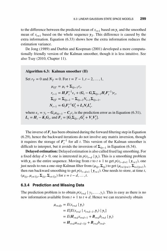
6.3 LINEAR GAUSSIAN STATE SPACE MODELS 299
to the difference between the predicted mean of xt+1 based on yt and the smoothedmean of xt+1 based on the whole sequence yT . This difference is caused by theextra information. Equation (6.33) shows how the extra information reduces theestimation variance.
De Jong (1989) and Durbin and Koopman (2001) developed a more computa-tionally friendly version of the Kalman smoother, though it is less intuitive. Seealso Tsay (2010, Chapter 11).
Algorithm 6.3: Kalman smoother (II)
Set rT = 0 and NT = 0. For t = T − 1, t − 2,… , 1,
𝜇t∣T = 𝜇t + 𝚺t∣t−1rt,
rt−1 = HtF−1t 𝜀t + (Gt − Gt𝚺t∣t−1HtF
−1t )rt,
𝚺t∣T = 𝚺t∣t−1 − 𝚺t∣t−1Nt−1𝚺t∣t−1,
Nt−1 = GtF−1t G′
t + LtNtL′t ,
where 𝜀t = yt − Gt𝜇t∣t−1 − Ctct is the prediction error as in Equation (6.31),Lt = Ht − KtGt, and Ft = [Gt𝚺t∣t−1G′
t + VtV′t].
The inverse of Ft has been obtained during the forward filtering step in Equation(6.29), hence the backward iterations do not involve any matrix inversion, thoughit requires the storage of F−1
t for all t. This version of the Kalman smoother isdifficult to interpret, but it avoids the inversion of 𝚺t∣t−1 in Equation (6.34).
Delayed estimation: Delayed estimation is also called fixed lag smoothing. Fora fixed delay d > 0, one is interested in p(xt−d ∣ yt). This is a smoothing problemwith yt as the entire sequence. Moving from t to t + 1 to get p(xt−d+1 ∣ yt+1), onejust needs to run a one-step Kalman filter from (𝜇t∣t,𝚺t∣t) to get (𝜇t+1∣t+1,𝚺t+1∣t+1),then run backward smoothing to get p(xt−d+1 ∣ yt+1). One needs to store, at time t,(𝜇s∣s,𝜇s+1∣s,𝚺s∣s,𝚺s+1∣s) for s = t − d,… , t.
6.3.4 Prediction and Missing Data
The prediction problem is to obtain p(xt+d ∣ y1,… , yt). This is easy as there is nonew information available from t + 1 to t + d. Hence we can recursively obtain
𝜇t+d∣t = E(xt+d ∣ yt)
= E[E(xt+d ∣ xt+d−1, yt) ∣ yt]
= E(Ht+dxt+d−1 + Bt+dbt+d ∣ yt)
= Ht+d𝜇t+d−1∣t + Bt+dbt+d,

300 6. STATE SPACE MODELS
and
𝚺t+d∣t = Var(xt+d ∣ yt)
= Var[E(xt+d ∣ xt+d−1, yt) ∣ yt] + E[Var(xt+d ∣ xt+d−1, yt) ∣ yt]
= Var(Ht+dxt+d−1 ∣ yt) + E(W′
t+dWt+d ∣ yt)
= H′
t+d𝚺t+d−1∣tHt+d + W′
t+dWt+d,
assuming bt+1,… , bt+d are available at time t.Dealing with missing data is also relatively easy via the Kalman filter. If yt is
missing, then 𝜇t∣t = 𝜇t∣t−1 and 𝚺t∣t = 𝚺t∣t−1 in the Kalman filter operation, with noupdating step. When only a component of yt is missing, the matrices Gt and Vtneed to be reconfigured to fully utilize the remaining components.
6.3.5 Sequential Processing
When the observational noise matrix Vt is diagonal, the noises of the componentsof the observation are independent. In this case it is often more computationallyefficient to sequentially process each component of the observation, while holdingthe state unchanged, before moving to the next time period. This is particularlyuseful when the dimension of yt changes over time. Sequential processing makesGt one dimensional, hence avoiding the matrix inversion in calculating the Kalmangain matrix Kt in Equation (6.29). To achieve this, one needs to stretch the time andadjust the coefficient matrices. Specifically, for all inserted extra times, Ht shouldbe set to the identity matrix and Wt = 0. Hence at those extra times, there is noevolution of xt, though its conditional distribution changes due to the processingof the components of the observation. Each Gt now is a 1 × d matrix and Vt is ascalar.
Even when Vt is not diagonal, one can compute a Cholesky decomposition ofthe covariance matrix VtV
′t and make a proper transformation of yt to make the
observational noise independent.
6.3.6 Examples and R Demonstrations
In this section we present four examples to illustrate the analysis of linear andGaussian systems.
Example 6.1: Three-dimensional tracking of a target with random accelera-tion in a clean environment In Section 6.2.4 we introduced the tracking prob-lem. Here we demonstrate a detailed implementation of tracking a target (e.g.,an airplane, a missile) moving in a three-dimensional space with no interference

6.3 LINEAR GAUSSIAN STATE SPACE MODELS 301
and with random acceleration. The state variable xt = (d1t, d2t, d3t, s1t, s2t, s3t)′ ≡
(x1t,… , x6t)′ consists of the three-dimensional true location and the speed of
the target at time t. The observation yt = (y1t, y2t, y3t) is the observed three-dimensional location contaminated with noise at time t. For simplicity, assume thetime unit between two observations is ΔT = 1. We also assume that the randomacceleration and the observational noise are all three-dimensional and indepen-dent. The SSM for the problem can then be written as
xt = Hxt−1 + Wwt,
yt = Gxt + Vvt,
where
H =
⎡⎢⎢⎢⎢⎢⎢⎣
1 0 0 1 0 00 1 0 0 1 00 0 1 0 0 10 0 0 1 0 00 0 0 0 1 00 0 0 0 0 1
⎤⎥⎥⎥⎥⎥⎥⎦, W =
⎡⎢⎢⎢⎢⎢⎢⎣
0.5q1 0 00 0.5q2 00 0 0.5q3q1 0 00 q2 00 0 q3
⎤⎥⎥⎥⎥⎥⎥⎦,
and
G =⎡⎢⎢⎣
1 0 0 0 0 00 1 0 0 0 00 0 1 0 0 0
⎤⎥⎥⎦, V =⎡⎢⎢⎣
r1 0 00 r2 00 0 r3
⎤⎥⎥⎦.There are six unknown parameters related to the random acceleration and obser-vational noise. Figures 6.10 and 6.11 show the tracking and smoothing errors ofthe first element of the location (i.e., x1t) and the speed (x4t) based on 100 simula-tions of a system with q1 = q2 = 1, q3 = 0.02, r1 = r2 = r3 = 1, and a total timeduration T = 200. The filter and smoothing are carried out using the true parame-ters. For ease in reading, the figures only show the errors of the first 20 time steps.From the plots, it is easy to see that, as expected, smoothing is much more accuratethan filtering because the former uses information in all observations y1:200. Thefigures also show that the errors are larger for smaller t because of the filter initia-tion. We used a diffusion initialization x0 ∼ N(𝜇0,𝚺0) where 𝜇0 = (0, 0, 0, 0, 0, 0)′
and 𝚺0 = 10000I. Figure 6.12 shows the histograms of MLE of q1 and r1 over100 simulations. In the estimation we do not restrict the parameters to be positive,though one can take their absolute values as the estimates.
The following R commands are used for filtering, smoothing, and MLE estima-tion using the R package dlm. The function buildTrackLinear(parm) is forbuilding the SSM for filtering, smoothing, and MLE estimation. Examples of howto obtain the filtered and smoothed states and MLE are shown.
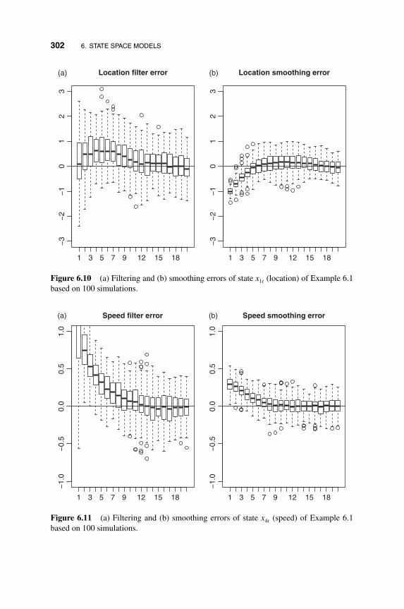
302 6. STATE SPACE MODELS
1 3 5 7 9 12 15 18
−3
−2
−1
01
23
Location filter error
1 3 5 7 9 12 15 18
−3
−2
−1
01
23
Location smoothing error(b)(a)
Figure 6.10 (a) Filtering and (b) smoothing errors of state x1t (location) of Example 6.1based on 100 simulations.
1 3 5 7 9 12 15 18
−1.
0−
0.5
0.0
0.5
1.0
Speed filter error
1 3 5 7 9 12 15 18
−1.
0−
0.5
0.0
0.5
1.0
Speed smoothing error(b)(a)
Figure 6.11 (a) Filtering and (b) smoothing errors of state x4t (speed) of Example 6.1based on 100 simulations.

6.3 LINEAR GAUSSIAN STATE SPACE MODELS 303
MLE error of q1
−0.04 0.00 0.02 0.04
05
1015
20MLE error of r1
−0.15 −0.05 0.05 0.15
05
1015
2025
3035
(b)(a)
Figure 6.12 Histograms of MLE estimation errors of (a) q1 and (b) r1 for Example 6.1based on 100 simulations.
R demonstration: Application of the Kalman filter.
#### Build function to MLE estimationbuildTrackLinear=function(parm){
q <- parm[1:3]r <- parm[4:6]H <- c(1,0,0,1,0,0,
0,1,0,0,1,0,0,0,1,0,0,1,0,0,0,1,0,0,0,0,0,0,1,0,0,0,0,0,0,1)
H <- matrix(H,ncol=6,nrow=6,byrow=T)G <- c(1,0,0,0,0,0,
0,1,0,0,0,0,0,0,1,0,0,0)
G <- matrix(G,ncol=6,nrow=3,byrow=T)W <- c(0.5*q[1], 0, 0,
0, 0.5*q[2], 0,0, 0, 0.5*q[3],q[1], 0, 0,0, q[2], 0,0, 0, q[3])
W <- matrix(W,ncol=3,nrow=6,byrow=T)

304 6. STATE SPACE MODELS
V <- diag(r)return(list(
m0=rep(0,6),C0=1000000*diag(6),FF=G,GG=H,V=V%*%t(V),W=W%*%t(W)
))}#### end function ###true parametersq <- c(0.1,0.1,0.02)r <- c(1,1,1)### Run Kalman filter with DLM packagelibrary(dlm)myModel <- buildTrackLinear(c(q,r)) #true modeloutFilter <- dlmFilter(y,myModel)outSmooth <- dlmSmooth(y,myModel)###Estimationpar.init <- c(1,1,1,10,10,10)outMLE <- dlmMLE(y,par.init,buildTrackLinear)
Example 6.2: Time-varying coefficient Fama–French factor models InSection 6.2.3 we briefly discussed the SSM setting that allows the coefficients ofa regression model to vary over time. Specifically, we mentioned the time-varyingcoefficient Fama–French factor model. Here we present an empirical analysis ofsuch a model. Fama and French (1993, 1996) introduced a size factor (SMB),an equity to book ratio factor (HML), and a momentum factor (MoM), in addi-tion to the excess market return factor (Market), to model portfolio returns as anextension of the capital asset pricing model (CAPM) of Sharpe (1964) and Fama(1970).
Figure 6.13 shows the four monthly Fama–French factors from January1946 to December 2010, obtained from http://mba.tuck.dartmouth.edu/pages/faculty/ken.french/Data Library. In the following analysis the time series of inter-est is the return series of the portfolios consisting of all stocks with capital sizesin the 20–40% range of all stocks and equity-to-book ratios also in the 20–40%range of all stocks, with equal weights, obtained from the same website. Figure6.14 shows the return of the portfolio. A quick regression analysis shows the fol-lowing results:
> out0 < lm(y˜xx)> summary(out0)

6.3 LINEAR GAUSSIAN STATE SPACE MODELS 305
1950 1970 1990 2010
−5
05
10Market
Time
Ret
urn
1950 1970 1990 2010
−4
−2
02
46
SMB
TimeR
etur
n
1950 1970 1990 2010
−5
05
HML
Time
Ret
urn
1950 1970 1990 2010
−5
05
10
MoM
Time
Ret
urn
Figure 6.13 Time plots of monthly Fama–French four factors from 1946.1 to 2010.12.
Coefficients:Estimate Std. Error t value Pr(>|t|)
(Intercept) 0.03369 0.05432 0.620 0.535367xxMkt.RF 0.99580 0.01268 78.544 < 2e16 ***xxSMB 0.86220 0.01902 45.330 < 2e16 ***xxHML 0.08927 0.01984 4.499 7.89e06 ***xxMoM 0.04479 0.01348 3.324 0.000929 ***–––Residual standard error: 1.441 on 775 degrees of freedomMultiple Rsquared: 0.9358, Adjusted Rsquared: 0.9355Fstatistic: 2825 on 4 and 775 DF, pvalue: < 2.2e16

306 6. STATE SPACE MODELS
1950 1960 1970 1980 1990 2000 2010
−5
05
10Portfolio
Time
Ret
urn
Figure 6.14 Return series of the portfolio of interest.
This shows that all four factors are highly significant. However, if one uses datain different subperiods, the estimation results are markedly different. Figure 6.15shows the estimated parameters and their 95% confidence intervals using a mov-ing 3-year window. The estimated coefficients and their 95% confidence intervalsusing the full data are also shown (straight lines). Although the estimated coeffi-cients using the entire data stayed mostly within the 3-year rolling 95% confidenceintervals, there are noticeable exceptions, especially for HML (around 1970, late1980, and early 2000), and occasionally for SMB and MoM. In the following weuse a varying-beta model to capture the changes in parameters. Specifically, weassume that
yt = 𝛽0t + 𝛽1t𝜂1t + 𝛽2t𝜂2t + 𝛽3t𝜂3t + 𝛽4t𝜂5t + et
where 𝜂𝑖t, 𝑖 = 1,… , 4 are the four Fama–French factors. We further assume a sim-ple random walk model for the coefficients 𝛽𝑖t = 𝛽𝑖(t−1) + 𝜀𝑖t for 𝑖 = 0,… , 4. Thecorresponding SSM becomes
xt = Hxt−1 + Wwt,
yt = Gtxt + Vvt,

6.3 LINEAR GAUSSIAN STATE SPACE MODELS 307
1950 1970 1990 2010
0.7
0.9
1.1
1.3
Market
Time
Bet
a
1950 1970 1990 2010
0.4
0.8
1.2
1.6
SMB
Time
Bet
a
1950 1970 1990 2010
−0.
40.
00.
20.
40.
60.
8
HML
Time
Bet
a
1950 1970 1990 2010
−0.
40.
00.
20.
40.
60.
8
MoM
Time
Bet
a
Figure 6.15 Estimated coefficients using a 3-year moving window. The dashed lines arethe estimated coefficients and their corresponding 95% confidence intervals using all data.
where xt = (𝛽0t,… , 𝛽4t)′, H = I5×5, W = d𝑖ag(w1,… , w5), and the time-varying
Gt is
Gt =[
1, 𝜂1t, 𝜂2t, 𝜂3t, 𝜂4t
],
and V = v.The MLEs of the parameters (w1,… , w5, v) are (0, 0, 0, 0.044,−0.001, 1.25),
with likelihood value −640.5. Figure 6.16 shows the smoothed states (the 𝛽 val-ues) against the estimated values using the 3-year moving window. The state for𝛽0t is omitted. Under this model, 𝛽0t, 𝛽1t and 𝛽2t are almost constant, while the

308 6. STATE SPACE MODELS
1950 1970 1990 2010
0.90
1.00
1.10
Market
Time
Bet
a
1950 1970 1990 2010
0.7
0.8
0.9
1.0
1.1
1.2
SMB
TimeB
eta
1950 1970 1990 2010
−0.
20.
00.
20.
4
HML
Time
Bet
a
1950 1970 1990 2010
−0.
3−
0.1
0.1
0.3
MoM
Time
beta
Figure 6.16 Smoothed states using a diffused state initial values (line) vs estimated coef-ficients with 3-year moving windows (dots).
coefficients corresponding to HML and MoM change markedly. The estimatedv = 1.25 is slightly smaller than the estimated standard deviation of residuals ofthe linear regression model. Note that the state variables are assumed to follow arandom walk model, which is sensitive to the specification of the initial state 𝜇0and 𝚺0. The MLE and filter/smoothing shown above were obtained using a dif-fused setting for the initial states. If instead we use a specific state initial value 𝜇0 =(1, 2,−0.2, 0.8,−0.3)′ and𝚺0 = d𝑖ag(0.1, 0.01, 0.1, 10, 10), one obtains a differentset of MLEs (w1,… , w5, v) = (0.0147, 0.025, 0.0275, 0.0397, 0.011, 1.230) withlikelihood value of −670. The results of these particular initial values are not asgood as those starting with the diffused setting. However, the resulting smoothed

6.3 LINEAR GAUSSIAN STATE SPACE MODELS 309
1950 1970 1990 2010
0.90
1.00
1.10
Market
Time
Bet
a
1950 1970 1990 2010
0.7
0.8
0.9
1.0
1.1
1.2
SMB
TimeB
eta
1950 1970 1990 2010
−0.
20.
00.
20.
4
HML
Time
Bet
a
1950 1970 1990 2010
−0.
3−
0.1
0.1
0.3
MoM
Time
Bet
a
Figure 6.17 Smoothed states using a specific state initial value (lines) vs estimated coef-ficients with 3-year moving windows (dots).
state variable is more interesting, with all five 𝛽 values changing over time (seeFigure 6.17).
R demonstration: Time-varying coefficient model.
library(dlm)
#### Build function to MLE estimation:
buildVaryingBeta1=function(parm){
phiW <- parm[1:5]
phiV <- parm[6]
H <- diag(c(1,1,1,1,1))
W0 <- diag(phiW)
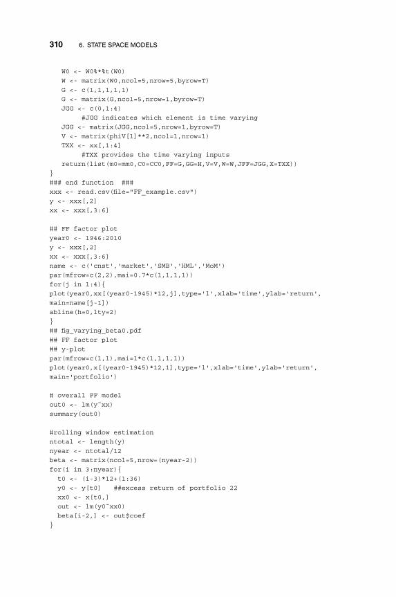
310 6. STATE SPACE MODELS
W0 <- W0%*%t(W0)
W <- matrix(W0,ncol=5,nrow=5,byrow=T)
G <- c(1,1,1,1,1)
G <- matrix(G,ncol=5,nrow=1,byrow=T)
JGG <- c(0,1:4)
#JGG indicates which element is time varying
JGG <- matrix(JGG,ncol=5,nrow=1,byrow=T)
V <- matrix(phiV[1]**2,ncol=1,nrow=1)
TXX <- xx[,1:4]
#TXX provides the time varying inputs
return(list(m0=mm0,C0=CC0,FF=G,GG=H,V=V,W=W,JFF=JGG,X=TXX))
}
### end function ###
xxx <- read.csv(file="FF_example.csv")
y <- xxx[,2]
xx <- xxx[,3:6]
## FF factor plot
year0 <- 1946:2010
y <- xxx[,2]
xx <- xxx[,3:6]
name <- c('cnst','market','SMB','HML','MoM')
par(mfrow=c(2,2),mai=0.7*c(1,1,1,1))
for(j in 1:4){
plot(year0,xx[(year0-1945)*12,j],type='l',xlab='time',ylab='return',
main=name[j-1])
abline(h=0,lty=2)
}
## fig_varying_beta0.pdf
## FF factor plot
## y-plot
par(mfrow=c(1,1),mai=1*c(1,1,1,1))
plot(year0,x[(year0-1945)*12,1],type='l',xlab='time',ylab='return',
main='portfolio')
# overall FF model
out0 <- lm(y˜xx)
summary(out0)
#rolling window estimation
ntotal <- length(y)
nyear <- ntotal/12
beta <- matrix(ncol=5,nrow=(nyear-2))
for(i in 3:nyear){
t0 <- (i-3)*12+(1:36)
y0 <- y[t0] ##excess return of portfolio 22
xx0 <- x[t0,]
out <- lm(y0˜xx0)
beta[i-2,] <- out$coef
}

6.3 LINEAR GAUSSIAN STATE SPACE MODELS 311
year <- 1948:2010
par(mfrow=c(2,2),mai=0.7*c(1,1,1,1))
for(j in 2:5){
ylim <- range(cbind(ucl[,j],lcl[,j]))
plot(year,beta[,j],type='l',xlab='time',ylab='beta',
main=name[j-1],ylim=ylim)
lines(year,year*0+summary(out0)$coef[j,1])
lines(year,year*0+summary(out0)$coef[j,1]+summary(out0)$coef[j,2]*2,lty=2)
lines(year,year*0+summary(out0)$coef[j,1]-summary(out0)$coef[j,2]*2,lty=2)
lines(year,ucl[,j],lty=2)
lines(year,lcl[,j],lty=2)
}
## fig_varying_beta1.pdf
## 3-year regression
##++++++ use diffused initial value
mm0 <- c(1,1,1,1,1)
CC0 <- diag(c(1,1,1,1,1))*1000
ww <- c(1,1,1,1,1)
vv <- 1
init.par <- c(ww,vv)
MLE2 <- dlmMLE(y,init.par,buildVaryingBeta1,debug=F)
MLE2
MyModel2 <- buildVaryingBeta1(MLE2$par)
ss2 <- dlmSmooth(y,MyModel2)
# smoothed state plot
year <- 1948:2010
par(mfrow=c(2,2),mai=0.7*c(1,1,1,1))
for (j in 2:5){
plot(year,beta[,j],type='p',xlab='time',ylab='beta',main=name[j-1])
lines(year,ss2$s[(3:65)*12+1,j])
}
##++++++ use an arbitrary state initial value
mm0 <- c(1,2,-0.2,0.8,-0.3)
CC0 <- diag(c(0.1,0.01,0.1,10,10))
ww <- c(30,30,30,10,10)
vv <- 1
init.par <- c(ww,vv)
MLE <- dlmMLE(y,init.par,buildVaryingBeta1,debug=F)
MyModel <- buildVaryingBeta1(MLE$par)
ss <- dlmSmooth(y,MyModel)
#
year <- 1948:2010
par(mfrow=c(2,2),mai=0.7*c(1,1,1,1))
for (j in 2:5){
plot(year,beta[,j],type='p',xlab='time',ylab='beta',main=name[j-1])
lines(year,ss$s[(3:65)*12+1,j])
}
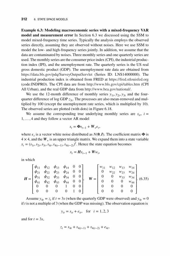
312 6. STATE SPACE MODELS
Example 6.3: Modeling macroeconomic series with a mixed-frequency VARmodel and measurement error In Section 6.3 we discussed using the SSM tomodel mixed-frequency time series. Typically the analysis employs the observedseries directly, assuming they are observed without noises. Here we use SSM tomodel the low- and high-frequency series jointly. In addition, we assume that thedata are contaminated by noises. Three monthly series and one quarterly series areused. The monthly series are the consumer price index (CPI), the industrial produc-tion index (IPI), and the unemployment rate. The quarterly series is the US realgross domestic product (GDP). The unemployment rate data are obtained fromhttps://data.bls.gov/pdq/SurveyOutputServlet (Series ID: LNS14000000). Theindustrial production index is obtained from FRED at https://fred.stlouisfed.org(code:INDPRO). The CPI data are from http://www.bls.gov/cpi/tables.htm (CPIAll Urban), and the real GDP data from http://www.bea.gov/national/.
We use the 12-month difference of monthly series y1t, y2t, y3t and the four-quarter difference of log GDP z3t. The processes are also mean-removed and mul-tiplied by 100 (except the unemployment rate series, which is multiplied by 10).The observed series are plotted (with dots) in Figure 6.18.
We assume the corresponding true underlying monthly series are s𝑖t, 𝑖 =1,… , 4 and they follow a vector AR model
st = 𝚽st−1 + W∗𝜀t,
where 𝜀t is a vector white noise distributed as N(0, I). The coefficient matrix 𝚽 is4 × 4, and the W∗ is an upper triangle matrix. We expand them into a state variablext = (s1t, s2t, s3t, s4t, s4(t−1), s4(t−2))
′. Hence the state equation becomes
xt = Hxt−1 + Wwt,
in which
H =
⎡⎢⎢⎢⎢⎢⎢⎣
𝜙11 𝜙12 𝜙13 𝜙14 0 0𝜙21 𝜙22 𝜙23 𝜙24 0 0𝜙31 𝜙32 𝜙33 𝜙34 0 0𝜙41 𝜙42 𝜙43 𝜙44 0 00 0 0 1 0 00 0 0 0 1 0
⎤⎥⎥⎥⎥⎥⎥⎦, W =
⎡⎢⎢⎢⎢⎢⎢⎣
w11 w12 w13 w140 w22 w23 w240 0 w33 w340 0 0 w440 0 0 00 0 0 0
⎤⎥⎥⎥⎥⎥⎥⎦. (6.35)
Assume y4t = zt if t = 3s (when the quarterly GDP were observed) and y4t = 0if t is not a multiple of 3 (when the GDP was missing). The observation equation is
y𝑖t = s𝑖t + e𝑖t, for 𝑖 = 1, 2, 3
and for t = 3s,
zt = s4t + s4(t−1) + s4(t−2) + e4t,

6.3 LINEAR GAUSSIAN STATE SPACE MODELS 313
0 50 100 150 200 250 300 350
−1.
0−
0.5
0.0
0.5
1.0
1.5
CP
I
0 50 100 150 200 250 300 350
−4
−2
02
4
IND
P
0 50 100 150 200 250 300 350
−5
05
UE
MP
0 20 40 60 80 100 120
−4
−2
02
46
GD
P
Figure 6.18 Plots of the mixed-frequency macroeconomic series (dots) and smoothedstates (lines).
where e𝑖t are independent noises following N(0, 𝜂2𝑖). Let yt = (y1t, y2t, y3t) when t
is not a multiple of 3, and yt = (y1t, y2t, y3t, zt) when t is a multiple of 3. Then theobservation equation can be written as
yt = Gtxt + Vtet,
where when t = 3s,
Gt =⎡⎢⎢⎢⎣
1 0 0 0 0 00 1 0 0 0 00 0 1 0 0 00 0 0 1 1 1
⎤⎥⎥⎥⎦, and Vt = diag(𝜂1, 𝜂2, 𝜂3, 𝜂4),

314 6. STATE SPACE MODELS
Φ W∗ V
CPI 0.70 0 0 0.02 0.17 −0.14 0.019 0.022 0.238INDP 0 0.80 0 −0.00 0 0.42 0.436 −0.032 0.774UEMP 0 0 0.91 0.07 0 0 0.155 −0.249 1.547GDP −0.16 −0.24 0.10 0.93 0 0 0 0.001 0.081
Table 6.1 MLEs of the mixed-frequency data example.
and when t is not a multiple of 3,
Gt =⎡⎢⎢⎣
1 0 0 0 0 00 1 0 0 0 00 0 1 0 0 0
⎤⎥⎥⎦, and Vt = diag(𝜂1, 𝜂2, 𝜂3).
Because the dimension of the observations changes over time, it is easier to usethe sequential processing approach of Section 6.3.5. To simplify the model andbecause we are more interested in the low-frequency component GDP, we assumethat 𝚽 satisfies the following simplifying structure
𝚽 =⎡⎢⎢⎢⎣𝜙11 0 0 𝜙140 𝜙22 0 𝜙240 0 𝜙33 𝜙34𝜙41 𝜙42 𝜙43 𝜙44
⎤⎥⎥⎥⎦.Table 6.1 shows the MLEs of the system with log-likelihood value −360.
In Figure 6.18, the lines show the smoothed states using the MLEs. For theGDP series, the line shown is the sum of the three consecutive monthly smoothedstates corresponding to the observed GDP series.
The following R codes are used to estimate the model using the maximum like-lihood method via the dlm package. The function buildMixedFreqSeq4(parm)uses the parameter values stored in parm to build the state space model by specify-ing the time-varying system matrices. The program is constructed to sequentiallyprocess one observation at a time, hence one quarter is stretched into 10 steps,three monthly observations from each of the three monthly series and one obser-vation for the quarterly GDP series. At steps 1, 4 and 7 the Ht matrix is that in(6.35). At all other steps, the state does not evolve, hence Ht is the 6 × 6 identitymatrix and the corresponding Wt = 0. The matrix Gt and Vt change according towhich series the observation comes from.
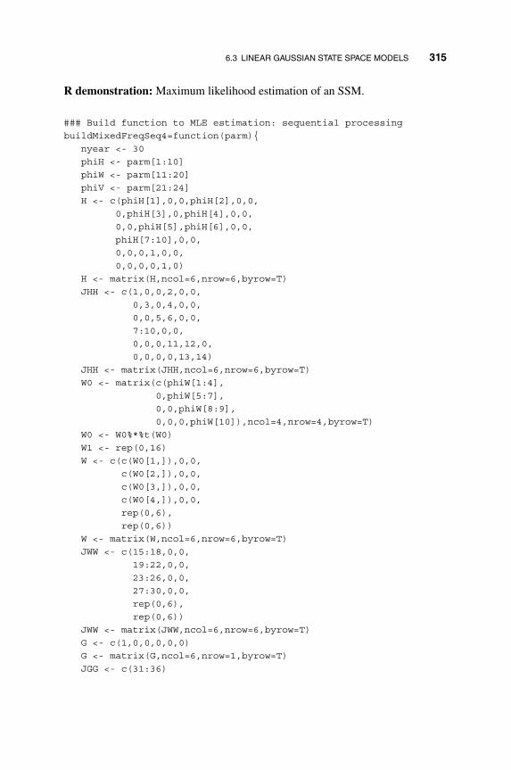
6.3 LINEAR GAUSSIAN STATE SPACE MODELS 315
R demonstration: Maximum likelihood estimation of an SSM.
### Build function to MLE estimation: sequential processingbuildMixedFreqSeq4=function(parm){
nyear <- 30phiH <- parm[1:10]phiW <- parm[11:20]phiV <- parm[21:24]H <- c(phiH[1],0,0,phiH[2],0,0,
0,phiH[3],0,phiH[4],0,0,0,0,phiH[5],phiH[6],0,0,phiH[7:10],0,0,0,0,0,1,0,0,0,0,0,0,1,0)
H <- matrix(H,ncol=6,nrow=6,byrow=T)JHH <- c(1,0,0,2,0,0,
0,3,0,4,0,0,0,0,5,6,0,0,7:10,0,0,0,0,0,11,12,0,0,0,0,0,13,14)
JHH <- matrix(JHH,ncol=6,nrow=6,byrow=T)W0 <- matrix(c(phiW[1:4],
0,phiW[5:7],0,0,phiW[8:9],0,0,0,phiW[10]),ncol=4,nrow=4,byrow=T)
W0 <- W0%*%t(W0)W1 <- rep(0,16)W <- c(c(W0[1,]),0,0,
c(W0[2,]),0,0,c(W0[3,]),0,0,c(W0[4,]),0,0,rep(0,6),rep(0,6))
W <- matrix(W,ncol=6,nrow=6,byrow=T)JWW <- c(15:18,0,0,
19:22,0,0,23:26,0,0,27:30,0,0,rep(0,6),rep(0,6))
JWW <- matrix(JWW,ncol=6,nrow=6,byrow=T)G <- c(1,0,0,0,0,0)G <- matrix(G,ncol=6,nrow=1,byrow=T)JGG <- c(31:36)

316 6. STATE SPACE MODELS
JGG <- matrix(JGG,ncol=6,nrow=1,byrow=T)V <- matrix(phiV[1]**2,ncol=1,nrow=1)JVV <- matrix(37,ncol=1,nrow=1)xx1 <- c(phiH[1:10],1,0,1,0,
c(W0),1,rep(0,5), phiV[1]**2)
xx2 <- c(1,0,1,0,1,0,0,0,0,1,0,1,0,1,c(W1),0,1,rep(0,4), phiV[2]**2)
xx3 <- c(1,0,1,0,1,0,0,0,0,1,0,1,0,1,c(W1),0,0,1,rep(0,3), phiV[3]**2)
xx4 <- c(1,0,1,0,1,0,0,0,0,1,0,1,0,1,c(W1),0,0,0,1,1,1,phiV[4]**2)
xx <- c(rep(c(xx1,xx2,xx3),3),xx4)TXX <- matrix(rep(xx,nyear),ncol=37,nrow=nyear*40,byrow=T)return(list(
m0=rep(0,6),C0=1000000*diag(6),FF=G,GG=H,V=V,W=W,JFF=JGG,JGG=JHH,JWW=JWW,JVV=JVV,X=TXX
))}### end function #### Analysisy_start=22 ## 1948+22=1970nyear <- 30#temp <- c(t(cbind(CPIuse_m,INDPuse_m,UEMPuse_m)))yseq <- 1:(nyear*40)for(i in 1:(nyear*4)){yseq[(i-1)*10+(1:9)] <- temp[(i-1)*9+(1:9)]yseq[(i-1)*10+10] <- GDPuse_m[i]
}#phi <- c(0.7,-0.3,0.7,-0.3,0.7,-0.3,0.1,0.1,0.1,0.8)ww <- c(0.3,0,0,0,0.5,0,0,0.5,0,0.3)vv <- c(1,1,1,1)

6.3 LINEAR GAUSSIAN STATE SPACE MODELS 317
parm <- c(phi,ww,vv)MLE <- dlmMLE(yseq,parm,buildMixedFreqSeq4)#MyModel <- buildMixedFreqSeq4(MLE$par)ss <- dlmSmooth(yseq,MyModel) ## ss provides smoothed states
Example 6.4: Analysis of dynamic factor model Finally, we demonstrate the useof SSMs in the estimation of a DFM for a panel of macroeconomic time series.Figure 6.19 shows the GDP growth series of Germany (DEU), France (FRA), theUnited States (USA), Great Britain (GBR), and Canada (CAN) from the secondquarter of 1990 to the fourth quarter of 2016 for a total of 107 observations. Theseries is demeaned and in percentage.
Table 6.2 shows the results of a PCA analysis of the panel of series, using itscovariance matrix. It reveals two (possibly three) important factors. Figures 6.21to 6.23 show the ACF, PACF, and cross-correlation plots of the first two empirical
0 20 40 60 80 100
−4
−2
02 DEU
0 20 40 60 80 100
−2.
0−
1.5
−1.
0−
0.5
0.0
0.5
1.0
FRA
0 20 40 60 80 100
−2
−1
01 USA
0 20 40 60 80 100
−2
−1
01
GBR
0 20 40 60 80 100
−3
−2
−1
01 CAN
Figure 6.19 Growth rates of gross domestic products of five countries (Germany, France,the USA, the UK, and Canada) (demeaned and in percentages).

318 6. STATE SPACE MODELS
0 20 40 60 80 100
−4
−2
02
DEU
0 20 40 60 80 100
−2.
0−
1.0
0.0
0.5
1.0
FRA
0 20 40 60 80 100
−2
−1
01
USA
0 20 40 60 80 100
−2
−1
01
GBR
0 20 40 60 80 100
−3
−2
−1
01
CAN
Figure 6.20 GDP growth rates of five countries (Germany, France, the USA, the UK, andCanada) (dots) and SSM fitted lines.
principle components. From the plots it seems that a VAR(1) model would beappropriate for the two estimated factors. Table 6.3 shows the estimated results ofa VAR(1) model 𝜂t = c + Φ𝜂t−1 + et fitted to the estimated factors.
Next we set up a corresponding SSM based on the results of the PCA exer-cise, with two dynamic factors following a VAR(1) model. Following the dis-cussion in Section 6.2.6, let yt be the five-dimensional observed time series, and
Component
1 2 3 4 5
Standard deviation 1.085 0.735 0.406 0.392 0.285Proportion of variance 0.556 0.255 0.078 0.073 0.038Cumulative proportion 0.556 0.811 0.889 0.962 1.000
Table 6.2 PCA analysis of the GDP growth rates of five countries.

6.3 LINEAR GAUSSIAN STATE SPACE MODELS 319
0 5 10 15 20
−0.
20.
20.
61.
0
Lag
AC
F
ACF: Component 1
5 10 15 20
−0.
20.
00.
20.
40.
6
Lag
Par
tial A
CF
PACF: Component 1(b)(a)
Figure 6.21 (a) ACF and (b) PACF plots of the first principle component of the GDPgrowth rates.
xt = (𝜂1t, 𝜂2t)′. We have
xt = Hxt−1 + Wwt,
yt = Gxt + Vvt,
where G = (g𝑖j) is a 5 × 2 loading matrix, V is a 5 × 5 diagonal matrix of stan-dard deviations of the measurement errors, H = (h𝑖j) is a 2 × 2 VAR(1) coefficientmatrix, W is a 2 × 2 square root matrix of the VAR(1) innovation process, and vt
0 5 10 15 20
−0.
20.
20.
61.
0
Lag
AC
F
ACF: Component 2
5 10 15 20
−0.
20.
00.
2
Lag
Par
tial A
CF
PACF: Component 2(b)(a)
Figure 6.22 (a) ACF and (b) PACF plots of the second principle component of the GDPgrowth rates.

320 6. STATE SPACE MODELS
−15 −10 −5 0 5 10 15
−0.
20.
00.
10.
2
Lag
AC
FCross−correlation
Figure 6.23 Cross-correlation plot of the first two principle components of the GDPgrowth rates.
and wt are independent Gaussian white noises of corresponding dimensions. Sincefor any invertible matrix 𝚪, the model can be written as
yt = (G𝚪−1)(𝚪xt) + Vvt and 𝚪xt = (𝚪H𝚪−1)(𝚪xt−1) + 𝚪Wwt,
therefore the model is not uniquely defined. Hence we impose the constraints thatg11 = g12 = 1 and h21 = 0. The MLEs of the model are shown in Table 6.4.
The solid lines in Figure 6.20 show the fitted series using the smoothed statesand the estimated loading matrix. The total sum of squares of residuals over thetotal sum of squares of the original demeaned series is 0.352. Figure 6.24 showsthe smoothed states. Note that the first two principal components explain approxi-mately 81% of the total variation, as shown in Table 6.2. This percentage is higherthan that of the DFM. Such a result is not surprising because the DFM does not tryto minimize the contemporary residual sum of squares. Instead, it tries to establishthe dynamics of the system. To see the benefit of the DFM, Table 6.5 shows the
Constant ΦComponent 1 −0.006 0.634 0.350
(0.079) (0.072) (0.107)Component 2 −0.006 0.089 0.360
(0.067) (0.061) (0.090)
Table 6.3 Estimated VAR(1) model of the first two PCA components ofthe GDP growth rates of five countries. Standard errors are shown in parenthesis.

6.3 LINEAR GAUSSIAN STATE SPACE MODELS 321
G V H WW′
DEU 1∗ 1∗ 0.62 0.695 0.050 0.415 −0.142FRA 0.75 1.20 0.23 0∗ 0.794 −0.142 0.069USA 0.68 1.56 0.42GBR 0.73 1.73 0.35CAN 0.77 1.78 0.42
Table 6.4 MLEs of the DFM for the five GDP growth rates. The entries marked * arefixed a priori.
comparisons of out-of-sample one-step to three-step ahead forecasts of the GDPgrowth rates of each country using the SSM and PCA-VAR, respectively. For SSM,𝓁-step prediction of the states (factors) is obtained by running the Kalman fore-casting step using the MLE, then using the estimated loading matrix to predictthe GDP growth rates. The PCA-VAR forecast is obtained by obtaining the firsttwo principle components, fitting a VAR(1) model to the components, obtainingthe 𝓁-step prediction of the factors, then using the estimate loading matrix for the𝓁-step ahead prediction. We also fit individual AR(1) models for each series and
0 20 40 60 80 100
−2
01
2
First factor
Time
f1
0 20 40 60 80 100
−1.
5−
0.5
0.5
Second factor
Time
f2
Figure 6.24 Time plots of the smoothed factors of the DFM for GDP growth rates.

322 6. STATE SPACE MODELS
𝓁 DEU FRA USA GRB CAN Average
1 DFM 1.94 1.69 2.86 2.52 4.61 2.724PCA-VAR 1.78 1.61 3.40 2.79 5.14 2.943Univ-AR 2.30 2.20 3.33 4.14 5.49 3.489
2 DFM 2.24 1.87 2.52 2.30 4.22 2.628PCA-VAR 2.27 2.23 2.70 2.55 4.18 2.787Univ-AR 2.27 1.60 3.08 1.68 4.05 2.535
3 DFM 2.02 1.59 2.68 2.42 4.39 2.619PCA-VAR 2.34 1.66 2.55 2.49 4.46 2.699Univ-AR 2.17 1.72 2.63 2.66 4.04 2.646
Table 6.5 Out-of-sample prediction comparison between SSM, PCA-VAR, and scalarAR models. Mean squared errors are used and 𝓁 denotes step.
obtain 𝓁-step out-of-sample predictions. For each of s = 88 − 𝓁,… , 107 − 𝓁, therespective models are estimated using data from t = 1 to s only, and 𝓁-step pre-diction is obtained and compared with the true observation at time s + 𝓁. Table6.5 shows the mean squared errors of out-of-sample 𝓁-step predictions. It can beseen that the DFM outperforms the other two competing models for USA, GRB,and CAN, but its performance was marginally worse for DEU and FRA.
Figure 6.25 shows the one-step ahead prediction of US GDP growth rate forthe three different methods employed.
The following R codes are used to estimate the models using the maximumlikelihood method and to obtain the out-of-sample predictions. The functionbuildDFM3(parm) uses the parameter values stored in parm to build the statespace model used in the analysis. The functions outsample.prediction.DFM,outsample.prediction.PCA, and outsample.prediction.uAR are usedto obtain the out-of-sample predictions for the three methods employed in theanalysis. We also include some essential commands, but do not display output ofthe commands.
R demonstration: DFM and model comparison.
####### buildDFM3buildDFM3=function(parm){
hh <- c(parm[1],parm[2],0,parm[3])gg <- c(1,1,parm[4:11])qq <- c(parm[12:13],0,parm[14])rr <- parm[15:19]H <- matrix(hh,ncol=2,nrow=2,byrow=T)
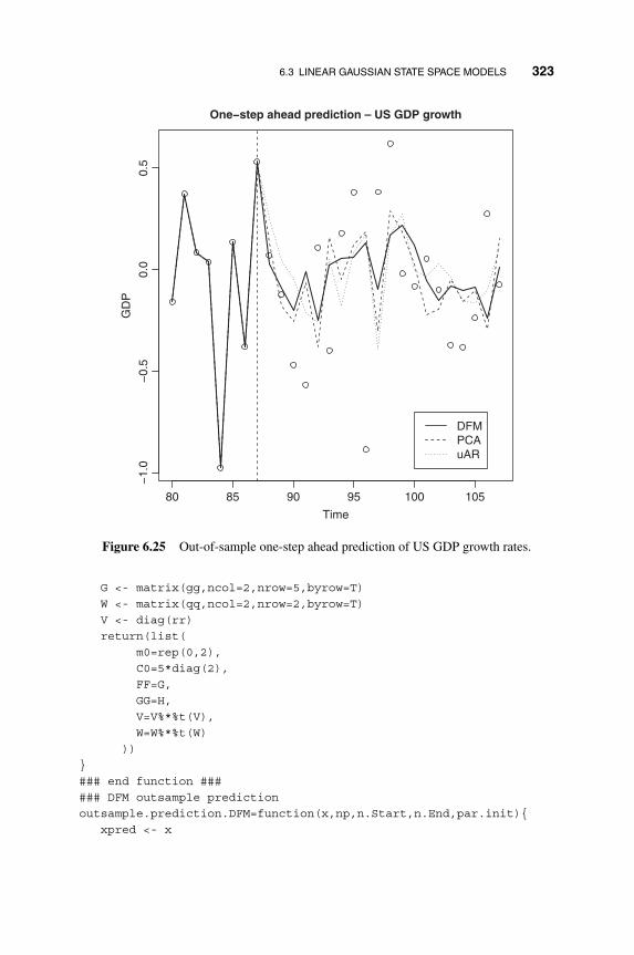
6.3 LINEAR GAUSSIAN STATE SPACE MODELS 323
80 85 90 95 100 105
−1.
0−
0.5
0.0
0.5
Time
GD
P
DFMPCAuAR
One−step ahead prediction – US GDP growth
Figure 6.25 Out-of-sample one-step ahead prediction of US GDP growth rates.
G <- matrix(gg,ncol=2,nrow=5,byrow=T)W <- matrix(qq,ncol=2,nrow=2,byrow=T)V <- diag(rr)return(list(
m0=rep(0,2),C0=5*diag(2),FF=G,GG=H,V=V%*%t(V),W=W%*%t(W)
))}### end function ###### DFM outsample predictionoutsample.prediction.DFM=function(x,np,n.Start,n.End,par.init){
xpred <- x

324 6. STATE SPACE MODELS
SS <- rep(0,5)for(i in (n.Start-np):(n.End-np)){
MLE <- dlmMLE(x[1:i,],par.init,buildDFM3)myMode <- buildDFM3(MLE$par)filter <- dlmFilter(x[1:i,],myMode)pp <- dlmForecast(filter,nAhead=np)xpred[i+np,] <- pp$f[np,]SS <- SS+(x[i+np,]-xpred[i+np,])**2
}return(list(xpred=xpred,SS=SS,meanSS=mean(SS)))
}### PCA outsample predictionoutsample.prediction.PCA=function(x,np,n.Start,n.End){
xpred <- xSS <- rep(0,5)for(i in (n.Start-np):(n.End-np)){
PCA <- princomp(x[1:i,], cor=F)ff <- PCA$score[,1:2]out <- VAR(ff)pp <- predict(out,n.ahead=np)pp0 <- c(pp$fcst$Comp.1[np,1],pp$fcst$Comp.2[np,1])xpred[i+np,] <- PCA$loading[,1:2]%*%pp0SS <- SS+(x[i+np,]-xpred[i+np,])**2
}return(list(xpred=xpred,SS=SS,meanSS=mean(SS)))
}### univariate AR predictionoutsample.prediction.uAR=function(x,np,n.Start,n.End){
xpred <- xSS <- rep(0,5)for(i in (n.Start-np):(n.End-np)){
for(j in 1:5){out <- arima(x[1:i,j],c(1,0,0))xpred[i+np,j] <- predict(out,n.ahead=np)$pred[np]
}SS <- SS+(x[i+np,]-xpred[i+np,])**2
}return(list(xpred=xpred,SS=SS,meanSS=mean(SS)))
}### Analysis ###xx.nm <- matrix(scan("GDP_panel_nm.dat"),ncol=5)#-------- PCA analysis ---------------#PCAout <- princomp(xx.nm, cor=F)ff <- PCAout$scores[,1:2]library(vars)out <- VAR(ff)

EXERCISES 325
#-------- DFM analysis ---------------#hh3 <- c(0.7,0.2,0.8)gg3 <- rep(c(0.7,0.7), 4)qq3 <- c(1,-1,1)rr3 <- rep(0.3,5)parm3 <- c(hh3,gg3,qq3,rr3) # initial parameter valuesoutMLE3 <- dlmMLE(xx.nm,parm3,buildDFM3)myModel3 <- buildDFM3(outMLE3$par)outSmooth3 <- dlmSmooth(xx.nm,myModel3)fit3 <- xx.nmfor(i in 1:5){
fit3[,i] <- outSmooth3$s[-1,]%*%myModel3$F[i,]}print(sum(xx.nm-fit3)**2)/sum(xx.nm**2))#---------- Prediction ---------------#for(np in 1:3){
pred.d <- outsample.prediction.DFM(xx.nm,np,88,107,outMLE3$par)pred.p <- outsample.prediction.PCA(xx.nm,np,88,107)pred.ar <- outsample.prediction.uAR(xx.nm,np,88,107)
}
6.4 EXERCISES
6.1 Consider the linear zero-mean ARMA(p, p) model
yt =p∑𝑖=1
𝜙𝑖yt−𝑖 + 𝜖t +p∑𝑖=1
𝜃𝑖𝜖t−𝑖,
where 𝜖t is a sequence of iid random variates following N(0, 𝜎2). Derive theShumway and Stoffer state space representation for yt given in Section 6.2.1.
6.2 Again, consider the linear zero-mean ARMA(p, p) model of question 1.Let yt|h = E(yt ∣ y1, y2,… , yh) be the conditional expectation of yt givenFh = 𝜎{y1,… , yh}, where h ≤ t. Let xt = (yt|t, yt+1|t,… , yt+p−1|t)′ be a p-dimensional state vector. Derive an SSM for yt using the state variable xt.This state space representation of ARMA models was proposed by Akaike(1975).
6.3 The file mdec5FF6117.txt contains the monthly returns of the CRSPDecile 5 portfolio and the Fama–French factors from January 1961 to June2017. The data are in percentages. The Decile 5 returns are from CRSP andhave been adjusted by removing the risk-free interest rates. Fama–Frenchfactors are from Professor K. French’s website.

326 6. STATE SPACE MODELS
(a) Fit a linear regression model relating the Decile 5 excess returns to theFama–French factors. Write down the fitted model and perform modelchecking.
(b) Fit a time-varying coefficient model relating the Decile 5 excess returnsto the Fama–French three factors as shown in Example 6.2.
(c) Show the time plots of smoothed states using a diffused initial value.
6.4 The file mstateunrate.txt contains the monthly unemployment ratesof the states of California, Illinois, Michigan, New York, Pennsylvania, andTexas from January 1976 to August 2017 for 500 observations. The data areseasonally adjusted and available from FRED. For simplicity, focus on thefirst differenced series and denote the differenced series by yt.
(a) Perform a principal component analysis on yt using a sample covari-ance matrix. Obtain the scree plot. What percentage of total variationsis explained by the first two principal components?
(b) Let zt be the first two principal component series. Obtain a suitable VARmodel to zt.
(c) Put the fitted VAR model for zt into a SSM.
(d) Fit a dynamic factor model to yt using two common factors similar tothat of Example 6.4.
(e) Obtain the time plots of smoothed factors based on the fitted SSM.
6.5 Seasonal adjustment via SSM. The file CAURN.csv contains the monthlyunemployment rates of California from January 1976 to August 2017. Therates are not seasonally adjusted. Let yt be the unemployment rate and con-sider the model
yt = Tt + St + It,
where Tt is the trend component following the local trend model, St denotesthe seasonal component following the model
∑12𝑖=1 St−𝑖+1 = 𝜖t, where 𝜖t is
a Gaussian white noise series with mean zero and variance 𝜎2𝜖 , and It is the
irregular component following an AR(5) model.
(a) Write down an SSM for yt. What is the dimension of the state vector?
(b) Fit the specified SSM model and write down the parameter estimates.
(c) Obtain a smoothed seasonal component St. Denote the series by St.
(d) Let zt = yt − St be the seasonally adjusted series of California monthlyunemployment rate. Let 𝜌12 be the lag-12 autocorrelation of zt. TestH0 : 𝜌12 = 0 versus Ha : 𝜌12 ≠ 0 and draw a conclusion using the 5%type-I error.

REFERENCES 327
REFERENCES
Adrian, T. and Franzoni, F. (2009). Learning about beta: Time-varying factor load-ings, expected returns, and the conditional CAPM. Journal of Empirical Finance 16:537–556.
Ahmad, B. I., Murphy, J. K., Langdon, P. M., Godsill, S. J., Hardy, R., and Skrypchuk, L.(2016). Intent inference for hand pointing gesture-based interactions in vehicles. IEEETransactions on Cybernetics 46: 878–889.
Aıt-Sahalia, Y. and Jacod, J. (2014). High-Frequency Financial Econometrics. PrincetonUniversity Press, Princeton, NJ.
Akaike, H. (1975). Markovian representation of stochastic processes by canonical variables.Siam Journal on Control 13: 162–173.
Andrieu, C., De Freitas, N., and Doucet, A. (1999). Sequential MCMC for Bayesian modelselection. IEEE Signal Processing Workshop on Higher-Order Statistics, pp 130–134.
Aoki, M. (2013). State Space Modeling of Time Series. Universitext, Springer-Verlag,Berlin, Heidelberg.
Arulampalam, M. S., Maskell, S., Gordon, N., and Clapp, T. (2002). A tutorial on parti-cle filters for online nonlinear/non-Gaussian Bayesian tracking. IEEE Transactions onSignal Processing 50: 174–188.
Arulampalam, M. S., Ristic, B., Gordon, N., and Mansell, T. (2004). Bearings-only track-ing of maneuvering targets using particle filters. EURASIP Journal of Applied SignalProcessing 2004: 2351–2365.
Avitzour, D. (1995). Stochastic simulation Bayesian approach to multitarget tracking. IEEProceedings on Radar, Sonar and Navigation 142: 41–44.
Bai, J. and Ng, S. (2002). Determining the number of factors in approximate factor models.Econometrica 70: 191–221.
Bai, J., and Ng, S. (2008). Large dimensional factor snalysis. Foundations and Trends inEconometrics 3(2): 89–163
Bar-Shalom, Y. and Fortmann, T. (1988). Tracking and Data Association. Academic Press,Boston.
Berzuini, C. and Best, N.G., Gilks, W.R., and Larizza, C. (1997). Dynamic conditionalindependence models and Markov chain Monte Carlo methods. Journal of the AmericanStatistical Association 92: 1403–1412.
Blake, A., Bascle, B., Isard, M., and MacCormick, J. (1998). Statistical models of visualshape and motion. Philosophical Transactions of the Royal Society A 356: 1283–1302.
Blake, A., Isard, M., and MacMormick, J. (2001). Statistic models of visual shape andmotion. In Doucet, A. and de Freitas, J. F. G. and Gordon, N. J. (eds), Sequential MonteCarlo in Practice. Springer-Verlag, New York.
Bouchard-Cote, A., Sankararaman, S., and Jordan, M. I. (2012). Phylogenetic inference viasequential Monte Carlo. Systematic Biology 61: 579–593.
Box, G. E. P. and Jenkins, G. M. (1976). Time Series Analysis, Forecasting and Control,revised edition. Holden Day, San Francisco.

328 6. STATE SPACE MODELS
Bruno, M. G. and Moura, J. M. (2000). Multiframe Bayesian tracking of cluttered targetswith random motion. Proceedings of the 2000 International Conference on Image Pro-cessing 3: 90–93.
Bruno, M. G., Araujo, R. V., and Pavlov, A. G. (2007). Sequential Monte Carlo methods forjoint detection and tracking of multiaspect targets in infrared radar images. EURASIPJournal of Advances in Signal Processing 2008: 217–373.
Caines, P. E. (1988). Linear Stochastic Systems. Wiley, New York.
Campbell, J. Y., Lettau, M., Malkiel, B. G. , and Xu, Y. (2001). Have individual stocksbecome more volatile? An empirical exploration of idiosyncratic risk. Journal ofFinance 56: 1–43.
Chamberlain, G. (1983). Funds, Factors, and Diversication in Arbitrage Pricing Models.Econometrica 51(5): 1305–1323.
Chamberlain, G. and Rothschild, M. (1983). Arbitrage, factor structure, and mean-varianceanalysis on large asset markets. Econometrica 51(5): 1281–1304. 304.
Chen, R., Wang, X., and Liu, J.S. (2000). Adaptive joint detection and decoding in flat-fading channels via mixture Kalman filtering. IEEE Transactions on Information Theory46: 2079–2094.
Chen, X., Sarkka, S., and Godsill, S. (2015). A Bayesian particle filtering method for brainsource localisation. Digital Signal Processing 47: 192–204.
Chitode, J. S. (2009). Digital Communications. Technical Publications.
Churchill, G. A. (1989). Stochastic models for heterogeneous DNA sequences. Bulletin ofMathematical Biology 51: 79–94.
Coates, M. J. and Nowak, R. (2002). Sequential Monte Carlo inference of internal delaysin nonstationary data networks. IEEE Transactions on Signal Processing 50: 366–376.
Cox, J. C., Ingersoll, J. E., and Ross, S. A. (1985). A theory of the term structure of interestrates. Econometrica 53: 385–407.
Creal, D. D. and Tsay, R. S. (2015). High dimensional dynamic stochastic copula models.Journal of Econometrics 189: 335–345.
de Freitas, J. F. G., Niranjan, M., Gee, A. H., and Doucet, A. (2000). Sequential MonteCarlo methods to train neural network models. Neural Computation 12: 955–993.
De Jong, P. (1989). Smoothing and interpolation with the state-space model. Journal of theAmerican Statistical Association 84: 1085–1088.
Dellaert, F., Burgard, W., Fox, D., and Thrun, S. (1999). Using the condensation algorithmfor robust, vision-based mobile robot localization. IEEE International Conference onComputer Vision and Pattern Recognition. IEEE, Fort Collins, CO.
Diebold, F. X. and Li, C. (2006). Forecasting the term structure of goverment bond yields.Journal of Econometrics 130: 337–364.
Djuric, P. (2001). Applications of Monte Carlo particle filters in signal processing. Pro-ceedings of the International Statistical Institute. Seoul, South Korea.
Djuric, P. M., Kotecha, J. H., Zhang, J., Hunag, Y., Ghirmai, T., Bugallo, M. F., and Miguez,J. (2003). Particle filtering. IEEE Signal Processing Magazine 20: 19–38.

REFERENCES 329
Douc, R., Moulines, E., and Stoffer, D. (2014). Nonlinear Time Series: Theory, Methodsand Applications with R Examples. Taylor & Francis.
Doz, C., Giannone, D., and Reichlin, L. (2007). A Two-Step Estimator for Large Approx-imate Dynamic Factor Models Based on Kalman Filtering. CEPR Discussion Papers6043, CEPR.
Duffie, D. and Kan, R. (1998). A yield factor model of interest rates. Mathematical Finance6: 379–406.
Durbin, J. and Koopman, S. J. (2001). Time Series Analysis by State Space Methods. OxfordUniversity Press, Oxford.
Faff, R. W., Hillier, D., and Hillier, J. (2000). Time varying beta risk: An analysis of alter-native modeling techniques. Journal of Business Finance & Accounting 27: 523–554.
Fama, E. F. (1970). Efficient capital markets: A review of theory and empirical work. Jour-nal of Finance 25: 383–417.
Fama, E. F. and French, K. R. (1993). The cross-section of expected stock returns. Journalof Finance 47: 427–465.
Fama, E. F. and French, K. R. (1996). Multifactor explanations of asset pricing anomalies.Journal of Finance 51: 55–84.
Fong, W., Godsill, S.J., Doucet, A., and West, M. (2002). Monte Carlo smoothing withapplication to speech enhancement. IEEE Transactions on Signal Processing 50:438–449.
Forni, M., Giannone, D., Lippi, M., and Reichlin, L. (2009). Opening the Black Box: Struc-tural factor models with large cross sections. Econometric Theory 25(05): 1319–1347.
Forni, M., Hallin, M., Lippi, M., and Reichlin, L. (2000). The generalized dynamic-factormodel: Identification and estimation. The Review of Economics and Statistics 82(4):540–554.
Fouque, J. P., Papanicolaou, G., and Sircar, K. R. (2000). Derivatives in Financial Marketswith Stochastic Volatility. Cambridge University Press, Cambridge.
Fouque, J. P., Papanicolaou, G., Sircar, R., and Sølna, K. (2011). Multiscale StochasticVolatility for Equity, Interest Rate, and Credit Derivatives. Cambridge University Press,Cambridge.
Fox, D., Burgard, W., Dellaert, F., and Thrun, S. (1999). Monte Carlo localization: Efficientposition estimation for mobile robots. Proceedings of National Conference on ArtificialIntelligence. AAAI, Orlando, FL.
Fox, D., Thrun, S., Burgard, W., and Dellaert, F. (2001). Particle filters for mobile robotlocalization. In Doucet, A. and de Freitas, J. F. G. and Gordon, N. J. (eds), SequentialMonte Carlo in Practice. Springer-Verlag, New York.
Gagliardini, P., Ghysels, E., and Rubin, M. (2017). Indirects inference estimation of mixedfrequency stochastic volatility state space models using MIDAS regressions and ARCHmodels. Journal of Financial Econometrics, nbw013.
Ghysels, E. (2016). Macroeconomics and the reality of mixed frequency data. Journal ofEconometrics 193: 294–314.

330 6. STATE SPACE MODELS
Ghysels, E., Harvey, A. C., and Renault, E. (1996). 5 Stochastic volatility. Handbook ofStatistics 14: 119–191.
Ghysels, E., Sinko, A., and Valkanov, R. (2007). MIDAS regressions: Further results andnew directions. Econometric Reviews 16: 53–90.
Gonzalez-Rivera, G. (1997). The pricing of time-varying beta. Empirical Economics 22:345–363.
Grelaud, A., Mitra, P., Xie, M., and Chen, R. (2018). State space approach for nuclearsurveillance with a mobile sensor network. Applied Stochastic Models in Business andIndustry. 34: 3–19.
Guo, D. and Wang, X. (2004). Dynamic sensor collaboration via sequential Monte Carlo.IEEE Journal on Selected Areas in Communications 22: 1037–1047.
Gustaffson, F., Gunnarsson, F., Bergman, N., Forssell, U., Jansson, J., Karlsson, R., andNordlund, P. J. (2002). Particle filters for positioning, navigation, and tracking. IEEETransaction on Signal Processing 50: 425–437.
Haggan, V. and Ozaki, T. (1981). Modeling nonlinear vibrations using an amplitude-dependent autoregressive time series model. Biometrika 68: 189–196.
Hallin, M. and Liska, R. (2007). Determining the number of factors in the general dynamicfactor model. Journal of the American Statistical Association 102: 603–617.
Hamilton, J. D. and Lin, G. (1996). Stock market volatility and the business cycle. Journalof Applied Econometrics 11: 573–593.
Hannan, E. J. and Deistler, M. (1988). The Statistical Theory of Linear Systems. Wiley,Hoboken, NJ.
Harvey, A. (1989). Forecasting, Structure Time Series Models and the Kalman Filter. Cam-bridge University Press, Cambridge.
Harvey, A. C. (1993). Time Series Models. Harvester Wheatsheaf, New York.
Harvey, A., Ruiz, E., and Shephard, N. (1994). Multivariate stochastic variance models.The Review of Economic Studies 61: 247–264.
Haug, A. J. (2012). Bayesian Estimation and Tracking: A Practical Guide. Wiley, Hoboken,NJ.
Huang, T., Koller, D., Malik, J., Ogasawara, G., Rao, B., Russell, S., and Weber, J. (1994).Automatic symbolic traffic scene analysis using belief networks. Proceedings of theTwelfth National Conference on Artificial Intelligence (AAAI), pp. 966–972.
Heath, D., Jarrow, R., and Morton, A. (1992). Bond pricing and the term structure of interestrates: a new methodology for contingent claims valuation. Econometrica 60: 77–105.
Hue, C., Le Cadre, J-P., and Perez, P. (2002). Sequential Monte Carlo methods for mul-tiple target tracking and data fusion. IEEE Transactions on Signal Processing 50:309–325.
Hull, J. and White, A. (1987). The pricing of options on assets with stochastic volatilities.Journal of Finance 42: 281–300.
Hull, J. and White, A. (1990). Pricing interest-rate-derivative securities. Review of FinancialStudies 3: 573–592.

REFERENCES 331
Irwin, M. E., Cressie, N., and Johannesson, G. (2002). Spatial-temporal nonlinear filteringbased on hierarchical statistical models. Test 11: 249–302.
Irwing, M., Cox, N., and Kong, A. (1994). Sequential imputation for multilocus linkageanalysis. Proceedings of the National Academy of Science, USA 91: 11684–11688.
Isard, M. and Blake, A. (1996). Contour tracking by stochastic propagation of conditionaldensity. European Conference on Computer Vision, pp 343–356. Springer, Berlin, Hei-delberg.
Itohara, T., Otsuka, T., Mizumoto, T., Ogata, T., and Okuno, H.G. (2011). Particle-filter based audio-visual beat-tracking for music robot ensemble with human guitarist.IEEE/RSJ International Conference on Intelligent Robots and Systems. pp 118–124.
Jacquier, E., Polson, N. G., and Rossi, P. E. (1994). Bayesian analysis of stochastic volatilitymodels (with discussion). Journal of Business and Economic Statistics 12: 371–417.
Kalman, R. E. (1960). A new approach to linear filtering and prediction problems. Journalof Basic Engineering 82: 35–45.
Koller, D. and Lerner, U. (2001). Sampling in factored dynamic systems. In SequentialMonte Carlo in Practice, A. Doucet, J. F. G. de Freitas, and N. J. Gordon (eds), Springer-Verlag, New York.
Kong, A., Liu, J., and Wong, W. (1994). Sequential imputations and Bayesian missing dataproblems. Journal of the American Statistical Association 89: 278–288.
Krough, A., Brown, M., Mian, I.S., Sjolander, K., and Haussler, D. (1994). Hidden Markovmodels in computational biology: Applications to protein modeling. Journal of Molec-ular Biology 235: 1501–1531.
Kronhamn, T. R. (1998). Bearings-only target motion analysis based on a multihypothesisKalman filter and adaptive ownship motion control. IEE Proceedings – Radar, Sonarand Navigation 145: 247–252.
Kung, S. Y. (1988). VLSI Array Processors. Prentice Hall, Englewood Cliffs, NJ.
Liang, J., Chen, R., and Zhang, J. (2002). On statistical geometry of packing defects oflattice chain polymer. Journal of Chemical Physics 117: 3511–3521.
Lillo, F. and Mantegna, R. N. (2000a). Statistical properties of statistical ensemble of stockreturns. International Journal of Theoretical and Applied Finance 3: 405–408.
Lillo, F. and Mantegna, R. N. (2000b). Symmetry alteration of ensemble return distributionin crash and rally days of financial markets. European Physical Journal B – CondensedMatter and Complex Systems 15: 603–606.
Lin, M. and Chen, R. (2017). Functional and distributional time series driven by dynamicprocesses. Technical Report, Department of Statistics, Rutgers University.
Lin, M., Chen, R., and Mykland, P. (2010). On generating Monte Carlo samples ofcontinuous diffusion bridges. Journal of the American Statistical Association 105:820–838.
Liu, T., Bahl, P., and Chlamtac, I. (1998). Mobility modeling, location tracking, and trajec-tory prediction in wireless ATM networks. IEEE Journal on Selected Areas in Commu-nications 16: 922–936.

332 6. STATE SPACE MODELS
Liu, J. S., Neuwald, A. F., and Lawrence, C. E. (1999). Markovian structures in bio-logical sequence alignments. Journal of the American Statistical Association 94:1–15.
Lopes, H. and Tsay, R. S. (2011). Particle filters and Bayesian inference in financial econo-metrics. Journal of Forecasting 30: 168–209.
Marrs, A. D. (2001). In-Situ ellipsometry solutions using sequential Monte Carlo. InSequential Monte Carlo in Practice, A. Doucet, J. F. G. de Freitas, and N. J. Gordon(eds), Springer-Verlag, New York.
Murphy, K. and Russell, S. (2001). Rao–Blackwellised particle filtering for dynamicBayesian networks. In Sequential Monte Carlo in Practice, A. Doucet, J. F. G. de Fre-itas, and N. J. Gordon (eds), Springer-Verlag, New York.
Naesseth, C. A., Lindsten F., and Schon, T. B. (2014). Sequential Monte Carlo for graphicalmodels. Advances in Neural Information Processing Systems 27: 1862–1870.
Nelson, C. and Seigel, A. (1987). Parsimonious modeling of yield curve. Journal of Busi-ness 60: 473–489.
Nickel, K., Gehrig, T., Ekenel, H. K., McDonough, J., and Stiefelhagen, R. (2007). Anaudio-visual particle filter for speaker tracking on the CLEAR’06 evaluation dataset.In Multimodal Technologies for Perception of Humans: First International Evalua-tion Workshop on Classification of Events, Activities and Relationships, CLEAR 2006,Southampton, UK, April 6–7, 2006, Revised Selected Papers, R. Stiefelhagen and J.Garofolo (eds), pp. 69–80. Springer, Berlin.
Orton, M. and Fitzgerald, W. (2002). A Bayesian approach to tracking multiple targetsusing sensor arrays and particle filters. IEEE Transactions on Signal Processing 50:216–223.
Paris, S. and Jauffret, C. (2004). Frequency line tracking using HMM-based schemes[passive sonar]. IEEE Transactions on Aerospace and Electronic Systems 39:439–449.
Peach, N. (1995). Bearings-only tracking using a set of range-parameterized extendedKalman filters. IEE Proceedings – Control Theory and Applications 142: 73–80.
Pitt, M. K. and Shephard, N. (1999). Filtering via simulation: auxiliary particle filters. Jour-nal of the American Statistical Association 94: 590–599.
Proakis, J. G. (2001). Digital Communications. Electrical Engineering Series. McGrawHill, New York.
Ristic, B., Arulampalam, S., and Gordon, N. (2004). Beyond the Kalman filter: Particlefilters for tracking applications. Artech House Publishers.
Salmond, D. and Gordon, N. (2001). Particles and mixtures for tracking and guidance. InSequential Monte Carlo in Practice, pp 517–532. Springer, New York.
Sargent, T. J. and Sims, C. A. (1977). Business cycle modeling without pretending to havetoo much a priori economic theory. In New Methods in Business Research, C. A. Sims(ed.).
Schwert, G. W. (1989). Why does stock market volatility change over time? Journal ofFinance 44: 1115–1153.
REFERENCES 333
Sharpe, W. F. (1964). Capital asset prices: a theory of market equilibrium under conditionsof risk. Journal of Finance 19: 425–442.
Shephard, N. (1996). Statistical aspects of ARCH and stochastic volatility. Monographs onStatistics and Applied Probability 65: 1–68.
Shephard, N. and Pitt, M. K. (1997). Likelihood analysis of non-Gaussian measurementtime series. Biometrika 84: 653–667.
Shumway, R. and Stoffer, D. (1982). An approach to time series smoothing and forecastingusing the EM algorithm. Journal of Time Series Analysis 3: 253–264.
Shumway, R. and Stoffer, D. (1991). Dynamic linear models with switching. Journal of theAmerican Statistical Association 86: 763–769.
Shumway, R. and Stoffer, D. (2006). Time Series Analysis and Its Applications: With RExamples. Springer.
Smith, R. A., Ionides, E. L., and King, A. A. (2017). Infectious disease dynamics inferredfrom genetic data via sequential Monte Carlo. Molecular Biology and Evolution 34:2065–2084.
Spiegelhalter, D. J. and Lauritzen, S. L. (1990). Sequential updating of conditional proba-bilities on directed graphical structures. Network 20: 579-605.
Srivastava, A., Lanterman, A. D., Grenander, U., Loizeaux, M., and Miller, M. I. (2001).Monte Carlo techniques for automated target recognition. Sequential Monte Carlo inPractice, pp 533–552. Springer, New York.
Stock, J. H. and Watson, M. W. (2006). Forecasting with Many Predictors. In Handbook ofEconomic Forecasting, G. Elliott, C. Granger, and A. Timmermann (eds), pp. 515–554.North Holland.
Stock, J. H. and Watson, M. W. (2012). Dynamic Factor Models. In The Oxford Handbookof Economic Forecasting, M. P. Clements and D. F. Hendry (eds), Oxford UniversityPress.
Tong, H. (1990). Nonlinear Time Series Analysis: A Dynamical System Approach. OxfordUniversity Press, London.
Torma, P. and Szepesvari, C. (2003). Sequential importance sampling for visual track-ing reconsidered. International Workshop on Artificial Intelligence and Statistics (AIS-TATS), pp. 271–278, January 2003.
Tsay, R. S. (2005). Analysis of Financial Time Series, 2nd edition. Wiley, Hoboken, NJ.
Tsay, R. S. (2010). Analysis of Financial Time Series, 3rd edition. Wiley, Hoboken, NJ.
Tsay, R. S. (2016). Some methods for analyzing big dependent data. Journal of Business &Economic Statistics 34: 673–688.
Wang, X., Chen, R., and Liu, J. S. (2002). Monte Carlo Bayesian signal processing forwireless communication. Journal of VLSI Signal Processing 30: 89–105.
West, M. and Harrison, J. (1989). Bayesian Forecasting and Dynamic Models. Springer-Verlag, New York.
Wong, W. H. and Liang, F. (1997). Dynamic weighting in Monte Carlo and optimization.Proceedings of the National Academy of Sciences 94: 14220–14224.

334 6. STATE SPACE MODELS
Zhang, J., Chen, R., Tang, C., and Liang, J. (2003). Origin of scaling behavior of proteinpacking density: A sequential Monte Carlo study of compact long chain polymer. Jour-nal of Chemical Physics 118: 6102–6109.
Zhang, J., Dundas, J., Lin, M., Chen, R., Wang, W., and Liang, J. (2009). Prediction of geo-metrically feasible three-dimensional structures of pseudo-knotted RNA through freeenergy estimation. RNA 15: 2248–2263.
Zheng, T. and Chen, R. (2017). Dirichlet ARMA models for compositional time series.Journal of Multivariate Analysis 158: 31–46.

CHAPTER 7
NONLINEAR STATE SPACE MODELS
This chapter is a continuation of Chapter 6, focusing on analysis and applica-tions of nonlinear state space models (NLSSMs), including hidden Markov models(HMMs). The goal of the chapter is to demonstrate further that state space models(SSMs) and their nonlinear extensions are widely applicable. Our discussions startwith using linear and Gaussian SSMs to approximate NLSSMs and introducingvarious extensions of the Kalman filter. Some simulated examples are used in thedemonstration for ease in understanding. We then turn to hidden Markov modelsand discuss the associated filtering and smoothing methods. Two real examplesare used to demonstrate the applications of HMM.
7.1 LINEAR AND GAUSSIAN APPROXIMATIONS
In many applications, the underlying system is often nonlinear and non-Gaussian,resulting in an NLSSM. For such a model, although p(x1,… , xt ∣ yt) can explicitly
Nonlinear Time Series Analysis, First Edition. Ruey S. Tsay and Rong Chen.© 2019 John Wiley & Sons, Inc. Published 2019 by John Wiley & Sons, Inc.Companion website: www.wiley.com/go/tsay/nonlineartimeseries
335

336 7. NONLINEAR STATE SPACE MODELS
be written, as shown in Equation (6.5), it is often impossible to obtain any mean-ingful inference in an analytical form, such as computing the expectation of thestate xt given yt = (y1,… , yt),
E(xt ∣ yt) = ∫⋯
∫xtp(x1,… , xt ∣ yt)dx1 … dxt,
for which a high dimensional integration is needed. Traditional approaches tostudying systems like this one are to apply linear approximations.
7.1.1 Kalman Filter for Linear Non-Gaussian Systems
The Kalman filter can be used as the best linear unbiased estimator (BLUE) for lin-ear non-Gaussian systems. When the system is linear but the noise is not Gaussian,𝜇t∣t obtained through running the Kalman filter is the BLUE of xt (at time t with-out future observations) and 𝜇t∣T obtained through running the Kalman smootheris also the BLUE, given the entire sequence of data y1,… , yT .
Assume that we have the system in Equations (6.18) and (6.19), but the noisesvt and wt are not Gaussian. We still assume E(vt) = 0, Var(vt) = I, E(wt) = 0,Var(wt) = I and start with the initial values 𝜇0 and 𝚺0. Duncan and Horn (1972)showed that the Kalman filter is the BLUE of xt given yt. Their argument is similarto that of the Gauss–Markov theorem. Durbin and Koopman (2001, Section 4.3)provided an alternative argument. For two random variables (x, y), the BLUE of xgiven y can be shown to be in the form of 𝝁x + 𝚺xy𝚺−1
yy (y − 𝝁y). This is exactly inthe same form as the BLUE under the joint normal distribution. Since the Kalmanfilter and the Kalman smoother are recursive ways of finding the solution of suchan estimator, they also provide the BLUE for non-Gaussian systems. Note thatthe BLUE property of the Kalman filter and the Kalman smoother only holds forlinear systems (with non-Gaussian innovations and noises), since only in linearsystems are the mean and variance structure of the joint distribution the same asin the Gaussian case, and the conditional mean and variance formula under theGaussian case remain BLUE for non-Gaussian linear systems.
7.1.2 Extended Kalman Filters for Nonlinear Systems
Gelb (1974) used the Taylor expansion to approximate nonlinear but Gaussiansystems. Specifically, consider the Markovian SSM in Equations (6.3) and (6.4).We assume E(𝜀t) = 0, E(et) = 0, Var(𝜀t) = R1t, and Var(et) = R2t. Let 𝜀t = R1∕2
1t wt
and et = R1∕22t vt and let the functions ht(⋅) and gt(⋅) absorb the covariance matrices
R1t and R2t. Then we have
xt = ht(xt−1, wt), (7.1)
yt = gt(xt, vt), (7.2)
where wt ∼ N(0, I) and vt ∼ N(0, I) of proper dimensions.
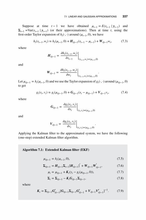
7.1 LINEAR AND GAUSSIAN APPROXIMATIONS 337
Suppose at time t − 1 we have obtained 𝜇t−1 = E(xt−1 ∣ yt−1) and𝚺t−1 =Var(xt−1 ∣ yt−1) (or their approximations). Then at time t, using thefirst-order Taylor expansion of ht(⋅, ⋅) around (𝜇t−1, 0), we have
ht(xt−1, wt) ≈ ht(𝜇t−1, 0) + Ht∣t−1(xt−1 − 𝜇t−1) + Wt∣t−1wt, (7.3)
where
Ht∣t−1 =𝜕ht(xt−1, wt)
𝜕xt−1
||||(xt−1,wt)=(𝜇t−1,0)
and
Wt∣t−1 =𝜕ht(xt−1, wt)
𝜕wt
||||(xt−1,wt)=(𝜇t−1,0).
Let 𝜇t∣t−1 = ht(𝜇t−1, 0) and we use the Taylor expansion of gt(⋅, ⋅) around (𝜇t∣t−1, 0)to get
gt(xt, vt) ≈ gt(𝜇t∣t−1, 0) + Gt∣t−1(xt − 𝜇t∣t−1) + Vt∣t−1vt, (7.4)
where
Gt∣t−1 =𝜕gt(xt, vt)
𝜕xt
||||(xt ,vt)=(𝜇t∣t−1,0)
and
Vt∣t−1 =𝜕gt(xt, vt)
𝜕vt
||||(xt ,vt)=(𝜇t∣t−1,0).
Applying the Kalman filter to the approximated system, we have the following(one-step) extended Kalman filter algorithm.
Algorithm 7.1: Extended Kalman filter (EKF)
𝜇t∣t−1 = ht(𝜇t−1, 0), (7.5)
𝚺t∣t−1 = Ht∣t−1𝚺t−1[Ht∣t−1]′ + Wt∣t−1W
′
t∣t−1, (7.6)
𝜇t = 𝜇t∣t−1 + Kt(yt − gt(𝜇t∣t−1, 0)), (7.7)
𝚺t = 𝚺t∣t−1 − KtGt∣t−1𝚺t∣t−1, (7.8)
where
Kt = 𝚺t∣t−1G′t∣t−1[Gt∣t−1𝚺t∣t−1G′
t∣t−1 + Vt∣t−1V′t∣t−1]−1. (7.9)

338 7. NONLINEAR STATE SPACE MODELS
The extended Kalman filter only uses the first-order Taylor expansions. Theapproximation accuracy can be poor in some cases. For example, (7.5) uses theapproximation in the form of
E(xt ∣ yt−1) = E(h(xt−1, wt) ∣ yt−1)
≈ h(E(xt−1 ∣ yt−1), E(wt ∣ yt−1))
= ht(𝜇t−1, 0).
For certain nonlinear functions ht(⋅), such an approximation should be avoided.One can extend the EKF to include the second-order terms in the Taylor expansionto obtain a better approximation. See Tanizaki (1996) and Roth and Gustafsson(2011) for further details.
The extended Kalman smoother is the same as the standard Kalman smoother,with the approximation (7.3). Note the Kalman smoother in Equations (6.32) and(6.33) only involves Ht+1.
7.1.3 Gaussian Sum Filters
Gaussian sum filters (GSFs) belong to the class of density-based filters in whichthe procedure concentrates on the propagation of the underlying distributionof the states of a nonlinear and non-Gaussian system. In GSFs, the underlyingconditional distribution of xt (given yt or yT ) is approximated by a mixturenormal distribution, and the system is locally linearized at the center of eachcomponent of the mixture distribution in the same way as that in the EKF.Hence GSFs can be viewed as a mixture of EKFs, providing improvements viausing a mixture Gaussian distribution to approximate the underlying conditionaldistribution, instead of a single Gaussian distribution. This extension has aclose relationship to the mixture Kalman filter algorithm, which is discussed inSection 8.6.2
Specifically, in the filtering case, assume p(xt−1 ∣ yt−1) is approximated by∑mj=1 wj,t−1N(𝜇j,t−1∣t−1,𝚺j,t−1∣t−1), where the mixture weights wj,t−1 are non-
negative and∑m
j=1 wj,t−1 = 1. At time t, each component j is updated using theEKF to N(𝜇j,t∣t,𝚺j,t∣t), with linear localization done around the jth component(𝜇j,t−1 and 𝜇j,t∣t−1), ignoring all other components. The weights need to be updatedas well. In the prediction step, each component j produces a prediction of y,𝜇
yj,t∣t−1
= gt(𝜇j,t∣t−1, 0), with a covariance matrix
𝚺yj,t = Gj,t∣t−1𝚺j,t∣t−1G′
j,t∣t−1 + Vj,t∣t−1V′j,t∣t−1.

7.1 LINEAR AND GAUSSIAN APPROXIMATIONS 339
Then the weight wj,t is updated using
wj,t =wj,t−1𝜙(y;𝜇y
j,t,𝚺yj,t∣t−1
)∑m𝑖=1 w𝑖,t−1𝜙(y;𝜇y
𝑖,t,𝚺y𝑖,t∣t−1
).
This is similar to Bayesian updating of the posterior proportion of mixture distri-butions. More detailed discussions can be found in Anderson and Moore (1979)and Sorenson and Alspach (1971).
7.1.4 The Unscented Kalman Filter
The GSF uses a mixture Gaussian distribution to approximate the underlying con-ditional distributions and has to rely on local linearization for the propagation ofeach Gaussian component of the mixture Gaussian distribution. An alternativeapproach is to use a discrete distribution to approximate the conditional distri-butions, with matching first and second moments. The discrete distribution can bepropagated through the nonlinear system without any local linearization. With acarefully constructed approximation, a Kalman-filter type of recursive updatingscheme can be used to obtain the conditional means and conditional variances ofthe filtering and smoothing distributions. The unscented Kalman filter (UKF) ofJulier and Uhlmann (1997, 2004) is such an algorithm.
Julier and Uhlmann (1997) noted that the first and second moments of Y = f (X),a nonlinear transformation of the random variable X, can be approximated by
𝜇y =m∑
𝑖=−m
w𝑖f (x𝑖) and 𝚺y =m∑
𝑖=−m
w𝑖(f (x𝑖) − 𝜇y)′(f (x𝑖) − 𝜇y),
where x𝑖, 𝑖 = −m,… , m is a set of points in the domain of X and w𝑖 is a set of pos-itive weights such that
∑𝑖 w𝑖 = 1,
∑𝑖 w𝑖x𝑖 = 𝜇x, and
∑𝑖 w𝑖(x𝑖 − 𝜇x)′(x𝑖 − 𝜇x) =
𝚺x, with given 𝜇x and 𝚺x. In addition, the covariance between X and Y = f (X) canbe approximated by
𝚺xy =m∑
𝑖=−m
w𝑖(f (x𝑖) − 𝜇y)′(x𝑖 − 𝜇x). (7.10)
The accuracy of such an approximation depends on the choice of (x𝑖, w𝑖). Julierand Uhlmann (1997) suggested using
x0 = 𝜇x; x±𝑖 = 𝜇x ±√
m + k√
𝚺x,𝑖;
w0 = km + k
; w±𝑖 =1
2(m + k), (7.11)

340 7. NONLINEAR STATE SPACE MODELS
where m is the dimension of x and√𝚺x,𝑖 is the 𝑖th column of the matrix square root
of 𝚺x. The authors showed that, with this construction, the approximation of 𝚺yis accurate to the second order. The extra parameter k can be used to match somehigher-order moments, if needed. Note that this approximation is deterministicand is different from using a (weighted) random sample of X to approximate thedistribution of X, which we will discuss in Chapter 8.
Consider the SSM model with additive noises:
xt = ht(xt−1) + Wtwt, (7.12)
yt = gt(xt) + Vtvt, (7.13)
where Var(wt) = I and Var(vt) = I. Armed with the discrete approximation inEquation (7.11), an unscented Kalman filter engages a Kalman-filter type of recur-sion. Specifically, suppose at time t − 1 we have obtained 𝜇t−1 and 𝚺t−1, witha corresponding discrete approximation (x𝑖,t−1, w𝑖,t−1), 𝑖 = −m,… , m. Then theKalman prediction step is carried out as
𝜇t∣t−1 =m∑
𝑖=−m
w𝑖,t−1h(x𝑖,t−1),
𝚺t∣t−1 =m∑
𝑖=−m
w𝑖,t−1(h(x𝑖,t−1) − 𝜇t∣t−1)′(h(x𝑖,t−1) − 𝜇t∣t−1) + W′tWt,
based on the designed approximation. With given 𝜇t∣t−1 and 𝚺t∣t−1, we obtain thenew set of (x𝑖,t∣t−1, w𝑖,t∣t−1), 𝑖 = −m,… , m, for the distribution p(xt ∣ yt−1), usingthe approximation in Equation (7.11). Then the updating step can be carried outby noting that the approximation in Equation (7.10) implies
𝚺xy,t∣t−1 = Cov(xt, yt ∣ yt−1) =m∑
𝑖=−m
w𝑖,t∣t−1(g(x𝑖,t∣t−1) − 𝜇(y)t∣t−1
)′(x𝑖,t∣t−1 − 𝜇t∣t−1),
where 𝜇(y)t∣t−1
=∑m𝑖=−m w𝑖,t∣t−1g(x𝑖,t∣t−1), and
𝚺yy,t∣t−1 = Var(yt ∣ yt−1)
=m∑
𝑖=−m
w𝑖,t∣t−1(g(x𝑖,t∣t−1) − 𝜇(y)t∣t−1
)′(g(x𝑖,t∣t−1) − 𝜇(y)t∣t−1
) + VtV′t .
Then the BLUEs of the first and second moments of p(xt ∣ yt) are
𝜇t∣t = 𝜇t∣t−1 + 𝚺xy,t∣t−1𝚺−1yy,t∣t−1(yt − 𝜇
(y)t∣t−1
),
𝚺t∣t = 𝚺t∣t−1 − 𝚺xy,t∣t−1𝚺−1yy,t∣t−1𝚺
′xy,t∣t−1.

7.1 LINEAR AND GAUSSIAN APPROXIMATIONS 341
The unscented Kalman smoother can be developed along the same lines as theKalman smoother.
7.1.5 Ensemble Kalman Filters
In many applications of SSMs, such as those in geophysics and climate model-ing, the dimension d of the underlying state variable xt can be extremely large,sometimes in the range of millions. In such cases, updating and storing the d × dfiltering and smoothing covariance matrices in the Kalman filter becomes an infea-sible task. The ensemble Kalman filter (EnKF) of Evensen (1994, 2003, 2007) is aclass of approximation methods in which the filtering (and smoothing) distributionis represented and stored by a set of samples (called ensembles) from the corre-sponding distributions. The number of samples m is assumed to be much smallerthan d, hence achieving dimension reduction. In EnKF, instead of updating theunderlying filtering and smoothing distributions, the ensembles are updated, mim-icking the updating procedure of the Kalman filter and UKF, and any inference iscarried out using the ensembles.
Assume that the SSM is linear and Gaussian,
xt = Htxt−1 + Wtwt,
yt = Gtxt + Vtvt.
Assume also that at time t − 1 we have stored an ensemble x(j)t−1, j = 1,… , m such
that x(j)t−1 ∼ N(𝜇t−1,𝚺t−1) = p(xt−1 ∣ yt−1). At time t, we have the prediction step
x(j)t∣t−1
= Htx(j)t−1 + Wtw
(j)t ,
where w(j)t is simulated from N(0, I). Then x(j)
t∣t−1∼ N(𝜇t∣t−1,𝚺t∣t−1). The corre-
sponding (would-be) realization of yt is y(j)t = Gtx
(j)t∣t−1
+ Vtv(j)t , where v(j)
t is sim-ulated from N(0, I). Next the update step can be achieved by
x(j)t = x(j)
t∣t−1+ Kt(yt − y(j)
t )
where Kt is the Kalman gain matrix in Equation (6.29). It can easily be shown thatx(j)
t ∼ N(𝝁t,𝚺t).However, the above updating step requires knowing the Kalman gain matrix Kt,
which requires knowing the high dimensional 𝚺t∣t−1, something we try to avoid inthe first place. In practice, an estimate of 𝚺t∣t−1 based on the sample covariance
matrix of the predicted x(j)t∣t−1
is used. (In fact, a more accurate estimate is the sam-
ple covariance matrix of Hx(j)t−1 plus WtW
′t .) Since m is much smaller than d, the
rank of the estimator is much smaller than that of 𝚺t∣t−1, inducing some bias. Often

342 7. NONLINEAR STATE SPACE MODELS
the covariance inflation (Anderson, 2007) and localization (Furrer et al., 2006)techniques are used to improve the accuracy and stabilize the algorithm.
The updating step can be approximated with a deterministic approach as well.See Tippett et al. (2003), Anderson (2001), and Bishop et al. (2001). Smoothingand parameter estimation using EnKF have been studied by Stroud et al. (2010).EnKF can be used in conjunction with the EKF for nonlinear and non-Gaussiansystems.
7.1.6 Examples and R implementations
In this section we consider some examples and the associated analyses using Rpackages.
Example 7.1: Bearings-only tracking using the EKF In Section 6.2.4 webriefly introduced the problem of tracking a target with passive sonars, in whichthe observations are the bearing of the target related to the sensors, but no dis-tance information can be obtained. The system is nonlinear. Here we present animplementation of filtering and smoothing using EKF.
Suppose two sensors are placed as 𝜂1 = (0, 0) and 𝜂2 = (20, 0). A target moveswith a random acceleration with variance 0.032 in both directions and ΔT = 1.Figure 7.1 shows a simulated trajectory for t = 1,… , 200, which contains a
0 10 20 30 40
−20
−10
010
20
x
y
Figure 7.1 Trajectory of a simulated target. Two sensors are marked by solid squares.

7.1 LINEAR AND GAUSSIAN APPROXIMATIONS 343
−0.4 −0.2 0.0 0.2 0.4 0.6 0.8
−1.
5−
1.0
−0.
50.
00.
51.
01.
5
phi 1
phi 2
Figure 7.2 Observed bearings of a simulated target by two sensors.
sharp turn in the middle of the observational period. Assume that the sensorshave measurement errors e1t and e2t that follow N(0, 0.022). Figure 7.2 showsthe observed bearings (y1t, y2t). The bearings are restricted to [−𝜋∕2,𝜋∕2]by modulation. The jump of the path in the middle is due to the modulation.Figure 7.3 shows the true simulated trajectory, and the filtered and the smoothedtrajectories from t = 100 to 200, the more difficult part of the tracking task dueto the turns. Tracking is actually quite accurate during the first sharp turn, butbecomes less accurate during the second turn. Smoothing was able to correctsome of the filtering errors. Note that the largest errors are in the x direction,when the target is close to the x axis. This is because both sensors are placedon the x axis, hence the angles are small when the target is close to the x axis.During this period, the signal-to-noise ratio is small, resulting in large trackingerrors.
Figures 7.4 and 7.5 show the tracking errors of locations in the x and y direc-tions, respectively. Figures 7.6 and 7.7 show the tracking errors of speeds in thex and y directions, respectively. It is seen that the error in the x direction is largerthan that of the y direction, again due to the placement of the sensors.
The following R codes are used in the example. Note that in this particularinstance, the state equation is linear and Gaussian. Hence, to use EKF, approxi-mation is only needed for the observation equation, in the form of Equation (7.4).

344 7. NONLINEAR STATE SPACE MODELS
28 30 32 34
−15
−10
−5
05
10
x
y
truefilteredsmoothed
Figure 7.3 The filtered and smoothed trajectories of a simulated target, for t =100,… , 200.
0 50 100 150 200
−1
01
2
Time
Err
or
Filtering errorSmoothing error
Figure 7.4 Tracking error in x direction locations.

7.1 LINEAR AND GAUSSIAN APPROXIMATIONS 345
0 50 100 150 200
−1.
0−
0.5
0.0
0.5
Time
Err
or
Filtering errorSmoothing error
Figure 7.5 Tracking error in y direction locations.
0 50 100 150 200
−0.
2−
0.1
0.0
0.1
0.2
0.3
Time
Err
or
Filtering errorSmoothing error
Figure 7.6 Tracking error in x direction speeds.

346 7. NONLINEAR STATE SPACE MODELS
0 50 100 150 200
−0.
20.
00.
20.
4
Time
Err
or
Filtering errorSmoothing error
Figure 7.7 Tracking error in y direction speeds.
Specifically, with two sensors located at 𝜂𝑖 = (𝜂𝑖1, 𝜂𝑖2) (𝑖 = 1, 2), and with given𝜇t∣t−1 = (𝜇1,t∣t−1,𝜇2,t∣t−1,𝜇3,t∣t−1,𝜇4,t∣t−1), we have
Gt∣t−1 =
⎡⎢⎢⎢⎢⎣−
𝜏1,t∣t−1
(1 + 𝜏21,t∣t−1
)(𝜇1,t∣t−1 − 𝜂11)
1
(1 + 𝜏21,t∣t−1
)(𝜇1,t∣t−1 − 𝜂11)0 0
−𝜏2,t∣t−1
(1 + 𝜏22,t∣t−1
)(𝜇1,t∣t−1 − 𝜂21)
1
(1 + 𝜏22,t∣t−1
)(𝜇1,t∣t−1 − 𝜂21)0 0
⎤⎥⎥⎥⎥⎦,
where
𝜏𝑖,t∣t−1 =𝜇2,t∣t−1 − 𝜂𝑖2𝜇1,t∣t−1 − 𝜂𝑖1
, 𝑖 = 1, 2.
The function simPassiveSonar generates a sample trajectory of the tar-get and the corresponding observations, with sensor locations at (0, 0) and(20, 0). The functions KF1pred, KF1update and KF1smoother perform one-step ahead prediction in Equations (6.25) and (6.26), one-step updating in Equa-tions (6.27) and (6.28), and one-step smoothing in Equations (6.32) and (6.33), ofthe Kalman filter and Kalman smoothing, respectively. The functions EKF1predand EKF1update perform one-step ahead prediction and updating of EKF inEquations (7.5) to (7.6), respectively. In our setting, since the state equation is lin-ear and Gaussian, only EKF1update is used. In addition, since the state transition

7.1 LINEAR AND GAUSSIAN APPROXIMATIONS 347
matrix Ht does not change and there is no approximation, the extended Kalmansmoother is the same as the Kalman smoother.
R demonstration: Extended Kalman filter.
## 2-D passive sonar tracking example
###
# function to simulate the data
###
simPassiveSonar=function(nn=200,q,r,start,s2,seed){
set.seed(seed)
### s2 : second sonar location at (s2,0)
H <- c(1,0,1,0,
0,1,0,1,
0,0,1,0,
0,0,0,1)
H <- matrix(H,ncol=4,nrow=4,byrow=T)
G <- c(1,0,0,0,
0,1,0,0)
G <- matrix(G,ncol=4,nrow=2,byrow=T)
W <- c(0.5*q[1], 0,
0, 0.5*q[2],
q[1],0,
0,q[2])
W <- matrix(W,ncol=2,nrow=4,byrow=T)
V <- diag(r)
x <- matrix(nrow=4,ncol=nn)
y <- matrix(nrow=2,ncol=nn)
for(ii in 1:nn){
if(ii == 1) x[,ii] <- start
if(ii > 1) x[,ii] <- H%*%x[,ii-1]+W%*%rnorm(2)
y[1,ii] <- atan(x[2,ii]/x[1,ii])
y[2,ii] <- atan(x[2,ii]/(x[1,ii]-s2))
y[,ii] <- y[,ii]+V%*%rnorm(2)
y[,ii] <- (y[,ii]+0.5*pi)%%pi-0.5*pi
}
return(list(xx=x,yy=y,G=G,H=H,W=W,V=V))
}
####
### KF-single step ahead prediction
####
KF1pred=function(mu,SS,HH,bb,WW){
mu <- HH%*%mu+bb
SS <- HH%*%SS%*%t(HH)+WW%*%t(WW)
return(list(mu=mu,SS=SS))
}

348 7. NONLINEAR STATE SPACE MODELS
####
### KF-single step update, no likelihood
####
KF1update=function(mu,SS,yy,GG,cc,VV){
KK <- SS%*%t(GG)%*%solve(GG%*%SS%*%t(GG)+VV%*%t(VV))
mu <- mu+KK%*%(yy-cc-GG%*%mu)
SS <- SS-KK%*%GG%*%SS
return(list(mu=mu,SS=SS))
}
####
### KF-single step smoother
####
KF1smoother=function(mu,SS,mu1,SS1,muT,SST,HH,VV){
JJ <- SS%*%HH%*%solve(SS1)
mu <- mu+JJ%*%(muT-mu1)
SS <- SS+JJ%*%(SST-SS1)%*%t(JJ)
return(list(mu=mu,SS=SS))
}
####
### EKF-single step ahead prediction, with input mu_pred
####
EKF1pred=function(mu,SS,HH,bb,WW){
SS <- HH%*%SS%*%t*t(HH)+WW%*%t(WW)
return(list(mu=mu,SS=SS))
}
####
### EKF-single step update, with input yy_pred, no likelihood
####
EKF1update=function(mu,SS,yy,yy_pred,GG,VV){
KK <- SS%*%t(GG)%*%solve(GG%*%SS%*%t(GG)+VV%*%t(VV))
res <- (yy-yy_pred+0.5*pi)%%pi-0.5*pi
mu <- mu+KK%*%res
SS <- SS-KK%*%GG%*%SS
return(list(mu=mu,SS=SS))
}
##### KF for passive sonar
## parameters
s2 <- 20 #second sonar location at (s2,0)
q <- c(0.03,0.03)
r <- c(0.02,0.02)
nn <- 200
## simulation
start <- c(10,10,0.01,0.01)
simu_out <- simPassiveSonar(nn,q,r,start,s2,seed=20)
yy <- simu_out$yy

7.1 LINEAR AND GAUSSIAN APPROXIMATIONS 349
## parameter for filtering and smoothing
HH <- c(1,0,1,0,
0,1,0,1,
0,0,1,0,
0,0,0,1)
HH <- matrix(HH,ncol=4,nrow=4,byrow=T)
WW <- c(0.5*q[1], 0,
0, 0.5*q[2],
q[1],0,
0,q[2])
WW <- matrix(WW,ncol=2,nrow=4,byrow=T)
GG <- matrix(rep(0,8),ncol=4,nrow=2)
VV <- diag(r)
## setup storage
muall <- matrix(nrow=4,ncol=nn)
mu1all <- matrix(nrow=4,ncol=nn)
muTall <- matrix(nrow=4,ncol=nn)
SSall <- array(dim=c(4,4,nn))
SS1all <- array(dim=c(4,4,nn))
SSTall <- array(dim=c(4,4,nn))
##initial value
mu0 <- c(10,10,0.1,0.1)
SS0 <- diag(c(1,1,1,1))*10000
bb <- 0*mu0
yy_pred <- yy[,1]*0
##start
for(ii in 1:nn){
if(ii==1) out_pred <- KF1pred(mu0,SS0,HH,bb,WW)
if(ii > 1) out_pred <- KF1pred(muall[,ii-1],SSall[„ii-1],HH,bb,WW)
mu1all[,ii] <- out_pred$mu
SS1all[„ii] <- out_pred$SS
temp1 <- mu1all[2,ii]/mu1all[1,ii]
temp2 <- mu1all[2,ii]/(mu1all[1,ii]-s2)
yy_pred[1] <- atan(temp1)
yy_pred[2] <- atan(temp2)
GG[1,1] <- -mu1all[2,ii]/(1+temp1**2)/mu1all[1,ii]**2
GG[1,2] <- 1/(1+temp1**2)/mu1all[1,ii]
GG[2,1] <- -mu1all[2,ii]/(1+temp2**2)/(mu1all[1,ii]-s2)**2
GG[2,2] <- 1/(1+temp2**2)/(mu1all[1,ii]-s2)
out_update <- EKF1update(mu1all[,ii],SS1all[„ii],yy[,ii],yy_pred,GG,VV)
muall[,ii] <- out_update$mu
SSall[„ii] <- out_update$SS
}
### smoothing
muTall[,nn] <- muall[,nn]

350 7. NONLINEAR STATE SPACE MODELS
SSTall[„nn] <- SSall[„nn]
for(ii in (nn-1):1){
out_smooth <- KF1smoother(muall[,ii],SSall[„ii],
mu1all[,ii+1],SS1all[„ii+1],
muTall[,ii+1],SSTall[„ii+1],HH,VV)
muTall[,ii] <- out_smooth$mu
SSTall[„ii] <- out_smooth$SS
}
### Plotting
plot(simu_out$xx[1,],simu_out$xx[2,],type='l',lwd=2,
xlim=c(0,40),ylim=c(-20,20),xlab="x",ylab="y")
points(c(0,s2),c(0,0),pch=15,cex=2)
title("target trajectory")
#Figure 7.1
plot(simu_out$yy[1,],simu_out$y[2,],type='l',lwd=2,
xlab="phi 1",ylab="phi 2")
title("observed bearings")
#Figure 7.2
tt <- 100:200
plot(simu_out$xx[1,tt],simu_out$xx[2,tt],xlab="x",ylab="y",
ylim=c(-18,13),xlim=c(26,34))
title("target trajectory, filtering and smoothing")
lines(muall[1,tt],muall[2,tt])
lines(muTall[1,tt],muTall[2,tt],lty=2)
legend(32,10,legend=c("true","filtered","smoothed"),
pch=c(1,NA,NA),lty=c(0,1,2))
#Figure 7.3
plot(simu_out$xx[1,]-muall[1,],ylab='error',xlab='time')
lines(simu_out$xx[1,]-muTall[1,])
abline(h=0,lty=2)
title("x-director tracking error")
legend(2,2.3,legend=c("filtering error","smoothing error"),
pch=c(1,NA),lty=c(0,1))
#Figure 7.4
plot(simu_out$xx[2,]-muall[2,],ylab='error',xlab='time')
lines(simu_out$xx[2,]-muTall[2,])
abline(h=0,lty=2)
title("y-director tracking error")
legend(2,-0.7,legend=c("filtering error","smoothing error"),
pch=c(1,NA),lty=c(0,1))
#Figure 7.5

7.2 HIDDEN MARKOV MODELS 351
plot(simu_out$xx[3,]-muall[3,],ylab='error',xlab='time')
lines(simu_out$xx[3,]-muTall[3,])
abline(h=0,lty=2)
title("x-director speed error")
legend(2,0.27,legend=c("filtering error","smoothing error"),
pch=c(1,NA),lty=c(0,1))
#Figure 7.6
plot(simu_out$xx[4,]-muall[4,],ylab='error',xlab='time')
lines(simu_out$xx[4,]-muTall[4,])
abline(h=0,lty=2)
title("y-director speed error")
legend(150,0.5,legend=c("filtering error","smoothing error"),
pch=c(1,NA),lty=c(0,1))
#Figure 7.7
7.2 HIDDEN MARKOV MODELS
The HMM is a special case of the Markovian SSM in Equations (6.3) and (6.4),when the state xt is a Markov chain taking values in a discrete set {𝜂1,… , 𝜂K}.The state equation is specified by the conditional transition probability matrix P.Specifically, an HMM takes the form
xt ∼ Markov chain(P), (7.14)
yt = gt(xt, et) or yt ∼ ft(⋅ ∣ xt), (7.15)
where the (𝑖, j)th element of the transition probability matrix P is p[𝑖, j] = p(xt =𝜂j ∣ xt−1 = 𝜂𝑖).
HMM has a wide range of applications in various scientific fields. In time seriesanalysis, the Markov switching autoregressive model is one of the most commonlyused HMMs. A detailed treatment of such a model with K = 2 has been given inChapter 2, in parallel with the threshold AR model.
7.2.1 Filtering
Filtering of the state of an HMM gives the marginal probability pt∣t[𝑖] = p(xt =𝜂𝑖 ∣ yt). It can be carried out similarly to the approach of the Kalman filter, exceptit is done in discrete space under the transition matrix P. Specifically, at time t − 1

352 7. NONLINEAR STATE SPACE MODELS
suppose we have obtained pt−1∣t−1[𝑖] = p(xt−1 = 𝜂𝑖 ∣ yt−1) for 𝑖 = 1,… , K. Thenthe predictive probability is
pt∣t−1[j] = p(xt = 𝜂j ∣ yt−1)
=K∑𝑖=1
p(xt = 𝜂j ∣ xt−1 = 𝜂𝑖)p(xt−1 = 𝜂𝑖 ∣ yt−1)
=K∑𝑖=1
p[𝑖, j]pt−1∣t−1[𝑖].
To incorporate the new information yt, we note that
pt∣t[𝑖] = p(xt = 𝜂𝑖 ∣ yt−1, yt)
∝ p(yt ∣ xt = 𝜂𝑖, yt−1)p(xt = 𝜂𝑖 ∣ yt−1)
= ft(yt ∣ xt = 𝜂𝑖)pt∣t−1[𝑖].
Hence, we have the update equation
pt∣t[𝑖] =ft(yt ∣ xt = 𝜂𝑖)pt∣t−1[𝑖]∑Kj=1 ft(yt ∣ xt = 𝜂j)pt∣t−1[j]
, 𝑖 = 1,… , K.
In summary, suppose at time t − 1 we have obtained pt−1∣t−1[𝑖] = p(xt−1 = 𝜂𝑖 ∣yt−1). Then the one-step HMM filter at time t is as follows.
Algorithm 7.2: HMM filtering
pt∣t−1[j] =K∑𝑖=1
p[𝑖, j]pt−1∣t−1[𝑖], j = 1,… , K
pt∣t[𝑖] =ft(yt ∣ xt = 𝜂𝑖)pt∣t−1[𝑖]∑Kj=1 ft(yt ∣ xt = 𝜂j)pt∣t−1[j]
, 𝑖 = 1,… , K.
7.2.2 Smoothing
Smoothing of an HMM gives the marginal distribution of the state given the entireobserved series, i.e. pt∣T [𝑖] = p(xt = 𝜂𝑖 ∣ yT ). It can be done by using a proceduresimilar to the forward and backward two-pass disentanglement of the Kalman

7.2 HIDDEN MARKOV MODELS 353
smoother. Specifically, we first carry out the forward filtering from t = 1 to T andobtain pt∣t[𝑖] for 𝑖 = 1,… , K, t = 1,… , T . We then use the disentanglement oper-ation by inserting xt+1. Specifically, we notice that
pt∣T [𝑖] = p(xt = 𝜂𝑖 ∣ yT )
=K∑
j=1
p(xt = 𝜂𝑖 ∣ xt+1 = 𝜂j, yT )p(xt+1 = 𝜂j ∣ yT )
=K∑
j=1
p(xt = 𝜂𝑖 ∣ xt+1 = 𝜂j, yt)p(xt+1 = 𝜂j ∣ yT )
=K∑
j=1
pt+1∣T [j]𝛾t[𝑖, j],
where
𝛾t[𝑖, j] = p(xt = 𝜂𝑖 ∣ xt+1 = 𝜂j, yt)
=p(xt = 𝜂𝑖, xt+1 = 𝜂j ∣ yt)
p(xt+1 = 𝜂j ∣ yt)
=p(xt+1 = 𝜂j ∣ xt = 𝜂𝑖, yt)p(xt = 𝜂𝑖 ∣ yt)
p(xt+1 = 𝜂j ∣ yt)
=p[𝑖, j]pt∣t[𝑖]∑K
𝓁=1 p[𝓁, j]pt∣t[𝓁]. (7.16)
In summary, we have the following algorithm.
Algorithm 7.3: HMM smoothing
For t = T − 1,… , 1,
pt∣T [𝑖] =K∑
j=1
pt+1∣T [j]𝛾t[𝑖, j]
where
𝛾t[𝑖, j] =p[𝑖, j]pt∣t[𝑖]∑K
𝓁=1 p[𝓁, j]pt∣t[𝓁].

354 7. NONLINEAR STATE SPACE MODELS
Another approach is to use p(yt+1,… , yT ∣ xt = 𝜂𝑖). Specifically, we have
pt∣T [𝑖] = p(xt = 𝜂𝑖 ∣ yT )
∝ p(yt+1,… , yT ∣ xt = 𝜂𝑖)p(xt = 𝜂𝑖 ∣ yt)
∝ p(yt+1,… , yT ∣ xt = 𝜂𝑖)pt∣t[𝑖].
Let
𝛽t[𝑖] = p(yt+1,… , yT ∣ xt = 𝜂𝑖).
Starting with 𝛽T [𝑖] = 1, for 𝑖 = 1,… , K, and by inserting xt+1, we have, for t =T − 1, T − 2,… , 1,
𝛽t[𝑖] = p(yt+1,… , yT ∣ xt = 𝜂𝑖)
=K∑
j=1
p(yt+1,… , yT ∣ xt+1 = 𝜂j, xt = 𝜂𝑖)p(xt+1 = 𝜂j ∣ xt = 𝜂𝑖)
=K∑𝑖=1
p(yt+1,… , yT ∣ xt+1 = 𝜂j)p(xt+1 = 𝜂j ∣ xt = 𝜂𝑖)
=K∑𝑖=1
p(yt+2,… , yT ∣ yt+1, xt+1 = 𝜂j)p(yt+1 ∣ xt+1 = 𝜂j)p[𝑖, j]
=K∑𝑖=1
𝛽t+1[j]p[𝑖, j]ft(yt+1 ∣ xt+1 = 𝜂j).
Hence we have the following algorithm.
Algorithm 7.4: HMM smoothing (II)
Starting with 𝛽T [𝑖] = 1, for 𝑖 = 1,… , K, let
𝛽t[𝑖] =K∑𝑖=1
𝛽t+1[j]p[𝑖, j]ft(yt+1 ∣ xt+1 = 𝜂j)
and
pt∣T [𝑖] =𝛽t[𝑖]pt∣t[𝑖]∑K
k=1 𝛽t[k]pt∣t[k].
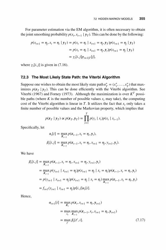
7.2 HIDDEN MARKOV MODELS 355
For parameter estimation via the EM algorithm, it is often necessary to obtainthe joint smoothing probability p(xt, xt−1 ∣ yT ). This can be done by the following:
p(xt+1 = 𝜂j, xt = 𝜂𝑖 ∣ yT ) = p(xt = 𝜂𝑖 ∣ xt+1 = 𝜂j, yT )p(xt+1 = 𝜂j ∣ yT )
= p(xt = 𝜂𝑖 ∣ xt+1 = 𝜂j, yt)p(xt+1 = 𝜂j ∣ yT )
= 𝛾t[𝑖, j]pt+1∣T [j],
where 𝛾t[𝑖, j] is given in (7.16).
7.2.3 The Most Likely State Path: the Viterbi Algorithm
Suppose one wishes to obtain the most likely state path s∗T = (x∗1,… , x∗T ) that max-imizes p(xT ∣ yT ). This can be done efficiently with the Viterbi algorithm. SeeViterbi (1967) and Forney (1973). Although the maximization is over KT possi-ble paths (where K is the number of possible values xt may take), the computingcost of the Viterbi algorithm is linear in T . It utilizes the fact that xt only takes afinite number of possible values and the Markovian property, which implies that
p(xT ∣ yT ) ∝ p(xT , yT ) =T∏
t=1
p(yt ∣ xt)p(xt ∣ xt−1).
Specifically, let
𝛼t[𝑖] = maxxt−1
p(xt−1, xt = 𝜂𝑖, yt),
𝛽t[𝑖, j] = maxxt−1
p(xt−1, xt = 𝜂𝑖, xt+1 = 𝜂j, yt+1, yt).
We have
𝛽t[𝑖, j] = maxxt−1
p(xt−1, xt = 𝜂𝑖, xt+1 = 𝜂j, yt+1, yt)
= maxxt−1
p(yt+1 ∣ xt+1 = 𝜂j)p(xt+1 = 𝜂j ∣ xt = 𝜂𝑖)p(xt−1, xt = 𝜂𝑖, yt)
= p(yt+1 ∣ xt+1 = 𝜂j)p(xt+1 = 𝜂j ∣ xt = 𝜂𝑖)maxxt−1
p(xt−1, xt = 𝜂𝑖, yt)
= ft+1(yt+1 ∣ xt+1 = 𝜂j)p[𝑖, j]𝛼t[𝑖].
Hence,
𝛼t+1[𝑖] = maxxt
p(xt, xt+1 = 𝜂𝑖, yt+1)
= maxxt
maxxt−1
p(xt−1, xt, xt+1 = 𝜂𝑖, yt+1)
= max𝓁𝛽t[𝓁, 𝑖]. (7.17)

356 7. NONLINEAR STATE SPACE MODELS
Let 𝛼1[𝑖] = f1(y1 ∣ x1 = 𝜂𝑖)p[𝑖] and x∗1[𝑖] = 𝜂𝑖, for 𝑖 = 1,… , K, and iterating fromt = 1,… , T , we obtain x∗t [𝑖] = (x∗t−1[𝓁∗
𝑖], 𝜂𝑖) where 𝓁∗
𝑖is the index 𝓁 that maxi-
mizes 𝛽t[𝓁, 𝑖] in Equation (7.17). Once we reach T , let 𝑖∗ be the index that maxi-mized 𝛼T [𝑖], then the most likely path is x∗T [𝑖∗].
In summary, we have the following algorithm.
Algorithm 7.5: Viterbi algorithm
� Let 𝛼1[𝑖] = f1(y1 ∣ x1 = 𝜂𝑖)p[𝑖] and x∗1[𝑖] = 𝜂𝑖,
� For t = 1,… , T , let
𝛽t[𝑖, j] = ft+1(yt+1 ∣ xt+1 = 𝜂j)p[𝑖, j]𝛼t[𝑖].
𝛼t+1[𝑖] = max𝓁𝛽t[𝓁, 𝑖].
𝓁∗t [𝑖] = argmax
𝓁𝛽t[𝓁, 𝑖]
x∗t [𝑖] = (x∗t−1[𝓁∗t [𝑖]], 𝜂𝑖).
for 𝑖 = 1,… , K, j = 1,… , K.
� Let 𝑖∗ be the index that maximized 𝛼T [𝑖], then the most likely path isx∗T [𝑖∗].
This algorithm belongs to a larger class of algorithms called dynamic program-ming (Bellman, 2003) and is useful in many applications.
7.2.4 Parameter Estimation: the Baum–Welch Algorithm
To estimate the unknown parameters of the HMM model in Equations (7.14) and(7.15), including the transition probability P and unknown parameters in ft(⋅),the EM algorithm of Dempster et al. (1977) can be used. This procedure is alsoreferred to as the Baum–Welch algorithm. See Baum and Petrie (1966), Baumet al. (1970), and Baggenstoss (2001). For convergence of the EM algorithm, seeWu (1983).
Specifically, the full data log likelihood function is
ln p(xT , yT , 𝜃) =T∑
t=1
ln p(xt ∣ xt−1, 𝜃) +T∑
t=1
ln p(yt ∣ xt, 𝜃).
The EM algorithm requires us to obtain the 𝜃 that maximizesE[ln p(xT , yT , 𝜃 ∣ yT , 𝜃∗)]
= E
[T∑
t=1
ln p(xt ∣ xt−1, 𝜃) ∣ yT , 𝜃∗]+ E
[T∑
t=1
ln p(yt ∣ xt, 𝜃) ∣ yT , 𝜃∗]
,(7.18)
where 𝜃∗ is the parameter value of the current iteration.

7.2 HIDDEN MARKOV MODELS 357
The evaluation of E[ln p(xt ∣ xt−1, yT , 𝜃∗)] involves the joint smoothing proba-bilities p(xt, xt−1 ∣ yT ) in Section 7.2.2, that is,
p(xt ∣ xt−1, yT , 𝜃∗) =p(xt, xt−1 ∣ yT , 𝜃∗)
p(xt−1 ∣ yT , 𝜃∗)=𝛾t[𝑖, j]pt+1∣T [j]
pt∣T [𝑖],
where 𝛾t[𝑖, j] and pt∣T [𝑖] are given in Section 7.2.2, obtained under 𝜃∗. Since thesecond summation in Equation (7.18) does not involve the transition matrix, onecan maximize the first term to obtain an updated estimate of p[𝑖, j] using
p[𝑖, j] =∑T
t=1 p(xt = 𝜂𝑖, xt+1 = 𝜂j ∣ yT , 𝜃∗)∑Tt=1
∑K𝓁=1 p(xt = 𝜂𝓁 , xt+1 = 𝜂j ∣ yT , 𝜃∗)
.
To evaluate the second summation, we notice that
E
[T∑
t=1
ln p(yt ∣ xt, 𝜃 ∣ yT , 𝜃∗)
]=
T∑t=1
E
[K∑𝑖=1
I(xt = 𝜂𝑖) ln p(yt ∣ xt = 𝜂𝑖, 𝜃 ∣ yT , 𝜃∗)
]
=T∑
t=1
K∑𝑖=1
E[I(xt = 𝜂𝑖) ∣ yT , 𝜃∗] ln p(yt ∣ xt = 𝜂𝑖, 𝜃)
=T∑
t=1
K∑𝑖=1
pt∣T [𝑖] ln ft(yt ∣ xt = 𝜂𝑖, 𝜃).
This term only involves the parameters in the observation Equation (7.15) and canbe viewed as a weighted sum (or finite mixture) of the likelihood of the obser-vations. For complex observations, the Newton–Raphson method can be used toupdate the parameters. For simpler cases, the maximum can be obtained analyt-ically. For example, if yt is also discrete, taking values in {𝜉1,… , 𝜉M} and theunknown parameters are the assignment probability p∗[𝑖, j] = p(yt = 𝜉j ∣ xt = 𝜂𝑖),then they can be estimated by
p∗[𝑖, j] =∑T
t=1∑K𝑖=1 pt∣n[𝑖]I(yt = 𝜉j)∑T
t=1
∑K𝑖=1 pt∣n[𝑖]
,
for 𝑖 = 1,… , K and j = 1,… , M.For a hidden Markov mixture Gaussian model with ft(yt ∣ xt = 𝜂𝑖) ∼ N(𝜇𝑖,𝚺𝑖),
we have
��𝑖 =∑T
t=1 pt∣n[𝑖]yt∑Tt=1 pt∣n[𝑖]
and ��𝑖 =∑T
t=1 pt∣n[𝑖](yt − ��𝑖)(yt − ��𝑖)′∑Tt=1 pt∣n[𝑖]
.
A hidden Markov regression model with Gaussian errors can be written as
yt = z′t𝛽𝑖 + 𝜎𝑖et, if xt = 𝑖,

358 7. NONLINEAR STATE SPACE MODELS
where xt is the regime indicator, zt is a set of observed (p-dimensional) co-variates,and (𝛽𝑖, 𝜎
2𝑖) are the corresponding coefficients and noise variance in the 𝑖th regime.
When zt includes the lag variables of yt, this model becomes the Markov switchingautoregressive model we discussed in detail in Section 2.3.
In this case, the observation equation is ft(yt ∣ xt = 𝑖) ∼ N(zt𝛽𝑖, 𝜎2𝑖). We have
𝛽𝑖 =
(T∑
t=1
pt∣n[𝑖]z′t zt
)−1 ( T∑t=1
pt∣n[𝑖]z′tyt
)and ��2
𝑖 =∑T
t=1 pt∣n[𝑖](yt − zt𝛽𝑖)2∑T
t=1 pt∣n[𝑖].
7.2.5 HMM Examples and R Implementation
In this section we show two detailed examples of applying HMMs.
Example 7.2: Multi-regime stock return mean and volatility The stock mar-ket often shows periods of growth (bull market), neutral, and contraction (bearmarket). It is commonly expected that the mean and volatility of stock returns aredifferent in different periods. A hidden Markov mixture Gaussian model can beused to model such phenomenon.
Figure 7.8(a) shows the monthly log return of S&P 500 index from January1987 to December 2016. The associated histogram is shown in Figure 7.8(b), indi-cating clearly certain non-normality in the log returns. A Markovian three-statemixture Gaussian model, xt ∼ N(𝜇It
, 𝜎2It
) with It ∈ {1, 2, 3} is fitted to the datausing the Baum–Welch algorithm. The estimated transition probability matrix andthe estimated parameters of the normal distribution in each regime are shown inTables 7.1 and 7.2.
It can be seen from the estimated parameters that state 1 corresponds to a statewith a negative average return and high volatility. State 2 has a medium positive
1990 2000 2010
−0.
100.
000.
05
Time
SP
500
SP
Fre
quen
cy
−0.10 −0.05 0.00 0.05
010
2030
4050
Figure 7.8 Log returns of monthly S&P 500 index and their histogram. The period isfrom January 1987 to December 2016.

7.2 HIDDEN MARKOV MODELS 359
State 1 State 2 State 3
𝜇 −0.0216 0.005 0.0068𝜎 0.0303 0.0099 0.0185
Table 7.1 Parameter estimates of fitting athree-state HMM to the monthly log returns of theS&P 500 Index from 1987.1 to 2016.12.
state 1 2 3
1 0.638 0 0.3622 0 0.972 0.0283 0.0663 0.0264 0.907
Table 7.2 Estimated state transition probabilitymatrix of fitting a three-state HMM to the monthlylog returns of the S&P 500 Index from 1987.1 to2016.12.
mean return and low volatility, and state 3 has the largest positive mean returnwith medium volatility. Furthermore, state 1 represents a relatively rare state sinceits probability to transit out to other states is large. States 2 and 3 are relativelystable, with state 2 being the most persistent one. Most interestingly, state 1 onlytransits to state 3 (from negative mean return with high volatility to positive meanreturn with medium volatility). Such a mean-reverting phenomenon has been welldocumented in the finance literature. It is also interesting to see that there exists acertain probability for a bull market to be followed by a bear market.
Figure 7.9 shows the smoothed probabilities of P(It = k) for k = 1, 2, 3. It isreassuring to see that state 1 occurs only occasionally whereas the other two statesare relatively stable. Figure 7.10 shows the estimated most likely states using theViterbi algorithm. The corresponding smoothed probabilities of each state on themost likely path are shown in Figure 7.11. Some of these states have marginalsmoothed probability less than 0.5.
Figure 7.12 compares the partial autocorrelation function (PACF) of thesquared residuals of the fitted three-state HMM model (a) and that of the squaredS&P 500 return series (b). Figure 7.13 compares the normal Q-Q plots of the resid-ual series (a) and the original series (b). It seems that the fitted HMM model iseffective in handling the autocorrelations in the squared return series and its resid-uals follow more closely a Gaussian distribution.
A two-state HMM and a four-state HMM were also fitted to the log returnseries. For the two-state HMM model, the estimation results show that in
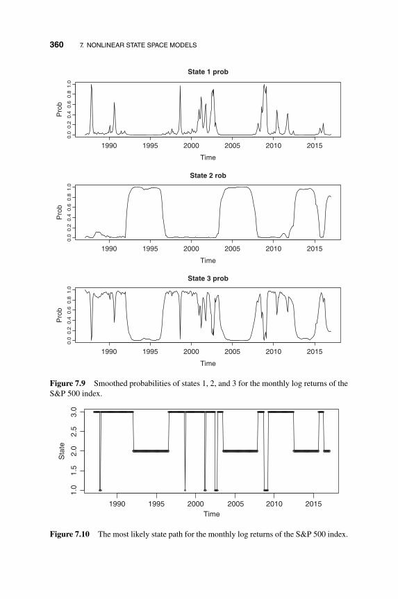
360 7. NONLINEAR STATE SPACE MODELS
1990 1995 2000 2005 2010 2015
0.0
0.2
0.4
0.6
0.8
1.0
State 1 prob
Time
1990 1995 2000 2005 2010 2015
Time
1990 1995 2000 2005 2010 2015
Time
Pro
b0.
00.
20.
40.
60.
81.
0
State 2 rob
Pro
b0.
00.
20.
40.
60.
81.
0
State 3 prob
Pro
b
Figure 7.9 Smoothed probabilities of states 1, 2, and 3 for the monthly log returns of theS&P 500 index.
1990 1995 2000 2005 2010 2015
1.0
1.5
2.0
2.5
3.0
Time
Sta
te
Figure 7.10 The most likely state path for the monthly log returns of the S&P 500 index.

7.2 HIDDEN MARKOV MODELS 361
1990 1995 2000 2005 2010 2015
0.0
0.4
0.8
Time
Pro
babi
lity
Figure 7.11 Smoothed probabilities of states on the most likely path for the monthly logreturns of the S&P 500 index.
5
(a) (b)
10 15 20 25
−0.
100.
000.
10
Lag
Par
tial A
CF
PACF residual squared
5 10 15 20 25
−0.
100.
000.
10
Lag
Par
tial A
CF
PACF SP return squared
Figure 7.12 Partial autocorrelations of (a) the squared residuals and (b) the original seriesof the monthly log returns of the S&P 500 index.
−3
(a) (b)
−2 −1 0 1 2 3
−3
−1
01
2
Residual
Theoretical quantiles
Sam
ple
quan
tiles
−3 −2 −1 0 1 2 3
−0.
100.
000.
05
SP return
Theoretical quantiles
Sam
ple
quan
tiles
Figure 7.13 Normal Q-Q plot of (a) the residual series and (b) the original series for themonthly log returns of the S&P 500 index.

362 7. NONLINEAR STATE SPACE MODELS
State 1 State 2 State 3 State 4
𝜇 −0.0170 0.0056 0.0273 0.0372𝜎 0.0252 0.0124 0.0060 0.0081
Table 7.3 Parameter estimates of fitting a four-stateHMM to the monthly log returns of the S&P 500 Indexfrom 1987.1 to 2016.12.
State 1 2 3 4
1 0.730 0 0.091 0.1802 0.055 0.945 0 03 0.156 0.312 0.533 04 0 0.967 0.011 0.021
Table 7.4 Estimated transition probabilities of fitting afour-state HMM to the monthly log returns of the S&P 500Index from 1987.1 to 2016.12.
state 1 the returns follow N(−0.0034, 0.0282), i.e. a negative mean return and highvolatility state. In state 2 the distribution is N(0.0065, 0.01242), hence it has pos-itive mean return with relatively lower volatility. Both states are relatively stable,with the probability of staying in the same state being 0.86 and 0.94, respectively.Tables 7.3 and 7.4 show the MLEs of a four-state HMM model. The results aredifficult to interpret. In particular, state 4 is extremely transitive. The log likeli-hood values of the two-, three- and four-state HMM models are 949, 961, and963, respectively. Taking into account the number of parameters used, it seemsthat the three-state model is preferred.
R demonstration: Analysis of the monthly log returns of the S&P 500 index viaHMM with the HiddenMarkov package.
> ## SP500 HMM Mixture Gaussian Example
> data <- read.csv(file="SP500.csv",header=T)
> sp <- data[,3]
> tt <- as.Date(data[,1],format="%d-%b-%Y")
> plot(tt,sp,type='l',xlab='Time',ylab='SP500')
> abline(h=0)
> hist(sp,nclass=40,main="")
> ## HMM modeling
> require("HiddenMarkov")
> # three-regime
> ## setting initial values
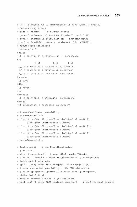
7.2 HIDDEN MARKOV MODELS 363
> Pi <- diag(rep(0.8,3))+matrix(rep(1,9)/3*0.2,ncol=3,nrow=3)
> delta <- rep(1,3)/3
> dist <- 'norm' # mixture normal
> pm <- list(mean=c(-0.3,0.05,0.2),sd=c(0.1,0.1,0.5))
> temp <- dthmm(x,Pi,delta,dist,pm) #setting model
> out3 <- BaumWelch(temp,control=bwcontrol(prt=FALSE))
> #Baum Welch estimation
> summary(out3)
$delta
[1] 1.222375e-79 6.275890e-243 1.000000e+00
$Pi
[,1] [,2] [,3]
[1,] 6.379404e-01 2.597030e-22 0.36205961
[2,] 7.020327e-08 9.717455e-01 0.02825443
[3,] 6.626644e-02 2.645275e-02 0.90728081
$nonstat
[1] TRUE
$distn
[1] "norm"
$pm
$pm$mean
[1] -0.021637295 0.005144475 0.006810866
$pm$sd
[1] 0.030305953 0.009929002 0.018494987
> # smoothed State probability
> par(mfrow=c(3,1))
> plot(tt,out3$u[,1],type='l',xlab='time',ylim=c(0,1),
ylab='prob',main='State 1 Prob')
> plot(tt,out3$u[,2],type='l',xlab='time',ylim=c(0,1),
ylab='prob',main='State 2 Prob')
> plot(tt,out3$u[,3],type='l',xlab='time',ylim=c(0,1),
ylab='prob',main='State 3 Prob')
> par(mfrow=c(1,1))
> logLik(out3) # log likelihood value
[1] 961.0367
> v3 <- Viterbi(out3) # most likely path: Viterbi
> plot(tt,v3,cex=0.5,xlab='time',ylab='state'); lines(tt,v3)
> #plot most likely path
> pp <- 1:360; for(i in 1:360)pp[i] <- out3$u[i,v3[i]]
> # obtain smoothed probability of the Viterbi states
> plot(tt,pp,type='l',ylim=c(0,1),xlab='time',ylab='prob')
> abline(h=0.5,lty=2)
> res3 <- residuals(out3) # get residuals
> pacf(res3**2,main='PACF residual squared') # pacf residual squared
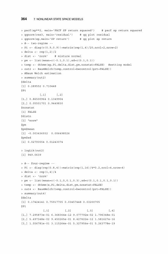
364 7. NONLINEAR STATE SPACE MODELS
> pacf(sp**2, main='PACF SP return squared') # pacf sp return squared
> qqnorm(res3, main='residual') # qq plot residual
> qqnorm(sp,main='SP return') # qq plot sp return
> # two-regime
> Pi <- diag(c(0.9,0.9))+matrix(rep(1,4)/20,ncol=2,nrow=2)
> delta <- rep(1,2)/2
> dist <- 'norm' # mixture normal
> pm <- list(mean=c(-0.1,0.1),sd=c(0.1,0.1))
> temp <- dthmm(sp,Pi,delta,dist,pm,nonstat=FALSE) #setting model
> out2 <- BaumWelch(temp,control=bwcontrol(prt=FALSE))
> #Baum Welch estimation
> summary(out2)
$delta
[1] 0.289552 0.710448
$Pi
[,1] [,2]
[1,] 0.86500964 0.1349904
[2,] 0.05501701 0.9449830
$nonstat
[1] FALSE
$distn
[1] "norm"
$pm
$pm$mean
[1] -0.003436932 0.006498526
$pm$sd
[1] 0.02793554 0.01243074
> logLik(out2)
[1] 949.0639
> # four-regime
> Pi <- diag(rep(0.8,4))+matrix(rep(1,16)/4*0.2,ncol=4,nrow=4)
> delta <- rep(1,4)/4
> dist <- 'norm'
> pm <- list(mean=c(-0.1,0,0.1,0.3),sd=c(0.1,0.1,0.1,0.1))
> temp <- dthmm(x,Pi,delta,dist,pm,nonstat=FALSE)
> out4 <- BaumWelch(temp,control=bwcontrol(prt=FALSE))
> summary(out4)
$delta
[1] 0.17424141 0.75917705 0.03457448 0.03200705
$Pi
[,1] [,2] [,3] [,4]
[1,] 7.295873e-01 6.368364e-12 9.077792e-02 1.796348e-01
[2,] 5.497348e-02 9.450265e-01 8.427622e-12 1.581627e-16
[3,] 1.556781e-01 3.115264e-01 5.327956e-01 5.263778e-19

7.2 HIDDEN MARKOV MODELS 365
[4,] 4.188804e-09 9.674036e-01 1.050020e-02 2.209623e-02
$nonstat
[1] FALSE
$distn
[1] "norm"
$pm
$pm$mean
[1] -0.017055821 0.005591701 0.027254630 0.037185901
$pm$sd
[1] 0.025168944 0.012357184 0.005992786 0.008122566
> logLik(out4)
[1] 963.0156
Example 7.3: Multi-regime Fama–French multi-factor models Example 6.2illustrates the analysis of time-varying coefficient regression of the Fama–Frenchmulti-factor model. See Fama and French (1993, 1996). The coefficients therechange constantly at each time point. Here we adopt an alternative approachassuming that the coefficients follow a Markov regime-switching mechanism. Inother words, the coefficients change stochastically according to a transition prob-ability matrix.
Tables 7.5 and 7.6 show the estimation results of a two-state HMM usingthe same data as in Example 6.2. Figure 7.14 shows the smoothed probabili-ties pt∣T [1], the probabilities that the state is in State 1, given the entire series.Note that pt∣T [2] = 1 − pt∣T [1]. From the plot, it is clear that the system stays inState 1 significantly more often than in State 2. The coefficients associated with
Constant Market SMB HML MoM 𝜎
State 1 0.225 1.015 0.963 0.441 −0.081 2.171State 2 0.012 1.009 0.880 −0.039 −0.032 1.110
Table 7.5 Parameter estimates of a two-state HMM of the Fama–Frenchmulti-factor model. The sample period is from January 1946 to December 2010.
State 1 2
1 0.854 0.1462 0.024 0.976
Table 7.6 Estimated state transition probabilities of atwo-state HMM of the Fama–French multi-factor model.The sample period is from January 1946 to December 2010.
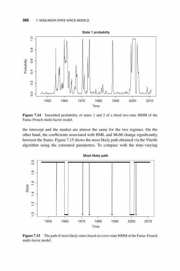
366 7. NONLINEAR STATE SPACE MODELS
1950 1960 1970 1980 1990 2000 2010
0.0
0.2
0.4
0.6
0.8
1.0
Time
Pro
babi
lty
State 1 probabilty
Figure 7.14 Smoothed probability of states 1 and 2 of a fitted two-state HMM of theFama–French multi-factor model.
the intercept and the market are almost the same for the two regimes. On theother hand, the coefficients associated with HML and MoM change significantlybetween the States. Figure 7.15 shows the most likely path obtained via the Viterbialgorithm using the estimated parameters. To compare with the time-varying
1950 1960 1970 1980 1990 2000 2010
1.0
1.2
1.4
1.6
1.8
2.0
Time
Sta
te
Most likely path
Figure 7.15 The path of most likely states based on a two-state HMM of the Fama–Frenchmulti-factor model.

7.2 HIDDEN MARKOV MODELS 367
1950 1960 1970 1980 1990 2000 2010
−0.
8−
0.4
0.0
0.2
0.4
Cnst
Time
Bet
a
1950 1960 1970 1980 1990 2000 2010
−0.
8−
0.4
0.0
0.2
0.4
Market
Time
Bet
a
1950 1960 1970 1980 1990 2000 2010
−0.
8−
0.4
0.0
0.2
0.4
SMB
Time
Bet
a
1950 1960 1970 1980 1990 2000 2010
−0.
8−
0.4
0.0
0.2
0.4
HML
Time
Bet
a
1950 1960 1970 1980 1990 2000 2010
−0.
8−
0.4
0.0
0.2
0.4
MoM
Time
Bet
a
Figure 7.16 Comparison between a two-state HMM and the time-varying coefficientmodel of the Fama–French multi-factor model. Dots are the estimated coefficients with a3-year moving window. The thin line is the smoothed state estimate under the time-varyingcoefficient model and the thick line is the estimated coefficients of the most likely path ofregime switchings.
coefficient analysis in Example 6.2, in Figure 7.16 we show the estimated coeffi-cients using a three-year moving window, the smoothed states under the varyingcoefficient model, and the estimated coefficients under the most likely regime-switching path of the HMM model. It seems that for the coefficients of the HML,both the time-varying coefficient model and the HMM model try to capture thesame time-varying feature of the data.

368 7. NONLINEAR STATE SPACE MODELS
Constant Market SMB HML MoM 𝜎
State 1 0.988 0.823 1.535 0.390 0.040 2.094State 2 −0.015 1.017 0.863 −0.076 −0.026 1.100State 3 −0.006 1.006 0.827 0.214 −0.079 1.525
Table 7.7 Parameter estimates of a three-state HMM of the Fama–Frenchmulti-factor model. The sample period is from January 1946 to December 2010.
State 1 2 3
1 0.816 0.184 02 0.006 0.977 0.0163 0.006 0.025 0.969
Table 7.8 Estimated state transition probabilities of athree-state HMM of the Fama–French multi-factor model.The sample period is from January 1946 to December 2010.
Tables 7.7 and 7.8 show the estimation results of fitting a three-state HMM.Figure 7.17 shows the smoothed probabilities of states. Comparing with the two-state HMM model, it is seen that the three-state model essentially splits the majorstate of the two-state model into two subregimes, with almost the same coeffi-cients in both subregimes. The likelihood value of the three-state model is−1, 281,whereas that of the two-state model is −1, 301. The improvement in the thirdstate seems to be marginal given that the three-state model employs 10 additionalparameters over the two-state model.
R demonstration: HMM modeling via the HiddenMarkov package.
## FF HMM Mixture Regression Example
xxx <- read.csv(file="FF_example.csv",header=T)
year0 <- 1946:2010
y <- xxx[,2]
xx <- xxx[,3:6]
xx <- as.matrix(xx)
ntotal <- length(y)
## HMM modeling
require("HiddenMarkov")
# two-regime
Pi <- diag(rep(0.95,2))+matrix(rep(1,4)/2*0.05,ncol=2,nrow=2)
delta <- rep(1,2)/2

7.2 HIDDEN MARKOV MODELS 369
1950 1960 1970 1980 1990 2000 2010
0.0
0.2
0.4
0.6
0.8
1.0
State 1 probabilty
State 2 probabilty
State 3 probabilty
Time
1950 1960 1970 1980 1990 2000 2010Time
1950 1960 1970 1980 1990 2000 2010Time
Pro
babi
ltyP
roba
bilty
Pro
babi
lty0.
00.
20.
40.
60.
81.
00.
00.
20.
40.
60.
81.
0
Figure 7.17 Smoothed probabilities of states 1, 2, and 3 in a three-state HMM of theFama–French multi-factor model.
sd <- c(1,1)*10
beta1 <- c(-1,-1,-1,-1,-1)
beta2 <- c(1,1,1,1,1)
beta <- cbind(beta1,beta2)
glmformula <- formula(˜xx)
glmfamily <- gaussian(link="identity")
ones <- rep(1,ntotal)

370 7. NONLINEAR STATE SPACE MODELS
data <- data.frame(xx=cbind(ones,xx))
Xdesign <- model.matrix(glmformula,data)
MyModel <- mmglm1(y,Pi,delta,glmfamily,beta,Xdesign,sigma=sd)
out <- BaumWelch(MyModel, bwcontrol(posdiff=FALSE, maxiter=200))
summary(out)
tt <- (1:780)/12+1946
par(mfrow=c(1,1),mai=0.9*c(1,1,1,1))
plot(tt,out$u[,1],type='l',xlab='time',ylim=c(0,1),ylab='prob')
title('State 1 Prob') # smoothed State 1 probability
## Figure 7.14
par(mfrow=c(1,1),mai=c(1,1,1,1))
logLik(out) # log likelihood value
v2 <- Viterbi(out) # most likely path: Viterbi
plot(tt,v2,cex=0.5,xlab='time',ylab='state'); lines(tt,v2)
title("Most Likely Path")
#plot most likely path #Figure 7.15
### compare with time-varying_beta example
ntotal <- length(y)
nyear <- ntotal/12
beta.v <- matrix(ncol=5,nrow=(nyear-2))
for(i in 3:nyear){
t0 <- (i-3)*12+(1:36)
y0 <- y[t0] ##excess return of portfolio 22
xx0 <- as.matrix(xx[t0,])
out.v <- lm(y0˜xx0)
beta.v[i-2,] <- out.v$coef
}
year <- 1948:2010
par(mfrow=c(3,2),mai=0.7*c(1,1,1,1))
for(jj in 1:5){
plot(year,beta.v[,1],type='p',xlab='time',ylab='beta',main=name[jj])
pp <- 1:780; for(i in 1:780)pp[i] <- out$beta[1,v2[i]]
lines(tt,pp,lwd=2);
lines(tt,ss2$s[-1,jj])
}
## ss2 from time-varying beta example
## Figure 7.16
### three regimes
## setting initial values
Pi <- diag(rep(0.8,3))+matrix(rep(1,9)/3*0.2,ncol=3,nrow=3)
delta <- rep(1,3)/3

EXERCISES 371
sd <- c(1,1,1)*10
beta1 <- c(-1,-1,-1,-1,-1)
beta2 <- c(1,-1,-1,1,1)
beta3 <- c(1,1,1,1,1)
beta <- cbind(beta1,beta2,beta3)
glmformula <- formula(˜xx)
glmfamily <- gaussian(link="identity")
Xdesign <- model.matrix(glmformula,data)
MyModel <- mmglm1(y,Pi,delta,glmfamily,beta,Xdesign,sigma=sd)
out3 <- BaumWelch(MyModel, bwcontrol(posdiff=FALSE, maxiter=200))
summary(out)
par(mfrow=c(3,1),mai=0.5*c(1,1,1,1))
plot(tt,out3$u[,1],type='l',xlab='time',ylim=c(0,1),ylab='prob',
main='State 1 Prob')
# smoothed State 1 probability
plot(tt,out3$u[,2],type='l',xlab='time',ylim=c(0,1),ylab='prob',
main='State 2 Prob')
# smoothed State 2 probability
plot(tt,out3$u[,3],type='l',xlab='time',ylim=c(0,1),ylab='prob',
main='State 3 Prob')
# smoothed State 3 probability
## Figure 7.17
7.3 EXERCISES
7.1 Let seed = 11. Repeat the simulation study of Example 7.1 with 200 obser-vations and a second sonar at (25,0), i.e. s2 = 25 in R, using the same initialvalue and parameters.
7.2 Consider the weekly crude oil price from January 3, 1986 to October6, 2017. The data are available from FRED and are also in the filewcoilwtico.csv. Let yt be the first differenced series of the weekly crudeoil price. Part of the series was analyzed in Example 1.2 of Chapter 1. Applya two-state HMM to the series yt.
(a) Obtain parameter estimates, including estimates of the transition prob-ability matrix.
(b) Show the time plot of smoothed probabilities of state 1.
(c) Obtain the most likely state path.
(d) Compare with the analysis of Example 1.2.

372 7. NONLINEAR STATE SPACE MODELS
7.3 Consider again the first differenced series yt of the weekly crude oil pricesfrom January 3, 1986 to October 6, 2017. Suppose that yt follows the expo-nential autoregressive model
yt = exp(b)yt−1 + exp(c + dy2t−1)yt−8 + 𝜖t,
where 𝜖t is a sequence of iid N(0, 𝜎2e ).
(a) Put the exponential autoregressive model into a nonlinear Gaussianstate space model.
(b) Fit the model using the extended Kalman filter with the first-order Tay-lor expansion. Write down the parameter estimates.
(c) Check the model using the residuals 𝜖t = yt − exp(b)yt−1 − exp(c +dy2
t−1)yt−8. Are there serial correlations in the residuals? You may useLjung–Box statistics with 10 lags.
7.4 Consider the daily gold fixing prices at 10:30am in the London Bullion Mar-ket (in US dollars) from October 19, 2012 to October 18, 2017. The data areavailable from FRED and are also in the file dgoldamGBD228nlbm.csv.There are some missing values in the FRED data and we have deleted thosemissing values. Let yt be the log returns of the daily gold price, i.e. the first-differenced of the log prices. Fit a two-state HMM model to yt. You may useyt−1 and yt−6 as input variables. Write down the fitted model, including esti-mates of the transition probabilities. Obtain the time-plot of the smoothedstate probabilities as well.
7.5 Consider the data set mdec5FF6117.txt used in question 3 of the exer-cise in Chapter 6. Fit a two-state HMM Fama–French multi-factor model tothe excess returns of Decile 5 portfolio. Perform similar analysis to that inExample 7.3.
REFERENCES
Anderson, J. L. (2001). An Ensemble Adjustment Kalman Filter for Data Assimilation.Monthly Weather Review 129: 2884–2903.
Anderson, J. L. (2007). An adaptive covariance inflation error correction algorithm forensemble filters. Tellus A 59: 210–224.
Anderson, B. D. O. and Moore, J. B. (1979). Optimal filtering. Prentice-Hall, EnglewoodCliffs, NJ.
Baggenstoss, P. M. (2001). A modified Baum–Welch algorithm for hidden Markov modelswith multiple observation spaces. IEEE Transactions on Speech and Audio Processing 9:411–416.

REFERENCES 373
Baum, L. E. and Petrie, T. (1966). Statistical inference for probabilistic functions of finitestate Markov chains. Annals of Mathematical Statistics 37: 1554–1563.
Baum, L. E., Petrie, T., Soules, G., and Weiss, N. (1970). A maximization technique occur-ring in the statistical analysis of probabilistic functions of Markov chains. Annals ofMathematical Statistics 41: 164–171.
Bellman, R. E. (2003). Dynamic Programming. Dover Publications, Inc., New York.
Bishop, C.H., Etherton, B.J., and Majumdar, S.J. (2001). Adaptive sampling with theensemble transform Kalman filter. Part I: Theoretical aspects. Monthly WeatherReview 129: 420–436.
Dempster, A. P., Laird, N. M., and Rubin, D. B. (1977). Maximum-likelihood from incom-plete data via the EM algorithm. Journal of the Royal Statistical Society Series B 39:1–38.
Duncan, D. B. and Horn, S. D. (1972). Linear dynamic recursive estimation from theviewpoint of regression analysis. Journal of the American Statistical Association 67:815–821.
Durbin, J. and Koopman, S. J. (2001). Time Series Analysis by State Space Methods. OxfordUniversity Press, Oxford.
Evensen, G. (1994). Sequential data assimilation with a nonlinear quasi-geostrophicmodel using Monte Carlo methods to forecast error statistics. Journal of GeophysicalResearch 99: 10143–10162.
Evensen, G. (2003). The ensemble Kalman filter: theoretical formulation and practicalimplementation. Ocean Dynamics 53: 343–367.
Evensen, G. (2007). Data Assimilation: the Ensemble Kalman Filter. Springer, New York.
Fama, E. F. and French, K. R. (1993). The cross-section of expected stock returns. Journalof Finance 47: 427–465.
Fama, E. F. and French, K. R. (1996). Multifactor explanations of asset pricing anomalies.Journal of Finance 51: 55–84.
Forney, G. D. (1973). The Viterbi algorithm. Proceedings of the IEEE 61: 268–278.
Furrer, R., Genton, M. G., and Nychka, D. (2006). Covariance tapering for interpolation oflarge spatial datasets. Journal of Computational and Graphical Statistics 15: 502–523.
Gelb, A. (1974). Applied Optimal Estimation. MIT Press, Cambridge, MA.
Julier, S. J. and Uhlmann, J. K. (1997). New extension of the Kalman filter to nonlinearsystems. Proceedings of the SPIE 3068: 182–193.
Julier, S. J. and Uhlmann, J. K. (2004). Unscented filtering and nonlinear estimation. Pro-ceedings of the IEEE 92: 401–422.
Roth, M. and Gustafsson, F. (2011). An efficient implementation of the second orderextended Kalman filter. In Proceedings of the 14th International Conference on Infor-mation Fusion, pp. 1–6. IEEE.
Sorenson, H. W. and Alspach, D. L. (1971). Recursive Bayesian estimation using Gaussiansums. Automatica 7: 465–479.

374 7. NONLINEAR STATE SPACE MODELS
Stroud, J.R., Stein, M.L., Lesht, B.M., Schwab, D.J., and Beletsky, D. (2010). An ensem-ble Kalman filter and smoother for satellite data assimilation. Journal of the AmericanStatistical Association 105: 978–990.
Tanizaki, H. (1996). Nonlinear Filters: Estimation and Applications. Springer, New York.
Tippett, M. K., Anderson, J. L., Bishop, C. H., Hamill, T. M., and Whitaker, J. S. (2003).Ensemble Square Root Filters. Monthly Weather Review 131: 1485–1490.
Viterbi, A. J. (1967). Error bounds for convolutional codes and an asymptotically optimumdecoding algorithm. IEEE Transactions on Information Theory 13: 260–269.
Wu, C. F. (1983). On the convergence properties of the EM algorithm. Annals of Statis-tics 11: 95–103.

CHAPTER 8
SEQUENTIAL MONTE CARLO
In Chapter 7 we discussed several approaches for dealing with nonlinear andnon-Gaussian state space models (SSMs). Except for the hidden Markov model(HMM), all the approaches discussed use approximations as there are no analyticsolutions for filtering or smoothing in most nonlinear and non-Gaussian models.In some applications, these approximation approaches may not be sufficient or beable to provide the required accuracy. Some alternatives must be sought. With theadvances in computational capability, Monte Carlo methods have become a pop-ular and useful tool in solving complex problems. In this chapter we discuss aneffective Monte Carlo approach designed specifically for dealing with SSMs. It isreferred to as the sequential Monte Carlo (SMC) method. This method tries to uti-lize fully the sequential and dynamic nature of SSMs, yet enjoys the flexibility ofthe powerful Monte Carlo approaches. The SMC approach is parallel to that of theKalman filter in which the conditional distribution of the state xt given the entirehistory of the observations yt is obtained and updated based on the results obtainedfor xt−1 given yt−1 at the previous time step. Because there are no parametric and
Nonlinear Time Series Analysis, First Edition. Ruey S. Tsay and Rong Chen.© 2019 John Wiley & Sons, Inc. Published 2019 by John Wiley & Sons, Inc.Companion website: www.wiley.com/go/tsay/nonlineartimeseries
375

376 8. SEQUENTIAL MONTE CARLO
analytical forms available for the conditional distributions, SMC uses discrete ran-dom samples to represent those conditional distributions. This approach belongsto the class of density-based filtering approaches. The Gaussian sum filters andthe unscented Kalman filters introduced in Chapter 7 also belong to this class. Thedifference is that SMC uses random samples instead of a deterministic mixturedistribution approximation or a fixed-point approximation.
A Monte Carlo method tries to generate a set of samples x(1),… , x(m) froma target distribution 𝜋(x). Statistical inferences, such as estimating E𝜋(h(x)), canthen be obtained through the Monte Carlo samples such as the sample averageestimator
E𝜋[h(x)] ≈∑m
𝑖=1 h(x(𝑖))
m.
SMC achieves estimation and optimization tasks by recursively generating MonteCarlo samples of the state variables of a system. The basic principle behind SMCdates back to the “growth Monte Carlo” method known in molecular physicsin the 1950s; see Hammersley and Morton (1954) and Rosenbluth and Rosen-bluth (1955). With modern computing power it has generated significant interestin recent years.
In this chapter we start with a brief introduction to general Monte Carlo meth-ods, then establish a general framework of SMC, followed by some detailed dis-cussions of its implementation. Several specific implementations are discussed fora wide range of nonlinear non-Gaussian SSMs.
8.1 A BRIEF OVERVIEW OF MONTE CARLO METHODS
Monte Carlo methods are essentially a class of numerical methods to evaluate (orestimate) some integrals. They rely on random sampling, which is the key principlebehind all statistical analyses, and use statistical methods to assess the estimationaccuracy. Specifically, we focus on two types of integrals:
(I) Normalizing constant:
Z =∫
𝜋∗(x)dx, (8.1)
where 𝜋∗(x) is a non-negative integrable function.
(II) Expectation:
𝜇h =∫
h(x)𝜋(x)dx, (8.2)
where 𝜋(x) is a probability density and h(x) is an 𝜋-integrable real function.

8.1 A BRIEF OVERVIEW OF MONTE CARLO METHODS 377
Many statistical inference problems can be reformulated as an integration prob-lem with a properly chosen function h(x) and a target distribution 𝜋(x) or a non-negative integrable function 𝜋∗(x). The integral Z is essentially the normalizingconstant of a probability density 𝜋(x) = 𝜋∗(x)∕Z. It has a broad range of appli-cations, including likelihood calculation, entropy calculation (Gelman and Meng,1998), and communication systems (Smith et al., 1997).
The integral 𝜇h is the expectation of h(x) under the distribution 𝜋(x). By choos-ing a proper h(x), various moments and the probability of a certain (maybe rare)event can be estimated. For example, if h(x) = x, 𝜇h is the mean of the distribu-tion 𝜋(x), higher-order moments can be obtained using h(x) = xk. To obtain theprobability P(X ∈ Ω), if X ∼ 𝜋(x), one can use h(x) = IΩ(x), the indicator func-tion. A histogram of 𝜋(x) can be obtained by changing Ω. The expected shortfalloften used in financial risk management can be obtained using h(x) = xI(x ≥ c). Ifh(x) = K((x − x0)∕h), a kernel function around a fixed point x0, then 𝜇h is essen-tially a (unnormalized) kernel estimation of 𝜋(x0).
In a typical statistical inference problem, one is interested in estimating andassessing the estimation accuracy of some unknown parameter 𝜃 of a distributionp(⋅, 𝜃) based on a set of random samples X1,… , Xn drawn from the distributionp(⋅, 𝜃). Often the random samples are physically observed (e.g., survey sampling,physical measurements, etc.). Monte Carlo methods start with a known distribu-tion 𝜋(⋅, 𝜃) with a known parameter 𝜃 and try to estimate𝜇h or Z. In fact𝜇h dependson 𝜃 and can be viewed as a re-parameterized parameter to be estimated. Mimick-ing the traditional estimation approach, we would need a set of random samplesfrom the given distribution 𝜋(⋅, 𝜃). Instead of trying to get physical samples, theMonte Carlo method tries to generate pseudo random samples (random numbers)using computers. Using these samples, the integrals can be estimated and the esti-mation accuracy can be assessed.
For example, to estimate 𝜇h, if we can generate an iid random sample(x1,… , xm) from 𝜋(x), then
��h = 1m
m∑𝑖=1
h(x𝑖)
is an unbiased estimator of 𝜇h with variance Vh∕m, where Vh = ∫ h2(x)𝜋(x)dx −𝜇2
h is the variance of h(X). Note that Vh can also be estimated using
Vh = 1m
m∑𝑖=1
h2(x𝑖) − ��2h .
The key to Monte Carlo methods is to find ways to efficiently generate thepseudo numbers from a distribution 𝜋(x), and if it is difficult to generate such ran-dom samples directly from 𝜋(x), then find an alternative way to achieve the same

378 8. SEQUENTIAL MONTE CARLO
objectives. Often the random samples themselves are of interest. For example, ifone is able to generate samples {x(j)
1 , x(j)2 ,… , x(j)
d }, (j = 1,… , m), from a joint dis-
tribution 𝜋(x1,… , xd), then the marginal samples {x(1)1 ,… , x(m)
1 } can be used tostudy the marginal distribution 𝜋(x1), such as a kernel density estimation of 𝜋(x1).
8.1.1 General Methods of Generating Random Samples
In this section we consider some methods for generating random samples.
1. Computer-generated pseudo random numbers: Monte Carlo methodsdepend on generating random numbers. Physical devices such as coins, dice, col-ored balls in an urn, or lottery machines are not practical for large experiments.Except for some high-end physical random number generating devices such asthose in Fischer and Drutarovsky (2003) and Majzoobi et al. (2011), computer-generated pseudo random numbers are often used in Monte Carlo methods. Theresulting random numbers are often from a deterministic sequence, but behave likea random sequence following a uniform distribution on [0, 1]. Robert and Casella(2004) provide a good introduction. Pseudo random number generators are widelyavailable on almost all platforms and softwares.
2. Transformation: If a complicated random variable Y is a function of a simplerrandom variable X, then a set of random samples of Y can be obtained through a setof random samples from X. Specifically, if Y = f (X) and x ∼ X, then y = f (x) ∼ Y .
For example, random samples of a normal distribution can be obtained via thosefrom a uniform distribution. Specifically, if X1 and X2 are independent Unif(0, 1)random variables, and
Y1 =√−2 ln(X1) cos(2𝜋X2), Y2 =
√−2 ln(X1) sin(2𝜋X2),
then Y1 and Y2 are two independent N(0, 1) random variables. This transformationis often referred to as the Box–Muller algorithm.
To generate samples from N(𝜇, 𝜎2), one can use the transformation Y = 𝜇 +𝜎X, where X ∼ N(0, 1). If Z1,… , Zk are independent N(0, 1) random variables,then Y =
∑k𝑖=1 Z2
𝑖follows a 𝜒2
k distribution. Hence a 𝜒2k random sample can be
obtained from k standard Normal random samples. When k is small, this methodof generating 𝜒2
k samples is efficient, but it becomes inefficient when k is large.Many commonly used distributions can be obtained using transformations
based on the standard exponential random variable. Let X𝑖 be iid standard expo-nential random samples, which are easy to generate using the inverse cumulativedistribution function (CDF) method discussed below. Then 𝜒2
2k distribution can be
obtained using Y = 2∑k
𝑖=1 X𝑖, gamma(𝛼, 𝛽) distribution with shape parameter 𝛼

8.1 A BRIEF OVERVIEW OF MONTE CARLO METHODS 379
and scale parameter 𝛽 can be obtained using Y = 𝛽∑𝛼
𝑖=1 X𝑖, and beta(a, b) distribu-
tion can be obtained using Y = A∕(A + B) with A =∑a
𝑖=1 X𝑖 and B =∑a+b
𝑖=a+1 X𝑖),For a 𝜒2 distribution with 2k + 1 degrees of freedom, one can use Y = X1 + X2
2 ,where X1 ∼ 𝜒2
2k and X2 ∼ N(0, 1).To generate a random sample from a Student-t distribution with k degrees of
freedom, we notice the transformation T = Z√X
where Z ∼ N(0, 1) and X ∼ 𝜒2k ,
and Z and X independent. Random samples of an F distribution can be obtained bygenerating two independent 𝜒2 random samples with proper degrees of freedom.
3. Inverse CDF: The method of inverse CDF is a general transformation methodto generate random samples. The following lemma provides a direct connectionbetween any random variable and the uniform distribution, the simplest and mostcommonly available distribution.
Lemma 8.1 If a random variable X has a CDF F(⋅), then Y = F(X) ∼ Un𝑖f (0, 1).Furthermore, F−1(U) ∼ X where U ∼ Un𝑖f (0, 1) and
F−1(u) = argminx
{F(x) ≥ u}, 0 ≤ u ≤ 1
is the generalized inverse of F(x).
To see why this is true, let Y = F(X). Then for any 0 ≤ u ≤ 1,
P(Y ≤ u) = P(F(X) ≤ u) = P(X ≤ F−1(u)) = F(F−1(u)) = u.
Hence Y = F(X) ∼ Un𝑖f (0, 1). In addition, let X∗ = F−1(U), then
P(X∗ < x) = P(F−1(U) < x) = P(U < F(x)) = F(x).
If the CDF F(x) has an analytical inverse, the method is very effective. Forexample, if X has a probability density function (pdf) p(x) = 2x, (0 < x < 1), its
CDF is F(x) = x2. Then X can be generated using the transformation X =√
U,U ∼ Un𝑖f (0, 1). The most important distribution in this class is the standard expo-nential distribution with pdf p(x) = e−x for x > 0. Its CDF is F(x) = 1 − e−x,hence F−1(u) = − ln(1 − u). Then a sample of the standard exponential distribu-tion exp(1) can be obtained by generating U from Un𝑖f [0, 1] and X = − ln(1 − U)or, equivalently, X = − ln(U). For general exponential distributions, we note thatY = X∕𝜆 ∼ exp(𝜆) with pdf p(y) = 𝜆 exp(−𝜆y), where X ∼ exp(1). This providesa simple approach to generate random samples from 𝜒2
2k, gamma, beta, and otherdistributions.
4. Rejection method: The rejection method is an effective approach to generaterandom samples from complicated distributions. It is based on the following twofacts.
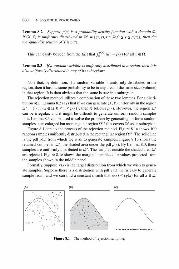
380 8. SEQUENTIAL MONTE CARLO
Lemma 8.2 Suppose p(x) is a probability density function with a domain Ω.If (X, Y) is uniformly distributed in Ω∗ = {(x, y), x ∈ Ω, 0 ≤ y ≤ p(x)}, then themarginal distribution of X is p(x).
This can easily be seen from the fact that ∫ p(x)0 1dy = p(x) for all x ∈ Ω.
Lemma 8.3 If a random variable is uniformly distributed in a region, then it isalso uniformly distributed in any of its subregions.
Note that, by definition, if a random variable is uniformly distributed in theregion, then it has the same probability to be in any area of the same size (volume)in that region. It is then obvious that the same is true in a subregion.
The rejection method utilizes a combination of these two lemmas. For a distri-bution p(x), Lemma 8.2 says that if we can generate (X, Y) uniformly in the regionΩ∗ = {(x, y), x ∈ Ω, 0 ≤ y ≤ p(x)}, then X follows p(x). However, the region Ω∗
can be irregular, and it might be difficult to generate uniform random samplesin it. Lemma 8.3 can be used to solve the problem by generating uniform randomsamples in an enlarged but more regular regionΩ∗∗ that coversΩ∗ as its subregion.
Figure 8.1 depicts the process of the rejection method. Figure 8.1a shows 100random samples uniformly distributed in the rectangular regionΩ∗∗. The solid lineis the pdf p(x) from which we wish to generate samples. Figure 8.1b shows theretained samples in Ω∗, the shaded area under the pdf p(x). By Lemma 8.3, thesesamples are uniformly distributed in Ω∗. The samples outside the shaded area Ω∗
are rejected. Figure 8.1c shows the marginal samples of x values projected fromthe samples shown in the middle panel.
Formally, suppose 𝜋(x) is the target distribution from which we wish to gener-ate samples. Suppose there is a distribution with pdf g(x) that is easy to generatesample from, and we can find a constant c such that 𝜋(x) ≤ cg(x) for all x ∈ Ω.
(a) (b) (c)
Figure 8.1 The method of rejection sampling.

8.1 A BRIEF OVERVIEW OF MONTE CARLO METHODS 381
The density g(x) is then called an envelop density of 𝜋(x). The rejection methodcan be summarized as follows.
Algorithm 8.1: Rejection Sampling
� Generate m samples x1,… , xm according to the distribution g(x).
� Generate m samples u1,… , um following Unif[0, 1].
� Retain the samples x𝑖 that satisfy u𝑖 < 𝜋(x𝑖)∕cg(x𝑖).
The above approach is equivalent to generating uniform random samples inthe region Ω∗∗ = {(x, y), x ∈ Ω, 0 ≤ y ≤ cg(x)}, then rejecting those outside Ω∗ ={(x, y), x ∈ Ω, 0 ≤ y ≤ 𝜋(x)}.
The efficiency of the rejection sampling depends on the proportion of therejected samples, as rejections waste computation. Hence the sampling regionΩ∗∗ needs to be as small as possible, or the ratio of the areas |Ω∗|∕|Ω∗∗| needs tobe as large as possible. For the given 𝜋(x) and g(x), the smaller c, the higher theefficiency.
Uniform distribution on a rectangle is easy to generate samples from. In thiscase g(x) is a uniform distribution. It is often used when 𝜋(x) has a finite support.In many other situations one needs to carefully choose a g(x) that balances theefficiency and the ease in generating samples from it.
We demonstrate the rejection method with some examples. We generate a trun-cated distribution 𝜋(x) = c𝜋∗(x)I(x > a), where 𝜋∗(x) is a probability density func-tion and c = 1∕ ∫ ∞
a 𝜋∗(x)dx is the normalizing constant of 𝜋∗(x)I(x > a). Theobvious envelop distribution is g(x) = 𝜋∗(x) and we have 𝜋(x) ≤ c𝜋∗(x) for all x.Since 𝜋(x)∕c𝜋∗(x) = 1 for all x > a and 𝜋(x)∕c𝜋∗(x) = 0 for all x < a, the rejectionmethod accepts all samples xj generated from 𝜋∗(x) satisfying xj > a and rejectsthose smaller than a. This is simple if it is easy to generate random samples from𝜋∗(x). However, when a is very large (or small) so c is very large, this approach isnot efficient. For example, for a truncated normal distribution, if a = 𝜇 + 3𝜎, oneonly accepts about 0.13% of the samples. For large a, a better trial distribution inthis case is the translated exponential distribution. Consider the truncated standardnormal distribution
𝜋(x) = 1
(1 − Φ(a))√
2𝜋exp(−x2∕2)I(x > a),
where 1 − Φ(a) = P(X > a) is the normalizing constant. We can useg(x) = 𝜆e−𝜆(x−a)I(x > a), a shifted exponential distribution. One can easily

382 8. SEQUENTIAL MONTE CARLO
generate random samples from this distribution by simply adding the constant a toan exponential exp(𝜆) random variate (using the inverse CDF method). Note that
exp{−x2∕2}
exp{−𝜆(x − a)}I(x > a) = exp
{−1
2(x2 − 2𝜆x + 𝜆2) + 1
2𝜆2 − 𝜆a
}I(x > a)
≤ exp{1
2𝜆2 − 𝜆a
}for all x > a.
Choosing 𝜆 = a + 12
√a2 + 4, we minimize the envelop constant
c = 1
𝜆(1 − Φ(a))√
2𝜋exp{
12𝜆2 − 𝜆a},
and 𝜋(x) ≤ cg(x) for all x. For a = 3 and a = 4, the acceptance rates are 6% and1.9%, respectively, compared to 0.13% and 3.16 × 10⁻⁵, respectively, when usingthe standard normal trial distribution.
5. Sequential sampling: Sequential sampling is one of the most commonly usedapproaches for generating Monte Carlo samples of a high dimensional distribu-tion. It sequentially generates low dimensional components one at a time until thesample is completed. It is based on the chain rule
p(X1, X2,… , Xn) = p(X1)p(X2 ∣ X1)⋯ p(Xn ∣ X1,… , Xn−1).
Specifically, if (X, Y) ∼ p(x, y), sequential sampling starts with sampling X = xfrom the marginal distribution p(x) = ∫ p(x, y)dy, then sampling Y = y from theconditional distribution p(y ∣ X = x) = p(x, y)∕p(x). Then (x, y) is a sample fromthe joint distribution of p(x, y).
For example, suppose
(X, Y) ∼ N
([𝜇1
𝜇2
],
[𝜎2
1 𝜌𝜎1𝜎2
𝜌𝜎1𝜎2 𝜎22
]).
To generate a sample of (X, Y), one first generates X = x from N(𝜇1, 𝜎21), then
generates Y = y from p(Y ∣ X = x) ∼ N(𝜇2 − 𝜌𝜎2𝜎1
(x − 𝜇1), (1 − 𝜌2)𝜎22).
To generate an AR(1) process, Xt = 𝜙Xt−1 + et where et ∼ N(0, 𝜎2), onestarts with simulating X0 = x0 from N(𝜇0, 𝜎2
0) (often the stationary distribu-tion with 𝜇0 = 0 and 𝜎2
0 = 𝜎2∕(1 − 𝜙2)), then iteratively generates Xt = xt fromN(𝜙xt−1, 𝜎2). The sample (x1, x2,… , xn) forms a realization of the time series.
For sequential sampling, one may choose the order of the variables or compo-nents to generate random samples from. The criterion is to make the sampling ofthe marginal and conditional distributions easier.
8.1 A BRIEF OVERVIEW OF MONTE CARLO METHODS 383
6. Augmentation: In many cases it is not easy to generate random samples directlyfrom a distribution. However, by augmenting an additional component and usingsequential sampling, one can simplify the problem. Specifically, if pX(x) is not easyto generate sample from, one can increase the dimension by augmenting an extracomponent Y so that the joint distribution p(X, Y) is easy to generate sample fromthrough the sequential sampling of pY (y) and p(X ∣ Y = y). This is based on the factthat if (X, Y) ∼ p(x, y), then X ∼ pX(x). Hence if we have a sample (x, y) ∼ p(x, y),then the marginal sample x (dropping y) follows pX(x). This method is particularlyuseful when one can easily generate random samples from pY (y) and p(X ∣ Y = y).
Generating samples from a mixture distribution is often done by augmentingan indicator representing which of the mixture components the sample comesfrom. For example, if Y ∼ (1 − p)N(𝜇0, 𝜎2
0) + pN(𝜇1, 𝜎21), one samples I = 𝑖 from
Bernoulli(p), where p is the mixture proportion, then generates a sample Y fromN(𝜇𝑖, 𝜎
2𝑖). It can easily be verified that the marginal distribution of Y follows the
mixture distribution.The augmentation method also works naturally for continuous compound mix-
ture distribution 𝜋(y) = ∫ 𝜔(x)𝜋2(y, x)dx where 𝜔(x) ≥ 0 and ∫ 𝜔(x)dx = 1 (basi-cally a density function) and 𝜋2(y, x) is a density function for every x (basically aconditional density function). For example, the non-central 𝜒2 distribution with mdegrees of freedom with a non-central parameter 𝜆 is a Poisson mixture of central𝜒2 distributions
Xm ∼∞∑
k=0
P(K = k)𝜒22k+m,
where K ∼ Po𝑖sson(𝜆). Hence a random sample of Xm can be obtained by gener-ating a Poisson random sample K = k first, then a 𝜒2
2k+m random sample. In factthere is another formulation to make the problem easier. It can be shown that
Xm = (Z + 𝜆)2 + X∗m−1,
where Z follows a standard normal distribution and X∗m−1 follows the central 𝜒2
distribution with m − 1 degrees of freedom. This representation provides an easierway to generate Xm. The method can be extended to non-central gamma distribu-tions.
A remark is in order. The rejection method utilizes the idea of augmentation.Since p(x) is difficult to generate samples from directly, we augment an additionalcomponent Y , so (X, Y) follows the uniform distribution in the region of Ω∗ ={(x, y), x ∈ Ω, 0 ≤ y ≤ p(x)}. Lemma 8.2 makes sure that the marginal distributionof X follows p(x). The samples of the joint uniform distribution in Ω∗ are drawnby generating a set of samples uniformly distributed in a larger region Ω∗∗.

384 8. SEQUENTIAL MONTE CARLO
8.1.2 Variance Reduction Methods
Another important issue in using Monte Carlo methods is variance reduction.The goal of variance reduction is to reduce the variation in Monte Carlo sampleswhile maintain the consistency in estimation. In this section, we consider someapproaches to variance reduction.
1. Control variates: Suppose we have iid samples X1,… , Xm from 𝜋(x) and use�� = m−1∑m
𝑖=1 h(X𝑖) to estimate 𝜇h = ∫ h(x)𝜋(x)dx. The variance of the estimatoris
mVar(��) = Var[h(X)].
An alternative estimator of 𝜇h is
��C = 1m
m∑𝑖=1
[h(X𝑖) − c(𝜂(X𝑖) − 𝜇∗)],
where 𝜂(⋅) is a function with a known expectation 𝜇∗ = ∫ 𝜂(x)𝜋(x)dx and c is aconstant to be chosen. Clearly, E(��C) = 𝜇h and, hence, ��C is a valid estimator of𝜇h. Its variance is
mVar(��C) = Var[h(X)] + c2Var[𝜂(X)] − 2cCov[h(X), 𝜂(X)].
For a properly chosen 𝜂(x) and a constant c, the variance of ��C can be reduced.Specifically, for a given 𝜂(⋅), the optimal choice of c is
c = Cov[h(X), 𝜂(X)]∕Var[𝜂(X)].
The variance then becomes (1 − 𝜌2)Var[h(X)], where 𝜌 is the correlation coeffi-cient between h(X) and 𝜂(X). For 𝜌 ≠ 0, Var(��C) is smaller than Var(��).
The basic requirement of using this approach is the ability to find a function𝜂(x) with a known expectation 𝜇∗ = E𝜋[𝜂(X)] = ∫ 𝜂(x)𝜋(x)dx. One would choosea 𝜂(⋅) to make the correlation coefficient between h(X) and 𝜂(X) large (in abso-lute value). In practice, the optimal c can be estimated after sampling, using theestimated sample correlation between h(X) and 𝜂(X).
One commonly used 𝜂(⋅) is
𝜂(x) =h(x)g(x)𝜋(x)
,
where g(x) is a known and easy density so that ∫ h(x)g(x)dx = Eg(h(X)) = 𝜇∗ canbe obtained analytically. In this case,
∫𝜂(x)𝜋(x)dx =
∫h(x)g(x)dx = 𝜇∗.

8.1 A BRIEF OVERVIEW OF MONTE CARLO METHODS 385
Ideally, g(x) should be close to 𝜋(x) so the correlation between 𝜂(x) and h(x) islarge. For example, g(x) can be a normal approximation of 𝜋(x), with its modeclose to that of 𝜋(x), and with (approximately) matching curvature around themode.
If the first two moments of 𝜋(x) are available, another effective 𝜂(x) to use is
𝜂(x) = h(��) + h′(��)(x − ��) + 1
2h′′
(��)(x − ��)2,
which uses the first two terms of Taylor expansion of h(x) around ��, where �� is arough estimate of 𝜇.
More generally, if one can generate control variates Y1,… , Yn such that(h(X𝑖), Y𝑖) are correlated (e.g., Y𝑖 = 𝜂(X𝑖) in the above discussion), then we canachieve variance reduction. Specifically,
1. If E(Y𝑖) = b is known, we can use
��C = 1m
m∑𝑖=1
[h(X𝑖) − c(Y𝑖 − b)].
2. If E(Y𝑖) = a𝜇 with a known constant a (𝜇 is to be estimated), we can use
��C =( 1
1 − ac
) 1m
m∑𝑖=1
(h(X𝑖) − cY𝑖).
3. If E(Y𝑖) = a𝜇 + b with known constants a and b, we can use
��C =( 1
1 − ac
) 1m
m∑𝑖=1
[h(X𝑖) − cY𝑖 − b].
Further information can be found in Rubinstein and Kroese (2008).
2. Antithetic variates: To reduce Monte Carlo variation in some cases we can usepairs of negatively correlated random samples.
Consider again the estimation of 𝜇h = ∫ h(x)𝜋(x)dx. We can generate iid pairs(X1, Y1), …, (Xn, Yn) such that (h(X𝑖), h(Y𝑖)) are negatively correlated and X𝑖 andY𝑖 both follow 𝜋(x). Then an antithetic variate estimator of 𝜇h takes the form
��C = 12n
n∑𝑖=1
[h(X𝑖) + h(Y𝑖)].
Its variance (comparing to 2n iid samples) is
12n
[Var(h(X1)) + Cov(h(X1), h(Y1))
]<
12n
Var(h(X1)).
In many cases, antithetic variate estimator requires less computation and hassmaller variance. For example, if U𝑖 ∼ Un𝑖f [0, 1], then 1 − U𝑖 is its antithetic
386 8. SEQUENTIAL MONTE CARLO
variate. Or, more generally, under the CDF inverse method, if X = F−1(U), thenY = F−1(1 − U) is its antithetic variate. A more commonly used situation is when𝜋(x) is symmetric around a constant c, then X𝑖 and c − X𝑖 are antithetic and can beused.
Of course, how useful the antithetic pair (X, Y) is depends on h(⋅), since the effi-ciency improvement depends on the correlation between h(X) and h(Y). For exam-ple, if 𝜋(x) is symmetric around 0, then (X,−X) is extremely effective if h(x) = x(or any odd function of x), but has no impact at all if h(x) = |x| (or any even func-tion of x).
3. Stratified sampling: For a mixture distribution such as
𝜋(x) = p𝜋1(x) + (1 − p)𝜋2(x), (8.3)
it is often more efficient to use stratified sampling, as often used in the surveysampling literature. Specifically, to obtain m samples from the mixture distributionin Equation (8.3), one can generate m1 = mp samples x1,… , xm1
from 𝜋1(x) andgenerate m2 = m(1 − p) samples y1,… , ym2
from 𝜋2(x). Then 𝜇 = ∫ h(x)𝜋(x)dxcan be estimated by
�� = 1m
[ m1∑𝑖=1
h(x𝑖) +m2∑𝑖=1
h(y𝑖)
]= p��1 + (1 − p)��2,
where ��1 = (1∕m1)∑m1
𝑖=1 h(x𝑖) and ��2 = (1∕m2)∑m2
𝑖=1 h(y𝑖). Clearly, E(��1) =∫ h(x)𝜋1(x)dx and E(��2) = ∫ h(x)𝜋2(x)dx, hence E(��) = ∫ h(x)𝜋(x)dx. The vari-ance of the estimator is
mVar(��) = pV1 + (1 − p)V2,
where V1 = ∫ h2(x)𝜋1(x)dx − 𝜇21 and V2 = ∫ h2(x)𝜋2(x)dx − 𝜇2
2. On the otherhand, one can generate x1,… , xm directly from 𝜋(x), via the augmentation method,by generating an indicator I𝑖 = 1 with probability p and I𝑖 = 2 with probability1 − p, then generating x𝑖 from 𝜋I𝑖
(x). The variance of the sample mean of such arandom sample is Var(X1)∕m, where
Var(X1) = E[Var(X1 ∣ I1)] + Var[E(X1 ∣ I1)]
= pV1 + (1 − p)V2 + (𝜇1 − 𝜇2)2p(1 − p).
Hence the augmented estimator has a larger variance due to the variation inBernoulli sampling of the indicator I𝑖. In addition, the stratified sampling savedthe computation by avoiding generating the indicators.
Sometimes if a non-mixture distribution can be reformulated into a mixture dis-tribution (e.g., partition the space into non-overlapping regions with known mix-ture proportions), stratified sampling may have some advantages.

8.1 A BRIEF OVERVIEW OF MONTE CARLO METHODS 387
8.1.3 Importance Sampling
The importance sampling (IS) of Marshall (1956) is one of the most commonlyused methods in applying Monte Carlo samples to perform numerical integrationand to make statistical inference. It is often mentioned on an equal footing withthe rejection method discussed in Section 8.1.1, but since it is mostly related tothe SMC methods of this chapter, we provide a more detailed introduction here.
IS is designed for approximating analytically intractable integrals. Again, wefocus on the two types of integrals Z and 𝜇h in Equations (8.1) and (8.2).
Suppose a set of Monte Carlo samples, {x(j), j = 1,… , m}, has been generatedfrom a trial distribution g(⋅), which is different from the target distribution 𝜋(⋅).Note that, if the support of g(x) contains that of integral function 𝜋∗(x) (or 𝜋∗(x)is absolutely continuous with respect to g(x)), then
Z =∫
𝜋∗(x)dx =∫
[𝜋∗(x)g(x)
]g(x)dx.
Hence Z is essentially the expectation of the function 𝜋∗(x)∕g(x) under the densityg(x). With the set of Monte Carlo samples {x(j), j = 1,… , m} from g(x), Z can beapproximated by the sample average
Z = 1m
m∑j=1
𝜋∗(x(j))
g(x(j)).
That is, the integral of 𝜋∗(⋅) can be estimated using the random samples generatedfrom the distribution g(⋅). Note that in this case we need to be able to evaluatethe functions 𝜋∗(x) and g(x) explicitly and be able to generate samples from g(x)easily.
For approximating 𝜇h, we use
𝜇h =∫
h(x)𝜋(x)dx =∫
[h(x)
𝜋(x)g(x)
]g(x)dx = Eg[h(X)w(X)], (8.4)
where w(x) = 𝜋(x)∕g(x). Using samples generated from g(x), we have
��h = 1m
m∑j=1
w(j)h(x(j)),
where w(j) = 𝜋(x(j))∕g(x(j)). Here the expectation with respect to 𝜋 is estimatedusing the samples generated from the distribution g(x). However, the samples needto be properly weighted.
Note that even if one can generate samples from 𝜋(x) easily, using a differentsampling distribution g(x) can be more efficient for some h(x). For example, wecan make g(x) to concentrate more in the areas of importance, where both h(x) and𝜋(x) are large. Note that there is no need to have samples in the area where h(x)

388 8. SEQUENTIAL MONTE CARLO
is zero. In areas where h(x) is relatively flat, only a few samples are needed. Onthe other hand, in the area where h(x) is large and changes significantly locally,one would need more samples to zoom in to capture the differences. Of course thevalue of 𝜋(x) is important, since it is the baseline distribution. If one used fewersamples in an area than what 𝜋(x) demands, one may need to adjust the weight ofthe samples so they can properly reflect the underlying distribution.
Mathematically, the estimation error, measured by the sample variance of theestimator ��h, is in the form
mVarg(��h) =∫
[h(x)2𝜋(x)2
g(x)2
]g(x)dx − 𝜇2
h ,
which is minimized if g(x) ∝ |h(x)𝜋(x)|. Similarly,
mVarg(Z) = Z2∫
[𝜋(x)2
g(x)2− 1
]g(x)dx.
For estimating Z, to increase the estimation accuracy, one would like to have g(x)as close to 𝜋(x) as possible. However, any samples directly from 𝜋(x) cannot beused because we do not know how to evaluate g(x) = 𝜋(x) = 𝜋∗(x)∕Z for Z beingunknown.
In certain cases, such as the rare event probability calculation (e.g., when h(x) =I(x > c) for large c), the improvement in IS can be of several orders of magnitude.See, for instance, Hesterberg (1995).
Often, calculating the exact value of w(x) = 𝜋(x)∕g(x) in Equation (8.4) is dif-ficult, since it involves the evaluation of the normalizing constants for both 𝜋(x)and g(x). A simple solution is then to use weighted averages in estimation. If wecan only evaluate the weights w(x) up to a multiplicative constant w∗(x) = cw(x),we have
Eg[w∗(x)] = Eg
[c𝜋(x)g(x)
]= c,
so Eg(∑m
j=1 w(j)∗ ) = cm. As a result, the weighted average
1∑mj=1 w(j)
∗
m∑j=1
w(j)∗ h(x(j)) =
m∑j=1
⎡⎢⎢⎣w(j)∗∑m
j=1 w(j)∗
⎤⎥⎥⎦ h(x(j)) ≈ E𝜋(h(X)), (8.5)
can be used for estimation. With this formulation, the weight w(x) only needs to beevaluated up to a multiplicative constant, hence avoiding the evaluation of the nor-malization constants in the distributions of 𝜋(x) and g(x). In the following, unlessspecifically mentioned otherwise, we always use the weighted average estimatorand for notational simplicity w(x) is used to denote either normalized or unnor-malized weight.

8.1 A BRIEF OVERVIEW OF MONTE CARLO METHODS 389
Another way of understanding IS is from a distribution approximation point ofview. In IS, the distribution 𝜋(x) is essentially being approximated by a discretedistribution taking values at the set {x(j), j = 1,… , m} with probabilities propor-tional to the w(j), or the CDF of 𝜋(x) is approximated by
F(x) = P(X ≤ x) = 1m
m∑j=1
w(j)I(x(j) ≤ x) or F(x) =∑m
j=1 w(j)I(x(j) ≤ x)∑mj=1 w(j)
.
Note that this approximation is independent of the function h(x), though the effi-ciency in estimating 𝜇h depends on the choice of g(x).
The following concept is useful.
Definition: A random sample {(x(j), w(j)), j = 1,… , m} is said to be properlyweighted with respect to the distribution 𝜋(⋅) if for all 𝜋-integrable function h(⋅),we have
1∑mj=1 w(j)
m∑j=1
w(j)h(x(j)) → E𝜋[h(x)],
and
supj=1,…,m
w(j) < ∞,
as m → ∞.
Lemma 8.4 If 𝜋(x) is absolutely continuous with respect to g(x), let w(x) =𝜋(x)∕g(x). If supw(x) < ∞, then {(x(j), w(j)), j = 1,… , m} is properly weightedwith respect to 𝜋(x), where x(j) are iid following g(x).
Lemma 8.5 Suppose {(x(j), w(j)), j = 1,… , m} is properly weighted withrespect to 𝜋1(x). If 𝜋2(x) is absolutely continuous with respect to 𝜋1(x) andu(x) = 𝜋2(x)∕𝜋1(x) with supx u(x) < ∞, then {(x(j), w(j)), j = 1,… , m} is properlyweighted with respect to 𝜋2(x), where w(j) = w(j)u(x(j)).
Lemma 8.5 can be seen from the following:
1m
m∑j=1
w(j)h(x(j)) = 1m
m∑j=1
w(j)[u(x(j))h(x(j))]
→∫
u(x)h(x)𝜋1(x)dx
=∫
h(x)𝜋2(x)dx
= E𝜋2[h(x)].

390 8. SEQUENTIAL MONTE CARLO
Lemma 8.6 If x = (x1,… , xd) and {(x(j), w(j)), j = 1,… , m} is properly
weighted with respect to 𝜋(x), then the weighted marginal samples {(x(j)𝑖
, w(j)), j =1,… , m} is properly weighted with respect to the marginal distribution 𝜋𝑖(x𝑖)given by 𝜋𝑖(x𝑖) = ∫ 𝜋(x)dx1 … dx𝑖−1dx𝑖+1 … dxd.
The lemma can be seen from the following: Let h∗(x) = h(x𝑖).
1m
m∑j=1
w(j)h(x(j)𝑖
) = 1m
m∑j=1
w(j)h∗(x(j)) →∫
h∗(x)𝜋(x)dx =∫
h(x𝑖)𝜋(x)dx
=∫
h(x𝑖)
[∫
𝜋(x1,… , x𝑖−1, x𝑖, x𝑖+1 … xd)dx1 … dx𝑖−1dx𝑖+1 … dxd
]dx𝑖
=∫
h(x𝑖)𝜋𝑖(x𝑖)dx𝑖
= E𝜋𝑖[h(x𝑖)].
The efficiency of a Monte Carlo integration is often measured by the estimationvariation. Kong et al. (1994) proposed a general purpose measure of efficiency thatdoes not depend on the function h(⋅). It is termed the effective sample size (ESS):
ESS = m1 + cv2(w)
, (8.6)
where
cv(w) =
∑mj=1(w(j) − w)2
mw2, w = 1
m
m∑j=1
w(j).
Heuristically, it says that the weighted samples are equivalent to a set of samplesof size ESS directly generated from 𝜋.
In the following, we discuss some implementation issues of IS.
1. Selecting the proposal distribution: There are four key considerations inselecting a proposal distribution g(⋅) using IS. A poorly chosen one not only mayresult in loss of efficiency, but, in some cases, may fail to work at all. The fourmain considerations are as follows.
(1) The support: A key condition for IS to work properly is that the support ofg(⋅) should cover that of 𝜋(x). However, in some cases this condition may holdtheoretically, yet it fails empirically with a finite sample size. For example, ifg(x) ∼ N(𝜇, 𝜎2), then its empirical support (i.e., empirical range) of a sample of
size m is approximately [𝜇 − 𝜎√
2 lnm,𝜇 + 𝜎√
2 lnm], since the maximum orminimum of m iid samples from a standard normal distribution is in the order

8.1 A BRIEF OVERVIEW OF MONTE CARLO METHODS 391
40200−20−40
0.4
0.3
0.2
0.1
0.0
Den
sity
N(0,10^2)
N(20,1)
Effective range
Figure 8.2 Illustration of empirical range: g(⋅) ∼ N(20, 1) and 𝜋(⋅) ∼ N(0, 102).
of√
2 lnm. IS requires the empirical support to have an effective coverage of thetarget distribution 𝜋(x). Figure 8.2 shows a situation where the empirical supportis too small. The other side of the same question is that one needs to have suffi-cient sample size in order to have the empirical support covering the support ofthe target distribution.
(2) Covering important areas: It is important to find a g(x) that covers all theimportant parts of h(x)𝜋(x). For example, when the function h(⋅)𝜋(x) is multimodal(often when 𝜋(x) itself is multimodal or h(⋅) is a periodic function), a unimodalg(x) will not be efficient. See, for instance, Owen and Zhou (1999) and Ford andGregory (2007).
(3) Tail dominance: If the target distribution 𝜋(x) has an infinite support, theng(x) cannot have a tail thinner than that of 𝜋(x), in order to fulfill the requirementthat supj w(j) < ∞.
For example, if 𝜋(x) ∼ N(0, 𝜎2𝜋) and g(x) ∼ N(0, 𝜎2
g ), and we use �� =1m
∑mj=1 xjw(xj) to estimate 𝜇 = E𝜋(X), the variance of the estimator is
mVarg(��) =∫
x2 𝜋2(x)
g2(x)g(x)dx =
√𝜎g√
2𝜋𝜎𝜋∫
x2 exp
{−x2
2
(2𝜎2
g − 𝜎2𝜋
𝜎2𝜋𝜎
2g
)}dx.

392 8. SEQUENTIAL MONTE CARLO
1050−5−10
N(0,3^2)
N(0,1)Log(weight)/1000.
40.
30.
20.
10.
0
Den
sity
Figure 8.3 Importance weight distribution for 𝜋(x) ∼ N(0, 32) and g(x) ∼ N(0, 1).
If 2𝜎2g < 𝜎2
𝜋 , the estimator has infinite variance. Figure 8.3 shows the weight dis-
tribution for 𝜋(x) ∼ N(0, 32) and g(x) ∼ N(0, 1).If 𝜋(x) ∼ t𝛼 and g(x) ∼ t𝛽 , then it is required to have 𝛽 < 2(𝛼 − 1). Figure 8.4
shows the weight distribution for 𝜋(x) ∼ t5 and g(x) ∼ t9.
(4) Efficiency: The requirement that the proposal distribution needs to dominatethe tails of the target distribution can easily be achieved by using some heavy-taildistributions as the trial distribution. However, this choice may be less efficientsince there may be too many samples in the tails and too few samples in the middleand more important part of the distribution, that is, one cannot be too conservative.If g(x) has a very large empirical support and a tail that is too heavy, one may loseefficiency significantly. Table 8.1 shows the effective sample size for various targetand trial distributions.
2. Using a mixture of multiple proposal distributions: Multiple proposal dis-tributions are often used to address all the aforementioned concerns. The mainidea of using multiple proposal distributions is to use simple, but different, distri-butions to cover different regions of importance in order to gain efficiency. Typi-cally, one uses light-tail proposals (e.g., normal) for the main part of the target dis-tribution to gain efficiency while safeguarding the tails with a heavy tail proposal.For example, Oh and Berger (1993) and Owen and Zhou (1999) used a family of
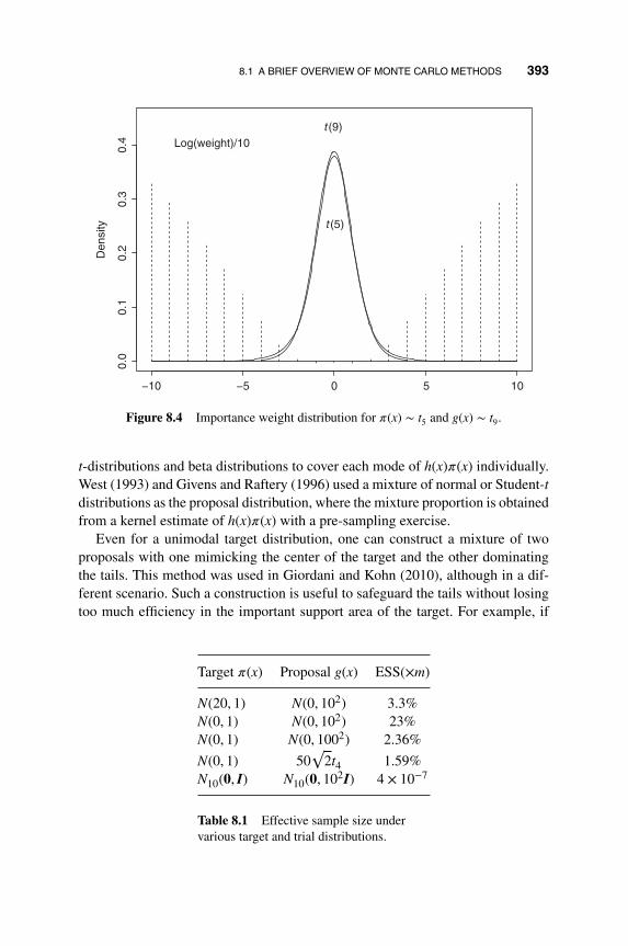
8.1 A BRIEF OVERVIEW OF MONTE CARLO METHODS 393
t(9)
t(5)
Log(weight)/10
1050−5−10
0.4
0.3
0.2
0.1
0.0
Den
sity
Figure 8.4 Importance weight distribution for 𝜋(x) ∼ t5 and g(x) ∼ t9.
t-distributions and beta distributions to cover each mode of h(x)𝜋(x) individually.West (1993) and Givens and Raftery (1996) used a mixture of normal or Student-tdistributions as the proposal distribution, where the mixture proportion is obtainedfrom a kernel estimate of h(x)𝜋(x) with a pre-sampling exercise.
Even for a unimodal target distribution, one can construct a mixture of twoproposals with one mimicking the center of the target and the other dominatingthe tails. This method was used in Giordani and Kohn (2010), although in a dif-ferent scenario. Such a construction is useful to safeguard the tails without losingtoo much efficiency in the important support area of the target. For example, if
Target 𝜋(x) Proposal g(x) ESS(×m)
N(20, 1) N(0, 102) 3.3%N(0, 1) N(0, 102) 23%N(0, 1) N(0, 1002) 2.36%
N(0, 1) 50√
2t4 1.59%N10(0, I) N10(0, 102I) 4 × 10⁻⁷
Table 8.1 Effective sample size undervarious target and trial distributions.

394 8. SEQUENTIAL MONTE CARLO
one includes the target distribution itself as one of the proposal distributions, thenone obtains an upper bound for the estimation variance. See Hesterberg (1995).For distributions with a bounded domain, including a uniform distribution in thedomain can safeguard the variance (Owen and Zhou, 2000). Other approaches canbe found in Liang et al. (2007) and Ford and Gregory (2007).
Given multiple potentially useful proposals, a straightforward combinationmethod is to use their mixture as the proposal distribution. Specifically, supposeg1(x),… , gp(x) are p probability densities serving as proposals. Given a mixtureproportion vector 𝜶 = (𝛼1,… , 𝛼p) satisfying
∑pk=1 𝛼k = 1 (0 ≤ 𝛼k < 1), we can
use the mixture distribution g𝜶(x) =∑p
k=1 𝛼kgk(x) as the proposal distribution andestimate 𝜇 and Z by
��MIS = 1m
m∑𝑖=1
h(x𝑖)𝜋(x𝑖)
g𝜶(x𝑖), ZMIS = 1
m
m∑𝑖=1
𝜋(x𝑖)
g𝜶(x𝑖),
where{
x1,… , xm
}are generated from g𝜶(x).
Hesterberg (1988) proposed that, instead of generating samples directly fromthe mixture distribution, one can use stratified samples
{xk1,… , xkm
}, discussed in
Section 8.1.2, with mk = m𝛼k samples from the kth proposal gk(⋅). The estimatorsthen become
��SIS = 1m
p∑k=1
mk∑𝑖=1
h(xk𝑖)𝜋(xk𝑖)
gk(xk𝑖), ZSIS = 1
m
p∑k=1
mk∑𝑖=1
𝜋(xk𝑖)
gk(xk𝑖).
Veach and Guibas (1995) and Raghavan and Cox (1998) proposed an extension ofthis approach.
Owen and Zhou (2000) pointed out that it is possible that using a mixture pro-posal distribution may lose some efficiency due to mixing good (efficient) pro-posal distributions with poor (inefficient) but necessary ones (for safeguarding). Itis possible that a mixture can lose efficiency by several orders of magnitude if theoriginal proposal is nearly perfect. The impact can be reduced by combining IS andcontrol variates discussed in Section 8.1.2. Specifically, Owen and Zhou (2000)proposed using g(x) = (g2(x) − g1(x),… , gp(x) − g1(x))′ as the control variates to
modify the estimator ZSIS to
ZReg = 1m
p∑k=1
mk∑𝑖=1
𝜋(xk𝑖) − ��′𝜶
g(xk𝑖)
g𝜶(xk𝑖), (8.7)
where
��𝜶 = Var
[g(X)
g𝜶(X)
]−1
Cov′[𝜋(X)g𝜶(X)
,g(X)
g𝜶(X)
],
8.1 A BRIEF OVERVIEW OF MONTE CARLO METHODS 395
and Var and Cov denote the pooled-sample variance and covariance estima-tors. It can be easily seen that g(x) serves as a set of valid control variates. Itcan also be shown that, using this set of control variates, the asymptotic vari-ance of ZReg is zero when 𝜋(x) is indeed a linear combination of the proposals.
More importantly, it can be shown that ZReg has a smaller asymptotic variancethan every IS estimator constructed solely by gk with mk samples, k = 1,… , p.That is, ZReg is always at least as good as the best one among the individualproposals.
An important issue of using mixture distributions is to determine the mix-ture weights 𝜶. Emond et al. (2001) showed that proper mixture proportions canincrease the efficiency by an order of magnitude. Fan et al. (2006) and Raghavanand Cox (1998) used some heuristic rules derived from experience or interpreta-tion of the proposals.
It is natural to use a pilot sample to select the mixture proportions before theactual sampling and estimation. Oh and Berger (1993) and Hesterberg (1995)studied the numerical properties of such an idea. Li et al. (2013) proposed a moresophisticated two-stage approach. In the first stage, pilot samples are obtainedusing a mixture proposal with predetermined proportions. Based on the pilotsamples, the optimal mixture proportions are then estimated by minimizingthe estimated asymptotic variance of the final estimator, with control variates.In the second stage, the sample is drawn from the mixture proposal with theestimated proportions. Final estimators are based on all observations, includingthose from the pilot stage. They show that the two-stage estimators are consistentand asymptotically normal with minimum asymptotic variance over all mixtureproportions. This two-stage procedure can also serve as a selection tool amongmany potential proposal candidates.
3. Weight equivalence: Another special feature of IS is that a sample can beaccompanied by different sets of weights while still being properly weighted withrespect to the same target distribution. For example, if {(x𝑖, y𝑖), 𝑖 = 1,… , m} iidfrom g(x, y) and w𝑖 = 𝜋(x𝑖, y𝑖)∕g(x𝑖, y𝑖), then {((x𝑖, y𝑖), w𝑖), 𝑖 = 1,… , m} is prop-erly weighted with respect to 𝜋(x, y). Hence the weighted sample {(y𝑖, w𝑖), 𝑖 =1,… , m} is properly weighted with respect to 𝜋Y (y), the marginal distributionderived from 𝜋(x, y), according to Lemma 8.6. On the other hand, by discardingx𝑖, the marginal sample y𝑖 is iid from gY (y), where gY (y) is the marginal distri-bution derived from g(x, y). Let w∗
𝑖= 𝜋Y (y)∕gY (y). Then {(y𝑖, w∗
𝑖), 𝑖 = 1,… , m}
is also properly weighted with respect to 𝜋(y). Note that the samples {y𝑖, 𝑖 =1,… , m} are the same, but the weights are different, even though the targetdistribution is the same. One may wonder which set of weights is better. We

396 8. SEQUENTIAL MONTE CARLO
notice that
Varg(w𝑖) = Varg
[𝜋(x𝑖, y𝑖)
g(x𝑖, y𝑖)
]= VargY
[Eg
{𝜋(x𝑖, y𝑖)
g(x𝑖, y𝑖)∣ y𝑖
}]+ EgY
[Varg
{𝜋(x𝑖, y𝑖)
g(x𝑖, y𝑖)∣ y𝑖
}]= VargY
[𝜋(y𝑖)
g(y𝑖)
]+ EgY
[Varg
{𝜋(x𝑖, y𝑖)
g(x𝑖, y𝑖)∣ y𝑖
}]= VargY
(w∗𝑖 ) + EgY
[Varg
{𝜋(x𝑖, y𝑖)
g(x𝑖, y𝑖)∣ y𝑖
}].
Hence w∗𝑖
is better. It has a smaller variance since it removes the Monte Carlovariation in x𝑖 when calculating the weights. However, one would need to be ableto evaluate the marginal distributions gY (y) and 𝜋Y (y). This is often called themarginal weighting.
A particularly useful application of the marginal weighting approach is ingenerating samples from a mixture distribution. Suppose 𝜋(x) = (1 − p)𝜋1(x) +p𝜋2(x) and we use trial distribution g(x) = (1 − p)g1(x) + pg2(x). To generate sam-ples from g(x), it is often easier to use the sequential sampling approach bygenerating an indicator I𝑖 ∼ Bernull𝑖(p) first, then generating x𝑖 ∼ gI𝑖
(⋅). Hence(x𝑖, I𝑖) ∼ gI𝑖
(x𝑖)p(I𝑖). Its corresponding target distribution is then 𝜋I𝑖(x𝑖)p(I𝑖), hence
w𝑖 = 𝜋I𝑖(x𝑖)∕gI𝑖
(x𝑖). On the other hand, since x𝑖 ∼ g(⋅), we have
w∗𝑖 =
𝜋(x𝑖)
g(x𝑖)=
(1 − p)𝜋1(x𝑖) + p𝜋2(x𝑖)
(1 − p)g1(x𝑖) + pg2(x𝑖).
We have shown that w∗𝑖
is a better set of weights. The basic principle is that oneshould carry out as much analytical calculation as possible to improve the effi-ciency. We use this feature later in Section 8.6.
4. Resampling in IS: As discussed before, a useful interpretation of IS is that itessentially approximates the distribution 𝜋(x) by a discrete distribution taking val-ues in the set {x(j), j = 1,… , m} with probabilities proportional to w(j). It leads tothe following resampling approach to generate (unweighted) samples that followthe distribution 𝜋(x). Since the CDF of 𝜋(x) is approximated by
F(x) = P(X ≤ x) = 1m
m∑j=1
w(j)I(x(j) ≤ x),

8.1 A BRIEF OVERVIEW OF MONTE CARLO METHODS 397
generating samples from F(x) can be done by sampling X = x from the set {x(j), j =1,… , m} with probabilities proportional to w(j). Then X approximately follows𝜋(x). Particularly, such a sample satisfies
EF(h(X)) = E𝜋(h(X)),
since {(x(j), w(j)), j = 1,… , m} is properly weighted with respect to 𝜋.The following lemma extends the results to any set of resampling probabilities
0 < 𝛼(x(j)) < 1, called the priority score.
Lemma 8.7 Suppose {(x(j), w(j)), j = 1,… , m} are independent and properlyweighted with respect to 𝜋(x). Let {Ij, j = 1,… , k} be a set of samples generatedfrom the set {1,… , m} with probability 𝛼(j), where 0 < 𝛼(j) < 1 and
∑j 𝛼
(j) = 1.
Then the set {(x(Ij), w(Ij)), j = 1,… , k} is properly weighted with respect to 𝜋(x),where w(j) = w(j)∕𝛼(j).
To see why this is true, let S = {x(1),… , x(m)}. For any 𝜋-integrable functionh(⋅), we have
EI,g
[1k
k∑j=1
w(Ij)h(x(Ij))
]= Eg
[EI1
(w(I1)h(x(I1)) ∣ S)]
= Eg
[m∑
j=1
𝛼(j)w(j)h(x(j))
]
= Eg
[m∑
j=1
w(j)h(x(j))
]= cE𝜋(h(x)),
where
c = EI,g
[1k
k∑j=1
w(Ij)
]= Eg
[m∑
j=1
w(j)
].
For a more rigorous proof, see Douc et al. (2014, Chapter 10).If one generated x(1),… , x(k) using this method, with 𝛼(j) = w(j), the set of sam-
ples can be treated as iid samples from 𝜋(⋅) for inferences, if k ≪ m. The resam-pled weight in this case is constant 1. However, if k is not small (or in many cases,k = m), even though they are independent given the original weighted samples{(x(j), w(j)), j = 1,… , m}, the samples are marginally dependent, since there willbe duplicates, the same x(j) being sampled multiple times. The samples with largeweights w(j) tend to be duplicated and the samples with small weights may not be

398 8. SEQUENTIAL MONTE CARLO
sampled. Note that inference should be done using the original weighted samples,instead of the resampled (unweighted) samples x1,… , xm, because
mVar
[1m
m∑j=1
w(Ij)h(x(Ij))
]≥ mVar
[1m
m∑j=1
w(j)h(x(j))
].
Hence for making inference, one should not use the resampled samples. However,resampling is a critical step in the SMC method, which we discuss later.
5. Comparison with rejection sampling: Rejection sampling and IS are sim-ilar in that both use a trial distribution g(⋅) and both require that 𝜋(x)∕g(x) < c,though for IS the condition can be relaxed if one focuses on a specific h(x). Inaddition, rejection sampling does not use the samples that are rejected. IS keepsthese samples, but uses importance weights as adjustments. The rejection sam-pling produces a set of iid samples, which can be useful in certain situations andmakes theoretical investigation easier when it is embedded as a component in aprocedure. In a way, ESS for IS is the acceptance rate for the rejection sampling.
8.1.4 Markov Chain Monte Carlo
Markov chain Monte Carlo (MCMC) methods are a class of powerful methods forgenerating samples (not necessarily iid) from a complex and possibly high dimen-sional target distribution 𝜋(x). The key idea is to construct a Markov chain suchthat its equilibrium (stationary) distribution is 𝜋(x). Then the Monte Carlo real-izations of such a Markov chain can be used as samples of the target distribution𝜋(x).
In the appendix of Chapter 2 we discussed some important concepts and prop-erties of a Markov chain taking values in a finite set. Here we expand the theoryto the general spaces.
A Markov chain (MC) is a stochastic process X1,… , Xt,… with the propertythat the conditional density
p(Xt ∣ Xt−1, Xt−2,…) = p(Xt ∣ Xt−1).
Hence a homogeneous Markov chain is completely specified by the one-steptransition probability density p(⋅ ∣ x) = p(Xt+1 ∣ Xt = x) for all t. Clearly, the k-step transition density p(k)(⋅ ∣ x) = p(Xt+k ∣ Xt = x) can be obtained through theChapman–Kolmogorov equation
p(k)(y ∣ x) =∫
p(𝑖)(y ∣ z)p(j)(z ∣ x)dz,
where 𝑖 + j = k.MCMC methods are based on the following key result.

8.1 A BRIEF OVERVIEW OF MONTE CARLO METHODS 399
Lemma 8.8 For an 𝜙-irreducible and aperiodic Markov chain with transitiondensity p(xt ∣ xt−1), if it is invariant respect to 𝜋(x), then the Markov chain isergodic, with 𝜋(x) as its equilibrium distribution.
Some brief descriptions of the terms used in Lemma 8.8 are in order. Theyare parallel to the discussion on the finite-space Markov chain in the appendix ofChapter 2, hence the discussion here is brief. A Markov chain is said to be irre-ducible if it has a connected support. Conceptually, it requires that, for any regionA with non-zero 𝜙-measure in the support of the chain Ω, there is a positive proba-bility that, starting with X0 = x for any x ∈ Ω, the chain will reach A in finite steps.Alternatively, there is a t < ∞ such that P(Xt ∈ A ∣ X0 = x) > 0. A Markov chainis said to be aperiodic if it is not periodic, that is, the largest common divider of{t : P(Xt ∈ A ∣ X0 = x) > 0} is 1, for any A and starting location x ∈ Ω. A Markovchain is invariant if there is a density 𝜋(x) such that 𝜋(y) = ∫ p(y ∣ x)𝜋(x)dx. Thismeans that, if at time t, xt ∼ 𝜋(x), then at time t + 1, xt+1 still follow 𝜋(x), underthe transition density p(y ∣ x). The invariance condition is satisfied if one can showa perfect balance condition
p(y ∣ x)𝜋(x) = p(x ∣ y)𝜋(y). (8.8)
This is because, under the balance condition, we have
∫p(y ∣ x)𝜋(x)dx =
∫p(x ∣ y)𝜋(y)dx = 𝜋(y).
Ergodicity is one of the most useful properties of a stochastic process (if thechain is ergodic). One key result we use here is the ergodic theorem, which saysthat if a Markov chain is ergodic, then the law of large number holds. That isx → E𝜋(x), where 𝜋(⋅) is the equilibrium distribution. It also says that, starting withx0 ∼ g(x), the distribution of Xt converges to 𝜋(x). For more detailed discussions,see Robert and Casella (2004) and Liu (2001), among others.
Using the above result, MCMC methods construct a transition rule p(y ∣ x) sothe resulting Markov chain is ergodic, with the target distribution𝜋(⋅) as its equilib-rium distribution. Given an appropriate p(y ∣ x) that is easy to sample y from x, westart with X0 = x0 ∈ Ω, and iteratively generate samples xt ∼ p(y ∣ Xt−1 = xt−1),t = 1,… . The resulting samples xK+1,… , xK+m approximately follow 𝜋(x), afterremoving samples in the burning period (t = 1,… , K) to reduce the impact of theinitial value. Then 𝜇h = E𝜋(x) can be estimated by
��h = 1m
K+m∑j=K+1
h(xj).
There are two widely used constructions of the transition density p(y ∣ x).

400 8. SEQUENTIAL MONTE CARLO
1. Metropolis–Hastings algorithm. Consider a target distribution 𝜋(x) that canbe evaluated up to a normalizing constant. Let T(x, y) be a proposal move rule thatproposes a (random) move from x to y. In practice one should choose a T(x, y) thatis easy to generate the move.
Algorithm 8.2: Metropolis–Hastings Algorithm
� Start with any X0 = x0.
� Suppose at time t, Xt = xt. At time t + 1,
– Draw y ∼ T(xt, y) (i.e., propose a move for the next step).
– Compute the metropolis ratio (or ‘goodness’ ratio)
r =𝜋(y)𝜋(xt)
T(y, xt)
T(xt, y).
– Acceptance/rejection decision: let
Xt+1 =
{y with prob p = min{1, r}
xt with prob 1 − p.
With such a movement, the Markov chain is invariant with respect to 𝜋(x). Notethat the actual transition probability from x to y is
p(y ∣ x) = T(x, y)min{
1,𝜋(y)𝜋(x)
T(y, x)T(x, y)
}and the transition probability from y to x is
p(x ∣ y) = T(y, x)min{
1,𝜋(x)𝜋(y)
T(x, y)T(y, x)
}.
To check the balance condition in (8.8), for x ≠ y, we have
𝜋(x)p(y ∣ x) = 𝜋(x)T(x, y)min{
1,𝜋(y)𝜋(x)
T(y, x)T(x, y)
}= min{𝜋(x)T(x, y),𝜋(y)T(y, x)}
= 𝜋(y)T(y, x)min{
1,𝜋(x)𝜋(y)
T(x, y)T(y, x)
}= 𝜋(y)p(x ∣ y).
Hence the balance condition is satisfied. Along with irreducible and aperiodic con-ditions (by the design of T(x, y)), the Markov chain is ergodic.

8.1 A BRIEF OVERVIEW OF MONTE CARLO METHODS 401
In the special case of symmetric move T(x, y) = T(y, x), we have
r =𝜋(y)𝜋(x)
and p = min{1, r}.
Hence if 𝜋(y) ≥ 𝜋(xt), we move to y with probability 1 (so xt+1 = y). If 𝜋(y) <𝜋(xt), we move to y with probability r. The smaller 𝜋(y) is, the lower the chance ofmoving. Unlike deterministic accent (decent) algorithms, we always move uphillwith probability one, but also allow some probability to move downhill.
A different acceptance rule (Baker’s acceptance rule) can also be used:
𝜌(x, y) = r1 + r
=𝜋(y)T(y, x)
𝜋(x)T(x, y) + 𝜋(y)T(y, x).
Some commonly used proposal move rules include the random-walk metropoliswhich uses proposal y = xt + 𝜀t, where 𝜀t ∼ N(0,Σ0) in continuous cases, or 𝜀t ∼Bernoull𝑖{−1, 1} in discrete cases, with r = min{1,𝜋(y)∕𝜋(xt)}. The metropolizedindependent sampler uses proposal y ∼ g(y) (a proposal distribution) with
r = min{
1,w(y)w(x)
}where w(x) = 𝜋(x)
g(x).
This is similar to the importance weight in IS.
2. Gibbs sampler: Suppose the target distribution is multidimensional 𝜋(x) =𝜋(x1,… , xp). Sequential sampling requires the ability to generate samples froma marginal distribution 𝜋(x1) and the partial conditional distributions p(x𝑖 ∣x1,… , x𝑖−1) of the joint distribution 𝜋(x1,… , xp), which are not always available.Gibbs sample is a MCMC implementation in the cases where marginal distributionand partial conditional distributions are not available, but sampling from the fullconditional distributions 𝜋(x𝑖 ∣ x1,… , x𝑖−1, x𝑖+1,… , xn) (denoted as 𝜋(x𝑖 ∣ x−𝑖))are easy for each 𝑖.
Algorithm 8.3: Gibbs Sampler
� Start with an initial value x(1) = (x(1)1 ,… , x(1)
p ).
� At iteration j + 1,
– sample x(j+1)1 ∼ 𝜋(x1 ∣ x(j)
2 ,… , x(j)p )
– sample x(j+1)2 ∼ 𝜋(x2 ∣ x(j+1)
1 , x(j)3 ,… , x(j)
p )
– ⋮
– sample x(j+1)p ∼ 𝜋(xp ∣ x(j+1)
1 , x(j+1)2 ,… , x(j+1)
p−1 ).

402 8. SEQUENTIAL MONTE CARLO
Under some mild conditions, such a Markov chain {(x(j)1 ,… , x(j)
p ), j = 1, 2,…} isergodic with 𝜋(x1,… , xp) as its invariant distribution.
Note that, if (x(j)1 ,… , x(j)
p ) ∼ 𝜋(x1,… , xp), then the marginal distribution (with-
out x1) follows (x(j)2 ,… , x(j)
p ) ∼ 𝜋(x2,… , xp). Hence
(x(j+1)1 , x(j)
2 ,… , x(j)p ) ∼ 𝜋(x(j+1)
1 ∣ x(j)2 ,… , x(j)
p )𝜋(x(j)2 ,… , x(j)
p )
= 𝜋(x(j+1)1 , x(j)
2 ,… , x(j)p ).
Similarly, if (x(j+1)1 , x(j)
2 ,… , x(j)p ) ∼ 𝜋(x(j+1)
1 , x(j)2 ,… , x(j)
p ), then
(x(j+1)1 , x(j)
3 ,… , x(j)p ) ∼ 𝜋(x(j+1)
1 , x(j)3 ,… , x(j)
p ).
Hence
(x(j+1)1 , x(j+1)
2 , x(j)3 ,… , x(j)
p )
∼ 𝜋(x(j+1)2 ∣ x(j+1)
1 , x(j)3 ,… , x(j)
p )𝜋(x(j+1)1 , x(j)
3 ,… , x(j)p )
= 𝜋(x(j+1)1 , x(j+1)
2 , x(j)3 ,… , x(j)
p ).
Repeating this process, we have that if (x(j)1 ,… , x(j)
p ) ∼ 𝜋(x1,… , xp), then
(x(j+1)1 ,… , x(j+1)
p ) ∼ 𝜋(x1,… , xp). Hence the Markov chain is invariant under sucha transition rule.
There are many more advanced implementations of MCMC methods. Detailscan be found in Robert and Casella (2004), and Liu (2001).
8.2 THE SMC FRAMEWORK
Consider the SSM:
State equation: xt = st(xt−1, 𝜀t) or xt ∼ qt(⋅ ∣ xt−1),
Observation equation: yt = ht(xt, et) or yt ∼ ft(⋅ ∣ xt).
When the system is nonlinear and non-Gaussian, filtering and smoothing canbe difficult as there are no analytic solutions for the predicting and the updatingsteps. In Chapter 7 we discussed several approaches to deal with nonlinear andnon-Gaussian systems based on approximations. SMC follows the prediction andupdating steps of the Kalman filter and maintains the recursive nature of the algo-rithm for fast on-line processing, achieving real-time filtering. It performs the pre-diction and updating steps based on Monte Carlo approximations. The approachfocuses on the conditional distributions in the filtering and smoothing steps. As
8.2 THE SMC FRAMEWORK 403
no analytical forms are available, they are represented by Monte Carlo samples.In the literature, SMC methods or some of its specific implementations are alsoreferred to as particle filtering and particle smoothing, e.g. Douc et al. (2014). TheMonte Carlo samples are often called particles in this context.
Suppose {x(1)t−1,… , x(m)
t−1} is a set of random samples following p(xt−1 ∣ yt−1)where yt = (y1,… , yt). At time t, with a new observation yt, we would like toobtain a set of samples {x(1)
t ,… , x(m)t } following the distribution p(xt ∣ yt). There
are two things that have changed here. The first change is that the samples are nowabout the state xt, instead of xt−1. The second is that the information set changesfrom yt−1 to yt, with an extra observation yt. A simple approach is to deal with thetwo changes separately. The first step is to move into the space of xt from xt−1,without changing the information set yt−1, similar to the prediction step of theKalman filter. To generate xt from p(xt ∣ yt−1), we note that
p(xt, xt−1 ∣ yt−1) = p(xt ∣ xt−1, yt−1)p(xt−1 ∣ yt−1)
= p(xt ∣ xt−1)p(xt−1 ∣ yt−1).
Hence we can use the sequential sampling approach by first generating samplesfrom p(xt−1 ∣ yt−1) (which has been done at time t − 1), then drawing xt from theconditional distribution p(xt ∣ xt−1), which is the state equation. Let
x(j)t ∼ qt(xt ∣ x(j)
t−1).
Then {(x(1)t , x(1)
t−1),… , (x(m)t , x(m)
t−1)} is a set of random samples following the dis-
tribution p(xt, xt−1 ∣ yt−1). The marginal samples {x(1)t ,… , x(m)
t } then follow p(xt ∣yt−1). However, this set of samples is not exactly what we wanted, as we wish tohave a set of samples from p(xt ∣ yt−1, yt), that is, the sample we have is from awrong distribution. Not all is lost, however, as proper adjustments can be made.The adjustment can be carried out using the IS idea. The samples {x(1)
t ,… , x(m)t }
can be viewed as having been generated from a trial distribution p(xt ∣ yt−1) andour target distribution is p(xt ∣ yt−1, yt). Hence the weight function is
wt(xt) =p(xt ∣ yt−1, yt)
p(xt ∣ yt−1)
∝p(xt, yt ∣ yt−1)
p(xt ∣ yt−1)
=p(yt ∣ xt, yt−1)p(xt ∣ yt−1)
p(xt ∣ yt−1)
= p(yt ∣ xt).
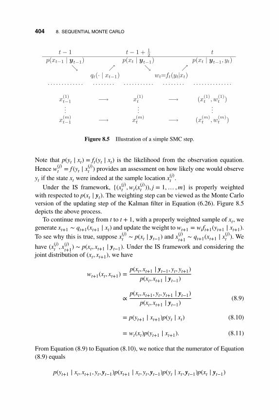
404 8. SEQUENTIAL MONTE CARLO
t− 1 t− 1 + 12 t
p(xt−1 | yt−1) p(xt | yt−1) p(xt | yt−1, yt)↘ ↗ ↘ ↗
qt(· | xt−1) wt=ft(yt|xt). . . . . . . . . . . . . . . . . . . . . . . . . . . . . . . . . . . . . . . . . . . . . . . . . . . . . .
x(1)t−1 −→ x
(1)t −→ (x(1)
t , w(1)t )
......
...x
(m)t−1 −→ x
(m)t −→ (x(m)
t , w(m)t )
Figure 8.5 Illustration of a simple SMC step.
Note that p(yt ∣ xt) = ft(yt ∣ xt) is the likelihood from the observation equation.Hence w(j)
t = f (yt ∣ x(j)t ) provides an assessment on how likely one would observe
yt if the state xt were indeed at the sample location x(j)t .
Under the IS framework, {(x(j)t , wt(x
(j)t )), j = 1,… , m} is properly weighted
with respected to p(xt ∣ yt). The weighting step can be viewed as the Monte Carloversion of the updating step of the Kalman filter in Equation (6.26). Figure 8.5depicts the above process.
To continue moving from t to t + 1, with a properly weighted sample of xt, wegenerate xt+1 ∼ qt+1(xt+1 ∣ xt) and update the weight to wt+1 = wtft+1(yt+1 ∣ xt+1).
To see why this is true, suppose x(j)t ∼ p(xt ∣ yt−1) and x(j)
t+1 ∼ qt+1(xt+1 ∣ x(j)t ). We
have (x(j)t , x(j)
t+1) ∼ p(xt, xt+1 ∣ yt−1). Under the IS framework and considering thejoint distribution of (xt, xt+1), we have
wt+1(xt, xt+1) =p(xt, xt+1 ∣ yt−1, yt, yt+1)
p(xt, xt+1 ∣ yt−1)
∝p(xt, xt+1, yt, yt+1 ∣ yt−1)
p(xt, xt+1 ∣ yt−1)(8.9)
= p(yt+1 ∣ xt+1)p(yt ∣ xt) (8.10)
= wt(xt)p(yt+1 ∣ xt+1). (8.11)
From Equation (8.9) to Equation (8.10), we notice that the numerator of Equation(8.9) equals
p(yt+1 ∣ xt, xt+1, yt, yt−1)p(xt+1 ∣ xt, yt, yt−1)p(yt ∣ xt, yt−1)p(xt ∣ yt−1)

8.2 THE SMC FRAMEWORK 405
and the denominator equals
p(xt+1 ∣ xt, yt−1)p(xt ∣ yt−1).
Since (xt, xt+1, wt+1) is properly weighted with respect to p(xt, xt+1 ∣ yt+1), wealso have (xt, wt+1) properly weighted with respect to p(xt ∣ yt+1). In fact, (x1, wt+1)is properly weighted with respect to p(x1 ∣ yt+1). The whole process can be carriedout recursively starting with a set of initial samples x0 and weight w0.
Figures 8.6 to 8.8 illustrate the aforementioned procedure with a simple SSM
xt = xt−1 + et, yt = xt + 𝜀t,
where et ∼ N(0, 1), 𝜀t ∼ N(0, 1), and x0 ∼ N(0, 1). Seven samples of x0 ∼ N(0, 1)are generated. Their initial weights are set to 1, as they are iid from the prior dis-tribution p(x0). They are shown as dots on the left (t = 0) line in Figure 8.6. Theircorresponding vertical lines depict their weights. Moving from t = 0 to t = 1, x(j)
1
is simulated from x(j)1 ∼ p(x1 ∣ x0 = x(j)
0 ), or equivalently x(j)1 = x(j)
0 + 𝜀(j)1 , where
𝜀(j)1 ∼ N(0, 1). They follow p(x1) without using the observation y1 and their weights
remain one. These samples are shown on the middle (t = 1∕2) line in Figure 8.6.The corresponding vertical lines depict their weights. The observation y1 is shownas the diamond dot on the right (t = 1) line in Figure 8.6. Based on this observa-tion, we obtained the weights of the seven samples w(j)
t ∝ exp{−0.5(y1 − x(j)1 )2}
according to the observation equation yt = xt + et. The samples and their weights
151050
2015
105
0
-2-1
01
2
-2-1
01
2
-2-1
01
2
Figure 8.6 Simple illustration of updating scheme (I).

406 8. SEQUENTIAL MONTE CARLO
-2-1
01
2
-2-1
01
2
-2-1
01
2
151050
2015
105
0
Figure 8.7 Simple illustration of updating scheme (II).
are shown on the t = 1 line. It is seen that the samples closer to the observationhave larger weights.
Figure 8.7 shows how the samples move from t = 1 to t = 2. The middle (t = 1)line shows the weighted samples of x1, the same as that in Figure 8.6. The dotson the right (t = 2) line are samples of x(j)
2 , obtained by x(j)2 = x(j)
1 + 𝜀(j)2 , where
𝜀(j)2 ∼ N(0, 1). The weights are adjusted by w(j)
1 f2(y2 ∣ x(j)2 ), where y2 is marked by
the diamond dot on the line. One feature stands out in the figure: the weights of thesamples at t = 2 are now concentrated on only two or three of the samples, while allother samples have weights almost zero. For example, the sample on the far rightis far away from the observed y2, and it comes from the sample of x1 that is also faraway from the observed y1, with a very small weight w1. The accumulating effectmakes its weight extremely small. Since inference (e.g., estimating E(x2 ∣ y1, y2))is based on the weighted averages, samples with almost zero weights have negli-gible contributions to the inference. It is seen that among the seven samples, thereare only three samples that are important enough to make contributions to theinference. In other words, the effective sample size defined in Equation (8.6) hasbeen reduced to less than 30% of the original sample size in just two time steps(ESS = 2.8 in this case). That is, this set of seven samples is equivalent to onlyhaving 2.8 iid samples directly from p(x2 ∣ y1, y2). One can imagine that movingfrom t = 2 to t = 3 we may lose even more effective samples. The reason for thisis that the samples of x1 are generated without using the information of y1 and

8.2 THE SMC FRAMEWORK 407
y2. The variation in the weights reflects the distance between the sampling distri-bution p(x1) and the target distribution p(x1 ∣ y1, y2). As t increases, the distancebetween p(x1) and p(x1 ∣ yt) would increase. Since (x1, w2) is properly weightedwith respect to p(x1 ∣ y1, y2), such a discrepancy is reflected in the weight distri-bution. Hence the effective sample size will decrease, and often decreases quicklyas t increases. Kong et al. (1994) showed that the effective sample size decreases(stochastically) as t increases. Hence, the estimation accuracy would decrease ast increases. In addition, continuing propagating the samples with small weightsforward is a waste of computational resources as their weights are unlikely to getbetter. Discarding these samples reduces the total number of sample points, andregenerating new samples starting from t = 0 is computationally expensive. Onesolution is to use the resampling schemes introduced in Section 8.1.3 to duplicatethe important samples and to eliminate the ones with low weights. Resampling isdone randomly so the resampled samples remain properly weighted with respectto the target distribution.
Figure 8.8 shows the results of an improved sampling procedure in which thesamples of x1 are generated utilizing the information of y1, and the samples of x2are generated utilizing the information of y2. We see clearly the improvements. Att = 2, the effective sample size is 5.1. It shows that proper propagation (movingsamples through time) is very important in terms of efficiency. Note that it is notnecessary to use qt(xt ∣ xt−1) for moving from xt−1 to xt in the predictive step. Sincewe are using IS adjustment in the updating step, any proposal distribution can be
-2-1
01
2
-2-1
01
2
-2-1
01
2
151050
2015
105
0
Figure 8.8 Simple illustration of updating scheme (III).

408 8. SEQUENTIAL MONTE CARLO
used here, though the weighting needs to be modified accordingly. Specifically, ifwe have (x(j)
t−1, w(j)t−1) properly weighted with respect to p(xt−1 ∣ yt−1) and if we use
x(j)t ∼ gt(xt ∣ x(j)
t−1, yt) for propagation, then ((x(j)t , x(j)
t−1), w(j)t−1) is properly weighted
with respect to gt(xt ∣ x(j)t−1, yt)p(xt−1 ∣ yt−1). Our target distribution is p(xt, xt−1 ∣
yt). Hence by Lemma 8.5, the weight function is
w(j)t ∝ w(j)
t−1
p(x(j)t , x(j)
t−1 ∣ yt)
p(x(j)t−1 ∣ yt−1)gt(x
(j)t ∣ x(j)
t−1, yt)∝ w(j)
t−1
p(yt ∣ x(j)t )p(x(j)
t ∣ x(j)t−1)
gt(x(j)t ∣ x(j)
t−1, yt).
Once the samples are generated, one also needs to use an efficient estimatorfor inference. Based on these observations, Liu and Chen (1998) formulated thefollowing SMC framework.
Suppose (x(j)t−1, w(j)
t−1), j = 1,… , m, are properly weighted with respect top(xt−1 ∣ yt−1). When the system evolves from stage t − 1 to stage t, three oper-ations can be performed. Note that not all three operations have to be performedand the order of the operations can also vary.
Algorithm 8.4: Propagation Step
At time t, for j = 1,… , m:
(A) Draw x(j)t from a trial distribution gt(xt ∣ x(j)
t−1, yt). Attach it to x(j)t−1 to
form x(j)t = (x(j)
t−1, x(j)t ).
(B) Compute the incremental weight
u(j)t ∝
qt(x(j)t ∣ x(j)
t−1)ft(yt ∣ x(j)t )
gt(x(j)t ∣ x(j)
t−1, yt)
and the new weight
w(j)t = w(j)
t−1u(j)t .
The resulting sample {(x(j)t , w(j)
t ), j = 1,… , m} is properly weighted with
respect to p(xt ∣ yt). The partial sample {(x(j)t , w(j)
t ), j = 1,… , m} is properlyweighted with respect to p(xt ∣ yt) for filtering problems. See Section 8.3 for amore detailed discussion. For more general dynamic systems, similar propagationstep can be performed.
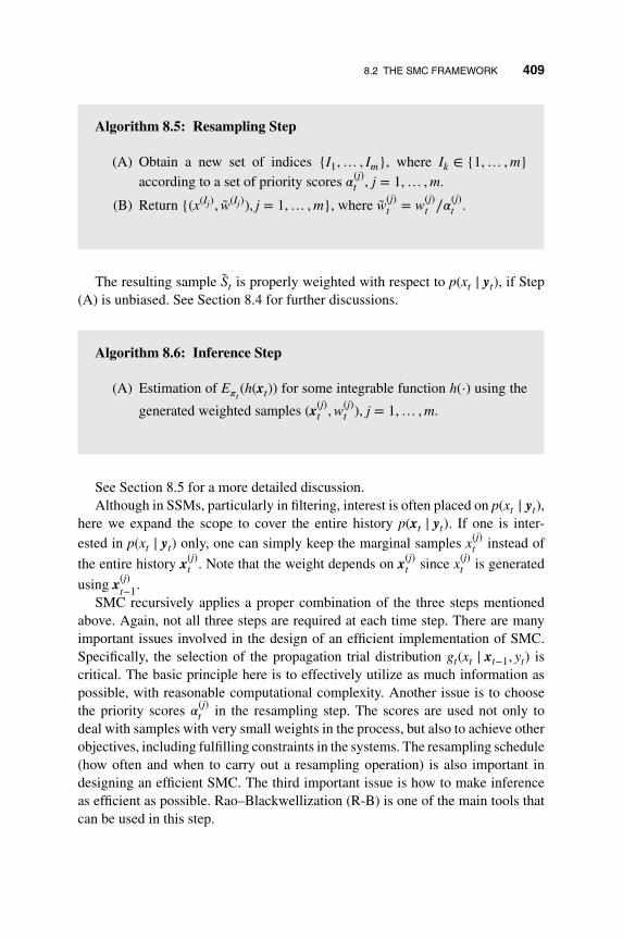
8.2 THE SMC FRAMEWORK 409
Algorithm 8.5: Resampling Step
(A) Obtain a new set of indices {I1,… , Im}, where Ik ∈ {1,… , m}according to a set of priority scores 𝛼(j)
t , j = 1,… , m.
(B) Return {(x(Ij), w(Ij)), j = 1,… , m}, where w(j)t = w(j)
t ∕𝛼(j)t .
The resulting sample St is properly weighted with respect to p(xt ∣ yt), if Step(A) is unbiased. See Section 8.4 for further discussions.
Algorithm 8.6: Inference Step
(A) Estimation of E𝜋t(h(xt)) for some integrable function h(⋅) using the
generated weighted samples (x(j)t , w(j)
t ), j = 1,… , m.
See Section 8.5 for a more detailed discussion.Although in SSMs, particularly in filtering, interest is often placed on p(xt ∣ yt),
here we expand the scope to cover the entire history p(xt ∣ yt). If one is inter-ested in p(xt ∣ yt) only, one can simply keep the marginal samples x(j)
t instead of
the entire history x(j)t . Note that the weight depends on x(j)
t since x(j)t is generated
using x(j)t−1.
SMC recursively applies a proper combination of the three steps mentionedabove. Again, not all three steps are required at each time step. There are manyimportant issues involved in the design of an efficient implementation of SMC.Specifically, the selection of the propagation trial distribution gt(xt ∣ xt−1, yt) iscritical. The basic principle here is to effectively utilize as much information aspossible, with reasonable computational complexity. Another issue is to choosethe priority scores 𝛼
(j)t in the resampling step. The scores are used not only to
deal with samples with very small weights in the process, but also to achieve otherobjectives, including fulfilling constraints in the systems. The resampling schedule(how often and when to carry out a resampling operation) is also important indesigning an efficient SMC. The third important issue is how to make inferenceas efficient as possible. Rao–Blackwellization (R-B) is one of the main tools thatcan be used in this step.

410 8. SEQUENTIAL MONTE CARLO
8.3 DESIGN ISSUE I: PROPAGATION
The propagation step in Algorithm 8.4 is the key to an efficient implementationof SMC. Its design is mainly concerned with the selection of the trial distributiongt(⋅).
The following alternative interpretation of Algorithm 8.4 is useful. Considerthe problem of generating samples from the target distribution p(xt ∣ yt). This is ahigh dimensional and difficult problem. To employ the IS approach, we need tofind a trial distribution g(xt). Since xt is high dimensional, sequential sampling isa standard approach, and we can construct g(xt) sequentially, building one com-ponent at a time, conditioning on the previous ones. Specifically, we use
g(xt) = g1(x1)g2(x2 ∣ x1)… gt(xt ∣ xt−1). (8.12)
Each of the component conditional distribution gs(xs ∣ xs−1) is of low dimension.The associated weight function is
wt =p(xt ∣ yt)
g(xt).
The following expression is useful in obtaining some guidance for selecting gs(xs ∣xs−1) (ignoring p(x0)).
wt =p(xt ∣ yt)∏t
s=1 gs(xs ∣ xs−1)
=t∏
s=1
p(xs ∣ ys)
p(xs−1 ∣ ys−1)gs(xs ∣ xs−1)
∝t∏
s=1
p(xs, ys ∣ ys−1)
p(xs−1 ∣ ys−1)gs(xs ∣ xs−1)
∝t∏
s=1
p(xs ∣ xs−1, ys−1)p(ys ∣ xs)p(xs−1 ∣ ys−1)
p(xs−1 ∣ ys−1)gs(xs ∣ xs−1)
∝t∏
s=1
p(xs ∣ xs−1)p(ys ∣ xs)
gs(xs ∣ xs−1).
Hence, letting
us =p(xs ∣ xs−1)p(ys ∣ xs)
gs(xs ∣ xs−1)=
qs(xs ∣ xs−1)fs(ys ∣ xs)
gs(xs ∣ xs−1),
we have ws = ws−1us, s = 1,… , t. If the trial distribution gs(xs ∣ xs−1) onlyinvolves xs−1 and ys, then the procedure can be made sequentially for t = 1, 2,….

8.3 DESIGN ISSUE I: PROPAGATION 411
Since the efficiency of the process depends on the weight distribution and theincremental weight is
u(j)t ∝
qt(x(j)t ∣ x(j)
t−1)ft(yt ∣ x(j)t )
gt(x(j)t ∣ x(j)
t−1, yt), (8.13)
one would naturally want to choose gt(⋅) so the ratio in Equation (8.13) is close toa constant.
8.3.1 Proposal Distributions
In Kong et al. (1994) and Liu and Chen (1995, 1998), the trial distribution
gt(xt ∣ xt−1) = p(xt ∣ xt−1, yt) ∝ qt(xt ∣ xt−1)ft(yt ∣ xt) (8.14)
was recommended for the SSM. This selection of gt makes the ratio in Equation(8.13) a constant. Specifically, we have the following algorithm.
Algorithm 8.7: Full Information Propagation Step
At time t, for j = 1,… , m:
(A) Draw x(j)t from the local posterior distribution,
gt(xt ∣ x(j)t−1, yt) = p(xt ∣ x(j)
t−1, yt)
∝ ft(yt ∣ xt)qt(xt ∣ x(j)t−1). (8.15)
(B) Compute the incremental weight
u(j)t =
∫ft(yt ∣ xt)qt(xt ∣ x(j)
t−1)dxt
and the new weight
w(j)t = w(j)
t−1u(j)t .
The incremental weight formula is based on Equation (8.13). Note that thedenominator of that equation is a normalized version of the numerator, hence u(j)
t
is the normalizing constant of ft(yt ∣ xt)qt(xt ∣ x(j)t−1) as a density of xt. It does not
depend on the sampled x(j)t . This is a nice feature that we will make use of later in
estimation.

412 8. SEQUENTIAL MONTE CARLO
The proposal distribution in Equation (8.14) utilizes information from both thestate and observation equations, hence is termed a full information propagationstep. However, in many cases this trial distribution requires complicated compu-tations and can be difficult to generate samples from. In certain cases, the incre-mental weight can be difficult to evaluate as well.
Berzuini et al. (1997) proposed using local MCMC algorithms to generate sam-ples from the full information trial distribution qt(xt ∣ xt−1)ft(yt ∣ xt) when directsampling is difficult.
One can also use a suitable approximation of the full information trial distribu-tion to achieve efficiency with reasonable computational complexity. For example,one can use
gt(xt ∣ xt−1) ∝ qt(xt ∣ xt−1)ft(yt ∣ xt),
with incremental weight
ut ∝qt(xt ∣ xt−1)ft(yt ∣ xt)
qt(xt ∣ xt−1)ft(yt ∣ xt) ∫qt(xt ∣ xt−1)ft(yt ∣ xt)dxt,
where qt and ft are approximations of qt and ft, respectively. For ease of samplingand evaluating the integral ∫ qt(xt ∣ xt−1)ft(yt ∣ xt)dxt, normal or a mixture of nor-mal distributions is often used for qt and ft. However, since the weight depends onthe sampled x(j)
t , this is technically not a full information propagation.Another algorithm that uses approximation to the full information proposal
distribution is the unscented particle filter (van der Merwe et al., 2002). Thisis closely related to the unscented Kalman filter discussed in Section 7.1.4. Thekey idea is to use the unscented transformation (UT) to estimate the mean andvariance of the full information proposal distribution gt(xt ∣ xt−1, yt) in Equation(8.14). Specifically, suppose the random noise terms rt = (𝜀t, et) at step t hasmean 𝜇r and covariance matrix Σr. The UT chooses a set of weighted points{(𝜉𝓁 ,𝜔𝓁),𝓁 = 0,±1,… ,±n} as follows:
𝜉0 = 𝜇r; 𝜔0 = 𝜅∕(2n + 𝜅),
𝜉±𝓁 = 𝜇r ±√
2n + 𝜅Q𝓁; 𝜔±𝓁 = 1∕(2n + 𝜅), 𝓁 = 1,… , n
where n is the dimension of rt, 𝜅 is a constant, and Q𝓁 is the 𝓁th column ofthe square root matrix of Σr. With a given x(j)
t−1, the state and observation com-bination (xt, yt) is a nonlinear function of rt = (𝜀t, et) and the value of xt−1. Let(xt, yt) = 𝜑(j)(rt) = (st(x
(j)t−1, 𝜀t), ht(st(x
(j)t−1, 𝜀t), et)), corresponding to x(j)
t−1. Then the

8.3 DESIGN ISSUE I: PROPAGATION 413
mean and covariance of p(xt, yt ∣ x(j)t−1) can be estimated by:
��(j) =n∑
𝓁=−n
𝜔𝓁𝜑(j)(𝜉l),
��(j) =n∑
𝓁=−n
𝜔𝓁(𝜑(j)(𝜉𝓁) − ��(j))(𝜑(j)(𝜉𝓁) − ��(j))′.
We can then use p(xt, yt ∣ x(j)t−1) ∼ N(𝜇(j),𝚺(j)) as an approximation to p(xt, yt ∣
x(j)t−1) and derive an approximation of the full information trial distribution gt(xt ∣
yt, x(j)t−1) from the approximate normal distribution.
The bootstrap filter of Gordon et al. (1993) and Kitagawa (1996) uses the stateequation only, with gt(xt ∣ xt−1, yt) = qt(xt ∣ xt−1) and weight wt = wt−1ft(yt ∣ xt).
Algorithm 8.8: Propagation Step in a Bootstrap Filter
At time t, for j = 1,… , m:
(A) Draw x(j)t using the state equation
x(j)t ∼ qt(xt ∣ x(j)
t−1).
This is the same as generating 𝜀(j)t first and obtaining x(j)
t =st(x
(j)t−1, 𝜀(j)
t ).
(B) Compute the new weight w(j)t = w(j)
t−1ft(yt ∣ x(j)t ).
This algorithm is usually easy to implement and fast to compute when 𝜀(j)t is
easy to generate and st(⋅) and ft(⋅) are easy to evaluate. However, it is often notefficient since the generation of xt does not utilize the information in the currentobservation yt, especially if yt contains significant information on xt (e.g., if yt hasa very small measurement error). The information in yt is only used in calculatingthe weight. As a result, the trial distribution may be further away from the targetdistribution than the full information propagation, and the weight may degeneratefaster.
At the other extreme, the independent particle filters (IPF) of Lin et al. (2005)use the observation equation only as the trial distribution, that is,
gt(xt ∣ xt−1, yt) ∝ ft(yt ∣ xt),

414 8. SEQUENTIAL MONTE CARLO
with incremental weight ut ∝ qt(xt ∣ xt−1). This choice is convenient when the statedynamics qt(⋅) is weak and the information from the observation ft(⋅) is strong. Itis called the independent particle filter because the samples x(j)
t are independent
of each other and independent of the past samples x(𝑖)t−1 too. Hence there is no
direct connection between the current sample x(j)t with the past sample x(j)
t−1, but
the weight calculation ut ∝ qt(x(j)t ∣ x(j)
t−1) requires a matching. Lin et al. (2005)proposed using a multiple matching scheme and showed its advantages.
Algorithm 8.9: Propagation Step in Independent Particle Filter
At time t, for j = 1,… , m:
(A) Draw x(j)t from the observation equation gt(xt ∣ yt) ∝ ft(yt ∣ xt).
(B) Select L different permutations of {1,… , m}: Kl = {kl,1,… , kl,m},l = 1,… , L. Compute the incremental weight
u(kl,j,j)t ∝ qt(x
(j)t |x(kl,j)
t−1 )
for each permutation. Compute the multiple matching weight
w(j)t = 1
L
L∑l=1
u(kl,j,j)t w
(kl,j)
t−1 . (8.16)
The permutation does not need to be random since the samples are randomalready. The number of multiple matches L controls the efficiency and computa-tional cost of the procedure. A very large L achieves disengagement similar to thatdiscussed in IS weight equivalence in Section 8.1.3. Specifically, if one uses fullsample matching L = m and
w(j)t = 1
m
m∑𝑖=1
u(𝑖,j)t w(𝑖)
t−1,
then we have
w(j)t ≈
∫qt(x
(j)t ∣ xt−1)p(xt−1 ∣ yt−1)dxt−1
= p(x(j)t ∣ yt−1)
=p(x(j)
t ∣ yt−1)ft(yt ∣ x(j)t )
ft(yt ∣ x(j)t )
∝p(xt ∣ yt)
gt(xt ∣ yt). (8.17)

8.3 DESIGN ISSUE I: PROPAGATION 415
Note that if one generates xt ∼ gt(xt ∣ yt) and is able to evaluate p(xt ∣ yt) andgt(xt ∣ yt), then Equation (8.17) would be the weight and it does not involve xt−1at all (disengagement). Hence the full matching scheme approximately achievesdisengagement. This is a version of the marginal weight we discussed in Section8.1.3, and it is better than if we use L = 1 and
wt = w(j)t−1qt(x
(j)t ∣ x(j)
t−1) =p(xt ∣ yt)∏t
s=1 fs(ys ∣ x(j)s )
.
Of course, it is more computationally expensive to use L = m matchings. Lin et al.(2005) showed that partial matching improves efficiency while maintaining lowcomputational cost.
If it is difficult to generate samples xt from ft(yt ∣ xt) (as a distribution of xtwith yt fixed), one can use a trial distribution gt(xt ∣ yt) that is close to ft(yt ∣ xt)but easy to generate samples from. Here gt(xt ∣ yt) does not depend on xt−1. Theincremental weight becomes
u(kl,j,j)t ∝
qt(x(j)t |x(kl,j)
t−1 )ft(yt ∣ x(j)t )
gt(x(j)t ∣ yt)
.
Some special cases of IPFs can be found in Isard and Blake (2004) and Fox et al.(2001).
Mixed proposal distribution: In our discussion of IS in Section 8.1.3, a usefulapproach to ensure the quality of the proposal distribution is to use a mixture ofmultiple proposal distributions in finding the important areas of the target distribu-tion and in defending the tails. Li et al. (2016) studied the use of such an approachin SMC.
8.3.2 Delay Strategy (Lookahead)
In Section 8.1.3, we discussed that it is in general good practice to include asmuch information as possible. The full information propagation step uses both theinformation from the state dynamics (from xt−1) and the current information ytto generate the samples of xt. Since SSMs often process strong memory in whichfuture observations contain substantial information on the current state, it is oftenbeneficial if the inference on the current state xt is delayed until future observationsyt+1 to yt+d become available. In practice, a slight delay is often tolerable. In thiscase, the target distribution at time t becomes
𝜋∗t (xt) = p(xt ∣ y1,… , yt, yt+1,… , yt+d)
=∫
p(xt, xt+1,… , xt+d ∣ y1,… , yt, yt+1,… , yt+d)dxt+1 … dxt+d.

416 8. SEQUENTIAL MONTE CARLO
This distribution is of course closer to the ultimate target distribution p(xt ∣y1,… , yT ) when all observations are available. Hence this is a special case of thesmoothing problem to be discussed in Section 8.7.
There are several different approaches to achieve the borrowing of future infor-mation.
1. Delayed weighting methodAs discussed in Section 8.1.3, if (x(k)
t+d, w(k)t+d) is properly weighted with respect
to p(xt+d ∣ yt+d), then the partial sample (x(k)t , w(k)
t+d) is properly weighted withrespect to the marginal distribution p(xt ∣ yt+d). Hence, inference on xt can bemade using (x(k)
t , w(k)t+d) at time t + d when yt+d is available. Specifically, suppose
(x(j)t+d−1, w(j)
t+d−1) is properly weighted with respect to p(xt+d−1 ∣ yt+d−1).
Algorithm 8.10: Propagation Step in Delayed Weighting
At time t, for j = 1,… , m:
(A) Draw x(j)t+d from a trial distribution gt+d(xt+d ∣ x(j)
t+d−1, yt+d).
(B) Compute the incremental weight
u(j)t+d ∝
qt+d(x(j)t+d ∣ x(j)
t+d−1)ft+d(yt+d ∣ x(j)t+d)
gt+d(x(j)t+d ∣ x(j)
t+d−1, yt+d)
and the new weight
w(j)t+d = w(j)
t+d−1u(j)t+d.
(C) Return (x(j)t+d, w(j)
t+d) (j = 1,… , m) for further propagation. Return
(x(j)t , w(j)
t+d) (j = 1,… , m) for inference on xt. Retain samples {x(j)t+k}
(j = 1,… , m; k = 0,… , d).
The trial distribution gt+d(⋅) can be any of those discussed in Section 8.3.1.Inference is discussed in Section 8.5. A typical estimator of E(h(xt) ∣ yt+d) would
be m−1∑mj=1 w(j)
t+dh(x(j)t ). This approach is based on the standard propagation step
and only requires slight additional buffer space and no additional computation.However, the future information {yt+1,… , yt+d} is only utilized in the weight cal-culation, not in the generation of the samples of xt, since these samples of xt aregenerated at time t, with information yt. For more information, see Wang et al.(2002).
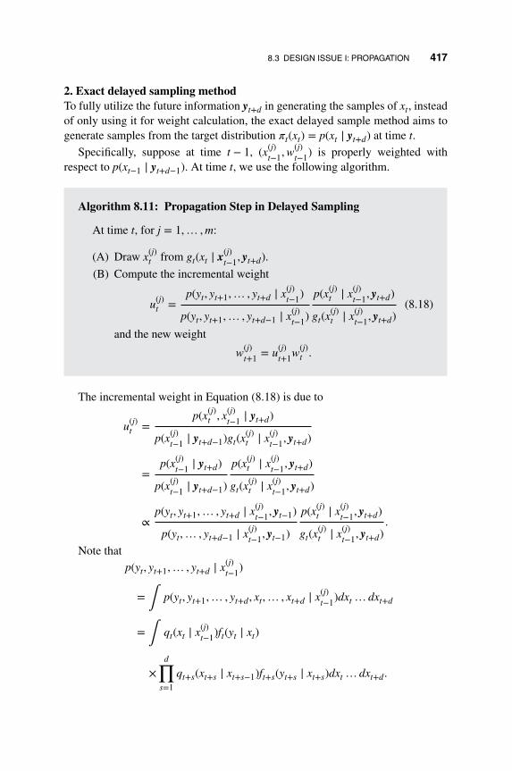
8.3 DESIGN ISSUE I: PROPAGATION 417
2. Exact delayed sampling methodTo fully utilize the future information yt+d in generating the samples of xt, insteadof only using it for weight calculation, the exact delayed sample method aims togenerate samples from the target distribution 𝜋t(xt) = p(xt ∣ yt+d) at time t.
Specifically, suppose at time t − 1, (x(j)t−1, w(j)
t−1) is properly weighted withrespect to p(xt−1 ∣ yt+d−1). At time t, we use the following algorithm.
Algorithm 8.11: Propagation Step in Delayed Sampling
At time t, for j = 1,… , m:
(A) Draw x(j)t from gt(xt ∣ x(j)
t−1, yt+d).
(B) Compute the incremental weight
u(j)t =
p(yt, yt+1,… , yt+d ∣ x(j)t−1)
p(yt, yt+1,… , yt+d−1 ∣ x(j)t−1)
p(x(j)t ∣ x(j)
t−1, yt+d)
gt(x(j)t ∣ x(j)
t−1, yt+d)(8.18)
and the new weight
w(j)t+1 = u(j)
t+1w(j)t .
The incremental weight in Equation (8.18) is due to
u(j)t =
p(x(j)t , x(j)
t−1 ∣ yt+d)
p(x(j)t−1 ∣ yt+d−1)gt(x
(j)t ∣ x(j)
t−1, yt+d)
=p(x(j)
t−1 ∣ yt+d)
p(x(j)t−1 ∣ yt+d−1)
p(x(j)t ∣ x(j)
t−1, yt+d)
gt(x(j)t ∣ x(j)
t−1, yt+d)
∝p(yt, yt+1,… , yt+d ∣ x(j)
t−1, yt−1)
p(yt,… , yt+d−1 ∣ x(j)t−1, yt−1)
p(x(j)t ∣ x(j)
t−1, yt+d)
gt(x(j)t ∣ x(j)
t−1, yt+d).
Note that
p(yt, yt+1,… , yt+d ∣ x(j)t−1)
=∫
p(yt, yt+1,… , yt+d, xt,… , xt+d ∣ x(j)t−1)dxt … dxt+d
=∫
qt(xt ∣ x(j)t−1)ft(yt ∣ xt)
×d∏
s=1
qt+s(xt+s ∣ xt+s−1)ft+s(yt+s ∣ xt+s)dxt … dxt+d.

418 8. SEQUENTIAL MONTE CARLO
The full information proposal using information yt+d is
gt(xt ∣ xt−1, yt+d) = p(xt ∣ xt−1, yt+d−1, yt+d)
∝ p(yt, yt+1,… , yt+d ∣ x(j)t )qt(x
(j)t ∣ x(j)
t−1).
Its corresponding incremental weight is
ut ∝p(yt, yt+1,… , yt+d ∣ x(j)
t−1)
p(yt, yt+1,… , yt+d−1 ∣ x(j)t−1)
=∫ p(yt, yt+1,… , yt+d, xt,… , xt+d ∣ x(j)
t−1)dxt … dxt+d
∫ p(yt, yt+1,… , yt+d−1, xt,… , xt+d−1 ∣ x(j)t−1)dxt … dxt+d−1
.
For example, if xt is a discrete random variable taking values in the set{a1,… , aK}, then let
c(j)t (a𝑖) = gt(xt = a𝑖 ∣ x(j)
t−1, yt+d)
= p(xt = a𝑖 ∣ x(j)t−1, yt+d)
∝ p(yt, yt+1,… , yt+d ∣ xt = a𝑖)qt(xt = a𝑖 ∣ x(j)t−1)
= qt(xt = a𝑖 ∣ x(j)t−1)ft(yt ∣ xt = a𝑖)
∑xt+1,…,xt+d
t+d∏s=t+1
qs(xs ∣ xs−1)fs(ys ∣ xs).
The incremental weight is
u(j)t =
K∑𝑖=1
c(j)t (a𝑖).
Figure 8.9 illustrates the method with xt ∈ = {0, 1} and d = 2. The trial dis-tribution is, for 𝑖 = 0, 1,
gt(xt = 𝑖 ∣ x(j)t−1, yt, yt+1, yt+2)
=∑xt+1
∑xt+2
p(xt = 𝑖, xt+1, xt+2 ∣ x(j)t−1, yt, yy+1, yt+2)
∝ qt(xt = 𝑖 ∣ x(j)t−1)ft(yt ∣ xt = 𝑖)
∑xt+1
∑xt+2
qt+1(xt+1 ∣ xt = 𝑖)𝜏(xt+1, xt+2),
where𝜏(xt+1, xt+2) = ft+1(yt+1 ∣ xt+1)qt+2(xt+2 ∣ xt+1)ft+2(yt+2 ∣ xt+2).
Although this approach fully utilizes the future information in generating thesamples, the d-dimensional summation or integration is often computationallyintensive, if it is not analytically available. For example, in the discrete state spacecase, each iteration requires the evaluation of a summation of Kd terms for the

8.3 DESIGN ISSUE I: PROPAGATION 419
xt−1
xt+1
xt+2
qt(xt=1� xt−1) qt(xt=0� xt−1)
xt1
1 0 0 1
1 0 0 1 0 1 1 0
0
Figure 8.9 Illustration of the exact delayed sampling method.
exploration of the space of future states (xt+1,… , xt+d). For more information, seeWang et al. (2002). Lin et al. (2013) showed that the delayed sampling method ismore efficient than the delayed weighting method and, under mild conditions, theestimator is more accurate as the delay d increases.
3. Delayed pilot sampling methodTo overcome the computational issue in the exact delayed sampling method,Wang et al. (2002) and Lin et al. (2013) proposed using pilot samples to partiallyexplore the future space, while maintaining low computational cost. These aredesigned for discrete state space xt ∈ {a1,… , aK}. In this algorithm, pilot samplesof future states are generated with the standard propagation step discussed in Sec-tion 8.3 and an approximation of the trial distribution gt(xt = a𝑖 ∣ x(j)
t−1, yt,… , yt+d)is obtained, along with an evaluation of the incremental weight. Specifically, sup-pose at time t − 1 a set of properly weighted samples (x(j)
t−1, w(j)t−1), j = 1,… , m with
respect to p(xt−1 ∣ yt−1) is available.
Algorithm 8.12: Propagation Step in Delayed Pilot Sampling
At time t, for j = 1,… , m:
(A) For each 𝑖 ∈ {a1,… , aK}, send out a pilot, starting at xt = a𝑖, toexplore the space of future state xt+1,… , xt+d by using standard

420 8. SEQUENTIAL MONTE CARLO
propagation steps. Specifically, set x(𝑖,j)t = a𝑖 and 𝛾
(𝑖,j)t = 1. For s =
1,… , d:
(A.1) Generate x(𝑖,j)t+s from gt+s(xt+s ∣ x(𝑖,j)
t+s−1, yt+s).
(A.2) Calculate the incremental cumulative weight
𝛾(𝑖,j)t+s = 𝛾
(𝑖,j)t+s−1
qt+s(x(𝑖,j)t+s ∣ x(𝑖.j)
t+s−1)ft+s(yt+s ∣ x(𝑖,j)t+s )
gt+s(x(𝑖,j)t+s ∣ x(𝑖,j)
t+s−1, yt+s).
(B) Draw Ij ∈ {1,… , K} with probability proportional to 𝛾(𝑖,j)t+d . Let x(j)
t =
(x(j)t−1, x
(Ij,j)t ).
(C) Return two weights:
w(j)t = w(j)
t−1qt(x(Ij,j)t ∣ x(j)
t−1)ft(yt ∣ x(Ij,j)t )
∑K𝑖=1 𝛾
(𝑖,j)t+d
𝛾(Ij,j)t+s
,
waux(j)t = w(j)
t−1
K∑k=1
𝛾(𝑖,j)t+d .
The weight w(j)t is the importance weight of x(j)
t with respect to p(xt ∣ yt), that
is, (x(j)t , w(j)
t ) is properly weighted with respect to p(xt ∣ yt). It is used for propaga-
tion in the next step. The auxiliary weight waux(j)t is the importance weight of x(j)
t
with respect to p(xt ∣ yt, yt+1,… , yt+d), i.e. (x(j)t , waux(j)
t ) is properly weighted withrespect to p(xt ∣ yt+d). It is used for inference on xt with information yt+d.
Figure 8.10 illustrates the delayed pilot sampling operation, with = {0, 1}and d = 2, in which the pilot path for (x(j)
t−1, xt = 0) is (xt+1 = 1, xt+2 = 1) and the
pilot path for (x(j)t−1, xt = 1) is (xt+1 = 0, xt+2 = 1). Both are shown by the bold
paths.We can also use multiple pilots for each xt = 𝑖 to increase the accuracy, but also
possibly with additional computational cost.This method has been successfully used in signal processing (Wang et al.,
2002) and bioinformatics (Zhang and Liu, 2002). Lin et al. (2013) obtained certaintheoretical properties of the delayed pilot method.
There are more advanced delayed methods, including the hybrid method, inwhich a combination of delayed sampling and delayed pilot methods are used,and the multi-level method, in which preliminary samples are first generated ina coarse state space using delayed SMC, then these samples are refined in theoriginal state space to obtain the final samples. In addition, one can adaptively

8.4 DESIGN ISSUE II: RESAMPLING 421
0 1
1 0 1
1 0 0 1 0 1 1 0
0
qt(xt=1� xt−1) qt(xt=0� xt−1)
xt−1
xt
xt+1
xt+2
Figure 8.10 Illustration of a single-pilot delay method.
choose the length of delay, e.g. using long delay when information is weak andshort/no delay when information is strong. See Lin et al. (2013) for more details.
8.4 DESIGN ISSUE II: RESAMPLING
The resampling step in Algorithm 8.5 is an indispensable component of SMC. Asdiscussed before, the variance of wt increases stochastically as t increases, result-ing in a decrease in effective sample sizes. This is commonly known as the sam-ple degeneracy problem. Hence, as the system evolves, it is preferable to insert aresampling/reallocation step between propagation recursions in order to stabilizethe weight distribution and to prevent the samples from weight collapse. See Konget al. (1994), Liu (2001), and Liu and Chen (1998). After a resampling step, thesamples with a low priority score tend to be replaced by those with high priorityscores. Priority scores reflect our preferences over different samples, according tocertain objectives. See Chen et al. (2005), Fearnhead (2008), Chen et al. (2000),Wang et al. (2002), among others.
Some theoretical and heuristic arguments of resampling are given in Liu andChen (1995). Note that if the weights w(j)
t are nearly constant, resampling onlyreduces the number of distinctive samples from the past states and incurs extraMonte Carlo variation when making inference about the past states. However,when the weights become very skewed, carrying many samples with small weights
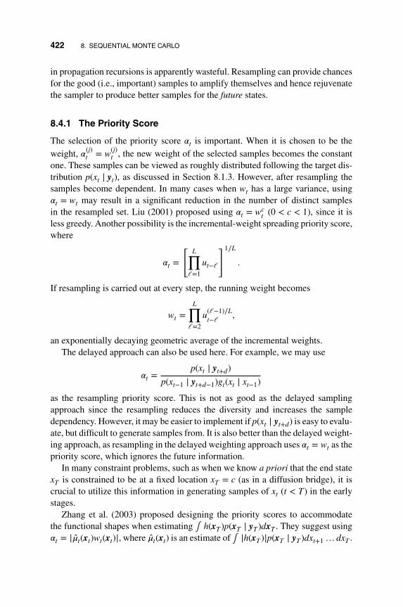
422 8. SEQUENTIAL MONTE CARLO
in propagation recursions is apparently wasteful. Resampling can provide chancesfor the good (i.e., important) samples to amplify themselves and hence rejuvenatethe sampler to produce better samples for the future states.
8.4.1 The Priority Score
The selection of the priority score 𝛼t is important. When it is chosen to be theweight, 𝛼(j)
t = w(j)t , the new weight of the selected samples becomes the constant
one. These samples can be viewed as roughly distributed following the target dis-tribution p(xt ∣ yt), as discussed in Section 8.1.3. However, after resampling thesamples become dependent. In many cases when wt has a large variance, using𝛼t = wt may result in a significant reduction in the number of distinct samplesin the resampled set. Liu (2001) proposed using 𝛼t = wc
t (0 < c < 1), since it isless greedy. Another possibility is the incremental-weight spreading priority score,where
𝛼t =
[L∏
𝓁=1
ut−𝓁
]1∕L
.
If resampling is carried out at every step, the running weight becomes
wt =L∏
𝓁=2
u(𝓁−1)∕Lt−𝓁 ,
an exponentially decaying geometric average of the incremental weights.The delayed approach can also be used here. For example, we may use
𝛼t =p(xt ∣ yt+d)
p(xt−1 ∣ yt+d−1)gt(xt ∣ xt−1)
as the resampling priority score. This is not as good as the delayed samplingapproach since the resampling reduces the diversity and increases the sampledependency. However, it may be easier to implement if p(xt ∣ yt+d) is easy to evalu-ate, but difficult to generate samples from. It is also better than the delayed weight-ing approach, as resampling in the delayed weighting approach uses 𝛼t = wt as thepriority score, which ignores the future information.
In many constraint problems, such as when we know a priori that the end statexT is constrained to be at a fixed location xT = c (as in a diffusion bridge), it iscrucial to utilize this information in generating samples of xt (t < T) in the earlystages.
Zhang et al. (2003) proposed designing the priority scores to accommodatethe functional shapes when estimating ∫ h(xT )p(xT ∣ yT )dxT . They suggest using𝛼t = |��t(xt)wt(xt)|, where ��t(xt) is an estimate of ∫ |h(xT )|p(xT ∣ yT )dxt+1 … dxT .

8.4 DESIGN ISSUE II: RESAMPLING 423
In the prune-and-enrichment algorithm (Grassberger, 1997), 𝛼t values areassigned as
𝛼(j)t =
⎧⎪⎨⎪⎩2 if w(j)
t ≥ U,
1 if U > w(j)t ≥ L,
0.5 if L > w(j)t ,
where U and L are the upper and lower thresholds. In this case, a sample is fourtimes more likely to be resampled if its weight is greater than U than those whoseweight is less than L.
In the auxiliary particle filters (Pitt and Shephard, 1999) for SSMs, the pri-ority score 𝛼t is based on the future information yt+1. Specifically, for each j,
j = 1,… , m, the predictive mean 𝜇(j)t+1 = E(xt+1 ∣ x(j)
t , yt) is first calculated or esti-mated. Then the priority score is set as
𝛼(j)t = w(j)
t p(yt+1 ∣ xt+1 = 𝜇(j)t+1, x(j)
t , yt)
for resampling x(j)t before sampling the new xt+1. This score tries to evaluate the
current sample x(j)t based on the future information yt+1 without carrying out the
sampling of xt+1.In discrete SSMs, we can use the priority score to combine propagation (sam-
pling) and the resampling scheme. Specifically, if xt takes values in {a1,… , ak},we can then evaluate 𝛼t(x
(j)t−1, a𝑖) ∝ p(yt ∣ xt = a𝑖, x(j)
t−1), 𝑖 = 1,… , k, j = 1,… , m,
then sample m distinct samples from {(x(j)t−1, a𝑖), 𝑖 = 1,… , k, j = 1,… , m} with
probability proportional to 𝛼t(x(j)t−1, a𝑖) and finally update the weights accordingly.
8.4.2 Choice of Sampling Methods in Resampling
There are various ways to perform resampling in SMC. The key is to ensure thatthe resampled samples remain properly weighted, with minimum computationalcost. Suppose St = {(x(j)
t , w(j)), j = 1,… , m} is properly weighted with respect to
p(xt ∣ yt). Suppose the priority scores 𝛼(j)t are normalized (sum up to one).
Algorithm 8.13: Simple Random Sampling
(A) Sample Ij, j = 1,… , m independently from the set {1,… , m} (with
replacement) with probability 𝛼(j)t .
(B) Let w(j)t = w(j)
t ∕𝛼(j)t .
(C) Return S′t = {(x(Ij)t , w(Ij)), j = 1,… , m}.

424 8. SEQUENTIAL MONTE CARLO
In Section 8.1.3 we showed that S′t is properly weighted with respect to p(xt ∣ yt)under mild conditions. This method is time consuming and has the largest MonteCarlo variation. However, because the resulting samples are iid given St, its theo-retical properties are easy to investigate.
Algorithm 8.14: Residual Sampling (Liu and Chen, 1998)
(A) Obtain kj = [m𝛼(j)] copies of j, where [x] denotes the integer part of
x, that is, I𝑖 = j if∑j−1
𝓁=1k𝓁 < 𝑖 ≤
∑j𝓁=1
k𝓁 , for 𝑖 = 1,… ,∑m
j=1 kj.
(B) Let mr = m −∑m
j=1 kj. Generate mr iid samples Ij, j =∑m
j=1 kj +1,… , m from {1,… , m} (with replacement) with probabilities pro-portional to m𝛼(j) − kj = m𝛼(j) − [m𝛼(j)].
(C) Let w(j)t = w(j)
t ∕𝛼(j)t .
(D) Return S′t = {(x(Ij)t , w(Ij)), j = 1,… , m}.
This is the stratified sampling approach discussed in Section 8.1.2. It reduces thesampling variation as well as computation.
Algorithm 8.15: Stratified Sampling (Kitagawa, 1996)
(A) Set c0 = 0, cj = cj−1 + 𝛼(j)t , j = 1,… , m.
(B) Draw a starting point u1 ∼ Un𝑖f [0, 1∕m], and let u𝑖 = u1 + (𝑖 −1)∕m.
(C) If cj−1 ≤ u𝑖 < cj, then I𝑖 = j.
(D) Let w(j)t = w(j)
t ∕𝛼(j)t .
(E) Return S′t = {(x(Ij)t , w(Ij)), j = 1,… , m}.
In this approach only one random number u1 needs to be generated. Thismethod provides more systematic coverage of the space. For example, if all 𝛼(j)
are the same, then the resampled set is exactly the same as the original one, andno sample is lost. The computational complexity of this resampling method is oforder O(m).
Sometimes it is possible to combine sampling (propagation) with resampling.

8.4 DESIGN ISSUE II: RESAMPLING 425
Algorithm 8.16: Local Monte Carlo Method (Liu and Chen, 1998)
(A) Use a local Monte Carlo method to generate (Jk, x(k)t ) from distribu-
tion
p(J, xt) ∝p(x(J)
t−1, xt ∣ yt)
p(x(J)t−1 ∣ yt−1)
𝛼(J)t .
(B) Let the new set of samples (for t) be St = {x(k)t , k = 1,… , m}. The
weight for each sample x(k)t is w
(Jk)t ∕𝛼(Jk)
t .
5. Resampling with added diversificationSimple random sampling is based on the discrete approximation of p(xt ∣ yt)
using
F(x) = 1∑mj=1 w(j)
t
m∑j=1
w(j)t I(x(j)
t < x).
Liu and West (2001) suggested using a kernel smoother to approximate p(xt ∣ yt).Specifically, let
p(x ∣ yt) =1∑m
j=1 w(j)t
m∑j=1
w(j)t Kh(x(j)
t − x).
If the kernel function Kh(⋅) is chosen as the normal density with mean zero andvariance matrix d𝑖ag(h2), the distribution is a mixture normal. Resampling usingp(⋅) is essentially sampling from the set {x(1)
t ,… , x(m)t } with probability propor-
tional to w(j)t (using one of the methods discussed above), then adding a Gaus-
sian noise e(Ij)t ∼ N(0, diag(h2)) to each resampled sample. The resulting sample
is more diversified, though choosing the bandwidth h becomes an issue.
8.4.3 Resampling Schedule
When to resample is also important. Frequent resampling can be shortsighted sinceresampling introduces strong dependency among the samples, as there are manyduplicated samples in the resampled set. It also reduces the diversity among thesamples in the sense that after frequent resampling, the survived samples tend toshare common ancestors. In addition, frequent resampling makes the algorithmsensitive to outliers. For example, if yt is an outlier, then many of the “good” sam-ples tend to have small weights. Resampling using the weights as priority scores

426 8. SEQUENTIAL MONTE CARLO
tends to eliminate those samples but retains the samples that happen to be closerto the outlying observation. One may completely lose track of the problem (e.g.,no samples are good enough to recover in the future with non-outlying futureobservations). If resampling is done later, then the non-outlying future informa-tion {yt+1,… , yt+d} may correct the impact of yt, hence one does not lose these“good” samples.
A deterministic resampling schedule performs resampling at time t0, 2t0, 3t0,etc. A dynamic sampling schedule tries to maintain a minimum effective samplesize. Specifically, given a sequence of thresholds {0 < ct < 1} in advance, doresampling when the effective sample size ESS in Equation (8.6) is less than mct.For further information, see Liu and Chen (1995). In Section 8.10.2 we demon-strate the importance of the resampling schedule.
In addition, the resampling step should be inserted before xt is sampled if thefull information proposal distribution of Algorithm 8.7 is used. This is becausethe weight w(j)
t at time t is a function of x(j)t−1 and does not depend on the sample
x(j)t , as discussed in Section 8.3.1. Hence, by resampling x(j)
t−1 first (with possible
duplications) then sampling x(j)t based on these resampled x(j)
t−1, the samples x(j)t are
more diverse. Otherwise we may have duplicated x(j)t .
8.4.4 Benefits of Resampling
So why is resampling beneficial? Chopin (2004) provided a detailed analysis ofthe variance of
1m
m∑j=1
w(j)t h(x(j)
t ) (8.19)
for estimating 𝜇 = E[h(xt) ∣ yt]. To simplify the notations, denote 𝜋t(xs) = p(xs ∣yt) and 𝜋t(xs ∣ xs−1) = p(xs ∣ xs−1, yt). In addition, for s ≤ t, define the conditionalmean
𝜇t(xs) = E[h(xt) ∣ xs, yt]
=∫
h(xt)p(xt ∣ yt)dxs+1 … dxt
=∫
h(xt)p(xs+1:t ∣ xs, yt)dxs+1 … dxt.
Note that E𝜋s[𝜇t(xs)] = 𝜇 for all s = 1,… , t and Var𝜋s1
[𝜇t(xs1)] ≥ Var𝜋s2
[𝜇t(xs2)]
for s1 > s2. Roughly speaking,𝜇t(xs) is the best estimate of𝜇 given a known partialstate path xs. It changes as xs changes. Since xs1
has more variates than xs2for s1 >
s2, 𝜇t(xs1) has a larger total variance than 𝜇t(xs2
) does. Another way to look at it

8.4 DESIGN ISSUE II: RESAMPLING 427
is that 𝜇t(xs2) integrates out more terms of the overall integral ∫ h(xt)p(xt ∣ yt)dxt,
hence it has a smaller variance.Chopin (2004) showed that, if we use simple random resample at every time
step, with w(j)t as the priority score, then the variance of the estimator of Equation
(8.19) is
∫
𝜋2t (x1)
g1(x1)(𝜇1(x1) − 𝜇)2dx1 +
t∑s=2
∫
𝜋2t (xs)
𝜋s(xs−1)gs(xs ∣ xs−1)(𝜇s(xs) − 𝜇)2dxs.
(8.20)
This is to compare with the one without resampling
∫
𝜋2t (xt)∏t
s=1 gs(xs ∣ xs−1)(h(xt) − 𝜇)2dxt. (8.21)
To gain some insight into the variance in Equation (8.20), we note that the sthterm,
∫
𝜋2t (xs)
𝜋s(xs−1)gs(xs ∣ xs−1)(𝜇s(xs) − 𝜇)2dxs,
corresponds to the variance of the following estimator. Suppose we can generateiid samples x(j)
s−1 from 𝜋s−1(xs−1) = p(xs−1 ∣ ys−1), the target distribution at time
s − 1, and we generate xs from a trial distribution x(j)s ∼ gs(xs ∣ x(j)
s−1) with corre-
sponding weight w(j)s = 𝜋t(xs)∕[𝜋s−1(xs−1)gs(xs ∣ xs−1)], and we are able to evalu-
ate 𝜇s(x(j)s ) = E(h(xt) ∣ x(j)
s , yt). We would estimate 𝜇 using
1m
m∑j=1
w(j)s 𝜇s(x
(j)s ).
The variance of this estimator is the sth term in Equation (8.20). Note this estimatordiffers from the SMC one in two places. First, the first s − 1 terms xs−1 is sampledfrom the true target distribution p(xs−1 ∣ ys−1). It is in a way the best one can hopeto achieve at time s − 1. The second is that 𝜇s(x
(j)s ) is a much more accurate esti-
mate of 𝜇 than h(xt), as it integrates out all the future terms from xs+1 to xt. There is
only one term x(j)t involving IS. Hence the sth term is significantly better than that
in Equation (8.21). Of course we have t terms in Equation (8.20). In addition, eachterm in the summation of Equation (8.20) has its advantages and disadvantages.For smaller s, 𝜇s(xs) has smaller variation, but typically the importance ratio
𝜋t(xs)
𝜋s−1(xs−1)g(xs ∣ xs−1)=
p(xs ∣ yt)
p(xs−1 ∣ ys−1)g(xs ∣ xs−1)

428 8. SEQUENTIAL MONTE CARLO
can be more divergent, since the trial distribution at time s typically depends onlyon ys, not yt.
8.5 DESIGN ISSUE III: INFERENCE
Standard inference with IS is in the form of Equation (8.5)
��t = E[𝜑(xt) ∣ yt] =∑m
j=1 w(j)t 𝜑(x(j)
t )∑mj=1 w(j)
t
.
There are several alternatives that may improve the efficiency of the estimator.
1. Estimation before resampling: A resampling step does not provide any extrainformation on the current and past states. It only adds additional Monte Carlovariations in the samples of the current and past states, as discussed in Section8.1.3, even though it is critical in obtaining better samples of the future states.Hence, estimation should be done before carrying out a resampling step.
2. Rao–Blackwellization: If wt does not depend on xt, (as in the case when fullinformation propagation step (8.14) is used as the propagation sampling distribu-tion), then we can use
��t =
∑mj=1 w(j)
t E[𝜑(xt) ∣ x(j)t−1, yt]∑m
j=1 w(j)t
, (8.22)
if E[𝜑(xt) ∣ x(j)t−1, yt] can be analytically carried out. This is because
E[𝜑(xt) ∣ yt] = E[E{𝜑(xt) ∣ xt−1, yt
}∣ yt]
≈
∑mj=1 w(j)
t E[𝜑(xt) ∣ x(j)t−1, yt]∑m
j=1 w(j)t
.
This estimator of E[𝜑(xt) ∣ yt] is carried out without using the samples of xt. Itremoves the sampling variation in xt. In fact, this operation is equivalent to havingan infinite number of iid copies of x(j)
t for each single x(j)t−1 and using their weighted
averages.
3. Use delayed estimation if possible: This is because estimation of E[𝜑(xt) ∣yt+d] at time t is usually more accurate (closer to the true 𝜑(xt)) than E[𝜑(xt) ∣ yt].

8.6 DESIGN ISSUE IV: MARGINALIZATION AND THE MIXTURE KALMAN FILTER 429
The former estimation uses more information, as shown in Lin et al. (2013), andit can be done with a simple delayed weighting method based on
E[𝜑(xt) ∣ yt+d] =
∑mj=1 w(j)
t+d𝜑(x(j)t )∑m
j=1 w(j)t+d
,
or with the delayed sampling method using p(xt ∣ yt+d) as the target distribution attime t.
8.6 DESIGN ISSUE IV: MARGINALIZATION AND THE MIXTUREKALMAN FILTER
When implementing Monte Carlo strategies, it is often good practice to carry outas much analytical computation as possible (Hammersley and Handscomb, 1964;Liu et al., 1994; MacEachern et al., 1998). In IS, it can easily be shown that thealgorithm is more efficient after some components of the system are integrated out(marginalization).
Following the marginalization principle and the spirit of mixture Gaussianapproximations, Chen and Liu (2000) developed a mixture Kalman filter (MKF)approach. It makes use of special properties of a conditional or partial conditionaldynamic linear system and combines the SMC with the efficient Kalman filter.West (1992) pioneered the use of mixture Gaussian approximations in nonlinearSSMs.
8.6.1 Conditional Dynamic Linear Models
Conditional dynamic linear models (CDLMs) assume the form
xt = HΛtxt−1 + WΛt
wt
Λt ∼ 𝜓t(⋅ ∣ Λt−1)
yt = GΛtxt + VΛt
vt,
where wt ∼ N(0, I) and vt ∼ N(0, I) with proper dimensions and they are inde-pendent. The indicator Λt is an unobserved latent variable with transition prob-ability density 𝜓t(⋅). For any possible value 𝜆 in the support of Λt, the matricesH𝜆, G𝜆, W𝜆 and V𝜆 are known. The model appears in many applications, includ-ing those in Section 6.2.

430 8. SEQUENTIAL MONTE CARLO
8.6.2 Mixture Kalman Filters
Let yt = (y1,… , yt) and 𝚲t = (Λ1,… ,Λt). Note that
p(xt ∣yt)=∫ p(xt ∣𝚲t, yt)dF(𝚲t ∣yt), (8.23)
in which
p(xt ∣ 𝚲t, yt) ∼ N(𝜇t(𝚲t), 𝜎2t (𝚲t)). (8.24)
Equation (8.24) is due to the fact that, given the trajectory of the indicator{Λ1,… ,Λt}, the system is linear and Gaussian, hence p(xt ∣ 𝚲t, yt) is a Gaussiandistribution. The corresponding 𝜇t(𝚲t) and 𝜎2
t (𝚲t) in Equation (8.24) can readilybe obtained through the Kalman filter discussed in Section 6.3.1. For simplicity,we denote
KFt(𝚲t) ≡ (𝜇t(𝚲t), 𝜎2t (𝚲t)).
Because of Equation (8.24), p(xt ∣ y1,… , yt) in Equation (8.23) is a mixture Gaus-sian distribution. If Λt takes values in a finite set of size K, then p(xt ∣ yt) is afinite mixture of normal distributions, though the number of components is large(Kt). If Λt is a continuous random variable, then p(xt ∣ y1,… , yt) is a continuouscompound mixture of normal distributions. Sampling from such a distribution canbe done with discrete samples directly from the distribution, but a more efficientmethod is to sample the Gaussian components. In our context, this is the same assampling the unobserved latent indicator 𝚲t. It can be shown that, if
{(𝝀(1)t , w(1)
t ),… , (𝝀(m)t , w(m)
t )}
is a properly weighted sample with respect to p(𝚲t ∣ yt), then we have
E[h(xt) ∣ yt] = ∫h(xt)p(xt ∣ yt)dxt
=∫
[∫
h(xt)p(xt ∣ 𝚲t, yt)dxt
]p(𝚲t ∣ yt)d𝚲t
=∫
E[h(xt) ∣ 𝚲t, yt]p(𝚲t ∣ yt)d𝚲t
≈
∑mj=1 w(j)
t E(h(xt) ∣ 𝝀(j)t , yt)∑m
j=1 w(j)t
,
where
E[h(xt) ∣ 𝝀(j)t , yt] = ∫
h(x)𝜙(x;𝜇t(𝝀(j)t ), 𝜎2
t (𝝀(j)t ))dx,
due to Equation (8.24).

8.6 DESIGN ISSUE IV: MARGINALIZATION AND THE MIXTURE KALMAN FILTER 431
For example, to estimate the mean E(xt ∣ yt) (the most encountered inferenceproblem), we have h(x) = x and
E(xt ∣ yt) ≈∑m
j=1 w(j)t 𝜇t(𝝀
(j)t )∑m
j=1 w(j)t
.
The estimator of the variance is
Var(xt ∣ yt) ≈
∑mj=1 w(j)
t 𝜎2t (𝝀(j)
t )∑mj=1 w(j)
t
.
Note that this is equivalent to using a random mixture of normal distributionsm∑
j=1
w(j)t N(𝜇t(𝝀
(j)t ), 𝜎2
t (𝝀(j)t ))
to approximate the mixture Gaussian distribution p(xt ∣ yt) in Equation (8.23). Thisapproximation is more efficient than the discrete approximation using samplesdirectly from the distribution. This can be seen from the fact that
Var[h(xt) ∣ yt] ≥ Var[E(h(xt) ∣ 𝚲t, yt) ∣ yt].
Formally, suppose that at time t − 1 we have a properly weighted sample(𝝀(j)
t−1, KF(j)t−1, w(j)
t−1) with respect to 𝜋(𝝀t−1 ∣ yt−1). At time t, we have the followingalgorithm.
Algorithm 8.17: Propagation Step in the MKF Algorithm
For j = 1,… , m:
(A) Generate 𝜆(j)t from a trial distribution gt(Λt ∣ 𝝀
(j)t−1, KF(j)
t−1, yt).
(B) Run one-step Kalman filter conditioning on (𝜆(j)t , KF(j)
t−1, yt) and
obtain KF(j)t .
(C) Calculate the incremental weight
u(j)t =
p(𝝀(j)t−1, 𝜆(j)
t ∣ yt)
p(𝝀(j)t−1 ∣ yt−1)gt(𝜆t ∣ 𝝀
(j)t−1, KF(j)
t−1, yt)
and the new weight w(j)t = w(j)
t−1u(j)t .
When Λt is a discrete random variable on a finite set, we can use the full infor-mation proposal distribution p(Λt ∣ 𝝀
(j)t−1, KF(j)
t−1, yt). Specifically, suppose Λt takes

432 8. SEQUENTIAL MONTE CARLO
values in {1,… , K} and suppose that at time t − 1 we have a properly weightedsample (𝝀(j)
t−1, KF(j)t−1, w(j)
t−1) with respect to p(𝝀t−1 ∣ yt−1). At time t, we have thefollowing algorithm.
Algorithm 8.18: Full Information Propagation Step in the MKF Algo-rithm
For j = 1,… , m:
(A) For each k = 1,… , K, run the one-step Kalman filter to obtain KF(j,k)t
and
u(j)k = p(yt ∣ Λt = k, KF(j)
t−1)p(Λt = k ∣ 𝝀(j)t−1).
(B) Sample 𝜂 from the set {1,… , K} with probability proportional to{u(j)
1 ,… , u(j)K }. Let 𝜆(j)
t = 𝜂. In this case 𝜆(j)t ∼ p(Λt ∣ 𝝀
(j)t−1, KF(j)
t−1, yt).
(C) Let KF(j)t = KF(j,𝜂)
t .
(D) The new weight is
w(j)t ∝ w(j)
t−1p(yt ∣ 𝝀(j)t−1, KF(j)
t−1) ∝ w(j)t−1
K∑k=1
u(j)k .
Note that p(yt ∣ Λt = k, KF(j)t−1) is a by-product of the Kalman filter in
Equation (8.24).When Λt is a continuous random variable, a simple (but not optimal) algorithm
is as follows.
Algorithm 8.19: State Equation Propagation Step in the MKF Algo-rithm
For j = 1,… , m:
(A) Sample a 𝜆(j)t from the state equation of Λt, p(Λt ∣ 𝚲t−1 = 𝝀
(j)t−1).
(B) Run one-step Kalman filter conditioning on (𝜆(j)t , KF(j)
t−1, yt) and
obtain KF(j)t .
(C) The new weight is
w(j)t = w(j)
t−1p(yt ∣ 𝜆(j)t , KF(j)
t−1).
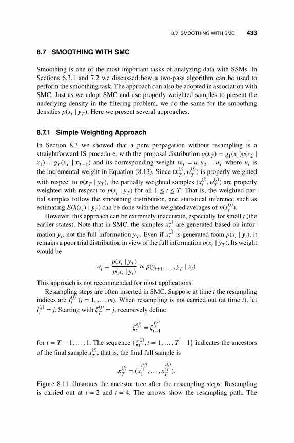
8.7 SMOOTHING WITH SMC 433
8.7 SMOOTHING WITH SMC
Smoothing is one of the most important tasks of analyzing data with SSMs. InSections 6.3.1 and 7.2 we discussed how a two-pass algorithm can be used toperform the smoothing task. The approach can also be adopted in association withSMC. Just as we adopt SMC and use properly weighted samples to present theunderlying density in the filtering problem, we do the same for the smoothingdensities p(xt ∣ yT ). Here we present several approaches.
8.7.1 Simple Weighting Approach
In Section 8.3 we showed that a pure propagation without resampling is astraightforward IS procedure, with the proposal distribution g(xT ) = g1(x1)g(x2 ∣x1)… gT (xT ∣ xT−1) and its corresponding weight wT = u1u2 … uT where ut isthe incremental weight in Equation (8.13). Since (x(j)
T , w(j)T ) is properly weighted
with respect to p(xT ∣ yT ), the partially weighted samples (x(j)t , w(j)
T ) are properlyweighted with respect to p(xt ∣ yT ) for all 1 ≤ t ≤ T . That is, the weighted par-tial samples follow the smoothing distribution, and statistical inference such asestimating E(h(xt) ∣ yT ) can be done with the weighted averages of h(x(j)
t ).However, this approach can be extremely inaccurate, especially for small t (the
earlier states). Note that in SMC, the samples x(j)t are generated based on infor-
mation yt, not the full information yT . Even if x(j)t is generated from p(xt ∣ yt), it
remains a poor trial distribution in view of the full information p(xt ∣ yT ). Its weightwould be
wt =p(xt ∣ yT )
p(xt ∣ yt)∝ p(yt+1,… , yT ∣ xt).
This approach is not recommended for most applications.Resampling steps are often inserted in SMC. Suppose at time t the resampling
indices are I(j)t (j = 1,… , m). When resampling is not carried out (at time t), let
I(j)t = j. Starting with 𝜁
(j)T = j, recursively define
𝜁(j)t = 𝜁
I(j)t
t+1
for t = T − 1,… , 1. The sequence {𝜁 (j)t , t = 1,… , T − 1} indicates the ancestors
of the final sample x(j)T , that is, the final full sample is
x(j)T = (x
𝜁(j)1
1 ,… , x𝜁
(j)T
T ).
Figure 8.11 illustrates the ancestor tree after the resampling steps. Resamplingis carried out at t = 2 and t = 4. The arrows show the resampling path. The

434 8. SEQUENTIAL MONTE CARLO
1 2 3 4 5x
(1)1 x
(1)2 x
(1)3 x
(1)4 x
(1)5
x(2)1 x
(2)2 x
(2)3 x
(2)4 x
(2)5
x(3)1 x
(3)2 x
(3)3 x
(3)4 x
(3)5
x(4)1 x
(4)2 x
(4)3 x
(4)4 x
(4)5
Figure 8.11 An illustration of sample ancestor tree after resampling.
ancestor lineage of x(j)5 , j = 1,… , 4 is shown by the bold arrows. For example,
x(1)5 = (x(2)
1 , x(2)2 , x(2)
3 , x(1)4 , x(1)
5 ) as one traces back following the bold arrows, start-
ing at x(1)5 . In this case all samples of {x(j)
5 , j = 1,… , 4} came from one ancestor
x(2)1 . Each resampling step reduces the number of unique ancestors. Suppose at
time T each sample x(j)T is properly weighted with w(j)
T (taking into account ofthe resampling priority as shown in Section 8.4). As before, the estimation ofE(h(xt) ∣ yT ) can be done with the weighted average
��t =
∑mj=1 h(x
𝜁(j)t
t )w(j)T∑m
j=1 w(j)T
=
∑𝜈∈Ξt
h(x(𝜈)t )[∑
𝜁(j)t =𝜈 w(j)
T ]∑mj=1 w(j)
T
,
where Ξt is the set of unique values in the set {𝜁 (j)t , j = 1,… , m}. With frequent
resampling and for t ≪ T , the set Ξt can be very small. For instance, there is onlyone element in Ξ1 in Figure 8.11. Hence the weighted average is done with a verysmall number of unique terms. Obviously the estimation error increases.
8.7.2 Weight Marginalization Approach
The Kalman smoother discussed in Section 6.3.3 uses the disentangled approachto link the filtering density p(xt ∣ yt) and the future information (yt+1,… , yT )by inserting xt+1. This approach can be used for SMC smoothing as well. Theapproach relies on the disentangle equation
p(xt ∣ yT ) =∫
p(xt, xt+1 ∣ yT )dxt+1
=∫
p(xt ∣ xt+1, yT )p(xt+1 ∣ yT )dxt+1
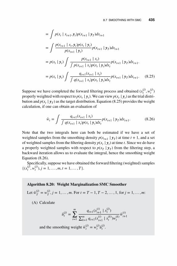
8.7 SMOOTHING WITH SMC 435
=∫
p(xt ∣ xt+1, yt)p(xt+1 ∣ yT )dxt+1
=∫
p(xt+1 ∣ xt, yt)p(xt ∣ yt)
p(xt+1 ∣ yt)p(xt+1 ∣ yT )dxt+1
= p(xt ∣ yt)∫p(xt+1 ∣ xt)
∫ p(xt+1 ∣ xt)p(xt ∣ yt)dxt
p(xt+1 ∣ yT )dxt+1.
= p(xt ∣ yt)∫qt+1(xt+1 ∣ xt)
∫ q(xt+1 ∣ xt)p(xt ∣ yt)dxt
p(xt+1 ∣ yT )dxt+1. (8.25)
Suppose we have completed the forward filtering process and obtained (x(j)t , w(j)
t )properly weighted with respect to p(xt ∣ yt). We can view p(xt ∣ yt) as the trial distri-bution and p(xt ∣ yT ) as the target distribution. Equation (8.25) provides the weightcalculation, if one can obtain an evaluation of
wt = ∫
qt+1(xt+1 ∣ xt)
∫ q(xt+1 ∣ xt)p(xt ∣ yt)dxt
p(xt+1 ∣ yT )dxt+1. (8.26)
Note that the two integrals here can both be estimated if we have a set ofweighted samples from the smoothing density p(xt+1 ∣ yT ) at time t + 1, and a setof weighted samples from the filtering density p(xt ∣ yt) at time t. Since we do havea properly weighted samples with respect to p(xT ∣ yT ) from the filtering step, abackward iteration allows us to evaluate the integral, hence the smoothing weightEquation (8.26).
Specifically, suppose we have obtained the forward filtering (weighted) samples{(x(j)
t , w(j)t ), j = 1,… , m, t = 1,… , T}.
Algorithm 8.20: Weight Marginalization SMC Smoother
Let w(j)T = w(j)
T , j = 1,… , m. For t = T − 1, T − 2,… , 1, for j = 1,… , m:
(A) Calculate
u(j)t =
m∑𝑖=1
qt+1(x(𝑖)t+1 ∣ x(j)
t )∑mk=1 qt+1(x(𝑖)
t+1 ∣ x(k)t )w(k)
t
w(𝑖)t+1
and the smoothing weight w(j)t = w(j)
t u(j)t .

436 8. SEQUENTIAL MONTE CARLO
The resulting weighted samples {(x(j)t , w(j)
t ), j = 1,… , m} are properly weightedwith respect to p(xt ∣ yT ).
This procedure was proposed by Tanizaki and Mariano (1994), Hrzeler andKnsch (1998), and Doucet et al. (2000). It does not regenerate samples during thesmoothing step. It only adjusts the weights. Note that both (x(j)
t , w(j)T ) and (x(j)
t , w(j)t )
are properly weighted with respect to p(xt ∣ yT ). We have discussed this feature ofIS in Section 8.1.3. The weights w(j)
t are marginal weights and, hence, are moreefficient.
The procedure requires the recording of all forward filtering samples andweights (x(j)
t , w(j)t ) and the backward smoothing weight w(j)
t . Resampling can bedone in both the forward process and the backward process, though ancestorsshould not be resampled.
8.7.3 Two-filter Sampling
Briers et al. (2010) proposed a two-filter procedure for SMC smoothing. A stan-dard SMC forward filter is carried out first to obtain (x(j)
t , w(j)t ) properly weighted
with respect to p(xt ∣ yt). Then, a second SMC backward filter is carried out, start-ing at t = T to t = 1, using backward propagation distribution gt(xt ∣ xt+1, yt) and(backward) weight
wt ∝ wt+1qt+1(xt+1 ∣ xt)ft(yt ∣ xt)
gt(xt ∣ xt+1, yt)
to get (x(j)t , w(j)
t ) properly weighted with respect to p(xt ∣ yt:T ), where yt:T =(yt,… , yT ). Because
p(xt ∣ yT ) ∝ p(yt:T ∣ xt)p(xt ∣ yt−1)
∝ p(yt:T ∣ xt)∫p(xt ∣ xt−1)p(xt−1 ∣ yt−1)dxt−1,
we have
p(xt ∣ yT )
p(xt ∣ yt)p(yt:T ∣ xt)∝∫
p(xt ∣ xt−1)p(xt−1 ∣ yt−1)dxt−1
≈∑m
k=1qt(x
(j)t ∣ x(k)
t−1)w(k)t−1,
where the last term is the result of integral approximation using the importancesamples. Hence the sample x(j)
t should be weighted by
w∗(j)t = w(j)
t
m∑k=1
qt(x(j)t ∣ x(k)
t−1)w(k)t−1,
8.7 SMOOTHING WITH SMC 437
and they are properly weighted with respect to p(xt ∣ yT ). This matching procedureis similar to that in IPF discussed in Section 8.3.
This procedure is similar to the weight marginalization algorithm. It adjusts theweights of the backward samples using the forward matching samples. If the back-ward sampling distribution gt is arbitrary, this procedure presents little advantage,as the backward samples xt only rely on the partial information yt:T . Hence thesample xT ∼ p(xT ∣ yT ) is similar to x1 ∼ p(x1 ∣ y1). However, if one starts with atrial distribution gT (⋅) that is close to p(xT ∣ yT ), the advantage can be significant.Unlike the weight marginalization algorithm, this is achievable, since we have theforward filtering samples (x(j)
T , w(j)T ) properly weighted with respect to p(xT ∣ yT ),
which can be used to construct the sampling distribution xT ∼ gT (xT ∣ yT ) that isclose to p(xt ∣ yT ). Unfortunately, the samples themselves cannot be directly used,since one needs to be able to evaluate the trial distribution gT (⋅) up to a normaliz-ing constant. However, any reasonable approximation, such as a mixture normaldistribution approximation, can be useful.
Fearnhead et al. (2010) proposed an extension of the two-filter algorithm.Again, a standard SMC forward filter is carried out to obtain (x(j)
t , w(j)t ) properly
weighted with respect to p(xt ∣ yt), and a second SMC backward filter is carriedout to get (x(j)
t , w(j)t ) properly weighted with respect to p(xt ∣ yt:T ). In addition, we
also use a trial distribution gt(xt ∣ xt−1, xt+1, yt). At time t, we generate m2 samples
x(j,k)t ∼ gt(xt ∣ x(j)
t−1, x(k)t+1, yt)
with weight
w(j,k)t =
ft(yt ∣ x(j,k)t )qt(x
(j,k)t ∣ x(j)
t−1)qt+1(x(k)t+1 ∣ x(j,k)
t )
gt(xt ∣ x(j)t−1, x(k)
t+1, yt)w(j)
t−1w(k)t+1.
Then {(x(j,k)t , w(j,k)
t ), j, k = 1,… , m} is properly weighted with respect to p(xt ∣ yT ).This is due to the fact that
p(xt ∣ yT ) ∝ p(yt:T ∣ xt)p(xt ∣ yt−1)
∝ p(yt ∣ xt)∫p(xt ∣ xt−1)p(xt−1 ∣ yt−1)dxt−1 ×
∫p(xt+1 ∣ xt)p(xt+1 ∣ yt+1:T )dxt+1.
Because this is an m2-operation, computational cost can be high.

438 8. SEQUENTIAL MONTE CARLO
8.8 PARAMETER ESTIMATION WITH SMC
SSMs in practice often contain unknown parameters. Our previous discussionfocuses on filtering and smoothing, with a completely specified SSM withoutunknown parameters. In this section we discuss how to use these techniques toestimate the parameters in a given model.
8.8.1 Maximum Likelihood Estimation
Maximum likelihood estimation requires the evaluation of the likelihood function
L(𝜃 ∣ yT ) = p𝜃(yT ) =∫
p𝜃(yT , xT )dxT . (8.27)
This is the normalizing constant of
𝜋∗𝜃(xT ∣ yT ) =
p∏t=1
qt(xt ∣ xt−1, 𝜃)ft(yt ∣ xt, 𝜃).
Hence IS can be used, as discussed in Section 8.1.3, for estimating Z = ∫ 𝜋∗(x)dx.
Specifically, if we generate samples x(j)T , j = 1,… , m from a trial distribution
g(xT ), then we can use
L(𝜃 ∣ yT ) = 1m
m∑j=1
𝜋∗𝜃(x(j)
T ∣ yT , 𝜃)
g(x(j)T ∣ yT , 𝜃)
as an estimator of L(𝜃 ∣ yT ). Therefore, if one uses sequential construction ofthe trial distribution g(xT ∣ yT , 𝜃) =
∏Tt=1 gt(xt ∣ yt, 𝜃) in (8.12), and if there is no
resampling, the final weight w(j)T obtained through SMC can then be used to esti-
mate the likelihood
L(𝜃 ∣ yT ) = 1m
m∑j=1
w(j)T . (8.28)
If we resample at time steps t1,… , tk (where 1 = t0 < t1 < … < tk < tk+1 = T)
using the weights w(j)t𝑖
as the priority scores, and use the fact that
p𝜃(yT ) = p𝜃(y1,… yt1)
k∏𝑖=2
p𝜃(yt𝑖+1,… , yt𝑖+1∣ yt𝑖
),
we can obtain
L(𝜃 ∣ yT ) =k+1∏𝑖=1
[1m
m∑j=1
w(j)t𝑖
]. (8.29)

8.8 PARAMETER ESTIMATION WITH SMC 439
With the estimated likelihood function, one can obtain the MLE using opti-mization procedures. However, one critical problem with this approach is that thevalues of the estimated likelihood function are subject to Monte Carlo variation,as they are estimated using Monte Carlo samples. The resulting function may notbe smooth, even though the true likelihood function is smooth. This creates sig-nificant difficulties for any optimization procedure to find stable estimates. Malikand Pitt (2011) proposed to use the same random numbers in evaluating the like-lihood function for different 𝜃 values, hence obtaining a smooth estimator of thelikelihood function. However, the procedure becomes difficult if the dimension ofthe state variable is high.
Since optimization algorithms such as the steepest ascent algorithm requirethe gradient (and curvature) of the function to be optimized, Poyiadjis et al.(2011) developed procedures to directly estimate the score and informa-tion matrix of the likelihood function of an SSM. Using Equation (8.27),we have
∇ log p𝜃(yT ) =∫
∇ log(p𝜃(xT , yT ))p𝜃(xT ∣ yT )dxT ,
and
−∇2 log p𝜃(yT ) = ∇ log p𝜃(yT )∇ log p𝜃(yT )′ −∇2p𝜃(yT )
p𝜃(yT ),
where
∇2p𝜃(yT )
p𝜃(yT )=∫
∇ log p𝜃(xT , yT )∇ log p𝜃(xT , yT )′p𝜃(xT ∣ yT )dxT
+∫
∇2 log p𝜃(xT , yT )p𝜃(xT ∣ yT )dxT ,
due to Louis’ identity (Cappe et al., 2005). All aforementioned integrals can beapproximated with a set of samples {(x(j)
T , w(j)T ), j = 1,… , m} properly weighted
with respect to p(xT ∣ yT ). However, such an approximation suffers the same prob-lem as using w(j)
T to estimate the likelihood.Poyiadjis et al. (2011) refined the procedure using an alternative formulation
based only on the integration with respect to the final marginal distribution ofp𝜃(xT ∣ yT ). Specifically,
∇ log p𝜃(yT ) =∫
∇ log(p𝜃(xT , yT ))p𝜃(xT ∣ yT )dxT

440 8. SEQUENTIAL MONTE CARLO
and
∇2p𝜃(yT )
p𝜃(yT )=∫
∇ log p𝜃(xT , yT )∇ log p𝜃(xT , yT )′p𝜃(xT ∣ yT )dxT
+∫
∇2 log p𝜃(xT , yT )p𝜃(xT ∣ yT )dxT .
However, in this case∇ log(p𝜃(xT , yT )) and∇2 log(p𝜃(xT , yT )) are not immediatelyavailable. Poyiadjis et al. (2011) suggested a recursive formula:
∇ log(p𝜃(xt, yt)) =∇p𝜃(xt, yt)
p𝜃(xt, yt),
where
∇p𝜃(xt, yt) = p𝜃(yt−1)ft(yt ∣ xt, 𝜃)∫
qt(xt ∣ xt−1, 𝜃)𝜂t(xt−1, xt, yt)p𝜃(xt−1 ∣ yt−1)dxt−1
and
p𝜃(xt, yt) = p𝜃(yt−1)ft(yt ∣ xt, 𝜃)∫
qt(xt ∣ xt−1, 𝜃)𝜂t(xt−1, xt, yt)dxt−1.
The function 𝜂t(⋅) in the prior equations is
𝜂t(xt−1, xt, yt) = ∇ log ft(yt ∣ xt, 𝜃) + ∇ log qt(xt ∣ xt−1, 𝜃) + ∇ log p𝜃(xt−1, yt−1).
To implement the procedure, suppose at time t − 1 we have obtained a weightedsample {(x(j)
t−1, w(j)t−1), j = 1,… , m} properly weighted with respect to p(xt−1 ∣ yt−1)
and a(j)t−1 = ∇p𝜃(x(j)
t−1, yt), the score function evaluated at x(j)t−1, j = 1,… , m. With a
standard propagation step we obtain a weighted sample {(x(j)t , w(j)
t ), j = 1,… , m}
properly weighted with respect to p(xt ∣ yt). We can then approximate a(j)t =
∇p𝜃(x(j)t , yt) with IS integration using the weighted sample. Specifically, let
a(j)t =
∑mk=1 w(k)
t−1qt(x(j)t ∣ x(k)
t−1)𝜑(x(k)t−1, x(j)
t , a(k)t−1)∑m
k=1 w(k)t−1qt(x
(j)t ∣ x(k)
t−1),
where
𝜑(x(k)t−1, x(j)
t , a(k)t−1) = ∇ log ft(yt ∣ x(j)
t , 𝜃) + ∇ log qt(x(j)t ∣ x(k)
t−1, 𝜃) + a(k)t−1.
Finally, at t = T , an estimate of the score ∇logp𝜃(yT ) can be obtained by
ST =
∑mj=1 a(j)
T w(j)T∑m
j=1 w(j)T
.
An estimate of the information matrix can be obtained similarly.

8.8 PARAMETER ESTIMATION WITH SMC 441
8.8.2 Bayesian Parameter Estimation
1. Parameter as the initial state x0: To make Bayesian inference, one needs toobtain the posterior distribution p(𝜃 ∣ yT ) for a given prior distribution p(𝜃). Thesimplest way to accomplish this using SMC is to treat the unknown parameter 𝜃as the initial state variable x0 with the initial distribution p(x0) = p(𝜃). Startingwith a set of samples of 𝜃 from the prior distribution, 𝜃(j) ∼ p(𝜃), one proceedswith SMC to generate weighted samples {(𝜃(j), x(j)
T , w(j)T ), j = 1,… , m} properly
weighted with respect to p(𝜃, xT ∣ yT ). Then the marginal sample (𝜃(j), w(j)T ) is prop-
erly weighted with respect to the posterior distribution p(𝜃 ∣ yT ). As discussed inSection 8.7, such a procedure yields poor estimation of x0 (or 𝜃) due to weightdegeneracy or less of diversity in the surviving samples of 𝜃 after resampling.Since this is essentially a smoothing problem, the approaches discussed in Sec-tion 8.7 can be used. However, since the SSM in this case is no longer Markovian(as all xt depends on 𝜃), the smoothing algorithms designed for Markovian SSMsdo not produce accurate estimates.
2. MCMC approach: An alternative is to use an MCMC algorithm to gener-ate samples from the joint posterior distribution p(𝜃, xT ∣ yT ). However, a vanillaimplementation of MCMC algorithms is often ineffective in dealing with SSMsdue to high dimensionality and poor mixing since p(xt ∣ xt−1, xt+1, yT ) is oftensticky.
Andrier et al. (2010) proposed the particle MCMC algorithm that combinesMCMC and SMC. To generate samples from the posterior distribution p(𝜃 ∣ yT )using the metropolis–Hastings algorithm discussed in Section 8.1.4, one wouldgenerate, at iteration 𝑖, a sample 𝜃∗ ∼ g(𝜃 ∣ 𝜃(𝑖−1)) and accept 𝜃(𝑖) = 𝜃∗ with prob-ability
p = min{
1,p𝜃∗ (yT )p(𝜃∗)
p𝜃(𝑖−1) (yT )p(𝜃(𝑖−1))
g(𝜃(𝑖−1) ∣ 𝜃∗)
g(𝜃∗ ∣ 𝜃(𝑖−1))
}.
Otherwise, set 𝜃(𝑖) = 𝜃(𝑖−1). This requires the evaluation of the likelihood functionp𝜃(yT ). Andrier et al. (2010) showed that using the SMC estimator in Equation(8.28) or (8.29) produces a valid Markov chain for 𝜃(𝑖) with equilibrium distribu-tion p(𝜃 ∣ yT ). These authors also introduced a particle Gibbs sampler.
8.8.3 Varying Parameter Approach
The main difficulty in using SMC for parameter estimation is that the parame-ters are fixed while SMC is designed to deal with constantly changing latent vari-ables. Treating the unknown parameters as state x0 = 𝜃 at time t = 0 is not a goodapproach as we discussed before because we run into the sample degenerating

442 8. SEQUENTIAL MONTE CARLO
problem. Once the samples of 𝜃 are generated, they will not be changed. The infor-mation from the observations are incorporated in the weight. As more and moreinformation accumulates, the posterior distribution of 𝜃 is more and more differentfrom the prior, making the weights more and more skewed. One possible alterna-tive is to assume that the parameters are (slow) time-varying and to integrate theminto the state variable, xt = (xt, 𝜃t). For example, let 𝜃t = 𝜃t−1 + 𝜏t. Then we cancarry out the filtering and smoothing operations using SMC.
8.9 IMPLEMENTATION CONSIDERATIONS
SMC is a computational intensive method. Often, an efficient coding can signif-icantly reduce the computation burden and, hence, can either obtain more accu-rate results by using the same computing time with more Monte Carlo samplesor achieve the same estimation accuracy with less computing time. The follow-ing simple steps should always be kept in mind in programming SMC. They aresimple to do, without engaging advanced programming methods, and can achievebetter results than a straightforward implementation.
1. Avoid loops and use vector and matrix operations if possible: Most software,such as R or Matlab, is structured to take advantage of efficient linear vector andmatrix operations, with built-in accelerators. Basic programming languages suchas C++ and Python also have libraries that are optimized for these operations.On the other hand, using for loops can significantly slow down the computation.SMC has an inherit structure that is ideal for vector and matrix operations since theupdating of Monte Carlo samples has the same structure and can often be vector-ized. One can also use a graphical processing unit (GPU) to achieve parallelization(Lee at al., 2010).
2. Use log weight when possible: Notice that the weight updating formationwt = wt−1ut is in a product form. Repeated multiplications are not only computa-tionally expensive, but also create numerical overflow and underflow. Using logweight in the updating step turns multiplications into summations, with much bet-ter numerical properties. In addition, in many situations the incremental weight isin an exponential form (e.g., normal or exponential family). Using log weight alsosaves the expensive exp operation.
3. Ignore common constants in weight calculation if possible: In most cases weuse the weighted average for estimation and, hence, can ignore any multiplicativeconstant that is common to all Monte Carlo samples in weight calculation. If oneretains the log weight ln(wt), a common additive constant can be ignored.

8.9 IMPLEMENTATION CONSIDERATIONS 443
4. Avoid overflow and underflow in calculating the normalized weight forresampling: To perform resampling, if the weight is used as the priority score,the log weights need to be transformed back to its original scale, then normal-ized. Taking the exp transformation often creates numerical instability, resultingin numerical overflow and underflow in computation. The problem can easily besolved by subtracting the maximum from each log weight before doing the exp
transformation. This simple step ensures that there is at least one term equal to 1in the summation in the denominator.
5. Efficient resampling procedure: Resampling can be one of the most expen-sive components in SMC implementation, especially when the Monte Carlo sam-ple size is large. Simple random sampling using the priority scores is often used fortheoretical investigation, but it can be slow in computation. In practice, a combi-nation of residual sampling and stratified sampling is often used, with good prop-erties. See Section 8.4 for more details.
Figures 8.12 and 8.13 show two implementations of performing a simple par-ticle filter for the toy system
xt = xt−1 + 𝜀t, yt = xt + et
where 𝜀t ∼ N(0, 𝜎2) and 𝜀t ∼ N(0, 𝜎2e ). To fully use vector operations, the inner
loop (lines B1 to B4) should be avoided in Implementation (II), shown inFigure 8.13, compared to its vectorized version (lines A1 and A2) in
## Implementation (I)## observations in yy. state in xx. estimation in mumm <- 10000tt <- 100xx <- 1:mmlogw <- rep(0,mm)mu <- 1:ttfor(t in 1:tt){
Line A1 xx <- rnorm(mm)*ss1Line A2 logw <- logw+(xx*yy[t]-xx**2/2)/ss2Line A3 logw <- logw-max(logw)Line A4 w <- exp(logw)
mu[t] <- xx*w/sum(w)}
Figure 8.12 Efficient implementation of a simple SMC.

444 8. SEQUENTIAL MONTE CARLO
## Implementation (II)## observations in yy. states in xx. estimation in mumm <- 10000tt <- 100xx <- 1:mmw <- rep(1,mm)mu <- 1:ttfor(t in 1:tt){
Line B1 for(j in 1:mm){Line B2 xx[j] <- rnorm(1)*ss1Line B3 w[j] <- w[j]/sqrt{2*pi}*exp(-(xx-yy[t])**2/2/ss2)Line B4 }
mu[t] <- xx*w/sum(w)}
Figure 8.13 Poor implementation of a simple SMC.
Implementation (I), shown in Figure 8.12. The log weight operation in Line A2is much simpler and faster than the multiplication operation in Line B3. Note that
Line A2 ignores the constant√
2𝜋 and the common term y2t in the calculation. The
use of −2xtyt + x2t is numerically more accurate than (xt − yt)
2. Lines A3 and A4perform the stabilization (subtracting the maximum log weight) before the exp
transformation.
8.10 EXAMPLES AND R IMPLEMENTATION
8.10.1 R Implementation of SMC: Generic SMC and ResamplingMethods
8.10.1.1 Generic R Code for SMC Implementation In this section weintroduce four generic R codes of SMC implementation. They are available in theNTS package. The first code is for a proposal distribution that is not the full infor-mation proposal distribution. The second code is for using the full informationproposal distribution. The difference between the two is the resampling timing.For the full information proposal distribution, because the incremental weightsu(j)
t do not depend on the sample of x(j)t , resampling should be done before the
sampling of xt. The third code uses R-B when full information proposal is usedand R-B is possible. The fourth code is an MKF implementation using full infor-mation proposal and R-B estimation. We also include the generic R code for an
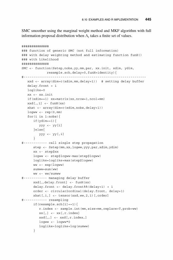
8.10 EXAMPLES AND R IMPLEMENTATION 445
SMC smoother using the marginal weight method and MKF algorithm with fullinformation proposal distribution when Λt takes a finite set of values.
################# function of generic SMC (not full information)### with delay weighting method and estimating function funH()### with Likelihood##############SMC <- function(Sstep,nobs,yy,mm,par, xx.init, xdim, ydim,
resample.sch,delay=0,funH=identity){#
xxd <- array(dim=c(xdim,mm,delay+1)) # setting delay bufferdelay.front = 1loglike=0xx <- xx.initif(xdim==1) xx=matrix(xx,nrow=1,ncol=mm)xxd[,,1] <- funH(xx)xhat <- array(dim=c(xdim,nobs,delay+1))logww <- rep(0,mm)for(i in 1:nobs){
if(ydim==1){yyy <- yy[i]
}else{yyy <- yy[,i]
}# call single step propagation
step <- Sstep(mm,xx,logww,yyy,par,xdim,ydim)xx <- step$xxlogww <- step$logww-max(step$logww)loglike=loglike+max(step$logww)ww <- exp(logww)sumww=sum(ww)ww <- ww/sumww
# managing delay bufferxxd[,,delay.front] <- funH(xx)delay.front <- delay.front%%(delay+1) + 1order <- circular2ordinal(delay.front, delay+1)xhat[,i,] <- tensor(xxd,ww,2,1)[,order]
# resamplingif(resample.sch[i]==1){
r.index <- sample.int(mm,size=mm,replace=T,prob=ww)xx[,] <- xx[,r.index]xxd[,,] <- xxd[,r.index,]logww <- logww*0loglike=loglike+log(sumww)
}

446 8. SEQUENTIAL MONTE CARLO
}if(resample.sch[nobs]==0){
ww <- exp(logww)sumww=sum(ww)loglike=loglike+log(sumww)
}# rearranging delay output
if(delay > 0){for(dd in 1:delay){xhat[,1:(nobs-dd),dd+1] <- xhat[,(dd+1):nobs,dd+1]xhat[,(nobs-dd+1):nobs,dd+1] <- NA
}}return(list(xhat=xhat,loglike=loglike))
}#end function
Some explanations:
� Sstep: A function that performs one step propagation using a proposal distri-bution. Its input includes (mm,xx,logww,yyy,par,xdim,ydim), wherexx and logww are the last iteration samples and log weight. yyy is the obser-vation at current time step. It should return xx (the samples xt) and 𝚕𝚘𝚐𝚠𝚠(their corresponding log weights).
� nobs: The number of observations T .
� yy: The observations, with T columns and yd𝑖m rows.
� mm: The Monte Carlo sample size m.
� par: A list of parameter values to pass to Sstep.
� xx.init: The initial samples of x0.
� xdim, ydim: The dimension of the state variable xt and the observation yt.
� resample.sch: A binary vector of length nobs, reflecting the resamplingschedule. resample.sch[i]= 1 indicating resample should be carried out atstep 𝑖.
� delay: The maximum delay lag for delayed weighting estimation. Default iszero.
� funH: A user supplied function h(⋅) for estimating E(h(xt) ∣ yt+d). Default isidentity(⋅) for estimating the mean. The function should be able to take vectoror matrix as input and operates on each element of the input.

8.10 EXAMPLES AND R IMPLEMENTATION 447
The function returns xhat, an array with dimensions (xd𝑖m, nobs, delay + 1),and the scaled log-likelihood value loglike. If loglike is needed, the log weightcalculation in the Sstep function should retain all constants that are related tothe parameters involved. Otherwise, the Sstep function may remove all constantsthat are common to all the Monte Carlo samples. It needs a utility function circu-lar2ordinal, also included in the NTS package, for efficient memory management.It requires the tensor package in R.
The following is the R function for SMC using the full information proposal.The inputs and outputs are the same as above, except the function Sstep.Fullrequires an additional binary indicator for resampling and it also returns an addi-tional resampling indices. We skip the full R code here. It can be extracted fromthe NTS package.
##################### function of generic SMC (full information) ### no R-B### with delay weighting method and estimating function funH()##################SMC.Full <- function(Sstep.Full,nobs,yy,mm,par,xx.init,xdim,
ydim, resample.sch,delay=0,funH=identity){...}#
The following is the R function for SMC using the full information proposal andR-B estimation of the mean only. No delay is allowed. The function Sstep.Full.RBshould return the R-B estimate of the mean of the state at the current step.
################### function of generic SMC (full information)### with R-B estimation. No delay################SMC.Full.RB=function(Sstep.Full.RB,nobs,yy,mm,par,xx.init,xdim,
ydim,resample.sch){...}#
The following is a generic SMC smoother in Algorithm 8.20. It requires anadditional user-specified function Sstep.Smooth for the backward smoothing step.The input of this additional function includes the samples x(j)
t and x(j)t+1 at times t
and t + 1, and their corresponding forward weight w(j)t and backward weight u(j)
t+1.
Its output should be the new backward weight u(j)t at time t. Note that resampling
is only for future samples. Previous samples are not changed.

448 8. SEQUENTIAL MONTE CARLO
##################### function of generic SMC Smoother### with estimating function funH()##################SMC.Smooth=function(Sstep,Sstep.Smooth,nobs,yy,mm,par,
xx.init,xdim,ydim,resample.sch,funH=identity){...}#
The following is a generic function of an MKF implementation for dis-crete indicator Λt. It requires a function that performs one-step propagationunder the MKF, with full information proposal distribution. Its input includes(mm,II,mu,SS,logww,yyy,par,xdim,ydim) where II, mu, SS are thesamples of Λt−1 and its corresponding mean and variance matrix of the Kalmanfilter components in the last iterations. logww is the log weight of the last iteration.It returns the R-B estimation of the mean and variance.
################### function of generic MKF (full information)### with R-B estimation. No delay################MKF.Full.RB <- function(MKFstep.Full.RB,nobs,yy,mm,par,II.init,
mu.init,SS.init,xdim,ydim,resample.sch){...}#
8.10.1.2 R Code for Resampling The following R codes implement theresidual resampling and stratified resampling procedures.
##################### Residual resample step##################resampling.res <- function(mm,ww){
mj <- floor(mm*ww)index <- rep.int(1,mj[1])for(j in 2:mm) index <- c(index,rep.int(j,mj[j]))ww2 <- mm*ww-mjif(sum(ww2)>0){
ww2 <- ww2/sum(ww2)mres <- mm-sum(mj)indexrex <- sample.int(mm,size=mres,replace=T,prob=ww2)index <- c(index,indexrex)
}return(list(index=index))
}#end function

8.10 EXAMPLES AND R IMPLEMENTATION 449
#################### Stratified resample step#################resampling.str=function(mm,ww){
u <- runif(1)cusumw <- cumsum(ww)mj <- floor(mm*cusumw-u)+1mj[mj<0] <- 0index <- rep(1,mj[1])for(j in 2:mm) index <- c(index,rep.int(j,mj[j]-mj[j-1]))return(list(index=index))
}#end function
The R implementation of the function sample.int implements Walker’s aliasmethod (Walker, 1974; Ripley, 1987). It is optimized and much faster than theimplements above, using rudimentary R codes. The following shows the CPU timeof a simple trial. Clearly sample.int is much faster. Of course, it is possible to opti-mize the implementation of the residual sampling and stratified sampling methods.In all examples considered, we use sample.int.
> mm=8*10000> ww=c(0,0,4,1,1,1,1,10)> ww=rep(ww,10000)> ww=ww/sum(ww)> system.time(for(i in 1:10) resampling.res(mm,ww))
user system elapsed43.59 0.17 44.09
> system.time(for(i in 1:10) resampling.str(mm,ww))user system elapsed
70.93 0.55 71.73> system.time(for(i in 1:10)
sample.int(mm,size=mm,replace=T,prob=ww))user system elapsed0.01 0.00 0.02
8.10.2 Tracking in a Clutter Environment
In this section we revisit the example of target tracking in a clutter environment dis-cussed in Section 6.2.4. To simplify the demonstration, we set ΔT = 1, the detec-tion region Ω = [−A, A], and a fixed number of signals mt. The probability thatall the observed yt𝑖 are noises is 1 − pd. It is the probability that the true signal is

450 8. SEQUENTIAL MONTE CARLO
0 20 40 60 80 100
−50
050
Time
Sig
nal
Figure 8.14 Plot of the signals observed in a clutter environment.
missing. Hence the model becomes
dt = dt−1 + st−1 + 0.5wt, (8.30)
st = st−1 + wt, (8.31)
P(It = 0) = 1 − pd and P(It = 𝑖) = pd∕mt, 𝑖 = 1,… , mt. (8.32)
The observation equation is
ytIt= dt + vt, for It ≠ 0 and yt𝑖 ∼ Un𝑖f (Ω), for 𝑖 ≠ It.
In simulation, we set the initial values to d1 = 0 and s1 = 0.1. The detection rangeis set to be [−80, 80]. pd = 0.95 and mt = 50. The noise variances are set as 𝜎2
w =0.12 and 𝜎2
v = 0.52. Figure 8.14 shows one set of simulated data.We consider three different proposal distributions.
1. Full state equation: Given x(j)t−1 = (d(j)
t−1, s(j)t−1, I(j)
t−1), generate x(j)t = (d(j)
t , s(j)t , I(j)
t )
using Equations (8.30) to (8.32). The incremental weight u(j)t ∝ p(yt ∣ x(j)
t )

8.10 EXAMPLES AND R IMPLEMENTATION 451
becomes
u(j)t ∝ 1√
2𝜋𝜎v
exp
{−
(yt𝑖 − d(j)t )2
2𝜎2v
}if I(j)
t = 𝑖 ≠ 0,
u(j)t ∝ 1|Ω| if I(j)
t = 0,
where |Ω| is the size of the monitoring region. In our simulation |Ω| = 80 −(−80) = 160. Note that in both cases there is a common constant |Ω|−(mt−1), whichis common to all x(j)
t and hence can be omitted.
2. Partial state equation: In this case we marginalize out the indicator It from thestate equation to enhance efficiency. Given x(j)
t−1 = (d(j)t−1, s(j)
t−1), we generate x(j)t =
(d(j)t , s(j)
t ) using Equations (8.30) and (8.31). The incremental weight u(j)t ∝ p(yt ∣
x(j)t ) =
∑m𝑖=0 p(yt ∣ x(j)
t , It = 𝑖)p(It = 𝑖) becomes
u(j)t ∝
1 − pd|Ω| +pd
m
m∑𝑖=1
1√2𝜋𝜎v
exp
{−
(yt𝑖 − d(j)t )2
2𝜎2v
}.
This weight evaluation is more expensive than that of the full state proposal, butclearly this is more efficient, since a randomly selected It has a small chance ofbeing the correct one. The marginalization takes out this layer of variation.
3. Full information proposal: Given x(j)t−1 = (d(j)
t−1, s(j)t−1, I(j)
t−1), generate x(j)t =
(d(j)t , s(j)
t , I(j)t ) from the full information distribution that includes the observations:
p(xt ∣ x(j)t−1, yt) ∝ p(xt ∣ x(j)
t−1)p(yt ∣ xt)
∝ p(dt, sd ∣ d(j)t−1, s(j)
t−1)p(It)p(yt ∣ It, dt, sd)
∝ c(j)tIt𝜙(dt|𝜇(j)
tIt, 𝜏2
tIt)p(It)I(st = s(j)
t−1 + 2(dt − d(j)t−1 − s(j)
t−1)),
where 𝜙(⋅) is the normal density and
𝜏2t𝑖 =
14𝜎2
w+ 1
𝜎2v
, 𝜇(j)t𝑖 =
4(d(j)t−1+s(j)
t−1)
𝜎2w
+ yt𝑖
𝜎2v
4𝜎2
w+ 1
𝜎2v
for 𝑖 ≠ 0,

452 8. SEQUENTIAL MONTE CARLO
and 𝜏2t0 = 𝜎2
w∕4, 𝜇(j)t0 = d(j)
t−1 + s(j)t−1 for 𝑖 = 0. The constants are
c(j)t𝑖 =
𝜏t𝑖√𝜋𝜎w𝜎v
exp
{−
2(d(j)t−1 + s(j)
t−1)2
𝜎2w
−y2
t𝑖
2𝜎2v
+𝜇
(j)2t𝑖
2𝜏2t𝑖
}for 𝑖 ≠ 0,
and c(j)t0 = 1. In addition P(It = 𝑖) = pd∕m for 𝑖 ≠ 0 and P(It = 0) = (1 − pd)∕|Ω|.
To generate samples from p(xt ∣ x(j)t−1, yt), we first generate I(j)
t with probability
P(It = 𝑖 ∣ x(j)t−1, yt) =
pdc(j)t𝑖
mC(j)t
for 𝑖 ≠ 0 and
P(It = 0 ∣ x(j)t−1, yt) =
(1 − pd)|Ω|C(j)t
,
where
C(j)t =
1 − pd|Ω| +pd
m
m∑𝑖=1
c(j)t𝑖 .
Conditioning on I(j)t , we generate samples of d(j)
t and s(j)t . When I(j)
t ≠ 0, we have
d(j)t ∼ N(𝜇
tI(j)t
, 𝜏2
tI(j)t
) and s(j)t = s(j)
t−1 + 2(d(j)t − d(j)
t−1 − s(j)t−1).
When I(j)t = 0, there is no real signal and we use
d(j)t = d(j)
t−1 + s(j)t−1 + 0.5𝜎w𝜀
(j)t and s(j)
t = s(j)t−1 + 𝜎w𝜀
(j)t ,
where 𝜀(j)t ∼ N(0, 1). The incremental weight is
u(j)t ∝
∫p(xt ∣ x(j)
t−1)p(yt ∣ xt)dxt ∝ C(j)t ,
which has already been obtained.For full information proposal distribution, the incremental weight u(j)
t = C(j)t
does not depend on the sampled x(j)t , hence resampling at time t should be done
before xt is sampled, and R-B in the form of Equation (8.22) can be used to esti-mate the location 𝜇t = E(xt ∣ yt). Specifically, we have
x(j)t = E(xt ∣ x(j)
t−1, yt) =1
C(j)t
(1 − pd|Ω| (x(j)
t−1 + s(j)t−1) +
m∑𝑖=1
𝜇(j)t𝑖 c(j)
t𝑖
).

8.10 EXAMPLES AND R IMPLEMENTATION 453
10
(a) (b)
30 50 70 90
Time
−60
−40
−20
020
10 30 50 70 90
Time−
0.6
−0.
4−
0.2
0.0
0.2
0.4
0.6
Figure 8.15 Boxplots for tracking error comparison between different resamplingschedules.
Hence, the estimation of 𝜇t = E(xt ∣ yt) should be done before x(j)t is sampled, but
after the weight is calculated. We use
��t =
∑mj=1 x(j)
t w(j)t∑m
j=1 w(j)t
.
To demonstrate various properties of SMC, we first focus on the data set shownin Figure 8.14, with 𝜎2
w = 0.12, 𝜎2v = 0.52, and mt = 50. With Monte Carlo sample
size m = 10, 000, and using the marginal state equation as the proposal distribu-tion, we run an SMC implementation 50 times (on the same data set) using each ofthe six resampling schedules sch=(1, 2, 5, 10, 20, 100), where sch(1) means resam-ple at every step and sch(100) means no resample (since the total time is 100).Using the properly weighted samples, the location dt is estimated and comparedwith the true location. Figure 8.15(a) shows the boxplot of the estimation errorsat times t = (10, 30, 50, 70, 90). The six boxes at each time point show the errorsof the six resampling schedules. The leftmost box corresponds to sch= 1. It isclear that resampling significantly improves the performance. Figure 8.15(b) is anenlarged version of Figure 8.15a and only shows the results of the first five resam-pling schedules. It seems that resampling once every two steps or resampling everystep performs well for this particular data set. Note that the results are based onthe same data set. Hence all variations shown are due to Monte Carlo variation.

454 8. SEQUENTIAL MONTE CARLO
10 30 50 70 90
Time
−0.
50.
00.
5
Figure 8.16 Boxplots for tracking error comparison between different Monte Carlo sam-ple sizes.
To see the impact of the Monte Carlo sample size used in SMC implementation,using the same data and using the marginal state equation as the proposal distribu-tion, we run an SMC implementation 50 times for each of the Monte Carlo simplesizes m = (1000, 4000, 16000, 64000). Resampling is done at every step. Figure8.16 shows the results also at times t = (10, 30, 50, 70, 90). Roughly speaking, thevariation reduces at the
√m rate as expected.
To see the impact of delay estimation, we use a smaller observation noise𝜎2
v = 0.12 and simulate the series 50 times and run an SMC implementation oneach data set with the delayed weighting method using delay lags d = 0 to d = 8.Resampling is done at every step. Figure 8.17(a) shows the error distribution,where the errors are computed using the difference of the estimated location andthe concurrent Kalman filter estimation with known signal indicator. Only the oneswithout losing tracks are shown. It is seen that for d ≥ 0, the errors are larger.This is because the Kalman filter estimator is based on the current information yt,while the delayed estimation is based on yt+d. Figure 8.17(b) shows the differencebetween the estimated location and the true location. It can be seen that delay

8.10 EXAMPLES AND R IMPLEMENTATION 455
10
(a) (b)
30 50 70 90
Time
−0.
3−
0.2
−0.
10.
00.
10.
20.
3
10 30 50 70 90
Time−
0.3
−0.
2−
0.1
0.0
0.1
0.2
0.3
Figure 8.17 Boxplots for tracking the error comparison between the delayed estimation(using delay weighting method) using the partial state equation proposal with mt = 50 and𝜎2
v = 0.01.
estimation improves the accuracy of estimating the true location, though longerdelay does not help much.
To check the difference in general estimation accuracy between the partial stateequation proposal and the full information proposal, we generated 50 data setsusing the aforementioned parameter set. With m = 10, 000 Monte Carlo samplesize and resampling every step, the tracking errors are obtained. Figure 8.18 showsthe boxplot of the differences in estimating the location. In each of the two graphs,the left-hand boxes show the errors using the partial state equation as the proposaldistribution and the right-hand boxes shows that using the full information pro-posal distribution. From Figure 8.18(a) it is clear that the SMC filter fails to trackthe target in one of the simulated data sets, resulting in an outlying point. Figure8.18(b) is an enlarged version of the boxplots by removing the extreme case. Inthis particular instance, the differences between the two proposal distributions arenot significant.
We repeated the experiment with a different set of parameters. The detectionrange remains the same, but the number of total observations at each time mt is setto 10 (instead of 50). The state equation noise level 𝜎2
v is increased to 0.152 andthe observational noise 𝜎2
v is changed to 0.022. These changes make the identityof the true signals more important, since the signal now is sparse and with smallermeasurement error. The Monte Carlo sample size is reduced to m = 2000. Figure8.19 shows the difference between the location estimates of the SMC filter andthat from a Kalman filter estimator with the true observation indicator It. Under

456 8. SEQUENTIAL MONTE CARLO
10
(a) (b)
30 50 70 90
Time
−10
010
2030
4060
50
10 30 50 70 90
Time
−0.
4−
0.2
0.0
0.2
0.4
Figure 8.18 Boxplots for tracking the error comparison between the partial state equationproposal and the full information proposal, with mt = 50 and 𝜎2
v = 0.01.
the true observation indicators, the Kalman filter provides the optimal solution fora linear and Gaussian system. Figure 8.19(a) shows the results of the 50 simulatedsamples. The left, middle, and right boxes at each time point show the results usingthe partial state equation proposal, full information proposal, and full informationproposal with R-B estimator, respectively. It is seen that in this case the SMC filterfails to track the target more frequently when the partial state equation proposal
10
(a) (b)
30 50 70 90
Time
10 30 50 70 90
Time
−10
0−
500
5010
015
0
−0.
010
−0.
005
0.00
00.
005
0.01
0
Figure 8.19 Boxplots for tracking the error comparison between the partial state equationproposal, the full information proposal, and the full information proposal with R-B. Theboxplots show the differences between the SMC estimator and the Kalman filter estimatorwith true signal indicator I𝑖. The parameters used are mt = 10, 𝜎2
w = 0.152, and 𝜎2v = 0.22.

8.10 EXAMPLES AND R IMPLEMENTATION 457
10
(a) (b)
30 50 70 90
Time
10 30 50 70 90
Time
−10
0−
500
5010
015
0
−0.
10−
0.05
0.00
0.05
0.10
Figure 8.20 Boxplots for tracking the error comparison between the partial state equationproposal, the full information proposal, and the full information proposal with R-B. Theboxplots show the difference between the SMC estimator and the Kalman filter estimatorwith true signal indicator I𝑖. The fourth boxplot shows the difference between the Kalmanfilter with true signal indicator I𝑖 and the true location. The parameters used are mt = 10,𝜎2
w = 0.152 and 𝜎2v = 0.04.
is used. The full information proposal fares much better. Figure 8.19(b) shows thetracking errors of the successful tracking data sets. It is clear now that the fullinformation proposal improves the performance significantly. The R-B improveseven further.
Figure 8.20 shows results of the same estimates as those of Figure 8.19. Theerrors are now calculated as the difference between the estimates and the true loca-tion. The additional fourth box shows the errors between the Kalman filter withtrue signal indicator and the true location. We can see that SMC with full informa-tion proposal works similarly to the Kalman filter with genie-aided true signals.
The following R functions for the propagation steps are used for the trackingin clutter problem, under partial state proposal, full information proposal, and fullinformation with R-B estimation. We provide detailed codes for using the par-tial state proposal and the full information proposal, to illustrate how to constructthe function as an input to the generic SMC main function. The full informationpropagation is more complicated not just to incorporate the yt information, butalso carry out resampling within the step before generating the new samples ofx(j)
t . We also implemented a Kalman filter estimation procedure, assuming thatthe true signal indicator It is known. The filter provides the optimal solutionfor the given series. Often we compare SMC estimators with this genie-aidedsolution.

458 8. SEQUENTIAL MONTE CARLO
R demonstration: Selected R code.
#################### Function of propagation step: Clutter. partial state proposal.Sstep.Clutter=function(mm,xx,logww,yyy,par,xdim,ydim){## state equation propagation
ee <- rnorm(mm)*par$sswxx[1,] <- xx[1,]+xx[2,]+0.5*eexx[2,] <- xx[2,]+eeuu <- 1:mm
# for each MC sample. Vectorized on all yyy observationsfor(j in 1:mm){temp <- sum(exp(-(yyy-xx[1,j])**2/2/par$ssv**2))uu[j] <- temp/par$ssv/sqrt(2*pi)*par$pd/par$nyy+(1-par$pd)/par$yr}
# update weightlogww <- logww+log(uu)-max(log(uu))return(list(xx=xx,logww=logww))
}#end function ################### Function of Clutter Propagation step Full Information.Sstep.Clutter.Full <- function(mm,xx,logww,yyy,par,xdim,ydim,
resample.sch){## passing the parameters
ssw2 <- par$ssw**2; ssv2 <- par$ssv**2nyy <- par$nyy; pd <- par$pd; yr <- par$yr
# setting needed temp variablesmu.i <- matrix(nrow=nyy,ncol=mm)cc.i <- matrix(nrow=nyy,ncol=mm)CC <- 1:mmtau2 <- 1/(4/ssw2+1/ssv2); tau <- sqrt(tau2)aa <- 0.5*(-log(pi)+log(tau2)-log(ssw2)-log(ssv2))for(jj in 1:mm){mu.i[,jj] <- (4*(xx[1,jj]+xx[2,jj])/ssw2+yyy/ssv2)*tau2temp <- -2*(xx[1,jj]+xx[2,jj])**2/ssw2-yyy**2/2/ssv2cc.i[,jj] <- temp +mu.i[,jj]**2/2/tau2+aacc.i[,jj] <- exp(cc.i[,jj])*pd/nyyCC[jj] <- sum(cc.i[,jj])+(1-pd)/yr
# updating weightlogww[jj] <- logww[jj]+log(CC[jj])
}# resampling
if(resample.sch==1){logpp <- logww-max(logww)

8.10 EXAMPLES AND R IMPLEMENTATION 459
pp <- exp(logpp)pp <- pp/sum(pp)r.index <- sample.int(mm,size=mm,replace=T,prob=pp)xx[,] <- xx[,r.index]mu.i[,] <- mu.i[,r.index]cc.i[,] <- cc.i[,r.index]CC <- CC[r.index]
}# generating new samplesfor(jj in 1:mm){
ind <- sample.int(nyy+1,1,prob=c((1-pd)/yr,cc.i[,jj])/CC[jj])if(ind == 1){
ee <- rnorm(1)xx[1,jj] <- xx[1,jj]+xx[2,jj]+0.5*ee*sswxx[2,jj] <- xx[2,jj]+ee*ssw
}if(ind >1){
xx[2,jj] <- -2*xx[1,jj]-xx[2,jj]xx[1,jj] <- rnorm(1)*tau+mu.i[ind-1,jj]xx[2,jj] <- xx[2,jj]+2*xx[1,jj]
}}return(list(xx=xx,logww=logww,r.index=r.index))
}#end function ################### Function of Clutter propagation step Full Information### with R-B estimation of mean.Sstep.Clutter.Full.RB=function(mm,xx,logww,yyy,par,xdim,ydim,
resample.sch){...}################### Function KF for tracking in clutter with known indicator I_t.
clutterKF <- function(nobs,ssw,ssv,yy,ii){...}################### Function of simulating target moving in clutter.simuTargetClutter <- function(nobs,pd,ssw,ssv,xx0,ss0,nyy,
yrange){...}#
Some explanations are in order:Sstep.Clutter performs one-step propagation using a partial state proposal.
It requires a list in par that includes
par=list(ssw=ssw,ssv=ssv,nyy=nyy,pd=pd,yr=yr).
It returns the one-step propagation samples xx and logww.

460 8. SEQUENTIAL MONTE CARLO
Sstep.Clutter.Full performs one-step propagation using a full informa-tion proposal. In additional to par, it requires a binary indicator resample.schto indicate whether a resampling is required at this step. It returns the one-steppropagation samples xx and logww, and the resampling index, if a resampling isperformed. Resampling is done before the current samples are drawn.
Sstep.Clutter.Full.RB performs one-step propagation using a full infor-mation proposal, and returns R-B estimate xhatRB for the mean for the currentstate. No delay is allowed. It also returns a non-Blackwellization estimate xhat
for comparison.clutterKF performs Kalman filter estimation with known indicator.simuTargetClutter simulates the target signal under the clutter environ-
ment. A utility function myboxplot is also included in the NTS package.The following R codes are used in the reported analysis.
R demonstration: Selected R code.
library("NTS")#################### simulation of one data set#set.seed(1)# parameternobs <- 100; pd <- 0.95; ssw <- 0.1; ssv <- 0.5;xx0 <- 0; ss0 <- 0.1; nyy <- 50;yrange <- c(-80,80); xdim <- 2; ydim <- nyy;# simulationsimu <- simuTargetClutter(nobs,pd,ssw,ssv,xx0,ss0,nyy,yrange)plot(1,1,type='n',xlim=c(0,nobs+1),ylim=yrange,xlab='time',ylab='signal')for(i in 1:nyy) points(1:nobs,simu$yy[i,],cex=0.4)#fig_clutterSignal.pdf############# KF with known indicators.#outKF <- clutterKF(nobs,ssw,ssv,simu$yy,simu$ii)xhat.kf <- outKF$xhat
############ Check Resampling Schedule. 50 SMC runs. Same data#set.seed(1)mm <- 10000sch <- c(1,2,5,10,20,100)nk <- 50par <- list(ssw=ssw,ssv=ssv,nyy=nyy,pd=pd,yr=range)xhat.r <- array(dim=c(nobs,6,nk))for(m in 1:6){

8.10 EXAMPLES AND R IMPLEMENTATION 461
resample.sch <- rep.int(c(rep(0,sch[m]-1),1),nobs/sch[m])for(kk in 1:nk){
xx.init <- matrix(nrow=2,ncol=mm)xx.init[1,] <- yrange[1]+runif(mm)*yrxx.init[2,] <- rep(0.1,mm)out <- SMC(Sstep.Clutter,nobs,simu$yy,mm,par,
xx.init,xdim,ydim,resample.sch)xhat.r[,m,kk] <- out$xhat[1,,1]
}}tstep <- c(10,30,50,70,90);res.r <- array(dim=c(nobs,6,nk))for(m in 1:6){for(ii in 1:nk) res.r[,m,ii] <- xhat.r[,m,ii]-simu$xx
}myboxplot(res.r,tstep,xlab='time') #fig_clutterR1.pdfmyboxplot(res.r[,1:5,],tstep,xlab='time') #fig_clutterR2.pdf############# Check MC sample size: resample every time step:### 50 SMC runs. Same data#set.seed(1)par <- list(ssw=ssw,ssv=ssv,nyy=nyy,pd=pd,yr=yr)resample.sch <- rep.int(1,nobs)nk <- 50xhat.m <- array(dim=c(nobs,4,nk))mall <- c(1000,4000,16000,64000)for(m in 1:4){
for(kk in 1:nk){mm <- mall[m]xx.init <- matrix(nrow=2,ncol=mm)xx.init[1,] <- yrange[1]+runif(mm)*yrxx.init[2,] <- rep(0.1,mm)out <- SMC(Sstep.Clutter,nobs,simu$yy,mm,par,
xx.init,xdim,ydim,resample.sch)xhat.m[,m,kk] <- out$xhat[1,,1]
}}tstep <- c(10,30,50,70,90);res.m <- array(dim=c(nobs,4,nk))for(m in 1:4){for(ii in 1:nk) res.m[,m,ii] <- xhat.m[,m,ii]-simu$xx
}myboxplot(res.m,tstep,xlab='time') #fig_clutterM.pdf##################### Check Delay. resample every step. 50 SMC runs. Same data#set.seed(1)mm <- 10000; nk <- 50;

462 8. SEQUENTIAL MONTE CARLO
resample.sch <- rep.int(1,nobs)delay <- 8xhat.d <- array(dim=c(nobs,delay+1,nk))for(kk in 1:nk){
xx.init <- matrix(nrow=2,ncol=mm)xx.init[1,] <- yrange[1]+runif(mm)*yrxx.init[2,] <- rep(0.1,mm)out <- SMC(Sstep.Clutter,nobs,simu$yy,mm,par,
xx.init,xdim,ydim,resample.sch,delay=delay)xhat.d[,,kk] <- out$xhat[1,,]
}res1.d <- array(dim=c(nobs-8,8,nk))res2.d <- array(dim=c(nobs-8,8,nk))tt <- 1:(nobs-delay)for(m in 1:delay){for(ii in 1:nk){
res1.d[tt,m,ii] <- xhat.d[tt,m,ii]-xhat.kf[tt]res2.d[tt,m,ii] <- xhat.d[tt,m,ii]-simu$xx[tt]
}}myboxplot(res1.d,tstep,xlab='time') #fig_clutterD1.pdfmyboxplot(res2.d,tstep,xlab='time') #fig_clutterD2.pdf################### check with different samples nyy=50, ssv=0.1################nk <- 50nobs <- 100; pd <- 0.95; ssw <- 0.1; ssv <- 0.1;xx0 <- 0; ss0 <- 0.1; nyy <- 50; yrange <- c(-80,80);xdim <- 2; ydim <- nyy; yr <- yrange[2]-yrange[1]par <- list(ssw=ssw,ssv=ssv,nyy=nyy,pd=pd,yr=yr)# simulation for repeated useYy <- array(dim=c(nyy,nobs,nk))Xx <- matrix(ncol=nk,nrow=nobs)Ii <- matrix(ncol=nk,nrow=nobs)kk <- 0seed.k <- 1while(kk < nk){seed.k <- seed.k+1set.seed(seed.k)kk <- kk+1simu <- simuTargetClutter(nobs,pd,ssw,ssv,xx0,ss0,nyy,yrange)if(max(abs(simu$yy))>80){
kk <- kk-1}else{
Xx[,kk] <- simu$xx; Yy[,,kk] <- simu$yy; Ii[,kk] <- simu$ii}
}# KF with known indicator

8.10 EXAMPLES AND R IMPLEMENTATION 463
Xxhat.kf <- matrix(ncol=nk,nrow=nobs)for(kk in 1:nk){outKF <- clutterKF(nobs,ssw,ssv,Yy[,,kk],Ii[,kk])Xxhat.kf[,kk] <- outKF$xhat
}### different delayresample.sch <- rep.int(1,nobs)delay <- 8mm <- 10000;Xxhat.d <- array(dim=c(nobs,delay+1,nk))set.seed(1)for(kk in 1:nk){
xx.init <- matrix(nrow=2,ncol=mm)xx.init[1,] <- yrange[1]+runif(mm)*yrxx.init[2,] <- rep(0.1,mm)out <- SMC(Sstep.Clutter,nobs,Yy[,,kk],mm,par,
xx.init,xdim,ydim,resample.sch,delay=delay)Xxhat.d[,,kk] <- out$xhat[1,,]
}tstep <- c(10,30,50,70,90);Xres1.d <- array(dim=c(nobs-8,9,nk))Xres2.d <- array(dim=c(nobs-8,9,nk))tt <- 1:(nobs-8)for(m in 1:9){for(ii in 1:nk){Xres1.d[tt,m,ii] <- Xxhat.d[tt,m,ii]-Xxhat.kf[tt,ii]Xres2.d[tt,m,ii] <- Xxhat.d[tt,m,ii]-Xx[tt,ii]
}}myboxplot(Xres1.d,tstep,xlab='time',ylim=c(-0.3,0.3))#fig_clutterXD2.pdfmyboxplot(Xres2.d,tstep,xlab='time',ylim=c(-0.3,0.3))#fig_clutterXD4.pdf
# compare Partial and Full resample.sch <- rep.int(1,nobs)delay <- 0; mm <- 10000;
Xxhat.full <- array(dim=c(nobs,1,nk))Xxhat.p <- array(dim=c(nobs,1,nk))Xres.com2 <- array(dim=c(nobs,2,nk))
set.seed(1)for(kk in 1:nk){
xx.init <- matrix(nrow=2,ncol=mm)xx.init[1,] <- yrange[1]+runif(mm)*yrxx.init[2,] <- rep(0.1,mm)out1 <- SMC(Sstep.Clutter,nobs,Yy[,,kk],mm,par,
xx.init,xdim,ydim,resample.sch)

464 8. SEQUENTIAL MONTE CARLO
Xxhat.p[,1,kk] <- out1$xhat[1,,1]out2 <- SMC.Full(Sstep.Clutter.Full,nobs,Yy[,,kk],mm,par,
xx.init,xdim,ydim,resample.sch)Xxhat.full[,1,kk] <- out2$xhat[1,,1]
}tstep <- c(10,30,50,70,90);for(ii in 1:nk){Xres.com2[,1,ii] <- Xxhat.p[,1,ii]-Xx[,ii]Xres.com2[,2,ii] <- Xxhat.full[,1,ii]-Xx[,ii]
}myboxplot(Xres.com2,tstep,xlab='time')#fig_clutterXCom3.pdfmyboxplot(Xres.com2,tstep,xlab='time',ylim=c(-0.5,0.5))#fig_clutterXCom4.pdf
##################Check with different samples nyy=10, ssv=0.02,ssw=0.15################### generate samples for repeated usenobs <- 100; pd <- 0.95; ssw <- 0.15; ssv <- 0.02;xx0 <- 0; ss0 <- 0.1; nyy <- 10; yrange <- c(-80,80);xdim <- 2; ydim <- nyy; nk <- 50yr <- yrange[2]-yrange[1]par <- list(ssw=ssw,ssv=ssv,nyy=nyy,pd=pd,yr=yr)
Yy10 <- array(dim=c(nyy,nobs,nk))Xx10 <- matrix(ncol=nk,nrow=nobs)Ii10 <- matrix(ncol=nk,nrow=nobs)
kk <- 0seed.k <- 1while(kk < nk){seed.k <- seed.k+1set.seed(seed.k)kk <- kk+1simu <- simuTargetClutter(nobs,pd,ssw,ssv,xx0,ss0,nyy,yrange)if(max(abs(simu$yy))>80){
kk <- kk-1}else{
Xx10[,kk] <- simu$xx; Yy10[,,kk] <- simu$yy; Ii10[,kk] <- simu$ii}
}## KF with known indicatorsXxhat.kf10 <- matrix(ncol=nk,nrow=nobs)for(kk in 1:nk){outKF <- clutterKF(nobs,ssw,ssv,Yy10[,,kk],Ii10[,kk])Xxhat.kf10[,kk] <- outKF$xhat
}

8.10 EXAMPLES AND R IMPLEMENTATION 465
### compare Partial and Full mm=2000resample.sch <- rep.int(1,nobs)delay <- 0; mm <- 2000; nk <- 50Xxhat.p10 <- array(dim=c(nobs,1,nk))Xxhat.RB10 <- array(dim=c(nobs,2,nk))Xres.com1.10 <- array(dim=c(nobs,3,nk))Xres.com2.10 <- array(dim=c(nobs,4,nk))
set.seed(1)for(kk in 1:nk){
xx.init <- matrix(nrow=2,ncol=mm)xx.init[1,] <- yrange[1]+runif(mm)*yrxx.init[2,] <- rep(0.1,mm)out1 <- SMC(Sstep.Clutter,nobs,Yy10[,,kk],mm,par,
xx.init,xdim,ydim,resample.sch)Xxhat.p10[,1,kk] <- out1$xhat[1,,1]
}
set.seed(1)for(kk in 1:nk){
cat('\n','iteration',kk);flush.console()xx.init <- matrix(nrow=2,ncol=mm)xx.init[1,] <- yrange[1]+runif(mm)*yrxx.init[2,] <- rep(0.1,mm)out3 <- SMC.Full.RB(Sstep.Clutter.Full.RB,nobs,Yy10[,,kk],mm,par,
xx.init,xdim,ydim,resample.sch)Xxhat.RB10[,1,kk] <- out3$xhatRB[1,]Xxhat.RB10[,2,kk] <- out3$xhat[1,]
}
tstep <- c(10,30,50,70,90);for(ii in 1:nk){Xres.com1.10[,1,ii] <- Xxhat.p10[,1,ii]-Xxhat.kf10[,ii]Xres.com1.10[,2,ii] <- Xxhat.RB10[,2,ii]-Xxhat.kf10[,ii]Xres.com1.10[,3,ii] <- Xxhat.RB10[,1,ii]-Xxhat.kf10[,ii]Xres.com2.10[,1,ii] <- Xxhat.p10[,1,ii]-Xx10[,ii]Xres.com2.10[,2,ii] <- Xxhat.RB10[,2,ii]-Xx10[,ii]Xres.com2.10[,3,ii] <- Xxhat.RB10[,1,ii]-Xx10[,ii]Xres.com2.10[,4,ii] <- Xxhat.kf10[,ii]-Xx10[,ii]
}myboxplot(Xres.com1.10,tstep,xlab='time')#fig_clutterXcom10_1.pdfmyboxplot(Xres.com1.10,tstep,xlab='time',ylim=c(-0.01,0.01))#fig_clutterXcom10_2.pdfmyboxplot(Xres.com2.10,tstep,xlab='time')#fig_clutterXcom10_3.pdfmyboxplot(Xres.com2.10,tstep,xlab='time',ylim=c(-0.1,0.1))#fig_clutterXCom10_4.pdf

466 8. SEQUENTIAL MONTE CARLO
0 10 20
target trajectory
30 40
−20
−10
010
20
x
y
Figure 8.21 Simulated path of the bearing-only track example.
8.10.3 Bearing-only Tracking with Passive Sonar
For demonstration, we revisit the two-dimensional bearing-only tracking problemin Section 7.1.6. In simulation, we set the initial values to x0 = c(10, 10, 0.01, 0.01)The noise variances are set to 𝜎2
w = 0.052, and 𝜎2v = 0.52. Figure 8.21 shows the
same set of simulated data we used in Example 7.1.The state equation can be written as
xt = Hxt−1 + Wwt (8.33)
where
H =
⎡⎢⎢⎢⎢⎣1 0 1 0
0 1 0 1
0 0 1 0
0 0 0 1
⎤⎥⎥⎥⎥⎦, W =
⎡⎢⎢⎢⎢⎣0.5q1 0
0 0.5q2
q1 0
0 q2
⎤⎥⎥⎥⎥⎦.
The observation equation is
𝜙𝑖t = arctan(
d2t − 𝜂𝑖2d1t − 𝜂𝑖1
)+ e𝑖t for 𝑖 = 1, 2. (8.34)
We consider using the state question as the proposal distribution. Specifically,given x(j)
t−1, generate x(j)t using (8.33). The incremental weight u(j)
t ∝ p(yt ∣ x(j)t ) =∑m
𝑖=0 p(yt ∣ x(j)t ) becomes
u(j)t ∝ exp
{−
(𝜙1t − ��(j)1t )2 + (𝜙2t − ��
(j)2t )2
2𝜎2v
}.

8.10 EXAMPLES AND R IMPLEMENTATION 467
26 28 30 32 34
−15
−10
−5
05
10
x
y
delay 0delay 10delay 20
Figure 8.22 Delayed filtering results for the bearing-only track example.
Using the same data as in Example 7.1, Figure 8.22 shows the delayed estimationusing the delay weighting method with delay d = 0, 10, and 20 and with MonteCarlo sample size m = 10, 000. The benefit of using delayed estimation can beclearly seen. Figures 8.23 and 8.24 show the estimation error in the x and y direc-tions. Again, in this particular case long delay is beneficial.
Figure 8.25 shows the smoothed estimation using the weight marginalizationmethod with T = 200 as the end point. Due to intensive computation, m = 5000Monte Carlo samples are used. We also include the EKF smoothing estimatorshown in Example 7.1 as the dashed line for comparison. It is clear that the SMCmethod outperforms the EKF method.
The following R functions are used in the example.
#################Function of single step propagation: passive sonar.# proposal used: state equationSstep.Sonar=function(mm,xx,logww,yy,par,xdim=1,ydim=1){...}#####################Function of simple step smooth step: passive sonarSstep.Smooth.Sonar=function(mm,xxt,xxt1,ww,vv,par){...}###################
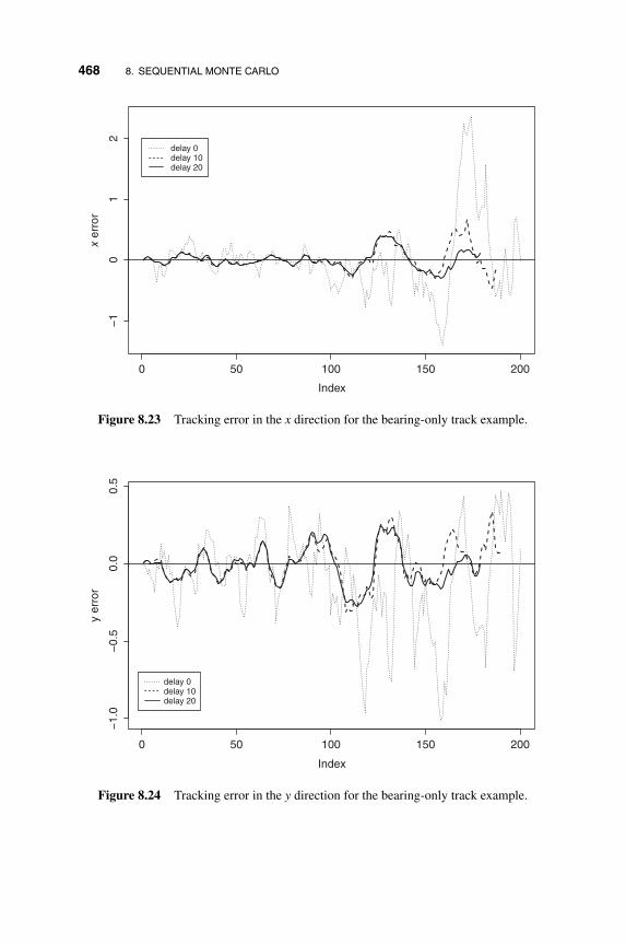
468 8. SEQUENTIAL MONTE CARLO
0 50 100 150 200
−1
01
2
Index
x er
ror
delay 0delay 10delay 20
Figure 8.23 Tracking error in the x direction for the bearing-only track example.
0 50 100 150 200
−1.
0−
0.5
0.0
0.5
Index
y er
ror
delay 0delay 10delay 20
Figure 8.24 Tracking error in the y direction for the bearing-only track example.

8.10 EXAMPLES AND R IMPLEMENTATION 469
SMC SmootherEKF Smoother
26 28 30 32 34
−15
−10
−5
05
10
x
y
Figure 8.25 SMC smoothing and EKF smoothing for the bearing-only track example.
#Function to simulate the datasimPassiveSonar=function(nobs,q,r,start,seed=20){...}#
R demonstration: Two-dimensional passive sonar tracking.
#parameters
s2 <- 20 #second sonar location at (s2,0)
q <- c(0.03,0.03)
r <- c(0.02,0.02)
nobs <- 200
start <- c(10,10,0.01,0.01)
H <- c(1,0,1,0,
0,1,0,1,
0,0,1,0,
0,0,0,1)
H <- matrix(H,ncol=4,nrow=4,byrow=T)
W <- c(0.5*q[1], 0,
0, 0.5*q[2],
q[1],0,
0,q[2])

470 8. SEQUENTIAL MONTE CARLO
W <- matrix(W,ncol=2,nrow=4,byrow=T)
V <- diag(r)
mu0 <- start
SS0 <- diag(c(1,1,1,1))*0.01
#simulation
simu_out <- simPassiveSonar(nobs,q,r,start,seed=20)
yy <- simu_out$yy
tt <- 100:200
plot(simu_out$xx[1,tt],simu_out$xx[2,tt],xlab='x',ylab='y',xlim=c(25.8,34))
#
#Run delayed filtering. Maximum delay 20
#
mm <- 100000
set.seed(1)
resample.sch <- rep(1,nobs)
xdim <- 4;ydim <- 2;
xx.init <- mu0+SS0%*%matrix(rnorm(mm*4),nrow=4,ncol=mm)
par <- list(H=H,W=W,V=V,s2=s2)
delay <- 20
out <- SMC(Sstep.Sonar,nobs,yy,mm,par,xx.init,xdim,ydim,resample.sch,delay)
tt <- 100:200
plot(simu_out$xx[1,tt],simu_out$xx[2,tt],xlab='x',ylab='y',xlim=c(25.8,34))
for(dd in c(1,11,21)){
tt <- 100:(200-dd)
lines(out$xhat[1,tt,dd],out$xhat[2,tt,dd],lty=22-dd,lwd=2)
}
legend(26.1,-12,legend=c("delay 0","delay 10","delay 20"),lty=c(21,11,1))
## PassiveSonar.Fig1.pdf
plot(simu_out$xx[1,]-out$xhat[1,,1],ylab='x error',type='n')
lines(simu_out$xx[1,]-out$xhat[1,,1],lty=21,lwd=1)
lines(simu_out$xx[1,1:189]-out$xhat[1,1:189,11],lty=2,lwd=2)
lines(simu_out$xx[1,1:179]-out$xhat[1,1:179,21],lty=1,lwd=2)
abline(h=0)
legend(0,2,legend=c("delay 0","delay 10","delay 20"),lty=c(21,2,1))
## PassiveSonar.Fig2.pdf
plot(simu_out$xx[2,]-out$xhat[2,,1],ylab='y error',type='n')
lines(simu_out$xx[2,]-out$xhat[2,,1],lty=21,lwd=1)
lines(simu_out$xx[2,1:189]-out$xhat[2,1:189,11],lty=2,lwd=2)
lines(simu_out$xx[2,1:179]-out$xhat[2,1:179,21],lty=1,lwd=2)
abline(h=0)
legend(-2,-0.7,legend=c("delay 0","delay 10","delay 20"),lty=c(21,2,1))
## PassiveSonar.Fig3.pdf
#
#Run smoothing
#
set.seed(1)
mm <- 5000
par <- list(H=H,W=W,V=V,s2=s2)

8.10 EXAMPLES AND R IMPLEMENTATION 471
xx.init <- mu0+SS0%*%matrix(rnorm(mm*4),nrow=4,ncol=mm)
out.s5K <- SMC.Smooth(Sstep.Sonar,Sstep.Smooth.Sonar,nobs,yy,mm,par,
xx.init,xdim,ydim,resample.sch)
tt <- 100:200
plot(simu_out$xx[1,tt],simu_out$xx[2,tt],xlab='x',ylab='y',xlim=c(25.8,34))
lines(out.s5K$xhat[1,tt],out.s5K$xhat[2,tt],lty=1,lwd=2)
## from Example 6.4.1 EKF smoothing results
lines(muTall[1,tt],muTall[2,tt],lty=2,lwd=2)
legend(26.1,-12,legend=c("SMC Smoother","EKF Smoother"),lty=c(1,2),lwd=2)
## PassiveSonar.Fig4.pdf
8.10.4 Stochastic Volatility Models
In Section 6.2.9 we discussed the stochastic volatility model of asset returns in theform
xt = 𝜙0 + 𝜙1xt−1 + 𝜎𝜂t, 𝜂t ∼ N(0, 1)
yt = exp(xt)vt, vt ∼ N(0, 1),
where yt is the observed asset return and xt is the latent log volatility of yt. This isan alternative approach to the volatility modeling discussed in Section 5.4.
In this section we demonstrate that SMC can be used in volatility modeling.We use the first 250 observations (in 2007) of daily log returns of the SPY indexused in Example 5.3. Figure 8.26(a) shows the time plot of the series. Using thestate equation as the proposal distribution gt(xt) = p(xt ∣ xt−1) and Monte Carlosample size m = 20, 000, resampling once every five time steps, we estimated thelog likelihood function of a set of parameters on a grid of 20 × 20 × 20 in therange of 𝜇 ∈ (−5,−4.4), 𝜙 ∈ (0.9, 1), 𝜎 ∈ (0.2, 0.5). The maximum is located at�� = −4.779, �� = 0.9421 and �� = 0.4053. Figure 8.27 shows the estimated loglikelihood value by changing one of the parameters while fixing the other two attheir maximum estimates. We also perform an iterative grid search, starting on acoarse grid (10 grids on each dimension), finding the maximum, then setting anew set of 10 × 10 × 10 grids around the maximum and reducing the grid size bya half. This procedure results in �� = −4.7667, �� = 0.9500, and �� = 0.3958.
Using this set of parameters, we run SMC to obtain the filtered series and thesmoothed series, shown in Figure 8.26(b) and (c), respectively.
We also checked local variability of the likelihood function. Without any resam-pling, we obtained the estimated log likelihood function using the same randomseed for the SMC evaluation on all parameter grids, as well as using different ran-dom seeds. Figure 8.28 shows the results. Clearly, using the same seed producesa smoother log likelihood function estimator. Note that resampling would induceextra variability and, hence, the resulting estimator may not be smooth.

472 8. SEQUENTIAL MONTE CARLO
−0.
04−
0.01
0.02
Ret
urn
−5.
4−
5.0
−4.
6−
4.2
xhat
0 50 100 150 200 250
−5.
2−
4.8
−4.
4
Time
0 50 100 150 200 250
Time
0 50 100 150 200 250
Time
xhat
(a)
(b)
(c)
Figure 8.26 (a) Top panel: daily log returns of the SPDR S&P 500 ETF index (SPY)in 2007. (b) Middle panel: filtered estimates of stochastic volatility. (c) Bottom panel:smoothed estimates of stochastic volatility.
The following R functions are used for the stochastic volatility model. We usedthe parallel package for evaluating the likelihood function on a grid. It onlyworks on linux/unix-based systems.
########Function of single step propagation using state equation: SVSstep.SV=function(mm,xx,logww,yyy,par,xdim,dim){...}########Function of SMC implementation for parallel processingwrap.SMC=function(par.natural,setseed=T,resample=T){...}#

8.10 EXAMPLES AND R IMPLEMENTATION 473
−5.0 −4.9 −4.8 −4.7 −4.6 −4.5 −4.4
1539
.515
40.0
1540
.515
41.0
1541
.515
42.0
1542
.5Likelhood for mu
mu
Log
likel
ihoo
d
0.90 0.92 0.94 0.96 0.98 1.00
1538
1539
1540
1541
1542
Likelhood for phi
phi
Log
likel
ihoo
d
0.20 0.25 0.30 0.35 0.40 0.45 0.50
1537
1538
1539
1540
1541
1542
Likelhood for sigma
sigma
Log
likel
ihoo
d
Figure 8.27 Estimated log likelihood functions on a grid, centered at the maximum ofeach parameter from a grid search.
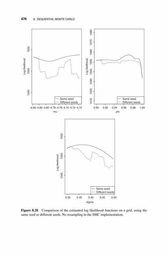
474 8. SEQUENTIAL MONTE CARLO
−4.84−4.82−4.80−4.78−4.76−4.74−4.72−4.70
1045
1050
1055
mu
Log
likel
ihoo
d
Same seedDifferent seeds
Same seedDifferent seeds
Same seedDifferent seeds
0.90 0.92 0.94 0.96 0.98 1.00
1010
1020
1030
1040
1050
1060
1070
1080
phi
Log
likel
ihoo
d
0.30 0.35 0.40 0.45 0.50
1045
1050
1055
sigma
Log
likel
ihoo
d
Figure 8.28 Comparison of the estimated log likelihood functions on a grid, using thesame seed or different seeds. No resampling in the SMC implementation.

8.10 EXAMPLES AND R IMPLEMENTATION 475
R demonstration: Stochastic volatility via SMC.
source("Rfunction.R")library(tensor)## Read in datay <- matrix(scan("SPY0717.dat"),ncol=2,byrow=T)yy <- y[,1]yy <- yy-mean(yy)yy <- yy[1:250]## Define search grid and prepare for parallel run##range.mu <- seq(-5, -4.4, length=20)range.phi <- seq(0.9, 1.0, length=20)range.sigma <- seq(0.2, 0.5, length=20)range <- list(range.mu, range.phi, range.sigma)nobs <- length(yy)mm <- 20000
grid <- expand.grid(range.mu, range.phi, range.sigma)names(grid) <- c("mu", "phi", "sigma")list.par <- as.list(data.frame(t(grid)))## Run grid search parallel###library(parallel)RNGkind("L'Ecuyer-CMRG")### Use same seed for all computationset.seed(1)lll <- mcmapply(wrap.SMC, list.par,
MoreArgs=list(setseed=T),mc.cores=detectCores(), mc.set.seed=T)
lll.array <- array(lll, dim=c(20,20,20))lll.max <- max(lll.array)max.index <- which(lll.array==lll.max, arr.ind=T)### Plotpdf('Loglike_grid.pdf', width=12, height=6)par(mfrow=c(1,3))plot(lll.array[,max.index[2],max.index[3]]˜range.mu,
xlab="mu", ylab="log likelihood",main="likelihood for mu", type='l',cex.lab=1.2)
plot(lll.array[max.index[1],,max.index[3]]˜range.phi,xlab="phi", ylab="log likelihood",main="likelihood for phi", type='l',,cex.lab=1.2,ylim=c(1538,1542.5))
plot(lll.array[max.index[1],max.index[2],]˜range.sigma,xlab="sigma", ylab="log likelihood",main="likelihood for sigma", type='l',,cex.lab=1.2)

476 8. SEQUENTIAL MONTE CARLO
dev.off()## MLE: iterative grid search##### Define search boxLU.mu <- c(-5,-4.4)LU.phi <- c(0.7,1.0)LU.sigma <- c(0.2,0.5)LU <- list(LU.mu, LU.phi, LU.sigma)### Initial pointpar.current <- c(-4.7, 0.9, 0.35)grid.current <- matrix(rep(par.current, 10), ncol=3, byrow=T)names(grid.current) <- c('mu','phi','sigma')### Accuracyepsilon <- c(0.01, 0.005, 0.005)within.epsilon <- 0
while(within.epsilon<3){within.epsilon <- 0for(i in 1:3){
sequence <- seq(LU[[i]][1], LU[[i]][2], length=10)grid.current[,i] <- sequenceset.seed(1)lll.tmp <- mcmapply(wrap.SMC,
as.list(data.frame(t(grid.current))),MoreArgs=list(setseed=T),mc.cores=detectCores(), mc.set.seed=T)
par.current[i] <- sequence[which.max(lll.tmp)]grid.current[,i] <- par.current[i]if (LU[[i]][2]-LU[[i]][1] <= epsilon[i]){
within.epsilon <- within.epsilon + 1}else {
# Shrink the interval by halfLU[[i]] <- 0.5*LU[[i]] + 0.5*par.current[i]
}}
}mle <- par.currentlll.mle <- vector('list', 3)## Local variability around MLE without resampling###n.grid <- 30range.local.mu <- seq(mle[1]-0.07, mle[1]+0.07, length=n.grid)range.local.phi <- seq(mle[2]-0.05, mle[2]+0.05, length=n.grid)range.local.sigma <- seq(mle[3]-0.1, mle[3]+0.1, length=n.grid)range.local <- list(range.local.mu, range.local.phi,
range.local.sigma)

8.10 EXAMPLES AND R IMPLEMENTATION 477
lll.local <- vector('list', 3)
for(i in 1:3){grid.tmp <- matrix(rep(mle, n.grid), ncol=3, byrow=T)grid.tmp[,i] <- range.local[[i]]
### Use same seed for all computationset.seed(1)lll.tmp <- mcmapply(wrap.SMC,
as.list(data.frame(t(grid.tmp))),MoreArgs=list(setseed=T, resample=F),mc.cores=detectCores(), mc.set.seed=T)
### Use different seeds for all computationset.seed(1)lll2.tmp <- mcmapply(wrap.SMC,
as.list(data.frame(t(grid.tmp))),MoreArgs=list(setseed=F, resample=F),mc.cores=detectCores(), mc.set.seed=F)
lll.local[[i]] <- list(lll.tmp, lll2.tmp)}### Plotpdf('Variability.pdf', width=12, height=6)par(mfrow=c(1,3))for(i in 1:3){
lll.tmp <- lll.local[[i]][[1]]lll2.tmp <- lll.local[[i]][[2]]m <- min(lll.tmp,lll2.tmp)M <- max(lll.tmp,lll2.tmp)plot(range.local[[i]],lll.tmp,
xlab=c("mu","phi","sigma")[i], ylab="log likelihood",type='l', ylim=c(2*m-M, 2*M-m), cex.lab=1.2)
lines(range.local[[i]], lll2.tmp, lty=2)legend('bottomright', lty=c(1,2),legend=c('Same seed','Different Seeds'))
}dev.off()## Posterior Mean, Smoothing and filtering###ww <- exp(lll-max(lll))ww <- ww/sum(ww)###Posterior Meanpar.hat <- ww%*%as.matrix(grid)###Filtering and Smoothingpar <- natural2ar(par.hat)resample.sch <- rep(c(0,0,0,0,1), length=nobs)set.seed(1)xx.init <- par.hat[1] + par.hat[3]*rnorm(mm)

478 8. SEQUENTIAL MONTE CARLO
out <- SMC(Sstep.SV, nobs, yy, mm, par,xx.init, 1, 1, resample.sch, delay=nobs-1)
out.filtering <- out$xhat[1,,1]out.smoothing <- diag(out$xhat[1,, nobs:1])### Plotpdf('Filtering.pdf', width=10, height=8)par(mfrow=c(3,1))par(mar=c(0,6,4,1))plot(yy, xaxt='n', ylab='Y', type='l', main='Filtering')par(mar=c(6,6,0,1))plot(out.filtering,xlab='Time',ylab='xhat',type='l')plot(out.smoothing, xlab='Time', ylab='xhat', type='l')dev.off()
8.10.5 Fading Channels as Conditional Dynamic Linear Models
In Section 6.2.5 we discussed using SSM in modeling and solving digital commu-nication problems. In particular, we discussed recovering signals from a systemwith Rayleigh flat-fading channels. Here we demonstrate the use of conditionaldynamic linear models and the MKF of Section 8.6 for the recovery of signals viathe Butterworth filter of order r = 3. Specifically, we consider the model used inChen et al. (2000), namely
𝛼t − 2.37409𝛼t−1 + 1.92936𝛼t−2 − 0.53208𝛼t−3
= 0.01(0.894909ut + 2.58227ut−1 + 2.58227ut−2 + 0.894909ut−3),
and rewrite the model in the form of
State equations:
{xt = Hxt−1 + Wwt,
dt ∼ Bernoull𝑖({−1, 1}, 0.5),Observation equation: yt = Gdt
xt + Vvt,
where
H =
⎡⎢⎢⎢⎢⎣2.37409 −1.92936 0.53208 0
1 0 0 0
0 1 0 0
0 0 1 0
⎤⎥⎥⎥⎥⎦, W =
⎡⎢⎢⎢⎢⎣1
0
0
0
⎤⎥⎥⎥⎥⎦,
and
G1 = 10−2 × [0.894909, 2.58227, 2.58227, 0.894909],
G−1 = −10−2[0.894909, 2.58227, 2.58227, 0.894909].

8.10 EXAMPLES AND R IMPLEMENTATION 479
0
(a) (b)
50 100 150 200
−2
−1
01
2
Time
Alp
ha
0 50 100 150 200
−2
−1
01
2Time
y
Figure 8.29 (a) Underlying changing channel coefficient 𝛼t and (b) received signal yt ofa simulated sample of a fading channel.
In communication yt is often a complex variable. For simplicity, here we con-sider the case that yt only takes real values. The resulting error rate we encounter ishigher than that in Chen et al. (2000), since they essentially observed two indepen-dent series of yt (the real part and the imaginary part of the variable). In addition,we only consider the case of independent signals and simple Gaussian state andobservational noises.
In our study xt is a four-dimensional state variable, dt ∈ {−1, 1} is the differ-ential encoded signals, and we are interested in estimating the information bit st =dtdt−1 (see Section 6.2.5 for details). In addition, wt ∼ N(0, 1) and vt ∼ N(0, 𝜎2
v ).We will vary 𝜎v to control the signal to noise ratio.
Figure 8.29(a) shows the underlying channel coefficient 𝛼t = Gxt. The abso-lute values of the roots of the AR polynomial 𝜙(z) = 1 − 𝜙1z − 𝜙2z2 − 𝜙3z3 are1.149, 1.149, and 1.42. They are close to the unit circle and, hence, the series isslow moving. The long-run frequency for the 𝛼t to change its sign is 0.0732 inthe stationary case. This is the lower error bound for differential decoder esti-mator st = dtdt−1 = s𝑖gn(ytyt−1) as it assumes that 𝛼t does not change sign. Fig-ure 8.29(b) shows the observed yt, with the signal-to-noise ratio around 25.8 dB,defined as 10 ln10(var(𝛼t)∕𝜎2
v ).We used an MKF with R-B with full information proposal to estimate the dif-
ferential code st = dtdt−1. In all cases, we used m = 100 Monte Carlo samples.The performance improvement of using a larger m is small. Only the results ofconcurrent estimation (i.e., estimation st based on yt with no delay) are obtained,as an illustration. Resampling is done at every step.
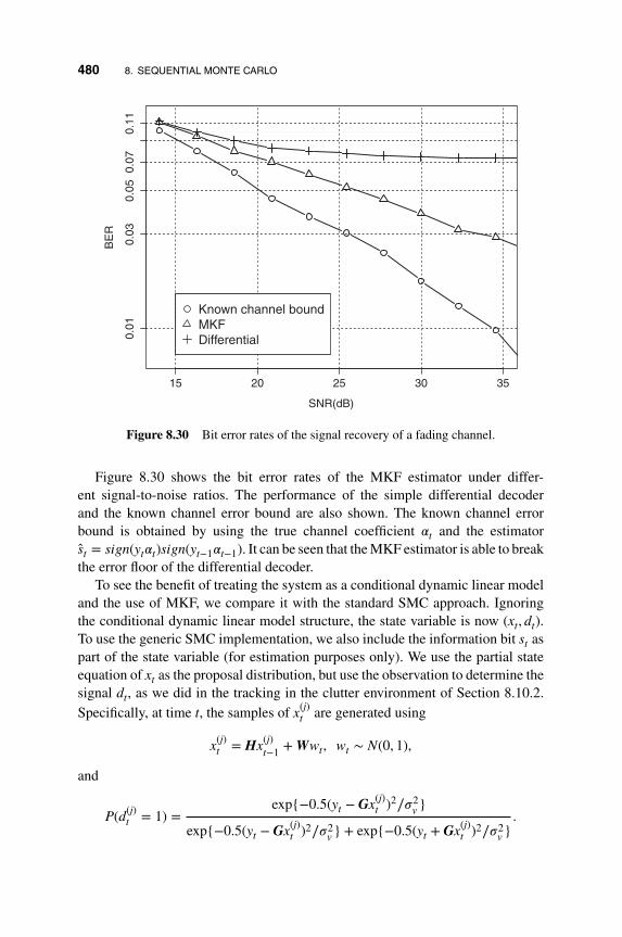
480 8. SEQUENTIAL MONTE CARLO
15 20 25 30 35
SNR(dB)
BE
R
0.01
0.03
0.05
0.07
0.11
Known channel boundMKFDifferential
Figure 8.30 Bit error rates of the signal recovery of a fading channel.
Figure 8.30 shows the bit error rates of the MKF estimator under differ-ent signal-to-noise ratios. The performance of the simple differential decoderand the known channel error bound are also shown. The known channel errorbound is obtained by using the true channel coefficient 𝛼t and the estimatorst = s𝑖gn(yt𝛼t)s𝑖gn(yt−1𝛼t−1). It can be seen that the MKF estimator is able to breakthe error floor of the differential decoder.
To see the benefit of treating the system as a conditional dynamic linear modeland the use of MKF, we compare it with the standard SMC approach. Ignoringthe conditional dynamic linear model structure, the state variable is now (xt, dt).To use the generic SMC implementation, we also include the information bit st aspart of the state variable (for estimation purposes only). We use the partial stateequation of xt as the proposal distribution, but use the observation to determine thesignal dt, as we did in the tracking in the clutter environment of Section 8.10.2.Specifically, at time t, the samples of x(j)
t are generated using
x(j)t = Hx(j)
t−1 + Wwt, wt ∼ N(0, 1),
and
P(d(j)t = 1) =
exp{−0.5(yt − Gx(j)t )2∕𝜎2
v }
exp{−0.5(yt − Gx(j)t )2∕𝜎2
v } + exp{−0.5(yt + Gx(j)t )2∕𝜎2
v }.
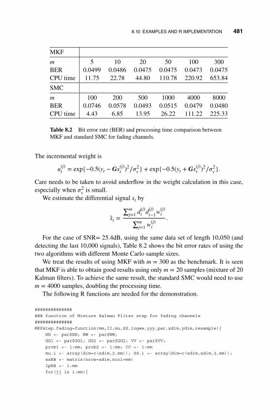
8.10 EXAMPLES AND R IMPLEMENTATION 481
MKF
m 5 10 20 50 100 300BER 0.0499 0.0486 0.0475 0.0475 0.0473 0.0475CPU time 11.75 22.78 44.80 110.78 220.92 653.84
SMC
m 100 200 500 1000 4000 8000BER 0.0746 0.0578 0.0493 0.0515 0.0479 0.0480CPU time 4.43 6.85 13.95 26.22 111.22 225.33
Table 8.2 Bit error rate (BER) and processing time comparison betweenMKF and standard SMC for fading channels.
The incremental weight is
u(j)t = exp{−0.5(yt − Gx(j)
t )2∕𝜎2v } + exp{−0.5(yt + Gx(j)
t )2∕𝜎2v }.
Care needs to be taken to avoid underflow in the weight calculation in this case,especially when 𝜎2
v is small.We estimate the differential signal st by
st =∑m
j=1 d(j)t d(j)
t−1w(j)t∑m
j=1 w(j)t
.
For the case of SNR= 25.4dB, using the same data set of length 10,050 (anddetecting the last 10,000 signals), Table 8.2 shows the bit error rates of using thetwo algorithms with different Monte Carlo sample sizes.
We treat the results of using MKF with m = 300 as the benchmark. It is seenthat MKF is able to obtain good results using only m = 20 samples (mixture of 20Kalman filters). To achieve the same result, the standard SMC would need to usem = 4000 samples, doubling the processing time.
The following R functions are needed for the demonstration.
##############
### function of Mixture Kalman Filter step for fading channels
##############
MKFstep.fading=function(mm,II,mu,SS,logww,yyy,par,xdim,ydim,resample){
HH <- par$HH; WW <- par$WW;
GG1 <- par$GG1; GG2 <- par$GG2; VV <- par$VV;
prob1 <- 1:mm; prob2 <- 1:mm; CC <- 1:mm
mu.i <- array(dim=c(xdim,2,mm)); SS.i <- array(dim=c(xdim,xdim,2,mm));
xxRB <- matrix(nrow=xdim,ncol=mm)
IpRB <- 1:mm
for(jj in 1:mm){

482 8. SEQUENTIAL MONTE CARLO
out1 <- KFoneLike(mu[,jj],SS[,,jj],yyy,HH,GG1,WW,VV)
out2 <- KFoneLike(mu[,jj],SS[,,jj],yyy,HH,GG2,WW,VV)
prob1[jj] <- exp(-out1$like)
prob2[jj] <- exp(-out2$like)
CC[jj] <- prob1[jj]+prob2[jj]
mu.i[,1,jj] <- out1$mu
mu.i[,2,jj] <- out2$mu
SS.i[,,1,jj] <- out1$SS
SS.i[,,2,jj] <- out2$SS
xxRB[,jj] <- (prob1[jj]*mu.i[,1,jj]+prob2[jj]*mu.i[,2,jj])/CC[jj]
IpRB[jj] <- prob1[jj]/CC[jj]*(2-II[jj])+(1-prob1[jj]/CC[jj])*(II[jj]-1)
logww[jj] <- logww[jj]+log(CC[jj])
}
ww <- exp(logww-max(logww))
ww <- ww/sum(ww)
xhatRB <- sum(xxRB*ww)
IphatRB <- sum(IpRB*ww)
if(resample==1){
r.index <- sample.int(mm,size=mm,replace=T,prob=ww)
mu.i[,,] <- mu.i[,,r.index]
SS.i[,,,] <- SS.i[,,,r.index]
prob1 <- prob1[r.index]
CC <- CC[r.index]
II <- II[r.index]
logww <- logww*0
}
II.new <- (runif(mm) > prob1/CC)+1
for(jj in 1:mm){
mu[,jj] <- mu.i[,II.new[jj],jj]
SS[,,jj] <- SS.i[,,II.new[jj],jj]
}
xhat <- sum(mu*ww)
Iphat <- sum(((2-II)*(2-II.new)+(II-1)*(II.new-1))*ww)
return(list(mu=mu,SS=SS,II=II.new,logww=logww,xhat=xhat,
xhatRB=xhatRB,Iphat=Iphat,IphatRB=IphatRB))
}
#################
### function of SIS step: Fading
#################
SISstep.fading=function(mm,xx,logww,yyy,par,xdim2,ydim){
HH <- par$HH; WW <- par$WW; VV <- par$VV; GG <- par$GG
xxx <- xx[1:4,]
xxx <- HH%*%xxx+WW%*%matrix(rnorm(mm),nrow=1,ncol=mm)
alpha <- GG%*%xxx
pp1 <- 1/(1+exp(-2*yyy*alpha/VV**2))
temp1 <- -(yyy-alpha)**2/2/VV**2
temp2 <- -(yyy+alpha)**2/2/VV**2
temp.max <- apply(cbind(temp1,temp2),1,max)
temp1 <- temp1-temp.max
temp2 <- temp2-temp.max
loguu <- temp.max+log(exp(temp1)+exp(temp2))

8.10 EXAMPLES AND R IMPLEMENTATION 483
logww <- logww+loguu
logww <- as.vector(logww)-max(logww)
II.new <- (runif(mm) > pp1)+1
xx[6,] <- (2-xx[5,])*(2-II.new)+(xx[5,]-1)*(II.new-1)
xx[5,] <- II.new
xx[1:4,] <- xxx
return(list(xx=xx,logww=logww))
}
R demonstration: Fading channel example.
### Fading channel analysisHH <- matrix(c(2.37409, -1.92936, 0.53028,0,
1,0,0,0,0,1,0,0,0,0,1,0),ncol=4,byrow=T)
WW <- matrix(c(1,0,0,0),nrow=4)GG <- matrix(0.01*c(0.89409,2.68227,2.68227,0.89409),nrow=1)VV <- 1.3**15*0.001par <- list(HH=HH,WW=WW,GG=GG,VV=VV)set.seed(1)par(mfrow=c(1,2))simu <- simu_fading(200,par)plot(simu$alpha,type='l',ylim=range(simu$yy),ylab='alpha',xlab='time')abline(h=0,lty=2)plot(simu$yy,type='l',ylab='y',xlab='time')#fig_fading0
# get SNR and root of AR polynomialSNR0=10*log(var(simu$alpha)/VV**2)/log(10)print(SNR0)abs(polyroot(c(1,-2.37409, +1.92936, -0.53028)))
# MKF setupGG1 <- GG; GG2 <- -GGxdim <- 4; ydim <- 1nobs <- 10050mm <- 100; resample.sch <- rep(1,nobs)
kk <- 20SNR <- 1:kk; BER1 <- 1:kk; BER0 <- 1:kk; BER.known <- 1:kktt <- 50:(nobs-1)for(i in 1:kk){
VV <- 1.3**i*0.001par <- list(HH=HH,WW=WW,GG=GG,VV=VV)par2 <- list(HH=HH,WW=WW,GG1=GG1,GG2=GG2,VV=VV)

484 8. SEQUENTIAL MONTE CARLO
set.seed(1)simu <- simu_fading(nobs,par)mu.init <- matrix(0,nrow=4,ncol=mm)SS0 <- diag(c(1,1,1,1))for(n0 in 1:20){SS0 <- HH%*%SS0%*%t(HH)+WW%*%t(WW)
}SS.init <- aperm(array(rep(SS0,mm),c(4,4,mm)),c(1,2,3))II.init <- floor(runif(mm)+0.5)+1out <- MKF.Full.RB(MKFstep.fading,nobs,simu$yy,mm,par2,II.init,
mu.init,SS.init,xdim,ydim,resample.sch)SNR[i] <- 10*log(var(simu$yy)/VV**2-1)/log(10)Strue <- simu$ss[2:nobs]*simu$ss[1:(nobs-1)]Shat <- rep(-1,(nobs-1))Shat[out$IphatRB[2:nobs]>0.5] <- 1BER1[i] <- sum(abs(Strue[tt]-Shat[tt]))/(nobs-50)/2Shat0 <- sign(simu$yy[1:(nobs-1)]*simu$yy[2:nobs])BER0[i] <- sum(abs(Strue[tt]-Shat0[tt]))/(nobs-50)/2S.known <- sign(simu$yy*simu$alpha)Shat.known <- S.known[1:(nobs-1)]*S.known[2:nobs]BER.known[i] <- sum(abs(Strue[tt]-Shat.known[tt]))/(nobs-50)/2
}
plot(SNR,BER.known,panel.first=grid(abline(v=c(15,20,25,30,35),h=0.01*c(1,3,5,7,9,11),lty=2)),log='y',xlim=c(14,35),yaxt="n",ylim=c(0.007,0.12),type='b',ylab='BER',xlab='SNR(dB)',pch=1,lwd=2,cex=1.5)
axis(2,0.01*c(1,3,5,7,9,11))lines(SNR,BER1,type='b',pch=2,lwd=2,cex=1.5)lines(SNR,BER0,type='b',pch=3,lwd=2,cex=1.5)legend(15,0.015,pch=c(1,2,3),cex=1.5,
legend=c('known channel bound','MKF','differential'))
## comparison of MKF and SMC with partial state equation proposal## get processing time
VV <- 1.3**15*0.001par <- list(HH=HH,WW=WW,GG=GG,VV=VV)par2 <- list(HH=HH,WW=WW,GG1=GG1,GG2=GG2,VV=VV)nobs <- 10050set.seed(2)simu <- simu_fading(nobs,par)
time.M=NULLmm.all <- c(5,10,20,50,100,300)kk <- 6BER.M <- 1:kk
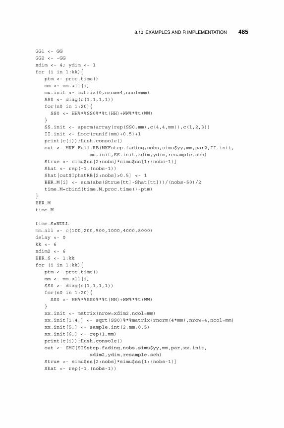
8.10 EXAMPLES AND R IMPLEMENTATION 485
GG1 <- GGGG2 <- -GGxdim <- 4; ydim <- 1for (i in 1:kk){
ptm <- proc.time()mm <- mm.all[i]mu.init <- matrix(0,nrow=4,ncol=mm)SS0 <- diag(c(1,1,1,1))for(n0 in 1:20){SS0 <- HH%*%SS0%*%t(HH)+WW%*%t(WW)
}SS.init <- aperm(array(rep(SS0,mm),c(4,4,mm)),c(1,2,3))II.init <- floor(runif(mm)+0.5)+1print(c(i));flush.console()out <- MKF.Full.RB(MKFstep.fading,nobs,simu$yy,mm,par2,II.init,
mu.init,SS.init,xdim,ydim,resample.sch)Strue <- simu$ss[2:nobs]*simu$ss[1:(nobs-1)]Shat <- rep(-1,(nobs-1))Shat[out$IphatRB[2:nobs]>0.5] <- 1BER.M[i] <- sum(abs(Strue[tt]-Shat[tt]))/(nobs-50)/2time.M=cbind(time.M,proc.time()-ptm)
}BER.Mtime.M
time.S=NULLmm.all <- c(100,200,500,1000,4000,8000)delay <- 0kk <- 6xdim2 <- 6BER.S <- 1:kkfor (i in 1:kk){
ptm <- proc.time()mm <- mm.all[i]SS0 <- diag(c(1,1,1,1))for(n0 in 1:20){SS0 <- HH%*%SS0%*%t(HH)+WW%*%t(WW)
}xx.init <- matrix(nrow=xdim2,ncol=mm)xx.init[1:4,] <- sqrt(SS0)%*%matrix(rnorm(4*mm),nrow=4,ncol=mm)xx.init[5,] <- sample.int(2,mm,0.5)xx.init[6,] <- rep(1,mm)print(c(i));flush.console()out <- SMC(SISstep.fading,nobs,simu$yy,mm,par,xx.init,
xdim2,ydim,resample.sch)Strue <- simu$ss[2:nobs]*simu$ss[1:(nobs-1)]Shat <- rep(-1,(nobs-1))

486 8. SEQUENTIAL MONTE CARLO
Shat[out$xhat[6,2:nobs,1]>0.5] <- 1BER.S[i] <- sum(abs(Strue[tt]-Shat[tt]))/(nobs-50)/2time.S=cbind(time.S,proc.time()-ptm)
}BER.S; time.S
8.11 EXERCISES
8.1 Box–Muller algorithm. Show that, if X1 and X2 are independent, followingUn𝑖f [0, 1], then
Y1 =√−2 ln(X1) cos(2𝜋X2), Y2 =
√−2 ln(X1) sin(2𝜋X2)
are independent, following N(0, 1).
8.2 Compare the execution time of the two implementations shown in Figures8.12 and 8.13 in Section 8.9 by generating a series of length tt = 100 fromthe simple model xt = xt−1 + wt and yt = xt + vt, where wt ∼ N(0, 1) andvt ∼ N(0, 1) independent of wt, and record the execution time. Change theMonte Carlo sample size mm and series length tt to see the differences.
8.3 For the simple model xt = xt−1 + 𝜎wwt and yt = xt + 𝜎vvt, where wt ∼N(0, 1), vt ∼ N(0, 1), and they are independent. Implement the followingalgorithms:
� (A.1) SMC using the full information proposal distribution.� (A.2) Bootstrap particle filter (state equation as proposal distribution).� (A.3) Independent particle filter (observation equation as proposal distri-
bution) with single matching L = 1.� (A.4) Kalman filter.
Use the following variances when simulating data:
� (B.1) 𝜎w = 1 and 𝜎v = 1.� (B.2) 𝜎w = 4 and 𝜎v = 1.� (B.3) 𝜎w = 1 and 𝜎v = 4.
Use the following resampling schedules:
� (C.1) Resample every step.� (C.2) Resample every five steps.� (C.3) No resampling.

REFERENCES 487
Simulate 500 series, each of 200 observations, starting at x0 = 0 under thethree variance settings, and run the four algorithms under the three resam-pling schedules (for SMC algorithms). Use initial distribution x0 ∼ N(0, 1).Make comparisons.
8.4 Use SMC to re-analyze Example 1.4.
(a) Use the estimated model in Example 1.4 to obtain the filtered andsmoothed estimate of 𝜆t and compare.
(b) Treat the estimated 𝛾0, 𝛾1 and 𝛿13 obtained in Example 4 as known, andestimate the dispersion parameter 𝛼 by evaluating the log-likelihoodfunction using SMC on a grid between 0.05 to 0.15. Obtain estimatesand compare them with those obtained in Example 1.4.
REFERENCES
Andrier, C., Doucet, A., and Holensterin, R. (2010). Particle Markov chain Monte Carlomethods. Journal of the Royal Statistical Society, Series B 72: 269–341.
Berzuini, C., Best, N., Gilks, W., and Larizza, C. (1997). Dynamic conditional indepen-dence models and Markov chain Monte Carlo methods. Journal of the American Statis-tical Association 92: 1403–1412.
Briers, M., Doucet, A., and Maskell, S. (2010). Smoothing algorithms for state-spacemodels. Annals of the Institute Statistical Mathematics 62: 61–89.
Brunnermeier, M. K. (2009). Deciphering the liquidity and credit crunch 2007–2008. Jour-nal of Economic Perspectives 23: 77–100.
Campbell, J. Y. and Shiller, R. J. (1988). The dividend-price ratio and expectations of futuredividends and discount factors. Review of Financial Studies 1: 195–228.
Cappe, O., Moulines, E., and Ryden, T. (2005). Inference in Hidden Markov Models.Springer-Verlag, New York.
Chen, R. and Liu, J. S. (2000). Mixture Kalman filter. Journal of the Royal Statistical Soci-ety, Series B 62: 493–508.
Chen, R., Wang, X., and Liu, J. S. (2000). Adaptive joint detection and decoding in flat-fading channels via mixture Kalman filtering. IEEE Transactions on Information Theory46: 2079–2094.
Chen, Y., Xie, J., and Liu, J. S. (2005). Stopping-time resampling for sequential MonteCarlo methods. Journal of the Royal Statistical Society, Series B 67: 199–217.
Chopin, N. (2004). Central limit theorem for sequential Monte Carlo methods and its appli-cations to Bayesian inference. Annals of Statistics 32: 2385–2411.
Douc, R., Moulines, E., and Stoffer, D. (2014). Nonlinear Time Series: Theory, Methodsand Applications with R Examples. Taylor & Francis, CRC Press, Boca Raton, FL.

488 8. SEQUENTIAL MONTE CARLO
Doucet, A., Godsill, S., and Andrieu, C. (2000). On sequential Monte Carlo sampling meth-ods for Bayesian filtering. Statistics and Computing 10: 197–208.
Emond, M., Raftery, A., and Steele, R. (2001). Easy computation of Bayes factors andnormalizing constants for mixture models via mixture importance sampling. Technicalreport, Department of Statistics, University of Washington, Seattle.
Evans, G. W. (1991). Pitfalls in testing for explosive bubbles in asset prices. AmericanEconomic Review 81: 922–930.
Fan, S., Chenney, S., Hu, B., Tsui, K., and Lai, Y. (2006). Optimizing control variate esti-mators for rendering. Computer Graphics Forum 25: 351–357.
Fearnhead, P. (2008). Computational methods for complex stochastic systems: a review ofsome alternatives to MCMC. Statistics and Computing 18: 151–171.
Fearnhead, P., Wyncoll, D., and Tawn, J. (2010). A sequential smoothing algorithm withlinear computational cost. Biometrika 97: 447–464.
Fischer, V. and Drutarovsky, M. (2003). True random number generator embedded in recon-figurable hardware. In Cryptographic Hardware and Embedded Systems – CHES 2002,B. S. Kaliski, K. Ko, and C. Paar (eds), Lecture Notes in Computer Science, vol. 2523,pp. 415–430. Springer, Berlin.
Ford, E. and Gregory, P. (2007). Bayesian model selection and extrasolar planet detection.In Statistical Challenges in Modern Astronomy IV, G. J. Babu and E. D. Feigelson (eds),vol. 371, pp. 189–205.
Fox, D., Thrun, S., Burgard, W., and Dellaert, F. (2001). Particle filters for mobile robotlocalization. In Sequential Monte Carlo in Practice, A. Doucet, J. F. G. de Freitas, andN. J. Gordon (eds), Springer-Verlag, New York.
Gelman, A. and Meng, X. (1998). Simulating normalizing constants: From importance sam-pling to bridge sampling to path sampling. Statistical Science 13: 163–185.
Giordani, P. and Kohn, R. (2010). Adaptive independent Metropolis–Hastings by fast esti-mation of mixtures of normals. Journal of Computational and Graphical Statistics 19:243–259.
Givens, G. and Raftery, A. (1996). Local adaptive importance sampling for multivariatedensities with strong nonlinear relationships. Journal of the American Statistical Asso-ciation 91: 132–141.
Gordon, N., Salmon, D., and Smith, A. (1993). A novel approach to nonlinear/non-GaussianBayesian state estimation. IEE Proceedings on Radar and Signal Processing 140:107–113.
Grassberger, P. (1997). Pruned-enriched Rosenbluth method: Simulation of polymers ofchain length up to 1,000,000. Physical Review E 56: 3682–3693.
Hammersley, J. M. and Handscomb, D. C. (1964). Monte Carlo Methods. Methuen’s Mono-graphs on Applied Probability and Statistics. Wiley, London.
Hammersley, J. M. and Morton, K. W. (1954). Poor man’s Monte Carlo. Journal of theRoyal Statistical Society, Series B 16: 23–38.
Hesterberg, T. (1988). Advances in Importance Sampling, PhD thesis, Stanford University.

REFERENCES 489
Hesterberg, T. (1995). Weighted average importance sampling and defensive mixture dis-tributions. Technometrics 37: 185–194.
Hrzeler, M. and Knsch, H. R. (1998). Monte Carlo approximations for gen eral state-spacemodels. Journal of Computational and Graphical Statistics 7: 175–193.
Isard, M. and Blake, A. (2004). ICONDENSATION: Unifying low-level and high leveltracking in a framework. Technical Report, Oxford University, http://robots.ox.ac.uk/ab.
Kitagawa, G. (1996). Monte Carlo filter and smoother for non-Gaussian nonlinear Statespace models. Journal of Computational and Graphical Statistics 91: 1–25.
Kong, A., Liu, J., and Wong, W. (1994). Sequential imputations and Bayesian missing dataproblems. Journal of the American Statistical Association 89: 278–288.
Lee, A., Yau, C., Giles, M. B., Doucet, A., and Holmes, C. C. (2010). On the utility of graph-ics cards to perform massively parallel simulation of advanced Monte Carlo methods.Journal of Computational and Graphical Statistics 19: 769–789.
Li, W., Tan, Z., and Chen, R. (2013). Two-stage importance sampling with mixture propos-als. Journal of the American Statistical Association 108: 1350–1365.
Li, W., Chen, R., and Tan, Z. (2016). Efficient sequential Monte Carlo with multipleproposals and control variates. Journal of the American Statistical Association 111:298–313.
Liang, F., Liu, C., and Carroll, R. J. (2007). Stochastic approximation in Monte Carlo com-putation. Journal of the American Statistical Association 102: 305–320.
Lin, M., Zhang, J., Cheng, Q., and Chen, R. (2005). Independent particle flters. Journal ofthe American Statistical Association 100: 1412–1421.
Lin, M., Chen, R., and Liu, J. S. (2013). Lookahead strategies for sequential Monte Carlo.Statistical Science 28: 69–94.
Liu, J. S. (2001). Monte Carlo Strategies in Scientific Computing, Springer, New York.
Liu, J. S. and Chen, R. (1995). Blind deconvolution via sequential imputations. Journal ofthe American Statistical Association 90: 567–576.
Liu, J. S. and Chen, R. (1998). Sequential Monte Carlo methods for dynamic systems.Journal of the American Statistical Association 93: 1032–1044.
Liu, J. and West, M. (2001). Combined parameter and state estimation in simulation-basedfiltering. In Sequential Monte Carlo in Practice, A. Doucet, J. F. G. de Freitas, and N.J. Gordon (eds). Springer-Verlag, New York.
Liu, J., Wong, W., and Kong, A. (1994). Covariance structure of the Gibbs sampler withapplications to the comparisons of estimators and augmentation schemes. Biometrika81: 27–40.
MacEachern, S., Clyde, M., and Liu, J. (1998). Sequential importance sampling for non-parametric Bayes models: The next generation. Canadian Journal of Statistics 27:251–267.
Majzoobi, M., Koushanfar, F., and Devadas, S. (2011). FPGA-based true random num-ber generation using circuit metastability with adaptive feedback control. In CHES,pp. 17–32. Springer, Berlin.

490 8. SEQUENTIAL MONTE CARLO
Malik, S. and Pitt, M. K. (2011). Particle filters for continuous likelihood evaluation andmaximization. Journal of Econometrics 165: 190–209.
Marshall, A. (1956). The use of multi-stage sampling schemes in Monte Carlo computa-tions. In Symposium on Monte Carlo Methods, M. Meyer (ed.), pp. 123–140. Wiley,New York.
Oh, M. and Berger, J. (1993). Integration of multimodal functions by Monte Carlo impor-tance sampling. Journal of the American Statistical Association 88: 450–456.
Owen, A. B. and Zhou, Y. (1999). Adaptive importance sampling by mixtures of productsof beta distributions. Technical Report, Department of Statistics, Stanford University.
Owen, A. and Zhou, Y. (2000). Safe and effective importance sampling. Journal of theAmerican Statistical Association 95: 135–143.
Pitt, M. and Shephard, N. (1999). Filtering via simulation: auxiliary particle filters. Journalof the American Statistical Association 94: 590–599.
Poyiadjis, G., Doucet, A., and Singh, S. (2011). Particle approximations of the score andobserved information matrix in state space models with application to parameter esti-mation. Biometrika 98: 65–80.
Raghavan, N. and Cox, D. (1998). Adaptive mixture importance sampling. Journal of Sta-tistical Computation and Simulation 60: 237–260.
Ripley, B. (1987). Stochastic Simulation. John Wiley and Sons, New York.
Robert, C. and Casella, G. (2004). Monte Carlo Statistical Methods. Springer, New York.
Rosenbluth, M. N. and Rosenbluth, A. W. (1955). Monte Carlo calculation of the averageextension of molecular chains. Journal of Chemical Physics 23: 356-359.
Rubinstein, R. and Kroese, D. (2008). Simulation and the Monte Carlo Method. Wiley,Hoboken, NJ.
Smith, P., Sha, M., and Gao, H. (1997). Quick simulation: A review of importance sam-pling techniques in communications systems. Selected Areas in Communications, IEEEJournal 15: 597–613.
Tanizaki, H. and Mariano, R. S. (1994). Prediction, filtering and smoothing in non-linearand non-normal cases using Monte Carlo integration. Journal of Applied Econometrics9: 163–179.
van der Merwe, R., Doucet, A., de Freitas, N., and Wan, E. (2002). The unscented particlefilter. In Advances in Neural Information Processing Systems (NIPS13), T. K. Leen,T. G. Dietterich, and V. Tresp (eds). MIT Press, Cambridge, MA.
Veach, E. and Guibas, L. (1995). Optimally combining sampling techniques for MonteCarlo rendering. In Proceedings of the 22nd Annual Conference on Computer Graphicsand Interactive Techniques, pp. 419–428. ACM.
Walker, A. J. (1974). New fast method for generating discrete random numbers with arbi-trary frequency distributions. Electronics Letters 10: 127–128.
Wang, X., Chen, R., and Guo, D. (2002). Delayed pilot sampling for mixture Kalman fil-ter with application in fading channels. IEEE Transaction on Signal Processing 50:241–264.

REFERENCES 491
West, M. (1992). Mixture models, Monte Carlo, Bayesian updating and dynamic models.Computer Science and Statistics 24: 325–333.
West, M. (1993). Approximating posterior distributions by mixture. Journal of the RoyalStatistical Society. Series B 55: 409–422.
Zhang, J. L. and Liu, J. S. (2002). A new sequential importance sampling method and itsapplication to the two-dimensional hydrophobic Chydrophilic model. Journal of Chem-ical Physics 117: 3492–3498.
Zhang, J., Chen, R., Tang, C., and Liang, J. (2003). Origin of scaling behavior of proteinpacking density: A sequential Monte Carlo study of compact long chain polymer. Jour-nal of Chemical Physics 118: 6102–6109.

INDEX
Activation function, 175Akaike information criterion, 4Antithetic variate, 385AR model, 5ARCH model, 25, 110ARIMA model, 269ARMA model, 3Arranged autoregression, 36,
53Augmentation method, 383Autocorrelation function, 3Autocovariance function, 2Autoregressive conditional duration (ACD)
model, 229Autoregressive conditional mean (ACM)
model, 229Auxiliary particle filter, 423
Back-prorogation, 176Backfitting
ACE algorithm, 158, 160BRUTO algorithm, 158, 159
Backtesting, 9Bagging, 209Bandwidth, 120Baum-Welch algorithm, 356BLUE: best linear unbiased estimator, 336,
341Boltzmann machine, 182
Restricted, 183Bootstrap filter, 413Box-Muller algorithm, 378
CAPM model, 139, 273, 304Causal time series, 3
Nonlinear Time Series Analysis, First Edition. Ruey S. Tsay and Rong Chen.© 2019 John Wiley & Sons, Inc. Published 2019 by John Wiley & Sons, Inc.Companion website: www.wiley.com/go/tsay/nonlineartimeseries
493

494 INDEX
Compound Poisson process, 51Conditional dynamic linear model,
429Conditional heteroscedasticity, 10Contrastive divergence, 183Correlation
Spearman, 3Correlation integral, 22Cross validation, 122
DataU.S. unemployment rate, 4Amazon return, 185Canadian lynx, 34Crude oil price, 9, 160, 180ECG, 153Electricity demand, 245Fama-French factors, 304, 365Gas furnace, 16Gasoline price, 160GDP, 196GM return, 139Industrial production index, 95PM2.5, 202Real GDP, 143S&P 500 index, 358SPY, 234SPY log return, 471SPY return, 237Sunspot, 133TAQ, 190Temperature, 254U.S. GDP, 82Unemployment duration, 126
Decision tree, 195Deep belief net, 182, 184Deep learning, 181Distribution
Beta, 379Chi-square, 379Double Poisson, 229Exponential, 379, 382F, 379Gamma, 379Negative binomial, 20, 229Poisson, 20
Student-t, 379Uniform, 378
Distributional time series, 285
Effective sample size, 390, 398, 426EGARCH model, 243EM algorithm, 356Energy function, 183Ensemble, 42Ergodicity, 43, 399Exponential AR model, 100Exponential family distribution, 218
Factor modelDynamic, 283Fama-French, 273
FilterHigh pass, 150Low pass, 150
Filtering, 66Functional time series, 284
Autoregressive model, 248Convolution, 248
Functional-coefficient AR model, 99
GARCH model, 10, 235Gauss-Markov theorem, 336Gaussian sum filter, 338Generalized autoregressive moving
average model, 218Generalized cross validation, 122, 159Geometric drift condition, 234Gibbs sampler, 401Gini index, 202GJR model, 242Great moderation, 82Growth principle, 428
Haar basis function, 138Harmonium, 183Heaviside function, 175Hidden Markov model, 289Hypoblic tangent, 175
Identifiability, 65Importance sampling, 387

INDEX 495
Independent particle filter, 413Index model, 164Innovation process, 296Inverse CDF, 379
Kalman filter, 105, 293, 295, 429–431Ensemble, 341Extended, 337Unscented, 339
Kalman gain, 295Kalman smoothing, 297, 299Kernel estimator
Expanechnikov, 120Gasser-Muller, 122
KurtosisExcess, 8
Leverage effect, 242Likelihood, 268, 438
Complete data, 69Linearity, 3Link function, 218, 232
y, 233Locally weighted scatterplot smoothing,
131Long short-term memory (LSTM), 182
Marginal weighting, 396Markov chain, 111, 112, 398
Absorbing, 113Aperiodic, 113Ergodic, 114Irreducible, 113Recurrent, 113Stationary distribution, 114
Markov switching model, 12, 63, 289MCMC, 72, 398
Aperiodic, 399Baker acceptance rule, 401Irreducible, 399Proposal, 412, 441
Metropolis-Hasting algorithm, 75,400
MIDASMixed frequency data analysis,
291
Mixing𝛼, 126𝜙, 126
Multiresolution analysis, 149
NAAR, 160NAARX model, 160Nadaraya-Watson estimator, 120Neural network, 174
Node, 174Nonlinear additive model
AR, 158Nonlinearity test
BDS test, 22F-test, 33Keenan, 32Lagrange multiplier test, 25McLeod-Li test, 25Rank-based test, 27RESET, 32Tar-F, 37
Nuisance parameter, 35
Ordered probit model, 191Ornstein-Uhlenbeck process, 248Out-of-bag observation, 210
Particle filter, 403Unscented, 412
Particle smoothing, 403Perceptron, 175Phase ambiguity, 280Piecewise linear regression, 43Portmanteau test, 25Priority score, 397
Rao-Blackwellization, 428, 444, 452RCA model, 110Realization, 42Realized volatility, 105Rejection method, 379Residuals
Identity, 222Pearson, 221Pseudo predictive, 210Score-type, 222

496 INDEX
Sample degeneracy, 421Self-avoiding walk, 420Sequential sampling, 382Sieve estimators, 254Sigmoid function, 175Signal processing, 279Single index model, 164SIR, 164
Procedure, 165Skeleton, 42Skewness, 8Slice inverse regression, 164Smooth transition AR model, 92
Exponential, 93Logistic, 93
Smoothing, 66Fixed lag, 299
Smoothing parameter, 120Softmax function, 175Spline
B-spline, 138Egrees of freedom, 143Knot, 134Natural cubic, 138Smoothing, 141
State space model, 104, 266, 402, 423Local level model, 271Local trend model, 271Markovian, 266Seasonal model, 272Time-varying coefficient model,
273State variable, 266Stationarity
Functional time series, 247
Strict, 2Weak, 2
Stochastic volatility, 285, 290, 471SURE shrinkage, 152
Target tracking, 273Mobile network, 278Other, 278Passive sonar, 277
TGARCH model, 242Threshold
Universal, 151Threshold autoregressive model, 5, 43Thresholding
Hard, 151Soft, 151
Time-varying AR model, 104Time-varying coefficient model, 99Transfer function model, 15Transition probability, 112, 351Tree
Classification, 201Regression, 195
Viterbi algorithm, 355Volatility, 10, 358Volterra series, 31
Wavelet, 145Father, 145Mother, 145
Wavelet transform, 150
Yield curve, 285Nelson-Siegel, 286
Copyright © 2022 FDOKUMEN