Modelling Interval Time Series with Space-Time Processes
39
Modeling interval time series with Space-time processes Paulo Teles and Paula Brito Faculdade de Economia & LIAAD-INESC Porto LA, University of Porto Rua Dr. Roberto Frias, 4200-464 Porto, Portugal Corresponding author: Paulo Teles Faculdade de Economia & LIAAD-INESC Porto LA, University of Porto Rua Dr. Roberto Frias, 4200-464 Porto, Portugal Email: [email protected] Short Title: Space-time processes for interval time series 1
Transcript of Modelling Interval Time Series with Space-Time Processes
Modeling interval time series with Space-time processes
Paulo Teles and Paula Brito
Faculdade de Economia & LIAAD-INESC Porto LA, University of Porto
Rua Dr. Roberto Frias, 4200-464 Porto, Portugal
Corresponding author:
Paulo Teles
Faculdade de Economia & LIAAD-INESC Porto LA, University of Porto
Rua Dr. Roberto Frias, 4200-464 Porto, Portugal
Email: [email protected]
Short Title: Space-time processes for interval time series
1

Abstract. We consider interval-valued time series, i.e., series resulting from collecting real
intervals as an ordered sequence through time. Since the lower and upper bounds of the observed
intervals at each time point are in fact values of the same variable, they are naturally related.
We propose modeling interval-time series with Space-time autoregressive models and, based on the
process appropriate for the interval bounds, we derive the model for the intervals’ center and radius.
A simulation study and an application with data of daily wind speed at different meteorological
stations in Ireland illustrate that the proposed approach is appropriate and useful.
Keywords. Interval time series; Interval data; Space-time AR model; Prediction.
1 Introduction
In classical data analysis, variables describing entities are usually mono-valued, that is,
each entity takes exactly one value for each variable at each point in time. However, this
model is too restrictive to represent complex data which may comprehend variability and/or
uncertainty. The need to consider data containing information that cannot be represented
within the classical framework led to the development of Symbolic Data Analysis. Symbolic
data extend the classical model, where each individual takes exactly one value for each
variable, by allowing multiple, possibly weighted, values for each variable. New variable
types have been introduced enabling us to represent variability and/or uncertainty inherent
to the data: multi-valued variables, interval variables and modal variables (Bock and Diday,
2000). A variable is called set-valued if its values are nonempty subsets of the underlying
domain; it is multi-valued if its values are finite subsets of the domain and it is an interval
variable if its values are intervals of IR. A survey of this new area can be found in Billard
and Diday (2006), Diday and Noirhomme (2008), or, more recently, in Noirhomme and
Brito (2011).
Interval data refers to data sets where the observed values of the variables are inter-
vals of IR and may arise in multiple situations that result from temporal aggregation or
systematic sampling such as recording monthly temperatures or the daily wind speed in
different locations or daily stock prices or returns. Other important sources of interval data
are the aggregation of huge data-bases in groups or classes, when the individual real values
are generalized by intervals, or situations where there is some inaccuracy or uncertainty
2
in recording the value of a (classical) variable (e.g., due to measurement errors). Interval-
valued data may be represented by the lower (li) and upper (ui) bounds of each observed
interval Ii = [li, ui] , i = 1, ..., n, or, alternatively, by its center ci =li + ui
2and radius
ri =ui − li
2.
Many different approaches have now been developed to analyze interval data. Assuming
a uniform distribution in each observed interval, Bertrand and Goupil (2000) have proposed
central tendency and dispersion measures for interval data. Billard and Diday (2003) devel-
oped this approach introducing association measures. Duarte Silva and Brito (2006) discuss
the properties of dispersion and association measures for interval data and their implications
in the definition of linear combinations of interval-valued variables. Based on the uniform
assumption, Billard and Diday (2000) have proposed a regression model for interval-valued
data. Principal Component Analysis of interval data has first been addressed by Chouakria
et al (2000) either by representing the observed intervals by their centers (“centers method”)
or by considering all the vertices of the hypercube representing each of the n individuals in
a p-dimensional space (“vertices method”). A different approach is based on representing
each variable by the midpoints and ranges of its interval values, a line of work followed by
Lauro and Palumbo (2005) on Principal Component Analysis and also by Neto et al (2008,
2010) on Regression Analysis. In Duarte Silva and Brito (2006) different approaches for
Linear Discriminant Analysis of interval data are investigated.
When the interval-valued data such as in the examples mentioned above are collected
as an ordered sequence through time (daily, monthly, quarterly, etc) or any other dimen-
sion, they form a time series and consequently the appropriate methodology to study and
model them is time series analysis. To describe time series data, ARIMA (Autoregressive
Integrated Moving Average) models are usually considered (Box, Jenkins and Reinsel, 2008;
Brockwell and Davis, 2002; Wei, 2006) but these are appropriate for single-valued data sets.
New developments to model interval time series have recently been proposed.
Teles and Brito (2005) were the first to consider interval-valued time series data using
an approach based on fitting univariate ARIMA processes to the interval bounds (see also
Brito, 2007). Maia, De Carvalho and Ludermir (2008) propose fitting univariate ARIMA
processes applied to the center and radius and use them to forecast the interval bounds,
3
since the latter can be obtained from the former. They also propose an approach based on
an artificial neural network model as well as a combination of both.
Arroyo (2008), Garcıa-Ascanio and Mate (2009), Gonzalez-Rivera and Arroyo (2011)
and Han et al. (2008) define interval stochastic process, interval-valued time series, weak
stationarity for interval processes and, based on the sample moments previously proposed
(Bertrand and Goupil, 2000), also define the empirical autocovariance and autocorrelation
functions for interval time series data, aiming at uncovering the data-generating process
behind this type of symbolic data sets. Arroyo (2008), Garcıa-Ascanio and Mate (2009)
and Arroyo, Gonzalez-Rivera and Mate (2010) focus on forecasting based on Vector Au-
toregressive models (VAR), Vector Error Correction models (VEC) and smoothing filters.
Other approaches may provide a new insight into modeling interval time series data,
particularly concerning its description, understanding and forecasting. In this paper, we
propose modeling such data with Space-time processes, thus taking into account the exis-
tence of contemporaneous correlation or dependence between the intervals’ lower and upper
bounds (or center and radius). The main contribution of the paper is therefore the proposal
of Space-time models as an adequate approach to model interval time series.
In the next section we introduce interval time series and review the main models used
in the literature. Section 3 presents the class of Space-time autoregressive models which are
then used in Section 4 to model interval time series. In Section 5, a simulation experiment
is conducted to compare the predictive performance of the different approaches considered
and Section 6 describes an application to real data. Finally, concluding remarks are given
in Section 7.
2 Interval time series
An interval time series (ITS) is a realization of an interval stochastic process (see the
references mentioned above), i.e., for each moment in time t = 1, . . . , N , let XLt and XUt
denote the lower and the upper bounds of the observed interval, with XLt ≤ XUt ; the
interval time series is then
[XL1 , XU1 ] , [XL2 , XU2 ] , . . . , [XLN, XUN
] . (1)
4
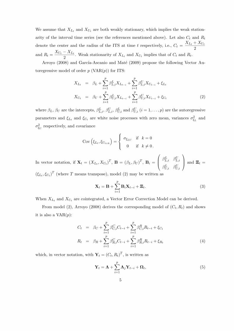
We assume that XLt and XUt are both weakly stationary, which implies the weak station-
arity of the interval time series (see the references mentioned above). Let also Ct and Rt
denote the center and the radius of the ITS at time t respectively, i.e., Ct =XLt +XUt
2
and Rt =XUt −XLt
2. Weak stationarity of XLt and XUt implies that of Ct and Rt.
Arroyo (2008) and Garcıa-Ascanio and Mate (2009) propose the following Vector Au-
toregressive model of order p (VAR(p)) for ITS:
XLt = βL +p∑i=1
βLL,iXLt−i +p∑i=1
βUL,iXUt−i + ξLt
XUt = βU +p∑i=1
βLU,iXLt−i +p∑i=1
βUU,iXUt−i + ξUt (2)
where βL, βU are the intercepts, βLL,i, βUL,i, β
LU,i and βUU,i (i = 1, . . . , p) are the autoregressive
parameters and ξLt and ξUt are white noise processes with zero mean, variances σ2ξL and
σ2ξU respectively, and covariance
Cov(ξLt , ξUt+k
)=
σξLUif k = 0
0 if k 6= 0 .
In vector notation, if Xt = (XLt , XUt)T , B = (βL, βU )T , Bi =
βLL,i βUL,i
βLU,i βUU,i
and Ξt =
(ξLt , ξUt)T (where T means transpose), model (2) may be written as
Xt = B +p∑i=1
BiXt−i + Ξt. (3)
When XLt and XUt are cointegrated, a Vector Error Correction Model can be derived.
From model (2), Arroyo (2008) derives the corresponding model of (Ct, Rt) and shows
it is also a VAR(p):
Ct = βC +p∑i=1
βCC,iCt−i +p∑i=1
βRC,iRt−i + ξCt
Rt = βR +p∑i=1
βCR,iCt−i +p∑i=1
βRR,iRt−i + ξRt (4)
which, in vector notation, with Yt = (Ct, Rt)T , is written as
Yt = Λ +p∑i=1
ΛjYt−i + Ωt, (5)
5
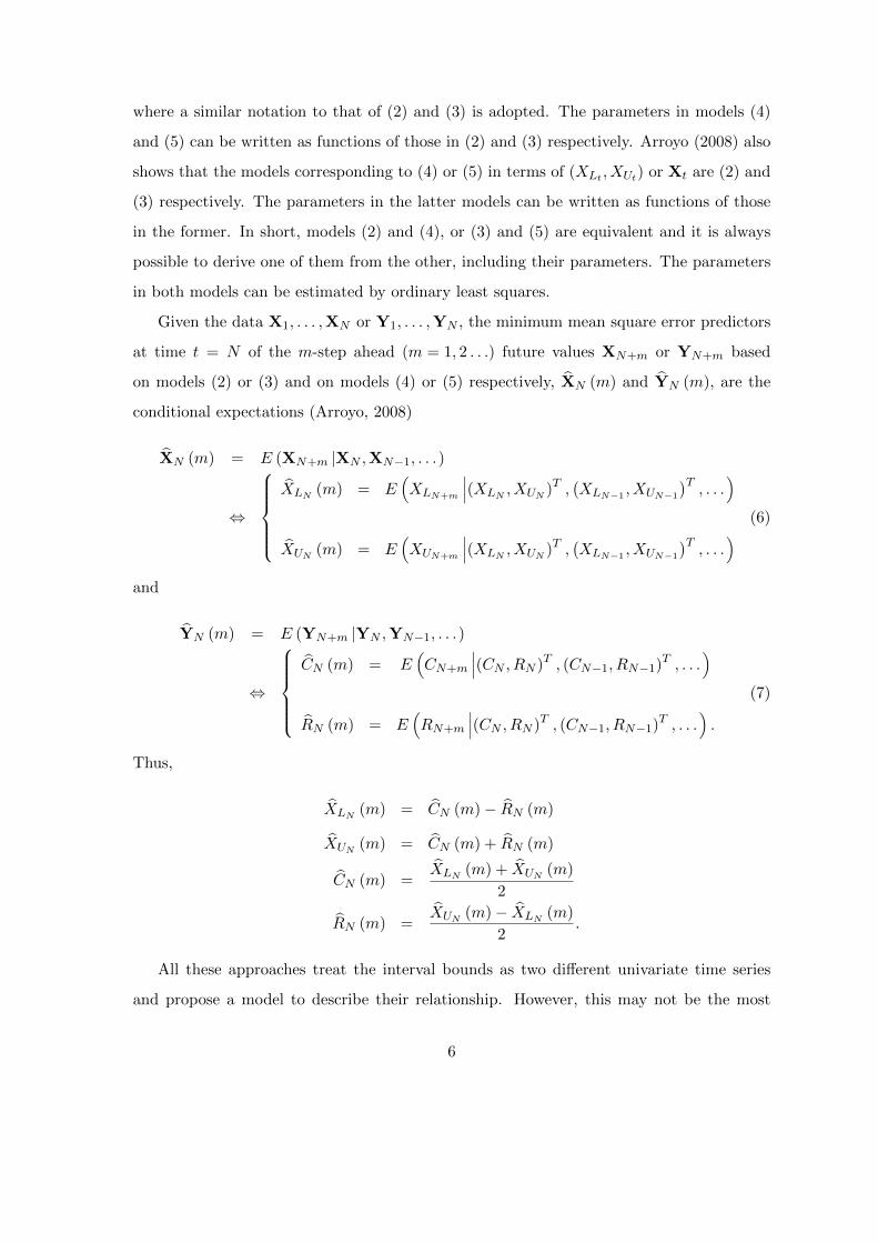
where a similar notation to that of (2) and (3) is adopted. The parameters in models (4)
and (5) can be written as functions of those in (2) and (3) respectively. Arroyo (2008) also
shows that the models corresponding to (4) or (5) in terms of (XLt , XUt) or Xt are (2) and
(3) respectively. The parameters in the latter models can be written as functions of those
in the former. In short, models (2) and (4), or (3) and (5) are equivalent and it is always
possible to derive one of them from the other, including their parameters. The parameters
in both models can be estimated by ordinary least squares.
Given the data X1, . . . ,XN or Y1, . . . ,YN , the minimum mean square error predictors
at time t = N of the m-step ahead (m = 1, 2 . . .) future values XN+m or YN+m based
on models (2) or (3) and on models (4) or (5) respectively, XN (m) and YN (m), are the
conditional expectations (Arroyo, 2008)
XN (m) = E (XN+m |XN ,XN−1, . . .)
⇔
XLN
(m) = E(XLN+m
∣∣∣(XLN, XUN
)T ,(XLN−1
, XUN−1
)T, . . .
)
XUN(m) = E
(XUN+m
∣∣∣(XLN, XUN
)T ,(XLN−1
, XUN−1
)T, . . .
) (6)
and
YN (m) = E (YN+m |YN ,YN−1, . . .)
⇔
CN (m) = E
(CN+m
∣∣∣(CN , RN )T , (CN−1, RN−1)T , . . .
)
RN (m) = E(RN+m
∣∣∣(CN , RN )T , (CN−1, RN−1)T , . . .
).
(7)
Thus,
XLN(m) = CN (m)− RN (m)
XUN(m) = CN (m) + RN (m)
CN (m) =XLN
(m) + XUN(m)
2
RN (m) =XUN
(m)− XLN(m)
2.
All these approaches treat the interval bounds as two different univariate time series
and propose a model to describe their relationship. However, this may not be the most
6
appropriate since interval data result from observations of the same variable made at differ-
ent points. Therefore, an approach that takes this important feature of interval time series
data into account is required.
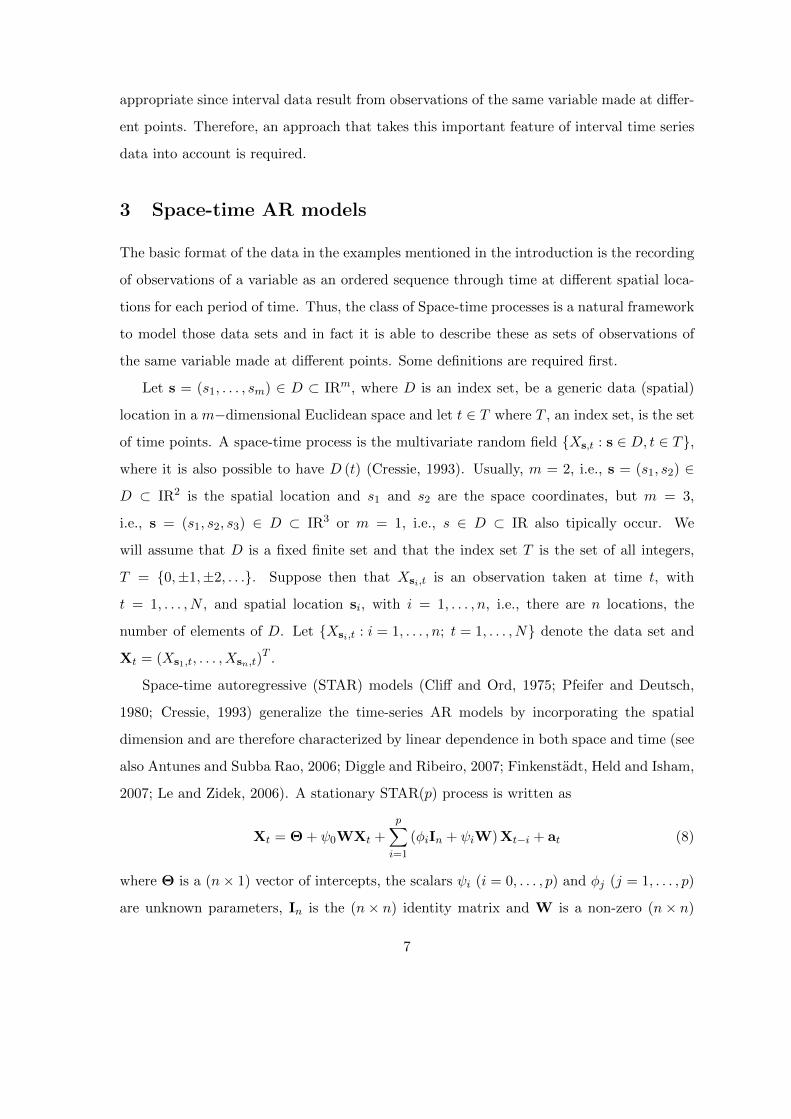
3 Space-time AR models
The basic format of the data in the examples mentioned in the introduction is the recording
of observations of a variable as an ordered sequence through time at different spatial loca-
tions for each period of time. Thus, the class of Space-time processes is a natural framework
to model those data sets and in fact it is able to describe these as sets of observations of
the same variable made at different points. Some definitions are required first.
Let s = (s1, . . . , sm) ∈ D ⊂ IRm, where D is an index set, be a generic data (spatial)
location in a m−dimensional Euclidean space and let t ∈ T where T , an index set, is the set
of time points. A space-time process is the multivariate random field Xs,t : s ∈ D, t ∈ T,
where it is also possible to have D (t) (Cressie, 1993). Usually, m = 2, i.e., s = (s1, s2) ∈
D ⊂ IR2 is the spatial location and s1 and s2 are the space coordinates, but m = 3,
i.e., s = (s1, s2, s3) ∈ D ⊂ IR3 or m = 1, i.e., s ∈ D ⊂ IR also tipically occur. We
will assume that D is a fixed finite set and that the index set T is the set of all integers,
T = 0,±1,±2, . . .. Suppose then that Xsi,t is an observation taken at time t, with
t = 1, . . . , N , and spatial location si, with i = 1, . . . , n, i.e., there are n locations, the
number of elements of D. Let Xsi,t : i = 1, . . . , n; t = 1, . . . , N denote the data set and
Xt = (Xs1,t, . . . , Xsn,t)T .
Space-time autoregressive (STAR) models (Cliff and Ord, 1975; Pfeifer and Deutsch,
1980; Cressie, 1993) generalize the time-series AR models by incorporating the spatial
dimension and are therefore characterized by linear dependence in both space and time (see
also Antunes and Subba Rao, 2006; Diggle and Ribeiro, 2007; Finkenstadt, Held and Isham,
2007; Le and Zidek, 2006). A stationary STAR(p) process is written as
Xt = Θ + ψ0WXt +p∑i=1
(φiIn + ψiW) Xt−i + at (8)
where Θ is a (n× 1) vector of intercepts, the scalars ψi (i = 0, . . . , p) and φj (j = 1, . . . , p)
are unknown parameters, In is the (n× n) identity matrix and W is a non-zero (n× n)
7
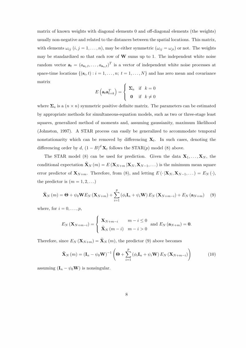
matrix of known weights with diagonal elements 0 and off-diagonal elements (the weights)
usually non-negative and related to the distances between the spatial locations. This matrix,
with elements ωij (i, j = 1, . . . , n), may be either symmetric (ωij = ωji) or not. The weights
may be standardized so that each row of W sums up to 1. The independent white noise
random vector at = (as1,t, . . . , asn,t)T is a vector of independent white noise processes at
space-time locations (si, t) : i = 1, . . . , n; t = 1, . . . , N and has zero mean and covariance
matrix
E(ata
Tt+k
)=
Σa if k = 0
0 if k 6= 0
where Σa is a (n× n) symmetric positive definite matrix. The parameters can be estimated
by appropriate methods for simultaneous-equation models, such as two or three-stage least
squares, generalized method of moments and, assuming gaussianity, maximum likelihood
(Johnston, 1997). A STAR process can easily be generalized to accommodate temporal
nonstationarity which can be removed by differencing Xt. In such cases, denoting the
differencing order by d, (1−B)d Xt follows the STAR(p) model (8) above.
The STAR model (8) can be used for prediction. Given the data X1, . . . ,XN , the
conditional expectation XN (m) = E (XN+m |XN ,XN−1, . . .) is the minimum mean square
error predictor of XN+m. Therefore, from (8), and letting E (· |XN ,XN−1, . . .) = EN (·),
the predictor is (m = 1, 2, . . .)
XN (m) = Θ + ψ0WEN (XN+m) +p∑i=1
(φiIn + ψiW)EN (XN+m−i) + EN (aN+m) (9)
where, for i = 0, . . . , p,
EN (XN+m−i) =
XN+m−i m− i ≤ 0
XN (m− i) m− i > 0and EN (aN+m) = 0.
Therefore, since EN (XN+m) = XN (m), the predictor (9) above becomes
XN (m) = (In − ψ0W)−1
(Θ +
p∑i=1
(φiIn + ψiW)EN (XN+m−i)
)(10)
assuming (In − ψ0W) is nonsingular.
8
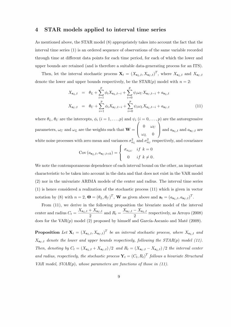
4 STAR models applied to interval time series
As mentioned above, the STAR model (8) appropriately takes into account the fact that the
interval time series (1) is an ordered sequence of observations of the same variable recorded
through time at different data points for each time period, for each of which the lower and
upper bounds are retained (and is therefore a suitable data-generating process for an ITS).
Then, let the interval stochastic process Xt = (XsL,t, XsU ,t)T , where XsL,t and XsU ,t
denote the lower and upper bounds respectively, be the STAR(p) model with n = 2:
XsL,t = θL +p∑i=1
φiXsL,t−i +p∑i=0
ψiωUXsU ,t−i + asL,t
XsU ,t = θU +p∑i=1
φiXsU ,t−i +p∑i=0
ψiωLXsL,t−i + asU ,t (11)
where θL, θU are the intercepts, φi (i = 1, . . . , p) and ψi (i = 0, . . . , p) are the autoregressive
parameters, ωU and ωL are the weights such that W =
0 ωU
ωL 0
and asL,t and asU ,t are
white noise processes with zero mean and variances σ2aL and σ2aU respectively, and covariance
Cov (asL,t, asU ,t+k) =
σaLU if k = 0
0 if k 6= 0 .
We note the contemporaneous dependence of each interval bound on the other, an important
characteristic to be taken into account in the data and that does not exist in the VAR model
(2) nor in the univariate ARIMA models of the center and radius. The interval time series
(1) is hence considered a realization of the stochastic process (11) which is given in vector
notation by (8) with n = 2, Θ = (θL, θU )T , W as given above and at = (asL,t, asU ,t)T .
From (11), we derive in the following proposition the bivariate model of the interval
center and radius Ct =XsL,t +XsU ,t
2and Rt =
XsU ,t −XsL,t
2respectively, as Arroyo (2008)
does for the VAR(p) model (2) proposed by himself and Garcıa-Ascanio and Mate (2009).
Proposition Let Xt = (XsL,t, XsU ,t)T be an interval stochastic process, where XsL,t and
XsU ,t denote the lower and upper bounds respectively, following the STAR(p) model (11).
Then, denoting by Ct = (XsL,t +XsU ,t) /2 and Rt = (XsU ,t −XsL,t) /2 the interval center
and radius, respectively, the stochastic process Yt = (Ct, Rt)T follows a bivariate Structural
VAR model, SVAR(p), whose parameters are functions of those in (11).
9
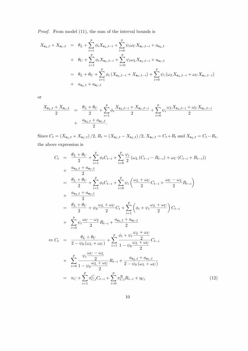
Proof. From model (11), the sum of the interval bounds is
XsL,t +XsU ,t = θL +p∑i=1
φiXsL,t−i +p∑i=0
ψiωUXsU ,t−i + asL,t
+ θU +p∑i=1
φiXsU ,t−i +p∑i=0
ψiωLXsL,t−i + asU ,t
= θL + θU +p∑i=1
φi (XsL,t−i +XsU ,t−i) +p∑i=0
ψi (ωLXsL,t−i + ωUXsU ,t−i)
+ asL,t + asU ,t
or
XsL,t +XsU ,t
2=
θL + θU2
+p∑i=1
φiXsL,t−i +XsU ,t−i
2+
p∑i=0
ψiωLXsL,t−i + ωUXsU ,t−i
2
+asL,t + asU ,t
2.
Since Ct = (XsL,t +XsU ,t) /2, Rt = (XsU ,t −XsL,t) /2, XsU ,t = Ct+Rt and XsL,t = Ct−Rt,
the above expression is
Ct =θL + θU
2+
p∑i=1
φiCt−i +p∑i=0
ψi2
(ωL (Ct−i −Rt−i) + ωU (Ct−i +Rt−i))
+asL,t + asU ,t
2
=θL + θU
2+
p∑i=1
φiCt−i +p∑i=0
ψi
(ωL + ωU
2Ct−i +
ωU − ωL2
Rt−i
)+
asL,t + asU ,t2
=θL + θU
2+ ψ0
ωL + ωU2
Ct +p∑i=1
(φi + ψi
ωL + ωU2
)Ct−i
+p∑i=0
ψiωU − ωL
2Rt−i +
asL,t + asU ,t2
⇔ Ct =θL + θU
2− ψ0 (ωL + ωU )+
p∑i=1
φi + ψiωL + ωU
2
1− ψ0ωL + ωU
2
Ct−i
+p∑i=0
ψiωU − ωL
2
1− ψ0ωL + ωU
2
Rt−i +asL,t + asU ,t
2− ψ0 (ωL + ωU )
= πC +p∑i=1
πCC,iCt−i +p∑i=0
πRC,iRt−i + ηCt (12)
10

where, assuming ψ0 6= 2 /(ωL + ωU ) ,
πC =θL + θU
2− ψ0 (ωL + ωU ); πCC,i =
φi + ψiωL + ωU
2
1− ψ0ωL + ωU
2
i = 1, . . . , p ;
πRC,i =ψiωU − ωL
2
1− ψ0ωL + ωU
2
i = 0, . . . , p ; ηCt =asL,t + asU ,t
2− ψ0 (ωL + ωU )(13)
and ηCt is an independent white noise process with mean and variance
E (ηCt) = E
(asL,t + asU ,t
2− ψ0 (ωL + ωU )
)= 0
V (ηCt) = σ2ηC = V
(asL,t + asU ,t
2− ψ0 (ωL + ωU )
)=
σ2aL + σ2aU + 2σaLU
(2− ψ0 (ωL + ωU ))2. (14)
Similarly, from (11), the interval range is
XsU ,t −XsL,t = θU +p∑i=1
φiXsU ,t−i +p∑i=0
ψiωLXsL,t−i + asU ,t
−(θL +
p∑i=1
φiXsL,t−i +p∑i=0
ψiωUXsU ,t−i + asL,t
)
= θU − θL +p∑i=1
φi (XsU ,t−i −XsL,t−i) +p∑i=0
ψi (ωLXsL,t−i − ωUXsU ,t−i)
+ asU ,t − asL,t
or
XsU ,t −XsL,t
2=
θU − θL2
+p∑i=1
φiXsU ,t−i −XsL,t−i
2+
p∑i=0
ψiωLXsL,t−i − ωUXsU ,t−i
2
+asU ,t − asU ,t
2.
Therefore, this expression may be written as
Rt =θU − θL
2+
p∑i=1
φiRt−i +p∑i=0
ψi2
(ωL (Ct−i −Rt−i)− ωU (Ct−i +Rt−i))
+asU ,t − asL,t
2
=θU − θL
2+
p∑i=1
φiRt−i −p∑i=0
ψi
(ωU − ωL
2Ct−i +
ωL + ωU2
Rt−i
)+
asU ,t − asL,t2
11
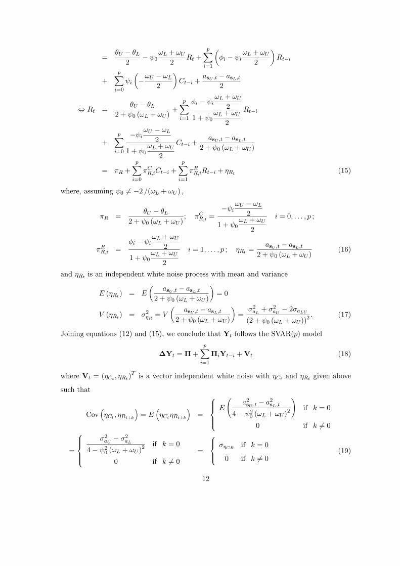
=θU − θL
2− ψ0
ωL + ωU2
Rt +p∑i=1
(φi − ψi
ωL + ωU2
)Rt−i
+p∑i=0
ψi
(−ωU − ωL
2
)Ct−i +
asU ,t − asL,t2
⇔ Rt =θU − θL
2 + ψ0 (ωL + ωU )+
p∑i=1
φi − ψiωL + ωU
2
1 + ψ0ωL + ωU
2
Rt−i
+p∑i=0
−ψiωU − ωL
2
1 + ψ0ωL + ωU
2
Ct−i +asU ,t − asL,t
2 + ψ0 (ωL + ωU )
= πR +p∑i=0
πCR,iCt−i +p∑i=1
πRR,iRt−i + ηRt (15)
where, assuming ψ0 6= −2 /(ωL + ωU ) ,
πR =θU − θL
2 + ψ0 (ωL + ωU ); πCR,i =
−ψiωU − ωL
2
1 + ψ0ωL + ωU
2
i = 0, . . . , p ;
πRR,i =φi − ψi
ωL + ωU2
1 + ψ0ωL + ωU
2
i = 1, . . . , p ; ηRt =asU ,t − asL,t
2 + ψ0 (ωL + ωU )(16)
and ηRt is an independent white noise process with mean and variance
E (ηRt) = E
(asU ,t − asL,t
2 + ψ0 (ωL + ωU )
)= 0
V (ηRt) = σ2ηR = V
(asU ,t − asL,t
2 + ψ0 (ωL + ωU )
)=
σ2aL + σ2aU − 2σaLU
(2 + ψ0 (ωL + ωU ))2. (17)
Joining equations (12) and (15), we conclude that Yt follows the SVAR(p) model
∆Yt = Π +p∑i=1
ΠiYt−i + Vt (18)
where Vt = (ηCt , ηRt)T is a vector independent white noise with ηCt and ηRt given above
such that
Cov(ηCt , ηRt+k
)= E
(ηCtηRt+k
)=
E
(a2sU ,t − a
2sL,t
4− ψ20 (ωL + ωU )2
)if k = 0
0 if k 6= 0
=
σ2aU − σ
2aL
4− ψ20 (ωL + ωU )2
if k = 0
0 if k 6= 0
=
σηCR if k = 0
0 if k 6= 0(19)
12
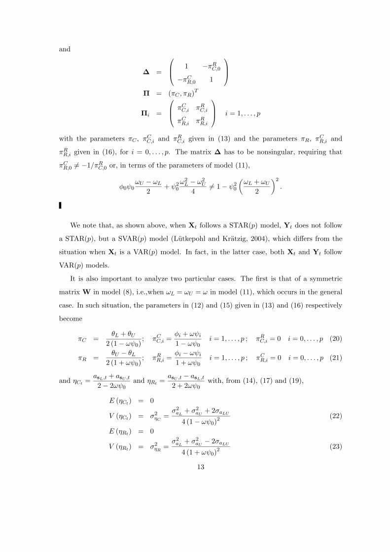
and
∆ =
1 −πRC,0−πCR,0 1
Π = (πC , πR)T
Πi =
πCC,i πRC,i
πCR,i πRR,i
i = 1, . . . , p
with the parameters πC , πCC,i and πRC,i given in (13) and the parameters πR, πCR,i and
πRR,i given in (16), for i = 0, . . . , p. The matrix ∆ has to be nonsingular, requiring that
πCR,0 6= −1/πRC,0 or, in terms of the parameters of model (11),
φ0ψ0ωU − ωL
2+ ψ2
0
ω2L − ω2
U
46= 1− ψ2
0
(ωL + ωU
2
)2
.
We note that, as shown above, when Xt follows a STAR(p) model, Yt does not follow
a STAR(p), but a SVAR(p) model (Lutkepohl and Kratzig, 2004), which differs from the
situation when Xt is a VAR(p) model. In fact, in the latter case, both Xt and Yt follow
VAR(p) models.
It is also important to analyze two particular cases. The first is that of a symmetric
matrix W in model (8), i.e.,when ωL = ωU = ω in model (11), which occurs in the general
case. In such situation, the parameters in (12) and (15) given in (13) and (16) respectively
become
πC =θL + θU
2 (1− ωψ0); πCC,i =
φi + ωψi1− ωψ0
i = 1, . . . , p ; πRC,i = 0 i = 0, . . . , p (20)
πR =θU − θL
2 (1 + ωψ0); πRR,i =
φi − ωψi1 + ωψ0
i = 1, . . . , p ; πCR,i = 0 i = 0, . . . , p (21)
and ηCt =asL,t + asU ,t
2− 2ωψ0and ηRt =
asU ,t − asL,t2 + 2ωψ0
with, from (14), (17) and (19),
E (ηCt) = 0
V (ηCt) = σ2ηC =σ2aL + σ2aU + 2σaLU
4 (1− ωψ0)2 (22)
E (ηRt) = 0
V (ηRt) = σ2ηR =σ2aL + σ2aU − 2σaLU
4 (1 + ωψ0)2 (23)
13
Cov(ηCt , ηRt+k
)=
σηCR if k = 0
0 if k 6= 0=
σ2aU − σ
2aL
4(1− ω2ψ2
0
) if k = 0
0 if k 6= 0
(24)
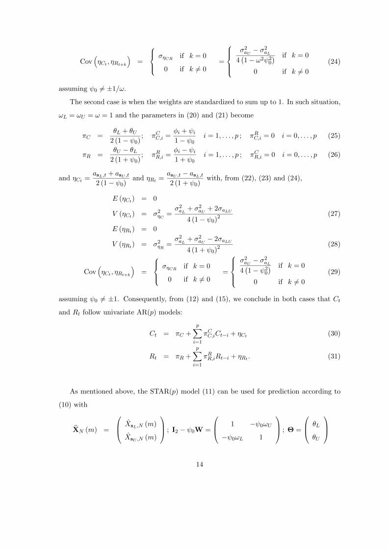
assuming ψ0 6= ±1/ω.
The second case is when the weights are standardized to sum up to 1. In such situation,
ωL = ωU = ω = 1 and the parameters in (20) and (21) become
πC =θL + θU
2 (1− ψ0); πCC,i =
φi + ψi1− ψ0
i = 1, . . . , p ; πRC,i = 0 i = 0, . . . , p (25)
πR =θU − θL
2 (1 + ψ0); πRR,i =
φi − ψi1 + ψ0
i = 1, . . . , p ; πCR,i = 0 i = 0, . . . , p (26)
and ηCt =asL,t + asU ,t2 (1− ψ0)
and ηRt =asU ,t − asL,t2 (1 + ψ0)
with, from (22), (23) and (24),
E (ηCt) = 0
V (ηCt) = σ2ηC =σ2aL + σ2aU + 2σaLU
4 (1− ψ0)2 (27)
E (ηRt) = 0
V (ηRt) = σ2ηR =σ2aL + σ2aU − 2σaLU
4 (1 + ψ0)2 (28)
Cov(ηCt , ηRt+k
)=
σηCR if k = 0
0 if k 6= 0=
σ2aU − σ
2aL
4(1− ψ2
0
) if k = 0
0 if k 6= 0
(29)
assuming ψ0 6= ±1. Consequently, from (12) and (15), we conclude in both cases that Ct
and Rt follow univariate AR(p) models:
Ct = πC +p∑i=1
πCC,iCt−i + ηCt (30)
Rt = πR +p∑i=1
πRR,iRt−i + ηRt . (31)
As mentioned above, the STAR(p) model (11) can be used for prediction according to
(10) with
XN (m) =
XsL,N (m)
XsU ,N (m)
; I2 − ψ0W =
1 −ψ0ωU
−ψ0ωL 1
; Θ =
θL
θU
14
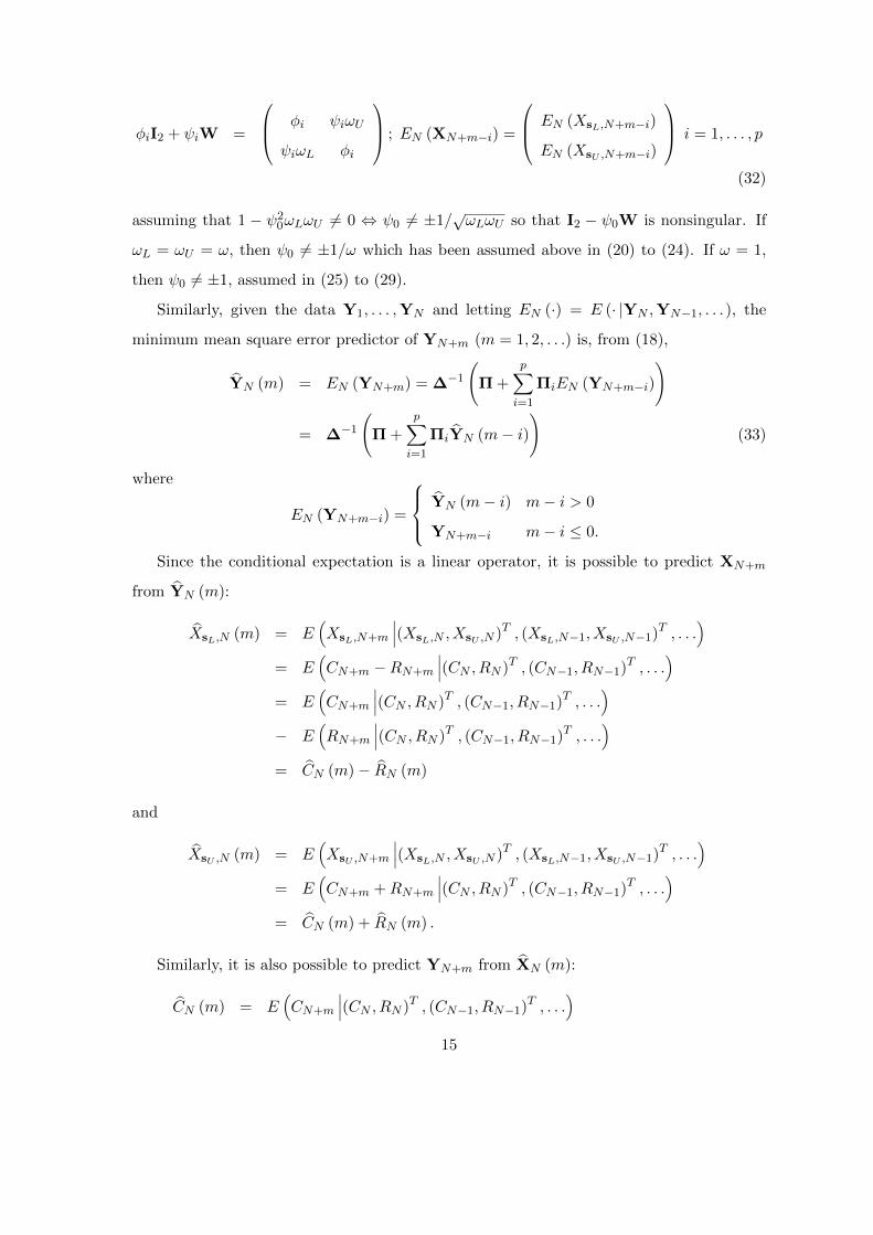
φiI2 + ψiW =
φi ψiωU
ψiωL φi
; EN (XN+m−i) =
EN (XsL,N+m−i)
EN (XsU ,N+m−i)
i = 1, . . . , p
(32)
assuming that 1 − ψ20ωLωU 6= 0 ⇔ ψ0 6= ±1/
√ωLωU so that I2 − ψ0W is nonsingular. If
ωL = ωU = ω, then ψ0 6= ±1/ω which has been assumed above in (20) to (24). If ω = 1,
then ψ0 6= ±1, assumed in (25) to (29).
Similarly, given the data Y1, . . . ,YN and letting EN (·) = E (· |YN ,YN−1, . . .), the
minimum mean square error predictor of YN+m (m = 1, 2, . . .) is, from (18),
YN (m) = EN (YN+m) = ∆−1
(Π +
p∑i=1
ΠiEN (YN+m−i)
)
= ∆−1
(Π +
p∑i=1
ΠiYN (m− i))
(33)
where
EN (YN+m−i) =
YN (m− i) m− i > 0
YN+m−i m− i ≤ 0.
Since the conditional expectation is a linear operator, it is possible to predict XN+m
from YN (m):
XsL,N (m) = E(XsL,N+m
∣∣∣(XsL,N , XsU ,N )T , (XsL,N−1, XsU ,N−1)T , . . .
)= E
(CN+m −RN+m
∣∣∣(CN , RN )T , (CN−1, RN−1)T , . . .
)= E
(CN+m
∣∣∣(CN , RN )T , (CN−1, RN−1)T , . . .
)− E
(RN+m
∣∣∣(CN , RN )T , (CN−1, RN−1)T , . . .
)= CN (m)− RN (m)
and
XsU ,N (m) = E(XsU ,N+m
∣∣∣(XsL,N , XsU ,N )T , (XsL,N−1, XsU ,N−1)T , . . .
)= E
(CN+m +RN+m
∣∣∣(CN , RN )T , (CN−1, RN−1)T , . . .
)= CN (m) + RN (m) .
Similarly, it is also possible to predict YN+m from XN (m):
CN (m) = E(CN+m
∣∣∣(CN , RN )T , (CN−1, RN−1)T , . . .
)15
= E
(XsL,N +XsU ,N
2
∣∣∣∣∣(XsL,N , XsU ,N )T , (XsL,N−1, XsU ,N−1)T , . . .
)
=1
2
[E(XsL,N+m
∣∣∣(XsL,N , XsU ,N )T , (XsL,N−1, XsU ,N−1)T , . . .
)+ E
(XsU ,N+m
∣∣∣(XsL,N , XsU ,N )T , (XsL,N−1, XsU ,N−1)T , . . .
)]=
XsL,N (m) + XsU ,N (m)
2
and
RN (m) = E(RN+m
∣∣∣(CN , RN )T , (CN−1, RN−1)T , . . .
)= E
(XsU ,N −XsL,N
2
∣∣∣∣∣(XsU ,N , XsL,N )T , (XsL,N−1, XsU ,N−1)T , . . .
)
=XsU ,N (m)− XsL,N (m)
2.
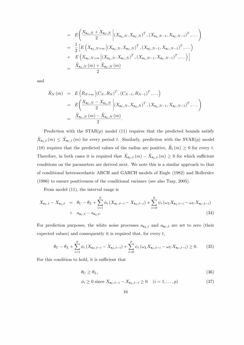
Prediction with the STAR(p) model (11) requires that the predicted bounds satisfy
XsL,t (m) ≤ XsU ,t (m) for every period t. Similarly, prediction with the SVAR(p) model
(18) requires that the predicted values of the radius are positive, Rt (m) ≥ 0 for every t.
Therefore, in both cases it is required that XsU ,t (m) − XsL,t (m) ≥ 0 for which sufficient
conditions on the parameters are derived next. We note this is a similar approach to that
of conditional heteroscedastic ARCH and GARCH models of Engle (1982) and Bollerslev
(1986) to ensure positiveness of the conditional variance (see also Tsay, 2005).
From model (11), the interval range is
XsU ,t −XsL,t = θU − θL +p∑i=1
φi (XsU ,t−i −XsL,t−i) +p∑i=0
ψi (ωLXsL,t−i − ωUXsU ,t−i)
+ asU ,t − asL,t. (34)
For prediction purposes, the white noise processes asL,t and asU ,t are set to zero (their
expected values) and consequently it is required that, for every t,
θU − θL +p∑i=1
φi (XsU ,t−i −XsL,t−i) +p∑i=0
ψi (ωLXsL,t−i − ωUXsU ,t−i) ≥ 0. (35)
For this condition to hold, it is sufficient that
θU ≥ θL, (36)
φi ≥ 0 since XsU ,t−i −XsL,t−i ≥ 0 (i = 1, . . . , p) (37)
16
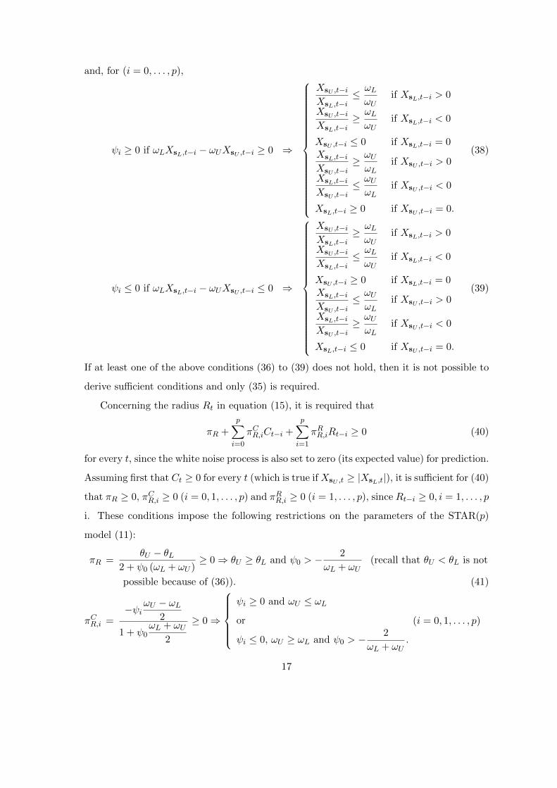
and, for (i = 0, . . . , p),
ψi ≥ 0 if ωLXsL,t−i − ωUXsU ,t−i ≥ 0 ⇒
XsU ,t−iXsL,t−i
≤ ωLωU
if XsL,t−i > 0
XsU ,t−iXsL,t−i
≥ ωLωU
if XsL,t−i < 0
XsU ,t−i ≤ 0 if XsL,t−i = 0XsL,t−iXsU ,t−i
≥ ωUωL
if XsU ,t−i > 0
XsL,t−iXsU ,t−i
≤ ωUωL
if XsU ,t−i < 0
XsL,t−i ≥ 0 if XsU ,t−i = 0.
(38)
ψi ≤ 0 if ωLXsL,t−i − ωUXsU ,t−i ≤ 0 ⇒
XsU ,t−iXsL,t−i
≥ ωLωU
if XsL,t−i > 0
XsU ,t−iXsL,t−i
≤ ωLωU
if XsL,t−i < 0
XsU ,t−i ≥ 0 if XsL,t−i = 0XsL,t−iXsU ,t−i
≤ ωUωL
if XsU ,t−i > 0
XsL,t−iXsU ,t−i
≥ ωUωL
if XsU ,t−i < 0
XsL,t−i ≤ 0 if XsU ,t−i = 0.
(39)
If at least one of the above conditions (36) to (39) does not hold, then it is not possible to
derive sufficient conditions and only (35) is required.
Concerning the radius Rt in equation (15), it is required that
πR +p∑i=0
πCR,iCt−i +p∑i=1
πRR,iRt−i ≥ 0 (40)
for every t, since the white noise process is also set to zero (its expected value) for prediction.
Assuming first that Ct ≥ 0 for every t (which is true if XsU ,t ≥ |XsL,t|), it is sufficient for (40)
that πR ≥ 0, πCR,i ≥ 0 (i = 0, 1, . . . , p) and πRR,i ≥ 0 (i = 1, . . . , p), since Rt−i ≥ 0, i = 1, . . . , p
i. These conditions impose the following restrictions on the parameters of the STAR(p)
model (11):
πR =θU − θL
2 + ψ0 (ωL + ωU )≥ 0⇒ θU ≥ θL and ψ0 > −
2
ωL + ωU(recall that θU < θL is not
possible because of (36)). (41)
πCR,i =−ψi
ωU − ωL2
1 + ψ0ωL + ωU
2
≥ 0⇒
ψi ≥ 0 and ωU ≤ ωL
or
ψi ≤ 0, ωU ≥ ωL and ψ0 > −2
ωL + ωU.
(i = 0, 1, . . . , p)
17
(42)
Note that ψi ≤ 0, ωU ≤ ωL and ψ0 < −2
ωL + ωUis not valid because, although it
satisfies πCR,i ≥ 0, the condition on ψ0 violates (41).
πRR,i =φi − ψi
ωL + ωU2
1 + ψ0ωL + ωU
2
≥ 0⇒ φi ≥ ψiωL + ωU
2and ψ0 > −
2
ωL + ωU(i = 1, . . . , p) .
Note that φi ≤ ψiωL + ωU
2and ψ0 < −
2
ωL + ωUis not valid because, although it
satisfies πRR,i ≥ 0, the condition on ψ0 violates (41).
Assuming now that Ct ≤ 0 for every t (which is true if XsU ,t ≤ |XsL,t|), it is sufficient for
(40) that πR ≥ 0, πCR,i ≤ 0 (i = 0, 1, . . . , p) and πRR,i ≥ 0 (i = 1, . . . , p). The conditions on
πR and πRR,i are the same as above and thus lead again to (41) and (43) respectively, the
new restrictions on the parameters of the STAR(p) model (11) are as follows:
πCR,i =−ψi
ωU − ωL2
1 + ψ0ωL + ωU
2
≤ 0⇒
ψi ≤ 0, ωU ≤ ωL and ψ0 > −
2
ωL + ωU
or
ψi ≥ 0 and ωU ≥ ωL.
(i = 0, 1, . . . , p)
(43)
Note that ψi ≤ 0, ωU ≥ ωL and ψ0 < −2
ωL + ωUis not valid because, although it
satisfies πCR,i ≥ 0, the condition on ψ0 violates (41).
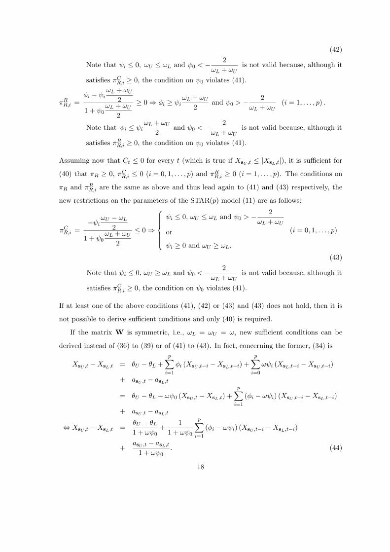
If at least one of the above conditions (41), (42) or (43) and (43) does not hold, then it is
not possible to derive sufficient conditions and only (40) is required.
If the matrix W is symmetric, i.e., ωL = ωU = ω, new sufficient conditions can be
derived instead of (36) to (39) or of (41) to (43). In fact, concerning the former, (34) is
XsU ,t −XsL,t = θU − θL +p∑i=1
φi (XsU ,t−i −XsL,t−i) +p∑i=0
ωψi (XsL,t−i −XsU ,t−i)
+ asU ,t − asL,t
= θU − θL − ωψ0 (XsU ,t −XsL,t) +p∑i=1
(φi − ωψi) (XsU ,t−i −XsL,t−i)
+ asU ,t − asL,t
⇔ XsU ,t −XsL,t =θU − θL1 + ωψ0
+1
1 + ωψ0
p∑i=1
(φi − ωψi) (XsU ,t−i −XsL,t−i)
+asU ,t − asL,t
1 + ωψ0. (44)
18
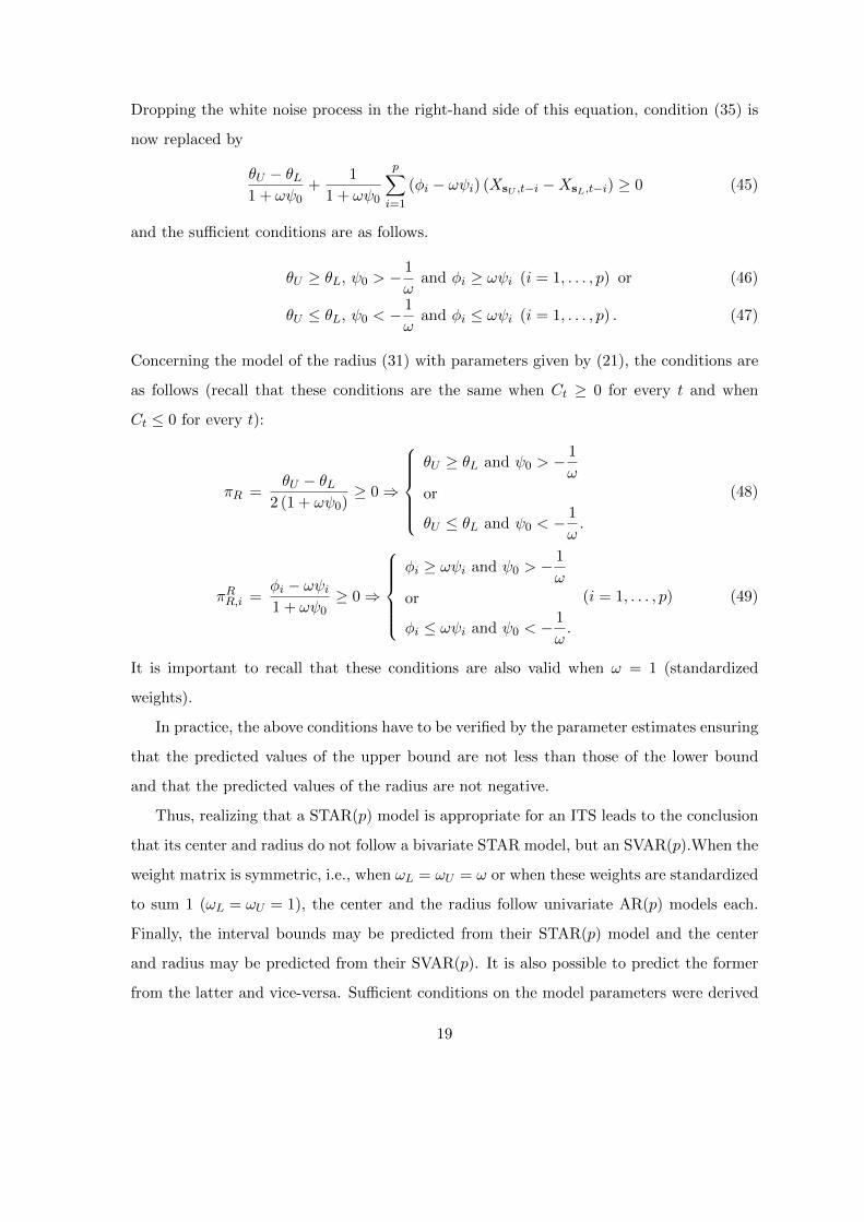
Dropping the white noise process in the right-hand side of this equation, condition (35) is
now replaced by
θU − θL1 + ωψ0
+1
1 + ωψ0
p∑i=1
(φi − ωψi) (XsU ,t−i −XsL,t−i) ≥ 0 (45)
and the sufficient conditions are as follows.
θU ≥ θL, ψ0 > −1
ωand φi ≥ ωψi (i = 1, . . . , p) or (46)
θU ≤ θL, ψ0 < −1
ωand φi ≤ ωψi (i = 1, . . . , p) . (47)
Concerning the model of the radius (31) with parameters given by (21), the conditions are
as follows (recall that these conditions are the same when Ct ≥ 0 for every t and when
Ct ≤ 0 for every t):
πR =θU − θL
2 (1 + ωψ0)≥ 0⇒
θU ≥ θL and ψ0 > −
1
ω
or
θU ≤ θL and ψ0 < −1
ω.
(48)
πRR,i =φi − ωψi1 + ωψ0
≥ 0⇒
φi ≥ ωψi and ψ0 > −
1
ω
or
φi ≤ ωψi and ψ0 < −1
ω.
(i = 1, . . . , p) (49)
It is important to recall that these conditions are also valid when ω = 1 (standardized
weights).
In practice, the above conditions have to be verified by the parameter estimates ensuring
that the predicted values of the upper bound are not less than those of the lower bound
and that the predicted values of the radius are not negative.
Thus, realizing that a STAR(p) model is appropriate for an ITS leads to the conclusion
that its center and radius do not follow a bivariate STAR model, but an SVAR(p).When the
weight matrix is symmetric, i.e., when ωL = ωU = ω or when these weights are standardized
to sum 1 (ωL = ωU = 1), the center and the radius follow univariate AR(p) models each.
Finally, the interval bounds may be predicted from their STAR(p) model and the center
and radius may be predicted from their SVAR(p). It is also possible to predict the former
from the latter and vice-versa. Sufficient conditions on the model parameters were derived
19
in order to ensure that the upper bound predicted value is not smaller than that of the
lower bound, or, equivalently, that the predicted value of the radius is not negative.
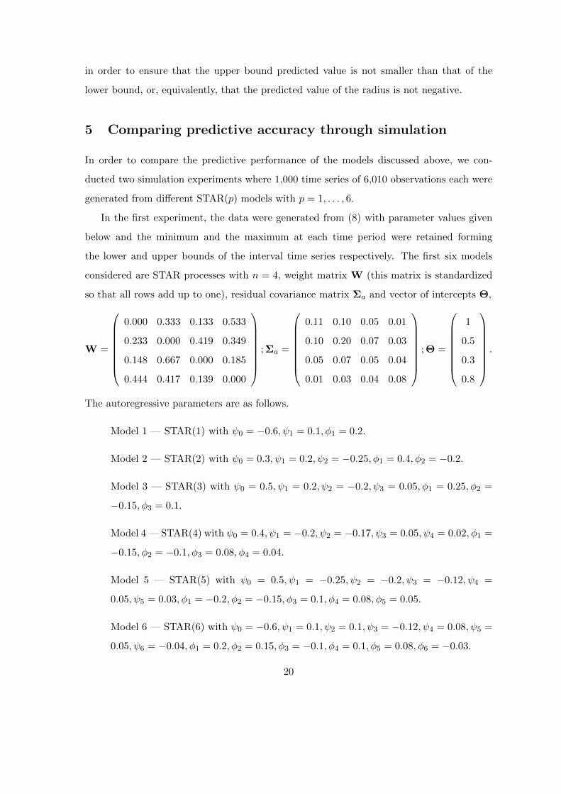
5 Comparing predictive accuracy through simulation
In order to compare the predictive performance of the models discussed above, we con-
ducted two simulation experiments where 1,000 time series of 6,010 observations each were
generated from different STAR(p) models with p = 1, . . . , 6.
In the first experiment, the data were generated from (8) with parameter values given
below and the minimum and the maximum at each time period were retained forming
the lower and upper bounds of the interval time series respectively. The first six models
considered are STAR processes with n = 4, weight matrix W (this matrix is standardized
so that all rows add up to one), residual covariance matrix Σa and vector of intercepts Θ,
W =
0.000 0.333 0.133 0.533
0.233 0.000 0.419 0.349
0.148 0.667 0.000 0.185
0.444 0.417 0.139 0.000
; Σa =
0.11 0.10 0.05 0.01
0.10 0.20 0.07 0.03
0.05 0.07 0.05 0.04
0.01 0.03 0.04 0.08
; Θ =
1
0.5
0.3
0.8
.
The autoregressive parameters are as follows.
Model 1 — STAR(1) with ψ0 = −0.6, ψ1 = 0.1, φ1 = 0.2.
Model 2 — STAR(2) with ψ0 = 0.3, ψ1 = 0.2, ψ2 = −0.25, φ1 = 0.4, φ2 = −0.2.
Model 3 — STAR(3) with ψ0 = 0.5, ψ1 = 0.2, ψ2 = −0.2, ψ3 = 0.05, φ1 = 0.25, φ2 =
−0.15, φ3 = 0.1.
Model 4 — STAR(4) with ψ0 = 0.4, ψ1 = −0.2, ψ2 = −0.17, ψ3 = 0.05, ψ4 = 0.02, φ1 =
−0.15, φ2 = −0.1, φ3 = 0.08, φ4 = 0.04.
Model 5 — STAR(5) with ψ0 = 0.5, ψ1 = −0.25, ψ2 = −0.2, ψ3 = −0.12, ψ4 =
0.05, ψ5 = 0.03, φ1 = −0.2, φ2 = −0.15, φ3 = 0.1, φ4 = 0.08, φ5 = 0.05.
Model 6 — STAR(6) with ψ0 = −0.6, ψ1 = 0.1, ψ2 = 0.1, ψ3 = −0.12, ψ4 = 0.08, ψ5 =
0.05, ψ6 = −0.04, φ1 = 0.2, φ2 = 0.15, φ3 = −0.1, φ4 = 0.1, φ5 = 0.08, φ6 = −0.03.
20
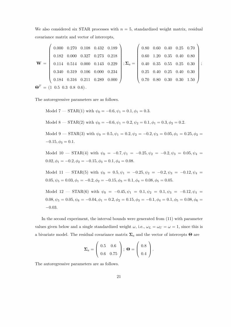
We also considered six STAR processes with n = 5, standardized weight matrix, residual
covariance matrix and vector of intercepts,
W =
0.000 0.270 0.108 0.432 0.189
0.182 0.000 0.327 0.273 0.218
0.114 0.514 0.000 0.143 0.229
0.340 0.319 0.106 0.000 0.234
0.184 0.316 0.211 0.289 0.000
; Σa =
0.80 0.60 0.40 0.25 0.70
0.60 1.20 0.35 0.40 0.80
0.40 0.35 0.55 0.25 0.30
0.25 0.40 0.25 0.40 0.30
0.70 0.80 0.30 0.30 1.50
;
ΘT = (1 0.5 0.3 0.8 0.6) .
The autoregressive parameters are as follows.
Model 7 — STAR(1) with ψ0 = −0.6, ψ1 = 0.1, φ1 = 0.3.
Model 8 — STAR(2) with ψ0 = −0.6, ψ1 = 0.2, ψ2 = 0.1, φ1 = 0.3, φ2 = 0.2.
Model 9 — STAR(3) with ψ0 = 0.5, ψ1 = 0.2, ψ2 = −0.2, ψ3 = 0.05, φ1 = 0.25, φ2 =
−0.15, φ3 = 0.1.
Model 10 — STAR(4) with ψ0 = −0.7, ψ1 = −0.25, ψ2 = −0.2, ψ3 = 0.05, ψ4 =
0.02, φ1 = −0.2, φ2 = −0.15, φ3 = 0.1, φ4 = 0.08.
Model 11 — STAR(5) with ψ0 = 0.5, ψ1 = −0.25, ψ2 = −0.2, ψ3 = −0.12, ψ4 =
0.05, ψ5 = 0.03, φ1 = −0.2, φ2 = −0.15, φ3 = 0.1, φ4 = 0.08, φ5 = 0.05.
Model 12 — STAR(6) with ψ0 = −0.45, ψ1 = 0.1, ψ2 = 0.1, ψ3 = −0.12, ψ4 =
0.08, ψ5 = 0.05, ψ6 = −0.04, φ1 = 0.2, φ2 = 0.15, φ3 = −0.1, φ4 = 0.1, φ5 = 0.08, φ6 =
−0.03.
In the second experiment, the interval bounds were generated from (11) with parameter
values given below and a single standardized weight ω, i.e., ωL = ωU = ω = 1, since this is
a bivariate model. The residual covariance matrix Σa and the vector of intercepts Θ are
Σa =
0.5 0.6
0.6 0.75
; Θ =
0.8
0.4
.The autoregressive parameters are as follows.
21
Model 13 — STAR(1) with ψ0 = 0.5, ψ1 = −0.3, φ1 = 0.6.
Model 14 — STAR(2) with ψ0 = −0.6, ψ1 = 0.5, ψ2 = 0.1, φ1 = 0.6, φ2 = 0.2.
Model 15 — STAR(3) with ψ0 = −0.6, ψ1 = 0.3, ψ2 = −0.25, ψ3 = 0.05, φ1 = 0.4, φ2 =
−0.2, φ3 = 0.1.
Model 16 — STAR(4) with ψ0 = −0.5, ψ1 = 0.2, ψ2 = 0.1, ψ3 = −0.1, ψ4 = −0.07,
φ1 = 0.25, φ2 = 0.2, φ3 = −0.1, φ4 = −0.05.
Model 17 — STAR(5) with ψ0 = −0.65, ψ1 = 0.25, ψ2 = 0.1, ψ3 = −0.1, ψ4 =
−0.08, ψ5 = 0.02, φ1 = 0.3, φ2 = 0.15, φ3 = 0.1, φ4 = −0.08, φ5 = 0.05.
Model 18 — STAR(6) with ψ0 = −0.45, ψ1 = 0.1, ψ2 = 0.1, ψ3 = −0.12, ψ4 =
0.08, ψ5 = 0.05, ψ6 = −0.04, φ1 = 0.2, φ2 = 0.15, φ3 = −0.1, φ4 = 0.1, φ5 = 0.08, φ6 =
−0.03.
In both experiments, the last 10 observations were left out from the data for an assess-
ment of the models’ out-of-sample predictive performance. For each time series, model (11)
was estimated by three-stage least squares (we considered a symmetric matrix W with a
single standardized weight ω, i.e., ωL = ωU = ω = 1, since this is a bivariate model) and
the VAR model (2) (Arroyo, 2008; Garcıa-Ascanio and Mate, 2009) and the univariate AR
models of the center and radius (Maia, De Carvalho and Ludemir, 2008) were estimated by
ordinary least squares or maximum likelihood.
The 10 out-of-sample observations of the interval time series were then predicted with
the fitted models (the predictions of the center and radius of the univariate AR approach
were used to compute those of the interval bounds). The accuracy of those predictions
was measured by the interval bounds’ Mean Absolute Error (MAE) and Root Mean Square
Error (RMSE) and by computing interval distance measures between the actual and the
predicted values (since the data have an interval form). To this purpose, different measures
are available in the literature and we will consider three interval distance measures: the
Hausdorff distance, the interval Euclidean distance and the interval City-Block distance.
Let Ii = [li, ui] and Ij = [lj , uj ] two intervals to be compared. The Hausdorff distance,
the interval Euclidean distance and the interval City-Block distance between Ii and Ij are
22
respectivelydH(Ii, Ij) = max |li − lj | , |ui − uj |
d2(Ii, Ij) =√
(li − lj)2 + (ui − uj)2
d1(Ii, Ij) = |li − lj |+ |ui − uj | .
The Hausdorff distance between two sets is the maximum distance of a set to the nearest
point in the other set, i.e., two sets are close in terms of the Hausdorff distance if every
point of either set is close to some point of the other set. Interval Euclidean and City-Block
distances are just the counterparts of the corresponding distances for real values; if we
embed the interval set in IR2, where one dimension is used for the lower and the other for
the upper bound of the intervals, then these distances are just the Euclidean and City-Block
distances between the corresponding points in the two-dimensional space.
Table 1 (in the Appendix) shows the values of the accuracy measures for the different
models considered in both experiments and for the three approaches, namely the STAR
model (11), the VAR model (2) and the univariate AR models of the center and radius,
denoted by STAR, VAR and AR respectively. The results show that none of the approaches
outperforms the others, since their predictive accuracy is always extremely close or even
coincident. It is also interesting to note that the predictive accuracy is better for models
with ψ0 < 0, i.e., when the interval bounds are contemporaneously related in the opposite
direction. Many other STAR models were tried as data-generating processes in the two
experiments with similar results.
6 Application
As a practical application, we consider the Irish wind data of Haslett and Raftery (1989),
available at Statlib (http://lib.stat.cmu.edu/datasets/), which consists of time series of daily
average wind speed at eleven synoptic metereological stations in Ireland in the period 1961-
1978. Detailed information on this dataset can be found in Haslett and Raftery (1989),
in Gneiting, Genton and Guttorp (2007) and in the references therein. From the eleven
stations, we selected five: Birr, Dublin, Kilkenny, Shannon and Valentia. The observations
for February 29 were removed for a better estimation of the seasonal trend component. The
year of 1978 was left out from the dataset for an out-of-sample evaluation of predictive
performance and therefore only the 1961-1977 data will be modeled. Following the authors
23
mentioned above, the square root transform was first applied to the time series of daily aver-
age wind speed stabilizing the variance over both stations and time periods and bringing the
marginal distributions closer to normality. The seasonal effect was estimated by calculating
the average of the square root of the daily means over all years and stations for each day of
the year and then regressing the results on a small set of annual harmonics. Subtraction of
the estimated seasonal effect from the square root of the daily means yields deseasonalized
data. The station-specific means were also removed and the result will be referred to as
the time series of velocity measures. The same transformations were applied to the year of
1978 with the seasonal trend component and the station-specific means estimated from the
1961-1977 period.
The minimum and the maximum of the daily velocity measures at the five selected
stations are respectively the lower and upper bounds of an interval time series to which the
bivariate STAR(p) model (11) was fitted. We consider a symmetric matrix W with a single
standardized weight ω, i.e., ωL = ωU = ω = 1, since this is a bivariate model. The order
of the model, i.e., the value of p, was determined by starting with a large value, estimating
the parameters, applying tests sequentially and decreasing that order until a suitable model
is found. We started with p = 8 and selected p = 6, since the estimated parameters for
both p = 7 and p = 8 were not statistically significant. Order selection criteria were also
used (Lutkepohl and Kratzig, 2004) such as the Akaike Information Criterion (AIC), the
Hannan-Quinn Criterion (HQC) and the Schwarz Criterion (SC) and they suggest p = 3,
but the model diagnostic checking showed a better fit with p = 6. Therefore, model (11)
with p = 6 was estimated by three-stage least squares and the results are given in table 2.
Model diagnostic checking shows a satisfactory fit. The estimated parameters up to
lag 3 are significant and, although φ4, φ5, ψ4 and ψ5 are not, we decided to keep p = 6
because φ6 and ψ6 are clearly significant (5% significance level). Moreover, as mentioned
above, model selection criteria such as AIC, HQC and SC suggest p = 3 (because of the
lack of significance of the parameters at lags 4 and 5) but, even though this would still be
acceptable, p = 6 shows a much better fit. In fact, the residuals of both equations asL,t
and asU ,t are approximately white noise, since their plots show no clear defficiencies and
their correlograms show very few significant autocorrelations that do not give rise to concern
because they occur only occasionally and at very high lags. The p-values of the portmanteau
24
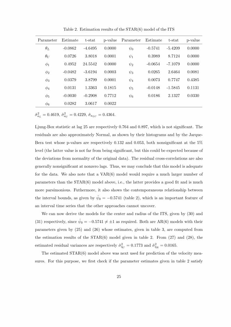
Table 2. Estimation results of the STAR(6) model of the ITS
Parameter Estimate t-stat p-value Parameter Estimate t-stat p-value
θL -0.0862 -4.6495 0.0000 ψ0 -0.5741 -5.4209 0.0000
θU 0.0726 3.8018 0.0001 ψ1 0.3989 8.7124 0.0000
φ1 0.4952 24.5542 0.0000 ψ2 -0.0654 -7.1079 0.0000
φ2 -0.0482 -3.6194 0.0003 ψ3 0.0265 2.6464 0.0081
φ3 0.0379 3.8799 0.0001 ψ4 0.0073 0.7747 0.4385
φ4 0.0131 1.3363 0.1815 ψ5 -0.0148 -1.5845 0.1131
φ5 -0.0030 -0.2908 0.7712 ψ6 0.0186 2.1327 0.0330
φ6 0.0282 3.0617 0.0022
σ2aL = 0.4619, σ2aU = 0.4229, σaLU = 0.4364.
Ljung-Box statistic at lag 25 are respectively 0.764 and 0.897, which is not significant. The
residuals are also approximately Normal, as shown by their histograms and by the Jarque-
Bera test whose p-values are respectively 0.132 and 0.053, both nonsignificant at the 5%
level (the latter value is not far from being significant, but this could be expected because of
the deviations from normality of the original data). The residual cross-correlations are also
generally nonsignificant at nonzero lags. Thus, we may conclude that this model is adequate
for the data. We also note that a VAR(6) model would require a much larger number of
parameters than the STAR(6) model above, i.e., the latter provides a good fit and is much
more parsimonious. Futhermore, it also shows the contemporaneous relationship between
the interval bounds, as given by ψ0 = −0.5741 (table 2), which is an important feature of
an interval time series that the other approaches cannot uncover.
We can now derive the models for the center and radius of the ITS, given by (30) and
(31) respectively, since ψ0 = −0.5741 6= ±1 as required. Both are AR(6) models with their
parameters given by (25) and (26) whose estimates, given in table 3, are computed from
the estimation results of the STAR(6) model given in table 2. From (27) and (28), the
estimated residual variances are respectively σ2ηC = 0.1773 and σ2ηR = 0.0165.
The estimated STAR(6) model above was next used for prediction of the velocity mea-
sures. For this purpose, we first check if the parameter estimates given in table 2 satisfy
25
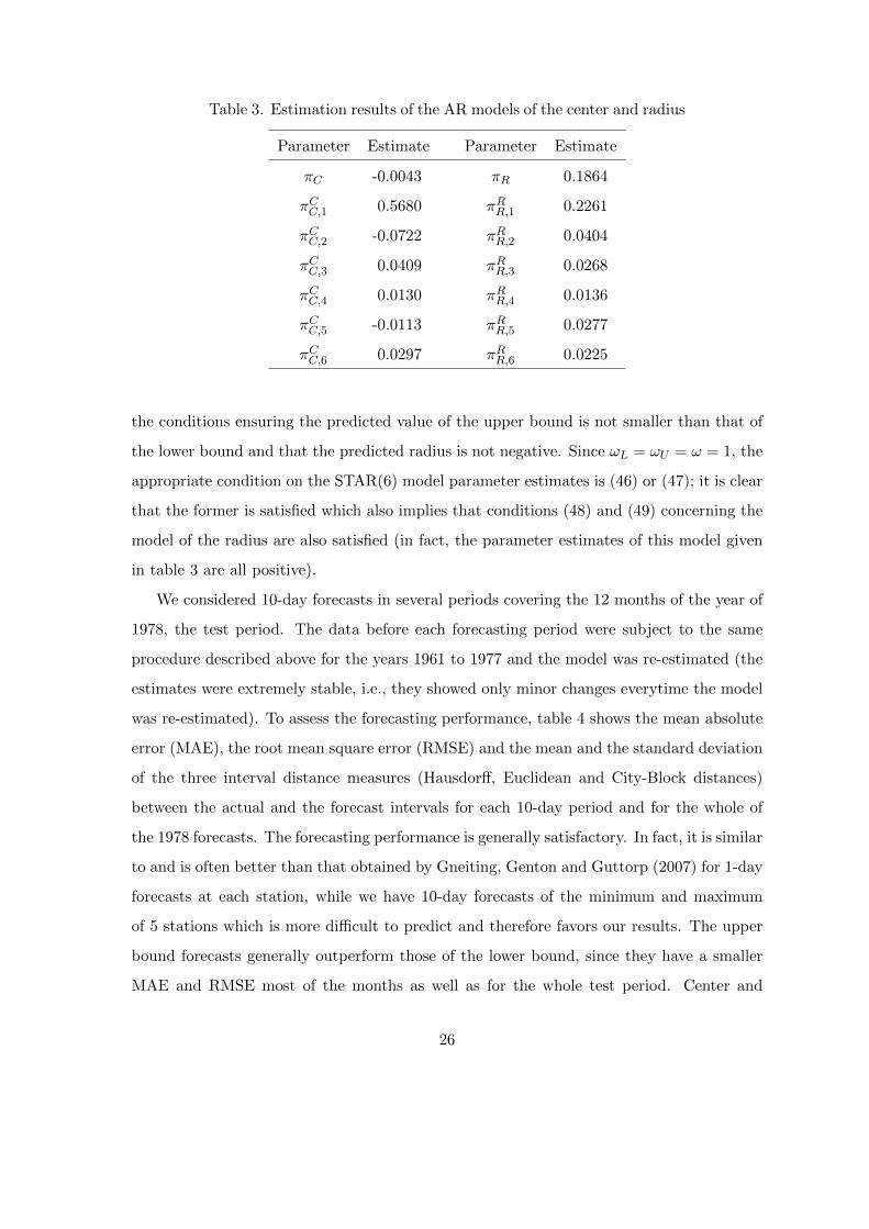
Table 3. Estimation results of the AR models of the center and radius
Parameter Estimate Parameter Estimate
πC -0.0043 πR 0.1864
πCC,1 0.5680 πRR,1 0.2261
πCC,2 -0.0722 πRR,2 0.0404
πCC,3 0.0409 πRR,3 0.0268
πCC,4 0.0130 πRR,4 0.0136
πCC,5 -0.0113 πRR,5 0.0277
πCC,6 0.0297 πRR,6 0.0225
the conditions ensuring the predicted value of the upper bound is not smaller than that of
the lower bound and that the predicted radius is not negative. Since ωL = ωU = ω = 1, the
appropriate condition on the STAR(6) model parameter estimates is (46) or (47); it is clear
that the former is satisfied which also implies that conditions (48) and (49) concerning the
model of the radius are also satisfied (in fact, the parameter estimates of this model given
in table 3 are all positive).
We considered 10-day forecasts in several periods covering the 12 months of the year of
1978, the test period. The data before each forecasting period were subject to the same
procedure described above for the years 1961 to 1977 and the model was re-estimated (the
estimates were extremely stable, i.e., they showed only minor changes everytime the model
was re-estimated). To assess the forecasting performance, table 4 shows the mean absolute
error (MAE), the root mean square error (RMSE) and the mean and the standard deviation
of the three interval distance measures (Hausdorff, Euclidean and City-Block distances)
between the actual and the forecast intervals for each 10-day period and for the whole of
the 1978 forecasts. The forecasting performance is generally satisfactory. In fact, it is similar
to and is often better than that obtained by Gneiting, Genton and Guttorp (2007) for 1-day
forecasts at each station, while we have 10-day forecasts of the minimum and maximum
of 5 stations which is more difficult to predict and therefore favors our results. The upper
bound forecasts generally outperform those of the lower bound, since they have a smaller
MAE and RMSE most of the months as well as for the whole test period. Center and
26
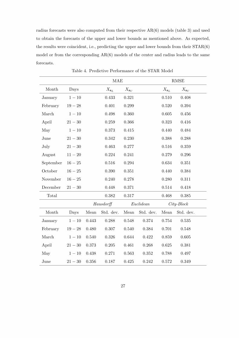
radius forecasts were also computed from their respective AR(6) models (table 3) and used
to obtain the forecasts of the upper and lower bounds as mentioned above. As expected,
the results were coincident, i.e., predicting the upper and lower bounds from their STAR(6)
model or from the corresponding AR(6) models of the center and radius leads to the same
forecasts.
Table 4. Predictive Performance of the STAR Model
MAE RMSE
Month Days XsL XsU XsL XsU
January 1− 10 0.433 0.321 0.510 0.408
February 19− 28 0.401 0.299 0.520 0.394
March 1− 10 0.498 0.360 0.605 0.456
April 21− 30 0.259 0.366 0.323 0.416
May 1− 10 0.373 0.415 0.440 0.484
June 21− 30 0.342 0.230 0.388 0.288
July 21− 30 0.463 0.277 0.516 0.359
August 11− 20 0.224 0.241 0.279 0.296
September 16− 25 0.516 0.294 0.634 0.351
October 16− 25 0.390 0.351 0.440 0.384
November 16− 25 0.240 0.278 0.280 0.311
December 21− 30 0.448 0.371 0.514 0.418
Total 0.382 0.317 0.468 0.385
Hausdorff Euclidean City-Block
Month Days Mean Std. dev. Mean Std. dev. Mean Std. dev.
January 1− 10 0.443 0.288 0.548 0.374 0.754 0.535
February 19− 28 0.480 0.307 0.540 0.384 0.701 0.548
March 1− 10 0.540 0.326 0.644 0.422 0.859 0.605
April 21− 30 0.373 0.205 0.461 0.268 0.625 0.381
May 1− 10 0.438 0.271 0.563 0.352 0.788 0.497
June 21− 30 0.356 0.187 0.425 0.242 0.572 0.349
27
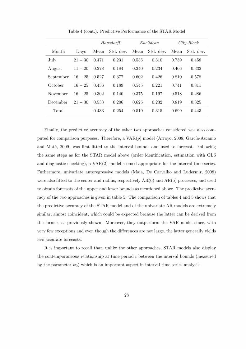
Table 4 (cont.). Predictive Performance of the STAR Model
Hausdorff Euclidean City-Block
Month Days Mean Std. dev. Mean Std. dev. Mean Std. dev.
July 21− 30 0.471 0.231 0.555 0.310 0.739 0.458
August 11− 20 0.278 0.184 0.340 0.234 0.466 0.332
September 16− 25 0.527 0.377 0.602 0.426 0.810 0.578
October 16− 25 0.456 0.189 0.545 0.221 0.741 0.311
November 16− 25 0.302 0.140 0.375 0.197 0.518 0.286
December 21− 30 0.533 0.206 0.625 0.232 0.819 0.325
Total 0.433 0.254 0.519 0.315 0.699 0.443
Finally, the predictive accuracy of the other two approaches considered was also com-
puted for comparison purposes. Therefore, a VAR(p) model (Arroyo, 2008; Garcıa-Ascanio
and Mate, 2009) was first fitted to the interval bounds and used to forecast. Following
the same steps as for the STAR model above (order identification, estimation with OLS
and diagnostic checking), a VAR(2) model seemed appropriate for the interval time series.
Futhermore, univariate autoregressive models (Maia, De Carvalho and Ludermir, 2008)
were also fitted to the center and radius, respectively AR(6) and AR(5) processes, and used
to obtain forecasts of the upper and lower bounds as mentioned above. The predictive accu-
racy of the two approaches is given in table 5. The comparison of tables 4 and 5 shows that
the predictive accuracy of the STAR model and of the univariate AR models are extremely
similar, almost coincident, which could be expected because the latter can be derived from
the former, as previously shown. Moreover, they outperform the VAR model since, with
very few exceptions and even though the differences are not large, the latter generally yields
less accurate forecasts.
It is important to recall that, unlike the other approaches, STAR models also display
the contemporaneous relationship at time period t between the interval bounds (measured
by the parameter ψ0) which is an important aspect in interval time series analysis.
28
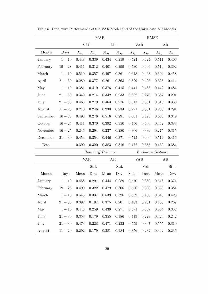
Table 5. Predictive Performance of the VAR Model and of the Univariate AR Models
MAE RMSE
VAR AR VAR AR
Month Days XsL XsU XsL XsU XsL XsU XsL XsU
January 1− 10 0.448 0.339 0.434 0.319 0.524 0.424 0.511 0.406
February 19− 28 0.411 0.312 0.401 0.299 0.530 0.406 0.519 0.392
March 1− 10 0.510 0.357 0.497 0.361 0.618 0.463 0.604 0.458
April 21− 30 0.280 0.377 0.261 0.363 0.329 0.426 0.323 0.414
May 1− 10 0.381 0.419 0.376 0.415 0.441 0.483 0.442 0.484
June 21− 30 0.340 0.214 0.342 0.233 0.382 0.276 0.387 0.291
July 21− 30 0.465 0.279 0.463 0.276 0.517 0.361 0.516 0.358
August 11− 20 0.240 0.246 0.230 0.234 0.291 0.301 0.286 0.291
September 16− 25 0.493 0.276 0.516 0.291 0.601 0.323 0.636 0.349
October 16− 25 0.411 0.370 0.392 0.350 0.456 0.400 0.442 0.383
November 16− 25 0.246 0.294 0.237 0.280 0.306 0.339 0.275 0.315
December 21− 30 0.454 0.354 0.446 0.371 0.515 0.400 0.514 0.416
Total 0.390 0.320 0.383 0.316 0.472 0.388 0.469 0.384
Hausdorff Distance Euclidean Distance
VAR AR VAR AR
Std. Std. Std. Std.
Month Days Mean Dev. Mean Dev. Mean Dev. Mean Dev.
January 1− 10 0.458 0.291 0.444 0.289 0.570 0.380 0.548 0.374
February 19− 28 0.490 0.322 0.479 0.306 0.556 0.390 0.539 0.384
March 1− 10 0.546 0.337 0.539 0.326 0.652 0.436 0.643 0.423
April 21− 30 0.392 0.197 0.375 0.201 0.483 0.251 0.460 0.267
May 1− 10 0.445 0.259 0.439 0.271 0.571 0.337 0.564 0.352
June 21− 30 0.353 0.179 0.355 0.186 0.419 0.229 0.426 0.242
July 21− 30 0.473 0.228 0.471 0.232 0.559 0.307 0.555 0.310
August 11− 20 0.292 0.179 0.281 0.184 0.356 0.232 0.342 0.236
29
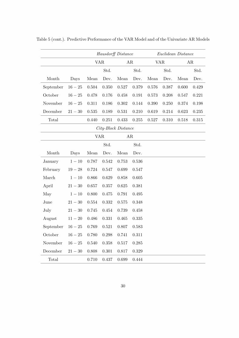
Table 5 (cont.). Predictive Performance of the VAR Model and of the Univariate AR Models
Hausdorff Distance Euclidean Distance
VAR AR VAR AR
Std. Std. Std. Std.
Month Days Mean Dev. Mean Dev. Mean Dev. Mean Dev.
September 16− 25 0.504 0.350 0.527 0.379 0.576 0.387 0.600 0.429
October 16− 25 0.478 0.176 0.458 0.191 0.573 0.208 0.547 0.221
November 16− 25 0.311 0.186 0.302 0.144 0.390 0.250 0.374 0.198
December 21− 30 0.535 0.189 0.531 0.210 0.619 0.214 0.623 0.235
Total 0.440 0.251 0.433 0.255 0.527 0.310 0.518 0.315
City-Block Distance
VAR AR
Std. Std.
Month Days Mean Dev. Mean Dev.
January 1− 10 0.787 0.542 0.753 0.536
February 19− 28 0.724 0.547 0.699 0.547
March 1− 10 0.866 0.629 0.858 0.605
April 21− 30 0.657 0.357 0.625 0.381
May 1− 10 0.800 0.475 0.791 0.495
June 21− 30 0.554 0.332 0.575 0.348
July 21− 30 0.745 0.454 0.739 0.458
August 11− 20 0.486 0.331 0.465 0.335
September 16− 25 0.769 0.521 0.807 0.583
October 16− 25 0.780 0.298 0.741 0.311
November 16− 25 0.540 0.358 0.517 0.285
December 21− 30 0.808 0.301 0.817 0.329
Total 0.710 0.437 0.699 0.444
30
7 Concluding remarks
When interval-valued symbolic data are collected as an ordered sequence through time,
they form an interval time series (ITS). In this paper, we proposed to model an ITS with a
Space-time autoregressive process STAR(p), which appears to be appropriate for such data,
given the link between the lower and upper bounds of the observed intervals. Based on
this model for the ITS bounds we also showed that its center and radius follow a bivariate
Structural Vector Autoregressive process SVAR(p) whose parameters are functions of those
in the STAR(p) model; two especially relevant particular cases were analyzed. Concerning
prediction, we derived the minimum mean square error predictor and sufficient conditions
on the parameters to ensure that the predicted upper bound is not less than the lower bound
or that the predicted values of the radius are not negative. A simulation study showed that
the predictive accuracy of the different approaches discussed is very similar and that none
of them outperforms the others. Finally, these models were applied to an ITS of the Irish
wind speed and 10-day forecasts were computed showing good accuracy. We may thus
conclude that modeling an interval time series with a Space-time Autoregressive process is
appropriate and provides accurate forecasts.
References
Antunes, A.M.C. and Subba Rao, T. (2006). On hypotheses testing for the selection of
spatio-temporal models, Journal of Time Series Analysis 27, 767-791.
Arroyo, J. (2008). Metodos de prediccion para series temporales de intervalos e histogra-
mas, Unpublished Ph.D. Dissertation, Universidad Pontificia Comillas, Madrid.
Arroyo, J., Gonzalez-Rivera, G. and Mate, C. (2010). Forecasting with interval and his-
togram data. Some financial applications In: Ullah, A. and Giles, D., Balakrishnan,
N., Schucany, W. and Schilling, E., eds. Handbook of Empirical Economics and Fi-
nance,(forthcoming). New York: Chapman and Hall/CR.
Bertrand, P. and Goupil, F. (2000). Descriptive statistics for symbolic data. In: Bock, H.-
H. and Diday, E., eds.,Analysis of Symbolic Data. Exploratory Methods for Extracting
Statistical Information from Complex Data. Heidelberg: Springer, 106-124.
31

Billard, L. and Diday, E. (2000). Regression analysis for interval-valued data. In: Kiers,
H.A.L. and Rasson, J.P., eds. Data Analysis, Classification, and Related Methods,
Proceedings IFCS’2000, Namur. Heidelberg: Springer Verlag, 369-374.
Billard, L. and Diday, E. (2003). From the Statistics of Data to the Statistics of Knowledge:
Symbolic Data Analysis, Journal of the American Statistical Association 98, 470-487.
Billard, L. and Diday, E. (2006). Symbolic Data Analysis: Conceptual Statistics and Data
Analysis. Chichester: John Wiley and Sons.
Bock, H.-H. and Diday, E. (Eds.) (2000) Analysis of Symbolic Data, Exploratory Methods
for Extracting Statistical Information from Complex Data. Heidelberg: Springer.
Bollerslev, T. (1986). Generalized autoregressive conditional heteroskedasticity, Journal
of Econometrics 31, 307-327.
Box, G.E.P., Jenkins, G.M. and Reinsel G.C. (2008). Time Series Analysis: Forecasting
and Control, 4th. ed. Hoboken, New Jersey: John Wiley and Sons.
Brito, P. (2007). Modelling and Analysing Interval Data. In: Decker, R., Lenz, H.-J., eds.
Advances in Data Analysis. Berlin, Heidelberg, New-York: Springer, 197-208.
Brockwell, P.J., Davis, R.A. (2002). Introduction to Time Series and Forecasting. New
York: Springer Verlag.
Chouakria, A., Cazes, P., Diday, E. (2000). Symbolic Principal Component Analysis. In:
Bock, H.-H. and Diday, E., eds. Analysis of Symbolic Data. Exploratory Methods for
Extracting Statistical Information from Complex Data. Heidelberg: Springer. 200-
212.
Cliff, A.D. and Ord, J.K. (1975). Model building and the analysis of spatial pattern in
human geography, Journal of the Royal Statistical Society B 37, 297-328.
Cressie, N.A.C. (1993). Statistics for Spatial Data. New York: John Wiley and Sons.
Diday, E. and Noirhomme, M. (Eds.) (2008). Symbolic Data and the SODAS Software.
Chichester: John Wiley and Sons.
32
Diggle, P.J. and Ribeiro, P.J. Jr. (2007). Model-based Geostatistics, Springer, New York.
Duarte Silva, A.P. and Brito, P. (2006). Linear discriminant analysis for interval data,
Computational Statistics 21, 2, 289-308.
Engle, R. F. (1982). Autoregressive conditional heteroscedasticity with estimates of the
variance of United Kingdom inflations, Econometrica 50, 987-1007.
Finkenstadt, B., Held, L. and Isham, V. (Eds.) (2007). Statistical Methods for Spatio-
Temporal Systems. London: Chapman and Hall/CRC.
Garcıa-Ascanio, C. and Mate, C. (2009). Electric power demand forecasting using interval
time series: A comparison between VAR and iMLPC, Energy Policy 38, 715-725.
Gneiting, T., Genton, M.G. and Guttorp, P. (2007). Geostatistical space-time models,
stationarity, separability, and full symmetry. In: Finkenstadt, B., Held, L. and Isham,
V., eds. Statistical Methods for Spatio-Temporal Systems. London: Chapman and
Hall/CRC, 151-175.
Gonzalez-Rivera, G. and Arroyo, J. (2011). Time series modelling of histogram-valued
data: The daily histogram time series of S&P500 intradaily returns. International
Journal of Forecasting 28(1), 20-33.
Han, A., Hong, Y., Lai, K. and Wang, S. (2008). Interval time series analysis with an ap-
plication to the Sterling-Dollar exchange rate, Journal of Systems Science and Com-
plexity 21(4), 558-573.
Haslett, J. and Raftery, A.E. (1989). Space-time modelling with long-memory dependence:
assessing Ireland’s wind-power resource (with discussion), Applied Statistics 38, 1, 1-
50.
Johnston, J. and Dinardo, D. (1997). Econometric Methods, 4th. ed. New York: McGraw-
Hill.
Lauro, C. and Palumbo, F. (2005). Principal component analysis for non-precise data. In:
Vichi, M. et al eds. New Developments in Classification and Data Analysis. Berlin,
Heidelberg: Springer, 173-184.
33
Le, N.D. and Zidek, J.V. (2006). Statistical Analysis of Environmental Space-Time Pro-
cesses. New York: Springer.
Lutkepohl, H. and Kratzig, M. (Eds.) (2004). Applied Time Series Econometrics, Cam-
bridge University Press, New York.
Maia, A.L.S., De Carvalho, F.A.T. and Ludermir, T.D. (2008). Forecasting models for
interval-valued time series, Neurocomputing 71 (16-18), 3344-3352.
Neto, E.A.L. and De Carvalho, F.A.T. (2008). Centre and range method for fitting a
linear regression model to symbolic intervalar data, Computational Statistics & Data
Analysis 52, 3, 1500-1515.
Neto, E.A.L. and De Carvalho, F.A.T. (2010). Constrained linear regression models for
symbolic interval-valued variables, Computational Statistics & Data Analysis 54, 2,
333-347.
Noirhomme-Fraiture, M. and Brito, P. (2011). Far Beyond the Classical Data Models:
Symbolic Data Analysis. Statistical Analysis and Data Mining 4, 2, 157-170.
Pfeifer, P. and Deutsch, S. (1980). A three stage interactive procedure for space-time
modeling, Technometrics 22, 35-47.
Teles, P. and Brito, P. (2005). Modelling interval time series data, Proceedings of the 3rd
IASC World Conference on Computational Statistics and Data Analysis, Limassol,
Cyprus.
Tsay, R. (2005). Analysis of Financial Time Series, 2nd ed. Hoboken, New Jersey: John
Wiley and Sons.
Wei, W.W.S. (2006). Time Series Analysis: Univariate and Multivariate Methods, 2nd.
ed. New York: Addison-Wesley.
34

Appendix
35
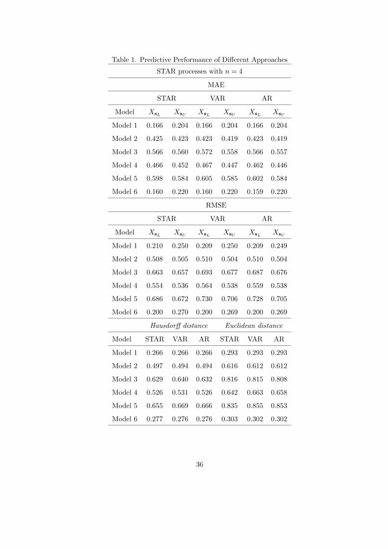
Table 1. Predictive Performance of Different Approaches
STAR processes with n = 4
MAE
STAR VAR AR
Model XsL XsU XsL XsU XsL XsU
Model 1 0.166 0.204 0.166 0.204 0.166 0.204
Model 2 0.425 0.423 0.423 0.419 0.423 0.419
Model 3 0.566 0.560 0.572 0.558 0.566 0.557
Model 4 0.466 0.452 0.467 0.447 0.462 0.446
Model 5 0.598 0.584 0.605 0.585 0.602 0.584
Model 6 0.160 0.220 0.160 0.220 0.159 0.220
RMSE
STAR VAR AR
Model XsL XsU XsL XsU XsL XsU
Model 1 0.210 0.250 0.209 0.250 0.209 0.249
Model 2 0.508 0.505 0.510 0.504 0.510 0.504
Model 3 0.663 0.657 0.693 0.677 0.687 0.676
Model 4 0.554 0.536 0.564 0.538 0.559 0.538
Model 5 0.686 0.672 0.730 0.706 0.728 0.705
Model 6 0.200 0.270 0.200 0.269 0.200 0.269
Hausdorff distance Euclidean distance
Model STAR VAR AR STAR VAR AR
Model 1 0.266 0.266 0.266 0.293 0.293 0.293
Model 2 0.497 0.494 0.494 0.616 0.612 0.612
Model 3 0.629 0.640 0.632 0.816 0.815 0.808
Model 4 0.526 0.531 0.526 0.642 0.663 0.658
Model 5 0.655 0.669 0.666 0.835 0.855 0.853
Model 6 0.277 0.276 0.276 0.303 0.302 0.302
36
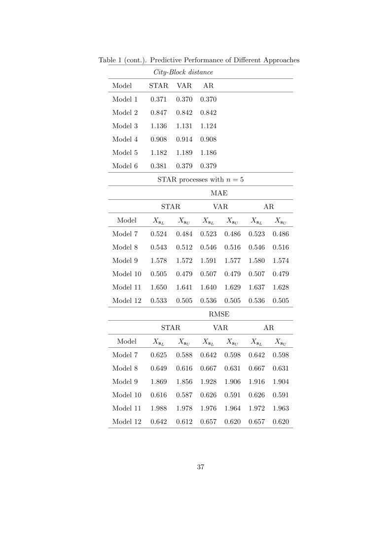
Table 1 (cont.). Predictive Performance of Different Approaches
City-Block distance
Model STAR VAR AR
Model 1 0.371 0.370 0.370
Model 2 0.847 0.842 0.842
Model 3 1.136 1.131 1.124
Model 4 0.908 0.914 0.908
Model 5 1.182 1.189 1.186
Model 6 0.381 0.379 0.379
STAR processes with n = 5
MAE
STAR VAR AR
Model XsL XsU XsL XsU XsL XsU
Model 7 0.524 0.484 0.523 0.486 0.523 0.486
Model 8 0.543 0.512 0.546 0.516 0.546 0.516
Model 9 1.578 1.572 1.591 1.577 1.580 1.574
Model 10 0.505 0.479 0.507 0.479 0.507 0.479
Model 11 1.650 1.641 1.640 1.629 1.637 1.628
Model 12 0.533 0.505 0.536 0.505 0.536 0.505
RMSE
STAR VAR AR
Model XsL XsU XsL XsU XsL XsU
Model 7 0.625 0.588 0.642 0.598 0.642 0.598
Model 8 0.649 0.616 0.667 0.631 0.667 0.631
Model 9 1.869 1.856 1.928 1.906 1.916 1.904
Model 10 0.616 0.587 0.626 0.591 0.626 0.591
Model 11 1.988 1.978 1.976 1.964 1.972 1.963
Model 12 0.642 0.612 0.657 0.620 0.657 0.620
37

Table 1 (cont.). Predictive Performance of Different Approaches
Hausdorff distance Euclidean distance
Model STAR VAR AR STAR VAR AR
Model 7 0.704 0.714 0.714 0.764 0.793 0.793
Model 8 0.726 0.748 0.748 0.809 0.832 0.832
Model 9 1.771 1.796 1.780 2.259 2.284 2.271
Model 10 0.695 0.703 0.702 0.756 0.777 0.777
Model 11 1.840 1.831 1.828 2.359 2.349 2.345
Model 12 0.715 0.726 0.726 0.810 0.812 0.811
City-Block distance
Model STAR VAR AR
Model 7 0.973 1.009 1.009
Model 8 1.030 1.062 1.062
Model 9 3.154 3.169 3.154
Model 10 0.974 0.986 0.985
Model 11 3.285 3.269 3.265
Model 12 1.039 1.041 1.041
STAR processes with n = 2
MAE
STAR VAR AR
Model XsL XsU XsL XsU XsL XsU
Model 13 1.569 1.467 1.569 1.467 1.569 1.467
Model 14 0.621 0.301 0.620 0.300 0.546 0.300
Model 15 0.631 0.365 0.633 0.363 0.628 0.361
Model 16 0.596 0.354 0.595 0.352 0.595 0.352
Model 17 0.650 0.330 0.657 0.330 0.651 0.328
Model 18 0.586 0.362 0.589 0.359 0.588 0.359
38
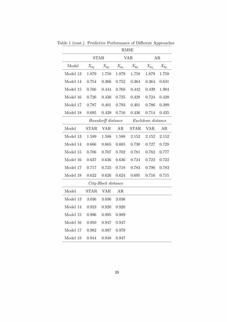
Table 1 (cont.). Predictive Performance of Different Approaches
RMSE
STAR VAR AR
Model XsL XsU XsL XsU XsL XsU
Model 13 1.879 1.758 1.879 1.758 1.879 1.758
Model 14 0.754 0.366 0.752 0.364 0.364 0.631
Model 15 0.766 0.444 0.768 0.442 0.439 1.904
Model 16 0.726 0.430 0.725 0.428 0.724 0.428
Model 17 0.787 0.401 0.793 0.401 0.786 0.399
Model 18 0.695 0.439 0.716 0.436 0.714 0.435
Hausdorff distance Euclidean distance
Model STAR VAR AR STAR VAR AR
Model 13 1.589 1.588 1.588 2.152 2.152 2.152
Model 14 0.666 0.665 0.665 0.730 0.727 0.728
Model 15 0.706 0.707 0.702 0.781 0.782 0.777
Model 16 0.637 0.636 0.636 0.724 0.722 0.722
Model 17 0.717 0.725 0.718 0.783 0.790 0.783
Model 18 0.622 0.626 0.624 0.695 0.716 0.715
City-Block distance
Model STAR VAR AR
Model 13 3.036 3.036 3.036
Model 14 0.923 0.920 0.920
Model 15 0.996 0.995 0.989
Model 16 0.950 0.947 0.947
Model 17 0.982 0.987 0.979
Model 18 0.944 0.948 0.947
39