New Jersey Institute of Technology New Jersey Institute of Technology

Digital Commons @ NJIT Digital Commons @ NJIT

Dissertations Electronic Theses and Dissertations

Fall 1-31-1996

Real time control of nonlinear dynamic systems using neuro-fuzzy Real time control of nonlinear dynamic systems using neuro-fuzzy

controllers controllers

Amitava Jana New Jersey Institute of Technology

Follow this and additional works at: https://digitalcommons.njit.edu/dissertations

Part of the Mechanical Engineering Commons

Recommended Citation Recommended Citation Jana, Amitava, "Real time control of nonlinear dynamic systems using neuro-fuzzy controllers" (1996). Dissertations. 1009. https://digitalcommons.njit.edu/dissertations/1009

This Dissertation is brought to you for free and open access by the Electronic Theses and Dissertations at Digital Commons @ NJIT. It has been accepted for inclusion in Dissertations by an authorized administrator of Digital Commons @ NJIT. For more information, please contact digitalcommons@njit.edu.

Copyright Warning & Restrictions

The copyright law of the United States (Title 17, UnitedStates Code) governs the making of photocopies or other

reproductions of copyrighted material.

Under certain conditions specified in the law, libraries andarchives are authorized to furnish a photocopy or other

reproduction. One of these specified conditions is that thephotocopy or reproduction is not to be “used for any

purpose other than private study, scholarship, or research.”If a, user makes a request for, or later uses, a photocopy orreproduction for purposes in excess of “fair use” that user

may be liable for copyright infringement,

This institution reserves the right to refuse to accept acopying order if, in its judgment, fulfillment of the order

would involve violation of copyright law.

Please Note: The author retains the copyright while theNew Jersey Institute of Technology reserves the right to

distribute this thesis or dissertation

Printing note: If you do not wish to print this page, then select“Pages from: first page # to: last page #” on the print dialog screen

The Van Houten library has removed some of thepersonal information and all signatures from theapproval page and biographical sketches of thesesand dissertations in order to protect the identity ofNJIT graduates and faculty.

ABSTRACT

REAL TIME CONTROL OF NONLINEAR DYNAMIC SYSTEMS USING NEURO-FUZZY CONTROLLERS

by Amitava Jana

The problem of real time control of a nonlinear dynamic system using intelligent

control techniques is considered. The current trend is to incorporate neural networks and

fuzzy logic into adaptive control strategies. The focus of this work is to investigate the

current neuro-fuzzy approaches from literature and adapt them for a specific application.

In order to achieve this objective, an experimental nonlinear dynamic system is considered.

The motivation for this comes from the desire to solve practical problems and to create a

test-bed which can be used to test various control strategies. The nonlinear dynamic

system considered here is an unstable balance beam system that contains two fluid tanks,

one at each end, and the balance is achieved by pumping the fluid back and forth from the

tanks.

A popular approach, called ANFIS (Adaptive Networks-based Fuzzy Inference

Systems), which combines the structure of fuzzy logic controllers with the learning aspects

from neural networks is considered as a basis for developing novel techniques, because it

is considered to be one of the most general framework for developing adaptive controllers.

However, in the proposed new method, called Generalized Network-based Fuzzy

Inferencing Systems (GeNFIS), more conventional fuzzy schemes for the consequent part

are used instead of using what is called the Sugeno type rules. Moreover, in contrast to

ANFIS which uses a full set of rules, GeNFIS uses only a limited number of rules based on

certain expert knowledge. GeNFIS is tested on the balance beam system, both in a real-

time actual experiment and the simulation, and is found to perform better than a

comparable ANFIS under supervised learning. Based on these results, several

modifications of GeNFIS are considered, for example, synchronous defuzzification

through triangular as well as bell shaped membership functions. Another modification

involves simultaneous use of Sugeno type as well as conventional fuzzy schemes for the

consequent part, in an effort to create a more flexible framework. Results of testing

different versions of GeNFIS on the balance beam system are presented.

REAL-TIME CONTROL OF NONLINEAR DYNAMIC SYSTEMS USING NEURO-FUZZY CONTROLLERS

by Amitava Jana

A Dissertation

Submitted to the Faculty of

New Jersey Institute of Technology in Partial Fulfillment of the Requirements for the Degree of

Doctor of Philosophy

Department of Mechanical Engineering

January 1996

Copyright © 1996 by Amitava Jana

ALL RIGHTS RESERVED

APPROVAL PAGE

REAL TIME CONTROL OF NONLINEAR DYNAMIC SYSTEMS USING NEURO-FUZZY CONTROLLERS

Amitava Jana

Dr. Rajesh N Dave, Advisor Date Associate Professor of Mechanical Engineering, MIT

David M Auslander, Advisor Date Professor of Mechanical Engineering, University of California, Berkeley

Dr. Rong-Yaw Chen, Committee Member Date Professor of Mechanical Engineering and Associate Chairperson for Graduate Studies, MIT

Dr. Zhiming Ji, Committee Member Date Assistant Professor of Mechanical Engineering, MIT

Dr. Bernard Koplik, Committee Member Date Professor and Chairperson of Mechanical Engineering,NJIT

BIOGRAPHICAL SKETCH

Author: Amitava Jana

Degree: Doctor of Philosophy in Mechanical Engineering

Date: January 1996

Date of Birth:

Place of Birth:

Undergraduate and Graduate Education:

Doctor of Philosophy in Mechanical Engineering, New Jersey Institute of Technology, Newark, NJ, 1996

Master of Science in Mechanical Engineering,

New Jersey Institute of Technology, Newark, NJ, 1987

Bachelor of Engineering in Mechanical Engineering, Calcutta University, Calcutta, India, 1976

Major: Mechanical Engineering

Presentations and Publications:

Jana, A., and Auslander, D.M., "Workcell Programming Environment for Intelligent Manufacturing Systems," Design and Implementation of Intelligent Manufacturing Systems, Parsaei, H.R., and Jamshidi, M., Eds. Prentice-Hall, 1995 Chapter 1, pp. 1-18, 1995.

Jana, A., Auslander, D.M., Dave, R.N., Chehl, S.S.," Task Planning for Cooperating Robot Systems," Proc. of 199-I Int. Symposium on Robotics and Manufacturing, Maui, Hawaii, August 14-18, 1994.

Jana, A., Dave, R.N., Chehl, S.S., Wang, C. S.,"Computer-Integrated Manufacturing and Robotics Laboratory Design for Undergraduate Education," Proc. of 1994 Int. Symposium on Robotics and Manufacturing, Maui, Hawaii, August 14-18, 1994.

Jerro, H. D., Jana, A., Dave R. N., "Multiprocessing Systems: A Design Experience," Proc. of 1994 ASEE GSW Conference, Baton Rouge, LA, March 1994,

iv

Jana, A., Wang, C. S., Chehl, S.S.,"Integrated System Design and Simulation," Proc. of 1993 Intl Simulation Technology) Multiconference, San Francisco, LA, November 8-10,1993.

Auslander, D.M.,Hanidu, G., Jana, A., Jothimurugesan, K , Seif, S., Young, Y.,"Tools for Teaching Mechatronics," Proc. of 1993 ASEE Annual Conference, Univ. of

Illinois, IL, June 18-21,1993.

Jana, A., Chehl, S.S.,"Developing Instrumentation Laboratory with Real Time Control Component," Proc. of 1993 American Control Conference, San Francisco, June 1993, pp. 2046-2049.

Auslander, D.M., Hanidu, G., Jana, A., Landesberger, S., Seif, S., Young, Y.,"Mechatronics Curriculum in the Synthesis Coalition,"Proc. of 1992

IEEE/CHMT Int'l Electronic Manufacturing Tech. Symp., Baltimore,MD,Sept 1992,pp.165-168.

Jana, A., Wang, C. S., Chehl, S.S.,"Development of a Flexible Manufacturing Workcell,"

Presented in the 9th Int'l Conf. on CAD/CAM, Robotics and Factories of the Future, Newark, NJ, August 18-20,1993.

Dave, R.N., Jana,A.,"Development of a PC-Based Robotic Simulation Package," Proc. of 1987 ASME Computers in Engineering Conference, pp 295-300.

ACKNOWLEDGMENT

I would like to express my sincere gratitude to my advisors Dr. Rajesh N. Dave of New Jersey Institute of Technology, and Dr. David M. Auslander of University of California, Berkeley. This work would not have been possible without their guidance and moral support throughout this research.

I am also grateful to Dr. Rong-Yaw Chen, Dr. Zhiming Ji, and Dr. Bernard Koplik for serving as members on my doctoral committee.

Special thanks to Dean M Q. Burrel, Dr. S.S Chehl, and Dr. George Whitfield of Southern University, Baton Rouge, for their continuous support and encouragement.

I would also like to thank my friends Yang, Mark, Chris of UC Berkeley, Reza of Southern University, Sumit and Anupam of NJIT for their very helpful ideas, constructive comments and technical supports during various phases of this research.

Finally, and most importantly, I would like to thank my parents for the love and encouragement they have given me all my life and specially to reach this milestone of my life by sacrificing their happiness.

vi

TABLE OF CONTENTS

Chapter Page

1 INTRODUCTION 1

1.1 Background 3

L2 Objective and Scope of the work 5

2 NEURO FUZZY CONTROL 7

2.1 Introduction 7

2.2 Fuzzy Inferencing System 7

2.2.1 Fuzzy Control 11

2,3 Neural Network 16

2.4 Neuro Fuzzy Controller 18

2.5 Proposed Neuro-Fuzzy Controller

2.5.1 GeNFIS Architecture 73

3 A NON LINEAR DYNAMIC SYSTEM 30

3.1 Introduction 30

3.2 Balance Beam System 31

3.2.1 System Model 32

3.2.2 Plant Simulation 34

4 REAL TIME CONTROL

4.1 Implementation 37

4.2 Real Time Programming 38

4.3 Rule Construction 40

4.4 Experimental Results 46

4.4.1 Simulation 46

4.4.2 Real Time Control 30

Vii

Chapter Page

5 EXPERIMENTING WITH GeNFIS 55

5.1 Synchronous Defuzzification Scheme 55

5.2 Experimental Results 57

5.2.1 Simulation 57

5.2.2 Plant Control 58

5.3 Hybrid Learning 62

5.3.1 Experimental Results 63

5.4 ANFIS Implementation 65

5.4.1 Experimental Results 65

5.4.2 Limitations of ANTIS Implementation 67

5.5 Modified Rules for ANFIS and GeNFIS 68

5.5.1 Experimental Results 69

6 CONCLUSIONS AND FUTURE WORK 72

6.1 Conclusions 73

6.2 Future Work 77

APPENDIX A TRAINING OF GeNFIS 78

APPENDIX B SYNCHRONOUS DEFUZZIFICATION 84

APPENDIX C BALANCE BEAM PARAMETERS 87

REFERENCES 92

viii

LIST OF FIGURES

Figure Page

2.1 Fuzzy Controller 11

2.2 Fuzzy Inferencing; Mamdani Type 12

2.3 Symmetrical MF, Product Operator, MOM Defuzzification 13

2.4 Tsukamoto Type Fuzzy Inferencing 14

2.5 Sugeno Type Fuzzy Inferencing System 15

2.6 Multilayered Neural Net 16

2.7 Processing element--Neuron 17

2.8 Fuzzy Associative Memories (FAM) 19

2.9 Adaptive network based fuzzy inferencing system (ANTIS)

2.10 GARIC

2.11 Fuzzy logic adaptive network (FLAN)

2.12 GeNFIS Architecture 74

2.13 Single Rule Defuzzification 75

2.14 Local Defuzzification Method 77

3.1 Balance beam System 31

3.2 Net torque in the same direction of rotation 32

3.4 (a)Position,(b)water level, (c)velocity errors and (d)motor voltage 36

3.5 (a)Position vs velocity error (b) pumpflow rate 36

4.1 Schematic diagram of the balance beam set up 37

4.2 Synchronous program 38

4.3 Asynchronous Program 39

4.4 Output control voltage. Training data, and after learning 43

4.5 Initial MF, and Final MF of position error(volt) 44

ix

Figure Page

4.6 Initial Mg, and Final MF of velocity and left hand water height error 45

4.7 Initial and Final MF of moto control voltage 45

4.8 Simulation with GeNFIS controller: Initial position 0.03 radians, (a) position

(b)water level (c) velocity errors,and (d) Motor input voltage 46

4.9 Simulation with GeNFIS controller: Initial position 0.03 radians, (a) state space

(b)pump flow rate 46

4.10 Simulation with GeNFIS controller: initial position -0.03 radians, (a) position (b)water level (c) velocity errors,and (d) Motor input voltage 47

4.11 Simulation with GeNFIS controller: Initial position -0.03 radians, (a) state space

(b)pump flow rate 48

4.12 GeNFIS simulation with initial angle -0.025 radians and initial water height error -0.2 cm 48

4.13 Simulation with GeNFIS controller: Initial pos. 0.025 rad., and initial water height error -0.2cm; pos. error Vs (a) vel. and water level errors 49

4.14 GeNFIS simulation with initial angle -0.05 radians 49

4.15 Simulation with GeNFIS controller, initial pos. -0.05 rad; pos. error against (a) velocity and (b) water level errors 50

4.16 Control of balance beam using GeNFIS at 0 rad set point ( horizontal) (a) pos. error (b) vel. error (c) water height error (d) control voltage 51

4.17 Control of balance beam using PID at 0 rad set point ( horizontal) (a) pos. error (b) vel. error (c) water height error (d) control voltage 52

4.18 Control of balance beam using GeNFIS with a disturbance of 6 volts 52

4.19 Control of balance beam using PID with a disturbance of 8 volts 53

4.20 Failure of balance beam using GeNFIS at a distubance of 7 volts 53

4.21 Failure of balance beam using PID at a distubance of 9 volts 54

5.1 Modified GeNFIS Structure 56

5.2 (a)LMOM of triangular ME (b) Linear ME 57

5.3 Input Membership functions 58

Figure Page

5.4 Final membership functions: control voltage 58

5.5 Output with modified rules: Training data ( solid) and output (dashed) 59

5.6 Simulation with modified rule antecedent 60

5.7 Modified rules; (a) state ( position error vs. velocity error) (b) pump flow rate 60

5.8 Modified rules: Normal operation (disturbance 3.0 volts) 61

5.9 Modified GeNFIS with Sugeno type rules 62

5.10 Simulation with modified GeNFIS ( weights 0.5 in both) 64

5.11 Modified GeNFIS with 4 volt disturbance level ( weights 0.75:0.25) 64

5.12 ANFIS: Training and output data 66

5.13 ANFIS controller, Initial position -0.3 radians 66

5.14 Simulation ANFIS (initial position -0.3 rad) (a) state (b) pump flow rate 67

5.15 Simulation ANTIS controller Initial pos -0.25 67

5.16 Controller failure (real time) 68

5.17 Simulation: Failure of ANFIS with pre selected rule antecedent 70

5.18 Experiment: Failure of ANFIS with preselected rule antecedent 70

5.19 Simulation with ANFIS with modified rules 71

5.20 Experiment results: ANFIS with modified rules 71

C.1 Cascaded Control Loops 89

C.2 Net torque in the same direction of rotation 89

xi

LIST OF TABLES

Table Page

4.1 Different labels of input variables 41

4.2 Different labels of output 41

4.3 The 11 fuzzy control rules of GeNFIS 42

5.1 Initial and final linear functions 59

6 1 Summary of Results 76

xii

CHAPTER 1

INTRODUCTION

The field of intelligent control has emerged due to the need for increased autonomy in

manufacturing, demand for intelligent manufacturing processes and intelligent products,

and also to cope with the increased complexity and stringent performance requirement of

modern control systems. The recent advancements in connectionist and linguistic based

learning research offer opportunities for designing approximate reasoning based intelligent

control systems and management. Artificial neural networks and fuzzy logic are two most

significant areas related to the field of intelligent control. Artificial neural networks or

simply neural networks (NN) were developed to emulate human brain's neural-synaptic

mechanism which can learn and retrieve information [13]. On the other hand, fuzzy logic

was developed to emulate human reasoning, which is not just two-valued or multivalued

logic but the logic of fuzzy truths and are represented by linguistic terms like high or low.

In 1965, Zadeh suggested a modified set theory to characterize nonprobabilistic

uncertainties, which he called fuzzy sets and developed a consistent framework for dealing

with them [62]. Over the past few decades, fuzzy sets and their associated fuzzy logic

have been applied to a wide range of multi-disciplinary problems. These include automatic

control, pattern recognition and classification, consumer electronics, signal processing,

management and decision making, operations research, data base management, and others.

In the recent years, new research initiatives to integrate the field of neural network with

fuzzy logic have been made, and a new research field known as neuro-fuzzy modeling and

control has emerged.

In this thesis, the problem of real time control of a nonlinear dynamic system is

considered. The emphasis is on the use of practical approaches which exploit good

features from recently developed schemes that successfully combine neural networks and

fuzzy logic controllers. There is an abundance of literature in the areas of conventional as

1

2

well as modern control of nonlinear systems. However, in general most reported methods

are based on either an assumption regarding linearization of the model or some knowledge

about the type and order of nonlinear ty [19,48]. For many industrial and manufacturing

problems, the knowledge of the plant may be very limited and the task of utilizing the

latest state-of-the-art technique from literature becomes formidable for a practicing

engineer. This fact has led to the emergence of the area called intelligent control, and the

use of alternate approaches such as neural networks and fuzzy logic controllers. The

justification for using such an approach is based in part due to the fact that humans can

achieve complicated control tasks without having an exact knowledge of the plant. The

reasons for using neural networks or fuzzy logic then are quite natural, since most of the

decision making by humans is based on the intrinsic use of logic and learning within human

brain that perhaps is closely imitated by these two technologies. Both fuzzy logic and

neural networks have been proven to be universal approximators [32], thus they become

good candidates for tasks such as control of a nonlinear dynamic system, where the exact

model is unknown and the system behavior must be understood from its input-output

relations.

Ever since Mamdani [41] applied fuzzy logic for control of steam engine boiler

combination, there has been a tremendous growth in application of fuzzy logic for

controls, see for example [25,34,35]. Similarly, after pioneering work such as Narendra's

[38,43,44] where neural networks were used for adaptive control, there has been an

abundance of articles in a variety of journals and magazines, see [20] and references

therein. In the next section, a very brief review of the prior work which is relevant to this

thesis is presented. This is followed by the section that outlines the main objectives and

the scope of this work.

3

1.1 Background

The use of neural networks (NTNs) and fuzzy logic control (FLC) to solve the problem of

controlling nonlinear dynamic systems has received attention from many researchers due

to their potential in dealing with complex and nonlinear mappings. NN can map complex

relations without an explicit set of rules and has a very good learning ability, on the other

hand fuzzy logic can estimate functions and control systems with partial knowledge of the

systems. Encouraging results of applying these methods for the control of complex

systems are available in literature. Narendra and Parthasarathi used NN [43] in the

problem of system identification and control of nonlinear systems. Takagi and Sugeno

used fuzzy logic for system identification and control [55]. Although both the techniques

have a great potential to solve the problem of controlling nonlinear systems, there are

some drawbacks in each method. The architecture of NN depends on designer's

experience, and there is no guideline to determine the number of layers or the number of

nodes in each layer. In the case of FLC, the development of the linguistic rules and

corresponding membership functions relies on the availability of expert knowledge, and

this domain knowledge is often not available. Inspite of these limitations, these methods

have complimenting strengths. For example, FLC provides a compact structure for rule

representation that NN lacks, whereas NN provides structured learning ability which is not

available with FLC. Recent research trend indicates a use of combined approach to

overcome these limitations. The cooperative use of neural network and fuzzy logic are

also appearing in consumer goods [64].

In NN driven fuzzy reasoning (NDF), Takagi and Hayashi used Ns to define

membership functions[31]. Hayashi el al [33] proposed an algorithm that can adjust fuzzy

inference rules to compensate for a change of inference environment. This neural network

driven fuzzy reasoning with learning function (NDFL) can determine the optimal

4

membership functions and obtain the coefficients of linear equations in the consequent

parts by the searching function of the pattern search method. The authors used a

computer controlled inverted pendulum system to test the control algorithm. The input

output data were collected by manually balancing the pendulum.

Jang has developed an adaptive network-based fuzzy inference system (ANTIS),

by using linear functions in the consequent part of the fuzzy inferencing rules[17]. He

used a hybrid learning approach that combines the gradient descent method and least-

squares estimator for fast identification of parameters. He also proposed a self learning

method using temporal back propagation for model based adaptive control problems[16].

Park el al, proposed a controller design method for an on-line self-organizing fuzzy logic

controller without using any plant model [29]. The controller is developed from the

concept of human learning process and called as fuzzy auto-regressive moving average

(FARMA). Berenji and Khedkar proposed a generalized approximate-reasoning based

intelligent control architecture which consists of action evaluation network (AEN), action

selection network (ASN), and a stochastic action modifier (SAM) [15]. ASN is the fuzzy

controller whose output and a reinforcement signal produced by neural network AEN are

fed into SAM to generate final control action.

It appears that there are a number of good schemes that combine concepts from

neural network and fuzzy logic. However, in most of them, few authors have used actual

systems to test their results. Generally, they test their results through simulated examples.

There appears to be a need for real-time testing of some of the more attractive schemes

using an experimental test-bed, which is suitable for an academic environment. This is the

main objective of this dissertation. In the next section, specific objectives are outlined.

5

1.2 Objective and Scope of the Work

As mentioned earlier, the main objective of this dissertation is the study of the problem of

real time control of a nonlinear dynamic system. In order to achieve this objective, a real

experimental nonlinear dynamic system is considered. The focus is to investigate the

current neuro-fuzzy approaches from literature and adapt them for the specific application.

The motivation for this comes from the desire to solve practical problems and to create an

experimental test-bed which can be used to test various control strategies. The nonlinear

dynamic system considered here is an unstable balance beam system that contains two

fluid tanks, one at each end, and the balance is achieved by pumping the fluid back and

forth from the tanks. This system is in many ways similar to the ubiquitous inverted

pendulum system, since both are examples of unstable nonlinear fourth order nonlinear

dynamic systems. However, it is perhaps a more realistic example of engineering control

problems. This system is interfaced to a personal computer and various control schemes

are applied for its balance. This system is also simulated through its known dynamic

equations for making detailed observations regarding controller performance.

Neuro-fuzzy inference systems used for control of dynamic systems are considered

in chapter 2. The chapter begins with the introduction to fuzzy inference systems, fuzzy

control schemes, and neural networks. This is followed by a brief description of neuro-

fuzzy controller schemes popular in the literature. This discussion naturally leads to a

conclusion that ANFIS (Adaptive networks-based fuzzy inference systems) is one of the

most general framework for representing such schemes. The specific version of ANFIS as

described by Jang [17] utilizes linear form of what is called the Sugeno type rules in the

consequent part of the inference system. Although the use of these rules along with a

minimization of least-squared error based approach to learning the consequent parameters

results in an extremely fast learning algorithm, it may be worthwhile to explore other more

6

conventional fuzzy schemes for the consequent part, albeit at a certain loss of speed of

learning. This is the motivation for development of a neuro-fuzzy inference scheme, called

Generalized Network-based Fuzzy Inferencing Systems (GeNFIS), which is introduced in

this chapter. One disadvantage of ANTIS is that the structure of the network increases

very rapidly with an increase in the number of inputs and the number of rules. One may

utilize certain schemes (for example [ 18]) to alleviate this problem. However, in GeNFIS

this problem is avoided by using some expert knowledge to specify a limited number of

rules. The chapter ends with the derivation of the equations for the network output and

back-propagation training.

In chapter 3, the balance beam system and the system model are described. The

simulation of this system using a conventional PID controller is also presented. Real-time

control of this system is presented in chapter 4. In this chapter, rule construction for

GeNFIS is considered and the performance of this control scheme is studied.

Chapter 5, experimenting with GeNFIS, presents the test results of different ideas

which have been implemented to improve the performance of GeNFIS.

Chapter 6 concludes this dissertation with summary of the research results and the

directions for the future research.

The derivation of the proposed schemes are given in appendix A and B. The

details of balance beam system parameters are included in appendix C.

CHAPTER 2

NEURO FUZZY CONTROL

2.1 Introduction

Control systems have been the most successful application of the fuzzy set theory and the

fuzzy inferencing system. Fuzzy inferencing systems are also popularly known as fuzzy

controllers, fuzzy-rule based systems or fuzzy associative memories. Ever since Prof.

Lofti Zadeh introduced the fuzzy set theory in his seminal paper "Fuzzy sets", there have

been a tremendous growth in the research of fuzzy logic and fuzzy set theory [62].

In this chapter, the basics of fuzzy logic and neural networks are briefly discussed.

These include, the fundamental definitions and methods popularly used in these areas as

well as the basic techniques to blend neural network and fuzzy inferencing systems for

control applications. This is followed by the discussion on some of the more cited work in

the field of neuro-fuzzy control and modeling. Finally, the proposed neuro-fuzzy

controller is presented.

2.2 Fuzzy inferencing Systems

The fundamental idea of the theory of fuzzy sets is that the human reasoning is not

just two-valued or multivalued logic but the logic of fuzzy truths. Fuzzy sets are the

extension of crisp sets which allow partial memberships, whereas crisp sets allow only full

membership or no membership [9].

Fuzzy Set: A fuzzy set, A for a set of objects of interest X = {x 1, x2 ,x3 . .xn} is defined

as a set of ordered pairs

A = {(x ,μA (x1 ), i = 1,2,3 n} (2.1)

The variable μA (xi ) is a real number in the interval of [0,1] and called a membership

function. The value of the membership function or MF in short, represents the

membership grade or truth value of x, in A. A subset of X for which the valueμA(x1

)

7

8

of each element is positive, is called the support of A. The value μA (x,) = 1 indicates

that the support x, is completely in A. Similarly // A (x,) = 0 indicates that x, does not

belong to A. The Xis generally referred as the "Universe of Discourse" and can also have

continuous values.

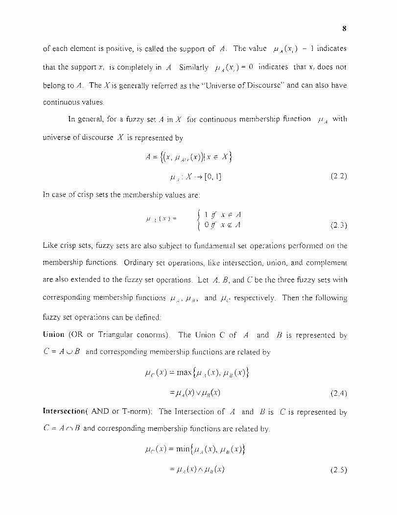
In general, for a fuzzy set A in X for continuous membership function ,u, with

universe of discourse X is represented by

(2.2)

In case of crisp sets the membership values are:

(2.3)

Like crisp sets, fuzzy sets are also subject to fundamental set operations performed on the

membership functions. Ordinary set operations, like intersection, union, and complement

are also extended to the fuzzy set operations. Let A, B, and C be the three fuzzy sets with

corresponding membership functions ,a3, and pc respectively. Then the following

fuzzy set operations can be defined:

Union (OR or Triangular conorms): The Union C of A and B is represented by

C = A c B and corresponding membership functions are related by

(2.4)

Intersection( AND or T-norm): The Intersection of A and B is C is represented by

C = A n B and corresponding membership functions are related by:

(2.5)

9

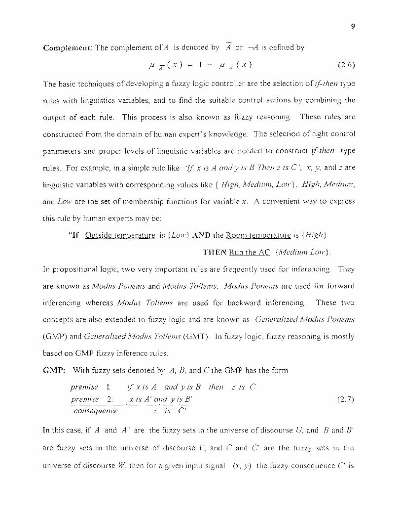
Complement: The complement ofA is denoted by A or —A is defined by

μ -A (x) = 1— uA (x) (2.6)

The basic techniques of developing a fuzzy logic controller are the selection of if-then type

rules with linguistics variables, and to find the suitable control actions by combining the

output of each rule. This process is also known as fuzzy reasoning. These rules are

constructed from the domain of human expert's knowledge. The selection of right control

parameters and proper levels of linguistic variables are needed to construct if-then type

rules. For example, in a simple rule like if x is A and y is B Then z is C', x, y, and z are

linguistic variables with corresponding values like { High, Medium, Low). High, Medium,

and Low are the set of membership functions for variable x. A convenient way to express

this rule by human experts may be:

"If Outside temperature is {Lou'} AND the Room temperature is gh}

THEN Run the AC {Medium Low).

In propositional logic, two very important rules are frequently used for inferencing. They

are known as Modus Ponems and Modus Tollems. Modus Ponems are used for forward

inferencing whereas Modus Tollems are used for backward inferencing. These two

concepts are also extended to fuzzy logic and are known as Generalized Modus Ponems

(GMP) and Generalized Modus Tollems (GMT). In fuzzy logic, fuzzy reasoning is mostly

based on GMP fuzzy inference rules.

GMP: With fuzzy sets denoted by A, B, and C the GMP has the form

premise I: if x is A and y is B then z is Cpremise 2: x is A' and y is B' (2.7)

consequence: z is C'

In this case, if A and A' are the fuzzy sets in the universe of discourse CI, and B and B'

are fuzzy sets in the universe of discourse I:, and C and C' are the fuzzy sets in the

universe of discourse W, then for a given input signal (x, y) the fuzzy consequence C' is

10

evaluated by taking the 'max-min' composition (operator o ) of the fuzzy relation

(Plana' B] in UxVxW and the fuzzy set (A 'and B') in UxV. This can be written

as:

(2.8)

(2.9)

Again the relation (/A and B] ›C) can be transformed into a ternary fuzzy relation R

and can he specified by:

(2.10)

Thus the relation (2.9) can be written as

(2 11)

If w, is the degree of match between A and A', evaluated from the operation

and if w, is the degree of match between B and 13', evaluated similarly from

then the relation (2.11) can be written as:

(2 12)

14; A W2 is called the firing strength of the rule or consequence C' [25].

CRISP

OUTPUTCRISPINPUT

1 FUZZIFICATIONUNIT

DEFUZZIFICATIONUNIT

11

2.2.1 Fuzzy Control

Conventional controllers, both linear and nonlinear, are derived from control theory based

on mathematical models of the systems to be controlled. Linear controllers are the

mapping of n input state vectors of a process and the control action to a hyperplane of

(n+1) dimensions. Nonlinear controllers are very difficult to synthesize, and this difficulty

is the key factor in the research of alternative control synthesis techniques, such as Fuzzy

Logic Controllers (FLC ) [12].

KNOWLEDGE BASE

RULE DATABASE BASE

FUZZY REASONING

MECHANISM

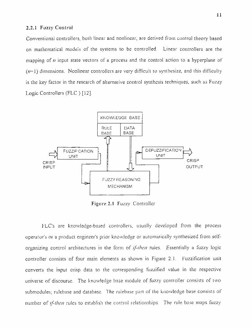
Figure 2.1 Fuzzy Controller

FLC's are knowledge-based controllers, usually developed from the process

operator's or a product engineer's prior knowledge or automatically synthesized from self-

organizing control architectures in the form of if-then rules. Essentially a fuzzy logic

controller consists of four main elements as shown in Figure 2.1. Fuzzification unit

converts the input crisp data to the corresponding fuzzified value in the respective

universe of discourse. The knowledge base module of fuzzy controller consists of two

submodules; rulebase and database. The rulebase part of the knowledge base consists of

number of if-then rules to establish the control relationships. The rule base maps fuzzy

12

values of the input to fuzzy values of the output, whereas database defines the membership

functions of the fuzzy sets, used as values for each system variable. Fuzzy reasoning

mechanism performs fuzzy inference to determine the fuzzy control actions by fuzzified

inputs. The final crisp control action is inferred through defuzzification unit by combining

the calculated outputs of each rule.

Ever since Mamdani [41] applied fuzzy set theory to control a steam engine and

boiler combination by a set of rules, there have been several fuzzy inferencing systems

proposed by various researchers reported in literature [34,35,27]. The popular methods,

which are related to this work will be discussed here.

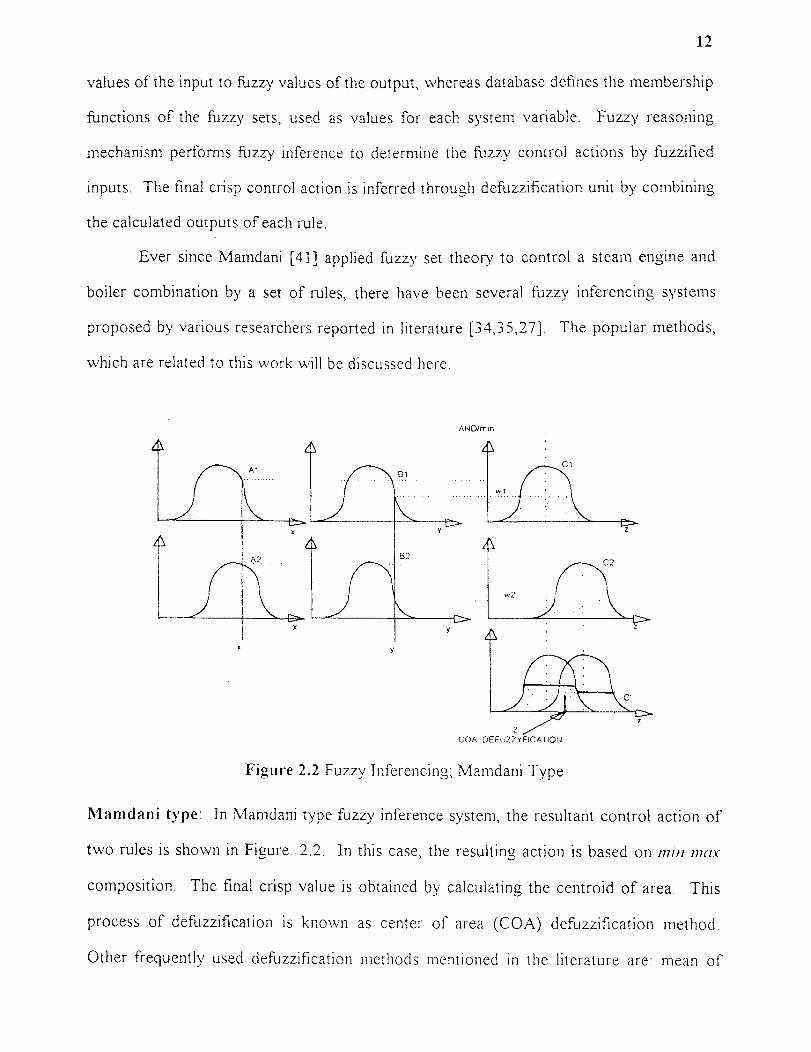
Figure 2.2 Fuzzy Inferencing; Mamdani Type

Mamdani type: In Mamdani type fuzzy inference system, the resultant control action of

two rules is shown in Figure. 2.2. In this case, the resulting action is based on Mill max

composition. The final crisp value is obtained by calculating the centroid of area. This

process of defuzzification is known as center of area (COA) defuzzification method.

Other frequently used defuzzification methods mentioned in the literature are: mean of

13 ,

maximum (MOM), largest of maximum, bisector of area etc. All these strategies are

computation intensive and there is no systematic way to evaluate them except through

experiments [25]. As Mendel mentioned in his tutorial paper on fuzzy logic systems,

"Many defuzzifiers have been proposed in the literature; however, there are no scientific

bases for any of them (i.e. no defuzzifier has been derived from a first principle, such as

maximization of fuzzy information or entropy), consequently, defuzzification is an art

rather than a science" [42].

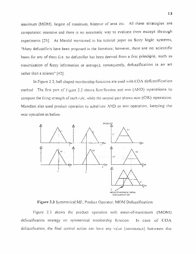
In Figure 2.2, bell shaped membership functions are used with COA defuzzification

method. The first part of Figure 2.2 shows fuzzification and Mill (AND) operations to

compute the firing strength of each rule, while the second part shows max (OR) operation.

Mamdani also used product operation to substitute AND or Mill operation, keeping the

max operation as before.

Figure 2.3 Symmetrical MF, Product Operator, MOM Defuzzification

Figure 2.3 shows the product operation with mean-of-maximum (MOM)

defuzzification strategy on symmetrical membership function. In case of COA

defuzzification, the final control action can have any value (continuous) between the

14

centers of two output membership functions (C 1 and C,), whereas in MOM defuzzification

the final control action will oscillate (jump around or discrete) between the centers of

consequent membership functions.

Tsukamoto type: Figure 2.4 shows Tsukamoto type fuzzy model for the same rules as

discussed in the Mamdani fuzzy model. Here the operations on premise parts i.e.

fuzzification and min operations, are same as before. However, Tsukamoto used

monotonical membership functions in the consequent part [58]. The overall control action

is the weighted average of each rule's crisp output. Although the consequent membership

functions are not compatible with linguistic terms such as "medium" whose membership

function should be bell shaped [27], this method is computationally efficient.

AND/min

Figure 2.4 Tsukamoto Type Fuzzy Inferencing

Sugeno type: In Sugeno type fuzzy model, also known as the TSK fuzzy model, the

output of each fuzzy rule is evaluated by a crisp function. The final control action is the

weighted average of each rule's crisp output. This model was originally proposed

Takagi, Sugeno and Kang [52,55]. For a three input fuzzy inferencing system the typical

output of a rule is given by:

if x 1 is A and x„ is B and is C then y —1(.v ) , x x 3) (2.13',

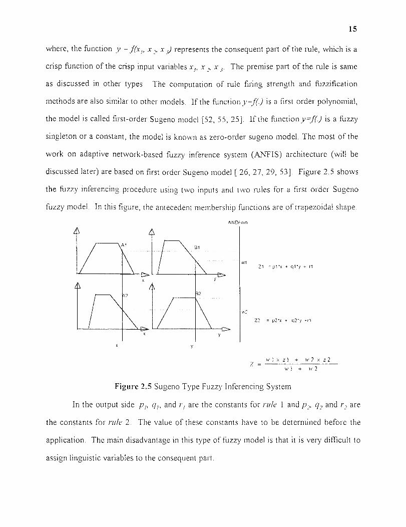
15

where, the function y =1(x,, x ) represents the consequent part of the rule, which is a

crisp function of the crisp input variables x 1 , x x 3 . The premise part of the rule is same

as discussed in other types. The computation of rule firing strength and fuzzification

methods are also similar to other models. If the function y----10 is a first order polynomial,

the model is called first-order Sugeno model [52, 55, 25]. if the function y="1.) is a fuzzy

singleton or a constant, the model is known as zero-order sugeno model. The most of the

work on adaptive network-based fuzzy inference system (ANFIS) architecture (will be

discussed later) are based on first order Sugeno model [ 26, 27, 29, 53]. Figure 2.5 shows

the fuzzy inferencing procedure using two inputs and two rules for a first order Sugeno

fuzzy model. In this figure, the antecedent membership functions are of trapezoidal shape.

AND/min

Figure 2.5 Sugeno Type Fuzzy Inferencing System

In the output side p 1 , q 1 , and r 1 are the constants for rule I and p,, q 2 and r, are

the constants for rule 2. The value of these constants have to be determined before the

application. The main disadvantage in this type of fuzzy model is that it is very difficult to

assign linguistic variables to the consequent part.

16

2.3 Neural Networks

A neural network (NN) is a structure that contains several neuron-like processing

elements connected together. A multilayered feed forward neural network is shown in

Figure 2.6. Each neuron receives several input signals which are then modified by the

interconnection weights and summed up to a single result. This result is then modified by

a transfer function, also known as activation function, and is then transmitted to the output

path.

INPUT HIDDEN OUTPUT

WEIGHTS . '

-WEIGHTS

NEURON

Figure 2.6 Multilayered Neural Net

In Figure 2.6, one hidden layer is shown between input and output layers. There

may be many intermediate hidden layers, but each neuron in hidden units must send its

output to a forward layer and must receive its input from a layer behind. Figure 2.7 shows

the activities of a neuron or processing element. The ith input to a neuron is x,„ and the

corresponding weight is 14'„. The activation function g(.) may be a sigmoid (1/(1 +e') ),

hyperbolic tangent (tanh(x)) or sinh(x), etc. A bias is may also be added to the sum.

For a given input vector, output vector will be computed by processing the input

vector layer by layer through each neuron until the output layer is reached. Each neuron

)0

17

will use the following relation for computation:

(2.14)

In most of the applications, sigmoid is used as function g(). There is no standard method

to deter 'nine the number of layers or the number of neurons in each layer of a neural

network. However, it has been shown that one hidden layer is enough to represent any

standard function [18].

BIAS

ActivationFunction g(.)

NEURON j

Figure 2.7 Processing element--Neuron

The learning of network is done by two phases: the forward pass and the backward

pass. In forward pass, the input is presented to the input layer and is fed forward from

layer to layer until the output is obtained. The output is compared with the desired output

and an error term is computed. In backward pass, this error is fed back to the input layer

and the weights are updated to minimize the error. The algorithm can be described as

follows:

For 17 training samples, the objective is to minimize total error E

(2 15)

18

where, X and Yd are input and desired output. NNw(Xi) is network output which

depends on the weights w of network NN. E is the mean squared error of the network

output and is differentiable over w. By minimizing E using gradient descent method, we

get the weight update equation as:

(2.16)

where i1 is the learning rate. The partial derivative of weights for each layer is computed

by chain rule [31].

2.4 Neuro Fuzzy Controller

Neural networks and fuzzy systems are universal approximators. As stated before, NN

can map complex relations without an explicit set of rules, while fuzzy systems can

estimate functions and control systems with only a partial description of system behavior

[31]. Recent research on applying NN and FLC techniques in the control of highly

complicated systems has shown encouraging results [65]. Although both NN and FLC are

independently useful for controlling nonlinear systems, each method has some limitations.

NN are very slow in learning and also need sufficient amount of training data to map a

relation. FLC needs a large number of rules which are often not available. Consequently,

recent research trend is to combine both the techniques in order to overcome the

limitations of individual schemes.

The basic concept of most of the hybrid controllers (Neuro-fuzzy controller) is to

design a FLC whose rules can be modified using NN learning techniques. In addition,

some of the reported hybrid controllers provide the facilities for the structure

identification. In this section, the research growth of the neuro-fuzzy controllers as well

as some popular schemes to blend NN concepts with fuzzy logic controllers are reviewed.

19

Kosko developed a fuzzy associative memory system, popularly known as FAM

[31] to map fuzzy input sets to fuzzy output sets. The system consists of a set of rules and

a set of weights associated with rules. By feeding the system with the training data, the

firing frequency of each rule is calculated. The weights are then modified by comparing

the firing frequency of each rule with a prescribed threshold value. Thus the learning

process determines a set of weights which can produce an optimal association of a fuzzy

output to a fuzzy input. The scheme doesn't allow any modification of the membership

functions and requires a large number of training cycles for learning. However, the

scheme provides a way to find the number of rules required for mapping. The FAM can be

treated as a FLC and has no direct relation with NN, other than the concept of weights

and training. Figure 2.8 shows the FAM architecture with one input and one output.

RULE I 1

RULE 2 I

FUZZY

INPUT

CRISPOUTDEFUZZIFIER

RULE n 1

Figure 2.8 Fuzzy Associative Memories (FAM)

Jang has developed a neuro fuzzy controller known as Adaptive Network-based

Fuzzy Inference System (ANFIS) [26,27] which can modify the parameters of the

membership functions of fuzzy control rules. Although several other researchers, like Lin

and Lee [40] and Wang and Mendel [59], independently proposed similar types of neuro

fuzzy frame work, Jang's main contribution is in the development of a hybrid learning

algorithm which combines the gradient descent method and least-squares estimators for

fast identification of parameters. However, this hybrid learning scheme is mostly suitable

AEN

FailureSignal

Internalreinforcernent

INPUTSTATE

OUTPUTACTION

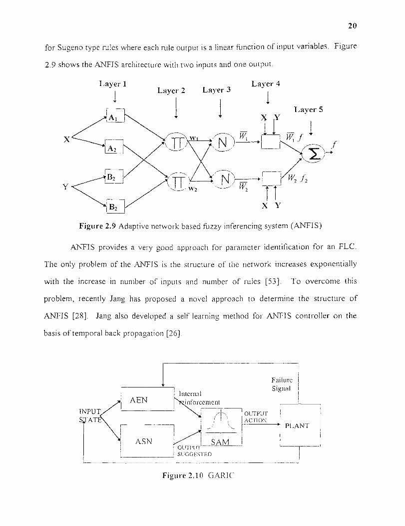
20

for Sugeno type rules where each rule output is a linear function of input variables. Figure

2.9 shows the ANTIS architecture with two inputs and one output.

Layer 1Layer 2 Layer 3

Layer 4

Layer 5

Figure 2.9 Adaptive network based fuzzy inferencing system (ANFIS)

ANTIS provides a very good approach for parameter identification for an FLC.

The only problem of the ANTIS is the structure of the network increases exponentially

with the increase in number of inputs and number of rules [53]. To overcome this

problem, recently Jang has proposed a novel approach to determine the structure of

ANTIS [28]. Jang also developed a self learning method for ANTIS controller on the

basis of temporal back propagation [26].

ASNOUTPUT ITNFr

SUGGESTED

Figure 2.10 GARIC

21

Supervised learning algorithms for neural networks and neuro-fuzzy controllers

require precise training data sets for identification of weights and parameters. This precise

training/learning data are generally difficult and expensive to obtain for some real-world

applications. For this reason, reinforcement learning algorithms are initially developed for

NN [39,40]. In case of reinforcement learning, the training data are not precise like

supervised learning, instead they are evaluative. Using reinforcement learning paradigm,

Berenji and Khedkar proposed a generalized approximate reasoning-based intelligent

control architecture (GARIC). The GARIC architecture consists of three main elements:

the action selection network (AEN), the action evaluation network(ASN), and a stochastic

action modifier (SAM). The ASN is a fuzzy controller which maps a state vector into a

recommended action. The AEN is a two-layer NN used to produce an internal

reinforcement based on a given state and failure signal. The SAM uses both

recommended action and internal reinforcement to produce a final output which is applied

to the plant. The learning takes place by fine-tuning the weights of AEN and the

parameters describing membership functions of ASN using reinforcement learning

algorithm. Figure 2.10 shows the architecture of GARIC.

Although GARIC has been reported as an effective tool to control nonlinear

dynamic systems, the main problem in practical implementation is the need to determine

the structure of ASE. Lin and Lee [39], independently proposed a similar reinforcement

neural-network-based fuzzy logic control systems (RNN-FLCS) like GARIC to solve

various reinforcement learning problems.

Recently, Chang has proposed a scheme known as Fuzzy Logic Adaptive Network

(FLAN) by combining some features of ANFIS and FAM [14]. The FLAN is basically the

ANFIS structure with the weights associated with each rule as mentioned in FAM. The

performance of FLAN is comparable with ANFIS and in some situations training time of

FLAN is less than ANTIS. Figure 2.11 shows the architecture of FLAN. Chang has used

A1.B1 -> CI

A2 -->

22

FLAN to identify nonlinear dynamic systems with unknown parameters using the

identification models from Narendra and Parthasarathy [43].

B1

[B,

A1,B2-> C3

A 2.B2 ->

Figure 2.11 Fuzzy logic adaptive network (FLAN)

Although all of the above mentioned schemes are very important, it is evident that

more efficient hybrid controller can be developed by cleverly combining certain good

features from the above methods. The main objective of this research is to develop a

generalized scheme to design an adaptive FLC and to apply the controller on a nonlinear

engineering system to study the performance. ANTIS, as discussed earlier, can be treated

as a generic framework, and in that sense appears to be an excellent basis for an improved

neuro-fuzzy controller. However, Sugeno type rules with hybrid learning scheme [26,27]

may result in unbounded, nonphysical defuzzification. To avoid this problem of

defuzzification, more conventional fuzzy schemes for the consequent part are used instead

of using Sugeno type rules. The proposed FLC is trained by using the learning concepts

of NN. The back propagation algorithm, which is the most popular for the training of NN

is used to train the proposed controller. The proposed controller is also used on a

nonlinear dynamic system to study its performance.

23

2.5 Proposed Neuro-Fuzzy Controller

As discussed in the section 2.4, the main thrust in the research of neuro-fuzzy controller is

to find a novel method to structure the fuzzy inferencing systems in the form of a node

based network with differentiable parameters. This will allow the network to train by

using a suitable back propagation algorithm available in the neural network literature.

There should be enough flexibility to accommodate multiple input with various

combination of rules. In the first part of this dissertation, a network architecture suitable

to represent all types of fuzzy model is developed. Since the philosophy behind this

architecture is to blend fuzzy inferencing system with neural network, the proposed

structure resembles action selection network (ASN) of GARIC [9], and ANFIS [26].

However, provisions are provided to incorporate new concepts resulting from

experimental part of this research. The findings of the experimental research and the

subsequent modifications will be discussed in the next chapters. Since this proposed

network will be used to incorporate strengths of various independently developed neuro-

fuzzy networks, hereafter this network will be referred as Generalized Network based

Fuzzy Inferencing System or in short GeNFIS.

2.5.1 GeNFIS Architecture

GeNFIS is a five layer network as shown in Figure 2.12. Each layer consists of several

nodes which perform specified action to represent fuzzy inferencing mechanism. For

simplicity a two input three rule network is considered for illustration. Although the rules

selected here are of Mamdani type with bell shaped membership functions, the final

control action is very similar to Tsukamoto type with suitable modifications. In Figure

2.12, k, is the output of rule i, and is given by:

(2 17)

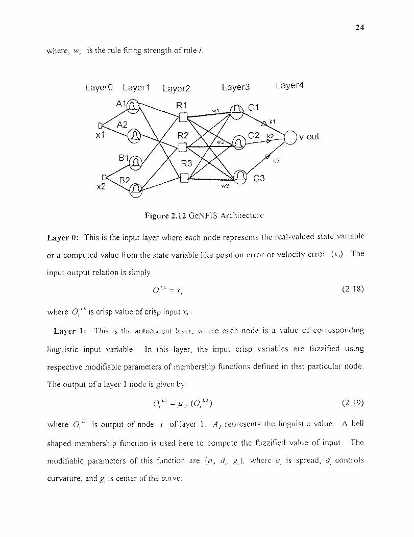
where, w, is the rule firing strength of rule i.

Layer0 Layerl Layer2 Layer3 Layer4

24

Figure 2.12 GeNFIS Architecture

Layer 0: This is the input layer where each node represents the real-valued state variable

or a computed value from the state variable like position error or velocity error (x,). The

input output relation is simply

0 L° = x (2. 1 8)

where 0," is crisp value of crisp input x, .

Layer 1: This is the antecedent layer, where each node is a value of corresponding

linguistic input variable. In this layer, the input crisp variables are fuzzified using

respective modifiable parameters of membership functions defined in that particular node.

The output of a layer 1 node is given by

OLi=μAI (OiL0) (2.19)

where 0, n is output of node i of layer 1. A I represents the linguistic value. A bell

shaped membership function is used here to compute the fuzzified value of input. The

modifiable parameters of this function are {a,, d,, g,}, where a, is spread, d, controls

curvature, and g, is center of the curve.

25

(2 20)

Layer 2: This layer computes AND or rain operations to evaluate the value of if part of

each rule. A differentiable softmin operator is used here [9] to perform the T-norm

operation. The output of this layer is given by

(2 21)

where k is a constant, controls the hardness of the softmin operation, and for k = cc, the

original min operator is recovered [9]. In ANTIS a product operator is used [27]. These

operators (product or solimiii) are suitable for computing derivatives for backpropagation

learning algorithm.

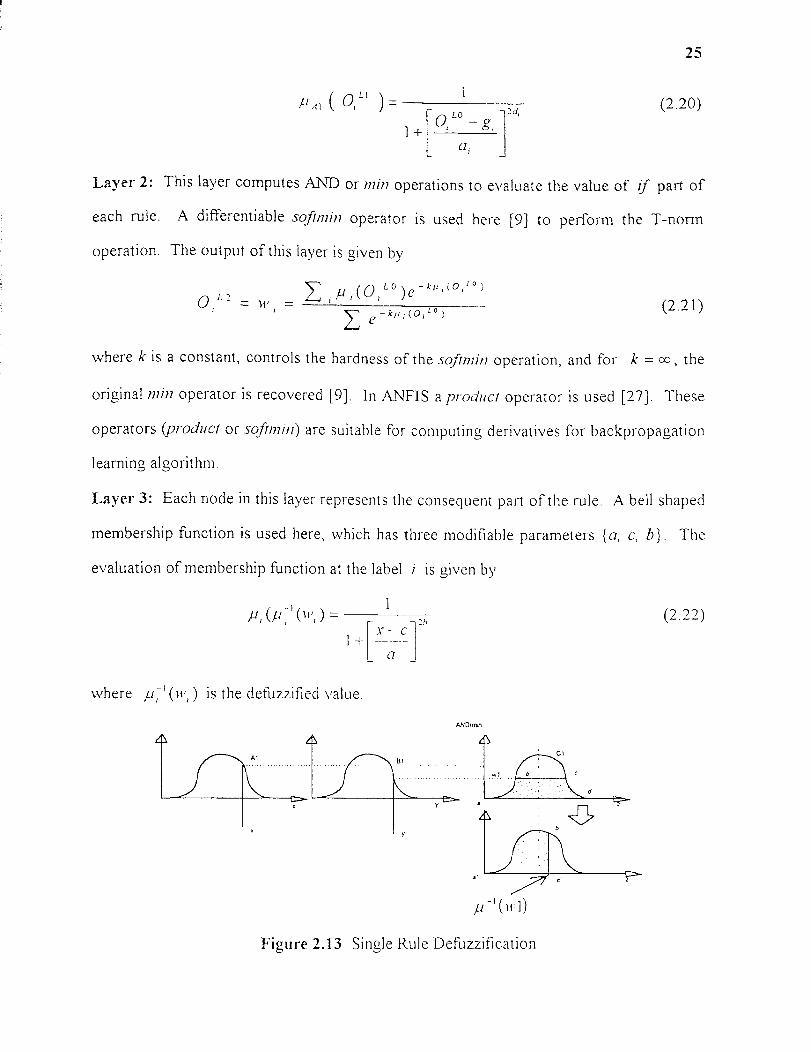
Layer 3: Each node in this layer represents the consequent part of the rule. A bell shaped

membership function is used here, which has three modifiable parameters {a, c, b}. The

evaluation of membership function at the label i is given by

(2.22)

where 11 - '(w,) is the defuzzified value.

1( w1 )

Figure 2.13 Single Rule Defuzzification

CO = / = f(a),

or I = k * (2.23)

26

A local defuzzification method has been used at each label. This local

defuzzifiction method (LDM) is suitable for a symmetrical membership function. For a

symmetrical membership function, a local defuzzification method like LMOM (local

mean-of-maximum) [9], will always yield a constant value. Hence LDM is developed

from the concept of area of a membership function clipped by a single rule firing strength

[25] and mapping this area from the left hand side as shown in Figure 2.13. In Figure

2.13, the clipped area abed has been mapped as a'b'c' for defuzzification, and the final

defuzzified value is c'. For a given rule firing strength, multiplying the clipped area by a

suitable scale factor X ( 1.0 > X 0.5) and by mapping the scaled area as before, we can

set the upper limit of defuzzification.

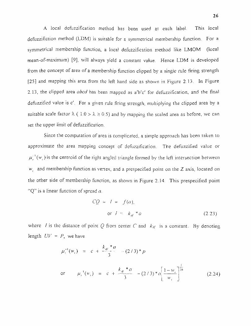
Since the computation of area is complicated, a simple approach has been taken to

approximate the area mapping concept of defuzzification. The defuzzified value or

(w, ) is the centroid of the right angled triangle formed by the left intersection between

w, and membership function as vertex, and a prespecified point on the Z axis, located on

the other side of membership function, as shown in Figure 2.14. This prespecified point

"Q" is a linear function of spread a.

where I is the distance of point 0 from center C and kdf is a constant. By denoting

length UV = P, we have

(2.24)

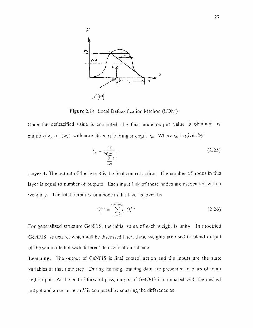
27

,u 1 (14/

Figure 2.14 Local Defuzzification Method (LDM)

Once the defuzzified value is computed, the final node output value is obtained by

multiplying with normalized rule firing strength t„,. Where 1„, is given by

(2.25)

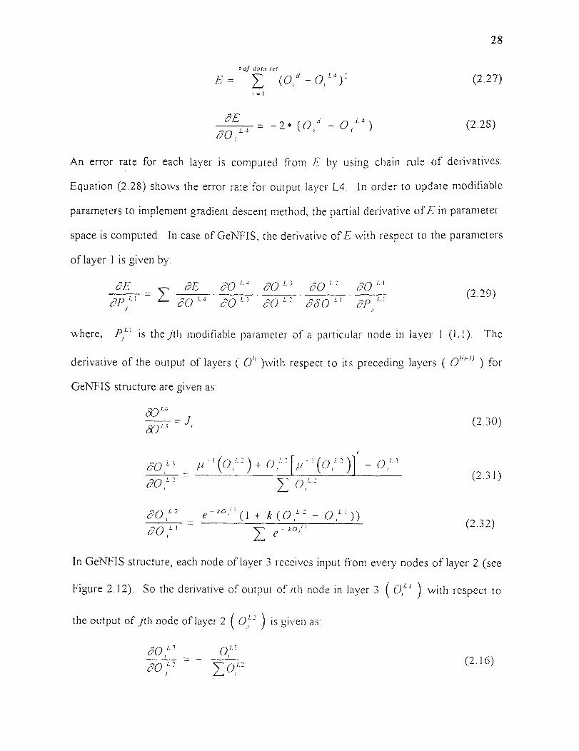
Layer 4: The output of the layer 4 is the final control action. The number of nodes in this

layer is equal to number of outputs. Each input link of these nodes are associated with a

weight j,. The total output 0, of a node in this layer is given by

(2.26)

For generalized structure GeNFIS, the initial value of each weight is unity. In modified

GeNFIS structure, which will be discussed later, these weights are used to blend output

of the same rule but with different defuzzification scheme.

Learning. The output of GeNFIS is final control action and the inputs are the state

variables at that time step. During learning, training data are presented in pairs of input

and output. At the end of forward pass, output of GelNFIS is compared with the desired

output and an error term E is computed by squaring the difference as:

of data setE (0 _ 0, 1.4 )2

of

i =1

L4 0 d= -2* — n L 4

tin (

)i

28

(2.27)

(2.28)

An error rate for each layer is computed from E by using chain rule of derivatives.

Equation (2.28) shows the error rate for output layer L4. In order to update modifiable

parameters to implement gradient descent method, the partial derivative of E in parameter

space is computed. In case of GeNFIS, the derivative of E with respect to the parameters

of layer 1 is given by:

(2.29)

where, Pin is the jth modifiable parameter of a particular node in layer I (L1). The

derivative of the output of layers ( )with respect to its preceding layers ( 0' 4' ) for

GeNFIS structure are given as:

(2.30)

(2.31)

(2.32)

In GeNFIS structure, each node of layer 3 receives input from every nodes of layer 2 (see

Figure 2.12). So the derivative of output of ith node in layer 3 ( 0/ -3 ) with respect to

the output of jth node of layer 2 ( ) is given as:

(2.16)

29

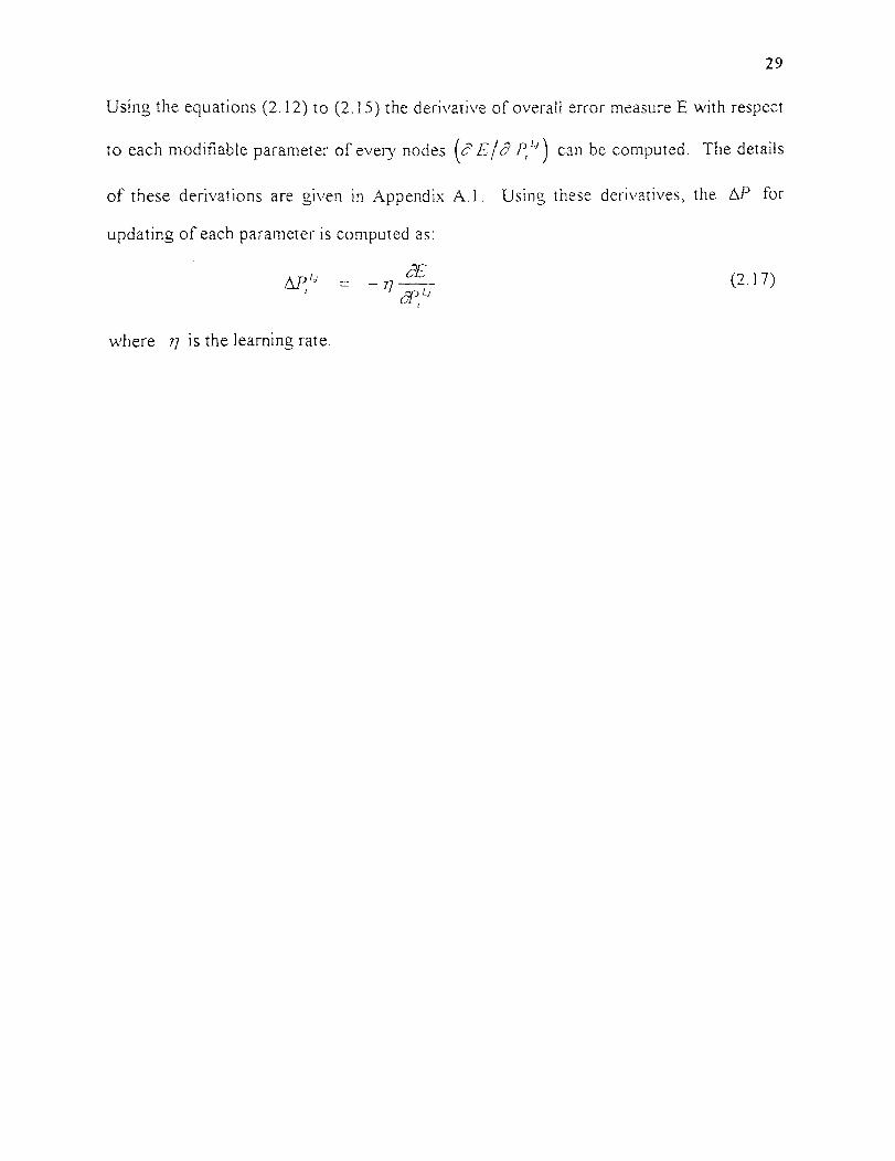
Using the equations (2.12) to (2.15) the derivative of overall error measure E with respect

to each modifiable parameter of every nodes (∂E/∂ P1LJ can be computed. The details

of these derivations are given in Appendix A1. Using these derivatives, the ΔP for

updating of each parameter is computed as:

(2.17)

where η is the learning rate

CHAPTER 3

A NON LINEAR DYNAMIC SYSTEM

3.1 Introduction

Application of fuzzy logic in control of nonlinear dynamic systems is advantageous, in

particular when the mathematical model of the plant under control is either not available or

very complicated. Moreover, when the operating conditions of the plant vary

significantly, designing a controller using conventional control theory becomes difficult.

After Mamdani's first effort to control a steam engine and boiler combination by a set of

linguistic control rules using the knowledge of experienced operators [25,41], a significant

effort has been made by various investigators to apply fuzzy logic to industrial problems

where the model of the plants are not available or ill defined. However, in the literature,

most of the results reported on the research of neuro-fuzzy controllers are tested on

simulation. Most newly proposed neuro-fuzzy controllers are evaluated through

simulation of the bench mark problem of balancing an inverted pendulum to represent

nonlinear dynamic system charectaristics [9,26,39,46,25]. However, in [56] an

experimental setup of an inverted pendulum is used to test the proposed neural network

driven fuzzy reasoning (NNDF) model. In this experiment, training data sets were

collected by balancing the pendulum manually. Other than this work [56], few

experimental studies on neuro-fuzzy controllers, suitable for academic environment are

reported in the literature.

One of the major objective of this dissertation is to develop a neuro-fuzzy

controller and to apply it in an experimental setup suitable for academic environment. In

order to meet this objective a fluid beam balancing system is used as a test bed of non-

linear dynamic system for this work. In this chapter the details of experimental setup, the

model of the system, and its simulation using a conventional controller are presented.

30

Tank 1 Tank 2

Pressure Sensors• Potentiometer

31

3.2. Balance Beam System.

The basic problem of the balance beam system is to balance a beam containing two fluid

tanks, one at each end, by pumping the fluid back and forth from the tanks [37].

Figure3.1 shows the schematic diagram of the fluid beam balancing system. The beam is

comprised of a wooden plank clamped on top of a shaft about which it can rotate. The

shaft is supported by two low friction bearings, and at the one end of the shaft a Hall

effect sensor is connected to measure angular position of the beam. The center of the

mass of the complete system is above the center of rotation. This feature makes the

system unstable. Figure 3.2 shows that the net torque due to disturbance is in the same

direction of rotation.

Pumps

WoodenBeam

Figure 3.1 Balance beam system

Control effort is created by pumping water between two plastic tanks, thereby creating a

moment due to weight imbalance. Two d.c. pumps powered by linear amplifiers are

biased and connected in parallel to provide the pumping between the two tanks. The

32

input/output characteristics of the pump shows that there exists a dead zone in the region

of small input where input cannot incur effective output. To avoid this dead zone two

pumps are used in parallel [37]. In addition to position measurement sensor, there are two

pressure sensors to measure the mass of the liquid provided for each tank. Signal

conditioning and calibration of the pressure readings provide necessary mass information.

Right Ann

Arm

Figure 3.2 Net torque in the same direction of rotation

3.2.1 System Model

The balance beam system has been modeled as a fourth order nonlinear system by the

following relations

(3.1)

(3.2)

(3.3)

(3.4)

33

where

x 1 = angular position of beam

= angular velocity of beam

h= height of water in left tank

0= flow rate of water

B= friction coefficient of bearing

T(xl,h) =torque due to water

J(h)= rotational moment of inertia of the system

A= area of tank

K pump= motor constant of pump

pumpT = time constant of motor

U = output of controller ( voltage)

The equations (3.1) and (3.2) are from the dynamics of beam, which is given by

(3.5)

and the equation (3.3) is from the dynamics of tank. The fourth equation (3.4) is the

equation of pump flow rate which has been modeled as a first order system with the

following transfer function

(3.6)

Using this equations, a state feedback control law is given in equation (3.7). Details of

these equations and the values of the constants are provided in the Appendix C.

U(k) = kp*(xl-ref(k) -x 1 (k)) T ki* 2:( (k) -X (k)) -4"

kJ* (

kill *(/7(k) -h_ref(k)) (3.7)

where

34

xl-ref= position set point

x2_„! -- velocity set point

h ref= equilibrium height of the left tank( i.e. water height needed to make

T(x1, h) = 0), which is given by

h ref= ( -7.429 - 0.2238 *H) *x i + H/2 (3. 7A)

x2 estimate = estimated velocity=(x l (k+ 1))-xl(k))/sample_time;H is the total water height.

The cascaded control loops equivalent to the control law of equation (3.7) is given in

Appendix.C.

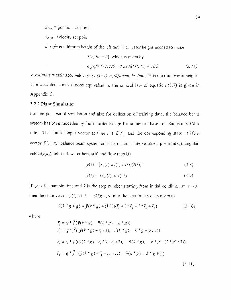
3.2.2 Plant Simulation

For the purpose of simulation and also for collection of training data, the balance beam

system has been modelled by fourth order Runge-Kutta method based on Simpson's 3/8th

rule. The control input vector at time t is u(/), and the corresponding state variable

vector 5(t) of balance beam system consists of four state varables; position(x 1 ), angular

velocity(x2), left tank water height(h) and flow rate(Q).

y=x,(t)x2(t),x2(t),h(t)O(t)]T (3.8)

53 M = (y(t)u(t),t) (3.9)

If g is the sample time and k is the step number starting from initial condition at t =0,

then the state vector 5)(/) at t = (k*g g) or at the next time step is given as

y(k * g + g) =53 (k * g) + (118)(1 + 3 + 3 * r3 +i, ) (3 . 1 0)

where

g* 10- (k * g), (k * g), k * g))

= g * I ((yak * g)+ 13), u(k *g), k* g + g I 3))

7:1 = g *.f ((y(k * g)+ F, 13 +F., / 3), * g), k * g + (2 * g) 1 3))

g * ( (y)(k * g) + —r, u(k * g), k * g + g)

(3.11)

35

The relations (3.1) to (3.2) are used for simulation. By tuning the control gains, it is

observed that the control law given in equation (3.7) can balance the beam form the

folowing initial conditions

at t=0, .1- 1 (t) =-0.03 rad, .1- 2 (1) = 0.0 rads/sec

H = 10.4 cm and h _ref from equation (3.7A)

where position set point (1 .71.,,f) is 0.0 rad and velocity set point (x2-ref) is 0.0 rads//sec.

In simulation the initial value of water height error (h(t) - h_ref(t)) has been assumed to be

zero, but in real application this is not true and very difficult to compute.

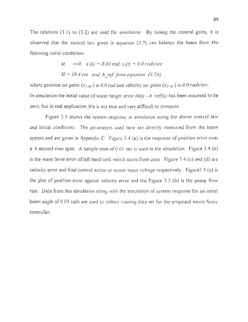
Figure 3.5 shows the system response in simulation using the above control law

and initial conditions. The parameters used here are directly measured from the beam

system and are given in Appendix C. Figure 3.4 (a) is the response of position error over

a 6 second time span. A sample time of 0.01 sec is used in the simulation. Figure 3.4 (b)

is the water level error of left hand tank which starts from zero. Figure 3.4 (c) and (d) are

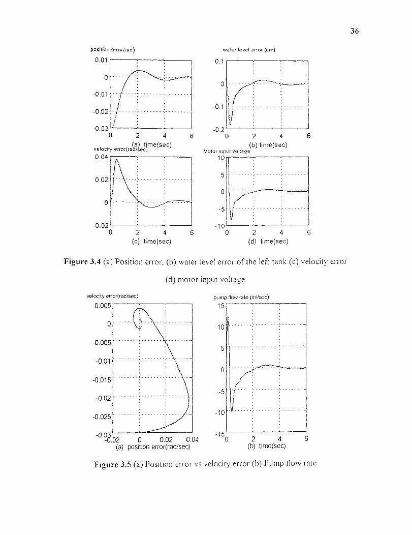
velocity error and final control action or motor input voltage respectively. Figure3.5 (a) is

the plot of position error against velocity error and the Figure 3.5 (b) is the pump flow

rate. Data from this simulation along with the simulation of system response for an initial

beam angle of 0.03 rads are used to collect training data set for the proposed neuro fuzzy

controller.

36

position error(rad) water level error (cm)

(c) time(sec) (d) time(sec)

velocity error(rad/sec) pump flow rate (ml/sec)

(a) pos ition error(rad/sec) (b) time(sec)

(a) time(sec)velocity error(rad/sec)

(b) time(sec)Motor input voltage

Figure 3.4 (a) Position error, (b) water level error of the Jell tank (c) velocity error

(d) motor input voltage

Figure 3.5 (a) Position error vs velocity error (b) Pump flow rate

CHAPTER 4

REA LTIM E CONTROL

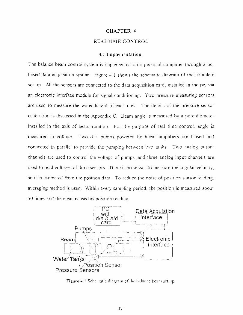
4.1 Implementation.

The balance beam control system is implemented on a personal computer through a pc-

based data acquisition system. Figure 4.1 shows the schematic diagram of the complete

set up. All the sensors are connected to the data acquisition card, installed in the pc, via

an electronic interface module for signal conditioning. Two pressure measuring sensors

are used to measure the water height of each tank. The details of the pressure sensor

calibration is discussed in the Appendix C. Beam angle is measured by a potentiometer

installed in the axis of beam rotation. For the purpose of real time control, angle is

measured in voltage. Two d.c. pumps powered by linear amplifiers are biased and

connected in parallel to provide the pumping between two tanks. Two analog output

channels are used to control the voltage of pumps, and three analog input channels are

used to read voltages of three sensors. There is no sensor to measure the angular velocity,

so it is estimated from the position data. To reduce the noise of position sensor reading,

averaging method is used. Within every sampling period, the position is measured about

50 times and the mean is used as position reading.

PCwith

d/a & a/dcard

Pumps

Beam

Data AcquistionInterface

ElectronicInterface

Water Tanks,Position Sensor

Pressure Sensors

Figure 4.1 Schematic diagram of the balance beam set up

37

38

4.2 Real Time Programming

Real time computer systems should deliver the results in correct coordination with other

systems operating asynchronously to the computer and to each other. The most of the

simple real time problems can be solved by synchronous programming. A typical program

of this class has a section to initialize data, place physical devices in appropriate initial

states and run the program in an unending loop. A sample real time synchronous program

for data acquisition is shown in Figure 42. In this program an analog voltage is read from

a sensor through "analog in" channel of the data acquisition card, and the instantaneous

digital value of this voltage is sent to the "analog out" channel using a continuos loop.

#include <stdio.h>#include "io-fun.h" /* 1/O function definition */main()

double volts;int channel l = 1, channel 2 =2;

while(!kbhitO

volts = a2d(channel_2);/* read a voltage from analog inchannel 2 */

d2a(channel_l ,volts); /* output the same voltage toanalog out channel 2 */

Figure 4.2 Synchronous program

In order to achieve true multitasking environment in a time critical or event driven

situation, asynchronous, or multi-thread programming is needed [3]. Asynchronous

programs are implemented by interrupts, which are hardware mechanisms in the computer

that allow for the interruption of one thread of execution by another higher priority thread.

The terms foreground and background are often used in connection with the high and low

priority sections of such programs [3].

Figure 4.3 shows a program template which has been used to build the control

program. This requires an action taking place on a strict time schedule plus another

activity that is not time critical. In a control program, the time-critical section is used to

implement a controller loop while the non-time critical section is used to get a new

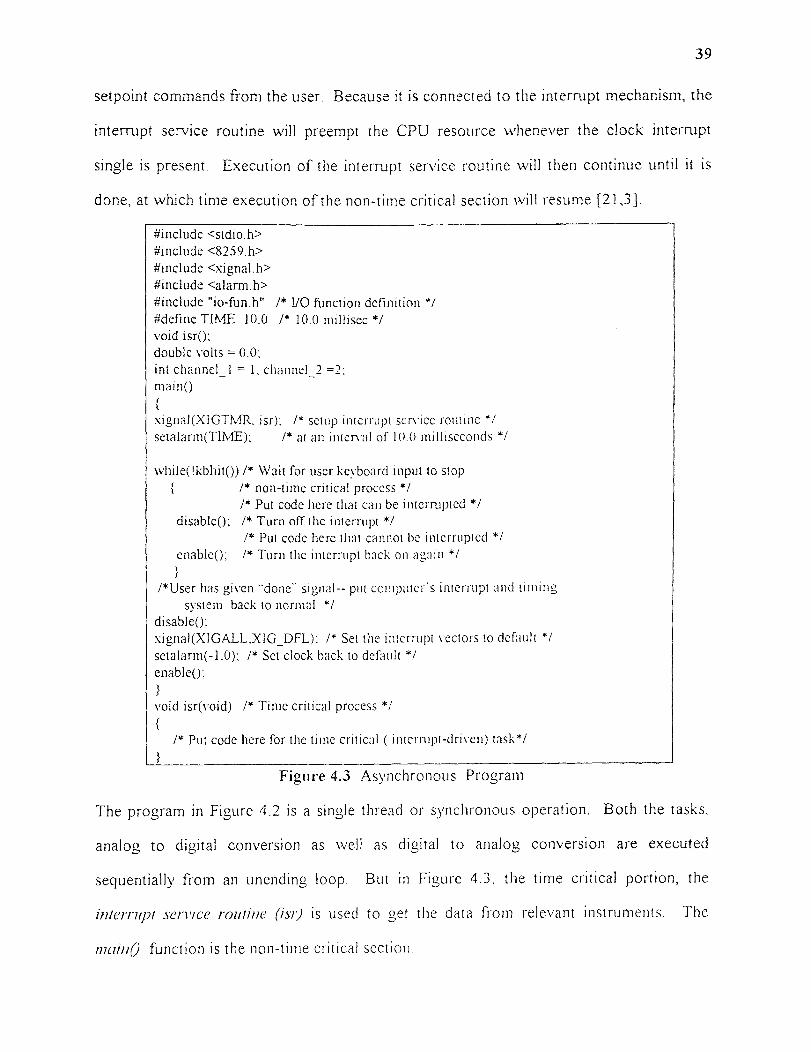
39

setpoint commands from the user. Because it is connected to the interrupt mechanism, the

interrupt service routine will preempt the CPU resource whenever the clock interrupt

single is present. Execution of the interrupt service routine will then continue until it is

done, at which time execution of the non-time critical section will resume [21,3].

#include <stdio.h>#include <8259.h>#include <xignal.h>#include <alarm.h>#include "io-fun.h" /* I/O function definition */#define TIME 10.0 /* 10.0 millisec */void isr();double volts = 0.0:int channel_l = 1, channel_2 =2:main()

xignal(XIGTMR. isr); /* setup interrupt service routine */setalarm(TIME); /* at an interval of 10.0 milliseconds */

while(!kbhit()) /* Wait for user keyboard input to stop/* non-time critical process *//* Put code here that can be interrupted */

disable(); /* Turn off the interrupt *//* Put code here that cannot be interrupted */

enable(); /* Turn the interrupt back on again */

/*User has given "done" signal-- put computer's interrupt and timingsystem back to normal */

disable();xignal(XIGALL,XIG_DFL): /* Set the interrupt vectors to default */setalarm(-1.0): /* Set clock back to default */enable();

void isr(void) /* Time critical process */

/* Put code here for the time critical ( interrupt-driven) task*/

Figure 4.3 Asynchronous Program

The program in Figure 4.2 is a single thread or synchronous operation. Both the tasks,

analog to digital conversion as well as digital to analog conversion are executed

sequentially from an unending loop. But in Figure 4.3, the time critical portion, the

interrupt service routine (isr) is used to get the data from relevant instruments. The

177(11110 function is the non-time critical section.

40

4.3 Rule Construction

As discussed in the section on GeNFIS architecture, the structure of proposed neuro-

fuzzy controller depends on the selection of rules. The fuzzy control rules for the beam

balancing system have been constructed from the training data set. Although no formal

rule generation algorithm has been developed in this work, the rules have been selected by

finding the relation between input space and output space as discussed in FAM [31]. In

addition, the association between different inputs are used to construct the premise part of

the rules. The output and input data sets are first grouped in the different fuzzy sets like

positive high, negative low, zero, etc. Next for each of the output fuzzy level, all the

corresponding fuzzy sets of each input variables are tabulated. Each row of such table is a

possible rule. The initial set of rules are selected by resolving the conflict among the rules.

Then the conflict from the premise parts of the rules are removed. A further reduction in

number of rules, if required, is done by removing similar type of rules. Finally, the rule

base is enhanced by observing the performance of the system under control. The success

of this rule generation method depends on the availability of a good set of training data.

In this work, the training data sets are generated from simulation.

The GeNFIS structure used in this experiment consists of three inputs, eleven rules

and one output. After an exhaustive on line investigation, starting from seven rules, it has

been observed that eleven rules and three inputs are required to balance the beam in the

horizontal position or at zero set point. It has also been observed that a GeNFIS

controller can even balance the beam with only seven to nine rules. But in case of fewer

number of rules, the controller can not stabilize the beam around the given set point. The

beam will move away from the set point in a balanced condition.

The three inputs used here are position error, velocity error, and the water height

error of left hand beam. The output of the controller is the motor control voltage. As

41

discussed in chapter two, the fu77y control rules are constructed by using linguistic

variables. Table 4.1 shows the different labels used to represent state variables. The

position of the beam is measured directly by using a potentiometer, whereas the velocity is

calculated from position data and time. The water height error is also computed from the

two pressure measuring sensors located at the bottom of each water tank Five labels are

used to define the linguistic values of position error and water height error. These labels

are: Negative Large (NL), Negative Small (NS), Zero (ZE), Positive Small (PS), Positive

Large (PL). Since the measurement of velocity is indirect, only three labels, Negative (N),

Zero (Z) and Positive (P) are used to define velocity error. Table 4.2 explains the nine

labels of output voltage recommended by the fuzzy control rules.

Table 4.1 Different labels of input variablesSTATE VARIABLES LABELS

NLNS

8 (Position error) ZEPSPL NT

8 (Velocity error)

NLNS

h....(Water height error) ZEPSPL

Table 4.2 Different labels of outputOUTPUT VARIABLE LABELS

NM (Negative Maximum)NL (Negative Large)MN (Medium Negative)NS (Negative Small)

21.-- (Control voltage) ZE (Zero)PS (Positive Small)MP (Medium Positive)PL (Positive Large)PM (Positive Maximum)

42

As mentioned earlier, a total number of eleven fuzzy control rules are stored in the

rule base of GeNFIS for this experiment. Table 4.3 shows the details of each rule. These

rules can be read as:

Rule If position error is ML and velocity error is N and water height error is NL

then the control output is NM

Rule 2: If position error is NS and water height error is NL

then the control output is NL

Rule 11: If position error is PL and velocity error is P and water height error is PL

then the control output is PM

Table 4.3 The 11 fuzzy control rules of GeNFISRULE # Position Velocity Leff water height Control voltage

1 NL N NL NM 2 NS -- NL NL 3 --- Z NS MN 4 NI_ Z --- MN5 NL -- ZE NS6 ZE Z ZE ZE7 PL -- ZE PS8 PL Z --- MP. 9 --- Z PS MP10 PS -- PL PL11 PL P PL PM

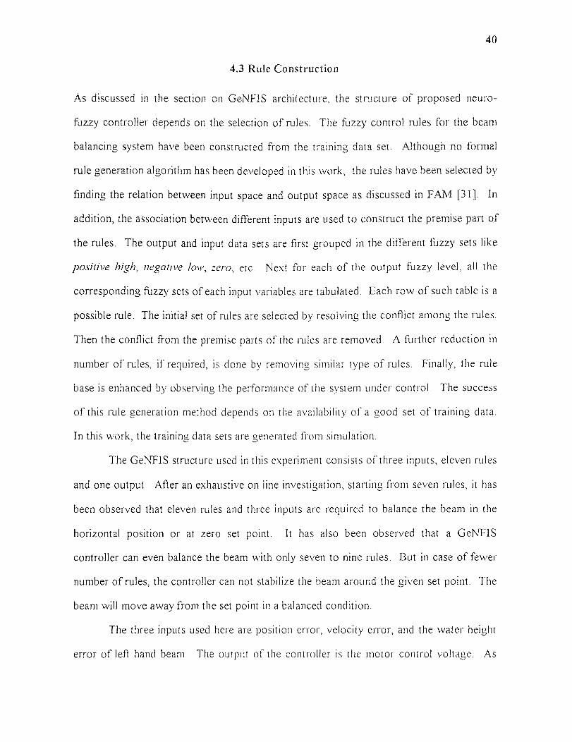
Mier finalizing the structure of GeNFIS, training is done by using the data set

obtained from simulation, as discussed in the section of plant simulation (section 3.2.2).

The input-output data pairs are collected by running the simulation program twice, with

two different sets of initial conditions. In both the cases, initial values of velocity and

water height errors are taken as zero. The initial angle of beam is taken as 0.03 radians for -

the first run, and -0.03 radians for the second run. In each simulation, a sample time of

0.01 second is used with the run time of 6 seconds. The simulation results (Figure 3.4)

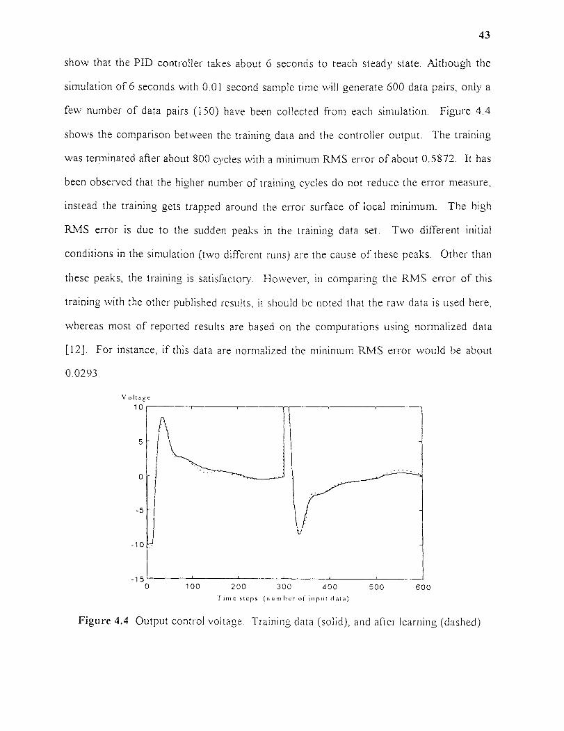
43

show that the PID controller takes about 6 seconds to reach steady state. Although the

simulation of 6 seconds with 0.01 second sample time will generate 600 data pairs, only a

few number of data pairs (150) have been collected from each simulation. Figure 4.4

shows the comparison between the training data and the controller output. The training

was terminated after about 800 cycles with a minimum RMS error of about 0.5872. It has

been observed that the higher number of training cycles do not reduce the error measure,

instead the training gets trapped around the error surface of local minimum. The high

RMS error is due to the sudden peaks in the training data set. Two different initial

conditions in the simulation (two different runs) are the cause of these peaks. Other than

these peaks, the training is satisfactory. However, in comparing the RMS error of this

training with the other published results, it should be noted that the raw data is used here,

whereas most of reported results are based on the computations using normalized data

[12]. For instance, if this data are normalized the minimum RMS error would be about

0,0293.

Time steps (number of input data)

Figure 4.4 Output control voltage. Training data (solid), and after learning (dashed)

44

Figure 4.5(a) shows the five initial membership functions (MF) of the position

error input. All the parameters of each initial MFs are same. The centers of the bell shape

functions are equally spaced in the input data space. The position is measured in voltage,

so for training and simulation the conversion from radians to voltage is needed. Figure

4.5(b) shows the final MFs.

(a) Initial membership functions; position error(volt)

(b) Final membership functions; position error(volt)

Figure 4.5 (a)Initial MF, and (b) Final MT . of position error (volt)

The three initial and final membership functions for the velocity error are shown in

Figure 4.6 (a) and (b) respectively. The initial and final membership functions for left hand

water height error are shown in Fig. 4.6(c) and (d) respectively. It may be noted that the

width of the three membership functions became very small. The water height error is

computed in cm from the raw pressure data in voltage. The eleven output initial and final

membership functions are shown in Figure 4.7 (a) and (b) respectively. Although the

range of output control voltage is from -10.0 to +10.0, the centers of some of the final

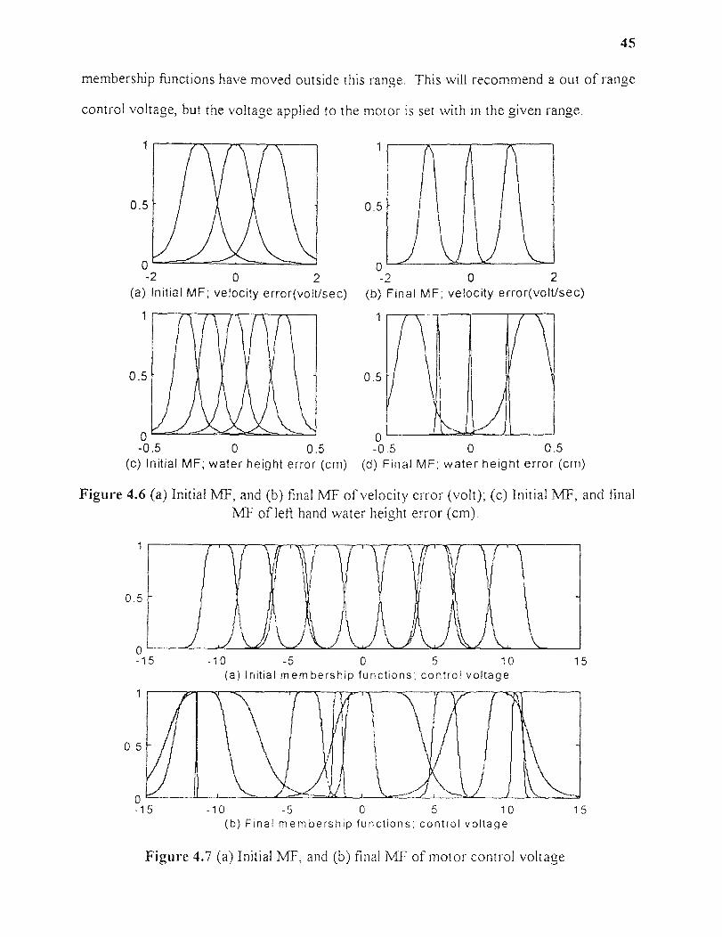
45

membership functions have moved outside this range. This will recommend a out of range

control voltage, but the voltage applied to the motor is set with in the given range.

(a) Initial MF; velocity error(volUsec) (b) Final MF; velocity error(volUsec)

(c) Initial MF; water height error (cm)-•-

(d) Final MF; water height error (cm)

Figure 4.6 (a) Initial MF, and (b) final MF of velocity error (volt); (c) Initial MT, and finalMT of left hand water height error (cm).

(a) Initial membership functions; control voltage

(b) Final membership functions; control voltage

Figure 4.7 (a) Initial MF, and (b) final MF of motor control voltage

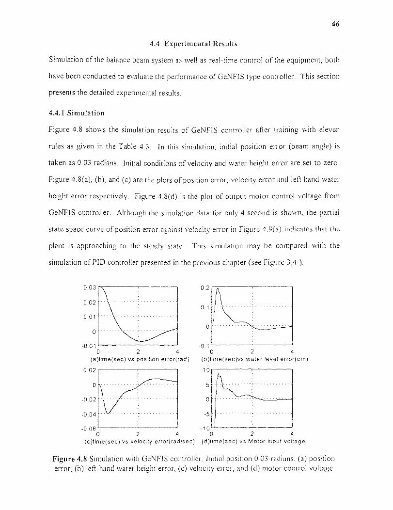
46

4.4 Experimental Results

Simulation of the balance beam system as well as real-time control of the equipment, both

have been conducted to evaluate the performance of GeNFIS type controller. This section

presents the detailed experimental results.

4.4.1 Simulation

Figure 4.8 shows the simulation results of GeNFIS controller after training with eleven

rules as given in the Table 4.3. In this simulation, initial position error (beam angle) is

taken as 0.03 radians. Initial conditions of velocity and water height error are set to zero.

Figure 4.8(a), (b), and (c) are the plots of position error, velocity error and left hand water

height error respectively. Figure 4.8(d) is the plot of output motor control voltage from

GeNFIS controller. Although the simulation data for only 4 second is shown, the partial

state space curve of position error against velocity error in Figure 4.9(a) indicates that the

plant is approaching to the steady state. This simulation may be compared with the

simulation of PID controller presented in the previous chapter (see Figure 3.4 ).

(a)time(sec) vs position error(rad) (b)time(sec)vs water level error(cm)

(c)time(sec) vs velocity error(rad/sec) (d)time(sec) vs Motor input voltage

Figure 4.8 Simulation with GeNFIS controller: Initial position 0.03 radians. (a) positionerror, (b) left-hand water height error, (c) velocity error, and (d) motor control voltage

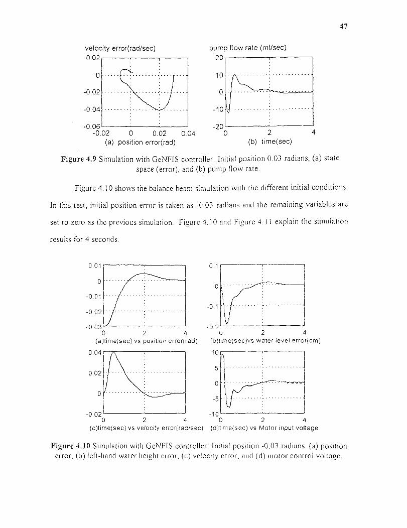
(a) position error(rad) (b) time(sec)

velocity error(rad/sec) pump flow rate (ml/sec)

47

Figure 4.9 Simulation with GeNFIS controller: Initial position 0.03 radians, (a) statespace (error), and (b) pump flow rate.

Figure 4.10 shows the balance beam simulation with the different initial conditions.

In this test, initial position error is taken as -0.03 radians and the remaining variables are

set to zero as the previous simulation. Figure 4.10 and Figure 4.11 explain the simulation

results for 4 seconds.

(a)time(sec) vs position error(rad) (b)time(sec)vs water level error(cm)

(c)time(sec) vs velocity error(rad/sec) (d)time(sec) vs Motor input voltage

Figure 4.10 Simulation with GeNFIS controller: Initial position -0.03 radians. (a) positionerror, (b) left-hand water height error, (c) velocity error, and (d) motor control voltage.

(a) position error(rad) (b) time(sec)

velocity error(rad/sec) pump flow rate (ml/sec)

48

0

Figure 4.11 Simulation with GeNFIS controller: Initial position -0.03 radians, (a) statespace (error), and (b) pump flow rate.

To test the robustness of the GeNFIS controller, two more experiments were

done. In each of these, the controller is asked to balance the beam from different sets of

initial conditions. In the first test, initial position error is taken as -0.025 radians and the

velocity error is set to zero as earlier. However, an initial left hand water height error of -

0.2 cm is introduced. Figure. 4.12 shows that the controller can balance the beam within a

reasonable time. Figure 4.13(a) and (b) are the plot of position error against velocity error

and water height error respectively.

(a)time(sec) vs position error(rad) (b)time(sec)vs water level error(cm)

(c)time(sec) vs velocity error(rad/sec) (d)time(sec) vs Motor input voltage

Figure 4.12 GeNFIS simulation with initial angle -0.025 radians and initial water heighterror -0.2 cm

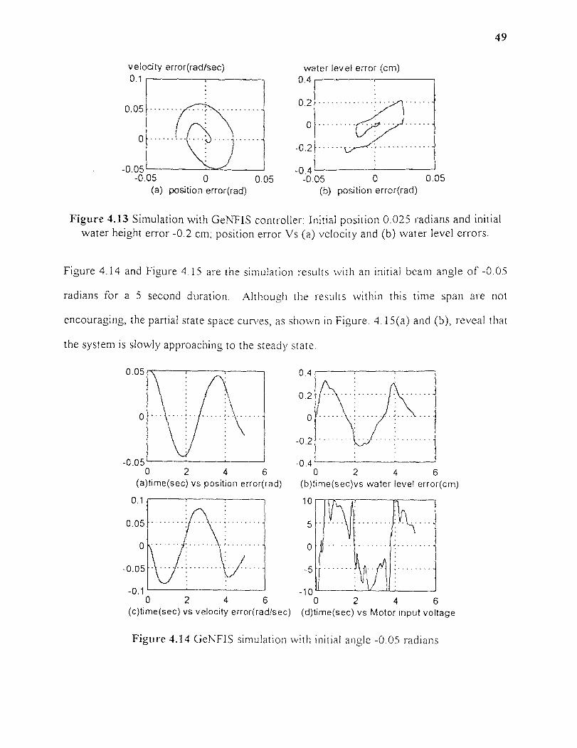
velocity error(rad/sec)0.1

water level error (cm)0.4

49

(a) position error(rad) (b) position error(rad)

Figure 4.13 Simulation with GeNFIS controller: Initial position 0.025 radians and initialwater height error -0.2 cm; position error Vs (a) velocity and (b) water level errors.

Figure 4.14 and Figure 4.15 are the simulation results with an initial beam angle of -0.05

radians for a 5 second duration. Although the results within this time span are not

encouraging, the partial state space curves, as shown in Figure. 4.15(a) and (b), reveal that

the system is slowly approaching to the steady state.

(a)time(sec) vs position error(rad) (b)time(sec)vs water level error(cm)

(c)time(sec) vs velocity error(rad/sec) (d)time(sec) vs Motor input voltage

Figure 4.14 GeNFIS simulation with initial angle -0.05 radians

velocity error(rad/sec)0.1

water level error (cm)0.4

50

(a) position error(rad) (b) position error(rad)

Figure 4.15 Simulation with GeNFIS controller; initial position -0.05 radians; positionerror against (a) velocity and (b) water level errors.

4.4.2 Real-Time Control

In real time operation, the performance of GeNFIS controller is investigated

against a PID controller. The same GeNFIS controller, which has been used in the

simulation, is included in the real time control program. Figure 4.16 shows the steady

state control of balance beam at the horizontal position using GeNFIS controller.

Whereas Figure 4.17 shows the same control using a PID controller. Figure 4.16(a)

indicates a very small steady state position error, oscillating on one side of the set point,

with the GeNFIS controller. The corresponding figure under PID controller, Figure

4.17(a), shows that the position error is oscillating around the set point. A sample time of

30 milliseconds is used in all the experiments.

To test robustness of the controllers, different levels of disturbances are applied on

the system. These disturbances are of step input type, and are created in the software.

The software will be able to produce the same level of disturbances repeatedly. To

measure the robustness, step inputs of different voltage levels are applied to the system at

the steady state with the zero set point. It has been observed that the GeNFIS controller

can sustain such disturbances up to the magnitude of 6 volts. Figure 4.18 shows the test

results of 6 volt step input for GeNFIS controller. The system survives and recovers

slowly after the impact. In case of PID controller, it has been observed that the system

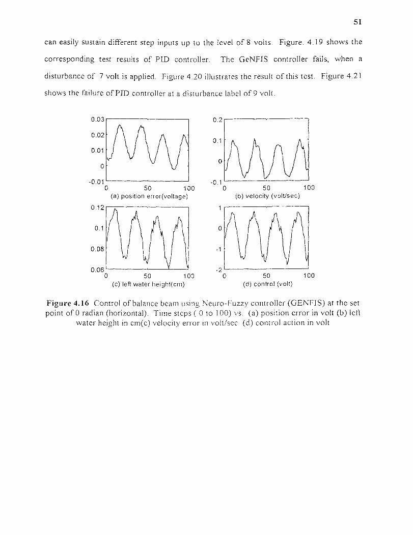
(a) position error(voltage) (b) velocity (volt/sec)

(c) left water height(cm) (d) control (volt)

51

can easily sustain different step inputs up to the level of 8 volts. Figure. 4.19 shows the

corresponding test results of PID controller. The GeNFIS controller fails, when a

disturbance of 7 volt is applied. Figure 4.20 illustrates the result of this test. Figure 4.21

shows the failure of PID controller at a disturbance label of 9 volt.

Figure 4.16 Control of balance beam using Neuro-Fuzzy controller (GENETS) at the setpoint of 0 radian (horizontal). Time steps ( 0 to 100) vs. (a) position error in volt (b) left

water height in cm(c) velocity error in volt/sec (d) control action in volt

52

50(b) velocity (volt/sec)(a) position error(voltage)

50 (c) left water height(cm) (d) control (volt)

(c)Velocity error (volt/sec) (c) Control (volt)

Figure 4.17 Control of balance beam using PID controller at the set point of 0 radian(horizontal). Time steps ( 0 to 100) vs. (a) position error in volt (b) left water height in

cm(c) velocity error in volt/sec (d) control action in volt

(a)Position error(voltage) (b)Left water height error(cm)

Figure 4.18 Control of balance beam using Neuro-Fuzzy controller with a disturbance of6 Volt. Time steps ( 0 to 300) vs. (a) position error in volt (b) left water height in cm(c)

velocity error in volt/sec (d) control action in volt

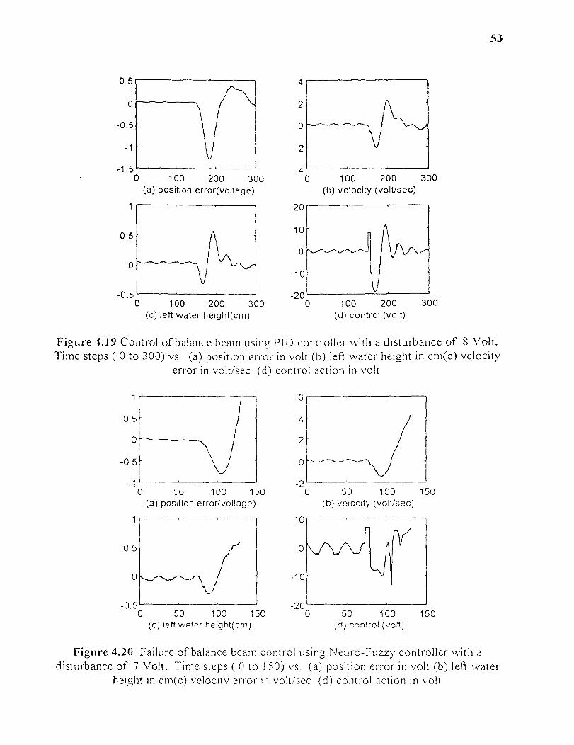
(c) left water height(cm) (d) control (volt)

(a) position error(voltage) (b) velocity (volt/sec)

(c) left water height(cm) (d) control (volt)

(b) velocity (volt/sec)(a) position error(voltage)

53

Figure 4.19 Control of balance beam using PID controller with a disturbance of 8 Volt.Time steps ( 0 to 300) vs. (a) position error in volt (b) left water height in cm(c) velocity

error in volt/sec (d) control action in volt

Figure 4.20 Failure of balance beam control using Neuro-Fuzzy controller with adisturbance of 7 Volt. Time steps ( 0 to 150) vs. (a) position error in volt (b) left water

height in cm(c) velocity error in volt/sec (d) control action in volt

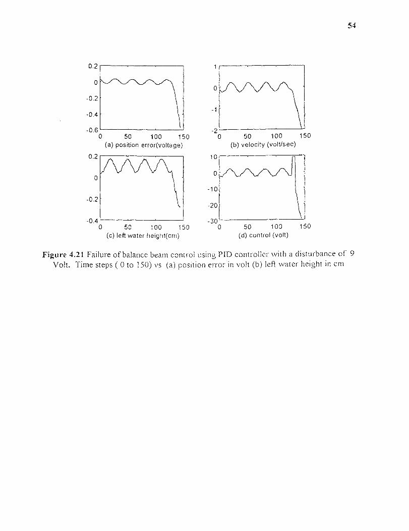
(b) velocity (volt/sec)(a) position error(voltage)

(c) left water height(cm) (d) control (volt)

54

Figure 4.21 Failure of balance beam control using PID controller with a disturbance of 9Volt. Time steps ( 0 to 150) vs (a) position error in volt (b) left water height in cm

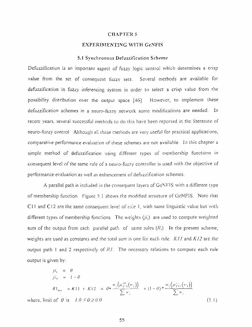
CHAPTER 5

EXPERIMENTING WITH GeNFIS

5.1 Synchronous Defuzzification Scheme

Defuzzification is an important aspect of fuzzy logic control which determines a crisp

value from the set of consequent fuzzy sets. Several methods are available for

defuzzification in fuzzy inferencing system in order to select a crisp value from the

possibility distribution over the output space {46]. However, to implement these

defuzzification schemes in a neuro-fuzzy network some modifications are needed. In

recent years, several successful methods to do this have been reported in the literature of

neuro-fuzzy control. Although all these methods are very useful for practical applications,

comparative performance evaluation of these schemes are not available. In this chapter a

simple method of defuzzification using different types of membership functions in

consequent level of the same rule of a neuro-fuzzy controller is used with the objective of

performance evaluation as well as enhancement of defuzzification schemes.

A parallel path is included in the consequent layers of GeNFIS with a different type

of membership function. Figure 5.1 shows the modified structure of GeNFIS. Note that

C11 and C12 are the same consequent level of rule 1, with same linguistic value but with

different types of membership functions. The weights 010 are used to compute weighted

sum of the output from each parallel path of same rules (10. In the present scheme,

weights are used as constants and the total sum is one for each rule. K11 and K12 are the

output path 1 and 2 respectively of RI. The necessary relations to compute each rule

output is given by:

ji1,=0

ji2, = 1-θ

R1out = K11 + K12

where, limit of θ is 1.0 > 0.0 (5 I )

55

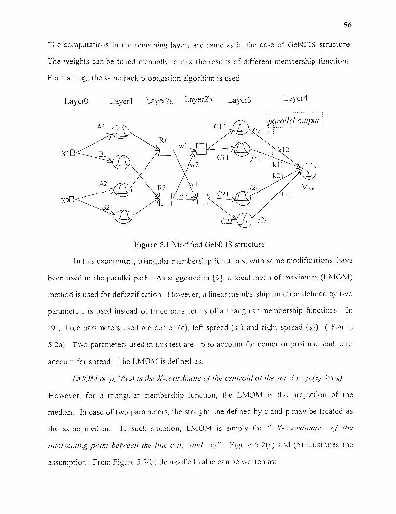
56

The computations in the remaining layers are same as in the case of GeNFIS structure.

The weights can be tuned manually to mix the results of different membership functions.

For training, the same back propagation algorithm is used.

Layer() Layer 1 Lay er2a Layer2b Layer; Layer4

parallel output

Figure 5.1 Modified GeNFIS structure

In this experiment, triangular membership functions, with some modifications, have

been used in the parallel path. As suggested in [9], a local mean of maximum (LMOM)

method is used for defuzzification. However, a linear membership function defined by two

parameters is used instead of three parameters of a triangular membership functions. In

[9], three parameters used are center (c), left spread (s L) and right spread (s R) ( Figure

5.2a). Two parameters used in this test are: p to account for center or position, and c to

account for spread. The LMOM is defined as:

LMOM or μc-¹(wR) is the X-coordinate of the centroid of the set ( x: μ c(x) _> wR}

However, for a triangular membership function, the LMOM is the projection of the

median. In case of two parameters, the straight line defined by c and p may be treated as

the same median. In such situation, LMOM is simply the " X-coordinate of the

intersecting point between the line c p, and wR". Figure 5.2(a) and (b) illustrates the

assumption. From Figure 5.2(b) defuzzified value can be written as:

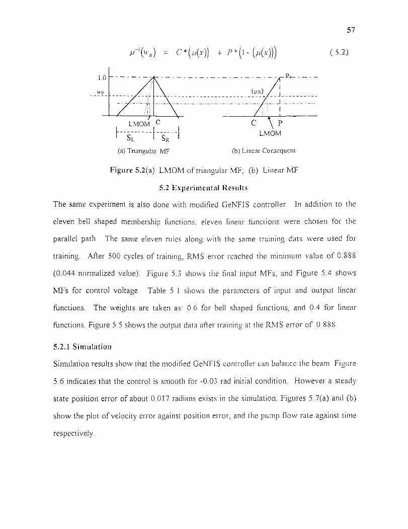
R ) C *(μ(x)) P (1 — (μ(x)))

57

( 5 2)

(a) Triangular ME (b) Linear Consequent

Figure 5.2(a) LMOM of triangular MF; (b) Linear MT

5.2 Experimental Results

The same experiment is also done with modified GeNFIS controller. In addition to the

eleven bell shaped membership functions, eleven linear functions were chosen for the

parallel path. The same eleven rules along with the same training data were used for

training. After 500 cycles of training, RMS error reached the minimum value of 0.888

(0.044 normalized value). Figure 5.3 shows the final input MFs, and Figure 5.4 shows

MFs for control voltage. Table 5.1 shows the parameters of input and output linear

functions. The weights are taken as: 0.6 for bell shaped functions, and 0.4 for linear

functions. Figure 5.5 shows the output data after training at the RMS error of 0.888.

5.2.1 Simulation

Simulation results show that the modified GeNFIS controller can balance the beam. Figure

5.6 indicates that the control is smooth for -0.03 rad initial condition. However a steady

state position error of about 0.017 radians exists in the simulation. Figures 5.7(a) and (b)

show the plot of velocity error against position error, and the pump flow rate against time

respectively.

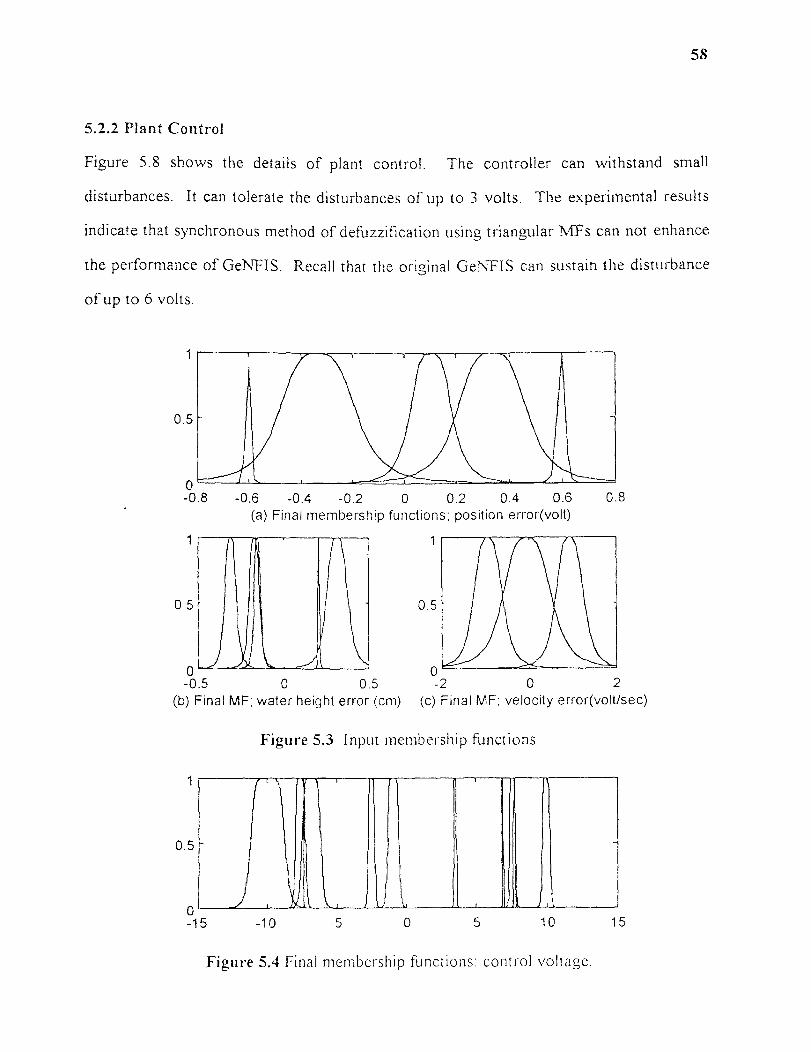
58

5.2.2 Plant Control

Figure 5.8 shows the details of plant control. The controller can withstand small

disturbances. It can tolerate the disturbances of up to 3 volts. The experimental results

indicate that synchronous method of defuzzification using triangular MFs can not enhance

the performance of GeNFIS. Recall that the original GeNFIS can sustain the disturbance

of up to 6 volts .

(a) Final membership functions: position error(volt)

(b) Final MF; water height error (cm) (c) Final MF; velocity error(volt/sec)

Figure 5.3 Input membership functions

Figure 5.4 Final membership functions: control voltage.

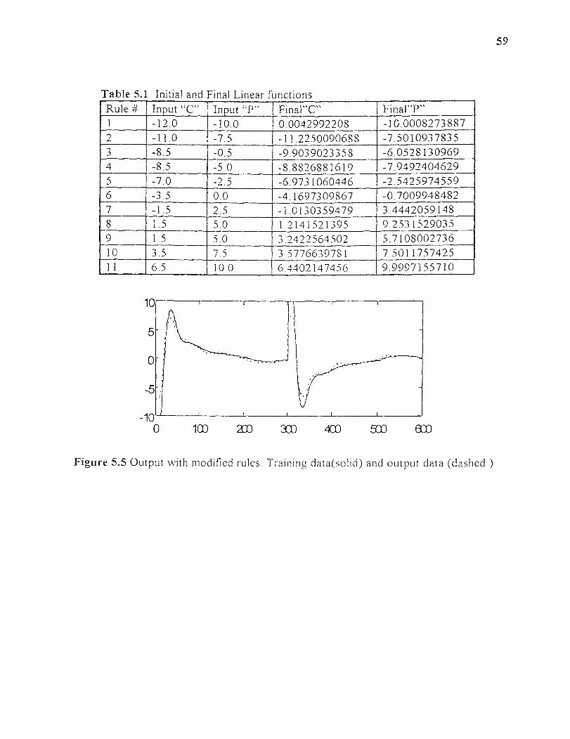
Table 5.1 Initial and Final Linear functions Rule .,4-i Input "C" Input "P" Final"C" Final" P" 1 -12.0 -10.0 0.0042992208 -10.0008273887 2 -11.0 -7.5 -11.2250090688 -7.5010937835 3 -8.5 -0.5 -9.9039023358 -6.0528130969 4 -8.5 -5.0 -8.8826881619 -7.9492404629 5 -7.0 _7,5 -6.9731060446 -2.5425974559 6 -3.5 0.0 -4.1697309867 -0.7009948482 7 -1.5 2.5 -1.0130359479 3.4442059148 8 1.5 5.0 1.2141521395 9.2531529035 9 1.5 5.0 3.9472564502 5.7108002736 10 3.5 7.5 3.5776639781 7.5011757425 11 6.5 10.0 6.4402147456 9.9997155710

59

Figure 5.5 Output with modified rules: Training data(solid) and output data (dashed )

(a) position error(rad) (b) time(sec)

(a)time(sec) vs position error(rad) (b)time(sec)vs water level error(cm)

60

(c)time(sec) vs velocity error(rad/sec) (d)time(sec) vs Motor input voltage

Figure 5.6 Simulation with modified rule antecedent

velocity error(rad/sec) pump flow rate (ml/sec)

Figure 5.7 Modified rules;(a) state ( position error vs. velocity error) (b) pump flow rate

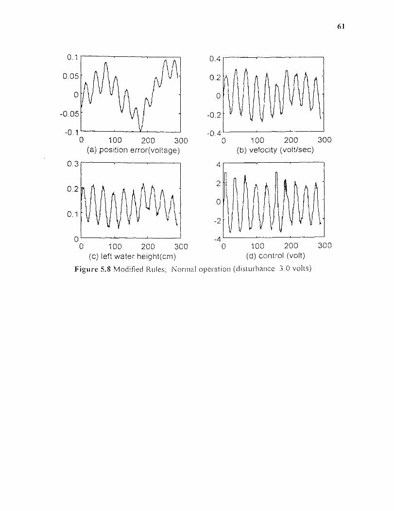
(c) left water height(cm) (d) control (volt)

(b) velocity (volt/sec)(a) position error(voltage)

61

Figure 5.8 Modified Rules; Normal operation (disturbance 3.0 volts)

62

5.3 Hybrid Learning

Since the synchronous defuzzification scheme with triangular membership function does

not improve the performance of GeNFIS, it is replaced by Sugeno type rule consequent.

The modified GeNFIS structure is shown in Figure 5.9. The weight equations are same as

before (see Equation 5.1). However, the rule output computation is changed due to the

introduction of first-order Sugeno fuzzy model [251. The modified relation is given by

R1out, = K11 + K12 =

where, p i and r1 are the constants of Sugeno type rule consequent.

Layer() Layer I Layer2 a Layer2b Layer3 Layer4

(5. 3 )

Figure 5.9 Modified GeNFIS with Sugeno type rules

The training is done in two phases. First, the GeNFIS parameters are trained using

only back propagation algorithm with unit weights. The premise membership functions

are tuned in this phase. The weights of the synchronous Sugeno layers are treated as zero.

In the second phase, Sugeno parameters are identified by using least-square estimators.

63

The parameters of the input layers are kept as constants with the trained values from the

phase one. In this phase, the weights in the Sugeno layers were set to one, whereas the

weights in GeNFIS layers were set to zero. During experiment, the weights were adjusted

or tuned to get the best results.

5.3.1 Experimental Results

First, we test the controller using equal weights of 0.5 in both the paths. Figure 5.10

shows the simulation results with initial position of -0.3 radians. The results indicate that

the controller can balance the beam smoothly. Comparing with the previous simulation

results, Figure 5.10 shows a very smooth motor input voltage curve. However, in the

actual experiment, the controller could not balance the beam using 0.5:0.5 weight

allocation. Next, we tuned the weights to find a feasible controller. We observed the

controller can reasonably balance the beam when the weight ratio is 0.75:0.25. The

weights of 0.25 were used in the Sugeno layers. Figure 5.11 shows that the controller can

even sustain a disturbance of 4 volts. These results lead us to investigate further about the

ANFIS scheme.

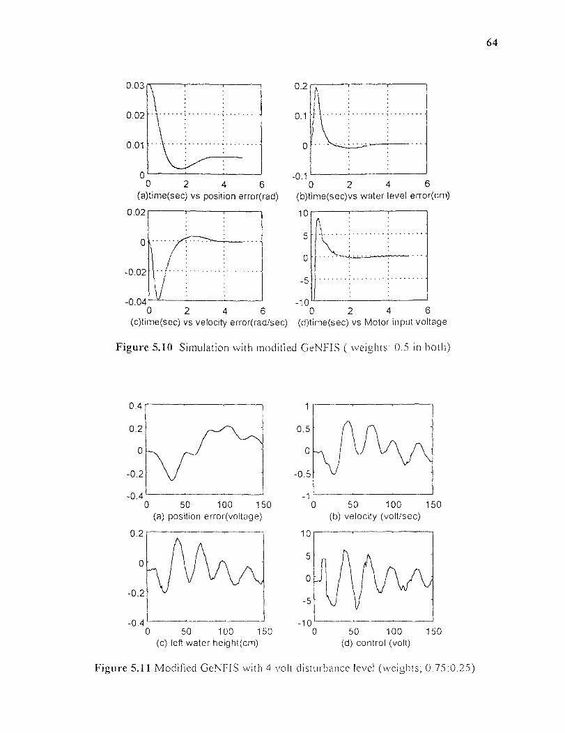
(a) position error(voltage) (b) velocity (volt/sec)

•100(c) left water height(cm) (d) control (volt)

•(a)time(sec) vs position error(rad) (b)time(sec)vs water level error(cm)

(c)time(sec) vs velocity error(rad/sec) (d)time(sec) vs Motor input voltage

Figure 5.10 Simulation with modified GeNFIS ( weights: 0.5 in both)

64

Figure 5.11 Modified GeNFIS with -I volt disturbance level (weights; 0.75:0.25)

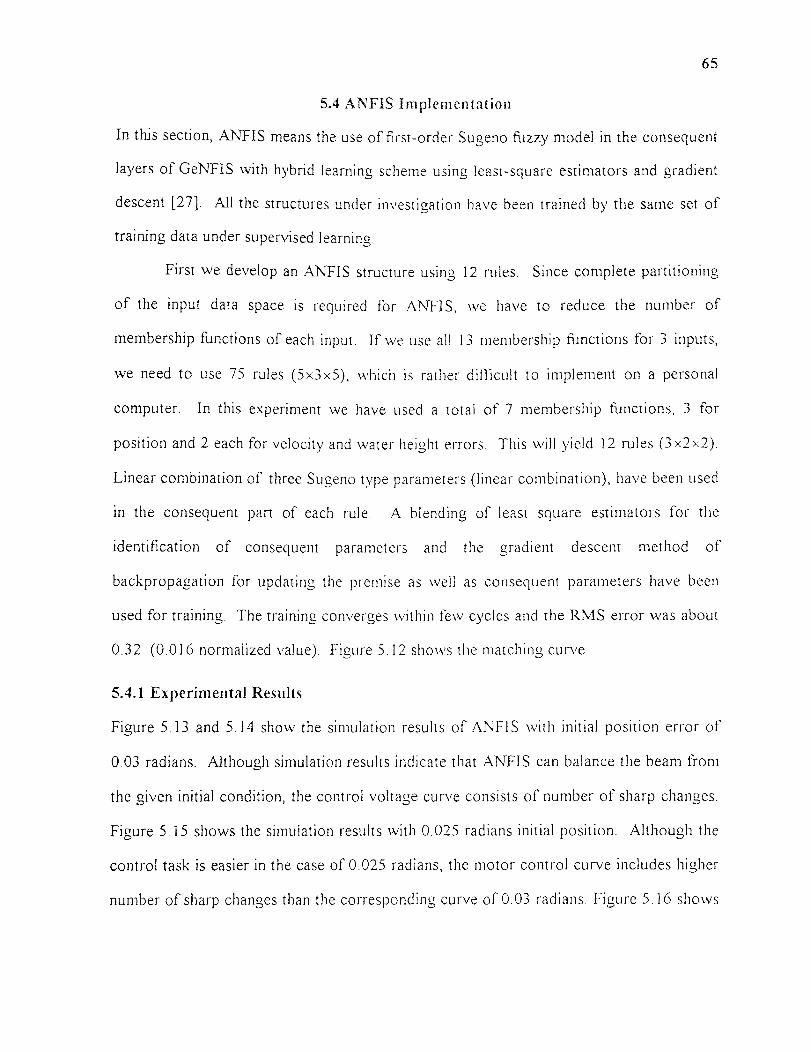
65

5.4 ANFIS Implementation

In this section, ANTIS means the use of first-order Sugeno fuzzy model in the consequent

layers of GeNFIS with hybrid learning scheme using least-square estimators and gradient

descent [27]. All the structures under investigation have been trained by the same set of

training data under supervised learning.

First we develop an ANFIS structure using 12 rules. Since complete partitioning

of the input data space is required for ANTIS, we have to reduce the number of

membership functions of each input. If we use all 13 membership functions for 3 inputs,

we need to use 75 rules (5x3x5), which is rather difficult to implement on a personal

computer. In this experiment we have used a total of 7 membership functions, 3 for

position and 2 each for velocity and water height errors. This will yield 12 rules (3 x2x2).

Linear combination of three Sugeno type parameters (linear combination), have been used

in the consequent part of each rule. A blending of least square estimators for the

identification of consequent parameters and the gradient descent method of

backpropagation for updating the premise as well as consequent parameters have been

used for training. The training converges within few cycles and the RMS error was about

0.32 (0.016 normalized value). Figure 5.12 shows the matching curve.

5.4.1 Experimental Results

Figure 5.13 and 5.14 show the simulation results of ANFIS with initial position error of

0.03 radians. Although simulation results indicate that ANFIS can balance the beam from

the given initial condition, the control voltage curve consists of number of sharp changes.

Figure 5.15 shows the simulation results with 0.025 radians initial position. Although the

control task is easier in the case of 0.025 radians, the motor control curve includes higher

number of sharp changes than the corresponding curve of 0.03 radians. Figure 5.16 shows

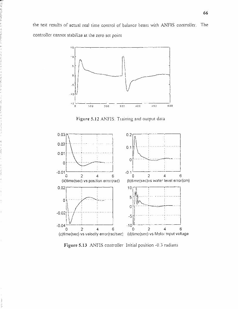
66

the test results of actual real time control of balance beam with .ANFIS controller. The

controller cannot stabilize at the zero set point

Figure 5.12 ANFIS : Training and output data

(a)time(sec) vs position error(rad) (b)time(sec)vs water level error(cm)

(c)time(sec) vs velocity error(rad/sec) (d)time(sec) vs Motor input voltage

Figure 5.13 ANFIS controller Initial position -0.3 radians

(a) position error(rad) (b) time(sec)

velocity error(rad/sec) pump flow rate (ml/sec)20

67

6

Figure 5.14 Simulation ANFIS ( initial position -0.3 rad); (a)state (b) pump flow rate

(a)time(sec) vs position error(rad) (b)time(sec)vs water level error(cm)

(c)time(sec) vs velocity error(rad/sec) (d)time(sec) vs Motor input voltage

Figure 5.15 Simulation ANFIS controller Initial pos -0.25

5.4.2 Limitations of ANFIS Implementation

In the above experiment, ANFIS was trained with the static data collected from model

simulation with PID controller. So the least square technique have been used for

identification of consequent parameters which converges very quickly with low RMS

error. However, in his later work, king [26} has used self learning method with temporal

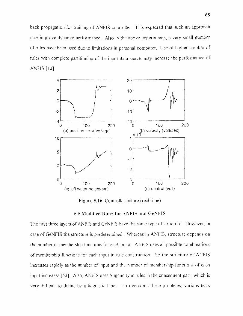
(0) velocity (volt/sec)(a) position error(voltage)

(c) left water height(cm)100 (d) control (volt)

68

back propagation for training of ANFIS controller. It is expected that such an approach

may improve dynamic performance. Also in the above experiments, a very small number

of rules have been used due to limitations in personal computer. Use of higher number of

rules with complete partitioning of the input data space, may increase the performance of

ANFIS [12].

Figure 5.16 Controller failure (real time)

5.5 Modified Rules for ANFIS and GeNFIS

The first three layers of ANFIS and GeNFIS have the same type of structure. However, in

case of GeNFIS the structure is predetermined. Whereas in ANFIS, structure depends on

the number of membership functions for each input. ANFIS uses all possible combinations

of membership functions for each input in rule construction. So the structure of ANFIS

increases rapidly as the number of input and the number of membership functions of each

input increases [53]. Also, ANFIS uses Sugeno type rules in the consequent part, which is

very difficult to define by a linguistic label. To overcome these problems, various tests

69

were conducted with both ANFIS and GeNFIS, with minor modifications in the structures

as well as in the rules. Results of two such tests are presented here.

5.5.1 Experimental Results

Test 1: ANFIS with preselected rule antecedent and Sugeno type consequent:

The same 11 rules which have been used earlier with GeNFIS, are used here with modified

consequent. In this case, consequent part of each rule is replaced by a Sugeno type

consequent. So the consequent part of each rule is now having four modifiable

parameters. The initial values of all these parameters are set to zero. The rules are now

like:

if a- is A and y is B and z is C then u = qy + r z + s (5.4)

The same data were used for training, and after about 20 cycles minimum RMS error was

observed as 0.32 (0.016 normalized value). Figure 5.17 shows the simulation results. It is

clear from the simulation results that the state variables (error) can not smoothly reach to

the desired (zero) state. Experiment results as shown in Figure 5.18 also indicate failure

of the controller.

Test 2: ANFIS and GeNFIS with modified Sugeno type consequent:

In this test, the same 11 rules were used with some modification in the Sugeno type

consequent. The constant 's' is now replaced by a predefuzzified consequent.

Predefuzzified consequent is also known as a fuzzy singleton. In this case, 's' of each

rule is initialized by the value of center ( bell shaped MF) of corresponding linguistic level.

Rest of the parameters are initialized with zero as before. In training algorithm, instead of

using the combination of least-squares and gradient descent methods, only gradient

descent method is used.

The same data were used for training. However, in using only the gradient descent

method, the training took about 600 cycles to reach a level of 0.65 RMS error (0.033

normalized value). Figure 5.19 shows the simulation results with initial position errors of

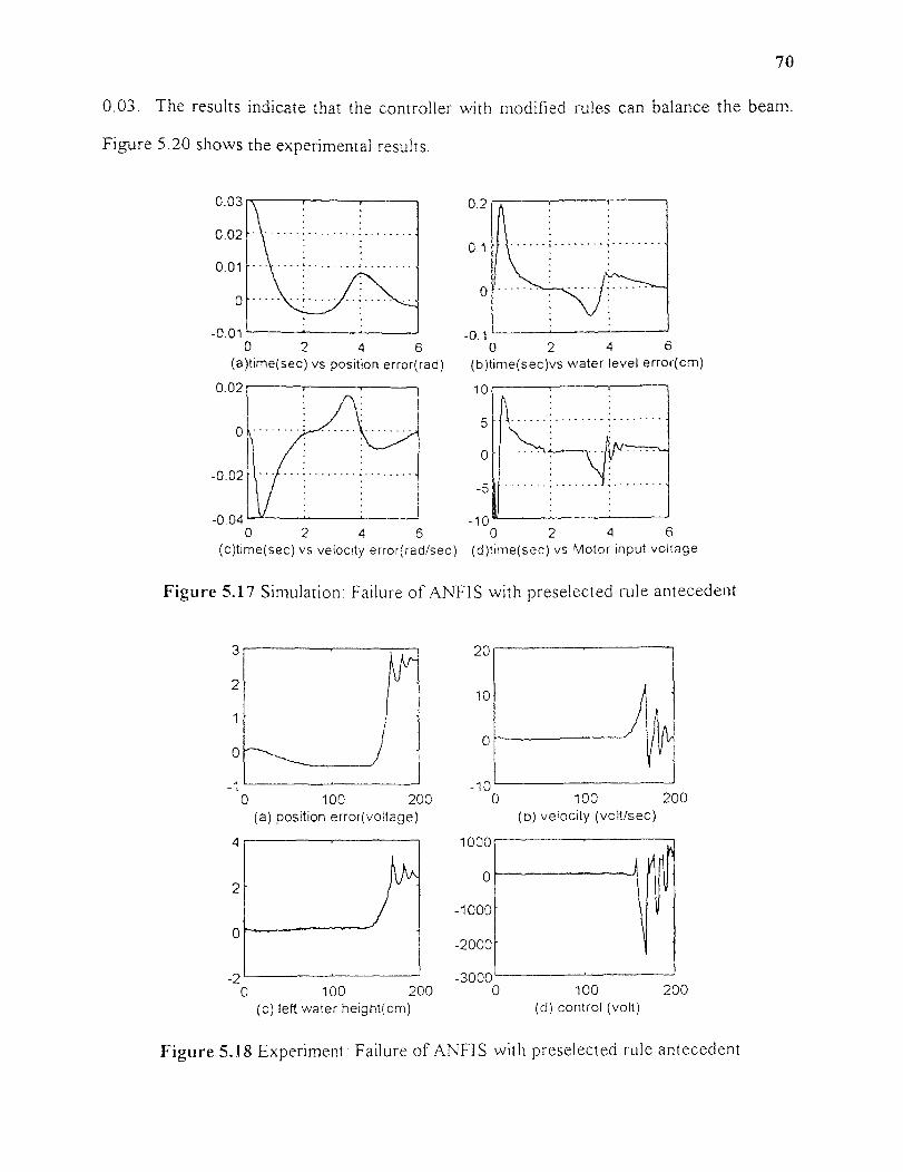
(c) left water height(cm) (d) control (volt)

70

0.03. The results indicate that the controller with modified rules can balance the beam.

Figure 5.20 shows the experimental results.

(a)time(sec) vs position error(rad) (b)time(sec)vs water level error(cm)

(c)time(sec) vs velocity error(rad/sec) (d)time(sec) vs Motor input voltage

Figure 5.17 Simulation: Failure of ANFIS with preselected rule antecedent

(a) position error(voltage (b) velocity (volt/sec)

Figure 5.18 Experiment: Failure of ANFIS with preselected rule antecedent

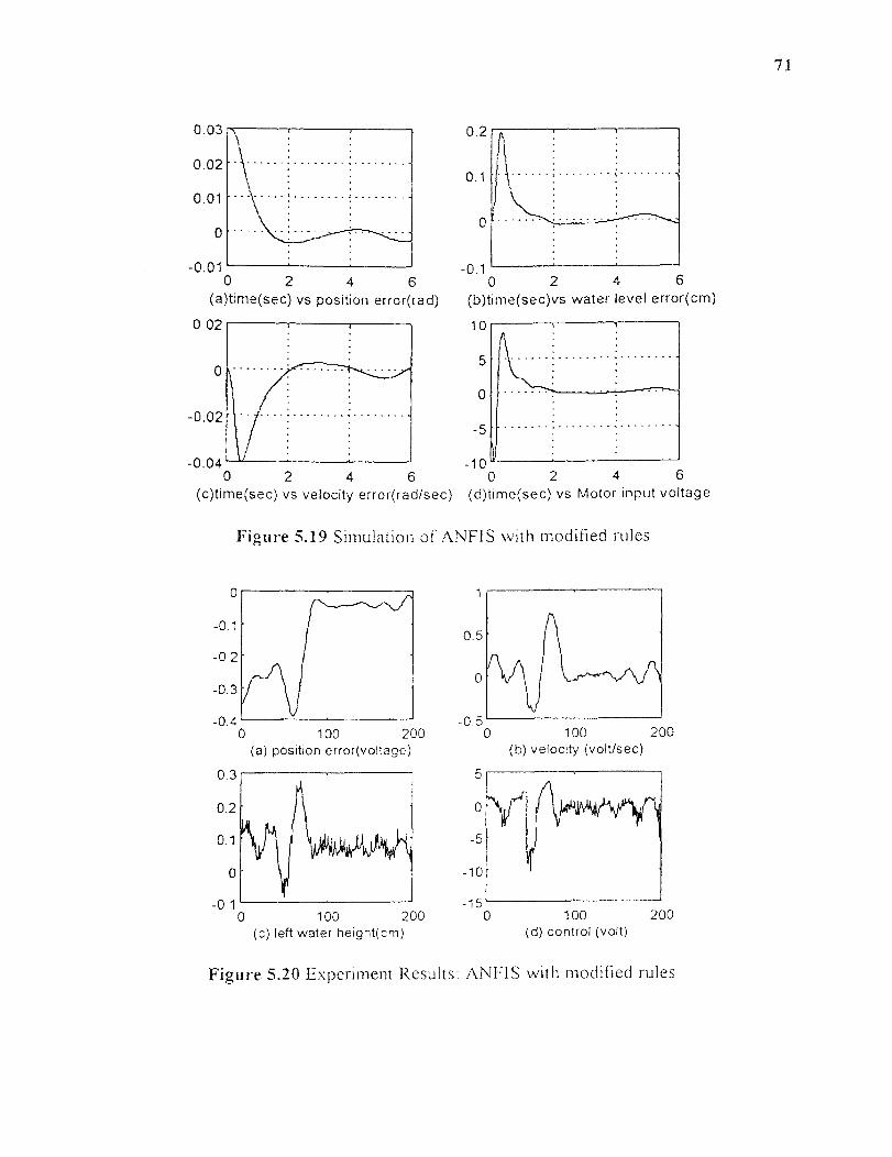
(a) position error(voltage) (b) velocity (volt/sec)

(c) left water height(cm) (d) control (volt)

(a)time(sec) vs position error(rad) (b)time(sec)vs water level error(cm)

71

(c)time(sec) vs velocity error(rad/sec) (d)time(sec) vs Motor input voltage

Figure 5.19 Simulation of ANTIS with modified rules

Figure 5.20 Experiment Results: ANFIS with modified rules

72

The results obtained in this section point out some interesting features of the

neuro-fuzzy controllers. The most noteworthy of these is the fact that even when the

matching of the input data is very well, i.e. small RMS error, the controller may not be

successful in balancing of the beam. In the next chapter, these and other results are

summarized.

CHAPTER 6

CONCLUSIONS AND FUTURE WORK

6.1 Conclusions

In this dissertation, a flexible network called Generalized Network-based Fuzzy

Inferencing System (GeNFIS) is developed by combining the good features from neural

networks and fuzzy inferencing systems, and is applied to the problem of controlling a

higher order nonlinear dynamic system. The nonlinear dynamic system used here is an

unstable balance beam system that contains two fluid tanks, one at each end, and the

balance is achieved by pumping the fluid back and forth from the tanks. Both the results,

simulation as well as experimental, indicate that GeNFIS controller can successfully

balance the beam in real time. The GeNFIS is designed to be flexible and can accomodate

different variations of rule structure and defuzzification schemes. The results obtained are

summarized in this chapter.

First, the performance of GeNFIS controller was evaluated against a conventional

PID controller. The test results indicate that the PID controller is more stable and

sensitive to the set point than GeNFIS controller. However, it may be mentioned that the

GeNFIS is a rule-based controller and only eleven rules have been used to control the

system, and did not explicitly require the exact model of the plant. Moreover, the

performance of GeNFIS can be improved by increasing the number of rules. Besides, the

objective here was not to find a best neuro-fuzzy controller for comparison with a

conventional PID controller, but to find a feasible neuro-fuzzy controller with a flexible

structure which can be used to investigate the current neuro-fuzzy approaches from

literature for performance evaluation.

Next, as a part of the flexible structure for GeNFIS, a concept of synchronous

defuzzification is proposed in this work. This method allows simultaneous use of different

types of membership functions in the consequent part of GeNFIS rules and provides the

73

74

flexibility to incorporate strengths from other neuro-fuzzy approaches. Using this concept,

different versions of GeNFIS are tested with the balance beam control problem, and the

results of these tests are presented next.

First, synchronous defuzzification is implemented on GeNFIS with simultaneous

use of triangular as well as bell shaped membership functions. However, no significant

improvement is noticed with the use of this scheme for this particular nonlinear dynamic

system. Nevertheless, through this experiment it is shown that it is possible to combine

two different defuzzification schemes in any proportion, train the controller and achive

success in balance of the beam. The structure developed can allow for future experiments

on different nonlinear systems. In the next experiment, the triangular membership

functions are replaced by the first order Sugeno type rules, thus there is a simultaneous

use of Sugeno type rules as well as bell shaped membership functions. A hybrid learning

scheme [25,27] is used, such that the consequent parameters of Sugeno type rules are

trained through least squared error minimization, while rest of the parameters are trained

through back propoagation. The weights of the final layer are all set to 0.5 for equal

mixing of results from each defuzzification scheme. The results in this case are not

satisfactory, i.e., the beam balancing is not possible. When the weight of 0.25 is used in

the consequent layer of Sugeno type rules, the controller is able to balance the beam.

However, the performance of the controller is not very smooth. This brings out an

interesting feature of the proposed neuro-fuzzy control scheme. It appears that the

proposed scheme is better at beam balancing under the supervised learning than the

scheme which uses Sugeno type rules. Since ANTIS also uses Sugeno type rules, this is a

motivation for some additional tests on balance beam system using only ANFIS [27] type

controller under supervised learning. In this work, ANTIS means the use of Sugeno type

rules in the consequent part of GeNFIS along with hybrid learning scheme. The system is

tested with only 12 rules (3x2x2) using complete partitioning of the input data space as

75

discussed in [27]. In this case, the controller fails to balance the beam. It appears that

although the training is good, i.e. resulting in a very low RMS error, the tests under

dynamic conditions indicate failure of the controller. This failure can be attributed in part

to the fact that only a small number of fuzzy labels, hence rules are utilized.

Next, in order to do a fair comparison of GeNFIS and ANFIS, the premise parts of

the original 11 rules (used in GeNFIS) are used with Sugeno type consequent and the

training is done by using hybrid learning method. This scheme is equivalent to ANFIS with

pre-selected, limited set of rules. However, this scheme, although succesful in simulation,

fails to balance the beam for the actual physical experiment. In both these experiments,

the training data is matched very well by ANFIS-like schemes, yet they fail in dynamic

situations. It is noted that these results are a special case where a limited number of rules,

and a specific training data are utilized, thus the failure of ANFIS-like scheme is not a

general conclusion. However, these results raise a flag regarding the use of Sugeno type

rules when the rule base is limited. For practical problems where one cannot utilize a full

set of rules, or an optimal smaller set of rules is not known, one may excercise caution in

using ANFIS-like schemes, and it may be worthwhile to consider the proposed GeNFIS

scheme.

Although a detailed mathematical analysis of the use of Sugeno type rules in

ANTIS is not done in this work, it appears that the hybrid learning scheme may produce

arbitrary values for the Sugeno constants, and it would be difficult to assign any good

physical significance to the values obtained. Consequently, a modification in the

consequent part of Sugeno type rules is proposed. This modification replaces the constant

term by a suitable fuzzy singleton in order to bound the rule output around the desired

linguistic label (say for example, high). For training, back propagation algorithm may still

be used. As shown in the previous chapter, the test results for ANFIS/GeNFIS controller

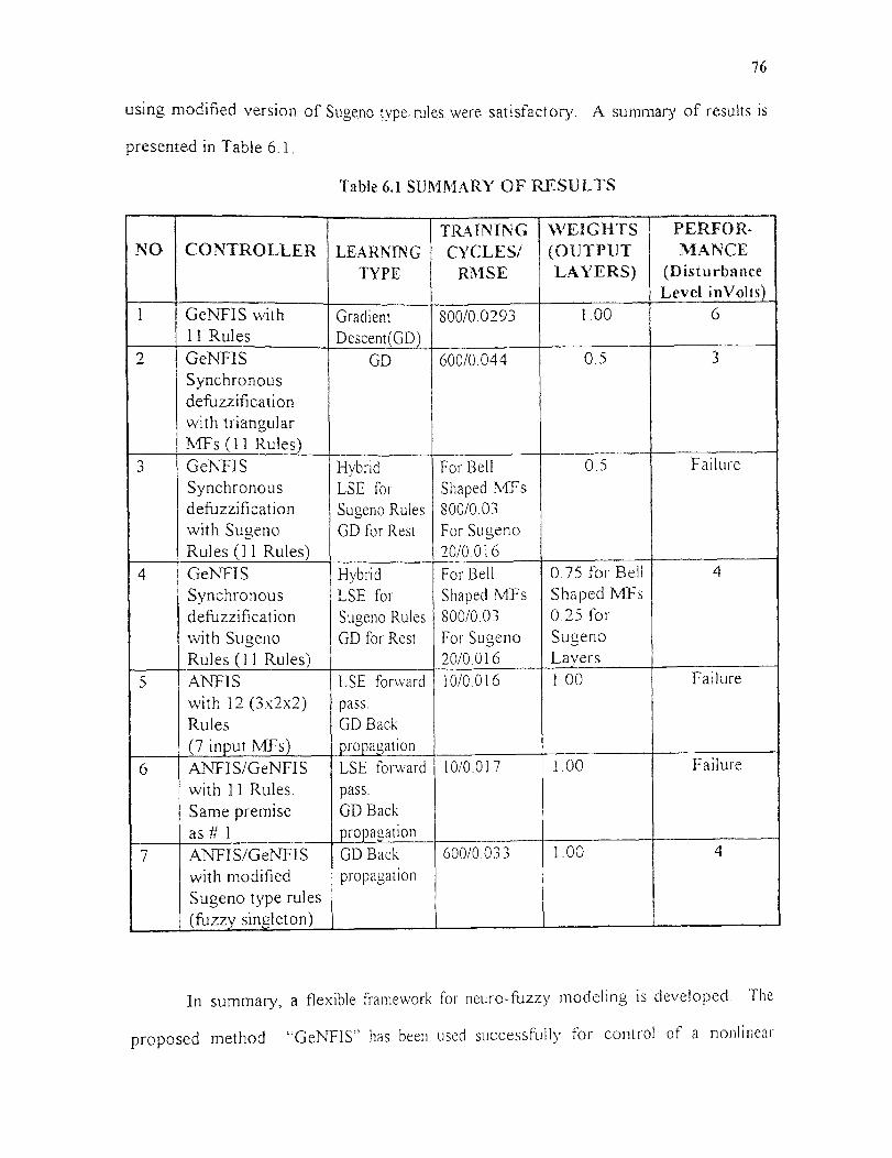
76

using modified version of Sugeno type rules were satisfactory. A summary of results is

presented in Table 6,1.

Table 6.1 SUMMARY OF RESULTS

TRAINING WEIGHTS PERFOR-NO CONTROLLER LEARNING CYCLES/ (OUTPUT MANCE

TYPE RMSE LAYERS) (DisturbanceLevel inVolts

1 GeNFIS with Gradient 800/0.0293 1.00 611 Rules Descent(GD)

2 GeNFIS GD 600/0.044 0.5 3Synchronousdefuzzificationwith triangularMFs (11 Rules)

3 GeNFIS Hybrid For Bell 0.5 FailureSynchronous LSE for Shaped MFsdefuzzification Sugeno Rules 800/0.03with Sugeno GD for Rest For SugenoRules (11 Rules) 20/0.016

4 GeNFIS Hybrid For Bell 0.75 for Bell 4Synchronous LSE for Shaped MFs Shaped MFsdefuzzification Sugeno Rules 800/0.03 0.25 forwith Sugeno GD for Rest For Sugeno SugenoRules (11 Rules) 20/0 016 Layers

5 ANFIS LSE forward 10/0.016 I.00 Failure

with 12 (3x2x2) pass.Rules GD Back(7 input MFs) pro aoation

6 ANFIS/GeNFIS LSE forward 10/0.017 1.00 Failure

with 11 Rules. pass.Same premise GD Backas # I fro )agation

7 ANFIS/GeNFIS GD Back 600/0.033 1.00 4

with modified propagationSugeno type rules(fuzzy singleton)

In summary, a flexible framework for neuro-fuzzy modeling is developed. The

proposed method "GeNFIS" has been used successfully for control of a nonlinear

77

dynamic system using real time control methodologies. However, considerable amount of

research is needed to explore the full potential of GeNFIS and to develop a suitable self

learning scheme for GeNFIS. The GeNFIS architecture along with the fluid beam

balancing system developed here provide an excellent test-bed for further research in

neuro-fuzzy modeling and real time control.

5.2 Future work

The GeNFIS has been developed with the objective of providing a flexible structure which

can accommodate different types of fuzzy control rules. However, a suitable learning

scheme is requred so that the controller can learn from the system behavior. The possible

approachs are to implement reinforcement learning or real time recurrent learning schemes

on GeNFIS architecture. In the present work, the rules were generated from the expert

knowledge along with the training data set. No formal algorithm for rule generation is

developed. Considerable amount of research is needed to develop a rule generation

algoritm for GeNFIS. A discussion on the rule generation procedure, used in this

research, has been presented in chapter 4. The methods used here may be used as a

guideline for the development of an automatic rule generation algorithm.

Another area of further research is development of techniques to find a suitable

fuzzy controller which can balance the beam from the raw sensor data. In the present

balance beam system, two linear pressure sensors are used to measure the water pressures

of two tanks. Although the relation between water pressure and sensor output voltage is

linear, the constant amount of water may have different output voltage at different angular

positions due to geometric effect. The actual water height is a function of position and

pressure, which is calibrated by using Least Square Method. See Appendix C for details.

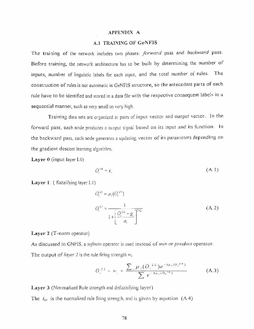
APPENDIX A

A.1 TRAINING OF GeNFIS

The training of the network includes two phases: forward pass and backward pass.

Before training, the network architecture has to be built by determining the number of

inputs, number of linguistic labels for each input, and the total number of rules. The

construction of rules is not automatic in GeNFIS structure, so the antecedent parts of each

rule have to be identified and stored in a data file with the respective consequent labels in a

sequential manner, such as very small to very high.

Training data sets are organized in pairs of input vector and output vector. In the

forward pass, each node produces a output signal based on its input and its function. In

the backward pass, each node generates a updating vector of its parameters depending on

the gradient descent learning algorithm.

Layer 0 (input layer LO)

(A.1)

Layer 1: ( fuzzifying layer L1)

(A 2)

Layer 2 (T-norm operator)

As discussed in GNFIS, a softmin operator is used instead of min or product operator.

The output of layer 2 is the rule firing strength w,.

(A.3)

Layer 3 (Normalized Rule strength and defuzzifying layer)

The tni is the normalized rule firing strength, and is given by equation (A.4)

78

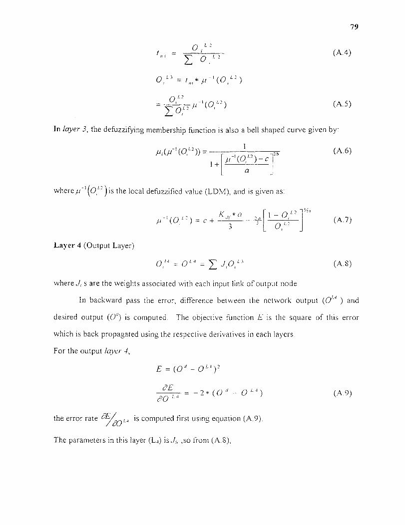
79

(A.4)

(A 5)

In layer 3, the defuzzifying membership function is also a bell shaped curve given by:

(A 6)

whereμ-¹(O1L² )is the local defuzzified value (LDM), and is given as:

(A.7)

Layer 4 (Output Layer)

(A 8)

where J, s are the weights associated with each input link of output node.

In backward pass the error, difference between the network output (OL4 ) and

desired output (Od) is computed. The objective function E is the square of this error

which is back propagated using the respective derivatives in each layers.

For the output layer 4,

(A 9)

the error rate aE/a0 L, is computed first using equation (A.9).

The parameters in this layer (L 4 ) is d„ ,so from (A.8),

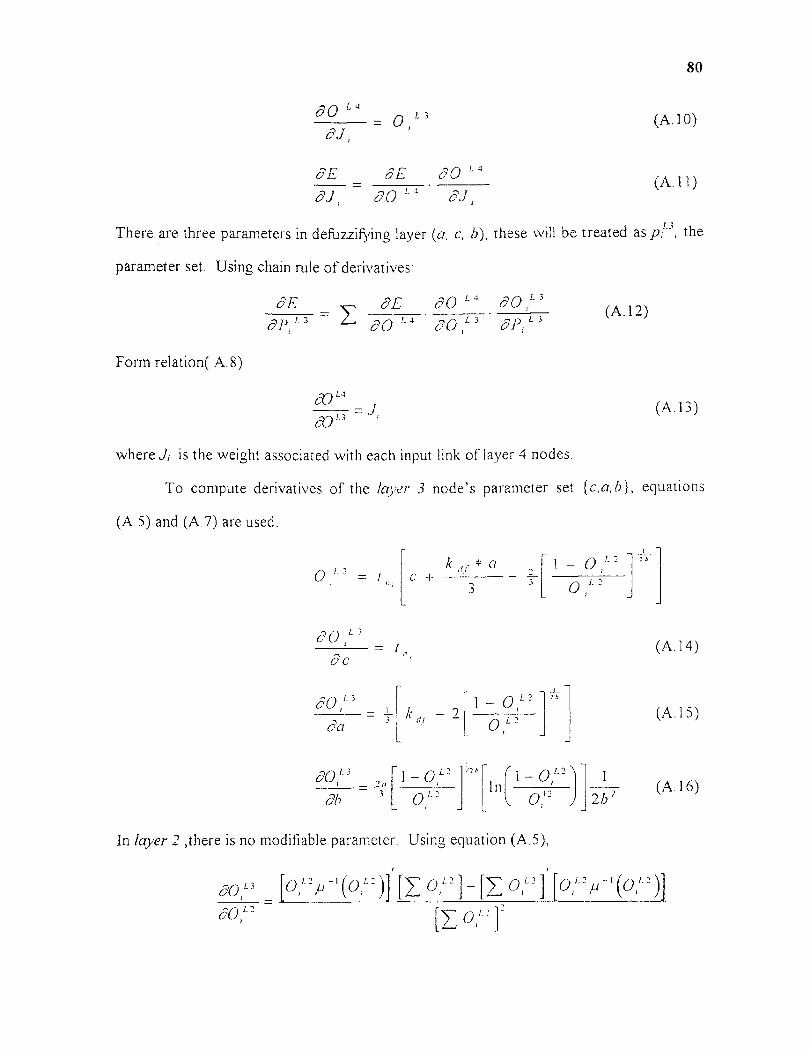
80

(A 10)

(A 1 1)

There are three parameters in defuzzifying layer (a, c, h), these will be treated as p 3, the

parameter set. Using chain rule of derivatives:

Form relation( A.8)

(A.13)

where ]1 is the weight associated with each input link of layer 4 nodes.

To compute derivatives of the layer 3 node's parameter set {c,a,b}, equations

(A.5) and (A.7) are used.

(A.14)

(A.15)

(A 16)

In layer 2 ,there is no modifiable parameter. Using equation (A.5),

— 1 [o' (0 , 1 2 )j

e 0 , f = [10 : 2 ]∂o _ [o,' P (o ² )] [I 0 `

81

(A 17)

where OP and 0 1 L3 are on the same rule

The derivative of output of./ th node in layer 3 ( 0,1-3 ) with respect to the output

of j th node of layer 2 (0 ,L2 ) is given as

(A.18)

Using equation (A.7) (012 )1 may be computed as:

(A.19)

There are also three parameters (p,L1 ) in each node of layer I. These modifiable

parameters {a, d, g} are given by the equation of bell shaped membership function.

(A 20)

The chain rule to compute the derivatives of error E with respect to each

parameters of layer] node is given by

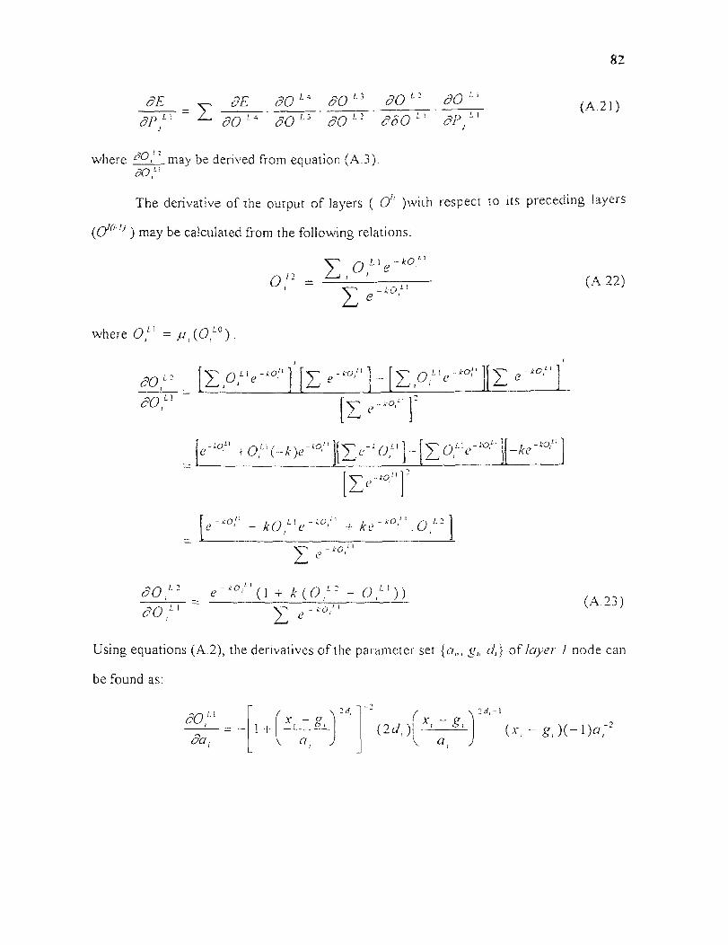
82

(A.21)

The derivative of the output of layers ( )with respect to its preceding layers

(CY") ) may be calculated from the following relations:

(A 22)

(A.23)

Using equations (A.2), the derivatives of the parameter set {a„, g„ di } of layer I node can

be found as:

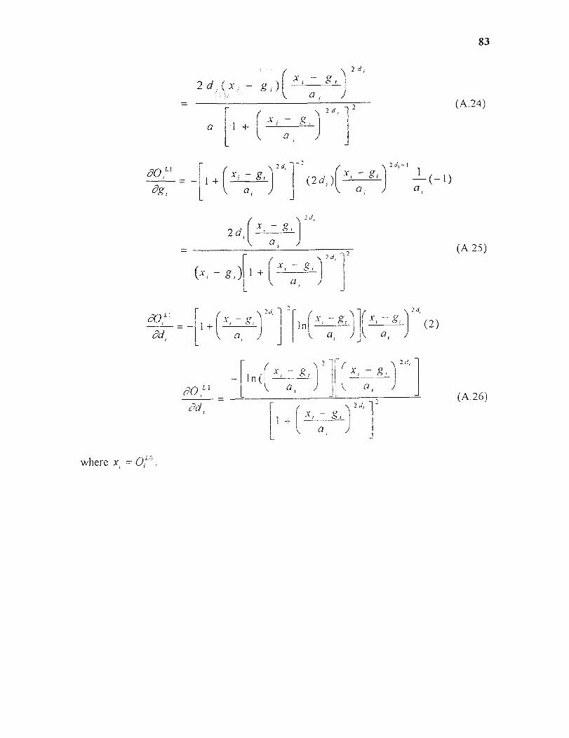
83

(A 24)

(A,25)

(A 26)

where x, = 0 L0 .

APPENDIX B

SYNCHRONOUS DEFUZZIFICATION

B.1 Triangular IMF in defuzzification level

Derivations for the consequent layers are only presented:

Layer 4 (Output layer)

(B. 1)

where, P, is a modifiable parameter

From equation (B.1)

So (B 2)

Layer L3(Defuzzification layer)

For defuzzification Triangular MFs are replaced by linear functions

From Equation 5.2 ( chapter 5): (c, p are modifiable parameters)

(B 3)

(B 4)

Each rule output (For details, see also appendix A)

(B 6)

84

85

(B.7)

(B.8)

B.2 Defuzzification with Sugeno type rule

Layer 4 (Output layer--L4)

Using the same steps as in B.1

(B 9)

Layer L3(Defuzzification layer--L3)

where, f is the rule output, and p,q,r,t are constants.

0 1-3 = 1„ f

where, t nn is the normalized rule firing strength.

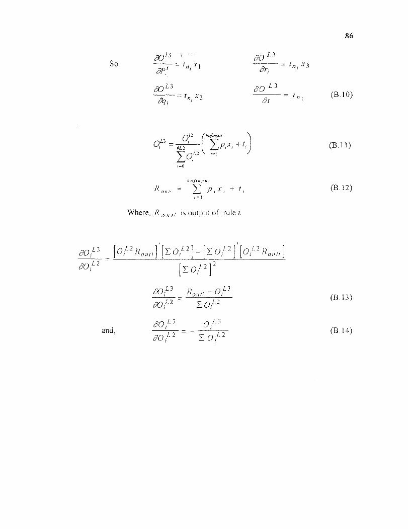
(B 13)

and, (13 14)

S o

86

(B 10)

(B.11)

(B.12)

Where, Routi is output of rule i.

APPENDIX C

BALANCE BEAM PARAMETERS

C.1 Balance Beam System Parameters

See chapter 3 for details of balance beam system model ( section 3.2.1):

x1= angular position of beam

x2 = angular velocity of beam

h= height of water in left tank

Q= flow rate of water

B= friction coefficient of bearing

=0.015 newton m.s/rad = 150000 dyne cm.s/rad

T( x1,,h) torque due to water

= 261186.67*(2h-H)*cos(x 1) + 1114.3265

*(0.5*(h2 + (H -h)2)+4.2*H*sin(x1 ) + 4190627* sin(x1 )

(Cl).

H = total water height (left tank water height h plus the water height of right tank)

J(h)=rotational moment of inertia of the system

= 389836.99+2.8353*((h3 + (H -h)3)+47.6328*(h2 + (H -h)2) +6463.21 *H

(C.2)

A= area of tank

= 3.14*(1.9*1.9) sq cm

Kpump = motor constant of pump

=1.389

Tpump = time constant of motor

0.061 sec

U = output of controller ( voltage)

87

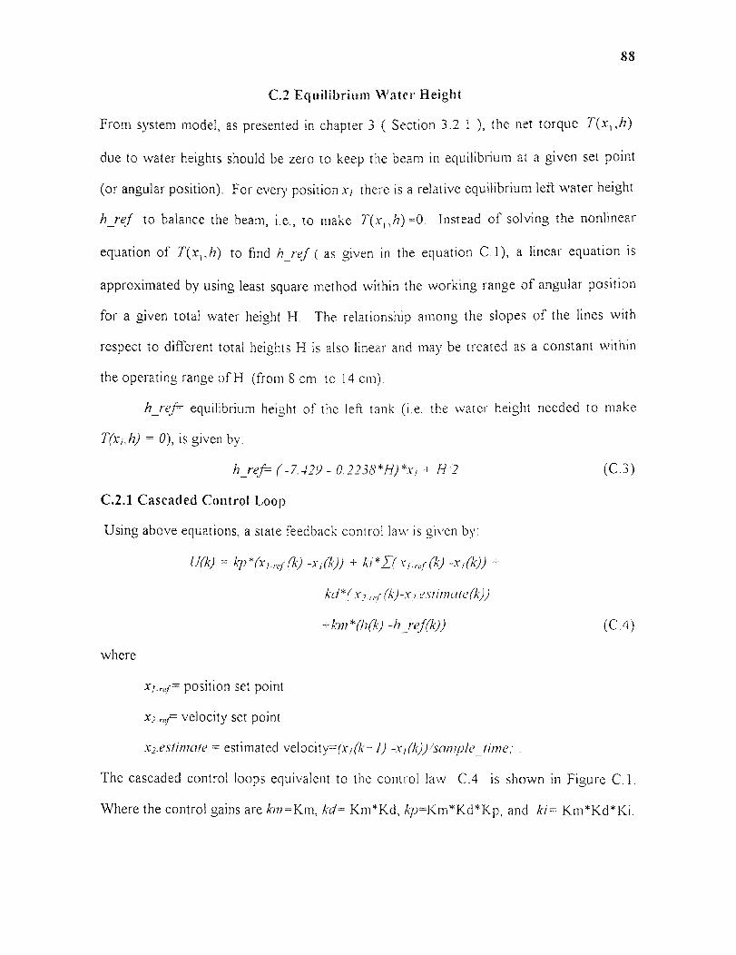
88

C.2 Equilibrium Water Height

From system model, as presented in chapter 3 ( Section 3.2.1 ), the net torque T(xI,h)

due to water heights should be zero to keep the beam in equilibrium at a given set point

(or angular position). For every position x i there is a re.1ative equilibrium .1efi water height

h_ref to balance the beam, i.e., to make T(xI,h) =O. Instead of solving the nonlinear

equation of T(xI,h) to find h_ref ( as given in the equation C.1), a linear equation is

approximated by using least square method within the working range of angular position

for a given total water height H. The relationship among the slopes of the lines with

respect to different total heights H is also linear and may be treated as a constant within

the operating range of H (from 8 cm to 14 cm).

h ref— equilibrium height of the .1efi tank (i.e. the water height needed to make

T(xI,h) = 0), is given by:

h_ref= (-7.429 - 0.2238*H)*xI T H/2 (C.3)

C.2.1 Cascaded Control Loop

Using above equations, a state feedback control .1aw is given by:

U(k) = kp*(xi1-ref(k)-x1 (k)) + ki*Ʃ(xi-ref(k)-x1(k)

kp*x2-ref(k)-x2.estimate(k))

-km*(h(k) -h_ref(k)) (C.4)

where

xI-ref= position set point

x2-ref= velocity set point

x2.estimate = estimated velocity=(xI(k-+1) -x 1(k))/sample _rime: .

The cascaded control loops equivalent to the control law C.4 is shown in Figure C.1.

Where the control gains are km=Km, kd= Km*Kd, kp=Km*Kd*Kp, and ki= Km*Kd*Ki.

h(p,x1)

1 Balance Beam

h_equ(x1)

Velocityestimator

x1 = position x2 = ve.1ocity; p = pressure ., h = water height; u = contro.1 vo.1tage

Figure C.1 Cascaded Control Loops

The following control gains have been used in simu.1ation:

Kp = 2.0 * 0.1*55.0*2.0/0.046

Ki = 4.0 * 0.1*55.0*2.0/0.046

Kd = 0.1 * 0.1*55.0*2.0/0.046

Km = 55.0*2.0 where 0.046 is the conversion factor from volts to radians. The total

water height H is used as 10.4 cm in all simulation.

Key to Keep Balance.. The Figure C.2 indicates that to ba.1ance the beam in the position

R¹ght Arm

89

'Left Arm

Figure C.2 Net torque in the same direction of rotation

90

as shown in figure, the right tank water height should be higher than the left tank water

height since the right moment arm is much less than the .1eft moment arm. To move the

beam from above equilibrium position to the horizonta.1 position (i.e. to rotate clock

wise), first a little water is to be pumped from left tank to right tank in order to start the

rotation in c.1ockwise direction and then immediately the water should be pumped in the

opposite direction to keep the ba.1ance until it arrives in the horizonta.1 position.

C.2.1 Push-Pull Control

As mentioned in chapter 3, two equivalent gear pumps in para.1le.1 have been used to pump

the water back and forth from the tanks. The "Push-Pu.1l" strategy is used to avoid the

dead zone of the pumps. General.1y the dead zone exists in the region of small input where

input cannot incur effective output. In order to avoid dead zone and a.1so to use the .1inear

region of pumping operation, two actuators are used in the same contro.1 channe.1 but in the

opposite directions such that their tota.1 effect is equiva.1ent to the origina.1 desired control

effect. If C is the centra.1 operating vo.1tage of the pumps, and the desired control vo.1tage

is U, then the following relations are used to compute vo.1tage input of each pump:

ul = C + U/2;

u2 -(C -U/2);

Where, ul and u2 are the input voltages of pump .1 and pump2 respectively. This strategy

wi.1.1 a.1so prevent the pumps from changing directions.

C.2.2 Pressure Sensor Calibration

Two linear pressure sensors are used to measure the water pressures of two tanks.

Although the relation between water pressure and sensor output voltage is linear, the

constant amount of water may have different output voltage at different angu.1ar positions

due to geometric effect. The actua.1 water height is a function of position and pressure.

91

The fo.1.1owing relation is used to find the water height from the position and pressure

sensors data.

water_height = C0 C 1 *position -4- C2*position*pressure C3*pressure (CA)

Where water heights are read from the rulers on tanks at horizonta.1 beam position while

values of position and pressure come from the potentiometer and pressure sensors

respective.1y The coefficients C0,C1,C2, and C3 are obtained by using Least Square

Method during ca.1ibration procedure In the present system a dynamic ca.1ibration method

is used in order to reduce the hysteresis effect [37]

REFERENCE S

[ 1] H.Ade.1i, and S.L.Hung,"Fuzzy neural network learning mode.1 for imagerecognition," Integrated Computer-Aided Engineering, Wi.1.1ey-Interscience,vol I,no1,1993.

[2] K.J. Astron and B. Wittenmark, Computer Controller Systems: Theory and Design,Prentice Hall, Engle wood C.1iffs, NJ, 1984.

[3] D.M. Auslander and C.H. Tham, Real-Time Software for Control, Prentice Ha.1l,Englewood Cliffs, NJ, 1989.

[4] D.M.Aus.1ander, G.Hanidu, A.Jana, S.Landsberger, S.Seif, and Y.Young,"Mechatronics Curricu.1um in the Synthesis Coalition," in Proc. of 1992 IEEE/CHMT Ina Electronic Manufacturing. Tech. Symp., Ba.1timore, MD, Sept. 1992,pp. 165-168.

[5] D.M.Auslander, "Unified real time task notation for mechanical system control,"Symposium on Mechatronics, DSC-Vol.50, ASME 1993, pp.143-149.

[6] D.M.Auslander, G.Hanidu, A.Jana, K.Jothimurugesan, S.Seif, andY.Young, "Too.1sfor Teaching Mechatronics," Proc. of 1993 ASEE Annual Conference, Univ. of

Illinois, IL, June 18-21,1993.

[7] D.M Auslander and Paul Sagues, Microprocessor for Measurement and Control,Berke.1ey, CA, Osborne/McGraw-Hi.1.1, 1981.

[8] A.G.Barto, R.S.Sutton, and C.W.Anderson, "Neuron.1ike adaptive e.1ements that cansolve difficult learning control problems, " IEEE Trans. Systems., M011, andCybernetics., vol. SMC-13, no. 5,pp. 834-846,1983.

[9] H.R.Berenji and P. Khedkar, "Learning and tuning fuzzy .1ogic controllers throughreinforcements," IEEE Trans. Nural Networks, vol. 3,pp. 724-740, May 1992.

[1 0] H. R.Berenji, "Fuzzy Q-.1earning: A new approach for fuzzy dynamicprogramming,"in Proc. IEEE Int. Conf. 011 Fuzzy Syst., Orlando, FL, June 1994. vol.I,pp.486-487.

[11] H.R. Berenji, "A reinforcement learning-based architecture for fuzzy .1ogic control,"Int.J.of Approximate Reasoning,vol.6,pp267-292, 1992.

[12] P.P.Bonissone, V. Badami, K.H Chaing, P.S.Khedkar, K.W. Marcelle, and M.J.Schutten, "Industrial app.1ications of fuzzy .1ogic at General Electric," in Proc. IEEE,vol.83, no.3., pp.450-465, MarchI995.

93

[13] M.Brown, and C. Haris, Neurofuzzy Adaptive Modelling and Control, Prentice HallHa.1l International (UK) Limited,1994.

[14] S.-C.Chang, "Adaptive Nonlinear Control Using Fuzzy Logic and Neural Network,"Ph.D Dissertation, Department of Mechanica.1 Engineering, NJIT, May 1994.

[15] I.Hayashi,H.Nomura,H.Yamasaki,and N.Wakami, "Construction of fuzzy inferenceru.1es by NDF and NDFL," Ini.JofAppro.vimaie Reasoning, vol. 6,pp241-261, 1992.

[16] C.M.Higgins, and Rodney M. Goodman, "Fuzzy ru.1e-based networks for contro.1,"IEEE Trans. Fuzzy Syst,,vol. 2 ,no.1,pp. 82-88, Feb.1994.

[17] G.E.Hinton, "Connectionist .1earning procedures," Artificial Intelligence, vol. 40,no.I, pp.143-150, 1989.

[18] K.Hornik, M. Stinchcombe, and H White, "Multi.1ayer feed forward networks areuniversa.1 approximators," Neural Networks, no. 2, pp 359-366, 1989.

[19] L.R.Hunt, and J. Turi, "A new algorithm for constructing approximatetransformation for non.1inear systems," IEEE Transaction on Automatic Control,38:10, pp. 1553-1556.

[20] K.J.Hunt, D. Sbarbaro, R.Zbikowski, and P.J.Gawthrop, "Neura.1 Networks forcontrol systems-A survey," Automatica, vol.28., no.6, pp 1083-1112, 1992.

[21] A.Jana, and D.M. Auslander, "Worked Programming Environment for inte.1ligentManufacturing Systems," Design and Implementation of Intelligent ManufacturingSystems, Parsaei, H.R., and Jamshidi, M., Eds., Chapter 1, pp. I-18, 1995. Prentice-Hall, 1995

[22] A.Jana, D.M. Auslander,R.N Dave, and S.S. Chehl, "Task P.1anning for CooperatingRobot Systems," Proc. of 1994 International Symposium on Robotics AndManufacturing, Maui, Hawaii, August 14- I 8, 1994.

[23] A.Jana, R.N. Dave, S.S. Chehl, C. S. Wang, "Computer-Integrated Manufacturingand Robotics Laboratory Design for Undergraduate Education," Proc. of 1994International Symposium on Robotics And Manufacturing, Maui, Hawaii, August14-18, 1994.

[24] A.Jana, S.S. Chehl, "Developing Instrumentation Laboratory with Real Time ControlComponent," Proc. of 1993 American Control Conference, San Francisco, June1993, pp. 2046- 2049.

[25] J.-S.R.Jang and C.-T.Sun, "Neuro-fuzzy modeling and control," in Proc. IEEE, vol.

83, no.3., pp.378-406, March 1995.

94

[26] J.-S.RJang, "Self-learning fuzzy controller based on temporal back-propagation," IEEE Tralls. NuralNerworks, \101.3, pp714-723, Sept. 1992.

[27] l-S.RJang, ".~·NFIS: Adaptive-network-based fuzzy inference systems," IE~""E Trans. Systems .. Alan. alld Cybernetics., vol. 23,pp.665-685,I\1ay 1993.

[28] .T.-S.R.lang, "Structure Determination in fuzzy modeling: A filZZY C/\.RT approach," in Proc. IEEE Int. Conf. 011 FII:':::Y SYSI., Orlando, FL, vol. 1, pp480-485,lune 1994.

[29] .T.-S.RJang and C.-T.Sun, "Functional equivalence between radial basis function networks and fuzzy inference systems," IEEE Trans. NlJra/ Networks, vol. 4, no. 1 pp.156-159, Jan 1993.

[30J H. D. lerro, A Jana, R.N. Dave, "Multiprocessing Systems: A Design Experience," 1994 ASEEIGSW Conference, Baton Rouge, LA, March '94.

[31] B. Kosko, Neural Networks and FII:':::y S)'srems: A Dynamical Systems Approach., Prentice Hall, Englewood Cliffs, NJ, 1991

[32] B. Kosko, "Fuzzy systems as universal approximators," in Proc. of IEEE Int. Conference 011 Fu::zy Systems 1992, SanDiego, March 8-12, pp. 1153-1162.

[33] W.AKwong, KM Passino, EG.Laukonen, and S.Yurkovich, "Expert supervision offuzzy learning systems for tolerant aircraft control," in Pmc. IEEE, vo1.83, no.3., pp.466-483, March 1995.

[34] C-c. Lee, "Fuzzy logic in control systems: Fuzzy logic controller-Part 1," IEEE 1'·ans. Systems., M{(Il, and Cybeme!lcs .. vol. 20,pp.404-418,Feb.1990.

[35] C-c. Lee, "Fuzzy logic in control systems: Fuzzy logic controller-Part 2," IEEE TrailS. Systems., Mall, {(lid Cybernefics., vol. 20,pp.419-43 5, Feb. 1990.

[36] C-c. Lee, "A self learning rule based controller employing approximate reasoning and neural net concept," Int. J. InreIl.S),sf., vol. 5, no. 3, pp 71-93, 1991.

[37J M.Lemkin, P.H. Yang, and D.M.Auslander, "Using hydraulically balanced beam as a case study in control implementation for control education," !1~C 1994.

[38] A.U.Levin,and KS. Narendra, "Control of nonlinear dynamical systems using neural networks: Controllability and stabilization," IEEE TrailS. Nlira/ Networks, vol.4, no.2, pp 192-206,March 1993.

95

[39] c.-T.Lin and C. S.G Lee, "Reinforcement structure/parameter learning for neural­network based fuzzy logic control systems," Jl:.,~E Trans. Fuzzy S:}lst.,vol. 2, Jan. 1994.

[40] c.-T.Lin and C. S.G Lee, "Neural-network-based fi.1ZZY logic control and decision system," IEEE Trans. Compufers, vol. 40. pp.1320-1336, Dec.1991.

[41] E.H.Mamdani and S.Assilian, "An experiment in linguistic synthesis with a fi.lZZy logic controller," Int. 1. ofMan-A1achine Studies,vol.7,no.l, pp.1-13,l975.

[42] lM.Mendel, "Fuzzy logic systems for engineering: A tutorial,"in Proc. IEEE, vo1.83 no.3.,pp34S-377, March 1995.

[43] KS. Narendra,and KParthasarathy, "Identification and control of dynamical systems using Neural Networks," IEEE Trans. Nellral NeMorks, vol. 1, no. 1 ppA- 27, March 1990.

[44] KS. Narendra,and KParthasarathy, "Gradient methods for the optimization of dynamical systems containing neural net\vorks," JEEE Trails. Nellral Nerworks, vol. 2, no.2, pp 241-262, March 1991.

[45] D.H.Nguyen and B. Widrov.,f, "Neural networks for self-learning control systems," IEEE Comrol Syst. A1aga::iJl I! , pp.18-23, Apr. 1990.

[46] Y.-M. Park, U Moon, and K.Y.Lee, "A self-organizing fuzzy logic controller for dynamic systems using a fuzzy auto-regressive moving average (F ARMA) model," IEEE Trans. Flizzy SYSf.,vo13, no.l, pp 75-82,Feb.1995.

[47] T.1Procyk and E.H.Mamdani, "A linguistic self-organizing process controller," Automatica, vol. 15,pp. 15-30,1978

[48] H. Serraji, "A new approach to adaptive control of manipulators," Transaction of the ASME, JOlfrnal (?f Dynamic S)lslems, l\1easlfremen{, and COllll'01 109, pp. 193-202.

[49] G. Strang, Introduction 10 Applied Mathematics, Wellesley-Cambridge Press, Wellesley, MA,1986.

[50] M.Sugeno,Ed.Jnd/lslr;a/ Applications C?f j-:"n::::y Comrol. New York: Elsevier, 1985.

[51] M.Sugeno and T. Yasukawa, "A fuzzy-logic-based approach to qualitative modeling," IEEE hailS. FII::::y S)'SI., vo!.l ,pp. 7 -31 ,Feb. 1993.

[52] M.Sugeno and G.T.Kang., "Structure Identification of fuzzy model," F1I::::Y 5;ers' and Sysfems,vo1.28,pp.15-33,1988.

96

[53] C-T.Sun, "Rulebase structure identification in an adaptive network based fuzzy inference system," IEEE Trans. Fu::::y .5)'51.,vo1.2 pp. 64-73, Feb.1994.

[54] C-T.Sun ,T.Y.Shuai, and G.-L. Dai, "Using fuzzy filters as feature detectors," in Proc. IEEE In!. COl~f 011 Fu::zy SySf., Orlando, FL, June 1994. vol. 1 ,ppA06-41O.

[55J T.Takagi and M. Sugeno, "Fuzzy identification of systems and its applications to modeling and control", IEEE Trails. S:yslems., lv/all, and Cybernetics., vol. 15, pp. 1]6-]32,1985.

[56J H.Takagi, and 1. Hayashi, "NN-driven fuzzy reasoning," Inr.J.of Approximate

Reasoning, vol. 5,pp] 91-212, 1991.

[57J K.Tanaka and M. Sugeno, "Stability analysis and design of fuzzy control systems,"Fu::zy Sets alld Sysrems volA5,pp.13 5-156,1992.

[58J Y.Tsukamoto, "An approach to fuzzy reasoning method," in Advancec ill FlI:'::Y Set TheolY and Applicatiolls, M.M. Gupta, R.K.Ragade, and R.R.Yager, Eds. Amsterdam: North-Holland, 1979, PP.137-149

[59] L.-x. \\Tang, and 1M. Mendel, "Back-propagation fuzzy systems as nonlinear dynamic system identifiers," in Pmc. IEEJ:; lilt. COI?f all FII:::::Y Systems, voL 1, pp. 161-170, March 1992.

[60J B.Widrow and M.A.Lehr, "30 years of adaptive neural nehvorks: Perceptron, madline, and backpropagation,"in Pmc. IEEE, vol. 78 pp.1415-1442, Sept.1990.

[61J R.R.Yager and DPFilev, "SLIDE A simple adaptive defuzzification method," IEEE Trans.Fuzzy SYSl., vol. l,pp. 69-78, Feb. 1993.

[62] LA Zadeh, "Fuzzy sets," II?/orI1l0Iioll alld cOI71I'OI, Vol. 8,pp 338-353,1965.

[63] L.A Zadeh, "Outline of a new approach to the analysis of complex systems and decision processes," IEI-"E Trans. sys·t. , A1an,alld Cybcr., voL3,pp.28-44, Jan.1973.

[64] L.AZadeh, Indllstrial AppficOlioJl (?/ FII::':::Y Logic and Illtel/igenr Syatems, J Yen, R. Lanagri, and L A Zadeh, Eds. New York, IEEE Press, 1995.