Neuro Semantic Thresholding for HighPrecision OCR Applications

Jesus Lazaro Jose Luis Martın Jagoba AriasArmando Astarloa Carlos Cuadrado

November 11, 2005

This paper shows a novel approach to binarization techniques. It presentsa way to obtain an optimum threshold using a semantic description of thehistogram and a neural network. The intended applications of this techniqueare high precision OCR algorithms over a limited number of document types.

The histogram of the input image is smoothed and its derivative is found.Using a polygonal version of the derivative and the smoothed histogram, anew description of the histogram is calculated. Using this description a gen-eral regression neural network is capable of obtaining an optimum thresholdfor our application.

1 Introduction

Thresholding is one of the first steps applied to any complex image processing. Severalapproaches have been taken over the past years, from thresholding techniques basedon histogram shape to algorithms based on information theory. One problem faced bymany of the proposed techniques is the fact that several images with the same histogramyield to the same threshold. As Kapur [1] noted, images with the same histogram,may not have the same optimum threshold. The solutions provided for this probleminclude taking into account second order statistics and full image processing. The firstsolution involves higher computational load and opens the door to calculating higherorder statistics to avoid first and second order coincidences. The second solution solvesthe problem of coincidental statistics among different images at a cost of an overwhelmingcomputational cost.

A second problem is the computational complexity. The traditional computationalcost refers to the time to solve a problem. The computational complexity is related tothe silicon area needed to perform such an algorithm. The algorithm proposed in thispaper fulfils both requirements: it takes into account the image’s higher order propertiesas well as the histogram and minimizes both the computational cost and complexity.

1

The proposed method obtains a semantic description of the histogram of the inputimage, which efficiently describes it. With this description and a general regressionneural network, an optimum threshold is obtained. The correctness of this thresholdis attained through the training set of the neural network that is adequately chosendepending on the application.

In our case, the test application has been an electronic voting system. In such asystem the number of different input type documents is limited (limited number of typeof votes) and the accuracy required is high (it is not admissible for a vote to be countedbadly, that is, to be counted as a different option).

The text is organized as follows: first a brief description of different kinds of threshold-ing techniques is done, next the proposed algorithm is described, after that some resultsand comparison charts are presented to finish with some conclusions.

2 Thresholding approaches

During the last 25 years multiple thresholding algorithms have been developed. Severalsurveys have been made to categorize all these algorithms. Lee, Chung and Park [2]compared five global thresholding techniques and presented several criteria for theirevaluation. Trier and Jain [3] compared 19 methods while Palumbo, Swaminathan andSrihari [4] compared three methods. Other surveys include [5][6][7], where different kindsof algorithms were tested. The categorization is a difficult task since most algorithmsuse strategies of several groups. In one of the several surveys, the binarization techniquesare divided into six groups:

1. Systems based on the form of the histograms. The processing is performed search-ing peaks and valleys of the histogram or finding the curvature and zero crossing ofthe derivative of the histogram. Among many others, we can find the thresholdingalgorithm of Rosenfeld [8] in which the main difference between the convex hull ofthe histogram and the histogram is selected as threshold. Other approaches usean all-pole model where the threshold is selected by maximizing the between-classvariance [9].

2. Clustering systems. These algorithms try to divide the pixels into two groups orclusters, one for the object and the other one for the background. Algorithms inthis group range from the classic Otsu’s algorithm [10], in which the histogram isdivided as the sum of two Gaussian functions, to Jawahar’s method [11] where theclustering is performed in terms of fuzzy clustering.

3. Entropy based systems. These algorithms make use of the information theory toobtain the threshold. Kapur [1] used the maximization of the a priori entropy ofthe object and background classes. Li [12] obtained the threshold by minimizingthe cross entropy between the original image and the binarized one. Shanbag [13],on the other side, relies on a fuzzy membership coefficient.

2

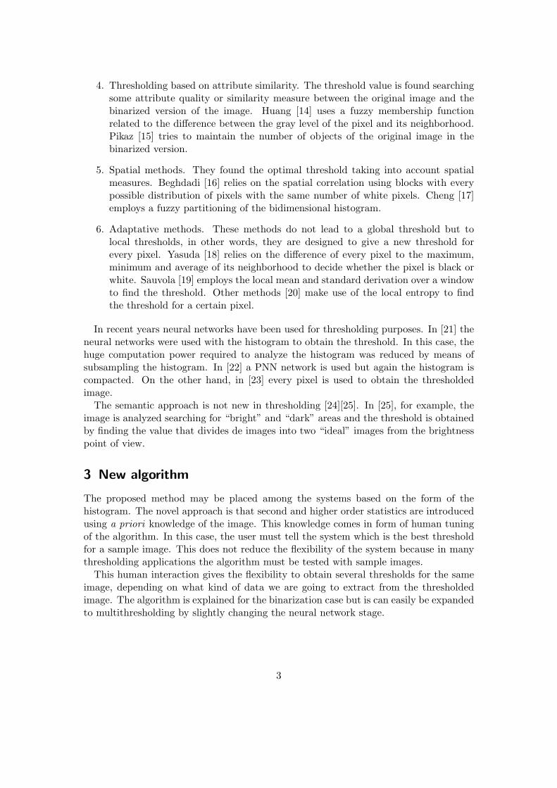
4. Thresholding based on attribute similarity. The threshold value is found searchingsome attribute quality or similarity measure between the original image and thebinarized version of the image. Huang [14] uses a fuzzy membership functionrelated to the difference between the gray level of the pixel and its neighborhood.Pikaz [15] tries to maintain the number of objects of the original image in thebinarized version.

5. Spatial methods. They found the optimal threshold taking into account spatialmeasures. Beghdadi [16] relies on the spatial correlation using blocks with everypossible distribution of pixels with the same number of white pixels. Cheng [17]employs a fuzzy partitioning of the bidimensional histogram.

6. Adaptative methods. These methods do not lead to a global threshold but tolocal thresholds, in other words, they are designed to give a new threshold forevery pixel. Yasuda [18] relies on the difference of every pixel to the maximum,minimum and average of its neighborhood to decide whether the pixel is black orwhite. Sauvola [19] employs the local mean and standard derivation over a windowto find the threshold. Other methods [20] make use of the local entropy to findthe threshold for a certain pixel.

In recent years neural networks have been used for thresholding purposes. In [21] theneural networks were used with the histogram to obtain the threshold. In this case, thehuge computation power required to analyze the histogram was reduced by means ofsubsampling the histogram. In [22] a PNN network is used but again the histogram iscompacted. On the other hand, in [23] every pixel is used to obtain the thresholdedimage.

The semantic approach is not new in thresholding [24][25]. In [25], for example, theimage is analyzed searching for “bright” and “dark” areas and the threshold is obtainedby finding the value that divides de images into two “ideal” images from the brightnesspoint of view.

3 New algorithm

The proposed method may be placed among the systems based on the form of thehistogram. The novel approach is that second and higher order statistics are introducedusing a priori knowledge of the image. This knowledge comes in form of human tuningof the algorithm. In this case, the user must tell the system which is the best thresholdfor a sample image. This does not reduce the flexibility of the system because in manythresholding applications the algorithm must be tested with sample images.

This human interaction gives the flexibility to obtain several thresholds for the sameimage, depending on what kind of data we are going to extract from the thresholdedimage. The algorithm is explained for the binarization case but is can easily be expandedto multithresholding by slightly changing the neural network stage.

3

The algorithm has been tested in an electronic voting system. The explanation ofthe whole system [26] is out of the scope of this article but basic procedure can besummarized as follows:

• There is a different ballot for each candidate in an election. Each ballot have aplaintext view of the name that will be hidden prior to casting the vote. Eachballot has the same name written in invisible ink (visible with UV light).

• The voter selects the ballots, tests that both, the invisible and visible texts, arethe same (optional), hides the visible one, and casts the vote.

• The systems reads the invisible texts and validates that the vote is correct.

• The system introduces the ballot into a secure box.

The proposed technique is composed of six steps:

1. Smoothed histogram.

2. First derivative of the histogram.

3. Polygonal descriptions of the derivative.

4. Polygonal descriptions of the histogram.

5. Semantic description of the polygon.

6. Threshold obtention using a general regression neural network (GRNN) and thesemantic description.

The algorithm has a prior step done off line. The first thing we must do is find thecorrect training set for the neural network. This is done taking sample images of theapplication, finding a correct thresholding and composing the training set. The easiestway to obtain a correct training set is to find every different kind of image that is goingto be thresholded. It can be a very difficult task involving thorough statistical analysis ofthe images. On the other hand, in the electronic voting application where the algorithmhas been tested, the number of different images can be chosen in an easy way; we canchose one ballot randomly for every different candidate. This approach has proofed tobe efficient as the results are satisfactory. If one particular kind of error is very common(for example votes with a degraded ink in a particular way) it could be introduced in thetraining set to increase the robustness. However, on doing so, the amount of memoryand resources also increases.

Once the image training set is selected, a series of operation must be performed toobtain the training set that will be introduced into the neural network:

• Thresholding of the selected images. Every test image should be thresholded withall the possible values, 256 in the case of 8 bit gray scale images.

4

• Run the final application on every image. In an optical reconnaissance application,an OCR software. This will establish the validity of each threshold. Find a meritfigure for every image. In our case, number of erroneous characters.

• Find the largest range of thresholding values that satisfy the required level ofaccuracy for each image. If no range is found, that means that a global thresholdingapproach cannot be used. The threshold should be the middle value of the range.

• Describe in a semantic way the selected image. This is done using every step ofthe proposed algorithm except from the final neural network stage (see followingsubsections).

• Select the desired thereshold in relation to the semantic description. We must finda target for our neural network, so we must express the threshold value as a positionin the semantic description. From prior stages we have the semantic descriptionof the histogram as well as the the limits of each “letter” in the histogram so theproblem of finding the target is reduced to find in which “letter” the threshold is.

• Training set creation. Using the semantic description of the selected images andthe targets found in the prior step, we can build the training set.

3.1 Smoothed histogram

The purpose of obtaining a smoothed histogram is to eliminate spurious maxima andminima, as well as reducing the computational and storage costs. The smoothing isperformed calculating a histogram with a length inferior to the number of grays. Math-ematically:

histogramlpf(i) =lpf·(i+1)∑

j=lpf·ihistogram(j) ∀ 0 ≤ i ≤ m (1)

where lpf is the reduction factor and m is the total number of possible grays in theoriginal image. It can be easily seen that the output histogram is of length m/lpf (seefigures 1 and 2).

The result of this step is a new histogram of reduced size. This new histogram main-tains the form of the original but it is low pass filtered to reduce both spurious valuesand data size. In order to reduce the computational cost, power of two numbers arepreferred for the reduction factor (see table 1). It must be noted that more complexlow pass filters could be used but the accuracy obtained satisfies the requirements. Inthe accuracy tests of the 5 section, the value of the reduction factor is four as it is theoptimal value from table 1.

3.2 Derivative of the histogram

The discrete derivation of the histogram corresponds to the slope of the curve. Thisderivative is obtained from the smoothed histogram leading to a description, in terms of

5

0 50 100 150 200 2500

100

200

300

400

500

600

700

800

Figure 1: Histogram (solid line) and smoothed histogram (dotted line).

Table 1: Different accuracies (see section 5 for further details on how accuracy is defined)for set 2 ballots (see figure 8) using different values of histogram reduction andsegments of the derivative

reduction factor/number of segments 2 4 8 162 0.43 0.78 0.60 0.884 0.37 0.99 0.98 0.988 0.94 0.56 0.54 0.9316 0.16 0.00 0.66 0.75

slope, of the histogram. Mathematically this operation can be described as (see figures2 and 3):

derivatelpf(i) = histogramlpf(i + 1)−− histogramlpf(i) ∀ 0 ≤ i < bm/lpfc (2)

It can be seen that the derivative of the histogram is simply calculated subtractingthe next element from the current one. This step can be performed at the same time asthe smoothed histogram and both can be reckoned as the image is entering the systemfrom a capture device.

3.3 Polygonal description of the derivative

The next step is to describe the derivative as a simple polygon. This is done limitingthe number of different slopes that the polygon may have. In this way, the followingprocessing is further simplified. The operations performed are described in equation 3(see figure 3).

6

Figure 2: Histogram (continuous line), smoothed histogram by 4 (dashed line) andderivative (arrows).

polygonald(i) =⌊derivatelpf(i) · number of segments

max(derivatelpf)

⌋−

− 12· sign(derivatelpf(i)) (3)

After this step, the obtained polygonal description of the derivative has only a limitednumber of values. The absolute value of the polygonal description will only have numberof segments values. As with the smoothing of the histogram, in order to reduce thecomputational cost, number of segments should be a power of two (see table 1).Thepolygonal description is shifted downwards half step to reduce the error from (0 → 1) to(±0.5). In the accuracy tests of the section 5, the value of number of segments is fouras it is the optimal value from table 1.

0 10 20 30 40 50 60 -1000

-800

-600

-400

-200

0

200

400

600

800

1000

Figure 3: Polygonal description of the derivative (solid line) and smoothed version of thederivative (dotted line).

7

3.4 Polygonal description of the histogram

Once a simple polygonal description of the derivative of the histogram is obtained, thenext step is to obtain a description of the histogram. This description is calculated takinginto account the polygonal description of the derivative and the smoothed histogram (seefigure 4).

0 10 20 30 40 50 60 700

500

1000

1500

2000

2500

3000

Figure 4: Smoothed histogram (solid line) and polygonal description of the histogram(dotted line).

In this stage, the polygonal description of the derivative is read. Using this data andthe smoothed histogram, a new histogram is found. This new histogram must havethe same area as the smoothed one. If the value of the polygonal description remainsunchanged, nothing is done, when a change occurs the type of the area is found. If thederivative was 0, the histogram is a plain otherwise it is a triangle.

The area of every zone is obtained as the area below the histogram curve, in otherwords, as the sum of every value in the histogram from the prior zone end to the currentpoint (including both) plus the area below the curve of the histogram and over thehistogram bars (see figure 5)

Figure 5: Calculated area is the sum of the single shaded zones.

If we are in a plain zone, the new height (AT ) is obtained by simply dividing the areaby the width and the new histogram segment is a plain of this new height.

8

If we are in hill zone, the new height is calculated as a triangle over a plain zone(see figure 6). The new histogram segment is a triangle that begins where the previoussegment ends.

base

AT

width

AREA

Figure 6: New histogram form when in a hill.

It should be noted that, in the process of calculating the area, the end of the priorsegment is taken into account. This means that the values in the segment border areused twice. This makes the newly described histogram different from the original oneand not merely an scaled or smoothed one. The new histogram takes into account pastvalues to obtain the new ones.

3.5 Semantic description

Once the new histogram has been generated, the semantic description is inferred. Thisis simply done by inspecting the type of segments located, the start and end heightsand the slopes. If we found a plain, we infer a plain. In any other case we compare theheights of the polygonal description of the histogram. If the start height is less than theend height, we consider we are going uphill, comparing the slopes we can determine thekind of slope, big or small angle. Otherwise we are going downhill.

The resulting “word” will describe the histogram and will be used by the neuralnetwork to find the threshold. Since the neural network can only work with numbers, asimple traduction is made from the descriptive letters to numbers. The translation tablecan be found in table 2.

Table 2: Semantic conversion table.U → 2u → 1P → 0d → -1D → -2

The result of the process so far is a simple description of the histogram. In this

9

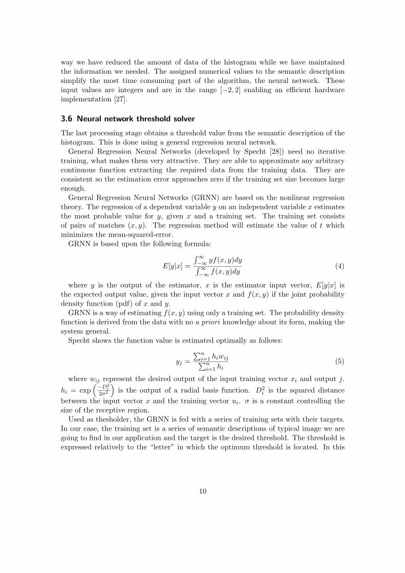
way we have reduced the amount of data of the histogram while we have maintainedthe information we needed. The assigned numerical values to the semantic descriptionsimplify the most time consuming part of the algorithm, the neural network. Theseinput values are integers and are in the range [−2, 2] enabling an efficient hardwareimplementation [27].

3.6 Neural network threshold solver

The last processing stage obtains a threshold value from the semantic description of thehistogram. This is done using a general regression neural network.

General Regression Neural Networks (developed by Specht [28]) need no iterativetraining, what makes them very attractive. They are able to approximate any arbitrarycontinuous function extracting the required data from the training data. They areconsistent so the estimation error approaches zero if the training set size becomes largeenough.

General Regression Neural Networks (GRNN) are based on the nonlinear regressiontheory. The regression of a dependent variable y on an independent variable x estimatesthe most probable value for y, given x and a training set. The training set consistsof pairs of matches (x, y). The regression method will estimate the value of t whichminimizes the mean-squared-error.

GRNN is based upon the following formula:

E[y|x] =

∫∞−∞ yf(x, y)dy∫∞−∞ f(x, y)dy

(4)

where y is the output of the estimator, x is the estimator input vector, E[y|x] isthe expected output value, given the input vector x and f(x, y) if the joint probabilitydensity function (pdf) of x and y.

GRNN is a way of estimating f(x, y) using only a training set. The probability densityfunction is derived from the data with no a priori knowledge about its form, making thesystem general.

Specht shows the function value is estimated optimally as follows:

yj =∑n

i=1 hiwij∑ni=1 hi

(5)

where wij represent the desired output of the input training vector xi and output j.

hi = exp(−D2

i2σ2

)is the output of a radial basis function. D2

i is the squared distancebetween the input vector x and the training vector ui. σ is a constant controlling thesize of the receptive region.

Used as thesholder, the GRNN is fed with a series of training sets with their targets.In our case, the training set is a series of semantic descriptions of typical image we aregoing to find in our application and the target is the desired threshold. The threshold isexpressed relatively to the “letter” in which the optimum threshold is located. In this

10

way the system is robust against movements of the histogram between images due tochanging illumination, camera degradation, etc.

If we wanted a multithresholder, the only difference would be in the target sectionof the training set. Instead of having only one value (threshold) it would have severalvalues (one for each threshold).

4 Computational cost

The algorithm is composed of very simple operations except for the neural network andthe divisions in the polygonal description of the derivative. If the number of segmentsis a power of two, the divisions may completely be substituted by shifts in a softwareimplementation and by correct wiring in hardware circuits.

In a non optimized Matlab implementation, the time needed to binarize an image(512x500 pixels, 256 gray scale), once subtracted the time to load it from disk was 0.024seconds in a AMD AthlonXP 1600 running WindowsXP SP2. More than 60% of thetime was invested in the neural network.

The algorithm can also be implemented in hardware. In such an implementation, thesmoothing of the histogram and the calculus of the first derivative can be calculated atthe same time and while the image is arriving from the capture sensor. The polygonaldescription of the derivative, once a power of two number of segments are used, is reducedto comparisons. The polygonal description of the histogram is a little bit more complexsince we need to multiply and divide. In modern FPGA devices we can find hardwaremultipliers. The division is not very complex since the divisor has very few bits (if thehistogram reduction factor is four, the divisor is smaller than 64, 256/4) it has very fewstages and can be very fast. The semantic description can be reduced to comparisons.As in the software implementation, the neural network has the greatest complexity butsince the input data has a very few possible values it can efficiently be implemented [27].

5 Results

The algorithm has been tested against two sets of ballots from different elections. Oneof the sets comprises 6 different candidates while the other has 3. For every ballot 1024different captures have been made. The images of each set are depicted in 7 and 8.

Although all the images are similar, due to differences in the printing process, camera,temperature and others, the histograms are different (see figure 9). Each of the poll haveeach the training set, it is formed using the images in 7 and 8 and following the processexplained before.

The proposed algorithm (NST) has been tested against ten different algorithms. Thealgorithm used are Otsu [10], Brink [29], Rdiler [30], Rosenfeld [8], Li [12], Abutaleb [31],Begdhadi [16], Kittler [32] and Niblak [33]. The ballot character recognition has beenmade, in all the cases, using a commercial OCR software. This software is capable ofreading images in gray scale and the results are also included. The results can be found

11

Figure 7: Image samples of first set

in table 3 and 4. The results of the recognition are catalogued correct or wrong. A wrongrecognition is defined as an image with more than one character badly recognized.

In table 5 the overall results for both ballot sets can be found. Using the valuesfrom table 3 and 4 we can state that: using the ballots from set 1, the only algorithmswith an accuracy over 90% are the proposed one and Rosenfeld, while the rest lay farbehind. It is when comparing the variances that the greatest differences appear. TheNST algorithm has a much greater uniformity than the rest of algorithms.

In the case of set 2 we have a similar situation. Only two algorithms have an accuracyover 90%, NST and Kittler. In this case, both algorithms have a very good variance.The NST algorithm is slightly better but without any statistical significance.

So far, we have used the accuracy and variance intraelection (accuracy among ballotsof the same election), the next step is the accuracy and variance interelection (accuracyamong elections). In table 5 we have the mean and variance between both sets. In thiscase only NST algorithm offers high accuracy and low variance.

It must be noted that images that are correctly thresholded do not defer greatly fromthose which are not. In figure 10 we can see two different ballots from set 2. Bothof them are correctly binarized by the proposed algorithm but Kittler’s algorithm (thesecond best with the second set) fails to correctly binarize one of them.

One question that my arise is what happens if the different image groups have verydifferent semantic description. An example can be found in figure 11. This new extraimages have completely different semantic description (one of them is the opposite fromone of images in the original set). When including these images in the training set the

12

Figure 8: Image samples of second set

0 50 100 150 200 2500

20

40

60

80

100

120

140

160

Figure 9: Standard deviation of the histograms of the first testing set

performance is slightly degraded. We can find the accuracy results in table 6. The reasonfor this is that images with different semantic descriptions do not interfere among themdue to the negative exponential characteristic of the GRNN. The main concern shouldbe images with the same, or very similar, semantic description and different threshold.This case should be the equivalent to equal histogram and different threshold for shapebased thresholding approaches.

6 Conclusions

The proposed method uses a smoothed histogram to reduce the computational cost ofthe algorithm. Apart from that, the most time consuming part of the algorithm, theneural network, is applied over a semantic description of the histogram that is muchsimpler than the original.

From the result’s point of view, the proposed algorithm works better than any othertested algorithm. The algorithm has the particularity of working equally good withsimilar images, characteristic that many other algorithms do not have. In other words,its performance is equal among different images from the same set and among set,

13

Table 3: Percentage of correct images in recognition for set 7. Each column representsthe results for each of the images.Method 1 2 3 4 5 6 Mean Variance

NST 99.8 99.9 92.6 100.0 98.9 98.9 98.4 8.2Otsu 0.0 1.1 0.0 0.0 0.0 0.1 0.2 0.2Brink 0.0 0.0 0.0 0.0 0.0 0.0 0.0 0.0Ridler 0.0 7.4 0.0 0.0 0.0 5.3 2.1 11.2

Rosenfeld 99.1 96.4 83.1 96.6 92.6 97.2 94.2 33.9Li 0.1 84.8 2.2 1.6 55.5 65.0 36.5 1327.9

Abutaleb 0.0 0.0 0.0 0.4 0.1 0.0 0.1 0.0Begdhadi 0.0 0.0 0.0 0.0 0.0 0.0 0.0 0.0Kittler 28.7 99.4 0.0 71.9 91.4 97.3 64.8 1702.7Niblak 0.0 0.0 0.0 0.0 0.0 0.0 0.0 0.0Ocr 0.9 0.3 10.3 34.1 10.1 0.5 9.4 169.1

ensuring the privacy.The proposed algorithm is specially suited for OCR application where the number of

different types of input documents is reduced and the admissible number of erroneousrecognized characters per image is very strict.

References

[1] J.N. Kapur, P.K. Sahoo, and A.K.C. Wong. A New Method for Gray-Level PictureThresholding Using the Entropy of the Histogram. Computing Vision GraphicsImage Processing, 29:273–285, 1985.

[2] H. Lee, S.Y. Chung, and R.H. Park. A Comparative Performace Study of SeveralGlobal Thresholding Techniques for Segmentation. Computer Vision Graphics andImage Processing, 52(2):171–190, 1990.

[3] Ø.D. Trier and A.K. Jain. Goal-Directed Evaluation of Binarization Methods.IEEE Transactions on Pattern Analysis and Machine Intelligence, 17(12):1191–1201, 1995.

[4] P.W. Palumbo, P. Swaminathan, and S.N. Srihari. Document Image Binarization:Evaluation of Algorithms. In Proc. SPIE Applications of Digital Image Proc., vol-ume 697, pages 278–286, 1986.

[5] P.K. Sahoo, S. Soltani, A.K.C. Wong, and Y.C. Chen. A Survey of ThresholdingTechniques. Computer Graphics and Image Processing, 41(2):233–260, 1988.

[6] C.A. Glasbey. An Analysis of Histogram-Based Thresholding Algorithms. GraphicalModels and Image Processing, 55(6):532–537, 1993.

14

Table 4: Percentage of correct images in recognition for set 8. Each column representsthe results for each of the images.

Method 1 2 3 Mean VarianceNST 99.9 98.6 99.6 99.4 0.5Otsu 0.0 0.0 0.0 0.0 0.0Brink 0.0 0.0 0.0 0.0 0.0Ridler 0.0 0.0 55.8 18.6 1037.9

Rosenfeld 0.0 0.0 0.0 0.0 0.0Li 17.6 14.6 95.2 42.5 2087.9

Abutaleb 0.6 0.0 91.6 30.7 2778.7Begdhadi 0.0 0.0 0.0 0.0 0.0Kittler 97.1 99.1 98.4 98.2 1.0Niblak 0.0 0.0 0.0 0.0 0.0Ocr 4.7 6.5 85.1 32.1 2107.6

[7] B. Sankur and M. Sezgin. A Survey Over Image Thresholding Techniques AndQuantitative Performance Evaluation.

[8] A. Rosenfeld and P. de la Torre. Histogram Concavity Analysis as an Aid in Thresh-old Selection. IEEE Transactions on Systems, Man and Cybernetics, 13(3):231–235,1983.

[9] R. Guo and S.M. Pandit. Automatic Threshold Selection Based on HistogramModes and a Discriminant Criterion. Machine Vision and Applications, 10(5-6):331–338, 1998.

[10] N. Otsu. A Threshold Selection Method from Gray-Level Histograms. IEEE Trans-actions on Systems, Man and Cybernetics, 9(1):62–66, 1979.

[11] C.V. Jawahar, P.K. Biswas, and A.K. Ray. Investigation on Fuzzy ThresholdingBased on Fuzzy Clustering. Pattern Recognition, 30(10):1605–1613, 1997.

[12] C.H. Li and C.K. Lee. Minimum Cross Entropy Thresholding. Pattern Recognition,26(4):617–625, 1993.

[13] A.G. Shanbhag. Utilization of Information Measure as a Means of Image Thresh-olding. Computer Vision Graphics and Image Processing, 56(5):414–419, 1994.

[14] L.-K. Huang and M.-J.J. Wang. Image Thresholding by Minimizing the Measuresof Fuzziness. Pattern Recognition, 28(1):41–51, 1995.

[15] A. Pikaz and A. Averbuch. Digital Image Thresholding Based on Topological StableState. Pattern Recognition, 29(5):829–843, 1996.

15

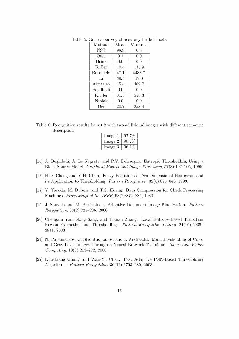
Table 5: General survey of accuracy for both sets.Method Mean Variance

NST 98.9 0.5Otsu 0.1 0.0Brink 0.0 0.0Ridler 10.4 135.9

Rosenfeld 47.1 4433.7Li 39.5 17.6

Abutaleb 15.4 469.7Begdhadi 0.0 0.0Kittler 81.5 558.3Niblak 0.0 0.0Ocr 20.7 258.4

Table 6: Recognition results for set 2 with two additional images with different semanticdescription

Image 1 97.7%Image 2 98.2%Image 3 96.1%

[16] A. Beghdadi, A. Le Negrate, and P.V. Delesegno. Entropic Thresholding Using aBlock Source Model. Graphical Models and Image Processing, 57(3):197–205, 1995.

[17] H.D. Cheng and Y.H. Chen. Fuzzy Partition of Two-Dimensional Histogram andits Application to Thresholding. Pattern Recognition, 32(5):825–843, 1999.

[18] Y. Yasuda, M. Dubois, and T.S. Huang. Data Compression for Check ProcessingMachines. Proccedings of the IEEE, 68(7):874–885, 1980.

[19] J. Sauvola and M. Pietikainen. Adaptive Document Image Binarization. PatternRecognition, 33(2):225–236, 2000.

[20] Chengxin Yan, Nong Sang, and Tianxu Zhang. Local Entropy-Based TransitionRegion Extraction and Thresholding. Pattern Recognition Letters, 24(16):2935–2941, 2003.

[21] N. Papamarkos, C. Strouthopoulos, and I. Andreadis. Multithresholding of Colorand Gray-Level Images Through a Neural Network Technique. Image and VisionComputing, 18(3):213–222, 2000.

[22] Kuo-Liang Chung and Wan-Yu Chen. Fast Adaptive PNN-Based ThresholdingAlgorithms. Pattern Recognition, 36(12):2793–280, 2003.

16

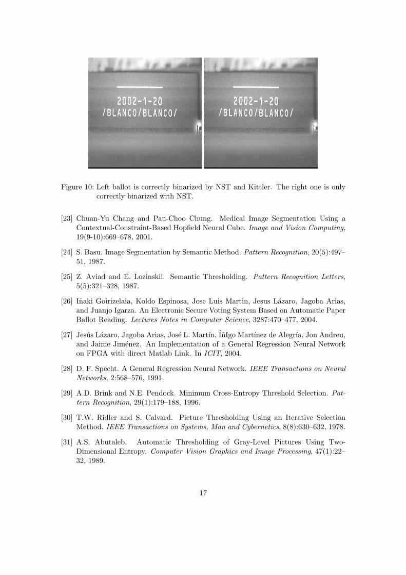
Figure 10: Left ballot is correctly binarized by NST and Kittler. The right one is onlycorrectly binarized with NST.

[23] Chuan-Yu Chang and Pau-Choo Chung. Medical Image Segmentation Using aContextual-Constraint-Based Hopfield Neural Cube. Image and Vision Computing,19(9-10):669–678, 2001.

[24] S. Basu. Image Segmentation by Semantic Method. Pattern Recognition, 20(5):497–51, 1987.

[25] Z. Aviad and E. Lozinskii. Semantic Thresholding. Pattern Recognition Letters,5(5):321–328, 1987.

[26] Inaki Goirizelaia, Koldo Espinosa, Jose Luis Martin, Jesus Lazaro, Jagoba Arias,and Juanjo Igarza. An Electronic Secure Voting System Based on Automatic PaperBallot Reading. Lectures Notes in Computer Science, 3287:470–477, 2004.

[27] Jesus Lazaro, Jagoba Arias, Jose L. Martın, InIgo Martınez de Alegrıa, Jon Andreu,and Jaime Jimenez. An Implementation of a General Regression Neural Networkon FPGA with direct Matlab Link. In ICIT, 2004.

[28] D. F. Specht. A General Regression Neural Network. IEEE Transactions on NeuralNetworks, 2:568–576, 1991.

[29] A.D. Brink and N.E. Pendock. Minimum Cross-Entropy Threshold Selection. Pat-tern Recognition, 29(1):179–188, 1996.

[30] T.W. Ridler and S. Calvard. Picture Thresholding Using an Iterative SelectionMethod. IEEE Transactions on Systems, Man and Cybernetics, 8(8):630–632, 1978.

[31] A.S. Abutaleb. Automatic Thresholding of Gray-Level Pictures Using Two-Dimensional Entropy. Computer Vision Graphics and Image Processing, 47(1):22–32, 1989.

17

Figure 11: Extra images included in set 2.

[32] J. Kittler and J. Illingworth. On Threshold Selection Using Clustering Criteria.IEEE Transactions on Systems, Man and Cybernetics, 15(5):652–655, 1985.

[33] W. Niblack. An Introduction to Image Processing, pages 115–116. Prentice-Hall,1986.

18