Classification of time series by shapelet transformation

1 23

Data Mining and KnowledgeDiscovery ISSN 1384-5810 Data Min Knowl DiscDOI 10.1007/s10618-013-0322-1

Classification of time series by shapelettransformation

Jon Hills, Jason Lines, EdgarasBaranauskas, James Mapp & AnthonyBagnall

1 23

Your article is protected by copyright and all

rights are held exclusively by The Author(s).

This e-offprint is for personal use only

and shall not be self-archived in electronic

repositories. If you wish to self-archive your

article, please use the accepted manuscript

version for posting on your own website. You

may further deposit the accepted manuscript

version in any repository, provided it is only

made publicly available 12 months after

official publication or later and provided

acknowledgement is given to the original

source of publication and a link is inserted

to the published article on Springer's

website. The link must be accompanied by

the following text: "The final publication is

available at link.springer.com”.

Data Min Knowl DiscDOI 10.1007/s10618-013-0322-1

Classification of time series by shapelet transformation

Jon Hills · Jason Lines · Edgaras Baranauskas ·James Mapp · Anthony Bagnall

Received: 7 February 2013 / Accepted: 6 May 2013© The Author(s) 2013

Abstract Time-series classification (TSC) problems present a specific challenge forclassification algorithms: how to measure similarity between series. A shapelet is atime-series subsequence that allows for TSC based on local, phase-independent sim-ilarity in shape. Shapelet-based classification uses the similarity between a shapeletand a series as a discriminatory feature. One benefit of the shapelet approach is thatshapelets are comprehensible, and can offer insight into the problem domain. Theoriginal shapelet-based classifier embeds the shapelet-discovery algorithm in a deci-sion tree, and uses information gain to assess the quality of candidates, finding a newshapelet at each node of the tree through an enumerative search. Subsequent researchhas focused mainly on techniques to speed up the search. We examine how best touse the shapelet primitive to construct classifiers. We propose a single-scan shapeletalgorithm that finds the best k shapelets, which are used to produce a transformeddataset, where each of the k features represent the distance between a time series and ashapelet. The primary advantages over the embedded approach are that the transformed

Responsible editor: Eamonn Keogh.

J. Hills (B) · J. Lines · E. Baranauskas · J. Mapp · A. BagnallUniversity of East Anglia, Norwich NR4 7TJ, UKe-mail: [email protected]

J. Linese-mail: [email protected]

E. Baranauskase-mail: [email protected]

J. Mappe-mail: [email protected]

A. Bagnalle-mail: [email protected]

123

Author's personal copy

J. Hills et al.

data can be used in conjunction with any classifier, and that there is no recursivesearch for shapelets. We demonstrate that the transformed data, in conjunction withmore complex classifiers, gives greater accuracy than the embedded shapelet tree. Wealso evaluate three similarity measures that produce equivalent results to informationgain in less time. Finally, we show that by conducting post-transform clustering ofshapelets, we can enhance the interpretability of the transformed data. We conduct ourexperiments on 29 datasets: 17 from the UCR repository, and 12 we provide ourselves.

1 Introduction

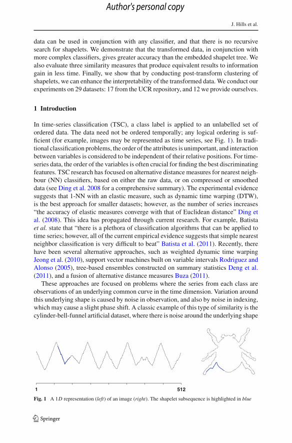
In time-series classification (TSC), a class label is applied to an unlabelled set ofordered data. The data need not be ordered temporally; any logical ordering is suf-ficient (for example, images may be represented as time series, see Fig. 1). In tradi-tional classification problems, the order of the attributes is unimportant, and interactionbetween variables is considered to be independent of their relative positions. For time-series data, the order of the variables is often crucial for finding the best discriminatingfeatures. TSC research has focused on alternative distance measures for nearest neigh-bour (NN) classifiers, based on either the raw data, or on compressed or smootheddata (see Ding et al. 2008 for a comprehensive summary). The experimental evidencesuggests that 1-NN with an elastic measure, such as dynamic time warping (DTW),is the best approach for smaller datasets; however, as the number of series increases“the accuracy of elastic measures converge with that of Euclidean distance” Ding etal. (2008). This idea has propagated through current research. For example, Batistaet al. state that “there is a plethora of classification algorithms that can be applied totime series; however, all of the current empirical evidence suggests that simple nearestneighbor classification is very difficult to beat” Batista et al. (2011). Recently, therehave been several alternative approaches, such as weighted dynamic time warpingJeong et al. (2010), support vector machines built on variable intervals Rodriguez andAlonso (2005), tree-based ensembles constructed on summary statistics Deng et al.(2011), and a fusion of alternative distance measures Buza (2011).

These approaches are focused on problems where the series from each class areobservations of an underlying common curve in the time dimension. Variation aroundthis underlying shape is caused by noise in observation, and also by noise in indexing,which may cause a slight phase shift. A classic example of this type of similarity is thecylinder-bell-funnel artificial dataset, where there is noise around the underlying shape

1 512

Fig. 1 A 1D representation (left) of an image (right). The shapelet subsequence is highlighted in blue

123


Classification of time series

and in the index where the shape transitions. Intuitively, time-domain NN classifiersare ideal for this type of problem, as DTW can be used to mitigate noise in the indexing.

There is another set of problems involving cases where similarity in shape definesclass membership. Series within a class may be distinguished by common sub-shapesthat are phase independent; i.e., the defining shape may begin at any point in the series.If the underlying phase-independent shape that defines class membership is global,that is to say, the shape is (approximately) the length of the series, then techniquesbased on transformation into the frequency domain can be employed to constructclassifiers Janacek et al. (2005). However, if the discriminatory shape is local, i.e.significantly shorter than the series as a whole, then it is unlikely that the differencesbetween classes will be detected using spectral approaches. Ye and Keogh (2009)propose shapelets to address this type of problem.

A shapelet is a time-series subsequence that can be used as a primitive for TSC basedon local, phase-independent similarity in shape. Shapelet-based classification involvesmeasuring the similarity between a shapelet and each series, then using this similarityas a discriminatory feature for classification. The original shapelet-based classifierembeds the shapelet discovery algorithm in a decision tree, and uses informationgain to assess the quality of candidates. A shapelet is found at each node of the treethrough an enumerative search. Shapelets have been used in applications such as earlyclassification Xing et al. (2011, 2012), gesture recognition Hartmann and Link (2010),gait recognition Sivakumar et al. (2012), and clustering Zakaria et al. (2012).

The exhaustive search for shapelets is time consuming. Thus, the majority ofshapelet research has focused on techniques to speed up the search He et al. (2012),Mueen et al. (2011), Rakthanmanon and Keogh (2013), Ye and Keogh (2009, 2011).This makes the search for shapelets more tractable, but does not address the funda-mental issue of how best to use shapelets to solve TSC problems. Decision trees areuseful and robust classifiers, but are outperformed in many problem domains by otherclassifiers, such as support vector machines, Bayesian networks and random forests.

We propose a single-scan algorithm that finds the best k shapelets in a set of n timeseries. We use this algorithm to produce a transformed dataset, where each of the kfeatures is the distance between the series and one shapelet. Hence, the value of the ithattribute of the jth record is the distance between the jth record and the ith shapelet.The primary advantages of this approach are that we can use the transformed datain conjunction with any classifier, and that we do not have to search sequentially forshapelets at each node. Threading the shapelet transform is an embarrassingly parallelproblem.

Many of the shapelets generated by the transform are similar to one another. Interms of accuracy, this is not a problem if the classifier employed can handle correlatedattributes; however, it does reduce the interpretability of the transformed dataset. Tomitigate this problem, we propose a post-transform clustering procedure that groupssimilar shapelets. We demonstrate that this dimensionality reduction allows us to mapthe shapelets back to the problem domain easily, without substantially reducing theaccuracy of the classifiers.

We also address how to assess shapelet quality. The similarity between each can-didate shapelet and each series is measured, and this sequence of distances, withassociated class membership, is used to assess shapelet quality. One implication of

123


J. Hills et al.

constructing a recursive decision tree is that there is a need to find a split point at eachnode based on the sequence of distances. This requirement makes it natural to useinformation gain as the shapelet quality measure. However, calculating informationgain for a continuous attribute requires the evaluation of all split points, and onlyevaluates binary splits. This introduces a time overhead, and means that, for multi-class problems, information gain may not capture fully the quality of the shapelet. Incontrast, there is no need to split the data when constructing the shapelet transform.Therefore, we can base the quality measure on a hypothesis test of differences in dis-tribution of distances between class populations. This allows us to assess multi-classproblems fully, and provides some speed improvement. We experiment with measuresbased on the analysis of variance test for differences in means, and the non-parametricKruskal-Wallis and Mood’s median tests for difference in medians.

We conduct our experiments on 29 datasets, 17 from the UCR repository and 12of we provide ourselves. This research is an extension of the work presented at twoconferences Lines and Bagnall (2012), Lines et al. (2012). The code and datasets areavailable from Bagnall et al. (2012). Our contributions can be summarised as follows:

1. We describe a shapelet-discovery algorithm to find the best k shapelets in a singlepass, and evaluate it with numerous experiments on benchmark time-series datasetsand on new data.

2. We evaluate three alternative quality measures for use with our algorithm. Twomeasures were proposed for the shapelet tree in Lines and Bagnall (2012). We per-form comprehensive experiments and show that the new measures offer improvedspeed over information gain.

3. We demonstrate that classifiers built on the shapelet-transformed data are moreaccurate than the tree-based shapelet classifier on a wide range of problems.

4. We compare the performance of classifiers constructed on shapelet-transformeddata to classifiers constructed in the time domain.

5. We extend the original shapelet transform by using post-transform clustering torelate the shapelets to the problem domain.

6. We provide three new time-series classification problems: Beetle/Fly,Bird/Chicken, and Otoliths.

The paper is structured as follows. Section 2 provides background on time-seriesclassification and shapelets. In Sect. 3, we define three shapelet quality measures thatare an alterative to information gain. In Sect. 4, we propose a shapelet transformalgorithm. We discuss the datasets used for our experiments in Sect. 5. In Sect. 6, wedescribe our experimental design and results, and perform qualitative analysis. Finally,in Sect. 7, we form our conclusions.

2 Background

2.1 Time-series classification

A time series is a sequence of data that is typically recorded in temporal order atfixed intervals. Suppose we have a set of n time series T = {T1, T2, . . . , Tn}, whereeach time series Ti has m real-valued ordered readings Ti =< ti,1, ti,2, . . . , ti,m >,

123



and a class label ci . We assume that all series in T are of length m, but this is not arequirement (see Hu et al. 2013 for discussion of this issue). Given a dataset T, thetime-series classification problem is to find a function that maps from the space ofpossible time series to the space of possible class values.

As with all time-series data mining, time-series classification relies on a similar-ity measure to compare data. Similarity measures can be embedded into the clas-sifier or introduced through data transformation prior to classification. Discrimina-tory similarity features typically fall into one of three categories: similarity in time(correlation-based), similarity in change (autocorrelation-based), and similarity inshape (shape-based). We focus on representations that best capture similarity in shape.

If function fc describes the common shape for class c, then a time series can bedescribed as

ti, j = fci ( j, si )+ ε j ,

where si is the offset for series i , and ε j is some form of noise. Similarity in shapecan be differentiated into global and local similarity. Global shape similarity is wherethe underlying shape that defines class similarity is approximately the same length asthe series, but series within the same class can have different offsets. So, for example,function fc could be sinusoidal,

fci ( j, s) = sin

(j + s

ci · π)

.

This form of global similarity can be detected through explicit realignment or, morecommonly, through transformation into the frequency domain Janacek et al. (2005),Wu et al. (2000). However, these approaches are unlikely to work when the shape-based similarity is local. In this scenario, the discriminating shape is much smallerthan the series, and can appear at any point. For example, the shape could be a sinewave embedded in noise that is triggered randomly for a short period. The functionfc would then be of the form

fci ( j, s) ={

sin(

jci ·π

)if s ≤ j < s + l

0 otherwise,

where l is length of the shape. It is unlikely that techniques based on Fourier trans-forms of the whole series will detect these embedded shapes, and spectral envelopeapproaches based on sliding windows are inappropriate, as we are assuming l is small.Shapelets were introduced in Ye and Keogh (2009) to measure this type of similarity.

2.2 Shapelets

A shapelet is a subsequence of one time series in a dataset T. Every subsequence ofevery series in T is a candidate. Shapelets are found via an exhaustive search of everycandidate between lengths min and max . Shapelets are independently normalised;

123


J. Hills et al.

since we are interested in detecting localised shape similarity, they must be invariant toscale and offset. Shapelet discovery has three main components: candidate generation,a similarity measure between a shapelet and a time series, and some measure of shapeletquality. The generic shapelet-finding algorithm is defined in Algorithm 1.

Algorithm 1 ShapeletSelection (T, min, max)1: best ← 02: best Shapelet ← ∅3: for l ← min to max do4: Wl ← generateCandidates(T, l)5: for all subsequence S in Wl do6: DS ← f ind Distances(S, T)

7: quali t y← assessCandidate(S, DS)

8: if quali t y > best then9: best ← quali t y10: best Shapelet ← S11: return best Shapelet

2.2.1 Generating candidates

A time series of length m contains (m − l)+ 1 distinct candidate shapelets of lengthl. We denote the set of all normalised subsequences of length l for series Ti to be Wi,l

and the set of all subsequences of length l for dataset T to be

Wl = {W1,l ∪W2,l ∪ · · · ∪Wn,l}.

The set of all candidate shapelets for dataset T is

W = {Wmin ∪Wmin+1 ∪ · · · ∪Wmax },

where min ≥ 3 and max ≤ m. The set W has |W| =∑maxl =min n(m− l+1) candidate

shapelets.

2.2.2 Shapelet distance calculations

The squared Euclidean distance between two subsequences S and R, where both areof length l, is defined as

dist (S, R) =l∑

i=1

(si − ri )2

The distance between a time series Ti and a subsequence S of length l is theminimum distance between S and all normalised length l subsequences of Ti

dS,i = minR∈Wi,l

dist (S, R)

123



We compute distances between a candidate shapelet S and all series in T to generatea list of n distances,

DS =< dS,1, dS,2, . . . , dS,n >

2.2.3 Shapelet assessment

Algorithm 1 requires a function to assess shapelet quality. Shapelet quality is basedon how well the class values V are separated by the set of distances DS . The standardapproach is to use information gain (IG) Shannon et al. (1949) to determine the qualityof a shapelet Mueen et al. (2011), Ye and Keogh (2009, 2011). DS is sorted, and theIG at each possible split point sp is assessed for S, where a valid split point is theaverage between any two consecutive distances in DS . For each possible split point, IGis calculated by partitioning all elements of DS < sp into AS , and all other elementsinto BS . The IG at sp is calculated as

I G(DS, sp) = H(DS)−( |AS||DS|H(AS)+ |BS|

|DS|H(BS)

)

where |DS| is the cardinality of the set DS , and H(DS) is the entropy of DS ,

H(DS) = −∑v∈V

pv log pv

The IG of shapelet S, I GS , is calculated as

I GS = maxsp∈DS

I G(DS, sp)

The fact that the IG calculation requires sorting DS and then evaluating all splitpoints introduces a time overhead of O(n log n) for each shapelet, although this isgenerally trivial in comparison to the time taken to calculate DS , which is O(nml).

We propose three new quality measures in Sect. 3; our experimental results(Sect. 6.1) show that the F-stat measure is significantly faster, and more discrimi-native, than IG.

2.2.4 Speed-up techniques

Since the shapelet search is enumerative, there are n(m − l + 1) candidates for anygiven shapelet length l. Finding the distances DS for a single candidate requires a scanalong every series, performing O(m) distance function calls, each of which requiresO(l) pointwise operations. Hence, the complexity for a single shapelet is O(nml),and the full search is O(n2m4). It is perhaps unsurprising that the majority of researchinto shapelets has focused on speed-up techniques for shapelet discovery. Three typesof speed-up technique have been proposed.

123


J. Hills et al.

Early abandon of the distance calculations for shapelet S and series Ti . Since dS,i isa minimum of the m − l + 1 subsequence distances between S and Ti , individual cal-culations can be abandoned if they are larger than the best found so far. Further speedimprovements, proposed in Rakthanmanon et al. (2012), can be achieved by normal-ising subsequences during the distance calculation, and by reordering the candidate Sto compare the largest values first. Algorithm 2 summarises these improvements.

Algorithm 2 Similarity search with online normalisation and reordered early abandonInput: A time series T =< t1, . . . , tm > and a subseries S =< s1, . . . , sl >, where l < m.Output: Minimum distance between S and all l length subseries in T .

S′ ←normalise(S, 1, l)A←sortIndexes(S′) {Ai is the index of the i th largest absolute value in S′}F ← normalise(T, 1, l)p← 0, q ← l { p stores the running sum, q the running sum of squares}b← dist(S, F) {find first distance, set to best so far, b}{scan through all subseries}for i ← 1 to m − l do

p← p − ti {update running sums}q ← q − t2

ip← p + ti+lq ← q + t2

i+lx̄ ← p

ls ← q

l − x̄2

j ← 1, d ← 0{distance between S and < ti+1 . . . ti+l+1 > with early abandon}while j ≤ l & d < b do

d ← d +(

SA j −ti+A j

−x̄

s

)2{ reordered online normalisation}

j ← j + 1if j = l & d < b then

b← dreturn b

Precalculation of distance statistics between series. Because every subsequence iscompared to every other, there is duplication in the calculations. So, for example, whenthe subsequence starting at position a is compared to the subsequence at position b,many of the calculations that were previously performed in comparing the subsequencestarting at position a−1 to the one starting at b−1 are duplicated. A method involvingtrading memory for speed is proposed in Mueen et al. (2011). For each pair of seriesTi , Tj , cumulative sum, squared sum, and cross products of Ti and Tj are precalculated.With these statistics, the distance between subsequences can be calculated in constanttime, making the shaplet-discovery algorithm O(n2m3). However, precalculating ofthe cross products between all series prior to shapelet discovery requires O(n2m2)

memory, which is infeasible for most problems. Instead, Mueen et al. (2011) proposecalculating these statistics prior to the start of the scan of each series, reducing therequirement to O(nm2) memory, but increasing the time overhead.Early abandon of the shapelet. An early abandon of the shapelet assessment is proposedin Ye and Keogh (2011). After the calculation of each value dS,i , an upper bound on the

123



IG is found by assuming the most optimistic future assignment. If this upper bound fallsbelow the best found so far, the calculation of DS can be abandoned. Huge potentialspeed up by abandoning poor shapelets comes at a small extra overhead for calculatingthe best split and upper bound for each new dS,i . However, for multi-class problems,a correct upper bound can be found only through enumerating split assignments forall possible classes, which can dramatically increase the overhead.

3 Alternative shapelet quality measures

Unlike the shapelet tree, our shapelet transform does not require an explicit split pointto be found by the quality measure. IG introduces extra time overhead and may not beoptimal for multi-class problems, since it is restricted to binary splits. We investigatealternative shapelet quality measures based on a hypothesis tests of differences indistribution of distances between class populations. We look at three alternative waysof quantifying how well the classes can be split by the list of distances DS .

3.1 Kruskal-Wallis

Kruskal (1952) (KW) is a non-parametric test of whether two samples originate froma distribution with the same median. The test statistic is the squared-weighted dif-ference between ranks within a class and the global mean rank. Given a sorted listof distances D split by class membership into sets D1, . . . , DC , and a list of ranksR =< 1, 2, . . . , n > split so that the ranks of elements in Di in R are assigned to setRi , the KW statistic is defined as

K = 12

n(n + 1)

C∑i=1

|Ri |(R̄i − R̄)2,

where R̄i is the mean ranks for class i and R̄ =∑n

i=1 in . This simplifies to

K = 12

n · (n + 1)

c∑i=1

∑r j∈Ri

r2j

|Ri | − 3(n + 1).

3.2 Analysis of variance F-statistic

The F-statistic (F-stat) for analysis of variance is used to test the hypothesis of differ-ence in means between a set of C samples. The null hypothesis is that the populationmean from each sample is the same. The test statistic for this hypothesis is the ratio ofthe variability between the groups to the variability within the groups. The higher thevalue, the greater the between-group variability compared to the within-group vari-ability. A high-quality shapelet has small distances to members of one class and largedistances to members of other classes; hence, a high-quality shapelet yields a high

123


J. Hills et al.

F-stat. To assess a list of distances D =< d1, d2, . . . , dn >, we first split them byclass membership, so that Di contains the distances of the candidate shapelet to timeseries of class i . The F-statistic shapelet quality measure is

F =∑i

(D̄i − D̄

)2/(C − 1)

C∑i=1

∑d j∈Di

(d j − D̄i

)2/(n − C)

where C is the number of classes, n is the number of series, D̄i is the average ofdistances to series of class i and D̄ is the overall mean of D.

3.3 Mood’s median

Mood et al. (1974) median (MM) is a non-parametric test to determine whether themedians of two samples originate from the same distribution. Unlike IG and KW, MMdoes not require D to be sorted. Only the median is required for calculating MM,which can be found in O(n) time using Quickselect Hoare (1962). The median is usedto create a contingency table from D, where the counts of each class above and belowthe median are recorded. Let oi1 represent the count of class i above the median andoi2 the count of those below the median. If the null hypothesis is true, we would expectthe split above and below the median to be approximately the same. Let ei1 and ei2denote the expected number of observations above and below the median if the nullhypothesis of independence is true. The MM statistic is

M =C∑

i=1

2∑j=1

(oi j − ei j )2

ei j

4 Shapelet transform

Bagnall et al. (2012) demonstrate the importance of separating the transformationfrom the classification algorithm with an ensemble approach, where each memberof the ensemble is constructed on a different transform of the original data. Theyshow that, firstly, on problems where the discriminatory features are not in the timedomain, operating in a different data space produces greater performance improve-ment than designing a more complex classifier. Secondly, a basic ensemble on trans-formed datasets can significantly improve simple classifiers. We apply this intuitionto shapelets, and separate the transformation from the classifier.

Our transformation processes shapelets in three distinct stages. Firstly, the algorithmperforms a single scan of the data to extract the best k shapelets. k is a cut-off valuefor the maximum number of shapelets to store, and has no effect on the quality ofthe individual shapelets that are extracted. Secondly, the set of k shapelets can bereduced, either by ignoring the shapelets below a cut-off point (e.g. reducing a set of

123



256 shapelets to 10 shapelets), or by clustering the shapelets (see Sect. 4.4). Finally,a new transformed dataset is created, where each attribute represents a shapelet, andthe value of the attribute is the distance between the shapelet and the original series.Transforming the data in this way disassociates shapelet finding from classification,allowing the transformed dataset to be used in conjunction with any classifier.

4.1 Shapelet generation

The process to extract the best k shapelets is defined in Algorithm 3.

Algorithm 3 ShapeletCachedSelection(T, min, max , k)1: kShapelets ← ∅2: for all Ti in T do3: shapelets ← ∅4: for l ← min to max do5: Wi,l ← generateCandidates(Ti , l)6: for all subsequence S in Wi,l do7: DS ← f ind Distances(S, T)

8: quali t y← assessCandidate(S, DS)

9: shapelets.add(S, quali t y)

10: sort ByQuali t y(shapelets)11: removeSel f Similar(shapelets)12: kShapelets ← merge(k, kShapelets, shapelets)13: return kShapelets

The algorithm processes data in a manner similar to the original shapelet algorithmYe and Keogh (2011) (Algorithm 1). For each series in the dataset, all subsequencesof lengths between min and max are examined. However, unlike Algorithm 1, whereall candidates are assessed and the best is stored, our caching algorithm stores allcandidates for a given time series, along with their associated quality measures (line9). Once all candidates of a series have been assessed, they are sorted by quality, andself-similar shapelets are removed. Self-similar shapelets are taken from the sameseries and have overlapping indices. We merge the set of non-self-similar shapeletsfor a series with the current best shapelets and retain the top k, iterating through thedata until all series have been processed. We do not store all candidates indefinitely;after processing each series, we retain only those that belong to the best k so far, anddiscard all other shapelets. Thus, we avoid the large space overhead required to retainall candidates.

When handling self-similarity between candidates, it is necessary to temporarilystore and evaluate all candidates from a single series before removing self-similarshapelets. This prevents shapelets being rejected incorrectly. For example, in a givenseries, candidate A may be added to the k-best-so-far. If candidate B overlaps with Aand has higher quality, A will be rejected. If a third candidate of even higher quality, C ,is identified that is self-similar to B, but not to A, C would replace B, and the deletedA would be a valid candidate for the k-best. We overcome this issue by evaluatingall candidates for a given series before deleting those that are self-similar (line 9 in

123


J. Hills et al.

Algorithm 3). Once all candidates for a given series have been assessed, they are sortedinto descending order of quality (line 10). The sorted set of candidates can then beassessed for self-similarity in order of quality (line 11), so that the best candidates arealways retained, and self-similar candidates are safely removed.

4.1.1 Length parameter approximation

Both the original algorithm and our caching algorithm require two length parameters,min and max . These values define the range of candidate shapelet lengths. Smallerranges improve speed, but may compromise accuracy if they prevent the most infor-mative subsequences from being considered. To accommodate running the shapeletfilter on a range of datasets without any specialised knowledge of the data, we definea simple algorithm for estimating the min and max parameters.

Algorithm 4 EstimateMinAndMax(T)1: shapelets ← ∅2: for i ← 1 to 10 do3: randomiseOrder(T)

4: T ′ ← [T1, T2, ..., T10]5: current Shapelets ← ShapeletCached Selection(T ′, 1, n, 10)

6: shapelets.add(current Shapelets)7: order ByLength(shapelets)8: min← shapelets25.length9: max ← shapelets75.length10: return min, max

The procedure described in Algorithm 4 randomly selects ten series from dataset Tand uses Algorithm 3 to find the best ten shapelets in this subset of the data. For thissearch, min = 3 and max is set to n. The selection and search procedure is repeatedten times in total, yielding a set of 100 shapelets. The shapelets are sorted by length,with the length of the 25th shapelet returned as min and the length of the 75th shapeletreturned as max . While this does not necessarily result in the optimal parameters, itdoes provide an automatic approach to approximate min and max across a numberof datasets. Hence, we can compare our filter fairly against the original shapelet-treeimplementation.

4.2 Data transformation

The main motivation for our shapelet transformation is to allow shapelets to be usedwith a diverse range of classification algorithms, rather than the decision tree used inprevious research. Our algorithm uses shapelets to transform instances of data intoa new feature space; the transformed data can be viewed as a generic classificationproblem. The transformation process is defined in Algorithm 5.

The transformation is carried out using the subsequence distance calculationdescribed in Sect. 2.2.2. A set of k shapelets, S, is generated from the training dataT. For each instance of data Ti , the subsequence distance is computed between Ti

123



Algorithm 5 ShapeletTransform(Shapelets S, Dataset T)1: T ′ ← ∅2: for all Ti in T do3: for all shapelets s j in S do4: dist ← subsequenceDist (s j , Ti )

5: Ti, j = dist6: T ′ = T ′ ∪ Ti7: return T ′

and s j , where j = 1, 2, . . . , k. The resulting k distances are used to form a newinstance of transformed data, where each attribute corresponds to the distance betweena shapelet and the original time series. When using data partitioned into training andtest sets, the shapelet extraction is carried out on the training data to avoid bias;these shapelets are used to transform each instance of the training and test data tocreate transformed data sets, which can be used with any traditional classificationalgorithm.

4.3 Shapelet selection

Using k shapelets in the filter will not necessarily yield the best data for classification.Using too few shapelets does not provide enough information to the classifier; usingtoo many may cause overfitting, or dilute the influence of important shapelets. For ourexperiments, we use n

2 shapelets in the filter, where n is the length of a single seriesof the data.

4.4 Clustering shapelets

By definition, a shapelet that discriminates well between classes will be similar to a setof subsequences from other instances of the same class. It is common for the transformto include multiple shapelets that match one another. In some datasets, includingthe matches of a discriminative shapelet can mean that useful shapelets are missed;additionally, the duplication can reduce the comprehensibility of the transformed data.To mitigate these problems, we hierarchically cluster shapelets after the transform withthe procedure given in Algorithm 6. A distance map is created representing the shapeletdistance between each pair of shapelets. For k shapelets, this is a k × k matrix withreflective symmetry around the diagonal (which consists of zeros). The pair with thesmallest shapelet distance between them are clustered, and an updated k − 1× k − 1distance map is created with the clustered pair removed and the cluster added. Theprocess is repeated until a user-specified number of clusters are formed. We computethe shapelet distance between two clusters, Ci and C j , as the average of the shapeletdistance between each member of Ci and each member of C j . For any cluster ofshapelets, we represent the cluster with the cluster member that is the best by theappropriate shapelet quality measure. The other members of the cluster are assumedto be matches of this shapelet.

123


J. Hills et al.

Algorithm 6 ClusterShapelets(Shapelets S, noClusters)1: C ← ∅ //C is a set of sets.2: for all si ∈ S do3: C ← C ∪ {si }4: while |C | > noClusters do5: M← |C | × |C | matrix6: for all Ci ∈ C do7: for all C j ∈ C do8: distance← 09: comparisons ← |Ci | × |C j |10: for all cl ∈ Ci do11: for all ck ∈ C j do12: dist ← dist + dS(cl , ck )

13: Mi, j ← distcomparisons //store average linkage distances in distance map.

14: best ←∞15: posi tion← {0, 0}16: for all Mi, j ∈M do17: if Mi, j < best ∧ i �= j then18: x ← i19: y← j20: best ←Mi, j //Find smallest distance in distance map.21: C ′ ← Cx ∪ Cy22: C ← C − {Cx } − {Cy}23: C ← C ∪ C ′ //Update set of clusters, merging the closest pair.24: return C

5 Datasets

We perform experiments on 17 datasets from the UCR time-series repository. Weselected these particular UCR datasets because they have relatively few cases; evenwith optimisation, the shapelet algorithm is time consuming.

We also provide a number of new datasets that we have donated to the UCR repos-itory and make freely available to researchers. We have eight bone-outline problems(Sect. 5.3), synthetic data designed to be optimal for the shapelet approach (Sect. 5.1),two new image-processing outline-classification problems derived from the MPEG-7dataset Bober (2001), and an outline-classification problem involving classifying her-ring based on their otoliths (see Sects. 5.1.1 and 5.2 respectively). The datasets we useare summarised in Table 1.

For all but the smallest problems, we partition the data into training and testingsets and report the accuracy on the test set. Shapelet selection, model selection, andclassifier training are performed exclusively on the training set; the test set is usedonly with the final trained classifier.

5.1 Synthetic data

We create a number of synthetic datasets designed to be tractable to the shapeletapproach. The datasets consist of 1,100 time series representing a two-class classi-fication problem. The series are length 500, normally-distributed (N (0, 1)) randomnoise. For each dataset, two shapes (see Bagnall et al. 2012), A and B, are randomly

123



Table 1 Summary of datasets

Assessment Instances Length No. Shapelet(train/test) classes min/max

Adiac Train/Test 390/391 176 37 3/10

Beef Train/Test 30/30 470 5 8/30

Beetle/Fly LOOCV 40 512 2 30/101

Bird/Chicken LOOCV 40 512 2 30/101

ChlorineConcentration Train/Test 467/3,840 166 3 7/20

Coffee Train/Test 28/28 286 2 18/30

DiatomSizeReduction Train/Test 16/306 345 4 7/16

DP_Little Train/Test 400/645 250 3 9/36

DP_Middle Train/Test 400/645 250 3 15/43

DP_Thumb Train/Test 400/645 250 3 11/47

ECGFiveDays Train/Test 23/861 136 2 24/76

FaceFour Train/Test 24/88 350 4 20/120

GunPoint Train/Test 50/150 150 2 24/55

ItalyPowerDemand Train/Test 67/1029 24 2 7/14

Lighting7 Train/Test 70/73 319 7 20/80

MedicalImages Train/Test 381/760 99 10 9/35

MoteStrain Train/Test 20/1252 84 2 16/31

MP_Little Train/Test 400/645 250 3 15/41

MP_Middle Train/Test 400/645 250 3 20/53

Otoliths Train/Test 64/64 512 2 30/101

PP_Little Train/Test 400/645 250 3 13/38

PP_Middle Train/Test 400/645 250 3 14/34

PP_Thumb Train/Test 400/645 250 3 14/41

SonyAIBORobotSurface Train/Test 20/601 70 2 15/36

Symbols Train/Test 25/995 398 6 52/155

SyntheticControl Train/Test 300/300 60 6 20/56

SyntheticData Train/Test 100/1,000 500 2 25/35

Trace Train/Test 100/100 275 4 62/232

TwoLeadECG Train/Test 23/1,139 82 2 7/13

selected. One instance of A is added to the noise at random locations in 550 of the timeseries; an instance of B is added to the remaining 550 series. The series are split intoa size 100 training set and a size 1,000 testing set. Hence, we create a classificationproblem where the distinguishing feature of the classes is a representative subsequencelocated somewhere in the series. Each dataset gives a random instance of this type ofproblem. This allows us to test whether one approach is significantly better for a classof problem where the shapelet approach should be optimal. All the results presentedfor synthetic data are averaged over 200 runs of independently generated train and testsets.

123


J. Hills et al.

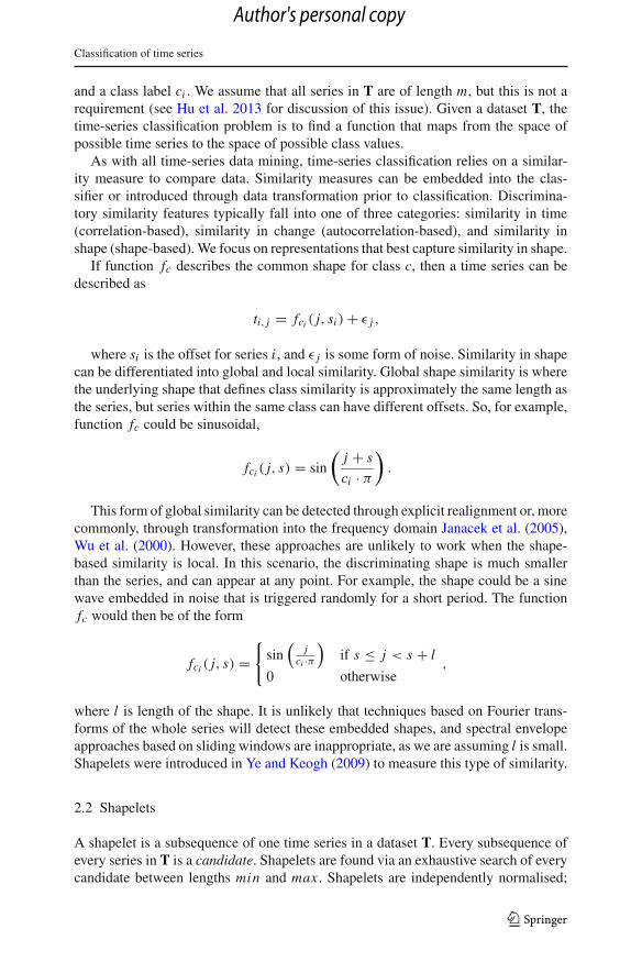
Fig. 2 Five beetle images (top left) and five fly images (top right) from the Beetle/Fly problem. Fivebird images (bottom left) and five chicken images (bottom right) from the Bird/Chicken problem. There isconsiderable intra-class variation, as well as inconsistent size and rotation

5.1.1 MPEG-7 shapes

MPEG-7 CE Shape-1 Part B Bober (2001) is a database of binary images developedfor testing MPEG-7 shape descriptors, and is available free online. It is used for testingcontour/image and skeleton-based descriptors Latecki et al. (2000). Classes of imagesvary broadly, and include classes that are similar in shape to one another. There are20 instances of each class, and 60 classes in total. We have extracted the outlinesof these images and mapped them into 1-D series. We have created two time-seriesclassification problems from the shapes, Beetle/Fly and Bird/Chicken. Figure 2 showssome of the images from the two problems.

5.2 Otoliths

Otoliths are calcium carbonate structures present in many vertebrates, found withinthe sacculus of the pars inferior. There are three types of otoliths: sagittae, lapilli, andasterisci. In fish, it is primarily the sagittal otoliths that are studied, as they are largerand easier to prepare and observe. Otoliths vary markedly in shape and size betweenspecies, but are of similar shape to other stocks of the same species (Fig. 3). Otolithscontain information that can be used by ‘expert readers’ to determine several keyfactors important in managing fish stock. Analysis of otolith boundaries may allowestimation of stock composition, including whether the samples are from one stockor multiple stocks Campana and Casselman (1993), De Vries et al. (2002), Duarte-Neto et al. (2008), allowing management decisions to be made Stransky (2005). Weconsider the problem of classifying herring stock (either North sea or Thames) basedon the otolith outline (Fig. 4).

5.3 Bone outlines

The bone datasets (DP_Little, DP_Middle, DP_Thumb, MP_Little, MP_Middle,PP_Little, PP_Middle, and PP_Thumb) consist of image outlines from hand X-rays,converted into 1-D series. The original images can be found at (Image Processingand Informatics Lab). Each of the eight datasets represents a different bone of thehand, and is labelled as belonging to one of three classes, Infant, Junior, or Teen. Theclassification problem is to predict the class to which a bone belongs, a process that islargely performed manually by doctors. For more information, see Davis et al. (2012).

123



Fig. 3 Otoliths from North-Sea Herring (a), Thames Herring (b) and two distinct populations of Plaice(c and d)

1 512

Fig. 4 A 1D time-series representation of the herring otolith shown in Fig. 3a

5.4 Scalability

At best, finding shapelets of a single length by exhaustive search has complexityO(n2m3) where n is the size of the dataset and m is the length of the series Rak-thanmanon and Keogh (2013). This is untenable for very large datasets. Our slowestexperiments were with the Otolith dataset, which has 64 training examples of length512. We used 71 different shapelet lengths. In the worst case, this requires 3.9× 1013

operations. The experiments took several days to perform in our high-performancecomputing facility.

6 Results

We present our experimental results in three stages. In Sect. 6.1, we compare IG andthe three alternative quality measures described in Sect. 3. In Sect. 6.2, we compre-hensively evaluate the effectiveness of the shapelet transform. Finally, In Sect. 6.3, we

123


J. Hills et al.

demonstrate the explanatory power of shapelets by mapping them back to the problemdomain.

All algorithms and experiments are implemented in Java within the Weka Hall etal. (2009) framework; the shapelet transform is implemented as a Weka batch filter toallow for easy integration with existing classification code. The code to generate ourresults is available at Bagnall et al. (2012).

6.1 Shapelet quality measures

To evaluate the quality measures in isolation, we perform these experiments with ourimplementation of the shapelet tree described in Ye and Keogh (2011). We compareIG, KW, F-stat, and MM in terms of accuracy and speed. The alternative statisticsdo not explicitly split the data when searching for the best shapelet. To make thecomparison to IG as fair as possible, once the best shapelet has been selected with astatistic, we use IG on the resulting set of distances to find the best split point. We dothis to focus on the ability of the statistic to assess shapelets, rather than perform datasplits.

6.1.1 Effect of quality measures on classification accuracy

Table 2 shows the accuracies and ranks of shapelet-tree classifiers built using the fourquality measures on 29 datasets. The tree based on the F-stat is the most accurateclassifier on 15 of the 29 data sets, and has the highest average rank. Furthermore, theF-stat is significantly better than the other three measures tested on 200 repetitions ofthe synthetic data. However, we cannot claim that F-Stat is universally better, sincetheir is no significant difference in ranks between the four measures when we considerall 29 data sets. Figure 5 shows the a critical difference diagram for ranked accuracies(see Demšar 2006). The diagram is derived from the overall test of significance ofmean ranks, where classifiers are grouped into cliques represented by solid bars. Thediagram shows that all classifiers are part of a single clique, and therefore that theyare not significantly different from one another.

6.1.2 Timing results

Table 3 shows the time required to find the best shapelet using IG, KW, F-stat, andMM. We adopt this approach to ensure fair comparisons are made between measures,as comparing the build times of whole decision trees is biased if the classifiers areof different depths. Extracting a single shapelet ensures that the same number ofcandidates are processed for each quality measure.

Table 3 shows that there are no datasets where IG is fastest. F-stat is the fastestmeasure on average, and has the fastest time on the most datasets. Figure 6 shows that,based on ranked timings, the F-stat is significantly faster than both IG and KW (usingthe Friedman rank order test). However, the speed up is not of an order of magnitude,and it is possible the difference could diminish with code and hardware optimisation.Nevertheless, we argue that the F-stat should be the default choice for shapelet quality.

123



Table 2 Classification accuracies for shapelet-tree classifiers

Dataset Information gain Kruskal-Wallis F-stat Mood’s median

Adiac 29.92 % (1) 26.60 % (3) 15.60 % (4) 27.11 % (2)

Beef 50.00 % (2) 33.33 % (3) 56.67 % (1) 30.00 % (4)

Beetle/Fly 77.50 % (3) 70.00 % (4) 90.00 % (1) 80.00 % (2)

Bird/Chicken 85.00 % (4) 87.50 % (2.5) 90.00 % (1) 87.50 % (2.5)

ChlorineConcentration 58.80 % (1) 51.95 % (4) 53.52 % (2) 52.11 % (3)

Coffee 96.43 % (2) 85.71 % (3.5) 100 % (1) 85.71 % (3.5)

DiatomSizeReduction 72.22 % (2) 62.11 % (3) 76.47 % (1) 44.77 % (4)

DP_ Little 65.44 % (3) 68.00 % (2) 60.31 % (4) 71.00 % (1)

DP_ Middle 70.53 % (2) 69.33 % (3) 61.86 % (4) 73.67 % (1)

DP_ Thumb 58.11 % (3) 72.00 % (1) 55.97 % (4) 70.33 % (2)

ECGFiveDays 77.47 % (4) 87.22 % (3) 99.00 % (1) 92.80 % (2)

FaceFour 84.09 % (1) 44.32 % (3) 75.00 % (2) 40.91 % (4)

GunPoint 89.33 % (4) 94.00 % (2) 95.33 % (1) 92.00 % (3)

ItalyPowerDemand 89.21 % (4) 90.96 % (3) 93.10 % (1) 91.06 % (2)

Lighting7 49.32 % (1) 47.95 % (2) 41.10 % (3) 27.40 % (4)

MedicalImages 48.82 % (3) 47.11 % (4) 50.79 % (1) 48.95 % (2)

MoteStrain 82.51 % (4) 83.95 % (2) 83.95 % (2) 83.95 % (2)

MP_ Little 66.39 % (3) 69.67 % (2) 57.83 % (4) 70.33 % (1)

MP_ Middle 71.01 % (3) 75.00 % (1) 60.93 % (4) 72.00 % (2)

Otoliths 67.19 % (1) 60.93 % (2) 57.81 % (3) 54.69 % (4)

PP_ Little 59.64 % (3) 72.00 % (1) 58.60 % (4) 67.33 % (2)

PP_ Middle 61.42 % (3) 68.33 % (2) 58.14 % (4) 69.67 % (1)

PP_ Thumb 60.83 % (3) 71.33 % (2) 59.07 % (4) 73.00 % (1)

SonyAIBORobotSurface 84.53 % (2) 72.71 % (4) 95.34 % (1) 74.87 % (3)

Symbols 77.99 % (2) 55.68 % (4) 80.10 % (1) 57.39 % (3)

SyntheticControl 94.33 % (2) 90.00 % (3) 95.67 % (1) 85.67 % (4)

SyntheticData 93.30 % (2) 80.56 % (3.5) 100 % (1) 80.56 % (3.5)

Trace 98.00 % (2.5) 94.00 % (4) 98.00 % (2.5) 100 % (1)

TwoLeadECG 85.07 % (3) 76.38 % (4) 97.01 % (1) 85.34 % (2)

Average rank 2.53 2.78 2.22 2.47

This experiment can be reproduced with method DMKD_2013, Bagnall et al. (2012)The best result for each dataset is shown in bold

Fig. 5 Critical differencediagram of the ranked accuraciesfor the four shapelet-treeclassifiers

CD

4 3 2 1

2.2241 F2.4655 MM2.5345IG

2.7759KW

123


J. Hills et al.

Table 3 Time to find first shapelet for each dataset

Dataset Information gain Kruskal-Wallis F-stat Mood’s median

Adiac 17758.48 (4) 4974.50 (1) 4509.91 (2) 4752.63 (3)

Beef 1284.46 (4) 1253.17 (3) 1251.21 (2) 1228.51 (1)

Beetle-fly 21707.02 (4) 21400.71 (2) 21496.51 (3) 21133.98 (1)

Bird-chicken 20258.90 (2) 20349.63 (3) 20465.63 (4) 19996.78 (1)

ChlorineConcentration 26233.51 (4) 16699.23 (3) 15681.39 (1) 16572.67 (2)

Coffee 261.27 (2) 264.75 (4) 258.15 (1) 263.82 (3)

DiatomSizeReduction 55.35 (4) 54.61 (3) 53.91 (1) 54.36 (2)

DP_Little 97508.12 (4) 80556.13 (2) 78005.70 (1) 82052.11 (3)

DP_Middle 106382.47 (4) 94081.04 (3) 91208.52 (1) 91664.80 (2)

DP_Thumb 149567.07 (4) 125334.92 (3) 123766.49 (1) 124508.41 (2)

ECGFiveDays 151.64 (3) 150.90 (2) 149.10 (1) 155.43 (4)

FaceFour 4695.97 (4) 4621.97 (2) 4556.41 (1) 4648.45 (3)

GunPoint 592.00 (4) 569.51 (2) 569.42 (1) 580.76 (3)

ItalyPowerDemand 3.18 (4) 1.56 (2) 1.75 (3) 1.46 (1)

Lighting7 15497.07 (4) 15157.93 (3) 14912.74 (1) 14940.20 (2)

MedicalImages 15703.95 (4) 8148.76 (3) 7742.97 (1) 8111.36 (2)

MoteStrain 11.55 (4) 11.02 (3) 10.76 (1) 11.00 (2)

MP_Little 108518.67 (4) 89849.25 (3) 88071.50 (1) 89634.65 (2)

MP_Middle 156750.20 (4) 135852.37 (3) 134731.54 (1) 134756.02 (2)

Otoliths 55090.54 (2) 56141.82 (4) 55874.19 (3) 54986.19 (1)

PP_Little 97987.27 (4) 79285.08 (1) 79993.31 (2) 80514.60 (3)

PP_Middle 68730.32 (4) 59579.27 (3) 57815.02 (1) 58389.16 (2)

PP_Thumb 110204.43 (4) 91183.51 (1) 91401.49 (3) 91202.87 (2)

SonyAIBORobotSurface 7.80 (4) 6.79 (2.5) 6.73 (1) 6.79 (2.5)

Symbols 8992.15 (4) 8941.21 (3) 8901.28 (1) 8922.01 (2)

SyntheticControl 2280.82 (4) 1029.95 (3) 984.36 (2) 974.27 (1)

SyntheticData 403.50 (4) 401.28 (2) 401.74 (3) 399.99 (1)

Trace 54829.06 (3) 55155.36 (4) 54128.53 (1) 54205.65 (2)

TwoLeadECG 3.61 (4) 3.15 (3) 3.12 (2) 3.11 (1)

Average rank 3.72 2.64 1.62 2.02

This experiment can be reproduced with method DMKD_2013, Bagnall et al. (2012)The best result for each dataset is shown in bold

Fig. 6 Critical differencediagram of the ranked timings ofthe four shapelet-tree classifiers

CD

4 3 2 1

1.5862 F1.9828 MM2.7069KW

3.7241IG

123



Using the F-stat measure is marginally, but significantly, faster, and the accuracy ishighly competitive on the 29 data sets as a whole. The F-stat is also significantly moreaccurate on the synthetic data.

6.2 Shapelet transformation

Despite our conclusion from the previous set of experiments, we use IG as the shapeletquality measure in all consequent experiments. Fixing the shapelet quality measureremoves a source of variation in performance and allows us to focus on our keyhypothesis that it is better to transform then use a more complex classifier than it is toembed the shapelet discovery in a decision tree.

Our first objective is to establish that dissociating shapelet discovery from classifi-cation does not reduce classification accuracy. We implement a shapelet decision-treeclassifier as described in Ye and Keogh (2011), and compare the performance to a C4.5decision tree trained and tested on shapelet-transformed data. The shapelet tree hasgreater accuracy on 15 datasets and the C4.5 tree has greater accuracy on 14 datasets.No significant difference is detected between the classifiers using a paired t-test or aWilcoxon signed rank test. We conclude that performing the shapelet extraction priorto constructing the decision tree does not reduce the accuracy of the classifier. Figure 7presents the findings graphically.

Using classifiers other than decision trees can improve the accuracy of classificationwith shapelets. Tables 4 and 5 shows the classification test accuracy of the C4.5, 1-NN,naive Bayes, Bayesian network, Random Forest, Rotation Forest, and support vectormachine classifiers, all built using the default Weka settings on shapelet-transformeddata. A Bayesian network is an acyclic directed graph with associated probabilitydistributions Friedman et al. (1997). It predicts class labels without assuming inde-pendence between variables. The Random Forest algorithm classifies examples by

Fig. 7 Comparison of C4.5 treeon shapelet-transformed dataand shapelet tree on raw data

123


J. Hills et al.

Table 4 Testing accuracies and ranks of 1NN-DTW on raw data, and simple classifiers (C4.5, 1NN, andNaïve Bayes) constructed on the shapelet-transformed data with n

2 shapelets

Data 1 % NN-DTW raw C4.5 1NN-Euclidean Naive Bayes

Adiac 49.10 % (1) 24.30 % (7) 25.32 % (5) 28.13 % (4)

Beef 43.33 % (8) 60.00 % (6.5) 83.33 % (3) 73.33 % (4)

Beetle/Fly 65.00 % (8) 75.00 % (7) 100.00 % (1) 92.50 % (5)

Bird/Chicken 72.50 % (8) 90.00 % (6) 97.50 % (1) 87.50 % (7)


Coffee 46.43 % (8) 85.71 % (7) 100.00 % (2) 92.86 % (5)


DP_Little 49.30 % (8) 65.92 % (7) 72.78 % (6) 73.49 % (3)

DP_Middle 54.57 % (8) 71.24 % (7) 73.73 % (6) 73.96 % (5)

DP_Thumb 53.02 % (7) 57.99 % (8) 60.71 % (6) 62.96 % (5)

ECGFiveDays 82.81 % (8) 96.17 % (6) 98.37 % (4) 96.40 % (5)

FaceFour 82.95 % (7) 76.14 % (8) 100.00 % (1.5) 97.73 % (4.5)

GunPoint 91.33 % (7) 90.67 % (8) 98.00 % (4) 92.00 % (6)

ItalyPowerDemand 96.11 % (1) 90.96 % (8) 92.13 % (5.5) 92.52 % (3)

Lighting7 72.60 % (1) 53.42 % (7) 49.32 % (8) 57.53 % (6)

MedicalImages 68.95 % (1) 44.87 % (6) 45.66 % (5) 17.37 % (8)

MoteStrain 81.55 % (8) 84.42 % (7) 90.34 % (1) 88.82 % (3)

MP_Little 55.81 % (8) 63.43 % (7) 68.52 % (6) 68.76 % (5)

MP_Middle 46.98 % (8) 73.25 % (4) 70.89 % (7) 71.95 % (5)

Otoliths 59.38 % (7.5) 65.63 % (3.5) 71.88 % (1) 68.75 % (2)

PP_Little 49.46 % (8) 57.40 % (7) 67.22 % (5) 69.23 % (4)

PP_Middle 49.92 % (8) 62.49 % (7) 68.52 % (6) 69.82 % (5)

PP_Thumb 52.56 % (8) 59.53 % (7) 67.69 % (6) 69.35 % (4)

Data 1NN-DTW Raw C4.5 1NN-Euclidean Naive Bayes


Symbols 93.37 % (1) 47.14 % (8) 85.63 % (3) 77.99 % (7)


SyntheticData 70.03 % (8) 93.24 % (7) 97.66 % (5) 98.13 % (2)

Trace 99.00 % (2) 98.00 % (5.5) 98.00 % (5.5) 98.00 % (5.5)

woLeadECG 79.46 % (8) 85.25 % (7) 99.47 % (1) 99.12 % (3)

Average rank 5.81 6.60 4.09 5.00

The ranks include the results in Table 5. This experiment can be reproduced with method DMKD_2013Bagnall et al. (2012)The best result for each dataset is shown in bold

generating a large number of decision trees with controlled variation and using themodal classification decision Breiman (2001). The Rotation Forest algorithm trainsa number of decision trees by applying principal components analysis on a randomsubset of attributes Rodriguez et al. (2006). A support vector machine finds the bestseparating hyperplane for a set of data by selecting the margin that maximises the

123



Table 5 Testing accuracies and ranks of complex classifiers (Bayesian Network, random Forest, RotationForest, and linear SVM) constructed on the shapelet-transformed data with n

2 shapelets

Data Bayesian network Random forest Rotation forest SVM (linear)

Adiac 25.06 % (6) 30.43 % (3) 30.69 % (2) 23.79 % (8)

Beef 90.00 % (1) 60.00 % (6.5) 70.00 % (5) 86.67 % (2)

Beetle/Fly 97.50 % (2.5) 90.00 % (6) 95.00 % (4) 97.50 % (2.5)

Bird/Chicken 95.00 % (3) 95.00 % (3) 92.50 % (5) 95.0 % (3)


Coffee 96.43 % (4) 100.00 % (2) 89.29 % (6) 100.00 % (2)


DP_Little 72.90 % (5) 73.02 % (4) 74.67 % (2) 75.15 % (1)

DP_Middle 74.67 % (4) 75.50 % (3) 76.80 % (2) 79.64 % (1)

DP_Thumb 63.91 % (4) 64.14 % (3) 67.10 % (2) 69.82 % (1)

ECGFiveDays 99.54 % (1) 93.26 % (7) 98.61 % (3) 98.95 % (2)

FaceFour 100.00 % (1.5) 87.50 % (6) 98.86 % (3) 97.73 % (4.5)

GunPoint 99.33 % (2) 96.00 % (5) 98.67 % (3) 100.00 % (1)

ItalyPowerDemand 92.42 % (4) 93.00 % (2) 92.03 % (7) 92.13 % (5.5)

Lighting7 65.75 % (3.5) 64.38 % (5) 65.75 % (3.5) 69.86 % (2)

MedicalImages 28.16 % (7) 50.79 % (4) 51.45 % (3) 52.50 % (2)

MoteStrain 89.06 % (2) 84.58 % (6) 86.98 % (5) 88.66 % (4)

MP_Little 69.47 % (4) 71.36 % (3) 75.15 % (1) 75.03 % (2)

MP_Middle 71.12 % (6) 75.15 % (2) 74.67 % (3) 76.92 % (1)

Otoliths 64.06 % (5.5) 65.63 % (3.5) 59.38 % (7.5) 64.06 % (5.5)

PP_Little 70.06 % (2) 66.63 % (6) 69.82 % (3) 72.07 % (1)

PP_Middle 71.36 % (3) 70.53 % (4) 75.38 % (2) 75.86 % (1)

PP_Thumb 69.47 % (3) 67.81 % (5) 72.78 % (2) 75.50 % (1)


Symbols 92.26 % (2) 84.62 % (4.5) 84.42 % (6) 84.62 % (4.5)


SyntheticData 98.00 % (3) 96.94 % (6) 97.72 % (4) 98.40 % (1)

Trace 100.00 % (1) 98.00 % (5.5) 98.00 % (5.5) 98.00 % (5.5)

TwoLeadECG 98.77 % (4) 96.14 % (6) 97.98 % (5) 99.30 % (2)

Average rank 3.48 4.45 3.64 2.93

The ranks include the results in Table 4. This experiment can be reproduced with method DMKD_2013,Bagnall et al. (2012)The best result for each dataset is shown in bold

distance between the nearest examples of each class Cortes and Vapnik (1995). It canalso transform the data into a higher dimension to make it linearly separable; we useonly the linear support vector machine.

For comparison purposes, Table 4 includes the accuracy for a 1-NN-DTW classifierbuilt on the raw data. The support vector machine is the best classifier, with an averagerank of 2.93, and best performance in 10 out of 29 problems. The decision tree is theworst classifier on average; in fact, it has a worse average rank than the 1-NN-DTW

123


J. Hills et al.

Fig. 8 Critical differencediagram for eight shapelet-basedclassifiers derived from theresults in Tables 4 and 5

CD

8 7 6 5 4 3 2 1

2.931 SVM3.4828 BayesNet3.6379 RotationFor4.0862 NN4.4483RandomFor

5NaiveBayes

5.8448NNDTWRaw

6.569C45

Fig. 9 Change in classification accuracy between raw data and shapelet-transformed data. Each point isthe median difference; the bar shows the minimum and maximum change in classifier accuracy for thatdataset. The results are available from Bagnall et al. (2012)

classifier based on raw data. The critical difference diagram in Fig. 8 shows that C4.5and 1-NN-DTW are significantly worse than SVM, Bayesian network, and RotationForest. There may be a trade off between interpretability and accuracy (a tree is easierto understand than a support vector machine), but by separating shapelet discoveryand classification, there is greater potential to explore possible solutions.

Next, we compare the accuracy of seven classifiers trained on raw data with thesame classifiers trained on shapelet-transformed data. Figure 9 presents the differencein classification accuracy for each classifier on each dataset. A positive value indicatesthat the classifier is more accurate on the transformed data, a negative value the con-verse. As can be seen, the change in accuracy is strongly indexed to the dataset, aswell as to the classifier. There are broad similarities between classifiers, but there arecases, such as Rotation Forest on the FaceFour dataset, where the change in accuracyis very different to that of the other classifiers.

123



Fig. 10 An illustration of the Gun/NoGun problem taken from Ye and Keogh (2009). The shapelet thatthey extract is highlighted at the end of the series

There are a number of datasets where the shapelet-transform has been detrimentalto the accuracy of the classifier, for example Adiac, where the classifiers each losebetween 20 and 40 % accuracy. The image datasets and spectrograph datasets (Beef,Coffee, Beetle/Fly, Bird/Chicken) show good improvement from the shapelet trans-form. The synthetic data that was designed to work well with the shapelet transformshows the best and most consistent improvement, as would be expected.

The shapelet transform offers improvements in classification accuracy over severaldifferent datasets that represent a number of different types of data. This supports theshapelet approach, and suggests that it fills a classification niche that has not beencovered in the literature.

6.3 Exploratory data analysis

We have shown that using shapelets to transform data can improve classification accu-racy. One of the strengths of using shapelets as a classification tool is that they providea level of interpretability that other classification approaches cannot. One of the goalsof our work with shapelets is to produce accurate classification decisions that are inter-pretable. We demonstrate in this section that our filter retains the interpretability ofthe original shapelet implementation.

The GunPoint dataset consists of time series representing an actor appearing to drawa gun; the classification problem is to determine whether or not the actor is holdinga prop (the Gun/NoGun problem). In Ye and Keogh (2009), the authors identify thatthe most important shapelet for classification occurs when the actor’s arm is lowered;if there is no gun, a phenomenon called ‘overshoot’ occurs, and causes a dip in thetime-series data. This is summarised in Fig. 10, taken from Ye and Keogh (2009).

The shapelet decision tree trained in Ye and Keogh (2009) contains a single shapeletat the end of the series corresponding to the arm being lowered. To demonstrate thatour filter agrees with this and extracts the important information from the data, wefilter the GunPoint dataset using the length parameters specified in the original paper.The top five shapelets that we extract are shown in Fig. 11, along with the shapeletreported in Ye and Keogh (2009).

123


J. Hills et al.

Fig. 11 An illustration of the five best shapelets extracted by our filter and the shapelet found by Ye andKeogh. The graph to the right shows how closely they match

Fig. 12 The 10 best shapelets for the Gun/NoGun problem. The shapelets form two distinct clusters. Thegraph on the left shows shapelets 1–6. They represent the ‘overshoot’ motion identified in Ye and Keogh(2009). The graph on the right shows shapelets 7–10. They represent the extra movement necessary to liftthe prop gun when the arm is raised

Figure 11 shows that each of the top five shapelets from our filter is closely matchedwith the shapelet from Ye and Keogh (2009). Figure 12 shows that the best ten shapeletsform two distinct clusters. Interestingly, the shapelets to the right of the figure corre-spond to the moments where the arm is lifted, and are instances where there is a gun.These shapelets could correspond to the subtle extra movements required to lift theprop, aiding classification by providing more information.

To explore our findings further, we hierarchically cluster the shapelets extractedfrom the GunPoint dataset. Our intuition is that reducing the number of shapelets willincrease interpretability. The top shapelets extracted by the filter overlap to a largedegree; we expect that, in cases like this, reducing k will result in a larger loss of accu-racy than clustering the shapelets. In addition, multiple instances representing the sameshapelet give the user less information than instances representing different shapelets.

Table 6 presents the accuracies of seven classifiers on the different transforms ofthe data. The transforms consist of three shapelet filters with k = 75, k = 10, andk = 5, and two clustered shapelet filters based on k = 75 shapelets clustered to 10 and5 clusters. For the C4.5 tree, all of the transformed datasets give the same accuracy.However, for the other classifiers, the general trend is that reducing the number ofshapelets results in a slight loss of accuracy (in 5 of 6 cases, the classifiers trained onthe k = 75 shapelet-transformed data have the best, or joint best accuracy). In most

123



Table 6 Accuracies of seven classifiers on the GunPoint dataset

Classifier Raw data (%) k = 75 (%) k = 10 (%) 10 Clusters (%) k = 5 (%) 5 Clusters (%)

C4.5 77.33 89.33 89.33 89.33 89.33 89.33

1NN 91.33 98.00 98.00 97.33 90.00 96.00

Naive Bayes 78.67 92.67 90.00 90.67 87.33 89.33

Bayesian network 85.33 99.33 94.67 99.33 91.33 98.67

Random forest 91.33 98.67 90.00 98.00 94.00 95.33

Rotation forest 87.33 96.00 95.33 98.67 92.00 90.67

SVM (linear) 79.33 100.00 89.33 98.67 84.67 91.33

The accuracies are presented for the raw data, data transformed by filters with 75, 10, and 5 shapelets, anddata transformed by a 75-shapelet filter clustered to 10 and 5 clustersThe best result for each classifier is shown in bold

Fig. 13 The five best clustered shapelets from the Beetle/Fly dataset. The shapelets are highlighted on theoutline in blue

cases (10 of 12), clustering the shapelets gives better accuracy than setting k to thatvalue. This is likely to be the case because many of the top shapelets from GunPoint arevery similar, which results in fewer differences between the classes in the transformedspace than with the full set of shapelets. When the shapelets are clustered, the set ofshapelets is likely to be more diverse, resulting in greater classification accuracy.

The main benefit of clustering the shapelets is improved interpretability. The topshapelets in the GunPoint dataset form two distinct clusters (Fig. 12). When we clusterthe shapelets into 10 or 5 clusters, we find that the top two shapelets represent the twoclusters found by the filter.

Other datasets show similar results when transformed using clustered shapelets.Figure 13 shows the top five clustered shapelets from the Beetle/Fly dataset. Table 7presents the classification accuracies for the different transforms.

Clustering the shapelets for the Beetle/Fly dataset provides superior classificationaccuracy compared to lowering k to the same value for all but three of the fourteen

123


J. Hills et al.

Table 7 Accuracies of seven classifiers on the Beetle/Fly dataset


C4.5 70.00 75.00 80.00 82.50 82.50 77.50

1NN 65.00 100.00 87.50 95.00 90.00 95.00

Naive Bayes 72.50 92.50 90.00 95.00 85.00 95.00

Bayesian network 72.50 97.50 87.50 92.50 80.00 87.50

Random forest 72.50 90.00 77.50 82.50 77.50 70.00

Rotation forest 77.50 95.00 87.50 92.50 87.50 80.00

SVM (linear) 77.50 97.50 87.50 97.50 85.00 95.00


cases. There are two cases where the full shapelet transform is inferior to transformsusing fewer shapelets; for the C4.5 tree, the difference is large, suggesting that the treeoverfits the data when using a full set of shapelets.

In Fig. 13, the first two shapelets distinguish members of the beetle class, andthe remaining three distinguish members of the fly class. By clustering down to fiveshapelets, we gain insight into the problem that would be less obvious from the original256 shapelets. The beetle class is distinguished by a relatively simple angle between thelegs and body; the only feature is a knee joint on the leg. The fly class is distinguishedby a more complex shapelet, related to the more intricate features of the fly images.

Using only these five shapelets, three of the classifiers were able to achieve 95 %accuracy. In contrast, because of the high intraclass variation, classifiers trained on thewhole outline achieved at best 77.5 % accuracy. In this case, using shapelets providesa considerable increase in classifier accuracy, and clustering down to five shapeletsgives great interpretability.

For the Bird/Chicken data, the clustered shapelets (Fig. 14) are outperformed by thek best shapelets where the number of clusters is equal to k (Table 8). This shows thatit is not necessarily the case that clustering improves accuracy. For different datasets,it may be worth using a validation set, or cross-validation if the dataset is small, todetermine which method provides better accuracy.

The accuracies on the transformed data are all superior to the accuracies on theraw data. In many cases, using a smaller value of k results in better classification thanusing the full set of shapelets, perhaps because the full set overfits the data. If thisis the case, it may also explain why clustering the full set is inferior to using fewershapelets.

7 Conclusions

We investigate quality measures for shapelets, and propose a shapelet-transform algo-rithm.

We demonstrate the effectiveness of the Kruskal-Wallis, F-statistic, and MM statis-tics as quality measures for shapelet discovery by training shapelet decision-tree clas-sifiers in the style of Ye and Keogh (2011), with these statistics in place of Information

123



Fig. 14 The five best clustered shapelets from the Bird/Chicken dataset. The shapelets are highlighted onthe outline in blue

Table 8 Accuracies of seven classifiers on the Bird/Chicken dataset


C4.5 75.00 90.00 90.00 87.50 87.50 87.50

1NN 85.00 97.50 92.50 90.00 92.50 90.00

Naive Bayes 60.00 87.50 95.00 92.50 92.50 90.00

Bayesian Network 60.00 95.00 97.50 97.50 95.00 82.50

Random Forest 80.00 95.00 87.50 90.0 87.50 85.00

Rotation Forest 87.50 92.50 95.00 90.00 90.00 90.00

SVM (linear) 77.50 95.00 95.00 85.00 85.00 82.50


Gain. Our results show that Information Gain is the slowest measure to compute, andis no better in terms of accuracy than the other measures. The F-statistic is significantlymore accurate on the synthetic data designed to be optimal for shapelets, and is thehighest ranked measure overall. We believe that it should be the default measure ofchoice for future work with shapelet-transformed data.

We propose a shapelet-transform algorithm for time-series classification thatextracts the k-best shapelets from a dataset in a single pass using a caching algo-rithm, and allows the shapelets to be clustered to enhance interpretability. We trans-form 29 datasets with our filter, and demonstrate that a C4.5 decision-tree classifiertrained with transformed data is competitive with the original shapelet tree of Ye andKeogh (2009). Our transformed data can be used with other classifiers, which achieveimproved accuracy while maintaining the interpretability of the shapelet approach.We provide exploratory data analysis of the shapelets extracted by our filter on theGun/NoGun, Beetle/Fly, and Bird/Chicken problems, and show that shapelets can giveinsight into the problem domain.

123


J. Hills et al.

There are limitations to the approach. First, the shapelet transform will not be opti-mal for all problems. Figure 9 shows that there are some datasets where the transformimproves all classifiers, but others where the classifiers in the shapelet domain areless accurate than those in the time domain. Our results suggest that shapelets maybe a good approach for image-outline classification, spectrograms, and ECG mea-surements, but these are qualitative observations. An obvious area of future work is toinvestigate whether there are problem domains where the shapelet approach is the beston average. Second, though the transform is faster on average than the shapelet deci-sion tree, finding the best shapelets is slow. Exact techniques for shapelet discovery areunsuitable for large problems. Approximate techniques, such as the SAX compressiondescribed in Rakthanmanon and Keogh (2013), can mitigate this problem. Finally, thepost clustering we perform improves intelligibility, but it also introduces the risk ofremoving important discriminatory features, and introduces a further parameter intothe transform.

Despite these limitations, we believe shapelets are an important new approach forsolving time-series classification problems where localised similarity in shape definesclass membership. We have demonstrated that the most flexible and accurate way ofusing shapelets for time-series classification is as a transformation performed prior toclassifier construction.

References

Bagnall A, Hills J, Lines J (2012) Shapelet based time series classification. http://www.uea.ac.uk/computing/machine-learning/Shapelets. Accessed 14 May 2013

Bagnall A, Davis L, Hills J, Lines J (2012) Transformation based ensembles for time series classification.Proceedings of the twelfth SIAM conference on data mining (SDM)

Batista G, Wang X, Keogh E (2011) A complexity-invariant distance measure for time series. Proceedingsof the eleventh SIAM conference on data mining (SDM)

Bober M (2001) Mpeg-7 visual shape descriptors. IEEE Trans Circ Syst Video Technol 11(6):716–719Breiman L (2001) Random forests. Mach Learn 45(1):5–32Buza K (2011) Fusion methods for time-series classification. Ph.D. thesis, University of Hildesheim, Ger-

manyCampana S, Casselman J (1993) Stock discrimination using otolith shape analysis. Can J Fish Aquat Sci

50(5):1062–1083Cortes C, Vapnik V (1995) Support-vector networks. Mach Learn 20(3):273–297Davis LM, Theobald B-J, Lines J, Toms A, Bagnall A (2012) On the segmentation and classification of

hand radiographs. Int J Neural Syst 22(5):1250020Demšar J (2006) Statistical comparisons of classifiers over multiple data sets. J Mach Learn Res 7:1–30Deng H, Runger G, Tuv E, Vladimir M (2011) A time series forest for classification and feature extraction.

Tech. rep., Arizona State UniversityDe Vries D, Grimes C, Prager M (2002) Using otolith shape analysis to distinguish eastern gulf of mexico

and atlantic ocean stocks of king mackerel. Fish Res 57(1):51–62Ding H, Trajcevski G, Scheuermann P, Wang X, Keogh E (2008) Querying and mining of time series data:

experimental comparison of representations and distance measures. Proc VLDB Endow 1(2):1542–1552Duarte-Neto P, Lessa R, Stosic B, Morize E (2008) The use of sagittal otoliths in discriminating stocks of

common dolphinfish (coryphaena hippurus) off northeastern brazil using multishape descriptors. ICESJ Mar Sci J du Conseil 65(7):1144–1152

Friedman N, Geiger D, Goldszmidt M (1997) Bayesian network classifiers. Mach Learn 29(2–3):131–163Hall M, Frank E, Holmes G, Pfahringer B, Reutemann P, Witten IH (2009) The WEKA data mining software:

an update. ACM SIGKDD Explor Newsl 11(1):10–18

123


http://www.uea.ac.uk/computing/machine-learning/Shapelets

http://www.uea.ac.uk/computing/machine-learning/Shapelets


Hartmann B, Link N (2010) Gesture recognition with inertial sensors and optimized dtw prototypes. Systemsman and cybernetics (SMC), 2010 IEEE international conference on. IEEE pp 2102–2109

He Q, Dong Z, Zhuang F, Shi Z (2012) Fast Time Series Classification based on infrequent shapelets.Machine learning and applications (ICMLA), 2012 11th international conference on. IEEE, pp 215–219

Hoare C (1962) Quicksort. Comput J 5(1):10–16Image Processing and Informatics Lab, University of Southern California, The Digital Hand Atlas Database

System. http://www.ipilab.org/BAAwebJanacek G, Bagnall A, Powell M (2005) A likelihood ratio distance measure for the similarity between

the fourier transform of time series. Proceedings of the Ninth Pacific-Asia Conference on knowledgediscovery and data mining (PAKDD)

Jeong Y, Jeong M, Omitaomu O (2010) Weighted dynamic time warping for time series classification.Pattern Recognit 44:2231–2240

Hu B, Chen Y, Keogh E (2013) Time series classification under more realistic assumptions. Proceedings ofthe thirteenth SIAM conference on data mining (SDM)

Kruskal W (1952) A nonparametric test for the several sample problem. Ann Math Stat 23(4):525–540Latecki L, Lakamper R, Eckhardt T (2000) Shape descriptors for non-rigid shapes with a single closed

contour. Computer vision and pattern recognition, 2000. Proceedings. IEEE conference on vol. 1. IEEE,pp 424–429

Lines J, Bagnall A (2012) Alternative quality measures for time series shapelets. Intelligent data engineeringand automated learning (IDEAL). Lect Notes Comput Sci 7435:475–483

Lines J, Davis L, Hills J, Bagnall A (2012) A shapelet transform for time series classification. Proceedingsof the 18th ACM SIGKDD international conference on Knowledge discovery and data mining. ACM,pp 289–297

Mood AM, Graybill FA, Boes DC (1974) Introduction to the theory of statistics, 3rd edn. McGraw-Hill,New York

Mueen A, Keogh E, Young N (2011) Logical-shapelets: an expressive primitive for time series classification.Proceedings of the 17th ACM SIGKDD international conference on Knowledge discovery and datamining. ACM, pp 1154–1162

Rakthanmanon T, Campana B, Mueen A, Batista G, Westover B, Zhu Q, Zakaria J, Keogh E (2012) Searchingand mining trillions of time series subsequences under dynamic time warping. Proceedings of the 18thACM SIGKDD international conference on Knowledge discovery and data mining, pp 262–270

Rakthanmanon T, Keogh E (2013) Fast Shapelets: A Scalable Algorithm for Discovering Time SeriesShapelets. Proceedings of the thirteenth SIAM conference on data mining (SDM)

Rodriguez J, Alonso C (2005) Support vector machines of interval-based features for time series classifi-cation. Knowl-Based Syst 18:171–178

Rodriguez JJ, Kuncheva LI, Alonso CJ (2006) Rotation forest: a new classifier ensemble method. PatternAnal Mach Intell IEEE Trans 28(10):1619–1630

Shannon C, Weaver W, Blahut R, Hajek B (1949) The mathematical theory of communication, vol 117.University of Illinois press, Urbana

Sivakumar P et al. (2012) Human gait recognition and classification using time series shapelets. Internationalconference on advances in computing and communications (ICACC)

Stransky C (2005) Geographic variation of golden redfish (sebastes marinus) and deep-sea redfish(s. mentella) in the north atlantic based on otolith shape analysis. ICES J Mar Sci J du Conseil 62(8):1691–1698

Wu Y, Agrawal D, Abbadi AE (2000) A comparison of dft and dwt based similarity search in time-seriesdatabases. Proceedings of the ninth international conference on information and knowledge management(ACM CIKM)

Xing Z, Pei J, Yu P (2012) Early classification on time series. Knowl Inform syst 31(1):105–127Xing Z, Pei J, Yu P, Wang K (2011) Extracting interpretable features for early classification on time series.

Proceedings of the eleventh SIAM conference on data mining (SDM)Ye L, Keogh E (2009) Time series shapelets: a new primitive for data mining. Proceedings of the 15th ACM

SIGKDD international conference on Knowledge discovery and data mining. ACM, pp 947–956Ye L, Keogh E (2011) Time series shapelets: a novel technique that allows accurate, interpretable and fast

classification. Data Min Knowl Discov 22(1):149–182Zakaria J, Mueen A, Keogh E (2012) Clustering time series using unsupervised-shapelets. Data mining

(ICDM), 2012 IEEE 12th international conference. pp. 785–794

123


http://www.ipilab.org/BAAweb

Classification of time series by shapelet transformation

Documents

Transcript of Classification of time series by shapelet transformation