Working Paper 08 - 74Statistics and Econometrics Series 27December 2008

Departamento de Estadística Universidad Carlos III de Madrid

Calle Madrid, 12628903 Getafe (Spain)

Fax (34) 91 624-98-49

A FUNCTIONAL DATA BASED METHOD

FOR

TIME SERIES CLASSIFICATION

Andrés M. Alonso1, David Casado2, Sara López-Pintado3 and Juan Romo4

AbstractWe propose using the integrated periodogram to classify time series. The method assigns a new element to the group minimizing the distance from the integrated periodogram of the element to the group mean of integrated periodograms. Local computation of these periodograms allows the application of the approach to non- -stationary time series. Since the integrated periodograms are functional data, we apply depth-based techniques to make the classification robust. The method provides small error rates with both simulated and real data, and shows good computational behaviour.

Keywords: time series, classification, integrated periodogram, data depth

JEL Classification: C14 and C22

1 Departamento de Estadística. Universidad Carlos III de Madrid, C/ Madrid 126, 28903 Getafe (Madrid), e-mail: andres.alonso@uc3m.es2 Departamento de Estadística. Universidad Carlos III de Madrid, C/ Madrid 126, 28903 Getafe (Madrid), e-mail: david.casado@uc3m.es3 Departamento de Economía, Métodos Cuantitativos e Historia Económica. Universidad Pablo de Olavide, Ctra. de Utrera, Km.1 - 41013 Sevilla, email: sloppin@upo.es 4 Departamento de Estadística. Universidad Carlos III de Madrid, C/ Madrid 126, 28903 Getafe (Madrid), e-mail: juan.romo@uc3m.es

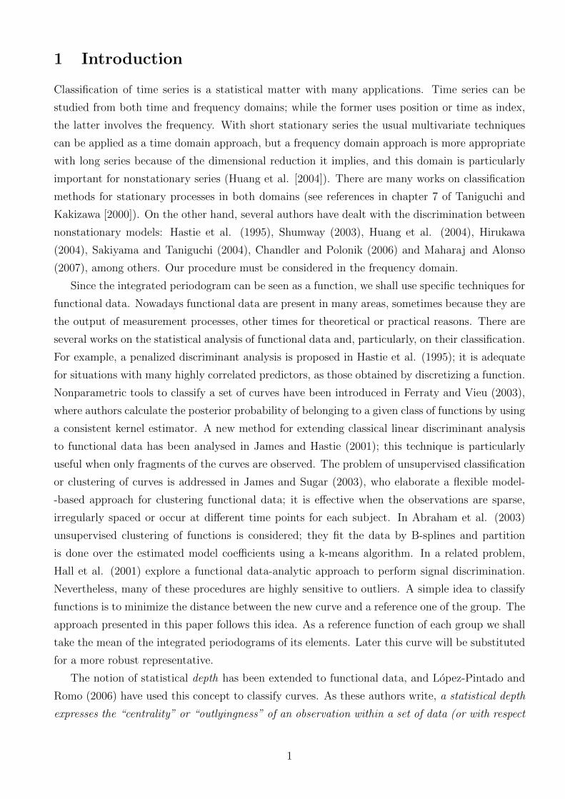
1 Introduction

Classification of time series is a statistical matter with many applications. Time series can be

studied from both time and frequency domains; while the former uses position or time as index,

the latter involves the frequency. With short stationary series the usual multivariate techniques

can be applied as a time domain approach, but a frequency domain approach is more appropriate

with long series because of the dimensional reduction it implies, and this domain is particularly

important for nonstationary series (Huang et al. [2004]). There are many works on classification

methods for stationary processes in both domains (see references in chapter 7 of Taniguchi and

Kakizawa [2000]). On the other hand, several authors have dealt with the discrimination between

nonstationary models: Hastie et al. (1995), Shumway (2003), Huang et al. (2004), Hirukawa

(2004), Sakiyama and Taniguchi (2004), Chandler and Polonik (2006) and Maharaj and Alonso

(2007), among others. Our procedure must be considered in the frequency domain.

Since the integrated periodogram can be seen as a function, we shall use specific techniques for

functional data. Nowadays functional data are present in many areas, sometimes because they are

the output of measurement processes, other times for theoretical or practical reasons. There are

several works on the statistical analysis of functional data and, particularly, on their classification.

For example, a penalized discriminant analysis is proposed in Hastie et al. (1995); it is adequate

for situations with many highly correlated predictors, as those obtained by discretizing a function.

Nonparametric tools to classify a set of curves have been introduced in Ferraty and Vieu (2003),

where authors calculate the posterior probability of belonging to a given class of functions by using

a consistent kernel estimator. A new method for extending classical linear discriminant analysis

to functional data has been analysed in James and Hastie (2001); this technique is particularly

useful when only fragments of the curves are observed. The problem of unsupervised classification

or clustering of curves is addressed in James and Sugar (2003), who elaborate a flexible model-

-based approach for clustering functional data; it is effective when the observations are sparse,

irregularly spaced or occur at different time points for each subject. In Abraham et al. (2003)

unsupervised clustering of functions is considered; they fit the data by B-splines and partition

is done over the estimated model coefficients using a k-means algorithm. In a related problem,

Hall et al. (2001) explore a functional data-analytic approach to perform signal discrimination.

Nevertheless, many of these procedures are highly sensitive to outliers. A simple idea to classify

functions is to minimize the distance between the new curve and a reference one of the group. The

approach presented in this paper follows this idea. As a reference function of each group we shall

take the mean of the integrated periodograms of its elements. Later this curve will be substituted

for a more robust representative.

The notion of statistical depth has been extended to functional data, and Lopez-Pintado and

Romo (2006) have used this concept to classify curves. As these authors write, a statistical depth

expresses the “centrality” or “outlyingness” of an observation within a set of data (or with respect

1

to a probability distribution) and provides a criterion to order observations from center-outward.

Since robustness is an interesting feature of the statistical methods based on depth, we have applied

the ideas of Lopez-Pintado and Romo (2008) to add robustness to our time series classification

procedure. Their method considers the α-trimmed mean as a reference curve of each group, which

is defined as the average of the 1 − α proportion of the deepest curves of the sample; that is, it

leaves 100α% of data out. This trim is the responsible for adding robustness.

Next sections are organized as follows. In section 2 we include some definitions and describe

the classification algorithm. In section 3 we explain how depth can be used to make the method

robust. Next two sections, 4 and 5, show the behavior of the procedure with simulated and real

data, respectively. A brief summary of conclusions is given in section 6.

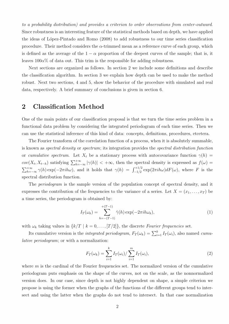
2 Classification Method

One of the main points of our classification proposal is that we turn the time series problem in a

functional data problem by considering the integrated periodogram of each time series. Then we

can use the statistical inference of this kind of data: concepts, definitions, procedures, etcetera.

The Fourier transform of the correlation function of a process, when it is absolutely summable,

is known as spectral density or spectrum; its integration provides the spectral distribution function

or cumulative spectrum. Let Xt be a stationary process with autocovariance function γ(h) =

cov(Xt, Xt−h) satisfying∑+∞

h=−∞ |γ(h)| < +∞, then the spectral density is expressed as f(ω) =∑+∞h=−∞ γ(h) exp(−2πihω), and it holds that γ(h) =

∫ +1/2

−1/2 exp(2πihω)dF (ω), where F is the

spectral distribution function.

The periodogram is the sample version of the population concept of spectral density, and it

expresses the contribution of the frequencies to the variance of a series. Let X = (x1, . . . , xT ) be

a time series, the periodogram is obtained by:

IT (ωk) =

+(T−1)∑h=−(T−1)

γ(h) exp(−2πihωk), (1)

with ωk taking values in {k/T | k = 0, . . . , [T/2]}, the discrete Fourier frequencies set.

Its cumulative version is the integrated periodogram, FT (ωk) =∑k

i=1 IT (ωi), also named cumu-

lative periodogram; or with a normalization:

FT (ωk) =k∑i=1

IT (ωi)/m∑i=1

IT (ωi), (2)

where m is the cardinal of the Fourier frequencies set. The normalized version of the cumulative

periodogram puts emphasis on the shape of the curves, not on the scale, as the nonnormalized

version does. In our case, since depth is not highly dependent on shape, a simple criterion we

propose is using the former when the graphs of the functions of the different groups tend to inter-

sect and using the latter when the graphs do not tend to intersect. In that case normalization

2

dissolves the confusing area caused by the intersections. In general, among other advantages of

the integrated periodogram are: it is nondecreasing and quite smooth curve (the integration is

a sort of smoothing); it has good asymptotic properties (while the periodogram is an asymptot-

ically unbiased but inconsistent estimator of the spectral density, the integrated periodogram is a

consistent estimator of the spectral distribution); although in practice for stationary processes the

integrated spectrum is usually estimated via the estimation of the spectrum, from the theoretical

point of view the spectral distribution always exists and only when it is absolutely continuous the

spectral density exists; finally, theoretically the integrated spectrum determines completely the

stochastic processes.

Previous definitions, (1) and (2), are limited to some discrete values of the frequency ω, but

they can be extended to any value in the interval (−1/2,+1/2). Apart from anything else the

periodogram is defined only for stationary series, but in order to be able to classify nonstationary

time series we shall consider that series are locally stationary. With this assumption we shall be

allowed to split them into blocks, compute the integrated periodogram of each block and merge

these periodograms in a final curve; that is, the idea is to approximate the locally stationary

processes by piecewise stationary processes. In figure 1(b) we illustrate our blockwise spectral

distribution estimation of the locally stationary process spectrum. It is worth mentioning that

there are two opposite effects as a consequence of splitting: one is that the narrower blocks are,

the closer to the locally stationarity assumption we are; the other is that when the length of blocks

decreases, also decreases the quality of the integrated periodogram as estimator of the integrated

spectrum.

When functions—instead of time series—need to be classified, a possible criterion is to assign

them to the group minimizing some distance from the new data to the group. In our context

this criterion means that we classify new series in the group minimizing the distance between the

integrated periodogram of the series and a reference curve. As a reference function of each group

we take the mean of its elements, as it summarizes the general behaviour of the sample. Let

Ψgi(ω); i = 1, . . . , N be functions of group g, the mean is defined as:

Ψg =1

N

N∑i=1

Ψgi(ω). (3)

In our case, Ψgi(ω) is the joint of the integrated periodograms of the blocks for the i-th series in

group g.

As a distance measurement between two functions we have taken the L1 distance that, for the

functions Ψ1(ω) and Ψ2(ω), is defined as:

d(Ψ1,Ψ2) =

∫ +1/2

−1/2|Ψ1(ω)−Ψ2(ω)|dω. (4)

Notice that the functions we are working with, that is, the integrated periodograms, belong to

the L1[−1/2,+1/2] space. Some other distance could be considered, since in general there is not

3

“the best” one. For example, with the L2 distance big differences between functions would be

highlighted and so would be the corresponding values of the independent variable (frecuency).

With these definitions, we can enunciate the classification algorithm:

Algorithm 1

Let {X1, . . . , XNx} be a sample containing Nx time series from the population PX ,

and let {Y1, . . . , YNy} be a sample containing Ny series from PY . The classification

method comprises the following steps:

1. To obtain the functional data, the associate curve of each time series is constructed

by merging the integrated periodograms of the k blocks into which series are

split: {ΨX1 , . . . ,ΨXNx} and {ΨY1 , . . . ,ΨYNy

}, where ΨXi= (F

(1)Xi. . . F

(k)Xi

) , ΨYi =

(F(1)Yi. . . F

(k)Yi

) and F(j)Xi

is the integrated periodogram of the j-th block of the i-th

series of the population X; for the population Y notation F(j)Yi

has the equivalent

meaning.

2. For both PX and PY populations the group mean of these functions is calculated:

ΨX and ΨY .

3. Let ΨZ be the associate curve of a new series Z, that is ΨZ = (F(1)Z . . . F

(k)Z ), then

Z is classified in the group PX if d(ΨZ , ΨX) < d(ΨZ , ΨY ), and in the group PY

otherwise.

Remark 1: To apply the algorithm to stationary series k can be set equal to 1. We have used

a dyadic splitting of the series into blocks in the simulation and real data computations, that

is, k = 2p, p = 0, 1, . . .; but the implementation with blocks of different lengths, as it could be

suggested by visual inspection of data, is also possible.

Remark 2: Though we are considering G = 2 in this paper, the classification method is obvi-

ously extended to the general case in which there are G different groups or populations, Pg, with

g = 1, . . . , G.

Remark 3: The same methodology that we propose in this paper could be implemented using

some different classification criterion between curves, reference function —or functions— of each

group (as we do in the following section) and distance between curves.

3 Robust Version

Our classification method depends on the group reference curve to which the distance is measured.

The mean of a set of functions is not robust to the presence of outliers. Then robustness can be

4

added to the classification procedure by using a robust reference curve. Instead of considering

the mean of the integrated periodograms of all the elements of the group, we shall consider the

α-trimmed mean, where only the deepest elements are averaged. The trim adds robustness by

making the reference curve more resistant to the presence of outliers. In this section we describe

the concept of depth extended to functional data by Lopez-Pintado and Romo (2008). Then we

propose a robust version of our classification algorithm.

The statistical concept of depth is a measurement of the “centrality” of each element inside

the sample. This means, for example, that in a set of points of Rn the closer to the mass center a

point is, the deepest it is. The same general idea applies to other type of data, including functions.

Different definitions of depth for functions can be given.

Let G(Ψ) = {(t,Ψ(t)) | t ∈ [a, b]} denote the graph in R2 of a function Ψ ∈ C[a, b]. Let

Ψi(t), i = 1, . . . , N , be functions in C[a, b], then a subset of this functions, Ψij(t), j = 1, . . . , k,

determines a band in R2

B(Ψi1 , . . . ,Ψik) = {(t, y) | t ∈ [a, b], minr=1,...,k

Ψir(t) ≤ y ≤ maxr=1,...,k

Ψir(t)}. (5)

For any of the functions Ψ, the quantity

BD(j)N (Ψ) =

(N

j

)−1 ∑1≤i1<i2<...<ij≤N

I{G(Ψ) ⊂ V (Ψi1 , . . . ,Ψij)}, j ≥ 2 (6)

expresses the proportion of bands, determined by j different curves, Ψi1 , . . . ,Ψij , containing the

graph of Ψ (the indicator function takes the value I{A} = 1 if A occurs, and I{A} = 0 otherwise).

The definition of depth for functional data introduced by Lopez-Pintado and Romo (2008) states

that for functions Ψi(t), i = 1, . . . , N , the band depth of any of these curves Ψ is

BDN,J(Ψ) =J∑j=2

BD(j)N (Ψ), 2 ≤ J ≤ N. (7)

If Ψ is the stochastic process that has generated the observations Ψi(t), i = 1, . . . , N , the

population versions of these indexes are BD(j)(Ψ) = P{G(Ψ) ⊂ B(Ψi1 , . . . , Ψij)}, j ≥ 2, and

BDJ(Ψ) =∑J

j=2 S(j =

∑Jj=2 P{G(Ψ) ⊂ B(Ψi1 , . . . , Ψij)}, J ≥ 2, respectively.

A more flexible notion of depth is also defined in Lopez-Pintado and Romo (2008): the modified

band depth. The indicator function in definition (6) is replaced by the length of the set where

the function is inside the corresponding band. For any function Ψ of Ψt(t), i = 1, . . . , N , and

2 ≤ j ≥ N , let

Aj(Ψ) ≡ A(Ψ; Ψi1 , . . . ,Ψij) ≡ {t ∈ [a, b] | minr=i1,...,ij

Ψr(t) ≤ Ψ(t) ≤ maxr=i1,...,ij

Ψr(t)}. (8)

be the set of points in the interval [a, b] where the function Ψ is inside the band. If λ is the

Lebesgue measure on the interval [a, b], λ(Aj(Ψ)) is the “proportion of time” that Ψ is inside the

band. Then,

MBD(j)N (Ψ) =

(N

j

)−1λ([a, b])−1

∑1≤i1<i2<...<ij≤N

λ(A(Ψ; Ψi1 , . . . ,Ψij)), 2 ≤ j ≤ N, (9)

5

is the generalized version of BD(j)N . If Ψ is always inside the band, the measure λ(Aj(Ψ)) is 1 and

this generalizes the definition of depth given in (7). Finally, the generalized band depth of any of

the curves Ψ in Ψi(t), i = 1, . . . , N , is

MBDN,J(Ψ) =J∑j=2

MBD(j)N (Ψ), 2 ≤ J ≤ N. (10)

If Ψi(t), i = 1, . . . , N , are independent copies of the stochastic process Ψ which generates the

observations Ψi(t), i = 1, . . . , N , the population versions of these depth indexes are, respectively,

MBD(j)(Ψ) = Eλ(A(Ψ; Ψi1 , . . . , Ψij)), 2 ≤ J ≥ N , and MBDJ(Ψ) =∑J

j=2MBD(j)(Ψ) =∑Jj=2 Eλ(A(Ψ; Ψi1 , . . . , Ψij)), 2 ≤ J ≤ N . We have used the value J = 2, since the modified

band depth is very stable in J , providing similar center-outward order in a collection of functions

(Lopez-Pintado and Romo [2006, 2008]).

In order to add robustness to the algorithm presented in the previous section, now we take

the group α-trimmed mean of its elements as the reference function. Let Ψg(i)(t), i = 1, . . . , N , be

functions of the class g ordered by decreasing depth, the α-trimmed mean is defined as:

Ψαg =

1

N − [Nα]

N−[Nα]∑i=1

Ψg(i)(t), (11)

where [·] is the integer part function. Notice that the median (in the sense of “the deepest”)

function is also included in the previous expression; nevertheless, the α-trimmed mean is robust

either, as the median, and summarizes the general behaviour of the functions, as the mean. In

our simulation and real data exercises, a value of α = 0.2 is used. It means that for each group

the 20% of the less depth data are leaved out. This is the value used in Lopez-Pintado and Romo

(2006).

With this little—but essential—difference the algorithm hardly changes. At step 2 the group

α-trimmed mean is taken instead of the group mean, that is, now the distance from the series to

the class is measured from a different reference curve of the class.

Algorithm 2

Let {X1, . . . , XNx} be a sample containing time series from the population PX , and let

{Y1, . . . , YNy} be a sample from PY . The classification method comprises the following

steps:

1. To obtain the functional data, the associate curve of each time series is constructed

by merging the integrated periodograms of the k blocks into which series are

split: {ΨX1 , . . . ,ΨXNx} and {ΨY1 , . . . ,ΨYNy

}, where ΨXi= (F

(1)Xi. . . F

(k)Xi

) , ΨYi =

(F(1)Yi. . . F

(k)Yi

) and F(j)Xi

is the integrated periodogram of the j-th block of the i-th

series of the population X; for the population Y notation F(j)Yi

has the equivalent

meaning.

6

2. For both PX and PY populations the α-trimmed group mean of these functions

is computed: ΨαX and Ψα

Y .

3. Let ΨZ be the associate curve of a new series Z, that is ΨZ = (F(1)Z . . . F

(k)Z ), then

Z is classified in the group PX if d(ΨZ , ΨαX) < d(ΨZ , Ψ

αY ), and in the group PY

otherwise.

Remark 4: The same algorithm could be implemented using a different functional depth.

4 Simulations

In the simulation studies we evaluate our two algorithms and, as a reference, the method pro-

posed in Huang et al. (2004). The results obtained with algorithm 1 are denoted by DbC,

the results with algorithm 2 by DbC-α and the method of Huang et al. (2004) by SLEXbC.

Ombao et al. (2001) introduced the SLEX (smooth localized complex exponentials) model of

a nonstationary random process, and the method of Huang et al. (2004) uses SLEX, a set of

Fourier-type bases that are at the same time orthogonal and localized in both time and frequency

domains. In a first step, they select from SLEX a basis explaining as good as possible the diffe-

rence between the classes of time series. After this they construct a discriminant criterion that is

related to the SLEX spectra of the different classes: a time series is assigned to the class mini-

mizing the Kullback-Leibler divergence between the estimated spectrum and the spectrum of the

class. For the SLEXbC method we have used an implementation provided by the authors (see

http://www.stat.uiuc.edu/~ombao/research.html). To select the parameters for this method,

we have done a small optimization for each simulation exercise and the results were similar to the

values recommended to us by the authors.

We have used the same models than Huang et al. (2004). For each comparison of two classes,

we run 1000 times the following steps. We generate training and test sets of each model/class.

Training sets have the same sizes (sample size and series length) they used, and test sets contain

always 10 series of the length involved in each particular simulation exercise. Then the methods

are called with exactly the same data sets; that is, in these models exactly the same simulated

time series are used by the three methods, including the calls to our algorithms with different

values of k.

Simulation Exercise 1: We compare an autoregressive process of order one (Xt) with

Gaussian white noise (Yt):

X(i)t = φ ·X(i)

t−1 + ε(i)t t = 1, . . . , Tx and i = 1, . . . , Nx

Y(j)t = ε

(j)t t = 1, . . . , Ty and j = 1, . . . , Ny,

(12)

7

where ε(i)t y ε

(j)t are i.i.d. N(0, 1). Each training data set has Nx = Ny = 8 series

of length Tx = Ty = 1024. Six comparisons have been run, with the parameter φ of

the AR(1) model taking the values −0.5, −0.3, −0.1, +0.1, +0.3 and +0.5. Series are

stationary in this exercise.

Simulation Exercise 2: We compare two processes composed half by white noise and

half by an autoregressive process of order one. The value of the AR(1) parameter is

−0.1 in the first class and +0.1 in the second class:

X(i)t =

{ε(i)t if t = 1, . . . , Tx/2

X(i)t = −0.1 ·X(i)

t−1 + ε(i)t if t = Tx/2 + 1, . . . , Tx

Y(j)t =

{ε(j)t if t = 1, . . . , Ty/2

Y(j)t = +0.1 · Y (j)

t−1 + ε(j)t if t = Ty/2 + 1, . . . , Ty

(13)

with i = 1, . . . , Nx and j = 1, . . . , Ny. Different combinations of training sample sizes

—Nx = Ny = 8 and 16— and series lengths —Tx = Ty = 512, 1024 and 2048— are

considered. In this exercise series are composed of stationary parts (they are piecewise

stationary series), but series themselves are not.

Simulation Exercise 3: In this exercise the stochastic models of both classes are slowly

time-varying second order autoregressive processes:

X(i)t = at;0.5 ·X(i)

t−1 − 0.81 ·X(i)t−2 + ε

(i)t t = 1, . . . , Tx

Y(j)t = at;τ · Y (j)

t−1 − 0.81 · Y (j)t−2 + ε

(j)t t = 1, . . . , Ty

(14)

with i = 1, . . . , Nx, j = 1, . . . , Ny and at;τ = 0.8 · [1 − τ cos(πt/1024)], where τ is a

parameter. Each training data set has Nx = Ny = 10 series of length Tx = Ty = 1024.

Three comparisons have been done, the first class having always the parameter τ = 0.5,

and the second class having respectively the values τ = 0.4, 0.3 and 0.2. Notice that a

coefficient of the autoregressive structure is not fixed but it varies in time; this cause

that the processes are not stationary. See figure 1(a) for an example of the integrated

spectrum corresponding to these processes.

We have tested that the values between τ = −0.9 and τ = +0.9 do not produce

that, for some value of t, the characteristic polynomial of the autoregressive process

had roots inside the unit circle.

In order to test the robustness of our procedure and the SLEXbC procedure, we perform

additional experiments where the training set is contaminated with an outlier time series. In all

8

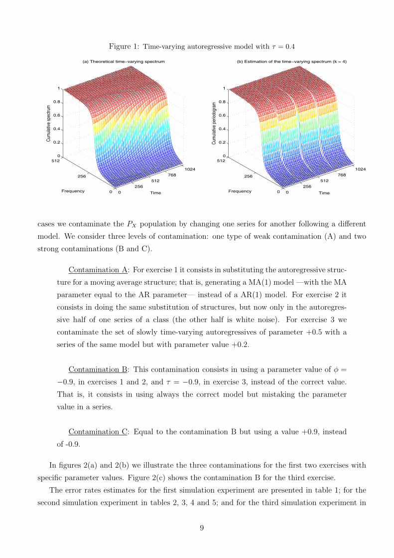
Figure 1: Time-varying autoregressive model with τ = 0.4

0

256

512

768

1024

0

256

5120

0.2

0.4

0.6

0.8

1

Time

(a) Theoretical time−varying spectrum

Frequency

Cum

ulat

ive s

pect

rum

0

256

512

768

1024

0

256

5120

0.2

0.4

0.6

0.8

1

Time

(b) Estimation of the time−varying spectrum (k = 4)

Frequency

Cum

ulat

ive p

erio

dogr

am

cases we contaminate the PX population by changing one series for another following a different

model. We consider three levels of contamination: one type of weak contamination (A) and two

strong contaminations (B and C).

Contamination A: For exercise 1 it consists in substituting the autoregressive struc-

ture for a moving average structure; that is, generating a MA(1) model —with the MA

parameter equal to the AR parameter— instead of a AR(1) model. For exercise 2 it

consists in doing the same substitution of structures, but now only in the autoregres-

sive half of one series of a class (the other half is white noise). For exercise 3 we

contaminate the set of slowly time-varying autoregressives of parameter +0.5 with a

series of the same model but with parameter value +0.2.

Contamination B: This contamination consists in using a parameter value of φ =

−0.9, in exercises 1 and 2, and τ = −0.9, in exercise 3, instead of the correct value.

That is, it consists in using always the correct model but mistaking the parameter

value in a series.

Contamination C: Equal to the contamination B but using a value +0.9, instead

of -0.9.

In figures 2(a) and 2(b) we illustrate the three contaminations for the first two exercises with

specific parameter values. Figure 2(c) shows the contamination B for the third exercise.

The error rates estimates for the first simulation experiment are presented in table 1; for the

second simulation experiment in tables 2, 3, 4 and 5; and for the third simulation experiment in

9

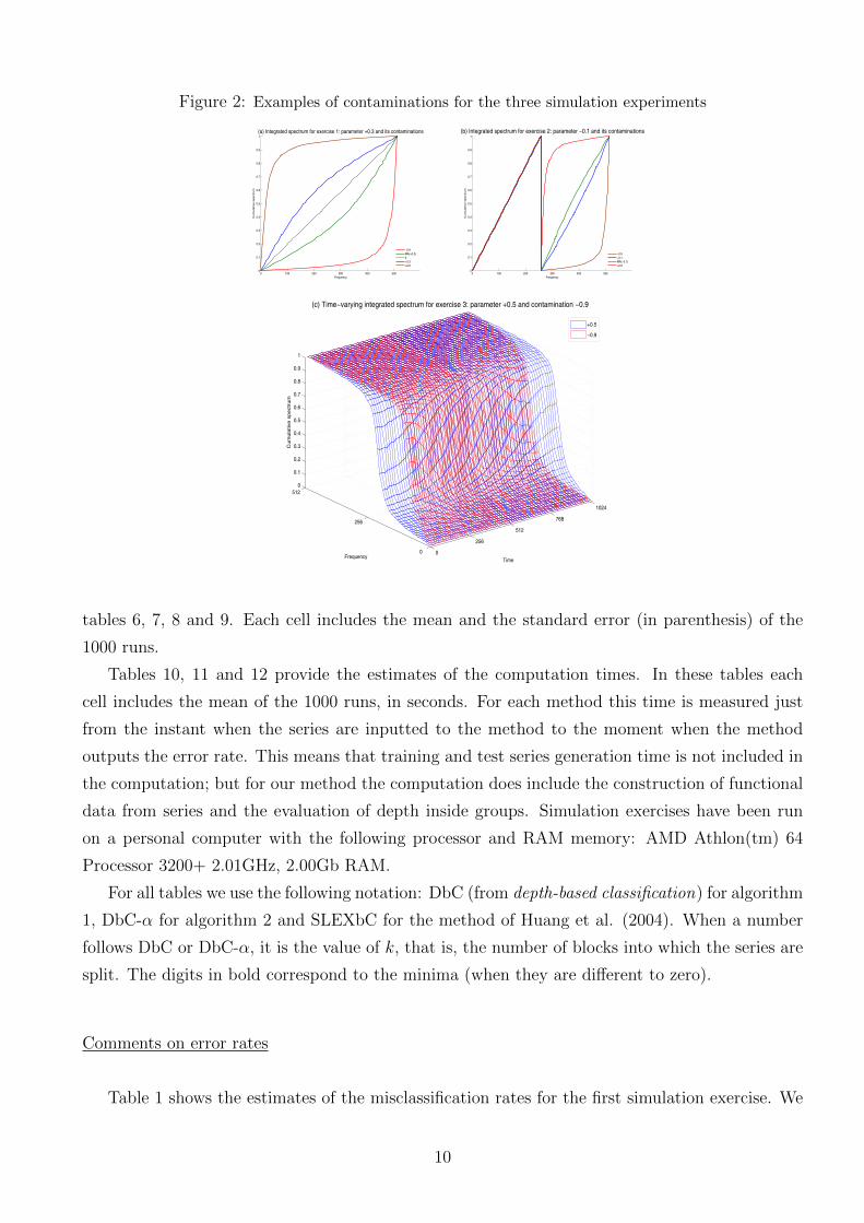
Figure 2: Examples of contaminations for the three simulation experiments

0 100 200 300 400 5000

0.1

0.2

0.3

0.4

0.5

0.6

0.7

0.8

0.9

1

Frequency

Cu

mu

lative

spe

ctr

um

(a) Integrated spectrum for exercise 1: parameter +0.3 and its contaminations

−0.9MA(+0.3)0+0.3+0.9

0 100 200 300 400 5000

0.1

0.2

0.3

0.4

0.5

0.6

0.7

0.8

0.9

1(b) Integrated spectrum for exercise 2: parameter −0.1 and its contaminations

Frequency

Cu

mu

lative

spe

ctr

um

−0.9−0.1MA(−0.1)+0.9

0

256

512

768

1024

0

256

5120

0.1

0.2

0.3

0.4

0.5

0.6

0.7

0.8

0.9

1

Time

(c) Time−varying integrated spectrum for exercise 3: parameter +0.5 and contamination −0.9

Frequency

Cum

ula

tive s

pect

rum

+0.5

−0.9

tables 6, 7, 8 and 9. Each cell includes the mean and the standard error (in parenthesis) of the

1000 runs.

Tables 10, 11 and 12 provide the estimates of the computation times. In these tables each

cell includes the mean of the 1000 runs, in seconds. For each method this time is measured just

from the instant when the series are inputted to the method to the moment when the method

outputs the error rate. This means that training and test series generation time is not included in

the computation; but for our method the computation does include the construction of functional

data from series and the evaluation of depth inside groups. Simulation exercises have been run

on a personal computer with the following processor and RAM memory: AMD Athlon(tm) 64

Processor 3200+ 2.01GHz, 2.00Gb RAM.

For all tables we use the following notation: DbC (from depth-based classification) for algorithm

1, DbC-α for algorithm 2 and SLEXbC for the method of Huang et al. (2004). When a number

follows DbC or DbC-α, it is the value of k, that is, the number of blocks into which the series are

split. The digits in bold correspond to the minima (when they are different to zero).

Comments on error rates

Table 1 shows the estimates of the misclassification rates for the first simulation exercise. We

10

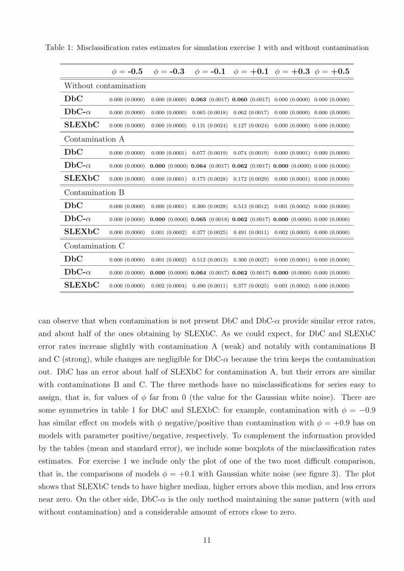
Table 1: Misclassification rates estimates for simulation exercise 1 with and without contamination

φ = -0.5 φ = -0.3 φ = -0.1 φ = +0.1 φ = +0.3 φ = +0.5

Without contamination

DbC 0.000 (0.0000) 0.000 (0.0000) 0.063 (0.0017) 0.060 (0.0017) 0.000 (0.0000) 0.000 (0.0000)

DbC-α 0.000 (0.0000) 0.000 (0.0000) 0.065 (0.0018) 0.062 (0.0017) 0.000 (0.0000) 0.000 (0.0000)

SLEXbC 0.000 (0.0000) 0.000 (0.0000) 0.131 (0.0024) 0.127 (0.0024) 0.000 (0.0000) 0.000 (0.0000)

Contamination A

DbC 0.000 (0.0000) 0.000 (0.0001) 0.077 (0.0019) 0.074 (0.0019) 0.000 (0.0001) 0.000 (0.0000)

DbC-α 0.000 (0.0000) 0.000 (0.0000) 0.064 (0.0017) 0.062 (0.0017) 0.000 (0.0000) 0.000 (0.0000)

SLEXbC 0.000 (0.0000) 0.000 (0.0001) 0.175 (0.0028) 0.172 (0.0029) 0.000 (0.0001) 0.000 (0.0000)

Contamination B

DbC 0.000 (0.0000) 0.000 (0.0001) 0.300 (0.0028) 0.513 (0.0012) 0.001 (0.0002) 0.000 (0.0000)

DbC-α 0.000 (0.0000) 0.000 (0.0000) 0.065 (0.0018) 0.062 (0.0017) 0.000 (0.0000) 0.000 (0.0000)

SLEXbC 0.000 (0.0000) 0.001 (0.0002) 0.377 (0.0025) 0.491 (0.0011) 0.002 (0.0003) 0.000 (0.0000)

Contamination C

DbC 0.000 (0.0000) 0.001 (0.0002) 0.512 (0.0013) 0.300 (0.0027) 0.000 (0.0001) 0.000 (0.0000)

DbC-α 0.000 (0.0000) 0.000 (0.0000) 0.064 (0.0017) 0.062 (0.0017) 0.000 (0.0000) 0.000 (0.0000)

SLEXbC 0.000 (0.0000) 0.002 (0.0004) 0.490 (0.0011) 0.377 (0.0025) 0.001 (0.0002) 0.000 (0.0000)

can observe that when contamination is not present DbC and DbC-α provide similar error rates,

and about half of the ones obtaining by SLEXbC. As we could expect, for DbC and SLEXbC

error rates increase slightly with contamination A (weak) and notably with contaminations B

and C (strong), while changes are negligible for DbC-α because the trim keeps the contamination

out. DbC has an error about half of SLEXbC for contamination A, but their errors are similar

with contaminations B and C. The three methods have no misclassifications for series easy to

assign, that is, for values of φ far from 0 (the value for the Gaussian white noise). There are

some symmetries in table 1 for DbC and SLEXbC: for example, contamination with φ = −0.9

has similar effect on models with φ negative/positive than contamination with φ = +0.9 has on

models with parameter positive/negative, respectively. To complement the information provided

by the tables (mean and standard error), we include some boxplots of the misclassification rates

estimates. For exercise 1 we include only the plot of one of the two most difficult comparison,

that is, the comparisons of models φ = +0.1 with Gaussian white noise (see figure 3). The plot

shows that SLEXbC tends to have higher median, higher errors above this median, and less errors

near zero. On the other side, DbC-α is the only method maintaining the same pattern (with and

without contamination) and a considerable amount of errors close to zero.

11

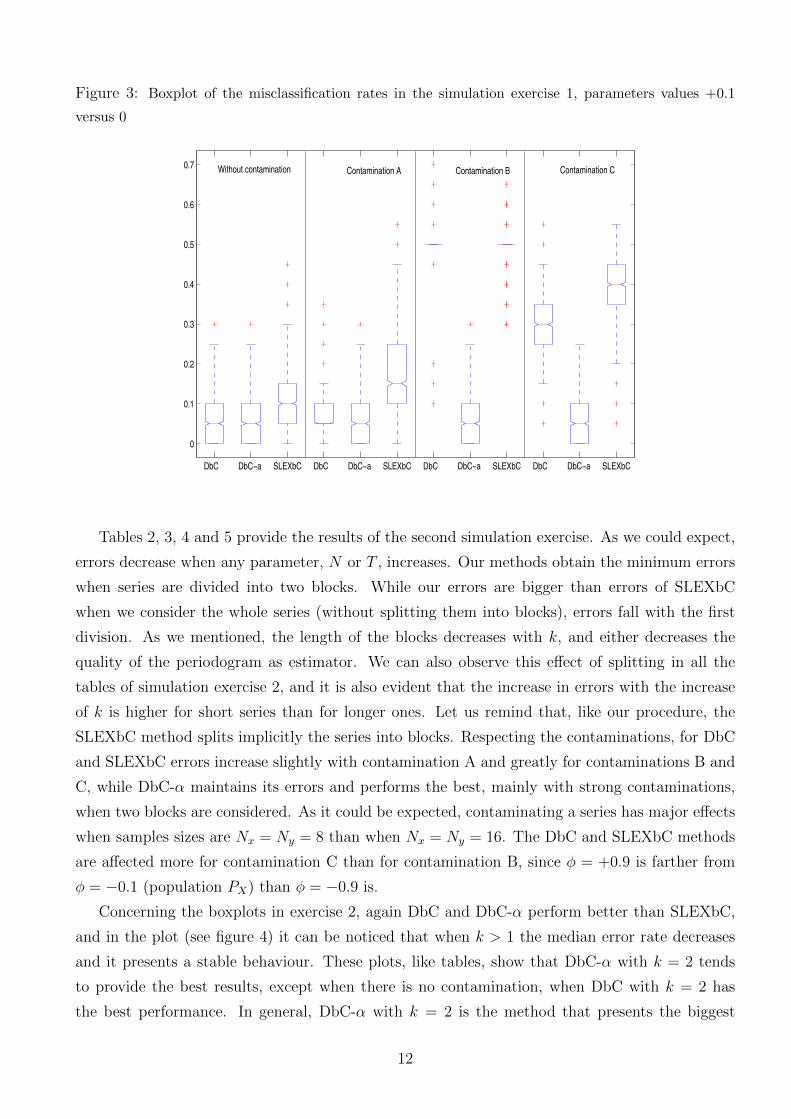
Figure 3: Boxplot of the misclassification rates in the simulation exercise 1, parameters values +0.1

versus 0

DbC DbC−a SLEXbC DbC DbC−a SLEXbC DbC DbC−a SLEXbC DbC DbC−a SLEXbC

0

0.1

0.2

0.3

0.4

0.5

0.6

0.7Contamination BWithout contamination Contamination A Contamination C

Tables 2, 3, 4 and 5 provide the results of the second simulation exercise. As we could expect,

errors decrease when any parameter, N or T , increases. Our methods obtain the minimum errors

when series are divided into two blocks. While our errors are bigger than errors of SLEXbC

when we consider the whole series (without splitting them into blocks), errors fall with the first

division. As we mentioned, the length of the blocks decreases with k, and either decreases the

quality of the periodogram as estimator. We can also observe this effect of splitting in all the

tables of simulation exercise 2, and it is also evident that the increase in errors with the increase

of k is higher for short series than for longer ones. Let us remind that, like our procedure, the

SLEXbC method splits implicitly the series into blocks. Respecting the contaminations, for DbC

and SLEXbC errors increase slightly with contamination A and greatly for contaminations B and

C, while DbC-α maintains its errors and performs the best, mainly with strong contaminations,

when two blocks are considered. As it could be expected, contaminating a series has major effects

when samples sizes are Nx = Ny = 8 than when Nx = Ny = 16. The DbC and SLEXbC methods

are affected more for contamination C than for contamination B, since φ = +0.9 is farther from

φ = −0.1 (population PX) than φ = −0.9 is.

Concerning the boxplots in exercise 2, again DbC and DbC-α perform better than SLEXbC,

and in the plot (see figure 4) it can be noticed that when k > 1 the median error rate decreases

and it presents a stable behaviour. These plots, like tables, show that DbC-α with k = 2 tends

to provide the best results, except when there is no contamination, when DbC with k = 2 has

the best performance. In general, DbC-α with k = 2 is the method that presents the biggest

12

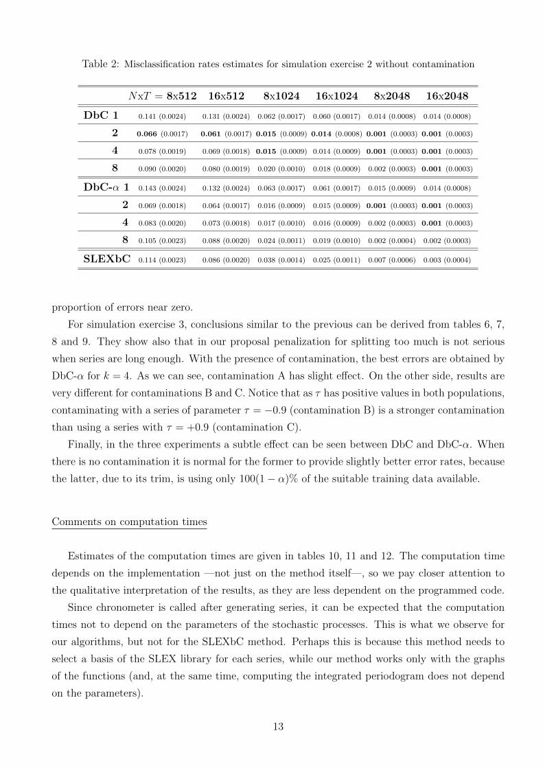
Table 2: Misclassification rates estimates for simulation exercise 2 without contamination

NxT = 8x512 16x512 8x1024 16x1024 8x2048 16x2048

DbC 1 0.141 (0.0024) 0.131 (0.0024) 0.062 (0.0017) 0.060 (0.0017) 0.014 (0.0008) 0.014 (0.0008)

2 0.066 (0.0017) 0.061 (0.0017) 0.015 (0.0009) 0.014 (0.0008) 0.001 (0.0003) 0.001 (0.0003)

4 0.078 (0.0019) 0.069 (0.0018) 0.015 (0.0009) 0.014 (0.0009) 0.001 (0.0003) 0.001 (0.0003)

8 0.090 (0.0020) 0.080 (0.0019) 0.020 (0.0010) 0.018 (0.0009) 0.002 (0.0003) 0.001 (0.0003)

DbC-α 1 0.143 (0.0024) 0.132 (0.0024) 0.063 (0.0017) 0.061 (0.0017) 0.015 (0.0009) 0.014 (0.0008)

2 0.069 (0.0018) 0.064 (0.0017) 0.016 (0.0009) 0.015 (0.0009) 0.001 (0.0003) 0.001 (0.0003)

4 0.083 (0.0020) 0.073 (0.0018) 0.017 (0.0010) 0.016 (0.0009) 0.002 (0.0003) 0.001 (0.0003)

8 0.105 (0.0023) 0.088 (0.0020) 0.024 (0.0011) 0.019 (0.0010) 0.002 (0.0004) 0.002 (0.0003)

SLEXbC 0.114 (0.0023) 0.086 (0.0020) 0.038 (0.0014) 0.025 (0.0011) 0.007 (0.0006) 0.003 (0.0004)

proportion of errors near zero.

For simulation exercise 3, conclusions similar to the previous can be derived from tables 6, 7,

8 and 9. They show also that in our proposal penalization for splitting too much is not serious

when series are long enough. With the presence of contamination, the best errors are obtained by

DbC-α for k = 4. As we can see, contamination A has slight effect. On the other side, results are

very different for contaminations B and C. Notice that as τ has positive values in both populations,

contaminating with a series of parameter τ = −0.9 (contamination B) is a stronger contamination

than using a series with τ = +0.9 (contamination C).

Finally, in the three experiments a subtle effect can be seen between DbC and DbC-α. When

there is no contamination it is normal for the former to provide slightly better error rates, because

the latter, due to its trim, is using only 100(1− α)% of the suitable training data available.

Comments on computation times

Estimates of the computation times are given in tables 10, 11 and 12. The computation time

depends on the implementation —not just on the method itself—, so we pay closer attention to

the qualitative interpretation of the results, as they are less dependent on the programmed code.

Since chronometer is called after generating series, it can be expected that the computation

times not to depend on the parameters of the stochastic processes. This is what we observe for

our algorithms, but not for the SLEXbC method. Perhaps this is because this method needs to

select a basis of the SLEX library for each series, while our method works only with the graphs

of the functions (and, at the same time, computing the integrated periodogram does not depend

on the parameters).

13

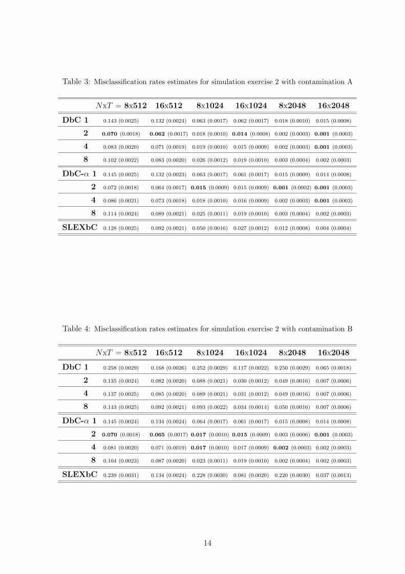
Table 3: Misclassification rates estimates for simulation exercise 2 with contamination A

NxT = 8x512 16x512 8x1024 16x1024 8x2048 16x2048

DbC 1 0.143 (0.0025) 0.132 (0.0024) 0.063 (0.0017) 0.062 (0.0017) 0.018 (0.0010) 0.015 (0.0008)

2 0.070 (0.0018) 0.062 (0.0017) 0.018 (0.0010) 0.014 (0.0008) 0.002 (0.0003) 0.001 (0.0003)

4 0.083 (0.0020) 0.071 (0.0019) 0.019 (0.0010) 0.015 (0.0009) 0.002 (0.0003) 0.001 (0.0003)

8 0.102 (0.0022) 0.083 (0.0020) 0.026 (0.0012) 0.019 (0.0010) 0.003 (0.0004) 0.002 (0.0003)

DbC-α 1 0.145 (0.0025) 0.132 (0.0023) 0.063 (0.0017) 0.061 (0.0017) 0.015 (0.0009) 0.014 (0.0008)

2 0.072 (0.0018) 0.064 (0.0017) 0.015 (0.0009) 0.015 (0.0009) 0.001 (0.0002) 0.001 (0.0003)

4 0.086 (0.0021) 0.073 (0.0018) 0.018 (0.0010) 0.016 (0.0009) 0.002 (0.0003) 0.001 (0.0003)

8 0.114 (0.0024) 0.089 (0.0021) 0.025 (0.0011) 0.019 (0.0010) 0.003 (0.0004) 0.002 (0.0003)

SLEXbC 0.128 (0.0025) 0.092 (0.0021) 0.050 (0.0016) 0.027 (0.0012) 0.012 (0.0008) 0.004 (0.0004)

Table 4: Misclassification rates estimates for simulation exercise 2 with contamination B

NxT = 8x512 16x512 8x1024 16x1024 8x2048 16x2048

DbC 1 0.258 (0.0029) 0.168 (0.0026) 0.252 (0.0029) 0.117 (0.0022) 0.250 (0.0029) 0.065 (0.0018)

2 0.135 (0.0024) 0.082 (0.0020) 0.088 (0.0021) 0.030 (0.0012) 0.049 (0.0016) 0.007 (0.0006)

4 0.137 (0.0025) 0.085 (0.0020) 0.089 (0.0021) 0.031 (0.0012) 0.049 (0.0016) 0.007 (0.0006)

8 0.143 (0.0025) 0.092 (0.0021) 0.093 (0.0022) 0.034 (0.0014) 0.050 (0.0016) 0.007 (0.0006)

DbC-α 1 0.145 (0.0024) 0.134 (0.0024) 0.064 (0.0017) 0.061 (0.0017) 0.015 (0.0008) 0.014 (0.0008)

2 0.070 (0.0018) 0.065 (0.0017) 0.017 (0.0010) 0.015 (0.0009) 0.003 (0.0006) 0.001 (0.0003)

4 0.081 (0.0020) 0.071 (0.0019) 0.017 (0.0010) 0.017 (0.0009) 0.002 (0.0003) 0.002 (0.0003)

8 0.104 (0.0023) 0.087 (0.0020) 0.023 (0.0011) 0.019 (0.0010) 0.002 (0.0004) 0.002 (0.0003)

SLEXbC 0.239 (0.0031) 0.134 (0.0024) 0.228 (0.0030) 0.081 (0.0020) 0.220 (0.0030) 0.037 (0.0013)

14

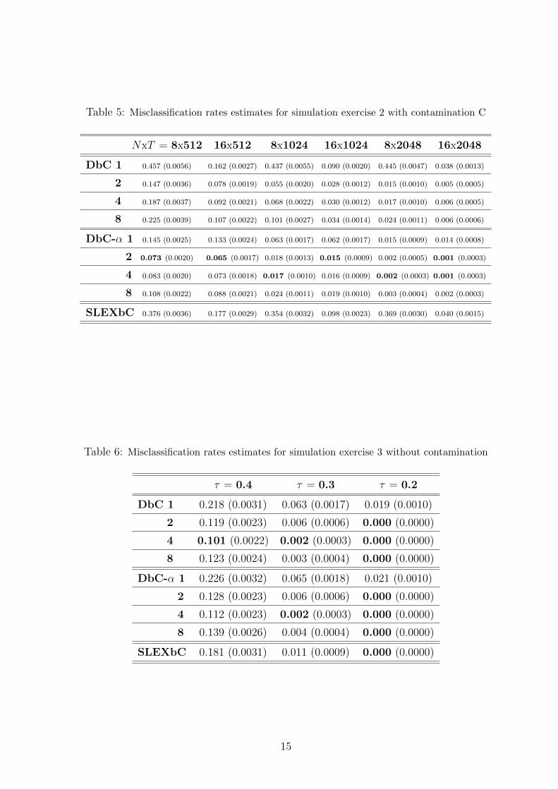
Table 5: Misclassification rates estimates for simulation exercise 2 with contamination C

NxT = 8x512 16x512 8x1024 16x1024 8x2048 16x2048

DbC 1 0.457 (0.0056) 0.162 (0.0027) 0.437 (0.0055) 0.090 (0.0020) 0.445 (0.0047) 0.038 (0.0013)

2 0.147 (0.0036) 0.078 (0.0019) 0.055 (0.0020) 0.028 (0.0012) 0.015 (0.0010) 0.005 (0.0005)

4 0.187 (0.0037) 0.092 (0.0021) 0.068 (0.0022) 0.030 (0.0012) 0.017 (0.0010) 0.006 (0.0005)

8 0.225 (0.0039) 0.107 (0.0022) 0.101 (0.0027) 0.034 (0.0014) 0.024 (0.0011) 0.006 (0.0006)

DbC-α 1 0.145 (0.0025) 0.133 (0.0024) 0.063 (0.0017) 0.062 (0.0017) 0.015 (0.0009) 0.014 (0.0008)

2 0.073 (0.0020) 0.065 (0.0017) 0.018 (0.0013) 0.015 (0.0009) 0.002 (0.0005) 0.001 (0.0003)

4 0.083 (0.0020) 0.073 (0.0018) 0.017 (0.0010) 0.016 (0.0009) 0.002 (0.0003) 0.001 (0.0003)

8 0.108 (0.0022) 0.088 (0.0021) 0.024 (0.0011) 0.019 (0.0010) 0.003 (0.0004) 0.002 (0.0003)

SLEXbC 0.376 (0.0036) 0.177 (0.0029) 0.354 (0.0032) 0.098 (0.0023) 0.369 (0.0030) 0.040 (0.0015)

Table 6: Misclassification rates estimates for simulation exercise 3 without contamination

τ = 0.4 τ = 0.3 τ = 0.2

DbC 1 0.218 (0.0031) 0.063 (0.0017) 0.019 (0.0010)

2 0.119 (0.0023) 0.006 (0.0006) 0.000 (0.0000)

4 0.101 (0.0022) 0.002 (0.0003) 0.000 (0.0000)

8 0.123 (0.0024) 0.003 (0.0004) 0.000 (0.0000)

DbC-α 1 0.226 (0.0032) 0.065 (0.0018) 0.021 (0.0010)

2 0.128 (0.0023) 0.006 (0.0006) 0.000 (0.0000)

4 0.112 (0.0023) 0.002 (0.0003) 0.000 (0.0000)

8 0.139 (0.0026) 0.004 (0.0004) 0.000 (0.0000)

SLEXbC 0.181 (0.0031) 0.011 (0.0009) 0.000 (0.0000)

15

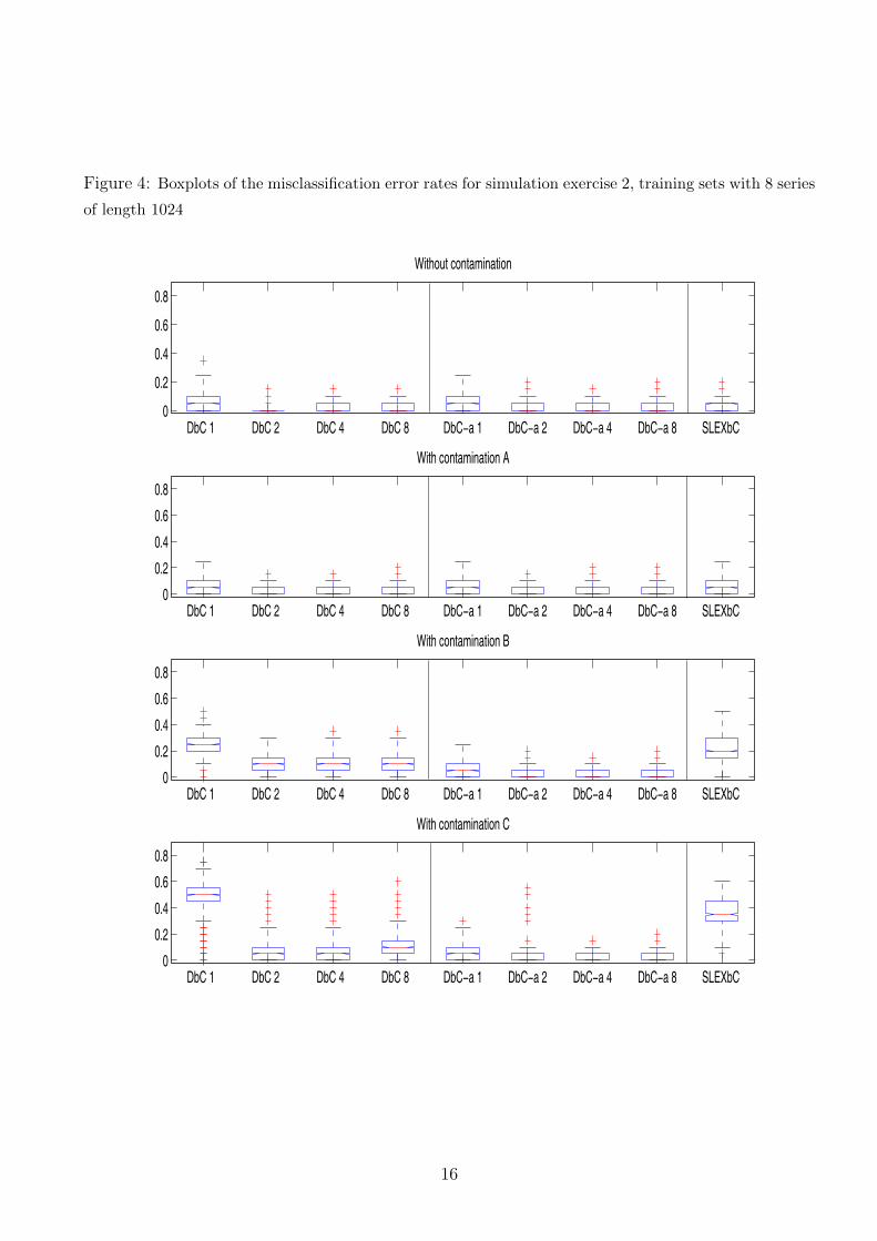
Figure 4: Boxplots of the misclassification error rates for simulation exercise 2, training sets with 8 series

of length 1024

DbC 1 DbC 2 DbC 4 DbC 8 DbC−a 1 DbC−a 2 DbC−a 4 DbC−a 8 SLEXbC 0

0.2

0.4

0.6

0.8

Without contamination

DbC 1 DbC 2 DbC 4 DbC 8 DbC−a 1 DbC−a 2 DbC−a 4 DbC−a 8 SLEXbC 0

0.2

0.4

0.6

0.8

With contamination A

DbC 1 DbC 2 DbC 4 DbC 8 DbC−a 1 DbC−a 2 DbC−a 4 DbC−a 8 SLEXbC 0

0.2

0.4

0.6

0.8

With contamination B

DbC 1 DbC 2 DbC 4 DbC 8 DbC−a 1 DbC−a 2 DbC−a 4 DbC−a 8 SLEXbC 0

0.2

0.4

0.6

0.8

With contamination C

16

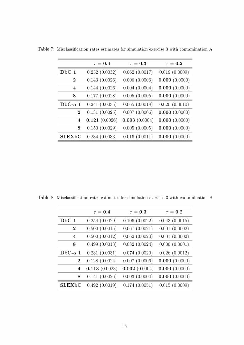
Table 7: Misclassification rates estimates for simulation exercise 3 with contamination A

τ = 0.4 τ = 0.3 τ = 0.2

DbC 1 0.232 (0.0032) 0.062 (0.0017) 0.019 (0.0009)

2 0.143 (0.0026) 0.006 (0.0006) 0.000 (0.0000)

4 0.144 (0.0026) 0.004 (0.0004) 0.000 (0.0000)

8 0.177 (0.0028) 0.005 (0.0005) 0.000 (0.0000)

DbC-α 1 0.241 (0.0035) 0.065 (0.0018) 0.020 (0.0010)

2 0.131 (0.0025) 0.007 (0.0006) 0.000 (0.0000)

4 0.121 (0.0026) 0.003 (0.0004) 0.000 (0.0000)

8 0.150 (0.0029) 0.005 (0.0005) 0.000 (0.0000)

SLEXbC 0.234 (0.0033) 0.016 (0.0011) 0.000 (0.0000)

Table 8: Misclassification rates estimates for simulation exercise 3 with contamination B

τ = 0.4 τ = 0.3 τ = 0.2

DbC 1 0.254 (0.0029) 0.106 (0.0022) 0.043 (0.0015)

2 0.500 (0.0015) 0.067 (0.0021) 0.001 (0.0002)

4 0.500 (0.0012) 0.062 (0.0020) 0.001 (0.0002)

8 0.499 (0.0013) 0.082 (0.0024) 0.000 (0.0001)

DbC-α 1 0.231 (0.0031) 0.074 (0.0020) 0.026 (0.0012)

2 0.128 (0.0024) 0.007 (0.0006) 0.000 (0.0000)

4 0.113 (0.0023) 0.002 (0.0004) 0.000 (0.0000)

8 0.141 (0.0026) 0.003 (0.0004) 0.000 (0.0000)

SLEXbC 0.492 (0.0019) 0.174 (0.0051) 0.015 (0.0009)

17

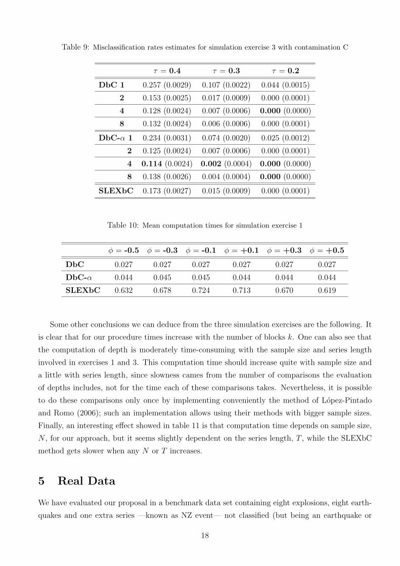
Table 9: Misclassification rates estimates for simulation exercise 3 with contamination C

τ = 0.4 τ = 0.3 τ = 0.2

DbC 1 0.257 (0.0029) 0.107 (0.0022) 0.044 (0.0015)

2 0.153 (0.0025) 0.017 (0.0009) 0.000 (0.0001)

4 0.128 (0.0024) 0.007 (0.0006) 0.000 (0.0000)

8 0.132 (0.0024) 0.006 (0.0006) 0.000 (0.0001)

DbC-α 1 0.234 (0.0031) 0.074 (0.0020) 0.025 (0.0012)

2 0.125 (0.0024) 0.007 (0.0006) 0.000 (0.0001)

4 0.114 (0.0024) 0.002 (0.0004) 0.000 (0.0000)

8 0.138 (0.0026) 0.004 (0.0004) 0.000 (0.0000)

SLEXbC 0.173 (0.0027) 0.015 (0.0009) 0.000 (0.0001)

Table 10: Mean computation times for simulation exercise 1

φ = -0.5 φ = -0.3 φ = -0.1 φ = +0.1 φ = +0.3 φ = +0.5

DbC 0.027 0.027 0.027 0.027 0.027 0.027

DbC-α 0.044 0.045 0.045 0.044 0.044 0.044

SLEXbC 0.632 0.678 0.724 0.713 0.670 0.619

Some other conclusions we can deduce from the three simulation exercises are the following. It

is clear that for our procedure times increase with the number of blocks k. One can also see that

the computation of depth is moderately time-consuming with the sample size and series length

involved in exercises 1 and 3. This computation time should increase quite with sample size and

a little with series length, since slowness cames from the number of comparisons the evaluation

of depths includes, not for the time each of these comparisons takes. Nevertheless, it is possible

to do these comparisons only once by implementing conveniently the method of Lopez-Pintado

and Romo (2006); such an implementation allows using their methods with bigger sample sizes.

Finally, an interesting effect showed in table 11 is that computation time depends on sample size,

N , for our approach, but it seems slightly dependent on the series length, T , while the SLEXbC

method gets slower when any N or T increases.

5 Real Data

We have evaluated our proposal in a benchmark data set containing eight explosions, eight earth-

quakes and one extra series —known as NZ event— not classified (but being an earthquake or

18

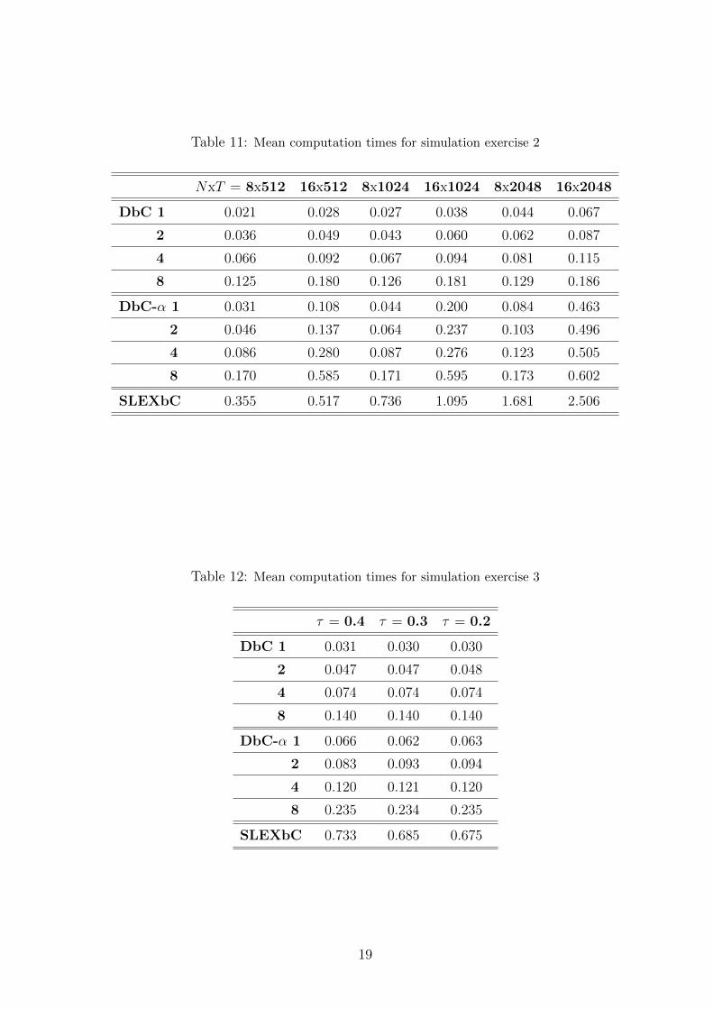
Table 11: Mean computation times for simulation exercise 2

NxT = 8x512 16x512 8x1024 16x1024 8x2048 16x2048

DbC 1 0.021 0.028 0.027 0.038 0.044 0.067

2 0.036 0.049 0.043 0.060 0.062 0.087

4 0.066 0.092 0.067 0.094 0.081 0.115

8 0.125 0.180 0.126 0.181 0.129 0.186

DbC-α 1 0.031 0.108 0.044 0.200 0.084 0.463

2 0.046 0.137 0.064 0.237 0.103 0.496

4 0.086 0.280 0.087 0.276 0.123 0.505

8 0.170 0.585 0.171 0.595 0.173 0.602

SLEXbC 0.355 0.517 0.736 1.095 1.681 2.506

Table 12: Mean computation times for simulation exercise 3

τ = 0.4 τ = 0.3 τ = 0.2

DbC 1 0.031 0.030 0.030

2 0.047 0.047 0.048

4 0.074 0.074 0.074

8 0.140 0.140 0.140

DbC-α 1 0.066 0.062 0.063

2 0.083 0.093 0.094

4 0.120 0.121 0.120

8 0.235 0.234 0.235

SLEXbC 0.733 0.685 0.675

19

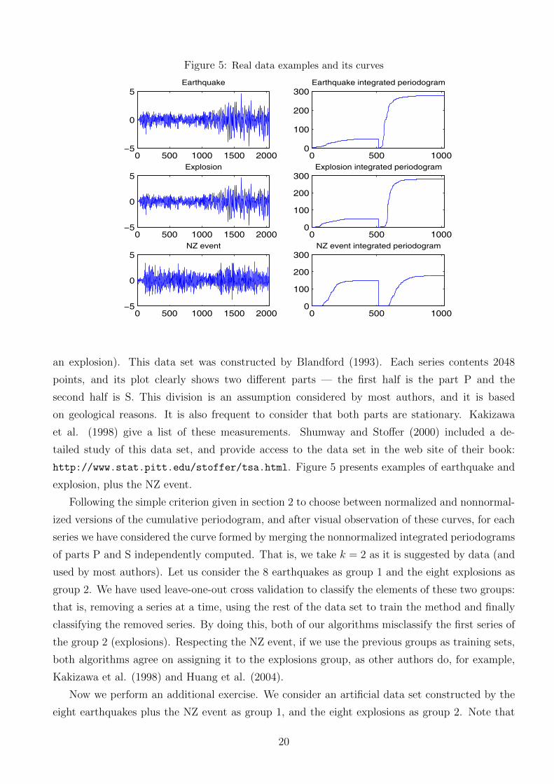
Figure 5: Real data examples and its curves

0 500 1000 1500 2000−5

0

5Earthquake

0 500 10000

100

200

300Earthquake integrated periodogram

0 500 1000 1500 2000−5

0

5Explosion

0 500 10000

100

200

300Explosion integrated periodogram

0 500 1000 1500 2000−5

0

5NZ event

0 500 10000

100

200

300NZ event integrated periodogram

an explosion). This data set was constructed by Blandford (1993). Each series contents 2048

points, and its plot clearly shows two different parts — the first half is the part P and the

second half is S. This division is an assumption considered by most authors, and it is based

on geological reasons. It is also frequent to consider that both parts are stationary. Kakizawa

et al. (1998) give a list of these measurements. Shumway and Stoffer (2000) included a de-

tailed study of this data set, and provide access to the data set in the web site of their book:

http://www.stat.pitt.edu/stoffer/tsa.html. Figure 5 presents examples of earthquake and

explosion, plus the NZ event.

Following the simple criterion given in section 2 to choose between normalized and nonnormal-

ized versions of the cumulative periodogram, and after visual observation of these curves, for each

series we have considered the curve formed by merging the nonnormalized integrated periodograms

of parts P and S independently computed. That is, we take k = 2 as it is suggested by data (and

used by most authors). Let us consider the 8 earthquakes as group 1 and the eight explosions as

group 2. We have used leave-one-out cross validation to classify the elements of these two groups:

that is, removing a series at a time, using the rest of the data set to train the method and finally

classifying the removed series. By doing this, both of our algorithms misclassify the first series of

the group 2 (explosions). Respecting the NZ event, if we use the previous groups as training sets,

both algorithms agree on assigning it to the explosions group, as other authors do, for example,

Kakizawa et al. (1998) and Huang et al. (2004).

Now we perform an additional exercise. We consider an artificial data set constructed by the

eight earthquakes plus the NZ event as group 1, and the eight explosions as group 2. Note that

20

our method and most of the published papers classify NZ as an explosion. Then we could consider

this artificial suite as a case where some atypical observation is presented in group 1. In this

situation, the results using our algorithm 1 are that it misclassifies the first and the third elements

of group 2 (explosions), not only the first. But again algorithm 2 misclassifies only the first series

of group 2. This seems to show the robustness of our second algorithm. Obviously, as we are using

leave-one-out cross validation, both algorithms classifies the NZ event in the explosions group, as

we mentioned in the previous paragraph.

6 Conclusions

We define a new time series classification method based on the integrated periodograms of the

series (so it is a frequency domain approach). When series are nonstationary, they are split into

blocks and the integrated periodograms of the blocks are merged to construct a curve; this idea

relays on the assumption of local stationarity of the series. Since the integrated periodogram is a

function, the statistical concepts of this type of data can be applied. New series are assigned to

the class minimizing the distance between its group mean of curves and the curve of the new data.

Since the group mean can be affected by the presence of atypical observations, to add robustness to

the classification we proposed substituting the mean curve by the α-trimmed mean, where for each

group only the deepest elements are averaged. We evaluate our proposal in different scenarios.

We run three simulations exercises containing several models and parameters values, one with

stationary series and the other with two types of nonstationarity. After running the exercises

without contamination, we repeat all comparisons three more times using exactly the same series

but one (the contamination series). We consider one kind of weak contamination and two strong

contaminations. We also illustrate the performance of our procedure in a benchmark real data

set. Our proposal provides small error rates, robustness and a good computational behavior, what

makes the method suitable to classify long time series. Finally, this paper suggests the integrated

periodogram contents information useful to classify time series.

Acknowledgements

This research has been supported by CICYT (Spain) grants SEJ2005-06454 and SEJ2007-64500.

The first author also acknowledges the support of “Comunidad de Madrid” grant CCG07-UC3M/

HUM-3260.

References

[1] Abraham, C., P.A. Cornillon, E. Matzner-Løber and N. Molinari (2003). Unsupervised Curve

Clustering using B-Splines. Scandinavian Journal of Statistics. 30 (3), 581–595.

21

[2] Blandford, R.R. (1993). Discrimination of Earthquakes and Explosions at Regional Distances

Using Complexity. Report AFTAC-TR-93-044 HQ, Air Force Technical Applications Center,

Patrick Air Force Base, FL.

[3] Chandler, G., and W. Polonik (2006). Discrimination of Locally Stationary Time Series Based

on the Excess Mass Functional. Journal of the American Statistical Association. 101 (473),

240–253.

[4] Ferraty, F., and P. Vieu (2003). Curves Discrimination: A Nonparametric Functional Ap-

proach. Computational Statistics and Data Analysis. 44, 161-173.

[5] Hall, P., D.S. Poskitt and B. Presnell (2001). A Functional Data-Analytic Approach to Signal

Discrimination. Technometrics. 43 (1), 1-9.

[6] Hastie, T., A. Buja and R.J. Tibshirani (1995). Penalized Discriminant Analysis. The Annals

of Statistics. 23 (1), 73-102.

[7] Hirukawa, J. (2004). Discriminant Analysis for Multivariate Non-Gaussian Locally Stationary

Processes. Scientiae Mathematicae Japonicae. 60 (2), 357–380.

[8] Huang, H., H. Ombao and D.S. Stoffer (2004). Discrimination and Classification of Nonsta-

tionary Time Series Using the SLEX Model. Journal of the American Statistical Association.

99 (467), 763–774.

[9] James, G.M., and T. Hastie (2001). Functional Linear Discriminant Analysis for Irregularly

Sampled Curves. Journal of the Royal Statistical Society. Series B, 63, 533-550.

[10] James, G.M., and C. A. Sugar (2003). Clustering for Sparsely Sampled Functional Data.

Journal of the American Statistical Association. 98 (462), 397-408.

[11] Kakizawa, Y., R.H. Shumway and M. Taniguchi (1998). Discrimination and Clustering for

Multivariate Time Series. Journal of the American Statistical Association. 93 (441), 328-340.

[12] Lopez-Pintado, S., and J. Romo. (2006). Depth-Based Classification for Functional Data. DI-

MACS Series in Discrete Mathematics and Theoretical Computer Science, American Mathe-

matical Society. Vol. 72.

[13] Lopez-Pintado, S., and J. Romo (2008). On the Concept of Depth for Functional Data.

Journal of the American Statistical Association, In press.

[14] Maharaj, E.A., and A.M. Alonso (2007). Discrimination of Locally Stationary Time Series

Using Wavelets. Computational Statistics and Data Analysis. 52, 879–895.

22

[15] Ombao, H.C., J.A. Raz, R. von Sachs and B.A. Malow (2001). Automatic Statistical Analysis

of Bivariate Nonstationary Time Series. Journal of the American Statistical Association. 96

(454), 543-560.

[16] Priestley, M. (1965). Evolutionary Spectra and Nonstationary Processes. Journal of the Royal

Statistical Society. Series B, 27 (2), 204-237.

[17] Sakiyama, K., and M. Taniguchi (2004). Discriminant Analysis for Locally Stationary Proc-

esses. Journal of Multivariate Analysis. 90, 282–300.

[18] Shumway, R.S. (2003). Time-Frequency Clustering and Discriminant Analysis. Statistics &

Probability Letters. 63, 307–314.

[19] Shumway, R.H., and D.S. Stoffer (2000). Time Series Analysis and Its Applications. New

York: Springer.

[20] Taniguchi, M., and Y. Kakizawa (2000). Asymptotic Theory of Statistical Inference for Time

Series. New York: Springer.

23