Temporal Classification: Extending the Classification Paradigm to Multivariate Time Series
307
The University of New South Wales School of Computer Science and Engineering Temporal Classification: Extending the Classification Paradigm to Multivariate Time Series Mohammed Waleed Kadous A Thesis submitted as a requirement for the Degree of Doctor of Philosophy October 2002 Supervisor: Claude Sammut
-
Upload
independent -
Category
Documents
-
view
1 -
download
0
Transcript of Temporal Classification: Extending the Classification Paradigm to Multivariate Time Series
The University of New South Wales
School of Computer Science and Engineering
Temporal Classification: Extending the
Classification Paradigm to Multivariate
Time Series
Mohammed Waleed Kadous
A Thesis submitted as a requirement for the Degree ofDoctor of Philosophy
October 2002
Supervisor: Claude Sammut


Abstract
Machine learning research has, to a great extent, ignored an important aspect
of many real world applications: time. Existing concept learners predominantly
operate on a static set of attributes; for example, classifying flowers described by
leaf size, petal colour and petal count. The values of these attributes is assumed
to be unchanging – the flower never grows or loses leaves.
However, many real datasets are not “static”; they cannot sensibly be repre-
sented as a fixed set of attributes. Rather, the examples are expressed as fea-
tures that vary temporally, and it is the temporal variation itself that is used
for classification. Consider a simple gesture recognition domain, in which the
temporal features are the position of the hands, finger bends, and so on. Looking
at the position of the hand at one point in time is not likely to lead to a suc-
cessful classification; it is only by analysing changes in position that recognition
is possible.
This thesis presents a new technique for temporal classification. By extracting
sub-events from the training instances and parameterising them to allow feature
construction for a subsequent learning process, it is able to employ background
knowledge and express learnt concepts in terms of the background knowledge.
The key novel results of the thesis are:

• A temporal learner capable of producing comprehensible and accurate clas-
sifiers for multivariate time series that can learn from a small number of
instances and can integrate non-temporal features.
• A feature construction technique that parameterises sub-events of the train-
ing set and clusters them to construct features for a propositional learner.
• A technique for post-processing classification rules produced by the learner
to give a comprehensible description expressed in the same form as the
original background knowledge.
The thesis discusses the implementation of TClass, a temporal learner, and
demonstrates its application on several artificial and real-world domains, and
compares its performance against existing techniques (such as hidden Markov
models). Results show rules that are comprehensible in many cases and accu-
racy results close to or better than existing techniques – over 98 per cent for
sign language and 72 per cent for ECGs (equivalent to the accuracy of a human
cardiologist). One further surprising result is that a small set of very primi-
tive sub-events proves to be functional, avoiding the need for labour-intensive
background knowledge if it is not available.
ii

Declaration
I hereby declare that this submission is my own work and to the best of my knowl-edge it contains no materials previously published or written by another person,nor material which to a substantial extent has been accepted for the award ofany other degree or diploma at UNSW or any other educational institution, ex-cept where due acknowledgement is made in the thesis. Any contribution madeto the research by others, with whom I have worked at UNSW or elsewhere, isexplicitly acknowledged in the thesis.
I also declare that the intellectual content of this thesis is the product of my ownwork, except to the extent that assistance from others in the project’s design andconception or in style, presentation and linguistic expression is acknowledged.
................................................................................................Mohammed Waleed Kadous
i

Contents
1 Introduction 11.1 Summary of the thesis . . . . . . . . . . . . . . . . . . . . . . . . 4
2 Definition of The Problem, Terms Used and Basic Issues 92.1 Examples of Temporal Classification . . . . . . . . . . . . . . . . 10
2.1.1 Tech Support . . . . . . . . . . . . . . . . . . . . . . . . . 102.1.2 Recognition of signs from a sign language . . . . . . . . . . 11
2.2 Definition of Terms . . . . . . . . . . . . . . . . . . . . . . . . . . 122.2.1 Channel . . . . . . . . . . . . . . . . . . . . . . . . . . . . 132.2.2 Stream . . . . . . . . . . . . . . . . . . . . . . . . . . . . . 152.2.3 Frame . . . . . . . . . . . . . . . . . . . . . . . . . . . . . 162.2.4 Stream Set . . . . . . . . . . . . . . . . . . . . . . . . . . 17
2.3 Statement of the problem . . . . . . . . . . . . . . . . . . . . . . 182.3.1 Weak temporal classification . . . . . . . . . . . . . . . . . 182.3.2 Strong classification . . . . . . . . . . . . . . . . . . . . . . 192.3.3 Pre-segmented TC . . . . . . . . . . . . . . . . . . . . . . 20
2.4 Assessing success . . . . . . . . . . . . . . . . . . . . . . . . . . . 212.4.1 Assessing Accuracy of Weak TC . . . . . . . . . . . . . . . 212.4.2 Assessing Accuracy of Strong TC . . . . . . . . . . . . . . 222.4.3 Comprehensibility – A subjective goal . . . . . . . . . . . 24
2.5 The major difficulties in temporal classification . . . . . . . . . . 262.6 Conclusion . . . . . . . . . . . . . . . . . . . . . . . . . . . . . . . 29
3 Relationship to existing work 303.1 Related fields . . . . . . . . . . . . . . . . . . . . . . . . . . . . . 313.2 Established techniques . . . . . . . . . . . . . . . . . . . . . . . . 33
3.2.1 Hidden Markov Models . . . . . . . . . . . . . . . . . . . . 333.2.2 Recurrent Neural Networks . . . . . . . . . . . . . . . . . 433.2.3 Dynamic Time Warping . . . . . . . . . . . . . . . . . . . 46
3.3 Recent interest from the AI community . . . . . . . . . . . . . . . 49
iii
CONTENTS iv
4 Metafeatures: A Novel Feature Construction Technique 544.1 TClass Overview . . . . . . . . . . . . . . . . . . . . . . . . . . . 554.2 Tech Support revisited . . . . . . . . . . . . . . . . . . . . . . . . 554.3 Inspiration for metafeatures . . . . . . . . . . . . . . . . . . . . . 614.4 Definition . . . . . . . . . . . . . . . . . . . . . . . . . . . . . . . 644.5 Practical metafeatures . . . . . . . . . . . . . . . . . . . . . . . . 66
4.5.1 A more practical example . . . . . . . . . . . . . . . . . . 664.5.2 Representation . . . . . . . . . . . . . . . . . . . . . . . . 684.5.3 Extraction from a noisy signal . . . . . . . . . . . . . . . . 72
4.6 Using Metafeatures . . . . . . . . . . . . . . . . . . . . . . . . . . 754.7 Disparity Measures . . . . . . . . . . . . . . . . . . . . . . . . . . 79
4.7.1 Gain Ratio . . . . . . . . . . . . . . . . . . . . . . . . . . 814.7.2 Chi-Square test . . . . . . . . . . . . . . . . . . . . . . . . 82
4.8 Doing the search . . . . . . . . . . . . . . . . . . . . . . . . . . . 834.9 Examples . . . . . . . . . . . . . . . . . . . . . . . . . . . . . . . 89
4.9.1 With K-Means . . . . . . . . . . . . . . . . . . . . . . . . 894.9.2 With directed segmentation . . . . . . . . . . . . . . . . . 91
4.10 Further refinements . . . . . . . . . . . . . . . . . . . . . . . . . . 984.10.1 Region membership measures . . . . . . . . . . . . . . . . 984.10.2 Bounds on variation . . . . . . . . . . . . . . . . . . . . . 103
4.11 Conclusion . . . . . . . . . . . . . . . . . . . . . . . . . . . . . . . 107
5 Building a Temporal Learner 1095.1 Building a practical learner employing metafeatures . . . . . . . . 1095.2 Expanding the scope of TClass . . . . . . . . . . . . . . . . . . . 116
5.2.1 Global attributes . . . . . . . . . . . . . . . . . . . . . . . 1165.2.2 Integration . . . . . . . . . . . . . . . . . . . . . . . . . . 119
5.3 Signal processing . . . . . . . . . . . . . . . . . . . . . . . . . . . 1225.3.1 Smoothing and filtering . . . . . . . . . . . . . . . . . . . 122
5.4 Learners . . . . . . . . . . . . . . . . . . . . . . . . . . . . . . . . 1245.4.1 Voting and Ensembles . . . . . . . . . . . . . . . . . . . . 124
5.5 Practical implementation . . . . . . . . . . . . . . . . . . . . . . . 1265.5.1 Architecture . . . . . . . . . . . . . . . . . . . . . . . . . . 1265.5.2 Providing input . . . . . . . . . . . . . . . . . . . . . . . . 1285.5.3 Implemented global extractors . . . . . . . . . . . . . . . . 1355.5.4 Implemented segmenters . . . . . . . . . . . . . . . . . . . 1375.5.5 Implemented metafeatures . . . . . . . . . . . . . . . . . . 1405.5.6 Developing metafeatures . . . . . . . . . . . . . . . . . . . 1465.5.7 Producing human-readable output in TClass . . . . . . . . 147
5.6 Temporal and spatial Analysis of TClass . . . . . . . . . . . . . . 1505.7 Conclusion . . . . . . . . . . . . . . . . . . . . . . . . . . . . . . . 153

CONTENTS v
6 Experimental Evaluation 1546.1 Methodology . . . . . . . . . . . . . . . . . . . . . . . . . . . . . 155
6.1.1 Practical details . . . . . . . . . . . . . . . . . . . . . . . . 1556.2 Artificial datasets . . . . . . . . . . . . . . . . . . . . . . . . . . . 159
6.2.1 Cylinder-Bell-Funnel - A warm-up . . . . . . . . . . . . . . 1606.2.2 TTest - An artificial dataset for temporal classification . . 173
6.3 Real-world datasets . . . . . . . . . . . . . . . . . . . . . . . . . . 1996.3.1 Why these data sets? . . . . . . . . . . . . . . . . . . . . . 2006.3.2 Auslan . . . . . . . . . . . . . . . . . . . . . . . . . . . . . 2006.3.3 ECG . . . . . . . . . . . . . . . . . . . . . . . . . . . . . . 220
6.4 Conclusions . . . . . . . . . . . . . . . . . . . . . . . . . . . . . . 235
7 Future Work 2377.1 Work on extending TClass . . . . . . . . . . . . . . . . . . . . . . 237
7.1.1 Improving directed segmentation . . . . . . . . . . . . . . 2387.1.2 Automatic metafeatures . . . . . . . . . . . . . . . . . . . 2437.1.3 Extending applications of metafeatures . . . . . . . . . . . 2447.1.4 Strong Temporal Classification . . . . . . . . . . . . . . . 2447.1.5 Speed and Space . . . . . . . . . . . . . . . . . . . . . . . 2457.1.6 Downsampling . . . . . . . . . . . . . . . . . . . . . . . . 2457.1.7 Feature subset selection . . . . . . . . . . . . . . . . . . . 247
7.2 Alternative approaches . . . . . . . . . . . . . . . . . . . . . . . . 2487.2.1 Signal Matching . . . . . . . . . . . . . . . . . . . . . . . . 2497.2.2 Approximate string-matching approaches . . . . . . . . . . 2527.2.3 Inductive Logic Programming . . . . . . . . . . . . . . . . 2567.2.4 Graph-based induction . . . . . . . . . . . . . . . . . . . . 259
7.3 Conclusions . . . . . . . . . . . . . . . . . . . . . . . . . . . . . . 261
8 Conclusion 262
A Early versions of TClass 279A.1 Line-based segmentation . . . . . . . . . . . . . . . . . . . . . . . 279A.2 Per-class clustering . . . . . . . . . . . . . . . . . . . . . . . . . . 283
List of Figures
1.1 The gloss for the Auslan sign thank [Joh89]. . . . . . . . . . . . . 4
2.1 An example of a stream from the sign recognition domain withthe label come. . . . . . . . . . . . . . . . . . . . . . . . . . . . . 13
2.2 The relationship between channels, frames and streams. . . . . . . 14
3.1 A diagram illustrating an HMM and the different ways a,a,b,c canbe generated by the HMM. . . . . . . . . . . . . . . . . . . . . . . 34
3.2 A typical feedforward neural network. . . . . . . . . . . . . . . . . 443.3 Recurrent neural network architecture. . . . . . . . . . . . . . . . 453.4 Dynamic time warping. . . . . . . . . . . . . . . . . . . . . . . . . 48
4.1 Parameter space for the LoudRun metafeature applied to the TechSupport domain. . . . . . . . . . . . . . . . . . . . . . . . . . . . 58
4.2 Parameter space for the LoudRun metafeature in the Tech Supportdomain, but this time showing class information. Note that thepoint (3,3) is a “double-up”. . . . . . . . . . . . . . . . . . . . . . 59
4.3 Three synthetic events and the regions around them for LoudRuns
in the Tech Support domain. . . . . . . . . . . . . . . . . . . . . . 604.4 Rule for telling happy and angry customers apart. . . . . . . . . . 604.5 The gloss for the sign building, from [Joh89]. . . . . . . . . . . . 674.6 An example of the variation in the y value of the sign building. . 674.7 Two different possible representations of an Increasing event. . . . 694.8 The y channel of another instance of the sign building, but this
one with much greater noise than Figure 4.6. . . . . . . . . . . . . 734.9 Instantiated features extracted from Figure 4.6. . . . . . . . . . . 754.10 Instantiated features extracted from Figure 4.8. . . . . . . . . . . 754.11 K-means algorithm. . . . . . . . . . . . . . . . . . . . . . . . . . . 854.12 Random search algorithm. . . . . . . . . . . . . . . . . . . . . . . 884.13 K-means clustered LoudRun parameter space for Tech Support
domain. . . . . . . . . . . . . . . . . . . . . . . . . . . . . . . . . 904.14 Trial 1 points and region boundaries. . . . . . . . . . . . . . . . . 924.15 Trial 2 points and region boundaries. . . . . . . . . . . . . . . . . 92
vi
LIST OF FIGURES vii
4.16 Trial 3 points and region boundaries. . . . . . . . . . . . . . . . . 934.17 Rule for telling happy and angry customers apart, using synthetic
features from trial 2. . . . . . . . . . . . . . . . . . . . . . . . . . 974.18 Human readable form of rules in Figure 4.17. . . . . . . . . . . . . 974.19 Human readable form of rules in Figure 4.4. . . . . . . . . . . . . 974.20 Distance measures in the parameter space. c1 and c2 are two
centroids, A and B are instantiated features. . . . . . . . . . . . . 994.21 Rule for telling happy and angry customers apart, using synthetic
features from trial 2 and using relative membership. . . . . . . . . 1024.22 The bounding boxes in the case of Trial 2 random search. . . . . . 1054.23 Human readable form of rules in Figure 4.17. . . . . . . . . . . . . 1054.24 Transforming relative membership into readable rules. . . . . . . . 106
5.1 The stages in the application of a single metafeature in TClass. . 1115.2 The TClass pipeline for processing test instances. . . . . . . . . . 1125.3 Instantiated feature extraction. . . . . . . . . . . . . . . . . . . . 1145.4 Synthetic feature construction. . . . . . . . . . . . . . . . . . . . . 1145.5 Training set attribution. . . . . . . . . . . . . . . . . . . . . . . . 1155.6 The TClass system: training stage. . . . . . . . . . . . . . . . . . 1205.7 The TClass system: testing stage. . . . . . . . . . . . . . . . . . . 1215.8 Domain description file for Tech Support Domain. . . . . . . . . . 1295.9 Domain description file for Powerglove Auslan Domain. . . . . . . 1295.10 An example of a TClass Stream Data (tsd) file. . . . . . . . . . . 1305.11 An example of a TClass Stream Data (tsd) file from the sign
language domain. . . . . . . . . . . . . . . . . . . . . . . . . . . . 1315.12 An example of a TClass class label file from the Tech Support
domain. . . . . . . . . . . . . . . . . . . . . . . . . . . . . . . . . 1315.13 Component description file for Tech Support domain. . . . . . . . 1325.14 Learnt classifier for Tech Support domain after running TClass
on it. . . . . . . . . . . . . . . . . . . . . . . . . . . . . . . . . . . 1495.15 Post-processing Figure 5.14 to make it more readable. . . . . . . . 149
6.1 Cylinder-bell-funnel examples. . . . . . . . . . . . . . . . . . . . . 1626.2 An instance of the trees produced by naive segmentation for the
CBF domain. . . . . . . . . . . . . . . . . . . . . . . . . . . . . . 1676.3 One decision tree produced by TClass on the CBF domain. . . . 1686.4 Events used by the decision tree in Figure 6.3. . . . . . . . . . . . 1696.5 A ruleset produced by TClass using PART as the learner. . . . . 1716.6 Event index for the ruleset in Figure 6.5. . . . . . . . . . . . . . . 1726.7 Prototype for class A . . . . . . . . . . . . . . . . . . . . . . . . . 1756.8 Prototype for class B . . . . . . . . . . . . . . . . . . . . . . . . . 1766.9 Prototype for class C . . . . . . . . . . . . . . . . . . . . . . . . . 1766.10 Effect of adding duration variation to prototypes of class A. . . . 179

LIST OF FIGURES viii
6.11 Effect of adding Gaussian noise to prototypes of class A. . . . . . 1806.12 Effect of adding sub-event variation to prototypes of class A. . . . 1816.13 Effect of adding amplitude variation to prototypes of class A. . . . 1826.14 Effect of replacing gamma channel with irrelevant signal to class A.1826.15 Examples of class A with default parameters. . . . . . . . . . . . 1876.16 Examples of class B with default parameters. . . . . . . . . . . . . 1896.17 Examples of class C with default parameters. . . . . . . . . . . . . 1896.18 Learner accuracy and noise . . . . . . . . . . . . . . . . . . . . . . 1916.19 Voting different runs of TClass to reduce error with g=0.2. . . . . 1926.20 Error rates of different learners with 100 and 1000 examples. . . . 1936.21 A decision tree produced by TClass on TTest with no noise. It is
a perfect answer; ignoring gamma altogether as a noisy channeland having the absolute minimum number of nodes. . . . . . . . . 195
6.22 Events used by the decision tree in Figure 6.21. . . . . . . . . . . 1956.23 A decision list produced by TClass on TTest with 10 per cent noise.1966.24 Events used by the decision tree in Figure 6.23. . . . . . . . . . . 1976.25 A decision tree produced by TClass on TTest with 20 per cent
noise. . . . . . . . . . . . . . . . . . . . . . . . . . . . . . . . . . . 1986.26 Voting TClass generated classifiers approaches the error of hand-
selected features. . . . . . . . . . . . . . . . . . . . . . . . . . . . 2096.27 A decision list produced by TClass on the Nintendo sign data for
the sign thank. . . . . . . . . . . . . . . . . . . . . . . . . . . . . 2126.28 Events referred to in Figure 6.27 with bounds. . . . . . . . . . . 2136.29 Effect of voting on the Flock sign data domain. . . . . . . . . . . 2156.30 A decision list produced by TClass on the Flock sign data for the
sign thank. . . . . . . . . . . . . . . . . . . . . . . . . . . . . . . 2186.31 Events referred to in Figure 6.27 with bounds. . . . . . . . . . . 2196.32 The components of a heartbeat. Taken from [dC98]. . . . . . . . 2216.33 The ECG data as it arrives when seen by TClass. . . . . . . . . . 2246.34 The effect of applying de Chazal’s filter to the ECG data (taken
from [dC98]). . . . . . . . . . . . . . . . . . . . . . . . . . . . . . 2256.35 Voting TClass learners improves accuracy. . . . . . . . . . . . . . 2296.36 Voting TClass learners asymptotes to error the hand-selected fea-
ture extraction technique. . . . . . . . . . . . . . . . . . . . . . . 2316.37 A two way classifier for the RVH class in the ECG domain. . . . . 2336.38 Events referenced by Figure 6.37. . . . . . . . . . . . . . . . . . . 234
7.1 Random search algorithm, using the learner itself . . . . . . . . . 2417.2 The SMI of the z channel of one instance of building with itself. 2507.3 The SMI of the z channel of an instance of building and an
instance of make. . . . . . . . . . . . . . . . . . . . . . . . . . . . 2517.4 The subword tree for abracadabra. . . . . . . . . . . . . . . . . . 255

LIST OF FIGURES ix
A.1 Line-based segmentation example for y channel of sign come. . . . 281A.2 The parameter space of local maxima of the y channel in the Flock
sign domain. All instantiated local maxima are shown. . . . . . . 284A.3 The parameter space of local maxima of the y channel in the Flock
sign domain, but shown for only two classes. . . . . . . . . . . . . 285

List of Tables
2.1 The training set for the Tech Support domain. . . . . . . . . . . . 112.2 Information provided by gloves. . . . . . . . . . . . . . . . . . . . 12
4.1 The training set for the Tech Support domain. . . . . . . . . . . . 564.2 Instantiated LoudRun features for the Tech Support domain. . . . 574.3 Attribution of synthetic features for the Tech Support domain. . . 594.4 A general contingency table . . . . . . . . . . . . . . . . . . . . . 804.5 Random sets of centroids generated for the Tech Support domain. 914.6 Contingency table for Trial 1. . . . . . . . . . . . . . . . . . . . . 944.7 Contingency table for Trial 2. . . . . . . . . . . . . . . . . . . . . 944.8 Contingency table for Trial 3. . . . . . . . . . . . . . . . . . . . . 944.9 Evaluation of trials 1, 2 and 3 using Gain, Gain Ratio and Chi-
Squared disparity measures. . . . . . . . . . . . . . . . . . . . . . 954.10 Attribution of synthetic features for the Tech Support domain in
Trial 2. . . . . . . . . . . . . . . . . . . . . . . . . . . . . . . . . . 974.11 Numerical attribution of synthetic features for the Tech Support
domain in Trial 2. . . . . . . . . . . . . . . . . . . . . . . . . . . . 1024.12 Relative membership (RM) for instantiated features in region 2 of
Trial 2. . . . . . . . . . . . . . . . . . . . . . . . . . . . . . . . . . 106
6.1 Previously published error rates on the CBF domain. . . . . . . . 1636.2 Error rates using the current version of TClass on the CBF domain.1636.3 Error rates for the naive segmentation algorithm on the CBF do-
main. . . . . . . . . . . . . . . . . . . . . . . . . . . . . . . . . . . 1636.4 Error rates of hidden Markov models on CBF domain. . . . . . . 1646.5 Error rates on the TTest domain. . . . . . . . . . . . . . . . . . . 1886.6 Error rates of naive segmentation on the TTest domain. . . . . . . 1886.7 Error rates when using hidden Markov models on TTest domain. . 1886.8 Error rates for high-noise situation (g=0.2) on TTest domain. . . 1906.9 Error rates with no Gaussian noise (g=0) on TTest domain. . . . 1906.10 Error rates for high-noise situation (g=0.2), but with only 100
examples on TTest domain. . . . . . . . . . . . . . . . . . . . . . 1936.11 Some statistics on the signs used. . . . . . . . . . . . . . . . . . . 204
x

LIST OF TABLES xi
6.12 Error rates for the Nintendo sign language data. . . . . . . . . . . 2076.13 Error rates with different TClass parameters. . . . . . . . . . . . 2086.14 Error rates for the Flock sign language data. . . . . . . . . . . . . 2116.15 Error rates with minor refinements for the Flock data. . . . . . . 2146.16 Class distribution for the ECG learning task. . . . . . . . . . . . . 2236.17 Error rates for the ECG data (dominant beats only) . . . . . . . . 2286.18 Effect of only allowing “wide” maxima and minima on dominant
beats. There is not a significant difference in terms of accuracy. . 2306.19 Error rates for the ECG data with all beats used . . . . . . . . . 231

In the Name of The Unique God, the Beneficent, the Merciful


Acknowledgements
My thanks go firstly, as they should always be, to The Unique God (whomMuslims call Allah), the one who blessed me with the ability to undertake andfinally complete this work.
My family, of course, deserve great thanks for their immense support, asdoes my wife. They have been patient, encouraging and understanding. I thankmy father for his advice, my mother for her guidance, and my siblings Hediah,Kareema, Hassan and Amatullah for their tolerance. My wife, Agnes Chong,also deserves my unending gratitude for her help on innumerable fronts.
My gratitude also extends to my teachers and staff at the University of NewSouth Wales: Claude Sammut for his supervision, Andrew Taylor for his encour-agement, Ross Quinlan for his assistance and advice especially in the early stagesof the PhD, Arun Sharma for keeping my nose to the grindstone and the staffthe Computing Support Group for their assistance with hardware and operatingsystem related issues.
I also owe a great debt to my local colleagues: Andrew Mitchell for helping methink through some of the issues in the PhD, Phil Preston for being an excellentsounding board on new ideas and a guide on all things practical, Charles Willockfor his presentation of the alternative point of view on so many issues, Mark Reidfor helping with lots of things, but particularly the hairy maths, Paul Wong forhis friendship and advice and Michael Harries for his advice. Thanks also toAshesh Mahidadia for pointing out that metafeatures may have applicationsbeyond temporal classification. I would also like to thank Bernhard Hengst andMark Peters for sharing their experiences and for proofreading early drafts; andalso to two other proofreaders: Peter Gammie and Peter Rickwood.
My thanks also extend to those who helped with the datasets: with theSign Language dataset, my thanks go particularly to Todd Wright, but alsoto those who helped with the undergraduate work: Adam Schembri and AdamYoung. Also Philip de Chazal and Branko Celler for providing me with the ECGdata, not to mention Philip’s thesis which contained a wealth of resources. AndPeter Vamplew for many discussions and data on automated recognition of signlanguage.
And also to my international colleagues: Eamonn Keogh for advice and dis-cussion of his work, Hiroshi Motoda for his assistance with graph-based induc-tion, Tom Dietterich for his advice and encouragement, to Ivan Bratko for hisassistance; and also to the many interesting people I met at conferences and with
xiv

whom I had many interesting conversations.
Finally to the Open Source and Free Software communities for provision ofmany excellent tools – in particular I would like to thank everyone involved inWeka, especially Eibe Frank and Ian Witten.
I’m sure I’ve forgotten someone. I assure you that this is a shortcoming onmy part and not on yours. I beg you to forgive me for my oversight.
xv

Mathematical terminology
Symbol Meaning
〈a, b, c〉 A tuple (in this case triple) of values{a, b, c} A set with three elements a, b, c
{a1, ..., an} A set containing the elements a1, a2 etc.all the way to an
a ∈ A The value a is an element of A
[a, b, c] A list containing the elements a, b, c
{x|b(x)} The set of all values of x for which b(x) is true
f : A → B f is a function that maps from an elementof A into an element of B
domain(f) If f : A → B, then domain(f) = A
range(f) If f : A → B, then range(f) = B
P(X) The set of all possible subsets of X
X∗ The set of all lists generatedby selection of elements from X
X+ X∗ − []
e〈i〉 The ith value of the tuple e∑
s∈S f(s) The sum of f(s) over all elements in S∑n
i=m f(i) f(m) + f(m + 1) + ... + f(n)
argmins∈S f(s) The value of s for which f(s) is the least
argmaxs∈S f(s) The value of s for which f(s) is the most
xvi

Abbreviations
Abbrev Meaning
Abbrev Abbreviation
AI Artificial Intelligence
Auslan Australian Sign Language
CBF Cylinder-Bell-Funnel
DTW Dynamic Time Warping
ECG Electrocardiograph
FIR Finite Impulse Response
HMM Hidden Markov Model
HTK HMM Tool Kit
ILP Inductive Logic Programming
ML Machine Learning
PEP Parametrised Event Primitive
RNN Recurrent Neural Network
SMI Signal Match Image
TC Temporal Classification
xvii

Chapter 1
Introduction
Machine learning has generally ignored time in supervised classification. While
there are many tools for learning static information, such as classifying different
flowers according to their attributes, or determining people’s credit worthiness,
these are not the only type of real world classification problem.
Most real domains changes over time. What is interesting and useful to
learn is not just to recognise when our classification is obsolete (changes in
the economic environment, for example, may affect the accuracy of a credit-
worthiness classifier); but also to use the patterns of change over time itself
directly as a means of classification.
Consider a typical real-world temporal domain: speech. Our vocal chords
generate amplitude and frequency values that vary over time. These variations
denote a higher level concept, such as a word. Looking at the amplitude or
1

1. Introduction 2
frequency at one point in time is unlikely to help recognise words; it is only by
looking at how the amplitude and frequency vary that classification becomes
possible. Other examples include:
• Recognising action sequences or gestures. These arise in areas such as
human-computer interaction, handwriting recognition and robot imitation.
• Medical applications. A patient’s body rhythms are frequently recorded
and used for diagnosis, for example: electrocardiographs, electroencephalo-
graphs, levels of various chemicals in the body and so on.
• Observing sequences of events and extracting higher level meaning from
them. For example, looking at network logs and trying to identify causes
of congestion problems.
• Economic and financial time series, where the user may be interested in
event patterns indicating a particular phenomena or preceding particu-
lar phenomena. For example, the user might be interested in the events
preceding a large market crash.
• Industrial/scientific data often includes temporal data; increasingly, to-
day’s production facilities have many embedded sensors which produce
measurements at regular time intervals. The task of interest may, for
example, be detecting when catastrophic events will occur, based on mea-
surements of volume, pressure, temperature or thickness.
This thesis explores the design and implementation of a general classification

1. Introduction 3
tool for such temporal domains that tries to balance the specific properties of
each domain against the general issues that arise in temporal classification. To
do so, it proceeds in the following way:
• A brief explanation of the terminology and key problems are presented
together with a theoretical foundation and formalisation.
• Existing techniques for dealing with temporal classification are discussed.
These include hidden Markov models, dynamic time warping and recurrent
neural networks. Current research in the artificial intelligence community
is also explored.
• Metafeatures, the core of the TClass system, are presented.
• A general system for classification of multivariate time series, based on
metafeatures, is proposed.
• The performance of the new system, TClass, is evaluated on two artifi-
cial and two real-world datasets: sign recognition and electrocardiograph
(ECG) diagnosis.
• Extensive avenues for future research are discussed. This includes both di-
rect extensions to the current work and also some very different approaches
to doing temporal classification.
• Conclusions on the work are presented.

1. Introduction 4
1.1 Summary of the thesis
In this section a brief outline of the thesis is given, and its novel contributions
are outlined.
One way that one might characterise multivariate time series such as sign
language is by looking for sub-events that a human might detect as part of a
sign. Consider one class in the Auslan domain, say thank. The gloss for thank
is shown in Figure 1.1. The sign is described by its sub-events such as “placed
on chin” and “moved away with stress”.
Figure 1.1: The gloss for the Auslan sign thank [Joh89].
The sign could be characterised as consisting of even simpler sub-events: a
raising of the hand to touch the chin (in other words an increase in the vertical
position of the hand), a vertical maximum as the hand touches the chin, followed
by the hand moving down and away from the body (in other words a decrease
in the vertical position of the hand, as well as an increase in the lateral distance
from the body). Humans are quite comfortable talking about time series in these
terms: increasing, decreasing, local maximum and so on. However, humans

1. Introduction 5
might also talk of different sub-events – we might talk of a person making a
circular movement, for example.
Metafeatures parametrise events in a way that capture their properties, in-
cluding the temporal characteristics. A simple metafeature might be a local
maximum. The parameters of this metafeature might be the time at which the
local maximum occurs and its height. To take a more complicated example,
another metafeature might be a circle motion; which is parameterised as centre,
radius, angular velocity, start time and duration. Metafeatures themselves are
not novel; concepts such as extracting the minima and maxima of the signal, or
even increasing, decreasing, or flat periods of the signal for classification have
been previously explored.
Our application of them, however, is novel. One can imagine that each local
maximum we find in the training instances is a point in a 2-dimensional space
(one axis being the time, the other being the height). This parameter space
provides a rich ground for feature construction.
For example, we may find that local maxima that occur around the height of
the chin result in very different classifications to signs that have local maxima
only a few centimetres higher (in fact the sign smell is almost identical to thank
aside from the position) – at the nose. If we discovered that the class distribution
of local maxima is significantly different if it’s near the nose or the chin, then
two interesting local maxima are selected: one near the chin and one near the
nose.

1. Introduction 6
Term these “interesting examples” synthetic events. Features for learning
are constructed by detecting if each training instance has an actual (or as it is
termed in this thesis, instantiated) event that is similar to the synthetic one.
We describe several algorithms for discovering interesting examples, including a
novel and effective one: directed segmentation.
TClass uses these synthetic events as the basis for feature construction. For
example, an unlabelled test instance would be searched for local maxima. It
would be analysed to see if any of the local maxima were similar to the synthetic
events. If it did have a local maximum near the nose it would be labelled as
such. In fact, two new features are constructed: HasYMaxNearChin and HasY-
MaxNearNose. Of course, these are human labels that we’ve associated with each
of the two centroids, and they would really be called YMax0 and YMax1. Each
training and test instances is attributed with these newly created features.
Several metafeatures can be applied to the training instances, each construct-
ing synthetic features. Each list of features is an attribute vector and hence
these can be concatenated to form one long attribute vector. Furthermore, non-
temporal features (like age and gender of an ECG patient) and temporal aggre-
gate features (like standard deviations, averages, maxima and minima) can also
be appended. TClass makes it easy to mix temporal and non-temporal features,
unlike many other temporal classification systems.
These combined attribute vectors can now be used as inputs to a proposi-
tional learner to produce a classifier. Furthermore, we can replace the attributes

1. Introduction 7
constructed from synthetic events with the original description, leading to a con-
cept description expressed as the metafeatures. For example, if a rule has the
form If YMax0 = True; then this could be rewritten using the original synthetic
event as something like If y has local max of height 0.54 at time 20 (assuming that
the chin is at a height of 0.54 units). This is a major novel contribution of this
thesis: a temporal classifier that actually produces comprehensible but accurate
descriptions.
However, the above gives no feel for the “scope” of acceptable variation for
each metafeature. For example, if a rule contains a comparison of the form above,
it is not clear what reasonable bounds are to be expected. Does “approximately
0.54” mean from to 0.4 to 0.7 or from 0 to 1? By looking at the original training
data, we can extract bounds that allow the user to have a “feel” for what is
reasonable. While these do not form a complete picture of the learnt concept,
they give some intuition. This process of postprocessing the output of the learner
to convey the bounds on variation is also novel.
We have implemented this system, and tested it on two artificial datasets and
two real-world ones. We compare TClass with two “controls” – hidden Markov
models and naive segmentation (dividing the data into a number of segments,
averaging and then using a propositional learner). The first artificial dataset,
proposed by other researchers, turns out to be too easy – all learners, including
controls and TClass, attained 100 per cent accuracy. Still TClass generated
rules that closely corresponded to the original (known) concepts. We propose
our own second artificial more difficult dataset, on which TClass performs better

1. Introduction 8
in terms of accuracy and also produces comprehensible descriptions. The two
real-world domains are Auslan (Australian Sign Language) and Type I ECGs. In
the Auslan domain, we obtain 98 per cent accuracy; and in the ECG domain, we
obtain about 72 per cent accuracy, comparable to a human expert with accuracy
of 70 per cent, and similar to a hand-extracted set of features with 71 per cent.
There is a great opening for expanded research in the field, at a time when
data mining is growing at a phenomenal rate. There are many avenues of future
work. Some detailed descriptions of avenues for future work are given, including
some early explorations of totally different approaches to temporal classification.
Finally, some important conclusions are drawn.
Chapter 2
Definition of The Problem,
Terms Used and Basic Issues
This chapter begins with two simple examples of temporal classification. Termi-
nology that is useful in discussing the problem is introduced and formal defini-
tions are given for several important terms. This is followed by a brief discussion
of the special features that make temporal classification distinct from (and more
difficult than) traditional classification. This will set the foundation for subse-
quent chapters.
9

2. Definition of The Problem, Terms Used and Basic Issues 10
2.1 Examples of Temporal Classification
2.1.1 Tech Support
This pedagogical domain is meant as an extremely simple example of temporal
classification. Consider the following scenario1: A computer company, called
SoftCorp, makes an extremely buggy piece of software; hence they get many
irate phone calls to their technical support department. These phone calls are
recorded for later analysis. SoftCorp discovers that how these phone calls are
handled has a huge impact on future buying patterns of its customers, so based
on the recordings of tech support responses, they are hoping to find the critical
difference between happy and angry customers.
An intelligent engineer suggests that the volume level of the conversation is
an indication of frustration level. So SoftCorp takes its recorded conversations
and analyses the phone call. They divide each phone call into 30-second seg-
ments; and work out the average volume in each segment. If it is a high-volume
conversation, it is marked as “H”, while if it is at a reasonable volume level, it
is labelled as “L”. On some subset of their data (in fact, six customers), they
determine whether the tech support calls resulted in happy or angry customers
by some independent means. Note that conversations are not of fixed length;
some conversations can be dealt with quickly, others take a bit longer.
Six examples of recorded phone conversations (with the process discussed
1Any correspondence to real software companies is purely coincidental.

2. Definition of The Problem, Terms Used and Basic Issues 11
above applied to them) are show in Table 2.1.
Call Volume level over time Outcome0 1 2
0 1 2 3 4 5 6 7 8 9 0 1 2 3 4 5 6 7 8 9 0
1 L L L H H H L L L L L L Happy2 L L L H L L H L L H H H H Angry3 L L H L L H L L L L L L H H H Angry4 L L L L H H H H L L L L L Happy5 L L L H H H L L L L Happy6 L L H H L L H L L H H H Angry
Table 2.1: The training set for the Tech Support domain.
SoftCorp would like to employ some kind of machine learning tool to aid in
finding rules to predict whether, at the end of a conversation, a customer is likely
to be happy or angry, based on observing these volume levels.
2.1.2 Recognition of signs from a sign language
Consider the task of recognising signs from a sign language2 using instrumented
gloves. The glove provides the information shown in Table 2.2.
Each instance is labelled with its class, and all of the values are sampled
approximately 23 times a second. Each training instance consists of a sequence
of measurements. Training instances differ in the number of samples; depending
on the duration of the sign itself – some like my are short, while others like
computer are longer.
2Note that recognising sign language as a whole is extremely difficult – to mention threeserious difficulties: the use of spatial pronouns (a certain area of space is set to represent anentity); the use of classifiers – signs that are physically descriptive but are not rigidly defined;and finally improvised signs.

2. Definition of The Problem, Terms Used and Basic Issues 12
Channel Descriptionx Hand’s position along horizontal axis (parallel with shoulders).y Hand’s position along vertical axis (parallel with sides of body).z Hand’s position along lateral axis (towards or away from body).roll Hand’s orientation along arm axis (i.e. palm facing up/down).thumb Thumb bend (0 = straight, 1 = completely bent)fore Forefinger bend (0 = straight, 1 = completely bent)middle Middle finger bend (0 = straight, 1 = completely bent)ring Ring finger bend (0 = straight, 1 = completely bent)
Table 2.2: Information provided by gloves.
An example training instance is shown in Figure 2.1. This is a recording of
the Auslan3 sign come. The horizontal axis represents the time and the other
axes represent normalised values between -1 and 1 for x, y, and z and between 0
and 1 for the remaining values.
The objective in this domain is: given labelled recordings of different signs,
learn to classify an unlabelled instance.
2.2 Definition of Terms
In order to simplify the rest of the thesis, some terms are defined here. Mostly,
these are related to the representation of the input data, and the format it’s in.
Figure 2.2 provides a visual representation of three important terms: channels,
frames and streams.
3Auslan is the name used for AUstralian Sign LANguage, and it is the language used bythe Deaf in Australia.

2. Definition of The Problem, Terms Used and Basic Issues 13
Figure 2.1: An example of a stream from the sign recognition domain with thelabel come.
2.2.1 Channel
Consider the sign language domain discussed in Section 2.1.2. There are different
sources of information, each of which we sample at each time interval – things like
the x position, the thumb bend and so on. Each of these “sources” of information

2. Definition of The Problem, Terms Used and Basic Issues 14
β
α
γ g g g g b bgr r r r r r r r rr b b b bb b
time
Channels
Stream
Frames
Temporal Classification Data Representation
0 1 2 3 4 5 6 7 8 9 10 11 12 13 14 15 16 17 18 19 20 21 22 23
Figure 2.2: The relationship between channels, frames and streams.
we term a channel. In Figure 2.1, each of the sub-graphs represents a channel.
The Tech Support domain contains a single channel, that of the volume of the
conversation.
Formally, a channel can be defined as a function c which maps from a set of
timestamps T to a set of values, V , i.e.
c : T → V
T can be thought of as the set of times for which the value of the channel c is
defined. For simplicity in this thesis, we assume that:
T = [0, 1, .., tmax ]

2. Definition of The Problem, Terms Used and Basic Issues 15
In the Tech Support domains, tmax varies between 9 and 14. Looking at
Figure 2.1 from the sign language domain, we can see that tmax = 40.
The set of values V obviously depends on the classification task. In the Tech
Support domain, V = {L, H}. In the sign language domain, V for the fingers
is [0, 1], but for the x, y and z position may be [−1.5, 1.5], since the x, y and z
positions (measured in metres) can take these values.
2.2.2 Stream
Consider the sign language domain once again. Each training instance consists of
the individual channels. It is convenient to talk of all of the channels collectively.
For example, Figure 2.1 shows a number of channels, but we want to talk about
all of the channels at once. This is the definition of a stream.
A stream is a sequence of channels S, such that the domain of each channel
in S is the same, i.e.
S = [c1, c2, ..., cn] s.t. domain(c1) = domain(c2) = ... = domain(cn)
where n is the number of channels in the stream S. Each channel has the
same domain – this corresponds to the timepoints where samples of each of the
channels exist.
A stream allows us to collect all these various measurements and treat them,
in some ways, as part of the same object. The Tech Support domain is very

2. Definition of The Problem, Terms Used and Basic Issues 16
simple: each training stream has one channel. However, the Auslan domain has
eight.
2.2.3 Frame
Consider once again Figure 2.1. A channel is a “horizontal” cut through the
data; and a stream is the name for whole object, but at times it is useful to
talk of a vertical cut through the data; in essence to talk about the data on all
channels at a particular point in time. For example, one might talk about time
t = 29 and ask what are the values of each of the channels at that time. This is
exactly what a frame is. For a given stream S = [c1, c2, ..., cn], the function fr
is defined as:
fr : domain(c1) → range(c1) × range(c2) × ... × range(cn)
fr(t) = 〈c1(t), c2(t), ..., cn(t)〉
Intuitively, a frame represents a “slice” of each of the channels at a given
point in time. It represents the values of each of a channel for a given time t.
Note that in the above, the domain of c1 is used, but any other ci would do.
The connection between channels, frames and streams is illustrated in Figure
2.2. In this diagram, we have three channels α, β and γ, with the range of the
first two being the real numbers, and the range of the last being {r, g, b}. The
stream consists of these three channels together. The “length” of the stream

2. Definition of The Problem, Terms Used and Basic Issues 17
is 24 time-slices; in other words it consists of 24 frames. Each frame has three
channels, and the domain of the function fr in this case is [0..23].
2.2.4 Stream Set
At times, it might be convenient to talk about a set of streams – for example,
Table 2.1 lists several streams. For the sign language domain, there may be
many sign samples that have been collected. However, it’s important that these
sets have streams that are of the same “type”.
Let SS be a set of streams of the same type. Having the same type can be
defined as follows:
Let Sa = [ca1, ca2, ..., can] and Sb = [cb1, cb2, ..., cbn]. Then
SameType(Sa, Sb) ≡ cai = cbi s.t. ∀i : 1 ≤ i ≤ n
So the stream set SS is one with the property that:
∀Si, Sj ∈ SS : SameType(Si, Sj)
In other words, the range of each channel is the same for each element of SS .
Note that the domain of the streams is not necessarily the same; in other words
the streams may be of different lengths or “duration” – the above imposes limits
on the types of the channels, but not on the number of frames.

2. Definition of The Problem, Terms Used and Basic Issues 18
2.3 Statement of the problem
There are three obvious variants on the temporal classification problems: weak
temporal classification, strong temporal classification and presegmented tempo-
ral classification.
2.3.1 Weak temporal classification
The simplest type of temporal classification is based on associating a single class
label with each stream. In the Tech Support domain, the classification is the
outcome, happy or angry, after a phone call. In the sign language problem, the
classification is of the sign, based on the samples from a single stream. Each of
these are weak temporal classification tasks.
Let SS be a set of streams with the same type. Let CL be a set of labels,
that describes the set of possible classes.
Define a function
class : SS → CL
which takes an element of SS and returns an element of CL.
The goal is: given a subset of the function class (say classT ), produce a
function classP which is as similar to class as possible. The exact meaning of
“similar” is explored in Section 2.4.

2. Definition of The Problem, Terms Used and Basic Issues 19
Mathematically, this can be viewed as trying to develop a function L:
L : classT → classP
such that the symmetric difference between classP and class is as small as
possible. This is the definition of traditional concept learning and is included
here for completeness.
Intuitively, our goal is: given a limited example of streams and their classes,
in other words, some subset of the function class, can we determine the rest of
the function?
2.3.2 Strong classification
Consider the sign language domain. What if, when we record the original data,
each stream corresponds not to a single sign, but to a sentence (i.e. a sequence)
of signs? Then there would not be a simple association of one stream to a class,
but from a stream to a sequence of classes. This would be an example of a strong
classification problem.
A formal definition of strong classification is a modification of the definition
of weak classification: Rather than have a function class(S), we have a function
classseq(S) which has the following type:
classseq(S) : SS → CL+
In other words, classseq(S) returns a sequence of classes for a given stream,

2. Definition of The Problem, Terms Used and Basic Issues 20
rather than a single class.
Our problem can be restated as: given a subset of the function classseq (say
classseqT ), produce a function classseqP which is a similar to classseq as possible.
If there are m possible classes, and we assume that for each stream, the
longest possible class sequence is n, then in general there are m(mn−1)m−1
possible
class sequences; because there could be anywhere between 1 and n classes in
the class sequence. Theoretically, therefore, the two variants are equivalent;
as each sentence could be treated as a single label. This is not practical, of
course, and generally, strong temporal classification is harder than weak temporal
classification.
2.3.3 Pre-segmented TC
In some strong TC domains, it may be possible to obtain more information
than just a sequence of classes; we may also be provided with a function Seg :
SS → T ∗SS
, where TSS is the union of the domains of all the elements of SS , in
other words, all the possible timepoints in the data. This function returns the
“breakpoints” between different classes in the class sequence. For example, if the
strong TC domain is sign language, this function Seg when applied to a single
stream, would return all the times when one sign ends and another begins. In
general if there are n classes in the class sequence, Seg will return a sequence of
n − 1 time points.

2. Definition of The Problem, Terms Used and Basic Issues 21
In some domains, such information is provided in a slightly different form.
Rather than return a single point in time, Seg returns a tuple, representing an
interval, during which a “transition” from one class to another occurs. The
first element of the tuple represents the start of the transition, and the second
represents the end of the transition.
2.4 Assessing success
In order to assess success, we consider two issues: firstly accuracy and secondly
comprehensibility.
2.4.1 Assessing Accuracy of Weak TC
On a single element S, one way to measure success is to say that if classP (S) =
class(S) then it is accurate, and inaccurate otherwise.
This works for most cases. However, in some domains, the above is too sim-
plistic – not all inaccuracies are equally bad. Some errors may be worse than
others. For example, consider working on a medical TC application involving
a diagnosis, where CL = {yes, no}, with “yes” indicating they have some con-
dition and “no” indicating they do not. A “false positive” classification (i.e.
misclassifying a negative as a positive) may not be as bad as a “false negative”
(i.e. misclassifying a positive as a negative). This is an old problem in machine

2. Definition of The Problem, Terms Used and Basic Issues 22
learning, and a field termed cost-sensitive learning has studied this problem.
Typically, it is solved by introducing a function cost(i, j) : CL×CL → [0..1]
which tells us what the cost of misclassifying an i as a j. The function need not
be i-j symmetric, i.e. cost(i, j) 6= cost(j, i). Universally, cost(i, i) = 0.
We can represent the above simple case (where all errors are equally bad) as:
cost(i, j) = 0, if i = j
= 1, otherwise
However, we can always have a more complex cost function.
Secondly, it is better to get higher accuracy on frequently occurring elements
than on rare ones. So to give a more accurate measure of accuracy, this too
must be included. We use the function PSS (S) to indicate the probability that
a stream S has of occurring in the stream set SS .
Our goal can therefore be defined as minimising:
∑
S∈SS
cost(class(S), classP (S)) PSS (S)
2.4.2 Assessing Accuracy of Strong TC
Strong TC is a little harder to assess, because the types of error that can occur
are more complex.
One possible initial definition would be the following. The classification for

2. Definition of The Problem, Terms Used and Basic Issues 23
an unseen stream is correct if classseq(U) = classseqP (U); i.e. it is correct if and
only if the predicted and actual class sequences are identical.
However, in many domains this is over-simplistic. If there are two classes a
and b, then the class sequence aaabab is in some sense “closer” to aabab than
bbbbba is, even though the above classification system would consider them both
equally wrong.
To solve this problem, the notion of edit distance is introduced. In such
systems, strings are not either “correct” or “incorrect”, but some strings are
closer to other strings. One such measure is the Levenshtein distance [Lev66].
The Levenshtein distance between strings x and y is the minimum number of
differences between the two strings. These differences can take three forms:
• A character that is in x and is different in y. This is known as a substi-
tution. For example, aaababa and aabbaba have a substitution difference
on the third character.
• A character that is in x and is not in y. This is known as a deletion.
For example aaababa and aababa have a deletion difference on the third
character.
• A character that is in y and not in x. This is known as insertion. For
example aabbaba and aabababa has an insertion difference between the third
and fourth characters.
Of course, there is more than one way to get from one string to another.

2. Definition of The Problem, Terms Used and Basic Issues 24
For example, a substitution can be thought of as a deletion and an insertion.
However, the Levenshtein distance is defined as the minimum number of changes
to go from one string to the other.
The Levenshtein distance measure can be used on class sequences. Each
class maps to a symbol in the alphabet, and each class sequence maps to a
string. Other distance measures may be appropriate for different domains.
Again, we should give greater weight to those elements of the stream set
which are likely to occur. The strong temporal classification task can now be
defined as minimising:
∑
S∈SS
LevDist(classseq(S), classseqP (S)) PSS (S)
2.4.3 Comprehensibility – A subjective goal
In some domains we may also be interested in gaining insight into how the
classifier works. For example, if a simple rule is generated for classification
that can be understood by a human, it may be more desirable than another
classifier which has a greater accuracy, but whose internal representation is a list
of statistical tables.
Consider once again the Tech Support domain. It is possible to build a
temporal classifier that does not produce comprehensible descriptions, and that
predicted whether or not the customer was happy or angry. However, this would
not be very useful in helping us to understand why people are unhappy.

2. Definition of The Problem, Terms Used and Basic Issues 25
It is, however, notoriously difficult to subjectively measure “understandabil-
ity”, as this is a matter of taste. Some people can extract meaning from 200
numbers because of their knowledge of the domain and learning algorithm; in
other cases, simple rules might provide no insight.
Although comprehensibility is subjective, researchers in machine learning
often use a number of heuristics to measure comprehensibility. Unfortunately,
these methods are tied to particular learners. For example, with decision trees,
the number of nodes in the tree are often used as measures of comprehensibility.
The number of leaf nodes is sometimes also used. This system has obvious
limitations; since it ignores the complexity of the nodes – it could for example
be as simple as a comparison on a single attribute, or as complex as a linear
combination of all attribute values. Obviously the latter is much simpler than
the former.
For decision lists, a count of the number of rules is sometimes used. However,
this too has limitations, since some rules can contain more disjuncts than others,
and the disjuncts themselves can vary in their complexity. Some users therefore
also consider the average number of disjuncts per rule.

2. Definition of The Problem, Terms Used and Basic Issues 26
2.5 The major difficulties in temporal classifi-
cation
What is it that makes TC such a challenge, whether it be strong or weak TC?
In particular, what are the challenges that distinguish it from typical (static)
temporal classification problems?
Intra-channel variation
This is similar to the variation of the values of attributes in attribute-value
learning. This is where, between one instance and another instance of the same
class, the value of a channel at a given time differ. In the sign language domain,
consider someone trying to express great thanks, so he extends his hands further
downwards than usual. Hence, the y values resulting from such an action may
be much larger, although the sign is still the same.
Intra-channel temporal variation
TC has the unique problem of temporal variation. This variation is due to
things happening sooner or later, or taking longer or shorter amounts of time to
complete. How do we “align” events within different instances? For example,
what if a signer is feeling a bit hesitant to thank someone, so he slowly raises his
hands rather than quickly raising it, but the remainder of the sign remains the
2. Definition of The Problem, Terms Used and Basic Issues 27
same?
Cross-channel temporal variation
If there are relationships between events on various channels, so for example,
event A on channel 1 usually occurs at around the same time as event B on
channel 2, what do we do if event A occurs before event B instead? For example,
what if a signer bends his finger slightly after his hand moves downwards, even
though the beginning of the downwards movement and the bending of the finger
are usually synchronous?
Noise
This is a shared problem with other learning tools. However, the forms of noise
are somewhat different in TC than normal ML. Noise can take the form of
temporal noise (measurements being taken slightly too soon or too late – this is
unique to TC), channel noise (changes in channel values that do not represent
the underlying data) and classification noise (incorrect classification of a training
instance). For example, in the sign language data, the gloves themselves may
use sensors that are subject to Gaussian or other noise; instead of sampling at
20 millisecond intervals, it may be that sometimes the time between this and
the previous sample was 18 or 23 milliseconds; and the training data may have
instances where surprise is mislabelled as danger.

2. Definition of The Problem, Terms Used and Basic Issues 28
Segmentation
This is unique to strong TC. Clearly, not every possible sequence of classes can be
learned. Consider the speech recognition task, this would be like trying to learn
how to recognise every possible sentence. Any training set is unlikely to contain
even a small percentage of the possible sentences; how would it be possible to
make a system that classifies all possible sentences?
The most obvious solution is to break the training sentences into individual
words, learn to recognise them, and then somehow combine these individual
word recognisers into something that can recognise whole sentences. However,
this introduces other problems. If all that is given is a training stream and
the corresponding class sequence, when does one class in the class sequence end
and the next begin? How are “transition periods” from one class to the next
handled? How does one cope with the problem that classes in the sequence are
not independent4? If the stream is segmented incorrectly then any learner will
then get the wrong data: one class will get a part of a stream that belongs to
the next class, and the other will get less frames then it should get.
4For example, in the speech recognition community, this is known as “coarticulation”,where the current word being pronounced depends on the prior and subsequent word. Similarproblems exist in other domains.

2. Definition of The Problem, Terms Used and Basic Issues 29
2.6 Conclusion
We have laid the theoretical foundations for the remainder of the thesis, giving
several pedagogical examples of classification tasks and showing how the theoret-
ical model applies to them. We also briefly outlined some of the unique problems
that occur in temporal classification domains.

Chapter 3
Relationship to existing work
Temporal classification is not a new problem: it has been explored extensively
in different fields, although it has not emerged as a discipline in its own right.
There are well-established techniques (such as hidden Markov models, recurrent
neural networks and dynamic time-warping), but there has also recently been
interest from the artificial intelligence and machine learning communities.
The established methods for temporal classification are first explored. In-
terest from the machine learning and artificial intelligence community is then
discussed.
30

3. Relationship to existing work 31
3.1 Related fields
While temporal classification may be relatively unexplored, time series have been
studied extensively in different fields, including statistics, signal processing and
control theory.
The study of time series in statistics has a long history [BJ76, And76]. The
two main goals of time series analysis in statistics are (a) to characterise, describe
and interpret time series (b) to forecast future time series behaviour [Sta02]. The
focus in most of the time series analysis work is on long-duration historical data
(months/years), because it was typically modelling time series from fields such as
biology, economics and demographics. Approaches typically tried to model time
series as an underlying “trend” – a long term pattern – together with a season-
ailty – short term patterns. The most popular techniques in this type of analysis
are Autoregressive Integrated Moving Averages (ARIMA) and Autocorrelation.
Many of the techniques, however, make assumptions of stationarity.
The field of signal processing has also explored time series. The objective
of signal processing is to characterise time series in such a manner as to allow
transformations and modifications of them for particular purposes; e.g. optimal
transmission over a phone line. One of the oldest techniques for time series anal-
ysis is the Fourier transform [Bra65]. The Fourier transform converts from a
time-series representation to a frequency representation. Fourier’s Theory states
that any periodic time series can be represented as a sum of sinusoidal waves of
different frequencies and phases. Converting from a time series representation to

3. Relationship to existing work 32
a frequency representation allowed certain patterns to be observed more easily.
However, the limitation of periodicity is quite significant, and so recently much
work has focused on wavelet analysis [Mal99], where any time series can be rep-
resented not as a sum of sinusoidal waves, but “wavelets” – non-periodic signals
that approach zero in the positive and negative limits. Signal processing has
seen applications in the design of electrical circuits, building of audio amplifiers,
the design of telecommunications equipment and more.
Control theory is another field that has explored time series. Control theory
studies systems that produce output values at regular time intervals on the
basis of certain inputs. However, the relationship between outputs and inputs
depends on previous values of the outputs and inputs. Control theory observes
patterns in the past inputs and outputs to try to set new inputs so as to achieve a
desired output. Typical applications of control theory are to operating industrial
equipment such as steel mills and food production processes. Recent work has
seen a move towards “adaptive control” [GRC80]; approaches that modify the
control theory on the basis of past observations.
All of these fields relate closely to the current work in their study of time
series; however, our work differs in that its objective is not to predict future
values or to modify behaviour, but rather to classify new time series based on past
observations of time series, rather than analysing a single time series’ patterns.

3. Relationship to existing work 33
3.2 Established techniques
3.2.1 Hidden Markov Models
Hidden Markov models (HMMs) are the most popular means of temporal clas-
sification. They have found application in areas like speech, handwriting and
gesture recognition. An excellent text on HMMs is [RJ86].
Informally speaking, a hidden Markov model is a variant of a finite state
machine. However, unlike finite state machines, they are not deterministic.
A normal finite state machine emits a deterministic symbol in a given state.
Further, it then deterministically transitions to another state. Hidden Markov
models do neither deterministically, rather they both transition and emit under
a probabilistic model.
Usually, with a finite state machine, a string of symbols can be given and
it can be easily determined (a) whether the string could have been generated
by the finite state machine in the first place (b) if it could have been generated
by the finite state machine, what the sequence of state transitions it undertook
were. With a hidden Markov model, (a) is replaced with a probability that the
HMM generated the string and (b) is replaced with nothing: in general the exact
sequence of state transitions undertaken is “hidden”, hence the name.
Formally, a HMM consists of the following parts:

3. Relationship to existing work 34
State 1 State 2 State 3
0.5
10.3
0.5
2
0.2
0.5
1
3
a
b
c
0.8
0.1
0.1
a
b
c
0.2
0.6
0.2
a
b
c
0.7
0.3
0.1
What is probability of HMM producing "a,a,b,c"?
Pr(a,a,b,c) via 1,1,2,3 = 0.8 x 0.5 x 0.8 x 0.3 x 0.6 x 0.5 x 0.1 = 0.004068Pr(a,a,b,c) via 1,2,3,3 = 0.8 x 0.3 x 0.2 x 0.5 x 0.3 x 1 x 0.1 = 0.00072Pr(a,a,b,c) via 1,3,3,3 = 0.8 x 0.2 x 0.7 x 1.0 x 0.3 x 1.0 x 0.1 = 0.00336
Output Prob’y Output Prob’yOutput Prob’y
Figure 3.1: A diagram illustrating an HMM and the different ways a,a,b,c canbe generated by the HMM.
• A set of states S = {1, ..., n}.
• a set of output symbols Y .
• Two special subsets of S, the starting states and the ending states. Typi-
cally the HMM starts in state 1 and end in state n (although multiple start
and end points are also possible).
• A set of allowed transitions T between states. T is a subset of S × S, in
other words, a transition goes from one state to another. Self-transitions
(eg. from state 1 to state 1) are allowed.

3. Relationship to existing work 35
• For each transition, from state i to state j, a probability that the transition
is taken. This probability is usually represented as aij. For disallowed
transitions aij = 0. These are known as transition probabilities.
• For each state j, and for each possible output, a probability that a par-
ticular output symbol o is observed in that state. This is represented by
the function bj(o), which gives the probability that o is emitted in state j.
These are called the emission probabilities.
Figure 3.1 shows an example of an HMM. Assume that the starting state is
1 and the ending state is 3. For this simple example, the output symbols (Y )
are {a, b, c}. In Figure 3.1 the transition probabilities (the aij) are shown above
each transition. Under each state are the emission probabilities.
The HMM can be used to calculate the probability that a particular output
sequence was generated by the HMM. Consider the sequence aabc. Some dif-
ferent state sequences that generate the sequence aabc are also shown in Figure
3.1. For the moment, assume that we know the state sequence as well as the
the observed sequence. Under these circumstances, the total probability of the
observed sequence can easily be determined – it is the product of the probability
of emission in each state multiplied by the probability of transition to the next
state, then multiplied by the emission probability in the next state. For exam-
ple, consider the sequence aabc and the state sequence 1, 1, 2, 3. Then we start
in state 1, emit an a (probability 0.8), then a transition to state 1 (probability
0.5), then emit another a in state 1 (probability 0.8), then transition to state 2

3. Relationship to existing work 36
(probability 0.3), then emit a b in state 2 (probability 0.6), then transition to
state 3 (probability 0.5), then emit an c in state 3 (probability 0.1). We multiply
all of these together to get the final probability for that sequence of states. The
total probability that the HMM will generate the sequence aabc is the sum of
the probabilities of all the paths that produce the sequence aabc.
In general, given the transition and the emission probabilities of an HMM,
we can work out the probability that a sequence of observations O = [o1, .., otmax]
(where tmax is the lengths of the sequence; or in our parlance, tmax is the number
of frames) was generated by a given model λ, often expressed as Pr(O|λ):
Pr(O|λ) =∑
s∈valid(S)
T∏
t=1
ast−1stbst
(ot)
where valid(S) are all the valid state sequences starting in a starting state
and ending in an ending state. Each state sequence therefore has the form
[s1, ..., stmax], where si is the state at time i.
There are algorithms for calculating the sum of the probabilities over all
possible paths. However, the algorithms are slow, so typically, only the proba-
bility of most probable path is calculated as the “merit” figure. This has been
shown not to impact too adversely on accuracy, while decreasing the computa-
tional complexity substantially. The algorithm for doing so is called the Viterbi
algorithm.
HMMs can be employed for classification in the following way: given several
3. Relationship to existing work 37
models1, it is possible to determine the model which will produce a given se-
quence of observations with the highest probability. Thus, if for each class there
is a model with the states, transitions and probabilities set appropriately, the
Viterbi algorithm can be used to calculate the model that most probably “gen-
erated” the sequence of observations. It is easy to see how this can be extended
to a weak temporal classification system – a single model is constructed for each
class, and given an unlabelled instance, the probability that that sequence of
output symbols was generated by each HMM is calculated. The model with the
highest probability is the class prediction.
There are three remaining issues to resolve. Firstly, how is the correct model
chosen, i.e. what are the appropriate states and transitions? There is no defini-
tive answer to this problem, and in general, experts use domain knowledge,
experience and trial and error.
Secondly, once we have selected a model, how do we set the transition (aij)
and emission probabilities (bj(ot)) so as to maximise the observed sequences
that are associated with a particular class? The Baum-Welch reestimation
algorithm provides a mechanism for doing so efficiently. It takes the sequence of
observations and allocates observations to particular states based on the current
values of aij and bj(ot) using the Viterbi algorithm. It then updates aij and
bj(ot) to reflect this allocation. The process is run again until the probability
converges. From the description it should be clear that it is an E-M (expectation-
1To avoid confusion, we use the term “model” here to represent a single hidden Markovmodel – that is, a single state transition diagram plus the associated probabilities – and willuse the term “HMM” to represent the concept as a whole.

3. Relationship to existing work 38
maximisation) style algorithm.
Thirdly, so far we have only considered simple observed symbols from a fixed
alphabet. In real life, the observed symbols are actually far more complex than
discrete symbols; using our notation, each observed symbol corresponds to an
entire frame; usually consisting of a vector of real and discrete values. Can
hidden Markov models be extended to cope with these as observations instead
of single symbols?
One approach that is sometimes used is vector quantisation, which is a general
approach for discretisation of multivariate data. Using this approach, a certain
number of vectors is chosen, typically a power of 2; e.g. 64. These 64 vectors
form the codebook. Each frame is represented as the element of the codebook
that is most similar to it (according to some metric). Each entry in the codebook
becomes an output symbol. There are well-developed techniques for generating
appropriate vector codebooks from data.
The most common approach is to realise that the important aspect of the
observed symbol is not the symbol itself, but the probability associated with that
symbol. All that the algorithm requires to function is an estimate of the emission
probability in a given state. Hence, if bj(ot) is represented as a function over
frames that returns the probability of that frame, rather than over individual
symbols, the probability can be estimated as before, with no other changes to
the algorithm.
This is accomplished by modelling the distribution of each state as a Gaussian

3. Relationship to existing work 39
mixture (the same as a Gaussian distribution, but for vectors, rather than a
scalars). Thus, for each element of the feature vector (or frame) the mean and
standard deviation is calculated for that state. Hence, the total probability of
a given frame can be calculated using the Gaussian mixture2. Such an HMM
is termed a continuous-density hidden Markov model (CD-HMM) and it is the
most commonly used HMM model.
These solutions have all been implemented in practical systems. HTK (hid-
den Markov model toolkit) is a freely available but very complete implementation
of an HMM system that includes all of the above [YKO+].
Advantages of HMMs
HMMs are used because they have proved effective in a number of domains. The
most significant of these is speech recognition, where it forms the basis of most
commercial systems. They have also proved effective for a number of other tasks,
such as handwriting recognition [PC97] and sign language recognition [SP95].
One of the most important advantages of HMMs is that they can easily
be extended to deal with strong TC tasks. In the training stages, HMMs are
dynamically assembled according to the class sequence. For example, if the class
sequence was my hat, then two models for each word would be linked, with the
2Note that the Gaussian mixture is typically implemented under the assumption that thechannels are independent, and hence if there are c channels, then there are 2c parameters –a mean and a variance for each channel. Strictly speaking, however, c
2 + c parameters arerequired: c
2 for the covariance matrix (needed if the channels are dependent) and c for themeans.

3. Relationship to existing work 40
last state of the first linking to the first state of the second. The re-estimation
algorithm is then applied as usual. Once training on that instance is complete,
the models are unlinked again. When recognition is attempted, large HMMs are
assembled from the smaller individual models. This is done by converting from a
grammar into a graph representation, then replacing each node in the graph with
the appropriate model. This process is called “embedded re-estimation”. To find
out what the class sequence was, the most probable path is calculated. The path
traversed corresponds to a sequence of classes, which is our final classification.
Because each HMM uses only positive data, they scale well; since new words
can be added without affecting learnt HMMs. It is also possible to set up HMMs
in such a way that they can learn incrementally. As mentioned above, gram-
mar and other constructs can be built into the system by using embedded re-
estimation. This gives the opportunity for the inclusion of high-level domain
knowledge, which is important for tasks like speech recognition where a great
deal of domain knowledge is available.
The basic theory of HMMs is also very elegant and easy to understand. This
makes it easier to analyse and develop implementations for.
Disadvantages of HMMs
However, there are several problems with HMMs:
• They make very large assumptions about the data:

3. Relationship to existing work 41
– They make the Markovian assumption: that the emission and the
transition probabilities depend only on the current state. This has
subtle effects; for example, the probability of staying in a given state
falls off exponentially (for example the transition probability of stay-
ing in state 1 for n timesteps is an11), which does not map well to many
real-world domains; where a linear decrease in probability in duration
is appropriate.
– The Gaussian mixture assumption for continuous-density hidden Markov
models a huge one. We cannot always assume that the values are dis-
tributed in a normal manner. Because of the way Gaussian mixture
models work, they must either assume that the channels are indepen-
dent of one another, or use full covariance matrices, which introduces
many more parameters.
• The number of parameters that need to be set in an HMM is huge. For
example, the very simple three-state HMM shown in Figure 3.1 there are
a total of 15 parameters that need to be evaluated. For a simple four-state
HMM, with five continuous channels, there would be a total of 50 parame-
ters that would need to be evaluated3. Note also that 40 of the parameters
are means and standard deviations, which are themselves aggregate val-
ues. Also, because of the way the Viterbi algorithm allocates frames to
states, the frames associated with a state can often change, causing fur-
ther susceptibility to the parameters. Those involved in HMMs often use
310 transition variables, and assuming independence of channels, a mean and standardvariation for each of the 5 variables in the 4 different states; if we were using covariancematrices, there would be 130 parameters

3. Relationship to existing work 42
the technique of “parameter-tying” to reduce the number of variables that
need to be learnt by forcing the emission probabilities in one state to be
the same as those in another. For example, if one had two words: cat and
mad, then the parameters of the states associated with the “a” sound could
be tied together.
• As a result of the above, the amount of data that is required to train an
HMM is very large. This can be seen by considering typical speech recog-
nition corpora that are used for training. The TIMIT database [DAR], for
instance, has a total of 630 readers reading a text; the ISOLET database
[CMF90] for isolated letter recognition has 300 examples per letter. Many
other domains do not have such large datasets readily available.
• HMMs only use positive data to train. In other words, HMM training
involves maximising the observed probabilities for examples belonging to a
class. But it does not minimise the probability of observation of instances
from other classes.
• While in some domains, the number of states and transitions can be found
using an educated guess or trial and error, in general, there is no way to
determine this. Furthermore, the states and transitions depend on the
class being learnt. For example, is there any reason why the words cat
and watermelon would have similar states and transitions4?
4This is not what happens in real speech recognition systems. Usually, speech recognitionsystems each HMM is trained on a phoneme; and these phonemes are assembled to form thestarting HMMs for words. However, we do not always have this sort of information availableto us.

3. Relationship to existing work 43
• While the basic theory is elegant, by the time you get to an implementation,
several additions have been made to the simple algorithm. We have already
discussed parameter-tying and handling of continuous values, but there are
also adjustments to the state duration model and adding null emissions.
• The concept learnt by a hidden Markov model is the emission and tran-
sition probabilities. If one is trying to understand the concept learnt by
the hidden Markov model, then this concept representation is difficult to
understand. In speech recognition, this issue is of little significance, but in
other domains, it may be even more important than accuracy.
3.2.2 Recurrent Neural Networks
Another tool that has been used for temporal classification problems is recurrent
neural networks. A neural network is made of individual units termed neurons.
Each neuron has a weight associated with each input. A function of the weights
and inputs (typically, a squashing function applied to the sum of the weight-input
products) is then generated as an output.
These individual units are connected together as shown in Figure 3.2, with
an input layer, an output layer and usually one or more hidden layers. Typically,
the input layer consists of one unit per attribute, and the output layer of one
unit per class. The number of units and topology within the hidden layer is
defined by the user. Through algorithms such as backpropagation, the weights
of the neural net can be adjusted so as to produce an output on the appropriate

3. Relationship to existing work 44
unit when a particular pattern at the input is observed. The backpropagation
algorithm works by running the training instance through the neural network,
and calculating the difference between the desired and actual outputs. These
differences are then “propagated back” from the output layer to the hidden and
input layers in the form of modifications to the weights of each of the component
neurons. This modification is done in a manner proportional to the contribution
to the difference in output, so that the weights most responsible for the difference
are modified the most. The interested reader may wish to find out more in
[RM86].
unit
unit
unit
unit
unit
unit
unit
unit
unit
unit
Input Layer Hidden Layers Output Layer
Figure 3.2: A typical feedforward neural network.
A recurrent neural network (RNN) is a modification to this architecture to
allow for temporal classification, as shown in Figure 3.3. In this case, a “context”
layer is added to the structure, which retains information between observations.
At each timestep, new inputs are fed into the RNN. The previous contents of
the hidden layer are passed into the context layer. These then feed back into the

3. Relationship to existing work 45
hidden layer in the next time step.
In an algorithm similar to the backpropagation algorithm, called back propa-
gation through time (BPTT), the weights of the hidden layers and context layers
are set.
To do classification, postprocessing of the outputs from the RNN is per-
formed; so, for example, when a threshold on the output from one of the nodes
is observed, we register that a particular class has been observed.
Inputs
Input Layer
Hidden Layer
Output Layer
Outputs
Context Layer
Figure 3.3: Recurrent neural network architecture.
Recurrent neural networks suffer from many of the same problems as HMMs,
namely:
• There are many parameters. These include parameters such as the number
of units in the hidden layer, the appropriate structure, the correct param-
eter adjustment algorithm (there are many alternatives to backpropaga-
tion), the learning rate, the encoding and more. Well-formed techniques

3. Relationship to existing work 46
for deciding appropriate values for these parameters are in the development
stage.
• Their efficacy for learning long connected sequences is doubtful. Attempts
to learn long sequences of events, for example, [Ben96], lasting for hundreds
of samples, have not shown good results. They do seem capable of learning
short sequences (tens of frames), such as learning individual phonemes,
rather than whole words.
• There is work on extracting meaning from neural networks [Thr95, TAGD98],
and there is also some work on extracting meaning from recurrent neural
networks for learning very simple noise-free discrete finite state automata
[OG95, VO99] with mixed results. However, whether these techniques can
be applied to recurrent neural networks used to classify long-term, noisy,
time-series is an open question.
3.2.3 Dynamic Time Warping
An older technique that has fallen out of favour since the advent of HMMs is
dynamic time warping [MR81] (DTW). It can be understood as the temporal
domain equivalent of instance-based learning.
In DTW, one begins with a set of template streams, each labelled with a
class. Given an unlabelled input stream, the minimum distance between the
input stream and each template is computed, and the class is attributed to the

3. Relationship to existing work 47
nearest template.
The cleverness of dynamic time warping lies in the computation of the dis-
tance between input streams and templates. Rather than comparing the value
of the input stream at time t to the template stream at time t, an algorithm is
used that searches the space of mappings from the time sequence of the input
stream to that of the template stream, so that the total distance is minimised.
This is not always a linear mapping; for example, we may find that time t1 in the
input stream corresponds to the time t1 +5 in the template stream, whereas t2 in
the input stream corresponds to t2 −3 in the template stream. The search space
is constrained to reasonable bounds, such as the mapping function from input
time to template time must be monotonically nondecreasing (in other words, the
sequence of events between input and template is preserved).
This is shown in Figure 3.4, where the horizontal axis represents the time
of the input stream, and the vertical axis represents the time sequence of the
template stream. The path shown results in the minimum distance between the
input and template streams. The shaded in area represents the search space for
the input time to template time mapping function. Any monotonically nonde-
creasing path within the space is an alternative to be considered. Using dynamic
programming techniques, the search for the minimum distance path can be done
in polynomial time: O(N 2V ) where N is the length of the sequence, and V is
the number of templates to be considered.
There are several weaknesses of DTW. Firstly, it is still O(N 2V ), which is

3. Relationship to existing work 48
between input and templateMinimum distance mapping
Input signal Time
SignalTime
LinearTime Warp
Dynamic TimewarpSearch space
Template
Figure 3.4: Dynamic time warping.
not particularly fast. Secondly, a distance metric between frames must be de-
fined, which may be difficult with different channels with distinct characteristics.
Thirdly, it does not create any meaningful descriptions of the data. Fourthly,
creation of the template streams from data is non-trivial – and typically is ac-
complished by pairwise warping of training instances. Alternatively, all observed
instances are stored as templates, but this is incredibly slow. Fifthly, although
there have been several attempts to extend dynamic time warping to strong TC
tasks, these have largely proved unsuccessful, and indeed prompted the move
away from dynamic time warping towards hidden Markov models.
DTW is relatively simple and has been used commercially for several indus-
trial weak TC tasks, like isolated spoken digit recognition.

3. Relationship to existing work 49
Recently, there has been a resurgence in interest in dynamic time warping.
Keogh and Pazzani [KP99, KP01] improve the performance of DTW by repre-
senting a time series hierarchically. Oates et al [OSC00] also use dynamic time
warping to cluster experiences of mobile robots from real world data.
3.3 Recent interest from the AI community
Many other ML researchers have looked at issues closely related to temporal clas-
sification. These have included work on sequence prediction (e.g. Dietterich and
Michalski’s work with Eleusis [DM86]), temporal logics and their applications
to recognising events, for example Kumar’s work on temporal event conceptu-
alisation [KM87] and the recent work in context detection and extraction for
machine learning applications [Wid96, HHS98]. While some of these areas bear
interesting relations to temporal classification, they differ in several regards.
Sequence prediction is not about learning from labelled examples. The event
conceptualisation work focuses on recognition of temporal events, but not learn-
ing the events themselves. The work on context detection is about selecting
which static classifier to use on a dynamic basis; whereas temporal classification
is about classifying the dynamics themselves.
There have been several other major works on issues related to temporal
properties. Hau and Coiera’s work on learning qualitative models of dynamic
systems [HC93] is an illustrative example. Genmodel (the system developed
by Coiera) might discover that the amount of blood the heart is able to pump

3. Relationship to existing work 50
out depends on the the volume of blood already in the heart, and when one
increases so does the other. Such work has also been explored by Bratko in
various projects, most notably KARDIO [IB89] and also by his students who
have extended the approach to applications in behavioural cloning of humans in
dynamic systems [SB99].
Syntactic representations of signals have also been explored. Fu [Fu82] looks
at hand-constructing grammars for syntactic parsing (with error correction) of
signals. In the syntactic pattern recognition approach, a time series is converted
to a sequence of symbols or terminals. A grammar is then defined that allows
or disallows particular sequences of terminals corresponding to each class.
Lee and Kim [LK95] take this syntactic approach further by adding an in-
ductive step and applying it to financial markets. Based on knowledge of the
financial markets, they develop a grammar for events. In our parlance, they are
developing a fixed set of metafeatures for the problem. Two operators are al-
lowed between events: CONC (concurrent events) and SEQ (sequential events).
In some ways their work is similar to our own. Their use of terminals with
parameters correspond closely to our concept of metafeatures (see Chapter 4).
However, their technique does not appear to be generalisable. They are also not
interested so much in classification as prediction of financial time series.
Some research has also been conducted into exactly how to detect sub-events
of time series – in other words how to build metafeature extractors. Horn [Hor93]
developed RDR-C4: a system for both manually building ripple-down rules and

3. Relationship to existing work 51
inducing them from data. Horn also allowed rules to be applied to time se-
ries including options such as no change, increasing, decreasing, step up, step
down and peaks. Although the rule editor was developed it is unclear whether
the detection algorithm was implemented or not, and if so, how it was done.
He cites work by Love and Simaan [LS98] and the closely related work of An-
derson et al [ACH+89] which develops techniques for extracting the following
events from univariate time series data: peaks, steps and ramps. Using these
three metafeatures, the authors manually develop a system for extracting these
features using filters, and subsequently manually build a ruleset to classify dif-
ferent events that can occur based on such observations. The authors used their
system for recognising “out-of-condition” detection in industrial systems rather
than classification.
Shi and Shimizu [SS92] built a neuro-fuzzy controller for yeast production.
They discretised both the time and concentration, and then had a temporal
sliding window go through the data. Each time-concentration pair was associated
with a single neuron, and this was fed into a standard backpropagation network.
Increasingly, this area has become a popular research topic. For example,
a workshop held at AAAI ’98 [Dan98], while focusing on temporal prediction,
also contained several papers on learning from time series. For example, Keogh
and Pazzani [KP98] looks at automated ways of clustering time series from ECG
signals and Shuttle information, by using a piecewise model combined with seg-
mentation and agglomerative clustering. In Oates et al. [OJC98], a system is
applied to extracting patterns from network failures, by looking at all possible

3. Relationship to existing work 52
sequences of events and keeping tabs on the frequency of these events.
Shahar [SM95] suggests an expert system architecture for knowledge-based
temporal abstraction and also suggests that this system could be used for learn-
ing, though he does not actually do so. He then applies the techniques to clinical
domains. Paliouras [Pal97] discusses refinement of temporal parameters in an
existing temporal expert system; but does not have a capacity for modifying the
model itself. Manganaris [Man97] developed a system for supervised classifica-
tion of univariate signals using piecewise polynomial modelling combined with
a scale-space analysis technique (i.e. a technique that allows the system to cope
with the problem that patterns occur at different temporal scales) and applies
them to space shuttle data as well as an artificial dataset.
Mannila et al [MTV95] have also been looking at temporal classification
problems, in particular applying it to network traffic analysis. In their model,
streams are a sequence of time-labelled events rather than regularly sampled
channels. Learning is accomplished by trying to find sequences of events and the
relevant time constraints that fit the data.
Das et al [DLM+98] also worked on ways of extracting rules from a single
channel of data by trying to extract rules of the form “A is followed by B”, where
A and B are events in terms of changes in value.
Rosenstein and Cohen [RC98] used delay portraits (a representation where
the state at time t− n is compared to its state at time t). These delay portraits
are then clustered to create new representations, but they tend to be sensitive

3. Relationship to existing work 53
to variations in delay and speed.
Keogh and Pazzani, in addition to the previously mentioned work on dynamic
time warping, have been working on time series classification techniques for use
with large databases of time series [KCMP01], using a representation of time
series as a tree structure, with the root being the mean of the time series, the
two children being the mean of the first half and second half respectively and so
on. This allows very fast computations to be done on time series.
Another interesting development is the application of dynamic Bayesian net-
works to temporal classification tasks. While they are not specifically designed
for temporal classification (they are more commonly used for prediction, or for
estimating current state given the previous state estimate), Zweig and Russell
[ZR98] have applied them to the task of speech recognition. The main problem
with using dynamic Bayesian network is that while algorithms for learning the
parameters of a Bayes net are well-advanced, learning the structure of Bayes
nets has proved more difficult5. Friedman et al. [FMR98] are developing tech-
niques for learning the structure of dynamic Bayes networks; it remains to be
seen whether these techniques can be applied in temporal classification domains.
5In many ways, dynamic Bayes nets suffer the same problems as HMMs. In fact, it can beproved that dynamic Bayes nets and hidden Markov models are isomorphic. Dynamic Bayesnets have the advantage that they do allow for far more complex state models and provide amuch more intuitive mechanism than HMMs for inclusion of background knowledge.

Chapter 4
Metafeatures: A Novel Feature
Construction Technique
This chapter focuses on metafeatures, which forms the core of our method for
temporal classification. It begins with an example of the application of the tech-
niques that will be implemented in TClass. TClass is discussed in greater depth
in Chapter 5. This first taste of TClass is intended to give the “big picture”
and to show how metafeatures are employed to accomplish temporal classifica-
tion. The inspiration behind metafeatures is then outlined, followed by a formal
definition of metafeatures. Practical details of metafeature implementation are
discussed, and finally two cute refinements of metafeatures are given.
54

4. Metafeatures: A Novel Feature Construction Technique 55
4.1 TClass Overview
A summary of how TClass works is as follows:
• Look for sub-events – in the form specified by the user – in the training
streams.
• Analyse the extracted sub-events and select sub-events that are important,
typical or distinctive.
• For each of the training instances, look for these sub-events. The pres-
ence or absence of these temporal patterns can be used as attributes for
propositional learning.
• Apply a propositional learner.
To illustrate how these work in practice, we return to the Tech Support
domain.
4.2 Tech Support revisited
This section continues on with the Tech Support domain described in Section
2.1.1. For convenience, Table 4.1 replicates the data of Table 2.1, but using
our terminology for channels and streams. To revise, each stream represents the
volume levels of phone conversations to the Tech Support line.

4. Metafeatures: A Novel Feature Construction Technique 56
Stream v(0)...v(tmax) Class0 1 2
0 1 2 3 4 5 6 7 8 9 0 1 2 3 4 5 6 7 8 9 0
s1 L L L H H H L L L L L L Happys2 L L L H L L H L L H H H H Angrys3 L L H L L H L L L L L L H H H Angrys4 L L L L H H H H L L L L L Happys5 L L L H H H L L L L Happys6 L L H H L L H L L H H H Angry
Table 4.1: The training set for the Tech Support domain.
The channel v in the Tech Support dataset is discrete, and in fact, binary –
i.e., the value at each time frame is either H (high volume) or L (low volume).
How could a classifier be built for the Tech Support domain? One expert
advises that “runs” of high volume conversation – continuous periods where
the conversation runs at a high volume level – are important for classification
purposes. Runs of loud volume could be represented as a tuple (t, d) consisting
of:
• The time at which the conversation becomes loud (t).
• How long it remains loud (d).
This is our first metafeature, called LoudRun.
Each instance can now be characterised as having a set of LoudRun events.
These can be extracted simply by looking for sequences of high-volume conver-
sation. For example, s2, has one run of highs starting at time 3 lasting for 1
timestep, a high run starting at time 6 lasting for one timestep and a high run

4. Metafeatures: A Novel Feature Construction Technique 57
starting at time 9 for 4 timesteps. Hence the set of LoudRuns produced from
the training instance s2 is {(3, 1), (6, 1), (9, 4)}. These tuples are examples of
instantiated features.
Stream Instantiated featuress1 {(3, 3)}s2 {(3, 1), (6, 1), (9, 4)}s3 {(2, 1), (5, 1), (12, 3)}s4 {(4, 4)}s5 {(3, 3)}s6 {(2, 2), (6, 1), (9, 3)}
Table 4.2: Instantiated LoudRun features for the Tech Support domain.
These instantiated features can be plotted in the two-dimensional space
shown in Figure 4.1. This is the parameter space. This two-dimensional
space consists of one axis for the start time and another for the duration. Each
LoudRun lies within the parameter space. Figure 4.2 is the same as Figure 4.1,
but each instantiated feature is marked with its original class.
Once the points are in parameter space, “typical examples” of LoudRuns can
be selected. In this case, the points labelled A, B and C are selected as typical
examples, as shown in Figure 4.3. These typical examples are synthetic events.
They may or may not be the same as an observed event – so for example, point
A actually corresponds to a real event (the instantiated event (3,3) actually was
observed in the data), whereas B and C do not.
These synthetic events can be used to segment the parameter space into
different regions in the following way: for each point in the parameter space, the
nearest synthetic event is found. The set of points associated with each synthetic

4. Metafeatures: A Novel Feature Construction Technique 58
0
1
2
3
4
5
0 2 4 6 8 10 12 14
Dur
atio
n (d
)
Start time (t)
Instantiated features
Figure 4.1: Parameter space for the LoudRun metafeature applied to the TechSupport domain.
event form a region. Without too much trouble, the boundaries of each region
can be calculated. These are shown as dotted lines in Figure 4.3.
The next step is to make use of these regions. Questions like: “does a given
stream have an instantiated feature that belongs in the area around A?” can
be asked. If the question is repeated for B and C, the result is Table 4.3.
To construct this table, Table 4.2 is examined, and for each region if there
is an instantiated feature that lies within that region, a synthetic feature
corresponding to the point is marked as a “yes”.
This is now in a learner-friendly format. In fact, if it is fed it to C4.5, the
simple tree in Figure 4.4 results.

4. Metafeatures: A Novel Feature Construction Technique 59
0
1
2
3
4
5
0 2 4 6 8 10 12 14
Dur
atio
n (d
)
Start time (t)
AngryHappy
Figure 4.2: Parameter space for the LoudRun metafeature in the Tech Supportdomain, but this time showing class information. Note that the point (3,3) is a“double-up”.
Stream Class Synthetic EventsRegion A Region B Region C
1 Happy Yes Yes No2 Angry No Yes Yes3 Angry No Yes Yes4 Happy Yes Yes No5 Happy Yes Yes No6 Angry Yes Yes Yes
Table 4.3: Attribution of synthetic features for the Tech Support domain.
This tree says that if the training instance has an instantiated feature that
lies within in region C (i.e. a run of high values that starts around time t=10
and goes for approximately 3.33 timesteps), then its class is Angry. Conversely,
if it doesn’t have such a synthetic feature, then its classification is Happy. In

4. Metafeatures: A Novel Feature Construction Technique 60
0
1
2
3
4
5
0 2 4 6 8 10 12 14
Dur
atio
n (d
)
Start time (t)
A
B
C
AngryHappy
Centroids
Figure 4.3: Three synthetic events and the regions around them for LoudRuns inthe Tech Support domain.
rgnC = yes: Angry (3.0)
rgnC = no: Happy (3.0)
Figure 4.4: Rule for telling happy and angry customers apart.
other words, as long as there is not a long high-volume run towards the end of
the conversation, the customer is likely to be happy.
This is the core of TClass and also shows the application of metafeatures to
temporal classification tasks. Now, let’s take a more in-depth look at metafeat-
ures.

4. Metafeatures: A Novel Feature Construction Technique 61
4.3 Inspiration for metafeatures
In the previous section, an overview of the application of metafeatures to a real
problem was demonstrated. The motivation and inspiration behind metafeatures
is now explained in greater depth.
At the core of many machine learning problems – and especially that of
temporal classification – is the issue of appropriate representation: how to rep-
resent the learning problem in a manner that makes it amenable to established
and well-understood machine learning techniques, and how to convert from the
representation we are provided with as input into the required representation.
The nature and difficulty of this change in representation depends on our target
learning technique. Three possible approaches to temporal classification are:
• Develop learning algorithms to deal specifically with temporal classifica-
tion. This is an approach taken, for example, with dynamic time warping
and hidden Markov models.
• Represent the problem in such a way as to allow the application of rela-
tional learning techniques (e.g. ILP).
• Represent the problem in such a way as to allow the application of propo-
sitional concept learners.
Each of these approaches is valid and presents different representational chal-
lenges. Even the first approach requires a representation that makes sequential

4. Metafeatures: A Novel Feature Construction Technique 62
learning possible: raw sound signals, for instance, are not usually fed directly
into a hidden Markov model; rather the original audio data are converted into a
sequence of short term Fourier transform coefficients and energy spectrum coef-
ficients. It is also true that the second, theoretically, allows for a more complex
representation, as relational learning systems have a richer observation language
than propositional learners. In particular, unlike propositional learners, rela-
tional learning does not limit us to a fixed set of features. In practice, there are
two major weaknesses of relational learners that arise in temporal domains: large
data sets and noisy data. This necessitates certain cleverness in the selection of
appropriate representation, and has been explored in [RAB00] to some extent1.
Rodriguez’ does this by allowing temporal statements that are more robust to
noise, for instance “during this time period, the value exceeds 0.5 80 per cent of
the time”.
The approach taken in this thesis is the third: finding a general way to convert
temporal problems into a propositional form; then using existing propositional
machine learning techniques.
It also should be stated that the approaches aren’t quite as discrete as the
above would indicate. For example, there are relational learners such as LINUS
[LD94] that accomplish relational learning by converting relational data into a
propositional form. Similarly, with hidden Markov models, it is not unusual to
find that emission probabilities are modelled not by the traditional Gaussian
1This paper makes significant use of the work presented here, although the techniques aredifferent in many ways.

4. Metafeatures: A Novel Feature Construction Technique 63
distribution, but by a neural network. Also, there is a “middle ground” be-
tween relational and propositional learning such as graph-based induction, as is
explored in Section 7.2.4.
Metafeatures are the basis of the change in representation to a format for
propositional learners. They allow for the inclusion of background knowledge
and domain knowledge for temporal classification. They also allow concepts
learnt by the propositional learner to be re-expressed in the original temporal
domain.
The key steps in using metafeatures is to find some kind of sub-event, some
temporal pattern that can be used in the domain for which the following can be
defined:
• A set of parameters: For example, with the LoudRun metafeature, this was
the start time (t) and the duration (d).
• A means of extracting such temporal patterns from training and test in-
stances and converting them into the parameters above. In the Tech Sup-
port domain, with LoudRun, this is trivial – look for the first “high” value
and count how many high values come after it before a low value. In
general, however, this might be very difficult.
Once the training data has had the instantiated features extracted from it,
these can be plotted in a space, termed the parameter space. Within the param-
eter space, we can try to find typical examples that will allow the construction

4. Metafeatures: A Novel Feature Construction Technique 64
of features that make it possible to represent the original temporal data in a
format that facilitates propositional learning.
The application of metafeatures is not limited to temporal domains. Any
problem where we can characterise instances in the domain as having substruc-
tures that can be represented parametrically can use metafeatures. Such domains
include image recognition (where lines and shapes can be represented with pa-
rameters), optical character recognition and more. The exploration of these is
beyond the scope of this thesis, but it is one extremely interesting avenue of
future work.
4.4 Definition
A metafeature is an abstraction of some substructure that is observed within the
data. In the temporal domain, the substructures we are interested in are sub-
events, like the LoudRuns of the Tech Support domain. Formally, a metafeature
has two parts:
• A tuple of parameters p = (p1, ..., pk), which represents a particular in-
stantiated feature. Let P1 represent the set of possible values of the
parameter p1. Let P be the space of possible parameter values, i.e. P =
P1 × P2 × ... × Pk. P is termed the parameter space.
• An extraction function f which takes an instance s ∈ SS (reminder:

4. Metafeatures: A Novel Feature Construction Technique 65
SS is the set of all possible streams) for the domain and returns a set of
instantiated features from P , i.e. f : SS → P(P ).
For every instance in the training set classT that we apply a metafeature
to, a set of points in the parameter space are returned. Each point returned
represents an “occurrence” or “instance” of the metafeatures, which we will
term an instantiated feature. In other words, an instantiated feature is a
tuple (v1 ∈ P1, v2 ∈ P2, ...vk ∈ Pk), where v1, ..., vk are values for each of the
parameters.
The parameter space represents all the possible instantiated features we could
possibly generate or observe in the data. Hence all instantiated features lie in
the parameter space.
A simple example is the LoudRun metafeature. As previously outlined, the
LoudRun metafeature has two parameters for each instance: the starting time t
and the duration d. Hence, our parameter space is two dimensional. In fact, it
is easy to show that our parameter space is N2, although sometimes it will be
convenient to treat it as R2.
In this case, it is easy to define the LoudRun extraction function as:
f(v) = {(t, d) | v(t − 1) = L
∧ v(t) = v(t + 1) = ... = v(t + d − 1) = H
∧ v(t + d) = L}

4. Metafeatures: A Novel Feature Construction Technique 66
In other words, the extraction function f , when applied to an training stream
finds all the subsections of the channel when there is an extended period of high-
volume conversation, flanked by low-volume conversation on either side2. This
matches our intuition of a loud run.
4.5 Practical metafeatures
The LoudRun metafeature is a nice toy example, but there are not many domains
for which LoudRun is of practical use. When we extend the concept of metafeat-
ures to real-world problems, we encounter some difficulties. In this section, we
discuss some of these issues; others will manifest themselves in the remainder of
the thesis. In order to understand these issues, it is necessary to first consider
such a real-world domain, and some of the data from it.
4.5.1 A more practical example
Consider the sign language domain discussed earlier. Figure 4.5 shows the gloss
for building. It is clear that the y value (the vertical up and down movement)
for this sign is important for classification.
A plot of the y value for an instance of the sign building, recorded from a
native signer, is shown in Figure 4.6.
2Note the extraction function given is a little simplified and does not take into account thepossibility of the sequence beginning or ending in high volume. However, in practice, we would

4. Metafeatures: A Novel Feature Construction Technique 67
Figure 4.5: The gloss for the sign building, from [Joh89].
-0.1
0
0.1
0.2
0.3
0.4
0.5
0.6
0.7
0.8
0.9
1
0 10 20 30 40 50 60
Y p
ositi
on
Timestep
Figure 4.6: An example of the variation in the y value of the sign building.
One type of event of interest is intervals when the signal is increasing. Hence
we might consider developing an Increasing metafeature that would allow us to
implement it to handle such cases.
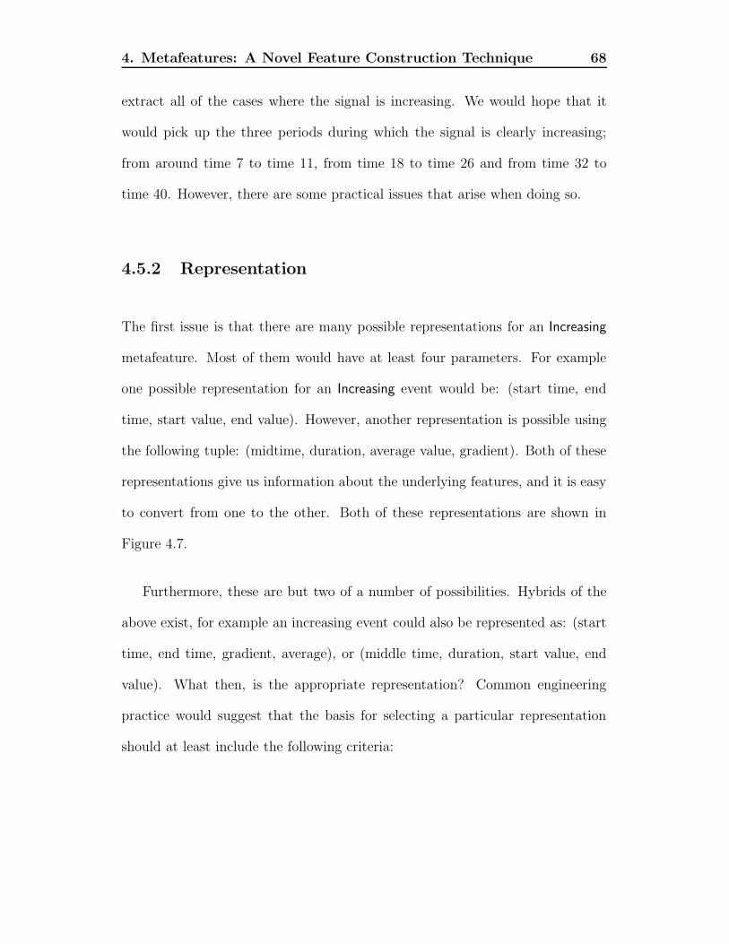
4. Metafeatures: A Novel Feature Construction Technique 68
extract all of the cases where the signal is increasing. We would hope that it
would pick up the three periods during which the signal is clearly increasing;
from around time 7 to time 11, from time 18 to time 26 and from time 32 to
time 40. However, there are some practical issues that arise when doing so.
4.5.2 Representation
The first issue is that there are many possible representations for an Increasing
metafeature. Most of them would have at least four parameters. For example
one possible representation for an Increasing event would be: (start time, end
time, start value, end value). However, another representation is possible using
the following tuple: (midtime, duration, average value, gradient). Both of these
representations give us information about the underlying features, and it is easy
to convert from one to the other. Both of these representations are shown in
Figure 4.7.
Furthermore, these are but two of a number of possibilities. Hybrids of the
above exist, for example an increasing event could also be represented as: (start
time, end time, gradient, average), or (middle time, duration, start value, end
value). What then, is the appropriate representation? Common engineering
practice would suggest that the basis for selecting a particular representation
should at least include the following criteria:

4. Metafeatures: A Novel Feature Construction Technique 69
Val
ue
midtime
duration
avg_value
gradient
Time
start_value
end_valueV
alue
start_time end_time Time
Figure 4.7: Two different possible representations of an Increasing event.
Robust to noise
We should try to choose parameters that are robust to noise. In the above ex-
ample, the start value and the end value are both sensitive to noise, as compared
to, say average and gradient, both of which are aggregate measures of the data
points belonging to the period of increase. Hence it would be better to represent
an increasing event using the latter two parameters rather than the former. In
general, an aggregate of the signal will be more robust than a single measure-
ment of the signal, so average value and gradient are robust than start value and
end value.

4. Metafeatures: A Novel Feature Construction Technique 70
Temporal variations are mapped to proximal parameter values
One important characteristic of any solution to temporal classification is that
it should be robust to temporal variations of the kind that occur in temporal
domains, which were previously discussed in Section 2.5. Careful consideration
reveals that metafeatures implicitly capture the temporal variation as parameter
values, and in so doing, allow temporal variation to be handled. For instance, if
an Increasing event occurred slightly later than expected, then the difference is
mapped into a difference of the midtime parameter; and the greater the difference
in the midtime, the greater the difference in that parameter’s value. Hence, the
temporal variation between the two cases is mapped into proximal parameter
values, where the usual distance metrics still apply in a sensible manner. In terms
of the parameter space, this means that two instantiated features that occur
at approximately the same time or last for approximately the same duration
should be close. Hence the representation as midtime and duration would be
more appropriate.
Orthogonality
The parameters in a given metafeature should be orthogonal to one another. For
instance, if we were to represent an increasing event by start time, end time and
duration, then this would be redundant. Any two of these would be sufficient to
uniquely represent such an event. Fewer parameters reduce processing time of
the instantiated features; furthermore, some learning and clustering algorithms
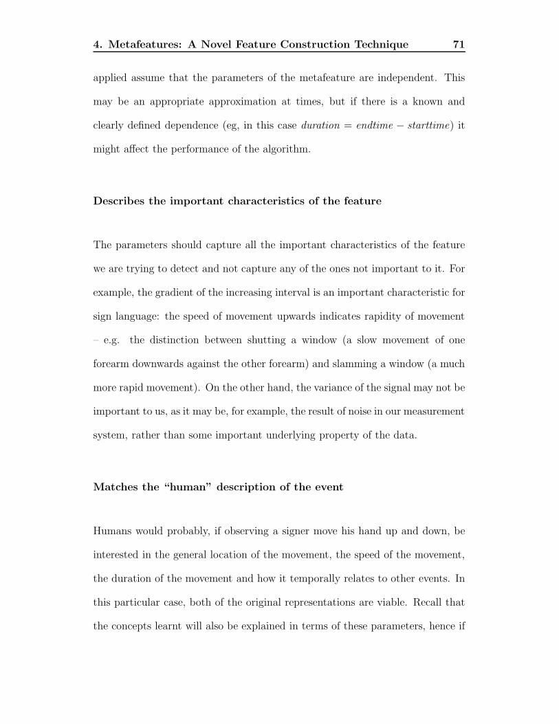
4. Metafeatures: A Novel Feature Construction Technique 71
applied assume that the parameters of the metafeature are independent. This
may be an appropriate approximation at times, but if there is a known and
clearly defined dependence (eg, in this case duration = endtime − starttime) it
might affect the performance of the algorithm.
Describes the important characteristics of the feature
The parameters should capture all the important characteristics of the feature
we are trying to detect and not capture any of the ones not important to it. For
example, the gradient of the increasing interval is an important characteristic for
sign language: the speed of movement upwards indicates rapidity of movement
– e.g. the distinction between shutting a window (a slow movement of one
forearm downwards against the other forearm) and slamming a window (a much
more rapid movement). On the other hand, the variance of the signal may not be
important to us, as it may be, for example, the result of noise in our measurement
system, rather than some important underlying property of the data.
Matches the “human” description of the event
Humans would probably, if observing a signer move his hand up and down, be
interested in the general location of the movement, the speed of the movement,
the duration of the movement and how it temporally relates to other events. In
this particular case, both of the original representations are viable. Recall that
the concepts learnt will also be explained in terms of these parameters, hence if

4. Metafeatures: A Novel Feature Construction Technique 72
they are not in a form that a human comprehends, then the definitions generated
by this method won’t be correct either.
4.5.3 Extraction from a noisy signal
The second practical difficulty is extracting instantiated features from noisy data.
For example, if one is detecting a period of increase, what if one suddenly gets
a “downwards spike” caused by non-Gaussian noise (e.g. in the case of the sign
language recognition using instrumented gloves, by bogus ultrasound reflections
that interfere with positional triangulation used to calculate the y values shown)?
One could argue that this is a preprocessing issue and not really an issue for the
learner3. Even so, preprocessing will never get rid of all of the noise, although
it may minimise it. Our extraction functions must be designed to be robust
to noise. It is more important to detect a generally increasing signal, even if
it means that there are short periods within the signal where the property of
monotonic increase is not strictly true. For example, Figure 4.8 shows another
recording of the y channel of the sign building, but this one with much greater
noise than in Figure 4.6.
This makes the implementation of such an extraction function difficult; and in
general the pursuit of the ultimate extraction function could be as consuming as
the whole process of learning to classify in the first place. Certainly, it would be
3The line between preprocessing and learning is a blurred one. One view of TClass is aslittle more than an automated preprocessor, which doesn’t do any learning itself. However,preprocessing the data into a format for learning seems to be something that machines are badat and people are good at, so perhaps it is not so little after all.

4. Metafeatures: A Novel Feature Construction Technique 73
-0.1
0
0.1
0.2
0.3
0.4
0.5
0.6
0.7
0.8
0.9
0 10 20 30 40 50 60
Y p
ositi
on
Timestep
Figure 4.8: The y channel of another instance of the sign building, but this onewith much greater noise than Figure 4.6.
possible to define a group of metafeatures IsInstanceOfClassA, IsInstanceOfClassB,
etc that operated on all channels simultaneously4 and whose parameters consist
of a single boolean value that told us if the stream belonged to a particular class.
If we could do so, it would be immensely useful, but if we knew how to develop
the extraction functions IsInstanceOfClassX, then we would not need to learn in
the first place – since all we need to know is encapsulated in our metafeatures.
Hence like most things in engineering, the development of the extraction
4There is nothing in the theory or the practice that prevents a metafeature from looking atmultiple channels simultaneously. Recall that the extraction function takes an instance, andnot a channel from an instance; hence it would be possible to look at multiple channels toextract events. This would be logical, for example, in the case of the three spatial featuresx,y,z, where some features e.g. circular motion in the xz plane, as occurs with the sign “all”,when it is necessary to look at both planes simultaneously to determine whether in fact acircular motion was performed.

4. Metafeatures: A Novel Feature Construction Technique 74
function is a tradeoff. If the extraction function is made too simple, then a
useful representation will not reach the learning algorithm. If a great deal of
time is spent developing the extraction function, then this undercuts the whole
purpose of using a learner in the first place.
The surprising fact is, however, which we demonstrate in the remainder of
the thesis, that even using a very primitive group of metafeatures, it is possible
to obtain high levels of performance in temporal domains.
Consider implementing the Increasing metafeature and apply it to the y axis.
Also assume that we use the representation (midtime, average, gradient, dura-
tion). Consider the period of increase from time 32 to time 45 in Figure 4.8.
Then depending on how we implement the extraction function, it might be pos-
sible to ignore the small dips in the generally increasing pattern between that
time; or it might be possible to break it up into three separate events: an increase
from time 34 to 35, an increase from time 37 to 39 and an increase from time 40
to 43. One way to do this is to allow a certain amount of exceptions; another is
to “smooth” the data to get rid of such bumps. In any case, Figures 4.9 and 4.10
show the instantiated features extracted by applying one implementation of the
Increasing metafeature to Figures 4.6 and 4.8 respectively. Note that the events
are in many ways similar, and that our filtering and noise handling techniques
have worked to some extent.

4. Metafeatures: A Novel Feature Construction Technique 75
midTime = 9.5 avg = 0.13671875 gradient = 0.0546873 durn = 4.0
midTime = 22.0 avg = 0.5100447 gradient = 0.08286842 durn = 7.0
midTime = 35.5 avg = 0.7942707 gradient = 0.06473206 durn = 6.0
Figure 4.9: Instantiated features extracted from Figure 4.6.
midTime = 12.5 avg = 0.1867187 gradient = 0.038778342 durn = 10.0
midTime = 26.5 avg = 0.48242223 gradient = 0.053906284 durn = 4.0
midTime = 40.5 avg = 0.7187502 gradient = 0.045982197 durn = 6.0
Figure 4.10: Instantiated features extracted from Figure 4.8.
4.6 Using Metafeatures
The key insight to the application of metafeatures is realising that the distri-
bution of instantiated features in the parameter space is probably not uniform.
This can be exploited to create features that may help in classification.
An initial approach might be to use normal clustering in the parameter space;
i.e., clustering that groups points in such a way that distance between points
within the same cluster is small, and distances between points in different clusters
is large. However, this is merely one approach to answering the real question
that we are interested in: “Which are the instantiated features whose presence or
absence indicate that the instances belong to a particular class?” The clustering
approach can certainly be used to answer this question – the theory being that
the different clusters represent the different types of instantiated features. This
is an example of undirected segmentation.
However, a more refined approach is possible: one that takes into account

4. Metafeatures: A Novel Feature Construction Technique 76
the class of the instantiated features. One way to do this is to augment the
parameter space with the class as an extra dimension. However, this would likely
not work either, as the distance metric between classes is not obvious; and the
weight given to the class label relative to other features in the parameter space
is not easy to determine. Likely, such an algorithm would be caught between
ignoring class completely, leading to traditional clustering, and paying too much
attention to the class, leading to too many clusters.
Another approach is to re-pose the question as: “Are there regions in the
parameter space where the class distribution is significantly different to what
is statistically expected?” This question is very similar to typical problems of
supervised classification; in particular, if we pose the question as “Are there
attribute-value pairs for which the class distribution is significantly different to
what we would expect?”, then this is the same question that is the basis of many
decision tree and rule induction systems. This is an example of directed seg-
mentation: segmentation directed towards creating good features for learning.
This suggests that rather than looking at Figure 4.1 where class is completely
ignored, a more appropriate way to look at the data is that shown in Figure 4.2.
Suddenly, one can see immediately what a learner could employ in order to
make the classification. We see that all the instantiated features coming from
training instances whose class label was Happy occupy the top left hand region
of the space. However, there are some practical issues. How, given a parameter
space, is a region defined?

4. Metafeatures: A Novel Feature Construction Technique 77
The solution used in this work is as follows: We have to select a group of
synthetic events to query on, and we have to divide the space into regions. Hence,
one approach is to select a number of instantiated features which we will term
centroids5. Let the set of all instantiated features be I. Let the set of points we
select as centroids be C = {c1, c2, c3, ..., ck}, where there are k points selected.
Define the set of regions R = {R1, ..., Rk} be defined as follows:
Ri = {x ∈ P |closest(x, C) = ci}
and
closest(x, C) = argminc∈C
dist(x, c)
where dist is the distance metric we are using for the parameter space.
In other words, each region Ri is defined as the set of points in the parameter
space P for which ci is the closest point (using the distance metric dist) in the
set C. This is the definition of a Voronoi diagram. A good review of Voronoi
diagrams and their (many) applications can be found in [AK00].
If these regions were selected randomly, it would be expected that the class
distribution in each region would be similar to the global class distribution.
However, if the distribution of instantiated features differed significantly from the
global class distribution, then this would be interesting and useful for a machine
learning algorithm. Asking whether a training stream has an instantiated feature
within a region would be informative of class of the training stream that the
instantiated feature came from.
5The use of this name will become obvious in a moment.

4. Metafeatures: A Novel Feature Construction Technique 78
In general, the objective is to find the subset of the instantiated features
that would give us the most “different” class distribution for each region. This
would then give something for the learner in the subsequent stage to use for
the basis for learning. However, one might then suggest that the solution to
this problem is simple: Make C = I – in other words, make each instantiated
feature a centroid. Then each region will have exactly one instantiated feature
in it; with a very non-random class distribution. Hence we need a measure that
“trades off” number of regions for size. We will term this measure the disparity
measure. The disparity measure measures the difference between the expected
and observed class distribution. For now, let us assume that we have such a
measure, say, called DispMeas. Then we are looking to find:
R = argmaxC∈P(I)
DispMeas(C)
In other words, we are looking to find the subset of I (the set of all instantiated
features), C, for which the disparity measure is the greatest.
The above equation looks simple, but there is a problem. The problem is
the P(I) in the above equation: this is the set of all subsets of I. In general,
if there are n elements in I (i.e. n = ‖I‖), then there are 2n elements in P(I).
If we wanted to do an exhaustive search, we would therefore have to look at a
number of subsets that was exponential in the number of instantiated features.
For example, if there are only 100 elements in I, we would still have to check
more than 1030 possible sets. Even if we were to constrain it to a reasonable
size, say no more than 10 regions, C is still combinatorially large in I.

4. Metafeatures: A Novel Feature Construction Technique 79
Still, it might be possible to search part of the feature space and come up
with a reasonable set C that is effective in constructing features.
4.7 Disparity Measures
Disparity measures are a recurring theme in supervised learning. For example,
in decision-tree building algorithms like C4.5 [Qui93], the algorithm proceeds by
dividing the instances into two or more regions, based on attribute values. The
disparity measure used by C4.5 is the gain ratio; however there are several other
possible disparity measures.
In fact there is a whole area of study of different disparity measures. White
and Liu [WL94] provide an extensive survey of disparity measures, and we adopt
their notation. There are many similarities between decision tree induction
(which is built on segmentation based on attribute values) and the creation of
regions around centroids (which is built on segmentation based on a Euclidean
distance measure). The only adaptation we make is that rather than talking
about attributes a1, ..., am, we use regions R1, ..., Rm; and, indeed, this points to
an interesting analogy.
Suppose that we are dealing with a problem with k classes and that we have
m different regions. Then Table 4.4 represents the cross-classification of classes
and regions.

4. Metafeatures: A Novel Feature Construction Technique 80
R1 R2 Rm
L1 n11 n12 . . . n1m n1.
L2 n21 n22 . . . n2m n2.
......
... . . ....
...Lk nk1 nk2 . . . nkm nk.
n.1 n.2 . . . n.m n..
Table 4.4: A general contingency table
In the contingency table, Li(i = 1, k) and Rj(j = 1, m) represent class and
region respectively; nij(i = 1, k; j = 1, m) represent the frequency counts of the
instantiated features in region Rj coming from an instance with class Li. Also,
define:
ni. =
m∑
j=1
nij
n.j =
k∑
i=1
nij
and
n.. =k
∑
i=1
m∑
j=1
nij = N
We can also define the following probabilities:
pij =nij
n..
pi. =ni.
n..
p.j =n.j
n..

4. Metafeatures: A Novel Feature Construction Technique 81
4.7.1 Gain Ratio
Given this notation, we can define the following information measures, for each
of the cell, class and regions :
Hcell = −k
∑
i=1
m∑
j=1
pij log2(pij)
HC = −k
∑
i=1
pi. log2(pi.)
HA = −
m∑
j=1
p.j log2(p.j)
The information gain is the difference between the information stored in the
cells and the information about class, that is to say:
HT = HC + HA − Hcell
This is the heuristic that was originally used by Quinlan in ID3 [Qui86].
However, it has one significant drawback: it does not take into account the
number of regions. If information gain were to be used “raw” without regard to
the number of regions, then this would lead to a bias to having a huge number
of regions. Imagine a region for each point in the space, such that each region
only has one instantiated feature and therefore one class. By substituting in
the above formula, we get that such a selection of regions has an information
gain of 1, which is the most possible. But it is of no use to us. Hence, in C4.5,
Quinlan introduces the gain ratio. The gain ratio compensates for the number

4. Metafeatures: A Novel Feature Construction Technique 82
of attributes by normalising by the information encoded in the split itself. It can
be shown that using the above formula the gain ratio is HT
HA.
In these experiments with metafeatures, therefore, we used the gain ratio as
one of our disparity measures. The higher the gain ratio, the more likely the
subdivision into regions is useful for classification.
4.7.2 Chi-Square test
Another approach, this one from statistics, is the chi-square test. The chi-square
test measures the difference between the expected values in each of the cells in the
contingency table. By comparing this against a chi-square statistic, a measure
of the probability that the distribution of instantiated features we see in the
contingency table is random. The smaller that this probability is, the less likely
it is that the distribution is due to chance. This probability is called the power
of the test.
The χ2 statistic can be computed as:
χ2 =∑
i
∑
j
(Eij − Oij)2
Eij
where Oij is the observed number of instantiated features belonging to region
Rj in class Li; i.e. Oij = nij and Eij is the number of instantiated features that
we would expect for nij if the region was independent of the class. Hence
Eij =n.jni.
n..

4. Metafeatures: A Novel Feature Construction Technique 83
In statistics, there is not one chi-square distribution but one for each degree
of freedom. It can be shown that the degrees of freedom ν in this case are
(k − 1)(m − 1). Once we have computed the χ2 statistic for our contingency
table, we can compute the probability from the definition of the χ2 distribution,
the probability that this particular contingency table was the result of random
chance. The smaller that this probability is, the more confident we can be that
the distribution we have before is likely to be useful for discriminative purposes.
Unlike information gain, the χ2 distribution does not suffer from the same
issues of bias to more regions, at least theoretically. However, it is more difficult
and time-consuming to calculate than the information gain or gain ratio (since
to compute the probability mentioned above requires computing the integral of
the probability density function of the of χ2 function).
4.8 Doing the search
So far, we have disparity measures for judging whether a group of centroids or
regions are discriminative. However, we still do not have a search algorithm to
find the set of points. As pointed out in Section 4.6, the problem is that the
search space is exponential in the number of instantiated features. As previ-
ously discussed, two general approaches are possible: undirected and undirected
segmentation.
With undirected segmentation, any clustering or density estimation algo-

4. Metafeatures: A Novel Feature Construction Technique 84
rithm can be used. There are some nice algorithms for clustering, especially if
the number of clusters is known, such as K-means clustering. The algorithm
for K-means is shown in Figure 4.11. Alternatively, other algorithms, such as
AutoClass [CS96] and SNOB [WD94] could be used.
The algorithm works by randomly selecting centroids, finding out which el-
ements are closest to the centroid, then working out the mean of the points
belonging to each centroid, which becomes the new centroid. Region member-
ship is checked again, and the new centroids are computed again. This operation
continues until there are no points that change their region membership.
The problems with the K-means approach is that (a) we have to specify the
number of clusters ahead of time (b) it can be sensitive to the initial random
choice of centroids (c) it does not make any use of class information. Note also
that it makes use of a special type of locality or stability in the way it works:
region membership is unlikely to change too much, and the information is slowly
refined to come up with the final solution.
The K-means algorithm can be made to look at a range of different number
of clusters by the addition of a “quality” heuristic. The algorithm is relatively
simple. Let us say we have a range of say, 2 to 10 clusters. Then we try to
get the best possible clustering with 2 clusters, take a global measure of quality
of clustering (e.g. total distance from centroids) and then try again with 3
centroids, etc. until we find the number of clusters that work the best.
Most importantly, it can be shown that under the assumption of there actu-

4. Metafeatures: A Novel Feature Construction Technique 85
Inputs:I = {i1, ..., ik} (Instances to be clustered)n (Number of clusters)
Outputs:C = {c1, ..., cn} (cluster centroids)m : I → C (cluster membership)
procedure KMeansSet C to initial value (e.g. random selection of I)For each ij ∈ I
m(ij) = argmink∈{1..n}
distance(ij , ck)
EndWhile m has changed
For each j ∈ {1..n}Recompute ij as the centroid of {i|m(i) = j}
EndFor each ij ∈ P
m(ij) = argmink∈{1..n}
distance(ij , ck)
EndEnd
return CEnd
Figure 4.11: K-means algorithm.

4. Metafeatures: A Novel Feature Construction Technique 86
ally being k centroids with Gaussian distribution, that the K-means algorithm
will eventually converge to the correct answer. “Correct” in this case means the
clustering that minimises the total distance of all points from the centroids.
However, K-Means does not make use of a disparity measure; so we would
like to adapt it to take advantage of one. The problem is that we do not have this
easy-to-define and “smooth” criterion. The K-means algorithm is an estimation-
maximisation algorithm; it gradually moves towards a more optimal solution by
using the previous iteration to “inform” the next iteration. However, in the
case of directed segmentation, the solution space is not smooth – the disparity
measure can vary irregularly, since it involves the choice of different centroids.
There is no easy “pattern” in the solution space to exploit.
The easiest algorithm to implement would be a “random search” algorithm.
This random search algorithm is shown in Figure 4.12. While it may first seem
that using a random search algorithm is not productive, work by Ho [HSV92] in
the field of ordinal optimisation shows that random search is an effective means
of finding near-optimal solution. This was also used by Srinivarsan [Sri00] in his
Aleph ILP system where it was shown to perform well even compared to complex
search methods.
Ordinal optimisation can be applied to our problem as follows. Let us assume
that our objective is to find a subset of points that is in the top k per cent of
possible subsets (i.e. whose disparity measure ranks it in the top k per cent).
If we test n possible subsets randomly, then the probability P of getting an

4. Metafeatures: A Novel Feature Construction Technique 87
instance in the top k per cent can be shown to be:
P (1 or more subsets in top k%) = 1 − P (0 subsets in top k %)
= 1 − (1 − k)n
For example, if n = 1000 and k = 1% then the probability of finding an
instance in the top 1 per cent of possible cases is 1− (1− 0.01)1000 = .999957. In
other words, if we try 1000 instances, then there is a better than 99.995 per cent
chance that we will get one instance in the top 1 per cent. Hence by softening
the goal (trying to find one of the best rather than the best subset of points) we
can be highly confident of getting a solution in the top percentile.
An algorithm for random search is shown in Figure 4.12. It assumes the
following auxiliary functions:
• randBetween(min, max) returns a random number between min and max
inclusive.
• randSubset(num, set) returns a random subset of set with num elements
in it, but with no repetitions.
Also note that DispMeas takes a set of centroids, a set of points and their class
labels. Using this information, it then creates a contingency table as mentioned
above, and then applies whatever disparity measure is required.

4. Metafeatures: A Novel Feature Construction Technique 88
Inputs:I = {i1, ..., ik} (Instances to be clustered)L = {l1, ..., lk} (Class labels of instances)N = {nmin, ..., nmax} (Possible number of centroids)DispMeas(Centroids, Instances, Labels) (Disparity measure)numTrials (number of trials to attempt)
Outputs:C = {c1, ..., cn} (cluster centroids)
procedure RandSearchbestMeasure := 0bestCentroids := {}for i := 1 to numTrials
r := randBetween(nmin, nmax)currentC := randSubset(r, I)currentMetric := DispMeas(currentC , I, L)if(currentMetric > bestMetric)
bestMetric := currentMetricbestCentroids := currentC
EndEnd
C := bestCentroidsreturn CEnd
Figure 4.12: Random search algorithm.

4. Metafeatures: A Novel Feature Construction Technique 89
The random search is not a particularly efficient algorithm in terms of search,
compared to K-Means. However, we will show that the advantage of using di-
rected segmentation over undirected segmentation means that in practice, di-
rected segmentation is preferred.
Also note that the random search algorithm is highly parallelisable. The
main for loop can be run in parallel across many different processors and/or
computers, provided that the final if statement that updates the best instance
seen so far is done atomically. This is a significant advantage over the K-Means
algorithm, which is not easy to parallelise at all, as it is inherently iterative.
In either case, whether using the undirected segmentation or the directed
segmentation, the centroids become synthetic features; in other words, we can
now ask the question: “does a particular stream have an instantiated feature
lying in the region belonging to centroid X?” This binary information can be
used as a synthetic feature that can be passed on to a learner. We will explore
this in practice in the next two chapters.
4.9 Examples
4.9.1 With K-Means
To bring this all together, consider the following example, from the Tech Support
domain. Figure 4.13 reproduces Figure 4.3 here for convenience. In fact, Figure

4. Metafeatures: A Novel Feature Construction Technique 90
4.3 did in fact use K-Means clustering to determine the centroids.
0
1
2
3
4
5
0 2 4 6 8 10 12 14
Dur
atio
n (d
)
Start time (t)
A
B
C
AngryHappy
Centroids
Figure 4.13: K-means clustered LoudRun parameter space for Tech Support do-main.
Centroids are marked with diamonds. Also note that a simple Euclidean
distance metric is used, and different standard deviations for the different axes
are not taken into account (hence the results look a little unusual). Also note
that a priori we specified three clusters. The dotted lines represent the region
boundaries; these are easy to compute as they are the loci of points that are
equidistant from the two nearest centroids.

4. Metafeatures: A Novel Feature Construction Technique 91
4.9.2 With directed segmentation
Now, we do the same thing, using a directed segmentation approach. We will
set nmin = 2, nmax = 3 and numTrials = 3. We will look at several disparity
measures.
It should be noted that one of the advantages of directed over undirected
segmentation is that it chooses an instance which is an observed instantiated
feature. Quinlan [Qui93] notes that experts who look at the results of learning
with continuous attributes find it easier to understand cutpoints that can be
found in the data, rather than averages, since it may be that certain averages are
physically impossible (e.g. in the case of the previous result, a LoudRun that has
a duration of 3.33 timesteps). Although his results were with cutpoints, and ours
are with regions, the result still holds. We will use the random search algorithm
proposed above, but run three iterations in parallel for ease of comparison.
The first stage of the algorithm is to generate 3 random subsets with between
2 and 3 elements. The results of this step are shown in Table 4.5.
Trial Centroids1 c1 = (4, 4), c2 = (5, 1)2 c1 = (4, 4), c2 = (3, 1), c3 = (9, 4)3 c1 = (3, 3), c2 = (12, 1)
Table 4.5: Random sets of centroids generated for the Tech Support domain.
For each of these, it is possible to generate a region boundary diagram. Figure
4.14, 4.15 and 4.16 show the parameter space using trials 1,2 and 3 respectively.

4. Metafeatures: A Novel Feature Construction Technique 92
0
1
2
3
4
5
0 2 4 6 8 10 12 14
Dur
atio
n (d
)
Start time (t)
c1
c2
AngryHappy
Centroids
Figure 4.14: Trial 1 points and region boundaries.
0
1
2
3
4
5
0 2 4 6 8 10 12 14
Dur
atio
n (d
)
Start time (t)
c1
c2
c3
AngryHappy
Centroids
Figure 4.15: Trial 2 points and region boundaries.

4. Metafeatures: A Novel Feature Construction Technique 93
0
1
2
3
4
5
0 2 4 6 8 10 12 14
Dur
atio
n (d
)
Start time (t)
c1 c2
AngryHappy
Centroids
Figure 4.16: Trial 3 points and region boundaries.
Now we can calculate the contingency tables for each trial. We do this by
counting the number of instances of each class in each region. For example, in
Table 4.6, there is 1 instantiated feature in the region around centroid 1 (R1)
which came from a stream whose class was Angry, and 3 whose original class
was Happy6. These go into the first column. Similarly, in region 2 (R2), the
region surrounding c2, there are 7 “Angry” instantiated features and no “Happy”
instantiated features (counting the border case as belonging to this region). This
goes into the second column. The final column is just the row totals (i.e. 1 + 7
and 3 + 0) and the final row is just the column totals (i.e. 1 + 3 and 7 + 0). The
value in the bottom right hand corner is the sum of either the row totals or the
6Note that there are two points at the location (3,3), hence it actually counts as twoinstances. Also note that in the case of an instance lying exactly on the border, we randomlyselect which region it belongs to.

4. Metafeatures: A Novel Feature Construction Technique 94
column totals. These should of course be the same value and it should be equal
to the total number of instantiated features.
R1 R2
Angry 1 7 8Happy 3 0 3
4 7 11
Table 4.6: Contingency table for Trial 1.
R1 R2 R3
Angry 0 5 3 8Happy 3 0 0 3
3 5 3 11
Table 4.7: Contingency table for Trial 2.
R1 R2
Angry 5 3 8Happy 3 0 3
8 3 11
Table 4.8: Contingency table for Trial 3.
Finally, we can calculate a number of disparity measures from the contingency
tables, based on the methods discussed in Section 4.7. The results are shown in
Table 4.9.
For example, to work out the information gain in the first trial, this can be
computed using:

4. Metafeatures: A Novel Feature Construction Technique 95
Trial Information Gain Chi-squaredGain Ratio Statistic DoF Prob − log2 Prob
1 0.550 0.582 9.79 1 0.0176 9.152 0.845 0.549 11.0 2 0.0408 7.933 0.151 0.179 1.55 1 0.22 2.18
Table 4.9: Evaluation of trials 1, 2 and 3 using Gain, Gain Ratio and Chi-Squareddisparity measures.
Gain = HC + HA − Hcell
=∑k
i=1
∑m
j=1 i(pij) −∑k
i=1 i(pi.) −∑m
j=1 i(p.j)
= i( 111
) + i( 711
) + i( 311
) + i( 011
) − i( 811
) − i( 311
) − i( 411
) − i( 711
)
= 0.550
where i(x) = x log2(x)
The gain ratio can be computed by dividing the information gain by HA,
which in this case is: −(i( 411
) + i( 711
)) = 0.945. Hence the gain ratio is 0.5500.945
=
0.582.
Computing the χ2 heuristic is more involved. For first cell in trial 1, Eij =
8×411
= 2.91. We can then compute the χ2 component for that particular cell
using (e−o)2
eas (1−2.91)2
2.91= 1.25. If we repeat this total for the remaining three
cells in trial 1, and sum them, we get a total of 9.79. This number is known as
the χ2 statistic. Note also that there are two classes and two regions, hence the
degree of freedom of the statistic is (2 − 1)(2 − 1) = 1.
Usually this statistic is compared against a value in a critical-values table
in a significance test. For example, it is used to decide whether there is a less

4. Metafeatures: A Novel Feature Construction Technique 96
than 5 per cent chance that such a distribution is random. However, we want
to know for a particular χ2 statistic and the degrees of freedom probability that
this process was the result of random chance. This can be computed easily
using the cumulative distribution function of the χ2 distribution. The result is
shown in the fourth column of Table 4.9. Finally, for comparison, we take the
negative log of the probability. This is mainly for to match the direction of the
other heuristics (bigger is better) and because it just as easy to compute without
suffering floating-point difficulties in the implementation.
Looking at Table 4.9, it seems that the results for Trial 3 are inferior to the
other two. However, Trials 1 and 2 are quite close; information gain puts Trial 2
ahead of Trial 1, unlike the other two measures. A tradeoff has occurred: even
though Trial 2 produced a “purer” result (in that there is only one class in each
region), it did so using 3 centroids, Trial 1 accomplishes an “almost as pure”
result using only 2 centroids.
These regions, much as for the previous case with K-means, can now be used
to create synthetic events. If we use Trial 2, for example, we get the features
shown in Table 4.10.
Feeding it to C4.5 produces Figure 4.17. Note that we can easily post-process
the result to produce something that is far more readable by using the LoudRun
metafeature, which is shown in Figure 4.18.
Note that if we did the same for the K-means value, we would get the slightly
nonsensical definition shown in Figure 4.19.

4. Metafeatures: A Novel Feature Construction Technique 97
Stream Class Synthetic EventsRegion 1 Region 2 Region 3
1 Happy Yes No No2 Angry No Yes Yes3 Angry No Yes Yes4 Happy Yes No No5 Happy Yes No No6 Angry No Yes Yes
Table 4.10: Attribution of synthetic features for the Tech Support domain inTrial 2.
rgn1 = yes: Happy (3.0)
rgn1 = no: Angry (3.0)
Figure 4.17: Rule for telling happy and angry customers apart, using syntheticfeatures from trial 2.
Does have a Loud run
approximately starting from timestep 4 AND
approximately going for 4 timesteps : Happy (3.0)
Otherwise: Angry (3.0)
Figure 4.18: Human readable form of rules in Figure 4.17.
Does have a True run
approximately starting from timestep 10 AND
approximately going for 3.33 timesteps : Angry (3.0)
Otherwise: Happy (3.0)
Figure 4.19: Human readable form of rules in Figure 4.4.

4. Metafeatures: A Novel Feature Construction Technique 98
4.10 Further refinements
Metafeatures can be refined in several ways: firstly, by the addition of region
membership measures and secondly by giving the user some bounds for the
descriptions generated by the learner.
4.10.1 Region membership measures
In the earlier parts of this chapter, training streams either had an instantiated
feature belonging to a particular region, or they didn’t. For this reason, Table
4.10 contains only yes and no values – a binary membership test. However,
it is possible to ascribe to each event a membership value that denotes the
confidence that the point belongs to a particular region. It is generally the case
that the closer the instance is to a particular centroid, the more confident one
can be that it belongs to that region. Work in areas such as fuzzy set theory
[Zad65] and rough sets [Paw82] have similarities to the idea of using non-binary
region memberships.
A first guess at a region membership measure is normalised Euclidean dis-
tance from the centroid. By normalised, we mean that the distance along each
axis is divided by its standard deviation. Doing so ensures that no one feature
dominates the calculation of distance. This copes with differences in scale of
different measurements. For example, let us assume that position is initially
measured in metres; but is later changed to use millimetres. If we fail to adjust

4. Metafeatures: A Novel Feature Construction Technique 99
for the fact that millimetres are three orders of magnitude as large as metres,
then in our distance calculations the position would have three orders of mag-
nitude more impact on the distance. However, if we divide by the observed
standard deviation in the data, then this will adjust for the fact that different
axes may have different units.
Normalised distance from the centroid is a good first approximation, however
it has some notable problems. Consider a simple vertical region boundary as
shown in Figure 4.20.
B
Param 2
A
c c1 2
Param 1
Figure 4.20: Distance measures in the parameter space. c1 and c2 are twocentroids, A and B are instantiated features.
Point A is approximately three times as close to c1 as B. Hence normalised
distance implies that A is far more likely than B to be a member of the region
around c1. We know that though A is closer to c1, it is also much closer to a

4. Metafeatures: A Novel Feature Construction Technique 100
region boundary than B is, hence it would intuitively make sense if we were less
confident about the membership of A then we were of B. How can we define a
more appropriate region membership measure?
Recall that the region boundary tells us the points which are equidistant
from two centroids, in other words, for points along the region boundary the
distance between two of the centroids is equal. This suggests an alternative
region membership measure: the relationship between the normalised distance to
the nearest centroid and the normalised distance to the second nearest centroid.
Consider the following region membership measure. Let d1 be the distance
to the nearest centroid cn1 and d2 be the distance to the second nearest centroid
cn2. Then consider the measure:
D = log2(d2
d1)
We will term this measure the relative membership. When a point is on
the the region boundary by definition the distance to cn1 and cn2 is equal. Hence
the ratio d2
d1
will be equal to 1, hence D = 0. Consider a point like A in Figure
4.20. It is slightly closer to c1 than c2; assume that the distance to c1 is 5 and
the distance to c2 is 6. Then the relative membership is log2(6/5) = 0.263. Now
consider a point like B, which is, say 30 units from c2 and 15 units from c1. Its
relative membership will be log2(30/15) = 1. Hence, one is more confident that
B is in the region defined by c1 than A, which matches our intuitions.
Note that if the point we are looking at is actually the centroid of a region,

4. Metafeatures: A Novel Feature Construction Technique 101
then the relative membership is log2(d20) = ∞ This also makes sense; as we are
absolutely sure that the point c1 lies in its own region R1.
With this minor change, relative membership can be used in place of binary
membership. There are some complications, however. What happens if there
is more than one instantiated feature lying in a particular region? With rela-
tive membership, two instances in the same region can have different relative
memberships, unlike binary memberships. For example, consider s3 from Tech
Support domain. Its events are {(2, 1), (5, 1), (12, 3)}. Now consider that we use
the segmentation that we examined in Trial 2 of the random search (see Figure
4.15). Then both of the instances (2, 1) and (5, 1) lie within region 2. If the
relative membership for each of these is calculated, we would get two different
values. For the point (2, 1), the relative membership (using unnormalised Eu-
clidean distance for ease) is 1.84, while for (5, 1) it is 0.66. Table 4.12 shows
the relative membership for each point within R2 for trial 2. There are several
possible solutions to this problem; but a simple one is to take the point with
the greatest relative membership7. So, when constructing a table for Trial 2 as
before, rather than a yes/no value, we would now put in a “1.84”. Table 4.11
shows the table with relative rather than binary attributes. Note that if there
is no instance in the space, we simply enter a “0”. This is equivalent to saying
that there are no instantiated features within that region.
Feeding this into C4.5, the results in Figure 4.21 are produced.
7This is very similar to the approach taken in fuzzy logic. The fuzzy “or” of two fuzzyvalues is usually the maximum of the two.

4. Metafeatures: A Novel Feature Construction Technique 102
Stream Class Synthetic EventsRegion 1 Region 2 Region 3
1 Happy 0.5 0 02 Angry 0 ∞ ∞3 Angry 0 1.84 1.354 Happy ∞ 0 05 Happy ∞ 0 06 Angry 0 0.265 2.35
Table 4.11: Numerical attribution of synthetic features for the Tech Supportdomain in Trial 2.
rgn1 <= 0: Angry (3.0)
rgn1 > 0: Happy (3.0)
Figure 4.21: Rule for telling happy and angry customers apart, using syntheticfeatures from trial 2 and using relative membership.
This result seems surprising. In this case, the rule learnt is identical to the
binary attribute rule learnt. rgn1 > 0 means that there is an instance within
region 1; whereas rgn1 <=0 means that there is no instance in region 1. This
also correctly indicates that by using relative membership, the hypothesis lan-
guage expands greatly and is a strict superset of the binary membership system.
Although there is no use made of it in this particular case, it is quite possible
that a rule may take the form rgn1 > 1, in which case it is not simply sufficient
for there to be an instance within region 1, but it would also be necessary for
there to be an instance within region 1 which also has a relative membership
greater than 1. In other words, not only must the instance lie in region 1, but it
must be twice as close to the point c1 as to any of the other centroids.
While it may at first seem that this can impede readability, it can be em-

4. Metafeatures: A Novel Feature Construction Technique 103
ployed, as with the next section to assist in making the concept description more
useful.
4.10.2 Bounds on variation
A second possible refinement is to create bounds on the variation of parameters
when converting rules back to human-readable form.
In the human-readable definition generated in Figure 4.18, there is no guide
given to the typical variation in attribute values. All that can be said is that it is
at “approximately” time 10 and for a duration of “approximately” 4 timesteps.
In real-world datasets, this may not be good enough a characterisation; in some
cases “approximately” 10 means “between 9 and 11”, and in other cases, it means
“between 5 and 15”. How can we give the user some idea of the extent of the
variation?
One approach is to give the user the region boundaries as output. After
all, this would provide exactly what the classifier uses. However, a moment’s
thought will show that this may be a less than ideal solution. Firstly, most
people do not have a sufficiently good grasp of mathematics to be able to deal
with the region boundary expressed in this form. Secondly, this may work for a
two-dimensional metafeature like LoudRun or LocalMax, but many metafeatures
are four or five-dimensional. In a five-dimensional space, the region boundaries
would be expressed as convex hyper-polyhedra. This representation is not likely

4. Metafeatures: A Novel Feature Construction Technique 104
to be of much use in practice.
However, there is no reason why the explanation of the concept learnt by our
system needs to be expressed so that it exactly matches the classifier produced by
our system. We can give the user a simplified explanation of what our system has
learnt, but when it comes to actual classification, we need not use the simplified
model at all.
This is a subtle idea8. For example, a traditional learner, like C4.5, outputs
the scheme that it actually uses to classify – a decision tree. Imagine if, for its
own internal calculations, C4.5 retained the original tree, but applied various
heuristics to reduce the size of the tree so that a human reader would get an
approximation of what C4.5 had learnt, with enough of a characterisation that
it’s still useful.
This suggests an approach: assuming that the learner uses binary member-
ship, then one can find the bounding boxes on the instantiated features within
each region. These boxes could then be included in the definition. Figure 4.22
shows the bounding boxes for each of the different centroids.
It is an approximation of the actual concept used for classification, but it
does give the user some intuition about what the system was doing. Using this,
the original definition would take on the form shown in Figure 4.23.
8This is one of those ideas that is kind of obvious once explained, but is not so obvious toone’s own intuitions. The penny dropped for me during a lecture by Thierry van der Mercktat the University of Sydney.

4. Metafeatures: A Novel Feature Construction Technique 105
0
1
2
3
4
5
0 2 4 6 8 10 12 14
Dur
atio
n (d
)
Start time (t)
c1
c2
c3
AngryHappy
Centroids
Figure 4.22: The bounding boxes in the case of Trial 2 random search.
Does have a True run
starting between time 3 and 4 AND
going for 3 or 4 timesteps : Happy (3.0)
Otherwise: Angry (3.0)
Figure 4.23: Human readable form of rules in Figure 4.17.
There is a complication if we want to use relative membership and varia-
tion bounds at the same time: the binary membership means we can create the
“bounding box” for all the instances in a region. However, if relative member-
ships are used for attribute values, our propositional rule learner may produce a
rule of the form rgn2 >= 0.9 for Random Search Trial 2. This means that we
can no longer use the bounding box for all of the instances in region 2 shown in
Figure 4.22, as not all of the points in region fulfil the requirement.

4. Metafeatures: A Novel Feature Construction Technique 106
Does have a LoudRun
starting between time 2 and 3 AND
going for 1 or 2 timesteps
Figure 4.24: Transforming relative membership into readable rules.
How do we solve the problem? We can still calculate the relative membership
for each point in the region, and we only draw the bounding box around those
points fulfilling the requirement. The relative membership for each point in
region 2 is shown in Table 4.12.
Point RM(2,1) 1.85(2,2) 1.0(3,1) ∞(5,1) 0.66(6,1) 0.27
Table 4.12: Relative membership (RM) for instantiated features in region 2 ofTrial 2.
Hence we can see that only the points (2, 1), (2, 2), (3, 1) lie in the region
defined by the constraint rgn2 >= 0.9. Hence the bounding box would be
(2, 1)− (3, 2). The human-readable version of the rule rgn2 >= 0.9 is shown in
Figure 4.24.
So, rather than being a problem, the use of relative region membership allows
us to build more exact definitions, especially insofar as the bounds, while also
giving the learner more flexibility.

4. Metafeatures: A Novel Feature Construction Technique 107
4.11 Conclusion
Metafeatures are a novel feature construction technique that can be applied
whenever there is some kind of underlying substructure to the training instances
and there is some way to extract these substructures. In temporal domains, these
substructures take the form of sub-events, like intervals of increase or decrease.
Metafeatures first extract substructures within the training instances. Then,
interesting, typical or distinctive examples are selected. These substructures
become synthetic features, which are then fed to a propositional learner. We can
then convert the output of the learner back to a human-readable form that is
described in terms of the metafeatures we began with.
The extraction of typical or distinctive examples is done by segmenting the
parameter space into regions. The division of the parameter space into re-
gions can be approached using two methods: traditional undirected segmenta-
tion which simply treats each instance as a point in space; or the novel directed
segmentation approach. The directed segmentation approach is specifically de-
signed to facilitate subsequent learning by dividing the space into regions where
the class distribution is non-uniform; hence trying to find regions which could
potentially be useful for discrimination between classes.
The novelty of metafeatures lies not in the idea of parametrised substructures
within training instances; these are ideas that have been used for ad hoc temporal
classification for a very long time. However, the novelty lies in these metafeatures

4. Metafeatures: A Novel Feature Construction Technique 108
as a general concept, and that they form a parameter space. The novelty lies in
segmenting the parameter space in such a way as to:
• Create distinctive features so that a subsequent learning algorithm can
learn effective concept descriptions.
• Define substructures within training instance that can be used to construct
a description of the learnt concept in terms of those metafeatures. This
makes metafeatures one of the few techniques that can produce compre-
hensible descriptions of multivariate time series.
Finally, two novel enhancements are suggested:
• Rather than using a simple binary measure of region membership, relative
membership is used.
• Bounds on the size of the regions are produced for the definitions generated
by propositional learning.

Chapter 5
Building a Temporal Learner
In Chapter 4, metafeatures were introduced as a means of feature construction,
and a pedagogical example with one metafeature was demonstrated. In this
chapter, we explore how to build a temporal learner (in particular, a weak tem-
poral learner) for real-world practical domains using many metafeatures. We
also consider several specific metafeatures and consider the implementation of a
temporal learner called TClass.
5.1 Building a practical learner employing met-
afeatures
In Chapter 4, we discussed metafeatures generally. However, we did not con-
sider them from a computational point of view or discuss much in the way of
109

5. Building a Temporal Learner 110
implementation details. Some contemplation of the application of metafeatures
leads to a natural division of their implementation into three subprocesses:
• Instantiated feature extraction: This involves applying the extraction
function (see Section 4.4) to every training stream. The output is a set of
class-labelled instantiated features.
• Synthetic feature construction: Given these class-labelled instantiated
features, the techniques discussed in Section 4.6, namely directed and undi-
rected segmentation, are applied to construct the synthetic features.
• Training set attribution: Each synthetic feature becomes an attribute
for the propositional learner. For each training instance, the value of the
attribute is determined by the presence of instantiated features in the re-
gion around the synthetic feature, as outlined in Section 4.10.1.
This sequence of steps is represented diagrammatically in Figure 5.1. In fact,
this is exactly the steps followed in the Tech Support domain presented in Section
4.2. The training instances are shown in Table 4.1. The results of instantiated
feature extraction are shown in Table 4.2. Several different possible outcomes of
synthetic feature construction are shown in Table 4.5. Training set attribution
leads to Table 4.10 (or, if relative membership is used, Table 4.11).
So far, only the training stage has been discussed. What are the changes
that occur once we want to apply the system to unseen instances? The main
distinguishing factor of unseen instances is that the class label is not known.
5. Building a Temporal Learner 111
Attribution
Class−labelledinstatiatedfeatures
SyntheticFeatureConstr’n
TrainingInstances
InstantiatedFeature
Extraction
Synthetic
features
class labels
Synth attribute values +
Figure 5.1: The stages in the application of a single metafeature in TClass.
In the field of machine learning, a strict separation of training and test sets is
usually enforced. In this particular case, this separation should extend to include
not only the learning algorithm, but also the synthetic feature construction stage.
If synthetic features are constructed using test data, then we have access to
information that should not be available to the temporal learner.
However, using the output of the synthetic feature construction in the train-
ing stage as an input to the attribution stage is no problem. Figure 5.2 shows
the typical procedural pipeline for using the system for temporal classification.

5. Building a Temporal Learner 112
Instatiated
features
InstantiatedFeature
Extraction
Syntheticfeatures
(from training)
Synth attribute values
(no class label)
Attribution
TestInstances
Figure 5.2: The TClass pipeline for processing test instances.
Note that the synthetic features created in the training stage are provided
as an input in this case to the attributor. Note also that the attributor in the
training and test cases need not be any different at all except in one regard:
the output of the attributor in the training case includes class information that
the propositional attribute-value learner system can use to build its classifier,
whereas in the case of the attributor at test time, the output does not include
the class information.
To further clarify the role of each of these components, Figures 5.3, 5.4 and
5.5 show pseudocode for instantiated feature extraction, synthetic feature con-

5. Building a Temporal Learner 113
struction and attribution.
The algorithm for instantiated feature construction takes a list of training
examples, a list of labels, and returns a list of tuples. Each tuple consists of a
list of instantiated features, and a class. In Figure 5.3 append(I , x ) appends x
to the list I; also assume there is a method called extract for each metafeature
that takes a training instance and, as defined in Chapter 4, returns a list of
instantiated features.
For the segmentation algorithm in Figure 5.4, the data must be converted
into a format appropriate for segmentation. This means making a single list of
tuples each consisting of an instantiated feature and a class label, rather than the
original format, which is a list of 2-tuples, each consisting of a list of instantiated
features and a class label. Also note that SegAlg could be any segmentation
algorithm, for example either of the algorithms discussed in Chapter 4.
The attribution algorithm shown in Figure 5.5 takes a membership function,
such as the ones we discussion in Section 4.10.1; such as relative membership,
and finds if there is an instantiated feature from a particular training instance
that is similar to each synthetic feature.

5. Building a Temporal Learner 114
Inputs:T = [t1, ..., tn] (Training streams)L = [l1, ..., ln] (Class labels of training streams)extract (Extraction function for this metafeature)
Outputs:I = [〈[i11, ..., i1m1
], l1〉, ..., 〈[in1, ..., inmn], ln〉]
(class-labelled instantiated features)
procedure ExtractionI := {}For i := 1 to n
append(I, 〈extract(t1), l1〉)Endreturn I
End
Figure 5.3: Instantiated feature extraction.
Inputs:I = [〈[i11, ..., i1m1
], l1〉, ..., 〈[in1, ..., inmn], ln〉]
(class-labelled instantiated features)SegAlg(Instances) (Segmentation algorithm to use)
Outputs:C = [c1, ..., ck] (synthetic features)
procedure Construction/* First we must “flatten” input data. */D := []For each 〈P, l〉 in I
For each p in Pappend(D, 〈p, l〉)
EndEnd/* Now apply the segmentation */C := SegAlg(D)return C
End
Figure 5.4: Synthetic feature construction.

5. Building a Temporal Learner 115
Inputs:I = [〈[i11, ..., i1m1
], l1〉, ..., 〈[in1, ..., inmn], ln〉]
(class-labelled instantiated features)C = [c1, ..., ck] (synthetic features)mem(Centroid , Instances)
(Membership function we are using)Outputs:
E = [〈f11, ..., f1k, l1〉, ...〈fn1, ..., fnk, ln〉](Training data in format for propositional learner)
procedure AttributeFor each 〈P, l〉 in I
e := 〈〉k+1 /* e is a new tuple with k + 1 fields */For i := 1 to k
ei := mem(ci ,P)/* In other words, for each centroid, work out theif there is an instantiated feature like ci in P */
Endek+1 := l /* Append class label to attribute vector */append(E , e)
Endreturn E
End
Figure 5.5: Training set attribution.

5. Building a Temporal Learner 116
5.2 Expanding the scope of TClass
The above system is sufficient for the implementation of a single metafeature.
However, in practice, there are two observations that necessitate important ad-
ditions to TClass.
Firstly, the set of domains where a single metafeature is sufficient for learning
purposes is limited. Typically, there will be many metafeatures for a given
problem domain, and as we will see later, the same metafeature may be applied to
a number of channels within the same problem domain. Hence we have to expand
our architecture to support multiple metafeatures and multiple applications of
metafeatures.
Secondly, while in general it is the temporal characteristics of a signal that
are important, there are many cases when other non-temporal attributes are
useful. These will be termed global attributes.
5.2.1 Global attributes
Aggregate global attributes
Another technique for extracting information from the training data is to evalu-
ate some aggregate values and use them as propositional attributes. This would
cover features of a stream that are not localised. For example, for continuous
channels, the global maximum and minimum value of a channel, or the mean of

5. Building a Temporal Learner 117
each channel may be useful. Such attributes are examples of aggregate global
attributes – they measure some property of each training instance as a whole,
rather than looking at the temporal structure. Such features can be surprisingly
useful for classification. For example, [Kad95] shows that in the sign language
domain task discussed in Section 6.3.2 almost 30 per cent accuracy can be ob-
tained in classifying 95 signs based solely on the maxima and minima of they x,
y, and z positions of the right hand.
Global features may be more complicated than simple maxima, minima and
averages. For example, we could count the number of local maxima and minima,
we could measure the total “distance” covered by each channel, or use some
measure of energy. For discrete binary channels, it might be something like how
many changes there are, the percentage of time for which the value is true and
so on. Duration is another example of an aggregate temporal feature, which may
be useful for some classification purposes.
Note that global features may be associated with either single or multiple
channels. For example, in the Auslan domain, we could measure the distance
using a Euclidean metric on the x, y and z channels, or on each channel sepa-
rately. For simplicity below, we consider global feature calculation for a single
channel.

5. Building a Temporal Learner 118
Example global attributes
For a given channel, we could define the global maximum max for a given channel
as
max (c) = m s.t. ∀t c[t] ≤ m, t ∈ domain(c) ∧ ∃t s.t. c[t] = m
Similarly, we could define a distance measure on a single channel as:
dist(c) =
√
√
√
√
tmax∑
t=1
c[t]2 − c[t − 1]2
These global features can be useful for classification; in fact, in the past this
has been one of the most popular means of ad-hoc feature extraction technique
in temporal classification domains. However, they are usually not sufficient for
doing high-accuracy classification. In addition, used alone, they do not usu-
ally lead to the production of useful human-readable descriptions of the learnt
concept.
Other global attributes
Another type of global attribute is a conventional intrinsically non-temporal
feature. For example, consider diagnosing medical patients by observing the
electrical patterns and behaviour of their heart – in other words, an electrocar-
diograph (ECG) – as discussed in Section 6.3.3. Obviously there are important
temporal characteristics of the ECG; for example, the rates of change of the elec-

5. Building a Temporal Learner 119
trical signal, the order of various sub-components of the heart’s beats and so on.
Aggregate temporal attributes as outlined before are also useful. But there are
also other attributes which are important to classification and diagnosis, such
as the patient’s age, height, weight and gender. These are not directly temporal
measures, but they do have impact on the diagnosis. One of the advantages of
the TClass approach is that it allows the integration of conventional features,
aggregate global features and temporal features while other systems (such as
dynamic time warping and hidden Markov models) do not. The practicalities of
such integration are the topic of the next section.
5.2.2 Integration
How can we integrate all of these data sources? Since all of these processes
produce attribute values, they can simply be concatenated into a single long
attribute value tuple. This leads to the diagram shown in Figure 5.6.
Note that there are several new “boxes”. The first of these is the learner;
and the second is attribute combination. The attribute combiner takes attributes
from multiple sources and concatenates the attributes from the different sources
into a single attribute value tuple, ready for passing to a propositional learner.
Certain aspects of TClass are not included in Figure 5.6, in particular the cre-
ation of human-readable output. In Section 4.10.2, we discussed post-processing
the learnt concept to generate more human-readable descriptions in situations

5. Building a Temporal Learner 120
TrainingInstances
Metafeature
1Application
Synthetic
features 1
values 1Synth attribute
Synthetic
features nMetafeature
nApplication
values nSynth attribute
����
����
����
Metafeature
2Application
Synthetic
features 2
values 2Synth attribute
Global
features 2
Global
Extraction 2Feature
Global
features m
Global
Extraction mFeature
Classifier
Attributevalues + classes
����
�
Global
features 1
Global
Extraction 1Feature
Conventional attribute values
Attributecombination
PropositionalLearning
Figure 5.6: The TClass system: training stage.
where the generated classifier represents the concept as a set of constraints on
the attribute values. This requires several sources: firstly and most obviously,
the learnt concept; secondly, the synthetic features to post-process the concept
description, and thirdly, the original instantiated features to generate the bounds

5. Building a Temporal Learner 121
on values. The practical implementation of this is discussed in Section 5.5.7.
The architecture for testing is almost the same as that for training, and is
shown in Figure 5.7. The most notable difference is that the synthetic features
generated by parameter space segmentation in the training stage are reused.
TrainingInstances
Global
features 2
Global
Extraction 2Feature
Global
features m
Global
Extraction mFeature
Attributevalues
Classifier
ClassPrediction
Metafeature
1Attribution
values 1Synth attribute
Synthetic
features 1
����
����
����
����
�
Global
features 1
Global
Extraction 1Feature
Conventional attribute values
Attributecombination
Synthetic
features 2
Synthetic
Metafeature
Attribution
Synth attribute
Synth attribute
features n
n
Metafeature
Attribution2 values 2
values n
Figure 5.7: The TClass system: testing stage.

5. Building a Temporal Learner 122
5.3 Signal processing
Before applying TClass, it is sometimes useful to use domain knowledge to ma-
nipulate the signal in some way.
5.3.1 Smoothing and filtering
Smoothing and filtering are two approaches to the same problem, but from differ-
ent areas. Filtering comes from signal processing, while smoothing comes from
statistics.
Filters are functions of input signal. For example, let a single channel of data
be represented as x[t], and the output data y[t]. Then any linear finite impulse
response (FIR1) filter can be thought of as a function:
y[t] =
k∑
i=−j
αix[t − i]
The αi are termed the weights of the filter. The art and science of filter design
is in the appropriate setting of these weights. For example, a simple 5th-order
moving average filter might be:
y[t] =1
5x[t − 2] +
1
5x[t − 1] +
1
5x[t] +
1
5x[t + 1] +
1
5x[t + 2]
This averages five points to create the output. There are also non-linear
filters. Non-linear FIR filters can not be expressed as a linear combination of
1There is another type of filter, known as the Infinite Impulse Response or IIR filter. Forbrevity, we will limit our discussion to FIR filters.

5. Building a Temporal Learner 123
the input, but as some other (non-linear) function on the inputs. A simple
example of a useful non-linear filter is a 5th order median filter. This is the filter
represented by:
y[t] = median(x[t − 2], x[t − 1], x[t], x[t + 1], x[t + 2])
This type of filter is extremely useful for data with non-Gaussian noise, re-
moving outliers very efficiently. A significant amount of research effort has gone
into the development of appropriate filters for various purposes.
Statistics has taken a different tack to the problem: early approaches were
similar to moving average filters. However, rather than using a simple moving
average, the early work realised that linear regression could be used around the
point we were trying to estimate; in other words, rather than simply averaging
the five values around a point, a linear fit of the points, using a least squares
estimate, could be used to give a better-looking result. Further, they realised
that (a) if linear regression could be applied, so could other shapes, in particular
splines (b) the weights for the instances used in regression could be changed.
This led to further work by Cleveland [WCS92]. Friedman’s super smoother
[Fri84] extends Cleveland’s work automatically setting parameter values based
on minimising cross-validated error.
These have also been included in software. In this thesis we use the imple-
mentation provided by the statistics package R [Hor01] to do smoothing. In
future chapters we will show the impact that using smoothing has.

5. Building a Temporal Learner 124
Each of filtering and smoothing has their advantages. Filter design allows the
use of domain knowledge to overcome domain-specific problems, while smoothing
is flexible enough to be used more independently of the domain.
The main reason that smoothing is useful is that it allows the metafeature
extraction functions to be simpler. Rather than a lot of effort being devoted to-
wards making the metafeature extraction functions robust to noise, and simplify
their implementation.
5.4 Learners
Learners, required to do the “backend” learning for TClass, are implemented
through an interface to Weka, a free machine learning library [WF99]. In general
TClass can be used with any learner. However, as previously mentioned, in order
to produce comprehensible descriptions, the learner must produce a concept
description that uses inequalities of single attribute values. We may also wish
to consider ensemble methods of learning, discussed below.
5.4.1 Voting and Ensembles
One of the most active areas of recent research in machine learning has been
the use of ensemble classifiers. In an ensemble classifier, rather than a single
classifier, there is a collection of classifiers, each of which are built by the learner

5. Building a Temporal Learner 125
given different parameters or data. Each classifier is run on the test instances
and each classifier casts a “vote”. The votes are then collated and the class with
the greatest number of votes becomes the final classification.
Two approaches are popular:
1. Bagging ([Bre96]): The training set is randomly sampled with replacement
so that each learner gets a different input. The results are then voted.
2. Boosting ([Sch99]): The learner is applied to the training set as usual,
except that each instance has an associated weight. All instances start
with equal weight. Any misclassified training instances are given greater
weight. The process is repeated until (a) a maximum number of classifiers
is constructed or (b) there are no incorrectly classified training instances.
To make a classification, each of the individual classifiers is then applied2,
and the results are then voted.
Research indicates (in particular the excellent work in [BK99]) that bagging
gives a reliable (i.e. is effective in many domains) but modest improvement in
accuracy; whereas boosting produces a less reliable but greater improvement in
accuracy (when it does work). The problem is that neither approach improves
readability3.
2Within the boosting framework, each classifier may have a different weight; not all classi-fiers vote with a value of 1.
3There has been some work on this however, also discussed in [BK99]. More recently,Freund [FM99] has introduced the concept of alternating decision trees, which incorporateboosting as part of the classifier.

5. Building a Temporal Learner 126
With TClass, a third way of building an ensemble is possible if synthetic
feature construction is non-deterministic (e.g. if the RandSearch algorithm of
Figure 4.12 is used). If this is the case, each TClass run produces different
synthetic features on the same data and hence a different classifier is produced.
The outcomes of each classifier can be voted. Indeed, because TClass is learner-
independent, the two approaches can be combined. For instance, within each
run of TClass we could employ AdaBoost with decision trees; and then vote
each of the TClass classifiers as well.
5.5 Practical implementation
In this section, we talk about the implementation of the TClass system in Java.
We discuss the file formats used and the way the data is processed.
TClass consists of approximately 10,000 lines of non-comment code (approx-
imately 23,000 lines total). It is a complex but modular and object-oriented
system, the complexity attributable to the flexibility required to handle different
temporal domains.
5.5.1 Architecture
TClass implements the architecture suggested in Figures 5.1 and 5.2. As a his-
torical artifact, it also implements several other architectures (for example, the
5. Building a Temporal Learner 127
per-class clustering approach discussed in [Kad99], and also covered in Section
A.2). It also implements several baseline algorithms (for example, the naive
segmentation approach, discussed in Section 6.1.1). There are classes that cor-
respond directly to the combiners, feature extractors and learners discussed in
Section 5.1. In particular, three things are implemented using inheritance; mak-
ing it very easy to implement additional components:
• Global feature extractors: These are objects that extract aggregate
global features, such as means, and global maxima and minima. Conven-
tional attribute values (like patient age and gender) are easily implemented
within this framework.
• Metafeatures: Metafeature objects encapsulate the extraction functions
that are applied to training streams, as well as the characteristics of that
metafeature’s parameter space.
• Parameter Space Segmenters: Segementers segment the parameter
space into regions marked by synthetic events. As discussed in Section 4.8,
this includes undirected segmenters like K-Means and directed segmenters
like the random segmenter.
• Learners: These are conventional attribute value learners. This is a thin
wrapper around the functionality provided by Weka.
Each of these components can be mixed and matched. For example, any
metafeature can be used with any segmenter.

5. Building a Temporal Learner 128
For added flexibility, each of these components has a mechanism for setting
whatever settings are useful to it. For example, if one is applying K-Means,
one may wish to specify the number of clusters or ask that it be determined
automatically.
5.5.2 Providing input
The input to TClass consists of a number of files, each describing different parts
of the system. These inputs include:
• A description of the domain and the format of streams in the domain (i.e.
how many channels there are, the classes in it and so on).
• A description of what metafeatures, globals and parameter space seg-
menters to apply.
• Training and test streams. Each stream stored in its own file.
• A list of training streams and their class labels. A test streams list may
also be provided if TClass is being used in batch mode to estimate its
accuracy.
Domain description
The first file required is a description of the domain. This consists of the classes
and the types of the channels. These are usually suffixed with a “.tdd” (TClass
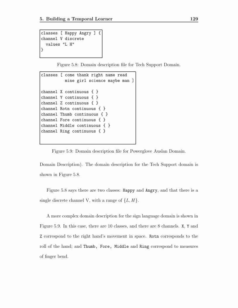
5. Building a Temporal Learner 129
classes [ Happy Angry ] {
channel V discrete
values "L H"
}
Figure 5.8: Domain description file for Tech Support Domain.
classes [ come thank right name read
mine girl science maybe man ]
channel X continuous { }
channel Y continuous { }
channel Z continuous { }
channel Rotn continuous { }
channel Thumb continuous { }
channel Fore continuous { }
channel Middle continuous { }
channel Ring continuous { }
Figure 5.9: Domain description file for Powerglove Auslan Domain.
Domain Description). The domain description for the Tech Support domain is
shown in Figure 5.8.
Figure 5.8 says there are two classes: Happy and Angry, and that there is a
single discrete channel V, with a range of {L, H}.
A more complex domain description for the sign language domain is shown in
Figure 5.9. In this case, there are 10 classes, and there are 8 channels. X, Y and
Z correspond to the right hand’s movement in space. Rotn corresponds to the
roll of the hand; and Thumb, Fore, Middle and Ring correspond to measures
of finger bend.

5. Building a Temporal Learner 130
L
L
L
H
H
H
L
L
L
L
L
L
Figure 5.10: An example of a TClass Stream Data (tsd) file.
Stream data files
Each stream (and hence each training or test instance) is stored in an individual
file; typically in a data subdirectory. So, for example, the first instance from the
Tech Support domain s1, might be stored in the file data/s1.tsd. The suffix
“.tsd” stands for TClass Stream Data. The contents of data/s1.tsd are shown
in Figure 5.10.
This is not a particularly interesting example. The first few lines of one
stream from the sign recognition domain is shown in Figure 5.11. Rather than
a single value on each line, there are 8, one corresponding to each channel. This
tells us, for instance, that to start with, the x position is -0.023 (i.e. to the right
of the body), and by the fifth frame, it has moved closer to the centre of the
body (i.e. 0.000).

5. Building a Temporal Learner 131
-0.023 0.015 0.000 0.000 0.250 0.750 0.500 0.000
-0.023 -0.015 0.000 0.000 0.250 0.750 0.500 0.000
-0.023 -0.015 0.000 0.000 0.250 0.750 0.500 0.000
-0.008 -0.039 0.000 0.083 0.250 0.750 0.500 0.000
0.000 0.000 0.000 0.083 0.250 0.750 0.500 0.000
...
Figure 5.11: An example of a TClass Stream Data (tsd) file from the sign lan-guage domain.
data/s1.tsd Happy
data/s2.tsd Angry
data/s3.tsd Angry
data/s4.tsd Happy
data/s5.tsd Happy
data/s6.tsd Angry
Figure 5.12: An example of a TClass class label file from the Tech Supportdomain.
Class label files
In order to tell the learner what the class of each file is, a class label file (usually
ending with “.tsl” for training data and “.ttl” for testing data; although this can
be modified at the command line) is also provided. The format for this file is
simple, and an example is shown in Figure 5.12. Each line consists of a filename
(relative to the current directory, or alternatively, given as an absolute path),
followed by a space and then the class label. The class label must be one of the
classes listed in the domain description file.

5. Building a Temporal Learner 132
globalcalc {
global V-mean mean {
channel V
}
}
metafeatures {
metafeature loudrun rle {
channel V
minrun "1"
limitvalues " H "
}
}
segmentation {
segmenter loudrun directed {
metafeature loudrun
numTrials "10000"
dispMeasure chisquare
}
}
Figure 5.13: Component description file for Tech Support domain.
Domain application file
In order to decide which components are to be used for a particular problem
domain, TClass uses an application file (usually suffixed with a “.tal” – short
for TClass Application List). This describes what global features, metafeatures
and parameter space segmenters to use for a particular domain. An example
component description file for the Tech Support domain is shown in Figure 5.134.
The first part of the file in Figure 5.13 describes the global feature extractors.
4NOTE: Because the terminology has changed and to avoid confusion, we have modifiedthe file slightly and replaced all the old terminology with the new terms. The actual file isidentical structurally but uses different terms.

5. Building a Temporal Learner 133
The first is a mean volume level (L is treated as 0 and H is treated as 1 – this
is effectively the same as calculating the percentage of time the conversation
volume is high). The format for the entries in the global section is:
global <attribute name> <feature type> {
<parameter> <value>
...
<parameter> <value>
}
Figure 5.13 shows a typical example of a global declaration. It creates a
global attribute called V-mean. It is uses a mean global feature extractor (other
types of global feature extractors would include min and max). The mean global
feature extractor accepts the parameter channel which tells it which channel to
extract the mean for. The channel must be listed the in the domain description
file. More information about globals can be found in Section 5.5.3.
The next section describes which metafeatures to use. Each metafeature
application is described in a section like:
metafeature <metafeature name> <metafeature type> {
<parameter> <value>
...
<parameter> <value>
}

5. Building a Temporal Learner 134
The metafeature’s name is later used in the segmentation sections. The
type governs what type of metafeature will be applied. For instance, in Figure
5.13, the rle (short for run-length encoding) metafeature is a straightforward
generalisation of the LoudRun metafeature. In this case, we are looking for “runs”
on the channel V that last for a minimum of length 1. Also we are only interested
in runs of high-volume, not low-volume. Hence we limit our interest to runs of
“H”s.
The final section is for setting up parameter space segmentation. Typically,
there will be equal number of metafeature applications and parameter space
segmenters. The segmenter specifies which segmenters to apply to which meta-
features. The general format is:
segmenter <attribute prefix> <segmenter type> {
<parameter> <value>
...
<parameter> <value>
}
The attribute prefix is the name that will be used for attribute values (al-
though a number will be appended indicating which centroid number it is). The
segmenter type governs whether we are using k-means (kmeans), expectation-
maximisation (em) or directed segmentation (directed). The segmenters take
one required parameter: the metafeature to apply the segmentation to. Hence
we are building a segmenter for the metafeature loudrun, which is a directed

5. Building a Temporal Learner 135
segmenter (i.e., the random search algorithm described in Section 4.12). We
specify that it should try 10000 random subsets for centroids; and we wish to
use the χ2 disparity measure.
This describes all of the inputs into the TClass system. We now discuss some
of the available components.
5.5.3 Implemented global extractors
The available global extractors include:
Duration
For some problem domains, the duration (i.e. the number of frames in an in-
stance) is important attribute for a “first cut” at classification. This particular
global extractor does not take any parameters.
Mean
This calculates the mean value of a channel. It assumes the channel is continuous.
It takes only one parameter, the channel. If the channel is not provided, it uses
the first channel defined in the domain description file.

5. Building a Temporal Learner 136
Max and Min
These global feature extractors calculate the minimum and maximum of a chan-
nel. They take only one parameter, which is the channel to calculate the maxi-
mum or minimum for. As before, if no channel is specified, it assumes the first
channel defined in the domain description file.
Mode
This calculates the mode of a channel (i.e., the most frequently observed value).
It can be used for either continuous or discrete values; but is typically used for
discrete values. As before, if no channel is specified, it assumes the first channel
defined in the domain description file.
First
This accepts the first observed value on the channel. This is a “back-door” way
to implement conventional global attributes. By simply adding the conventional
attributes to the first line of each file, this can be used to add conventional
attribute values within TClass. A better way to implement this functionality
would be to have this global read values from a file. As before, if no channel is
specified, it assumes the first channel defined in the domain description file.

5. Building a Temporal Learner 137
5.5.4 Implemented segmenters
Segmenters try to create prototypical synthetic features from the instantiated
features extracted from data. All segmenters in TClass accept a setting meta-
feature that describes which set of instantiated features are to be segmented.
K-Means
K-Means is a simple algorithm, the pseudocode for which can be found in Figure
4.11. However, initial settings for K-means (e.g. initial cluster membership and
number of clusters) are set using problem-specific information. The K-Means
algorithm implementation is largely historical, and is of limited practical use
in the current version of TClass, its role being largely replaced by the E-M
algorithm.
In our implementation, K-Means accepts the following parameters:
• numClusters: The number of clusters to create. It also accepts the value
“auto”. Since K-Means has no mechanism for estimating the number of
clusters, some alternative means must be used. Using “auto” works out
the number of clusters as the average number of instantiated features of
the type we are interested in per training stream. For instance, if we look
at Table 4.2, we see that there are a total of 12 instantiated features from
6 training streams, and hence it would calculate that there are 126
= 2
clusters of data. Default value is “auto”.

5. Building a Temporal Learner 138
• initialdist: Initial distribution of points (i.e., which clusters the points
end up in) can be accomplished in two ways: random, where each point
is allocated to a random cluster, or ordered. In the ordered method, just
as we “guessed” at the number of clusters using the average number of
instances, so we can also allocate cluster membership based on the order
of events. For instance, if the number of clusters is calculated automatically
to be two, and there are two events, then if over all of the data we put the
first instantiated feature detected into the first cluster, and the second into
the second cluster, then that would be a reasonable initial distribution of
instantiated features. Default value is ordered.
• closeness: When computing the distance of instances for the evaluation
of membership measures, should the distance from the centroid to the
instantiated feature being considered be used, or should the distance to the
nearest point belonging to the cluster be used? Default value is distance
from the centroid.
Expectation-Maximisation
Expectation-Maximisation can be thought of as the K-Means algorithm aug-
mented with a means of evaluating the number of clusters. The approach begins
by attempting to cluster the data into two clusters, and then increases to three.
If, on some holdout set of unseen data (or alternatively, using cross-validation)
it performs better than two clusters, then three clusters are used. This process

5. Building a Temporal Learner 139
is repeated for four clusters, and so on until an optimal number of clusters is
found.
We do not really have an implementation of the E-M algorithm. Rather, we
rely on the one supplied with Weka, with some minor modifications (namely,
3-fold cross-validation is used for assessing the number of clusters, rather than
10-fold cross-validation). It accepts the following settings:
• numClusters: The number of clusters to create. It also accepts the valued
“auto”. “auto” uses the expectation-maximisation method to determine
the number of clusters. If you don’t use “auto” then it is equivalent to
running a standard K-means algorithm.
Random Segmentation
This is an implementation of the algorithm discussed in Section 4.12. It accepts
the following parameters:
• numTrials: The number of random trials to run. Default value is 1000.
• minCent: The minimum number of centroids to consider. Default value
is 2.
• maxCent: The maximum number of centroids to consider. Default value
is 8.

5. Building a Temporal Learner 140
• clustBias: The algorithm currently selects a random number between
minCent and maxCent based on a linear probability distribution. In other
words, the probability of choosing n centroids is (n − minCent) times
the probability of choosing minCent centroids. Strictly speaking, this is
incorrect, since there are far more subsets with, 8 instances than there
are with 2 instances. In fact, it follows a binomial distribution – and for
cases where there are far more instances than centroids, it approximates a
factorial distribution. To compensate for this, one can set a cluster bias b,
so that the probability of choosing a subset with n instances is proportional
(n − minCent)b. Default value is 1 (i.e. linear).
• dispMeasure: The disparity measure to use. Possible values are gainratio,
gain and chisquare.
5.5.5 Implemented metafeatures
When implementing TClass a basic set of metafeatures were implemented that
are meant to be universal. However, it is useful to have additional settings
to tune the metafeatures to particular purposes. For example, all of the basic
metafeatures are single-channel (that is, they only look at a single channel of
information at a time). It is therefore necessary to designate which channel the
metafeature should be applied to.

5. Building a Temporal Learner 141
Increasing
The Increasing metafeature detects when a continuous signal is increasing. It
operates on continuous values only. The output from Increasing is a list of tuples
consisting of four parameters:
• midTime: The middle point temporally of the event. May be expressed
in either frame number or relative representation (where the beginning of
the stream is 0 and the end is 1); depending on the useRelativeTime
setting.
• average: The average value of the event. This value is expressed in terms
of the data type of the channel. If the useRelativeHeight parameter is
true then this average is expressed as height above or below the mean of
the channel for this training instance.
• gradient: This is the rate of change of the channel. To be exact, a line of
best fit is fitted to the increasing interval, and the gradient of the line is
calculated.
• duration: This is the length of the increasing interval. May be expressed
in either number of frames or in a relatively (where the whole stream has
a duration of 1) depending on the useRelativeTime setting.
It operates on a single channel. It accepts the following settings:

5. Building a Temporal Learner 142
• channel: Which channel to extract increasing intervals from. Default
value is the first channel defined in the domain description file.
• exceptions: Because of noise, it may occur that there are two intervals
of increase separated by one noisy sample. Were it not for the noise, this
would be considered one increasing interval. We may wish to allow a certain
number of exceptional samples which do not meet the strictly increasing
property. Default value is 1.
• useRelativeTime: Time measures (in particular duration and midtime)
can be expressed either in absolute terms (i.e. if it happens at the 19th
frame, it occurs at time 19), or relative terms (if it occurs at the 19th frame,
and the whole stream is 38 frames long, then it happens halfway along
the stream). Using relative time improves robustness to linear temporal
variation, but loses absolute temporal information. Default value is false.
• useRelativeHeight: Just as for time measures, average values can be
expressed in absolute (i.e. average value for this interval is 1.3) or relative
terms (the average for the increasing interval is 0.3 higher than the mean
of the channel). Default value is false.
• minDurn: This is the shortest duration signal (in frames) that will be
accepted as an increasing interval. If there is a increasing interval shorter
than this, it is not considered. Default value is 3 frames.

5. Building a Temporal Learner 143
Decreasing
Decreasing is identical to Increasing in almost every way. It accepts the same
parameters and produces the same outputs, with one obvious exception: it tries
to isolate intervals of decrease rather than increase. This means that the gradient
parameter is negative, not positive.
Plateau
The Plateau metafeature detects when a continuous signal is not changing, give
or take noise. The output from Plateau is a list of tuples consisting of three
parameters:
• midTime: This is as for Increasing.
• average: This is as for Increasing.
• duration: This is as for Increasing.
It operates on a single channel. It accepts the following settings:
• channel: This is as for Increasing.
• exceptions: This is as for Increasing. However, because it can be trickier
to detect plateaus the default is higher. Default value is 2.
• useRelativeTime: This is as for Increasing.

5. Building a Temporal Learner 144
• useRelativeHeight: This is as for Increasing.
• minDurn: This is as for Increasing; however, because it is difficult to
detect if the signal is “flat”, a longer interval is required. Default value is
4 frames.
LocalMax
The LocalMax metafeature detects when a signal has a local maximum; i.e. a
point in time when just prior and just after that point the signal is less. It
should not be confused with the global maximum and minimum functions that
operate on the whole channel. It produces instantiated feature tuples consisting
of the following parameters:
• time: This is as for the midTime parameter for the Increasing metafeat-
ure.
• value: The height of the maximum. If useRelativeHeight is used, then
the height above the mean for the channel is given.
It operates on a single channel. It accepts the following settings:
• channel: This is as for Increasing.
• useRelativeTime: This is as for Increasing.
• useRelativeHeight: This is as for Increasing.

5. Building a Temporal Learner 145
• windowSize: This controls the minimum “width” of the maximum. It
is an odd positive integer. A value of 3, for instance, on a channel c
would mean that c[t − 1] < c[t] > c[t + 1]. A value of 5 would mean that
c[t − 2] < c[t − 1] < c[t] > c[t + 1] > c[t + 2]. In general, if the window
size is w then this means that for a point to be considered a maximum
c[t − bw2c] < ... < c[t − 1] < c[t] > c[t + 1] > ... > c[t + bw
2c]. The default
value is 3 (i.e., the values immediately to the left and right must be less
than the current value).
LocalMin
LocalMin is identical in most respects to LocalMax, except that it detects local
minima. Hence all signs must be inverted. For example, a point is considered
a local minimum for a window size w if: c[t − bw2c] > ... > c[t − 1] > c[t] <
c[t + 1] < ... < c[t + bw2c].
RLE
Run-length encoding (RLE) is a process where a single value repeated several
times is encoded as that value, its starting point and its duration. For exam-
ple, the string “ABBBBBBCCCCCAAAAA” might be encoded as A1B6C5A5
(which implicitly encodes starting time, since the string is in order). RLE is the
generalisation of the LoudRun metafeature. RLE instantiated features consist of
the following tuple:

5. Building a Temporal Learner 146
• value: The value that is repeated.
• start: The frame at which that sequence of repetitions begins.
• duration: The number of frames that the value remains the same as the
starting value.
It operates on a single channel. It accepts the following settings:
• channel: Which channel to extract runs from. Default value is the first
channel defined in the domain description file.
• minrun: The minimum run of identical values for a run to be of interest.
Default value is 2 (i.e. runs of length 1 don’t count).
• limitvalues: In some cases, we are not interested in runs of all possible
values of a channel. For instance, in the Tech Support domain, we were
only interested in runs of high-volume conversation, not low volume ones.
Hence we can constrain our interest to only some possible values and not
all of them.
5.5.6 Developing metafeatures
Metafeatures can be easily implemented, usually in less than 200 lines of code. To
add metafeatures, they must implement the interface of the Java class MetafeatureI,
which has a total of 8 methods. Most of these are housekeeping functions

5. Building a Temporal Learner 147
(e.g. String name() to return a metafeature’s name). The most important
are setParam(String param, String value) to set the various settings above
(e.g. useRelativeTime, etc), and EventVec findEvents(Stream s) that ap-
plies the metafeature extraction function to a training stream and returns a
vector of events (i.e. instantiated features).
5.5.7 Producing human-readable output in TClass
One of the advantages of metafeatures is that they provide a mechanism for
generation of human-readable descriptions of temporal processes. How then do
we fit this into the TClass architecture?
Firstly, we can not produce human readable descriptions without making
some assumptions of the learner: it must produce a classifier that expresses the
learnt concept as bounds on attribute values. In other words, each part of the
concept is expressed as a test on a single attribute value being less than, greater
than or equal to a particular value5. This is a fairly wide family of learners and
includes decision trees, decision lists, stumps and ensembles of any of these.
We can postprocess the generated classifier by checking for any temporal
attributes6. We can then use an attribute relabelling approach to create a com-
prehensible description using the synthesised feature as a substitute for the in-
stantiated feature as discussed in Section 4.10.2. This obviously requires the
5Of course, less than or equal to and greater than or equal to are also acceptable.6If it is a global attribute, of either the aggregate or conventional type, we leave it alone.

5. Building a Temporal Learner 148
synthesised features. As discussed in that section, we can also use the instanti-
ated features to create useful bounds.
Although we do produce a classifier intended for human understanding, it is
not the one used to classify. It is an approximation of the learnt concept, rather
than the learnt concept itself. Experts exhibit similar behaviour ([Sha88] and
[CJ89]) – very few can express their expertise completely enough for someone
else to understand what they have learnt totally; but rather they provide an
approximation for what has been learnt7.
To describe how attribute relabelling works, let the synthetic features be
denoted by the notation metn, where met is a metafeature applied to the data
and n is the attribute value based on the relative membership of the nth synthetic
feature. If the classifier contains a test of the form metn > c this means that
the classifier checks for an instantiated feature that has a relative membership
for the nth synthesised feature exceeding c. Conversely, if it has a predicate of
the form metn ≤ c it is checking the absence of such an instantiated feature.
Attribute relabelling in this manner is easy to implement as a sequence of
string substitutions on the output from the learner. Figure 5.14 shows the ac-
tual classifier produced by TClass on the Tech Support domain. Using this
information, together with the information about the instantiated features, we
can convert this to the form showed in Figure 5.15.
7The former paper is extremely interesting – it shows that in many cases, experts don’teven agree with their own diagnoses after sufficient time has passed, and they disagree withtheir own rules. Furthermore, agreement between the expert system developed by one expertand another expert was extremely low – less than 40 per cent.

5. Building a Temporal Learner 149
--- Cluster centroids ---
V-loudrun_0: Cluster centroid is: LoudRun: start = 9 durn = 3
SDs are [ 4.78 1.59 ]
V-loudrun_1: Cluster centroid is: LoudRun: start = 3 durn = 1
SDs are [ 2.13 0.59 ]
V-loudrun_2: Cluster centroid is: LoudRun: start = 3 durn = 3
SDs are [ 1.59 1.59 ]
--- Learnt Classifier ---
PART decision list
------------------
V-loudrun_0 <= 0: Happy (3.0)
: Angry (3.0)
Number of Rules : 2
Figure 5.14: Learnt classifier for Tech Support domain after running TClass onit.
PART decision list
------------------
IF V HAS NO LoudRun: start = 9 durn = 3 (*1) THEN Happy (3.0)
: Angry (3.0)
Number of Rules : 2
Event index
-----------
*1: loudrun
start=9.0 r=[9.0,12.0]
durn=3.0 r=[3.0,4.0]
Figure 5.15: Post-processing Figure 5.14 to make it more readable.

5. Building a Temporal Learner 150
Figure 5.15 shows the post-processed form of Figure 5.14. For simplicity, the
information on the bounds has been separated to a separate event index. The
event index shows the range of bounds for the start and the duration of the
LoudRun.
5.6 Temporal and spatial Analysis of TClass
How long will TClass take to learn and how much memory/space will it take in
order to calculate the results? A rather informal analysis of each will be pre-
sented. First, some notation: Let n be the number of streams in the training
set. Let m be the number of metafeatures we are applying to the domain. Fur-
thermore, let us assume that applying a particular metafeature will on average
generate i instantiated features. Also, assume that on average, the length of the
streams is t.
The instantiated feature extraction consists of an inner loop that examines
each of the n streams in turn. Within that inner loop, the function extract is
called for each instance. Assuming that the extract function is linear in the
length of the stream (i.e. is O(t))8, then the feature extraction will take O(tn)
time. However, the function is called once for every metafeature, and hence the
extraction stage is O(tnm).
As to space, under the previous assumptions, the amount of data to be stored
8This is a fairly realistic assumption. All of the implemented metafeature extraction func-tions are linear.

5. Building a Temporal Learner 151
is to be stored is O(nim): for n streams, and for m metafeatures, i instantiated
features must be stored.
Synthetic feature construction is called once for each metafeature. It is flat-
tened into a single layer, but the amount of data for each metafeature is still
O(ni). Consider the random search algorithm. At each stage, it chooses a ran-
dom subset of points with some upper bound (in the default case eight). It then
compares each point (of which there are O(ni)) to each of the elements of the
subset. This operation is repeated a fixed number of times, so this is still O(ni).
Since it is called once for each metafeature, the total amount of time is also
O(nim).
Since there is some upper bound on the number of regions that will be pro-
duced, then there will be O(m) centroids which need to be stored.
Then there is the attribution stage. For each instance, of which there are n,
i instances (on average) with m metafeatures must be compared. This involves
looking against a set of centroids with an upper bound. Hence this too is an
O(nim) operation.
The data storage requirements are O(nm), since for each instance, there are a
certain maximum number of metafeatures and a maximum number of centroids
per metafeature.
The final stage is the learning stage. However in general, we do not know
what the amount of time for the learning algorithm is. Let us assume that the

5. Building a Temporal Learner 152
learning algorithm depends linearly on the number of attributes and the number
of instances. Then in this case, there are n instances, each with O(m) features,
so the learner will take O(nm) time.
The global feature extraction will generate O(ng) features. Since many global
features depend on things like working out the mean, each one may take up to
t time. Hence the total time is O(ntg).
Hence finally, the total time is O(tnm)+O(nm)+O(ntg)+O(nim), or after
simplifying, it is O(ntm) + O(nim) + O(ntg). As for the space, the most space
is required to store the data is O(ntm) + O(nim) + O(ntg).
This is good. It means that the total time and space used is linear in five
components:
• The number of training instances.
• The number of metafeatures applied in the domain.
• The average length of each training instance.
• The average number of metafeatures extracted from each instance.
• The number of global variables.

5. Building a Temporal Learner 153
5.7 Conclusion
TClass is a practical, working system for weak temporal classification. In this
chapter we discussed the design and implementation of TClass. In the remaining
chapters, we will look at the application of TClass to a number of practical
problems.

Chapter 6
Experimental Evaluation
After discussing the implementation of TClass, it is now applied to several
datasets to evaluate its behaviour.
This chapter begins with a discussion of what the issues to be investigated
are and how the investigation will proceed.
TClass is tested on two artificial domains: the cylinder-bell-funnel domain,
and a new artificial classification problem, the TTest domain. Using the lessons
learnt on the artificial datasets, two real datasets are then tested: Auslan sign
recognition and ECG analysis.
154

6. Experimental Evaluation 155
6.1 Methodology
There are many questions that can be asked about TClass’ performance such
as:
• How accurate is TClass on classification tasks?
• How comprehensible are the results and definitions generated by TClass?
• How much data does TClass need to learn concepts (i.e., data efficiency)?
• How does TClass compare to other learning methods in terms of perfor-
mance, comprehensibility, execution time and data efficiency?
• How do the the settings of TClass’ parameters (eg. number of random
subsets to use, whether we use smoothing or not, etc.) affect its perfor-
mance?
• How do different TClass back end learners perform?
6.1.1 Practical details
In order to answer the above questions, some decisions about practical tests need
to be considered.

6. Experimental Evaluation 156
Metafeatures
Since TClass is novel, in this first series of experiments, it was decided the simple
set of metafeatures discussed in the previous chapter would be used (increasing,
decreasing, plateau, local maximum and local minimum). This would allow us
to focus on the algorithm itself and make observations about the generalisabil-
ity of these simple metafeatures. Further, these simple metafeatures provide
a lower bound on performance; more complex metafeatures could only poten-
tially improve performance (otherwise, temporal classifiers could revert to simple
metafeatures).
Accuracy measurement
To measure accuracy, single runs of cross validation were used (either 5-fold or
10-fold depending on the data set). Stratified cross-validation was considered,
however, the quantity of the data and the processing time are such that this
would have resulted in overly long computation times.
Backend learners
TClass relies on a propositional learner at the backend. We consider four propo-
sitional learners: J48 (the Weka equivalent of c4.5), PART (the Weka equivalent
of c4.5rules), IB1 (nearest neighbour algorithm) and Naive Bayes (with the
Laplace adjustment to prevent zero probabilities and Fayyad-Irani [FI93] based

6. Experimental Evaluation 157
discretisation).
Ensemble learners
AdaBoost and Bagging can be incorporated as part of the propositional learner
– that is within the TClass framework. We will consider both AdaBoost and
Bagging, using J48 as the base learner as possible backends.
Voting
If we use a means for non-deterministic parameter space segmentation, then
every time we run TClass we are going to get a different set of features. Hence
we can vote these results. As discussed in Section 5.4.1, this be combined with
boosting and/or bagging.
Smoothing
As outlined in Section 5.3.1, smoothing and filtering can be a useful tool for
preprocessing data. We consider Friedman’s super-smoother [Fri84] in domains
where it is appropriate (i.e. high-noise).

6. Experimental Evaluation 158
Baseline algorithms
In order to evaluate the effectiveness of our learners, it is useful to compare the
performance of TClass against other temporal learners. We consider:
Naive segmentation One approach that has been previously explored and
employed (e.g. [Kad95]) is naive segment-based feature extraction. This can
be thought of as downsampling to a fixed size. Each channel is divided into n
segments temporally. For example if n = 5 and the stream is 35 frames long, then
the first 7 frames of each channel will be “binned” in first segment, the second
7 in the next segment and so on. The mean of each segment is calculated, and
this becomes an attribute.
Hence, if there are c channels, this will generate nc features. These can be
used as input to a conventional attribute-value learner1. Four possible values
of n: 3, 5, 10, 20 will be considered. In the following experiments, we also
consider several different learners for the segmented attributes: J48, PART, IB1,
AdaBoost with J48 and bagging with J48. Unless otherwise indicated the best
result amongst the different learner-segment (there are 20 possible) combinations
are presented. This does place a bias in the results towards the segmented
learner, since it has more opportunities to randomly fit the test set. However,
this was thought the fairest way to compare against TClass’s performance, since
an average over all learners and segment counts was not fair either.
1We have not found references to this as a general technique. However it seemed so obviousthat it was not considered worthy of publication. Other researchers such as [Geu01] have sincecited us for the algorithm.

6. Experimental Evaluation 159
Hidden Markov Models We employed the implementation of hidden Markov
models provided by HTK (the HMM Tool Kit) [YKO+]. Each class is modelled
using the same topology. The following number of states are considered: 3, 5,
10, 20; and the following topologies: left-right, left-right with 1 skip allowed and
ergodic. Each state in a left-right HMM allows transitions only to itself or the
next state – hence each state must be visited. to A 1-skip model is a left-right
model that also allows the transition from state i to state i+2, effectively allowing
to skip certain states. Ergodic HMMs allow all possible transitions. HMMs that
include the raw data as well as both the raw data and the first derivative are
considered. As with the naive segmenter, unless otherwise indicated the best
results, over all the topologies, states and both raw data and raw data with first
derivative (a total of 32 possibilities) were reported. It should be noted this is
biased in favour of hidden Markov models.
6.2 Artificial datasets
Now to the first tests. There are several reasons why artificial datasets are useful.
These include:
• Evaluation is simplified. For example, the induced concept can be com-
pared with the correct concept. It can also be used to explore factors of
interest such as noise, etc.
• There is a chicken-and-egg problem as far as temporal learners and datasets

6. Experimental Evaluation 160
are concerned. Because there are few (if any) generic temporal learners,
people do ad hoc feature extraction themselves. For example, an examina-
tion of the UCI repository ([MM98]) reveals at least seven datasets which
are inherently temporal in nature, but where the researchers did the feature
extraction themselves and the raw data is not available2.
• In order to compare our results with other researchers.
6.2.1 Cylinder-Bell-Funnel - A warm-up
The first artificial domain we will be considering is a simple one, but one that
has been used and explored by other researchers.
The artificial cylinder-bell-funnel task was originally proposed by Saito [Sai94],
and further worked on by Manganaris [Man97]. The task is to classify a stream
as one of three classes, cylinder (c), bell (b) or funnel (f). Samples are generated
as follows:
2These datasets are: arrythmia, audiology, bach chorales, echocardiogram, isolet, mobilerobots, waveform.

6. Experimental Evaluation 161
c(t) = (6 + η) · χ[a,b](t) + ε(t)
b(t) = (6 + η) · χ[a,b](t) · (t − a)/(b − a) + ε(t)
f(t) = (6 + η) · χ[a,b](t) · (b − t)/(b − a) + ε(t)
χ[a,b] =
0 t < a,
1 a ≤ t ≤ b
0 t > b
where η and ε(t) are drawn from a standard normal distribution N(0, 1),
a is an integer drawn uniformly from [16, 32] and b− a is an integer drawn
uniformly from [32, 96]. Figure 6.1 shows instances of each class. The cylinder
class is characterised by a plateau from time a to b, the bell class by a gradual
increase from a to b followed by a sudden decline and the funnel class by a sudden
increase at a and a gradual decrease until b. Although univariate (i.e., only has
one channel) and of a fixed length (128 frames), the CBF task attempts to
characterise some of the typical properties of temporal domains. Firstly, there is
random amplitude variation as a result of the η in the equation. Secondly, there
is random noise (represented by the ε(t)). Thirdly, there is significant temporal
variation in both the start of events (since a can vary from 16 to 32) and the
duration of events (since b−a can vary from 32 to 96).
266 instances of each class were generated. For ease of comparison with
previous results, 10-fold cross validation was used.
We have previously looked at the cylinder-bell-funnel domain [Kad99]. In

6. Experimental Evaluation 162
-4
-2
0
2
4
6
8
10
0 20 40 60 80 100 120
Val
ue
Time
Cylinder examples
-4
-2
0
2
4
6
8
10
0 20 40 60 80 100 120
Val
ue
Time
Bell examples
-4
-2
0
2
4
6
8
10
0 20 40 60 80 100 120
Val
ue
Time
Funnel examples
Figure 6.1: Cylinder-bell-funnel examples.
that work, we compared an earlier version of TClass (see Appendix A) against
naive segmentation and showed that we performed significantly better. Table
6.1 shows the table of results from that work.
As an initial test, we ran all the learners, with and without smoothing. In
all tables, the bounds represent the standard error of the mean (the standard

6. Experimental Evaluation 163
Features/Learner CBFTClass/Naıve Bayes 3.67 ± 0.61
Segments/Naıve Bayes 6.20 ± 0.67TClass/C4.5 1.90 ± 0.57
Segment/C4.5 2.41 ± 0.48
Table 6.1: Previously published error rates on the CBF domain.
Approach Unsmoothed SmoothedTClass with J48 2.28 ± 0.69 1.14 ± 0.24
TClass with PART 4.56 ± 0.82 1.77 ± 0.36TClass with IBL 56 ± 1.24 42.78 ± 1.78
TClass with Bagging/J48 1.9 ± 0.48 1.27 ± 0.43TClass with AdaBoost/J48 1.39 ± 0.33 1.01 ± 0.24TClass with Naive Bayes 3.16 ± 0.70 2.78 ± 0.61
Naive Segmentation 0 ± 0 0 ± 0Hidden Markov Model 0 ± 0 0.38 ± 0.18
Table 6.2: Error rates using the current version of TClass on the CBF domain.
deviation divided by the number of of folds).
The above table shows the best of the performers for the naive segmentation
and hidden Markov models. The complete results for naive segmentation and
HMMs for unsmoothed classification are shown in Tables 6.3 and 6.4.
Approach Segments3 5 10 20
J48 7.47 ± 0.90 3.16 ± 0.54 1.90 ± 0.37 1.27 ± 0.47PART 8.10 ± 0.67 2.78 ± 0.61 2.15 ± 0.51 1.52 ± 0.69IB1 6.58 ± 0.85 2.28 ± 0.67 0.00 ± 0.00 0.00 ± 0.00AB 6.84 ± 0.67 2.03 ± 0.45 1.27 ± 0.47 1.01 ± 0.47Bag 6.84 ± 0.78 2.28 ± 0.61 1.90 ± 0.45 1.27 ± 0.51
Table 6.3: Error rates for the naive segmentation algorithm on the CBF domain.

6. Experimental Evaluation 164
Topology Raw Raw + Derivativelr-3 7.85 ± 0.87 5.06 ± 0.62lr-5 0.25 ± 0.16 0.00 ± 0.00lr-10 0.25 ± 0.16 0.00 ± 0.00lr-20 0.00 ± 0.00 0.00 ± 0.00lrs1-3 65.57 ± 1.22 60.38 ± 1.23lrs1-5 0.51 ± 0.27 32.15 ± 1.32lrs1-10 0.63 ± 0.20 0.00 ± 0.00lrs1-20 0.13 ± 0.12 0.13 ± 0.12er-3 36.20 ± 1.43 5.82 ± 0.82er-5 36.71 ± 1.23 36.20 ± 1.53er-10 36.71 ± 1.23 36.20 ± 1.53er-20 36.71 ± 1.23 36.20 ± 1.53
Table 6.4: Error rates of hidden Markov models on CBF domain.
The results are very surprising. For example, one surprise is the performance
of the baseline algorithms: nowhere else in the literature has their performance
been compared. It’s surprising therefore to see them perform amongst the best
and they even do better than previously published results (including our own,
which were previously the best).
It turns out that the dataset may be too simple to test the capabilities of
our system. This makes it difficult to evaluate accuracy and other phenomena.
Hence we need to construct a dataset that is (a) more difficult and (b) more
typical of the domains that we are interested in.
Let us suggest why the two controls performed so well – they are capturing
the natural aggregate nature of the data. There is only one real event in each of
the three classes; and all of these events are of extended duration – at a bare min-
imum the one event characterises itself over 25 per cent of the data (32 frames)

6. Experimental Evaluation 165
and possibly as much as 75 per cent of the data (96 frames). On average, the
one event therefore occupies 50 per cent of the channel. Although the underlying
signal is masked by the noise; the noise has a Gaussian distribution: exactly the
type of noise that aggregate approaches (such as naive segmentation and HMMs)
are designed to exclude. Further investigation reveal an interesting result in the
HMMs: the self-transition probability for each state was almost always approx-
imately 0.8. This means the hidden Markov model spends approximately the
same time in each state. Some simple mathematics show that if aii = 0.8 we
stay in each state for about 7 time steps, very close to the size of a segment used
by the naive segmenter (6.25 timesteps). It seems that the HMM defaulting to
a naive segmentation approach: equal size regions; with a mean and an average
for each region functioning as a probabilistic model.
The above results might lead one to despair of the performance of TClass,
since it doesn’t appear to compete that well in terms of accuracy. However,
if one’s objective becomes the relentless pursuit of accuracy, then TClass can
be used with voting to improve accuracy. The above experiment was therefore
repeated with 10 repetitions of TClass with an AdaBoost backend, and the
outcomes voted. 100 per cent accuracy was obtained. Indeed, 100 per cent 10-
fold cross-validated accuracy was obtained with as few as 3 voters – the minimum
number of possible voters.

6. Experimental Evaluation 166
Comprehensibility
Are the results produced using TClass comprehensible? In this particular case,
we can compare the induced to the real definitions. Output from J48 and PART,
the two learners that produced comprehensible classifiers were examined. It is
also compared against the definitions generated by naive segmentation.
For naive segmentation, almost identical trees were generated by different
folds. An example of such a tree is shown in Figure 6.2. Examination of the trees
reveals that the average value in the fifth segment (time 32 to 38) is important.
this is a time guaranteed to be in the “characteristic” part of the signal, since
the latest time the “middle” part (with either a plateau, increase or decrease)
can begin is at time 32. Clearly, if this value is low, it can’t be a cylinder or
funnel, since they must be high during that period. The next point it looks at
is the time period from time 51 to 57; a region that’s guaranteed is soon enough
in the period that either the cylinder is at its peak or the funnel has begun to
reduce.
Figure 6.3 shows an example with post-processing of the decision tree gener-
ated by TClass. Again, there is very clear meaning here. It appears that TClass
can not discern the underlying increase in the data, but it nonetheless produces
interesting results. The accuracies of the classifiers produced above and those
produced below are about the same.
Can we read anything into the meaning of the tree? Certainly we can: The

6. Experimental Evaluation 167
C_5 <= 2.86: bell (235.0)
C_5 > 2.86
| C_8 <= 4.96
| | C_4 <= 5.79
| | | C_9 <= 0.05
| | | | C_4 <= 2.96: bell (4.0)
| | | | C_4 > 2.96: funnel (5.0)
| | | C_9 > 0.05: funnel (235.0)
| | C_4 > 5.79
| | | C_6 <= 5.26: funnel (4.0)
| | | C_6 > 5.26: cyl (7.0)
| C_8 > 4.96: cyl (229.0)
Figure 6.2: An instance of the trees produced by naive segmentation for theCBF domain.
first thing it checks for is a local minimum with a high value the kind that
can occur only if it’s a cylinder at around time 48 (the bell and the funnel are
either gradually increasing or decreasing by that time). It then checks for a local
maximum very early on in the signal. This could only have come from a cylinder
or a funnel. To tell these apart, it then looks for a sudden decrease (indicated
by the high negative gradient of -0.5) around time 70. If it is present, this is
indicative of a cylinder, whereas if it has no sudden drop, it must be a funnel.
Otherwise, the classifier looks for a rapid increase at the beginning, indicated
once again by the large gradient and the time early in the sequence. If it does
not have this sudden increase, it’s a bell; otherwise, depending once again on
the sudden drop at the end, it’s either a funnel or a cylinder.
As can be seen, the above definition, once translated into words, is quite
comprehensible.
We did the same thing with the PART rule learner. Figure 6.5 shows a
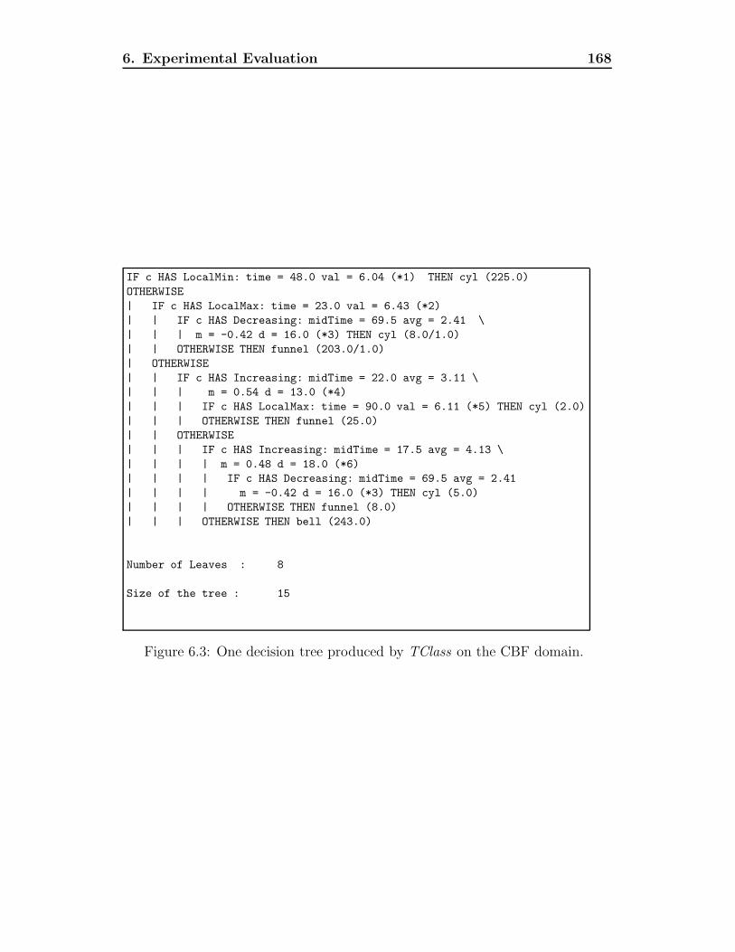
6. Experimental Evaluation 168
IF c HAS LocalMin: time = 48.0 val = 6.04 (*1) THEN cyl (225.0)
OTHERWISE
| IF c HAS LocalMax: time = 23.0 val = 6.43 (*2)
| | IF c HAS Decreasing: midTime = 69.5 avg = 2.41 \
| | | m = -0.42 d = 16.0 (*3) THEN cyl (8.0/1.0)
| | OTHERWISE THEN funnel (203.0/1.0)
| OTHERWISE
| | IF c HAS Increasing: midTime = 22.0 avg = 3.11 \
| | | m = 0.54 d = 13.0 (*4)
| | | IF c HAS LocalMax: time = 90.0 val = 6.11 (*5) THEN cyl (2.0)
| | | OTHERWISE THEN funnel (25.0)
| | OTHERWISE
| | | IF c HAS Increasing: midTime = 17.5 avg = 4.13 \
| | | | m = 0.48 d = 18.0 (*6)
| | | | IF c HAS Decreasing: midTime = 69.5 avg = 2.41
| | | | m = -0.42 d = 16.0 (*3) THEN cyl (5.0)
| | | | OTHERWISE THEN funnel (8.0)
| | | OTHERWISE THEN bell (243.0)
Number of Leaves : 8
Size of the tree : 15
Figure 6.3: One decision tree produced by TClass on the CBF domain.

6. Experimental Evaluation 169
Event index
-----------
*1: lmin
time=48.0 r=[35.0,112.0]
value=6.04 r=[4.88,6.91]
*2: lmax
time=23.0 r=[20.0,54.0]
value=6.43 r=[3.18,6.58]
*3: dec
midtime=69.5 r=[50.5,123.0]
avg=2.41 r=[1.24,4.88]
m=-0.42 r=[-0.94,-0.30]
duration=16.0 r=[9.0,24.0]
*4: inc
midtime=22.0 r=[13.5,33.5]
avg=3.11 r=[1.42,4.18]
m=0.54 r=[0.37,0.77]
duration=13.0 r=[8.0,18.0]
*5: lmax
time=90.0 r=[57.0,107.0]
value=6.11 r=[5.00,7.42]
*6: inc
midtime=17.5 r=[10.0,36.0]
avg=4.13 r=[0.77,4.49]
m=0.48 r=[0.23,0.51]
duration=18.0 r=[12.0,32.0]
Figure 6.4: Events used by the decision tree in Figure 6.3.

6. Experimental Evaluation 170
typical ruleset created by TClass with PART. The first rule for instance checks
for a high local minimum around time 44, which should only be possible if it is
a cylinder or a funnel; and failing these, looks for a nice gentle decreasing signal
that is characteristic of the funnel. If this is not present it’s a cylinder. If it’s not
a cylinder, then it looks for a sudden increase early on in the signal (typical of
cylinders or funnels) or a gradual decrease (typical of funnel). If it doesn’t have
either of these, then it’s a bell. To finally ensure it’s a funnel, it checks to see if
there is either a middle time high maximum (more characteristic of a cylinder)
or a middle time low maximum (only possible with a bell). If it has neither of
these it must be a funnel. Between them, these three rules cover 88 per cent
of instances. In the author’s opinion, these rules are more comprehensible than
either the naive segmentation approaches or the J48 TClass trees.
Conclusions
The CBF dataset turns out to be largely trivial as a learning problem. All three
approaches, TClass, naive segmentation and hidden Markov models attain 100
per cent accuracy on it. It may be possible to prove theoretically that a naive
segmentation approach with 20 segments can be guaranteed with some very high
probability to produce a learner which can classify instances in the CBF domain
perfectly. The effect of smoothing on the outcome appears to be minor in this
case; but slightly positive overall for the TClass classifiers.
This makes the CBF domain a poor one for evaluation of some of the other

6. Experimental Evaluation 171
IF c HAS LocalMin: time = 44.0 val = 5.76 (*1) AND
IF c HAS NO Decreasing: midTime = 59.0 avg = 1.98 \
m = -0.09 d = 53.0 (*2) \
THEN cyl (239.0/1.0)
IF c HAS NO Increasing: midTime = 23.5 avg = 1.95 \
m = 0.29 d = 18.0 (*3) AND
IF c HAS NO Decreasing: midTime = 59.0 avg = 1.98
m = -0.09 d = 53.0 (*2) THEN bell (233.0)
IF c HAS NO LocalMax: time = 72.0 val = 6.14 (*5) AND
IF c HAS NO LocalMax: time = 65.0 val = -0.36 (*6) THEN funnel (228.0)
IF c HAS NO Increasing: midTime = 59.0 avg = 3.93 \
m = 0.21 d = 11.0 (*7) AND
IF c HAS LocalMax: time = 27.0 val = 4.82 (*8) THEN funnel (9.0)
IF c HAS NO Increasing: midTime = 59.0 avg = 3.93 \
m = 0.21 d = 11.0 (*8) THEN cyl (7.0)
: bell (3.0)
Number of Rules : 6
Figure 6.5: A ruleset produced by TClass using PART as the learner.

6. Experimental Evaluation 172
Event index
-----------
*1: lmin
time=44.0 r=[28.0,112.0]
value=5.76 r=[4.76,6.91]
*2: dec
midtime=59.0 r=[41.5,106.5]
avg=1.98 r=[-0.26,6.17]
m=-0.09 r=[-0.23,-0.01]
duration=53.0 r=[26.0,102.0]
*3: inc
midtime=23.5 r=[2.5,45.5]
avg=1.95 r=[-0.74,4.81]
m=0.29 r=[0.18,0.77]
duration=18.0 r=[6.0,41.0]
*5: lmax
time=72.0 r=[51.0,108.0]
value=6.14 r=[5.01,7.90]
*6: lmax
time=65.0 r=[42.0,76.0]
value=-0.36 r=[-0.67,2.40]
*7: inc
midtime=59.0 r=[35.5,88.5]
avg=3.93 r=[1.64,6.27]
m=0.21 r=[0.09,0.37]
duration=11.0 r=[6.0,42.0]
*8: lmax
time=27.0 r=[21.0,53.0]
value=4.82 r=[2.60,5.58]
Figure 6.6: Event index for the ruleset in Figure 6.5.
6. Experimental Evaluation 173
issues we are interested in; since it is likely that in many cases we hit the “100 per
cent barrier”; which does not give good guidance to the real-world performance
of the classifier.
However, one thing that can be compared as a result of these experiments is
comprehensibility; in particular between naive segmentation and TClass. While
both results are readable and provide some useful description of the learnt con-
cept; we claim subjectively that the TClass definitions are easier to understand,
as they are expressed in terms that a human looking at the data might use: the
height of maxima, gentle changes in gradient, and sudden changes in gradient;
rather than averages of particular temporal segments of the data.
6.2.2 TTest - An artificial dataset for temporal classifi-
cation
In order to better understand the behaviour of the algorithm a new artificial
dataset was created to overcome the difficulties mentioned above with the CBF
domain. This artificial dataset tries to capture some of the variations that occur
in real-world data.
Objectives of artificial dataset
What characteristics are desirable in our artificial dataset? Firstly, it must
be multivariate; that is to say, there must be more than one channel of data.

6. Experimental Evaluation 174
Secondly, it must show some of the forms of variation discussed in Chapter 3,
namely:
• Variation in the total duration.
• Variation in the duration and timing of “sub-events” or components of the
instances.
• Variation in the amplitude of the signal.
• Gaussian noise.
Thirdly, it would be worth considering the effects of noise at the feature level,
as well as at the Gaussian level; that is to say, to have, say one channel of data
irrelevant or insignificant. Fourthly, we want the “correct” or ideal solution to
the problem to be known; hence we can compare concepts produced by TClass
with the known concepts. Fifthly, we want it to be reproducible, so that we can
produce as many data as we like.
Furthermore, we want all of these parameters to be tunable, hence allowing
us to look at the effect that each has individually.
TTest
To fulfil this role, the artificial dataset TTest has been designed. TTest is a
learning problems with three classes and three channels. It has a total of five
parameters controlling various characteristics.

6. Experimental Evaluation 175
There are three classes, imaginatively called A, B and C. The three channels,
likewise, are imaginatively termed alpha, beta and gamma. For each of the
three classes, there is a prototype, as shown in Figures 6.7, 6.8 and 6.9. All the
prototypes are all exactly a hundred units of time long.
0.0
0.2
0.4
0.6
0.8
1.0
alph
a
−1.
0−
0.5
0.0
0.5
1.0
beta
−1.
0−
0.5
0.0
0.5
1.0
gam
ma
0 20 40 60 80 100
Time
Class A Prototype
Figure 6.7: Prototype for class A
These prototypes can be mathematically defined as follows:

6.
Experim
enta
lEvalu
atio
n176
0.0 0.2 0.4 0.6 0.8 1.0
alpha
0.0 0.2 0.4 0.6 0.8 1.0
beta
−1.0 −0.5 0.0 0.5 1.0
gamma
020
4060
80100
Tim
e
Class B
Pro
totyp
e
Figu
re6.8:
Prototy
pe
forclass
B
0.0 0.2 0.4 0.6 0.8 1.0
alpha
−1.0 −0.5 0.0 0.5 1.0
beta
−1.0 −0.8 −0.6 −0.4 −0.2 0.0
gamma
020
4060
80100
Tim
e
Class A
Pro
totyp
e
Figu
re6.9:
Prototy
pe
forclass
C

6. Experimental Evaluation 177
Aα(t) =
135
t if t ≤ 35
0 if 35 < t ≤ 65
135
(100 − t) if 65 < t ≤ 100
Aβ(t) =
1 if t ∈ {25, 48, 75}
−1 if t = 52
0 otherwise
Aγ(t) = 0
Bα(t) =
135
t if t ≤ 35
0 if 35 < t ≤ 65
135
(100 − t) if 65 < t ≤ 100
Bβ(t) =
1 if t ∈ {25, 75}
0 otherwise
Bγ(t) = 0
Cα(t) =
135
t if t ≤ 35
0 if 35 < t ≤ 65
135
(t − 65) if 65 < t ≤ 100
Cβ(t) = 0
Cγ(t) =
−1 if t = 50
0 otherwise

6. Experimental Evaluation 178
Now, these are not particularly interesting as a learning task. Even feeding
the features into a traditional learner, such as C4.5, treating each channel/frame
combination as a single feature (hence generating 300 features), would work,
except that the definitions produced would be really difficult to read. So, we’ve
got to spice it up somehow.
Obviously, the solution lies in randomisation. For the purposes of this thesis,
let us define a function unif (), which returns a uniformly distributed real number
in the range [−1, 1]. Also, let us define a function ε(), which returns a real number
of normal distribution, with a mean of 0 and a variance of 1.
One form of variation is temporal stretching. In general, temporal stretching
is non-linear; in other words, temporal stretching need not be of the kind where
the signal is uniformly slowed down or sped up; rather, some parts can be sped
up while others can be slowed down. However, for simplicity, we will assume
linear temporal stretching. The amount of temporal (linear) stretching for the
TTest dataset is controlled by the parameter d (short for overall duration). The
duration is computed as:
durn = (1 + d ∗ unif ()) ∗ 100
That is to say that d specifies the percentage variation of the duration. For
example, if d = 0.1, this would mean that duration in frames would vary from
90 to 110.
To illustrate this, consider a prototype A signal. Figure 6.10 shows a variety
of different instances of A, with d = 0.2. Similar effects can be observed on the

6. Experimental Evaluation 179
other classes.
0.0
0.2
0.4
0.6
0.8
1.0
alph
a
−1.
0−
0.5
0.0
0.5
1.0
beta
−1.
0−
0.5
0.0
0.5
1.0
gam
ma
0 20 40 60 80 100
Time
Instances of class A, d=0.2
Figure 6.10: Effect of adding duration variation to prototypes of class A.
Another form of variation is random noise. For this problem, we will assume
that such noise is Gaussian. This is not an unreasonable assumption, as Gaussian
noise is typical of many types of sensors and measurements that are used in
temporal data. For the TTest dataset, the amount of noise is controlled by the
parameter g; the noise on all channels is taken by multiplying the parameter g
by the random Gaussian noise function; i.e.,
noise() = g ∗ ε()
then this can be added to the signal. The more noise; the more the underlying
signal is obscured. The effect of adding Gaussian noise with g = 0.1 can be seen
in Figure 6.11.

6. Experimental Evaluation 180
−0.
20.
20.
40.
60.
81.
0
alph
a
−1.
0−
0.5
0.0
0.5
1.0
beta
−0.
2−
0.1
0.0
0.1
0.2
gam
ma
0 20 40 60 80 100
Time
Instances of class A, g=0.1
Figure 6.11: Effect of adding Gaussian noise to prototypes of class A.
As mentioned before, temporal stretching is only a linear approximation of
a non-linear process. Hence, we can also modify the times of events within each
instance relative to one another. In TTest, this is controlled by the parameter c.
Within the dataset, the startpoints and endpoints of increases and decreases, as
well as the timing of local maxima and minima are all randomly offset in time.
The amount of variation of these temporal events is modified by a random value
c ∗ unif () ∗ 100. The effect of setting c = 0.1 on the three instances of class A
are shown in Figure 6.12.
Also, as with real datasets, sometimes the amplitudes of the various events
varies. In TTest the parameter h determines the amount of variation in the
amplitude of the local maxima of the signal. Each of these maxima is perturbed

6. Experimental Evaluation 181
0.0
0.2
0.4
0.6
0.8
1.0
alph
a
−1.
0−
0.5
0.0
0.5
1.0
beta
−1.
0−
0.5
0.0
0.5
1.0
gam
ma
0 20 40 60 80 100
Time
Instances of class A, c=0.2
Figure 6.12: Effect of adding sub-event variation to prototypes of class A.
by an amount h∗unif (). The effect of setting h = 0.2 on three instances of class
A can be seen in Figure 6.13.
Finally, one thing that often occurs in real datasets is that there is some
data on a channel that looks useful, but in fact is irrelevant. For this reason,
for classes A and B, the gamma channel was replaced with something that looks
plausible as a signal: a sequence of between 2 and 9 random line segments whose
endpoints are randomly generated. For class C, the beta channel is replaced
with a similarly generated sequence of random line segments. Note that this is
meant to explore a different issue to that of the Gaussian noise above; this is
meant to test the learner’s ability to cope with data that is irrelevant.
Three instances of class A are shown in Figure 6.14, with the irrelevant

6. Experimental Evaluation 182
0.0
0.2
0.4
0.6
0.8
1.0
1.2
alph
a
−1.
0−
0.5
0.0
0.5
1.0
beta
−1.
0−
0.5
0.0
0.5
1.0
gam
ma
0 20 40 60 80 100
Time
Instances of class A, h=0.2
Figure 6.13: Effect of adding amplitude variation to prototypes of class A.
0.0
0.2
0.4
0.6
0.8
1.0
alph
a
−1.
0−
0.5
0.0
0.5
1.0
beta
−3.
0−
2.0
−1.
00.
0
gam
ma
0 20 40 60 80 100
Time
Instances of class A with irrelevant features
Figure 6.14: Effect of replacing gamma channel with irrelevant signal to class A.

6. Experimental Evaluation 183
features added.
Having included all of these factors, we can now redefine our original sig-
nals, in terms of the parameters g, c, d, h; as well as whether we choose to have
irrelevant features or not. The definitions hence become:

6. Experimental Evaluation 184
dur = (1 + d ∗ unif ()) ∗ 100
tα1 = (0.35 + c ∗ unif ()) ∗ dur
tα2 = (0.65 + c ∗ unif ()) ∗ dur
hα1 = (1 + h ∗ unif ())
hα2 = (1 + h ∗ unif ())
Aα(t) =
hα1
tα1
∗ t + g ∗ ε(t) if t < tα1
g ∗ ε(t) if tα1 ≤ t < tα2
dur−tdur−tα2
∗ t + g ∗ ε(t) if tα2 ≤ t ≤ dur
tβ1 = (0.25 + c ∗ unif ()) ∗ dur
tβ23 = (0.5 + c ∗ unif ()) ∗ dur
tβ4 = (0.75 + c ∗ unif ()) ∗ dur
hβ1 = (1 + h ∗ unif ())
hβ2 = (1 + h ∗ unif ())
hβ3 = (−1 + h ∗ unif ())
hβ4 = (1 + h ∗ unif ())
Aβ(t) =
hβ1 + g ∗ ε(t) if t = tβ1
hβ2 + g ∗ ε(t) if t = tβ23 − 1
hβ3 + g ∗ ε(t) if t = tβ23 + 1
hβ4 + g ∗ ε(t) if t = tβ4
g ∗ ε(t) otherwise
Aγ(t) =
g ∗ ε(t) if irrel is off
irrel(t) + g ∗ ε(t) if irrel is on

6. Experimental Evaluation 185
dur = (1 + d ∗ unif ()) ∗ 100
tα1 = (0.35 + c ∗ unif ()) ∗ dur
tα2 = (0.65 + c ∗ unif ()) ∗ dur
hα1 = (1 + h ∗ unif ())
hα2 = (1 + h ∗ unif ())
Bα(t) =
hα1
tα1
∗ t + g ∗ ε(t) if t < tα1
g ∗ ε(t) if tα1 ≤ t < tα2
dur−tdur−tα2
∗ t + g ∗ ε(t) if tα2 ≤ t ≤ dur
tβ1 = (0.25 + c ∗ unif ()) ∗ dur
tβ23 = (0.5 + c ∗ unif ()) ∗ dur
tβ4 = (0.75 + c ∗ unif ()) ∗ dur
hβ1 = (1 + h ∗ unif ())
hβ2 = (1 + h ∗ unif ())
Bβ(t) =
hβ1 + g ∗ ε(t) if t = tβ1
hβ2 + g ∗ ε(t) if t = tβ2
g ∗ ε(t) otherwise
Bγ(t) =
g ∗ ε(t) if irrel is off
irrel(t) + g ∗ ε(t) if irrel is on

6. Experimental Evaluation 186
dur = (1 + d ∗ unif ()) ∗ 100
tα1 = (0.35 + c ∗ unif ()) ∗ dur
tα2 = (0.65 + c ∗ unif ()) ∗ dur
hα1 = (1 + h ∗ unif ())
hα2 = (1 + h ∗ unif ())
Cα(t) =
hα1
tα1
∗ t + g ∗ ε(t) if t < tα1
g ∗ ε(t) if tα1 ≤ t < tα2
t−tα2
dur−tα2
∗ t + g ∗ ε(t) if tα2 ≤ t ≤ dur
Cβ(t) =
g ∗ ε(t) if irrel is off
irrel(t) + g ∗ ε(t) if irrel is on
tγ = (0.25 + c ∗ unif ()) ∗ dur
hγ = (−1 + h ∗ unif ())
Cγ(t) =
hγ + g ∗ ε(t) if t = tγ
g ∗ ε(t) otherwise
This dataset has some useful properties. Firstly, it is truly multivariate. Sec-
ondly, it has variation in the length of streams and the onset and duration of
sub-events. Thirdly, it has variation in the amplitudes of events as well as Gaus-
sian noise (as does CBF). Fourthly, it has several sub-events and a complicated
relation between sub-events which is typical of real-world domains. CBF only
had one of these properties.

6. Experimental Evaluation 187
Experimental Results
As a starting dataset, we generated 1000 instances, using the following param-
eters: g = 0.1, d = 0.2, c = 0.2, h = 0.2 with irrelevant features switched on.
Figures 6.15, 6.16 and 6.17 instances of classes A, B and C respectively.
0.0
0.5
1.0
alph
a
−1.
00.
00.
51.
01.
52.
0
beta
−1.
5−
1.0
−0.
50.
00.
51.
0
gam
ma
0 20 40 60 80 100 120
Time
Class A: g=0.1,c=0.2,d=0.2,h=0.2
Figure 6.15: Examples of class A with default parameters.
The results are shown in Table 6.5.
As we can see, for this particular training set, TClass performs better in
terms of accuracy.
To examine the effect of noise, we increased g to 0.2; and also looked at what
happens when g = 0. The results for more noise are shown in Table 6.8; and the
results with zero noise are shown in Table 6.9. For brevity, the in-depth results

6. Experimental Evaluation 188
Approach ErrorTClass with J48 3.3 ± 0.9
TClass with PART 2.3 ± 0.3TClass with IBL 68.1 ± 1.5
TClass with Bagging/J48 2.5 ± 0.4TClass with AdaBoost/J48 1.0 ± 0.3TClass with Naive Bayes 9.8 ± 1.5
Naive Segmentation 7.2 ± 0.7Hidden Markov Model 4.4 ± 1.5
Table 6.5: Error rates on the TTest domain.
Approach Segments3 5 10 20
J48 28.7 ± 0.9 34.1 ± 1.3 23.4 ± 0.9 7.4 ± 1.0NB 28.2 ± 1.3 31.1 ± 1.3 25.9 ± 1.2 16.4 ± 1.3IB1 34.0 ± 1.5 33.2 ± 1.3 31.6 ± 1.0 32.6 ± 1.2AB 30.5 ± 1.5 29.7 ± 1.3 26.3 ± 1.0 7.8 ± 1.2Bag 30.6 ± 0.9 32.3 ± 1.4 23.1 ± 1.0 7.2 ± 0.7
Table 6.6: Error rates of naive segmentation on the TTest domain.
Topology Raw Raw + Derivativelr-3 17.0 ± 1.2 15.4 ± 1.7lr-5 13.4 ± 2.1 25.3 ± 0.9lr-10 18.3 ± 2.4 21.7 ± 1.5lr-20 21.9 ± 1.3 19.9 ± 1.6lrs1-3 21.8 ± 1.8 22.1 ± 1.3lrs1-5 29.8 ± 1.9 23.5 ± 1.2lrs1-10 26.0 ± 1.3 23.6 ± 1.9lrs1-20 24.8 ± 1.7 24.1 ± 1.8er-3 26.0 ± 1.7 15.9 ± 1.2er-5 12.5 ± 1.0 4.8 ± 0.4er-10 12.5 ± 1.0 4.4 ± 0.6er-20 12.5 ± 1.0 4.8 ± 0.4
Table 6.7: Error rates when using hidden Markov models on TTest domain.

6. Experimental Evaluation 189
0.0
0.5
1.0
alph
a
−0.
20.
20.
61.
0
beta
−1.
5−
0.5
0.5
1.5
gam
ma
0 20 40 60 80
Time
Class B: g=0.1,c=0.2,d=0.2,h=0.2
Figure 6.16: Examples of class B with default parameters.
0.0
0.5
1.0
alph
a
−2
−1
01
beta
−1.
0−
0.6
−0.
20.
2
gam
ma
0 20 40 60 80 100
Time
Class C: g=0.1,c=0.2,d=0.2,h=0.2
Figure 6.17: Examples of class C with default parameters.

6. Experimental Evaluation 190
Approach ErrorTClass with J48 17.4 ± 2.1
TClass with PART 16.1 ± 1.5TClass with IBL 67.3 ± 1.3
TClass with Bagging/J48 11.3 ± 1.2TClass with AdaBoost/J48 14.9 ± 2.1TClass with Naive Bayes 13.9 ± 1.8
Naive Segmentation 13.2 ± 1.6Hidden Markov Model 9.9 ± 1.1
Table 6.8: Error rates for high-noise situation (g=0.2) on TTest domain.
Approach ErrorTClass with J48 1.6 ± 0.4
TClass with PART 1.4 ± 0.5TClass with IB1 66.7 ± 1.4
TClass with Naive Bayes 11.2 ± 2.3TClass with Bag/J48 1.6 ± 0.4
TClass with AdaBoost/J48 0.9 ± 0.3Naive Segmentation 2.1 ± 0.5
Hidden Markov Model 4.8 ± 0.9
Table 6.9: Error rates with no Gaussian noise (g=0) on TTest domain.
for naive segmentation and HMMs are omitted.
We plotted the results for each of these in Figure 6.18, excluding TClass/IB1,
because its performance is so poor relative to the other learners.
Clearly, the noise level has a significant effect on the quality of the learning.
With no noise, every TClass learner outperforms the baseline learners. With
the noise level at 0.2, most of the learners perform poorly. The least poorly
affected is the hidden Markov model; its statistical nature seems to helped it
cope. Again, if we are willing to sacrifice readability, we can simply vote TClass.
Figure 6.19 shows the effect of voting to improve accuracy, using bagging as

6. Experimental Evaluation 191
J48 PART NB Bag AB Vote/AB Vote/Bag Seg HMM
g=0.0g=0.1g=0.2
Learner
Err
or r
ate
(%)
05
1015
Figure 6.18: Learner accuracy and noise
the base learner. Bagging was chosen because it was the best performer in the
unvoted results among the TClass learners, but it could be done with any of the
other learners.
This shows the dramatic effect that voting can have on performance. In
the limit, using voted TClass does approximately twice as well as the best-
performing hidden Markov model: it appears to asymptotically reach an error
of about 4.7 per cent, when doing voting of 11 bagged TClass learners3. Un-
fortunately, this comes at a price: readability. For the minimum error case, the
human would have to look at the results of 110 trees and consider how each of
them votes.
3There is no result for 2 bagged learners, since the result is arbitrary: if one learner votesone way and the other votes another then it’s an arbitrary choice as to which is correct, andbecause of the binomial theorem, in the limit you can’t do any better than a single voter.

6. Experimental Evaluation 192
4
5
6
7
8
9
10
11
12
0 2 4 6 8 10 12 14 16
Err
or (
%)
Number of Voters
Improving error rate using multiple TClass runs
TClass/BagHMM/ergodic 10 state
Figure 6.19: Voting different runs of TClass to reduce error with g=0.2.
We were also curious as to why hidden Markov models and naive segmenta-
tion performed so well. Since HMMs are statistical models, they perform best
when there are many instances – especially with the high level of noise when
g = 0.2. Given that in the above experiments, there are 300 training examples
for each class, perhaps the TTest provides too many examples. We therefore
generated a smaller dataset consisting of only 100 examples – hence having 30
examples per class for training.
We ran further experiments with this set of 100 examples. Abbreviated
results are shown in Table 6.10. In order to get statistically significant results,
the TClass runs were repeated 3 times and averaged (not voted).
The results are surprising. Firstly, note that for the TClass learners, the

6. Experimental Evaluation 193
Approach ErrorTClass with J48 16.7 ± 2.0
TClass with PART 19.7 ± 2.3TClass with IBL 69.2 ± 2.0
TClass with Bagging/J48 12.7 ± 2.3TClass with AdaBoost/J48 11.0 ± 1.5TClass with Naive Bayes 19.0 ± 2.3
Naive Segmentation 21.0 ± 3.0Hidden Markov Model 17.0 ± 3.5
Table 6.10: Error rates for high-noise situation (g=0.2), but with only 100 ex-amples on TTest domain.
J48 PART NB Bag AB Seg HMM
100 training instances1000 training instances
Learner
Err
or r
ate
(%)
05
1015
20
Figure 6.20: Error rates of different learners with 100 and 1000 examples.
performance of the bagging and boosting seems to have improved over when
they had 300 examples. This suggests that the boosting and bagging systems
are overfitting the data. To confirm this, we looked at the average number of
leaves in each tree produced when bagging with 100 examples and 1000 exam-

6. Experimental Evaluation 194
ples. We found that with 100 examples, there were an average of 5.8 leaves
per tree, whereas with 1000 examples there was an average of 37.0 leaves per
tree. Theoretically, the three classes are orthogonal; in other words, we know
they could, in the absence of noise, be classified with 3 leaf nodes. It does show,
however, that the TClass learners perform better than the statistical approaches
when the number of training instances in this domain is small.
This indicated that it was perhaps possible to get more accurate trees in
high noise situations by setting the pruning parameters higher for the tree-based
learners. We set the confidence for pruning to 5% instead of the default 25%;
and set the minimum number of instances per node to 10, instead of the default
2. In the high noise case (g=0.2), this led to a massive reduction in tree size with
an improvement in accuracy. For J48, the average tree size was reduced from
47.3 leaf nodes to 12.2 leaf nodes. At the same time, the error rate was reduced
from 17.4 per cent to 13.2 per cent. This seems to be a strong gain; making the
results both more comprehensible and at the same time more accurate.
Comprehensibility
Once the above high pruning criteria were introduced, the definitions became
much clearer, even in the high noise case.
The definitions arrived at for the no-noise case shown in Figure 6.21 are
exactly correct. It looks for the increasing alpha value distinctive of the C
channel; as well as the fact that class A has a big decreasing timestep right in
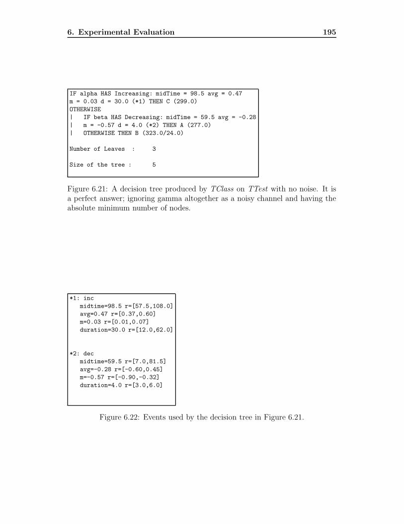
6. Experimental Evaluation 195
IF alpha HAS Increasing: midTime = 98.5 avg = 0.47
m = 0.03 d = 30.0 (*1) THEN C (299.0)
OTHERWISE
| IF beta HAS Decreasing: midTime = 59.5 avg = -0.28
| m = -0.57 d = 4.0 (*2) THEN A (277.0)
| OTHERWISE THEN B (323.0/24.0)
Number of Leaves : 3
Size of the tree : 5
Figure 6.21: A decision tree produced by TClass on TTest with no noise. It isa perfect answer; ignoring gamma altogether as a noisy channel and having theabsolute minimum number of nodes.
*1: inc
midtime=98.5 r=[57.5,108.0]
avg=0.47 r=[0.37,0.60]
m=0.03 r=[0.01,0.07]
duration=30.0 r=[12.0,62.0]
*2: dec
midtime=59.5 r=[7.0,81.5]
avg=-0.28 r=[-0.60,0.45]
m=-0.57 r=[-0.90,-0.32]
duration=4.0 r=[3.0,6.0]
Figure 6.22: Events used by the decision tree in Figure 6.21.

6. Experimental Evaluation 196
IF beta HAS LocalMax: time = 48.0 val = 0.07 (*1) AND
IF beta HAS NO LocalMin: time = 64.0 val = -0.72 (*2) AND
IF beta HAS NO LocalMin: time = 63.0 val = 0.31 (*3) THEN B (299.0/3.0)
IF gamma HAS LocalMin: time = 59.0 val = -0.00 (*4) AND
IF gamma HAS NO LocalMin: time = 56.0 val = 0.46 (*5) AND
IF gamma HAS LocalMax: time = 26.0 val = 0.03 (*6) THEN C (301.0/3.0)
: A (299.0/2.0)
Number of Rules : 3
Figure 6.23: A decision list produced by TClass on TTest with 10 per cent noise.
the middle.
But what happens as we add noise? Do we still get such high quality defi-
nitions? If we use the high pruning levels we used above, we can sustain good
definitions while g = 0.1. The results are shown in Figure 6.23.
The definitions here are still understandable. The first rule looks for the
beta channel with no significant local minima ant at least one local maximum,
indicating a B class. Similarly, it looks for the big local minimum of the C class
in the gamma channel.
Finally,we look at the effect when g = 0.2 as shown in Figure 6.25. For
brevity, we have omitted the event index. Although it is hard to understand
such a complicated tree, some understanding can still be gained. For instance
if the beta channel has a local maximum in the middle, and a nearby local
minimum, it is likely to be of class A.

6. Experimental Evaluation 197
Event index
-----------
*1: lmax
time=48.0 r=[1.0,52.0]
value=0.07 r=[-0.11,0.54]
*2: lmin
time=64.0 r=[6.0,114.0]
value=-0.72 r=[-4.69,-0.35]
*3: lmin
time=63.0 r=[4.0,116.0]
value=0.31 r=[0.08,1.33]
*4: lmin
time=59.0 r=[51.0,116.0]
value=-0.00 r=[-0.52,0.48]
*5: lmin
time=56.0 r=[46.0,116.0]
value=0.46 r=[0.20,4.30]
*6: lmax
time=26.0 r=[14.0,41.0]
value=0.03 r=[-0.43,0.37]
Figure 6.24: Events used by the decision tree in Figure 6.23.

6. Experimental Evaluation 198
J48 pruned tree
------------------
IF beta HAS LocalMax: time = 57.0 val = 0.25 (*1)
| IF beta HAS LocalMin: time = 42.0 val = -0.83 (*2)
| | IF beta HAS LocalMax: time = 47.0 val = -0.67 (*3)
| | | IF gamma HAS LocalMin: time = 41.0 val = -0.21 (*4)
| | | THEN C (44.0/4.0)
| | | OTHERWISE THEN A (11.0)
| | OTHERWISE THEN A (261.0/13.0)
| OTHERWISE
| | IF beta HAS Decreasing: midTime = 52.0 avg = 0.95
| | m = -0.09 d = 3.0 (*5) THEN C (23.0)
| | OTHERWISE
| | | IF gamma HAS Plateau: midTime = 42.0 avg = -0.03 d = 85.0 (*6)
| | | | IF gamma HAS LocalMax: time = 32.0 val = -0.54 (*7)
| | | | THEN B (28.0/5.0)
| | | | OTHERWISE THEN C (23.0/5.0)
| | | OTHERWISE THEN B (281.0/31.0)
OTHERWISE
| IF gamma HAS LocalMin: time = 41.0 val = -0.21 (*8)
| THEN C (218.0)
| OTHERWISE THEN A (10.0/5.0)
Figure 6.25: A decision tree produced by TClass on TTest with 20 per centnoise.

6. Experimental Evaluation 199
Conclusions
TClass is able to achieve high accuracy, comprehensible description of the TTest
dataset; it is competitive in its generation of correct and accurate descriptions –
especially in situations where there is little or no noise. Smoothing does not ap-
pear to help. If one is not interested in comprehensibility of the learnt concepts,
voting methods can be employed to great effect – obtaining accuracies far in
excess of those of the baseline learners; on this data, at least half the error rate.
Further, it shows better results than the baseline learners with fewer instances.
There does seem to be a problem with overfitting, however. This is likely be-
cause there are so many features generated. The trees produced are much larger
than optimal, and by adjusting the parameters of decision-tree based learners to
be more aggressive in their pruning we can generate more comprehensible rules
with equivalent or higher accuracy. We will have to take this into account with
our real-world datasets.
6.3 Real-world datasets
We now examine real-world datasets to see if TClass functions as well on real-
world problems as it did on the artificial ones.

6. Experimental Evaluation 200
6.3.1 Why these data sets?
Finding temporal classification data sets can be difficult. As previously men-
tioned (Section 6.2), although many data sets are inherently temporal, many
people are eager to convert them to propositional form immediately. Although
time series data is easy come by, what is hard to obtain from experts is the
classification – this exclude many of the dynamic-systems or financial time series
data sets.
The first data set, the Auslan data set, was selected because the author had
collected the data himself and was one of the motivating problems behind this
research; there did not seem to be many different algorithms for recognising time
series. Secondly, unlike other data sets, rules produced by the system could be
directly compared with the definitions found in the Auslan dictionary [Joh89].
The second data set, the ECG data set, was selected for a number of reasons.
Firstly, work had recently concluded on a “propositionalisation” of the data
set [dC98] that converted an ECG into a list of attribute values. This would
allow easy comparisons between results using domain-specific information and a
temporal classification system.
6.3.2 Auslan
As stated previously, Auslan is the language used by the Australian Deaf and
non-vocal communities. Auslan is a dialect of British Sign Language. It is

6. Experimental Evaluation 201
dissimilar to American Sign Language, although some signs have been adopted.
Auslan also has about 4000 signs in it. However, there are many ways these
signs can be modified to alter the meaning slightly, and even more powerfully,
signs can be combined to give new signs. Fingerspelling is not the same as
Auslan, it is merely a fallback used fo proper names, words for which there is
no sign and people who cannot sign Auslan but still need to communicate with
Deaf.
Structure of signs in Auslan
There are several components of a sign. By mixing and matching these, a wide
variety of signs can be formed. These components are:
Handshape Handshapes in Auslan can be classified into 31 different shapes
(although there are 63 variations, these are typically considered minor). Fur-
thermore, there are one-handed signs (where only one hand is used), two-handed
signs (where both hands are used, but each hand is executing a different hand-
shape) and double-handed signs (where both hands have the same handshape).
There is a tendency in two-handed signs for one hand to dominate (usually
the right in right-handed signers) and also that double-handed signs tend to be
symmetrical (that is, both hands also tend to move in the same, if mirrored,
motion).

6. Experimental Evaluation 202
Location This is where the sign is started. If the sign is within the “neutral
space” – a half-ellipsoid centred on the person’s chest, the location is not impor-
tant. However, if the location is outside the neutral space, it may be important.
Orientation This refers to the orientation of the hand in terms of the
wrist’s rotation (the roll), whether the hand is pointing up or down (the pitch)
and which direction the hand is facing (the yaw).
Movement There are many movements used in sign language, including arcs,
straight lines and “wavy” patterns. They are not necessarily two-dimensional
(consider the sign for crazy, which in Auslan is the universal gesture of pointing
to the head and making small circles directed away from the head), and can
include changes in orientation and handshape as well as position. Typically, they
can include multiple steps, such as the sign for science which is characterised
by “mixing test-tubes”.
Expression Facial expressions are an important part of signing. While it does
not play a major role in individual signs, it becomes very important at the
sentence level. For example, negation can be made by making the normal sign
and shaking one’s head at the same time, and questions are formed by raising
the eyebrows or tilting the head (depending on the type of question).

6. Experimental Evaluation 203
Summary of previous research
The work that has been published in the specific area of recognition of individual
signs is still limited. Murakami and Taguchi considered ten signs using a recur-
rent neural net and obtained accuracy of 96 per cent ([MT91]). Charayaphan
and Marble considered 31 ASL symbols, but only sampled each sign once and
simulated the variation and consistently got 27 out of the 31 correct, with the re-
maining four sometimes correct using a Hough transform. Starner considered 40
signs used in brief sentences and ([Sta95, SP95]) obtained accuracies of 91.3 per
cent on raw signs and 99.2 per cent by using a very strict grammar for sentences.
More detailed information can be found in [Kad95].
Two datasets of sign language data were captured. The first (original) data
was captured for [Kad95], using very cheap equipment. The second, collected
for this work, used much higher quality equipment. We discuss the differences
between the two sources. For convenience the older dataset will be termed the
Nintendo data, and the newer dataset will be termed the Flock data.
Nintendo data
The original sign language data was captured using a single Nintendo Power-
glove, connected through a Powerglove Serial interface to a Silicon Graphics
4D/35G. A subset of Auslan consisting of 95 signs was selected to cover all the
typical handshapes and movements. In some cases, signs that were difficult to

6. Experimental Evaluation 204
distinguish were deliberately chosen. A complete list of the signs chosen can be
found in Appendix B of [Kad95]. For convenience, a table from [Kad95] is shown
Table 6.11, giving an overview of the sign selection process.
Item Numberof signs
Total number of signs 95Hand usage
- One-handed 59- Double-handed 27- Two-handed 9
Reasons for selection- Common sign 66- Similarity to other signs 11- Uncommon Handshape 9- Sign Complexity 5- Other 4
Table 6.11: Some statistics on the signs used.
The Powerglove proved itself to be a less than stellar performer. The x, y and
z position are encoded as 8-bit values. Because it used ultrasound to compute
position, it was quite susceptible to bogus echoes. Finger bend was only avail-
able for the first four fingers4, and then, only two bits. Even more disastrously,
the fingers were subject to hysteresis and unpredictability. No orientation in-
formation was available other than roll, which could take one of 12 values (i.e.
measurements were +/- 30 degrees). Hence, in total, there were eight channels
(x, y, z, roll, thumb, fore, middle, ring).
Further, the refresh rate was very low; approximately 23 to 25 frames per
4The little finger is actually important in many sign languages. For example, in Auslanand British Sign Language, a fist with the little finger extended indicates bad. It is also usedas a modifier for other signs that indicate badness - e.g. sick is a bad handshape against thebody and swear is a bad handshape starting at the mouth and moving away.

6. Experimental Evaluation 205
second. Finally, the glove only captured one hand, as there are no left-handed
Powergloves.
Data was collected from several individuals. However for these experiments
we used one individual. A total of 20 samples were collected from the signer for
a total of 1900 signs.
Flock data
The Flock data was based on a similar setup to the Nintendo data. In fact, the
same software (with minor modifications to cope with two sets of data: one left,
one right) was mostly used. However, much improved equipment was used.
The new equipment consists of:
• Two Fifth Dimension Technologies (5DT) gloves, one right and one left.
• Two Ascension Flock-of-Birds magnetic position trackers, one attached to
each hand.
• A four-port serial card to cope with four data sources5.
• A PC (128MB RAM, Intel Pentium II 266MHz) was used.
In terms of the quality of the data, the Flock system was far superior to the
Nintendo system. Firstly, this was a two-hand system. Secondly, each position
5In practice, it proved to be easier for synchronisation purposes to link the two Flock-of-Birds units using the Flock-of-Birds Bus (FBB) and interleave their data into a single serialport.

6. Experimental Evaluation 206
tracker provided 6 degrees of freedom – i.e. roll, pitch and yaw as well as x, y and
z. The gloves also provided a full five fingers of data. But the big improvements
were in resolution – both accuracy and temporal. Position and orientation were
defined to 14-bit accuracy, giving position information with a typical positional
error less than one centimetre and angle error less than one half of a degree6.
Finger bend was measured with 8 bits per finger, of which probably 6 bits were
usable once the glove was calibrated. The refresh rate of the complete system
was close to 100 frames per second; and all signals had significantly less noise
than the Nintendo data.
Samples from a single signer (a native Auslan signer)7 were collected over a
period of nine weeks. In total, 27 samples per sign, and a total of 2565 signs
were collected. The average length of each sign was approximately 57 frames.
Experimental results
We began with the Nintendo data. TClass was used with all five basic meta-
features, as well as global feature extractors for means, maxima and minima of
each channel. The results of the runs of our data with the default values are
shown in Table 6.12. We have omitted the complete results for the segmentation
approach and HMMs; including only the best accuracy from each family.
6In fact, the main source of orientation error (and to some extent position error) was thedifficulty in attaching the magnetic trackers to the gloves. It is very difficult to attach thesesensors to the hands in such a way that it simultaneously provides relatively free movementand also connects firmly to some reference point on the hand. Some tradeoff is involved.
7My deepest gratitude extends to Todd Wright for his help on this project.

6. Experimental Evaluation 207
Approach ErrorTClass with J48 61.0 ± 0.6
TClass with PART 67.8 ± 1.0TClass with IB1 77.9 ± 1.7
TClass with Naive Bayes 50.5 ± 1.3TClass with Bag 47.5 ± 0.7TClass with AB 42.5 ± 1.2
Naive Segmentation 30.7 ± 1.0Hidden Markov Model 28.8 ± 0.3
Table 6.12: Error rates for the Nintendo sign language data.
This looks very much like a disaster for our learners. However, it is actually
a very hard domain: there is the noise level and the quality of the sensing.
The gloves are very poor quality, and when similar samples are provided using
high-quality gloves, the results are much much better – see the Flock section.
Secondly, it has a number of characteristics that make it more difficult. There are
many more classes than usual for machine learning tasks: 95 – an investigation
of the UCI repository [MM98] reveals that only one learning task contains more
classes than this. Furthermore, they occur with equal frequency. This means
that a “random guess” algorithm – a generic baseline – would get an error rate
of 99 per cent or so.
However, previous experiments have managed to perform well. In earlier work
[Kad95], we hand-built feature extractors specifically designed for the domain
that were able to achieve a 17.0 per cent error rate on this data set. Earlier
work [Kad99] also achieved an accuracy of 24.0 per cent using an early version of
TClass, that did not use the directed segmentation for generating prototypical
features (the approach is discussed in greater depth in Section A.2). So the

6. Experimental Evaluation 208
Learner Base Smooth Centroids Relative All ThreeJ48 61.0 ± 0.6 61.2 ± 0.9 58.4 ± 1.0 61.9 ± 0.9 55.4 ± 1.1
PART 67.8 ± 1.0 62.2 ± 0.9 60.3 ± 1.7 64.0 ± 0.9 59.2 ± 1.9IB1 77.9 ± 1.7 43.2 ± 1.0 42.5 ± 1.0 80.7 ± 0.8 38.7 ± 1.0Bag 47.5 ± 0.7 43.0 ± 0.4 41.4 ± 0.8 47.2 ± 0.5 39.8 ± 1.1AB 42.5 ± 1.2 41.2 ± 0.6 37.4 ± 0.9 44.0 ± 1.0 35.5 ± 1.0
Table 6.13: Error rates with different TClass parameters.
results are quite disappointing.
We suspected the same overfitting phenomena exhibited in the TTest dataset
were appearing here. However, on further examination this was not case – there
is not much room for overfitting. There are only 16 samples per sign used
for learning for a situation with 95 classes, so it is unlikely that overfitting is
the issue. Further experiments confirmed that using pruning did not improve
accuracy and had little impact on tree size.
However, we did try a number of ways of increasing the performance of
the classifiers. These were (i) smoothing the data (ii) sampling more random
centroids (10000 instead of 1000) and (iii) using relative values of heights and
time rather than absolute values.
The results are very promising. Each of these processes improves the accuracy
in this case. What is more, with the information-based learners, it actually
results in a reduced tree size and/or rule size. Between the base case and the
final case, tree size is reduced by 9 per cent for J48, while error rate is reduced
by 11 per cent. Similarly for PART, the number of rules is reduced by 15 per
cent and the error is reduced by 9 per cent. Since the remainder of the learning

6. Experimental Evaluation 209
algorithm remains the same in both cases, this implies that this improvement is
a result of higher quality features being extracted.
Finally, in order to get higher accuracy, we voted the best performing indi-
vidual TClass learner – AdaBoost. The results are shown in Figure 6.26.
16
18
20
22
24
26
28
30
32
34
36
38
0 5 10 15 20 25 30 35
Err
or (
%)
Number of Voters
Improving error rate using multiple TClass runs
TClass/AdaBoostHMM/left-right skip 20 statesSeg/10 segments AdaBoost
Hand selected features
Figure 6.26: Voting TClass generated classifiers approaches the error of hand-selected features.
We see that this improves results. With 4 voting TClass classifiers, we out-
perform all other learners. With 25 voting TClass learners, it appears that
we are asymptotically approaching the accuracy of the hand-extracted features.
Again, this comes at the expense of comprehensibility, but the results are still
good.

6. Experimental Evaluation 210
Comprehensibility
Determining comprehensibility for something that classifies 95 classes is some-
what difficult. For the above cases, very large trees are generated – with an
average with J48 of 637 nodes. PART generates rules; and for the above case
with all the bells and whistles turned on it still averages 233 rules. However,
this is only 2.45 rules per class; which is reasonable.
A subjective correlation of the rules produced by PART and the Auslan
dictionary proved largely unsuccessful. This was thought to be due to the large
number of classes. Hence, to simplify the learning task and produce better
definitions, a simple approach was taken: turn the classification problem into a
binary one and see if the definitions come out clearer.
And indeed these do. Figure 6.27 shows a definition of the sign thank. The
gloss for the sign thank is shown in Figure 1.1. The definition looks rather
strange; however, it is the result of the way the learner works. The first two
rules are “quick reject” rules to eliminate most possibilities (for example, the
first rule eliminates approximately 93 per cent of all training instances). The
first rule says that if there is no movement toward the body early in the sign
(midtime=0.19) and then no movement away from the body late in the sign and
there is no local minimum in the movement it can’t be the sign thank. This is
encouraging, since of course, the sign thank is exactly the opposite: a movement
towards the body then away from the body.

6. Experimental Evaluation 211
Approach ErrorTClass with J48 14.5 ± 0.4
TClass with PART 16.7 ± 0.9TClass with IB1 60.3 ± 1.1
TClass with Naive Bayes 29.2 ± 0.8TClass with Bag 9.4 ± 0.8TClass with AB 6.4 ± 0.4
Naive Segmentation 5.5 ± 0.5Hidden Markov Model 12.9 ± 0.6
Table 6.14: Error rates for the Flock sign language data.
The second rule says that if the middle finger isn’t closing towards the end of
the sign, and that the z value doesn’t change towards the end of the sign, then it
is not thank. The y value check is probably an oddity of the data, but it doesn’t
matter since the first two parts of the rule will probably prevent checking of the
third part. Again, since the sign is open-handed, this means that the middle
finger stays stable.
The third rule says that if the the first two rules haven’t eliminated the
possibility and the hand moves towards the centre of the body, then it is the
sign thank.
The fourth and fifth rules can also be explained, but it is omitted here for
brevity since they cover less than 1 per cent of the training set.
Flock data
The Flock data is much “cleaner” than the Nintendo data. The results of the
first test are shown in Table 6.14.

6. Experimental Evaluation 212
PART decision list
------------------
IF z HAS NO Increasing: midTime = 0.19 avg = 0.04 m = 0.41 d = 0.29 (*1) AND
IF z HAS NO Decreasing: midTime = 0.53 avg = 0.01 m = -0.77 d = 0.29 (*2) AND
IF z HAS NO LocalMin: time = 0.69 val = -0.05 (*3)
THEN not-thank (1768.0/1.0)
IF middle HAS NO Increasing: midTime = 0.63 avg = 0.01 m = 4.6 d = 0.20 (*4) AND
IF z HAS NO LocalMax: time = 0.94 val = -0.02 (*5) AND
IF y HAS NO Increasing: midTime = 0.15 avg = 0.05 m = 2.00 d = 0.33 (*6)
THEN not-thank (103.0/1.0)
IF x HAS Decreasing: midTime = 0.17 avg = 0.03 m = -1.06 d = 0.37 (*7)
THEN thank (15.0)
IF z HAS NO Plateau: midTime = 0.78 avg = -0.04 d = 0.11 (*8)
THEN not-thank (11.0)
: thank (3.0)
Number of Rules : 5
Figure 6.27: A decision list produced by TClass on the Nintendo sign data forthe sign thank.

6. Experimental Evaluation 213
Event index
-----------
*1: inc
midtime=0.19 r=[0.11,0.52]
avg=0.04 r=[-0.02,0.09]
m=0.41 r=[0.17,0.70]
duration=0.29 r=[0.18,0.37]
*2: dec
midtime=0.53 r=[0.23,0.86]
avg=0.01 r=[-0.03,0.08]
m=-0.77 r=[-1.27,-0.52]
duration=0.29 r=[0.12,0.42]
*3: min
time=0.69 r=[0.59,0.75]
value=-0.05 r=[-0.14,-0.03]
*4: inc
midtime=0.63 r=[0.45,0.76]
avg=0.01 r=[-0.14,0.09]
m=4.6 r=[3.53,5.4]
duration=0.20 r=[0.15,0.25]
*5: max
time=0.94 r=[0.88,0.95]
value=-0.02 r=[-0.06,-0.01]
*6: inc
midtime=0.15 r=[0.08,0.47]
avg=0.05 r=[-0.02,0.28]
m=2.00 r=[0.61,3.67]
duration=0.33 r=[0.12,0.41]
*7: dec
midtime=0.17 r=[0.1,0.41]
avg=0.03 r=[-0.15,0.17]
m=-1.06 r=[-2.95,-0.57]
duration=0.37 r=[0.12,0.53]
*8: plat
midtime=0.78 r=[0.47,0.97]
avg=-0.04 r=[-0.10,0.00]
duration=0.11 r=[0.03,0.14]
Figure 6.28: Events referred to in Figure 6.27 with bounds.

6. Experimental Evaluation 214
Learner Base Smooth Centroids Relative C + RJ48 14.5 ± 0.4 18.0 ± 0.4 15.3 ± 1.0 14.2 ± 0.4 15.1 ± 0.6
PART 16.7 ± 0.9 18.4 ± 0.6 17.6 ± 0.5 16.7 ± 0.8 16.8 ± 0.4IB1 60.3 ± 1.1 56.5 ± 1.6 60.1 ± 1.4 52.2 ± 3.2 49.6 ± 1.5Bag 9.4 ± 0.8 9.4 ± 0.8 8.8 ± 0.6 6.8 ± 0.3 6.7 ± 0.2AB 6.4 ± 0.4 7.7 ± 0.6 6.2 ± 0.2 5.3 ± 0.5 5.1 ± 0.3
Table 6.15: Error rates with minor refinements for the Flock data.
It seems that the hidden Markov model is not performing as well as it used
to. Our hypothesis for this is that the streams in this case are much longer and
contain many more channels. Hence, there are likely to be confusions as to the
attribution of particular states.
We ran the same tests on smoothing as before, and searching with higher
number of instances to see if it had any effect.
Smoothing did not improve results – in fact it made them worse. This is
because the data from our gloves is almost noise-free – the sensors are much
higher quality. In fact the improvement from one to the other is huge – the error
rate is typically one quarter of what it was in the Nintendo data.
This also puts paid to one of the concerns in the design – that the TClass
system would not be able to handle copious data. Altogether, each sign in the
Flock data contains approximately 11 times the data of the Nintendo data. It
was feared that this additional processing load would actually have and adverse
impact on the accuracy. As it turns out, this was not the case – it took full
advantage of the additional channels in both accuracy and comprehensibility.

6. Experimental Evaluation 215
Also notable is that the difference in accuracy between the final algorithm and
the base algorithm. In the case of AdaBoost, the difference is very significant;
the error rate now less than any competing method, without applying voting.
To see how well we could do, we ran boosting on the final method. The results
are shown in Figure 6.29. The show that the accuracy obtained is significantly
lower.
1.5
2
2.5
3
3.5
4
4.5
5
5.5
0 2 4 6 8 10 12
Err
or (
%)
Number of Voters
Improving error rate using multiple TClass runs
TClass/AdaBoost
Figure 6.29: Effect of voting on the Flock sign data domain.
However, the gain from the search for more random centroids is probably
not worth the additional computational effort. For example, if we look at com-
putation times8 for running the J48 classifier, the average with 1000 random
centroids is 3542 seconds (i.e. just under an hour), while with 10000 centroids
8All timing results measure the user time (i.e. those directly used for calculations) on aPentium-III 450MHz with 512MB RAM. One has to take these measurements with a grain ofsalt, since the code is not particularly optimised and is written in Java).

6. Experimental Evaluation 216
it is 27417 seconds (ie. about 7 hours 40 minutes). It does not seem to lead
to an increase in accuracy in the J48 case, and the effect in the AdaBoost case
of about 0.2 per cent which may not be statistically significant makes the point
even further. The difference in tree size between the two is negligible.
Also notable is the effect on tree size. For almost the same learning task, the
Nintendo data produces trees that contain on average 322.8 leaf nodes. With
the Flock data, the tree size is massively reduced to only 132.6 leaf nodes. This
is a 59 per cent reduction in tree size. 132.6 is close to the 95 classes we have;
optimally the tree would have exactly 95 nodes, assuming that the concepts are
disjunctive. This means that there are an average of 1.4 leaf nodes for every
class. Furthermore, for the decision rule learner PART, there are 108.6 rules on
average.
Comprehensibility
As with the Nintendo data, binary classification tasks were given to investigate
readability. The tree produced for the sign thank is shown in Figure 6.30. The
sign thank was chosen specifically to make comparisons with the results for the
Nintendo sign data shown in Figure 6.27 possible.
The rules are much simpler. It makes use of the additional channels. First,
it uses the roll of the hand. The first rule says: if the right hand does not roll to
a palm up position early in the sign, then it can not be the sign thank9. This is
9There are two events tested against here; this is an artifact of the random segmentation

6. Experimental Evaluation 217
a logical first-cut: there are very few signs that begin in a palm-up position and
it eliminates about 92 per cent of the training instances.
The second rule checks to see if the hand is moved horizontally and laterally
towards the body. If it has either of these characteristics, then it can not be the
sign thank.
The third rule checks the ring finger (a good indication of the state of the
palm). If the ring finger is, on average, very close to unbent (as would be the case
for an open-palm sign like thank) and the left hand doesn’t move horizontally
at all, then it is the sign for thank. The “at all” comes from looking at the
event index. The bounds on event 6 are quite large, for example, the midtime is
anywhere from 0.0 to 0.82, and the duration is anything from 0.04 to 1.0. These
values are expressed in relative terms: in other words a duration of 1.0 would
mean the length of the whole sign.
It’s obvious that this rule is clearer than the rule shown in Figure 6.27. It
uses 20 per cent fewer events and rules and uses the additional channels in a way
that produces a much more intuitive description.
Conclusions on Auslan
Using TClass we have created a learner that can produce low error rates on
classification when voted. On the Nintendo data, we are able to produce accuracy
process

6. Experimental Evaluation 218
PART decision list
------------------
IF rroll HAS NO LocalMin: time = 0.19 val = -0.28 (*1) AND
IF rroll HAS NO LocalMin: time = 0.21 val = -0.26 (*2)
THEN not-thank (2367.0)
IF rx HAS NO Increasing: midTime = 0.11 avg = 0.0 m = 0.18 d = 0.23 (*3) AND
IF rz HAS NO Decreasing: midTime = 0.14 avg = 0.04 m = -1.00 d = 0.17 (*4) AND
IF lroll HAS NO Increasing: midTime = 0.72 avg = 0.00 m = 0.01 d = 0.5 (*5)
THEN not-thank (154.0)
rring-mean <= 0.01 AND
IF lx HAS NO Increasing: midTime = 0.32 avg = -0.02 m = 0.35 d = 0.20 (*6)
THEN thank (27.0)
: not-thank (17.0)
Number of Rules : 4
Figure 6.30: A decision list produced by TClass on the Flock sign data for thesign thank.
that is comparable to hand-selected set of features. On the Flock data, we attain
an error of just 2 per cent.
When not voted, it can be used to create comprehensible descriptions that
are easily understood in this context. The Nintendo data definitions are quite
difficult to comprehend, mostly because of the limitations of the sensors. The
Flock data produces definitions that can be compared (favourably) against defi-
nitions in the Auslan dictionary – perhaps not quite as comprehensible, but still,
it is easy to see what the classifier is using.

6. Experimental Evaluation 219
Event index
-----------
*1: lmin
time=0.19 r=[0.04,0.31]
value=-0.28 r=[-0.37,-0.27]
*2: lmin
time=0.21 r=[0.02,0.34]
value=-0.26 r=[-0.27,-0.15]
*3: inc
midtime=0.11 r=[0.02,0.35]
avg=8.81E-4 r=[-0.12,0.08]
m=0.18 r=[0.02,1.40]
duration=0.23 r=[0.06,0.38]
*4: dec
midtime=0.14 r=[0.03,0.46]
avg=0.04 r=[-0.05,0.12]
m=-1.00 r=[-2.74,-0.39]
duration=0.17 r=[0.05,0.25]
*5: inc
midtime=0.72 r=[0.22,0.87]
avg=0.00 r=[-0.09,0.07]
m=0.01 r=[0.00,0.57]
duration=0.5 r=[0.21,0.98]
*6: inc
midtime=0.32 r=[0.01,0.82]
avg=-0.02 r=[-0.12,0.09]
m=0.35 r=[0.00,2.27]
duration=0.20 r=[0.04,0.98]
Figure 6.31: Events referred to in Figure 6.27 with bounds.

6. Experimental Evaluation 220
6.3.3 ECG
Electrocardiograms (commonly abbreviated as ECGs) are a non-invasive tech-
nique for measuring the heart’s electrical activity. By “listening in” on these
signals, we can diagnose problems within two main areas: firstly, the electrical
system itself (these are called Type B diagnostic statements); and secondly tissue
damage to the heart, such as valve blockages, muscle misfires and other phys-
iological issues that manifest themselves as alterations to the heart’s electrical
system (these are referred to as Type A diagnostic statements). Type A prob-
lems are more difficult to diagnose from ECGs, since we are observing the effect
of physiological phenomena on the electrical system, rather than the electrical
system itself.
ECGs are captured by attaching a number of electrodes around the body,
most of which are near the heart, but some of which are at the extremities. Once
the electrodes are connected; voltages, and differences between the voltages at
different electrodes, are recorded as time series.
The structure of an individual heartbeat is shown in Figure 6.32. As can
be seen, the heartbeat is analysed in terms of several components, commonly
labelled the P, Q, R, S and T waves.
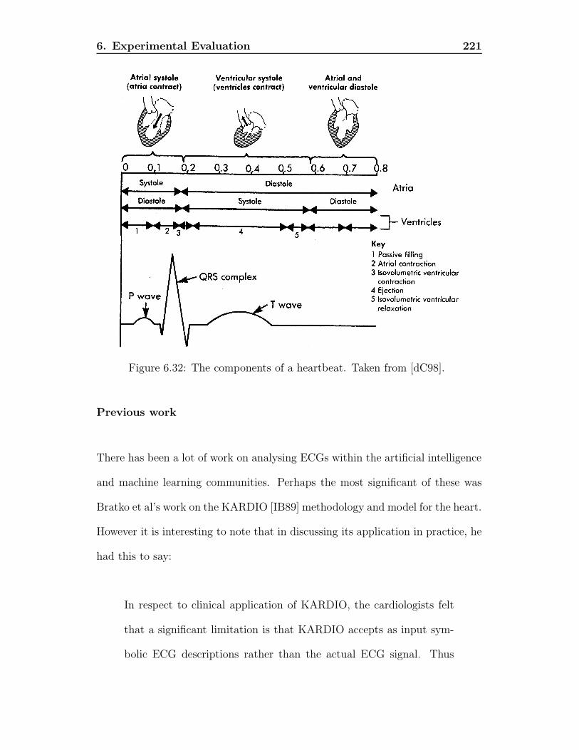
6. Experimental Evaluation 221
Figure 6.32: The components of a heartbeat. Taken from [dC98].
Previous work
There has been a lot of work on analysing ECGs within the artificial intelligence
and machine learning communities. Perhaps the most significant of these was
Bratko et al’s work on the KARDIO [IB89] methodology and model for the heart.
However it is interesting to note that in discussing its application in practice, he
had this to say:
In respect to clinical application of KARDIO, the cardiologists felt
that a significant limitation is that KARDIO accepts as input sym-
bolic ECG descriptions rather than the actual ECG signal. Thus

6. Experimental Evaluation 222
the user is at present required to translate the patient’s ECG wave-
form into the corresponding symbolic descriptions. ... In presently
available ECG analysers, these difficulties [in extracting symbolic de-
scriptions] lead to unreliable recognition of some of the ECG features.
TClass provides a mechanism for overcoming this problem: it takes as input
the ECG with some basic filtering applied. Further, KARDIO was developed to
diagnose Type B problems; whereas in this chapter we tackle the harder Type
A classification problem.
Our dataset was a random selection of 500 recordings from the full CSE di-
agnostic database [WALA+90]. This dataset was also explored by de Chazal
[dC98]. The records come from men and women with an average age 52 ± 13
years. The sample rate was 500Hz. There were seven possible classes: nor-
mal (NOR), left ventricular hypertrophy (LVH), right ventricular hypertrophy
(RVH), biventricular hypertrophy (BVH), acute myocardial infarction (AMI),
inferior myocardial infarction and (IMI) and combined myocardial infarction
(MIX). The classes are not evenly distributed, with the class distribution shown
in Table 6.16. The class labels were determined independently through medical
means (e.g. surgery after the ECGs were recorded), so the class labels can be
assumed to be free of noise.
Each recording consists of 15 channels. These include the three Frank leads
that provide a 3D representation of the heart: X, Y and Z, but also include the
raw sensors V1 through to V6 as well as aVF, aVR and aVL. Figure 6.33 shows

6. Experimental Evaluation 223
Class NumberNOR 155LVH 73RVH 21BVH 25AMI 75IMI 106MIX 31
Table 6.16: Class distribution for the ECG learning task.
the data as it reaches the TClass learning algorithm, after some preprocessing
steps, which we discuss below.
The focus of de Chazal’s thesis was the manual construction of a set of fea-
tures for classification of Frank Lead electrocardiogram. As part of this project,
he also created software for filtering the ECG signals to get rid of noise, and also
software for automatically segmenting an ECG recording into beats.
The filter design can be found on page 48 of his thesis. It is mainly designed
to exclude “baseline wander” due to the patient’s respiration at about 0.5Hz,
and mains electricity at 50Hz. The effects of the filter are shown in Figure 6.34
on the three orthogonal leads (X, Y and Z) over a sequence of heartbeats. For
ease of comparison, we used the same filter as de Chazal.
We also used the de Chazal’s segmentation of the ECG recordings into indi-
vidual beats. A typical ECG recording consists of several beats. These heart-
beats must be segmented into individual heartbeats so that learning can take
place. For our data, the ECGs are segmented according to the Q wave onset
time.

6. Experimental Evaluation 224
Figure 6.33: The ECG data as it arrives when seen by TClass.
de Chazal’s feature
The features extracted by de Chazal concentrate on the X, Y, and Z axes. They
fall into three main categories:
• Scalar lead features: These include measurements of heights, angles,
time durations and areas relating to the QRS complex of the wave. For

6. Experimental Evaluation 225
Figure 6.34: The effect of applying de Chazal’s filter to the ECG data (takenfrom [dC98]).
example, they include scalar measurements of the heights of the QRS com-
plex at 8 points – very similar to our naive segmentation. They also include
measurements of times, and areas underneath the QRS complex.
• Loop features: The heart’s beating can be characterised as a loop in the
3D space made by the X, Y and Z axes. Various characteristics of this loop
can be captured, such as its axis, its plane, the deviation from planarity
and so on.
• Global features: These included the age and the sex of the patient.
Other features were ratios and differences between other features. Some
of these features were extracted from the ECG literature, while others were
developed within the Biomedical Systems Laboratory at the University of New

6. Experimental Evaluation 226
South Wales. In total, 229 features were generated. In many cases, this includes
both sines and cosines of angles to make presentation to the learning system
simpler.
In de Chazal’s work, a variety of learners were applied. The two main families
examined were voted softmax neural networks and C5.0. He also employed a
number of feature selection techniques.
The best accuracy value of 71.3 per cent (28.7 per cent error) was obtained by
using 100 voted softmax-neural networks, each with different initial conditions
applied to all features. These results compare extremely well with median values
for human cardiologists of 70.3 per cent (a human panel obtained approximately
74.8 per cent accuracy).
However, there are some issues with de Chazal’s work. Firstly, because neural
networks were used (and in particular, 100 voted neural networks) the results
are not very comprehensible. Clearly it would be desirable, especially from
a medico-legal standpoint, for explanations for classifications of ECGs to be
given. Secondly, de Chazal, from his work obviously a brilliant and dedicated
PhD student, building on decades of research, spent at least 3 years developing
software for extracting features. In other domains, such background knowledge
may not be available.

6. Experimental Evaluation 227
Experimental results
In his thesis, de Chazal took each of the ECGs with its heartbeats, and selected
what is termed the “dominant” heartbeat. The dominant heartbeat is the one
that is the most free of noise. Each ECG consisted of between 4 and 16 heart-
beats, with an average of approximately 8. Typically, the dominant heartbeat
was the 6th heartbeat; however, domain experts analysed each example to see
if they were “typical” examples of the beat. This of course, requires domain
knowledge.
For comparison with de Chazal’s, we used the same dominant beats as he
did for our first group of experiments.
It is interesting to note that these data files are much larger than a typical
instance in a propositional problem: each training instances was between 20
kilobytes and 84 kilobytes, with the average being 47 kilobytes. Even considering
just dominant beats, then that is still approximately 24 megabytes of raw data.
Each dominant beat was extracted and labelled by the class. Using 10-fold
cross validation (as de Chazal did), we used TClass to learn all 7 classes. The
results of the experiments are shown in Table 6.17. For TClass we used both
relative time and height because this makes more sense in this domain: The
amplitudes depend greatly on the peculiarities of the ECG electrodes; and the
beats of the heart vary greatly in duration.
The results in Table 6.17 seems to be very close between TClass and the

6. Experimental Evaluation 228
Approach ErrorTClass with J48 51.4 ± 2.0
TClass with PART 45.2 ± 3.0TClass with IB1 52.4 ± 3.1TClass with NB 36.6 ± 2.2TClass with Bag 39.0 ± 2.6TClass with AB 35.4 ± 3.8
Naive Segmentation 34.2 ± 2.7Hidden Markov Model 34.4 ± 2.0
de Chazal 28.6 ± 2.4Human expert 29.7Human panel 25.2
Table 6.17: Error rates for the ECG data (dominant beats only)
baseline learners. However, it does not compare well with de Chazal’s work, or
even human experts. The results for human cardiologists are shown from de
Chazal’s thesis. The cardiologists were asked to classify the same database. The
“Human expert” result is the median value for a single expert and the “Human
panel” for a voted panel of experts. Note that we are learning based on a small
training set of only 500 examples (or in fact, 450 examples once we take into
account cross validation); and if we were given more data we may very well
perform better.
As before, we can improve the results of TClass by using multiple runs and
then voting them. Figure 6.35 shows the result of such a voting scheme on
accuracy. Although this shows some improvement, it is still not competitive
with de Chazal’s work. Perhaps this is not unexpected; given the amount of
work de Chazal put in to feature extraction.
However, there is another way to improve accuracy: As mentioned before,

6. Experimental Evaluation 229
24
26
28
30
32
34
36
0 2 4 6 8 10 12
Err
or (
%)
Number of Voters
Improving error rate using multiple TClass runs
TClass/ABde Chazal
Human expertHuman panel
Figure 6.35: Voting TClass learners improves accuracy.
each ECG recording consists of multiple beats, with an average of 8 beats per
recording. Unfortunately, these other beats do not represent “good” data for the
following reasons:
• They are likely to very strongly correlated with other beats from the same
recording – so it is not really new data in some sense. What is more, we’ll
be multiplying the data by a factor of 8, which will consequently have an
impact on performance and time consumed.
• Some instances have more examples than others, so we may be “biasing”
the learning to people with faster heartbeats (since they will have more
heartbeats recorded).

6. Experimental Evaluation 230
Approach Error Reduced eventsTClass with J48 51.4 ± 2.0 50.2 ± 2.5
TClass with PART 45.2 ± 3.0 46.6 ± 2.2TClass with IB1 52.4 ± 3.1 52.6 ± 2.0TClass with Bag 39.0 ± 2.6 35.4 ± 3.3TClass with AB 35.4 ± 3.8 37.4 ± 2.4
Table 6.18: Effect of only allowing “wide” maxima and minima on dominantbeats. There is not a significant difference in terms of accuracy.
• The data has not been “vetted” by domain experts as typical heartbeats.
Hence our algorithm will have to be robust to noise and able to cope with
biases in the input data, as well as able to cope with large amounts of data. In
fact, using this approach will use approximately 200 megabytes of input data.
TClass was able to cope with this amount of data, even on a computer with
only 512 megabytes of RAM. It necessitated setting some of the parameters for
the feature extractors to not produce superfluous events – e.g. tiny maxima and
minima of no importance to classification. Tests were run to compare the effect
on accuracy and TClass’s function was not affected by having stricter constraints
that only picked up minima that were a certain width. The results are shown in
Table 6.18 for the dominant beats only.
One other observation is that the results can easily be voted across all the
heartbeats in the test set. Also note that this is applicable not just to the TClass
methods but to naive segmentation and hidden Markov models as well.
Table 6.19 shows how this worked in practice.
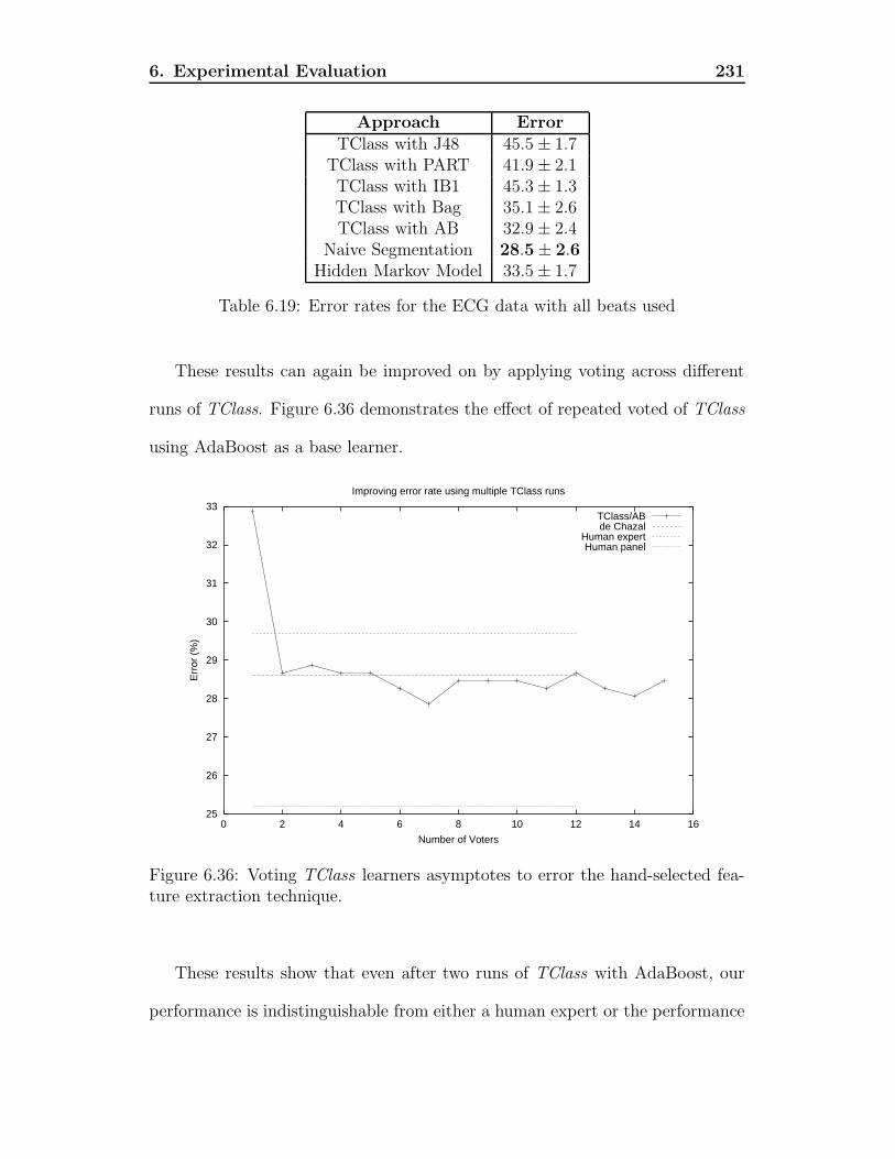
6. Experimental Evaluation 231
Approach ErrorTClass with J48 45.5 ± 1.7
TClass with PART 41.9 ± 2.1TClass with IB1 45.3 ± 1.3TClass with Bag 35.1 ± 2.6TClass with AB 32.9 ± 2.4
Naive Segmentation 28.5 ± 2.6Hidden Markov Model 33.5 ± 1.7
Table 6.19: Error rates for the ECG data with all beats used
These results can again be improved on by applying voting across different
runs of TClass. Figure 6.36 demonstrates the effect of repeated voted of TClass
using AdaBoost as a base learner.
25
26
27
28
29
30
31
32
33
0 2 4 6 8 10 12 14 16
Err
or (
%)
Number of Voters
Improving error rate using multiple TClass runs
TClass/ABde Chazal
Human expertHuman panel
Figure 6.36: Voting TClass learners asymptotes to error the hand-selected fea-ture extraction technique.
These results show that even after two runs of TClass with AdaBoost, our
performance is indistinguishable from either a human expert or the performance

6. Experimental Evaluation 232
that de Chazal achieved. With minimal background knowledge about the do-
main, we are able to achieve equivalent accuracy results to someone who used
years of domain knowledge to prepare an appropriate set of features.
Comprehensibility
We suspected that part of the cause of the lacklustre accuracy performance of
TClass was the issue of pruning with such a large dataset. Hence we investigated
by setting the minimum number of instances (m) at each leaf. For example, we
tried m = 42. For the PART learner, the error rate actually decreased slightly
to 40.5 per cent, while the average number of rules was reduced from 94 rules to
24 rules. A set of 24 rules for recognising ECGs with a 40.5 per cent error rate,
when a human expert has a 30 per cent error rate is quite an accomplishment.
Still, it is hard to study the comprehensibility of such rules. Hence we used
the binary classification rules approach as used on the Auslan datasets to see
if there were any intelligent concepts that could be deduced. The results are
shown in Figure 6.37.
To gain some insight as to whether this was a useful rule, it was compared
with the rules used by a commercial ECG classifier based on an expert system
[A97]10. The definitions produced shows the same characteristics as the defini-
tions produced in this manner for the Auslan domains: the first few rules provide
10Unfortunately, companies are unwilling to disclose the exact performance of their systemsfor direct comparison.

6. Experimental Evaluation 233
PART decision list
------------------
IF aVL HAS LocalMin: time = 0.49 val = -43.53 (*1) AND
IF x HAS NO LocalMin: time = 0.11 val = -1103.50 (*2) AND
IF V1 HAS NO Plateau: midTime = 0.55 avg = -2.38 d = 0.07 (*3)
THEN not-RVH (3727.0/32.0)
aVL-max > 554.61: not-RVH (92.0)
x-min <= -212.28 AND
IF aVL HAS LocalMax: time = 0.54 val = 45.15 (*4) AND
IF z HAS LocalMax: time = 0.42 val = 269.06 (*5)
THEN RVH (82.0/3.0)
x-min <= -221.53 AND
V1-max <= 317.57 AND
IF z HAS LocalMin: time = 0.45 val = -24.93 (*6)
THEN RVH (67.0/31.0)
V1-max <= 352.09: not-RVH (108.0/4.0)
: RVH (62.0/14.0)
Number of Rules : 6
Figure 6.37: A two way classifier for the RVH class in the ECG domain.
a “first cut” exclusion. The third rule looks for a very low minimum on the X
value. This is because patients with RVH have a depression in the S wave [A97],
leading to a very large minimum x value. In de Chazal’s work [dC98] (page 179),
he found that the minimum x value is the most discriminant feature based on
rank-correlation analysis. The other criteria look for local maxima in the aVL
and Z channels that are unique to right ventricular hypertrophy cases: the T
wave is biphasic, i.e. rather than having a single maximum, it has two maxima;
while most normal heartbeats will have one maximum occurring slightly later
(around time 0.7) [A97].

6. Experimental Evaluation 234
Event index
-----------
*1: lmin
time=0.49 r=[0.01,0.60]
value=-43.53 r=[-337.57,21.89]
*2: lmin
time=0.11 r=[0.02,0.51]
value=-1103.50 r=[-2877.34,-595.36]
*3: plat
midtime=0.55 r=[0.06,0.99]
avg=-2.38 r=[-1491.40,190.67]
duration=0.07 r=[0.01,0.35]
*4: lmax
time=0.54 r=[0.01,0.73]
value=45.15 r=[12.82,286.97]
*5: lmax
time=0.42 r=[0.02,0.65]
value=269.06 r=[62.69,3244.42]
*6: lmin
time=0.45 r=[0.3,0.60]
value=-24.93 r=[-296.24,42.04]
Figure 6.38: Events referenced by Figure 6.37.
6. Experimental Evaluation 235
ECG conclusions
Our accuracy results are competitive with a median human cardiologist; and also
competitive to a learner trained on the same dataset, but with the application
of copious quantities of background knowledge. Given that we did not use any
background knowledge, the results are good. As for comprehensibility, our sys-
tem might be an appropriate “first cut” classifier that with just 24 rules obtains
60 per cent accuracy. Further investigations of individual classifiers shows some
correspondence to rules found in commercial ECG classifiers and also show some
correspondence to findings by de Chazal.
6.4 Conclusions
TClass has proved to be an effective learner in terms of accuracy if one is willing
to use a voting mechanism. In every domain, voting different learners allowed it
to exceed the performance of our baseline learners. Furthermore, on the two real-
world domains, it proved competitive even with hand-selected domain-specific
features. This is a somewhat surprising result.
However, clearly voting leads to a destruction of the readability of the clas-
sifier. This is a definite problem with the current implementation of TClass.
However, the definitions it produces, while not as accurate as those created by
voting, are still very informative. In the artificial domains, we saw that the in-
duced concepts corresponded closely to the correct concepts. Similarly, in the

6. Experimental Evaluation 236
real-world domains, correlations between known concept descriptions and the
induced concept descriptions are visible. However, as noise is increased, the
readability of the induced rules is reduced.
There is a question as to which kinds of domains and problems TClass is
suited to. Results show that TClass performs better, even without voting, in
the following situations:
• Where there is little noise in the signal. This was particularly revealed
in the TTest artificial domain, in Figure 6.18. This diagram showns that
TClass’ performance is much better than the baseline learners at low noise
levels, but as the noise level becomes very great, the baseline learners like
Naive Segmentation and Hidden Markov Models perform better.
• Where there are fewer training instances. This was particularly shown in
6.20,, where TClass outperformed other classifiers when there were fewer
training instances.

Chapter 7
Future Work
There is much more work to do in temporal classification. In this chapter, we
examine two approaches to improving temporal classification: firstly, extending
TClass, and secondly, looking at other possible approaches encountered in the
development of TClass.
7.1 Work on extending TClass
TClass presents an interesting platform for future work. The current work has
explored some parameters and options, but it has barely scratched the surface.
Furthermore, this work has revealed certain problems with TClass that need to
be addressed. Some of the most important are discussed below.
237

7. Future Work 238
7.1.1 Improving directed segmentation
Improving the directed segmentation would be the most straightforward and
beneficial way to improve performance.
The indications are clear that the random search used for directed segmenta-
tion is suboptimal. The most obvious of these is the huge difference in accuracy
between TClass when producing individual classifiers and when producing a
voting ensemble. The fact that repeated executions of random segmentation im-
prove accuracy dramatically indicate that the random segmentation algorithm
could choose synthetic events better.
Here we make several suggestions for improving directed segmentation.
Issues with region description
A side effect of region segmentation is that all regions are accepted as synthetic
features. Consider Figure A.3. Consider now if one centroid c1 is placed at (5,
0.35), c2 at (10, 0.1) and c3 at (40,-0.1).
It is clear that the centroids c1 and c2 make good synthetic features. But c3,
although important for a good segmentation (indeed, it is necessary to define
the concept boundaries), does not itself make a useful synthetic feature. This is
because the region around c3 contains a mix of instances from different clases,
hence its usefulness as a discriminative attribute is not likely to be high. How-

7. Future Work 239
ever, without c3, all of the points formerly considered as associated with c3 would
now be associated with c2, including the mixed class area of centred around (40,
-0.1). This would make c2 a less useful discriminative features. Hence, c3 is use-
ful overall for providing a highly discriminative features – in particular making
c2 more discriminative – but c3 itself is not a discriminative feature.
If the learner we are using were smart enough, this synthetic feature should
be eliminated. Quinlan points out [Qui93] that the more attributes that are
given to the learner, the greater the probability that amongst them there will
be one attribute that performs highly on the train data but poorly on the test
data. Hence, if we can remove c3 before it gets to the learner, it would likely
improve our classification performance. Using fewer features may also aid in the
production of more comprehensible rules, since it would likely lead to shallower
trees.
Improving the directed segmentation search
Perhaps some kind of hill-climbing or genetic algorithm may function to improve
the search.
Improving by Direct Feedback from the Learner
So far, we have used a disparity measure to evaluate the “goodness” of a par-
ticular region segmentation. This disparity measure is really a low-computation

7. Future Work 240
proxy for the learner, built on the assumption that what has a high disparity
measure will be useful to the learner. Realising this leads to an obvious conclu-
sion: if the disparity measure is a proxy for the learner, then why not use the
learner itself to evaluate the effectiveness of a region segmentation directly? This
suggests that rather than our random search algorithm, we modify it so that it
(a) the disparity measure is the cross-validated accuracy (hence, the higher the
accuracy, the higher the disparity measure) (b) the most accurate subset of fea-
tures is selected. This would lead to the improved algorithm shown in Figure
7.1. Here we have used the Attribute function defined in Figure 5.5. Also, we
assume that a learner’s accuracy can be evaluated using the method crossValAcc
which takes a learner and a dataset and returns the cross-validated accuracy.
The algorithm in Figure 7.1 uses the learner to evaluate the real performance.
Some difficulties arise, however: Firstly, the whole point of using the disparity
measure was speed – it would be too slow to evaluate each region segmentation
this way. For example, consider the new Auslan dataset. There are approx-
imately 110 metafeatures. Let us assume we use 10-fold cross-validation with
numTrials = 1000. Then this would require us to run a learner 110×10×1000 =
1.1 × 10⁶. Even assuming that each learner takes an average of 0.1 seconds to
generate a classifier, then this would still take well over a day to execute.
Secondly, we are actually testing the performance of each metafeature in
isolation. As pointed out in Section 5.2.2, the results of the execution of the
random search algorithms are all combined to form a single feature vector. While
a particular segmentation may work well if it is the only set of synthetic features,

7. Future Work 241
Inputs:I = [〈[i11, ..., i1m1
], l1〉, ..., 〈[in1, ..., inmn], ln〉]
(Feature-extracted training data)N = {nmin, ..., nmax} (Appropriate range of clusters)Learner(PropData) (What learner to use)numTrials (number of trials to attempt)mem(Centroid , Instances)
(Membership function we are using)Outputs:
C = {c1, ..., cn} (cluster centroids)procedure RandSearch2
/* First we must “flatten” input data. */D := {}For each 〈P, l〉 in I
For each p in Pappend(D, 〈p, l〉)
EndEndbestMeasure := 0bestCentroids := {}for i := 1 to numTrials
r := randBetween(nmin, nmax)currentC := randSubset(r, D)/* Turn the data into propositional form */E := Attribute(I , currentC ,mem)/* Find the cross-validated accuracy of the learner */currentMetric := crossValAcc(Learner, E)if(currentMetric > bestMetric)
bestMetric := currentMetricbestCentroids := currentC
EndEnd
C := bestCentroidsreturn CEnd
Figure 7.1: Random search algorithm, using the learner itself

7. Future Work 242
it may be of no use when it is combined with the segmentation of other regions.
Similarly, it may be that a set of synthetic features are only useful in combination
with another set. Hence, even using the learner itself is only an approximation
of how useful it would be in the end. And if it is an approximation, then what
it the guarantee that cross-validated accuracy using the learner is any better a
disparity measure than chi-squared or the gain ratio?
This idea has certain similarities to the “wrapper” method suggested by John,
Kohavi and Pfleger [JKP94] for handling the feature selection issue, and indeed
we are using a kind of wrapper, albeit in a very different way.
But what about speed? This too can be addressed. Firstly, it may not be
necessary to run the same number of trials as when using the disparity measure.
Secondly, it may be possible to use a hybrid approach, taking advantage of
both disparity measures and cross-validation accuracy. This could be done, for
instance, by using a disparity measure to “short list” the region segmentations
with the highest disparity measures (say the top 20) and then the learner’s cross-
validated accuracy is used to choose the best among these 20 instances.
Using learners for region segmentation
One way to look at the region segmentation problem is as a learning task: to
classify the areas of the parameter space that have more of one class than the
other. Hence one obvious way to segment the region is to use a segmenter that
subdivides the parameter space appropriately.

7. Future Work 243
One obvious learner that would do this is an axis-orthogonal decision tree
builder, like C4.5 or J48. However, it is unlikely that we would want to use
the full depth of the tree: this would generate as many regions as there are leaf
nodes. However, if we were to enforce some heavy pruning regime (for example,
requiring that no leaf node contain less than 5 per cent of the instances), this
would essentially segment the parameter space into hypercubes; each represent-
ing region. Hence, rather than a Voronoi tiling applying, instances would be
evaluated as to their presence in different regions of the parameter space.
This would require some other minor changes to the algorithm; for instance,
the region membership. Furthermore, making the definitions comprehensible
would require some work – one alternative is simply to give the description of
the hypercube, but this may be inappropriate or not provide enough information
into what is actually happening.
7.1.2 Automatic metafeatures
Is there some way, by observing the data, to automatically make educated guesses
at what the appropriate metafeatures are? This is a difficult question, and it is
the temporal classification equivalent of constructive induction in inductive logic
programming – something of a holy grail. It may be possible, however it looks
extremely difficult.
However, there are alternatives. For instance, it may be possible to have a

7. Future Work 244
good-sized library of metafeatures, and, given a new domain, somehow work out
which are the appropriate metafeatures for it.
7.1.3 Extending applications of metafeatures
The scope of use of metafeatures is huge. The technique looks like it is gener-
alisable to areas such as spatial analysis, image processing, basket analysis and
more. The problem is finding the appropriate metafeatures and actually doing
the experiments to see if it does work.
7.1.4 Strong Temporal Classification
Although in Chapters 1 and 2 we proposed the strong temporal classification
task, the focus in this thesis has been on weak temporal classification. Since we
don’t know how to do weak temporal classification in a symbolic, comprehensible
way, it was felt it was a more fundamental issue.
Extending the metafeatures approach to do strong temporal classification
would be worthwhile, but it is probably another thesis of work. However, there
are some simple and obvious things that can be done to make inroads into
the problem. One potential approach to the problem is a “weak train, strong
test” approach. This would be based on the “pre-segmented TC” approach
discussed in Section 2.3.3. TClass would be trained on pre-segmented instances.
However, when it came to testing, a “window” of the data observed so far could

7. Future Work 245
be used to see if it matches any of the learnt classes. We then “slide” the window
forward and repeat the process to get a sequence of classifications. By using some
kind of voting mechanism, it might be possible to actually do strong temporal
classification.
7.1.5 Speed and Space
The implementation of TClass was inherently experimental. There are signifi-
cant optimisations possible. For example, feature extraction need only be done
once and can be stored for reuse. It could be reimplemented in a faster language
(eg. C++) and take advantage of certain data redundancies and repeated cal-
culations. In particular, many data structures are non-contiguous in memory
in the current implementation. By reorganising the data structures in memory
to lead to greater contiguity and hence better memory locality it is likely that
performance will improve significantly.
7.1.6 Downsampling
When presented with data, it is frequently presented at a high data rate. For
example, sign language information about the hand might be received at 200
frames per second. Hence an average 2 second sign might be 400 frames long.
Similarly, with ECG data, the electrical signals may be sample at 500 frames per
second (sometimes also described as 500 Hertz); hence an individual heartbeat
7. Future Work 246
consists of 400 to 700 samples (corresponding to heart rates between 70 beats
per minute and 50 beats per minute). This can be a huge amount of data to
consider.
Therefore, the data could be resampled at a lower frequency – commonly
called downsampling1. Under certain circumstances, this may not adversely
affect the learning and classification performance and simultaneously reducing
feature extraction time. For example, say we were examining the sign language
data at 200 frames per second. We could take every two consecutive samples
from the original data for each channel, average them, and for each two frames in
the input, the output would have only one frame. In this case we are applying a
downsampling factor of two: the data is reduced in size by a factor of 2. Hence, a
400 frame sample would be reduced to a 200 frame sample – halving the amount
of data that must be dealt with. Similarly, a downsampling factor of 4 would
reduce the data to one quarter of its original size2.
Of course, this works well for continuous attributes, but not so well for dis-
crete attributes. For discrete attributes, other methods can be employed, such
as voting.
1There is also the case of upsampling, but it is is of little use to us in this context.2Note that the downsampling factor, strictly speaking, need not be an integer. If it is not
integral, a weighted average must be taken of the points that are shared. For instance, with adownsampling factor of 1.5, each point in the output would average one whole value plus halfof the next or prior value.

7. Future Work 247
7.1.7 Feature subset selection
Another way to improve the accuracy and comprehensibility that has been ex-
plored in machine learning is the use of feature subset selection. Sometimes,
using all the features available has a detrimental effect on accuracy when com-
pared to using some subset of the features. This is because some features are
dependent on other features – and hence, there is no need to include the feature
– or are noisy. Furthermore, the more features there are, the more likely that
some feature will randomly fit the data and hence the probability of overfitting
increases. Thus removing these features would lead to both improved accuracy,
and clearer descriptions of learnt concepts, since there are less features that the
user has to deal with. Furthermore, since we are generating many hundreds of
features, many of which are likely to be irrelevant, we would expect to benefit
from finding some optimal subset of features.
However, there is a problem: feature subset selection is a difficult problem.
If there are n features, then there are 2n possible feature subsets. Searching this
space for a “good” set of features can be extremely time-consuming. There are
two possible approaches to feature subset selection: the wrapper approach and
the filter approach [JKP94]. In the wrapper approach, the learner is applied
to subsets of features and tested on an hold-out set (or, if execution time is
not an issue, using cross-validation). From the results of these tests, a good
subset of features is selected. For example, for forward selection, a classifier is
built for each feature individually; and the most accurate feature is “accepted”

7. Future Work 248
into the subset of good features. That feature is removed, and the process is
repeated, adding each of the remaining features and evaluating its performance.
The “best” set of two features is thus created. This proceeds incrementally until
a feature set with maximal accuracy is achieved. Similarly, backward selection
proceeds by eliminating one feature at a time, finding the least beneficial feature
and eliminating it, and repeating the process, eliminating the least accurate
features until eliminating further features decreases accuracy.
The other approach to feature subset selection is the “filter” approach, which
looks at correlations between features and other performance measures to decide
a priori, independent of any particular learner, what a good subset of features is.
Although such techniques do not perform nearly as well as the wrapper approach,
they are much faster. In general, if there are n features, the wrapper approach
requires O(n2) runs of the learner, whereas the filter approach requires only one
run of the learner and some simple statistics on the dataset to be calculated.
7.2 Alternative approaches
In developing TClass, some other approaches were also explored, with some
preliminary experiments. We present some of the more interesting approaches
here. The interested reader may also wish to read Appendix A to understand
the development of TClass itself.

7. Future Work 249
7.2.1 Signal Matching
At its core, the problem of classifying temporal signals lay in finding segments
of temporal signals that recur. These segments could then be used to construct
grammars or build classifiers in some way. In other words, the core of the problem
is developing an intuition of what makes two temporal signals similar and what
makes them different.
Hence, if temporal signals could be “matched” against one another in some
way to work out parts of the signal that were similar, this could be used in some
way for classification purposes.
How can one compare whole signals with one another while looking for pat-
terns? For the moment, let us consider a single channel of data. Two such
channels can be compared by creating a 2D image. Each pixel of the 2D image
represents the difference between signals at that timepoint. In other words, let
x[t] and y[t] be two signals that we are trying to compare. Let lx and ly be the
length of each of the two. Then for each pixel aij of the image, let its intensity
be determined by |x[i]− y[j]|. This will result in an image – which we will term
the signal match image – or SMI for short.
This image is useful for a number of purposes; for instance we could use it
to implement a dynamic time warping algorithm by looking at which path from
the top right to the bottom left accumulates the least “black”; in other words,
accumulates the least distance. But it is also useful in other ways. Anything that

7. Future Work 250
has low difference along a top right to lower left diagonal indicates similarity.
Figure 7.2: The SMI of the z channel of one instance of building with itself.
Figure 7.2 shows what happens when an SMI is created for a signal with
itself. In this particular case, it is they z value from the Auslan sign building.
In this case, black is used to represent the largest observed difference, and white
is used for zero difference. Along the diagonal the signal is of course white, since
the difference between the signal and itself is zero.
Figure 7.3 shows an instance of building as against an instance of make. As

7. Future Work 251
can be seen, the instances are quite similar, and hence indicates that perhaps
the z value is not a good feature to look at for telling signs like building and
make apart.
Figure 7.3: The SMI of the z channel of an instance of building and an instanceof make.
At the same time as this work was being looked at, many people in the image
processing world were encountering mathematical morphology, a means of image
processing ideally suited to the purposes of extracting lines from such images.
One way to thing of mathematical morphology is to think of each intensity point
as a height, where in our case, white corresponds areas of low altitude and black
to high. By modelling the flow of water in such a situation, it is easy to work
out what the “valleys” are; and hence the parts of each signal that are common.

7. Future Work 252
One approach to classification is to to extract typical sub-events correspond-
ing to near-diagonal near-white lines, and then use these labelled sub-events to
develop a grammar for each class.
7.2.2 Approximate string-matching approaches
Approximate string matching is an active area of research. In approximate string
matching, one is given an text and a target. The objective is to find a string
within the text that is similar to the target. Similarity is usually defined using
the Levenshtein distance defined in Section 2.4.2.
Hence one approach to classification of temporal signals is to convert each
frame into a character. Approaches such as the vector quantisation approach
discussed in Section 3.2.1 could be used. Once converted, approximate string
matching techniques could be used to extract discriminative string sequences.
However, the act of finding recurring approximate strings in a text and evalu-
ating whether that is of any practical use for classification is not a well-developed
area of research.
We explored techniques for finding recurring strings in a situation where the
grammar is known. Techniques can be quite easily employed for doing so. For
example, one can employ a minimum-message length approach to find recurring
strings. Hence we implemented a simple algorithm based on the MML that
looked at texts and isolate strings that recurred with sufficient frequency to sug-

7. Future Work 253
gest they may have been useful as primitives on which to construct a grammar.
As an initial exploration of such techniques we looked at string constructed
from the phonetic alphabet. The phonetic alphabet is used to overcome the pho-
netic ambiguity of spoken letters. Each letter of the English alphabet is allocated
a word that begins with that letter. For instance “alpha” denotes A, “bravo”
denotes B, “charlie” denotes C and so on. Let us say that we did not know
the phonetic alphabet; but that we had been listening to people pronouncing
phonetic alphabet sequences like “alphabravocharlie”, “bravobravoalpha” (ABC
and BBA respectively). Our objective was to see if we could by analysis isolate
the original sequences for each letter without making use of any of the informa-
tion about what the sequence of alphabet letters corresponding to each phonetic
string was.
We found that we could do this. However, we then tried to extend this to
another practical domain: Morse code. In Morse code, each letter of the alphabet
can be represented as a binary sequence of ones and zeros. Our performance on
this particular domain proved to be much worse. This may have been because
Morse code was always designed to be as compressed and efficient as possible
due to its historical use for telegraphic communications, whereas the phonetic
alphabet is designed for redundancy.
It appears that this approach could be revisited. In view of the shift of
approach to a more weak temporal classification system, a two-level approach
might be possible:

7. Future Work 254
1. Find the n most commonly recurring strings in the data; within a certain
edit distance of each other.
2. As with its application in directed segmentation, use a chi-squared distri-
bution to try to find recurring strings that help discriminate between one
class and another.
This was the first attempt to look at recurring strings. Further research
uncovered a whole area of study related to the location and search of recurring
strings based on a data structure called a subword tree [AG85]3. Given a string,
the subword tree of the string can be used to quickly search the string for any
substrings. A formal description is beyond the scope of this work, but perhaps
an example will serve us best. Consider the string abracadabra. The subword
tree for abracadabra is shown in Figure 7.4. In the diagram, nodes of the form
c=2 mean that the node has two leaf nodes among its children, and nodes of
the form p=1 mean that there is a subword beginning at position 1 (the first
character is position 0). The end of the string is marked by “$”.
We can use the tree in the following ways. Consider if we wish to match the
substring cad. We begin at the root node. The first character is matched against
the c and we hit a leaf node with p=4. This means that it is possible that if I
look at position 4 onwards, I might find a match for cad. Sure enough, there is
a match. Now consider searching for the string abr. Following the characters
down the tree, I find that I get to a node that has two children. If I follow all
3Subword trees are known by many different names. These include B-trees, position trees,prefix trees, suffix trees, subword finders etc

7. Future Work 255
Figure 7.4: The subword tree for abracadabra.
subtrees to the leaf nodes, I can determine that the the string abr occurs twice
in the string abracadabra: one beginning in position 0, and one at position 7.
This subword tree is ripe for the picking for discovering patterns within
strings. Note the number of children gives us a very quick way to estimate
the number of occurrences of any target string. If any target string occurs more
than once in the text, it will appear as a node in the subword tree. For our
purposes, the nodes (and hence substrings) that would be of great interest are
the ones that are very deep in the tree, but with many child nodes. By using
this data structure, it would be possible to quickly locate good candidate strings
for recurring patterns.
As a first attempt, it was tested with finding common strings in texts. A
system was developed which could read whole files, parse them, produce the
subword tree and prune it4. This picked out interesting patterns, e.g. common
4Note that Figure 7.4 displays a lot of redundancy. For example, the whole subtree begin-

7. Future Work 256
recurring syllables in English language (if that was what was fed to it).
It was therefore hoped that this system could be extended to learning to
classify discretised time series as discussed above. Subword trees have been
applied successfully to approximate string matching, and it was the hope of
our research that the ability to do approximate string matching for locating
substrings could be turned to advantage in finding strings that approximately
recur.
However, this turned out not to be the case. Although it is possible to use
subword trees to find approximate matches, and can also be used to discover
recurring target strings; it can not (at least, to our knowledge) be used to find
approximately recurring substrings; i.e., substrings that can be recur approxi-
mately within the text.
7.2.3 Inductive Logic Programming
After the development of metafeatures, we considered using inductive logic pro-
gramming as a means of learning definitions. Inductive logic programming is a
type of machine learning where the background and domain knowledge are ex-
pressed in terms of logical predicates. In particular, each instance was presented
as a collection of logical predicates.
To do so, the following predicates were introduced. instance(X) indicated
ning with r is actually a subtree of the one beginning with ab.

7. Future Work 257
that X was a training instance. class(X) was used to denote the possible classes
of each instance. Finally a predicate called classification(X, Y) was also
defined, linking each instance with its class.
Data was provided in the form of predicates based on metafeatures, but us-
ing only the extraction functions, rather than the parameter space. For example,
there was an Increasing predicate that took the form Increasing(InstanceId,
Channel, Gradient, Average, Duration, EventId).
We also gave an extensional definition of the temporal relations between
events. Our hope was that these temporal relations could be used by the ILP
system. To begin with, we defined two relations, with plans of implementing
full Allen’s interval logic [All83]. The two relations were during(EventId1,
EventId2) and after(EventID1, EventID2).
Unfortunately, this approach did not work well for a number of reasons. FOIL
[Qui90], GOLEM [MF92] and PROGOL [Mug95] were all tested on simplified
datasets with unsuccessful results. Each did not succeed for different reasons.
The first was the size of the dataset. Even with a small number of events and
training instances, the number of generated predicates was huge – especially
that extensional definitions of temporal relations had to be generated for FOIL
and GOLEM. Secondly, these three ILP systems do not handle noise well at
all, when the detection of sub-events of time series is inherently noisy. Thirdly,
FOIL and GOLEM do not handle numerical attributes at all, and PROGOL does
not do it particularly well, requiring a discretisation stage. Fourthly, the above

7. Future Work 258
representation is not deterministic; for example, consider the after predicate.
Consider a simple sequence of events that occur in the same instance in the
order 1,2,3,4,5,6,7. Then after(2,1) is true, but so is after(3,1) and so on.
This means, for example, that if a clause is of the form after(X,1) then X can
take many values. This has dramatic consequences. For a specific-to-general
learner like GOLEM, this means that bottom clauses are going to be gigantic.
For general-to-specific learners like FOIL, this means that the search space of
possible clauses is going to be very large. Fifthly, the previous effect is worsened
by the need for clauses composed of many predicates. Even a relatively simple
temporal concept such as “channel A goes up while channel B goes down” would
require a total of 6 predicates in our representation. Most ILP systems do not
handle long clauses very well.
However, some hope for future work has been given by the work of Rodriguez
et al [RAB00]. Although the work is preliminary and makes use of highly sim-
plified versions of the same datasets we employ (for example, he deals with a
variant of the Auslan dataset provided by us but using only ten classes, and all
instances are downsampled to a fixed length of 20 samples); one of the represen-
tations he uses that turns out to function well is a “true-percentage” predicate. A
true-percentage predicate takes the form true-percentage(Instance, Channel,
TimeInterval, Min, Max, Percentage). In other words, if a channel’s value
is between Min and Max at least Percentage of the time in the TimeInterval
on the channel Channel, the predicate is true.
This predicate has the advantage of being robust to noise, since the asser-

7. Future Work 259
tions don’t have to be absolutely true – they can be true 80 per cent of the
time, for instance. Secondly, they are self-contained, removing the need for non-
deterministic expressions of predicates. However, they require a very careful and
customised definition of the search function. If one contemplates the above for
a moment, it is clear if one naively extracted all the true-percentage predi-
cates from the training instances, then very large numbers of predicates would
be generated. The net result is that Rodriguez et al have to carefully constrain
the search algorithm of the ILP in order to induce reasonable clauses. Their
results show that the true-percentage measure is of some benefit combined with
other predicates (e.g. Euclidean distance measures, etc). It is not clear whether
such techniques generalise to larger, real-world domains, but it does point to the
possibility of temporal classification using ILP.
7.2.4 Graph-based induction
Matsuda et al [MHMW00] propose graph-based induction as a model for learn-
ing. In graph-based induction, training instances are represented as graphs.
Temporal classification instances can also be represented as a graph: each
sub-event can be represented as a node and each temporal relation (such as the
during and after relations mentioned above) represented as an edge.
Graph-based induction was examined as a possibility and code provided by
ISIR at Osaka University was applied to some simple test learning examples.

7. Future Work 260
The GBI software provided works by pairwise chunking : looking for a pair of
nodes in the training instances that recur, and turning them into a single node.
The general plan for the algorithm was as follows: use the pairwise chunking
approach to find recurring subgraphs, then use tests based on the presence or
absence of the subgraphs as features.
However, problems were encountered. The first has to is one of representa-
tion: In graph theory a distinction is made between uncoloured graphs (where
nodes are unmarked – each node has the same “colour”) and coloured graphs
(where nodes are marked in some way – some nodes have the same “colour” while
others may have a different colour). In general, induction on coloured graphs is
more complex. If we are to represent temporal events of different types (such
as increasing, decreasing, local maxima, etc), then the colours can be associated
with the different types of events. If we use the type of event as the sole indi-
cation of colour, this means that all Increasing events will be treated the same.
This means a slow increase or a fast increase, a high increase or a low increase
will all be treated the same by the algorithm. Hence the synthetic events were
generated as for TClass and each event was coloured by the synthetic event that
most closely corresponded to it.
The second problem encountered had to do with the edges. Consider once
again, the after(ev1, ev2) temporal relation. On average, half of events are
going to occur after the other events. This means that if we want to represent
the after relation, we are going to generate a very dense graph: one where

7. Future Work 261
approximately half the maximum possible edges are present. In general, this
will lead to O(e2) edges, where e is the number of events for each instance. This
led to the algorithm being slow.
The third problem is that there were many frequent pairwise chunks that
were found that proved not to be useful in discriminating between classes. The
pairwise chunking algorithm employed does not use class information, and it is
not clear how to modify it to do so. This meant that the creation of useful
subgraphs for feature extraction did not work very well.
7.3 Conclusions
TClass and temporal classification have a long way to go. Ideas for extending
and approaching both problems have been reviewed in this chapter.

Chapter 8
Conclusion
This thesis implements the first general, accurate, comprehensible, robust, weak
temporal classifier. While other systems have implemented some of these char-
acteristics, this is the first to capture all of them.
It is a general algorithm that has been applied to two real-world and two arti-
ficial domains, one of which was specifically designed to model the characteristics
of real-world domains. It has been tested on situations with up to 22 channels,
110 metafeatures, over 200 megabytes of data, 95 classes and highly skewed class
distributions (8:1 ratio between the most common and least common classes in
the ECG domain).
It is accurate: in all of the domains tested it was able to equal or better the
two baseline algorithms, and in the case of ECG classification, performs better
than a single human expert: Our system obtains 71.5 per cent accuracy versus
262

8. Conclusion 263
a human expert with 70.3 per cent accuracy, despite the fact that TClass learnt
with only 450 examples, including one class with only 21 examples. In the Auslan
domain, it obtains an accuracy of approximately 98 per cent. Considering that
there are 95 signs in the Flock Auslan domain, and the default accuracy would
be approximately 1 per cent, this is no easy feat. Furthermore, it matched the
performance of hand-crafted feature sets in both the ECG and Nintendo Auslan
domains.
It is comprehensible: metafeatures allow the expression of learnt concepts
in the background knowledge presented to the learner. Experiments show that
in artificial domains, the generating concept is recovered. In the real-world
domains, the produced concepts correspond to known definitions.
It is robust: in artificial domains, when the noise level was increased, clas-
sification was still possible. With the notoriously poor quality Nintendo sign
language data, it was able to achieve accuracy equivalent to hand selected fea-
tures.
However, it is not without its flaws. TClass has the following weaknesses
presently:
• While it can be used to produce either accurate or comprehensible concepts,
it has not proved possible to do both simultaneously.
• While it is a linear time algorithm, in cases with huge data it is not par-
ticularly fast. Run times for all of the domains were reasonable, under two

8. Conclusion 264
hours in most cases on a PII-450MHz PC. However, for the ECG domain,
when all data were being learnt from, this extended to approximately 8
hours.
• It is still only a weak learner: it does not yet classify sequences of classes.
In this regard, it particularly falls behind hidden Markov models, although
it has an edge over them in terms of comprehensibility.
• While it produces readable concept descriptions in low-noise situations, it
does not do so well in high-noise situations. Noise leads to an explosion in
the size of decision trees and rules.
The problems above are not insoluble; merely beyond the scope of the cur-
rent research – some of the problems have quite obvious solutions, which were
discussed in the Chapter 7. Hopefully, TClass will serve as a useful platform for
exploring temporal classification issues.

Bibliography
[A97] Schiller Medical S. A. The Schiller ECG Measurement and Inter-
pretation Programs Physicians Guide, 1997.
[ACH+89] Kenneth R. Anderson, David E. Coleman, C. Ray Hill, Andrew P.
Jaworski, Patrick L. Love, Douglas A. Spindler, and Marwan
Simaan. Knowledge-based statistical process control. In Proceed-
ings of the First Annual Conference on Innovative Applications of
Artificial Intelligence, pages pp. 23–9. American Assoc. Artificial
Intelligence, 1989.
[AG85] Alberto Apostolico and Zvi Galil. Combinatorial Algorithms on
Words. NATO ASI Series. Springer-Verlag, 1985.
[AK00] F. Aurenhammer and R. Klein. In J. Sack and G. Urruita, Hand-
book of Computational Geometry, chapter Voronoi diagrams. Else-
vier Science, 2000.
[All83] James F. Allen. Maintaining knowledge about temporal intervals.
Communications of the ACM, 26(11):832–843, 1983.
265

BIBLIOGRAPHY 266
[And76] O. D. Anderson. Time Series Analysis and Forecasting. Butter-
worths, london edition, 1976.
[Ben96] Yoshua Bengio. Neural Networks for Speech and Sequence Recogni-
tion. International Thomson Publishing Inc., 1996.
[BJ76] G. E. P. Box and G. M. Jenkins. Time Sereis Analysis: Forecasting
and Control. Holden Day, 1976.
[BK99] Eric Bauer and Ronny Kohavi. An empirical comparison of voting
classification algorithms: Bagging, boosting and variants. Machine
Learning, 36:105–142, 1999.
[Bra65] Ron N. Bracewell. The Fourier Transform and Its Applications.
McGraw-Hill, New York, 1965.
[Bre96] Leo Breiman. Bagging predictors. Machine Learning, 24:123–140,
1996.
[CJ89] Paul Compton and R. Jansen. A philosophical basis for knowledge
acquisition. In 3rd European Knowledge Acquisition for Knowledge
Based Systems Workshop, 1989.
[CMF90] Ron Cole, Yeshwant Muthusamy, and Mark Fanty. The ISOLET
spoken letter database. Technical Report CS/E 90-004, Oregon
Graduate Institute, 1990.

BIBLIOGRAPHY 267
[CS96] Peter Cheeseman and John Stutz. Bayesian classification (auto-
class): Theory and results. In Advances in Knowledge Discovery
and Data Mining, pages 153–180. 1996.
[Dan98] Andrea Danyluk. Predicting the Future: AI Approaches to Time-
Series Problems. AAAI Press, 1998.
[DAR] DARPA. Darpa timit database. CD-ROM.
[dC98] Philip de Chazal. Automatic Classification of the Frank Lead Elec-
trocardiogram. PhD thesis, University of New South Wales, 1998.
[DLM+98] Gautam Das, King-Ip Lin, Heikki Mannila, Gopal Renganathan,
and Padhraic Smyth. Rule discovery from time series. In Proceed-
ings of the Fourth International Conference on Knowledge Discov-
ery and Data Mining (KDD-98). AAAI Press, 1998.
[DM86] T. G. Dietterich and R. S. Michalski. Machine Learning: An Arti-
ficial Intelligence Approach, Volume II, chapter Learning to predict
sequences, pages 63–106. Morgan Kaufmann, Los Altos, CA, 1986.
[FI93] Usama M. Fayyad and Keki B. Irani. Multi-interval discretization
of continuous-valued attributes for classification learning. In IJCAI-
93: Proceedings of the Thirteenth International Joint Conference on
Artificial Intelligence, pages 1022–1027. Morgan-Kaufmann, 1993.
[FM99] Yoav Freund and Liam Mason. The alternating decision tree learn-
ing algorithm. In Ivan Bratko and Saso Dzeroski, editors, Proceedins

BIBLIOGRAPHY 268
of the 16th International Conference on Machile Learning. Morgan
Kaufmann, 1999.
[FMR98] Nir Friedman, Kevin Murphy, and Stuart Russell. Learning the
structure of dynamic probabilistic networks. In Proceedings Uncer-
tainty in Artificial Intelligence Conference 1998 (UAI-98). AAAI
Press, 1998.
[Fri84] Jerome H. Friedman. A variable span smoother. Technical Report 5,
Laboratory for Computational Statistics, Department of Statistics,
Stanford University, 1984.
[Fu82] K. Fu. Syntactic pattern recognition and applications. Prentice-Hall,
1982.
[Geu01] Pierre Geurts. Pattern extraction for time series classification. In
Luc de Raadt and Arno Sieves, editors, Principles of Data Min-
ing and Knowledge Discovery, 5th European Conference, PKDD
2001, Freiburg, Germany, September 3-5, 2001, Proceedings, Lec-
ture Notes in Computer Science. Springer-Verlag, 2001.
[GRC80] G. C. Goodwin, P. J. Ramage, and P. E. Caines. Discrete time
multivariable adaptive control. IEEE Trans. Automatic Contro,
25:449–456, 1980.
[HC93] David T. Hau and Enrico W. Coiera. Learning qualitative models
of dynamic systems. Machine Learning, 26:177–211, 1993.

BIBLIOGRAPHY 269
[HHS98] Michael Harries, Kim Horn, and Claude Sammut. Extracting hid-
den context. Machine Learning, 32(2), August 1998.
[Hor93] Kim Horn. RDR-C4: A system for monotonic knowledge acquisi-
tion and maintenance employing induction in context. Technical
report, Telstra Technical Development, 1993.
[Hor01] Kurt Hornik. The R FAQ. http://www.ci.tuwien.ac.at/%7Ehornik/R/,
2001.
[HSV92] Y. C. Ho, R. S. Sreenivas, and P. Vakili. Ordinal optimization of
DEDS. Discrete Event Dynamic Systems: Theory and Applications,
2(1):61–88, 1992.
[IB89] Nada Lavrac Ivan Bratko, Igor Mozetic. KARDIO: A Study in Deep
and Qualitative Knowledge for Expert Systems. MIT Press, 1989.
[JKP94] George H. John, Ron Kohavi, and Karl Pfleger. Irrelevant features
and the subset selection problem. In Proceedings of the Interna-
tional Conference on Machile Learning 1994, pages 121–129, 1994.
[Joh89] Trevor Johnston. Auslan Dictionary: a Dictionary of the Sign Lan-
guage of the Australian Deaf Community. Deafness Resources Aus-
tralia Ltd, 1989.
[Kad95] Mohammed Waleed Kadous. GRASP: Recognition of Australian
sign language using instrumented gloves. Honours Thesis, 1995.

BIBLIOGRAPHY 270
[Kad98] Mohammed Waleed Kadous. A general architecture for supervised
classification of multivariate time series. Technical Report UNSW-
CSE-TR-9806, School of Computer Science & Engineering, Univer-
sity of New South Wales, 1998.
[Kad99] Mohammed Waleed Kadous. Learning comprehensible descriptions
of multivariate time series. In Ivan Bratko and Saso Dzeroski, edi-
tors, Machine Learning: Proceedings of the Sixteenth International
Conference (ICML ’99), pages 454–463. Morgan-Kaufmann, 1999.
[KCMP01] Eamonn J. Keogh, Kaushik Chakrabarti, Sharad Mehrotra, and
Michael J. Pazzani. Locally adaptive dimensionality reduction for
indexing large time series databases. In SIGMOD Conference, 2001.
[KM87] K. Kumar and A. Mukerjee. Temporal event conceptualization. In
Proc. of the 10th IJCAI, pages 472–475, Milan, Italy, 1987.
[KP98] Eamonn J. Keogh and Michael J. Pazzani. An enhanced represen-
tation of time series which allows fast and accurate classification,
clustering and relevance feedback. In Predicting the Future: AI
Approaches to Time-Series Problems [Dan98], pages 44–51.
[KP99] Eamonn Keogh and Michael Pazzani. Scaling up dynamic time
warping to massive datasets. In 3rd European Conference on Prin-
ciples and Practice of Knowledge Discovery in Databases, 1999.

BIBLIOGRAPHY 271
[KP01] Eamonn Keogh and Michael Pazzani. Dynamic time warping with
higher order features. In SIAM International Conference on Data
Mining, SDM 2001. SIAM, 2001.
[LD94] N. Lavrac and S. Dzeroski. Inductive Logic Programming: Tech-
niques and Applications. Ellis Horwood, 1994.
[Lev66] V. I. Levenshtein. Binary codes capable of correcting deletions,
insertions and reversals. Soviet Phys. Dokl., 6:707–701, 1966.
[LK95] Jae Kyu Lee and Hyun Soon Kim. Intelligent Systems for Finance
and Business, chapter 13. John Wiley and Sons Ltd, 1995.
[LS98] Patrick L. Love and Marwan Simaan. Automatic recognition of
primitive changes in manufacturing process signals. Pattern Recog-
nition, 21(4):pp. 333–42, 1998.
[Mal99] Stephane Mallat. A wavelet tour of signal processing. Academic
Press, 1999.
[Man97] Stefanos Manganaris. Supervised Classification with Temporal Data.
PhD thesis, Computer Science Department, School of Engineering,
Vanderbilt University, December 1997.
[MF92] S. Muggleton and C. Feng. Efficient induction of logic programs,
1992.

BIBLIOGRAPHY 272
[MHMW00] Takashi Matsuda, Tadashi Horiuchi, Hiroshi Motoda, and Takashi
Washio. Extension of graph-based induction for general graph
structured data. In PAKDD2000, pages 420–431, 2000.
[MM98] C.J. Merz and P.M. Murphy. UCI repository of machine learning
databases, 1998.
[MR81] C. S. Myers and L. R. Rabiner. A comparative study of several
dynamic time-warping algorithms for connected word recognition.
The Bell System Technical Journal, 60(7):1389–1409, September
1981.
[MT91] Kouichi Murakami and Hitomi Taguchi. Gesture recognition us-
ing recurrent neural networks. In CHI ’91 Conference Proceedings,
pages 237–242. Human Interface Laboratory, Fujitsu Laboratories,
ACM, 1991.
[MTV95] Heikki Mannila, Hannu Toivonen, and A. Inkeri Verkamo. Discov-
ering frequent episodes in sequences. In Proceedings of the First
International Conference on Knowledge Discovery and Data Min-
ing (KDD-95), pages 210–215, 1995.
[Mug95] S. Muggleton. Inverse entailment and Progol. New Generation
Computing, Special issue on Inductive Logic Programming, 13(3-
4):245–286, 1995.

BIBLIOGRAPHY 273
[OG95] C.W. Omlin and C. Lee Giles. Extraction of rules from discrete-time
recurrent neural networks. Technical Report TR 95-23, Computer
Science, Troy, N.Y., August 1995.
[OJC98] Tim Oates, David Jensen, and Paul R. Cohen. Discovering rules
for clustering and predicting asynchronous events. In Predicting
the Future: AI Approaches to Time-Series Problems [Dan98], pages
73–79.
[OSC00] Tim Oates, Matthew D. Schmill, and Paul R. Cohen. A method
for clustering the experiences of a mobile robot that accords with
human judgments. In Proceedings 17th National Conference on
Artificial Intelligence, pages 846–851. AAAI Press, 2000.
[Pal97] Georgios Paliouras. Refinement of Temporal Constraints in an
Event Recognition System using Small Datasets. PhD thesis, Uni-
versity of Manchester, 1997.
[Paw82] Z. Pawlak. Rough sets. International Journal of Computer and
Information Sciences, 11:341–356, 1982.
[PC97] Adrian Pearce and Terry Caelli. Schematic interpretation and the
CLARET consolidated learning algorithm. In KES ’97, 1997.
[Ped89] Edwin P. D. Pednault. Some experiments in applying inductive in-
ference to surface reconstruction. In AAAI Conference Proceedings,
pages 1603–1608. AAAI, 1989.

BIBLIOGRAPHY 274
[Qui86] J. Ross Quinlan. Induction of decision trees. Machine Learning,
1:81–106, 1986.
[Qui90] J. Ross Quinlan. Learning logical definitions from relations. Ma-
chine Learning, 5:239–267, 1990.
[Qui93] J. Ross Quinlan. C4.5: Programs for Machine Learning. Morgan
Kaufmann, 1993.
[RAB00] Juan J. Rodrıguez, Carlos J. Alonso, and Henrik Bostrom. Learning
first order logic time series classifiers. In J. Cussens and A. Frisch,
editors, Proceedings of ILP2000, pages 260–275, 2000.
[RC98] Michal T. Rosenstein and Paul R. Cohen. Concepts from time
series. In AAAI ’98: Fifteenth National Conference on Artificial
Intelligence, pages 739–745. AAAI, AAAI Press, 1998.
[RJ86] L. R. Rabiner and B. H. Juang. An introduction to hidden markov
models. IEEE Magazine on Accoustics, Speech and Signal Process-
ing, 3(1):4–16, 1986.
[RM86] D. E. Rumelhart and J. L. McClelland. Parallel Distributed Pro-
cessing: Explorations in the microstructure of Cognition, volume 1.
Foundations. MIT Press/Bradford Books, 1986.
[Sai94] Naoki Saito. Local feature extraction and its application using a
library of bases. PhD thesis, Yale University, December 1994.

BIBLIOGRAPHY 275
[SB99] D. Suc and I. Bratko. Modelling of control skill by qualitative con-
straints. In C. Price, editor, Proceedings of the 13th International
Workshop on Qualitative Reasoning, pages 212–220, University of
Aberystwyth. Loch Awe, Scotland., 1999.
[Sch99] Robert E. Schapire. A brief introduction to boosting. In Proceed-
ings of the Sixteenth International Joint Conference on Artificial
Intelligence, 1999.
[Sha88] Mildred L. G. Shaw. Validation in a knowledge acquisition system
with multiple experts. In Proceedings of the International Con-
ference on Fifth Generation Computer Systems, pages 1259–1266,
1988.
[SM95] Yuval Shahar and Mark A. Musen. Knowledge-based temporal ab-
straction in clinical domains. Technical report, Stanford University,
1995.
[SP95] Thad Starner and Alex Pentland. Visual recognition of Amer-
ican Sign Language using Hidden Markov Models. Tech-
nical Report TR-306, Media Lab, MIT, 1995. URL:
ftp://whitechapel.media.mit.edu/pub/tech-reports/TR-306.ps.Z.
[Sri00] Ashwin Srinivarsan. The Aleph manual. Technical report, Oxford
University, 2000.

BIBLIOGRAPHY 276
[SS92] Zhongping Shi and Kazuyuki Shimizu. Neuro-fuzzy control of biore-
actor systems with pattern recognition. Journal of Fermentation
and Bioengineering, 74(1):39–45, 1992.
[Sta95] Thad Starner. Visual recognition of American Sign Language
using Hidden Markov Models. Master’s thesis, MIT Media
Lab, Jul 1995. URL: ftp://whitechapel.media.mit.edu/pub/tech-
reports/TR-316.ps.Z.
[Sta02] Statsoft. Electronic Statistics Textbook
(http://www.statsoft.com/textbook/stathome.html). Statsoft,
Tulsa, OK, 2002.
[TAGD98] A. Tickle, R. Andrews, M. Golea, and J. Diederich. The truth will
come to light: Directions and challenges in extracting rules from
trained neural networks. IEEE Transactions on Neural Networks,
9:1057–1068, 1998.
[Thr95] Sebastian Thrun. In G. Tesauro, D. Touretzky and T. Leen Ad-
vances in Neural Information Processing Systems, volume 7, chap-
ter Extracting rules from artificial neural networks with distributed
representations, pages 505–512. MIT Press, 1995.
[VO99] A. Vahed and C. Omlin. Rule extraction from recurrent neural
networks using a symbolic machine learning algorithm. In 6th In-
ternational Conference on Neural Information Processing, Perth,
Australia, 1999.

BIBLIOGRAPHY 277
[WALA+90] J. L. Willems, C. Abreu-Lima, P. Arnaud, C.R. Brohet, and
B. Denic. Evaluation of ECG interpretation results obtained by
computer and cardiologists. Methods of Information in Medicine,
29(4):pp. 308–316, 1990.
[WB68] C. Wallace and D. Boulton. An information measure for classifica-
tion, 1968.
[WCS92] E. Grosse W.S. Cleveland and M. Shyu. Statistical Models in S,
chapter 8: Local Regression Models. Brooks and Cole, 1992.
[WD94] C. S. Wallace and D. L. Dowe. Intrinsic classification by mml – the
snob program. In Proceedings of the 7th Australian Joint Confer-
ence on Artificial Intelligence, pages 37–44, 1994.
[WF99] Ian H. Witten and Eibe Frank. Data Mining: Practical Machine
Learning Tools and Techniques with Java Implementations. Morgan
Kaufmann, 1999.
[Wid96] Gerhard Widmer. Recognition and exploitation of contextual clues
via incremental meta-learning. In Proceedings of the Thirteenth In-
ternational Conference on Machine Learning, pages 525–533. Mor-
gan Kaufmann, 1996.
[WL94] Allan P. White and Wei Zhong Liu. Bias in information-based
measures in decision tree induction. Machine Learning, 15:321–329,
1994.

BIBLIOGRAPHY 278
[YKO+] Steve Young, Dan Kershaw, Julian Odell, Dave Ollason, Valtcho
Valtchev, and Phil Woodland. The HTK Book. Microsoft Corpo-
ration.
[Zad65] Lotfi Zadeh. Fuzzy sets. Information and Control, 8:338–353, 1965.
[ZR98] Geoffrey Zweig and Stuart Russell. Speech recognition with dy-
namic Bayesian networks. In Fifteenth National Conference on Ar-
tificial Intelligence (AAAI’98), pages 173–180. AAAI Press, 1998.

Appendix A
Early versions of TClass
In order to understand some of the earlier papers published by the author, such
as [Kad99], it may be useful to understand the development of TClass and some
of the earlier terminology used.
A.1 Line-based segmentation
Most of our time series consist of continuous channels; and hence one obvious
solution to converting a time series into a form more amenable to learning was
to convert it into a sequence of lines. This idea is not novel: these ideas have
been explored by both Pednault [Ped89] and Manganaris [Man97]. We contacted
both authors for implementations of their algorithms for reuse, but received no
replies. We therefore tried to reimplement their work using our own algorithm.
279

A. Early versions of TClass 280
Approaches are typically based on minimum-message length (MML) [WB68]
principles: Assume that you wish to transmit the time series over a communi-
cation channel, then what is the minimum number of bits required to transmit
that information? The number of bits can be expressed as the number of bits
required to send the model of the time series (e.g. a piecewise-linear model of the
time series) plus the number of bits to transmit the deviations from the model
(in other words, the error of the model). Hence all one has to do to perform
line segmentation is generate all possible models, calculate the number of bits
for the model, calculate the number of bits for the residuals and simply choose
the model that has the lowest number of bits.
In practice, the above is slow to implement – it requires in general the con-
sideration of O(f 3) models, where f is the average number of frames. Some op-
timisations are therefore necessary. Furthermore, assumptions have to be made
on prior distributions of values in order to get correct approximations of such
models.
Our implementation used a very simple algorithm with some very basic as-
sumptions. The assumptions were that encoding a line segment was assumed
to take a fixed number of bits; and encoding the residuals depended on the
normalised distance from our model for each timestep. The algorithm was also
simple: to begin with, the signal starts out with each pair of points being a line
segment. The algorithm then evaluates the reduction in the total number of bits
for the whole signal of fusing each pair of adjacent line segments into one. The
pair that maximises the reduction in message length is fused. This process is

A. Early versions of TClass 281
repeated until there are no more line segment fusions that reduce the message
length.
-0.2
0
0.2
0.4
0.6
0.8
1
1.2
0 5 10 15 20 25 30 35 40
MDL-based line approximation
y position for sign ’Come’Line approximation for sign ’Come’
Figure A.1: Line-based segmentation example for y channel of sign come.
Although incredibly simple, it works well. Figure A.1 shows a typical exam-
ple. However, there were a few problems with this approach:
• It’s a greedy algorithm. This means, for example, that if there are two
segments separated by an extremely noisy segment, the three would never
be fused. It also means it can be a little bit sensitive to noise.
• Although it is faster than other approaches, it is still O(f 2) and so relatively
slow, compared to simply detecting when a signal is increasing.

A. Early versions of TClass 282
It is also interesting to note that line segmentation could easily be included
(and is in fact included) in the TClass system: Each line segment corresponds
to a metafeature. The main problem is the speed.
The problem at the time was: what to do with these line segments? Several
things were attempted:
• Label each line segment with the class of the instance it came from, throw it
at C4.5 to learn to classify it; then apply voting across all line segments to
produce a classification. This can be thought of as an extremely primitive
one-step version of TClass.
• Cluster them and then use string matching – i.e. look for sequences of
repeated characters, where each character represents a particular class of
line segment (obviously, this is getting closer and closer to TClass). How-
ever, clustering did not seem to work particularly well with the tools being
used at the time: AutoClass and SNOB. The reasons for this failing can
be found in the next section.
• Convert these lines into a relational form and then use ILP. This also did
not come to fruition; for very much the same reasons as mentioned in
Section 7.2.3.
The clustering mentioned above was performed in parameter space. The
parameter space for line segments was four-dimensional: midtime, gradient, du-
ration and average.
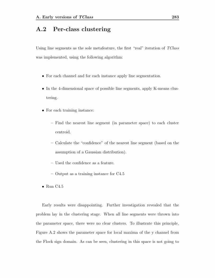
A. Early versions of TClass 283
A.2 Per-class clustering
Using line segments as the sole metafeature, the first “real” iteration of TClass
was implemented, using the following algorithm:
• For each channel and for each instance apply line segmentation.
• In the 4-dimensional space of possible line segments, apply K-means clus-
tering.
• For each training instance:
– Find the nearest line segment (in parameter space) to each cluster
centroid.
– Calculate the “confidence” of the nearest line segment (based on the
assumption of a Gaussian distribution).
– Used the confidence as a feature.
– Output as a training instance for C4.5
• Run C4.5
Early results were disappointing. Further investigation revealed that the
problem lay in the clustering stage. When all line segments were thrown into
the parameter space, there were no clear clusters. To illustrate this principle,
Figure A.2 shows the parameter space for local maxima of the y channel from
the Flock sign domain. As can be seen, clustering in this space is not going to

A. Early versions of TClass 284
be easy. And in fact, K-means clustering would simply not converge even after
50 iterations.
-0.2
-0.1
0
0.1
0.2
0.3
0.4
0.5
0.6
0 10 20 30 40 50 60 70 80 90 100
Hei
ght
Time
LocalMax parameter space for channel y of PhD sign domain
All instances
Figure A.2: The parameter space of local maxima of the y channel in the Flocksign domain. All instantiated local maxima are shown.
Hence, we sought another solution: per class clustering. Rather than clus-
tering all instances at once, only instances belonging to a single class would be
clustered. Figure A.3 shows instantiated features for two classes. As can be
seen, clustering either of these two classes would be relatively easy compared to
clustering the instances in Figure A.2.
Hence, early versions of TClass, as published in [Kad98] and [Kad99] use per-
class clustering: For each class, cluster instances from only that class. Use the
clusters generated to re-attribute all training instances. Create classifiers using
the learner with only the synthetic features generated from that class and the
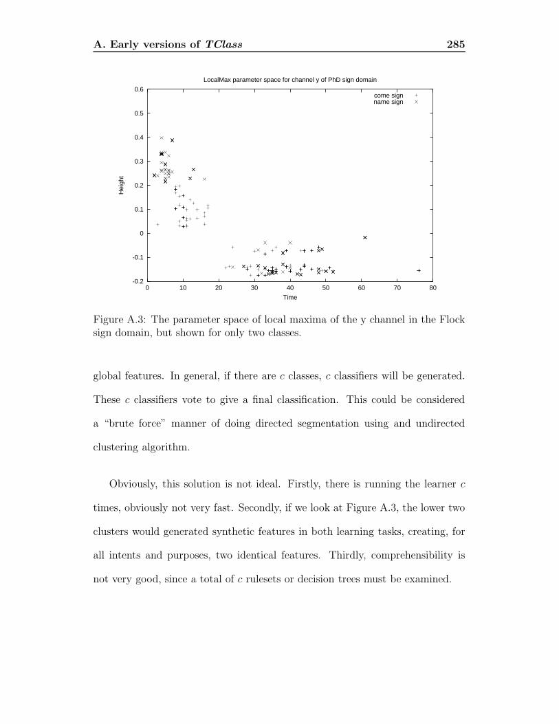
A. Early versions of TClass 285
-0.2
-0.1
0
0.1
0.2
0.3
0.4
0.5
0.6
0 10 20 30 40 50 60 70 80
Hei
ght
Time
LocalMax parameter space for channel y of PhD sign domain
come signname sign
Figure A.3: The parameter space of local maxima of the y channel in the Flocksign domain, but shown for only two classes.
global features. In general, if there are c classes, c classifiers will be generated.
These c classifiers vote to give a final classification. This could be considered
a “brute force” manner of doing directed segmentation using and undirected
clustering algorithm.
Obviously, this solution is not ideal. Firstly, there is running the learner c
times, obviously not very fast. Secondly, if we look at Figure A.3, the lower two
clusters would generated synthetic features in both learning tasks, creating, for
all intents and purposes, two identical features. Thirdly, comprehensibility is
not very good, since a total of c rulesets or decision trees must be examined.

A. Early versions of TClass 286
Early papers used the term PEPS – short for parametrised event primitives,
rather than metafeatures. It was not realised until after the publication of these
documents that metafeatures might well have applications beyond temporal clas-
sification.