Functional clustering of time series gene expression data by Granger causality

Fujita et al. BMC Systems Biology 2012, 6:137http://www.biomedcentral.com/1752-0509/6/137

METHODOLOGY ARTICLE Open Access

Functional clustering of time series geneexpression data by Granger causalityAndre Fujita1*, Patricia Severino2, Kaname Kojima3, Joao Ricardo Sato4, Alexandre Galvao Patriota1

and Satoru Miyano3

Abstract

Background: A common approach for time series gene expression data analysis includes the clustering of geneswith similar expression patterns throughout time. Clustered gene expression profiles point to the joint contribution ofgroups of genes to a particular cellular process. However, since genes belong to intricate networks, other features,besides comparable expression patterns, should provide additional information for the identification of functionallysimilar genes.

Results: In this study we perform gene clustering through the identification of Granger causality between and withinsets of time series gene expression data. Granger causality is based on the idea that the cause of an event cannotcome after its consequence.

Conclusions: This kind of analysis can be used as a complementary approach for functional clustering, whereingenes would be clustered not solely based on their expression similarity but on their topological proximity builtaccording to the intensity of Granger causality among them.

BackgroundGene network analysis of complex datasets, such as DNAmicroarray results, aims to identify relevant structuresthat help the understanding of a certain phenotype or con-dition. These networks comprise hundreds to thousandsof genes that may interact generating intricate structures.Consequently, pinpointing genes or sets of genes that playa crucial role becomes a complicated task.Common analyses explore gene-gene level relationships

and generate broad networks. Although this is a valu-able approach, genes might interact more intensely toa few members of the network, and the identificationof these so-called sub-networks should lead to a bettercomprehension of the entire regulatory process.Several in silico methodologies are available for the

identification of sub-networks, or clusters, within a givendataset [1-5]. Most of the times, the identified clustersgroup genes based on similar patterns of expression intime. In a different manner, the identification of Granger

*Correspondence: [email protected] of Mathematics and Statistics, University of Sao Paulo, Rua do Matao,1010, Sao Paulo 05508-090, BrazilFull list of author information is available at the end of the article

causality [6] within a network allows the clustering ofgenes based on their topological proximity in the net-work [7,8]. Briefly, Granger causality [6] analysis identifiesinteraction in terms of temporal precedence (the causecomes before its effect) [6] and may generate a set of sub-networks within whichGranger causality is intense amonggenes. As a result, genes are grouped depending on howclose they are in terms of Granger causality. Figure 1aillustrates the clustering based on the network topologicalproximity while Figure 1b shows the clustering based onsimilar expression patterns.The concept of Granger causality [6] has been previ-

ously shown to help in the identification and interpreta-tion of regulatory networks in time series gene expressiondatasets [9-18]. The main advantage of Granger causal-ity analysis in the context of gene expression datasetsconsists in the fact that each edge of the network repre-sents the information flow from one gene to another [19].Nevertheless, it is necessary to point out that Grangercausality is not effective causality in the Aristothelic sensebecause it is based on prediction and numerical calcu-lations. Fujita et al. [20-22] suggested a concept for theidentification of Granger causality between groups of timeseries. The application was, however, limited to scenarios

© 2012 Fujita et al.; licensee BioMed Central Ltd. This is an Open Access article distributed under the terms of the CreativeCommons Attribution License (http://creativecommons.org/licenses/by/2.0), which permits unrestricted use, distribution, andreproduction in any medium, provided the original work is properly cited.

Fujita et al. BMC Systems Biology 2012, 6:137 of 12http://www.biomedcentral.com/1752-0509/6/137

Functional

(a) (b)

clustering Usual

clustering

Figure 1 Regulatory networks. (a) Functional clustering. Genes areclustered based on their topological proximity given by Grangercausality. (b) Usual clustering. Genes are clustered based on thesimilarity between gene expression levels.

when clusters could be previously defined based on par-ticular data characteristics. Here, we propose a method todefine clusters by their topological proximity in the net-work. For this purpose we introduce an extension of theconcept of functional clustering, initially proposed by [23]in neuroscience. In [23], they applied mutual informationin order to group the most active brain regions. We areinterested in clustering the genes by using the conceptof information flow [19] between sets of time series [20].The gene expression time series are grouped dependingon the hidden structure underlying the network topol-ogy, in a way that genes which are topologically close interms of Granger causality are clustered (Figure 1a). Weuse the generalization of Granger causality for sets of timeseries datasets proposed by [20,21] in order to define con-cepts of distance, degree and flow useful to determinegene sets that highly interact in terms of Granger causality.In other words, we will derive the Granger causality-basedfunctional clustering directly from the time series geneexpression data. For this purpose, an approach that allowsthe identification of the optimum number of clusters for agiven dataset is also presented.

Materials andMethodsGranger causality for sets of time seriesGranger causality identification is a potential approachfor the detection of possible interactions in a data drivenframework couched in terms of temporal precedence. Themain idea is that temporal precedence does not imply, butmay help to identify causal relationships, since a causenever occurs after its effect.

A formal definition of Granger causality for sets of timeseries [20] can be given as follows.

Definition 1. [20] Granger causality for sets of timeseries: Suppose that �t is a set containing all relevant infor-mation available up to and including time-point t. Let Xt ,Xit and Xj

t be sets of time series containing p, m and ntime series, respectively, where Xi

t and Xjt are disjoint sub-

sets of Xt , i.e., each time series only belongs to one set, andthus, p ≥ m + n. Let Xt(h|�t) be the optimal (i.e., the onewhich produces the minimum mean squared error (MSE)prediction) h-step predictor of the set of m time series Xi

tfrom the time point t, based on the information in �t .The forecast MSE of the linear combination of Xi

t will bedenoted by �X(h|�t). The set of n time series Xj

t is said toGranger-cause the set of m time series Xi

t if

�X(h|�t)<�X(h|�t\{Xjs|s ≤ t}) for at least one h=1, 2, . . .

(1)

where �t\{Xjs|s ≤ t} is the set containing all relevant infor-

mation except for the information in the past and presentofXj

t . In other words, ifXit can be predictedmore accurately

when the information in Xjt is taken into account, then Xj

tis said to be Granger-causal for Xi

t .

For the linear case,Xjt is Granger non-causal forXi

t if thefollowing condition holds:

CCA(Xit ,X

jt−1|Xt\{Xj

t−1}) = ρ = 0, (2)

where ρ is the largest correlation calculated by CanonicalCorrelation Analysis (CCA).In order to simplify both notation and concepts, only the

identification of Granger causality for sets of time seriesin an Autoregressive process of order one is presented.Generalizations for higher orders are straightforward.

Functional clustering in terms of Granger causalityThere are numerous definitions for clusters in networksin the literature [24]. A functional cluster in terms ofGranger causality can be defined as a subset of genes thatstrongly interact among themselves but interact weaklywith the rest of the network.A usual approach for network clustering when the struc-

ture of the graph is known is the spectral clustering pro-posed by [25]. However, in biological data, the structure ofthe regulatory network is usually unknown.In order to overcome this limitation, we developed a

framework to cluster genes by their topological proxim-ity using the time series gene expression information. Wedeveloped concepts of distance and degree for sets oftime series based on Granger causality, and combined


them to the modified spectral clustering algorithm. Theprocedures are detailed below.

Functional clusteringGiven a set of time series x1t , x2t , . . . , x

pt (where p is the

number of time series) and a definition of similarity wij ≥0 between all pairs of data points xit and xjt , the intuitivegoal of clustering is to divide the time series into severalgroups such that time series in the same group are highlyconnected by Granger causality and time series in differ-ent groups are not connected or show few connections toeach other. One usual representation of the connectivitybetween time series is in the form of graph G = (V ,E).Each vertex vi in this graph represents a time series geneexpression xit . Two vertices are connected if the similar-ity wij between the corresponding time series xit and xjtis not zero (the edge of the graph is weighted by wij). Inother words, a wij > 0 represents existence of Grangercausality between time series xit and xjt and wij = 0 rep-resents Granger non-causality. The problem of clusteringcan now be reformulated using the similarity graph: wewant to find a partition of the graph such that there isless Granger causality between different groups and moreGranger causality within the group.Let G = (V ,E) be an undirected graph with vertex

set V = {v1, . . . , vp} (where each vertex represents onetime series) and weighted edges set E. In the followingwe assume that the graph G is weighted, that is eachedge between two vertices vi and vj carries a non-negativeweight wij ≥ 0. The weighted adjacency matrix of thegraph is the matrixW = wij; i, j = 1, . . . , p. If wij = 0, thismeans that the vertices vi and vj are not connected by anedge. As G is undirected, we require wij = wji. Therefore,in terms of Granger causality,wij can be set as the distancebetween two time series xit and xjt . This distance can bedefined as

Definition 2. Distance between two (sets of ) time seriesxit and xjt :

dist(xit , x

jt

)= 1− |CCA(xit , x

jt−1)| + |CCA(xjt , xit−1)|

2.

(3)

Notice that CCA(xit , xjt−1) is the Granger causality from

time series xjt to xit . In the case of sets of time series,just replace xit and xjt by the set of time series Xi

t and Xjt

[20,21]. Since absolute value of CCA ranges from zero toone and the higher the CCA, the higher is the quantity ofinformation flow, it is possible to see that the higher theCCA, the shorter the distance is. Furthermore, it is neces-sary to point out that the average between CCA(xit , x

jt−1)

and CCA(xjt , xit−1) is calculated because the distance mustbe symmetric. The intuitive idea consists on the fact thatthe higher is the CCA coefficient, the lower is the dis-tance between the time series (or sets of time series)independent of the direction of Granger causality.Moreover, notice that the CCA is the Pearson cor-

relation after dimension reduction, therefore, dist(xit , xjt)

satisfies three out of four criteria for distances: (i) non-negativity; (ii) identity of indiscernible; and (iii) symmetry;and does not satisfy the (iv) triangular inequality, there-fore, Pearson correlation is not a real metric. However, itis commonly used as a distance measure in several geneexpression data analysis [26,27]. The main advantage withthis definition of distance is the fact that it is possibleto interpret the clustering process by a Granger causalityconcept.Another necessary concept is the idea of degree of a

time series xit (vertex vi) which can be defined as

Definition 3. Degree of xit is defined by:

degree(xit) = in-degree(xit) + out-degree(xit)2

, (4)

where in-degree and out-degree are respectively

in-degree(xit) = |CCA(xit ,Xt−1|Xt\{Xt−1})| (5)

out-degree(xit) = |CCA(Xt , xit−1|Xt\{xit−1})|. (6)

Notice that in-degree and out-degree represent the totalinformation flow that “enters” and “leaves” the vertex vi,respectively. Therefore, the degree of vertex vi containsthe total information flow passing through vertex vi.Without loss of generality, it is possible to extend the

concept of degree of a vertex vi (time series xit) to a set oftime series (sub-network) Xu

t , where u = 1, . . . , k and k isthe number of sub-networks.

Definition 4. Degree of sub-network Xut is defined by:

degree(Xut ) = in-degree(Xu

t ) + out-degree(Xut )

2, (7)

where in-degree and out-degree are respectively

in-degree(Xut ) = |CCA(Xu

t ,Xt−1|Xt\{Xt−1})|, (8)

out-degree(Xut ) = |CCA(Xt ,Xu

t−1|Xt\{Xut−1})|. (9)

Now, by using the definitions of distance and degreesfor time series and sets of time series in terms of Granger


causality, it is possible to develop a spectral clustering-based algorithm to identify sub-networks (set of timeseries that are highly connected within sets and poorlyconnected between sets) in the regulatory networks. Thealgorithm based on spectral clustering [25] is as follows:

Input: The p time series (xit ; i = 1, . . . , p) and thenumber k of sub-networks to construct.Step 1: LetW be the (p × p) symmetric weightedadjacency matrix wherewi,j = wj,i = 1− dist(xit ; x

jt), i, j = 1, . . . , p.

Step 2: Compute the non-normalized (p × p)Laplacian matrix L as (Mohar, 1991)

L = D − W (10)

where D is the (p × p) diagonal matrix with thedegrees d1, . . . , dp (degree(xit) = di; i = 1, . . . , p) onthe diagonal.Step 3: Compute the first k eigenvectors {e1, . . . , ek}(corresponding to the k largest eigenvalues) of L.Step 4: Let U ∈ �p×k be the matrix containing thevectors {e1, . . . , ek} as columns.Step 5: For i = 1, . . . , p, let yi ∈ �k be the vectorcorresponding to the i th row of U.Step 6: Cluster the points (yi)i=1,...,p ∈ �k with thek-means algorithm into clusters {X1, . . . ,Xk}. Fork-means, one may select a large number of initialvalues to achieve (or to be closer) the globaloptimum configuration. In our simulations, wegenerated 100 different initial values.Output: Sub-networks {X1, . . . ,Xk}.

Notice that this clustering approach does not infer theentire structure of the network.

Estimation of the number of clustersThe method presented so far describes a framework forclustering genes (time series) using their topological prox-imity in terms of Granger causality.Now, the challenge consists in determining the opti-

mum number of sub-networks k. The choice of the num-ber of sub-networks k is often difficult depending on whatthe researcher is interested in. In our specific problem,one is interested in identifying the clusters presentingdense connectivity within a cluster and sparse connectiv-ity between clusters.In order to determine the most appropriate number of

clusters in this specific context, we used a variant of thesilhouette method [28].Let us first define the cluster index s(i) in the case of

dissimilarities. Take any time series xit in the data set,and denote by A the sub-network to which it has beenassigned. When sub-network A contains other time seriesapart from xit , then we can compute: a(i) = dist(xit ,A),

which is the average dissimilarity of xit to A. Let us nowconsider any sub-networkCwhich is different fromA andcompute: dist(xit ,C) which is the dissimilarity of xit to C.After computing dist(xit ,C) for all sub-networks C �= A,we set the smallest of those numbers and denote it byb(i) = minC�=Adist(xit ,C). The sub-network B for whichthis minimum value is attained (that is, dist(xit ,B) = b(i))we call the neighbor sub-network, or cluster of xit . Theneighbor cluster would be the second-best cluster for timeseries xit . In other words, if xit could not belong to sub-network A, the best sub-network to belong to would be B.Therefore, b(i) is very useful to know the best alternativecluster for the time series in the network. Note that theconstruction of b(i) depends on the availability of othersub-networks apart from A, thus it is necessary to assumethat there is more than one sub-network k within a givennetwork [28].After calculating a(i) and b(i), the cluster index s(i) can

be obtained by combining them as follows:

s(i) = b(i) − a(i)max(a(i), b(i))

. (11)

Indeed, from the above definition we easily see that−1 ≤ s(i) ≤ 1 for each time series xit . Therefore, there areat least three cases to be analyzed, namely, when s(i) ≈ 1or s(i) ≈ 0 or s(i) ≈ −1. For cluster index s(i) to be closeto one we require a(i) b(i). As a(i) is a measure of howdissimilar i is to its own sub-network, a small value meansit is well matched. Furthermore, a large b(i) implies that iis badly matched to its neighboring sub-network. Thus, acluster index s(i) close to onemeans that the gene is appro-priately clustered. If s(i) is close to negative one, then bythe same logic we see that xit would be more appropriate ifit was clustered in its neighboring sub-network. A clusterindex s(i) near zero means that the gene is on the borderof two sub-networks. In other words, the cluster index s(i)can be interpreted as the fitness of the time series xit to theassigned sub-network.The average cluster index s(i) of a sub-network is a

measure of how tightly grouped all the genes in the sub-network are. Thus, the average cluster index s(i) of theentire dataset is a measure of how appropriately the geneshave been clustered in a topological point of view and interms of Granger causality.

Estimation of the number of clusters in biological dataIn order to estimate the most appropriate number ofsub-networks present in the data set, we estimate theaverage cluster index s of the entire dataset for eachnumber of clusters k. When the number of identifiedsub-networks is equal or lower than the adequate num-ber of sub-networks, the cluster index values are very


Figure 2 (a) The representation of network with four clusters; (b) The network obtained by applying the proposedmethod with fourclusters (k=4); (c) The representation of the network when the number of clusters is set to five; (d) The network obtained by applying theproposedmethod with five clusters (k=5). The solid edges represent Granger causality. Notice that the structure of the “true” network ((a) and(c)) is not observed and it can only be estimated.

similar. However, when the number of identified sub-networks becomes higher than the adequate number ofsub-networks, the cluster index value s decreases abruptly.This is due to the fact that one of the highly connectedsub-networks is split into two new sub-networks. Noticethat these two new sub-networks present high connec-tivity between them because they are in fact, only onesub-network. In order to illustrate this event, see Figure 2for an example. In Figure 2a, genes in cluster 1 are highlyinterconnected. Now, suppose that one wants to increasethe number of clusters by splitting cluster 1 into twoclusters namely clusters 1 and 5 (Figure 2c). Notice thatclusters 1 and 5 are highly connected between them. Ifthe number of clusters is higher than the adequate num-ber of clusters (four, in our case), the value s decreasessubstantially, since the Granger causality between clustersincreases and the within cluster decreases. The breakpointwhere the value s decreases abruptly can be used to deter-mine the adequate number of sub-networks. In fact, thiscan be visually identified by analyzing the breakpoint atthe plot similarly to the standard elbow method used in k-means. However, if one wants to determine the breakpointin an objective manner, this can be done by adjusting twolinear regressions, one with the first q dots and anotherwith the remaining dots, thus identifying the breakpoint

(the value q) that minimizes the sum of squared errors(Figure 3).

Network constructionThe network connecting clusters is constructed fol-lowing procedures previously described [20,21]. Briefly,after Classification ExpectationMaximization (CEM) [29]Principal Component Analysis (PCA) is used to removeredundancy and to extract the eigen-time series fromeach cluster. PCA allows us to keep only the most sig-nificant components leading to variability in the dataset,thus reducing the number of variables for subsequentprocessing. In this study, we retained only componentsaccounting for more than 5% of the temporal variance ineach cluster [22]. The eigen-time series are then clusteredas described in the section Functional clustering and thenetwork can be inferred by applying the method proposedby [20,21].The Granger causality between cluster is identified by:

CCA(Xit ,X

jt−1|Xt\{Xj

t−1}) = ρ for all i, j = 1, . . . , k (12)

where ρ is the sample canonical correlation between thesets Xi

t and Xjt−1 partialized by all information contained

in Xt minus the set Xjt−1.


Number of sub-networks

Clu

ster

inde

x va

lue

1 2 3 4 5 6

of sub-networks

Figure 3 The optimum number of sub-networks is indicated bythe breakpoint in the graph. The breakpoint appears when thenumber of sub-networks is greater than the adequate number ofsub-networks. The breakpoint selection criterion is based on twolinear regressions that best fit the data.

Then, testH0 : CCA(Xi

t ,Xjt−1|Xt\{Xj

t−1}) = ρ = 0 (Granger non-causality)H1 : CCA(Xi

t ,Xjt−1|Xt\{Xj

t−1}) = ρ �= 0 (Grangercausality) where H0 and H1 are the null and alternativehypothesis, respectively.

SimulationsFour sets of Monte Carlo simulations were carriedout in order to evaluate the proposed approach undercontrolled conditions. The first scenario represents foursub-networks without Granger causality between them(Figure 4a). The second scenario consists of four sub-networks constituting a cyclic graph (Figure 4b). The thirdscenario presents a feedback loop between sub-networksA and B (Figure 4c). The fourth scenario is composed of anetwork with one sub-network (sub-network D) that onlyreceives Granger causality and one sub-network (sub-network A) that only sends Granger causality (Figure 4d).Since biological data usually possess several highly corre-lated genes (genes which hold the same information froma statistical stand point), we constructed 10 highly corre-lated time series for each xit , i = 1, . . . , 20. In other words,x1t is represented by 10 time series with correlation of 0.6between them, x2t is represented by 10 time series withcorrelation of 0.6 between them and so on. Therefore,instead of 20 time series, each scenario is in fact composedof 200 time series.For each scenario, time series lengths varied: 50, 75,

1000 and 200 time points. The number of repetitionsfor each scenario is 1,000. The synthetic gene expres-sion time series data in sub-networks A, B, C and Dwere generated by the following equations describedbelow.

A

B

C

D

A B

C D

A B C

D

A

B

C D

(a) (b)

(c) (d)

Figure 4 (a) Four independent sub-networks without Granger causality between them; (b) Four sub-networks in a cyclic graph; (c)Feedback loop between sub-networks A and B; (d) A network between sub-networks, where sub-networks A only sends Grangercausality and D only receives Granger Causality.


Simulation 1:⎧⎪⎪⎪⎪⎪⎪⎪⎪⎪⎪⎪⎪⎪⎪⎪⎪⎪⎪⎪⎪⎪⎪⎪⎪⎪⎪⎪⎪⎪⎪⎪⎪⎪⎪⎪⎪⎪⎪⎪⎪⎪⎪⎪⎪⎪⎪⎪⎪⎪⎪⎪⎨⎪⎪⎪⎪⎪⎪⎪⎪⎪⎪⎪⎪⎪⎪⎪⎪⎪⎪⎪⎪⎪⎪⎪⎪⎪⎪⎪⎪⎪⎪⎪⎪⎪⎪⎪⎪⎪⎪⎪⎪⎪⎪⎪⎪⎪⎪⎪⎪⎪⎪⎪⎩

xA1,t = βxA1,t−1 − βxA4,t−1 + βxA3,t−1 + ε1,t


xA3,t = βxA1,t−1 − βxA5,t−1 + ε3,t

xA4,t = βxA3,t−1 − βxA5,t−1 + ε4,t


xB6,t = βxB9,t−1 − βxB7,t−1 + ε6,t

xB7,t = βxB10,t−1 − βxB7,t−1 + ε7,t

xB8,t = βxB10,t−1 − βxB6,t−1 + βxB7,t−1 + ε8,t

xB9,t = βxB7,t−1 − βxB8,t−1 + βxB9,t−1 − βxB6,t−1 + ε9,t


xC11,t = βxC12,t−1 − βxC15,t−1 + ε11,t

xC12,t = βxC14,t−1 − βxC13,t−1 + ε12,t

xC13,t = βxC14,t−1 − βxC11,t−1 + ε13,t

xC14,t = βxC13,t−1 − βxC11,t−1 + ε14,t

xC15,t = βxC15,t−1 − βxC12,t−1 + βxC13,t−1 − βxC14,t−1 + ε15,t

xD16,t = βxD19,t−1 − βxD20,t−1 + βxD17,t−1 − βxD18,t−1 + ε16,t

xD17,t = βxD20,t−1 − βxD17,t−1 + βxD18,t−1 + ε17,t

xD18,t = βxD20,t−1 − βxD18,t−1 + ε18,t

xD19,t = βxD17,t−1 − βxD18,t−1 + ε19,t

xD20,t = βxD20,t−1 − βxD19,t−1 + ε20,t

Simulation 2:⎧⎪⎪⎪⎪⎪⎪⎪⎪⎪⎪⎪⎪⎪⎪⎪⎪⎪⎪⎪⎪⎪⎪⎪⎪⎪⎪⎪⎪⎪⎪⎪⎪⎪⎪⎪⎪⎪⎪⎪⎪⎪⎪⎪⎪⎪⎪⎪⎪⎪⎪⎪⎨⎪⎪⎪⎪⎪⎪⎪⎪⎪⎪⎪⎪⎪⎪⎪⎪⎪⎪⎪⎪⎪⎪⎪⎪⎪⎪⎪⎪⎪⎪⎪⎪⎪⎪⎪⎪⎪⎪⎪⎪⎪⎪⎪⎪⎪⎪⎪⎪⎪⎪⎪⎩



xA3,t = βxA1,t−1 − βxA5,t−1 + γ xD19,t−1 + ε3,t

xA4,t = βxA3,t−1 − βxA5,t−1 + ε4,t


xB6,t = βxB9,t−1 − βxB7,t−1 + γ xA3,t−1 + ε6,t

xB7,t = βxB10,t−1 − βxB7,t−1 + ε7,t




xC11,t = βxC12,t−1 − βxC15,t−1 + ε11,t

xC12,t = βxC14,t−1 − βxC13,t−1 + ε12,t

xC13,t = βxC14,t−1 − βxC11,t−1 + ε13,t

xC14,t = βxC13,t−1 − βxC11,t−1 + γ xB10,t−1 + ε14,t




xD18,t = βxD20,t−1 − βxD18,t−1 + ε18,t

xD19,t = βxD17,t−1 − βxD18,t−1 + ε19,t

xD20,t = βxD20,t−1 − βxD19,t−1 + γ xC15,t−1 + ε20,t

Simulation 3:⎧⎪⎪⎪⎪⎪⎪⎪⎪⎪⎪⎪⎪⎪⎪⎪⎪⎪⎪⎪⎪⎪⎪⎪⎪⎪⎪⎪⎪⎪⎪⎪⎪⎪⎪⎪⎪⎪⎪⎪⎪⎪⎪⎪⎪⎪⎪⎪⎪⎪⎪⎪⎨⎪⎪⎪⎪⎪⎪⎪⎪⎪⎪⎪⎪⎪⎪⎪⎪⎪⎪⎪⎪⎪⎪⎪⎪⎪⎪⎪⎪⎪⎪⎪⎪⎪⎪⎪⎪⎪⎪⎪⎪⎪⎪⎪⎪⎪⎪⎪⎪⎪⎪⎪⎩



xA3,t = βxA1,t−1 − βxA5,t−1 + γ xB6,t−1 + ε3,t

xA4,t = βxA3,t−1 − βxA5,t−1 + ε4,t


xB6,t = βxB9,t−1 − βxB7,t−1 + ε6,t





xC11,t = βxC12,t−1 − βxC15,t−1 + ε11,t

xC12,t = βxC14,t−1 − βxC13,t−1 + ε12,t

xC13,t = βxC14,t−1 − βxC11,t−1 + ε13,t





xD18,t = βxD20,t−1 − βxD18,t−1 + ε18,t

xD19,t = βxD17,t−1 − βxD18,t−1 + ε19,t


Simulation 4:⎧⎪⎪⎪⎪⎪⎪⎪⎪⎪⎪⎪⎪⎪⎪⎪⎪⎪⎪⎪⎪⎪⎪⎪⎪⎪⎪⎪⎪⎪⎪⎪⎪⎪⎪⎪⎪⎪⎪⎪⎪⎪⎪⎪⎪⎪⎪⎪⎪⎪⎪⎪⎨⎪⎪⎪⎪⎪⎪⎪⎪⎪⎪⎪⎪⎪⎪⎪⎪⎪⎪⎪⎪⎪⎪⎪⎪⎪⎪⎪⎪⎪⎪⎪⎪⎪⎪⎪⎪⎪⎪⎪⎪⎪⎪⎪⎪⎪⎪⎪⎪⎪⎪⎪⎩



xA3,t = βxA1,t−1 − βxA5,t−1 + ε3,t

xA4,t = βxA3,t−1 − βxA5,t−1 + ε4,t


xB6,t = βxB9,t−1 − βxB7,t−1 + ε6,t





xC11,t = βxC12,t−1 − βxC15,t−1 + ε11,t

xC12,t = βxC14,t−1 − βxC13,t−1 + ε12,t


xC14,t = βxC13,t−1 − βxC11,t−1 + γA5,t−1 + ε14,t




xD18,t = βxD20,t−1 − βxD18,t−1 + ε18,t

xD19,t = βxD17,t−1 − βxD18,t−1 + ε19,t



where β = 0.6, γ = 0.3, εi,t ∼ N(0,�) with

� = I(20×20) ⊗ � (13)

and

� =

⎛⎜⎜⎜⎜⎝

1 0.6 . . . 0.6

0.6 1. . .

......

. . . . . . 0.60.6 . . . 0.6 1

⎞⎟⎟⎟⎟⎠

(10×10)

(14)

for i = 1, . . . , 20.

Actual biological dataIn order to illustrate an application of the proposedapproach, a dataset collected by [30] was used. The workpresents whole genome gene expression data during thecell division cycle of a human cancer cell line (HeLa) char-acterized using cDNA microarrays. The dataset containsthree complete cell cycles of ∼16 hours each, with a totalof 48 time points distributed at intervals of one hour. Thefull dataset is available at: http://genome-www.stanford.edu/Human-CellCycle/HeLa/.In order to evaluate our proposed approach, we chose

to analyze the same gene set examined in Figure 5 of [10],which comprised a set of 50 genes.

ResultsSimulated dataIn order to study the properties of the proposed func-tional clustering method and to check its consistency, weperformed four simulations with distinct network charac-teristics in terms of structure and Granger causality.Table 1 describes the frequency that each number of

clusters was identified as optimal in each simulation andtime series length. Notice that the accuracy of the methodin identifying the correct number of clusters clearly con-verges to 100% as the time series length increases (the

108642

0.0

0.2

0.4

0.6

Number of sub−networks

Clu

ster

inde

x va

lue

Figure 5 The optimum number of sub-networks in the actualbiological data is indicated by the breakpoint in the graph (theoptimum number in this case is three).

correct number of clusters is four for all the scenarios).The same result was obtained with varying numbers ofsub-networks or when Granger causality within clustersincreased, demonstrating the consistency of the method.Moreover, both the cluster indices value and the respec-tive standard deviation for each simulation and time serieslength are described. The average cluster index valuewas calculated by using the value at the breakpoint asdescribed in Figure 3 in 1,000 repetitions. By analyzingTable 1, it is possible to verify that the longer the timeseries length, the smaller are the standard deviations andthe greater is the silhouette width demonstrating that themethod is consistent.Table 2 describes the average of the frequency (in per-

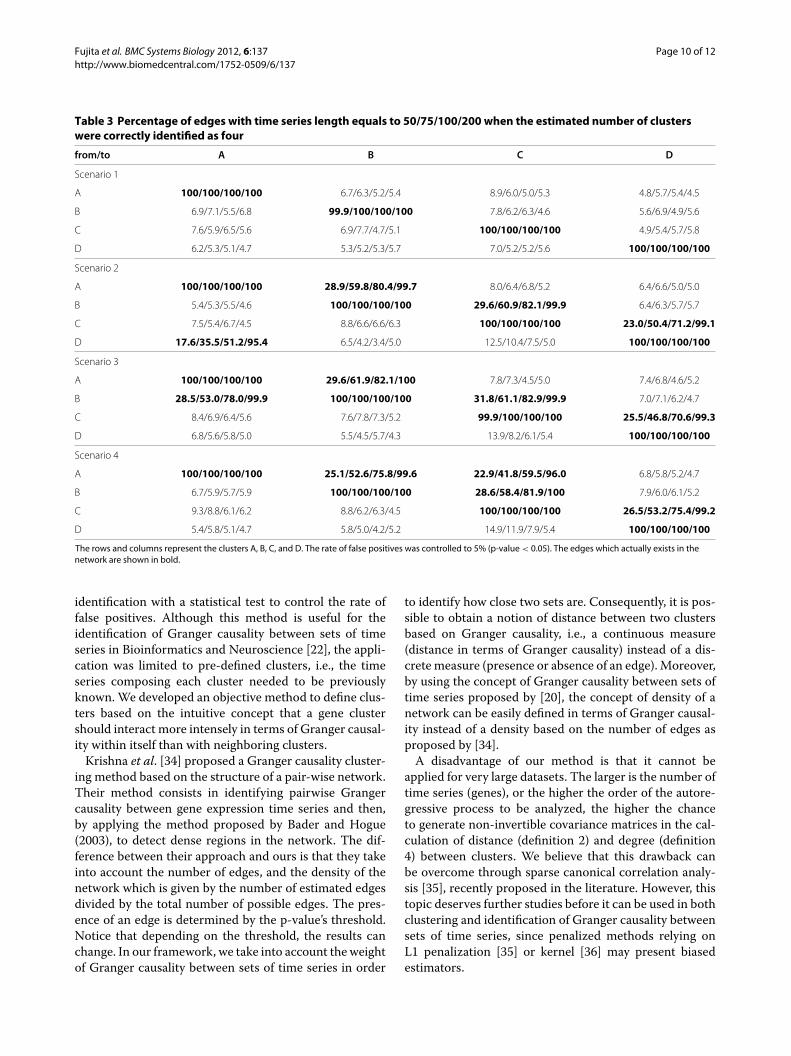
centage) the time series were correctly clustered for eachscenario and each time series length given the correctnumber of clusters. It is important to point out that thenumber of correctly classified time series increases as thetime series length increases.Table 3 represents the frequency (in percentage) each

edge of the simulated network was identified when theestimated number of clusters were correctly identified asfour. The correctly identified edges are in bold. Since thep-value threshold was set to 0.05, it is expected to iden-tify ≈ 5% of false positive edges where there is indeedno Granger causality. In fact, where there is no Grangercausality, the rate of false positives was controlled to5%, and where there is Granger causality, the number ofidentified edges is clearly higher than where there is noGranger causality.

Biological dataBy applying the method described in section Functionalclustering to the biological dataset, the optimum num-ber of sub-networks was identified as three. Notice inFigure 5 that there is a clear breakpoint when the numberof clusters is three.Once clusters were obtained, the cluster-cluster net-

work (Figure 6) was modeled by applying the methoddescribed in [20,21]. Two of the depicted clusters, clustersone and two, provide interesting material for biologicalinterpretation. Genes belonging to cluster two highlightexpected interconnections in cell cycle regulation. Forinstance, aberrant activation of signal transcription fac-tors NF-κB or STAT3, and alterations in p53 status, haveeach been reported to affect cell survival individually.The presence of the three genes in the same cluster isin agreement with a recent study which examined thehypothesis that alterations in a signal network involv-ing NF-κB, STAT3 and p53 could modulate expressionof proapoptotic BAX and antiapoptotic BCL-XL proteins,promoting cell survival [31]. The authors show that over-expression of p53 together with inhibition of NF-κB orSTAT3 induced greater increase in the BAX/BCL-XL ratio

http://genome-www.stanford.edu/Human-CellCycle/HeLa/

http://genome-www.stanford.edu/Human-CellCycle/HeLa/


Table 1 Frequency of the selected number of clusters for each scenario and time series length

Time series length/Number of clusters 1 2 3 4 5 6 silhouette width

Scenario 1

50 0 0 48 700 252 0 0.502 (0.098)

75 0 0 1 785 214 0 0.582 (0.054)

100 0 0 3 805 192 0 0.610 (0.042)

200 0 0 4 825 171 0 0.641 (0.034)

Scenario 2

50 0 0 65 713 222 0 0.479 (0.112)

75 0 0 28 760 212 0 0.555 (0.071)

100 0 0 9 834 157 0 0.587 (0.050)

200 0 0 3 883 114 0 0.621 (0.029)

Scenario 3

50 0 0 63 666 271 0 0.461 (0.123)

75 0 0 18 784 198 0 0.552 (0.078)

100 0 0 8 851 141 0 0.586 (0.050)

200 0 0 6 883 111 0 0.618 (0.031)

Scenario 4

50 0 0 53 686 261 0 0.465 (0.110)

75 0 0 17 786 197 0 0.551 (0.075)

100 0 0 11 815 174 0 0.581 (0.055)

200 0 0 6 887 107 0 0.619 (0.033)

In bold are the correct number of clusters. Between brackets is one standard deviation for the silhouette width calculated in the breakpoint. For each scenario andeach time series length, the number of repetitions was set to 1,000.

than modulation of these transcription factors individu-ally. As discussed earlier in this paper, this is a situationin which similar patterns of gene expression are not suffi-cient to comprehend the biological process.In [10], a network depicting Granger interaction among

genes from this same gene dataset was presented. Theauthors analyzed the network in the context of tumorprogression and identified gene-gene connections associ-ated with NF-κB, p53, and STAT3. Here, cluster 1 groupsnot only NF-κB, p53, and STAT3, but also the function-ally associated gene BCL-XL, NF-κB regulator A20 andtargets IAP and iκBα. The presence of NF-κB and fibrob-last growth factors (FGFs) and receptors (FGFRs) in thesame cluster is also in agreement with the previous work.Members of the FGF family and NF-κB have been shown

Table 2 Average of the percentage of correctly clusteredtime-series in 1,000 repetitions given the correct numberof clusters

Scenario/Time series length 50 75 100 200

1 78.8 96.0 98.9 99.9

2 72.9 91.2 95.8 99.2

3 71.6 90.6 95.2 99.7

4 68.9 88.7 93.7 99.1

to interact in various contexts and, despite distinct roles,are involved in cell proliferation, migration and survival[32,33].Even thoughMCL-1 and P21 play important roles in cell

survival, and BAI1 is transcriptionally regulated by P53,the analysis run here clustered them separately from P53containing cluster. This result suggests that, in the con-text of this dataset, their interaction is stronger with genessuch as c-JUN, also functionally related to cell survival,proto-oncogeneMET and tumor suppressorMASPIN, forinstance. Also worth noticing is the interaction of thiscluster with the two members of cluster 3: FGF5 and FOP.Like the other members of FGF family grouped in clus-ter 2, FGF5 is involved in cell survival activities, whileFOP was originally discovered as a fusion partner withFGFR1 in oncoproteins that give raise to stem cell myelo-proliferative disorders. It would be interesting to identifyspecific details regarding the intensity and direction of theinformation flow within this cluster for a clearer under-standing of their relationship in the context of cell cycleprogression.

DiscussionsFujita et al. [20,21] suggested both a concept of Grangercausality for sets of time series and a method for its


Table 3 Percentage of edges with time series length equals to 50/75/100/200 when the estimated number of clusterswere correctly identified as four

from/to A B C D

Scenario 1

A 100/100/100/100 6.7/6.3/5.2/5.4 8.9/6.0/5.0/5.3 4.8/5.7/5.4/4.5

B 6.9/7.1/5.5/6.8 99.9/100/100/100 7.8/6.2/6.3/4.6 5.6/6.9/4.9/5.6

C 7.6/5.9/6.5/5.6 6.9/7.7/4.7/5.1 100/100/100/100 4.9/5.4/5.7/5.8

D 6.2/5.3/5.1/4.7 5.3/5.2/5.3/5.7 7.0/5.2/5.2/5.6 100/100/100/100

Scenario 2

A 100/100/100/100 28.9/59.8/80.4/99.7 8.0/6.4/6.8/5.2 6.4/6.6/5.0/5.0

B 5.4/5.3/5.5/4.6 100/100/100/100 29.6/60.9/82.1/99.9 6.4/6.3/5.7/5.7

C 7.5/5.4/6.7/4.5 8.8/6.6/6.6/6.3 100/100/100/100 23.0/50.4/71.2/99.1

D 17.6/35.5/51.2/95.4 6.5/4.2/3.4/5.0 12.5/10.4/7.5/5.0 100/100/100/100

Scenario 3

A 100/100/100/100 29.6/61.9/82.1/100 7.8/7.3/4.5/5.0 7.4/6.8/4.6/5.2

B 28.5/53.0/78.0/99.9 100/100/100/100 31.8/61.1/82.9/99.9 7.0/7.1/6.2/4.7

C 8.4/6.9/6.4/5.6 7.6/7.8/7.3/5.2 99.9/100/100/100 25.5/46.8/70.6/99.3

D 6.8/5.6/5.8/5.0 5.5/4.5/5.7/4.3 13.9/8.2/6.1/5.4 100/100/100/100

Scenario 4

A 100/100/100/100 25.1/52.6/75.8/99.6 22.9/41.8/59.5/96.0 6.8/5.8/5.2/4.7

B 6.7/5.9/5.7/5.9 100/100/100/100 28.6/58.4/81.9/100 7.9/6.0/6.1/5.2

C 9.3/8.8/6.1/6.2 8.8/6.2/6.3/4.5 100/100/100/100 26.5/53.2/75.4/99.2

D 5.4/5.8/5.1/4.7 5.8/5.0/4.2/5.2 14.9/11.9/7.9/5.4 100/100/100/100

The rows and columns represent the clusters A, B, C, and D. The rate of false positives was controlled to 5% (p-value < 0.05). The edges which actually exists in thenetwork are shown in bold.

identification with a statistical test to control the rate offalse positives. Although this method is useful for theidentification of Granger causality between sets of timeseries in Bioinformatics and Neuroscience [22], the appli-cation was limited to pre-defined clusters, i.e., the timeseries composing each cluster needed to be previouslyknown. We developed an objective method to define clus-ters based on the intuitive concept that a gene clustershould interact more intensely in terms of Granger causal-ity within itself than with neighboring clusters.Krishna et al. [34] proposed a Granger causality cluster-

ing method based on the structure of a pair-wise network.Their method consists in identifying pairwise Grangercausality between gene expression time series and then,by applying the method proposed by Bader and Hogue(2003), to detect dense regions in the network. The dif-ference between their approach and ours is that they takeinto account the number of edges, and the density of thenetwork which is given by the number of estimated edgesdivided by the total number of possible edges. The pres-ence of an edge is determined by the p-value’s threshold.Notice that depending on the threshold, the results canchange. In our framework, we take into account the weightof Granger causality between sets of time series in order

to identify how close two sets are. Consequently, it is pos-sible to obtain a notion of distance between two clustersbased on Granger causality, i.e., a continuous measure(distance in terms of Granger causality) instead of a dis-crete measure (presence or absence of an edge). Moreover,by using the concept of Granger causality between sets oftime series proposed by [20], the concept of density of anetwork can be easily defined in terms of Granger causal-ity instead of a density based on the number of edges asproposed by [34].A disadvantage of our method is that it cannot be

applied for very large datasets. The larger is the number oftime series (genes), or the higher the order of the autore-gressive process to be analyzed, the higher the chanceto generate non-invertible covariance matrices in the cal-culation of distance (definition 2) and degree (definition4) between clusters. We believe that this drawback canbe overcome through sparse canonical correlation analy-sis [35], recently proposed in the literature. However, thistopic deserves further studies before it can be used in bothclustering and identification of Granger causality betweensets of time series, since penalized methods relying onL1 penalization [35] or kernel [36] may present biasedestimators.


MET

P21

PAI

RGS5

TRF4-2

Wip1

c-jun

BAI-1

FGF20

IGF-BP3

MASPIN

Mcl-1

A20

IAP

ICAM-1

JunB

MCP-1

TSP1

Bcl-2

FGF1

FGF2

FGF11

FGF12B

FGF18

NRBP

PKIG

PUMA

RNAHP

Bcl-XL

c-myc

Fas

CAMK2B

CyclinD1

CyclinE1

FGFR1

FGFR3

FGFR4

GADD45

IkappaBa

IRF-2

NFkB

Noxa

P53

PERP

STAT3

STK12

CDK7

DIP1

FGF5 3

FOP-FGFR1 3

Cluster 1

Cluster 2

Cluster 3

Figure 6 The network obtained with three (k=3) sub-networks. Solid arrows are significant Granger causality with p-value < 0.05 and dashedarrow is significant Granger causality with p-value < 0.10. The circles represent the clusters.

We only analyzed the autoregressive process of orderone because gene expression time series data, possibly dueto experimental limitations, are typically not large. How-ever, if one is interested in analyzing greater orders, oneminus the maximum canonical correlation analysis valueamong all the tested autoregressive orders can be used asthe distance measure between two time series.The clustering algorithm used here is based on the well-

known spectral clustering. Although results were satisfac-tory, other graph clustering methods may be used. Thenormalized cuts algorithm proposed by [37], for instance,presents better results in non Gaussian data sets.Finally, which biological process underlie time series

datasets correlation, remains a difficult question to beanswered. Studies suggest that correlated genes maybelong to common pathways or present the same bio-logical function. However, it is also known that methodsbased exclusively on correlation cannot reconstruct entiregene networks. Further studies in the field of systemsbiologymight be able to answer this question in the future.

ConclusionsWe propose a time series clustering approach based onGranger causality and a method to determine the num-ber of clusters that best fit the data. This method consistsof (1) the definition of degree and distance, usually usedin graph theory but now generalized for time series dataanalysis in terms of Granger causality; (2) a clusteringalgorithm based on spectral clustering and (3) a criterionto determine the number of clusters. We demonstrate, by

simulations, that our approach is consistent evenwhen thenumber of genes is greater than the time series’ length.We believe that this approach can be useful to under-

stand how gene expression time series relate to each other,and therefore help in the functional interpretation of data.

Competing interestsThe authors declare that they have no competing interests.

Authors’ contributionsAF has made substantial contributions to the conception and design of thestudy, analysis and interpretation of data. KK, AGP and JRS contributed to theanalysis and interpretation of mathematical results. PS contributed to theanalysis and interpretation of biological data. AF and PS have been involved indrafting of the manuscript. SM directed the work. All authors read approvedthe final manuscript.

AcknowledgementsThe supercomputing resource was provided by Human Genome Center (Univ.of Tokyo). This work was supported by FAPESP and CNPq - Brazil and RIKEN -Japan.

Author details1Institute of Mathematics and Statistics, University of Sao Paulo, Rua do Matao,1010, Sao Paulo 05508-090, Brazil. 2Center for Experimental Research, AlbertEinstein Research and Education Institute, Av. Albert Einstein, 627 - Sao Paulo,05652-000, Brazil. 3Human Genome Center, Institute of Medical Science, TheUniversity of Tokyo, 4-6-1 Shirokanedai, Minato-ku, Tokyo, 108-8639, Japan.4Center of Mathematics, Computation and Cognition, Universidade Federaldo ABC, Rua santa Adelia, 166 - Santo Andre, 09210-170, Brazil.

Received: 14 October 2011 Accepted: 17 October 2012Published: 30 October 2012

References1. Ng SK, McLachlan GJ, Wang K, Jones LB-T, Ng S-W: Amixture model

with random-effects components for clustering correlatedgene-expression profiles. Bioinformatics 2006, 22:1745–1752.


2. Segal E, Shapira M, Regev A, Pe’er D, Botstein D, Koller D, Friedman N:Module networks: identifying regulatory modules and theircondition-specific regulators from gene expression data. Nat Genet2003, 34:166–176.

3. Shiraishi Y, et al: Inferring cluster-based networks from differentlystimulatedmultiple time-course gene expression data. Bioinformatics2010, 26:1073–1081.

4. Stuart JM, Segal E, Koller D, Kim SK: A gene co-expression network forglobal discovery of conserved genetics modules. Science 2003,302:249–55.

5. Yamaguchi R, Yoshida R, Imoto S, Higuchi T, Miyano S: Findingmodule-based networks with state-space models - mininghigh-dimensional and short time-course gene expression data. IEEESignal Process Mag 2007, 24:37–46.

6. Granger CWJ: Investigating causal relationships by econometricmodels and cross-spectral methods. Econometrica 1969, 37:424–438.

7. Ahmed HA, Mahanta P, Bhattacharyya DK, Kalita JK: GERC: tree basedclustering for gene expression data. 11th IEEE Int Conference BioinfBioeng 2011:299–302 .

8. Bandyopadhyay S, Bhattacharyya M: A biologically inspired measurefor coexpression analysis. IEEE/ACM Trans comput biol bioinf 2011,8:929–942.

9. Fujita A, Sato JR, Garay-Malpartida HM, Morettin PA, Sogayar MC, FerreiraCE: Time-varying modeling of gene expression regulatory networksusing wavelet dynamic vector autoregressive method. Bioinformatics2007a, 23:16253–1630.

10. Fujita A, Sato JR, Garay-Malpartida HM, Yamaguchi R, Miyano S, SogayarMC, Ferreira CE:Modeling gene expression regulatory networks withthe sparse vector autoregressive model. BMC Syst Biol 2007b, 1:39.

11. Fujita A, Sato JR, Garay-Malpartida HM, Sogayar MC, Ferreira CE, Miyano S:Modeling nonlinear gene regulatory networks from time-seriesgene expression data. J Bioinf Comput Biol 2008, 6:961–79.

12. Fujita A, Patriota AG, Sato JR, Miyano S: The impact of measurementerror in the identification of regulatory networks. BMC Bioinf 2009,10:412.

13. Guo S, Wu J, Ding M, Feng J: Uncovering interactions in the frequencydomain. PLoS Comput Biol 2008, 4:e1000087.

14. Kojima K, Fujita A, Shimamura T, Imoto S, Miyano S: Estimation ofnonlinear gene regulatory networks via L1 regularized NVAR fromtime series gene expression data. Genome Informatics 2008, 20:37–51.

15. Lozano AC, Abe N, Liu Y, Rosset S: Grouped graphical Grangermodeling for gene expression regulatory networks discovery.Bioinformatics 2009, 25:i110—i118.

16. Mukhopadhyay ND, Chatterjee S: Causality and pathway search inmicroarray time series experiments. Bioinformatics 2007, 23:442–449.

17. Nagarajan R: A note on inferring acyclic network structures usingGranger causality tests. Int J Biostatistics 2009, 5:10.

18. Shojaie A, Michailidis G: Discovering graphical Granger causality usingthe truncating lasso penalty. Bioinformatics 2010, 26:i517—i523.

19. Baccala LA, Sameshima K: Partial directed coherence: A new conceptin neural structure determination. Biol Cybernetics 2001, 84:463–474.

20. Fujita A, Sato JR, Kojima K, Gomes LR, Nagasaki M, Sogayar MC, Miyano S:Identification of Granger causality between gene sets. J BioinfComput Biol 2010a, 8:679–701.

21. Fujita A, Kojima K, Patriota AG, Sato JR, Severino P, Miyano S: A fast androbust statistical test based on Likelihood ratio with Bartlettcorrection to identify Granger causality between gene sets.Bioinformatics 2010b, 26:2349–2351.

22. Sato JR, Fujita A, Cardoso EF, Thomaz CE, Brammer MJ, Amaro E:Analyzing the connectivity between regions of interest: Anapproach based on cluster Granger causality for fMRI data analysis.NeuroImage 2010, 52:1444–1455.

23. Tononi G, McIntosh AR, Russel DP, Edelman GM: Functional clustering:identifying strongly interactive brain regions in neuroimaging data.NeuroImage 1998, 7:133–149.

24. Edachery J, Sen A, Brandenburg F: Graph clustering using distance-kcliques. In Proceedings of the Seventh International Symposium on GraphDrawing. Lecture Notes in Computer Science. vol. 1731. Edited by Smith Y.Berlin, Heidelberg, Germany: Springer-Verlag GmbH:1999.

25. Ng A, et al: Advances in Neural Information Processing Systems. New York:MIT Press; 2002.

26. Bhattacharya A, De RK: Divisive correlation clustering algorithm(DCCA) for grouping of genes: detecting varying patterns inexpression profiles. Bioinformatics 2008, 24:1359–1366.

27. Ihmels J, Bergmann S, Berman J, Barkai N: Comparative gene expressionanalysis by differential clustering approach: applications to theCandida albicans transcription program. PLoS Genet 2005, 1:e39.

28. Rousseeuw PJ: Silhouettes: a graphical aid to the interpretation andvalidation of cluster analysis. J Comput Appl Math 1987, 20:53–65.

29. Celeux G, Govaert G: A classification EM algorithm for clustering andtwo stochastic versions. Comput Stat Data Anal 1992, 14:315–332.

30. Whitfield ML, Sherlock G, Saldanha AJ, Murray JI, Ball CA, Alexander KE,Matese JC, Perou CM, Hurt MM, Brown PO, Botstein D: Identification ofgenes periodically expressed in the human cell cycle and theirexpression in tumors.Mol Biol Cell 2002, 13:1977–2000.

31. Lee TL, Yeh J, Friedman J, Yan B, Yang X, Yeh NT, Waes CV, Chen Z: Asignal network involving coactivated NF-κB and STAT3 and alteredp53modulates BAX/BCL-XL expression and promotes cell survivalof head and neck squamous cell carcinomas. Int J Cancer 2008,122:1987–1998.

32. Lungu G, Covaleda L, Mendes O, Martini-Stoica H, Stoica G:FGF-1-inducedmatrix metalloproteinase-9 expression in breastcancer cells is mediated by increased activities of NF-κB andactivating protein-1.Mol Carcinog 2008, 47:424–435.

33. Drafahl KA, McAndrew CW, Meyer AN, Haas M, Donoghue DJ: TheReceptor Tyrosine Kinase FGFR4 Negatively Regulates NF-kappaBSignaling. PLoS ONE 2010, 5:e14412.

34. Krishna R, Li CT, Buchanan-Wollaston V: A temporal precedence basedclustering method for gene expression microarray data. BMC Bioinf2010, 11:68.

35. Witten DM, Tibshirani R, Hastie T: A penalized matrix decomposition,with applications to sparse principal components and canonicalcorrelation analysis. Biostatistics 2010, 10:515–534.

36. Hardoon DR, Shawe-Taylor J: Sparse canonical correlation analysis.Machine Learning 2011, 83:331–353.

37. Shi J, Malik J: Normalized cuts and image segmentation. IEEE TransPattern Anal Machine Intelligence 2000, 22:888–905.

doi:10.1186/1752-0509-6-137Cite this article as: Fujita et al.: Functional clustering of time series geneexpression data by Granger causality. BMC Systems Biology 2012 6:137.

Submit your next manuscript to BioMed Centraland take full advantage of:

• Convenient online submission

• Thorough peer review

• No space constraints or color figure charges

• Immediate publication on acceptance

• Inclusion in PubMed, CAS, Scopus and Google Scholar

• Research which is freely available for redistribution

Submit your manuscript at www.biomedcentral.com/submit

Functional clustering of time series gene expression data by Granger causality

Documents

Transcript of Functional clustering of time series gene expression data by Granger causality