International Review of Economics and Finance 33 (2014) 12–27

Contents lists available at ScienceDirect

International Review of Economics and Finance

j ourna l homepage: www.e lsev ie r .com/ locate / i re f

Causality and contagion in EMU sovereign debt markets

Marta Gómez-Puig a, Simón Sosvilla-Rivero b,⁎a Department of Economic Theory, Universitat de Barcelona, Av. Diagonal 696, 08034 Barcelona, Spainb Department of Quantitative Economics, Universidad Complutense de Madrid, Campus de Somosaguas, 28223 Madrid, Spain

a r t i c l e i n f o

⁎ Corresponding author at: Department of Quantitativ942 591.

E-mail addresses: marta.gomezpuig@ub.edu (M. G1 Moro (in press) and Aizenman (2013) offer a liter

http://dx.doi.org/10.1016/j.iref.2014.03.0031059-0560/© 2014 Elsevier Inc. All rights reserved.

a b s t r a c t

Article history:Received 28 October 2013Received in revised form 7 March 2014Accepted 10 March 2014Available online 18 March 2014

This paper contributes to the literature by applying the Granger-causality approach and endog-enous breakpoint test to offer an operational definition of contagion to examine EuropeanEconomic and Monetary Union (EMU) countries public debt behavior. A database of yields on10-year government bonds issued by 11 EMU countries covering fourteen years of monetaryunion is used. Themain results suggest that the 41 new causality patterns, which appeared for thefirst time in the crisis period, and the intensification of causality recorded in 70% of the casesprovide clear evidence of contagion in the aftermath of the current euro debt crisis.

© 2014 Elsevier Inc. All rights reserved.

JEL classification:E44F36G15C52

Keywords:Sovereign bond yieldsGranger-causalityContagionEuro area

1. Introduction

From the introduction of the euro in January 1999 until the collapse of the US financial institution Lehman Brothers inSeptember 2008, sovereign yields of euro area issues moved in a narrow range with only very slight differences across countries(see Figs. 1 and 2). Nevertheless, following the Lehman Brothers collapse severe tensions emerged in financial marketsworldwide, including the euro zone bond market. In fact, not only did the period of financial turmoil turn into a global financialcrisis, but it also began to spread to the real sector, with a rapid, synchronized deterioration in most major economies. Thisfinancial crisis put the spotlight on the macroeconomic and fiscal imbalances within European Economic and Monetary Union(EMU) countries which had largely been ignored during the period of stability when markets had seemed to underestimate thepossibility that governments might default (see Beirne & Fratzscher, 2013). Furthermore, in some EMU countries, problems in thebanking sector spread to sovereign states because of their excessive debt issues made in order to save the financial industry;eventually, the global financial crisis grew into a full-blown sovereign debt crisis. Indeed, since 2010, Greece has been bailed outtwice and Ireland, Portugal and Cyprus have also needed bailouts to stay afloat. These events brought to light the fact that theorigin of sovereign debt crises in the euro area varies according to the country and reflects the strong interconnection betweenpublic debt and private debt (see Gómez-Puig & Sosvilla-Rivero, 2013).1

e Economics, Universidad Complutense deMadrid, 28223Madrid, Spain. Tel.: +34 913 942 342; fax:+34 913

ómez-Puig), sosvilla@ccee.ucm.es (S. Sosvilla-Rivero).ature review on the Eurozone economic and financial crisis.

0

5

10

15

20

25

30

35

40

45

5001

/01/

1999

01/0

5/19

99

01/0

9/19

99

01/0

1/20

00

01/0

5/20

00

01/0

9/20

00

01/0

1/20

01

01/0

5/20

01

01/0

9/20

01

01/0

1/20

02

01/0

5/20

02

01/0

9/20

02

01/0

1/20

03

01/0

5/20

03

01/0

9/20

03

01/0

1/20

04

01/0

5/20

04

01/0

9/20

04

01/0

1/20

05

01/0

5/20

05

01/0

9/20

05

01/0

1/20

06

01/0

5/20

06

01/0

9/20

06

01/0

1/20

07

01/0

5/20

07

01/0

9/20

07

01/0

1/20

08

01/0

5/20

08

01/0

9/20

08

01/0

1/20

09

01/0

5/20

09

01/0

9/20

09

01/0

1/20

10

01/0

5/20

10

01/0

9/20

10

01/0

1/20

11

01/0

5/20

11

01/0

9/20

11

01/0

1/20

12

01/0

5/20

12

01/0

9/20

12

GERMANY AUSTRIA BELGIUM FINLAND FRANCE GREECE IRELAND ITALY NETHERLAND PORTUGAL SPAIN

Fig. 1. Daily 10-year sovereign yields in EMU-11 countries: 1999–2012.

13M. Gómez-Puig, S. Sosvilla-Rivero / International Review of Economics and Finance 33 (2014) 12–27

In this scenario, some of the research to date has focused on the analysis of interactions between the sovereign market and thefinancial sector [see Mody (2009), Ejsing and Lemke (2009), Gennaioli, Martin, and Rossi (2014), Broner and Ventura (2011),Bolton and Jeanne (2011) and Andenmatten and Brill (2011)]. Other researchers have discussed transmission and/or contagionbetween sovereigns in the euro area context [see Kalbaska and Gatkowski (2012), Metieu (2012), Caporin, Pelizzon, Ravazzolo,and Rigobon (2013), Beirne and Fratzscher (2013) and Gorea and Radev (2014) to name a few]. Finally, a strand of research hasexamined structural breaks and sovereign credit risk in the euro area [see, e. g., Basse, Friedrich, and Kleffner (2012), Gruppe andLange (in press) and Basse (2014)].

-10

0

10

20

30

40

50

01/0

1/19

99

01/0

5/19

99

01/0

9/19

99

01/0

1/20

00

01/0

5/20

00

01/0

9/20

00

01/0

1/20

01

01/0

5/20

01

01/0

9/20

01

01/0

1/20

02

01/0

5/20

02

01/0

9/20

02

01/0

1/20

03

01/0

5/20

03

01/0

9/20

03

01/0

1/20

04

01/0

5/20

04

01/0

9/20

04

01/0

1/20

05

01/0

5/20

05

01/0

9/20

05

01/0

1/20

06

01/0

5/20

06

01/0

9/20

06

01/0

1/20

07

01/0

5/20

07

01/0

9/20

07

01/0

1/20

08

01/0

5/20

08

01/0

9/20

08

01/0

1/20

09

01/0

5/20

09

01/0

9/20

09

01/0

1/20

10

01/0

5/20

10

01/0

9/20

10

01/0

1/20

11

01/0

5/20

11

01/0

9/20

11

01/0

1/20

12

01/0

5/20

12

01/0

9/20

12

AUSTRIA BELGIUM FINLAND FRANCE GREECE IRELAND ITALY NETHERLAND PORTUGAL SPAIN

Fig. 2. Daily 10-year sovereign yield spreads over Germany: 1999–2012.

14 M. Gómez-Puig, S. Sosvilla-Rivero / International Review of Economics and Finance 33 (2014) 12–27

The aim of this paper is to contribute to the last two branches of the literature by examining not only the transmission ofsovereign risk, but also the contagion in euro area public debt markets. In the literature there is a considerable amount ofambiguity concerning the precise definition of contagion. There is no theoretical or empirical definition on which researchersagree and, consequently, the debate on exactly how to define contagion not only is academic, but also has important implicationsfor measuring the concept and for evaluating policy responses. Pericoli and Sbracia (2003) note five definitions of contagion usedin the literature. Two of them have been predominantly used in empirical studies to analyze it in financial markets and have beenadopted in common usage by governments, citizens and policymakers. The first defines contagion depending on the channels oftransmission that are used to spread the effects of the crisis, while the second defines it depending on whether the transmissionmechanisms are stable through time.

Masson (1999) and Kaminsky and Reinhart (2000) apply the first definition, which argues that contagion arises whencommon shocks and all channels of potential interconnection either are not present or have been controlled for. So, the termcontagion will only be applied when a crisis in one country may conceivably trigger a crisis elsewhere for reasons unexplained bymacroeconomic fundamentals2 — perhaps because it leads to shifts in market sentiment, or changes the interpretation given toexisting information. According to the second definition, which was proposed in a seminal paper by Forbes and Rigobon (2002),contagion is a significant increase in cross-market linkages after a shock to one country (or group of countries).3 Therefore, if twomarkets show a high degree of co-movement during periods of stability, even if they continue to be highly correlated after a shockto one market, this may not constitute contagion, but only the outcome of the “interdependence” that has always been present inthe markets. The empirical analysis of Forbes and Rigobon definition of contagion implies then the presence of a tranquil,pre-crisis period in order to be able to examine whether a change in the intensity of the transmission has occurred after the shock.

In this paper, we will use an operational approach based on the second definition4 in order to capture the phenomenon ofcontagion quantitatively. Besides, among the five general strategies5 that have been used in the literature, our analysis will berelated to one of the most conventional methodologies for testing for contagion: the analysis of cross-market correlations.However, we not only investigate changes in cross-market interdependencies via cointegration analysis, but also explore changesin the existence and direction of causality by means of a Granger-causality approach6 before and after endogenously (data-based)identified crises. Hence, the definition of contagion that we will explore in the remainder of this paper is the following: anabnormal increase in the number or in the intensity of causal relationships, compared with that of tranquil period, triggered afteran endogenously detected shock.

Most studies in the literature investigate changes in cross-market correlations (see, e.g., Syllignakis & Kouretas, 2011); veryfew explore changes in the existence and direction of causality. Exceptions are studies by Edwards (2000) who focuses on Chile,Baig and Goldfajn (2001) who investigate contagion from Russia to Brazil, Gray (2009) who examines spillovers in Central andEastern European countries, and both Granger, Huang, and Yang (2000) and Sander and Kleimeier (2003) who investigatespillovers during the Asian crisis. However, a small number of studies have applied a Granger-causality approach to theinvestigation of changes in the existence and direction of transmission in euro area debt markets. Among them, Kalbaska andGatkowski (2012) analyze the dynamics of the credit default swap (CDS) market of peripheral EMU countries along with threecentral European countries (France, Germany and the UK) for the period of 2008–2010, and Gómez-Puig and Sosvilla-Rivero(2013) focus on the existence of possible Granger-causal relationships between the evolution of the yield of bonds issued solelyby peripheral EMU countries during the period 1999–2010.

Therefore, our study contributes to this literature by applying a Granger-causality approach to 10-year sovereign yields7 ofboth peripheral and central EMU countries8 on an extended time period spanning from the inception of the euro in January 1999,well before the global financial and sovereign debt crises, to December 2012. But, unlike previous studies in the literature (seeSander & Kleimeier, 2003 o Kalbaska & Gatkowski, 2012), we do not set a specific breakpoint based on a priori knowledge of thepotential break date. In our analysis, we use two techniques that take into consideration that the timing of the break is unknown

2 The theory of “monsoonal effects” suggests that financial crises appear to be contagious because underlying macroeconomic variables are correlated. In thiscontext, several important papers have focused on the macroeconomic causes of crises, for example, Eichengreen, Rose, and Wyplosz (1996).

3 The distinction between contagion which occurs at times of crisis, and interdependence which is a result of normal market interaction, has become the focalpoint of many contagion studies: see for example Corsetti, Pericoli, and Sbracia (2005) or Bae, Karolyi, and Stulz (2003).

4 In a very recent paper, Gómez-Puig and Sosvilla-Rivero (2014) analyze contagion using an approach that is based in the first definition of contagion [(Masson,1999) and Kaminsky and Reinhart (2000) among others]. Concretely, they examine whether the transmission of the recent crisis in euro area sovereign debtmarkets was due to fundamentals-based or pure contagion. Their results suggest the importance of both variables proxying market sentiment andmacrofundamentals in determining contagion and underline the coexistence of “pure contagion” and “fundamentals-based contagion” during the recentEuropean debt crisis.

5 Probability analysis, cross-market correlations, VAR models, latent factor/GARCH models, and extreme value/co-exceedance/jump approach (see Forbes,2012).

6 Forbes and Rigobon (2002) suggest the use of this methodology when they point out that, if the source of the crisis is not well identified and endogeneity maybe severe, it may be useful to utilize Granger-causality tests to determine the extent of any feedback from each country in the sample to the initial crisis country.

7 Our analysis focuses on 10-year yields instead of CDS since CDS data are not available for all the countries in the study until late 2008 — only one year beforethe onset of the euro sovereign debt crisis.

8 Gómez-Puig and Sosvilla-Rivero (2013) report data of consolidated claims on an immediate borrower basis provided by the Bank for InternationalSettlements by nationality of reporting banks as a proportion of total foreign claims on each country. These data suggest that the problems of peripheral countriescan trigger contagion which may affect not only other peripheral countries but also central EMU countries, since some of these banks (mostly German and Frenchbanks) are highly exposed to the debt of peripheral countries.

15M. Gómez-Puig, S. Sosvilla-Rivero / International Review of Economics and Finance 33 (2014) 12–27

and allow the data to indicate when regime shifts occur. Thus, break dates that identify the shock triggering contagion aredetermined endogenously by the model in each of the potential pair-wise causal relationships.9

The rest of the paper is organized as follows. The next section explains the econometric methodology. The dataset used toanalyze causality is described in Section 3. Section 4 presents the empirical findings, while Section 5 offers some concludingremarks.

2. Econometric methodology

2.1. Testing for causality

Granger's (1969) causality test is widely used to test for the relationship between two variables. A variable X is said toGranger-cause another variable Y if past values of X help predict the current level of Y better than past values of Y alone, indicatingthat past values of X have some informational content that is not present in past values of Y. This definition is based on the conceptof causal ordering: two variables X and Ymay be contemporaneously correlated by chance, but it is unlikely that the past values ofX will be useful in predicting Y, giving all the past values of Y.10

Granger-causality tests are sensitive to lag length and, therefore, it is important to select the appropriate lengths.11 Otherwise,the model estimates will be inconsistent and the inferences drawn may be misleading (see Thornton & Batten, 1985). In thispaper, we use Hsiao's (1981) generalization of the Granger notion of causality. Hsiao proposed a sequential method to test forcausality, which combines Akaike's (1974) final predictive error (FPE, from now on) and the definition of Granger-causality(Canova, 1995, 62–63). Essentially, the FPE criterion trades off the bias that arises from underparameterization of a model againstthe loss in efficiency that results from its overparameterization.

Consider the following models,

whereproced

9 In ta previoidentify10 Gracontem11 Theinefficie

Yt ¼ α0 þXM

i¼1

δiYt−i þ εt ð1Þ

Yt ¼ α0 þXM

i¼1

δiYt−i þXN

j¼1

γ jXt− j þ εt ð2Þ

Xt and Yt are covariance-stationary variables [i.e., they are I(0) variables]. The following steps are used to apply Hsiao'sure for testing causality:

i) Treat Yt as a one-dimensional autoregressive process (1), and compute its FPE with the order of lagsmi varying from 1 toM.Examine the FPE

FPEY mi;0ð Þ ¼ T þmi þ 1T−mi−1

� SSRT

where T is the total number of observations and SSR is the sum of squared residuals of OLS regression (1). Choosemi for thevalue of m that minimizes the FPE, say m, and denote the corresponding value as FPEY (m, 0).

ii) Treat Yt as a controlled variable with m number of lags, and treat Xt as a manipulated variable as in (2). Compute again theFPE of (2) by varying the order of lags ni of Xt from 1 to N. Examine the FPE

FPEY mi;nið Þ ¼ T þmi þ ni þ 1T−mi−ni−1

� SSRT

:

Choose the order ni which gives the smallest FPE, say n, and denote the corresponding FPE as FPEY (m,n).

iii) Compare FPEY (m, 0) with FPEY (m,n) [i.e., compare the smallest FPE in step (i) with the smallest FPE in step (ii)]. If

FPEY (m,0) − FPEY (m,n) N 0, then Xt is said to cause Yt. If FPEY (m,0) − FPEY (m,n) b 0, then Yt is an independent process.iv) Repeat steps i) to iii) for the Xt variable, treating Yt as the manipulated variable.

he analysis we only analyze shock transmission between pairs, considering in each test that only one country is responsible for spreading the shock. Unlikeus crisis, since in the euro area sovereign debt crisis several peripheral countries entered a fiscal crisis at roughly the same time, it is very difficult tothe country responsible for the origin of the shock.nger causality is not identical to causation in the classical philosophical sense, but it demonstrates the likelihood of this causation more forcefully thanporaneous correlation (Geweke, 1984).general principle is that the smaller lag length has smaller variance but runs a risk of bias, while larger lags will reduce the bias problem but may lead toncy.

16 M. Gómez-Puig, S. Sosvilla-Rivero / International Review of Economics and Finance 33 (2014) 12–27

When Xt and Yt are not stationary variables, but are first-difference stationary [i.e., they are I(1) variables] and cointegrated(see Dolado, Jenkinson, & Sosvilla-Rivero, 1990), it is possible to investigate the causal relationships from ΔXt to ΔYt and from ΔYtto ΔXt, using the following error correction models:

where

12 Theestimat13 And

ΔYt ¼ α0 þ βZt−1 þXM

i¼1

δiΔYt−i þ εt ð3Þ

ΔYt ¼ α0 þ βZt−1 þXM

i¼1

δiΔYt−i þXN

j¼1

γ jΔXt− j þ εt ð4Þ

Zt is the OLS residual of the cointegrating regression (Yt = μ + λXt), known as the error-correction term. Note that, if Xt

are I(1) variables but are not cointegrated, then β in (3) and (4) is assumed to be equal to zero.

and YtIn both cases [i.e., Xt and Yt are I(1) variables, and they are or they are not cointegrated], we can use Hsiao's sequential

procedure substituting Yt with ΔYt and Xt with ΔXt in steps (i) to (iv), as well as substituting expressions (1) and (2) with Eqs. (3)and (4).

2.2. Stability diagnostics

In the conventional Granger-causality analysis, the relationship between two variables is assumed to exist at all times.However, in a context of financial crisis, parameter non-constancy may occur and may generate misleading inferences if leftundetected (see, Bai & Perron, 1998, 2003; Perron, 1989; Zivot & Andrews, 1992). Furthermore, the pre-testing issue in earlystudies may induce a size distortion of the resulting test procedures (Bai, 1997). Thus, it is desirable to let the data select whenand where regime shifts occur (i. e., we need to test for the null hypothesis of no structural change versus the alternativehypothesis that changes are present). To this end, we first identify a single structural change using the Quandt–Andrews one-timeunknown structural break test. We then use the procedure suggested by Bai (1997) and Bai and Perron (1998, 2003) to detectmultiple unknown breakpoints in order to obtain further evidence of the existence of the breakpoints previously detectedendogenously. These breakpoints allow the identification of pre-crisis and crisis periods for each pair-wise causal relationshipwhich, as explained in Introduction, are needed for the detection of a possible contagion episode according to our operationaldefinition based on the Forbes and Rigobon (2002) approach.

2.2.1. Quandt–Andrews breakpoint testA particular challenge in empirical time series analysis is to determine the appropriate timing of a potential structural break. In

a traditional Chow (1960) test,12 we have to set a specific breakpoint based on a priori knowledge about the potential break date.In our analysis, however, we do not assume any prior knowledge about potential break dates, but we make use of a data-basedprocedure to determine the most likely location of a break. In particular, we use the Quandt–Andrews unknown breakpoint test,originally introduced by Quandt (1960) and later developed by Andrews (1993) and Andrews and Ploberger (1994). The ideabehind the Quandt–Andrews test is that a single Chow breakpoint test is performed at every observation between two dates, orobservations (τ1 and τ2). The k test statistics from those Chow tests are then summarized into one test statistic for a test againstthe null hypothesis of no breakpoints between τ1 and τ2.

For the unknown break date, Quandt (1960) proposed likelihood ratio test statistics for an unknown change point, calledSupremum test, while Andrews (1993) supplied analogous Wald and Lagrange Multiplier test statistics for it. Then Andrews andPloberger (1994) developed Exponential (LR, Wald and LM) and Average (LR, Wald and LM) tests. These tests are calculated byusing individual Chow Statistics for each date of the data except for some trimmed portion from both ends of it. While theSupremum test finds the date that maximizes Chow Statistics, the most possible breakpoint, the Average and Exponential testsuse all the Chow statistic values and are only informative about the existence of the break but not about its date.13

We set a search interval τ ∈ [0.15, 0.85] for the full sample T to allow a minimum of 15% of effective observations contained inboth pre- and post-break periods. These tests allow us to determine a structural change with unknown timing endogenously fromthe data after examining each date of the data except for some trimmed portion from both ends of it.

2.2.2. Multiple breakpoint testsBai and Perron (1998) develop tests for multiple structural changes. Their methodology can be disentangled in two separate

and independent parts. First, they propose a sequential method to identify any number of breaks in a time series, regardless oftheir statistical significance. Second, once the breaks have been identified, they propose a series of statistics to test for thestatistical significance of these breaks, using asymptotic critical values.

basic idea of the breakpoint Chow test is to fit the equation separately for each subsample and to see whether there are significant differences in theed equations. A significant difference indicates a structural change in the relationship.rews (1993) and Andrews and Ploberger (1994) provide tables of critical values, and Hansen (1997) provides a method to calculate p-values.

17M. Gómez-Puig, S. Sosvilla-Rivero / International Review of Economics and Finance 33 (2014) 12–27

The sequential procedure is as follows:

i. Begin with the full sample and perform a test of parameter constancy with unknown break.ii. If the test rejects the null hypothesis of constancy, determine the break date, divide the sample into two samples and

perform single unknown breakpoint tests in each subsample. Add a breakpoint whenever in a subsample null is rejected.iii. Repeat the procedure until all of the subsamples do not reject the null hypothesis, or until the maximum number of

breakpoints allowed or maximum subsample intervals to test are reached.

For a specific set of unknown breakpoints (T1, …, Tp), we use the following set of tests developed by Bai and Perron (1998,2003) to detect multiple structural breaks: the sup F type test, the double maximum tests, and the test for ‘ versus ‘ + 1 breaks.First, we consider the sup F type test of no structural breaks (p = 0) versus the alternative hypothesis that there are p = k breaks.Second, we use the double maximum tests, UDmax and WDmax, testing the null hypothesis of no structural breaks against anunknown number of breaks given some upper bound m*. Finally, the sup FT(‘ + 1/‘) test, which is a sequential test of the nullhypothesis of ‘, breaks against the alternative of ‘ + 1 breaks. The test is applied to each segment containing the observationsT̂ i−1 to T̂ i where i = 1, …, (‘ + 1). To run these tests it is necessary to decide the minimum distance between two consecutivebreaks, h, which is obtained as the integer part of a trimming parameter, ε, multiplied by the number of observations T (we useε = 0.15 and allow up to four breaks).

2.3. Testing for causality intensification

As stated above, Granger causality measures precedence and information content. Therefore, the statement “X Granger causesY” implies that past values of X provide relevant and valuable information about the future behavior of Y that is not present in pastvalues of Y.

Since the statistic that we use to detect Granger-causality is FPEY (m,0) − FPEY (m,n), we can compute this statistic before andafter the endogenously identified breakpoint, and thus assess the intensification or reduction in the causal relationship for thosepairs in which we have found Granger-causality in both periods. Therefore, we take an increase of Granger causality as anamplification of the statistical predictability of one time series for another as evidence of intensification in the transmissionmechanism between them.

To this end, for each pair-wise relationship where we find causality both in the tranquil and in the crisis period, we compareFPEY (m,0) − FPEY (m,n) in these periods. If this statistic is higher in the crisis than in the tranquil period, we can conclude thatintensification in the causal relationship has taken place. Indeed, this result shows that in the crisis period, even though theuncertainty is by definition higher, the Xt (or ΔXt) in Eq. (2) [or in Eq. (4)] contains relatively more useful information forforecasting the Yt (or ΔYt) which is not contained in past values of Yt (or ΔYt), than during the pre-crisis period. Conversely, if thisstatistic is lower in the crisis period than in the tranquil one, we can infer a reduction in the causal relationship, since the extralagged variables are less useful now for providing information about the future behavior of the yield under study during the crisisperiod than during the pre-crisis period.

In doing so, we are first evaluating the “forecast conditional efficiency” in the terminology of Granger and Newbold (1973,1986) [or “forecast encompassing” according to Chong and Hendry (1990) and Clements and Hendry (1993)] of the manipulatedvariable Xt (or ΔXt) in Eq. (2) [or Eq. (4)] for each period, by examining whether Xt (or ΔXt) contains useful information forforecasting Yt (or ΔYt) which is not contained in past values of Yt (or ΔYt), and then comparing them and assessing the relativegains in forecast accuracy in each period.

3. Data

We use daily data of 10-year bond yields from January 1st 1999 to December 31st 2012 collected from Thomson ReutersDatastream for EMU-11 countries: both central (Austria, Belgium, Finland, France, Germany and the Netherlands) and peripheral(Greece, Ireland, Italy, Portugal and Spain) countries.

Fig. 1 plots the evolution of daily 10-year bond yields for each country in our sample, while Fig. 2 displays the evolution of theirspread against the German bund. A simple look at these figures allows us to identify two periods, although the breakpoint is notthe same in all countries. Between January 1999 and summer 2008, the 10-year bond yields of different countries were evolvingsimultaneously, and spreads presented only small differences across countries. Only at the end of this period, following thecollapse of Lehman Brothers in September 2008, did the major tensions emerging in the financial markets worldwide affect theeuro area sovereign debt market since, in a context in which the crisis had already reached the real sector, the problems in thebanking sector began to spread to euro area sovereign states.

The descriptive statistics of the 10-year government bond yields in EMU countries during the sample period (not reportedhere to save space, but available from the authors upon request) suggest that the mean is not significantly different from zero forthe first differences and that normality is strongly rejected for both the levels and first differences. Our results also indicate thepresence of heteroscedasticity, in line with the findings by Favero and Missale (2012) and Groba, Lafuente, and Serrano (2013)among many others.

18 M. Gómez-Puig, S. Sosvilla-Rivero / International Review of Economics and Finance 33 (2014) 12–27

4. Empirical results

4.1. Preliminary analysis

As a first step, we tested for the order of integration of the 10-year bond yields by means of the Augmented Dickey–Fuller(ADF) tests. Then, following Cheung and Chinn's (1997) suggestion, we confirm the results using the Kwaitkowski, Phillips,Schmidt, and Shin (1992) (KPSS) tests, where the null is a stationary process against the alternative of a unit root. The results, notshown here to save space but available from the authors upon request, decisively reject the null hypothesis of non-stationarity inthe first regressions. They do not reject the null hypothesis of stationarity in first differences, but strongly reject it in levels, in thesecond ones. So, they suggest that both variables can be treated as first-difference stationary.

As a second step, we tested for cointegration between each of the 55 pair combinations14 of EMU-11 yields using Johansen's (1991,1995) approach. The results suggest15 that only for the Austria–Finland, Austria–France, Finland–France, Finland–Netherlands,Greece–Ireland, Greece–Portugal, Ireland–Italy, Ireland–Portugal, Italy–Netherlands and Italy–Portugal cases does the trace testindicate the existence of one cointegrating equation at least at the 0.05 level. Therefore, for these pairs we test for Granger-causality inthe first difference of the variables,with an error-correction termadded [i. e., Eqs. (3) and (4)],whereas for the remaining cases,we testfor Granger-causality in the first difference of the variables, with no error-correction term added [i. e., Eqs. (3) and (4) with β = 0].

4.2. Detecting structural breakpoints

As we explained above, in order to detect contagion in the euro area sovereign debt markets, we need to identify a tranquil orpre-crisis period. To do so, unlike previous studies, we do not set a specific breakpoint based on a priori knowledge about thepotential break date; first we apply the Quandt–Andrews breakpoint test and let the data select when regime shifts occur in eachpotential causal relationship, and later we confirm the identified breakpoint by using the tests developed by Bai and Perron (1998,2003) to detect multiple structural breaks.16 Table 1 shows that 70% of the total break dates (77 out of the 110 cases analyzed) canbe explained by some of the following five triggering events17: (1) the increase in the ECB interest rates by 25 basis points on July3rd 2008; (2) the Lehman Brothers collapse on September 15th 2008; (3) the admission by Papandreou's government that itsfinances were far worse than in previous announcements in November 2009; (4) Greece's request for financial support on April23rd 2010; and (5) Ireland's request of financial support on November 21st 2010.

These results suggest that not only can most of the breakpoints be explained by systemic shocks, but also more than half ofthem (60 out of 110) are directly connected to the euro sovereign debt crisis (triggering events 4 to 5). Besides, 69 out of the 110breakpoints (i.e., 63%) occur after November 2009, after Papandreou's government had disclosed that its finances were far worsethan previously announced,18 with a yearly deficit of 12.7% of GDP, four times more than the euro area's limit (and more thandouble the previously published figure), and a public debt of $410 billion. We should recall that this announcement only served toworsen the severe crisis in the Greek economy, and the country's debt rating was lowered to BBB+ (the lowest in the euro zone)on December 8th. These episodes marked the beginning of the euro area sovereign debt crisis.

Furthermore, it is also notable that all break dates, including the 30% which are not related to one of the five triggering eventsmentioned above,19 occur between January 2008 and December 2010, suggesting that systemic rather than idiosyncratic factorsexplain euro area sovereign debt market turmoil. Therefore, since the precise regime shift date changes depending on the causalrelationship, our analysis improves on previous studies by using in each relationship the breakpoint obtained from the Quandt–Andrews and Bai–Perron tests.

4.3. Changes in the number of Granger-causal relationships

Given the evidence presented in the previous sub-section, in ten relationships (Austria–Finland, Austria–France, Finland–France, Finland–Netherlands, Greece–Ireland, Greece–Portugal, Ireland–Italy, Ireland–Portugal, Italy–Netherlands and Italy–Portugal) we test for Granger-causality in the first difference of the variables, with an error-correction term added. In all othercases, we test for Granger-causality in the first difference of the variables, with no error-correction term added. The causalrelationships resulting from the estimated FPE statistics for the pre-crisis and crisis periods jointly with the break dates resultingfrom the Quandt–Andrews and Bai–Perron tests are shown in Tables 2 and 3.20

14 Recall that the number of possible pairs between our sample of EMU-11 yields is given by the formula n!r! n−rð Þ! ¼ 11!

2! 11−2ð Þ! ¼ 55.15 The results are not presented, either, to save space but are available from the authors upon request.16 We compute the breakpoint tests using a statistic which is robust to heteroscedasticity, since we estimate our original equations with Newey and West(1987) standard errors.17 In order to save space, the numerical results of Quandt–Andrews and Bai–Perron tests are not reported in Table 1, but they are also available upon request.18 These results are in line with Gómez-Puig and Sosvilla-Rivero (2014) who find that none of the variables measuring global (world) market sentiment wasstatistically significant, suggesting that shifts in local (country-specific) or regional (European) rather than global market sentiment are behind euro area debtcrisis transmission.19 We make use of equality tests to formally evaluate the null hypothesis that the mean and variance in the pre-crisis and crisis periods are equal against thealternative that they are different. The results (not shown here to save space, but available from the authors upon request) indicate strong evidence that theydiffer across periods.20 These results were confirmed using both Wald statistics to test the joint hypothesis γ̂1 ¼ γ̂2 ¼ … ¼ γ̂n ¼ 0; and the Williams–Kloot test for forecastingaccuracy (Williams, 1959). These additional results are not shown here to save space, but are available from the authors upon request.

Table 1Causal relationships' break dates.a

Causal relationship Break date

Panel A: 07/03/2008: ECB increases interest rates by 25 basis pointsPT → NL 07/04/2008SP → NL 07/04/2008FR → NL 07/04/2008GE → FI 07/04/2008GE → NL 07/04/2008NL → GE 07/04/2008IE → NL 07/04/2008IT → GE 07/04/2008GR → GE 07/04/2008GR → NL 07/04/2008FR → PT 07/04/2008FR → SP 07/04/2008IE → GE 07/04/2008BE → NL 07/24/2008

Panel B: 09/15/2008: Lehman Brothers files for bankruptcyPT → IT 09/15/2008PT → GE 10/08/2008SP → GE 10/08/2008FR → FI 10/08/2008SP → IT 10/08/2008NL → FI 10/28/2008BE → GE 11/04/2008IE → IT 11/14/2008GR → IT 11/28/2008

Panel C: November 2009: Papandreou's government reveals that its finances were far worse than previous announcementsBE → PT 11/30/2009IT → PT 12/03/2009IT → SP 12/03/2009GR → AT 12/21/2009PT → FR 12/21/2009SP → FR 12/21/2009

Panel D: 04/23/2010: Greece seeks financial supportIT → AT 05/05/2010FR → IT 05/07/2010GE → IT 05/10/2010GR → SP 05/10/2010NL → IT 05/10/2010IT → NL 05/10/2010SP → AT 05/10/2010FR → AT 05/10/2010FR → BE 05/11/2010FI → IT 05/11/2010FI → GR 05/11/2010AT → GR 05/11/2010AT → PT 05/11/2010BE → IT 05/11/2010BE → GR 05/11/2010IE → BE 05/11/2010IE → GR 05/12/2010IT → GR 05/12/2010SP → GR 05/12/2010

Panel E: 11/21/2010: Ireland seeks financial supportFI → PT 11/21/2010FI → SP 11/21/2010BE → SP 11/21/2010FI → IE 11/21/2010BE → IE 11/21/2010NL → IE 11/21/2010AT → BE 11/21/2010AT → NL 11/21/2010BE → FR 11/21/2010FI → FR 11/21/2010IT → IE 11/21/2010PT → IE 11/21/2010SP → IE 11/21/2010

(continued on next page)

19M. Gómez-Puig, S. Sosvilla-Rivero / International Review of Economics and Finance 33 (2014) 12–27

Table 1 (continued)

Causal relationship Break date

SP → PT 11/21/2010GE → IE 11/22/2010AT → SP 11/23/2010AT → IT 11/23/2010GE → BE 11/24/2010NL → BE 11/24/2010NL → FR 11/24/2010FI → BE 11/24/2010SP → BE 11/24/2010GR → BE 11/24/2010IT → BE 11/24/2010PT → BE 11/24/2010AT → FI 11/25/2010NL → SP 11/25/2010GE → GR 12/10/2010NL → GR 12/10/2010

AT, BE, FI, FR, GE, GR, IE, IT, NL, PT, and SP stand for Austria, Belgium, Finland, France, Germany, Greece, Ireland, Italy, theNetherlands, Portugal and Spain, respectively.

a Notes: Five triggering events explain 70% of total break dates.

20 M. Gómez-Puig, S. Sosvilla-Rivero / International Review of Economics and Finance 33 (2014) 12–27

The changes in causal relationships in the crisis period compared to the pre-crisis period are illustrated in Figs. 3 and 4 (grayarrows represent relationships that did not exist before the breakpoint, while discontinuous arrows reflect relationships thatdisappear with the crisis).

Specifically, Table 2 and Fig. 3 present the evolution of the causality running from EMU peripheral countries. The behavior ofcausality running from EMU peripheral to central countries is displayed in Panel A of Table 2 and Fig. 3a, while Panel B of Table 2and Fig. 3b show the evolution of causality running within EMU peripheral countries. Likewise, Table 3 and Fig. 4 present thechanges in causality running from EMU central countries. Panel A of Table 3 and Fig. 4a illustrate the evolution of causalityrunning from EMU central to peripheral countries while Panel B of Table 3 and Fig. 4b report how causality running within EMUcentral countries has evolved during the two periods.

As can be seen, for the four subsamples of countries, the number of causal relationships increases as the financial andsovereign debt crisis develops in the euro area. If we focus on the evolution of causality between EMU peripheral and EMU centralcountries (Panel A of Tables 2 and 3 and Figs. 3a and 4a), it can be observed that in the pre-crisis period causality is higher if EMUcentral countries rather than EMU peripheral countries are the triggers In particular, our results indicate the existence of 19 causalrelationships in the first case (Fig. 4a) and 10 in the second (Fig. 3a). Two interesting findings are worth pointing out: (1) in thepre-crisis period, the evolution of Greek sovereign yields does not Granger-cause that of other EMU central countries, and (2) theNetherlands' yield behavior is not Granger-caused by the evolution of yields of any EMU peripheral country (see Fig. 3a).

During the crisis period, even though the number of causal relationships detected increases in both directions, they are morefrequent when EMU peripheral countries are the triggers.

We find 27 out of 30 causal relationships when the EMU peripheral countries are the triggers (Fig. 3a), while the number ofcausality linkages rises from 19 to 24 if the triggers are EMU central countries (Fig. 4a). Interestingly, Greece now Granger-causesAustria, Belgium, Finland and France while Netherlands' yield behavior is caused by the Spanish and the Irish one. Moreover,another relevant finding is that with the crisis, four causal relationships from central to peripheral countries disappear: Austria–Ireland, Belgium–Greece, France–Portugal and Netherlands–Ireland, suggesting a temporal disconnection between them.

Panel B of Table 2 and Fig. 3b, which show the results regarding causal relationships running within EMU peripheral countriesin the two periods under study, also suggest that their number is boosted as the financial and sovereign debt crises expand in theeuro area. We find evidence of 14 relationships in the pre-crisis period (Fig. 3b) and 20 in the crisis period. In the pre-crisis periodthe exceptions are: a) Greece–Ireland, where there is no evidence of Granger-causality in either direction, and b) somerelationships where we do not find unidirectional Granger-causality: from Greece to Italy and Spain, and from Portugal and Spainto Ireland. Nevertheless, we find evidence of bidirectional causality in all the relationships during the crisis period.

Finally, Panel B of Table 3 and Fig. 4b present the results regarding causality running within EMU central countries in the twoperiods. From these results it can be inferred that the number of causal relationships also increases in the crisis period, since wefind evidence of bidirectional causality in all 15 relationships (Fig. 4b). Hence, causality linkages increase from 21 to 30 during thecrisis compared to the pre-crisis period.

4.4. Changes in the intensity of Granger-causal relationships

As mentioned above, for each of the 60 cases where we find causality in both the tranquil and the crisis period, we compareFPEX (m,0) − FPEX (m,n) in the two periods. If this statistic is higher in the crisis than in the tranquil period, we can conclude thatthe causal relationship has intensified. Conversely, if this statistic is lower in the crisis period than in the tranquil one, we can infera reduction in the causal relationship.

Table 2Causality running from EMU peripheral countries.b

Pre-crisis period Crisis period Break date Causality Changes

Panel A: Causality running from EMU peripheral to central countriesIE → AT No Yes 09/18/2009 NewIE → BE No Yes 05/11/2010 NewIE → FI Yes Yes 01/29/2009 IntensificationIE → FR No Yes 03/23/2010 NewIE → GE Yes Yes 07/04/2008 ReductionIE → NL No Yes 07/04/2008 NewIT → AT Yes Yes 05/05/2010 ReductionIT → BE Yes Yes 11/24/2010 IntensificationIT → FI Yes Yes 07/04/2010 IntensificationIT → FR No Yes 01/05/2009 NewIT → GE Yes Yes 07/04/2008 ReductionIT → NL No No 05/10/2010 –

GR → AT No Yes 12/21/2009 NewGR → BE No Yes 11/24/2010 NewGR → FI No Yes 07/04/2010 NewGR → FR No Yes 01/06/2009 NewGR → GE No No 07/04/2008 –

GR → NL No No 07/04/2008 –

PT → AT No Yes 01/06/2009 NewPT → BE Yes Yes 11/24/2010 IntensificationPT → FI Yes Yes 07/04/2010 ReductionPT → FR No Yes 12/21/2009 NewPT → GE No Yes 10/08/2008 NewPT → NL No Yes 07/04/2008 NewSP → AT Yes Yes 05/10/2010 IntensificationSP → BE No Yes 11/24/2010 NewSP → FI No Yes 07/04/2010 NewSP → FR Yes Yes 12/21/2009 IntensificationSP → GE No Yes 10/08/2008 NewSP → NL No Yes 07/04/2008 New

Panel B: Causality running within EMU peripheral countriesIE → IT Yes Yes 11/14/2008 IntensificationIE → GR No Yes 05/12/2010 NewIE → PT Yes Yes 06/22/2009 IntensificationIE → SP Yes Yes 03/02/2009 IntensificationIT → IE Yes Yes 11/21/2010 IntensificationIT → GR Yes Yes 05/12/2010 IntensificationIT → PT Yes Yes 12/03/2009 ReductionIT → SP Yes Yes 12/03/2009 IntensificationGR → IE No Yes 07/05/2010 NewGR → IT No Yes 11/28/2008 NewGR → PT Yes Yes 02/02/2010 IntensificationGR → SP No Yes 05/10/2010 NewPT → IE No Yes 11/21/2010 NewPT → IT Yes Yes 09/15/2008 ReductionPT → GR Yes Yes 08/05/2010 IntensificationPT → SP Yes Yes 15/01/2010 IntensificationSP → IE No Yes 11/21/2010 NewSP → IT Yes Yes 10/08/2008 IntensificationSP → GR Yes Yes 05/12/2010 IntensificationSP → PT Yes Yes 11/21/2010 Intensification

Bold values indicate absence of Granger-causality.b Notes: AT, BE, FI, FR, GE, GR, IE, IT, NL, PT, and SP stand for Austria, Belgium, Finland, France, Germany, Greece, Ireland, Italy, the Netherlands, Portugal and

Spain, respectively.

21M. Gómez-Puig, S. Sosvilla-Rivero / International Review of Economics and Finance 33 (2014) 12–27

In the last column in Tables 2 and 3, we report the results of this exploratory exercise. As can be seen, even though in theaftermath of the crisis there is an increase in volatility (see Fig. 1), we obtain evidence of causality intensification with respect tothe more stable pre-crisis period.21 The causing yields improve the forecast accuracy of the caused yields during the crisis periodcompared with the tranquil period, indicating that after the detected breakpoint they carry even more useful informationalcontent about the future behavior of the caused yields.

21 Note that, in contrast to tests for contagion based on cross-market correlation measures, we do not need to adjust for the shift in volatility from the tranquilperiod to the crisis period.

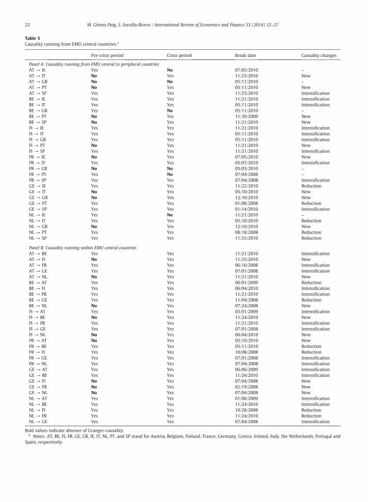
Table 3Causality running from EMU central countries.a

Pre-crisis period Crisis period Break date Causality changes

Panel A: Causality running from EMU central to peripheral countriesAT → IE Yes No 07/05/2010 –

AT → IT No Yes 11/23/2010 NewAT → GR No No 05/11/2010 –

AT → PT No Yes 05/11/2010 NewAT → SP Yes Yes 11/23/2010 IntensificationBE → IE Yes Yes 11/21/2010 IntensificationBE → IT Yes Yes 05/11/2010 IntensificationBE → GR Yes No 05/11/2010 –

BE → PT No Yes 11/30/2009 NewBE → SP No Yes 11/21/2010 NewFI → IE Yes Yes 11/21/2010 IntensificationFI → IT Yes Yes 05/11/2010 IntensificationFI → GR Yes Yes 05/11/2010 IntensificationFI → PT No Yes 11/21/2010 NewFI → SP Yes Yes 11/21/2010 IntensificationFR → IE No Yes 07/05/2010 NewFR → IT Yes Yes 05/07/2010 IntensificationFR → GR No No 05/03/2010 –

FR → PT Yes No 07/04/2008 –

FR → SP Yes Yes 07/04/2008 IntensificationGE → IE Yes Yes 11/22/2010 ReductionGE → IT No Yes 05/10/2010 NewGE → GR No Yes 12/10/2010 NewGE → PT Yes Yes 01/08/2008 ReductionGE → SP Yes Yes 01/14/2010 IntensificationNL → IE Yes No 11/21/2010 –

NL → IT Yes Yes 05/10/2010 ReductionNL → GR No Yes 12/10/2010 NewNL → PT Yes Yes 08/18/2008 ReductionNL → SP Yes Yes 11/25/2010 Reduction

Panel B: Causality running within EMU central countriesAT → BE Yes Yes 11/21/2010 IntensificationAT → FI No Yes 11/25/2010 NewAT → FR Yes Yes 06/10/2008 IntensificationAT → GE Yes Yes 07/01/2008 IntensificationAT → NL No Yes 11/21/2010 NewBE → AT Yes Yes 06/01/2009 ReductionBE → FI Yes Yes 06/04/2010 IntensificationBE → FR Yes Yes 11/21/2010 IntensificationBE → GE Yes Yes 11/04/2008 ReductionBE → NL No Yes 07/24/2008 NewFI → AT Yes Yes 05/01/2009 IntensificationFI → BE No Yes 11/24/2010 NewFI → FR Yes Yes 11/21/2010 IntensificationFI → GE Yes Yes 07/01/2008 IntensificationFI → NL No Yes 06/04/2010 NewFR → AT No Yes 05/10/2010 NewFR → BE Yes Yes 05/11/2010 ReductionFR → FI Yes Yes 10/08/2008 ReductionFR → GE Yes Yes 07/01/2008 IntensificationFR → NL Yes Yes 07/04/2008 IntensificationGE → AT Yes Yes 06/06/2009 IntensificationGE → BE Yes Yes 11/24/2010 IntensificationGE → FI No Yes 07/04/2008 NewGE → FR No Yes 02/19/2008 NewGE → NL No Yes 07/04/2008 NewNL → AT Yes Yes 01/06/2009 IntensificationNL → BE Yes Yes 11/24/2010 IntensificationNL → FI Yes Yes 10/28/2008 ReductionNL → FR Yes Yes 11/24/2010 ReductionNL → GE Yes Yes 07/04/2008 Intensification

Bold values indicate absence of Granger-causality.a Notes: AT, BE, FI, FR, GE, GR, IE, IT, NL, PT, and SP stand for Austria, Belgium, Finland, France, Germany, Greece, Ireland, Italy, the Netherlands, Portugal and

Spain, respectively.

22 M. Gómez-Puig, S. Sosvilla-Rivero / International Review of Economics and Finance 33 (2014) 12–27

a) b)

Fig. 3. Causal relationships from EMU peripheral countries. a: Causal relationships from EMU peripheral to central countries. b: Causal relationships within EMU peripheral countries.

23M.G

ómez-Puig,S.Sosvilla-Rivero

/InternationalReview

ofEconomics

andFinance

33(2014)

12–27

a) b)

Fig. 4. Causal relationships from EMU central countries. a: Causal relationships from EMU central to peripheral countries. b: Causal relationships within EMU central countries.

24M.G

ómez-Puig,S.Sosvilla-Rivero

/InternationalReview

ofEconomics

andFinance

33(2014)

12–27

25M. Gómez-Puig, S. Sosvilla-Rivero / International Review of Economics and Finance 33 (2014) 12–27

Regarding the causal relationships running from EMU peripheral to EMU central countries, an increase in causality after theendogenously identified crisis is detected in six of the 10 possible cases (Panel A of Table 2). As for the causality linkages goingfrom EMU central to EMU peripheral countries, in 10 out of the 15 cases where we find causality both in the tranquil and in thecrisis period, we find that the relationship intensifies (Panel A of Table 3). With regard to the causal relationships within EMUperipheral countries, we find evidence of significant relative rise in causality after the crisis in 12 out of the 14 possible cases(Panel B of Table 2). Finally, when examining the causal relationships within EMU central countries we conclude that theyincrease after the crisis in 14 of the 21 possible cases (Panel B of Table 3).

4.5. Contagion assessment

From the above analysis we can conclude that, in the crisis period, we do find not only some new causality patterns which hadbeen absent before its start, but also an intensification of causality in 70% of the cases which would allow us to establish that thoselinkages may be purely crisis-contingent.

Specifically, causal relationships running from EMU peripheral countries record an important increase in the crisis period: notonly relationships within peripheral countries (Fig. 3b shows six new linkages), but also causal relationships running from EMUperipheral to EMU central countries (Fig. 3a displays 17 new causality patterns). This suggests that the problems of peripheralcountries can spill over not only to other peripheral countries but also to EMU central countries since some of these banks (mostlyGerman and French banks) are highly exposed to the debt of peripheral countries (see Gómez-Puig & Sosvilla-Rivero, 2013).Moreover, several studies show that sovereign bond yields are not only driven by country-specific risk factors but alsosignificantly affected by global risk factors [see Groba et al. (2013) and Dieckmann and Plank (2012) among them]. These globalrisk factors reflect global investors' risk aversion, since in times of uncertainty, they become more risk averse and the“flight-to-safety” motive favors bonds of countries that are generally regarded to have a low default risk (e.g. during the crisisGermany experienced one of its lowest yields' levels in history). Therefore, an increase in the Granger-causality of bond yieldsfrom peripheral to central countries might also reflect a general increase in investors' risk aversion which might have driven anincrease of yields in those countries. Indeed, 10-year yield spreads over Germany of Austrian, Finish, French and Dutchgovernment's bonds achieved a maximum level of 183, 83, 189 and 84 basis points (in November 2011 in the first three countriesand in April 2012 in the case of the Netherlands, see Fig. 2) while the credit rating provided by the three most important agencies(Moody's, Standard & Poor's and Fitch) at the same date was, like in Germany, the highest one. The reason behind sovereign riskrise in central countries, triggered by the behavior of peripheral countries, can be related to herding behavior or panic amonginvestors which leads to what is named by the literature as “pure contagion” (see Gómez-Puig & Sosvilla-Rivero, 2014). Besides,the fact that tensions in sovereign debt markets also spread to EMU central countries is also stressed by the nine new linkages thatappear (see Fig. 4a and b) both in the causal relationships running from EMU central to EMU peripheral countries and betweenEMU central countries.

In our view, these 41 new causality patterns out of the 101 causal relationships that exist in the crisis period within the 11 euroarea countries analyzed (which were absent before the break date, determined endogenously for each causal relationship),together with the intensification of the causal relationship in 42 of the 60 cases in which we find causality both in the tranquil andin the crisis period, can be considered an important operative measure of contagion consistent with both our definition and theliterature, as they represent additional linkages during crisis periods in excess of those that arise during non-crisis periods; see forexample, Forbes and Rigobon (2002), Masson (1999), Pericoli and Sbracia (2003) or Dungey, Fry, González-Hermosillo, andMartin (2006).

5. Conclusions

This paper has three main objectives: to test for the existence of possible Granger-causal relationships in the evolution of theyield of bonds issued by both peripheral and central EMU countries, to determine endogenously the breakpoints in the evolutionof those relationships and to detect contagion episodes according to an operative definition: an abnormal increase in the numberor in the intensity of causal relationships compared with that of tranquil periods, triggered by an endogenously detected shock.

The most important results that emerge from our analysis are the following: (1) Around two thirds out of the totalendogenously identified breakpoints occur after November 2009, when Papandreou's government revealed that its finances werefar worse than previous announcements, suggesting that most of the breakpoints can be explained by systemic shocks directlyconnected to the euro sovereign debt crisis. (2) The number of causal relationships increases as the financial and sovereign debtcrisis unfolds in the euro area, and causality patterns after the break dates are more frequent when EMU peripheral countries arethe triggers. (3) In the crisis period we find evidence of 101 causal relationships: 41 represent new causality linkages and 60 arepatterns that already existed in the tranquil period. However, we find an intensification of the causal relationship in 42 out of the60 cases. In our opinion, these 41 new causality patterns, together with the intensification of the causal relationship in 70% of thecases can be considered an important operative measure of contagion that is consistent with the definition that we haveproposed.

Regarding policy implications, our results seem to indicate that EMU has brought about strong interlinkages of theparticipating countries which are reasonable within a group of countries that share an exchange rate agreement (a commoncurrency in the case of the euro area) and where financial crises tend to be clustered (see Beirne & Fratzscher, 2013). Therefore,we consider that our results might have some practical meaning for investors and policymakers, as well as some theoretical

26 M. Gómez-Puig, S. Sosvilla-Rivero / International Review of Economics and Finance 33 (2014) 12–27

insights for academic scholars interested in the behavior of EMU sovereign debt markets. Our methodology could be used as a toolto provide information regarding the drivers and the time-varying intensity of crisis transmission, in the euro area sovereign debtmarkets, after a shock, which is an important question that can help policymakers to react in the future in order to avoid another.

Finally, it should be noted that our analysis is devoted to bivariate series analysis. The extension to multivariate series analysisis reserved for future research. In view of the encouraging results of the present study, some optimism about the benefits fromimplementing this analysis seems justified.

Acknowledgments

The authors thank the editor and two anonymous referees for useful comments and suggestions on a previous draft of thisarticle, substantially improving the content and quality of the article. The authors are very grateful to Petros Migiakis from theBank of Greece for his comments and suggestions on an earlier draft. Responsibility for any remaining errors rests with theauthors.

References

Aizenman, J. (2013). The eurozone crisis: Muddling through on the way to a more perfect euro union? Social Sciences, 2, 221–223.Akaike, H. (1974). A new look at the statistical model identification. IEEE Transactions on Automatic Control, 19, 716–723.Andenmatten, S., & Brill, G. (2011). Measuring co-movements of CDS premia during the Greek debt crisis. Discussion papers 11-04. Department of Economics,

University of Bern.Andrews, D. W. K. (1993). Tests for parameter instability and structural change with unknown change point. Econometrica, 61, 821–856.Andrews, D., & Ploberger, W. (1994). Optimal tests when a nuisance parameter is present only under the alternative. Econometrica, 62, 1383–1414.Bae, K. H., Karolyi, G. A., & Stulz, R. M. (2003). A new approach to measuring financial contagion. Review of Financial Studies, 16, 717–763.Bai, J. (1997). Estimating multiple breaks one at a time. Econometric Theory, 13, 315–352.Bai, J., & Perron, P. (1998). Estimating and testing linear models with multiple structural changes. Econometrica, 66, 47–78.Bai, J., & Perron, P. (2003). Computation and analysis of multiple structural change models. Journal of Applied Econometrics, 6, 72–78.Baig, T., & Goldfajn, I. (2001). The Russian default and the contagion to Brazil. In S. Claessens, & K. Forbes (Eds.), International financial contagion. Boston: Kluwer

Academic Publishers.Basse, T. (2014). Searching for the EMU core member countries. European Journal of Political Economy (in press).Basse, T., Friedrich, M., & Kleffner, A. (2012). Italian government debt and sovereign credit risk: an empirical exploration and some thoughts about consequences

for European insurers. Zeitschrift für die gesamte Versicherungswissenschaft, 101, 571–579.Beirne, J., & Fratzscher, M. (2013). The pricing of sovereign risk and contagion during the European sovereign debt crisis. Journal of International Money and

Finance, 34, 60–82.Bolton, P., & Jeanne, O. (2011). Sovereign default risk and bank fragility in financially integrated economies. Discussion paper 8368. Centre for Economic Policy

Research.Broner, F., & Ventura, J. (2011). Globalization and risk sharing. Review of Economic Studies, 78, 49–82.Canova, F. (1995). The economics of VAR models. In K. D. Hoover (Ed.), Macroeconometrics: Developments, tensions and prospects. Dordrecht: Kluwer Academic

Publishers.Caporin, M., Pelizzon, L., Ravazzolo, F., & Rigobon, R. (2013). Measuring sovereign contagion in Europe. Working paper 18741. National Bureau of Economic

Research.Cheung, Y. -W., & Chinn, M. D. (1997). Further investigation of the uncertain unit root in GNP. Journal of Business and Economic Statistics, 15, 68–73.Chong, Y. Y., & Hendry, D. F. (1990). Econometric evaluation of linear macroeconomic models. Review of Economic Studies, 53, 671–690.Chow, G. C. (1960). Tests of equality between sets of coefficients in two linear regressions. Econometrica, 28, 591–605.Clements, M. P., & Hendry, D. F. (1993). On the limitations of comparing mean square forecast errors. Journal of Forecasting, 12, 617–637.Corsetti, G., Pericoli, M., & Sbracia, M. (2005). ‘Some contagion, some interdependence’: More pitfalls in tests of financial contagion. Journal of International Money

and Finance, 24, 1177–1199.Dieckmann, S., & Plank, T. (2012). Default risk of advanced economies: An empirical analysis of credit default swaps during the financial crisis. Review of Finance,

16, 902–934.Dolado, J. J., Jenkinson, T., & Sosvilla-Rivero, S. (1990). Cointegration and unit roots. Journal of Economic Surveys, 4, 149–173.Dungey, M., Fry, R., González-Hermosillo, B., & Martin, V. (2006). Contagion in international bond markets during the Russian and the LTCM crises. Journal of

Financial Stability, 2, 1–27.Edwards, S. (2000). Contagion. World Economy, 23, 873–900.Eichengreen, B., Rose, A. K., & Wyplosz, C. (1996). Contagious currency crises: First tests. Scandinavian Journal of Economics, 98, 463–484.Ejsing, J., & Lemke, W. (2009). The Janus-headed salvation: Sovereign and bank credit risk premia during 2008–09. Working Paper 1127. European Central Bank.Favero, C., & Missale, A. (2012). Sovereign spreads in the euro area: Which prospects for a Eurobond? Economic Policy, 27, 231–273.Forbes, K. (2012). The big C: Identifying contagion. Working paper 18465. National Bureau of Economic Research.Forbes, K., & Rigobon, R. (2002). No contagion, only interdependence: Measuring stock market comovements. Journal of Finance, 57, 2223–2261.Gennaioli, N., Martin, A., & Rossi, S. (2014). Sovereign default, domestic banks and financial institutions. The Journal of Finance, 69, 819–866.Geweke, J. (1984). Inference and causality in economic time series models. In Z. Girliches, & M. D. Intriligator (Eds.), Handbook of econometrics. Amsterdam:

Elservier Science Publishers.Gómez-Puig, M., & Sosvilla-Rivero, S. (2013). Granger causality in peripheral EMU debt markets: A dynamic approach. Journal of Banking and Finance, 37,

4627–4649.Gómez-Puig, M., & Sosvilla-Rivero, S. (2014). EMU sovereign debt markets crisis: Fundamental-based or pure contagion? Institut de Recerca en Economia Aplicada

(IREA) working papers. Universitat de Barcelona (2014/02).Gorea, D., & Radev, D. (2014). The euro area sovereign debt crisis: Can contagion spread from the periphery to the core? International Review of Economics and

Finance, 30, 78–100.Granger, C. W. J. (1969). Investigating causal relations by econometric models and cross-spectral methods. Econometrica, 37, 24–36.Granger, C. W. J., Huang, W. N., & Yang, C. W. (2000). A bivariate causality between stock prices and exchange rates: Evidence from the recent Asian flu. The

Quarterly Review of Economics and Finance, 40, 337–354.Granger, C. W. J., & Newbold, P. (1973). Some comments on the evaluation of economic forecasts. Applied Economics, 5, 35–47.Granger, C. W. J., & Newbold, P. (1986). Forecasting economic time series. Orlando, FL: Academic Press.Gray, D. (2009). Financial contagion among members of the EU-8: A cointegration and Granger causality approach. International Journal of Emerging Markets, 4,

299–314.Groba, J., Lafuente, J. A., & Serrano, P. (2013). The impact of distressed economies on the EU sovereign market. Journal of Banking and Finance, 37, 2520–2532.Gruppe, M., & Lange, C. (2014). Spain and the European sovereign debt crisis. European Journal of Political Economy (in press).

27M. Gómez-Puig, S. Sosvilla-Rivero / International Review of Economics and Finance 33 (2014) 12–27

Hansen, B. E. (1997). Approximate asymptotic p values for structural-change tests. Journal of Business and Economic Statistics, 15, 60–67.Hsiao, C. (1981). Autoregressive modelling and money-income causality detection. Journal of Monetary Economics, 7, 85–106.Johansen, S. (1991). Estimation and hypothesis testing of cointegration vectors in gaussian vector autoregressive models. Econometrica, 59, 1551–1580.Johansen, S. (1995). Likelihood-based inference in cointegrated vector autoregressive models. Oxford: Oxford University Press.Kalbaska, A., & Gatkowski, M. (2012). Eurozone sovereign contagion: Evidence from the CDS market (2005–2010). Journal of Economic Behaviour and Organization,

83, 657–673.Kaminsky, G. L., & Reinhart, C. M. (2000). On crises, contagion, and confusion. Journal of International Economics, 51, 145–168.Kwaitkowski, D., Phillips, P. C. B., Schmidt, P., & Shin, Y. (1992). Testing the null hypothesis of stationarity against the alternative of a unit root: How sure are we

that economic time series have a unit root? Journal of Econometrics, 54, 159–178.Masson, P. (1999). Contagion, monsoonal effects, spillovers, and jumps between multiple equilibria. In P. -R. Agenor, M. Miller, D. Vines, & A. Weber (Eds.), The

Asian financial crisis: Causes, contagion and consequences. Cambridge, UK: Cambridge University Press.Metieu, N. (2012). Sovereign risk contagion in the eurozone. Economics Letters, 117, 35–38.Mody, A. (2009). From Bear Sterns to Anglo Irish: How Eurozone sovereign spreads related to financial sector vulnerability. Working paper 09/108. International

Monetary Fund.Moro, B. (2014). Lessons from the European economic and financial great crisis: A survey. European Journal of Political Economy (in press).Newey, W. K., & West, K. D. (1987). A simple, positive semi-definite, heteroskedasticity and autocorrelation consistent covariance matrix. Econometrica, 55,

703–708.Pericoli, M., & Sbracia, M. (2003). A primer on financial contagion. Journal of Economic Surveys, 17, 571–608.Perron, P. (1989). The great crash, the oil price shock and the unit root hypothesis. Econometrica, 57, 1361–1401.Quandt, R. E. (1960). Tests of the hypothesis that a linear regression system obeys two separate regimes. Journal of the American Statistical Association, 55,

324–330.Sander, H., & Kleimeier, S. (2003). Contagion and causality: An empirical investigation of four Asian crisis episodes. International Financial Markets, Institutions and

Money, 13, 171–186.Syllignakis, M. N., & Kouretas, G. P. (2011). Dynamic correlation analysis of financial contagion: Evidence from the Central and Eastern European markets.

International Review of Economics and Finance, 20, 717–732.Thornton, D. L., & Batten, D. S. (1985). Lag-length selection and tests of Granger causality between money and income. Journal of Money, Credit, and Banking, 27,

164–178.Williams, E. J. (1959). Regression analysis. New York: Wiley.Zivot, E., & Andrews, D. W. K. (1992). Further evidence on the great crash, the oil-price shock, and the unit-root hypothesis. Journal of Business and Economic

Statistics, 10, 251–270.