Is energy consumption effective to spur economic growth in Pakistan? New evidence from bounds test...

(This is a sample cover image for this issue. The actual cover is not yet available at this time.)

This article appeared in a journal published by Elsevier. The attachedcopy is furnished to the author for internal non-commercial researchand education use, including for instruction at the authors institution

and sharing with colleagues.

Other uses, including reproduction and distribution, or selling orlicensing copies, or posting to personal, institutional or third party

websites are prohibited.

In most cases authors are permitted to post their version of thearticle (e.g. in Word or Tex form) to their personal website orinstitutional repository. Authors requiring further information

regarding Elsevier’s archiving and manuscript policies areencouraged to visit:

http://www.elsevier.com/copyright

http://www.elsevier.com/copyright

Author's personal copy

Is energy consumption effective to spur economic growth in Pakistan? New evidencefrom bounds test to level relationships and Granger causality tests

Muhammad Shahbaz a,⁎, Muhammad Zeshan b, Talat Afza a

a COMSATS Institute of Information Technology, Defence Road, Off Raiwind, Lahore, Pakistanb School of Economics, Quaid-i-Azam University, Islamabad, Pakistan

a b s t r a c ta r t i c l e i n f o

Article history:Accepted 23 June 2012Available online xxxx

Keywords:Energy consumptionEconomic growthPakistan

The present study investigates the relationship between energy (renewable and nonrenewable) consumption andeconomic growth using Cobb–Douglas production function in case of Pakistan over the period of 1972–2011. Wehave used the ARDL bounds testing and Gregory and Hansen (1990) structural break cointegration approachesfor long run while stationarity properties of the variables have been tested applying Clemente-Montanes-Reyes(1998) structural break unit root test.Our results confirm cointegration between renewable energy consumption, nonrenewable energy consumption,economic growth, capital and labor in case of Pakistan. The findings show that both renewable and nonrenewableenergy consumption add in economic growth. Capital and labor are also important determinants of economicgrowth. The VECM Granger causality analysis validates the existence of feedback hypotheses between renewableenergy consumption and economic growth, nonrenewable energy consumption and economic growth, economicgrowth and capital.

© 2012 Elsevier B.V. All rights reserved.

1. Introduction

Kyoto Protocol, our environmental responsibilities, volatile energyprices, and energy security are the contemporaneous issues that bindnations to diversify their energy supplies. Kyoto Protocol necessitatesits members to maintain the level of greenhouse gas emissions since1990 to date. It is hoped that this mutual effort, by both the developingand the developed countries, would help to mitigate the detrimentalconsequences of global warming. In addition, it would also help to dis-pirit the increasing volume of CO2 emissions in environment. Of course,the lower level of CO2 emissions can only be achieved by the lesser con-sumption of fossil fuels but this solution would also bring severe ail-ment to economic growth since the economic cost of utilizing thefossil fuels has increased tremendously. Therefore, one cannot overlookthe long run consequences of the extensive utilization of the fossil fuelsfor some short run economic gains.

Volatility in energy prices creates difficulties for oil importing coun-tries in balancing their payments each year. All the major economic re-cessions are preceded by the rising energy shocks (Hamilton, 1983) andthe rise in energy prices invokes the inflationary expectations. Given thecommitment of the central bank to the economic stability and to mini-mize inflationary expectations, central bank raises the interest rate(Harris et al., 2009). As a consequence, although, the overall inflationtends to fall but the rising interest rate also lowers the level of investment

(Leduc and Sill, 2004); resultantly, the growth rate is adversely affected. Itis worth mentioning that renewable energy emits lower level of CO2 inthe environment, and is helpful in solving the environmental problemsof climate change (Elliot, 2007; Ferguson, 2007).

Energy requirements are rapidly increasing in Pakistan and the pri-mary energy requirements in Pakistan have witnessed 80% increase inthe last 15 years; it rose from 34 million TOE in 1994–95 to 61 millionTOE in 2009–10. Indigenous natural gas comprises of 45% of the energymix, oil imports constitutes 35%, hydel power covers 12%, coal 6% andfinally nuclear energy constitutes 2% of the energy mix respectively(Government of Pakistan, 2010). Pakistan is heavily dependent on con-ventional sources of energy to satisfy its energy consumption require-ments. Conventional source of nonrenewable energy satisfy more than99% of the energy requirements (Sheikh, 2010). Nonetheless, Govern-ment of Pakistan has assigned the target to the Pakistan Alternative Ener-gy Board to generate 5% of the total installed power through thealternative/renewable energy up to year 2030 (Khalil et al., 2005).

Pakistan is a country blessedwith somany natural sources of energythat, if utilized properly may reduce the dependence on foreign aid foroil imports. These available unexplored energy resources in Pakistanhave the potential not only to satisfy the domestic energy requirementsbut these can also be exported to other energy deficit countries. But un-fortunately, these resources have not been explored properly.

Pakistan is located on the high insulation beltwhichgives it the com-parative advantage in the creation of solar energy. This source of energyis much cheaper than the fossil fuels because neither it needs refiningnor it requires any transportation cost. It is the most attractive substi-tute of fossil fuels because it adds no pollution in the environment. It

Economic Modelling 29 (2012) 2310–2319

⁎ Corresponding author.E-mail addresses: [email protected] (M. Shahbaz), [email protected]

(M. Zeshan), [email protected] (T. Afza).

0264-9993/$ – see front matter © 2012 Elsevier B.V. All rights reserved.doi:10.1016/j.econmod.2012.06.027

Contents lists available at SciVerse ScienceDirect

Economic Modelling

j ourna l homepage: www.e lsev ie r .com/ locate /ecmod


is employed in rural telephone exchanges, emergency telephones athigh ways, vaccine and medicine refrigeration utilized in the hospitalsetc. In Pakistan, Sindh and Balochistan provinces are the ideal locationsfor the production and utilization of solar energy. In Balochistan, 77% ofthe population lives in villages and 90% of them live without electrifica-tion facilities. These villages are located far away from each other; resul-tantly, there is no scope of the grid stations and solar energy networksare more suitable sources of energy for these location. Recently, a 100solar energy homes' project has been completed in 9 villages of theseprovinces which have the potential to enlighten the 26,000 homes(Sheikh, 2010).

The coastal areas of Sind and Baluchistan provinces and the desertareas of Punjab and Sind provinces provide the huge potential for thewind energy. The coastal belt has a 60 kmwide and 180 km long corri-dor with a potential to generate the 50,000 MW of the renewable ener-gy through the wind energy. In addition, there are other sites in theseareas as well as in Northern areas which are suitable for the microwind turbines. Although, thesewind turbines have the potential to elec-trify 5000 village in Pakistan but unfortunately just 18 villages havebeen electrifiedwith this source of energy (Sheikh, 2010). The Northernareas of Pakistan are rich in waterfalls which makes it a suitable candi-date for the hydro energy. In addition to the big plants which have thepotential to generate 1 MW of renewable energy or greater, there areother sites suitable for themicro hydro energy plants having the poten-tial to produce 100 KW of renewable energy. Altogether, these microplantsmay have the potential of producing 300 MWof renewable ener-gy. These areas are densely populated and fossil fuel power plants forproducing non-renewable energy might be costly, therefore thesemicro hydro plants are more suitable for these areas. The canal net-works in Punjab have also such sites which provide a great opportunityfor the renewable energy production. It is estimated that Punjab com-prises of 300 such sites which can produce 350 MWof renewable ener-gy. Whereas, there are only 228 micro plants which just have thepotential to produce the 3 MW of renewable energy to the householdsand small industrial units (Sheikh, 2010).

Biogas is also one of the important sources of energy which notonly increases the land fertility but is also used to fulfill the energy re-quirements. There are 48 million animals in Pakistan comprising ofbuffaloes, bullocks and cows, as per livestock census of 2002–03.Keeping in view the daily dung dropping and assuming 50% collect-ability, it is estimated that 17.25 million m3 of biogas can be pro-duced daily with the help of biogas plants. Cooking requirements of50 million people can be entertained with it. In addition, it also pro-vides fertility to land through the provision of 35.04 million ofbio-fertilizers each year. The formal initiation, for this source of ener-gy, was taken in 1974 and up to 1987, there were 4137 units of biogasplants in the country. Unfortunately, the lack of funds made this pro-ject difficult to sustain during 1990s but later on this program wasreinitiated with the help of 1700 biogas plants in many villages inthe country.1

Energy (renewable and non-renewable energy consumption) is animportant determinant of economic growth like other factors of pro-duction such as labor and capital. Existing energy literature providesfour competing hypotheses of energy consumption (renewable andnonrenewable energy consumption) and economic growth in caseof Pakistan. These competing hypotheses are very important for poli-cy point of view. For instance, reductions in energy would not haveadverse impact on economic growth if economic growth Granger cau-ses energy consumption or neutral hypothesis exists between boththe variables. If bidirectional causality is found between both the vari-ables or energy consumption Granger causes economic growth then

new sources of energy should be encouraged. Energy is an importantstimulus of production process and energymust Granger cause economicgrowth. An expansion in production is linked with energy demand andeconomic growth might Granger cause energy consumption. The mainobjective of present study is to investigate the relationship betweenrenewable energy consumption, nonrenewable energy consumption,capital, labor and economic growth in case of Pakistan of using Cobb–Douglas production function over the period of 1972–2011. In case ofPakistan, this study contributed to energy literature by five folds apply-ing: (i) Clemente et al. (1998) structural break unit root test forstationarity properties of the variables; (ii) the ARDL bound testing ap-proach to cointegration for long run relationship; (iii) Gregory andHansen (1996) structural break test to check the reliability and robust-ness of the ARDL results, (iv) OLS and ECM for long run and short runimpacts of renewable and nonrenewable energy consumption on eco-nomic growth; (v) VECMGranger causality approach to examine causalrelationship between the variables.

Our findings reveal that cointegration between renewable energyconsumption, nonrenewable energy consumption, economic growth,capital and labor exists in case of Pakistan. Additionally, our empiricalevidence also reports that renewable energy consumption and non-renewable energy consumption have positive impact on economicgrowth. Capital and labor also adds in economic growth. Furthermore,estimated results indicate bidirectional causality relationship be-tween renewable energy consumption and economic growth, non-renewable energy consumption and economic growth, economicgrowth and capital.

2. Review of literature on energy–growth nexus

Theorists have divided the review of literature on energy and growthnexus in four competing hypotheses such as growth hypothesis, conser-vation hypothesis, feedback hypothesis and neutrality hypothesis.Growth hypothesis asserts the unidirectional causality running from en-ergy consumption to economic growth, whereas the conservation hy-pothesis supports the reverse process of the unidirectional causalityrunning from economic growth to energy consumption. Empirical evi-dence also supports the interdependence between energy consumptionand economic growth, and in some cases there is no relationship(Payne, 2010a, 2010b, 2010c). The last two cases are formally known asfeedback and neutrality hypotheses respectively. The present studytends to review the literature and report the empirical evidence underthese four competing hypotheses.

2.1. Growth hypothesis

Ewing et al. (2007) investigated the correlation between dis-aggregated energy consumption and real GDP in United States byusing generalized variance decomposition approach for empirical anal-ysis. They found that coal, natural gas, and fossil fuels explain the max-imum variations in output, whereas renewable energy consumptionexplains a little variation in output. These estimated results werequite consistent with the growth hypothesis. Later on, Payne (2010a,2010b, 2010c) employed the Toda–Yamamoto causality tests to exam-ine causal relationship between the biogas energy consumption andreal output over the period of 1949–2007 in the US economy. Payne(2010a, 2010b, 2010c) reported unidirectional causality running frombiogas consumption to real output confirming growth hypothesis. Incase of India, Tiwari (2011a, 2011b) postulated the relationship be-tween renewable energy consumption, economic growth and CO2

emissions by applying Johansen-Juselius (1990) long run and structuralinnovative accounting approach (IAA) within framework of VAR (vec-tor autoregression) to test the direction of causal relationship betweenthese variables. The empirical evidence reported no cointegration be-tween renewable energy consumption, economic growth and CO2

emissions during the study period of 1965–2009. Furthermore, results

1 The information regarding the renewable energy potential has been borrowedfrom various reports, available on the official website of Alternative Energy Develop-ment Board, Ministry of Water and Power, Government of Pakistan.

2311M. Shahbaz et al. / Economic Modelling 29 (2012) 2310–2319


showed that renewable energy consumption attributes to economicgrowth through its positive innovative shocks and economic growthleads to increase CO2 emissions in response. Therefore it can be con-cluded that renewable energy consumption Granger causes economicgrowth. Later on, Tiwari (2011b) applied panel VAR to investigate therelationship between renewable energy consumption, nonrenewableenergy consumption, economic growth and CO2 emissions in case ofEurope and Eurasian countries using the data over the period of1965–2009.2 The results indicated that the innovative response of eco-nomic growth is positive due to one standard shock in renewable ener-gy consumption and thus supporting the growth hypothesis. For Italianeconomy, Magnani and Vaona (2011) tested the spillover effects ofrenewable energy generation applying panel cointegration andGrangernon-causality within framework of GMM (generalized method of mo-ments) systems. Their results support that renewable energy genera-tion promotes economic growth and policies promoting renewableenergy should be encouraged. Similarly, Bobinaite et al. (2011) exam-ined the causal relationship between renewable energy consumptionand economic growth by applying Johansen cointegration for longrun and Granger causality test for causal relationship between boththe variables. Their results reported no evidence of cointegration be-tween renewable energy consumption and economic growth while re-newable energy consumption Granger causes economic growth. Thisimplies that energy conservation policies should be discouraged inLithuanian economy.

2.2. Conservation hypothesis

Sari et al. (2008) followed Ewing et al. (2007) by applying differentestimation techniques in case of United States. They employed auto-regressive distributive lag approach or the ARDL bounds testing ap-proach cointegration to test long run relationship between thevariables using monthly data over the period of 2001–2005. Theyused capital and labor as the main determinants of fossil fuel, hydro-electric power, solar energy, waste energy and wing energy consump-tion, whereas these two variables have no long-run relationship withnatural gas and wood energy. Their empirical investigation confirmedthe existence of conservation hypothesis. Sadorsky (2009a) appliedpanel cointegration test to explore the causal relationship betweenrenewable energy consumption and economic growth using apanel of 18 emerging countries.3 Sadorsky (2009a) reported that a1% rise in income per capita increase the energy requirements upto 3.5% in long run for the period of 1994–2003. This also tends tosupport the conservation hypothesis. Chang et al. (2009) focusedon the linkages between renewable energy consumption and eco-nomic growth using a panel threshold regression model for 30OECD countries4 under different economic growth regimes. Their re-sults indicated that economic growth positively Granger causes renew-able energy consumption but regime with lower economic growth,showed no relationship between economic growth and renewable ener-gy consumption. Sadorsky (2009b) estimated the energy demandmodel using data of G7 countries. The panel cointegration was appliedto test the long run relationship between renewable energy consump-tion, oil prices, economic growth and energy pollutants. The estimatedresults reported that economic growth and CO2 emissions are major de-terminants of renewable energy consumptionwhile rise in oil prices hasnegative impact on renewable energy consumption. The causality

analysis revealed unidirectional causal relationship running from eco-nomic growth to renewable energy consumption.

2.3. Feedback hypothesis

Apergis and Payne (2010a) conducted a study to test the causal re-lationship between renewable energy consumption and economicgrowth for a panel of thirteen OECD countries applying panelcointegration and error correction mechanism (ECM) over the periodof 1985–2005.5 The empirical investigation revealed the bidirectionalcausality between renewable energy consumption and economicgrowth in the long run as well as in short run which confronts thefeedback hypothesis. Apergis and Payne (2010b) used the panelcointegration and error correction mechanism (ECM) to examinethe causal relationship between renewable energy consumption andeconomic growth using the data of 13 Eurasian countries6 for 1992–2007 time period. Their results confirmed that renewable energy con-sumption and economic growth Granger cause each other. In case ofItaly, Vaona (2010) used structural break unit tests for integratingorder of nonrenewable energy consumption and economic growth,Johansen cointegration approach for long run and Toda andYamamoto (1995) for causality analysis. The empirical exercise vali-dated that variables are not cointegrated for long run relationshipwhile nonrenewable energy consumption and economic growth areinterdependent supporting feedback hypothesis.

The same empirical exercise was undertaken by Apergis andPayne (2011) to find the causal relationship between renewable en-ergy consumption and economic growth using the data of 6 CentralAmerican countries over the period of 1980–2006.7 The estimated re-sults revealed the bidirectional causality between the two variables,which also confirm the existence of feedback hypothesis. Later on,Apergis and Payne (2012b) tested the direction of causal relationshipbetween renewable energy consumption and non-renewable energyconsumption and economic growth using a panel of 80 countries8 using data for the period of 1990–2007. The empirical evidenceshowed bidirectional causal relationship between renewable energyand economic growth, non-renewable energy and economic growthvalidating the feedback hypothesis. Furthermore, results also provid-ed the evidence of substitution between renewable energy consump-tion and nonrenewable energy consumption. Apergis and Payne(2012a) investigated the impact of renewable and non-renewable en-ergy consumption on economic growth in case of Latin Americancountries by applying Larsson et al. (2001) panel cointegration test.Their results found cointegration between the series and renewableand nonrenewable energy consumption has positive impact on eco-nomic growth. Causality analysis reveals feedback hypothesis be-tween renewable (nonrenewable) energy consumption and economicgrowth.9

2 Austria, Belgium and Luxembourg, Bulgaria, Finland, France, Germany, Greece,Republic of Ireland, Italy, Norway, Portugal, Spain, Sweden, Switzerland, Turkey andUnitedKingdom.

3 Argentina, Brazil, Chile, China, Colombia, Czech Republic, Hungary, India, Indonesia,Korea, Mexico, Peru, Philippines, Poland, Portugal, Russia, Thailand and Turkey.

4 Australia, Austria, Belgium, Canada, the Czech Republic, Denmark, Finland, France,Germany, Greece, Hungary, Iceland, Ireland, Italy, Japan, Korea, Luxembourg, Mexico,the Netherlands, New Zealand, Norway, Poland, Portugal, the Slovak Republic, Spain,Sweden, Switzerland, Turkey, the United Kingdom and United States.

5 Australia, Austria, Belgium, Canada, Denmark, France, Germany, Iceland, Italy, Japan,Luxembourg, Netherlands, New Zealand, Norway, Portugal, Spain, Sweden, Switzerland,United Kingdom and United States.

6 Armenia, Azerbaijan, Belarus, Estonia, Georgia, Kazakhstan, Kyrgyzstan, Latvia,Moldova, Russia, Tajikistan, Ukraine and Uzbekistan.

7 Costa Rica, El Salvador, Guatemala, Honduras, Nicaragua and Panama.8 Algeria, Argentina, Australia, Austria, Bangladesh, Belgium, Bolivia, Brazil, Bulgaria,

Canada, Cameron, Chile, China, Comoros, Costa Rica, Denmark, Dominican Republic,Ecuador, Egypt, El Salvador, Ethiopia, Finland, France, Gabon, Germany, Ghana, Greece,Guatemala, Guinea, Honduras, Hungary, Iceland, India, Indonesia, Iran, Ireland, Italy, Japan,Jordan, Kenya, Korea, Luxembourg,Madagascar,Malawi,Malaysia,Mali,Mauritius,Mexico,Morocco, Mozambique, Netherlands, New Zealand, Nicaragua, Norway, Pakistan, Panama,Paraguay, Peru, Philippines, Poland, Portugal, Romania, Senegal, South Africa, Spain, SriLanka, Sudan, Swaziland, Sweden, Switzerland, Syria, Thailand, Tunisia, Turkey, Uganda,United Kingdom, United States, Uruguay, Venezuela and Zambia.

9 Costa Rica, El Salvador, Guatemala, Honduras, Nicaragua and Panama.

2312 M. Shahbaz et al. / Economic Modelling 29 (2012) 2310–2319


2.4. Neutrality hypothesis

In energy literature, Payne (2009) applied Toda–Yamamoto teststo investigate the nature of causal relationship between renewableenergy consumption, nonrenewable energy consumption and realoutput in case of United States. The study used annual data for the pe-riod of 1949–2006. The results showed no causality between the vari-ables and, therefore, supported the existence of neutrality hypothesis.Using panel of 27 European countries, Menegaki (2011) investigatedthe causal relation between renewable energy consumption and eco-nomic growth over the period of 1997–2007.10 The study applied ran-dom effect model for estimation purpose, and estimated resultssupported that no causality is found between these two series corrobo-rating the neutrality hypothesis.

2.5. Some mixed results

In case of United States, Bowden and Payne (2010) also utilizedthe Toda–Yamamoto long run causality approaches to test the causalitybetween renewable energy consumption, non-renewable energy con-sumption and real output over the period of 1949–2006. Their resultsindicated no causal relationship between commercial and industrial re-newable energy consumption and real output but bidirectional causalrelationship is found between commercial, residential non-renewableenergy consumption and real output. Furthermore, empirical evidenceconfirmed that residential renewable energy consumption and indus-trial non-renewable energy consumption Granger causes real output.Likewise, Menyah andWolde-Rufael (2010) also investigated the direc-tion of causal relationship between CO2 emissions, renewable energyconsumption, nuclear energy consumption and real output in case ofUSA. They used annual data covering the period of 1960–2007. Theirempirical exercise revealed that nuclear energy Granger causes CO2

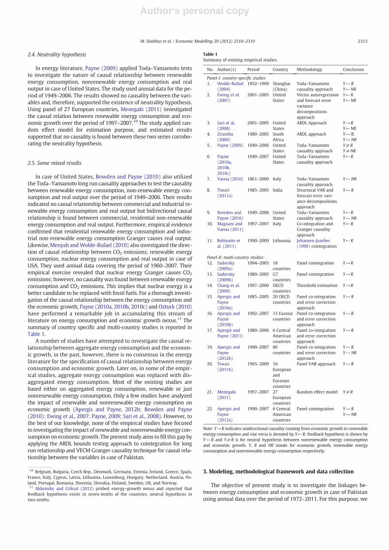
emissions; however, no causalitywas found between renewable energyconsumption and CO2 emissions. This implies that nuclear energy is abetter candidate to be replaced with fossil fuels. For a thorough investi-gation of the causal relationship between the energy consumption andthe economic growth, Payne (2010a, 2010b, 2010c) and Ozturk (2010)have performed a remarkable job in accumulating this stream ofliterature on energy consumption and economic growth nexus.11 Thesummary of country specific and multi-country studies is reported inTable 1.

A number of studies have attempted to investigate the causal re-lationship between aggregate energy consumption and the econom-ic growth, in the past, however, there is no consensus in the energyliterature for the specification of causal relationship between energyconsumption and economic growth. Later on, in some of the empir-ical studies, aggregate energy consumption was replaced with dis-aggregated energy consumption. Most of the existing studies arebased either on aggregated energy consumption, renewable or justnonrenewable energy consumption. Only a few studies have analyzedthe impact of renewable and nonrenewable energy consumption oneconomic growth (Apergis and Payne, 2012b; Bowden and Payne(2010); Ewing et al., 2007; Payne, 2009; Sari et al., 2008). However, tothe best of our knowledge, none of the empirical studies have focusedto investigating the impact of renewable and nonrenewable energy con-sumption on economic growth. The present study aims tofill this gap byapplying the ARDL bounds testing approach to cointegration for longrun relationship and VECM Granger causality technique for causal rela-tionship between the variables in case of Pakistan.

3. Modeling, methodological framework and data collection

The objective of present study is to investigate the linkages be-tween energy consumption and economic growth in case of Pakistanusing annual data over the period of 1972–2011. For this purpose, we

10 Belgium, Bulgaria, Czech Rep., Denmark, Germany, Estonia, Ireland, Greece, Spain,France, Italy, Cyprus, Latvia, Lithuania, Luxemburg, Hungary, Netherland, Austria, Po-land, Portugal, Romania, Slovenia, Slovakia, Finland, Sweden, UK, and Norway.11 Akkemike and Göksal (2012) probed energy–growth nexus and reported thatfeedback hypothesis exists in seven-tenths of the countries, neutral hypothesis intwo-tenths.

Table 1Summary of existing empirical studies.

No. Author(s) Period Country Methodology Conclusion

Panel-I: country-specific studies1. Wolde-Rufael

(2004)1952–1999 Shanghai

(China)Toda–Yamamotocausality approach

Y↔RY←NR

2. Ewing et al.(2007)

2001–2005 UnitedStates

Vector autoregressionand forecast errorvariancedecompositionsapproach

Y←RY←NR

3. Sari et al.(2008)


ARDL Approach Y→RY←NR

4. Ziramba(2009)

1980–2005 SouthAfrica

ARDL approach Y↔R,Y↔NR

5. Payne (2009) 1949–2006 UnitedStates

Toda–Yamamotocausality approach

Y≠RY≠NR

6. Payne(2010a,2010b,2010c)



Y←R

7. Vaona (2010) 1861–2000 Italy Toda–Yamamotocausality approach

Y↔NR

8. Tiwari(2011a)

1985–2005 India Structural VAR andforecast error vari-ance decompositionsapproach

Y↔R

9. Bowden andPayne (2010)



Y←RY↔NR

10. Magnani andVaona (2011)

1997–2007 Italy Co-integration andGranger causalityapproach

Y←R

11. Bobinaite etal. (2011)

1990–2009 Lithuania Johansen-Juselies(1990) cointegration

Y←R

Panel-II: multi-country studies:12. Sadorsky

(2009a)1994–2003 18

countriesPanel cointegration Y→R

13. Sadorsky(2009b)

1980–2005 G7countries

Panel cointegration Y→R

14. Chang et al.(2009)

1997–2006 OECDcountries

Threshold estimation Y→R

15. Apergis andPayne(2010a)

1885–2005 20 OECDcountries

Panel co-integrationand error correctionapproach

Y↔R

16. Apergis andPayne(2010b)

1992–2007 13 Eurasiacountries


Y↔R

17. Apergis andPayne (2011)

1980–2006 6 CentralAmericancountries


Y↔R

19. Apergis andPayne(2012b)

1990–2007 80countries


Y↔RY↔NR

20. Tiwari(2011b)

1965–2009 16EuropeanandEurasiancountries

Panel VAR approach Y↔R

21. Menegaki(2011)

1997–2007 27Europeancountries

Random effect model Y≠R

22. Apergis andPayne(2012a)

1990–2007 6 CentralAmericancountries

Panel cointegration Y↔RY↔NR

Note: Y→R indicates unidirectional causality running from economic growth to renewableenergy consumption and vise versa is denoted by Y←R; feedback hypothesis is shown byY↔R and Y≠R is for neutral hypothesis between nonrenewable energy consumptionand economic growth. Y, R and NR stands for economic growth, renewable energyconsumption and nonrenewable energy consumption respectively.



employ Cobb–Douglas production function to investigate the relation-ship between energy consumption and economic growth includingcapital and labor as additional factors of production. The general formof Cobb-Douglas production function as following:

Y ¼ AEα1Kα2Lα3eu: ð1Þ

Where Y is domestic output in real terms; E, K and L denote energy,real capital and labor respectively. A is for the level of technological ad-vancements and e is the residual term assumed to be identically, inde-pendently and normally distributed. The returns to scale is associatedwith energy consumption, capital and labor and, is shown by α1,α2

and α3 respectively. We have converted all the series into logarithmsto linearize the form of nonlinear Cobb–Douglas production. It shouldbe noted that simple linear specification does not seem to provide con-sistent results therefore to cover this problem, we use log-linear speci-fication to investigate the relationship between energy consumptionand economic growth in case of Pakistan. Ehrlich (1977, 1996),Cameron (1994) and Layson (1983) recommended to use log-linearmodeling in attaining better, consistent and efficient empirical results.12 The log-linear functional form of Cobb–Douglas production functionis modeled as follows:

logYt ¼ logAþ α1 logEt þ α2 logKt þ α3 logLt þ ut : ð2Þ

The empirical equation to investigate the relationship betweenenergy consumption and economic growth is modeled by keepingtechnology constant. Furthermore, we decompose energy consump-tion into renewable and non-renewable energy consumption inorder to measure the impact of individual components of energyon domestic production and hence on economic growth. The issueis debatable in case of Pakistan as to which source of energy shouldbe utilized to sustain economic growth. The log-linear specificationto explore the relationship between energy consumption and eco-nomic growth is as follows:

lnYt ¼ α0 þ α1 lnRt þ α2 lnNRt þ α3 lnKt þ α4 lnLt þ ut ð3Þ

where lnYt, lnRt, lnNRt, lnKt and lnLt is the logarithm of per capitareal GDP, renewable energy consumption (kg of oil equivalent percapita), non-renewable energy consumption (kg of oil equivalentper capita), real capital per capita and per capita labor respectively.

The long run relationship between energy consumption (renewableand non-renewable) and economic growth in case of Pakistan over theperiod of 1972–2011 is investigated by applying the ARDL bounds testingapproach of Pesaran et al. (2001). Numerous cointegration approachesare available in empirical literature to test cointegration between the se-ries but the ARDL bounds testing is considered to be superior and prefer-able due to its various advantages. For instance, order of integration of theseries does notmatter for applying the ARDL bounds testing if no variableis found to be stationary at I(2). The approach is more appropriate ascompared to conventional cointegration techniques for small sam-ple (Haug, 2002). Within the general-to-specific framework,unrestricted version of the ARDL chooses proper lag order to capturethe data generating procedure.13 Appropriate modification of orderof the ARDL model is sufficient to simultaneously correct for residualserial correlation and endogeneity problems (Pesaran and Shin,1999). The equations of unrestricted error correction model (UECM)

to investigate the long-and-short run relations between the series arethe following:

Δ lnYt ¼ ϑ1 þ ϑTT þ ϑY lnYt−1 þ ϑR lnRt−1 þ ϑNR lnNRt−1 þ ϑK lnKt−1 þ ϑL lnLt−1

þXp

i¼1

ϑiΔ lnYt−i þXq

j¼0

ϑjΔ lnRt−j þXr

k¼0

ϑkΔ lnNRt−k þXs

l¼0

ϑlΔ lnKt−l

þXt

m¼0

ϑmΔ lnLt−m þ μ t

ð4Þ

Δ lnRt ¼ α1 þ αTT þ αY lnYt−1 þ αR lnRt−1 þ αNR lnNRt−1 þ αK lnKt−1 þ αL lnLt−1

þXp

i¼1

αiΔ lnRt−i þXq

j¼0

αjΔ lnYt−j þXr

k¼0

αkΔ lnNRt−k þXs

l¼0

αlΔ lnKt−l

þXt

m¼0

αmΔ lnLt−m þ μ t

ð5Þ

Δ lnNRt ¼ β1 þ βTT þ βY lnYt−1 þ βR lnRt−1 þ βNR lnNRt−1 þ βK lnKt−1 þ βL lnLt−1

þXp

i¼1

βiΔ lnNRt−i þXq

j¼0

βjΔ lnYt−j þXr

k¼0

βkΔ lnRt−k þXs

l¼0

βlΔ lnKt−l

þXt

m¼0

βmΔ lnLt−m þ μ t

ð6Þ

Δ lnKt ¼ ρ1 þ ρTT þ ρY lnYt−1 þ ρR lnRt−1 þ ρNR lnNRt−1 þ ρK lnKt−1 þ ρL lnLt−1

þXp

i¼1

ρiΔ lnKt−i þXq

j¼0

ρjΔ lnYt−j þXr

k¼0

ρkΔ lnRt−k þXs

l¼0

ρlΔ lnNRt−l

þXt

m¼0

ρmΔ lnLt−m þ μt

ð7Þ

Δ lnLt ¼ σ1 þ σTT þ σY lnYt−1 þ σR lnRt−1 þ σNR lnNRt−1 þ σK lnKt−1 þ σ L lnLt−1

þXp

i¼1

σ iΔ lnLt−i þXq

j¼0

σ jΔ lnYt−j þXr

k¼0

σkΔ lnRt−k þXs

l¼0

σ lΔ lnNRt−l

þXt

m¼0

σmΔ lnKt−m þ μ t :

ð8Þ

Where Δ is the differenced operator and μt is residual term in pe-riod t. The Akaike information criterion (AIC) is followed to chooseappropriate lag length of the first differenced regression. The appro-priate computation of F-statistic depends upon the suitable lagorder selection of the series to be included in the model.14 The jointsignificance of the coefficients of lagged variables is investigated byapplying an F-test of Pesaran et al. (2001). The null hypothesis of nolong run relationship between the variables in Eq. (3) is H0:ϑY=ϑR=ϑNR=ϑK=ϑL=0 against alternate hypothesis of long run rela-tionship i.e. H0 :ϑY≠ϑR≠ϑNR≠ϑK≠ϑL≠0. Two asymptotic criticalvalues have been generated by Pesaran et al. (2001). These boundsare upper critical bound (UCB) and lower critical bound (LCB) andare used to decide whether variables are cointegrated for long run re-lationship or not. If all the variables are stationary at I(0) then we useLCB to test cointegration between the series. We use UCB to examinelong run relationship between the series if the variables are integrat-ed at I(1) or I(1)/I(0). We compute the value of F-test applying fol-lowing models such as FY(Y/R,NR,K,L), FR(R/Y,NR,K,L), FNR(NR/Y,R,K,L), FK(K/Y,R,NR,F,L) and FL(L/Y,R,NR,F,K) for Eqs. (4) to (8) re-spectively. There is a cointegration between the series if upper criticalbound (UCB) is less than our computed F-statistic. If computedF-statistic does not exceed lower critical bound then no cointegrationexists between the variables. The decision about cointegration be-tween the series is questionable if computed F-statistic is found be-tween LCB and UCB.15 In such a situation, error correction methodis an easy and suitable way to test the existence of cointegration be-tween the variables.

Since our sample is small and consists of 40 observations i.e. 1972–2011 and critical values generated by Pesaran et al. (2001) are

12 See Shahbaz (2010) for more details.13 See Shahbaz and Lean (2012) for more details.

14 For details see Shahbaz et al. (2011).15 If the variables are integrated at I(0) then F-statistic should be greater than lowercritical bound for the existence of cointegration between the series.



inappropriate. Therefore, we have used lower and upper critical boundsgenerated by Narayan (2005). The critical bounds generated by Pesaranet al. (2001) are suitable for large sample size (T=500 to T=40, 000). Itis pointed out by Narayan and Narayan (2005) that the critical valuescomputed by Pesaran et al. (2001) may provide biased decision regard-ing cointegration between the series. The critical bounds by Pesaran etal. (2011) are significantly downwards (Narayan and Narayan, 2004).The upper and lower critical bounds computed by Narayan (2005) aremore appropriate for small samples ranging from T=30 to T=80.

Once, it is confirmed that cointegration exists between renewableenergy consumption, non-renewable energy consumption, capital,labor and economic growth then we should move to investigate thecausal relation between the series over the period of 1972–2011.Granger (1969) argued that once the variables are integrated at I(1)then vector error correction method (VECM) is a suitable approachto test the direction of causal rapport between the variables. Compar-atively, the VECM is a restricted form of unrestricted VAR (vectorautoregressive) and restriction is levied on the presence of long runrelationship between the series. All the series are endogenouslyused in the system of error correction model (ECM). This showsthat in such an environment, response variable is explained both byits own lags and lags of independent variables as well as the error cor-rection term and residual term. The VECM in five variable case can bewritten as follows:

Δ lnYt ¼ α∘1 þXl

i¼1

α11Δ lnYt−i þXm

j¼1

α22Δ lnRt−j þXn

k¼1

α33Δ lnNRt−k þXo

r¼1

α44Δ lnKt−r

þXp

s¼1

α55Δ lnLt−s þ η1ECTt−1 þ μ1i

ð9Þ

Δ lnRt ¼ β∘1 þXl

i¼1

β11Δ lnRt−i þXm

j¼1

β22Δ lnYt−j þXn

k¼1

β33Δ lnNRt−k þXo

r¼1

β44Δ lnKt−r

þXp

s¼1

β55Δ lnKt−s þ η2ECTt−1 þ μ2i

ð10Þ

Δ lnNRt ¼ ϕ∘1 þXl

i¼1

ϕ11Δ lnNRt−i þXm

j¼1

ϕ22Δ lnRt−j þXn

k¼1

ϕ33Δ lnYt−k þXo

r¼1

ϕ44Δ lnKt−r

þXP

s¼1

ϕ55Δ lnLt−s þ η3ECTt−1 þ μ3i

ð11Þ

Δ lnKt ¼ φ∘1 þXl

i¼1

φ11Δ lnKt−i þXm

j¼1

φ22Δ lnYt−j þXn

k¼1

φ33Δ lnRt−k þXo

r¼1

φ44Δ lnNRt−r

þXp

s¼1

φ55Δ lnLt−s þ η4ECTt−1 þ μ4i

ð12Þ

Δ lnLt ¼ δ∘1 þXl

i¼1

δ11Δ lnLt−i þXm

j¼1

δ22Δ lnYt−j þXn

k¼1

δ33Δ lnRt−k þXo

r¼1

δ44Δ lnNRt−r

þXp

s¼1

δ55Δ lnKt−s þ η4ECTt−1 þ μ4i:

ð13Þ

Where Δ indicates differenced operator and uit denotes residualterms and assumed to be identically, independently and normally dis-tributed. The statistical significance of lagged error term i.e. ECTt−1

further validates the established long run relationship between thevariables. The estimate of ECTt−1 also shows the speed of conver-gence from short run toward long run equilibrium path in all themodels. The VECM Granger causality is superior to test the causal re-lation once series are cointegrated and causality must be found atleast from one direction. Further, VECM Granger causality helps todistinguish between short-and-long run causal relationships. TheVECM Granger causality is also used to detect causality in long run,short run and joint i.e. short-and-long runs respectively.

A negative coefficient of the error correction term assures the con-vergence of system, it also indicates the long-run causality among thevariables. However, short-run causality is gauged with the help ofgiven differenced variables. In the present context, α22,i≠0∀ i indicatesthat renewable energy consumption Granger causes the economic

growth while β22,i≠0∀ i portrays that causality is running from eco-nomic growth to renewable energy consumption and vice versa. Inthe final stage, Wald test is applied on the lagged values of given vari-ables along with error correction term which leads to the final conclu-sion about the presence of short-run and long-run causality in thevariables (Oh and Lee, 2004; Shahbaz et al., 2011).

The data span of present study is 1972–2011. The data on renew-able and non-renewable energy consumption is collected from GoP(2010–11). We have used world development indicators (CD-ROM,2011) to collect data on real GDP, real capital and labor. The variableof population is also used to convert all the series into per capita (seeLean and Smyth, 2010).

4. Results and discussions

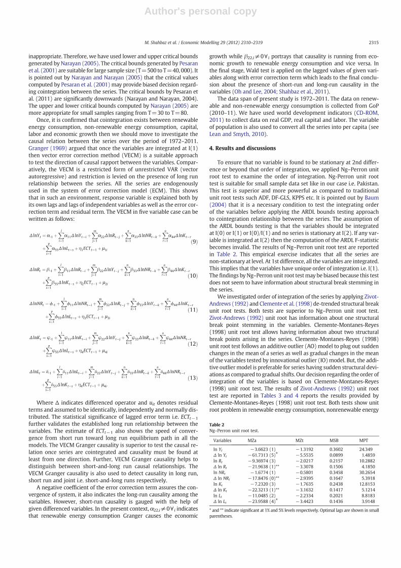
To ensure that no variable is found to be stationary at 2nd differ-ence or beyond that order of integration, we applied Ng–Perron unitroot test to examine the order of integration. Ng-Perron unit roottest is suitable for small sample data set like in our case i.e. Pakistan.This test is superior and more powerful as compared to traditionalunit root tests such ADF, DF-GLS, KPPS etc. It is pointed out by Baum(2004) that it is a necessary condition to test the integrating orderof the variables before applying the ARDL bounds testing approachto cointegration relationship between the series. The assumption ofthe ARDL bounds testing is that the variables should be integratedat I(0) or I(1) or I(0)/I(1) and no series is stationary at I(2). If any var-iable is integrated at I(2) then the computation of the ARDL F-statisticbecomes invalid. The results of Ng–Perron unit root test are reportedin Table 2. This empirical exercise indicates that all the series arenon-stationary at level. At 1st difference, all the variables are integrated.This implies that the variables have unique order of integration i.e. I(1).Thefindings by Ng–Perron unit root testmay be biased because this testdoes not seem to have information about structural break stemming inthe series.

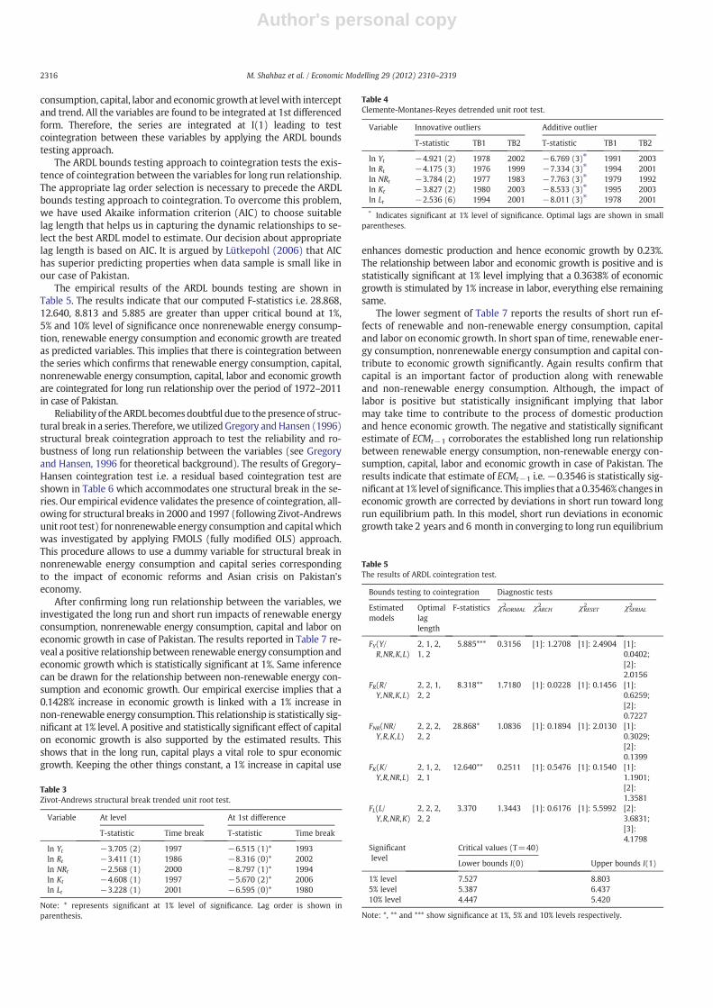
We investigated order of integration of the series by applying Zivot-Andrews (1992) and Clemente et al. (1998) de-trended structural breakunit root tests. Both tests are superior to Ng–Perron unit root test.Zivot-Andrews (1992) unit root has information about one structuralbreak point stemming in the variables. Clemente-Montanes-Reyes(1998) unit root test allows having information about two structuralbreak points arising in the series. Clemente-Montanes-Reyes (1998)unit root test follows an additive outlier (AO)model to plug out suddenchanges in the mean of a series as well as gradual changes in the meanof the variables tested by innovational outlier (IO)model. But, the addi-tive outliermodel is preferable for series having sudden structural devi-ations as compared to gradual shifts. Our decision regarding the order ofintegration of the variables is based on Clemente-Montanes-Reyes(1998) unit root test. The results of Zivot-Andrews (1992) unit roottest are reported in Tables 3 and 4 reports the results provided byClemente-Montanes-Reyes (1998) unit root test. Both tests show unitroot problem in renewable energy consumption, nonrenewable energy

Table 2Ng–Perron unit root test.

Variables MZa MZt MSB MPT

ln Yt −3.6623 (1) −1.3192 0.3602 24.349Δ ln Yt −61.7313 (5)⁎ −5.5535 0.0899 1.4859ln Rt −9.36974 (3) −2.0217 0.2157 10.2882Δ ln Rt −21.9638 (1)** −3.3078 0.1506 4.1850ln NRt −1.6774 (1) −0.5801 0.3458 30.2654Δ ln NRt −17.8476 (0)** −2.9395 0.1647 5.3918ln Kt −7.2320 (3) −1.7635 0.2438 12.8153Δ ln Kt −22.3213 (1)** −3.1632 0.1417 5.1214ln Lt −11.0485 (2) −2.2334 0.2021 8.8183Δ ln Lt −23.9588 (4)⁎ −3.4423 0.1436 3.9148

* and ** indicate significant at 1% and 5% levels respectively. Optimal lags are shown in smallparentheses.



consumption, capital, labor and economic growth at levelwith interceptand trend. All the variables are found to be integrated at 1st differencedform. Therefore, the series are integrated at I(1) leading to testcointegration between these variables by applying the ARDL boundstesting approach.

The ARDL bounds testing approach to cointegration tests the exis-tence of cointegration between the variables for long run relationship.The appropriate lag order selection is necessary to precede the ARDLbounds testing approach to cointegration. To overcome this problem,we have used Akaike information criterion (AIC) to choose suitablelag length that helps us in capturing the dynamic relationships to se-lect the best ARDL model to estimate. Our decision about appropriatelag length is based on AIC. It is argued by Lütkepohl (2006) that AIChas superior predicting properties when data sample is small like inour case of Pakistan.

The empirical results of the ARDL bounds testing are shown inTable 5. The results indicate that our computed F-statistics i.e. 28.868,12.640, 8.813 and 5.885 are greater than upper critical bound at 1%,5% and 10% level of significance once nonrenewable energy consump-tion, renewable energy consumption and economic growth are treatedas predicted variables. This implies that there is cointegration betweenthe series which confirms that renewable energy consumption, capital,nonrenewable energy consumption, capital, labor and economic growthare cointegrated for long run relationship over the period of 1972–2011in case of Pakistan.

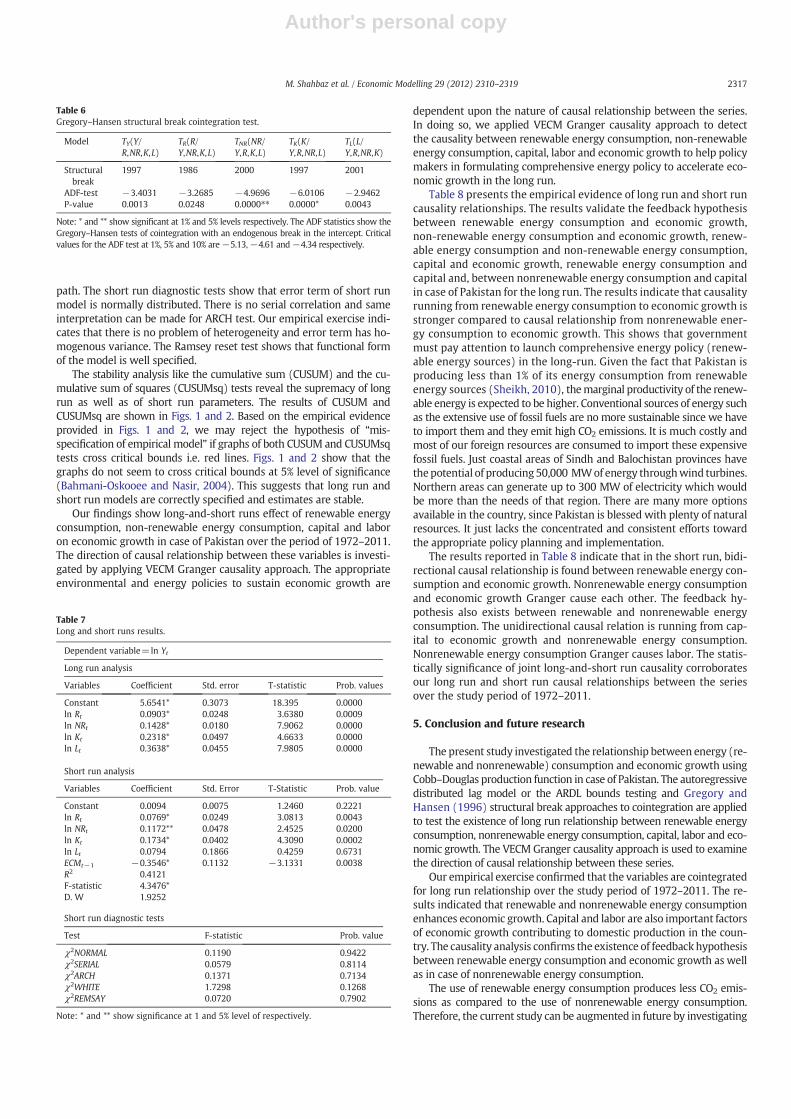
Reliability of theARDLbecomesdoubtful due to the presence of struc-tural break in a series. Therefore, we utilized Gregory andHansen (1996)structural break cointegration approach to test the reliability and ro-bustness of long run relationship between the variables (see Gregoryand Hansen, 1996 for theoretical background). The results of Gregory–Hansen cointegration test i.e. a residual based cointegration test areshown in Table 6 which accommodates one structural break in the se-ries. Our empirical evidence validates the presence of cointegration, all-owing for structural breaks in 2000 and 1997 (following Zivot-Andrewsunit root test) for nonrenewable energy consumption and capitalwhichwas investigated by applying FMOLS (fully modified OLS) approach.This procedure allows to use a dummy variable for structural break innonrenewable energy consumption and capital series correspondingto the impact of economic reforms and Asian crisis on Pakistan'seconomy.

After confirming long run relationship between the variables, weinvestigated the long run and short run impacts of renewable energyconsumption, nonrenewable energy consumption, capital and labor oneconomic growth in case of Pakistan. The results reported in Table 7 re-veal a positive relationship between renewable energy consumption andeconomic growth which is statistically significant at 1%. Same inferencecan be drawn for the relationship between non-renewable energy con-sumption and economic growth. Our empirical exercise implies that a0.1428% increase in economic growth is linked with a 1% increase innon-renewable energy consumption. This relationship is statistically sig-nificant at 1% level. A positive and statistically significant effect of capitalon economic growth is also supported by the estimated results. Thisshows that in the long run, capital plays a vital role to spur economicgrowth. Keeping the other things constant, a 1% increase in capital use

enhances domestic production and hence economic growth by 0.23%.The relationship between labor and economic growth is positive and isstatistically significant at 1% level implying that a 0.3638% of economicgrowth is stimulated by 1% increase in labor, everything else remainingsame.

The lower segment of Table 7 reports the results of short run ef-fects of renewable and non-renewable energy consumption, capitaland labor on economic growth. In short span of time, renewable ener-gy consumption, nonrenewable energy consumption and capital con-tribute to economic growth significantly. Again results confirm thatcapital is an important factor of production along with renewableand non-renewable energy consumption. Although, the impact oflabor is positive but statistically insignificant implying that labormay take time to contribute to the process of domestic productionand hence economic growth. The negative and statistically significantestimate of ECMt−1 corroborates the established long run relationshipbetween renewable energy consumption, non-renewable energy con-sumption, capital, labor and economic growth in case of Pakistan. Theresults indicate that estimate of ECMt−1 i.e.−0.3546 is statistically sig-nificant at 1% level of significance. This implies that a 0.3546% changes ineconomic growth are corrected by deviations in short run toward longrun equilibrium path. In this model, short run deviations in economicgrowth take 2 years and 6 month in converging to long run equilibrium

Table 3Zivot-Andrews structural break trended unit root test.

Variable At level At 1st difference

T-statistic Time break T-statistic Time break

ln Yt −3.705 (2) 1997 −6.515 (1)* 1993ln Rt −3.411 (1) 1986 −8.316 (0)* 2002ln NRt −2.568 (1) 2000 −8.797 (1)* 1994ln Kt −4.608 (1) 1997 −5.670 (2)* 2006ln Lt −3.228 (1) 2001 −6.595 (0)* 1980

Note: * represents significant at 1% level of significance. Lag order is shown inparenthesis.

Table 4Clemente-Montanes-Reyes detrended unit root test.

Variable Innovative outliers Additive outlier

T-statistic TB1 TB2 T-statistic TB1 TB2

ln Yt −4.921 (2) 1978 2002 −6.769 (3)⁎ 1991 2003ln Rt −4.175 (3) 1976 1999 −7.334 (3)⁎ 1994 2001ln NRt −3.784 (2) 1977 1983 −7.763 (3)⁎ 1979 1992ln Kt −3.827 (2) 1980 2003 −8.533 (3)⁎ 1995 2003ln Lt −2.536 (6) 1994 2001 −8.011 (3)⁎ 1978 2001

⁎ Indicates significant at 1% level of significance. Optimal lags are shown in smallparentheses.

Table 5The results of ARDL cointegration test.

Bounds testing to cointegration Diagnostic tests

Estimatedmodels

Optimallaglength

F-statistics χNORMAL2 χARCH

2 χRESET2 χSERIAL

2

FY(Y/R,NR,K,L)

2, 1, 2,1, 2

5.885*** 0.3156 [1]: 1.2708 [1]: 2.4904 [1]:0.0402;[2]:2.0156

FR(R/Y,NR,K,L)

2, 2, 1,2, 2

8.318** 1.7180 [1]: 0.0228 [1]: 0.1456 [1]:0.6259;[2]:0.7227

FNR(NR/Y,R,K,L)

2, 2, 2,2, 2

28.868* 1.0836 [1]: 0.1894 [1]: 2.0130 [1]:0.3029;[2]:0.1399

FK(K/Y,R,NR,L)

2, 1, 2,2, 1

12.640** 0.2511 [1]: 0.5476 [1]: 0.1540 [1]:1.1901;[2]:1.3581

FL(L/Y,R,NR,K)

2, 2, 2,2, 2

3.370 1.3443 [1]: 0.6176 [1]: 5.5992 [2]:3.6831;[3]:4.1798

Significantlevel

Critical values (T=40)

Lower bounds I(0) Upper bounds I(1)

1% level 7.527 8.8035% level 5.387 6.43710% level 4.447 5.420

Note: *, ** and *** show significance at 1%, 5% and 10% levels respectively.



path. The short run diagnostic tests show that error term of short runmodel is normally distributed. There is no serial correlation and sameinterpretation can be made for ARCH test. Our empirical exercise indi-cates that there is no problem of heterogeneity and error term has ho-mogenous variance. The Ramsey reset test shows that functional formof the model is well specified.

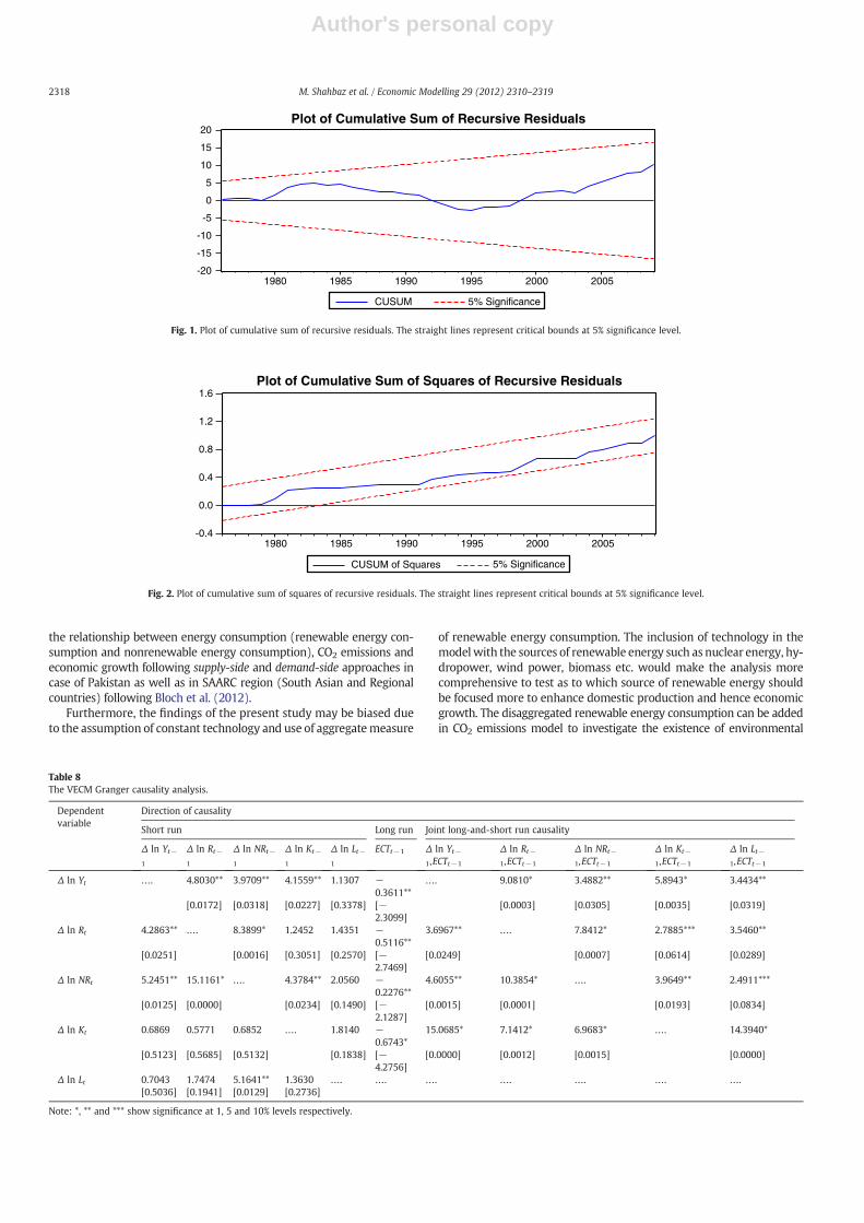
The stability analysis like the cumulative sum (CUSUM) and the cu-mulative sum of squares (CUSUMsq) tests reveal the supremacy of longrun as well as of short run parameters. The results of CUSUM andCUSUMsq are shown in Figs. 1 and 2. Based on the empirical evidenceprovided in Figs. 1 and 2, we may reject the hypothesis of “mis-specification of empirical model” if graphs of both CUSUM and CUSUMsqtests cross critical bounds i.e. red lines. Figs. 1 and 2 show that thegraphs do not seem to cross critical bounds at 5% level of significance(Bahmani-Oskooee and Nasir, 2004). This suggests that long run andshort run models are correctly specified and estimates are stable.

Our findings show long-and-short runs effect of renewable energyconsumption, non-renewable energy consumption, capital and laboron economic growth in case of Pakistan over the period of 1972–2011.The direction of causal relationship between these variables is investi-gated by applying VECM Granger causality approach. The appropriateenvironmental and energy policies to sustain economic growth are

dependent upon the nature of causal relationship between the series.In doing so, we applied VECM Granger causality approach to detectthe causality between renewable energy consumption, non-renewableenergy consumption, capital, labor and economic growth to help policymakers in formulating comprehensive energy policy to accelerate eco-nomic growth in the long run.

Table 8 presents the empirical evidence of long run and short runcausality relationships. The results validate the feedback hypothesisbetween renewable energy consumption and economic growth,non-renewable energy consumption and economic growth, renew-able energy consumption and non-renewable energy consumption,capital and economic growth, renewable energy consumption andcapital and, between nonrenewable energy consumption and capitalin case of Pakistan for the long run. The results indicate that causalityrunning from renewable energy consumption to economic growth isstronger compared to causal relationship from nonrenewable ener-gy consumption to economic growth. This shows that governmentmust pay attention to launch comprehensive energy policy (renew-able energy sources) in the long-run. Given the fact that Pakistan isproducing less than 1% of its energy consumption from renewableenergy sources (Sheikh, 2010), themarginal productivity of the renew-able energy is expected to be higher. Conventional sources of energy suchas the extensive use of fossil fuels are no more sustainable since we haveto import them and they emit high CO2 emissions. It is much costly andmost of our foreign resources are consumed to import these expensivefossil fuels. Just coastal areas of Sindh and Balochistan provinces havethepotential of producing50,000 MWof energy throughwind turbines.Northern areas can generate up to 300 MW of electricity which wouldbe more than the needs of that region. There are many more optionsavailable in the country, since Pakistan is blessed with plenty of naturalresources. It just lacks the concentrated and consistent efforts towardthe appropriate policy planning and implementation.

The results reported in Table 8 indicate that in the short run, bidi-rectional causal relationship is found between renewable energy con-sumption and economic growth. Nonrenewable energy consumptionand economic growth Granger cause each other. The feedback hy-pothesis also exists between renewable and nonrenewable energyconsumption. The unidirectional causal relation is running from cap-ital to economic growth and nonrenewable energy consumption.Nonrenewable energy consumption Granger causes labor. The statis-tically significance of joint long-and-short run causality corroboratesour long run and short run causal relationships between the seriesover the study period of 1972–2011.

5. Conclusion and future research

The present study investigated the relationship between energy (re-newable and nonrenewable) consumption and economic growth usingCobb–Douglas production function in case of Pakistan. The autoregressivedistributed lag model or the ARDL bounds testing and Gregory andHansen (1996) structural break approaches to cointegration are appliedto test the existence of long run relationship between renewable energyconsumption, nonrenewable energy consumption, capital, labor and eco-nomic growth. The VECM Granger causality approach is used to examinethe direction of causal relationship between these series.

Our empirical exercise confirmed that the variables are cointegratedfor long run relationship over the study period of 1972–2011. The re-sults indicated that renewable and nonrenewable energy consumptionenhances economic growth. Capital and labor are also important factorsof economic growth contributing to domestic production in the coun-try. The causality analysis confirms the existence of feedbackhypothesisbetween renewable energy consumption and economic growth as wellas in case of nonrenewable energy consumption.

The use of renewable energy consumption produces less CO2 emis-sions as compared to the use of nonrenewable energy consumption.Therefore, the current study can be augmented in future by investigating

Table 6Gregory–Hansen structural break cointegration test.

Model TY(Y/R,NR,K,L)

TR(R/Y,NR,K,L)

TNR(NR/Y,R,K,L)

TK(K/Y,R,NR,L)

TL(L/Y,R,NR,K)

Structuralbreak

1997 1986 2000 1997 2001

ADF-test −3.4031 −3.2685 −4.9696 −6.0106 −2.9462P-value 0.0013 0.0248 0.0000⁎⁎ 0.0000* 0.0043

Note: * and ** show significant at 1% and 5% levels respectively. The ADF statistics show theGregory–Hansen tests of cointegration with an endogenous break in the intercept. Criticalvalues for the ADF test at 1%, 5% and 10% are−5.13,−4.61 and−4.34 respectively.

Table 7Long and short runs results.

Dependent variable=ln Yt

Long run analysis

Variables Coefficient Std. error T-statistic Prob. values

Constant 5.6541* 0.3073 18.395 0.0000ln Rt 0.0903* 0.0248 3.6380 0.0009ln NRt 0.1428* 0.0180 7.9062 0.0000ln Kt 0.2318* 0.0497 4.6633 0.0000ln Lt 0.3638* 0.0455 7.9805 0.0000

Short run analysis

Variables Coefficient Std. Error T-Statistic Prob. value

Constant 0.0094 0.0075 1.2460 0.2221ln Rt 0.0769* 0.0249 3.0813 0.0043ln NRt 0.1172** 0.0478 2.4525 0.0200ln Kt 0.1734* 0.0402 4.3090 0.0002ln Lt 0.0794 0.1866 0.4259 0.6731ECMt−1 −0.3546* 0.1132 −3.1331 0.0038R2 0.4121F-statistic 4.3476*D. W 1.9252

Short run diagnostic tests

Test F-statistic Prob. value

χ2NORMAL 0.1190 0.9422χ2SERIAL 0.0579 0.8114χ2ARCH 0.1371 0.7134χ2WHITE 1.7298 0.1268χ2REMSAY 0.0720 0.7902

Note: * and ** show significance at 1 and 5% level of respectively.



the relationship between energy consumption (renewable energy con-sumption and nonrenewable energy consumption), CO2 emissions andeconomic growth following supply-side and demand-side approaches incase of Pakistan as well as in SAARC region (South Asian and Regionalcountries) following Bloch et al. (2012).

Furthermore, the findings of the present study may be biased dueto the assumption of constant technology and use of aggregatemeasure

of renewable energy consumption. The inclusion of technology in themodelwith the sources of renewable energy such as nuclear energy, hy-dropower, wind power, biomass etc. would make the analysis morecomprehensive to test as to which source of renewable energy shouldbe focused more to enhance domestic production and hence economicgrowth. The disaggregated renewable energy consumption can be addedin CO2 emissions model to investigate the existence of environmental

Plot of Cumulative Sum of Recursive Residuals

-20

-15

-10

-5

0

5

10

15

20

1980 1985 1990 1995 2000 2005

CUSUM 5% Significance

Fig. 1. Plot of cumulative sum of recursive residuals. The straight lines represent critical bounds at 5% significance level.

Plot of Cumulative Sum of Squares of Recursive Residuals

-0.4

0.0

0.4

0.8

1.2

1.6

1980 1985 1990 1995 2000 2005

CUSUM of Squares 5% Significance

Fig. 2. Plot of cumulative sum of squares of recursive residuals. The straight lines represent critical bounds at 5% significance level.

Table 8The VECM Granger causality analysis.

Dependentvariable

Direction of causality

Short run Long run Joint long-and-short run causality

Δ ln Yt−1

Δ ln Rt−1

Δ ln NRt−1

Δ ln Kt−

1

Δ ln Lt−1

ECTt−1 Δ ln Yt−1,ECTt−1

Δ ln Rt−1,ECTt−1

Δ ln NRt−1,ECTt−1

Δ ln Kt−

1,ECTt−1

Δ ln Lt−1,ECTt−1

Δ ln Yt …. 4.8030** 3.9709** 4.1559** 1.1307 −0.3611**

…. 9.0810* 3.4882** 5.8943* 3.4434**

[0.0172] [0.0318] [0.0227] [0.3378] [−2.3099]

[0.0003] [0.0305] [0.0035] [0.0319]

Δ ln Rt 4.2863** …. 8.3899* 1.2452 1.4351 −0.5116**

3.6967** …. 7.8412* 2.7885*** 3.5460**

[0.0251] [0.0016] [0.3051] [0.2570] [−2.7469]

[0.0249] [0.0007] [0.0614] [0.0289]

Δ ln NRt 5.2451** 15.1161* …. 4.3784** 2.0560 −0.2276**

4.6055** 10.3854* …. 3.9649** 2.4911***

[0.0125] [0.0000] [0.0234] [0.1490] [−2.1287]

[0.0015] [0.0001] [0.0193] [0.0834]

Δ ln Kt 0.6869 0.5771 0.6852 …. 1.8140 −0.6743*

15.0685* 7.1412* 6.9683* …. 14.3940*

[0.5123] [0.5685] [0.5132] [0.1838] [−4.2756]

[0.0000] [0.0012] [0.0015] [0.0000]

Δ ln Lt 0.7043 1.7474 5.1641** 1.3630 …. …. …. …. …. …. ….[0.5036] [0.1941] [0.0129] [0.2736]

Note: *, ** and *** show significance at 1, 5 and 10% levels respectively.



Kuznets curve (EKC) which would help policy makers in formulatingcomprehensive energy policy to spur economic growth by improving en-vironmental quality in case of Pakistan.

References

Akkemike, K.A., Göksal, K., 2012. Energy consumption–GDP nexus: heterogeneouspanel causality analysis. Energy Economics 34, 865–873.

Apergis, N., Payne, J.E., 2010a. Renewable energy consumption and economic growth:evidence from a panel of OECD countries. Energy Policy 38, 656–660.

Apergis, N., Payne, J.E., 2010b. Renewable energy consumption and growth in Eurasia.Energy Economics 32, 1392–1397.

Apergis, N., Payne, J.E., 2011. The renewable energy consumption–growth nexus inCentral America. Applied Energy 88, 343–347.

Apergis, N., Payne, J.E., 2012a. The electricity consumption–growth nexus: renewableversus non-renewable electricity in Central America. Energy Sources, Part B: Eco-nomics, Planning and Policy 7, http://dx.doi.org/10.1080/15567249.2011.639336.

Apergis, N., Payne, J.E., 2012b. Renewable and non-renewable energy consumption-growth nexus: evidence from a panel error correction model. Energy Economics34, 733–738.

Bahmani-Oskooee, M., Nasir, A.B.M., 2004. ARDL approach to test the productivity biashypothesis. Review of Development Economics 8, 483–488.

Baum, C.F., 2004. A review of Stata 8.1 and its time series capabilities. InternationalJournal of Forecasting 20, 51–161.

Bloch, H., Rafiq, S., Salam, R., 2012. Coal consumption, CO2 emission and economicgrowth in China: empirical evidence and policy responses. Energy Economics 34,518–528.

Bobinaite, V., Juozapaviciene, A., Konstantinaviciute, I., 2011. Assessment of causalityrelationship between renewable energy consumption and economic growth inLithuania. Inzinerine Ekonomika—Engineering Economics 22, 510–518.

Bowden, N., Payne, J.E., 2010. Sectoral analysis of the causal relationship between re-newable and non-renewable energy consumption and real output in the US. Ener-gy Sources, Part B: Economics, Planning and Policy 5, 400–408.

CD-ROM, 2011. World Development Indicators (WDI). The World Bank, WashingtonDC, USA.

Chang, T.-H., Huang, C.-M., Lee, M.-C., 2009. Threshold effect of the economic growthrate on the renewable energy development from a change in energy price: evi-dence from OECD countries. Energy Policy 37, 5796–5802.

Cameron, S., 1994. A review of the econometric evidence on the effects of capital punish-ment. Journal of Socio-economics 23, 197–214.

Clemente, J., Antonio, M., Marcelo, R., 1998. Testing for a unit root in variables with adouble change in the mean. Economics Letters 59, 175–182.

Ehrlich, I., 1977. The deterrent effect of capital punishment: reply. American EconomicsReview 67, 452–458.

Ehrlich, I., 1996. Crime, punishment and the market for offences. Journal of EconomicPerspectives 10, 43–67.

Elliot, D., 2007. Nuclear or Not? Does Nuclear Power Have a Place in Sustainable EnergyFuture? Palgrave Macmillan, Houndmills, Basingstoke.

Ewing, B.T., Sari, R., Soyta, U., 2007. Disaggregate energy consumption and industrialoutput in the United States. Energy Policy 35, 1274–1281.

Ferguson, C.D., 2007. Nuclear Energy: Balancing Benefits and Risks. Council of ForeignRelations. CRS No. 28.

Government of Pakistan, 2010. Economic Survey of Pakistan. Ministry of Finance, Is-lamabad, Pakistan.

Granger, C.W.J., 1969. Investigating causal relations by econometric models and cross-spectral methods. Econometrica 37, 424–438.

Gregory, A.W., Hansen, B.E., 1996. Residual-based tests for cointegration in modelswith regime shifts. Journal of Econometrics 70, 99–126.

Hamilton, J.D., 1983. Oil and the macroeconomy since world war-II. Journal of PoliticalEconomy 91, 228–248.

Harris, E.S., Kasman, B.C., Shapiro, M.D., West, K.D., 2009. ‘Oil and the macroeconomy:lessons for monetary policy’, Unpublished Working Paper.

Haug, A., 2002. Temporal aggregation and the power of cointegration tests: a MonteCarlo study. Oxford Bulletin of Economics and Statistics 64, 399–412.

Johansen, S., Juselius, K., 1990. Maximum likelihood estimation and inference oncointegration with applications to the demand for money. Oxford Bulletin of Eco-nomics and Statistics 52, 169–210.

Khalil, M.S., Khan, N.A., Mirza, I.A., 2005. Renewable Energy in Pakistan: Status andTrends. Pakistan Alternative Energy Development Board.

Larsson, R., Lyhagen, J., Lothgren, M., 2001. Likelihood-based cointegration tests in het-erogeneous panels. The Econometrics Journal 4, 109–142.

Layson, S., 1983. Homicide and deterrence: another view of the Canadian time seriesevidence. Canadian Journal of Economics 16, 52–73.

Lean, H.H., Smyth, R., 2010. Multivariate granger causality between electricity genera-tion, exports, prices and GDP in Malaysia. Energy 35, 3640–3648.

Leduc, S., Sill, K., 2004. A quantitative analysis of oil-price shocks, systematic monetarypolicy, and economic downturns. Journal of Monetary Economics 51, 781–808.

Lütkepohl, H., 2006. Structural vector autoregressive analysis for cointegrated vari-ables. AStA Advances in Statistical Analysis 90, 75–88.

Magnani, N., Vaona, A., 2011. Regional spillover effects of renewable energy generationin Italy. Working Papers 12/2011. Dipartimento di Scienzeeconomiche, Universitàdi Verona.

Menegaki, A.N., 2011. Growth and renewable energy in Europe: a random effect modelwith evidence for neutrality hypothesis. Energy Consumption 33, 257–263.

Menyah, K., Wolde-Rufael, Y., 2010. CO2 emissions, nuclear energy, renewable energyand economic growth in the US. Energy Policy 38, 2911–2915.

Narayan, P.K., 2005. The saving and investment nexus for China: evidence fromcointegration tests. Applied Economics 37, 1979–1990.

Narayan, P.K., Narayan, S., 2005. Estimating income and price elasticities of imports forFiji in a cointegration framework. Economic Modelling 22, 423–438.

Oh, W., Lee, K., 2004. Causal relationship between energy consumption and GDP: thecase of Korea 1970–1999. Energy Economics, 51–59.

Ozturk, I., 2010. A literature survey on energy–growth nexus. Energy Policy 38,340–349.

Payne, J.E., 2009. On the dynamics of energy consumption and output in the US. Ap-plied Energy 86, 575–577.

Payne, J.E., 2010a. On biomass energy consumption and real output in the US. EnergySources, Part B: Economics, Planning and Policy 6, 47–52.

Payne, J.E., 2010b. Survey of the international evidence on the causal relationship be-tween energy consumption and growth. Journal of Economic Studies 37, 53–95.

Payne, J.E., 2010c. A survey of the electricity consumption–growth literature. AppliedEnergy 87, 723–731.

Pesaran, M.H., Shin, Y., 1999. An autoregressive distributed lag modeling approach tocointegration analysis. In: Strom, S. (Ed.), Chapter 11 in Econometrics and EconomicTheory in the 20th Century: The Ragnar Frisch Centennial Symposium. CambridgeUniversity Press, Cambridge.

Pesaran, M.H., Shin, Y., Smith, R.J., 2001. Bounds testing approaches to the analysis oflevel relationships. Journal of Applied Econometrics 16, 289–326.

Sadorsky, P., 2009a. Renewable energy consumption and income in emerging econo-mies. Energy Policy 37, 4021–4028.

Sadorsky, P., 2009b. Renewable energy consumption, CO2 emissions and oil prices inthe G7 countries. Energy Economics 31, 456–462.

Sari, R., Ewing, B.T., Soytas, U., 2008. The relationship between disaggregate energyconsumption and industrial production in the United States: an ARDL approach.Energy Economics 30, 2302–2313.

Shahbaz, M., 2010. Income inequality–economic growth and non-linearity: a case ofPakistan. International Journal of Social Economics 37, 613–636.

Shahbaz, M., Lean, H.H., 2012. The dynamics of electricity consumption and economicgrowth: a revisit study of their causality in Pakistan. Energy 39, 146–153.

Shahbaz, M., Tang, C.F., Shabbir, M.S., 2011. Electricity consumption and economicgrowth nexus in Portugal using cointegration and causality approaches. EnergyPolicy 39, 3529-2536.

Sheikh, M.A., 2010. Energy and renewable energy scenario of Pakistan. Renewable andSustainable Energy Reviews 14, 354–363.

Tiwari, A.K., 2011a. A structural VAR analysis of renewable energy consumption, realGDP and CO2 emissions: evidence from India. Economic Bulletin 31, 1793–1806.

Tiwari, A.K., 2011b. Comparative performance of renewable and nonrenewable energysource on economic growth and CO2 emissions of Europe and Eurasian countries: aPVAR approach. Economic Bulletin 31, 2356–2372.

Toda, H.Y., Yamamoto, T., 1995. Statistical inference in vector autoregressions withpossibly integrated processes. Journal of Econometrics 66, 225–250.

Vaona, A., 2010. Granger non-causality tests between (non)renewable energy con-sumption and output in Italy since 1861: the (ir)relevance of structural breaks.Working Paper Series. Department of Economics, University of Verona.

Wolde-Rufael, Y., 2004. Disaggregated industrial energy consumption and GDP: thecase of Shanghai, 1952–1999. Energy Economics 26, 69–75.

Ziramba, E., 2009. Disaggregate energy consumption and industrial production inSouth Africa. Energy Policy 37, 2214–2220.

Zivot, E., Andrews, D., 1992. Further evidence of great crash, the oil price shock and unitroot hypothesis. Journal of Business and Economic Statistics 10, 251–270.


Is energy consumption effective to spur economic growth in Pakistan? New evidence from bounds test...

Documents

Transcript of Is energy consumption effective to spur economic growth in Pakistan? New evidence from bounds test...