Revisiting Error-Autocorrelation Correction: Common Factor Restrictions and Granger Non-Causality

Revisiting Error Autocorrelation Correction:Common Factor Restrictions and Granger

Non-Causality

Anya McGuirk∗Department of Agricultural and Applied Economics,

Department of Statistics, Virginia Tech, <[email protected]>

Aris SpanosDepartment of Economics,

Virginia Tech, <[email protected]>

American Agricultural Economics Association Meetings, 2004Key words: Linear Regression Model, error autocorrelation, common factor

restrictions, Granger causality, Durbin- Watson test, OLS, GLS,temporal dependence, Dynamic Linear Regression Model.

JEL classification: C2, C4

Abstract

This paper demonstrates that linear regression models with an AR(1) error structureimplicitly assume that yt does not Granger cause any of the exogenous variables in Xt.An indirect test of the common factor restrictions based on this Granger non-causalityis proposed and shown to outperform existing tests.

∗Copyright 2004 by Anya McGuirk and Aris Spanos. All rights reserved.

1

2

1 IntroductionThe Linear Regression Model (LRM) first used by pioneers like Moore and Schultz,has been the quintessential statistical model for econometric modeling since the early 20thcentury; see Morgan (1990). Yule (1921, 1926) scared econometricians away from theLRM for time series data by demonstrating that such regressions often lead to spuriousresults. The first attempt to address this problem was by Cochrane and Orcutt (1949)who proposed extending the LRM to include autocorrelated errors following a low orderARMA(p,q) formulation. They also demonstrated by simulation that the Von Neuman ratiotest for autocorrelation was not very effective in detecting autocorrelated errors. Durbinand Watson (1950, 1951) addressed this testing problem in the case of the linear regressionmodel:

(1) yt = β>xt + ut, t ∈ T,

where xt is a k × 1 vector, supplemented with an AR(1) error:

(2) ut = ρut−1 + εt, |ρ| < 1, t ∈ T,

by proposing the well known Durbin-Watson (D-W) test based on the hypotheses:

(3) H0 : ρ = 0 vs. H1 : ρ 6= 0.

The traditional econometrics literature has treated this extension of the LRM as providinga way to test for the presence of error autocorrelation in the data, as well as a solution tothe misspecification problem if one rejects H0. Under this approach, error autocorrelationis viewed as a problem of efficiency for the Ordinary Least Squares (OLS) estimatorbβOLS= (X>X)−1X>y. It is argued that in the presence of error autocorrelation:

E(uu> | X) = Ω 6= σ2IT ,

the OLS estimator maintains its unbiasedness and consistency, but it is no longer as efficientas the Generalized Least Squares (GLS) estimator bβGLS= (X>Ω−1X)−1X>Ω−1y. Thetraditional way to deal with the inefficiency of OLS is to adopt the Autocorrelation-Corrected LRM (ACLRM):

(4) yt = β>xt + ρyt−1 − ρβ>xt−1 + εt, t ∈ T.

That is, when the D-W test rejects H0, the modeler adopts (4), estimated using GLS, as away to ‘correct’ for serial correlation (see inter alia, Judge et al, 1985, Greene, 2000).

The practice of adopting the alternative model when the data reject the no-autocorrelation assumption is often inappropriate. The problem is that the presence ofresidual autocorrelation is interpreted as evidence for the ACLRM. This is an example ofthe classic fallacy of rejection: ‘evidence against the null is interpreted as evidence forthe alternative’. The ACLRM is presumed to be ‘the’ appropriate model, even though theresidual autocorrelation could have arisen in numerous alternative ways, one of which is thatthe error follows an AR(1) process. It goes without saying that if the appropriate model isnot the ACLRM, the OLS estimator is no longer unbiased or consistent, and the ACLRMsimply constitutes another misspecified model; see Spanos (1986). Hence, adopting theACLRM does not usually improve the reliability of inference.

3

Sargan (1964) was the first to view (4) as a restricted version of a more general statisticalmodel:

(5) yt = α1yt−1 + β>0 xt + β>1 xt−1 + εt, t ∈ T,

known as the Dynamic Linear Regression Model (DLRM), where the restrictions takethe form:

(6) H0 : β1 − β0α1 = 0.

He proposed a likelihood ratio test for these so-called Common Factor (CF) restrictions.This test is valid under the presumption that the DLRM is statistically adequate; itsprobabilistic assumptions are data-acceptable. Sargan’s proposal was further elaboratedupon by Hendry and Mizon (1978) and Sargan (1980) who suggested testing the CFrestrictions before imposing them. Despite additional warnings concerning the unrealisticnature of the CF restrictions from Hoover (1988) and Mizon (1995), inter alia, the practiceof autocorrelation correction without testing the CF restrictions is still common. In fact,its use may even be on the rise largely due to the increased use of spatial data whichexhibit dependencies (see Anselin, 2001), and ‘advances’ in techniques for autocorrelationcorrecting systems of simultaneous equations and panel data models (see Greene, 2000).

In an attempt to demonstrate the restrictive nature of the ACLRM (4), Spanos (1988)investigated the probabilistic structure of the vector stochastic process Zt, t ∈ T,Zt := (yt,x

>t )>, that would give rise to the CF restrictions (6). It was shown that the

CF restrictions arise naturally when Zt, t ∈ T is a Normal, Markov, and Stationaryprocess: µ

ZtZt−1

¶v N

µµ00

¶,

µΣ(0) Σ(1)>

Σ(1) Σ(0)

¶¶, t ∈ T,

with a temporal covariance structure of the form:

(7) Σ(1) = ρΣ(0).

The sufficient conditions in (7) are ‘highly unrealistic’ because, as shown in Spanos (1988),they give rise to a very restrictive Vector AutoRegressive (VAR) model for Zt, t ∈ T:

Zt = A>Zt−1 +Et, Et v N(0,Ω), t ∈ T,

A = ρIk+1, Ω = (Σ(0)− ρ2Σ(0)).

That is, they imply yt and Xt are mutually Granger non-causal and have “largelyidentical temporal structure”. Mizon (1995), in a paper entitled “A Simple Messageto Autocorrelation Correctors: Don’t,” elaborated on these sufficient conditions andrecommended that the traditional way of ‘correcting for serial correlation’ is a bad idea.Unfortunately, that advice is largely ignored by the recent applied econometrics literature.As we will demonstrate, the consequences are very serious in terms of the reliability ofinference based on such models.

In this paper, we elaborate on Spanos (1988) and Mizon (1995) by deriving necessaryand sufficient conditions for the CF restrictions. Based on these conditions, we propose anew, easy-to-implement test of the common factor restrictions in the context of the VARmodel. We then conduct Monte Carlo experiments to examine the relative performance ofthe LRM, the ACLRM, and the (unrestricted) DLRM when the common factor restrictions

4

do and do not hold. We also examine the performance of various popular misspecificationand common factor restriction tests under the different situations. Finally, we also brieflyinvestigate the performance of the Heteroskedastic and Autocorrelation Consistent standarderrors (HAC) proposed by Newey and West (1987) in dealing with the unreliability ofinference issue.

2 Revisiting the Common Factor RestrictionsIn this section, we try to elucidate the constrictive nature of the CF restrictions byexamining the implicit restrictions imposed on the probabilistic structure of the observablevector stochastic process Zt, t ∈ T, where Zt := (yt,x

>t )>. It is argued that by

modeling the error term one implicitly imposes restrictions on the probabilistic structure ofZt, t ∈ T, which are both unrealistic and unnecessary. The argument is based on derivingboth necessary and sufficient conditions on the probabilistic structure of Zt, t ∈ Tgiving rise to the CF restrictions (6). We first establish that if the ACLRM holds thenthe implied parameterization φ∗ constitutes a restrictive form of φ of the joint distributionD(Zt,Zt−1;φ)1. We then show that if φ∗ is assumed, the reduction:

D(Zt,Zt−1;φ∗) = D(Zt|Zt−1;ψ∗1) ·D(Zt−1;ψ∗2) == D(yt|Xt,Zt−1;θ∗1) ·D(Xt|Zt−1;θ∗2) ·D(Zt−1;ψ∗2),

gives rise to the ACLRM based onD(yt|Xt,Zt−1;θ∗1), θ∗1 := (ρ,β,σ2). It is then shown thatthe parameterization of the Vector Autoregressive (VAR) model (ψ∗1), specified in terms ofD(Zt|Zt−1;ψ∗1), is particularly useful in elucidating the nature of the CF restrictions.

The ACLRM is specified by:

(8)

yt = β>xt + ut, ut = ρut−1 + εt, |ρ| < 1, t ∈ T,

[a1] E(εt) = 0, V ar(εt) = σ2, Cov(εt, εs) = 0, t 6= s,[a2] Cov(Xt, us) = 0, ∀ (t, s) ∈ T.

Given the ACLRM (8) (including [a1]-[a2]), we can derive the implicit statistical parame-terizations for the model parameters (β, ρ,σ2) in terms of the primary parameters φ of thejoint distribution D(Zt,Zt−1;φ). In presenting the results we use the following notationfor the variance-covariance of (yt, yt−1,Xt,Xt−1) :

(9) Cov(yt, yt−1,xt,xt−1) = Σ =

σ11(0) σ11(1) σ>21(0) σ>21(1)σ11(1) σ11(0) σ>21(1) σ>21(0)σ21(0) σ21(1) Σ22(0) Σ22(1)σ21(1) σ21(0) Σ22(1) Σ22(0)

We adopt the simplifying assumption that all random variables have mean zero, withoutany loss of generality.

Theorem 1. The mapping between the primary parameters Σ and theparameters θ∗1 := (ρ,β,σ2) of the ACLRM (8) takes the form:

[1] V ar(u2t ) = σuu(0) =σ2

1−ρ2 [4] Cov(xt, yt−1) = σ21(1) = Σ22(1)β

[2] Cov(utut−1) = σuu(1) =ρσ2

1−ρ2 [5] V ar(yt) = σ11(0) = β>Σ22(0)β + σ2

1−ρ2[3] Cov(xt, yt) = σ21(0) = Σ22(0)β [6] Cov(yt, yt−1) = σ11(1) = β>Σ22(1)β + ρσ2

1−ρ2 .

1The one lag restriction follows from the Markovness of the process.

5

See Appendix A for the derivations.Using [3]-[6] the variance-covariance matrix of (yt, yt−1,Xt,Xt−1) implied by the

ACLRM is:

(10) Σ∗ =

β>Σ22(0)β + σ2

1−ρ2 β>Σ22(1)β + ρσ2

1−ρ2 β>Σ22(0) β>Σ22(1)β>Σ22(1)β + ρσ2

1−ρ2 β>Σ22(0)β + σ2

1−ρ2 β>Σ22(1) β>Σ22(0)Σ22(0)β Σ22(1)

>β Σ22(0) Σ22(1)Σ22(1)

>β Σ22(0)β Σ22(1) Σ22(0)

Note that the sufficient conditions in Spanos (1988), Σ(1) = ρΣ(0), follow from [3]-[6]

above:

(11)β = Σ22(0)

−1σ21(0) = Σ22(1)−1σ21(1).

σ2 =£σ11(0)− β>Σ22(0)β

¤(1− ρ2) =

³1ρ

´ £σ11(1)− β>Σ22(1)β

¤(1− ρ2),

giving rise to:

(12) σ11(1)− ρσ11(0) = β> [Σ22(1)− ρΣ22(0)]β.

Hence, σ11(1) = ρσ11(0) iff Σ22(1) = ρΣ22(0).

In order to derive necessary and sufficient conditions for the common factorrestrictions we make use of Σ∗ in (10) and the following lemma from Spanos and McGuirk(2002).

Lemma 1. Consider the Linear Regression Model:

yt = γ0 + γ>1 xt + ut, ut v IID(0,σ2u), t ∈ T,

where xt is a k × 1 vector. Under the assumptions E(ut|Xt) = 0 andE(u2t |Xt) = σ2u, the model parameters (γ0,γ1,σ

2u) are related to the primary

parameters of the stochastic process Zt, t ∈ T ,Zt ≡ (yt,X>t )> :

E(Zt) := µ =

µµyµx

¶, Cov(Zt) := Σ =

µσyy σ>xyσxy Σxx

¶,

assuming Σ > 0, via:

(13) γ0 = µy − γ>1 µx, γ1 = Σ−1xxσxy, σ2u = σyy − σ>xyΣ−1xxσxy.

The relationship between the model parameters θ1 := (α1,β0,β1,σ2ε) of the (unre-

stricted) DLRM model (5):

yt = α1yt−1 + β>0 xt + β>1 xt−1 + εt, εt v IID(0,σ2ε), t ∈ T,and the primary parameters of the joint distribution (9) was derived in Spanos (1986).Next we derive this relationship for the DLRM under the CF restrictions.

6

Theorem 2. The statistical parameterization of the DLRM model parameters(α1,β0,β1,σ

2ε) implied by the restricted Σ

∗ in (10) is:(14) α1

β0β1

=

β>Σ22(0)β + σ2

1−ρ2 β>Σ22(1) β>Σ22(0)Σ22(1)

>β Σ22(0) Σ22(1)Σ22(0)β Σ22(1) Σ22(0)

−1 β>Σ22(1)β + ρσ2

1−ρ2Σ22(0)βΣ22(1)β

=

ρ∆(Σ22(0)−Σ22(1)Σ22(0)−1Σ22(1))β

−ρβ + (∆Σ22(1)−Σ22(0)−1Σ22(1)∆Σ22(0))β

=

ρβ−ρβ

σ2ε = β>Σ22(0)β+σ2

1− ρ2−³β>Σ22(1)β + ρσ2

1−ρ2 β>Σ22(0) β>Σ22(1)´ α1

β0β1

= σ2.

giving rise to the ACLRM, i.e. a DLRM where the common factor (CF) restrictions (6)hold. See Appendix A for the details.

Taken together, Theorems 1 and 2 indicate that (10) constitutes a set of necessary andsufficient conditions for the common factor restrictions to hold. However, the restrictivenature of these CF conditions is not completely evident from (10). To shed light on therestrictiveness of these conditions in terms of the probabilistic structure of the vector processZt, t ∈ T, we use Σ∗ in (10) and Lemma 1 to derive the Vector Autoregressive (VAR)model based on D(Zt|Zt−1;ψ∗1).

Theorem 3. The implicit statistical parameterization of the VAR model, based onD(Zt|Zt−1;ψ∗1) :

(15) Zt = A>Zt−1 +Et, Et v IID(0,Ω), t ∈ T.

implied by the restricted variance-covariance matrix Σ∗ in (10), takes the form:

A> =µ

ρ (D− ρIk)β0 D

¶, Ω =

µσ2 + β>Λβ β>ΛΛβ Λ

¶where:

D =Σ22(0)−1Σ22(1) Λ = Σ22(0)−Σ22(1)Σ22(0)−1Σ22(1)

and Ik is a k × k identity matrix. See Appendix A for the proof.Theorem 3 sheds ample light on just how unappetizing the necessary and sufficient

conditions for an ACLRM are in terms of the implied restrictions on the vector stochasticprocess Zt, t ∈ T :

(a) yt does not Granger cause any of the regressors in Xt, and

(b) Cov(Xt, yt|Zt−1) = Cov(Xt|Xt−1)Cov(Xt)−1Cov(Xt, yt) = Λβ.

In addition, these results suggest that one can test the appropriateness of the CFrestrictions (6) by testing the implied Granger non-causality in the context of theunrestricted VAR (15). The performance of this new test is considered in the Monte Carloexperiments presented below.

7

3 Monte Carlo SimulationsIn an attempt to illustrate the restrictive nature of ‘correcting for serial correlation’ bymodeling the error, even in the unlikely event that the Common Factor (CF) restrictionsdo hold, we consider a number of Monte Carlo experiments. All experimental resultsreported are based on 10,000 replications of sample sizes T = 25, T = 50 and T = 100.The experiments and results below use the following notation for the model parameters ofthe DLRM:

(16) yt = α0 + β1x1t + β2x2t + α1yt−1 + β3x1t−1 + β4x2t−1 + εt, t ∈ T.When the CF restrictions hold this model is rewritten as:

(17) yt = α∗0 + β1x1t + β2x2t + ut; ut = ρut−1 + εt, t ∈ T,where ρ = α1, and α∗0 =

α01−ρ .

3.1 Experiment 1 - Unrestricted DLRM vs. ACLRM (ρ = .588)In Experiment 1 we generate data with two very similar implied Dynamic Linearregression Models (1A-1B). They differ by the model parameters, (β3,β4), the coefficientsof (x1t−1, x2t−1) and, therefore, also by the intercept α0. All other model parameters arethe same.2

Experiment 1A - Primary parameters underlying DLRME(Yt) = 2, V ar(Yt) = 1.115, Cov(Yt,X1t) = −.269, Cov(Yt,X2t) = 0.5,E(X1t) = 1, V ar(X1t) = 1, Cov(X1t,X1t−1) = 0.6, Cov(Yt, Yt−1) = 0.446,E(X2t) = .5, V ar(X2t) = 1, Cov(X2t,X2t−1) = 0.54, Cov(Yt,X1t−1) = −.678,

Cov(X1t,X2t) = −.4, Cov(X1t,X2t−1) = −.32, Cov(Yt,X2t−1) = .42,

giving rise to an (unrestricted) DLRM:

(18)yt = 0.946 + 0.749x1t + 0.215x2t + 0.589yt−1 − 0.936x1t−1 − 0.089x2t−1 + εt,

σ2ε = 0.349, <2 = 0.687.The implied VAR parameters are:(19)

a0 =

2.1021.5190.081

, A> = 0.236 −0.596 0.045−0.535 0.498 0.1050.222 −0.156 0.262

, Ω = 0.586 0.263 0.1860.263 0.372 −0.0730.186 −.073 1.116

.3

Consider the ACLRM experimental set-up:

Experiment 1B - Primary parameters underlying ACLRME(Yt) = 2, V ar(Yt) = 1.032, Cov(Yt,X1t) = .663, Cov(Yt,X2t) = 0.001,E(X1t) = 1, V ar(X1t) = 1, Cov(X1t,X1t−1) = 0.6, Cov(Yt, Yt−1) = 0.574,E(X2t) = .5, V ar(X2t) = 1.4, Cov(X2t,X2t−1) = 0.54, Cov(Yt,X1t−1) = .381,

Cov(X1t,X2t) = −.4, Cov(X1t,X2t−1) = −.32, Cov(Yt,X2t−1) = −.124,2Experiments 1A and 1B not only have several model parameters in common, but they are also similar

in the sense that in both cases, det(Σ) = 0.163.3The data in these experiments are all generated using the implied VAR. The initial values (y0, x10, x20)

for each run are drawn randomly from the joint distribution of (y0, x10, x20) implied by the experimentalsetup.

8

giving rise to the ACLRM:

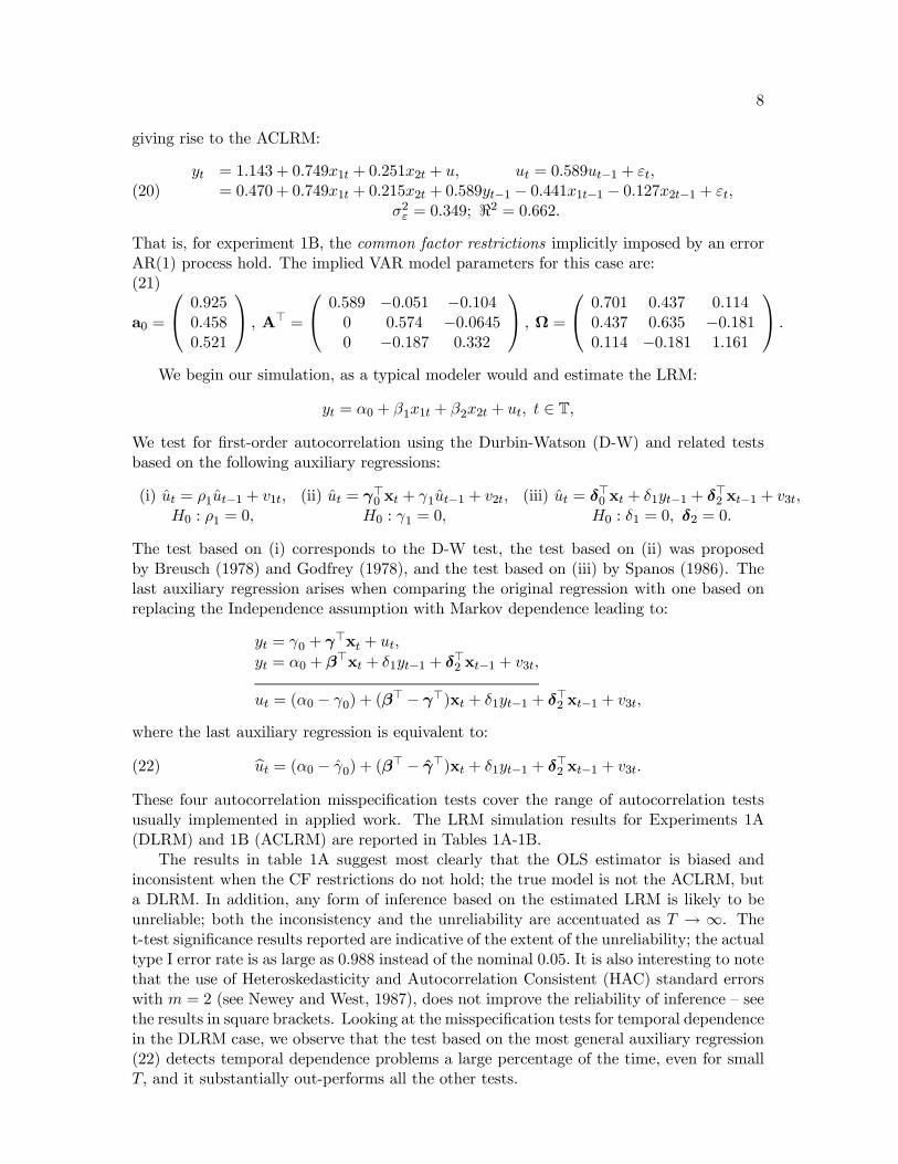
(20)yt = 1.143 + 0.749x1t + 0.251x2t + u, ut = 0.589ut−1 + εt,

= 0.470 + 0.749x1t + 0.215x2t + 0.589yt−1 − 0.441x1t−1 − 0.127x2t−1 + εt,σ2ε = 0.349; <2 = 0.662.

That is, for experiment 1B, the common factor restrictions implicitly imposed by an errorAR(1) process hold. The implied VAR model parameters for this case are:(21)

a0 =

0.9250.4580.521

, A> = 0.589 −0.051 −0.104

0 0.574 −0.06450 −0.187 0.332

, Ω = 0.701 0.437 0.1140.437 0.635 −0.1810.114 −0.181 1.161

.We begin our simulation, as a typical modeler would and estimate the LRM:

yt = α0 + β1x1t + β2x2t + ut, t ∈ T,We test for first-order autocorrelation using the Durbin-Watson (D-W) and related testsbased on the following auxiliary regressions:

(i) ut = ρ1ut−1 + v1t, (ii) ut = γ>0 xt + γ1ut−1 + v2t, (iii) ut = δ>0 xt + δ1yt−1 + δ>2 xt−1 + v3t,H0 : ρ1 = 0, H0 : γ1 = 0, H0 : δ1 = 0, δ2 = 0.

The test based on (i) corresponds to the D-W test, the test based on (ii) was proposedby Breusch (1978) and Godfrey (1978), and the test based on (iii) by Spanos (1986). Thelast auxiliary regression arises when comparing the original regression with one based onreplacing the Independence assumption with Markov dependence leading to:

yt = γ0 + γ>xt + ut,yt = α0 + β>xt + δ1yt−1 + δ>2 xt−1 + v3t,

ut = (α0 − γ0) + (β> − γ>)xt + δ1yt−1 + δ>2 xt−1 + v3t,

where the last auxiliary regression is equivalent to:

(22) but = (α0 − γ0) + (β> − γ>)xt + δ1yt−1 + δ>2 xt−1 + v3t.

These four autocorrelation misspecification tests cover the range of autocorrelation testsusually implemented in applied work. The LRM simulation results for Experiments 1A(DLRM) and 1B (ACLRM) are reported in Tables 1A-1B.

The results in table 1A suggest most clearly that the OLS estimator is biased andinconsistent when the CF restrictions do not hold; the true model is not the ACLRM, buta DLRM. In addition, any form of inference based on the estimated LRM is likely to beunreliable; both the inconsistency and the unreliability are accentuated as T → ∞. Thet-test significance results reported are indicative of the extent of the unreliability; the actualtype I error rate is as large as 0.988 instead of the nominal 0.05. It is also interesting to notethat the use of Heteroskedasticity and Autocorrelation Consistent (HAC) standard errorswith m = 2 (see Newey and West, 1987), does not improve the reliability of inference — seethe results in square brackets. Looking at the misspecification tests for temporal dependencein the DLRM case, we observe that the test based on the most general auxiliary regression(22) detects temporal dependence problems a large percentage of the time, even for smallT, and it substantially out-performs all the other tests.

9

These DLRM results are in marked contrast to those of table 1B, where the CFrestrictions do hold. When the CF restrictions hold, the OLS estimators of the regressioncoefficients seem both unbiased and consistent, even though the estimates of σ2 and <2are still problematic. Notice also that the difference between the actual type I errors andthe nominal significance level is not as large as it was in table 1A, though there is stillsome indication of unreliable inferences. Also the use of the HAC standard errors does notsignificantly improve reliability. As expected, the D-W test and auxiliary regression-basedtests utilizing ut−1, (i)-(ii), do better than the test based on yt−1 and Xt−1, (iii), but thedifference in effectiveness disappears with increasing sample size. Given the unrealisticnature of the CF restrictions and the dominance of (iii) in the DLRM case, sole reliance onthe D-W test is not recommended.

Suppose that on the basis of the misspecification tests in 1A and 1B, a modeler decides to‘correct’ the apparent autocorrelation problem by adopting an ACLRM model. Tables 2A-2B present simulation results for this ACLRM estimated using an iterative Cochrane-Orcuttcorrection (GLS) estimation procedure; the results based on other iterative proceduresare very similar. In table 2A the true model is a DLRM and, as we can see, theACLRM estimators are both biased and inconsistent, giving rise to unreliable inferences;the unreliability is as bad as estimating the LRM. Not surprisingly, when the true model isthe ACLRM, the ACLRM estimation results (table 2B) are quite reliable, particularly forlarger T .

Table 1A - True: DLRM // Estimated: LRM (OLS)∗

T=25 T=50 T=100

True Mean Std Mean Std Mean Std

α0 0.946 1.515 0.834 1.693 0.580 1.829 0.389β1 0.749 0.346 0.358 0.157 0.289 0.020 0.219β2 0.215 0.264 0.179 0.286 0.129 0.300 0.093σ2 0.349 0.631 0.257 0.742 0.215 0.824 0.166<2 0.687 0.271 0.165 0.201 0.115 0.176 0.089

t-statistics Mean % R(.05) Mean % R(.05) Mean % R(.05)

τα0 =α0−α0σα0

2.460[2.749]

.577[.609]

3.874[4.003]

.731[730]

5.996[5.938]

0.907[.898]

τβ1 =β1−β1σβ1

-1.857[-2.197]

0.446[.495]

-3.962[-4.172]

0.823[.815]

-7.015[-6.895]

0.988[.984]


0.318[.378]

0.102[.164]

0.625[.677]

0.122[.159]

1.025[1.060]

0.198[.214]

M-S (F-test) Statistic % R(.05) Statistic % R(.05) Statistic % R(.05)

D-W 1.518 0.272 1.590 0.398 1.685 0.413(i) ut−1 1.025 0.157 1.346 0.282 1.509 0.341(ii) ut−1,xt 2.718 0.209 4.225 0.371 5.290 0.441(iii) yt−1,xt−1,xt 8.257 0.829 19.922 0.998 46.255 1.00∗’% R(.05)’ denotes the percentage of actual rejections at .05 significance level and numbers insquare brackets refer to the t-test using the Newey West HAC standard errors with m=2.

10

Table 1B- True: ACLRM // Estimated: LRM (OLS)∗

T=25 T=50 T=100


α∗0 1.143 1.138 0.383 1.137 0.269 1.142 0.190β1 0.749 0.752 0.220 0.751 0.154 0.750 0.109β2 0.215 0.214 0.159 0.216 0.111 0.216 0.079σ2 0.349 0.451 0.184 0.488 0.142 0.512 0.105<2 0.662 0.527 0.173 0.506 0.131 0.493 0.097


τα∗0=

α∗0−α∗0σα∗0

0.018[.015]

0.226[.260]

-.036[-.027]

0.220[.207]

-.012[-.008]

0.217[.178]


0.011[.011]

0.151[.205]

0.019[.017]

0.152[.159]

0.005[.002]

0.151[.131]


-0.010[-.016]

0.106[.167]

0.006[.004]

0.101[.122]

0.014[.014]

0.101[.100]

M-S Tests Statistic % R(.05) Statistic % R(.05) Statistic % R(.05)

D-W 1.174 0.652 1.004 0.967 0.912 1.0(i) ut−1 2.130 0.535 3.991 0.938 6.447 0.999(ii) ut−1,xt 6.318 0.504 17.997 0.935 43.86 1.0(iii) yt−1,xt−1,xt 3.637 0.451 7.548 0.885 16.275 0.998∗’% R(.05)’ denotes the percentage of actual rejections at .05 significance level and numbers insquare brackets refer to the t-test using the Newey West HAC standard errors with m=2.

Table 2A- True: DLRM // Estimated: ACLRM∗

T=25 T=50 T=100


α0 0.946 1.045 1.352 1.025 1.300 1.017 1.236β1 0.749 0.837 0.458 0.864 0.451 0.873 0.454β2 0.215 0.215 0.143 0.213 0.097 0.212 0.074ρ 0.586 0.421 0.705 0.365 0.755 0.345σ2 0.349 0.414 0.167 0.452 0.175 0.473 0.182



0.826 0.366 0.767 0.318 0.9603 0.270


0.622 0.453 1.143 0.682 1.785 0.917


-0.034 0.098 -0.091 0.082 -0.148 0.095

τρ =ρσρ

6.103 0.839 11.774 0.926 19.218 0.934

CF Test Statist. % R(.05) Statistic % R(.05) Statistic % R(.05)

D-M F 10.289 0.764 (0.381) 19.204 0.945 (0.753) 39.11 0.997 (0.980)LR 3.719 0.169 (0.381) 6.592 0.389 (0.753) 12.853 0.812 (0.980)G-C VAR 15.184 0.787 (0.595) 30.982 0.987 (0.974) 66.36 1.0 (1.0)∗’% R(.05)’ denotes the percentage of actual rejections at .05 significance level and othernumbers in parentheses refer to size-corrected power.

11

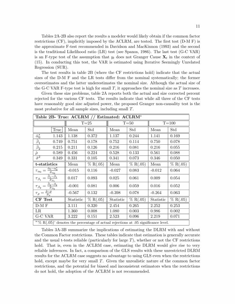
Tables 2A-2B also report the results a modeler would likely obtain if the common factorrestrictions (CF), implicitly imposed by the ACLRM, are tested. The first test (D-M F) isthe approximate F-test recommended in Davidson and MacKinnon (1993) and the secondis the traditional Likelihood ratio (LR) test (see Spanos, 1986). The last test (G-C VAR)is an F-type test of the assumption that yt does not Granger Cause Xt in the context of(15). In conducting this test, the VAR is estimated using Iterative Seemingly UnrelatedRegression (SUR).

The test results in table 2B (where the CF restrictions hold) indicate that the actualsizes of the D-M F and the LR tests differ from the nominal systematically; the formeroverestimates and the latter underestimates the nominal size. Although the actual size ofthe G-C VAR F-type test is high for small T, it approaches the nominal size as T increases.

Given these size problems, table 2A reports both the actual and size corrected percentrejected for the various CF tests. The results indicate that while all three of the CF testshave reasonably good size adjusted power, the proposed Granger non-causality test is themost probative for all sample sizes, including small T .

Table 2B- True: ACLRM // Estimated: ACLRM∗

T=25 T=50 T=100


α∗0 1.143 1.138 0.372 1.137 0.244 1.141 0.169β1 0.749 0.751 0.178 0.752 0.114 0.750 0.078β2 0.215 0.211 0.126 0.216 0.081 0.216 0.055ρ 0.589 0.456 0.224 0.528 0.133 0.561 0.088σ2 0.349 0.331 0.105 0.341 0.073 0.346 0.050


τα0 =α0−α∗0σα0

-0.015 0.116 -0.027 0.083 -0.012 0.064


0.017 0.093 0.025 0.061 0.009 0.054


-0.001 0.081 0.006 0.059 0.016 0.052

τρ =ρ−ρσρ

-0.567 0.132 -0.398 0.078 -0.264 0.063

CF Test Statistic % R(.05) Statistic % R(.05) Statistic % R(.05)

D-M F 3.111 0.320 2.454 0.265 2.252 0.253LR 1.360 0.008 1.080 0.003 0.986 0.002G-C VAR 3.222 0.151 2.523 0.096 2.219 0.071∗’% R(.05)’ denotes the percentage of actual rejections at .05 significance level.

Tables 3A-3B summarize the implications of estimating the DLRM with and withoutthe Common Factor restrictions. These tables indicate that estimation is generally accurateand the usual t-tests reliable (particularly for large T ), whether or not the CF restrictionshold. That is, even in the ACLRM case, estimating the DLRM would give rise to veryreliable inferences. In fact, a comparison of the GLS results with these unrestricted DLRMresults for the ACLRM case suggests no advantage to using GLS even when the restrictionshold, except maybe for very small T . Given the unrealistic nature of the common factorrestrictions, and the potential for biased and inconsistent estimators when the restrictionsdo not hold, the adoption of the ACLRM is not recommended.

12

Table 3A- True: DLRM // Estimated: DLRM (OLS)T=25 T=50 T=100


α0 0.946 1.026 0.772 0.987 0.361 0.970 0.233β1 0.749 0.772 0.228 0.758 0.149 0.752 0.102β2 0.215 0.212 0.134 0.215 0.086 0.216 0.058α1 0.589 0.458 0.206 0.522 0.131 0.556 0.087β3 -0.936 -0.788 0.229 -0.861 0.137 -0.900 0.089β4 -0.09 -0.068 0.140 -0.078 0.091 -0.084 0.062σ2 0.349 0.339 0.111 0.345 0.074 0.348 0.051<2 0.687 0.642 0.120 0.637 0.095 0.653 0.076

t-statistics Mean % R(.05) Mean % R(.05) Mean % R(.05)τα0 =

α0−α0σα0

0.137 0.087 0.109 0.067 0.096 0.056


0.104 0.063 0.062 0.053 0.023 0.054


-0.023 0.066 0.004 0.057 0.015 0.048


-0.633 0.09 -0.498 0.079 -0.369 0.065


0.664 0.111 0.541 0.089 0.395 0.069


0.175 0.064 0.134 0.055 0.096 0.054

Table 3B- True: ACLRM // Estimated: DLRM (OLS)T=25 T=50 T=100


α0 0.470 0.648 0.399 0.557 0.243 0.512 0.158β1 0.749 0.752 0.181 0.751 0.116 0.750 0.080β2 0.215 0.215 0.135 0.216 0.087 0.216 0.058α1 0.589 0.432 0.210 0.511 0.131 0.551 0.088β3 -0.441 -0.326 0.239 -0.384 0.152 -0.413 0.103β4 -0.127 -0.095 0.140 -0.110 0.090 -0.119 0.061σ2 0.349 0.343 0.113 0.347 0.075 0.349 0.051<2 0.662 0.681 0.122 0.665 0.091 0.662 0.066



0.427 0.091 0.315 0.072 0.222 0.059


0.013 0.068 0.016 0.054 0.006 0.053


-0.003 0.066 0.012 0.060 0.019 0.050


-0.698 0.107 -0.532 0.075 -0.377 0.064


0.491 0.090 0.367 0.072 0.266 0.063


0.245 0.071 0.186 0.055 0.126 0.050

13

3.2 Experiment 2 - Unrestricted DLRM vs. ACLRM (ρ = .2)The main purpose of Experiment 2 is to examine the extent to which the previousexperimental results change when the parameter on yt−1 (the degree of autocorrelationin the ACLRM) is reduced. To reduce this model parameter, we made only two changes tothe moments of the joint distribution (primary parameters) of Experiment 1A. First, theCov(yt, yt−1) is reduced from 0.446 to 0.185. This decreased the coefficient of yt−1 (to .20from .60), but also reduced the overall fit of the DLRM. In order to maintain a model fitclose to that in Experiment 1A, we also reduced V ar(yt) from 1.115 to 0.85.

Experiment 2B differs from Experiment 2A, in the same way as Experiment 1B differsfrom 1A. That is, the two DLRMs differ by the model parameters, (β3,β4), the coefficientsof (x1t−1, x2t−1), and, therefore, also by the intercept α0. All other model parameters remainthe same.4

Experiment 2A - Primary parameters underlying DLRME(Yt) = 2, V ar(Yt) = .85, Cov(Yt,X1t) = −.269, Cov(Yt,X2t) = 0.5,E(X1t) = 1, V ar(X1t) = 1, Cov(X1t,X1t−1) = 0.6, Cov(Yt, Yt−1) = 0.185,E(X2t) = .5, V ar(X2t) = 1, Cov(X2t,X2t−1) = 0.54, Cov(Yt,X1t−1) = −.678,

Cov(X1t,X2t) = −.4, Cov(X1t,X2t−1) = −.32, Cov(Yt,X2t−1) = .42,

giving rise to the DLRM:

(23)yt = 1.842 + 0.455x1t + 0.237x2t + 0.200yt−1 − 0.818x1t−1 + 0.0076x2t−1 + εt,

σ2ε = 0.259, <2 = 0.695The implied VAR parameters are:

(24)

a0 =

2.7051.950−0.097

, A> = −0.068 −0.640 0.142−0.752 0.46712 0.1730.311 −0.143 0.234

,Ω = 0.369 0.114 0.2470.114 0.265 −0.0280.247 −0.028 1.097

.For the ACLRM, the experimental set-up is as follows:

Experiment 2B - Primary parameters underlying ACLRME(Yt) = 2, V ar(Yt) = .469, Cov(Yt,X1t) = .360, Cov(Yt,X2t) = 0.150,E(X1t) = 1, V ar(X1t) = 1, Cov(X1t,X1t−1) = 0.6, Cov(Yt, Yt−1) = 0.139,E(X2t) = .5, V ar(X2t) = 1.4, Cov(X2t,X2t−1) = 0.54, Cov(Yt,X1t−1) = .197,

Cov(X1t,X2t) = −.4, Cov(X1t,X2t−1) = −.32, Cov(Yt,X2t−1) = −.017,giving rise to the ACLRM:

(25)yt = 1.427 + 0.455x1t + 0.237x2t + ut, ut = 0.200ut−1 + εt

= 1.142 + 0.455x1t + 0.237x2t + 0.200yt−1 − 0.091x1t−1 + 0.047x2t−1 + εt,σ2ε = 0.259; <2 = 0.448,

The implied VAR parameters for this case are:(26)

a0 =

1.4730.4580.521

, A> = 0.200 0.126 0.002

0 0.574 −0.0640 −0.187 0.332

, Ω = 0.416 0.246 0.1930.246 0.635 −0.1810.193 −0.181 1.161

.4Experiments 2A and 2B are also similar in the sense that in both cases, Det(Σ) = 0.061.

14

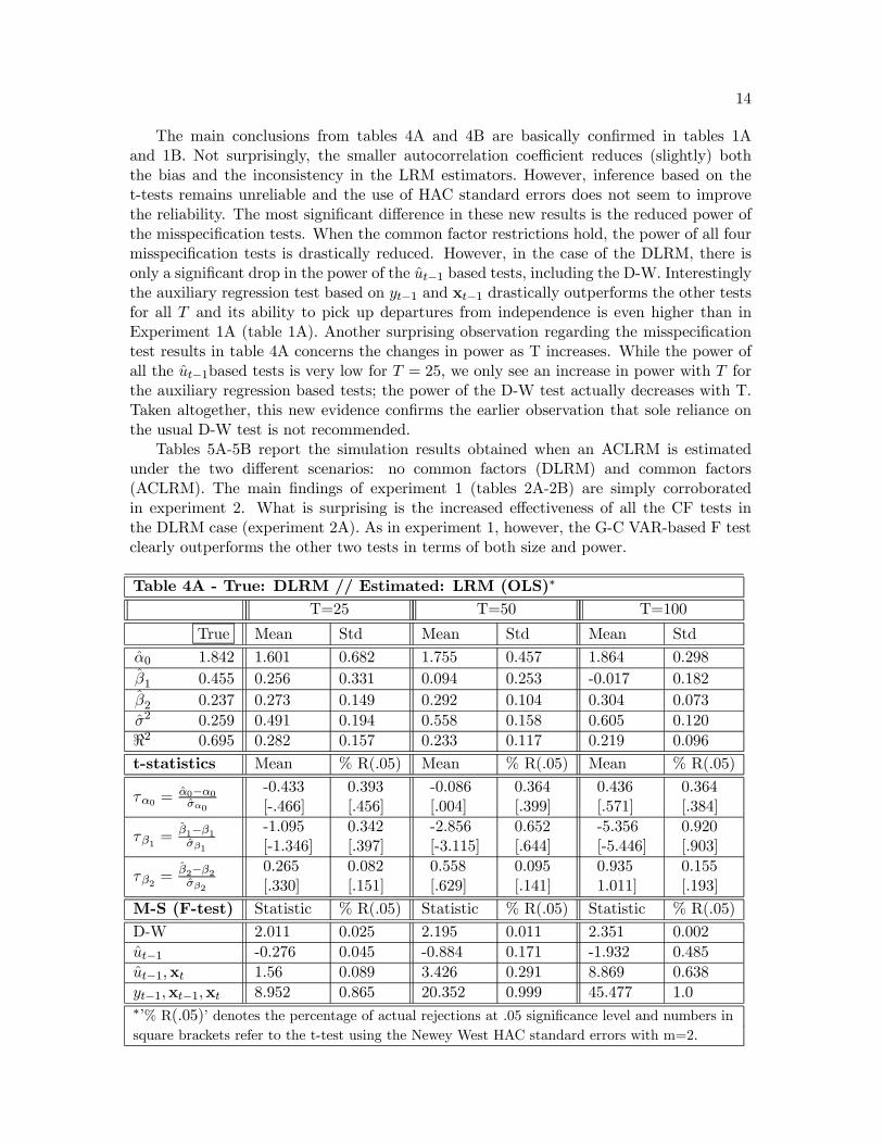
The main conclusions from tables 4A and 4B are basically confirmed in tables 1Aand 1B. Not surprisingly, the smaller autocorrelation coefficient reduces (slightly) boththe bias and the inconsistency in the LRM estimators. However, inference based on thet-tests remains unreliable and the use of HAC standard errors does not seem to improvethe reliability. The most significant difference in these new results is the reduced power ofthe misspecification tests. When the common factor restrictions hold, the power of all fourmisspecification tests is drastically reduced. However, in the case of the DLRM, there isonly a significant drop in the power of the ut−1 based tests, including the D-W. Interestinglythe auxiliary regression test based on yt−1 and xt−1 drastically outperforms the other testsfor all T and its ability to pick up departures from independence is even higher than inExperiment 1A (table 1A). Another surprising observation regarding the misspecificationtest results in table 4A concerns the changes in power as T increases. While the power ofall the ut−1based tests is very low for T = 25, we only see an increase in power with T forthe auxiliary regression based tests; the power of the D-W test actually decreases with T.Taken altogether, this new evidence confirms the earlier observation that sole reliance onthe usual D-W test is not recommended.

Tables 5A-5B report the simulation results obtained when an ACLRM is estimatedunder the two different scenarios: no common factors (DLRM) and common factors(ACLRM). The main findings of experiment 1 (tables 2A-2B) are simply corroboratedin experiment 2. What is surprising is the increased effectiveness of all the CF tests inthe DLRM case (experiment 2A). As in experiment 1, however, the G-C VAR-based F testclearly outperforms the other two tests in terms of both size and power.

Table 4A - True: DLRM // Estimated: LRM (OLS)∗

T=25 T=50 T=100


α0 1.842 1.601 0.682 1.755 0.457 1.864 0.298β1 0.455 0.256 0.331 0.094 0.253 -0.017 0.182β2 0.237 0.273 0.149 0.292 0.104 0.304 0.073σ2 0.259 0.491 0.194 0.558 0.158 0.605 0.120<2 0.695 0.282 0.157 0.233 0.117 0.219 0.096



-0.433[-.466]

0.393[.456]

-0.086[.004]

0.364[.399]

0.436[.571]

0.364[.384]


-1.095[-1.346]

0.342[.397]

-2.856[-3.115]

0.652[.644]

-5.356[-5.446]

0.920[.903]


0.265[.330]

0.082[.151]

0.558[.629]

0.095[.141]

0.9351.011]

0.155[.193]

M-S (F-test) Statistic % R(.05) Statistic % R(.05) Statistic % R(.05)

D-W 2.011 0.025 2.195 0.011 2.351 0.002ut−1 -0.276 0.045 -0.884 0.171 -1.932 0.485ut−1,xt 1.56 0.089 3.426 0.291 8.869 0.638yt−1,xt−1,xt 8.952 0.865 20.352 0.999 45.477 1.0∗’% R(.05)’ denotes the percentage of actual rejections at .05 significance level and numbers insquare brackets refer to the t-test using the Newey West HAC standard errors with m=2.

15

Table 4B- True: ACLRM // Estimated: LRM (OLS)∗

T=25 T=50 T=100


α∗0 1.142 1.424 0.214 1.423 0.145 1.426 0.100β1 0.455 0.457 0.140 0.457 0.093 0.455 0.064β2 0.237 0.237 0.110 0.238 0.074 0.238 0.051σ2 0.259 0.260 0.081 0.265 0.057 0.267 0.040<2 0.448 0.449 0.156 0.437 0.114 0.430 0.083


τα∗0 =α∗0−α∗0σα∗0

0.014[-.074]

0.091[.146]

-.030[-.032]

0.091[.111]

-.014[-.012]

0.085[.85]


0.014[.015]

0.084[.044]

0.024[.024]

0.081[.107]

0.009[.008]

0.079[.085]


-0.005[.009]

0.076[.140]

0.014[.014]

0.070[.100]

0.018[.017]

0.065[.075]

M-S Tests Statistic % R(.05) Statistic % R(.05) Statistic % R(.05)

D-W 1.759 0.110 1.686 0.259 1.644 0.483ut−1 0.418 0.069 0.997 0.163 1.723 0.403ut−1,xt 1.190 0.056 2.020 0.153 4.033 0.402yt−1,xt−1,xt 1.304 0.077 1.460 0.121 2.107 0.278∗’% R(.05)’ denotes the percentage of actual rejections at .05 significance level

Table 5A- True: DLRM // Estimated: ACLRM∗

T=25 T=50 T=100


α0 1.842 1.607 0.975 1.877 0.721 2.124 0.399β1 0.455 0.261 0.649 -0.017 0.583 -0.272 0.361β2 0.237 0.258 0.136 0.280 0.093 0.298 0.061ρ -0.051 0.611 -0.245 0.542 -0.455 0.335σ2 0.259 0.366 0.130 0.428 0.108 0.473 0.080

t-statistics Mean % R(.05) Mean % R(.05) Mean % R(.05)τα0 =

α0−α0σα0

0.243 0.502 1.593 0.648 3.921 0.863


-1.616 0.871 -5.531 0.987 -12.233 1.0


0.204 0.130 0.599 0.161 1.205 0.265

τρ =ρσρ

0.272 0.817 -1.587 0.962 -5.257 0.998

CF Test Statist. % R(.05) Statistic % R(.05) Statistic % R(.05)

D-M: F 16.669 0.939 (0.722) 38.111 0.999 (0.993) 88.007 1.0 (1.0)LR 5.646 0.401 (0.722) 12.367 0.920 (0.993) 27.516 1.0 (1.0)G-C - VAR 29.452 0.952(0.896) 62.257 0.999 (0.999) 133.05 1.0 (1.0)∗’% R(.05)’ denotes the percentage of actual rejections at .05 significance level and numbersin parentheses refer to size-corrected power.

16

Table 5B- True: ACLRM // Estimated: ACLRM∗

T=25 T=50 T=100


α∗0 1.427 1.424 0.222 1.423 0.145 1.425 0.099β1 0.455 0.457 0.147 0.457 0.093 0.455 0.063β2 0.237 0.237 0.114 0.238 0.073 0.238 0.050ρ 0.200 0.099 0.229 0.151 0.151 0.176 0.103σ2 0.259 0.245 0.078 0.253 0.054 0.256 0.038


τα0 =α0−α∗0σα0

-0.0122 0.091 -0.029 0.071 -0.015 0.056


0.013 0.096 0.0234 0.071 0.011 0.060


-0.008 0.094 0.0115 0.069 0.017 0.056

τρ =ρ−ρσρ

-0.454 0.108 -0.318 0.077 -0.219 0.063

CF Test Statistic % R(.05) Statistic % R(.05) Statistic % R(.05)

D-M: F-test 2.813 0.274 2.320 0.242 2.181 0.239LR test 1.241 0.004 1.024 0.002 0.956 0.002G-C - VAR 2.886 0.127 2.394 0.085 2.155 0.060∗’% R(.05)’ denotes the percentage of actual rejections at .05 significance level.

3.3 Summary of Monte Carlo resultsThe above Monte Carlo results demonstrate most clearly that when the common factor(CF) restrictions do not hold:

(a) the Linear Regression Model (LRM) OLS estimators are both biased andinconsistent and inference based on them highly unreliable,

(b) the ‘autocorrelation correction’ GLS estimators, based on the AutocorrelationCorrected LRM (ACLRM), do not improve the situation; they gives rise to different butequally misleading inferences, and

(c) utilizing heteroskedastic and autocorrelation consistent standard errors does notameliorate the reliability of inference.

When the common factor (CF) restrictions do hold, our Monte Carlo results demon-strate that:

(d) the Dynamic Linear Regression Model (DLRM) OLS estimators are equally reliableas the ACLRM GLS estimators with hardly any loss of efficiency, particularly for T = 50;the same is true for the VAR estimators.

Taking (a)-(d) together, the main conclusion is that, in view of the misleading resultsfrom the ACLRM when the CF restrictions do not hold, the adoption of the ACLRM whenresidual autocorrelation is detected in practice is not a good idea.

The Monte Carlo experiments in this paper also call into question the usual practiceof relying solely on the Durbin-Watson test (D-W) to assess the independence assumption.Not surprisingly, we find that the power of the D-W is much higher when the common factorrestrictions do hold than when they do not. However, a more general test of autocorrelationis shown to perform almost as well as the D-W when the common factor restrictions do holdand significantly better than the D-W when the restrictions do not hold. Given that theCF restrictions may be unlikely for most data applications anyway, sole reliance on D-W

17

test seems problematic. Our Monte Carlo results recommend the use of the test based onthe auxiliary regression:

(27) but = (α0 − γ0) + (β> − γ>)xt + δ1yt−1 + δ>2 xt−1 + v3t.

The most important advise for practitioners is that they should test the common factorrestrictions before imposing them, irrespective of the test of autocorrelation used to detectresidual autocorrelation. The Monte Carlo results suggest that the simple (approximate)F-test suggested by Davidson and MacKinnon (1993) as well as a Likelihood Ratio testsuffer from size problems. A more probative test for the CF restrictions, based on theGranger non-causality of yt on Xt, is proposed.

As mentioned in the introduction, however, these CF restriction tests are based on thepresumption that the DLRM is statistically adequate for data (y,X). This is the issue weaddress next.

4 ‘Autocorrelation Correction’ as a modeling strategyThe question of whether or not autocorrelation correcting is appropriate raises severalmethodological issues that have not been addressed adequately in the literature. Forinstance, ‘why is it problematic to adopt the alternative hypothesis in the case of a D-W test?’ It is generally accepted that there is no problem when one adopts the alternativein the case of a t-test for the hypotheses:

(28) H0 : β1 = 0 vs. H1 : β1 6= 0.

The purpose of this section is to address briefly these methodological issues in the contextof the Probabilistic Reduction framework; see Spanos (1986,1995).

Despite the apparent similarity between a t-test (28) and the D-W test based on:

(29) H0 : ρ = 0 vs. H1 : ρ 6= 0,

in terms of the hypotheses being tested, they are very different in nature. As argued inSpanos (1999), the D-W test is a misspecification test, but the t-test is a proper Neyman-Pearson test. The crucial difference between them is that the D-W is probing beyond theboundaries of the original model, the LRM (see table A):

Table A - The Linear Regression Model (LRM)

yt = β0 + β>1 xt + ut, t ∈ T,[1] Normality: D(yt | xt;θ), is Normal[2] Linearity: E(yt | xt) = β0 + β>1 xt,[3] Homoskedasticity: V ar(yt | xt) = σ2, free of xt,[4] t-homogeneity: θ :=(β0,β1,σ

2) are t-invariant ∀t ∈ T,[5] Independence: (yt | xt−1), t ∈ T - independent process.

The t-test, on the other hand, is probing within those boundaries. In a Neyman-Pearsontest there are only two types of errors (reject the null when true and accept the null whenfalse) because one assumes that the prespecified statistical model (LRM) is valid. Thisensures that the estimated model contains the ‘true’ model. Hence, rejection of the nullleaves only one choice—the alternative—as the union of the null and the alternative span theoriginal model. In the case of a misspecification test, one is probing beyond the boundaries

18

of the prespecified model by extending it in specific directions; the D-W test extends theLRM by attaching an AR(1) error. A rejection of the null in a misspecification test doesnot entitle the modeler to infer that the extended model is true; only that the originalmodel is misspecified. In order to infer the validity of the alternative model one needs totest its own assumptions. More formally, the alternative hypothesis in (29) has not passeda severe test ; see Mayo (1996), Mayo and Spanos (2004).

In the case of the D-W test, if the null is rejected one can only infer that the LRM ismisspecified since the data exhibit some kind of dependence over the dimension of the indext = 1, 2, ..., T . However, the type of dependence present in the data can only be establishedby thorough misspecification testing of alternative statistical models which allow for suchdependence.5 The alternative model involved in a D-W test (4) is only one of an infinitenumber of potential models that could have given rise to data (y,X) ; the DLRM (5) isanother such model. The advantage of the latter is that it nests the former and thus, if(5) is misspecified, so is (4). In terms of respecifying the LRM to allow for dependence,the DLRM (5) is considerably more general than (4) because it allows for a much lessrestrictive form of dependence. This suggests that if one wanted to consider the ACLRMas a respecification of the original LRM, one has to establish two things. To begin with,one should estimate the DLRM (5) and ensure its statistical adequacy by testing and notrejecting the assumptions [1]-[5] in table B. That will provide the framework to ensure thestatistical validity of the CF restrictions test itself. If these restrictions are tested and notrejected, the ACLRM model will provide a reliable framework for any inference concerningthe model parameters θ. If either of these conditions is not met, the inference is likely tobe unreliable.

Table B - The Dynamic Linear Regression (DLR) Model

yt = β0 + β>1 xt + γ1yt−1 + β>2 xt−1 + ut, t ∈ T,[1] Normality: D(yt | xt,Zt−1;θ), Zt = (yt,xt), is Normal[2] Linearity: E(yt | xt,Zt−1) = β0 + β>1 xt + γ1yt−1 + β>2 xt−1,[3] Homoskedasticity: V ar(yt | xt,Zt−1) = σ20, free of (xt,Zt−1) ,[4] t-homogeneity: θ :=(β0,β1,γ1,β2,σ

20) are t-invariant ∀t ∈ T,

[5] Markovness: (Zt | Z0t−1), t ∈ T - Markov process,where Z0t−1 := (Zt−1,Zt−2, ...,Z0).

5 ConclusionThe primary aim of this paper is to demonstrate that the restrictions implicitly imposed onthe dependence structure of yt and Xt when an AR(1) error formulation is adopted seemunreasonably restrictive for most real applications. We derive necessary and sufficientconditions on the probabilistic structure of the vector stochastic process Zt, t ∈ T,Zt := (yt,x

>t )> for the common factor restrictions (CF) to hold. These restrictions, in

the context of the VAR model, amount to:

(a) yt does not Granger cause any of the regressors in Xt, and

(b) Cov(Xt, yt|Zt−1) = Cov(Xt|Xt−1)Cov(Xt)−1Cov(Xt, yt) = Λβ.5By thorough misspecification testing, we mean that all the testable assumptions underlying the DLRM

are tested (see Spanos, 1986 or 1999).

19

Condition (a) seems most unrealistic, but it is a testable hypothesis. A new test of theCF restrictions is proposed based on Granger non-causality, and the results of our MonteCarlo experiments suggest that the proposed test outperforms, in terms of correct size andhigh power, the approximate F-test suggested by Davidson and MacKinnon (1993) as wellas a Likelihood Ratio test first proposed by Sargan (1964).

The Monte Carlo evidence also suggests that testing for dependence using only theD-W test is not an effective strategy because its power is considerably reduced when theCF restrictions do not hold. In contrast, the misspecification test based on the DLRM (see(27)) is most probative in general.

The main conclusion of this paper, based on both the theoretical as well as extensiveMonte Carlo results, is that adopting the ACLRM as an alternative to the LRM whenresidual autocorrelation is detected is a bad modeling strategy; echoing the main messagein Hendry and Mizon (1978), Hoover (1988), Spanos (1988) and Mizon (1995). Ingeneral, we do not recommend the modeling of the error term when misspecifications aredetected. This is because the modeling of the error imposes implicit assumptions on theprobabilistic structure of the observable vector processes, which are often both unrealisticand unnecessary.

Although we have only considered the implications of error ‘correcting’ under the verysimple AR(1) scenario, typically implemented using time series data, similar unrealisticrestrictions are implicitly imposed when researchers use spatial data and model errors as afunction of ‘near-by’ errors. Similarly, it is also clear, that more complicated error structures(i.e. higher order AR or ARMA models) will impose more complicated and unrealisticrestrictions. In general, before any kind of ‘correcting’ for misspecifications by modelingthe error takes place, it seems prudent to make explicit, and then test, the restrictions beingimplicitly imposed on the probabilistic structure of the data.

References

[1] Anselin, L. (2001), “Spatial Econometrics," ch. 14 in A Companion to Theoretical Economet-rics, edited by B. H. Baltagi, Blackwell Publishers, Oxford.

[2] Breusch, T. S. (1978), “Testing for autocorrelation in dynamic linear models," AustralianEconomic Papers, 17, 334-355.

[3] Davidson, R. and J. G. MacKinnon (1993), Estimation and Inference in Econometrics, OxfordUniversity Press, Oxford.

[4] Durbin, J. and G. S. Watson (1950), “Testing for serial correlation in least squares regressionI”, Biometrika, 37, 409-428.

[5] Durbin, J. and G. S. Watson (1951), “Testing for serial correlation in least squares regressionII”, Biometrika, 38, 159-178.

[6] Godfrey, L. G. (1978), “Testing against general autoregressive and moving average error modelswhen the regressors include lagged endogenous variables," Econometrica, 46, 1293-1302.

[7] Greene, W. H. (2000), Econometric Analysis, 4rd ed., Prentice-Hall, New Jersey.[8] Hendry, D. F. and G. E. Mizon (1978) “Serial correlation as a convenient simplification, not a

nuisance: A comment on a study of the demand for money by the Bank of England,” EconomicJournal, 88, 549-563.

[9] Hoover, K. D. (1988), “On the pitfalls of untested common-factor restrictions: The case of theinverted Fisher hypothesis”, Oxford Bulletin of Economics and Statistics, 50, 125-138.

[10] Mayo, D. G. (1996), Error and Growth of Scientific Knowledge, Chicago University Press,Chicago.

[11] Mayo, D. G. and A. Spanos (2004), “Methodology in Practice: Statistical MisspecificationTesting,” forthcoming, Philosophy of Science.

20

[12] Morgan, M. S. (1990), The history of econometric ideas, Cambridge University Press,Cambridge.

[13] Newy, W. K. and K. West (1987), “A Simple, Positive Semi-Definite, Heteroskedastic andAutocorrelation Consistent Covariance Matrix," Econometrica, 55, 703-708.

[14] Sargan, J. D. (1964), “Wages and Prices in the United Kingdon: A study in econometricmethodology,” in P.E. Hart, G. Mills and J.K. Whitaker, eds., Econometric Analysis forEconomic Planning, Butterworths, London.

[15] Sargan, J. D. (1980), “Some tests of dynamic specification for a single equation,” Econometrica,48, 879-897.

[16] Spanos, A. (1986), Statistical Foundations of Econometric Modelling, (1986), CambridgeUniversity Press, Cambridge.

[17] Spanos, A. (1995), “On theory testing in Econometrics: modeling with nonexperimental data”,Journal of Econometrics, 67, 189-226.

[18] Spanos, A. (1988) “Error-autocorrelation revisited: the AR(1) case”, Econometric Reviews, 7,pp. 285-94.

[19] Spanos, A. (1999), Probability Theory and Statistical Inference: Econometric modeling withobservational data, Cambridge University Press, Cambridge.

[20] Spanos, A. and A. McGuirk (2002), “The problem of near-multicollinearity revisited: erraticvs systematic volatility”, The Journal of Econometrics, 108, 365-393.

[21] Yule, G.U. (1921), “On the time-correlation problem”, Journal of the Royal Statistical Society,84, 497-526.

[22] Yule, G.U. (1926), “Why do we sometimes get nonsense correlations between time series-astudy in sampling and the nature of time series ”, Journal of the Royal Statistical Society, 89,2-41.

21

6 Appendix AThe ACLRM is specified as follows:

(30)

yt = β>xt + ut, ut = ρut−1 + εt, |ρ| < 1, t ∈ T,

[a1] E(εt) = 0, V ar(εt) = σ2, Cov(εt, εs) = 0, t 6= s,[a2] Cov(Xt, us) = 0, ∀ (t, s) ∈ T.

Theorem 1. The mapping between the primary parameters Σ and the parametersθ∗1 := (α1,β0,σ2) of the ACLRM (8) takes the form [1]-[6].

[1] V ar(u2t ) = σuu(0) =σ2

1−ρ2 .

V ar(u2t ) = E(u2t ) = E [(ρut−1 + εt)(ρut−1 + εt)] = ρ2E(u2t−1) + E(ε2t ) =

ρ2E(u2t ) +E(ε2t ), from [a1]. Given |ρ| < 1, E(u2t ) = σuu(0) =

σ2

1−ρ2 .

[2] Cov(utut−1) = σuu(1) =ρσ2

1−ρ2 .

Cov(utut−1) = E(utut−1) = E [(ρut−1 + εt)ut−1] = ρE(u2t−1) = ρσuu(0) =ρσ2

1−ρ2from [a1] and [1].

[3] σ21(0) = Σ22(0)β.

σ21(0) = E(xtyt) = Ehxt¡β>xt + ut

¢0i= E [xtx

0t]β = Σ22(0)β from [a2].

Thus, σ21(0) = Σ22(0)β or β = Σ−122 (0)σ21(0).

[4] σ21(1) = Σ22(1)β.

σ21(1) = E(xtyt−1) = Ehxt¡β>xt−1 + ut−1

¢0i= E

£xtx

0t−1¤β = Σ22(1)β from

[a2]. Thus, σ21(1) = Σ22(1)β or β = Σ−122 (1)σ21(1).

[5] σ11(0) = β>Σ22(0)β + σ2

1−ρ2 .

σ11(0) = E(ytyt) = Eh¡β>xt + ut

¢ ¡β>xt + ut

¢>i= E

£¡β>xtx>t β + u2t

¢¤using [a2]. Using E(u2t ) =

σ2

1−ρ2 from [1], σ11(0) = β>Σ22(0)β + σ2

1−ρ2 .

[6] σ11(1) = β>Σ22(1)β + ρσ2

1−ρ2 .

σ11(1) = E(ytyt−1) = Eh¡β>xt + ut

¢ ¡β>xt−1 + ut−1

¢>i=

E£¡β>xtx>t−1β + utut−1

¢¤using [a2]. From [2], σ11(1) = β>Σ22(1)β + ρσ2

1−ρ2 .

22

Theorem 2. The implicit statistical parameterization for (α1,β0,β1,σ2ε) implied bythe variance-covariance matrix Σ∗ in (10) is:(31) α1

β0β1

=

β>Σ22(0)β + σ2

1−ρ2 β>Σ22(1) β>Σ22(0)Σ22(1)

>β Σ22(0) Σ22(1)Σ22(0)β Σ22(1) Σ22(0)

−1 β>Σ22(1)β + ρσ2

1−ρ2Σ22(0)βΣ22(1)β

σ2ε = β>Σ22(0)β+σ2

1− ρ2−

³β>Σ22(1)β + ρσ2

1−ρ2 β>Σ22(0) β>Σ22(1)´ α1

β0β1

.Using the partitioned matrix inverse result in Searle (1982):

(32)·A BB> C

¸−1=

" ¡A−BC−1B>¢−1 − ¡A−BC−1B>¢−1BC−1

−C−1B> ¡A−BC−1B>¢−1 C−1 +C−1B>¡A−BC−1B>¢−1BC−1

#

we proceed to derive the inverse of the matrix:β>Σ22(0)β + σ2

1−ρ2 β>Σ22(1) β>Σ22(0)Σ22(1)β Σ22(0) Σ22(1)Σ22(0)β Σ22(1) Σ22(0)

where we define A =

"β>Σ22(0)β + σ2

1−ρ2 β>Σ22(1)Σ22(1)β Σ22(0)

#, B =

·β>Σ22(0)Σ22(1)

¸, and

C = Σ22(0), to find:

β>Σ22(0)β + σ2

1−ρ2 β>Σ22(1) β>Σ22(0)Σ22(1)β Σ22(0) Σ22(1)Σ22(0)β Σ22(1) Σ22(0)

−1

=

=

(1−ρ2)σ2

0(1xk) − (1−ρ2)σ2

β>

0(kx1) ∆ −∆Σ22(1)Σ22(0)−1³− (1−ρ2)

σ2β>´ ¡−Σ22(0)−1Σ22(1)∆¢ ³

Ψ+ ββ> (1−ρ2)

σ2

´

where:Ψ = Σ22(0)

−1 +Σ22(0)−1Σ22(1)∆Σ22(1)Σ22(0)−1,

∆ =£Σ22(0)−Σ22(1)Σ22(0)−1Σ22(1)

¤−1.

Noting that:∆ =Ψ

(see Henderson and Searle, 1981, p. 53), the inverse simplifies to: (1−ρ2)σ2

0(1xk) − (1−ρ2)σ2

β>

0(kx1) ∆ −∆Σ22(1)Σ22(0)−1− (1−ρ2)

σ2β> −Σ22(0)−1Σ22(1)∆ ∆+ ββ> (1−ρ

2)σ2

.

23

Thus,(33) α1

β0β1

=

(1−ρ2)σ2

0(1xk) − (1−ρ2)σ2

β>

0(kx1) ∆ −∆Σ22(1)Σ22(0)−1− (1−ρ2)

σ2β> −Σ22(0)−1Σ22(1)∆ ∆+ ββ> (1−ρ

2)σ2

β>Σ22(1)β +

ρσ2

1−ρ2Σ22(0)βΣ22(1)β

Multiplying and simplifying the right-hand-side yields: (1−ρ2)

σ2β>Σ22(1)β+ρ− (1−ρ2)

σ2β>Σ22(1)β

∆Σ22(0)β −∆Σ22(1)Σ22(0)−1Σ22(1)β− (1−ρ2)

σ2ββ>Σ22(1)β − ρβ −Σ22(0)−1Σ22(1)∆Σ22(0)β +∆Σ22(1)β + (1−ρ2)

σ2β>β>Σ22(1)β

,thus, α1

β0β1

=

ρ∆(Σ22(0)−Σ22(1)Σ22(0)−1Σ22(1))β

−ρβ + (∆Σ22(1)−Σ22(0)−1Σ22(1)∆Σ22(0))β

=

ρβ−ρβ

since Σ22(0) − Σ22(1)Σ22(0)−1Σ22(1) = ∆−1 and ∆Σ22(1) = Σ22(0)−1Σ22(1)∆Σ22(0).This follows from:

(D − V A−1U)−1V A−1 = D−1V (A− UD−1V )−1,(see Henderson and Searle, 1981, p.56) by letting A = D = Σ22(0) and U = V = Σ22(1).

Substituting this result into the expression for σ2ε :

σ2ε = β>Σ22(0)β+σ2

1− ρ2−³β>Σ22(1)β + ρσ2

1−ρ2 β>Σ22(0) β>Σ22(1)´ ρ

β−ρβ

= σ2,

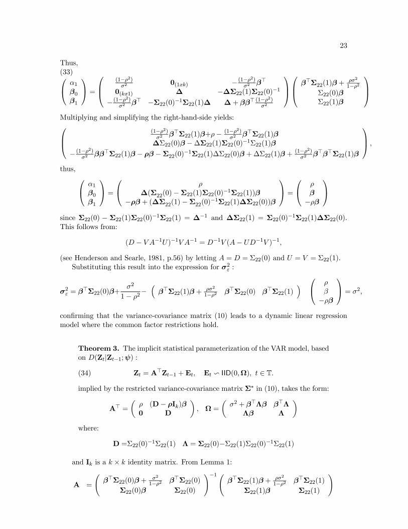
confirming that the variance-covariance matrix (10) leads to a dynamic linear regressionmodel where the common factor restrictions hold.

Theorem 3. The implicit statistical parameterization of the VAR model, basedon D(Zt|Zt−1;ψ) :(34) Zt = A

>Zt−1 +Et, Et v IID(0,Ω), t ∈ T.implied by the restricted variance-covariance matrix Σ∗ in (10), takes the form:

A> =µ

ρ (D− ρIk)β0 D

¶, Ω =


¶where:

D =Σ22(0)−1Σ22(1) Λ = Σ22(0)−Σ22(1)Σ22(0)−1Σ22(1)

and Ik is a k × k identity matrix. From Lemma 1:

A =

Ãβ>Σ22(0)β + σ2

1−ρ2 β>Σ22(0)Σ22(0)β Σ22(0)

!−1Ãβ>Σ22(1)β + ρσ2

1−ρ2 β>Σ22(1)Σ22(1)β Σ22(1)

!

24

and

Ω =

Ãβ>Σ22(0)β + σ2

1−ρ2 β>Σ22(0)Σ22(0)β Σ22(0)

!−Ãβ>Σ22(1)β + ρσ2

1−ρ2 Σ22(1)βΣ22(1)β Σ22(1)

!A.

Using (32) to find the inverse of:Ãβ>Σ22(0)β + σ2

1−ρ2 β>Σ22(0)Σ22(0)β Σ22(0)

!

yields: ³1−ρ2σ2

´−³1−ρ2σ2

´β>

−³1−ρ2σ2

´β

³Σ22(0)

−1 +³1−ρ2σ2

´ββ>

´ .Thus,

A =

³1−ρ2σ2

´−³1−ρ2σ2

´β>

−³1−ρ2σ2

´β

³Σ22(0)

−1 +³1−ρ2σ2

´ββ>

´ Ã ³β>Σ22(1)β + ρσ2

1−ρ2´

β>Σ22(1)Σ22(1)β Σ22(1)

!

A =

µρ 0

Σ22(0)−1Σ22(1)β − ρβ Σ22(0)

−1Σ22(1)

¶.

Substituting this result for A into the expression for Ω and multiplying yields:Ãβ>Σ22(0)β + σ2

1−ρ2 β>Σ22(0)Σ22(0)β Σ22(0)

!−Ãβ>Σ22(1)Σ22(0)

−1Σ22(1)β + ρ2σ2

1−ρ2 β>Σ22(1)Σ22(0)−1Σ22(1)Σ22(1)Σ22(0)

−1Σ22(1)β Σ22(1)Σ22(0)−1Σ22(1)

!.

Simplifying further we obtain:

Ω =

µσ2 + β>(Σ22(0)−Σ22(1)Σ22(0)−1Σ22(1))β β>(Σ22(0)−Σ22(1)Σ22(0)−1Σ22(1))

(Σ22(0)−Σ22(1)Σ22(0)−1Σ22(1))β Σ22(0)−Σ22(1)Σ22(0)−1Σ22(1)¶.

Using Lemma 1, to obtain the parameterization of the VAR model for Xt based onD(Xt | Xt−1;θ) :

(35) Xt = D>Xt−1 +Vt,Vt v IID(0,Λ),

we obtain:D =Σ22(0)

−1Σ22(1) Λ = Σ22(0)−Σ22(1)Σ22(0)−1Σ22(1).Thus, we can rewrite the above expressions for the VAR parameters (A,Ω), based onD(Zt|Zt−1;ψ) as follows:

A =

µρ 0

(D− ρIk)β D

¶, Ω =


¶,

where Ik is a k × k identity matrix.

Revisiting Error-Autocorrelation Correction: Common Factor Restrictions and Granger Non-Causality

Documents

Transcript of Revisiting Error-Autocorrelation Correction: Common Factor Restrictions and Granger Non-Causality