Can Unemployment Insurance Spur Entrepreneurial Activity?

NBER WORKING PAPER SERIES

CAN UNEMPLOYMENT INSURANCE SPUR ENTREPRENEURIAL ACTIVITY?

Johan HombertAntoinette Schoar

David SraerDavid Thesmar

Working Paper 20717http://www.nber.org/papers/w20717

NATIONAL BUREAU OF ECONOMIC RESEARCH1050 Massachusetts Avenue

Cambridge, MA 02138November 2014

This is the substantially revised version of a paper previously titled “Should the Government Makeit Safer to Start a Business? Evidence From a French Reform”. We thank participants at many conferencesand seminars for comments and suggestions. In particular, we are indebted to Ashwini Agrawal, SteveDavis, Guy Laroque, David Matsa, Toby Moskowitz, Marina Niessner, and Elena Simintzi for theirvaluable insights. The data used in this paper is confidential but not the authors’ exclusive access.The views expressed herein are those of the authors and do not necessarily reflect the views of theNational Bureau of Economic Research.

NBER working papers are circulated for discussion and comment purposes. They have not been peer-reviewed or been subject to the review by the NBER Board of Directors that accompanies officialNBER publications.

© 2014 by Johan Hombert, Antoinette Schoar, David Sraer, and David Thesmar. All rights reserved.Short sections of text, not to exceed two paragraphs, may be quoted without explicit permission providedthat full credit, including © notice, is given to the source.

Can Unemployment Insurance Spur Entrepreneurial Activity?Johan Hombert, Antoinette Schoar, David Sraer, and David ThesmarNBER Working Paper No. 20717November 2014JEL No. G3,H25,J65

ABSTRACT

We study a large-scale French reform that provided generous downside insurance for unemployedindividuals starting a business. We study whether this reform affects the composition of people whoare drawn into entrepreneurship. New firms started in response to the reform are, on average, smaller,but have similar growth expectations and education levels compared to start-ups before the reform.They are also as likely to survive or to hire. In aggregate, the effect of the reform on employment islargely offset by large crowd-out effects. However, because new firms are more productive, the reformhas the impact of raising aggregate productivity. These results suggest that the dispersion of entrepreneurialabilities is small in the data, so that the facilitation of entry leads to sizable Schumpeterian dynamicsat the firm-level.

Johan HombertHEC Paris1 rue de la Liberation78351 Jouy en [email protected]

Antoinette SchoarMIT Sloan School of Management100 Main Street, E62-638Cambridge, MA 02142and [email protected]

David SraerHaas School of BusinessUniversity of California, Berkeley545 Student Services BuildingBerkeley, CA 94720-1900and [email protected]

David ThesmarHEC Paris1 rue de la libération78351 Jouy-en-Josas [email protected]

“The problem with the French is that they have no word for entrepreneur”, attributed to GeorgeW. Bush.

1 Introduction

Over the last decade, policy makers and academics alike have embraced entrepreneurship as apanacea for many economic challenges. Reducing barriers to entrepreneurship has consequentlybecome a major policy objective and an object of intense academic evaluation.1 The primaryfocus of this literature has been on how reduction in barriers to entrepreneurship affects the levelof entrepreneurship. However, this focus may be misleading. Entrepreneurial rates conceal asubstantial amount of heterogeneity, as entrepreneurs vary in their ability to manage their firm orto grow and create jobs (Nanda (2008)), from self-employed individuals—looking for subsistenceopportunities—to transformational entrepreneurs who aim at building large firms (Schoar (2010)or Haltiwanger et al. (2013)). Beyond ability, entrepreneurs have different degrees of risk tolerance,ambition, or optimism (Hurst and Pugsley (2011), Landier and Thesmar (2009), or Holtz-Eakinet al. (1994a)). The welfare implications of barriers to entrepreneurship thus crucially depend onhow individuals select into this activity. For instance, policies that draw less qualified individualsinto entrepreneurship may deteriorate allocative efficiency, as scarce resources are diverted to lessproductive firms.

Beyond ability, an important dimension of selection into entrepreneurship is risk-aversion, sinceentrepreneurs have to bear significant idiosyncratic and possibly fundamental risk (Kihlstrom andLaffont (1979)). The academic literature has been struggling to evaluate conclusively whether thisinherent risk associated with entrepreneurship and self-employment is an undesirable constraintor a necessary selection criterion. When designing interventions that defray some of the downsiderisk of entrepreneurship, policy-makers face an inherent tension. On the one hand, entrepreneurialrisk might dissuade many able individuals from starting a business, if these individuals are riskaverse and can only learn about their ability as entrepreneurs by starting a firm (see Jovanovic(1982) or Caves (1998)). As a result, many promising businesses might not get set up. In such aworld, providing a form of downside insurance to would-be entrepreneurs could lead to increasedefficient entry into self-employment. On the other hand, this downside insurance could distortthe pool of entrepreneurs who start businesses. If people have ex ante private information abouttheir entrepreneurial abilities, being forced to bear downside risk might serve as an effective way

1See, for example, the fast-growing literature on the impact of financial market reforms on entrepreneurship,e.g., Bertrand et al. (2007) or Cole (2009). For papers on regulatory constraints, see Djankov et al. (2002) orKlapper et al. (2006).

2

to screen out entrepreneurs who have low expectations about the success of their venture.To investigate this trade-off, we first develop a general equilibrium model of selection into self-

employment that features risk-averse individuals and heterogeneity in the distribution of talent.We show that the effect of downside insurance provision on the pool of entrepreneurs dependson the size of the wedge that is created by risk aversion and the heterogeneity of talents. Iftalents are relatively heterogeneous, the “self-selection” effect dominates: an intervention thatlowers downside risk draws in low-quality entrepreneurs. In contrast, if the talent distribution ismore homogeneous, such an intervention draws in entrepreneurs of similar ex ante quality andthus allows risk averse individuals to learn about their success as entrepreneurs. We refer to thisas the “experimentation channel”.2

We then evaluate the above trade-off in the context of a large-scale reform implemented inFrance in 2002, which aimed at facilitating (small) business creation for unemployed workers,called PARE—Plan d’Aide au Retour à l’Emploi. The reform provided downside insurance tounemployed individuals starting businesses, mostly by allowing them to retain their rights tounemployment benefits for three years in case of failure of their venture, which previously theywould lose by becoming entrepreneurs. Additionally, the reform gave “unemployed entrepreneurs”the possibility to fill any gap between their entrepreneurial revenues and their unemploymentbenefits by using their accrued unemployment benefits, providing insurance against cash flowshortfalls in the first three years.

As soon as the reform is implemented, monthly firm creation immediately increases by 25%.This is strongly suggestive of the large impact of the reform. To filter out the effect of other macroe-conomic shocks, we employ a standard difference-in-difference estimation. The treatment groupconsists of industries where newly created firms tend to be small before the reform. By contrast,the control group contains industries where small firms are not prevalent at creation. The idea un-derlying this choice is that since the reform provided downside insurance for unemployed workers,it should have mostly affected industries that are most likely to attract small-scale entrepreneurs.Therefore, our treatment industries should have a larger exposure to the reform than our controlindustries. The identifying assumption is that absent the policy reform, both types of industrieswould have experienced similar changes in entrepreneurial activity relative to pre-reform levels.Under this assumption, which we make more explicit in Section 5, the difference-in-difference es-timator allows us to reject the null hypothesis that the reform did not increase entrepreneurialactivity. Empirically, we find a very large effect of the reform on business creation across indus-

2One can also extend this model to allow for heterogeneous talent and heterogeneity in risk aversion. The neteffect of greater downside insurance then depends on the sign of the correlation between talent and risk aversion.In the limit, if very talented individuals are the most (resp. least) risk averse, providing downside insurance leadsto an increase (resp. a decrease) in average entrepreneurial talent.

3

tries: Post-reform entry growth is larger by more than 12 percentage points in industries wheresmall firms are prevalent at creation.

Using the same identification strategy, we further document that the firms created in responseto the reform are not of (observably) worse quality ex post. We do not observe a significant changein the failure rate, hiring rate, or growth rate of young firms in treated industries following thereform relative to control industries. We also find that the reform did not significantly affect thecomposition of educational backgrounds of founders. Somewhat surprisingly, the reform seemsto have led to a significant entry of “ambitious” founders, where ambition is measured from asurvey that asks founders of new firms about their growth expectations and intention to hireworkers in the next year. Firms created in the treatment industries are 3.5 percentage pointsmore likely to intend to hire relative to firms in control industries. This is a sizable effect sincethe sample average is 18% for these industries. Overall, the evidence is more consistent with the“experimentation view”, whereby providing downside insurance allowed unemployed workers toenter into self-employment without significantly lowering the average quality of the pool. Thissuggests that the ex ante selection into self-employment was not based on steep differences in thetalent distribution of would-be entrepreneurs.

The final part of the paper focuses on the equilibrium effects of the reform and looks at potentialspillovers on incumbent firms in treated industries. The significant entry of new firms post-reformmay have eroded incumbent firms’ market shares, which is the key idea underlying the conceptof creative destruction. Our analysis reveals that employment growth among small incumbents islower by 2.6 percentage points after the reform in treated industries relative to control industries.However, we do not find any evidence for spillover effects on large incumbent firms. This isconsistent with the idea that the competition from increased entrepreneurial activity is strongerfor small incumbents than for large ones, at least in the short-run. The crowding-out effects onsmall incumbents are economically large. According to our estimates, they offset most of the directeffects of the reform on employment creation by start-ups. These results bear some similarity tothe literature on financial reforms, which also documents that increased entry is detrimental toincumbent firms (Cetorelli and Strahan (2006), Bertrand et al. (2007), Kerr and Nanda (2009a)).

We also document that wages and productivity (measured as value added or sales per worker)are larger in newly created firms, both in treated and control industries as well as before and afterthe reform, when compared with “shrinking” incumbents, i.e., incumbents whose employment hasrecently decreased. Two years after creation, value added per worker is e7,000 per year higher innewly created firms relative to these incumbents. This suggests that, even if the jobs created bynewly created firms after the reform are fully offset by jobs destroyed in small incumbent firms, thislabor reallocation process from incumbents to start-ups can have a positive impact on aggregateproductivity, since newly created firms in the data are, on average, more productive than the firms

4

they displace.In the final part of the paper we offer an assessment of the aggregate cost-benefit analysis of

these reforms. We calculate that the reform had a positive impact on the French economy in theorder of magnitude of about e350 million per year. The analysis weighs the benefits of the reformdue to shorter unemployment spells and labor reallocation to more productive and higher-payingjobs against the costs of subsidizing the move of marginal and infra-marginal unemployed intoself-employment. We also find that the cost to the unemployment agency is about e100 millionper year.

Related Literature

Our results make two novel contributions to the existing literature on barriers to entry into en-trepreneurship: (1) we provide detailed micro-evidence on the composition of entrepreneurs whoget drawn into self-employment when entry barriers are relaxed; (2) we document how removingbarriers to entry affect incumbent firms. The earlier literature has looked at cross-country differ-ences in barriers to entry and the aggregate implications for entry rates (Djankov et al. (2002),Desai et al. (2003), Klapper et al. (2006)). Because of its focus on cross-country outcomes, thisliterature has mostly overlooked how barriers to entry affect the composition of the pool of actualentrepreneurs. There are few country-level studies on the impact of entry regulations that usemicro-data. Most of these papers focus on the effect of simplifications in the registration processand/or reduction in the transaction costs associated with entry (Branstetter et al. (2014), Mul-lainathan and Schnabl (2010), or Bruhn (2011)). These reforms affect not only the incentivesfor individuals to create new firms but also the willingness to formalize existing activities. Addi-tionally, these papers typically examine entry rates and do not consider how these de-regulationsaffect entrepreneurial quality or labor reallocation across entire industries, which is the focus ofour paper.

Our paper is also related to a large literature on the role of financing constraints on en-trepreneurship. Many papers have shown that limited access to finance affects business creationand growth (Evans and Jovanovic (1989), Holtz-Eakin et al. (1994a), Holtz-Eakin et al. (1994b),Hurst and Lusardi (2004), de Mel et al. (2008), Kerr and Nanda (2009b), Adelino et al. (2013),Schmalz et al. (2013)). The policy experiment in this paper can be viewed as a monetary transferto entrepreneurs, but in the form of increased insurance in case of failure. Our results demon-strate that these types of subsidies also increase entrepreneurial activity, thereby fostering creativedestruction in affected industries.

Our paper also contributes to the literature on selection into entrepreneurship (Kihlstromand Laffont (1979), Blanchflower and Oswald (1998), Hamilton (2000), Moskowitz and Vissing-

5

Jørgensen (2002), Hurst and Pugsley (2011)). These papers have documented a large heterogeneityin the talent, ambition, and risk-preferences of entrepreneurs, which translates into different in-vestment and effort choices following entry. Our results show that at the time of entry, potentialentrepreneurs seem to ignore this heterogeneity: In our sample, the marginal entrepreneurs thatenter post-reform share characteristics similar to infra-marginal ones. Consequently, the distribu-tion of entrepreneurial talent does not worsen following a reduction in entry costs as individualsare able to experiment with setting-up a firm and learn about their type.3

Finally, our paper is also related to the vast literature that examines how unemployment ben-efits distort labor supply, and in particular unemployment duration (Solon (1985), Moffitt (1985),Katz and Meyer (1990), Card and Levine (2000) among others). Relative to these papers, ourcontribution highlights a new, important distortive margin of unemployment insurance by lookingspecifically at the supply of self-employed workers. In the same way that unemployment insurancecan reduce the incentives of unemployed workers to find a new job, the risk of losing unemploymentbenefits can reduce the incentive of unemployed individuals to start a new firm/create their ownjob. Our results show that this margin is quantitatively large. When the risk of losing unemploy-ment benefits are reduced, which is precisely the experiment we are looking at, we observe a largeand significant increase in the supply of self-employment.

The rest of the paper is organized as follows. We present the reform in Section 2, a simpleeconomic framework in Section 3, the data in Section 4, the empirical strategy in Section 5, theresults on the direct effect of the reform on the number and quality of new firms in Section 6, theaggregate impact effect of the reform on employment and productivity in Section 7. Section 8 isan attempt to provide a cost-benefit analysis.

2 The Reform and Institutional Details

2.1 Describing the Reform

We focus on a reform passed by the French Ministry of Labor in 2001 that aimed at reducing theimplicit disincentives for unemployed workers to start a business. These changes were decided inmid-2001, as part of a larger negotiation on unemployment benefits, and became fully effectivein mid-2002. In July 2001, a new agreement between labor unions and employer organizationswas signed (PARE, Plan d’Aide au Retour à l’Emploi), which established new rules on unemploy-ment benefits. The overall goal was to provide more generous benefits for unemployed workers

3By emphasizing the role of experimentation for entrepreneurs, our paper is also related to Manso (2011), whoshows that the combination of tolerance for early failure and reward for long-term success is optimal to motivateinnovation when entrepreneurs need to experiment.

6

who engage in an active employment search.4 An important part of this reform included theprovision of insurance to unemployed workers starting a new firm. First, the new system allowedunemployed entrepreneurs to claim unemployment benefits in case of business failure. Before thereform, an unemployed worker would lose eligibility to its accumulated unemployment benefitswhen starting a business, even if the business subsequently failed. The new agreement allowedunemployed individuals starting a firm to retain their rights to the remaining unemployment ben-efits for up to three years.5 Second, the reform also stipulated that unemployed could keep theirunemployment benefits while starting their own firm (Rieg (2004)) if the income derived from theentrepreneurial activity remained below 70% of the pre-unemployment income. Unemploymentbenefits were in this case calculated so as to complement entrepreneurial income up to 70% of thepre-unemployment income level. Finally, unearned benefits were not voided, but could be paidin the future if entrepreneurial income would ever fall back below 70% of the pre-unemploymentthreshold.6 Therefore, unemployed workers who decided to start a business were guaranteed toreceive at least their unemployment benefits for at least two and up to three years.

INSERT FIGURE 1 ABOUT HERE

The unemployment agency began massively advertising the reform to unemployed individualsin the fall of 2002 (Rieg (2004)). While it is not possible to directly observe the timing of thisadvertisement effort, the Ministry of Labor provides us with monthly data on the take-up of theACCRE program, a subsidy allocated to unemployed entrepreneurs only.7 Figure 1 shows themonthly number of new firms receiving the ACCRE subsidy, which is therefore a lower bound ofthe number unemployed entrepreneurs. As is clear from Figure 1, the number of new firms createdby unemployed entrepreneurs increases sharply between 2002 and 2005. We discuss the aggregatemagnitude in Section 4.

4In France, labor and employer unions jointly run the unemployment benefit agency. Every third year, a newagreement is signed to adapt unemployment insurance to changing labor market conditions. In 2001, against abackdrop of strong economic recovery in the late 1990s, the unemployment insurance regime was running a largesurplus, and was expected to do so over the next few years.

5Article 1-5 of the PARE agreement.6Each month, the unemployment agency uses the daily pre-unemployment wage w as a benchmark. It then

divides monthly entrepreneurial income by daily wage w to obtain the number d of days in the months in whichthe jobless person has received the equivalent of her former salary. The agency then pays unemployment benefitsbased on 28− d days of unemployment. The person does, however, retain the “rights” over unpaid unemploymentbenefits corresponding to d worked days, which she can claim for up to three years.

7This program significantly reduces payroll taxes paid by entrepreneurs up to three years after starting theirfirm.

7

2.2 External Validity

Since the reform we analyze takes place in France, a valid concern is that certain characteristics ofthe French labor market might explain the effect the reform had on entry and average firm quality.This section provides a comparison of the relevant aspects of the French labor market with otherOECD countries’ labor markets.

First, our results on the relatively high quality of new entrepreneurs may in part be driven bythe fact that France has a particularly large pool of highly-skilled unemployed. France is a highunemployment economy, with an unemployment rate of 8.3% in 2002 vs. 7.3% on average in theOECD. Long-term unemployment is more prevalent than in Anglo-Saxon countries.8 This pointstoward France having, if anything, a lower-skilled pool of individuals in unemployment. So wewould expect the reform to draw in relatively less-skilled individuals.

Second, the reform could have a large effect on entry because large unemployment benefitscreated, prior to the reform, a strong disincentive to start a company. The Net Replacement Ratecomputed by OECD for the average wage in France is 62%, compared to an OECD average of56%. It is thus the case that the French unemployment insurance system is slightly more generousthan the typical developed economy, but the difference is marginal.

Third, the strength of the response to the reform may be related to the fact that France hadtoo few entrepreneurs to start with. Using World Bank data from 2004, we see that the Frenchfirm creation rate (2.8 new corporations per 1,000 inhabitants) is slightly above the Eurozoneaverage, which is at 2.6, and slightly below the OECD median of 3.3. However, the firm creationrate in France in the 2004 World Bank data shows a very large gap with the rate observed inAnglo-Saxon countries (e.g., 9.8 for the UK). Clearly, continental Europe faces stronger barriersto entry than Anglo-Saxon countries, so that reforms like the one we analyze in the paper mayhave a weaker effect on firm creation in the latter countries.

3 Economic Framework

This section lays out the theoretical framework that will guide our empirical strategy. We firstdescribe the model, and then use it to derive predictions. The key insight is that these predictionsallow to indirectly measure the degree of heterogeneity in entrepreneurial ability.

8About 32% of the unemployed in France have been unemployed for less than 3 months vs. more than 50% inthe US or Canada, and 45% for the UK.

8

3.1 The Model

We start from the model of entrepreneurship in equilibrium in Lucas (1978). We only make twomodifications. First, we make entrepreneurship risky, and introduce some level of governmentinsurance. Second, we introduce two separate sectors, which differ by their scale of production, inorder to fit our difference-in-difference empirical strategy.

There are two industries, T (Treatment) and C (Control), which produce differentiated goods.Let xs be the consumption of the good produced in industry s ∈ {T,C}. All agents maximize a

CES utility function U(xT , xC) = log

((xσ−1σ

T + xσ−1σ

C

) σσ−1

), where σ > 0. Let ps be the price of

each good s and y be the income of an agent, its indirect utility is given by:

U(y, pT , pC) = log(y) +1

σ − 1log(p1−σT + p1−σ

C

).

The model has two periods. First, agents choose between starting a firm or supplying la-bor. Second, production takes place, entrepreneurs in each industry receive profits and workerssalaries—which we normalize without loss of generality to 1. All agents consume.

All agents in the economy are potential entrepreneurs. There is a measure 1 of potential en-trepreneurs tied to each industry s. Industry knowledge is crucial for entrepreneurs, but irrelevantfor workers. An agent tied to s can work in any industry, but only start a firm in s. Starting afirm is risky: When an individual decides to become an entrepreneur, he first needs to find outwhether there is a market for his idea. If there is no such market (with probability 1− q), it is toolate to become a worker and he gets b. b is a government subsidy given to failed entrepreneurs.This subsidy is financed through a proportional income tax, which creates no distortion since wehave assumed log utility.

With probability q, the business lives but the profit depends on ability. The entrepreneur thenhires l workers and produces g(θ)A1−βlβ, where A is an aggregate productivity parameter, θ isentrepreneurial ability, and β ∈ (0, 1). We posit g(θ) ≡ θ1−β

(1−β)1−βββto simplify expressions. In

each industry, entrepreneurial abilities are distributed according to a Pareto distribution of c.d.f.F (θ) = 1− (θ0/θ)

φ, φ ≥ 1. Total costs consist of the wage bill l and a fixed cost cs that dependson the industry. Industry T has a lower scale of production, i.e., a lower fixed cost: cT < cC .Entrepreneurial profit is thus given by πs(θ, l, ps) = psA

1−βg(θ)lβ − l − cs.

3.2 Predictions

Similarly to Lucas (1978), the equilibrium is characterized by an ability cutoff θs in each industryabove which all agents become entrepreneurs and below which all agents become workers.

We then model the reform as an increase in the downside protection for failed entrepreneurs

9

b. We look at how this impacts entry, firm quality, and incumbent size. These quantities reactdifferently in sectors T and C, and the model leads to closed-form solutions for all three differentialreactions. We solve the model in Appendix A and gather the results in proposition 1.

Proposition 1. Assume the reform leads to a marginal increase in b by ∆b. Then:

1. The differential increase in the number of firms Ns = 1− F (θs) is given by:

∆ log(NT )−∆ log(NC) = E(φ)

2. The differential increase in average quality of firms qs = E(log(θ)|θ ≥ θs) is given by:

∆qT −∆qC = −Q(φ)

3. The average size of “incumbents” firms log(Ls) = E(log(l(θ))|θ > θs) is given by:

∆ log(LT )−∆ log(LC) = −S(φ)

where E is positive and increasing. Q is positive, decreasing and tends to 0 when φ → ∞. S ispositive, increasing and S(1) = 0. Neither E, Q nor S depend on aggregate productivity A.

The first output of the model is the difference-in-difference specification. Proposition 1 showsthat comparing outcomes between T and S allows to filter out the (unobserved) aggregate pro-ductivity shock A. It also shows the intuitive result that the reform has a stronger impact onthe low-scale industry T . To see why, notice first that the minimum ability to start a businessis lower in industry T , since the fixed cost is lower. A key assumption is that the distributionof abilities has a decreasing hazard rate F ′(θ)/(1 − F (θ)) (as is the case with Pareto). Thus, inindustry T , the number of “marginal entrepreneurs” right below the threshold is larger, and thereform brings in a heavier mass of entrepreneurs into that industry. This induces more entry andmore crowding-out in sector T . This also induces a bigger deterioration of quality.

Second, the effect of the reform depends on the degree of entrepreneurial skill homogeneity.When the shape parameter φ is close to 1, entrepreneurial skills are very heterogeneous. Thissetting would be consistent with the “self-selection view” described in introduction, whereby entryis determined by large differences in talents. In this case, Proposition 1 establishes that the reformonly has a small (positive) effect on entry. When b goes up, the ability threshold above whichagents become entrepreneurs goes down: There is more entry, but the effect is small becauseagents are more “spread out” on the ability spectrum. Average quality does, however, responda lot, since the new entrepreneurs are much worse than the inframarginal ones. Because entry

10

is limited, however, there is very little crowding-out of incumbents (in the limit, not at all sinceS(1) = 0).

The picture changes drastically when entrepreneurial skills are very homogeneous, a settingmore consistent with the “experimentation view” discussed in introduction, whereby entrepreneursare similar ex ante, and entry is mostly determined by business risk. When the shape parameterφ is large, the model predicts a big positive effect on entry, strong crowding-out, and a smalldeterioration in firm quality. Intuitively, an increase in b reduces the ability threshold by the sameamount as before, but since the c.d.f. is a steeper function of ability, the amount of entry is muchlarger. As a result, new entrants exert a stronger competitive pressure on incumbent firms, whichin turn shrink more. Since skills are more homogeneous however, the quality of new entrants isnot much lower than the quality of infra-marginal entrepreneurs. Our empirical findings are moreconsistent with this second case.

4 Data

We use three sources of data, which we obtain from the French Statistical Office (INSEE): the firmregistry, accounting data on firm performance and employment, and a survey that is conductedevery four years on a sixth of all French entrepreneurs who start in that year.

4.1 Registry

The firm registry contains the universe of firms that are registered each month in France. This isa monthly data set. It is available from 1993 to 2008. For each newly created firm, it includes theindustry the firm operates in, using a 4-digit classification system similar to the 4-digit NAICS.It also provides the firm’s legal status (Sole Proprietorship, Limited Liability Corporation, orCorporation). The registry dataset also contains the exhaustive list of French firms at the end ofeach year, which we use to construct an exit dummy.


As Figure 2 shows, the reform was followed by a steep increase in firm creation. This figurereports the 12-month moving-average of the number of monthly creations over different categoriesof firms and sample periods. Panel A looks at monthly firm creation for all types of firms between1993 and 2008. It shows that, starting in 2003, the number of firms created each month increasesfrom 14,000 in early 2003 to about 18,000 at the end of 2004. This increase in firm creation is verylarge compared to previous fluctuations (1995 and 2000). After reaching a plateau in 2005, firmcreation starts increasing again. This increase is often linked to a series of later reforms, including

11

the possibility to declare a company online (June 2006) and a reform (“auto-entrepreneur”, inAugust 2008) designed to facilitate self-employment (for individuals billing less than e30,000 peryear). The study of these reforms is beyond the scope of this paper. To avoid any contaminationin the post-period, we focus our analysis on the 1999–2005 time frame. Panel B narrows in onthis period. Panel C looks separately at the number of firms created each month that have zeroemployees at creation (blue, dotted line) or that have zero employees two years after creation (red,solid line). It shows that, in the aggregate, the reform is accompanied by a surge in the creationof firms that are started very small and remain so after two years. Panel D presents, for the1999–2005 period, the number of firms created each month with at least one employee at creation(blue, dotted line) and with at least one employee two years after creation (red, solid line). Aswe see in Panel D, the reform is not associated with an increase in the number of firms createdwith more than one employee. The bulk of the aggregate effect of the reform is thus to increasethe creation of firms created with no employees, as we see in Panel C. However, as we again see inPanel D, the reform is also followed by a large increase in the creation of firms that will have atleast one employee two years after creation—from about 4,000 to 5,000 monthly creations. Takentogether, Panels C and D suggest that, while the reform fostered the creation of firms with zeroemployees at creation, these firms grow and eventually hire employees after two years.

Consistent with the idea that the increase in entrepreneurial activity observed in Figure 2 isin fact triggered by the reform, we find that the dramatic surge in firm creation mostly consistsof unemployed entrepreneurs targeted by the reform. As shown in Figure 1, the number of newfirms that receive the ACCRE subsidy (a subsidy only accessible for unemployed entrepreneurs)progressively increased from 3,000 per month in 2002, to about 6,000 per month in 2005. Hence,between 2002 and 2005, the number of firms created by unemployed people rose by at least 3,000per month.9 This is to be compared to the aggregate increase in firm creation reported in Figure 2,which is somewhere between 3,500 and 4,000. Hence, in the aggregate, the increase in firm creationby unemployed entrepreneurs is enough to explain most of the rise in aggregate firm creation.

INSERT TABLE 1 ABOUT HERE

Table 1 provides annual data on firm creation for 8 broad industries, for both the pre-reformperiod (1999–2001) and the post-reform period (2003–2005). Table 1 shows that both pre- andpost-reform, newly-created firms are mostly in Services, Construction, and Retail Trade. Thesethree industries constitute about 70% of all firm creations in the pre-reform years. Table 1 alsoshows that the industries where the growth in the number of newly-created firms following the

9It could be higher as some unemployed entrepreneurs may not take the ACCRE subsidy when starting theirbusiness.

12

reform is the largest are Services, Retail Trade, Construction and FIRE, which could be charac-terized as labor-intensive, low fixed-cost industries.10


Table 2, Panel A aggregates creation data at the 4-digit industry level (290 industries), andthen averages the monthly number of newly-created firms across all months from January 1, 1999to December 31, 2002 (our pre-reform period). It shows that the average industry experiences,pre-reform, approximately 43.6 creations per month, which leads to an annual number of newlycreated firms of about 152,000 per year.

4.2 Accounting Data

To analyze the long-term performance of new ventures, we complement the registry data withaccounting information from tax files (see Bertrand et al. (2007) for a more detailed description).Tax files provide us with the number of employees at creation as well as two years after creation.They cover all firms subject to the regular corporate tax regime (Bénéfice Réel Normal) or to thesimplified corporate tax regime (Régime Simplifié d’Imposition), which together represent 55%of newly created firms during our sample period. Small firms with annual sales below e32,600(e81,500 in retail and wholesale trade) can opt-out and choose a special micro-business tax regime(Micro-Entreprise), in which case they do not appear in the tax files. Since expenses, and inparticular, wages cannot be deducted from taxable profits under the micro-business tax regime,firms opting for this regime are likely to have zero employees. For this reason, in the empiricalanalysis we will assume that firms that do not appear in the tax files do not have employees.

Table 2, Panel B presents descriptive statistics from the tax files. The average firm has 0.49employees at creation. This number includes the entrepreneur if she pays herself a salary. There is,however, considerable skewness. Only 20% of firms have at least one employee at birth. Two yearsafter creation, firms have, on average, 0.87 employees. 25% of the new firms in the pre-reformsample hire in the first two years in the sense that the number of employees they report aftertwo years is strictly larger than the number of employees at creation. 16% of the firms in thepre-reform sample exit the sample before the end of the second fiscal year.

4.3 SINE Survey

To obtain additional demographic and personal information on the entrepreneurs (such as edu-cation, age, growth expectations, etc.), we use a large-scale survey run by the French Statistical

10A finer exploration of the data shows that, within the FIRE industry, most of the increase in the number ofnewly-created firms occurs for real estate agencies.

13

Office every four years called the SINE survey (see Landier and Thesmar (2009) for an extensivedescription of this survey). The SINE survey is a detailed questionnaire sent out to individualsregistering new firms, which contains questions about both the entrepreneur as well as the firmshe creates.11 We only have two cross-sections of the survey in the relevant time period: 2002 and2006. 2002 corresponds to the pre-reform period—the survey is done during the first semester of2002, while the unemployment agency advertises the reform only in the second half of 2002. 2006corresponds to the post-reform period. SINE has a remarkably large coverage, with a responserate typically around 85%. It covers approximately a third of newly created firms in the first sixmonths of a survey year (26,683 observation, in 2002, and 29,538 observations in 2006).

The SINE survey provides information on the characteristics of entrepreneurs and their firm.We construct two dummy variables related to the entrepreneur’s education—a dummy variablefor high school graduate and a dummy variable for college graduate. The survey also containsinformation on entrepreneurial ambition, which we measure by the answer to the survey question,“Do you plan to hire in the next twelve months?”. Table 2, Panel C reports descriptive statistics onthese three variables. 50% of the entrepreneurs surveyed in SINE are at least high school graduatesand 14% have at least a five-year college degree (which is equivalent to having a graduate degreein the US). 23% of surveyed entrepreneurs plan to hire in the year following creation. Finally,we construct two more variables in order to check that entrepreneurs are not just past employeesre-hired as contractors. The first variable is a dummy equal to 1 if the entrepreneur declares tobe “a supplier or client of his former employer”. The second variable is a dummy equal to 1 if theentrepreneur responds that her firm “has at most 2 different customers”.

5 Empirical Strategy

5.1 Identifying Assumption

We seek to evaluate the reform’s impact on various firm- and industry-level outcomes, in particular,whether it led to an increase in entrepreneurial activity. The main identification challenge is toseparate the effect of the reform from any other shock to macroeconomic fundamentals that couldhave affected these outcomes. To this effect, we use a standard difference-in-difference analysiswith differing treatment intensity.

In the spirit of our model, we use “small scale” industries as the treatment group. Concretely,the intensity of treatment is measured, in the pre-reform period, as the fraction of sole proprietor-ships among newly created firms at the industry level. In the model, the effect of the reform is

11The survey uses stratified sampling, where the strata are the headquarter’s region and the 2-digit industry ofthe firm.

14

expected to be stronger in industries where starting a business is comparatively less costly. In prac-tice, the reform was aimed at unemployed individuals with limited capital, and thus, much morelikely to start as a sole proprietorship (we also use size at creation in alternative specifications—seebelow). The relationship between employment status and the legal form of newly created firmsis obvious from the 2002 SINE survey: In the 2002 wave of the SINE survey, 70% of unemployedentrepreneurs choose to create their firm as a sole proprietorship, while only 45% of previouslyemployed entrepreneurs make this choice.12 In our empirical specification, we split industries intoquartiles of our treatment intensity variable. Our treatment (resp. control) group is thus com-posed of industries in the top (resp. bottom) quartile of the distribution of the industry-levelfraction of sole proprietorships among newly created firms.13 Appendix Table B.1 reports thename of the industries that belong to the least treated industries and the most treated ones. Un-surprisingly, in the most treated group, we find industries such as street vendors (which operate onfarmers’ markets), taxi drivers, healthcare specialists, and personal services. In the least treatedgroup, we find real estate developers and operators, movie and TV producers, wholesale trades,supermarkets, and publishers. The identifying assumption is that absent the reform, these mostand least treated industries would have experienced similar evolutions in entry rates and otheroutcomes of interest. In particular, this assumes that the industry characteristic used in definingtreatment intensity (i.e., the fraction of sole proprietors among entrepreneurs) is unrelated to howindustry-level entry rates are exposed to the business cycle. We discuss this assumption and thesources of its potential violation in Section 5.3.

For robustness, we also repeat our analysis using an alternative definition of treatment intensity:the fraction of firms created with zero employees at the 4-digit industry level. Again, we expectthe reform to have a negligible impact on those industries where newly created firms are large, sothat industries with a small fraction of firms created with zero employees provide a valid controlgroup. Tables B.2-B.10, in Appendix B, report regression results using this alternative treatmentdefinition and show that our results hold.

In Table 2, we split our pre-reform sample into four quartiles of treatment intensity (i.e., thefraction of sole proprietorships among newly created firms) and present summary statistics forfirms/industries in each of these quartiles. In industries where newly created firms are predom-

12The fraction of sole proprietorships among newly created firms is measured using the monthly creation file fromthe registry at the 4-digit industry level. It is computed in the pre-reform period.

13An alternative treatment intensity variable could be the fraction of newly created firms started by unemployedworkers in each industry, using the 2002 wave of the SINE survey. We chose our treatment variable for two reasons.First, the SINE survey is available only in 2002, while we can compute the fraction of sole proprietorships amongnewly created firms every year in the pre-period. Second, we use a fine definition of industries (290 industries), sothat a sizeable fraction of industries have a scarce representation in the SINE survey, while we can compute ourtreatment variable over the exhaustive sample of newly created firms every year. We therefore believe that thetreatment variable is estimated more precisely this way.

15

inantly sole proprietors, the average firm is smaller at creation and is less likely to hire at leastone employee in the two years following creation. Comparing firms in the fourth and first quartileof treatment intensity, we see that firms in the most treated industries have 0.54 less employeesat creation and are 11 percentage points less likely to hire at least one employee in their first twoyears relative to firms in the least treated industries. Entrepreneurs in the most treated industriesare also, on average, less educated (7 percentage point less likely to have a high school degree thanfirms in the least treated industries) and less ambitious (16 percentage point less likely to declarea plan to hire an employee in the next twelve months).

As an illustration of our empirical strategy, we report, in Appendix Table B.11, the top 204-digit industries in terms of their contribution to the post-reform surge in new firm creation, aswell as the quartile of treatment intensity these industries belong to. More precisely, we simplycompute for each industry s over the 2002-2005 period, ∆Ns

∆Nwhere ∆Ns is the increase in the

average monthly number of creations and ∆N =∑

s ∆Ns. As can be seen in Appendix Table B.11,the increase in new firm creation is concentrated and mostly occurs in the most treated industries:(1) the top 20 4-digit industries contribute to more than half of the aggregate surge in new firmcreations; (2) out of these 20 industries, 13 belong to the fourth quartile (Q4) of treatment, and18 belong to either Q4 or Q3.

5.2 Empirical Specification

Our main specification for industry-level outcomes is as follows:

Yst =4∑

k=1

αk ·Qks × postt +

4∑k=1

βk ·Qks × t+ µs + MONTHt + εst, (1)

For firm-level outcomes (e.g., the probability that a firm exits in the two years followingcreation), our main specification is as follows:

Yist =4∑

k=1

αk ·Qks × postt +

4∑k=1

βk ·Qks × t+ µs + MONTHt + εist, (2)

where Yist is the outcome for firm i created in industry s in month t. We also cluster standarderrors at the industry level in this specification.

For specifications using dependent variables from the SINE survey, where only two cross-

16

sections of data are available in 2002 and 2006, our main specification becomes:

Yist =4∑

k=1

αk ·Qks × postt + µs + εist, (3)

where the post dummy is equal to 1 for outcomes measured in the 2006 wave of the SINE surveyand 0 when measured in the 2002 wave.


Figure 3 provides a graphical illustration of our identification strategy and our main regressionanalysis. For each industry, we compute the log number of firms created each month from 1999to 2005 normalized by the average monthly log number of firms created in the same industryfrom January 1, 1999 to December 31, 2000. This corresponds to an industry log-growth of firmcreation in month t and industry j relative to 1999–2000, our benchmark years. We then averagethese growth rates across industries for each quartile of our treatment intensity variable (i.e., thefraction of sole proprietorships among newly created firms by industry). We then plot a 12-monthbackward moving-average of this average growth rate for the four quartiles.

Figure 3 first illustrates an important aggregate surge in entrepreneurial activity followingthe reform, which is consistent with Figure 2. However, this surge was much more pronounced inindustries with a larger fraction of sole proprietorships among newly created firms. Entrepreneurialactivity increased by about 10% in industries in the bottom quartile of treatment intensity, whileit increased by 25% in industries in the top quartile. More generally, growth in entrepreneurialactivity increases monotonically with treatment intensity.

5.3 Discussion of Identifying Assumption

Two types of omitted variable concerns arise from the way we design our treatment intensity.


A first concern, already stated in Section 5.1, is our assumption that the treatment intensityvariable (i.e., the industry-level fraction of sole proprietors) is not correlated with industry exposureto macroeconomic fluctuations. If this is not the case, then industries in the control and treatmentgroups could experience different evolutions, even in the absence of a reform—a violation of theparallel trend assumption. To invalidate this hypothesis, we estimate equation (1) using the log ofindustry sales as our left-hand side variable. If economic recovery is stronger in treated sectors, weshould expect aggregate industry sales to pick up more sharply in treated sectors. Industry sales

17

are computed by aggregating firm-level sales at the industry level, and since financial statementsare only observed annually, they are annual. Table 3 reports the results. Because we includeindustry fixed effects, the coefficient on postt captures total industry sales growth between thepre- and the post-period. Column (1) includes only the post variable and shows that industrysales increased overall by 8.2% around the reform: This is the 2003 recovery, which can be seen atthe macroeconomic level. However, columns (2) and (3) show that this recovery is uncorrelatedwith treatment intensity. In column (3), none of the estimates of αk—the interaction of the postdummy and the quartiles of treatment intensity—are statistically significant. Columns (4)-(6)reach the same conclusion using value added (which is easier to aggregate at the sectoral level)instead of sales to measure industry growth.14

Relatedly, the treatment may correlate with other industry characteristics that could explainhow entry in these industries reacted to the 2003 aggregate recovery. For instance, industries wherefirms start on a small scale could be industries with better growth opportunities, or more labor-intensive industries. At the same time, entry in growing or labor-intensive sectors may be moreresponsive to aggregate shocks. Table 3 has already shown that overall, treated industries did notgrow faster post-reform. To further account for this concern, we augment our main specification,equation (1), by interacting both the post dummy and a trend variable with a measure of industrycapital intensity (the average assets-to-labor ratio of firms in the industry from 1999 to 2001) andindustry growth (the average growth rate of sales for firms in the industry from 1999 to 2001).In most regressions, the inclusion of these additional controls does not affect our results, neitherquantitatively nor qualitatively.

A second concern with our strategy is that results could be driven by changes in the poolof unemployed individuals. For instance, if skilled individuals tend to create firms in small-scale industries and that the post-reform period coincides with an increase in the fraction ofskilled individuals in the unemployment pool, then our most treated industries could experiencean increase in entrepreneurial activity that would not have anything to do with the reform itself.In the data, however, it is not the case that educated individuals are more likely to start businessesin our treated industries. To obtain this result, we use the SINE survey and simply regress, usingthe pre-reform wave of the survey (2002), our education dummies (high school graduate, college

14As an alternative way to rule out that our main results are not driven by treated sectors being overall more pro-cyclical, we simply compute industry betas with respect to GDP, and then use these betas as controls in our mainregression analysis. More precisely, for each industry, we use the 1993-1998 period to regress, in the time-series,aggregate industry value added on GDP, using annual data. We then retrieve the coefficient estimate (i.e., theindustry beta), which captures the extent to which each industry is sensitive to aggregate economic conditions inthe mid-1990s. We then run our main regression analysis specified in equation (1), but include an additional termthat interacts this estimated industry beta and the post dummy or the national GDP growth rate. Controlling inthis way for the differential exposure of industries to the business cycle, we find that our main estimates are leftunchanged. These results are reported in Appendix Table B.12.

18

graduate) on the quartiles of treatment intensity. As one can see in the Appendix Table B.13,the fraction of educated entrepreneurs does not significantly differ across industries. We are thusconfident that changes in the skill composition of the pool of unemployed individuals are notdriving the post-reform increase in new firm creation.

6 Effect on the Number and Quality of New Firms

In this section, we investigate the first two predictions of our model: (1) the reform should increasethe number of creations and (2) the quality of new firms should decrease. The model shows that(1) should be stronger, and (2) weaker, if entrepreneurial talent is very heterogeneous.

6.1 Impact of the Reform on the Creation of New Firms


We first analyze the growth in firm creation induced by the reform. We estimate equation(1) using the log number of firms created in industry s in month t as our dependent variable.15

The regressions use a balanced sample of 290 industries over 84 months—from January 1999 toDecember 2001 for the pre-period and January 2002 to December 2005 for the post-period—andthus a total of 24,360 industry-month observations. Column (1) is a simple time-series differenceestimate of the reform. It only includes the post dummy. The estimated coefficient on the postdummy is 0.1 and significant at the 1% confidence level. Following the reform, the monthly numberof newly created firms increased, on average, by 10% across all industries. Given that there are 290industries and that 44 firms are created every month in the average industry prior to the reform(see Table 2), this amounts to 1,300 additional firms per month being created after the reform.This result differs in magnitude from the aggregate growth of new creation observed in Figure 2,which reports an increase by about 3,500 per month between 2001 and 2004. This discrepancycomes from the fact that we conservatively define the post dummy as equal to 1 starting in January2002, while the effect of the reform only starts to materialize in late 2002 and is progressive.16

Column (2) estimates our main specification (equation (1)) without including the treatment-specific trends. Column (3) and column (4) show that our estimates are robust to treatment-specific trends and other controls (capital intensity and industry growth). As seen in Figure 3, post-reform growth in firm creation increases monotonically with treatment “intensity”. For industries

15More precisely, our dependent variable is log(1+ # firms created). Some smaller industries experience monthswithout any creation. Using log(# firms created) as our dependent variable would lead us to drop these industries.To keep a balanced sample of industries, we instead use log(1+ # firms created). The results are similar whenusing log(# firms created).

16Our results are naturally stronger if we exclude 2002 from the sample.

19

in the top quartile of the treatment variable, firm creation grows by 12 percentage points morefollowing the reform than for industries in the bottom quartile (i.e., industries with the lowestfraction of sole proprietorships at creation). Given that there are 72 industries in the top quartileof sole proprietorships, and that these industries create 87 firms per month prior to the reform(see Table 2), this corresponds to an increase of 750 newly created firms each month. This numberunderestimates the overall impact of the reform, since firm creation also grows significantly morein the third quartile relative to the bottom quartile (approximately 250 new creations per month).Taking the third and fourth quartile of treatment together (the treatment group), we find thattreated industries experience an increase in firm creation following the reform of about 1,000 newlycreated firms per month. This is only one fourth of the aggregate increase in firm creation (about3,500 - 4,000 new firms per month). These aggregate estimates are conservative since they assumethat the increase in new firm creation observed in the control industries (i.e., industries in thebottom quartile of our treatment intensity variable) is unrelated to the reform.

A less excessively conservative estimate can be obtained if (1) we assume that the effect of thereform on “tiny firm growth” is the same in all industries and (2) we attribute all of the differentialeffect across sectors to the differential prevalence of small firms across industries. To fix ideas,assume that the reform increases the number of “tiny” firms by g % in all industries, but has noeffect on “serious” firms. Industries vary by the fraction of tiny firms in total creations: Let us callαs the fraction of tiny firms in total creations in industry s. Then, the post-reform growth in firmcreation in industry s is equal to g × αs: The reform has a bigger impact on industries where alot of the creations tend to be tiny firms. The differential growth in firm creation between treatedand control industries, which is what our difference-in-difference estimate measures, should thuswrite as g× (αQ4−αQ1). Hence, one could obtain an estimate of g by dividing the DD estimate byαQ4 − αQ1, the difference in the share of tiny firms in treated and control sectors. Taking the DDestimate of column (4) and “sole proprietorships” as our measure of tiny firms, we find that thereform increases the creation of new sole proprietorships by some 14/(0.72− 0.11) ≈ 23 %.17 Thisis to be compared with the actual aggregate post-reform growth in sole proprietorship creation,or about 44%.18 Hence, using this alternative method, we estimate a larger aggregate impact ofthe reform, closer to economy-level numbers. To remain conservative, however, in the rest of thepaper we will focus on the difference between the most and the least treated group.

17In the pre-period, the fraction of sole proprietorships in the most treated industries is 72%, versus 11% in theleast treated ones.

18In the pre-period, the French economy creates about 7,500 such firms per month, while in the post-period itcreates some 10,800.

20

6.2 The Quality of Post-Reform Start-Ups

6.2.1 Job Creation

We now explore whether the reform led to a significant change in the characteristics of newlycreated firms (the second prediction of our model). The first measure of firm success or qualitywe look at is job creation. If the main effect of the reform was to draw in individuals of lowerability, start-ups should be less likely to create jobs, particularly in treated sectors (the “selectionview”). Alternatively, if entrepreneurial talent is homogeneous and entrepreneurial success is hardto predict ex ante, after the reform, start-ups should be as likely as before to create jobs (the“experimentation channel”).


Table 5 explores the effect of the reform on job creation by newly created firms, both at thetime of creation and two years after creation. Columns (1)-(4) break down the results from Table 4by splitting the sample into businesses that start with at least one employee and businesses thatdon’t. More precisely, we estimate equation (1) using as a dependent variable the number offirms created in industry s in month t with zero employees at creation (columns (1) and (2))and the number of firms created in industry s in month t with at least one employee at creation(columns (3) and (4)). We find that newly created firms tend to be smaller at birth followingthe reform. While the reform leads to a large increase in the number of firms created with zeroemployees (columns (1) and (2)), it has no effect on the number of firms created with more thanone employee (columns (3) and (4)). Quantitatively, the creation of firms with zero employeesincreases by a significant 16 percentage points following the reform in the most treated industriesrelative to the least treated industries (Q4 vs. Q1 of our treatment intensity variable). In contrast,the creation of firms with at least one employee increases by an insignificant 0.8 percentage pointsfollowing the reform in the most treated industries relative to the least treated industries. In otherwords, the bulk of the effect of the reform on new firm creation is concentrated on firms with zeroemployees at creation. This is not surprising given that the reform was targeted to unemployedindividuals, who are typically more likely to start very small firms.

That the reform mostly had an impact on the creation of zero-employee firms does not meanthat it had no effect on job creation overall. As long as zero-employee firms create jobs in thefuture with some probability, the reform still has the potential to stimulate employment in theaggregate. Table 5, columns (5)-(8) show that the reform does lead to a significant increase inthe creation of firms that do not hire any employee after two years (column (6), increase of 9.3percentage points, significant at the 1% confidence level). The reform “created” some tiny firmsthat do not eventually grow. But more interestingly, the number of firms that eventually have at

21

least one employee two years after creation also increases significantly, and by a larger amount(column (8), increase of 14 percentage points, also significant at the 1% confidence level). Overall,the reform thus mostly leads to an increase in tiny firms, that eventually grow. This result isnot consistent with the reform worsening the pool of entrepreneurs, at least on the job-creationdimension.


An alternative way to show the effect of the reform on average firm quality is to directly checkthat firms created in the most treated industries are as likely to hire as firms in the least treatedindustries. To this end, we estimate equation (2) using as a dependent variable a firm-level dummyequal to 1 if the firm hires at least one employee between its creation date and the end of thesecond calendar year after creation. We do not find any differential change in the propensityto hire between firms in the most vs. least treated industries. As is apparent from Table 6,columns (1)-(3), firms created in the most treated industries after the reform are not less likely tohire. Hence, an increase in entrepreneurial activity, even from zero-employee firms, mechanicallyleads to a proportionate increase in the number of firms with at least one employee two years aftercreation.19

6.2.2 Exit

Another dimension of quality is the probability of exit. In our sample, 16% of newly-created firmsexit the sample in the two years following creation. This high attrition rate is consistent withexisting cross-country evidence on young ventures. Our data does not indicate why entrepreneursleave the sample. However, it is very likely that firms dropping out of the sample are closeddown, so that we interpret exit as a measure of failure.20 In Table 6, columns (4)-(6), we estimateequation (2) using a dummy of exit within two years as our dependent variable. As is apparent fromTable 6, the reform has a similar effect on the probability of exit at two years across industries. Theprobability of exiting the sample in the first two years after creation increases by 1.1 percentagepoint in the aggregate, which is small relative to the large surge in firm creation observed inTable 1. But this increase in exit probability is unrelated to the treatment (column (6)). Overall,the additional firms created by the reform are not more likely to exit.

INSERT TABLE 7 ABOUT HERE19In unreported regressions, we also run this specification using the actual number of hired employees as a

dependent variable and find similar results.20The 1998 wave of the SINE survey shows that only 5% of newly created firms that no longer exist two years

after creation have been purchased or transmitted, i.e., 95% correspond to firms that have closed down permanently.

22

6.2.3 Characteristics of Entrepreneurs

In this section, we provide further evidence that firm quality does not decline after the reform usingalternative, ex ante, measures of quality: education of the entrepreneur and her self-declared “am-bition to grow”. These variables come from the SINE survey, only available once before (2002H1)and once after (2006H1) the reform (see Section 4.3 for more details).

Table 7, Panel A checks that ex ante measures of quality correlate well with ex post en-trepreneurial success. Entrepreneurial success is measured as the firm’s employment four yearsafter creation, i.e., in 2006 (columns (1)-(3)), the probability that the firm has more than one em-ployee in 2006 (columns (4)-(6)), and the probability that the firm has more than five employees(columns (7)-(9)). More educated and ambitious entrepreneurs are more likely to start eventuallysuccessful firms. For instance, entrepreneurs who “plan to hire” at creation end up with a largerprobability of having at least one employee (column (5), increase of 17 percentage points) as wellas a higher probability of having at least five employees four years after creation (column (8),increase of 7.9 percentage points).

Table 7, Panel B looks at the impact of the reform on ex ante quality. Our empirical strategyis similar to that of Table 6, except we use our ex ante measures of quality as dependent variablesand work on the restricted sample of newly created firms surveyed in SINE in the first six monthsof 2002 (pre-period) and in the first six months of 2006 (post-period). Table 7 shows no significantchange in the composition of entrepreneurs by education. Although the average level of educationof entrepreneurs increases across all industries following the reform, perhaps reflecting the positivetrend in educational attainment in France, our most treated industries do not differ from the leasttreated ones in this dimension. Overall, these results are not consistent with the hypothesis thatthe reform lowered the education of the average entrepreneur.

6.2.4 Marginal Versus Average Effect

The results on firm quality in Table 6 and Table 7 are obtained by comparing the average qualityof newly created firms across industries following the reform. As a consequence, these averageeffects do not directly isolate the effect of the reform on the quality of marginal entrants, i.e.,those newly-created firms that would not have been created absent the reform. In this section,we attempt to provide a quantification of the effect of the reform on the quality of these marginalentrants.

First note that, by definition, infra-marginal entrepreneurs would be created irrespective ofwhether the reform takes place or not, so that infra-marginal entrants constitute 100% of the firmscreated in all industries before the reform. We then make two simplifying assumptions: (1) allfirms created in the least treated industries (industries in the first quartile of treatment intensity)

23

following the reform are created by infra-marginal entrepreneurs and (2) marginal entrepreneursconstitute 100% of the differential entry between treated and control sectors. Let qi (resp. qm)be a measure of the average quality of infra-marginal (resp. marginal) entrepreneurs. We knowfrom Table 4 that the number of firms created in the most treated industries increases by δ = 14%

relative to the least treated industries. Thanks to the second assumption above, all these firmsare marginal and thus of expected quality qm. The average quality in the most treated industries,relative to the least treated ones, thus increases by an amount ∆q = δ

1+δ× (qm − qi). Given that

we observe the change in average quality ∆q and the fraction of marginal firms δ = .14, we caninfer, under our set of simplifying assumptions, the difference in observable quality between themarginal and the infra-marginal entrants.

Consider for instance the probability of hiring as a measure of quality, as we did in Table 6.Column (3) of Table 6 shows that for this measure of quality, ∆q = −0.0089 and is insignificant.Applying the formula derived above yields a difference in average quality between marginal andinfra-marginal entrepreneurs of about qm − qi = −7%. Before the reform, all entrepreneurs areinfra-marginal so that qi is equal to the average pre-reform hiring rate, which is 25%. Our estimatesthus suggest that the hiring rate of marginal entrepreneurs is 18%, on average, while it is 25% forinfra-marginal entrepreneurs. The two numbers are not statistically different from one another.

The same calculation can be made for the other measures of observable quality used in thepaper. For instance, using the same methodology, we find that the average 2-year exit rateof marginal entrepreneurs is 10%, compared to 17% for infra-marginal ones. According to thisestimate, it is thus very unlikely that the exit rate of marginal entrepreneurs is higher.

6.2.5 Disguised Employment

In this section, we check that the new start-ups are not just disguised employment. One couldworry that the reform allowed employers and employees to engage in regulatory arbitrage by trans-forming workers into self-employed contractors who receive unemployment benefits at the sametime. To check this, we extract from the SINE survey information on the number of customers,and on the business relationships with the entrepreneur’s former employer (see Section 4.3 formore details).


Results are reported in Table 8. This table first shows that the propensity to work with apast employer and have only one or two clients seems to have slightly increased after the reform.For instance, column (7) of Table 8 shows that the proportion of entrepreneurs reporting both towork with their former employer and to have one or two customers has increased by about 0.5

24

percentage points. There is, however, no difference across industries. The results in Table 8 arethus hard to reconcile with the view that many entrepreneurs drawn in by the reform are simplyemployees “in disguise”.

7 Aggregate Effect on Employment and Productivity

7.1 Direct Effect of the Reform on Job Creation

We first estimate the aggregate effect of the reform on total job creation. We defer the discussionon potential crowding-out effects to the next Section 7.2. To estimate this direct effect, we firstre-estimate equation (1) on industry-level employment data. We use the log of one plus Lst as ourdependent variable, where Lst is the total number of jobs reported after two years of existence byall firms created in industry s in month t, as reported by the tax files. Lst measures the overallnumber of jobs that firms created today will create in two years. Importantly, this measure takesexit into account: firms that will exit before two years will simply not contribute to Lst, whatevertheir total employment at creation. One issue in the measure of Lst is that we might be missingthe entrepreneur’s job itself. The tax files do not specify whether the entrepreneur is one of thefirm’s employees or whether or not she receives a wage or business income. We thus make twoalternative assumptions to bound this potential measurement error. In columns (1)-(2), we makethe aggressive assumption that the entrepreneur is never a wage earner, and add one to reportedfirm employment. In columns (3)-(4), we make the conservative assumption that all entrepreneursare already counted as employees of their own firm.21


Whatever the convention we take, we find that the reform had a large impact on aggregate jobcreation. We assume that the least treated industries Q1 are not affected by the reform. Table 9reports the regression estimates. After the reform, the number of jobs created by entrepreneurialfirms two years after creation increases by 21 percentage points more in the most treated industriesrelative to the least treated industries (column (2)). We know from Table 2, in the last line ofPanel A, that the most treated industries (i.e., industries in the top quartile of the fraction of soleproprietorships among newly created firms) create, on average, 118 jobs per month pre-reform.Focusing on the most treated sectors only, we find that the reform leads to at least 118×(e.21−1) =

28 additional jobs created monthly. Since the top quartile of our treatment intensity variable has72 industries, this implies that 2,000 jobs per month are created in these industries through the

21If the firm reports zero employees after two years, we implicitly assume that the entrepreneur’s main job is notwith the firm.

25

reform. Under the more conservative assumption that the tax files’ employment figure alwaysincludes the entrepreneur herself, we obtain a smaller estimate of 750 new jobs created monthlyin the treated industries (Table 9, column (4)). 22 These results suggest that the reform led tothe direct creation of between 9,000 and 24,000 new jobs every year.

7.2 Accounting for Crowding-Out

The third prediction of our model is that in equilibrium existing firms should shrink in order toallow new firms to hire. This prediction hinges on the assumption that there is little slack on thelabor market, an assumption that can be disputed in the case of France, a high-unemploymenteconomy.

To investigate possible crowding out of existing jobs triggered by the reform, we re-run ourindustry-level regressions (equation (1)) using the employment growth of incumbent firms as adependent variable. We report the results in Table 10. More precisely, we first define incumbentsas firms present in our sample in year t but created before year t− 4. This long lag ensures thatall incumbents were started before the reform we are studying. We then define our dependentvariable as the growth rate of total industry employment of all incumbent firms. In columns (1)-(2) of Table 10, we first focus on small incumbents only (i.e., incumbents with five employees orless). These small incumbents are more likely to be competing directly with these new entrants,either on the product or the labor market. In columns (3)-(4), we compute the growth rate of totalemployment at large incumbents only (i.e., incumbent firms with more than five employees). Sincewe use industry-level annual data, there are 2,610 observations in these regressions, correspondingto a balanced panel of 290 industries followed over the 1999–2007 period.23


Table 10 shows that the reform led to lower employment growth for small incumbent firms.Following the reform, annual employment growth fell by a significant 2.2 percentage points inthe most treated industries relative to the least treated ones (columns (1) and (2)). This resultis robust to controlling for industry capital intensity and industry growth and is consistent withcompetitive dynamics whereby newly created firms partially crowd out existing small firms, asillustrated in the third prediction of Proposition 1. As a form of a placebo test, we also analyze

22Naturally, this wedge comes from the difference in the base rate of jobs created by entrepreneurial firms underthe two assumptions: Under the conservative assumption, newly created firms in treated industries generate 43jobs, on average, while the aggressive assumption lead to 118 jobs created monthly.

23Note that in Table 9, the sample stopped in 2005, while it stops in 2007 in Table 10. The reason is that inTable 9, we need to observe employment counts two years after a firm’s creation. Since 2007 is the last year wherewe have employment data, we need to stop at the 2005 cohort. In Table 10, we compute the overall employmentof incumbent firms, i.e., all firms created more than four years ago, which we can do up to 2007.

26

the effect of the reform on larger incumbents. Large incumbents—incumbent firms with morethan five employees—are less likely to directly compete with new entrants, who tend to be verysmall.24 Table 10, columns (3)-(4) show that in fact, employment growth at large incumbent firmsdoes not significantly change following the reform in the most treated industries relative to theleast treated ones (insignificant 0.9 percentage points estimate in column (4)).

In Table 10, columns (5)-(6), we look directly at the overall effect of the reform on industryemployment. To this end, we compute, for each industry, the total number of jobs at small incum-bents firms and at firms created over the last two years and use the growth rate of this variableas our dependent variable in equation (1). This variable cumulates the direct effect of the reformon job creation at new firms with the crowding-out effect leading to job destruction at small in-cumbents. We exclude the contribution of large incumbents to total industry employment sincecolumns (3)-(4) of Table 10 have shown that the reform had no effect on large incumbents’ employ-ment. Columns (5)-(6) show that the most treated industries do experience a two percentage pointlarger growth in employment coming from entrepreneurial firms and small incumbents followingthe reform and relative to the least treated industries. While this interaction coefficient is large,it is not statistically significant. Overall, we conclude that, while the reform allowed unemployedworkers to start firms on a large scale, it is important to consider the effect of crowding-out whenquantifying the aggregate employment gains from such a reform.

Based on the estimates of column (3), we can quantify how many jobs are being displacedfollowing the massive entry of new firms triggered by the reform. Since the average industry inour group of most treated industries has, on average, 5,196 employees working for small incumbents(Table 2, Panel D), the industry-level effect of the reform on small incumbents is estimated to be5, 196× 0.022 = 114 jobs destroyed per year and per industry. Aggregating over all the industriesin the treatment group, this amounts to about 8,000 jobs per year. This aggregate effect has to becompared to the approximate (and admittedly conservative) 9,000 to 24,000 jobs directly createdper year that we estimated in Section 7.1 using the same treatment variable. Of course, thesenumbers are imprecisely estimated. Nevertheless, this analysis suggests that crowding out effectsare of the same order of magnitude as the direct effect of the reform.

7.3 Efficiency

The previous section has demonstrated that the reform led to a significant reallocation of laborfrom small incumbent firms to newly created firms. A natural question in this context is whetheror not such a reallocation is productivity enhancing. In this section, we test whether new entrantsare more productive than incumbents.

24In fact, the median employment among newly created firms is zero.

27

Table 11 provides regression evidence to this effect. It estimates the following equation:

Yist =4∑

k=1

ak ·Qks × postt × New firmist +

4∑k=1

βk ·Qks × New firmist

+ γ · New firmist × postt + ζ · New firmist + δst + εist (4)

where Yist is a measure of productivity for firm i created in industry s in month t. We useseveral simple firm-level measures of productivity as dependent variables in Panel A of Table 11.Productivity is measured through average wage (columns (1) and (2)), value added per worker(columns (3) and (4)), and sales per worker (columns (5) and (6)). In principle, value added perworker is a better measure of productivity than sales per worker, as it excludes intermediate inputpurchases, but for small firms, total sales may be better reported. We also restrict the sampleto two categories of firms: (1) entrepreneurial firms created in year t and (2) small incumbentfirms that are the most likely affected by the crowding-out effects. We construct category (2) as“shrinking incumbents”, i.e., firms whose labor force decreases by at least one body count betweent and t + 1—including those incumbents who exit the sample in t + 1. The new firm dummy inequation (4) takes the value of 1 if the observation corresponds to a newly-created firm and 0otherwise. For each new firm created in year t, productivity is measured as of year t + 2. Wecluster standard errors at the industry level.


Columns (1), (3), and (5) of Panel A in Table 11 show that, prior to the reform, wages andproductivity in newly created firms are larger than those of shrinking incumbents. Annual wagesare larger by about e5,200; value added per worker is higher by about e7,000 per year. Thisdifference is sizable, considering that the average wage (including payroll taxes, as in our data) inFrance is about e50,000 per year. These regressions also show that this productivity advantage ofnewly created firms does not change following the reform. The interaction of the new firm dummywith the post dummy is quantitatively small and statistically insignificant. This shows that theproductivity distribution of newly created firms did not change very much following the reform.However, this result could mask a relative drop in the productivity of newly created firms in themost treated industries, and a relative increase in the productivity of newly created firms in theleast treated industries. Columns (2), (4), and (6) show that this productivity advantage of newlycreated firms remained constant following the reform, irrespective of the industries where firmsare operating. For instance, the larger average wage observed for newly created firms does notincrease differentially following the reform for firms in the control industries relative to firms inthe most treated industries.

28

In Panel B, Table 11, we repeat these tests using standard measures of Total Factor Productiv-ity. TFP1 is obtained as the residual of the following regression, where i is a firm, s its industry,t is the year of observation and we use the universe of firms present in the tax files:

log(Yist) = αst + βst log(List) + γst log(Kist) + εist,

where List is one plus firm i’s total employment (thus setting employment of zero-employee firmsto 1), Kist is firm i’s fixed assets, and Yist is firm i’s value added. TFP2 is obtained directly bycomputing TFP2ist = log(Yist) − ws log(List) + (1 − ws) log(Kist), where ws is the average laborshare in value added in industry s. We then re-estimate equation (4) comparing the productivityof new entrants vs. incumbent firms using these TFP measures as dependent variables and reportthe results in Panel B, Table 11. We find results very similar to Panel A: The TFP of new firmsis higher, but the difference between entrants and incumbents does not change after the reform.

As pointed out in Section 7.2, the aggregate employment effects of this reform are blurred bythe reallocation of labor across firms. Yet the evidence in this section points out that the reformcan still improve efficiency. Since newly-created firms are more productive, both before and afterthe reform, and in all industries, the reallocation of labor from small incumbent firms to newentrepreneurial firms has the potential to lead to significant productivity gains.

8 Cost-Benefit Analysis of the Reform

In this section, we propose a rough cost-benefit analysis of the reform. Such an analysis inevitablyhas to be somewhat tentative as it relies on many assumptions. We focus on three main channels:job reallocation, subsidizing unemployed entrepreneur, and savings on unemployment benefits.

8.1 Job Reallocation

The first channel is that more productive jobs are created, which leads to e350 million of additionalGDP per year. This, in our view, is the main aggregate benefit of the reform. To get this estimate,we start from the conservative assumption that the reform led to zero net new job creation.25

We showed in Section 7.3 that because new firms are more productive than incumbents, jobreallocation creates additional value added. Our baseline estimation suggests that about 10,000jobs are reallocated annually. Value added per worker in these new jobs is higher by about e7,000

25While the overall employment effect uncovered in column (6) of Table 10 is positive, it is not significantlydifferent from 0, so that we use 0 as a conservative estimate.

29

(see Table 11). Finally, we assume that, on average, these new firms survive five years.26 With theseassumptions, the overall value added created by the reform, in steady state, is 7, 000×10, 000×5 =

e350 million every year. We believe that this calculation is a lower bound since we estimated inSection 7.1 that new job creation through the reform was between 9,000 and 24,000, while jobdestruction in incumbent firms was estimated to be around 8,000 in Section 7.2.

8.2 The Cost of Subsidizing Unemployed Entrepreneurs

Prior to the reform, an unemployed individual starting a business would give up all unemploymentbenefits. After the reform, all unemployed entrepreneurs (about 70,000 creations per year—seeFigure 1) can claim the difference between entrepreneurial income and the benefit they are entitledto. This section estimates this cost.

To calculate the subsidy per entrepreneur, we collect data on unemployed individuals tran-sitioning into entrepreneurship. We use the 2003–2006 waves of the French Labor Force Survey(equivalent to the CPS in the US, see for instance Goux et al. (2014) for a description). TheFrench Labor Force Survey is a quarterly panel with about 280,000 individuals where householdsare followed during 6 consecutive quarters. In this sample we can isolate 352 unemployed indi-viduals who become entrepreneurs.27 Since we also need to observe unemployment benefits andentrepreneurial income after starting a firm, the sample size goes down to 38 individuals. For eachof these unemployed entrepreneurs, we can then compute:

Subi = min{(36− Ti)×max(0, UBi − EIi), (24− Ti)× UBi},

where Ti is the number of months between the beginning of the unemployment spell and the dateof firm creation, UBi is the unemployment benefits the entrepreneur is entitled to, and EIi is thereported entrepreneurial income. We observe all these numbers for each of the 38 individuals inour sample. The above formula mimics the spirit of the reform: The entrepreneur receives thedifference between the unemployment benefit and the entrepreneurial income (if this difference ispositive) every month until one of two conditions is met: (1) three years have passed since thebeginning of the unemployment spell—in which case the entrepreneur receives the subsidy for36− Ti months; or (2) the entrepreneur has exhausted her rights to two full years of benefits—inwhich case she receives a total subsidy of (24− Ti)× UBi. On average, this subsidy is small and

26This assumption is consistent with the fact that about 50% of firms in our sample are active for more than fiveyears, and that firms created through the reform do not have a differential exit rate, as shown in Table 6.

27Our selection criterion is conservative, as we are excluding individuals that experience inactivity betweenunemployment and entrepreneurship. The quarterly frequency also forces us to miss many employees that losetheir job and start a business a few weeks after: In such cases, the Labor Force Survey observes a transition fromemployment into entrepreneurship.

30

represents only some e2,000 annually. This number is small because about 70% of the unemployedgenerate more entrepreneurial income than their benefits. Overall, the cost of the reform for theunemployment insurance fund is thus about 2, 000× 70, 000 = e140 million annually.

8.3 Savings from Shortening Unemployment Spells

As some unemployed return to work more quickly, the unemployment agency saves on unem-ployment benefits. Our most conservative estimates suggest that about 12,000 additional firmsare created every year thanks to the reform. We then use the French Labor Force Survey tocompute the corresponding savings for the unemployment insurance fund. For each unemployedindividual transitioning to entrepreneurship, we calculate UBi× ([1−p(Xi, Ti)]+ [1−p(Xi, Ti)]

2 +

... + [1 − p(Xi, Ti)]24−Ti), where Ti is the length (in months) of the unemployment spell before

the unemployed is observed to start his business. p(Xi, ti) is the conditional probability that anunemployed finds a paid job during in the coming quarter, conditional on fixed observed charac-teristics Xi (age, education, gender, 1-digit occupation classification), and ti, which is the numberof months since the unemployment spell started. p(Xi, ti) is estimated with a logit model usingthe entire sample of unemployed from the Labor Force Survey (i.e., some 50,000 observations intotal). UBi is the average unemployment benefit claimed by the unemployed before the observedtransition to entrepreneurship. This formula computes the savings to the unemployment insurancefund coming from the reform as the sum of the benefits that would have been paid had the unem-ployed remained jobless. An obvious limitation of this approach is that unemployed entrepreneursmay have a higher probability of returning to the workforce, for unobservable reasons. If this isthe case, our savings estimation will be upward biased. We finally compute the average of thisimputed saving across all 92 transitioning individuals for which we have enough data to make thiscomputation (out of the 352 transitions observed in the sample). The average total savings isequal to e3,600, which leads to aggregate savings of some 12, 000× 3, 600 ≈ e45 million annually.

Overall, savings are about a third of the costs of the reform to the unemployment agency. Theintuition is that savings are larger per individual, but only apply to marginal entrepreneurs. Costsper individual are smaller, but apply to both marginal and infra-marginal entrepreneurs.

9 Conclusion

This paper looks at a large-scale policy reform that provided significant downside insurance tounemployed workers who enter into entrepreneurship. Our identification rests on the idea thatthe reform had a differential effect on some industries, where new businesses are smaller. Perhapsunsurprisingly, we find that the reform led to a large increase in the level of firm creation, espe-

31

cially in those treated industries. More surprisingly, our results suggest that the reform did notlead to a significant change (worsening) in the composition of the pool of entrepreneurs. Whilemost firms start out small at creation, they show no differences in their survival rate, firm growthor likelihood to hire workers over the three years following creation. Similarly, personal character-istics of entrepreneurial quality such as educational attainment or ambition are not lower for theentrepreneurs drawn in by the reform. As a result, newly created firms are estimated to createdirectly between 9,000 and 24,000 jobs annually.

The paper also emphasizes the importance of going beyond a partial equilibrium analysis ofthese types of reforms. We document that the entry of the new firms had strong crowd-out effects,especially on small incumbents, which experienced a reduction in employment growth because ofthe reform. This crowding-out effect is of the same order of magnitude as the direct creationeffect, so that the overall effect on job creation is neutral. At the same time, we show that thenewly created firms are more productive than incumbents. Therefore, on net, we calculate thatthe reforms had a positive impact on the French economy. We weigh the benefits of the reformdue to shorter unemployment spells and labor reallocation to more productive and higher-payingjobs against the costs of subsidizing the move of marginal and infra-marginal unemployed intoself-employment. We find that the benefits are roughly 350 million euros while 100 million eurosare transferred from the unemployment agency to unemployed entrepreneurs.

32

References

Adelino, Manuel, Antoinette Schoar, and Felipe Severino, “House Prices, Collateral andSelf-Employment,” NBER Working Papers 18868, National Bureau of Economic Research, IncMarch 2013.

Bertrand, Marianne, Antoinette Schoar, and David Thesmar, “Banking Deregulation andIndustry Structure: Evidence from the French Banking Reforms of 1985,” Journal of Finance,04 2007, 62 (2), 597–628.

Blanchflower, David G and Andrew J Oswald, “What Makes an Entrepreneur?,” Journalof Labor Economics, January 1998, 16 (1), 26–60.

Branstetter, Lee, Francisco Lima, Lowell J. Taylor, and Ana Venâncio, “Do Entry Regu-lations Deter Entrepreneurship and Job Creation? Evidence from Recent Reforms in Portugal,”Economic Journal, 06 2014, 124 (577), 805–832.

Bruhn, Miriam, “License to Sell: The Effect of Business Registration Reform on EntrepreneurialActivity in Mexico,” The Review of Economics and Statistics, February 2011, 93 (1), 382–386.

Card, David and Phillip B. Levine, “Extended benefits and the duration of UI spells: evidencefrom the New Jersey extended benefit program,” Journal of Public Economics, October 2000,78 (1-2), 107–138.

Caves, Richard E., “Industrial Organization and New Findings on the Turnover and Mobilityof Firms,” Journal of Economic Literature, December 1998, 36 (4), 1947–1982.

Cetorelli, Nicola and Philip E. Strahan, “Finance as a Barrier to Entry: Bank Competitionand Industry Structure in Local U.S. Markets,” Journal of Finance, 02 2006, 61 (1), 437–461.

Cole, Shawn, “Financial Development, Bank Ownership, and Growth: Or, Does Quantity ImplyQuality?,” The Review of Economics and Statistics, February 2009, 91 (1), 33–51.

de Mel, Suresh, David McKenzie, and Christopher Woodruff, “Returns to Capital inMicroenterprises: Evidence from a Field Experiment,” The Quarterly Journal of Economics,November 2008, 123 (4), 1329–1372.

Desai, Mihir, Paul Gompers, and Josh Lerner, “Institutions, Capital Constraints and En-trepreneurial Firm Dynamics: Evidence from Europe,” NBER Working Papers 10165, NationalBureau of Economic Research, Inc December 2003.

33

Djankov, Simeon, Rafael La Porta, Florencio Lopez-De-Silanes, and Andrei Shleifer,“The Regulation Of Entry,” The Quarterly Journal of Economics, February 2002, 117 (1), 1–37.

Evans, David S and Boyan Jovanovic, “An Estimated Model of Entrepreneurial Choice underLiquidity Constraints,” Journal of Political Economy, August 1989, 97 (4), 808–27.

Goux, Dominique, Eric Maurin, and Barbara Petrongolo, “Worktime Regulations andSpousal Labor Supply,” American Economic Review, January 2014, 104 (1), 252–76.

Haltiwanger, John, Ron S. Jarmin, and Javier Miranda, “Who Creates Jobs? Small versusLarge versus Young,” The Review of Economics and Statistics, May 2013, 95 (2), 347–361.

Hamilton, Barton H., “Does Entrepreneurship Pay? An Empirical Analysis of the Returns toSelf-Employment,” Journal of Political Economy, June 2000, 108 (3), 604–631.

Holtz-Eakin, Douglas, David Joulfaian, and Harvey S. Rosen, “Entrepreneurial Decisionsand Liquidity Constraints,” RAND Journal of Economics, Summer 1994, 25 (2), 334–347.

, , and Harvey S Rosen, “Sticking It Out: Entrepreneurial Survival and Liquidity Con-straints,” Journal of Political Economy, February 1994, 102 (1), 53–75.

Hurst, Erik and Annamaria Lusardi, “Liquidity Constraints, Household Wealth, and En-trepreneurship,” Journal of Political Economy, April 2004, 112 (2), 319–347.

and Benjamin Wild Pugsley, “What do Small Businesses Do?,” Brookings Papers on Eco-nomic Activity, 2011, 43 (2 (Fall)), 73–142.

Jovanovic, Boyan, “Selection and the Evolution of Industry,” Econometrica, May 1982, 50 (3),649–70.

Katz, Lawrence F and Bruce D Meyer, “Unemployment Insurance, Recall Expectations,and Unemployment Outcomes,” The Quarterly Journal of Economics, November 1990, 105 (4),973–1002.

Kerr, William and Ramana Nanda, “Financing Constraints and Entrepreneurship,” NBERWorking Papers 15498, National Bureau of Economic Research, Inc November 2009.

Kerr, William R. and Ramana Nanda, “Democratizing entry: Banking deregulations, financ-ing constraints, and entrepreneurship,” Journal of Financial Economics, October 2009, 94 (1),124–149.

34

Kihlstrom, Richard E and Jean-Jacques Laffont, “A General Equilibrium EntrepreneurialTheory of Firm Formation Based on Risk Aversion,” Journal of Political Economy, August 1979,87 (4), 719–48.

Klapper, Leora, Luc Laeven, and Raghuram Rajan, “Entry regulation as a barrier toentrepreneurship,” Journal of Financial Economics, December 2006, 82 (3), 591–629.

Landier, Augustin and David Thesmar, “Financial Contracting with Optimistic En-trepreneurs,” Review of Financial Studies, January 2009, 22 (1), 117–150.

Lucas, Robert E., “On the Size Distribution of Business Firms,” Bell Journal of Economics,Autumn 1978, 9 (2), 508–523.

Manso, Gustavo, “Motivating Innovation,” Journal of Finance, October 2011, 66 (5), 1823–1860.

Moffitt, Robert, “Unemployment insurance and the distribution of unemployment spells,” Jour-nal of Econometrics, April 1985, 28 (1), 85–101.

Moskowitz, Tobias J. and Annette Vissing-Jørgensen, “The Returns to EntrepreneurialInvestment: A Private Equity Premium Puzzle?,” American Economic Review, September 2002,92 (4), 745–778.

Mullainathan, Sendhil and Philipp Schnabl, “Does Less Market Entry Regulation GenerateMore Entrepreneurs? Evidence from a Regulatory Reform in Peru,” in “International Differ-ences in Entrepreneurship” NBER Chapters, National Bureau of Economic Research, Inc, 2010,pp. 159–177.

Nanda, Ramana, “Cost of External Finance and Selection into Entrepreneurship,” HarvardBusiness School Working Papers 08-047, Harvard Business School January 2008.

Rieg, Christian, “Forte Hausse des Créations d’Entreprises en 2003,” INSEE Première, 2004,994.

Schmalz, Martin C., David A. Sraer, and David Thesmar, “Housing Collateral and En-trepreneurship,” NBER Working Papers 19680, National Bureau of Economic Research, IncNovember 2013.

Schoar, Antoinette, “The Divide between Subsistence and Transformational Entrepreneurship,”in “Innovation Policy and the Economy, Volume 10” NBER Chapters, National Bureau of Eco-nomic Research, Inc, 2010, pp. 57–81.

35

Solon, Gary R, “Work Incentive Effects of Taxing Unemployment Benefits,” Econometrica,March 1985, 53 (2), 295–306.

36

Figure 1: Monthly Number of New Firms Started With the ACCRE Subsidy

Source: French Ministry of Labor. Note: This figure shows the monthly number of individuals receiving the ACCREsubsidy, which is granted to unemployed individuals creating a new firm. The sample period covers 1999 to 2006.

37

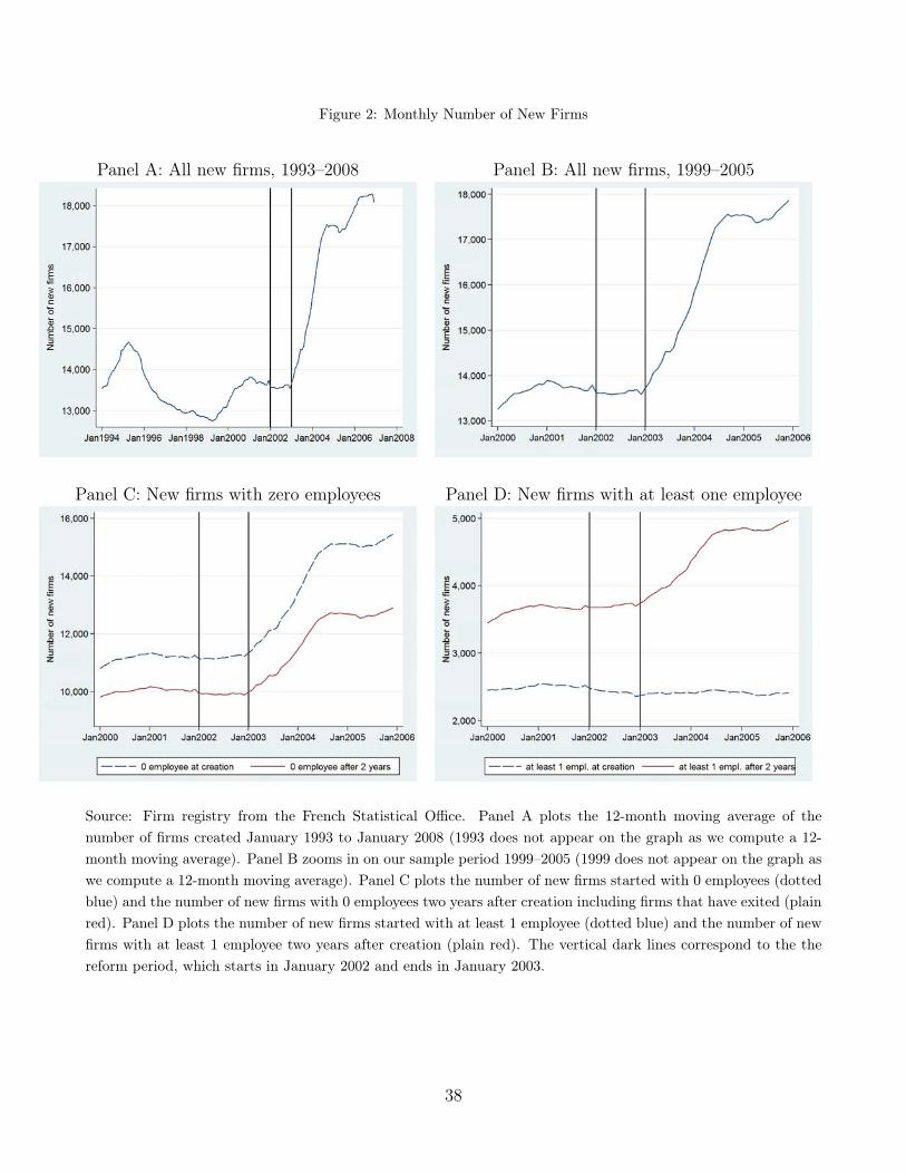
Figure 2: Monthly Number of New Firms

Panel A: All new firms, 1993–2008 Panel B: All new firms, 1999–2005

Panel C: New firms with zero employees Panel D: New firms with at least one employee

Source: Firm registry from the French Statistical Office. Panel A plots the 12-month moving average of thenumber of firms created January 1993 to January 2008 (1993 does not appear on the graph as we compute a 12-month moving average). Panel B zooms in on our sample period 1999–2005 (1999 does not appear on the graph aswe compute a 12-month moving average). Panel C plots the number of new firms started with 0 employees (dottedblue) and the number of new firms with 0 employees two years after creation including firms that have exited (plainred). Panel D plots the number of new firms started with at least 1 employee (dotted blue) and the number of newfirms with at least 1 employee two years after creation (plain red). The vertical dark lines correspond to the thereform period, which starts in January 2002 and ends in January 2003.

38

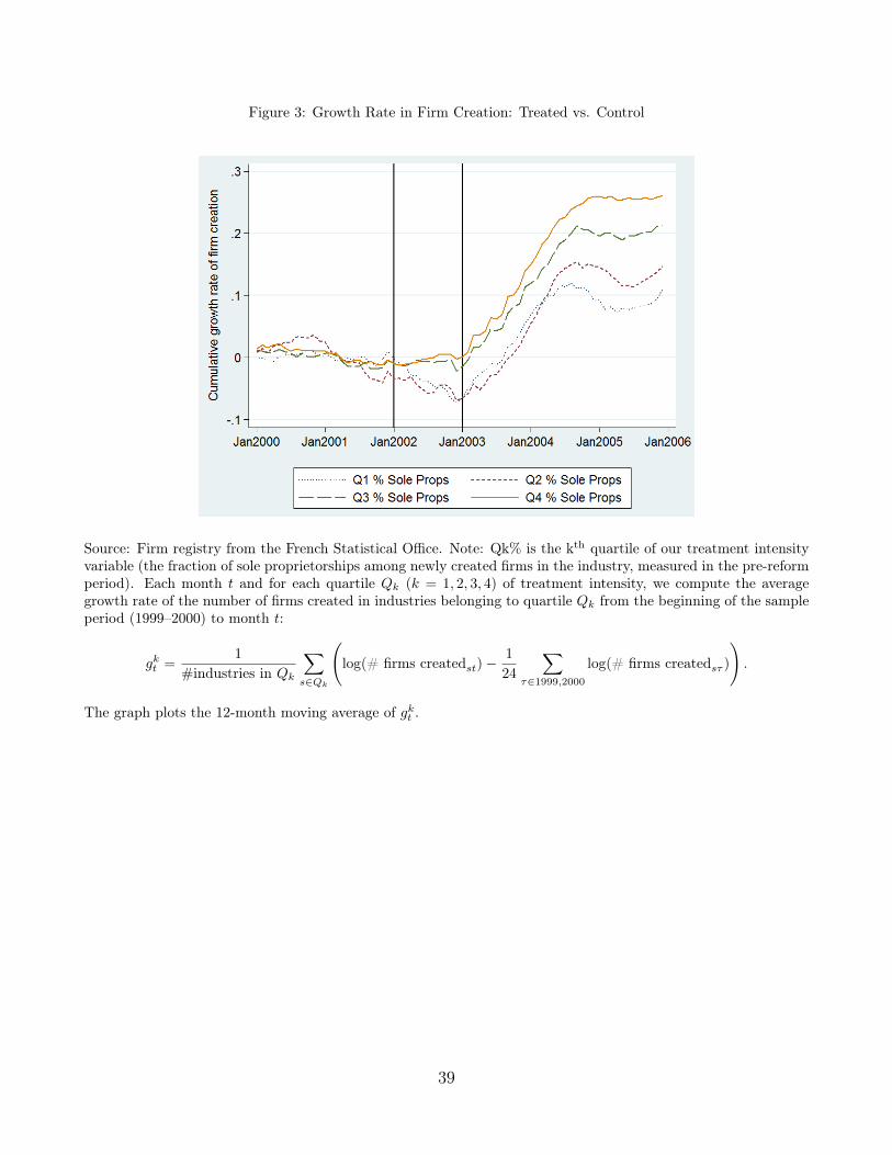
Figure 3: Growth Rate in Firm Creation: Treated vs. Control

Source: Firm registry from the French Statistical Office. Note: Qk% is the kth quartile of our treatment intensityvariable (the fraction of sole proprietorships among newly created firms in the industry, measured in the pre-reformperiod). Each month t and for each quartile Qk (k = 1, 2, 3, 4) of treatment intensity, we compute the averagegrowth rate of the number of firms created in industries belonging to quartile Qk from the beginning of the sampleperiod (1999–2000) to month t:

gkt =1

#industries in Qk

∑s∈Qk

(log(# firms createdst)−

1

24

∑τ∈1999,2000

log(# firms createdsτ )

).

The graph plots the 12-month moving average of gkt .

39

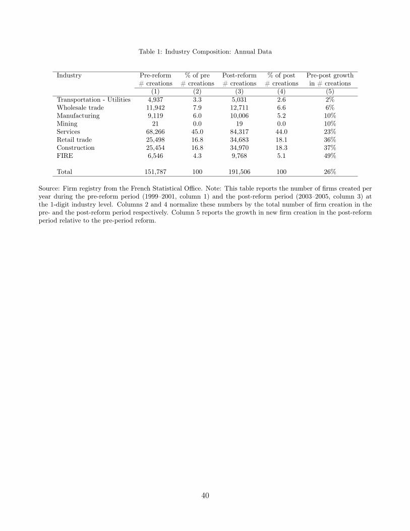
Table 1: Industry Composition: Annual Data

Industry Pre-reform % of pre Post-reform % of post Pre-post growth# creations # creations # creations # creations in # creations

(1) (2) (3) (4) (5)Transportation - Utilities 4,937 3.3 5,031 2.6 2%Wholesale trade 11,942 7.9 12,711 6.6 6%Manufacturing 9,119 6.0 10,006 5.2 10%Mining 21 0.0 19 0.0 10%Services 68,266 45.0 84,317 44.0 23%Retail trade 25,498 16.8 34,683 18.1 36%Construction 25,454 16.8 34,970 18.3 37%FIRE 6,546 4.3 9,768 5.1 49%

Total 151,787 100 191,506 100 26%

Source: Firm registry from the French Statistical Office. Note: This table reports the number of firms created peryear during the pre-reform period (1999–2001, column 1) and the post-reform period (2003–2005, column 3) atthe 1-digit industry level. Columns 2 and 4 normalize these numbers by the total number of firm creation in thepre- and the post-reform period respectively. Column 5 reports the growth in new firm creation in the post-reformperiod relative to the pre-period reform.

40

Table 2: Summary Statistics

N Mean SDPanel A: New firms, industry-levelAvg # firms created (monthly) 290 43.62 84Avg # jobs created after two years (monthly) 290 32.49 62———– adding entrepreneurs’ jobs (monthly) 290 69.30 123

Panel B: New firms, firm-levelEmployment at creation 381,683 0.49 1.9Dummy at least 1 employee at creation 381,683 0.20 .4Employment two years after creation 381,683 0.87 2.5Dummy at least 1 employee two years after creation 381,683 0.29 .45Hire during first two years 381,683 0.25 .43Exit during first two years 381,683 0.16 .36

Panel C: New firms, survey, firm-levelHigh school graduate 26,783 0.50College graduate 26,783 0.14Plan to hire 26,783 0.23

Panel D: Incumbents, industry-level# small incumbents 290 2,779 5,289# jobs in small incumbents 290 3,647 7,667# large incumbents 290 804 1,243# jobs in large incumbents 290 21,967 38,740

Mean by quartile of % ofSole Prop. new firms

Q1 Q2 Q3 Q422 18 44 8722 22 41 4339 37 78 118

0.86 0.72 0.55 0.320.26 0.27 0.22 0.151.06 1.38 1.08 0.600.36 0.42 0.36 0.230.31 0.36 0.31 0.200.21 0.15 0.15 0.14

0.54 0.59 0.53 0.470.12 0.16 0.16 0.120.34 0.34 0.27 0.18

1,039 1,466 3,597 4,7471,497 2,381 5,200 5,196705 791 992 715

27,527 24,135 24,802 11,948

Source: Firm registry and tax files from the French Statistical Office and 2002 SINE survey. Panels A and B reportsummary statistics on all new firms started during the pre-reform period (1999–2001). Statistics are computedat the 4-digit industry level in Panel A and at the firm level in Panel B. Panel C reports summary statisticson entrepreneurs’ education and ambition using the 2002 wave of the SINE survey. Panel D reports summarystatistics on incumbent firms in the 1999–2001 period, where incumbents are defined as firms that have been inthe tax files for the last four years; small incumbents are defined as incumbents with 5 employees or less and whichare not reported to be part of a conglomerate; large incumbents are incumbents with more than 5 employees andthose that belong to a conglomerate. The last four columns provide summary statistics by splitting the sampleinto four quartiles of treatment intensity. Qi is the ith quartile of our treatment intensity variable (the fraction ofsole proprietorships among newly created firms in the industry, measured in the pre-reform period).

41

Table 3: Aggregate Growth Rate: Treated vs. Control

Sales Value added(1) (2) (3) (4) (5) (6)

POST .082*** .095*** -.0026 .1*** .13*** .013(.013) (.021) (.013) (.013) (.02) (.011)

Q2 % Sole Props × POST -.063* -.031 -.086** -.02(.034) (.022) (.036) (.024)

Q3 % Sole Props × POST -.0084 -.011 -.041 -.029*(.028) (.021) (.029) (.016)

Q4 % Sole Props × POST .017 -.0021 .0058 -.003(.039) (.018) (.038) (.016)

Constant 15*** 15*** -40*** 14*** 14*** -44***(.0074) (.0073) (8.2) (.0077) (.0076) (9.2)

Treatment-specific trend No No Yes No No YesIndustry FE Yes Yes Yes Yes Yes YesObservations 2,030 2,030 2,030 2,030 2,030 2,030R-squared .99 .99 .99 .98 .98 .98

Source: Tax files from the French Statistical Office. Sample: 290 industries from 1999–2005, annual observations.Note: In columns (1) to (3) the dependent variable is the log of total industry sales. In columns (4) to (6) thedependent variable is the log of total industry value added. POST is a dummy variable equal to 0 for observationsin the 1999-2001 period and equal to 1 from 2002 to 2005. Qi% Sole Props is a dummy equal to 1 if the industrybelongs to the ith quartile of our treatment intensity variable (the fraction of sole proprietorships among newlycreated firms in the industry, measured in the pre-reform period). Treatment-specific trends are the interactions ofQ2, Q3 and Q4 with linear time trends. All regressions include industry fixed effects. Standard errors are clusteredat the industry level. *, **, and *** mean statistically different from zero at 10, 5 and 1% levels of significance.

42

Table 4: Firm Creation: Treated vs. Control

Number of firms created(1) (2) (3) (4)

POST .1*** .046* -.16*** -.25***(.014) (.027) (.031) (.072)

Q2 % Sole Props × POST .019 .035 .027(.043) (.044) (.043)

Q3 % Sole Props × POST .08** .11*** .11***(.038) (.037) (.036)

Q4 % Sole Props × POST .12*** .13*** .14***(.038) (.039) (.039)

Industry capital intensity .041*× POST (.025)Industry growth × POST -.048

(.038)Industry capital intensity -.014× Trend (.0085)Industry growth × Trend .054***

(.017)Constant 3.2*** 3.2*** .98*** .98***

(.017) (.018) (.24) (.23)Treatment-specific trend No No Yes YesMonth-of-the-year FE Yes Yes Yes YesIndustry FE Yes Yes Yes YesObservations 24,360 24,360 24,360 24,360R-squared .92 .92 .92 .92

Source: Firm registry from the French Statistical Office. Sample: 290 industries, 1999–2005, monthly observations.Note: The dependent variable is the log of one plus the number of new firms created in an industry in a month.POST is a dummy equal to 0 for observations in the 1999-2001 period and equal to 1 from 2002 to 2005. Qi%Sole Props is a dummy equal to 1 if the industry belongs to the ith quartile of our treatment intensity variable(the fraction of sole proprietorships among newly created firms in the industry, measured in the pre-reform period).Treatment-specific trends are the interactions of Q2, Q3 and Q4 with linear time trends. Trend is a linear timetrend. Industry capital intensity is the average assets-to-labor ratio of firms in the industry from 1999 to 2001.Industry growth is the average growth rate of sales for firms in the industry from 1999 to 2001. All regressionsinclude industry and month-of-the-year fixed effects. Standard errors are clustered at the industry level. *, **, and*** mean statistically different from zero at 10, 5 and 1% levels of significance.

43

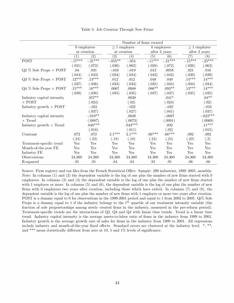
Table 5: Job Creation Through New Firms

Number of firms created0 employees ≥ 1 employee 0 employees ≥ 1 employeeat creation at creation after 2 years after 2 years

(1) (2) (3) (4) (5) (6) (7) (8)POST -.17*** -.31*** -.055** -.054 -.11*** -.21*** -.15*** -.25***

(.031) (.072) (.026) (.062) (.028) (.072) (.026) (.063)Q2 % Sole Props × POST .04 .031 -.016 -.019 .013 .0058 .021 .016

(.044) (.043) (.034) (.034) (.043) (.043) (.039) (.039)Q3 % Sole Props × POST .12*** .13*** .012 .012 .048 .049 .14*** .14***

(.037) (.036) (.033) (.033) (.035) (.034) (.034) (.034)Q4 % Sole Props × POST .15*** .16*** .0067 .0088 .086** .093** .13*** .14***

(.039) (.038) (.035) (.035) (.037) (.037) (.035) (.035)Industry capital intensity .057** .0038 .041* .04**× POST (.024) (.02) (.024) (.02)Industry growth × POST -.031 -.032 -.035 -.016

(.037) (.027) (.041) (.037)Industry capital intensity -.019** .0038 -.0087 -.023***× Trend (.0087) (.0073) (.0091) (.0069)Industry growth × Trend .048*** .043*** .032 .11***

(.018) (.011) (.02) (.015)Constant .072 .072 2.1*** 2.1*** .66*** .66*** .092 .092

(.24) (.23) (.18) (.18) (.24) (.24) (.22) (.2)Treatment-specific trend Yes Yes Yes Yes Yes Yes Yes YesMonth-of-the-year FE Yes Yes Yes Yes Yes Yes Yes YesIndustry FE Yes Yes Yes Yes Yes Yes Yes YesObservations 24,360 24,360 24,360 24,360 24,360 24,360 24,360 24,360R-squared .91 .91 .84 .84 .91 .91 .86 .86

Source: Firm registry and tax files from the French Statistical Office. Sample: 290 industries, 1999–2005, monthly.Note: In columns (1) and (2) the dependent variable is the log of one plus the number of new firms started with 0employees. In columns (3) and (4) the dependent variable is the log of one plus the number of new firms startedwith 1 employee or more. In columns (5) and (6), the dependent variable is the log of one plus the number of newfirms with 0 employees two years after creation, including those which have exited. In columns (7) and (8), thedependent variable is the log of one plus the number of new firms with 1 employee or more two years after creation.POST is a dummy equal to 0 for observations in the 1999-2001 period and equal to 1 from 2002 to 2005. Qi% SoleProps is a dummy equal to 1 if the industry belongs to the ith quartile of our treatment intensity variable (thefraction of sole proprietorships among newly created firms in the industry, measured in the pre-reform period).Treatment-specific trends are the interactions of Q2, Q3 and Q4 with linear time trends. Trend is a linear timetrend. Industry capital intensity is the average assets-to-labor ratio of firms in the industry from 1999 to 2001.Industry growth is the average growth rate of sales for firms in the industry from 1999 to 2001. All regressionsinclude industry and month-of-the-year fixed effects. Standard errors are clustered at the industry level. *, **,and *** mean statistically different from zero at 10, 5 and 1% levels of significance.

44

Table 6: Firm Quality: Ex Post Measures

Hire Exit(1) (2) (3) (4) (5) (6)

POST .01*** .0076 -.0021 .011*** .0036 .019(.0038) (.0046) (.013) (.0017) (.0058) (.014)

Q2 % Sole Props × POST -.0058 -.0088 .0032 .0038(.008) (.0081) (.0096) (.01)

Q3 % Sole Props × POST .0053 .0052 .000016 -.00077(.007) (.0069) (.0074) (.007)

Q4 % Sole Props × POST -.0064 -.0089 -.0087 -.0086(.0056) (.0061) (.0083) (.0077)

Industry capital intensity .0066 -.006× POST (.0044) (.0052)Industry growth × POST -.0086* -.0011

(.005) (.0062)Industry capital intensity -.0029 .0032**× Trend (.002) (.0015)Industry growth × Trend .0082* .0023

(.0043) (.0021)Constant .26*** .21*** .21*** .17*** .048 .048

(.0043) (.049) (.05) (.0028) (.034) (.033)Treatment-specific trend No Yes Yes No Yes YesMonth-of-the-year FE Yes Yes Yes Yes Yes YesIndustry FE Yes Yes Yes Yes Yes YesObservations 1,034,674 1,034,674 1,034,674 1,034,674 1,034,674 1,034,674R-squared .091 .091 .091 .037 .038 .038

Source: Firm registry and tax files from the French Statistical Office. Sample: 1,034,674 new firms started in the1999–2005 period. Note: In columns (4) to (6) the dependent variable is replaced by a dummy equal to 1 if thefirm exits during the first two years. POST is a dummy equal to 0 for observations in the 1999-2001 period andequal to 1 from 2002 to 2005. Qi% Sole Props is a dummy equal to 1 if the industry belongs to the ith quartileof our treatment intensity variable (the fraction of sole proprietorships among newly created firms in the industry,measured in the pre-reform period). Treatment-specific trends are the interactions of Q2, Q3 and Q4 with lineartime trends. Trend is a linear time trend. Industry capital intensity is the average assets-to-labor ratio of firms inthe industry from 1999 to 2001. Industry growth is the average growth rate of sales for firms in the industry from1999 to 2001. All regressions include industry and month-of-the-year fixed effects. Standard errors are clustered atthe industry level. *, **, and *** mean statistically different from zero at 10, 5 and 1% levels of significance.

45

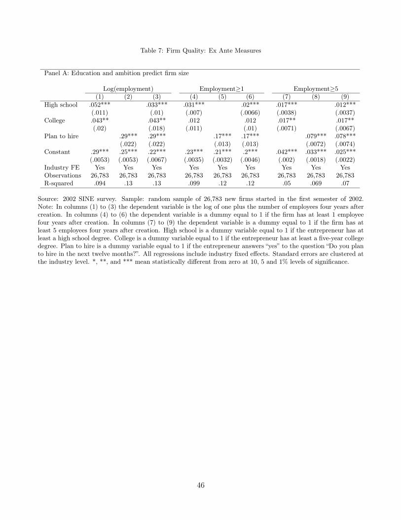
Table 7: Firm Quality: Ex Ante Measures

Panel A: Education and ambition predict firm size

Log(employment) Employment≥1 Employment≥5(1) (2) (3) (4) (5) (6) (7) (8) (9)

High school .052*** .033*** .031*** .02*** .017*** .012***(.011) (.01) (.007) (.0066) (.0038) (.0037)

College .043** .043** .012 .012 .017** .017**(.02) (.018) (.011) (.01) (.0071) (.0067)

Plan to hire .29*** .29*** .17*** .17*** .079*** .078***(.022) (.022) (.013) (.013) (.0072) (.0074)

Constant .29*** .25*** .22*** .23*** .21*** .2*** .042*** .033*** .025***(.0053) (.0053) (.0067) (.0035) (.0032) (.0046) (.002) (.0018) (.0022)

Industry FE Yes Yes Yes Yes Yes Yes Yes Yes YesObservations 26,783 26,783 26,783 26,783 26,783 26,783 26,783 26,783 26,783R-squared .094 .13 .13 .099 .12 .12 .05 .069 .07

Source: 2002 SINE survey. Sample: random sample of 26,783 new firms started in the first semester of 2002.Note: In columns (1) to (3) the dependent variable is the log of one plus the number of employees four years aftercreation. In columns (4) to (6) the dependent variable is a dummy equal to 1 if the firm has at least 1 employeefour years after creation. In columns (7) to (9) the dependent variable is a dummy equal to 1 if the firm has atleast 5 employees four years after creation. High school is a dummy variable equal to 1 if the entrepreneur has atleast a high school degree. College is a dummy variable equal to 1 if the entrepreneur has at least a five-year collegedegree. Plan to hire is a dummy variable equal to 1 if the entrepreneur answers “yes” to the question “Do you planto hire in the next twelve months?”. All regressions include industry fixed effects. Standard errors are clustered atthe industry level. *, **, and *** mean statistically different from zero at 10, 5 and 1% levels of significance.

46

Table 7 (continued)

Panel B: Education and ambition after the reform

High school College Plan to hire(1) (2) (3) (4) (5) (6)

POST .03** .026 -.0047 -.009 -.031** -.026(.015) (.035) (.008) (.023) (.014) (.025)

Q2 % Sole Props × POST .0073 .000073 -.0094 -.014 -.00082 -.0035(.022) (.022) (.019) (.02) (.019) (.019)

Q3 % Sole Props × POST .033* .031* .0078 .0068 .029* .028(.019) (.018) (.011) (.011) (.018) (.017)

Q4 % Sole Props × POST .012 .0052 .0047 .00076 .038** .035**(.018) (.017) (.0092) (.0097) (.015) (.016)

Industry capital intensity × POST .0088 .0058 .00089(.014) (.0092) (.0084)

Industry growth × POST -.023** -.013** -.012(.012) (.0063) (.01)

Constant .5*** .5*** .14*** .14*** .25*** .25***(.0038) (.0037) (.0022) (.0021) (.0029) (.0028)

Industry FE Yes Yes Yes Yes Yes YesObservations 56,321 56,321 56,321 56,321 56,321 56,321R-squared .25 .25 .29 .29 .07 .07

Source: 2002 and 2006 SINE survey. Sample: random sample of 56,321 new firms started in the first semester of2002 and the first semester of 2006. Note: In columns (1) and (2), the dependent variable is a dummy variableequal to 1 if the entrepreneur has at least high school degree. In columns (3) and (4) the dependent variable is adummy equal to 1 if the entrepreneur has at least a five-year college degree. In columns (5) and (6), the dependentvariable is a dummy equal to 1 if the entrepreneur answers “yes” to the question “Do you plan to hire in the nexttwelve months?”. POST is a dummy equal to 0 for observations from the 2002 wave of the survey and equal to 1for observations from the 2006 wave of the survey. Qi% Sole Props is a dummy equal to 1 if the industry belongsto the ith quartile of our treatment intensity variable (the fraction of sole proprietorships among newly createdfirms in the industry, measured in the pre-reform period). Industry capital intensity is the average assets-to-laborratio of firms in the industry from 1999 to 2001. Industry growth is the average growth rate of sales for firms inthe industry from 1999 to 2001. All regressions include industry fixed effects. Standard errors are clustered at theindustry level. *, **, and *** mean statistically different from zero at 10, 5 and 1% levels of significance.

47

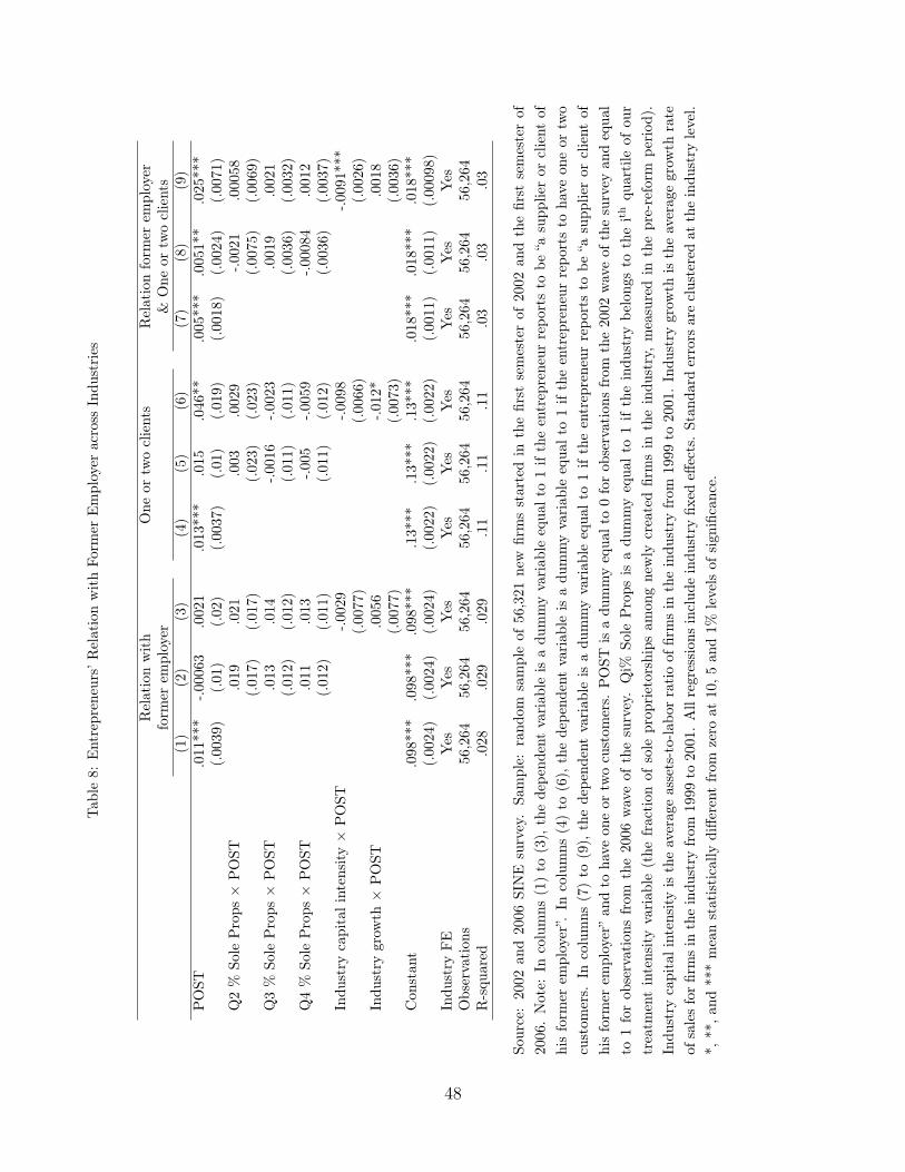
Tab

le8:

Entrepreneurs’R

elationwithFo

rmer

Employer

across

Indu

stries

Relationwith

One

ortw

oclients

Relationform

erem

ployer

form

erem

ployer

&One

ortw

oclients

(1)

(2)

(3)

(4)

(5)

(6)

(7)

(8)

(9)

POST

.011***

-.00063

.0021

.013***

.015

.046

**.005

***

.005

1**

.025

***

(.0039)

(.01)

(.02)

(.0037)

(.01)

(.01

9)(.00

18)

(.00

24)

(.00

71)

Q2%

Sole

Props×

POST

.019

.021

.003

.002

9-.0

021

.000

58(.017)

(.017)

(.023)

(.02

3)(.00

75)

(.00

69)

Q3%

Sole

Props×

POST

.013

.014

-.0016

-.002

3.001

9.002

1(.012)

(.012)

(.011)

(.01

1)(.00

36)

(.00

32)

Q4%

Sole

Props×

POST

.011

.013

-.005

-.005

9-.0

0084

.001

2(.012)

(.011)

(.011)

(.01

2)(.00

36)

(.00

37)

Indu

stry

capitalintensity×

POST

-.0029

-.009

8-.0

091*

**(.0077)

(.00

66)

(.00

26)

Indu

stry

grow

th×

POST

.0056

-.012

*.001

8(.0077)

(.00

73)

(.00

36)

Con

stan

t.098***

.098***

.098***

.13***

.13***

.13*

**.018

***

.018

***

.018

***

(.0024)

(.0024)

(.0024)

(.0022)

(.0022)

(.00

22)

(.00

11)

(.00

11)

(.00

098)

Indu

stry

FE

Yes

Yes

Yes

Yes

Yes

Yes

Yes

Yes

Yes

Observation

s56,264

56,264

56,264

56,264

56,264

56,264

56,264

56,264

56,264

R-squ

ared

.028

.029

.029

.11

.11

.11

.03

.03

.03

Source:20

02an

d2006

SINE

survey.Sa

mple:

rand

omsampleof

56,321

new

firmsstartedin

thefirst

semesterof

2002

andthefirst

semesterof

2006

.Note:

Incolumns

(1)to

(3),

thedepe

ndentvariab

leis

adu

mmyvariab

leequa

lto1iftheentrepreneur

repo

rtsto

be“a

supp

lieror

client

ofhisform

erem

ployer”.

Incolumns

(4)to

(6),

thedepe

ndentvariab

leis

adu

mmyvariab

leequa

lto1iftheentrepreneur

repo

rtsto

have

oneor

two

custom

ers.

Incolumns

(7)to

(9),

thedepe

ndentvariab

leis

adu

mmyvariab

leequa

lto

1iftheentrepreneur

repo

rtsto

be“a

supp

lieror

client

ofhisform

erem

ployer”an

dto

have

oneor

twocustom

ers.

POST

isadu

mmyequa

lto0forob

servations

from

the20

02waveof

thesurvey

andequa

lto

1forob

servations

from

the2006

waveof

thesurvey.Qi%

Sole

Props

isadu

mmyequa

lto

1iftheindu

stry

belong

sto

theith

quartile

ofou

rtreatm

entintensityvariab

le(the

fraction

ofsole

prop

rietorshipsam

ongnewly

createdfirmsin

theindu

stry,measuredin

thepre-reform

period

).Indu

stry

capitalintensity

istheaverageassets-to-labo

rratioof

firmsin

theindu

stry

from

1999

to2001

.Indu

stry

grow

thistheaverag

egrow

thrate

ofsalesforfirmsin

theindu

stry

from

1999

to2001.Allregression

sinclud

eindu

stry

fixed

effects.Stan

dard

errors

areclusteredat

theindu

stry

level.

*,**

,and

***meanstatistically

diffe

rent

from

zero

at10,5

and1%

levels

ofsign

ificance.

48

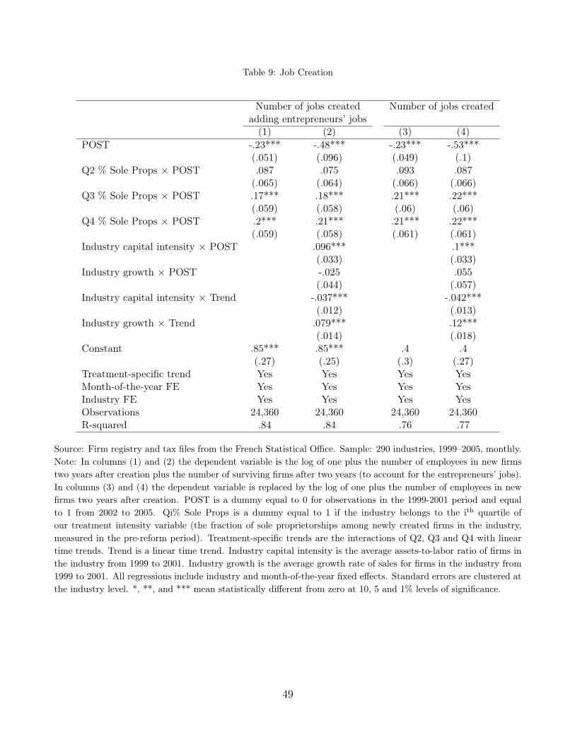
Table 9: Job Creation

Number of jobs created Number of jobs createdadding entrepreneurs’ jobs(1) (2) (3) (4)

POST -.23*** -.48*** -.23*** -.53***(.051) (.096) (.049) (.1)

Q2 % Sole Props × POST .087 .075 .093 .087(.065) (.064) (.066) (.066)

Q3 % Sole Props × POST .17*** .18*** .21*** .22***(.059) (.058) (.06) (.06)

Q4 % Sole Props × POST .2*** .21*** .21*** .22***(.059) (.058) (.061) (.061)

Industry capital intensity × POST .096*** .1***(.033) (.033)

Industry growth × POST -.025 .055(.044) (.057)

Industry capital intensity × Trend -.037*** -.042***(.012) (.013)

Industry growth × Trend .079*** .12***(.014) (.018)

Constant .85*** .85*** .4 .4(.27) (.25) (.3) (.27)

Treatment-specific trend Yes Yes Yes YesMonth-of-the-year FE Yes Yes Yes YesIndustry FE Yes Yes Yes YesObservations 24,360 24,360 24,360 24,360R-squared .84 .84 .76 .77

Source: Firm registry and tax files from the French Statistical Office. Sample: 290 industries, 1999–2005, monthly.Note: In columns (1) and (2) the dependent variable is the log of one plus the number of employees in new firmstwo years after creation plus the number of surviving firms after two years (to account for the entrepreneurs’ jobs).In columns (3) and (4) the dependent variable is replaced by the log of one plus the number of employees in newfirms two years after creation. POST is a dummy equal to 0 for observations in the 1999-2001 period and equalto 1 from 2002 to 2005. Qi% Sole Props is a dummy equal to 1 if the industry belongs to the ith quartile ofour treatment intensity variable (the fraction of sole proprietorships among newly created firms in the industry,measured in the pre-reform period). Treatment-specific trends are the interactions of Q2, Q3 and Q4 with lineartime trends. Trend is a linear time trend. Industry capital intensity is the average assets-to-labor ratio of firms inthe industry from 1999 to 2001. Industry growth is the average growth rate of sales for firms in the industry from1999 to 2001. All regressions include industry and month-of-the-year fixed effects. Standard errors are clustered atthe industry level. *, **, and *** mean statistically different from zero at 10, 5 and 1% levels of significance.

49

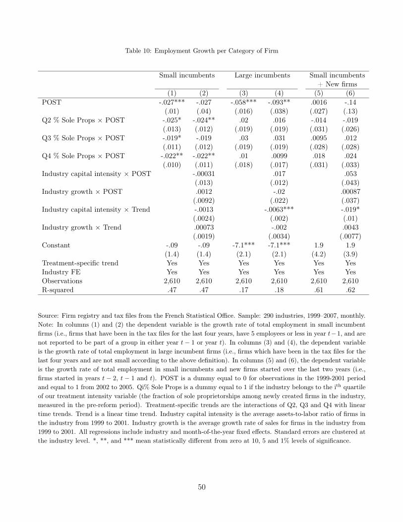
Table 10: Employment Growth per Category of Firm

Small incumbents Large incumbents Small incumbents+ New firms

(1) (2) (3) (4) (5) (6)POST -.027*** -.027 -.058*** -.093** .0016 -.14

(.01) (.04) (.016) (.038) (.027) (.13)Q2 % Sole Props × POST -.025* -.024** .02 .016 -.014 -.019

(.013) (.012) (.019) (.019) (.031) (.026)Q3 % Sole Props × POST -.019* -.019 .03 .031 .0095 .012

(.011) (.012) (.019) (.019) (.028) (.028)Q4 % Sole Props × POST -.022** -.022** .01 .0099 .018 .024

(.010) (.011) (.018) (.017) (.031) (.033)Industry capital intensity × POST -.00031 .017 .053

(.013) (.012) (.043)Industry growth × POST .0012 -.02 .00087

(.0092) (.022) (.037)Industry capital intensity × Trend -.0013 -.0063*** -.019*

(.0024) (.002) (.01)Industry growth × Trend .00073 -.002 .0043

(.0019) (.0034) (.0077)Constant -.09 -.09 -7.1*** -7.1*** 1.9 1.9

(1.4) (1.4) (2.1) (2.1) (4.2) (3.9)Treatment-specific trend Yes Yes Yes Yes Yes YesIndustry FE Yes Yes Yes Yes Yes YesObservations 2,610 2,610 2,610 2,610 2,610 2,610R-squared .47 .47 .17 .18 .61 .62

Source: Firm registry and tax files from the French Statistical Office. Sample: 290 industries, 1999–2007, monthly.Note: In columns (1) and (2) the dependent variable is the growth rate of total employment in small incumbentfirms (i.e., firms that have been in the tax files for the last four years, have 5 employees or less in year t−1, and arenot reported to be part of a group in either year t − 1 or year t). In columns (3) and (4), the dependent variableis the growth rate of total employment in large incumbent firms (i.e., firms which have been in the tax files for thelast four years and are not small according to the above definition). In columns (5) and (6), the dependent variableis the growth rate of total employment in small incumbents and new firms started over the last two years (i.e.,firms started in years t − 2, t − 1 and t). POST is a dummy equal to 0 for observations in the 1999-2001 periodand equal to 1 from 2002 to 2005. Qi% Sole Props is a dummy equal to 1 if the industry belongs to the ith quartileof our treatment intensity variable (the fraction of sole proprietorships among newly created firms in the industry,measured in the pre-reform period). Treatment-specific trends are the interactions of Q2, Q3 and Q4 with lineartime trends. Trend is a linear time trend. Industry capital intensity is the average assets-to-labor ratio of firms inthe industry from 1999 to 2001. Industry growth is the average growth rate of sales for firms in the industry from1999 to 2001. All regressions include industry and month-of-the-year fixed effects. Standard errors are clustered atthe industry level. *, **, and *** mean statistically different from zero at 10, 5 and 1% levels of significance.

50

Table 11: Comparison New Firms vs. Shrinking Incumbents

Panel A: Simple measures of productivity

Wage Value added Salesper worker per worker

(1) (2) (3) (4) (5) (6)New firm 5.2*** 5.7*** 7*** 6.6*** 9.3*** 5.4***

(.39) (1.6) (.37) (.78) (.51) (1.9)New firm × POST .014 .18 .19 .62 .23 1.8

(.18) (.39) (.15) (.55) (.29) (1.1)Q2 % Sole Props × New firm × POST -.41 -.22 -2.2

(.54) (.65) (1.3)Q3 % Sole Props × New firm × POST -.72 -.94 -2.3*

(.47) (.63) (1.2)Q4 % Sole Props × New firm × POST .56 -.25 -1.4

(.53) (.6) (1.2)Constant 22*** 22*** 26*** 26*** 43*** 43***

(.11) (.11) (.61) (.61) (.86) (.88)Industry × Year FE Yes Yes Yes Yes Yes YesQuartile treatment × New firm No Yes No Yes No YesObservations 265,586 265,586 1,269,812 1,269,812 1,258,595 1,258,595R-squared .16 .16 .12 .12 .2 .2

Source: Firm registry and tax files from the French Statistical Office. Sample: all new firms and small “shrinking”incumbents in the tax files, 1999-2005. Note: Incumbent firms are defined as firms that have been in the tax filesfor the last four years. “Shrinking” incumbents are defined as incumbents whose employment decreases from yeart to year t + 1). For new firms, all dependent variables are computed two years after creation. In columns (1) and(2) the dependent variable is total wages divided by number of employees (requires that the firm has at least 1employee). In columns (3) to (4), the dependent variable is value added divided by one plus number of employees.In columns (5) and (6), the dependent variable is sales divided by one plus number of employees. New firm is adummy variable equal to 0 if the observation corresponds to a “shrinking” incumbent and 1 if it corresponds to anewly-created firm. POST is a dummy equal to 0 for observations in the 1999-2001 period and equal to 1 from2002 to 2005. Qi% Sole Props is a dummy equal to 1 if the industry belongs to the ith quartile of our treatmentintensity variable (the fraction of sole proprietorships among newly created firms in the industry, measured in thepre-reform period). Quartile treatment × New firm are the interactions of Q2, Q3 and Q4 with the new firmdummy. All regressions include industry × year fixed effects. Standard errors are clustered at the industry level.*, **, and *** mean statistically different from zero at 10, 5 and 1% levels of significance.

51

Table 11 (continued)

Panel B: Total Factor Productivity

TFP1 TFP2(1) (2) (3) (4)

New firm .16*** .13*** .33*** .2***(.0061) (.023) (.013) (.057)

New firm × POST -.0053 -.0025 -.02*** .029(.0032) (.014) (.0063) (.038)

Q2 % Sole Props × New firm × POST .0039 -.042(.015) (.04)

Q3 % Sole Props × New firm × POST -.0076 -.051(.015) (.039)

Q4 % Sole Props × New firm × POST -.0019 -.062(.014) (.038)

Constant -.14*** -.14*** -.27*** -.27***(.0036) (.0035) (.011) (.012)

Industry × Year FE Yes Yes Yes YesQuartile treatment × New firm No Yes No YesObservations 966,938 966,938 966,786 966,786R-squared .035 .035 .079 .08

Source: Firm registry and tax files from the French Statistical Office. Sample: all new firms and small “shrinking”incumbents in the tax files, 1999-2005. Note: Incumbent firms are defined as firms that have been in the tax filesfor the last four years. “Shrinking” incumbents are defined as incumbents whose employment decreases from yeart to year t + 1). For new firms, all dependent variables are computed two years after creation. In column (1)and (2), the dependent variable is TFP1, the residual of a Cobb-Douglas production function estimated industryby industry. In column (3) and (4), the dependent variable is TFP2, which uses the industry-level labor share ascoefficients in the industry-level Cobb-Douglas production function. New firm is a dummy variable equal to 0 ifthe observation corresponds to a “shrinking” incumbent and 1 if it corresponds to a newly-created firm. POST isa dummy equal to 0 for observations in the 1999-2001 period and equal to 1 from 2002 to 2005. Qi% Sole Propsis a dummy equal to 1 if the industry belongs to the ith quartile of our treatment intensity variable (the fractionof sole proprietorships among newly created firms in the industry, measured in the pre-reform period). Quartiletreatment × New firm are the interactions of Q2, Q3 and Q4 with the new firm dummy. All regressions includeindustry × year fixed effects. Standard errors are clustered at the industry level. *, **, and *** mean statisticallydifferent from zero at 10, 5 and 1% levels of significance.

52

A Derivation of the Model

A.1 Solving the model

Solving the model is simple. First, start with the entrepreneurial decisions. Maximizing profitsw.r.t. l gives labor demand and the expected profit of a successful entrepreneur:

l =β

1− βp

11−βs Aθ and π = p

11−βs Aθ − cs.

Given the indirect utility written above, an individual becomes entrepreneur if and only if:

q log(p1

1−βs Aθ − cs) + (1− q) log(b) ≥ ln(1)

⇔ Aθ ≥ θs ≡ p− 1

1−βs

(b−

1−qq + cs

), (5)

so that production in industry s is given by:

Ys =

∫Aθ≥θs

q1

1− βp

β1−βs AθdF (θ) =

q

1− βp

β1−βs

φ

φ− 1θs

(Aθ0

θs

)φ.

We now write the two product market clearing conditions. Aggregating over individual con-sumption leads to:

pTX1σT = pCX

1σC .

Given that markets clear, we have that Xs = Ys for s ∈ {T,C}. This implies that:

pβ+σ(1−β)σ(1−β)

T

θφ−1σ

T

=pβ+σ(1−β)σ(1−β)

C

θφ−1σ

C

≡ k. (6)

A.2 The Reform

Once the equilibrium conditions are written, we can investigate the effect of the reform. Wefirst compute the differential increase in the number of entrepreneurs in industries T and C as aresponse to the reform. We model the reform as a increase in b. Differentiating (5), we get:

∆ log θs = − 1

1− β∆ log(ps)−

1−qq

1 + csb1−qq

∆ log(b),

53

and differentiating (6), we get:

β + σ(1− β)

σ(1− β)∆ log(ps)−

φ− 1

σ∆ log(θs) = ∆ log(k).

Therefore:

∆ log θs = − σ

φ+ (σ − 1)(1− β)∆ log(k)− 1 + (σ − 1)(1− β)

φ+ (σ − 1)(1− β)

1−qq

1 + csb1−qq

∆ log(b). (7)

We can write our first prediction:

Proposition 2. Assume the reform leads to a marginal increase in b by ∆b. Then, the Difference-in-Difference (DD) estimate of the increase in the number of entrepreneurs is given by:

∆ log(NT )−∆ log(NC) =φ+ φ(σ − 1)(1− β)

φ+ (σ − 1)(1− β)

1−qq

(cC − cT )b1−qq

(1 + cT b1−qq )(1 + cCb

1−qq )

∆ log(b).

Proof. The log number of entrepreneurs in industry s is given by:

log(Ns) = log(1− F (θs/A)) = φ log θ0 − φ log θs + φ logA.

We then use equation (7) to calculate the DD.

Firm creation increases more in industry T than in industry C. When φ increases, the popula-tions of entrepreneurs become more homogeneous. The differential effect increases, and eventuallyconverges to 1 + (σ − 1)(1− β) as φ goes to infinity. If the “experimentation view” prevails (i.e.,when ex post outcomes are the dominant source of heterogeneity—φ is very large), the effect ofthe reform is the largest.

The second prediction is about average quality of entrepreneurs, which we define as:

qs ≡ E[log(θ)|Aθ ≥ θs] =1

φ+ log θs − logA.

We directly combine this definition with equation (7) to obtain our second proposition:

Proposition 3. Assume the reform leads to a marginal increase in b by ∆b. Then, the DDestimate of the average quality of entrepreneurs is given by:

∆qT −∆qC = −1 + (σ − 1)(1− β)

φ+ (σ − 1)(1− β)

1−qq

(cC − cT )b1−qq

(1 + cT b1−qq )(1 + cCb

1−qq )

∆ log b.

54

Quality decreases more in industry T than in industry C. This happens because there is moreentry in industry T . When potential entrepreneurs are however more similar, this effect vanishes(the quality threshold θs responds less in both industries). The difference goes to zero whenφ→ +∞, i.e., when ex post outcomes are the dominant source of heterogeneity.

Finally, we compute the size of “incumbents”. Employment in a firm of given quality is pro-portional to p

11−βs . So employment change in existing firms is:

∆ log(Ls) =1

1− β∆ log ps + ∆ logA

=σ

φ+ (σ − 1)(1− β)∆ log k − φ− 1

φ+ (σ − 1)(1− β)

1−qq

1 + csb1−qq

∆ log b+ ∆ logA.

This allows us to write down our third prediction:

Proposition 4. Assume the reform leads to a marginal increase in b by ∆b. Then, the DDestimate of the average size of “incumbents” is given by:

∆ log(LT )−∆ log(LC) = − φ− 1

φ+ (σ − 1)(1− β)

1−qq

(cC − cT )b1−qq

(1 + cT b1−qq )(1 + cCb

1−qq )

∆ log(b).

Since there is more entry in industry T , competition is fiercer there. Marginal revenues fall, andentrepreneurs hire less. When φ increases, the effect of the reform is even larger, which reinforcesthe crowding-out.

55

B Appendix Tables and Figures

Figure B.1: Growth Rate in Firm Creation. Alternative Treatment Intensity Variable.

Source: Firm registry from the French Statistical Office. Note: Qk% is the kth quartile of the alternative treatmentintensity variable (the fraction of zero-employee firms among newly created firms in the industry, measured in thepre-reform period (1999-2001)). For each month t and for each quartile Qk (k = 1, 2, 3, 4) of treatment intensity,we compute the average growth rate of the number of firms created in industries belonging to quartile Qk from thebeginning of the sample period (1999–2000) to month t:

gkt =1

#industries in Qk

∑s∈Qk

(log(# firms createdst)−

1

24

∑τ∈1999,2000

log(# firms createdsτ )

).

The graph plots the 12-month moving average of gkt .

56

Table B.1: Industries in Treatment and Control Industries

Industry name % Sole Proprietorships Treatment Quartile

Infrastructure development 1.3 Q1Temporary work agencies 2.1 Q1Holding Companies 2.5 Q1Residential real estate development 2.6 Q1Property operators 2.9 Q1Television film production 4.9 Q1Periodical publishing 5.8 Q1Television non-film production 5.8 Q1Wholesale trade: Footwear 6.0 Q1Wholesale trade: Apparel 6.0 Q1Wholesale trade: Packaged frozen food 6.3 Q1Motion picture production 6.3 Q1Arrangement of Transportation of Freight and Cargo 6.7 Q1Department stores 7.5 Q1Newspaper publishing 7.6 Q1

Secretaries and translators 83.1 Q4Miscellaneous trade intermediaries 83.3 Q4Other sport services 87.2 Q4Other educational services 87.3 Q4Fairground attractions 88.0 Q4Other personal services 89.4 Q4Taxis 92.0 Q4Food non-store retailers 92.5 Q4Independent artists 92.9 Q4Veterinary offices 93.6 Q4Dental offices 95.9 Q4Non-food non-store retailers 96.2 Q4Medical offices 96.5 Q4Legal services 96.6 Q4Medical aides 99.7 Q4

57

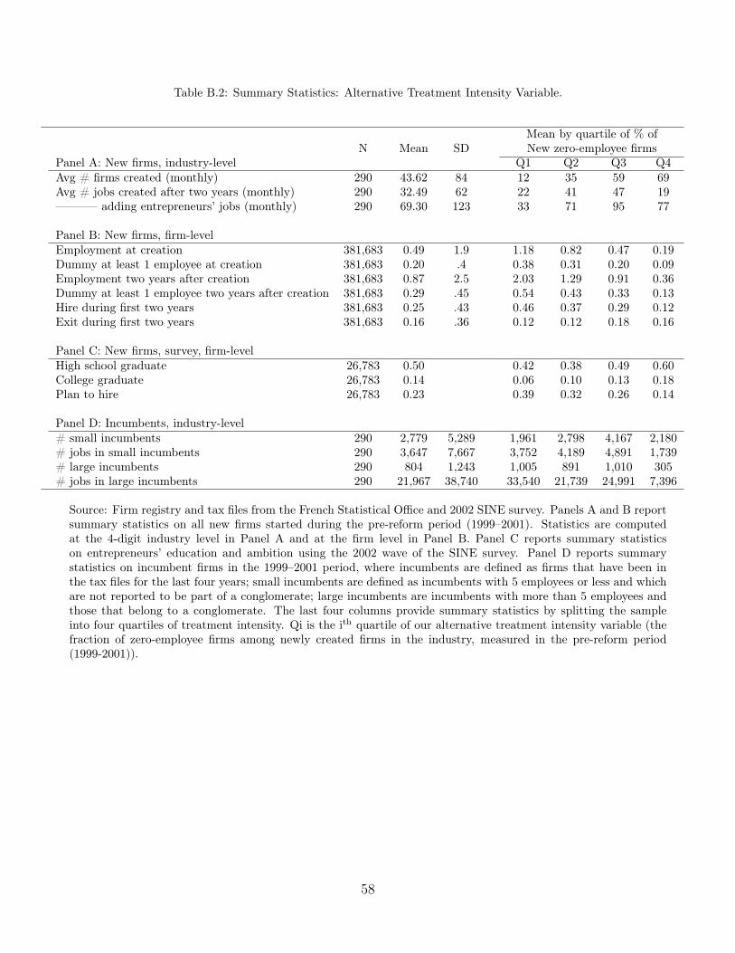
Table B.2: Summary Statistics: Alternative Treatment Intensity Variable.

N Mean SDPanel A: New firms, industry-levelAvg # firms created (monthly) 290 43.62 84Avg # jobs created after two years (monthly) 290 32.49 62———– adding entrepreneurs’ jobs (monthly) 290 69.30 123

Panel B: New firms, firm-levelEmployment at creation 381,683 0.49 1.9Dummy at least 1 employee at creation 381,683 0.20 .4Employment two years after creation 381,683 0.87 2.5Dummy at least 1 employee two years after creation 381,683 0.29 .45Hire during first two years 381,683 0.25 .43Exit during first two years 381,683 0.16 .36

Panel C: New firms, survey, firm-levelHigh school graduate 26,783 0.50College graduate 26,783 0.14Plan to hire 26,783 0.23

Panel D: Incumbents, industry-level# small incumbents 290 2,779 5,289# jobs in small incumbents 290 3,647 7,667# large incumbents 290 804 1,243# jobs in large incumbents 290 21,967 38,740

Mean by quartile of % ofNew zero-employee firms

Q1 Q2 Q3 Q412 35 59 6922 41 47 1933 71 95 77

1.18 0.82 0.47 0.190.38 0.31 0.20 0.092.03 1.29 0.91 0.360.54 0.43 0.33 0.130.46 0.37 0.29 0.120.12 0.12 0.18 0.16

0.42 0.38 0.49 0.600.06 0.10 0.13 0.180.39 0.32 0.26 0.14

1,961 2,798 4,167 2,1803,752 4,189 4,891 1,7391,005 891 1,010 30533,540 21,739 24,991 7,396

Source: Firm registry and tax files from the French Statistical Office and 2002 SINE survey. Panels A and B reportsummary statistics on all new firms started during the pre-reform period (1999–2001). Statistics are computedat the 4-digit industry level in Panel A and at the firm level in Panel B. Panel C reports summary statisticson entrepreneurs’ education and ambition using the 2002 wave of the SINE survey. Panel D reports summarystatistics on incumbent firms in the 1999–2001 period, where incumbents are defined as firms that have been inthe tax files for the last four years; small incumbents are defined as incumbents with 5 employees or less and whichare not reported to be part of a conglomerate; large incumbents are incumbents with more than 5 employees andthose that belong to a conglomerate. The last four columns provide summary statistics by splitting the sampleinto four quartiles of treatment intensity. Qi is the ith quartile of our alternative treatment intensity variable (thefraction of zero-employee firms among newly created firms in the industry, measured in the pre-reform period(1999-2001)).

58

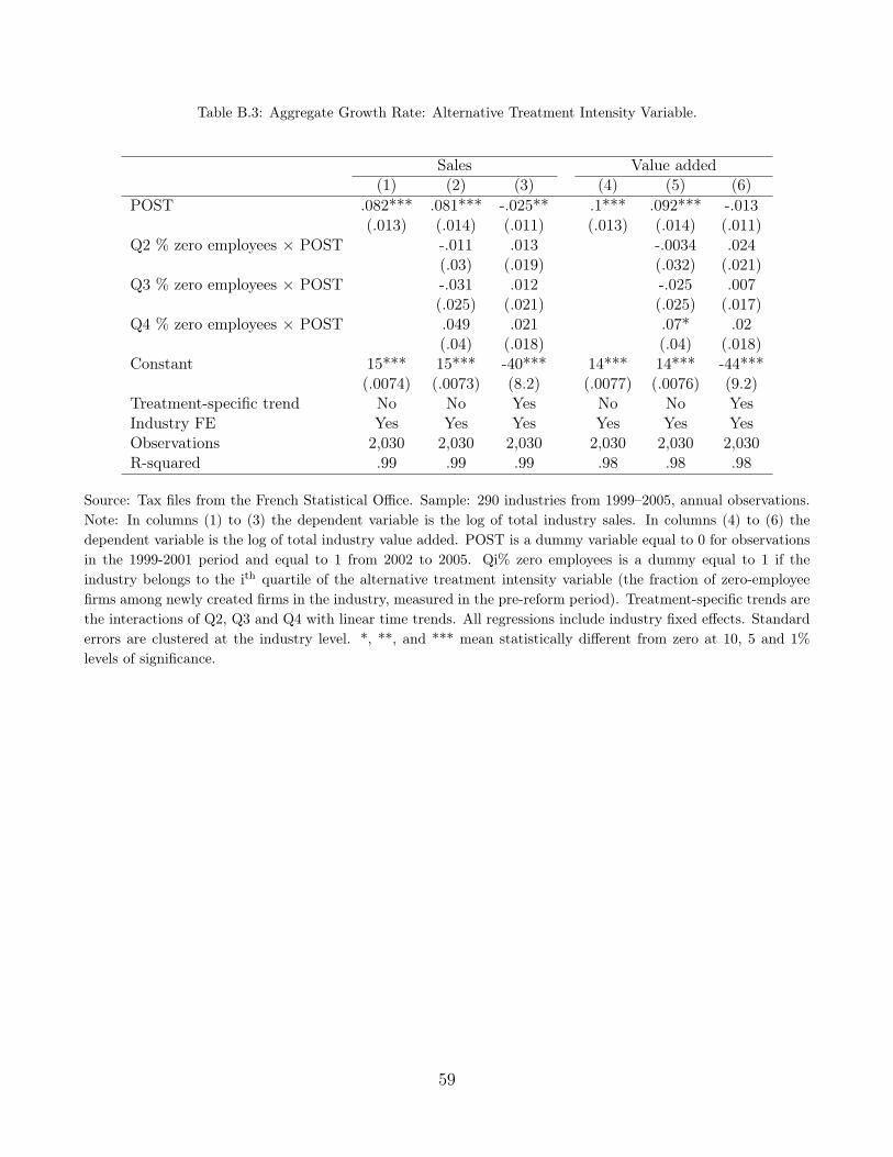
Table B.3: Aggregate Growth Rate: Alternative Treatment Intensity Variable.

Sales Value added(1) (2) (3) (4) (5) (6)

POST .082*** .081*** -.025** .1*** .092*** -.013(.013) (.014) (.011) (.013) (.014) (.011)

Q2 % zero employees × POST -.011 .013 -.0034 .024(.03) (.019) (.032) (.021)

Q3 % zero employees × POST -.031 .012 -.025 .007(.025) (.021) (.025) (.017)

Q4 % zero employees × POST .049 .021 .07* .02(.04) (.018) (.04) (.018)

Constant 15*** 15*** -40*** 14*** 14*** -44***(.0074) (.0073) (8.2) (.0077) (.0076) (9.2)

Treatment-specific trend No No Yes No No YesIndustry FE Yes Yes Yes Yes Yes YesObservations 2,030 2,030 2,030 2,030 2,030 2,030R-squared .99 .99 .99 .98 .98 .98

Source: Tax files from the French Statistical Office. Sample: 290 industries from 1999–2005, annual observations.Note: In columns (1) to (3) the dependent variable is the log of total industry sales. In columns (4) to (6) thedependent variable is the log of total industry value added. POST is a dummy variable equal to 0 for observationsin the 1999-2001 period and equal to 1 from 2002 to 2005. Qi% zero employees is a dummy equal to 1 if theindustry belongs to the ith quartile of the alternative treatment intensity variable (the fraction of zero-employeefirms among newly created firms in the industry, measured in the pre-reform period). Treatment-specific trends arethe interactions of Q2, Q3 and Q4 with linear time trends. All regressions include industry fixed effects. Standarderrors are clustered at the industry level. *, **, and *** mean statistically different from zero at 10, 5 and 1%levels of significance.

59

Table B.4: Firm Creation: Alternative Treatment Intensity Variable.

Number of firms created(1) (2) (3) (4)

POST .1*** .059** -.13*** -.2***(.014) (.023) (.028) (.074)

Q2 % zero employees × POST .046 .045 .046(.038) (.035) (.035)

Q3 % zero employees × POST .041 .024 .021(.036) (.038) (.038)

Q4 % zero employees × POST .088** .1*** .11***(.04) (.04) (.039)

Industry capital intensity .033× POST (.024)Industry growth × POST -.051

(.037)Industry capital intensity -.013× Trend (.0083)Industry growth × Trend .056***

(.017)Constant 3.2*** 3.2*** .98*** .98***

(.017) (.018) (.23) (.23)Treatment-specific trend No No Yes YesMonth-of-the-year FE Yes Yes Yes YesIndustry FE Yes Yes Yes YesObservations 24,360 24,360 24,360 24,360R-squared .92 .92 .92 .92

Source: Firm registry from the French Statistical Office. Sample: 290 industries, 1999–2005, monthly observations.Note: The dependent variable is the log of one plus the number of new firms created in an industry in a month.POST is a dummy equal to 0 for observations in the 1999-2001 period and equal to 1 from 2002 to 2005. Qi% zeroemployees is a dummy equal to 1 if the industry belongs to the ith quartile of the alternative treatment intensityvariable (the fraction of zero-employee firms among newly created firms in the industry, measured in the pre-reformperiod (199-2001)). Treatment-specific trends are the interactions of Q2, Q3 and Q4 with linear time trends. Trendis a linear time trend. Industry capital intensity is the average assets-to-labor ratio of firms in the industry from1999 to 2001. Industry growth is the average growth rate of sales for firms in the industry from 1999 to 2001. Allregressions include industry and month-of-the-year fixed effects. Standard errors are clustered at the industry level.*, **, and *** mean statistically different from zero at 10, 5 and 1% levels of significance.

60

Table B.5: Job Creation Through New Firms: Alternative Treatment Intensity Variable

Number of firms created0 employees ≥ 1 employee 0 employees ≥ 1 employeeat creation at creation after 2 years after 2 years(1) (2) (3) (4) (5) (6) (7) (8)

POST -.13*** -.24*** -.1*** -.097 -.1*** -.18** -.13*** -.21***(.026) (.074) (.025) (.063) (.026) (.072) (.024) (.061)

Q2 % zero employees × POST .034 .037 .076** .075** .018 .021 .067* .07**(.035) (.035) (.033) (.033) (.035) (.035) (.035) (.035)

Q3 % zero employees × POST .029 .028 .03 .027 .0074 .0052 .032 .032(.037) (.037) (.033) (.033) (.037) (.037) (.036) (.036)

Q4 % zero employees × POST .11*** .12*** .079** .083** .087** .092** .1*** .11***(.04) (.039) (.034) (.034) (.039) (.038) (.035) (.035)

Industry capital intensity .046* .0037 .034 .031× POST (.024) (.02) (.023) (.02)Industry growth × POST -.033 -.036 -.04 -.015

(.036) (.026) (.039) (.038)Industry capital intensity -.017** .0025 -.0076 -.023***× Trend (.0084) (.0068) (.0088) (.0067)Industry growth × Trend .05*** .044*** .035* .1***

(.017) (.011) (.019) (.016)Constant .072 .072 2.1*** 2.1*** .66*** .66*** .092 .092

(.24) (.23) (.18) (.18) (.24) (.24) (.23) (.2)Treatment-specific trend Yes Yes Yes Yes Yes Yes Yes YesMonth-of-the-year FE Yes Yes Yes Yes Yes Yes Yes YesIndustry FE Yes Yes Yes Yes Yes Yes Yes YesObservations 24,360 24,360 24,360 24,360 24,360 24,360 24,360 24,360R-squared .91 .91 .84 .84 .91 .91 .86 .86

Source: Firm registry and tax files from the French Statistical Office. Sample: 290 industries, 1999–2005, monthly.Note: In columns (1) and (2) the dependent variable is the log of one plus the number of new firms started with 0employees. In columns (3) and (4) the dependent variable is the log of one plus the number of new firms startedwith 1 employee or more. In columns (5) and (6), the dependent variable is the log of one plus the number of newfirms with 0 employees two years after creation, including those which have exited. In columns (7) and (8), thedependent variable is the log of one plus the number of new firms with 1 employee or more two years after creation.POST is a dummy equal to 0 for observations in the 1999-2001 period and equal to 1 from 2002 to 2005. Qi%zero employees is a dummy equal to 1 if the industry belongs to the ith quartile of our treatment intensity variable(the fraction of zero-employee firms among newly created firms in the industry, measured in the pre-reform period(1999-2001)). Treatment-specific trends are the interactions of Q2, Q3 and Q4 with linear time trends. Trend isa linear time trend. Industry capital intensity is the average assets-to-labor ratio of firms in the industry from1999 to 2001. Industry growth is the average growth rate of sales for firms in the industry from 1999 to 2001. Allregressions include industry and month-of-the-year fixed effects. Standard errors are clustered at the industry level.*, **, and *** mean statistically different from zero at 10, 5 and 1% levels of significance.

61

Table B.6: Firm Quality: Ex Post Measures. Alternative Treatment Intensity Variable.

Hire Exit(1) (2) (3) (4) (5) (6)

POST .01*** .0033 -.013 .011*** .019*** .037**(.0038) (.0061) (.014) (.0017) (.0051) (.017)

Q2 % zero employees × POST .0084 .011 -.0047 -.0072(.0071) (.0072) (.0068) (.0072)

Q3 % zero employees × POST .0088 .013* -.016*** -.02***(.0075) (.0069) (.0061) (.0068)

Q4 % zero employees × POST -.008 -.0051 -.034*** -.037***(.0067) (.0069) (.0072) (.0072)

Industry capital intensity .0069 -.0072× POST (.0044) (.006)Industry growth × POST -.0058 .0038

(.0046) (.0048)Industry capital intensity -.0035* .0036**× Trend (.0019) (.0018)Industry growth × Trend .0073* .00053

(.004) (.0019)Constant .26*** .21*** .21*** .17*** .049* .049*

(.0043) (.048) (.048) (.0028) (.029) (.028)Treatment-specific trend No Yes Yes No Yes YesMonth-of-the-year FE Yes Yes Yes Yes Yes YesIndustry FE Yes Yes Yes Yes Yes YesObservations 1,034,674 1,034,674 1,034,674 1,034,674 1,034,674 1,034,674R-squared .091 .091 .092 .037 .038 .038

Source: Firm registry and tax files from the French Statistical Office. Sample: 1,034,674 new firms started in the1999–2005 period. Note: In columns (4) to (6) the dependent variable is replaced by a dummy equal to 1 if thefirm exits during the first two years. POST is a dummy equal to 0 for observations in the 1999-2001 period andequal to 1 from 2002 to 2005. Qi% zero employees is a dummy equal to 1 if the industry belongs to the ith quartileof our treatment intensity variable (the fraction of zero-employee firms among newly created firms in the industry,measured in the pre-reform period (1999-2001)). Treatment-specific trends are the interactions of Q2, Q3 and Q4with linear time trends. Trend is a linear time trend. Industry capital intensity is the average assets-to-labor ratioof firms in the industry from 1999 to 2001. Industry growth is the average growth rate of sales for firms in theindustry from 1999 to 2001. All regressions include industry and month-of-the-year fixed effects. Standard errorsare clustered at the industry level. *, **, and *** mean statistically different from zero at 10, 5 and 1% levels ofsignificance.

62

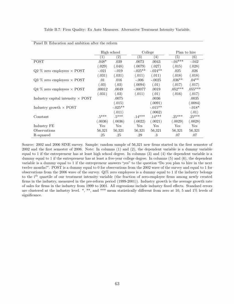
Table B.7: Firm Quality: Ex Ante Measures. Alternative Treatment Intensity Variable.

Panel B: Education and ambition after the reform

High school College Plan to hire(1) (2) (3) (4) (5) (6)

POST .048* .039 .0073 .0043 -.04*** -.042(.029) (.048) (.0079) (.027) (.015) (.028)

Q2 % zero employees × POST -.021 -.019 -.025** -.024** .025 .026(.031) (.031) (.011) (.011) (.018) (.018)

Q3 % zero employees × POST .01 .016 -.006 -.0025 .036** .04**(.03) (.03) (.0094) (.01) (.017) (.017)

Q4 % zero employees × POST .00012 .0049 -.00077 .0019 .052*** .055***(.031) (.03) (.011) (.01) (.016) (.017)

Industry capital intensity × POST .0075 .0036 .0035(.015) (.0091) (.0084)

Industry growth × POST -.025** -.015** -.018*(.011) (.0062) (.01)

Constant .5*** .5*** .14*** .14*** .25*** .25***(.0036) (.0036) (.0022) (.0021) (.0029) (.0028)

Industry FE Yes Yes Yes Yes Yes YesObservations 56,321 56,321 56,321 56,321 56,321 56,321R-squared .25 .25 .29 .3 .07 .07

Source: 2002 and 2006 SINE survey. Sample: random sample of 56,321 new firms started in the first semester of2002 and the first semester of 2006. Note: In columns (1) and (2), the dependent variable is a dummy variableequal to 1 if the entrepreneur has at least high school degree. In columns (3) and (4) the dependent variable is adummy equal to 1 if the entrepreneur has at least a five-year college degree. In columns (5) and (6), the dependentvariable is a dummy equal to 1 if the entrepreneur answers “yes” to the question “Do you plan to hire in the nexttwelve months?”. POST is a dummy equal to 0 for observations from the 2002 wave of the survey and equal to 1 forobservations from the 2006 wave of the survey. Qi% zero employees is a dummy equal to 1 if the industry belongsto the ith quartile of our treatment intensity variable (the fraction of zero-employee firms among newly createdfirms in the industry, measured in the pre-reform period (1999-2001)). Industry growth is the average growth rateof sales for firms in the industry from 1999 to 2001. All regressions include industry fixed effects. Standard errorsare clustered at the industry level. *, **, and *** mean statistically different from zero at 10, 5 and 1% levels ofsignificance.

63

Table B.8: Job Creation: Alternative Treatment Intensity Variable.

Number of jobs created Number of jobs createdadding entrepreneurs’ jobs(1) (2) (3) (4)

POST -.17*** -.39*** -.16*** -.42***(.046) (.099) (.048) (.1)

Q2 % zero employees × POST .058 .067 .071 .082(.057) (.058) (.062) (.062)

Q3 % zero employees × POST .041 .041 .034 .041(.059) (.057) (.064) (.062)

Q4 % zero employees × POST .12** .12** .12** .12*(.059) (.057) (.063) (.062)

Industry capital intensity × POST .085** .09***(.033) (.035)

Industry growth × POST -.025 .056(.044) (.057)

Industry capital intensity × Trend -.037*** -.043***(.012) (.013)

Industry growth × Trend .078*** .12***(.014) (.019)

Constant .85*** .85*** .4 .4(.27) (.25) (.3) (.27)

Treatment-specific trend Yes Yes Yes YesMonth-of-the-year FE Yes Yes Yes YesIndustry FE Yes Yes Yes YesObservations 24,360 24,360 24,360 24,360R-squared .84 .84 .76 .77

Source: Firm registry and tax files from the French Statistical Office. Sample: 290 industries, 1999–2005, monthly.Note: In columns (1) and (2) the dependent variable is the log of one plus the number of employees in new firmstwo years after creation plus the number of surviving firms after two years (to account for the entrepreneurs’ jobs).In columns (3) and (4) the dependent variable is replaced by the log of one plus the number of employees in newfirms two years after creation. POST is a dummy equal to 0 for observations in the 1999-2001 period and equalto 1 from 2002 to 2005. Qi% zero employees is a dummy equal to 1 if the industry belongs to the ith quartile ofour treatment intensity variable (the fraction of zero-employee firms among newly created firms in the industry,measured in the pre-reform period (1999-2001)). Treatment-specific trends are the interactions of Q2, Q3 and Q4with linear time trends. Trend is a linear time trend. Industry capital intensity is the average assets-to-labor ratioof firms in the industry from 1999 to 2001. Industry growth is the average growth rate of sales for firms in theindustry from 1999 to 2001. All regressions include industry and month-of-the-year fixed effects. Standard errorsare clustered at the industry level. *, **, and *** mean statistically different from zero at 10, 5 and 1% levels ofsignificance.

64

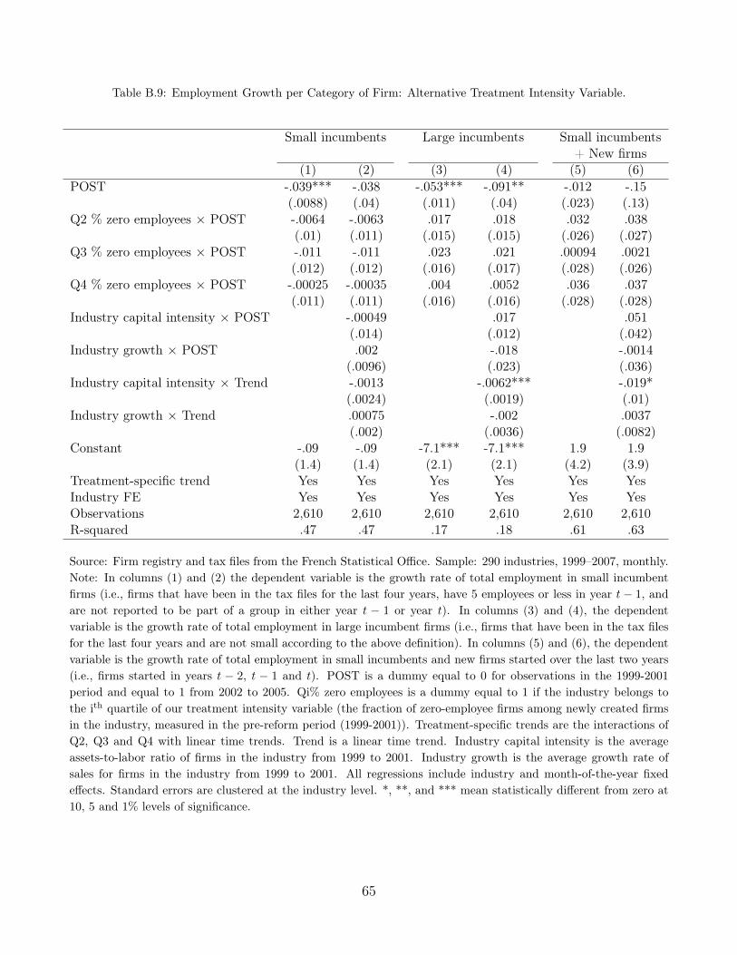
Table B.9: Employment Growth per Category of Firm: Alternative Treatment Intensity Variable.

Small incumbents Large incumbents Small incumbents+ New firms

(1) (2) (3) (4) (5) (6)POST -.039*** -.038 -.053*** -.091** -.012 -.15

(.0088) (.04) (.011) (.04) (.023) (.13)Q2 % zero employees × POST -.0064 -.0063 .017 .018 .032 .038



(.011) (.011) (.016) (.016) (.028) (.028)Industry capital intensity × POST -.00049 .017 .051

(.014) (.012) (.042)Industry growth × POST .002 -.018 -.0014

(.0096) (.023) (.036)Industry capital intensity × Trend -.0013 -.0062*** -.019*

(.0024) (.0019) (.01)Industry growth × Trend .00075 -.002 .0037

(.002) (.0036) (.0082)Constant -.09 -.09 -7.1*** -7.1*** 1.9 1.9

(1.4) (1.4) (2.1) (2.1) (4.2) (3.9)Treatment-specific trend Yes Yes Yes Yes Yes YesIndustry FE Yes Yes Yes Yes Yes YesObservations 2,610 2,610 2,610 2,610 2,610 2,610R-squared .47 .47 .17 .18 .61 .63

Source: Firm registry and tax files from the French Statistical Office. Sample: 290 industries, 1999–2007, monthly.Note: In columns (1) and (2) the dependent variable is the growth rate of total employment in small incumbentfirms (i.e., firms that have been in the tax files for the last four years, have 5 employees or less in year t − 1, andare not reported to be part of a group in either year t − 1 or year t). In columns (3) and (4), the dependentvariable is the growth rate of total employment in large incumbent firms (i.e., firms that have been in the tax filesfor the last four years and are not small according to the above definition). In columns (5) and (6), the dependentvariable is the growth rate of total employment in small incumbents and new firms started over the last two years(i.e., firms started in years t − 2, t − 1 and t). POST is a dummy equal to 0 for observations in the 1999-2001period and equal to 1 from 2002 to 2005. Qi% zero employees is a dummy equal to 1 if the industry belongs tothe ith quartile of our treatment intensity variable (the fraction of zero-employee firms among newly created firmsin the industry, measured in the pre-reform period (1999-2001)). Treatment-specific trends are the interactions ofQ2, Q3 and Q4 with linear time trends. Trend is a linear time trend. Industry capital intensity is the averageassets-to-labor ratio of firms in the industry from 1999 to 2001. Industry growth is the average growth rate ofsales for firms in the industry from 1999 to 2001. All regressions include industry and month-of-the-year fixedeffects. Standard errors are clustered at the industry level. *, **, and *** mean statistically different from zero at10, 5 and 1% levels of significance.

65

Table B.10: Comparison New Firms vs. Shrinking Incumbents: Alternative Treatment Intensity Variable

Wage Value added Salesper worker per worker

(1) (2) (3) (4) (5) (6)New firm 5.2*** 4*** 7*** 6.6*** 9.3*** 9.2***

(.39) (.31) (.37) (1) (.51) (1.1)New firm × POST .014 .67 .19 .79* .23 1.1

(.18) (.53) (.15) (.45) (.29) (.69)Q2 % zero employees × New firm × POST -.79 -.75 -1

(.61) (.5) (.77)Q3 % zero employees × New firm × POST -1.1* -1* -1.4

(.58) (.53) (.89)Q4 % zero employees × New firm × POST -.0032 .1 -.13

(.7) (.58) (.93)Constant 22*** 22*** 26*** 26*** 43*** 43***

(.11) (.12) (.61) (.61) (.86) (.86)Industry × Year FE Yes Yes Yes Yes Yes YesQuartile treatment × New firm No Yes No Yes No YesObservations 265,586 265,586 1,269,812 1,269,812 1,258,595 1,258,595R-squared .16 .16 .12 .12 .2 .2

Source: Firm registry and tax files from the French Statistical Office. Sample: all new firms and small “shrinking”incumbents in the tax files, 1999-2005. Note: Incumbent firms are defined as firms that have been in the tax filesfor the last four years. “Shrinking” incumbents are defined as incumbents whose employment decreases from yeart to year t + 1). For new firms, all dependent variables are computed two years after creation. In columns (1) and(2) the dependent variable is total wages divided by number of employees (requires that the firm has at least 1employee). In columns (3) to (4), the dependent variable is value added divided by one plus number of employees.In columns (5) and (6), the dependent variable is sales divided by one plus number of employees. New firm is adummy variable equal to 0 if the observation corresponds to a “shrinking” incumbent and 1 if it corresponds to anewly-created firm. POST is a dummy equal to 0 for observations in the 1999-2001 period and equal to 1 from2002 to 2005. Qi% zero employees is a dummy equal to 1 if the industry belongs to the ith quartile of our treatmentintensity variable (the fraction of zero-employee firms among newly created firms in the industry, measured inthe pre-reform period (1999-2001)). Quartile treatment × New firm are the interactions of Q2, Q3 and Q4 withthe new firm dummy. All regressions include industry × year fixed effects. Standard errors are clustered at theindustry level. *, **, and *** mean statistically different from zero at 10, 5 and 1% levels of significance.

66

Table B.11: 20 Industries with Largest Post-reform Surge in Aggregate Creation

Industry name % Share of Aggregate Quartile ofIncrease in Creation Treatment

Business and management consulting services 7.7 Q3Non-food non-store retail trade 6.8 Q4Masonry contractors 4.4 Q4Real estate agents 3.9 Q4Electrical contractors 3.5 Q4Miscellaneous trade intermediaries 3.3 Q4Other Miscellaneous store retailers 2.8 Q4Beauty parlors 2.4 Q4Other business services 2.4 Q3Real estate brokers 2.4 Q1Apparel retail trade 2.4 Q3Painting contractors 2.4 Q4Plumbing contractors 2.0 Q4Full-service restaurants 1.9 Q3Legal services 1.8 Q4Hairdressers 1.7 Q4Food non-store retail trade 1.7 Q4Carpentry contractors 1.7 Q4Engineering services 1.7 Q2Computer maintenance services 1.7 Q3

Total 58

Source: Firm registry data from French Statistical Office. Note: In this Table, we list the 20 4-digit industries thatcontribute the most to the increase in average monthly firm creation between the pre period (1999-2001) and thepost period (2002-2005). Column 1 is the industry’s name. Column 2 is the contribution in percentage points tothe aggregate surge in creation. For industry s, it is computed as ∆Ns

∆N where ∆Ns is the increase in the averagemonthly number of creations and ∆N =

∑s ∆Ns. Column 3 reports the quartile of treatment (measured through

the % of sole proprietorships in industry creations, as in the main text). Overall, the 20 top contributors contributeto 58% of the total surge in business creation. The rise in masonry creation contributes to 4.4% of the total surge.

67

Table B.12: Firm Creation: Controlling for Industry-level Exposure to the Cycle

Number of firms created(1) (2) (3)

POST -.28*** -.28*** -.29***(.076) (.075) (.075)

Q2 % Sole Props × POST .03 .031 .031(.044) (.044) (.044)

Q3 % Sole Props × POST .11*** .11*** .11***(.036) (.036) (.036)

Q4 % Sole Props × POST .14*** .14*** .14***(.039) (.038) (.038)

Industry capital intensity × POST .042* .042* .042*(.025) (.025) (.025)

Industry growth × POST -.00018 .00075 .00075(.036) (.035) (.035)

Industry capital intensity × Trend -.014* -.014* -.014*(.0087) (.0086) (.0086)

Industry growth × Trend .006 .0052 .0052(.014) (.014) (.014)

GDP growth .062*** .063***(.0087) (.0085)

Beta × GDP growth -.1 .058(.069) (.065)

Beta × POST -.14 -.15(.14) (.14)

Beta × Trend .12*** .12***(.042) (.044)

Constant .69*** .98*** .69***(.25) (.23) (.25)

Treatment-specific trend Yes Yes YesMonth-of-the-year FE Yes Yes YesIndustry FE Yes Yes YesObservations 24,360 24,360 24,360R-squared .92 .92 .92

Source: Firm registry and tax files from the French Statistical Office. Sample: 290 industries, 1999–2005, monthly.Note: The dependent variable is the log of one plus the number of new firms created in an industry in a month.POST is a dummy equal to 0 for observations in the 1999-2001 period and equal to 1 from 2002 to 2005. Qi%Sole Props is a dummy equal to 1 if the industry belongs to the ith quartile of our treatment intensity variable(the fraction of sole proprietorships among newly created firms in the industry, measured in the pre-reform period).Treatment-specific trends are the interactions of Q2, Q3 and Q4 with linear time trends. Trend is a linear timetrend. Industry capital intensity is the average assets-to-labor ratio of firms in the industry from 1999 to 2001.Industry growth is the average growth rate of sales for firms in the industry from 1999 to 2001. Beta is computedfor each industry by regressing, in the time-series, the aggregate industry value added on national GDP, usingannual data. All regressions include industry and month-of-the-year fixed effects. Standard errors are clustered atthe industry level. *, **, and *** mean statistically different from zero at 10, 5 and 1% levels of significance.

68

Table B.13: Entrepreneur’s education across Industries

High school graduate College graduateAll Unemployed All Unemployed

entrepreneurs entrepreneurs entrepreneurs entrepreneurs(1) (2) (3) (4)

Q2 % Sole Props .066 .042 .044 .056(.079) (.073) (.054) (.056)

Q3 % Sole Props .023 -.0037 .063 .028(.088) (.075) (.062) (.056)

Q4 % Sole Props -.053 -.13** .0054 -.029(.079) (.058) (.042) (.028)

Constant .52*** .53*** .12*** .1***(.057) (.042) (.022) (.02)

Observations 27,157 9,479 27,157 9,479R-squared .0072 .018 .0056 .011

Source: SINE survey. Sample: 27,157 new firms created in 1998, 9,479 new firms created by unemployed en-trepreneurs. Note: The dependent variable is a dummy variable equal to 1 if the entrepreneur is a high schoolgraduate (columns (1) and (2)) or a dummy variable equal to 1 if the entrepreneur is a college graduate (columns(3) and (4)). Columns (1) and (3) use the whole sample. Columns (2) and (4) restricts the analysis to the sampleof unemployed entrepreneurs. Qi% Sole Props is the ith quartile of our treatment intensity variable (the fractionof sole proprietorships among newly created firms in the industry, measured in the pre-reform period). *, **, and*** mean statistically different from zero at 10, 5 and 1% levels of significance.

69

Can Unemployment Insurance Spur Entrepreneurial Activity?

Documents

Transcript of Can Unemployment Insurance Spur Entrepreneurial Activity?