The European Unemployment Dilemma

by

Lars Ljungqvist and Thomas J. Sargent�

May 1997

Post World War II European welfare states experienced several decades of relatively lowunemployment, followed by a plague of persistently high unemployment since the 1980's.We impute the higher unemployment to welfare states' diminished ability to cope withmore turbulent economic times, such as the ongoing restructuring from manufacturing tothe service industry, adoption of new information technologies and a rapidly changing in-ternational economy. We use a general equilibrium search model where workers accumulateskills on the job and lose skills during unemployment.

� Ljungqvist: Stockholm School of Economics and Federal Reserve Bank of Chicago; Sar-gent: Hoover Institution, Stanford, and University of Chicago. We thank George Akerlof,Sherwin Rosen, Jose Scheinkman, two anonymous referees and seminar participants atvarious institutions for criticisms and suggestions. We are grateful to Cristina De Nardi,Juha Seppala and Christopher Sleet for excellent research assistance. The views expressedhere are ours and not necessarily those of the Federal Reserve System. Sargent's researchwas supported by a grant to the National Bureau of Economic Research from the NationalScience Foundation.

1

1. Introduction

During their �rst decades, European welfare states exhibited unemployment rates equal

to or less than those of other market economies; but in the 1980's, they su�ered large

increases in unemployment, which have endured. Figure 1 shows that unemployment

in European OECD countries has from 1983 persistently exceeded the OECD average

by around two percentage points. Higher occurrences of long term unemployment have

accompanied higher levels of unemployment. According to Table 1, more than half of all

European unemployment in 1989 was classi�ed as long-term unemployment with a duration

of a year and over, up from less than a third of unemployment in 1979.1 Table 1 shows

that the increasing incidence of long-term unemployment is common to the European

OECD countries.2 In contrast, the United States escaped such a persistent increase in

unemployment, and U.S. long-term unemployment has remained low.

1 Sin�eld (1968) provides a longer historical perspective on long-term unemployment in Europe.

He studied it during the 1960's when, except for Belgium, it was not considered a major problem.

De�ning `long-term' as six months and over, Sin�eld concluded that long-term unemployment

typically a�ected half a percent of a country's labor force. In countries such as former West

Germany and the Scandinavian countries, it was less than two tenths of a percent.

2 A glaring exception in Table 1 to the European unemployment dilemma in the 1980's is Swe-

den. Ljungqvist and Sargent (1995b) provide an explanation of the Swedish unemployment expe-

rience including the current crisis with more than 13 per cent of the labor force either unemployed

or engaged in labor market programs.

2

1960 1965 1970 1975 1980 1985 1990 19950

2

4

6

8

10

12

YEAR

UN

EM

PLO

YM

EN

T R

AT

E

Figure 1. Unemployment rate in OECD as a percent of the labor force. The solid line is unem-ployment in the European OECD countries and thedashed line is unemployment in the total OECD.Source: Data for 1961{1977 are fromOECD (1984a),and data for 1978{1994 are from OECD (1995).

3

Table 1: Unemployment and long-term unemployment in OECD

Unemployment Long-term unemployment

(Per cent) of six months and over

(Per cent of total unemployment)

1974{79a 1980{89a 1995b 1979c 1989d 1995e

Belgium 6.3 10.8 13.0 74.9 87.5 77.7

France 4.5 9.0 11.6 55.1 63.7 68.9

Germanyg 3.2 5.9 9.4 39.9 66.7 65.4

Netherlands 4.9 9.7 7.1 49.3 66.1 74.4

Spain 5.2 17.5 22.9 51.6 72.7 72.2

Sweden 1.9 2.5 7.7 19.6 18.4 35.2

United Kingdom 5.0 10.0 8.2 39.7 57.2 60.7

United States 6.7 7.2 5.6 8.8 9.9 17.3

OECD Europe 4.7 9.2 10.3 ... ... ...

Total OECD 4.9 7.3 7.6 ... ... ...

a) Unemployment in 1974{79 and 1980{89 is from OECD, Employment

Outlook (1991), Table 2.7.

b) Unemployment in 1995 is from OECD, Employment Outlook (1996),

Table 1.3.

c) Long-term unemployment in 1979 is from OECD, Employment Outlook

(1984b), Table H.; except for the OECD aggregate �gures that are averages

for 1979 and 1980 from OECD, Employment Outlook (1991), Table 2.7.

4

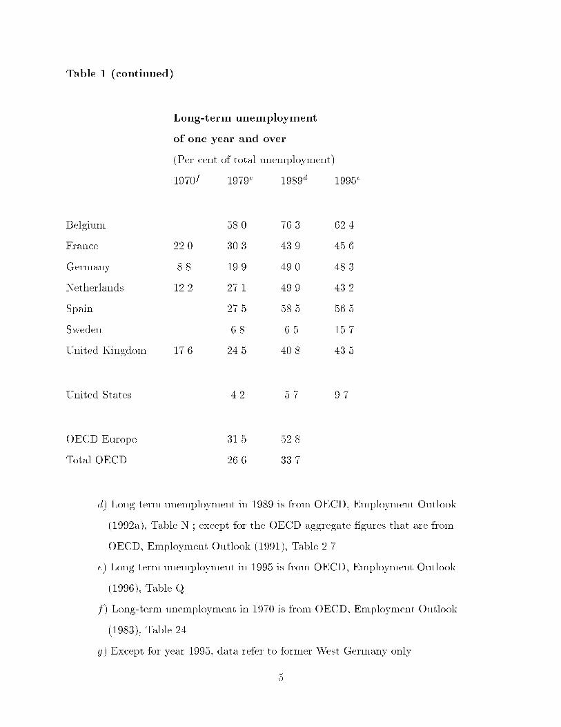
Table 1 (continued)

Long-term unemployment

of one year and over

(Per cent of total unemployment)

1970f 1979c 1989d 1995e

Belgium ... 58.0 76.3 62.4

France 22.0 30.3 43.9 45.6

Germany 8.8 19.9 49.0 48.3

Netherlands 12.2 27.1 49.9 43.2

Spain ... 27.5 58.5 56.5

Sweden ... 6.8 6.5 15.7

United Kingdom 17.6 24.5 40.8 43.5

United States ... 4.2 5.7 9.7

OECD Europe ... 31.5 52.8 ...

Total OECD ... 26.6 33.7 ...

d) Long-term unemployment in 1989 is from OECD, Employment Outlook

(1992a), Table N.; except for the OECD aggregate �gures that are from

OECD, Employment Outlook (1991), Table 2.7.

e) Long-term unemployment in 1995 is from OECD, Employment Outlook

(1996), Table Q.

f) Long-term unemployment in 1970 is from OECD, Employment Outlook

(1983), Table 24.

g) Except for year 1995, data refer to former West Germany only.

5

Various theories have been proposed to explain the rise in European unemployment.

Blanchard and Summers (1986) and Lindbeck and Snower (1988) impute the outcome to

\insider-outsider" con icts between employed and unemployed workers that arose in the

highly unionized economies of Europe. Bentolila and Bertola (1990) study the idea that

excessive European hiring and �ring costs contributed to higher unemployment. Malinvaud

(1994) emphasizes a capital shortage in Europe caused by high real wages in the 1970's

and high real interest rates in the 1980's. All these explanations assign the problem to

the demand for labor, making the decisions either of employers or of unionized employed

workers sustain a high unemployment rate. In contrast, we focus on the e�ects of the

welfare state on the supply of labor. It is well known that high income taxation and

generous welfare bene�ts distort workers' labor supply decisions. We hope to contribute a

sense of how the welfare state adversely a�ects the dynamic responses to economic shocks

and to increasing turbulence in the economic environment.3

One reason for the past lack of emphasis on workers' distorted incentives as an ex-

planation for high European unemployment must be the scarce empirical support for the

idea. As pointed out by OECD (1994a, chapter 8), most earlier empirical studies have

failed to �nd any cross-country correlation between unemployment bene�ts and aggregate

unemployment. In fact, there was even a negative correlation between bene�t levels and

unemployment in the 1960's and early 1970's. A common conclusion has therefore been

that generous entitlement programs are not to be blamed for high unemployment rates.

However, the same OECD study presents an opposing view and interprets the time-series

evidence as indicating that unemployment rates do respond to bene�t entitlements, but

with a considerable lag of 5 to 10 years, and in some cases 10 to 20 years. A natural

question then becomes, why are there such lags between rises in bene�ts and later sharp

rises in unemployment? Our analysis suggests that the lags are purely coincidental, and

that the real explanation for persistently higher European unemployment from the 1980's

is to be found in a changed economic environment.

3 Our analysis will bear out the assertion by Layard, Nickell and Jackman (1991, page 62)

that the \unconditional payment of bene�ts for an inde�nite period is clearly a major cause of

high European unemployment." However, our model di�ers sharply from their framework, which

emphasizes hysteresis and nominal inertia in wage and price setting.

6

−2 −1.5 −1 −0.5 0 0.5 1 1.50

5

10

15

20

25

Mean of log annual earnings

Per

cent

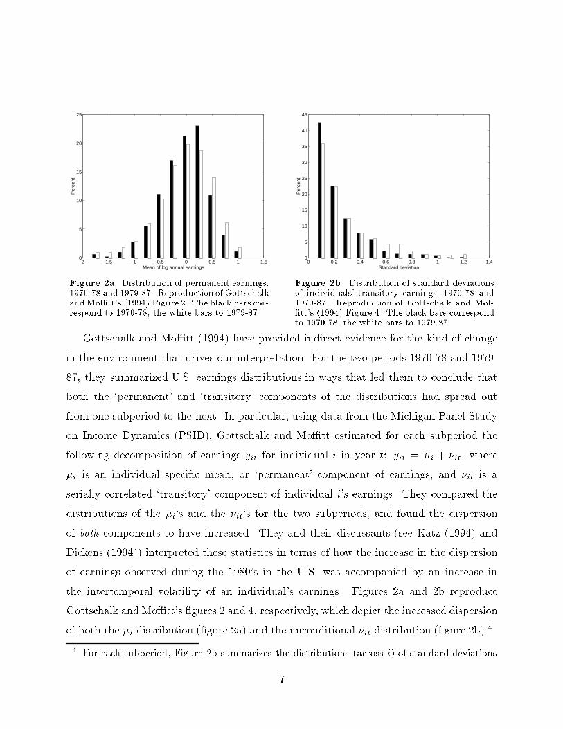
Figure 2a. Distribution of permanent earnings,1970-78 and 1979-87. Reproduction of GottschalkandMo�tt's (1994) Figure 2. The black bars cor-respond to 1970-78, the white bars to 1979-87.

0 0.2 0.4 0.6 0.8 1 1.2 1.40

5

10

15

20

25

30

35

40

45

Standard deviation

Per

cent

Figure 2b. Distribution of standard deviationsof individuals' transitory earnings, 1970-78 and1979-87. Reproduction of Gottschalk and Mof-�tt's (1994) Figure 4. The black bars correspondto 1970-78, the white bars to 1979-87.

Gottschalk and Mo�tt (1994) have provided indirect evidence for the kind of change

in the environment that drives our interpretation. For the two periods 1970-78 and 1979-

87, they summarized U.S. earnings distributions in ways that led them to conclude that

both the `permanent' and `transitory' components of the distributions had spread out

from one subperiod to the next. In particular, using data from the Michigan Panel Study

on Income Dynamics (PSID), Gottschalk and Mo�tt estimated for each subperiod the

following decomposition of earnings yit for individual i in year t: yit = �i + �it, where

�i is an individual speci�c mean, or `permanent' component of earnings, and �it is a

serially correlated `transitory' component of individual i's earnings. They compared the

distributions of the �i's and the �it's for the two subperiods, and found the dispersion

of both components to have increased. They and their discussants (see Katz (1994) and

Dickens (1994)) interpreted these statistics in terms of how the increase in the dispersion

of earnings observed during the 1980's in the U.S. was accompanied by an increase in

the intertemporal volatility of an individual's earnings. Figures 2a and 2b reproduce

Gottschalk and Mo�tt's �gures 2 and 4, respectively, which depict the increased dispersion

of both the �i distribution (�gure 2a) and the unconditional �it distribution (�gure 2b).4

4 For each subperiod, Figure 2b summarizes the distributions (across i) of standard deviations

7

The Gottschalk-Mo�tt �ndings would be expected if the economic environment had

become more turbulent between the earlier and later subperiods. Likewise, many informal

accounts assert that the economic environment has become more turbulent in the last cou-

ple of decades. The oil price shocks of the 1970's and reallocations from manufacturing to

services have each put economic turbulence into the industrialized world. In addition, the

spread of new information technologies, declines in government regulation, competition

from newly industrialized countries, and increasing internationalization of the production,

distribution, and marketing of goods and services are rapidly changing the economic envi-

ronment. Harris (1993) argues that `globalization' has sped up in the last two decades and

perhaps in the last decade in particular. We use Gottschalk and Mo�tt's data description

partly to inspire and partly to cross-check our model. Below, we show how increasing a

key `turbulence' parameter in our model serves to push the earnings distribution in ways

depicted by Gottschalk and Mo�tt.

Our thesis is that changed economic conditions from the mid-1970's onward can ex-

plain the high (long-term) unemployment in the welfare states. We formulate a general

equilibrium search model where workers' skills depreciate during unemployment spells,

and unemployment bene�ts are determined by workers' past earnings. Simulations of the

model bring out the sensitivity of the equilibrium unemployment rate to the amounts of

skills lost at lay o�s. The analysis attributes the welfare states' persistently higher unem-

ployment from the 1980's to increased turbulence in the economic environment, while also

explaining how lower unemployment rates in the 1950's, the 1960's and the early 1970's

were sustainable under more tranquil economic conditions.5

Relative to our `tranquil times' setting, the 1980's (turbulent times) parameterization

of our model exposes workers to the type of situation detected by Jacobson, LaLonde,

and Sullivan (1993), who found that long-tenured displaced workers experienced large and

of �it across time.

5 Our analysis agrees with the basic conclusion in a recent OECD study and policy report

(1994a,b) that \it is an inability of OECD economies and societies to adapt rapidly and inno-

vatively to a world of rapid structural change that is the principal cause of high and persistent

unemployment". But we believe that a greater emphasis should have been put on reforming

bene�t systems, instead of putting it last among policy recommendations.

8

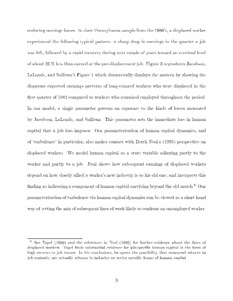
enduring earnings losses. In their Pennsylvania sample from the 1980's, a displaced worker

experienced the following typical pattern: a sharp drop in earnings in the quarter a job

was left, followed by a rapid recovery during next couple of years toward an eventual level

of about 25 % less than earned at the pre-displacement job. Figure 3 reproduces Jacobson,

LaLonde, and Sullivan's Figure 1 which dramatically displays the pattern by showing the

disparate expected earnings patterns of long-tenured workers who were displaced in the

�rst quarter of 1982 compared to workers who remained employed throughout the period.

In our model, a single parameter governs an exposure to the kinds of losses measured

by Jacobson, LaLonde, and Sullivan. This parameter sets the immediate loss in human

capital that a job loss imposes. Our parameterization of human capital dynamics, and

of `turbulence' in particular, also makes contact with Derek Neal's (1995) perspective on

displaced workers. We model human capital as a state variable adhering partly to the

worker and partly to a job. Neal shows how subsequent earnings of displaced workers

depend on how closely allied a worker's new industry is to his old one, and interprets this

�nding as indicating a component of human capital surviving beyond the old match.6 Our

parameterization of turbulence via human capital dynamics can be viewed as a short hand

way of setting the mix of subsequent lines of work likely to confront an unemployed worker.

6 See Topel (1990) and the references in Neal (1995) for further evidence about the fates of

displaced workers. Topel �nds substantial evidence for job-speci�c human capital in the form of

high returns to job tenure. In his conclusions, he opens the possibility that measured returns to

job seniority are actually returns to industry or sector speci�c forms of human capital.

9

1974 1976 1978 1980 1982 1984 1986 19882000

3000

4000

5000

6000

7000

8000

Figure 3. Quarterly earnings of high-attachmentworkers separating in the �rst quarter of 1982 andworkers staying through 1986. The solid line refersto stayers, the dashed line separators. Reproduc-tion of Jacobson, LaLonde and Sullivan's (1993)Figure 1.

The unlucky workers in Jacobson, LaLonde, and Sullivan's study su�ered substantial

capital losses, but by returning to work, they partly recovered their lost earnings. What

would similarly unlucky workers have done if they had been exposed to European levels

of unemployment compensation? Our model suggests that such long-tenured displaced

workers in Europe are likely to end up among the numerous long-term unemployed in the

prime-age and older worker category. (Table 2 depicts the distribution of long-term unem-

ployment across age categories.) The OECD has computed the welfare bene�ts available

to the average 40-year-old worker with a long period of previous employment. Depending

on family status, Table 3 shows net unemployment bene�t replacement rates after tax and

housing bene�ts.7 These generous bene�ts should be compared to the substantial income

losses of displaced workers in Jacobson, LaLonde and Sullivan's study.

7 There are also other welfare programs in Europe, such as early retirement and disability

insurance, which remove the assisted individuals from the labor force and the unemployment

statistics. For example, totally disabled persons in the Netherlands in the 1980's were entitled to

70 % (80 % prior to 1984) of last earned gross wage until the age of 65 { after which they moved

into the state pension system. At the end of 1990, disability bene�ts were paid to 14 % of the

Dutch labor force and 80 % of them were reported to be totally disabled. (See OECD, 1992b.)

10

Table 2: Distribution of long-term unemployment (one year and over) by

age group in 1990

Distribution of long-term unemployment

(per cent of total long-term unemployment)

15{24 25{44 45+

years years years

Belgium 17 62 20

Francea 13 63 23

Germany 8 43 48

Netherlands 13 64 23

Spaina 34 38 28

Sweden 9 24 67

United Kingdom 18 43 39

United Statesa 14 53 33

a) Data for France, Spain and the United States refer to 1991.

Source : OECD, Employment Outlook (1993), Table 3.3.

11

Table 3: Net unemployment bene�t replacement ratesa in 1994 for single-earner

households by duration categories and family circumstances

Single With dependent spouse

First Second Fourth First Second Fourth

year & third & �fth year & third & �fth

year year year year

Belgium 79 55 55 70 64 64

France 79 63 61 80 62 60

Germany 66 63 63 74 72 72

Netherlands 79 78 73 90 88 85

Spain 69 54 32 70 55 39

Swedenb 81 76 75 81 100 101

United Kingdomb 64 64 64 75 74 74

United States 34 9 9 38 14 14

a) Bene�t entitlement on a net-of-tax and housing bene�t basis as a

percentage of net-of-tax earnings.

b) Data for Sweden and the United Kingdom refer to 1995.

Source : Martin (1996), Table 2.

The next section extends our earlier model (Ljungqvist and Sargent, 1995a) by intro-

ducing a stochastic technology for skill accumulation and depreciation. Section 3 describes

the calibration of the model. We compare the steady state for the welfare state to the

laissez-faire outcome in Section 4. The two economies exhibit similar performance un-

der tranquil economic conditions, when the loss of e�ciency associated with the welfare

state seems minimal. However, compared to the laissez-faire economy, the welfare state

is much more vulnerable to economic shocks and turbulence. Section 5 traces out the

12

impulse-response from an unexpected transient unemployment shock. The transient shock

results in a prolonged period of long-term unemployment in the welfare state, whereas the

recovery is almost immediate in the laissez-faire economy.8 Section 6 demonstrates how

persistent economic turbulence leads to higher steady state unemployment in the welfare

state than in the laissez-faire economy. In Section 7, we generate arti�cial earnings data

from our model and compare them with the empirical patterns discerned by Gottschalk

and Mo�tt (1994), and Jacobson, LaLonde and Sullivan (1993). The �nal section contains

concluding comments.

2. The Economy

There is a continuum of workers with geometrically distributed life spans, indexed on

the unit interval with births equaling deaths. An unemployed worker in period t chooses

a search intensity st � 0 at a disutility c(st) increasing in st. Search may or may not

generate a wage o�er in the next period. With probability �(st), the unemployed worker

receives one wage o�er from the distribution F (w) = Prob(wt+1 � w). With probability

(1 � �(st)), the worker receives no o�er in period t + 1. We assume �(st) 2 [0; 1], and

that it is increasing in st. Accepting a wage o�er wt+1 means that the worker earns that

wage (per unit of skill) for each period he is alive, not laid o�, and has not quit his job.

The probability of being laid o� at the beginning of a period is � 2 (0; 1). In addition, all

workers are subjected to a probability of � 2 (0; 1) of dying between periods.

Employed and unemployed workers experience stochastic accumulation or deterioration

of skills. There is a �nite number of skill levels with transition probabilities from skill level

h to h0 denoted by �u(h; h0) and �e(h; h0) for an unemployed and an employed worker,

respectively. That is, an unemployed worker with skill level h faces a probability �u(h; h0)

that his skill level at the beginning of next period is h0, contingent on not dying. Similarly,

�e(h; h0) is the probability that an employed worker with skill level h sees his skill level

8 Pissarides (1992) analyzes loss of skills during unemployment in a matching model, where it is

also true that a transient shock to unemployment can have persistent e�ects. Firms are shown to

create fewer jobs after the shock, since they are matching with workers of a lower average quality.

Thus, this is another model of unemployment that is driven by the demand side for labor, while

our paper focuses on the supply of labor in a welfare state.

13

change to h0 at the beginning of next period, contingent on not dying and not being laid o�.

In the event of a lay o�, the transition probability is given by �l(h; h0). After this initial

period of a lay o�, the stochastic skill level of the unemployed worker is again governed by

the transition probability �u(h; h0). All newborn workers begin with the lowest skill level.

A worker observes his new skill level at the beginning of a period before deciding

to accept a new wage o�er, choose a search intensity, or quit a job. The objective of

each worker is to maximize the expected value Et

P1i=0 �

i(1 � �)iyt+i, where Et is the

expectation operator conditioned on information at time t, � is the subjective discount

factor, and 1 � � is the probability of surviving between two consecutive periods; yt+i

is the worker's after-tax income from employment and unemployment compensation at

time t + i net of disutility of searching and working.9

Workers who were laid o� are entitled to unemployment compensation bene�ts that are

a function of their last earnings. Let b(I) be the unemployment compensation to an un-

employed worker whose last earnings were I. Unemployment compensation is terminated

if the worker turns down a job o�er with earnings that are deemed to be `suitable' by the

government in view of the worker's past earnings. Let Ig(I) be the government determined

`suitable earnings' of an unemployed worker whose last earnings were I. Newborn workers

and workers who have quit their previous job are not entitled to unemployment compensa-

tion. Both income from employment and unemployment compensation are subject to a at

income tax of � . The government policy functions b(I) and Ig(I) and the tax parameter �

must be set so that income taxes cover the expenditures on unemployment compensation

in an equilibrium.

Let V (w;h) be the value of the optimization problem for an employed worker with

wage w and skill level h at the beginning of a period. The value associated with being un-

employed and eligible for unemployment compensation bene�ts is given by Vb(I; h), which

is both a function of the unemployed worker's past earnings I and his current skill level h.

In the case of an unemployed worker who is not entitled to unemployment compensation,

9 Our analysis focuses on how the welfare state a�ects labor market incentives and e�ciency in

skill accumulation. We have abstracted from the bene�ts of risk sharing that government policies

can provide when capital markets are incomplete. Adding such considerations would modify our

results, but the forces at work in our analysis would remain.

14

the corresponding value is denoted by Vo(h) and depends only on the worker's current skill

level. The Bellman equations can then be written as follows.

V (w;h) = maxaccept;reject

n(1 � � )wh + (1 � �)�

h(1 � �)

Xh0

�e(h; h0)V (w;h0)(1)

+ �Xh0

�l(h; h0)Vb(wh; h

0)i; Vo(h)

o;

Vb(I; h) = maxs

(�c(s) + (1� � )b(I) + (1� �)�

Xh0

�u(h; h0)(2)

"�1� �(s)

�Vb(I; h

0) + �(s)

Zw�Ig(I)=h0

V (w;h0)dF (w)

+

Zw<Ig(I)=h0

maxaccept;reject

n(1� � )wh0

+ (1� �)�h(1� �)

Xh00

�e(h0; h00)V (w;h00)

+ �Xh00

�l(h0; h00)Vb(wh

0; h00)i; Vb(I; h

0)odF (w)

!#);

Vo(h) = maxs

n�c(s) + (1� �)�

Xh0

�u(h; h0)h(1� �(s))Vo(h

0)(3)

+ �(s)

ZV (w;h0)dF (w)

io:

Associated with the solution of equations (1){(3) are two functions, �sb(I; h) and �wb(I; h),

giving an optimal search intensity and a reservation wage of an unemployedworker with last

earnings I and current skill level h, who is eligible for unemployment compensation bene�ts;

and two functions, �so(h) and �wo(h), giving an optimal search intensity and a reservation

wage of an unemployed worker with skill level h, who is not entitled to unemployment

compensation. The reservation wage of an employed worker will be the same as for an

unemployed worker without bene�ts, �wo(h), since anyone who quits his job is not eligible

for unemployment compensation.

15

We will study stationary equilibria, or steady states, for our economy. A steady state

is de�ned in a standard way, as a set of government policy parameters, optimal policies

(�so(h); �wo(h); �sb(I; h); �wb(I; h)) and associated time invariant employment and unemploy-

ment distributions and total unemployment compensation payments that satisfy workers'

optimality conditions and the government's budget constraint. We compute a steady state

as a �xed point in the tax rate � . For a �xed tax rate � , we solve workers' optimization

problem and use the implied search intensities and reservation wages to deduce stationary

employment and unemployment distributions, and unemployment compensation. A bal-

anced government budget de�nes a �xed point in � , which is associated with a stationary

equilibrium.10 After having found a stationary equilibrium, we compute various quantities

such as GNP per capita, average productivity of employed workers, average skill level,

average duration of unemployment, and measures of long-term unemployment.

3. Calibration

We set the model period to be two weeks. We set the discount factor � = 0:9985,

making the annual interest rate 4.0 percent. The probabilities of dying and being laid o�

are � = 0:0009, and � = 0:009, respectively. The working life of an individual is then

geometrically distributed with an expected duration of 42.7 years. Similarly, the average

time before being laid o� (given that the worker has not quit or died) is 4.3 years.11

There are 21 di�erent skill levels evenly partitioning the interval [1; 2]. All newborn

workers start out with the lowest skill level equal to one. After each period of employment

that is not followed by a lay o�, with a probability of 0.1 the worker's skills increase by

one level (0.05 units of skills), and with probability .9 they remain unchanged. Employed

workers who have reached the highest skill level retain those skills until becoming unem-

ployed. As a point of reference, someone who starts out working with the lowest skill level

10 The iterative procedure picks the lowest possible � consistent with a stationary equilibrium.

We choose to focus on this the least distortionary tax rate and ignore any higher tax rates that

might be consistent with other steady states. For example, there will always exist another sta-

tionary equilibrium with a 100 % tax rate where all economic activities are closed down.

11 The parameterization of the probability of being laid o� is motivated by Hall's (1982) obser-

vation that the average worker will hold 10 jobs in an entire career.

16

will on average reach the highest skill level after seven years and eight months, conditional

upon no job loss. The stochastic depreciation of skills during unemployment is twice as

fast as the accumulation of skills. That is, after each period of unemployment, there is

a probability of 0.2 that the worker's skills decrease by one level; otherwise they remain

unchanged. The lowest skill level reached through depreciation is also an absorbing state

until the unemployed worker gains employment. Upon being laid o� in a period, the worker

retains his skill level from the latest period of employment.

The disutility from searching and the function mapping search intensities into proba-

bilities of obtaining a wage o�er are assumed to be

c(s) = 0:5 s ;

�(s) = s0:3 ; where s 2 [0; 1] :

The exogenous wage o�er distribution is assumed to be a normal distribution with a

mean of 0.5 and a variance of 0.1 that has been truncated to the unit interval (and then

normalized to integrate to one). Since a worker's earnings are the product of his wage and

his current skill level, it follows that observed earnings fall in the interval [0; 2].

For purposes of awarding unemployment compensation, the government divides the

earnings interval [0; 2] evenly into 15 earnings classes; let the upper limits of these classes

be denotedWi, for i = 1; 2; :::; 15. A laid o� worker with last earnings belonging to earnings

class i receives an unemployment compensation of 0:7�Wi in each period of unemployment.

However, the bene�t is terminated if the worker does not accept a job o�er associated with

earnings greater than or equal to 0:7�Wi. That is, a laid o� worker faces both a `replacement

ratio' and `suitable earnings' criterion equal to 70% of the upper limit of the earnings class

containing his own last earnings before being laid o�. New workers and quitters are not

entitled to unemployment compensation.

The following numerical simulations will make it clear that there are two key parame-

ters driving our analysis; the fact that unemployment compensation is a function of past

earnings (70% replacement ratio), and the amount of immediate loss in human capital that

a job loss imposes (zero in this initial parameterization of `tranquil times'). Perturbations

in the latter parameter will be used to capture the notion of `economic turbulence'. Our

17

qualitative �ndings are fairly robust to changes in other parameters. For example, similar

results were obtained in earlier simulations where we had doubled both the range of skills

and the transition probabilities of gaining a skill level when remaining employed for two

periods and of losing a skill level when being unemployed for two consecutive periods.

4. Economic Forces at Work

Given the calibration above, the tax rate that balances the government budget is � =

0:0285. To shed light on the workings of this welfare state (WS), we will now contrast

its steady state to that of a laissez-faire economy (LF), in which there is no government

intervention whatsoever.

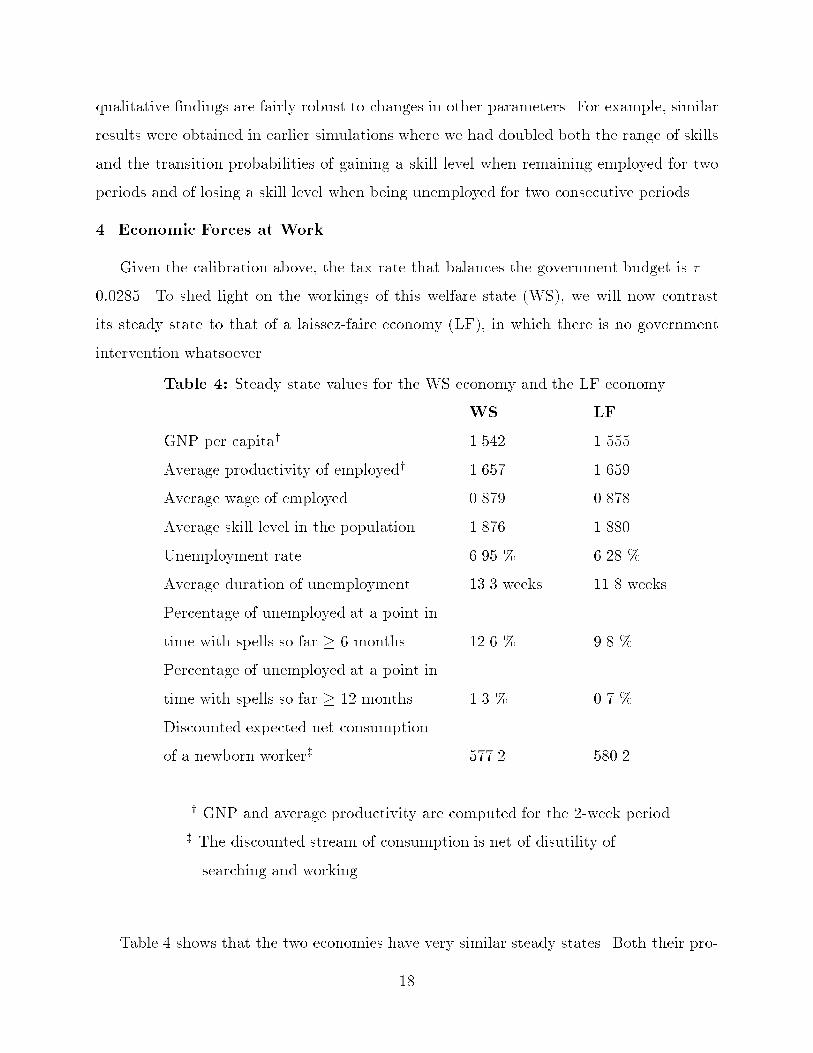
Table 4: Steady state values for the WS economy and the LF economy.

WS LF

GNP per capitay 1.542 1.555

Average productivity of employedy 1.657 1.659

Average wage of employed 0.879 0.878

Average skill level in the population 1.876 1.880

Unemployment rate 6.95 % 6.28 %

Average duration of unemployment 13.3 weeks 11.8 weeks

Percentage of unemployed at a point in

time with spells so far � 6 months 12.6 % 9.8 %

Percentage of unemployed at a point in

time with spells so far � 12 months 1.3 % 0.7 %

Discounted expected net consumption

of a newborn workerz 577.2 580.2

y GNP and average productivity are computed for the 2-week period.

z The discounted stream of consumption is net of disutility of

searching and working.

Table 4 shows that the two economies have very similar steady states. Both their pro-

18

duction and average skill levels are indistinguishable, and the unemployment rate is less

than seven tenths of a percentage point higher in the WS economy. As a welfare measure,

the discounted expected net consumption stream of a newborn worker di�ers by only four

weeks of per capita GNP (two 2-week periods). We conclude that the e�ciency costs

associated with the welfare system are relatively small. However, behind these numbers

lurk important di�erences in unemployment dynamics. It is true that the average unem-

ployment spell is very similar across the two economies: 13.3 weeks in the WS economy

as compared to 11.8 weeks in the LF economy. But the WS economy has more disper-

sion in the duration of unemployment spells, as indicated by the fractions of long-term

unemployed at any point in time. The percentage of currently unemployed workers with

spells to date greater than or equal to 6 months (12 months) is 12.6 % (1.3 %) in the WS

economy as compared to 9.8 % (0.7 %) in the LF economy.

0

0.5

1

1.5

2

11.21.41.61.82

0.7

0.75

0.8

0.85

0.9

0.95

1

LAST EAR

CURRENT SKILLS

RE

SE

RV

AT

ION

WA

GE

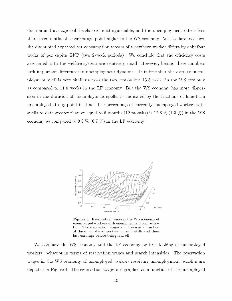
Figure 4. Reservation wages in the WS economy ofunemployedworkers with unemployment compensa-tion. The reservation wages are drawn as a functionof the unemployed workers' current skills and theirlast earnings before being laid o�.

We compare the WS economy and the LF economy by �rst looking at unemployed

workers' behavior in terms of reservation wages and search intensities. The reservation

wages in the WS economy of unemployed workers receiving unemployment bene�ts are

depicted in Figure 4. The reservation wages are graphed as a function of the unemployed

19

workers' current skills and their last earnings before being laid o�. Not surprisingly, the

reservation wage is a positive function of last earnings, which determine the level of un-

employment compensation. For example, the reservation wage of someone with the lowest

skill level of one, but with the highest possible last earnings, is 0.93. This corresponds to

a worker who once had attained a high skill level while making a wage at the top of the

wage distribution. If such a worker with a high unemployment bene�t happens to lose all

his skills due to a prolonged period of unemployment, he will be extremely picky in terms

of the wage o�ers he will accept. That is, before giving up his generous bene�ts, he wants

to �nd a very good wage o�er to compensate for his skill loss. Since such high wage o�ers

are hard to �nd, this worker will also be unwilling to expend too much energy in searching

for a new job. As can be seen in Figure 5, the optimal search intensity of such a worker is

a mere 0.06. Figure 5 shows also how the search intensity is lower for unemployed workers

with both high bene�ts and high current skills that have not yet deteriorated due to un-

employment. The 70 % replacement ratio causes these workers to consume some \leisure"

by reducing their search intensity.

0

0.5

1

1.5

2 11.2

1.41.6

1.82

0

0.2

0.4

0.6

0.8

1

LAST EARNINGS CURRENT SKILLS

SE

AR

CH

INT

EN

SIT

Y

Figure 5. Search intensities in the WS economy ofunemployed workers with unemployment compen-sation. The search intensities are drawn as a func-tion of the unemployed's current skills and their lastearnings before being laid o�.

20

1 1.1 1.2 1.3 1.4 1.5 1.6 1.7 1.8 1.9 2

0.66

0.68

0.7

0.72

0.74

0.76

0.78

0.8

0.82

0.84

CURRENT SKILLS

RE

SE

RV

AT

ION

WA

GE

Figure 6. Reservation wages of unemployed work-ers without bene�ts drawn as a function of their cur-rent skills. The solid line describes the WS economyand the dashed line refers to the LF economy.

Unemployed workers without bene�ts in the WS economy and the unemployed in the

LF economy prefer to choose the maximum search intensity of one. Their reservation

wages can be found in Figure 6. Contrasting Figure 6 to Figure 4 for the WS economy, the

reservation wage of an unemployed worker without bene�ts is always less than or equal

to the reservation wage of an unemployed worker with bene�ts, for any given skill level.

Unemployment spells are of course more costly to the unemployed without unemployment

compensation. Across the WS and the LF economies, there is a slight tendency for higher

reservation wages in the WS economy. An unemployed worker without bene�ts in the

WS economy takes into account the future potential bene�ts from the unemployment

compensation program. It is important for the worker to become vested at a high wage

rate in the event of being laid o�. The U-shaped pattern for reservations wages in Figure 6

emerges from the depreciation and accumulation of skills. On the one hand, at the lower

end of the skill spectrum, unemployed workers have less to lose in terms of skills from an

extended period of unemployment. They therefore tend to choose higher reservation wages

as compared to unemployed workers with skills in the intermediate range. On the other

hand, at the upper end of the skill spectrum, the potential for further skill accumulation

becomes smaller and the emphasis shifts towards the search for higher wages, i.e., the

reservation wage curve starts to slope upward.

21

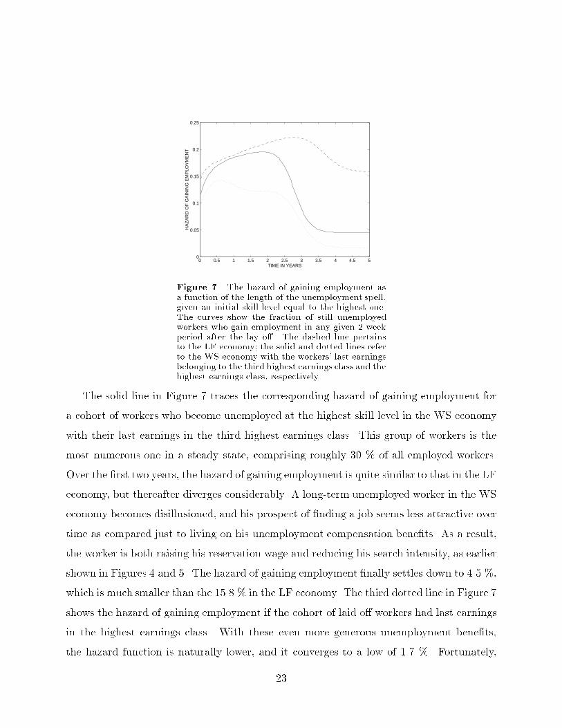
The e�ects of di�erent search behavior in the LF economy and the WS economy are

illustrated in Figure 7. The �gure follows a cohort of workers who lost their jobs after

having reached the highest skill level. At di�erent lengths of the unemployment spell, the

curves show the fraction of still unemployed workers who gain employment in the current

2-week period (`hazard rate'). The dashed curve pertains to the LF economy without any

unemployment compensation bene�ts. Since all unemployed workers in the LF economy

choose the highest search intensity, the shape of the curve is solely determined by how

reservation wages vary with skill levels. Recall from Figure 6 that reservation wages must

initially be decreasing when skills start depreciating from the maximum level. That is,

over time, unemployed workers become more and more concerned about additional losses

of skills. Their willingness successively to reduce their reservation wages explains the

rising hazard of gaining employment during the �rst couple of years of unemployment.

After three years, the remaining unemployed have lost enough of their skills that further

losses are less of a concern to them. Their increasing reservation wage policy in Figure 6

translates into a falling hazard of gaining employment in Figure 7. The hazard of gaining

employment in any given 2-week period levels out at 15.8 % in the LF economy.

22

0 0.5 1 1.5 2 2.5 3 3.5 4 4.5 50

0.05

0.1

0.15

0.2

0.25

TIME IN YEARS

HA

ZA

RD

OF

GA

ININ

G E

MP

LOY

ME

NT

Figure 7. The hazard of gaining employment asa function of the length of the unemployment spell,given an initial skill level equal to the highest one.The curves show the fraction of still unemployedworkers who gain employment in any given 2-weekperiod after the lay o�. The dashed line pertainsto the LF economy; the solid and dotted lines referto the WS economy with the workers' last earningsbelonging to the third highest earnings class and thehighest earnings class, respectively.

The solid line in Figure 7 traces the corresponding hazard of gaining employment for

a cohort of workers who become unemployed at the highest skill level in the WS economy

with their last earnings in the third highest earnings class. This group of workers is the

most numerous one in a steady state, comprising roughly 30 % of all employed workers.

Over the �rst two years, the hazard of gaining employment is quite similar to that in the LF

economy, but thereafter diverges considerably. A long-term unemployed worker in the WS

economy becomes disillusioned, and his prospect of �nding a job seems less attractive over

time as compared just to living on his unemployment compensation bene�ts. As a result,

the worker is both raising his reservation wage and reducing his search intensity, as earlier

shown in Figures 4 and 5. The hazard of gaining employment �nally settles down to 4.5 %,

which is much smaller than the 15.8 % in the LF economy. The third dotted line in Figure 7

shows the hazard of gaining employment if the cohort of laid o� workers had last earnings

in the highest earnings class. With these even more generous unemployment bene�ts,

the hazard function is naturally lower, and it converges to a low of 1.7 %. Fortunately,

23

these potential incentive problems have only a small impact on the steady state of the WS

economy, as earlier shown in Table 4. Loosely speaking, the incentive problems are minor

thanks to the relatively low average duration of unemployment.

5. A Transient Economic Shock

The unemployment dynamics described in the previous section make the WS economy

more vulnerable to economic shocks. This section demonstrates how a transient shock can

cause a prolonged period of long-term unemployment in the WS economy while the LF

economy is more resilient. Speci�cally, we will trace out both economies' responses to an

unexpected transient unemployment shock. We assume that once and for all, the normal

lay o� rate of 0.009 rises 20-fold to 0.18 in a single 2-week period at time 0 in the following

�gures. Also, everyone who becomes unemployed in this particular period immediately

loses all of his accumulated skills. After this one-period shock, both economies once again

experience the normal lay o� rate and rates of skill depreciation and accumulation. All

policy parameters such as taxes and the unemployment compensation program are kept

constant throughout the experiment, which means that the workers' decision rules stay the

same over time, and that the economies will eventually return to their steady states. During

the transition, additional government expenditures on unemployment compensation in the

WS economy are assumed to be �nanced by levying lump-sum taxes.

0 1 2 3 4 5 6-2

0

2

4

6

8

10

12

14

16

TIME IN YEARS

DE

VIA

TIO

N IN

PE

RC

EN

TA

GE

PO

INT

S F

RO

M S

TE

AD

Y S

TA

TE

Figure 8. Response of unemployment. The solidline describes the WS economy and the dashed linerefers to the LF economy.

24

As can be seen in Figure 8, the unemployment rates in both economies jump up initially

by roughly 16 percentage points. However, the unemployment rates take very di�erent

paths thereafter. In the LF economy, the high unemployment rate dies out quickly because

the unemployed workers `bite the bullet' and search intensively for less well-paying jobs as

compared to their lost earnings. In contrast, the WS economy is plagued by a prolonged

period of unemployment since the unemployed workers with their depreciated skills have

di�culty �nding jobs that they prefer to their unemployment compensation based on

past earnings. Besides their higher reservation wages, these workers also reduce search

intensities to balance the small prospective gains from search against the utility costs

associated with search.

0 1 2 3 4 5 60

10

20

30

40

50

60

70

80

90

100

TIME IN YEARS

PE

RC

EN

TA

GE

SH

AR

E O

F T

OT

AL

UN

EM

PLO

YM

EN

T

Figure 9.a. Response of the decomposition of theunemployed in the WS economy with respect to thelength of their unemployment spells so far. The per-centage of unemployed workers with at least 6 months(12 months) of unemployment to date is below the solidline (dashed line). The percentage above the solid lineis then unemployed workers who have until now beenunemployed for less than 6 months.

0 1 2 3 4 5 60

10

20

30

40

50

60

70

80

90

100

TIME IN YEARS

PE

RC

EN

TA

GE

SH

AR

E O

F T

OT

AL

UN

EM

PLO

YM

EN

T

Figure 9.b. Response of the decomposition of theunemployed in the LF economy with respect to thelength of their unemployment spells so far. The per-centage of unemployed workers with at least 6 months(12 months) of unemployment to date is below the solidline (dashed line). The percentage above the solid lineis then unemployed workers who have until now beenunemployed for less than 6 months.

The drawn out unemployment response in the WS economy is naturally associated

with longer unemployment spells. Figures 9.a and 9.b show how long-term unemployment

gradually emerges after the shock. At any point in time, the �gures decompose unemploy-

ment into the fraction of unemployed workers who have to date been unemployed for at

25

least one year (below the dashed line), those who have so far su�ered unemployment of less

than a year but at least 6 months (between the solid line and the dashed line), and those

who have until now been unemployed for less than 6 months (above the solid line). Not

surprisingly, both of the �rst two measures of unemployment fall at the time of the shock,

since there is a ood of newly laid o� workers into unemployment. The two measures then

rise predictably after 6 months and 12 months, respectively. The problem of long-term

unemployment in the WS economy shows up starkly in Figure 9.a. At the peaks of the two

long-term unemployment measures, there is �rst a fraction of 66.6 % of all unemployed

workers being unemployed for at least half a year, and later 49.5 % of all unemployed

have to date experienced unemployment for a year or more. In contrast, the corresponding

numbers for the LF economy in Figure 9.b are 33.3 % and 4.2 %, respectively. Besides the

lower incidence of long-term unemployment, the LF economy shows hardly any persistence

in the fractions of long-term unemployed as compared to the WS economy.

The exogenous jump in the lay o� rate and the accompanying depreciation of workers'

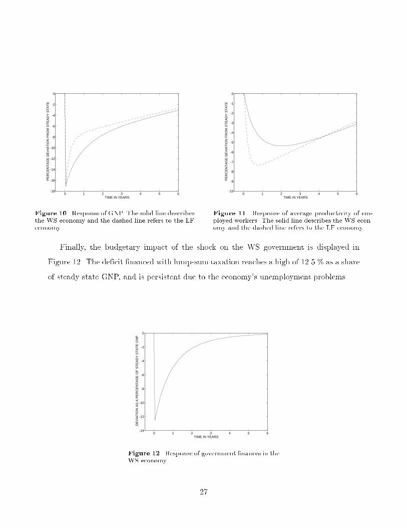
skills a�ect the economies' GNP adversely. Figure 10 shows a sharp drop of around 17 %

in GNP. The faster recovery in the LF economy as compared to the WS economy is due to

the fact that its labor force is returning to work more quickly. A conceivably misleading

measurement of the economies' performances is the change in average productivity of em-

ployed workers. At the end of the �rst year, Figure 11 shows that the average productivity

in the WS economy falls by 4.7 % while the decline in the LF economy is signi�cantly

larger at 7.2 %. The explanation for this di�erence is that laid o� workers with depreci-

ated skills return to employment much faster in the LF economy, while they are slowly

phased in to the WS economy. The long-term unemployment in the WS economy is in this

way concealing the severity of the exogenous shock to workers' skills.

26

0 1 2 3 4 5 6-18

-16

-14

-12

-10

-8

-6

-4

-2

0

TIME IN YEARS

PE

RC

EN

TA

GE

DE

VIA

TIO

N F

RO

M S

TE

AD

Y S

TA

TE

Figure 10. Response of GNP. The solid line describesthe WS economy and the dashed line refers to the LFeconomy.

0 1 2 3 4 5 6-10

-9

-8

-7

-6

-5

-4

-3

-2

-1

0

TIME IN YEARS

PE

RC

EN

TA

GE

DE

VIA

TIO

N F

RO

M S

TE

AD

Y S

TA

TE

Figure 11. Response of average productivity of em-ployed workers. The solid line describes the WS econ-omy and the dashed line refers to the LF economy.

Finally, the budgetary impact of the shock on the WS government is displayed in

Figure 12. The de�cit �nanced with lump-sum taxation reaches a high of 12.5 % as a share

of steady state GNP, and is persistent due to the economy's unemployment problems.

0 1 2 3 4 5 6-14

-12

-10

-8

-6

-4

-2

0

TIME IN YEARS

DE

VIA

TIO

N A

S A

PE

RC

EN

TA

GE

OF

ST

EA

DY

ST

AT

E G

NP

Figure 12. Response of government �nances in theWS economy.

27

6. Persistent Economic Turbulence

The previous section indicated that the welfare state is prone to experience enduring

periods of long-term unemployment after transient economic shocks. This section demon-

strates how persistent economic turbulence increases the unemployment rate in welfare

states. Speci�cally, we compute and compare the steady states for di�erent economic envi-

ronments with more or less economic turbulence. Economic turbulence is de�ned in terms

of the mean and variance of skill losses associated with lay o�s. We now let the skills of

a newly laid o� worker be distributed according to the left half of a normal distribution

with the range starting at the lowest possible skill level and ending at the worker's skill

level before the lay o�. During the unemployment spell itself and at times of continu-

ing employment, skill depreciation and accumulation are governed by the same transition

probabilities as before.

With this de�nition of economic turbulence, the earlier steady state serves as a bench-

mark case with zero variance. Recall that our earlier assumption was that a newly laid

o� worker kept his skill level from last period of employment. Let us now consider three

alternative environments with di�erent probability distributions for skills of newly laid o�

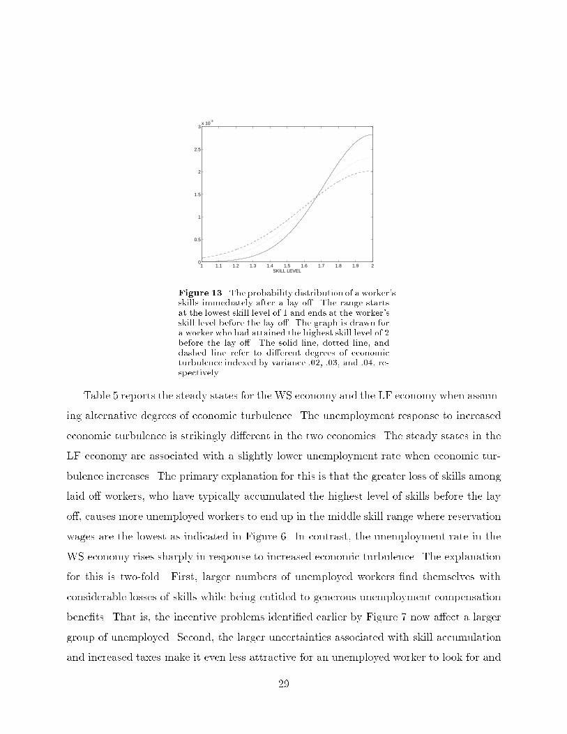
workers, as depicted in Figure 13. The graph is drawn for a worker who had attained

the highest skill level of 2 before being laid o�. The same distributions apply to a worker

with another skill level so long as we rescale the range so that it ends at that particular

worker's skill level before the lay o�. The exact distributions in Figure 13 are obtained by

taking the left side of a normal distribution that is con�ned to and centered on the unit

interval. The solid, dotted, and dashed lines correspond to variances of :02, :03, and :04,

respectively. The left halves of these distributions are then normalized to integrate to one.

Finally, since there is a discrete number of skill levels in the model, the distributions in

Figure 13 are transformed into step functions for each kind of laid o� worker.

28

1 1.1 1.2 1.3 1.4 1.5 1.6 1.7 1.8 1.9 20

0.5

1

1.5

2

2.5

3x 10

-3

SKILL LEVEL

Figure 13. The probability distribution of a worker'sskills immediately after a lay o�. The range startsat the lowest skill level of 1 and ends at the worker'sskill level before the lay o�. The graph is drawn fora worker who had attained the highest skill level of 2before the lay o�. The solid line, dotted line, anddashed line refer to di�erent degrees of economicturbulence indexed by variance :02, :03, and :04, re-spectively.

Table 5 reports the steady states for the WS economy and the LF economy when assum-

ing alternative degrees of economic turbulence. The unemployment response to increased

economic turbulence is strikingly di�erent in the two economies. The steady states in the

LF economy are associated with a slightly lower unemployment rate when economic tur-

bulence increases. The primary explanation for this is that the greater loss of skills among

laid o� workers, who have typically accumulated the highest level of skills before the lay

o�, causes more unemployed workers to end up in the middle skill range where reservation

wages are the lowest as indicated in Figure 6. In contrast, the unemployment rate in the

WS economy rises sharply in response to increased economic turbulence. The explanation

for this is two-fold. First, larger numbers of unemployed workers �nd themselves with

considerable losses of skills while being entitled to generous unemployment compensation

bene�ts. That is, the incentive problems identi�ed earlier by Figure 7 now a�ect a larger

group of unemployed. Second, the larger uncertainties associated with skill accumulation

and increased taxes make it even less attractive for an unemployed worker to look for and

29

accept a job, especially if he is currently receiving generous unemployment compensation.

As a result, these unemployed workers choose to lower their search intensities and raise

their reservation wages. This exacerbates the economy's unemployment problem.

Table 5 shows also that a higher WS unemployment rate in a more turbulent economic

environment is accompanied by considerably longer average unemployment spells. In the

most turbulent environment, the average duration of unemployment is 31.8 weeks as com-

pared to the 13.3 weeks in the benchmark case without any turbulence. Moreover, the

fractions of long-term unemployed explode in the WS economy. The percentage of cur-

rently unemployed workers with spells to date of six months or more rises from 12.6 % in

the WS economy without turbulence to 63.1 % in the WS economy with most economic

turbulence. Concerning the percentage of unemployed workers with spells to date of one

year or more, the corresponding increase for the WS economy is from 1.3 % to 55.6 %.

In contrast, the small numbers of long-term unemployed in the LF economy stay virtually

unchanged in response to increased economic turbulence.

Since economic turbulence is modeled in the form of risk of more skill losses at a

moment of lay o�, it follows that a higher degree of turbulence must be associated with

welfare reductions. The LF economy in Table 5 posts a 8.0 % reduction in the discounted

expected net consumption of a newborn worker when moving from an environment with no

turbulence to the highest degree of turbulence. The corresponding relative welfare loss in

the WS economy is close to twice as large at 15.8 %, due to its malfunctioning labor market

with excessive unemployment. Despite the dismal performance of the WS economy, the

average productivity of employed is comparable to the LF economy for di�erent degrees

of turbulence. The good productivity record in the WS economy actually re ects the low

job �nding rate among long-term unemployed workers with depreciated skills.

Finally, when trying to solve for a WS steady state with a variance of :05, a vicious

circle develops on the computer. Exploding government expenditures on unemployment

compensation chase an exploding unemployment rate without �nding a feasible steady

state with government budget balance. This breakdown of the computations mirrors a

potential instability of a generous welfare state. The feasibility of the system depends crit-

ically upon the number of workers that has virtually withdrawn from active labor market

30

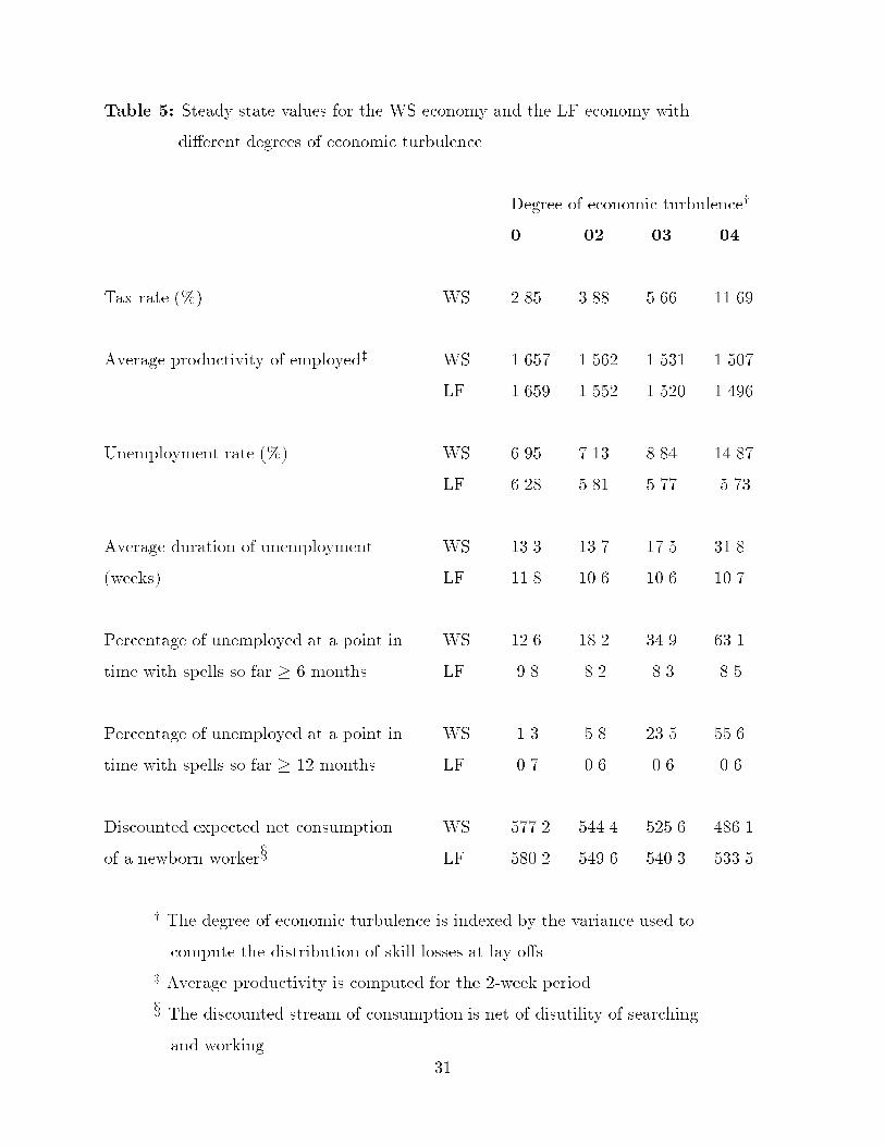
Table 5: Steady state values for the WS economy and the LF economy with

di�erent degrees of economic turbulence.

Degree of economic turbulencey

0 .02 .03 .04

Tax rate (%) WS 2.85 3.88 5.66 11.69

Average productivity of employedz WS 1.657 1.562 1.531 1.507

LF 1.659 1.552 1.520 1.496

Unemployment rate (%) WS 6.95 7.13 8.84 14.87

LF 6.28 5.81 5.77 5.73

Average duration of unemployment WS 13.3 13.7 17.5 31.8

(weeks) LF 11.8 10.6 10.6 10.7

Percentage of unemployed at a point in WS 12.6 18.2 34.9 63.1

time with spells so far � 6 months LF 9.8 8.2 8.3 8.5

Percentage of unemployed at a point in WS 1.3 5.8 23.5 55.6

time with spells so far � 12 months LF 0.7 0.6 0.6 0.6

Discounted expected net consumption WS 577.2 544.4 525.6 486.1

of a newborn workerx LF 580.2 549.6 540.3 533.5

y The degree of economic turbulence is indexed by the variance used to

compute the distribution of skill losses at lay o�s.

z Average productivity is computed for the 2-week period.

x The discounted stream of consumption is net of disutility of searching

and working.

31

participation because of disincentives. The size of this group can increase dramatically in

response to a more turbulent economic environment. As a consequence, a welfare regime

that was earlier sustainable under more tranquil economic conditions can suddenly become

infeasible, and lead to a mounting budget de�cit.

7. Arti�cial Earnings Data

We can use our model as a laboratory for trying to replicate aspects of earnings dy-

namics described Gottschalk and Mo�tt (1994) and Jacobson, LaLonde, and Sullivan

(1993), described in section 1. We �rst use a comparison of our model under `tranquil'

and `turbulent' times to replicate Gottschalk and Mo�tt's earnings decompositions across

two subperiods.

An equilibrium of our model yields earning dynamics for a distribution of individuals.

For given parameter values, an equilibrium of our model produces a stationary probability

distribution over the individual state variables, namely, (h;w; I) and an additional state

variable recording whether an individual is employed or unemployed with or without un-

employment compensation. We can draw a set of `initial conditions' { really individuals {

from this distribution, then apply the individual equilibrium transition dynamics to con-

struct a panel of individuals' earnings. We can then use arti�cial panels for two parameter

settings, one with lower turbulence than the other, to prepare versions of Gottschalk and

Mo�tt's �gures. This tells whether our way of modeling increased turbulence generates

the observed altered earnings outcomes.

For the laissez-faire economy, we generated arti�cial panels of length nine years with

10,000 individuals for two di�erent subperiods; relatively `tranquil' economic times and

more `turbulent' times as indexed in Table 5 by variances :02 and :04, respectively. The

former panel is meant to represent the period 1970-78 in the Gottschalk-Mo�tt study,

while the latter panel would then correspond to the period 1979-87. For both panels, we

use the equilibrium distribution of workers who have been in the labor force for 20 years

as initial conditions. A period of 20 years should su�ce to remove the initial life cycle

pattern in the accumulation of human capital among newborn workers. (Recall that, in

our calibration, it takes on average seven years and eight months to move from the lowest

to the highest skill level for someone who is continuously employed.)

32

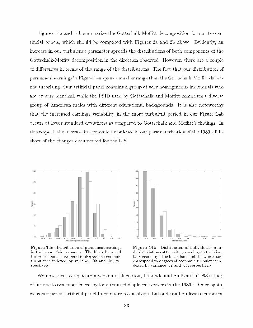
Figures 14a and 14b summarize the Gottschalk-Mo�tt decomposition for our two ar-

ti�cial panels, which should be compared with Figures 2a and 2b above. Evidently, an

increase in our turbulence parameter spreads the distributions of both components of the

Gottschalk-Mo�tt decomposition in the direction observed. However, there are a couple

of di�erences in terms of the range of the distributions. The fact that our distribution of

permanent earnings in Figure 14a spans a smaller range than the Gottschalk-Mo�tt data is

not surprising. Our arti�cial panel contains a group of very homogeneous individuals who

are ex ante identical, while the PSID used by Gottschalk and Mo�tt comprises a diverse

group of American males with di�erent educational backgrounds. It is also noteworthy

that the increased earnings variability in the more turbulent period in our Figure 14b

occurs at lower standard deviations as compared to Gottschalk and Mo�tt's �ndings. In

this respect, the increase in economic turbulence in our parameterization of the 1980's falls

short of the changes documented for the U.S.

−0.5 −0.4 −0.3 −0.2 −0.1 0 0.1 0.2 0.3 0.4 0.50

5

10

15

20

25

30

Per

cent

Mean of log annual earnings

Figure 14a. Distribution of permanent earningsin the laissez-faire economy. The black bars andthe white bars correspond to degrees of economicturbulence indexed by variance :02 and :04, re-spectively.

0 0.1 0.2 0.3 0.4 0.5 0.6 0.7 0.8 0.9 10

5

10

15

20

25

30

35

40

45

Per

cent

Standard deviation

Figure 14b. Distribution of individuals' stan-dard deviations of transitory earnings in the laissez-faire economy. The black bars and the white barscorrespond to degrees of economic turbulence in-dexed by variance :02 and :04, respectively.

We now turn to replicate a version of Jacobson, LaLonde and Sullivan's (1993) study

of income losses experienced by long-tenured displaced workers in the 1980's. Once again,

we construct an arti�cial panel to compare to Jacobson, LaLonde and Sullivan's empirical

33

�ndings. We study the earnings losses that arise in our model of turbulent times as indexed

by variance :04 in Table 5. Using the equilibrium distribution of workers who have been

in the labor force for 20 years as initial conditions, we follow 100,000 workers in our model

who survive for the next 11 years. Let us call this period `1976-86'. At the end of 1986, a

total of 2889 workers have stayed with the same job over the whole period. This reference

group is labeled the `stayers', borrowing Jacobson, LaLonde and Sullivan's terminology,

and their earnings are given by the solid line in Figure 15.

76 77 78 79 80 81 82 83 84 85 86 872000

3000

4000

5000

6000

7000

8000

12−

wee

k ea

rnin

gs

Year

Figure 15. 12-week earnings of high-attachmentworkers separating in the �rst 12-week period of1982 with skill losses exceeding 40% and work-ers staying through 1986. The solid line refers tostayers, the dashed line separators. The simula-tion is based on the laissez-faire economy witheconomic turbulence indexed by variance :04.(The earnings �gures are multiplied by a factorof 600 to facilitate comparison with Figure 3.)

In the arti�cial panel, 629 workers retain the same job during the �rst six years of

the period but get laid o� in the �rst 12 weeks of 1982. At the time of the layo�, these

`separators' experience various amounts of instantaneous loss in human capital (when their

new skill levels are drawn from the dashed distribution in Figure 13); skill losses exceeding

10%, 20%, 30% and 40% are experienced by 298, 157, 71 and 19 workers, respectively.12 To

12 In our calibration, no one can lose more than 50% of his skills since the highest skill level is 2

while the lowest possible (endowed) skill level is 1.

34

reproduce the earnings dynamics in Figure 3 above from Jacobson, LaLonde and Sullivan's

study (their Figure 1), we are led to draw the dashed line in Figure 15 representing the

earnings of the worst losers, i.e., the displaced workers experiencing skill losses in excess of

40%. The patterns in the data (Figure 3) and the arti�cial data (Figure 15) are the same.

To conclude, the arti�cial earnings data implied by our analysis are encouraging for

our theoretical approach but discouraging for the viability of current welfare systems in

Europe. The simulations suggest that the mechanism generating high long-term unem-

ployment in our model operates at much lower levels of economic turbulence than those

observed in the U.S. The analysis therefore raises grave concerns about the sustainability

of the generous European unemployment compensation schemes in Table 3 with virtually

inde�nite duration.

8. Concluding Discussion

High unemployment rates in the European welfare states have been attributed to many

causes such as insiders versus outsiders, adjustment costs in �ring and hiring, lack of wage

exibility, shortage of physical capital, mismatch in labor markets, and insu�cient demand.

All these alternative theories focus on the demand side for labor while largely ignoring the

supply side. Our paper takes the opposite approach and only explores the e�ects of the

welfare state upon the supply of labor. As mentioned in the introduction, explanations

based on workers' distorted incentives in the face of generous entitlement programs have

been rare in this context, the main reason probably being that empirical work has had

di�culties in establishing causal relationships between changes in welfare programs and

the unemployment rate. Speci�cally, the persistent increase in European unemployment

since the 1980's does not seem to have been preceded by any major welfare reform. Instead,

the generosity of welfare programs has been increasing steadily over a long period of time

without any discrete jump at the time when the unemployment rate rose.

Our analysis suggests that the smooth performance of the welfare states in the 1950's

and 1960's concealed an inherent instability in these economies. In our model, a welfare

state with a very generous entitlement program is a virtual `time bomb' waiting to explode.

So long as the economy is not subject to any major economic shocks, the welfare state can

function well. Workers who get laid o� with generous unemployment compensation can

35

without too much trouble get back into employment at working conditions similar to their

previous jobs. That is, the availability of `good jobs' for unemployed workers counteracts

the adverse e�ects of generous unemployment compensation. However, at the time of a

large shock, generous unemployment compensation hinders the process of restructuring

the economy. Laid o� workers then lack the incentives quickly to accept the transition

to new jobs where skills will once again have to be accumulated. Consequently, there

can be a lengthy transition phase with long-term unemployment largely attributable to

the existence of welfare programs. This causality is hard to detect from time series data

because there need not have been any changes in the welfare programs at the time of the

shock.

Our model of ex ante identical individuals who can only accumulate human capital

through work experience is best thought of as a model of blue-collar workers. When joining

the labor force, all workers in our model face the same probability of experiencing long-

term unemployment during their working life. The workers who end up being unemployed

for long terms are ones who have lost considerable amounts of skills at the time of their

lay o�s and/or during their unemployment spells. The fact that welfare bene�ts are based

on past earnings causes these workers with depreciated skills literally to `bail out' from the

active labor force by choosing low search intensities and high reservation wages. In other

words, our model predicts that workers who have accumulated signi�cant amounts of skills

and subsequently lose these skills are more prone to end up as long-term unemployed. This

view is consistent with OECD's (1992a, page 67) observation that \[f]ormer manufacturing

workers tend to be over-represented among the long-term unemployed, re ecting the impact

of structural adjustment in industry."

Our model bears some interesting connections to aspects of the literature on `dura-

tion dependence' and `heterogeneity' as determinants of the observed hazard of leaving

unemployment.13 Our model combines elements of both. Our speci�cation makes human

13 An example of a study �nding `duration dependence' in unemployment spells is Jackman

and Layard (1991). However, it is fair to say that the general evidence for duration-dependence

is mixed and controversial. See Heckman and Borjas (1981) for a treatment of the conceptual

issues, and for an interpretation of a data set in terms of illusory duration dependence coming

from heterogeneity and sample selection bias.

36

capital reside partly in the worker, partly in the `job' or `industry'. Loss of the job-speci�c

or industry-speci�c part (see Derek Neal (1995)) is captured by the instantaneous capital

loss that a separation triggers. The remaining human capital dynamics are attached to the

individual, when unemployed; they build in a `duration dependence' for the probability

of leaving unemployment. As indicated by our calculations with the model as calibrated

for `tranquil' times, the depreciation of skills during spells of unemployment (the source of

duration dependence) is simply too slow to have much a�ect on the amount of long-term

unemployment. The primary cause of long-term unemployment in our `turbulent' times is

the instantaneous loss of skills at layo�s. Our probabilistic speci�cation of this instanta-

neous loss creates heterogeneity among laid o� workers having the same lost earnings. Since

unemployed people with the same past earnings receive identical unemployment compen-

sation, our analysis shows that workers with larger losses of skills tend to choose relatively

higher reservation wages (per unit of remaining skills) and lower search intensities. These

explain their higher incidence of long-term unemployment.

Our analysis highlights the welfare state's vulnerability in times of economic turbu-

lence. In the last two decades, the rapid restructuring from manufacturing to the service

industry, the adoption of new information technologies and the increasing international

competition in both goods and services seem to have been major sources of economic tur-

bulence. In the case of internationalization, national economies have found themselves

forced to respond to changing economic conditions in farther away places. There seems

to be no slowing of the pace of this development. Instead, ongoing market liberalizations

in countries such as China, India and the former centrally planned economies in Eastern

Europe are accentuating the need for national economies to be exible and responsive to

changing international competition. It follows that the welfare states of today would ben-

e�t from restructuring. In designing social safety nets, it is more important than ever to

incorporate incentives to work.14 Failure to do so threatens to sustain high and long-term

unemployment, and needlessly to waste human capital.

14 An analysis of the optimal design of social safety nets would have to consider the question of

market failures which is not present in our model of risk-neutral individuals.

37

References

Bentolila, Samuel and Giuseppe Bertola (1990) \Firing Costs and Labour Demand: How

Bad is Eurosclerosis?," Review of Economic Studies, 57, 381{402.

Blanchard, Olivier J. and Lawrence H. Summers (1986) \Hysteresis and the European

Unemployment Problem," in NBER Macroeconomics Annual, 1, ed. Stanley Fischer.

Cambridge, MA: MIT Press.

Dickens, William T. (1994) \Comments and Discussion," Brookings Papers on Economic

Activity, 2, 262{269.

Gottschalk, Peter and Robert Mo�tt (1994) \The Growth of Earnings Instability in the

U.S. Labor Market," Brookings Papers on Economic Activity, 2, 217{272.

Hall, Robert E. (1982) \The Importance of Lifetime Jobs in the U.S. Economy," American

Economic Review, 72, 716{724.

Harris, Richard (1993) \Globalization, Trade, and Income," Canadian Journal of Eco-

nomics, 26, 755{776.

Heckman, James J. and George J. Borjas (1980) \Does Unemployment Cause Future Un-

employment? De�nitions, Questions and Answers from a Continuous Time Model of

Heterogeneity and State Dependence," Economica, 47, 247{283.

Jackman, Richard and Richard Layard (1991) \Does Long-term Unemployment Reduce a

Person's Chance of a Job? A Time-series Test," Economica, 58, 93{106.

Jacobson, Louis S., Robert J. LaLonde, and Daniel G. Sullivan (1993) \Earnings Losses

of Displaced Workers," The American Economic Review, 83, 685{709.

Katz, Lawrence F. (1994) \Comments and Discussion," Brookings Papers on Economic

Activity, 2, 255{261.

Layard, Richard, Stephen Nickell and Richard Jackman (1991) Unemployment: Macro-

economic Performance and the Labour Market. Oxford: Oxford University Press.

Lindbeck, Assar and Dennis J. Snower (1988) The Insider-Outsider Theory of Unemploy-

ment. Cambridge, MA: MIT Press.

Ljungqvist, Lars and Thomas J. Sargent (1995a) \Welfare States and Unemployment,"

Economic Theory, 6, 143{160.

Ljungqvist, Lars and Thomas J. Sargent (1995b) \The Swedish Unemployment Experi-

ence," European Economic Review, 39, 1043{1070.

38

Malinvaud, Edmond (1994) Diagnosing Unemployment. Cambridge, Great Britain: Cam-

bridge University Press.

Martin, John P. (1996) \Measures of Replacement Rates for the Purpose of International

Comparisons: A Note," OECD Economic Studies, No. 26, 99{115.

Neal, Derek (1995) \Industry-Speci�c Human Capital: Evidence from Displaced Workers,"

Journal of Labor Economics, 13, 653{677.

OECD (1983) \Employment Outlook," Paris.

OECD (1984a) \Labour Force Statistics," Paris.

OECD (1984b) \Employment Outlook," Paris.

OECD (1991) \Employment Outlook," Paris.

OECD (1992a) \Employment Outlook," Paris.

OECD (1992b) \OECD Economic Surveys { Netherlands," Paris.

OECD (1993) \Employment Outlook," Paris.

OECD (1994a) \The OECD Jobs Study: Evidence and Explanations," Paris.

OECD (1994b) \The OECD Jobs Study: Facts, Analysis, Strategies," Paris.

OECD (1995) \Employment Outlook," Paris.

OECD (1996) \Employment Outlook," Paris.

Pissarides, Christopher, A. (1992) \Loss of Skill during Unemployment and the Persistence

of Employment Shocks," Quarterly Journal of Economics, 107, 1371-1391.

Sin�eld, Adrian (1968) The Long-Term Unemployed: A Comparative Survey, Employment

of Special Groups, No. 5, OECD, Paris. : .

Topel, Robert (1991) \Speci�c Capital, Mobility and Wages: Wages Rise with Job Senior-

ity," Journal of Political Economy, 99, 145{176.

39