TODA-YAMAMOTO CAUSALITY TEST BETWEEN ... - CORE

European Scientific Journal March 2013 edition vol.9, No.7 ISSN: 1857 – 7881 (Print) e - ISSN 1857- 7431

125

TODA-YAMAMOTO CAUSALITY TEST BETWEEN MONEY MARKET INTEREST RATE AND EXPECTED INFLATION:

THE FISHER HYPOTHESIS REVISITED

Santos R. Alimi

Chris C. Ofonyelu Economics Department, Adekunle Ajasin University, Akungba-Akoko, Ondo State, Nigeria

Abstract

This paper investigates the relationship between expected inflation and nominal

interest rates in Nigeria and the extent to which the Fisher effect hypothesis holds, for the

period 1970-2011. We made attempt to advance the field by testing the traditional closed-

economy Fisher hypothesis and an augmented Fisher hypothesis by incorporating the foreign

interest rate and nominal effective exchange rate variable in the context of a small open

developing economy, like Nigeria. We used Johansen cointegration approach, error

correction model and the Toda and Yamamoto (1995) causality testing method. This study

found: (i) that money market interest rates and expected inflation move together in the long

run but not on one-to-one basis. This indicates that full Fisher hypothesis does not hold but

there is a strong Fisher effect in the case of Nigeria over the period under study (ii)

consistency with the international Fisher hypothesis, these domestic variables have a long run

relationship with the international variables (iii) that in the closed-economy context, the

causality run strictly from expected inflation to nominal interest rates as suggested by the

Fisher hypothesis and there is no “reverse causation.” But in the open economy context, the

expected inflation and international variables contain the information that predict the nominal

interest rate (iv) finally that only about 22 percent of the disequilibrium between long term

and short term interest rate is corrected within the year.

Keywords: Fisher Effect, Cointegration, Error Correction Model, Toda-Yamamoto Causality

Test

CORE Metadata, citation and similar papers at core.ac.uk

Provided by European Scientific Journal (European Scientific Institute)

https://core.ac.uk/display/236407087?utm_source=pdf&utm_medium=banner&utm_campaign=pdf-decoration-v1


126

Introduction The hypothesis, proposed by Fisher (1930), that the nominal rate of interest should

reflect movements in the expected rate of inflation has been the subject of much empirical

research in many developed countries. This wealth of literature can be attributed to various

factors including the pivotal role that the nominal rate of interest and, perhaps more

importantly, the real rate of interest plays in the economy. Real interest rate is an important

determinant of saving and investment behavior of households and businesses, and therefore

crucial in the growth and development of an economy (Duetsche Bundesbank, 2001). The

validity of the Fisher effect also has important implications for monetary policy and needs to

be considered by central banks.

A significant amount of research has been conducted in developed countries and

emerging economies to establish this hypothesis. In the work of Froyen and Davidson (1978),

they confirmed a partial existence of fisher hypothesis, because the reaction of nominal

interest rates to an increase in the expected inflation rate is not one-on-one, for the period

they studied. Perez and Siegler (2003) employed both univariate and multivariate techniques

to estimate the expected price level changes for United State during the pre-World War I

period. They found in their study that expected inflation has a significant positive influence

on nominal interest rates. Moreso, they confirmed the fisher effect hold in the short-run.

Johnson (2005) reported that both inflation and interest rates are co-integrated, even though

the fuller fisher effect does not exist. Coppock and Poitras (2000) examined the fisher

hypothesis in Brazil and Peru. Their results did not support the evidence of full fisher effect.

After controlling for risk, the authors found that interest rates did not fully adjust to changes

in inflation. Mitchell-Innes et al (2008) examined whether the fisher effect holds during the

period of inflation targeting in South Africa (2000-2005). They found that in the short-run

fisher hypothesis did not hold during the inflation targeting period. The authors blamed the

South African Reserve Bank's (SARB) for controlling short-term interest rates. But, in the

long run a partial fisher effect exists. On his part, Lee (2007) employed the Johansen’s

technique to test the fisher hypothesis for Singapore for the period 1976-2006. The author

discovered a long term fisher effect, and a positive relation was found to exist between

inflation rate and interest rates. However, there was no evidence of a full fisher effect.

Whereas, Mitchell-Innes (2006) discovered a long run fisher effect, there was no evidence in

the short run in South Africa.

Westerlund (2008) used panel co-integration to test the fisher hypothesis among

OECD countries. The author confirmed the existence of fisher effect. Beyer et al (2009)


127

investigated the fisher hypothesis for a group of 15 countries, and found a long term

relationship between inflation and interest rates. Darby (1975) on the contrary, showed that

interest rates change by more than one for a unit change in inflation rate due to the tax effect

on interest income. Panpoulou (2005) attempted to test the existence of the fisher effect

among 14 OECD countries, and observed a full fisher effect as interest rates move one-to-one

with the inflation rate. Weidmann (1997) re-examined the long run relationship between

nominal interest rates and inflation in Germany. The results illustrate that interest rates do not

fully adjust to changes in inflation, thus rejecting full fisher effect. (see Appendix 1 for a

summary of some more empirical Literature on Fisher Hypothesis)

But few studies have been conducted in Nigeria to validate this important hypothesis,

among which are; Obi, Nurudeen and Wafure (2009), Akinlo (2011) and Awomuse and

Alimi (2012). The finding these works are similar, their results show that the nominal interest

rates and inflation move together in the long run but not on one-to-one basis. This indicates

that full Fisher hypothesis does not hold but there is a very strong Fisher effect in the case of

Nigeria

Moreso, there has been renewed academic interest in the empirical testing of the

Fisher effect due to inflation-targeting monetary policy in many countries of the world and

the advances in the time series techniques for studying non-stationary data with the help of

various cointegration techniques and recently developed Auto-regressive Distributed Lag.

This study is important because empirical studies on the existence of the fisher effect in

developing countries are sparse, especially study on Nigeria. Furthermore, the high rates of

inflation and interest have continued to be of intense concern to government and policy-

makers. Thus, we investigate the relationship between expected inflation and nominal interest

rates in Nigeria and the extent to which the Fisher effect hypothesis holds, for the period

1970-2011 and make use of annual data.

The remainder of this paper is structured as follows: The next section describes the

data and methodology employed in this study. This is followed by results and interpretation.

The final section concludes this study.

Data And Methods Model specification Fisher (1930) asserted that a percentage increase in the expected rate of inflation

would lead to a percentage increase in the nominal interest rates. This is described by the

following Fisher identity:

it = rt + πet (1)


128

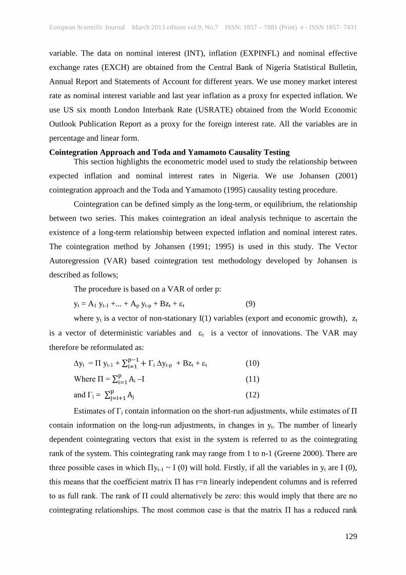
where it is the nominal interest rate, rt is the ex-ante real interest rate, and πet is the

expected inflation rate. Using the rational expectations model to estimate inflation

expectations would mean that the difference between actual inflation (πt) and expected

inflation (πet) is captured by an error term (εt):

πt - πet = εt (2)

This rational expectations model for inflation expectations can be incorporated into

the Fisher equation as follows.

it = rt + πt (3)

Rearranging equation 2:

πt = πet + εt (4)

where εt is a white noise error term. If we assume that the real interest rate is also

generated under a stationary process, where rate is the ex ante real interest rate and υt is the

stationary component, we obtain:

rt = rte + υt (5)

Now by substituting equation (4) and (5) into equation (3):

it = rte + πt

e+ μt (6)

Equation (6) is the traditional closed-economy Fisher hypothesis. Incorporating the

foreign interest rate and nominal effective exchange rate variable in the context of a small

open developing economy, we thus modify equation (6) as

it = rte + πt

e+ firt + excht + μt (7)

Therefore we estimate the following model:

INTt = δ + φ1EXPINFLt + φ2USRATEt + φ3EXCHt + μt (8)

where μt is the sum of the two stationary error terms (i.e εt+υt), rte (δ) is the long run

real interest rate, πte is the expected rate of inflation, firt is the foreign interest rate and excht

is the nominal effective exchange rate. The strong form Fisher hypothesis is validated if a

long-run unit proportional relationship exists between expected inflation (EXPINFLt) and

nominal interest rates (INTt) and φ1=1, if φ1<1 this would be consistent with a weak form

Fisher hypothesis.

The first challenge facing any empirical Fisherian study is to derive an inflation

expectations proxy. Wooldridge (2003) suggested that the expected inflation this year should

take the value of last year’s inflation: πte = πt−1.

Type and Sources of Data The empirical analysis was carried out using time series model. The study uses long

and up-to-date annual time-series data (1970-2011), with a total of 42 observations for each


129

variable. The data on nominal interest (INT), inflation (EXPINFL) and nominal effective

exchange rates (EXCH) are obtained from the Central Bank of Nigeria Statistical Bulletin,

Annual Report and Statements of Account for different years. We use money market interest

rate as nominal interest variable and last year inflation as a proxy for expected inflation. We

use US six month London Interbank Rate (USRATE) obtained from the World Economic

Outlook Publication Report as a proxy for the foreign interest rate. All the variables are in

percentage and linear form.

Cointegration Approach and Toda and Yamamoto Causality Testing This section highlights the econometric model used to study the relationship between

expected inflation and nominal interest rates in Nigeria. We use Johansen (2001)

cointegration approach and the Toda and Yamamoto (1995) causality testing procedure.

Cointegration can be defined simply as the long-term, or equilibrium, the relationship

between two series. This makes cointegration an ideal analysis technique to ascertain the

existence of a long-term relationship between expected inflation and nominal interest rates.

The cointegration method by Johansen (1991; 1995) is used in this study. The Vector

Autoregression (VAR) based cointegration test methodology developed by Johansen is

described as follows;

The procedure is based on a VAR of order p:

yt = A1 yt-1 +... + Ap yt-p + Bzt + εt (9)

where yt is a vector of non-stationary I(1) variables (export and economic growth), zt

is a vector of deterministic variables and εt is a vector of innovations. The VAR may

therefore be reformulated as:

∆yt = П yt-1 + ∑ +p−1i=1 Γi ∆yt-p + Bzt + εt (10)

Where П = ∑ Api=1 i –I (11)

and Γi = ∑ Apj=i+1 j (12)

Estimates of Γi contain information on the short-run adjustments, while estimates of Π

contain information on the long-run adjustments, in changes in yt. The number of linearly

dependent cointegrating vectors that exist in the system is referred to as the cointegrating

rank of the system. This cointegrating rank may range from 1 to n-1 (Greene 2000). There are

three possible cases in which Πyt-1 ~ I (0) will hold. Firstly, if all the variables in yt are I (0),

this means that the coefficient matrix Π has r=n linearly independent columns and is referred

to as full rank. The rank of Π could alternatively be zero: this would imply that there are no

cointegrating relationships. The most common case is that the matrix Π has a reduced rank


130

and there are r<(n−1) cointegrating vectors present in β . This particular case can be

represented by:

Π =αβ′ (13)

where α andβ are matrices with dimensions n x r and each column of matrix α

contains coefficients that represent the speed of adjustment to disequilibrium, while matrix β

contains the long-run coefficients of the cointegrating relationships.

In this case, testing for cointegration entails testing how many linearly independent

columns there are in Π , effectively testing for the rank of Matrix Π (Harris, 1995:78-79). If

we solve the eigenvalue specification of Johansen (1991), we obtain estimates of the

eigenvalues λ1 > … > λr > 0 and the associated eigenvectors β = (ν1, … νr). The co-

integrating rank, r, can be formally tested with two statistics. The first is the maximum

eigenvalue test given as:

λ- max = -T ln (1- λr+1), . (14)

Where the appropriate null is r = g cointegrating vectors against the alternative that r

≤ g+1. The second statistic is the trace test and is computed as:

λ-trace = -T∑ ln (1 − λi)ni=r+1 , (15)

where the null being tested is r = g against the more general alternative r ≤ n. The

distribution of these tests is a mixture of functional of Brownian motions that are calculated

via numerical simulation by Johansen and Juselius (1990) and Osterwald - Lenum (1992).

Cheung and Lai (1993) use Monte Carlo methods to investigate the small sample properties

of Johansen’s λ-max and λ-trace statistics. In general, they find that both the λ-max and-λ

trace statistics are sensitive to under parameterization of the lag length although they are not

so to over parameterization.

The causality analysis The most common way to test the causal relationship between two variables is the

Granger-Causality proposed by Granger (1969). The test involves estimating the following

simple vector autoregressions (VAR):

Xt =∑ 𝛼𝑛𝑖=1 i Yt-i + ∑ 𝛽𝑛

𝑗=1 jXt-j + µ1t (16)

Yt =∑ λ𝑚𝑖=1 i Xt-i + ∑ 𝛿𝑚

𝑗=1 jYt-j + µ2t (17)

Where it is assumed that the disturbances µ1t and µ2t are uncorrelated. Equation (16)

represents that variable X is decided by lagged variable Y and X, so does equation (17)

except that its dependent variable is Y instead of X.


131

Granger-Causality means the lagged Y influence X significantly in equation (16) and

the lagged X influence Y significantly in equation (17). In other words, researchers can

jointly test if the estimated lagged coefficient Σαi and Σλj are different from zero with F-

statistics. When the jointly test reject the two null hypotheses that Σαi and Σλj both are not

different from zero, causal relationships between X and Y are confirmed. The Granger-

Causality test is easy to carry out and be able to apply in many kinds of empirical studies.

However, traditional Granger-Causality has its limitations.

First, a two-variable Granger-Causality test without considering the effect of other

variables is subject to possible specification bias. As pointed out by Gujarati (1995), a

causality test is sensitive to model specification and the number of lags. It would reveal

different results if it was relevant and was not included in the model. Therefore, the empirical

evidence of a two-variable Granger-Causality is fragile because of this problem.

Second, time series data are often non-stationary (Maddala, 2001). This situation

could exemplify the problem of spurious regression. Gujarati (2006) had also said that when

the variables are integrated, the F-test procedure is not valid, as the test statistics do not have

a standard distribution. Although researchers can still test the significance of individual

coefficients with t-statistic, one may not be able to use F-statistic to jointly test the Granger-

Causality. Enders (2004) proved that in some specific cases, using F-statistic to jointly test

first differential VAR is permissible, when the two-variable VAR has lagged length of two

periods and only one variable is nonstationary. Other shortcomings of these tests have been

discussed in Toda and Phillips (1994).

Toda and Yamamoto (1995) propose an interesting yet simple procedure requiring the

estimation of an augmented VAR which guarantees the asymptotic distribution of the Wald

statistic (an asymptotic χ2-distribution), since the testing procedure is robust to the integration

and cointegration properties of the process.

We use a bivariate VAR (m + dmax) comprised of expected inflation and nominal

interest rate, following Yamada (1998);

Xt = ω + ∑ 𝜃𝑚𝑖=1 i Xt-i + ∑ 𝜃𝑚+𝑑𝑚𝑎𝑥

𝑖=𝑚+1 iXt-i + ∑ 𝛿𝑚𝑖=1 i Yt-i + ∑ 𝛿𝑚+𝑑𝑚𝑎𝑥

𝑖=𝑚+1 iYt-i + v1 (18)

Yt = ψ + ∑ φ𝑚𝑖=1 i Yt-i + ∑ φ𝑚+𝑑𝑚𝑎𝑥

𝑖=𝑚+1 iYt-i + ∑ 𝛽𝑚𝑖=1 i Xt-i + ∑ 𝛽𝑚+𝑑𝑚𝑎𝑥

𝑖=𝑚+1 iXt-i + v2t (19)

Where X= expected inflation and Y=nominal interest rate, and ω, θ’s, δ’s, ψ, φ’s and

β’s are parameters of the model. dmax is the maximum order of integration suspected to

occur in the system; ν1t ~N(0, Σv1 ) and ν2t ~N(0, Σv2 ) are the residuals of the model and Σv1


132

and Σv2 the covariance matrices of ν1t and ν2t , respectively. The null of non-causality from

expected inflation to nominal interest rate can be expressed as H0: δi= 0, ∀ i=1, 2, ..., m.

Two steps are involved with implementing the procedure. The first step includes the

determination of the lag length (m) and the second one is the selection of the maximum order

of integration (dmax ) for the variables in the system. Measures such as the Akaike

Information Criterion (AIC), Schwarz Information Criterion (SC), Final Prediction Error

(FPE) and Hannan-Quinn (HQ) Information Criterion can be used to determine the

appropriate lag order of the VAR.

We use the Augmented Dickey-Fuller (ADF) test for which the null hypothesis is

non-stationarity as well as Kwiatkowski-Phillips-Schmidt-Shin (KPSS) test for which the

null hypothesis is stationarity to determine the maximum order of integration. We choose

KPSS to have a crosscheck. Many economists have argued against using the standard unit

root tests and proposed using other powerful tests, such as tests that can be used to test the

null of stationarity against the alternative of non-stationarity. A number of tests have been

developed; the most popular one is the KPSS test developed by Kwiatkowski, Phillips,

Schmidt, and Shin (1992). Kwiatkowski et al. (1992) argue that their test is “intended to

complement unit root tests, such as the Dickey-Fuller tests. By testing both the unit root

hypothesis and the stationarity hypothesis, we can distinguish between series that appear to

be stationary, series that appear to have unit root, and series for which the data (or the tests)

are not sufficiently informative to be sure whether they are stationary or integrated.” Joint

testing of both nulls can strengthen inferences made about the stationarity or non-stationarity

of a time series especially when the outcomes of the two nulls corroborate each other. This

joint testing has been known as “confirmatory analysis.” For example, if the null of

stationarity is accepted (rejected) and the null of non-stationarity is rejected (accepted), we

have confirmation that the series is stationary (non-stationary). Conversely, we cannot have

confirmation if both nulls are accepted or both are rejected.

Empirical Findings Our main reason for conducting unit root tests is to determine the extra lags to be

added to the vector autoregressive (VAR) model for the Toda and Yamamoto test.


133

Table 1: Augmented Dickey-Fuller (ADF) Unit Root Test Variables Constant, with Trend Order of Integration

I(0) I(1) EXPINFL -3.521994

(-3.529758) -6.116158* (-3.533083)

I(1)

INTR

-0.372509 (-3.529758)

-7.161797* (-3.529758)

I(1)

EXCH -0.614710 (-3.523623)

-4.859365* (-3.526609)

I(1)

USRATE -5.620988* (-3.526609)

- I(0)

Notes: * denotes rejection of the null hypothesis of unit root the at 5% level. Critical values at 0.05 are in parenthesis.

Table 2: Kwiatkowski-Phillips-Schmidt-Shin (KPSS) Unit Root Test

Variables Constant, with Trend Order of Integration EXPINFL 0.133313

(0.146000) I(0)

INT 0.177541 (0.146000)

I(1)

EXCH 0.173273 (0.146000)

I(1)

USRATE 0.085406 (0.146000)

I(0)

Notes: * denotes rejection of the null hypothesis of stationarity the at 5% level. Critical values at 0.05 are in parenthesis.

Table 3: Confirmatory Analysis

Variables ADF KPSS Decision EXPINFL I(1) I(0) Inconclusive Decision (Insufficient

Information) INT I(1) I(1) Conclusive Decision (Non-Stationary) EXCH I(1) I(1) Conclusive Decision (Non-Stationary) USRATE I(0) I(0) Conclusive Decision (Stationary)

Confirmatory analysis presented in Table 3 is drawn from the two unit root tests

shown in Table 1 and Table 2 and it shows that only USRATE is stationary at level while the

variables INT and EXCH are non-stationary at level. However, for EXPINFL variable, the

unit root decision is inconclusive. Hence, VAR models will add only one extra lag (i.e

dmax=1) for the implementation of the causality test. Following the modelling approach

described earlier, we determine the appropriate lag length and conducted the cointegration

test. Table 4: Lag Length Selection

Lag LR FPE AIC SC HQ 0 NA 1.26e+08 30.00559 30.17974 30.06699 1 154.3346 2428155* 26.04750 26.91826* 26.35448* 2 18.89087 3035786 26.23769 27.80507 26.79026 3 28.02917* 2441756 25.93467* 28.19866 26.73283 4 13.29489 3543459 26.13479 29.09540 27.17854

*indicates lag order selected by the criterion


134

Table 4 reports the optimal lag length of one (i.e m=1) out of a maximum of 4 lag

lengths as selected by Final Prediction Error (FPE), Schwarz Information Criterion (SC) and

Hannan-Quinn Information Criterion. We employed VAR Residual Serial Correlation LM

Tests and inverse roots of the characteristic AR polynomial and found that the VAR is well-

specified; there is no autocorrelation problem at the optimal lag at 10% level, all the inverse

roots of the characteristic AR polynomial must lie inside the unit circle and the modulus

values are 0.89, 0.78, 0.78, 0.67, 0.67, 0.31, 0.19 and 0.19 thus VAR satisfies the stability

condition. Table 5: Result of Cointegration Test

Null Hypothesis Test Statistics

0.05 Critical Value

Probability Value

Lags 1 Trace Statistics

r=0 52.66960 47.85613 0.0165 r=1 19.14699 29.79707 0.4824

Max-Eigen Statistics

r=0 33.52261 27.58434 0.0077 r≤1 14.01310 21.13162 0.3640

Trace No of Vectors 1 Max-Eigen No of Vectors 1 aDenotes rejection of the null hypothesis at 0.05 level

Table 5 provides the results from the application of Johansen cointegration test among

the data set. Empirical findings show that both the maximum eigenvalue and the trace tests

reject the null hypothesis of no cointegration at the 5 percent significance level according to

critical value estimates. The result shows a cointegration rank of one in both trace test and

max-eigen value test at 5% significance level. Thus the maximum order of integration (dmax

) for the variables in the system is one (dmax=1)

The results above are based on the assumptions of linear deterministic trend and lag

interval in first differences of 1 to 2. Overall, the Johansen cointegration test suggests that

there exists a sustainable cum long-run equilibrium relationship between the variable. This

suggests causality in at least one direction.

Since the existence of a long-run relationship has been established between long-term

interest rates and expected inflation and other variables, the short-run dynamics of the model

can be established within an error correction model. In order to estimate the Fisher effect we

will use a simple formulation of an error correction model. We specify the error correction

term as follows;

INTt = δ + φ1EXPINFLt + φ2USRATEt + φ3EXCHt + μt (from equation 8)

μt = INTt - δ - φ1EXPINFLt - φ2USRATEt - φ3EXCHt (20)


135

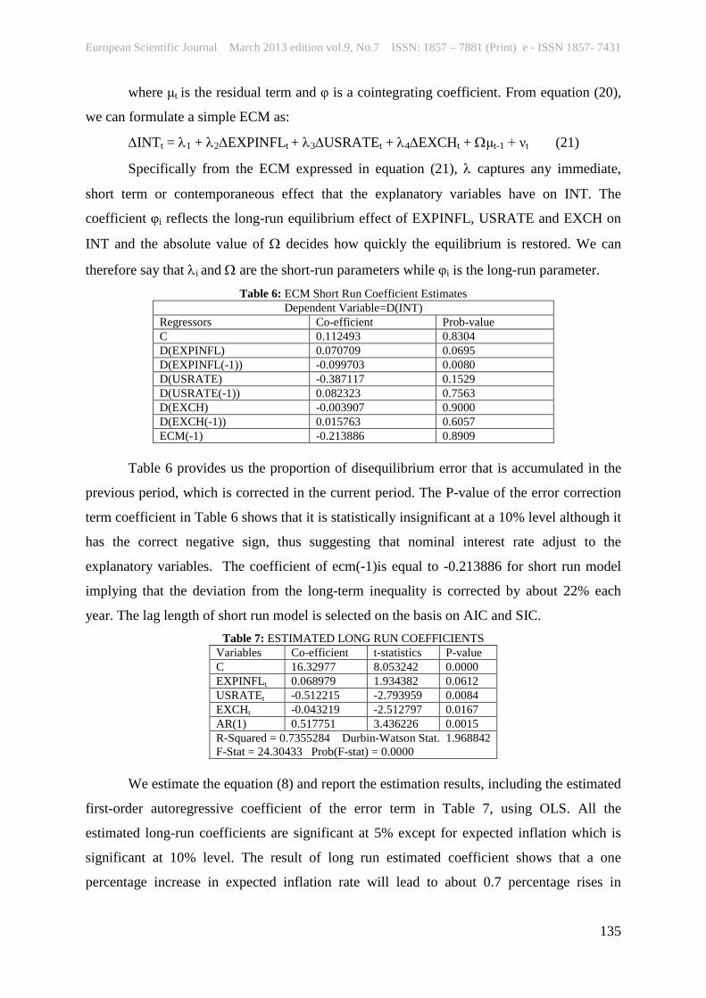
where μt is the residual term and φ is a cointegrating coefficient. From equation (20),

we can formulate a simple ECM as:

∆INTt = λ1 + λ2∆EXPINFLt + λ3∆USRATEt + λ4∆EXCHt + Ωμt-1 + νt (21)

Specifically from the ECM expressed in equation (21), λ captures any immediate,

short term or contemporaneous effect that the explanatory variables have on INT. The

coefficient φi reflects the long-run equilibrium effect of EXPINFL, USRATE and EXCH on

INT and the absolute value of Ω decides how quickly the equilibrium is restored. We can

therefore say that λi and Ω are the short-run parameters while φi is the long-run parameter. Table 6: ECM Short Run Coefficient Estimates

Dependent Variable=D(INT) Regressors Co-efficient Prob-value C 0.112493 0.8304 D(EXPINFL) 0.070709 0.0695 D(EXPINFL(-1)) -0.099703 0.0080 D(USRATE) -0.387117 0.1529 D(USRATE(-1)) 0.082323 0.7563 D(EXCH) -0.003907 0.9000 D(EXCH(-1)) 0.015763 0.6057 ECM(-1) -0.213886 0.8909

Table 6 provides us the proportion of disequilibrium error that is accumulated in the

previous period, which is corrected in the current period. The P-value of the error correction

term coefficient in Table 6 shows that it is statistically insignificant at a 10% level although it

has the correct negative sign, thus suggesting that nominal interest rate adjust to the

explanatory variables. The coefficient of ecm(-1)is equal to -0.213886 for short run model

implying that the deviation from the long-term inequality is corrected by about 22% each

year. The lag length of short run model is selected on the basis on AIC and SIC. Table 7: ESTIMATED LONG RUN COEFFICIENTS

Variables Co-efficient t-statistics P-value C 16.32977 8.053242 0.0000 EXPINFLt 0.068979 1.934382 0.0612 USRATEt -0.512215 -2.793959 0.0084 EXCHt -0.043219 -2.512797 0.0167 AR(1) 0.517751 3.436226 0.0015 R-Squared = 0.7355284 Durbin-Watson Stat. 1.968842 F-Stat = 24.30433 Prob(F-stat) = 0.0000

We estimate the equation (8) and report the estimation results, including the estimated

first-order autoregressive coefficient of the error term in Table 7, using OLS. All the

estimated long-run coefficients are significant at 5% except for expected inflation which is

significant at 10% level. The result of long run estimated coefficient shows that a one

percentage increase in expected inflation rate will lead to about 0.7 percentage rises in


136

nominal interest rate while a ten percentage rise in foreign interest rate (USRATE) will bring

about a fall in nominal interest rate by 5.12 percent. Furthermore, a unit increase in nominal

effective exchange rate will lead to about 0.45 unit fall in nominal interest rate. The

coefficient of determination (R2) is about 0.74. The result shows that about 74% of variation

in nominal interest rate is caused by variations in the explanatory variables. The Durbin-

Watson statistics are 1.968842 which shows the absence of serial correlation.

We conducted next the Wald coefficient tests to investigate whether full Fisher

Hypothesis holds for Nigeria or not, and if not, to verify if there is Fisher effect at all. The

results of these tests are reported in tables 8 and 9. The Wald test results shown in Table 8

reveal that full (standard) Fisher’s hypothesis does not hold in the Nigerian economy. The

Wald tests in table 10 show that Fisher effect is strong in the economy and that the other

variables are significantly different from zero. Table 8: Wald coefficient test for strong Fisher Hypothesis

Estimated equation; INTt = δ + φ1EXPINFLt + φ2USRATEt + φ3EXCHt

Null Hypothesis; φ1=1 Test Statistics Value Df Probability t-statistics -26.10862 35 0.0000 F- statistics 681.6602 (1,35) 0.0000 x2 – statistics 681.6602 1 0.0000

Table 9: Wald coefficient test for the significance of constant and other dependent variable

Estimated equation; INTt = δ + φ1EXPINFLt + φ2USRATEt + φ3EXCHt

Null Hypothesis; δ=0, φ1=0, φ2=0, φ3=0, Test Statistics Value Df Probability F- statistics 40.46246 (4,35) 0.0000 x2 – statistics 161.8499 4 0.0000

Toda-Yamamoto Granger Causality Test Having ascertained that a cointegrating relationship exist between among nominal

interest rates, expected inflation rate, foreign interest rate and nominal effective exchange

rate, the final step in this study is to verify if inflation Granger Cause nominal interest as

posed by Fisher Hypothesis using the Toda and Yamamoto causality test. If so then we can

say that it is nominal interest rates that respond to movements in inflation expectations. The

empirical results of Granger Causality test based on Toda and Yamamoto (1995)

methodology is estimated through MWALD test and reported in Table: 11. The estimates of

MWALD test show that the test result follows the chi-square distribution with 3 degrees of

freedom in accordance with the appropriate lag length along with their associated probability.


137

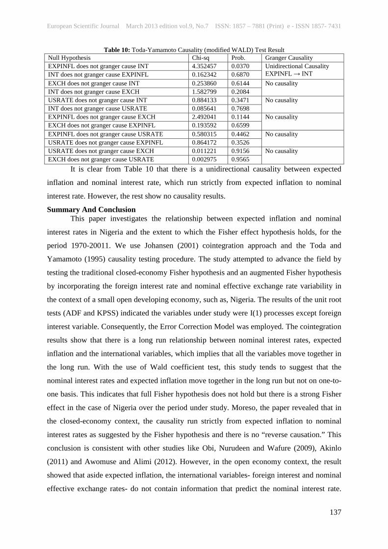
Table 10: Toda-Yamamoto Causality (modified WALD) Test Result Null Hypothesis Chi-sq Prob. Granger Causality EXPINFL does not granger cause INT 4.352457 0.0370 Unidirectional Causality

EXPINFL → INT INT does not granger cause EXPINFL 0.162342 0.6870 EXCH does not granger cause INT 0.253860 0.6144 No causality INT does not granger cause EXCH 1.582799 0.2084 USRATE does not granger cause INT 0.884133 0.3471 No causality INT does not granger cause USRATE 0.085641 0.7698 EXPINFL does not granger cause EXCH 2.492041 0.1144 No causality EXCH does not granger cause EXPINFL 0.193592 0.6599 EXPINFL does not granger cause USRATE 0.580315 0.4462 No causality USRATE does not granger cause EXPINFL 0.864172 0.3526 USRATE does not granger cause EXCH 0.011221 0.9156 No causality EXCH does not granger cause USRATE 0.002975 0.9565

It is clear from Table 10 that there is a unidirectional causality between expected

inflation and nominal interest rate, which run strictly from expected inflation to nominal

interest rate. However, the rest show no causality results.

Summary And Conclusion This paper investigates the relationship between expected inflation and nominal

interest rates in Nigeria and the extent to which the Fisher effect hypothesis holds, for the

period 1970-20011. We use Johansen (2001) cointegration approach and the Toda and

Yamamoto (1995) causality testing procedure. The study attempted to advance the field by

testing the traditional closed-economy Fisher hypothesis and an augmented Fisher hypothesis

by incorporating the foreign interest rate and nominal effective exchange rate variability in

the context of a small open developing economy, such as, Nigeria. The results of the unit root

tests (ADF and KPSS) indicated the variables under study were I(1) processes except foreign

interest variable. Consequently, the Error Correction Model was employed. The cointegration

results show that there is a long run relationship between nominal interest rates, expected

inflation and the international variables, which implies that all the variables move together in

the long run. With the use of Wald coefficient test, this study tends to suggest that the

nominal interest rates and expected inflation move together in the long run but not on one-to-

one basis. This indicates that full Fisher hypothesis does not hold but there is a strong Fisher

effect in the case of Nigeria over the period under study. Moreso, the paper revealed that in

the closed-economy context, the causality run strictly from expected inflation to nominal

interest rates as suggested by the Fisher hypothesis and there is no “reverse causation.” This

conclusion is consistent with other studies like Obi, Nurudeen and Wafure (2009), Akinlo

(2011) and Awomuse and Alimi (2012). However, in the open economy context, the result

showed that aside expected inflation, the international variables- foreign interest and nominal

effective exchange rates- do not contain information that predict the nominal interest rate.


138

Next we estimated short run dynamics of the model which suggested that about 22 percent of

the disequilibrium between long term and short term interest rate is corrected within the year.

Policy implication based on the partial Fisher effect in Nigeria is that more credible

policy should anchor a stable inflation expectation over the long-run and the level of actual

inflation should become the central target variable of the monetary policy. In addition, the

government should encourage and support the real sector through subsidies and investment in

infrastructure as a way of curbing inflation. This gesture in turn will reduce interest rates and

consequentially promote economic growth.

References:

Akinlo, A. E. (2011). A re-examination of the Fisher Hypothesis for Nigeria. Akungba

Journal of Economic Thought. Vol.5, Number 1

Atkins, F.J. & Serletis, A. (2002). A bounds test of the Gibson paradox and the Fisher effect:

evidence from low-frequency international data. Discussion Paper 2002-13. Calgary:

Department of Economics, University of Calgary.

Awomuse, B.O. & Alimi, R.S (2012), The relationship between Nominal Interest Rates and

Inflation: New Evidence and Implications for Nigeria. Journal of Economics and Sustainable

development, Vol. 3, No 9.

Beyer, A., Haug, A.A. and Dewald, W.G. (2009), Structural Breaks, Co-integration and the

Fisher Effect,” ECB Working Paper Series, No. 1013, February.

Booth, G. G. & Ciner, C., (2001). The relationship between nominal interest rates and

inflation: international evidence. Journal of Multinational Financial Management 11, 269-

280.

Carneiro, F.G., Divino, J.A.C.A. & Rocha, C.H., (2002). Revisiting the Fisher hypothesis for

the cases Argentina, Brazil and Mexico. Applied Economics Letters. 9, 95-98.

Cheung, Y., & Lai, K., (1993). Finite-sample sizes of Johansen’s likelihood ratio tests for

cointegration. Oxford bulletin of Economics and Statistics 55, 313-328.

Choudhry, A., (1997). Cointegration analysis of the inverted Fisher effect: Evidence from

Belgium, France and Germany. Applied Economics Letters 4, 257-260.

Coppock, L & Poitras, M (2000), Evaluating the Fisher Effect in Long-term Cross-country

Averages, International Review of Economics and Finance, Vol. 9 Issue 2, pp. 181-192,

Summer.Retrieved from http://www.sciencedirect.com/science/journal/10590560

Crowder, W.J. & Hoffman, D.L. (1996). The Long-run relationship between nominal interest

rates and inflation: The Fisher equation revisited. Journal of Money, Credit, and Banking. 28,


139

1:102-118.

Darby, M. R. (1975). “The Financial and Tax Effects of Monetary Policy on Interest Rates,”

Economic Inquiry, Vol. 13 No. 2, pp. 226-276.

Deutsch Bundesbank report (2001). “Real Interest Rates: Movement and Determinants,” pp.

31-47, July.

Dutt, S.D. & Ghosh, D. (1995). The Fisher hypothesis: Examining the Canadian experience.

Applied Economics. 27, 11:1025-1030.

Esteve, V., Bajo-Rubio, O. & Diaz-Roldan, C., (2003). Testing the Fisher effect in the

presence of structural change: a case study of the UK, 1961-2001. Documento de trabajo,

Serie Economia E2003/22. Sevilla: Fundacion Centro de Estudios Andaluces.

Fahmy, Y.A.F. & Kandil, M., (2003). The Fisher effect: New evidence and implications.

International Review of Economics & Finance. 12, 4:451-465.

Fisher, I., (1930). The Theory of Interest. New York: Macmillan.

Froyen, R.T. & Davidson, L.S. (1978), Estimates of the Fisher Effect: A Neo-Keynesian

Approach, Atlantic Economic Journal Vol. 6, No. 2 July. Retrieved from

http://www.springerlink.com/content/wh8251553282/?p=cc91ee845f6f4179aa6af1ae217866

9d&pi=0

Garcia, M.G.P., (1993). The Fisher effect in a signal extraction framework: The recent

Brazilian experience. Journal of Development Economics. 41, 1:71-93.

Ghazali, N.A. & Ramlee, S., (2003). A long memory test of the long-run Fisher effect in the

G7 countries. Applied Financial Economics. 13,10:763-769.

Granger, C. W. J. (1969) Investigating causal relations by econometric models and cross

spectral methods, Econometrica, 37, 424- 38

Greene, W.H., (2000). Econometric Analysis (4e). New Jersey: Prentice-Hall, Inc.

Gujarati, D.N (2006) Essential of Econometrics, 3rd Edition, McGraw Hill

Harris, R., (1995). Using cointegration analysis in econometric modelling. London: Prentice

Hall.

Hawtrey, K. M., (1997). The Fisher effect and Australian interest rates. Applied Financial

Economics. 7, 4:337-346.

Johansen, S. & Juselius, K., (1990). Maximum likelihood estimation and inference on

cointegration – with applications to the demand for money. Oxford Bulletin of Economics and

Statistics. 52, 2:169-210.

Johansen, S., (1991). Estimation and hypothesis testing of cointegration vectors in Gaussian

vector autoregressive models. Econometrica. 59, 1551-1580.


140

Johansen, S., (1992). Cointegration in partial systems and the efficiency of single-equation

analysis. Journal of Econometrics. 52, 389-402.

Johansen, S., (1995). Likelihood-Based Inference in Cointegrated Vector Autoregressive

Models. Oxford: Oxford University Press.

Johnson, PA (2005), Is It Really the Fisher Effect? Vassar College Economics Working

Paper #58. Retrieved from http://irving.vassar.edu/VCEWP/VCEWP58.pdf

Jorgensen, J.J. & Terra, P.R.S., (2003). The Fisher hypothesis in a VAR framework: Evidence

from advanced and emerging markets. Conference Paper. Helsinki: European Financial

Management Association. Annual Meetings, 25-28 June.

Juntitila, J., (2001). Testing an augmented Fisher hypothesis for a small open economy: The

case of Finland. Journal of Macroeconomics. 23, 4:577-599.

Koustas, Z. & Serletis, A., (1999). On the Fisher effect. Journal of Monetary Economics. 44,

1:105-130.

Kwiatkowski, D. et al. (1992), “Testing the Null Hypothesis of Stationarity against the

Alternative of a Unit Root,” Journal of Economics, 54, 159-178.

Laatsch, F.E and Klien, D.P., (2002). Nominal rates, real rates and expected inflation U.S

treasury inflation: Results from a study of U.S. treasury inflation protected securities. The

Quarterly Review of Economics and Finance. 43, 3: 405-417.

Lardic, S. and Mignon, V., (2003). Fractional cointergration between nominal interest rates

and inflation: A re-examination of the Fisher relationship in the G7 countries. Economic

Bulletin. 3, 14:1-10.

Lee, J.L., Clark, C. & Ahn, S.K., (1998). Long- and short-run Fisher effects: new tests and

new results. Applied Economics. 30, 1:113-124.

Lee, K. F. (2007), An Empirical Study of the Fisher Effect and the Dynamic Relation

between Nominal Interest Rates and Inflation in Singapore, MPRA Paper No. 12383.

Maddala, G.S (2001) Introduction to Econometrics, 3rd Edition, Wiley and Sons, Inc

Mishkin, F.S. & Simon, J., (1995). An empirical examination of the Fisher effect in Australia.

Economic Record. 71, 214:217-229.

Mitchell-Innes H. A. (2006), The Relationship between Interest Rates and Inflation in South

Africa: Revisiting Fisher’s Hypothesis. (Master’s Dissertation, Rhodes University 2006)

Mitchell-Innes, H. A. (2006), The Relationship between Interest Rates and Inflation in South

Africa: Revisiting the Fisher’s Hypothesis. A Masters Thesis Submitted to Rhodes

University, South Africa.

Mitchell-Innes, H. A., Aziakpono, M.J. & Faure, A. P. (2008), Inflation Targeting and the


141

Fisher Effect in South Africa: An Empirical Investigation, South African Journal of

Economics, Volume 75 Issue 4, Pages 693 – 707. Retrieved from

http://www3.interscience.wiley.com/journal/117961981/home

Miyagawa, S. and Morita, Y., (2003). The Fisher effect and the long- run Phillips curve - in

the case of Japan, Sweden and Italy. Working Paper in Economics No. 77. Göteborg:

Department of Economics, Göteborg University.

Mohsen, Bahmani-Oskooee, Ng R.. W., (2002), “Long Run Demand for Money in Hong

Kong: An Application of the ARDL Model, International journal of business and economics,

Vol. 1, No. 2, pp. 147-155.

Muscatelli, V.A. & Spinelli, F., (2000). Fisher, Barro, and the Italian interest rate 1845-93.

Journal of Policy Modeling. 22, 2:149-169.

Obi, B., Nurudeen, A., & Wafure, O. G., (2009). An empirical investigation of the Fisher

effect in Nigeria: a cointegration and error correction approach. International Review of

Business Research Papers 5, 96-109.

Obstfeld M. Krugman, P. R., (2003) International Economics: Theory and Policy. Addison

Wesley, 6th edition.

Osterwald-Lenum, M., (1992). A note with quintiles of the asymptotic distribution of the

maximum likelihood cointegration rank test statistics. Oxford bulletin of Economics and

Statistics 54, 461-472

Panopoulou, E. (2005), A Resolution of the Fisher Effect Puzzle: A Comparison of

Estimators, Retrieved from

http://economics.nuim.ie/research/workingpapers/documents/N1500205.pdf

Perez, S.J. & Siegler, M.V. (2003), Inflationary Expectations and the Fisher Effect Prior to

World War I, Journal of Money, Credit, and Banking, Vol. 35, No 6, December 2003, pp.

947-965. Retrieved from

http://muse.jhu.edu/journals/journal_of_money_credit_and_banking/toc/mcb35.6a.html

Phylaktis, K. & Blake, D., (1993). The Fisher hypothesis: Evidence from three high inflation

economies. Weltwirtschaftliches Archiv. 129, 3:591-599.

Suleiman (2005), “The Impact of Investment and Financial Intermediation on economic

Growth: New Evidence from Jordan. Abstract mimeo.

Toda, H.Y. & P.C.B. Phillips (1994) : “Vector Autoregressions and Causality: A Theoretical

Overview and Simulation Study”, Econometric Reviews 13, 259-285

Toda, H.Y. & Yamamoto (1995) Statistical inference in Vector Autoregressions with

possibly integrated processes. Journal of Econometrics, 66, 225-250.


142

Weidmann, J. (1997), New Hope for the Fisher Effect? A Re-examination Using Threshold

Co-integration, University of Bonn Discussion Paper B-385.

Wesso, G.R., (2000). Long-term yield bonds and future inflation in South Africa: a vector

error-correction analysis. Quarterly Bulletin. Pretoria: South African Reserve Bank. June.

Westerlund, J. (2008), Panel Co-integration Tests of the Fisher Effect. Journal of Applied

Economics, 23, pp.193-233.

Wooldridge, J. M., (2003). Introductory Econometrics: A Modern Approach. Southwestern.

Yamada, H. (1998). A note on the causality between export and productivity: an empirical re-

examination. Economics Letters, 61, 111-114.

Yuhn, K., (1996). Is the Fisher effect robust? Further evidence. Applied Economics Letters. 3,

41–44.

APPENDIX 1:

Summary of some empirical Literature on Fisher Hypothesis Author and Date Country Methods Expected

Inflation Proxy

Period Fisher Effect

Choudhry, 1997 Belgium* E&G= Engle & Granger and Harris & Inder cointegration analysis

CPI 1955-1994

Rejected

Cameriro, Divino and Rocha, 2002

Brazil* Johansen cointegration analysis

REH, Moving Average

1980-1998

Accepted

Atkins & Serletis, 2002

Canada* Pesaran, M. H., Shin, Y. and Smith, R.J. ARDL bound;

CPI 1880-1983

Rejected

Ghazali & Ramlee, 2003

Canada* Autoregressive fractionally integrated moving average;

CPI 1974-1996

Rejected

Ghazali & Ramlee, 2003

Canada* Ordinary least squares CPI 1974-1996

Accepted

Jorgensen & Terra, 2003

Chile Four Variable VAR CPI 1977-1999

Rejected

Junita, 2001 Finland Johansen cointegration analysis

ARIMA 1987-1996

Rejected

Lardic & Mignon, 2003

France Granger fractional cointegration analysis

CPI 1970-2004

Accepted

Wesso, 2000 South Africa

Johansen cointegration analysis

CPI 1985-1999

Accepted

Esteve, Bajo-Rubio & Diaz-Roldan, 2003

United Kingdom

Stock & Watson (DOLS) dynamic ordinary least squares

GDP Deflator

1961-2001

Accepted

Fahmy & Kandil, 2003

USA Johansen cointegration analysis

CPI 1980’s 1990’s

Accepted

Laatsch & Klien, 2002

USA Regression Break-even 1997-2001

Accepted

TODA-YAMAMOTO CAUSALITY TEST BETWEEN ... - CORE

Documents

Transcript of TODA-YAMAMOTO CAUSALITY TEST BETWEEN ... - CORE