Modeling Count Time SeriesFollowing

Generalized Linear Models

DissertationTobias Liboschik

In partial fulfillment of therequirements for the degree of

Doktor der Naturwissenschaftenpresented to the

Department of StatisticsTU Dortmund University

Advisors:Prof. Dr. Roland Fried, TU Dortmund University

Prof. Dr. Konstantinos Fokianos, University of Cyprus

Dortmund, 13th July 2016

Abstract

Count time series are found in many different applications, e.g. from medicine, financeor industry, and have received increasing attention in the last two decades. The class ofcount time series following generalized linear models is very flexible and can describeserial correlation in a parsimonious way. The conditional mean of the observed process islinked to its past values, to past observations and to potential covariate effects. In thisthesis we give a comprehensive formulation of this model class. We consider models withthe identity and with the logarithmic link function. The conditional distribution can bePoisson or Negative Binomial. An important special case of this class is the so-calledINGARCH model and its log-linear extension.

A key contribution of this thesis is the R package tscount which provides likelihood-basedestimation methods for analysis and modeling of count time series based on generalizedlinear models. The package includes methods for model fitting and assessment, predictionand intervention analysis. This thesis summarizes the theoretical background of thesemethods. It gives details on the implementation of the package and provides simulationresults for models which have not been studied theoretically before. The usage of thepackage is illustrated by two data examples. Additionally, we provide a review of Rpackages which can be used for count time series analysis. A detailed comparison oftscount to those packages demonstrates that tscount is an important contribution whichextends and complements existing software.

A thematic focus of this thesis is the treatment of all kinds of unusual effects influencingthe ordinary pattern of the data. This includes structural changes and different forms ofoutliers one is faced with in many time series. Our first study on this topic is concernedwith retrospective detection of such changes. We analyze different approaches for modelingsuch intervention effects in count time series based on INGARCH models. Other authorstreated a model where an intervention affects the non-observable underlying mean processat the time point of its occurrence and additionally the whole process thereafter via itsdynamics. As an alternative, we consider a model where an intervention directly affects

v

the observation at its occurrence, but not the underlying mean, and then also enters thedynamics of the process. While the former definition describes an internal change of thesystem, the latter can be understood as an external effect on the observations due to e.g.immigration. For our alternative model we develop conditional likelihood estimation and,based on this, develop tests and detection procedures for intervention effects. Both modelsare compared analytically and using simulated and real data examples. The proceduresfor our new model work reliably and we find some robustness against misspecification ofthe intervention model.

The aforementioned methods are applied after the complete time series has been observed.In another study we investigate the prospective detection of structural changes, i.e. in realtime. For example in public health, surveillance of infectious diseases aims at recognizingoutbreaks of epidemics with only short time delays in order to take adequate actionpromptly. We point out that serial dependence is present in many infectious disease timeseries. Nevertheless it is still ignored by many procedures used for infectious diseasesurveillance. Using historical data, we design a prediction-based monitoring procedurefor count time series following generalized linear models. We illustrate benefits but alsopitfalls of using dependence models for monitoring.

Moreover, we briefly review the literature on model selection, robust estimation androbust prediction for count time series. We also make a first study on robust modelidentification using robust estimators of the (partial) autocorrelation.

Keywords: Count time series, generalized linear models, serial correlation, temporaldependence, autoregressive models, regression models, likelihood, mixed Poisson, modelselection, prediction, forecasting, statistical software, R, intervention analysis, level shifts,outliers, statistical process control, online monitoring, change point detection, aberrationdetection, outbreak detection, infectious disease surveillance, epidemiology, public health.

vi

Contents

1 Introduction 11.1 Motivation . . . . . . . . . . . . . . . . . . . . . . . . . . . . . . . . . . . 11.2 Models . . . . . . . . . . . . . . . . . . . . . . . . . . . . . . . . . . . . . 21.3 Outline . . . . . . . . . . . . . . . . . . . . . . . . . . . . . . . . . . . . . 5

2 Basic methods and implementation 92.1 Introduction . . . . . . . . . . . . . . . . . . . . . . . . . . . . . . . . . . 92.2 Estimation and inference . . . . . . . . . . . . . . . . . . . . . . . . . . . 11

2.2.1 Estimation . . . . . . . . . . . . . . . . . . . . . . . . . . . . . . . 112.2.2 Inference . . . . . . . . . . . . . . . . . . . . . . . . . . . . . . . . 132.2.3 Implementation . . . . . . . . . . . . . . . . . . . . . . . . . . . . 14

2.3 Prediction . . . . . . . . . . . . . . . . . . . . . . . . . . . . . . . . . . . 152.4 Model assessment . . . . . . . . . . . . . . . . . . . . . . . . . . . . . . . 162.5 Intervention analysis . . . . . . . . . . . . . . . . . . . . . . . . . . . . . 202.6 Usage of the package . . . . . . . . . . . . . . . . . . . . . . . . . . . . . 22

2.6.1 Campylobacter infections in Canada . . . . . . . . . . . . . . . . 242.6.2 Road casualties in Great Britain . . . . . . . . . . . . . . . . . . . 27

2.7 Comparison with other software packages . . . . . . . . . . . . . . . . . . 312.7.1 Packages for independent data . . . . . . . . . . . . . . . . . . . . 312.7.2 Packages for time series data . . . . . . . . . . . . . . . . . . . . . 35

2.8 Discussion . . . . . . . . . . . . . . . . . . . . . . . . . . . . . . . . . . . 44

3 Retrospective intervention detection 473.1 Introduction . . . . . . . . . . . . . . . . . . . . . . . . . . . . . . . . . . 473.2 Intervention models . . . . . . . . . . . . . . . . . . . . . . . . . . . . . . 483.3 Estimation and inference . . . . . . . . . . . . . . . . . . . . . . . . . . . 51

3.3.1 Starting value for optimization . . . . . . . . . . . . . . . . . . . . 523.3.2 Properties of the maximum likelihood estimator . . . . . . . . . . 54

3.4 Testing for intervention effects . . . . . . . . . . . . . . . . . . . . . . . . 573.4.1 Intervention of known type at known time . . . . . . . . . . . . . 573.4.2 Intervention of known type at unknown time . . . . . . . . . . . . 603.4.3 Multiple interventions of unknown type at unknown time . . . . . 633.4.4 Misspecification of the intervention model . . . . . . . . . . . . . 64

3.5 Real data application . . . . . . . . . . . . . . . . . . . . . . . . . . . . . 653.6 Discussion . . . . . . . . . . . . . . . . . . . . . . . . . . . . . . . . . . . 67

vii

4 Online monitoring in the context of infectious disease surveillance 694.1 Introduction . . . . . . . . . . . . . . . . . . . . . . . . . . . . . . . . . . 694.2 Models for the in-control process . . . . . . . . . . . . . . . . . . . . . . 724.3 Prediction-based monitoring . . . . . . . . . . . . . . . . . . . . . . . . . 77

4.3.1 Monitoring procedure . . . . . . . . . . . . . . . . . . . . . . . . . 774.3.2 Calibration and performance measures . . . . . . . . . . . . . . . 78

4.4 Simulation study . . . . . . . . . . . . . . . . . . . . . . . . . . . . . . . 804.5 Case study . . . . . . . . . . . . . . . . . . . . . . . . . . . . . . . . . . . 85

4.5.1 Model selection and fitting in the set-up phase . . . . . . . . . . . 864.5.2 Nonstationarity vs. serial dependence . . . . . . . . . . . . . . . . 954.5.3 Monitoring in the operational phase . . . . . . . . . . . . . . . . . 96

4.6 Discussion . . . . . . . . . . . . . . . . . . . . . . . . . . . . . . . . . . . 98

5 Further topics 1015.1 Towards a comprehensive model selection strategy . . . . . . . . . . . . . 1015.2 Robust model identification with the (partial) autocorrelation function . 1035.3 Robust estimation and prediction . . . . . . . . . . . . . . . . . . . . . . 108

6 Summary 111

Acknowledgements 113

References 115

A Implementation details 125A.1 Parameter space for the log-linear model . . . . . . . . . . . . . . . . . . 125A.2 Recursions for inference and their initialization . . . . . . . . . . . . . . . 126A.3 Starting value for optimization . . . . . . . . . . . . . . . . . . . . . . . . 128A.4 Stable inversion of the information matrix . . . . . . . . . . . . . . . . . 130

B Additional simulations 133B.1 Covariates . . . . . . . . . . . . . . . . . . . . . . . . . . . . . . . . . . . 133B.2 Negative Binomial distribution . . . . . . . . . . . . . . . . . . . . . . . . 139B.3 Quasi information criterion . . . . . . . . . . . . . . . . . . . . . . . . . . 140

viii

Chapter 1

Introduction

1.1 Motivation

Count time series appear naturally in various areas whenever a number of events per timeperiod is observed over time. Examples for the wide range of applications in medicine arethe weekly number of patients recruited for a clinical trial, the daily number of hospitaladmissions or the weekly number of epileptic seizures of a patient. An important examplefrom epidemiology is the weekly number of registered infections by certain pathogens,which is routinely collected by public health authorities. Important objectives of suchdata analysis are the prediction of future values for adequate planning of resources, thedetection of unusual values pointing at some epidemics or the proper description ofe.g. seasonal patterns for better understanding and interpretation of data generatingmechanisms. Examples from other fields are the number of stock market transactionsper minute, from finance, or the hourly number of defect items, from industrial qualitycontrol.

Models for count time series should take into account that the observations are nonnegativeintegers and they should capture suitably the dependence among observations. Aconvenient and flexible approach is to employ the generalized linear model (GLM)methodology (Nelder and Wedderburn, 1972) for modeling the observations conditionallyon the past information. This methodology is implemented by choosing a suitabledistribution for count data and an appropriate link function. Such an approach ispursued by Fahrmeir and Tutz (2001, Chapter 6) and Kedem and Fokianos (2002,Chapters 1–4), among others. Another important class of models for time series ofcounts is based on the thinning operator, like the integer autoregressive moving average(INARMA) models, which, in a way, imitate the structure of the common autoregressive

1

moving average (ARMA) models (see the review article by Weiß, 2008). A different typeof count time series models are the so-called state space models. We refer to the reviewsof Fokianos (2011), Jung and Tremayne (2011), Fokianos (2012), Tjøstheim (2012) andFokianos (2015) for an in-depth overview of models for count time series. Advantages ofGLM-based models compared to the models which are based on the thinning operatorare the following:

(a) They can describe covariate effects and negative correlations in a straightforwardway.

(b) There is a rich toolkit available for this class of models.

State space models allow to describe even more flexible data generating processes thanGLM models but at the cost of a more complicated model specification. On the otherhand, GLM-based models yield predictions in a convenient manner due to their explicitformulation.

This thesis is concerned with methods for count time series based on generalized linearmodels. In the following section we give a comprehensive formulation of this model class.

1.2 Models

Denote a count time series by {Yt : t ∈ N}. We will denote by {X t : t ∈ N} a time-varyingr-dimensional covariate vector, say X t = (Xt,1, . . . , Xt,r)

>. We model the conditionalmean E (Yt|Ft−1) of the count time series by a process, say {λt : t ∈ N}, such thatE (Yt|Ft−1) = λt. Denote by Ft0 the history of the joint process {Yt, λt,X t+1 : t ∈ N}up to time t0 including the covariate information at time t0 + 1. The distributionalassumption for Yt given Ft−1 is discussed later. We are interested in models of the generalform

g(λt) = β0 +

p∑k=1

βk g(Yt−ik) +

q∑`=1

α`g(λt−j`) + η>X t, (1.1)

where g : R+ → R is a link function and g : N0 → R is a transformation function.The parameter vector η = (η1, . . . , ηr)

> corresponds to the effects of covariates. In theterminology of GLMs we call νt = g(λt) the linear predictor. To allow for regressionon arbitrary past observations of the response, define a set P = {i1, i2, . . . , ip} andintegers 0 < i1 < i2 . . . < ip < ∞, with p ∈ N0. This enables us to regress on thelagged observations Yt−i1 , Yt−i2 , . . . , Yt−ip . Analogously, define a set Q = {j1, j2, . . . , jq},q ∈ N0 and integers 0 < j1 < j2 . . . < jq <∞, for regression on lagged conditional means

2

λt−j1 , λt−j2 , . . . , λt−jq . This case is covered by the theory for models with P = {1, . . . , p}and Q = {1, . . . , q} by choosing p and q suitably and setting some model parametersto zero. Our formulation is useful particularly when dealing with modeling stochasticseasonality (see Section 2.6.1, for an example). Specification of the model order, i.e., ofthe sets P and Q, are guided by considering the empirical autocorrelation functions of theobserved data. This approach is described for ARMA models in many time series analysistextbooks and transfers to the above model by employing its ARMA representation (see(A.4) in Appendix A.3). Parameter constraints which ensure stationarity and ergodicityof two important special cases of (1.1) are given in Section 2.2.1.

We give several examples of model (1.1). Consider the situation where g and g equalthe identity, i.e., g(x) = g(x) = x. Furthermore, let P = {1, . . . , p}, Q = {1, . . . , q} andη = 0. Then model (1.1) becomes

λt = β0 +

p∑k=1

βk Yt−k +

q∑`=1

α`λt−`. (1.2)

Assuming further that Yt given the past is Poisson distributed, then we obtain an integer-valued GARCH model of order p and q, abbreviated as INGARCH(p,q). These modelsare also known as autoregressive conditional Poisson (ACP) models. They have beendiscussed by Heinen (2003), Ferland, Latour, and Oraichi (2006) and Fokianos, Rahbek,and Tjøstheim (2009), among others. An example of an INGARCH model with covariatesis given in Section 2.5, where we fit a count time series model which includes interventioneffects.

Consider again model (1.1) but now with the logarithmic link function g(x) = log(x),g(x) = log(x+ 1) and P , Q as before. Then, we obtain a log-linear model of order p andq for the analysis of count time series. Indeed, set νt = log(λt) to obtain from (1.1) that

νt = β0 +

p∑k=1

βk log(Yt−k + 1) +

q∑`=1

α`νt−`. (1.3)

This log-linear model is studied by Fokianos and Tjøstheim (2011), Woodard, Matteson,and Henderson (2011) and Douc, Doukhan, and Moulines (2013). We follow Fokianosand Tjøstheim (2011) in transforming past observations by employing the functiong(x) = log(x+ 1), such that they are on the same scale as the linear predictor νt. Theseauthors show that the addition of a constant c to each observation for avoiding zerovalues does not affect inference; in addition they argue that a reasonable choice for c is 1.Note that model (1.3) allows modeling of negative serial correlation, whereas model (1.2)accommodates positive serial correlation only. Additionally, (1.3) accommodates covari-

3

ates easier than (1.2) since the log-linear model implies positivity of the conditional meanprocess {λt}. The linear model (1.2) with covariates should be fitted with some carebecause it is limited to positive effects on {λt}. This is so because we need to ensurethat the resulting mean process is positive. The effects of covariates on the response aremultiplicative for model (1.3); they are additive though for model (1.2). For a discussionon the inclusion of time-dependent covariates see Fokianos and Tjøstheim (2011, Section4.3).

In model (1.1) the effect of a covariate fully enters the dynamics of the process andpropagates to future observations both by the regression on past observations and bythe regression on past conditional means. The effect of such covariates can be seen asan internal influence on the data-generating process, which is why we refer to it as aninternal covariate effect. We also allow to include covariates in a way that their effectonly propagates to future observations by the regression on past observations but notdirectly by the regression on past conditional means. Following Liboschik, Kerschke,Fokianos, and Fried (2016), who make this distinction for the case of intervention effectsdescribed by deterministic covariates, we refer to the effect of such covariates as anexternal covariate effect. Let e = (e1, . . . , er)

> be a vector specified by the user withei = 1 if the i-th component of the covariate vector has an external effect and ei = 0

otherwise, i = 1, . . . , r. Denote by diag(e) a diagonal matrix with diagonal elementsgiven by e. The generalization of (1.1) allowing for both internal and external covariateeffects is given by

g(λt) = β0 +

p∑k=1

βk g(Yt−ik) +

q∑`=1

α`(g(λt−j`)− η>diag(e)X t−j`

)+ η>X t. (1.4)

Basically, the effect of all covariates with an external effect is subtracted in the feedbackterms such that their effect enters the dynamics of the process only via the observations.We refer to Chapter 3 (based on Liboschik et al., 2016) for an extensive discussion andcomparison of internal and external effects. It is our experience with these models thaton the one hand an empirical discrimination between internal and external covariateeffects is difficult but on the other hand there is some robustness against misspecificationof the type of covariate effect.

So far we have only specified the mean of Yt|Ft−1 but not its distribution. Model (1.1)together with the Poisson assumption, i.e., Yt|Ft−1 ∼ Poisson(λt), implies

P (Yt = y|Ft−1) =λyt exp(−λt)

y!, y ∈ N0. (1.5)

4

It holds VAR (Yt|Ft−1) = E (Yt|Ft−1) = λt. Hence in the case of a conditional Poissonresponse model the conditional mean is identical to the conditional variance of theobserved process.

The Negative Binomial distribution allows for a conditional variance to be larger than themean λt, which is often referred to as overdispersion and observed in many time series.Following Christou and Fokianos (2014), it is assumed that Yt|Ft−1 ∼ NegBin(λt, φ),where the Negative Binomial distribution is parametrized in terms of its mean with anadditional dispersion parameter φ ∈ (0,∞) (Hilbe, 2011), i.e.,

P (Yt = y|Ft−1) =Γ(φ+ y)

Γ(y + 1)Γ(φ)

(φ

φ+ λt

)φ(λt

φ+ λt

)y, y ∈ N0. (1.6)

In this case it again holds E (Yt|Ft−1) = λt but VAR (Yt|Ft−1) = λt + λ2t/φ, i.e., the

conditional variance increases quadratically with λt. The Poisson distribution is alimiting case of the Negative Binomial when φ→∞.

Note that the Negative Binomial distribution belongs to the class of mixed Poissonprocesses. A mixed Poisson process is specified by setting Yt = Nt(0, Ztλt], where {Nt}are i.i.d. Poisson processes with unit intensity and {Zt} are i.i.d. random variables withmean 1 and variance σ2, independent of {Yt}. When {Zt} is an i.i.d. process of Gammarandom variables, then we obtain the Negative Binomial process with σ2 = 1/φ. Werefer to σ2 as the overdispersion coefficient because it is proportional to the extent ofoverdispersion of the conditional distribution. The limiting case of σ2 = 0 correspondsto the Poisson distribution, i.e., no overdispersion. The estimation procedure we studyis not confined to the Negative Binomial case but to any mixed Poisson distribution.However, the Negative Binomial assumption is required for prediction intervals and modelassessment; these topics are discussed in Sections 2.3 and 2.4.

1.3 Outline

Chapter 2 introduces the R package tscount which implements methods for the class ofcount time series following GLMs. This package includes methods for model fitting andassessment, prediction and intervention analysis. The chapter summarizes the theoreticalbackground of these methods. It gives details on the implementation of the package andprovides simulation results for models which have not been studied theoretically before.The usage of the package is illustrated by two data examples. Additionally, we provide areview of R packages which can be used for count time series analysis. This includes a

5

detailed comparison of tscount to those packages. The chapter is based on a manuscriptentitled “tscount: An R package for Analysis of Count Time Series Following GeneralizedLinear Models” which is currently under revision for Journal of Statistical Software. Aprevious version of that manuscript has been published as a discussion paper (Liboschik,Fokianos, and Fried, 2015) and the most recent version is available as a vignette of thepackage.

In many applications, unusual external effects or measurement errors can lead to eithersudden or gradual changes in the structure of the data, so-called intervention effects.A goal of an intervention analysis is to examine the effect of known interventions, forexample to judge whether a policy change had the intended impact, or to search forunknown intervention effects and to find explanations for them. Chapter 3 studiesdifferent approaches for modeling intervention effects by deterministic covariates, focusingon INGARCH models from the class of GLM-based count time series models. Fokianosand Fried (2010) treated a model where an intervention has an internal effect accordingto the definition in the previous section, which describes an internal change of the system.We consider an alternative model where an intervention has an external effect on theobservations due to e.g. immigration. For our alternative model we develop conditionallikelihood estimation and, based on this, tests and detection procedures for interventioneffects. We compare both models analytically and using simulated and real data examples.Our simulations confirm that the procedures for our new model perform well. It turnsout that there is some robustness against misspecification of the intervention model.The chapter is based on the article “Modelling interventions in INGARCH processes”published in the International Journal of Computer Mathematics (Liboschik et al., 2016,accepted for publication in July 2014).

The aforementioned methods are applied after the complete time series has been observed.Chapter 4 investigates the prospective detection of structural changes, i.e. in real time.For example in public health, surveillance of infectious diseases aims at recognizingoutbreaks of epidemics with only short time delays in order to take adequate actionpromptly. We point out that serial dependence is present in many infectious disease timeseries. Nevertheless it is still ignored by many procedures used for infectious diseasesurveillance. This chapter studies how accommodating temporal dependence can improvemonitoring procedures. Using historical data, we design a prediction-based monitoringprocedure for count time series following GLMS. Our simulations and a data exampledemonstrate that such a procedure can substantially improve the immediate detection ofoutbreaks but that its dependence on previous observations may also yield undesiredeffects in some situations. We discuss some ideas how to utilize the promising features ofdependent models for monitoring and at the same time to overcome their weakness.

6

Chapter 5 discusses three further topics, all of particular interest in the context ofinfectious disease surveillance, and points to directions where further research is needed.Section 5.1 reviews some further tools for model selection. The other two sectionsare concerned with robust methods which work reliably in the presence of outliers orintervention effects. Section 5.2 is a first study on robust identification of the model orderfor count time series with the robustly estimated (partial) autocorrelation function. ThisSection is based on Section 4 of the article “On Outliers and Interventions in Count TimeSeries following GLMs” published in the Austrian Journal of Statistics (Fried, Liboschik,Elsaied, Kitromilidou, and Fokianos, 2014, Sections 4 and 5 are written by the author ofthis thesis). Section 5.3 reviews robust methods for parameter estimation and prediction.Chapter 6 concludes this thesis with a brief summary of its most important results.

7

Chapter 2

Basic methods and implementation

2.1 Introduction

Recently, there has been an increasing interest in regression models for time series ofcounts and a considerable number of publications on this subject has appeared in theliterature. However, many of the proposed methods are not yet available in a statisticalsoftware package and hence they cannot be applied easily. We aim at filling this gapand publish a package named tscount for the popular free and open source softwareenvironment R (R Core Team, 2016). In fact, our main goal is to develop softwarefor models whose conditional mean depends on previous observations and on its ownprevious values. These models are quite analogous to the generalized autoregressiveconditional heteroscedasticity (GARCH) models (Bollerslev, 1986) which were proposedfor describing the conditional variance.

In the first version of the package tscount we provide likelihood-based methods for theframework of count time series following GLMs. Some simple autoregressive models canbe fitted with standard software by treating the observations as if they were independent(see Section 2.7 and Appendix A.3), for example, using the R function glm. However, theseprocedures are in general not tailored for dependent data and may yield invalid model fits.The implementation in the package tscount allows for a more general dependence structurewhich is specified conveniently by the user. We consider general time series models whoseconditional mean may depend on time-varying covariates, previous observations and,similar to the conditional variance of a GARCH model, on its own previous values. Theusage and output of our functions is in parts inspired by the R functions arima and glm

in order to provide a familiar user experience. Furthermore tscount is object-oriented andprovides many standard S3 methods for well-known generic functions. There are several

9

other R functions available which can be employed for analyzing count time series. Manyof those are related to GLMs and have been developed for independent observations butare, with some limitations, also capable to describe simple forms of serial dependence.There are also some functions available for extending such models to time series. Anothergroup of functions handles state space models for count time series. We briefly reviewthese functions and the corresponding model classes in Section 2.7 and compare themto tscount. As it turns out, there are special cases for which our model corresponds toexisting ones. In these cases we obtain quite similar results with functions from someother packages, thus confirming the reliability of our package. However, many features oftscount, like the flexible dependence structure, outreach the capability of other packages.Admittedly, some packages provide features like zero-inflation or more general forms ofthe linear predictor which cannot be accommodated yet by tscount but could possiblybe included in future versions. As a conclusion, this package is a valuable addition to theR environment which fills some significant gaps associated with time series fitting.

The functionality of tscount partly goes beyond the theory available in the literaturesince theoretical investigation of these models is still an ongoing research theme. Forinstance the problem of accommodating covariates in such GLM-type count time seriesmodels or fitting a mixed Poisson log-linear model have not been studied theoretically.We have checked their appropriateness by simulations reported in Appendix B. However,some care should be taken when applying the package’s programs to situations which arenot covered by existing theory.

This chapter is organized as follows. At first the theoretical background of the methodsincluded in the package is briefly summarized with references to the literature for moredetails. Section 2.2 describes quasi maximum likelihood estimation of the unknownmodel parameters and gives some details regarding its implementation. Section 2.3 treatsprediction with such models. Section 2.4 sums up tools for model assessment. Section 2.5discusses procedures for the detection of interventions. Section 2.6 demonstrates theusage of the package with two data examples. Section 2.7 reviews other R packageswhich are capable to model count time series and compares them with our package.Finally, Section 2.8 gives an outlook on possible future extensions of our package. In theAppendix we give further details and we confirm empirically some of the new methodsthat we discuss but which have not been studied, as of yet.

10

2.2 Estimation and inference

2.2.1 Estimation

The tscount package fits models of the form (1.1) by quasi conditional maximum likelihood(ML) estimation (function tsglm). If the Poisson assumption holds true, then we obtainan ordinary ML estimator. However, under the mixed Poisson assumption we obtain aquasi-ML estimator. Denote by θ = (β0, β1, . . . , βp, α1, . . . , αq, η1, . . . , ηr)

> the vector ofregression parameters. Regardless of the distributional assumption, the parameter spacefor the INGARCH model (1.2) with covariates is given by

Θ =

{θ ∈ Rp+q+r+1 : β0 > 0, β1, . . . , βp, α1, . . . , αq, η1, . . . , ηr ≥ 0,

p∑k=1

βk +

q∑`=1

α` < 1

}.

The intercept β0 must be positive and all other parameters must be nonnegative toensure positivity of the conditional mean λt. The other condition ensures that the fittedmodel has a stationary and ergodic solution with moments of any order (Ferland et al.,2006; Fokianos et al., 2009; Doukhan, Fokianos, and Tjøstheim, 2012); see also Tjøstheim(2015) for a recent review. For the log-linear model (1.3) with covariates the parameterspace is taken to be

Θ =

{θ ∈ Rp+q+r+1 : |β1|, . . . , |βp|, |α1|, . . . , |αq| < 1,

∣∣∣∣∣p∑

k=1

βk +

q∑`=1

α`

∣∣∣∣∣ < 1

},

see Appendix A.1 for a discussion. Christou and Fokianos (2014) point out that withthe parametrization (1.6) of the Negative Binomial distribution the estimation of theregression parameters θ does not depend on the additional dispersion parameter φ. Thisallows to employ a quasi maximum likelihood approach based on the Poisson likelihood toestimate the regression parameters θ, which is described below. The nuisance parameterφ is then estimated separately in a second step. This approach is different from a fullmaximum likelihood estimation based on the Negative Binomial distribution, which forexample has been implemented in the function glm.nb in the R package MASS (Venablesand Ripley, 2002). In that algorithm, maximization of the Negative Binomial likelihoodfor an estimated dispersion parameter φ and estimation of φ given the estimated regressionparameters θ are iterated until convergence. The quasi negative binomial approach hasbeen chosen for simplicity and its usefulness on deriving consistent estimators when themodel for λt has been correctly specified (see also Ahmad and Francq, 2016).

11

The log-likelihood, score vector and information matrix are derived conditionally onpre-sample values of the time series and the conditional mean process {λt}, precisely onF0. An appropriate initialization is needed for their evaluation, which is discussed in thenext subsection. For a vector of observations y = (y1, . . . , yn)>, the conditional quasilog-likelihood function, up to a constant, is given by

`(θ) =n∑t=1

log pt(yt;θ) =n∑t=1

(yt ln(λt(θ))− λt(θ)

), (2.1)

where pt(y;θ) = P(Yt = y|Ft−1) is the probability density function of a Poisson distribu-tion as defined in (1.5). The conditional mean is regarded as a function λt : Θ→ R+ andthus it is denoted by λt(θ) for all t. The conditional score function is the (p+ q + r + 1)-dimensional vector given by

Sn(θ) =∂`(θ)

∂θ=

n∑t=1

(yt

λt(θ)− 1

)∂λt(θ)

∂θ. (2.2)

The vector of partial derivatives ∂λt(θ)/∂θ can be computed recursively by the recursionsgiven in Appendix A.2. Finally, the conditional information matrix is given by

Gn(θ;σ2) =n∑t=1

COV

(∂`(θ;Yt)

∂θ

∣∣∣∣Ft−1

)=

n∑t=1

(1

λt(θ)+ σ2

)(∂λt(θ)

∂θ

)(∂λt(θ)

∂θ

)>. (2.3)

In the case of the Poisson assumption it holds σ2 = 0 and in the case of the NegativeBinomial assumption σ2 = 1/φ. For the ease of notation let G∗n(θ) = Gn(θ; 0), which isthe conditional information matrix in case of a Poisson distribution.

The quasi maximum likelihood estimator (QMLE) θn of θ, assuming that it exists, isthe solution of the non-linear constrained optimization problem

θ := θn = arg maxθ∈Θ

`(θ). (2.4)

Denote the fitted values by λt = λt(θ). Following Christou and Fokianos (2014), thedispersion parameter φ of the Negative Binomial distribution is estimated by solving theequation

n∑t=1

(Yt − λt)2

λt + λ2t/φ)

= n− (p+ q + r + 1), (2.5)

12

which is based on Pearson’s χ2 statistic. The variance parameter σ2 is estimated byσ2 = 1/φ. For the Poisson distribution we set σ2 = 0. Strictly speaking, the log-linearmodel (1.3) does not fall into the class of models considered by Christou and Fokianos(2014). However, results obtained by Douc et al. (2013) (for p = q = 1) and Sim (2016)(for p = q) allow us to use this estimator also for the log-linear model. This issue isaddressed by simulations in Appendix B.2, which support that the estimator obtainedby (2.5) provides good results also for models with the logarithmic link function.

2.2.2 Inference

Inference for the regression parameters is based on the asymptotic normality of theQMLE, which has been studied by Fokianos et al. (2009) and Christou and Fokianos(2014) for models without covariates. For a well behaved covariate process {X t} weconjecture that

√n(θn − θ0

)d−→ Np+q+r+1

(0, G−1

n (θn; σ2)G∗n(θn)G−1n (θn; σ2)

), (2.6)

as n→∞, where θ0 denotes the true parameter value and σ2 is a consistent estimatorof σ2. We suppose that this applies under the same assumptions usually made for theordinary linear regression model (see for example Demidenko, 2013, p. 140 ff.). Fordeterministic covariates these assumptions are ||X t|| < c, where || · || denotes the usualEuclidean norm, i.e., the covariate process is bounded, and limn→∞ n

−1∑n

t=1X tX>t = A,

where c is a constant and A is a nonsingular matrix. For stochastic covariates it is assumedthat the expectations E (X t) and E

(X tX

>t

)exist and that E

(X tX

>t

)is nonsingular.

The assumptions imply that the information on each covariate grows linearly with thesample size and that the covariates are not linearly dependent. Fuller (1996, Theorem9.1.1) shows asymptotic normality of the least squares estimator for a regression modelwith time series errors under even more general conditions which allow the presence ofcertain types of trends in the covariates. For the special case of a Poisson model withthe identity link, Agosto, Cavaliere, Kristensen, and Rahbek (2015) show asymptoticnormality of the MLE for a model with covariates that are functions of Markov processeswith finite second moments and that are not collinearly related to the response. Theasymptotic normality of the QMLE in our context is supported by the simulationspresented in Appendix B.1. A formal proof requires further research. To avoid numericalinstabilities when inverting Gn(θn; σ2) we apply an algorithm which makes use of thefact that it is a real symmetric and positive definite matrix; see Appendix A.4.

13

As an alternative method to the normal approximation (2.6) for obtaining standarderrors and confidence intervals (function se) we include a parametric bootstrap procedure(argument B), for which computation time is many times higher. Accordingly, B timeseries are simulated from the model fitted to the original data. The empirical standarderrors of the parameter estimates for these B time series are the bootstrap standarderrors. Confidence intervals are based on quantiles of the bootstrap sample, see Efronand Tibshirani (1993, Chapter 13). This procedure can compute standard errors andconfidence intervals both for θ and σ2. In our experience B = 500 yields stable results.

2.2.3 Implementation

This section and Appendix A provide some details on the implementation of the functiontsglm and explain its technical arguments. The default settings of this arguments arechosen wisely based on plenty of experiments and should be sufficient for most situationsthough.

The parameter restrictions which are imposed by the condition θ ∈ Θ can be formulated asd linear inequalities. This means that there exists a matrixU of dimension d×(p+q+r+1)

and a vector c of length d, such that Θ = {θ | Uθ ≥ c}. For the linear model (1.2) oneneeds d = p+ q + r + 2 constraints to ensure nonnegativity of the conditional mean λtand stationarity of the resulting process. For the log-linear model (1.3) there are not anyconstraints on the intercept term and on the covariate coefficients; hence d = 2(p+ q+ 1).In order to enforce strict inequalities the respective constraints are tightened by anarbitrarily small constant ξ > 0; this constant is set to ξ = 10−6 by default (argumentslackvar).

For solving numerically the maximization problem (2.4) we employ by default the functionconstrOptim. This function applies an algorithm described by Lange (1999, Chapter14), which essentially enforces the constraints by adding a barrier value to the objectivefunction and then employs an algorithm for unconstrained optimization of this newobjective function, iterating these two steps if necessary. By default the quasi-NewtonBroyden-Fletcher-Goldfarb-Shanno (BFGS) algorithm is employed for the latter taskof unconstrained optimization, which additionally makes use of the score vector (2.2).It is possible to tune the optimization algorithm and even to employ an unconstrainedoptimization (argument final.control).

Note that the log-likelihood (2.1) and the score (2.2) are given conditional on unobservedpre-sample values. They depend on the linear predictor and its partial derivatives, which

14

can be computed recursively using any initialization. We give the recursions and presentseveral strategies for their initialization in Appendix A.2 (arguments init.method andinit.drop). Christou and Fokianos (2014, Remark 3.1) show that the effect of theinitialization vanishes asymptotically. Nevertheless, from a practical point of view theinitialization of the recursions is crucial. Especially in the presence of strong serialdependence, the resulting estimates can differ substantially even for long time series with1000 observations; see the simulated example in Table A.1 in Appendix A.2.

Solving the non-linear optimization problem (2.4) requires a starting value for theparameter vector θ. This starting value can be obtained from fitting a simpler model forwhich an estimation procedure is readily available. We consider either to fit a GLM or tofit an ARMA model. A third possibility is to fit a naive i.i.d. model without covariates.Furthermore, the user can assign fixed values. All these possibilities are available by theargument start.control. It turns out that the optimization algorithm converges veryreliably even if the starting values are not close to the global optimum of the likelihood.A starting value which is closer to the global optimum usually requires fewer iterationsuntil convergence. However, we have encountered some examples where starting valuesclose to a local optimum, obtained by one of the first two aforementioned methods, donot yield the global optimum. Consequently, we recommend fitting the naive i.i.d. modelwithout covariates to obtain starting values. More details on these approaches are givenin Appendix A.3.

2.3 Prediction

In terms of the mean square error, the optimal 1-step-ahead predictor Yn+1 for Yn+1,given Fn, i.e., the past of the process up to time n and potential covariates at time n+ 1,is the conditional expectation λn+1 given in (1.1) (S3 method of function predict). Byconstruction of the model the conditional distribution of Yn+1 is a Poisson (1.5) respec-tively Negative Binomial (1.6) distribution with mean λn+1. An h-step-ahead predictionYn+h for Yn+h is obtained by recursive 1-step-ahead predictions, where unobserved valuesYn+1, . . . , Yn+h−1 are replaced by their respective 1-step-ahead prediction, h ∈ N. Thedistribution of this h-step-ahead prediction Yn+h is not known analytically but can beapproximated numerically by a parametric bootstrap procedure, which is described below.

In applications, λn+1 is substituted by its estimator λn+1 = λn+1(θ), which depends onthe estimated regression parameters θ. The dispersion parameter φ of the NegativeBinomial distribution is replaced by its estimator φ. Note that plugging in the estimated

15

parameters induces additional uncertainty to the predictive distribution. This estimationuncertainty is not taken into account for the construction of prediction intervals describedin the following paragraphs.

Prediction intervals for Yn+h with a given coverage rate 1 − α (argument level) aredesigned to cover the true observation Yn+h with a probability of 1− α. Simultaneousprediction intervals achieving a global coverage rate for Yn+1, . . . , Yn+h can be obtainedby a Bonferroni adjustment of the individual coverage rates to 1− α/h each (argumentglobal = TRUE).

There are two different principles for constructing predictions intervals available which inpractice often yield identical intervals. Firstly, the limits can be the (α/2)- and (1−α/2)-quantile of the (approximated) predictive distribution (argument type = "quantiles").Secondly, the limits can be chosen such that the interval has minimal length given that,according to the (approximated) predictive distribution, the probability that a value fallsinto this interval is at least as large as the desired coverage rate 1− α (argument type =

"shortest").

One-step-ahead prediction intervals can be straightforwardly obtained from the condi-tional distribution (argument method = "conddistr"). Prediction intervals obtainedby a parametric bootstrap procedure (argument method = "bootstrap") are based onB simulations of realizations y(b)

n+1, . . . , y(b)n+h from the fitted model, b = 1, . . . , B (argu-

ment B). To obtain an approximative prediction interval for Yn+h one can either use theempirical (α/2)- and (1− α/2)-quantile of y(1)

n+h, . . . , y(B)n+h (if type = "quantiles") or

find the shortest interval which contains at least d(1− α) ·Be of these observations (iftype = "shortest"). This bootstrap procedure can be accelerated by distributing itto multiple cores simultaneously (argument parallel = TRUE), which requires a com-puting cluster registered by the R package parallel (see the help page of the functionsetDefaultCluster).

2.4 Model assessment

Tools originally developed for generalized linear models as well as for time series can beutilized to asses the model fit and its predictive performance. Within the class of counttime series following generalized linear models it is desirable to asses the specificationof the linear predictor as well as the choice of the link function and of the conditionaldistribution. The tools presented in this section facilitate the selection of an adequatemodel for a given data set. Note that all tools are introduced as in-sample versions,

16

meaning that the observations y1 . . . , yn are used for fitting the model as well as forassessing the obtained fit. However, it is straightforward to apply such tools as out-of-sample criteria.

Recall that the fitted values are denoted by λt = λt(θ). Note that these do not dependon the chosen distribution, because the mean is the same regardless of the responsedistribution. There are various types of residuals available (S3 method of functionresiduals). Response (or raw) residuals (argument type = "response") are given by

rt = yt − λt, (2.7)

whereas a standardized alternative are Pearson residuals (argument type = "pearson")

rPt = (yt − λt)/√λt + λ2

t σ2, (2.8)

or the more symmetrically distributed standardized Anscombe residuals (argument type= "anscombe")

rAt =3/σ2

((1 + ytσ

2)2/3 −

(1 + λtσ

2)2/3)

+ 3(y

2/3t − λ

2/3t

)2(λt + λ2

t σ2)1/6

, (2.9)

for t = 1, . . . , n (see for example Hilbe, 2011, Section 5.1). The empirical autocorrelationfunction of these residuals is useful for diagnosing serial dependence which has not beenexplained by the fitted model. A plot of the residuals against time can reveal changesof the data generating process over time. Furthermore, a plot of squared residuals r2

t

against the corresponding fitted values λt exhibits the relation of mean and variance andmight point to the Poisson distribution if the points scatter around the identity functionor to the Negative Binomial distribution if there exists a quadratic relation (see Ver Hoefand Boveng, 2007).

Christou and Fokianos (2015b) and Jung and Tremayne (2011) extend tools for assessingthe predictive performance to count time series, which were originally proposed byGneiting, Balabdaoui, and Raftery (2007) and others for continuous data and trans-ferred to independent but not identically distributed count data by Czado, Gneiting,and Held (2009). These tools follow the prequential principle formulated by Dawid(1984), depending only on the realized observations and their respective forecast dis-tributions. Denote by Pt(y) = P

(Yt ≤ y|Ft−1

)the cumulative distribution function

(c.d.f.), by pt(y) = P(Yt = y|Ft−1

)the probability density function, y ∈ N0, and by

υt =√

VAR (Yt|Ft−1) the standard deviation of the predictive distribution, which is either

17

a Poisson distribution with mean λt or a Negative Binomial distribution with mean λtand overdispersion coefficient σ2 (recall Section 2.3 on 1-step-ahead prediction).

A tool for assessing the probabilistic calibration of the predictive distribution (seeGneiting et al., 2007) is the probability integral transform (PIT), which will follow auniform distribution if the predictive distribution is correct. For count data Czado et al.(2009) define a non-randomized PIT value for the observed value yt and the predictivedistribution Pt(y) by

Ft(u|y) =

0, u ≤ Pt(y − 1)

u− Pt(y − 1)

Pt(y)− Pt(y − 1), Pt(y − 1) < u < Pt(y)

1, u ≥ Pt(y)

.

The mean PIT is then given by

F (u) =1

n

n∑t=1

Ft(u|yt), 0 ≤ u ≤ 1.

To check whether F (u) is the c.d.f. of a uniform distribution Czado et al. (2009) proposeplotting a histogram withH bins, where bin h has the height fj = F (h/H)−F ((h−1)/H),h = 1, . . . , H (function pit). By default H is chosen to be 10. A U-shape indicatesunderdispersion of the predictive distribution, whereas an upside down U-shape indicatesoverdispersion. Gneiting et al. (2007) point out that the empirical coverage of central,e.g., 90% prediction intervals can be read off the PIT histogram as the area under the90% central bins.

Marginal calibration is defined as the difference of the average predictive c.d.f. and theempirical c.d.f. of the observations, i.e.,

1

n

n∑t=1

Pt(y)− 1

n

n∑t=1

1(yt ≤ y) (2.10)

for all y ∈ R. In practice we plot the marginal calibration for values y in the rangeof the original observations (Christou and Fokianos, 2015b) (function marcal). If thepredictions from a model are appropriate the marginal distribution of the predictionsresembles the marginal distribution of the observations and (2.10) should be close tozero. Major deviations from zero point to model deficiencies.

Gneiting et al. (2007) show that the calibration assessed by a PIT histogram or a marginalcalibration plot is a necessary but not sufficient condition for a forecaster to be ideal.

18

Scoring rule Abbreviation Definition

squared error score sqerror (yt − λt)2

normalized squared error score normsq (yt − λt)2/υ2t

Dawid-Sebastiani score dawseb (yt − λt)2/υ2t + 2 log(υt)

logarithmic score logarithmic − log(pt(yt))

quadratic (or Brier) score quadratic −2pt(yt) + ‖pt‖2

spherical score spherical −pt(yt)/ ‖pt‖ranked probability score rankprob

∑∞y=0 (Pt(y)− 1(yt ≤ y))2

Table 2.1: Definitions of proper scoring rules s(Pt, yt) (cf. Czado et al., 2009) and theirabbreviations in the package; ‖pt‖2 =

∑∞y=0 p

2t (y).

They advocate to favor the model with the maximal sharpness among all sufficientlycalibrated models. Sharpness is the concentration of the predictive distribution andcan be measured by the width of prediction intervals. A simultaneous assessment ofcalibration and sharpness summarized in a single numerical score can be accomplished byproper scoring rules (Gneiting et al., 2007). Denote a score for the predictive distributionPt and the observation yt by s(Pt, yt). A number of possible proper scoring rules is givenin Table 2.1. The mean score for each corresponding model is given by

∑nt=1 s(Pt, yt)/n.

Each of the different proper scoring rules captures different characteristics of the predictivedistribution and its distance to the observed data (function scoring). Except for thenormalized error score, the model with the lowest score is preferable. The mean squarederror score is the only one which does not depend on the distribution and is also knownas mean squared prediction error. The mean normalized squared error score measuresthe variance of the Pearson residuals and is close to one if the model is adequate. TheDawid-Sebastini score is a variant of this with an extra term to penalize overerstimationof the standard deviation.

Other popular tools are model selection criteria like Akaike’s information criterion (AIC)and the Bayesian information criterion (BIC) (functions AIC and BIC). The model withthe lowest value of the respective information criterion is preferable. Denote the log-likelihood by ˜(θ, σ2) =

∑nt=1 log (pt(yt)). Note that this is the true and not the quasi

log-likelihood given in (2.1). Furthermore, ˜(θ, σ2) includes all constant terms whichhave been omitted on the right hand side of (2.1). The AIC and BIC are given byAIC = −2˜(θ, σ2) + 2df and BIC = −2˜(θ, σ2) + log(neff)df , respectively. Here df is thetotal number of parameters (including the dispersion coefficient) and neff the numberof effective observations (excluding those only used for initialization when argumentinit.drop = TRUE). The BIC generally yields more parsimonious models than the AIC.Note that for other distributions than the Poisson, θ maximizes the quasi log-likelihood

19

(2.1) but not ˜(θ, σ2). In such cases the quasi information criterion (QIC), proposed byPan (2001) for regression analysis based on the generalized estimating equations, is aproperly adjusted alternative to the AIC (function QIC). We have verified by a simulationreported in Appendix B.3 that in case of a Poisson distribution the QIC approximatesthe AIC quite satisfactory.

2.5 Intervention analysis

In many applications sudden changes or extraordinary events occur. Box and Tiao (1975)refer to such special events as interventions. This could be for example the outbreak ofan epidemic in a time series which counts the weekly number of patients infected witha particular disease. It is of interest to examine the effect of known interventions, forexample to judge whether a policy change had the intended impact, or to search forunknown intervention effects and find explanations for them a posteriori.

Fokianos and Fried (2010, 2012) model interventions affecting the location by includinga deterministic covariate of the form δt−τ1(t ≥ τ), where τ is the time of occurrence andthe decay rate δ is a known constant (function interv_covariate). This covers varioustypes of interventions for different choices of the constant δ: a singular effect for δ = 0

(spiky outlier), an exponentially decaying change in location for δ ∈ (0, 1) (transientshift) and a permanent change of location for δ = 1 (level shift). Similar to the case ofcovariates, the effect of an intervention is essentially additive for the linear model andmultiplicative for the log-linear model. However, the intervention enters the dynamics ofthe process and therefore its effect on the linear predictor is not purely additive. Ourpackage includes methods to test for such intervention effects developed by Fokianosand Fried (2010, 2012), suitably adapted to the more general model class described inSection 1.2. The linear predictor of a model with s types of interventions according toparameters δ1, . . . , δs occurring at time points τ1, . . . , τs reads

g(λt) = β0 +

p∑k=1

βk g(Yt−ik) +

q∑`=1

α`g(λt−j`) + η>X t +s∑

m=1

ωmδt−τmm 1(t ≥ τm), (2.11)

where ωm, m = 1, . . . , s are the intervention sizes. At the time of its occurrence anintervention changes the level of the time series by adding the magnitude ωm, for alinear model like (1.2), or by multiplying the factor exp(ωm), for a log-linear model like(1.3). In the following paragraphs we briefly outline the proposed intervention detectionprocedures and refer to Chapter 3 and to the original articles for details.

20

Our package allows to test whether s interventions of certain types occurring at giventime points, according to model (2.11), have an effect on the observed time series, i.e.,to test the hypothesis H0 : ω1 = . . . = ωs = 0 against the alternative H1 : ω` 6= 0

for some ` ∈ {1, . . . , s}. This is accomplished by employing an approximate score test(function interv_test). Under the null hypothesis the score test statistic Tn(τ1, . . . , τs)

has asymptotically a χ2-distribution with s degrees of freedom, assuming some regularityconditions (Fokianos and Fried, 2010, Lemma 1).

For testing whether a single intervention of a certain type occurring at an unknown timepoint τ has an effect, the package employs the maximum of the score test statistics Tn(τ)

and determines a p value by a parametric bootstrap procedure (function interv_detect).If we consider a set D of time points at which the intervention might occur, e.g.,D = {2, . . . , n}, this test statistic is given by Tn = maxτ∈D Tn(τ). The bootstrapprocedure can be computed on multiple cores simultaneously (argument parallel =

TRUE). The time point of the intervention is estimated to be the value τ which maximizesthis test statistic. Our empirical observation is that such an estimator usually has a largevariability. It is possible to speed up the computation of the bootstrap test statisticsby using the model parameters used for generation of the bootstrap samples insteadof estimating them for each bootstrap sample (argument final.control_bootstrap =

NULL). This results in a conservative procedure, as noted by Fokianos and Fried (2012).

If more than one intervention is suspected in the data, but neither their types nor the timepoints of its occurrences are known, an iterative detection procedure is used (functioninterv_multiple). Consider the set of possible intervention times D as before and aset of possible intervention types ∆, e.g., ∆ = {0, 0.8, 1}. In a first step the time series istested for an intervention of each type δ ∈ ∆ as described in the previous paragraph andthe p values are corrected to account for the multiple testing by the Bonferroni method.If none of the p values is below a previously specified significance level, the procedurestops and does not identify an intervention effect. Otherwise the procedure detects anintervention of the type corresponding to the lowest p value. In case of equal p valuespreference is given to interventions with δ = 1, that is level shifts, and then to thosewith the largest test statistic. In a second step, the effect of the detected interventionis eliminated from the time series and the procedures starts anew and continues untilno further intervention effects are detected. Finally, model (2.11) with all detectedintervention effects can be fitted to the data to estimate the intervention sizes and theother parameters jointly (which are in general different than when estimated in separatesteps). Note that statistical inference for this final model fit has to be done with care.

21

In practical applications, the decay rate δ of a particular intervention effect is oftenunknown and needs to be estimated. Since the parameter δ is not identifiable when thecorresponding intervention size ω is zero, its estimation is nonstandard. As suggestedby a reviewer of the Journal of Statistical Software, estimation could be carried out byprofiling the likelihood over this parameter. For a single intervention effect this could bedone by computing the (quasi) ML estimator of all other parameters for a given decayrate δ. This is repeated for all δ ∈ ∆, where ∆ is a set of possible decay rates, andthe value which results in the maximum value of the log-likelihood is chosen (apply thefunction tsglm repeatedly). Note that this approach affects the validity of the usualstatistical inference for the other parameters.

Chapter 3 (based on Liboschik et al., 2016) studies a model for external interventioneffects (modeled by external covariate effects, recall (1.4) and the related discussion) andcompare it to internal intervention effects studied in the two aforementioned publications(argument external).

2.6 Usage of the package

The most recent stable version of the tscount package is distributed via the Compre-hensive R Archive Network (CRAN). A current development version is available fromthe project’s website http://tscount.r-forge.r-project.org on the developmentplatform R-Forge. After installation of the package it can be loaded in R by typinglibrary("tscount").

The central function for fitting a GLM for count time series is tsglm, whose help page(accessible by ?tsglm) is a good starting point to become familiar with the usage of thepackage. The most relevant functions of the package are summarized in Table 2.2. Thereare many standard S3 methods available for well-known generic functions. A detaileddescription of the functions’ usage including examples can be found on the accompanyinghelp pages. There is also a number of auxiliary functions which are not intended to becalled by the average user. In total the package currently consists of about 1600 linesof code and a manual of more than forty pages. The package provides some data setswhich are also listed in Table 2.2.

In the following sections we demonstrate typical applications of the package by two dataexamples.

22

Name Description

Functions tsglm Fitting a model to given data (class "tsglm")tsglm.sim Simulating from the model

Generic functions with methods for class "tsglm":plot Diagnostic plotsse Standard errors and confidence intervalssummary Summary of the fitted modelfitted Fitted valuesresiduals ResidualsAIC Akaike’s information criterionBIC Bayesian information criterionQIC Quasi information criterionpit Probability integral transform histogrammarcal Marginal calibration plotscoring Proper scoring rulespredict Predictioninterv_test Test for intervention effectsinterv_detect Detection of single intervention effectsinterv_multiple Iterative detection of multiple intervention effects

Data sets campy Campylobacter infections in Québececoli E. coli infections in North Rhine-Westphalia (NRW)ehec EHEC/HUS infections in NRWinfluenza Influenza infections in NRWmeasles Measles infections in NRW

Table 2.2: Most important functions of the R package tscount and the included data sets.

23

Time

Num

ber

of c

ases

1990 1992 1994 1996 1998 2000

010

2030

4050

Figure 2.1: Number of campylobacterosis cases (reported every 28 days) in the North ofQuébec in Canada.

2.6.1 Campylobacter infections in Canada

We first analyze the number of campylobacterosis cases (reported every 28 days) inthe North of Québec in Canada. The data are shown in Figure 2.1 and were firstreported by Ferland et al. (2006). These data are made available in the package (objectcampy). We fit a model to this time series using the function tsglm. Following theanalysis of Ferland et al. (2006) we fit model (1.2) with the identity link function,defined by the argument link. For taking into account serial dependence we include aregression on the previous observation. Seasonality is captured by regressing on λt−13,the unobserved conditional mean 13 time units (which is about one year) back in time.The aforementioned specification of the model for the linear predictor is assigned by theargument model, which has to be a list. We also include the two intervention effectsdetected by Fokianos and Fried (2010) in the model by suitably chosen covariates providedby the argument xreg, see also Section 3.5. We compare a fit of a Poisson with that of aNegative Binomial conditional distribution, specified by the argument distr. The callfor both model fits is then given by:

R> interventions <- interv_covariate(n = length(campy), tau = c(84, 100),+ delta = c(1, 0))R> campyfit_pois <- tsglm(campy, model = list(past_obs = 1, past_mean = 13),+ xreg = interventions, distr = "poisson")R> campyfit_nbin <- tsglm(campy, model = list(past_obs = 1, past_mean = 13),+ xreg = interventions, distr = "nbinom")

The resulting fitted models campyfit_pois and campyfit_nbin have class "tsglm", forwhich a number of methods is provided (see help page), including summary for a detailed

24

model summary and plot for diagnostic plots. The diagnostic plots like in Figure 2.2can be produced by:

R> acf(residuals(campyfit_pois), main = "ACF of response residuals")R> marcal(campyfit_pois, ylim = c(-0.03, 0.03), main = "Marginal calibration")R> lines(marcal(campyfit_nbin, plot = FALSE), lty = "dashed")R> legend("bottomright", legend = c("Pois", "NegBin"), lwd = 1,+ lty = c("solid", "dashed"))R> pit(campyfit_pois, ylim = c(0, 1.5), main = "PIT Poisson")R> pit(campyfit_nbin, ylim = c(0, 1.5), main = "PIT Negative Binomial")

0.0 0.5 1.0 1.5

−0.

20.

20.

61.

0

Lag (in years)

AC

F

ACF of response residuals

0 10 20 30 40 50

−0.

03−

0.01

0.01

0.03

Marginal calibration

Threshold value

Diff

. of p

red.

and

em

p. c

.d.f

PoisNegBin

PIT Poisson

Probability integral transform

Den

sity

0.0 0.2 0.4 0.6 0.8 1.0

0.0

0.5

1.0

1.5

PIT Negative Binomial

Probability integral transform

Den

sity

0.0 0.2 0.4 0.6 0.8 1.0

0.0

0.5

1.0

1.5

Figure 2.2: Diagnostic plots after model fitting to the campylobacterosis data.

The response residuals are identical for the two conditional distributions. Their empiricalautocorrelation function, shown in Figure 2.2 (top left), does not exhibit any serialcorrelation or seasonality which has not been taken into account by the models. Figure 2.2(bottom left) points to an approximately U-shaped PIT histogram indicating that thePoisson distribution is not adequate for model fitting. As opposed to this, the PIThistogram which corresponds to the Negative Binomial distribution appears to approachuniformity better. Hence the probabilistic calibration of the Negative Binomial model issatisfactory. The marginal calibration plot, shown in Figure 2.2 (top right), is inconclusive.As a last tool we consider the scoring rules for the two distributions:

25

R> rbind(Poisson = scoring(campyfit_pois), NegBin = scoring(campyfit_nbin))logarithmic quadratic spherical rankprob dawseb normsq sqerror

Poisson 2.750 -0.07669 -0.2751 2.200 3.662 1.3081 16.51NegBin 2.722 -0.07800 -0.2766 2.185 3.606 0.9643 16.51

All considered scoring rules are in favor of the Negative Binomial distribution. Basedon the PIT histograms and the results obtained by the scoring rules, we decide forthe Negative Binomial model. The degree of overdispersion seems to be small, as theestimated overdispersion coefficient sigmasq of 0.0297 given in the output below is closeto zero.

R> summary(campyfit_nbin)

Call:tsglm(ts = campy, model = list(past_obs = 1, past_mean = 13),

xreg = interventions, distr = "nbinom")

Coefficients:Estimate Std.Error CI(lower) CI(upper)

(Intercept) 3.3184 0.7851 1.7797 4.857beta_1 0.3690 0.0696 0.2326 0.505alpha_13 0.2198 0.0942 0.0352 0.404interv_1 3.0810 0.8560 1.4032 4.759interv_2 41.9541 12.0914 18.2554 65.653sigmasq 0.0297 NA NA NAStandard errors and confidence intervals (level = 95 %) obtainedby normal approximation.

Link function: identityDistribution family: nbinom (with overdispersion coefficient 'sigmasq')Number of coefficients: 6Log-likelihood: -381.1AIC: 774.2BIC: 791.8QIC: 787.6

The coefficient beta_1 corresponds to regression on the previous observation, alpha_13corresponds to regression on values of the conditional mean thirteen units back intime. The output reports the estimation of the overdispersion coefficient σ2, which isrelated to the dispersion parameter φ of the Negative Binomial distribution by φ = 1/σ2.Accordingly, the fitted model for the number of new infections Yt in time period t is givenby Yt|Ft−1 ∼ NegBin(λt, 33.61) with

λt = 3.32 + 0.37Yt−1 + 0.22λt−13 + 3.081(t = 84) + 41.951(t ≥ 100), t = 1, . . . , 140.

26

The standard errors of the estimated regression parameters and the correspondingconfidence intervals in the summary above are based on the normal approximationgiven in (2.6). For the additional overdispersion coefficient sigmasq of the NegativeBinomial distribution there is no analytical approximation available for its standard error.Alternatively, standard errors (and confidence intervals, not shown here) of the regressionparameters and the overdispersion coefficient can be obtained by a parametric bootstrap(which takes about 15 minutes computation time on a single 3.2 GHz processor for 500replications):

R> se(campyfit_nbin, B = 500)$se

(Intercept) beta_1 alpha_13 interv_1 interv_2 sigmasq0.89850 0.06941 0.10136 0.93836 11.16856 0.01460

Warning message:In se.tsglm(campyfit_nbin, B = 500) :

The overdispersion coefficient 'sigmasq' could not be estimatedin 5 of the 500 replications. It is set to zero for thesereplications. This might to some extent result in a biased estimationof its true variability.

Estimation problems for the dispersion parameter (see warning message) occur occasion-ally for models where the true overdispersion coefficient σ2 is small, i.e., which are closeto a Poisson model; see Appendix B.2. The bootstrap standard errors of the regressionparameters are slightly larger than those based on the normal approximation. Notethat neither of the approaches reflects the additional uncertainty induced by the modelselection.

2.6.2 Road casualties in Great Britain

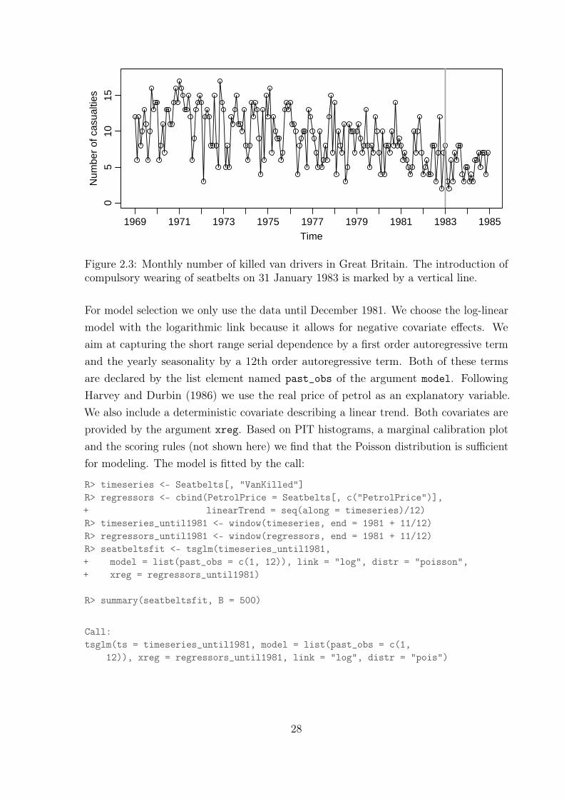
Next we study the monthly number of killed drivers of light goods vehicles in GreatBritain between January 1969 and December 1984 shown in Figure 2.3. This time seriesis part of a dataset which was first considered by Harvey and Durbin (1986) for studyingthe effect of compulsory wearing of seatbelts introduced on 31 January 1983. The dataset,including additional covariates, is available in R in the object Seatbelts. In their paperHarvey and Durbin (1986) analyze the numbers of casualties for drivers and passengersof cars, which are so large that they can be treated with methods for continuous-valueddata. The monthly number of killed drivers of vans analyzed here is much smaller (itsminimum is 2 and its maximum 17) and therefore methods for count data are to bepreferred.

27

Time

Num

ber

of c

asua

lties

05

1015

1969 1971 1973 1975 1977 1979 1981 1983 1985

Figure 2.3: Monthly number of killed van drivers in Great Britain. The introduction ofcompulsory wearing of seatbelts on 31 January 1983 is marked by a vertical line.

For model selection we only use the data until December 1981. We choose the log-linearmodel with the logarithmic link because it allows for negative covariate effects. Weaim at capturing the short range serial dependence by a first order autoregressive termand the yearly seasonality by a 12th order autoregressive term. Both of these termsare declared by the list element named past_obs of the argument model. FollowingHarvey and Durbin (1986) we use the real price of petrol as an explanatory variable.We also include a deterministic covariate describing a linear trend. Both covariates areprovided by the argument xreg. Based on PIT histograms, a marginal calibration plotand the scoring rules (not shown here) we find that the Poisson distribution is sufficientfor modeling. The model is fitted by the call:

R> timeseries <- Seatbelts[, "VanKilled"]R> regressors <- cbind(PetrolPrice = Seatbelts[, c("PetrolPrice")],+ linearTrend = seq(along = timeseries)/12)R> timeseries_until1981 <- window(timeseries, end = 1981 + 11/12)R> regressors_until1981 <- window(regressors, end = 1981 + 11/12)R> seatbeltsfit <- tsglm(timeseries_until1981,+ model = list(past_obs = c(1, 12)), link = "log", distr = "poisson",+ xreg = regressors_until1981)

R> summary(seatbeltsfit, B = 500)

Call:tsglm(ts = timeseries_until1981, model = list(past_obs = c(1,

12)), xreg = regressors_until1981, link = "log", distr = "pois")

28

Coefficients:Estimate Std.Error CI(lower) CI(upper)

(Intercept) 1.7872 0.39925 1.1927 2.727beta_1 0.0854 0.08515 -0.1055 0.209beta_12 0.1581 0.10082 -0.0334 0.314PetrolPrice 1.1893 2.76888 -4.0278 6.427linearTrend -0.0306 0.00885 -0.0489 -0.016Standard errors and confidence intervals (level = 95 %) obtainedby parametric bootstrap with 500 replications.

Link function: logDistribution family: poissonNumber of coefficients: 5Log-likelihood: -396.1AIC: 802.2BIC: 817.5QIC: 802.2

Accordingly, the fitted model for the number of van drivers Yt killed in month t is givenby Yt|Ft−1 ∼ Poisson(λt) with

log(λt) = 1.9 + 0.09Yt−1 + 0.15Yt−12 + 0.08Xt − 0.03t/12, t = 1, . . . , 156,

where Xt denotes the real price of petrol at time t. The estimated coefficient beta_1corresponding to the first order autocorrelation is very small and even slightly below thesize of its approximative standard error, indicating that there is no notable dependence onthe number of killed van drivers of the preceding week. We find a seasonal effect capturedby the twelfth order autocorrelation coefficient beta_12. Unlike in the model for the cardrivers by Harvey and Durbin (1986), the petrol price does not seem to influence thenumber of killed van drivers. An explanation might be that vans are much more oftenused for commercial purposes than cars and that commercial traffic is less influenced bythe price of fuel. The linear trend can be interpreted as a yearly reduction of the numberof casualties by a factor of 0.97 (obtained by exponentiating the corresponding estimatedcoefficient), i.e., on average we expect 2.9% fewer killed van drivers per year (which isbelow one in absolute numbers).

Based on the model fitted to the training data until December 1981, we can predictthe number of road casualties in 1982 given the respective petrol price. Coherent, i.e.integer-valued forecasts could be obtained by rounding the predictions. A graphicalrepresentation of the following predictions is given in Figure 2.4.

R> timeseries_1982 <- window(timeseries, start = 1982, end = 1982 + 11/12)R> regressors_1982 <- window(regressors, start = 1982, end = 1982 + 11/12)

29

Time

Num

ber

of c

asua

litie

s

1979 1980 1981 1982 1983

05

1015

20

Figure 2.4: Fitted values (dashed line) and predicted values (solid line) according to themodel with the Poisson distribution. Prediction intervals (grey bars) are designed toensure a global coverage rate of 90%. They are chosen to have minimal length and arebased on a simulation with 2000 replications.

R> predict(seatbeltsfit, n.ahead = 12, level = 0.9, global = TRUE,+ B = 2000, newxreg = regressors_1982)$pred

Jan Feb Mar Apr May Jun Jul Aug Sep Oct Nov Dec1982 7.71 7.45 7.57 7.41 7.21 6.99 7.15 7.83 7.49 7.82 8.02 7.45

Finally, we test whether there was an abrupt shift in the number of casualties occurringwhen the compulsory wearing of seatbelts is introduced on 31 January 1983. Theapproximative score test described in Section 2.5 is applied:

R> seatbeltsfit_alldata <- tsglm(timeseries, link = "log",+ model = list(past_obs = c(1, 12)),+ xreg = regressors, distr = "poisson")

R> interv_test(seatbeltsfit_alldata, tau = 170, delta = 1, est_interv = TRUE)

Score test on intervention(s) of given type at given time

Chisq-Statistic: 1.153 on 1 degree(s) of freedom, p-value: 0.2829

Fitted model with the specified intervention:

Call:tsglm(ts = fit$ts, model = model_extended, xreg = xreg_extended,

link = fit$link, distr = fit$distr)

30

Coefficients:(Intercept) beta_1 beta_12 PetrolPrice linearTrend

0.19508 0.08819 0.80446 3.17408 -0.04788interv_10.24570

With a p value of 0.28 the null hypothesis of no intervention cannot be rejected at a 5%significance level. Note that this result does not rule out that there is an effect of theseatbelts law which is either too small for being significant or of a different type than itis tested for. For illustration we fit the model under the alternative of a level shift afterthe introduction of the seatbelts law (see the output above). The multiplicative effectsize of the intervention is found to be 1.279. This indicates that according to this modelfit 27.9% less van drivers are killed after the law enforcement. For comparison, Harveyand Durbin (1986) estimate a reduction of 18% for the number of killed car drivers.

2.7 Comparison with other software packages

In this section we review functions (and the corresponding models) from other R packageswhich can be employed for count time series analysis. Many of them have been publishedonly very recently, a fact that demonstrates the raising interest in count time seriesanalysis. We discuss how these packages differ from our package tscount. For illustrationwe use the time series of Campylobacter infections analyzed in Section 2.6.1 ignoring theintervention effects. For the presentation of other models we use a notation parallel tothe one used in the previous sections to highlight similarities. Interpretation of the finalmodel should be done carefully, though.

We consider a large number of somehow related packages which makes this comparisonquite extensive yet interesting for those readers who want guidance on choosing themost appropriate package for their data. In the first subsection we present packages forindependent data and in the second subsection we discuss packages for dependent data.

2.7.1 Packages for independent data

We start reviewing functions which have been introduced for independent observationsbut can, with certain limitations, be employed for time series whose temporal dependenceis rather simple. This is exemplarily discussed in the following paragraph.

31

The function glm in the package stats and, for the Negative Binomial distribution, thefunction glm.nb in the package MASS (Venables and Ripley, 2002) can fit standard GLMsto count time series with the iteratively reweighted least squares (IRLS) algorithm. Justlike with our tsglm function, one can choose the identity or logarithmic link in combinationwith a Poisson or Negative Binomial conditional distribution. Standard GLMs havebeen introduced to model independent but not identically distributed observations. Inprinciple, one could also fit simple models for time series by including lagged valuesof the time series, i.e., Yt−i1 , . . . , Yt−ip , as covariates. However, the glm function hasseveral limitations; the most important being that it does not allow for regression onpast values of the conditional mean. For example, the glm function cannot be used tofit the model which included stochastic seasonality; recall Section 2.6.1. Furthermore,the glm function does not induce the constraints on the vector of parameters given inSection 2.2.1, which are necessary to ensure stationarity of the fitted process. Modelswhich are violating these parameter constraints are generally not suitable for prediction.We have also experienced that glm occasionally does not find good starting values for itsoptimization procedure such that it returns an error and requests the user to providestarting values. At least for the very simple case of a Poisson INGARCH(1,0) modelfitted to the Campylobacterosis data the glm function performs well and we obtain verysimilar parameter estimates like with the tsglm function:

R> campydata <- data.frame(ts = campy[-1], lag1 = campy[-length(campy)])R> coef(glm(ts ~ lag1, family = poisson(link = "identity"), data = campydata))(Intercept) lag1

4.0322 0.6556R> coef(tsglm(campy, model = list(past_obs = 1), link = "identity"))(Intercept) beta_1

4.0083 0.6501

As described in more detail in Section A.3, a fit by the glm function can be used as astarting value to the function tsglm.

The class of generalized additive models for location, scale and shape (GAMLSS) hasbeen introduced by Rigby and Stasinopoulos (2005) as an extension of a GLM anda generalized additive model (GAM). In addition to the location parameter furtherparameters of the conditional distribution can be modeled as functions of the explanatoryvariables. In the following example we use the package gamlss (authored by Rigby andStasinopoulos, 2005) to fit an INGARCH(1,0) model to the Campylobacterosis data. Theoverdispersion coefficient σ2

t of the Negative Binomial distribution is not constant butchanges with time according to the equation

σ2t = exp (β∗0 + β∗1 log(Yt−1 + 1)) .

32

R> library("gamlss")R> gamlss(ts ~ lag1, sigma.formula = ~ log(lag1+1), data = campydata,+ family = NBI(mu.link = "identity", sigma.link = "log"))[c(25, 43)]GAMLSS-RS iteration 1: Global Deviance = 803.7GAMLSS-RS iteration 2: Global Deviance = 803.7GAMLSS-RS iteration 3: Global Deviance = 803.7$mu.coefficients(Intercept) lag1

3.8409 0.6768

$sigma.coefficients(Intercept) log(lag1 + 1)

-4.2986 0.7167

GAMLSS-RS iteration 1: Global Deviance = 803.7GAMLSS-RS iteration 2: Global Deviance = 803.7GAMLSS-RS iteration 3: Global Deviance = 803.7GAMLSS-RS iteration 1: Global Deviance = 805.6GAMLSS-RS iteration 2: Global Deviance = 805.6GAMLSS-RS iteration 3: Global Deviance = 805.6

The possibility of a time dependent dispersion coefficient does not improve the fit for thisdata example (according to the AIC, which is 811.72 compared to 811.64 for a model withconstant overdispersion coefficient) but might be quite useful for other data examples.However, it is clear that such a complex model yields more uncertainty of the parameterestimations (i.e., larger standard errors, which are not shown here).

The package ZIM (Yang, Zamba, and Cavanaugh, 2014) fits zero-inflated models (ZIM)for count time series with excess zeros. These models are suitable for data where thevalue zero occurs more frequently than it would be expected when assuming other counttime series models. The main idea of these models is to replace the ordinary Poisson orNegative Binomial distribution by its respective zero-inflated version, which is a mixtureof a singular distribution in zero (with probability ωt) and a Poisson or Negative Binomialdistribution (with probability 1−ωt), respectively. The model proposed by Yang, Zamba,and Cavanaugh (2013) allows both, the probability ωt and the conditional mean λt ofthe ordinary count data distribution, to vary over time. The conditional mean λt ismodeled by using a logistic regression model. The probability ωt is modeled by a GLMwith the logistic link. Other methods for count data with excess zeros, which also havethese limitations, are provided by the well-established functions zeroinfl and hurdle

from the package pscl (Zeileis, Kleiber, and Jackman, 2008). However, the package ZIMincludes an extension of ZIM to state space models, which is treated in the next section.The parameters of a ZIM are fitted by the function zim employing an EM algorithm.Zero-inflation models are definitely appealing for count time series which occasionally

33

exhibit excess zeros. For our data example of Campylobacter infections, which does notinclude any zero observations, ZIM are not applicable.

The current version of the tscount package considered in this chapter is limited tomodeling univariate data. A possible extension to models for vectors of counts is providedby the package VGAM (Yee, 2016) introduced by Yee (2015). The function vglm in thispackage fits a vector GLM (VGLM) (see Yee and Wild, 1996) where the conditionaldensity function of a d-dimensional response vector Y t given an r-dimensional covariatevector X t is assumed to be of the form

f(Y t|X t;H) = h(Y t, ν1, . . . , νs),

where νj = η>j X t, j = 1, . . . , s and h(·) is a suitably defined function. The modelparameters are given by the (r × s)-dimensional parameter matrix H = (η>1 , . . . ,η

>s )>.

Choosing d = s = 1 results in the special case of an ordinary, univariate GLM. Wedemonstrate a fit of an INGARCH(1,0) model to the Campylobacterosis data by thefollowing code:

R> library("VGAM")R> coef(vglm(ts ~ lag1, family = poissonff(link = "identitylink"),+ data = campydata))(Intercept) lag1

4.0322 0.6556

We note that the function vglm produces exactly the same output as the function glm

for this special case. The function vgam from the same package would allow to fit aneven more general vector generalized additive model (VGAM), which is a multivariategeneralization of a generalized additive model (GAM), see Yee (2015) for more details.

Due to the aforementioned limitations of the procedures developed for independent datawe would generally suggest the use of the function tsglm for modeling count time series.However, in certain situations, where features of the data are currently not supportedby tsglm, the aforementioned packages can be employed with care; recall the secondparagraph of this section. For count time series with many zeros one might want toconsider using, for example, the package ZIM. If there are reasons to assume a time-varying overdispersion coefficient, the package gamlss is a good choice. Multivariatecount time series could be analyzed with the package VGAM.

34

2.7.2 Packages for time series data

In this section we present R packages developed for count time series data.

The package acp (Siakoulis, 2015) has been published recently and provides maximumlikelihood fitting of autoregressive conditional Poisson (ACP) regression models. Theseare the INGARCH models given by (1.2); see Section 1.2. The acp package also allows toinclude covariate effects. In its latest version 2.1, which has been published in December2015, the package has been extended to fit models of general order p and q. The tsglmfunction of our package includes these models as special cases and is more general in thefollowing aspects:

• The acp package is different in many technical details. Notably, it does not allowto incorporate the parameter constraints given in Section 2.2.1.

• Quasi maximum likelihood fitting allows to choose a more flexible Negative Binomialmodel instead of a Poisson model (argument distr = "nbinom").

• The tsglm function additionally comprises a log-linear model (argument link =

"log"), which is more adequate for many count time series.• The tsglm function allows for more flexible dependence modeling by allowing

arbitrary specification of dynamics. This flexibility is missing by the acp functionfor model fitting because it requires all variables up to a given order to be included(e.g. λt−1, . . . , λt−12 and not just λt−12). For instance, tsglm allows for stochasticseasonality (see Section 2.6.1).

• The tsglm function differentiates between covariates with so-called external andinternal effect (see Equation (1.4) and the accompanying discussion).

In the following example, an INGARCH(1,1) model (ignoring the seasonal effect) is fittedto the Campylobacterosis data analyzed in Section 2.6.1:

R> library("acp")R> coef(acp(campy ~ -1, p = 1, q = 1))[1] 2.5320 0.5562 0.2295R> coef(tsglm(campy, model = list(past_obs = 1, past_mean = 1)))(Intercept) beta_1 alpha_1

2.3890 0.5183 0.2693

The parameter estimations obtained by the acp function are very similar to those obtainedby the tsglm function when fitting the same model.

The class of generalized linear autoregressive moving average (GLARMA) models com-bines GLM with ARMA processes. A software implementation is available in the packageglarma (Dunsmuir and Scott, 2015). The GLARMA model assumes the conditional

35

distribution of Yt given the past Ft−1 to be Poisson or Negative Binomial with mean λtand density f(Yt|λt), with λt given by

g(λt) = η>X t +Ot + Zt,

where Ot is an offset term. An intercept is included by choosing the first column ofthe time-varying covariate matrix X t to be the vector (1, . . . , 1)>. Serial correlation isinduced by an autoregressive moving average (ARMA) structure of Zt, which is given by

Zt =

p∑k=1

φk(Zt−ik + et−ik) +

q∑`=1

ψ`et−j` .

Hereby the process {Zt : t ∈ N} is defined by means of residuals et which can be possiblyrescaled, see (2.7) and (2.8). In the example below we choose Pearson residuals. Forthe link function g(·), the glarma package currently supports only the logarithm but notthe identity, which is available in our function tsglm. Like in our package, the user canspecify the model order by considering the sets P = {i1, . . . , ip} and Q = {j1, . . . , jq}.The formulation of the GLARMA model we consider describes the modeling possibilitiesprovided by the glarma package. In fact, this formulation is more general than theaccompanying article by Dunsmuir and Scott (2015), where the authors consider thecase Q = {1, . . . , q} and P = {1, . . . , p}. Choosing P and Q, in the context of GLARMAmodeling, should be done cautiously (see Dunsmuir and Scott, 2015, Seection 3.4). Ourlimited experience shows that the minimum element of the set Q should be chosen insuch a way that it is larger than the maximum element of P for avoiding errors. Unlikeordinary ARMA models, GLARMA models are not driven by random innovations butby residuals et. Note that the model fitted by the function tsglm is also related toARMA processes, see (A.4) in the Appendix. The function glarma implements maximumlikelihood fitting of a GLARMA model. We compare the following model fitted to theCampylobacterosis data by the function glarma with a fit by tsglm (see Section 2.6.1,but without the intervention effects):

R> library("glarma")R> glarmaModelEstimates(glarma(campy, phiLags = 1:3, thetaLags = 13,+ residuals = "Pearson", X = cbind(intercept=rep(1, length(campy))),+ type = "NegBin"))[c("Estimate", "Std.Error")]

Estimate Std.Errorintercept 2.34110 0.10757phi_1 0.22101 0.03940phi_2 0.05978 0.04555phi_3 0.09784 0.04298theta_13 0.08602 0.03736alpha 10.50823 1.91232

36

With the notation introduced above the fitted model for the number of new infections Ytin time period t is given by Yt|Ft−1 ∼ NegBin(λt, 10.51) with log(λt) = 2.34 + Zt and

Zt = 0.22(Zt−1 + et−1) + 0.06(Zt−2 + et−2) + 0.1(Zt−3 + et−3) + 0.09et−13.

We focus on the models’ capability to explain the serial correlation which is present in thedata. Considering the GLARMA model, a choice of P = {1, 2, 3} and Q = {13} leavesapproximately uncorrelated residuals (see the autocorrelation function in Figure 2.5(top right)). For the model class fitted by our function tsglm we have chosen the moreparsimonious model with P = {1} and Q = {13} to obtain a fit with approximatelyuncorrelated residuals. Figure 2.6 shows that both models seem to provide an adequatefit to given data. The package glarma provides a collection of functions which can beapplied to a fitted GLARMA model. For example it provides a function for testingwhether there exists serial dependence and it offers tools for model diagnostics. Toconclude, both models are able to explain quite general forms of serial correlation but therole of the dependence parameters is quite different and any results should be interpretedcarefully. A more detailed comparison would be interesting but is beyond the scope ofthis thesis.

Another class of models, which is closely related to the GLARMA models, are the so-calledgeneralized autoregressive moving average (GARMA) models developed by Benjamin,Rigby, and Stasinopoulos (2003). Dunsmuir and Scott (2015, Section 3) remark that bothmodel classes are similar in their structure but they have some important differences.The GARMA model is formulated by

g(λt) = η>X t +

p∑k=1

φk(g(Yt−k)− η>X t−k

)+

q∑`=1

ψ` (g(Yt−k)− g(λt−`)) ,

where the notation follows the GLARMA notation. Compared to the GLARMA model,the GARMA model does not include an offset and the ARMA structure applies to valueswhich are transformed by the link function g, i.e., on the scale of the linear predictor. Incase of a logarithmic link, the observations Yt are replaced by max(Yt, c) for a thresholdc ∈ (0, 1), such that g(Yt) is well-defined. In our package this problem is handled replacingYt by Yt + 1. The package gamlss.util (Stasinopoulos, Rigby, and Eilers, 2015) containsthe function garmaFit for fitting such GLARMA models. Like ordinary GLMs, thesemodels are fitted by maximum likelihood employing the IRLS algorithm. As pointed outon the accompanying help page, the function garmaFit does not guarantee stationarityof the fitted model. Additionally, the function garmaFit does not allow to specify serial

37

dependence of higher order without including all lower orders, which would be necessaryfor parsimoniously describing stochastic seasonality. The following example shows a fitof a Negative Binomial GARMA model of order p = 1 and q = 1 with link g(·) = log(·)to the Campybacterosis data:

R> library("gamlss.util")R> coef(garmaFit(campy ~ 1, order = c(1, 1), family = NBI(mu.link = "log")))deviance of linear model= 891.1deviance of garma model= 803.3beta.(Intercept) phi theta

2.6216 0.7763 -0.2917

In the above output the AR coefficient φ1 is named phi and the MA coefficient ψ1

theta. The function garma from the package VGAM (Yee, 2016) is an alternativeimplementation for fitting GARMA models. However, the accompanying help pagewarns that this function is still in premature stage and points to potential problemswith the initialization (in version 1.0-1 of the package). In addition, garma allows onlyfor autoregressive modeling (i.e. q = 0) and the Negative Binomial distribution is notsupported. Hence our example can only show a fit of a Poisson GARMA model of orderp = 1 and q = 0 to the Campylobacterosis data:

R> coef(vglm(campy ~ 1, family = garma(link="loge", p.ar.lag = 1, q.ma.lag = 0,+ coefstart = c(0.1, 0.1))))(Intercept) (lag1)

1.948 1.123

In this example the estimated coefficient for the autoregressive term is larger than one,which suggests that the fitted process is not stationary. We could not find settings forwhich the functions garmaFit and garma fit the same model and give identical or atleast similar results. Due to the close relationship of GARMA and GLARMA models werefrain from presenting a comparison to a fit with our package and refer to the comparisonin the previous paragraph made for GLARMA models.

The models presented so far are determined by a single source of randomness, i.e., givenall past observations, uncertainty is only induced by the Poisson or Negative Binomialdistribution from which the observations are assumed to be drawn. These models belongto the class of observation-driven models according to the classification of Cox (1981).In the following paragraphs we present parameter-driven models. These models aredetermined by multiple sources of randomness introduced by one or more innovationprocesses. Helske (2016a) comment on the merits of both approaches. He argues thatparameter-driven models are appealing because they allow to introduce even multiplelatent structures in a flexible way. On the other hand, he observes that observation-driven

38

models like the ones we consider are of advantage for prediction because of their explicitdependence on past observations and covariates.

The package surveillance (Salmon, Schumacher, and Höhle, 2016b) includes methods foronline change point detection in count time series. One of the models used here is ahierarchical time series (HTS) model proposed by Manitz and Höhle (2013) based on thework by Heisterkamp, Dekkers, and Heijne (2006). This particular state space modelaccounts for serial dependence by a time-varying intercept. More precisely, it is assumedthat Yt ∼ NegBin(λt, φ), where the conditional mean λt is given by

λt = exp(β0,t + δt+ γt + η>X t

).

The time-varying intercept β0,t is assumed to depend on its previous values according to

∆dβ0,t|β0,t−1, . . . , β0,t−d ∼ N(0, κ−1β0

),

where ∆d is the difference operator of order d ∈ {0, 1, 2} and κβ0 a precision parameter.Explicitly, it holds β0,t ∼ N(0, κ−1

β0), β0,t|β0,t−1 ∼ N(β0,t−1, κ

−1β0

) and

β0,t|β0,t−1, β0,t−2 ∼ N(2β0,t−1 − β0,t−2, κ−1β0

)

for d = 1, 2, 3, respectively. For d > 0 this induces dependence between successiveobservations. The other parameters, δ for the linear trend, γt for a seasonal effect, andthe vector η for the effect of a covariate vector X t, are also assumed to be normallydistributed with certain priors. Inference is done in a Bayesian framework and utilizes anefficient integrated nested Laplace approximation (INLA) provided by the package INLA(Lindgren and Rue, 2015) (available from http://www.r-inla.org). In the followingexample we fit a Negative Binomial model without trend, seasonality or covariate effectsbut with a time-varying intercept of order d = 1 to the Campylobacterosis data:

R> library("INLA")R> campyfit_INLA <- inla(ts ~ f(time, model = "rw1", cyclic = FALSE),+ data = data.frame(time = seq(along = campy), ts = campy),+ family = "nbinomial", E = mean(campy),+ control.predictor = list(compute = TRUE, link = 1),+ control.compute = list(cpo = FALSE, config = TRUE),+ control.inla = list(int.strategy = "grid", dz = 1,+ diff.logdens = 10))R> posterior <- inla.posterior.sample(1000, campyfit_INLA)R> rowMeans(sapply(posterior, function(x) (unname(x$hyperpar))))

[1] 9.314 169.208

39

The estimates for the parameters φ (the former) and κβ0 (the latter) in the output aboveare based on means of a sample of size 1000 from the posterior distribution. Fitted valuesλ1, . . . , λ140 are obtained in the same way (not shown in the above code). With theBayesian approach it is very natural to obtain prediction intervals for future observationsfrom the posterior distribution which account for the estimation and observation uncer-tainties. This is a clear advantage over the classical likelihood-based approach pursuedin our package (cf. Section 2.3). A disadvantage of the Bayesian approach is its muchhigher computational effort which could be an obstacle for real-time applications andsimultaneous analysis of several time series. The above example runs more than eightseconds on a standard office computer (Intel Xeon CPU with 2.83 GHz); this is seventimes longer than tsglm takes to fit the model. An additional difference between ourapproach and that taken by INLA is the specification of temporal dependence. Thecomparison of the final fitted values, shown in Figure 2.6, illustrates that the modelwith a time-varying intercept fitted by inla possess a much smoother line through theobserved values when compared to the model fitted by tsglm. For this example, theempirical autocorrelation function of the response residuals in Figure 2.5 (bottom left)is significantly different from zero at lag one; hence short term temporal correlation isnot explained sufficiently by the hierarchical model. It also becomes clear by this plotthat we should have included seasonality by employing the term γt. The residuals of theGLM-based fit by the function tsglm do not exhibit any serial correlation which has notbeen explained by the model (see Figure 2.5 (top left)). In general, the GLM-based modelis expected to provide more accurate 1-step-ahead predictions whilst the hierarchicalmodel prediction obtained by inla is more stable. Either of these two features couldbe preferable depending upon the specific application. It would be interesting to studythese two ways of modeling temporal dependence in a future work.

The package KFAS (Helske, 2016b) treats state space models for multivariate time serieswhere the distribution of the observations belongs to the exponential family (and alsoincludes the Negative Binomial distribution). Its name refers to Kalman filtering andsmoothing, which are the two key algorithms employed by the package. This package isable to cope with very general state space models at the cost of a rather big effort for itscorrect specification. However, some auxiliary functions and the use of symbolic modeldescription reduces this effort. In contrast to the package INLA, which is also capableof fitting state space models, KFAS implements maximum likelihood estimation (for acomparison of these two packages see Helske, 2016a). One possible univariate modelfor the Campylobacterosis data could be the state space model Yt|Ft−1 ∼ NegBin(λt, φ)

where λt = exp(νt) and the state equation is

40

0.0 0.5 1.0 1.5

−0.

20.

20.

61.

0

Lag

AC

F

tsglm

0.0 0.5 1.0 1.5

−0.

20.

20.

61.

0

Lag

AC

F

glarma

0.0 0.5 1.0 1.5

−0.

20.

20.

61.

0

Lag

AC

F

INLA

0.0 0.5 1.0 1.5

−0.

20.

20.

61.

0

Lag

AC

F

KFAS

Figure 2.5: Empirical autocorrelation function of the response residuals for a model fit ofthe campylobacterosis data by our function tsglm (see Section 2.6.1, but without theintervention effects) and the packages glarma, INLA and KFAS (see Section 2.7).

νt = νt−1 + εt.

The initialization ν1 is specified by assuming ν1 ∼ N(λ, σ2ν). The degree of serial

dependence is induced by independently distributed innovations εt for which it is assumedthat εt ∼ N(0, σ2

ε). This model has unknown parameters λ ∈ R, and φ, σ2ν1, σ2

ε ∈ [0,∞)

and can be fitted as follows:

R> library("KFAS")R> model <- SSModel(campy ~ SSMcustom(Z = 1, T = 1, R = 1, Q = 0,+ a1 = NA, P1 = NA) - 1,+ distribution = "negative binomial", u = NA)R> updatefn <- function(pars, model, ...){+ model$a1[1, 1] <- pars[1]+ model$u[, 1] <- exp(pars[2])+ model$P1[1, 1] <- exp(pars[3])+ model$Q[1,1,1] <- exp(pars[4])+ return(model)+ }R> campyfit_KFAS <- fitSSM(model = model, inits = c(mean(campy), 0, 0, 0),+ updatefn = updatefn)R> exp(campyfit_KFAS$optim.out$par)[1] 3.427e+00 9.148e+01 2.775e-16 4.334e-02

41

Time

Num

ber

of c

ases

1996 1997 1998 1999 2000

010

2030

4050 tsglm

glarmaINLAKFAS

Figure 2.6: Comparison of a model fit of the campylobacterosis data by our functiontsglm (see Section 2.6.1, but without the intervention effects) and the packages glarma,INLA and KFAS (see Section 2.7).

The output above corresponds to the estimated parameters λ, φ, σ2ν1

and σ2ε , respectively.

We observe that the estimation procedure is quite sensitive to given starting values; thisfact has been pointed out by Helske (2016a). As shown by the empirical autocorrelationfunction of the residuals in Figure 2.5 (bottom right), the fitted model explains thetemporal dependence of the data quite adequately. The values fitted by this model(see Figure 2.6) do not show any delay when compared to the fit obtained by tsglm.The algorithm used by tsglm yields fitted values by 1-step-ahead forecasts based onprevious observations; note that only the model parameters are fitted using all availableobservations. The algorithm of the KFAS package for obtaining fitted values includesfuture observations which naturally lead to a more accurate fit. However, this methodologydoes not guarantee better out-of-sample forecasting performance since future observationswill not be available in general. Further empirical comparison between KFAS and tscountis required to compare the accuracy of predictions obtained by both models.

Another state space model which could be used to describe count time series is a partiallyobserved Markov process (POMP). The package pomp (King, Nguyen, and Ionides, 2016)provides a general and abstract representation of such models. One example by Kinget al. (2016, Sections 4.5 and 4.6) is the so-called Ricker model for describing the size Nt

of a population which is assumed to fulfill

Nt+1 = rNt exp(−Nt + εt)

with innovations εt ∼ N(0, σ2ε). The actual observations Yt are noisy measurements of the

population size Nt and it is assumed to hold Yt ∼ Poisson(φNt), where φ is an unknown

42

dispersion parameter. Specification and fitting of this rather simple model with thepackage pomp requires more than thirty lines of code. This complexity is an obstaclefor using the package in standard situations but might prove beneficial in very specialscenarios.

The package gcmr provides methodology for Gaussian copula marginal regression (Masarottoand Varin, 2012), a framework which is also capable to model count time series. Themarginal distribution of a time series Yt given a covariate vector X t can be modeled bya Poisson or Negative Binomial distribution with mean λt using that g(λt) = β0 + η>X t.This is similar to model (1.1) but it does not include the terms for regression on past valuesof Yt and λt. Furthermore, randomness is introduced through an unobserved error process{εt : t ∈ N} by assuming that Yt = F−1

t (Φ(εt)), where Ft is the cumulative distributionfunction of the Poisson or Negative Binomial distribution with mean λt and Φ is thecumulative distribution function of the standard normal distribution. Hence the actualvalue of Yt is the Φ(εt)-quantile of the Poisson or Negative Binomial distribution withmean λt. As pointed out by Masarotto and Varin (2012), copulas with discrete marginalsmight not be unique (see also Genest and Nešlehová, 2007). Temporal dependence of{Yt} is modeled through the error process {εt} by assuming an autoregressive movingaverage (ARMA) model of order p and q. Note that although this model accounts forserial dependence it does not model the conditional distribution of Yt given the past butonly its time-varying marginal distribution. The mean λt of this marginal distribution isnot influenced by the actual (unobserved) value of the error εt. Hence this model is notsuitable for accurate 1-step-ahead predictions but rather for quantifying the additionaluncertainty induced by the serial dependence. The following example presents a fit of aNegative Binomial model with an ARMA error process of order p = 1 and q = 1:

R> library("gcmr")R> gcmr(ts ~ 1, marginal = negbin.marg(link = "identity"),+ cormat = arma.cormat(p=1, q=1), data = data.frame(ts = campy))

Call:gcmr(formula = ts ~ 1, data = data.frame(ts = campy),

marginal = negbin.marg(link = "identity"),cormat = arma.cormat(p = 1, q = 1))

Marginal model parameters:(Intercept) dispersion

11.320 0.255

Gaussian copula parameters:ar1 ma1

0.823 -0.269

43

The estimated ARMA parameters of the error process indicate that there is a considerableamount of serial correlation in the data. Some of the observed variability is explainedby this serial dependence. As discussed above, the fitted values are based solely onthe estimated marginal distribution and are therefore constant over time (equal to theestimated intercept in the above output).

An extension of the zero-inflated models of the package ZIM, which was presented in theprevious section, are the so-called dynamic zero-inflated models (DZIM) as proposed byYang, Cavanaugh, and Zamba (2015). These fall within the framework of state spacemodels and introduce serial dependence by an unobserved autoregressive process of orderp. Fitting is based on the EM algorithm and MCMC simulation.

The package tsintermittent (Kourentzes and Petropoulos, 2016) provides methods forso-called intermittent demand time series (see for example Kourentzes, 2014). These aretime series giving the number of requested items of a particular product (e.g., rarelyneeded spare parts) which is demanded in a sporadic fashion with periods of zero demand.Reliable forecasts of such time series are important for companies to efficiently planstocking the respective items. In principle, these are count time series which could beanalyzed with the methods in our package. However, it is known that classical forecastingmethods perform unsatisfactorily for this kind of data (Kourentzes, 2014). More successfulapproaches, which are included in the tsintermittent package, are based on the idea ofseparately modeling the non-zero demand size and the inter-demand intervals. Thesemethods do not take into account that the observations are integers and do not includecovariate effects, as the methods in our package do. Temporal dependence is consideredimplicitly, by assuming that there are periods where subsequent observations are zero.Our functions consider explicit time dependence. The methods in the tsintermittentpackage are possibly more appropriate for the specific context they are tailored for (whichwould need further examination), but not suitable for count time series in general. Theycompete with other types of models for zero excess time series data, for example withDZIM.

2.8 Discussion

We are the first to provide such a general formulation and comprehensive treatment ofcount time series following generalized linear models. In its current version, the R packagetscount allows for the analysis of count time series with this quite broad class of models.Our comparison with other packages shows that tscount is an important contribution

44

which extends and complements existing software. It will hopefully prove to be useful fora wide range of applications.

There are a number of desirable extensions of the package which could be included infuture releases. The most important ideas for extending tscount are described in thefollowing paragraphs. We invite other researchers and developers to contribute to thispackage.

As an alternative to the Negative Binomial distribution, one could consider the so-calledQuasi-Poisson model. It allows for a conditional variance of φλt (instead of λt + φλ2

t , asfor the Negative Binomial distribution), which is linearly and not quadratically increasingin the conditional mean λt (for the case of independent data see Ver Hoef and Boveng,2007). A scatterplot of the squared residuals against the fitted values could reveal whethera linear relation between conditional mean and variance is more adequate for a giventime series. A generalization of the test for overdispersion in INGARCH(1,0) processesproposed by Weiß and Schweer (2015) could provide guidance for choosing an appropriateconditional distribution.

The common regression models for count data are often not capable to describe anexceptionally large number of observations with the value zero. In the literature so-calledzero-inflated and hurdle regression models have become popular for zero excess countdata (for an introduction and comparison see Loeys, Moerkerke, De Smet, and Buysse,2012). A first attempt to utilize zero-inflation for INGARCH time series models is madeby Zhu (2012).

In some applications the variable of interest is not the number of events but the rate,which expresses the number of events per unit. For example the number of infectedpeople per 10 000 inhabitants, where the population size is a so-called exposure variablewhich varies over time. For models with a logarithmic link function such a rate couldbe described by a model where the number of events is the response variable and thelogarithm of the exposure variable is a so-called offset. An offset is supported by manystandard functions for GLMs and could be part of a future release of our package.

Alternative nonlinear models are for example the threshold model suggested by Woodardet al. (2011) or the models studied by Fokianos and Tjøstheim (2012). Fokianos andNeumann (2013) propose a class of goodness-of-fit tests for the specification of thelinear predictor, which are based on the smoothed empirical process of Pearson residuals.Christou and Fokianos (2015a) develop suitably adjusted score tests for parameters whichare identifiable as well as non-identifiable under the null hypothesis. These tests can beemployed to test for linearity of an assumed model.

45

In practical applications one is often faced with outliers. Elsaied and Fried (2014)and Kitromilidou and Fokianos (2016) develop M-estimators for the linear and the log-linear model, respectively. Fried et al. (2014) compare robust estimators of the (partial)autocorrelation (see also Dürre, Fried, and Liboschik, 2015a) for time series of counts,which can be useful for identifying the correct model order.

In the long term, related models for binary or categorical time series (Moysiadis andFokianos, 2014) or potential multivariate extensions of count time series following GLMscould be included as well.

The models which are so far included in the package or mentioned above fall into the classof time series following GLMs. There is also quite a lot of literature on thinning-basedtime series models but we are not aware of any publicly available software implementations.To name just a few of many publications, Weiß (2008) reviews univariate time seriesmodels based on the thinning operation, Pedeli and Karlis (2013) study a multivariateextension and Scotto, Weiß, Silva, and Pereira (2014) consider models for time serieswith a finite range of counts. For the wide class of state space models there are the Rpackages INLA, KFAS and pomp available, although it is quite complex to apply theseto count time series. A future version of our package could provide simple interfaces tosuch packages specifically for fitting certain count time series models.

46

Chapter 3

Retrospective intervention detection

3.1 Introduction

In many applications, unusual external effects or measurement errors can lead to eithersudden or gradual changes in the structure of the data. Furthermore such effects can resultin several singular observations of a distinct nature than the rest. Following Box andTiao (1975) we use the term intervention for all kinds of unusual effects influencing theordinary pattern of the data, including structural changes and different forms of outliers.Considering for example the monthly number infections with a certain disease, wherea disease outbreak would be a possible intervention effects. A goal of an interventionanalysis is to examine the effect of known interventions, for example to judge whether apolicy change had the intended impact (for practical applications see for example Boxand Tiao, 1975). Another possible goal is to search for unknown intervention effects andto find explanations for them a posteriori. Such sudden events are often included in themodel by deterministic covariates (e.g., Box and Tiao, 1975; Abraham and Box, 1979).These goals are fundamentally different from the goal of a robust estimation approach,where methods are expected to ignore the effect of aberrant observations.

The main focus of this chapter is to model various types of interventions in so-calledINGARCH (or ACP) processes which are defined by (1.2). An extension to the count timeseries based on generalized linear models as defined in Section 1.2 is briefly discussed inSection 2.5. This includes log-linear models, models with a Negative Binomial conditionaldistribution, models with additional covariates as well as those with more than oneintervention effect.

47

We introduce a new model to describe intervention effects within the class of INGARCHprocesses and compare it to an existing intervention model proposed by Fokianos andFried (2010). Our proposal is able to describe interventions which enter the dynamicsof the process in a different way when compared to the existing model. It allows todescribe an external effect on the observed value rather than an internal change of theunderlying state of the process. Such a model can be more realistic for some applications,as discussed in the last paragraph of Section 3.2.

Section 3.2 defines both intervention models and compares them analytically. Section 3.3presents joint maximum likelihood estimation of the ordinary model parameters andthe intervention effects and studies its properties by simulations. Section 3.4 presentsasymptotic procedures to test for single interventions at a given time, or to detect one ormultiple interventions at unknown positions. We verify these procedures by simulations.Furthermore, we discuss the problem of misspecification of the intervention model andshed some light on the question of discriminating between the two intervention models.Section 3.5 applies some of the methods to the weekly number of campylobacterosisinfections. Section 3.6 concludes this chapter with a short discussion on related issues.

3.2 Intervention models

As a first intervention model in the framework of INGARCH(p,q) processes, Fokianosand Fried (2010) define a contaminated observed process {Zt}t∈N with an intervention attime τ by

Zt|FZ,κt−1 ∼ Poisson(κt), κt = β0 +

p∑k=1

βkZt−k +

q∑`=1

α`κt−` + νXt, (i)

where Xt = δt−τI[τ,∞)(t) is a deterministic process describing the intervention effect,ν ≥ 0 denotes the intervention size, the predefined constant δ ∈ [0, 1] specifies the typeof intervention and all other model parameters are as before. The information aboutthe past of the process is denoted by FZ,κt0−1 = σ(Z1−p, . . . , Zt0−1, κ1−q, . . . , κ0). Model (i)covers three types of interventions with different choices of δ: a spiky outlier (SO) forδ = 0, a transient shift (TS) for δ ∈ (0, 1) and a level shift (LS) for δ = 1. Singular effectsare modeled by a SO, exponentially decaying effects by a TS and a permanent change oflocation by a LS.

The intervention effect is added to the underlying conditional mean process {κt} andnot to the observations itself. Through the regression on past observations and on

48

past conditional means the intervention effect enters the dynamics of the process. Theparameter δ has both a direct and an indirect impact on the observations. Its valuedirectly influences the impact of the intervention on the conditional mean and henceits impact on the future values of the process. In addition, the value of δ affects futurevalues of the process because of the dependence in (i) on past values of {κt} and {Zt}.Small values of δ yield less impact than larger ones.

We study an alternative intervention model for INGARCH(p,q) processes {Zt} followingthe definition

Zt|FZ,κt−1 ∼ Poisson(κt), κt = λt + νXt, λt = β0 +

p∑k=1

βkZt−k +

q∑`=1

α`λt−`, (ii)

where the intervention process {Xt}, the regular INGARCH parameters and the additionalintervention parameters are as before. Models (i) and (ii) look somewhat similar buttheir difference becomes more obvious, if we rewrite the equation for the conditionalmean κt of intervention model (ii) as

κt = β0 +

p∑k=1

βkZt−k +

q∑`=1

α`(κt−` −νXt−`︸ ︷︷ ︸not for model (i)

) + νXt. (3.1)

Apart from the labelled term, it is identical to the conditional mean equation of in-tervention model (i). For the alternative specification (ii) the intervention effect isnot propagated via the feedback mechanism of the conditional mean but only via thecontaminated observations. From (3.1) we see that both intervention models can bewritten in a unified way and are fully specified by their observable process {Zt} and theirunobservable conditional mean process {κt}, in addition to the deterministic interventionprocess {Xt}.

One could gain more insight about the difference between the intervention models byconsidering another representation, which turns out to be useful for cleaning the processesfrom any intervention effects (see Section 3.4). For intervention model (i) Fokianos andFried (2010) show that it is possible to decompose {Zt} into an intervention-free process{Yt} and a contamination process {Ct}, which are mutually independent conditionally onthe past, such that Zt = Yt +Ct. The intervention-free process {Yt} is an INGARCH(p,q)process with conditional mean process {λt} and the same parameters as {Zt}. Thecontamination process {Ct} underlies the same structure as {Zt} and can be describedby

49

●● ●

●

●

●

● ●

●

● ●

●

0

10

20

30

40

Time

Val

ue

1 2 3 4 5 6 7 8 9 10 11 12

●● ●

●

●

●

● ●

●

● ●

●

●

intervention model (i) ●

(ii)

time seriesmean process

Figure 3.1: Comparison of the intervention models for a simulated INGARCH(1,1)processes with parameters β0 = 3, β1 = 0.4 and α1 = 0.3 with a transient shift (δ = 0.8)of size ν = 20 at time τ = 5 (vertical line).

Ct|FC,υt−1 ∼ Poisson(υt), υt =

p∑k=1

βkCt−k +

q∑`=1

α`υt−j`︸ ︷︷ ︸not for model (ii)

+νXt, (3.2)

with {υt} the conditional mean process of {Ct} and κt = λt + υt. It is straightforward toshow that a similar decomposition holds for intervention model (ii) without the labelledsummand. Naturally, {υt} and thus also {Ct} are zero for t < τ .

In both models the intervention affects the conditional mean from time τ inwards.However, for model (ii) its effect does not enter the dynamics of the process directly butonly via the observations. This can be seen more clearly in (3.2): only for interventionmodel (i) the intervention effect propagates directly via the conditional mean υt. Thedifference can also be seen from (3.1), where for model (ii) the feedback mechanismis adjusted by the intervention effect. The larger the feedback parameters αi are, thegreater is the difference between both models. For α1 = · · · = αq = 0 both models areequivalent.

The simulated example of a transient shift, see Figure 3.1, illustrates the differencebetween the intervention models. After the intervention occurred, the conditional meanreturns faster to its previous level before the intervention for model (ii) rather than formodel (i).

An intervention following model (ii) can be interpreted as a sudden external effect, whilstan intervention following model (i) can be rather seen as an internal change of the datagenerating process. We will therefore refer to model (ii) as the external and to model (i)as the internal intervention model. This nomenclature corresponds to external andinternal covariate effects as they are defined at the end of Section 1.2.

50

For illustration consider the weekly number of registered cases of a disease spreadinghuman to human and by contaminated nutrition. A level shift could for instance becaused by a change of the reporting requirements, an enhanced detection method or justa new and more aggressive type of pathogen. A spiky outlier in the external interventionmodel could be caused by the return of a large number of infected persons from anotherarea, which will affect the future number of cases only by human to human spread. Incontrast, a spiky outlier from the internal intervention model could be caused by a largequantity of contaminated food resulting in many more infections than usual. This willaffect the future number of cases not only by human to human spread of the additionallyinfected patients, but also by a larger number of pathogens circulating for example infood processing establishments.

3.3 Estimation and inference

Estimation of model (ii) proceeds along the lines of Fokianos and Fried (2010) after somemodifications, treating the intervention as a time-dependent covariate process {Xt} andestimating the vector of unknown model parameters θ = (β0, β1, . . . , βp, α1, . . . , αq, ν)>

jointly by maximum likelihood. Note that this falls within the more general frameworkof model (1.1); recall the maximum likelihood estimation procedure in Section 2.2. Notethat for the contaminated process we denote observations by zt and the conditional meanby κt unlike for the clean process with yt and λt, respectively. We present estimationformulas valid for both intervention models and point out where these differ from eachother. Note that the time τ when the intervention occurs, as well as the parameter δspecifying the type of intervention, are treated as known for estimation. We assume thatθ ∈ Θ, with

Θ =

{θ ∈ Rp+q+2

∣∣∣∣∣β0 > 0, β1, . . . , βp, α1, . . . , αq ≥ 0,

p∑k=1

βk +

q∑`=1

α` < 1, ν ≥ 0

}.

The following equations are conditional on the unobserved past FZ,κ0 of the process;recall the notation of (i). For an observed time series z = (z1, . . . , zn)> the conditionallog-likelihood function is up to a constant given by

`(θ; z) =n∑t=1

(zt ln(κt(θ))− κt(θ)

),

51

where the conditional mean is regarded as a function κt : Θ→ R+ and thus denoted byκt(θ) for all t. The conditional score function is the (p+ q + 2)-dimensional vector

Snτ (θ; z) =∂`(θ; z)

∂θ=

n∑t=1

(zt

κt(θ)− 1

)∂κt(θ)

∂θ.

Finally, the conditional information matrix is given by

Gnτ (θ) =n∑t=1

1

κt(θ)

(∂κt(θ)

∂θ

)(∂κt(θ)

∂θ

)>.

The additional index τ indicates that Snτ and Gnτ depend on the time of the interventioneffect. The conditional maximum likelihood (CML) estimator θn of θ is the solution ofthe non-linear constrained optimization problem

θn = arg maxθ∈Θ

`(θ; z), (3.3)

assuming that it exists. As discussed in Section 2.2.3 and Appendix A.2, the evaluationof log-likelihood function, score vector and information matrix is carried out recursivelywith an appropriate initialization.

3.3.1 Starting value for optimization

To solve the non-linear optimization problem (3.3) subject to the induced constraints, weneed to give a starting value for the parameter vector θ. We obtain this starting valuefrom a fit of an ARMA model with the same second order properties as the consideredINGARCH model (cf. Appendix A.3). We compare a method of moments (MM) and aconditional least squares (CLS) estimator with respect to their efficiency, computationtime and robustness against interventions in a simulation study.

For the simulations in this study we consider an INGARCH(1,1) process with trueparameters β0 = 3, β1 = 0.4 and α1 = 0.3, unless stated otherwise. Without anintervention, such process has a marginal mean of 10 and a marginal variance of 13.14and thus exhibits moderate overdispersion. The autocorrelation function is 0.47 for lag 1and decays to a value below 0.01 after 12 lags. Following Fokianos and Fried (2010), theparameter δ of a transient shift is set to 0.8 for simulation as well as for estimation. Inthe simulations we choose different sizes ν for different types of interventions, because aspiky outlier needs to be of much larger size to be noticeable than a transient shift oreven more a level shift (see discussion in Section 3.4.1). Moreover, in applications outlier

52

50 100 200 500 1000 2000 5000 10000

0.0

0.5

1.0

1.5

2.0

2.5

Length of time series

RM

SE

●

●

●

●●

●● ● ●

● ● ●

β0

50 100 200 500 1000 2000 5000 10000

0.00

0.05

0.10

0.15

0.20

Length of time series

RM

SE

●

●

●

●● ● ● ● ●

● ● ●

β1● MM

CLS

50 100 200 500 1000 2000 5000 10000

0.00

0.05

0.10

0.15

0.20

0.25

0.30

Length of time series

RM

SE

●

●

●

●●

●● ● ●

● ● ●

α1

0 2000 4000 6000 8000 10000

0

20

40

60

80

Length of time series

Dur

atio

n in

ms

●●● ● ● ● ● ● ● ● ● ●

Computation time

Figure 3.2: Root mean square error (RMSE) and computation time of different startestimators for a simulated intervention-free INGARCH(1,1) process averaged over 5000repetitions.

effects are particularly relevant if they are large whereas level shifts are of interest evenif they are only of moderate size. In the case that the simulation setup is modified it willbe stated explicitly.

The results of the simulations in Figure 3.2 suggest that both start estimators are meansquare consistent, although several thousand observations are needed to reduce the rootmean square error (RMSE) for each parameter to less than 10% of its respective parametervalue. Particularly for smaller sample sizes of up to about thousand observations the CLSestimator has a considerably lower RMSE than the MM estimator. The computationtime grows linearly in the sample size for both estimators. It is much faster and increasesslower with the sample size for the MM estimator than for the CLS estimator (seeFigure 3.2 bottom right). However, even though the MM estimator is more than tentimes faster for time series with 200 or more observations, the computation times of bothstart estimators are negligible compared to the computation time required to obtain thefinal CML estimation.

In this work we are particularly interested in the behavior of the estimators in thepresence of interventions. The simulation presented in Figure 3.3 shows that with a TSor LS type of intervention both estimators become heavily biased, whilst the singularevent of a SO does not really affect them. If the time of possible interventions is known,the start estimation could be done using only an intervention-free part of the time series.This approach is certainly not always possible, because in many applications the times ofpossible interventions are not known or the intervention-free part of the time series is too

53

●●●●

●●

●

●

●

●

●●●●●

●●●●●●

●

●

●

●●● ●

●●●

●

●

●●●

●

●

●●

●

●●

●

●●

●●

●●●

●

●●

●●●

●●●●●●●●●●●●

●

●●●●●●●●●●● ●

●

●

●

●

●●●●

●

●●●●●●

●

●● ●●

●●●●●●●

●

●●

●

●●●●●

●

●●●●●

●

●●

●●

●

●

●●●●●

●

●●●

●

●

●●●●●●

●●

●

●

●●●●●●●●●●

●

●

●●●●●●

●

●●

●

●●●●

●

●

●

●

●●●

●

●

●●●●●●

●

●●●●●●●●

●

●●●●

●●

●

●●●

●

●●●

●

●●●●

●

●●

●

●●

●

●

●●●●

●

●●●

●

●●●●●●●

●●●●●●●●●

●●●●

●

●●●●●●

●

●●●

●

●●●

●●

●●●

●

●●●●●●●●

●

●●●●

●●●●●●●●●●●

●●

●

●●●●●

●

●●●●●●

●●●●●

●

●●●●●●●

●

●

●●●

●●●●

●

●●●●●●

●

●●●●●●●

●

●

●●●●●●

●

●●

●

●

●

●●●●●

●

●●

●

●●

●

●●●●●●●

●

●●

●●●●●

●●●●

●

●●●●

●

●●

●

●●

●●●

●

●●●●●●●●●●●●●●

●

●●●●●

●

●●

●

●●

●●●●●●

●●●●●●●

●

●

●

●

●

●

●●●●●●●

●

●●

●●●●●●●

●

●●●●●●●●●

●

●

●

●●●●●●

●●

MM CLS MM CLS MM CLS MM CLS

0

2

4

6

8

β0

Type of estimator

Est

imat

ed p

aram

eter

val

ueClean SO TS LS

●

●

●●

●

●●

●

●

●

●

●

●

●

●●

●

●

●

●

●

●

●

●●

●

●

●●

●●●

●

●

●

●●

●

●

●●●●

●

●●●

●●

●

●●

●

●●

●

●●

●●

●

●

●●

●

●

●

●

●●●

●

●

●●

●

●

●●●

●●

●●●

●

●●

●

●●●

●●●

●●●

●

●

●

●●

●●●

●●

●

●

●

●

●●

●●●

●●●

●●

●●

●●

●

●

●●●●

●

●

●●●●

●

●

●●

●●

●

●

●

●

●●

●

●

●

●●

●

●

●

●

●

●

●

●

●●

●

●●

●

●●●●●●●●

●

●

●●

●●●●●

●

●

●●

●

●

●

●

●●●●●●

●

●

●●●

●●●●

●

●●●●●

●

●

●●

●●●●

●●●

●

●●

●

●●●

●

●

●

●●●●●●●

●●

●●●

●●

●

●

●

●

●

●●

●

●●

●

●●

●

●

●●

●●

●

●

●

●●

●●

●●

●

●

●

●

●

●

●

●●●

●

●

●●

●●

●

●

●●

●●●●

●

●●

●

●

●●●

●

●●●

●

●

●●●●

●●●

●

●

●

●

●●●

●

●●●●●

●

●●

●●

●

●

●●

●●

●

●

●

●●●●

●

●

●●●

●

●●●●

●

●

●

●

●

●●

●●

●

●●●

●

●

●●

●

●

●●●●

●●●●

●

●

●

●

●

●

●

●

●●

●

●

●

●

●

●

●

●●●●

●●

●

●

●

●

●

●

●

●●

●

●●

●●●

●

●

●

●

●

●

●

●

●●

●

●

●

●

●

●

●

●

●

●

●●

●

●●●

●

●

●

●●

●

●●●●●

●●●

●

●

●

●

●

●

●

●●●●●

●

●

●●●

●

●

●●●●

●●

●

●

●

●●

●

●

●●

●

●

●●

●

●●

●

●●●

●

●●

●

●

●

●●

●●

●●●

●

●●●●●●

●●

●

●●●

●●

●

●

●

●

●●

●●

●●

●●●

MM CLS MM CLS MM CLS MM CLS

0.0

0.2

0.4

0.6

0.8

1.0

β1

Type of estimator

Clean SO TS LS

●

●●●●

●

●

●

●

●●

●

●

●

●

●

●

●

●

●●

●

●●

●

●

●

●

●

●

●●●●●

●●

●

●

●

●●

●●

●●●

●

●●

●

●●

●

●

●

●●●

●

●

●

●

●●

●

●

●

●

●●

●

●

●

●

●

●●

●

●

●

●

●●

●

●

●●

● ●

●

●●●●●

●

●●●

●

●

●

●

●●●

●

●

●

●

●●

●●

●

●

●

●

●●

●

●

●

●●

●●●●

●

●

●

●

●●

●●

●●●

●

●

●

●

●

●

●●

●●●●●●●

●●●

●

●

●●

●●●●●

●

●●●●●

●

●

●

●●

●●

●

●

●

●●

●●●

●●●●●

●●●●

●

●

●

●

●●

●●

●

●

●

●

●●

●

●

●

●●●●

●

●

●

●●

●●●●●●●●

●●

●●

●●●

●

●●●

●

●

●●●●●

●

●

●●

●

●

●

●●

●

●

●●●●●●●

●

●●

●

●●●●●●

●

●●

●

●

●●●

●●●●

●●●●

●

●

●

●

●

●

●●

●

●

●

●

●

●

●●●●

●●

●

●

●

●●

●

●

●●

●

●●

●●●

●

●

●

●

●

●●

●

●

●

●

●

●

●

●

●

●

●●

●

●●●

●

●

●

●●●●●●

●●●

●

●

●

●

●

●

●●

●●●

●

●●

●

●●●

●

●

●●●

●●

●

●

●

●●

●

●

●●

●

●

●●

●

●

●

●●●

●●●

●

●●●

●

●●

●

●

●●

●

●●●

●●●●●●

●●

●

●●●

●●

●

●

●●

●●●●

●●

●

MM CLS MM CLS MM CLS MM CLS

0.0

0.2

0.4

0.6

0.8

1.0

α1

Type of estimator

Clean SO TS LS

Figure 3.3: Start estimates of a simulated INGARCH(1,1) process with n = 200 observa-tions and an intervention in the middle (Clean without intervention, SO with interventionof size ν = 24, TS with ν = 18, LS with ν = 3). The true value is marked by a grey line,the sample mean by a cross. Simulation results are based on 5000 repetitions.

short for a sensible start estimation. However, our simulations presented in Figures 3.4and 3.5 indicate that the CML estimation of β0, β1 and α1 works well, although the startestimation is biased by an intervention. With respect to its behavior in the presence ofan intervention, none of the two initial estimation methods seems to be superior.

Overall we suggest conditional least squares estimation for obtaining starting valuesbecause it possesses better properties in small and moderately large samples. Thisestimator will therefore be used to obtain starting values in all subsequent simulations.Note that we come to a different conclusion when considering start estimation for modelswith arbitrary covariates; see Appendix A.3.

3.3.2 Properties of the maximum likelihood estimator

Fokianos and Fried (2010) conjecture asymptotic normality of the CML estimator fortheir intervention model (i) and verify this by simulations. We assume that the samealso holds for the alternative intervention model (ii). In other words,

√n(θn − θ0

)d−→ Np+q+2

(0, Gnτ (θn)−1

), (3.4)

as n→∞, where θ0 denotes the true parameter value, which has to be in the interior ofthe parameter space Θ. Note that (3.4) is a special case of (2.6). Simulations reportedbelow suggest that (3.4) holds for τ = bρnc with 0 < ρ < 1. However, a formal proofrequires further research. Assuming that the bivariate process {(Zt, κt)} is ergodic andhas moments of at least fourth order, we could in fact show that the score vector forms asquare integrable martingale. The main obstacle on proving the asymptotic normalityis the convergence of the information matrix because of the non-stationarity of the

54

●

●

●

●

●

●

●●

●

●

●

●

●

●

●

●

●

●

●●

●●

●

●

●

●

●

●

●

●

●

●

●

●

●

●

●

●

●

●

●

●

●

●

●

●

●

●

●

●

●●

●

●●

●

●

●

●

●

●

●

●

●

●

●

●

●

●

●

●

●

●

●

●

●

●

●

●●

●

●●

●

●●

●

● ●

●

●

●

●

●

●

●

●

●

●

●

●

●●

●

●

●

●

●

●●

●

●

●

●

●

●

●

●

●●

●

●

●

●

●

●●

●●

●●

●

●

●

●

●

●

●

●

●●

●

●

●

●

●

●

●

●

●

●

●

●

●

●

●

●

●

●

●●

●

●

●

●

●

●

●

●●

●

●

●

●

●

●

●

●

●

●

●

●

●

●

●

●

●●

●

●

●

●

●

●

●

●

●

●

●

●

●

●

●

●●

●

●

●

●

●

●

●

●

●

●

●

●

●

●

●

●

●

●

●

●

●

●

●

●

●

●

●

●

●

●

●

●

●

●

●

●●

●

●

●

●

●

●

●

●

●

●

●

●

●

●

●

●

●

●

●

●

●

●

●

●

●

●

●

●

●●

●

●

●●

●●

●

●

●

●

●

●

●

●

●●

●

●

●

●

●

●

●

●

●

●

●

●

●

●

●

●

●

●

●

●●

●

●

●

●●

●

●●

●

●

●

●

●

●

●

●

●

●

●

●

●

●

●

●

●

●

●

●

●

●

●

●

●

●

●

●

●

●

●

●

●

●

●

●

●

●●

●

●

●

●●

●●

●

●

●

●

●

●

●

●

●

●

●

●

●

● ●

●

●

●

●

●

●

●

●

●

●

●

●

●

●

●

●

●

●●

●

●

●

●

●

●

●

●

●

●

●

●

●

●

● ●

●

●

●

●

●

●

●

●●

●

●

●

●

●

●

●

●

●

●

●

●

●

●

●

●

●

●

●

●

●

●

●

●

●

●

●

●

●

●

●●

●

●

●

●

●

●

●

●

●

●

●

●

●

●

●

●

●

●

●

●

●●

●●

●

●

●

●

●

●

●

●

●

●●

●

●

●

●

●

●

●

●

●

●

●

●

●

●

●

●

●

●

●●

●

●

●

●

●

●

●

●

●

●●

●

●

●

●

●

●

●

●

●

●

●

●

●

●

●

●

●

●

●

●

●

●

●

●

●

●

●

●

●

●

●

●

●

●

●

●

●

●

●

●

●

●●

●●

●

●

●

●

●

●

●

●

●

●

●

●

●

●

●

●

●

●

●●

●●

●

●

●

●

●

●

●

●

●

●

●●●

●

●●

●

●

●

●

●

●

●

●

●

●

●

●

●

●

●

●

●

●

●

●

●

●

●

●

●

●

●

●

●

●

●

●

●

●

●

●

●

●●

●

●

●

●

●

●

●

●

●

●

●

●

●

●

●

●

●

●

●

●

●

●

●

●

●

●

●

●

●

●

●

●

●

●

●

●

●

●

●

●

●

●

●

●

●

●

●

●

●●

●

●

●●

●

●●

●

●●

●

●

●

●

●

●

●

●

●

●

●

●

●

●

●

●

●

●

●

●

●

●

●

●

●●

●

●

●

●

●

●

●

●

●●

●

●

●

●●

●

●

●

●

●

●

●

●

●

●

●

●

●●

●

●

●

●

●

●

●

●

●

●

●

●

●

●

●

●●

●

●●

●

●

●●

●

●

●

●●

●

●

●

●

●

●

●

●

●

●

●

●

●

●

●

●

●

●

●

●

●

●

●

●

●●

●

●

●

●

●

●

●

●●

●

●●

●

●

●

●

●

●

●

●

●

●

●

●

●

●

●

●

●

●●

●

●

●

●

●●●

●

●

●

●

●

●

●

●

●

●

●●

●●

●

●

●

●

●

●

●●

●

●

●

●

●

●

●

●

●

●

●

●

●

●

●

●

●

●

●

●

●

●

●

●●

●

●

●●

●

●

●

●

●

●●

●

●

●

●

●

●

●

●

●

●

●

●

●

●

●

●

●

●

●

●

●

●

●

●

●●

●

●

●

●

●

●

●

●

●

●

●

●

●

●

●

●

●

●

●

●

●

●

●

●

●

●

●

●

●

●

●

●●

●

●

●

●

●

●

●

●

●

●

●

●

●

●

●

●

●

●

●●

●

●

●

●

●

●

●

●

●

●

●

●

●

1234567

Sam

ple

quan

t.

β0●

●

●

●

●

●

●●

●

●

●

●

●

●

●

●

●

●

●●

●●

●

●

●

●

●

●

●

●

●

●

●

●

●

●

●

●

●

●

●

●

●

●

●

●

●

●

●

●

●●

●

●●

●

●

●

●

●

●

●

●

●

●

●

●

●

●

●

●

●

●

●

●

●

●

●

●●

●

●●

●

●●

●

● ●

●

●

●

●

●

●

●

●

●

●

●

●

●●

●

●

●

●

●

●●

●

●

●

●

●

●

●

●

●●

●

●

●

●

●

●●

●●

●●

●

●

●

●

●

●

●

●

●●

●

●

●

●

●

●

●

●

●

●

●

●

●

●

●

●

●

●

●●

●

●

●

●

●

●

●

●●

●

●

●

●

●

●

●

●

●

●

●

●

●

●

●

●

●●

●

●

●

●

●

●

●

●

●

●

●

●

●

●

●

●●

●

●

●

●

●

●

●

●

●

●

●

●

●

●

●

●

●

●

●

●

●

●

●

●

●

●

●

●

●

●

●

●

●

●

●

●●

●

●

●

●

●

●

●

●

●

●

●

●

●

●

●

●

●

●

●

●

●

●

●

●

●

●

●

●

●●

●

●

●●

●●

●

●

●

●

●

●

●

●

●●

●

●

●

●

●

●

●

●

●

●

●

●

●

●

●

●

●

●

●

●●

●

●

●

●●

●

●●

●

●

●

●

●

●

●

●

●

●

●

●

●

●

●

●

●

●

●

●

●

●

●

●

●

●

●

●

●

●

●

●

●

●

●

●

●

●●

●

●

●

●●

●●

●

●

●

●

●

●

●

●

●

●

●

●

●

● ●

●

●

●

●

●

●

●

●

●

●

●

●

●

●

●

●

●

●●

●

●

●

●

●

●

●

●

●

●

●

●

●

●

● ●

●

●

●

●

●

●

●

●●

●

●

●

●

●

●

●

●

●

●

●

●

●

●

●

●

●

●

●

●

●

●

●

●

●

●

●

●

●

●

●●

●

●

●

●

●

●

●

●

●

●

●

●

●

●

●

●

●

●

●

●

●●

●●

●

●

●

●

●

●

●

●

●

●●

●

●

●

●

●

●

●

●

●

●

●

●

●

●

●

●

●

●

●●

●

●

●

●

●

●

●

●

●

●●

●

●

●

●

●

●

●

●

●

●

●

●

●

●

●

●

●

●

●

●

●

●

●

●

●

●

●

●

●

●

●

●

●

●

●

●

●

●

●

●

●

●●

●●

●

●

●

●

●

●

●

●

●

●

●

●

●

●

●

●

●

●

●●

●●

●

●

●

●

●

●

●

●

●

●

●●●

●

●●

●

●

●

●

●

●

●

●

●

●

●

●

●

●

●

●

●

●

●

●

●

●

●

●

●

●

●

●

●

●

●

●

●

●

●

●

●

●●

●

●

●

●

●

●

●

●

●

●

●

●

●

●

●

●

●

●

●

●

●

●

●

●

●

●

●

●

●

●

●

●

●

●

●

●

●

●

●

●

●

●

●

●

●

●

●

●

●●

●

●

●●

●

●●

●

●●

●

●

●

●

●

●

●

●

●

●

●

●

●

●

●

●

●

●

●

●

●

●

●

●

●●

●

●

●

●

●

●

●

●

●●

●

●

●

●●

●

●

●

●

●

●

●

●

●

●

●

●

●●

●

●

●

●

●

●

●

●

●

●

●

●

●

●

●

●●

●

●●

●

●

●●

●

●

●

●●

●

●

●

●

●

●

●

●

●

●

●

●

●

●

●

●

●

●

●

●

●

●

●

●

●●

●

●

●

●

●

●

●

●●

●

●●

●

●

●

●

●

●

●

●

●

●

●

●

●

●

●

●

●

●●

●

●

●

●

●●●

●

●

●

●

●

●

●

●

●

●

●●

●●

●

●

●

●

●

●

●●

●

●

●

●

●

●

●

●

●

●

●

●

●

●

●

●

●

●

●

●

●

●

●

●●

●

●

●●

●

●

●

●

●

●●

●

●

●

●

●

●

●

●

●

●

●

●

●

●

●

●

●

●

●

●

●

●

●

●

●●

●

●

●

●

●

●

●

●

●

●

●

●

●

●

●

●

●

●

●

●

●

●

●

●

●

●

●

●

●

●

●

●●

●

●

●

●

●

●

●

●

●

●

●

●

●

●

●

●

●

●

●●

●

●

●

●

●

●

●

●

●

●

●

●

●

●

●

●

●

●

●●

●

●

●

●

●

●

●

●

●

●

●

●

●

●

●

●

●

●

●

●

●

●

●

●

●

●

●

●

●

●

●

●

●

●

●

●

●

●

●

●

●

●

●

●

●

●

●

●

●

●

●

●

●

●

●

●

●

●

●

●

●

●

●

●

●

●

●

●●

●

●

●

●

●

●

●

●

●

●

●

●●

●

●

●

●

●●

●

●

●

●

●

●

●

●

●

●

●

●

●

●

●

●

●

●

●

●

●

●

●

●●

●●

●

●

●

●

●

●

●

●

● ●

●

●

●

●

●

●

●

●

●

●

●●

●

●

●

●

●

●

●

●

●

●

●●

●●

●

●

●

●

●●

●

●

●

●

●

●

●

●

●

●

●

●

●

●●

●

●

●

●

●

●

●

●

●

●●

●

●

●

●

●

●

●

●

●

●

●

●

●

●

●

●

●

●

●

●

●

●

●

●●

●●

●

●

●

●

●

●

●

●●●

●

●

●

●

●●

●

●

●●

●

●

●

●●

●

●

●

●

●

●

●

●

●

●

●

●

●

●

●

●

●

●

●

●

●

●

●

●

●

●

●

●

●

●

●

●●

●

●

●

●

●

●

●

●

●

●

●

●

●

●

●

●

●

●

●

●

●●

●

●

●

●

●

●

●

●

●

●

●

●

●

●

●

●

●

●

●

●

●●

●

●

●

●

●

●

●●

●

●

●

●●

●

●●

●

●

●

●

●

●

●

●

●

●

●

●●

●●

●

●

●

●

●

●

●

●

●

●

●

●

●

●

●

●

●

●

●

●

●

●

●

●

●●

●

●

●

●

●

●

●

●

●●

●

●

●

●●

●

●

●

●

●

●

●●

●

●

●

●

●

●

●

●●

●

●

●

●

●

●

●

●

●

●

●

●

●

●

●

●

●

●

●

●

●

●

●

●

●

●

●

●

●

●

●

●

●

●

●

●

●●

●

●

●

●

●

●

●

●

●

●

●

●

●

●

●

●

●

●

●

●●

●

●

●

●

●

●

●

●

●

●

●

●

●

●

●

●

●

●

●

●

●

●

●

●

●● ●

●

●

●

●

●

●

●

●●

●●

●

●

●

●

●

●

●

●

●

●

●

●

●

●

●

●●

●

●

●

●●

●

●

●

●

●

●

●●

●

●

●

●

●

●●

●

●

●

●

●

●

●

●

●

●

●

●

●

●

●

●●

●

●

●

●

●

●●

●

●

●

●

●●

●

●●

●

●

●

●

●

●

●

●

●

●

●

●

●●

●

●

●

●

●

●

●

●

●

●

●

●

●

●

●

●

●

●

●

●

●

●

●

●

●

●

●

●

●

●

●

●

●

●

●

●

●

●

●

●

●

●

●

●

●

●

●

●

●

●

●

● ●

●

●●

●●

●

●

●

●

●

●

●

●

●

●

●

●

●

●

●●

●

●

●●

●

●●

●

●

●●

●

●

●

●

●

●

●

●

●

●

●

●

●

●

●

●

●

●

●

●

●

●

●●

●

●

●

●

●

●

●

●

●

●

●

●

●

●

●

●

●

●●

●

●

●

●

●

●

●

●

●

●

●

●

●

●●

●

●

●

●

●

●

●

●

●

●

●

●

●

●

●

●

●

●●

●

●

●

●

●

●

●

●

●

●

●

●

●

●

●

●

●

●

●

●

●

●

●

●

●

●

●

●

●

●

●

●

●

●

●

●

●

●

●

●

●

●

●

●

●●

●

●

●

●

●

●

●

●

●

●

●

●

●

●

●

●

●

●

●

●

●

●

●

●

●

●

●

●

●

●

●

●

●

●

●

●

●

●

●

●

●

●

●

●

●

●

●

●

●

●

●

●

●

●

●

● ●

●

●

●

●

●

●

●

●

●

●

●

●

●

●

●

●

●

●

●

●

●

●

●●

●

●

●

●

●

●

●

●

●

●

●●

●

●

●

●

●

●

●

●

●

● ●

●

●

●●

●

●

●

●

●

●

●

●

●

●

●

●

●

●

●

●

●

●

●

●

●

●

●

●

●

●

●

●

●

●

●

●

●

●●

●

●

●

●

●

●

●

●

●

●

●

●

●

●

●

●

●

●

●

●

●

●

●

●

●

●●

●

●●

●

●

●

●

●

●

●

●

●

●

●

●

●

●

●

●

●

●

●

●

●

●

●

●

●

●

●

●

●

●

0.2

0.3

0.4

0.5

0.6 β1 ●

●

●

●

●

●●

●

●

●

●

●

●

●

●

●

●

●

●

●

●

●

●

●

●

●

●

●

●

●

●

●

●

●

●

●

●

●

●

●

●

●

●

●

●

●

●

●

●

●

●

●

●

●

●

●

●

●

●

●

●

●

●

●

●

●

●

●

●

●

●

●

●

●

●●

●

●

●

●

●

●

●

●

●

●

●

●●

●

●

●

●

●●

●

●

●

●

●

●

●

●

●

●

●

●

●

●

●

●

●

●

●

●

●

●

●

●●

●●

●

●

●

●

●

●

●

●

● ●

●

●

●

●

●

●

●

●

●

●

●●

●

●

●

●

●

●

●

●

●

●

●●

●●

●

●

●

●

●●

●

●

●

●

●

●

●

●

●

●

●

●

●

●●

●

●

●

●

●

●

●

●

●

●●

●

●

●

●

●

●

●

●

●

●

●

●

●

●

●

●

●

●

●

●

●

●

●

●●

●●

●

●

●

●

●

●

●

●●●

●

●

●

●

●●

●

●

●●

●

●

●

●●

●

●

●

●

●

●

●

●

●

●

●

●

●

●

●

●

●

●

●

●

●

●

●

●

●

●

●

●

●

●

●

●●

●

●

●

●

●

●

●

●

●

●

●

●

●

●

●

●

●

●

●

●

●●

●

●

●

●

●

●

●

●

●

●

●

●

●

●

●

●

●

●

●

●

●●

●

●

●

●

●

●

●●

●

●

●

●●

●

●●

●

●

●

●

●

●

●

●

●

●

●

●●

●●

●

●

●

●

●

●

●

●

●

●

●

●

●

●

●

●

●

●

●

●

●

●

●

●

●●

●

●

●

●

●

●

●

●

●●

●

●

●

●●

●

●

●

●

●

●

●●

●

●

●

●

●

●

●

●●

●

●

●

●

●

●

●

●

●

●

●

●

●

●

●

●

●

●

●

●

●

●

●

●

●

●

●

●

●

●

●

●

●

●

●

●

●●

●

●

●

●

●

●

●

●

●

●

●

●

●

●

●

●

●

●

●

●●

●

●

●

●

●

●

●

●

●

●

●

●

●

●

●

●

●

●

●

●

●

●

●

●

●● ●

●

●

●

●

●

●

●

●●

●●

●

●

●

●

●

●

●

●

●

●

●

●

●

●

●

●●

●

●

●

●●

●

●

●

●

●

●

●●

●

●

●

●

●

●●

●

●

●

●

●

●

●

●

●

●

●

●

●

●

●

●●

●

●

●

●

●

●●

●

●

●

●

●●

●

●●

●

●

●

●

●

●

●

●

●

●

●

●

●●

●

●

●

●

●

●

●

●

●

●

●

●

●

●

●

●

●

●

●

●

●

●

●

●

●

●

●

●

●

●

●

●

●

●

●

●

●

●

●

●

●

●

●

●

●

●

●

●

●

●

●

● ●

●

●●

●●

●

●

●

●

●

●

●

●

●

●

●

●

●

●

●●

●

●

●●

●

●●

●

●

●●

●

●

●

●

●

●

●

●

●

●

●

●

●

●

●

●

●

●

●

●

●

●

●●

●

●

●

●

●

●

●

●

●

●

●

●

●

●

●

●

●

●●

●

●

●

●

●

●

●

●

●

●

●

●

●

●●

●

●

●

●

●

●

●

●

●

●

●

●

●

●

●

●

●

●●

●

●

●

●

●

●

●

●

●

●

●

●

●

●

●

●

●

●

●

●

●

●

●

●

●

●

●

●

●

●

●

●

●

●

●

●

●

●

●

●

●

●

●

●

●●

●

●

●

●

●

●

●

●

●

●

●

●

●

●

●

●

●

●

●

●

●

●

●

●

●

●

●

●

●

●

●

●

●

●

●

●

●

●

●

●

●

●

●

●

●

●

●

●

●

●

●

●

●

●

●

● ●

●

●

●

●

●

●

●

●

●

●

●

●

●

●

●

●

●

●

●

●

●

●

●●

●

●

●

●

●

●

●

●

●

●

●●

●

●

●

●

●

●

●

●

●

● ●

●

●

●●

●

●

●

●

●

●

●

●

●

●

●

●

●

●

●

●

●

●

●

●

●

●

●

●

●

●

●

●

●

●

●

●

●

●●

●

●

●

●

●

●

●

●

●

●

●

●

●

●

●

●

●

●

●

●

●

●

●

●

●

●●

●

●●

●

●

●

●

●

●

●

●

●

●

●

●

●

●

●

●

●

●

●

●

●

●

●

●

●

●

●

●

●

●

●

●

●

●

●

●

●

●

●

●

●

●

●

●

●

●

●

●

●

●

●

●

●

●

●

●

●

●

●

●

●

●

●

●

●

●

●●

●

●

●

●

●

●

●●

●

●

●

●

●

●

●

●

●

●

●

●

●●

●

●

●

●

●

●

●

●

●

●

●

●

●

●

●

●

●●

●

●

●

●

●

●

●

●

●

●

●

●

●

●

●

●●

●

●

●

●

●

●

●

●

●

●

●

●●

●

●

●

●

●

●

●

●

●

●

●●

●

●

●

●

●

●●

●

●

●

●

●

●

●

●

●

●

●

●

●

●

●●

●

●

●

●

●

●

●

●

●

●

●

●

●

●

●

●

●

●

●

●

●

●

●

●

●

● ●

●

●

●●

●

●

●

●

●

●●●

●●

●

●

●

●

●

●

●

●

●

●

●

●

●

●

●

●

●

●

●

●●

●

●

●

●

●

●

●

●

●

●

●

●

●

●

●

●

●

●●

●

●

●

●

●

●

●

●

●

●

●

●

●

●

●

●

●

●

●

●

●

●

●

●

●

●

●

●

●

●

●

●

●

●

●

●

●

●●

●

●

●

●

●

●

●

●●

●

●

●●

●

●●

●

●

●

●

●

●

●

●

●

●

●

●

●

●

●

●

●

●

●

●

●

●●

●

●

●

●

●

●

●

●●

●

●

●

●

●

●

●

●●

●

●

●

●

●

●

●

●

●

●

●

●

●

●

●

●

●

●

●

●

●

●

●

●

●

●

●

●

●

●

●●

●

●

●

●

●

●

●

●

●

●

●

●

●

●

●

●

●

●

●

●

●

●

●

●

●

●

●

●

●

●

●

●

●

●

●

●

●

●

●

●

●

●

●

●

●

●

●

●

●

●

●

●

●

●

●

●

●

●

●

●

●●

●●

●

●

●

●

●●

●

●

●

●

●

●

●

●

●

●

●

●

●

●

●

●●

●

●

●

●

●

●

●

●

●

●●

●

●

●

●

●●

●

●

●

●

●

●

●

●●

●

●

●

●

●

●

●

●●

●

●

●

●

●

●

●

●

●

●

●

●

●●

●

●

●

●

●

●

●

●

●

●

●

●●

●

●

●

●

●

●●

●

●

●

●

●

●

●

●

●

●●

●

●

●

●

●

●

●

●

●

●

●

●

●

●

●

●

●

●

●

●

●

●●

●

●

●

●

●

●

●

●●

●

●

●

●

●

●

●

●

●

●

●

●

●●

●

●

●

●

●

●

●

●

●

●

●

●

●

●

●

●

●

●

●

●

●

●

●

●

●

●

●

●

●

●

●

●

●

●

●

●

●

●●

●

●

●

●

●

●

●●

●

●

●

●

●

●●

●

●

●

●

●

●

●

●

●

●

●

●

●

●

●

●●

●

●

●

●

●●

●

●

●

●

●

●

●

●

●

●

●

●

●

●●●

●

●

●

●●

●

●

●●

●

●

●

●

●

●

●

●

●

●

●

●

●

●

●

●

●●

●

●

●

●

●

●

●

●

●

●

●

●

●

●

●

●

●

●

●

●

●

●

●

●

●

●

●

●

●

●

●

●

●

●●

●

●

●

●

●●

●

●

●

●

●

●

●

●

●

●

●

●

●

●

●

●

●

●

●

●

●●●

●

●

●

●

●

●

●

●

●

●

●

●

●

●

●

●

●

●

●

●

●

●

●

●

●

●

●

●

●

●

●

●

●

●

●

●

●

●

●

●

●

●

●

●

●

●

●

●

●

●

●

●

●

●

●

●

●

●

●

●

●

●

●

●

●

●

●

●

●

●

●

●

●

●

●●

●

●

●

●

●

●

●

●

●●

●

●●●

●

●

●

●

●

●

●

●

●

●

●

●

●

●●

●

●

●

●

●

●

●

●

●

●

●

●

●

●

●

●

●

●

●●

●

●

●

●

●

●

●

●

●

●

●

●

●

●

●

●

●

●

●●

●

●

●

●

●

●

●

●

●

●

●

●

●

●

●

●

●

●

●

●

●

●

●

●

●

●

●

●

●

●

●

●

●

●

●

●

●

●

●

●

●

●

●

●

●

●

●

●

●

●

●

●

●

●

●

●

●

●

●

●

●

●

●●

●

●●

●

●

●

●

●

●

●

●

●

●

●

●

●

●

●

●

●

●

●

●

●

●

●

●

●

●

●

●

●

●

●

●

●

●

●

●●

●

●

0.0

0.2

0.4

0.6

0.8

Theoretical quantiles

Sam

ple

quan

t.

α1

●

●

●

●

●

●

●

●

●

●

●

●

●

●

●

●

●

●

●

●

●

●

●

●

●

●

●

●

●

●

●

●

●

●

●

●

●●

●

●

●

●

●

●

●●

●

●

●

●

●

●

●

●

●

●

●

●

●●

●

●

●

●

●

●

●

●

●

●

●

●

●

●

●

●

●●

●

●

●

●

●

●

●

●

●

●

●

●

●

●

●

●●

●

●

●

●

●

●

●

●

●

●

●

●●

●

●

●

●

●

●

●

●

●

●

●●

●

●

●

●

●

●●

●

●

●

●

●

●

●

●

●

●

●

●

●

●

●●

●

●

●

●

●

●

●

●

●

●

●

●

●

●

●

●

●

●

●

●

●

●

●

●

●

● ●

●

●

●●

●

●

●

●

●

●●●

●●

●

●

●

●

●

●

●

●

●

●

●

●

●

●

●

●

●

●

●

●●

●

●

●

●

●

●

●

●

●

●

●

●

●

●

●

●

●

●●

●

●

●

●

●

●

●

●

●

●

●

●

●

●

●

●

●

●

●

●

●

●

●

●

●

●

●

●

●

●

●

●

●

●

●

●

●

●●

●

●

●

●

●

●

●

●●

●

●

●●

●

●●

●

●

●

●

●

●

●

●

●

●

●

●

●

●

●

●

●

●

●

●

●

●●

●

●

●

●

●

●

●

●●

●

●

●

●

●

●

●

●●

●

●

●

●

●

●

●

●

●

●

●

●

●

●

●

●

●

●

●

●

●

●

●

●

●

●

●

●

●

●

●●

●

●

●

●

●

●

●

●

●

●

●

●

●

●

●

●

●

●

●

●

●

●

●

●

●

●

●

●

●

●

●

●

●

●

●

●

●

●

●

●

●

●

●

●

●

●

●

●

●

●

●

●

●

●

●

●

●

●

●

●

●●

●●

●

●

●

●

●●

●

●

●

●

●

●

●

●

●

●

●

●

●

●

●

●●

●

●

●

●

●

●

●

●

●

●●

●

●

●

●

●●

●

●

●

●

●

●

●

●●

●

●

●

●

●

●

●

●●

●

●

●

●

●

●

●

●

●

●

●

●

●●

●

●

●

●

●

●

●

●

●

●

●

●●

●

●

●

●

●

●●

●

●

●

●

●

●

●

●

●

●●

●

●

●

●

●

●

●

●

●

●

●

●

●

●

●

●

●

●

●

●

●

●●

●

●

●

●

●

●

●

●●

●

●

●

●

●

●

●

●

●

●

●

●

●●

●

●

●

●

●

●

●

●

●

●

●

●

●

●

●

●

●

●

●

●

●

●

●

●

●

●

●

●

●

●

●

●

●

●

●

●

●

●●

●

●

●

●

●

●

●●

●

●

●

●

●

●●

●

●

●

●

●

●

●

●

●

●

●

●

●

●

●

●●

●

●

●

●

●●

●

●

●

●

●

●

●

●

●

●

●

●

●

●●●

●

●

●

●●

●

●

●●

●

●

●

●

●

●

●

●

●

●

●

●

●

●

●

●

●●

●

●

●

●

●

●

●

●

●

●

●

●

●

●

●

●

●

●

●

●

●

●

●

●

●

●

●

●

●

●

●

●

●

●●

●

●

●

●

●●

●

●

●

●

●

●

●

●

●

●

●

●

●

●

●

●

●

●

●

●

●●●

●

●

●

●

●

●

●

●

●

●

●

●

●

●

●

●

●

●

●

●

●

●

●

●

●

●

●

●

●

●

●

●

●

●

●

●

●

●

●

●

●

●

●

●

●

●

●

●

●

●

●

●

●

●

●

●

●

●

●

●

●

●

●

●

●

●

●

●

●

●

●

●

●

●

●●

●

●

●

●

●

●

●

●

●●

●

●●●

●

●

●

●

●

●

●

●

●

●

●

●

●

●●

●

●

●

●

●

●

●

●

●

●

●

●

●

●

●

●

●

●

●●

●

●

●

●

●

●

●

●

●

●

●

●

●

●

●

●

●

●

●●

●

●

●

●

●

●

●

●

●

●

●

●

●

●

●

●

●

●

●

●

●

●

●

●

●

●

●

●

●

●

●

●

●

●

●

●

●

●

●

●

●

●

●

●

●

●

●

●

●

●

●

●

●

●

●

●

●

●

●

●

●

●

●●

●

●●

●

●

●

●

●

●

●

●

●

●

●

●

●

●

●

●

●

●

●

●

●

●

●

●

●

●

●

●

●

●

●

●

●

●

●

●●

●

●

−3 −2 −1 0 1 2 3Theoretical quantiles

●

●

●●

●●

●

●

●

●

●

●

●

●

●●

●

●

●

●●

●

●●

●

●

●

●

●

●

●

●

●

●

●

●

●

●

●

●

●

●

●

●

●

●

●

●

●

●

●

●

●●

●

●●

●

●

●

●

●

●

●

●●

●

●

●

●

●

●

●

●

●

●

●

●

●

●

●

●●

●

●

●

●

●

●

●

●

●

●

●

●

●

●

●

●

●

●

●

●

●

●

●

●

●●

●

●

●

●

●

●

●

●

●

●

●

●

●

●

●

●

●

●

●

●

●

●

●

●

●●

●

●●

●

●

●

●

●●

●

●

●

●

●

●

●

●

●

●

●

●

●

●●

●

●

●

●

●●

●

●

●●

●

●

●

●

●

●

●

●

●

●

●

●

●

●

●

●

●

●

●●

●

●

●

●

●

●

●

●

●

●

●

●

●

●

●

●

●

●

●

●

●

●

●

●

●

●

●

●

●

●

●

●

●

●

●

●

●

●

●

●

●

●

●●

●

●●

●

●

●

●

●

●

●

●

●

●●

●

●

●

●

●

●●

●

●

●

●

●

●

●

●

●

●

●

●●

●●

●

●

●

●

● ●

●

●

●

●

●

●

●

●

●

●

●

●

●

●

●

●

●

●

●

●●

●

●

●

●

●

●

●

●

●

●

●

●

●●

●●

●

●

●

●●

●

●

●

●

●

●

●

●

●

●

●

●

●

●

●

●

●

●

●

● ●

●

●●

●

●

●

●●

●

●●

●

●

●

●

●

●

●

●●

●

●

●

●

●

●

●

●

●

●

●

●

●

●

●

●

●

●

●

●

●

●

●

●

●

●

●

●

●

●

●

●

●

●

●

●

●●

●

●

●

●

●

●

●

●

●

●

●

●

●

●

●

●

●

●●

●

●

●

●

●

●

●

●

●

●

●

●

●

●

●

●

●

●

●

●

●

●

●

●

●

●

●●

●

●

●

●

●

●

●

●

●

●

●●

●

●

●

●

●

●

●

●

●

●

●●

●

●

●

●

●●

●

●

●

●

●

●

●

●

●

●

●

●

●

●

●

●

●

●

●

●

●

●

●

●

●

●

●

●

●

●

●

●

●

●

●

●

●

●

●

●

●●

●

●

●

●

●●

●

●

●

●

●

●

●

●●

●

●●

●

●

●

●

●

●

●

●

●

●

●

●

●●●

●

●

●

●

●

●

●

●

●

●

●

●

●

●

●●

●

●

●

●

●

●

●

●

●

●

●

●

●

●

●

●

●

●

●

●

●

●

●

●

●●

●

●●

●

●

●

●

●

●●

●

● ●

●

●

●

●

●

● ●

●

●

●

●

●

●

●

●●

●

●

●

●

●

●

●

●

●

●

●

●

●

●●

●●

●

●

●

●

●

●

●

●

●

●

●

●

●

●

●

●

●

●

●

●

●

●

●

●

●

●

●

●

●

●

●

●

●

●●

●

●

●

●

●●

●

●

●

●●●

●

●

●

●

●

●

●●

●

●

●

●

●

●

●

●●

●●

●●

●

●

●

●

●

●

●

●

●

●

●

●●

●●

●

●

●

●

●●

●

●

●

●

●

●

●

●

●

●

●

●

●●

●

●

●

●

●

●

●

●

●●

●

●

●●

●

●

●●

●

●●

●

●

●

●

●

●

●

●

●

●

●

●

●

●

●

●

●

●●

●

●

●

●

●

●

●

●

●●●

●●

●

●

●

●

●●

●

●●

●

●

●

● ●

●

●

●

●

●●

●

●●●

●

●

●

●

●

●

●

●

●

●

●

●

●

●

●

●

●

●

●

●●●

●

●●

●

●

●

●

●

●

●

●

●

●

●

●

●

●

●

●

●

●

●

●

●●

●●

●

●

●

●

●

●

●

●

●

●

●

●

●

●

●

●

●

●

●

●

●

●

●

●

●

●

●

●

●

●

●

●

●

●●

●

●

●

●

●

●

●

●●

●

●

●

●

●

●

●

●

●

●

●

●

●

●

●

●

●

●

●

●

●

●

●

●

●

●●

●●

● ●

●

●

●

●

●

●●

●

●

●

●

●

●

●●

●

●

●

●

●

●●●

●

●

●

●

●

●

●

●

●

●

●

●

●

●

●

●

●

●

●

●

●

●

●

●

●

●

●

●

●

●

●

●

●●

●●●

0

5

10

15

20

Theoretical quantiles

ν●

●

●●

●●

●

●

●

●

●

●

●

●

●●

●

●

●

●●

●

●●

●

●

●

●

●

●

●

●

●

●

●

●

●

●

●

●

●

●

●

●

●

●

●

●

●

●

●

●

●●

●

●●

●

●

●

●

●

●

●

●●

●

●

●

●

●

●

●

●

●

●

●

●

●

●

●

●●

●

●

●

●

●

●

●

●

●

●

●

●

●

●

●

●

●

●

●

●

●

●

●

●

●●

●

●

●

●

●

●

●

●

●

●

●

●

●

●

●

●

●

●

●

●

●

●

●

●

●●

●

●●

●

●

●

●

●●

●

●

●

●

●

●

●

●

●

●

●

●

●

●●

●

●

●

●

●●

●

●

●●

●

●

●

●

●

●

●

●

●

●

●

●

●

●

●

●

●

●

●●

●

●

●

●

●

●

●

●

●

●

●

●

●

●

●

●

●

●

●

●

●

●

●

●

●

●

●

●

●

●

●

●

●

●

●

●

●

●

●

●

●

●

●●

●

●●

●

●

●

●

●

●

●

●

●

●●

●

●

●

●

●

●●

●

●

●

●

●

●

●

●

●

●

●

●●

●●

●

●

●

●

● ●

●

●

●

●

●

●

●

●

●

●

●

●

●

●

●

●

●

●

●

●●

●

●

●

●

●

●

●

●

●

●

●

●

●●

●●

●

●

●

●●

●

●

●

●

●

●

●

●

●

●

●

●

●

●

●

●

●

●

●

● ●

●

●●

●

●

●

●●

●

●●

●

●

●

●

●

●

●

●●

●

●

●

●

●

●

●

●

●

●

●

●

●

●

●

●

●

●

●

●

●

●

●

●

●

●

●

●

●

●

●

●

●

●

●

●

●●

●

●

●

●

●

●

●

●

●

●

●

●

●

●

●

●

●

●●

●

●

●

●

●

●

●

●

●

●

●

●

●

●

●

●

●

●

●

●

●

●

●

●

●

●

●●

●

●

●

●

●

●

●

●

●

●

●●

●

●

●

●

●

●

●

●

●

●

●●

●

●

●

●

●●

●

●

●

●

●

●

●

●

●

●

●

●

●

●

●

●

●

●

●

●

●

●

●

●

●

●

●

●

●

●

●

●

●

●

●

●

●

●

●

●

●●

●

●

●

●

●●

●

●

●

●

●

●

●

●●

●

●●

●

●

●

●

●

●

●

●

●

●

●

●

●●●

●

●

●

●

●

●

●

●

●

●

●

●

●

●

●●

●

●

●

●

●

●

●

●

●

●

●

●

●

●

●

●

●

●

●

●

●

●

●

●

●●

●

●●

●

●

●

●

●

●●

●

● ●

●

●

●

●

●

● ●

●

●

●

●

●

●

●

●●

●

●

●

●

●

●

●

●

●

●

●

●

●

●●

●●

●

●

●

●

●

●

●

●

●

●

●

●

●

●

●

●

●

●

●

●

●

●

●

●

●

●

●

●

●

●

●

●

●

●●

●

●

●

●

●●

●

●

●

●●●

●

●

●

●

●

●

●●

●

●

●

●

●

●

●

●●

●●

●●

●

●

●

●

●

●

●

●

●

●

●

●●

●●

●

●

●

●

●●

●

●

●

●

●

●

●

●

●

●

●

●

●●

●

●

●

●

●

●

●

●

●●

●

●

●●

●

●

●●

●

●●

●

●

●

●

●

●

●

●

●

●

●

●

●

●

●

●

●

●●

●

●

●

●

●

●

●

●

●●●

●●

●

●

●

●

●●

●

●●

●

●

●

● ●

●

●

●

●

●●

●

●●●

●

●

●

●

●

●

●

●

●

●

●

●

●

●

●

●

●

●

●

●●●

●

●●

●

●

●

●

●

●

●

●

●

●

●

●

●

●

●

●

●

●

●

●

●●

●●

●

●

●

●

●

●

●

●

●

●

●

●

●

●

●

●

●

●

●

●

●

●

●

●

●

●

●

●

●

●

●

●

●

●●

●

●

●

●

●

●

●

●●

●

●

●

●

●

●

●

●

●

●

●

●

●

●

●

●

●

●

●

●

●

●

●

●

●

●●

●●

● ●

●

●

●

●

●

●●

●

●

●

●

●

●

●●

●

●

●

●

●

●●●

●

●

●

●

●

●

●

●

●

●

●

●

●

●

●

●

●

●

●

●

●

●

●

●

●

●

●

●

●

●

●

●

●●

●●●

−3 −2 −1 0 1 2 3Theoretical quantiles

Figure 3.4: Normal QQ-plots of the CML estimation of an INGARCH(1,1) processaccording to model (ii) with a transient shift of size ν = 9 in the center of n = 200observations. Simulation results are based on 1000 repetitions.

intervention process {Xt}. However, from our extensive experience with these modelsthe information matrix converges to a non-random limit. In Section 2.2.2 asymptoticnormality of the maximum likelihood estimator is discussed for a model with arbitrarilycovariates; see also the simulation study in Appendix B.1.

Figure 3.4 and our simulations for several other parameter settings and sample sizessupport our conjecture of asymptotic normality, but also show that the convergence israther slow if the true parameter is close to the boundary of the parameter space. Inthis case the estimator is skewed for moderate sample sizes. In the example shown inFigure 3.4 there are many estimations of α1 very close to its lower parameter constraintzero, which is an artifact of the constrained optimization. This problem disappears ifthe true value of α1 is further away from the boundary of the parameter space Θ or thesample size n becomes larger and thus the variance of the estimations decreases. For thisexample with a true value of α1 = 0.3 estimation based on n = 500 observations turnsout to be sufficient for adequate normal approximation. In contrast, the case of a truevalue of α1 = 0.1 requires several thousands of observations for achieving approximatenormality. The same problem occurs when estimating the constant term β0, see Fokianoset al. (2009), or the intervention size ν. This problem is not inherent in the externalintervention model (ii), but arises in the same way for intervention model (i) and alsofor the intervention-free model (1.2), as we have confirmed by simulations which arenot shown here. The practical implication is that if the estimated parameter is close tothe boundary of the parameter space, then a larger sample size is needed for reliableinference.

55

50 100 200 500 1000 2000 5000 10000

0.0

0.5

1.0

1.5

2.0

RM

SE

●

●

●

●●

●● ● ●

● ● ●

β0

50 100 200 500 1000 2000 5000 10000

0.00

0.05

0.10

0.15

0.20

0.25

●

●

●

● ● ● ● ● ● ● ● ●

β1● MM

CLS

50 100 200 500 1000 2000 5000 10000

0.00

0.05

0.10

0.15

0.20

0.25

Length of time series

RM

SE

●

●

●

●●

●● ● ●

● ● ●

α1

50 100 200 500 1000 2000 5000 10000

0

2

4

6

8

Length of time series

●

●●

● ● ● ●● ● ● ● ●

ν

Figure 3.5: Root mean square error (RMSE) for the CML estimator with differentinitial estimations (see legend) for a simulated INGARCH(1,1) process with TS of sizeν = 9. Here the time of intervention is τ = n/2 for a varying length n of the time series.Simulation results are averaged over 1000 repetitions.

Another issue showed up during the simulation experiments for situations with δ < 1

only. In the case of a level shift (i.e. δ = 1) all observations after time τ carry roughly thesame amount of information about the unknown intervention size ν, whereas for δ < 1

this amount decreases for observations which are far apart from the time of interventionτ . Hence, estimation of the parameter ν becomes quite challenging in these situationsbecause the log-likelihood function is very flat in the direction of the parameter ν. In ourempirical works we observed, for a considerable number of cases, that the algorithm usedfor optimization had not moved away from its starting value, although the log-likelihoodfunction was not even close to its maximum there. This happens especially when thesample size is large. In most cases, we can overcome this burden by choosing a verystrict stopping rule for the optimization algorithm, which leads to a considerably longercomputation time but on the other hand also to reasonable results.

The CML estimation of the INGARCH parameters β0, β1 and α1 turns out to be meansquare consistent in our simulations under intervention model (ii), as illustrated inFigure 3.5 for the case of a TS. Regarding the parameter ν, with growing sample size theRMSE decays very slowly except if δ = 1, and it does not get close to zero even for asample size of 10 000 observations. This is in accordance with the above remarks and isalso the case in simulations for intervention model (i) which are not shown here.

Based on the asymptotic distribution in (3.4) we can obtain approximative standard errorsfor the estimated parameters. Another approach is based on a parametric bootstrap, i.esimulate B time series from the fitted model, fit the model to each of this B artificialtime series and compute the empirical standard deviation of the parameter estimators

56

β0 β1 α1 ν

n = 200 Norm. approx. 0.94 (0.227) 0.07 (0.004) 0.13 (0.018) 3.00 (0.359)Bootstrap 1.06 (0.220) 0.07 (0.003) 0.14 (0.023) 2.95 (0.273)

500 Norm. approx. 0.62 (0.100) 0.04 (0.002) 0.08 (0.008) 2.80 (0.315)Bootstrap 0.67 (0.098) 0.04 (0.001) 0.09 (0.009) 2.77 (0.257)

Table 3.1: Standard errors of the parameters of an INGARCH(1,1) process with atransient shift of size ν = 9 in the center according to model (ii). Bootstrap standarderrors are based on B = 1000 random samples. Simulation results are averaged over 150replications with standard deviations given in parentheses.

(see Section 2.2.2). We compare both approaches in a simulation study, see Table 3.3.2.Standard errors for β0 and α1 based on the approximate normality are on averageslightly lower than those based on the parametric bootstrap method. For the otherparameters the average standard errors are pretty close to each other. The normalapproximation standard errors suffer from the issue discussed before. To be on the safeside we recommend to rely on bootstrap standard errors whenever the substantiallylonger computation time is acceptable.

3.4 Testing for intervention effects

In this section we modify the procedures proposed by Fokianos and Fried (2010) forthe internal intervention model (i) for the case of the external intervention model (ii),using the conditional score function and information matrix presented in Section 3.3. Weextend the simulations presented by Fokianos and Fried (2010) in the new context, verifythat these procedures are also valid for the external intervention model (ii) and includefurther comparisons.

3.4.1 Intervention of known type at known time

The presence of an intervention effect of a given type (i.e. δ known and fixed) occurringat a known time τ can be checked by a score test, which only requires fitting a modelunder the null hypothesis of no intervention unlike likelihood ratio or Wald tests whichare based on the alternative hypotheses. The null hypothesis H0 : ν = 0 is tested againstthe alternative H1 : ν 6= 0. Let θ = (η>, 0)>, with η = (β0, β1, . . . , βp, α1, . . . , αq)

> bethe CML estimator under the null model, which is the intervention-free model (1.2). Thescore test statistic is given by

57

τ = 0.25n 0.5n 0.75n

Significance level1.0 5.0 10.0 1.0 5.0 10.0 1.0 5.0 10.0 Type

n = 200 1.3 4.9 10.3 0.8 4.0 8.8 1.3 4.8 9.7 spiky500 0.3 5.4 10.9 0.7 4.4 9.0 1.2 4.1 9.2 outlier1000 0.7 3.3 8.1 1.5 6.4 11.1 0.7 4.4 8.25000 1.9 5.3 9.6 0.9 5.7 10.2 0.8 5.0 10.3200 1.4 5.2 10.4 0.9 5.0 10.1 1.5 5.7 11.5 transient500 0.6 4.2 9.2 1.3 4.9 10.3 1.5 6.8 12.1 shift1000 0.5 4.5 10.1 0.7 6.0 10.0 0.9 4.9 10.85000 1.2 5.4 10.2 0.9 5.3 10.9 1.2 4.6 9.8200 1.6 5.6 11.3 0.8 6.4 12.9 1.3 6.5 12.2 level500 1.5 6.0 10.6 1.2 5.0 10.6 1.8 5.7 11.0 shift1000 0.7 4.5 9.1 0.8 5.1 8.7 0.9 5.6 10.15000 0.8 3.3 7.4 0.5 4.3 10.2 1.0 5.5 10.8

Table 3.2: Size (in percent) of the test for an intervention of a given type occurring atknown time from model (ii) under the null hypothesis of no intervention averaged over1000 replications. We varied the type of intervention we tested for, the position of theoutlier τ and the sample size n.

T (τ) = [Snτ (θ;Z)]> G−1nτ (θ) [Snτ (θ;Z)].

Note that the score vector Snτ (θ;Z) and the information matrix Gnτ (θ) depend onδ and τ . Under the null hypothesis H0 : ν = 0 the test statistic T (τ) converges indistribution to a chi-square distribution with one degree of freedom, as n→∞, providedthat certain regularity conditions hold (Fokianos and Fried, 2010, Lemma 1). This yieldsan asymptotic test for this hypothesis, rejecting for large values of the test statistic.

We examine the finite sample behavior of this test procedure for intervention model (ii)by simulation. Table 3.4.1 gives the averaged observed significance levels under the nullhypothesis. These results do not reveal any large deviations between the achieved and thenominal significance levels 1%, 5% and 10% for various sample sizes, types and positionsof interventions. This supports that the chi-square approximation of the test statistic isadequate also for intervention model (ii).

The bold lines in Figure 3.6 give the average simulated power of the test for an interventionfollowing model (ii). From the left column we see that naturally interventions of largersize are detected better than interventions of smaller size. We also see that a level shift(even of a much lower size) is easier to detect than a transient shift, which is in turneasier to detect than a spiky outlier. The reason for this is that larger values of δ yieldmore information about the intervention to the subsequent observations. In a situationwith a certain type of intervention the corresponding test for this type of intervention hasthe highest power, among all other test statistics. This will be important for classifying

58

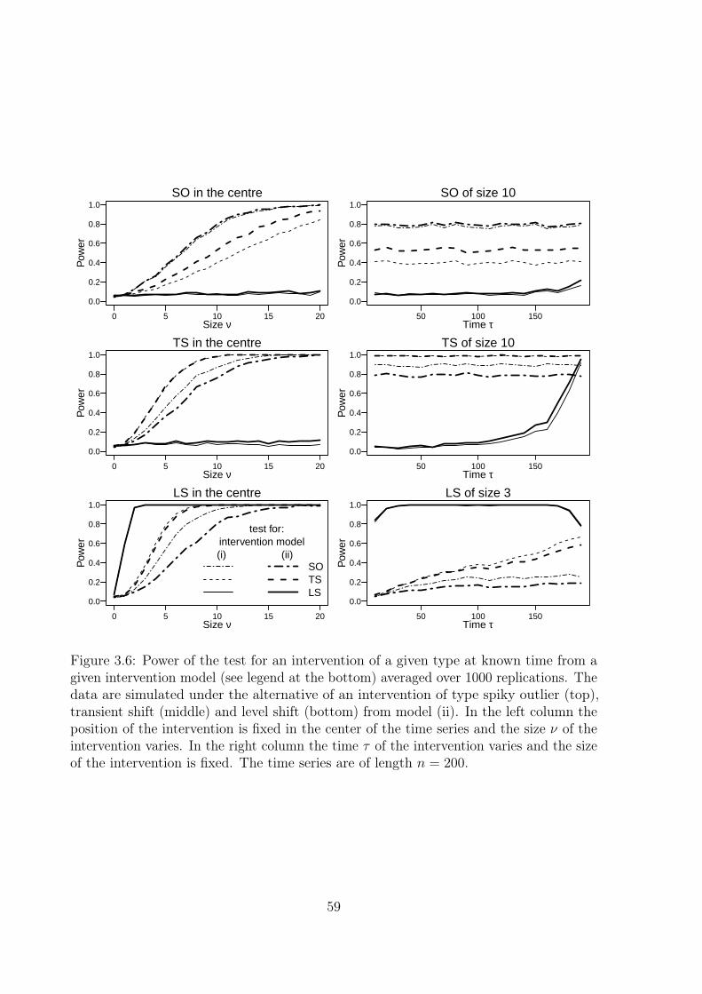
0 5 10 15 20

0.0

0.2

0.4

0.6

0.8

1.0SO in the centre

Size ν

Pow

er

0 5 10 15 20

0.0

0.2

0.4

0.6

0.8

1.0TS in the centre

Size ν

Pow

er

0 5 10 15 20

0.0

0.2

0.4

0.6

0.8

1.0LS in the centre

Size ν

Pow

er

SO TS LS

test for: intervention model(i) (ii)

50 100 150

0.0

0.2

0.4

0.6

0.8

1.0SO of size 10

Time τP

ower

50 100 150

0.0

0.2

0.4

0.6

0.8

1.0TS of size 10

Time τ

Pow

er

50 100 150

0.0

0.2

0.4

0.6

0.8

1.0LS of size 3

Time τ

Pow

er

Figure 3.6: Power of the test for an intervention of a given type at known time from agiven intervention model (see legend at the bottom) averaged over 1000 replications. Thedata are simulated under the alternative of an intervention of type spiky outlier (top),transient shift (middle) and level shift (bottom) from model (ii). In the left column theposition of the intervention is fixed in the center of the time series and the size ν of theintervention varies. In the right column the time τ of the intervention varies and the sizeof the intervention is fixed. The time series are of length n = 200.

59

the type of an intervention when it is not known, as it is done in Section 3.4.3. The rightcolumn shows that for interventions at the end of a time series, it is more challengingto distinguish a level shift from a transient shift or spiky outlier, since we have littleinformation on the evolution of the time series after the time of intervention.

For further insight, we run simulations based on intervention model (i) with our standardparameter setting as before. The results for both models are quite similar, but as ageneral observation, it is easier to detect interventions from model (i), since interventionsfrom this model have stronger effects. Model (i) and (ii) represent different forms ofintervention effects. We will examine the consequences of misspecifying an interventionmodel in Section 3.4.4.

3.4.2 Intervention of known type at unknown time

An intervention of a given type occurring at unknown time can be detected using thetest statistic

T ∗ = maxτ∈D

T (τ),

i.e. the maximum of the test statistics for an intervention at each possible time. Denotethe time of a possible intervention by τ ∗ = arg maxτ∈D T (τ). A priori knowledgeabout the time where an intervention might occur could be included by restrictingthe maximization to a predefined smaller set D of values for τ , which is chosen to beD = {2, . . . , n} by default. The p value of a test for the hypothesis H0 : ν = 0 ∀τ ∈ D isapproximated by a parametric bootstrap procedure as proposed by Fokianos and Fried(2010):

1. Generate B bootstrap replicates from an intervention-free INGARCH model withparameter vector θ, the estimate under H0 defined in the previous section.

2. Compute the test statistic T ∗b for each bootstrap replicate b = 1, . . . , B.3. The p value is given by the number of bootstrapped test statistics at least as large

as the original test statistic, divided by B + 1.

We choose B = 500 for our study. Our simulations presented in Figure 3.7 (a) supportthat this testing procedure behaves well also for intervention model (ii). Under the nullhypothesis the p values show a reasonable approximation to the uniform distribution andthe achieved significance levels do not deviate from the respective nominal significancelevels much. The positions of the erroneously detected interventions in Figure 3.7 (b) showno peculiarities for the test for SO and TS. The test on a LS detects more interventions

60

●●●●●●●●●●●●●●●

●●●●●●●●●

●●●●●●●●●●●●●●●●

●●●●●●●●●●●●●●●

●●●●●●●●●

●●●●●●●●●●●●●●●●●●

●●●●●●●●●●●●●

●●●●●●●●●●●●●●●●●●●

●●●●●●●●●●●●●●

●●●●●●●●●●●●●●●

●●●●●●●●●●●●●●●

●●●●●●●●●●●●●●●●●●●●●●

●●●●●●●●●

●●●●●●●●●●●●●●●●●●●●●

●●●●●●●●●●●●●●●●●

●●●●●●●●●●●●●●●●●●●

●●●●●●●●●●●●●●●●●●●

●●●●●●●●●●

●●●●●●●●●

●●●●●●●●●●●●●●●

●●●●●●●●●●●●●●

●●●●●●●●●●●●●●●●●●●●●●

●●●●●●●●●●●●●●

●●●●●●●●●●●●●●●●

●●●●●●●●

●●●●●●●●●●●●●●●●●●

●●●●●●●●●●●●●●●●●●

●●●●●●●●●

●●●●●●●●●●●●●

●●●●●●●●●●●●●

●●●●●●●●●●●●●

●●●●●●●●●●●

●●●●●●●●●●●●●●●

●●●●●●●●●●●●●●●●●●●

●●●●●●●●●●●●●●

●●●●●●●●●●●●●●●●●●●

●●●●●●●●●●●●●●

●●●●●●●●●●●●●●●

●●●●●●●●●●●●●●●●●●

●●●●●●●●●●●●●●●

●●●●●●●●

●●●●●●●●●

●●●●●●●●●●●●●

●●●●●●●●●●●●●●●●●

●●●●●●●●●●●●●●●●●

●●●●●●●●●●●●●●●●●

●●●●●●●●●●●●●●

●●●●●●●●●●●●●●●●●●●

●●●●●●●●●●●●

●●●●●●●●●●●●●●●●●●

●●●●●●●●●●●●●●●

●●●●●●●●●●●●●●●●●●●●

●●●●●●●●●●●●●●●●

●●●●●●●●●

●●●●●●●●●●●●●●●●

●●●●●●●●●●●●●●

●●●●●●●●●●●●●●

●●●●●●●●●●●●●●●●●●

●●●●●●●●●●●●●●●●●

●●●●●●●●●●●●●●●●

●●●●●●●●●●●●●●●●

●●●●●●●●●●●●●●●●●●

●●●●●●●●●●●●●

●●●●●●●●●●●●●●

●●●●●●●●●●●

●●●●●●●●●●●●●

●●●●●●●●●●●●●●●●

●●●

0.0 0.2 0.4 0.6 0.8 1.0

0.0

0.2

0.4

0.6

0.8

1.0

Expected p−value

Obs

erve

d p−

valu

e

●●●●●●●●●●●●●●●

●●●●●●●●●

●●●●●●●●●●●●●●●●

●●●●●●●●●●●●●●●

●●●●●●●●●

●●●●●●●●●●●●●●●●●●

●●●●●●●●●●●●●

●●●●●●●●●●●●●●●●●●●

●●●●●●●●●●●●●●

●●●●●●●●●●●●●●●

●●●●●●●●●●●●●●●

●●●●●●●●●●●●●●●●●●●●●●

●●●●●●●●●

●●●●●●●●●●●●●●●●●●●●●

●●●●●●●●●●●●●●●●●

●●●●●●●●●●●●●●●●●●●

●●●●●●●●●●●●●●●●●●●

●●●●●●●●●●

●●●●●●●●●

●●●●●●●●●●●●●●●

●●●●●●●●●●●●●●

●●●●●●●●●●●●●●●●●●●●●●

●●●●●●●●●●●●●●

●●●●●●●●●●●●●●●●

●●●●●●●●

●●●●●●●●●●●●●●●●●●

●●●●●●●●●●●●●●●●●●

●●●●●●●●●

●●●●●●●●●●●●●

●●●●●●●●●●●●●

●●●●●●●●●●●●●

●●●●●●●●●●●

●●●●●●●●●●●●●●●

●●●●●●●●●●●●●●●●●●●

●●●●●●●●●●●●●●

●●●●●●●●●●●●●●●●●●●

●●●●●●●●●●●●●●

●●●●●●●●●●●●●●●

●●●●●●●●●●●●●●●●●●

●●●●●●●●●●●●●●●

●●●●●●●●

●●●●●●●●●

●●●●●●●●●●●●●

●●●●●●●●●●●●●●●●●

●●●●●●●●●●●●●●●●●

●●●●●●●●●●●●●●●●●

●●●●●●●●●●●●●●

●●●●●●●●●●●●●●●●●●●

●●●●●●●●●●●●

●●●●●●●●●●●●●●●●●●

●●●●●●●●●●●●●●●

●●●●●●●●●●●●●●●●●●●●

●●●●●●●●●●●●●●●●

●●●●●●●●●

●●●●●●●●●●●●●●●●

●●●●●●●●●●●●●●

●●●●●●●●●●●●●●

●●●●●●●●●●●●●●●●●●

●●●●●●●●●●●●●●●●●

●●●●●●●●●●●●●●●●

●●●●●●●●●●●●●●●●

●●●●●●●●●●●●●●●●●●

●●●●●●●●●●●●●

●●●●●●●●●●●●●●

●●●●●●●●●●●

●●●●●●●●●●●●●

●●●●●●●●●●●●●●●●

●●●

SO

1.5% 4.8% 9.5%●●●●●●●●●●●

●●●●●●●●●●●

●●●●●●●●●●●●●●

●●●●●●●●●●●●●●●

●●●●●●●●●●●●●●●

●●●●●●●●●●●●●

●●●●●●●●●●●●●●●●●●●●

●●●●●●●●●●●●●●

●●●●●●●●●●●●●●●●●●●●●

●●●●●●●●●●●●●●●●●

●●●●●●●●●●

●●●●●●●●●●●●●●●●●

●●●●●●●●●●●●●●●●●●

●●●●●●●●●●●●●●●

●●●●●●●●●●●●●●●●●●●●●

●●●●●●●●●●

●●●●●●●●●●●●●●●●●

●●●●●●●●●

●●●●●●●●●●●●●●●●●

●●●●●●●●●●●●●●●●

●●●●●●●●●●●

●●●●●●●●●

●●●●●●●●●●●●●●●

●●●●●●●●●●●●●●●

●●●●●●●●●●

●●●●●●●●●●●●●

●●●●●●●●●●●●●●●●●●●

●●●●●●●●●●●●●●●●●●●●●●●

●●●●●●●●●●●

●●●●●●●●●●●●●●●●

●●●●●●●●●●●

●●●●●●●●●

●●●●●●●●●●●●●●●●●●●●●

●●●●●●●●●●●●

●●●●●●●●●●●●●●●●●●●

●●●●●●●●●●●●●

●●●●●●●●●

●●●●●●●●●●●●●

●●●●●●●●●●●●

●●●●●●●●●●●●●●●●●

●●●●●●●●●●●●

●●●●●●●●●●●●●●●

●●●●●●●●●●●●●●●●●●●●

●●●●●●●●●●●●●●●●●

●●●●●●●●●●●●●●●●

●●●●●●●●●●●●●●●●

●●●●●●●●●●●●●●●●●●

●●●●●●●●●●●●●

●●●●●●●●●●●●●

●●●●●●●●●●●●●●●●●●●●●●

●●●●●●●●●●●●●●●●●●

●●●●●●●●●●●●

●●●●●●●●●●●●

●●●●●●●●●●●●●●

●●●●●●●●●●●●●●●●●

●●●●●●●●●●●●●●

●●●●●●●●●●●●

●●●●●●●●●●●●●●●●●●●●●●

●●●●●●●●●

●●●●●●●

●●●●●●●●●●●●●

●●●●●●●●●●●●●●●●

●●●●●●●●●●●●●●●●●●●●●

●●●●●●●●●●●●

●●●●●●●●●●●●

●●●●●●●●●●

●●●●●●●●●●●●●

●●●●●●●●●●●●●●●

●●●●●●●●●●

0.0 0.2 0.4 0.6 0.8 1.0

0.0

0.2

0.4

0.6

0.8

1.0

Expected p−value

●●●●●●●●●●●

●●●●●●●●●●●

●●●●●●●●●●●●●●

●●●●●●●●●●●●●●●

●●●●●●●●●●●●●●●

●●●●●●●●●●●●●

●●●●●●●●●●●●●●●●●●●●

●●●●●●●●●●●●●●

●●●●●●●●●●●●●●●●●●●●●

●●●●●●●●●●●●●●●●●

●●●●●●●●●●

●●●●●●●●●●●●●●●●●

●●●●●●●●●●●●●●●●●●

●●●●●●●●●●●●●●●

●●●●●●●●●●●●●●●●●●●●●

●●●●●●●●●●

●●●●●●●●●●●●●●●●●

●●●●●●●●●

●●●●●●●●●●●●●●●●●

●●●●●●●●●●●●●●●●

●●●●●●●●●●●

●●●●●●●●●

●●●●●●●●●●●●●●●

●●●●●●●●●●●●●●●

●●●●●●●●●●

●●●●●●●●●●●●●

●●●●●●●●●●●●●●●●●●●

●●●●●●●●●●●●●●●●●●●●●●●

●●●●●●●●●●●

●●●●●●●●●●●●●●●●

●●●●●●●●●●●

●●●●●●●●●

●●●●●●●●●●●●●●●●●●●●●

●●●●●●●●●●●●

●●●●●●●●●●●●●●●●●●●

●●●●●●●●●●●●●

●●●●●●●●●

●●●●●●●●●●●●●

●●●●●●●●●●●●

●●●●●●●●●●●●●●●●●

●●●●●●●●●●●●

●●●●●●●●●●●●●●●

●●●●●●●●●●●●●●●●●●●●

●●●●●●●●●●●●●●●●●

●●●●●●●●●●●●●●●●

●●●●●●●●●●●●●●●●

●●●●●●●●●●●●●●●●●●

●●●●●●●●●●●●●

●●●●●●●●●●●●●

●●●●●●●●●●●●●●●●●●●●●●

●●●●●●●●●●●●●●●●●●

●●●●●●●●●●●●

●●●●●●●●●●●●

●●●●●●●●●●●●●●

●●●●●●●●●●●●●●●●●

●●●●●●●●●●●●●●

●●●●●●●●●●●●

●●●●●●●●●●●●●●●●●●●●●●

●●●●●●●●●

●●●●●●●

●●●●●●●●●●●●●

●●●●●●●●●●●●●●●●

●●●●●●●●●●●●●●●●●●●●●

●●●●●●●●●●●●

●●●●●●●●●●●●

●●●●●●●●●●

●●●●●●●●●●●●●

●●●●●●●●●●●●●●●

●●●●●●●●●●

TS

1.1% 5.6% 11.9%●●●●●

●●●●●●●●●●●●

●●●●●●●●●●●●●●●●●●

●●●●●●●●●●

●●●●●●●●●●●●●●●●●●●●●

●●●●●●●●●●●●●

●●●●●●●●●●●●●●●●●●●●

●●●●●●●●●●●●●●●●

●●●●●●●●●●●●●●●

●●●●●●●●●●●●●

●●●●●●●●●●●●●

●●●●●●●●●●●●●●●●●●●

●●●●●●●●●●●●●●●●●●

●●●●●●●●●●●●●●●●●●●●●

●●●●●●●●●●●●●●●●●●●

●●●●●●●●●●●●●●●●

●●●●●●●●●●●●●●●●●

●●●●●●●●●●●●●●●●●●●●●

●●●●●●●●●●

●●●●●●●●●●●●●●

●●●●●●●●●●

●●●●●●●●●●●●●●●●●

●●●●●●●●●●●

●●●●●●●●●●●●●●

●●●●●●●●●●●●●●●●

●●●●●●●●●●●●●●●●●●●●●●●

●●●●●●●●●●●●

●●●●●●●●●●●●●●●●

●●●●●●●●●●●

●●●●●●●●●●

●●●●●●●●●●●●●●●

●●●●●●●●●●●

●●●●●●●●●●

●●●●●●●●●●●●●●●

●●●●●●●●●●●●●●●●●●●●

●●●●●●●●●●●●●

●●●●●●●●●●●●●●●●●●●●●●

●●●●●●●●●●

●●●●●●●●●●●●●●●●●●

●●●●●●●●●●●●●●●●●●●

●●●●●●●●●●●●●●●●

●●●●●●●●●●●●●●●

●●●●●●●●●●●●●●●

●●●●●●●●●●●●●●

●●●●●●●●●●●●●●

●●●●●●●●●●●

●●●●●●●●●●●●●●●●●●●

●●●●●●●●●●●●●●●

●●●●●●●●●●●●●●●

●●●●●●●●●●●

●●●●●●●●●●●●●●●●●

●●●●●●●●●●

●●●●●●●●

●●●●●●●●●●●●●●●●●

●●●●●●●●●●●

●●●●●●●●●●●●●●

●●●●●●●●●●●●●

●●●●●●●●●●●●

●●●●●●●●●●●●●●●●●●●●●●

●●●●●●●●●●●●

●●●●●●●●●●●●●●●●

●●●●●●●●●●●

●●●●●●●●●●●●●●●●●

●●●●●●●●●●●●●●●●●●●●●●●

●●●●●●●●●●

●●●●●●●●●●●●

●●●●●●●●●●

●●●●●●●●●●●

●●●●●

0.0 0.2 0.4 0.6 0.8 1.0

0.0

0.2

0.4

0.6

0.8

1.0

Expected p−value

●●●●●●●●●●●●

●●●●●●●●●●●●●●●●●●●●●●●

●●●●●●●●●●

●●●●●●●●●●●●●●●●●●●●●

●●●●●●●●●●●●●

●●●●●●●●●●●●●●●●●●●●

●●●●●●●●●●●●●●●●

●●●●●●●●●●●●●●●

●●●●●●●●●●●●●

●●●●●●●●●●●●●

●●●●●●●●●●●●●●●●●●●

●●●●●●●●●●●●●●●●●●

●●●●●●●●●●●●●●●●●●●●●

●●●●●●●●●●●●●●●●●●●

●●●●●●●●●●●●●●●●

●●●●●●●●●●●●●●●●●

●●●●●●●●●●●●●●●●●●●●●

●●●●●●●●●●

●●●●●●●●●●●●●●

●●●●●●●●●●

●●●●●●●●●●●●●●●●●

●●●●●●●●●●●

●●●●●●●●●●●●●●

●●●●●●●●●●●●●●●●

●●●●●●●●●●●●●●●●●●●●●●●

●●●●●●●●●●●●

●●●●●●●●●●●●●●●●

●●●●●●●●●●●

●●●●●●●●●●

●●●●●●●●●●●●●●●

●●●●●●●●●●●

●●●●●●●●●●

●●●●●●●●●●●●●●●

●●●●●●●●●●●●●●●●●●●●

●●●●●●●●●●●●●

●●●●●●●●●●●●●●●●●●●●●●

●●●●●●●●●●

●●●●●●●●●●●●●●●●●●

●●●●●●●●●●●●●●●●●●●

●●●●●●●●●●●●●●●●

●●●●●●●●●●●●●●●

●●●●●●●●●●●●●●●

●●●●●●●●●●●●●●

●●●●●●●●●●●●●●

●●●●●●●●●●●

●●●●●●●●●●●●●●●●●●●

●●●●●●●●●●●●●●●

●●●●●●●●●●●●●●●

●●●●●●●●●●●

●●●●●●●●●●●●●●●●●

●●●●●●●●●●

●●●●●●●●

●●●●●●●●●●●●●●●●●

●●●●●●●●●●●

●●●●●●●●●●●●●●

●●●●●●●●●●●●●

●●●●●●●●●●●●

●●●●●●●●●●●●●●●●●●●●●●

●●●●●●●●●●●●

●●●●●●●●●●●●●●●●

●●●●●●●●●●●

●●●●●●●●●●●●●●●●●

●●●●●●●●●●●●●●●●●●●●●●●

●●●●●●●●●●

●●●●●●●●●●●●

●●●●●●●●●●

●●●●●●●●●●●

●●●●●

LS

1.2% 3.3% 7.2%

(a)

Time τ

Fre

quen

cy

0 50 100 150 200

0

2

4

6

8

10

12SO

Time τ0 50 100 150 200

0

2

4

6

8

10

12TS

Time τ0 50 100 150 200

0

2

4

6

8

10

12LS

(b)

Figure 3.7: (a) Size of the test for an intervention of given type (see title) at unknown timefrom intervention model (ii) using B = 500 bootstrap samples. The data are simulatedunder the null hypothesis of no intervention. Simulation results are averaged over 1000repetitions. A point above the bisecting line indicates that the test is conservative forthis particular size. The percentages given at the bottom of each panel are the achievedsignificance levels for a nominal level of 1%, 5% and 10%, respectively. The time seriesare of length n = 200.(b) Detected times of intervention τ ∗ for tests with a p value below 10% in the simulationsabove.

61

●

●

●

●●

●

●

●

●

●

●

●

●

●

●

●

●

●●

●

●

●

●

●

●

●

●

●●

●

●

●

●●●

●

●

●

●●

●

●

●●

●

●

●

●

●

●●

●

●

●

●

●

●

●

●

●

●

●●

●

●●

●

●

●

●

●

●

●

●

●

●

●

●

●

●

●

●

●

●

●

●

●

●●

●●

●●

●

●

●

●

●

●

●

●

●

●

●

●

●

●●

●

●●

●

●

●

●

●

●●

●

●

●

●

●

●

●

●

●

●

●

●

●

●

●

●

●●

●

●

●●●●

●

●

●●●●●●●●●●●●●

●

●

●

●●●

●

●

●

●●●●

●●

●

●

●

●●●●●

●●●

●

●

●●●

●

●

●●

●

●

●

●

●

●●

●●●●●●●

●

●

●

●

●

●

●●

●●●●●●●●

●●●

●

●

●●

●

●

●●

●

●●●●●●

●

●●●●●

●

●

●

●

●●●●●●●●

●

●

●●

●

●

●

●

●●●

●

●●●●

●

●

●

●●

●

●

●

●●●●●●

●●

●●●●

●

●

●

●

●

●

●●●

●

●●●●●●

●●●

●

●

●●●

●

●

●

●

●●

●

●●

●

●●●

●

●

●

●

●

●●●●●

●

●

●●

●

●●●●●●

●●●●●●●●

●

●

●

●

●

●

●

●

●

●

●

●●

●●

●

●

●

●

●

●

●

●●

●

●

●●●

●

●

●

●

●

●

●

●

●●

●

●●

●

●

●

●

●●

●

●

●

●

●

●

●

●

●

●

●

●

●

●

●

●

●

●

●●

●

●

●

●

●

●

●

●

●

●

●

●

●

●

●

●●

●

●

●

●

●

●

●

●

●

●●

●

●

●

●

●

●

●

●●

●●

●

●

●

●

●

●

●●

●

●

●

●

●

●

●

●

●●

●

●

●

●

●

●

●

●

●●

●

●

●

●

●

●

●

●

●

●

●

●

●

●

●

●

●

5 10 15 20 5 10 15 20 5 10 15 20

0.0

0.2

0.4

0.6

0.8

1.0

Simulated SO

Size ν

P−

valu

eSO TS LSSO

●

●

●●●

●

●

●

●

●●

●

●

●●

●

●

●

●

●●

●

●●

●

●

●

●

●

●

●

●●

●

●

●

●

●

●

●

●

●

●

●

●

●

●

●

●

●

●

●

●

●●●●

●

●

●

●

●

●

●

●

●

●

●●

●

●

●

●

●

●

●●●

●

●

●

●

●

●

●

●

●

●

●

●●

●

●●

●

●

●

●

●

●

●●

●

●

●

●

●

●

●

●

●

●

●

●

●●

●

●

●

●●●●●●

●

●

●

●

●●

●

●●

●

●

●

●

●

●

●

●

●

●

●

●●

●

●

●

●

●

●

●

●

●

●

●

●

●

●

●

●

●

●●

●

●

●

●●

●

●

●

●

●

●

●●

●

●

●

●

●

●

●

●

●

●

●

●

●

●

●

●

●

●

●●

●

●

●

●

●

●●

●

●

●

●

●

●

●

●

●

●

●

●

●

●

●

●

●●

●

●

●

●

●

●●●

●

●●

●

●

●

●●

●

●

●

●

●

●

●

●●

●

●●

●

●

●

●

●

●

●

●

●●

●●

●

●

●

●

●

●●●●●●

●●●●●●●●●●●●●●

●

●●●●●●●●●●●●●●●●●●●●●●●●●

●

●●●●

●

●●

●●●●●●●●●●●●

●

●●●

●

●●●●●●

●●

●●●

●

●●●●●●●●●

●

●●●●●●●

●

●●●●

●

●●●●●●●●

●

●

●

●●●●●●●●●●●●

●

●●●●●

●●●●●●●●●●●●●●●●●●●●●●●

●

●

●●●●●●

●

●●●

●

●●●●●●●●●●

5 10 15 20 5 10 15 20 5 10 15 20

0.0

0.2

0.4

0.6

0.8

1.0

Simulated TS

Size ν

SO TS LSSO● ●

●●

●●●

●

●

●●

●●

●

●

●●●●

●

●

●

●

●

●

●

●●

●

●●

●●

●

●●

●

●●

●

●●

●

●

●●

●●●

●

●●

●●

●●

●

●

●

●

●

●

●

●●

●

●●

●

●

●

●

●

●

●

●

●

●

●

●

●●

●●

●

●●

●

●

●

●

●●●●

●

●

●

●

●

●

●

●

●

●

●

●

●

●

●

●

●

●

●

●

●

●

●

●●●●

●

●●

●

●

●

●

●

●

●

●●

●●

●

●●●

●●●●

●

●●●●

●

●

●●●

●

●

●●●

●

●

●

●●

●

●

●

●

●

●

●●●

●

●

●●●●

●

●

●●

●

●

●

●●

●

●●

●

●

●●●●

●●●

●

●

●

●●

●

●

●

●

●

●●●

●

●

●

●

●

●

●

●●

●

●

●

●●●

●

●

●

●●

●

●

●●

●

●●

●

●●●●●●

●

●

●●

●●

●●

●

●●

●●●●●●

●

●

●

●●

●

●●

●●●

●

●●

●

●

●●

●

●

●

●

●●

●●

●

●

●

●

●

●

●

●

●●

●

●

●

●●

●

●●●●●

●

●

●

●

●

●●

●

●

●

●

●

●●

●

●

●

●●

●

●

●●●

●

●

●

●

●●

●

●

●

●●●

●●●●

●●

●

●

●

●

●●

●●

●

●●

●●●●

●

●●

●

●●●●

●

●●

●

●

●

●

●●

●

●

1 2 3 5 1 2 3 5 1 2 3 5

0.0

0.2

0.4

0.6

0.8

1.0

Simulated LS

Size ν

SO TS LSSO

(a)

Time τ

Fre

quen

cy

90 95 100 105 110

0

200

400

600

800

1000 SO

Time τ90 95 100 105 110

0

200

400

600

800

1000 TS

Time τ90 95 100 105 110

0

100

200

300

400

500 LS

(b)

Figure 3.8: (a) Power of the test for an intervention of given type (see segments withineach plot) at unknown time from intervention model (ii) using B = 500 bootstrap samples.The data are simulated under the alternative of an intervention of given type (see title)from model (ii) in the center of a time series of length n = 200. We vary the size of theintervention (see horizontal axis). Simulation results are averaged over 1000 repetitions.(b) Detected times of intervention τ ∗ for tests with a p value below 10% in the simulationsabove. The simulated intervention is of the same type which is also tested for (see title)and is of size 20 for SO and TS and of size 5 for LS.

at the beginning and at the end of the time series. For level shifts at these positionsthere are only very few observations available for estimating the level before and afterthe shift, respectively. Therefore randomly occurring extreme observations can hardly bedistinguished from a LS.

To investigate the power of the test we consider the simulations shown in Figure 3.8 (a).A test for a SO requires an intervention size of about ν = 15 to detect it right in morethan 50% of the cases (see left segment in the left plot). For a test regarding a LS, asize of ν = 2 of a LS is needed to attain a detection above 50% (see right segment inthe right plot). Note that a LS of size ν does imply a shift in the marginal mean byν/(1 − β1 − α1), i.e. by about 6.6 in this simulation with ν = 2. The timing of theintervention shown in Figure 3.8 (b) is very accurate for SO and TS (over 85% of the

62

Time τ

Fre

quen

cy

0 50 100 150 200

0

100

200

300

400

500

600

Figure 3.9: Times of interventions found by the iterative detection procedure for model (ii)using B = 500 bootstrap samples. The data are simulated with two transient shifts frommodel (ii) at time 50 (δ = 0.7, size ν = 12) and at time 151 (δ = 0.9, size ν = 9). Thetime series are of length n = 200. Simulation results are based on 1000 repetitions.

cases are detected correctly) and somewhat less accurate for the LS (about 40% detectedcorrectly, the other cases are up to ten observations away from the true value).

3.4.3 Multiple interventions of unknown type at unknown time

A common situation in several applications is that both the position and the type ofintervention are unknown. From Figure 3.8 (a) we get an idea that it is possible toclassify the type of an intervention by the minimum p value of all (three) tests. Onaverage the p values of the tests for the matching type are lower than the p values of thetests on the other types. To overcome the problem of multiple testing we use a Bonferronicorrection, i.e. multiply the p values by the number of intervention types considered.The intervention type is classified according to the lowest p value, if below the chosensignificance level. In case of equal p values we prefer a LS with δ = 1 (since its effectis usually more dominant) and then opt for the intervention type with the highest teststatistic, as in Fokianos and Fried (2010).

Furthermore, there might be more than one intervention in a time series. Fokianos andFried (2010) propose a stepwise procedure to detect, classify and eliminate multipleintervention effects in a time series. The elimination of intervention effects is basedon (3.2). We adopt their iterative procedure for the alternative intervention model (ii)by using the modified equations from Section 3.2. We refer to their paper for details andshow some simulation results for the alternative intervention model (ii).

We apply the iterative detection procedure to simulated time series with two transientshifts at time 50 with size ν = 12 and δ = 0.7, and at time 151 with ν = 9 and δ = 0.9.In 27% of the 1000 repetitions we find both interventions exactly at the time of their

63

occurrence, and no others. Each of the interventions is found in around 50% of the cases,at least one of them in about 72%. Notably, only in about 20% of the repetitions wedetect an intervention at a wrong time and this happens quite often close to the actualtimes of interventions, see Figure 3.9. Although we test for interventions with δ = 0.8 andthus slightly misspecify their type, our results are satisfactory. There are no systematicsimulations of Fokianos and Fried (2010) for intervention model (i), but their examplespoint into the same direction.

3.4.4 Misspecification of the intervention model

An important question is the effect of model misspecification on the detection procedure.Consider the situation with an intervention of a given type occurring at a given time.We look at the thin lines in Figure 3.6 for the test on an intervention of model (i) andcompare them with the bold ones of the same kind, which stand for the test basedon model (ii) from which the data are in fact simulated. We note that both tests arecomparable and misspecification of the data generating process does not affect the powera lot. This also applies when model (ii) is the true data generating process, as we haveconfirmed by simulations not reported here. Hence, there is some robustness againstmisspecification of the intervention model.

Another interesting finding from Figures 3.6 is that for example a transient shift frommodel (ii) is somewhat similar to a spiky outlier from model (i). In general, an interventioneffect from model (ii) resembles somewhat one from model (i) with a slightly lower valueof δ and vice versa. This is in line with the explanations given in Section 3.2.

We also study the effect of misspecification of the intervention model on the iterativeprocedure for detection of multiple interventions. Applying the detection procedurefor internal interventions to 1000 time series from the external intervention model (ii),identical to those used in Section 3.4.3, yields almost the same rates of truly and falselydetected interventions as for the correctly specified situation. For the converse situation,i.e. data generation according to the internal model (i) and detection assuming theexternal model (ii), we detect both interventions correctly in 40% of the cases, whichis more than a third higher than for data generation from the external model. On theother hand we find interventions at wrong times in another 40% of the cases, comparedto 20% when simulating from the external model. In a nutshell, the above empiricalresults suggest that a successful identification procedure for interventions is based onthe amount of information that the data carry. The choice of the model is of secondaryimportance.

64

Time

Num

ber

of c

ases

0

10

20

30

40

50

●●●●

●●

●

●●

●

●●

●●●

●

●

●●●

●●●

●●

●●

●

●●

●

●

●●

●●●

●●

●●

●●

●●●

●●

●●●

●●●●

●

●

●

●●●

●

●●●●●

●●●

●●●

●●●●

●●

●●●

●

●●●

●

●

●

●

●●

●

●

●

●●

●

●

●

●

●

●

●

●

●

●●

●●

●

●

●

●●

●

●

●

●●

●●

●●

●

●

●

●

●●●

●

●●

●

●●

●

●

●●●●

●

●●

●●●

●

●

●●●●

●●

●●

●●

●●

●●●●

●

●●

●●●

●●

●●●●

●●

●

●●

●

●●●●

●●●

●●●

●

●

1. LS with ν=4.06

2. SO with ν=19.70 ●

●

originalcleanedIntervention model (i)

Num

ber

of c

ases

1990 1992 1994 1996 1998 2000

0

10

20

30

40

50

●●●●

●●

●

●●

●

●●

●●●

●

●

●●●

●●●

●●

●●

●

●●

●

●

●●

●●●

●●

●●

●●

●●●

●●

●●●

●●●●

●

●

●

●●●

●

●●●●●

●●●

●●●

●●●●

●●

●●●

●

●●●

●

●

●

●

●●

●

●

●

●●

●

●

●

●

●

●

●

●

●

●●

●●

●

●

●

●●

●

●

●

●●

●●

●●

●

●

●

●

●●●

●

●●

●

●●

●

●

●●●●

●

●●

●●●

●

●

●●●●

●●●

●●

●●

●

●●●●

●

●

●

●●●●

●●●

●●

●●

●

●●

●

●●●●

●●●

●●●

●

●

1. LS with ν=4.27

2. SO with ν=14.99Intervention model (ii)

Time

Figure 3.10: Number of campylobacterosis infections (reported every 28 days) in thenorth of Québec in Canada. The original time series is displayed in grey, the modifiedtime series cleaned by the procedure from Section 3.4.3 in black.

A related question is whether we can deduce from the data which intervention model ismore suitable for describing a certain data pattern. Some experiments with classificationbased on the out-of-sample prediction error, as suggested by a reviewer, did not providegood results.

3.5 Real data application

We again study the time series of campylobacterosis cases considered in Section 2.6.1.The original time series with n = 140 observations is shown in grey in Figure 3.10. Aninfection with the bacterium Campylobacter may be caused mainly by contaminatedfood but also by contact with infected animals. Human to human spread is possibleparticularly for infants. The incubation period is typically 2-5 days. Infected patientsoften do not show any symptoms and are potentially infectious via their excrements for2-4 weeks on average. The number of cases is higher in warm seasons. More details onmodeling Campylobacter infections for epidemiological surveillance (applied to data fromGermany) are given by Manitz and Höhle (2013).

Following Ferland et al. (2006) we fit an INGARCH(1,13) model to the data withα1 = · · · = α12 = 0 and the regression on the conditional mean for lag 13 accounting forseasonal variation.

Since we do not have any prior information on the occurrence of possible interventions,we apply the iterative detection procedure from Section 3.4.3 to the data. We first

65

search for interventions following our new intervention model (ii). In the first step, thebootstrapped p values for all considered types (SO, TS with δ = 0.8 and LS) are zero,using B = 500 bootstrap replicates. The procedure decides in favor of the LS withan estimated size of 4.27 found at time 84, following the classification rule given inSection 3.4.3. The detected intervention effect is removed from the time series accordingto the decomposition presented in Section 3.2, applying the procedure proposed byFokianos and Fried (2010). In a second step, both the test on a SO and on a TS give ap value of zero at time 100, the same position already found in the first step for these typesof interventions. We decide in favor of the SO with an estimated size of 14.99, becauseit has a higher value of the test statistic than the TS. Again, the time series is cleanedfrom the detected intervention effect. In a third step, no further interventions with ap value lower than 5% are detected and the procedure stops with two intervention effectsfound. The estimated parameters for the cleaned time series are β0 = 2.28, β1 = 0.36

and α13 = 0.35. The cleaned time series and both interventions are shown in Figure 3.10(bottom).

Finally we fit the full model with both detected interventions to the original time seriesand obtain

Zt|FZ,κt−1 ∼ Poisson(κt),

κt = λt + 3.52(0.80) I[84,∞)(t) + 36.67(7.31) I{100}(t), (3.5)

λt = 2.25(0.58) + 0.36(0.06)Zt−1 + 0.35(0.08)λt−13.

The jointly estimated parameters in (3.5) clearly differ from those by the iterativedetection procedure reported before. The standard errors of the regression coefficientsbased on the normal approximation (3.4) are given in parentheses. Standard errorsobtained by a parametric bootstrap based on 1000 replications are 1.27 (β0), 0.07 (β1),0.17 (α13), 0.98 (LS at time 84) and 7.65 (SO at time 100). Note that these standard errorsdo not reflect the additional model uncertainty induced by the intervention detectionprocedure for either of the two approaches. The bootstrapped standard errors largelyagree with the normal approximation ones, but are much higher for β0 and α13. Becauseof the long delay of 13 time points the estimation of α13 can make less use of the dataand is, as a regression coefficient of an unobserved variable, more difficult to estimateanyway. Estimation of the intercept β0 and α13 strongly interfere. In this challengingsituation with a small sample size the normal approximation standard errors do notexpress this uncertainty adequately. However, for a simpler INGARCH(1,1) process theirperformance was quite good in case of 200 or more observations (see Section 3.3.2).

66

0 1 2 3 4 5 6

0.0

0.2

0.4

0.6

0.8

1.0

Frequency (in weeks)

Intervention model (i)

0 1 2 3 4 5 6

0.0

0.2

0.4

0.6

0.8

1.0

Frequency (in weeks)

Intervention model (ii)

Figure 3.11: Cumulative periodogram of the Pearson residuals of model (3.5) for thecampylobacterosis infections time series (right). For intervention model (i) the samedetection procedure has found the same two intervention effects and a full model includingboth interventions is fitted to the data (left). The dashed lines give approximative 95%confidence limits of a Kolmororov-Smirnov test on a constant spectral density (cf. Venablesand Ripley, 2002, p. 396), which are used as a visual check for uncorrelated residuals.

We also apply this procedure for intervention model (i) and find the same types ofinterventions at the same times with only slightly different estimated intervention sizes.These results are presented in Figure 3.10 (top). The average of the squared Pearsonresiduals for the fitted models with both interventions is 18.8 for model (i), comparedto 19.3 for our new intervention model (ii). An INGARCH model without interventioneffects has a much higher value of 30.9. Hence the internal intervention model (i) fitsin this sense a little better to the data than the external one and both interventionmodels clearly outperform a model without intervention effects. Note that the cumulativeperiodograms in Figure 3.11 show that there is less structure left in the residuals of ournew intervention model (ii) than for intervention model (i). However, both models mightsuffer from lacking covariates. Manitz and Höhle (2013) list some studies which suggestan association of campylobacterosis cases with certain weather conditions like absolutehumidity, on which we do not have information for our data example.

3.6 Discussion

In this chapter we study a new variant of an intervention model for INGARCH processesand adopt a maximum likelihood approach for detection and estimation of interventioneffects proposed by Fokianos and Fried (2010) to this new model. With the obtainedprocedures one can test for intervention effects at given times but also search for inter-vention effects at unknown times. Simulations support that the presented procedureswork quite reliably. In comparison to the intervention effects studied by Fokianos andFried (2010), those in the new model have less influence on subsequent observations afterthe occurrence of an intervention. The new model describes an external effect which

67

propagates only via the observations, whereas an intervention effect from the old modelcan be seen as an internal change of the underlying mean. Our application to the weeklynumber of campylobacterosis cases illustrates the usefulness of our new model.

We find some robustness against misspecification of the intervention model. Thus onecan expect a reasonable performance for this kind of intervention effects applying eitherof the two models. On the other hand this finding suggests that a test to discriminatethe intervention models might have low power.

One undesirable feature of the procedures for detection of interventions are the highcomputational costs. For the example in Section 3.5 with B = 500 bootstrap samples andn = 140 observations each step of the iterative detection procedure runs about 72 minutesfor intervention model (i) and about 75 minutes for model (ii) on a single processorunit (Intel Xeon CPU with 2.83 GHz). The reason for the long computation time is theimplementation of the parametric bootstrap. Fokianos and Fried (2012) reduced thecomputation time of the bootstrap considerably by not estimating the parameter vectorfor each bootstrap replicate but using the true value used for its generation instead. Thismodification results in quite conservative procedures. With parallelized computation ofthe bootstrap we have greatly shortened its duration using multiple processors.

This chapter has shown that there are capable tools available for modeling and retrospec-tive detection of intervention effects in count time series based on INGARCH models.These methods have been generalized to the framework of count time series followinggeneralized linear models and are included in the R package tscount; see Section 2.5.In many applications it is not sufficient to detect intervention effects retrospectively,i.e. once the complete time series has been observed. Instead, the goal is to detectintervention effects in real-time. This problem of prospective intervention detection isthe topic of the next chapter.

68

Chapter 4

Online monitoring in the context ofinfectious disease surveillance

4.1 Introduction

Prospective detection of aberrations in count time series is of interest in various appli-cations. For example in public health, surveillance of infectious diseases aims at timelyrecognizing outbreaks of epidemics for taking proper actions promptly. Other possible ap-plications are industrial quality control, where an unusually large number of faulty piecesmay indicate a flawed production process (Weiß, 2015), or finance, where exceptionallylarge numbers of transactions may point to anomalies at the stock market. Monitoringprocedures need to be applicable in an online manner such that the decision that anaberration has occurred is made in real-time with only short time delays. The statisticalmethods employed in this context have their roots in the literature on statistical processcontrol (SPC), time series analysis, sequential testing and change point detection.

The focus of this chapter is on the application of these statistical methods to the problemof infectious disease surveillance. However, most of the considerations in this studyare meant to be of general relevance and do also apply to many data problems beyondpublic health. Recent introduction to the topic of infectious disease surveillance aregiven by Unkel, Farrington, Garthwaite, Robertson, and Andrews (2012) and Held andPaul (2013). Salmon, Schumacher, Burmann, Frank, Claus, and Höhle (2016a) describea system for automated outbreak detection which employs the R package surveillance(Salmon et al., 2016b). We summarize the crucial aspects of infectious disease surveillance.Its principal aim is to timely recognize disease outbreaks which manifest by an unusuallylarge number of infections. As a data basis one constantly observes the number of patients

69

per day, week or month which have been infected by a certain pathogen. These timeseries are typically collected by public health authorities and they are available for anumber of different pathogens. For each pathogen, the data is subdivided into differentgeographical units and sometimes further into age groups. Consequently, there may bethousands of time series under surveillance, requiring the use of automatic procedures foroutbreak detection which not require manual (and thus subjective) decisions. Monitoringprocedures are also referred to as control charts because they were originally employedas graphical tools.

The general goal of a monitoring procedure is to timely detect potential aberrations in atime series whilst not giving too many false alarms. An aberration is a sudden or gradualchange of the data generating process (DGP) occurring at an unknown time point, whenthe process is said to be out-of-control. This change can basically be of any form. Theoutbreak of a disease for instance is expected to result in an increase of the location andpossibly also of the strength of temporal dependence (Höhle and Paul, 2008, Section 4).Notably, control charts based on the likelihood ratio are designed to optimally detectspecific out-of-control scenarios (Höhle and Paul, 2008; Weiß and Testik, 2012). In thisstudy we focus on methods which particularly aim at detecting location increases butare not designed for a specific out-of control scenario.

In order to assess whether the DGP has changed one needs to learn about its characteristicsbefore the aberration, when the process is assumed to be in-control. This can be doneby assuming a parametric model for the time series before a potential change. In theapplications we are aiming at, the model parameters are in fact unknown and need tobe estimated using historical data. The setting for our study is to have observed a timeseries up to time n and to start monitoring future observations at time n+ 1. The timeperiod of the first n observations used for learning about the DGP is referred to as theset-up phase (phase I). The time period thereafter, in which the actual monitoring takesplace, is referred to as the operational phase (phase II).

The characteristics of infectious disease time series may vary with the respective pathogen,geographical unit or age group. Typical features of this kind of data are seasonal variation(caused by environmental effects, varying severity of pathogens and other factors like publicholidays), trends, temporal dependence (possibly resulting from the disease transmissionmechanism) and the occurrence of irregularities (such as disease outbreaks). The numberof infected persons is also driven by the size and structure of the population at risk.Note that the number of reported cases is generally lower than the actual incidence. Theextent of this under-reporting is not constant over time but follows a seasonal patternitself and also reacts to singular events (e.g., increased media coverage on an infectious

70

disease). This may cause seasonal effects as well as irregular artifacts in the observednumber of cases. The various aspects of modeling seasonality are studied by Held andPaul (2012).

Classical control charts for count data are based on the assumption of independent andidentically distributed observations from a distribution which is fully specified (Gan,1990). Such procedures do not account for the typical characteristics of infectiousdisease time series which are described in the previous paragraph. In the context ofinfectious disease surveillance, monitoring procedures for non-identically distributedobservations based on GLMs have been proposed; so-called regression charts which areable to consider trends and seasonal effects (Farrington, Andrews, Beale, and Catchpole,1996; Rossi, Lampugnani, and Marchi, 1999; Höhle and Paul, 2008; Noufaily, Enki,Farrington, Garthwaite, Andrews, and Charlett, 2013). However, these procedures stillassume independent observations. In the recent literature on control charts for countdata the case of dependent observations has received more attention (Weiß and Testik,2012; Manitz and Höhle, 2013). These methods do neither require the observations to beidentically distributed nor to be independent. Most research has been on methods basedon the marginal distribution of an observation.

In this study we investigate how accommodating temporal dependence can enhancemonitoring procedures. We introduce a monitoring procedure which is based on one-stepahead predictions, i.e. the conditional distribution of an observation given the past.Our main finding is that such a procedure can substantially improve the immediatedetection of outbreaks (compared to procedures based on the marginal distribution) butthat its dependence on previous observations may also yield undesired effects in somesituations. Our monitoring procedure assumes that the DGP is from the class of counttime series following GLMs as it is presented in Section 1.2. Models from this appealingand flexible class are able to capture typical characteristics of infectious disease data likeserial dependence and seasonality. These models are formulated recursively, describingthe underlying mean of the time series conditionally on the past. Serial dependenceis included by regression on past observations and on past values of the conditionalmean. The latter is called feedback mechanism and helps to model serial dependenceparsimoniously.

Notwithstanding the model which is assumed for the DGP, there are different types oftest statistics which are used to built control charts for count time series: the observationsthemselves (Manitz and Höhle, 2013), transformed residuals (Rossi et al., 1999; Noufailyet al., 2013), (generalized) likelihood ratios (Höhle and Paul, 2008; Weiß and Testik, 2012)or an estimator of the model parameters. Moreover it is important to distinguish between

71

different construction principles for control charts. A Shewhart-type control chart basesits decision on the information of the current time point only, whilst a CUSUM-typecontrol chart accumulates information of successive time points. The former type hasmore power than the latter type to detect large aberrations without delay. Conversely,CUSUM-type charts have more power than Shewhart-type charts to detect moderateaberrations, albeit with some delay. Our simulations show that monitoring based onmodels with temporal dependence is particularly good for immediate detection, but,at least in our current implementation, not so good for delayed detection of outbreaks.We therefore decide to build a Shewhart-type monitoring procedure, which is also thestate of the art at the German infectious disease surveillance system at the Robert Kochinstitute (see for example Salmon et al., 2016a).

This chapter is organised as follows. Section 4.2 very briefly describes the GLM-basedcount time series models for the in-control process and compares them to other proposalsfrom the literature. We discuss in some more detail how to model seasonality. Section 4.3introduces a monitoring procedure based on one-step-ahead predictions. Section 4.4studies the performance of the monitoring procedure by simulations. We compare theresults of the procedure for models with and without temporal dependence in differentdata situations. We discuss benefits but also pitfalls of using models with temporaldependence for monitoring. In Section 4.5 we present a comprehensive case study usinga data example from infectious disease surveillance, again considering models with andwithout temporal dependence. We demonstrate that these data in fact exhibit temporaldependence. We illustrate the process of model selection and fitting in the set-up phaseand apply the monitoring procedure in the operational phase. Section 4.6 summarizesour results and gives an outlook on further directions of research.

4.2 Models for the in-control process

For low counts, standard models based on the assumption of normality, or at leastcontinuously and symmetrically distributed data, are often inappropriate even aftersuitable transformation (cf. Held and Paul, 2013). Models which have been particularlytailored for count data are usually more appropriate. In the context of infectious diseasedata, several count data models have been proposed. Many of those assume that theobservations are independently but not identically distributed (e.g. Noufaily et al., 2013).However, such models are not adequate if there is a considerable amount of serialdependence among data, as it is usually observed in practice. A comprehensive reviewof models for count time series which are able to describe serial dependence is given in

72

Section 2.7. In this section we review models which have been proposed particularly formodeling infectious disease time series. All these models originate from the idea of ageneralized linear model (GLM).

We first introduce some notation. Let {yt : t ∈ N} be a univariate count time series tobe monitored, where yt is e.g. the number of registered infections in week t. We assumethis observed count time series to be a realization of the stochastic process {Yt : t ∈ N}.In some cases there is additional covariate information available, for instance on weatherconditions. Let {X t : t ∈ N} be a corresponding time-varying r-dimensional covariatevector, i.e., X t = (Xt,1, . . . , Xt,r)

>. Denote by Ft0 the information on past observationsup to time t0 as well as on covariates up to time t0 + 1. All presented models assumethat Yt|Ft−1 has a Negative Binomial or Poisson distribution but differ in the way theyspecify the conditional mean E (Yt|Ft−1) = λt.

In the model proposed by Held, Höhle, and Hofmann (2005) the conditional mean is asum of a deterministic (endemic) component and a first order autoregressive (epidemic)component and is given by

λt = exp

(β0 + δt+

S∑s=1

(γ1,s sin(ωst) + γ2,s cos(ωst))

)+ β1Yt−1,

where β0, δ, γ1,1, . . . , γ1,S, γ2,1, . . . , γ2,S, β1 are unknown parameters but S is fixed. Theendemic component includes a linear trend and a deterministic seasonal figure withfrequency ωs. The exponential function is applied to the covariate effects but not to theautoregressive component such that this model is not a GLM (since the linear predictoris not linear in the parameters) but could instead be regarded as a generalized additivemodel (GAM). Wei, Schüpbach, and Held (2015) additionally include the effect of time-varying covariates either to the endemic or to the epidemic component. Inference is basedon the likelihood approach.

Another proposal by Manitz and Höhle (2013) based on Heisterkamp et al. (2006) is ahierarchical time series (HTS) model (see Section 2.7.2). This model does not explicitlyhave an autoregressive component but is able to account for serial dependence by atime-varying intercept. The conditional mean λt is given by

λt = exp(β0,t + δt+ γt + η>X t

).

The time-varying intercept β0,t is assumed to depend on its previous values according to

∆dβ0,t|β0,t−1, . . . , β0,t−d ∼ N(0, κ−1β0

),

73

where ∆d is the difference operator of order d ∈ {0, 1, 2} and κβ0 a precision parameter.For d = 0 this yields an independence model but for higher orders d this inducesdependence between successive observations. The other parameters, δ for the lineartrend, γt for a seasonal effect and the vector η for the effect of a covariate vector X t,are also assumed to be normally distributed with certain priors. Inference is done in aBayesian framework and utilizes an efficient integrated nested Laplace approximation(INLA) (Rue, Martino, and Chopin, 2009).

In our study the process {Yt : t ∈ N} is assumed to belong to the class of count timeseries following generalized linear models as it has been introduced in Section 1.2. Recallthat the regression equation specifying the conditional mean λt is of the general formgiven by (1.1), i.e.,

g(λt) = β0 +

p∑k=1

βk g(Yt−ik) +

q∑`=1

α`g(λt−j`) + η>X t.

Here g : R+ → R is a link function and g : R+ → R is a transformation. A choiceof g(x) = g(x) = x yields the INGARCH model whereas choosing g(x) = log(x) andg(x) = log(x+ 1) yields the log-linear model studied by Fokianos and Tjøstheim (2011),Woodard et al. (2011) and Douc et al. (2013). Note that the INGARCH model withthe identity link function accommodates only positive temporal correlation and requiresthe covariates to be nonnegative. In contrast, the log-linear model, which impliesa multiplicative effect of the regressors on the response, is able to describe negativeand positive temporal correlation and allows for covariates with negative values. Thedependence on previous values of the mean, the so-called feedback mechanism, allowsfor parsimoniously modeling serial correlation. It can, to some extent, also model time-varying means and generally yields smoother models than only with dependence onprevious observations. Denote by θ = (β0, β1, . . . , βp, α1, . . . , αq, η1, . . . , ηr)

> the vectorof all regression parameters. The conditional distribution of Yt given Ft−1 is assumedto belong to the class of mixed Poisson processes (see Christou and Fokianos, 2015a).An important special case is to assume a Poisson distribution, i.e. Yt|Ft−1 ∼ Poisson(λt).Another special case studied by Christou and Fokianos (2014) is to assume a NegativeBinomial distribution parametrized in terms of its mean with an additional dispersionparameter φ ∈ (0,∞), i.e. Yt|Ft−1 ∼ NegBin(λt, φ). This allows for more variabilityof the process, which is otherwise fully specified by the mean and the degree of serialdependence. The Poisson distribution is a limiting case for φ→∞.

Compared to the model by Held et al. (2005), the class of GLM-based count time seriesused in this study allows for more general forms of serial correlation of higher order and

74

with a feedback mechanism. By way of comparison to the model proposed by Manitz andHöhle (2013) recall our findings in Section 2.7.2: An advantage of their Bayesian approachis that prediction intervals which reflect both observation and estimation uncertaintycan be obtained in a natural way. A disadvantage is the much higher computationaleffort, which is particularly a problem for a real-time application to thousands of timeseries. A fit of their model turns out to be very smooth (cf. Figure 2.5) and is thusexpected to provide less accurate one-step-ahead predictions than models includingexplicit dependence on past observations.

Infectious disease time series often exhibit a seasonal pattern. There are several possibili-ties to account for seasonal effects within the class of count time series based on GLMs,see Kedem and Fokianos (2002, Section 4) and many textbooks on regression models.These approaches are briefly reviewed in the following paragraphs. The length of oneseason T is assumed to be known. An extension of the considered approaches to severalsuperimposed periodicities of different lengths, say T1, . . . , Tr, would be straightforward.

One popular approach is to include deterministic periodic covariates, which impliesthat the seasonal pattern does not change over time. The most common choice fordeterministic seasonality is a superposition of sinusoidal waves of the Fourier frequenciesωs = 2πs/T , s = 1, . . . , S, where S is chosen based on a model selection criterion (see forexample Held and Paul, 2012). For each value of s, the two covariates Xt,s(1) = sin(ωst)

and Xt,s(2) = cos(ωst) with the corresponding coefficients ηs(1) and ηs(2), respectively, areadded to the model. The resulting 2S covariates are linearly independent from eachother and from a constant vector, which guarantees a unique and identifiable solution.Another, more flexible choice of deterministic periodic covariates would be a periodicB-splines basis for polynomial splines using the R package pbs (Wang, 2013), where apolynomial degree of three yields good smoothness and the number of knots K can bechosen based on a model selection criterion. The number of knots is equal to the numberof covariates and hence the number of parameters which are introduced. The resulting Kcovariates Xt,1, . . . , XtK are nonnegative and not linearly independent from a constantvector such that the corresponding parameters interfere with the intercept parameter andthere is not necessarily a unique solution. An example of periodic B splines with K = 5

knots is shown in Figure 4.1. A variant of the approach with deterministic covariatesis employed by the improved Farrington method (Noufaily et al., 2013), where dummyvariables account for seasonality. However, the division of the whole period into windowsis not fixed but depends on the week for which a prediction is needed (see also Salmonet al., 2016b, p. 8). We do not consider this variant in our study because the time-varyingwindows conflict with the idea of a global seasonal pattern and because dummy variablesusually introduce more parameters than the other types of periodic covariates. Note that

75

Week

Cov

aria

te v

alue

1 5 10 15 20 25 30 35 40 45 50 52

00.

20.

40.

6

Figure 4.1: Covariates Xt,1 (circle), Xt,2 (triangle), Xt,1 (cross), Xt,1 (diamond) and Xt,1

(asterisk) of periodic B splines with K = 5 knots for a period length of T = 52. Thecovariates are periodic with Xt,k = Xt+52,k, k = 1, . . . , K.

infectious disease time series do not only show smooth seasonal patterns but sometimesalso sharp periodic effects that take place in only one or two weeks of the year (e.g. lesscases around Christmas or New Year). Such effects can be described by a single dummyvariables (see for example Salmon et al., 2016b).

A second and completely different approach for modeling seasonality accommodatestemporal dependence on observations (Yt−T ) and/or conditional means (λt−T ) which areT time units (i.e. one period) back in time. This stochastic seasonality is employed by forinstance Ferland et al. (2006). This approach allows to describe seasonal patterns of anyshape which might possibly even change slightly over time. Stochastic seasonality is moreflexible than deterministic one but tends to be less suitable for very pronounced seasonalpatterns. A third approach pursued by Held and Paul (2012) explains seasonality bytime-varying dependence parameters. We do not consider this approach in our studybecause it is quite complicated and difficult to interpret.

Fitting models of the form (1.1) can be done by quasi conditional maximum likelihoodestimation of the unknown regression parameters θ. For the dispersion parameter φ of theNegative Binomial distribution one can use an estimator based on Pearson’s χ2 statisticsas proposed by Christou and Fokianos (2014). For a sample of n observations, theseestimators are denoted by θn and φn, respectively. Details on the estimation procedureincluding formulas, technical considerations regarding the implementation and propertiesof the estimators are given in Section 2.2.2.

One usually assumes that the process is in-control in the set-up phase. However, it mighthappen that this assumption is violated. A likely scenario is the presence of outbreaksin the set-up phase which have not been detected previously. Such outbreaks could be

76

included in the above framework model by the intervention model studied by Fokianosand Fried (2010, 2012) and Liboschik et al. (2016), which describes intervention effectsby deterministic covariates (see Section 2.5 and Chapter 3). Their approach also allowsto search for retrospective detection of intervention effects of unknown type occurring atunknown time points. One could also consider robust approaches for model selectionand fitting in the set-up phase. In Section 5.2 we investigate robust estimators of the(partial) autocorrelation for identifying the model order. Section 5.3 discusses someexisting approaches for robust parameter estimation.

4.3 Prediction-based monitoring

Let us assume that we have observed the time series yt, . . . , yn and possible covariatesX1, . . . ,Xn of the complete set-up phase. Based on that data we have selected and fittedan adequate model from the class of count time series based on GLMs. This includesthat we have fully specified a model for the conditional mean λt(θ) and estimated theregression parameters by θn. To simplify notation we consider a model with a NegativeBinomial conditional distribution, i.e. Yt|Ft−1 ∼ NegBin(λt(θ), φ), of which we haveestimated the dispersion parameter by φn. The case of Yt|Ft−1 ∼ Poisson(λt(θ)) iscovered as a limiting case, where φ does not need to be estimated because it approachesinfinity. Note that in our setting the model parameters are not re-estimated in each stepof the following monitoring procedure since this bears the risk of overfitting by adaptingto gradually increasing outbreaks. For this reason Noufaily et al. (2013) do not considerthe last six months for designing their monitoring procedure.

4.3.1 Monitoring procedure

Based on the model obtained from the set-up phase, we want to successively monitorincoming observations in the operational phase. We study a monitoring procedurewhich gives an alarm if the actually observed realization yt0+1 of Yt0+1 is implausiblewith respect to the one-step-ahead predictive distribution for that time t0 + 1. Becauseof the conditional construction of the considered model, one-step-ahead prediction isstraightforward. Recall that Ft0 is the available information before yt0+1 is observed.If the true parameters θ and φ were known, the distribution of Yt0+1 given Ft0 isNegBin(λt0+1(θ), φ). In practice we plug in the estimated parameters θn and φn toapproximate the distribution of the one-step-ahead prediction Y (t0)

t0+1 of Yt0+1 by

77

Y(t0)t0+1 ∼ NegBin(λt0+1, ψn) with λt0+1 = λ(θn). (4.1)

Note that this distribution does only reflect the sampling uncertainty but neither theestimation uncertainty nor the uncertainty induced by model selection. We will discussin Section 4.6 how our procedure could be extended to account for estimation uncertainty.In the context of infectious disease surveillance one is only interested in detecting positivedeviations from the in-control model. Denote a one-sided one-step-ahead predictioninterval with a coverage rate of 1− α by

PI(t0)t0+1(1− α) =

[0, U

(t0)t0+1

].

Its upper bound U (t0)t0+1 is chosen to be the (1−α)-quantile of (4.1) for attaining the given

coverage rate; recall Section 2.3. An alarm is given if yt0+1 lies outside this predictioninterval, which is referred to as the stopping rule. The time since the procedures hasstarted until the first alarm is called run length, which is here given by

R = inf{s ≥ 1 : Yn+s /∈ PI(n+s−1)

n+s (1− α)}. (4.2)

4.3.2 Calibration and performance measures

There is a trade off between the chance to timely detect aberrations (out-of-controlperformance) and the chance of a false alarm (in-control performance). On the one handthe procedure should not produce too many false alarms since this will fatigue the usersof the system. On the other hand the procedure should not detect disease outbreaks toolate (or even not at all) since this can affect the health of many people. This conflictof objectives is solved by maximizing the out-of-control performance subject to a givenin-control performance (chance of a false alarm). Different monitoring procedures arethen compared with respect to their out-of-control performance.

We briefly review some performance measures. All of them can be formulated in termsof the distribution of the run length R. If the process is assumed to be in-control, thenR is the time until a false alarm. If the process is assumed to be in-control before timet0 = n + τ (i.e. at the τ -th observation of the operational phase) and out-of-controlthereafter, then R − τ is the detection delay. One should consider R − τ + 1 insteadof R to measure the out-of-sample performance if τ > 1. Note that the support of therun length distribution is the set of positive integers and this distribution is generallypositively skewed. In case of i.i.d. observations the run length of certain control chartshas a geometric distribution and is quite easy to handle. However, Tartakovsky (2008)

78

demonstrates that this does not hold for non-i.i.d. models and argues that many principlesfor designing control charts are not suitable in that case. One should bear in mind thatin case of time series models some of the performance measures may have a differentinterpretation than in the classical case. In our study we approximate the distribution ofthe run length R by simulation. Accordingly, we pay some attention to this approximationin our discussion of the performance measures.

The average run length (ARL) is defined by the expectation of the run length distributionE(R). It is a standard practice in SPC to fix the in-control ARL (often denoted by ARL0)to a given value, say a0. This has the interpretation that we can on average expect afalse alarm once every a0 observations. Approximation of the ARL is problematic sincethe expectation depends on the upper tail of the run length distribution. In practice oneneeds to stop the procedure when there has not been an alarm within a certain (large)number of time points, say M . Therefore the simulated approximation of the run lengthdistribution is truncated at M such that the mean of this distribution is a negativelybiased estimator of the ARL.

One could also consider quantiles of the run length distribution. Gan (1994) proposeto use the median run length (MRL) instead of the ARL to measure the performanceof a control chart. He argues that the MRL has a more meaningful interpretation (theprobability of run lengths lower (respectively greater) than the MRL is 50%). Whilstthe ARL is more convenient for analytical calculations, the MRL is easier to obtain bysimulation since one can approximate it from a truncated run length distribution (aslong as the truncation is above the MRL).

Another measure is the probability of an alarm within r0 time units, i.e., POAr0 = P (R ≤r0). In the context of infectious disease surveillance one might want to use this as anout-of-control performance measure to attain a large probability of detecting an outbreakwithin only r0 weeks. This measure is also meaningful in an in-control situation, whereone would choose r0 sufficiently large and adjust the control chart to given (low) value ofPOAr0 . For weekly data one could choose t0 = 52 to control the probability of a falsealarm within one year. Lai and Chan (2008) propose the probability of a false alarm perunit of time, which coincides with POAr0/r0 in the case of independent in-control data.This is identical to the false-positive rate (FPR) used by e.g. Noufaily et al. (2013) andManitz and Höhle (2013). When fixing the in-control FPR one might want account formultiple testing, e.g. by a Bonferroni correction of the desired level. For out-of-controlsituations Noufaily et al. (2013) and Manitz and Höhle (2013) measure the performanceof a control chart by the probability of detection (POD). It is given by POA∆, where ∆

79

Scenario β0 β1 α1 η1 φ

Independent 1.570 0.0 0.0 0.4 8.5Weak autocorrelation 1.220 0.2 0.0 0.4 14.5Medium autocorrelation 0.880 0.4 0.0 0.3 17.0Strong autocorrelation 0.187 0.8 0.0 0.1 1000.0With feedback 0.266 0.4 0.4 0.1 17.0

Table 4.1: Parameter settings for model (4.3) considered in the simulation study.

is the duration of the aberration which has to be detected. It measures the probabilitythat an aberration is detected during its occurrence.

4.4 Simulation study

We study the performance of the monitoring procedure presented in Section 4.3.1 by asimulation study. The scenarios used in this simulation study are chosen to imitate arealistic application like it is presented in Section 4.5. Our study is a proof of conceptfor prediction-based monitoring procedures for models with dependence and points outsome notable features. We consider a set-up phase with a length of nine years and 52observations per year, i.e. n = 468 observations. The performance of the procedure isassessed in an operational phase of one year, i.e. m = 52 observations.

The in-control data are randomly generated trajectories from the GLM-based count timeseries model (1.1) with a Negative Binomial conditional distribution, the logarithmiclink function and dependence on the previous observation as well as on the previousconditional mean. A seasonal effect is added by a cosine function with a period length ofone year, i.e. 52 weeks. This model is given by Yt|Ft−1 ∼ NegBin(λt, φ), t = 1, . . . , n+m,with

log(λt) =β0 + β1 log(Yt−1 + 1) + α1 log(λt−1) + η1 cos(2πt/52). (4.3)

The considered parameter settings for that model are given in Table 4.1 and cover a varietyof scenarios. The parameters are chosen such that the resulting process approximatelyhas a marginal mean of 5 and a marginal variance of 10. Model (4.3) is a realistic choicefor the DGP since it is very similar to models which have been selected for a real dataexample; see Section 4.5.1.

For the out-of-control data we need to decide how to model the effect of a disease outbreak.Most proposals from the literature are modifications of the respective in-control model.

80

This is based on the assumption that at least the general principles of the DGP still holdin the presence of the outbreak. One suggestion is to consider a multiplicative shift ofthe mean in case of an outbreak (Höhle and Paul, 2008, Section 2). Another possibilityis that, due to an outbreak, serial correlation is introduced to the process (Höhle andPaul, 2008, Section 4) or, more generally, the extent of serial correlation is increased.One could also consider changes in the mean which enter the dynamics of the process,like spiky outliers or transient shifts (Fokianos and Fried, 2010, 2012), see also Chapter 3.Based on knowledge about the distribution of the incubation period, the shape of alog-normal distribution might be adequate to describe an outbreak (Lotze, Shmueli, andYahav, 2007). A similar approach is to first draw the total number of additional cases ofan outbreak starting at time t0 from a Poisson distribution whose mean depends on thenumber of baseline cases at time t0, and then to distribute these cases in time accordingto a discretized log-normal distribution (Noufaily et al., 2013; Salmon, Schumacher, Stark,and Höhle, 2015). Another strategy to synthetically generate realistic outbreak effects isto use data from real outbreaks (Hutwagner, Browne, Seeman, and Fleischauer, 2005)and superimpose those on data from the in-control DGP.

In this study we consider an abrupt additive shift of the mean which does not enterthe dynamics of the process. This outbreak scenario might not be realistic. However,this simple outbreak scenario makes it easier to interpret the simulation results andthus to understand the properties of our monitoring procedure. We place an outbreakwith a duration of ` = 6 weeks starting at a random position τ , where all positionsτ ∈ {n+ 1, . . . , n+m− `} are equally likely. This random placement of the outbreakwill average out an undesired effect of seasonality on our results. The out-of-control datadenoted by Zt are given by Zt = Yt +Ot, t = 1, . . . , n+m. Realizations of Y1, . . . , Yn+m

are generated in the same way as the in-control data. The outbreak effects Ot areindependent realizations of Poisson distributions with mean ∆t, i.e. Ot ∼ Poisson(∆t),and also independent from Yt, t = 1, . . . , n + m. The outbreak size at time t is givenby ∆t = ∆ · υt · 1(t ∈ {τ, . . . , τ + `}), where ∆ ∈ R is a global factor determining theoutbreak size. The size of the outbreak is proportional to the conditional standarddeviation at the respective time, i.e. υt =

√λt + λ2

t/φ, such that an outbreak causesmore additional infections if the baseline number of infections is large. This seems to bea realistic assumption for an outbreak. From a rather technical point of view this ensuresthat outliers are more or less equally difficult to detect irrespective of the current meanof the process.

We study the prediction-based monitoring procedure introduced in Section 4.3.1 consid-ering two different models: the time series model

81

Scenario Independence model (4.5) Time series model (4.4)

Independence 2.06 (64.5) 2.12 (64.7)Weak autocorrelation 2.11 (65.4) 2.08 (65.0)Medium autocorrelation 2.21 (61.2) 2.08 (64.2)Strong autocorrelation 2.42 (52.3) 1.63 (56.3)With feedback 2.60 (59.6) 2.03 (61.5)

Table 4.2: Average false positive rate in percent for different scenarios (procedurescalibrated to a FPR of 2.5%). The values in parantheses are the proportion of sampleswith a false alarm in any of the 52 weeks of the observational period.

log(λt) =β0 + β1 log(Yt−1 + 1) + α1 log(λt−1) +2∑s=1

(ηs(1) sin(ωst) + ηs(2) cos(ωst)

)(4.4)

and the independence model

log(λt) =β0 +2∑s=1

(ηs(1) sin(ωst) + ηs(2) cos(ωst)

), (4.5)

both with Yt|Ft−1 ∼ NegBin(λt, φ) and ωs = 2πs/52, t = 1, . . . , n+m. The time seriesmodel (4.4) has eight and the independence model (4.5) has six unknown parameters.Note that the time series model covers all models (4.3) of the DGP (although it isoverparametrized) whilst the independence model lacks serial dependence for all parametersettings in Table 4.1 except the first. Following Noufaily et al. (2013), the monitoringprocedures are adjusted to a FPR of 2.5%. Hence the probability of a false alarm for anyof the 52 observations of the operational phase is at most 1− (1− 0.025)52 = 73.2%.

The simulations are carried out on a computation cluster using the R packages batchJobsand batchExperiments (Bischl, Lang, Mersmann, Rahnenführer, and Weihs, 2015). Thereported results are averages of 1000 replications.

We first examine the behavior of the monitoring procedure in an in-control situation.The results in Table 4.2 confirm that the procedure complies with the desired FPR of2.5% in all scenarios and produces usually even less false alarms. This particularly holdsfor time series with strong temporal correlation if the procedure is based on the timeseries model (4.4). Considering the complete operational phase of 52 weeks, one canexpect at least one false alarm in at most 66% of the cases. This is far below the definedupper bound of 73.2%. Overall, the procedure has a satisfying in-control behavior in allconsidered scenarios and seems to be a bit conservative.

82

0

00

0.25

0.5

0.75

1D

etec

tion

rate

Independence

0

0

Medium autocorrelation

0

00

0.25

0.5

0.75

1D

etec

tion

rate

0 1 2 3 4Outbreak size ∆

Strong autocorrelation

0

0

0 1 2 3 4Outbreak size ∆

With feedback

Figure 4.2: Outbreak detection rates of prediction-based monitoring procedures for fourdifferent data scenarios (each in a different panel). The plot symbol indicates whether themonitoring procedure is based on the time series model (cross) or on the independencemodel (circle). The line type indicates detection at the first time point (dotted), up tothe second time point (dashed) or up to the last time point (solid) of the outbreak.

Next, we compare the out-of-control performance of monitoring procedures based onthe time series model (4.4) and on the independence model (4.5). The dotted lines inFigure 4.2 show the probability of detecting the outbreak in the first week of its occurrence,i.e. POA1, for different outbreak sizes ω. Naturally, the detection rate becomes largerfor increasing outbreak size. If the data are independent, then the detection rate isalmost the same for the procedure based on the time series model and the one basedon the independence model. However, in case of dependent data the time series modeloutperforms the independence model. This advantage becomes larger with the degreeof temporal dependence in the data. It is not very surprising though, that a modelaccounting for temporal dependence yields a superior monitoring procedure in case ofdependent observations.

The estimated probability of detecting the outbreak with a delay of one time period, i.e.POA2 − POA1, shown by dashed lines in Figure 4.3 reveals that if an outbreak has not

83

0

00

0.1

0.2

0.3

Det

ectio

n ra

te Independence

0

0

Medium autocorrelation

0

00

0.1

0.2

0.3

Det

ectio

n ra

te

0 1 2 3 4Outbreak size ∆

Strong autocorrelation

0

0

0 1 2 3 4Outbreak size ∆

With feedback

Figure 4.3: Estimated probabilities that the prediction-based monitoring proceduredetects an outbreak with a delay of one time period for four different data scenarios (eachin a different panel). The plot symbol indicates whether the monitoring procedure isbased on the time series model (4.4) (cross) or on the independence model (4.5) (circle).Note that the vertical axis ranges to 0.3 only.

been detected at the first time point of its occurrence, then a procedure based on the timeseries model has a lower chance to detect it at the second time point than one based onthe independence model – in case of actually dependent data. Hence a procedure whichincludes temporal correlation has a higher chance of immediately detecting an outbreakbut a lower chance of detecting it at a later time. The explanation for this phenomenonis as follows: The procedure compares a new observation with the distribution of itsone-step-ahead prediction, which depends on previous observations in case of the timeseries model. If the first observation of an outbreak is large (but not large enoughsuch that the outbreak is detected), then the one-step-ahead prediction for the secondobservation of the outbreak is shifted upwards in case of positive autocorrelation. Withrespect to this shifted one-step-ahead predictive distribution, the second observationof the outbreak does not appear to be implausibly large. Hence this observation lieswithin the one-step-ahead prediction interval and no alarm is given. The described effectbecomes stronger when increasing serial correlation of the fitted model. The dashed linesin Figure 4.2 show the estimated probability of detection with a delay of at most one timeperiod, i.e. POA2, which is equal to the sum of the estimated probabilities of immediate(dotted line in Figure 4.2) and of one time period delayed (Figure 4.3) detection. Overall,the monitoring procedure based on the time series model is superior in case of strongtemporal correlation but slightly inferior in case of medium temporal correlation.

Finally, we evaluate the estimated probability of detection (POD) of an outbreak withinits total duration of ∆ = 6 time points, i.e. POA6, shown by solid lines in Figure 4.2.

84

020

4060

8010

012

0

Time

Num

ber

of in

fect

ions

2006 2007 2008 2009 2010 2011 2012 2013

Set−up phase Operational phase

Figure 4.4: Number of registered EHEC cases per week in North Rhine-Westphalia.

The monitoring procedure based on the time series model is only superior if there isstrong temporal correlation in the data. In situations with lower correlation its lowerrate of delayed outbreak detection is not compensated by its higher rate of immediatedetection. We revisit this issue in Section 4.6.

4.5 Case study

We illustrate phases I and II of a monitoring procedure by a real-data problem frominfectious disease surveillance. Infection of humans with the bacterium enterohemorrhagicE. coli (EHEC) is notifiable under the German Protection against Infection Act. Theweekly number of reported cases broken down to a regional level is recorded by the RobertKoch Institute (RKI) and publicly accessible by their web application SurvStat@RKI2.0 (Robert Koch Institut, 2015). We consider the number of reported EHEC infectionsin the German state North Rhine-Westphalia from January 2006 to May 2013 (646observations), see Figure 4.4. The first five years (n = 261 observations) until December2010 are used as the set-up phase for selecting and fitting an appropriate in-control model.There would be more data available before 2006 but it is quite common in the field ofinfectious disease surveillance to only consider the previous few years to avoid problemswith a potentially unstable DGP (for instance because laboratories change their methodsor the number of probes sent to laboratories is varying over time). We will discuss thestability of the DGP in Section 4.5.2.

85

05

1015

Time

Num

ber

of in

fect

ions

2006 2007 2008 2009 2010 2011

Trainingsample

Validationsample

Figure 4.5: Number of registered EHEC cases per week in North Rhine-Westphalia (onlydata of the set-up phase).

4.5.1 Model selection and fitting in the set-up phase

Building a reliable control chart requires knowledge about the in-control process. Withina parametric approach this means selection of an adequate model and fitting this modelto the available data. We split up the set-up phase into a training sample (the first fouryears until December 2009, 209 observations) and a validation sample (the remainingyear, 52 observations).

In a first step we study the characteristics of the DGP with tools not based on a specificmodel. We hold back the validation sample and use only the training sample highlightedby a dark grey background in Figure 4.5. These considerations shall give an idea whichfeatures an adequate model for the data needs to have and allow to identify a range ofcandidate models.

The empirical marginal mean of 3.83 is quite low. For low means an approximation by acontinuous-valued distribution is usually not appropriate and a distribution accountingfor the discreteness of the observations is preferable. The data is overdispersed, i.e. theempirical marginal variance of 5.94 is substantially larger than the empirical marginalmean. Although a Poisson model with serial dependence explains overdispersion up to acertain degree, we also consider a more flexible Negative Binomial distribution.

A plot of the training sample against time in Figure 4.5 indicates that the number ofregistered cases is larger at the beginning and drops to a lower level in 2007. A globaltrend model does not seem to be adequate for this kind of change in the mean. It seemsmore promising to use models which allow for a more flexible change in the mean like

86

Lag

AC

F

1 5 10 15 20 25 30 35 40 45 50 55

−0.

10

0.1

0.2

0.3

0.4

ACF

Lag

Par

tial A

CF

1 5 10 15 20 25 30 35 40 45 50 55

−0.

10

0.1

0.2

0.3

0.4

PACF

Figure 4.6: Estimated autocorrelation function (left) and partial autocorrelation function(right) of the EHEC training sample. The (partial) autocorrelation at lag 52, correspond-ing to a seasonality of about one year, is marked by a circle.

those with a feedback mechanism, i.e. a dependence on previous conditional means. Wewill nevertheless also consider models with a linear trend to make sure that we do notoverlook this issue. In case of neglecting an upward trend the monitoring procedureproduces too many false alarms, whilst ignoring a downward trend bears the risk ofmissing a relevant aberration. We also consider models with a level shift at some unknowntime point.

The empirical autocorrelation function in Figure 4.6 (left) is about 0.39 at lag one andclearly different from zero for the first few lags. This shows that there is a considerableamount of temporal dependence present in the data. The empirical partial autocorrelationin Figure 4.6 (right) is clearly different from zero for the first and the third lag. Thisindicates that a regression only on one previous observation is not sufficient for describingthe existing serial dependence. In such a case, regression on previous conditional meansoften yields a more parsimonious model which fits the data equally well or even betterthan regression on more than one previous observation. We consider models regressingon one or more previous observations Yt−1, . . . , Yt−p and those additionally regressing onthe conditional mean one week back in time λt−1.

The time series plot in Figure 4.5 slightly indicates that there might be a yearly seasonalfluctuation with larger values in the summer. However, the empirical autocorrelation andempirical partial autocorrelation in Figure 4.6 are very close to zero at lags around T = 52

and hence do not confirm this periodicity. We consider the techniques for modelingseasonality described in the previous section and also models without seasonal effects. Itis neglected that the length of a year is not exactly 52 weeks and varies slightly.

87

We decide for the log-linear model which has more flexibility in including covariates sinceit does not induce restrictions on covariates and on the corresponding parameters. Weindeed experience that the limitation of the identity link model to positive covariatesimpede properly fitting the seasonal pattern. Furthermore, the logarithm is a commonlyused link function for that kind of data (see for example Höhle and Paul, 2008). Thischoice implies that the effect of covariates is multiplicative (and not additive as for amodel with identity link function). This includes that a seasonal effect modeled bycovariates is multiplicative. Trends also have a multiplicative effect, such that a lineartrend in the linear predictor is actually an exponential trend on the original scale of theresponse. For slight trends and short time series such a trend is approximately linear onthe original scale. However, this results in instabilities when extrapolating to long timehorizons. We stress that multiplicative trends should be used with care.

In a second step we use the training data to fit the candidate models which have beenidentified initially. Since the conditional mean is fitted independently of the chosenconditional distribution, we assume a Poisson distribution and reassess this at a laterstage. These fitted models are compared by the (in-sample) Akaike information criterion(AIC) and the out-of-sample measures ranked probability score (RPS), coverage rate (CR)of a one-sided 95% 1-step-ahead prediction interval and prediction bias (see Section 2.4on model assessment). The out-of-sample measures are evaluated on the validation data.The results of the model comparison are presented in Tables 4.3 and 4.4 for models withand without serial dependence, respectively.

We have to decide on a) how to model seasonality, b) whether to include a trend and c)the model orders for serial correlation (excluding stochastic seasonality). We expect (andhave also verified empirically) that decisions b) and c) are strongly interdependent butthat they do not interfere much with decision a). Hence we first decide which approachfor modeling seasonality is preferable while fixing the two other decisions. Regardingthe Fourier approach, the AIC would opt for the first S = 3 Fourier frequencies whilstthe out-of-sample RPS would opt for S = 2. Regarding the periodic B splines approach,both considered criteria consistently choose K = 5 knots (corresponding to 5 additionalparameters). Stochastic seasonality seems to be described better by dependence onthe conditional mean λt−T than on the observation Yt−T observed one year ago. Theformer two approaches employing deterministic covariates clearly outperform the latterstochastic approach, which is not better than not considering seasonality at all. Overall,the periodic B splines approach performs best. In addition to this numerical measures,we examine the seasonal patterns resulting from the Fourier approach with S = 2 andfrom B splines with K = 5 which are shown in Figure 4.7 (top). Both patterns have theirmaximum in August and their minimum in November, though not in exactly the same

88

Seasonality Trend Dependence DoF AIC RPS CR Bias

no no p=1, q=1 3 899.0 1.104 0.942 -0.213

Fourier (S=1) no p=1, q=1 5 901.6 1.091 0.962 -0.220Fourier (S=2) no p=1, q=1 7 900.0 1.076 0.962 -0.224Fourier (S=3) no p=1, q=1 9 898.4 1.097 0.942 -0.210

B splines (K=3) no p=1, q=1 6 900.9 1.070 0.923 0.204B splines (K=4) no p=1, q=1 7 904.3 1.089 0.962 -0.252B splines (K=5) no p=1, q=1 8 892.5 1.058 0.942 0.218B splines (K=6) no p=1, q=1 9 893.7 1.075 0.942 0.211

stochastic (Yt−T ) no p=1, q=1 4 911.2 1.178 0.923 -0.346stochastic (λt−T ) no p=1, q=1 4 900.3 1.102 0.942 -0.191

B splines (K=5) no p=0, q=0 6 940.8 1.109 0.962 -0.433B splines (K=5) no p=1, q=0 7 910.7 1.116 0.962 -0.307B splines (K=5) no p=2, q=0 8 910.5 1.101 0.962 -0.285B splines (K=5) no p=2, q=1 9 888.1 1.106 0.904 0.637B splines (K=5) no p=3, q=0 9 903.1 1.115 0.962 -0.254B splines (K=5) no p=4, q=0 10 903.8 1.108 0.962 -0.248

B splines (K=5) linear p=0, q=0 7 894.3 1.300 0.846 1.259B splines (K=5) linear p=1, q=0 8 888.1 1.222 0.885 1.062B splines (K=5) linear p=1, q=1 9 887.2 1.283 0.865 1.165B splines (K=5) linear p=2, q=0 9 890.0 1.225 0.885 1.067B splines (K=5) linear p=2, q=1 10 888.0 1.243 0.885 1.070B splines (K=5) linear p=3, q=0 10 889.5 1.196 0.885 0.964B splines (K=5) linear p=4, q=0 11 891.4 1.192 0.885 0.957

Table 4.3: Comparison of the fitted candidate models (assuming a Poisson conditionaldistribution). Degrees of freedom (DoF) indicates the number of regression parameters.The considered measures are Akaike’s information criterion (AIC), ranked probabilityscore (RPS), coverage rate (CR) of a one-sided 95% 1-step-ahead prediction interval andprediction bias. The AIC is an in-sample measure evaluated on the training data, wherasall others are out-of-sample measures evaluated on the validation data.

89

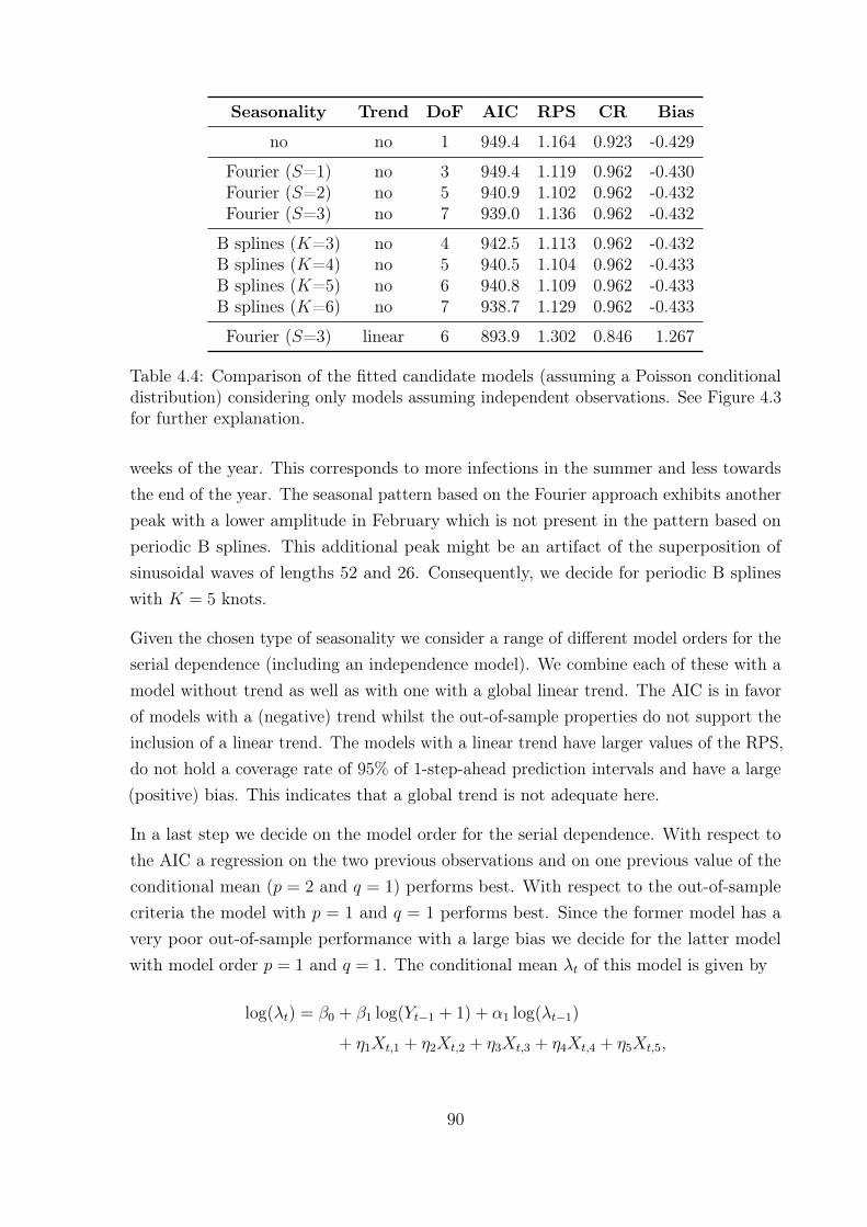
Seasonality Trend DoF AIC RPS CR Bias

no no 1 949.4 1.164 0.923 -0.429

Fourier (S=1) no 3 949.4 1.119 0.962 -0.430Fourier (S=2) no 5 940.9 1.102 0.962 -0.432Fourier (S=3) no 7 939.0 1.136 0.962 -0.432

B splines (K=3) no 4 942.5 1.113 0.962 -0.432B splines (K=4) no 5 940.5 1.104 0.962 -0.433B splines (K=5) no 6 940.8 1.109 0.962 -0.433B splines (K=6) no 7 938.7 1.129 0.962 -0.433

Fourier (S=3) linear 6 893.9 1.302 0.846 1.267

Table 4.4: Comparison of the fitted candidate models (assuming a Poisson conditionaldistribution) considering only models assuming independent observations. See Figure 4.3for further explanation.

weeks of the year. This corresponds to more infections in the summer and less towardsthe end of the year. The seasonal pattern based on the Fourier approach exhibits anotherpeak with a lower amplitude in February which is not present in the pattern based onperiodic B splines. This additional peak might be an artifact of the superposition ofsinusoidal waves of lengths 52 and 26. Consequently, we decide for periodic B splineswith K = 5 knots.

Given the chosen type of seasonality we consider a range of different model orders for theserial dependence (including an independence model). We combine each of these with amodel without trend as well as with one with a global linear trend. The AIC is in favorof models with a (negative) trend whilst the out-of-sample properties do not support theinclusion of a linear trend. The models with a linear trend have larger values of the RPS,do not hold a coverage rate of 95% of 1-step-ahead prediction intervals and have a large(positive) bias. This indicates that a global trend is not adequate here.

In a last step we decide on the model order for the serial dependence. With respect tothe AIC a regression on the two previous observations and on one previous value of theconditional mean (p = 2 and q = 1) performs best. With respect to the out-of-samplecriteria the model with p = 1 and q = 1 performs best. Since the former model has avery poor out-of-sample performance with a large bias we decide for the latter modelwith model order p = 1 and q = 1. The conditional mean λt of this model is given by

log(λt) = β0 + β1 log(Yt−1 + 1) + α1 log(λt−1)

+ η1Xt,1 + η2Xt,2 + η3Xt,3 + η4Xt,4 + η5Xt,5,

90

seaseff_pbsplines5df$week

seas

eff_

pbsp

lines

5df$

seas

eff

0.95

11.

05S

easo

nal e

ffect

B splines (K=5)Fourier (S=2)

Time series model

seaseff_pbsplines4df_indep$weekseas

eff_

pbsp

lines

4df_

inde

p$se

asef

f

1 5 10 15 20 25 30 35 40 45 50 52Week

0.8

11.

52

Sea

sona

l effe

ct

B splines (K=4)Fourier (S=2)

Independence model

Figure 4.7: Seasonal patterns of B splines with K knots and of a superposition of sineand cosine functions for the first S Fourier frequencies. The seasonal effect expresses theestimated factor by which the conditional mean is multiplied in the respective week andis shown on a logarithmic scale. The time series model (4.4) with serial correlation oforder p = 1, q = 1 (top) and the independence model (4.5) (bottom) are fitted to thetraining data.

where the covariates Xt,1, . . . , Xt,5 specify the value of the periodic B splines at time t(see Figure 4.1). We call this best model the (best) time series model.

For comparison, we also select the best model assuming independent observations.According to a comparison of the out-of-sample in Table 4.4 there is little difference inthe performance of models with seasonality based on the first S = 2 Fourier frequenciesand based on periodic B splines with K = 4 knots with respect to the (out-of-sample)ranked probability score. The seasonal patterns of both approaches shown in Figure 4.7(bottom) are of quite similar shape but displaced. Unlike for the Fourier approach, theparameters of periodic B splines may interfere with the intercept and actually do soin this data example. Again, a model with a linear trend has a low AIC but a verypoor out-of-sample behavior. Consequently we choose a model without a trend and withthe first S = 2 Fourier frequencies to be the best model of those assuming independentobservations. We call this model the (best) independence model. The conditional meanλt of this model is given by

91

Lag

AC

F

1 5 10 15 20 25 30 35 40 45 50 55

−0.

10

0.1

0.2

0.3

0.4

Time series model

Lag

AC

F

1 5 10 15 20 25 30 35 40 45 50 55

−0.

10

0.1

0.2

0.3

0.4

Independence model

Figure 4.8: Estimated autocorrelation function of the residuals. The time series modelwith serial correlation of order p = 1, q = 1 (left) and the independence model withoutserial correlation (right) are fitted to the training data.

log(λt) = β0 + η1(1) sin(2πt/52) + η1(2) cos(2πt/52)

+ η2(1) sin(2πt/26) + η2(2) cos(2πt/26).

Given the linear predictor of the model we can now decide which conditional distributionto use. We compare a Poisson and a Negative Binomial model by (in-sample) probabilityintegral transform (PIT) histograms (see Section 2.4) shown in Figure 4.9. For thetime series model both PIT histograms appear to be uniform. Hence we decide for thesimpler Poisson model. For the independence model the PIT histogram is uniform for theNegative Binomial but U-shaped for the Poisson distribution. It seems that the NegativeBinomial distribution needs to account for the variability which is otherwise explainedby temporal dependence.

We compare the fit to the training data of the selected best time series model and the bestindependence model as shown in Figure 4.10. The fit of the independence model repeatsthe same seasonal pattern each year and is otherwise constant over time. Consequentlythis also holds for the predictions of the validation sample, which do not depend onprevious observations. The fit of the time series model also exhibits a seasonal patternwith a peak in the summer. However, this pattern is superimposed by the effect of serialcorrelation. The model reacts to the large observations in the summer of the year 2006where its fit has an especially pronounced peak in the summer as compared to the years2007 and 2009. As mentioned before, the mean of the data appears to vary slowly overtime. The time series model reacts to this change in location and has a larger meanuntil 2007 than in the years thereafter. By contrast, the independence model tends tounderestimate the observations until 2007 and to overestimate them thereafter. The

92

Poisson

Probability integral transform

Den

sity

0.0 0.2 0.4 0.6 0.8 1.0

0.0

0.4

0.8

1.2

Time series modelNegative Binomial

Probability integral transform

Den

sity

0.0 0.2 0.4 0.6 0.8 1.0

0.0

0.4

0.8

1.2

Time series model

Poisson

Probability integral transform

Den

sity

0.0 0.2 0.4 0.6 0.8 1.0

0.0

0.4

0.8

1.2

Independence modelNegative Binomial

Probability integral transform

Den

sity

0.0 0.2 0.4 0.6 0.8 1.0

0.0

0.4

0.8

1.2

Independence model

Figure 4.9: Probability integral transform (PIT) histograms for model with Poisson andNegative Binomial conditional distribution. The time series model with serial correlationof order p = 1, q = 1 (top) and the independence model without serial correlation(bottom) are fitted to the training data.

residuals of the independence model exhibit a considerable amount of serial correlationwhilst the residuals of the time series model appear to be uncorrelated, see Figure 4.8.This shows very clearly that the selected model for independent observations does notcapture the serial correlation which is present in the data. The purpose of the fittedmodels is their use for prediction-based monitoring of future observations. This requiresthat not only the predicted value but also the corresponding prediction interval is reliable.The latter is for example assessed by the ranked probability score (RPS), which is infavor of the time series model: the out-of-sample RPS evaluated on the validation datais 1.148 for the time series model and 1.281 (based on the selected Negative Binomialdistribution) for the independence model. Figure 4.10 illustrates the predictions andcorresponding prediction intervals of the validation sample. In case of the independencemodel, the upper limits of the one-sided one-step-ahead prediction intervals reflect theseasonal pattern of the fitted model and are uniformly larger than those of the timeseries model. Applying the monitoring procedure (calibrated to a FPR of 2.5%) to thevalidation data would sound no alarm (since all observations lie in the 97.5%PI) if it is

93

05

1015

Time

Num

ber

of in

fect

ions

2006 2007 2008 2009 2010 2011

Trainingsample

Validationsample

Figure 4.10: Fitted values and 1-step-ahead predictions (thick lines) with upper boundsof one-sided 97.5% PI (thin lines). The time series model with serial correlation of orderp = 1, q = 1 (solid line) and the independence model without serial correlation (dashedline) are fitted to the training data (grey background).

based on the independence model and two alarms if it is based on the time series model.If we assume the data of the validation phase to follow the in-control DGP, these alarmswill actually be false alarms. Nevertheless, we see more evidence in favor of the timeseries model.

Finally, we fit the two models on the complete data of the set-up phase. Assume thenumber or registered EHEC cases in week t to be a realization of Yt, t = 1, . . . , 261. Thefit of the best time series model is given by Yt|Ft−1 ∼ Poisson(λt) with

log(λt) = 1.423 · 10−5(0.461) + 0.062(0.043) log(Yt−1 + 1) + 0.938(0.356) log(λt−1)

− 0.031(0.125)Xt,1 + 0.114(0.174)Xt,2 − 0.166(0.207)Xt,3

+ 0.059(0.107)Xt,4 − 0.046(0.187)Xt,5.

Standard errors obtained by a parametric bootstrap procedure are given in parentheses.Remarkably, the coefficient of log(λt−1) is very close to one. This term allows the modelto describe the change in the mean over time. However, this comes along with quitelarge standard errors, pointing to a possibly unstable model fit. The fit of the bestindependence model is given by Yt|Ft−1 ∼ NegBin(λt, 9.280) with

log(λt) = 1.310(0.040)− 0.127(0.052) sin(2πt/52)− 0.031(0.053) cos(2πt/52)

+ 0.094(0.053) sin(2πt/26)− 0.140(0.052) cos(2πt/26).

94

The estimated overdispersion coefficient is σ2 = 1/9.280 = 0.108 (0.035). The conditionalvariance is on average roughly yσ2 = 40% larger under a Poisson model. These twofitted models form the basis for the prediction-based monitoring procedure which isdemonstrated in Section 4.5.3.

4.5.2 Nonstationarity vs. serial dependence

Before using the fitted models for monitoring we discuss their reliability. Both models donot assume the DGP to be stationary but allow the expected number of cases to changeperiodically during the year. Apart from that seasonal effect, the expected number ofcases is assumed to be stable over time. For the independence model stable does actuallymean constant whilst the time series model only assumes that the process emerges in thesame way given its previous expected value and its previous observation. The decreasein the number of infections in the year 2007 questions the assumption that the DGP isstable over time, even if we account for the seasonal effect. Models including a globallinear trend have not proven to be appropriate, see the previous section. However, wehave not considered other forms of nonstationarity of the DGP like more general trendsor abrupt changes in location. To some extent serial correlation is able to describe suchnonstationarities. It is a challenging problem to decide whether an explicit model forthe trend or change is more appropriate than a model explaining such phenomenons by(usually strong) serial correlation. We investigate this question in some more detail inthis section.

As mentioned before, Figure 4.5 suggests that there might be an abrupt shift in locationin the year 2007 which could possibly be modeled explicitly. We test whether thereis a level shift (LS) at an unknown time point in the training data by applying theprocedure described in Section 2.5 (and in more detail for models with the identity link inSection 3.4.2). The overall test statistic of this test is the maximum of local test statisticsat each time which are illustrated in Figure 4.11. For the time series model this test isnot significant on a 5% level (p value 0.17, test statistic 15.2). For the independencemodel the test is significant (p value 0, test statistic 23.15) and detects a level shift inweek 15 of the year 2007. The estimated size of the LS is −0.63, which corresponds to adecrease of the expected number of cases by the factor exp(−0.63) = 0.53. Consideringthis level shift for the independence model does indeed yield a model with more or lessuncorrelated residuals whose ACF looks very similar to that of the time series model inFigure 4.8 (left). This indicates that the observed serial dependence, recall Figure 4.6, islargely induced by this change in location.

95

05

1015

2025

Time

Test

sta

tistic

2006 2007 2008 2009 2010

Figure 4.11: Test statistic for detecting a level shift in the training data. The time seriesmodel with serial correlation of order p = 1, q = 1 (filled circle) and the independencemodel without serial correlation (empty circle) are fitted to the training data. Thevertical line indicates at which time the test statistic has its maximum and the horizontalline is the critical value of the test statistic at a 95% level for the time series model (solidlines) and for the independence (dashed lines) model, respectively.

One might come to the conclusion that is not necessary to fit a model with temporaldependence once we haven taken into account the level shift. However, the data ofincluding the years before the set-up phase in Figure 4.12 tell that there is more changein the average location than just one abrupt downward shift in 2007. A moving averagewith a window width of one year suggests that the location changes in a way whichcannot be described adequately by a global trend and/or a few abrupt changes. Themodel with serial dependence is capable to model such a slowly varying trend.

4.5.3 Monitoring in the operational phase

The prediction-based monitoring procedure is illustrated in Figure 4.13. The procedure isbased on the time series respectively independence model fitted to the data of the set-upphase. It starts in the first week of the year 2011. The available information at that timeare all previous observations, the fitted values of the set-up phase and the covariates ofthat time. The alarm threshold is the upper bound of a one-sided 97.5% one-step-aheadprediction interval. This threshold is 8 for the time series model (solid line) and 9 forthe independence model, both larger than the value of 2 EHEC cases which has beenregistered for that week. For both models the procedures continues without an alarm. Forthe second week of 2011 we can use the observation of the first week and the covariatesof the second week. However, monitoring based on the independence model does (by

96

05

1015

Time

Num

ber

of in

fect

ions

2001 2002 2003 2004 2005 2006 2007 2008 2009 2010 2011

Set−up phase

Figure 4.12: Number of registered EHEC cases per week in North Rhine-Westphaliaincluding data before the chosen set-up phase. The thick line is the moving average witha window width of one year.

construction) not make use of the previous observation but only of the current covariates.There have been 4 infections registered in the second week, which is again well below thethresholds of both models. Both procedures successively continue like that. In week 20the time series model yields a threshold of 7 and the independent one a threshold of 9.In that week the actual observation is 11 and exceeds both thresholds. Both proceduressound an alarm. In fact there is the beginning of an outbreak in that week.

As noted before, the procedure for the independence model is not affected by the previousobservations at all. Its threshold values do only depend on the seasonal pattern. Asopposed to this, the prediction of the time series model directly depends very little on theprevious observation (with a factor of 0.062) and very much on the previous prediction(0.938). Due to the recursive formulation this means that the very large observation inweek 20 has a strong positive effect on the prediction and hence also on the thresholdfor week 22. The following seven observations in weeks 21 to 27 also belong to theoutbreak and are even larger (they are not shown in the plot because the vertical axis istruncated at a value of 25). The previously described effect results in a steep increaseof the one-step-ahead predictions and hence also of the corresponding thresholds. Theeffect of serial correlation is desired as long as the DGP is in-control but not when itis out-of-control. In this example the first observation of the outbreak is large enoughto detect it immediately. Even if we would not have detected the outbreak in week 20,the gradient of the outbreak is so steep that the following observations of the outbreakare still above the corresponding thresholds, even though these thresholds are increasedbecause of the outbreak. However, we know from the simulations in Section 4.4 that this

97

05

1015

2025

Time

Num

ber

of in

fect

ions

2010 2011 2012 2013

Set−up phase Operational phase

Figure 4.13: Illustration of the prediction-based monitoring procedure in the operationalphase for the time series model (solid line) and the independence model (dashed line).If an observation lies above the one-sided one-step-ahead 95% PI (thin lines) an alarmis given. The first alarm (concurrently detected by both models) is marked by a filledcircle. The thick lines are the one-step-ahead predictions. Note that the vertical axis istruncated at 25 in order to show more details and hence seven larger observations (seeFigure 4.4) are not shown but only represented by the arrow.

behavior of the time series model may also circumvent the detection of only moderateoutbreaks.

4.6 Discussion

We demonstrate by the data example of EHEC infections in this chapter and also by theCampylobacter infections analyzed in other chapters (see Sections 2.6.1 and 3.5) thatthere are infectious disease time series which exhibit serial correlation. This suggests toemploy time series models with temporal dependence for monitoring procedures. Weintroduce a simple monitoring procedure for the class of count time series followinggeneralized linear models which is based on successive one-step-ahead predictions. Weinvestigate by a simulation study how using a model with temporal dependence affectsthe performance of such a procedure compared to an independence model. Our mostimportant findings are:

• If the data are uncorrelated there is no perceivable loss in performance.• If the data are correlated, more outbreaks can be immediately detected.

98

• If an outbreak is not detected immediately, a model with dependence is influencedby this outbreak. This impedes its detection at a later time with the prediction-based monitoring procedure considered in this chapter.

The last result is particularly a problem when outbreaks emerge gradually, which is oftenthe case in practice. It can be explained as follows: Predictions by independence modelsdo only depend on the covariates of the respective time. If we disregard the covariateseffect for a moment, these predictions are only based on the marginal distribution. Incontrast, time series models make predictions based on the conditional distribution givenprevious observations. They are using more information which makes them more efficientin many situations. On the other hand this also makes them more vulnerable to theeffect of unusual observations.

We have several ideas to utilize the promising features of time series models for monitoringand at the same time to overcome their weakness:

1. Simultaneously apply a control chart based on the conditional distribution (whichis good for immediate detection of large outbreaks) and another one based onthe marginal distribution (which is good for delayed detection of only moderateoutbreaks). We recommend CUSUM-type charts for the latter. Both charts needto be combined into a single procedure by a decision rule (e.g. sound an alarm ifany of the charts exceeds its control limits). A challenge will be to calibrate thisprocedure to attain a desired in-control performance.

2. Limit the influence of previous observations on the prediction. One strategy forthat is to employ ideas from robust statistics (e.g. truncate or replace implausiblylarge previous observations) to obtain robust predictions. Another strategy is toreplace one-step-ahead predictions by h-step-ahead predictions (see Section 2.3)such that the previous h− 1 observations have no influence at all on the prediction,see also Section 5.3. The distribution of h-step-ahead predictions would need to beapproximated by simulation, which is of course computationally expensive.

3. Compare a vector of the most recent h subsequent observations to its h-dimensionalmarginal distribution. Give an alarm if the observed vector is implausible withrespect to that distribution. One challenge of this approach is to find a regionwhich covers observed vectors from the in-control model with a probability of 1−α.This is much more difficult for discrete count data distributions than for continuousdistributions, for which this approach has been originally proposed by Gather,Bauer, and Fried (2002). Another challenge is how to account for covariate effects,which are essential for modeling seasonality.

99

In its current form our monitoring procedure does not account for estimation uncertainty.A recent review on the effect of estimation uncertainty on control charts is provided byPsarakis, Vyniou, and Castagliola (2014). Schmid (1995, Theorem 4.3) give an analyticalresult for the average run length of a control chart in case of autoregressive processeswith normal errors. In the case of count time series, the Bayesian approach by Manitzand Höhle (2013) accommodates estimation uncertainty. Our monitoring procedurecould easily be extended to accommodate estimation uncertainty by approximating theone-step-ahead prediction intervals with the parametric bootstrap procedure describedin Section 2.3. Some first experiments with this approach yields promising results at thecost of a several times longer computation time. One could also employ the delta methodto analytically approximate the prediction distribution by combining the conditionaldistribution of the observations given the true parameter, and the approximate normaldistribution of the maximum likelihood estimator. Freeland and McCabe (2004, Theorem2) do this for so-called INAR models of order one, which are very different from themodels considered in this work.

It has been pointed out in Section 4.5.1 that a linear trend has a multiplicative effecton the conditional mean in case of the logarithm link function. This explosive behavioris usually undesirable. With a generalized additive model (GAM) one could fit modelswith a conditional mean of λt = η0t + νt, where νt is the linear predictor given on theright hand side of (1.1) with g(x) = log(x+ 1) and g(x) = log(x). Note that the GAMproposed by Held et al. (2005) (see Section 4.1) is different from the above suggestionand has a multiplicative trend. Another issue which requires further investigation is thediscrimination between serial dependence and nonstationarity which has been discussedin Section 4.5.2.

Summing up, this chapter is an important step towards efficient monitoring proceduresbased on models with temporal dependence. However, this topic is still ongoing researchand we outlined some directions of further research. The discussed ideas need to beelaborated, implemented and compared with established procedures. The followingchapter takes up the issue of model selection and deals with some further topics whichare relevant to the problem of online monitoring.

100

Chapter 5

Further topics

This chapter discusses three further topics which are particularly (but of course notexclusively) of interest for monitoring count time series in the context of infectious diseasesurveillance. We do not present a conclusive treatment but rather point to directionswhere further research is needed.

Section 5.1 reviews tools that have been proposed for model selection for count timeseries and those which have been proposed in another context but could possibly beextended to count time series. These tools complement and enhance the ones presented inSection 2.4. Such methods can from the basis of comprehensive model selection strategywhich does not require manual intervention. The other two sections are concerned withrobust methods which work reliably in the presence of outliers or intervention effects.Section 5.2 is a first study on robust identification of the model order for count timeseries by means of autocorrelations. Section 5.3 reviews robust methods for parameterestimation and prediction.

5.1 Towards a comprehensive model selection strategy

An essential step of model-assisted statistical analysis is the selection of a suitable modelamong the many candidates arising from different choices of the link function, of themodel orders, of the type of seasonality (if any), or of the conditional distribution, evenwhen restricting to GLM-based models. Besides well-known model selection criterialike the Akaike Information Criterion (AIC), there are several tools for model selectionavailable in the literature, which are briefly reviewed in the following paragraphs. Some

101

of them have been developed only for a special count time series model or even only forindependent or continuous-valued data and need to be generalized.

In order to assess the predictive performance of a model in a general context, a nonpara-metric diagnostic approach has been proposed by Gneiting et al. (2007). This comprisesprobability integral transform histograms, marginal calibration plots, sharpness diagramsand proper scoring rules. This approach is transferred to count data by Czado et al.(2009). Christou and Fokianos (2014, 2015b) employ these tools for comparison of thePoisson and the negative binomial conditional distribution in the context of count timeseries models. These tools have been presented in 2.4 and are implemented in the packagetscount. Moreover, there are proposals for hypothesis tests based on scoring rules. Forcomparison of two models, Paul and Held (2011) suggest a Monte Carlo permutation testfor paired individual scores. For independent count data, Wei and Held (2014) proposecalibration tests based on conditional exceedance probabilities and on proper scoringrules, which could possibly be generalized to the case of dependent data.

For choosing the conditional mean function, a specification test has been proposedby Neumann (2011) for a first order Poisson model. Fokianos and Neumann (2013)improve this procedure, proposing a goodness-of-fit test with non-trivial power for localalternatives. Christou and Fokianos (2015a) develop a score test which is also applicablewhen parameters are non-identifiable under the null hypothesis and apply it to test forlinearity considering two non-linear specifications of the conditional mean under thealternative.

For choosing the conditional distribution (e.g. Poisson or Negative Binomial), specificationtests based on the characteristic function have been proposed by Klar, Lindner, andMeintanis (2012) in the context of GARCH models and by Klar and Meintanis (2012) inthe context of GLMs for independent data. These procedures could possibly be adaptedto test for the conditional distribution of count time series following GLMs. Hudecová,Hušková, and Meintanis (2015) propose tests based on the probability generating functionand demonstrate that they have power against the alternative of a different conditionaldistribution and even against the alternative of a different model class.

A test proposed by Weiß and Schweer (2015) is based on the empirical index of dispersionfor the degree of overdispersion of a Poisson INGARCH(1,0) model. They employ itfor testing against the alternative of additional conditional overdispersion and againstthe alternative of a so-called integer-valued autoregressive (INAR) model, which belongsto the class of thinning-based count time series models. This is a first approach todiscriminate between these model classes, though only for a special case.

102

We have seen in Section 4.5.1 that model selection is a cumbersome task which requiresa practitioner to take many decisions. It is often not very clear how to decide such thatthe whole model selection process is currently not very satisfying. All tools mentioned sofar aim at single aspects of the model selection problem only. So far there is no soundadvice for a comprehensive model selection strategy. For some applications there is aneed for an automated model selection strategy. Consider, for example, the surveillanceof infectious diseases in Germany, where several hundred thousand time series are undersurveillance. This large number of time series results from about fifty (subtypes of)pathogens which each are observed in more than 400 regional units and further dividedby sex and age group. For now all of them are monitored using the same quite generalalgorithm which works reasonably well for most time series. However, using models moretailored to e.g. each disease could potentially improve monitoring. Such models could befound by automated model selection strategies.

5.2 Robust model identification with the (partial) auto-

correlation function

The proper identification of the model orders gets more complicated in the presence ofoutliers or intervention effects. In the following we provide a first robustness study forthe identification of the model orders in case of the INGARCH model (1.2).

Two common tools for the choice of the model orders of linear time series models are thesample autocorrelation function (SACF) and the sample partial autocorrelation function(SPACF). However, these are strongly affected by outlying observations so that there is aneed for robust and efficient alternatives. Dürre, Fried, and Liboschik (2015a) reviewrobust alternatives to the SACF and the SPACF in the context of continuous-valued data.However, our investigation shows that some estimators which perform well in their studyare not suitable for discrete-valued count data. Implementations of robust estimators areprovided in the R package robts (Dürre, Fried, Liboschik, and Rathjens, 2015b).

Let y = (y1, . . . , yn)> be an observed time series. We consider estimation of the auto-correlation at lag h by a robust bivariate correlation estimator applied to the vectoryht = (y1+h, . . . , yn)> and the vector of lagged observations yht−h = (y1, . . . , yn−h)

>. Weconsider the rank-based correlation estimators Spearman’s ρ, Kendall’s τ and Gaussianrank (for a comparison in the bivariate context see Boudt, Cornelissen, and Croux, 2012).Another class of autocorrelation estimators, which is based on an idea of Gnanadesikanand Kettenring (1972), employs any robust univariate scale estimator VAR(·). We use a

103

variant bounded between −1 to +1 inclusive, which at lag h is given by

ACFGK(y;h) =VAR(yht + yht−h)− VAR(yht − yht−h)VAR(yht + yht−h) + VAR(yht − yht−h)

.

If VAR(·) is the sample variance, this is equivalent to the ordinary SACF. Ma and Genton(2000) study this Gnanadesikan-Kettenring (GK) approach in the Gaussian framework,using the highly robust Qn estimator of scale proposed by Croux and Rousseeuw (1992).We additionally consider the median absolute deviation from the median (MAD), the10% and 20% winsorized variance, the interquartile range (IQR), as well as the highlyrobust Sn (Croux and Rousseeuw, 1992) and τ (Maronna and Zamar, 2002) estimatorsof scale. Apart from the winsorized variance, these estimators are on the scale of theoriginal data and need to be squared.

We compare estimators which are corrected such that they achieve consistency at thenormal distribution. Note that the normal distribution is a limiting case of a Poissondistribution with mean tending to infinity. However, we cannot expect this Fisher-consistency correction to hold true, especially in the case of a clearly skewed Poissondistribution with a small mean. Moreover, the marginal distribution of a time seriesfrom an INGARCH model is strictly speaking only Poisson under the null hypothesis ofindependence.

In our simulation study we generate time series with 100 observations from an IN-GARCH(1,0) model. We consider scenarios with a true autocorrelation at lag h = 1 ofzero (β1 = 0) and of 0.5 (β1 = 0.5). The results are averaged over 10 000 repetitions foreach scenario and reported as a function of the marginal mean µ = β0/(1 − β1). Theshown relative efficiencies are the ratio of the mean square errors of the SACF and therespective estimator.

The GK autocorrelation estimators based on Qn (see Figure 5.1), Sn, MAD and IQR areunsuitable for small counts, as these estimators are unstable due to the high proportionof ties in such data. It frequently happens that the scale estimations VAR(yht + yht−h)

and VAR(yht − yht−h) coincide, resulting in an autocorrelation estimate of zero, or thatone or both of them collapse to zero, resulting in an estimate of ±1 or a non-computableautocorrelation estimation, respectively. Particularly for small marginal means, we getzero estimates with high probability, causing a super-efficient performance if the trueautocorrelation is zero. Implosion, that is breakdown to zero, is a known problem ofmany robust scale estimators. But not even the Qn estimator, which showed the bestperformance with respect to implosion among many other alternatives in a study of

104

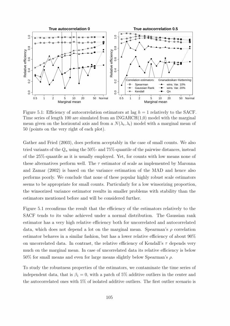
0.0

0.2

0.4

0.6

0.8

1.0

True autocorrelation 0

Marginal mean

Rel

ativ

e ef

ficie

ncy

0.5 1 2 5 10 20 50 Normal

● ● ● ● ● ● ● ● ●●

● ● ● ● ●

●

●

●

●

●

●

●●

● ● ● ●● ● ●

●

●

0.0

0.2

0.4

0.6

0.8

1.0

True autocorrelation 0.5

Marginal mean

Rel

ativ

e ef

ficie

ncy

0.5 1 2 5 10 20 50 Normal

● ●●

● ● ●●

●● ●

● ● ● ● ●

●

●

●

●

●

●

●

●

●

●● ● ● ● ●

●

●

●

●

Correlation estimators: Gnanadesikan−Kettenring:

SpearmanGaussian Rank Kendall

wins. Var. 10%wins. Var. 20%Qn

Figure 5.1: Efficiency of autocorrelation estimators at lag h = 1 relatively to the SACF.Time series of length 100 are simulated from an INGARCH(1,0) model with the marginalmean given on the horizontal axis and from a N(λt, λt) model with a marginal mean of50 (points on the very right of each plot).

Gather and Fried (2003), does perform acceptably in the case of small counts. We alsotried variants of the Qn using the 50%- and 75%-quantile of the pairwise distances, insteadof the 25%-quantile as it is usually employed. Yet, for counts with low means none ofthese alternatives perform well. The τ estimator of scale as implemented by Maronnaand Zamar (2002) is based on the variance estimation of the MAD and hence alsoperforms poorly. We conclude that none of these popular highly robust scale estimatorsseems to be appropriate for small counts. Particularly for a low winsorizing proportion,the winsorized variance estimator results in smaller problems with stability than theestimators mentioned before and will be considered further.

Figure 5.1 reconfirms the result that the efficiency of the estimators relatively to theSACF tends to its value achieved under a normal distribution. The Gaussian rankestimator has a very high relative efficiency both for uncorrelated and autocorrelateddata, which does not depend a lot on the marginal mean. Spearman’s ρ correlationestimator behaves in a similar fashion, but has a lower relative efficiency of about 90%on uncorrelated data. In contrast, the relative efficiency of Kendall’s τ depends verymuch on the marginal mean. In case of uncorrelated data its relative efficiency is below50% for small means and even for large means slightly below Spearman’s ρ.

To study the robustness properties of the estimators, we contaminate the time series ofindependent data, that is β1 = 0, with a patch of 5% additive outliers in the center andthe autocorrelated ones with 5% of isolated additive outliers. The first outlier scenario is

105

0.0

0.2

0.4

0.6

0.8

1.0

Outlier patch (true autocor. 0)

Marginal mean

Rel

ativ

e ef

ficie

ncy

0.5 1 2 5 10 20 50

●

●●

● ● ● ● ● ● ● ● ● ● ● ●

●

● ●

●

●

●

●

●●

●● ● ● ● ●

● ●

Correlation estimators: Gnanadesikan−Kettenring:

SACFSpearmanGaussian Rank Kendall

wins. Var. 10%wins. Var. 20%

0.0

0.2

0.4

0.6

0.8

1.0

Isolated outliers (true autocor. 0.5)

Marginal mean

Rel

ativ

e ef

ficie

ncy

0.5 1 2 5 10 20 50

●● ●

● ●● ●

● ● ● ● ● ● ● ●

●

●

●

●

●

●●

●

●●

● ● ●● ●

Figure 5.2: Efficiency of autocorrelation estimators at lag h = 1 for contaminated Poissondata relatively to the SACF for uncontaminated Poisson data. We contaminated 5%of the 100 observations with additive outliers of size five times the marginal standarddeviation. Left: Patchy outliers in the center. Right: Isolated outliers at arbitrarilychosen positions 17, 40, 55, 72 and 92.

known to bias the estimation towards one and the latter one biases towards zero, whichis away from the true values of zero and 0.5, respectively. For autocorrelation estimationwhen β1 = 0, outlier patches are the worst case, whereas for time series with β1 > 0 theycan even compensate for an existing downward bias in finite samples. The simulationresults in Figure 5.2 can be interpreted as the loss of efficiency compared to the SACFfor uncontaminated data from the same model.

The outlier patch has a strong effect on the efficiency of the autocorrelation estimators foruncorrelated data (see Figure 5.2 left). The ordinary SACF is not robust and drops downto a relative efficiency of around 5%. The rank-based autocorrelation estimators showqualitatively the same pattern of increasing relative efficiency for increasing marginalmean. The Gaussian rank correlation, which has been the most efficient rank-basedestimator for clean uncorrelated data, is the least robust one, because it gives moreinfluence to the largest and the smallest observations. The 10%-winsorized variance hasan efficiency of around 10% relatively to the SACF for clean data, which also increaseswith the marginal mean to about 40%. The 20%-winsorized variance is in principleslightly less efficient and shows a similar behavior but is, as for uncontaminated data,quite unstable for low means.

The same number of isolated outliers for moderately correlated data has a weaker effecton the efficiency of the autocorrelation estimators than the outlier patch for uncorrelated

106

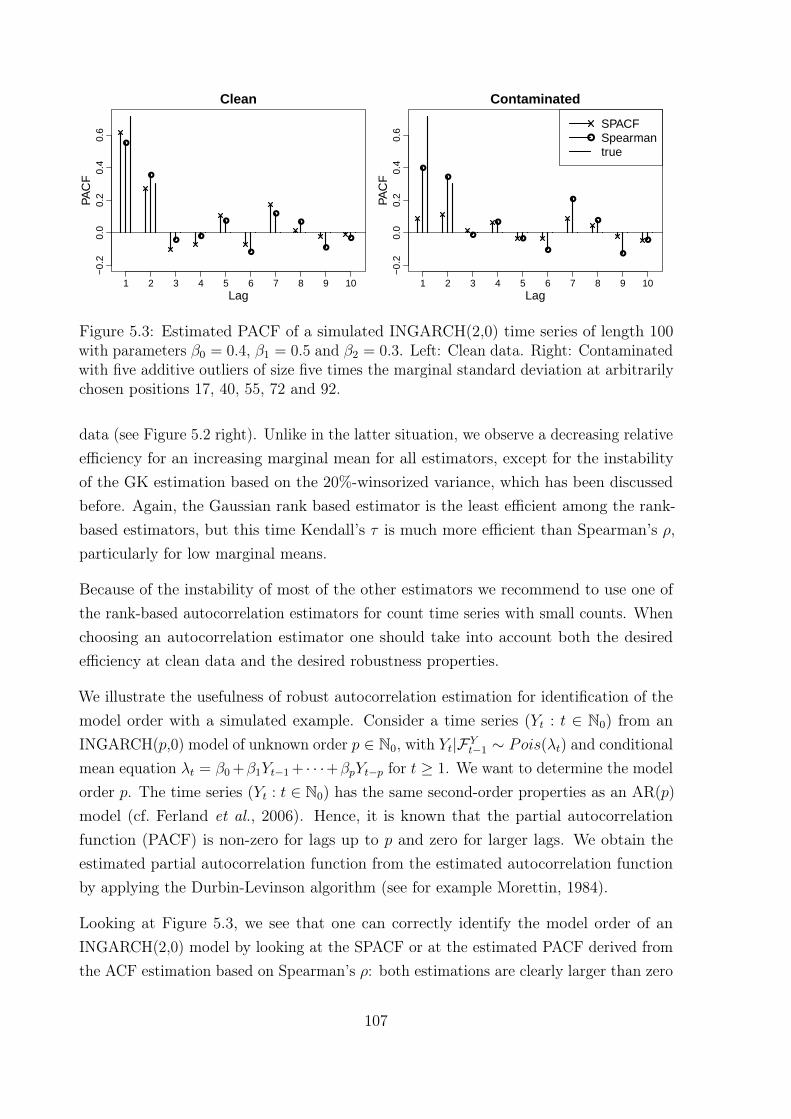
−0.

20.

00.

20.

40.

6Clean

Lag

PAC

F

1 2 3 4 5 6 7 8 9 10

●

●

●●

●

●

●

●

●

●

−0.

20.

00.

20.

40.

6

Contaminated

Lag

PAC

F

1 2 3 4 5 6 7 8 9 10

●

●

●

●

●

●

●

●

●

●

●

SPACFSpearmantrue

Figure 5.3: Estimated PACF of a simulated INGARCH(2,0) time series of length 100with parameters β0 = 0.4, β1 = 0.5 and β2 = 0.3. Left: Clean data. Right: Contaminatedwith five additive outliers of size five times the marginal standard deviation at arbitrarilychosen positions 17, 40, 55, 72 and 92.

data (see Figure 5.2 right). Unlike in the latter situation, we observe a decreasing relativeefficiency for an increasing marginal mean for all estimators, except for the instabilityof the GK estimation based on the 20%-winsorized variance, which has been discussedbefore. Again, the Gaussian rank based estimator is the least efficient among the rank-based estimators, but this time Kendall’s τ is much more efficient than Spearman’s ρ,particularly for low marginal means.

Because of the instability of most of the other estimators we recommend to use one ofthe rank-based autocorrelation estimators for count time series with small counts. Whenchoosing an autocorrelation estimator one should take into account both the desiredefficiency at clean data and the desired robustness properties.

We illustrate the usefulness of robust autocorrelation estimation for identification of themodel order with a simulated example. Consider a time series (Yt : t ∈ N0) from anINGARCH(p,0) model of unknown order p ∈ N0, with Yt|FYt−1 ∼ Pois(λt) and conditionalmean equation λt = β0 +β1Yt−1 + · · ·+βpYt−p for t ≥ 1. We want to determine the modelorder p. The time series (Yt : t ∈ N0) has the same second-order properties as an AR(p)model (cf. Ferland et al., 2006). Hence, it is known that the partial autocorrelationfunction (PACF) is non-zero for lags up to p and zero for larger lags. We obtain theestimated partial autocorrelation function from the estimated autocorrelation functionby applying the Durbin-Levinson algorithm (see for example Morettin, 1984).

Looking at Figure 5.3, we see that one can correctly identify the model order of anINGARCH(2,0) model by looking at the SPACF or at the estimated PACF derived fromthe ACF estimation based on Spearman’s ρ: both estimations are clearly larger than zero

107

for the first two lags and close to zero for all other lags. In case of a contamination withisolated outliers the non-robust estimation with the SPACF is pushed towards zero, suchthat one might falsely identify a model of order p = 0. As opposed to this, the robustestimation of the PACF with Spearman’s ρ is not so strongly affected by the outliersand would still allow a correct model specification.

5.3 Robust estimation and prediction

Atypical observations occurring in the period used for model fitting complicate anymodel-based statistical analysis. For example in infectious disease time series there are(sometimes unrecognized) disease outbreaks or singular artifacts resulting from increasedreporting due to media coverage. Estimators and predictions should thus preferably berobust against outliers or other unusual events so that prediction is not overly influencedby outliers in past data.

In order to reduce the effects of such extraordinary events, observations with largeresiduals can be downweighted (Farrington et al., 1996, Section 3.6). This has beenimplemented in currently applied procedures for disease surveillance, starting from anonrobust initial fit (Noufaily et al., 2013). However, it is well known in robust statisticsthat this can give misleading results since such residuals are not reliable and since thedegree of uncertainty is misjudged. Moreover, in models for dependent data unusualobservations enter the estimation equations several times which complicates the designof appropriate weighting schemes and subsequent statistical inference.

A first approach to robust estimation of INGARCH(p,0) models has been developed byElsaied (2012), see also Elsaied and Fried (2014, 2016). She studies robust M-estimation inthis context, employing Tukey’s bisquare function with a bias correction. The developedmethods offer good efficiency for clean data and a superior performance as compared tomaximum likelihood estimation and uncorrected M-estimation in the presence of outliers.However, note that first attempts to generalize them to INGARCH(p,q) models havefailed because the observations lack a Markovian structure (Elsaied, 2012). Kitromilidou(2015); Kitromilidou and Fokianos (2015, 2016) study robust estimation for a log-linearcount time series model with the conditionally unbiased bounded-influence estimator andthe Mallows quasi-likelihood estimator. Robust fitting based on divergences has beensuggested by Kang and Lee (2014). An approach by Agostinelli (2004) for robustly fittingof ARMA models by weighted likelihood could be transferred to count time series. Elsaiedand Fried (2016) obtain promising results by applying this weighted likelihood approach

108

(implemented in the R package wle by Agostinelli and SLATEC Common MathematicalLibrary (2013)) to independent Poisson data. For the case of independent observations,Aeberhard, Cantoni, and Heritier (2014) study robust estimation of the overdispersioncoefficient from a negative binomial regression model. Such robust parameter estimationswould need to be generalized to the class of count time series following GLMs and canform the basis of a robust prediction procedure.

Multi-step ahead prediction in GLM-type models for time series of counts and the deriva-tion of corresponding prediction intervals allows generalization of currently applied pro-cedures for infectious disease surveillance based on independence assumptions. However,the distribution of such multi-step-ahead predictions is not easily tractable so that MonteCarlo algorithms are needed. Another option is usage of better accessible successive1-step-ahead predictions for the monitoring, but these can be strongly affected after thetime of occurrence of a strongly deviating observation, so that subsequent deviatingobservations are masked. Using robust parameter estimates obtained from an initialsequence, 1-step ahead predictions can be calculated successively, truncating observationsoutside an (1 − α) prediction interval by the respective upper or lower quantile whenusing it in predictions of later time points.

Alternatively, one could choose an approach which is not strictly model-based. Robustversions of exponential smoothing techniques for prediction of continuous-valued timeseries in the presence of outliers have been suggested by Cipra (2006), Gelper, Fried, andCroux (2010) and Cipra and Hanzák (2011). In a similar vein, Ruckdeschel, Spangl, andPupashenko (2014) robustify Kalman filtering approaches for estimation of the state ofa time series in the presence of outliers and shifts, see also Ruckdeschel (2001, 2010).These need to be adapted to discrete-valued time series.

109

Chapter 6

Summary

This thesis provides a unified formulation and comprehensive treatment of the class ofcount time series following generalized linear models. Such models link the conditionalmean of the observed process to its past values, to past observations and to covariate effects.An integral part of these models is the dependence on past values of the conditional mean,the so-called feedback mechanism, which allows for parsimonious modelling of temporalcorrelation. We present the first systematic study on incorporating covariate effectswithin this framework. Models with the identity link function accommodate only positivetemporal correlation and imply additive effects of necessarily nonnegative covariates.Models with the logarithmic link allow to accommodate negative temporal correlationand imply multiplicative effects of covariates. Assuming a Poisson or Negative Binomialconditional distribution facilitates model-based prediction and model assessment.

We develop likelihood-based methods for model fitting and assessment, prediction andintervention analysis for this unified model framework. This generalizes existing theoryfor popular special cases from the class of GLM-based count time series, for instancethe so-called INGARCH model. A key contribution of this thesis is the open sourceimplementation of these methods for the statistical software R provided by the packagetscount (available from CRAN). This package is comprehensively documented by avignette (the basis for Chapter 2) and detailed help pages with examples for all availablefunctions. It complements and extends the functionality of existing software for theanalysis of count time series.

A major part of this thesis is concerned with the treatment of unusual effects influencingthe ordinary pattern of a count time series. This has important applications in the fieldof infectious diseases surveillance, which plays a prominent role in this work. In thatcontext one aims at detecting disease outbreaks by analyzing time series of disease counts.

111

We show that such time series may exhibit temporal correlation and are not describedadequately by the commonly used models which assume independent observations. Wedesign procedures for the detection of unusual effects both for retrospective applicationand for prospective application in real-time which are based on count time series followingGLMs. For the former case we study a new model which describes such interventioneffects by deterministic covariates which enter the dynamics in a different way thanit is the case for an existing model. We develop likelihood-based tests and detectionprocedures and find some robustness against misspecification of the intervention model.For the latter case we introduce a sequential procedure for online monitoring of counttime series based on one-step-ahead predictions. Our procedure relies on the conditionaldistribution (and thus on previous observations) to decide whether a new observationis unusual. Simulations show that in case of actually dependent data our procedure issuperior to a procedure based on an independence model. However, this applies onlyfor the detection at the first unusual observation. If there are many unusually largeobservations in a row, e.g. due to a disease outbreak, then our procedure is influencedby the first unusual observation and has a lower chance to detect the following onesthan under an independence model. We outline some ideas how to utilize the promisingfeatures of models with temporal dependence for designing a monitoring procedure whilstavoiding their undesirable shortcomings.

In the last part of this thesis we discuss some important steps on the way to an automatedmonitoring procedure for count time series. We review tools which could form the basis of acomprehensive model selection strategy for count time series that does not involve manualintervention. There is a need to obtain reliable results even in the presence of atypicalobservations. We thus present a first study on robust estimation of autocorrelationfunctions, which is a useful tool for identifying the model orders and potential seasonaleffects. It turns out that many robust estimators which are highly efficient for continuous-valued data are not suitable for discrete-valued counts. Instead, it is recommended touse rank-based estimators of the (partial) autocorrelation function for robust modelidentification. Finally, we review approaches for robust estimation and prediction whichcould be employed to design a robust monitoring procedure.

112

Acknowledgements

This thesis is a result of my work in the group of Professor Roland Fried at the Departmentof Statistics of TU Dortmund University. I am much obliged for his guidance and support.It was also a pleasure to have Professor Konstantinos Fokianos from the University ofCyprus as my second advisor and I am deeply grateful for his commitment.

I thank the whole department and particularly my colleagues and friends Max Wornowizkiand Alexander Dürre for many stimulation discussions. I further thank Pascal Kerschkefor assisting me to run the simulations in Chapter 3, Philipp Probst for his contributionsto an early version of the package and Jonathan Rathjens for carefully checking it.The fruitful discussions with Maëlle Salmon (formerly at Robert Koch Institute, Berlin,Germany; currently at Center for Research in Environmental Epidemiology, Barcelona,Spain) have improved both the package and this thesis. The comments by R. Fried,K. Fokianos, M. Wornowizki and M. Salmon on previous versions of this manuscript haveenhanced the presentation of this research. I also thank the editors and referees of theJournal of Statistical Software and the International Journal of Computer Mathematicsfor their helpful and constructive comments on the manuscripts which form the basisof Chapters 2 and 3, respectively. I very much appreciated the hospitality of StellaKitromilidou, Xanthi Pedeli, Vasiliki Christou and Maria Pitsillou during my two visitsat the Department of Mathematics and Statistics of the University of Cyprus.

My research and several visits of K. Fokianos have been supported financially by theGerman Research Foundation (DFG, SFB 823 “Statistical modelling of nonlinear dynamicprocesses”). Part of this work was done while K. Fokianos was a Gambrinus Fellow atTU Dortmund University in 2014.

113

References

Abraham B, Box GEP (1979). “Bayesian analysis of some outlier problems in time series.”Biometrika, 66(2), 229–236. 10.1093/biomet/66.2.229.

Aeberhard WH, Cantoni E, Heritier S (2014). “Robust inference in the negative binomialregression model with an application to falls data.” Biometrics, 70(4), 920–931.10.1111/biom.12212.

Agostinelli C (2004). “Robust time series estimation via weighted likelihood.” In R Dutter,P Filzmoser, U Gather, PJ Rousseeuw (eds.), Developments in robust statistics, pp.1–16. Physisca-Verlag, Heidelberg.

Agostinelli C, SLATEC Common Mathematical Library (2013). “wle: Weighted likelihoodestimation.” R package version 0.9-9, http://cran.r-project.org/package=wle.

Agosto A, Cavaliere G, Kristensen D, Rahbek A (2015). “Modeling corporate defaults:Poisson autoregressions with exogenous covariates (PARX).” Creates research paper,School of Economics and Management, University of Aarhus. http://econpapers.repec.org/RePEc:aah:create:2015-11.

Ahmad A, Francq C (2016). “Poisson QMLE of count time series models.” Journal ofTime Series Analysis, 37(3), 291–314. 10.1111/jtsa.12167.

Benjamin MA, Rigby RA, Stasinopoulos DM (2003). “Generalized autoregressive movingaverage models.” Journal of the American Statistical Association, 98(461), 214–223.10.1198/016214503388619238.

Bischl B, Lang M, Mersmann O, Rahnenführer J, Weihs C (2015). “BatchJobs andBatchExperiments: Abstraction mechanisms for using R in batch environments.” Jour-nal of Statistical Software, 64(11). 10.18637/jss.v064.i11.

Bollerslev T (1986). “Generalized autoregressive conditional heteroskedasticity.” Journalof Econometrics, 31(3), 307–327. 10.1016/0304-4076(86)90063-1.

Boudt K, Cornelissen J, Croux C (2012). “The Gaussian rank correlation es-timator: Robustness properties.” Statistics and Computing, 22(2), 471–483.10.1007/s11222-011-9237-0.

Box GEP, Tiao GC (1975). “Intervention analysis with applications to economic andenvironmental problems.” Journal of the American Statistical Association, 70(349),70–79. 10.2307/2285379.

115

Christou V, Fokianos K (2014). “Quasi-likelihood inference for negative binomial timeseries models.” Journal of Time Series Analysis, 35(1), 55–78. 10.1111/jtsa.12050.

Christou V, Fokianos K (2015a). “Estimation and testing linearity for non-linearmixed poisson autoregressions.” Electronic Journal of Statistics, 9, 1357–1377.10.1214/15-EJS1044.

Christou V, Fokianos K (2015b). “On count time series prediction.” Journal of StatisticalComputation and Simulation, 85(2), 357–373. 10.1080/00949655.2013.823612.

Cipra T (2006). “Robust exponential smoothing.” Journal of Forecasting, 11(1), 57–69.10.1002/for.3980110106.

Cipra T, Hanzák T (2011). “Exponential smoothing for time series with outliers.”Kybernetika, 47(2), 165–178. http://dml.cz/dmlcz/141565.

Cox DR (1981). “Statistical analysis of time series: Some recent developments.” Scandi-navian Journal of Statistics, 8(2), 93–115. http://www.jstor.org/stable/4615819.

Croux C, Rousseeuw PJ (1992). “Time-efficient algorithms for two highly robust estimatorsof scale.” In Y Dodge, J Whittaker (eds.), Computational Statistics, volume 1, pp.411–428. Physica-Verlag, Heidelberg.

Czado C, Gneiting T, Held L (2009). “Predictive model assessment for count data.”Biometrics, 65(4), 1254–1261. 10.1111/j.1541-0420.2009.01191.x.

Dawid AP (1984). “Statistical theory: The prequential approach.” Journal of the RoyalStatistical Society A, 147(2), 278–292. 10.2307/2981683.

Demidenko E (2013). Mixed Models: Theory and Applications with R. Wiley series inprobability and statistics, 2nd edition. John Wiley & Sons, Hoboken.

Douc R, Doukhan P, Moulines E (2013). “Ergodicity of observation-driven time seriesmodels and consistency of the maximum likelihood estimator.” Stochastic Processesand their Applications, 123(7), 2620–2647. 10.1016/j.spa.2013.04.010.

Doukhan P, Fokianos K, Tjøstheim D (2012). “On weak dependence conditionsfor Poisson autoregressions.” Statistics & Probability Letters, 82(5), 942–948.10.1016/j.spl.2012.01.015.

Dunsmuir WTM, Scott DJ (2015). “The glarma package for observation-driven time seriesregression of counts.” Journal of Statistical Software, 67(7). 10.18637/jss.v067.i07.

Dürre A, Fried R, Liboschik T (2015a). “Robust estimation of (partial) autocorrelation.”WIREs Computational Statistics, 7(3), 205–222. 10.1002/wics.1351.

Dürre A, Fried R, Liboschik T, Rathjens J (2015b). “robts: Robust time series analysis.”R package version 0.1.0, http://robts.r-forge.r-project.org.

Efron B, Tibshirani R (1993). An Introduction to the Bootstrap. Number 57 in Monographson statistics and applied probability. Chapman & Hall, New York.

116

Elsaied H (2012). Robust Modelling of Count Data. Ph.D. thesis, Technische UniversitätDortmund, Dortmund. http://hdl.handle.net/2003/29404.

Elsaied H, Fried R (2014). “Robust fitting of INARCH models.” Journal of Time SeriesAnalysis, 35(6), 517–535. 10.1111/jtsa.12079.

Elsaied H, Fried R (2016). “Tukey’s M-estimator of the Poisson parameter with aspecial focus on small means.” Statistical Methods and Applications, 25(2), 191–209.10.1007/s10260-015-0295-x.

Fahrmeir L, Tutz G (2001). Multivariate Statistical Modelling Based on GeneralizedLinear Models. Springer-Verlag, New York.

Farrington CP, Andrews NJ, Beale AD, Catchpole MA (1996). “A statistical algorithm forthe early detection of outbreaks of infectious disease.” Journal of the Royal StatisticalSociety A, 159(3), 547–563. 10.2307/2983331.

Ferland R, Latour A, Oraichi D (2006). “Integer-valued GARCH process.” Journal ofTime Series Analysis, 27(6), 923–942. 10.1111/j.1467-9892.2006.00496.x.

Fokianos K (2011). “Some recent progress in count time series.” Statistics, 45(1), 49–58.10.1080/02331888.2010.541250.

Fokianos K (2012). “Count time series models.” In T Subba Rao, S Subba Rao, C Rao(eds.), Time series – methods and applications, Handbook of Statistics, pp. 315–347.Elsevier, Amsterdam.

Fokianos K (2015). “Statistical analysis of count time series models: A glm perspective.”In R Davis, S Holan, R Lund, N Ravishanker (eds.), Handbook of discrete-valued timeseries, Handbooks of Modern Statistical Methods, pp. 3–28. Chapman & Hall, London.

Fokianos K, Fried R (2010). “Interventions in INGARCH processes.” Journal of TimeSeries Analysis, 31(3), 210–225. 10.1111/j.1467-9892.2010.00657.x.

Fokianos K, Fried R (2012). “Interventions in log-linear Poisson autoregression.” StatisticalModelling, 12(4), 299–322. 10.1177/1471082X1201200401.

Fokianos K, Neumann MH (2013). “A goodness-of-fit test for Poisson count processes.”Electronic Journal of Statistics, 7, 793–819. 10.1214/13-EJS790.

Fokianos K, Rahbek A, Tjøstheim D (2009). “Poisson autoregression.” Journal of theAmerican Statistical Association, 104(488), 1430–1439. 10.1198/jasa.2009.tm08270.

Fokianos K, Tjøstheim D (2011). “Log-linear Poisson autoregression.” Journal ofMultivariate Analysis, 102(3), 563–578. 10.1016/j.jmva.2010.11.002.

Fokianos K, Tjøstheim D (2012). “Nonlinear Poisson autoregression.” Annals of theInstitute of Statistical Mathematics, 64(6), 1205–1225. 10.1007/s10463-012-0351-3.

Freeland R, McCabe B (2004). “Forecasting discrete valued low count time series.” Inter-national Journal of Forecasting, 20(3), 427–434. 10.1016/S0169-2070(03)00014-1.

117

Fried R, Liboschik T, Elsaied H, Kitromilidou S, Fokianos K (2014). “On outliers andinterventions in count time series following GLMs.” Austrian Journal of Statistics,43(3), 181–193. 10.17713/ajs.v43i3.30.

Fuller WA (1996). Introduction to Statistical Time Series. 2nd edition. John Wiley &Sons, New York.

Gan FF (1990). “Monitoring Poisson observations using modified exponentially weightedmoving average control charts.” Communications in Statistics - Simulation andComputation, 19(1), 103–124. 10.1080/03610919008812847.

Gan FF (1994). “An optimal design of cumulative sum control chart based on median runlength.” Communications in Statistics - Simulation and Computation, 23(2), 485–503.10.1080/03610919408813183.

Gather U, Bauer M, Fried R (2002). “The identification of multiple outliers in onlinemonitoring data.” Estadística, 54, 289–338.

Gather U, Fried R (2003). “Robust estimation of scale for local linear temporal models.”Tatra Mountains Mathematical Publications, 26, 87–101.

Gelper S, Fried R, Croux C (2010). “Robust forecasting with exponential and Holt–Winterssmoothing.” Journal of Forecasting, 29(3), 285–300. 10.1002/for.1125.

Genest C, Nešlehová J (2007). “A primer on copulas for count data.” ASTIN Bulletin,37(02), 475–515. 10.1017/S0515036100014963.

Gnanadesikan R, Kettenring JR (1972). “Robust estimates, residuals, and outlier detectionwith multiresponse data.” Biometrics, 28(1), 81–124. 10.2307/2528963.

Gneiting T, Balabdaoui F, Raftery AE (2007). “Probabilistic forecasts, calibra-tion and sharpness.” Journal of the Royal Statistical Society B, 69(2), 243–268.10.1111/j.1467-9868.2007.00587.x.

Harvey AC, Durbin J (1986). “The effects of seat belt legislation on british road casualties:A case study in structural time series modelling.” Journal of the Royal StatisticalSociety A, 149(3), 187–227. 10.2307/2981553.

Heinen A (2003). “Modelling time series count data: An autoregressive conditionalpoisson model.” CORE discussion paper, 62. 10.2139/ssrn.1117187.

Heisterkamp SH, Dekkers ALM, Heijne JCM (2006). “Automated detection of infectiousdisease outbreaks: Hierarchical time series models.” Statistics in Medicine, 25(24),4179–4196. 10.1002/sim.2674.

Held L, Höhle M, Hofmann M (2005). “A statistical framework for the analysis ofmultivariate infectious disease surveillance counts.” Statistical Modelling, 5(3), 187–199.10.1191/1471082X05st098oa.

Held L, Paul M (2012). “Modeling seasonality in space-time infectious disease surveillancedata.” Biometrical Journal, 54(6), 824–843. 10.1002/bimj.201200037.

118

Held L, Paul M (2013). “Statistical modeling of infectious disease surveillance data.” InNM M’ikanatha, R Lynfield, CA Van Beneden, H de Valk (eds.), Infectious diseasesurveillance. John Wiley & Sons, Oxford.

Helske J (2016a). “KFAS: Exponential family state space models in R.” Vignette ofthe R package KFAS submitted to Journal of Statistical Software, https://cran.r-project.org/web/packages/KFAS/vignettes/KFAS.pdf.

Helske J (2016b). “KFAS: Kalman filter and smoother for exponential family state spacemodels.” R package version 1.1.2, http://cran.r-project.org/package=KFAS.

Hilbe JM (2011). Negative Binomial Regression. 2nd edition. Cambridge UniversityPress, Cambridge.

Höhle M, Paul M (2008). “Count data regression charts for the monitoring of surveil-lance time series.” Computational Statistics & Data Analysis, 52(9), 4357–4368.10.1016/j.csda.2008.02.015.

Hudecová Š, Hušková M, Meintanis SG (2015). “Tests for time series ofcounts based on the probability-generating function.” Statistics, 49(2), 316–337.10.1080/02331888.2014.979826.

Hutwagner L, Browne T, Seeman G, Fleischauer A (2005). “Comparing aberrationdetection methods with simulated data.” Emerging infectious diseases, 11(2), 314–316.10.3201/eid1102.040587.

Jung R, Tremayne A (2011). “Useful models for time series of counts or simply wrong ones?”AStA Advances in Statistical Analysis, 95(1), 59–91. 10.1007/s10182-010-0139-9.

Kang J, Lee S (2014). “Minimum density power divergence estimator for Poissonautoregressive models.” Computational Statistics & Data Analysis, 80, 44–56.10.1016/j.csda.2014.06.009.

Kedem B, Fokianos K (2002). Regression Models for Time Series Analysis. Wiley seriesin probability and statistics. John Wiley & Sons, Hoboken.

King AA, Nguyen D, Ionides EL (2016). “Statistical inference for partially observedmarkov processes via the R package pomp.” Journal of Statistical Software, 69(12),1–43. 10.18637/jss.v069.i12. To appear.

Kitromilidou S (2015). Robust Inference for Log-Linear Count Time Series Models. Ph.D.thesis, University of Cyprus, Nicosia.

Kitromilidou S, Fokianos K (2015). “Mallows’ quasi-likelihood estimation for log-linear Poisson autoregressions.” Statistical Inference for Stochastic Processes.10.1007/s11203-015-9131-z. Published online.

Kitromilidou S, Fokianos K (2016). “Robust estimation methods for a class of log-linearcount time series models.” Journal of Statistical Computation and Simulation, 86(4),740–755. 10.1080/00949655.2015.1035271.

119

Klar B, Lindner F, Meintanis SG (2012). “Specification tests for the error distributionin GARCH models.” Computational Statistics & Data Analysis, 56(11), 3587–3598.10.1016/j.csda.2010.05.029.

Klar B, Meintanis SG (2012). “Specification tests for the response distribu-tion in generalized linear models.” Computational Statistics, 27(2), 251–267.10.1007/s00180-011-0253-5.

Kourentzes N (2014). “On intermittent demand model optimisation and se-lection.” International Journal of Production Economics, 156, 180–190.10.1016/j.ijpe.2014.06.007.

Kourentzes N, Petropoulos F (2016). “tsintermittent: Intermittent time series forecasting.”R package version 1.9, http://cran.r-project.org/package=tsintermittent.

Lai TL, Chan HP (2008). “Discussion on “Is average run length to false alarm alwaysan informative criterion?” by Yajun Mei.” Sequential Analysis, 27(4), 385–388.10.1080/07474940802445964.

Lange K (1999). Numerical Analysis for Statisticians. Statistics and computing. Springer-Verlag, New York.

Liboschik T, Fokianos K, Fried R (2015). “tscount: An R package for analysis of counttime series following generalized linear models.” TU Dortmund, SFB 823 DiscussionPaper, 06/15. 10.17877/DE290R-7239.

Liboschik T, Kerschke P, Fokianos K, Fried R (2016). “Modelling interventions inINGARCH processes.” International Journal of Computer Mathematics, 93(4), 640–657. 10.1080/00207160.2014.949250.

Lindgren F, Rue H (2015). “Bayesian spatial modelling with R-INLA.” Journal ofStatistical Software, 63(19). 10.18637/jss.v063.i19.

Loeys T, Moerkerke B, De Smet O, Buysse A (2012). “The analysis of zero-inflated countdata: Beyond zero-inflated Poisson regression.” British Journal of Mathematical andStatistical Psychology, 65(1), 163–180. 10.1111/j.2044-8317.2011.02031.x.

Lotze T, Shmueli G, Yahav I (2007). “Simulating multivariate syndromic time seriesand outbreak signatures.” Robert H. Smith School Research Paper, RHS-06-054.10.2139/ssrn.990020.

Ma Y, Genton MG (2000). “Highly robust estimation of the autocovariance function.”Journal of Time Series Analysis, 21(6), 663–684. 10.1111/1467-9892.00203.

Manitz J, Höhle M (2013). “Bayesian outbreak detection algorithm for monitoringreported cases of campylobacteriosis in Germany.” Biometrical Journal, 55(4), 509–526. 10.1002/bimj.201200141.

Maronna RA, Zamar RH (2002). “Robust estimates of location and dis-persion for high-dimensional datasets.” Technometrics, 44(4), 307–317.10.1198/004017002188618509.

120

Masarotto G, Varin C (2012). “Gaussian copula marginal regression.” Electronic Journalof Statistics, 6, 1517–1549. 10.1214/12-EJS721.

Morettin PA (1984). “The Levinson algorithm and its applications in time series analysis.”International Statistical Review / Revue Internationale de Statistique, 52(1), 83–92.10.2307/1403247.

Moysiadis T, Fokianos K (2014). “On binary and categorical time seriesmodels with feedback.” Journal of Multivariate Analysis, 131, 209–228.10.1016/j.jmva.2014.07.004.

Nelder JA, Wedderburn RWM (1972). “Generalized linear models.” Journal of the RoyalStatistical Society A, 135(3), 370–384. 10.2307/2344614.

Neumann MH (2011). “Absolute regularity and ergodicity of Poisson count processes.”Bernoulli, 17(4), 1268–1284. 10.3150/10-BEJ313.

Noufaily A, Enki DG, Farrington P, Garthwaite P, Andrews N, Charlett A (2013). “Animproved algorithm for outbreak detection in multiple surveillance systems.” Statisticsin Medicine, 32(7), 1206–1222. 10.1002/sim.5595.

Pan W (2001). “Akaike’s information criterion in generalized estimating equations.”Biometrics, 57(1), 120–125. 10.1111/j.0006-341X.2001.00120.x.

Paul M, Held L (2011). “Predictive assessment of a non-linear random effects model formultivariate time series of infectious disease counts.” Statistics in Medicine, 30(10),1118–1136. 10.1002/sim.4177.

Pedeli X, Karlis D (2013). “On composite likelihood estimation of a multivariate INAR(1)model.” Journal of Time Series Analysis, 34(2), 206–220. 10.1111/jtsa.12003.

Psarakis S, Vyniou AK, Castagliola P (2014). “Some recent developments on theeffects of parameter estimation on control charts.” Quality and Reliability EngineeringInternational, 30(8), 1113–1129. 10.1002/qre.1556.

R Core Team (2016). “R – A language and environment for statistical computing.”http://www.r-project.org.

Rigby RA, Stasinopoulos DM (2005). “Generalized additive models for location, scale andshape (with discussion).” Journal of the Royal Statistical Society C, 54(3), 507–554.10.1111/j.1467-9876.2005.00510.x.

Robert Koch Institut (2015). “SurvStat@RKI 2.0. Web-based query on data reportedunder the German ’Protection against infection act’.”

Rossi G, Lampugnani L, Marchi M (1999). “An approximate CUSUM procedurefor surveillance of health events.” Statistics in Medicine, 18(16), 2111–2122.10.1002/(SICI)1097-0258(19990830)18:16<2111::AID-SIM171>3.0.CO;2-Q.

Ruckdeschel P (2001). Ansätze Zur Robustifizierung Des Kalman-Filters. Ph.D. thesis,Universität Bayreuth, Bayreuth. http://www.mathematik.uni-kl.de/~ruckdesc/pubs/Diss_hpt.pdf.

121

Ruckdeschel P (2010). “Optimally (distributional-)robust Kalman filtering.” Unpublishedmanuscript, http://arxiv.org/abs/1004.3393.

Ruckdeschel P, Spangl B, Pupashenko D (2014). “Robust Kalman tracking and smoothingwith propagating and non-propagating outliers.” Statistical Papers, 55(1), 93–123.10.1007/s00362-012-0496-4.

Rue H, Martino S, Chopin N (2009). “Approximate Bayesian inference for latentGaussian models by using integrated nested Laplace approximations.” Journal ofthe Royal Statistical Society: Series B (Statistical Methodology), 71(2), 319–392.10.1111/j.1467-9868.2008.00700.x.

Salmon M, Schumacher D, Burmann H, Frank C, Claus H, Höhle M (2016a). “A system forautomated outbreak detection of communicable diseases in Germany.” Eurosurveillance,21(13). 10.2807/1560-7917.ES.2016.21.13.30180.

Salmon M, Schumacher D, Höhle M (2016b). “Monitoring count time series in R:Aberration detection in public health surveillance.” Journal of Statistical Software,70(10), 1–35. 10.18637/jss.v070.i10.

Salmon M, Schumacher D, Stark K, Höhle M (2015). “Bayesian outbreak detec-tion in the presence of reporting delays.” Biometrical Journal, 57(6), 1051–1067.10.1002/bimj.201400159.

Schmid W (1995). “On the run length of a Shewhart chart for correlated data.” StatisticalPapers, 36(1), 111–130. 10.1007/BF02926025.

Scotto MG, Weiß CH, Silva ME, Pereira I (2014). “Bivariate binomial autoregressive mod-els.” Journal of Multivariate Analysis, 125, 233–251. 10.1016/j.jmva.2013.12.014.

Siakoulis V (2015). “acp: Autoregressive conditional Poisson.” R package version 2.1,http://cran.r-project.org/package=acp.

Sim T (2016). Maximum Likelihood Estimation in Partially Observed Markov Modelswith Applications to Time Series of Counts. Ph.D. thesis, Télécom ParisTech, Paris.

Stasinopoulos DM, Rigby RA, Eilers P (2015). “gamlss.util: GAMLSS utilities.” Rpackage version 4.3-2, http://cran.r-project.org/package=gamlss.util.

Tartakovsky AG (2008). “Discussion on “Is average run length to false alarm alwaysan informative criterion?” by Yajun Mei.” Sequential Analysis, 27(4), 396–405.10.1080/07474940802446046.

Tjøstheim D (2012). “Some recent theory for autoregressive count time series.” TEST,21(3), 413–438. 10.1007/s11749-012-0296-0.

Tjøstheim D (2015). “Count time series with observation-driven autoregressive parameterdynamics.” In R Davis, S Holan, R Lund, N Ravishanker (eds.), Handbook of discrete-valued time series, Handbooks of Modern Statistical Methods, pp. 77–100. Chapman& Hall, London.

122

Unkel S, Farrington CP, Garthwaite PH, Robertson C, Andrews N (2012).“Statistical methods for the prospective detection of infectious disease out-breaks: A review.” Journal of the Royal Statistical Society A, 175(1), 49–82.10.1111/j.1467-985X.2011.00714.x.

Venables WN, Ripley BD (2002). Modern Applied Statistics with S. Statistics andcomputing, 4th edition. Springer-Verlag, New York.

Ver Hoef JM, Boveng PL (2007). “Quasi-Poisson vs. negative binomial regression:How should we model overdispersed count data?” Ecology, 88(11), 2766–2772.10.1890/07-0043.1.

Wang S (2013). “pbs: Periodic b splines.” R package version 1.1, http://cran.r-project.org/package=pbs.

Wei W, Held L (2014). “Calibration tests for count data.” TEST, 23(4), 787–805.10.1007/s11749-014-0380-8.

Wei W, Schüpbach G, Held L (2015). “Time-series analysis of Campylobac-ter incidence in Switzerland.” Epidemiology & Infection, 143(09), 1982–1989.10.1017/S0950268814002738.

Weiß CH (2008). “Thinning operations for modeling time series of counts—a survey.”Advances in Statistical Analysis, 92(3), 319–341. 10.1007/s10182-008-0072-3.

Weiß CH (2015). “SPC methods for time-dependent processes of counts—A literaturereview.” Cogent Mathematics, 2(1), 1111116. 10.1080/23311835.2015.1111116.

Weiß CH, Schweer S (2015). “Detecting overdispersion in INARCH(1) processes.” StatisticaNeerlandica, 69(3), 281–297. 10.1111/stan.12059.

Weiß CH, Testik MC (2012). “Detection of abrupt changes in count data time series:Cumulative sum derivations for INARCH (1) models.” Journal of quality technology,44(3), 249–264.

Woodard DB, Matteson DS, Henderson SG (2011). “Stationarity of generalized au-toregressive moving average models.” Electronic Journal of Statistics, 5, 800–828.10.1214/11-EJS627.

Yang M, Cavanaugh JE, Zamba GK (2015). “State-space models for count time serieswith excess zeros.” Statistical Modelling, 15(1), 70–90. 10.1177/1471082X14535530.

Yang M, Zamba GK, Cavanaugh JE (2013). “Markov regression models for count timeseries with excess zeros: A partial likelihood approach.” Statistical Methodology, 14,26–38. 10.1016/j.stamet.2013.02.001.

Yang M, Zamba GK, Cavanaugh JE (2014). “ZIM: Zero-inflated models for count timeseries with excess zeros.” R package version 1.0.2, http://cran.r-project.org/package=ZIM.

Yee TW (2015). Vector generalized linear and additive models: with an implementationin R. Springer series in statistics. Springer-Verlag, New York.

123

Yee TW (2016). “VGAM: Vector generalized linear and additive models.” R packageversion 1.0-1, http://cran.r-project.org/package=VGAM.

Yee TW, Wild CJ (1996). “Vector generalized additive models.” Journal of the RoyalStatistical Society B, 58(3), 481–493. http://www.jstor.org/stable/2345888.

Zeileis A, Kleiber C, Jackman S (2008). “Regression models for count data in R.” Journalof Statistical Software, 27(8), 1–25. 10.18637/jss.v027.i08.

Zhu F (2012). “Zero-inflated Poisson and negative binomial integer-valued GARCHmodels.” Journal of Statistical Planning and Inference, 142(4), 826–839.10.1016/j.jspi.2011.10.002.

124

Appendix A

Implementation details

A.1 Parameter space for the log-linear model

The parameter space Θ for the log-linear model (1.3) which guarantees a stationary andergodic solution of the process is subject of current research. In the current implementationof tsglm the parameters need to fulfill the condition

max

{|β1|, . . . , |βp|, |α1|, . . . , |αq|,

∣∣∣∣∣p∑

k=1

βk +

q∑`=1

α`

∣∣∣∣∣}< 1. (A.1)

At the time we started developing tscount, (A.1) appeared as a reasonable extension ofthe condition

max {|β1|, |α1|, |β1 + α1|} < 1,

which Douc et al. (2013, Lemma 14) derive for p = q = 1. However, in a recent work,Sim (2016, Proposition 5.4.7) derives sufficient conditions for a model of order p = q. Forthe first order model he obtains the weaker condition

max {|α1|, |β1 + α1|} < 1.

For p = q = 2 the required condition is

max{|α1|+ |α2|+ |β2| , |α1α2|+

∣∣α2α21

∣∣+ |α1 + β2| , |α2|+ |α1 + β1|+ |β2| ,

|α2(α1 + β1)|+ |α2 + α1(α1 + β1)|+ |(α1 + β1)β2| , |α2|+ |α1|+ |β2| ,

125

|α2(α1 + β1)|+ |α2 + α1(α1 + β1)|+ |(α1 + β1)β2| , |α2|+ |α1 + β1|+ |β2| ,

|(α1 + β1)α2|+∣∣α2 + (α1 + β1)2 + β2

∣∣+ |(α1 + β1)β2|}< 1. (A.2)

There are parameters which fulfill (A.1) but not (A.2) (e.g. β1 = −0.9, β2 = 0.9, α1 = 0,α2 = 0) and vice versa (e.g. β1 = −1.8, β2 = 0, α1 = 0.9, α2 = 0). However, there exists alarge intersection between values which fulfill (A.1) and (A.2). For the general case p = q

the condition can be obtained by considering the maximum among p elements of the normsof matrix products with p factors, where each factor corresponds to a (2p− 1)× (2p− 1)

matrix. The implementation of this condition is a challenging problem and therefore wehave decided in favor of (A.1). Alternatively, we can obtain unconstrained estimates(argument final.control = list(constrained = NULL)), which should be examinedcarefully.

A.2 Recursions for inference and their initialization

Let h be the inverse of the link function g and let h′(x) = ∂h(x)/∂x be its derivative. Inthe case of the identity link g(x) = x it holds h(x) = x and h′(x) = 1 and in the case ofthe logarithmic link g(x) = log(x) it holds h(x) = h′(x) = exp(x). The partial derivativeof the conditional mean λt(θ) is given by

∂λt(θ)

∂θ= h′ (νt(θ))

∂νt(θ)

∂θ,

where the vector of partial derivatives of the linear predictor νt(θ),

∂νt(θ)

∂θ=

(∂νt(θ)

∂β0

,∂νt(θ)

∂β1

, . . . ,∂νt(θ)

∂βp,∂νt(θ)

∂α1

, . . . ,∂νt(θ)

∂αq,∂νt(θ)

∂η1

, . . . ,∂νt(θ)

∂ηr

)>,

can be computed recursively. The recursions are given by

∂νt(θ)

∂β0

= 1 +

q∑`=1

α`∂νt−j`(θ)

∂β0

,

∂νt(θ)

∂βs= g(Yt−is) +

q∑`=1

α`∂νt−j`(θ)

∂βs, s = 1, . . . , p,

∂νt(θ)

∂αs=

q∑`=1

α`∂νt−j`(θ)

∂αs+ νt−js(θ), s = 1, . . . , q,

∂νt(θ)

∂ηs=

q∑`=1

α`∂νt−j`(θ)

∂ηs+Xt,s, s = 1, . . . , r.

126

The recursions for the linear predictor νt = g(λt) and its partial derivatives depend onpast values of the linear predictor and its derivatives, which are generally not observable.We implemented three possibilities for initialization of these values. The default andpreferable choice is to initialize by the respective marginal expectations, assuming a modelwithout covariate effects, such that the process is stationary (argument init.method =

"marginal"). For the linear model (1.2) it holds (Ferland et al., 2006)

E(Yt) = E(νt) =β0

1−∑p

k=1 βk −∑q

`=1 α`=: µ(θ). (A.3)

For the log-linear model (1.3) we instead consider the transformed time series Zt :=

log(Yt + 1), which has approximately the same second order properties as a time seriesfrom the linear model (1.2). It approximately holds E(Zt) ≈ E(νt) ≈ µ(θ). Specifically,we initialize past values of νt by µ(θ) and past values of ∂νt(θ)/∂θ by

∂µ(θ)

∂θ=

(∂µ(θ)

∂β0

,∂µ(θ)

∂β1

, . . . ,∂µ(θ)

∂βp,∂µ(θ)

∂α1

, . . . ,∂µ(θ)

∂αq,∂µ(θ)

∂η1

, . . . ,∂µ(θ)

∂ηr

)>,

which is explicitly given by

∂µ(θ)

∂β0

=1

1−∑p

k=1 βk −∑q

`=1 α`,

∂µ(θ)

∂βk=∂µ(θ)

∂α`=

β0(1−

∑pk=1 βk −

∑q`=1 α`

)2 , k = 1, . . . , p, ` = 1, . . . , q, and

∂µ(θ)

∂ηm= 0, m = 1, . . . , r.

Another possibility is to initialize νt by β0 and ∂νt(θ)/∂θ by zero. In this case themodel corresponds to standard i.i.d. Poisson random variables (argument init.method= "iid"). A third possibility would be a data-dependent initialization of νt, for exampleby g(y1). In this case, the partial derivatives of νt are initialized by zero (argumentinit.method = "firstobs").

The recursions also depend on unavailable past observations of the time series, priorto the sample which is used for the likelihood computation. The package allows tochoose between two strategies to cope with that. The default choice is to replace thesepre-sample observations by the same initializations as used for the linear predictor νt(see above), transformed by the inverse link function h (argument init.drop = FALSE).An alternative is to use the first ip observations for initialization and to compute thelog-likelihood on the remaining observations yip+1, . . . , yn (argument init.drop = TRUE).Recall that ip is the highest order for regression on past observations.

127

β0 β1 α1 `(θ)

init.method = "marginal", init.drop = FALSE 0.500 0.733 0.249 -3024.7init.method = "marginal", init.drop = TRUE 0.567 0.746 0.236 -2568.0init.method = "iid", init.drop = FALSE 0.867 0.757 0.218 -3037.2init.method = "iid", init.drop = TRUE 0.563 0.738 0.246 -2587.8init.method = "firstobs", init.drop = FALSE 0.559 0.739 0.246 -3018.7init.method = "firstobs", init.drop = TRUE 0.559 0.739 0.246 -2578.1

Table A.1: Estimated parameters and log-likelihood of a time series of length 1000simulated from model (1.2) for different initialization strategies. The true parametersare β0 = 0.5, β1 = 0.77 and α1 = 0.22. Likelihood values are included for completenessof the presentation. There are not comparable as they are based on a different numberof observations.

Particularly in the presence of strong serial dependence, the different methods forinitialization can affect the estimation substantially even for quite long time series with1000 observations. We illustrate this by the simulated example presented in Table A.1.

A.3 Starting value for optimization

The numerical optimization of the log-likelihood function requires a starting value forthe parameter vector θ, which can be obtained by initial estimation based on a simplermodel. Different strategies for this (controlled by the argument start.control) arediscussed in this section. We call this start estimation (and not initial estimation) toavoid confusion with the initialization of the recursions described in the previous section.

The start estimation by the R function glm utilizes the fact that a time series following aGLM without feedback (as in Kedem and Fokianos, 2002) can be fitted by employingstandard software. Neglecting the feedback mechanism, the parameters of the GLM

Yt|F∗t−1 ∼ Poi(λ∗t ), with ν∗t = g(λ∗t ) and

ν∗t = β∗0 + β∗1 g(Yt−i1) + . . .+ β∗p g(Yt−ip) + η∗1Xt,1 + . . .+ η∗rXt,r, t = ip + 1, . . . , n,

with F∗t the history of the joint process {Yt,X t}, are estimated using the R function glm.Denote the estimated parameters by β∗0 , β∗1 , . . . , β∗p , η∗1, . . . , η∗r and set α∗1, . . . , α∗q to zero(argument start.control$method = "GLM").

Fokianos et al. (2009) suggest start estimation of θ, for the first order linear model (1.2)without covariates, by employing its representation as an ARMA(1,1) process withidentical second-order properties, see Ferland et al. (2006). For arbitrary orders P and

128

Q with s := max(P,Q) and the general model from Section 1.2 this representation, afterstraightforward calculations, is given by

(g(Yt)− µ(θ)︸︷︷︸=:ζ

)−s∑i=1

(βi + αi)︸ ︷︷ ︸=:ϕi

(g(Yt−i)− µ(θ)) = εt +

q∑i=1

(−αi)︸ ︷︷ ︸=:ψi

εt−i, (A.4)

where βi := 0 for i /∈ P , αi := 0 for i /∈ Q and {εt} is a white noise process.Recall that g is defined by g(x) = x for the linear model and g(x) = log(x + 1)

for the log-linear model. Given the autoregressive parameters ϕi and the movingaverage parameters ψi of the ARMA representation of {Yt}, the parameters of theoriginal process are obtained by αi = −ψi and βi = ϕi + ψi. We get β0 fromβ0 = ζ

(1 −

∑pk=1 βk −

∑q`=1 α`

)using the formula for the marginal mean of {Yt}.

With these formulas estimates β∗0 , β∗i and α∗i are obtained from ARMA estimates ζ,ϕi and ψi. Estimation of the ARMA parameters is implemented by conditional leastsquares (argument start.control$method = "CSS"), maximum likelihood assumingnormally distributed errors (argument start.control$method = "ML"), or, for modelsup to first order, the method of moments (argument start.control$method = "MM").If covariates are included, a linear regression is fitted to g(Yt), whose errors follow anARMA model like (A.4). Consequently, the covariate effects do not enter the dynamicsof the process, as it is the case in the actual model (1.1). It would be preferable to fit anARMAX model, in which covariate effects are included on the right hand side of (A.4),but this is currently not readily available in R.

We compare both approaches to obtain start estimates. The GLM approach apparentlydisregards the feedback mechanism, i.e., the dependence on past values of the conditionalmean. As opposed to this, the ARMA approach does not treat covariate effects in anappropriate way. From extensive simulations we note that the final estimation resultsare almost equally good for both approaches.

However, we also found out that in some situations (especially in the presence of certaintypes of covariates) both approaches occasionally provoke the likelihood optimizationalgorithms to run into a local optimum. This happens more often for increasing samplesize. To overcome this problem we recommend a naive start estimation assuming ani.i.d. model without covariates, which only estimates the intercept and sets all otherparameters to zero (argument start.control$method = "iid"). This starting valueis usually not close to any local optimum of the likelihood function. Hence we expect,possibly, a larger number of steps for the optimization algorithm to converge. This is thedefault method of start estimation as we do not guarantee a global optimum with theother two methods, in some special cases.

129

Particularly for the linear model, some of the aforementioned approaches do not yield astarting value θ

∗= (β∗0 , β

∗1 , . . . , β

∗p , α

∗1, . . . , α

∗q , η∗1, . . . , η

∗r )> for θ which lays in the interior

of the parameter space Θ. To overcome this problem, θ∗is suitably transformed to be

used as a starting value. For the linear model (1.2) this transformation is done accordingto the following procedure (Liboschik et al., 2016):

1a. Set β∗k := min{β∗k , ε

}and α∗` := min

{α∗` , ε

}.

1b. If c :=∑p

k=1 β∗k +∑q

`=1 α∗` > 1−ξ−ε, then shrink each β∗k and α∗` by multiplication

with the factor (1− ξ − ε)/c.

2a. Set β∗0 := β∗0 ·(

1−∑p

k=1 β∗k +

∑q`=1 α

∗`

)/c.

2b. Set β∗0 := max{β∗0 , ξ + ε

}.

3. Set η∗m := max{η∗m, ε

}.

A small constant ε > 0 ensures that the initial value lies inside the parameter space Θ

and not on its boundaries. It is chosen to be ε = 10−6 by default (argument epsilon).Another small constant ξ > 0 enforces the inequalities to be strict (i.e. < instead of ≤).This constant is set to ξ = 10−6 by default (argument slackvar); recall Section 2.2.3.The shrinkage factor in step 1b is chosen such that the sum of the parameters equals1− ξ− ε after possible shrinkage in this step. The choice of β∗0 in step 2a ensures that themarginal mean remains unchanged after possible shrinkage in step 1b. For the log-linearmodel (1.3) it is not necessary to ensure positivity of the parameters. A valid startingvalue θ

∗is transformed with the following procedure:

1a. Set β∗k := sign(β∗k)·min

{∣∣β∗k∣∣, ε} and α∗` := sign(α∗`)·min

{∣∣α∗` ∣∣, ε}.1b. If c :=

∣∣∣∑pk=1 β

∗k +

∑q`=1 α

∗`

∣∣∣ > 1−ξ−ε, then shrink each β∗k and α∗` by multiplicationwith the factor (1− ξ − ε)/c.

A.4 Stable inversion of the information matrix

In order to obtain standard errors from the normal approximation (2.6) one needs toinvert the information matrix Gn(θ; σ2). To avoid numerical instabilities we make useof the fact that an information matrix is a real symmetric and positive definite matrix.We first compute a Choleski factorization of the information matrix. Then we applyan efficient algorithm to invert the matrix employing the upper triangular factor of

130

the Choleski decomposition (see R functions chol and chol2inv). This procedure isimplemented in the function invertinfo in our package.

131

Appendix B

Additional simulations

In this section we present simulations supporting that the methods that have not yetbeen treated thoroughly in the literature work reliably.

B.1 Covariates

We present some limited simulation results for the problem of including covariates, inboth linear and log-linear models. For simplicity we employ first order models with onecovariate and a conditional Poisson distribution, that is, we consider the linear modelwith the identity link function

Yt|Ft−1 ∼ Poisson(λt), λt = β0 + β1 Yt−1 + α1λt−1 + η1Xt, t = 1, . . . , n,

and the log-linear model with the logarithmic link function

Yt|Ft−1 ∼ Poisson(λt), log(λt) = β0 + β1 log(Yt−1 + 1) + α1 log(λt−1) + η1Xt, t = 1, . . . , n.

The parameters are chosen to be β1 = 0.3 and α1 = 0.2. The intercept parameter isβ0 = 4 · 0.5 for the linear and β0 = log(4) · 0.5 for the log-linear model in order to obtaina marginal mean (without the covariate effect) of about 4 in both cases. We consider thecovariates listed in Table B.1, covering a simple linear trend, seasonality, interventioneffects, i.i.d. observations from different distributions and a stochastic process. Thecovariates are chosen to be nonnegative, which is necessary for the linear model but notfor the log-linear model. All covariates have a mean of about 0.5, such that their effect

133

Abbreviation Definition

Linear t/nSine (sin(2π · 5 · t/n) + 1)/2Spiky outlier 1(t = τ)Transient shift 0.8t−τ1(t ≥ τ)Level shift 1(t ≥ τ)GARCH(1,1)

√htεt with εt ∼ N(0.5, 1) and ht = 0.002 + 0.1X2

t−1 + 0.8ht−1

Exponential i.i.d. Exponential with mean 0.5Normal i.i.d. Normal with mean 0.5 and variance 0.04

Table B.1: Covariates {Xt : t = 1, . . . , n} considered in the simulation study. Theinterventions occur at time τ = n/2. The GARCH model is defined recursively (seeBollerslev, 1986).

sizes are somewhat comparable. The regression coefficient is chosen to be η1 = 2 · β0 forthe linear and η1 = 1.5 · β0 for the log-linear model.

Apparently, certain types of covariates can to some extent be confused with serialdependence. This is the case for the linear trend and the level shift, but also for thesinusoidal term, since these lead to data patterns which resemble positive serial correlation;see Figure B.1.

A second finding is that the effect of covariates, like a transient shift or a spiky outlier,is hard to be estimated precisely. Note that both covariates have most of their valuesvalues different from zero only at very few time points (especially the spiky outlier) whichexplains this behavior of the estimation procedure. The estimators for the coefficientsof such covariates have a large variance which decreases only very slowly with growingsample size; see the bottom right plots in Figures B.2 and B.3 for the linear and thelog-linear model, respectively. This does not affect the estimation of the other parameters,see the other three plots in the same figures. For all other types of covariates the varianceof the estimator for the regression parameter decreases with growing sample size, whichindicates consistency of the estimator.

The conjectured approximative normality of the model parameters stated in (2.6) seemsto hold for most of the covariates considered here even in case of a rather moderatesample size of 100, as indicated by the QQ plots shown in Figure B.4. The only seriousdeviation from normality happens for the spiky outlier in the linear model, a case wheremany estimates of the covariate coefficient η1 lie close to zero. This value is the lowerboundary of the parameter space for this model. Due to the consistency problem for thiscovariate (discussed in the previous paragraph) the observed deviation from normalityis still present even for a much larger sample size of 2000 (not shown here). Note that

134

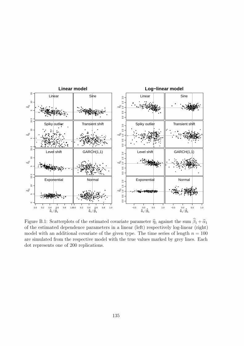
estimates_dep[, j]

estim

ates

_cov

[, j]

05

1015

η 1

Linear

estimates_dep[, j]

estim

ates

_cov

[, j] Sine

estimates_dep[, j]

estim

ates

_cov

[, j]

05

1015

η 1

Spiky outlier

estimates_dep[, j]

estim

ates

_cov

[, j] Transient shift

estimates_dep[, j]

estim

ates

_cov

[, j]

05

1015

η 1

Level shift

estimates_dep[, j]

estim

ates

_cov

[, j] GARCH(1,1)

estimates_dep[, j]

estim

ates

_cov

[, j]

0.0 0.2 0.4 0.6 0.8 1.0

α1 + β1

05

1015

η 1

Exponential

estimates_dep[, j]

estim

ates

_cov

[, j]

0.0 0.2 0.4 0.6 0.8 1.0

α1 + β1

Normal

Linear model

estimates_dep[, j]

estim

ates

_cov

[, j]

0.0

0.5

1.0

1.5

2.0

η 1

Linear

estimates_dep[, j]

estim

ates

_cov

[, j] Sine

estimates_dep[, j]

estim

ates

_cov

[, j]

0.0

0.5

1.0

1.5

2.0

η 1Spiky outlier

estimates_dep[, j]es

timat

es_c

ov[,

j] Transient shift

estimates_dep[, j]

estim

ates

_cov

[, j]

0.0

0.5

1.0

1.5

2.0

η 1

Level shift

estimates_dep[, j]

estim

ates

_cov

[, j] GARCH(1,1)

estimates_dep[, j]

estim

ates

_cov

[, j]

−0.5 0.0 0.5 1.0

α1 + β1

0.0

0.5

1.0

1.5

2.0

η 1

Exponential

estimates_dep[, j]

estim

ates

_cov

[, j]

−0.5 0.0 0.5 1.0

α1 + β1

Normal

Log−linear model

Figure B.1: Scatterplots of the estimated covariate parameter η1 against the sum β1 + α1

of the estimated dependence parameters in a linear (left) respectively log-linear (right)model with an additional covariate of the given type. The time series of length n = 100are simulated from the respective model with the true values marked by grey lines. Eachdot represents one of 200 replications.

135

0 2 4 6

β0

Normal

Exponential

GARCH(1,1)

Level shift

Transient shift

Spiky outlier

Sine

Linear

0.0 0.1 0.2 0.3 0.4 0.5

β1

Normal

Exponential

GARCH(1,1)

Level shift

Transient shift

Spiky outlier

Sine

Linear

0.0 0.2 0.4 0.6 0.8

α1

Normal

Exponential

GARCH(1,1)

Level shift

Transient shift

Spiky outlier

Sine

Linear

0 2 4 6 8 10 12

η1

Normal

Exponential

GARCH(1,1)

Level shift

Transient shift

Spiky outlier

Sine

Linear

Figure B.2: Estimated coefficients for a linear model of order p = q = 1 with an additionalcovariate of the given type. The time series of length n = 100, 500, 1000, 2000 (fromtop to bottom in each panel) are simulated from the respective model with the truecoefficients marked by a grey vertical line. Each boxplot is based on 200 replications.

136

0.0 0.5 1.0 1.5 2.0 2.5 3.0

β0

Normal

Exponential

GARCH(1,1)

Level shift

Transient shift

Spiky outlier

Sine

Linear

0.0 0.1 0.2 0.3 0.4 0.5 0.6

β1

Normal

Exponential

GARCH(1,1)

Level shift

Transient shift

Spiky outlier

Sine

Linear

−1.0 −0.5 0.0 0.5 1.0

α1

Normal

Exponential

GARCH(1,1)

Level shift

Transient shift

Spiky outlier

Sine

Linear

−0.5 0.0 0.5 1.0 1.5 2.0

η1

Normal

Exponential

GARCH(1,1)

Level shift

Transient shift

Spiky outlier

Sine

Linear

Figure B.3: Identical simulation results as those shown in Figure B.2 but for the log-linearmodel.

137

Theoretical quantiles

Sam

ple

quan

tiles

02

46

810

Sam

ple

quan

tiles Linear

Theoretical quantiles

Sam

ple

quan

tiles Sine

Theoretical quantiles

Sam

ple

quan

tiles

02

46

810

Sam

ple

quan

tiles Spiky outlier

Theoretical quantiles

Sam

ple

quan

tiles Transient shift

Theoretical quantiles

Sam

ple

quan

tiles

02

46

810

Sam

ple

quan

tiles Level shift

Theoretical quantiles

Sam

ple

quan

tiles GARCH(1,1)

Theoretical quantiles

Sam

ple

quan

tiles

−3 −2 −1 0 1 2 3Theoretical quantiles

02

46

810

Sam

ple

quan

tiles Exponential

Theoretical quantiles

Sam

ple

quan

tiles

−3 −2 −1 0 1 2 3Theoretical quantiles

Normal

Linear model

Theoretical quantilesS

ampl

e qu

antil

es0.

00.

51.

01.

52.

0S

ampl

e qu

antil

es Linear

Theoretical quantiles

Sam

ple

quan

tiles Sine

Theoretical quantiles

Sam

ple

quan

tiles

0.0

0.5

1.0

1.5

2.0

Sam

ple

quan

tiles Spiky outlier

Theoretical quantiles

Sam

ple

quan

tiles Transient shift

Theoretical quantiles

Sam

ple

quan

tiles

0.0

0.5

1.0

1.5

2.0

Sam

ple

quan

tiles Level shift

Theoretical quantiles

Sam

ple

quan

tiles GARCH(1,1)

Theoretical quantiles

Sam

ple

quan

tiles

−3 −2 −1 0 1 2 3Theoretical quantiles

0.0

0.5

1.0

1.5

2.0

Sam

ple

quan

tiles Exponential

Theoretical quantiles

Sam

ple

quan

tiles

−3 −2 −1 0 1 2 3Theoretical quantiles

Normal

Log−linear model

Figure B.4: Normal QQ-plots for the estimated covariate coefficient η1 in a linear (left)respectively log-linear (right) model of order p = q = 1 with an additional covariate ofthe given type. The time series of length n = 100 are simulated from the respectivemodel with the true coefficient marked by a grey horizontal line. Each plot is based on200 replications.

138

Mean Median Std.dev. MAD Failures (in %)

σ2 = 1.00 0.98 0.97 0.18 0.17 0.000.20 0.20 0.20 0.05 0.05 0.000.10 0.10 0.10 0.03 0.03 0.100.05 0.05 0.05 0.03 0.03 3.300.00 0.02 0.02 0.01 0.01 52.10

Table B.2: Summary statistics for the estimated overdispersion coefficient σ2 of theNegative Binomial distribution. The time series are simulated from a log-linear modelwith the true overdispersion coefficient given in the rows. Each statistic is based on 200replications.

for the spiky outlier the conditions for asymptotic normality in linear regression modelsstated in Section 2.2.2 are not fulfilled. QQ plots for the other model parameters β0, β1

and α1 look satisfactory for all types of covariates and are not shown here.

B.2 Negative Binomial distribution

As mentioned before, the model with the logarithmic link function is not covered bythe theory derived by Christou and Fokianos (2014). Consequently, we confirm bysimulations that estimating the additional dispersion parameter φ of the NegativeBinomial distribution by equation (2.5) yields good results. We consider both thelinear model with the identity link

Yt|Ft−1 ∼ NegBin(λt, φ), λt = β0 + β1 Yt−1 + α1λt−1, t = 1, . . . , n,

and the log-linear model with the logarithmic link

Yt|Ft−1 ∼ NegBin(λt, φ), log(λt) = β0 + β1 log(Yt−1 + 1) + α1 log(λt−1), t = 1, . . . , n.

The parameters β0, β1 and α1 are chosen like in Section B.1. For the dispersion parameterφ we employ the values 1, 5, 10, 20 and ∞, which are corresponding to overdispersioncoefficients σ2 of 1, 0.2, 0.1, 0.05 and 0, respectively.

The estimator of the dispersion parameter φ has a positively skewed distribution. It isthus preferable to consider the distribution of its inverse σ2 = 1/φ, which is only slightlynegatively skewed; see Table B.2. In certain cases it is numerically not possible to solve(2.5) and the estimation fails. This happens when the true value of φ is large and weare close to the limiting case of a Poisson distribution (see the proportion of failures

139

2000

1000

500

100

0.5 1.0 1.5 2.0 2.5

Linear model

σ2

Leng

th o

f tim

e se

ries

0.5 1.0 1.5 2.0 2.5

Log−linear model

σ2

Sam

ple

size

Figure B.5: Estimated overdispersion coefficient σ2 of the Negative Binomial distributionfor a linear (left) respectively log-linear (right) model of order p = q = 1. The time seriesare simulated from the respective model with the true overdispersion coefficient markedby a grey vertical line. Each boxplot is based on 200 replications.

in the last column of the table). In such a case our fitting function gives an error andrecommends fitting a model with a Poisson distribution instead. These results are verysimilar for the linear model and thus not shown here.

We check the consistency of the estimator by a simulation for a true value of σ2 = 1/φ = 1.Our results shown in Figure B.5 indicate that on average the deviation of the estimationfrom the true value decreases with increasing sample size for both, the linear and thelog-linear model. The boxplots also confirm our above finding that the estimator has aclearly asymmetric distribution for sample sizes up to several hundred.

B.3 Quasi information criterion

We confirm by simulation that the quasi information criterion (QIC) approximatesAkaike’s information criterion (AIC) in case of a Poisson distribution. Like in Section B.2,we consider both the linear model with the identity link

Yt|Ft−1 ∼ Poisson(λt), λt = β0 + β1 Yt−1 + α1λt−1, t = 1, . . . , n,

and the log-linear model with the logarithmic link

Yt|Ft−1 ∼ Poisson(λt), log(λt) = β0 + β1 log(Yt−1 + 1) + α1 log(λt−1), t = 1, . . . , n,

but now with a Poisson distribution. Again, the parameters β0, β1 and α1 are chosenlike in Section B.1.

140

380 400 420 440 460

380

400

420

440

460

Linear model

AIC

QIC

380 400 420 440 460

380

400

420

440

460

Log−linear model

AICQ

IC

Figure B.6: Relationship of QIC and AIC for a linear (left) respectively log-linear (right)model of order p = q = 1. Each of the 200 points represents the QIC and AIC of a fit toa time series of length n = 100 simulated from the respective model. The diagonal line isthe identity, i.e. it represents values for which the QIC equals the AIC.

From each of the two models we simulate 200 time series of length n = 100 and computethe QIC and AIC of the fitted model. Figure B.6 shows that the relationship betweenQIC and AIC is very close to the identity, i.e. the QIC is approximately equal to theAIC. There is only one out of 200 cases (for the linear model) where the QIC deviateslargely from the AIC.

141