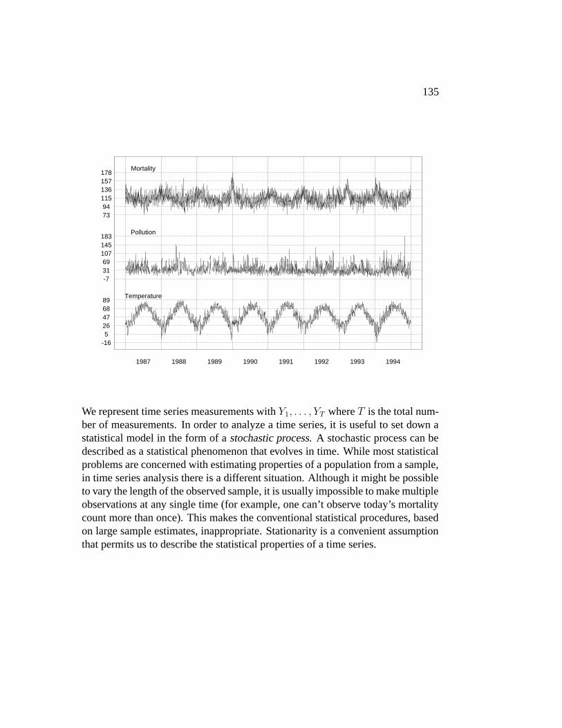
Chapter 10

Introduction to Time Series Analysis

A time series is a collection of observations made sequentially in time. Examplesare daily mortality counts, particulate air pollution measurements, and tempera-ture data. Figure 1 shows these for the city of Chicago from 1987 to 1994. Thepublic health question is whether daily mortality is associated with particle levels,controlling for temperature.

134

135

1987 1988 1989 1990 1991 1992 1993 1994

-165

26476889

-73169

107145183

7394

115136157178

Temperature

Pollution

Mortality

We represent time series measurements with Y1, . . . , YT where T is the total num-ber of measurements. In order to analyze a time series, it is useful to set down astatistical model in the form of a stochastic process. A stochastic process can bedescribed as a statistical phenomenon that evolves in time. While most statisticalproblems are concerned with estimating properties of a population from a sample,in time series analysis there is a different situation. Although it might be possibleto vary the length of the observed sample, it is usually impossible to make multipleobservations at any single time (for example, one can’t observe today’s mortalitycount more than once). This makes the conventional statistical procedures, basedon large sample estimates, inappropriate. Stationarity is a convenient assumptionthat permits us to describe the statistical properties of a time series.

136 CHAPTER 10. INTRODUCTION TO TIME SERIES ANALYSIS

10.1 Stationarity

Broadly speaking, a time series is said to be stationary if there is no systematictrend, no systematic change in variance, and if strictly periodic variations or sea-sonality do not exist. Most processes in nature appear to be non-stationary. Yetmuch of the theory in time-series literature is only applicable to stationary pro-cesses.

One way of describing a stochastic process is to specify the joint distribution ofthe observations Y (t1), . . . , Y (tn) for any set of times t1, . . . , tn and any valueof n. A time series is said to be strictly stationary if the joint distribution ofY (t1), . . . , Y (tn) is the same as that of Y (t1 + h), . . . Y (tn + h) for all t1, . . . , tnand h. To see how this is a useful assumption, notice that the above conditionimplies that the expected value and covariance structure of any two components,Ya(t) and Yb(t), of a time series are constant in time

E{Ya(t)} = µa , var{Ya(t)} = σ2

a and corr{Ya(t), Yb(t + h)} = γab(h). (10.1)

The function γab(h) is called the cross-correlation function if a 6= b and the auto-correlation function if a = b.

In practice it is often useful to define stationarity in a less restricted way than thatdescribed above. In many cases, the statistical structure of the processes can becompletely described with the second-order properties of equation (10.1). We canestimate the quantities in (10.1) using standard statistical procedures, for examplewe may estimate the cross-correlation at lag h, γa,b(h) with the sample correlationof Ya(1), . . . , Ya(T − h) and Yb(h + 1), . . . , Yb(T ).

10.1.1 An example: Fetal Monitoring

Measurements of fetal heart rate (FHR) and fetal movement (FM) are generated bymaternal-fetal monitoring. Approximately 5 measurements per second are takenduring 50 minutes on 120 subjects that are monitored at 20,24,28,32,36, and 38-39 weeks of gestation. Both FHR and FM are recorded giving us a multiple timeseries Y (t), t = 1, . . . , 50× 60× 5, where Y (t) is a vector with 2 entries.

10.1. STATIONARITY 137

The association between accelerations of FHR and FM has been documented sincethe 1930s. For example, it has been observed that in the third trimester mostlarge fetal heart accelerations are associated with fetal activity. In Section 4.2we will describe how relatively straight-forward time series techniques provide avisual descriptions of how these associations vary with weeks gestation. Thesedescription have motivated a methodology that will provide us is with a morerigorous assessment of this relationship.

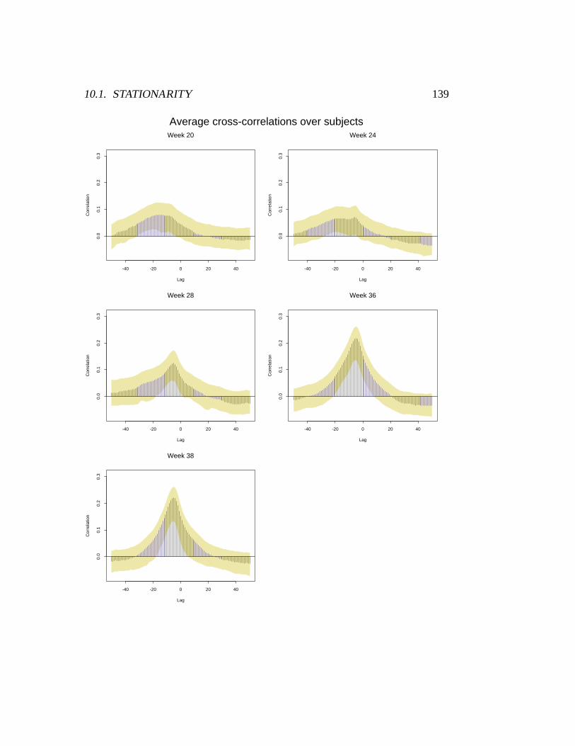
If we consider the FM and FHR measurements, seen in Figure 5, as outcomesfrom a two component time series, we may consider the cross-correlation functionof these two components as a description of the association between these twoprocesses. Notice that the measurements taken for each fetus at each gestationweek has a cross-correlation function associated with them. In Figure 6, as adescriptive plot, we show the average, over individuals, of these functions foreach gestation week. Notice that a peak at around the −6 second lag starts toappear in the plot for the 24 week gestation. As the fetus gets older, this peakgrows and becomes more defined. This result can be considered a first step in thecharacterization of the relationship between FM and FHR.

138 CHAPTER 10. INTRODUCTION TO TIME SERIES ANALYSIS

Time in minutes

Act

ivity

0 10 20 30 40 50

4

16

36

64

Time in minutes

Hea

rt R

ate

0 10 20 30 40 50

120

130

140

150

160

Time Series Plots of Fetal Activity and Heart Rate

10.1. STATIONARITY 139

Week 20

Lag

Cor

rela

tion

-40 -20 0 20 40

0.0

0.1

0.2

0.3

Week 24

Lag

Cor

rela

tion

-40 -20 0 20 40

0.0

0.1

0.2

0.3

Week 28

Lag

Cor

rela

tion

-40 -20 0 20 40

0.0

0.1

0.2

0.3

Week 36

Lag

Cor

rela

tion

-40 -20 0 20 40

0.0

0.1

0.2

0.3

Week 38

Lag

Cor

rela

tion

-40 -20 0 20 40

0.0

0.1

0.2

0.3

Average cross-correlations over subjects

140 CHAPTER 10. INTRODUCTION TO TIME SERIES ANALYSIS

10.2 Spectral Analysis

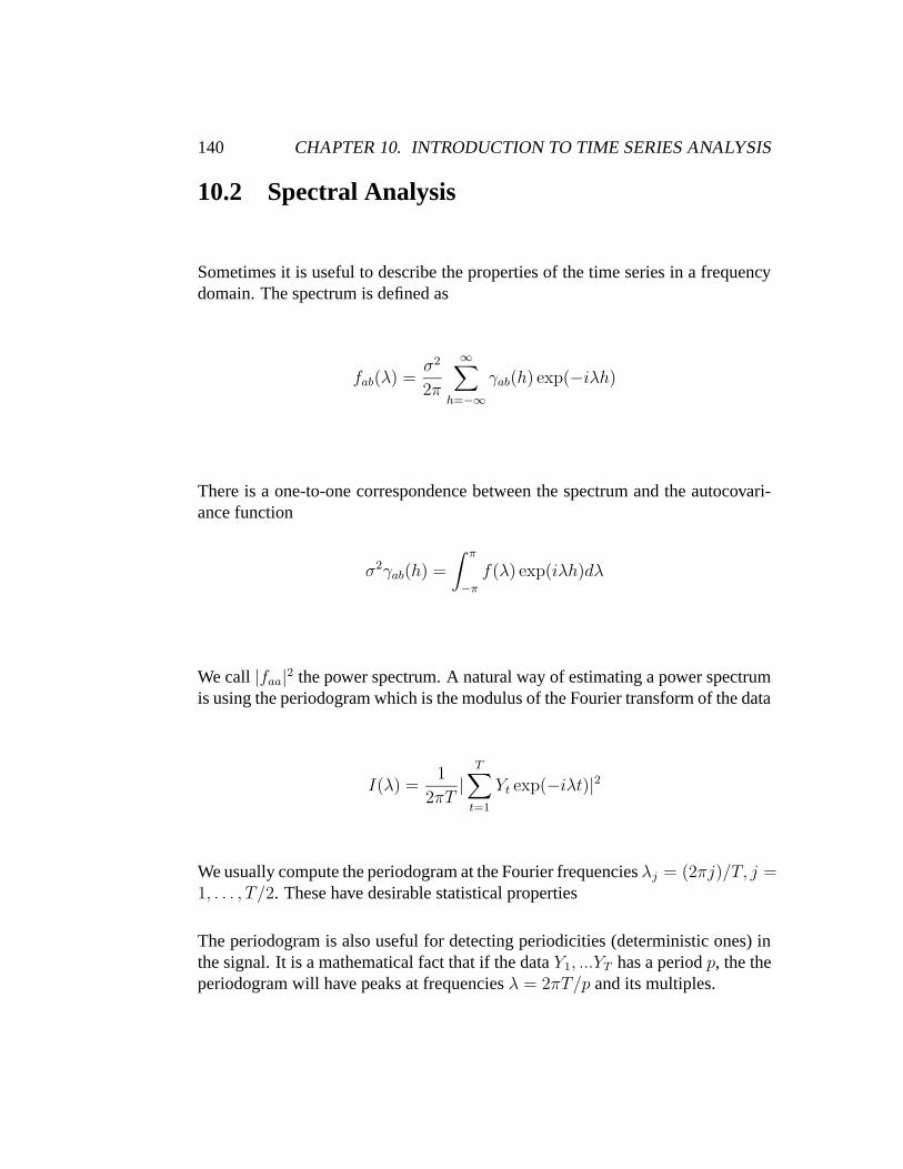
Sometimes it is useful to describe the properties of the time series in a frequencydomain. The spectrum is defined as

fab(λ) =σ2

2π

∞∑

h=−∞

γab(h) exp(−iλh)

There is a one-to-one correspondence between the spectrum and the autocovari-ance function

σ2γab(h) =

∫ π

−π

f(λ) exp(iλh)dλ

We call |faa|2 the power spectrum. A natural way of estimating a power spectrum

is using the periodogram which is the modulus of the Fourier transform of the data

I(λ) =1

2πT|

T∑

t=1

Yt exp(−iλt)|2

We usually compute the periodogram at the Fourier frequencies λj = (2πj)/T, j =1, . . . , T/2. These have desirable statistical properties

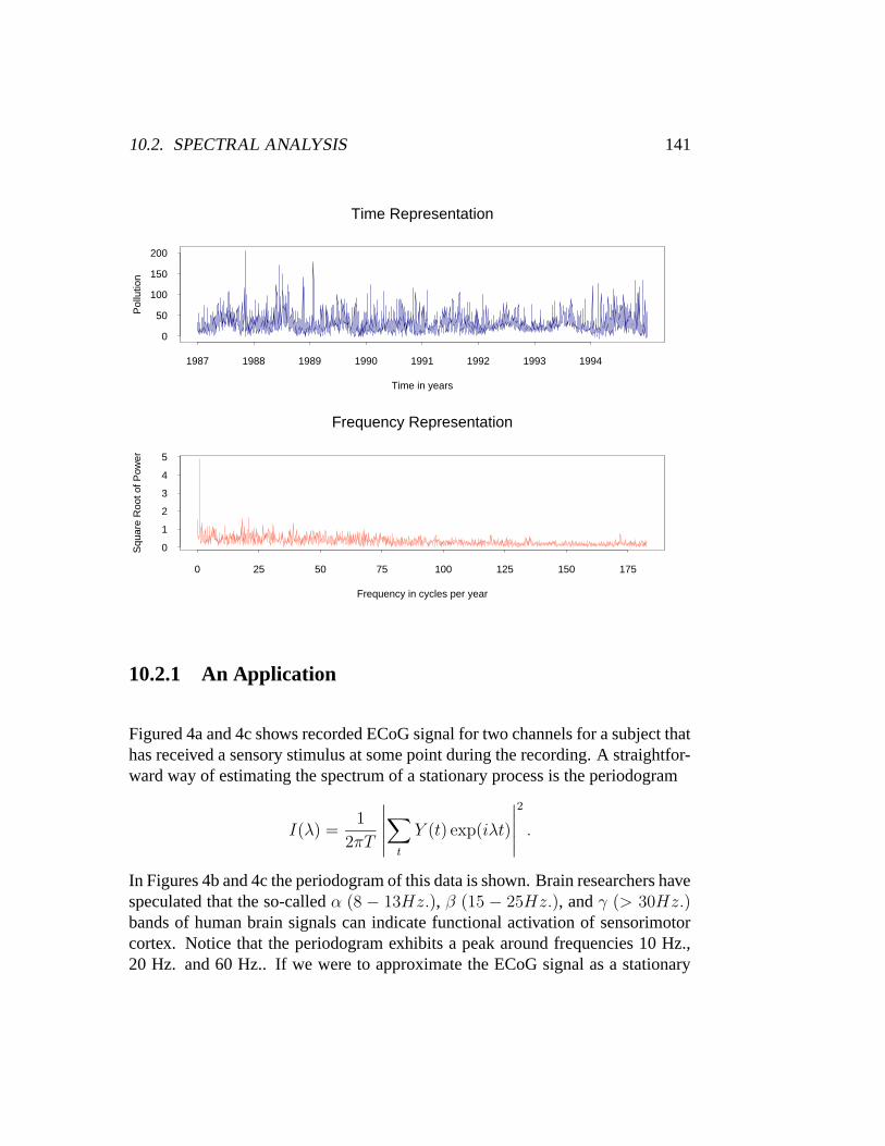
The periodogram is also useful for detecting periodicities (deterministic ones) inthe signal. It is a mathematical fact that if the data Y1, ...YT has a period p, the theperiodogram will have peaks at frequencies λ = 2πT/p and its multiples.

10.2. SPECTRAL ANALYSIS 141

Time Representation

Time in years

Pol

lutio

n

0

50

100

150

200

1987 1988 1989 1990 1991 1992 1993 1994

Frequency Representation

Frequency in cycles per year

Squ

are

Roo

t of P

ower

0

1

2

3

4

5

0 25 50 75 100 125 150 175

10.2.1 An Application

Figured 4a and 4c shows recorded ECoG signal for two channels for a subject thathas received a sensory stimulus at some point during the recording. A straightfor-ward way of estimating the spectrum of a stationary process is the periodogram

I(λ) =1

2πT

∣

∣

∣

∣

∣

∑

t

Y (t) exp(iλt)

∣

∣

∣

∣

∣

2

.

In Figures 4b and 4c the periodogram of this data is shown. Brain researchers havespeculated that the so-called α (8 − 13Hz.), β (15 − 25Hz.), and γ (> 30Hz.)bands of human brain signals can indicate functional activation of sensorimotorcortex. Notice that the periodogram exhibits a peak around frequencies 10 Hz.,20 Hz. and 60 Hz.. If we were to approximate the ECoG signal as a stationary

142 CHAPTER 10. INTRODUCTION TO TIME SERIES ANALYSIS

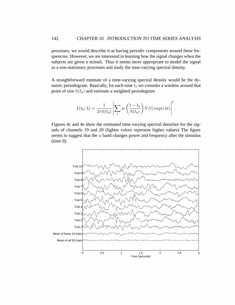
processes, we would describe it as having periodic components around these fre-quencies. However, we are interested in learning how the signal changes when thesubjects are given a stimuli. Thus it seems more appropriate to model the signalas a non-stationary processes and study the time-varying spectral density.

A straightforward estimate of a time-varying spectral density would be the dy-namic periodogram. Basically, for each time t0 we consider a window around thatpoint of size h(t0) and estimate a weighted periodogram

I(t0; λ) =1

2πh(t0)

∣

∣

∣

∣

∣

∑

t

w

(

t− t0h(t0)

)

Y (t) exp(iλt)

∣

∣

∣

∣

∣

2

.

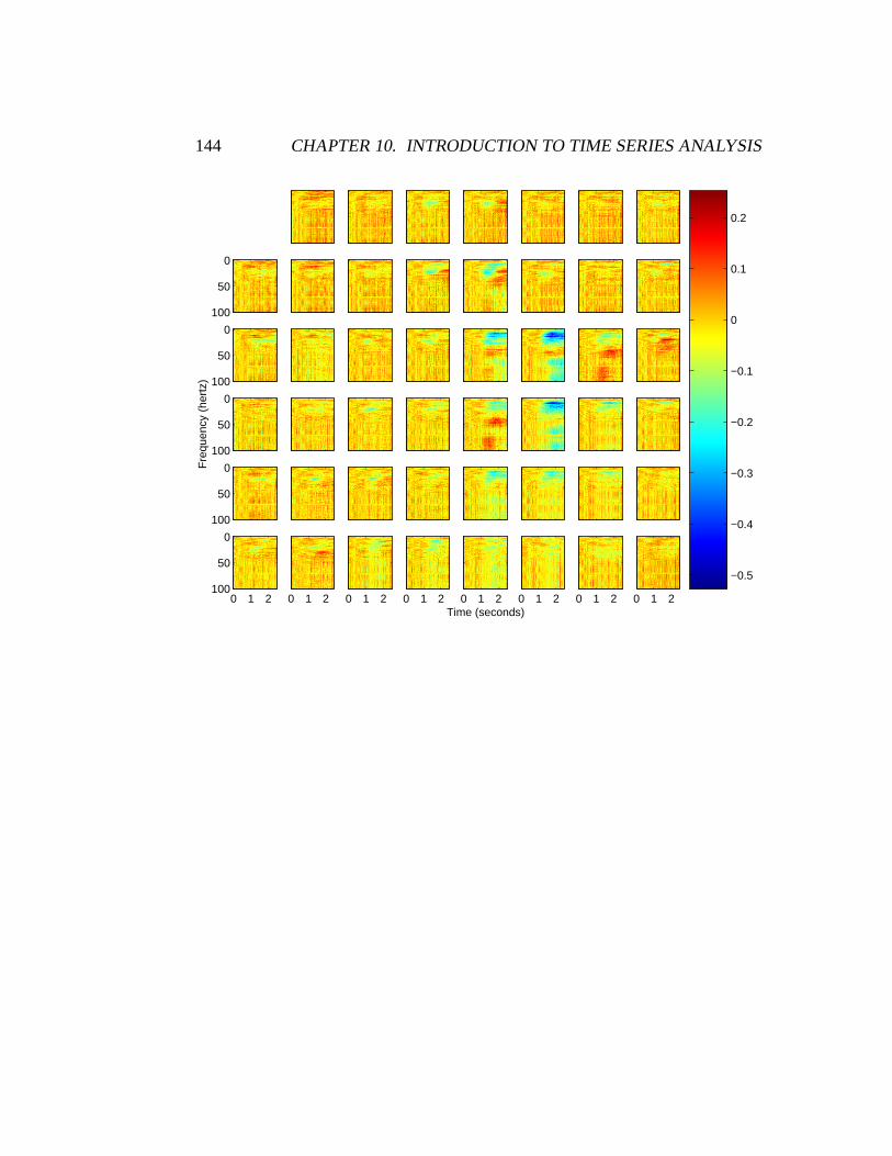
Figures 4c and 4e show the estimated time-varying spectral densities for the sig-nals of channels 19 and 20 (lighter colors represent higher values) The figureseems to suggest that the α band changes power and frequency after the stimulus(time 0).

0 0.5 1 1.5 2 2.5 3

Mean of all 50 trials

Mean of these 10 trials

Trial 1

Trial 2

Trial 3

Trial 4

Trial 5

Trial 6

Trial 7

Trial 8

Trial 9

Trial 10

Time (seconds)

10.2. SPECTRAL ANALYSIS 143

0 1 20 1 20 1 2Time (seconds)

0 1 20 1 20 1 20 1 20 1 2

0

5

10

0

5

10

Fre

quen

cy (

hert

z)

0

5

10

0

5

10

0

5

10

0

0.2

0.4

0.6

0.8

1

1.2

144 CHAPTER 10. INTRODUCTION TO TIME SERIES ANALYSIS

0 1 20 1 20 1 2Time (seconds)

0 1 20 1 20 1 20 1 20 1 2

0

50

100

0

50

100

Fre

quen

cy (

hert

z)

0

50

100

0

50

100

0

50

100

−0.5

−0.4

−0.3

−0.2

−0.1

0

0.1

0.2