NONLINEAR DIFFRACTIVE OPTICSWITH CURVED PHASES: BEAM DISPERSION

AND TRANSITION BETWEEN LIGHT AND SHADOW.

E. DumasLaboratoire de Mathematiques et Physique Theorique

Parc de Grandmont37200 Tours, FRANCE

tel: 02-47-36-73-14 fax: 02-47-36-70-68dumas@gargan.math.univ-tours.fr

Abstract: We give asymptotic descriptions of smooth oscillating solu-tions of hyperbolic systems with variable coefficients, in the weakly nonlineardiffractive optics regime. The dependence of the coefficients of the system inthe space-time variable (corresponding to propagation in a non-homogeneousmedium) implies that the rays are not parallel lines –the same occurs withnon-planar initial phases. Approximations are given by WKB asymptoticswith 3-scales profiles and curved phases. The fastest scale concerns oscilla-tions, while the slowest one describes the modulation of the envelope, whichis along rays for the oscillatory components. We consider two kinds of be-haviors at the intermediate scale: ‘weakly decaying’ (Sobolev), giving thetransverse evolution of a ‘ray packet’, and ‘shock-type’ profiles describing aregion of rapid transition for the amplitude.

Contents

Introduction 2Long time propagation in homogeneous media . . . . . . . . . . . . 2Variable coefficients . . . . . . . . . . . . . . . . . . . . . . . . . . . 4Description of the paper . . . . . . . . . . . . . . . . . . . . . . . . 6

1 Dispersion of beams 91.1 The Ansatz . . . . . . . . . . . . . . . . . . . . . . . . . . . . 101.2 First equations . . . . . . . . . . . . . . . . . . . . . . . . . . 101.3 The sublinearity condition . . . . . . . . . . . . . . . . . . . . 13

1.3.1 Function spaces . . . . . . . . . . . . . . . . . . . . . . 141.3.2 Operators . . . . . . . . . . . . . . . . . . . . . . . . . 16

1.3.3 Profile equations . . . . . . . . . . . . . . . . . . . . . 191.4 Existence of profiles . . . . . . . . . . . . . . . . . . . . . . . . 201.5 Approximation of solutions . . . . . . . . . . . . . . . . . . . . 22

1.5.1 Estimates on the residual . . . . . . . . . . . . . . . . 221.5.2 Stability . . . . . . . . . . . . . . . . . . . . . . . . . . 24

1.6 Diffraction for the weakly compressible, isentropic 3-d Eulerequations . . . . . . . . . . . . . . . . . . . . . . . . . . . . . 29

2 Transition between light and shadow (for odd nonlinearities) 322.1 Framework, notations . . . . . . . . . . . . . . . . . . . . . . . 342.2 Function spaces, and the mean operator M . . . . . . . . . . 362.3 Formal derivation of profile equations . . . . . . . . . . . . . . 36

2.3.1 Using the mean operator M . . . . . . . . . . . . . . . 372.3.2 Fast scale analysis . . . . . . . . . . . . . . . . . . . . 382.3.3 Analysis w.r.t. the (remaining) intermediate variables . 39

2.4 Existence of profiles and approximation of exact solutions . . . 412.4.1 Solving the profile equations . . . . . . . . . . . . . . . 412.4.2 Stability . . . . . . . . . . . . . . . . . . . . . . . . . . 42

3 Wave transitions for systems of conservation laws 443.1 The system and the Ansatz . . . . . . . . . . . . . . . . . . . 463.2 The approximate solution . . . . . . . . . . . . . . . . . . . . 463.3 Stability . . . . . . . . . . . . . . . . . . . . . . . . . . . . . . 48

3.3.1 The conjugation operator Vε . . . . . . . . . . . . . . . 493.3.2 The singular system . . . . . . . . . . . . . . . . . . . 543.3.3 Example of phases for Euler equations . . . . . . . . . 58

Introduction

Long time propagation in homogeneous media

Geometric optics provides asymptotic approximations of waves in the limit ofzero wavelength. These approximations are valid only for some propagationdistances (see [22]). When looking at longer propagation scales, a diffractivecorrection is needed. The first rigorous works in this context are probably[7] and [8]. Under oddness assumptions on the nonlinearities, these authorsgive an approximation to the solution of the initial value problem associatedwith a nonlinear hyperbolic system L(u, ∂)u = F (u), where L(u, ∂) = ∂t +

2

∑j Aj(u)∂j. Here, the Aj(u) are symmetric matrices possibly depending on

u, but not on the coordinates (t, x): this means that the wave propagates ina homogeneous medium. The initial data oscillate at frequency 1/ε, and theapproximation is provided, on the Rayleigh distance (of order 1/ε), by:

(0.0.1) εm∑

n∈mN

εnan

(εX,X,

β ·Xε

), X = (T, Y ) ∈ R

1+d,

i.e. : There is t? such that, for all ε ∈]0, 1], the exact solution uε is smoothon [0, t?/ε] × Rd, and admits the asymptotic expansion (0.0.1) as ε → 0.

The amplitude εm is smaller than the one of geometric optics (for O(1)propagation), so that diffraction affects the principal term of the asymptoticsat the same time as the accumulated effects of nonlinearities. The phase ofthe oscillating wave is β · x =

∑j βjxj . The profiles an(X,X, θ) are smooth,

periodic in θ (with mean equal to zero). They are solutions to a coupled sys-tem of transport equation at the intermediate scale and Schrodinger equationwith slow time. The system is nonlinear for the first profile:

πa0 = a0,(0.0.2a)

V (∂X)a0 = 0,(0.0.2b)

V (∂X)a0 +R(∂Y )∂−1θ a0 + π[Φ(a0) + Λ(a0)∂θa0] = 0.(0.0.2c)

The next profiles are solutions to systems with the same structure, but linear.Equation (0.0.2a) expresses the polarization of a0, and π is a (matrix) pro-

jector associated to L and β. The operator V (∂X) = ∂T+v.∂Y is the transportfield along rays, with group velocity v. These two equations are similar to theones of usual geometric optics. Finally, (0.0.2c) represents transverse diffrac-tion, at the time scale T , via the scalar operator R(∂Y ) =

∑i,j ri,j∂Yi

∂Yj,

whose coefficients are related to the curvature of the characteristic variety ofL. The nonlinear term is the same as the one arising in the weakly nonlineargeometric optics equations.

A qualitative difference between the approximate solution (0.0.1) andthe geometric optic’ one comes from Equation (0.0.2c), which implies non-conservation of supports: Even if the initial data have compact support,a0(εX,X, β·X/ε) does not, whereas the geometric optics approximation does,because it is transported along rays. This explains the spatial dispersion ofa laser beam, for example.

This kind of asymptotics has also been studied by Joly, Metivier, Rauch in[19], when rectification effects are present, i.e. when interactions of oscillating

3

modes can generate non-oscillatory waves. In [21], D. Lannes considers thecase of dispersive systems, with rectification. G. Schneider has treated thecase of one equation, in space dimension one, by means of normal forms (see[26]). In [6], T. Colin has studied systems with a ‘transparency’ property,allowing solutions with greater amplitude; the profiles are then solutions ofDavey-Stewartson systems (see also [20]). Diffraction for pulses (i.e. whenthe profiles an(X,X, θ) have compact support in θ) leads to a somewhatdifferent approximation, with a typical profile equation 2∂T∂θan − ∆Y an =∂θf(an); see [2], [1], and [3] for an approach via ‘continuous spectra’.

All these results have been obtained in the general framework of ‘longtime’ propagation (of order 1/ε when the wavelength is ε), and oscillationswith respect to one linear phase (Ansatz εm

∑εnun(εX,X, β ·X/ε)).

Variable coefficients

The previous results break down as soon as one considers equations with vari-able coefficients, for example the following wave equation with non-constant

refractive index (see Example 0.1):

(n(εX)2

c2∂2T − ∆Y

)uε = 0.

Here, we are interested in the case of curved phases, for which rays areno longer parallel lines –but before focusing (or caustics): Our study onlyconcerns smooth (C1) phases. We begin with a change of scale, so that thepropagation occurs for times of the order one. Using the slow variable x = εX(= O(1)) instead of X, the approximate solution (0.0.1) reads

(0.0.3) εm∑

n∈mN

εnan

(x,x

ε,β · xε2

),

and setting ε =√ε,

εm/2∑

n∈mN

εn/2an

(x,

x√ε,β · xε

).

Now, in the case of variable coefficient systems, nonlinear phases are involved,a priori defined on a bounded domain Ω (as ε → 0) only. That’s why we usethe Ansatz

(0.0.4) εm/2∑

n∈mN

εn/2an

(x,ψ(x)√ε,φ(x)

ε

),

4

where an = an(x, ω, θ) ∈ ∩sHs(Ω × Rp × Tq).This Ansatz was introduced by J.K. Hunter in [16], and becomes

(0.0.5) εm∑

n∈mN

εnan

(εX,

ψ(εX)

ε,φ(εX)

ε2

)

in the scales of (0.0.1) (propagation on distances of order 1/ε). The phasesφ and ψ depend slowly on X, and this regime is called weakly nonplanar.

Example 0.1. Consider the linear wave equation(n(εX)2

c2∂2T − ∆Y

)uε = 0,

with refractive index n smooth and bounded, and initial data

uε|T=0= εmg

(Y,η · Yε

)

∂tuε|T=0

= εm−1h

(Y,η · Yε

).

We choose h = cn|η|∂θg (polarized data), and g ∈ ∩sHs(Rd×T) with

∫gdθ =

0 (purely oscillating profiles).We are interested in the behavior of uε for times of the order 1/ε. So

as to apply the results of Paragraph 1.5, we change variables: x = εX,vε

2

(x) = uε(X), and set ε2 = ε.

(n(x)2

c2∂2t − ∆y

)vε = 0

vε|t=0= εm/2g

(y√ε,η · yε

)

∂tvε|t=0

= ε(m−1)/2h

(y√ε,η · yε

).

Theorems 1.1 and 1.2 give an approximation of vε on the cone Ω = x =(t, y) ∈ R

1+d/0 ≤ t ≤ t?, δt + |y| ≤ ρ: There are Vε,Vεapp ∈ ∩sHs(Ω ∩ t ≤t × Rd × T) (for t < t?) such that:

vε(x) = εm/2Vε(x,ψ′√ε,φ

ε

),

∀s ∈ R, ‖Vεapp − Vε‖Hs −→ε→0

0.

5

The phases φ, ψ′ = (ψ1, . . . , ψd) are defined by:n(x)c∂tφ = |∂yφ|

φ|t=0= η · y ,

Vφ(∂x)ψµ = 0ψµ|t=0

= yµ,

where Vφ(x, ∂x) =n(x)

c∂∂t −

∂yφ

|∂yφ|.∂y: φ satisfies an eikonal equation asso-

ciated with n2

c2∂2t − ∆, and each ψµ is annihilated by the associated tangent

transport, i.e. for the vector field corresponding to the group velocity. Whenthe refractive index really depends on x = εX, none of these phases is linear.

The approximate profile Vεapp is given by Vεapp = v0 +√εv1 + εv2. The

terms vn(x, ω, θ) are determined by equations (1.3.2) to (1.3.4c) and (1.2.5d)to (1.2.5g), which here restrict to (see Remark 1.4, iii)):

Vφ(∂x)vn −D(∂ω)∂−1θ vn = fn,

withD(∂ω) =1

2

∑

µ

(n2

c2(∂tψµ)

2 − |∂yψµ|2)∂2ωµ

, and fn a function of vn−1, vn−2

and their derivatives.Coming back to the original scales and setting Uε

app = Vε2app, we get anapproximation of uε for times T ∼ 1/ε:

∀t < t?, ∀α ∈ N1+d, on

(1

εΩ

)∩ T ≤ t/ε ,

∥∥∥∥(ε∂)α

(uε − εmUε

app

(εX,

ψ′(εX)

ε,φ(εX)

ε2

))∥∥∥∥L∞

= o(εm).

One cannot obtain such an approximation (on Ωt/ε) using plane phases:ψµ(εX)/ε differs from its linear part ∂xψµ(0) · X by a O(ε|X|2) = O(1/ε)term. Because of decaying of Uε

app, replacing ψµ(εX)/ε by its linear partwould generate a O(εm) error in the approximate solution.

Description of the paper

The main difficulties in the analysis are nonlinearities and variable coeffi-cients. Nonlinearities allow interactions between propagating modes, andthus phase mixing, and induce coupling in the profile equations. These equa-tions also have variable coefficients when the original system does. A solvablesystem determining the profiles can be obtained only when the operators in-volved commute. This is guaranteed by coherence assumptions on the phases

6

(cf. Paragraph 1.3.2 and Paragraph 1.4). The asymptotic system finally in-herits properties from the initial one, which provide energy estimates, infunction spaces with different regularities for different variables; see Para-graph 1.4.

Our study deals with quasilinear hyperbolic systems, and the same meth-ods apply to semilinear systems. The paper is organized as follows:

1-In the first part, we look at the weakly decaying case, when the initialprofiles gn(y, Y, θ) ∈ ∩sHs(Ω0 × R

p−1 × T). The Ansatz is given in Para-graph 1.1. We formally derive the first profile equations by the method ofmultiple scales in Paragraph 1.2.

We introduce an ‘intermediate time’ T (X = (T, Y )) in order to analyseand solve these equations. In particular, it is natural to require the profileu1 to be sublinear with respect to T , so that the term

√εu1 is a corrector of

u0 (Paragraph 1.3).The next step consists in looking at the interactions between waves con-

stituting u0, so as to determine which ones have an influence at leading order:the others are considered as correctors. Thanks to our coherence assumptionson the phases, the conditions under which the profiles are sublinear can be de-rived via the techniques of Joly, Metivier, Rauch [19] or Lannes [21]. The sizeof the correctors cannot be more specified, because of interactions betweenoscillatory and non-oscillatory terms (rectification phenomenon). Hence, theasymptotics is based on a first term and two correctors only.

We show existence of u0, u1 and u2 (Paragraph 1.4), and then, stabilityof exact solutions near the approximate one, via a singular system methodand an additional coherence assumption involving both fast and slow phases(Paragraph 1.5).

We illustrate these results with the concrete example of isentropic Eulerequations, exhibiting explicit coherent nonlinear phases and profile equations.

2-In the second part, we study oscillating waves whose amplitudes havea rapid variation across some hypersurface: they decay to zero on one side,whereas on the other side, they behave like usual slowly modulated oscillatingwaves. This describes transition between light and shadow (or sound andsilence, in the case of sound waves). Instead of treating a ‘matching problem’(such as in [16]), we construct waves with WKB asymptotics in terms of‘shock’ profiles: they admit finite limits at +∞ and −∞ with respect to oneof the intermediate variables, Y1. The rays associated with φ are then tangentto the surface ψ1 = 0. The profiles un split into un = χ(Y1)an(Y2, . . . , Yp) +bn(Y1, . . . , Yp), where χ is a fixed ‘step’ (function with finite limits at +∞

7

and −∞). The term an gives the behavior ‘at infinity’ (w.r.t. Y1), while bnrepresents the transition layer (of width

√ε).

χak

bk

χak + bk

Y1 Y1Y1

Figure 1: The profiles’ shape.

The equations determining the an are independent of the bn. In particular,in the model case when p = 1, an does not depend on Y , and satisfies theusual equations of weakly nonlinear optics in ψ > 0: see Remark 2.2.

incident rays

Y1 = ψ1/√ε

Ω

obstacle

ψ1 = 0

coordinate stretching

shadow light

φ-rays

ψ1 = 0

√ε

Figure 2: From ‘macroscopic’ to ‘microscopic’ description.

In Paragraphs 2.1 and 2.2, we give the Ansatz. We explain in Example 2.1why only one intermediate phase ψ1 can govern the rapid transition, and thus,why rectification effects must be avoided at each step of the asymptotics.The simplest way to do so consists in imposing a strong condition on thenonlinearities: their Taylor expansion (at zero) includes odd powers only.We are then able to construct infinite-order asymptotics, based on purelyoscillating (or ‘zero-mean’) profiles.

We construct the profiles in Paragraph 2.4 (under the same coherenceassumptions as in Section 1). They satisfy a stronger condition than T -sublinearity (they are bounded).

Finally, thanks to the infinite order asymptotics, we prove stability of theexact solutions via a smooth perturbation method (in the spirit of O. Gues,[13]).

8

3-The third part is devoted to another approach concerning this kind ofrapid transitions, where we get rid of the previous oddness assumption onnonlinearities. We extend the singular system technique of Part 1 to the func-tion spaces of Part 2, using semi-classical pseudo-differential calculus. Thismethod simply requires non-generation of profile mean values at first order(which is for example satisfied in the case of systems of conservation laws),but as a consequence, we only obtain leading-order asymptotics. An addi-tional geometrical ‘coherence-type’ assumption on the intermediate phase ψis needed to ensure converge.

These assumptions are satisfied by the explicit example of acoustic wavesin Paragraph 3.3.3.

Remark 0.1. Our profiles depend on several intermediate phases, and onlyone rapid phase φ. One may prove the same existence and stability propertiesfor multiphase asymptotics, and treat interactions of diffracted waves (addinga coherence assumption on the phases φ; see [10], [9]).

1 Dispersion of beams

We study the solutions of a quasilinear symmetric hyperbolic system

(1.0.6) L(x, u, ∂)u = ∂tu+d∑

j=1

Aj(x, u)∂ju =d∑

j=0

Aj(x, u)∂ju = 0.

We denote by x = (t, y) a point in Ω. Ω is a connected open subset of R1+d

on which the matrices Aj satisfy:

Assumption 1.1. The matrices Aj ∈ C∞(Ω× CN ,MN(C)) are Hermitian,and A0 ≡ I.

We are interested in the Cauchy problem associated to (1.0.6), for initialdata of the form

εg

(y,ψ0(y)√

ε,φ0(y)

ε

), where g ∈ ∩sHs(Ω × R

p−1 × T).

9

1.1 The Ansatz

The profiles are ‘weakly decaying’ (i.e. Hs) with respect to the intermediatevariable. We denote by Ψ the (real) vector space with generators ψ. Weintroduce an intermediate time T = t/

√ε (thus, a phase ψ0 ≡ t), so as

to treat Cauchy problems. The phases ψ = (ψ0, . . . , ψp−1) are R-linearlyindependent. The size of correctors is also measured by T (see 1.3), so thatwe avoid ill-posed systems such as proposed in [16].

Remark 1.1. In the sequel, the vector space Ψ will satisfy coherence as-sumptions. As explained in [18] (p. 56; see also [17]), such a space usuallycontains a timelike phase ψ0. Changing variables, one can use this ψ0 astime variable. But in this case, the matrix A0 (coefficient of ∂t in (1.0.6))then depends on (t, y). For the sake of simplicity, we suppose that ψ0 ≡ t.

One of the features emphasized in [8] and [19] is rectification, i.e. thepossibility of interaction between oscillating and non-oscillating modes (trav-elling at the same speed). This forces the use of an Ansatz with only oneterm and two correctors, which reads:

(1.1.1) uε ∼ ε

2∑

n=0

εn/2un

(x,

t√ε,ψ′(x)√

ε,φ(x)

ε

),

where ψ = (t, ψ′) ∈ Ψp, with un = un(x,X, θ) = un(x, T, Y, θ) periodic w.r.t.θ and smooth, and un(x, T, ., θ) ∈ ∩sHs(Rp−1).

Notation 1.1. We denote by Ψ′ the (real) space generated by the phases ψ′;it is a dimension p− 1 subspace of Ψ, such that Ψ = Ψ′ ⊕ tR.

1.2 First equations

One formally gets an asymptotic solution to (1.0.6) by plugging the Ansatzinto the system and insisting that the coefficients of ε0, ε1/2 and ε in theresidual all vanish. This yields :

(1.2.1) L1(dφ)∂θu0 = 0,

(1.2.2) L1(dφ)∂θu1 + L1(dψ)∂Xu0 = 0,

10

(1.2.3) L1(dφ)∂θu2 + L1(dψ)∂Xu1 + L1(∂x)u0 +B(u0)∂θu0 = 0,

where we have set:

Notation 1.2. L1(x, ξ) := L(x, 0, ξ),

L1(dψ)∂X :=∑p−1

µ=0 L1(x, dψµ(x))∂Yµ ,

B(u) :=∑d

j=1 ∂jφ(x)(∂uAj(x, 0).u).

Equation (1.2.1) has an oscillating solution only if the matrix L1(dφ) issingular. In others words, we assume the phase φ satisfies an eikonal equation:

Assumption 1.2. The quantity detL1(x, dφ(x)) is identically zero on Ω.So, there is an eigenvalue λ of the matrix A(x, η) :=

∑dj=1 ηjAj(x, 0) such

that: ∂tφ+λ(x, ∂yφ) = 0. In addition, we assume ∂yφ does not vanish on Ω.

Now, (1.2.1), (1.2.2), (1.2.3) are analyzed by means of projections, so thatsome parts of the profiles are immediately determined. First, we separateoscillations and mean values:

Notation 1.3. Fourier series u =∑

α∈Zuα(x,X)eiα.θ decompose into: u =

u(x,X) + u?(x,X, θ) = 〈u〉 + u?.

Next, we perform matrix analysis. In order to get smoothness of geometricobjects, we assume the characteristic variety of L1 is a smooth manifoldoutside the origin:

Assumption 1.3. The eigenvalues λ1(x, η) < · · · < λZ(x, η) of the (Her-mitian) matrix A(x, η) :=

∑dj=1 ηjAj(x, 0) have constant multiplicity (on

Ω × (Rd \ 0)).

Proposition 1.1. Under Assumptions 1.1-1.3, the spectral projection ofL1(dφ) onto its Kernel is smooth on Ω, and L1(x, dφ(x)) admits a smooth(also symmetric) partial inverse Q(x):

π(x)L1(x, dφ(x)) = L1(x, dφ(x))π(x) = 0,(1.2.4a)

Q(x)L1(x, dφ(x)) = L1(x, dφ(x))Q(x) = 1 − π(x), Q(x)π(x) = 0.(1.2.4b)

11

Using projection of (1.2.1)-(1.2.3) on oscillating and non-oscillating modes,and then applying π and Q, we get:

πu?0 = u?0L1(dψ)∂Xu0 = 0

πL1(dψ)∂Xπu?0 = 0

(1 − π)u?1 = −∂−1θ QL1(dψ)∂Xu

?0

L1(dψ)∂Xu1 + L1(∂x)u0 + 〈B(u0)∂θu0〉 = 0

πL1(dψ)∂Xπu?1 + πL1(dψ)∂X(1 − π)u?1 + πL1(∂x)πu

?0 + π(B(u0)∂θu0)

? = 0

(1 − π)u?2 = −∂−1θ Q [L1(dψ)∂Xu

?1 + L1(∂x)u

?0 + (B(u0)∂θu0)

?] .

It is well-known (cf. [23], [7], [8]) that the new operators arising in theseequations admit a simple diagonal structure:

Proposition 1.2. Under assumptions 1.3 and 1.2,i) πL1(∂x)π = π[V (x, ∂x) + C(x)] = π[(∂t + v(x).∂y) + C(x)],

where v(x) := ∂ηλ(x, ∂yφ(x)), and C(x) :=d∑

j=0

Aj(x, 0)(∂jπ)(x) ;

ii) ∀ρ ∈ C∞, πL1(dρ)π = πV (x, dρ) ;

iii) πL1(dψ)∂XQL1(dψ)∂Xπ = −1

2π

d∑

j,k=1

∂2λ

∂ηj∂ηk(x, ∂yφ(x)).(∂jψ(x).∂X)2

= −1

2π

d∑

j,k=1

∂2λ

∂ηj∂ηk(x, ∂yφ(x)).(∂jψ

′(x).∂Y )2

:= πD(x, ∂Y ).

12

Finally, the profiles must be determined by:

πu?0 = u?0,

(1.2.5a)

L1(x, dψ)∂Xu0 = 0,(1.2.5b)

V (x, dψ)∂Xu?0 = 0,

(1.2.5c)

(1 − π)u?1 = −∂−1θ Q(x)L1(x, dψ)∂Xu

?0,

(1.2.5d)

L1(x, dψ)∂Xu1 = −L1(x, ∂x)u0 − 〈B(x, u0)∂θu0〉,(1.2.5e)

πV (x, dψ)∂Xu?1 = ∂−1

θ D(x, ∂Y )u?0 − V (x, ∂x)u?0 − πC(x)u?0 − π(B(x, u0)∂θu0)

?,(1.2.5f)

(1 − π)u?2 = −∂−1θ Q(x) [L1(x, dψ)∂Xu

?1 + L1(x, ∂x)u

?0 + (B(x, u0)∂θu0)

?] .(1.2.5g)

Now, equations (1.2.5e) and (1.2.5f) must be analysed.

1.3 The sublinearity condition

We proceed in the same way as in [19]: for√εu1(x, ψ/

√ε, φ/ε) to be a

corrector of u0(x, ψ/√ε, φ/ε), it is sufficient that the profile u1(x,X, θ) is

sublinear with respect to T . This imposes constraints on the right-hand sideof (1.2.5e) and (1.2.5f).

Simply setting these right-hand sides equal to zero leads to overdeter-mined systems of equations on u?0 and u0. So, we have to look closely at thestructure of the waves u?0 and u0 given by equations (1.2.5b) and (1.2.5c),and to understand the role played by the possible resonances.

13

1.3.1 Function spaces

Our strategy for solving the profile equations is to use energy estimates. Theyare local, so from now on, Ω is the cone

Ω := x = (t, y) ∈ R1+d/0 ≤ t ≤ t0, δt+ |y| ≤ ρ,

where ρ > 0 is fixed, and δ is sufficiently large, so that on Ω,

δId+

d∑

j=1

yj|y|Aj(x, 0) is positive definite and

(δ +

d∑

j=1

yj|y|vj(x)

)> 0.

Set ωt := y ∈ Rd/(t, y) ∈ Ω, and Ωt1 := Ω ∩ t ≤ t1 for 0 < t1 ≤ t0.The function spaces are of Sobolev type. Commutations between ∂x and

D(∂Y ) cause a loss of derivatives in Y , so we use anisotropic spaces:

Definition 1.1. For s ∈ N/2 and 0 < t1 ≤ t0, we consider functionsu(x,X, θ) on Ωt1 ×R

p×T such that (∂y,Y,θ)γu, extended by zero outside Ωt1,

belongs to C0(RT , C0([0, t1], L

2(Rd × Rp−1 × T))), when γ = (γy, γY , γθ) ∈

Nd+(p−1)+1 has weight [γ] := |γy|+|γY |/2+γθ/2 ≤ s. For such a u, when t andT are fixed, u(t, T ) belongs to the Hilbert space Ms(ωt) equipped with the nat-ural L2 inner product. For T fixed, we say u(T ) ∈ Es(t1) (u ∈ C0(R, Es(t1))),the Banach space with norm: ‖ u ‖Es(t1):= sup

t∈[0,t1]

‖ u(t) ‖Ms(ωt) .

Elements ofMs(ωt) are restrictions of functions of Sobolev type on Rd+p−1×T (see for example [5]), so that they satisfy the classical properties (see [27]for the proof in the isotropic case):

Proposition 1.3 (Sobolev’s embedding).For s ∈ N/2 and s > 2d+p

4, Ms(ωt) is a subspace of L∞(Rd×Rp−1 ×T). The

embedding has bounded norm for t ∈ [0, t0].

Proposition 1.4 (Gagliardo-Nirenberg’s inequality). If k, s ∈ N/2,

k ≤ s, and α, β ∈ [1,+∞], r ∈ [2,+∞], satisfy (1 − k

s)1

α+k

s

1

β=

1

r,

there is C > 0 such that, for all t ∈ [0, t0], u ∈ S(ωt×Rp−1×T) and γ ∈ Nd+p

such that [γ] = k,

‖ ∂γu ‖Lr≤ C ‖ u ‖1− ks

Lα ‖ ∂su ‖ks

Lβ .

14

Proposition 1.5 (Moser). For s > 2d+p4

, Es(t1) is a Banach algebra onwhich smooth functions act continuously, i.e. :If G : Ωt1 × Rp−1 × T × CN → Cn has regularity C∞, for all u, v ∈ Es(t1),

‖ G(x, Y, θ, u+v)−G(x, Y, θ, u) ‖Es(t1)≤ C(‖ u ‖Es(t1), ‖ v ‖L∞(Ωt1 )) ‖ v ‖Es(t1)

(If, in addition, G(., ., ., 0) ≡ 0, then G(x, Y, θ, u) ∈ Es(t1)).

We will also consider Ms(ωt) as a set of functions of some variables (Yor (y, θ)), with values as functions of the other variables:

Lemma 1.1. For every t ∈ [0, t0] and 0 ≤ k ≤ s, Ms(ωt) is a subspaceof H2k(Rp−1

Y , Ms−k(ωt×T)) and Mk(ωt×T, H2(s−k)(Rp−1Y )), with embedding

bounded on [0, t0], where Mk(ωt × T) is the space of functions u on ωt × T

such that ∂γu ∈ L2(ωt × T) for |γy| + |γθ|/2 ≤ k.

Proof :The proof is by induction on s and k. We give details only for the first

inclusion, in the case s = k = 1/2: when u ∈ M1/2(ωt), show that u ∈H1(Rp−1

Y , L2(ωt×T)). By definition, ‖u‖L2y,θ

belongs to L2Y ; we have to prove

∂Y ‖u‖L2y,θ

∈ L2Y .

First chose u in the dense subspace C∞c . Let ϕ ∈ S(RY ) be a test function.

Using the Dominated Convergence Theorem,

∣∣∣∣∫

‖u‖L2y,θ∂YµϕdY

∣∣∣∣ =∣∣∣∣ limZµ→0

∫‖u‖L2

y,θ

ϕ(Yµ + Zµ) − ϕ(Yµ)

ZµdY

∣∣∣∣

= limZµ→0

∣∣∣∣∫

‖u‖L2y,θ

ϕ(Yµ + Zµ) − ϕ(Yµ)

ZµdY

∣∣∣∣ ,

15

and, dropping indices,

= limZ→0

∣∣∣∣∫

‖u‖L2y,θ

ϕ(Y + Z) − ϕ(Y )

ZdY

∣∣∣∣

= limZ→0

∣∣∣∣∣

∫ ‖u‖L2y,θ

(Y ) − ‖u‖L2y,θ

(Y − Z)

Zϕ(Y )dY

∣∣∣∣∣

≤ limZ→0

∫ ∣∣∣∣∣‖u‖L2

y,θ(Y ) − ‖u‖L2

y,θ(Y − Z)

Z

∣∣∣∣∣ |ϕ(Y )| dY

≤ limZ→0

∫ ∥∥∥∥u(Y ) − u(Y − Z)

Z

∥∥∥∥L2

y,θ

|ϕ(Y )| dY

≤∫

‖∂Y u‖L2y,θ

(Y ) |ϕ(Y )| dY

≤ ‖u‖M1/2(ωt) ‖ϕ‖L2Y,

thanks to Fatou’s Lemma and Cauchy-Schwarz inequality.A density argument shows this is valid for u ∈M1/2(ωt).

1.3.2 Operators

Partial Fourier transform (in Y ) is the appropriate tool for the study of thelinear Cauchy problem associated with (1.2.5b) and (1.2.5c).

Notation 1.4. Let D be the characteristic set

D := (x, χ) ∈ Ω × (Rp \ 0) / detL1(x, d(χ.ψ(x))) = 0.

We write χ = (σ, ρ) ∈ R × Rp−1, so that L1(d(χ.ψ)) = σ + L1(d(ρ.ψ′)), and

we have the spectral decomposition of the symmetric matrix

L1(d(ρ.ψ′)) =

M∑

k=1

σk(x, ρ)Ek(x, ρ).

Once the evolution problem (w.r.t. the variable T ) is solved for u0, weplug the solution into equations (1.2.5e) and (1.2.5f). Now, we have to solvethe associated Cauchy problem for u1 (with vanishing data), expecting aT -sublinear solution. This requires vanishing of the resonances in the right-hand side of the equations. In order to identify clearly such phenomena, wemake some coherence assumptions (see [15], [18]):

16

Assumption 1.4. The (real) vector space Ψ, generated by the ψν’s, is L1-coherent, i.e. : ∀ϕ ∈ Ψ \ 0,

- either: ∀x ∈ Ω, dϕ(x) 6= 0 and detL1(x, dϕ(x)) = 0,

- or: ∀x ∈ Ω, detL1(x, dϕ(x)) 6= 0.

Assumption 1.5. The space Ψ is V -coherent, i.e. :

∀ϕ ∈ Ψ \ 0, - either: ∀x ∈ Ω, dϕ(x) 6= 0 and V (x, dϕ(x)) = 0,

- or: ∀x ∈ Ω, V (x, dϕ(x)) 6= 0.

Lemma 1.2. Under Assumption 1.3 of constant multiplicity, since ψ0 ≡ t,i) If Ψ is L1-coherent (Assumption 1.4), the eigenvalues σk depend on ρ only.Hence, D splits up into Ω ×D.ii) If Ψ is V -coherent (Assumption 1.5), each V (x, dψµ) is independent of x.

Proof :The proof is similar for the two items. For the first one, we decompose

L1(d(χ.ψ)) = σ + L1(d(ρ.ψ′)) =

M∑

k=1

(σ + σk(x, ρ))Ek(x, ρ),

so that detL1(d(χ.ψ)) =M∏

k=1

(σ + σk(x, ρ)) . Coherence says that this deter-

minant, when σ and ρ are fixed, is zero for every x, or does not vanish.Then, with ρ fixed, if we choose σ := −σk(x0, ρ) for a given x0, we havedetL1(x, d(χ.ψ)(x)) = 0 for all x. Hence, for each x, there is k such thatσk(x, ρ) = −σ.

But the index k does not depend on x, because of Assumption 1.3: for agiven k, there is k′ such that σk(x, ρ) = ∂t(ρ.ψ

′)(x)+λk′(x, ∂y(ρ.ψ′)(x)). Now,

when k 6= l, we have k′ 6= l′ and σk(x, ρ) − σl(x, ρ) = λk′(x, ∂y(ρ.ψ′)(x)) −

λl′(x, ∂y(ρ.ψ′)(x)), and this quantity can vanish only if ∂y(ρ.ψ

′) does. Finally,coherence implies that this is possible only if ρ.ψ′ identically vanishes:

Lemma 1.3. Assuming coherence of Ψ = tR⊕Ψ′, if ϕ ∈ Ψ′ \ 0, then ∂yϕdoes not vanish on Ω.

In the study of resonances, it is important to know whether waves travelwith the same speed, or interact only briefly, with transverse directions ofpropagation.

17

Lemma 1.4. Under Assumption 1.3 and Assumption 1.4, the functions σkare continuous on Rp−1 and analytic on Rp−1 \ 0, so that:

σk(ρ) = ck.ρ with ck ∈ Rp−1,

or: for all c ∈ Rp−1, σk(ρ) 6= c.ρ almost everywhere.

Proof :As in the proof of Lemma 1.2, we begin relating σk to λk:

L1(d(ρ.ψ′)) = ∂t(ρ.ψ

′) + A(∂y(ρ.ψ′))

=∑

k

(∂t(ρ.ψ

′) + λk(∂y(ρ.ψ′))

)πk(∂y(ρ.ψ

′)).(1.3.1)

Lemma 1.3 implies that ∂y(ρ.ψ′) does not vanish if ρ does not, and the

constant multiplicity assumption ensures analyticity of λk(x, .) on Rp−1\0.Distinction of plane and curved modes is then a consequence of the analyticcontinuation principle.

The profiles are decomposed by means of projections, thanks to the fol-lowing Fourier multipliers:

Lemma 1.5. Under Assumption 1.3 and Assumption 1.4,i) The operators Ek(x, ∂Y ), defined by FY (Ek(x, ∂Y )u) = Ek(x, ρ)u(T, ρ),are projectors on Es(t1), which are orthogonal for s = 0.ii) The operators σk(∂Y ), defined by FY (σk(∂Y )u) = iσk(ρ)u(T, ρ), are con-tinuous from Es(t1) to Es−1(t1).

Proof :The proof of ii) is analogous and simpler than the proof of i), so we only

give the proof of the first claim.From (1.3.1), we express Ek as (changing numbering if necessary):

Ek(x, ρ) = πk(∂y(ρ.ψ′)),

with πk the spectral projector associated to λk in Assumption 1.3. This givessmoothness of Ek on Ω × (Rp−1 \ 0).

Time variables t et T are only parameters, and continuity with respect tothese variables is obtained via Lebesgue’s dominated convergence theorem.

When s = 0, action on Es(t1) as orthogonal projector is clear, becauseπk is such a projector on CN . Action on Es(t1) (s 6= 0) follows from thecomputation of the commutators [∂, Ek(∂Y )]. From its definition, Ek(∂Y )commutes with ∂Y and ∂θ. For ∂y, we have:

18

Lemma 1.6. The norm of Ek(x, ρ) as linear mapping on CN , and the normsof the derivatives ∂γy (Ek(x, ρ)), are bounded independently of (x, ρ) ∈ Ω ×(Rp−1 \ 0).

(This is a consequence of continuity with respect to (x, ρ), of degree zerohomogeneity w.r.t. ρ and of the fact that x belongs to a compact set).

Remark 1.2. In the case p = 1, that is with a single phase ψ, the operatorsEk(x, ∂Y ) no more depend on ∂Y , so that they commute with multiplicationby Y . We can then define profiles with decay properties, i.e. (Y, ∂)su ∈ L2.

1.3.3 Profile equations

Our goal is to solve (1.2.5a)-(1.2.5f). We need to suppress u1 from equations(1.2.5e) and (1.2.5f) so as to determine u0, and then solve for u1. The keyis to use the constraint of T -sublinearity for u1, and to eliminate the termsinducing secular parts.

In [19], the structure imposed on u0 by equations (1.2.5a)-(1.2.5c) is anal-ysed, in order to sort out the nonlinear interactions. In [21], D. Lannes givesa new tool for this derivation, ‘average operators’ GW along the character-istic curves of W (∂X) := ∂T + σ(∂Y ), when σ is a degree one homogeneousfunction:

GWw(x,X, θ) := limS→+∞

1

S

∫ S

0

(∫ei(Y ·ρ+Sρ(σ))w(x, T + S, ρ, θ)dρ

)dS.

Here, the structure of u0 is understood thanks to the decomposition u0 =u?0 +

∑Mk=1 u0,k, where u0,k := Ek(x, ∂Y )u: equations (1.2.5b) and (1.2.5c)

read

(∂T + σk(∂Y ))u0,k = 0, with Ek(x, ∂Y )u0,k = u0,k, 1 ≤ k ≤ M,(1.3.2)

V (dψ)∂Xu?0 = 0, with πu?0 = u?0.(1.3.3)

Thanks to Lemma 1.2, the symbols σk(ρ) and V (d(ρ ·ψ′)) = V (dψ′) ·ρ areindependent of x, and we can apply the results of [19], [21]. We must separatethe case when u?0 interacts with the u0,k’s (i.e. when the characteristic varietyof V (dψ)∂X , which is a hyperplane, is contained in the characteristic varietyof L1(dψ)∂X):

19

Notation 1.5. Set ι = 1 if E := χ = (σ, ρ) ∈ Rp/V (dψ)·χ = 0 is containedin D ( cf. Lemma 1.2), ι = 0 if not. If ι = 1 ( i.e. ∃k, (−σk(ρ), ρ) ∈ E , ∀ρ),enumerate the eigenvalues σk so that σ1(ρ) = V (dψ′) · ρ.

Finally, T -sublinearity of u1 is equivalent to:

E1(∂Y )L1(∂x)u0,1 + ιE1(∂Y )〈B(u?0 + u0,1)∂θu?0〉 = 0;(1.3.4a)

for k ≥ 2, Ek(∂Y )L1(∂x)u0,k = 0;(1.3.4b)

πV (∂x)u?0 −D(∂Y )∂−1

θ u?0 + πCu?0 + π(B(u?0 + ιu0,1)∂θu?0)? = 0.(1.3.4c)

The first profile, u0, satisfies equations (1.3.2) to (1.3.4c). The correctorsu1 and u2 are given by equations (1.2.5d) to (1.2.5g).

1.4 Existence of profiles

In this section, we sketch the proof of:

Theorem 1.1. For s > 2d+p4

+ 1 and under Assumptions 1.1 to 1.5, wheng ∈Ms(ω0) is such that πg? = g?, there exist t? ∈]0, t0] and a unique solutionu0 ∈ Es(t), ∀t < t?, to (1.3.2)-(1.3.4c) with initial value u0|t=T=0

= g.In addition, given that u0, (1 − π)u?1 is uniquely determined by Equa-

tion (1.2.5d). The remaining components πu?1 and u1 are the unique solu-tions to Equations (1.2.5e), (1.2.5f) with polarized initial data in Ms(ω0),respectively. Then, (1 − π)u?2 is defined by Equation (1.2.5g).

The maximal time of existence t? := supt / u0 ∈ Es(t) is in fact inde-pendent of s: when s′ ∈]2d+p

4+ 1, s], then t?(s′) = t?(s).

Finally, we have the following estimates, for all t1 < t? and all s:

limT→+∞

‖u0(T )‖Es(t1) < +∞,

1

T‖uj(T )‖Es(t1) −→

T→+∞0, j = 1, 2.

(1.4.1)

As a preliminary remark, we must insist on the fact that coherence impliesthe commutation of the operators V (dψ)∂X and Wk(∂X) with ∂x. This is anecessary condition to obtain an integrable system of equations for the pro-files. Now, our strategy for solving the Cauchy problem associated to theseequations (in Es(t1)) consists in solving first (1.3.4a), (1.3.4b) and (1.3.4c) inT = 0, and then propagating the solutions thanks to (1.3.2) and (1.3.3).

20

In addition, Equations (1.2.5d) and (1.2.5g) determine completely theparts (1 − π)u1 and (1 − π)u2 of the correctors. The polarized parts πu1

and πu2 are solutions to linear inhomogeneous equations, and satisfy theestimates (1.4.1) thanks to the analysis of Paragraph 1.3.3, when u0 solves(1.3.2)-(1.3.4c). As a consequence, we shall only solve (in T = 0) the sys-tem constituted by Equations (1.3.4a) and (1.3.4c) with ι = 1. We considerthe linearized system:

(L)

E1(∂Y )L1(∂x)E1(∂Y )v + E1(∂Y )〈B(v′ + w′, ∂θ)w〉 = 0πV (∂x)w −D(∂Y )∂−1

θ w + πCw + π(B(v′ + w′, ∂θ)w)? = 0.

The existence (and uniqueness) of solution follows from classical tech-niques based on energy estimates, such as:

Proposition 1.6. Let v′, w′ ∈ Es(t1), and s > 2d+p4

+ 1. If (v, w) ∈ Es(t1)2

is a solution of (L), then

‖ v(t) ‖2s + ‖ w(t) ‖2

s≤ eCt(‖ v(0) ‖2

s + ‖ w(0) ‖2s

),

with a constant C depending on the Aj’s and on ‖ v′ ‖s, ‖ w′ ‖s only.

They are consequence of L2 estimates, and properties of the linear andnonlinear commutators:

Lemma 1.7. Take [γ] ≤ s.i) The operators [∂γ , L1(∂x)], [∂

γ , V (∂x)] and [∂γ , D(∂Y )∂−1θ ] have weight less

or equal to [γ], and map continuously Es(t1) into E0(t1).ii) The operators [∂γ , E1(∂Y )] and [∂γ , π] have weight less or equal to [γ]− 1,and map continuously Es(t1) into E1(t1).iii) When w, v′, w′ ∈ Es(t1), then for all t ∈ [0, t1],

‖ [∂γ , B(v′ + w′)∂θ]w ‖M0(ωt)≤ C(‖ v′ + w′ ‖Es(t1)) ‖ w ‖Ms(ωt) .

A duality argument then concludes for linear equations, and an iterativescheme (in Es, initialized for example at g0 and h0) is used for nonlinear ones:

E1(∂Y )L1(∂x)E1(∂Y )vm+1 + E1(∂Y )〈B(vm + wm, ∂θ)wm+1〉 = 0πV (∂x)wm+1 −D(∂Y )∂−1

θ wm+1 + πCwm+1 + π(B(vm + wm, ∂θ)wm+1)? = 0

E1(∂Y )vm+1 = vm+1

πwm+1? = wm+1

vm+1|t=0= g0 ∈ Es

wm+1|t=0= h0 ∈ Es

21

Convergence of this scheme is easily obtained in Es−1/2(t1) for some t1 > 0sufficiently small, and classical results show that the solution has the sameregularity as the initial data (see for example [11]).

Finally, the existence time for maximal solutions only depends on theexistence in a space W1,∞ (and, naturally, on initial data). We make use ofan ‘ODE’ argument (following A. Majda, [24]), relying on estimates of thesame type as the previous ones:

Proposition 1.7. If the maximal existence time t? for solutions v0 and w0

to Equations (1.3.4a) and (1.3.4c) (with smooth initial data) belonging to Es(s > 2d+p

4+ 1) is less than t0, then

lim supt→t?

(‖ v0(t) ‖W1,∞(ωt×Rp−1×T) + ‖ w0(t) ‖W1,∞(ωt×Rp−1×T)

)= +∞,

where W1,∞(ωt × Rp−1 × T) is the space of u ∈ L∞(ωt × Rp−1 × T) whichderivatives ∂γu w.r.t. y, Y and θ belong to L∞(ωt×Rp−1 ×T), when [γ] ≤ 1.

1.5 Approximation of solutions

From our profiles (for smooth initial data g), we construct a function uεapp,and our aim is that it provides an asymptotic solution of (1.0.6), which isclose to exact solutions: for t < t?,

uεapp(x) := εaε(x,ψ(x)√ε,φ(x)

ε

),(1.5.1)

aε(x,X, θ) := (u0 +√εu1 + εu2)(x,X, θ) ∈ ∩sEs(t).(1.5.2)

From now on, all previous assumptions are supposed to be verified.

1.5.1 Estimates on the residual

Proposition 1.8. Define the residual kε(x) := L(x, uεapp, ∂x)uεapp, which is

the evaluation at (x,X, θ) = (x, ψ/√ε, φ/ε) of

(1.5.3) Kε(x,X, θ) := L(x, εaε, ε∂x +√ε∂ψ.∂X + ∂φ∂θ)a

ε.

Then, for all t < t?:

∀s, sup0≤T≤t/√ε

‖Kε(T )‖Es(t) = o(ε), and(1.5.4)

∀α ∈ N1+d, ‖(ε∂x)αkε‖L∞(Ωt) = o(ε).(1.5.5)

22

Proof :We expand (1.5.3), and subtract

L1(dφ)∂θu0 +√ε[L1(dφ)∂θu1 + L1(dψ)∂Xu0]

+ ε[L1(dφ)∂θu2 + L1(dψ)∂Xu1 + L1(∂x)u0 +B(u0)∂θu0] = 0 :

L(x, εaε, ε∂x +√ε∂ψ∂X + ∂φ∂θ)a

ε =[∑

j

(∂jφ)Aj(εaε) − L1(dφ) − ε

∑

j

(∂jφ)∂uAj(0).u0

]∂θu0

+√ε

[(∑

j

(∂jφ)Aj(εaε) − L1(dφ)

)∂θu1

+∑

µ

(∑

j

(∂jψµ) (Aj(εaε) − Aj(0))

)∂Xµu0

]

+ε

[(∑

j

(∂jφ)Aj(εaε) − L1(dφ)

)∂θu2

+∑

µ

(∑

j

(∂jψµ) (Aj(εaε) − Aj(0))

)∂Xµu1 +

∑

j

(Aj(εaε) − Aj(0)) ∂ju0

]

+ε3/2∑

j

Aj(εaε)

(∑

µ

(∂jψµ)∂Xµu2 + ∂ju1

)

+ ε2∑

j

Aj(εaε)∂ju2.

The first term reads(1.5.6)[

ε∑

j

(∂jφ)∂uAj(0).(aε − u0) + ε2

(∫ 1

0

∂2uAj(rεa

ε)dr

).(aε, aε)

]∂θu0.

According to (1.4.1), u1 and u2 are sublinear functions of T . This implies

sup0≤T≤t/√ε

‖uj(T )‖Es(t) = o(1/√ε), j = 1, 2.

This estimate gives the answer concerning (1.5.6). For others terms, we

23

proceed in the same way, simply using the Taylor expansion at first order

Aj(εaε) − Aj(0) = ε

(∫ 1

0

∂uAj(rεaε)dr

).aε.

Hence, (1.5.4) is satisfied, and (1.5.5) follows from substitution.

1.5.2 Stability

We shall use a perturbation method for profiles: define Uε ∈ ∩sEs(t) =

∩sHs(Ωt × Rp−1 × T), t < t?, by Uε(x, Y, θ) := aε(x, t√

ε, Y, θ

), so that

(1.5.7) uεapp(x) = εaε(x,

ψ√ε,φ

ε

)= εUε

(x,

ψ′√ε,φ

ε

).

Phase variables Y and θ play the same role, and we need a new assumption:

Assumption 1.6. The space Φ+Ψ (generated by all phases) is L1-coherent.

Remark 1.3.i) Under geometrical conditions on the characteristic variety of L1, L1-coherenceof Φ + Ψ implies V -coherence of Ψ (Assumption 1.5); see [9].ii) Since we deal with the space generated by all phases, we choose these sothat ψ1 ≡ t /∈ Ψ′ + Φ.

Theorem 1.2. Consider g ∈ ∩sMs(ω0) as in Theorem 1.1, and f ε, hε suchthat for all s, supT ‖f ε(T )‖Es(t?) −→

ε→00 and ‖hε‖Ms(ω0) −→

ε→00.

Let ψ0, φ0 be initial values of the phases; choose any ψ′ ∈ Ψp−1 such thatψ′(0, y) = ψ0, and suppose that Assumptions 1.1 to 1.6 are satisfied (φ isthen defined by the Eikonal Equation). Then, there exists t > 0 such that

(1.5.8)

L(vε, ∂)vε = εf ε(x, ψ/

√ε, φ/ε)

vε|t=0= ε(gε + hε)(y, ψ′(0, y)/

√ε, φ(0, y)/ε),

admits a unique solution vε ∈ C1(Ωt) for all ε ∈]0, 1].

In addition, vε has the form vε(x) = εVε(x,

ψ′√ε,φ

ε

), with Vε ∈ ∩sEs(t).

The approximate solution uεapp from Equation (1.5.7) is accurate in the fol-lowing sense:

∀s, ‖Uε − Vε‖Es(t) −→ε→0

0.

24

Remark 1.4. Choosing phases:i) In order to define initial data for the profiles u0, u1 and u2, only the“matching” of u0(x, ψ/

√ε, φ/ε)|t=0

with 1εvε|t=0

is required. In particular, onlythe corresponding phases are necessary.ii) Once the principal part g(y, ψ0(y)/

√ε, φ0(y)/ε) of 1

εvε|t=0

is known, Ψ can

be built in the following way: From each ψ0j , construct all phases ψj,k solu-

tions to eikonal equations associated with L1 and V . Because of the coherenceassumptions, these phases must belong to Ψ (see [18]). Thus, define Ψ as thelinear span of the ψj,k’s, and assume it is coherent.iii) In the absence of rectification (conservative systems, or odd nonlineari-ties), and when the initial data are purely oscillating at first order (g = 0,implying u0|t=T=0

= 0), it is possible to consider expansions with purely os-cillating profiles un = u?n(x, Y, θ) independent of T (and, for example, witha single intermediate phase ψ), Equations (1.2.5b) and (1.2.5e) for averagesbeing trivially satisfied.iv) We could have considered profiles including parts involving different phases(e.g., initial oscillations g?(y, ψ1/

√ε, φ0/ε) and initial averages g(y, ψ2/

√ε)),

but this would lead to cumbersome notations.

Proof :For vε to be a solution to (1.5.8), it is sufficient for Vε to satisfy:

(1.5.9)

L

(x, εVε, ∂x +

1√ε∂xψ

′.∂Y +1

ε∂xφ∂θ

)Vε = f ε

(x,

t√ε, Y, θ

)

Vε|t=0= Uε

|t=0+ gε.

Here, L(εVε, 1√

ε∂xψ

′.∂Y + 1ε∂xφ∂θ

)Vε, which contains derivatives w.r.t. Y

and θ, writes out

1

εL(εVε,

√ε∂xψ

′.∂Y + ∂xφ∂θ)Vε =

1

εL1

(x,√ε∂xψ

′.∂Y + ∂xφ∂θ)Vε

+1

ε

[L(εVε,

√ε∂xψ

′.∂Y + ∂xφ∂θ)

− L1

(x,√ε∂xψ

′.∂Y + ∂xφ∂θ)]Vε

=1

εL1

(x,√ε∂xψ

′.∂Y + ∂xφ∂θ)Vε

+ T(ε,Vε,

√ε∂yψ

′.∂Y + ∂yφ∂θ)Vε,

25

where T (ε,V, η) :=

d∑

j=1

ηjTj(ε,V), and

(1.5.10) Aj(εVε) −Aj(0) = ε

(∫ 1

0

∂uAj(τεVε)dτ).Vε := εTj(ε,Vε).

This leads to the following (symmetric hyperbolic) singular system:

L (εVε, ∂x)Vε + T(ε,Vε,

√ε∂yψ

′.∂Y + ∂yφ∂θ)Vε

+1

εL1

(x,√ε∂xψ

′.∂Y + ∂xφ∂θ)Vε = f ε(x,

t√ε, Y, θ).

(1.5.11)

Our strategy consists in establishing energy estimates that do not dependon ε. The key is the conjugation of L1(

√ε∂xψ

′.∂Y + ∂xφ.∂θ) to a constantcoefficient operator:

Lemma 1.8. Under Assumptions 1.3 and 1.6, there exists a family of ellip-tic symbols V (x,

√ε, ρ, α) ∈ C∞(Ω, U(N)), homogeneous w.r.t. (ρ, α), with

degree zero, such that: ∀(x, ε, ρ, α) ∈ Ω×]0, 1] × Rp−1 × Z,

V (x,√ε, ρ, α)L1(x, d(

√ερ.ψ′ + αφ)(x))V ?(x,

√ε, ρ, α) = ∆(

√ε, ρ, α),

with ∆(√ε, ρ, α) diagonal, homogeneous w.r.t. (ρ, α), with degree one.

Furthermore, the family(V√ε,ρ,α

)is bounded in C∞(Ω).

Proof :We denote by χ′ a basis for Ψ′ + Φ: there exists a (constant) matrix S ′

such that (ψ′, φ) = S ′χ′. So, we have the relation:

L1(d(√ερ.ψ′ + αφ)) = L1(d(

tS ′(√ερ, α).χ′)).

Now, the symmetric matrix L1(d(γ′.χ′)) has eigenvalues with constant mul-

tiplicity when (x, γ′) ∈ Ω × (Rs \ 0), since ∂y(γ′.χ′) does not vanish (from

the coherence assumption, and because (t, χ′) is a free family), and in viewof the decomposition

L1(d(γ′.χ′)) =

∑

k

(∂t(γ′.χ′) + λk(∂y(γ

′.χ′))) πk(∂y(γ′.χ′)).

This allows us to construct a family of unitary matrices W (x, γ′), smooth onΩ × (Rs \ 0), homogeneous w.r.t. γ′ with degree zero, such that

(1.5.12) W (x, γ′)L1(d(γ′.χ′))W (x, γ′)? = D(x, γ′).

26

Here, D(x, γ′) is a diagonal matrix, which is smooth and homogeneous withdegree one. We continue Identity (1.5.12) for γ′ = 0 with W (x, 0) := Id,D(x, 0) := 0. Homogeneity then ensures that the family (Wγ′)γ′ is boundedin C∞(Ω), and coherence implies (Lemma 1.2) that eigenvalues do not dependon x, so that D does not neither: D(x, γ′) = D(γ′). Finally, set:

V (x,√ε, ρ, α) := W (x,tS ′(

√ερ, α)) , ∆(

√ε, ρ, α) := D(tS ′(

√ερ, α)).

We now perform a change of functions:

(1.5.13) Vε := Vε(x, ∂Y , ∂θ)Vε,

and get a new system (equivalent to (1.5.11)):

(1.5.14) Vε(∂Y , ∂θ)L(εV ?

ε (∂Y , ∂θ)Vε, ∂x)V ?ε (∂Y , ∂θ)Vε

+ Vε(∂Y , ∂θ)T(ε, V ?

ε (∂Y , ∂θ)Vε,√ε∂yψ

′.∂Y + ∂yφ∂θ

)V ?ε (∂Y , ∂θ)Vε

+1

ε∆ε(∂Y , ∂θ)Vε = Vε(∂Y , ∂θ)f

ε(x,t√ε, Y, θ).

This is again a symmetric (non-differential) hyperbolic system, and energyestimates are consequences of the following ones for commutators:

Lemma 1.9. Let W ∈ Es(t1), for s > 2d+p4

.i) Vε(x, ∂Y , ∂θ) (Lemma 1.8) commutes with ∂θ and ∂Y , and [∂yj

, Vε(x, ∂Y , ∂θ)] =(∂yj

V )ε(x, ∂Y , ∂θ) is bounded on Es(t1) independently of ε ∈]0, 1].ii) For all V ∈ Es(t1), there is C = C(‖W‖Es(t1)) such that:

∀ε ∈]0, 1],∥∥[∂s, T

(ε,W,

√ε∂yψ

′.∂Y + ∂yφ∂θ)]V∥∥E0(t1)

≤ C ‖V‖Es(t1) .

Proof :The proof is the same as for Lemma 1.7, with ε fixed. We get uniform

estimates just by remarking that ε is less than 1.

Just as Proposition 1.6, we have:

Proposition 1.9. Let W ∈ Es(t1), for s > 2d+p4

+ 1, and ε ∈]0, 1].

27

If Vε ∈ E1(t1) is a solution to

(1.5.15) Vε(∂Y , ∂θ)L (εW, ∂x)V?ε (∂Y , ∂θ)Vε

+ Vε(∂Y , ∂θ)T(ε,W,

√ε∂yψ

′.∂Y + ∂yφ∂θ)V ?ε (∂Y , ∂θ)Vε

+1

ε∆ε(∂Y , ∂θ)Vε = Vε(∂Y , ∂θ)f

ε(x,t√ε, Y, θ),

(1.5.16) Vε|t=0= Vε(∂Y , ∂θ)V|t=0

,

there is a constant C depending on ‖W, ∂y,Y,θW‖L∞ only, such that:

||Vε(t)||2M0(ωt)≤ eCt||V(0)||2M0(ω0) +

∫ t

0

eC(t−t′)||f ε(t′, y, t′

√ε, Y, θ)||2M0(ωt′ )

dt′.

Proposition 1.10. Let W ∈ Es(t1), where s > 2d+p4

+ 1, and ε ∈]0, 1].

If Vε ∈ Es(t1) is a solution to (1.5.15), (1.5.16), then

||Vε(t)||2Ms(ωt) ≤ C ′eCt||V(0)||2Ms(ω0) +

∫ t

0

eC(t−t′)||f ε(t′, y, t′

√ε, Y, θ)||2Ms(ω′

t)dt′,

where the constant C depends on ‖W‖Es(t1) only (and C ′ depends on theEs(t1) norm of ∂sjVε, bounded uniformly in ε).

As in Paragraph 1.4, we obtain existence and uniqueness of the solutionto the Cauchy problem via an iterative scheme.

So as to get the approximation by Uε, we use the same method for theperturbation Wε := Vε − Uε, which satisfies a system of the same type as(1.5.11):

L (εWε, ∂x)Wε + T(ε,Wε,

√ε∂yψ

′.∂Y + ∂yφ∂θ)Wε + εG(Wε)

+1

εL1

(x,√ε∂xψ

′.∂Y + ∂xφ∂θ)Wε = F ε,

with coefficients depending on x, Y and θ (via Uε):

L(∂x) = ∂t +d∑

j=1

Aj∂j , with Aj(W ) = Aj(x, εUε +W ),

T (W, η) =

d∑

j=1

ηjTj(W ), Tj(W ) = Tj(ε,Uε +W ) (see (1.5.10)),

G(W ) = [T (ε,Uε +W ) − T (ε,Uε)](√ε∂yψ

′.∂Y + ∂yφ∂θ)Uε

+ [L(ε(Uε +W ), ∂x) − L(εUε, ∂x)]Uε.

28

Here, in view of Estimate (1.5.4) for the residual Kε, the right-hand side

F ε

(x,

t√ε, Y, θ

)= f ε

(x,

t√ε, Y, θ

)− 1

εKε

(x,

t√ε, Y, θ

)

and the initial data gε are ‘small’. Again, we have

‖Wε(t)‖2Ms(ωt)

≤ C ′eCt ‖gε‖2Ms(ω0) +

∫ t

0

eC(t−t′)∥∥∥∥F

ε

(t′,

t′√ε

)∥∥∥∥2

Ms(ωt′)

dt′,

which supremum w.r.t. t goes to zero with ε.

1.6 Diffraction for the weakly compressible, isentropic

3-d Euler equations

Setting: The system of 3-dimensional (compressible) Euler equations reads:

(1.6.1)

∂tρ+ divy(ρv) = 0

∂tv + (v.∇y)v +∇yp

ρ= 0.

Here variables are x = (t, y) = (t, x1, x2, x3) ∈ R4, and unknowns are thedensity ρ and the fluid velocity v = (v1, v2, v3).

In the isentropic case, the pressure p is a function of ρ. We note f(ρ) :=p′(ρ)/ρ. Weak compressibility means that ρ is near a constant state ρ0 6= 0:ρ = ρ0 + ρ′, with ρ′ << 1. We assume that p′(ρ0) > 0, and denote byc =

√p′(ρ0) the sound speed.

We set u := (ρ′, v) = (u0, u1, u2, u3) ∈ R4 and symmetrize (1.6.1), takingthe product on the left with S(u) := Diag(f, ρ, ρ, ρ), so that it becomes(1.6.2)

L(u, ∂)u := S(u)∂tu+3∑

j=1

Aj(u)∂j u = 0, Aj(u) =

fuj fρ

ρuj...

fρ . . . ρuj . . .... ρuj

,

where the doted lines are the (j + 1)-th.Now, for ξ = (τ, η) ∈ R1+3, setting as a new unknown u := S(0)1/2u,

we conjugate the linearized (u = 0) operator L1 by S(0)−1/2 to L1(ξ) =

29

τId+

3∑

j=1

ηjAj(0), with symbol detL1(ξ) = τ 2(τ 2 − c2|η|2).

Initial data: This linearized operator has constant coefficients, but we con-sider initial data oscillating with respect to a non-planar phase φ0,

(1.6.3) u|t=0= εhε

(y,y3√ε,R

ε

),

with R = (y21 + y2

2)1/2 the polar radius in the plane (y1, y2). There are two

possible interpretations of the problem:Finite time diffraction: We look at a wave propagating in the horizontal di-rections (according to a cylindrical phase φ), and describe the diffractiontransversally to this plane. Can we give such a description on a domainindependent of ε? What is the qualitative influence of the diffractive pertur-bation?Long time propagation: Changing scales as in (0.0.3)- (0.0.5), let us considerthe initial value problem

(1.6.4) L(u, ∂)u = 0, u|t=0= ε2gε(Y3, |Y1, Y2|/ε)

(case when hε(y, ω, θ) does not depend on y). Such initial data correspondto an oscillating wave, modulated in the direction Y3. Since it has smallamplitude, we can ask the question of long-time (∼ 1/ε) existence of a smoothsolution to these nonlinear conservation laws.

More precisely, the function hε(y, Y, θ) splits into hε = h0 +√εh1 + εh2,

with each hn ∈ Hs(Ω0 × R × T) periodic w.r.t. θ, with mean value zero.Furthermore, we assume that h0 is polarized, so that the only eikonal phasegenerated by R is φ− = R − ct:

(1.6.5) π−(0, y)h0(y) = h0(y), i.e. h0 ∈ kerL1(dφ−) = r−R,

where r− := (1, y1/R, y2/R, 0)/√

2.The approximate solution: uεapp takes the form:

uεapp(x) = ε[u0 +

√εu1 + εu2

] (x,

ψ√ε,φ−ε

),

with purely oscillating profiles un ∈ ∩sHs(Ω × R × T) and a scalar phase ψ(no intermediate time is needed: see Remark 1.4iii)) determined by

V (dψ) =[∂t +

c

Ry′.∂y′

]ψ = 0 and ψ|t=0

= y3,

30

so that: ψ(x) = y3. Since they satisfy the corresponding eikonal equations,φ− and ψ respectively generate L1- and V -coherent spaces Φ = Rφ− and Ψ =Rψ. In order to apply Theorem 1.1, we only need to check that Vect(t, φ, ψ)is L1-coherent. Now, if ϕ := αt+ βφ+ γψ, detL1(dϕ) = (α−β)2[(α−β)2 −c2(β2 − γ2)], which is constant, and Assumption 1.6 is fulfilled.

We write the profile equations ((1.2.5d) to (1.2.5g), and (1.3.2) to (1.3.4c)for the principal part u0. When u = ar− is polarized, the nonlinear termB(u)∂θu is given by the auto-interaction coefficient c−:

B(ar−).r− = c−a, where c− =1 + h√

2, h = (

√p′)′|ρ=ρ0

.

Hence, we have for the amplitude a0(x, ω, θ) of u0 = a0r−:

∫ 2π

0

a0(x, Y, θ)dθ = 0

(∂t +

c

R(y1∂y1 + y2∂y2)

)a0 +

c

2∂2ω∂

−1θ a0 +

c

2Ra0 +

1 + h√2∂θ(a

20) = 0.

Finally, Theorem 1.1 ensures existence of u0, u1, u2 ∈ ∪sHs(Ωt × R × T)on some Ωt := Ω ∩ t ≤ t. The cone Ω avoids the origin:

Ω := (0, y) + x = (t, y) ∈ R4 / 0 ≤ t ≤ t0, δt+ |y| ≤ ρ.

Some polarization conditions are required for the data, and we may chooseu0|t=0

= h0. Then, we apply Theorem 1.2, taking as initial data uεapp|t=0

+

[√ε(h1 − u1|t=0

) + ε(h2 − u2|t=0)(x, y3/

√ε, R/ε): This provides existence and

uniqueness of uε ∈ C1(Ωt), solution to the Cauchy problem (1.6.2), (1.6.3) forall ε ∈]0, 1], together with the approximation (where Uε

app = u0+√εu1+εu2):

uε(x) = εUε

(x,

ψ√ε,φ−ε

),

‖Uε − Uεapp‖Hs(Ωt×R×T) −→

ε→00.

Conclusion:Finite time diffraction: We have obtained a solution on a domain independentof ε. This solution differs from the geometric optics’ one (approximating thesolution of the Cauchy problem with initial data εhε(y, R/ε)) by the diffusion

31

term c2∂2ω∂

−1θ in the profile equation, which induces dispersion of uε in the

y3 direction. In particular, there is decay and non-preservation of compactsupports in this direction.Long time propagation: We have proved existence of the (small) solution uε

to the Cauchy problem (1.6.4) with lifespan at least t/ε for some t > 0: Evenif it strongly oscillates, uε = ε2U ε2(εX, Y3, |Y1, Y2|/ε) remains smooth, i.e.does not develop any shock on this time interval.

2 Transition between light and shadow (for

odd nonlinearities)

We now wish to give an asymptotic description of waves for which the am-plitude has finite limits at +∞ and −∞ in a given direction. The previous3-scale asymptotics look appropriate for this purpose, the intermediate scalecorresponding to a transition layer (of width

√ε).

As shows the following example, rectification is an obstacle to the con-struction of appropriate smooth profiles.

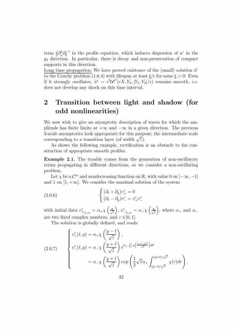
Example 2.1. The trouble comes from the generation of non-oscillatoryterms propagating in different directions, so we consider a non-oscillatingproblem.

Let χ be a C∞ and nondecreasing function on R, with value 0 on ]−∞,−1]and 1 on [1,+∞[. We consider the maximal solution of the system

(2.0.6)

(∂t + ∂y)v

ε+ = 0

(∂t − ∂y)vε− = vε+v

ε−

with initial data vε+|t=0= α+χ

(y√ε

), vε−|t=0

= α−χ(

y√ε

), where α+ and α−

are two fixed complex numbers, and ε ∈]0, 1].The solution is globally defined, and reads:

(2.0.7)

vε+(t, y) = α+χ

(y − t√ε

),

vε−(t, y) = α−χ

(y + t√ε

)eα+

∫ t0χ(

y+t−2t′√ε

)dt′

= α−χ

(y + t√ε

)exp

(1

2

√εα+

∫ (y+t)/√ε

(y−t)/√εχ(r)dr

).

32

The shape of the graph of vε−(t, .) is represented on Figure 3.

mn−t mnt

mnα−eα+t

mny

mnα−eα+t/2+O(

√ε)

Figure 3: The graph of vε−(t, .)

The scale for the variations of vε−(t, .) near t and −t is√ε, so one must

use variables (y − t)/√ε and (y + t)/

√ε (the function vε−(t, .) of the ‘slow’

variable y converges to a non smooth function, discontinuous at −t, and withdiscontinuous derivative at t). In fact, we can try to decompose vε− as a sumof profiles,

(2.0.8) vε−(t, y) = (v−,0 +√εv−,1)

(t, y,

y + t√ε,y − t√ε

).

Roughly speaking, if vε−(t, .) is a function of y near t, v−,0 is non smooth,and if vε−(t, .) depends on Y− = (y − t)/

√ε, it does not look like a ‘step’: at

y = 0, (y − t)/√ε → −∞ as

√ε → 0, but vε−(t, 0) = eα+t/2 6= 0.

More precisely, if we look for vε− under the form (2.0.8) with profilesv−,n(x, Y+, Y−) admitting limits as Y± → +∞ and going to 0 as Y± → −∞,we get (vε+ = v+,0((y − t)/

√ε), v+,0(Y−) = α+χ(Y−)):

(∂t−∂y)vε−(x) =

(−2√ε∂Y−v−,0 + (∂t − ∂y)v−,0 − 2∂Y−v−,1

)(t, y,

y + t√ε,y − t√ε

),

(2.0.9)

v−,0 = v−,0(x, Y+)

2∂Y−v−,1 = (∂t − ∂y)v−,0(x, Y+) − v+,0(Y−)v−,0(x, Y+).

33

Taking the limit (Y− → +∞) of the last equation, we obtain:

(2.0.10) (∂t − ∂y)v−,0 = α+v−,0, so v−,0 = α−χ(Y+)eα+t.

Now, if we want to integrate the derivative ∂Y−v−,1, we must impose, as Y−goes to −∞: (∂t − ∂y)v−,0 = 0. This is in contradiction with (2.0.10). Thesystem (2.0.9) is overdetermined, and the Ansatz (2.0.8) is not valid.

Conclusion: The rapid transition is impossible as soon as the system gen-erates several intermediate phases governing this transition. This is typicallythe case when rectification occurs, because the non-oscillating profiles aresolutions to a hyperbolic system (see Equation (1.2.5b)). As shown in Para-graph 2.3.3, the only admissible intermediate phase is constant along theφ-rays (eikonal equation in Assumption 2.2).

2.1 Framework, notations

We consider the same system as in the first part:

L(x, u, ∂)u = ∂tu+

d∑

j=1

Aj(x, u)∂ju = 0.

We assume again symmetric hyperbolicity (Assumption 1.1) and con-stant multiplicity (Assumption 1.3). Furthermore, nonlinearities will havean ‘oddness’ property:

Assumption 2.1. For all x, the Taylor expansions of the matrices Aj(x, u)at u = 0 contain only even powers. We denote the lowest order term of thisexpansion by Λj(x, .), (Kj − 1)-linear and symmetric (Kj − 1 ≥ 2):

Aj(x, u) − Aj(x, 0) = Λj(x, u, . . . , u) + O(|u|Kj).

Example 2.2. This kind of nonlinearity arises in optics models, such asMaxwell equations coupled with an anharmonic oscillator (see [4]),

∂tE = −curl B − ∂tP,

∂tB = curl E,

∂2t P +

1

T∂tP + ∇PV (P ) = γE,

34

when the potential V has a Taylor expansion at P = 0 containing only evenpowers.

Again, the phase φ is defined as solution to an eikonal equation asssociatedwith L1 (Assumption 1.2).

Now, the nonlinear term which will appear at leading order in the formalcomputations is Λ(x, u1, . . . , uK−1)∂θv:

Notation 2.1. We define K := minj≥1Kj, the smallest order for nonlin-

ear terms, and Λ(x, u1, . . . , uK−1) :=∑

Kj=K

∂jφ(x)Λj(x, u1, . . . , uK−1), modulo

permutations of arguments( i.e. Λ(x, u1, . . . , uK−1) stands for 1

(K−1)!

∑Λ(x, uj1, . . . , ujK−1

)).

Actually, our Ansatz has no mean (non-oscillating) term; its spectrumis odd, so that such non-oscillating terms do not appear through nonlinearinteraction. In addition, we have to modify the amplitude (in comparisonwith the weakly decaying case of Section 1), because of the change in theorder of the nonlinearity. So, our WKB expansion reads

uε ∼ εm∑

n∈mN

εnu2n

(x,ψ(x)√ε,φ(x)

ε

),

where m is linked to the order K of nonlinear terms: m :=1

K − 1, and the

profiles uk = uk(x,X, θ) split into:

uk = χ(Y1)ak(x, X, θ) + bk(x,X, θ).

Notation 2.2. From now on, X = (T, Y ) = (T, Y1, Y ) ∈ R1+p, and (T, Y ) =

X (corresponding to ψ = (ψ0, ψ′) = (ψ0, ψ1, ψ) and ψ = (ψ0, ψ)). Since we

are dealing with Cauchy problems again, we suppose that one of the interme-diate phases is timelike, and more precisely, we suppose it is t: ψ0 ≡ t.

As in [14] and [12], the term bk represents the transition layer. In fact,we first fix the function χ (‘step-function’):

χ ∈ C∞(R,R) with χ′ ∈ S, χ(Z) =

∫ Z

−∞χ′(Z ′)dZ ′,

∫ +∞

−∞χ′(Z ′)dZ ′ = 1.

35

Our goal is to construct

ak ∈ C∞(

RT × Ωt1 ,∩sHs(Rp−1

Y× Tθ)

), bk ∈ C∞ (RT × Ωt1 ,∩sHs(Rp

Y × Tθ)) ,

with odd spectrum (w.r.t. the periodic variable θ). The domain Ω is still thecone x = (t, y) ∈ R1+d/0 ≤ t ≤ t0, δt+ |y| ≤ ρ.

2.2 Function spaces, and the mean operator MDefinition 2.1. We denote by Hs(t1) the space Esp−1(t1)⊕Esp(t1) of functionsv on Ωt1 × Rp × T which split into v = χa + b, where

a ∈ Esx,Y ,θ

(t1) := Esp−1(t1), b ∈ Esx,Y,θ(t1) := Esp(t1).

Equipped with the following norm, Hs(t1) becomes a Banach space:

‖v‖s := ‖a‖Esp−1

+ ‖b‖Esp.

Such a decomposition is unique, since the ‘mean value’ b is given by thefollowing operator, M:

Lemma 2.1. Let u ∈ Hs(t1), s > 0 be given as u = χa + b. Then,

Mu(x, X, θ) := limY1→+∞

u(x,X, θ) exists, and a = Mu, b = u− χMu.

In this way, we define a linear and bounded operator M : Hs(t1) → Esp−1(t1) (⊂Hs(t1)).

We use M to analyse profile equations, with the following calculus:

Lemma 2.2. On Hs(t1), for s > 1/2, we have:

[M, ∂x] = [M, ∂X ] = [M, ∂θ] = 0, and M∂Y1= ∂Y1

M = 0.

2.3 Formal derivation of profile equations

Again, we plug the Ansatz into the equation, and let the (formal) asymptoticsvanish. Because of our choice of amplitude, which is a non-integer power εm

of ε (m = 1/(K − 1), from Notation 2.1), u0 is no longer given by the threelowest powers in the asymptotics, but by coefficients of εm−1, εm−1/2 and εm.

36

We will solve sets of equations corresponding to εn+m−1, εn+m−1/2 and εn+m,with increasing n ∈ mN:

L1(dφ)∂θu0 = 0,(2.3.1)

L1(dφ)∂θu1 + L1(dψ)∂Xu0 = 0,(2.3.2)

L1(dφ)∂θu2 + L1(dψ)∂Xu1 + L1(∂x)u0 + Λ(uK−10 )∂θu0 = 0,(2.3.3)

(2.3.4)

...

L1(dφ)∂θun+2 + L1(dψ)∂Xun+1 + L1(∂x)un + Λ(uK−10 )∂θun

+ Λ(uK−20 , un)∂θu0 + Fn(x, uk, ∂xuk, ∂Xuk, ∂θuk, k < n) = 0.

(2.3.5)

Notations are the same as in Section 1, and we set uk := 0 for k < 0.

2.3.1 Using the mean operator MEach equation (E) is equivalent to M(E) and (E) − χM(E), and this sep-arates (partially) an and bn:

L1(dφ)∂θa0 = 0

L1(dφ)∂θb0 = 0,

L1(dφ)∂θa1 + L1(dψ)∂Xa0 = 0

L1(dφ)∂θb1 + L1(dψ)∂Xb0 + χ′L1(dψ1)a0 = 0,

L1(dφ)∂θa2 + L1(dψ)∂Xa1 + L1(∂x)a0 + Λ(aK−10 )∂θa0 = 0

L1(dφ)∂θb2 + L1(dψ)∂Xb1

+ χ′L1(dψ1)a1 + L1(∂x)b0

+ Λ((χa0 + b0)

K−1)∂θ(χa0 + b0) − χΛ(aK−1

0 )∂θa0 = 0,

37

...

L1(dφ)∂θan+2 + L1(dψ)∂Xan+1 + L1(∂x)an + Λ(aK−10 )∂θan

+ Λ(aK−20 , an)∂θa0 + Fn(x, ak, ∂Xak, ∂θak, k < n) = 0

L1(dφ)∂θbn+2 + L1(dψ)∂Xbn+1 + χ′L1(dψ1)an+1 + L1(∂x)bn

+ Λ((χa0 + b0)

K−1)∂θ(χan + bn) − χΛ(aK−1

0 )∂θan

+ Λ((χa0 + b0)

K−2, (χan + bn))∂θu0 − χΛ(aK−2

0 , an)∂θa0

+ Fn[χak + bk, k < n] − χFn[ak, k < n] = 0.

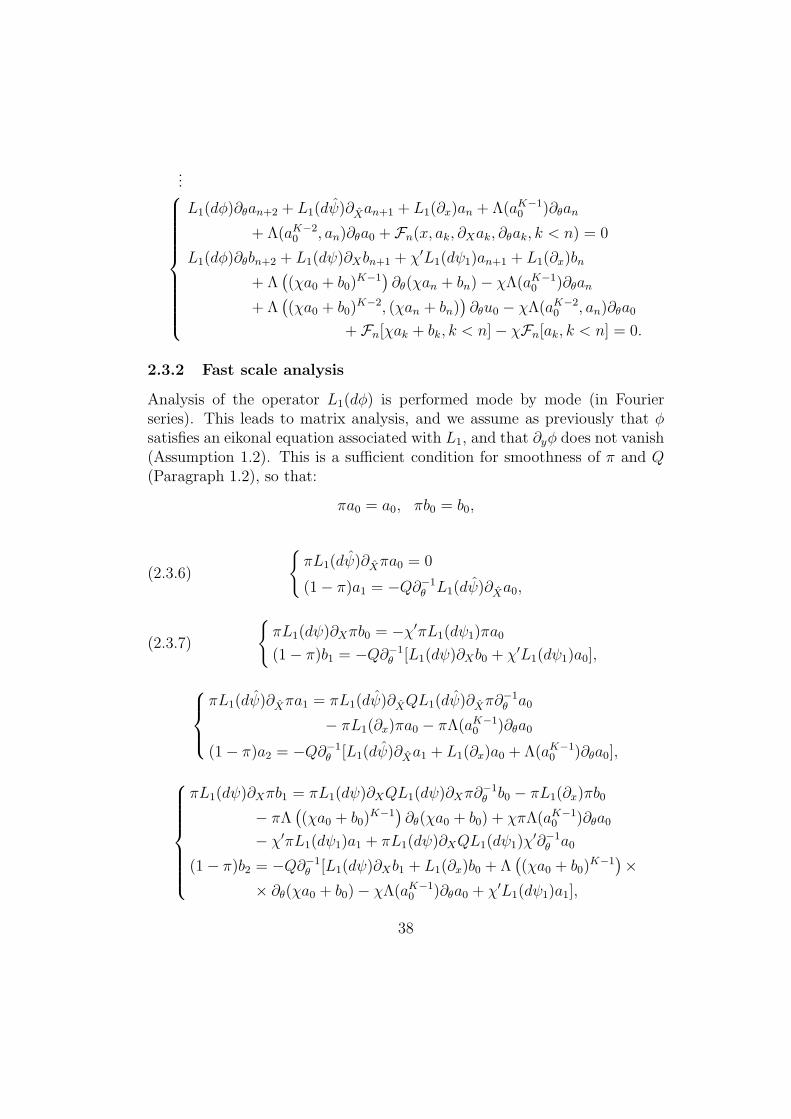
2.3.2 Fast scale analysis

Analysis of the operator L1(dφ) is performed mode by mode (in Fourierseries). This leads to matrix analysis, and we assume as previously that φsatisfies an eikonal equation associated with L1, and that ∂yφ does not vanish(Assumption 1.2). This is a sufficient condition for smoothness of π and Q(Paragraph 1.2), so that:

πa0 = a0, πb0 = b0,

(2.3.6)

πL1(dψ)∂Xπa0 = 0

(1 − π)a1 = −Q∂−1θ L1(dψ)∂Xa0,

(2.3.7)

πL1(dψ)∂Xπb0 = −χ′πL1(dψ1)πa0

(1 − π)b1 = −Q∂−1θ [L1(dψ)∂Xb0 + χ′L1(dψ1)a0],

πL1(dψ)∂Xπa1 = πL1(dψ)∂XQL1(dψ)∂Xπ∂−1θ a0

− πL1(∂x)πa0 − πΛ(aK−10 )∂θa0

(1 − π)a2 = −Q∂−1θ [L1(dψ)∂Xa1 + L1(∂x)a0 + Λ(aK−1

0 )∂θa0],

πL1(dψ)∂Xπb1 = πL1(dψ)∂XQL1(dψ)∂Xπ∂−1θ b0 − πL1(∂x)πb0

− πΛ((χa0 + b0)

K−1)∂θ(χa0 + b0) + χπΛ(aK−1

0 )∂θa0

− χ′πL1(dψ1)a1 + πL1(dψ)∂XQL1(dψ1)χ′∂−1θ a0

(1 − π)b2 = −Q∂−1θ [L1(dψ)∂Xb1 + L1(∂x)b0 + Λ

((χa0 + b0)

K−1)×

× ∂θ(χa0 + b0) − χΛ(aK−10 )∂θa0 + χ′L1(dψ1)a1],

38

...

πL1(dψ)∂Xπan+1 =πL1(dψ)∂XQL1(dψ)∂Xπ∂−1θ an − πL1(∂x)πan

− πΛ(aK−10 )∂θan − πΛ(aK−2

0 , an)∂θa0

− πFn(x, ak, ∂Xak, ∂θak, k < n)

(1 − π)an+2 = −Q∂−1θ [L1(dψ)∂Xan+1 + L1(∂x)an + Λ(aK−1

0 )∂θan

+ Λ(aK−20 , an)∂θa0 + Fn(x, ak, ∂Xak, ∂θak, k < n)],

πL1(dψ)∂Xπbn+1 = πL1(dψ)∂XQL1(dψ)∂Xπ∂−1θ bn − L1(∂x)bn

− πΛ((χa0 + b0)

K−1)∂θ(χan + bn) + χπΛ(aK−1

0 )∂θan

− πΛ((χa0 + b0)

K−2, (χan + bn))∂θu0 + χπΛ(aK−2

0 , an)∂θa0

− πFn[χak + bk, k < n] + χπFn[ak, k < n] − χ′πL1(dψ1)an+1

(1 − π)bn+2 = −Q∂−1θ

(L1(dψ)∂Xbn+1 + χ′L1(dψ1)an+1 + L1(∂x)bn

+ Λ((χa0 + b0)

K−1)∂θ(χan + bn) − χΛ(aK−1

0 )∂θan

+ Λ((χa0 + b0)

K−2, (χan + bn))∂θu0 − χΛ(aK−2

0 , an)∂θa0

+ Fn[χak + bk, k < n] − χFn[ak, k < n]

).

(Arguments between brackets indicate that Fn is a functional).

Remark 2.1. Remark that no bn appears in the equations determining thean’s: Behavior ‘at infinity’ does not depend on the transition layer.

2.3.3 Analysis w.r.t. the (remaining) intermediate variables

Of course, we take advantage of the reductions to the scalar form in Proposi-tion 1.2, which let the vector fields V (dψ)∂X and V (dψ)∂X appear. So as toavoid the creation of ‘steps’ in the bn’s (see (2.3.7i), for example), we assumethat ψ1 is constant along the φ-rays:

Assumption 2.2. On Ω, V (dψ1) ≡ 0.

This simplifies the equations: only one transport operator persists, V (dψ)∂X .As a consequence, we have to deal with only one linear problem, namely:

V (dψ)∂Xu = f

u|T=0= g,

39

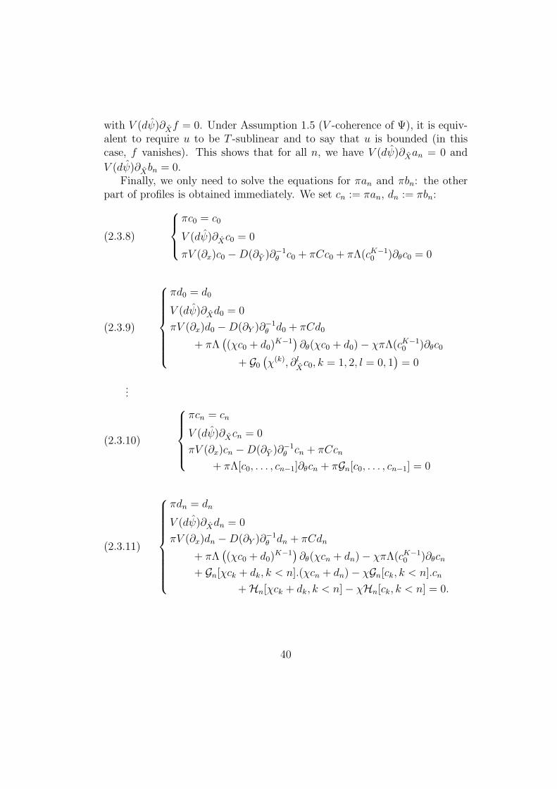
with V (dψ)∂Xf = 0. Under Assumption 1.5 (V -coherence of Ψ), it is equiv-alent to require u to be T -sublinear and to say that u is bounded (in thiscase, f vanishes). This shows that for all n, we have V (dψ)∂Xan = 0 and

V (dψ)∂Xbn = 0.Finally, we only need to solve the equations for πan and πbn: the other

part of profiles is obtained immediately. We set cn := πan, dn := πbn:

(2.3.8)

πc0 = c0

V (dψ)∂Xc0 = 0

πV (∂x)c0 −D(∂Y )∂−1θ c0 + πCc0 + πΛ(cK−1

0 )∂θc0 = 0

(2.3.9)

πd0 = d0

V (dψ)∂Xd0 = 0

πV (∂x)d0 −D(∂Y )∂−1θ d0 + πCd0

+ πΛ((χc0 + d0)

K−1)∂θ(χc0 + d0) − χπΛ(cK−1

0 )∂θc0

+ G0

(χ(k), ∂l

Xc0, k = 1, 2, l = 0, 1

)= 0

...

(2.3.10)

πcn = cn

V (dψ)∂Xcn = 0

πV (∂x)cn −D(∂Y )∂−1θ cn + πCcn

+ πΛ[c0, . . . , cn−1]∂θcn + πGn[c0, . . . , cn−1] = 0

(2.3.11)

πdn = dn

V (dψ)∂Xdn = 0

πV (∂x)dn −D(∂Y )∂−1θ dn + πCdn

+ πΛ((χc0 + d0)

K−1)∂θ(χcn + dn) − χπΛ(cK−1

0 )∂θcn

+ Gn[χck + dk, k < n].(χcn + dn) − χGn[ck, k < n].cn

+ Hn[χck + dk, k < n] − χHn[ck, k < n] = 0.

40

2.4 Existence of profiles and approximation of exactsolutions

2.4.1 Solving the profile equations

We look for (cn, dn) ∈ C(RT ,Hs(t1)). The only nonlinear equations are (2.3.8)and (2.3.9). In the case of (2.3.10)n, (2.3.11)n (n ∈ mN\0), there are right-hand sides, functions of the preceding profiles. For (2.3.9) and (2.3.11)n,nonlinearities and right-hand sides are of the form:

Lemma 2.3. Let H : Ω × CN → CN be smooth, and H(., 0) ≡ 0.If c ∈ Esp−1(t1) and d ∈ Esp(t1) for s > 2d+p+1

4, then

H(χc+ d) − χH(c) ∈ Esp(t1),

‖H(χc+ d) − χH(c)‖Esp≤ C

(‖c‖Es

p−1, ‖d‖Es

p

)(‖d‖Es

p−1+ 1).

Proof : First, decompose

H(χc+ d) − χH(c) = [H(χc+ d) −H(χc)] + [H(χc) − χH(c)].

The first term is equal to

∫ 1

0

∂vH(χc+ νd).d dν, and by differentiation,

∂γy,Y,θ

(∫ 1

0

∂vH(χc+ νd).d dν

)=

∑

α1+···+αk≤γ

∫ 1

0

∂αk+1

y,v H(χc+ νd).(∂α

1

d, ∂α2

(χc+ d), . . . , ∂αk

(χc + d))dν.

We then come back to the usual technique of the proof of Moser’s theorem,using Holder’s and Gagliardo-Nirenberg’s inequalities (in Esp). Indeed, χc ∈L∞(RY1

, Esp−1(t1)), and χ′c ∈ S(RY1, Esp−1(t1)).

For the second term, first notice that for all Y1, H(χc) and χH(c) areelements of Esp−1. So, we consider their difference as a Esp−1- valued functionof Y1. Taylor expanding shows:

H(χc) − χH(c) = χ

∫ 1

0

[∂vH(νχc) − ∂vH(νc)] .c dν

= χ(1 − χ)

∫ 1

0

ν

[∫ 1

0

∂2vH(νc+ µν(χ− 1)c).c dµ

].c dν.

41

We can apply Moser’s theorem in Esp−1 inside the integral, with χ(Y1) bounded.Finally, the χ(1 − χ) factor implies that H(χc) − χH(c) belongs to Esp .

The classical iterative schemes in Esp give existence and uniqueness of c0and d0, and the linear profile equations are then solved successively.

Proposition 2.1. Let gn ∈ ∩sHs(0) be polarized: ∀n ∈ mN, πgn = gn.Then, under the preceding assumptions (coherence, and ψ1 constant along

the φ-rays: Assumptions 1.1, 1.2, 1.3, 1.5, 2.1, 2.2), there exist t? > 0 and aunique maximal solution v0 = χc0 + d0 ∈ C(RT ,∩sHs(t)), t < t?, to (2.3.8),(2.3.9) with initial data g0. In addition, for all n > 0, there exists a uniquevn = χcn + dn ∈ C(RT ,∩sHs(t)), t < t?, solution to (2.3.10)n, (2.3.11)n withinitial data gn.

2.4.2 Stability

Once we have obtained profiles, Borel’s theorem exhibits an approximatesolution uεapp(x): ∀M ∈ mN, ∀α ∈ N1+d,

∥∥∥∥∥(ε∂)α

[uεapp(x) − εm

∑

n<M

εnu2n

(x,ψ(x)√ε,φ(x)

ε

)]∥∥∥∥∥L∞

= O(εm+M).

This is an asymptotic solution to the system, and exact solutions with initialdata close to uεapp|t=0

stay close to uεapp:

Theorem 2.1. For all t < t? ,i) L(uεapp, ∂)u

εapp ∼ 0 in C∞(Ωt).

ii) If f ε ∼ 0 in C∞(Ω) and v0,ε(y) ∼∑

n∈mNεnu2n|t=0

(y, ψ

0

√ε, φ

0

ε

), ε ∈]0, 1],

there exists εt such that the solution to the Cauchy problem

(2.4.1)

L(vε, ∂)vε = f ε

vε|t=0(y) = εmv0,ε(y)

exists on Ωt, for ε ≤ εt. In addition, vε − uεapp ∼ 0 in C∞(Ωt).

Proof :We seek vε as a perturbation, vε = uεapp + wε. First, rescale amplitudes

to 1: set vε = εmV ε, uεapp = εmUε, . . . Now, vε is solution to (2.4.1) if and

42

only if W ε satisfies

(2.4.2)

L (εm(Uε +W ε), ∂) (Uε +W ε) = F ε ∼ 0

W ε|t=0

(y) = Gε ∼ 0.

We adopt the same strategy as in [13], and introduce the following spaces:

Definition 2.2. We define Hsε (ω) (resp. Cs

ε (ω)) as the set of (families of)functions uε on ω such that

∀α ∈ Nd, ε > 0, ‖(ε∂y)αuε‖L2 ≤ Cα(resp. ‖(ε∂y)αuε‖L∞ ≤ Cα).

It is evident that Uε belongs to H∞ε = C∞

ε . These ε-derivatives will allowus to show existence of W ε in Hs

ε . The following properties deduce from theclassical ones (ε = 1) by change of scales:

Proposition 2.2. Let H be smooth on RN × RN and such that H(., 0) ≡ 0,and s > d/2. For all U ε ∈ Cs

ε(Ω), V ε ∈ Hsε (Ω),

‖V ε‖L∞ ≤ Csε−d/2‖V ε‖Hs

ε,

‖H (Uε, V ε) ‖Hsε≤ Cs

(‖Uε‖Cs

ε, ‖V ε‖L∞

)‖V ε‖Hs

ε.

When ε is fixed, in a classical way, we have existence of a smooth solutionW ε to the quasilinear hyperbolic system (2.4.2) on [0, Tε], with

‖W ε(t)‖2Hs

ε≤ Cs

[‖Gε‖2

Hsε

+ C (‖W ε, ∂W ε‖L∞)

∫ t

0

‖W ε(t′)‖2Hs

εdt′

+

∫ t

0

‖F ε(t′)‖2Hs

εdt′].

Gronwall’s lemma then implies:

‖W ε(t)‖2Hs

ε≤ Cs

[eCt(‖Gε‖2

Hsε+

∫ t

0

‖F ε(t′)‖2Hs

εdt′)

+

∫ t

0

eC(t−t′)

(‖Gε‖2

Hsε+

∫ t′

0

‖F ε(t′′)‖2Hs

εdt′′

)dt′

].

Hence, if Tε ≤ t is a time until which ‖W ε‖L∞ , ‖∂W ε‖L∞ ≤ R for a givenR > ‖Gε‖, then, for t ≤ Tε and M ∈ N:

‖W ε(t)‖2Hs

ε≤ CM,sε

M(1 + C(R)teCt

),

43

and by Sobolev’s embedding,

‖W ε‖L∞ , ‖∂W ε‖L∞ ≤ C(M, s,R)ε(M−d)/2.

When M > d is fixed, for ε ≤ εR, this quantity is lower than R. This provesexistence of W ε up to t.

Since M is as big as desired, we have the asymptotics W ε ∼ 0.

Remark 2.2. In the simplest case, with only one phase ψ (X = Y ∈ R, seeRemark 1.4iii)), Equations (2.3.8)-(2.3.11) become, for the first profile:

πc0 = c0(x, θ)

V (∂x)c0 + πCc0 + πΛ(cK−10 )∂θc0 = 0

πd0 = d0(x, Y, θ)

V (∂x)d0 −D(x)∂2Y ∂

−1θ d0 + πCd0

+ πΛ((χc0 + d0)

K−1)∂θ(χc0 + d0) − χπΛ(cK−1

0 )∂θc0

+ G0 (χ′, χ′′, c0, k = 1, 2) = 0

The profile c0 = a0 is exactly the one from (2 scales-)geometric optics onΩ, and the term b0 can be seen as a corrector of the profile χ(Y )a0(x, θ): Ifwe test the solution vε of (2.4.1) against ϕ ∈ C(Ω × T), we get:

ε−m∫

Ω

vε(x)ϕ

(x,φ

ε

)dx−→

ε→0

∫

ψ>0×T

a0(x, θ)ϕ(x, θ)dxdθ.

The ‘main part’ of vε is effectively given by geometric optics on ψ > 0.

3 Wave transitions for systems of conserva-

tion laws

In this section, we give an alternative method for the treatment of sys-tems which do not satisfy the Oddness Hypothesis 2.1. In fact, we re-strict to conservative systems. In that case, the mean value u0 of thefirst profile vanishes, and we can define an approximate solution uεapp(x) =

44

ε(u0 +√εu1 + εu2)(x, ψ/

√ε, φ/ε) whose profiles have mean zero. The singu-

lar system technique of Paragraph 1.5.2 must be modified. If one wants tosolve Equation (1.5.9),

(3.0.3) L

(x, εVε, ∂x +

1√ε∂xψ∂Y +

1

ε∂xφ∂θ

)Vε = f ε (x, Y, θ) ,

for profiles Vε = χaε + bε ∈ Hs(t), projecting via M decouples the equationinto

L (εaε, ∂x) aε + T (ε, aε, ∂yφ∂θ) a

ε

+1

εL1 (x, ∂xφ∂θ) a

ε = Mf ε(x, θ)(3.0.4)

and

L (εVε, ∂x)Vε − χL (εaε, ∂x) aε

+ T(ε,Vε,

√ε∂yψ∂Y + ∂yφ∂θ

)Vε − χT (ε, aε, ∂yφ∂θ) a

ε

+1

εL1

(x,√ε∂xψ.∂Y + ∂xφ∂θ

)bε

= f ε(x, Y, θ) − χMf ε(x, θ) − 1√εχ′L1(∂xψ)aε.

(3.0.5)

Once Equation (3.0.4) is solved for aε, even if the singular term in Equa-

tion (3.0.5),1

εL1

(x,√ε∂xψ.∂Y + ∂xφ∂θ

)bε, can be treated in the same way

as in Paragraph 1.5.2 (by coherence), the forcing term1√εχ′L1(∂xψ)aε re-

mains, and leads to blow-up of bε as ε goes to zero.Our strategy consists in performing a change of (dependent) variables

(see Lemma 1.8) that leads to a decomposition of Equation (3.0.3) differentfrom Equations (3.0.4)-(3.0.5), which reveals that the singular forcing termsvanish (under some additional assumption on the phases, Assumption 3.4;Paragraph 3.3.3 gives an example from nonlinear acoustics for which it issatisfied).

45

3.1 The system and the Ansatz

Our system will now take the form of conservation laws:

(3.1.1) M(v, ∂) = ∂tv +

d∑

j=1

∂jFj(v) = 0,

with given smooth functions Fj : R2N ' CN → CN . The system (3.1.1) isassumed symmetrizable (with constant multiplicity):

Assumption 3.1. There exists a positive definite matrix S(v), smooth func-tion of v on a neighbourhood of zero in CN , such that, for all j, the ma-trix S(v)∂vFj(v) is symmetric, and the eigenvalues λ1(η) < · · · < λZ(η)

of A(η) :=∑d

j=1 ηjS(0)1/2∂vFj(0)S(0)−1/2 have constant multiplicity (on

Rd \ 0).

So as to depart from the Oddness Hypothesis 2.1, and in view of theexample at Paragraph 3.3.3, we fixThe order of nonlinearities: We assume ∂2

vFj(0) 6= 0 for some j.(But in fact, the following is valid for any order of nonlinearity, as well as forflux functions Fj depending explicitly on x).

The approximate solution we seek takes the form:

vεapp(x) = ε(v0 +

√εv1 + εv2

)(x,

ψ√ε,φ

ε

)

with profiles vn ∈ Hs(t1) = Es0(t1) ⊕ Es1(t1) (see Definition 2.1) and inde-pendent of T (we still denote by Hs(t1) this subspace of Hs(t1)). Just likebefore, we consider the case of only one fast phase φ, and now take only oneintermediate phase ψ too, but the same methods apply to the multi-ψ case,as in the previous section.

3.2 The approximate solution

The (formal) profile equations are obtained as in Paragraph 2.3, by a Taylorexpansion. So as to recover the same notations as before (and a coefficientId for ∂t), we change variables, setting v = S(0)−1/2u, and then multiply (onthe left) all equations (M(v, ∂)) by S(0)1/2.

46

Notation 3.1. In agreement with the previous notations, set L1(∂) := ∂t +∑dj=1Aj(0)∂j, where Aj(v) := S(0)1/2∂vFj(v)S(0)−1/2: Aj(0) is symmetric.

Set Λ(u) := S(0)1/2∑d

j=1 ∂jφ(x)(∂2vFj(0).S(0)−1/2u)S(0)−1/2u.

As in Section 2, the phases φ and ψ have to satisfy eikonal equations (seethe conclusion of Example 2.1):

Assumption 3.2. The phase φ is solution to an eikonal equation associatedwith L1 (Assumption 1.2), and ψ is solution to the eikonal equation associatedwith V (see Assumption 2.2).

Thus, for un(x, Y, θ) = χ(Y )an(x, θ)+bn(x, Y, θ), the profile equations are(with notations of Proposition 1.2):

(3.2.1)

πa0 = a0

V (∂x)a0 + πCa0 + πΛ(a0)∂θa0 = 0

(3.2.2)

πb0 =b0

V (∂x)b0 + πCb0 −D(∂Y )∂−1θ b0 + πΛ (χa0 + b0) ∂θ(χa0 + b0)

− χπΛ(a0)∂θa0 − π [D(∂Y )χ] ∂−1θ a0 = 0

(1 − π)a1 = 0(3.2.3)

(1 − π)b1 = −Q∂−1θ L1(dψ) [∂Y b0 + χ′a0](3.2.4)

(1 − π)a2 = −Q∂−1θ [L1(∂x)a0 + Λ (a0) ∂θa0](3.2.5)

(1 − π)b2 = −Q∂−1θ [L1(dψ)∂Y b1 + L1(∂x)b0

+Λ (χa0 + b0) ∂θ(χa0 + b0) − χΛ(a0)∂θa0](3.2.6)

These equations are solved in Paragraph 2.4 (Proposition 2.1), with maximalexistence time t?. Define the approximate solution vεapp (for t < t?) by

vεapp(x) := εVεapp(x,ψ(x)√ε,φ(x)

ε

),

Vεapp(x, Y, θ) := S(0)−1/2(u0 +√εu1 + εu2)(x, Y, θ) ∈ ∩sHs(t).

47

Proposition 3.1. Define the residual kε(x) := M(vεapp, ∂x), which is theevaluation at (x, Y, θ) = (x, ψ/

√ε, φ/ε) of

(3.2.7) Kε(x, Y, θ) :=1

εM(εVεapp, ε∂x +

√ε∂ψ∂Y + ∂φ∂θ).

Then, for all t < t?:

∀s, ‖Kε‖Hs(t) = O(ε3/2), and

∀α ∈ N1+d, ‖(ε∂x)αkε‖L∞(Ωt) = O(ε3/2).

Proof :Proceed as for Proposition 1.8, but now, profiles do not depend on T .

3.3 Stability

Notation 3.2. From now on, L(v, ∂)v =∑d

j=0Aj(v)∂jv simply denotesS(v)M(v, ∂) (the coefficient of ∂t no more needs to be Id).

Our approximate solution vεapp is based upon three profiles, so we provea stability theorem of the kind of Theorem 1.2, using a singular system. Weknow we have to make some coherence assumption:

Assumption 3.3. The real vector space generated by t, ψ and φ is L1-coherent. The functions φ and ψ are linearly independent.

(The second part is an addition to Assumption 1.6; see Lemma 3.1).Another assumption is necessary so as to deal with the singular terms (As-sumption 3.4). We shall explain it in the sequel. Our aim is to prove thefollowing:

Theorem 3.1. Under Assumptions 3.1, 3.2, 3.3 and 3.4 (see Section 3.3.2below), consider f ε and gε such that for all s, ‖f ε‖Hs(t?) −→

ε→00, ‖gε‖Hs(0) −→

ε→00,

and in addition, ‖M〈f ε〉‖Hs(t?) = o(√ε), ‖M〈gε〉‖Hs(0) = o(

√ε). Then,

there exist ε0 > 0 and t > 0 such that the Cauchy problem

(3.3.1)

M(vε, ∂) = εf ε(x, ψ/

√ε, φ/ε)

vε|t=0= vεapp|t=0

+ εgε(y, ψ(0, y)/√ε, φ(0, y)/ε)

48

admits a unique solution vε ∈ C1(Ωt) for all ε ≤ ε0.In addition, there is Vε ∈ ∩sHs(t) such that vε has the form

vε(x) = εVε(x,

ψ√ε,φ

ε

),

and ∀s, ‖Vεapp − Vε‖Hs(t) −→ε→0

0.(3.3.2)

We try to mimic the proof of Paragraph 1.5.2, so we seek Vε ∈ Hs (andindependent of T ) satisfying

L (εVε, ∂x)Vε + T ε(Vε,

√ε∂yψ∂Y + ∂yφ∂θ

)Vε

+1

εL1

(x,√ε∂xψ∂Y + ∂xφ∂θ

)Vε = S(εVε)f ε(x, Y, θ),

with T ε (V, η) =

d∑

j=0

ηj(

∫ 1

0

∂uAj(τεV)dτ).V.

The key point is the conjugation of1

εL1

(x,√ε∂xψ∂Y + ∂xφ∂θ

)to a con-

stant coefficient (singular) operator.

3.3.1 The conjugation operator Vε

From Lemma 1.8, there is a bounded family (Vρ,α) of unitary matrix valuedsmooth functions on Ω, homogeneous in (ρ, α) (degree zero), such that

V (x, ρ, α)L1(x, ∂x(ρψ + αφ)(x))V ?(x, ρ, α) = ∆(ρ, α).

The corresponding Fourier multipliers V (√εDY , Dθ) (C∞ parametrized by

x ∈ Ω) map SY,θ into itself. This section is devoted to the proof of thefollowing proposition:

Proposition 3.2. Under Assumptions 3.1, 3.2, 3.3, for every t1, the Fouriermultipliers V (

√εDY , Dθ) above define a bounded family (Vε)ε of unitary op-

erators on Hs(t1) for all s ≥ 0. Separating oscillations and mean value forχc+ d ∈ Hs(t1) (c = c0(x) + c?(x, θ) and d = d0(x, Y ) + d?(x, Y, θ)),

VεL1

(x,√ε∂xψDY + ∂xφDθ

)Vε

?(χc+ d) =

χ∆(0, Dθ)c?

+√ε∆(DY , 0)

(χc0 + d0

)

+ ∆(√εDY , Dθ)d

? − i√εχ′∂ρ∆(0, 1)c? + rε(c

?),

(3.3.3)

49

where ∆(ρ, α) is the (diagonal) matrix of eigenvalues of L1(ρdψ + αdφ),independent of x, and rε is a (linear) continuous operator from Es0(t1) to

Es−1/21 (t1), with norm O(ε).

First, this action is mode by mode on formal series (in θ):

Vε

∑uα(x, Y )eiαθ =

∑Vε

αuα(x, Y )eiαθ :

we now deal with functions in Hs(t1) = Es0(t1) ⊕ Es1(t1) (cst w.r.t. θ).• When α = 0, because of homogeneity,

V0ε = V (1, 0) (the matrix V (ρ, α) for α = 0, ρ = 1).

• The definition of Vαε (α 6= 0) as operator on Es1(t1) is the same as in 1.5.2:

it is a Fourier multiplier (in√εDY ), as well as [∂x,V

αε ] = ∂xV (x,

√εDY , α).

• The trouble comes from the action on the ‘step part’ χaα of uα. Toidentify ‘step’ and decaying parts of V

αεχa

α, first perform the commutation:

Vαεχa

α = χVαε a

α + [Vαε , χ]aα.

From now on, we will consider V (DY , α) and χ(Y ) as pseudo-differentialoperators, computing the commutator [Vα

ε , χ] by means of symbol calculus.But first, if we want V (DY , α) (α 6= 0) to act on the constant (w.r.t. Y ) aα,using the formula

V (DY , α)aα =1

2π

∫eiρY V (ρ, α)aα(ρ)dρ, with aα = 2πδ0,

V (ρ, α) must be continuous at ρ = 0. This was the aim of the independenceassumption (Assumption 3.3):

Lemma 3.1. Under Assumptions 3.1, 3.2, 3.3, the family (V α)α∈Z? is bounded

in C∞(Ω×R), and for all γ ∈ N1+d, δ ∈ N, there is a constant C independentof α ∈ Z? such that:

(3.3.4)∥∥∂γx∂δρV (., α, ρ)

∥∥L∞ ≤ C < ρ >−δ .

Proof :Because of the constant multiplicity assumption 3.1, V α is smooth on

the open subset O of Ω × Rρ where ∂y(αφ + ρψ)(x) does not vanish (seeLemma 1.8 and (1.5.12)). Now, if this derivative vanishes at a point x,

50

since φ and ψ satisfy eikonal equations (respectively associated with L1 andV (∂x)), ∂t(αφ + ρψ)(x) also vanishes. Coherence of Vect(φ, ψ) then impliesthat αφ = ρψ, contradicting the independence from Assumption 3.3. Thus,O = Ω × Rρ.

Boundedness of the family (V α)α∈Z? and of the constant Cα,ρ in (3.3.4)follows from this smoothness property and from degree zero homogeneity ofV (ρ, α).

Hence, the symbols V α(ρ) and χ(Y ) define (smooth functions of x, withvalues) semi-classical operators (V α(

√εDY ) and χ(Y )) on S ′

Y . So as totake into account the decay in Y , we could consider them as symbols S0,0

∞,1

and S0,0∞,∞, respectively, where p(Y, ρ) ∈ Sm,µr,δ if |∂aY ∂βρ p(Y, ρ)| ≤ Ca,β <

Y >m−r|a|< ρ >µ−δ|β|. Uniformity in α is immediate, and the role playedby

√ε in the asymptotic calculus is well-known (see for instance [25]). But

here, we are only interested in the action on constant functions (w.r.t. Y )aα(x) ∈ Es0(t1), so we prove the following lemma ‘by hand’:

Lemma 3.2. For α ∈ Z? and s ≥ 0, the family of operators V (√εDY , α)χ(Y ),

ε ∈]0, 1], maps Es0(t1) to Hs(t1). Precisely, for all a(x) ∈ Es0(t1),

V (√εDY , α)χ(Y )a = χV (0, 1)a+ [V α(

√εDY ), χ]a,

=χ(Y )V (0, 1)a(x) − i√εχ′(Y )∂ρV (0, α)a(x) + rαε (a),

and rαε maps Es0(t1) to Es1(t1), with norm O(ε) (uniformly in α).

Proof :The operators V (

√εDY , α) and (multiplication by) χ(Y ) are associated

with the symbols V αε (ρ) := V α(

√ερ) and χ(Y ), respectively, through the

formula

Op(σ)(Y,DY )u =1

2π

∫∫ei(Y−Z)ρσ(Y, ρ)u(Z)dZdρ.

The resulting composed operator V (√εDY , α)χ(Y ) then admits a symbol

σε, given byσε(Y, ρ) = J (V α

ε χ) , where J = eiDY Dρ .

Thus, the Taylor expansion J = 1 + iDYDρ −(∫ 1

0(1 − r)Jrdr

)(DYDρ)

2

provides the asymptotic expansion (where Jr = eirDY Dρ):

σε(Y, ρ) = χ(Y )V αε (ρ) − iχ′∂ρV

αε (ρ) −

∫ 1

0

(1 − r)Jr(χ′′∂2

ρVαε

)dr.

51

Then, the derivatives in ρ provide the expected factor ε, since ∂2ρV

αε (ρ) =

ε(∂2ρV

α)(√ερ), denoted as before: ε

(∂2ρV

α)ε(ρ).

Finally, recall that the action of Jr(χ′′ (∂2

ρVα)ε

)on Es0 is through multi-

plication by(Jr(χ′′ (∂2

ρVα)ε

))(Y, 0); the following lemma ends the proof:

Lemma 3.3. The family(Jr(χ′′ (∂2

ρVα)ε

))r,α,ε

(Y, 0), r ∈ [0, 1], α ∈ Z?,

ε ∈]0, 1], is bounded in C∞(Ω,S(RY )).

Proof :

The action of Jr is convolution (in Y, ρ) by F−1(eirY ρ

)= (4π2|r|)−1eir

−1Y ρ.

Hence, Jr(χ′′ (∂2

ρVα)ε

)(x, Y, ρ) is smooth. We prove estimates uniform

w.r.t. x. The same are valid for derivatives, simply replacing V by ∂γxV ,which has the same regularity, and homogeneity in ρ: ∀k ∈ 2N,

Jrχ′′ (∂2ρV

α)ε(Y, 0) =

1

4π2|r|

∫∫χ′′(Y + Z)

(∂2ρV

α)ε(ζ)e−ir

−1ZζdZdζ

=1

4π2|r|

∫∫χ′′(Y + Z)

(∂2ρV

α)ε(ζ) < r−1Z >−k< Dζ >

k e−ir−1ZζdZdζ

=1

4π2|r|

∫∫< r−1Z >−k χ′′(Y + Z) < Dρ >

k(∂2ρV

α)ε(ζ)e−ir

−1ZζdZdζ,

after integration by parts.Now, according to Peetre’s inequality,

|χ′′(Y + Z)| ≤ Cl < Y + Z >−l≤ Cl < Y >−l< Z >l .

Taking k = l + 2 ensures, for all l ∈ 2N (r ∈]0, 1]):

(3.3.5) | < r−1Z >−k χ′′(Y + Z)| ≤ C < r−1Z >−2< Y >−l .

The second term, < Dρ >k(∂2ρV

α)ε(ζ), is bounded thanks to homogeneity:

(3.3.6) | < Dρ >k(∂2ρV

α)ε(ζ)| ≤ Ckε

k/2 <√εζ >−2−k≤ Ck < ζ >−k .

Finally, thanks to (3.3.5) and (3.3.5), performing the change of variable

r−1Z = Z ′, the quantity∣∣∣Jrχ′′ (∂2

ρVα)ε(Y, 0)

∣∣∣ is estimated, for all l ∈ 2N,

by:

Cl < Y >−l∫∫

< ζ >−l−2< Z ′ >−2 dZ ′dζ = C ′l < Y >−l .

52

We can summarize the definition of Vε as: for χa+ b ∈ Hs(t1),

Vε(χa + b) =χ(V (1, 0)a0 + V (0, 1)a?

)

+ V (1, 0)b0 + V (√εDY , Dθ)b

? + [V (√εDY , Dθ), χ]a?,

Vε?(χc+ d) =χ

(V (1, 0)?c0 + V (0, 1)?c?

)

+ V (1, 0)?d0 + V ?(√εDY , Dθ)

(d? − [V (

√εDY , Dθ), χ]V (0, 1)?c?

)

=χ(V (1, 0)?c0 + V (0, 1)?c?

)

+ V (1, 0)?d0 + V ?(√εDY , Dθ)d

?

+ i√εχ′V ?(0, 1)∂ρV (0, Dθ)V

?(0, 1)c? + rε(c?).

The proof of (3.3.3) is then straightforward:

L1

(x,√ε∂xψDY + ∂xφDθ

)Vε

?(χc + d) =

χL1(∂xφDθ)V (0, 1)?c?

+√εL1(∂xψDY )V (0, 1)?

(χc0 + d0

)

+ L1(∂xψDY )χV (0, 1)?c? + L1

(√ε∂xψDY + ∂xφDθ

)V ?(

√εDY , Dθ)d

?

+ i√εL1(∂xφDθ)V (0, 1)?∂ρV (0, Dθ)V (0, 1)?c?

+ εRε(c?),

where the residual Rε writes

−χ′′L1(∂xψ)V (0, 1)?∂ρV (0, Dθ)V (0, 1)?c? + L1

(√ε∂xψDY + ∂xφDθ

) rε(c?)ε

,

which is O(1) in Es−1/21 , because of the derivatives in L1 (

√ε∂xψDY + ∂xφDθ).

Applying Vε gives:

χ∆(0, Dθ)c? +

√ε∆(DY , 0)

(χc0 + d0

)+ ∆(

√εDY , Dθ)d

?

+√εV (

√εDY , Dθ) [L1(∂xψDY )χV (0, 1)?c?

+iχ′L1(∂xφDθ)V (0, 1)?∂ρV (0, Dθ)V (0, 1)?c?]

− i√εχ′∂ρV (0, Dθ)L1(∂xφDθ)V (0, 1)?c? + εRε(c

?).

The residual Rε(c?) is now bounded in Es−1/2

1 (when c? is in Es0). Thefirst line above contains terms in (3.3.3), and there remain three terms, withfactor

√ε:

• −iχ′∂ρV (0, Dθ)L1(∂xφDθ)V (0, 1)?c? = −iχ′∂ρV (0, 1)L1(∂xφ)V (0, 1)?c?;

53

• V (√εDY , Dθ)L1(∂xψDY )χV (0, 1)?c?

=1

i

(χ′V (

√εDY , Dθ) + [V (

√εDY , Dθ), χ

′])L1(∂xψ)V (0, 1)?c?.

As in Lemma 3.2, the commutator is O(√ε) in Es1 , and this term finally

writes1

iχ′V (0, 1)L1(∂xψ)V (0, 1)?c? + O(

√ε);

• iχ′V (√εDY , Dθ) L1(∂xφDθ)V (0, 1)?∂ρV (0, Dθ)V (0, 1)?c?

= iχ′V (0, 1)L1(∂xφ)V (0, 1)?∂ρV (0, 1)V (0, 1)?c?.

Summing these three terms, we have, applied to (−i√εχ′c?), up to aO(

√ε) in Es1 :

∂ρV (0, 1)L1(∂xφ)V (0, 1)?+V (0, 1)L1(∂xψ)V (0, 1)?+V (0, 1)L1(∂xφ)∂ρV (0, 1)?,

using ∂ρV (0, 1)V (0, 1)? = −V (0, 1)∂ρV (0, 1)? for the third one. This is ex-actly ∂ρ∆(0, 1), as can be seen differentiating the identity V (ρ, 1)L1(ρ∂xψ +∂xφ)V (ρ, 1)? = ∆(ρ, 1). Thus, the proof of (3.3.3) is complete.

3.3.2 The singular system

The full systemWe now solve the Cauchy problem (3.3.1). First, using the symmetrizor S,it becomes

L(vε, ∂)vε = εS(vε)f ε(x, ψ/

√ε, φ/ε)

vε|t=0= vεapp|t=0

+ εgε(y, ψ(0, y)/√ε, φ(0, y)/ε),

where L(v, ∂) =∑d

j=0Aj(v)∂j is hyperbolic symmetric, with A0 = S, Aj =S∂vFj , j > 0 (and there are semilinear as well as quasilinear terms).

We look for vε of the form vε(x) = εVε(x, ψ/√ε, φ/ε), with Vε ∈ H∞(t)solving the singular system

(3.3.7)

L (εVε, ∂x)Vε + T(ε,Vε,

√ε∂xψ∂Y + ∂xφ∂θ

)Vε

+1

εL1

(√ε∂xψ∂Y + ∂xφ∂θ

)Vε = S(εVε)f ε

Vε|t=0= Vεapp|t=0

+ gε

where

T(ε,V,

√ε∂xψ∂Y + ∂xφ∂θ

)=

d∑

j=0

[(∫ 1

0

∂vAj(rεV)

).V]

(√ε∂jψ∂Y +∂jφ∂θ).

54

We first perform the change of variable Vε = Vε?Wε, which leads to the

hyperbolic symmetric pseudo-differential system(3.3.8)

VεL (εVε?Wε, ∂x) Vε

?Wε

+ VεT(ε,Vε

?Wε,√ε∂xψ∂Y + ∂xφ∂θ

)Vε

?Wε

+i

εVεL1

(√ε∂xψDY + ∂xφDθ

)Vε

?Wε = VεS(εVε?Wε)f ε

Wε|t=0

= VεVεapp|t=0

+ Vεgε

and the singular term is given by (3.3.3).The ‘step’ partThe strategy consists in projecting via M, and solving for MWε = c first.We know there could remain singular forcing terms in the equation for (1 −χM)Wε, such as

1√εχ′∆(1, 0)c. This one is in fact not singular, according

to the following estimates:

Proposition 3.3. Let Mf ε ∈ E∞0 (t?) and Mgε ∈ E∞

0 (0) with ‖Mf ε‖Es0(t?)

and ‖Mgε‖Es0(0) bounded (resp. → 0) for all s, as ε → 0.

Then, there are ε0 > 0 and t ≤ t? such that (3.3.8) determines a uniqueMWε ∈ E∞

0 (t) for all ε ≤ ε0, and for all s, ‖MWε‖Es0(t) is bounded (resp.

goes to zero) as ε→ 0.Furthermore, if ‖M〈f ε〉‖Es

0(t?), ‖M〈gε〉‖Es

0(0) = O(

√ε) (resp. o(

√ε)),

then ‖M〈Wε〉‖Es0(t) = O(

√ε) (resp. o(

√ε)).

Proof :We decompose Wε = χcε+dε, and write Vε

?cε for MVε?(χcε) (identifying

cε with χcε). Applying M to (3.3.8) gives

(3.3.9)

VεL (εVε?cε, ∂x) Vε

?cε + VεT (ε,Vε?cε, ∂xφ∂θ) Vε

?cε

+1

ε∆(0, 1)∂θc

ε = VεS(εVε?cε)Mf ε

cε|t=0= VεMVεapp|t=0

+ VεMgε

This is a symmetric pseudo-differential system with both semilinear andquasilinear terms. Energy estimates in Es0 with ε fixed are standard (asin Paragraph 1.5.2; commutators estimates for Vε are given in Lemma 1.9).The singular term is antisymmetric, and does not appear; one finds only

55

positive powers of ε, smaller than one. Hence, the estimates are uniform inε; ε0 is chosen small enough, so that all iterates from the iterative schemestay in the domain of definition of the symmetrizor S. Finally, the maximalexistence time in Es0 is the same for all s ≥ 1, as shows Proposition 1.7.

The estimates on the non-oscillating part cε (for the corresponding as-sumptions on the data) come from the conservative properties of the initialsystem M(v, ∂). Coming back to the function Vε = Vε

?Wε, its ‘step’ partaε = MVε ∈ E∞

0 (t) satisfies, in view of (3.3.9):

M

(εaε, ∂x +

1

ε∂xφ∂θ

)= εMf ε.

Take the mean value of this equation to suppress the θ-derivatives:

ε∂taε +∑

j>0

∂j〈Fj(εaε)〉 = ε〈Mf ε〉.

We now take advantage of the fact that aε is bounded (as ε goes to zero) inEs0(t): a Taylor expansion gives

(3.3.10) ∂ta+∑

j>0

∂uFj(0)∂jaε = 〈Mf ε〉 + εGε,

where Gε(x) = −d∑

j=1

⟨[(

∫ 1

0

∂2uFj(rεa

ε)dr).aε]∂ja

ε

⟩is bounded in Es0(t) for

all s. The result then follows from standard linear estimates.

The transition layerWe now look at the difference (3.3.8)-(3.3.9), which constitutes the system

56

for dε = (1 − χM)Wε:(3.3.11)

VεL (εVε?(χcε + dε), ∂x) Vε

?dε

+ VεL (εVε?(χcε + dε), ∂x) Vε

?χcε − χMVεL (εVε?χcε, ∂x) Vε

?χcε

+ VεT(ε,Vε

?(χcε + dε),√ε∂xψ∂Y + ∂xφ∂θ

)Vε

?(χcε + dε)

− χMVεT (ε,Vε?χcε, ∂xφ∂θ) Vε

?χcε

+1√ε∆(∂Y , 0)dε +

1

ε∆(

√ε∂Y , ∂θ)(d

ε)?

= VεS(εVε?(χcε + dε))f ε − χMVεS(εVε

?χcε)χMf ε

− 1√εχ′ (∆(1, 0)cε + ∂ρ∆(0, 1)(cε)?) − i

εrε((c

ε)?)

dε|t=0= (1 − χM)Vε

(Vεapp|t=0

+ gε).

As for cε, energy estimates (with ε fixed) follow from symmetry: cε is asmooth coefficient, and linear estimates of nonlinear terms are provided byLemma 2.3.

The singular antisymmetric terms don’t appear in these estimates. Thereremain forcing terms on the right-hand side. The residual rε((c

ε)?)/ε isbounded in Es1(t1) uniformly in ε, according to Propositions 3.3 and 3.2.From Proposition 3.3, χ′∆(1, 0)cε/

√ε is O(1) as soon as M〈f ε〉 and M〈gε〉

are O(√ε). In order to eliminate χ′∂ρ∆(0, 1)(cε)?/

√ε, we finally assume (see

the example at Paragraph 3.3.3 for a concrete situation where this occurs):

Assumption 3.4. The matrix ∂ρ∆(0, 1) vanishes.

Diminishing if necessary the time t for cε, we have:

Proposition 3.4. Assume ∂ρ∆(0, 1) = 0, and let f ε ∈ E∞0 (t?) and gε ∈

E∞0 (0) be such that for all s,

- ‖f ε‖Es0(t?) and ‖gε‖Es

0(0) are bounded (resp. go to zero) as ε→ 0,

- ‖M〈f ε〉‖Es0(t?), ‖M〈gε〉‖Es

0(0) = O(

√ε) (resp. o(

√ε)).

Then, there exist ε0 > 0 and t ≤ t? such that (3.3.11) determines a uniquedε = (1 − χM)Wε ∈ E∞

1 (t) for all ε ≤ ε0. In addition, for all s, ‖dε‖Es1(t) is

bounded (resp. goes to zero) as ε → 0.

Remark 3.1. We can interpret Assumption 3.4 geometrically: the coeffi-cients of the diagonal matrix ∆(ρ, 1) are the eigenvalues of L1(ρ∂xψ + ∂xφ).

57

These are exactly σk(ρ) := ∂t(ρψ+φ)+λk(ρ∂yψ+∂yφ), 1 ≤ k ≤ Z, followingnotations of Assumption 3.1. This assumption ensures that Ck := (τ, η) ∈R1+d \ 0 / τ + λk(η) = 0 is a smooth manifold. Differentiating σk, weget σ′

k(0) = ∂tψ + ∂ηλk(∂yφ).∂yψ, so that ∂ρ∆(0, 1) = 0 says that, for allk, ∇ψ belongs to the tangent plane T(τk ,∂yφ)Ck to Ck at the point above ∂yφ,(τk, ∂yφ) = (−λk(∂yφ), ∂yφ). In particular, this contains the assumption ofV -coherence of ψ.

The approximationThe perturbation result (3.3.2) is proven as in Paragraph 1.5.2, consideringthe Cauchy problem for Vεr = Vε−Vεapp: it is of the same kind as (3.3.7), butthe initial data is gε, assumed small, and the source term in the equation isS(εVε) (f ε −Kε) (with Kε the residual from (3.2.7), O(ε3/2) in Hs(t)). Wesimply make use of the second part of Proposition 3.3 with o(

√ε) instead of

O(√ε), in order to get solutions going to zero with ε.

3.3.3 Example of phases for Euler equations

We come back to the example of Paragraph 1.6, for which we prove that As-sumption 3.4 is satisfied. The symmetrizable system (1.6.1) of 3-d isentropicEuler equations is written in the conservative form

(3.3.12)

∂tρ+ divy(ρv) = 0

∂t(ρvj) + divy(ρvjv + pej) = 0, 1 ≤ j ≤ 3.

The characteristic variety of L1 is τ 2(τ 2 − c2|η|2) = 0, and we consideragain the phases

φ = R− ct = (y21 + y2

2)1/2 − ct , ψ = y3,

for which Vect(t, φ, ψ) is L1-coherent, and V (dψ) = ∂tψ +c

Ry′.∂yψ = 0.

Now, after Remark 3.1, it is equivalent, for Assumption 3.4 to be satisfied,to verify that the two remaining characteristic fields of L1, V0 = ∂t and

V+ = ∂t −c

Ry′.∂y, vanish on ψ, which is immediate.

References

[1] Deborah Alterman and Jeffrey Rauch. The linear diffractive pulse equa-tion. Methods and Applications of Analysis 7 (2000), no. 2, 263–274.

58

[2] Deborah Alterman and Jeffrey Rauch. Diffractive short pulse asymp-totics for nonlinear wave equations. Phys. Lett. A 264 (2000), no. 5,390–395.

[3] Karen Barrailh and David Lannes. A general framework for diffractiveoptics and its applications to lasers with large spectrum and short pulses.SIAM J. on Math. Analysis 34 (2003), no. 3, 636–674.

[4] N. Bloembergen, Nonlinear optics, W.A. Benjamin Inc., New York,1965.

[5] J. Chazarain and A. Piriou. Introduction a la theorie des equations auxderivees partielles lineaires. Gauthier-Villars, 1981.

[6] T. Colin. Rigorous derivation of the nonlinear Schrodinger equation andDavey-Stewartson systems from quadratic hyperbolic systems. Asymp-tot. Anal. 31 (2002), no. 1, 69–91.

[7] P. Donnat. Quelques contributions mathematiques en optique nonlineaire. PhD Thesis, 1994.

[8] P. Donnat, J.L. Joly, G. Metivier, and J. Rauch. Diffractive nonlin-ear geometric optics. Sminaire Equations aux Drives Partielles, EcolePolytechnique, Palaiseau, 1995-1996.

[9] E. Dumas. Periodic diffractive optics with curved phases. To appear inIndiana Univ. Math. J.

[10] E. Dumas. Un peu d’optique diffractive non lineaire a phases courbes.PhD Thesis, 2000.

[11] L. Garding. Probleme de cauchy pour les systemes quasi-lineaires d’ordreun strictement hyperboliques. In Colloques du CNRS 117 (1962), 33–40.

[12] E. Grenier and O. Gues. Boundary layers for viscous perturbations ofnoncharacteristic quasilinear hyperbolic problems. J. Differential Equa-tions 143 (1998), no. 1, 110–146.

[13] O. Gues. Developpement asymptotique de solutions exactes de systemeshyperboliques quasilineaires. Asymptotic Analysis 6 (1993), no. 3, 401–446.

59

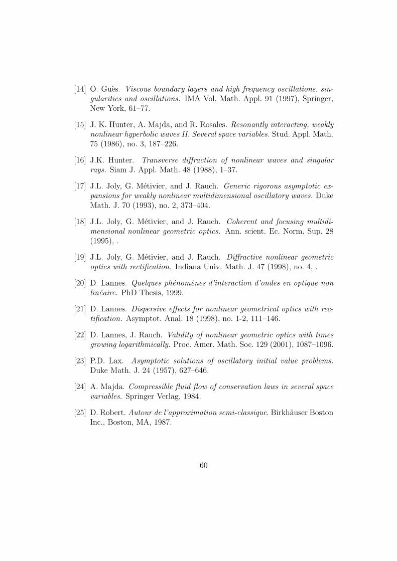
[14] O. Gues. Viscous boundary layers and high frequency oscillations. sin-gularities and oscillations. IMA Vol. Math. Appl. 91 (1997), Springer,New York, 61–77.

[15] J. K. Hunter, A. Majda, and R. Rosales. Resonantly interacting, weaklynonlinear hyperbolic waves II. Several space variables. Stud. Appl. Math.75 (1986), no. 3, 187–226.

[16] J.K. Hunter. Transverse diffraction of nonlinear waves and singularrays. Siam J. Appl. Math. 48 (1988), 1–37.

[17] J.L. Joly, G. Metivier, and J. Rauch. Generic rigorous asymptotic ex-pansions for weakly nonlinear multidimensional oscillatory waves. DukeMath. J. 70 (1993), no. 2, 373–404.

[18] J.L. Joly, G. Metivier, and J. Rauch. Coherent and focusing multidi-mensional nonlinear geometric optics. Ann. scient. Ec. Norm. Sup. 28(1995), .

[19] J.L. Joly, G. Metivier, and J. Rauch. Diffractive nonlinear geometricoptics with rectification. Indiana Univ. Math. J. 47 (1998), no. 4, .

[20] D. Lannes. Quelques phenomenes d’interaction d’ondes en optique nonlineaire. PhD Thesis, 1999.

[21] D. Lannes. Dispersive effects for nonlinear geometrical optics with rec-tification. Asymptot. Anal. 18 (1998), no. 1-2, 111–146.

[22] D. Lannes, J. Rauch. Validity of nonlinear geometric optics with timesgrowing logarithmically. Proc. Amer. Math. Soc. 129 (2001), 1087–1096.

[23] P.D. Lax. Asymptotic solutions of oscillatory initial value problems.Duke Math. J. 24 (1957), 627–646.

[24] A. Majda. Compressible fluid flow of conservation laws in several spacevariables. Springer Verlag, 1984.

[25] D. Robert. Autour de l’approximation semi-classique. Birkhauser BostonInc., Boston, MA, 1987.

60

[26] G. Schneider. Justification of modulation equations for hyperbolic sys-tems via normal forms. Nonlinear Differential Equations and Applica-tions 5 (1998), no. 1, 69–82.

[27] M. Taylor. Partial Differential Equations III. Appl. Math. Sc. 117,Springer Verlag, 1996.

[28] M. Williams. Boundary layers and glancing blow-up in nonlinear ge-ometric optics. Ann. Scient. de l’Ecole Norm. Sup. 33 (2000), n. 3,383-432.

61