arX

iv:0

811.

3246

v2 [

cond

-mat

.dis

-nn]

30

Aug

200

9

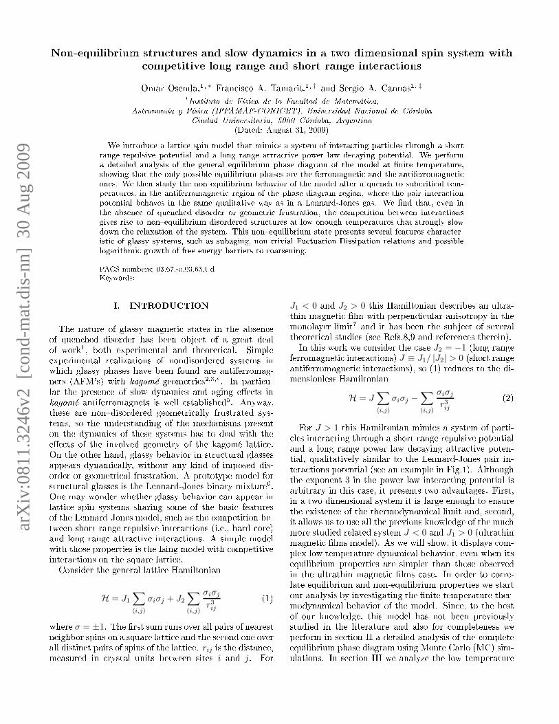
Non-equilibrium stru tures and slow dynami s in a two dimensional spin system with ompetitive long range and short range intera tionsOmar Osenda,1, ∗ Fran is o A. Tamarit,1, † and Sergio A. Cannas1, ‡1Instituto de Físi a de la Fa ultad de Matemáti a,Astronomía y Físi a (IFFAMAF-CONICET), Universidad Na ional de CórdobaCiudad Universitaria, 5000 Córdoba, Argentina(Dated: August 31, 2009)We introdu e a latti e spin model that mimi s a system of intera ting parti les through a shortrange repulsive potential and a long range attra tive power law de aying potential. We performa detailed analysis of the general equilibrium phase diagram of the model at �nite temperature,showing that the only possible equilibrium phases are the ferromagneti and the antiferromagneti ones. We then study the non equilibrium behavior of the model after a quen h to sub riti al tem-peratures, in the antiferromagneti region of the phase diagram region, where the pair intera tionpotential behaves in the same qualitative way as in a Lennard-Jones gas. We �nd that, even inthe absen e of quen hed disorder or geometri frustration, the ompetition between intera tionsgives rise to non�equilibrium disordered stru tures at low enough temperatures that strongly slowdown the relaxation of the system. This non�equilibrium state presents several features hara ter-isti of glassy systems, su h as subaging, non trivial Fu tuation Dissipation relations and possiblelogarithmi growth of free energy barriers to oarsening.PACS numbers: 03.67.-a,03.65.UdKeywords:I. INTRODUCTIONThe nature of glassy magneti states in the absen eof quen hed disorder has been obje t of a great dealof work1, both experimental and theoreti al. Simpleexperimental realizations of nondisordered systems inwhi h glassy phases have been found are antiferromag-nets (AFM's) with kagomé geometries2,3,4. In parti u-lar the presen e of slow dynami s and aging e�e ts inkagomé antiferromagnets is well established5. Anyway,these are non�disordered geometri ally frustrated sys-tems, so the understanding of the me hanisms presenton the dynami s of these systems has to deal with thee�e ts of the involved geometry of the kagomé latti e.On the other hand, glassy behavior in stru tural glassesappears dynami ally, without any kind of imposed dis-order or geometri al frustration. A prototype model forstru tural glasses is the Lennard-Jones binary mixture6.One may wonder whether glassy behavior an appear inlatti e spin systems sharing some of the basi featuresof the Lennard-Jones model, su h as the ompetition be-tween short range repulsive intera tions (i.e., hard ore)and long range attra tive intera tions. A simple modelwith those properties is the Ising model with ompetitiveintera tions on the square latti e.Consider the general latti e HamiltonianH = J1

∑

〈i,j〉

σiσj + J2

∑

(i,j)

σiσj

r3ij

(1)where σ = ±1. The �rst sum runs over all pairs of nearestneighbor spins on a square latti e and the se ond one overall distin t pairs of spins of the latti e. rij is the distan e,measured in rystal units between sites i and j. For

J1 < 0 and J2 > 0 this Hamiltonian des ribes an ultra-thin magneti �lm with perpendi ular anisotropy in themonolayer limit7 and it has been the subje t of severaltheoreti al studies (see Refs.8,9 and referen es therein).In this work we onsider the ase J2 = −1 (long rangeferromagneti intera tions) J ≡ J1/ |J2| > 0 (short rangeantiferromagneti intera tions), so (1) redu es to the di-mensionless HamiltonianH = J

∑

〈i,j〉

σiσj −∑

(i,j)

σiσj

r3ij

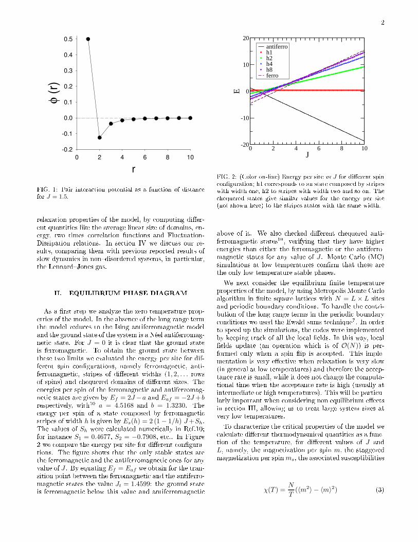
(2)For J > 1 this Hamiltonian mimi s a system of parti- les intera ting through a short range repulsive potentialand a long range power law de aying attra tive poten-tial, qualitatively similar to the Lennard-Jones pair in-tera tions potential (see an example in Fig.1). Althoughthe exponent 3 in the power law intera ting potential isarbitrary in this ase, it presents two advantages. First,in a two dimensional system it is large enough to ensurethe existen e of the thermodynami al limit and, se ond,it allows us to use all the previous knowledge of the mu hmore studied related system J < 0 and J1 > 0 (ultrathinmagneti �lms model). As we will show, it displays om-plex low temperature dynami al behavior, even when itsequilibrium properties are simpler than those observedin the ultrathin magneti �lms ase. In order to orre-late equilibrium and non-equilibrium properties we startour analysis by investigating the �nite temperature ther-modynami al behavior of the model. Sin e, to the bestof our knowledge, this model has not been previouslystudied in the literature and also for ompleteness weperform in se tion II a detailed analysis of the ompleteequilibrium phase diagram using Monte Carlo (MC) sim-ulations. In se tion III we analyze the low temperature

2

FIG. 1: Pair intera tion potential as a fun tion of distan efor J = 1.5.relaxation properties of the model, by omputing di�er-ent quantities like the average linear size of domains, en-ergy, two times orrelation fun tions and Flu tuation-Dissipation relations. In se tion IV we dis uss our re-sults, omparing them with previous reported results ofslow dynami s in non�disordered systems, in parti ular,the Lennard�Jones gas.II. EQUILIBRIUM PHASE DIAGRAMAs a �rst step we analyze the zero temperature prop-erties of the model. In the absen e of the long range termthe model redu es to the Ising antiferromagneti modeland the ground state of the system is a Néel antiferromag-neti state. For J = 0 it is lear that the ground stateis ferromagneti . To obtain the ground state betweenthese two limits we evaluated the energy per site for dif-ferent spin on�gurations, namely ferromagneti , anti-ferromagneti , stripes of di�erent widths (1, 2, . . . rowsof spins) and hequered domains of di�erent sizes. Theenergies per spin of the ferromagneti and antiferromag-neti states are given by Ef = 2J −a and Eaf = −2J +brespe tively, with10 a = 4.5168 and b = 1.3230. Theenergy per spin of a state omposed by ferromagneti stripes of width h is given by Es(h) = 2 (1 − 1/h) J +Sh.The values of Sh were al ulated numeri ally in Ref.10;for instan e S1 = 0.4677, S2 = −0.7908, et .. In Figure2 we ompare the energy per site for di�erent on�gura-tions. The �gure shows that the only stable states arethe ferromagneti and the antiferromagneti ones for anyvalue of J . By equating Ef = Eaf we obtain for the tran-sition point between the ferromagneti and the antiferro-magneti states the value Jt = 1.4599: the ground stateis ferromagneti below this value and antiferromagneti

0 2 4 6 8 10J

-20

-10

0

10

20

E

antiferroh1h2h4h8ferro

FIG. 2: (Color on-line) Energy per site vs J for di�erent spin on�guration; h1 orresponds to an state omposed by stripeswith width one, h2 to stripes with width two and so on. The hequered states give similar values for the energy per site(not shown here) to the stripes states with the same width.above of it. We also he ked di�erent hequered anti-ferromagneti states10, verifying that they have higherenergies than either the ferromagneti or the antiferro-magneti states for any value of J . Monte Carlo (MC)simulations at low temperatures on�rm that these arethe only low temperature stable phases.We next onsider the equilibrium �nite temperatureproperties of the model, by using Metropolis Monte Carloalgorithm in �nite square latti es with N = L × L sitesand periodi boundary onditions. To handle the ontri-bution of the long range terms in the periodi boundary onditions we used the Ewald sums te hnique7. In orderto speed up the simulations, the odes were implementedby keeping tra k of all the lo al �elds. In this way, lo al�elds update (an operation whi h is of O(N)) is per-formed only when a spin �ip is a epted. This imple-mentation is very e�e tive when relaxation is very slow(in general at low temperatures) and therefore the a ep-tan e rate is small, while it does not hange the omputa-tional time when the a eptan e rate is high (usually atintermediate or high temperatures). This will be parti u-larly important when onsidering non equilibrium e�e tsin se tion III, allowing us to treat large system sizes atvery low temperatures.To hara terize the riti al properties of the model we al ulate di�erent thermodynami al quantities as a fun -tion of the temperature, for di�erent values of J andL, namely, the magnetization per spin m, the staggeredmagnetization per spin ms, the asso iated sus eptibilities

χ(T ) =N

T(〈m2〉 − 〈m〉2) (3)

3χs(T ) =

N

T(〈m2

s〉 − 〈ms〉2), (4)the spe i� heat

C(T ) =1

NT 2(〈H2〉 − 〈H〉2) (5)and the fourth order umulant

V (T ) = 1 −

⟨

H4⟩

3 〈H2〉2 . (6)where 〈. . .〉 stands for an average over the thermal noise.All these quantities are al ulated starting from an ini-tially equilibrated high temperature on�guration andslowly de reasing the temperature. For every temper-ature the initial spin on�guration is taken as the �nal on�guration of the previous temperature; we let the sys-tem to equilibrate M1 Monte Carlo Steps (one MCS isde�ned as a omplete y le of N spin update trials) andaverage out the results of M2 MCS, typi al values of M1and M2 being around 105 and 5 × 105 respe tively.Figures (3) and (4) show the typi al results for the dif-ferent thermodynami al quantities in the antiferromag-neti region of the phase diagram, namely, for J > Jt.Fig.(4b) shows that the fourth order umulant exhibits avanishing minimum, onsistent with a se ond order phasetransition. Fig.(3b) shows that the staggered sus epti-bility exhibits a size dependent maximum whi h s alesas Lγ/ν, with γ/ν = 1.8 ± 0.1, onsistent with the ex-a t value γ/ν = 1.75 of the two dimensional short rangeIsing model. Moreover, as J in reases γ/ν approa hessystemati ally the value 1.75 (for instan e, for J = 3we found γ/ν = 1.74 ± 0.05; see Fig.(7). We see fromFig.(4a) that the spe i� heat exhibits a size dependentmaximum whi h s ales as Lα/ν , with α/ν = 0.23± 0.05;similar values were found for other values of J > Jt (seeFig.7). Although small, those values are larger than ex-pe ted for a phase transition in the universality lass ofthe two dimensional Ising model (α = 0). However, sin ethose values are also observed for large values of J , webelieve that this is a �nite size e�e t. Hen e, we on- lude that the whole line between the paramagneti andthe antiferromagneti phases (J > Jt) belongs to the uni-versality lass of the short range two dimensional Isingmodel.The riti al properties for J < Jt are a bit more om-plex. For J ≤ 1.3 the order parameter (magnetization),the sus eptibility, the spe i� heat and the fourth or-der umulant present qualitatively the same behavior asthose quantities in the J > Jt ase, but with a di�erentset of riti al exponents (see Fig.7). We found γ/ν ≈ 1.1and α/ν ≈ 0.14., whi h are lose to the renormalizationgroup estimates for the J = 0 ase11: ν = 1, α = 0and γ = 1; the small di�eren e between those values

FIG. 3: (Color on-line) Order parameter (absolute value of thestaggered magnetization) (a) and asso iated staggered sus ep-tibility (b) as a fun tion of the temperature for J = 1.6 andfor di�erent system sizes; the inset in (b) shows the �nite sizes aling of the maximum of χs.and ours an be attributed to �nite size e�e ts, whi hare very strong when the long range ferromagneti in-tera tions dominate. Hen e, we on lude that the wholeline for 0 ≤ J ≤ 1.3 belongs to the universality lass ofthe two dimensional 1/r3 ferromagneti Ising model. For1.3 < J < Jt we �nd a lear eviden e that the ferro-paratransition is a �rst order one. The typi al behavior ofthe thermodynami al quantities in this ase is illustratedin Figs. 5 and 6. We see that the fourth order umulantpresents a lear onverging minimum as the system sizesin reases, as expe ted in a �rst order transition12. The�nite size s aling of sus eptibility is also onsistent withthe L2 behavior expe ted for a �rst order transition ina two dimensional system13. The spe i� heat exponentfor J = 1.4 is α/ν = 1.1± 0.2. This value is ertainly farfrom 2 (the expe ted value in a �rst order transition), but

4

FIG. 4: (Color on-line) Moments of the energy as a fun tionof the temperature for J = 1.6 and for di�erent system sizes.(a) Spe i� heat C; the inset shows the �nite size s aling ofthe maximum of C. (b) Fourth order umulant.it is larger than the riti al exponent of any ontinuoustransition. Besides �nite size e�e ts, su h large di�eren eis probably also asso iated to the presen e of a tri riti alpoint somewhere between J = 1.3 and J = 1.4. This as-sumption is onsistent with the fa t that α/ν approa hesthe expe ted value α/ν = 2 as J in reases approa hingJ = Jt (we obtained α/ν = 1.8 ± 0.1 for J = 1.43; seeFig.7).We summarize the obtained results for the riti al ex-ponents in Fig.7 and the overall phase diagram in Fig.8.III. NON-EQUILIBRIUM PROPERTIESThis se tion deals with the far-from equilibrium prop-erties of the system at low temperatures, i.e., its relax-ation dynami s after a sudden quen h from T = ∞ to a

FIG. 5: (Color on-line) Order parameter (absolute value ofthe magnetization) (a) and asso iated sus eptibility (b) asa fun tion of the temperature for J = 1.4 and for di�erentsystem sizes; the inset in (b) shows the �nite size s aling ofthe maximum of χ.temperature T < Tc.A. Non equilibrium domain stru tures: energyrelaxation and hara teristi domain lengthFirst we analyze the time evolution of the energy,with the time measured in MCS. We onsider both theinstantaneous energy per spin E/N (i.e., the energyalong single MC runs) and the mean ex ess of energyδe(t) ≡ [H ] /N − u(T ), where [. . .] stands for averageover di�erent MC runs (i.e., over di�erent realizations ofthe thermal noise). u(T ) is the equilibrium energy perspin at temperature T ; u(T ) is obtained by equilibrating�rst the system during 104 MCS starting from the groundstate on�guration and then averaging over a single MC

5

FIG. 6: (Color on-line) Moments of the energy as a fun tionof the temperature for J = 1.4 and for di�erent system sizes.(a) Spe i� heat C; the inset shows the �nite size s aling ofthe maximum of C. (b) Fourth order umulant.run during 105 MCS.To he k out our results we �rst al ulate the evolu-tion of δe(t) in the simple ase J < Jt for di�erent quen htemperatures. The typi al behavior is shown in Figure9. We �nd that, after a short transient period and be-fore the system ompletely relaxes, the ex ess of energybehaves as δe(t) ∼ t−1/2 independently of T . Sin e itis expe ted that δe(t) ∝ 1/l(t), where l(t) is the har-a teristi length s ale of the domains, this behavior is onsistent with a normal oarsening pro ess of a systemwith non- onserved order parameter14, where l(t) ∼ t1/2.Next, we onsider the relaxation in the antiferromag-neti region J > Jt for di�erent quen h temperatures. Atlow enough temperatrues the relaxation of the system learly departs from that expe ted in a normal oars-ening pro ess. The typi al behavior of the instanta-

FIG. 7: Criti al exponents obtained from �nite size s aling asa fun tion of J . (a) Sus eptibility exponent γ/ν; (b) Spe i� heat exponent α/ν. The dashed lines indi ate the referen evalues 1, 1.75 and 2 in (a) and 0 and 2 in (b).neous energy is shown in Fig.10, together with typi aldomain on�gurations along single MC runs for J = 2and T = 0.04. In that �gure the domains orrespond toregions of antiferromagneti ordering, namely, bla k andwhite olors odify regions with lo al staggered magneti-zation ms ≈ 1 and ms ≈ −1 respe tively.Di�erent relaxation regimes an be identi�ed. Aftera short time qui k relaxation pro ess 0 < t < τ0 ≈20 MCS, in whi h lo al antiferromagneti order is set,the system always gets stu k in a omplex non equilib-rium disordered state omposed mainly by a few inter-mingled ma ros opi antiferromagneti domains; its typ-i al shape is illustrated for a larger system size in Fig.11.This state presents a sort of labyrinth stru ture, in thesense that there is always at least one ma ros opi on-ne ted domain, i.e., in su h domain any pair of points an be onne ted by a ontinuous path without ross-ing a domain wall (see for example the bla k domain inFig.11). Up to ertain hara teristi time τ1 the system

6

FIG. 8: Phase diagram T vs. J . The riti al temperatureswere estimated from the maxima of the spe i� heat. Filled ir les and open hexagons orrespond to se ond and �rst orderphase transitions respe tively.

FIG. 9: (Color on-line) Ex ess of energy δe(t) as a fun tionof time for J = 1, L = 100 and di�erent quen h temperaturesT < Tc. The results were averaged over 2000 MC runs.slowly relaxes by eliminating small domains and �u tua-tions lo ated in the large domain borders, in su h a waythat the lo al urvature of the domain walls is redu ed(Fig.10). Along this pro ess the area of the main domainsremains almost onstant. In this sense, su h pro ess isreminis ent of a spinodal de omposition. We will all thisthe glassy regime. For time s ales longer than a ertain hara teristi time τ1 both domains �nally disentangleand relaxation is dominated by the ompetition betweenonly two large domains, separated by rather smooth do-main walls. Fig.10 illustrates the two possible out omesof this pro ess: either the system relaxes dire tly to itsequilibrium state (Fig.10a) or it gets stu k in an ordered on�guration omposed of stripe shaped antiferromag-neti domains with almost �at domain walls (Fig.10b).

FIG. 10: Instantaneous energy per spin as a fun tion of timefor single realizations of the sto hasti noise for J = 2, L = 48and T = 0.04. Typi al antiferromagneti domain on�g-urations are shown along the evolutions, where bla k andwhite olors odify regions with lo al staggered magnetiza-tion ms ≈ 1 and ms ≈ −1 respe tively. The dashed lines orrespond to the equilibrium energy at this temperature. (a)After living the glassy regime the system equilibrates. (b) Af-ter living the glassy regime the system gets stu k in a striped on�guration.

FIG. 11: Typi al antiferromagneti domain on�guration forJ = 2, T = 0.04, L = 256 and t = 100; MCS. Bla k andwhite follows the same onvention as in Fig.10.

7

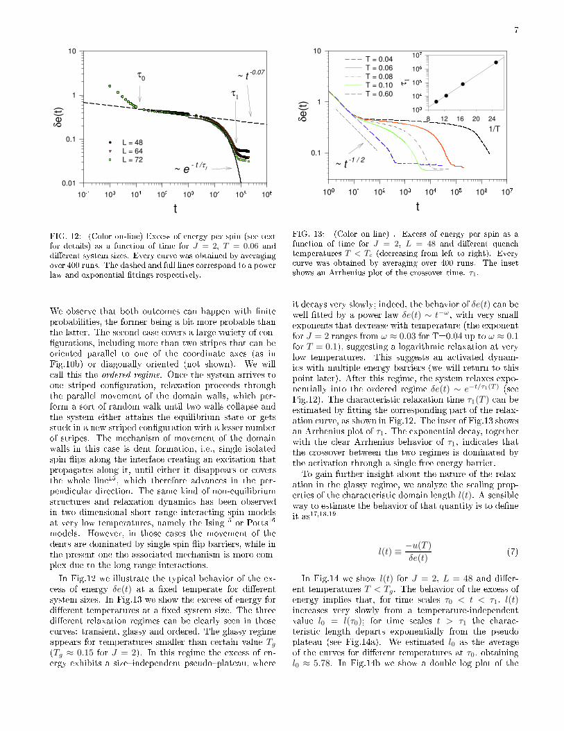
FIG. 12: (Color on-line) Ex ess of energy per spin (see textfor details) as a fun tion of time for J = 2, T = 0.06 anddi�erent system sizes. Every urve was obtained by averagingover 400 runs. The dashed and full lines orrespond to a powerlaw and exponential �ttings respe tively.We observe that both out omes an happen with �niteprobabilities, the former being a bit more probable thanthe latter. The se ond ase overs a large variety of on-�gurations, in luding more than two stripes that an beoriented parallel to one of the oordinate axes (as inFig.10b) or diagonally oriented (not shown). We will all this the ordered regime. On e the system arrives toone striped on�guration, relaxation pro eeds throughthe parallel movement of the domain walls, whi h per-form a sort of random walk until two walls ollapse andthe system either attains the equilibrium state or getsstu k in a new striped on�guration with a lesser numberof stripes. The me hanism of movement of the domainwalls in this ase is dent formation, i.e., single isolatedspin �ips along the interfa e reating an ex itation thatpropagates along it, until either it disappears or oversthe whole line15, whi h therefore advan es in the per-pendi ular dire tion. The same kind of non-equilibriumstru tures and relaxation dynami s has been observedin two dimensional short range intera ting spin modelsat very low temperatures, namely the Ising15 or Potts16models. However, in those ases the movement of thedents are dominated by single spin �ip barriers, while inthe present one the asso iated me hanism is more om-plex due to the long range intera tions.In Fig.12 we illustrate the typi al behavior of the ex- ess of energy δe(t) at a �xed temperate for di�erentsystem sizes. In Fig.13 we show the ex ess of energy fordi�erent temperatures at a �xed system size. The threedi�erent relaxation regimes an be learly seen in those urves: transient, glassy and ordered. The glassy regimeappears for temperatures smaller than ertain value Tg(Tg ≈ 0.15 for J = 2). In this regime the ex ess of en-ergy exhibits a size�independent pseudo�plateau, where

FIG. 13: (Color on-line) . Ex ess of energy per spin as afun tion of time for J = 2, L = 48 and di�erent quen htemperatures T < Tc (de reasing from left to right). Every urve was obtained by averaging over 400 runs. The insetshows an Arrhenius plot of the rossover time. τ1.it de ays very slowly; indeed, the behavior of δe(t) an bewell �tted by a power law δe(t) ∼ t−ω, with very smallexponents that de rease with temperature (the exponentfor J = 2 ranges from ω ≈ 0.03 for T=0.04 up to ω ≈ 0.1for T = 0.1), suggesting a logarithmi relaxation at verylow temperatures. This suggests an a tivated dynam-i s with multiple energy barriers (we will return to thispoint later). After this regime, the system relaxes expo-nentially into the ordered regime δe(t) ∼ e−t/τ1(T ) (seeFig.12). The hara teristi relaxation time τ1(T ) an beestimated by �tting the orresponding part of the relax-ation urve, as shown in Fig.12. The inset of Fig.13 showsan Arrhenius plot of τ1. The exponential de ay, togetherwith the lear Arrhenius behavior of τ1, indi ates thatthe rossover between the two regimes is dominated bythe a tivation through a single free energy barrier.To gain further insight about the nature of the relax-ation in the glassy regime, we analyze the s aling prop-erties of the hara teristi domain length l(t). A sensibleway to estimate the behavior of that quantity is to de�neit as17,18,19l(t) ≡

−u(T )

δe(t)(7)In Fig.14 we show l(t) for J = 2, L = 48 and di�er-ent temperatures T < Tg. The behavior of the ex ess ofenergy implies that, for time s ales τ0 < t < τ1, l(t)in reases very slowly from a temperature-independentvalue l0 = l(τ0); for time s ales t > τ1 the hara -teristi length departs exponentially from the pseudoplateau (see Fig.14a). We estimated l0 as the averageof the urves for di�erent temperatures at τ0, obtaining

l0 ≈ 5.78. In Fig.14b we show a double log plot of the

8

FIG. 14: (Color on-line) (a) Chara teristi domain length(see text for details) as a fun tion of time for J = 2, L = 48and di�erent temperatures T < Tc (de reasing from left toright). (b) Log-log plot of the normalized length (l−l0)/T a vs.ln(t) from the same data as in (a) for the lowest temperatures;l0 = 5.78 is indi ated in (a); the value of the exponent a = 2.7was hosen to obtain the best data ollapse of the urves inthe glassy regime. The straight line is a referen e (power withexponent a).res aled quantity (l(t) − l0)/T a vs. ln(t). The expo-nent a was hosen to obtain the best data ollapse in theglassy regime of the data presented in Fig.14a. A tually,a good data ollapse inside the error bars of the sta-tisti al �u tuations is obtained for values of a between2.65 and 2.75; for values of the exponent outside thatrange the urves learly do not ollapse. Hen e, we esti-mated a = 2.7±0.05. The power law like behavior of theres aled urves in Fig.14b shows that the hara teristi length behaves as

l(t) ∼ l0 +

[

T

bln t

]a (8)

10 12 14 16 18 201/T

102

103

104

105

τ s

5 6 7 8 9ls

0.3

0.4

0.5

slop

e

FIG. 15: (Color on-line) Arrhenius plot of the hara teristi time for shrinking squares for di�erent values of the squareside ls: from bottom to top ls = 5, 6, 7, 8, 9. The lines are aguide to the eye. The inset shows the energy barrier (slopeof the linear �ttings in the Arrhenius plot) as a fun tion ofls (the symbol size in the inset is larger than the statisti alerror bars).for t0 < t < τ1(T ) (a log-log plot of l(t) − l0 vs. t showsthat a power law �t in the entire time interval is learlyinferior than in Fig.14). Su h behavior is onsistent witha lass 4 system, a ording to Lai et al lassi� ation20,i.e., a system with domain size dependent free energybarriers to oarsening18 f(l). In our ase this would or-respond to f(l) ∼ b (l − l0)

1/a. The numeri al resultssuggest that in the present model su h growth wouldstop when some maximum hara teristi length lmax isrea hed at τ1(T ), where the barrier be omes indepen-dent of l. After this point the system relaxes exponen-tially with a hara teristi time τ1 ∝ exp(F/T ), whereF = f(lmax) and therefore lmax ≈ l0 + (F/b)a. Fromthe data of Fig.14b we estimate b ≈ 0.32, while from thedata of the inset of Fig.13 we estimated F ≈ 0.44, givingan estimation lmax ≈ 8.To he k the above interpretation we analyze the har-a teristi time τs for shrinking squares, i.e., the timeneeded for a square ex itation of linear size ls to om-pletely relax. This te hnique has been proved to be a sen-sitive way to he k the relaxation dynami s of short rangemodels when free energy barriers are involved18,19,21. Inparti ular, Shore et al18 have argued (and shown to bevalid in parti ular ases) that the energy barriers toshrink square-shaped ex itations should be a measure ofthe free energy barriers to oarsening. In our ase westarted with a ground state on�guration of size L witha square of inverted spins of size ls (L ≫ ls) and peri-odi boundary onditions. Although it is not lear to uswhether the arguments of Shore et al18 an be straightfor-wardly extended to a system with long range intera tions

9or not, one an still expe t the barriers to shrink a squareto provide at least a rough measure of the free energy bar-riers to oarsening. In our ase, this expe tation is basedon the dire t observation of the domain on�gurationsduring relaxation in the glassy regime. We observe thatrough domain walls tend to be ome �at rather fast, andthat relaxation pro eeds mainly at small jumps in theenergy every time a sharp edge moves. The results forthe time for shrinking squares support this onje ture.In Fig.15 we show an Arrhenius plot of τs for di�erentvalues of ls and temperatures T < Tg. We see that τs ex-hibits a lear Arrhenius behavior at all the temperaturesfor ls > 4 (for sizes ls ≤ 4 the squares shrink qui kly ina few MCS), with asso iated barriers that grow slowlyfor ls < 8 and saturate for ls ≥ 9 at a value around 0.5, lose to F = 0.44. Although the limited range of valuesof ls where the barrier shows a dependen y on it doesnot allow a more a urate omparison, the onsisten ywith the previous interpretation of the behavior of l(t) is lear.For temperatures larger than Tg the glassy regime om-pletely disappears and the system de ays through a nor-mal oarsening pro ess, i.e., δe(t) ∼ t−1/2 (see Fig.13).However, for some range of temperatures it still getsstu k in some long-lasting antiferromagneti striped on-�guration with high probability, so the orrespondingplateau in the ex ess of energy is still observable (forJ = 2 we observed it for temperatures up to T ≈ 1.5).Those on�gurations are highly stable, even at relativelyhigh temperatures. The hara teristi equilibration timeτ2, de�ned as the time after whi h the system attains theequilibrium state with probability one, is very di� ultto estimate, but it is at least three orders of magnitudelarger than τ1 for T < Tg.B. Time orrelation and response fun tionsAnother way to hara terize the out of equilibrium dy-nami s of omplex magneti systems is through the anal-ysis of the two-time auto orrelation fun tion C(t, t′). Asystem that has attained thermodynami al equilibriumor meta�equilibrium satis�es time translational invari-an e (TTI), i.e., C(t, t′) ≡ C(t − t′), al least for ertaintime s ales. Far from equilibrium TTI is broken andtime orrelations exhibits a dependen y on the history ofthe sample after the quen h. This phenomenon is alledaging and in real systems it an be observed through avariety of experiments. A typi al example is the zero-�eld- ooling22 experiment, in whi h the sample is ooledin zero �eld to a sub riti al temperature at time t = 0.After a waiting time tw a small onstant magneti �eldis applied and the time evolution of the magnetization isre orded. It is then observed that the longer the waitingtime tw the slower the relaxation and this is the originof the term aging. Moreover, the s aling properties oftwo-times quantities provides information about the un-derlying relaxation dynami s23,24.

0.01 0.1 1 10 100(t+t

w)/t

w

0.2

0.4

0.6

0.8

1

C(t

w,t w

+t)

tw

=100tw

=200tw

=400tw

=800

FIG. 16: (Color on-line) Two-times auto orrelation fun tionC(tw + t, tw) as a fun tion of (t + tw)/tw for J = 1 (ferro-magneti phase), T=0.2, L = 600 and di�erent values of thewaiting time tw (in reasing from bottom to top).Although aging an be dete ted through di�erent time-dependent quantities, a straightforward way to establishit in a numeri al simulation is to al ulate the spin auto- orrelation fun tion

C(tw + t, tw) =

[

1

N

N∑

i=1

σi(tw + t)σi(tw)

]

, (9)where tw is the waiting time from the quen h at t = 0( ompletely disordered initial state) and {σi(t)} is thespin on�guration at time t.First of all we al ulate C(tw + t, tw) in the ferromag-neti part of the phase diagram, i.e., for J < Jt. Wefound that C(tw + t, tw) depends on t and tw throughthe ratio t/tw, as shown in Fig.16. This type of s alingis alled simple aging and it is hara teristi of a simple oarsening (i.e., domain growth) pro ess. This result isin agreement with the observed behavior of the ex ess ofenergy (Fig.9)Next we onsider the behavior of the orrelations dur-ing the glassy regime observed in the previous se tion forJ > Jt. The typi al behavior of the auto orrelation fun -tion is shown in Figure 17, where we plot C(tw + t, tw) vst for T = 0.04, J = 2 and L = 256 and di�erent waitingtimes. The simulation was run up to t = 5 × 105 MCSand typi al averages were performed over 2000 realiza-tions of the thermal noise; both times were hosen su hthat τ0 < t+tw < τ1. A �rst trial to ollapse those urvesshowed that in this ase C(tw + t, tw) does not exhibitsimple aging. A similar behavior is observed for J = 2,T = 0.06 < Tg and τ0 < t + tw < τ1.

10

1000 10000 1e+05t

0.5

0.6

0.7

0.8

0.9

1C

(tw

,t w+

t)

tw

= 104

tw

= 2x104

tw

= 4x104

tw

= 8x104

FIG. 17: (Color online) Two-times auto orrelation fun tionas a fun tion of the di�eren e of times t for J = 2, T = 0.04,L = 256 and di�erent values of the waiting time tw (in reasingfrom left to right).It has been observed for a large variety of systems thatin the aging s enario the urves of C(tw + t, tw) for di�er-ent tw always ollapse into a single one using an adequates aling fun tion23. Although there is no theoreti al ba-sis for determining the s aling fun tion, there are a few hoi es that have been able to take into a ount bothexperimental and numeri al data, perhaps the most fre-quent one being the additive form

C(tw + t, tw) = Cst(t) + Cag

(

h(tw + t)

h(tw)

)

. (10)where Cst(t) is a stationary part, usually well des ribedby an algebrai de ayCst(t) = B t−γ . (11)The fun tion h, appearing in the aging part of the auto- orrelations Cag, is some s aling fun tion (in the ase ofsimple aging h(t) is a power law that des ribes the har-a teristi linear domain size growth). In our ase the bestdata ollapse of the auto orrelation urves was obtainedusing a s aling fun tion of the form

h(t) = exp

[

1

1 − µ

(

t

τ

)1−µ]

, (12)whi h has been used to a ount for experimental data23and in the Edwards�Anderson model for spin glasses25,where τ is a mi ros opi time s ale. It is worth to notethat the s aling fun tion (12) interpolates a range of s e-narios: from sub�aging for 0 < µ < 1, to super�aging forµ > 1, through simple aging for23 µ = 1; for µ = 0 TTI is

0.55

0.6

0.65

0.7

0.75

0.8

0.85

0.9

0.95

1

10-2 10-1 100 101 102 103 104

C(t

w,t w

+t)

h(t+tw)/h(tw)

tw=10000tw=20000tw=40000tw=80000

FIG. 18: (Color on-line) Data ollapse of the auto orrelation urves of Fig.17 (J = 2, T = 0.04 and L = 256) using the s al-ing fun tion Eq.(12) with s aling parameters shown in TableI.T B γ µ

0.04 0 - 0.50

0.06 0 - 0.30

0.6 0.19 0.22 0.25

1.0 0.16 0.30 0.14TABLE I: S aling parameter values obtained from the bestdata ollapse for the orrelation urves for J = 2 at di�erenttemperatures using the s aling forms Eqs.(10)-(12).re overed. In Figure 18 we show the ollapse of the datafrom Figure 17 using the s aling parameter values shownin Table I (τ was arbitrarily �xed to one). A similar data ollapse was observed for J = 2 and T = 0.06 (see param-eters in Table I). To he k possible �nite size e�e ts weperformed a similar al ulation for T = 0.04, J = 2 andL = 64, �nding the same ollapse shown for L = 256 inFigure 18 with the same s aling parameters; only a smallvariation in the master urve is observed. We see thatfor T < Tg the best data ollapse is obtained withoutstationary part and a lear sub-aging is observed.We also repeat the orrelation al ulation for temper-atures T > Tg at time s ales orresponding to the or-dered regime tw + t > τ1(T = 0.6 and T = 1 for J = 2and L = 64). Again, aging is observed in this regimeand a data ollapse similar to that shown in Figure 18using the s alings (10)-(12) is obtained. The orrespond-ing s aling parameter values are shown in Table I. Wesee that for this temperature range the best data ol-lapse is obtained by in luding a stationary part and thatthe s aling parameter µ de reases systemati ally as thequen h temperature in reases signaling that the systemapproa hes TTI. We �nd that µ be omes zero at a tem-perature T ≈ 1.5 < Tc, whi h an be onsidered as theonset of this non exponential relaxation.

11To further hara terize this non equilibrium behaviorwe also analyze the generalized Flu tuation-DissipationRelations (FDR), whi h an be expressed as26:R(tw + t, tw) =

X(tw + t, tw)

T

∂C(tw + t, tw)

∂tw(13)where R(tw + t, tw) = 1/N

∑

i ∂ 〈σi(tw + t)〉 /∂hi(tw)is the response to a lo al external magneti �eld hi(t)and X(tw + t, tw) is the �u tuation dissipation fa tor. Inequilibrium the Flu tuation Dissipation Theorem (FDT)holds and X(tw + t, tw) = 1, while out of equilibriumX depends on t and tw in a non trivial way. It has been onje tured26 that X(tw + t, tw) = X [C(tw + t, tw)]. This onje ture has proved valid in all systems studied to date.Instead of onsidering the response fun tion it is easierto analyze the integrated response fun tion

χ(tw + t, tw) =

∫ tw+t

tw

R(tw + t, s) ds. (14)Assuming X(tw + t, tw) = X [C(tw + t, tw)] one obtainsTχ(tw + t, tw) =

∫ 1

C(tw+t,tw)

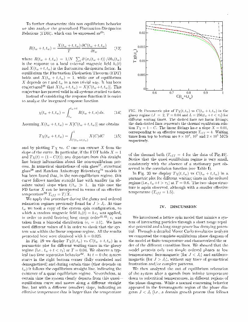
X(C)dC (15)and by plotting T χ vs. C one an extra t X from theslope of the urve. In parti ular, if the FDT holds X = 1and Tχ(t) = (1−C(t)); any departure from this straightline brings information about the non-equilibrium pro- ess. In numeri al simulations of spin glass27, stru turalglass28 and Random Anisotropy Heisenberg29 models ithas been found that, in the non-equilibrium regime, this urve follows another straight line with smaller (in ab-solute value) slope when t/tw ≫ 1. In this ase theFD fa tor X an be interpreted in terms of an e�e tivetemperature30 Teff = T/X .We apply this pro edure during the glassy and orderedrelaxation regimes previously found for J > Jt. At timetw we took a opy of the system spin on�guration, towhi h a random magneti �eld hi(t) = h ǫi was applied,in order to avoid favoring long range order31,32; ǫi wastaken from a bimodal distribution (ǫi = ±1). We haveused di�erent values of h in order to he k that the sys-tem was within the linear response regime. All the resultspresented here were obtained with h = 0.025.In Fig. 19 we display Tχ(t, tw) vs C(tw + t, tw) in aparametri plot for di�erent waiting times in the glassyregime (i.e., tw + t < τ1) at T = 0.04. We observe a typ-i al two time separation behavior33. At t = 0 the systemstarts in the right bottom orner (fully orrelated anddemagnetized) and during ertain time (that depends ontw) it follows the equilibrium straight line, indi ating theexisten e of a quasi equilibrium regime. Nevertheless, at ertain time the system learly departs from this quasi�equilibrium urve and moves along a di�erent straightline, but with a di�erent (smaller) slope, indi ating ane�e tive temperature that is larger than the temperature

0.6 0.7 0.8 0.9 1C(t

w+t,t

w)

0

0.005

0.01

0.015

0.02

T χ

(t,t w

)

FIG. 19: Parametri plot of Tχ(t, tw) vs C(tw + t, tw) in theglassy regime (J = 2, T = 0.04 and L = 256;tw + t < τ1) fordi�erent waiting times. The dashed lines are linear �ttings;the dash-dotted lines represents the thermal equilibrium rela-tion Tχ = 1 − C. The linear �ttings have a slope X = 0.01, orresponding to an e�e tive temperature Teff = 4. Waitingtimes from top to bottom are 8 × 104, 105 and 2 × 105 MCSrespe tively.of the thermal bath (Teff = 4 for the data of Fig.19).Noti e that the quasi equilibrium regime is very small, onsistently with the absen e of a stationary part ob-served in the orrelation fun tion (see Table I).In Fig. 20 we display Tχ(t, tw) vs C(tw + t, tw) in aparametri plot for di�erent waiting times in the orderedregime (i.e., tw+t > τ1) at T = 0.6. The two�slope stru -ture is again observed, although with a smaller e�e tivetemperature (Teff = 1.5).IV. DISCUSSIONWe introdu ed a latti e spin model that mimi s a sys-tem of intera ting parti les through a short range repul-sive potential and a long range power law de aying poten-tial. Through a detailed Monte Carlo simulation analysiswe omputed the omplete equilibrium phase diagram ofthe model at �nite temperature and hara terized the or-der of the di�erent transition lines. We showed that themodel presents only two simple ordered phases at lowtemperatures: ferromagneti (for J < Jt) and antiferro-magneti (for J > Jt), without any tra e of geometri alfrustration and/or omplex patterns.We then analyzed the out of equilibrium relaxationof the system after a quen h from in�nite temperaturedown to sub riti al temperatures, in di�erent regions ofthe phase diagram. While a normal oarsening behaviorappeared in the ferromagneti region of the phase dia-gram J < Jt (i.e., a domain growth pro ess that follows

12

0.8 0.85 0.9 0.95 1C(t

w+t,t

w)

0

0.05

0.1

T χ

(t,t w

)

FIG. 20: Parametri plot of Tχ(t, tw) vs C(tw + t, tw) in theordered regime (J = 2, T = 0.6 and L = 64; tw + t > τ1) fordi�erent waiting times. The dashed lines are linear �ttings;the dash-dotted lines represents the thermal equilibrium re-lation Tχ = 1 − C. The linear �ttings have a slope X = 0.4, orresponding to an e�e tive temperature Teff = 1.5. Wait-ing times from top to bottom are 4 × 104 , 8 × 104 and 105MCS respe tively.Allen-Cahn law l(t) ∼ t1/2) the system shows a om-plex relaxation s enario in the antiferromagneti regionJ > Jt. This is pre isely the most interesting situation,sin e for those values of J the pair intera tion potentialof the model shows the same qualitative features as a ontinuous, Lennard-Jones (LJ) like potential, namely,a nearest neighbors repulsive intera tion (i.e, �hard ore�like) and an attra tive, power law de aying intera tion atlonger distan es (see Fig.1). We must stress that we didnot intend to present a latti e version of the LJ gas, butto show that some very basi features present in it (i.e.,the ompetition between short and long range intera -tions) are enough to produ e non trivial slow relaxationproperties. We observed that su h ompetition gives riseto non�equilibrium stru tures that strongly slow downthe dynami s, even in the absen e of geometri al frus-tration and/or imposed disorder. The most interestingof those stru tures give rise to a relaxation regime withseveral appealing properties that strongly resemble thoseobserved in di�erent glassy systems.First of all, that regime is hara terized by a dynam-i ally generated disordered non-equilibrium state, har-a terized by a labyrinth stru ture, i.e., omposed of atleast one ma ros opi onne ted domain. The energy ofsu h state displays a pseudo-plateau and a �nite lifetimeτ1 that diverges when T → 0; both properties are in-dependent of the system size. Su h phenomenology isextremely reminis ent of transient parti les olloidal gelsobtained by quen hing a monodisperse gas of olloidalparti les under Brownian Dynami s (Langevin dynami s

in the overdamped limit) that intera t through a general-ized 2n−n LJ potentials34,35. A gel is a non�equilibriumdisordered state, hara terized as a per olating luster ofdense regions of parti les with voids that oarsen up to ertain size and freeze when the gel is formed; transientgels do not have permanent bonds between them and ol-lapse after a �nite life time35. The energy of transient gelsof 2n−n LJ olloidal parti les displays a slowly de ayingpseudo plateau36, as in the present ase. It has also beenobserved that the life time of the gel strongly in reasesas the intera tion range is de reased36, for instan e, by hanging the value of n. It would be interesting to he kif a similar e�e t an be obtained in the present model by hanging the intera tion range (for instan e, by hang-ing the exponent of the long range intera tion term inHamiltonian (2)).Se ond, during the glassy regime the dynami s appearsto be governed by free energy barriers to oarsening thats ale as a power law with the hara teristi domain size,with an asso iated logarithmi growth l(t) ∼ [T ln(t)]a(and therefore a logarithmi relaxation). Su h behavioris hara teristi of lass 4 systems, a ording to Lai et al lassi� ation20. Some examples of non�disordered short�range intera ting systems that present growing free en-ergy barriers with the domain size are already known,su h as the three dimensional Shore and Sethna (SS)model18,37,38 (i.e., an Ising model with nearest neigh-bors ferromagneti intera tions and next nearest neigh-bors antiferromagneti intera tions) and a generalizationof the previous one introdu ed by Lipowski et al19, in- luding a four spin plaquette intera tion term. However,in those models the barriers appears to grow linearly withthe domain size (whi h orresponds to a pure logarith-mi growth l(t) ∼ ln(t)) and therefore fall into the lass3 ategory of Lai et al18. So far, examples of lass 4 sys-tems were found only among disordered systems, su h asspin glasses39 and the Ising model with random quen hedimpurities40. To the best of our knowledge, this wouldbe the �rst possible example of lass 4 behavior in a nondisordered system. Nevertheless, an important di�eren ebetween the above mentioned non�disordered models andthe present one have to be remarked. While in thosemodels the logarithmi growth appears to lead to diver-gent barriers, in the present ase the apparently barriersgrowth stops at some maximum value F that determinesthe life time τ1. This implies the existen e of a hara ter-isti length lmax in the dynami s of the system. Althoughsu h limited length s ales makes very di� ult to obtainbetter numeri al eviden e of the existen e of growing bar-riers, the onsisten y between the s aling of the ex ess ofenergy and the time for shrinking square ex itations givessupport to our onje ture. Thus this system appears tobehave, at least for ertain time s ale that an be omevery long a very low temperatures, as a lass 4 system,even though in the long term it behaves as a lass 2 sys-tem in the sense that its ultimate dynami s is governedby a single free energy barrier. This opens the possibil-ity of having a truly non disordered lass 4 system if the

13lifetime of the glassy state at �nite temperature ouldbe extended by tuning the range of the intera tions, aspreviously dis ussed. Indeed, we believe that the possi-bility of having in a non�disordered lass 4 system makesit worth to further investigation.While we do not have an explanation for su h possi-ble relaxation s enario (i.e., power law growth of barrierswith a rather small exponent 1/a and limited length s alefor growing) probably a key ingredient to explain it wouldbe the moderated long range hara ter of the intera -tions. It would be very interesting to he k if the same be-havior an be dete ted in the LJ gas or its generalizations,whi h appear to present a similar phenomenology36.However, the range intera tions would be not enough inthe present model to generate dynami al frustration (inthe sense stated by Shore et al18, i.e., systems whose dy-nami s is slowed down by the presen e of growing freeenergy barriers), but the type of ompetition betweenintera tion would be equally important. This an be learly seen by looking at the non�equilibrium behaviorafter a quen h of the reverse model, namely, that givenby the Hamiltonian (1) with the inverse oe� ients sign(J1 < 0 and J2 > 0). While the equilibrium phase di-agram of that model is by far more omplex than thepresent one8,9, its domain growth behavior after a quen hto sub riti al temperatures is relatively simple, at leastfor the regions of the phase diagram explored up to now.Depending on the ratio of ouplings J1/J2 it behaves asa lass 2 system41 (whi h implies domain�size indepen-dent free energy barriers), like the 2D SS model18,37 ,or relaxation an be dominated by nu leation e�e ts42.

A ordingly, that system presents simple aging43,44 andtrivial FD relations32 (in�nite e�e tive temperature), atvarian e with the present ase.In the glassy regime of the present model we found nontrivial aging e�e ts, with s aling properties hara teris-ti of glassy systems (subaging). Non trivial aging hasalso been found in the non disordered four-spin ferromag-neti model45 (a parti ular ase of the model of Lipowskiet al19), but in this ase the system displays superaging,while the disordered version of the same model displayssubaging46. Subaging has also been reported in mole u-lar dynami simulations of small LJ lusters47.We also found FD relations displaying a well de�ned ef-fe tive temperature in the aging regime. It is interestingto note that, although non trivial behavior of time or-relations and responses are usually asso iated to glassysystems, they have also been observed in very simple sys-tems whi h undergo domain growth at intermediate times ales (as in the present ase), namely, the ferromagneti Ising hain48 and the 2D ferromagneti Ising and Pottsmodels with Kawasaki dynami s38. A similar behaviorhas been found in a non-disordered plaquette model forglasses introdu ed by Cavagna et al49,50. It is worth not-ing that the 3D SS model presents only trivial FD rela-tions, even for the temperature range where it appearsto present logarithmi growth of domains38.This work was partially supported by grants fromCONICET, SeCyT-Universidad Na ional de Córdobaand FONCyT grant PICT-2005 33305 (Argentina). Wethank D. Stariolo for riti al reading of the manus ript.∗ Ele troni address: osenda�famaf.un .edu.ar† Ele troni address: tamarit�famaf.un .edu.ar‡ Ele troni address: annas�famaf.un .edu.ar1 J. P. Bou haud, L. Cugliandolo, J. Kur han, andM. Mézard, in Spin�Glasses and Random Fields, editedby A. P. Young (World S ienti� , Singapore, 1997).2 A. S. Wills, A. Harrison, S. A. M. Mentink, T. E. Mason,and Z. Tun, Europhys. Lett 42, 325 (1998).3 A. S. Wills, A. Harrison, C. Ritter, and R. I. Smith, Phys.Rev. B 61, 6156 (2000).4 M. J. P. Gingras, C. V. Stager, N. P. Raju, B. D. Gaulin,, and J. E. Greedan, Phys. Rev. Lett. 78, 947 (1997).5 A. S. Wills, V. Dupuis, E. Vin ent, J. Hammann, andR. Calem zuk, Phys. Rev. B 62, R9264 (2000).6 W. Kob, J. Phys: Condens. Matter 11, R85 (1999).7 K. De'Bell, A. B. Ma Isaa , and J. P. Whitehead, Rev.Mod. Phys. 72, 225 (2000).8 S. A. Pighin and S. A. Cannas, Phys. Rev. B 75, 224433(2007).9 S. A. Cannas, M. F. Mi helon, D. A. Stariolo, and F. A.Tamarit, Phys. Rev. B 73, 184425 (2006).10 M. B. Taylor and B. L. Gyor�y, J. Phys.: Condens. Matter5, 4527 (1993).11 E. Luijten and H. W. J. Blöte, Phys. Rev. B 56, 8945(1997).12 M. S. S. Challa, D. P. Landau, and K. Binder, Phys. Rev.

B 34, 1841 (1986).13 J. Lee and J. M. Kosterlitz, Phys. Rev. B 43, 3265 (1991).14 A. J. Bray, Advan es in Physi s 51, 481 (2002).15 V. Spirin, P. L. Krapivsky, and S. Redner, Physi al ReviewE 65, 016119 (2001).16 E. E. Ferrero and S. A. Cannas, Physi al Review E 76,031108 (2007).17 D. Chowdhury, M. Grant, and J. D. Gunton, Phys. Rev.B 35, 6792 (1987).18 J. D. Shore, M. Holzer, and J. P. Sethna, Phys. Rev. B 46,11376 (1992).19 A. Lipowski, D. Johnston, and D. Espriu, Phys. Rev. E62, 3404 (2000).20 Z. W. Lai, G. F. Mazenko, and O. T. Valls, Phys. Rev. B37, 9481 (1988).21 A. Lipowski and D. Johnston, J. Phys. A: Math. Gen 33,4451 (2000).22 L. Lundgren, P. Svedlindh, P. Nordblad, and O. Be kman,Phys. Rev. Lett. 51, 911 (1983).23 E. Vin ent, J. Hammann, M. O io, J.-P. Bou haud, andL. Cugliandolo, in Pro eedings of the Stiges Conferen eon Glassy Dynami s, edited by M. Rubí (Springer Verlag,Berlin, 1997).24 M. Henkel, M. Pleimling, and R. San tuary, eds., Ag-ing and the Glass Transition (Springer, Berlin Heidelberg,2007).

1425 D. Stariolo, M. Montemurro, and F.A.Tamarit, Eur. Phys.J. B 32, 361 (2003).26 L. F. Cugliandolo and J. Kur han, Phys. Rev. Lett 71, 173(1993).27 G. Parisi, F. Ri i-Tersenghi, and J. J. Ruiz-Lorenzo, Phys.Rev. B 57, 13617 (1998).28 G. Parisi, Phys. Rev. Lett. 79, 3660 (1997).29 O. V. Billoni, S. A. Cannas, and F. A. Tamarit, Phys. RevB 72, 104407 (2005).30 L. F. Cugliandolo, J. Kur han, and L. Peliti, Phys. Rev. E55, 3898 (1997).31 A. Barrat, Phys. Rev. E 57, 3629 (1998).32 D. A. Stariolo and S. A. Cannas, Phys. Rev. B 60, 3013(1999).33 L. F. Cugliandolo, in Le ture notes in Slow Relaxationand non equilibrium dynami s in ondensed matter, LesHou hes, edited by J. L. Barrat, J. Dalibard, J. Kur han,and M. V. Feigelman (2002), vol. 77.34 J. F. M. Lodge and D. M. Heyes, Phys. Chem. Chem Phys1, 2119 (1999).35 E. Di kinson, J. Colloid. Interfa e S i. 225, 2 (2000).36 M. Carignano, (private ommuni ation) (2009).37 J. D. Shore and J. P. Sethna, Phys. Rev. B 43, 3782 (1991).38 F. Krzakala, Phys. Rev. Lett. 94, 077204 (2005).

39 D. S. Fisher and D. A. Huse, Phys. Rev. Lett 56, 1601(1986).40 D. A. Huse and C. L. Henley, Phys. Rev. Lett 54, 2708(1985).41 P. M. Gleiser, F. A. Tamarit, S. A. Cannas, and M. A.Montemurro, Phys. Rev. B 68, 134401 (2003).42 S. A. Cannas, M. F. Mi helon, D. A. Stariolo, and F. A.Tamarit, Phys. Rev. E 78, 051602 (2008).43 J. H. Toloza, F. A. Tamarit, and S. A. Cannas, Phys. Rev.B 58, R8885 (1998).44 P. M. Gleiser and M. A. Montemurro, Physi a A 369, 529(2006).45 M. R. Swift, H. Bokil, R. D. M. Travasso, and A. J. Bray,Phys. Rev. B 62, 11494 (2000).46 D. Alvarez, S. Franz, and F. Ritort, Phys. Rev. B 54, 9756(1996).47 O. Osenda, P. Serra, and F. A. Tamarit, Physi a D 168,336 (2002).48 E. Lippiello and M. Zannetti, Phys. Rev E 61, 3369 (2000).49 A. Cavagna, I. Giardina, and T. S. Grigera, Europhys.Lett. 61, 74 (2003).50 A. Cavagna, I. Giardina, and T. S. Grigera, J. Chem. Phys.118, 6974 (2003).