Short range co-operativity competing with long range inhibition explainsvegetation patterns

Olivier Lejeunea, Pierre Couteronb, René Lefevera*

a Faculté des Sciences, CP 231, Université Libre de Bruxelles, B-1050 Bruxelles, Belgium.b École nationale du génie rural des eaux et forêts (ENGREF), B.P. 5093, 34033 Montpellier cedex 01, France.

Received March 17, 1997; revised February 10, 1999; accepted March 15, 1999

Abstract — We model the non-local dynamics of vegetation communities and interpret the formation of vegetation patterns as a spatialinstability of intrinsic origin: the wavelength of the patterns predicted within the framework of this approach is determined by the parametersgoverning the dynamics rather than by boundary conditions and/or geometrical constraints. The spatial periodicity results from an interplaybetween short-range co-operative interactions and long-range self-inhibitory interactions inside the vegetation community. The influence ofenvironmental anisotropies on pattern symmetry and orientation is discussed. As a case study, the approach is applied to a system of vegetationbands situated in the north-west of Burkina Faso. The parameters describing the co-operative and inhibitory interactions at the origin of thepatterns are evaluated. © Elsevier, Paris

Tiger bush / vegetation dynamics / non-local interactions / intrinsic symmetry breaking / instability / effects of anisotropy

1. INTRODUCTION

In many uninhabited arid regions of the African,American and Australian continents, one finds vastterritories where the vegetation is distributed non-uniformly with a spatial periodicity in the order of 10to 500 m (seetable I). Generically, these large botani-cal and ecological structures are called ‘vegetationpatterns’. They have also been given more specificnames, such as vegetation arcs, bands, stripes, lanes,groves, tiger bush, spotted bush and pearled bush,which describe different modes of patterning. Thedifferences in aspect, symmetry, or orientation existingbetween these modes are phenotypical rather thanfundamental. They represent various manifestations ofa general botanical phenomenon. The following obser-vations have been made concerning its occurrence:

– Influence of aridity: Vegetation patterns are acharacteristic landscape in arid regions where rainfallsare intense, rare and of short duration. Such climaticconditions prevail over one third of the earth’s sur-face [34, 43]. These patterns are not specific to par-ticular plants or soils. They may consist of herbs andgrasses as well as shrubs and trees; they have been

observed on soils which range from sandy and silty toclayey [2, 15, 22, 23, 33, 38, 41, 44, 45, 46, 47].Comparing patterns consisting of the same vegetationshows that, on average, vegetation density diminishesas aridity increases. Simultaneously, the size of thespatial periodicities increases. Typically, the vegetatedbands of tiger bush (also often called vegetationstripes), become less densely populated while, at thesame time, the sum of the vegetated band width and ofthe bare inter-band width, i.e. the pattern wavelength,increases [11, 16, 42].

– Influence of environmental anisotropy: As mostecological systems, vegetation patterns are subjectedto environmental factors, such as the direction ofdominant winds, the sun’s course in the sky, the slopeof the ground surface, etc., which break the isotropy ofspace. But none of these ‘extrinsic anisotropies’ dis-plays a spatial periodicity which per se can impose theemergence of a well-defined wavelength in the organi-sation of vegetal communities. They can howeverdetermine the symmetry properties and/or patternorientation. In this respect, numerous evidences indi-cate that the existence of a small slope, on which waterflows without forming drainage channels, orients veg-

* Corresponding author (fax: +32 2 650 57 67; e-mail: rlefever@ulb.ac.be)

Acta Oecologica20 (3) (1999) 171−183 / © Elsevier, Paris

etation stripes [4, 13, 21, 28]. The orientation adoptedby the stripes can be either orthogonal to the groundslope, i.e. parallel to the contour lines, or parallel to theground slope [3, 13, 23, 41]. In the former case, anup-slope migration of the stripes has been observed forgrass patterns [45]. This invalidates the hypothesis thatan underlying soil pattern causes the formation ofvegetation stripes: it is unrealistic to think that a soil’sproperty moves upward and drives the stripe migra-tion. Up-slope motion has also been advocated withtrees and bushes, but on a much slower time scale [6,13, 27, 36], whilst several other authors remainedsceptical [42, 44].

In this paper, we discuss how vegetation patternscan occur as a consequence of processes which aretotally ‘intrinsic’ to the vegetation dynamics andwhich are at work even in an isotropic environmentimposing no oriented constraint or boundary conditionupon the vegetation. We show that the pattern’swavelength is determined by the kinetic parametersassociated with the plant’s life cycle and by theparameters controlling inter-plant interactions. Theprincipal ingredients explaining the patterning phe-nomenon are the aridity of the environment and theexistence of co-operative and inhibitory interactionsoperating over different ranges. Remarkably, this ex-

Table I. General characteristics of vegetation patterns in different geographic regions. h, Height; w, width; s, spacing; l, length.

Region Type of vegetation Patterns Slope, orientation Authors

British acacias, bushes and trees (h: 6–10 m) arcs 1:400, perpendicular [23]

Somaliland w: 30–40 m

s: 120–130 m

l: 0.5–1 km

lanes parallel

w: 80–100 m

s: 80–400 m

l: 3–4 km

Sudan grass stripes 1:160 to 1:300, perpendicular [45]

w: 8–12 m

s: 20–30 m

trees (h: 4–5 m) arcs 1:200 to 1:50 [44]

w: 40–50 m

s: 50–60 m

l: 150–300 m

WesternAustralia

tall shrubland, low woodland dominatedby Acacia aneura(h: 2–7.5 m)

bandsw: 10–40 ms: 15–120 m1: 1–3 km

1:50 to 1:500, perpendicular [21]

South Africa thorny wooded shrub, grassland (h: 3–5 ) stripesw: 20–50 ms: 20–50 m

less than 1:100 [38]

Mexico grassland (h: 15–60 cm) stripes 1:100 to 1:400, perpendicular [6]

w: 20–70 m

shrub (h: 1–2.5 m) s: 60–280 m

l: 100–300 m

Jordan shrub arcs and lines almost flat parallel and perpendicular [41]

w: 5 m

s: 25–100 m

l: 300–800 m

SouthernNiger

Combretumwoodland (h: 4 m) stripesw: 20–40 ms: 35–150 m

less than 1:100, perpendicular [42]

172 O. Lejeune et al.

Acta Oecologica

planation works without requiring the involvement ofa ground slope. It contrasts with the point of view,often expressed [10, 13, 14, 20, 45], that a slope is ofprimary importance for the formation of patterns. Wealso bring some clarification concerning the role ofenvironmental anisotropy as a ‘mechanism of patternselection’; the switching between organisations exhib-iting different symmetry properties, e.g. hexagonalsymmetry versus stripes, is exemplified. We find thatthe orientation of the patterns with respect to adirection of anisotropy depends on whether this anisot-ropy influences co-operative or inhibitory interactions.

We base our discussion on an extension to botanicalecosystems of the logistic equation initially introducedby Verhulst in 1848 and used since then in variousbiological and non biological contexts (for reviews,see e.g. [9, 17, 25, 30]). In the next section, we brieflyrecall the assumptions underlying our approach. Sub-sequently, we discuss its properties under isotropic andanisotropic environmental conditions. As a case studyin section 4, the approach is applied to a system ofvegetation bands situated in the north-west of BurkinaFaso.

2. A GENERALISED VERHULST EQUATION:THE π-MODEL

2.1. Formulation of the model

As a starting point for studying the mechanisms ofpattern formation of vegetal communities, we considera logistic equation of the form [18]:

­q~ r , t !­t = F1 × F2 − F3

= F* dr ′ w1~ r ′, L1 ! f1~ q~ r + r ′, t ! !G ×

F* dr ′ w2~ r ′ , L2 ! f2~ q~ r + r ′, t ! !G −

f3~ q~ r , t ! ! (1)

where q(r , t), q(r + r ′, t) represent the epigeneousphytomass density (units: kg⋅m–2) at time t, at spacepointsr andr + r ′. This density is defined as the planttotal phytomass (including the necromass) per unitarea. Considering a global variable,q, including allvegetal species present, is justified for patterns formedby a one-species pure strand and in all cases where

genotypic differences and age classes can be ne-glected. When several species are present, it amountsto assuming that the dominant species imposes itsspatial distribution [14]. We do not describe explicitlythe inter-species dynamics. A less global treatment ofthe space-time behaviour of vegetal communities,based on a discrete cellular automata model, has beenproposed recently by Mauchamp et al. [24] and Thiéryet al. [35].

The term F1 × F2 models vegetation propagationand maturation; the termF3 models vegetation death.Writing the former term as a product of two functionsaccounts for the fact that vegetation developmentinvolves processes fulfilling different biological func-tions, depending upon different plant structures andinfluenced by different systemic agents. The majordistinction we make here is between processes theactivation of which increases the phytomass density,which we associate with the ‘propagation distributionfunction’ F1 (units: kg⋅m–2⋅s–1), and processes which,on the contrary, limit the phytomass density, which weassociate with the (dimensionless) ‘inhibition distribu-tion function’ F2. The first processes mostly involveplant aerial structures, such as the canopy. Theycorrespond to reproduction, seed dissemination, ger-mination and the maturation of new plants. The secondprocesses mostly involve the root system and theuptake of nutrients. They rely on the availability offree soil, which new vegetation may colonise, and onsoil resources which are in limited supply. The time-evolution ofq at pointr depends at least in part on theplants living within the neighbourhood of the pointrconsidered, e.g. atr + r ′. Adopting a mean fieldapproach, continuous in time and in space, we associ-ate to each point of the vector fieldr ′ + r the propa-gation and inhibition densities, w1(r ′, L1)f1(q(r + r ′, t)) (units: kg⋅m–4⋅s–1) and w2(r ′, L2)f2(q(r + r ′, t)) (units: m–2) which introduce the weight-ing functions w1(r ′, L1) and w2(r ′, L2) (units: m–2).The parametersL1 and L2 control the steepness withwhich the weighting functions vary. They have thedimension of a length and determine the range overwhich propagative and inhibitory interactions operate.

RegardingF3 and the kinetics governing vegetationdeath, we suppose that plants do not kill each other ata distance or, at least, do not do so over distancescomparable toL1 andL2. Vegetation death is modelledas a local process the rate of which is proportional tothe vegetation density at the pointr :

F3 = f3~ q~ r , t ! !

= d q~ r , t ! (2)

π-Model of vegetation patterns 173

Vol. 20 (3) 1999

From a biological point of view, this simplification isplausible. It is noteworthy that its validity also condi-tions the use of a mean field treatment [18]. The rateconstantd (units: s–1) represents the inverse of thevegetation lifetime. When the vegetation consists ofseveral species, having different lifetimes, an effective< d > can be defined by weighting the lifetime of eachspecies according to its average phytomass density< qi >:

<d> = (i

di

<qi>S , where S= (

i<qi> (3)

To specify the propagation and inhibition functionsf1,andf2, we consider their Taylor expansion in terms ofthe vegetation densityq (it is superfluous to explainthe space and time dependency ofq here). Thedominant terms off1(q) read (prime′ denotes deriva-tion with respect toq):

f1~ q ! = f1~ 0 ! + f ′1~ 0 ! q + 12 f″1 ~ 0 ! q2

= q @ f ′1~ 0 ! + 12 f″1 ~ 0 ! q # (4)

By definition, the propagation distribution functionF1vanishes in the absence of vegetation which impliesthat f1(0) = 0 in equation (4);f1′(0) determines the rateat which phytomass increases when its density issmall. The term quadratic in the density, ½f1″(0) q2,amounts to a feedback effect of the vegetation on itspropagation rate. Clearly, this feedback is co-operative(anti-co-operative) iff1″(0) is positive (negative). Thedominant terms in the Taylor expansion off2(q) read

f2~ q ! = f2~ 0 ! + f ′2~ 0 ! q (5)

By definition, the inhibion distribution functionF2 ispositive and decreases withq. The inequalitiesf2(0) > 0 and f2′(0) < 0 must hold, so that vegetationdevelopment is turned off as the phytomass densitygets high and approaches the ratio

K = −f2~ 0 !

f ′2~ 0 !(6)

which has the dimensions of a vegetation density, andrepresents the territory’s carrying capacity. The notionof carrying capacity expresses that environmentalresources put an upper bound on the phytomassdensity. The very fact that mature plants have a sizeand thus need a minimum of physical space puts anupper bound to their density.K is the ‘close packeddensity’ of a fully occupied territory.

In practice, the quantities introduced in equations(4–6) can be estimated as follows. Knowing theaverage massm and average areaσ occupied by anisolated adult plant one has that

K = mr

The productf1′(0) f2(0), the units of which are theinverse of a time, determines the vegetationreproduction-maturation time scale. Setting

f ′1~ 0 ! f2~ 0 ! = ln 2t1/2

(7)

where t½ is the phytomass density doubling time,provides an estimate of it. Alternatively,t½ could beidentified with the time it takes for the vegetationdensity to recover its usual level after having beenhalved by some external cause, such as e.g. the actionof man, grazing, fire, unusual drought, etc.

Taking equation (7) as unit of time, the inhibitionrangeL2 as unit of length and the carrying capacityKas unit of vegetation density, we redefine time, space,vegetation density and vegetation inverse life time bysetting

$ t, r , q, d% = H t1/2

ln 2 s, r̃ L2, q̃ K, ln 2t1/2

µJ (8)

As a measure of (anti-)co-operative feedbacks andof the range of interactions, we introduce the dimen-sionless parameters

K =f″1 ~ 0 !

2 f ′1~ 0 !K and L =

L1

L2(9)

At this stage, one can already guess that within theframework of equation (1), the emergence of periodicpatterns characterised by a well-defined wavelengtharises from the competition between propagative andinhibitory interactions operating over different ranges.We shall therefore call equation (1) the ‘propagator-inhibitor model’, or in brief, theπ-model.

2.2. Isotropic version of theπ-model

For the model to be operational, the propagation andinhibition densities as well as their weighting func-tions must be specified. This requires that environmen-tal conditions and vegetation kinetics be further speci-fied. To begin with, we consider the ideal situation ofan environment having no structure of its own. Spaceis then isotropic, meaning that all space points and

174 O. Lejeune et al.

Acta Oecologica

directions are equivalent. Consequently, the weightingfunctions are invariant under rotation. In first approxi-mation, it is reasonable to assume that they areGaussian normalised decreasing functions of the dis-tanceur ′u separating the pointsr ′ + r and r :

wi~ r ′, Li ! = 12 pLi

2 exp~ − ur ′u2 /2 Li2!,

i = 1, 2 (10)

Placing equations (2–10) in equation (1) yields theisotropic version of theπ-model:

­q~ r , s !­s = F 1

2 pL2 * dr ′ e−ur ′u2

2 L2 q~ r + r ′, s !·

~ 1 + Kq~ r + r ′, s ! !G ×

F1 − 12 p * dr ′ e−

ur′u2

2 q~ r + r ′, s !G −µ q~ r , s ! (1’)

which allows us to study the mechanism governingpattern formation in botanical ecological systems interms of only three, basic parameters:µ which isrelated to the aridity of the environment,Λ whichdetermines the intrinsic co-operativity of the vegeta-tion andL which controls the range of spatial interac-tions. To simplify notations, we have dropped thetildes overr̃ and q̃ in equation (1’).

We shall discuss later how the values ofL1, L2 andΛ can be deduced from experimental observations.Before that, it is appropriate to examine the propertiesof the uniform stationary distributions predicted byequation (1’).

2.3. Uniform stationary distributions

When the phyto-density is uniform, i.e. whenq is afunction of the normalised timeτ only, equation (1’) isreduced to the ordinary differential equation:

dq~ s !ds = q~ s ! @1 + Kq~ s ! # ×

@1 − q~ s ! # − µq~ s ! (11)

which for Λ = 0, is the classical Verhulst logisticequation. By definition,µ is non-negative (µ ∈ [0,∞]).Its increase amounts to a decrease of the plants lifespan relative to the time they need to reproduce andmature, which clearly models the effect of an increas-

ingly arid environment. Hence, the most favourableenvironmental conditions is obviouslyµ = 0, meaningthat phytomass losses are negligible. The right handside of equation (11) models a ‘pure birth’ process therate of which vanishes only if no vegetation is present(the territory is a complete desert), i.e. if

q~ s ! = q0 = 0 (12)

or if the vegetation density has reached its maximumvalue, i.e. if

q~ s ! = H− 1K for K < −1

1 for −1 ≤ K(13)

Thus, whenµ = 0, any q(τ), initially close to zero,monotonously increases in the course of time untilasymptotically, forτ → ∞, it reaches the most denselypopulated state, i.e. either –1/Λ or 1 depending onwhetherΛ is less or greater than –1. The trivial stateq0is then unstable while the most densely populatedstates are stable. Forµ > 0 and τ → ∞, a vegetalpopulation can only survive, if the non-trivial roots,

q± =K − 1 ± =~ K − 1 !

2 + 4K~ 1 − µ!2K (14)

of equation (11) are real and positive. They represent ahomogeneous stationary state situation such that, ateach point of the territory, the vegetation reproductionand death are exactly balanced. Depending onΛ andµ, two cases are possible.

2.3.1. Case 1: feedback effects are co-operative(Λ > 0)

When co-operativity is weak (0< Λ ≤ 1), only theuniform branch of stationary solutionsq+ (curvesdrawn in full line in figure 1) is meaningful1 in so faras 0≤ µ ≤ 1. When aridity (µ) increases, the vegetalpopulation becomes sparser:q+ monotonously de-creases till zero which is reached forµ = 1. At thispoint,q+ intersects the trivial branchq0. Subsequently,for µ > 1, the trivial stateq0 is stable and remains theonly stationary solution possible of equation (11).Vegetation survival is then impossible; the vegetationdensity can only tend to zero forτ → ∞. Whenco-operative interactions are strong (Λ > 1), thebranch of solutionsq+ extends beyondµ = 1, up to theturning point (µ*, q*) given by

µ* =~ 1 + K !

2

4K , q* = K − 12K (15)

1 i.e. corresponds to real, non-negative values.

π-Model of vegetation patterns 175

Vol. 20 (3) 1999

Consequently, for 1≤ µ ≤ µ*, an hysteresis loop and abistability phenomenon appear: bothq0 and q+ arestable whileq–, which takes values in between thesestates (dashed curve infigure 1), is unstable. Whenµ > µ*, only the trivial stateq0 is possible.

2.3.2. Case 2: feedback effects are anti-co-operative(Λ < 0)

For

− ∞ < K < 0 and 0≤ µ ≤ 1 (16)

only the uniform stationary distributions given byq+

are stable and meaningful. They correspond in generalto a decrease of the average uniform vegetationdensity (dotted curves infigure 1). No hysteresis loopis possible; the stationary branch of solutionsq– (notdrawn because unphysical) is unstable.

2.3.3. In conclusion

Within the framework of this model, the parametersµ andΛ suffice for completely unfolding the proper-ties of uniform stationary vegetation distributions. Thefirst one measures the degree of aridity of the environ-

ment: it controls the switching of the trivial stateq0 = 0 from instability (for 0≤ µ < 1) to stability (forµ ≥ 1). In agreement with our assumption that non-local effects can be neglected in the kinetics governingvegetation death (cf. section 2.1) and its definitiongiven by equation (8),µ can be estimated by using therelationship

µ =<d> t1/2

ln 2 (17)

The switching pointµ = 1 then corresponds simply tothe situation where the vegetation average lifetime andaverage maturation time are equal.

The second parameter upon which the uniformstationary distributions depend,Λ, controls the rangeof µ-values for which a vegetation population cansurvive at densities given byq+. A crude estimation ofΛ can be made by reasoning as follows (we shallindicate later a more reliable method of determinationbased on the spatial characteristics of the patternsthemselves). First, we note that patterning can beviewed as a phenomenon of redistribution of thevegetation over space. In other words, the value ofq+,uniform stationary solution of equation (11), is likelyto approximate the average density obtained by redis-tributing the pattern’s vegetation over the entire terri-tory, i.e.

q+ ≈ <q> = 1A * dr q~ r , s ! (18)

whereA is the territory’s surface. Next, we rememberthat vegetation patterns are typical of arid climates. Wethus expect that their existence generally correspondsto values ofµ close to 1, which suggests consideringthe Taylor expansion ofq+ in the neighbourhood of theswitching pointµ = 1. Taking equation (18) into ac-count, and limiting the expansion to the dominantterm, this yields

<q> = H 1 − µ1 − K , if 0 ≤ K < 1

K − 1K , if 1 < K

(19)

which predicts, in the strongly co-operative case whereΛ is greater than 1, the existence of a quite simplerelationship betweenΛ and< q >:

K = 11 − <q> (20)

Figure 1. Uniform stationary distributions of vegetationqs as afunction of environmental aridity measured byµ, for different valuesof the vegetation feedback constantΛ (indicated on the curves). ForΛ = 0, the stationary solution is simply the straight lineqs= 1 –µ.The trivial uniform distribution,q0 = 0, is always a solution ofequation (11); it is unstable (dashed line) for 0≤ µ < 1 and stableotherwise (full line). Strong inter-plant co-operative interactions(Λ > 1) give rise to a hysteresis loop allowing the survival of a stablevegetal population under environmental conditions harsher than thosecorresponding toµ = 1.

176 O. Lejeune et al.

Acta Oecologica

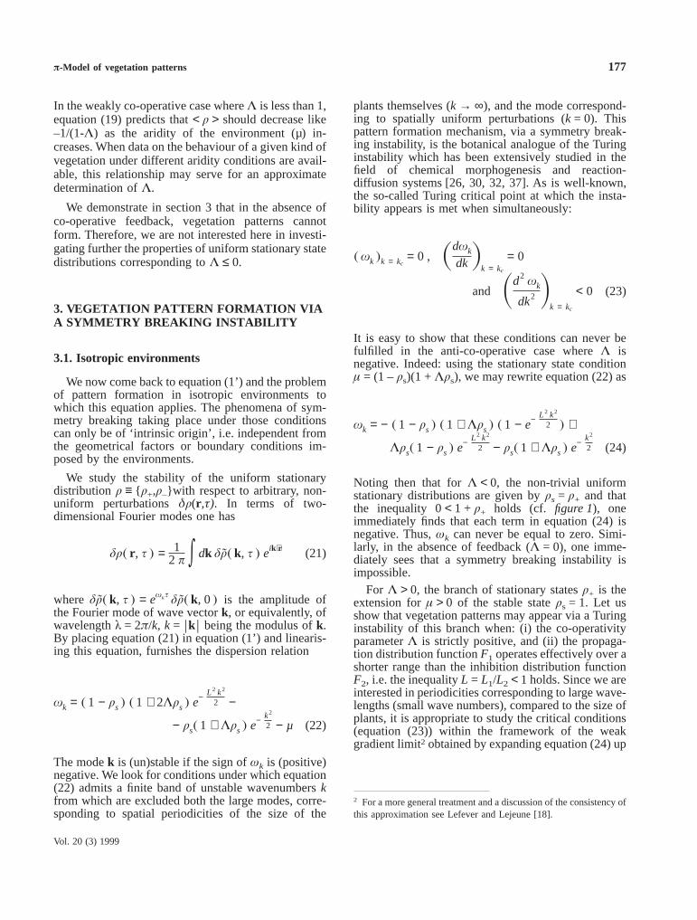
In the weakly co-operative case whereΛ is less than 1,equation (19) predicts that< q > should decrease like–1/(1-Λ) as the aridity of the environment (µ) in-creases. When data on the behaviour of a given kind ofvegetation under different aridity conditions are avail-able, this relationship may serve for an approximatedetermination ofΛ.

We demonstrate in section 3 that in the absence ofco-operative feedback, vegetation patterns cannotform. Therefore, we are not interested here in investi-gating further the properties of uniform stationary statedistributions corresponding toΛ ≤ 0.

3. VEGETATION PATTERN FORMATION VIAA SYMMETRY BREAKING INSTABILITY

3.1. Isotropic environments

We now come back to equation (1’) and the problemof pattern formation in isotropic environments towhich this equation applies. The phenomena of sym-metry breaking taking place under those conditionscan only be of ‘intrinsic origin’, i.e. independent fromthe geometrical factors or boundary conditions im-posed by the environments.

We study the stability of the uniform stationarydistribution q ≡ { q+,q–}with respect to arbitrary, non-uniform perturbationsδq(r ,τ). In terms of two-dimensional Fourier modes one has

dq~ r , s ! = 12 p * dk dq̃~ k, s ! eik⋅r (21)

where dq̃~ k, s ! = exjs dq̃~ k, 0! is the amplitude ofthe Fourier mode of wave vectork, or equivalently, ofwavelengthλ = 2π/k, k = uk u being the modulus ofk.By placing equation (21) in equation (1’) and linearis-ing this equation, furnishes the dispersion relation

xk = ~ 1 − qs! ~ 1 + 2Kqs! e− L2 k2

2 −

− qs~ 1 + Kqs! e− k2

2 − µ (22)

The modek is (un)stable if the sign ofωk is (positive)negative. We look for conditions under which equation(22) admits a finite band of unstable wavenumberskfrom which are excluded both the large modes, corre-sponding to spatial periodicities of the size of the

plants themselves (k → ∞), and the mode correspond-ing to spatially uniform perturbations (k = 0). Thispattern formation mechanism, via a symmetry break-ing instability, is the botanical analogue of the Turinginstability which has been extensively studied in thefield of chemical morphogenesis and reaction-diffusion systems [26, 30, 32, 37]. As is well-known,the so-called Turing critical point at which the insta-bility appears is met when simultaneously:

~ xk !k = kc= 0 , Sdxk

dkDk = kc

= 0

and Sd2 xk

dk2 Dk = kc

< 0 (23)

It is easy to show that these conditions can never befulfilled in the anti-co-operative case whereΛ isnegative. Indeed: using the stationary state conditionµ = (1 –qs)(1 + Λqs), we may rewrite equation (22) as

xk = − ~ 1 − qs! ~ 1 + Kqs! ~ 1 − e− L2 k2

2 ! +

Kqs~ 1 − qs! e− L2 k2

2 − qs~ 1 + Kqs! e− k2

2 (24)

Noting then that forΛ < 0, the non-trivial uniformstationary distributions are given byqs = q+ and thatthe inequality 0< 1 + q+ holds (cf. figure 1), oneimmediately finds that each term in equation (24) isnegative. Thus,ωk can never be equal to zero. Simi-larly, in the absence of feedback (Λ = 0), one imme-diately sees that a symmetry breaking instability isimpossible.

For Λ > 0, the branch of stationary statesq+ is theextension forµ > 0 of the stable stateqs = 1. Let usshow that vegetation patterns may appear via a Turinginstability of this branch when: (i) the co-operativityparameterΛ is strictly positive, and (ii) the propaga-tion distribution functionF1 operates effectively over ashorter range than the inhibition distribution functionF2, i.e. the inequalityL = L1/L2 < 1 holds. Since we areinterested in periodicities corresponding to large wave-lengths (small wave numbers), compared to the size ofplants, it is appropriate to study the critical conditions(equation (23)) within the framework of the weakgradient limit2 obtained by expanding equation (24) up

2 For a more general treatment and a discussion of the consistency ofthis approximation see Lefever and Lejeune [18].

π-Model of vegetation patterns 177

Vol. 20 (3) 1999

to O(k4). This transforms the dispersion relationωkinto the polynomial expression

xk = − 18 q+~ 1 + Kq+ ! k4 + 1

2 @q+~ 1 + Kq+ !

− ~ 1 − q+ ! ~ 1 + 2 Kq+ ! L2# k2

− q+~ 1 − K + 2 Kq+ ! (25)

from which we straightforwardly derive, using the firsttwo conditions of equation (23), that at the Turingcritical point, the wave numberkc of the first modebecoming unstable and the corresponding valueLc ofL read:

kc = F81 − K + 2Kq+

1 + Kq+G(1/4)

(26)

Lc =Î~ 1 + Kq+ − =2~ 1 + Kq+ ! ~ 1 − K + 2Kq+ ! ! q+

~ 1 + q+ ! ~ 1 + 2Kq+ !(27)

The analysis of equations (25–27) demonstratesthat:

(i) Lc is less than one for all physically acceptablevalues ofΛ andq+.

(ii) The values ofq+ close to one, as well as thevalues close to zero, are excluded from the domain ofexistence of the instability.

(iii) In agreement with experimental observations,the wavelength of the patterns (predicted as firstapproximation by the critical wavelengthλc = 2π/kc)increases as the aridity of the environment increases,i.e. for q+ decreasing (µ increasing) andΛ constant.(iv) As figure 2 exemplifies, decreasingL, for fixedvalues ofµ andΛ, in general destabilises the systemand broadens the band of unstable modes.

(v) Different symmetries are possible for the pat-terns establishing themselves in the course of time (forτ → ∞) whenq+ becomes unstable.Figure 3 reports atypical example showing that for a small variation inthe parameter values, the patterns may switch fromstripes to hexagonal symmetry.

The prediction that flat territories can support veg-etation stripes steps aside from the traditional theorythat a ground slope is a necessary factor for theformation of tiger bush [13, 14, 45]. The second kindof pattern, consisting of densely vegetated spots ar-ranged on an hexagonal lattice, could be related tospotted [5] or pearly bush [3]. More recently, this kindof symmetry has been unambiguously identified by

Couteron [7] in Burkina-Faso. We shall illustrate fur-ther the predictions of the model in the next sectionwhere we shall use it to analyse the tiger bush patternsstudied by one of us (P. Couteron) in Burkina Faso.Before, we will very briefly indicate some resultswhich clarify the ‘pattern selection role’ of environ-mental anisotropies.

Figure 2. Band of unstable modesk as a function ofL for µ = 1.1and Λ = 2. For L > Lc, all modes are stable;L = Lc, is the criticalvalue at whichωk = 0 for k = kc; whenL < Lc, the modes betweenkl

and ku are unstable. Vanishingly small modes and arbitrarily largemodes are always stable forL7 0. When the ratio of reproductionand inhibition ranges,L tends to zero,kl decreases to a finite valuedifferent from zero butku diverges. The caseL = 0 needs a specifictreatment and will not be considered here.

Figure 3. Patterns obtained by integrating the isotropicp-model (1′)for l = 0.95,L = 0.1 and two values ofK. The integration domain isa square-shaped territory subjected to periodic boundary conditions.The initial condition is a slightly perturbed uniform stationary statedistribution q+ (Gaussian perturbations of zero mean and 1 %variance). The model predicts a pattern of stripes ifK = 1 and apattern of hexagonal symmetry ifK = 0.8. As a consequence of theisotropy of space, the orientation finally adopted by the stripes andhexagons is determined by the random initial condition. Blackcorresponds to the highest phyto-density.

178 O. Lejeune et al.

Acta Oecologica

3.2. Anisotropic environments

The influence of anisotropy on the symmetry break-ing instability of the isotropicπ-model is best seen byinvestigating the two situations where an environmen-tal source of spatial anisotropy affects either only thepropagation distribution functionF1 or the inhibitiondistribution functionF2. We have proposed a simpletreatment permitting to deal with these situations [18].It consists in introducing a bias in the weightingfunctionsw1, w2 which fixes their mean to a non-zerovalue, respectivelyt1 and t2 for one of the planedirections, say they-direction; in thex-direction, asbefore, no bias is introduced. The evolution equationfor the epigeneous phytomass then becomes:

­s q~ r, s ! = F 12 pL2 * dr ′ e−

x′2 + ~ y′ − t1 !2

2 L2 q~ r + r ′, s !⋅

~ 1 + Kq~ r + r ′, s ! !

× F1 − 12 p * dr ′ e−

x′ 2 + ~ y′ − t2 !2

2 q~ r + r ′, s !G −

µq~ r , s ! (28)

Integrating this equation for the same values ofµ,Λ, L as in the isotropic case considered above, but fortwo choices of values oft1 andt2, we obtain the resultsreported infigure 4. Remarkably, they demonstrate not

Figure 4. Influence of an anisotropic environmental factor oriented in they-direction. The values ofµ, Λ andL are the same as in the isotropiccase described infigure 3; the patterns obtained for an isotropic environment are represented again on the left hand side of the figure (randomlyoriented stripes and hexagons). The patterns in the middle and on the right hand side report the effect of anisotropy respectively on the propagatorfunction (t1 = 1, t2 = 0) and on the inhibitor function (t1 = 0, t2 = 1). In the first case, both the randomly oriented stripes and the hexagons transforminto vegetation stripes parallel to the anisotropy directiony; in the second case, the patterns transform into more or less wavy stripes orthogonalto the anisotropy directiony. Stripes parallel to the direction of anisotropy are globally static whereas orthogonal stripes migrate upward (in thepositivey-direction).

π-Model of vegetation patterns 179

Vol. 20 (3) 1999

only that the presence of anisotropic factors deter-mines the orientation of the patterns and their symme-try properties (stripes replace hexagons) but also thatthe orientation selected is either parallel or orthogonalto the direction of anisotropy depending on whetherthe latter affects propagation or inhibition.

On the other hand, the model also predicts that whenthe anisotropy affecting inhibition increases further,arc-shaped patterns perpendicular to the direction ofanisotropy appear [18]. Vegetation arcs, the main axisof which is orthogonal to a ground slope, have beendescribed by Greenwood [13] and Boaler andHodge [3, 4]. A curvature of the ground surface isusually invoked in order to explain the origin of thesestructures. In contrast with widespread opinion, themodel predicts that arcuate vegetation patterns canappear even if the ground gradient is constant. Finally,we may still mention that vegetation stripes parallel tothe anisotropy direction are static whereas bands andarcs oriented at right angle to that direction moveupward (at least for the sets of parameters consideredin the simulations made so far (unpubl. results)).

4. A CASE STUDY: TIGER BUSH IN BURKINAFASO

The vegetation pattern represented infigure 5 islocated at and around 14°10’ N and 2°28’ W in thenorth-west part of Burkina Faso. Climate is tropicalsemi-arid; mean rainfall amounts to 490 mm⋅year–1

and potential evapotranspiration (Penman) is slightlyunder 2 000 mm⋅year–1 [8]. The vegetation under in-vestigation grows on a gentle slope (around 1 %)located on Paleozoic sandstones. Soils are shallow(between 10 and 20 cm), and poorly developed onferruginised sandstone debris, overtopping the un-weathered sandstone (encountered around 60–80 cmdepth). Vegetation belongs to the Sahel transition zonewith most species related to the Sudanian centre ofendemism [40]; it consists mainly of multistemmedshrubs/trees and of annual grasses. Dominant woodyspecies areCombretum micranthumG. Don, andPterocarpus lucensLepr., which account respectivelyfor 50 and 30 % of the total basal area. Average heightof woody individuals is around 3 m [7]. The siteexperiences a low grazing pressure (mainly goats) butneither wood-cutting nor cultivation.

The aerial photograph was obtained on October 10,1995 around 10h30 (U.T.), i.e. with a zenithal solarangle of about 38°. Pictures were taken from anelevation of 750 m with a Pentax ILX camera (50 mmfocus and 35 mm lens). The film (Kodak Gold 100ASA) was machine-processed into coloured

7.5× 5 cm printed outlooks, which have been numer-ised (grey-scale values in the range 0–255) at aresolution of 300 dots per inch (DPI) through a HPScanjet scanner (pixel side equivalent to 0.8 m in thefield). A square window of 400× 400 pixels (i.e.320× 320 m in the field) was extracted for analysis(figure 5). On the picture, bright pixels correspond tobare soils, whereas dark ones are dominated by woodyvegetation; intermediate grey-scale values can mainlybe interpreted as being dense grass cover. Sincecontinuous grass and woody vegetation have respec-tive epigeneous phytomass averaging 1 500 kg⋅ha–1

and 2⋅104 kg⋅ha–1 ( [19]; Couteron unpubl. data), grey-scale values can be seen as a monotonous function ofthe phytomass.

Fourier coefficients have been computed from themean-corrected valueszjk contained in the digitalimage as:

apq = 1n2 (

j, k

n

zjk cos @2 p~ pjn + qk

n ! #

bpq = 1n2 (

j, k

n

zjk sin @2 p~ pjn + qk

n ! # with n = 400

Figure 5. Banded system under investigation. The picture is ori-ented according to the main slope, with vegetation bands roughlyfollowing the contour. Note that herbaceous vegetation (intermediategrey tones), is mainly observed up-slope the woody thickets (darkgrey).

180 O. Lejeune et al.

Acta Oecologica

The periodogram values (sample spectrum) were cal-culated asIpq = n2(a2

pq + b2pq). In figure 6A, we dis-

play the Ipq-values as an × n grey-tone image (withrescaling in the range 0–255), for which the centrecorresponds top = q = 0. (I00 is set to zero by priorsubtraction of the mean). Such a picture displays asymmetry with respect to the centre sinceIp,–q = I–p,q.Ip′,q′/n

2 represents the portion of the variance of theimage accounted for by the cosine waveCjk withfrequency (p′, q′), i.e. Cjk = cos[2π(p′j/n + q′k/n)]. Aperiodogram with a spike at the pointp = +/–p′ andq = +/–q′ (Ipq = 0 for all other values ofp and q) isassociated to a digital image consisting solely of sucha wave (i.e. a pattern constituted of bands), whosetravel direction isθ = tan–1(p′/q′), while the associated

wavenumber isr = =p2+ q2. Hence Ipq can also beexpressed asGrθ. For a simple banded pattern, thedominant entry of the periodogram should indicate adirectionθ perpendicular to the bands (i.e. accountingfor the heterogeneity of the image) and a periodicityrcorresponding to the number of bands within thewindow. To enhance the interpretability of the results,polar spectra [29] have also been computed by binningGrθ values into polar segments, as –5°< θ ≤ 5°, ...,345°< θ ≤ 355° and 0< r ≤ 1, 1< r ≤ 2, etc.

The banded pattern under consideration yielded aperiodogram dominated by two groups of entries(figure 6A). A spike in the radial spectrum (figure 6B)for wave numbers 4 and 5 revealed a dominantwavelength ranging between 64 (i.e. 320/5) and 70 m.A main orientation between 90° and 100° was deducedfrom the angular spectra (figure 6C; dotted line corre-sponds to the isotropic situation). The average phyto-mass density< q > evaluated by redistributing thevegetation uniformly over the territory gives forq+ anapproximate value of 0.3. In summary, the spectral

analysis offigure 5 allows us to conclude that thevegetation pattern corresponds to

k = 70m and q+ ≈ <q> ≈ 0.3 (29)

Using these values we may now evaluate the propa-gator and inhibitor rangesL1 andL2 of the vegetation,as well as its co-operativityΛ. Transforming equations(26) and (27) to real space, we rewrite them as

L2

kc= 1

p F12

1 − K + 2Kq+1 + Kq+

G1/4

(30)

L1

L2=Î~ 1 + Kq+ − =2~ 1 + Kq+ ! ~ 1 − K + 2Kq+ ! ! q+

~ 1 − q+ ! ~ 1 + 2Kq+ !(31)

where λc is now expressed in physical space units.Since the value ofq+ is fixed by the spectral analysis,cf. equation (29), the right hand sides of these expres-sions is a function ofΛ only. Furthermore, in equation(30), we may equateλc to the measured wavelengthλgiven by equation (29). This procedure is exact at theTuring critical point. Below this point, when a finiteband of unstable modes (forL < Lc) exists, the value ofλc is generally close to that of the fastest growingmode and the relationshipλ = λc remains, even then, agood fit. On the other hand, the existence on the terrainof a small ground slope means that in reality theenvironment is anisotropic. The influence on the pat-tern wavelength of this anisotropy, asfigure 4 sug-gests3, can be neglected in a first approach such as the

3 Passing from the isotropic situation to the cases where thepropagation and inhibition densities are markedly anisotropic pro-duces no significant variation of the pattern wavelength.

Figure 6. Spectral analysis of the tiger bush represented infigure 5.

A. Periodogram B. Radical spectrum C. Angular spectrum

π-Model of vegetation patterns 181

Vol. 20 (3) 1999

one presented here. This point will be discussed in aforthcoming publication. Hence, by setting in equa-tions (30) and (31),q+ = 0.3,λc = 70 m, we solve theseequations forL1 andL2 in terms ofΛ. Figure 7reportsthe values ofL1 andL2 obtained in this manner. Onefinds that the values ofΛ andL1 for which the modelpredicts the existence of patterns are given by theinequalities

1011 < K < 2.5 and 0 m< L1 < 4 m (32)

In agreement with the general discussion presentedabove, in this domainL2 ranges between 0 and 18 mand the inequalityL2 > L1 always holds. One also seesthat for a fixed value ofL1, figure 7 predicts thepossible existence of two distinct values forΛ, andhence forL2.

The value ofL1 andL2 can be further discussed inlight of the field data. In semi-arid and arid situations,short-range co-operativity is likely to result from thefavourable influence exerted by the crown of a maturewoody individual on the surrounding vegetation. Suchinfluences have been extensively studied with respectto herbaceous vegetation (see [39] for a review), butthe results are likely to also hold for woody seedlings.On the other hand, long-range inhibition may resultfrom adverse influences exerted by the root system ofa pre-existing mature individual. Data regarding rootsystems are scarce, but it is well established that lateralroots do extend far beyond the limit of the crown [12,31]. Furthermore, having lateral roots extending out-side the crown (i.e.L2 > L1) may be an outcome of

aridity [1], a recording that may explain why periodicvegetation patterns are so frequent in arid and semi-arid zones.

On our field site, we found an average value of1.2 m for the radius of the crown of matureC.micranthum(the dominant species), and 1.3 m for allmature individuals, irrespective of species [7]. Sincefavourable influences are supposed to extend signifi-cantly up to 2L1 due to the properties of the Gaussiandistribution, it is reasonable to considerL1 < 1 m. Sucha range of values yields two contrasting sets ofsolutions forΛ andL2, which correspond either to low(Λ < 1) or to high (Λ ≈ 2.5) co-operativity. Low co-operativity determines high values forL2, around15 m, whilst high co-operativity implyL2 < 4 m. In thefirst case, the range of significant inhibition, 2L2, andhence of lateral root extension, should extend up to30 m. So a large extension, though not impossible, isnot reported in the literature, even for more aridconditions [12], whilst a lateral root extension between2 m and 8 m is fully consistent with most publishedresults. As a consequence, the high co-operativitysituation appears more realistic in the light of theavailable data.

Acknowledgments

The support of the ‘Instituts Internationaux de Physique et deChimie’, Solvay, and of the Centre for Nonlinear Phenomena andComplex Systems (U.L.B.) is gratefully acknowledged.

REFERENCES

[1] Belsky A.J., Influence of trees on savanna productivity: testsof shade, nutrients, and tree-grass competition, Ecology 75(1994) 922–932.

[2] Bernd J., The problem of vegetation stripes in semi-aridAfrica, Plant Res. Dev. 8 (1978) 37–50.

[3] Boaler S.B., Hodge C.A.H., Vegetation stripes in Somaliland,J. Ecol. 50 (1962) 465–474.

[4] Boaler S.B., Hodge C.A.H., Observations on vegetation arcsin the northern region, Somali Republic, J. Ecol. 52 (1964)511–544.

[5] Clos-Arceduc M., Étude sur photographies aériennes d’uneformation végétale sahélienne : La brousse tigrée, Bull. Inst.Afr. noire Sér. A 18 (1956) 677–684.

[6] Cornet A.F., Delhoume J.P., Montaña C., Dynamics of stripedvegetation patterns and water balance in the Chihuahuandesert, in: During H.J., Werger M.J.A., Willems J.H. (Eds.),Diversity and Pattern in Plant Communities, SPB AcademicPublishing, The Hague, 1988, pp. 221–231.

[7] Couteron P., Relations spatiales entre individus et structured’ensemble dans des peuplements ligneux soudano-sahéliensau nord-ouest du Burkina Faso, Ph.D. thesis, University ofToulouse, France, 1998, 223 p.

[8] Couteron P., Kokou K., Woody vegetation spatial patterns ina semi-arid savanna of Burkina Faso, West Africa, Plant Ecol.132 (1997) 211–227.

Figure 7. Range of interactionsL1 and L2 as a function ofΛ for< q > = 0.3 and λ = 70 m. The inset is a blow-up showing thebehaviour nearΛ = 2.5.

182 O. Lejeune et al.

Acta Oecologica

[9] Fife P.C., Mathematical Aspects of Reacting and DiffusingSystems. Lecture Notes in Biomathematics 28, Springer-Verlag, Berlin, 1979.

[10] Galle S., Seghieri J., Dynamics of soil water content inrelation to annual vegetation: the tiger bush in the SahelianNiger, Ann. Geophys. 12 (suppl. II) (1994) C443.

[11] Gavaud M., Étude pédologique du Niger Occidental, Éditionsde l’Orstom, Dakkar-Hann, 1966.

[12] Glover P.E., The root systems of some British-Somalilandplants-IV, East Afr. Agr. J. 17 (1951) 38–50.

[13] Greenwood J.E.G.W., The development of vegetation inSomaliland Protectorate, Geogr. J. 123 (1957) 465–473.

[14] Greig-Smith P., Pattern in vegetation, J. Ecol. 67 (1979)755–779.

[15] Hemming C.F., Vegetation arcs in Somaliland, J. Ecol. 53(1965) 57–67.

[16] d’Herbès J.M., Valentin C., Thiéry J.M., La brousse tigrée auNiger : synthèse des connaissances acquises. Hypothèse sur lagenèse et les facteurs déterminant les différentes structurescontractées, in: d’Herbès J.M., Ambouta J.M.K., Peltier R.(Eds.), Fonctionnement et gestion des écosystèmes contractéssahéliens, John Libbey Eurotext, Paris, 1997, pp. 131–152.

[17] Hoppensteadt F.C., Peskin C.S., Mathematics in Medicine andthe Life Sciences. Texts in Applied Mathematics 10, Springer-Verlag, Berlin, 1992.

[18] Lefever R., Lejeune O., On the origin of tiger bush, Bull.Math. Biol. 59 (1997) 263–294.

[19] Le Houerou H.N., The Grazing Land Ecosystems of theAfrican Sahel, Springer-Verlag, Berlin, 1989, 282 p.

[20] Litchfield W.H., Mabbutt J.A., Hardpan in soils of semi-aridWestern Australia, J. Soil Sci. 13 (1962) 148–159.

[21] Mabbutt J.A., Fanning P.C., Vegetation banding in aridWestern Australia, J. Arid Environ. 12 (1987) 41–59.

[22] Macfadyen W.A., Soil and vegetation in British Somaliland,Nature 165 (1950) 121.

[23] Macfadyen W.A., Vegetation patterns in the semi-desert plainsof British Somaliland, Geogr. J. 116 (1950) 199–211.

[24] Mauchamp A., Rambal S., Lepart J., Simulating the dynamicsof a vegetation mosaic: a spatialized functional model, Ecol.Model. 71 (1994) 107–130.

[25] May R.M., Stability and Complexity in Model Ecosystems,Princeton University Press, New Jersey, 1973.

[26] Meinhardt H., Models of Biological Pattern Formation, Aca-demic Press, New York, 1982.

[27] Montaña C., The colonization of bare areas in two-phasemosaics of an arid ecosystem, J. Ecol. 80 (1992) 315–327.

[28] Montaña C., Lopez-Portillo J., Mauchamp A., The response oftwo woody species to the conditions created by a shiftingecotone in an arid ecosystem, J. Ecol. 78 (1990) 789–798.

[29] Mugglestone M.A., Renshaw E., Detection of geologicallineations on aerial photographs using two-dimensional spec-tral analysis, Comput. Geosc. 24 (1998) 771–784.

[30] Murray J.D., Mathematical Biology. Biomathematics Texts19, Springer-Verlag, Berlin/New York, 1989.

[31] Poupon H., Structure et dynamique de la strate ligneuse d’unesteppe sahélienne au nord du Sénégal, Orstom, Paris, 1980,351 p.

[32] Prigogine I., Structure, dissipation and life, in: Marois M.(Ed.), Theoretical Physics and Biology, North-Holland, Am-sterdam, 1969.

[33] Ruxton B.P., Berry L., The Butana grass patterns, J. Soil Sci.11 (1960) 61–62.

[34] Schlesinger W.H., Reynolds J.F., Cunningham G.L., Huen-neke L.F., Jarrell W.M., Virginia R.A., Whitford W.G., Bio-logical feedbacks in global desertification, Science 247 (1990)1043–1048.

[35] Thiéry J.M., d’Herbès J.M., Valentin C., A model simulatingthe genesis of banded vegetation patterns in Niger, J. Ecol. 83(1995) 497–507.

[36] Tongway D.J., Ludwig J.A., Vegetation and soil patterning insemi-arid mulga lands of Eastern Australia, Aust. J. Ecol. 15(1990) 23–34.

[37] Turing A.M., The chemical basis of morphogenesis, Philos.Trans. R. Soc. Lond. Ser. B 237 (1952) 37–72.

[38] Van Der Meulen F., Morris J.W., Striped vegetation patterns ina Transvaal savanna, Geo. Eco. Trop. 3 (1979) 253–266.

[39] Vetaas O.R., Micro-site effects of trees and shrubs in drysavannas, J. Veg. Sci. 3 (1992) 337–344.

[40] White F., The Vegetation of Africa. A Descriptive Memoir toAccompany the Unesco/AEFTAT/UNSO Vegetation Map,Unesco/AEFTAT/UNSO, Paris, 1983, 356 p.

[41] White L.P., Vegetation arcs in Jordan, J. Ecol. 57 (1969)461–464.

[42] White L.P., Brousses tigréespatterns in southern Niger, J.Ecol. 58 (1970) 549–553.

[43] White L.P., Vegetation stripes on sheet wash surfaces, J. Ecol.59 (1971) 615–622.

[44] Wickens G.E., Collier F.W., Some vegetation patterns in theRepublic of the Sudan, Geoderma 6 (1971) 43–59.

[45] Worrall G.A., The Butana grass patterns, J. Soil Sci. 10 (1959)34–53.

[46] Worrall G.A., Patchiness in vegetation in the northern Sudan,J. Ecol. 48 (1960) 107–115.

[47] Worrall G.A., Tree patterns in the Sudan, J. Soil Sci. 11 (1960)63–67.

π-Model of vegetation patterns 183

Vol. 20 (3) 1999