Non-parametric Estimation for the Location of a Change-point in an Otherwise Smooth Hazard Function...

Non-parametric Estimation for the Locationof a Change-point in an Otherwise SmoothHazard Function under Random Censoring

ANESTIS ANTONIADIS

IMAG-LMC, University Joseph Fourier, Grenoble

IREÁ NE GIJBELS

Institute of Statistics, U. C. L., Louvain-La-Neuve

BRENDA MACGIBBON

University of Quebec at Montreal

ABSTRACT. A non-parametric wavelet based estimator is proposed for the location of a

change-point in an otherwise smooth hazard function under non-informative random right

censoring. The proposed estimator is based on wavelet coef®cients differences via an

appropriate parametrization of the time-frequency plane. The study of the estimator is

facilitated by the strong representation theorem for the Kaplan±Meier estimator established

by Lo and Singh (1986). The performance of the estimator is checked via simulations and

two real examples conclude the paper.

Key words: change-points, hazard function, right-censoring, wavelet coef®cients

1. Introduction

An important practical issue of many research papers in survival analysis is the study of

the risk patterns of disease or other events in time. Although most display results with

plots of the survival function (Kaplan & Meier, 1958) or the cumulative hazard function

(Nelson, 1972), a careful study of the hazard function itself would be bene®cial in many

cases as argued by Efron (1980). The hazard function of time-related events is often time-

varying in a structured fashion, which can sometimes be decomposed into additive phases.

Each phase is in general shaped by a different generic hazard function and the transition or

jump from one phase to the other (the change-point) is in general dif®cult to locate. One

way to conduct inference in such hazard rate change-point models is to use non-parametric

estimation procedures whose nature allow great ¯exibility in the possible form of the

generic functions modelling each phase.

MuÈller & Wang (1990) estimate the point of the most rapid change of a hazard function via

the location of an extremum of a non-parametric estimator of the derivative of the hazard

function. MuÈller & Wang (1994) considered the estimation of the location of a discontinuity in a

hazard function that is supposed to be left and right continuous at an unknown jump point. Their

analysis is based on differences of two one-sided kernel type estimators of the hazard function

and their change-point estimator is shown to be weakly consistent with a rate of convergence

that is faster than nÿ1=2 where n denotes the sample size. The procedure they propose is adopted

from the one MuÈller (1992) has developed for ` standard'' non-parametric regression. An

enhancement of their procedure for the regression setting has been proposed recently by Loader

(1996) and could possibly be adapted to the case of hazard function estimation.

In the regression setting, the theory of wavelets has been used recently to detect jumps or

# Board of the Foundation of the Scandinavian Journal of Statistics 2000. Published by Blackwell Publishers Ltd, 108 Cowley Road,

Oxford OX4 1JF, UK and 350 Main Street, Malden, MA 02148, USA Vol 27: 501±519, 2000

cusps in an otherwise smooth regression function. Using the fact that the oscillating property as

well as the multi-resolution structure allows a precise characterization of local regularity of a

signal in terms of its wavelet coef®cients, several authors (Mallat & Hwang, 1992; Wang, 1995;

Raimondo, 1996; Antoniadis & Gijbels, 1997) have proposed jump-point detection procedures

to estimate singularities in signals observed with noise. In all the regression setting papers

mentioned above, the models have been formulated by means of additive i.i.d. Gaussian noise.

The estimation of a smooth hazard function by wavelet methods has been addressed by

Antoniadis et al. (1994), and more recently by Antoniadis et al. (1999), but to our knowledge

there are no papers (yet) dealing with wavelet detection of change-points in hazard function with

censored observations, which is the primary goal of this paper.

For the sake of clarity, we consider here the simplest case of a single jump or a sharp cusp in

an otherwise smooth hazard function which presents some regularity before and after the

location of the change-point. It is, however, clear that our method can be easily extended to the

case where a jump or a sharp cusp occurs in higher derivatives of the hazard function.

The organization of the paper is as follows. In section 2 we introduce the notation and the

random censoring set-up, and present an i.i.d. strong representation of the Nelson estimator of

the cumulative hazard function, established by Lo et al. (1989), which will be needed later for

the study of the wavelet estimator proposed. Section 3 recalls some basic facts from Raimondo

(1996) on the behaviour of wavelet coef®cients differences for functions presenting local

singularities. These results have been adapted to the case of a function that presents an abrupt

discontinuity or a sharp cusp. The main results are discussed in section 4. The ®nal section is

devoted to the presentation of some simulations and to the analysis of some real examples.

Proofs are collected in the appendix.

2. Some preliminaries on hazard rates and change-points

Let T1, . . ., Tn be i.i.d. lifetimes with cumulative distribution function (c.d.f.) F, and let

C1, . . ., Cn be i.i.d. censoring times with c.d.f. G. Assume also that the Tis and Cis are

independent. The observed data is a realization of f(X i, äi), i � 1, . . ., ng with

X i � min(Ti, Ci), äi � IfX i�Tig � IfTi<Cig,

where IA denotes the indicator function of a set A. We will also assume that F is

absolutely continuous and we will denote by f its density with respect to Lebesque

measure. Denote by Ë the cumulative hazard function de®ned by

Ë(x) � ÿlog(1ÿ F(x)),

and let ë be the associated hazard rate function de®ned by

ë(x) � d

dx(Ë(x)) � f (x)

F(x), for x such that F(x) , 1,

where F(x) � 1ÿ F(x).

A change-point in a hazard function refers here to a localized jump or a sharp cusp in an

otherwise smooth hazard function. The change-point model that we are going to consider may

be de®ned as follows.

Let K, k, M , s, á, 0 < á, s < 1 be positive constants and denote by I an interval of the real

line R. The class of real functions presenting a single jump or a sharp cusp in the interior of I ,

say 8I, will be denoted by F s,á(K, k, M , I). More precisely, a function f belongs to the class

F s,á(K, k, M , I) if and only if, there exists a unique è f 2 8I such that:

502 A. Antoniadis et al. Scand J Statist 27

# Board of the Foundation of the Scandinavian Journal of Statistics 2000.

(1) there exists h0 . 0 such that for all h with jhj < h0 we have j f (è f ÿ h) ÿf (è f � h)j > Kj2hjá;

(2) for all (x, y) 2 I 3 I such that è f =2 [x, y] we have j f (x)ÿ f (y)j < kjxÿ yjs;(3) k f k1 � supx2 I j f (x)j < M .

Remark 1. Note that we assume that the regularity condition of the function with a jump or a

cusp is the same before and after the location of the singularity. This assumption can be easily

relaxed: if the HoÈlder exponents of a function before and after the change-point are s1 and s2

respectively everything remains valid by taking s � min(s1, s2) in the above de®nition of the

class F s,á(K, k, M , I).

The constants K, k and M will be assumed to be ®xed and, without loss of generality the

interval I will be assumed equal to [0, 1]. For ease of notation the class F s,á(K, k, M , I) will

be denoted F s,á hereafter.

We will assume henceforth that ë 2 F s,á(K, k, M , I) where I � [0, T ] with T ,

inffx > 0; L(x) � 1g equal to the right end of the support of the distribution function L of the

X is. To simplify the notation we will assume without any loss of generality that T � 1. We will

also denote by

L1(x) � P(X i < x, äi � 1)

the subdistribution function of the uncensored observations.

The assumption that ë belongs to the class F s,á leads naturally to a wavelet detection of

jumps based on the results of the next section. The basic idea for estimating the location of the

jump or the cusp consists in looking at the wavelet coef®cient differences for an appropriate

estimator of ë. Since these differences are of a smaller order of amplitude, except at the change-

point, it can be expected that the maximum of these differences occurs near the location of the

change-point. This reasoning will lead to the change-point estimator èë to be de®ned and

studied in section 4.

A basic tool for studying the behaviour of the estimates of the wavelet coef®cient differences

for ë will be an asymptotic representation of the product-limit (Nelson) estimator of the

cumulative hazard rate function established by Lo & Singh (1986) (see also the paper by Lo et

al. (1989)). Using the same notation as in these papers, let

g(x) ��x

0

dL1(s)

L(s)2, (1)

where L(x) � P(X i . x) � F(x)G(x) � P(Ti . x, Ci . x).

For positive real z and x, and ä taking values 0 or 1, let

î(z, ä, x) � g(min(z, x))� [L(z)]ÿ1Ifz<x,ä�1g, (2)

and set îi(x) � î(X i, äi, x). Note that the random variables îi are i.i.d. and uniformly

bounded on [0, 1]. Moreover, it is easy to see that E(îi(x)) � 0 and cov(îi(x),

îi(y)) � g(min(x, y)). In the sequel we will use the improved version of th. 1 of Lo &

Singh (1986), as it is proved in lem. 2.1 of Lo et al. (1989), which we state here for the

sake of completeness.

Let Ën denote the Nelson (1972) estimator of the cumulative hazard function Ë, given by

Ën(x) �X

X (i)<x

ä( i)

nÿ i� 1,

Scand J Statist 27 Estimating the location of change-points 503


where X (i) denotes the ith order statistic of X 1, . . ., X n and ä(i) the corresponding

censoring indicator variable. We then have, for all x 2 [0, 1]:

Ën � Ë(x)� 1

n

Xn

i�1

îi(x)� rn(x), (3)

where

supx2[0,1]

jrn(x)j � Olog n

n

� �, a:s: (4)

and for any â > 1,

supx2[0,1]

E(jrn(x)jâ) � Olog n

n

� �â !:

To end this preliminary results section we state the integration by parts lemma of FoÈldes et al.

(1981) which by now is a standard device in the hazard function estimation literature:

If G and H are non-decreasing mappings from R into R and if ÿ1, c , d ,1, then�[c,d]

G (x�) dH (x)��

[c,d]

H (xÿ) dG (x) � G (d�)H (d�)ÿ G (dÿ)H (dÿ), (5)

where G (x�) (resp. G (xÿ)) denotes the right- (resp. left-) hand limit of G at the point x.

3. Differences in wavelet coef®cients

We ®rst recall some results on wavelet coef®cients differences characterizing jumps or

sharp cusps of a function in F s,á. In this study of hazard rate change-points, we will

follow closely the presentation of Raimondo (1996), adapting it to our case. Note that only

the oscillating property and the multiresolution structure of the compactly supported spline

scaling function are used; the orthogonality of the associated wavelet basis is not used at

all.

We consider a smooth enough compactly supported scaling function whose ®rst order

derivative generates an admissible zero-mean wavelet. To be precise, the scaling function ö used

to derive our results will be a cubic B-spline (De Boor, 1978) whose support is the interval

[ÿ1, 1] and whose integral is equal to 1. Mallat & Hwang (1992) have also adopted such a cubic

B-spline for extrema detection. The ®rst order derivative ø � dö=dx of such a function

generates a compactly supported admissible wavelet. Figure 1 displays the scaling function öand the associated wavelet ø. Since a cubic B-spline is positive, we have�ö(x) dx � � jö(x)j dx � 1. Moreover, the function ö is smooth in the sense that it admits

derivatives of any order.

By translating and changing its scale we generate from ö a doubly-indexed family of scaling

functions and corresponding wavelets as follows:

ö j,k(x) � 2 j=2ö(2 jxÿ k), j > 0, k 2 Z,

ø j,k(x) � 2 j=2ø(2 jxÿ k), j > 0, k 2 Z,

Note that since ö and ø are supported on [ÿ1, 1], we have

Support (ö j,k) � Support (ø j,k) � ÿ1� k

2 j,

1� k

2 j

� �:



The scaling and wavelet coef®cients of a square-integrable function f are respectively

de®ned by:

s j,k ��

f (x)ö j,k(x) dx and d j,k ��

f (x)ø j,k(x) dx:

To characterize functions of F s,á, de®ned in section 2, via their scaling or wavelet

coef®cients, we will use the parametrization of time-scale space presented in Raimondo

(1996). For k 2 Z, let ô(k) � 2k � 1 and consider the following coef®cient differences:

Ä j,k( f ) � s j,ô(k) ÿ s j,ô(k�2)

��

f (x)ö j,ô(k)(x) dxÿ�

f (x)ö j,ô(k�2)(x) dx ��

f (x)Ö j,k(x) dx, (6)

where Ö j,k � ö j,ô(k) ÿ ö j,ô(k�2). Note that

Support (Ö j,k) � 2k

2 j,

2k � 2

2 j

� �[ 2k � 4

2 j,

2k � 6

2 j

� �:

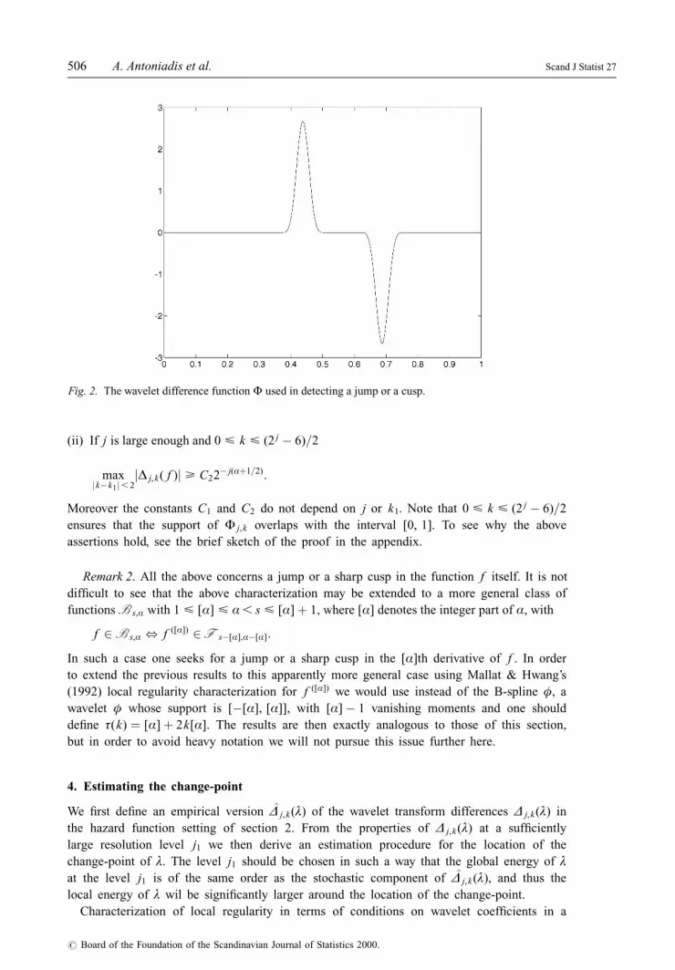
Figure 2 displays a typical graph of the function Ö j,k . It is the gap between the intervals

that allows the characterization of sharp cusps via the wavelet coef®cient differences

Ä j,k( f ) de®ned in (6). Indeed, for any positive resolution j and for any f 2 F s,á let us

denote by k1 the (unique) integer such that

è f 2 ô(k1)� 1

2 j,ô(k1)� 3

2 j

� �:

Then there exist two positive constants C1 and C2 such that:

(i) For all j . 0 and 0 < k < (2 j ÿ 6)=2 we have:

maxjkÿk1j>2

jÄ j,k( f )j < C12ÿ j(s�1=2):

Fig. 1. The scaling function ö and the associated wavelet ø.



(ii) If j is large enough and 0 < k < (2 j ÿ 6)=2

maxjkÿk1j, 2

jÄ j,k( f )j > C22ÿ j(á�1=2):

Moreover the constants C1 and C2 do not depend on j or k1. Note that 0 < k < (2 j ÿ 6)=2

ensures that the support of Ö j,k overlaps with the interval [0, 1]. To see why the above

assertions hold, see the brief sketch of the proof in the appendix.

Remark 2. All the above concerns a jump or a sharp cusp in the function f itself. It is not

dif®cult to see that the above characterization may be extended to a more general class of

functions B s,á with 1 < [á] < á, s < [á]� 1, where [á] denotes the integer part of á, with

f 2 B s,á , f ([á]) 2 F sÿ[á],áÿ[á]:

In such a case one seeks for a jump or a sharp cusp in the [á]th derivative of f . In order

to extend the previous results to this apparently more general case using Mallat & Hwang's

(1992) local regularity characterization for f ([á]) we would use instead of the B-spline ö, a

wavelet ö whose support is [ÿ[á], [á]], with [á]ÿ 1 vanishing moments and one should

de®ne ô(k) � [á]� 2k[á]. The results are then exactly analogous to those of this section,

but in order to avoid heavy notation we will not pursue this issue further here.

4. Estimating the change-point

We ®rst de®ne an empirical version Ä j,k(ë) of the wavelet transform differences Ä j,k(ë) in

the hazard function setting of section 2. From the properties of Ä j,k(ë) at a suf®ciently

large resolution level j1 we then derive an estimation procedure for the location of the

change-point of ë. The level j1 should be chosen in such a way that the global energy of ëat the level j1 is of the same order as the stochastic component of Ä j,k(ë), and thus the

local energy of ë wil be signi®cantly larger around the location of the change-point.

Characterization of local regularity in terms of conditions on wavelet coef®cients in a

Fig. 2. The wavelet difference function Ö used in detecting a jump or a cusp.



continuous white noise model has also been used by Wang (1995) for detecting cusps in a

classical non-parametric regression setting. The results of Jaffard (1989), however, show that the

existence of an irregularity at a given point for an otherwise smooth function does not imply

that the wavelet coef®cients of this function near the irregularity will be large for an arbitrarily

®ne scale (see also Antoniadis & Gijbels (1997)). Our results show, although they are designed

for a censored regression setting, that the latter property is satis®ed by wavelet coef®cient

differences provided the analysing wavelet has enough vanishing moments. It involves an

appropriate reparametrization of the scale-scale plane, introducing a ` gap'' in the supports of

our analysing functions. The use of this ` gap'' also distinguishes our method from kernel/local

polynomial approaches proposed in the literature for detecting change-points in otherwise

smooth hazard functions (see MuÈller & Wang 1990).

Using the notation of section 3, we may write:

Ä j,k(ë) � hë, Ö j,ki ��ë(x)Ö j,k(x) dx �

�Ö j,k(x) dË(x):

The support of Ö j,k is included within the interval

ô(k)ÿ 1

2 j,ô(k � 2)� 1

2 j

� �:

Using the integration by parts formula (5) we obtain

Ä j,k(ë) ��

[(ô(k)ÿ1)=2 j ,(ô(k�2)�1)=2 j

Ö j,k(x) dË(x) � ÿ�

[(ô(k)ÿ1)=2 j,(ô(k�2)�1)=2 j]

Ë(xÿ) dÖ j,k(x)

�Ö j,k

ô(k � 2)� 1

2 j

� �Ë

ô(k � 2)� 1

2 j

� �ÿÖ j,k

ô(k)ÿ 1

2 j

� �Ë

ô(k)ÿ 1

2 j

� �

� ÿ�Ë(x) dÖ j,k(x):

This alternative form of Ä j,k(ë) allows us now to de®ne an appropriate version of the

empirical coef®cient differences, namely:

Ä j,k(ë) � Ä j,k � ÿ�Ën(uÿ) dÖ j,k(u) �

�Ö j,k(x) dËn(u),

with Ën the Nelson estimator of Ë as de®ned in section 2. For practical use it is more

convenient to rewrite Ä j,k , as follows:

Ä j,k �Xn

i�1

Ö j,k(X (i))ä(i)

nÿ i� 1: (7)

We will use the notation în(x) for nÿ1Pn

i�1îi(x) with îi(x) the random variables de®ned in

(2). Using the strong representation result (3) for Ën we may write:

Ä j,k � ÿ�Ë(u) dÖ j,k(u)ÿ

�în(uÿ) dÖ j,k(u)ÿ

�rn(uÿ) dÖ j,k(u)

� Ä j,k(ë)ÿ�în(uÿ) dÖ j,k(u)ÿ

�rn(uÿ) dÖ j,k(u),

which splits the empirical coef®cient differences into a deterministic term and a stochastic

term. We already know that the deterministic term has an exponential decay in j for any

HoÈlder continuous function. What remains to be seen is the behaviour of the stochastic

term in order to select the appropriate level j1 for which



maxk�0,..., (2 j1ÿ6)=2

jÄ j1,k(ë)j

is of the same order as

maxk�0,..., (2 j1ÿ6)=2

jV j1,k j,

where

V j,k � ÿ�în(uÿ) dÖ j,k(u)ÿ

�rn(uÿ) dÖ j,k(u):

Note that, for any level j the coef®cients are only computed for k � 0, . . ., (2 j ÿ 6)=2,

since these are the only indices for which the support of Ö j,k overlaps with the interval

[0, 1].

To study the random variable V j,k we will separate it into two parts U j,k and W j,k de®ned by:

U j,k � ÿ�în(uÿ) dÖ j,k(u)

W j,k � ÿ�

rn(uÿ) dÖ j,k(u):

Since the stochastic process în is centred, the random variables U j,k have zero-mean. Let

k and l be two indices between 0 and (2 j ÿ 6)=2 and let us compute for the same

resolution level j, the covariance of U j,k and U j, l, cov(U j,k , U j, l) � E(U j,k , U j, l). Out ®rst

task is to show that the covariance of the U j,k and U j, l (k 6� l) is zero. (See proof in the

appendix).

When k � l, using the zero moment property of ø and Fubini's formula we obtain:

var(U j,k) � 22 j

n

�2k�2

2k

g(v=2 j)ø(vÿ 2k ÿ 1)(ö(1)ÿ ö(vÿ 2k ÿ 1)) dv

� 22 j

n

�2k�6

2k�4

g(v=2 j)ø(vÿ 2k ÿ 5)(ö(1)ÿ ö(vÿ 2k ÿ 5)) dv

� ÿ22 j

n

�1

ÿ1

[g(v=2ÿ j)(v� 2k � 5))� g(2ÿ j(v� 2k � 1))]ø(v)ö(v) dv:

By de®nition the function g is differentiable. Using Taylor's formula with integral

remainder we obtain the following bound for var(U j,k):

var(U j,k) < 22 j

n

�1

ÿ1

1

2 j

��v�1

0

g9(2ÿ j(2k � 1� vw) dw

� (v� 4)

�1

0

g9(2ÿ j(2k � 1� (v� 4)w) dwø(v)

��ö(v) dv <C

n,

where

C � 2 maxj;k�0,..., (2 jÿ6)=2

�1

ÿ1

��v�1

0

g9(2ÿ j(2k � 1� vw) dw

� (v� 4)

�1

0

g9(2ÿ j(2k � 1� (v� 4)w) dwø(v)

��ö(v) dv, (8)

which is ®nite since g9 is bounded on [0, 1].

By asymptotic normality of the sequence of stochastic processes (în(x); x 2 [0, 1]), it follows



that for any resolution level j, the sequence (U j,k)k�0,..., (2 jÿ6)=2 is asymptotically (in n) a

sequence of Gaussian independent random variables. Using the extremal results for independent

normal variables of Leadbetter et al. (1983), and letting j tend to in®nity at a log2 n rate we

have:

limn!1 P maxjU j,k j, (2C log n)1=2

n1=2

� �� 1: (9)

To end the study of the stochastic part of Ä j,k , note that

jW j,k j �� rn(uÿ) dÖ j,k(u)

�� < supjrn(u)j�jdÖ j,k(u)j < 2 j=2 supjrn(u)j

�jø(x)j dx:

Now by taking 2ÿ j ' ((log n)=n)1=(1�2=á) and recalling that by Lo et al. (1989),

krnk1 � O ((log n)=n) a.s., it is easy to see that the above integral behaves as

o((log n=n)1=2). By grouping the upper bounds of the stochastic terms U j,k and W j,k and

taking

j1(n) � log2(n=log n)

2á� 1

we conclude that:

limn!1 P max

k�0,..., (2 j1ÿ6)=2jV j1,k j < O

(log n)1=2

n1=2

� � !� 1: (10)

We may now state the following proposition whose proof is given in the appendix:

Proposition 1

Let ë 2 F s,á(K, k, M , [0, 1]) and j1(n) � [(log2(n=log n))=(2á� 1)]. Let k1 be the unique

integer such that èë 2 [2ÿ j1 (ô(k1)� 1), 2ÿ j1 (ô(k1 � 2)� 1)]. Then there exist two positive

constants C91 and C92 such that

(i)

maxk2f0,..., (2 j1ÿ6)=2g;jkÿk1j>2

jÄ j1,k(ë)j < C91log n

n

� �1=2

(ii)

supk2f0,..., (2 j1ÿ6)=2g;jkÿk1j, 2

jÄ j1,k(ë)j > C92log n

n

� �1=2

:

Our change-point location estimator is now de®ned as follows. Let j1(á, n) be the resolution

level given in proposition 1. We set

k n � arg maxk2f0,..., (2 j1ÿ6)=2g

jÄ j1,k j, (11)

and

èn � ô( k n)� ô( k n � 2)� 2

2 j1�1: (12)

Our next theorem proves that èn as de®ned by (12) is consistent with the rate

(log n=n)1=(2á�1) which is a little bit faster than the rate obtained by MuÈller & Wang

(1994).



Theorem 1

Using the notation of proposition 1, and assuming further that the constants K and k are

such that C92 > C91 � 2��2Cp

, we have

limn!1 sup

ë2F s,á

P(vÿ1n jèn ÿ èëj < 6) � 1,

with vn � (log n=n)1=(1�2á).

Recalling the de®nition of the constants C91, C92 and the expression of the variance upper

bound C de®ned in (2), the estimator will be consistent if the size of the jump at the jump point

is relatively large with respect to the HoÈlder constant k, since obviously C tends to 0 as n goes

to in®nity.

The proof of theorem 1 relies on all the previous bounds on the coef®cient differences and is

quite standard. For details see the appendix.

The previous result can be further sharpened in order to get rid of the extra (log n)1=(2á�1)

term in the rate of convergence of èn. This can be done following the same device as the one

used in Korostelev (1987), Raimondo (1996), MuÈller & Song (1997) or Gijbels et al. (1998) in

the non-parametric regression setting. To achieve this task we must introduce a narrower grid in

the neighbourhood of èn and update the position of the change-point on this new grid.

Let j0(á) � log2(n)=(2á� 1). Note that by de®nition of j1(á), we have j0(á) . j1(á). Let I n

be the interval de®ned by [èn ÿ 6(2ÿ j1 ), èn � 6(2ÿ j1 )] and let us denote by S0, . . ., Sm0the

points that partition I n into intervals of length 2=2 j0 . From theorem 1 it is known that the

probability that I n contains the point èë tends to 1 as n goes to in®nity. There exists therefore an

index k0, 0 < k0 < m0 ÿ 1 such that

P(èë 2 [Sk0, Sk0�1])! n!11:

To estimate èë it is therefore necessary to determine as accurately as possible this index

k0, i.e. in such a way that

P(j k0 ÿ k0j, c)! n!11,

with c an arbitrary positive number. The updated estimate of èë will be è�n � Sk0.

Computations that are similar to those used by the above cited authors, once the behaviour of

the stochastic part of the Ä j,k is controlled, reduces the problem of estimating k0 to the problem

of estimating a jump in a sequence of independent Bernoulli random variables. To construct the

estimator è�n we may proceed as follows:

(a) We ®rst translate the centre of the transform toward the point S0 � èn ÿ6(log n=n)1=(2á�1), i.e.

öcj,ô(k)(x) � 2 j=2ö((2 j(xÿ S0)ÿ ô(k)):

(b) We construct independent Bernoulli random variables at level j0(á) by

çk � If ��np jÄ�j0,kj. C�g

with C� an appropriate constant and where

Ä�j,k �1

n

Xn

i�1

(öcj,ô(k)(X (i))ÿ öc

j,ÿô(k)(X (i)))ä(i)

nÿ i� 1:

(c) We take



k0 � arg minl2f0,..., m0ÿ1g

Xl

k�0

çk �Xm0ÿ1

k� l�1

(1ÿ çk)

0@ 1A,

and put

è�n � Sk0:

With the above notation we then have

Proposition 2

limC�!1 lim sup

n!1sup

ë2F s,á

Pë(n1=(2á�1)jè�n ÿ èëj. C�) � 0

The proof of this theorem follows step by step the one given for example by Raimondo

(1996) in the non-parametric regression case and is therefore omitted.

5. Simulations and some real examples

It follows from the proof of theorem 1 that knowledge about the constant C is really

important for the practical application of the detection algorithm outlined in the previous

sections.

This constant C (up to a factor 1=n) appears as an upper bound on the variances of the

variables U j,k . Since the error term W j,k is uniformly bounded above by log n=n, this upper

bound on the variances of the U j,ks does not differ much from the upper bound of the variances

of the V j,k , which denotes the stochastic part of the estimates Ä j,k . One way to derive this upper

bound for practical purposes is to bootstrap the distribution of the Ä j,k , since the stochastic part

of these variables is unaffected by the presence of a jump or a cusp. We have seen that most of

our results rely upon the almost sure representation of the Nelson estimator of the cumulative

hazard function. In order to compute the variances of the Ä j,k it is suf®cient to approximate the

distribution of Ën by an appropriate consistent bootstrap approximation that also admits an

almost sure representation similar to the one used in section 2.

The bootstrap procedure can be described as follows: we resample with replacement pairs

(X�i , ä�i ) from (X1, ä1), . . ., (X n, än). Based on the bootstrap sample the analogue Ë�n of the

Nelson estimator is easily computed. In case of ties we adopt the usual convention that

uncensored observations are considered to occur just before censored observations. Most of the

conditions of th. 1 of Van Keilegom & Veraverbeke (1997) hold, even in the presence of a

discontinuity and therefore, asymptotically in n, the strong representation of the bootstrapped

cumulative hazard function holds with bounds similar to those of the true sample. A good

estimate of C is therefore obtained by computing, for the relevant resolution of j1 all the

associated ks the variances of the bootstrapped samples Ä�bj1,k , b � 1, . . ., B.

5.1. Simulation examples

A small simulation study was carried out to explore the properties of our change-point

detection procedure. The following case was considered for the hazard function:

ë(x) � ë0 � èI[ô,1[(x), (13)

where ë0 . 0 and ë0 � è. 0, and ô is a change-point parameter. This is a typical model

when testing for a constant hazard rate against alternatives with hazard rates involving a



single change-point. In the simulation, we generated 100 random samples for each of the

following parameter settings:

(a) ë0 � 4, è � ÿ3 and ô � 0:4

(b) ë0 � 1 and è � 0.

The parameter values in (a) might be typical of a clinical trial in which we would expect a

high initial rate and a lower hazard rate after the treatment has been in place for some time.

Model (b) with no change-point was designed to test the sensitivity of our detection procedure.

Independent random censoring times were generated from an exponential distribution with a

parameter ë � 0:69 selected to give an expected censoring proportion of 25%. For each Monte

Carlo run we generated samples of size n � 500. The number of bootstrap samples used to

compute the variances of the estimated wavelet coef®cients was set to 150. All computations

were done in Matlab.

Simulation results for the two cases are summarized below. For model (a), the change-point

could not be located six times among the 100 simulations (the standardized wavelet difference

coef®cients were below the threshold). For the remaining 94 runs, the results are given in Table

1 and graphically summarized with the boxplot of Fig. 3.

For case (b), designed to see how often our procedure detects change-points in models

without any change-point, among the 100 Monte Carlo runs, an estimated discontinuity was

detected three times, every time at the right end of the time interval containing the uncensored

observations and suggesting that much larger bootstrap samples are needed to properly estimate

the variance of wavelet difference coef®cients when the data are heavily censored.

The above results indicate that the change-point detection procedure in the presence of

censoring yields good results. One dif®culty, however, occurs in the estimation of the exact

location of the discontinuity. This is due to the discrete nature of our algorithm, which detects

the possible discontinuities within a grid de®ned by the resolution j1 � log2(n=log(n)), which,

for moderate sample sizes, can be quite large. The larger the sample size, the narrower will be

the grid and a more precise estimate of the location will then be obtained. One way to achieve

this is to introduce a narrower grid in the neighbourhood of the estimated location of the

change-point and update its position on this new grid, as suggested at the end of section 4.

However, this was not implemented here because it substantially increases the number of

numerical computations.

5.2. Real data examples

To illustrate the method developed in this paper we apply out procedure to two real

datasets.

First we consider a version of the Stanford heart transplant data from Loader (1991), which is

a subset of the full dataset given in Cox & Oakes (1984) and originally analysed by Miller and

Halpern (1982). It concerns 184 patients who received a heart transplant. Of these, 119 died

during the follow-up period, and 65 were censored. This dataset was previously analysed by

Table 1. Summary statistics for the estimation of change-point location by our wavelet

procedure over 94 out of the 100 Monte Carlo runs under the simulation setting (a)

Mean Std Median 5-percentile 95-percentile

0.39398224 0.01429710 0.39528437 0.37345025 0.41818359



Loader (1991), using likelihood ratio type tests and large deviation approximations in change-

point models.

In the left panel of Fig. 4 we report a plot of the estimated hazard rate using the local

likelihood method of Loader (1997), as it is implemented in the Splus library Loc®t. The

absolute values of the wavelet coef®cient differences, standardized by our bootstrap procedure,

are plotted on the right panel. The horizontal line indicates the thresholdp

(2 log(n)=n) above

which a coef®cient difference is judged as signi®cantly detecting a discontinuity. For this

particular dataset, the estimated location ô of the discontinuity is 71.75 days. Given the moderate

sample size, which implies a wide detection grid, this result is in a good agreement with the

results of Loader (1991) who showed a precipitous drop in the hazard rate function around 68

days. In fact, the value 71.75 is well within the approximate 95% con®dence interval for ôdetermined by Loader in the above mentioned paper.

The second example used to illustrate our method concerns a clinical trial in which non-

leukaemic causes of death after bone marrow transplant were studied (see Brochstein et al.,

1987). A subset of this dataset was analysed by MuÈller & Wang (1990) to illustrate a kernel-

based non-parametric method for detecting the point of the most rapid change of a hazard rate.

We ®rst applied our method to the same data subset used by MuÈller & Wang, concerning 53

patients, aged 20 years or above, with acute lymphocytic leukaemia after bone marrow

transplantation. The lifetime is the time in months from bone marrow transplantation to death

due to non-leukaemic causes. Of these 53 patients, 41 died of non-leukaemic causes by the end

of the study and 12 were thus censored. A hazard rate plot obtained by Loc®t is given on the left

panel of Fig. 5. The right panel plot displays the absolute values of the standardized wavelet

coef®cient differences and our procedures indicate that a change-point occurs at 2.9 months.

Fig. 3. Boxplot of the estimated location of the change-point for the 94 successful Monte Carlo runs.

Fig. 4. Left plot: local likelihood hazard estimation applied to heart transplant data. Right plot: absolute

values of the standardized wavelet coef®cient differences. The horizontal line indicates the thresholdp(2 log(n)=n) above which a coef®cient is signi®cantly detecting a discontinuity. The vertical line in the

left plot indicates the estimated location.



Considering that no observations occur between the observed times 2.79 and 4.17, and given

that the transition from one hazard to the other is quite smooth, our estimation is in close

agreement with the one found by MuÈller & Wang at around 3.5 months. It should be noted also

that the wavelet procedure does not support the existence of a relatively minor second change-

point at approximately 10.4 months as suggested by MuÈller & Wang.

We have also applied our procedure to the subset of the 73 ` young'' patients, aged less than

19.9 years. Of these 73 ` young'' patients 22 died from non-leukaemic causes. This is therefore

a dataset with heavy censoring. Our procedure did not detect any change-point in the hazard rate

for this dataset. The maximum of the absolute values of the standardized by bootstrap wavelet

differences coef®cients was found to be 0.119 which is well below the threshold 0.3429.

Concatenating the two subsets, ` old'' and ` young'' into one set and applying our procedure

leads to the same discontinuity position as for the ` old'' subset.

In conclusion, the method presented here seems to be well suited as an exploratory tool for

detecting possible change-points in hazard rates from censored data.

Acknowledgements

The authors thank the referees and the Associate Editor for helpful comments. Anestis

Antoniadis would like to thank the Institute of Statistics at Louvain-la-Neuve for its warm

hospitality and ®nancial support during the completion of this work. Financial support by

the contract ` Projet d'Actions de Recherches ConcerteÂes'', No. 93/98-164 of the Belgian

Government is gratefully acknowledged. The third author wishes to acknowledge the

support of the Natural Sciences and Engineering Research Council of Canada. All three

authors are grateful to the Sloan Kettering Memorial Cancer Center, to Dr R. J. O'Reilly,

and to Dr. Susan Groshen of the University of Southern California, Department of

Preventive Medicine for making available to us the bone marrow transplant data (see

Brochstein et al., 1987) that we used to illustrate our method here.

References

Antoniadis, A. & Gijbels, I. (1997). Detecting abrupt changes by wavelet methods. Discussion paper 9716,

Institute of Statistics, Louvain-la-Neuve.

Antoniadis, A., GreÂgoire, G. & McKeague, I. (1994). Wavelet methods for curve estimation. J. Amer. Statist.

Assoc. 89, 1340±1353.

Fig. 5. Left plot: local likelihood hazard estimation applied to leukaemia data. Right plot: absolute values

of them standardized wavelet coef®cient differences. The horizontal line indicates the thresholdp(2 log(n)=n) above which a coef®cient is signi®cantly detecting a discontinuity. The vertical line in the

left plot indicates the estimated location of the change-point.



Antoniadis, A., GreÂgoire, G. & Nason, G. (1999). Density and hazard rate estimation for right censored data

using wavelet methods. J. Roy. Statist. Soc. Ser. B 61, 63±84.

Brochstein, J. A., Kernan, N. A., Groshen, S., Cirrincione, C., Shank, B., Emanual, D., Laver, J. & O'Reilly,

R. J. (1987). Allogenic bone marrow transplantation after hyperfractionated total body irradiation and

cyclophosphamide in children with acute leukaemia. New England J. Med. 317, 1618±1624.

De Boor, C. (1978). A practical guide to splines. Springer Verlag, New York.

Cox, D. R. & Oakes, D. (1984). Analysis of survival data. Chapman & Hall, London.

Efron, B. (1980). Logistic regression, survival analysis and the Kaplan±Meier curve. J. Amer. Statist. Assoc.

83, 414±425.

FoÈldes, A., RejtoÈ, L. & Winter, B. B. (1981). Strong consistency properties of nonparametric estimators for

randomly censored data. II: estimation of density and failure rate. Period. Math. Hungar. 12, 15±29.

Gijbels, I., Hall, P. & Kneip, A. (1998). On the estimation of jump points in smooth curves. Ann. Inst. Statist.

Math. 51, 231±252.

Jaffard, S. (1989). Exposants de HoÈlder en des points donneÂs et coef®cients d'ondelettes. C. R. Acad. Sci.

Paris SeÂr. I Math. 308, 79±81.

Kaplan, E. L. & Meier, P. (1958). Non-parametric estimation from incomplete observations. J. Amer. Statist.

Assoc. 53, 457±481.

Korostelev, A. P. (1987). On minimax estimation of a discontinuous signal. Theory Probab. Appl. 32,

727±730.

Leadbetter, M. R., Lindgren, G. & RootzeÂn, H. (1983). Extremes and related properties of random sequences

and processes. Springer Verlag, New York.

Lo, S.-H. & Singh, K. (1986). The product-limit estimator and the bootstrap: some asymptotic representa-

tions. Probab. Theory Related Fields 71, 455±465.

Lo, S.-H., Mack, Y. P. & Wang, J.-L. (1989). Density and hazard rate estimation for censored data via strong

representation of the Kaplan±Meier estimator. Probab. Theory Related Fields 80, 461±473.

Loader, C. R. (1991). Inference for a hazard rate change point. Biometrika 78, 749±757.

Loader, C. R. (1996). Change-point estimation using nonparametric regression. Ann. Statist. 24, 1667±1678.

Loader, C. R. (1997). Loc®t: an introduction. Statist. Comput. Graphics 8, 11±17.

Mallat, S. & Hwang, W. L. (1992). Singularity detection and processing with wavelets. IEEE Trans. Inform.

Theory 2, 617±643.

Miller, R. & Halpern, J. (1982). Regression with censored data. Biometrika 69, 521±531.

MuÈller, H.-G. (1992). Change-points in nonparametric regression analysis. Ann. Statist. 20, 737±761.

MuÈller, H.-G. & Song, K.-S. (1992). Two-stage change-point estimators in smooth regression models. Statist.

Probab. Lett. 34, 323±335.

MuÈller, H.-G. & Wang, J.-L. (1990). Nonparametric analysis of changes in hazard rates for censored survival

data: an alternative to change-point models. Biometrika 77, 305±314.

MuÈller, H.-G. & Wang, J.-L. (1994). Change-point models for hazard functions. In Change-point problems,

IMS Lecture Notes, 23, 224±241.

Nelson, W. (1972). Theory and applications of hazard plotting for censored data. Technometrics 14, 27±52.

Raimondo, M. (1996). ModeÁles de ruptures: situations non ergodiques et utilisation de meÂthodes d'ondel-

ettes. Doctoral dissertation, UniversiteÂ Paris VII, France.

Van Keilegom, I. & Veraverbeke, N. (1997). Estimation and bootstrap with censored data in ®xed design

nonparametric regression. Ann. Inst. Statist. Math. 49, 467±491.

Wang, Y. (1995). Jump and sharp cusp detection by wavelets. Biometrika 82, 385±397.

Received October 1998, in ®nal form August 1999

Anestis Antoniadis, Laboratoire IMAG-LMC, UniversiteÂ Joseph Fourier, BP 53 38041 Grenoble Cedex 09,France.

Appendix

Proof of assertions (i) and (ii) about the wavelet coef®cients differences

Note that by a change of variables we have:

Ä j,k( f ) � 2ÿ j=2

�1

ÿ1

fx� ô(k)

2 j

� �ö(x) dxÿ 2ÿ j=2

�1

ÿ1

fx� ô(k � 2)

2 j

� �ö(x) dx:



We can now take advantage of the HoÈlder continuity of f away from its jump point or

cusp. By adding and subtracting f ([ô(k)]=2 j) and f ([ô(k � 2)]=2 j) inside the integrals we

obtain:

Ä j,k( f ) � 2ÿ j=2 fô(k)

2 j

� �ÿ f

ô(k � 2)

2 j

� ��

� 2ÿ j=2

�1

ÿ1

fv� ô(k)

2 j

� �ÿ f

ô(k)

2 j

� �� ö(v) dv

ÿ 2ÿ j=2

�1

ÿ1

fv� ô(k � 2)

2 j

� �ÿ f

ô(k � 2)

2 j

� �ö(v) dv,

�since

�ö(x) dx � 1 according to our assumptions on ö.

Let

Dj,k( f ) � 2ÿ j=2 fô(k)

2 j

� �ÿ f

ô(k � 2)

2 j

� �� , (14)

and

Rj,k( f ) � 2ÿ j=2

�1

ÿ1

fv� ô(k)

2 j

� �ÿ f

ô(k)

2 j

� �� ö(v) dv: (15)

Using expressions (14) and (15) we can therefore write

Ä j,k( f ) � Dj,k( f )� Rj,k( f )ÿ Rj,k�2( f ): (16)

For any index k, 0 < k < (2 j ÿ 6)=2, such that k , k1 ÿ 1 it is easy to see that, for any

v 2 [ÿ1, �1] we have:

ô(k � 2)� v

2 j<ô(k1)� 1

2 j:

Similarly, for k . k1 � 1, we have

ô(k)� v

2 j>ô(k1)� 3

2 j:

It follows that for any k such that jk ÿ k1j > 2 and using the facts that f 2 F s,á and

è f 2 ô(k1)� 1

2 j,ô(k1)� 3

2 j

� �,

the function f is HoÈlder continuous with exponent s within the intervals of integration

de®ning Rj,k( f ) and Rj,k�2( f ). We therefore have

jRj,k( f )j < 2ÿ j=2k�1

ÿ1

ö(v)jvjs2 js

dv � 2ÿ j(s�1=2)k�1

ÿ1

ö(v)jvjs dv,

and

jRj,k�2( f )j < 2ÿ j(s�1=2)k�1

ÿ1

ö(v)jvjs dv:

By the triangular inequality we therefore have:

jRj,k( f )ÿ Rj,k�2( f )j < 2ÿ j(s�1=2)2k�1

ÿ1

ö(v)jvjs dv:

We also have



jDj,k( f )j < 2ÿ j=2k�� ô(k)ÿ ô(k � 2)

2 j

��s � 2ÿ j(s�1=2)4sk:

Combining all these upper bounds we obtain for indices k such that jk ÿ k1j > 2

jÄ j,k( f )j < 2ÿ j(s�1=2) 4sk� 2L

�1

ÿ1

ö(v)jvjs dv

!: (17)

The constant C1 is therefore given by C1 � (4sk� 2k� 1

ÿ1ö(v)jvjs dv).

For 0 < k < (2 j ÿ 6)=2 with k � k1, note ®rst that, for all v 2 [ÿ1, �1]:

ô(k1)� v

2 j<ô(k1)� 1

2 jand

ô(k1 � 2)� v

2 j>ô(k1)� 3

2 j:

Now, since

è f 2 ô(k1)� 1

2 j,ô(k1)� 3

2 j

� �� ô(k1)

2 j,ô(k1 � 2)

2 j

� �,

we have

jDj,k( f )j > 2ÿ j=2 K

�� ô(k1)

2 jÿ ô(k1 � 2)

2 j

��á � 2ÿ j(á�1=2)4áK:

By the triangular inequality, for k � k1 and for j large enough we have:

jÄ j,k( f )j > 2ÿ j(á�1=2)4áK ÿ 2ÿ j(s�1=2)2k�1

ÿ1

ö(v)jvjs dv:

By our assumptions s .á. Hence,

jÄ j,k( f )j > 2ÿ j(á�1=2)4áK ÿ 2ÿ j(sÿá�á�1=2)k�1

ÿ1

ö(v)jvjs dv

� 2ÿ j(á�1=2) 4áK ÿ 2ÿ j(sÿá)k�1

ÿ1

ö(v)jvjs dv

" #:

For j large enough 4áK ÿ 2ÿ j(sÿá)k� 1

ÿ1ö(v)jvjs dv > K=2. Since

maxjkÿk1j, 2

jÄ j,k( f )j > jÄ j,k1( f )j,

this ®nishes the proof of (ii) with C2 � K=2.

B. Proof of cov( U j,k , U j, l) � 0 ( k 6� l)

Recalling the covariance structure of the îs and their independence, we obviously have:

cov(U j,k , U j, l � 1

n

��g(min(u, v)) dÖ j,k(u) dÖ j,k(v)

� 1

n

��g(min(u, v))[dö j,ô(k�2)(u) dö j,ô( l�2)(v)ÿ dö j,ô(k)(u) dö j,ô( l�2)(v)

ÿ dö j,ô(k�2)(u) dö j,ô( l)(v)� dö j,ô(k)(u) dö j,ô( l)(v)]:

Now,

dö j,k(u) � d(2 j=2ö(2 juÿ k)) � 2 jø j,k(u) du:



Therefore, with a change of variables, we have:

cov(U j,k , U j, l) � 2 j

n

��g(min(u=2 j, v=2 j))[ø(uÿ 2k ÿ 5)ø(vÿ 2l ÿ 5)

ÿ ø(uÿ 2k ÿ 5)ø(vÿ 2l ÿ 1)

ÿ ø(uÿ 2k ÿ 1)ø(vÿ 2l ÿ 5)� ø(uÿ 2k ÿ 1)ø(vÿ 2l ÿ 1)] du dv:

The support of ø is the interval [ÿ1, �1] and induces a decomposition of the domain of

integration into ([2k, 2k � 2] [ [2k � 4, 2k � 6]) 3 ([2l, 2l � 2] [ [2l � 4, 2l � 6]). It fol-

lows that:

cov(U j,k , U j, l) � 2 j

n

�2k�2

2k

�2 l�2

2 l

g(min(u=2 j, v=2 j))ø(uÿ 2k ÿ 1)ø(vÿ 2l ÿ 1) du dv

ÿ 2 j

n

�2k�2

2k

�2 l�6

2 l�4


ÿ 2 j

n

�2k�6

2k�4

�2 l�2

2 l


� 2 j

n

�2k�6

2k�4

�2 l�6

2 l�4

g(min(u=2 j, v=2 j))ø(uÿ 2k ÿ 5)ø(vÿ 2l ÿ 5) du dv:

When k 6� l (say l . k without any loss of generality), and since 2k � 2 < 2l, we have

2 j

n

�2k�2

2k

�2 l�2

2 l


� 2 j

n

�2k�2

2k

g(u=2 j)ø(uÿ 2k ÿ 1) du

�2 l�2

2 l

ø(vÿ 2l ÿ 1) dv � 0,

since�2 l�2

2 l

ø(vÿ 2l ÿ 1) dv ��1

ÿ1

ø(v) dv

and ø is a wavelet. Similar arguments on the other integrals involved in the cov(U j,k , U j, l)

lead ®nally to

cov(U j,k , U j, l) � 0, if k 6� l:

C. Proof of proposition 1

Using the inequalities of section 3, we have:

supk2f0,..., (2 j1ÿ6)=2g;jkÿk1j>2

jÄ j,k(ë)j < C12ÿ j1(s�1=2)

and since j1(n)!1 tends to 1,

supk2f0,..., (2 j1ÿ6)=2g;jkÿk1j, 2

jÄ j1,k(ë)j > C22ÿ j1(á�1=2):

Now at j1 � j1(n), for any s .á we have



2ÿ j1(s�1=2) , 2ÿ j1(á�1=2) � log n

n

� �1=2

,

and the result follows. h

D. Proof of theorem 1

Let

An � ù; maxk2f0,..., (2 j1ÿ6)=2g

jV j1,k(ù)j <��Cp 2 log n

n

� �1=2( )

:

Using proposition 1 and the triangular inequality on

Ä j1,k(ù) � Ä j1,k(ë)� V j1,k(ù)

we have, for any ù 2An:

maxk2f0,..., (2 j1ÿ6)=2g;kÿk1j>2

jÄ j1,k(ù)j < (C91 ��2C9p

)log n

n

� �1=2

and

maxk2f0,..., (2 j1ÿ6)=2g;kÿk1j, 2

jÄ j1,k(ë)j > (C92 ÿ��2C9p

)log n

n

� �1=2

:

The maximum of jÄ j1,k(ë)j will therefore be achieved for some k n(ù) such that

j k n(ù)ÿ k1j, 2 as soon as C92 > C91 � 2��2Cp

. It therefore follows that

An � ù;

�� ô( k n)� ô( k n � 2)� 2

2 j1�1ÿ ô(k1)� ô(k1 � 2)� 2

2 j1�1

�� <4

2 j1

( )

� ù;

��èn ÿ ô(k1)� ô(k1 � 2)� 2

2 j1�1

�� <4

2 j1

( )� ù; jèn ÿ èëj < 6

2 j1

� �by de®nition of k1. The result now follows by proposition 4.1.



Non-parametric Estimation for the Location of a Change-point in an Otherwise Smooth Hazard Function...

Documents

Transcript of Non-parametric Estimation for the Location of a Change-point in an Otherwise Smooth Hazard Function...