NN08201,575 - WUR eDepot

COMPUTER SIMULATION OF TRANSPORT PATTERNS OF

ASSOCIATING MACROMOLECULES

THE ELECTROPHORESIS OF ocsl- AND (3-CASEIN

H. N I J H U I S

NN08201,575

577.112.7:5 [ 8.61:543.545:577.112.852

H. NIJHUIS

COMPUTER SIMULATION OF TRANSPORT PATTERNS OF

ASSOCIATING MACROMOLECULES

with special attention to

THE ELECTROPHORESIS OF a s l - AND P-CASEIN

P R O E F S C H R I F T

TER VERKRIJGING VAN DE GRAAD VAN DOCTOR IN DE LANDBOUWWETENSCHAPPEN,

OP GEZAG VAN DE RECTOR MAGNIFICUS, PROF. DR. IR. H. A. LENIGER,

HOOGLERAAR IN DE TECHNOLOGIE, IN HET OPENBAAR TE VERDEDIGEN OP WOENSDAG 16 JANUARI 1974

TE VIER UUR IN DE AULA VAN DE LANDBOUWHOGESCHOOL TE WAGENINGEN

H. VEENMAN & ZONEN B.V. - WAGENINGEN - 1974

S T E L L I N G E N

I Het door CHOATE et al. waargenomen geheugen, dat de casei'nes bezitten, om micellen te vormen van een bepaalde grootte vindt een gerede verklaring in het voorkomen van complexen met verschillende stoechiometrie tussen de casei'ne componenten.

W. L. CHOATE, F. A. HECKMAN en T. F. FORD, J. Dairy Sci., 42 (1959)761. C. W. SLATTERY en R. EVARD, Biochim. Biophys. Acta, 317 (1973)529. dit proefschrift.

II Bij het gebruik van gemethyleerde eiwitten als substraat voor het meten van proteolytische activiteiten moet bij de beoordeling van de resultaten rekening gehouden worden met de specificiteit van het betrokken enzym.

W. K. PAIR en S. KIM, Biochemistry, 11 (1972) 2589.

Ill De wijze waarop JONES et al. de concentratie van cytochroom-B uit absorptie spectra bepalen kan tot zeer grote fouten aanleiding geven.

C. W. JONES, J. M. BRICE, V. WRIGHT en B. A. C. ACKRELL, Febs Letters, 29 (1973) 77. C. W. JONES en E. R. REDFEARN, Biochim. Biophys. Acta, 143 (1967) 340.

IV Er zijn bezwaren aan te voeren tegen de door NISHIYAMA en YAMADA voorge-stelde massaspectrometrische fragmentatie van 3-aryl-5-chloormethyl-1,2,3-oxathiazolidine-2-oxides.

T. NISHIYAMA en F. YAMADA, Bull. Chem. Soc. Japan, 46 (1973) 2166.

V De structuur die CRABBE en MISLOW voor het 7(3, 7'(3-biergostratrienol voor-stellen op grond van de door hun gepresenteerde PMR-spectra is onjuist.

P. CRABBE en K. MISLOW, Chem. Commun., 1968, 657.

VI De aanduiding „nieuw" voor de ruimtegroepbepaling van DRAGER en GATTOW

is overdreven.

M. DRAGER en G. GATTOW, Acta Crist., B27 (1971) 1477.

VII De door FOLTMANN voorgestelde genetische verklaring voor de (micro-)hetro-geniteit van rennine wordt op onvoldoende wijze door experimenten gesteund.

B. FOLTMANN, Compt. rend. trav. Lab. Carlsberg, 35 (8) (1966) 168. N. ASATO en A. G. RAND, Biochem. J., 129 (1972) 841.

VIII Vanuit didactisch oogpunt bezien verdient het aanbeveling om in scheikunde-leerboeken voor de middelbare school sterioafbeeldingen op te nemen van de tetraedrische omringing zoals die reeds in 1874 door VAN 'T HOFF is voorgesteld.

IX Het is wenselijk, dat voor kinderen boven 14 jaar de leerplichtwet wordt ver-vangen door een leerrechtwet.

H. NIJHUIS Wageningen, 16januari 1973

VOORWOORD

Het verschijnen van dit proefschrift biedt mij een goede gelegenheid mijn dank te betuigen aan alien die tot mijn wetenschappelijke vorming hebben bijgedra-gen, in het bijzonder aan de Hoogleraren en Lectoren van de Faculteit voor Wiskunde en Natuurwetenschappen van de Universiteit van Amsterdam.

Tevens wil ik op deze plaats het Ministerie van Onderwijs en Wetenschappen bedanken dat mij materieel in staat heeft gesteld de universitaire studie te voltooien. Eveneens komt veel dank toe aan de Directie van het Nederlands Instituut voor Zuivelonderzoek en aan de Nederlandse Organisatie voor Zuiver-Wetenschappelijk Onderzoek, die het promotie-onderzoek hebben mogelijk gemaakt.

Hooggeleerde Veeger, hooggeschatte pro motor, voor de mogelijkheid die U mij geboden hebt bij U te promoveren ben ik U zeer erkentelijk. Uw stimule-rende belangstelling en de grote mate van vrijheid die ik bij het onderzoek mocht ondervinden heb ik altijd zeer gewaardeerd.

Zeergeleerde Payens, beste Theo, zeer veel dank ben ik aan jou verschuldigd voor de voortdurende aandacht die je aan dit proefschrift hebt besteed. Zonder jouw vele waardevolle suggesties en opbouwende kritiek zou dit proefschrift in zijn huidige vorm niet tot stand zijn gekomen.

Zeergeleerde Schmidt, zeergeleerde Vreeman, beste Daan en Henk, veel dank voor jullie adviezen en de nauwkeurige wijze waarop jullie het manuscript hebben doorgelezen.

Voorts wil ik mejuffrouw P. Both en de heer J. A. Brinkhuis bedanken, die door het verrichten van experimenteel werk een bijdrage hebben geleverd aan dit proefschrift.

Verder dank ik de heren H. J. van Brakel en J. Mondria voor het vervaardi-gen van de figuren en de heer G. H. Stel voor het zuiveren van de Engelse tekst.

Ten slotte wil ik de medewerkers van het Nederlands Instituut voor Zuivelonderzoek bedanken voor de ondervonden collegialiteit; deze heeft mij de vreugde in het werk vergroot en het leven, ook buiten het instituut, veraan-genaamd.

CONTENTS

I INTRODUCTION 1

II FREE ELECTROPHORESIS OF COMPLEX FORMING asl- AND j?-CASEIN 7 2.1. Introduction 7 2.2. Materials and methods 8 2.3. Results 9 2.4. Discussion 14

III COMPUTER SIMULATION OF ELECTROPHORETIC EXPERIMENTS . . . 23 3.1. Introduction 23 3.2. Theory of the simulation method and discussion of the results 24 3.3. Alternative methods for the simulation of diffusional fluxes 31

IV A PROGRAM IN ALGOL FOR THE SIMULATION OF ELECTROPHORETIC REACTION BOUNDARIES OF INTERACTING BIOPOLYMERS 38 4.1. Construction of program 38 4.2. The computation parameters 42 4.3. The program lists 43

SUMMARY 53

SAMENVATTING 54

REFERENCES 55

I I N T R O D U C T I O N

The study of biopolymer interactions - e.g. polymerization and complex formation of proteins and nucleic acids and to a less extent of polysaccharides -has received considerable interest during the last few decades (REITHEL, 1963; NICHOL et al., 1964; SUND and WEBER, 1966; KLOTZ, 1967). This is due, no doubt, to the central role of such interactions in a number of widely divergent biological phenomena, such as the complex formation between a proteolytic enzyme and its substrate, an antigen and an antibody and the association between RNA and coat protein in virus particles.

The quantitative evaluation of the thermodynamic parameters involved in these associations has also reached a very satisfactory level.

Among the methods by which the interactions of biopolymers can be studied two different approaches may be distinguished. First, those measuring techniques in which thermodynamic equilibrium is maintained such as osmometry, light scattering and sedimentation equilibrium. Second, transport methods such as free electrophoresis, sedimentation velocity and gel chromatography in which the equilibrium between the reactants is continuously perturbed by application of an external potential field. Both kinds of methods may complement each other. Typical examples are the studies of the tetramerization of jS-lactoglobulin (TOWNEND et al., 1960A, 1960B; TOWNEND and TIMASHEFF,

1960; TIMASHEFF and TOWNEND, 1961), the polymerization of chymotrypsin (RAO and KEGELES, 1958) and the self-association of asl-casein (PAYENS and SCHMIDT, 1966; SCHMIDT, 1970).

With the equilibrium techniques mentioned above apparent molecular weights are obtained as a function of concentration. For example with light scattering and sedimentation equilibrium in the ultracentrifuge an apparent molecular weight is obtained (TANFORD, 1967; FUJITA, 1962) which is connected to the weight average molecular weight,

Mw = Y,ciMiTLci> by i i

\jMa = l/Mw + IBc + 0(c2)... (1.1)

The mean second virial coefficient, B, is obtained by averaging the interaction parameters Bu of the species i and j which are connected to the activity coefficients fi by the following equation (FUJITA, 1962):

ln/ f = MfcBtjCj + 0(c2) (1.2) j

STEINER (1954, 1970A, 1970B) has developed graphical procedures to obtain the association constants from the concentration dependence of the apparent

Meded. Landbouwhogeschool Wageningen 74-2 (1974) 1

molecular weight of polymerizing and complex forming proteins. A thorough discussion of the difficulties involved in the separation of the contributions of non-ideality (excluded volume effects) and association to the apparent molecular weights of polymerizing systems has been given by SCHMIDT and PAYENS (1972).

Independent information about the degree of polymerization of self-associating systems and of the association constants involved can also be obtained from the anomalies of the boundaries observed in transport experiments such as electrophoresis and ultracentrifugation (GILBERT, 1958; GILBERT and JENKINS, 1959). An additional advantage of this approach is that it may directly be concluded whether the self-association of the system under investigation is of the open or the discrete type. An open association is defined as one in which the polymers of a number of consecutive association steps are present simultaneously, whereas in discrete polymerization only one degree of polymerization is favoured.

GILBERT (1958) and GILBERT and JENKINS (1959) have given analytical solutions of the conservation-of-mass equation of relatively simple associating systems (nA^A„ and A+B^AB) during sedimentation or electrophoresis. In their theory these authors neglected the effect of diffusion and non-ideality on the spreading of the boundaries and the re-adjustment of the chemical equilibrium was assumed to be rapid as compared with the difference in migration of the various components. The first approximation actually means that the migration pattern is extrapolated to infinite time, since the spreading of a boundary due to diffusion is proportional to the square root of the time, whereas the spreading due to differential migration of the components is proportional to the time itself. The second approximation comes to accepting the velocities to be independent of concentration and neglecting activity coefficients in the definition of the equilibrium constants.

Some important conclusions from GILBERT'S theory are the following. 1. In the case of dimerization sedimentation in the ultracentrifuge yields an

asymmetric peak with a trailing edge. The same conclusions hold true for the trailing boundary in gel filtration since the migration behaviour in both cases is similar. The ascending electrophoretic boundary and the leading boundary in gel filtration, however, are found to be hypersharp and to move with weight-average velocities (GILBERT, 1958; ACKERS, 1967). 2. In the case of discrete polymerization of the type nAz±A„ with «>2 sedimen

tation will result in a bimodal peak. The degree of polymerization and the association constants can be obtained from the velocities of the maxima and minimum in the concentration gradient curves and the area distribution over the peaks. The same results are obtained from the trailing boundary in gel filtration (WINZOR and SCHERAGA, 1963). The leading boundaries in gel filtration and electrophoresis again will be hypersharp. 3. In the case of an open association similar pictures are obtained as with

dimerization. These cases can be distinguished from each other by analysis of the velocities of the peaks.

2 Meded. Lcmdbouwhogeschool Wageningen 74-2 (1974)

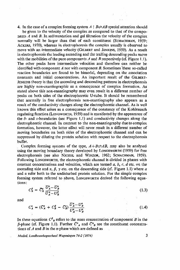
4. In the case of a complex forming system A+B^AB special attention should be given to the velocity of the complex as compared to that of the compo

nents A and B. In sedimentation and gel filtration the velocity of the complex normally will be larger than that of each constituent (SCHACHMAN, 1959; ACKERS, 1970), whereas in electrophoresis the complex usually is observed to move with an intermediate velocity (GILBERT and JENKINS, 1959). As a result in electrophoresis the leading ascending and the trailing descending peaks move with the mobilities of the pure components A and B respectively (cf. Figure 1.1). The other peaks have intermediate velocities and therefore can neither be identified with component A nor with component B. Sometimes 'these so-called reaction boundaries are found to be bimodal, depending on the association constants and initial concentrations. An important result of the GILBERT-

JENKINS theory is that the ascending and descending patterns in electrophoresis are highly non-enantiographic as a consequence of complex formation. As stated above this non-enantiography may even result in a different number of peaks on both sides of the electrophoretic U-tube. It should be remembered that normally in free electrophoresis non-enantiography also appears as a result of the conductivity changes along the electrophoretic channel. As is well known this effect arises as a consequence of the constancy of the Kohlrausch regulating function (LONGWORTH, 1959) and is manifested by the appearance of the 8- and e-boundaries (see Figure 1.1) and conductivity changes along the electrophoretic channel. In contrast to the non-enantiography due to complex formation, however, the latter effect will never result in a different number of moving boundaries on both sides of the electrophoretic channel and can be suppressed by diluting the protein solution with respect to the electrophoresis buffer.

Complex forming systems of the type, A-\-B^AB, may also be analysed using the moving boundary theory developed by LONGSWORTH (1959) for free electrophoresis (see also NICHOL and WINZOR, 1962; SCHACHMAN, 1959). Following LONGSWORTH, the electrophoretic channel is divided in phases with constant concentrations and velocities, which are termed a, b, c, d etc. on the ascending side and a, /?, y etc. on the descending side (cf. Figure 1.1) where a and a refer both to the undisturbed protein solution. For the simple complex forming system referred to above, LONGSWORTH derived the following equations:

CB = CB % ^ 1 (1.3)

and

CA = (CA + CB- CB) Vf^L (1.4)

In these equations CfB refers to the mass concentration of component B in the

jS-phase (cf. Figure 1.1). Further C"A and CaB are the constituent concentra

tions of A and B in the a-phase which are defined as


Descending Ascending

Protein Concentration

v ?>

' N /

_ i _

Concentration Gradient

^ X AA Conductivity

^£X. UA

distance

FIG 11 Schematic picture of moving boundary electrophoresis of the reacting system A -\- B ^± ABy

a. Concentration distribution after transport; a, b, c, d, a, fi and y indicate phases of constant concentrations and mobilities. b. Schlieren pattern of the system after transport; s and S are the stationary boundaries caused by the constancy of the Kohlrausch regulating function. c. Conductivity changes along the electrophoretic channel:

initial conductivity level; changes brought about by transport.

Meded. Landbouwhogeschool Wageningen 74-2 (1974)

cA = cA + CAB ) (1.5)

Cot r-ia • s-'K I

B ~ '-B "+" *-AB J

U'XA and U"B are the constituent velocities of A and B in the a-phase and were denned by LONGSWORTH as

UA = (UACA + UABCAB)ICA \

• ( L 6 >

UB = (UBCB + UABCAB)ICB J

UA and UB are measured from the volumes swept through by the a/?- and bc-boundaries respectively (LONGSWORTH, 1959). From Equation 1.4 and the known constituent concentrations of A and B the equilibrium constants may be calculated. In systems of higher stoichiometry Equation 1.4 can no longer be applied. It is still possible, however, to obtain useful information concerning the stoichiometry of the complexes by application of Equation 1.3 as will be demonstrated in Chapter 2.

This thesis will deal specifically with the electrophoretic analysis of the complex formation between cesl- and /2-casein, two major proteins from cow's milk (JENNESS, 1970).

The caseins occur in milk (JENNESS, 1970) as nearly spherical colloidal particles with diameters up to 300 nm: the casein micelle. The micelle also contains approximately 5 % of inorganic constituents of which calcium and phosphate are the most important (WAUGH, 1971). The protein part of the casein micelle is composed of three major components: asl- and /?-casein, mentioned already above and x-casein. Casein micelles behave more or less like hydrophobic colloids and already LINDERSTROM LANG (1929) hypothesized the existence of a protective component, stabilizing the micelles against floccula-tion by calcium ions. In 1956 WAUGH and VON HIPPEL rediscovered this stabilizing component and called it x-casein.

The stabilizing properties are completely destroyed after the action of the enzyme rennin, which results in the splitting-off of a polypeptide from x-casein with a length of approximately one third of the whole polypeptide chain (MACKINLAY and WAKE, 1971). The remaining part of the x-casein, which is called para-x-casein no longer stabilizes the casein micelle and as a consequence flocculation occurs. As is well known this process forms the basis of the cheese manufacturing.

From electronmicroscopy it has become clear that casein micelles are composed of a large number of small particles, called the submicelles (SCHMIDT

and BUCHHEIM, 1970). Dialysis experiments suggest that these submicelles contain mere casein. The casein micelles are therefore considered to be conglomerates of submicelles cemented together by inorganic ions, notably Ca+ + . The hypothesis according to which it is supposed that the submicelles are the


fundamental parts of the casein micelles is supported by recent work concerning the size distribution of the casein micelles (SCHMIDT etal., 1973), by electronmi-croscopical analysis of the calcium distribution in casein micelles (KNOOP et al., 1973) and by electronmicroscopic studies concerning the biosynthesis of the micelles in the golgi vesicles in the mammary gland (BUCHHEIM and WELSCH, 1973).

The precise structure of the casein micelles and in particular the structure and composition of the submicelles is not yet known. Clearly, interactions between the casein components will be of primary importance in this respect. It is obvious that caseins, being proteins with an open, more or less randomly coiled like structure (HERSKOVITS, 1966) and containing a more than average proportion of amino acids with non-polar side chains (WAUGH, 1954) have numerous possibilities for interaction through hydrophobic bonding. This has been amply verified in a number of polymerization studies during the last decade.

The self-association of asl- and )?-casein has been studied in particular (PAYENS and VAN MARKWUK, 1963; PAYENS et al., 1969; SCHMIDT, 1969, 1970;

SCHMIDT and PAYENS, 1972). It was found that asl-casein associates mainly by hydrophobic interaction and to a less extend by hydrogen bonding (SCHMIDT,

1969; SCHMIDT and PAYENS, 1972) whereas the association of ^-casein is probably entirely due to hydrophobic bonding (PAYENS et al., 1969). Also x-casein associates strongly (SWAISGOOD et al, 1964), but a full description of this association has not yet been given.

From the non-specificity of the bonds formed during self-association of asl- and ^-casein, it might be anticipated that the same type of bond will be formed with the complex formation between these casein components. Complex formation in total casein has already been observed by KREJCI et al. (1941), KREJCI (1942) and WARNER (1944) also applying the technique of free electrophoresis. The quantitative description of such complex formation is greatly complicated, however, by the self-association of the components. This results in the simultaneous occurrence of more than one association equilibrium which cannot be analysed with the simple theory of GILBERT and JENKINS, referred to above. The numerical solution of this problem in the case of the simultaneous association equilibria in the system asl- and jS-casein will be given in the next chapter of this thesis.

From the foregoing it will be clear that the study of the interactions between the different casein components will be of paramount importance for our understanding of the energetics of the casein micelles in milk and of their behaviour in a number of technological processes such as pasteurization, sterilization, concentration and homogenization. Also gelation of dairy products after UHTST heat treatment and the curdling of milk, will partly be influenced by the interaction between the caseins.

It should be emphasized that the analysis of reaction boundaries by the methods developed in this thesis is certainly not limited to the complex formation of the caseins. It may also be applied with equal success to interactions between other proteins or macromolecules of which examples have already been mentioned at the beginning of this chapter.


II F R E E E L E C T R O P H O R E S I S OF C O M P L E X F O R M I N G agl- A N D jS-CASEIN

2.1. I N T R O D U C T I O N

The study of interacting biopolymers by such transport methods as sedimentation, electrophoresis and gel filtration has received considerable impetus over the last decades (LONGSWORTH, 1959; NICHOL et al., 1964; ACKERS, 1970; CANN and GOAD, 1970). The relevancy of such studies is indicated by a number of biochemical phenomena in which complex formation plays a central role. As early as 1942, LONGSWORTH and MACINNES investigated the complex formation between a protein (ovomucoid) and nucleic acid (yeast RNA) by free electrophoresis and formulated the anomalies to be expected in the electro-phoretic patterns. Further examples are the study of the enzyme/substrate complex between pepsin and bovine serum albumin by CANN and KLAPPER

(1961) and that of antigen/antibody interaction by SINGER and CAMPBELL

(1955). The complex formation between bovine plasma albumin and charged dextran derivatives was studied by THOMPSON and MACKERNAN (1961).

In such studies the advantage of free electrophoresis and gel filtration over sedimentation lies in the fact that with the former techniques two moving boundaries are observed, whereas during ultracentrifugation only one. In electrophoresis the non-enantiography of rising and descending patterns yields additional information which is lacking in the sedimentation experiment and which often facilitates diagnosis.

Rapid progress in our understanding of the electrophoretic behaviour of interacting proteins is due to GILBERT and JENKINS (1959), who solved the conservation-of-mass equation for the equilibrium system A+B^AB. The GILBERT theory accepts fast re-adjustment of the equilibrium upon changes in concentration brought about by transport and neglects the influence of diffusion on the spreading of the boundaries. Another limitation of the theory is that the velocities are assumed to be constant, which is neither true in sedimentation (FUJITA, 1962; PAYENS and SCHMIDT, 1966) nor in electrophoresis (LONGS

WORTH, 1959). Despite these restriction, the GILBERT theory explains quite satisfactorily the anomalies observed during electrophoresis or sedimentation of complex forming biopolymers. Notably GILBERT and JENKINS (1959) were able to account for the occurrence of a different number of moving peaks on both sides of the electrophoretic channel and for their abnormal mobilities and percentages. The close resemblance of a number of experimental electrophoretic patterns (NICHOL et al., 1964; LONGSWORTH and MACINNES, 1942; CANN and KLAPPER, 1961; SINGER and CAMPBELL, 1955; THOMPSON and MAC

KERNAN, 1961) to those computed by GILBERT and JENKINS suggests that as a rule rapid re-equilibration occurs during electrophoresis of interacting biopolymers. As regards the diffusion, its influence on the spreading of the moving


boundary may often be neglected in prolonged experiments, as shown by BALDWIN (1957) and by GILBERT and JENKINS (1959). However, there always remains the possibility that small peaks or shoulders are obscured by the blurring effect of diffusion. This suspicion has prompted a number of authors (CANN and GOAD, 1970, 1965A, 1965B; BETHUNE, 1970; Cox, 1965A, 1965B, 1967, 1971 A, 197IB) to solve the complete conservation-of-mass equation by various simulation methods. The simulation technique applied in the present study is described in the next chapters.

This chapter deals especially with the complex formation between as l- and /?-casein, two major proteins from milk, the self-association behaviour of which is well known (SCHMIDT and PAYENS, 1972; SCHMIDT, 1970; PAYENS and VAN MARKWIJK, 1963). Under the experimental conditions of free electrophoresis, i.e. 2 °C , pH 6.5 and an ionic strength of 0.1, jS-casein is completely depolymerized (PAYENS and VAN MARKWIJK, 1963), whereas asl-casein undergoes a number of consecutive association steps, the association constants of which have been firmly established by SCHMIDT (1970). The study of asl-/? complex formation is of paramount importance to our understanding of the energetics of casein micelle formation in milk (PAYENS, 1966; WAUGH, 1971).

The results of the present investigation suggest that multiple association equilibria occur, which can be represented by

iA^Ah 0 ' = 2, 3... 6) ) (2.1)

Aj + B^AjB, (j = 1,2... 6) j ,

in which A and B stand for oesl- and /?-casein respectively. Preliminary reports of this investigation were published earlier (PAYENS,

1968; NIJHUIS and PAYENS, 1972). The pertinency of this study is by no means restricted to the field of casein

chemistry. It could well stand as a model for all those complex formations in which one of the components is subjected to self-association. The interaction between virus coat protein and RNA is an outstanding example of such a system (DURHAM et al., 1971; BUTLER and KLUG, 1972).

2.2. M A T E R I A L S AND METHODS

Alphasl-casein was isolated from bulk milk by the method of SCHMIDT and PAYENS (1963), whereas jS-casein was prepared in the manner described by PAYENS and VAN MARKWIJK (1963).

For electrophoresis the protein solutions were dialysed exhaustively against the appropriate buffer. The buffer of the last dialysis step was also used for the electrophoretic experiment. In those experiments were the salt anomaly had to be suppressed, the solution was enriched with protein and diluted after completion of dialysis (WIEDEMANN, 1947).


Sedimentation runs were performed in the Phywe airdriven ultracentrifuge under conditions comparable to those applied during electrophoresis.

Sedimentation coefficients, electrophoretic mobilities and peak areas were determined from enlarged tracings by routine measurements (LONGSWORTH,

1959; ELIAS, 1964). The computations simulating the electrophoretic transport were performed

with the university CDC-3200 digital computer. The source program was written in ALGOL-60. Details concerning the simulation procedure are given in Chapter 3 and 4.

2.3. RESULTS

Typical electrophoretic patterns of mixed solutions of asl- and /?-casein in two types of buffer are shown in Figure 2.1. Peak mobilities and percentages from these and other experiments have been collected in Table 2.1. The fast formation of complexes between asl- and /?-casein is clearly indicated by the different number of moving peaks on the ascending and descending sides (GILBERT and JENKINS, 1959). The mobilities of the trailing ascending and leading descending peaks, which are intermediate between those of pure as l- and /?-casein and the abnormal distribution of the protein over the different peaks also afford convincing evidence of complex formation (LONGSWORTH, 1959; GILBERT and JENKINS, 1959). As is shown by comparison of the patterns of Figure 2.1a and 2.1c or 2.1b and 2.1d and the data in Table 2.1, buffer composition does not influence the general appearance of the electrophoretic patterns. Proteinbuffer interactions seem therefore to be of no importance to the explanation of the anomalies observed (CANN and GOAD, 1970). Table 2.1 actually suggests that the mobilities of the complexes formed are intermediate between those of pure asl- and /?-casein (GILBERT and JENKINS, 1959)*.

The fast re-equilibration of the complex formation during the electrophoretic transport was further checked by comparing experiments at different field strengths. Figures 2.2a and 2.2b and the data in Table 2.1 demonstrate that indeed variation of the field does not affect the mobilities and percentages of the electrophoretic patterns, confirming rapid re-equilibration. The electrophoretic patterns in Figures 2.1 and 2.2 show well-developed 8- and e-boundaries. As is well known (LONGSWORTH, 1959). these boundaries are due to the constancy of the KOHLRAUSCH regulating function, as a result of which considerable conductivity changes may occur along the electrophoretic channel. A related consequence is - as was already pointed out by SVENSSON (1946) - that the fastest peaks are always enlarged at the cost of the slower ones.

The dilution factor, p, occurring at the -boundaries in Figures 2.1 and 2.2, was estimated in two independent ways.

* The relatively high mobilities observed with the 70/30 mixture in phosphate buffer probably should be explained by leakage during the electrophoretic experiment.


descending ascending

Ut U, Ur u. JB UA * u B uA

FIG. 2.1 Free electrophoresis of mixtures of a5l- and jS-casein at a total protein concentration of 1.20 g/dl. Experimental conditions: pH 6.6, 0.1 ionic strength and 2°C. Pictures taken after 4800 s. Mixing ratio: a. «sl/0 = 50/50; barbiturate buffer; b- asi IP = 70/30; barbiturate buffer; c- <*silP = 50/50; phosphate buffer; d-<WJ8 = 70/30; phosphate buffer.

10 Meded. Landbouwhogeschool Wageningen 74-2 (1974)

P. 13 a

o •Ei ft o

W

w

3

^

^

=3 6

S 60 a o U

CO

2 ' S rt 8"

•= .y «a.

"rt ^ | n ^ in t^ (N c> r4 <N (N r i

f i r ] oo in PH

vo t~ <n vo vo

oo M3 o oo in *$• <rt *& \c \o

r ) ^" w N in in >n m rn en

TJ- r-_ « (N I-H

q tn "n in r i \o vo v i v i v i

Tf ^t o\ N n o oo oo oo oo od od

<D cd IH 3

3 cj

&

t— t-* ©

o

rt t-3

."S

•e a •Q

o <N

., o i> * -tJ * a iz J3 3 ft.ti n *

2 ^--c a ft JD

o o (N <N

. , 4) ID ^ •s «* Pi LH

J3 3 0. . -S

2 TS J3 <a ftjO

o o (N (N

u 13 u 3

. •B C3 JO

O 00

d

^4 ci

ft . C3 g

•a a IE ts u —<

3 00 c3 (3

a a

" O O O O O M [ J n m i n ' n v i g 3 O ' O ' O ' O ' O 3

ft r > "n >n in N

« 2



FIG. 2.2 Free electrophoresis of a 1:1 mixture of asl- and y?-casein at a total protein concentration of 1.20 g/dl. Experimental conditions: pH 6.6, barbiturate buffer of 0.1 ionic strength and 2°C. a. Field strength 3.05 V/s; picture taken after 4800 s; b. Field strength 1.00 V/s; picture taken after 14400 s.

First, according to LONGSWORTH (1942).

P = Ypt-oa

i

(2.2)

where EOt is the total diagram area and 03 and 0E that of the <5-and e-bound-aries. The average value of p found in this way from the patterns in Figure 2.1 was 0.84.

Secondly, we gradually suppressed the 8- and 8-boundaries by diluting the protein solution with respect to the electrophoresis buffer (WIEDEMANN, 1947). Extrapolation of the decreasing <5-areas in Figures 2.2a, 2.3a and 2.3b to zero area then also yields p = 0.84 which is demonstrated in Figure 2.4.

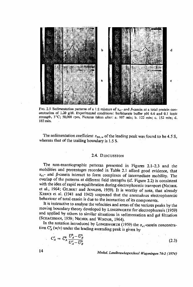
Sedimentation patterns of a 1:1 mixture of asl- and /?-casein under the same experimental conditions as those used with electrophoresis are presented in Figure 2.5. Rapid re-equilibration is suggested by the fact that between the peaks the schlieren pattern does not come back to the base line (GILBERT and JENKINS, 1959).



FIG. 2.3 Free electrophoresis of a 1:1 mixture of asl-and j8-casein at a total protein concentration of 1.20 g/dl. Experimental conditions: pH 6.6, barbiturate buffer of 0.1 ionic strength (electrophoresis buffer) and 2°C. Pictures taken after 4800 s. Ratio ionic strength of electrophoresis to dialysis buffer: a. 1.10; b. 1.15.

FIG. 2.4 Relationship between dilution factor (p) and area of the -boundary (arbitrary units).


—V k'-"""••* miAlnililfl

'V

FIG. 2.5 Sedimentation patterns of a 1:1 mixture of asl- and /?-casein at a total protein concentration of 1.20 g/dl. Experimental conditions: barbiturate buffer pH 6.6 and 0.1 ionic strength, 3°C; 50,000 rpm. Pictures taken after: a. 107 min; b. 122 min; c. 152 min; d. 183 min.

The sedimentation coefficient s20,w of the leading peak was found to be 4.5 S, whereas that of the trailing boundary is 1.5 S.

2.4. D ISCUSS ION

The non-enantiographic patterns presented in Figures 2.1-2.3 and the mobilities and percentages recorded in Table 2.1 afford good evidence, that <xsl- and ^-casein interact to form complexes of intermediate mobility. The overlap of the patterns at different field strengths (cf. Figure 2.2) is consistent with the idea of rapid re-equilibration during electrophoretic transport (NICHOL

et al., 1964; GILBERT and JENKINS, 1959). It is worthy of note, that already KREJCI et al. (1941 and 1942) suspected that the anomalous electrophoretic behaviour of total casein is due to the interaction of its components.

It is instructive to analyse the velocities and areas of the various peaks by the moving boundary theory developed by LONGSWORTH for electrophoresis (1959) and applied by others to similar situations in sedimentation and gel filtration (SCHACHMAN, 1959; NICHOL and WINZOR, 1964).

In the notation introduced by LONGSWORTH (1959) the asl-casein concentration CC

A (w/v) under the leading ascending peak is given by

C\ = C ** U\-TJ\

m •m (2.3)


In this equation C\ represents the constituent concentration of asl-casein in the 6-solution, denned as

cbA = M , + ZZ ^~-r cb

AjBk, (2.4) i j k jMA+kMB

where MA and MB are the molecular weights of asl- and /?-casein, which have been established as 23,000 (SCHMIDT, 1970) and 24,000 (NOELKEN and REIB-STEIN, 1968) respectively. Further, UA is the velocity of pure asl-casein in the c-solution and Ub

A is the constituent velocity of that component in the b-solution and defined as

U"A = kc"AlUAl + TZ _ ^ _ CAjBk UAjBk\lcA (2.5) (.; J k jMA+kMB yi

a corresponding definition holds for the constituent velocity UbB, and it can be

shown (LONGSWORTH, 1959) that

JT* _ J/bc UB = Vc (2.6)

where Vbc is the volume swept through by the froboundary per unit time. Similarly, for the concentration of pure /?-casein under the trailing descending

peak we have:

(2.7)

with

77" — I lx

np pa UA VB B BuA-u*

UA = v*" (2.8)

The velocities occurring in Equations 2.3 and 2.7 are approximated as follows: Ub

A is calculated from the maximum gradient velocity of the leading descending peak by:

V\ = UAlp *;

UbB is averaged over the maximum gradient velocities of the ascending bimodal

peak and E7£ is found from:

VB= UbBp*.

The pure component velocities UCA and V% are the average values from Table

2.1. We are now able to compare the experimental areas of the leading ascending

* It can readily be calculated that changes in the constituent mobilities due to shifts of the association equilibria in the ^-boundary are negligible.


TABLE 2.2. Comparing observed and computed pure component peak areas in the electrophoresis of interacting asl- and /?-casein.

mixing % leading % trailing

ratio velocities (10~5 cm/s) ascending descending

U"A U"A TB U*B UCA UPB obs. calc. obs. calc.

50/50 18.5 22.1 14.4 12.1 24.8 7.5 32 37 28 29 70/30 20.3 24.3 16.1 13.4 25.9 8.9 53 58 14 18

and trailing descending peaks with the computed CCA and Cl from Equations

2.3 and 2.7. The results are given in Table 2.2, from which it is seen that the calculated areas compare fairly well with the observed ones. It should also be noticed from this table that the leading ascending peaks cover as much as 70 % of the ^4-component, whereas on the descending side the trailing peaks contain about 50% of the 5-component. It is evident from Equations 2.3 and 2.7 that these abnormally high percentages are due to a relatively high constituent velocity UA which in turn suggests that complexes of a high stoichiometric ratio A/B dominate among the complexes (cf. Equation 2.5). The presence of higher complexes was already indicated by preliminary GiLBERT-type computations in an earlier attempt to reproduce the bimodal reaction boundary (PAYENS, 1968).

CHUN (1965) has analysed the ultracentrifugal pattern of mixture of asi-and jS-casein, assuming the formation of a 1:1 complex of depolymerized <xsl- and /?-casein with the aid of the theory developed by GILBERT (1959). Several objections can be made to his treatment however. First, the sedimentation method is much less sensitive in discriminating interaction than free electrophoresis, since only a descending boundary is available. More serious, however, is the fact that under the experimental conditions asl-casein is highly polymerized (SCHMIDT, 1970) and consequently the interaction between the asl-casein polymers and the jS-casein monomer should also be considered.

The sedimentation pattern presented in Figure 2.5 is also indicative of the presence of higher complexes. The slower sedimentation coefficient (1.5 S) corresponds to the monomer of /?-casein and the monomer of asl-casein which have comparable sedimentation coefficients (SCHMIDT et al., 1967). From these values it is readily calculated that the 1:1 complex of monomers, if it were spherical could have a sedimentation coefficient of 2.4 S at the atmost. This is far below the experimental value of 4.5 S found for the rapid peak in Figure 2.5. It should further be realized that in re-equilibrating systems the sedimentation of this faster peak is always slower than that of the complex itself (GILBERT

and JENKINS, 1959), which indicates that the complexes present must consist of at least four subunits.

We are now able to roughly qualify the association equilibria which occur under the experimental conditions of electrophoresis.

As is shown by PAYENS and VAN MARKWIJK (1963) jS-casein, on account of

1" Meded. Landbouwhogeschool Wageningen 74-2 (1974)

the low temperature, will be completely depolymerized. On the other hand, it can be obtained from SCHMIDT'S work (1970) that asl-casein, under the experimental conditions will be polymerized consecutively at least up to the hexamer. Among the complexes formed between asl- and jS-casein those of stoichiometry AjB(J> 1) will predominate.

This conclusion was confirmed by computer simulation of the be- and a/3-reaction boundaries. A preliminary account of the simulation method was given earlier (NIJHUIS and PAYENS, 1972) and a more detailed account is presented in the subsequent chapters.

The parameters introduced in the computations were obtained as follows: 1. the polymerization constants and electrophoretic mobilities of asl-casein

were taken from SCHMIDT'S (1970) and this work; notably SCHMIDT (1970) observed that ccsl-monomers and -polymers have equal mobilities; 2. the ^j-5-complex mobilities were calculated by linear interpolation between

the pure component mobilities; it is a fortunate coincidence that the computations are rather insensitive to the actual values accepted for the complex mobilities; 3. the equilibrium constants for the complex formation were defined as

Kj = CA.BjCA.CB

and, since the caseins interact through hydrophobic bonding (SCHMIDT, 1970; PAYENS and VAN MARKWIJK, 1963; VON HIPPEL and WAUGH, 1955), initial i^-values are chosen so as to compare with the polymerization constants given by SCHMIDT (1970) for pure asl-casein polymerization.

In accordance with the previous experience of PAYENS (1968), the computations demonstrate clearly that bimodality of the fcc-boundary could be produced only if complexes AjB w i th ;> 1 were taken into account. Moreover, it was observed that the agreement between the experimental and computed mobilities and percentages improved if more weight was given to the higher ^ - c o m plexes. This led us to introduce six parameters for the interactions between all kinds of copolymers and the ^-monomer. It is realized that the introduction of so many parameters in the computations certainly will not provide a unique solution. The point of interest is, however, that only the consideration of these multiple equilibria yield the observed bimodal Ac-boundaries and mobilities and percentages in agreement with the large constituent velocity UA arrived at before. Some typical simulation results are collected in Table 2.3 and in Figures 2.6 and 2.7.

It is seen that the computed mobilities and percentages compare satisfactorily with the experimental values. We do not consider further refinements of these calculations warrantable for the following reasons.

Firstly as may be noted from a comparison of Figure 2.6 with Figure 2.7, variations in the interaction parameters do not significantly influence the results of the computations once the existence of the higher complexes has been accepted. Of course this implies that such computations will never yield unique values for the equilibrium constants. Meded. Landbouwhogeschool Wageningen 74-2 (1974) 17

> > X V X X X X

X * X f x »• x v X X X • X X > x ;« * X J> X x x x

X X > -w X X X X X * . X X

X X X X X X X X X X

X > ' X X X X X X X X >• X x x x

X V X X X

X X X X X

X X X V X X X X X X » X X X X X X X X X X

X X X .1 > x X

x X X X x x X

X X X X x X X

X X X X X X X

X X X X X X X

X X X X X x x X W X X X I C V K X

X •• X X X x X X X X X X X X X x M X X X X X X X X X X X X X X X

X X X X x X X X x

X X > X X X X X X X X X X X X X X X

x ; » X X X X X X X X x x x « x x x x x x X X x w X X x x X V X X X X X X X X M X X X X X x x x X x X X X X X " » X X ir X X X X X K X X X M X

X X X X X M X X X X M X X X X X X X X W X x x x x x x w x x - x x x x *• x » > > v x x > x »>• x x » x x > x x x X X X X X X X X X > X X

x x x x : » x x x x x x x

M X X X X 'x M X M X X X X

X X X X X X X X X X X X X

X X M X X X X V X X X X X X X X x X X X X X X X X X X X

M X X X X X X X X X X X X X X X X X X X X X X X M X X X X X X X X X x X X X X M X X X X X X X

X X X X X X X X X X v M X X X X X X X X X X X X X X X X X X X X X X X X X X X X X X X X X X X X X X X X X

X X X X M X X M X X X X X X X X X X X X X • X X X X X X X X X X X X X M X X X X X X X

X X x X X x x X X X K X X X X

X X * X < X K. X < X < X K X X X X X •< X < X * X

X X X X

x X X X

X X X X

X X X X X x; x X X X X X X X X X X X X X X X X

X X X X X X X X X X X X X X X X X X X X X X X X X X X X X X X X X X X X X X X X X X X X X X X X X X X X X X X X X X X X X X . X X X X X X X X X X X X X X X X X X X X X X X X X X X X X X X X X X

X X X X X X X X X X X X X X " x x x X X X X X X X X X X X X

vX X X i X X : X ' X X X X X X - x X i X ' X ! X x ; .x" X X X X X X M X X X X X X X X K X X. X K * X X X X i X X 1 X >fr X XT X X X X X X X X X X X X X X X X X ^ - X * < c X X * « x X n r x x X X X X X X " : X K V K X X > f c i C X X X X J « X X X X X X T X X M x J* s t x x x x >v x X x x x X X X X X X X X X X K X X X X X X * X X X X X X X X X X X X X X < X X X X X K X X K X X X X X X X K X X X * X K X « X x M . X H X X X X X X X X ' X X * « X W « x. « M. JC " •* X X X X X X X X X X X X X X X X X X X X X X

x-x x^x x;« x*x K X X X X X X x x x x x x x

W X M - X > c « w - V W ^ w w w u- w ~ ~ >S

X i X X ' X X ^ X X X K X X X X X X X X X X X X x X X x X x t X * ^ X • X X X X X V. x x X x x x X X X: X X X X » X x . X X X X X X X X X x x X X

x x x x x x x x x x x ^ x x x x x x x * < x x x

X X X X X X X X X ' X X X X X X X X X . X ' v ' t s x x '

x x x x x x x x x x x x x x x x x r x x i X X X i X X - X x - x w - w — — — — •-*-— - - - - - - -

x 2 2 2 2 X *~»<x"* x x x x x x x x Q x x x x

J * * * * * £ » < » * > < x x x : x x x x x x x x x ; » « x * < 2 55555555 K l l < K K : x ' ' x ' i t > ( , 0 < '* > ( K K , <

x x x x x x x x x x x x x r x x x x x x x x x x x x

desccnding- ascending-*

FIG. 2.6 Simulated be- and a/?-reaction boundaries for complex forming <x5l- and ^-casein during electrophoresis. Parameters: Kt = 10, K2 = 15, tf3 « 50, # 4 = 100, 7r5 - 150, tf6-100 (g/dl). Average diffusion coefficients varying from 1-5.10~7 (cm2/s) (see chapter 3 and 4). Mixing ratio: a. aai/0 = 50/50; b. «Ml/fi = 70/30.


A *• > >• 1

, v - x -•» > :

•» »« x X x v

r In * X *• *• '

• X X I J. >. r ># >«

M X ^ » c At* X »* *•• " J M W X j i X M * x X •« « '

X X X X X X X *• * * » « > * * « ' [ X X X X X >« X > « » « » » * * • • r > M X X

« *• K »* •• f X X •« X X V

X X «. X X M »* X X X X * X X

V H ^ X f H K X

K M W U l C X K i i r - K X M M X * . « X X X * X X

•H M X i f X K H X i t M ' X n . K X X X • X j ' l ' M I t X M f e M X i f M X M J«>«

>* + It •* rfW**K#*X>'#',WXX«'1 * X X X * » X X » * X > ^ ^ X X X X X X * f X

j r K ^ w t c ^ ^ K K i K - ' v w X X ^ * X

. c H I . e - K W x ' W . X X - K X W ' K K K X . X X X W X. * « • T M . i ^ x X X M X X K X X X X X X ri- «( a- 4 « W * -t X *. * W . ' . X X X X X X*

x x x x i c w x « « * x x x x x - - * x x x x : x ; x K - - * K * X ^ H V K W - K * ' " . K X X X X ' X ' X I X X « v M- « - X * " X *• < x X « * * « X X X X X X

« ^ x a - X ^ ^ ^ K X w ^ K X ^ X X X X X ^ X X * * « . . < x « > c x < X f < x « - x x > i < X K X X : X X ; K X : X M. tc K X M X x M K X t a X X m X X X X X X X K

M X X H X <c •* rt ** •* K M - j r X X X ^ X X x X X X X X X X X M. M K X X J T X X H X X X X X X X X X X X K X X X X X X X X X M X - « X X X > « X X X X X X X K X X X X X X X X X X X X X X X X K X X X K X * *

X X X X X X X X X X X X X X X X K X X X X X i X X K

d&ccndin£ ascending-

Meded. Landbouwhogeschool Wageningen 74-2(1974) 19

J. V X X X X X *f > J.

X X X X X X X y. " X x x > J* X X

X > i * > X X X v X »• X w X J * X X

X X j . X X X

X X X X > X X X X J . > y JC » > • X X » * X X >€ x j r

r Mr X X «C K M

> X rf X ^ .je X ' X X X X X X t X V X X M X >• X X X X x X ' X * *t X v X ( X X X x x x I M X V X X X C J> X «- X X X c • x >- x x x

' X > X v « > . L X X X J* X M C X > X X X X

x x x v x x x x x x X M X X . K k , « > . . * X X X X x X X X X X X X X V x X x >. >• X > X X « J> > > JT > ,»

-r x x x M •« X X X X X

> X X X X X X N X X X X X X X X X X «r X X X ft X «- X X - X X - X X X X - V X M X X x X X X X r f f c X x X x x X X ) • . * * • V X X >• Nr * M X

x x x > x x x > » x x M X X V t X > X X X X V X X X ' W X X H X X X V V

- « x x x ^ x % x v x x x > X X X > X X . M X X > . X X X

x x i - x x x x x x x x x X x x x x x x x x ^ x x x x x x X X X X X X X X X . M X X X X X X X X X X X X X X A X X X

X X X X X X X X X X X X X X X X X X X X X X X X X X X X X X

X X X X X X X X X X X X X X X X x X X X X X X X X X M X X X X X X X

X X X X X X X X X X X J * X X X X X X

x x x x x x x ^ x x x x x x x x x x x x x S

X. X, X X X X X X X X X X X X x x x ; x x x

x x x X X X x x x x x x X XT K.

x x x X X X

x x x X X X X X X X X X x x x x x x x x x x x x x x x x X X X X x x x x. X X X X x x x x X X X x X X X X x x x x x x x x x X X K X X « <, K X X X X X *• X x -; x x x X X x K X "• •• x *• M-

X X X X X x x x x X x x X «. n. X X X X" X

x, X w x i

X K w x -

«. X X 4 * * < « X X X, K x x x * X X X X x «• x x x < x x •"• « x x X X X X " . " X X * X, X X X X X X x x x x x x x x x x x x X M X. X-X X X K X X X X x x- x x X X X X

x x x, it X • x x x X * x X X K < X X, x x x * X X x x x X X X x x x X X X x x, x x x x x x x X X X X X X X X X

X X X X X X X X X X X x. X * X x X - * x «: X X x x-x x. x < * X. X X X x. X X X X X X . x x x x X X X X x x x x X X X X X X X X X x x x X X X X

X X X X X X X X X X X X X X x- X X X K X X X X X

X X X X X X

X X H X x X X X X

X X * X. X X X X X X X X x x x x X X X X XI X >' x X w X- X x x x x x: x x x x x x- x x- X X X X X X X X. X X X x x x x X" X X. X X X X X X X X X X X X X X X X X

X X

x x x X X n. X x X •"

X X X X x* x x x x x i x X X X X x x x x x x x x J X X X X J x x i x i X X X. X i X H X X • X v X X v X X X X > X X X X ) X X X X • x •. x x ' x •* x x . x x x x J X X X X i X X X* X x x x" x X X X X X X X X X x X X x x x x X X X X X x X x X X X X x x x x

X X X x x x x x, X X » X* x X X x' x x x X X X X X X X X x x x x x: x x x X- x x: x x x x x

descending- ascending-

Parameters: K} = 10, # 2 = 25, Z 3 = 100, K4 = 200, tf5 = 300, K6 = 200 fe/dl) Average d.ffus.on coefficients varying from 1-5.10- (cm*/s) (see chapter 3 and 4) M.xing ratio: a. asl//? = 50/50; b. asl//? = 70/30. >-


*• V X X * x X X •* X * > >-»)•> x K * x

X <• X W It X

X X ~* X X X

> v » •. x x

X ;• X » X X

X M X X X X X X H X X X J* »* X X f » X X X X X X

X X X X X X

>• X X X X X *

X > v * > > > X X X X X X X J< X X X X X X X X X X X X X. X X X X X

x X X X X X w X

x x x x x x x x

X x - * X x x x x X V X X » > V >

X X X X X J T X X X > x x x x » t x x > ^r X X X X X X X X

X X X X X X X X X x x x x x x x x x X X " ic X X X X X x 1" x x x x x x x X X X X X X X X X x x x x x x x x x x X X x X X X X X X X X J C X X X X X W ^ X X - X X X X - K X X X

M W X X X X M V X X

> x w X > X X X X X " X X M X X X X X X X X X X X X X X X X X X X X X X > X X X X * X X . K X X X X X X X X > r X X X X - w x X X X X X X X V j e X V X X X X X X x x x x x x x " x >» x X X X X X X X X X X X X X X X X X X X X X X X X X X H X X . X X X X

X X X X X X X X X X X X X X X X X X X X X X X X X . x - x x x - x « » x - X > K W X X X X X x J> X « X X

X X X X X X X X X X X X X X X > r X X X X X X X X X X K W W V X X X X X X X X X

X v X > x v - X X X X X X X

M »r X X feXXXXXXXX^ w w X X X X X f X X X X X X *• M X X X X X V X X X X X X x » x x x x H X X X X X X X X X X X v X X X X X X X " X X

ti > X X K j r X * 4 « > > M ^ i X 1 > X X X X X X X X X X X X X K X X X X x J * x X X X X X X X X X X X X X x x x x x x x x x x x x x x x x X X X X M X X X X H X X I X X X

X X * x x x x x x x x x x x x x x X X X X X X X X X X X X X X X X X X X X X X X X X X X X X X X X X X . X

x x x x M X M X X X X X X M X X X X X X X X X X X X X X X X X X X X X X X X X X « X X X X X X X X X X X X X X X X

X X X X X X X X X X X X X X X X X X X X X ( X X x X X X X X X X X X X X X X X X X X X X X

X X » X * M X X X X X : K x H X > X ; X X X X J ' X > < «.

H X < * - < - f i \ < ^ i ^ - K rf<*X<«<*«»fc'« •«

H w •< <* J^ * - ^ • ^ t x X ^ X X X X K * : * * * ' ' ' * . IC 14 W + * • * * . ! * - <* 1 . < W 1 * X » . X * • * W j . •» • * X" X X. W *« X X X X ' X ' M - X * i t x w x : * > • " • x x x x H X . X ' k V * K , X . J * » - ' X K » « I » X » * * X I « . » ^ J * * ' X : * *. x. *e *c *. H « * J< i* x. >. x x x x x : - x x x x. * * J * X X X X - W T « - » C K . X W X X X X x X X J x «• K

*C K * X K * • X » ^ X X ^ ^ X - V K X X K K ^ X M . rf K i^ >C ^ ^ . ( X X H . X . X X X X X X ' X X X . K X X X X X X X , X X ' X J . X X , * K X * X x. x « *. x x x x x x w x x x x x X ~ x x x x x x x x x x x x x x x x . • e X . X X X X X . X ' X X X . K X X X X X ' X X r x . X . X X K x x w x x ' x x x x x ' x x ' x x ; x x x x x : x x : x ; x , x

^ X ' X W W X ' X X X X ' X ' X ' X ' X ' X . X X X K X X X H ' X X ' X . K X X K X - X X - X X X X X ' X X . X X X X X X X . X X . X ;

descending-^- ascending->


TABLE 2.3. Comparing simulated and experimental reaction boundaries for complex forming asl- and /?-casein during electrophoresis.

mixing

ratio «.ilfi

50/50

70/30

Fig. 2.5 Fig. 2.6 Exptl.1

Fig. 2.5 Fig. 2.6 Exptl.1

ascending

velocities (10";

10.8 10.8 12.7 13.8 13.1 13.9

' cm/s)

20.0 21.2 16.9 20.9 21.7 18.9

relative area

63.6 64.2 68 51.9 54.6 47

descending

velocities relative (10~5 cm/s) area

17.7 64.2 17.6 64.8 18.5 72 18.1 86.2 18.0 78.4 20.2 86

'Average values from Table 2.1.

Secondly, as a consequence of the KOHLRAUSCH-SVENSSON effect the faster peaks are always enlarged at the cost of the slower ones (LONGSWORTH, 1959; SVENSSON, 1946). This effect has not been accounted for in the present calculations, since its magnitude is difficult to evaluate in systems containing more than three ionic species.

Thirdly, on close inspection the electrophoretic patterns of Figures 2.1 to 2.3 show a non-zero gradient in the 6-phase, and sometimes a minor shoulder ahead of the ^-boundaries. It is suspected that these abnormalities are due to the presence of minor quantities of complexes which have a mobility approaching that of pure <xsl-casein, and which were not accounted in the present calculations.

In conclusion we state that the interaction between asl- and ^-casein gives rise to an intricate assembly of complexes in which asl-casein dominates. This is in line with the well-known tendency of these proteins to form colloidal micelles in milk (WAUGH, 1971).

22 Meded. Lahdbouwhogeschool Wageningen 74-2 (1974)

I l l COMPUTER S IMULATION OF E L E C T R O P H O R E T I C E X P E R I M E N T S

3.1. INTRODUCTION

Transport techniques such as electrophoresis, ultracentrifugation and gel filtration can be used to advantage in studying biopolymer interactions (GIL

BERT and JENKINS, 1959; CANN and GOAD, 1970; NICHOL et al., 1964; ACKERS,

1970; ZIMMERMAN and ACKERS, 1971; ZIMMERMAN et al., 1971; HENN and

ACKERS, 1969; THOMPSON and ACKERS, 1965; NICHOL and WINZOR, 1964;

WINZOR and SCHERAGA, 1963). Several methods have been proposed to solve the conservation-of-mass equation for a system of interacting biopolymers in transport experiments. GILBERT (1959) and GILBERT and JENKINS (1959) have presented analytical expressions for the concentration and the concentration gradient in polymerizing and complex forming systems neglecting the effect of diffusion on the spreading of a boundary. The usefulness of this approach resides in the fact that in prolonged experiments the contribution of diffusion often can be neglected when compared to the spreading caused by the differential migration of the different polymer species. It is realized, however, that in experiments of finite duration and/or with the occurrence of small peaks or shoulders, it may be important to assess the blurring effect of the diffusion on the shape of a boundary. This has led a number of authors to solve the complete conservation-of-mass equation by numerical or simulation methods (CANN and GOAD, 1970; Cox, 1965A, 1965B, 1967, 1969, 1971A, 1971B;

BETHUNE, 1970). Cox for instance (1969, 1971A, 1971B) simulated the sedimentation pattern

of polymerizing proteins by taking into account the non-uniform ultracentn-fugal field and radial dilution of the protein. Essentially, in this method the ultracentrifuge cell is divided into a large number of small segments the leading edges of which are displaced with the weight-average sedimentation coefficient of the protein present in the segment on the upstream side of that edge This transport cycle is followed by a diffusion step during an equal interval of time. Successive alternate rounds of sedimentation and diffusion permit the simulation of concentration-dependent ultracentrifugation, be it as a consequence of polymerization or hydrodynamic interaction.

CANN and GOAD (1970) solved the complete conservation-of-mass equation by considering the contributions of the individual species to the fluxes due to velocity and diffusional transport. Also in this approach the boundary is divided into a large number of segments and the flux at a particular segment edge is calculated from the average concentrations in a number of neighbouring boxes. Equilibrium between the individual spec.es is re-established after each transport cycle. Actually the flux at a particular edge, » related to the average concentration in all boxes. GOAD showed that if the veloc.ty flux , .

Meded.Landbouwhogeschool Wageningen 74-2 (1974)

http://spec.es

restricted to the transfer of material from one box to the next a diffusion-like error is introduced. This author therefore preferred to suppress this error by taking into account the contribution of the average concentrations of several boxes to the flux and to introduce the diffusional flux separately. This is certainly a most accurate procedure, but it will be demonstrated below that for practical purposes the diffusion-like error can be used to simulate the diffusional flux, which leads to a drastic reduction of the computations.

Still another approach to simulate boundaries in transport experiments was introduced by BETHUNE and KEGELES (1961A, 1961B, 1961C), who stressed the analogy of the equations governing the countercurrent distribution process with those describing the problem at hand. BETHUNE (1970) has simulated the boundary spreading of self-associating and complex forming polymers during electrophoresis and sedimentation and compared his results with the asymptotic solutions given by GILBERT (1959). BETHUNE (1970) also has discussed the proper choice of the countercurrent distribution coefficient in order to account quantitatively for the diffusional effect in polymerizing systems.

The method of simulation presented in this chapter is - as stated above -a simplification of the procedure outlined by CANN and GOAD (1970). It will be shown that the method also carries a close relationship to the countercurrent simulation approach of BETHUNE and KEGELES (1961A, 1961B, 1961C). Application of the method to the simulation of the anomalies observed during the electrophoresis of complex forming <xsl- and /J-casein has already been presented in Chapter 2.

3.2. THEORY OF THE SIMULATION METHOD AND

DISCUSSION OF THE RESULTS

Let us consider the following system of interacting biopolymers A and B:

iAv ^ A„ (i = 2, 3,..., p), \

(3.1) jA, +B- AjB, (j = 1, 2,..., q). )

The complex formation between ocsl- and jS-casein at the temperature of free electrophoresis and the interaction between RNA and virus coat protein (DURHAM etal., 1971) offer among others (NICHOL et al., 1964) excellent examples of such a system.

The computation of the equilibrium concentrations of the various species requires the solution of the foljowing set of equations

K^AJA'U (i = 2,3,...,p) (3.2)

Lj = AjBI(A{B), (J = 1, 2,..., q) (3.3)

Z = I Ai+ E ( l - W (3.4) i = l .7 = 1


B = B+ £ XJAJB (3.5)

In these equations Kt and Lj represent the equilibrium constants for the self-association of A and for the complex formation between A and B respectively, A and B stand for the constituent concentration (w/v) of A and B and X} is defined as

Xj = MBl(jMA + MB)

with MA and MB the monomer molecular weights of A and 5. Equations 3.2 - 3.5 lead to the following expression for the monomer concentration of component^:

I K(A E IjLjAi 7=o

+ E J = 0

{B-(A+B)A,}L,4 = 0 (3.6)

w i t h ^ = L0 = 1.

Equation 3.6 is a polynomial in the monomer concentration Au the graphical appearance of which is shown in Figure 3.1. In the computation of the equilibrium concentration, Al is found by NEWTON-RAPHSON iteration (MARGENAU

FIO. 3.1 Schematic plot of the polynomial (Equation 3.6) used for the computation of the monomer concentration (A,) of component A.


and MURPHY, 1955). The constituent concentration A, being the highest possible value of Au appears to be a natural starting value for the iteration. Actually, however, the number of iteration steps can be reduced considerably by estimating the starting value of Ax in a particular box from its concentration in the preceding one (see Chapter 4.).

The simulation of the free electrophoresis of a system of interacting biopoly-mers is achieved by subdividing the electrophoretic channel into a large number of small boxes of equal length Ax. The development of the reaction boundaries is brought about by alternate rounds of velocity transport of the individual species from one box to the next during an interval of time At, followed by re-equilibration according to Equation 3.2 - 3.5.

On the ascending side velocities are taken relative to the slowest species (i.e. component B) and the ratio Ax/At is chosen such that the fastest component just reaches the end of a box, therefore

VA- VB = AxjAt. (3.7)

The complexes, having intermediate mobilities, penetrate the boxes only partially. Similarly on the descending side the velocities are changed of sign and taken relative to the component with the highest absolute value of the electrophoretic mobility (i.e. component A).

The source program for the simulation, a flow scheme of which is presented in Figure 3.2, was written in ALGOL-60. All computations have been carried out on the CDC-3200 digital computer complex of the Agricultural University.

It is worth while to analyse the above simulation procedure somewhat further.

With the (n+/) th transfer, the change of mass in box r due to component / is given by

/ ! < .+ i = < „+1 — mi, „ = /; (ml_u „ - mj, „), (3.8)

where ft — ytAt\Ax

and v( is the relative velocity of species i, vt-vB. Obviously, from our choice of reference of the relative velocities and of A t/Ax (Equation 3.7), we have 0 <ft < 1.

The mass transfer of each species from one box to the next is thus seen to be determined by a constant fraction / , of the mass difference between adjacent boxes. This transfer is therefore found to be identical with the mass transfer taking place in the countercurrent distributional process. In the latter case we have / , = Pi/(P,+1), where Pt is the partition coefficient of the species i (CRAIG and CRAIG, 1950). As mentioned in the introduction, BETHUNE and KEGELES (1961A, 1961B, 1961C) and BETHUNE (1970) have used the mass distribution achieved in a continuous countercurrent process to account for the effect of the diffusional spreading on the transport pattern of interacting proteins. It is worth noting, however, that the countercurrent analog involves more computations than the present method of simulation, since it requires not only

2" Meded. Landbouwhogeschool Wageningen 74-2 (1974)

( START J

C READ

calculate starting conditions

k: = r

output

Q STOP )

S AjB in \ Vbox(k-l)? y

Tyes

mass transfer boxk- l-—k box k— k + 1

> n o .

re-equilibrate boxk

replace each box number k by k - 1

FIG. 3.2 Flow diagram for the simulation of reaction boundaries of complex forming pro-

teins in transport experiments.

the computation of the partition equilibrium but also those of the chemical equilibria in both the upper and lower layer of each countercurrent tube

Following BETHUNE (1970) we thus find for the mass distribution of species i after a sufficiently large number of transfer cycles n:

dQIdn = V2 / , (1 ~fd *CJ&>. - f, dCjUr, (3.10) 27


where r is box number and Ct is the concentration of species / in g/dl. Similarly, for the mixture of interacting biopolymers we have

d^Qdn = B2 (£ V2/, d -fd Q) Idr2 - dJJtCJdr (3.11) i I * i

If now - following again BETHUNE and KEGELES - we draw the following analogies: ««->/ and r<-»jc, then Equations 3.10 and 3.11 show the formal analogy with the complete conservation-of-mass equation in transport experiments in which the distance is expressed in units of length Ax and time in units At. As a consequence the simulated diffusion coefficients of component i, expressed in cm2/s, becomes

Di=1lifi(\-fdWx?IAt. (3.12)

In systems containing three migrating components atmost the Df values can generally adepted individually by a proper choice of Ax, At and fh as will be demonstrated in the next section. However, in the present case, dealing with more components only the simulated average diffusion coefficient can approximately brought into agreement with the actual value. In the mixture of biopolymers the actual diffusion flux is denned by (Cox, 1969):

JD = D^idCJdx), ( 3 13 )

where D is the gradient averaged diffusion coefficient

D = liDfiCJdxl/YjidCtldx] ( 3 .1 4 )

and D} is the true diffusion coefficient of component /. In accordance with liquation 3.12 the simulated gradient averaged diffusion coefficient, expressed in cm2/s, becomes

5 * = [ZClzf, (1 -fd dCJdryfcidCJdr}] (Ax)21 At (3.15)

The adjustment of the simulated to the actual diffusion coefficient now demands tnat we put

D* = D. (3.16)

S U r l 7 3 , 1 t " 3 ' 1 6 " f 3 J S h ° W t h a t Ax a n d M a r e fix«l by the values of dints Tci'r,7 T]' t hC d i f f U S i ° n C ° e f f i d e n t S D< a n d t h e concentration gra-tTs!I*u l a U e r T11 bC diSCUSSed b e l o w- T h e n ^ b e r of transfer a ^ fitX f VS n e C C S S r f ° r t hC s i m u l a t i o n o f ^ Particular reaction bound-S XJS? ^ f ratl° °f timC ° f thC CXperiment and At- Conver" sely in the simulation of a glVen experiment an arbitrary choice of n determines 28


together with the duration of the experiment an arbitrary At. The corresponding Ax then follows from Equation 3.7 and the diffusional spreading operative in this simulation from Equation 3.15. It is obvious that in general then D* will not equal D.

We are now able to elaborate upon the simulation of complex forming asl-and /f-casein dealt with in the previous chapter.

Since we have no a priori knowledge of the concentration gradients dctjdx existing in the reaction boundaries, we must start with a comparison of the simulated patterns computed for arbitrary numbers of transfer. Typical results of the simulation of the ascending electrophoretic pattern of a 1:1 mixture of asl- and /?-casein for n = 27, 46, 73 and a duration of the experiment of 4800 s are presented in figures 3.3a-3.3c, from which it is seen, that the general appearance of the pattern is not affected substantially by the number of transfers. More importantly, as is seen from Table 3.1, also the maximum and minimum gradient mobilities and the concentration changes over the reaction boundary do not change appreciably with n. This result, of course, is in agreement with GILBERT and JENKINS' conclusion (1959) that in prolonged experiments the effect of diffusional spreading on a boundary is negligible. In other words: the proper choice of the number of transfers is of minor importance for a correct simulation of the percentages and mobilities found from experimental electrophoretic patterns.

The calculations underlying Table 3.1 and Figure 3.3 also yield the concentration gradients necessary for a comparison of the averaged true and simulated diffusion coefficients defined by Equations 3.14 and 3.15. To this end we have approximated the various 8Q/dx by the total concentration change of the species i over the boundary. The actual value of D is then estimated as follows From existing data (SCHMIDT, 1970; NOELKEN and REIBSTEIN, 1968) we find the diffusion coefficient, Du of monomeric asl- and /?-casein, corrected for the temperature of free electrophoresis, to be 3.2-10"7 cm2/s*. The diffusion coefficients of the polymers or complexes containing i subunits are then calcu-

TABLE 3.1. Comparing velocities and percentages of the ascending electrophoretic boundaries

of complex forming «sl- and l-casein simulated for different numbers of transfer.

Number of number velocities1. percentages2

transfers of boxes OP"5 c"Vs) A l A* 3

~T1 ^ i~96 IM UW o l o 0 2 4 0.47 46 40 94 1-60 1-08 0.31 0.22 0.47 t 4 ° \Z 1.58 1.07 0.31 0.22 0.46 73 60 1.94 1-58

1 Velocities corresponding to the maximum and minimum gradients of the reaction boun-

'T r e l a t i v e area of pure «sl-casein; A2, A» relative areas under bimodal peak.

* The molecular parameters of monomeric «sl- and ^-casein are almost the same (SCHMIDT,

1970; NOELKEN and REIBSTEIN, 1968). 29


X X X X X X X X X X

X X X X X X X X X X X X X X X X X X X X X X X X X X

X X X X X

X X X X X x x X X X X X X X X

X x x x X X X X

X X X x X X X X X x x X X X X X X X X

X X x X X X X X X X X

X x X X

X X

X X

X x X X X X X X X X X X X X

K X K X X X X X X

X X

X x X X X x X x X x

X X x x X X X X X X X X X X

x x X x X X

X X

X X

X X X X X X X

X X X

X X X X X X

X X

<XKX*'«*«*''

X X X X X X X x x x x x x x x x x x x x x x x x x x x x x x x x x x x x x x x x x x x x x x x x x x x x X X X X X X X X X X X X X X X X X X X X X X X X X X X X x x x x x x x x x x x x x x x x x x x x x x x x x x x x x x X X X X X X X X X X X X X X X X x x x x x x x x x x v x x x x x v X M X K X X X X X X X X X X X X X

i * X * x»* *

X K K « X x »« x »e x$ , . „ -. »< K KK

K « K X

* K M X

H K V X

n x x x x * ) * *

511313s

35:3:3:

F IG . 3.3 Simulation of the ascending elec-trophoretic reaction boundaries for a 1:1 mixture of asl- and /?-casein; a: number of transfers 27, b. number of transfers 46, c. number of transfers 73.


TABLE 3.2. Comparing simulated and true :o the computations presented in Table 3.1

Number of transfers

27 46 73

At (s)

177.8 104.3 65.8

gradient averaged diffusion coefficients pertaining

Ax (nm)

277.3 162.8 102.6

D* (Ax)2IAt (10-.7cm2/s)

3.286 1.958 1.241

D-107

(cm2/s)

2.527 2.534 2.536

lated from that of the monomers by the STOKES-EINSTEIN relation:

D, = D, r 1 / 3 <3-17> A similar calculation is performed for the estimation of the simulated diffusion coefficient, D*, according to Equation 3.15.

The comparison of the D and D* estimated in this way for n = 27 46 and 73 is given in Table 3.2, from which it may be noted that the value of the diffusion coefficient, D, is hardly affected by this change of n. The simulated diffusion coefficients 25*, however, are found to be inversely proportional to n as expected from the theory presented above. Actually Table 3.2 indicates that the most accurate number of transfers should be about 35, corresponding to an averaged simulated diffusion coefficient of D* = 2.55-10- cm* /s. Similar " " " ^ n s hold for the simulation of descending electrophoretic or ultracentnfugal pat-

tCThe above analysis shows the ^ ^ ^ ^ f ^ J ^ Z ^ t simulation of the reaction boundaries observed in the e c ^ ™ ^ < £ ultracentrifugation) of interacting proteins. In a g r e e ^ ™ * J * " ^ " S arrived at by GILBERT and JENKINS (1959) the value rf^«J^ diffusion coefficient, 15*, thereby appears to be of w ™ ™ ^ ™ ^ t

reproduction of the experimental peak areas and ™ ^ - ^ j ^ f of the simulated to the true diffusion coefficient can ^ . ^ ^ ^ T ^ by carrying out a preliminary " J g j j ; ^ ^ f ^ i Z ^ s l ^ fers. From this the true average diffusion coemcient, u.» eaualiza-above. The most realistic number of transfers then ^ f ^ ^ Z l Z ) tion from the true and simulated average diffusion coefficients (Equation 3.16).

3 3 ALTERNATIVE METHODS FOR THE SIMULATION OF

DIFFUSIONAL FLUXES

s i n u ^ d and actual diffusioncoeffic,ens * k . o f £ ^ . ^ ^ ting system. His treatment can a s . 1 j * « " » J ^ ^ components as for example in complex tOT™"« » j ; , b e n o t i c e d t h a t

For the simulation of f ' f ^ ^ Z S Z ^ box, Ax. the dura-there are three undetermined parameters i.e. mc v ^ Meded. Landbouwhogeschool Wageningen 74-2 (1974)

tion of a transport cycle, At, and the fractional transfer parameter/(Equation 3.9). They are interconnected by two equations, viz.

v = fAx/At, (3.17)

£>= ll2f{i-f)(AxflAt. (3.18)

Thus we have one degree of freedom in the choice of At, At and/ . Also in this case the analytical solution of the complete conservation-of-

mass equation is available (CRANK, 1967):

(r—vn)'

— = 1 e l 4Dn

8r JAnDn (3.19)

We are therefore able to compare the results of the simulation procedure treated above with the analytical expression (Equation 3.19). As is shown in Table 3.3 the results obtained from the analytical expression compare satis-

TABLE 3.3. Comparison of exact and simulated schlieren patterns for one migrating component. Simulation parameters: n = 30, / = 1/2, At = Ax = 1, corresponding to D = 1/8 and V = 72.

box number

1 2 3 4 5 6 7 8 9

10 11 12 13 14 15 16 17 18 19 20 21 22 23 24 25

dCldr simulated

0.0000 0.0000 0.0000 0.0000 0.0001 0.0006 0.0019 0.0055 0.0133 0.0280 0.0509 0.0806 0.1115 0.1354 0.1445 0.1354 0.1115 0.0806 0.0509 0.0280 0.0133 0.0055 0.0019 0.0006 0.0001

dCldr Eqn. 3.19

0.0000 0.0000 0.0000 0.0000 0.0002 0.0007 0.0020 0.0056 0.0132 0.0275 0.0501 0.0799 0.1116 0.1363 0.1457 0.1363 0.1116 0.0799 0.0501 0.0275 0.0132 0.0055 0.0020 0.0007 0.0002


factorily with those from the simulation procedure. The discrepancies can be explained on the grounds of the analysis given by CANN and GOAD (1970). These authors showed that the relation of the concentration in a certain box and the concentrations at a particular point can be obtained by TAYLOR expansion. From their expression it is seen that our simulation procedure not only introduces a diffusion-like flux but also fluxes of higher order.

For the case of discrete self-association the proper choice of the simulation parameters is straightforward (BETHUNE, 1970). We now have 4 parameters {At, At,fM and fP) which are completely fixed by the four following Equations:

vM=fMAx/At, (3.20)

vP = fPAxlAt, (3.21)

DM= V 2 / M ( 1 - / M ) ( ^ ) 2 / ^ ^ (3-22)

Dp= '^fpil-foiAxflAt, (3.23)

where vM and vP and DM and DP denote the velocities and diffusion coefficients of monomer and polymer respectively. The solution of this set of equations is achieved in two stages.

First, Ax/At and {Ax)2/At are eliminated from the Equations 3.20-3.23. In this way the ratio of the diffusion coefficients and the ratio of the velocities are brought into agreement with the simulated ones. Since DM and DP are parabolic functions of/M and/P, whereas vM and vP are linear dependent on fu and fP the above procedure is equivalent to finding the proper set of (x, y)-values on the parabola relating the simulated diffusion coefficient and the velocity parameters fM and/P (Figure 3.4a).

Next, for one component (e.g. monomer) the simulated diffusion coefficient and the simulated velocity are scaled by calculating the proper Ax and At from Equations 3.20 and 3.21 with the value found for/M. It is easy to show that futfp, Ax and At are given by

JM — DM~VM (3-24)

2

fp =

DM VM

D;~V7 (3-25) DM pu Dp

2

vMDp-vpDMlvM (3.26) ZIX — Jm • " 2

V j t f V p - V p


Ifj (1-fj) diffusion coordinate

'M velocity coordinate

uc

FIG. 3.4 Schematic picture of the adjustment of simulated diffusion coefficients and simulated velocities; a. discrete polymerization: A/(onomer) <±P(olymer) in the case of gel filtration or ultracentri-lugation,

cemrirgation™^'011 ^ ^ C ° m p 0 n e n t s ) A + B * C i n t h e c™ of gel filtration or ultra-

c. as with b but in the case of electrophoresis.

Meded. Lcmdbouwhogeschool Wageningen 74-2 (1974)

DP—vP DMIVM (•$ 27) At = 2

In the case of a complex forming system like A+B^C, the problem arises that five parameters (Ax, At,fA,fB,fc) must conform to six Equations:

v; = / , (Ax)/At, (i = A , B, C), (3.28)

Dt = V2/, (1 ~fd i^f/At, (i = A, B, C). (3.29)

This difficulty, however, can be overcome by introducing a sixth parameter: the velocity of the frame, v0, related to the simulation parameter, u0, by v0 = u0AxjAt. This causes a new set of fractional transfer parameters, w, (i = A B, C), which must be used in the simulation procedure defined as

ut=ft-u0, (i = A,B,C). (3-3°)

Now u, becomes the fraction of mass moving from one box to the next thus 0 < M ; < 1 (1 = A , B, C). As is exposed above 1/, will then be determinative of the simulated diffusion, whereas/, still determines the velocity. In this method the simulated velocity and the simulated diffusion are no longer interdependent. Instead of Equations 3.28 and 3.29 we now have

v. = (Ui+u0) (Ax)/At, (« = A B, C), (3.31)

D, = V2«« ( i - « 0 V*)2lAt> (' = A' B>c)- (3'32)

Elimimating Ax/At and (Ax)2/At and putting vJvB = A, vjv* = B, DBjDA = C, and Dc//)^ = £ a set of Equations is obtained for ut (1 - O, 4 , # , CJ.

_ uA+u0 (3.33)

UQ-TUQ

UA + U0 (3.34)

« j , ( l - « n ) (3 '35>

"^(1-"J

«c( l -«c ) ( 3 3 6 )

B =

C =

D «^(1-«J

From Equations 3.33-3.36 the following expressions can be found for u0, uA,

«B and uc: 35


= V2 ± V21/--4! ± JA\-AA0A2 r 2A0

uB = V2 ± V2 V 4 C M A - *CuA +,1

(^-B)u i l + A(B-\)uB Uc =

M„ = AuB-uA

\-A

where

A0 = S2 - QDC

A1 = 1ST - Q(C+D-2CD)

A2 = T2 - Q(l-C)(l-D)

{ A-B J [ A-B j

A-B J (. ^1-B

After uA, uB, uc and u0 have been solved zl/ and Ax are found by the scaling procedure described for the two component system. In principle by equations 3.33-3.36 there are 8 sets of solutions. The values found in this way are restricted by the condition 0 <ut< 1 (i = A, B, C). It should further be kept in mind that there exist pairs of solutions which are symmetrical about u = \ and the overall transport of which will be opposite. Obviously such a pair may represent the corresponding ascending and descending limbs in free electrophoresis (or gel filtration). I f />0 (/ = A, B, C) we are dealing with the ascending side, whereas for/,<0 the descending side is simulated.

In the case of gel filtration the fastest component is the complex which has the smallest partition coefficient and diffusion coefficient. It is clear from Figure 3.4b that for this case a fit on the diffusion parabola can also be realized and proper values for ut (i = A, B, C) can be found. The same holds true for the case of ultracentnfugation, provided the conditions mentioned on page 38 are Stitisnccl,

From the electrophoresis of widely different complex forming systems it is or

Meded. Landbouwhogeschool Wageningen 74-2. (1974)

evident that the electrophoretic mobility of the complexes is always intermediate between those of the pure reactants (GILBERT and JENKINS, 1959; CANN and KLAPPER, 1961; THOMPSON and MACKERNAN, 1961). In this case no solution of Equations 3.33-3.35 is available, as is apparent from Figure 3.4c. By considering the average diffusional flux a satisfactory solution can also be found for this case, as was shown above.

37 Ueded. Landbouwhogeschool Wageningen 74-2 (1974)

IV A P R O G R A M I N A L G O L FOR T H E S I M U L A T I O N OF E L E C T R O P H O R E T I C R E A C T I O N B O U N D A R I E S O F

I N T E R A C T I N G B I O P O L Y M E R S

4.1. CONSTRUCTION OF PROGRAM

The program used for the simulation of reaction boundaries of interacting biopolymers during electrophoresis was written in ALGOL-60. Input and output procedures were adopted according to the conventions proposed in ALGOL-60, as published by NAUR et al. (1963). The program was adapted to the Control Data 3200 Computer of the Computer Centre of the Agricultural University at Wageningen.

The simulation programs for the ascending and descending electrophoretic patterns were named ASC-PQ and DESC-PQ respectively. The programs are also applicable to the rising and descending boundaries in gel filtration experiments with existing plateau region (WINZOR and SCHERAGA, 1963). The program DESC-PQ can also be applied to sedimentation of interacting macromolecules provided the influences of the non-uniformity of the centrifugal field and radial dilution effects (SCHACHMAN, 1959) may be neglected.

The main differences between these programs ASC-PQ and DESC-PQ were: first, the way in which the starting conditions were calculated; second, the manner in which the output is presented. The flow scheme (Figure 3.2) of both programs, however, is the same. The successful operation of the simulation program demands that special attention should be paid to the following facts. 1. According to the transfer Equation 3.8 new concentrations in a given box

after each transfer cycle are governed by the concentrations in that box and the preceding one before transfer. The transfers in a particular round should not influence each other. It is therefore necessary to carry out the successive transfers in upstream direction. 2. After each transfer the new equilibrium concentrations are calculated. This

calculation consists of three steps: First, the coefficients of the polynomial Equation 3.6 are calculated. Second, the monomer concentration At is found as the real and positive root of Equation 3.6 by NEWTON-RAPHSON iteration (MARGENAU and MURPHY, 1955). Third, the new concentrations of all components are calculated from A1 with the aid of Equations 3.2 and 3.3 and the accepted values for the various equilibrium constants.

It is advantageous to reduce the number of iteration steps in the computation of Au since this part of the program is repeated mostly. Therefore a starting value for Ax is chosen close as possible to its final value reached in the iteration. In this respect it should also be borne in mind that the degree of convergence of the NEWTON-RAPHSON iteration diminishes when the degree of the polynomial

3° Meded. Landbouwhogeschoo! Wageningen 74-2 (1974)

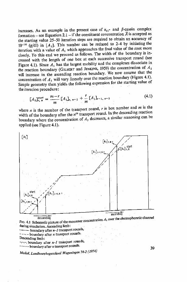
increases. As an example in the present case of asl- and jS-casein complex formation - see Equation 2.1 - if the constituent concentration A is accepted as the starting value 25-50 iteration steps are required to obtain an accuracy of 10~10 (g/dl) in [_A{\. This number can be reduced to 2-4 by initiating the iteration with a value of At which approaches the final value of the root more closely. To this end we proceed as follows. The width of the boundary is increased with the length of one box at each successive transport round (see Figure 4.1). Since Ax has the largest mobility and the complexes dissociate in the reaction boundary (GILBERT and JENKINS, 1959) the concentration of Ax

will increase in the ascending reaction boundary. We now assume that the concentration of A± will vary linearly over the reaction boundary (Figure 4.1). Simple geometry then yields the following expression for the starting value of the iteration procedure:

L^r" = m — r m m

(4.1)

where „ is the number of the transport round, r is box number and „ ,s he width of the boundary after the n«h transport round. ^ ^ ^ ^ T b l boundary where the concentration of A, decreases, a similar reasoning can be applied (see Figure 4.1).

descending FIG. 4.1 Schematic picture of the monomer during simulation. Ascending limb:

boundary after n-1 transport rounds, boundary after n transport rounds.

Descending limb: -•-.-. boundary after n-1 transport rounds,

boundary after n transport rounds.


ascending concentration A, over the electrophoretic channel

39

In the output the concentrations of the different components over the reaction boundary are listed (see Table 4.1). Also, the velocities and the concentration gradient are given in Table 4.1 The latter is also presented as a schlieren pattern (see for instance Figure 3a-c). Furthermore the velocities of the extrema of the schlieren pattern and the area distribution under the bimodal peak are computed.

TABLE 4.1 Representing the concentrations of the various species present, the concentration gradient and the velocities over the different boxes corresponding to the schlieren pattern shown in Figure 3.3b.

NR ALPHA BETA C0MPLEX1 C0MPLEX2 C0MPLEX3 C0MPLEX4 C0MPLEX5

0 +0.0175 +0.3469 +0.0606 +0.0533 +0.1354 +0.2488 +0.0696

1 +0.0176 +0.3335 +0.0589 +0.0522 +0.1339 +0.24R4 +0.0701 2 +0.0181 +0.3006 +0.0544 +0.0494 +0.1300 +0.2470 +0.0715 3 +0.0187 +0.2578 +0.0483 +0.0455 +0.1241 +0.2444 +0.0733 4 +0.0195 +0.2164 +0.0422 +0.0414 +0.1173 +0.2404 +0.0750 5 +0.0203 +0.1&14 +0.0368 +0.0375 +0.1104 +0.2353 +0.0763 6 +0.0210 +0.1532 +0.0322 +0.0340 +0.1039 +0.2295 +0.0772 7 +0.0217 +0.1308 +0.0284 +0.0310 +0.0979 +0.2233 +0.0776 8 +0.0224 +0.1129 +0.0253 +0.0284 +0.0923 +0.2169 +0.0776 9 +0.0230 +0.0985 +0.0226 +0.0261 +0.0871 +0.2103 +0.0773

10 +0.0235 +0.0866 +0.0204 +0.0241 +0.0824 +0.2037 +0.0767

11 +0.0241 +0.0767 +0.0184 +0.0223 +0.0779 +0.1q70 +0.0758 12 +0.0245 +0.0683 +0.0168 +0.0207 +0.0738 +0.1903 +0.0747 13 +0.0250 +0.0610 +0.0153 +0.0192 +0.0698 +0.1835 +0.0735 14 +0.0255 +0.0547 +0.0139 +0.0178 +0.0660 +0.1767 +0.0720

6 I n ' l l l l ' ^ l l l + ° ' 0 1 r +"-0166 + 0 - ° 6 2 4 •»• ^ 8 +"'"o° 16 +0.0263 +0.0442 +0.0116 +0.0154 +0.0588 +0.1627 +0 06H5 8 +0'0271 ll'llS + ? - 0 1 r + ° - 0 1 " + ° - 0 5 5 * *°- 5 « +0io665

18 + " ' 0 ^ ! +".0357 +0.0097 +0.0132 +0.0520 +0.1432 +0.0643 19 +0.0275 +0.0320 +0.0088 +0.0122 +0.0486 +0.1407 +0 0619 20 +0.0279 +0.0286 +0.0080 +0.0112 +0.0453 +0.1329 +0.0593 21 +0.0283 +0.0254 +0.0072 +0.0102 +0.0420 +0.1248 +0 0565 11 Z'llll +?*°?I5 + ° - 0 0 6 4 +n-&0" + 0 - " ^ *0 164 0 0534 24 0*0294 ^ :i'llll +n-00'i4 + 0 - 0 3 5 3 +°'1076 +0 500 IX In'n^oo 1' }lf +"-0050 +0.0075 +0.0319 +0.0985 +0.0463 " +0.0J01 +0.0125 +0.0038 +0.0057 +0.0250 +0 n7Q? +n niK?

ie :i:llll il'll^ :y°r, +o-00*-9 +"-^ + ° : ° ^ : • 29 • * ! ° , n 0 ^ + n ' 0 0 ^ +0.0182 +0.0588 +0.0290 11 !n nl\]

+ 0 - 0 0 6 7 +0-0021 +0.0033 +0.0148 +0.0485 +0.0242 30 +0.0314 +0.0051 +0.0016 +„.0O26 +0.0117 +0.0386 +S.0x94

32 lolllll ll'Tpl : y ° l t ^ - 0 ° 1 9 +0-0°S8 +0.0293 +0.0149

11 :i I : : : : - - - ! « « - ^ :!:!!?3H

£ : : : : : 2 : - « » - - ? ! - ^ *S:SSSS 37 * S : S i i : :s:0°So°? :C:So°o°§ :s:K :°:zi :5-'S„0?? iwill 3 :s:S!i: :0

0-o0oo°o0 - I S -ESSS

+no-ooon + ° : ° ° " • « : i : •

40 +0 032^ lo'oOOO ' + n ^ 0 0 0 + ° - 0 0 0 0 + 0 - 0 0 0 1 +0-°°°° ' +O.O0O0 +0.0000 +0.0000 +0.0000 +0.0000 +0.0000


The program calculates the reaction boundary using the equilibrium constants as variable parameters. The proper set of equilibrium constants is found by trial and error. This stage of the computations can be speeded up by calculating the areas of the leading ascending and trailing descending peaks and the constituent velocities for different sets of equilibrium constants only by Equations 2.3-2.8. As will be clear from the theory presented in Chapter 2, these

CUMPLF.Xb POLYMtR TOTAL UC/OK VELOCITY1

• 0.0369 + o.o:m> +1.0000 •0.000 000 +U.0OO 096 000

•0.037b •0.0392 +0.0416 +0.04*3 +0.0469 •0.0492 +0.0511 •0.0526 •0.0538 •0.054 7

•0.0552 +0.055b +0.0557 •0.055b +0.0552 +0.0547 +0.0539 +0.0529 +0.0516 +0.0501

+0.0484 +0.0463 +0.0440 +0.0413 •0.0382 +0.0349 +0.0311 +0.0271 +0.U228 +0.0185

+0.0143 +0.0104 +0.0071 +0.0044 +0.0025 +0.0013 +0.0006 +0.0002 +0.0000 +0.0000

+0.0320 +0.0 346 +0.0388 + 0.044 1 •0.0502 +0.0^8 7 +0.0633 +0.0700 +0.076H +0.0836

•0.0904 +0.09 73 +0.1041 •0.1111 +0.1181 +0.1253 + 0. 1326 + 0.1401 +0.1478 +0.1557

+0.1639 +0.1724 + 0.1811 +0.1901 +0.1994 +0.2090 +0.2187 +0.2284 +0.2379 +0.2470

+0.2554 +0.2627 +0.2687 +0.2732 +0.2763 +0.27H1 +0.2788 +0.2789 +0.2784 +0.2775

+0.9842 +0.94*7 +0.8926 +0.8407 +0.7951 •0.7569 +0.7251 +0.6983 +0.6755 •0.6556

+0.63/9 +0.O218 +0.6071 +0.5933 + 0.5802 +0.5676 + 0.5553 + 0.5432 + 0.5311 +0.5190

+ 0.5066 +0.4939 +0.4808 +0.4672 +0.4531 +0.4383 +0.4230 +0.4074 +0.3915 +0.3760

+ 0.3613 +0.3*79 +0.3366 +0.3277 +0.3212 +0.3168 •0.31*1 +0.3124 +0.3112 +0.3100

+0.015 791 +0.039 482 +0.052 159 +0.051 901 +0.045 575 +0.038 219 +0.031 806 +0.026 732 +0.022 85* +0.019 920

+0.01/ 701 •0.016 021 +0.01* 751 +0.013 79b •0.013 097 +0.012 602 +0.012 281 +0.012 110 +0.012 07* + 0.012 162.

+0.012 36 7 +0.012 082 + 0.013 096' +0.013 597 +0.01* 159 +0.01* 7*1 +0.015 279 +0.015 oV9 +0.015 8 17 +0.015 5*/

+0.01* 738 +0.013 313 +0.011 315 +0.008 9*0 +0.006 503 +0.004 3*9 +0.002 726 +0.001 709 +0.001 226 •0.001 1*?

+0.000 099 391 +0.000 102 ?B3 + 0.1)00 106 17* +0.000 109 5b5

MI. ooo 112 957 + 0.000 116 348 +U.0OO 119 739 + 0.0 00 +U.OO0 +0.000

123 126 129

130 522 913

+0.000 133 30* +0.000 136 696 +0.000 140 087 +0.000 1*3 *78 +0.000 1*6 b70 +0.000 150 261 +0.000 153 652 •0.000 157 0*3 +0.000 160 *35 +0.000 163 826

+0.000 167 217 +U.000 170 609 +0.000 174 000 +0.000 177 391 +0.000 180 783 +0.000 184 174 +0.000 187 565 +0.000 190 95 7 +0.000 194 348 +0.000 197 739

+0.000 201 130 +0.000 204 522 +0.000 207 913 +0.000 211 304 +0.000 214 696 +0.000 218 087 + 0.000 221 «7« +0.000 224 870 +0.000 228 261 +0.0 00 231 652

NP.

1 2 3 4 5 6 7 8 9

10

11 12 13 14 15 16 17 18 19 20

21 22 23 24 25 26 27 28 29 30

31 32 33 3* 35 36 37 38 39 4 0


quantities are indicative of the value of the equilibrium constants. The advantage of this procedure lies in the fact that only the equilibrium concentrations in the undisturbed solution are calculated, which requires a minimum of computer time.

4. 2. THE COMPUTATION PARAMETERS

The actual parameters necessary for the input of the program are presented in the following list of formal parameters. They have been placed in the order in which they are processed by the computer. n: number of boxes; A: initial concentration of A (g/dl); B: initial concentration of B (g/dl); E: electric field strength (V/cm); AM: molecular weight of component A; BM: molecular weight of component B; p: degree of polymerization (Ap); q: stoichiometry of complex (AgB); MU: array with elements MU[1]... MU[q+3], representing the mobilities

(cm2/V.s) of respectively A, B, AB, A2B,..., AaB and the polymers of A which have equal mobilities (see Chapter 2).

KQ: array with elements KQ[i], where i = 0(l)q; representing the complex forming constants defined as KQ[i] = A,B/A, B (dl/g); note that KQ[0] = 1;

KP: array with elements KP[i], where i = l ( l )p+l; representing the polymerization constants defined as KP[i] = At/A

l; note that KP[1] = 1 andKP[p+l] = 0.

Other actual parameters which are important corresponding to the formal parameters are: H: array with elements H[0]... H[p+q], representing the coefficients of the

polynomial of equation 3.6; T: array with elements T[l ]... T[p+q], representing the part of the former

polynomial which is independent of A and B (see Equation 3.6); LA: array with elements LA[i], where i = 0(l)q,

LA[i] = k, = MB/(iMA+MB); LO: array with elements LO[i], where i = 0(l)q, LO[i] = l-LA[i]; C: two dimensional array C[j, i], where j = 0(l)n and i = l(l)q+5. The

box number is represented by j , and i indicates the concentration of the q+2 solute species {A, B, AB, A2B,.. ,AqB), polymer concentration of A, total concentration and the concentration gradient.


4.3. THE PROGRAM LISTS

comment ASC-PQ ASS0CIATI0NTRANSP0RT H.NIJHUIS;

begin I n t e g e r n , i . . 1 ,p ,q , r , d , k , vo , v i ,m , s ; r e a l cl , c2 ,c3 , c4 ,c5 , a , b ,x ,y , c l i f f ,eps,tol,w,wa,AM,BM,E,

vb ,ve ,su ,xm,uw,vm,hp,cor ;

boolean g ood . s t yg ; a r r a y H,MA[0:20] ,T,KP,MU,KC ,LA ,L0,LK,KQ,KR[O:10];

AAA: lNPUT(60, i i , i i ,a ,b ,E,AM,BM,p,q ,eps) ; good:=tr^e.;

f o r j : = l £t£fi 1 u n t i l q+3 Oa INPUT(60,U ,MU[ J ] ) .

for j :=0 siss. 1 u n t i l q fla INPUT(60,« ,KQ[ j ])

f o r JS=1 fit£B. 1 " " t i l p+1 cia INPUT(60,«,KP[j]) :

if. KQ[0] =tl t hen good:=£a.lse.;

i f KP['l] 4=1 then good: =£a.l£e;

if. KP['p+l]iO then good:=£2.l££;

if. good=faise ifcaa sats S 0 S;

KC[0l:=KQ[0l; s:=p; if s < q IMS s:=q; £ox J:=l ateji 1 .UQiU Q flfl KC[Jl:=KQLJ xKPLJ]j fcffi J:=2 £ taa 1 UOiil P + l flft KR["J] :=KP[" j]/KP[" j - l ] ; diff:=l/(Ex(MU[l]-MU[2])); r

£ox J:=l aJaa T u n i i i ^ flfl MU[j] :=dif fxMULJ]^ Iffi J :=l ,3 rtU 1 Until ^ ^MU[3]:=MU[J^MU[2] ;

vo :=v i :=0 : c o r :=0 ; r :=p+q; d : - r - 1 ; £ « : J:=0 a taa 1 u n t i l Q aa U[J1:=BM/(BM+JXAM);

for j :=0 step 1 u n t i l q a s L0['j]i

for j :=0 s.tep 1 u n t i l 1 &* LK['J]: for j :=0 £t£E 1 UOti! r da H[j]:=0;

for i :=l sfrep 1 u n t i l P ^ r , Tlrr OvTfPril-for jS=o staa 1 until q sa HLI+J.I-^L J-'

for j:=i ataa i until q aa T[-J]:=HLJJ;

tol:=0.000l/n/n; hp:=H[r]; MA[0]:-T;

begin array c|"l :q+5,0:"];

££al procedure, NERA(x); real x; Pegj,p_ w:=wa:=hp; k :=d; SSS: w:=wxx+H[k"|; wa:=waxx+w; k :=k - l ;

- <- « Q . NERA-=(wXX+H[k])/wa;

i f k>0 ttten s a t a SSS; NiHA. v SQd. p rocedure NERA;

43 M«ferf. Landbouwhogeschool Wageningen 74-2 (1974)

=l-LA[j ] ; =LA[j]xKC[j];

rsal procedure REEQ(i); ifit£££r i;

begin y:=c[lfi]-cor; cl:=c2:=c4:=c5:=0;

for J:=l ste,p 1 until,; q da cl :=cl+L0[j]xc[j+2,i];

£ox j:=o ataa ' .until q i s C2S=C2+LA[-J]XCCJ+2,I]; c l :=c l+c[ l , i ]+c[q+3, i ] ; c3:=cl+c2; far. j:=0'si£ji 1 'yatU q d& H[j]:=T[j]+c2xKC[j]-c3xLK[j];

CYC: x :=y; y:=x-NERA(x); if. t o l<aBs(x-yJ j j i s a go.££ CYC;

£ox J:=l at£E I UOti l s 42 MA[j]:=yxMA[j-l]5

£o£ J:=0 s t ep 1 aafci i .q d a c5:'=c5+LK[ J]XMA[ j ] ;

c [ l , l ] : = y ; o [ 2 , i ] : = c 2 : = c 2 / o 5 ; fjjr. J :=l st,ep 1 UQt i l Q da c [ j+2 , i ] :=KC[j ]xMA[j ]xc2; IOC j : =2 s t ep 1 u n t i l p da c4:=c4+KP[ j]xMA[ j ] ' ; c [ q+3 , i ] : = c4

end. procedure REEQ;

fo r 1:=0 sfrep_ 1 a o i l i n d a

£OE j : = l s t ep 1 unt l , l q+5 da e [ j , i ] : = 0 ;

c [ l , 0 ] : = a ; c [ 2 , 0 ] : = b ; REEQ(O); c [q+4 ,0] :=a+b;

HHH: v i : = v i + l ; m:=0;

£o£ i :=n £ t §£ -1 unt i , l 1 do. bec;ln I f c r i i l - l 1 < t o l t hen g;oto VW:

,£aC j :=q+3 Step. -1 UOt i l 3 ,1 ô a a g i a c o r : = c [ j , ( i - l ) ] - c [ j , l ] .

c [ j , l ] : = c [ j , l ] + c o r x M U [ j ] end; if. m=0 then ra:=T; co r : =corx(m-l) /m; REEQ(i);

VW: end, t r a n s p o r t ;

s u :=0 ; £ac J := l sêp 1 untl,!, q+3 do

s u : = s u + c [ j , 0 ] - c [ j , l ] ;

if. abs ( su)<eps t hen

fregjln,

f o r i : = l sfrep 1 un t i l ; n-1 da

£px j : = l £i£p. 1 u n t i l Q+3 da e [ j , i ] : = c [ j , i + l ] ; vo:=vo+l ; ôtfQ HHH

end moving frame;


su :=0 ; f o r j : = 3 s t ep 1 u n t i l q+2 do. su:=su+c[ j ,n~|; if. su<eps t t i sa goto HHH;

£ox i : = l • s£ep, 1 mU\ » £©. begin, fo r j : = l s t ep 1 u n ^ l , q+3 dji

c [ q+4 , i ] : = c [ q+4 , i ] + c [ j , l ] ; c["q+5,i]:=o['q+4,i-l]-c|:q+4,i] snd.;

vb:=(MU[2]+vo/Vi)/diff; diff:=diffxtfi; lc:=0; ve:=n/diff+vb;

lox i:=0 gte.p,, 1 until n &2 begj,r) 1£ i=0 v i-kx50=l then

begin, k:=k+l;

0UTPUT(6l ,'tx/97b'tpagei,bzdi,k:);

0UTPUT(6l , V btor alpha beta H);

tar j :=i §i£p. i until q <1°. 0UTPUT(6l ,4 t complex>dlb} , j ) ; 0UTPUT(6l .•tbtpolymer t o t a l d c / d r i i ) ;

0UTPUT(6l , ^ { v e l o c i t y n r j / i ) ;

i t k>l t a s n 0UTPUT(6l , * / / * )

snsi; 3UTPUT(6l , l /2zd2b*, i ) ;

£ °£ J :=i gt?QT?, i u n t i l q + 4 4a 0UTPUT(6 l , t + zd . 4d l b i , o [ j , i ] ) ; 0UTPUT(6l , t + zd . 3db3d l b J , c [ q+5 , i ] ) ; 0UTPUT(6l ,< t+zd.3db3db3d,b2zdi , i /d i f f+vb, i ) ; i f i j .10=1/10 tnen. 0UTPUT(6l ,</*) enfl r e s u l t one box;

i t 25<n ibsa 0UTPUT(6l ,*xj) .alas 0UTPUT(6l , * / /* ) ; tar. i:=i atsn i unti l n sia begin

0UTPUT(6l , t / z z d 3 b J , i ) ; m:=c[q+5,l]xlOOOxnxn/625;

if. m>129 £uan k:=0 s l s s . k:=T;

i £ k=0 tUgn m:=128; t a r j : = l stSP. 1 U n t i l m &Q 0UTPUT(61 , « x » ) ;

i t k=0 t&eq 0UTPUT(6l ,UoW)

Snd. g raph ;

45 Merferf. Landbouwhogeschool Wageningen 74-2 (1974)

0UTPUT(6l ,ix. 97btpageJ , zd j ,0) • 0UTPUT(6l,4:/9b{ASC-PQ ASS0CIATI0NTRANSP0RT H.NIJHUISil) ; 0UTPUT(6l , - t5blascending r e a c t i o n boundary}}) ; 0UTPUT(6l,V 9b ta lpha - en b e t a - c a s e i n } } ) ;

0UTPUT(6l ,4: 2 b t a l p h a - c a s . polymeriz ing .}}) ; 0UTPUT(6l,t 2b t a lpha en b e t a complexes: a /b=q/ l } J ) ;

0UTPUT(61,t// 9b*boxes amount}21b2zd } ,n ) • 0UTPUT(6l,<t H b t f i e l d s t r e n g t h (vol t /cm) }8bzd.4d},E ) ; 0UTPUT(6l,V 9 b t i n i t i a l cone, a lpha ( g / d l ) } 8bzd.4d } , a ) ; 0UTPUT(6l ,* 9btmol weight a l p h a - c a s . }'7b5zd},AM);

0UTPUT(6l,*/ 9 b t i n i t i a l cone. be ta , ( g / d l ) } 9bzd.4d i , b ) ; 0UTPUT(6l,t 9btmol weight b e t a - c a s . } 8b5zd},BM); 0UTPUT(6l,i/ 9 b i d e l t a T / d e l t a x (sec/cm) } 5b5zd } , d i f f / v i ) ; 0UTPUT(6l,<t Hb t a c cu r a cy i n cone, ( g / d l ) J l0bd.7dJ , e p s ) ; 0UTPUT(61,I// 9 b t a s s . c o n s t . K C ( i ) = c ( i ) / b x ( a ) i ( d l / g ) i } } ) ; 0UTPUT(6l,<t4b*KQ[i]=ci/bxai ( d l / g ) } } ) ;

0UTPUT(6l ,{4b{KA[i]=ci/axc(l- l) ( d l / g ) }} ) •

0UTPUT(6l, i /20b,zd,5bd.5d$+3di,0,KC[0] ) ; f o r i : = l s t ep 1 un t i l , q dq

begin

0UTPUT(6l , - t /20b,zd,5bd.5d$+5dJ , i ,KC[i] ) • 0UTPUT(6l , i l3b2zd .d ,23b2zd.d i ,KQ[i ] ;KC[i ] /KC[i - l ] )

0UTPUT(6l,V/ 9 b t m o b i l i t i e s J J ) ; f o r j : = l , 3 £ tS£ 1 MOiil q+3 do. MU[j]:=MU[j]+MU[2]; £ox j : = l sfrgp 1 u n t i l q+3 d.2 MU[ j ] : =MU[' j ] x v i / (Exd i f f ) ; 0UTPUT(6l,V 9b ia lpha (cm2/volt 'xsec)i ' } ,MU[l ]) ; 0UTPUT(6l,V 9b*beta ( cm2/vol txsec)} },MU[;2])j

£fl£ j := l £t£U 1 uatU, q dja

0UTPUT(6l,V 9b*complex}d,*(cm2/voltxsec)> *,;) ,MU[ j+2]) • 0UTPUT(6l,V 9bipolymer ( cm2/vol txsec) i },MU[q+3]>; 0UTPUT(6l,V/ 9b ipo lymer i za t i on -cons . KP=ap/(al)p } J ) . 0UTPUT(6l ,UbtKR=a(p)/a(p-l)xa ( d l / g ) }} ) • 0UTPUT(6l,{ 4b{polymerizat ion degree a lpha }2zd} ,p ) ; 0UTPUT(6l,{/2Ob,zd,5bd.5d$+3d},l ,KP[l] ) ;

£ox i:=2 stgp 1 unfri; p+1 £o,

0UTPUT(6l ,V20b,zd,5bd.5d$+3d,llb2zd.dJ,i)KP[i],KR[i] );


0UTPUT(6l , i2/ l1bi tvansporb rounds executed *3b6zd} ,v i ) ; 0UTPUT(S1,< l lb imoving frame rounds executed }6zd},vo) ;

0UTPUT(6l , V / 2 0 b i v e l o c i t i e s ( cm/sec )}}) ; 0UTPUT(6l,* / l l b t b o x n r 0}+3zd.3db3db3d*,vb); 0UTPUT(6l,i / l l b t b o x n r>2zd,+3zd.3db3db3d},n ,ve) ; 0UTPUT(6l A / I lb<t :d i f ferencei+2zd.3db3db3dj )ve-vb) ;

0UTPUT(6l , i / / l 3b<tmaxima and minima i n g r ad i en t )});

0UTPUT(6l ,< /Hb*box:H2b*ve loc i tyJ9b*area}}) ;

c 2 :=c [q+5 .0 ] ; e3:=c[q+5 ,1 ] ; c 5 :=c [q+4 ,0 ] ;

i t c2<c3 then styg:=£ryje_ e l s e styg': =t&i££;

£°£ i:=2 ateji 1 \midl n sla

c l : = c 2 } c 2 : =c3 ; c 3 : = c [ q + 5 , i ] ; c4 :=c5 ; 1£ c2<c3 = s tyg frjie,n tfot;e 0UT; i t stygsJams. then s tyg:=fals je e^se s t yg : =txU£.; uw : = ( c l - c 3 ) / ( c l + c3 - 2xc2 ) / 2 ; xm:=i-l+uw; vm:=xm/diff+vb; i t uw>0 then k:=l ej.se k : = - l ; c 5 : = c [ q + 4 , i - l ] - k x u w x ( c [ q + 4 , i - l ] - c [ q + 4 , i + k - l ] ) ; s u : =c4-c5 ; 0UTPUT(6l ,<t/8b3z2d.3d,4b+zd.3db3db3d,5b+zd.4d>,xm,vm,su);

0UT: end:

0UTPUT(6l , t / 4 l b + z d . 4 d i , c 5 - c [ q + 4 , n ] ) ;

c l :=MU[l" ]x(c [ l ,0 ]+c[q+3 .0] ) ; c2 :=0; f o r j : = 3 fi£s£ 1 q n t i l q+2 .do. c l :=c1+L0[ j - 2 ] x c [ j ,OlxMU[ j ] ; f ox j : =2 sfrep 1 un t , l l q+2 £a c2:=c2+LA[-.j-2]xc['J ,0]xMU[-jl; c l : = c l / a ; c2 :=c2 /b ; s u : = ax ( o l - c 2 ) / (MU[ l ] - c 2 ) ; '

0UTPUT(6l A /I3b^area leading peak}});

0UTPUT(6l,V'2btobsi7b*peri6btcali7b*perJi);

0UTPUT(6l,VlOb+zd.4d3b,+zd.dJ,c[q+4,n],c[q+4,n]xlOO/(a+b));

0UTPUT(6l ,t+3bzd.4d3b,+zd.di,su,s'uxlOO/(a+b));

0UTPUT(6l ,* / /3b*oonst .ve loci ty a l phaHb+zd .3db3db3d i , c l ) ; 0UTPUT(6l ,4 /3b tcons t .ve loc i ty beta*5b+zd.3db3db3d*,c2)•

it KP[1]=1 A KP[p+l]=0 then goto AAA

sai; S0S: i t gnod=false then 0UTPUT(6l.Umistake}}) ;

gad.

4*7

M«fe/. Landbouwhogeschool Wageningen 74-2 (1974)

file:///midl

http://ej.se

comment, DESC-PQ ASS0CIATI0NTRANSP0RT H.NIJHUIS;

begin integer n.i..i .p ,q ,r ,d ,k,vo, vi ,m,s :

real cl ,c2 ,c3,c4 ,c5 >a,b,x;y,diff ,eps ,tol,w ,wa,AM,BM,E,

vb,ve,su,xm,uw,vm,hp,cor,mul,mu2,mud;

boolean good ,g ly)c , s tyg;

a r r ay H,MA[0:20],T,KP,MU,KC,LA,L0,LK,KQ,KR[O:10];

AAA: INPUT(60,O,r i ,a ,b ,E,AM,BM,p,q,eps) ; good:=glyk: =tEUa;

if. n<0 then RO^Q S0S;

fo r J :=l s t ep 1 u n t i l q+3 a a INPUT(60,<t} ,MU[j]):

£fix j:=0 step 1 until, q oa INPUT(6CM} ,KQ['j]); far. J :=l s,t,ep, 1 u n t U p+1 do. INPUT(60,ii ,KP['j]) :

if. KQ[0] ±1 then good := fa l s e :

if. KP[l] 4=1 then good := fa l s e ;

if. KP['p+l ]4=0 ih.eja good:=false;

if. good^fajse the.n, g,Q,tq S0S;

KC[0]:'=KQ[0]; s:=p; if. s < q then s:=q;

fox J:=l st£& 1 until q 6& KC[ j]: =KQ[j]xKP[ J "|;

£ox j:=2 step 1 until p+1 &a KR[' j]: =KP[" j]/KP[' j-1 ] ;

diff:=l/(Ex(MU[l]-MU[2])); vo:=vi:=0; cor:=0;

fox j:=l'sJi.g£ I unt?U q+3 do, MU[j]:=diffxMU[j]xE;

mul:=MU[l]; mu2:=MU[2]; mud:=mur-mu2; r:=p+q'; d:=r-l;

fox j:=r aiaa i until q+3 aa MU[J]:=MU[J]-RIU2;

£ox j : = l S,te,p 1 u £ i l q+3 SP. MUjj] :=mud-MU[ j ] ; £°Z J:=0 s t ep 1 u n t i l q djj LA[ J ] :=BM/(BM+JXAM) ;

£°£ j : = 0 atS.B l .UU t i l q do. L 0 E J ] : = 1 - L A [ . J ] ;

fj2C J:=0 Step 1 . un t i l Q 4 ° LK['J]:=LA[j]xKC[j];

£ox J:=0 stea 1 until r Ofi HU]:=0; for i:=l £jtep 1 imfr i 1 p da £ar. j:=o ataa J until q 4a H [ I+J] :=H[I+J]+LK[J]XKP[I] ; fjar. j:=o atau i .until q aa TE J ] : =H[ J ] ;

tol:=0.0001/n/n; hps=H[r]; MA[o]:=T;

hSaXn arxax c[l:q+5,0:n];

E£al procedure NERA(x); real x;

begirt w:=wa:=hp; k:=d;

SSS: w:=wxx+H[k]; wa:=waxx+w; k:=k-l;

if k>0 then goto SSS; NERA:=(wxx+H[k])/wa;

gnd, procedure NERA;


ra&l p rocedure REEQ(i); l ifteRer i ; b£giU y : = c [ l , i ] - c o r ; c l :=c2 :=c4 :=c5 :=0 ;

far. J:=l i?.ts,tt 1 UUtU q 4a c l :=cl+L0[j]xc[j+2,i] ; £CC j :=0 sfrep. 1 unfrll q 4a c2:=c2+LA|j j]xc[ j+2 , i ] ; c l :=o l+c [ l , i ]+c [q+3, i ] ; c3:=cl+c2; £ex . i ;=0 ' s t ep 1 ' u n t i l q a a H[ j ] : =T[ j]+c2xKC[ j ] - c3xLK[ j ] ;

CYC: x :=y ; y.=x-NERA(x); if. t o K a b s ( x - y ) t;hen £;ptp CYC;

l a c J := l qtqp_ 1 u n t i l s a a MA[j]:=yxMA[j-l];

lac j:=o stsa i uatii q 4a C5:=C5+LK[J]XMA[J]5

c [ l , i ] : = y ; c [ 2 , i ] : = c 2 : = c 2 / c 5 ; t o n ,3:=1 s t e p 1 u n t i l q a a c [ j+2, i ] :=KC[j]xMA[j]xc2; £ a c j : = 2 gjtey 1 u n t i l p d°- c4:=c4+KP[j]XMA[j]• c [ q+3 . i ] :=c4

end p rocedure REEQ;

lac i:=o atsp. i vmtu n 4a £ar. j := l s.t£U I un t i l q+5 dp. c [ j , i ] :=0 ; c [ l , 0 ] : = a ; c [ 2 , 0 ] : = b ; REEQ(O); c [q+4,0] :=a+b;

HHH: v i : = v l + l ; m:=0; g lyk := tn>£; f o r i :=n s t ep -1 u n t i l 1.do

befiln i £ c [ l , i - l ] < t o l t l iaa g.afia VW; f,or j :=q+3 ?t;ep -1 u n t i l 1 da bee;in co r : =c[ j , ( i - 1 ) ] - c [ J , i ] ;

c [ j , i ] : ' =c [ j , i ]+co rxMU[ j ] end.; I f m=0 fltlSU m:=I; cor : =corx(m-i)/rn; REEQ(i);

VW: end t r a n s p o r t ;

£ac J:=i s tep i m t i i q+2 4a if. a b s ( c [ j , 0 ] - c [ j , l ] ) > eps £&ga glylc:=£aiS£.;

if. giyk = t m a a i s a a ag in f.or, i:=l step 1 until n-1 4a

for j:=l step 1 un£il q+3 4a c[j ,i]:=c[j,i+l];

vo:=vo+l; KO^O HHH

e q" moving frame;

Meded. Landbouwhogeschool Wageningen 74-2 (1974) 4 "

su:=0; fo£ j:=3 ££&P. 1 UQtii Q+ 2 £& su:=su+o[J,n];

if. su<eps then goto HUH;

for i:=1 step 1 until n do

begin £o£ j:=l step, 1 until q+3 d£

c[q+4,i]:=c[q+4,i] + c[j,i];

o['q+5ii]:=c['q+4,i-l ]-c[q+4,i] end;

vb:=(mul-vo/vi)/diff; diff:=-diffxvi; k:=0; ve:=n/diff +vb;

for i:=0 step 1 until n °1°.

begin i£ 1=0 v l-kx50=l then

beci,n k:=k+l;

0UTPUT(6l.,*x/97b{pagei ,bzd* ,1c); 0UTPUT(6l,{ / b*nr a lpha be ta } } ) ;

£ax j := l step 1 im&LL q da 0UTPUT(6l , t { complex id lb} , j ) ;

0UTPUT (61 ,-tb-t polymer total do/drii);

0UTPUT(6l , t7b<tvelocity n r > / i ) ;

if. k>l J&sa 0UTPUT(6l,*//*)

sad.; 0UTPUT(6l , i / 2 zA2b i,1);

tax J:=i staa i uatil q+4 do. 0UTPUT(6l,<+zd.4dlbi,c[j,i]);

0UTPUT(6l .•t+zd.3db3dlbi,o[q+5,il);

0UTPUT(6l ,<t+zd.3db3db3d,b2zdi,i/diff+vb,l);

if iil0=1/10 then 0UTPUT(6l ,*/*)

en,4 result one box;

if. 25<n ibgn 0UTPUT(6l ,{xj) else 0UTPUT(6l ,t//i);

fjar. i:=n step -1 until 1 do begin

0UTPUT(6l,Vzzd3b*,i); m:=c[q+5,i]xl000xnxn/625;

if, m>129 £h£U k:=0 el^e, k:=I;

if. k=0 tksa m:=128;

£flS j:=l £taa I until m d£ 0UTPUT(6l , « x j i ) ; if. k=o ttisa 0UTPUT(6I ,Uo i i )

end graph;


0UTPUT(6l,*x 97b*page},zd*,0);

0UTPUT(6l,V9b*DESC-Pft ASS0CIATI0NTRANSP0RT H.NIJHUIS}*);

0UTPUT(6l^b^desc ending reaction boundary}});

0UTPUT(6l,</ gbtalpha- en beta-casein }));

0UTPUT(6l ,t 2b{alpha-cas. polymerizing }});

0UTPUT(6l,< 2btalpha and beta complexes: a/b=q/l }});

0UTPUT(6l,i// 9biboxes amount}21b2zd },n);

0UTPUT(6l ,i 14b<tfield strength (volt/cm) }8bzd.4d},E )•

0UTPUT(6l,i/ 9biinitial cone, alpha (g/dl)} 8bzd.4d },a);

0UTPUT(6l ,1 9b{mol weight alpha-cas. } 7b5zd},AM);

0UTPUT(6l ,«/ 9b<tinitial cone, beta (g/dl)} 9bzd.4d },b);

0UTPUT(6l,i gbimol weight beta-cas. } 8b5zd},BM);

0UTPUT(6l ,V 9bidelta T/delta x (sec/cm) } 5b5zd },-diff/vi);

0UTPUT(6l,< Hbtaccuracy in cone, (g/dl):H0bd.7d} ,eps) ;

0UTPUT(6l,V/ gbiass.const. KC(l)=c(i)/bx(a)i (dl/g)i }});

0UTPUT(6l ,Ub<tKQ[l]=ci/bxai (dl/g) ii);

0UTPUT(6l,Ub*KA[i]=ci/axc(i-l) (dl/g) }});

0UTPUT(6l ,<t/20b,zd,5bd.5d$+3di,0,KC[0] );

fox i:=i at£E i until q da bgKin

0UTPUT(6l ,<t/20b,zd,5bd.5d$+3d}.,i»KCLi] ) j 0UTPUT(6l , t l 3b2zd .d ,23b2zd .d i ,KQ[ i ] , 'KC[i]/KC[i-l ] )

sod;

=-MU[j]+mud;

=MU[j]+mu2;

=-MU[j]xvi/E/diff;

0UTPUT(6l,*// gbtmobilities}});

fas J:=i st.eg i imui q+3 da MU[J] ;

for, j:=i ataa i »ntii q+3 da MU[-J];

for, j:=l step 1 until q+3 da MU[j];

0UTPUT(6l,V gbialpha (cm2/vdltxsec)i },MU[l]);

0UTPUT(6l,</ gbJbeta (cm2/voltxsec)i JiMU[2]);

£££ j:=l step 1 UOiii q da

0UTPUT(6l ,<t/ gbtcomplex}d,<(cm2/voltxsec)} J , J ,MU[ j+2]) •

0UTPUT(6l,</ gbtpolymer (cm2/voltxsec)i i,MU[q+3]};

0UTPUT(6l,<// gbtpolymerization-cons. KP=ap/(al)p }});

0UTPUT(6l ,UbtKR=a(p)/a(p-l)xa (dl/g) }1) ;

0UTPUT(6l ,< 4b'tpolymerization degree alpha >2zd*,p);

0UTPUT(6l,</20b,zd,5bd.5d$+3d^»l»KP[l] ) ;

fox i:=2 alLsa i uatii P+1 da 0UTPUT(6l ,V20b , z d , 5bd . 5d$+3d , nb2zd . d i , i ,KP [ i ] ,KR[ i ] ) ;

Meded. Landbouwhogescliool Wageningen 74-2 (1974)

0UTPUT(6l ,42 / l lb i t ranspor t rounds executed }3b6zd} ,v i ) ; 0UTPUT(6l ,i l lb'tmoving frame rounds executed i6zdi , v o ) ; 0UTPUT(6l ,<t / /20b<tvelocit ies (cm/sec) H); 0UTPUT(6l,{ / l l b t b o x n r 0>+3zd.3db3db3d*,vb); 0UTPUT(6l,4 / l l b t b o x nr}2zd,+3zd.3db3db3d*,n , v e ) ; 0UTPUT(6l ,< /Hb- l :d l f ferenceJ+2zd.3db3db3dJ ,ve-vb) ;

0UTPUT(6l,V/I3b4maxima and minima i n g r ad i en t }});

0UTPUT(6l ,i/fib<boxi12hivelocltY^3i)ieirea.ii);

c2 :=c [q+5 ,0 ] ; c 3 :=c [q+5 .1 ] ; c 5 :=c [q+4 ,0 ] ; if c2<c3 £H£U styg:it£ue £is£ styg: =£&i££;

for i:=2 step 1 until n co.

begin

cl:=c2; c2:=c3; c3:=c[q+5,i]; e4:=c5;

if. c2<c3 = s tyg fcljsn. fioto 0UT; i £ s t ve= t rue iihSXi s tyg:=£a.l£e. e l s e s tyg:=£ru,e; uw := ( c l - c3 ) / ( c l+c3 -2xc2 ) / 2 ; xm:=i-l+uw; vm:=xm/diff+vb; if uw>0 then k:=l else k:=-l;

c5:=c[q+4,i-l]-kxuwx(c[q+4,i-l]-c[q+4,i+k-l]);' su:=c4-c5;

0UTPUT(6l,V8b3z2d.3d,4b+zd.3db3dB3d,5b+zd.4d^,xm,vm,su);

0UT: end.;

0UTPUT(6l ,V41b+zd.4di,c5-c[q+4,n]);

cl:=MU[l]x(c[l,0]+c[q+3,0]); c2:=0;

fox J:=3 step 1 .until q+2 &o cl: =cl+L0[ j-2]xc[ j ,o]xMU[j];

fox j:=2 step. 1 uatil q+2 do. C2:=C2+LA[-J-2]XC[-J,0]XMULJ];

cl:=cl/a; c2:=c2/b; su:=bx(cl-c2)/(cl-MU[2]);

0UTPUT(6l,4 /l3b*area trailing peak}});

0UTPUT(6l,t/12b4obs}7btper}6b4cal}7b4peri});

0UTPUT(6l,VlOb+zd.4d3b,+zd.d},cLq+4,n],c[q+4,n]xlOO/(a+b));

0UTPUT(6l , • t+3bzd.4d3b,+zd.d i . su ,suxlOO/(a+b)) ; 0UTPUT(6l , t / / 3b ' l : cons t . ve loc i t y a lpha}4b+zd.3db3db3d},c l ) ; 0UTPUT(6l , < t /3b tcons t .ve loc i ty beta}5b+zd.3db3db3d},c2);

if. KP[1]=1 A KP[p+l.]=0 £hen. rM.Q AAA end:

S0S: if. Kood=false £hen 0UTPUT(6l , i<mis t ake}}) ; gnd.

" Meded. Landbouwhogeschool Wageningen 74-2 (1974)

http://di.su

S U M M A R Y

The anomalous boundaries occurring during free electrophoresis or ultra-centrifugation of interacting biopolymers are investigated. As is already known from the early studies of LONGSWORTH and MACINNES (1942), such interactions can give rise to abnormal velocities and areas of the migrating peaks in transport patterns.

In this thesis in particular the complex formation between asl- and /?-casein two major proteins from milk, was studied. The importance of such complex formation for the cohesion of the natural casein micelles in milk has been stressed repeatedly.

Complex formation between these proteins was easily recognizable from the different number of moving peaks on both sides of the electrophoretic channel.

Application of the moving boundary theory (Chapter 2) leads to the conclusion that the constituent mobility of asl-casein is fairly high, which indicates the presence of complexes of a high stoichiometric ratio asl/fi.

The development of the reaction boundaries during electrophoresis was simulated in the ALGOL-programs presented in Chapter IV. In the computations the self-polymerization of asl-casein under the experimental conditions and the simultaneous formation of the various complexes was taken into account. The results of such a simulation was found to be consistent with the conclusions of the moving boundary theory.

The simulation (Chapter 3) is brought about by dividing the electrophoretic channel into a large number of small boxes of equal length. The development of the reaction boundary then was simulated by means of alternate rounds of transport of material from one box to the next and subsequent re-equilibration. Only the transport due to the velocity is accounted for, which makes the procedure a simplification of GOAD'S method for the numerical solution of the conservation-of-mass equation of a system of migrating and interacting macromolecules. By reducing the calculation in this way a diffusion-like error is introduced which is used to advantage to imitate the diffusional flux. It is shown that this procedure is essentially identical to the countercurrent analog developed by BETHUNE and KEGELES to account for the effect of diffusion on the transport pattern of interacting proteins.

The adjustment of the simulated diffusion coefficients to their actual values is discussed and the results of different calculations compared. It is shown that in agreement with expectation diffusional spreading had only a minor influence on the development of a reaction boundary in prolonged experiments.


SAMENVATTING

Onderzocht werden de anomalieen in de bewegende grenzen, die optreden tijdens vrije elektroforese of ultracentrifugering van biopolymeren waartussen interacties bestaan. Uit de studies van LONGSWORTH en MACINNES in 1942 was reeds bekend dat zulke interacties aanleiding kunnen geven tot abnormale snel-heden en oppervlakken van de zich verplaatsende pieken in transportexperi-menten.

In dit proefschrift wordt de complexvorming bestudeerd tussen twee hoofd-componenten van de melkeiwitten, namelijk asl- en /?-casei'ne. Op het belang van deze complexvorming voor de stabiliteit van casei'nemicellen is herhaaldelijk denadrukgelegd.

De complexvorming tussen deze twee eiwitten was gemakkelijk herkenbaar aan het verschillende aantal pieken dat optreedt in de beide benen van het U-vormige elektroforesekanaal.

Door de 'moving boundary'-theorie (hoofdstuk 2) toe te passen, kan worden geconcludeerd dat de constituentsnelheden van ccsl-caseine tamelijk hoog zijn, wat een aanwijzing is voor de aanwezigheid van complexen met een hoge stoichiometrische verhouding asl//?.

De ontwikkeling van de reactie-grenzen tijdens elektroforese is gesimuleerd in de ALGOL-programma's die in hoofdstuk 4 gegeven zijn. In de simulatie wordt rekening gehouden met de polymerisatie van <xsl-caselne onder de experimented omstandigheden en de gelijktijdige vorming van de verschillende complexen. Het resultaat van deze berekening bleek overeen te stemmen met dat van de 'moving boundary'-theorie.

In de simulatie (hoofdstuk 3) wordt het elektroforesekanaal in een groot aantal hokjes van gelijke diepte verdeeld. De vorming van de reactie-boundary wordt dan gesimuleerd door afwisselend de componenten van het ene naar het andere hokje te transporteren en daarna in de aldus ontstane inhoud van de hokjes het chemisch evenwicht zich opnieuw te laten instellen. Alleen het massa-transport ten gevolge van het van buiten aangebrachte potentiaalveld wordt in rekening gebracht.

De gebruikte methode is zodoende een vereenvoudiging van de methode van GOAD voor het numeriek oplossen van de conserveringsvergelijking van een systeem van transporterende componenten waartussen interacties bestaan. Door deze vereenvoudiging wordt er een diffusieachtige fout gei'ntroduceerd die ten nutte wordt aangewend om de diffusie te imiteren. Aangetoond wordt dat deze procedure in wezen vergelijkbaar is met de countercurrent-analogie waarmee BETHUNE en KEGELES de diffusie verdisconteerden in het transport van associerende eiwitten.

Het aanpassen van de gesimuleerde diffusiecoefficienten aan de werkelijke waarden wordt besproken en de resultaten van de verschillende berekeningen zijn vergeleken. Aangetoond wordt dat, overeenkomstig de verwachting, de spreiding ten gevolge van de diffusie slechts een ondergeschikte rol speelt in. de ontwikkeling van de reactie-boundaries in langdurige experimenten.

™ Meded. Landbouwhogeschool Wageningen 74-2 (1974)

REFERENCES

ACKERS, G, K. and THOMPSON, T. E., Proc. Natl. Acad. Sci. U.S., 53, (1965) 342. ACKERS, G. K., J. Biol. Chem., 242, (1967) 3026. ACKERS, G. K., Adv. Prot. Chem., 24, (1970) 343. BALDWIN, R. L., Biochem. J., 65, (1957) 503. BETHUNE, J. L. and KEGELES, G., J. Phys. Chem., 65, (1961A) 433. BETHUNE, J. L. and KEGELES, G., J. Phys. Chem. 65, (1961B) 1755. BETHUNE, J. L. and KEGELES, G., J. Phys. Chem., 65, (1961C) 1761. BETHUNE, J. L., J. PHYS. Chem., 74, (1970) 3837. BUCHHEIM, W. and WELSCH, U., Neth. Milk Dairy J., 27, (1973) 163. BUTLER, P. J. G. and KLUG, A., Proc. Natl. Acad. Sci. U.S., 69, (1972) 2950. CANN, J. R. and KLAPPER, J. A., J. Bioh Chem., 236, (1961) 2446. CANN, J. R. and GOAD, W. B., J. Biol. Chem., 240, (1965A) 148. CANN, J. R. and GOAD, W. B., J. Biol. Chem., 240, (1965B) 1162. CANN, J. R. and GOAD, W. B., Interacting Macromolecules, Acad. Press, New York, (1970). CHUN, P. W. L., Characterization of Interacting Casein Molecules, Thesis, University Micro

films, Inc. Ann Arbor, Michigan (1965). Cox, D. J., Arch. Biochem. Biophys., 112, (1965A) 249. Cox, D. J., Arch. Biochem. Biophys., 112, (1965B) 259. Cox, D. J., Arch. Biochem. Biophys., 119, (1967) 230. Cox, D. J., Arch. Biochem. Biophys., 129, (1969) 106. Cox, D. J., Arch. Biochem. Biophys., 142, (1971A) 514. Cox, D. J., Arch. Biochem. Biophys., 146, (1971B) 181. CRAIG, L. C. and CRAIG, D., in Technique of Organic Chemistry (Weissberger, A.) Inter-

sience Publishers, Inc., New York, Vol. Ill (1950) 171. CRANK, J., The Mathematics of Diffusion, Clarendon Press, Oxford, 1967. DURHAM, A. C. H., FINCH, J. T. and KLUG, A., Nature New Biol., 229, (1971) 37. ELIAS, H. G., Methodes de l'Ultracentrifugation Analytique, 3rd ed., Beckman Instruments

International, S. A. (1964). FUJITA, H., Mathematical theory of sedimentation analysis, Acad. Press, New York (1962)

194. GILBERT, G. A., Proc. Royal Soc. Ser. A., 250, (1959) 377. GILBERT, G. A. and Jenkins, R.C.LI., Proc. Roy. Soc. London, Series A, 253, (1959) 420. HENN, S. W. and Ackers, G. K., Biochemistry 8, (1969) 3829. HERSKOVITS, T. T., Biochemistry 5, (1966) 1018. VON HIPPEL, P. H. and WAUGH, D. F., J. Am. Chem. Soc, 77, (1955) 4311. JENNESS, R., in Milk Proteins (MACKENZIE, H. A.), Acad. Press, New York, Vol. 1, (1970) 17. KLOTZ, I. M., Sience 155, (1967) 697. KNOOP, A. M., KNOOP, E. and WIECHEN, A., Neth. Milk Dairy J., 27, (1973) 121. KREJCI, L. E., JENNINGS, R. K. and DE SPAIN SMITH, L., J. Franklin Inst., 232, (1941) 592. KREJCI, L. E., J. Franklin Inst., 234, (1942) 197. LINDERSTROM LANG, K., C. R. Trav. Lab. Carlsberg, 17, (9) (1929) 1. LONGSWORTH, L. G., Chem. Rev., 30, (1942) 323, LONGSWORTH, L. G. and MACINNES, D. A., J. Gen. Physiol., 25, (1942) 507. LONGSWORTH, L. G., in Electrophoresis (Bier, M.), Acad. Press, New York, Vol. 1, (1959) 91. MACKINLAY, A. G. and WAKE, R. G., in Milk Proteins (MACKENZIE, H. A.), Acad. Press,

New York, Vol. 2, (1971) 175. MARGENAU, H. and MURPHY, G. M., The Mathematics of Physics and Chemistry, D. van

Nostrand Company, Inc., New York, 15th ed., (1955) 475. NAUR P , BACKUS, J. W., BAUER, F. L., GREEN, J., KATZ, C , MACCARTHY, J., PERLIS, A. J.,

RUTISHAUSER, H„ SAMELSON, K., VAUQUOIS, B., WEGSTEIN, J. H., VAN WIJNGAARDEN, A. and WOODGER, M., Communications of the ACM 6, (1963) 1.


NICHOL, L. W., BETHUNE, J. L., KEGELES, G. and HESS, E. L. in The Proteins (Neurath, H.), Acad. Press, New York, 2nd ed., Vol. 2, (1964) 305.

NICHOL, L. W. and WINZOR, D. J., ;. Phys. Chem., 68, (1964) 2455. NIJHUIS, H. and PA YENS, T. A. J., Abstr. Commun. Meet. Fed. Eur. Biochem. Soc, 8, (1972)

1147. NOELKEN, M. and REIBSTEIN, M., Arch. Biochem. Biophys., 123, (1968) 397. PAYENS, T. A. J. and VAN MARKWIJK, B. W., Biochim. Biophys. Acta, 71, (1963) 517. PAYENS, T. A. J., J. Dairy Sci., 49, (1966) 1317. PAYENS, T. A. J. and SCHMIDT, D. G., Arch. Biochem. Biophys., 115, (1966) 136. PAYENS, T. A. J., Biochem. J., 108, (1968) 14P. PAYENS, T. A. J., BRINKHUIS, J. A. and VAN MARKWIJK, B. W., Biochim. Biophys. Acta, 175,

(1969)434. RAO, M. S. N. and KEGELES, G., J. Am. Chem. Soc, 80, (1958) 5724. REITHEL, F. J., Adv. Protein Chem., 18, (1963) 123. SCHACHMAN, H. K., Ultracentrifugation in Biochemistry, Acad. Press, (1959). SCHMIDT, D. G. and PAYENS, T. A. J., Biochim. Biophys. Acta, 78, (1963) 492. SCHMIDT, D. G., PAYENS, T. A. J., VAN MARKWIJK, B. W. and BRINKHUIS, J. A., Biochem.

Biophys. Res. Commun., 27, (1967) 448. SCHMIDT, D. G., On the Association of asl-Casein, Thesis, University of Utrecht, 1969,

H. Veenman & Zonen N.V., Wageningen. SCHMIDT, D. G., Biochim. Biophys. Acta, 207, (1970) 130. SCHMIDT, D. G. and BUCHHEIM, W., Milchwissenschaft, 25, (1970) 596. SCHMIDT, D. G. and PAYENS, T. A. J., J. Coll. Interf. Sci., 39, (1972) 655. SCHMIDT, D. G., WALSTRA, P., BUCHHEIM, W., Neth. Milk Dairy J., 27, (1973) 128. SINGER, S. J. and CAMBELL, D. H., J. Am. Chem. Soc, 77, (1955) 3499. STEINER, R. F., Arch. Biochem. Biophys., 49, (1954) 400. STEINER, R. F., Biopolymers, 9, (1970A) 1465. STEINER, R. F., Biochemistry, 9, (1970B) 4268. SUND, H. and WEBER, K., Angew. Chem., 78, (1966) 217. SVENSSON, H., Arkiv Kemi Min. Geol., 22A, (1946) 1. SWAISGOOD, H. E., BRUNNER, J. R. and LILLEVIK, H. A., Biochemistry 3, (1964) 1616. TANFORD, C , Physical Chemistry of Macromolecules, John Wiley & Sons, Inc., New York

(1967). THOMPSON, T. E. and MACKERNAN, W. M., Biochem. J., 81, (1961) 12. TIMASHEFF, S. N. and TOWNEND, R., J. Am. Chem. Soc, 83, (1961) 470. TOWNEND, R. and TIMASHEFF, S. N., J. Am. Chem. Soc, 82, (1960) 3168. TOWNEND, R., WINTERBOTTOM, R. J. and TIMASHEFF, S. N., J. Am. Chem. Soc, 82, (1960A)

3161. TOWNEND, R., WEINBERGER, L. and TIMASHEFF, S. N., J. Am. Chem. Soc, 82, (1960B) 3175. WARNER, R. C , J. Am. Chem. Soc, 66, (1944) 1725. WAUGH, D. F., Adv. Prot. Chem., 9, (1954) 325. WAUGH, D. F. and VON HIPPEL, P. H., J. Am. Chem. Soc, 78, (1956) 4576. WAUGH, D. F., in Milk Proteins (MACKENZIE, H. A.), Acad. Press, New York, Vol 2,

(1971) 3. WIEDEMANN, E., Hev. Chim. Acta, 30, (1947) 168. WINZOR, D. J. and SCHERAGA, H. A., Biochemistry 2, (1963) 1263. ZIMMERMAN, J. K. and ACKERS, G. K., J. Biol. Chem., 246, (1971) 7289. ZIMMERMAN, J. K., Cox, D. J. and ACKERS, G. K., J. Biol. Chem., 246, (1971) 4242.

^ " Meded. Landbouwhogeschool Wageningen 74-2 (1974)

C U R R I C U L U M VITAE

Herman Nijhuis is te Gennep geboren; na de H.B.S. in Gouda te hebben doorlopen is hij zijn studie aan de Universiteit van Amsterdam begonnen. Na het afleggen van het doctoraal examen, waarvoor hij organische scheikun-de als hoofdvak en kristallografie als bijvak heeft gekozen, is hij dit proef-schrift gaan voorbereiden aan de Landbouwhogeschool te Wageningen. Ge-durende deze periode is hij op het Nederlands Instituut voor Zuivelonderzoek te Ede als gastmedewerker gestageerd geweest. Na het voltooien van dit proefschrift is hij leraar in de scheikunde geworden aan het Dr. Mollercollege te Waalwijk.

NN08201,575 - WUR eDepot

Documents

Transcript of NN08201,575 - WUR eDepot