sensors

Article

Network Lifetime Improvement through Energy-EfficientHybrid Routing Protocol for IoT Applications

Mukesh Mishra * , Gourab Sen Gupta and Xiang Gui

Citation: Mishra, M.; Gupta, G.S.;

Gui, X. Network Lifetime

Improvement through

Energy-Efficient Hybrid Routing

Protocol for IoT Applications. Sensors

2021, 21, 7439. https://doi.org/

10.3390/s21227439

Academic Editors: Yoshiyasu Takefuji,

Subhas Mukhopadhyay and

Enrico Vezzetti

Received: 12 October 2021

Accepted: 4 November 2021

Published: 9 November 2021

Publisher’s Note: MDPI stays neutral

with regard to jurisdictional claims in

published maps and institutional affil-

iations.

Copyright: © 2021 by the authors.

Licensee MDPI, Basel, Switzerland.

This article is an open access article

distributed under the terms and

conditions of the Creative Commons

Attribution (CC BY) license (https://

creativecommons.org/licenses/by/

4.0/).

Department of Mechanical and Electrical Engineering, School of Food and Advanced Technology, MasseyUniversity, Palmerston North 4442, New Zealand; G.SenGupta@massey.ac.nz (G.S.G.); X.Gui@massey.ac.nz (X.G.)* Correspondence: M.Mishra@massey.ac.nz

Abstract: The application of the Internet of Things (IoT) in wireless sensor networks (WSNs) posesserious challenges in preserving network longevity since the IoT necessitates a considerable amountof energy usage for sensing, processing, and data communication. As a result, there are severalconventional algorithms that aim to enhance the performance of WSN networks by incorporatingvarious optimization strategies. These algorithms primarily focus on the network layer by developingrouting protocols to perform reliable communication in an energy-efficient manner, thus leadingto an enhanced network life. For increasing the network lifetime in WSNs, clustering has beenwidely accepted as an important method that groups sensor nodes (SNs) into clusters. Additionally,numerous researchers have been focusing on devising various methods to increase the networklifetime. The prime factor that helps to maximize the network lifetime is the minimization of energyconsumption. The authors of this paper propose a multi-objective optimization approach. It selectsthe optimal route for transmitting packets from source to sink or the base station (BS). The proposedmodel employs a two-step approach. The first step employs a trust model to select the cluster heads(CHs) that manage the data communication between the BS and nodes in the cluster. Further, anovel hybrid algorithm, combining a particle swarm optimization (PSO) algorithm and a geneticalgorithm (GA), is proposed to determine the routes for data transmission. To validate the efficacyof the proposed hybrid algorithm, named PSOGA, simulations were conducted and the resultswere compared with the existing LEACH method and PSO, with a random route selection forfive different cases. The obtained results establish the efficiency of the proposed approach, as itoutperforms existing methods with increased energy efficiency, increased network throughput, highpacket delivery rate, and high residual energy throughout the entire iterations.

Keywords: energy efficiency; network lifetime; hybrid routing protocol; genetic algorithm; particleswarm optimization

1. Introduction

A wireless sensor network (WSN) is a collection of small sensing devices (nodes)that performs communication with other devices through a wireless channel [1]. Theprime characteristics of SNs in WSNs are low cost, small size, low computational power,communication within short distances, and multifunctional capabilities such as sensing,routing, and data processing, [2]. The processing capabilities of SNs include sensingdata from the environment and communicating the collected data to the BS [3]. Thistransmission of data among the SNs and the BS requires energy to be expended. Often, theenergy consumed is more than the actual energy requirement, as there may be wastageof energy due to various factors. An example of a factor that causes energy wastage isthe transmission of redundant data [4]. Further, the transmission of data between the SNsand the BS may increase demand in cases of larger geographical areas owing to the hostilenature of the environment [5,6]. Energy consumption may also vary significantly betweensingle- and multi-hop communication [7]. To address these issues, hierarchical routing and

Sensors 2021, 21, 7439. https://doi.org/10.3390/s21227439 https://www.mdpi.com/journal/sensors

Sensors 2021, 21, 7439 2 of 26

the clustering of SNs have demonstrated proven competence to enhance the lifetime ofnetworks. [8]. The selection of CHs further reduces energy consumption, as it collects datafrom the cluster members (CMs) and forwards the same to the BS through the CH [9]. Ingeneral, most modern IoT devices perform faster data collection and, hence, require fasterdata processing and transmission to the BS [10].

The routing protocol aims to select the optimal path for data transmission, whichis a challenging task. The selection of an optimal path highly depends on the variousnetwork parameters, such as channel characteristics, network type, and performancemetrics [2]. In smaller IoT networks, the BS and SNs are in closer proximity and, therefore,communication may take place directly in a single hop. In contrast, the communicationin large-scale IoT networks uses multi-hops, as direct communication with the BS maynot be feasible. This can be attributed to many reasons—radio power, bandwidth, energy,or memory [3]. Hierarchical routing algorithms aim to enhance the network throughputand lifetime of WSNs in various geographical deployments. However, they may achieveenergy efficiency only to a limited extent, which motivated the authors to present a cluster-based optimization, centralizing energy efficiency [5], scalability [6], complexity [7], androbustness [8]. Additionally, the efficacy of hierarchical clustering approaches can befurther enhanced using a particle swarm optimization–genetic algorithm, a multi-objectiveoptimization model.

The optimization of a network’s lifetime is a challenging and vital issue in WSNsand, thus, has grabbed the attention of various researchers, as it is required in orderto conserve energy [11,12]. According to some researchers, the network lifetime can beconsidered the time elapsed until the first sensor node loses all its energy in the network.In order to optimize the network lifetime, researchers have been working in the directionof optimizing various parameters, namely hop count, path reliability, energy consumption,and so forth. The authors of this paper attempted to improve the network lifetime throughthe optimization of the routing protocol, hop count, and reliable path. In the proposedapproach, the authors used factors such as residual energy, hop count, and the reliable pathto the sink in order to maximize the network lifetime. The performance of the proposedapproach was validated with various metrics, such as packet delivery, throughput, energyconsumption, and more.

The following are the main contributions of the current research:

• The integration of the GA and PSO algorithms for optimal routing to transfer datafrom the CHs to the BS. The authors of this paper propose a PSOGA-based routingprotocol that works towards the optimization of the network lifetime of WSNs. Theproposed protocol determines a score based on the residual energy, buffer, hop count,and reliable path. The evaluated score is used to determine the next hop node inthe path.

• The authors redefined network lifetime using three important aspects of a network,namely the number of alive nodes, sink connectivity, and successful packet delivery.Further, a performance evaluation framework was employed based on the redefinednetwork lifetime to evaluate the performance of routing protocols.

• The proposed approach was implemented and tested for different scenarios withvarying grid sizes and node densities.

• The competence of the proposed approach was established by deploying the BS at theedges of the grid.

The paper is structured as follows: Section 2 presents related works; Section 3 discussesthe proposed PSOGA model; Section 4 discusses the proposed hybrid PSOGA model;Section 5 presents the network setup; Section 6 presents a comparison between the resultsof the proposed PSOGA model with the PSO and LEACH protocols; Section 7 concludesthe paper with suggestions for possible avenues of future research.

Sensors 2021, 21, 7439 3 of 26

2. Related Work

Numerous authors have undertaken research with the aim of devising effective routingfor WSNs. This section presents some of the prominent results and findings by suchresearchers in the field.

Anees, J., et al. [13] suggested a delay aware and energy-efficient opportunistic nodeselection in restricted routing (DA-EEORR). The authors claim the suggested model tobe novel and suitable for a delay-sensitive environment. The proposed model attains apromising balance between energy consumption and average end-to-end delay by findingan optimal path. The model uses the idea of an opportunistic connection random graph(OCRG) to select the next hop. OCRG is further used to calculate optimal path connectivity,using factors such as transmission frequencies, residual energy, link quality, and so forth.The concept of a restricted research space was also employed in the proposed modelto find the minimum distance next-hop node. The simulation findings advocate thatthe proposed method outperforms the current standards. This outperformance of thesuggested approach can be witnessed in terms of the network lifespan, power usage, theoverhead of the control packet, and the packet delivery ratio. Most of the findings showedonly a marginal improvement since the study was focused more on path correction and thetracking of routes rather than establishing the optimal path in a hierarchical network. Thus,the proposed work achieves great balance between energy consumption and end-to-enddelay; however, the work can still be extended further in the direction of incorporatingmultiple sink nodes to realize realistic delay-sensitive applications.

The authors Ullah, F., et al. [14] presented research on optimal route selection inwireless body area networks (WBANs). A WBAN is a network of miniaturized wearablesensing and computing devices that communicate the sensed data around a human body,and hence, they have been excessively used in remote patient monitoring, sports activitymonitoring, and so on. They may be used to monitor vital physical parameters, such aselectro-cardiograph (ECG), electro-encephalography (EEG), and so on. Now, as WBANsare resource constrained, they necessitate efficient and energy-efficient routing mechanisms.The authors of [14] proposed an energy-efficient and reliable routing scheme (ERRS)to increase reliability and resource stability in WBANs. To achieve this, the suggestedapproach implements two solutions, namely the selection of the forwarder node and therotation of the forwarder node. EERS employs adaptive static clustering routing to achievean enhanced stability period and a prolonged network life. During the simulation of theproposed approach, it was observed that the EERS achieved an improvement of 26% overthe established protocols. The performance of the EERS is measured in terms of throughputand network stability. Additionally, it achieved an improvement of 17% and 40% interms of end-to-end delay over the SIMPLE and M-ATTEMPT protocols, respectively,establishing the supremacy of the proposed algorithm. Although the study providedan efficient solution for WBANs during the simulation, motivating the researchers, itsscalability and mobility remain challenges that need to be addressed in order for its real-lifeand widespread deployment.

The need for longer network lifetimes and fast data transmissions for unattendedtime-sensitive nodes was also recognized by Maurya, S., et al. [15]. In their study, theauthors claimed that most of the routing approaches for such applications rarely considerall related issues at once, such as network traffic, the loss of packets, and energy consump-tion. Another associated challenge mentioned by the authors is the consideration of ahomogeneous sensor network, as real-life deployments need to handle heterogeneousnodes. To address these challenges, the authors of [15] proposed a novel delay-awareenergy-efficient reliable routing (DA-EERR) technique that considers heterogeneous nodes.The proposed approach defines a restricted search space to ensure the timely delivery oftime-sensitive data. Thereafter, an algorithm selects a delay-aware energy-balanced pathbetween the source and the sink within the search space to ensure fast communication. Thesuggested approach attains an improvement in successfully receiving data packets at thesink in large networks. The proposed routing method achieves significant improvement

Sensors 2021, 21, 7439 4 of 26

over comparative models for large and densely deployed networks. However, for smallerand sparse networks, the proposed approach will introduce a control packet overheadthat may cause the quick cessation of the ring node, thus limiting the application of theproposed approach to large networks only.

The authors of [9] addressed the obstruction of energy constraints in wireless sensornetworks as a motivating factor for their rigorous research to develop energy-efficientrouting protocols. The authors attempted to propose a new protocol, namely the equal-ized CH election routing protocol (ECHERP), which conserves energy using balancedclustering. The proposed model uses the Gaussian elimination algorithm to evaluate thenode combination to select the CH. The comparative evaluation of the proposed modelestablishes its effectiveness over standard protocols in terms of energy efficiency. Similarly,the authors of [16] also employed an energy-efficient dynamic clustering technique toorganize nodes in WSNs. Their model estimates the count of active nodes using signalsreceived from neighboring nodes. In addition, it computes the probability of an activenode becoming a CH based on the energy requirement for inter-cluster and intra-clustercommunication. The objective of the model is to maximize the network life. A simulationof the proposed approach demonstrated that the clustering method has the ability to scalewell for large-scale WSNs also. The authors aimed to extend the work by evaluating theapplication feasibility of the proposed technique to general WSNs.

From the above studies done by various researchers, it is evident that significantresearch is being conducted on energy-efficient routing in various network models. Amongthe various approaches, clustering has demonstrated its competence in achieving energyefficiency and, thus, has motivated the authors to pursue research in this direction.

3. Network Energy Models (Methods)

This section presents the models employed in this study. Initially, the system model ispresented, along with the necessary assumptions that have been made. Further, the energyconsumption model based on the first order radio model for transmission and reception ispresented. Subsequently, the proposed network model is also presented.

3.1. System Models and Assumptions

We considered a two-dimensional network model [17,18] with sensor nodes, as wellas the following assumptions:

• All sensor nodes are considered stationary.• In this study, we assumed there was one BS for which the data collected from the

source IoT nodes are destined.• The homogeneous SNs had similar processing and communication capabilities. In

addition, we considered that the SNs are deployed with the same initial energy.• The SNs deployed randomly are always located with their x and y coordinates in the

topological area.• The distance between the two neighboring SNs was evaluated using Euclidean distance.

3.2. Energy Consumption Models

We used a first order radio model as the energy consumption model for the purposeof the transmission/reception of messages of the same length, n-bits. This model computesenergy consumption Ei for the transmission of IoT nodes during one round. The energyconsumed to transmit n-bits of data to a node located at a distance d (using Euclideandistance metric) was estimated as follows [9]:

Etx(d) =(n

r

)(Φampdα + Φcir

)| α =

2, d < dcr4, d > dcr

(1)

where Φcir represents the power consumption during the operation of the transmittercircuit, and Φamp is the power consumed by amplifier. α is the exponent indicating the

Sensors 2021, 21, 7439 5 of 26

path loss component with the range [2, 4], and dcr is the crossover distance based on freepath loss and multipath loss. Here, α is 4 and 2 for multi-path loss and free path loss,respectively. The consumption of energy at the receiving node at rate r depends entirely onthe operation of the circuit, which is represented as follows:

Erx(d) = (n /r )Φcir (2)

Thus, for an intermediate sensor node i at a single-hop distance, the energy consump-tion Ei for transmission and reception for relaying over the distance d is given as follows:

Ei(d) = Etx(d) + Erx(d) =( n

r

)(Φampdα + 2Φcir

)(3)

3.3. Proposed Network Model

The details of the proposed model are given as follows:

Step 1: All the SNs are static in the network.Step 2: The initial step is to define the network dimensions; the proposed model will haveA × B dimensions.Step 3: The network area will be split into multiple grids or block clusters. In our model, itcan be 2 × 4 = 8 grid clusters (comprising 100 nodes), 4 × 4 = 16 grids clusters (comprising100 and 200 nodes) and 10 × 10 = 100 grids clusters (comprising 625 and 1250 nodes).Step 4: A CH for each grid is selected using the concept of trust model [19].Step 5: All the SNs in a particular grid sense the environment and transmit the sensed datato the CH.Step 6: The path between the CHs towards the sink is generated by considering thepaths between adjacent grids in a zigzag fashion, which means that the area of interestis divided into numerous zigzag patterns so that each pattern has line segments andcorners and each node is deployed in the corner of the zigzag pattern. The zigzag patternenables a high coverage efficiency of 91%. In addition, it helps to cover the whole areaof interest using the minimum number of nodes, thus generating the minimum coverageredundancy [20]. The score of each route is calculated using Equation (4) [21], wherethe weight factors are designated to assign the weights to the subcomponents and areconfigured as α + β + γ + δ = 1.

Score(P) = ωα + min.bu f f er(p)β +

(1 + maxHC− HC(P)

maxHC

)γ +

(1− no.DelayedPkts

totalPketsRecv

)δ (4)

The first component (ω) of Equation (4) refers to the energy consumption on a partic-ular path P and is calculated using Equation (5). ω is calculated from the energy consumedon a particular path until a critical point in the network, and afterwards, it calculates thevalue from the energy reserve along the path. The critical point in the network (Ω) is presetand is normally considered as 20% of the initial energy. If the minimum energy on thepath min.energy(P) is less than Ω, the component ω is calculated from the power consumedalong the path Pw(P); otherwise, it is evaluated from the energy reserve in the path and iscalculated using Equation (5).

ω =

min.energy(P), min.energy(P) < Ω

Pw(P), min.energy(P) ≥ Ω(5)

The power consumption Pw(P) is calculated from Equation (6); otherwise, it is equalto the minimum remaining energy calculated along path P.

Pw(P) = ∑d∈P

Etx(d) + ∑s∈P

Erx(d) (6)

Etx(d) and Erx(d) are the average values of power consumed during transmission andreception by the node along path P and calculated from Equations (1) and (2), respectively.

Sensors 2021, 21, 7439 6 of 26

The second component (min.buffer(p)) of Equation (4) represents the minimum bufferof a node along the path P.

The third component, 1+maxHC−HC(P)maxHC of Equation (4) estimates the number of hop

counts. maxHC is the maximum hop count allowed in the network, whereas HC(P) is thehop count of the calculated path.

Finally, 1 − no.DelayedPktstotalPketsRecv is the fourth component that calculates the reliability of

the path, that is, the ratio of packets delivered to the BS without delay to the totalpackets received.

Step 7: Once the scores are calculated for the current set of solutions, the solution with thebest score is saved and the same method is followed for each CH in the network.Step 8: Later, the optimization algorithm will process all the iterations and select a finalroute to transfer data from the CH to the BS.

4. Proposed Hybrid PSOGA

In this section, the routing algorithm for WSN that employs PSO and GA is discussed.This PSOGA method works in two steps. During the first phase, it obtains the populationfor a fixed number of epochs and holds the fittest M individuals while eliminating therest of the individuals. During the second phase, various GA operators, namely selection,crossover, and mutation, generate the number of individuals equal to the ones omittedduring the previous step. Further, these M individuals, in addition to the newly generatedindividuals, are used to generate the population of the next generation, thus integratingthe advantages of PSO and GA. As a result, the proposed approach achieves a highconvergence rate and global optima due to the PSO and GA, respectively. The proposedapproach gradually increases the number of fittest individuals over each generation. Aheadof discussing the proposed hybrid approach, we discuss the PSO and GA approaches forfurther understanding.

4.1. PSO Algorithm-Based Routing

PSO is a stochastic algorithm based on optimizing a candidate solution (or parti-cle) [22–26]. It is a competent method used in numerous domains, such as architecture,research, education, and so forth. Owing to the proven effectiveness of PSO due to its effi-ciency, robustness, simplicity, and extreme ease of use, it is suited for various optimizationproblems. PSO particles travel in swarms inside a search space to find the optimum swarmsolution by updating its location and speed, as shown in Figure 1.

In PSO, the swarm refers to the population, and the particle of the swarm correspondsto the solution. During the flight process, each particle moves in the problem spacewith a velocity that depends upon its previous position and the best position of theswarm. Now consider xi and vi are the position and velocity of the ith particle, where theswarm has N particles. Here, particle i with a set of solutions is generally representedas X1 = (Xi1, Xi2, Xi3 . . . ..XiN). The position and velocity update of each particle duringsubsequent iterations is shown by the following equations [25]:

xi,m(t) = xi,m(t− 1) + vi,m(t− 1) (7)

vi,m(t) = w ∗ v(t)i,m(t− 1) + c1 ∗ rand1() ∗ (pbesti,m − xi,m(t− 1)) + c2 ∗ rand2() ∗ (gbestm − xi,m(t− 1)) (8)

Here, m is the dimension of the solution space. rand1 ( ) and rand2 ( ) are the stochasticvariables with uniform distribution and these variables are considered independent func-tions, that is, rand1 (), rand2 () ∈ [0, 1]. c1 and c2 are the positive constants that refer tothe cognitive and social constants, respectively. pbesti,m is the best position that dependson the minimum path buffer, network lifetime, and hop count, with m solutions that areattained using the neighboring particles. Further, gbestm indicates the global optimal.

Sensors 2021, 21, 7439 7 of 26Sensors 2021, 21, x FOR PEER REVIEW 7 of 27

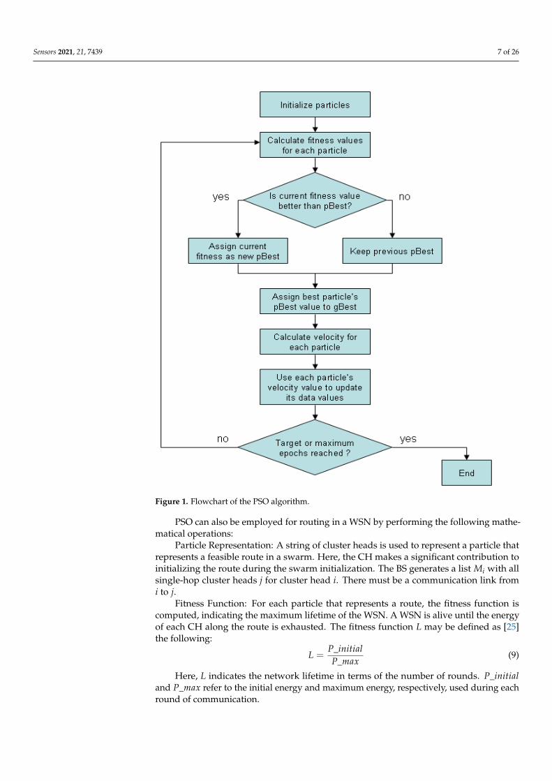
Figure 1. Flowchart of the PSO algorithm.

In PSO, the swarm refers to the population, and the particle of the swarm corre-sponds to the solution. During the flight process, each particle moves in the problem space with a velocity that depends upon its previous position and the best position of the swarm. Now consider 𝑥 and 𝑣 are the position and velocity of the 𝑖 particle, where the swarm has 𝑁 particles. Here, particle 𝑖 with a set of solutions is generally represented as 𝑋 = (𝑋 , 𝑋 , 𝑋 … . . 𝑋 ). The position and velocity update of each particle during subsequent iterations is shown by the following equations [25]: 𝑥 , (𝑡) = 𝑥 , (𝑡 − 1) + 𝑣 , (𝑡 − 1) (7) 𝑣 , (𝑡) = 𝑤 ∗ 𝑣 ,( ) (𝑡 − 1) + 𝑐 ∗ 𝑟𝑎𝑛𝑑1( ) ∗ 𝑝𝑏𝑒𝑠𝑡 , − 𝑥 , (𝑡 − 1) + 𝑐 ∗ 𝑟𝑎𝑛𝑑2() ∗ (𝑔𝑏𝑒𝑠𝑡 − 𝑥 , (𝑡 − 1)) (8)

Here, 𝑚 is the dimension of the solution space. rand1 ( ) and rand2 ( ) are the stochas-tic variables with uniform distribution and these variables are considered independent functions, that is, 𝑟𝑎𝑛𝑑1 ( ), 𝑟𝑎𝑛𝑑2 ( ) ∈ [0, 1] . 𝑐 and 𝑐 are the positive constants that refer to the cognitive and social constants, respectively. 𝑝𝑏𝑒𝑠𝑡 , is the best position that depends on the minimum path buffer, network lifetime, and hop count, with m solu-tions that are attained using the neighboring particles. Further, 𝑔𝑏𝑒𝑠𝑡 indicates the global optimal.

PSO can also be employed for routing in a WSN by performing the following math-ematical operations:

Particle Representation: A string of cluster heads is used to represent a particle that represents a feasible route in a swarm. Here, the CH makes a significant contribution to initializing the route during the swarm initialization. The BS generates a list 𝑀 with all

Figure 1. Flowchart of the PSO algorithm.

PSO can also be employed for routing in a WSN by performing the following mathe-matical operations:

Particle Representation: A string of cluster heads is used to represent a particle thatrepresents a feasible route in a swarm. Here, the CH makes a significant contribution toinitializing the route during the swarm initialization. The BS generates a list Mi with allsingle-hop cluster heads j for cluster head i. There must be a communication link fromi to j.

Fitness Function: For each particle that represents a route, the fitness function iscomputed, indicating the maximum lifetime of the WSN. A WSN is alive until the energyof each CH along the route is exhausted. The fitness function L may be defined as [25]the following:

L =P_initialP_max

(9)

Here, L indicates the network lifetime in terms of the number of rounds. P_initialand P_max refer to the initial energy and maximum energy, respectively, used during eachround of communication.

Sensors 2021, 21, 7439 8 of 26

Velocity: Velocity illustrates a binary operation that generates a new position for acluster head. For instance, a velocity of (1,6) implies that the position of CH 1 will beupdated to 6.

Position plus Velocity: if x and v indicate the position and velocity, respectively, theaddition operation may be performed as follows [25]:

x = (2, 7, 7, 4, 3, 5, 8)

v = (1, 6)(5, 5)

When performing x + v, for (1, 6), the new position of CH 1 will be 6, thus giving theresults of (6, 7, 7, 4, 3, 5, 8). Further, after applying a velocity of (5, 5), we get (6, 7, 7, 4, 5, 5, 8).

Position minus Position: The minus operation for a position produces a velocity.Suppose route r1 = 2, 4, 5, 6, 8, 8 and r2 = 2, 6, 5, 7, 8, 8. Then, the minus operationindicates the replaced cluster heads and is ((4, 6), (6, 7)).

Velocity plus Velocity: The addition of velocity v1 and v2 refers to the list of transposi-tions of CH in v1, followed by those in v2. With the addition of velocity, the identificationof the CH never has a copy in the resultant velocity.

Coefficient times Velocity (Multiplication): Consider that m and v represent the coeffi-cient and velocity, respectively. Here, velocity v = (i, j)|i ∈ 1, 2 . . . N . Now, m times vyields another velocity, v′ = (i, j)| i ∈ 1, 2 . . . N and j ∈ Ni (neighbor of CH i).

4.2. Genetic Algorithm-Based Routing

GA is a search-based optimization approach that employs the principle of geneticsand natural selection [27–29]. It is often used to provide optimal or suboptimal solutions tochallenging real-life problems that might take a longer time to resolve. The steps performedfor applying a GA to solve an energy optimization problem in a WSN are given as follows:

• Step 1: Initially, the chromosome is encoded in an efficient manner.• Step 2: In order to maximize the network lifetime, the individual with the highest

fitness function value is taken in the upcoming generation.• Step 3: The mating pool of good individuals is created through selection.• Step 4: Among the pool of good individuals, two parents are selected to exchange

their genes to create new offspring. The newly created offspring are expected to havebetter fitness values than the parents.

• Step 5: Mutation is also employed to achieve diversity in the offspring generatedduring the crossover.

4.3. PSOGA-Based Routing Algorithm

The genetic algorithm uses its individuals to find the local solution that feeds thePSO. The PSO is only able to find the global solution since the process of finding the localsolution, that is, the local best solution, is accomplished by the GA. The main aim is toreduce the premature convergence by the PSO that falls in the local optima. Hence, toobtain a developed solution, we mainly considered the formation of the local solutionby the genetic individuals or chromosomes. Here, each individual represents a potentialsolution. Furthermore, in the GA, each particle is regarded as an individual chromosome,and the swarm refers to the entire population.

The PSOGA starts with the process of generating random individuals while consider-ing the total iterations as a parameter for the algorithm. The population aims to providesolutions to the route planning, and the solution is considered in a distributed manner overthe whole IoT network. The initial population is allowed to pass through the GA in itsinitial iterations. This helps in reducing the route selection score, as the GA performanceentirely depends on encoding the solutions in particles and chromosomes. In addition, itconsiders the measurement of the fitness function, population size, and the total number ofiterations. Such parameters are adjusted after the evaluation of the GA on the initial trails.The PSO starts its operation after obtaining the local solutions by the GA during the initial

Sensors 2021, 21, 7439 9 of 26

iterations. The PSO uses particles to find the global solutions that represent the overallsolutions in finding the optimal routes. The steps are as follows:

• Step 1: Initialize a swarm of particles with a random position and zero velocity.• Step 2: Evaluate the objective values of the particles.• Step 3: Evaluate the fitness function value for each particle.• Step 4: Determine the local and global best solution.• Step 5: Until the termination condition is reached, update the velocity and position of

each particle, and update the local and global best solution.• Step 6: Arrange individuals in decreasing order of fitness function value and find the

M best particles.• Step 7: GA Evolution—reproduce Pop_size-M (performing subtraction) and GA in-

dividuals, and implement crossover and mutation operators to create Pop_size-Mparticles.

• Step 8: Combine and form Pop_size individuals.• Step 9: End.

The application of PSOGA is followed by updating the V* (see Table 1). Further,equation (4) is used to evaluate the route score, followed by a zigzag scan that starts in theupper-left corner of the grid. It sequentially scans the diagonals of the grid to determinethe route score. Once the evaluation has been done, the CH communicates the same to theneighboring grid. The same pattern is followed subsequently for the remaining grids. Thepresent work was focused on static WSN nodes. In case a CH fails, there is a packet dropin the network; all the parameters will be reset and the re-election of the CH will begin.

Table 1. Parameters used in the proposed PSOGA algorithm.

Parameter Description

Ir(Ni) Information register with information of individual node Ni in the network

A Area

Ni Node i

Ls Sink location

Ns Number of grids in a network

Fch Farthest CH

S Network sink

V* Set of random routes of a grid to adjacent grids in the network. Forexample, from the farthest CH to the sink from (Fch to S)

BestScore Best route score

Na All nodes in route

Rscore (i) Global route score

Score (i) Individual route score

GBestScore Global best score

LbestScore Local best score

4.4. Trust-Based Cluster Head Selection

Over the past few decades, researchers have employed a trust parameter in WSNs [30–34].For instance, the authors of [35] proposed a framework that forms clusters in a mannerso as to prevent the likelihood of compromised or malicious nodes being elected as CHs.For the same purpose, the current model uses statistical methods to evaluate trust withoutconsidering the trust among the sensor nodes. In [35], the authors suggested a model thatevaluates trust using a classical probability model. Furthermore, the suggested model em-ploys simple statistical methods for the same purpose, barring the trust recommendationamong sensor nodes that prevents nodes from reflecting trust in an accurate manner.

Sensors 2021, 21, 7439 10 of 26

The authors of [36] also proposed a trust-based LEACH (T-LEACH) protocol thatutilizes CH-assisted monitoring to reduce energy consumption. In the proposed model,the trust module consists of two different modules, namely, a monitoring module and atrust evaluation module. Here, the monitoring module observes the network and reportsto the trust evaluation module if any misbehavior is noticed. Further, a node also main-tains a neighbor situational trust table (NSTT) loaded with a trust value for each pair ofnode IDs and situation operations, such as data sensing, localization, and routing. As aresult, T-LEACH loses less data than LEACH, as half of all the information sent by clusterparticipants is processed by the gateway. However, it is not possible to stop the constantloss of data in T-LEACH because of the lack of monitoring on the cluster head.

Similar work is also carried out in [37] by the proposed node behavioral techniquestrust analysis algorithm banding belief theory (NBBTE), which combines the method of thenode behavioral strategy and Dempster–Shafer (DS) evidence theory. Here, a variety ofnetwork application-related trust factors, such as the packet size, the forwarding rate of thepacket, data reliability, and security grade and coefficients are considered to determine theconfidence values by measuring the weighted average of the trust factors. The simulationtests demonstrated that the proposed scheme is capable of effectively evaluating the trustnodes. However, the method of trust evaluation can entail excess energy, time, and costsdue to the cooperation and interaction with neighbors and other numerous parameters.

In [19], a cluster head selection method was proposed, which is based on a trust factorthat ensures all nodes are trustworthy and authentic during communication. To achievethis, direct trust is calculated using parameters such as the residual energy and the distancebetween the nodes, along with the use of the k-means clustering algorithm. The selectionfactor, F(f ), for recommended nodes is evaluated using the following weight function:

F( f ) = w1 ∗( e

d

)+ w2 ∗ trust_value (10)

w1 + w2 = 1 (11)

where w1 and w2 are the weight values, which can vary between 0 and 1. The sum of w1and w2 should be equal to 1. e is the energy and d is the distance.

After measuring the fitness function, the node with the highest fitness value is selectedas the cluster head.

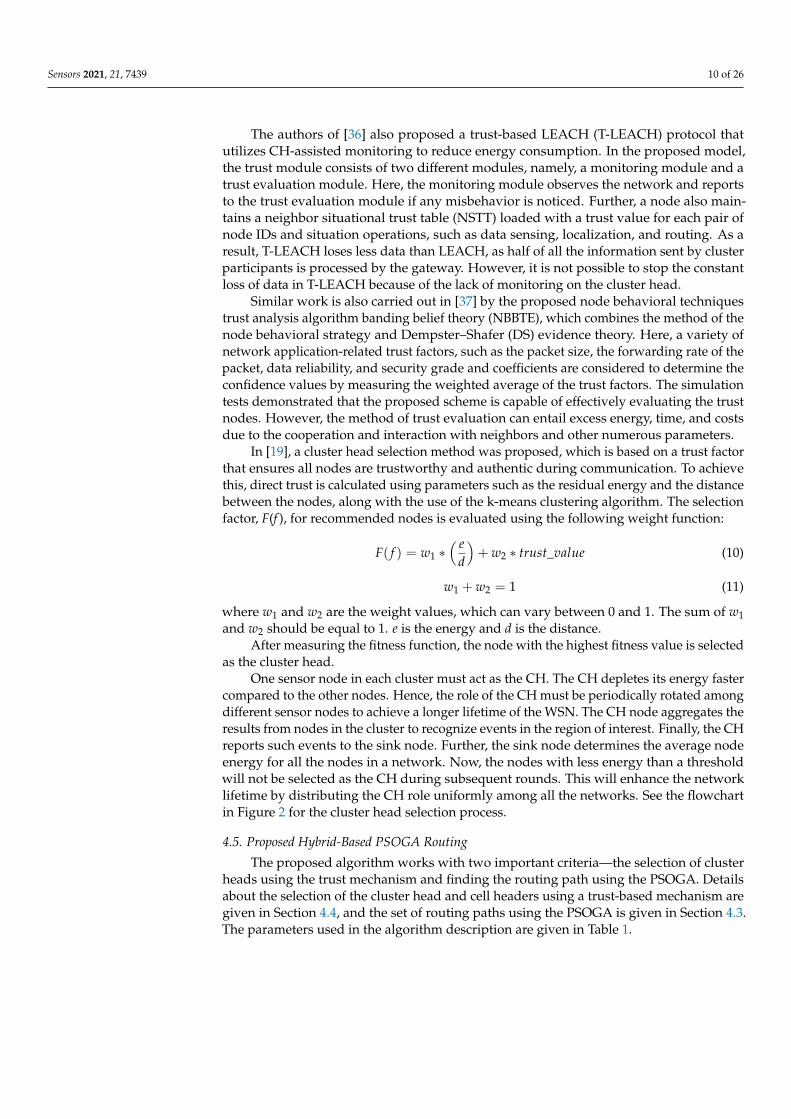
One sensor node in each cluster must act as the CH. The CH depletes its energy fastercompared to the other nodes. Hence, the role of the CH must be periodically rotated amongdifferent sensor nodes to achieve a longer lifetime of the WSN. The CH node aggregates theresults from nodes in the cluster to recognize events in the region of interest. Finally, the CHreports such events to the sink node. Further, the sink node determines the average nodeenergy for all the nodes in a network. Now, the nodes with less energy than a thresholdwill not be selected as the CH during subsequent rounds. This will enhance the networklifetime by distributing the CH role uniformly among all the networks. See the flowchartin Figure 2 for the cluster head selection process.

4.5. Proposed Hybrid-Based PSOGA Routing

The proposed algorithm works with two important criteria—the selection of clusterheads using the trust mechanism and finding the routing path using the PSOGA. Detailsabout the selection of the cluster head and cell headers using a trust-based mechanism aregiven in Section 4.4, and the set of routing paths using the PSOGA is given in Section 4.3.The parameters used in the algorithm description are given in Table 1.

Sensors 2021, 21, 7439 11 of 26

Sensors 2021, 21, x FOR PEER REVIEW 11 of 27

Finally, the CH reports such events to the sink node. Further, the sink node determines the average node energy for all the nodes in a network. Now, the nodes with less energy than a threshold will not be selected as the CH during subsequent rounds. This will en-hance the network lifetime by distributing the CH role uniformly among all the networks. See the flowchart in Figure 2 for the cluster head selection process.

Figure 2. Flowchart for cluster head selection.

4.5. Proposed Hybrid-Based PSOGA Routing The proposed algorithm works with two important criteria—the selection of cluster

heads using the trust mechanism and finding the routing path using the PSOGA. Details about the selection of the cluster head and cell headers using a trust-based mechanism are given in Section 4.4, and the set of routing paths using the PSOGA is given in Section 4.3. The parameters used in the algorithm description are given in Table 1.

Figure 2. Flowchart for cluster head selection.

The algorithm for the proposed model is given in Algorithm 1 as follows:

Algorithm 1 Proposed Trust-Based PSOGA Algorithm

1. For i = 1 to number of gridsWhile Fch 6= S

Generate V* using zigzag method

2. BestScore = 0;

3. For it = 1 to Max_IterationsFor i = 1 to rows (V*)

Temp = V*(i, Na)For j = 1 to length (Temp)For k = Temp(j)extract score factors from Ir(Ni)

End forEnd for

Rscore(i)= Score(i);//from equation 4 calculatedEnd forG_BestScore, index = max (Rscore);if L_BestScore > G_BestScoreG_BestScore = L_bestScore;SelR = V*(index,:);End ifUpdate V* using PSOGA Algorithm

End forEnd whileEnd for

4. Perform Communication between CH to sink using selected final route

5. Evaluate Network performance

6. Stop Algorithm

Sensors 2021, 21, 7439 12 of 26

In the proposed algorithm, Step 1 generates the random routes for each grid in thenetwork. The process of determining the random route continues while the farthest CHis not equal to the sink node. Step 2 initializes the best score to 0. Step 3 updates thepath V* determined in Step 1. For this, it uses the concept of the local score and globalscore. Step 4 initiates communication from the CH to the sink node through the pathobtained in Step 3. The performance of the network is evaluated as per Step 5 to obtain theperformance metrics, such as the longevity of the nodes, the network lifetime, the packetdelivery ratio and throughput, and so forth. The most prevalent genetic algorithm (GA)and swarm intelligence technique (PSO) benefits are taken into account for getting a betterconvergence and path to improve the network lifetime.

5. Network Setup

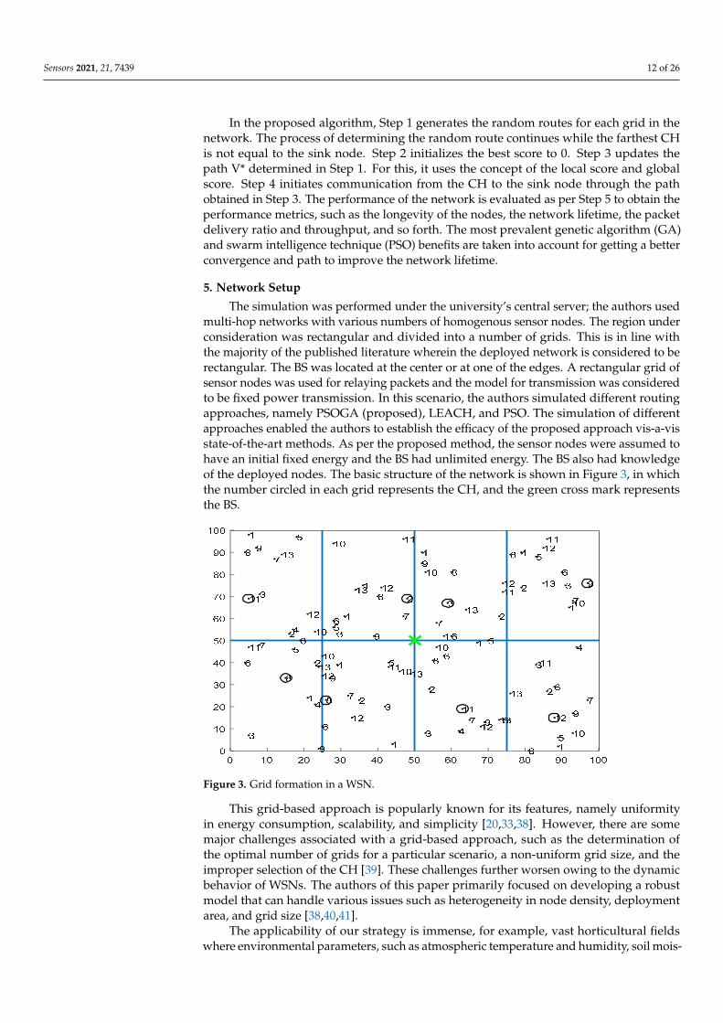
The simulation was performed under the university’s central server; the authors usedmulti-hop networks with various numbers of homogenous sensor nodes. The region underconsideration was rectangular and divided into a number of grids. This is in line withthe majority of the published literature wherein the deployed network is considered to berectangular. The BS was located at the center or at one of the edges. A rectangular grid ofsensor nodes was used for relaying packets and the model for transmission was consideredto be fixed power transmission. In this scenario, the authors simulated different routingapproaches, namely PSOGA (proposed), LEACH, and PSO. The simulation of differentapproaches enabled the authors to establish the efficacy of the proposed approach vis-a-visstate-of-the-art methods. As per the proposed method, the sensor nodes were assumed tohave an initial fixed energy and the BS had unlimited energy. The BS also had knowledgeof the deployed nodes. The basic structure of the network is shown in Figure 3, in whichthe number circled in each grid represents the CH, and the green cross mark representsthe BS.

Sensors 2021, 21, x FOR PEER REVIEW 13 of 27

rectangular. The BS was located at the center or at one of the edges. A rectangular grid of sensor nodes was used for relaying packets and the model for transmission was consid-ered to be fixed power transmission. In this scenario, the authors simulated different rout-ing approaches, namely PSOGA (proposed), LEACH, and PSO. The simulation of differ-ent approaches enabled the authors to establish the efficacy of the proposed approach vis-a-vis state-of-the-art methods. As per the proposed method, the sensor nodes were as-sumed to have an initial fixed energy and the BS had unlimited energy. The BS also had knowledge of the deployed nodes. The basic structure of the network is shown in Figure 3, in which the number circled in each grid represents the CH, and the green cross mark represents the BS.

Figure 3. Grid formation in a WSN.

This grid-based approach is popularly known for its features, namely uniformity in energy consumption, scalability, and simplicity [20,33,38]. However, there are some major challenges associated with a grid-based approach, such as the determination of the opti-mal number of grids for a particular scenario, a non-uniform grid size, and the improper selection of the CH [39]. These challenges further worsen owing to the dynamic behavior of WSNs. The authors of this paper primarily focused on developing a robust model that can handle various issues such as heterogeneity in node density, deployment area, and grid size [38,40,41].

The applicability of our strategy is immense, for example, vast horticultural fields where environmental parameters, such as atmospheric temperature and humidity, soil moisture, soil temperature, and soil pH, are to be measured [42]. In addition, it can be applied to any event detection application, such as wildfire detection [43] and seismic monitoring [44]. Apart from these, it can also be used in structural health monitoring where parameters such as humidity, temperature, stress, and strain are required to be measured [45]. In several of these above scenarios, it is cost effective to use non-recharge-able nodes.

In real-life deployments, the geographical area may not be rectangular. Our thinking is that a rectangle can be fitted to any irregular geographical area by using its extents, much like how irregular features in images are processed in a bounded rectangle. This is likely to have the effect of having some grids on the periphery of the geographic region where there may be very few nodes, or even none. An empty grid will not require a cluster head and will, thus, not participate in the path selection process.

It is assumed that a large number of radio channels are available for transmission, which will mitigate interference issues [46].

Figure 3. Grid formation in a WSN.

This grid-based approach is popularly known for its features, namely uniformityin energy consumption, scalability, and simplicity [20,33,38]. However, there are somemajor challenges associated with a grid-based approach, such as the determination ofthe optimal number of grids for a particular scenario, a non-uniform grid size, and theimproper selection of the CH [39]. These challenges further worsen owing to the dynamicbehavior of WSNs. The authors of this paper primarily focused on developing a robustmodel that can handle various issues such as heterogeneity in node density, deploymentarea, and grid size [38,40,41].

The applicability of our strategy is immense, for example, vast horticultural fieldswhere environmental parameters, such as atmospheric temperature and humidity, soil mois-

Sensors 2021, 21, 7439 13 of 26

ture, soil temperature, and soil pH, are to be measured [42]. In addition, it can be applied toany event detection application, such as wildfire detection [43] and seismic monitoring [44].Apart from these, it can also be used in structural health monitoring where parameters suchas humidity, temperature, stress, and strain are required to be measured [45]. In several ofthese above scenarios, it is cost effective to use non-rechargeable nodes.

In real-life deployments, the geographical area may not be rectangular. Our thinkingis that a rectangle can be fitted to any irregular geographical area by using its extents, muchlike how irregular features in images are processed in a bounded rectangle. This is likely tohave the effect of having some grids on the periphery of the geographic region where theremay be very few nodes, or even none. An empty grid will not require a cluster head andwill, thus, not participate in the path selection process.

It is assumed that a large number of radio channels are available for transmission,which will mitigate interference issues [46].

In Section 6, the evaluation of the PSOGA is presented with various performancemetrics, including the total residual energy, the network throughput, the total number ofalive nodes at the end of each iteration, and the packet delivery ratio (PDR). The PSOGAwas compared with the conventional LEACH protocol, with the parametric setting givenin Table 2.

Table 2. Network parameter setup.

Parameters Values

Network area 100 m × 100 m, 200 m × 200 m and 500 m × 500 m

Total number of nodes 100, 200, 625 and 1250

Initial energy 0.2 J

Power amplification (ε f s) 10 pj/bit/m2

Power amplification (εmp) 0.0013 pj/bit/m4

Transmitter/receiver energy (Eelec) 50 nJ/bit

Base station location (50, 50), (125, 125) and (250, 250)

Number of rounds 2500

6. Results and Discussion

The proposed strategy was further tested in five different scenarios with varyingnetwork area sizes, number of grids/clusters, and total number of nodes, as shown inTable 3, in which the number of grids varies with different cases and ranges between 8 and100, with the node population ranging from 100 to 1250 based on the size of the networkarea. The details of these scenarios are given in Table 3.

Table 3. Different network setups for simulation.

Case Study Network Area Number of Grids Total Number of Nodes

1 100 m × 100 m 2 × 4 100

2 100 m × 100 m 4 × 4 100

3 200 m × 200 m 4 × 4 200

4 500 m × 500 m 10 × 10 625

5 500 m × 500 m 10 × 10 1250

The entire setup was in an area with the base station located at the center, as shown inFigure 3.

The proposed PSOGA method was compared with the conventional LEACH protocol.The parametric settings are given in Table 2 and the grid formation is shown in Figure 3.

Sensors 2021, 21, 7439 14 of 26

The performance evaluation was done based on the total number of packets reaching theBS, the total number of alive nodes, the residual energy of the network, the packet deliveryratio (PDR), and the throughput of the network. The packet delivery ratio (PDR) indicatesthe ratio between the number of packets that the sink or destination receives and theentire number of packets sent by the source. Sections 6.1–6.7 demonstrate the performanceevaluation based on different grid configurations and network settings. For each scenario,the simulation was performed ten times and the mean was plotted for each metric.

6.1. Case Study 1

Figure 4 shows the results of Case Study 1: 2 × 4 grids, 100 nodes. The networkstructure (Figure 4a) shows eight grids with the selected cluster heads marked in num-bers in triangular shapes and connected by black lines. The comparative results of theperformance metrics are shown in Figure 4b–f. For each metric, the network was generatedand the simulation was performed 10 times. The average of the 10 simulations, each over2500 rounds, were plotted, along with the standard deviation.

The number of packets reaching the BS is shown in Figure 4b. After 2500 rounds, thepackets sent to the BS with the PSOGA improved by 278.94% and 5.55% as compared toLEACH and PSO, respectively. Figure 4c shows the number of nodes alive at each round.The points at which all the nodes were dead for LEACH, PSO, and the proposed PSOGAwere after 700, 1900, and 2000 rounds, respectively, which shows significant improvementsof 185.7% and 5.26% over LEACH and PSO, respectively. The residual energy also demon-strated promising improvement, as shown in Figure 4d. The energy was depleted after 500,1700, and 1800 rounds for LEACH, PSO, and the proposed PSOGA, respectively. Thus, thenetwork energy in the proposed PSOGA achieved an enhancement of 259.06% comparedto LEACH and 9.97% compared to PSO. Figure 4e demonstrates improvements in thePDR by 298.75% and 67.5% compared to LEACH and PSO, respectively. Furthermore, thethroughput with the PSOGA was increased by 7.13% and 49.5% as compared to PSO andLEACH, respectively, as shown in Figure 4f.

Figure 4g is a representative graph showing the nodes alive for each of the 10 sim-ulations for LEACH, PSO, and PSOGA. The average of the 10 simulations is shown inFigure 4c. As mentioned earlier, 10 simulations were similarly performed for each ofthe other metrics. The bar graph in Figure 4h shows the simulation times for LEACH,PSO, and PSOGA. Figure 4i shows the difference between PSO and PSOGA, from 1350 to1650 rounds.

6.2. Case Study 2

Figure 5 shows the results of Case Study 2: 4 × 4 grids, 100 nodes. The networkstructure (Figure 5a) shows 16 grids, with the selected cluster heads marked in numbersand connected by a black line. The results of the performance metrics show that with100 nodes, the packets sent to the BS (Figure 5b) improved by 268.42% and 9.36% whencompared to LEACH and PSO, respectively. Further, the PSOGA demonstrated an increasein the number of alive nodes by 155.43% and 10% as compared to the PSO and LEACH,respectively. The results in Figure 5d illustrate that the number of alive nodes became zeroafter 500, 1850, and 1994 rounds for LEACH, PSO, and the proposed PSOGA algorithm,respectively, leading to significant gains of 274.64% and 10.4% vis-à-vis LEACH and PSO,respectively. Similarly, the PDR was improved by 314.25% and 72.48% in comparison toLEACH and PSO, respectively (Figure 5e). Finally, the proposed PSOGA demonstratedthroughput enhancement of 37.5% and 4.84% compared to LEACH and PSO, respectively,as shown in Figure 5f.

Sensors 2021, 21, 7439 15 of 26Sensors 2021, 21, x FOR PEER REVIEW 15 of 27

(a) (b)

(c) (d)

(e) (f)

Avg.

/STD

PD

R (%

)

Avg.

/STD

Thr

ough

put

Figure 4. Cont.

Sensors 2021, 21, 7439 16 of 26Sensors 2021, 21, x FOR PEER REVIEW 16 of 27

(g) (h)

(i)

Figure 4. Results of Case Study 1: 2 × 4, 100 nodes. (a) Network structure for Case Study 1. (b) Packets reaching the BS. (c) Total alive nodes. (d) Total residual energy. (e) PDR. (f) Throughput. (g) Graph showing data plots of 10 simulations. (h) Simulation time for 10 simulations. (i) Error bound for alive nodes.

The number of packets reaching the BS is shown in Figure 4b. After 2500 rounds, the packets sent to the BS with the PSOGA improved by 278.94% and 5.55% as compared to LEACH and PSO, respectively. Figure 4c shows the number of nodes alive at each round. The points at which all the nodes were dead for LEACH, PSO, and the proposed PSOGA were after 700, 1900, and 2000 rounds, respectively, which shows significant improve-ments of 185.7% and 5.26% over LEACH and PSO, respectively. The residual energy also demonstrated promising improvement, as shown in Figure 4d. The energy was depleted after 500, 1700, and 1800 rounds for LEACH, PSO, and the proposed PSOGA, respectively. Thus, the network energy in the proposed PSOGA achieved an enhancement of 259.06% compared to LEACH and 9.97% compared to PSO. Figure 4e demonstrates improvements

Figure 4. Results of Case Study 1: 2 × 4, 100 nodes. (a) Network structure for Case Study 1. (b) Packets reaching the BS.(c) Total alive nodes. (d) Total residual energy. (e) PDR. (f) Throughput. (g) Graph showing data plots of 10 simulations.(h) Simulation time for 10 simulations. (i) Error bound for alive nodes.

As compared to Case study 1: 2 × 4 grids, 100 nodes, it is evident that although thenumber of nodes in both the case studies was the same, the difference lies in the gridstructure. In the case of the 4 × 4 grid, the network performed better in terms of theevaluated parameters. For instance, the number of packets sent to the BS in Case Study 2was 3.5 × 106, almost 3 × 105 higher than in Case Study 1, which had 3.2 × 106 packets.Similarly, the network structure demonstrated a slight improvement in the throughput,with a value of almost 17,500 as compared to 16,000 in the 8-grid structure.

Sensors 2021, 21, 7439 17 of 26

Sensors 2021, 21, x FOR PEER REVIEW 17 of 27

in the PDR by 298.75% and 67.5% compared to LEACH and PSO, respectively. Further-more, the throughput with the PSOGA was increased by 7.13% and 49.5% as compared to PSO and LEACH, respectively, as shown in Figure 4f.

Figure 4g is a representative graph showing the nodes alive for each of the 10 simu-lations for LEACH, PSO, and PSOGA. The average of the 10 simulations is shown in Fig-ure 4c. As mentioned earlier, 10 simulations were similarly performed for each of the other metrics. The bar graph in Figure 4h shows the simulation times for LEACH, PSO, and PSOGA. Figure 4i shows the difference between PSO and PSOGA, from 1350 to 1650 rounds.

6.2. Case Study 2 Figure 5 shows the results of Case Study 2: 4 × 4 grids, 100 nodes. The network struc-

ture (Figure 5a) shows 16 grids, with the selected cluster heads marked in numbers and connected by a black line. The results of the performance metrics show that with 100 nodes, the packets sent to the BS (Figure 5b) improved by 268.42% and 9.36% when com-pared to LEACH and PSO, respectively. Further, the PSOGA demonstrated an increase in the number of alive nodes by 155.43% and 10% as compared to the PSO and LEACH, respectively. The results in Figure 5d illustrate that the number of alive nodes became zero after 500, 1850, and 1994 rounds for LEACH, PSO, and the proposed PSOGA algorithm, respectively, leading to significant gains of 274.64% and 10.4% vis-à-vis LEACH and PSO, respectively. Similarly, the PDR was improved by 314.25% and 72.48% in comparison to LEACH and PSO, respectively (Figure 5e). Finally, the proposed PSOGA demonstrated throughput enhancement of 37.5% and 4.84% compared to LEACH and PSO, respectively, as shown in Figure 5f.

(a) (b)

0 20 40 60 80 100 120 140 160 180 200X-Axis

0

20

40

60

80

100

120

140

160

180

200

Y-Ax

is

Network Structure

12

3

4

56 7

8

9

10

11

12

13

14

15

16

Sensors 2021, 21, x FOR PEER REVIEW 18 of 27

(c) (d)

(e) (f)

Figure 5. Results of Case Study 2: 4 × 4, 100 nodes. (a) Network structure for Case Study 2. (b) Packets reaching the BS. (c) Total alive nodes. (d) Total residual energy. (e) PDR. (f) Throughput.

As compared to Case study 1: 2 × 4 grids, 100 nodes, it is evident that although the number of nodes in both the case studies was the same, the difference lies in the grid structure. In the case of the 4 × 4 grid, the network performed better in terms of the eval-uated parameters. For instance, the number of packets sent to the BS in Case Study 2 was 3.5 × 106, almost 3 × 105 higher than in Case Study 1, which had 3.2 × 106 packets. Similarly, the network structure demonstrated a slight improvement in the throughput, with a value of almost 17,500 as compared to 16,000 in the 8-grid structure.

6.3. Case Study 3 Figure 6 shows the results of Case Study 3: 4 × 4 grids, 200 nodes. The network struc-

ture (Figure 6a) shows 16 grids with the selected cluster heads marked in numbers and connected by a black line. The results of the performance metrics show that with 200 nodes, the packets sent to the BS (Figure 6b) with the PSOGA improved by 288.7% and 9.36% compared to LEACH and PSO, respectively. Furthermore, the number of alive nodes improved by 189.44% and 11.65% as compared to LEACH and PSO, respectively (Figure 6c). Figure 6d also demonstrates a similar trend with respect to residual energy, that is, the energy of the network was reduced to 0 after approximately 500 rounds, 1850

Avg.

/STD

Aliv

e N

odes

(%)

Figure 5. Results of Case Study 2: 4 × 4, 100 nodes. (a) Network structure for Case Study 2. (b) Packets reaching the BS.(c) Total alive nodes. (d) Total residual energy. (e) PDR. (f) Throughput.

Sensors 2021, 21, 7439 18 of 26

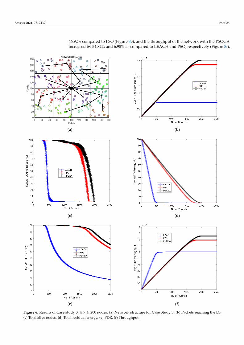
6.3. Case Study 3

Figure 6 shows the results of Case Study 3: 4 × 4 grids, 200 nodes. The networkstructure (Figure 6a) shows 16 grids with the selected cluster heads marked in numbersand connected by a black line. The results of the performance metrics show that with200 nodes, the packets sent to the BS (Figure 6b) with the PSOGA improved by 288.7%and 9.36% compared to LEACH and PSO, respectively. Furthermore, the number of alivenodes improved by 189.44% and 11.65% as compared to LEACH and PSO, respectively(Figure 6c). Figure 6d also demonstrates a similar trend with respect to residual energy, thatis, the energy of the network was reduced to 0 after approximately 500 rounds, 1850 rounds,and 1994 rounds for LEACH, PSO, and the proposed PSOGA, respectively, contributing toimprovement percentages of 279.2% and 12.5%, respectively. Similarly, the PDR was alsoenhanced by 304.9% and 67.3% compared to LEACH and PSO, respectively (Figure 6e).Figure 6f further demonstrates the efficacy of the PSOGA in terms of throughput improve-ment by 44.53% and 5.96% compared to LEACH and PSO, respectively.

We compared the performance metrics of Case Study 3 to Case Study 2, in whichthe number of grids was the same, that is, 16, but the number of nodes was higher, thatis, 200 nodes. The number of packets reaching the BS in Case Study 3 was higher, with3.6 × 106 vs. 3.5 × 106 packets, demonstrating a slight improvement of around 1 × 105

packets. Moreover, in Figures 5f and 6f, minimal improvement in the throughput canbe seen.

6.4. Case Study 4

Figure 7 shows the results of Case Study 4 with 10 × 10 grids, 625 nodes. The networkstructure (Figure 7a) shows 100 grids with the selected cluster heads marked in numbersand connected by a black line. The results of the performance metrics show that with625 nodes, the packets sent to the BS (Figure 7b) saw improvements of 325% and 30.76% ascompared to LEACH and PSO, respectively. The number of alive nodes was enhanced by232.22% and 6.26% as compared to LEACH and PSO, respectively. In Figure 7c, the residualenergy improved by 298.4% and 7.67% with respect to LEACH and PSO, respectively, asshown in Figure 7d. Furthermore, in Figure 7e, the PSOGA demonstrated increases of266.36% and 46.47% in the PDR as compared to LEACH and PSO, respectively. Similarly,Figure 7f shows increases in the throughput of the network by 46.3% and 6.87% whencompared to LEACH and PSO, respectively.

In Case Study 4, with 625 nodes and 100 grids, the performance of the networkdeteriorated as compared to the previous case studies. The number of packets sent to thebase station was 3.1 × 106, which is substantially lower than in the previous case studies.Similarly, the PDR was also reduced to 60% from the 70% achieved in Case Study 3. Thethroughput achieved in Case Study 4 was 15,500, much less than the 18,000 achieved inCase Study 3. The drastic reduction in the performance metrics can be attributed to thestructure, where, although the number of nodes was higher, the grid structure of 10 × 10made the process of path discovery cumbersome and, hence, reduced the throughput ofthe network.

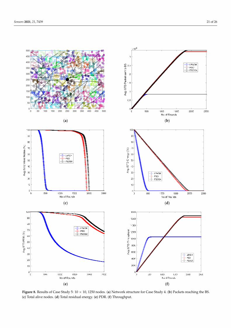
6.5. Case Study 5

Figure 8 shows the results of Case Study 5 with 10× 10 grids, 1250 nodes. The networkstructure (Figure 8a) shows 100 grids, with the selected cluster heads marked in numbersand connected by a black line. The results of the performance metrics show that with1250 nodes, the packets sent to the BS (Figure 8b) in the PSOGA achieved improvements of333% and 45.83%, respectively, as compared to LEACH and PSO. Furthermore, Figure 8cillustrates increases in the alive nodes by 236.7% and 5.89% when compared to LEACHand PSO, respectively. The PSOGA showed significant improvements in the residualenergy by 301% and 7.9% compared to LEACH and PSO, respectively (Figure 8d). PSOGAalso showed substantial improvements in the PDR by 274.7% compared to LEACH and

Sensors 2021, 21, 7439 19 of 26

46.92% compared to PSO (Figure 8e), and the throughput of the network with the PSOGAincreased by 54.82% and 6.98% as compared to LEACH and PSO, respectively (Figure 8f).

Sensors 2021, 21, x FOR PEER REVIEW 19 of 27

rounds, and 1994 rounds for LEACH, PSO, and the proposed PSOGA, respectively, con-tributing to improvement percentages of 279.2% and 12.5%, respectively. Similarly, the PDR was also enhanced by 304.9% and 67.3% compared to LEACH and PSO, respectively (Figure 6e). Figure 6f further demonstrates the efficacy of the PSOGA in terms of through-put improvement by 44.53% and 5.96% compared to LEACH and PSO, respectively.

(a) (b)

(c) (d)

(e) (f)

0 20 40 60 80 100 120 140 160 180 200X-Axis

0

20

40

60

80

100

120

140

160

180

200

Y-Ax

is

Network Structure

1

2

3

4

56

78

9 1011 12

1314

15 16

Figure 6. Results of Case study 3: 4 × 4, 200 nodes. (a) Network structure for Case Study 3. (b) Packets reaching the BS.(c) Total alive nodes. (d) Total residual energy. (e) PDR. (f) Throughput.

Sensors 2021, 21, 7439 20 of 26

Sensors 2021, 21, x FOR PEER REVIEW 20 of 27

Figure 6. Results of Case study 3: 4 × 4, 200 nodes. (a) Network structure for Case Study 3. (b) Packets reaching the BS. (c) Total alive nodes. (d) Total residual energy. (e) PDR. (f) Throughput.

We compared the performance metrics of Case Study 3 to Case Study 2, in which the number of grids was the same, that is, 16, but the number of nodes was higher, that is, 200 nodes. The number of packets reaching the BS in Case Study 3 was higher, with 3.6 × 106 vs. 3.5 × 106 packets, demonstrating a slight improvement of around 1 × 105 packets. More-over, in Figures 5f and 6f, minimal improvement in the throughput can be seen.

6.4. Case Study 4 Figure 7 shows the results of Case Study 4 with 10 × 10 grids, 625 nodes. The network

structure (Figure 7a) shows 100 grids with the selected cluster heads marked in numbers and connected by a black line. The results of the performance metrics show that with 625 nodes, the packets sent to the BS (Figure 7b) saw improvements of 325% and 30.76% as compared to LEACH and PSO, respectively. The number of alive nodes was enhanced by 232.22% and 6.26% as compared to LEACH and PSO, respectively. In Figure 7c, the resid-ual energy improved by 298.4% and 7.67% with respect to LEACH and PSO, respectively, as shown in Figure 7d. Furthermore, in Figure 7e, the PSOGA demonstrated increases of 266.36% and 46.47% in the PDR as compared to LEACH and PSO, respectively. Similarly, Figure 7f shows increases in the throughput of the network by 46.3% and 6.87% when compared to LEACH and PSO, respectively.

(a) (b)

(c) (d)

Sensors 2021, 21, x FOR PEER REVIEW 21 of 27

(e) (f)

Figure 7. Results of Case Study 4: 10 × 10, 625 nodes. (a) Network structure for Case Study 4. (b) Packets reaching the BS. (c) Total alive nodes. (d) Total residual energy. (e) PDR. (f) Throughput.

In Case Study 4, with 625 nodes and 100 grids, the performance of the network dete-riorated as compared to the previous case studies. The number of packets sent to the base station was 3.1 × 106, which is substantially lower than in the previous case studies. Simi-larly, the PDR was also reduced to 60% from the 70% achieved in Case Study 3. The throughput achieved in Case Study 4 was 15,500, much less than the 18,000 achieved in Case Study 3. The drastic reduction in the performance metrics can be attributed to the structure, where, although the number of nodes was higher, the grid structure of 10 × 10 made the process of path discovery cumbersome and, hence, reduced the throughput of the network.

6.5. Case Study 5 Figure 8 shows the results of Case Study 5 with 10 × 10 grids, 1250 nodes. The net-

work structure (Figure 8a) shows 100 grids, with the selected cluster heads marked in numbers and connected by a black line. The results of the performance metrics show that with 1250 nodes, the packets sent to the BS (Figure 8b) in the PSOGA achieved improve-ments of 333% and 45.83%, respectively, as compared to LEACH and PSO. Furthermore, Figure 8c illustrates increases in the alive nodes by 236.7% and 5.89% when compared to LEACH and PSO, respectively. The PSOGA showed significant improvements in the re-sidual energy by 301% and 7.9% compared to LEACH and PSO, respectively (Figure 8d). PSOGA also showed substantial improvements in the PDR by 274.7% compared to LEACH and 46.92% compared to PSO (Figure 8e), and the throughput of the network with the PSOGA increased by 54.82% and 6.98% as compared to LEACH and PSO, respectively (Figure 8f).

Figure 7. Results of Case Study 4: 10 × 10, 625 nodes. (a) Network structure for Case Study 4. (b) Packets reaching the BS.(c) Total alive nodes. (d) Total residual energy. (e) PDR. (f) Throughput.

Sensors 2021, 21, 7439 21 of 26

Sensors 2021, 21, x FOR PEER REVIEW 22 of 27

(a) (b)

(c) (d)

(e) (f)

Figure 8. Results of Case Study 5: 10 × 10, 1250 nodes. (a) Network structure for Case Study 4. (b) Packets reaching the BS. (c) Total alive nodes. (d) Total residual energy. (e) PDR. (f) Throughput.

In Case Study 5, with 1250 nodes and 100 grids, the performance of the network im-proved as compared to Case Study 4. The number of packets sent to the base station was

0 50 100 150 200 250 300 350 400 450 5000

50

100

150

200

250

300

350

400

450

500

Figure 8. Results of Case Study 5: 10 × 10, 1250 nodes. (a) Network structure for Case Study 4. (b) Packets reaching the BS.(c) Total alive nodes. (d) Total residual energy. (e) PDR. (f) Throughput.

Sensors 2021, 21, 7439 22 of 26

In Case Study 5, with 1250 nodes and 100 grids, the performance of the networkimproved as compared to Case Study 4. The number of packets sent to the base stationwas 3.2 × 106, which is higher than in the previous case study. Similarly, the PDR was alsoenhanced to 65% from the 60% achieved in Case Study 4. The throughput achieved in CaseStudy 5 was 17,000, higher than the 15,500 achieved in Case Study 4. The enhancement inthe performance metrics can be attributed to the structure, where, although the numberof grids is higher, the higher number of nodes—1250—sustained the network for a longertime and, thus, enhanced the performance metrics of the network.

6.6. Comparative Analysis

The results over various node densities and varying network grids were analyzed andthe comparative data of the network lifetime are presented in Figure 9. The first node dead(FND), half node dead (HND), and last node dead (LND) were the metrics of comparisonbetween LEACH, PSO, and the PSOGA. In all cases, the PSOGA showed significantimprovement over LEACH for all the metrics. The PSOGA also showed improvementsover PSO, albeit to a much lesser extent than the improvements compared to LEACH.

Sensors 2021, 21, x FOR PEER REVIEW 23 of 27

3.2 × 106, which is higher than in the previous case study. Similarly, the PDR was also enhanced to 65% from the 60% achieved in Case Study 4. The throughput achieved in Case Study 5 was 17,000, higher than the 15,500 achieved in Case Study 4. The enhance-ment in the performance metrics can be attributed to the structure, where, although the number of grids is higher, the higher number of nodes—1250—sustained the network for a longer time and, thus, enhanced the performance metrics of the network.

6.6. Comparative Analysis The results over various node densities and varying network grids were analyzed

and the comparative data of the network lifetime are presented in Figure 9. The first node dead (FND), half node dead (HND), and last node dead (LND) were the metrics of com-parison between LEACH, PSO, and the PSOGA. In all cases, the PSOGA showed signifi-cant improvement over LEACH for all the metrics. The PSOGA also showed improve-ments over PSO, albeit to a much lesser extent than the improvements compared to LEACH.

Figure 9. Overall lifetimes of sensor nodes, comparing the first node dead (FND), half node dead (HND), and last node dead (LND) between the proposed and existing models.

6.7. BS at the Edge To complete the study and evaluate the efficacy of the proposed algorithm, the BS

was placed at the edge of the network, as shown in Figure 10a. This case study enabled the evaluation of the performance of the PSOGA when the location of the base station is at the edge of a 2 × 4, 100 nodes configuration. In this case study, the PSOGA also showed notable improvements in various performance metrics. Figure 10b depicts the significant improvement in the number of packets sent to the BS, with the PSOGA exhibiting 278.94% and 9.0% improvements compared to LEACH and PSO, respectively. As shown in Figure 10c, PSOGA achieved improvements in the number of alive nodes by 192.93% and 12.47% as compared to LEACH and PSO, respectively. Furthermore, Figure 10d demonstrates the enhancements of 281.4% and 611.85% in the residual energy for PSOGA compared to LEACH and PSO, respectively. Similarly, substantial enhancements in the PDR by 302.96% and 66.28% for the PSOGA compared to LEACH and PSO, respectively, are vis-ualized in Figure 10e. Additionally, Figure 10f depicts the improvements of 45.87% and 6.54% in the throughput of the network with the PSOGA compared to LEACH and PSO, respectively. The plotted curves are the averages of the data from 10 simulations.

0

500

1000

1500

2000

2500

LEAC

H

PSO

PSOG

A

LEAC

H

PSO

PSOG

A

LEAC

H

PSO

PSOG

A

LEAC

H

PSO

PSOG

A

LEAC

H

PSO

PSOG

A

2X4 (100 nodes) 4X4 (100 nodes) 4X4 (200 nodes) 10X10 (625 nodes) 10X10 (1250nodes)

FND HND LND

Figure 9. Overall lifetimes of sensor nodes, comparing the first node dead (FND), half node dead (HND), and last nodedead (LND) between the proposed and existing models.

6.7. BS at the Edge

To complete the study and evaluate the efficacy of the proposed algorithm, the BSwas placed at the edge of the network, as shown in Figure 10a. This case study enabledthe evaluation of the performance of the PSOGA when the location of the base stationis at the edge of a 2 × 4, 100 nodes configuration. In this case study, the PSOGA alsoshowed notable improvements in various performance metrics. Figure 10b depicts thesignificant improvement in the number of packets sent to the BS, with the PSOGA exhibiting278.94% and 9.0% improvements compared to LEACH and PSO, respectively. As shownin Figure 10c, PSOGA achieved improvements in the number of alive nodes by 192.93%and 12.47% as compared to LEACH and PSO, respectively. Furthermore, Figure 10ddemonstrates the enhancements of 281.4% and 611.85% in the residual energy for PSOGAcompared to LEACH and PSO, respectively. Similarly, substantial enhancements in thePDR by 302.96% and 66.28% for the PSOGA compared to LEACH and PSO, respectively,are visualized in Figure 10e. Additionally, Figure 10f depicts the improvements of 45.87%and 6.54% in the throughput of the network with the PSOGA compared to LEACH andPSO, respectively. The plotted curves are the averages of the data from 10 simulations.

Sensors 2021, 21, 7439 23 of 26Sensors 2021, 21, x FOR PEER REVIEW 24 of 27

(a) (b)

(c) (d)

(e) (f)

Figure 10. Results of BS at edge, 2 × 4 100 nodes. (a) Network structure BS at edge. (b) Packets reaching the BS. (c) Total alive nodes. (d) Total residual energy. (e) PDR. (f) Throughput.

7. Conclusions and Future Scope In this study, a trust-based PSOGA model was developed to increase the network

lifetime in an IoT-based WSN environment. In this model, after the formation of grids, the optimal selection of the CH using a trust model among the stationary nodes enables reli-able data transmission from the sensor nodes to the cluster head. After forming the initial

Avg.

/STD

Ene

rgy

(%)

Avg.

/STD

Thr

ough

put

Figure 10. Results of BS at edge, 2 × 4 100 nodes. (a) Network structure BS at edge. (b) Packets reaching the BS. (c) Totalalive nodes. (d) Total residual energy. (e) PDR. (f) Throughput.

7. Conclusions and Future Scope

In this study, a trust-based PSOGA model was developed to increase the networklifetime in an IoT-based WSN environment. In this model, after the formation of grids,the optimal selection of the CH using a trust model among the stationary nodes enablesreliable data transmission from the sensor nodes to the cluster head. After forming the

Sensors 2021, 21, 7439 24 of 26

initial random paths using a zigzag strategy, the optimization algorithm helps in findingthe best routes that offer the quickest delivery of data packets to the sink node. Theconsideration of metrics, such as route score, number of received packets, number ofdelayed packets, residual energy, power consumed, and total hop counts, enables theoptimal selection of routes among the random paths. Such routes are reliable enough tocarry out the packet transmission, allowing for higher residual energy. The use of thePSOGA ensures the faster selection of routes than the existing LEACH mechanism; theproposed PSOGA obtained increased network lifetimes in all five different case studies.The percentages of dead nodes in the network after several iterations were significantlylower than those of the LEACH protocol, which shows the efficacy of the present system.

Currently, the authors are engaged in extending the presented work in the directionof data reduction, coupled with security, to further enhance the network efficiency andprivacy. In the future, deep learning algorithms can be deployed for bufferless systemsthat match the speed of input data acquisition from several IoT devices. In addition to this,further research will consider a cross-layer approach to increase the network efficiency andlifetime when faced with node failures.

Author Contributions: M.M. conducted the simulation, coding, and performance analysis. G.S.G.conceived the scenario impact and design of the manuscript. X.G. performed the scenario impact andsimulation and coding. All authors have read and agreed to the published version of the manuscript.

Funding: This research received no external funding.

Institutional Review Board Statement: Not applicable.

Informed Consent Statement: Not applicable.

Data Availability Statement: No new data were created or analyzed in this study. Data sharing isnot applicable in this article.

Conflicts of Interest: The authors declare no conflict of interest. The statements made herein aresolely the responsibility of the authors.

References1. Xie, H.; Yan, Z.; Yao, Z.; Atiquzzaman, M. Data collection for security measurement in wireless sensor networks: A survey.

IEEE Internet Things J. 2018, 6, 2205–2224. [CrossRef]2. Baniata, M.; Reda, H.T.; Chilamkurti, N.; Abuadbba, A. Energy-Efficient Hybrid Routing Protocol for IoT Communication

Systems in 5G and Beyond. Sensors 2021, 21, 537. [CrossRef]3. Jia, Y. LoRa-Based WSNs Construction and Low-Power Data Collection Strategy for Wetland Environmental Monitoring.

Wirel. Pers. Commun. 2020, 114, 1533–1555. [CrossRef]4. Seema, B.; Yao, N.; Carie, A.; Shah, S.B.H. Efficient data transfer in clustered IoT network with cooperative member nodes.

Multimed. Tools Appl. 2020, 79, 34241–34251. [CrossRef]5. Roy, S.; Mazumdar, N.; Pamula, R. An optimal mobile sink sojourn location discovery approach for the energy-constrained and

delay-sensitive wireless sensor network. J. Ambient. Intell. Humaniz. Comput. 2021, 12, 10837–10864. [CrossRef]6. Sharma, N.; Sharma, A.K. Cost analysis of hybrid adaptive routing protocol for heterogeneous wireless sensor network. Sadhana

2016, 41, 283–288. [CrossRef]7. Elhoseny, M.; Farouk, A.; Zhou, N.; Wang, M.M.; Abdalla, S.; Batle, J. Dynamic multi-hop clustering in a wireless sensor network:

Performance improvement. Wirel. Pers. Commun. 2017, 95, 3733–3753. [CrossRef]8. Daanoune, I.; Abdennaceur, B.; Ballouk, A. A comprehensive survey on LEACH-based clustering routing protocols in Wireless

Sensor Networks. Ad Hoc Netw. 2021, 14, 102409. [CrossRef]9. Nikolidakis, S.A.; Kandris, D.; Vergados, D.D.; Douligeris, C. Energy efficient routing in wireless sensor networks through

balanced clustering. Algorithms 2013, 6, 29–42. [CrossRef]10. Wala, T.; Chand, N.; Sharma, A.K. Energy efficient data collection in smart cities using iot. In Handbook of Wireless Sensor Networks:

Issues and Challenges in Current Scenario’s; Springer: Cham, Switzerland, 2020; pp. 632–654.11. Iqbal, M.; Naeem, M.; Anpalagan, A.; Ahmed, A.; Azam, M. Wireless sensor network optimization: Multi-objective paradigm.

Sensors 2015, 15, 17572–17620. [CrossRef] [PubMed]12. Aslam, N.; Xia, K.; Haider, M.T.; Hadi, M.U. Energy-aware adaptive weighted grid clustering algorithm for renewable wireless

sensor networks. Future Internet 2017, 9, 54. [CrossRef]13. Anees, J.; Zhang, H.C.; Lougou, B.G.; Baig, S.; Dessie, Y.G. Delay aware energy-efficient opportunistic node selection in restricted

routing. Comput. Netw. 2020, 181, 107536. [CrossRef]

Sensors 2021, 21, 7439 25 of 26

14. Ullah, F.; Khan, M.Z.; Faisal, M.; Rehman, H.U.; Abbas, S.; Mubarek, F.S. An energy efficient and reliable routing scheme toenhance the stability period in wireless body area networks. Comput. Commun. 2021, 165, 20–32. [CrossRef]

15. Maurya, S.; Jain, V.K.; Chowdhury, D.R. Delay aware energy efficient reliable routing for data transmission in heterogeneousmobile sink wireless sensor network. J. Netw. Comput. Appl. 2019, 144, 118–137. [CrossRef]

16. Yu, M.; Leung, K.K.; Malvankar, A. A dynamic clustering and energy efficient routing technique for sensor networks. IEEE Trans.Wirel. Commun. 2007, 6, 3069–3079. [CrossRef]

17. Pompili, D.; Melodia, T.; Akyildiz, I.F. Three-dimensional and two-dimensional deployment analysis for underwater acousticsensor networks. Ad Hoc Netw. 2009, 7, 778–790. [CrossRef]

18. Liang, J.; Wang, Z.; Liu, Y.; Liu, X. State estimation for two-dimensional complex networks with randomly occurring nonlinearitiesand randomly varying sensor delays. Int. J. Robust Nonlinear Control. 2014, 24, 18–38. [CrossRef]

19. Mishra, M.; Gupta, G.S.; Gui, X. Trust-Based Cluster Head Selection Using the K-Means Algorithm for Wireless Sensor Networks.In Proceedings of the 2019 International Conference on Smart Systems and Inventive Technology (ICSSIT), Tirunelveli, India,27–29 November 2019; pp. 819–825. [CrossRef]

20. Hawbani, A.; Wang, X. Zigzag Coverage Scheme Algorithm & Analysis for Wireless Sensor Networks. Netw. Protoc. Algorithms2013, 5, 19–38. [CrossRef]

21. El Kader, M.E.E.D.A.; Youssif, A.A.A.; Ghalwash, A.Z. Energy Aware and Adaptive Cross-Layer Scheme for Video TransmissionOver Wireless Sensor Networks. IEEE Sens. J. 2016, 16, 7792–7802. [CrossRef]

22. Harbaoui Dridi, I.; Ben Alaïa, E.; Borne, P.; Bouchriha, H. Optimisation of the multi-depots pick-up and delivery problems withtime windows and multi-vehicles using PSO algorithm. Int. J. Prod. Res. 2020, 58, 4201–4214. [CrossRef]

23. Krishna, S.R.K.M.; Ramanath, M.B.N.S.; Prasad, V.K. Optimal reliable routing path selection in MANET through hybrid PSO-GAoptimisation algorithm. Int. J. Mob. Netw. Des. Innov. 2018, 8, 195–206.

24. Chengetanai, G.; Osunmakinde, I.O. Q-PSO: Hybridisation of Particle Swarm Optimisation with Queuing Theory for MitigatingCongestion on Mobile Ad-hoc Networks While Optimising Network Lifetime. Adhoc Sens. Wirel. Netw. 2020, 48, 37–65.

25. Agnihotri, A.; Gupta, I.K. A hybrid PSO-GA algorithm for routing in wireless sensor network. In Proceedings of the 2018 4thInternational Conference on Recent Advances in Information Technology (RAIT), Dhanbad, India, 15–17 March 2018; pp. 1–6.

26. Pavani, M.; Rao, P.T. Adaptive PSO with optimised firefly algorithms for secure cluster-based routing in wireless sensor networks.IET Wirel. Sens. Syst. 2019, 9, 274–283. [CrossRef]

27. Ma, C. Network optimisation design of hazmat based on multi-objective genetic algorithm under the uncertain environment.Int. J. Bio-Inspired Comput. 2018, 12, 236–244. [CrossRef]

28. Mathiyalagan, G.; Wahi, A. Energy and mobility aware route optimisation technique based on genetic algorithm in MANETs.Int. J. Mob. Netw. Des. Innov. 2017, 7, 69–77. [CrossRef]

29. Devaraj, D.; Banu, R.N. Genetic algorithm-based optimisation of load-balanced routing for AMI with wireless mesh networks.Appl. Soft Comput. 2019, 74, 122–132.

30. Gandhi, G.S.; Vikas, K.; Ratnam, V.; Babu, K.S. Grid clustering and fuzzy reinforcement-learning based energy-efficient dataaggregation scheme for distributed WSN. IET Commun. 2020, 14, 2840–2848. [CrossRef]

31. Singh, S.K.; Kumar, P.; Singh, J.P. An energy efficient protocol to mitigate hot spot problem using unequal clustering in WSN.Wirel. Pers. Commun. 2018, 101, 799–827. [CrossRef]

32. Hemalatha, R.; Prakash, R.; Sivapragash, C. Analysis on energy consumption in smart grid WSN using path operator calculuscentrality based HSA-PSO algorithm. Soft Comput. 2019, 24, 10771–10783. [CrossRef]

33. Mishra, A.K.; Kumar, R.; Kumar, V.; Singh, J. A grid-based approach to prolong lifetime of WSNs using fuzzy logic. In Advancesin Computational Intelligence; Springer: Singapore, 2017; pp. 11–22.

34. Otoum, S.; Kantarci, B.; Mouftah, H.T. Hierarchical trust-based black-hole detection in WSN-based smart grid monitoring. InProceedings of the 2017 IEEE International Conference on Communications (ICC), Paris, France, 21–25 May 2017; pp. 1–6.

35. Crosby, G.V.; Pissinou, N.; Gadze, J. A framework for trust-based cluster head election in wireless sensor networks. In Proceedingsof the Second IEEE Workshop on Dependability and Security in Sensor Networks and Systems, Columbia, MD, USA, 24–28April 2006.

36. Song, F.; Zhao, B. Trust-based LEACH protocol for wireless sensor networks. In Proceedings of the 2008 Second InternationalConference on Future Generation Communication and Networking, Hainan, China, 13–15 December 2008; Volume 1, pp. 202–207.

37. Feng, R.; Xu, X.; Zhou, X.; Wan, J. A trust evaluation algorithm for wireless sensor networks based on node behaviors and dsevidence theory. Sensors 2011, 11, 1345–1360. [CrossRef]

38. Tang, L.; Lu, Z.; Fan, B. Energy Efficient and Reliable Routing Algorithm for Wireless Sensors Networks. Appl. Sci. 2020, 10, 1885.[CrossRef]

39. Jannu, S.; Jana, P.K. A grid based clustering and routing algorithm for solving hot spot problem in wireless sensor networks.Wirel. Netw. 2016, 22, 1901–1916. [CrossRef]

40. Abdullah, M.; Eldin, H.N.; Al-Moshadak, T.; Alshaik, R.; Al-Anesi, I. Density grid-based clustering for wireless sensors networks.Procedia Comput. Sci. 2015, 65, 35–47. [CrossRef]

41. Li, J.; Andrew, L.L.; Foh, C.H.; Zukerman, M.; Chen, H.H. Connectivity, coverage and placement in wireless sensor networks.Sensors 2009, 9, 7664–7693. [CrossRef] [PubMed]

Sensors 2021, 21, 7439 26 of 26

42. Keshtgari, M.; Deljoo, A. A Wireless Sensor Network Solution for Precision Agriculture Based on Zigbee Technology.Wirel. Sens. Netw. 2012, 4, 25–30. [CrossRef]

43. Serna, M.; Casado, R.; Bermúdez, A.; Pereira, N.; Tennina, S. Distributed Forest Fire Monitoring Using Wireless Sensor Networks.Int. J. Distrib. Sens. Netw. 2015, 2015, 1–18. [CrossRef]

44. Jornet-Monteverde, J.A.; Galiana-Merino, J.; Soler-Llorens, J. Design and Implementation of a Wireless Sensor Network forSeismic Monitoring of Buildings. Sensors 2021, 21, 3875. [CrossRef]

45. Abrardo, A.; Balucanti, L.; Belleschi, M.; Carretti, C.; Mecocci, A. Health monitoring of architectural heritage: The case studyof San Gimignano. In Proceedings of the Environmental Energy and Structural Monitoring Systems (EESMS), Taranto, Italy, 9September 2010; pp. 98–102.

46. Zhou, G.; He, T.; Stankovic, J.A.; Abdelzaher, T. RID: Radio interference detection in wireless sensor networks. In Proceedingsof the Proceedings IEEE 24th Annual Joint Conference of the IEEE Computer and Communications Societies, Miami, FL, USA,13–17 March 2005; pp. 891–901.