Available online at www.sciencedirect.com

www.elsevier.com/locate/enconman

Energy Conversion and Management 49 (2008) 326–335

Natural gas electric generator powered by polymer exchangemembrane fuel cell: Numerical model and experimental results

M. Radulescu a, V. Ayel b, O. Lottin a,*, M. Feidt a, B. Antoine a,C. Moyne a, D. Le Noc c, S. Le Doze c

a LEMTA, UMR 7563 CNRS, Institut National Polytechnique de Lorraine, Universite Henri Poincare, BP 160,

2 Avenue de la Foret de Haye, 54504 Vandoeuvre-les-Nancy, Franceb LET-ENSMA, UMR CNRS 6608, 1 Avenue Clement Ader, BP 40109, 86961 Futuroscope-Chasseneuil, France

c Gaz de France, Direction de la Recherche, 361 Avenue du President Wilson, Saint Denis La Plaine, France

Received 24 October 2006; accepted 4 June 2007Available online 2 August 2007

Abstract

The reduction of pollutant emissions is an important advantage of fuel cells in small stationary power systems, particularly in com-bined heat and power generation (CHP). In fact, fuel cells are one of the future practical solutions for micro-CHP systems (5–10 kW) inthe domestic environment. This paper reports numerical and experimental results of 5 kWe CHP H-Power units running on natural gas.The natural gas is reformed locally to produce hydrogen. The numerical model of the units allows the simulation of the operation of thereformer, the cooler-shift, the prox (preferential oxidation reactor) and of the PEMFC. The PEMFC polarization curve is determined bya subroutine taking into account mass and charge transfers and the condensation of liquid water in the electrodes membrane assembly(EMA). The molar flux of species through the anode and cathode porous backing layers is calculated analytically by means of the Stefan–Maxwell equations. The gas channels are assumed parallel to the EMA, and the effects of concentration variation are investigated. Therelevance of the numerical results is first validated by comparison with experimental data; then, the performances of the system are ana-lyzed in terms of electrical efficiency. Although the measured electrical performances are disappointing, the numerical simulations andanalyses of experimental data suggest promising improvements. The model is employed to evaluate the best possible electrical efficiencyand to establish the ideal operation domain of the installations.� 2007 Elsevier Ltd. All rights reserved.

Keywords: PEMFC; Reformer; Stefan–Maxwell; Electrical efficiency

1. Introduction

The direct conversion of chemical energy into electricityand heat makes fuel cells particularly attractive for manyapplications. Among the various types of fuel cells, Theproton exchange membrane (PEM) fuel cells are the mostsuitable to power vehicles or portable electronic devices.Because they operate at low temperature (50–80 �C), theyare also considered for low or mid-power cogeneration sys-tems with low temperature heat recovery. In this paper, we

0196-8904/$ - see front matter � 2007 Elsevier Ltd. All rights reserved.

doi:10.1016/j.enconman.2007.06.011

* Corresponding author.E-mail address: Olivier.Lottin@ensem.inpl-nancy.fr (O. Lottin).

consider a single family residential combined heat andpower (CHP) unit, but we focus only on the electrical effi-ciency. The electrical efficiency of a PEMFC working undernormal operating conditions is about 40–70%, i.e. 60–30%of the fuel chemical energy is dissipated into heat that mustbe evacuated [1]. Fuel cells are environmentally clean whenoperating on pure hydrogen. However, hydrogen must bestored or produced locally, which is the case with methanolor natural gas reforming. Among all the fossil fuels, naturalgas has the lowest greenhouse effect in terms of carbondioxide emissions: since it is mainly composed of methane(CH4), the number of hydrogen atoms per carbon is closeto 4. However, reforming requires a large amount of energy

Nomenclature

a activity (–)B Tafel slope (V)c concentration (mol m�3)D diffusion coefficient (m2 s�1)E potential (V)EW equivalent weight (kg mol�1)F Faraday constant (C mol�1)h molar enthalpy (J mol�1)i0 exchange current density (A m�2)I current intensity (A)J current density (A m2)L thickness (m)_n molar flow rate (mol s�1)N number of cells (–)_N molar flux (mol m�2 s�1)

P pressure (Pa)_Q thermal power (W)R universal gas constant (J mol�1 K�1)S surface (m2)St stoiechiometry (–)T temperature (K)_W electric power (W)

x, y, z coordinates (m)y mole fraction (–)

Greek symbolsDg free enthalpy of reaction (J mol�1)g overpotential (V)k water content (–)kNG natural gas excess coefficient (–)q density (kg m�3)r protonic conductivity (S m�1)

s0 osmotic coefficient (mol mol�1)

Subscripts and superscripts

a anodeair airamb ambient temperaturebr burnedc cathodediff diffusiondry drye inlet/electriceff effective valueFC fuel cellgas gas mixture in reforming unitgross gross electric powerH hydrogeni, j species indexL liquidm membraneMEA membrane electrode assemblymin minimumnet net electric powerNG natural gaso outletosm electro-osmoticprox prox elementref reformedshift cooler-shift elementth thermalv vapour0 initial condition

M. Radulescu et al. / Energy Conversion and Management 49 (2008) 326–335 327

and is at the origin of many heat losses that can reduce theoverall efficiency of the cogeneration system, especiallywhen low temperature fuel cells are used.

This work was performed within the framework of theEPACOP project (Experimentation de cinq Piles A Combus-

tible de petite taille sur sites OPerationnels), led by GDFand co-funded by ADEME, having the main objective oftesting five identical CHP systems in real operating condi-tions. These systems (RCU 4500 V2), designed and built byH-Power, were put in operation in France between Novem-ber 2002 and June 2003 in different sites chosen to offer var-ious climatic and operating conditions [2]. The citiesparticipating in these experiments in real operating condi-tions are Dunkerque (2 units), Nancy, Limoges andSophia-Antipolis. All the cogeneration units are set up inpublic buildings, such as city halls or university laborato-ries. Their net electric power is about 5 kW, and the heatrecovered is about 6 kW (at low temperature: 60 �C). Theaim of our study is to model the system, including the fuelprocessing unit (reformer, cooler-shift, prox), in order to

analyse its electric performance. Special attention is givento the fuel cell, whose polarization curve is carefully mod-elled, in order to analyse the electric performance of thewhole system by extrapolating its behaviour towardshigher intensities.

Proton exchange membrane fuel cells are composed of apolymer electrolyte inserted between two porous diffusionlayers forming a membrane electrode assembly (MEA).The active layers (anode and cathode) are at the interfacebetween the electrolyte membrane and the diffusion layers.The MEA is usually held by two graphite plates (the bipo-lar plates), collecting electric current and distributing thereactants thanks to micro or mini channels.

Numerous models have been designed in order to under-stand fuel cell behaviour. One dimensional models ofcharge and mass transfer were first proposed [3,4]. Thesemodels make it possible to investigate the influence ofwater management on the performances of the electrodesor the whole MEA [5]. Heat transfer was sometimestaken into account [6–10]. However, the need for a better

Legend:

A

C

Reformer

PEMFC

Liquidseparator

Fan

liquidH O

NG

moistair

H2O

H (l)

NG

CoolerShift

CombustionGas

Stea

m

2O5p

5

7

68

10

1

3

2b

2

9

4

A

B

C

PROX

H2O

air

H (l)

Primary cooling water circuit

A

C

Reformer

PEMFC

Liquidseparator

Fan

liquid

2

NG H2O

moistair

α

H2O

NG

CoolerShift

Stea

m

5p

5

7

68

10

1

3

2b

2

9

4

A

B

C

PROX

2O

2O

Steam circuit,

NG+H

Reformate circuit,

Fig. 1. System main components – fuel and water circuits.

328 M. Radulescu et al. / Energy Conversion and Management 49 (2008) 326–335

description of the physical phenomena occurring in thewhole MEA, including hydrodynamics and multi-compo-nents transport in the gas channels, necessitates the useof 2D or 3D models [9,11–13]. Hence, multi-dimensionalmodels have been implemented for description of the cath-ode catalytic layer [14], or for description of the wholeMEA, including gas flows and composition variationsalong the channels ([15–17] for 2D models and [18,19] for3D models). Some descriptions take into account the ther-mal gradients between the electrodes and the channels([20,21] for 2D models and [11,22,23] for 3D models).Unfortunately, these models are heavy and complex, espe-cially when two phase flows are considered. This complex-ity can be at the expense of the amount of informationprovided by the software when numerical simulationsrequire excessive CPU time. Recently, Bautista et al. [13]proposed a pseudo-bidimensional model of fuel cell elec-trochemical behaviour, including mass transport alongthe gas channels and diffusion through the porous elec-trodes. The pseudo-bidimensional model developed in thepresent study is based on a geometrical description closeto the one proposed by Bautista et al., with the exceptionthat the electrodes overpotentials are evaluated by theTafel law instead of the gas diffusion electrodes (GDE)model (taking account of the volumetric characteristics ofcatalyst layers). Indeed, Ramousse et al. [10] showed thatGDE exhibit Tafel behaviour in steady state. Molar fluxesthrough diffusion layers are calculated analytically bymeans of Stefan–Maxwell equations for multi-componentgas diffusion of CO2, N2, H2O and H2 in the reformateand of water, nitrogen and oxygen in air.

The fuel processing unit and the main hypotheses gov-erning its modelling are described in Section 2. The PEMfuel cell is described and modelled in Section 3 where theresults are compared with experimental data. Finally, thesystem performances are analysed in term of electrical effi-ciency in Section 4.

2. Description and modelling of hydrogen production unit

The operation of the hydrogen production unit is basedon steam reforming of natural gas [24]. It is fully describedin Ref. [25] (Fig. 1). Experimental data (temperatures, pres-sures, flow rates, intensities and voltages) were recordedevery 20 s, but some of the experimental results reportedhere refer only to stable operating points (for which theintensity remains constant during at least 30 min). Radule-scu et al. [26] showed that the system electrical efficiencywas decreased by up to 2% points in normal operation(compared to stable operation), while the fuel cell electricalefficiency was not affected.

2.1. Reformer

The natural gas, first admitted into a sulphur trap forremoval of the odorant compounds (H2S, COS,(C2H5)2S), is blended to steam in the reformer and trans-

formed into a hydrogen rich mixture (the reformate). Reac-tions (1)–(3) (with b = 1, 2 or 3 for methane, ethane orpropane, respectively) occur at 650 �C.

CH4 þH2O! COþ 3H2 ð1ÞCOþH2O! CO2 þH2 ð2ÞCbHð2bþ2Þ þ 2bH2O! bCO2 þ ð3bþ 1ÞH2 ð3Þ

Reactions (1) and (2) being incomplete, the reformatestill contains CH4 and CO at the reformer outlet. More-over, the water concentration is high (between 0.35 and0.55 molH2O/molgas [25,27,28]) because the steam is fed inexcess in order to displace the equilibrium toward the prod-ucts side and to avoid amorphous coke formation (thesteam to carbon S/C ratio is between 6.5 and 8.1 [25,28],cf. Table 1). Ethane and propane are fully decomposed inthe reformer. The methane steam reforming reaction 1 isstrongly endothermic (Dh(1)(650 �C) = 224 kJ mol�1): hightemperature and catalysts are required to achieve anacceptable conversion. On the other hand, the water–gasshift reaction 2 is slightly exothermic (Dh(2)(650 �C) =�35.5 kJ mol�1), occurring mostly in the reformer but alsoat lower temperature in the cooler-shift.

The minimum flow rate of hydrogen required by the fuelcell is imposed by the current density JFC crossing theN = 120 elementary cells: _nmin

H2¼ J FCSN=2F . Knowledge

of the natural gas composition allows determining the min-imum natural gas flow rate at the inlet of the reformer:

_nminNG ¼

J FCSN

2FX H

ð4Þ

where X H ¼ 4cCH4þ 7cC2H6

þ 10cC3H8stands for the maxi-

mum number of hydrogen moles produced per mole of nat-ural gas. The minimum gas flow rate leads to the definitionof the excess coefficient of reformed natural gas:kNG ¼ _nref

NG= _nminNG, which stands for the ratio between the

amount of natural gas supplied to the reformer and theminimal quantity required. Experimental values of kNG

Table 1Set of parameters used in the numerical simulation for comparison with experimental data

I (A) <20 20 30 40 50 60 70 80 100 >100

kNG (–) 3.13 3.13 2.5 2.2 1.85 1.75 1.72 1.7 1.7 1.7S/C ratio (–) 8 8 8 8 7.7 7.4 7 6.5 6.5 6.5Burner excess air (%) 20Tair cathode inlet (K) 333

RHair cathode inlet (–) 0.6Fuel cell excess air (%) 141

Values in bold are experimental data and the others are estimated.

M. Radulescu et al. / Energy Conversion and Management 49 (2008) 326–335 329

are available in Table 1. Note that the total amount of nat-ural gas supplied to the system equals _nbr

NG þ _nrefNG where _nbr

NG

denotes the burner consumption.

2.2. Burner

The role of the burner, fed by both natural gas and byanode off-gas, is to provide heat to the reformer. Part ofthis heat is used for vaporization of the water in a steamboiler. The steam flow is controlled only by the heat fluxfrom the burner. Assuming complete reactions (1)–(3),the stoichiometric air flow supplied to the burner dependson the amount of recycled hydrogen:

_nminair ¼

1

2

cH

0:21½ _nbr

NG þ _nminNGðkNG � 1Þ� ð5Þ

where _nbrNG is the natural gas molar flow rate supplied in the

burner, calculated by means of an enthalpy balance:

_nbrNGhNGðT ambÞ ¼ _n9;gash9ðT 9Þ þ _n2;gash2ðT 2Þ

� _nrefNGhNGðT ambÞ � _n10;gash10ðT FCÞ

� _nH2O½hH2OðT CÞ þ hH2OðT ambÞ� hH2OðT BÞ� � _nairhairðT ambÞ ð6Þ

where TFC is the fuel cell temperature, TB and TC are thewater temperatures at points C and B (Fig. 1), correlatedfrom Ref. [2] as functions of JFC [26]. No experimental databeing available to estimate the burner excess air value, wechoose _nair ¼ 1:2 _nmin

air (Table 1), which is close to the actualvalues with natural gas.

2.3. Cooler-shift

The cooler-shift eliminates, in two stages, most of theCO remaining in the reformate (point 2). The conversionof carbon monoxide reaches 99.4% at I = 40 A and98.6% at I = 80 A. It can be interpolated as a function ofthe current intensity [26].

In the first stage, the hot gas (T2 � 190–220 �C) heatssteam before it enters the reformer (point C). The steamtemperature TC at the outlet of the cooler-shift is calculatedthanks to the following enthalpy balance:

_n2;gas½h2ðT 2Þ � h2ðT 2bÞ� ¼ _nH2O½hH2OðT CÞ � hH2OðT BÞ� ð7Þwith _n2;gas the gas mixture molar flow rate at point 2 andT2b the gas mixture temperature at point 2b. T2 and TB

are also correlated as functions of current intensity [26].

In the second stage, the gas is cooled by the water circuitthrough an (assumed) adiabatic counter current heatexchanger. Its temperature decreases to about T3 = 60 �C:consequently, most of the steam contained in the gas con-denses in the exchanger. The heat flux _Qshift transferred tothe water circuit is determined by an enthalpy balance:

_Qshift ¼ _n2;gas h2ðT 2bÞ � h2ðT 3Þ½ � ð8Þ

2.4. Fan, liquid separator and prox

The fan and heat exchanger are located between thecooler-shift outlet and the fuel cell. Their role is to decreasethe reformate temperature to T4 � 45 �C and to evacuatethe condensates, which are recycled into the steam boiler.Finally, the prox eliminates the remaining carbon monox-ide by preferential oxidation in a catalytic reactor in thepresence of a small amount of air. The air flow suppliedto the prox is constant and part of the oxygen reacts withCO while another part reacts with H2. The amount ofhydrogen consumed is the highest at low intensity, whilethe gas mixture flow rate _n5 is small (Table 1). The finalconversion of carbon monoxide is correlated as a functionof current intensity [26]. Because of the presence of a heatexchanger in the prox, the reformate temperature at theinlet of the PEMFC is about T5p = 60 �C. An enthalpy bal-ance is used to determine the heat flux _Qprox transferred tothe water circuit:

_Qprox ¼ _n5h5ðT 5Þ þ _nproxair hairðT ambÞ � _n5ph5pðT FCÞ ð9Þ

3. Description and modelling of the PEMFC

The PEM fuel cell of the RCU 4500 V2 unit is a stackPrimea� made of 120 elementary cells of 217 cm2 activearea. It is fed by the reformate coming from the proxand by humid air. The elementary cell can be describedas an assembly of seven layers constituting four distinctareas:

• the bipolar plates ensuring thermal control, gas distribu-tion to the MEA and electronic connection;

• the gas diffusion layers (GDL), which homogenise gasdistribution to the electrodes. Since they are coated withhydrophobic materials, the GDLs also limit liquid wateraccumulation in the MEA;

Table 2Set of parameters used in PEMFC model

Parameters Unit Notation Value

Cell temperature (K) T 342Pressure (Pa) P 1.01325 · 10�5

Cell surface (m2) S 217 · 10�4

Thickness of diffusion layers (m) La = LC 230 · 10�6

Thickness of membrane (m) Lm 30 · 10�6

Membrane diffusivity (m2 s�1) Deffm 1.5 · 10�10

Equivalent weight (kg mol�1) EW 1.1Dry membrane density (kg m�3) qdry 2020Osmotic coefficient (mol mol�1) s0 2.5/22Tafel slope (V) bi 0.06Exchange current density (A m�2) i0 0.67

330 M. Radulescu et al. / Energy Conversion and Management 49 (2008) 326–335

• the catalyst layers, where the electrochemical reactionsoccur; and

• the electrolyte membrane through which protons andwater migrate.

The cell geometry is planar. The flow rate and composi-tion of the gases flowing in the channels can vary in thedirection parallel to the electrolyte (x in Fig. 2), while themass transfers in the gas diffusion and catalyst layers atboth the anode and cathode sides and in the electrolyteare assumed to occur only in the direction perpendicularto the membrane (z in Fig. 2). Hence, this model is calledpseudo-bidimensional since concentration and velocityvariations are described in one direction in the gas channelsand in another (perpendicular) direction in the membraneelectrode assembly: each MEA slice in Fig. 2 is consideredas an independent 1D fuel cell fed by gases whose molarcomposition results from species transfer and production/consumption in the preceding slice. This basic representa-tion of flows in the distribution channels does not take intoaccount the complexity of their design, but it makes it pos-sible to investigate simply and quickly the multi-dimen-sional effects in the elementary cells.

The PEMFC stack is considered isothermic and iso-baric. The gas temperature in the channels is also assumeduniform, and the gases are ideal mixtures. All stack elemen-tary cells are assumed to operate in strictly identical condi-tions. The model does not consider transient operation.

3.1. Mass transfer equations in the 1D-MEA

The MEA characteristics are given in Table 2. Thethickness of the catalyst layers is neglected by comparisonwith the thickness of the GDL and of the electrolyte: they

diffusion layer

diffusion layer

membrane

anode catalyst

layer

cathode catalyst

layer

feeding channel

feeding channel

H2 H2O N2 CO2

O2 H2O N2

slices

Fig. 2. Schematic description of the pseudo-bidimensional PEMFC singlecell.

are considered as interfaces between the membrane and theGDL [16]. The fluxes are considered positive along the z

direction, and the origin of the z axis is located at the inter-face between the distribution channels and the GDL at theanodic side (Fig. 2). Mass transfer modelling only accountsfor gas flows. As in Ref. [8], the possible occurrence ofliquid in the bipolar plate channels results from steam con-densation. Liquid water is assumed to flow by capillaryforces, parallel to the gas.

3.1.1. Gas diffusion layers

As in most of the models encountered in the literature,mass transport in the GDL is described by the Stefan–Maxwell Eq. (10) in isobaric conditions applied, along withthe conservation of species Eq. (11)

dyi

dz¼ 1

C

Xj 6¼i

yi_N j � yj

_N i

Deffi;j

!ð10Þ

Xi

yi ¼ 1 ð11Þ

with C = P/RT, i, j = H2, H2Ov, N2, CO2 and i, j = O2, N2,H2Ov at the cathode side. The flow rate of gas residues(CH4 and O2) at the anode side is neglected. The diffusioncoefficients are evaluated from Ref. [29], but the values arecorrected to take into account the GDL porosity [30]:Deff

i;j ¼ e2=3b Di;j. The steady state condition implies that all

the molar fluxes are uniform within a slice:8z; 8i; o _N i=oz ¼ 0. Considering water fluxes in the GDLas parameters and using the concentrations of gases inthe feeding channels y0

i as boundary conditions (with valuesdifferent for each slice), Eq. (10) leads to the following ana-lytic expressions for concentration distributions Eqs. (12)–(22). For convenience, let us define:

aaHC ¼

1

DeffH2;H2O

� 1

DeffH2;CO2

!;

aaHN ¼

1

DeffH2;H2O

� 1

DeffH2;N2

!;

acHN ¼

1

DeffO2;H2O

� 1

DeffO2;N2

!ð12Þ

M. Radulescu et al. / Energy Conversion and Management 49 (2008) 326–335 331

• In the anodic diffusion layer:

kC ¼1

C

_NH2

DeffH2;CO2

þ_NH2O;a

DeffH2O;CO2

" #;

kaN ¼

1

C

_N H2

DeffH2;N2

þ_N H2O;a

DeffH2O;N2

" #; and

kH ¼1

C

_NH2þ _NH2O;a

DeffH2;H2O

" #ð13Þ

This leads to:

yCO2ðzÞ ¼ y0

CO2expðkCzÞ and yN2

ðzÞ ¼ y0N2

expðkaNzÞ

ð14ÞIf (kC � kH) 50 and ðka

N � kHÞ 6¼ 0:

yH2ðzÞ¼ y0

H2�

_N H2

CDeffH2 ;H2O

1

kH

�y0CO2

aaHC

_NH2

CðkC�kHÞ�y0

N2

aaHN

_NH2

CðkaN�kHÞ

�"

�expðkHzÞþ y0CO2

aaHC

_NH2

CðkC�kHÞ

� �expðkCzÞ

þ y0N2

aaHN

_NH2

CðkaN�kHÞ

� �expðka

NzÞþ_NH2

CDeffH2 ;H2O

1

kH

ð15Þ

If (kC � kH) = 0 and ðkaN � kHÞ 6¼ 0:

yH2ðzÞ ¼ y0

H2�

_N H2

CDeffH2;H2O

1

kH

�y0N2

aaHN

_NH2

CðkaN� kHÞ

�expðkHzÞ

"

þ y0N2

aaHN

_NH2

CðkaN� kHÞ

� �expðka

NzÞþ_NH2

CDeffH2;H2O

1

kH

ð16Þ

If (kC � kH) 5 0 and ðkaN � kHÞ ¼ 0:

yH2ðzÞ ¼ y0

H2�

_N H2

CDeffH2;H2O

1

kH

� y0CO2

aaHC

_NH2

CðkC� kHÞ

" #expðkHzÞ

þ y0CO2

aaHC

_NH2

CðkC� kHÞ

� �expðkCzÞþ

_N H2

CDeffH2;H2O

1

kH

ð17Þ

Finally, if (kC � kH) = 0 and ðkaN � kHÞ ¼ 0:

yH2ðzÞ ¼ y0

H2�

_N H2

CDeffH2;H2O

1

kH

" #expðkHzÞ þ

_N H2

CDeffH2;H2O

1

kH

ð18Þ

• In the cathodic diffusion layer:

kcN ¼

1

C

_N O2

DeffO2;N2

þ_N H2O;c

DeffH2O;N2

" #; kO2

¼ 1

C

_NO2þ _NH2O;c

DeffO2;H2O

" #

ð19ÞThe analytic expressions for concentration in the cathodicdiffusion layer distribution are then [10]:

yN2ðzÞ ¼ y0

N2

expðkcNzÞ

expðkcNLMEAÞ

ð20Þ

If ðkcN � kOÞ 6¼ 0:

yO2ðzÞ¼ y0

O2� 1

kO

_NO2

CDeffO2;H2O

�y0N2

acHN

_NO2

CðkcN�kOÞ

!expðkOzÞ

expðkOLMEAÞ

þy0N2

acHN

_N O2

CðkcN�kOÞ

expðkcNzÞ

expðkcNLMEAÞ

þ 1

kO

_N O2

CDeffO2;H2O

ð21Þ

Finally, if ðkcN � kOÞ ¼ 0:

yO2ðzÞ¼ y0

O2� 1

kO

_NO2

CDeffO2;H2O

!expðkOzÞ

expðkOLMEAÞ

þ y0N2

acHN

_N O2

CexpðkOzÞ

expðkcNLMEAÞ

ðz�LMEAÞþ1

kO

_NO2

CDeffO2;H2O

ð22Þ

3.1.2. Membrane electrolyteThe electrolyte of the stack is a Gore-Select� membrane,

whose thickness ranges from 25 to 35 lm (model Primea5561). Its characteristics are also listed in Table 2. Themembrane is considered as perfectly impervious to gases;only water can pass through the membrane, in a directionstrongly depending on current density and gas hydratationat both sides [31]:

_N cH2O;L ¼

J FC

2Fþ _Nm

H2O;L and _N aH2O;L ¼ _N m

H2O;L ð23Þ

The model of water transport in the electrolyte is givenby Springer et al. [6,32]. In this model, the water content ofthe membrane is defined as the number of water moles permoles of sulfonic acid, i.e. k ¼ cH2OEW=qdry. EW repre-sents the dry membrane weight per mole of sulfonategroup, while qdry is the density of the dry polymer. Theliquid water flux crossing the electrolyte results from thesum of the electro-osmotic and diffusion fluxes:

_NmH2O;L ¼ _Nosm

H2O;L þ _N diffH2O;L ¼ ks0

J FC

F� Deff

m

qdry

EW

dkdz

ð24Þ

where s0 is the electro-osmotic drag coefficient correlatedwith the water content k. The water electro-osmotic fluxthrough the membrane _Nosm

H2O;L, always directed from anodeto cathode, is a linear function of the proton flux imposedby the current density JFC (left hand side term of Eq. (24))[31,33]. This justifies the use of a constant value for s0 (Ta-ble 2). According to Ju et al. [23], the water diffusivity ofGore-Select� membranes is about half that of the Nafionmembranes (given in Ref. [31]): Deff

m ¼ 12Dm. The water dif-

fusion flux _NdiffH2O;L depends linearly on the water concentra-

tion gradient (right hand side term of Eq. (24)). This lastequation leads to the following analytical expression:

_NmH2O ¼ s0

J FC

Fka þ

kC � ka

1� expðkmLmÞ

� �ð25Þ

where ka and kc stand for polymer water content at themembrane/anode and at the membrane/cathode interfaces,respectively, and km ¼ ðEWs0J FCÞ=ðqdryDeff

m F Þ. Assumingthermodynamic equilibrium between the vapour in the

0

0.2

0.4

0.6

0.8

1

1.2

0 1500 3000 4500 6000 7500 9000

Current density (A/m²)

Cel

l vol

tage

(V

)

Experimental data [2]

Pseudo-bidimensional model

Fig. 3. Polarisation curves: comparison of pseudo-bidimensional modeland experimental data.

332 M. Radulescu et al. / Energy Conversion and Management 49 (2008) 326–335

GDL and liquid in the electrolyte, the values of ka and kc

are associated with the water partial pressure at the inter-faces [34].

3.1.3. Mass transfer solving algorithm

Water, hydrogen and oxygen production/consumptionoccurs only at the electrodes, whose thickness is neglected.There is no source term in Eq. (10) nor in Eq. (24). Thecorresponding oxygen and hydrogen molar fluxes( _NH2

¼ �J FC=2F and _NO2¼ �J FC=4F Þ are boundary con-

ditions for Eq. (10), while the solving algorithm determinesthe water mole fraction at the GDL/membrane interface(or at the cathode catalyst layer) that satisfies Eq. (23).

3.2. Charge transfer equations

The cell potential is obtained by subtracting the overpo-tentials from the thermodynamic open circuit potential:

E ¼ ENernst � gm � ga � gc ð26Þwhere ENernst = �Dg (T,P)/2F � gconc is given by the Nernstequation [35], with gconc ¼ RT =2Fð Þ lnðaH2

a1=2O2

=aH2OÞthe concentration overpotential, ai being the activity ofproducts and reactants at the electrodes. gm stands for theohmic drop of the membrane Eq. (27):

gm ¼ J FC

Z LcþLm

Lc

1

reffHþðz; kÞ dz ð27Þ

According to Ju et al. [23], Gore-Select� membraneshave about half the ionic conductivity of Nafion mem-branes: reff

Hþ ¼ 12rHþ , with rHþ depending on its temperature

and water content according to the correlation of Springeret al. [6]. ga and gc result from the Tafel law, which is thesimplest and most widely used description based on thephenomenological equation. Both values have beengathered under the same expression:

ga þ gc ¼ bi logðJ FC=i0Þ ð28Þwhere a and c denote anode and cathode electrodes, respec-tively. The values of the kinetic coefficients bi and i0 arelisted in Table 2 [36]. Other overpotentials related to diffu-sional or convective effects have been neglected.

3.3. Pseudo-bidimensional formulation and model validation

The flows of gas in the feeding channels are uniform invelocity and concentration. The pseudo-bidimensional for-mulation consists in solving the 1D-MEA mass and chargetransfers in each slice considering that the gas compositionvaries along the gas channels due to the cell reactions. Thecell boundary conditions are determined by the flow pres-sure and temperature, the gas composition, the relativehumidity and the stoichiometric flow rate at both the anodeand cathode inlets. These parameters (cf. Table 2) arespecified according to the cell operating conditions [26].The 1D-MEA governing equations are solved using a spe-cific algorithm, while the overall pseudo-bidimensional

model is solved considering the convergence of the globalintensity and stoichiometry Eqs. (29) and (30), the bipolarplates being equipotential.

The gas composition variations in the gas channels arecalculated thanks to a mass balance (Fig. 2):

StH2¼ _nH2;e � _nH2;s

_nH2;e

¼P

slicesJ sliceDSF _nH2;e

ð29Þ

StO2¼ _nO2;e � _nO2;s

_nO2;e

¼P

slicesJ sliceDSF _nO2;e

ð30Þ

A 200 points uniform grid is used in the x direction. Thedifference between the results of grids of 200 and 600 pointsis less than 0.1%. The polarization curve predicted usingthe parameters listed in Table 2 is compared to experimen-tal data [2]. One can see in Fig. 3 that the pseudo-bidimen-sional model agrees well with the experimental results forcurrent densities ranging between 0 and 4600 A m�2

(i.e. for intensities between 0 and 100 A). No parameteradjustment was required to obtain this good agreement.For current intensities above 4600 A m�2 (100 A in Table1), the operating conditions remain similar and the refor-mate flow rate is assumed to be proportional to the inten-sity, starting from a reference value at I = 100 A. Thepolarisation curve can be fitted as a function of the inten-sity with the empirical model developed by [37]:E = E0 � b log (J) � RJ � mexp(nJ). The values of thecoefficients are then: E0 = 1.172 V; b = 0.057 V dec�1;R = 2.037 · 10�6 X m�2; m = 4.578 · 10�4 V and n =6.401 · 10�4 m2 A�1 (with maximal and mean relative devi-ations between experimental and simulated values of 1.3%and 0.65%, respectively).

3.4. Electrical and thermal efficiencies

Starting from the fuel cell gross electric power_W gross

e ¼ IEFC, the amount of heat evacuated by the waterloop is given by:

_QFC ¼ NI ½�Dhl;H2ðT FCÞ � xlðDhl;H2

ðT FCÞ� Dhv;H2

ðT FCÞÞ� � _W grosse ð31Þ

M. Radulescu et al. / Energy Conversion and Management 49 (2008) 326–335 333

where EFC = NE stands for the fuel cell total potential (forthe 120 elementary cells). xl is the molar ratio of water con-densing in the stack and Dhl;H2

ðT FCÞ and Dhv;H2ðT FCÞ are

the hydrogen oxidation enthalpies, water being producedin liquid or vapour phase, respectively. The temperatureof air at the cathode side and anode off-gas is consideredequal to TFC. The water produced at the cathode is evacu-ated by gases flowing in the anodic and cathodic channels.The net water flux through the membrane results from Eq.(25), averaged on the whole cell.

The fuel cell electrochemical efficiency is defined as theratio of its potential to the thermodynamic maximumpotential given by Nernst law:

ge;FC ¼EFC

NEGibbs

ð32Þ

The system electrical efficiency is the ratio of the electric(gross or net) power to the enthalpy flow rate. The enthalpyflow rate corresponds to the product of the total molar flowrate of natural gas _nref

NG þ _nbrNG consumed by the system and

its lower heating value (LHV) Dh0l;NG:

ggross=nete;system ¼

_W gross=nete

ð _nrefNG þ _nbr

NGÞDh0v;NG

ð33Þ

The net electric power is deduced from the fuel cell grosselectric power _W gross

e by subtracting the electrical consump-tion of the auxiliaries (i.e. pumps, fans, control systems,computer) and the losses in the electric converters, deter-mined experimentally by Le Doze et al. [2]:

_W nete ¼ ð _W gross

e � 1:076Þ=1:407 kW ð34Þ

4. Results and discussion

The PEMFC pseudo-bidimensional model developed insection 3 opens up the possibility of exploring the electricalefficiency of the unit system on the overall intensity rangeof the polarization curve (Fig. 3). The evolutions of thegross and net electrical efficiencies Eq. (33) are depictedin Fig. 4 as functions of the electric power. Both reach anoptimum between I = 60 A and I = 80 A, for a power of

0

0.05

0.1

0.15

0.2

0.25

0.3

0.35

0 1 2 3 4 5 6 7 8 9Electric power (kW)

Ele

ctric

al e

ffici

ency

(-)

Gross efficiency: numerical resultsGross efficiency: experimental dataNet efficiency: numerical resultsNet efficiency: experimental data

60 A

80 A

20 A

20 A

160 A

160 A

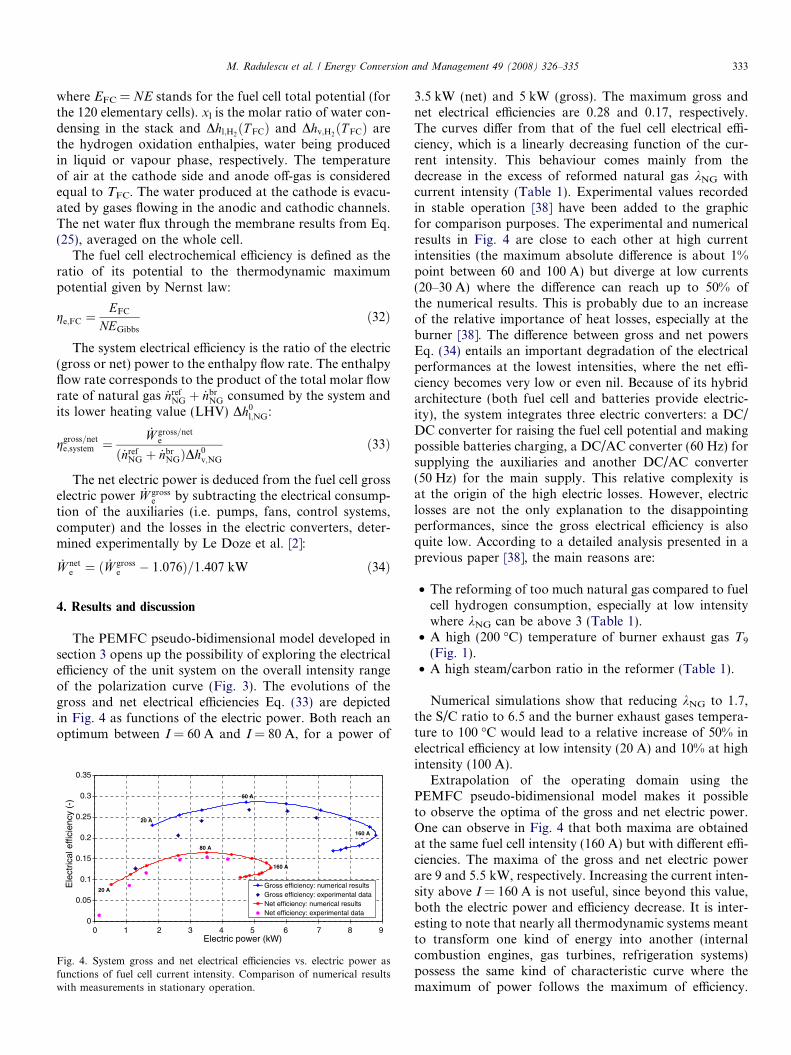
Fig. 4. System gross and net electrical efficiencies vs. electric power asfunctions of fuel cell current intensity. Comparison of numerical resultswith measurements in stationary operation.

3.5 kW (net) and 5 kW (gross). The maximum gross andnet electrical efficiencies are 0.28 and 0.17, respectively.The curves differ from that of the fuel cell electrical effi-ciency, which is a linearly decreasing function of the cur-rent intensity. This behaviour comes mainly from thedecrease in the excess of reformed natural gas kNG withcurrent intensity (Table 1). Experimental values recordedin stable operation [38] have been added to the graphicfor comparison purposes. The experimental and numericalresults in Fig. 4 are close to each other at high currentintensities (the maximum absolute difference is about 1%point between 60 and 100 A) but diverge at low currents(20–30 A) where the difference can reach up to 50% ofthe numerical results. This is probably due to an increaseof the relative importance of heat losses, especially at theburner [38]. The difference between gross and net powersEq. (34) entails an important degradation of the electricalperformances at the lowest intensities, where the net effi-ciency becomes very low or even nil. Because of its hybridarchitecture (both fuel cell and batteries provide electric-ity), the system integrates three electric converters: a DC/DC converter for raising the fuel cell potential and makingpossible batteries charging, a DC/AC converter (60 Hz) forsupplying the auxiliaries and another DC/AC converter(50 Hz) for the main supply. This relative complexity isat the origin of the high electric losses. However, electriclosses are not the only explanation to the disappointingperformances, since the gross electrical efficiency is alsoquite low. According to a detailed analysis presented in aprevious paper [38], the main reasons are:

• The reforming of too much natural gas compared to fuelcell hydrogen consumption, especially at low intensitywhere kNG can be above 3 (Table 1).

• A high (200 �C) temperature of burner exhaust gas T9

(Fig. 1).• A high steam/carbon ratio in the reformer (Table 1).

Numerical simulations show that reducing kNG to 1.7,the S/C ratio to 6.5 and the burner exhaust gases tempera-ture to 100 �C would lead to a relative increase of 50% inelectrical efficiency at low intensity (20 A) and 10% at highintensity (100 A).

Extrapolation of the operating domain using thePEMFC pseudo-bidimensional model makes it possibleto observe the optima of the gross and net electric power.One can observe in Fig. 4 that both maxima are obtainedat the same fuel cell intensity (160 A) but with different effi-ciencies. The maxima of the gross and net electric powerare 9 and 5.5 kW, respectively. Increasing the current inten-sity above I = 160 A is not useful, since beyond this value,both the electric power and efficiency decrease. It is inter-esting to note that nearly all thermodynamic systems meantto transform one kind of energy into another (internalcombustion engines, gas turbines, refrigeration systems)possess the same kind of characteristic curve where themaximum of power follows the maximum of efficiency.

334 M. Radulescu et al. / Energy Conversion and Management 49 (2008) 326–335

This curve can always be represented in an efficiency versuspower diagram. The variable defining the operating pointson the curve represents the amount of primary energy con-sumed by the system: there is, for instance, a direct linkbetween current intensity and hydrogen consumption infuel cells. In the particular case of a fuel cell alone (withoutauxiliaries), the maximum of electrochemical efficiency isobtained when there is no current. The operating rangeof such thermodynamic systems is usually between themaximum of efficiency and the maximum of power: opera-tion in nominal conditions below the maximum of effi-ciency is not interesting in terms of capacity, whileoperation above the maximum of power degrades the effi-ciency. These conditions are not fulfilled in our case sinceabout 70% of the operating range corresponds to a currentintensity lower than that of the maximum of efficiency.

Fig. 5 presents a comparison of the numerical resultswith measurements in transient operation. The data wererecorded on the Limoges’ unit between November 20thand December 4th, 2003. Their arrangement into groupsfollowing identical linear trends results from an oversizedgas meter with pulse output. A statistical study indicatesthat for most of the points (84.5%), the system gross elec-trical efficiency is below the curve corresponding to inter-polation of data recorded in stable operation. Thesupplementary loss of electrical efficiency due to transientoperation is estimated at about 1.5% points. This corre-sponds to a relative loss of electric power of about 6%. Fur-thermore, the mean current intensity is only 38.4 A, whichis far from the efficiency optimum.

Electric and gas meters allow evaluating mean values ofthe unit’s net electrical efficiencies over periods of opera-tion ranging from a few days to a full month. These valuestake account of all thermal and electric losses, includingstart up time (90 min) during which the units are suppliedwith natural gas without producing electricity. An analysisof all data recorded during more than one year shows thatthe net electrical efficiency (averaged for all units andweighted by the length of the operation periods) is only9.2%. The global mean value of current intensity is 36 A,which is quite far from the efficiency optimum range (60–

0

0.05

0.1

0.15

0.2

0.25

0.3

0.35

0 1 2 3 4 5 6 7 8 9Gross electric power (kW)

Gro

ss e

lect

rical

effi

cien

cy (

-)

Numerical results

All experimental data (Limoges unit:20/11 - 4/12/2003)Stable operating points (Limoges unit)

Fig. 5. System gross and net electrical efficiencies vs. electric power asfunctions of fuel cell current intensity. Comparison of numerical resultswith measurements in stable and transient operation.

80 A, Fig. 4) and more than four times lower than thehypothetical maximum of electric power.

In mid-2006, the five installations had cumulated a totalof more than 8500 hours of operation (more than 2500 hfor one Dunkerque’ unit). The Sophia-Antipolis’ unitreached almost 600 h (24 days) of continuous operation.

One of the five fuel cell stacks had to be replaced after1270 h, probably due to sulphur poisoning of the electrodesafter breaking an activated carbon cartridge used for natu-ral gas desulphuration. About 100 failures have beenreported, 60% of them caused by the lead batteries usedfor smoothing the variations in electricity demand. Thanksto these batteries, the fuel cell current intensity varies insteps and can be kept constant during several minutes toseveral hours. On the other hand, the batteries undergoimportant current intensity variations that reduce their life-span. They also revealed themselves very vulnerable tostorage conditions when the units are off.

5. Conclusion

Simulation software of a natural gas cogeneration sys-tem using a PEM fuel cell was build and tested by compar-ison with experimental results. The accuracy (in terms ofprediction of electrical efficiency) of the software resultsis satisfying, except at very low intensity. It also makes itpossible to extrapolate the system behaviour at currentintensities higher than those allowed by the fuel cell. Themain conclusion of this work is that the electric perfor-mances are low, but numerical simulations and analysesof experimental data suggest promising improvements,which are of four kinds:

• Modification of units internal control laws, which wouldresult in better values for key parameters like the excessof reformed natural gas kNG or the steam/carbon ratio.

• Small changes in the architecture of the units, resulting,for instance, in better heat recovery of burner exhaustgases or lower electric losses.

• Better correspondence between electric demand andunit’s power, so that they would be used at a mean cur-rent close to their efficiency optimum.

• Better control of electric production, which would limittransient operation.

References

[1] Cao Y, Guo Z. Performance evaluation of an energy recovery systemfor fuel reforming of PEM fuel cell power plants. J Power Sources2002;109:287–93.

[2] Le Doze S, Donnetti C, Le Noc D, Marencak E. Rapport annueld’avancement du projet EPACOP – bilan des installations, Gaz deFrance, Direction de la Recherche, Ref. M.DU.COGV.2004-00123SL-LP; 2004.

[3] Bernardi DM, Verbruge MW. Mathematical model of a gas diffusionelectrode bonded to a polymer electrolyte. AIChE J 1991;37:1151–63.

[4] Springer TE, Wilson MS, Gottesfeld S. Modeling and experimentaldiagnostics in polymer electrolyte fuel cells. J Electrochem Soc1993;140:3513–26.

M. Radulescu et al. / Energy Conversion and Management 49 (2008) 326–335 335

[5] Bernardi DM, Verbruge MK. A mathematical model of the solid-polymer-electrolyte fuel cell. J Electrochem Soc 1992;139:2477–91.

[6] Springer TE, Zawodzinski TA, Gottesfeld S. Polymer electrolyte fuelcell model. J Electrochem Soc 1991;138:2334–42.

[7] Wohr M, Bolwin K, Schnurnberger W, Fischer M, Neubrand W.Dynamic modelling and simulation of a polymer membrane fuel cellincluding mass transport limitation. Int J Hydrogen Energy1998;23:213–8.

[8] Rowe A, Li X. Mathematical modeling of proton exchange mem-brane fuel cells. J Power Sources 2001;102:82–96.

[9] Djilali N, Lu D. Influence of heat transfer on gas and water transportin fuel cells. Int J Therm Sci 2002;41:29–40.

[10] Ramousse J, Deseure J, Didierjean S, Lottin O, Maillet D. Modellingof heat, mass and charge transfer in a PEMFC single cell. J PowerSources 2005;145:416–27.

[11] Costamagna P. Transport phenomena in polymeric membrane fuelcells. Chem Eng Sci 2001;56:323–32.

[12] Costamagna P, Srinivasan S. Quantum jumps in the PEMFC scienceand technology from the 1960s to the year 2000: part II. Engineering,technology development and application aspects. J Power Sources2001;102:253–69.

[13] Bautista M, Bultel Y, Ozil P. Polymer electrolyte membrane fuel cellmodelling: DC and AC solutions. Chem Eng Res Des 2004;82:907–17.

[14] Yan WM, Soong CY, Chen F, Chu HS. Transient analysis of reactantgas transport and performance of PEM fuel cells. J Power Sources2005;143:48–56.

[15] Singh D, Lu DM, Djilali N. A two-dimensional analysis of masstransport in proton exchange membrane fuel cells. Int J Eng Sci1999;37:431–52.

[16] Hsing IM, Futerko P. Two-dimensional simulation of water transportin polymer electrolyte fuel cells. Chem Eng Sci 2000;55:4209–18.

[17] Um S, Wang CW, Chen KS. Computational fluid dynamics model-ling of proton exchange membrane fuel cell. J Electrochem Soc2000;147:4485–93.

[18] Um S, Wang CY. Three-dimensional analysis of transport andelectrochemical reactions in polymer electrolyte fuel cells. J PowerSources 2004;125:40–51.

[19] Lum KW, McGuirk JJ. Three-dimensional model of a completepolymer electrolyte membrane fuel cell – model formulation, valida-tion and parametric studies. J Power Sources 2005;143:103–24.

[20] Fuller TF, Newman J. Water and thermal management in solid-polymer-electrolyte fuel cells. J Electrochem Soc 1993;140:1218–25.

[21] Yi JS, Nguyen T. Multicomponent transport in porous electrodes ofproton exchange membrane fuel cells using the interdigitated gasdistributors. J Electrochem Soc 1999;146:38–45.

[22] Berning T, Djilali N. Three-dimensional computational analysis oftransport phenomena in a PEM fuel cell. J Power Sources2002;106:284–94.

[23] Ju H, Meng H, Wang CY. A single-phase, non-isothermalmodel for PEM fuel cells. Int J Heat Mass Trans 2005;48:1303–15.

[24] Kamarudin SK, Daud WR, Som AM, Takriff MS, Mohammad AW,Loke YK. Design of a fuel processor unit for PEM fuel cell viashortcut design method. Chem Eng J 2004;104:7–17.

[25] Lombard C, Marquaire P, Baronnet F, Lapicque F, Le Doze S,Marencak E, et al. Operation of stationary 5 kW H-Power PEMFCs:investigation of the hydrogen production unit. In: FDCD 2004: 2ndFrance-Deutschland Fuel Cell Conference, Belfort, France, Novem-ber 29th–December 2nd; 2004.

[26] Radulescu M, Lottin O, Feidt M, Lombard C, Le Noc D, Le Doze S.Experimental and theoretical analysis of the operation of a naturalgas cogeneration system using a polymer exchange membrane fuelcell. Chem Eng Sci 2006;61:743–52.

[27] Gigliucci G, Petruzzi L, Cerelli E. Demonstration of a resi-dential CHP system based on PEM fuel cells. J Power Sources2004;131:62–8.

[28] Newson E, Truong TB. Low-temperature catalytic partial oxidationof hydrocarbons (C1–C10) for hydrogen production. Int J HydrogenEnergy 2003;28:1379–86.

[29] Bird RB, Stewart WE, Lightfoot EN. Transport phenomena. NewYork: John Wiley; 1960.

[30] Arnost D, Schneider P. Dynamic transport of multicomponentmixtures of gases in porous solids. Chem Eng J Biochem Eng J1995;57:91–9.

[31] Okada T, Xie G, Tanabe Y. Theory of water management at theanode side of polymer electrolyte fuel cell membranes. J ElectroanalChem 1996;413:49–65.

[32] Springer TE, Zawodzinski TA, Wilson MS, Gottesfeld S. Character-ization of polymer electrolyte fuel cells using AC impedancespectroscopy. J Electrochem Soc 1996;143:587–99.

[33] Okada T, Xie G, Meeg M. Simulation for water management inmembranes for polymer electrolyte fuel cells. Electrochem Acta1998;43:2141–55.

[34] Hinatsu JT, Mizuhata M, Takenaka H. Water uptake of perfluoro-sulfonic acid membranes from liquid water and water vapor. JElectrochem Soc 1994;141:1493–8.

[35] Atkins P, Paula J. Physical chemistry. 7th ed. New York: OxfordUniversity Press; 2002.

[36] Larminie A, Dicks A. Fuel cell systems explained. John Wiley; 2000.53pp.

[37] Kim J, Lee SM, Srinivasan S, Chamberlin CE. Modeling of protonexchange membrane fuel cell performance with an empirical equation.J Electrochem Soc 1995;142:2670–4.

[38] Radulescu M, Lottin O, Feidt M, Lombard C, Le Noc D, Le Doze S.Experimental results with a natural gas cogeneration system using apolymer exchange membrane fuel cell. J Power Sources 2006;149:1142–6.