Multivariate Analysis of Prokaryotic Amino Acid Usage Bias
237
Wright State University Wright State University CORE Scholar CORE Scholar Browse all Theses and Dissertations Theses and Dissertations 2005 Multivariate Analysis of Prokaryotic Amino Acid Usage Bias: A Multivariate Analysis of Prokaryotic Amino Acid Usage Bias: A Computational Method for Understanding Protein Building Block Computational Method for Understanding Protein Building Block Selection in Primitive Organisms Selection in Primitive Organisms Douglas Whitmore Raiford III Wright State University Follow this and additional works at: https://corescholar.libraries.wright.edu/etd_all Part of the Computer Sciences Commons Repository Citation Repository Citation Raiford, Douglas Whitmore III, "Multivariate Analysis of Prokaryotic Amino Acid Usage Bias: A Computational Method for Understanding Protein Building Block Selection in Primitive Organisms" (2005). Browse all Theses and Dissertations. 21. https://corescholar.libraries.wright.edu/etd_all/21 This Thesis is brought to you for free and open access by the Theses and Dissertations at CORE Scholar. It has been accepted for inclusion in Browse all Theses and Dissertations by an authorized administrator of CORE Scholar. For more information, please contact [email protected].
-
Upload
khangminh22 -
Category
Documents
-
view
1 -
download
0
Transcript of Multivariate Analysis of Prokaryotic Amino Acid Usage Bias

Wright State University Wright State University
CORE Scholar CORE Scholar
Browse all Theses and Dissertations Theses and Dissertations
2005
Multivariate Analysis of Prokaryotic Amino Acid Usage Bias: A Multivariate Analysis of Prokaryotic Amino Acid Usage Bias: A
Computational Method for Understanding Protein Building Block Computational Method for Understanding Protein Building Block
Selection in Primitive Organisms Selection in Primitive Organisms
Douglas Whitmore Raiford III Wright State University
Follow this and additional works at: https://corescholar.libraries.wright.edu/etd_all
Part of the Computer Sciences Commons
Repository Citation Repository Citation Raiford, Douglas Whitmore III, "Multivariate Analysis of Prokaryotic Amino Acid Usage Bias: A Computational Method for Understanding Protein Building Block Selection in Primitive Organisms" (2005). Browse all Theses and Dissertations. 21. https://corescholar.libraries.wright.edu/etd_all/21
This Thesis is brought to you for free and open access by the Theses and Dissertations at CORE Scholar. It has been accepted for inclusion in Browse all Theses and Dissertations by an authorized administrator of CORE Scholar. For more information, please contact [email protected].

Multivariate analysis of prokaryotic amino acidusage bias: a computational method for
understanding protein building block selection inprimitive organisms
A thesis submitted in partial fulfillmentof the requirements for the degree of
Master of Science
By
DOUGLAS W. RAIFORD IIIB.S.C.S., Wright State University, 2002
2005Wright State University

COPYRIGHT BY
Douglas W. Raiford III
2005

WRIGHT STATE UNIVERSITYSCHOOL OF GRADUATE STUDIES
July 15, 2005
I HEREBY RECOMMEND THAT THE THESIS PREPARED UNDER MY SUPER-VISION BY Douglas W. Raiford III ENTITLED Multivariate analysis of prokaryotic aminoacid usage bias: a computational method for understanding protein building block selectionin primitive organisms BE ACCEPTED IN PARTIAL FULFILLMENT OF THE RE-QUIREMENTS FOR THE DEGREE OF Master of Science.
Michael L. Raymer, Ph.D.Thesis Director
Forouzan Golshani, Ph.D.Department Chair
Committee onFinal Examination
Michael L. Raymer , Ph.D.
Travis E. Doom , Ph.D.
Dan E. Krane , Ph.D.
Joseph F. Thomas, Jr. , Ph.D.Dean, School of Graduate Studies

July 15, 2005
ABSTRACT
Raiford III, Douglas . M.S., Department of Computer Science & Engineering, Wright State Uni-versity, 2005 . Multivariate analysis of prokaryotic amino acid usage bias: a computational methodfor understanding protein building block selection in primitive organisms.
Organisms expend a significant fraction of their overall energy budget in the creation
of proteins, particularly for those that are produced in large quantities. Recent research has
demonstrated that genes encoding these proteins are shaped by natural selection to produce
the proteins with low cost building blocks (amino acids) whenever possible. The negative
correlation between protein production rate and their energetic costs has been established
for two bacterial genomes: Escherichia coli and Bacillus subtilis. This thesis provides
scientific validation of this theory by automating the analysis and extending the research to
additional genomes.
Investigations into building block selection are highly computational in nature. Diverse
methodologies, including principal component analysis, calculation of Mahalanobis dis-
tance, and the execution of Mantel-Haenszel and Bonferroni tests, are required in order to
automate the process.
In order to verify that the cause of the observed trend is energetic cost minimization it is
necessary to eliminate as many alternative explanations as possible. This is accomplished
through demonstration that the trend is not localized to any particular region of the protein’s
primary structure and that the trend is consistent across all genes regardless of functionality.
This investigation of the energetic cost of polypeptide synthesis provides valuable in-
sights into protein building block selection. As an example, parasitic organisms appear
to exhibit no correlation between protein production rate and amino acid cost. When the
costs associated with building blocks that the parasite obtains from its host are removed,
however, a trend once again becomes evident.
iv

Contents
Contents v
List of Figures ix
List of Tables xi
1 Introduction 11.1 Overview . . . . . . . . . . . . . . . . . . . . . . . . . . . . . . . . . . . 11.2 Existing Solution . . . . . . . . . . . . . . . . . . . . . . . . . . . . . . . 21.3 Contribution . . . . . . . . . . . . . . . . . . . . . . . . . . . . . . . . . . 2
1.3.1 Structure of This Document . . . . . . . . . . . . . . . . . . . . . 31.3.2 Contributions from the Biomedical Sciences Program . . . . . . . . 4
2 Background and Literature Survey 62.1 Protein Production . . . . . . . . . . . . . . . . . . . . . . . . . . . . . . 6
2.1.1 DNA, Chromosomes, and the Genome . . . . . . . . . . . . . . . . 62.1.2 Base-Pairs and Strand Orientation . . . . . . . . . . . . . . . . . . 92.1.3 The Gene . . . . . . . . . . . . . . . . . . . . . . . . . . . . . . . 102.1.4 Codons and Degeneration . . . . . . . . . . . . . . . . . . . . . . 122.1.5 Central Dogma . . . . . . . . . . . . . . . . . . . . . . . . . . . . 13
2.2 Expressivity and Major Codons . . . . . . . . . . . . . . . . . . . . . . . . 152.3 Determining Major Codons . . . . . . . . . . . . . . . . . . . . . . . . . . 16
2.3.1 Principal Component Analysis (PCA) . . . . . . . . . . . . . . . . 172.3.2 Data Projection . . . . . . . . . . . . . . . . . . . . . . . . . . . . 182.3.3 Factor Loading: Correlation with Original Data . . . . . . . . . . . 20
2.4 Calculating Major Codon Usage . . . . . . . . . . . . . . . . . . . . . . . 202.5 Literature Survey: Expressivity Prediction . . . . . . . . . . . . . . . . . . 22
2.5.1 Frequency of preferred codons (FOP) . . . . . . . . . . . . . . . . 222.5.2 Indexes, Statistics, and Clustering . . . . . . . . . . . . . . . . . . 242.5.3 Codon Adaptation Index CAI . . . . . . . . . . . . . . . . . . . . 282.5.4 Scaled X2 . . . . . . . . . . . . . . . . . . . . . . . . . . . . . . . 292.5.5 Effective Number of Codons . . . . . . . . . . . . . . . . . . . . . 30
v

CONTENTS July 15, 2005
2.5.6 Morton’s Codon Bias Index (CBI) . . . . . . . . . . . . . . . . . . 312.5.7 Intrinsic Codon Deviation Index (ICDI) . . . . . . . . . . . . . . . 322.5.8 Correspondence Analysis Revisited . . . . . . . . . . . . . . . . . 332.5.9 CAI Revisited . . . . . . . . . . . . . . . . . . . . . . . . . . . . . 332.5.10 Summary . . . . . . . . . . . . . . . . . . . . . . . . . . . . . . . 35
2.6 Metabolic Costs of Amino Acid Biosynthesis . . . . . . . . . . . . . . . . 352.7 Refining the Data Set . . . . . . . . . . . . . . . . . . . . . . . . . . . . . 37
2.7.1 Non-protein Coding Sequences . . . . . . . . . . . . . . . . . . . 372.7.2 Candidates for Horizontal Gene Transfer . . . . . . . . . . . . . . 372.7.3 Overrepresented Genes . . . . . . . . . . . . . . . . . . . . . . . . 412.7.4 Short Genes . . . . . . . . . . . . . . . . . . . . . . . . . . . . . . 42
2.8 MCU/Energetic Cost Correlation . . . . . . . . . . . . . . . . . . . . . . . 422.9 Additional Statistical Analysis . . . . . . . . . . . . . . . . . . . . . . . . 44
2.9.1 Physicochemical Classes . . . . . . . . . . . . . . . . . . . . . . . 442.9.2 Functional Categories . . . . . . . . . . . . . . . . . . . . . . . . 46
3 Materials and Methods 513.1 Acquiring and Refining the Data Set . . . . . . . . . . . . . . . . . . . . . 51
3.1.1 Challenge . . . . . . . . . . . . . . . . . . . . . . . . . . . . . . . 513.1.2 Initial Data Acquisition . . . . . . . . . . . . . . . . . . . . . . . . 523.1.3 Genomes Processed . . . . . . . . . . . . . . . . . . . . . . . . . 523.1.4 Non-Computational Culling Criteria . . . . . . . . . . . . . . . . . 563.1.5 Horizontal Gene Transfer . . . . . . . . . . . . . . . . . . . . . . . 573.1.6 Paralogs . . . . . . . . . . . . . . . . . . . . . . . . . . . . . . . . 613.1.7 Functional Categories . . . . . . . . . . . . . . . . . . . . . . . . 633.1.8 Outcome . . . . . . . . . . . . . . . . . . . . . . . . . . . . . . . 65
3.2 Determining Major Codons and MCU . . . . . . . . . . . . . . . . . . . . 663.2.1 Challenge . . . . . . . . . . . . . . . . . . . . . . . . . . . . . . . 663.2.2 Create Codon Frequency Matrix . . . . . . . . . . . . . . . . . . . 673.2.3 PCA . . . . . . . . . . . . . . . . . . . . . . . . . . . . . . . . . . 693.2.4 Factor Loadings . . . . . . . . . . . . . . . . . . . . . . . . . . . 713.2.5 Eigenvector Direction . . . . . . . . . . . . . . . . . . . . . . . . 733.2.6 Outcome . . . . . . . . . . . . . . . . . . . . . . . . . . . . . . . 74
3.3 Statistical Analysis . . . . . . . . . . . . . . . . . . . . . . . . . . . . . . 753.3.1 Challenge . . . . . . . . . . . . . . . . . . . . . . . . . . . . . . . 753.3.2 Correlation Between Expressivity and Amino Acid Cost . . . . . . 763.3.3 Amino Acid Abundance . . . . . . . . . . . . . . . . . . . . . . . 793.3.4 Outcome . . . . . . . . . . . . . . . . . . . . . . . . . . . . . . . 85
4 Results 864.1 Data Acquisition and Refinement . . . . . . . . . . . . . . . . . . . . . . 864.2 Major Codons and Energetic Costs . . . . . . . . . . . . . . . . . . . . . . 87
4.2.1 Eigenvectors . . . . . . . . . . . . . . . . . . . . . . . . . . . . . 874.2.2 Distribution of Data in New Dimension . . . . . . . . . . . . . . . 874.2.3 Factor Loadings . . . . . . . . . . . . . . . . . . . . . . . . . . . 90
vi

CONTENTS July 15, 2005
4.2.4 Major Codons . . . . . . . . . . . . . . . . . . . . . . . . . . . . 924.2.5 Energetic Costs . . . . . . . . . . . . . . . . . . . . . . . . . . . . 97
4.3 Statistical Analysis . . . . . . . . . . . . . . . . . . . . . . . . . . . . . . 984.3.1 MCU to Energetic Costs Correlation . . . . . . . . . . . . . . . . . 984.3.2 Physicochemical . . . . . . . . . . . . . . . . . . . . . . . . . . 994.3.3 Correlation Coefficients . . . . . . . . . . . . . . . . . . . . . . . 994.3.4 Parasitic Behavior . . . . . . . . . . . . . . . . . . . . . . . . . . 1054.3.5 Functional Categories and Spearman . . . . . . . . . . . . . . . . . 1064.3.6 Amino Acid Abundance . . . . . . . . . . . . . . . . . . . . . . . 106
5 Discussion 1125.1 Findings . . . . . . . . . . . . . . . . . . . . . . . . . . . . . . . . . . . . 112
5.1.1 Expansion, Automation, and Clarification . . . . . . . . . . . . . . 1125.1.2 A Comparison with the Findings of the Original Research . . . . . 1135.1.3 Data Anomalies in Parasites . . . . . . . . . . . . . . . . . . . . . 1155.1.4 Amino Acid Abundance . . . . . . . . . . . . . . . . . . . . . . . 117
5.2 Summary and Contribution . . . . . . . . . . . . . . . . . . . . . . . . . . 1195.3 Future Work . . . . . . . . . . . . . . . . . . . . . . . . . . . . . . . . . . 120
5.3.1 Data Discrepancies . . . . . . . . . . . . . . . . . . . . . . . . . . 1205.3.2 Better Means of Predicting Expressivity . . . . . . . . . . . . . . . 1225.3.3 Eukaryotic Genomes . . . . . . . . . . . . . . . . . . . . . . . . . 1225.3.4 Energy Predictor . . . . . . . . . . . . . . . . . . . . . . . . . . . 1225.3.5 Increased Automation and Availability . . . . . . . . . . . . . . . . 123
Bibliography 124
A Appendix A: Degeneration Table (Codon-Amino Acid-Abbreviation Cross-reference) 131
B Appendix B: Required PERL Packages 132
C Appendix C: Description of PCA 133C.1 Covariance Matrix . . . . . . . . . . . . . . . . . . . . . . . . . . . . . . 133C.2 Eigenvector . . . . . . . . . . . . . . . . . . . . . . . . . . . . . . . . . . 133C.3 Determinants . . . . . . . . . . . . . . . . . . . . . . . . . . . . . . . . . 134C.4 Characteristic Equation and Polynomial . . . . . . . . . . . . . . . . . . . 135
D Appendix D: Entire Flow 136
E Appendix E: Correspondence 138E.1 Email to Dr. Hiroshi Akashi, March 04, 2004 . . . . . . . . . . . . . . . . 138E.2 Email from Dr. Hiroshi Akashi, March 10, 2004 . . . . . . . . . . . . . . . 138E.3 Email to Dr. Hiroshi Akashi, March 12, 2004 . . . . . . . . . . . . . . . . 139E.4 Email to Dr. Hiroshi Akashi, March 25, 2004 . . . . . . . . . . . . . . . . 140E.5 Email to Dr. Toshimichi Ikemura, April 08, 2004 . . . . . . . . . . . . . . 140E.6 Email from Dr. Hiroshi Akashi, April 12, 2004 . . . . . . . . . . . . . . . 141
vii

CONTENTS July 15, 2005
E.7 Email from Dr. Hiroshi Akashi, April 12, 2004 . . . . . . . . . . . . . . . 141E.8 Email to Dr. Toshimichi Ikemura, April 19, 2004 . . . . . . . . . . . . . . 142E.9 Email from Dr. Shigehiko Kanaya, April 22, 2004 . . . . . . . . . . . . . . 143E.10 Email from Dr. Shigehiko Kanaya, April 26, 2004 . . . . . . . . . . . . . . 143E.11 Email to Dr. Shigehiko Kanaya, April 26, 2004 . . . . . . . . . . . . . . . 144E.12 Email to Dr. Shigehiko Kanaya, May 04, 2004 . . . . . . . . . . . . . . . . 144
F Appendix F: Commands 146
G Appendix G: Source Code 154G.1 batchAll.pl . . . . . . . . . . . . . . . . . . . . . . . . . . . . . . . . . . 154G.2 getGenes.pl . . . . . . . . . . . . . . . . . . . . . . . . . . . . . . . . . . 159G.3 preprocessGenes.pl . . . . . . . . . . . . . . . . . . . . . . . . . . . . . . 166G.4 premoreGenes.pl . . . . . . . . . . . . . . . . . . . . . . . . . . . . . . . 168G.5 cullFromList.pl . . . . . . . . . . . . . . . . . . . . . . . . . . . . . . . . 172G.6 createFaa.pl . . . . . . . . . . . . . . . . . . . . . . . . . . . . . . . . . . 176G.7 blastFilterPrj.pl . . . . . . . . . . . . . . . . . . . . . . . . . . . . . . . . 178G.8 parseOutFile.pl . . . . . . . . . . . . . . . . . . . . . . . . . . . . . . . . 185G.9 Part4a.pl . . . . . . . . . . . . . . . . . . . . . . . . . . . . . . . . . . . . 186G.10 createMatrix.pl . . . . . . . . . . . . . . . . . . . . . . . . . . . . . . . . 188G.11 performPCA.pl . . . . . . . . . . . . . . . . . . . . . . . . . . . . . . . . 198G.12 aminoCorl.pl . . . . . . . . . . . . . . . . . . . . . . . . . . . . . . . . . 202G.13 Gene Object . . . . . . . . . . . . . . . . . . . . . . . . . . . . . . . . . . 215
Index 218
viii

List of Figures
1.1 Procedural Flow when Performing Analysis . . . . . . . . . . . . . . . . . 31.2 Research and Analysis Responsibilities Broken-down by Department and
Arranged by Position on Timeline . . . . . . . . . . . . . . . . . . . . . . 5
2.1 Chromosome and Gene . . . . . . . . . . . . . . . . . . . . . . . . . . . . 72.2 DNA and RNA . . . . . . . . . . . . . . . . . . . . . . . . . . . . . . . . 82.3 Base-pairing of Nucleotides in Complementary DNA Strands . . . . . . . . 92.4 1’ through 5’ Carbon Atoms . . . . . . . . . . . . . . . . . . . . . . . . . 112.5 tRNA Molecule with Amino Acid and Anticodon . . . . . . . . . . . . . . 142.6 The Central Dogma of Molecular Biology . . . . . . . . . . . . . . . . . . 152.7 Two Dimensional Example of Eigenvector . . . . . . . . . . . . . . . . . . 192.8 Correlation Between Codon and Z′
1 (Factor Loading) . . . . . . . . . . . . 212.9 Metabolic Pathways Involved in Amino Acid Biosynthesis and Energy Pro-
duction . . . . . . . . . . . . . . . . . . . . . . . . . . . . . . . . . . . . 382.10 2 × 2 Contingency Table Used in Mantel-Haenszel Test . . . . . . . . . . . 48
3.1 Typical Annotation for Phage Related Protein Expressing Gene . . . . . . . 523.2 Sample PDL Usage . . . . . . . . . . . . . . . . . . . . . . . . . . . . . . 603.3 Blast Filtering Process . . . . . . . . . . . . . . . . . . . . . . . . . . . . 623.4 Typical Results File – Output of BLAST. Only First Alignment Shown. . . 643.5 Sample Portion of Gene Functional Category File. COG file downloaded
from NCBI (NCBI, 2005). . . . . . . . . . . . . . . . . . . . . . . . . . . 653.6 General Flow during Data Acquisition and Refinement Stage . . . . . . . . 663.7 Covariance Matrix . . . . . . . . . . . . . . . . . . . . . . . . . . . . . . 69
4.1 MCU vs. Average Cost . . . . . . . . . . . . . . . . . . . . . . . . . . . . 1004.2 MCU vs. Average Cost - Internal Amino Acids . . . . . . . . . . . . . . . 1014.3 MCU vs. Average Cost - External Amino Acids . . . . . . . . . . . . . . . 1024.4 MCU vs. Average Cost - Ambivalent Amino Acids . . . . . . . . . . . . . 1034.5 Chlamydia trachomatis Adjusted vs. non-Adjusted for Amino Acid Biosyn-
thetic Costs . . . . . . . . . . . . . . . . . . . . . . . . . . . . . . . . . . 1074.6 Mycoplamsa genitalium Adjusted vs. non-Adjusted for Amino Acid Biosyn-
thetic Costs . . . . . . . . . . . . . . . . . . . . . . . . . . . . . . . . . . 108
ix

LIST OF FIGURES July 15, 2005
5.1 Chlamydia trachomatis Adjusted vs. non-Adjusted for Amino Acid Biosyn-thetic Costs . . . . . . . . . . . . . . . . . . . . . . . . . . . . . . . . . . 116
5.2 Mycoplamsa genitalium Adjusted vs. non-Adjusted for Amino Acid Biosyn-thetic Costs . . . . . . . . . . . . . . . . . . . . . . . . . . . . . . . . . . 117
D.1 Detailed View of Data Flow . . . . . . . . . . . . . . . . . . . . . . . . . 137
x

List of Tables
2.1 RNA Triplet Codons to Amino Acid Translation . . . . . . . . . . . . . . . 132.2 Summary of All Described Bias Measures . . . . . . . . . . . . . . . . . . 352.3 Physicochemical Classes for Amino Acids . . . . . . . . . . . . . . . . . . 452.4 Spearman Correlation Results when Limited to Physicochemical Classes . . 452.5 Gene Functional Categories . . . . . . . . . . . . . . . . . . . . . . . . . . 47
3.1 Primary Genomes Studied and Their Respective Metabolic Characteristics . 533.2 Secondary Genomes Studies and Their Associated Gene and Codon Counts 543.3 Factor Loading Determination . . . . . . . . . . . . . . . . . . . . . . . . 723.4 Physicochemical Classes for Amino Acids . . . . . . . . . . . . . . . . . . 793.5 2 × 2 Contingency Table Used in Mantel-Haenszel Test . . . . . . . . . . . 83
4.1 Number of Genes in the Genome and the Number Removed by each CullingCriteria . . . . . . . . . . . . . . . . . . . . . . . . . . . . . . . . . . . . 87
4.2 Eigenvectors for Primary Genomes . . . . . . . . . . . . . . . . . . . . . . 884.3 Histogram Depiction of Frequency Data Projected Upon First Principal
Component – New Axis . . . . . . . . . . . . . . . . . . . . . . . . . . . . 894.4 Histogram Depiction of Frequency Data (from Supplementary Genomes)
Projected Upon First Principal Component – New Axis . . . . . . . . . . . 914.5 Factor Loadings for Primary Genomes . . . . . . . . . . . . . . . . . . . . 934.6 RNA Triplet Codons Identified as Major for Bacillus subtillus . . . . . . . 944.7 RNA Triplet Codons Identified as Major for Escherichia coli K12 . . . . . 944.8 RNA Triplet Codons Identified as Major for Chlamydia trachomatis . . . . 954.9 RNA Triplet Codons Identified as Major for Mycoplasma genitalium . . . . 954.10 RNA Triplet Codons Identified as Major for Synechococcus sp WH 8102 . . 964.11 RNA Triplet Codons Identified as Major for Thermotoga maritima . . . . . 964.12 Energetic Costs in high energy Phosphate Bonds (∼P) for Amino Acids
within Chemoheterotrophic and Photoautotrophic Organisms . . . . . . . . 974.13 Spearman Rank Correlation Over Whole Genome, Internal, External, and
Ambivalent Amino Acids . . . . . . . . . . . . . . . . . . . . . . . . . . . 1044.14 Spearman Rank Correlation Over Whole Genome for Extended Genomes . 105
xi

LIST OF TABLES July 15, 2005
4.15 Number of Genes and Spearman Rank Correlation within Functional Cat-egories of five Bacterial Species . . . . . . . . . . . . . . . . . . . . . . . 109
4.16 Production Costs of Amino Acids, Spearman Rank Correlation and Z Scoresin Five Bacterial Species . . . . . . . . . . . . . . . . . . . . . . . . . . . 111
5.1 Comparison Between Historical and Current Results . . . . . . . . . . . . 1145.2 Thermophilic and Photoautotrophic Results . . . . . . . . . . . . . . . . . 1155.3 Removed Amino Acids from Parasitic Organisms . . . . . . . . . . . . . . 116
xii

Acknowledgement
As with any work of this scope there are many contributions that require my acknowledge-
ment and thanks. At the top of this list are those of my advisors Dr. Michael Raymer and Dr.
Travis Doom. Their confidence, assistance, and unflagging support have been an essential
component in the success of this project. I would also like to thank the remaining member
of my graduate committee, Dr. Dan Krane, for his insights and guidance throughout my
exploration of this challenging and interesting field, bioinformatics. A special thanks also
goes out to Dr. Hiroshi Akashi from the Institute of Molecular Evolutionary Genetics and
Department of Biology and to Dr. Shigehiko Kanaya from the Department of Electric and
Information Engineering of Yamagata University for their responsiveness to my enquiries.
Additionally I would like to thank Dr. Bob Miller, chair of the Microbiology and Molecular
Genetics Department at Oklahoma State University, for his assistance in metabolic pathway
assignment. Much of the credit for the success of this project is owed to the partnership
between the Departments of Computer Science and Biomedical Sciences of Wright State
University. In this regard I would like to thank my counterpart in the Biomedical Sciences
program, Esley Heizer, for his hard work and assistance in this most difficult of endeavors.
I would like to extend my gratitude to the Biomedical Research and Technology Transfer
Partnership Program (BRTT) and the Dayton Area Graduate Studies Institute (DAGSI) for
their financial assistance. Their support has been invaluable and in no small measure has
xiii

allowed me to realize my academic aspirations.
Any list of those deserving my thanks would be incomplete without my friends and asso-
ciates in the Bioinformatics Research Group. I would like to thank Paul Anderson, Gina
Cooper, Ryan Flynn, Akash Jain, David Paoletti, Michael Peterson, Sridhar Ramachandran,
and Deacon Sweeney for their encouragement and unselfish assistance.
A warm and heart-felt thanks goes out to my cousin, Teresa Hair, for convincing me to
begin this journey. She knew the importance I placed on the pursuit of truth and would not
let me forget it. Finally, I thank Dr. Oscar Garcia for believing in me, for recruiting me to
Wright State, and for introducing me to Dr. Raymer and Dr. Doom and, therefore, to the
field of research. My life has been enriched as a result.
xiv

Dedicated to the memory of Carolyn Sue Hair.Mother, friend, and confidante.
For instilling in methe belief that nothing is
beyond my grasp.
xv

Introduction
1.1 Overview
In biology the protein is paramount. It is ubiquitous. Proteins not only form some of the
basic building blocks in living organisms they also assist or cause many of the essential
chemical reactions that sustain life. Proteins are polymers that are comprised of chains of
amino acids (A polymer is a compound molecule made up of a chain of smaller, simpler
molecules). Some amino acids are more energetically expensive to create than others. It
would stand to reason that, over time, a protein, or rather the gene that encodes the protein,
would accumulate mutations that result in the preferential inclusion of the least expensive
amino acid that would still allow the protein to function properly.
Proteins are very complex, and while they can be described as a simple sequence
of amino acids, this polypeptide chain folds into complicated two and three-dimensional
shapes. A protein’s amino acid sequence determines this shape and the shape determines
the function of the protein. Minor changes can often be introduced into the sequence with-
out disrupting the shape and function of the protein. The changes must be made to amino
acids that, when modified, will have little impact on the tendency of the protein to fold
1

1.2. EXISTING SOLUTION July 15, 2005
into its characteristic shape. It also must not disrupt the way in which the protein interacts
chemically with other substances or the protein will cease to function properly. Amino
acids that can change in this way and not alter the function of the protein can be targeted by
natural selection. Changes where metabolic costs of amino acid biosynthesis are reduced
will allow the organism to preferentially survive in less than optimal situations, such as in
starvation conditions.
Those proteins that are expressed the most; that is, those proteins that are created in
the greatest quantity, will come under the greatest selective pressure. It is in these proteins
that the cost of amino acids is most critical because they are produced so often.
1.2 Existing Solution
Research (Akashi and Gojobori, 2002) has suggested that there is a correlation between the
rate of production for a protein and the metabolic costs of amino acid biosynthesis. This
work indicates that amino acids undergo natural selection for least-cost where possible.
This research was limited in scope to two microbial genomes (single celled organisms)
whose gene expressivity had already been determined.
1.3 Contribution
This thesis expands the study of metabolic efficiency in the biosynthesis of amino acids to
include more genomes while at the same time automating the data acquisition and results
2

1.3. CONTRIBUTION July 15, 2005
calculation. The intent is to allow for large scale genomic analysis leading to validation
of the proposition that natural selection acts at the level of amino acid biosynthetic cost in
highly expressed genes.
The existing literature describing research in this area assumes a thorough knowledge
of the techniques employed. Examples include the performance of principal component
analysis and the calculation of Mahalanobis distance. Additionally, many of the specifics
regarding data format, what data to include, which to exclude, thresholds, matching criteria,
etc., were omitted or listed indirectly in cited documents. An important contribution of this
thesis is to make clear the exact calculations and underlying assumptions, decisions, and
criteria used throughout the computational process.
1.3.1 Structure of This Document
The procedure for determining the correlation between the protein production rates and the
associated metabolic costs follows a fairly straightforward flow (Figure 1.1). Each of these
major steps depends upon the preceding steps for successful completion. The linear nature
of the analysis suggests that a similar layout would be appropriate for the thesis.
Acquire Genome Data
Cull Data Set
Determine Major Codons
Determine Expressivity
Statistical Analysis
Figure 1.1: Procedural Flow when Performing Analysis
Immediately following this section is a Background chapter describing, in detail, the
3

1.3. CONTRIBUTION July 15, 2005
work done previously in the field of metabolic cost analysis and the efficiency of amino acid
biosynthesis. Following that are chapters on work in the areas of generating and refining
the data set, determining major codons, calculating expressivity, and the statistical analysis
performed. Finally, the content of the thesis concludes with a chapter on Conclusions and
Future Work.
1.3.2 Contributions from the Biomedical Sciences Program
Bioinformatics is, by its very nature, an interdisciplinary branch of research. It combines
the efforts of computer scientists with those of biologists. The research described in this
thesis adheres to this principle. It is the result of a collaborative effort between the Com-
puter Science and the Biomedical Sciences programs of Wright State University.
Once again the linear nature of the analysis leads to relatively clean lines of demar-
cation between the efforts of the Computer Science department and that of the Biomedical
Sciences program (Figure 1.2). The first three stages, acquire genomic data, cull data
set, and determine major codons (Figure 1.1), are performed by the Computer Science de-
partment. The determine expressivity and energetic costs stage and part of the statistical
analysis stage are performed by the Biomedical Sciences program. My counterpart in that
department is Esley Heizer (Heizer, 2005). The statistical analyses performed by Esley
include the Spearman rank correlation analysis on the entire genomic data as well as on the
genomic data stratified by physicochemical property (Chapter 3, Materials and Methods).
Once the Biomedical Sciences program completes their calculations the energetic cost
data is transferred back to the Computer Science department where the rest of the statistical
4

1.3. CONTRIBUTION July 15, 2005
analysis is performed. This includes Spearman rank correlation calculated on the genomic
data stratified by functional category and amino acid abundance analysis. The amino acid
abundance analysis includes Spearman rank correlation, Mantel-Haenszel, and Bonferroni
correction analyses. For more detail on these tests see Chapter 3, Materials and Methods.
Acquire and refine data
(GC content, BLAST, Mahalanobis distance, etc)
Determine major codons (PCA)
Determine expressivity (percent major codons per gene)
Determine metabolic pathways (amino acid cost)
Determine ability to manufacture amino acids (BLAST, etc)
Determine energetic costs (average cost per amino acid)
Calculate Spearman rank
Stratify data by physicochemical properties
Calculate Spearman rank for each category
Stratify data by functional category
Calculate Spearman rank for each category
Calculate amino acid abundance
Calculate Spearman rank on abundances
Calculate Mantel-Haenszel on abundances and functional category data
Department of Computer Science Department of Biomedical Sciences
Timeline
Figure 1.2: Research and Analysis Responsibilities Broken-down by Department and Ar-ranged by Position on Timeline
5

Background and Literature Survey
2.1 Protein Production
In order to examine the relationship between the production rate of a gene and the cost to
produce the corresponding protein it is necessary to have a clear understanding of the pro-
tein production process. Proteins are tied in a very specific way to an organism’s genome.
Each protein is produced by one of the organism’s genes. The following sections will de-
scribe this process in enough detail to ensure an understanding of the subsequent analysis
and computations.
2.1.1 DNA, Chromosomes, and the Genome
The term genome refers to a complete set of chromosomes from a single species with its
associated genes. In microbial organisms there is usually a single circular chromosome.
An organism’s chromosomes are, essentially, long DNA molecules (Figure 2.1). DNA, or
deoxyribonucleic acid, is the now well-known double-helix molecule (Figure 2.2) found in
each of an organism’s cells (Watson and Crick, 1953).
6

2.1. PROTEIN PRODUCTION July 15, 2005
Figure 2.1: Chromosome and Gene
Overview of gene and chromosome structure. Reproduced from (Access Excellence,2005). Image resides at URL:http://www.accessexcellence.org/RC/VL/GG/gene.html
While a single molecule of DNA forms a chromosome, DNA itself is comprised of
constituent building blocks known as nucleotides (Figure 2.3). The four nucleotides that
make-up a DNA molecule are each composed of a phosphate group, a ribose sugar, and a
nitrogenous base. The nucleotides are differentiated from each other by the type of base
that each contains. They are guanine, adenine, thymine, and cytosine (Figure 2.2). The
abbreviations G, A, T, and C are often used to describe the nucleotides (McMurry, 1996,
pp. 1143-1146).
7

2.1. PROTEIN PRODUCTION July 15, 2005
Figure 2.2: DNA and RNA
Overview of composition and structure of DNA and RNA. Reproduced from (Access Ex-cellence, 2005). Image resides at URL:http://www.accessexcellence.org/RC/VL/GG/rna2.html
8

2.1. PROTEIN PRODUCTION July 15, 2005
Figure 2.3: Base-pairing of Nucleotides in Complementary DNA Strands
Adapted from (Access Excellence, 2005). Image resides at URL:http://www.accessexcellence.org/RC/VL/GG/basePair2.html
2.1.2 Base-Pairs and Strand Orientation
Cellular DNA usually exists as a two-stranded molecule, where the strands are held together
by weak molecular attraction (hydrogen bonds) between pairs of nucleotides. Specifically,
a guanine on one strand will always pair with a cytosine on the opposite strand. Likewise,
thymine is always paired with adenine (Figure 2.3). For this reason the strands are known
as complements. These complementary nucleotides (or bases) are known as base-pairs
9

2.1. PROTEIN PRODUCTION July 15, 2005
(Lehninger, 1975, p. 864).
Since nucleotides are oriented in opposite directions from one strand to the other,
one strand is said to be the reverse complement of the other. Organic chemists use the
orientation of the carbon atoms in the ribose sugars to differentiate the strands. The carbon
atoms are designated 1’ through 5’ (pronounced one prime through five prime) (Figure 2.4).
Nucleotides in one strand of the DNA molecule are aligned such that the 5’ carbon of one
nucleotide is connected by a covalent bond with the 3’ carbon of the next. If one strand
of the DNA molecule is oriented from its 3’ end to its 5’ end, the adjacent strand will be
oriented in the opposite direction (McMurry, 1996, p. 1145).
Most biological reactions take place in the 5’ to 3’ direction. It is for this reason that
the convention for describing a molecule of DNA is to list the nucleotides on one strand in
the 5’ to 3’ direction. With this knowledge a molecule of DNA can be exactly described by
a string of letters, each an abbreviation representing one nucleotide (Garrett and Grisham,
1995, pp. 191-193) (e.g. GATATTAT...).
2.1.3 The Gene
For the purpose of this investigation a gene is considered to be a sequence of nucleotides
within a strand of DNA that contains the information needed for the synthesis of a pro-
tein. Bacteria, or prokaryotic organisms, generally have a single chromosome with only
a few thousand genes. Eukaryotes are much more complex. They are distinguished from
prokaryotes by the existence of a cellular membrane separating the nucleus from the rest of
the cell. The research in this thesis pertains to the genomes found in microbial, prokaryotic
10

2.1. PROTEIN PRODUCTION July 15, 2005
O
Phosphate
CH2
C
C C
C
H
H
HH
OH
H
N
Base
1’
2’3’
4’
5’
OCH2
C
C C
C
H
OH
HH
OH
H
N
BaseO
C HH
OCH2
C
C C
C
H
OH
HH
O
H
N
BaseO
C HH
OCH2
C
C C
C
H
OH
HH
O
H
N
BaseO
C HH
Ribose Sugar RNA
Figure 2.4: 1’ through 5’ Carbon Atoms
Nucleotides are added to growing DNA and RNA molecules at their 3’ end.
11

2.1. PROTEIN PRODUCTION July 15, 2005
organisms. For this reason the discussion will be limited to the genomic composition of
these organisms (Garrett and Grisham, 1995, p. 20).
2.1.4 Codons and Degeneration
As stated before, proteins are chains of amino acids. There are twenty different amino acids
that can combine to make up these chains. It has been noted that proteins are synthesized
by following instructions encoded in genes. How does a gene, with its four constituent
nucleotides, encode a protein with its twenty component amino acids? Each amino acid is
coded by a triplet of consecutive nucleotides, called a codon.
There are sixty-four different triplet combinations formed by the four possible nu-
cleotides (43 = 64). This means that some codons code for the same amino acids as other
codons. This is known as degeneracy in the genetic code (Krane and Raymer, 2002, pp. 9-
11).
In prokaryotes the beginning and end of the contiguous set of nucleotides that form a
gene is easily recognized. A gene generally begins with triplet codon: alanine, threonine,
and glycine (ATG). The tail end of a gene is identified by the combinations TAA, TAG,
or TGA, also known as stop codons. Genes are typically long enough that the absence of
intervening stop codons is statistically unusual (Krane and Raymer, 2002, pp. 11-12).
12

2.1. PROTEIN PRODUCTION July 15, 2005
Leucine Serine Arginine Valine Alanine Glycine Proline ThreonineUUA UCU CGU GUU GCU GGU CCU ACUUUG UCC CGC GUC GCC GGC CCC ACCCUU UCA CGA GUA GCA GGA CCA ACACUC UCG CGG GUG GCG GGG CCG ACGCUA AGU AGACUG AGC AGG
Isoleucine Stop Phenylalanine Aspartate Histidine Glutamine GlutamateAUU UGA UUU GAU CAU CAA GAAAUC UAA UUC GAC CAC CAG GAGAUA UAG
Asparagine Lysine Cysteine Tyrosine Tryptophan MethionineAAU AAA UGU UAU UGG AUGAAC AAG UGC UAC
Table 2.1: RNA Triplet Codons to Amino Acid Translation
2.1.5 Central Dogma
Protein production is a multi-step process. The first step involves replicating one of the
gene’s DNA strands. This copy is in the form of ribonucleic acid (RNA) and is termed
messenger RNA (mRNA). The process of copying the DNA strand is known as transcrip-
tion. The next step in the process is translation. A ribosome attaches to the mRNA and
builds a chain of amino acids based upon the codons (triplets of nucleotides) in the mRNA
chain. The ribosome does not generate the amino acids but rather uses amino acids that it
encounters in its environment. This is facilitated by another form of RNA known as transfer
RNA (tRNA) (Tropp, 1997, pp. 693-701).
Transfer RNA has two very important regions within its sequence. The first is the 3’
aminoacyl acceptor. It is in this region that a bond is formed between the tRNA and an
amino acid. Each tRNA has an affinity for a specific amino acid and it is in this way that
13

2.1. PROTEIN PRODUCTION July 15, 2005
tRNA transports the amino acid to the ribosome for translation.
The other region of importance is the anticodon loop. When the ribosome is process-
ing a given codon within the messenger RNA it will bring in a tRNA with a complementary
anticodon (Figure 2.5). This determines the next link in the molecular chain of amino acids
that is the protein.
G
A
CGG
UA UUGCUC
UU
GA
GG GAG A GCG
CCA
AG
UGT
TC
TCU
G A AYG
C
U
GCC
A
ACC
A
UGGA UC U G U
C AG A C
G
A C CUAG
CUU
3’CC
C
RHCAmino AcidNH3
Anti Codon
C U U3’
mRNA5’
Codon
5’
Figure 2.5: tRNA Molecule with Amino Acid and Anticodon
The process of generating a protein through transcription then translation (Figure 2.6)
is known as the central dogma of molecular biology (Crick, 1958).
14

2.2. EXPRESSIVITY AND MAJOR CODONS July 15, 2005
Figure 2.6: The Central Dogma of Molecular Biology
2.2 Expressivity and Major Codons
The expressivity of a gene is a measure of that gene’s mRNA production rate. Direct
measurement of this rate is non-trivial though there are several techniques for estimating
it (Munoz et al., 2004). These include such techniques as microarray technology (Pease
et al., 1994; Brown and Botstein, 1999; Duggan et al., 1999; Nagpal et al., 2004; Romualdi
et al., 2003; Asyali et al., 2004), sequential analysis of gene expression (SAGE) (Veles-
culescu et al., 1995), various spinoffs of SAGE (Datson et al., 1999; Gowda et al., 2004;
Vilain et al., 2003), enzymatic fragmentation fingerprints (Shimkets et al., 1999), poly-
merase chain reaction (PCR) amplification (Uematsu et al., 2001), RNAi library analysis
(Shirane et al., 2004), and EST abundance (Gitton et al., 2002; Skrabanek and Campagne,
2001; Mu et al., 2001; Sorek and Safer, 2003). These methods are relatively expensive in
terms of time and reagent cost. Due to the difficulty in directly measuring expressivity,
scientists have long sought to determine alternate methods of predicting protein production
rates. One such method that has gained a great deal of attention is the examination of gene
sequence data for indicators of production rates.
Early research noted that genes with high expression rates tend to exhibit a bias in
their choice of codons (Gouy and Gautier, 1982). Most amino acids have several codons
from which they can be formed (for example, each of the codons GUU, GUC, GUA, and
15

2.3. DETERMINING MAJOR CODONS July 15, 2005
GUG code for the amino acid Valine) (Figure 2.1). In the absence of any bias one would
expect each of the codons to be present in equal numbers. In highly expressed genes there
tends to be a strong bias in codon usage. Those codons that tend to be used preferentially
are known as optimal, preferred, or major codons (Ikemura et al., 1980; Ikemura, 1981a,b,
1985).
If major codons can be identified through sequence analysis then each gene’s usage
of these codons can be used as a measure of the gene’s expressivity (Sharp and LI, 1987).
There have been many methods proposed for determining a gene’s level of bias (Shields
et al., 1988; Wright, 1990; Morton, 1993; Freire-Picos et al., 1994; Sharp and LI, 1987;
Ikemura, 1981b; Gouy and Gautier, 1982). For the purposes of this thesis the method
employed by Kanaya et al. (1999) has been chosen. This was the method used in the previ-
ously described Akashi-Gojobori research which inspired this study (Akashi and Gojobori,
2002). This method involves the use of principal component analysis to determine an over-
all genomic bias followed by the identification of codons that contribute positively to this
overall trend. This will be discussed in detail in the following sections.
2.3 Determining Major Codons
In previous work comparing expressivity of a gene to the cost of synthesizing the associ-
ated protein (Akashi and Gojobori, 2002) the authors relied on existing published results
(Kanaya et al., 1999) for major codon determination. This research extends the investi-
gation of metabolic efficiency by examining several additional genomes. For this reason
16

2.3. DETERMINING MAJOR CODONS July 15, 2005
existing data cannot be used. Instead, major codon data for the genomes in question must
be computed.
2.3.1 Principal Component Analysis (PCA)
In order to determine whether a codon contributes positively to the overall bias in an or-
ganism’s codon usage the organism’s bias must first be identified. Principal component
analysis, or PCA, is well suited for this task. It is a multivariate technique whereby the
axes of a data space are rotated until the primary axis extends along the direction of great-
est variance. In this way fewer dimensions can be used for data discrimination and still
capture most of the variation in the original data.
What follows is a high-level description of the process. A more detailed explanation
is provided in Chapter 3, Materials and Methods. The process begins with the creation of a
codon frequency matrix with each gene represented by a row and each codon by a column.
This representation allows a 59 (64 codons less start, stop, and codons with only one syn-
onymous codon) dimensional vector representation of the codon usage for any given gene,
as well as a vector representation of the frequency of use for each codon. The dimension-
ality of a codon vector (that is, the value of n below) is equal to the number of genes in the
organism.
17

2.3. DETERMINING MAJOR CODONS July 15, 2005
c1 c2 c3 · · · c59
g1 f1,1 f1,2 f1,3 · · · f1,59
g2 f2,1 f2,2 f2,3 · · · f2,59
g3 f3,1 f3,2 f3,3 · · · f3,59
......
......
......
gn fn,1 fn,2 fn,3 · · · fn,59
A 59 × 59 covariance matrix is generated from this data. Entry i, j in this covariance
matrix is the covariance between codon i (column i in the frequency matrix) and codon j.
The Eigenvalues and Eigenvectors of this matrix are then computed. The first Eigenvector
(the one associated with the greatest Eigenvalue) represents the axis of greatest variance in
the original data (Figure 2.7). The second Eigenvector (the one associated with the next
largest Eigenvalue) represents the axis that is orthogonal to the first Eigenvector, and cap-
tures the greatest possible remaining variance. Each subsequent Eigenvector/Eigenvalue
pair is orthogonal to all the previous axes, and captures decreasing amounts of variance in
the original data.
2.3.2 Data Projection
An Eigenvector is a unit vector. For this reason, taking a dot product with the original
data will yield a projection of the original data onto the new axis representing the single
dimension of highest variation.
18

2.3. DETERMINING MAJOR CODONS July 15, 2005
10 20 30 40 50 60 70 80 9010
20
30
40
50
60
70
80
90
Eigenvector
Figure 2.7: Two Dimensional Example of Eigenvector
This can be seen by observing that the formula for finding the projection u on v, given
that they are both nonzero vectors, is:
projvu =u · v|v|2 v (2.1)
Since v represents the Eigenvector and it is a unit vector, the denominator is 1 and
the projection formula reduces to the simple dot product of the two vectors. With X as the
original frequency matrix and b1 as the first Eigenvector, the following equation depicts the
operation of projecting the original data onto the axis defined by the Eigenvector.
X · b1 = Z′1 (2.2)
The contents of the Z′1 vector represent the gene data in a single dimension along
the axis of greatest variance. It has been shown that this data generally follows a normal
19

2.4. CALCULATING MAJOR CODON USAGE July 15, 2005
distribution (Kanaya et al., 1999). This distribution of gene data can be thought of as the
bias to which the organism adheres in the codon space. In the original research (Kanaya
et al., 1996) Z′1 is distinguished from Z1 in that Z1 is normalized. This data (Z1) is used
strictly to compare distributions, not in the calculation of major codons.
2.3.3 Factor Loading: Correlation with Original Data
If the distribution of a codon’s usage across all genes (vertical column in the frequency
matrix) positively contributes to the overall trend then this codon is deemed a major codon.
This is determined by a straightforward correlation calculation between the codon’s relative
frequency vector and Z′1 (Figure 2.8). This correlation between a codon’s frequency vector
and Z′1 is called a factor loading. If the correlation is significant and positive then the codon
is determined to be a major codon.
2.4 Calculating Major Codon Usage
Because the goal of this process is to rank the genes according to their expressivity, the
next step is to calculate the degree to which each gene uses major codons (to the exclusion
of non-major codons). Major codons are those codons selected most frequently in highly
expressed genes. It follows that the more a gene uses these codons the more likely it is that
the gene is highly expressed.
Major codon usage (MCU) of a gene is determined by generating a count of codons
that are major in the gene and dividing that count by the total number of codons in the
20

2.4. CALCULATING MAJOR CODON USAGE July 15, 2005
Figure 2.8: Correlation Between Codon and Z′1 (Factor Loading)
Z′1 contains the projection of the original relative frequency data matrix (X) onto the first
Eigenvector. Each dimension represents the corresponding gene’s location in the singledimension described by the first Eigenvector. This correlation between this vector and thefrequency vector for a particular codon indicates the contribution of the codon to the overalltrend. If the contribution is positive (significance of p < .05) then it is a major codon.
21

2.5. LITERATURE SURVEY: EXPRESSIVITY PREDICTION July 15, 2005
gene. This yields a percentage of codons that are major in the gene. This percentage, or
MCU, can be used to rank the genes. This ranking has been shown to be a strong positive
indicator of the relative expressivity of the gene (Gouy and Gautier, 1982; Ikemura, 1981b;
Post et al., 1979; Post and Nomura, 1980; Nichols and Yanofsky, 1979; Nakamura et al.,
1980; Yokota et al., 1980; Ikemura, 1981a; Ikemura et al., 1980; Fiers et al., 1975; Air
et al., 1976; Efstratiadis et al., 1976).
2.5 Literature Survey: Expressivity Prediction
One of the primary computational challenges of the work described here is the calculation
of MCU. Issues with the effectiveness of PCA, especially in the presence of a high or low
GC content environments (Section 5.3) indicate the need for a better approach to predicting
expressivity. The following sections survey the techniques devised and employed in the
prediction of expressivity.
2.5.1 Frequency of preferred codons (FOP)
The relationship between codon usage bias and expressivity was first documented in 1981
(Ikemura, 1981a). At that time there were only a few dozen genes sequenced for Es-
cherichia coli. Now there are over 4,000 (NC 000913) sequenced protein coding genes in
Escherichia coli. While research had already noted that a bias existed (Fiers et al., 1975;
Air et al., 1976; Efstratiadis et al., 1976) it was Ikemura et al. that identified the underlying
association with expressivity. Their research began by studying the correlation of codon
usage bias and tRNA abundance because it was becoming clear that the bias was “mostly
22

2.5. LITERATURE SURVEY: EXPRESSIVITY PREDICTION July 15, 2005
attributable to the availability of transfer RNA within a cell” (Post et al., 1979; Post and
Nomura, 1980; Nichols and Yanofsky, 1979; Nakamura et al., 1980; Yokota et al., 1980;
Ikemura, 1981a; Ikemura et al., 1980). This hypothesis is known as tRNA adaptation the-
ory (Garel et al., 1970; Chavancy and Garel, 1981). Ikemura et al. found that codon usage
bias did, indeed, adhere to the tRNA adaptation theories but they identified another inter-
esting trend. They wrote a second paper that same year proposing that synonymous codon
usage could be used as a predictor of expression rates (Ikemura, 1981b). The synonymous
codons that are revealed most often in highly expressed genes were termed optimal or pre-
ferred codons. Ikemura et al. found that there was a “tendency that the genes encoding
abundant protein species selectively use the [major codons].” Further, they found that this
choice is strictly constrained by tRNA availability.
This precipitated the identification of four rules that predict the choice of major codons.
Their earlier research (Ikemura, 1981a) yielded the first: thiolation of uridine in the wob-
ble position (the third and most highly variable nucleotide of a codon) of an anticodon
produces a preference for using an A-terminated codon over a G-terminated codon. Other
research (Grosjean et al., 1978) provided a second rule: codons of type (A or U)-(A or
U)-(pyrimidine) would support an optimal interaction strength between a codon and an an-
ticodon when the third nucleotide is C. To these Ikemura added two new constraints. The
first was: the introduction of inosine (a nucleoside formed by the deamination of adeno-
sine. Important because it fails to form specific pair bonds with the other bases) at the
wobble position may produce a possible preference for U- and C- terminated codons over
the A-terminated codon, which must lead to purine-purine wobble pairing. The second
23

2.5. LITERATURE SURVEY: EXPRESSIVITY PREDICTION July 15, 2005
was: synonymous codon usage is governed by the most highly available tRNA.
These rules and subsequent trends led to the concept of frequency of use of optimal
codons.
FOP =number of optimal codons
total number of codons in gene(2.3)
This frequency was found to be highly correlated with protein abundance. All the
rules except tRNA availability were the same from species to species and the translational
efficiency attained through tRNA abundance was presumed to be the driving force behind
the correlation.
2.5.2 Indexes, Statistics, and Clustering
Bennetzen and Hall’s Codon Bias Index (CBI)
Very soon after the publication of Ikemura’s Frequency of use of optimal codons paper,
Bennetzen and Hall published results of their work on a Codon Bias Index (Bennetzen
and Hall, 1982). The research was carried out in parallel with Ikemura’s and drew many
of the same conclusions. They characterized bias as a ratio whose numerator contained
the number of preferred codons in the gene less the number expected if codon usage is
random. The denominator was the total number of codons. In this research preferred
codons were identified by examining highly biased genes. Any codon with usage of 85% or
greater in highly expressed genes was identified as preferred. There were only eight genes
examined in this research, two of which were characterized as highly expressed (alcohol
24

2.5. LITERATURE SURVEY: EXPRESSIVITY PREDICTION July 15, 2005
dehydrogenase I and glyceraldehyde-3-phosphate dehydrogenase). From the behavior of
these codons four empirical rules were formulated to help identify preferred codons. These
rules were similar to Ikemura’s in that they were related to wobble position nucleotides and
tRNA abundance.
Correspondence Analysis
In 1981 Grantham et al. (1981b,a, 1985) employed correspondence analysis to compare
codon usage with expressivity. The method extracted the first two principal components
and projected the gene frequency data into the two dimensional space defined by these
axes. The genes were then manually labelled as highly or weakly expressed. Two highly
distinct groups of genes emerged from this analysis.
In 1986 additional work was done employing similar methods, though various addi-
tional parameters and relationships were examined (Holm, 1986).
P1 and P2 Index
Soon after this, in October of 1982, research confirmed that “bias in codon usage has two
main components: Correlation with tRNA level in the cell and non random choices be-
tween pyrimidine ending codons” (Gouy and Gautier, 1982). Gouy and Gautier went on to
quantify the relationships by creating two simple indexes based “on the differential usage
of iso-tRNA species during gene translation, the other on choice between Cytosine and
Uracile for [the] third base.” The first index was the average number of tRNA discrimina-
tions per elongation cycle (P1 index) and the second was the frequency of “right choices
between the pyrimidines among codons beginning with AA, AU, UA, UU, CC, CG, GC or
25

2.5. LITERATURE SURVEY: EXPRESSIVITY PREDICTION July 15, 2005
GG” (P2 index). Once again a large P1 index was strongly correlated to gene expressivity.
Codon Preference Bias
Yet another bias measurement was the Codon Preference Bias (McLachlan et al., 1984). It
calculated codon preference with no a priori knowledge of tRNA activity. It was a statisti-
cal method of measuring the codon preference but it was “defined strictly relative to a given
observed amino acid composition.” In other words, given an organism’s base composition,
how probable was any given gene’s observed codon frequency? The codon frequency bias
was large any time the codon usage pattern was “intrinsically improbable.” The approach
taken was to observe that if a sequence is completely random then the expected frequency
of a codon fc with a fractional base composition bi for base i could be determined by the
following relationship:
fc = bibjbk (2.4)
A multinomial approach was employed to determine the probability of deviation from
this expected frequency. Their results were compared to those achieved by Ikemura and
Bennetzen and Hall and were “well correlated.”
Clustering
In 1986 Sharp et al. (Sharp et al., 1986) used cluster analysis to predict expressivity. The
genes in yeast formed two clusters that could, by inspection, be classified as highly ex-
26

2.5. LITERATURE SURVEY: EXPRESSIVITY PREDICTION July 15, 2005
pressed and not highly expressed. Their method used a Relative Synonymous Codon Us-
age (RSCU, Equation 2.5) value as entries in a 64-dimensional vector. Each dimension is
associated with a codon while each vector is representative of a gene.
RSCUij =Xij
1ni
∑ni
j=1 Xij
(2.5)
Xij is the number of occurrences of the jth codon for the ith amino acid and ni is the
number (from one to six) of alternative codons. These gene data points (vectors) were then
clustered using Ward’s clustering algorithm (Ward, 1963) where the two most similar genes
are found and replaced by the gene that is on the midpoint between them. This process is
repeated until all genes have been replaced. The resulting dendrogram, built during the
clustering process, indicated the presence of two clusters that were subsequently charac-
terized as highly and not highly expressed genes. This characterization was performed by
inspection.
A chi-squared statistic (Equation 2.6) was calculated and used to determine the bias
levels of the genes.
χ2 =
64∑i=1
(CUi − CUi)2
σ2i
(2.6)
CUi is the codon usage for codon i (number of codon i used in the gene) and CUi is
the average codon usage for codon i across the entire genome. The resultant χ2 was then
scaled by two times the number of codons in the gene.
27

2.5. LITERATURE SURVEY: EXPRESSIVITY PREDICTION July 15, 2005
2.5.3 Codon Adaptation Index CAI
In 1986 Sharp was again involved in the development of a measure of synonymous codon
usage bias. It was called the Codon Adaptation Index (CAI) (Sharp and LI, 1987). The
measure was created to address several perceived weaknesses in the existing measures.
Prior to CAI the more popular measurements were essentially binary – either the codon
in question was optimal or it was not. There was no gradation. Also, it was not possible
to determine whether a codon was optimal in every case. Sometimes codons had to be
excluded because their status was unclear. Finally, Sharp and Li observe that no between-
species comparisons could be performed because the “proportional division of the codon
table into the two categories [differed from species to species].”
An already existing measure known as a codon preference statistic addressed the first
two issues (Gribskov et al., 1984). This statistic is calculated as the probability of finding
a particular codon in a highly expressed gene compared to the probability of finding it in
a random sequence made up of the same nucleotides. Unfortunately the codon preference
statistic could produce two very different results for genes with different amino acid com-
positions even if both used only optimal codons. The codon adaptation index corrected this
deficiency by including normalization. This makes interspecies comparisons possible and
convenient.
The process of calculating CAI required a priori knowledge of expression rates for an
organism’s genes. The gene set that was most highly expressed was known as the reference
set. From the sequences of these genes a table of codon usage values was built. Once again
Relative Synonymous Codon Usage (RSCU) values were used (Equation 2.5).
28

2.5. LITERATURE SURVEY: EXPRESSIVITY PREDICTION July 15, 2005
The relative adaptiveness (or weight) of a codon wij was:
wij =RSCUij
RSCUimax
=Xij
Ximax
(2.7)
Next, a geometric mean was taken of RSCU values to calculate CAI.
CAI =CAIobs
CAImax(2.8)
CAIobs = L
√√√√ L∏k=1
RSCUk (2.9)
CAImax = L
√√√√ L∏k=1
RSCUkmax (2.10)
2.5.4 Scaled X2
In 1988 a Scaled χ2 measure was introduced as a measure of codon bias (Shields et al.,
1988; Shields and Sharp, 1987). Sharp was involved (from the clustering and CAI methods
(Sharp and LI, 1987; Sharp et al., 1986)) so there were similarities in the methods employed
(e.g. RSCU was used along with the χ2 metric, though this time it was scaled). Drosophila
melanogaster (fruit flies) was the target genome. Drosophila melanogaster is eukaryotic
(vs. the single celled prokaryotic organisms commonly studied) and is, therefore, much
more complex. In this case, clustering was inappropriate since the within-species variation
was continuous rather than discrete.
29

2.5. LITERATURE SURVEY: EXPRESSIVITY PREDICTION July 15, 2005
A silent site was defined as a synonymously variable position within a codon and their
research uncovered evidence of bias in selecting nucleotides at these positions.
A χ2 calculation was performed that examined deviation of codon usage from ex-
pected values. “Since these values are generally highly correlated with gene length, they
were then scaled by division by the number of codons in the gene (excluding Trp and Met
codons, which do not contribute to chi).”
χ2 =
64∑i=1
(CUi − CUi)2
σ2i
(2.11)
χ2scaled =
χ2
Ncodons
(2.12)
2.5.5 Effective Number of Codons
The effective number of codons for a gene is a measure of how biased a gene is in favor of a
subset of codons (Wright, 1990). It was developed in 1990 as a means of determining codon
usage bias with sequence information only. No a priori knowledge of tRNA concentrations
or expressivity was required. There are 61 codons that can code for the 20 amino acids. The
index is designed such that uniform usage of codons yields an effective number of codons
of 61. If some codons are used more than others the number of effective codons begins to
decline. If, for each amino acid, a single codon is used to the exclusion of its synonymous
codons, an effective codon number of 20 can be attained.
A set of synonymous codons is analogous to a set of alleles (e.g. an amino acid with
four synonymous codons is analogous to a locus with four alleles). The analogy to alleles
30

2.5. LITERATURE SURVEY: EXPRESSIVITY PREDICTION July 15, 2005
allows for the use of existing techniques (Kimura and Crow, 1964) in the calculation and
use of homozygosity (F ).
F =
n
(k∑
i=1
p2i
)− 1
n − 1(2.13)
If ni represents the number of occurrences of codon i then the frequency (pi) of that
codon is ni/(n1 + n2 + . . . + nk) where k is the number of synonymous codons that code
for the associated amino acid. As an example, for an amino acid with four synonymous
codons that exhibit even usage; the homozygosity for each of the four codons would be .25.
If, however, only one codon were used to the exclusion of the other three, the homozygosity
of that codon would be 1. From this statistic the number of effective codons for this amino
acid can be calculated.
S =1
F(2.14)
S is the number of effective codons for a given amino acid. In the above example of
four synonymous codons, balanced usage would yield an effective number of codons equal
to four. Exclusive use would cause an effective number of one. The number of effective
codons across all amino acids is the sum for the 20 amino acids.
2.5.6 Morton’s Codon Bias Index (CBI)
Another Codon Bias Index (CBI) was developed in 1992 by Brian Morton. He created
this index to facilitate his studies of the chloroplast genome (Morton, 1993). Morton was
31

2.5. LITERATURE SURVEY: EXPRESSIVITY PREDICTION July 15, 2005
clearly influenced by the work of Sharp and Li and even borrowed their wij term from the
codon adaptation index formula (CAI ). This was clearly stated and cited in his paper. He
called this term Rij (see formula 2.15). Of the two CBI’s, Bennetzen and Hall’s is the better
known.
Rij =nij
nimax(2.15)
nij is the count of the jth synonymous codon for amino acid i and nimax is the count
of the maximal sibling for that amino acid.
Morton used this term to calculate his codon bias index (CBI) as follows:
CBI =18∑i=1
ni
ntot
(Si∑
j=1
(1 − Rij)2
Si − 1
)(2.16)
Si is the number of siblings for the ith amino acid and ni is the count for the ith
amino acid. The ntot term is the total number of residues excluding methionine (Met) and
tryptophan (Trp) since they have only one codon each.
Using this formula a gene exhibiting no bias receives a CBI of 0. A gene that is
extremely biased gets a score approaching 1.
2.5.7 Intrinsic Codon Deviation Index (ICDI)
In 1993 Freire-Picos et al. fashioned an index to address perceived weaknesses with the
previous codon bias indices (Freire-Picos et al., 1994). The new index was known as the
32

2.5. LITERATURE SURVEY: EXPRESSIVITY PREDICTION July 15, 2005
Intrinsic Codon Deviation Index (ICDI) and required no a priori knowledge of tRNA levels
or expression rates. It was calculated as follows:
ICDI =
∑S2 + S3 +
∑S4 +
∑S6
18(2.17)
Where Sk is calculated as:
Sk =
k∑i=1
(ni − 1)2
k(k − 1)(2.18)
In the above formula ni is the RSCU value (Equation 2.5) of the ith codon and k is the
corresponding value of degeneracy, 2, 3, 4, or 6. Once again 0 is indicative of an absence
of bias while 1 is strongly biased.
2.5.8 Correspondence Analysis Revisited
In 1999 Kanaya et al. used principal component analysis to identify major codons (Sec-
tion 2.3) (Kanaya et al., 1999, 1996). The resultant factor loadings were compared to the
preferred codons derived using the Ikemura 4-rule method (Ikemura, 1981a) in order to val-
idate their findings. No a priori knowledge of tRNA level is required to determine which
are major.
2.5.9 CAI Revisited
In 2003 Carbone et al. took the need for a priori knowledge of gene expressivity out of the
CAI calculation process (Carbone et al., 2003). Theirs was a greedy algorithm that worked
33

2.5. LITERATURE SURVEY: EXPRESSIVITY PREDICTION July 15, 2005
first to identify the proper reference set of genes and then calculate the CAI for each gene
based upon this reference set. The algorithm is iterative in nature. It starts with a reference
set of all genes and assigns a weight to each codon based upon the codon usage in that
reference set. The weight for a given codon is equal to the count of that codon (within the
subset of genes currently considered the reference set) divided by the count of its sibling
with highest count (the maximal sibling will have a weight of one). The following equation
describes the weight w of the ith codon for the jth amino acid. The x in the numerator is
the count for that codon and the denominator (y) is the count of the maximal sibling for the
amino acid in question.
wij =xij
yj(2.19)
Given this weight a CAI score is assigned to all the genes within the current reference
set. CAI is calculated as follows:
CAI(g) = L
√√√√ L∏i=1
wi (2.20)
L is the length of the gene (number of codons in the gene). The CAI value for a gene
is a geometric average of codon usage within that gene. The list of genes is sorted by CAI
score. The genes in the top half of the list are kept as the new reference set and new w
values are calculated, followed by new CAI values for the genes. This is repeated until the
set of genes equals roughly one percent of the original number of genes.
34

2.6. METABOLIC COSTS OF AMINO ACID BIOSYNTHESIS July 15, 2005
2.5.10 Summary
Table 2.2 is an abridged description of the bias measures covered in this literature survey.
The methods described are sorted by submission date as was the coverage in the literature
survey. This was done to facilitate an understanding of the way in which codon usage
measurement techniques have evolved since first employed in 1981.
Measure Date a priori Description Authors
FOP (Frequency of Preferred Codons)
1981 Yes FOP = number of optimal codons/total number of codons in gene. Optimal codons determined by 4 rules.
Ikemura
CBI (Codon Bias Index)Bennetzen and Hall
1981 Yes (preferred codons less expected if random)/ total number of codonsPreferred status determined by 4 rules.
Bennetzen and Hall
Correspondance AnalysisGrantham et al.'s
1981 No Project frequency data on first two principal components. Manually label as highly or weakly expressed. Similar to clustering.
Grantham et al.
P1 and P2 Index 1982 Yes P1: average number of tRNA discriminations per elongation cycle P2: frequency of right choices between the pyrimidines
Gouy and Gautier
Codon Preference Bias 1984 No Multinomial statistical method of measuring the codon preference. Answered question "how probable was any given gene's observed codon frequency?"
McLachlan et al
Clustering 1986 No 64 dim vector of RSCU scores. Ward's clustering algorithm followed by dendogram examination.
Sharp et al
CAI (Codon Adaptation Index) Sharp and Li
1986 Yes Reference set used to identify RSCU values. CAI score then generated for each gene using a geometric mean of RSCU values.
Sharp and Li
Scaled χ2 1988 No Chi squared statistic for codon usage scaled by gene length. Shields et al
Nc (Effective Number of Codons)
1990 No 64 effective codons implies balanced usage, only 20 effective codons implies extreme bias.
Wright
CBI (Codon Bias Index)Morton
1992 No Used CAI's w term to calculate. Took frequency of an amino acid and scaled it by its deviation from base composition.
Morton
ICDI (Intrinsic Codon Deviation Index)
1993 No Deviation from equal use of all codons (as apposed to base composition) Freire-Picos et al.
MCU (Major Codon Usage) 1999 No PCA to reduce codon frequency data to one dimension. Correlation of each codon to this distribution as indicator of contribution to bias.
Kanaya et al.
CAI (Codon Adaptation Index)Carbone et al.
2003 No Treat whole genome as reference set. Calculate CAI of genes. Throw out lower half and repeat. Once reference set gets to 1% of original gene set stop and give final CAI scores to genes.
Carbone et al.
Table 2.2: Summary of All Described Bias Measures
2.6 Metabolic Costs of Amino Acid Biosynthesis
The ultimate goal of this study is the comparison of gene expressivity with the metabolic
energy required to synthesize the associated protein. The steps up to this point have pro-
vided an alternate measure of expressivity (MCU). Next, the way in which energy costs are
35

2.6. METABOLIC COSTS OF AMINO ACID BIOSYNTHESIS July 15, 2005
derived will be examined.
Much of the process of protein synthesis is common to all prokaryotic proteins includ-
ing most of the steps involved in transcription and translation. The differences in energetic
requirements come mostly from the variation in cost for individual amino acids. During the
translation process individual amino acid-tRNA pairs available in the surrounding environ-
ment are assembled into a polypeptide chain. The energy that goes into formulating these
amino acids is the primary variable when calculating the energy required for synthesizing
a protein.
Amino acids are created through a series of chemical reactions. While the exact nature
of the chemical reactions is beyond the scope of this thesis it is important to understand that
the energy required to synthesize any given amino acid can be quantified and that the cost
is a fixed value for entire families of organisms.
The steps required to synthesize an amino acid are well defined. Combined they are
known as metabolic pathways and they can be used to determine the cost to synthesize
any amino acid within an organism. An important part of this calculation is to include the
energy that would have been gained had the amino acid not been formed and the metabolite
(any of the molecules found in the metabolic pathway) been allowed to remain in the energy
producing pathways. This can be thought of as opportunity costs and they are a very real
part of the cost to produce an amino acid (Zubay, 1998; Stanier et al., 1986).
The pathway depicted in Figure 2.9 is used for all chemoheterotrophic and photoau-
totrophic bacteria, which make up the bulk of the organisms studied. There are slight
modifications for other categories of organism, such as thermophiles.
36

2.7. REFINING THE DATA SET July 15, 2005
The cost for each amino acid is presented in units of high-energy phosphate bonds
(∼P). One of the many contributions of Esley Heizer of the Biomedical sciences program
at Wright State University was the pathway determination and energy requirements calcu-
lations (Heizer, 2005). The results are a listing of costs for each amino acid.
2.7 Refining the Data Set
2.7.1 Non-protein Coding Sequences
The discussion up to this point has involved the calculation of both the expressivity and
biosynthesis costs of an organism’s mRNA and protein populations. With this information
a correlation between expressivity and protein production costs can be calculated. What
has not been discussed is which genes were involved in the above analysis. Since the
expressivity of protein coding sequences is being quantified it only make sense to exclude
non-protein coding genes (e.g. tRNA coding genes). There are other genes that need
removal from consideration as well.
2.7.2 Candidates for Horizontal Gene Transfer
Since the assumptions about expressivity are based on each gene’s adherence to an estab-
lished bias within the genome, any genes that have entered the genome recently will not
necessarily have had time to evolve in such a way as to adhere to the bias. It is for this
37

2.7. REFINING THE DATA SET July 15, 2005
Figure 2.9: Metabolic Pathways Involved in Amino Acid Biosynthesis and Energy Produc-tion
penP, ribose 5-phosphate; PRPP, 5-phosphoribosyl pyrophosphate; eryP, erythrose 4-phosphate; 3pg, 3-phosphoglycerate;pep, phosphoenolpyruvate; pyr, pyruvate; acCoA,acetyl-CoA; αkg, α-ketoglutarate; oaa, oxaloacetate; RuBP, ribulose-bisphosphate; TCA,tricarboxylic acid cycle.
Reproduced from (Heizer, 2005).
38

2.7. REFINING THE DATA SET July 15, 2005
reason that genes that are candidates for horizontal gene transfer (HGT) are removed from
consideration. Horizontal gene transfer can occur in a number of ways. A detailed explana-
tion is outside the scope of this treatment; however, a high-level description of one method
of transfer is provided to enhance understanding.
Some genes are introduced through exposure to viruses or phages. This process is
known as transduction. A virus is essentially a strand of DNA or RNA encapsulated in a
protein membrane. Viruses depend upon the reproduction mechanisms found within living
cells to replicate themselves. Some viruses, or bacteriophages, carry with them the tools
necessary to insert most or all of their genetic material directly into the host’s DNA. The
tools are in the form of genes that express to form enzymes known as transposases. These
proteins enable the virus’s DNA to be inserted into the host’s genome (NCBI, 2005). This
is not as unusual as it may sound. A similar process takes place during the recombination
phase (meiosis) of sex cell creation. Sexually reproducing organisms have chromosomes
that contain a DNA strand from each parent. During sex cell formation portions of each
strand are combined (or re-combined) to form a new, unique, DNA strand. This increases
diversity in the offspring. The process, known as crossover, is similar to the insertion of
alien viral DNA.
Identifying horizontally transferred genes is done in a number of steps. The first is
by comparing the genes to other known phage related genes. Genes known to be phage
related are typically annotated in the sequence files provided by the National Center for
Biotechnology Information (NCBI) (NCBI, 2005). Any genes with these notations can be
easily removed from consideration.
39

2.7. REFINING THE DATA SET July 15, 2005
Another indicator of possible HGT candidacy can be found through the examination of
GC content (Kaplan and Fine, 1998). Given a random choice in nucleotides an organism’s
genome should contain about as many guanines and cytosines (Gs and Cs) as it has adenines
and thymines (As and Ts). Recall that Gs and Cs are complementary pairs and are always
found opposite each other on the DNA strands. This equal distribution is seldom the case.
Over time organisms tend to develop and adhere to a bias in GC content, particularly in the
first and third codon positions. If a gene’s GC1 and GC3 content (GCs found in the first
and third codon locations) are significantly different than those of the rest of the organism’s
genes it can be reasonably concluded that the gene has been recently introduced into the
genome, and thus has not had time to evolve into adherence with the rest of the genome
(known as the amelioration process).
Research in this area (Garcia-Vallve et al., 2000) selects candidates for HGT by ex-
amining a gene’s GC1 and GC3 deviation from the organism’s norm. If both deviate from
the norm in the same direction and at least one is greater than 1.5 standard deviations from
the mean it is considered a candidate. Using a sliding window of eleven genes, any window
with five or more extraneous genes is an indication of an alien genomic strip. This is an
area in the genome where multiple genes were incorporated in a single event.
Another criteria used to identify candidates for horizontal gene transfer is Maha-
lanobis distance (Mahalanobis, 1936; Kaplan and Fine, 1998; Chou and Zhang, 1995) from
a genome’s average codon usage. Mahalanobis distance can be thought of as the distance
between two points in a multidimensional space normalized by the variance of the overall
data in each dimension. A frequency matrix is generated similar to the one used in the
40

2.7. REFINING THE DATA SET July 15, 2005
MCU calculations. Each row represents a gene and each column a codon. The associated
gene/codon cell is the frequency with which that codon occurs within the gene. Genomic
averages are calculated for each codon frequency. The Mahalanobis distance is calculated
between each gene and the mean of the organism (Chou and Zhang, 1994).
The distances do not follow a normal distribution and so a Monte Carlo procedure
(Gillespie, 1977) is employed that generates a random sample of sequences based upon the
mean and standard deviations of the actual codon usage for the genome. Any that differ by
more than two standard deviations from the mean are considered extraneous. Calculation
of the Mahalanobis distance will be discussed in detail in Section 3.1.5.
2.7.3 Overrepresented Genes
Mutation is an ongoing process in an organism’s genome. While some mutations are the re-
sult of environmental factors (e.g. oxidation and radiation) some are the result of mistakes
in replication or repair. These varieties of mutation can take the form of gene deletion,
duplications, or even inversions. When duplication takes place one gene copy can continue
to fulfill its function while the other copy may begin to undergo mutation without unduly
affecting the survival of the organism. If the resultant gene/protein pair has no deleterious
effect on the organism’s chance of survival the mutated gene will be passed on and prop-
agated in the species. Such a gene is known as a paralog of the original gene (Zimmer,
2002).
To prevent such genes from being overrepresented they are culled, leaving only one
copy in the data set. In order to locate paralogs a sequence-searching tool is employed. The
41

2.8. MCU/ENERGETIC COST CORRELATION July 15, 2005
tool, known as the basic local alignment tool (BLAST) (Altschul et al., 1990), is capable
of finding sequences within an organism that are similar to a given search string. Previous
research into metabolic efficiency (Akashi and Gojobori, 2002) identifies paralogs by per-
forming BLAST searches using each protein in succession as the query string. All proteins
that are identified as having 60% identity are considered a cluster of paralogs. The member
of the cluster that has GC3 content most similar to the mean GC3 content for the organism
is kept and the rest are removed from the data set.
2.7.4 Short Genes
Another criterion for gene consideration is length. In order for a gene to adhere to a given
major codon induced bias, its resultant protein must contain amino acids that occupy slots
that can be held by several different amino acids without effecting function. Very short
genes tend to generate proteins where virtually every amino acid is specific and important
to the protein’s function. This implies that the gene will have great difficulty adhering to
an organism’s bias (Wang et al., 2001). For this reason, any gene with a length of less than
100 codons is removed from the data set.
2.8 MCU/Energetic Cost Correlation
Because it is unknown whether the underlying distributions of MCU and energetic cost are
normal, research in this area (Akashi and Gojobori, 2002) uses Spearman rank correlation
to examine their relationship. The organisms chosen in this research were limited to those
42

2.8. MCU/ENERGETIC COST CORRELATION July 15, 2005
for which MCU and HGT had already been calculated. These were Escherichia coli and
Bacillus subtilis.
Spearman rank correlation is performed by sorting the genes by MCU and assigning
each gene an associated rank. Next the gene set is sorted by energy and associated ranks are
assigned. The difference between the two ranks is the distance metric used in the following
equation (Spearman, 1904; Rosner, 2000):
rS = 1 −6
n∑i=1
d2
n(n2 − 1)(2.21)
In order to determine whether the Spearman rank correlation coefficient rS is signif-
icant a T statistic is calculated. The p value is calculated by determining the probability
associated with the T statistic and n−2 degrees of freedom. Significance is set at α = 0.05.
Tstat =rs ∗
√n − 2√
1 − r2s
(2.22)
p = pt(Tstat, n − 2) (2.23)
sig = pt(1 − α/2, n − 2) (2.24)
Utilizing this approach Akashi and Gojobori (2002) found that there is a highly sta-
tistically significant negative correlation between energetic costs and MCU (Spearman
rank correlation, B. subtilis: n = 3, 055, rS = 0.383, Z = 22.92, P < 10−5; E. coli:
n = 3, 397, rS = 0.240, Z = 14.43, P < 10−5). This negative correlation indicates that
43

2.9. ADDITIONAL STATISTICAL ANALYSIS July 15, 2005
less expensive amino acids are generally used more frequently in those genes that are ex-
pressed the most.
In order to expand upon and validate this research four additional genomes were ex-
amined for similar trends. To accomplish this all the techniques described so far were
brought together and automated. Rather than taking the results of previous research and
applying a statistical test, the genomic data were acquired and refined. MCU, energetic
costs, and correlations were then calculated.
2.9 Additional Statistical Analysis
While the findings regarding correlation between MCU and energetic costs are highly sig-
nificant there are questions that must be examined. Is it expressivity driving the correlation
or is there some other property shared by highly expressed genes driving the selection pro-
cess? To verify that expressivity was the driving factor in the correlation two additional
aspects of the data are examined: physicochemical classes and functional categories.
2.9.1 Physicochemical Classes
One property by which amino acids can be categorized is physicochemical class. Research
in this area divides amino acids into three distinct groups (Zubay, 1998): internal, external,
and ambivalent (Table 2.3). Internal amino acids tend to be hydrophobic (water hating)
and so are found more often in the interior of proteins, away from the surrounding water.
44

2.9. ADDITIONAL STATISTICAL ANALYSIS July 15, 2005
External amino acids are generally hydrophilic (water loving or strong affinity). Some
amino acids that are found in either region are classified as ambivalent.
Internal External AmbivalentPhenylalanine, Phe, F Histidine, His, H Tryptophan, Trp, WLeucine, Leu, L Arginine, Arg, R Tyrosine, Tyr, YIsoleucine, Ile, I Lysine, Lys, K Cysteine, Cys, CMethionine, Met, M Glutamine, Gln, Q Alanine, Ala, AValine, Val, V Glutamic acid, Glu, E Serine, Ser, S
Asparagines, Asn, N Glycine, Gly, GAspartic acid, Asp, D Praline, Pro, P
Threonine, Thr T
Table 2.3: Physicochemical Classes for Amino Acids
When the genomes were examined with only internal, external, or ambivalent amino
acids included a significantly negative correlation was still observed (Akashi and Gojobori,
2002) (Table 2.3).
Genome Internal External AmbivalentB. subtilis rS = 0.277 rS = 0.226 rS = 0.204
Z = 15.93 Z = 12.82 Z = 11.54P < 10−5 P < 10−5 P < 10−5
E. coli rS = 0.091 rS = 0.139 rS = 0.202Z = 5.31 Z = 8.19 Z = 12.03P < 0.002 P < 10−5 P < 10−5
Table 2.4: Spearman Correlation Results when Limited to Physicochemical Classes
45

2.9. ADDITIONAL STATISTICAL ANALYSIS July 15, 2005
2.9.2 Functional Categories
Every protein serves a specific function within an organism. Scientists have defined func-
tional categories into which proteins can be grouped (Tatusov et al., 1997, 2003; Riley,
1993) (Table 2.5). If a protein in a specific functional category were very inexpensive to
synthesize and the genes in the category also happened to exhibit high MCU it would ap-
pear as if there were a correlation between MCU and energetic costs when in reality the
correlation would be between membership in the category and energetic cost. This kind of
hidden contributing component is known as a confounding factor. Researchers in the area
of metabolic efficiency have attempted to eliminate functional categories as confounding
factors.
The method chosen to correct for functional categories as confounding factors is the
Mantel-Haenszel test (Snedecor and Cochran, 1989; Rosner, 2000; Mantel and Haenszel,
1959). Each amino acid is examined separately. A Spearman rank correlation is performed
to see if the abundance of each amino acid is correlated to MCU. One would expect the
abundance of very expensive amino acids to be negatively correlated to MCU and inexpen-
sive amino acids to be positively correlated.
Next the gene data set is stratified by functional category and a 2 × 2 contingency
table is constructed for each of the categories (Figure 2.10). Each gene in the data set is
flagged as either high or low based upon whether it falls in the upper or lower half of a
listing of genes sorted by MCU (above and below the median). The abundance of an amino
46

2.9. ADDITIONAL STATISTICAL ANALYSIS July 15, 2005
Code Information storage and processingJ Translation, ribosomal structure and biogenesisK TranscriptionL DNA replication, recombination and repair
Cellular processesD Cell division and chromosome partitioningO Posttranslational modification, protein turnover, chaperonesM Cell envelope biogenesis, outer membraneN Cell motility and secretionP Inorganic ion transport and metabolismT Signal transduction mechanisms
MetabolismC Energy production and conversionG Carbohydrate transport and metabolismE Amino acid transport and metabolismF Nucleotide transport and metabolismH Coenzyme metabolismI Lipid metabolismQ Secondary metabolites biosynthesis, transport and catabolism
Poorly characterizedR General function prediction onlyS Function unknown
Table 2.5: Gene Functional Categories
47

2.9. ADDITIONAL STATISTICAL ANALYSIS July 15, 2005
a b
c d
Figure 2.10: 2 × 2 Contingency Table Used in Mantel-Haenszel Test
Cells: a represents count of amino acid that resides in non-highly-expressed genes (belowmedian). b is count of all other amino acids that reside in highly expressed genes. c and d,similarly, are counts for the amino acid and all other amino acids except in genes with lowexpressivity.
acid within a given functional category that is found within highly expressed genes (high)
is placed into cell a. Cell b is the count of the rest of the amino acids in genes flagged as
having high MCU. Cell c is the count of the given amino acid in genes flagged as low, and
d is the count of the rest of the amino acids in genes flagged as low.
When the process is complete there is a set of contingency tables for each amino acid.
Each set will contain a table for each functional category. The Mantel-Haenszel test is
run on each set of tables for a single amino acid. Intuitively the test can be understood
by examining what happens with an expensive amino acid if it behaves as expected and is
used less in highly expressed genes. The process begins by comparing the cross products. If
aminohigh ∗restlow is the product of the amino acid’s abundance in highly expressed genes
and the abundance of all other amino acids with low expressivity (a ∗ d) and aminolow ∗
resthigh is the product of the amino acids with low expressivity and the abundance of all
other amino acids that are highly expressed (b ∗ c) then the following ratio is generated and
is known as the odds ratio:
OddsRatio =aminohigh ∗ restlow
aminolow ∗ resthigh(2.25)
48

2.9. ADDITIONAL STATISTICAL ANALYSIS July 15, 2005
In the above situation where the abundance of the amino acid goes down the terms
in the numerator of the ratio will tend to be smaller than the denominator. This will yield
an odds ratio of less than one. Should the reverse be the case and the abundance were
to go up then the odds ratio would tend to be greater than one. It can be seen that a
negative correlation is related to odds ratios (OR) with values less than one while positive
correlations are related to ORs that are greater than one.
There are eighteen functional categories (Table 2.5, (NCBI, 2005)), however func-
tional categories with fewer than 10 genes are excluded from the analyses. Additionally
poorly characterized categories (Table 2.5) are removed from consideration. The ORs
across the set of tables should form a Chi Squared Distribution and this characteristic can
be tested to determine if the result is significant. Any confounding factors (one or more of
the tables driving the overall behavior) will disrupt this behavior.
Because each category can be thought of as an experiment and because the signifi-
cance level is set at α = 0.05 it is expected that, randomly, almost one category per test will
(.05 ∗ 16 = .8) exhibit abnormal behavior and cause a rejection of the null hypothesis (sig-
nificance shown where none exists). For this reason a more stringent test for significance is
required. Researchers employ a sequential Bonferroni test (Rice, 1989; Bonferroni, 1936;
Rosner, 2000) to correct for this condition when calculating the probability that the χ2 value
is greater than the .95th quantile the α value is divided by the number of experiments. With
an α of .05 the following equation describes the principle.
P
(χ2 > quantilechisq
(1 − α
Ncategories, 1degreeoffreedom
))(2.26)
49

2.9. ADDITIONAL STATISTICAL ANALYSIS July 15, 2005
In order for an amino acid’s abundance to be deemed significantly rising or falling as
a function of MCU both its Spearman rank correlation and Mantel-Haenszel test must be
significant and in agreement as to polarity (positive or negative).
This was a high level description of the procedure that does not wholly capture the
details necessary for an accurate calculation. The exact formulae and steps will be covered
in Section 3.3, Statistical Analysis.
50

Materials and Methods
3.1 Acquiring and Refining the Data Set
3.1.1 Challenge
Acquiring the genomic data set and arranging it into a format suitable for analysis presents
several challenges. The nucleotide sequences must be located and an initial culling per-
formed. Only those sequences that code for proteins and that are greater than 300 nu-
cleotides in length (100 codons) are passed on to the next stage of calculation. Phage
related genes, paralogs, and genes that are candidates for horizontal transfer also need to
be eliminated from consideration. The functional category for each gene must be deter-
mined and stored with the gene for future use. Additionally, the necessary development
environment and tools must be chosen in order to perform the analysis and automate the
process.
51

3.1. ACQUIRING AND REFINING THE DATA SET July 15, 2005
3.1.2 Initial Data Acquisition
The sequence data for the microbial organisms were acquired from the National Center for
Biotechnology Information (NCBI) (NCBI, 2005). Fully annotated files were chosen so
that phage relationships and sequences that are protein coding could be determined. See
Figure 3.1 for a sample portion of an annotated file that contains the information about a
protein coding sequence with a phage relationship.
gene 167484..169727/gene="fhuA"/locus_tag="b0150"/note="synonyms: tonA, T5rec"
CDS 167484..169727/gene="fhuA"/locus_tag="b0150"/function="outer membrane protein receptor forferrichrome, colicin M, and phages T1, T5, and phi80"/codon_start=1/transl_table=11/product="FhuA"/protein_id="NP_414692.1"/db_xref="GI:16128143"/translation="MARSKTAQPKHSLRKIAVVVATAVSGMSVYAQAAVEPKEDTITVTAAPAPQESAWGPAATIAARQSATGTKTDTPIQKVPQSISVVTAEEMALHQPKSVKEALSYTPGVSVGTRGASNTYDHLIIRGFAAEGQSQNNYLNGLKLQGNFYNDAVIDPYMLERAEIMRGPVSVLYGKSSPGGLLNMVSKRPTTEPLKEVQFKAGTDSLFQTGFDFSDSLDDDGVYSYRLTGLARSANAQQKGSEEQRYAIAPAFTWRPDDKTNFTFLSYFQNEPETGYYGWLPKEGTVEPLPNGKRLPTDFNEGAKNNTYSRNEKMVGYSFDHEFNDTFTVRQNLRFAENKTSQNSVYGYGVCSDPANAYSKQCAALAPADKGHYLARKYVVDDEKLQNFSVDTQLQSKFATGDIDHTLLTGVDFMRMRNDINAWFGYDDSVPLLNLYNPVNTDFDFNAKDPANSGPYRILNKQKQTGVYVQDQAQWDKVLVTLGGRYDWADQESLNRVAGTTDKRDDKQFTWRGGVNYLFDNGVTPYFSYSESFEPSSQVGKDGNIFAPSKGKQYEVGVKYVPEDRPIVVTGAVYNLTKTNNLMADPEGSFFSVEGGEIRARGVEIEAKAALSASVNVVGSYTYTDAEYTTDTTYKGNTPAQVPKHMASLWADYTFFDGPLSGLTLGTGGRYTGSSYGDPANSFKVGSYTVVDALVRYDLARVGMAGSNVALHVNNLFDREYVASCFNTYGCFWGAERQVVATATFRF"
Figure 3.1: Typical Annotation for Phage Related Protein Expressing Gene
3.1.3 Genomes Processed
Research in the area of metabolic efficiency has been limited to just a few genomes (Akashi
and Gojobori, 2002). The goal of this thesis is to expand this capability to any sequenced
52

3.1. ACQUIRING AND REFINING THE DATA SET July 15, 2005
prokaryotic genome. To demonstrate this capacity six genomes were chosen (Table 3.1)
for analysis. The genomes were chosen for their metabolic characteristics. Bacillus subtilis
and Escherichia coli are generalists and tend to synthesize most of their amino acids and
precursor metabolites. They were also the two organisms studied in the original research
performed by Akashi and Gojobori (2002). Mycoplasma genitalium and Chlamydia tra-
chomatis are minimalists and tend to parasitically derive their building blocks from their
host. Thermotoga maritima and Synechococcus sp WH 8102 are thermophilic and photoau-
totrophic respectively. They were chosen in order to examine the impact these strategies
have on selection for energetic costs.
Genomes Metabolic CharacteristicBacillus subtilis GeneralistEscherichia coli K12 GeneralistChlamydia trachomatis ParasiticMycoplasma genitalium ParasiticSynechococcus sp WH 8102 PhotoautotrophicThermotoga maritima Thermaphilic
Table 3.1: Primary Genomes Studied and Their Respective Metabolic Characteristics
In addition to the six primary genomes several others were processed for the purposes
of technique and trend verification. The additional genomes are listed in Table 3.2.
PERL
Because of the textual nature of the data and the requirements to perform regular expression
searches, replacement, and translations PERL was chosen as the scripting language. In the
PERL development environment each block of text that represents the data for a protein
coding sequence (CDS) can easily, and with automation, be located. The sequence then
53

3.1. ACQUIRING AND REFINING THE DATA SET July 15, 2005
Genomes No. Genes No. CodonsAeropyrum pernix 1,480 426,803Chlorobium tepidum TLS 1,601 554,660Clostridium perfringens 2,182 737,591Helicobacter pylori J99 1,278 451,312Lactobacillus plantarum WCFS1 2,397 796,876Mycoplasma penetrans 709 277,093Mycobacterium tuberculosis CDC1551 3,180 1,111,951Nitrosomonas europaea ATCC 19718 1,759 603,207Nostoc sp. PCC 7120 4,126 1,496,674Prochlorococcus marinus str. MIT 9313 1,737 565,208Pseudomonas aeruginosa PA01 4,812 1,680,784Pseudomonas putida KT2440 4,306 1,542,935Pyrococcus furiosus DSM 3638 1,653 517,495Staphylococcus aureus subsp. aureus MW2 2,120 706,928Streptococcus pneumoniae R6 1,410 470,297Streptomyces coelicolor A3(2) 5,696 1,992,387Thermoplasma acidophilum 1,204 392,652Thermosynechococcus elongatus BP-1 1,920 650,933Thermus thermophilus HB27 1,719 557,721
Table 3.2: Secondary Genomes Studies and Their Associated Gene and Codon Counts
54

3.1. ACQUIRING AND REFINING THE DATA SET July 15, 2005
can be extracted and key words that indicate phage and viral relationships identified.
There are situations where the gene is on the complimentary DNA strand. This is
designated with a complement keyword. Since all sequences are described in terms of the
same strand those that are listed as complements must be reversed and translated to their
complementary sequences in order to generate the proper 5’ to 3’ sequence listing. PERL
is especially good at this form of textual manipulation. The following commands perform
the exact operations necessary for a reverse-complement.
$gene = reverse $gene;$gene =˜ tr/ACGTacgt/TGCAtgca/;
Another issue is the use of joins. A join is a coding region containing a frameshift.
Such a frameshift is thought to be corrected by ribosomal slippage during translation. A
typical join might look like the following:
CDS join(1080570..1080686,1080677..1081408)
This indicates that the sequence beginning at character 1080570 and continuing to
position 1080686 should be joined to the sequence beginning at 1080677 and continuing to
1081408. Again, PERL is able to perform such substring concatenation procedures easily.
The end result and primary goal of the data acquisition process is to acquire a simple
listing of genes that is suitable for analysis. Each gene must be uniquely identifiable so that
such measures as cost and MCU can be associated. The annotated files employed in this
analysis use two different naming standards for genes. One is an abbreviation of the formal
gene name and termed a functional name. Another, often called a locus tag, is a simple
55

3.1. ACQUIRING AND REFINING THE DATA SET July 15, 2005
alpha/numeric identifier that is specific to the genome being examined and indicates the
position within the overall order of the genes. NCBI’s use of these names is not consistent
between genomes. For this reason the script handles either naming convention. Because
a later stage of processing utilizes the locus tag for gene identification (HGT) the script
looks for that form of identification first and if it is not found the functional name is used.
Following is an example of the two forms for the same gene.
/gene="thrA"/locus_tag="b0002"
3.1.4 Non-Computational Culling Criteria
Several of the culling criteria are computationally intensive. Horizontal gene transfer, for
example, requires calculation of GC1 and GC3 content, their average values, standard de-
viation, and whether a gene is outside a certain number of standard deviations from the
organism’s norm. Other criteria do not require extensive calculation. Gene length is one
such criterion. Gene length can easily been checked during sequence extraction from the
annotated NCBI file. Any sequences with a length of 306 or less are discarded. This
equates to 102 codons. The start and stop codons are not counted so genes of length less
than 100 codons (excluding start and stop codon) are discarded.
All of these initial culling features are implemented through the use of flags. For
instance, if a gene is less than 100 codons it is flagged as less than 100 codons. The script
used to perform this task is passed parameters that determine whether the gene is actually
discarded or not. An example of such a command follows.
56
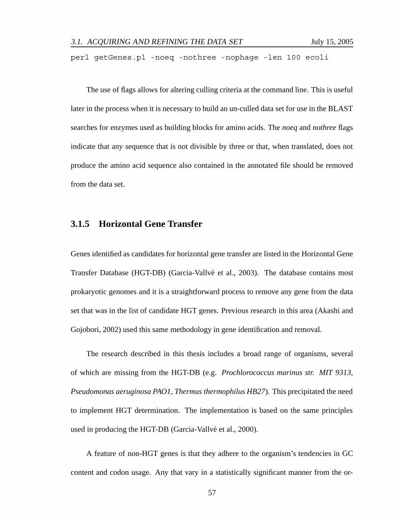
3.1. ACQUIRING AND REFINING THE DATA SET July 15, 2005
perl getGenes.pl -noeq -nothree -nophage -len 100 ecoli
The use of flags allows for altering culling criteria at the command line. This is useful
later in the process when it is necessary to build an un-culled data set for use in the BLAST
searches for enzymes used as building blocks for amino acids. The noeq and nothree flags
indicate that any sequence that is not divisible by three or that, when translated, does not
produce the amino acid sequence also contained in the annotated file should be removed
from the data set.
3.1.5 Horizontal Gene Transfer
Genes identified as candidates for horizontal gene transfer are listed in the Horizontal Gene
Transfer Database (HGT-DB) (Garcia-Vallve et al., 2003). The database contains most
prokaryotic genomes and it is a straightforward process to remove any gene from the data
set that was in the list of candidate HGT genes. Previous research in this area (Akashi and
Gojobori, 2002) used this same methodology in gene identification and removal.
The research described in this thesis includes a broad range of organisms, several
of which are missing from the HGT-DB (e.g. Prochlorococcus marinus str. MIT 9313,
Pseudomonas aeruginosa PAO1, Thermus thermophilus HB27). This precipitated the need
to implement HGT determination. The implementation is based on the same principles
used in producing the HGT-DB (Garcia-Vallve et al., 2000).
A feature of non-HGT genes is that they adhere to the organism’s tendencies in GC
content and codon usage. Any that vary in a statistically significant manner from the or-
57

3.1. ACQUIRING AND REFINING THE DATA SET July 15, 2005
ganism’s inherent GC content and codon usage characteristics are said to originate from
HGT.
The GC content of an organism is measured in three ways: overall GC, GC1, and
GC3 content. The overall GC content is simply a total of all Gs and Cs divided by the total
number of nucleotides. This yields an average GC content for a gene in the organism. If
a gene deviates by greater than 1.5σ from this value it was considered extraneous to the
genome. Additionally if the average number of Gs and Cs for a gene in the first and third
codon positions (GC1 and GC3) deviate from the organism’s norm by more than 1.5σ and
both deviate in the same direction, then the gene is deemed extraneous.
A series of horizontally transferred genes located near each other on the DNA strand is
evidence that an entire strip of genes was transferred in one operation. An 11-gene sliding
window is used to identify possible alien gene strips. Any window with five or more HGT
genes is considered an alien gene strip. Finally, these strips must be filtered to disregard
short isolated segments and to include genes that were not initially considered extraneous
but that have a deviation of their GC content of the same sign as the deviation of the strip
to which they belong.
Codon usage is measured by examining relative codon frequency in each gene (Chou
and Zhang, 1995). An expected frequency is determined for each codon and if a gene
has significantly different frequencies than this normal gene it is the result of horizontal
gene transfer. The high dimensionality of a gene (61 codon frequencies) makes similarity
metrics somewhat problematic. The measure used to determine whether a gene is similar to
an average gene is Mahalanobis distance (Mahalanobis, 1936; Kaplan and Fine, 1998; Chou
58

3.1. ACQUIRING AND REFINING THE DATA SET July 15, 2005
and Zhang, 1995). This distance metric is similar to Euclidean distance except that each
dimension is adjusted to reflect the amount of variance in that dimension. It can be thought
of as being a normalized distance with respect to variance. Computation of Mahalanobis
distance is facilitated by the use of a covariance matrix. The following formula represents
the covariance matrix S. Xk,i is the frequency of the ith codon in the kth gene, Xi is the
average frequency for the ith codon, and N is the total number of genes.
Sij =N∑
k=1
[Xk,i − Xi][Xk,j − Xj] (3.1)
The Mahalanobis distance for gene X is calculated using the following formula:
dM(X, X) = (X − X)T S−1(X − X) (3.2)
The current version of the implementation used in this research performs matching on
the first two criteria (overall GC and GC1 and GC3). The latter two are in development
(Mahalanobis distance and alien gene strips). This yields a useful and conservative approx-
imation of those genes that are extraneous. The numbers of genes identified appear to be
similar (relative to genome size) to other species.
These operations are somewhat outside the capabilities of the standard PERL scripting
language. An extension is needed to facilitate matrix and numerically intensive operations.
This same capability will also be required for major codon usage calculations (principal
component analysis, Eigenvector manipulation, etc.). The solution is found in Perl Data
Language (PDL) (PDL-Porters, 2005). It is an open source extension to standard PERL that
59

3.1. ACQUIRING AND REFINING THE DATA SET July 15, 2005
gives it “the ability to compactly store and speedily manipulate the large N-dimensional
data arrays.” It is installed and used as a module and can be downloaded from CPAN
(PAUSE, 2001). The project was begun with version PDL-2.4.1 and finished with PDL-
2.4.2.
PERL Data Language allows for the conversion of standard PERL arrays into objects
known as PDLs (pronounced piddles). Various standard matrix operations are available
that can be performed on PDLs. A few examples include calculating inverses, generating
a transpose of a matrix, and performing an inner product (dot product). See Figure 3.2 for
some sample commands.
#this line converts the array S into a PDL$Spdl=pdl(@S);
#this line finds the inverse of the covariance matrix S$invSpdl = inv($Spdl);
#these lines perform dot products$returnVal = inner($diff,$invSpdl);$returnVal = inner($returnVal,$diff);
Figure 3.2: Sample PDL Usage
Because the Mahalanobis distances do not tend to follow a normal distribution a ran-
dom (normally distributed) sample of sequences is generated utilizing the mean and stan-
dard deviations of each codon frequency. Any gene with a Mahalanobis distance greater
than 2 σ from the average gene is discarded.
60

3.1. ACQUIRING AND REFINING THE DATA SET July 15, 2005
3.1.6 Paralogs
The next step in refining the data set is to prevent overrepresentation of genes. If all the
genes in any set of homologous genes are included in the calculations then the effects of
that particular gene will be amplified and will skew the results. BLAST is used to identify
paralogs. BLAST can be downloaded from the NCBI (NCBI, 2005) web site and is a
compiled C++ program. PERL allows for the invocation of an external program from
within the script. In this way BLAST is invoked from within the overall driving PERL
script.
BLAST requires a database against which its searches can be performed. The search
can be performed against a nucleotide or amino acids (DNA or protein) database. Akashi
and Gojobori (2002) utilized an amino acid database. In order to maintain consistency and
in order to validate the employed methodology an amino acid database is utilized in the
current research. The paralog search procedure is a simple matter of progressing through
the list of proteins using each as a query, and identifying any similar proteins from the rest
of the list. The result is a cluster of paralog proteins. The protein that is closest to the
organism’s norm in terms of GC content is kept while the rest are discarded.
When BLAST is invoked it requires a query filename to be passed as a parameter. It
also requires a parameter dictating how sensitive the search should be (the more sensitive,
the more hits are returned). The criterion for a valid match, established in Akashi and
Gojobori’s original research (Akashi and Gojobori, 2002) is 60% identity over at least 60
amino acids. To determine an appropriate sensitivity level a randomly permuted protein
was generated. A query was then generated that met the bare minimum standard of simi-
61

3.1. ACQUIRING AND REFINING THE DATA SET July 15, 2005
larity with the randomly permuted protein in the database. Next, the query was run and the
resultant scores examined. The score threshold was set two orders of magnitude lower than
the average value that was returned. In this way the returns were limited while ensuring
that all valid hits were obtained.
The overall process (Figure 3.3) is: 1) read in each protein from the data set, 2) write-
out the protein to a query file, 3) perform the BLAST search, 4) read in the results from
the BLAST output file, 5) determine which of the proteins returned are valid paralogs
(60% identity), 6) determine which protein in the cluster of paralogs to keep (the one with
the GC3 content closest to the organism’s norm), and 7) flag the genes for retention and
removal.
Perl Script
Query File
Blast Program
OutputFile
DBFile
Figure 3.3: Blast Filtering Process
PERL is well suited for performing these operations. It is a scripting language that
62

3.1. ACQUIRING AND REFINING THE DATA SET July 15, 2005
can easily invoke external programs and capture the resulting screen or file output into
variables. The actual command in the PERL script takes the following form:
$command = "./blastall -p blastp -d ".$genom.".ppp.faa-i ".$genom."results.qry -o ".$genom."results.out -e 0.01";
The blastp argument indicates that the data is protein data. $genom is the vari-
able in which the genomic name is stored and $genom."results.out" is the file to
which results are sent. ".$genom.".ppp.faa is the filename associated with the pro-
tein database. The sensitivity of the search is set by the -e 0.01 argument.
The command is then invoked by surrounding it with “single left tic marks” the return
of which is the screen output of the invoked command.
$result = ‘$command‘;
The $genom."results.out" file is then examined to determine which proteins
are paralogs. See Figure 3.4 for a partial listing of a sample results file. Only the alignment
for the first hit is shown. Note that there are three hits and the first has a score of 95%
similarity.
3.1.7 Functional Categories
In addition to a culled listing of genes and their associated sequences the analysis of the data
set will require the functional category of each gene. This information, like the annotated
genome listing, is available from the NCBI (NCBI, 2005). There are 18 different functional
63

3.1. ACQUIRING AND REFINING THE DATA SET July 15, 2005
BLASTP 2.2.8 [Jan-05-2004]
Reference: Altschul, Stephen F., Thomas L. Madden, Alejandro A. Schaffer,Jinghui Zhang, Zheng Zhang, Webb Miller, and David J. Lipman (1997),"Gapped BLAST and PSI-BLAST: a new generation of protein database searchprograms", Nucleic Acids Res. 25:3389-3402.
Query=(227 letters)
Database: ecoli/ecoli.ppp.faa3522 sequences; 1,208,941 total letters
Searching........done
Score ESequences producing significant alignments: (bits) Value
gi|16003521|ref|NP_413521.1| =b4403= 416 e-118gi|16002003|ref|NP_412003.1| =b2532= 73 2e-14gi|16002894|ref|NP_412894.1| =b3651= 35 0.005
>gi|16003521|ref|NP_413521.1| =b4403=Length = 227
Score = 416 bits (1070), Expect = e-118Identities = 213/227 (93%), Positives = 213/227 (93%)
Query: 1 RITIILVXXXXXXXXXXXXXXMKTMGFSDLRIVDSQAHLEPATRWVAHGSGDIIDNIKVF 60RITIILV MKTMGFSDLRIVDSQAHLEPATRWVAHGSGDIIDNIKVF
Sbjct: 1 RITIILVAPARAENIGAAARAMKTMGFSDLRIVDSQAHLEPATRWVAHGSGDIIDNIKVF 60
Query: 61 PTLAESLHDVDFTVATTARSRAKYHYYATPVELVPLLEEKSSWMSHAALVFGREDSGLTN 120PTLAESLHDVDFTVATTARSRAKYHYYATPVELVPLLEEKSSWMSHAALVFGREDSGLTN
Sbjct: 61 PTLAESLHDVDFTVATTARSRAKYHYYATPVELVPLLEEKSSWMSHAALVFGREDSGLTN 120
Query: 121 EELALADVLTGVPMVADYPSLNLGQAVMVYCYQLATLIQQPAKSDATADQHQLQALRERA 180EELALADVLTGVPMVADYPSLNLGQAVMVYCYQLATLIQQPAKSDATADQHQLQALRERA
Sbjct: 121 EELALADVLTGVPMVADYPSLNLGQAVMVYCYQLATLIQQPAKSDATADQHQLQALRERA 180
Query: 181 MTLLTTLAVADDIKLVDWLQQRLGLLEQRDTAMLHRLLHDIEKNITK 227MTLLTTLAVADDIKLVDWLQQRLGLLEQRDTAMLHRLLHDIEKNITK
Sbjct: 181 MTLLTTLAVADDIKLVDWLQQRLGLLEQRDTAMLHRLLHDIEKNITK 227
Figure 3.4: Typical Results File – Output of BLAST. Only First Alignment Shown.
64

3.1. ACQUIRING AND REFINING THE DATA SET July 15, 2005
categories (Table 2.5) with an associated code for identification. In the final culled gene
listing the functional category code from the NCBI source is appended to the gene name.
Figure 3.5 is an example of a portion of the listing found on NCBI for functional categories.
By annotating the gene listing in this way the data can be stratified by functional category
and tested for confounding factors.
Escherichia coli K-12 MG1655 complete genome - 0..4639221 4289proteins Location Strand Length PID Gene Synonym CodeCOG Product
190..255 + 21 1786182 thrL b0001 - - thr operon leader...337..2799 + 820 1786183 thrA b0002 E COG0527 aspartokinase...
2801..3733 + 310 1786184 thrB b0003 E COG0083 homoserine...3734..5020 + 428 1786185 thrC b0004 E COG0498 threonine...5234..5530 + 98 1786186 b0005 b0005 - - orf, hypothetical...5683..6459 - 258 1786187 yaaA b0006 S COG3022 orf, hypothetical...
Figure 3.5: Sample Portion of Gene Functional Category File. COG file downloaded fromNCBI (NCBI, 2005).
3.1.8 Outcome
The goal of this section (Section 3.1, Acquiring and Refining the Data Set) is to acquire a
genomic data set and arrange it into a format suitable for analysis. This includes culling
unwanted genes and tagging the final set with a functional category. To accomplish this
(Figure 3.6) nucleotide sequences must be located and an initial culling performed. Only
those sequences that code for proteins and that are greater than 300 nucleotides in length are
passed on to the next stage of calculation. Phage related genes, paralogs, and genes that are
candidates for horizontal transfer need to be eliminated from consideration. Additionally
the necessary development environment and tools must be chosen in order to best perform
65

3.2. DETERMINING MAJOR CODONS AND MCU July 15, 2005
the analysis and automate the process.
Annotated File
<100 phage no3
Pre-culled Gene List
HGT Removal
Convert to Protein List
Intermediate-culled Gene
List
Protein List
Stats on GC3 Content
Paralog Removal
Fully-culled Gene List
with Functional Category
Tag
Figure 3.6: General Flow during Data Acquisition and Refinement Stage
The final product of the data acquisition and refinement stage is a text file that contains
the names, functional categories, and sequences of all retained genes. This will be the
foundation of all further analysis.
3.2 Determining Major Codons and MCU
3.2.1 Challenge
When analyzing a prokaryotic genome there are literally thousands of genes, each hav-
ing some number of each of the 59 codons being studied (64 less start and stop codons,
and Trp because it has a single synonymous codon). It is very difficult to analyze such
a high-dimensional data set for trends and bias. In order to facilitate analysis, this high
dimensional space is reduced to a single dimension via principal component analysis.
66

3.2. DETERMINING MAJOR CODONS AND MCU July 15, 2005
A genome is described by a matrix of genes and codon frequencies. By shrinking
a gene vector from 59 dimensions to a value in a single dimension a summarized gene
distribution that describes the codon usage trend for the organism can be examined. The
result of the analysis of this trend is a listing of major codons.
While some of the above steps are easily accomplished within the framework of a
PERL scripting environment, some are not. As an example, PCA requires some complex
matrix operations that native PERL cannot handle.
3.2.2 Create Codon Frequency Matrix
The relative frequency with which a codon is selected compared to the other codons that
code for the same amino acid is central to examining codon bias. Codon frequency is
calculated by dividing the number of occurrences of a particular codon by the average for
all its synonymous codons. For example, if there are two codons, c1 and c2, that code for a
particular amino acid and c1’s frequency is being sought, it would look something like:
freqc1 =count(c1)
(count(c1) + count(c2))/2(3.3)
The average is used instead of the total so that codons with different numbers of syn-
onymous codons can be compared. This is a form of normalization. Note that this is Sharp
et al.’s relative synonymous codon usage (RSCU, Section 2.5.2).
The next step involves building a matrix that contains the codon frequency for each of
the codons within each of the genes.
67

3.2. DETERMINING MAJOR CODONS AND MCU July 15, 2005
c1 c2 c3 · · · c59
g1 f1,1 f1,2 f1,3 · · · f1,59
g2 f2,1 f2,2 f2,3 · · · f2,59
g3 f3,1 f3,2 f3,3 · · · f3,59
......
......
......
gn fn,1 fn,2 fn,3 · · · fn,59
Any given row can now be treated as a vector representation of the codon frequencies
for a given gene. These vectors represent data points in a hyper-dimensional (59) space that
capture each gene’s codon usage. When principal component analysis is performed upon
this data a single axis described in terms of the original vector space is generated. This
new axis extends in a direction that corresponds to the widest scale of “gene distribution
in codon frequency space” (Kanaya et al., 1996). By projecting the original data (codon
frequency matrix) onto this axis a one-dimensional view of the data is obtained.
The codon frequency matrix is built in a straightforward manner using standard PERL
arrays and functions. Next a covariance matrix is created based upon this original frequency
matrix. The covariance is measured between vertical vectors whose dimensionality equals
the number of genes. The diagonal contains the variance of each of the codons, and the
matrix is symmetric with respect to the diagonal. PERL Data Language (PDL) is used to
create the covariance matrix. It has several tools that enable the calculation of the codon’s
covariance. For instance, general statistics can be extracted from a vector in a PDL. The
following extracts general statistics from a vertical slice of a matrix (PDL).
68

3.2. DETERMINING MAJOR CODONS AND MCU July 15, 2005
c1 c2 c3 · · · c59
c1 var1 cov1,2 cov1,3 · · · cov1,59
c2 cov2,1 var2 cov2,3 · · · cov2,59
c3 cov3,1 cov3,2 var3 · · · cov3,59
......
......
......
c59 cov59,1 cov59,2 cov59,3 · · · var59
Figure 3.7: Covariance Matrix
($mean1, $stdev, $median, $min, $max) = stats($geneFreqMatrix− > slice(“$i, : ”));
The covariance matrix is central to principal component analysis (PCA). The Eigen-
vector with the largest Eigenvalue derived from the covariance matrix is the vector that
extends along the axis of greatest variance in the original vector space.
3.2.3 PCA
The use of PDLs makes the process of generating an Eigenvector trivial. The following
commands extract Eigenvectors from the covariance matrix.
69

3.2. DETERMINING MAJOR CODONS AND MCU July 15, 2005
($ev, $e) = eigens($covMatrix);
$maxIndex = maximumind($e);
$b1 = $ev− > slice(“$maxIndex, : ”);
The first principal component, b1, is a vector that extends in a direction that corre-
sponds to the widest scale (largest λ value) of gene distribution. This vector is treated as a
new axis represented in terms of the old vector space.
To see where the data fall on this new axis a dot product operation is performed be-
tween the codon frequency matrix (X) and the first principal component. The result is a
vector containing the scalar values representing the length of each gene’s projection onto
the new axis, the first principal component.
X · b1 = Z′1 (3.4)
Using a PDL, this can be obtained by employing the following command:
$Zprime = inner($geneFreqMatrix, transpose($b1));
Each entry in the resultant Z′1 vector contains the scalar magnitude of the projection
of a gene on the new axis. In other words, Z′1 represents the location of the data points
(genes) on the new axis. It has been determined that the distribution of the genes in this one
70

3.2. DETERMINING MAJOR CODONS AND MCU July 15, 2005
dimensional space is roughly normal (Kanaya et al., 1996). This is useful when performing
correlation analysis, as parametric techniques can be employed. The distribution of these
codon usage values represents the overall bias in the genome (Figure 4.3 in the Results
chapter).
3.2.4 Factor Loadings
To determine which codons contribute positively to this trend the correlation of each codon’s
frequency across all genes and the values in the Z′1 vector (Figure 3.3) must be determined.
The codon frequency across all genes can be obtained by treating the columns in the codon
frequency matrix as vectors representing codon usage across all genes. The formula used
is the standard Pearson correlation between the codon frequency vector and Z′1.
The resultant correlation coefficient is known as a factor loading. If the factor loading
is significantly positive (the codon contributes positively to the overall trend, r is signifi-
cantly positive) then the codon in question is major. Significance is set at α = 0.05. The
following PERL code is used in determining significance:
$Tstat = $correlation ∗ sqrt($numGenes − 2)/sqrt(1 − $correlation ∗ ∗2);
$pval = pt($Tstat, $numGenes − 2);
$sig = qt(1 − $alpha/2, $numGenes − 2);
71

3.2. DETERMINING MAJOR CODONS AND MCU July 15, 2005
Table 3.3: Factor Loading Determination
The vertical column in the frequency matrix headed ci is a vector representation of the ith
codon’s frequency across all genes. Z′ also has a dimensionality equal to the number ofgenes. It was derived by projecting each gene vector (the horizontal representation for eachgene in the frequency matrix) onto the first Eigenvector.
72

3.2. DETERMINING MAJOR CODONS AND MCU July 15, 2005
If $correlation is positive and the T statistic ($Tstat) is greater than the $sig value
then it is significant and is considered a major codon.
3.2.5 Eigenvector Direction
While the first principle component (Eigenvector) lies along the axis of greatest variance, its
direction is somewhat arbitrary. The direction in which it extends along this axis depends on
the layout of the data. For this analysis it is necessary to direct the Eigenvector such that the
largest magnitude entry in the vector will be positive – thus if the largest magnitude value
is negative then all values in the Eigenvector are multiplied by negative one. The reasoning
for this can be intuitively understood by recognizing that large values in an Eigenvector
correspond to dimensions with large variance. It is desired that the dimension with the
greatest variance be positive. If the Eigenvector is not flipped when the greatest magnitude
value is negative then the genes using the most highly variable codons will be penalized
in terms of their Z′ value when they should be rewarded. Genes with highly positive Z′
values should be an indication of high variance codon usage and avoidance of low variance
codons.
In order to verify the validity of the choice, the major codons derived by principal
component analysis (PCA) are compared to the weights of those codons when derived by
the codon adaptation index (CAI) methodology. In CAI, codons with weights of one are
maximal siblings, and therefore major. If the sum of the weights of codons identified as
major by PCA divided by the number of those codons yields a number greater than .5
then there is greater than 50% agreement between the two methods and it is assumed that
73

3.2. DETERMINING MAJOR CODONS AND MCU July 15, 2005
the Eigenvector direction is correct (if the value were less than 50% then reversing the
direction of the Eigenvector would yield a value greater than 50%). As evidence of this
method’s suitability there is agreement with CAI in choice of major codons in 25 of 25
genomes examined. Equation 3.5 describes the measurement process where PA is percent
agreement, n is the number of major codons as determined by PCA, ci is the ith codon in
the set of codons identified as major by PCA, and wciis the weight associated with each of
those codons.
PA =
n∑i=1
wci(3.5)
3.2.6 Outcome
In order to determine major codons the dimensionality of the codon frequency matrix is
reduced through PCA to a single dimension described by the first principal component.
The gene vectors are then projected onto this axis to generate a new one dimensional vector
space. Each codon is then examined to determine whether it contributes positively to the
overall trend described by the distribution of data in the new vector space. Supportive
PERL modules are used to enable the above calculations.
The output from the determining major codons stage is a text file listing the major
codons for the organism. This text file is used in the statistical analysis phase to calculate
major codon usage for each of the genes.
74

3.3. STATISTICAL ANALYSIS July 15, 2005
3.3 Statistical Analysis
3.3.1 Challenge
Now that all of the raw data has been accumulated, the challenge in this stage is to deter-
mine whether or not “Amino acid composition . . . reflects the action of natural selection to
enhance metabolic efficiency” (Akashi and Gojobori, 2002). This is done through correla-
tion analysis where expressivity is compared with energetic cost to determine whether any
relationship exists.
The steps include calculation of MCU and average energetic cost per amino acid for
each gene followed by a Spearman rank correlation. While these are easily accomplished
within the framework of a PERL scripting environment, the test for significance presents
a subordinate objective that is not. This step requires the calculation of a probability of a
given T statistic.
In addition to these overarching goals this stage must also attempt to show that metabolic
efficiency is the most likely driving force in the correlation and not some other character-
istic of the environment. Physicochemical classes, individual amino acid behaviors, and
functional categories are all examined as potential confounding factors.
75

3.3. STATISTICAL ANALYSIS July 15, 2005
3.3.2 Correlation Between Expressivity and Amino Acid Cost
Calculating MCU
A gene’s Major codon usage (MCU) is determined by generating a count of codons that
are major and dividing that count by the total number of codons in the gene. This yields
a percentage of codons that are major in the gene. This percentage, or MCU, can be used
to rank the genes. This ranking has been shown to be a strong indicator of the ranking
achieved when examining expressivity (Kanaya et al., 1999). The higher the major codon
usage the higher the expressivity of the gene.
Energetic Cost Calculation
The energetic costs of protein production are largely the same from one protein to another.
The differentiating factor is the synthesis of the amino acid building blocks. Each amino
acid has a cost associated with it, and the cost of producing a protein can be determined by
summing the costs for each of the amino acids in the polypeptide chain. This total cost is
then divided by the number of amino acids yielding an average cost per amino acid.
The costs for each amino acid are determined by various pathways traversed dur-
ing the synthesis and are the same for all organisms within each broad category (e.g. all
chemoheterotrophic organisms generally use the same pathways). As noted previously,
amino acid energy costs were supplied by Esley Heizer of the BMS program at Wright
State University (Heizer, 2005).
76

3.3. STATISTICAL ANALYSIS July 15, 2005
Spearman Rank
At this stage of the analysis each gene has an MCU and Energetic Cost associated with
it. Spearman rank correlation is performed by sorting the genes by MCU and assigning
each gene an associated rank. Next the gene set is sorted by energy and associated ranks
are assigned. The difference between the two ranks is the distance metric d utilized in the
following equation (Spearman, 1904; Rosner, 2000):
rS = 1 −6
n∑i=1
d2
n(n2 − 1)(3.6)
All of these operations are easily performed within PERL. In order to determine
whether the Spearman rank correlation coefficient rS is significant a T statistic must be
calculated. The p value is calculated by determining the probability associated with the T
statistic and n − 2 degrees of freedom (see formulae 3.7 and 3.8). In order to support this
operation in PERL a module must be used that provides for the calculation of probabili-
ties. The module used to accomplish this is the cumulative distribution functions module or
Math::CDF (PAUSE, 2001) module. It is used to generate probabilities and quantiles from
several statistical probability functions.
Tstat =rs ∗
√n − 2√
1 − r2s
(3.7)
p = pt(Tstat, n − 2) (3.8)
77

3.3. STATISTICAL ANALYSIS July 15, 2005
Parasitic Behavior & Correction
In the initial analysis of the parasitic organisms Chlamydia trachomatis and Mycoplasma
genitalium, it was noted that these organisms exhibited no correlation between expressivity
and energetic costs. Upon closer examination it was determined that the reason for this
behavior is that the organism can acquire some of its amino acids and metabolites from the
environment in which it lives. To account for this behavior zero cost is assigned to amino
acids that can be obtained from the host.
In order to determine whether an amino acid is produced by the organism or acquired
from the host, the genome of the parasite is examined to see whether it can produce the
appropriate enzymes to synthesize the amino acid in question. This is done by performing a
BLAST search on an un-culled set of proteins (generated from the organism’s gene listing)
for each enzyme in the associated pathway for a given amino acid. If there are no proteins
with a 30% or better similarity to the associated enzyme then it is assumed that enzyme
cannot be produced by the organism. Further, if more than 50% of the enzymes are missing
from the pathway then it is assumed that the end product amino acid cannot be synthesized.
Effect of Protein Structure
To determine whether physicochemical properties of the amino acids impact the observed
trends, the amino acids are divided into three physicochemical classes, and all but one class
of amino acid are removed from the data before analysis. The three classes are internal,
78

3.3. STATISTICAL ANALYSIS July 15, 2005
external, and ambivalent. The amino acids in each of these classes can be seen in Table 3.4.
Internal External AmbivalentPhenylalanine, Phe, F Histidine, His, H Tryptophan, Trp, WLeucine, Leu, L Arginine, Arg, R Tyrosine, Tyr, YIsoleucine, Ile, I Lysine, Lys, K Cysteine, Cys, CMethionine, Met, M Glutamine, Gln, Q Alanine, Ala, AValine, Val, V Glutamic acid, Glu, E Serine, Ser, S
Asparagines, Asn, N Glycine, Gly, GAspartic acid, Asp, D Praline, Pro, P
Threonine, Thr T
Table 3.4: Physicochemical Classes for Amino Acids
The same MCU data is used in this analysis as in previous steps. If the major codon
usage were recalculated it would change the predicted expression level of the genes, and
that is not the intent of this analysis. The gene should maintain the same MCU value while a
new average cost per amino acid is calculated for the subset of amino acids being examined.
When calculating the new average energetic cost for a gene, only those amino acids in the
class being examined are included in the analysis. In this way it can be determined whether
one or more classes drive the correlations.
3.3.3 Amino Acid Abundance
Some insights into the mutational process may be gained by examining behavior of indi-
vidual amino acids. Intuition would lead one to expect the more expensive residues to have
a negative correlation with respect to expressivity. Consequently, less expensive amino
acids would be forced into a positive correlation. It would also be useful to eliminate gene
79

3.3. STATISTICAL ANALYSIS July 15, 2005
functional category as factors in the analysis. To do these things one must first calculate
amino acid abundance.
The PERL scripts perform this task in an object-oriented fashion. Gene objects are
created that have various attributes, including a sequence attribute and amino acid abun-
dance attribute for each individual amino acid.
The script reads in the list of genes along with their sequences from the previously
generated culled gene set file. For each gene a gene object is created and the gene’s name,
category, and sequence are stored within. The gene objects are then stored in an array of
gene objects.
The original data are nucleotide sequences, so they must be conceptually translated
into polypeptide sequences for the tabulation of amino acid frequencies. PERL’s regular
expression and string replacement capabilities make it well suited for this operation.
Since each individual amino acid will be examined and compared to major codon
usage, an MCU attribute is populated. The script retrieves MCU from another previously
generated file and stores it in the appropriate gene objects. Spearman rank correlation
requires a rank value based upon MCU. To generate this value the gene array is sorted by
the MCU and the corresponding rank value is entered as an attribute of each gene object.
Another pass is made through the gene object array counting the amino acids in their
sequences. These individual counts are then stored in the gene object. Thus, every gene
object has a count attribute for every amino acid.
80

3.3. STATISTICAL ANALYSIS July 15, 2005
Spearman Across Genome
With the array of populated gene objects in place the Spearman rank correlation can be
calculated for each amino acid verses expressivity (MCU). To do this the gene array is
sorted by the first amino acid’s abundance and its rank is stored in a field within the gene
object. The MCU rank is already stored as an attribute of the gene object. Next, that amino
acid’s Spearman rank correlation coefficient is calculated. This process is repeated for each
of the amino acids. During each of these steps a gene’s MCU rank is compared with its
rank based upon the abundance of a particular amino acid. The result is an examination of
amino acid abundance across the entire genome.
To verify that the generated coefficient is significant the associated T-statistic is calcu-
lated. This is done using the following PERL code with an $alpha value of 0.05.
$Tstat = $correlation ∗ sqrt($numGenes − 2)/sqrt(1 − $correlation ∗ ∗2);
$pval = pt($Tstat, $numGenes − 2);
$sig = qt(1 − $alpha/2, $numGenes − 2);
The script stores the Spearman rank coefficients and their associated significance val-
ues in a text file for easy retrieval.
Use of Mantel-Haenszel
Next, a Mantel-Haenszel test is employed to determine whether functional categories are
confounding factors. In the Mantel-Haenszel test the data is first stratified then the effects
81

3.3. STATISTICAL ANALYSIS July 15, 2005
of the strata are removed. In this case the data are the various amino acid abundances and
the strata are the gene categories.
First, all genes are sorted by MCU. The use of the gene objects described previously
is continued during this process. Any genes falling below the median are flagged as low
while those above are flagged as high. If the number of genes is odd then the median
gene is flagged as high. The effect of this assignment is negligible; however it seemed the
conservative choice.
Next, the entire list of genes is traversed accumulating counts. These are stored in 2×2
contingency tables (see the next section, Mantel-Haenszel Calculation for an explanation
as to the specific values that go into the tables).
When the process is complete there is a set of contingency tables for each amino acid.
Each set will contain a table for each functional category. The Mantel-Haenszel test is run
on each of the sets of tables.
Mantel-Haenszel Calculation
To perform the Mantel-Haenszel Test:
1. For each amino acid form k strata based on gene category, and construct a 2×2 table
relating amino acid abundance to MCU for each category. A sample table (Table 3.5)
is shown where a is the count of a given amino acid in genes flagged as high MCU,
and b is the count of the rest of the amino acids in genes flagged as high MCU. c
is the count of the given amino acid in genes flagged as low, and d is the count of
82

3.3. STATISTICAL ANALYSIS July 15, 2005
Count of AA Count of the rest of the AAs
High a b
Low c d
Table 3.5: 2 × 2 Contingency Table Used in Mantel-Haenszel Test
the rest of the amino acids in genes flagged as low. Remember, this table contains
information only pertaining to the abundance of a specific amino acid in those genes
within a single category.
2. Compute the total observed amino acids in the a cell over all strata. Note that there
are 16 categories. The poorly characterized categories (Table 2.5) are not included.
O =16∑i=1
ai (3.9)
3. Compute the total expected number of amino acids in the a cell over all strata
E =
16∑i=1
Ei =
16∑i=1
(ai + bi)(ai + ci)
ai + bi + ci + di(3.10)
4. Compute the variance of O.
V =16∑i=1
Vi =16∑i=1
(ai + bi)(ci + di)(ai + ci)(bi + di)
n2i (ni − 1)
(3.11)
Note that ni = ai + bi + ci + di.
5. The test statistic is
83

3.3. STATISTICAL ANALYSIS July 15, 2005
χ2MH =
(|O − E| − .5)2
V(3.12)
Under the null hypothesis (H0) the test statistic adheres to a chi-squared distribution
with one degree of freedom.
6. For a two-sided test with significance level α reject H0 if
χ2MH ≤ χ2
1,1−α (3.13)
7. The p-value for this test is given by
p = Pr(χ21 > χ2
MH) (3.14)
While the χ2 and p value are adequate to describe the significance of any correlation,
they do not give an indication of the strength of the association. To get a sense of this
strength an Odds Ratio (OR) is required. The odds ratio was described in Subsection 2.9.2
including an intuitive reason for why it captures the strength of the relationship.
ORMH =
k∑i=1
aidi/ni
k∑i=1
bici/ni
(3.15)
The natural log of the odds ratio adheres to a normal distribution. As such, the natural
log of the odds ratio divided by the square root of the variance (σ) will form a Z value
from a standard normal distribution. While the variance cannot be directly calculated the
84

3.3. STATISTICAL ANALYSIS July 15, 2005
variance of the natural log of the odds ratio can be (Robins et al., 1986). Following is a
formula for such a calculation.
V ar(ln ORMH) =
∑ki=1 PiRi
2(∑k
i=1 Ri)2+
∑ki=1 PiSi + QiRi
2(∑k
i=1 Ri)(∑k
i=1 Si)+
∑ki=1 QiSi
2(∑k
i=1 Si)2(3.16)
Where Pi, Qi, Ri, and Si are defined by the following relationships.
Pi =ai + di
ni, Qi =
bi + ci
ni, Ri =
aidi
ni, Si =
bici
ni(3.17)
Given these formulae a Z value can be computed as follows.
Z =ln(ORMH)√
V ar(ln(ORMH))
(3.18)
3.3.4 Outcome
The challenge during this phase was to determine whether or not “Amino acid composition
. . . reflects the action of natural selection to enhance metabolic efficiency” (Akashi and
Gojobori, 2002). This was accomplished through correlation analysis and the removal of
confounding factors.
The output of this phase of the analysis is various tables and figures depicting correla-
tions and stratified data. These figures and tables are the end result of this research and are,
therefore, the refined output of the overall process. They can be seen in the next chapter,
Results.
85

Results
4.1 Data Acquisition and Refinement
The main refinement criteria for the gene sets include eliminating any genes with less than
100 codons, genes that are candidates for horizontal gene transfer, and all but one gene in
a cluster of paralogs. Some additional criteria that emerged as necessary in the analysis
are the removal of genes that have premature stop codons (generally codes for an unusual
amino acid: selenocysteine) or that experienced a frame shift causing the number of nu-
cleotides in the sequence to be indivisible by three. Because these latter situations occurred
infrequently and often required human interaction, the genes matching these criteria were
discarded. Table 4.1 describes the number of genes in the initial data set, how many were
culled, for what reason, and the final number of genes. Some genes qualified for culling
for multiple reasons. In order to ensure that the sum of the number culled in each category
matched the total number culled an order was enforced in the culling process. The first cri-
terion matched is the one assigned to the gene. The order is phage, <100 , non translation
matching, partial codons, candidates for HGT, and finally, clusters of paralogs.
86

4.2. MAJOR CODONS AND ENERGETIC COSTS July 15, 2005
Organism Num.ofGenesinGenome
PartialCodons
Genes<100codons
Phagerelatedgenes
Sequencedoesnotmatchtransla-tion
HGT paralog Num.ofGenesAfterCulling
Num.ofCodons
Bacillus subtilis 4,112 2 488 89 2 433 58 3,040 1,010,337Escherichia coli K12 4,311 0 433 68 3 288 201 3,318 1,127,136
Chlamydia trachomatis 895 0 66 0 0 33 2 794 297,317Mycoplasma genitalium 484 0 24 0 0 49 0 411 152,946
Synechococcus sp WH 8102 3,167 0 247 107 0 160 61 2,592 923,920Thermotoga maritima 1,858 1 166 11 1 176 18 1,485 503,237
Table 4.1: Number of Genes in the Genome and the Number Removed by each CullingCriteria
NOTE- Num of genes in genome - number of protein coding genes in the genome, par-tial codons - a codon containing less than three nucleotides, Genes <100 codons - genesless than 100 codons not including start and stop codons, Phage related - genes that arephage or transposon related, sequence does not match translation - when translated the nu-cleotide sequence does not match the given protein sequence, HGT - any gene identified asa candidate for horizontal gene transfer, paralog - genes identified as paralogous.
4.2 Major Codons and Energetic Costs
4.2.1 Eigenvectors
Table 4.2 contains the Eigenvectors for the six primary genomes. They are generated from
the covariance matrix which is based upon the relative frequency matrix. The Eigenvector
for Bacillus subtilis had to be reversed as per the criteria set forth in Section 3.2.5.
4.2.2 Distribution of Data in New Dimension
Once the first principal component (Eigenvector with largest Eigenvalue) is determined the
original frequency data is projected upon this new axis. The first principal component ex-
tends along the axis of greatest variance. Since the Eigenvector is a unit vector a simple dot
87
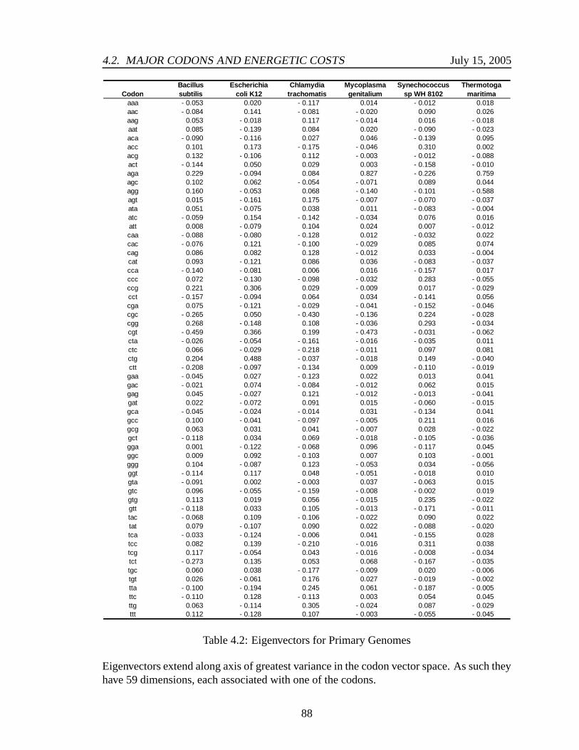
4.2. MAJOR CODONS AND ENERGETIC COSTS July 15, 2005
CodonBacillussubtilis
Escherichiacoli K12
Chlamydiatrachomatis
Mycoplasmagenitalium
Synechococcussp WH 8102
Thermotogamaritima
aaa - 0.053 0.020 - 0.117 0.014 - 0.012 0.018aac - 0.084 0.141 - 0.081 - 0.020 0.090 0.026aag 0.053 - 0.018 0.117 - 0.014 0.016 - 0.018aat 0.085 - 0.139 0.084 0.020 - 0.090 - 0.023aca - 0.090 - 0.116 0.027 0.046 - 0.139 0.095acc 0.101 0.173 - 0.175 - 0.046 0.310 0.002acg 0.132 - 0.106 0.112 - 0.003 - 0.012 - 0.088act - 0.144 0.050 0.029 0.003 - 0.158 - 0.010aga 0.229 - 0.094 0.084 0.827 - 0.226 0.759agc 0.102 0.062 - 0.054 - 0.071 0.089 0.044agg 0.160 - 0.053 0.068 - 0.140 - 0.101 - 0.588agt 0.015 - 0.161 0.175 - 0.007 - 0.070 - 0.037ata 0.051 - 0.075 0.038 0.011 - 0.083 - 0.004atc - 0.059 0.154 - 0.142 - 0.034 0.076 0.016att 0.008 - 0.079 0.104 0.024 0.007 - 0.012caa - 0.088 - 0.080 - 0.128 0.012 - 0.032 0.022cac - 0.076 0.121 - 0.100 - 0.029 0.085 0.074cag 0.086 0.082 0.128 - 0.012 0.033 - 0.004cat 0.093 - 0.121 0.086 0.036 - 0.083 - 0.037cca - 0.140 - 0.081 0.006 0.016 - 0.157 0.017ccc 0.072 - 0.130 - 0.098 - 0.032 0.283 - 0.055ccg 0.221 0.306 0.029 - 0.009 0.017 - 0.029cct - 0.157 - 0.094 0.064 0.034 - 0.141 0.056cga 0.075 - 0.121 - 0.029 - 0.041 - 0.152 - 0.046cgc - 0.265 0.050 - 0.430 - 0.136 0.224 - 0.028cgg 0.268 - 0.148 0.108 - 0.036 0.293 - 0.034cgt - 0.459 0.366 0.199 - 0.473 - 0.031 - 0.062cta - 0.026 - 0.054 - 0.161 - 0.016 - 0.035 0.011ctc 0.066 - 0.029 - 0.218 - 0.011 0.097 0.081ctg 0.204 0.488 - 0.037 - 0.018 0.149 - 0.040ctt - 0.208 - 0.097 - 0.134 0.009 - 0.110 - 0.019gaa - 0.045 0.027 - 0.123 0.022 0.013 0.041gac - 0.021 0.074 - 0.084 - 0.012 0.062 0.015gag 0.045 - 0.027 0.121 - 0.012 - 0.013 - 0.041gat 0.022 - 0.072 0.091 0.015 - 0.060 - 0.015gca - 0.045 - 0.024 - 0.014 0.031 - 0.134 0.041gcc 0.100 - 0.041 - 0.097 - 0.005 0.211 0.016gcg 0.063 0.031 0.041 - 0.007 0.028 - 0.022gct - 0.118 0.034 0.069 - 0.018 - 0.105 - 0.036gga 0.001 - 0.122 - 0.068 0.096 - 0.117 0.045ggc 0.009 0.092 - 0.103 0.007 0.103 - 0.001ggg 0.104 - 0.087 0.123 - 0.053 0.034 - 0.056ggt - 0.114 0.117 0.048 - 0.051 - 0.018 0.010gta - 0.091 0.002 - 0.003 0.037 - 0.063 0.015gtc 0.096 - 0.055 - 0.159 - 0.008 - 0.002 0.019gtg 0.113 0.019 0.056 - 0.015 0.235 - 0.022gtt - 0.118 0.033 0.105 - 0.013 - 0.171 - 0.011tac - 0.068 0.109 - 0.106 - 0.022 0.090 0.022tat 0.079 - 0.107 0.090 0.022 - 0.088 - 0.020tca - 0.033 - 0.124 - 0.006 0.041 - 0.155 0.028tcc 0.082 0.139 - 0.210 - 0.016 0.311 0.038tcg 0.117 - 0.054 0.043 - 0.016 - 0.008 - 0.034tct - 0.273 0.135 0.053 0.068 - 0.167 - 0.035tgc 0.060 0.038 - 0.177 - 0.009 0.020 - 0.006tgt 0.026 - 0.061 0.176 0.027 - 0.019 - 0.002tta - 0.100 - 0.194 0.245 0.061 - 0.187 - 0.005ttc - 0.110 0.128 - 0.113 0.003 0.054 0.045ttg 0.063 - 0.114 0.305 - 0.024 0.087 - 0.029ttt 0.112 - 0.128 0.107 - 0.003 - 0.055 - 0.045
Table 4.2: Eigenvectors for Primary Genomes
Eigenvectors extend along axis of greatest variance in the codon vector space. As such theyhave 59 dimensions, each associated with one of the codons.
88

4.2. MAJOR CODONS AND ENERGETIC COSTS July 15, 2005
product produces this projection. Figure 4.3 depicts the distributions of relative frequency
data for the six primary genomes in the single dimension represented by their first principal
component.
Bacillus subtilis
0
50
100
150
200
250
-3.6096018
-2.842979414
-2.076357028
-1.309734642
-0.543112256
0.22351013
0.990132516
1.756754902
2.523377288
3.289999674
4.05662206
4.823244446
5.589866832
6.356489218
7.123111604
Escherichia coli K12
0
50
100
150
200
250
-3.2197019
-2.336911739
-1.454121577
-0.571331416
0.311458746
1.194248907
2.077039068
2.95982923
3.842619391
4.725409553
5.608199714
6.490989875
7.373780037
8.256570198
9.13936036
Chlamydia trachomatis
0
10
20
30
40
50
60
-3.8921389
-3.520118814
-3.148098727
-2.776078641
-2.404058554
-2.032038468
-1.660018381
-1.287998295
-0.915978208
-0.543958122
-0.171938035
0.200082051
0.572102138
0.944122224
1.316142311
1.688162397
2.060182484
2.43220257
2.804222657
Mycoplasma genitalium
0
10
20
30
40
50
60
-2.4450448
-1.57532165
-0.7055985
0.16412465
1.0338478
1.90357095
2.7732941
3.64301725
4.5127404
5.38246355
More
Synechococcus sp WH 8102
0
50
100
150
200
250
-4.6372254
-4.035818574
-3.434411748
-2.833004922
-2.231598096
-1.63019127
-1.028784444
-0.427377618
0.174029208
0.775436034
1.37684286
1.978249686
2.579656512
3.181063338
3.782470164
4.38387699
4.985283816
Thermotoga maritima
020406080
100120140160
-3.2940223
-2.593480819
-1.892939338
-1.192397857
-0.491856376
0.208685105
0.909226586
1.609768068
2.310309549
3.01085103
3.711392511
4.411933992
5.112475473
Table 4.3: Histogram Depiction of Frequency Data Projected Upon First Principal Compo-nent – New Axis
Horizontal axis can be thought of as the new axis described by the first principal component(Eigenvector with greatest Eigenvalue). There is a point on this axis for every gene. Thehistograms above show the distribution of these data points.
The data form roughly normal distributions. An interesting exception is the Chlamydia
trachomatis genome. It forms a bimodal distribution and an interesting exercise would be
89

4.2. MAJOR CODONS AND ENERGETIC COSTS July 15, 2005
to examine the nature of the genes in these two regions to determine possible reasons.
Another interesting finding that seems somewhat related to these distributions is the
selection of directionality for the Eigenvectors. The original derived Eigenvectors for the
six primary genomes all point in the correct direction except Bacillus subtilis and Chlamy-
dia trachomatis. These two genomes also happen to exhibit a negative mean in their Z ′1
values. This leads to speculation as to the underlying cause and meaning for Bacillus sub-
tilis and Chlamydia trachomatis having negative means.
When the examination extends to the additional 19 genomes (Figure 4.4) the trend
continues to hold. Of the 19 genomes only two of them, Mycoplasma penetrans and My-
cobacterium tuberculosis CDC1551, required modification of Eigenvector direction. Of
the 25 genomes studied four generate default Eigenvectors exhibiting incorrect direction-
ality. Bacillus subtilis and Chlamydia trachomatis continue to be the only organisms that
exhibit a negative mean.
4.2.3 Factor Loadings
The dot product between Eigenvector and the original codon frequency matrix yields the
Z′1 vector. This represents the original codon frequency data projected onto a vector that ex-
tends along the axis of greatest variance within the codon frequency space. The correlation
between each codon frequency vector (across the entire culled genomic codon frequency
data set) and the Z′1 vector indicate the degree to which each codon contributes to the over-
all codon frequency trend. Each correlation is known as a factor loading. Table 4.5 depicts
90

4.2. MAJOR CODONS AND ENERGETIC COSTS July 15, 2005
Aeropyrum pernix
020406080
100120
-2.1178793
-1.514550895
-0.911222489
-0.307894084
0.295434321
0.898762726
1.502091132
2.105419537
2.708747942
3.312076347
3.915404753
4.518733158
5.122061563
5.725389968
6.328718374
6.932046779
7.535375184
8.138703589
8.742031995
More
Chlorobium tepidum TLS
020406080
100120
-2.8003866
-2.265776295
-1.73116599
-1.196555685
-0.66194538
-0.127335075
0.40727523
0.941885535
1.47649584
2.011106145
2.54571645
3.080326755
3.61493706
4.149547365
4.68415767
5.218767975
5.75337828
6.287988585
6.82259889
7.357209195
More
Clostridium perfringens
020406080
100120140160
-1.6435891
-0.938052648
-0.232516196
0.473020257
1.178556709
1.884093161
2.589629613
3.295166065
4.000702517
4.70623897
5.411775422
6.117311874
6.822848326
7.528384778
8.23392123
8.939457683
Helicobacter pylori J99
020406080
100120140160
-4.5320645
-4.001609294
-3.471154089
-2.940698883
-2.410243677
-1.879788471
-1.349333266
-0.81887806
-0.288422854
0.242032351
0.772487557
1.302942763
1.833397969
2.363853174
2.89430838
3.424763586
3.955218791
4.485673997
Lactobacillus plantarum WCFS1
020406080
100120140160
-4.8090067
-4.23468755
-3.6603684
-3.08604925
-2.5117301
-1.93741095
-1.3630918
-0.78877265
-0.2144535
0.35986565
0.9341848
1.50850395
2.0828231
2.65714225
3.2314614
3.80578055
More
Mycoplasma penetrans
020406080
100120
-3.6753425
-2.931074931
-2.186807362
-1.442539792
-0.698272223
0.045995346
0.790262915
1.534530485
2.278798054
3.023065623
3.767333192
4.511600762
5.255868331
More
Mycobacterium tuberculosis CDC1551
0
50
100
150
200
250
-1.8887703
-1.373159598
-0.857548896
-0.341938195
0.173672507
0.689283209
1.204893911
1.720504613
2.236115314
2.751726016
3.267336718
3.78294742
4.298558121
4.814168823
5.329779525
5.845390227
6.361000929
6.87661163
7.392222332
Nitrosomonas europaea ATCC 19718
020406080
100120140160
-2.4919219
-2.06656568
-1.641209461
-1.215853241
-0.790497022
-0.365140802
0.060215417
0.485571637
0.910927856
1.336284076
1.761640295
2.186996515
2.612352734
3.037708954
3.463065173
3.888421393
4.313777612
4.739133832
5.164490051
5.589846271
6.01520249
Nostoc sp. PCC 7120
050
100150200250300
-4.601288
-4.094578625
-3.58786925
-3.081159875
-2.5744505
-2.067741125
-1.56103175
-1.054322375
-0.547613
-0.040903625
0.46580575
0.972515125
1.4792245
1.985933875
2.49264325
2.999352625
3.506062
4.012771375
4.51948075
5.026190125
5.5328995
6.039608875
Prochlorococcus marinus str. MIT 9313
0102030405060708090
-3.4864689
-2.950292785
-2.41411667
-1.877940554
-1.341764439
-0.805588324
-0.269412209
0.266763907
0.802940022
1.339116137
1.875292252
2.411468367
2.947644483
3.483820598
4.019996713
4.556172828
Pseudomonas aeruginosa PA01
050
100150200250300350
-1.8355376
-1.167277432
-0.499017264
0.169242904
0.837503072
1.505763241
2.174023409
2.842283577
3.510543745
4.178803913
4.847064081
5.515324249
6.183584417
6.851844586
7.520104754
8.188364922
8.85662509
9.524885258
Pseudomonas putida KT2440
0
50
100
150
200
-0.47519839
-0.012331335
0.45053572
0.913402775
1.37626983
1.839136885
2.30200394
2.764870994
3.227738049
3.690605104
4.153472159
4.616339214
5.079206269
5.542073324
6.004940379
6.467807434
6.930674489
7.393541544
7.856408599
8.319275654
8.782142708
9.245009763
Pyrococcus furiosus DSM 3638
020406080
100120140
-4.1848648
-3.696463115
-3.20806143
-2.719659745
-2.23125806
-1.742856375
-1.25445469
-0.766053005
-0.27765132
0.210750365
0.69915205
1.187553735
1.67595542
2.164357105
2.65275879
3.141160475
3.62956216
4.117963845
4.60636553
5.094767215
More
Staphylococcus aureus subsp. aureus MW2
020406080
100120140160
-3.7230327
-3.009209048
-2.295385396
-1.581561743
-0.867738091
-0.153914439
0.559909213
1.273732865
1.987556517
2.70138017
3.415203822
4.129027474
4.842851126
5.556674778
6.27049843
6.984322083
Streptococcus pneumoniae R6
020406080
100120140
-2.479386
-1.88069807
-1.282010141
-0.683322211
-0.084634281
0.514053649
1.112741578
1.711429508
2.310117438
2.908805368
3.507493297
4.106181227
4.704869157
5.303557086
5.902245016
6.500932946
7.099620876
7.698308805
8.296996735
Streptomyces coelicolor A3(2)
050
100150200250300
-5.6744871
-4.978087244
-4.281687388
-3.585287532
-2.888887676
-2.19248782
-1.496087964
-0.799688108
-0.103288252
0.593111604
1.28951146
1.985911316
2.682311172
3.378711028
4.075110884
4.77151074
5.467910596
6.164310452
6.860710308
Thermoplasma acidophilum
020406080
100120
-2.9964215
-2.452001671
-1.907581841
-1.363162012
-0.818742182
-0.274322353
0.270097476
0.814517306
1.358937135
1.903356965
2.447776794
2.992196624
3.536616453
4.081036282
4.625456112
5.169875941
5.714295771
More
Thermosynechococcus elongatus BP-1
020406080
100120140160
-2.0027963
-1.608142542
-1.213488784
-0.818835026
-0.424181267
-0.029527509
0.365126249
0.759780007
1.154433765
1.549087523
1.943741281
2.33839504
2.733048798
3.127702556
3.522356314
3.917010072
4.31166383
4.706317588
5.100971347
5.495625105
5.890278863
6.284932621
Thermus thermophilus HB27
0
50
100
150
200
-4.4404831
-3.997748617
-3.555014134
-3.112279651
-2.669545168
-2.226810685
-1.784076202
-1.34134172
-0.898607237
-0.455872754
-0.013138271
0.429596212
0.872330695
1.315065178
1.757799661
2.200534144
2.643268627
3.08600311
3.528737593
3.971472076
4.414206559
Table 4.4: Histogram Depiction of Frequency Data (from Supplementary Genomes) Pro-jected Upon First Principal Component – New Axis
91

4.2. MAJOR CODONS AND ENERGETIC COSTS July 15, 2005
the factor loading vectors for the primary genomes.
4.2.4 Major Codons
The codons associated with factor loadings that have a significantly positive value are iden-
tified as major. The factor loadings are correlations and so their significance is determined
by its T statistic. In the formulae that follow n is the number of genes in the data set. The
p value is calculated by determining the probability that the that a value is outside the T
statistic with n− 2 degrees of freedom. Tables 4.6 through 4.11 indicate which codons are
major for the six primary genomes.
T = r
√n − 2√1 − r2
(4.1)
p = pt(T, n − 2) (4.2)
92

4.2. MAJOR CODONS AND ENERGETIC COSTS July 15, 2005
CodonBacillussubtilis
Escherichiacoli K12
Chlamydiatrachomatis
Mycoplasmagenitalium
Synechococcussp WH 8102
Thermotogamaritima
aaa 0.286 0.109 0.494 0.494 - 0.049 0.081aac 0.294 0.560 0.275 0.275 0.323 0.081aag - 0.289 - 0.101 - 0.494 - 0.494 0.062 - 0.081aat - 0.299 - 0.554 - 0.278 - 0.278 - 0.321 - 0.071aca 0.207 - 0.445 - 0.060 - 0.060 - 0.458 0.182acc - 0.307 0.449 0.457 0.457 0.610 0.000acg - 0.319 - 0.309 - 0.291 - 0.291 - 0.037 - 0.165act 0.405 0.177 - 0.061 - 0.061 - 0.399 - 0.022aga - 0.311 - 0.391 - 0.124 - 0.124 - 0.497 0.941agc - 0.191 0.132 0.153 0.153 0.180 0.077agg - 0.330 - 0.316 - 0.203 - 0.203 - 0.246 - 0.821agt - 0.042 - 0.416 - 0.423 - 0.423 - 0.123 - 0.069ata - 0.230 - 0.477 - 0.144 - 0.144 - 0.480 - 0.012atc 0.199 0.536 0.467 0.467 0.251 0.000att - 0.027 - 0.293 - 0.332 - 0.332 0.000 - 0.045caa 0.315 - 0.391 0.442 0.442 - 0.137 0.054cac 0.222 0.402 0.279 0.279 0.210 0.136cag - 0.310 0.395 - 0.442 - 0.442 0.142 - 0.008cat - 0.257 - 0.395 - 0.221 - 0.221 - 0.189 - 0.077cca 0.308 - 0.246 - 0.014 - 0.014 - 0.428 0.000ccc - 0.199 - 0.450 0.279 0.279 0.546 - 0.102ccg - 0.382 0.628 - 0.095 - 0.095 0.050 - 0.056cct 0.308 - 0.309 - 0.117 - 0.117 - 0.375 0.101cga - 0.163 - 0.436 0.000 0.000 - 0.366 - 0.124cgc 0.385 0.088 0.696 0.696 0.363 - 0.097cgg - 0.458 - 0.446 - 0.290 - 0.290 0.459 - 0.127cgt 0.671 0.602 - 0.314 - 0.314 - 0.058 - 0.180cta 0.126 - 0.377 0.478 0.478 - 0.118 0.065ctc - 0.218 - 0.127 0.640 0.640 0.293 0.132ctg - 0.444 0.849 0.153 0.153 0.394 - 0.084ctt 0.454 - 0.391 0.368 0.368 - 0.383 - 0.039gaa 0.237 0.165 0.510 0.510 0.069 0.190gac 0.092 0.384 0.354 0.354 0.263 0.000gag - 0.240 - 0.164 - 0.507 - 0.507 - 0.068 - 0.190gat - 0.094 - 0.368 - 0.361 - 0.361 - 0.254 - 0.050gca 0.131 - 0.102 0.000 0.000 - 0.496 0.092gcc - 0.306 - 0.160 0.352 0.352 0.534 0.000gcg - 0.177 0.107 - 0.155 - 0.155 0.098 - 0.048gct 0.338 0.154 - 0.176 - 0.176 - 0.324 - 0.078gga - 0.003 - 0.520 0.153 0.153 - 0.378 0.103ggc - 0.022 0.285 0.282 0.282 0.281 - 0.003ggg - 0.328 - 0.357 - 0.307 - 0.307 0.094 - 0.174ggt 0.353 0.358 - 0.142 - 0.142 - 0.048 0.000gta 0.285 0.000 0.000 0.000 - 0.226 0.057gtc - 0.260 - 0.213 0.480 0.480 - 0.007 0.059gtg - 0.315 0.056 - 0.171 - 0.171 0.488 - 0.054gtt 0.323 0.110 - 0.258 - 0.258 - 0.442 - 0.031tac 0.240 0.400 0.338 0.338 0.277 0.070tat - 0.277 - 0.386 - 0.273 - 0.273 - 0.271 - 0.063tca 0.066 - 0.359 0.000 0.000 - 0.448 0.055tcc - 0.199 0.370 0.511 0.511 0.506 0.058tcg - 0.304 - 0.146 - 0.133 - 0.133 - 0.026 - 0.064tct 0.508 0.336 - 0.097 - 0.097 - 0.361 - 0.057tgc - 0.107 0.097 0.414 0.414 0.043 - 0.010tgt - 0.050 - 0.165 - 0.385 - 0.385 - 0.036 - 0.003tta 0.235 - 0.611 - 0.517 - 0.517 - 0.428 - 0.022ttc 0.403 0.529 0.415 0.415 0.214 0.151ttg - 0.186 - 0.422 - 0.638 - 0.638 0.204 - 0.075ttt - 0.404 - 0.527 - 0.379 - 0.379 - 0.215 - 0.154
Table 4.5: Factor Loadings for Primary Genomes
Factor loadings have an entry for each codon that represents the correlation of that codon’sfrequency vector (vertical vector in the frequency matrix associated with that codon) and Z′.A significantly positive value represents a codon that positively contributes to the overalltrend in bias for the organism. Such a codon is considered major.
93

4.2. MAJOR CODONS AND ENERGETIC COSTS July 15, 2005
Leucine Serine Arginine Valine Alanine Glycine Proline ThreonineUUA UCU CGU GUU GCU GGU CCU ACUUUG UCC CGC GUC GCC GGC CCC ACCCUU UCA CGA GUA GCA GGA CCA ACACUC UCG CGG GUG GCG GGG CCG ACGCUA AGU AGACUG AGC AGG
Isoleucine Stop Phenylalanine Aspartate Histidine Glutamine GlutamateAUU UGA UUU GAU CAU CAA GAAAUC UAA UUC GAC CAC CAG GAGAUA UAG
Asparagine Lysine Cysteine Tyrosine Tryptophan MethionineAAU AAA UGU UAU UGG AUGAAC AAG UGC UAC
Table 4.6: RNA Triplet Codons Identified as Major for Bacillus subtillus
Codons in boldface type are major for the associated amino acid.
Leucine Serine Arginine Valine Alanine Glycine Proline ThreonineUUA UCU CGU GUU GCU GGU CCU ACUUUG UCC CGC GUC GCC GGC CCC ACCCUU UCA CGA GUA GCA GGA CCA ACACUC UCG CGG GUG GCG GGG CCG ACGCUA AGU AGACUG AGC AGG
Isoleucine Stop Phenylalanine Aspartate Histidine Glutamine GlutamateAUU UGA UUU GAU CAU CAA GAAAUC UAA UUC GAC CAC CAG GAGAUA UAG
Asparagine Lysine Cysteine Tyrosine Tryptophan MethionineAAU AAA UGU UAU UGG AUGAAC AAG UGC UAC
Table 4.7: RNA Triplet Codons Identified as Major for Escherichia coli K12
Codons in boldface type are major for the associated amino acid.
94

4.2. MAJOR CODONS AND ENERGETIC COSTS July 15, 2005
Leucine Serine Arginine Valine Alanine Glycine Proline ThreonineUUA UCU CGU GUU GCU GGU CCU ACUUUG UCC CGC GUC GCC GGC CCC ACCCUU UCA CGA GUA GCA GGA CCA ACACUC UCG CGG GUG GCG GGG CCG ACGCUA AGU AGACUG AGC AGG
Isoleucine Stop Phenylalanine Aspartate Histidine Glutamine GlutamateAUU UGA UUU GAU CAU CAA GAAAUC UAA UUC GAC CAC CAG GAGAUA UAG
Asparagine Lysine Cysteine Tyrosine Tryptophan MethionineAAU AAA UGU UAU UGG AUGAAC AAG UGC UAC
Table 4.8: RNA Triplet Codons Identified as Major for Chlamydia trachomatis
Codons in boldface type are major for the associated amino acid.
Leucine Serine Arginine Valine Alanine Glycine Proline ThreonineUUA UCU CGU GUU GCU GGU CCU ACUUUG UCC CGC GUC GCC GGC CCC ACCCUU UCA CGA GUA GCA GGA CCA ACACUC UCG CGG GUG GCG GGG CCG ACGCUA AGU AGACUG AGC AGG
Isoleucine Stop Phenylalanine Aspartate Histidine Glutamine GlutamateAUU UGA UUU GAU CAU CAA GAAAUC UAA UUC GAC CAC CAG GAGAUA UAG
Asparagine Lysine Cysteine Tyrosine Tryptophan MethionineAAU AAA UGU UAU UGG AUGAAC AAG UGC UAC
Table 4.9: RNA Triplet Codons Identified as Major for Mycoplasma genitalium
Codons in boldface type are major for the associated amino acid.
95

4.2. MAJOR CODONS AND ENERGETIC COSTS July 15, 2005
Leucine Serine Arginine Valine Alanine Glycine Proline ThreonineUUA UCU CGU GUU GCU GGU CCU ACUUUG UCC CGC GUC GCC GGC CCC ACCCUU UCA CGA GUA GCA GGA CCA ACACUC UCG CGG GUG GCG GGG CCG ACGCUA AGU AGACUG AGC AGG
Isoleucine Stop Phenylalanine Aspartate Histidine Glutamine GlutamateAUU UGA UUU GAU CAU CAA GAAAUC UAA UUC GAC CAC CAG GAGAUA UAG
Asparagine Lysine Cysteine Tyrosine Tryptophan MethionineAAU AAA UGU UAU UGG AUGAAC AAG UGC UAC
Table 4.10: RNA Triplet Codons Identified as Major for Synechococcus sp WH 8102
Codons in boldface type are major for the associated amino acid.
Leucine Serine Arginine Valine Alanine Glycine Proline ThreonineUUA UCU CGU GUU GCU GGU CCU ACUUUG UCC CGC GUC GCC GGC CCC ACCCUU UCA CGA GUA GCA GGA CCA ACACUC UCG CGG GUG GCG GGG CCG ACGCUA AGU AGACUG AGC AGG
Isoleucine Stop Phenylalanine Aspartate Histidine Glutamine GlutamateAUU UGA UUU GAU CAU CAA GAAAUC UAA UUC GAC CAC CAG GAGAUA UAG
Asparagine Lysine Cysteine Tyrosine Tryptophan MethionineAAU AAA UGU UAU UGG AUGAAC AAG UGC UAC
Table 4.11: RNA Triplet Codons Identified as Major for Thermotoga maritima
Codons in boldface type are major for the associated amino acid.
96

4.2. MAJOR CODONS AND ENERGETIC COSTS July 15, 2005
4.2.5 Energetic Costs
The cost to synthesize an amino acid (number of high-energy phosphate bonds (∼P)) is
derived from its associated metabolic pathway. The costs depicted in Table 4.12 were
provided by the Biomedical Sciences program of Wright State University (Heizer, 2005).
Amino Acid
Chemo. Cost
Photo. Cost
Ala 11.7 11.7 Gly 11.7 11.7 Asp 12.7 12.7 Asn 14.7 14.7 Glu 15.3 15.3 Gln 16.3 16.3 Thr 18.7 18.7 Pro 20.3 20.3 Ser 22.7 22.7 Val 23.3 23.3 Cys 24.7 24.7 Arg 27.3 27.3 Leu 27.3 27.3 Lys 30.3 30.3 Ile 32.3 32.3 Met 34.3 34.3 His 38.3 40.3 Tyr 50.0 52.0 Phe 52.0 54.0 Trp 74.3 76.3
Table 4.12: Energetic Costs in high energy Phosphate Bonds (∼P) for Amino Acids withinChemoheterotrophic and Photoautotrophic Organisms
The chemoheterotrophic costs were used in all the primary organisms except Syne-
chococcus sp WH 8102, photoautotrophic costs were used for this organism.
97

4.3. STATISTICAL ANALYSIS July 15, 2005
4.3 Statistical Analysis
4.3.1 MCU to Energetic Costs Correlation
To determine whether or not “Amino acid composition . . . reflects the action of natural
selection to enhance metabolic efficiency” (Akashi and Gojobori, 2002) the major codon
usage and energetic costs of each gene are compared. If there is a negative correlation –
that is, genes with higher MCU tend to use amino acids with lower energetic costs – it can
be inferred that selective pressure exists such that less expensive amino acids are preferred
in highly expressed genes (those with high MCU). Given the major codons derived earlier,
major codon usage is calculated by dividing the number of major codons found in each
gene by the total number of codons in that gene. The average energetic cost of each gene is
calculated by summing the energetic costs of all the amino acids in the associated protein
and dividing that number by the total number of amino acids.
The resulting MCU/Energy values are plotted. Genes are sorted according to major
codon usage and placed on the horizontal axis. Since there are thousands of genes they are
binned for the purposes of visualization. This also allows easy comparison with previous
research in which the same binning technique was employed (Akashi and Gojobori, 2002).
Although each data point represents a gene, bin size is based upon the total number of
codons accumulated with the addition of each gene. Each bin is allowed to contain 120th
of the total number of codons. If the last bin is less than 40% full then they are included
into the previous bin. The results of the binned MCU/Energy comparisons can be seen in
Figure 4.1.
98

4.3. STATISTICAL ANALYSIS July 15, 2005
4.3.2 Physicochemical
To remove the amino acid physicochemical properties as confounding factors, each of the
three physicochemical categories are examined separately to determine whether the neg-
ative correlation is consistent. This is accomplished by removing all but the amino acids
from one category for each of the analyses. See Table 2.3 for a listing of the internal,
external, and ambivalent amino acids. Tables 4.2, 4.3, and 4.4 show the MCU/Energy rela-
tionships with only internal, external, and ambivalent amino acids considered, respectively.
4.3.3 Correlation Coefficients
The results thus far have allowed for graphically visualizing the relationships between
MCU and Energy. In order to determine whether there is a negative correlation and whether
it is significant Spearman rank correlation is performed. Significance is determined by gen-
erating a T statistic and its p value.
Tstat =rs ∗
√n − 2√
1 − r2s
(4.3)
p = pt(Tstat, n − 2) (4.4)
99

4.3. STATISTICAL ANALYSIS July 15, 2005
Bacillus subtilis
23
24
25
26
30 40 50 60 70 80
Average MCU
Ave
rag
e C
ost
(~
P)
Escherichia coli K12
23
24
25
26
30 40 50 60 70 80
Average MCU
Ave
rag
e C
ost
(~
P)
Chlamydia trachomatis
16
17
18
19
30 40 50 60 70 80
Average MCU
Ave
rag
e C
ost
(~
P)
Mycoplasma genitalium G-37
11.4
11.8
12.2
12.6
13.0
1 2 3 4 5 6 7 8 9
Average MCU
Ave
rag
e C
ost
(~
P)
Synechococcus sp. WH 8102
23
24
25
26
30 40 50 60 70 80
Average MCU
Ave
rag
e C
ost
(~
P)
Thermotoga maritima MSB8
23
24
25
26
25 30 35 40 45 50
Average MCU
Ave
rag
e C
ost
(~
P)
Figure 4.1: MCU vs. Average Cost
Comparison of average MCU and average cost in high energy phosphate bonds (∼P)in six bacterial species: (A) Bacillus subtilis; (B) Escherichia coli K12; (C) Chlamydiatrachomatis; (D) Mycoplasma genitalium G-37; (E) Synechococcus sp WH 8102; (F)Thermotoga maritima MSB8, error bars represent standard error of the means.
Reproduced from (Heizer, 2005).
100

4.3. STATISTICAL ANALYSIS July 15, 2005
Bacillus subtilis
30
31
32
33
20 30 40 50 60 70 80
Average MCU
Ave
rag
e C
ost
(~
P)
Escherichia coli K12
30
31
32
33
20 30 40 50 60 70 80
Average MCU
Ave
rag
e C
ost
(~
P)
Chlamydia trachomatis
16
17
18
19
20
21
35 45 55 65 75 85
Average MCU
Ave
rag
e C
ost
(~
P)
Mycoplasma genitalium
12
13
14
15
1 2 3 4 5 6 7 8 9
Average MCU
Ave
rag
e C
ost
(~
P)
Synechococcus sp. WH8102
30
31
32
33
20 30 40 50 60 70 80
Average MCU
Ave
rag
e C
ost
(~
P)
Thermotoga maritima
30
31
32
33
20 25 30 35 40 45 50
Average MCU
Ave
rag
e C
ost
(~
P)
Figure 4.2: MCU vs. Average Cost - Internal Amino Acids
Comparison of average MCU and average cost in high energy phosphate bonds (∼P)among internal amino acids in six bacterial species: (A) Bacillus subtilis; (B) Escherichiacoli K12; (C) Chlamydia trachomatis; (D) Mycoplasma genitalium G-37; (E) Synechococ-cus sp WH 8102; (F) Thermotoga maritima MSB8, error bars represent standard error ofthe means.
Reproduced from (Heizer, 2005).
101

4.3. STATISTICAL ANALYSIS July 15, 2005
Bacillus subtilis
21
22
23
20 30 40 50 60 70 80
Average MCU
Ave
rag
e C
ost
(~
P)
Escherichia coli K12
21
22
23
20 30 40 50 60 70 80
Average MCU
Ave
rag
e C
ost
(~
P)
Chlamydia trachomatis
13
14
15
16
20 30 40 50 60 70 80
Average MCU
Ave
rag
e C
ost
(~
P)
Mycoplasma Genitalium G-37
9
10
11
12
1 2 3 4 5 6 7 8 9
Average MCU
Ave
rag
e C
ost
(~
P)
Synechococcus sp. WH8102
20
21
20 30 40 50 60 70 80
Average MCU
Ave
rag
e C
ost
(~
P)
Thermotoga maritima MSB8
21
22
23
20 30 40 50
Average MCU
Ave
rag
e C
ost
(~
P)
Figure 4.3: MCU vs. Average Cost - External Amino Acids
Comparison of average MCU and average cost in high energy phosphate bonds (∼P)among external amino acids in six bacterial species: (A) Bacillus subtilis; (B) Escherichiacoli K12; (C) Chlamydia trachomatis; (D) Mycoplasma genitalium G-37; (E) Synechococ-cus sp WH 8102; (F) Thermotoga maritima MSB8, error bars represent standard error ofthe means.
Reproduced from (Heizer, 2005).
102

4.3. STATISTICAL ANALYSIS July 15, 2005
Bacillus subtilis
19
21
23
25
30 40 50 60 70 80
Average MCU
Ave
rag
e C
ost
(~
P)
Escherichia coli K12
19
21
23
25
40 50 60 70 80
Average MCU
Ave
rag
e C
ost
(~
P)
Chlamydia trachomatis
16
17
18
19
20
40 50 60 70 80
Average MCU
Ave
rag
e C
ost
(~
P)
Mycoplasma genitalium G-37
12.4
12.8
13.2
13.6
14.0
14.4
1 2 3 4 5 6 7 8 9
Average MCU
Ave
rag
e C
ost
(~
P)
Synechococcus sp. WH8102
19
21
23
25
30 40 50 60 70 80
Average MCU
Ave
rag
e C
ost
(~
P)
Thermotoga maritima MSB8
21
22
23
24
20 30 40 50
Average MCU
Ave
rag
e C
ost
(~
P)
Figure 4.4: MCU vs. Average Cost - Ambivalent Amino Acids
Comparison of average MCU and average cost in high energy phosphate bonds (∼P)among ambivalent amino acids in six bacterial species: (A) Bacillus subtilis; (B) Es-cherichia coli K12; (C) Chlamydia trachomatis; (D) Mycoplasma genitalium G-37;(E) Synechococcus sp WH 8102; (F) Thermotoga maritima MSB8, error bars representstandard error of the means.
Reproduced from (Heizer, 2005).
103

4.3. STATISTICAL ANALYSIS July 15, 2005
The Spearman correlation coefficient for each of the analyses so far can be found in
table 4.13.
Organism rS rS int rS ext rS ambBacillus subtilis -0.37 -0.27 -0.2 -0.3
Chlamydia trachomatis -0.1 -0.24 -0.21 0.1Chlamydia trachomatis + -0.06* -0.16* -0.08* -0.01*
Escherichia coli K12 -0.27 -0.11 -0.16 -0.25Mycoplasma genitalium -0.15 0.06* -0.05* -0.02*
Mycoplasma genitalium + -0.04* -0.01* -0.08* 0.1Synechococcus sp WH 8102 -0.26 -0.3 -0.01* -0.26
Thermotoga maritima -0.19 -0.07 -0.07 -0.05*Thermotoga maritima* -0.21 -0.07 -0.07 -0.07
Table 4.13: Spearman Rank Correlation Over Whole Genome, Internal, External, and Am-bivalent Amino Acids
Note - * denotes no statistical significance (p>0.05), rS - Spearman rank correlationoverall, rS – Spearman rank correlation internal, rS – Spearman rank correlation external,rS – Spearman rank correlation ambivalent, number of codons does not include start orstop codon, + denotes values before adjusting for amino acids that the organism is unableto produce.
Reproduced from (Heizer, 2005).
While an in-depth analysis was not performed on the extended set of 19 genomes their
Spearman rank correlations were calculated for E vs. MCU (Table 4.14). Of the nineteen
genomes all but seven exhibited the expected negative correlation. It is unknown at this
time why the seven do not conform to the expected negative correlation; however, it is
thought to be related to GC content. Each genome has a mean GC content (percentage)
and an associated standard deviation. All but one of the genomes that exhibited contrary
behavior had GC content means well above two standard deviations from 50% (the one was
1.95 standard deviations from 50%). As will be presented in Section 5.3.1 this may explain
104

4.3. STATISTICAL ANALYSIS July 15, 2005
the non-conformance.
Organism rS
Aeropyrum pernix 0.04*Chlorobium tepidum TLS -0.03*
Clostridium perfringens -0.51Helicobacter pylori J99 -0.32
Lactobacillus plantarum WCFS1 0.13Mycoplasma penetrans -0.42
Mycobacterium tuberculosis CDC1551 0.07Nitrosomonas europaea ATCC 19718 -0.03*
Nostoc sp. PCC 7120 0.20Prochlorococcus marinus str. MIT 9313 -0.06
Pseudomonas aeruginosa PA01 0.19Pseudomonas putida KT2440 0.05
Pyrococcus furiosus DSM 3638 0.05Staphylococcus aureus subsp. aureus MW2 -0.43
Streptococcus pneumoniae R6 -0.50Streptomyces coelicolor A3(2) 0.15
Thermoplasma acidophilum -0.07Thermosynechococcus elongatus BP-1 -0.24
Thermus thermophilus HB27 -0.16
Table 4.14: Spearman Rank Correlation Over Whole Genome for Extended Genomes
Note - * denotes no statistical significance (p>0.05), rS - Spearman rank correlation.
4.3.4 Parasitic Behavior
Note that all of the six primary organisms exhibit a significantly negative correlation be-
tween metabolic costs and expressivity except the two parasitic organisms (Mycoplasma
genitalium and Chlamydia trachomatis) (Table 4.13). These organisms are minimalists and
tend to derive at least some of their amino acids from their host. When amino acids that are
freely available in the parasite’s environment (and that the parasites are unable to produce
105

4.3. STATISTICAL ANALYSIS July 15, 2005
on their own) are removed from the energetic calculations the rS values for their correla-
tions became -0.15 and -0.10 respectively (Table 4.13). Both are statistically significant
using the standard Spearman rank T statistic methodology. Figure 4.5 depicts a side-by-
side comparison of Chlamydia trachomatis adjusted and unadjusted. Figure 4.6 depicts
Mycoplamsa genitalium.
4.3.5 Functional Categories and Spearman
Similar to the way in which the physicochemical properties were removed as confounding
factors, genes within each functional category are examined separately. Table 4.15 portrays
the Spearman rank correlation for the MCU/Energy relationship within each functional
category. As before significance is set for the Spearman rank T statistic at α = 0.05. All
correlations for all functional categories were either negative or not significant.
4.3.6 Amino Acid Abundance
Intuitively, if there is a negative correlation between MCU and energetic costs, one would
expect more expensive amino acids to decrease in abundance in more highly expressed
genes. To see if this holds true amino acid abundance is examined in detail. Instead of
comparing MCU to energetic costs, amino acid abundance is compared to energetic costs.
106

4.3. STATISTICAL ANALYSIS July 15, 2005
Chlamydia trachomatis
15
16
17
30 40 50 60 70 80
Average MCU
Ave
rag
e C
ost
(~
P)
Chlamydia trachomatis
23
24
25
26
40 45 50 55 60 65 70
Average MCU
Ave
rag
e C
ost
(~
P)
Chlamydia trachomatis
16
17
18
19
20
21
30 40 50 60 70
Average MCU
Ave
rag
e C
ost
(~
P)
Chlamydia trachomatis
31
32
33
34
40 45 50 55 60 65 70
Average MCU
Ave
rag
e C
ost
(~
P)
Chlamydia trachomatis
13
14
15
16
30 40 50 60 70 80
Average MCU
Ave
rag
e C
ost
(~
P)
Chlamydia trachomatis
21
22
23
40 45 50 55 60 65 70
Average MCU
Ave
rag
e C
ost
(~
P)
Chlamydia trachomatis
13
14
15
16
17
30 40 50 60 70 80
Average MCU
Ave
rag
e C
ost
(~
P)
Chlamydia trachomatis
19
20
21
22
40 50 60 70
Average MCU
Ave
rag
e C
ost
(~
P)
Figure 4.5: Chlamydia trachomatis Adjusted vs. non-Adjusted for Amino Acid Biosyn-thetic Costs
(A) adjusted overall (B) non-adjusted overall (C) adjusted internal (D) non-adjustedinternal (E) adjusted external (F) non-adjusted external (G) adjusted ambivalent (H)non-adjusted ambivalent
Reproduced from (Heizer, 2005).
107

4.3. STATISTICAL ANALYSIS July 15, 2005
Mycoplasma genitalium G-37
11
12
13
0 2 4 6 8 10
Average MCU
Ave
rag
e co
st (
~P
)
Mycoplasma genitalium G-37
24
25
26
27
0 2 4 6 8 10
Average MCU
Ave
rag
e C
ost
(~
P)
Mycoplasma genitalium G-37
12
13
14
15
16
0 2 4 6 8 10
Average MCU
Ave
rag
e C
ost
(~
P)
Mycoplasma genitalium G-37
31
32
33
34
35
36
0 2 4 6 8 10
Average MCU
Ave
rag
e C
ost
(~
P)
Mycoplasma genitalium G-37
9
10
11
12
0 2 4 6 8 10
Average MCU
Ave
rag
e C
ost
(~
P)
Mycoplasma genitalium G-37
21
22
23
0 2 4 6 8 10
Average MCU
Ave
rag
e C
ost
(~
P)
Mycoplasma genitalium G-37
10
11
12
0 2 4 6 8 10
Average MCU
Ave
rag
e C
ost
(~
P)
Mycoplasma genitalium G-37
19
20
21
22
23
0 2 4 6 8 10
Average MCU
Ave
rag
e C
ost
(~
P)
Figure 4.6: Mycoplamsa genitalium Adjusted vs. non-Adjusted for Amino Acid Biosyn-thetic Costs
(A) adjusted overall (B) non-adjusted overall (C) adjusted internal (D) non-adjustedinternal (E) adjusted external (F) non-adjusted external (G) adjusted ambivalent (H)non-adjusted ambivalent
Reproduced from (Heizer, 2005).
108

4.3. STATISTICAL ANALYSIS July 15, 2005
Functional Classification Num. Genes rS Num. Genes rS Num. Genes rS Num. Genes rS Num. Genes rS
Translation; ribosomal structure and biogenesis 125 -0.46 137 -0.32 89 -0.04* 118 -0.27 110 -0.26Transcription 232 -0.14 188 -0.39 19 0.22* 61 -0.39 62 0.17*DNA replication; recombination and repair 96 -0.38 140 -0.47 52 -0.23* 72 -0.43 60 -0.02*Cell division and chromosome partitioning 32 -0.31* 27 -0.27* 9 N.A. 21 -0.31* 15 -0.06*Posttranslational modification; protein turnover; chaperones 86 -0.53 104 -0.45 25 0.48 109 -0.38 47 -0.10*Cell envelope biogenesis; outer membrane 153 -0.34 161 -0.15* 29 -0.02* 145 -0.30 59 -0.28Cell motility and secretion 43 -0.39 117 -0.11* 35 -0.28* 23 -0.12* 48 -0.19*Inorganic ion transport and metabolism 145 -0.21 134 -0.02* 15 -0.06* 137 -0.13* 60 -0.16*Signal transduction mechanisms 113 -0.45 110 -0.47 13 0.43* 153 -0.33 46 0.03*Energy production and converSion 143 -0.36 221 0.08* 36 -0.24* 128 -0.20 94 -0.09*Carbohydrate transport and metabolism 254 -0.45 302 -0.28 29 -0.14* 95 -0.23 143 -0.38Amino acid transport and metabolism 257 -0.30 295 -0.23 46 -0.05* 157 -0.29 142 -0.16*Nucleotide transport and metabolism 62 -0.19* 85 -0.32 15 0.13* 54 -0.36 40 0.22*Coenzyme metabolism 97 -0.28 113 -0.10* 31 -0.39 96 -0.24 45 -0.05*Lipid metabolism 80 -0.36 74 -0.36 32 -0.26* 42 -0.22* 18 -0.11*Secondary metabolites biosynthesis; transport and catabolism 75 -0.28 76 -0.28 4 N.A. 58 -0.02* 16 -0.30*
Thermotoga maritima MSB8Bacillus subtilis Escherichia coli K12
Chlamydia trachomatis D/UW-
3/CXSynechococcus sp.
WH 8102
Table 4.15: Number of Genes and Spearman Rank Correlation within Functional Cate-gories of five Bacterial Species
Note - functional categories were obtained from the NCBI website,* denotes no statisticalsignificance (p>0.05), rS is the Spearman rank correlation, Num. Genes is the number ofgenes within each functional category, N.A. – less than 10 genes in this category and thusis not applicable.
Data is the result of scripts written and executed by this author. Table format repro-duced from (Heizer, 2005).
109

4.3. STATISTICAL ANALYSIS July 15, 2005
Abundance is calculated for each amino acid in each gene. A Spearman rank correlation is
then calculated for that amino acid’s abundance against the energetic costs for the genes in
the organism. To remove functional categories as possible confounding factors a Mantel-
Haenszel test is performed. If both the Spearman rank coefficient and the Mantel-Haenszel
Z statistic are negative and significant then the amino acid abundance is said to decline
with respect to energetic costs. If they are both positive and significant they are said to rise.
If either is not significant or there is disagreement as to direction of change then they are
identified as having no change. Significance for the Spearman rank correlation coefficient
is set at α = 0.05. Significance in the Mantel-Haenszel test is set at α = 0.05k
where k is
the number of categories. This is done in order to provide correction using a sequential
Bonferroni test. Table 4.16 contains the Z and rS data on the primary genomes for which
functional category data was available.
110

4.3. STATISTICAL ANALYSIS July 15, 2005
Amino Acid Chemo. Cost Photo. Cost rS Z rS Z rS Z rS Z rS ZAla 11.70 11.70 0.06 0.11* 0.08 -0.15 -0.15 -0.30 0.26 0.64 -0.09 -0.37 Gly 11.70 11.70 -0.06 -0.05* 0.23 0.28 -0.31 -1.02 0.16 0.28 -0.06 -0.39 Asp 12.70 12.70 0.16 -0.07* 0.18 -0.48 -0.14 0.50 0.07 0.44 0.03* -0.18* Asn 14.70 14.70 0.21 0.53 0.04 0.83 0.17 -0.38 -0.18 -0.58 0.19 0.08* Glu 15.30 15.30 0.30 0.62 0.20 0.40 -0.12 0.82 0.09 0.48 0.33 0.49 Gln 16.30 16.30 0.07 0.73 -0.12 1.00 0.13 -0.67 -0.09 -0.36 0.13 1.19 Thr 18.70 18.70 0.14 0.09* 0.01* -0.36 0.35 0.51 0.03* 0.04* -0.02* 0.41* Pro 20.30 20.30 -0.06 0.25 -0.07 0.03* 0.24 1.31 -0.01* 0.02* -0.02* -0.07* Ser 22.70 22.70 -0.09 -0.14* -0.22 -0.30 0.10 0.94 -0.14 -0.28 -0.14 -0.13* Val 23.30 23.30 0.08 0.17 0.19 0.24 -0.50 -1.53 0.18 0.51 -0.22 -0.46 Cys 24.70 24.70 -0.14 -1.17 -0.14 -1.15 -0.05* -0.19* -0.06 -0.73 0.10 -0.03* Arg 27.30 27.30 -0.08 -0.29 -0.04 -0.01* -0.32 -1.10 0.11 0.39 0.09 0.18* Leu 27.30 27.30 -0.27 -0.63 -0.29 -0.85 0.18 0.48 -0.06 -0.29 -0.23 -0.43 Lys 30.30 30.30 0.32 0.83 0.26 1.28 0.11 0.13* -0.05 -0.11* 0.26 0.65 Ile 32.30 32.30 -0.15 -0.24 -0.04 -0.10* 0.23 0.61 -0.09 -0.37 -0.23 -0.63
Met 34.30 34.30 -0.14 -0.38 0.09 0.23* -0.11 -0.86 0.16 0.91 -0.06 -0.51 His 38.30 40.30 -0.12 -0.51 -0.14 -0.52 0.18 1.16 0.00* -0.35 0.16 0.72 Tyr 50.00 52.00 -0.14 -0.14* -0.01* 0.30 0.06* 0.20* -0.09 -0.49 0.11 0.34 Phe 52.00 54.00 -0.32 -1.09 -0.10 -0.30 0.07* 0.16* -0.22 -0.91 -0.13 -0.40 Trp 74.30 76.30 -0.16 -0.90 -0.21 -1.27 -0.06* -1.10 -0.14 -1.17 0.06 0.78
Thermotoga maritima MSB8Bacillus subtilis Esherichia coli K12
Chlamydia trachomatis D/UW-
3/CXSynechococcus sp.
WH 8102
Table 4.16: Production Costs of Amino Acids, Spearman Rank Correlation and Z Scoresin Five Bacterial Species
Note * - denotes no statistical significance (p>0.05), rS – Spearman rank correlation,Z – Mantel-Haenszel Z score, Chemo. Cost - chemoheterotrophic costs, Photo. Cost –photoautotrophic costs.
Data is the result of scripts written and executed by this author. Table format repro-duced from (Heizer, 2005).
111

Discussion
5.1 Findings
5.1.1 Expansion, Automation, and Clarification
The research described in this thesis has successfully expanded the study of metabolic
efficiency from the original two genomes (Akashi and Gojobori, 2002) to a complete anal-
ysis of four additional genomes and a partial analysis of nineteen supplementary genomes
(Table 3.1). The entire analytic procedure is completely automated. Automation is accom-
plished through the use of PERL scripts operating on data files downloaded from NCBI.
Much of the original research relied directly upon existent data from previous and sep-
arate research and did not actually calculate major codon usage or horizontal gene transfer
candidacy. In order to automate and make clear these activities many concepts and pro-
cedures from disparate research had to be gathered and rigorously codified. This included
such diverse methodologies as correspondence analysis, calculation of gene Mahalanobis
distance, and performance of Mantel-Haenszel tests. These unrelated procedures whose
descriptions reside in various and distinct publications have been brought together into one
cohesive and clearly described package.
Important decisions along the way included determining the precise meaning of state-
112

5.1. FINDINGS July 15, 2005
ments such as “Alignments with at least 60% identity over 60 or more amino acids” (Akashi
and Gojobori, 2002). Did this imply a sliding-window examination of the two sequences
looking for 36 exact matches somewhere within the alignment, or was it simply indicating
that the identity metric provided by BLAST (Altschul et al., 1990) should be examined and
a threshold of 60% utilized? Does the statement “The equivalent frequencies of synony-
mous codons are taken to be unity regardless of the synonymous codon numbers (Kanaya
et al., 1996)” hold true even if a particular amino acid is unused (a frequency of 0)? At
each instance of such questions an attempt was made to document within the code and lay-
out in this thesis the decisions and the reasons for which they were made. In many cases
simple reverse engineering techniques were employed while in others correspondence with
the original authors was necessary (see appendix E for documentation referencing author
correspondence).
5.1.2 A Comparison with the Findings of the Original Research
The original studies found that highly expressed genes tended to use less expensive amino
acids sometimes saving millions of high energy phosphate bonds (∼P) during biosynthesis
of macromolecules. Additionally it was found that the contribution of selection for ener-
getic efficiency is prevalent throughout the protein primary structure. That is, expensive
amino acids are used less in highly expressed proteins both in the internal and external
regions of the protein.
The findings of this thesis support those of the early research. As expected, a negative
correlation was found between expressivity and energetic costs associated with protein pro-
113

5.1. FINDINGS July 15, 2005
duction for the additional four genomes examined (Figure 4.1). This trend is not localized
to any individual or group of gene functional categories (Table 4.15) and it is isolated from
the constraints of protein primary structure (Table 4.13).
In order to ensure that the techniques employed in this research are in agreement
with those that came before, Bacillus subtilis and Escherichia coli were included in the
analysis. The results differ only slightly from those originally published (Table 5.1) and
those differences can be attributed to the fact that a small number (approximately 10 for
Bacillus subtilis) of new genes have been discovered since the original research and as
many as 25 genes have been discarded (Bacillus subtilis). This reduction in the number of
genes is believed to be due to subsequent decisions regarding the veracity of the original
data.
Original Research rS Current Research rS
Bacillus subtilis -0.351 -0.377Escherichia coli -0.252 -0.267
Table 5.1: Comparison Between Historical and Current Results
Values are Spearman rank correlation coefficient (rS) scores measuring the correlation be-tween MCU and average energetic costs for protein production with statistical significanceof p<0.05.
Thermophilic and Photoautotrophic Genomes
As part of the expansion of the metabolic efficiency research, thermophilic and photoau-
totrophic genomes (Thermotoga maritime and Synechococcus sp WH 8102, respectively)
114

5.1. FINDINGS July 15, 2005
were examined. These genomes were also consistent in exhibiting a negative correlation
between gene expressivity and protein biosynthesis costs (Figures 4.1 and 5.2). As with
the original research, they demonstrated a lack of localization to any individual or group
of gene functional categories (Table 4.15) and it is isolated from the constraints of protein
primary structure (Table 4.13).
Genome Correlation (rS)Thermotoga maritima -0.19
Synechococcus sp WH 8102 -0.26
Table 5.2: Thermophilic and Photoautotrophic Results
Values are Spearman rank correlation coefficient (rS) scores measuring the correlation be-tween MCU and average energetic costs for protein production with statistical significanceof p<0.05.
5.1.3 Data Anomalies in Parasites
In addition to thermophilic and photoautotrophic organisms, two parasitic species were
examined (Mycoplasma genitalium and Chlamydia trachomatis). Neither of these had sta-
tistically significant correlations between expressivity and metabolic costs (Table 4.13).
These organisms are minimalists and tend to derive some of their building blocks from
their host. When amino acids that are freely available in the parasite’s environment (and
that the parasites are unable to produce on their own) are removed from the energetic cal-
culations their rS values become -.15 and -.10 respectively (Table 4.13), both statistically
significant using the standard Spearman rank T statistic methodology. Figure 5.1 depicts
115

5.1. FINDINGS July 15, 2005
a side-by-side comparison of Chlamydia trachomatis adjusted and unadjusted. Figure 5.2
depicts Mycoplamsa genitalium. See Table 5.3 for a listing of the amino acids that are
removed in the above described process.
Chlamydia trachomatis
15
16
17
30 40 50 60 70 80
Average MCU
Ave
rag
e C
ost
(~
P)
Chlamydia trachomatis
23
24
25
26
40 45 50 55 60 65 70
Average MCU
Ave
rag
e C
ost
(~
P)
Figure 5.1: Chlamydia trachomatis Adjusted vs. non-Adjusted for Amino Acid Biosyn-thetic Costs
(A) adjusted overall (B) non-adjusted overall
Table reproduced from (Heizer, 2005).
Chlamydia trachomatis Mycoplasma genitaliumHIS ARGVAL LEUISO LYSTHR METMET PHEARG PROALA TRP
TYR
Table 5.3: Removed Amino Acids from Parasitic Organisms
This is an excellent example of the kinds of discoveries possible during the analysis of
116

5.1. FINDINGS July 15, 2005
Mycoplasma genitalium G-37
11
12
13
0 2 4 6 8 10
Average MCU
Ave
rag
e co
st (
~P
)
Mycoplasma genitalium G-37
24
25
26
27
0 2 4 6 8 10
Average MCU
Ave
rag
e C
ost
(~
P)
Figure 5.2: Mycoplamsa genitalium Adjusted vs. non-Adjusted for Amino Acid Biosyn-thetic Costs
(A) adjusted overall (B) non-adjusted overall
Table reproduced from (Heizer, 2005).
amino acid selection. A seemingly anomalous result leads to questions of cause followed
by discovery and verification.
5.1.4 Amino Acid Abundance
Intuitively, usage of less energetically costly amino acids should increase in more abundant
proteins. Previous research showed this to be the case for B. subtilis and E. coli (Akashi
and Gojobori, 2002). That same research indicated that it was not the result of membership
in any given functional category of gene. The research described in this thesis supports that
finding (Table 4.16).
Assure Equivalent Methodologies
Once again, to ensure equivalent methodologies Escherichia coli and Bacillus subtilis were
included in the analysis and the results are compared to those that came before. A direct,
117

5.1. FINDINGS July 15, 2005
side-by-side, comparison could not be performed between current Mantel-Haenszel results
and those derived earlier. This is because slightly different functional categories (Tatusov
et al., 1997, 2003; Riley, 1993) (Table 2.5) than those originally used were employed.
Clusters of Orthologous Groups of proteins (COGs) listed on NCBI were utilized because
they are standardized across all the target genomes and because they support automation.
Even without the per category comparison the overall result of whether a given amino
acid was confounded by functional categories and whether it was increasing or decreasing
in abundance can be compared. The results agreed very closely with those of previous
researchers. For Escherichia coli the same results were realized as previously achieved
for all amino acids except Asn and Pro. In these two amino acids the only difference was
whether both the change in abundance across the entire genome and the Mantel-Haenszel
results were significant. In order to be classified as increasing or decreasing in abundance
both statistics had to agree in direction and both be significant. In the previous results Asn
had an rS that was not significant and Pro had a Z that was not significant. Both were
significant in the current research. In Bacillus subtilis disagreement exists in three amino
acids; Ala, Gly, and Tyr. In all three cases the Mantel-Haenszel Z statistic did not achieve
significance while theirs did. These minor discrepancies are explained by the utilization
of different functional categories when stratifying the data. The overall trend of using less
expensive amino acids in highly expressed genes is still indicated and is still shown not to
be confounded by functional category.
118

5.2. SUMMARY AND CONTRIBUTION July 15, 2005
Additional Genomes
Included in this analysis were thermophilic and photoautotrophic genomes. Both organ-
isms (Thermotoga maritima and Synechococcus sp WH 8102) exhibited similar amino acid
abundance trends to the chemoheterotrophic organisms (Escherichia coli and Bacillus sub-
tilis). Expensive amino acids generally follow a decreasing trend as expressivity increases
(Table 4.16). Inexpensive amino acids generally follow an increasing trend under the same
circumstances. When the non-produced amino acids are removed from consideration for
the parasitic organisms (Table 5.3 for a listing of these amino acids) they too generally
follow the expected trends.
5.2 Summary and Contribution
From the outset the goal of this research has been to automate, clarify, and expand the
number of genomes examined in the analysis of metabolic efficiency in amino acid biosyn-
thesis. These goals support the terminal objective of allowing for large-scale genomic
analysis leading to validation of the theory of energetic cost as causative explanation for
amino acid selection in highly expressed genes. This has been accomplished. The use of
PERL scripts has automated the analytic process allowing the expansion of the in-depth
examination to six genomes (from two) and the supporting investigation to 19 genomes.
Additional genomes could easily be added.
The techniques and procedures for determining relative expression rates and candi-
dacy for horizontal gene transfer are described in various disparate articles and were not
119

5.3. FUTURE WORK July 15, 2005
implemented by the original metabolic efficiency researchers. Instead, the resultant data
from these articles was used directly to begin their analysis. In order to automate this pro-
cess the procedures described were implemented for the current research. At each step
where there was any question as to the appropriate action to be taken an effort was made
to ascertain the correct procedural task, to correctly implement it, and to clearly document
the reasons for the choice.
The theory of energetic cost as a primary factor in amino acid selection in highly
expressed genes is supported by the research described herein. It holds for the thermophilic,
photoautotrophic, and parasitic organisms in the study.
5.3 Future Work
While this research confirms earlier findings it also uncovered several inconsistencies in
the data. These apparent contradictions point the way to excellent opportunities for future
research.
5.3.1 Data Discrepancies
During the examination of data in a single dimension (determined by first principal com-
ponent) a few genomes exhibited unusual behavior in the form of bimodal distributions
(Figures 4.3 and 4.4). The genomes in question are Prochlorococcus marinus str. MIT
9313, Chlamydia trachomatis, and possibly Lactobacillus plantarum WCFS1. An inter-
esting exercise would be to examine what makes the genes different that fall into these
120

5.3. FUTURE WORK July 15, 2005
distinct modes. Some possible investigative techniques include increasing the dimension-
ality to two or three dimensions to see the gene distribution with increased granularity vs.
the simple distribution density. Certain categories could, perhaps, be displayed with dif-
ferent colors to see if the genes within any given category fall into specific regions of the
cloud. If so it may lead to a category predictive capability using codon frequency data and
some form of classifier.
Also, out of the 25 genomes there were only four in which the standard Eigenvector
derivation did not yield the correct directionality for the new axis. It would be interesting
to determine what it is about these four genomes that requires a reversal in direction for the
Eigenvector.
Finally, there are seven genomes in the 19 supplementary that exhibited a positive
correlation when energetic costs are compared with expressivity. This is unexpected and
raises concerns about the validity of the theory on selection. These organisms should be
a major focus for future study to determine why they do not adhere to the expected trend.
One explanation has been put forth in other research (McHardy et al., 2004). “Overall GC-
content of a genome has been found in a recent, large-scale study of 40 bacterial genomes
to constitute the major influence on codon usage. Expression-level dependent influences
thus may only be present if there is ‘room’ in codon usage and their effect is not overridden
by stronger forces such as maintaining the genomic GC-content in genomes with a biased
base composition.”
It is important to confirm whether or not this is the cause of the discrepancies in the
data. Further, it will be important to quantify just how much GC-content bias must exist in
121

5.3. FUTURE WORK July 15, 2005
order to mask the major codon usage.
5.3.2 Better Means of Predicting Expressivity
Issues with GC bias and with Eigenvector directionality indicate the need for a better
method for predicting expressivity. One approach would be to select the best method from
those already in existence (see Section 2.5, Literature Survey). In order to perform such
a comparison known good data representing actual expression rates for various genomes
will be required. It will then be possible to compare the various rankings generated by the
existent methods and determine which are best.
5.3.3 Eukaryotic Genomes
A rich area for research will be the exploration of the extent to which codon and energetic
requirement biases exist in eukaryotes. While more complex and difficult the payoff to
science is potentially much greater.
5.3.4 Energy Predictor
Over the duration of this research it has become increasingly clear that the energetic cost
trends might be used to uncover interesting phenomena within a given species (e.g. para-
sitic behavior). Additionally, there may be a way in which to identify an intrinsic or per-
ceived energetic cost for any given genome simply by examining a small subset of genes.
This could be used to predict certain behaviors for the organism. As more data is gathered
122

5.3. FUTURE WORK July 15, 2005
more and more classifications of behavior (such as parasitic behavior) could be accumu-
lated.
5.3.5 Increased Automation and Availability
While the procedure is indeed automated more can be done in this area. To make this set
of scripts truly user friendly, and therefore, a tool that can be used by users outside this
researcher’s lab, a much better user interface must be implemented. If a web interface is
employed then remote access to the tool can be achieved and the difficulties of software dis-
tribution avoided. There is room for improvement in speed, efficiency, and standardization.
One method of standardization would be to include the use of BioPERL.
123

Bibliography
Access Excellence (2005). Access Excellence @ The National Health Mu-seum. The Site for Health and Bioscience Teachers and Learners. (May 20)http://www.accessexcellence.org/.
Air, G., Blackburn, E., Coulson, A., Galibert, F., Sanger, F., Sedat, J., and Ziff, E. (1976).Gene F of bacteriophage phiX174. Correlation of nucleotide sequences from the DNAand amino acid sequences from the gene product. J. Mol. Biol., 107(4):445–58.
Akashi, H. and Gojobori, T. (2002). Metabolic efficiency and amino acid composition inthe proteomes of Escherichia coli and Bacillus subtilis. Proc. Natl. Acad. Sci. USA, Mar19(99(6)):3695–700.
Altschul, S., Gish, W., Miller, W., Myers, E., and Lipman, D. (1990). Basic local alignmentsearch tool. J. Mol. Biol., 215:403–410.
Asyali, M., Shoukri, M., Demirkaya, O., and Khabar, K. (2004). Assessment of reliabilityof microarray data and estimation of signal thresholds using mixture modeling. NucleicAcids Res., 32:2323–2335.
Bennetzen, J. and Hall, B. (1982). Codon selection in yeast. J. Biol. Chem., 257(6):3026–3031.
Bonferroni, C. E. (1936). Teoria statistica delle classi e calcolo delle probabilita. Pub-blicazioni del R Istituto Superiore di Scienze Economiche e Commerciali di Firenze,8:3–62.
Brown, P. and Botstein, D. (1999). Exploring the new world of the genome with dnamicroarrays. Nat Genetics, 21:33–37.
Carbone, A., Zinovyev, A., and Kepes, F. (2003). Codon adaptation index as a measure ofdominating codon bias. Bioinformatics, 19(16):2005–2015.
Chavancy, G. and Garel, J. (1981). Does quantitative tRNA adaptation to codon content inmRNA optimize the ribosomal translation efficiency? proposal for a translation systemmodel. Biochimie, 63(3):187195.
124

BIBLIOGRAPHY July 15, 2005
Chou, K. C. and Zhang, C. T. (1994). Predicting protein folding types by distance functionsthat make allowances for amino acid interactions. J Biol Chem, 269(35):22014–20.
Chou, K. C. and Zhang, C. T. (1995). Prediction of protein structural classes. Crit RevBiochem Mol Biol, 30(4):275–349.
Crick, F. (1958). The biological replication of macromolecules. Symposia of the Societyfor the Experimental Biology, XII(138).
Datson, N. A., van der Perk-de Jong, J., van den Berg, M. P., de Kloet, E. R., and Vreugden-hil, E. (1999). MicroSAGE: a modified procedure for serial analysis of gene expressionin limited amounts of tissue. Nucleic Acids Res, 27(5):1300–7.
Duggan, D., Bitter, M., Chen, Y., Meltzer, P., and Trent, J. (1999). Expression profilingusing cdna microarrays. Nat Genetics, 21:10–14.
Efstratiadis, A., Kafatos, F. C., Maxam, A. M., and Maniatis, T. (1976). Enzymatic in vitrosynthesis of globin genes. Cell, 7:279–288.
Fiers, W., Contreras, R., Duerinck, F., Haegeman, G., Iserentant, D., Merregaert, J., Jou,W., Molemans, F., Raeymaekers, A., Berghe, A., Volckaert, G., and Ysebaert, M. (1975).A-protein gene of bacteriophage ms2. Nature, 256(5515):273–278.
Freire-Picos, M. A., Gonzalez-Siso, M. I., Rodriguez-Belmonte, E., Rodriguez-Torre,A. M., Ramil, E., and Cerdan, M. E. (1994). Codon usage in kluyveromyces lactisand in yeast cytochrome c-encoding genes. Gene, 139:43–49.
Garcia-Vallve, S., Guzman, E., Montero, M. A., and Romeu, A. (2003). HGT-DB: adatabase of putative horizontally transferred genes in prokaryotic complete genomes.Nucl. Acids. Res., 31(1):187–189.
Garcia-Vallve, S., Romeu, A., and Palau, J. (2000). Horizontal Gene Transferin Bacterial and Archaeal Complete Genomes. Genome Res., 10(11):1719–1725.http://www.fut.es/˜debb/HGT/.
Garel, J. P., Mandel, P., Chavancy, G., and Daillie, J. (1970). Functional adaptation oftrnas to fibroin biosynthesis in the silkgland of bombyx mori l. Federation of EuropeanBiochemical Societies: Letters, 7(4):327–329.
Garrett, R. H. and Grisham, C. M. (1995). Biochemistry. Saunders College Publishing.
Gillespie, D. T. (1977). Exact stochastic simulation of coupled chemical reactions. J. Phys.Chem., 81:2340–2352.
Gitton, Y., Dahmane, N., Baik, S., i Altaba, A. R., Neidhardt, L., Scholze, M., Herrmann,B. G., Kahlem, P., Benkahla, A., Schrinner, S., Yildirimman, R., Herwig, R., Lehrach,H., Yaspo, M.-L., and expression map initiative, H. S. A. (2002). A gene expression mapof human chromosome 21 orthologues in the mouse. Nature, 420(6915):586–90.
125

BIBLIOGRAPHY July 15, 2005
Gouy, M. and Gautier, C. (1982). Codon usage in bacteria: correlation with gene expres-sivity. Nucleic Acids Res., 10 (22):7055–7074.
Gowda, M., Jantasuriyarat, C., Dean, R. A., and Wang, G.-L. (2004). Robust-LongSAGE(RL-SAGE): a substantially improved LongSAGE method for gene discovery and tran-scriptome analysis. Plant Physiol, 134(3):890–7.
Grantham, R., Gautier, C., Gouy, M., Jacobzone, M., and Mercier, R. (1981a). Codoncatalog usage is a genome strategy modulated for gene expressivity. Nucl. Acids Res.,9(1):r43–74.
Grantham, R., Gautier, C., Gouy, M., Mercier, R., and Pav, A. (1981b). Codon catalogusage and the genome hypothesis. Nucl. Acids Res., 8(1):r49r62.
Grantham, R., Greenland, T., Louail, S., Mouchiroud, D., Prato, J. L., and Gouy,M.and Gautier, C. (1985). Molecular evolution of viruses as seen by nucleic acid se-quence study. Bulletin de l’Institut Pasteur.
Gribskov, M., Devereux, J., and Burgess, R. R. (1984). The codon preference plot: graphicanalysis of protein coding sequences and prediction of gene expression. Nucleic AcidsResearch, 12(1):539–549.
Grosjean, H., Sankoff, D., Jou, W. M., Fiers, W., and Cedergren, R. (1978). BacteriophageMS-2 RNA: a correlation between the stability of codon-anticodon interaction and thechoice of code words. J. Mol. Evol., 12:113–119.
Heizer, E. M. (2005). Correlation between codon usage bias and amino acid biosyntheticcosts in eight bacterial species. Master’s thesis, Wright State University.
Holm, L. (1986). Codon usage and gene expression. Nucl. Acids Res., 14(7):3075–3087.
Ikemura, T. (1981a). Correlation between the abundance of Escherichia coli transfer rnasand the occurrence of the respective codons in its protein genes. J. Mol. Biol., 146:1–21.
Ikemura, T. (1981b). Correlation between the abundance of Escherichia coli transfer rnasand the occurrence of the respective codons in its protein genes: a proposal for a syn-onymous codon choice that is optimal for the E. coli translational system. J. Mol. Biol.,151:389–409.
Ikemura, T. (1985). Codon usage and trna content in unicellular and multicellular organ-isms. Mol. Biol. Evol., 2:13–34.
Ikemura, T., Osawa, S., Ozeki, H., Uchida, H., and Yura, T. (1980). The frequency ofcodon usage in E. coli genes: correlation with abundance of cognate tRNA. Universityof Tokyo Press.
Kanaya, S., Kudo, Y., Nakamura, Y., and Ikemura, T. (1996). Detection of genes in Es-cherichia coli sequences determined by genome projects and prediction of protein pro-duction levels, based on multivariate diversity in codon usage. Comput. Appl. Biosci,12:213–225.
126

BIBLIOGRAPHY July 15, 2005
Kanaya, S., Yamada, Y., Kudo, Y., and Ikemura, T. (1999). Studies of codon usage andtrna genes of 18 unicellular organisms and quantification of bacillus subtilis trnas: geneexpression level and species-specific diversity of codon usage based on multivariate anal-ysis. Gene, 238:143–155.
Kaplan, J. and Fine, D. (1998). Codon usage in Actinobacillus actinomycetemcomitans.FEMS Microbiol. Lett., 163:31–36.
Kimura, M. and Crow, J. F. (1964). The number of alleles that can be maintained in a finitepopulation. Genetics, 49(4):725–738.
Krane, D. E. and Raymer, M. L. (2002). Fundamental Concepts of Bioinformatics. Ben-jamin Cummings.
Lehninger, A. L. (1975). Biochemistry. Worth Publishers, Inc., 4th edition.
Mahalanobis, P. C. (1936). On the generalized distance in statistics. Proceedings of theNational Institute of Science of India, 2(1):49–55.
Mantel, N. and Haenszel, W. (1959). Statistical aspects of the analysis of data from retro-spective studies of disease. Journal of the National Cancer Institute, 22:719 –748.
McHardy, A. C., Phler, A., Kalinowski, J., and Meyer, F. (2004). Comparing expressionlevel-dependent features in codon usage with protein abundance: An analysis of ‘predic-tive proteomics’. Proteomics, 4(1):46–58.
McLachlan, A., Staden, R., and Boswell, D. (1984). A method for measuring the non-random bias of a codon usage table. Nucl. Acids Res., 12(24):9567–9575.
McMurry, J. E. (1996). Organic Chemistry. Brooks Cole, 4th edition.
Morton, B. R. (1993). Chloroplast DNA codon use: evidence for selection at the psb Alocus based on tRNA availability. J. Mol. Evol., 37:273–280.
Mu, X., Zhao, S., Pershad, R., Hsieh, T. F., Scarpa, A., Wang, S. W., White, R. A., Bere-mand, P. D., Thomas, T. L., Gan, L., and Klein, W. H. (2001). Gene expression in thedeveloping mouse retina by EST sequencing and microarray analysis. Nucleic Acids Res,29(24):4983–93.
Munoz, E. T., Bogarad, L. D., and Deem, M. W. (2004). Microarray and EST databaseestimates of mRNA expression levels differ: The protein length versus expression curvefor C. elegans. BMC Genomics, 5(30).
Nagpal, S., Karaman, M., Timmerman, M., Ho, V., Pike, B., and Hacia, J. (2004). Improv-ing the sensitivity and specificity of gene expression analysis in highly related organismsthrough the use of electronic masks. Nucleic Acids Res., 32:e51.
Nakamura, K., Pirtle, R. M., Pirtle, I. L., Takeishi, K., and Inouye, M. (1980). Messen-ger ribonucleic acid of the lipoprotein of the Escherichia coli outer membrane. II. Thecomplete nucleotide sequence. J. Biol. Chem., 255(1):210–216.
127

BIBLIOGRAPHY July 15, 2005
NCBI (2005). National center for biotechnology information. (May 20)http://www.ncbi.nih.gov/.
Nichols, B. P. and Yanofsky, C. (1979). Nucleotide Sequences of trpA of Salmonellatyphimurium and Escherichia coli: An Evolutionary Comparison. PNAS, 76(10):5244–5248.
PAUSE (2001). Perl Authors Upload SErver, Comprehensive Perl Archive Network(CPAN). (May 20) http://www.cpan.org/.
PDL-Porters (2005). PDL - The Perl Data Language. (May 20) http://pdl.perl.org/. [email protected].
Pease, A., Solas, D., Sullivan, E., Cronin, M., Holmes, C., and Fodor, S. (1994). Light-generated oligonucleotide arrays for rapid DNA-sequence analysis. Proc Natl Acad SciUSA, 91:50225026.
Post, L. and Nomura, M. (1980). DNA sequences from the str operon of Escherichia coli.J. Biol. Chem., 255(10):4660–4666.
Post, L. E., Strycharz, G. D., Nomura, M., Lewis, H., and Dennis, P. P. (1979). Nucleotidesequence of the ribosomal protein gene cluster adjacent to the gene for RNA polymerasesubunit beta in Escherichia coli. Proc. Natl. Acad. Sci. USA, 76(4).
Rice, W. R. (1989). Analyzing tables of statistical tests. Evolution, 43(1):223–225.
Riley, M. (1993). Functions of the gene products of Escherichia coli. Microbiol. Rev.,57(4):862–952.
Robins, J. M., Breslow, N., and Greenland, S. (1986). Estimators of the Mantel-Haenszelvariance consistent in both sparse data and large strata limiting models. Biometrics,42:311–323.
Romualdi, C., Trevisan, S., Celegato, B., Costa, G., and Lanfranchi, G. (2003). Improveddetection of differentially expressed genes in microarray experiments through multiplescanning and image integration. Nucleic Acids Res., 31:e149.
Rosner, B. (2000). Fundamentals of Biostatistics. Duxbury Press, 5th edition.
Sharp, P., Tuohy, T., and Mosurski, K. (1986). Codon usage in yeast: cluster analysisclearly differentiates highly and lowly expressed genes. Nucl. Acids Res., 14(13):5125–5143.
Sharp, P. M. and LI, W. H. (1987). The codon adaptation index - a measure of direc-tional synonymous codon usage bias, and its potential applications. Nucleic Acids Res.,15:1281–1295.
Shields, D., Sharp, P. M., Higgins, D. G., and Wright, F. (1988). “Silent” sites inDrosophilia genes are not neutral: evidence of selection among synonymous codons.Mol. Biol. Evol., 5:704–716.
128

BIBLIOGRAPHY July 15, 2005
Shields, D. C. and Sharp, P. M. (1987). Synonymous codon usage in Bacillus subtilis re-flects both translational selection and mutational biases. Nucl. Acids Res., 15(19):8023–8040.
Shimkets, R. A., Lowe, D. G., Tai, J. T., Sehl, P., Jin, H., Yang, R., Predki, P. F., Rothberg,B. E., Murtha, M. T., Roth, M. E., Shenoy, S. G., Windemuth, A., Simpson, J. W.,Simons, J. F., Daley, M. P., Gold, S. A., McKenna, M. P., Hillan, K., Went, G. T., andRothberg, J. M. (1999). Gene expression analysis by transcript profiling coupled to agene database query. Nat Biotechnol, 17(8):798–803.
Shirane, D., Sugao, K., Namiki, S., Tanabe, M., Iino, M., and Hirose, K. (2004). Enzymaticproduction of RNAi libraries from cDNAs. Nat Genet, 36(2):190–6.
Skrabanek, L. and Campagne, F. (2001). TissueInfo: high-throughput identification oftissue expression profiles and specificity. Nucleic Acids Res, 29(21):E102–2.
Snedecor, G. W. and Cochran, W. G. (1989). Statistical Methods. Iowa State Univ. Press,8th edition.
Sorek, R. and Safer, H. M. (2003). A novel algorithm for computational identification ofcontaminated EST libraries. Nucleic Acids Res, 31(3):1067–74.
Spearman, C. (1904). General intelligence objectively determined and measured. AmericanJournal of Psychology, 15:201–293.
Stanier, R. Y., Ingraham, J. L., Wheelis, M. L., and Painter, P. R. (1986). The MicrobialWorld. Prentice Hall.
Tatusov, R., Fedorova, N., Jackson, J., Jacobs, A., Kiryutin, B., Koonin, E., Krylov, D.,Mazumder, R., Mekhedov, S., Nikolskaya, A., Rao, B. S., Smirnov, S., Sverdlov, A.,Vasudevan, S., Wolf, Y., Yin, J., and Natale, D. (2003). The COG database: an updatedversion includes eukaryotes. BMC Bioinformatics, 4(1):41.
Tatusov, R. L., Koonin, E. V., and Lipman, D. J. (1997). A genomic perspective on proteinfamilies. Science, 278(5338):631–637.
Tropp, B. E. (1997). Biochemistry Concepts and Applications. BrooksCole PublishingCompany.
Uematsu, C., Nishida, J., Okano, K., Miura, F., Ito, T., Sakaki, Y., and Kambara, H. (2001).Multiplex polymerase chain reaction (PCR) with color-tagged module-shuffling primersfor comparing gene expression levels in various cells. Nucleic Acids Res, 29(16):E84.
Velesculescu, V., Zhang, L., Vogelstein, B., and Kinzler, K. (1995). Serial analysis of geneexpression. Science, 270:484487.
Vilain, C., Libert, F., Venet, D., Costagliola, S., and Vassart, G. (2003). Small amplifiedRNA-SAGE: an alternative approach to study transcriptome from limiting amount ofmRNA. Nucleic Acids Res, 31(6):e24.
129

BIBLIOGRAPHY July 15, 2005
Wang, H. C., Badger, J., Kearney, P., and Li, M. (2001). Analysis of codon usage patternsof bacterial genomes using the self-organizing map. Mol Biol Evol, 18(5):792–800.
Ward, J.H., J. (1963). Hierarchical grouping to optimize an objective function. Journal ofthe American Statistical Association, 58:236–244.
Watson, J. D. and Crick, F. H. (1953). Molecular structure of nucleic acids; a structure fordeoxyribose nucleic acid. Nature, 171(4356):737–8.
Wright, F. (1990). The effective number of codons used in a gene. Gene, 87:23–29.
Yokota, T., Sugisaki, H., Takanami, M., and Kajiro, Y. (1980). The nucleotide sequence ofthe cloned tufA gene of Escherichia coli. Gene, 12:25–31.
Zimmer, C. (2002). Evolution : The Triumph of an Idea. Perennial.
Zubay, G. (1998). Biochemistry. Brown.
130

Appendix A: Degeneration Table(Codon-Amino Acid-AbbreviationCross-reference)
U C A GU UUU Phenylalanine Phe F UCU Serine Ser S UAU Tyrosine Tyr Y UGU Cysteine Cys C
UUC Phenylalanine Phe F UCC Serine Ser S UAC Tyrosine Tyr Y UGC Cysteine Cys CUUA Leucine Leu L UCA Serine Ser S UAA Stop UGA StopUUG Leucine Leu L UCG Serine Ser S UAG Stop UGG Tryptophan Trp W
C CUU Leucine Leu L CCU Proline Pro P CAU Histidine His H CGU Arginine Arg RCUC Leucine Leu L CCC Proline Pro P CAC Histidine His H CGC Arginine Arg RCUA Leucine Leu L CCA Proline Pro P CAA Glutamine Gln Q CGA Arginine Arg RCUG Leucine Leu L CCG Proline Pro P CAG Glutamine Gln Q CGG Arginine Arg R
A AUU Isoleucine Ile I ACU Threonine Thr T AAU Asparagine Asn N AGU Serine Ser SAUC Isoleucine Ile I ACC Threonine Thr T AAC Asparagine Asn N AGC Serine Ser SAUA Isoleucine Ile I ACA Threonine Thr T AAA Lysine Lys K AGA Arginine Arg RAUG Methionine Met M ACG Threonine Thr T AAG Lysine Lys K AGG Arginine Arg R
G GUU Valine Val V GCU Alanine Ala A GAU Aspartate (Aspartic acid) Asp D GGU Glycine Gly GGUC Valine Val V GCC Alanine Ala A GAC Aspartate (Aspartic acid) Asp D GGC Glycine Gly GGUA Valine Val V GCA Alanine Ala A GAA Glutamate (Glutamic acid) Glu E GGA Glycine Gly GGUG Valine Val V GCG Alanine Ala A GAG Glutamate (Glutamic acid) Glu E GGG Glycine Gly G
131

Appendix B: Required PERL Packages
Math::CDF
PDL
PDL::MatrixOps
PDL::Matrix
132

Appendix C: Description of PCA
C.1 Covariance Matrix
A vector (first principal component) that extends along the axis of greatest variance is
desired. For this reason it is logical to begin with a covariance matrix.
var(x) =
∑(xi − x)(xi − x)
n − 1(C.1)
cov(x) =
∑(xi − x)(yi − x)
n − 1(C.2)
Cell 1,1 of the covariance matric contains the covariance between codon 1 and codon 1 (i.e.
the variance of codon 1). Cell 1,1 of the covariance matric contains the covariance between
codon 1 and codon 2.
C.2 Eigenvector
Next, generate Eigenvectors and values from the above covariance matrix.
Given a matrix A and an Eigenvector v and an Eigenvalue λ the following formula
holes.
Av = λv (C.3)
133

C.3. DETERMINANTS July 15, 2005
An alternative name for the Eigenvalue is proper or characteristic value. With a little
algebra, the following equation falls out:
Av = λv (C.4)
Av − λv = 0 (C.5)
Av − λIv = 0 (C.6)
(A − λI)v = 0 (C.7)
So given the Eigenvalues one should be able to solve for the Eigenvector using the
above equation. In order to solve for the Eigenvalues a determinant must be utilized.
C.3 Determinants
To solve the above equation a determinant must be employed. Determinants can be used to
determine if a matrix is invertible. The nomenclature is as follows:
A−1 =1
detA(C.8)
detA = |A| (C.9)
134

C.4. CHARACTERISTIC EQUATION AND POLYNOMIAL July 15, 2005
C.4 Characteristic Equation and Polynomial
If the reduced equation is presented as a characteristic polynomial:
P (λ) = det(Av − λI)v = 0 (C.10)
As an example if there were an A defined as follows:
A =
⎛⎜⎜⎝ a b
c d
⎞⎟⎟⎠ (C.11)
Solve for the λ by performing the following operations:
A − λI =
⎛⎜⎜⎝ a b
c d
⎞⎟⎟⎠−
⎛⎜⎜⎝ λ 0
0 λ
⎞⎟⎟⎠ (C.12)
=
⎛⎜⎜⎝ a − λ b
c d − λ
⎞⎟⎟⎠ (C.13)
det(A − λI) = ad − aλ − dλ + λ2 − bc = 0 (C.14)
P (λ) = λ2 − (a + d)λ + (ad − bc) = 0 (C.15)
If solve for λ will get 2 roots, λ1 and λ2. Now that the Eigenvalues have been acquired
we can solve for the Eigenvector (v below).
(A − λI)v = 0 (C.16)
Eigenvectors have the useful property of being perpendicular to each other. They are
also of unit length.
135

Appendix D: Entire Flow
A large portion of this research involves the manipulation and interrogation of text files
using PERL scripts. The design is modular with outputs of one script used as inputs to
other scripts. Figure D.1 illustrates the flow of data through the entire script network. At
the top left (bottom left if not viewed in the landscape mode) the first annotated sequence
file is fed into the first script. From there the data set is refined and passed through the
many states of analysis until the results are written in the lower right (top right in portrait
mode) portion of the figure.
136

July 15, 2005
.ige
tGen
es
<10
0 ph
age
preP
roce
ss
.ou
.to
preM
ore
cull
From
Li
st
HG
T fi
le
HG
T.t
xt
.cgs
St
ats
re
SD
.ppp
<
gene
>
seq,
crea
teFa
a conv
ert
.ppp
.faa
>
gi
pept
ide
form
atd
Bla
st
form
atte
d
blas
tFil
terP
rj
Bla
st.o
Eva
ls.o
Stop
.fla
pars
eOut
putF
ile
Rem
oved
.out
-L
ist o
f
Gen
ome.
out
-lis
t of
gene
s
Par
t4
NC
BI.p
Par
t4St
art.d
b -l
ist o
f ge
nes
w
ith
cog
wit
h se
q
Cre
ateM
atr
Mat
rix.
t
amin
oCor
l -r
ead
and
conv
ert
-cou
nt A
A
-spe
arra
nk a
ll
-SR
aa
abun
acr
oss
enti
re g
enom
e -S
R f
or e
ach
cat
hetm
cu
perf
orm
PC
A PC
Ara
w.o
maj
.t
cost
.t
mcu
.t
Num
_cod
ons.
t
all.o
u
bi n bin.
t
-bar
s.cs
v (M
H, t
able
4 fi
g 4)
-S
pear
Cat
.csv
(RS
for e
a ca
t, ta
ble
2,3
-mh.
csv
(mor
e th
an b
ars)
am
inoR
S.da
t(ab
un a
c ge
n, a
lso in
ba
rs
Ren
am e To
.ppp
.unc
ulle
d
Bla
st_m
et: U
sed
to ru
n B
last
in s
earc
h of
E
nzym
es u
sed
to s
ynth
esiz
e A
min
o ac
ids.
T
hen
man
uall
y A
lter
the
cost
.txt
file
Seri
es o
f qu
ery
file
s
Out
put f
ile.
Jud
gem
ent
alte
rs c
osts
use
d du
ring
he
tmcu
sta
ge.
Bla
st
Figure D.1: Detailed View of Data Flow
137

Appendix E: Correspondence
E.1 Email to Dr. Hiroshi Akashi, March 04, 2004
From: Doug Raiford [mailto:[email protected]] Sent: Thursday,March 04, 2004 3:03 PM To: [email protected] Cc: Esley Heizer;Michael L. Raymer PHD; Dan E. Krane PHD Subject: Request forintermediate data from metabolic efficiency paper
Dr. Hiroshi Akashi,
I am a graduate student and research assistant for Wright StateUniversity’s Bioinformatics Research Group. In preparation for ourresearch on metabolic costs in microbial genomes we examined yourpaper titled "Metabolic efficiency and amino acid composition inthe proteomes of Escherichia coli and Bacillus subtilis."
We were very impressed with the novelty and effectiveness of yourmethods. As a validation step in our work, we would like toreproduce the results published in your article.
If it would not be too much trouble we would like to see some ofyour intermediate results. In particular, a listing of the genes(for both Escherichia coli and Bacillus subtilis) upon which PCAwas performed and the subsequent listing of factor loadings andmajor codons would be most helpful.
Thank you very much for your help in this matter. If you have anyquestions or concerns feel free to contact me (or Dr. MichaelRaymer 937-775-5110 or Dr. Dan Krane 937-775-2257) by email or atthe address or phone number below.
Doug Raiford Wright State University (Russ 307) 3640 Colonel GlennHighway Dayton, Oh 45435 http://birg.cs.wright.edu/ (lab) (937)775-5173
E.2 Email from Dr. Hiroshi Akashi, March 10, 2004
From: Hiroshi Akashi [mailto:[email protected]] Sent: Wednesday,March 10, 2004 6:50 PM To: Doug Raiford Subject: Re: Request forintermediate data from metabolic efficiency paper
Dear Doug, The analysis in Akashi and Gojobori did not use PCA. Icould send along the original dna sequence files or a flat filewith codon counts and gene information. All analyses wereconducted on the latter file.
138

E.3. EMAIL TO DR. HIROSHI AKASHI, MARCH 12, 2004 July 15, 2005
It will look something like this with 4100 records:
>dnaA0 410..1750 + Linitiation_of_chromosome_replication_(DNA_synthesis) 1DNA_replication 0 bc66:- 44517,4,12,6,8,5,1,8,21,14,5,7,6,9,6,2,8,4,9,0,7,2,2,9,5,4,11,4,9,8,8,9,7,4,0,0,10,3,13,7,14,7,32,6,22,7,27,9,0,0,0,4,3,3,3,3,2,4,6,2,1,6,6,4
14,4,10,5,4,5,1,4,18,11,4,6,5,9,5,2,7,3,6,0,6,1,2,8,3,2,9,2,7,5,7,8,7,4,0,0,6,2,10,3,12,6,23,4,17,6,19,7,0,0,0,2,2,3,3,3,1,3,6,2,0,5,4,4
>dnaN0 1939..3075 + L DNA_polymerase_III_(beta_subunit) 1DNA_replication 0 bc66:- 3778,6,11,6,10,1,3,7,26,12,1,3,8,7,10,6,6,7,5,1,3,2,6,7,6,5,9,6,5,1,12,4,6,0,0,0,2,2,8,8,7,8,21,3,17,6,29,4,0,1,0,1,4,5,0,1,6,6,7,0,5,1,7,2
5,4,9,6,6,1,2,5,19,11,0,1,5,5,6,5,6,5,2,1,1,1,5,6,5,3,7,2,5,1,7,4,4,0,0,0,2,2,6,7,6,8,16,2,10,5,25,4,0,1,0,1,3,3,0,1,3,5,4,0,4,0,5,1
the fields are:>geneID#of alt names
list of names if #>0location orientation code product #micado_funcat_classes
list of micado_funcat_classesnumber of rejection criteria found
list of rejection criteria (i.e., premature termcod, nonATCG)blast paralog info (’-’ indicates no paralogs found) codon numbercodon_cts (I can give you the numbers corresponding to codons)codon_cts (excluding first and last 50 codons)
cheers, Hiroshi
=========================Hiroshi Akashi Institute of Molecular Evolutionary GeneticsDepartment of Biology 208 Mueller Laboratory Penn State UniversityUniversity Park, PA 16802 USA tel: (814) 865-5013 (office)
(814) 863-8577 (lab)fax: (814) 865-9131 email: [email protected]://www.bio.psu.edu/people/faculty/akashi/=========================
E.3 Email to Dr. Hiroshi Akashi, March 12, 2004
From: Doug Raiford [mailto:[email protected]] Sent: Friday,March 12, 2004 9:26 AM To: ’Hiroshi Akashi’ Cc: Esley HeizerSubject: RE: Request for intermediate data from metabolicefficiency paper
Dr. Akashi,
Thank you for the kind offer of sending us the data. I think we’lltake you up on it.
I spoke with the team and we think it will be useful in validatingsome of our results.
If you could send both ecoli and bsub it would be mostappreciated. If the data files are too large for email, let meknow and we can setup some kind of FTP server for the transfer.
Thanks again.----------------------
139

E.4. EMAIL TO DR. HIROSHI AKASHI, MARCH 25, 2004 July 15, 2005
Doug Raiford http://birg.cs.wright.edu/ Bioinformatics ResearchGroup Wright State University Dayton, OH----------------------
E.4 Email to Dr. Hiroshi Akashi, March 25, 2004
From: Doug Raiford [mailto:[email protected]] Sent: Thursday,March 25, 2004 8:10 PM To: ’Hiroshi Akashi’ Cc: Dan E. Krane PHD;Michael L. Raymer PHD; [email protected]; ’Esley Heizer’Subject: Metabolic efficiency: flat file and Z values
Dr. Akashi
Our efforts at replicating your metabolic efficiency results arecoming along nicely. We know that our gene set is slightlydifferent from yours and so our results are marginally different.We hope to remedy that when we get the "flat file" from you withyour gene data and codon counts. We will then be able to validateour methods and procedures. Additionally, we may be able toimprove our culling techniques to better match your gene set.
A question has come-up during our analysis with which you may beable to help. In our investigations of Spearman rank correlationsand Mantel-Haenszel Stratified Categorical Data Analysis we havenot been able to identify anything that resembles a Z value.
In Spearman Rank we found the correlation coeficient (rs) , rho,alpha, and a p-value (even an S statistic). For Mantel-Haenszel wefound an X-squared value (Chi-Squared), degrees of freedom (df =1), a p-value, a confidence interval for the odds ratio, and ofcourse, the odds ratio.
In your paper you provide a Z value for both the SpearmanCorrelation and the Mantel-Haenszel results. Can you help us withthis? How were these Z values derived?
Thanks----------------------Doug Raiford http://birg.cs.wright.edu/ Bioinformatics ResearchGroup Wright State University Dayton, OH
E.5 Email to Dr. Toshimichi Ikemura, April 08, 2004
From: Doug Raiford [mailto:[email protected]] Sent: Thursday,April 08, 2004 1:39 PM To: [email protected] Cc: Michael L.Raymer PHD; Dan E. Krane PHD; Esley Heizer Subject: Request forgene-list used in your paper "Studies of codon usage..."
Dr. Toshimichi Ikemura,
I am a research assistant in the Bioinformatics Research Group atWright State University in Dayton, OH (U.S.).http://birg.cs.wright.edu/
Our team is doing some research in metabolic efficiency ofmicrobial organisms following the work of Akashi, Gojobori:http://www.pubmedcentral.nih.gov/articlerender.fcgi?artid=122586
We would like to replicate the principal component analysis you
140

E.6. EMAIL FROM DR. HIROSHI AKASHI, APRIL 12, 2004 July 15, 2005
performed in your paper on "Studies of codon usage and tRNA genesof 18 unicellular organisms and quantification of Bacillussubtilis tRNAs: gene expression level and species-specificdiversity of codon usage based on multivariate analysis." Dr.Akashi indicated that they simply used the results from yourpaper. We would like to perform the actual analysis.
We believe that we have replicated the process; however, we wouldlike to perform the principal component analysis on the exact samegene set that you used for Escherichia coli and Bacillus subtilisto verify our results.
If it would not be too much trouble, could you send us a list ofthe genes that you used for these two genomes?
Thank you, Doug Raiford Wright State University BiRG Lab(Bioinformatics Research Group)
E.6 Email from Dr. Hiroshi Akashi, April 12, 2004
From: Hiroshi Akashi [mailto:[email protected]] Sent: Monday, April12, 2004 10:36 AM To: Doug Raiford Subject: Re: Metabolicefficiency: flat file and Z values
Dear Doug, Here’s the "raw" data file for Bsub. If it comesthrough ok, I will send the E. coli file.
cheers, Hiroshi
=========================Hiroshi Akashi Institute of Molecular Evolutionary GeneticsDepartment of Biology 208 Mueller Laboratory Penn State UniversityUniversity Park, PA 16802 USA tel: (814) 865-5013 (office)
(814) 863-8577 (lab)fax: (814) 865-9131 email: [email protected]://www.bio.psu.edu/people/faculty/akashi/
E.7 Email from Dr. Hiroshi Akashi, April 12, 2004
From: Hiroshi Akashi [mailto:[email protected]] Sent: Monday, April12, 2004 1:31 PM To: Doug Raiford Subject: Re: Metabolicefficiency: flat file and Z values
Dear Doug, Here are the codons and digit representations. Thecodcts are read in order from 1->64. Let me know if you have anyquestions about the data files.
Best Wishes, Hiroshi Akashi
=========================Hiroshi Akashi Institute of Molecular Evolutionary GeneticsDepartment of Biology 208 Mueller Laboratory Penn State UniversityUniversity Park, PA 16802 USA tel: (814) 865-5013 (office)
(814) 863-8577 (lab)fax: (814) 865-9131 email: [email protected]://www.bio.psu.edu/people/faculty/akashi/=========================
141

E.8. EMAIL TO DR. TOSHIMICHI IKEMURA, APRIL 19, 2004 July 15, 2005
TTT 1; TTC 2; TTA 3; TTG 4; CTT 5; CTC 6; CTA 7;CTG 8; ATT 9; ATC 10; ATA 11; ATG 12; GTT 13; GTC 14;GTA 15; GTG 16;
/*-----------------------------*/TCT 17; TCC 18; TCA 19; TCG 20; CCT 21; CCC 22; CCA23; CCG 24; ACT 25; ACC 26; ACA 27; ACG 28; GCT 29; GCC 30;GCA 31; GCG 32;
/*-----------------------------*/TAT 33; TAC 34; TAA 35; TAG 36; CAT 37; CAC 38; CAA39; CAG 40; AAT 41; AAC 42; AAA 43; AAG 44; GAT 45; GAC 46;GAA 47; GAG 48;
/*-----------------------------*/TGT 49; TGC 50; TGA 51; TGG 52; CGT 53; CGC 54; CGA55; CGG 56; AGT 57; AGC 58; AGA 59; AGG 60; GGT 61; GGC 62;GGA 63; GGG 64;
E.8 Email to Dr. Toshimichi Ikemura, April 19, 2004
From: Doug Raiford [mailto:[email protected]] Sent: Monday,April 19, 2004 10:46 AM To: [email protected] Cc: Travis DoomPhD; Dan E. Krane PHD; Esley Heizer; Michael L. Raymer PHD;[email protected] Subject: Request for gene-list used in yourpaper "Studies of codon usage..."
Dr. Toshimichi Ikemura,
I sent you a request for some data a little over a week ago (seebelow). Since I have received no reply I was concerned that theemail might have been lost.
Is there any possibility that you could send us the listing ofgenes that you used for Escherichia coli and Bacillus subtilis?
Your work in this area is very impressive and we would like to beable to reproduce your results.
Thank you Doug Raiford
-----Original Message-----From: Doug Raiford [mailto:[email protected]] Sent: Thursday,April 08, 2004 1:39 PM To: [email protected] Cc: Michael L.Raymer PHD; Dan E. Krane PHD; Esley Heizer Subject: Request forgene-list used in your paper "Studies of codon usage..."
Dr. Toshimichi Ikemura,
I am a research assistant in the Bioinformatics Research Group atWright State University in Dayton, OH (U.S.).http://birg.cs.wright.edu/
Our team is doing some research in metabolic efficiency ofmicrobial organisms following the work of Akashi, Gojobori:http://www.pubmedcentral.nih.gov/articlerender.fcgi?artid=122586
We would like to replicate the principal component analysis youperformed in your paper on "Studies of codon usage and tRNA genesof 18 unicellular organisms and quantification of Bacillussubtilis tRNAs: gene expression level and species-specificdiversity of codon usage based on multivariate analysis." Dr.Akashi indicated that they simply used the results from yourpaper. We would like to perform the actual analysis.
142

E.9. EMAIL FROM DR. SHIGEHIKO KANAYA, APRIL 22, 2004 July 15, 2005
We believe that we have replicated the process; however, we wouldlike to perform the principal component analysis on the exact samegene set that you used for Escherichia coli and Bacillus subtilisto verify our results.
If it would not be too much trouble, could you send us a list ofthe genes that you used for these two genomes?
Thank you, Doug Raiford Wright State University BiRG Lab(Bioinformatics Research Group)
E.9 Email from Dr. Shigehiko Kanaya, April 22, 2004
From: Doug Raiford [mailto:[email protected]] Sent: Thursday,April 22, 2004 1:44 PM To: [email protected] Cc:[email protected]; Travis Doom PhD; Dan E. Krane PHD; EsleyHeizer; Michael L. Raymer PHD; [email protected] Subject:Request for gene-list used in your paper "Studies of codonusage..."
Dr. Shigehiko Kanaya,
I am a research assistant in the Bioinformatics Research Group atWright State University in Dayton, OH (U.S.).http://birg.cs.wright.edu/
My team has been very impressed with your use of principalcomponent analysis in the study of codon usage (Studies of codonusage and tRNA genes of 18 unicellular organisms andquantification of Bacillus subtilis tRNAs: gene expression leveland species-specific diversity of codon usage based onmultivariate analysis).
The paper cited Dr. Toshimichi Ikemura as the principal contactfor additional information. We have attempted to contact Dr.Ikemura so that we might get a specific listing of the genes usedfor Escherichia coli and Bacillus subtilis. With such a listing weshould be able to verify that we are replicating your procedureproperly.
Unfortunately, Dr. Ikemura has not responded and so I fear he isout of town or otherwise occupied. Would you happen to have alisting of genes upon which you performed PCA for Escherichia coliand Bacillus subtilis? If so, we would very much appreciate it ifyou could send us the listing. If not, any information that youthink might be useful would be appreciated.
Thank you, Doug Raiford Wright State University BiRG Lab(Bioinformatics Research Group)
E.10 Email from Dr. Shigehiko Kanaya, April 26, 2004
From: Shigehiko Kanaya [mailto:[email protected]] Sent:Monday, April 26, 2004 5:45 AM To: [email protected] Subject:RE:Studies of ...
Dear Doug Raiford Wright State University BiRG Lab (Bioinformatics
143

E.11. EMAIL TO DR. SHIGEHIKO KANAYA, APRIL 26, 2004 July 15, 2005
Research Group)
Thank you for your E-mail. Prof. Ikemura has retired in NationalInstitute of Genetics and He moved the other position calledSOKENDAI (The Graduate Univ. for Advanced Studies).
Unfortunately, data set of Gene papars was lacked. But the allprograms analyzed for CODON USAGE are present in my PC. So I canre-examined CODON USAGE DIVERSITY for the new data set.
SO if you have a data set to analyzed codon usage. Please send methis data set. I will re-analyze your data set and return to you.
Thank you very much for you to contact me.
Sincerely yours
Shigehiko Kanaya
E.11 Email to Dr. Shigehiko Kanaya, April 26, 2004
From: Doug Raiford [mailto:[email protected]] Sent: Monday,April 26, 2004 10:43 AM To: ’Shigehiko Kanaya’ Cc: Travis DoomPhD; Dan E. Krane PHD; Esley Heizer; Michael L. Raymer PHD;[email protected] Subject: data sets
Dr. Kanaya,
Thank you so much for your kind offer to perform principalcomponent analysis on our data sets.
I have attached data sets for Escherichia coli and Bacillussubtilis. We are most interested in the results for Bacillussubtilis. The data sets are text files with each gene namefollowed by its nucleotide sequence.
If you require the data in some other format let me know and weshould be able to accommodate you. I did no pre-culling of thegene set so if you would like me to remove any that are less than100 codons in length, etc., just let me know. If your applicationperforms any gene culling, please let us know what criteria youuse.
Again, thank you very much. The factor loadings are our primaryinterest, and if you have time for only one data set pleasecompute the factor loadings for Bacillus subtilis.
Doug Raiford Bioinformatics Research Group Wright StateUniversity, Dayton OH
E.12 Email to Dr. Shigehiko Kanaya, May 04, 2004
From: Doug Raiford [mailto:[email protected]] Sent: Tuesday,May 04, 2004 6:26 PM To: ’Shigehiko Kanaya’ Cc: Travis Doom PhD;Dan E. Krane PHD; Esley Heizer; Michael L. Raymer PHD;[email protected] Subject: Factor loadings
Dr. Shigehiko Kanaya,
144

E.12. EMAIL TO DR. SHIGEHIKO KANAYA, MAY 04, 2004 July 15, 2005
I sent you an email last week (It was in response to the emailbelow and was sent on Wednesday). I wanted to, first of all,ensure that you had received that email. It appeared that the datasets I sent were too large to send all in one email, so I resentthem in two emails.
Secondly, I wanted to make sure that the data was in the properformat. If you need the data in some form different than what Isent please let me know. We can easily change the formatting andeven content.
I look forward to hearing from you.
Thank you, Doug Raiford
-----Original Message-----From: Shigehiko Kanaya [mailto:[email protected]] Sent:Monday, April 26, 2004 5:45 AM To: [email protected] Subject:RE:Studies of ...
Dear Doug Raiford Wright State University BiRG Lab (BioinformaticsResearch Group)
Thank you for your E-mail. Prof. Ikemura has retired in NationalInstitute of Genetics and He moved the other position calledSOKENDAI (The Graduate Univ. for Advanced Studies).
Unfortunately, data set of Gene papars was lacked. But the allprograms analyzed for CODON USAGE are present in my PC. So I canre-examined CODON USAGE DIVERSITY for the new data set.
SO if you have a data set to analyzed codon usage. Please send methis data set. I will re-analyze your data set and return to you.
Thank you very much for you to contact me.
Sincerely yours
Shigehiko Kanaya
145

Appendix F: Commands
Following is a list of commands that are invoked to perform the analysis.
perl getGenes.pl -nothree -nophage -len 100 -outfn tout aero/aerocp aero/aerotout.out aero/aero.outperl preprocessGenes.pl aero/aeroperl cullFromList.pl aero/aeroperl createFaa.pl aero/aerochmod +x formatdbchmod +x blastall./formatdb -i aero/aero.ppp.faaperl blastFilterPrj.pl -perc 60 aero/aeroperl parseOutFile.pl aero/aeroperl Part4a.pl aero/aeroperl createMatrix.pl aero/aeroperl performPCA.pl aero/aeroperl hetmcu.pl 1 4 aero/aeroperl aminoCorl.pl aero/aerocp aero/aeromaj.txt movecp aero/aerobars.csv movecp aero/aeroSpearCat.csv movecp aero/aeroall.out movecp aero/aeroPart4Start.db moveperl getGenes.pl -nothree -nophage -len 100 -outfn tout arab/arabcp arab/arabtout.out arab/arab.outperl preprocessGenes.pl arab/arabperl premoreGenes.pl arab/arabperl createFaa.pl arab/arabchmod +x formatdbchmod +x blastall./formatdb -i arab/arab.ppp.faaperl blastFilterPrj.pl -perc 60 arab/arabperl parseOutFile.pl arab/arabperl Part4a.pl arab/arabperl createMatrix.pl arab/arabperl performPCA.pl arab/arabperl hetmcu.pl 1 4 arab/arabperl aminoCorl.pl arab/arabcp arab/arabmaj.txt movecp arab/arabbars.csv movecp arab/arabSpearCat.csv movecp arab/araball.out movecp arab/arabPart4Start.db moveperl getGenes.pl -nothree -nophage -len 100 -outfn tout Bacillus/Bacilluscp Bacillus/Bacillustout.out Bacillus/Bacillus.outperl preprocessGenes.pl Bacillus/Bacillusperl cullFromList.pl Bacillus/Bacillusperl createFaa.pl Bacillus/Bacilluschmod +x formatdbchmod +x blastall./formatdb -i Bacillus/Bacillus.ppp.faaperl blastFilterPrj.pl -perc 60 Bacillus/Bacillus
146

July 15, 2005
perl parseOutFile.pl Bacillus/Bacillusperl Part4a.pl Bacillus/Bacillusperl createMatrix.pl Bacillus/Bacillusperl performPCA.pl Bacillus/Bacillusperl hetmcu.pl 1 4 Bacillus/Bacillusperl aminoCorl.pl Bacillus/Bacilluscp Bacillus/Bacillusmaj.txt movecp Bacillus/Bacillusbars.csv movecp Bacillus/BacillusSpearCat.csv movecp Bacillus/Bacillusall.out movecp Bacillus/BacillusPart4Start.db moveperl getGenes.pl -nothree -nophage -len 100 -outfn tout chlam/chlamcp chlam/chlamtout.out chlam/chlam.outperl preprocessGenes.pl chlam/chlamperl cullFromList.pl chlam/chlamperl createFaa.pl chlam/chlamchmod +x formatdbchmod +x blastall./formatdb -i chlam/chlam.ppp.faaperl blastFilterPrj.pl -perc 60 chlam/chlamperl parseOutFile.pl chlam/chlamperl Part4a.pl chlam/chlamperl createMatrix.pl chlam/chlamperl performPCA.pl chlam/chlamperl hetmcu.pl 1 4 chlam/chlamperl aminoCorl.pl chlam/chlamcp chlam/chlammaj.txt movecp chlam/chlambars.csv movecp chlam/chlamSpearCat.csv movecp chlam/chlamall.out movecp chlam/chlamPart4Start.db moveperl getGenes.pl -nothree -nophage -len 100 -outfn tout chloro/chlorocp chloro/chlorotout.out chloro/chloro.outperl preprocessGenes.pl chloro/chloroperl cullFromList.pl chloro/chloroperl createFaa.pl chloro/chlorochmod +x formatdbchmod +x blastall./formatdb -i chloro/chloro.ppp.faaperl blastFilterPrj.pl -perc 60 chloro/chloroperl parseOutFile.pl chloro/chloroperl Part4a.pl chloro/chloroperl createMatrix.pl chloro/chloroperl performPCA.pl chloro/chloroperl hetmcu.pl 1 4 chloro/chloroperl aminoCorl.pl chloro/chlorocp chloro/chloromaj.txt movecp chloro/chlorobars.csv movecp chloro/chloroSpearCat.csv movecp chloro/chloroall.out movecp chloro/chloroPart4Start.db moveperl getGenes.pl -nothree -nophage -len 100 -outfn tout clostri/clostricp clostri/clostritout.out clostri/clostri.outperl preprocessGenes.pl clostri/clostriperl cullFromList.pl clostri/clostriperl createFaa.pl clostri/clostrichmod +x formatdbchmod +x blastall./formatdb -i clostri/clostri.ppp.faaperl blastFilterPrj.pl -perc 60 clostri/clostriperl parseOutFile.pl clostri/clostriperl Part4a.pl clostri/clostriperl createMatrix.pl clostri/clostriperl performPCA.pl clostri/clostriperl hetmcu.pl 1 4 clostri/clostriperl aminoCorl.pl clostri/clostricp clostri/clostrimaj.txt movecp clostri/clostribars.csv move
147

July 15, 2005
cp clostri/clostriSpearCat.csv movecp clostri/clostriall.out movecp clostri/clostriPart4Start.db moveperl getGenes.pl -nothree -nophage -len 100 -outfn tout ecoli/ecolicp ecoli/ecolitout.out ecoli/ecoli.outperl preprocessGenes.pl ecoli/ecoliperl cullFromList.pl ecoli/ecoliperl createFaa.pl ecoli/ecolichmod +x formatdbchmod +x blastall./formatdb -i ecoli/ecoli.ppp.faaperl blastFilterPrj.pl -perc 60 ecoli/ecoliperl parseOutFile.pl ecoli/ecoliperl Part4a.pl ecoli/ecoliperl createMatrix.pl ecoli/ecoliperl performPCA.pl ecoli/ecoliperl hetmcu.pl 1 4 ecoli/ecoliperl aminoCorl.pl ecoli/ecolicp ecoli/ecolimaj.txt movecp ecoli/ecolibars.csv movecp ecoli/ecoliSpearCat.csv movecp ecoli/ecoliall.out movecp ecoli/ecoliPart4Start.db moveperl getGenes.pl -nothree -nophage -len 100 -outfn tout helico/helicocp helico/helicotout.out helico/helico.outperl preprocessGenes.pl helico/helicoperl cullFromList.pl helico/helicoperl createFaa.pl helico/helicochmod +x formatdbchmod +x blastall./formatdb -i helico/helico.ppp.faaperl blastFilterPrj.pl -perc 60 helico/helicoperl parseOutFile.pl helico/helicoperl Part4a.pl helico/helicoperl createMatrix.pl helico/helicoperl performPCA.pl helico/helicoperl hetmcu.pl 1 4 helico/helicoperl aminoCorl.pl helico/helicocp helico/helicomaj.txt movecp helico/helicobars.csv movecp helico/helicoSpearCat.csv movecp helico/helicoall.out movecp helico/helicoPart4Start.db moveperl getGenes.pl -nothree -nophage -len 100 -outfn tout lacto/lactocp lacto/lactotout.out lacto/lacto.outperl preprocessGenes.pl lacto/lactoperl premoreGenes.pl lacto/lactoperl createFaa.pl lacto/lactochmod +x formatdbchmod +x blastall./formatdb -i lacto/lacto.ppp.faaperl blastFilterPrj.pl -perc 60 lacto/lactoperl parseOutFile.pl lacto/lactoperl Part4a.pl lacto/lactoperl createMatrix.pl lacto/lactoperl performPCA.pl lacto/lactoperl hetmcu.pl 1 4 lacto/lactoperl aminoCorl.pl lacto/lactocp lacto/lactomaj.txt movecp lacto/lactobars.csv movecp lacto/lactoSpearCat.csv movecp lacto/lactoall.out movecp lacto/lactoPart4Start.db moveperl getGenes.pl -nothree -nophage -len 100 -outfn tout myco/mycocp myco/mycotout.out myco/myco.outperl preprocessGenes.pl myco/mycoperl premoreGenes.pl myco/mycoperl createFaa.pl myco/myco
148

July 15, 2005
chmod +x formatdbchmod +x blastall./formatdb -i myco/myco.ppp.faaperl blastFilterPrj.pl -perc 60 myco/mycoperl parseOutFile.pl myco/mycoperl Part4a.pl myco/mycoperl createMatrix.pl myco/mycoperl performPCA.pl myco/mycoperl hetmcu.pl 1 4 myco/mycoperl aminoCorl.pl myco/mycocp myco/mycomaj.txt movecp myco/mycobars.csv movecp myco/mycoSpearCat.csv movecp myco/mycoall.out movecp myco/mycoPart4Start.db moveperl getGenes.pl -nothree -nophage -len 100 -outfn tout mycoG/mycoGcp mycoG/mycoGtout.out mycoG/mycoG.outperl preprocessGenes.pl mycoG/mycoGperl cullFromList.pl mycoG/mycoGperl createFaa.pl mycoG/mycoGchmod +x formatdbchmod +x blastall./formatdb -i mycoG/mycoG.ppp.faaperl blastFilterPrj.pl -perc 60 mycoG/mycoGperl parseOutFile.pl mycoG/mycoGperl Part4a.pl mycoG/mycoGperl createMatrix.pl mycoG/mycoGperl performPCA.pl mycoG/mycoGperl hetmcu.pl 1 4 mycoG/mycoGperl aminoCorl.pl mycoG/mycoGcp mycoG/mycoGmaj.txt movecp mycoG/mycoGbars.csv movecp mycoG/mycoGSpearCat.csv movecp mycoG/mycoGall.out movecp mycoG/mycoGPart4Start.db moveperl getGenes.pl -nothree -nophage -len 100 -outfn tout mycoT/mycoTcp mycoT/mycoTtout.out mycoT/mycoT.outperl preprocessGenes.pl mycoT/mycoTperl cullFromList.pl mycoT/mycoTperl createFaa.pl mycoT/mycoTchmod +x formatdbchmod +x blastall./formatdb -i mycoT/mycoT.ppp.faaperl blastFilterPrj.pl -perc 60 mycoT/mycoTperl parseOutFile.pl mycoT/mycoTperl Part4a.pl mycoT/mycoTperl createMatrix.pl mycoT/mycoTperl performPCA.pl mycoT/mycoTperl hetmcu.pl 1 4 mycoT/mycoTperl aminoCorl.pl mycoT/mycoTcp mycoT/mycoTmaj.txt movecp mycoT/mycoTbars.csv movecp mycoT/mycoTSpearCat.csv movecp mycoT/mycoTall.out movecp mycoT/mycoTPart4Start.db moveperl getGenes.pl -nothree -nophage -len 100 -outfn tout nitro/nitrocp nitro/nitrotout.out nitro/nitro.outperl preprocessGenes.pl nitro/nitroperl premoreGenes.pl nitro/nitroperl createFaa.pl nitro/nitrochmod +x formatdbchmod +x blastall./formatdb -i nitro/nitro.ppp.faaperl blastFilterPrj.pl -perc 60 nitro/nitroperl parseOutFile.pl nitro/nitroperl Part4a.pl nitro/nitroperl createMatrix.pl nitro/nitroperl performPCA.pl nitro/nitro
149

July 15, 2005
perl hetmcu.pl 1 4 nitro/nitroperl aminoCorl.pl nitro/nitrocp nitro/nitromaj.txt movecp nitro/nitrobars.csv movecp nitro/nitroSpearCat.csv movecp nitro/nitroall.out movecp nitro/nitroPart4Start.db moveperl getGenes.pl -nothree -nophage -len 100 -outfn tout nostoc/nostoccp nostoc/nostoctout.out nostoc/nostoc.outperl preprocessGenes.pl nostoc/nostocperl cullFromList.pl nostoc/nostocperl createFaa.pl nostoc/nostocchmod +x formatdbchmod +x blastall./formatdb -i nostoc/nostoc.ppp.faaperl blastFilterPrj.pl -perc 60 nostoc/nostocperl parseOutFile.pl nostoc/nostocperl Part4a.pl nostoc/nostocperl createMatrix.pl nostoc/nostocperl performPCA.pl nostoc/nostocperl hetmcu.pl 2 4 nostoc/nostocperl aminoCorl.pl nostoc/nostoccp nostoc/nostocmaj.txt movecp nostoc/nostocbars.csv movecp nostoc/nostocSpearCat.csv movecp nostoc/nostocall.out movecp nostoc/nostocPart4Start.db moveperl getGenes.pl -nothree -nophage -len 100 -outfn tout prochloro/prochlorocp prochloro/prochlorotout.out prochloro/prochloro.outperl preprocessGenes.pl prochloro/prochloroperl premoreGenes.pl prochloro/prochloroperl createFaa.pl prochloro/prochlorochmod +x formatdbchmod +x blastall./formatdb -i prochloro/prochloro.ppp.faaperl blastFilterPrj.pl -perc 60 prochloro/prochloroperl parseOutFile.pl prochloro/prochloroperl Part4a.pl prochloro/prochloroperl createMatrix.pl prochloro/prochloroperl performPCA.pl prochloro/prochloroperl hetmcu.pl 1 4 prochloro/prochloroperl aminoCorl.pl prochloro/prochlorocp prochloro/prochloromaj.txt movecp prochloro/prochlorobars.csv movecp prochloro/prochloroSpearCat.csv movecp prochloro/prochloroall.out movecp prochloro/prochloroPart4Start.db moveperl getGenes.pl -nothree -nophage -len 100 -outfn tout pseudo/pseudocp pseudo/pseudotout.out pseudo/pseudo.outperl preprocessGenes.pl pseudo/pseudoperl cullFromList.pl pseudo/pseudoperl createFaa.pl pseudo/pseudochmod +x formatdbchmod +x blastall./formatdb -i pseudo/pseudo.ppp.faaperl blastFilterPrj.pl -perc 60 pseudo/pseudoperl parseOutFile.pl pseudo/pseudoperl Part4a.pl pseudo/pseudoperl createMatrix.pl pseudo/pseudoperl performPCA.pl pseudo/pseudoperl hetmcu.pl 1 4 pseudo/pseudoperl aminoCorl.pl pseudo/pseudocp pseudo/pseudomaj.txt movecp pseudo/pseudobars.csv movecp pseudo/pseudoSpearCat.csv movecp pseudo/pseudoall.out movecp pseudo/pseudoPart4Start.db moveperl getGenes.pl -nothree -nophage -len 100 -outfn tout pseudoP/pseudoP
150

July 15, 2005
cp pseudoP/pseudoPtout.out pseudoP/pseudoP.outperl preprocessGenes.pl pseudoP/pseudoPperl premoreGenes.pl pseudoP/pseudoPperl createFaa.pl pseudoP/pseudoPchmod +x formatdbchmod +x blastall./formatdb -i pseudoP/pseudoP.ppp.faaperl blastFilterPrj.pl -perc 60 pseudoP/pseudoPperl parseOutFile.pl pseudoP/pseudoPperl Part4a.pl pseudoP/pseudoPperl createMatrix.pl pseudoP/pseudoPperl performPCA.pl pseudoP/pseudoPperl hetmcu.pl 1 4 pseudoP/pseudoPperl aminoCorl.pl pseudoP/pseudoPcp pseudoP/pseudoPmaj.txt movecp pseudoP/pseudoPbars.csv movecp pseudoP/pseudoPSpearCat.csv movecp pseudoP/pseudoPall.out movecp pseudoP/pseudoPPart4Start.db moveperl getGenes.pl -nothree -nophage -len 100 -outfn tout pyro/pyrocp pyro/pyrotout.out pyro/pyro.outperl preprocessGenes.pl pyro/pyroperl cullFromList.pl pyro/pyroperl createFaa.pl pyro/pyrochmod +x formatdbchmod +x blastall./formatdb -i pyro/pyro.ppp.faaperl blastFilterPrj.pl -perc 60 pyro/pyroperl parseOutFile.pl pyro/pyroperl Part4a.pl pyro/pyroperl createMatrix.pl pyro/pyroperl performPCA.pl pyro/pyroperl hetmcu.pl 1 4 pyro/pyroperl aminoCorl.pl pyro/pyrocp pyro/pyromaj.txt movecp pyro/pyrobars.csv movecp pyro/pyroSpearCat.csv movecp pyro/pyroall.out movecp pyro/pyroPart4Start.db moveperl getGenes.pl -nothree -nophage -len 100 -outfn tout staph/staphcp staph/staphtout.out staph/staph.outperl preprocessGenes.pl staph/staphperl cullFromList.pl staph/staphperl createFaa.pl staph/staphchmod +x formatdbchmod +x blastall./formatdb -i staph/staph.ppp.faaperl blastFilterPrj.pl -perc 60 staph/staphperl parseOutFile.pl staph/staphperl Part4a.pl staph/staphperl createMatrix.pl staph/staphperl performPCA.pl staph/staphperl hetmcu.pl 1 4 staph/staphperl aminoCorl.pl staph/staphcp staph/staphmaj.txt movecp staph/staphbars.csv movecp staph/staphSpearCat.csv movecp staph/staphall.out movecp staph/staphPart4Start.db moveperl getGenes.pl -nothree -nophage -len 100 -outfn tout strept/streptcp strept/strepttout.out strept/strept.outperl preprocessGenes.pl strept/streptperl cullFromList.pl strept/streptperl createFaa.pl strept/streptchmod +x formatdbchmod +x blastall./formatdb -i strept/strept.ppp.faaperl blastFilterPrj.pl -perc 60 strept/strept
151

July 15, 2005
perl parseOutFile.pl strept/streptperl Part4a.pl strept/streptperl createMatrix.pl strept/streptperl performPCA.pl strept/streptperl hetmcu.pl 1 4 strept/streptperl aminoCorl.pl strept/streptcp strept/streptmaj.txt movecp strept/streptbars.csv movecp strept/streptSpearCat.csv movecp strept/streptall.out movecp strept/streptPart4Start.db moveperl getGenes.pl -nothree -nophage -len 100 -outfn tout streptC/streptCcp streptC/streptCtout.out streptC/streptC.outperl preprocessGenes.pl streptC/streptCperl cullFromList.pl streptC/streptCperl createFaa.pl streptC/streptCchmod +x formatdbchmod +x blastall./formatdb -i streptC/streptC.ppp.faaperl blastFilterPrj.pl -perc 60 streptC/streptCperl parseOutFile.pl streptC/streptCperl Part4a.pl streptC/streptCperl createMatrix.pl streptC/streptCperl performPCA.pl streptC/streptCperl hetmcu.pl 1 4 streptC/streptCperl aminoCorl.pl streptC/streptCcp streptC/streptCmaj.txt movecp streptC/streptCbars.csv movecp streptC/streptCSpearCat.csv movecp streptC/streptCall.out movecp streptC/streptCPart4Start.db moveperl getGenes.pl -nothree -nophage -len 100 -outfn tout synech/synechcp synech/synechtout.out synech/synech.outperl preprocessGenes.pl synech/synechperl cullFromList.pl synech/synechperl createFaa.pl synech/synechchmod +x formatdbchmod +x blastall./formatdb -i synech/synech.ppp.faaperl blastFilterPrj.pl -perc 60 synech/synechperl parseOutFile.pl synech/synechperl Part4a.pl synech/synechperl createMatrix.pl synech/synechperl performPCA.pl synech/synechperl hetmcu.pl 2 4 synech/synechperl aminoCorl.pl synech/synechcp synech/synechmaj.txt movecp synech/synechbars.csv movecp synech/synechSpearCat.csv movecp synech/synechall.out movecp synech/synechPart4Start.db moveperl getGenes.pl -nothree -nophage -len 100 -outfn tout thermoA/thermoAcp thermoA/thermoAtout.out thermoA/thermoA.outperl preprocessGenes.pl thermoA/thermoAperl cullFromList.pl thermoA/thermoAperl createFaa.pl thermoA/thermoAchmod +x formatdbchmod +x blastall./formatdb -i thermoA/thermoA.ppp.faaperl blastFilterPrj.pl -perc 60 thermoA/thermoAperl parseOutFile.pl thermoA/thermoAperl Part4a.pl thermoA/thermoAperl createMatrix.pl thermoA/thermoAperl performPCA.pl thermoA/thermoAperl hetmcu.pl 1 4 thermoA/thermoAperl aminoCorl.pl thermoA/thermoAcp thermoA/thermoAmaj.txt movecp thermoA/thermoAbars.csv move
152

July 15, 2005
cp thermoA/thermoASpearCat.csv movecp thermoA/thermoAall.out movecp thermoA/thermoAPart4Start.db moveperl getGenes.pl -nothree -nophage -len 100 -outfn tout thermoE/thermoEcp thermoE/thermoEtout.out thermoE/thermoE.outperl preprocessGenes.pl thermoE/thermoEperl premoreGenes.pl thermoE/thermoEperl createFaa.pl thermoE/thermoEchmod +x formatdbchmod +x blastall./formatdb -i thermoE/thermoE.ppp.faaperl blastFilterPrj.pl -perc 60 thermoE/thermoEperl parseOutFile.pl thermoE/thermoEperl Part4a.pl thermoE/thermoEperl createMatrix.pl thermoE/thermoEperl performPCA.pl thermoE/thermoEperl hetmcu.pl 1 4 thermoE/thermoEperl aminoCorl.pl thermoE/thermoEcp thermoE/thermoEmaj.txt movecp thermoE/thermoEbars.csv movecp thermoE/thermoESpearCat.csv movecp thermoE/thermoEall.out movecp thermoE/thermoEPart4Start.db moveperl getGenes.pl -nothree -nophage -len 100 -outfn tout thermoM/thermoMcp thermoM/thermoMtout.out thermoM/thermoM.outperl preprocessGenes.pl thermoM/thermoMperl cullFromList.pl thermoM/thermoMperl createFaa.pl thermoM/thermoMchmod +x formatdbchmod +x blastall./formatdb -i thermoM/thermoM.ppp.faaperl blastFilterPrj.pl -perc 60 thermoM/thermoMperl parseOutFile.pl thermoM/thermoMperl Part4a.pl thermoM/thermoMperl createMatrix.pl thermoM/thermoMperl performPCA.pl thermoM/thermoMperl hetmcu.pl 1 4 thermoM/thermoMperl aminoCorl.pl thermoM/thermoMcp thermoM/thermoMmaj.txt movecp thermoM/thermoMbars.csv movecp thermoM/thermoMSpearCat.csv movecp thermoM/thermoMall.out movecp thermoM/thermoMPart4Start.db moveperl getGenes.pl -nothree -nophage -len 100 -outfn tout thermus/thermuscp thermus/thermustout.out thermus/thermus.outperl preprocessGenes.pl thermus/thermusperl premoreGenes.pl thermus/thermusperl createFaa.pl thermus/thermuschmod +x formatdbchmod +x blastall./formatdb -i thermus/thermus.ppp.faaperl blastFilterPrj.pl -perc 60 thermus/thermusperl parseOutFile.pl thermus/thermusperl Part4a.pl thermus/thermusperl createMatrix.pl thermus/thermusperl performPCA.pl thermus/thermusperl hetmcu.pl 1 4 thermus/thermusperl aminoCorl.pl thermus/thermuscp thermus/thermusmaj.txt movecp thermus/thermusbars.csv movecp thermus/thermusSpearCat.csv movecp thermus/thermusall.out movecp thermus/thermusPart4Start.db move
153

Appendix G: Source Code
The following sections contain source code printouts of the code in place as of the pub-
lication of this document. The code is, of course, part of an evolving project and will
undoubtedly change over time. This listing is for archival purposes.
G.1 batchAll.pl
$|=1;#this flushes the buffer after every input#--------------------------------------------------------------------# The purpose of this script is to chain together the various scripts# required to perform the metabolic efficiency analysis. An input# file is required with a list of genomes to be analyzed. To get a# view of the many commands performed set $actuallyPerform to 0. This# will dump the commands to the screen but not execute them.## Because some of the genomes have no entry in the hgt database there# are conditionals that route those genomes to our implementation of# those operations. Also mycoG is a special case due to its large# number of premature stop codons. Removal of all genes with these# codons would result in a too small data set. Additionally, the# photoautotrophs require special energetic settings so there is a# conditional for those genomes as well.## In addition to the script invocations there are numerous house# keeping commands that must be run. For instance, all executables in# our system get their permissions routinely set to non executable as a# security precaution. For this reason the permissions must be changed# on the BLAST executables before running them. Also, this is a# collaborative project with the BMS department and certain files get# routinely shared. To help in this endeavor there are several copy# commands that place the important files in a holding directory for# transmittal.#--------------------------------------------------------------------
$actuallyPerform=0;#remove arab from ALL listunless( open(THELIST, "listOfGenomesAll.txt") ) {
print STDERR "Cannot open list file \n\n\n";exit;}
154

G.1. BATCHALL.PL July 15, 2005
foreach $genome (<THELIST>){runAllPerlScripts($genome);
}
sub runAllPerlScripts{my $genome = shift;chomp $genome;
if($genome != "mycoG\/mycoG"){$command ="perl getGenes.pl -noeq -nothree -nophage -len 100 -outfn tout ".
$genome."\n";}else{$command ="perl getGenes.pl -nothree -nophage -len 100 -outfn tout ".
$genome."\n";}if($actuallyPerform){print ‘$command‘;
}else{print $command;
}
$command = "cp ".$genome."tout.out ".$genome.".out\n";if($actuallyPerform){print ‘$command‘;
}else{print $command;
}
$command = "perl preprocessGenes.pl ".$genome."\n";if($actuallyPerform){print ‘$command‘;
}else{print $command;
}
#these do not have hgt fileif($genome eq "arab\/arab" || $genome eq "prochloro\/prochloro" ||
$genome eq "pseudoP\/pseudoP" || $genome eq "thermus\/thermus" ||$genome eq "thermoE\/thermoE" || $genome eq "lacto\/lacto" ||$genome eq "myco\/myco" || $genome eq "nitro\/nitro"){$command = "perl premoreGenes.pl ".$genome."\n";if($actuallyPerform){
print ‘$command‘;}else{
print $command;}
}else{$command = "perl cullFromList.pl ".$genome."\n";if($actuallyPerform){
print ‘$command‘;}else{
print $command;}
}
$command = "perl createFaa.pl ".$genome."\n";if($actuallyPerform){
155

G.1. BATCHALL.PL July 15, 2005
print ‘$command‘;}else{print $command;
}
$command = "chmod +x formatdb\n";if($actuallyPerform){print ‘$command‘;
}else{print $command;
}
$command = "chmod +x blastall\n";if($actuallyPerform){print ‘$command‘;
}else{print $command;
}
$command = "./formatdb -i ".$genome.".ppp.faa\n";if($actuallyPerform){print ‘$command‘;
}else{print $command;
}
$command = "perl blastFilterPrj.pl -perc 60 ".$genome."\n";if($actuallyPerform){print ‘$command‘;
}else{print $command;
}
$command = "perl parseOutFile.pl ".$genome."\n";if($actuallyPerform){print ‘$command‘;
}else{print $command;
}
$command = "perl Part4a.pl ".$genome."\n";if($actuallyPerform){print ‘$command‘;
}else{print $command;
}
$command = "perl createMatrix.pl ".$genome."\n";if($actuallyPerform){print ‘$command‘;
}else{print $command;
}
156

G.1. BATCHALL.PL July 15, 2005
$command = "perl performPCA.pl ".$genome."\n";if($actuallyPerform){print ‘$command‘;
}else{print $command;
}
if($genome eq "nostoc\/nostoc" || $genome eq "synech\/synech"){$command = "perl hetmcu.pl 2 4 ".$genome."\n";if($actuallyPerform){
print ‘$command‘;}else{
print $command;}
}else{$command = "perl hetmcu.pl 1 4 ".$genome."\n";if($actuallyPerform){
print ‘$command‘;}else{
print $command;}
}
$command = "perl aminoCorl.pl ".$genome."\n";if($actuallyPerform){print ‘$command‘;
}else{print $command;
}
$command = "cp ".$genome."maj.txt move\n";if($actuallyPerform){print ‘$command‘;
}else{print $command;
}
$command = "cp ".$genome."bars.csv move\n";if($actuallyPerform){print ‘$command‘;
}else{print $command;
}
$command = "cp ".$genome."SpearCat.csv move\n";if($actuallyPerform){print ‘$command‘;
}else{print $command;
}
$command = "cp ".$genome."all.out move\n";if($actuallyPerform){print ‘$command‘;
}else{print $command;
}
157

G.1. BATCHALL.PL July 15, 2005
$command = "cp ".$genome."Part4Start.db move\n";if($actuallyPerform){print ‘$command‘;
}else{print $command;
}
}
sub pcaAndBeyond{my $genome = shift;chomp $genome;
$command = "perl performPCA.pl ".$genome."\n";print ‘$command‘;
if($genome eq "nostoc\/nostoc" || $genome eq "synech\/synech"){$command = "perl hetmcu.pl 2 4 ".$genome."\n";print ‘$command‘;
}else{$command = "perl hetmcu.pl 1 4 ".$genome."\n";print "am about to do command: ".$command."\n";print ‘$command‘;
}
$command = "perl aminoCorl.pl ".$genome."\n";print ‘$command‘;
$command = "cp ".$genome."maj.txt move\n";print ‘$command‘;$command = "cp ".$genome."bars.csv move\n";print ‘$command‘;$command = "cp ".$genome."SpearCat.csv move\n";print ‘$command‘;$command = "cp ".$genome."all.out move\n";print ‘$command‘;$command = "cp ".$genome."Part4Start.db move\n";print ‘$command‘;
}
sub runJustCull{my $genome = shift;chomp $genome;$command ="perl getGenes.pl -noeq -nothree -nophage -len 100 -outfn tout ".
$genome."\n";print "performing\n";print $command;print ‘$command‘;
$command = "cp ".$genome."tout.out ".$genome.".out\n";print "will perform the following copy command\n";print $command;print ‘$command‘;
$command = "perl preprocessGenes.pl ".$genome."\n";print ‘$command‘;
if($genome eq "arab\/arab" || $genome eq "prochloro\/prochloro" ||$genome eq "pseudoP\/pseudoP" || $genome eq "thermus\/thermus" ){$command = "perl premoreGenes.pl ".$genome."\n";print ‘$command‘;
}
158

G.2. GETGENES.PL July 15, 2005
else{$command = "perl cullFromList.pl ".$genome."\n";print ‘$command‘;
}
$command = "cp ".$genome.".err move\n";print "will perform this command\n$command\n";print ‘$command‘;
}
G.2 getGenes.pl
$|=1;#--------------------------------------------------------------------# The purpose of this program is to extract gene information from# an annotated complete genome file downloaded from the gene# bank.## We are only interested in protein genes because we will be# working with codons. For this reason the program scans the# annotated portion of the file looking for the CDS keyword. From# the CDS line we collect the start and stop location of the gene and# extract the string of nucleotides from the sequence portion of the# file.## Occasionally there is a frame shift indicated by a "join" statement# on the CDS line. The program collects the various strings# indicated in the join statement and concatenates them together.# Also, occasionally, the CDS line indicates that the gene is on the# other strand with the key word "complement" in which case we# take the reverse complement of the gene sequence.## Every gene is tested against the amino acid protein sequence# embedded within the annotation. Additionally,# checked that they are evenly divisible by three.#--------------------------------------------------------------------
use strict;use warnings;
# declare and initialize variablesmy @annotation = ( ); #storage for first half of genbank filemy $annotation = ’’; #same but in one big string formatmy $sequence = ’’; #storage for second half (sequence data)my $fileroot = ""; #root of in and out file passed in as arg
#store in and out filenames
my $unculledFlag=0;my $filename = "";my $outFileSuffix = "";my $outputfile = "";my $errorFile = "";my $MINLEN = 306;my $shortGene = 0; #counter to track number of short genesmy $noteqGene = 0;my $firstNum; #each gene has a starting and ending locmy $secNum;my $numPhages = 0;my %genetic_code; #hash to lu aamy $numArgs = 0; #
159

G.2. GETGENES.PL July 15, 2005
my $NOTHREE = 0; #used as a flag to cull non divisible by 3s (cull if 1)my $NOPHAGE = 0; #used as a flag to cull phages (don’t cull unless tell)my $NOEQ = 0; #used as a flag to cull non equalsmy $errorMessage = "";my $tot=0; #counter used to track total number of CDS’s
#can have nothree, nophage, noeq, len num, followed by file name#loop through all args finding matches and setting Gs#if ever find an odd ball then exit with a help screen#get length of argv, last one should be file name$numArgs = @ARGV;
$errorMessage="syntax should be
perl getGenes.pl -nophage -nothree -len 100 -noeq -outfn suffix filerootor
perl getGenes.pl -nocull fileroot\nnophage culls phage relatedsnothree will cull genes that are not divisible by threelen NUM indicates minimum number of codons (throw out any with smaller number,
start and stop codons are automatically accounted for)noeq culls genes that do not equal the supplied protein seq. Usually this
is because a stop codon shows up in the middle,or some other unusual codon occurs.\n\n";
if($numArgs == 0){print $errorMessage;exit;
}
#last arg is filename so decrement numargs and it will index fileroot and work#for < nomenclature in for loop$numArgs--;$fileroot = $ARGV[$numArgs]."\n";chomp($fileroot);$filename = $fileroot.".in";$errorFile = $fileroot.".err";
for(my $i=0; $i<$numArgs; $i++){print "argument $i is $ARGV[$i] \n";if($ARGV[$i] eq "-nothree"){$NOTHREE = 1;
}elsif($ARGV[$i] eq "-nophage"){$NOPHAGE = 1;
}elsif($ARGV[$i] eq "-nocull"){$unculledFlag = 1;
}elsif($ARGV[$i] eq "-noeq"){$NOEQ = 1;
}elsif($ARGV[$i] eq "-len"){$MINLEN = $ARGV[$i+1]*3+6;#times 3 for codons, the six takes care of stop
#codons$i++; #this accounts for next argument which is the length
}elsif($ARGV[$i] eq "-outfn"){$outFileSuffix=$ARGV[$i+1];$i++; #this accounts for the next argument which is the file suffix
}else{print $errorMessage;exit;
}}
160

G.2. GETGENES.PL July 15, 2005
$outputfile = $fileroot.$outFileSuffix.".out";
unless( open(GET_FILE_DATA, $filename) ) {print STDERR "Cannot open file \"$filename\"\n\n";exit;}
open(OUTPUTFILE, ">$errorFile");#open it once to ensure emptyopen(OUTPUTFILE, ">$outputfile");
#open input fileprint "files open: ".$outputfile." ".$filename."\n";my @filedata = <GET_FILE_DATA>;#get all data from input fileclose GET_FILE_DATA;
my $in_sequence = 0; #used as flag to determine when have entered#sequence data portion of file
foreach my $line (@filedata) {if( $line =˜ /ˆ\/\/\n/ ) { # If $line is end-of-record line //\n,
last; #break out of the foreach loop.} elsif( $in_sequence) { # If we know we’re in a sequence,
$sequence .= $line; # add the current line to $$dna.} elsif ( $line =˜ /ˆORIGIN/ ) { # If $line begins a sequence,
$in_sequence = 1; # set the $in_sequence flag.} else{ # Otherwise
push( @annotation, $line); #add the current line to @annotation.} #and seq, its in BeginPerl use
}
$sequence =˜ s/[\s0-9]//g;#extract white space out of sequence
my $i=0; #count of genes foundmy $numNot3=0; #count of genes that are not divisible by three$annotation = join("",@annotation);#turn array into one big stringbuildResList(); #needed when looking up codons, populates
#global var genetic_code
#while( $annotation =˜ / CDS.*?gene="(.*?)"/sgm ) {#look for genes#the above broke down in thermo cause it sometimes used /gene and#sometimes used /locus_tag
while( $annotation =˜ / CDS.*?\/translation="/sgm ) {#look for genes$tot++;my $complement = 0; #flag used to tell if the gene is comp or not.my $join = 0; #flag used to tell if encountered a joinmy $value = $&;$value =˜ s/\%/perc_sign/;#now value has everything from CDS to beginning of sequence#print $value."\n--------\n";#print $geneName."\n----------------------------------\n\n";
my $geneName="";if($value =˜ /locus_tag="(.*?)"/){#do this for locustag#if($value =˜ /gene="(.*?)"/){#do this for regular gene name$geneName=$1;
}elsif($value =˜ /gene="(.*?)"/){#do this second if look for locus first#elsif($value =˜ /locus_tag="(.*?)"/){$geneName=$1;
}elsif($value =˜ /standard_name="(.*?)"/){#do this second if look for locus first$geneName=$1;
}elsif($value =˜ /note="(.*?)"/){#do this second if look for locus first$geneName=$1;
}elsif($value =˜ /protein_id="(.*?)"/){#do this second if look for locus first$geneName=$1;
}
161

G.2. GETGENES.PL July 15, 2005
else{print "ah oh, no gene name\n";#print $value."\n";#exit;
}#print $geneName."\n";
if($value =˜ /complement/){$complement = 1;#it is the complement
}
if($value =˜ /join\(/){$join = 1;
}
$value =˜ /[0-9]+/gm;#get start and end locations for gene$firstNum = $&;$value =˜ /[0-9]+/gm;$secNum = $&;#go get the sequence beginning at the first num and ending at secmy $gene = substr($sequence, $firstNum-1, $secNum-$firstNum+1);#print $firstNum." ".$secNum."\n";
if($join){#print "there was a join\n";while($value =˜ /,/gm){
$value =˜ /[0-9]+/gm;#get start and end locations for gene$firstNum = $&;$value =˜ /[0-9]+/gm;$secNum = $&;
if( !($firstNum =˜ /[0-9]+/) || !($secNum =˜ /[0-9]+/)) {print " ah oh \n"."first num ".$firstNum."\n";print " ah oh \n"."sedonc num ".$secNum."\n";print "gene is $gene \n";
exit;}
#go get the sequence beginning at the first num and ending at sec$gene = $gene.substr($sequence, $firstNum-1, $secNum-$firstNum+1);
}}
if ($complement){#print "there was a complement\n";$gene = reverse $gene;$gene =˜ tr/ACGTacgt/TGCAtgca/;#complement}
#print $gene."\n";my $phageCheckStr=$value;my $phageFlag = 0;
if ( $phageCheckStr =˜ /phage/i ||$phageCheckStr =˜ /virus/i ||$phageCheckStr =˜ /viral/i ||$phageCheckStr =˜ /transpos/i ){
#print "found a phage\n";open(OUTPUTFILE, ">>$errorFile");print OUTPUTFILE $phageCheckStr."\n";print OUTPUTFILE "---------------------\n";close(OUTPUTFILE);open(OUTPUTFILE, ">>$outputfile");if($NOPHAGE){
$numPhages=$numPhages+1;$phageFlag = 1;
}
162

G.2. GETGENES.PL July 15, 2005
}
my $shortFlag = 0;if(length($gene)<$MINLEN){if(!$phageFlag) {$shortGene = $shortGene+1;}$shortFlag = 1;
}
my $noteqFlag=0;my $not3Flag=0;if(!$shortFlag && !$phageFlag){#should be a good gene so go ahead and check for even divisionif ( (length($gene)%3!=0) ){
open(OUTPUTFILE, ">>$errorFile");printf OUTPUTFILE "modulus of gene ".$i." ".(length($gene)%3)."\n";printf OUTPUTFILE "gene name is ".$geneName."\n"."---------"."\n";close(OUTPUTFILE);open(OUTPUTFILE, ">>$outputfile");if($NOTHREE){
$numNot3=$numNot3+1;$not3Flag=1;
}} #ok, got gene, now check against protein
#convert nucs to residues
#now it is time to throw away the start codon$gene = substr($gene,3,length($gene)-3);my $protein = getSeq($gene); #get real seq from annotation
$annotation =˜ /[A-Z\s]*/sg;my $realProt = $&;
$realProt =˜ s/\s//g;$realProt = substr($realProt,1,length($realProt)-1);#start at 1 and go to
#one less than len to#get rid of start codon
#compare to my versionif($protein ne $realProt){
if($NOEQ){$noteqFlag=1;#set not equal flag to trueif(!$shortFlag && !$phageFlag && !$not3Flag){$noteqGene=$noteqGene+1;}
}
#print $protein."\n\n\n".$realProt; exit;open(OUTPUTFILE, ">>$errorFile");
printf OUTPUTFILE "Ah oh, my seq did not match the REAL protein: ".$geneName."\n";#print $gene."\n\n\n";#print $protein."\n\n\n";#print $realProt."\n";my $compIdx=0;while( substr($realProt,$compIdx,1)
eqsubstr($protein,$compIdx,1)){
$compIdx=$compIdx+1;}
printf OUTPUTFILE "strings are different at loc ".$compIdx."\n";printf OUTPUTFILE "the nuc seq was ".substr($gene,$compIdx*3,3)."\n";printf OUTPUTFILE "---------------\n";close(OUTPUTFILE);open(OUTPUTFILE, ">>$outputfile");
}}
if($unculledFlag){#set these flags to false if do not wish to cull$noteqFlag = 0;
163

G.2. GETGENES.PL July 15, 2005
$shortFlag = 0;$phageFlag = 0;
}
if( $geneName =˜ /operon/ ){print "got an operon $geneName \n";exit;
}if( $geneName =˜ /operon/ || $noteqFlag || $shortFlag ||
$phageFlag || $not3Flag) {#do not output or increment
}
else{$i=$i+1; #increment gene count but only if it is a gene#printf "<%s>\n%s\n",$geneName,$gene;printf OUTPUTFILE "<%s>\n%s\n",$geneName,$gene;
}
if($i%1000==0 && $i!=0){print $i."\n"; #every thousand genes send output to screen so we
#know the prog is alive}
}#output to screen total num of genesprint "Total number of genes (after culling) ".$i."\n";if($NOTHREE){
print "Total number of genes that are not divisible by 3 ".$numNot3."\n";}print "Total number of short genes ".$shortGene."\n";if($NOPHAGE){
print "Total number of phage relateds ".$numPhages."\n";}if($NOEQ){
print "Total number of not equals ".$noteqGene."\n";}print "Total number before culling ".$tot."\n";close(OUTPUTFILE);
open(OUTPUTFILE, ">>$errorFile");print OUTPUTFILE "Total number of genes ".$i."\n";if($NOTHREE){
print OUTPUTFILE "Total number of genes that are not divisible by 3 ".$numNot3."\n";}print OUTPUTFILE "Total number of short genes (not included) ".$shortGene."\n";if($NOPHAGE){
print OUTPUTFILE "Total number of phage relateds ".$numPhages."\n";}if($NOEQ){
print OUTPUTFILE "Total number of not equals ".$noteqGene."\n";}print OUTPUTFILE "Total number before culling ".$tot."\n";
close(OUTPUTFILE);exit;
sub getSeq{
my ($passedSeq) = @_;my $codon = ’’;my $residue = ’’;my $len = length($passedSeq);my $num = 0;my $protein = ’’;$passedSeq =˜ s/s/g/; #get rid of quotes$passedSeq =˜ s/r/g/; #get rid of quotes$passedSeq =˜ s/y/t/; #get rid of quotes
164

G.2. GETGENES.PL July 15, 2005
$passedSeq =˜ s/n/t/; #get rid of quotes$passedSeq =˜ s/m/a/; #get rid of quotes#for each codonfor ($num = 0; $num<$len-2; $num = $num+3){#convert to residue$codon = substr($passedSeq, $num, 3);
$residue = getRes($codon);#concat with growing proteinif($residue ne "_"){
$protein = $protein.$residue; } }return $protein;
}
sub getRes{
my($codon) = @_; $codon = uc $codon;#converts to uppercase
if(exists $main::genetic_code{$codon}) {return $main::genetic_code{$codon};
} else {print STDERR "Bad codon \"$codon\"!!\n";return ’-’;
}}
sub buildResList{%main::genetic_code = (
’TCA’ => ’S’, # Serine’TCC’ => ’S’, # Serine’TCG’ => ’S’, # Serine’TCT’ => ’S’, # Serine’TTC’ => ’F’, # Phenylalanine’TTT’ => ’F’, # Phenylalanine’TTA’ => ’L’, # Leucine’TTG’ => ’L’, # Leucine’TAC’ => ’Y’, # Tyrosine’TAT’ => ’Y’, # Tyrosine’TAA’ => ’_’, # Stop’TAG’ => ’_’, # Stop’TGC’ => ’C’, # Cysteine’TGT’ => ’C’, # Cysteine’TGA’ => ’_’, # Stop’TGG’ => ’W’, # Tryptophan’CTA’ => ’L’, # Leucine’CTC’ => ’L’, # Leucine’CTG’ => ’L’, # Leucine’CTT’ => ’L’, # Leucine’CCA’ => ’P’, # Proline’CCC’ => ’P’, # Proline’CCG’ => ’P’, # Proline’CCT’ => ’P’, # Proline’CAC’ => ’H’, # Histidine’CAT’ => ’H’, # Histidine’CAA’ => ’Q’, # Glutamine’CAG’ => ’Q’, # Glutamine’CGA’ => ’R’, # Arginine’CGC’ => ’R’, # Arginine’CGG’ => ’R’, # Arginine’CGT’ => ’R’, # Arginine’ATA’ => ’I’, # Isoleucine’ATC’ => ’I’, # Isoleucine’ATT’ => ’I’, # Isoleucine’ATG’ => ’M’, # Methionine’ACA’ => ’T’, # Threonine
165

G.3. PREPROCESSGENES.PL July 15, 2005
’ACC’ => ’T’, # Threonine’ACG’ => ’T’, # Threonine’ACT’ => ’T’, # Threonine’AAC’ => ’N’, # Asparagine’AAT’ => ’N’, # Asparagine’AAA’ => ’K’, # Lysine’AAG’ => ’K’, # Lysine’AGC’ => ’S’, # Serine’AGT’ => ’S’, # Serine’AGA’ => ’R’, # Arginine’AGG’ => ’R’, # Arginine’GTA’ => ’V’, # Valine’GTC’ => ’V’, # Valine’GTG’ => ’V’, # Valine’GTT’ => ’V’, # Valine’GCA’ => ’A’, # Alanine’GCC’ => ’A’, # Alanine’GCG’ => ’A’, # Alanine’GCT’ => ’A’, # Alanine’GAC’ => ’D’, # Aspartic Acid’GAT’ => ’D’, # Aspartic Acid’GAA’ => ’E’, # Glutamic Acid’GAG’ => ’E’, # Glutamic Acid’GGA’ => ’G’, # Glycine’GGC’ => ’G’, # Glycine’GGG’ => ’G’, # Glycine’GGT’ => ’G’, # Glycine);
}
G.3 preprocessGenes.pl
$|=1;use strict;use warnings;
my $avgCGPercent; # avgerage percentage of CGs in the genemy $avgTotCGPercent; # avgerage total percentage of CGs in the geneomemy $codon; # string containing a codonmy $fileRoot; # root name of the file being processedmy $geneCounter; # the number of the gene being processedmy $geneOutFileName; # filename of file containing gene usage datamy $i; # loop countermy $inOut; # values of IN or OUT designate gene remove based on CG contentmy $inputFileName; # name of the input filemy $j; # loop countermy $k; # loop countermy $line; # one line of inputmy $lineLength; # length of the input linemy $majCodonUse; # major codon usage valuemy $stdDev; # the standard deviation of C Gs in the third positionmy $sumDiffSqu; # the summation of the square of the differencemy $thirdPosTotCG; # hash containing count of Cs or Gs in third position for the geneomemy $thirdPosTotAT; # hash containing count of As or Ts in third position for the geneomemy $totalOutFileName; # filename of file containing genome codon usagemy $yesNo; # string containing Y for yes and N for nomy %codonTotal; # codon total hashmy %fractSynCodon; # fraction of synonymous codonsmy %gene; # hash of the genesmy %geneCGs; # hash of number of C or G in the third position in the genemy %geneCodon; # gene codon hashmy %geneName; # gene name hashmy %majorCodon; # major codon hash
166

G.3. PREPROCESSGENES.PL July 15, 2005
my %thirdPosGeneCG; # hash containing count of Cs or Gs in third position of the genemy %thirdPosGeneAT; # hash containing count of As or Ts in third position of the gene
$fileRoot = $ARGV[0];$inputFileName = $fileRoot.".out";print "$inputFileName\n";
# open input fileunless( open(INPUTFILE, $inputFileName) ) {
print STDERR "Cannot open file \"$inputFileName\"\n\n";exit;
}
# parse the string by gene then by codon and accumulate total codon use$geneCounter = 0;while(<INPUTFILE>) {
$line = $_;chomp($line);if ($line =˜ /</) { # if true line contains the gene name
$geneCounter++;$geneName{$geneCounter} = $line;
}else {
$gene{$geneCounter} = $line;}
}
## Compute total average of C’s and G’s in third position#
$thirdPosTotCG = 0;$thirdPosTotAT = 0;for ($i=1; $i<=$geneCounter; $i++) {
$thirdPosGeneCG{$i} = 0;$thirdPosGeneAT{$i} = 0;$lineLength = length($gene{$i});for ($j=2; $j<=$lineLength; $j=$j+3) {
if (substr($gene{$i},$j,1) eq "c" ||substr($gene{$i},$j,1) eq "g") {$thirdPosGeneCG{$i}=$thirdPosGeneCG{$i}+1;$thirdPosTotCG = $thirdPosTotCG + 1;
}elsif (substr($gene{$i},$j,1) eq "a" ||
substr($gene{$i},$j,1) eq "t") {$thirdPosGeneAT{$i}=$thirdPosGeneAT{$i}+1;$thirdPosTotAT = $thirdPosTotAT + 1;
}else {
print "ERROR IN CG COUNT gene = $geneName{$i} ";printf "Position %s = %s\n", $j, substr($gene{$i},$j,1);
}}
}
## Compute the standard deviation of CGs in the third position#
$sumDiffSqu = 0;$avgTotCGPercent = $thirdPosTotCG / ($thirdPosTotCG + $thirdPosTotAT);for ($i=1; $i<=$geneCounter; $i++) {
$avgCGPercent = $thirdPosGeneCG{$i}/($thirdPosGeneCG{$i} + $thirdPosGeneAT{$i});
$sumDiffSqu = $sumDiffSqu + ($avgCGPercent - $avgTotCGPercent )**2;}$stdDev = sqrt($sumDiffSqu / ($geneCounter - 1));
167

G.4. PREMOREGENES.PL July 15, 2005
$geneOutFileName = $fileRoot.".cgs";open(OUTPUTFILE, ">$geneOutFileName");
printf OUTPUTFILE "%s Standard Deviation=%s CG 3rd Position Avg=%s\n",$fileRoot, $stdDev, $avgTotCGPercent;
for ($i=1; $i<=$geneCounter; $i++) {$inOut = "IN";$avgCGPercent = $thirdPosGeneCG{$i}/
($thirdPosGeneCG{$i} + $thirdPosGeneAT{$i});if ($avgCGPercent < $avgTotCGPercent-(2*$stdDev)) {
$inOut = "OUT";}if ($avgCGPercent > $avgTotCGPercent+(2*$stdDev)) {
$inOut ="OUT";}printf OUTPUTFILE "%s, %s, %s\n", $geneName{$i}, $avgCGPercent, $inOut;
}
close(INPUTFILE);close(OUTPUTFILE);
$geneOutFileName = $fileRoot.".ppp";open(OUTPUTFILE, ">$geneOutFileName");
printf OUTPUTFILE "%s Standard Deviation=%s CG 3rd Position Avg=%s\n",$fileRoot, $stdDev, $avgTotCGPercent;
for ($i=1; $i<=$geneCounter; $i++) {$avgCGPercent = $thirdPosGeneCG{$i}/
($thirdPosGeneCG{$i} + $thirdPosGeneAT{$i});if ($avgCGPercent > $avgTotCGPercent-(2*$stdDev) &&
$avgCGPercent < $avgTotCGPercent+(2*$stdDev)) {printf OUTPUTFILE "%s\n", $geneName{$i};printf OUTPUTFILE "%s\n", $gene{$i};
}}
close(OUTPUTFILE);
exit;
G.4 premoreGenes.pl
$|=1;use strict;use warnings;
my $avg3rdCGPercent; # avgerage percentage of CGs in the genemy $avg3rdTotCGPerc; # avgerage total percentage of CGs in the geneomemy $codon; # string containing a codonmy $fileRoot; # root name of the file being processedmy $geneCounter; # the number of the gene being processedmy $geneOutFileName; # filename of file containing gene usage datamy $i; # loop countermy $inOut; # values of IN or OUT designate gene remove based on CG contentmy $inputFileName; # name of the input filemy $j; # loop countermy $k; # loop countermy $line; # one line of inputmy $lineLength; # length of the input linemy $majCodonUse; # major codon usage valuemy $stdDev3rd; # the standard deviation of C Gs in the third positionmy $sumDiffSqu; # the summation of the square of the differencemy $thirdPosTotCG; # hash containing count of Cs or Gs in third position for the geneomemy $thirdPosTotAT; # hash containing count of As or Ts in third position for the geneome
168

G.4. PREMOREGENES.PL July 15, 2005
my $totalOutFileName; # filename of file containing genome codon usagemy $yesNo; # string containing Y for yes and N for nomy $stdDevTot; # std deviation for entire genome
my $totCG = 0;my $totAT = 0;my $firstPosTotCG = 0;my $firstPosTotAT = 0;
my %totGeneCG;my %totGeneAT;my %firstPosGeneCG;my %firstPosGeneAT;
my $avg1stTotCGPerc;my $avgTotCGPerc;my $avg1stCGPercent;my $stdDev1st;my $avgCGPercent;
my %codonTotal; # codon total hashmy %fractSynCodon; # fraction of synonymous codonsmy %gene; # hash of the genesmy %geneCGs; # hash of number of C or G in the third position in the genemy %geneCodon; # gene codon hashmy %geneName; # gene name hashmy %majorCodon; # major codon hashmy %thirdPosGeneCG; # hash containing count of Cs or Gs in third position of the genemy %thirdPosGeneAT; # hash containing count of As or Ts in third position of the gene
my $numKept=0;my $numTossed=0;
$fileRoot = $ARGV[0];$inputFileName = $fileRoot.".out";print "$inputFileName\n";
# open input fileunless( open(INPUTFILE, $inputFileName) ) {
print STDERR "Cannot open file \"$inputFileName\"\n\n";exit;
}
# parse the string by gene then by codon and accumulate total codon use$geneCounter = 0;
print "HGT: Reading in gene info from file\n";while(<INPUTFILE>) {
$line = $_;chomp($line);if ($line =˜ /</) { # if true line contains the gene name
$geneCounter++;$geneName{$geneCounter} = $line;
}else {
$gene{$geneCounter} = $line;}
}
## Compute total average of C’s and G’s in third position#
$thirdPosTotCG = 0;$thirdPosTotAT = 0;$totCG = 0;$totAT = 0;$firstPosTotCG = 0;
169

G.4. PREMOREGENES.PL July 15, 2005
$firstPosTotAT = 0;
print "HGT: calculating GC content\n";for ($i=1; $i<=$geneCounter; $i++) {
$thirdPosGeneCG{$i} = 0;$thirdPosGeneAT{$i} = 0;$totGeneCG{$i} = 0;$totGeneAT{$i} = 0;$firstPosGeneCG{$i} = 0;$firstPosGeneAT{$i} = 0;
$lineLength = length($gene{$i});for ($j=2; $j<=$lineLength; $j=$j+3) {
#look in third posif (substr($gene{$i},$j,1) eq "c" ||
substr($gene{$i},$j,1) eq "g") {$thirdPosGeneCG{$i}=$thirdPosGeneCG{$i}+1;$thirdPosTotCG = $thirdPosTotCG + 1;$totGeneCG{$i}=$totGeneCG{$i}+1;$totCG=$totCG+1;
}elsif (substr($gene{$i},$j,1) eq "a" ||
substr($gene{$i},$j,1) eq "t") {$thirdPosGeneAT{$i}=$thirdPosGeneAT{$i}+1;$thirdPosTotAT = $thirdPosTotAT + 1;$totGeneAT{$i}=$totGeneAT{$i}+1;$totAT=$totAT+1;
}else {
print "ERROR IN CG COUNT gene = $geneName{$i} ";printf "Position %s = %s\n", $j, substr($gene{$i},$j,1);
}
#look in first posif (substr($gene{$i},$j-2,1) eq "c" ||
substr($gene{$i},$j-2,1) eq "g") {$firstPosGeneCG{$i}=$firstPosGeneCG{$i}+1;$firstPosTotCG = $firstPosTotCG + 1;$totGeneCG{$i} = $totGeneCG{$i}+1;$totCG=$totCG+1;
}elsif (substr($gene{$i},$j-2,1) eq "a" ||
substr($gene{$i},$j-2,1) eq "t") {$firstPosGeneAT{$i}=$firstPosGeneAT{$i}+1;$firstPosTotAT = $firstPosTotAT + 1;$totGeneAT{$i}=$totGeneAT{$i}+1;$totAT=$totAT+1;
}else {
print "ERROR IN CG COUNT gene = $geneName{$i} ";printf "Position %s = %s\n", $j, substr($gene{$i},$j,1);
}
#look in second posif (substr($gene{$i},$j-1,1) eq "c" ||
substr($gene{$i},$j-1,1) eq "g") {$totGeneCG{$i} = $totGeneCG{$i}+1;$totCG=$totCG+1;
}elsif (substr($gene{$i},$j-1,1) eq "a" ||
substr($gene{$i},$j-1,1) eq "t") {$totGeneAT{$i}=$totGeneAT{$i}+1;$totAT=$totAT+1;
}else {
print "ERROR IN CG COUNT gene = $geneName{$i} ";printf "Position %s = %s\n", $j, substr($gene{$i},$j,1);
170

G.4. PREMOREGENES.PL July 15, 2005
}
}}
## Compute the standard deviation of CGs in the third position#
$sumDiffSqu = 0;$avg3rdTotCGPerc = $thirdPosTotCG / ($thirdPosTotCG + $thirdPosTotAT);$avg1stTotCGPerc = $firstPosTotCG / ($firstPosTotCG + $firstPosTotAT);$avgTotCGPerc = $totCG / ($totCG + $totAT);
print "HGT: determining genome wide mean and standard deviation\n";for ($i=1; $i<=$geneCounter; $i++) {
$avg3rdCGPercent = $thirdPosGeneCG{$i}/($thirdPosGeneCG{$i} + $thirdPosGeneAT{$i});
$sumDiffSqu = $sumDiffSqu + ($avg3rdCGPercent - $avg3rdTotCGPerc )**2;}$stdDev3rd = sqrt($sumDiffSqu / ($geneCounter - 1));
$sumDiffSqu = 0;for ($i=1; $i<=$geneCounter; $i++) {
$avg1stCGPercent = $firstPosGeneCG{$i}/($firstPosGeneCG{$i} + $firstPosGeneAT{$i});
$sumDiffSqu = $sumDiffSqu + ($avg1stCGPercent - $avg1stTotCGPerc )**2;}$stdDev1st = sqrt($sumDiffSqu / ($geneCounter - 1));
$sumDiffSqu = 0;for ($i=1; $i<=$geneCounter; $i++) {
$avgCGPercent = $totGeneCG{$i}/($totGeneCG{$i} + $totGeneAT{$i});
$sumDiffSqu = $sumDiffSqu + ($avgCGPercent - $avgTotCGPerc )**2;}$stdDevTot = sqrt($sumDiffSqu / ($geneCounter - 1));
$geneOutFileName = $fileRoot.".cgs";open(OUTPUTFILE, ">$geneOutFileName");
printf OUTPUTFILE "%s Standard Deviation=%s CG 3rd Position Avg=%s\n",$fileRoot, $stdDev3rd, $avg3rdTotCGPerc;
#$thirdPosTotCG = 0;#$thirdPosTotAT = 0;#$totCG = 0;#$totAT = 0;#$firstPosTotCG = 0;#$firstPosTotAT = 0;
#$thirdPosGeneCG{$i} = 0;#$thirdPosGeneAT{$i} = 0;#$totGeneCG{$i} = 0;#$totGeneAT{$i} = 0;#$firstPosGeneCG{$i} = 0;#$firstPosGeneAT{$i} = 0;
print "HGT: building list of genes to throw-out\n";print "HGT: writing cgs file (gc content of each gene)\n";for ($i=1; $i<=$geneCounter; $i++) {
$inOut = "IN";
#third and first$avg1stCGPercent = $firstPosGeneCG{$i}/
($firstPosGeneCG{$i} + $firstPosGeneAT{$i});$avg3rdCGPercent = $thirdPosGeneCG{$i}/
($thirdPosGeneCG{$i} + $thirdPosGeneAT{$i});
171

G.5. CULLFROMLIST.PL July 15, 2005
#must both deviate in same dir, in first case negif ($avg3rdCGPercent-$avg3rdTotCGPerc<0 &&
$avg1stCGPercent-$avg1stTotCGPerc<0 &&( $avg3rdCGPercent < $avg3rdTotCGPerc-(1.5*$stdDev3rd) ||
$avg1stCGPercent < $avg1stTotCGPerc-(1.5*$stdDev1st)) ) {$inOut = "OUT";
}if ($avg3rdCGPercent-$avg3rdTotCGPerc>0 &&
$avg1stCGPercent-$avg1stTotCGPerc>0 &&( $avg3rdCGPercent > $avg3rdTotCGPerc+(1.5*$stdDev3rd) ||
$avg1stCGPercent > $avg1stTotCGPerc+(1.5*$stdDev1st)) ) {$inOut = "OUT";
}
#total$avgCGPercent = $totGeneCG{$i}/
($totGeneCG{$i} + $totGeneAT{$i});if ($avgCGPercent < $avgTotCGPerc-(1.5*$stdDevTot)) {
$inOut = "OUT";}if ($avgCGPercent > $avgTotCGPerc+(1.5*$stdDevTot)) {
$inOut ="OUT";}
printf OUTPUTFILE "%s, %s, %s\n", $geneName{$i}, $avg3rdCGPercent, $inOut;}
close(INPUTFILE);close(OUTPUTFILE);
$geneOutFileName = $fileRoot.".ppp";open(OUTPUTFILE, ">$geneOutFileName");
print "HGT: writing ppp file (file name and seq of all that are kept)\n";printf OUTPUTFILE "%s Standard Deviation=%s CG 3rd Position Avg=%s\n",
$fileRoot, $stdDev3rd, $avg3rdTotCGPerc;for ($i=1; $i<=$geneCounter; $i++) {
$avg3rdCGPercent = $thirdPosGeneCG{$i}/($thirdPosGeneCG{$i} + $thirdPosGeneAT{$i});
if ($avg3rdCGPercent > $avg3rdTotCGPerc-(2*$stdDev3rd) &&$avg3rdCGPercent < $avg3rdTotCGPerc+(2*$stdDev3rd)) {$numKept++;printf OUTPUTFILE "%s\n", $geneName{$i};printf OUTPUTFILE "%s\n", $gene{$i};
}else{
$numTossed++;}
}
print "num kept $numKept num tossed $numTossed\n";open (ERROUT, ">>".$fileRoot.".err") || die "Unable to open the err file for output";print ERROUT "the number culled due to HGT is $numTossed\n";print ERROUT "Now the total number is $numKept\n";close(ERROUT);
close(OUTPUTFILE);
exit;
G.5 cullFromList.pl$|=1;
172

G.5. CULLFROMLIST.PL July 15, 2005
$genom = $ARGV[0];#root of in and out file passed in as arguse Gene; #Gene object defined in Gene.pm
open (DB, $genom."tout.out") || die "Unable to open the input file";open (REM, $genom."HGT.txt") || die "Unable to open the input file";open (DBOUT, ">".$genom.".ppp") || die "Unable to open the aa file for output";
@genes = ();
$gene_count = 0;$numCulled = 0;# read in removal file
foreach $line (<REM>){chomp($line);$cullset->{$line}=1;#print $line."\n";
}close(REM);
foreach $line (<DB>){$totInOrigDB++;if ($line =˜ /ˆ<(.*)>/){$mygene = Gene->new();$mygene->name($1);#printf "gene %8s category %s\n",$mygene->name(),$mygene->cat();
}else{if($gene_count%100 == 0){
#print "$genom :generating aa sequence for gene ".$gene_count."\n";}#$mygene->seq(convert2AA($line));$mygene->seq($line);if($cullset->{$mygene->name()} != 1){
$gene_count++;#push (@genes, $mygene);print DBOUT "<".$mygene->name().">\n";print DBOUT $mygene->seq();
}else{
#print "I culled I culled\n";$numCulled++;#print "culled ".$mygene->name()."\n";#do nothing just don’t write to file
}#if($gene_count>20){last;}
}}
print "The total number of genes $gene_count.\n";if($totInOrigDB/2!=$gene_count+$numCulled){
print "they didn’t equal!!!\n";print "tot in orig $totInOrigDB\n";print "gene count $gene_count num culled $numCulled\n";
}
close(DB);close(DBOUT);
open (ERROUT, ">>".$genom.".err") || die "Unable to open the err file for output";print ERROUT "the number culled due to HGT is $numCulled\n";print ERROUT "Now the total number is $gene_count\n";close(ERROUT);
exit;
173

G.5. CULLFROMLIST.PL July 15, 2005
sub bymcu{return 1 if ($a->{MCU} > $b->{MCU});return -1 if ($a->{MCU} lt $b->{MCU});return 0;
}
sub byabun{return 1 if ($a->aa($sortbyAmino)/$a->len() > $b->aa($sortbyAmino)/$b->len());return -1 if ($a->aa($sortbyAmino)/$a->len() < $b->aa($sortbyAmino)/$b->len());return 0;
}
sub convert2AA(){
$seq = @_[0];$seq_len = length($seq);
$new_seq = "";
for ($j = 0; $j < $seq_len; $j += 3){$residue= getRes(substr($seq, $j, 1).substr($seq, $j+1, 1).substr($seq, $j+2, 1));if($residue ne -1) {$new_seq.=$residue;}#-1 is returned if stop codon
}$new_seq =˜ s/_//g;return $new_seq;
}
sub getRes{
my($codon) = @_;$codon = uc $codon;#converts to uppercase
my(%genetic_code) = (
’TCA’ => ’S’, # Serine’TCC’ => ’S’, # Serine’TCG’ => ’S’, # Serine’TCT’ => ’S’, # Serine’TTC’ => ’F’, # Phenylalanine’TTT’ => ’F’, # Phenylalanine’TTA’ => ’L’, # Leucine’TTG’ => ’L’, # Leucine’TAC’ => ’Y’, # Tyrosine’TAT’ => ’Y’, # Tyrosine’TAA’ => ’_’, # Stop’TAG’ => ’_’, # Stop’TGC’ => ’C’, # Cysteine’TGT’ => ’C’, # Cysteine’TGA’ => ’_’, # Stop’TGG’ => ’W’, # Tryptophan’CTA’ => ’L’, # Leucine’CTC’ => ’L’, # Leucine’CTG’ => ’L’, # Leucine’CTT’ => ’L’, # Leucine’CCA’ => ’P’, # Proline’CCC’ => ’P’, # Proline’CCG’ => ’P’, # Proline’CCT’ => ’P’, # Proline’CAC’ => ’H’, # Histidine’CAT’ => ’H’, # Histidine’CAA’ => ’Q’, # Glutamine’CAG’ => ’Q’, # Glutamine’CGA’ => ’R’, # Arginine’CGC’ => ’R’, # Arginine’CGG’ => ’R’, # Arginine
174

G.5. CULLFROMLIST.PL July 15, 2005
’CGT’ => ’R’, # Arginine’ATA’ => ’I’, # Isoleucine’ATC’ => ’I’, # Isoleucine’ATT’ => ’I’, # Isoleucine’ATG’ => ’M’, # Methionine’ACA’ => ’T’, # Threonine’ACC’ => ’T’, # Threonine’ACG’ => ’T’, # Threonine’ACT’ => ’T’, # Threonine’AAC’ => ’N’, # Asparagine’AAT’ => ’N’, # Asparagine’AAA’ => ’K’, # Lysine’AAG’ => ’K’, # Lysine’AGC’ => ’S’, # Serine’AGT’ => ’S’, # Serine’AGA’ => ’R’, # Arginine’AGG’ => ’R’, # Arginine’GTA’ => ’V’, # Valine’GTC’ => ’V’, # Valine’GTG’ => ’V’, # Valine’GTT’ => ’V’, # Valine’GCA’ => ’A’, # Alanine’GCC’ => ’A’, # Alanine’GCG’ => ’A’, # Alanine’GCT’ => ’A’, # Alanine’GAC’ => ’D’, # Aspartic Acid’GAT’ => ’D’, # Aspartic Acid’GAA’ => ’E’, # Glutamic Acid’GAG’ => ’E’, # Glutamic Acid’GGA’ => ’G’, # Glycine’GGC’ => ’G’, # Glycine’GGG’ => ’G’, # Glycine’GGT’ => ’G’, # Glycine);
if(exists $genetic_code{$codon}){
return $genetic_code{$codon};}else{
return -1;exit;}
}
sub populateAAarray{$aarray[0]=’A’; # Serine$aarray[1]=’C’; # Phenylalanine$aarray[2]=’D’; # Leucine$aarray[3]=’E’; # Tyrosine$aarray[4]=’F’; # Cysteine$aarray[5]=’G’; # Tryptophan$aarray[6]=’H’; # Leucine$aarray[7]=’I’; # Proline$aarray[8]=’K’; # Histidine$aarray[9]=’L’; # Glutamine$aarray[10]=’M’; # Arginine$aarray[11]=’N’; # Isoleucine$aarray[12]=’P’; # Methionine$aarray[13]=’Q’; # Threonine$aarray[14]=’R’; # Asparagine$aarray[15]=’S’; # Lysine$aarray[16]=’T’; # Serine$aarray[17]=’V’; # Arginine$aarray[18]=’W’; # Valine$aarray[19]=’Y’; # Alanine
175

G.6. CREATEFAA.PL July 15, 2005
}
sub buildCategoryArray{
#Information storage and processing$catArray[0]=’J’; #Translation, ribosomal structure and biogenesis$catArray[1]=’K’; #Transcription$catArray[2]=’L’; #DNA replication, recombination and repair
#Cellular processes$catArray[3]=’D’; #Cell division and chromosome partitioning$catArray[4]=’O’; #Posttranslational modification, protein turnover, chaperones$catArray[5]=’M’; #Cell envelope biogenesis, outer membrane$catArray[6]=’N’; #Cell motility and secretion$catArray[7]=’P’; #Inorganic ion transport and metabolism$catArray[8]=’T’; #Signal transduction mechanisms
#Metabolism$catArray[9]=’C’; #Energy production and conversion$catArray[10]=’G’; #Carbohydrate transport and metabolism$catArray[11]=’E’; #Amino acid transport and metabolism$catArray[12]=’F’; #Nucleotide transport and metabolism$catArray[13]=’H’; #Coenzyme metabolism$catArray[14]=’I’; #Lipid metabolism$catArray[15]=’Q’; #Secondary metabolites biosynthesis, transport and catabolism -
#Poorly characterized# $catArray[16]=’R’; #General function prediction only -# $catArray[17]=’S’; #Function unknown -}
#genes must be in array called genes and be sorted by mcu before call thissub flagHL{
for ($i=0; $i<=$gene_count/2; $i++){$genes[$i]->hlflag(’l’);$genes[$gene_count-($i+1)]->hlflag(’h’);
}}
G.6 createFaa.pl
$|=1;
$genom = $ARGV[0];#root of in and out file passed in as arg
#Create .faa file
open (GEN, $genom.".ppp") || die "Unable to open the input file";
@genes = ();@genes_all = ();
$gene_count = 0;$line = <GEN>;
while ($line){
if ($line =˜ /ˆ<(.*)>/){$genes{$gene_count} = {’Name’ => $1, ’Seq’ => ""};$genes_all{$gene_count++} = {’Name’ => $1, ’Seq’ => ""};
}
$line = <GEN>;while ($line ne "" and $line !˜ /ˆ<.*>/)
176

G.6. CREATEFAA.PL July 15, 2005
{$line =˜ s/\s|\n//g;$genes{$gene_count-1}->{’Seq’} .= $line;$genes_all{$gene_count-1}->{’Seq’} .= $line;$line = <GEN>;
}}
#>gi|16127995|ref|NP_414542.1| thr operon leader peptide [Escherichia coli K12]
$incr1 = 16000000;$incr2 = 410000;open (FAA, ">".$genom.".ppp.faa") || die "Unable to open the helico.ppp.faa file";
for ($i = 0; $i < $gene_count; $i++){
if($i%100 == 0){print "processing gene ".$i." of ".$gene_count."\n";
}print FAA ">gi|".$incr1++."|ref|NP_".$incr2++.".1| =$genes{$i}->{’Name’}= \n";print FAA convert2AA($genes{$i}->{’Seq’}), "\n";
}close (FAA);
sub convert2AA(){
$seq = @_[0];$seq_len = length($seq);
$new_seq = "";
for ($j = 0; $j < $seq_len; $j += 3){$new_seq.= getRes(substr($seq, $j, 1).substr($seq, $j+1, 1).substr($seq, $j+2, 1));
}$new_seq =˜ s/_//g;return $new_seq;
}
sub getRes{
my($codon) = @_;$codon = uc $codon;#converts to uppercase
my(%genetic_code) = (
’TCA’ => ’S’, # Serine’TCC’ => ’S’, # Serine’TCG’ => ’S’, # Serine’TCT’ => ’S’, # Serine’TTC’ => ’F’, # Phenylalanine’TTT’ => ’F’, # Phenylalanine’TTA’ => ’L’, # Leucine’TTG’ => ’L’, # Leucine’TAC’ => ’Y’, # Tyrosine’TAT’ => ’Y’, # Tyrosine’TAA’ => ’_’, # Stop’TAG’ => ’_’, # Stop’TGC’ => ’C’, # Cysteine’TGT’ => ’C’, # Cysteine’TGA’ => ’_’, # Stop’TGG’ => ’W’, # Tryptophan’CTA’ => ’L’, # Leucine’CTC’ => ’L’, # Leucine’CTG’ => ’L’, # Leucine
177

G.7. BLASTFILTERPRJ.PL July 15, 2005
’CTT’ => ’L’, # Leucine’CCA’ => ’P’, # Proline’CCC’ => ’P’, # Proline’CCG’ => ’P’, # Proline’CCT’ => ’P’, # Proline’CAC’ => ’H’, # Histidine’CAT’ => ’H’, # Histidine’CAA’ => ’Q’, # Glutamine’CAG’ => ’Q’, # Glutamine’CGA’ => ’R’, # Arginine’CGC’ => ’R’, # Arginine’CGG’ => ’R’, # Arginine’CGT’ => ’R’, # Arginine’ATA’ => ’I’, # Isoleucine’ATC’ => ’I’, # Isoleucine’ATT’ => ’I’, # Isoleucine’ATG’ => ’M’, # Methionine’ACA’ => ’T’, # Threonine’ACC’ => ’T’, # Threonine’ACG’ => ’T’, # Threonine’ACT’ => ’T’, # Threonine’AAC’ => ’N’, # Asparagine’AAT’ => ’N’, # Asparagine’AAA’ => ’K’, # Lysine’AAG’ => ’K’, # Lysine’AGC’ => ’S’, # Serine’AGT’ => ’S’, # Serine’AGA’ => ’R’, # Arginine’AGG’ => ’R’, # Arginine’GTA’ => ’V’, # Valine’GTC’ => ’V’, # Valine’GTG’ => ’V’, # Valine’GTT’ => ’V’, # Valine’GCA’ => ’A’, # Alanine’GCC’ => ’A’, # Alanine’GCG’ => ’A’, # Alanine’GCT’ => ’A’, # Alanine’GAC’ => ’D’, # Aspartic Acid’GAT’ => ’D’, # Aspartic Acid’GAA’ => ’E’, # Glutamic Acid’GAG’ => ’E’, # Glutamic Acid’GGA’ => ’G’, # Glycine’GGC’ => ’G’, # Glycine’GGG’ => ’G’, # Glycine’GGT’ => ’G’, # Glycine);
if(exists $genetic_code{$codon}){
return $genetic_code{$codon};}else{
#return -1;return "";
}}
G.7 blastFilterPrj.pl
$|=1;
#$genom = $ARGV[0];#root of in and out file passed in as arg$SLIDE=0;$PERC_ID=60;
178

G.7. BLASTFILTERPRJ.PL July 15, 2005
$numArgs = @ARGV;
$errorMessage="syntax should be
perl blastFilterPrj.pl -slide filerootorperl blastFilterPrj.pl -perc 60 fileroot
\nthe -slide option causes it to use the sliding 60 window.the -perc option causes it to use the percent identity method. The
default value is 60 percent\n\n";
if($numArgs == 0){print $errorMessage;exit;
}
#last arg is filename so decrement numargs and it will index fileroot and work#for < nomenclature in for loop$numArgs--;$genom = $ARGV[$numArgs]."\n";chomp($genom);
for(my $i=0; $i<$numArgs; $i++){print "argument $i is $ARGV[$i] \n";if($ARGV[$i] eq "-slide"){$SLIDE = 1;
}elsif($ARGV[$i] eq "-perc"){$PERC_ID = $ARGV[$i+1];#times 3 for codons, the six takes care of stop
#codons$i++; #this accounts for next argument which is the length
}else{print $errorMessage;exit;
}}
#### Extracting Genes from the output fileopen (GEN, $genom.".ppp.faa") || die "Unable to open the ppp.faa file";open (OUT, ">".$genom."Blast.out") || die "Unable to open Blast.out file";open (EVALS, ">".$genom."evals.wri") || die "Unable to open the evals.wri file";open (CHQ, ">".$genom."stop.flag");close CHQ;print "opened the $genom amino acid db file\n";
@genes = ();@genes_all = ();@genes_hash_index = ();$gene_count = 0;$line = <GEN>;while ($line){
if ($line =˜ /ˆ>gi.*=(.*)=/){$genes{$gene_count} = {’Name’ => $1, ’Seq’ => ""};$genes_all{$gene_count++} = {’Name’ => $1, ’Seq’ => "", ’Valid’ => 1};$genes_hash_index{$1} = {’Index’ => $gene_count-1};$counter=$counter+1;
}
$line = <GEN>;while ($line ne "" and $line !˜ /ˆ>gi.*=(.*)=/){
179

G.7. BLASTFILTERPRJ.PL July 15, 2005
$line =˜ s/\s|\n//g;$genes{$gene_count-1}->{’Seq’} .= $line;$genes_all{$gene_count-1}->{’Seq’} .= $line;$line = <GEN>;
}$genes{$gene_count-1}->{’Seq’} =˜ s/_//;$genes_all{$gene_count-1}->{’Seq’} =˜ s/_//;if($genes_all{$gene_count-1}->{’Seq’} eq "" ||
$genes{$gene_count-1}->{’Seq’} eq ""){print "had an empty sequence: ".$genes{$gene_count-1}->{’Name’}."\n";exit;
}
}print "Done loading database\nthere are $gene_count genes in the database\n";
#### End of Extracting Genes
#### Load Major Codon Usage ####open (GC3D, $genom.".cgs") || die "Unable to open the gc3 FILE";print "loading the gc3 data for decision making purposes\n";
@genes_gc3 = ();$line = <GC3D>;$line =˜ /.*Avg=(.*)/;$averageGC = $1;while ($line = <GC3D>){
$line =˜ /<(.*)>, (.*),.*/;$genes_gc3{$1} = {’GC3’ => $2};
}print "done loading gc3 stuff\n";
#### End Loading gc3 ####
$slide_window = 60;
for ($i = 0; $i < $gene_count ; $i++){
$flag_check = pauseCheck(); #this tries to open the stop flag file,#if anything is in it returns true, I think this#is so a user could put something in this file#and pause the program
while ($flag_check == 1){$flag_check = pauseCheck();sleep (60);
}
print OUT "_START________________________\n";print OUT "Query Gene: ", $genes{$i}->{’Name’}, "\n";print "$genom : Query Gene: ", $genes{$i}->{’Name’}, " number ".$i." of ".$gene_count."\n";open (QRY, ">".$genom."results.qry") || die "Unable to open Query file at Iteration $i";print QRY $genes{$i}->{’Seq’};
$command = "./blastall -p blastp -d ".$genom.".ppp.faa -i ".$genom."results.qry -o ".$genom."results.out -e 0.01";
$result = ‘$command‘;
#the blast command above outputed its results to the following results.out fileopen (RSLT, $genom."results.out") || die "Unable to open the results.out file";
@matches = ();$flag_done = 0;$line = <RSLT>;$match_count = 0;
180

G.7. BLASTFILTERPRJ.PL July 15, 2005
#print "parsing through results of blast for ".$genes{$i}->{’Name’}."\n";
while ($line ne "" and $flag_done == 0 and $genes_all{$i}->{’Valid’} == 1 ){if ($line =˜ /Sequences producing significant alignments:/){
$line = <RSLT>;$line = <RSLT>;
while ($line ne "" and $flag_done == 0){
if ($line =˜ /gi.*=(.*)=\s+(\d+)\s+(.*)/){$matches{$match_count++} = {’Name’ => $1, ’BitScore’ => $2, ’EValue’ => $3};#!!!$matches{++$match_count} = {’Name’ => $1};print OUT $line;
}else{
$flag_done = 1;}$line = <RSLT>;
}}elsif ($line =˜ /\*\*\*\*\* No hits found \*\*\*\*\*\*/){
print OUT " - No Hits found - \n";close RSLT;$line = "";next;
}$line = <RSLT>;
}
if ($match_count == 1){print OUT "__END________________________\n\n";next;
}
#the following line was $flag_done == 0; which would seem to do nothing#I changed it and set it to 0$flag_done = 0;@double_hits = ();$double_hit_cnt = 0;
print $match_count." matches were found for ".$genes{$i}->{’Name’}."\n";
#--------------------------------------#ok, now need to get each of the strings#--------------------------------------open (RSLT, $genom."results.out") || die "Unable to open the results.out file";$match_count=0;
foreach $line (<RSLT>){
#if contains Database: then doneif($line=˜/ Database:/){
#print "found the old database\n";last;
}
#if see an > then about to start a (new) string,elsif($line=˜/>/){
$query{$match_count} = $qseq;$subject{$match_count} = $sbjctseq;
181

G.7. BLASTFILTERPRJ.PL July 15, 2005
#print "printing query\n".$query{$match_count}."\n";#print "printing subject\n".$subject{$match_count}."\n";
$match_count++;
#print "getting string $match_count \n";$qseq="";$sbjctseq="";
}
#this is added just to see what happens with 60%elsif($line=˜/Identities/){
$line=˜/\((.*?)%\)/;#print $1."\n";$percs{$match_count} = $1;#print $matches{$match_count+1}->{’Percent’}."\n";#print $percs{$match_count+1}."\n";
}
elsif($line=˜/Query:/g){#concat any string that begins Query: # Str #$line=˜/\s+\d+\s+(.*)\s+\d+/;$qseq=$qseq.$1;
}
#concat any that say Sbjct: # str #elsif($line=˜/Sbjct:/g){
#concat any string that begins Query: # Str #$line=˜/\s+\d+\s+(.*)\s+\d+/;$sbjctseq=$sbjctseq.$1;
}
}#have to get the last seq into its storage bin$query{$match_count} = $qseq;#if($match_count){print $query{$match_count}."\n";}$subject{$match_count} = $sbjctseq;#if($match_count){print $subject{$match_count}."\n";}
#print "about to start sliding window comparisons for ".$genes{$i}->{’Name’}."\n";
for ($k = 1; $k <= $match_count; $k++){#print "looking at match number ".$k."\n";$first_seq = $query{$k};$second_seq = $subject{$k};if (isValid($matches{$k}->{’Name’})){
#open (SEQFIRST, ">".$genom."firstseq.txt") || die "Unable to open seq search file";#open (SEQSEC, ">".$genom."secseq.txt") || die "Unable to open seq search file";#print SEQFIRST $first_seq;#print SEQSEC $second_seq;#exit;
if($SLIDE){$result = compareSeqs($first_seq, $second_seq);
}else{
$result = newComp();}
if ($result == 1)#matches has all matches in it including the query gene{
$double_hits{$double_hit_cnt++}->{’Name’} = $matches{$k}->{’Name’};$double_hits{$double_hit_cnt-1}->{’EValue’} = $matches{$k}->{’EValue’};
182

G.7. BLASTFILTERPRJ.PL July 15, 2005
print OUT "Gene Passed 60 Sliding Window : ", $matches{$k}->{’Name’}, "\n";}
}}
print OUT "\n";
$keep = -1;$min_gc3 = 1000000;for ($it = 0; $it < $double_hit_cnt; $it++){if ($min_gc3 > abs ($genes_gc3{$double_hits{$it}->{’Name’}}->{’GC3’} - $averageGC)){
$min_gc3 = abs ($genes_gc3{$double_hits{$it}->{’Name’}}->{’GC3’} - $averageGC);$keep = $it;
}}
#Remove the undesired Genesfor ($it = 0; $it < $double_hit_cnt; $it++){if ($it != $keep){
$genes_all{$genes_hash_index{$double_hits{$it}->{’Name’}}->{’Index’}}->{’Valid’} = 0;print OUT "Gene Removed: ", $double_hits{$it}->{’Name’}, "\n";print EVALS $double_hits{$it}->{’Name’}." ".$double_hits{$it}->{’EValue’}."\n";
}else{
print OUT "Gene Kept: ", $double_hits{$it}->{’Name’}, "\n";}
}print OUT "__END________________________\n\n";
}
sub compareSeqs(){
#print "starting sliding window comparison\n";my $first = @_[0];my $second = @_[1];my $temp = "";
if (length($first) < length($second)){$temp = $first;$first = $second;$second = $temp;
}if(length($first<60)){
print "\n\n\n\n\nI had a less than 60!!!\n\n\n\n\n\n\n";return 0;
}
$start_pos = 0;
for ($h = 0; $h < (length($first) - length($second) + 1); $h++){if(length($first) != length($second)){
print "Genes of unequal lengths ".$genes{$i}->{’Name’}."\n";exit;}
$slide_cnt = 0;@slide_arr = ();for ($rr = 0; $rr < $slide_window; $rr++){
$slide_arr[$rr] = 0;}
183

G.7. BLASTFILTERPRJ.PL July 15, 2005
for ($a = 0; $a < length($second); $a++){
$mtch = 0;if (substr($first, $start_pos + $a, 1) eq substr($second, $a, 1)){
$mtch = 1;}if ($a >= $slide_window)#just stash the match flag in the slide array
#until reach end of the slide window. At that#time this if statement kicks in, and the#values in the slide array are all shifted left#and the new value is put into the last slot
{@slide_arr = incrArr(@slide_arr, $mtch);
}else{
$slide_arr[$a] = $mtch;}
if (countMtchs(@slide_arr) >= ($slide_window * 0.6)){
#print "sliding window comparison completed\n";return 1;
}}
$start_pos++;}#print "sliding window comparison completed\n";return 0;
}
sub newComp(){
$returnVar=0;#print "the percentage is ".$percs{$k}."\n";if ($percs{$k}>$PERC_ID){$returnVar=1;
}#print "the return var will be ".$returnVar."\n";return $returnVar;
}
#passed this function a slide array 60 in length and a flag# the flag goes into the last pos and all the rest are shifted#leftsub incrArr(){
my(@arr) = @_;my @temp_arr = ();
for ($rr = 1; $rr < $slide_window ; $rr++){$temp_arr[$rr-1] = $arr[$rr];
}$temp_arr[$slide_window-1] = $mtch;return @temp_arr;
}
sub countMtchs(){
my (@arr) = @_;my $count = 0;for ($rr = 0; $rr < $slide_window; $rr++){$count += $arr[$rr];
184

G.8. PARSEOUTFILE.PL July 15, 2005
}return $count;
}
sub getSeq4Name(){
my $name = @_[0];
for ($m = 0; $m < $gene_count; $m++){if ($name =˜ /$genes{$m}->{’Name’}/){
return $genes{$m}->{’Seq’};}
}
}
sub isValid(){
my $name = @_[0];
for ($m = 0; $m < $gene_count; $m++){if ($name =˜ /$genes_all{$m}->{’Name’}/){
return $genes_all{$m}->{’Valid’};}
}
}
sub pauseCheck(){
open (CHEQ, $genom."stop.flag") || print "Unable to Open stop.flag file";$line = <CHEQ>;close CHEQ;if (length($line) > 1){return 1;
}return 0;
}
sub getNextLine(){
$line = <RSLT>;while ($line eq ""){$line = <RSLT>;
}return $line;
}
G.8 parseOutFile.pl
$genom = $ARGV[0];
open (OUT, $genom."Blast.out") || die "Unable to open the output file";open (REM, ">".$genom."removed.out");
@removed = ();
185

G.9. PART4A.PL July 15, 2005
$removed_count = 0;while ($line = <OUT>){
if ($line =˜ /Gene Removed: (.*)\n/){$name = $1;$name =˜ s/\s|\n//g;print REM $1."\n";$removed{$1} = {’Valid’ => 1};
}}
#ppp is list of all genes (at least after gc3 cull)open (OUT2, $genom.".ppp") || die "Unable to open the output file";open (REM2, ">".$genom."Genome.out");#will hold names of kept genes
$removed_count = 0;while ($line = <OUT2>){
if ($line =˜ /<(.*)>/){if ($removed{$1}->{’Valid’} != 1){
$name = $1;$name =˜ s/\s|\n//g;print REM2 $1."\n";
}}
}
G.9 Part4a.pl
##########################################################Reads Input from list of genes from end of part III,#Gets functionality of each gene,#Output the Gene Name with functionality code embedded,#and generate output file with name, code and sequence.#########################################################
$genName = $ARGV[0];
$genesList_file = $genName."NCBI.ptt";
#files needed .ppp, .pttt, .*Genome.out#Extract Gene names from part III output file.open (LS, $genName."Genome.out") || die "Unable to open the filtered Genes from PIIIc";@genesAfterPIII = ();while ($line = <LS>)#genome.out holds the names of all kept genes{
if ($line =˜ /(.*)/){$genesAfterPIII{$1} = 1;#a one indicates that these are to be kept, they are hashed by name
}}#End of extracting genes
#### Extracting Genes from the output fileopen (GEN, $genName.".ppp") || die "Unable to open the input file";
@genes = ();$gene_count = 0;
186

G.9. PART4A.PL July 15, 2005
$line = <GEN>;@genes_hash_index = ();
#build a list of all genes (to be placed in genes{}), or at least all after gc3while ($line){
if ($line =˜ /ˆ<(.*)>/g){$genes{$gene_count++} = {’Name’ => $1, ’Seq’ => ""};$genes_hash_index{$1} = {’Index’ => $gene_count-1};
}
$line = <GEN>;#ppp file, output of gc3 cullingwhile ($line ne "" and $line !˜ /ˆ<.*>/){$line =˜ s/\s|\n//g;$genes{$gene_count-1}->{’Seq’} .= $line;$line = <GEN>;
}
$genes{$gene_count-1}->{’Seq’} =˜ s/_//;}#### End of Extracting Genes
#this is ptt fileopen (genes, $genesList_file) || die "Unable to open ".$genesList_file;#this is the output of kept genes and their sequences, the main purpose of this#scriptopen (OUT, ">".$genName."Part4Start.db");
$geneCount = -1;#@allGenes = ();$gLine = <genes>;#if($genom
while ($gLine = <genes>){
$badFlag=0;#the following is just for streptif( $gLine =˜ /transposase/ ||
$gLine =˜ /truncation/){$badFlag=1;
}
if ($gLine =˜ /(\d+)\.\.(\d+)\s*([+-])\s*(\d+)\s*(\d+)\s*([-\w+\.|truncated \w+]+)\s*([-\w+]+)\s*([-\w+]+)\s*([-\w+]+)\s*(.*)/)
{
#print $6."\n";
#the next is a hashed by name array that holds flags that when =1 means keepif ( ($genesAfterPIII{$6} == 1 || $genesAfterPIII{$7} == 1) && !$badFlag){
if ($genesAfterPIII{$6} == 1){
print OUT "<".$6."!_".$8.">\n";print OUT $genes{$genes_hash_index{$6}->{’Index’}}->{’Seq’}, "\n";$genesAfterPIII{$6} = 2;
}else{
print OUT "<".$7."!_".$8.">\n";print OUT $genes{$genes_hash_index{$7}->{’Index’}}->{’Seq’}, "\n";
187

G.10. CREATEMATRIX.PL July 15, 2005
$genesAfterPIII{$7} = 2;}
}#To retrieve data -> print $allGenes{32}->{’Gene’}, "\n";
}}
print "\nList of Unmatched Genes: \n";
open (LSE, $genName."Genome.out") || die "Unable to open the filtered Genes from PIIIc";while ($line = <LSE>){
if ($line =˜ /(.*)/){if ($genesAfterPIII{$1} != 2)#if it didn’t get dealt with above{
if($1 ne ""){print OUT "<".$1."!_->\n";print $1."\n";print OUT $genes{$genes_hash_index{$1}->{’Index’}}->{’Seq’}, "\n";$genesAfterPIII{$1} = 2;
}}
}}print "\nEnd of Unmatched Genes List\n";
G.10 createMatrix.pl
#This program takes a list of gene sequences and generates a matrix that#contains the codon frequency for each codon, for each gene# for g1 will yield row1 of c1,c2,c3...c61# for g2 will yield row1 of c1,c2,c3...c61# for g3 will yield row1 of c1,c2,c3...c61# for g4 will yield row1 of c1,c2,c3...c61
$fileRoot = $ARGV[0];$inputFileName = $fileRoot."Part4Start.db";$outputFileName = $fileRoot."Matrix.txt";print "Input file is $inputFileName\n";print "Output file is $outputFileName\n";
# open input fileunless( open(INPUTFILE, $inputFileName) ) {
print STDERR "Cannot open file \"$inputFileName\"\n\n";exit;
}
unless( open(OUTPUTFILE, ">".$outputFileName) ) {print STDERR "Cannot open file \"$outputFileName\"\n\n";exit;
}
#fill box hash#fillBox();
# parse the string by gene then by codon and accumulate codon counts$geneCounter = 0;while(<INPUTFILE>) {
#$line = $_;chomp($line);$lineLength = length($line);
188

G.10. CREATEMATRIX.PL July 15, 2005
$line = substr($line, 0, $lineLength);
# clear % codonTotal and $majorCodonfor ($i=1; $i<=4; $i++) {
for ($j=1; $j<=4; $j++) {for ($k=1; $k<=4; $k++) {
$codon = dig2Nuc($i).dig2Nuc($j).dig2Nuc($k);$codonTotal{$codon} = 0;#$majorCodon{$codon} = 0;
}}
}
if ($line =˜ /</) { # if true line contains the gene name$geneCounter++;$geneName{$geneCounter}=$_;if($geneCounter%500 == 0) {
print "$geneCounter\n";}
}
else {#OK, looking at a sequence$lineLength = length($line);$numCodonsInGene = $lineLength/3;
#get codon totals for each codonfor ($i=0; $i<$lineLength; $i=$i+3) {
$codon = substr($line, $i, 3);if (length($codon)<3) {
printf "SHORT CODON ERROR %s in ", $codon;printf "gene number=%s ", $geneCounter;printf "gene name=%s ", $geneName{$geneCounter};printf "gene length=%s\n", $lineLength;
}$codonTotal{$codon} = $codonTotal{$codon} + 1;
}
#calculate the frequencies of all codons#this is based upon codon box number and average numcalcFreq();
for ($i=1; $i<=4; $i++) {for ($j=1; $j<=4; $j++) {
for ($k=1; $k<=4; $k++) {$codon = dig2Nuc($i).dig2Nuc($j).dig2Nuc($k);if($codon eq ’tga’ || $codon eq ’tag’ || $codon eq ’taa’ ||
$codon eq ’tgg’ || $codon eq ’atg’){#do nothing
}else{
printf OUTPUTFILE "%0.4f",$freqCodon{$codon};#print $geneName{$geneCounter} ;#exit();#if($freqCodon{$codon}==0 && $geneCounter == 1) {#print "got a zero at codon $codon\n";
#}
if($i == 4 && $j == 4 && $k == 4){print OUTPUTFILE "\n";
}else{print OUTPUTFILE ",";
}}
}}
}
189

G.10. CREATEMATRIX.PL July 15, 2005
}
}
close(INPUTFILE);close(OUTPUTFILE);
## dig2Nuc returns a nucleotice abreviation corresponding to the# number passed to it 1->a, 2->c, 3->g, 4->t#sub dig2Nuc {
my $val; # the nucleotide abrev to be returnedif ($_[0] == 1) {
$val = "a";}elsif ($_[0] == 2) {
$val = "c";}elsif ($_[0] == 3) {
$val = "g";}elsif ($_[0] == 4) {
$val = "t";}else {
print "Invalid input $_[0] in dig2Nuc\n";}
return $val;}
sub fillBox{
## find Alanine major codon#$box{’gca’} = 4;$box{’gcc’} = 4;$box{’gcg’} = 4;$box{’gct’} = 4;
## find Arginine major codon#$box{’aga’} = 6;$box{’agg’} = 6;$box{’cga’} = 6;$box{’cgc’} = 6;$box{’cgg’} = 6;$box{’cgt’} = 6;
## find Asparagine major codon#$box{’aac’} = 2;$box{’aat’} = 2;
## find Aspartic acid major codon#$box{’gac’} = 2;$box{’gat’} = 2;
## find Cysteine major codon#$box{’tgc’} = 2;
190

G.10. CREATEMATRIX.PL July 15, 2005
$box{’tgt’} = 2;
## find Glutamine major codon#$box{’caa’} = 2;$box{’cag’} = 2;
## find Glutamic acid major codon#$box{’gaa’} = 2;$box{’gag’} = 2;
## find Glycine major codon#$box{’gga’} = 4;$box{’ggc’} = 4;$box{’ggg’} = 4;$box{’ggt’} = 4;
## find Histidine major codon#$box{’cac’} = 3;$box{’cat’} = 3;
## find Isoleucine major codon#$box{’ata’} = 3;$box{’atc’} = 3;$box{’att’} = 3;
## find Leucine major codon#$box{’cta’} = 6;$box{’ctc’} = 6;$box{’ctg’} = 6;$box{’ctt’} = 6;$box{’tta’} = 6;$box{’ttg’} = 6;
## find Lysine major codon#$box{’aaa’} = 2;$box{’aag’} = 2;
## set Methionine as a major codon#$box{’atg’} = 1;
## find Phenylalanine major codon#$box{’cca’} = 2;$box{’ccc’} = 2;
## find Proline major codon#$box{’cca’} = 4;$box{’ccc’} = 4;$box{’ccg’} = 4;
191

G.10. CREATEMATRIX.PL July 15, 2005
$box{’cct’} = 4;
## find Serine major codon#$box{’agc’} = 6;$box{’agt’} = 6;$box{’tca’} = 6;$box{’tcc’} = 6;$box{’tcg’} = 6;$box{’tct’} = 6;
## find Threonine major codon#$box{’aca’} = 4;$box{’acc’} = 4;$box{’acg’} = 4;$box{’act’} = 4;
## set Tryptophan as a major codon#$box{’tgg’} = 1;
## find Tyrosine major codon#$box{’tac’} = 2;$box{’tat’} = 2;
## find Valine major codon#$box{’gta’} = 4;$box{’gtc’} = 4;$box{’gtg’} = 4;$box{’gtt’} = 4;
## find stop major codon#$box{’taa’} = 3;$box{’tag’} = 3;$box{’tag’} = 3;
}
sub calcFreq{
## find Alanine major codon#
$AlanineAve = ($codonTotal{"gca"}+$codonTotal{"gcc"}+$codonTotal{"gcg"}+$codonTotal{"gct"})/4;
if ($AlanineAve != 0){$freqCodon{"gca"} = $codonTotal{"gca"}/$AlanineAve;$freqCodon{"gcc"} = $codonTotal{"gcc"}/$AlanineAve;$freqCodon{"gcg"} = $codonTotal{"gcg"}/$AlanineAve;$freqCodon{"gct"} = $codonTotal{"gct"}/$AlanineAve;}
else{$freqCodon{"gca"} = 0;$freqCodon{"gcc"} = 0;$freqCodon{"gcg"} = 0;
192

G.10. CREATEMATRIX.PL July 15, 2005
$freqCodon{"gct"} = 0;}
## find Arginine major codon#$ArginineAve = ($codonTotal{"aga"}+$codonTotal{"agg"}+$codonTotal{"cga"}
+$codonTotal{"cgc"}+$codonTotal{"cgg"}+$codonTotal{"cgt"})/6;
if ($ArginineAve != 0){$freqCodon{"aga"} = $codonTotal{"aga"}/$ArginineAve;$freqCodon{"agg"} = $codonTotal{"agg"}/$ArginineAve;$freqCodon{"cga"} = $codonTotal{"cga"}/$ArginineAve;$freqCodon{"cgc"} = $codonTotal{"cgc"}/$ArginineAve;$freqCodon{"cgg"} = $codonTotal{"cgg"}/$ArginineAve;$freqCodon{"cgt"} = $codonTotal{"cgt"}/$ArginineAve;}
else{$freqCodon{"aga"} = 0;$freqCodon{"agg"} = 0;$freqCodon{"cga"} = 0;$freqCodon{"cgc"} = 0;$freqCodon{"cgg"} = 0;$freqCodon{"cgt"} = 0;}
## find Asparagine major codon#$AsparagineAve = ($codonTotal{"aac"}+$codonTotal{"aat"})/2;
if ($AsparagineAve != 0){$freqCodon{"aac"} = $codonTotal{"aac"}/$AsparagineAve;$freqCodon{"aat"} = $codonTotal{"aat"}/$AsparagineAve;}
else{$freqCodon{"aac"} = 0;$freqCodon{"aat"} = 0;}
## find Aspartic acid major codon#$AsparticAve = ($codonTotal{"gac"}+$codonTotal{"gat"})/2;
if ($AsparticAve != 0){$freqCodon{"gac"} = $codonTotal{"gac"}/$AsparticAve;$freqCodon{"gat"} = $codonTotal{"gat"}/$AsparticAve;}
else{$freqCodon{"gac"} = 0;$freqCodon{"gat"} = 0;}
## find Cysteine major codon#
$CysteineAve = ($codonTotal{"tgc"}+$codonTotal{"tgt"})/2;
if ($CysteineAve != 0){$freqCodon{"tgc"} = $codonTotal{"tgc"}/$CysteineAve;$freqCodon{"tgt"} = $codonTotal{"tgt"}/$CysteineAve;}
else{$freqCodon{"tgc"} = 0;$freqCodon{"tgt"} = 0;}
193

G.10. CREATEMATRIX.PL July 15, 2005
## find Glutamine major codon#
$GlutamineAve = ($codonTotal{"caa"}+$codonTotal{"cag"})/2;
if ($GlutamineAve != 0){$freqCodon{"caa"} = $codonTotal{"caa"}/$GlutamineAve;$freqCodon{"cag"} = $codonTotal{"cag"}/$GlutamineAve;}
else{$freqCodon{"caa"} = 0;$freqCodon{"cag"} = 0;}
## find Glutamic acid major codon#
$GlutamicAve = ($codonTotal{"gaa"}+$codonTotal{"gag"})/2;
if ($GlutamicAve != 0){$freqCodon{"gaa"} = $codonTotal{"gaa"}/$GlutamicAve;$freqCodon{"gag"} = $codonTotal{"gag"}/$GlutamicAve;}
else{$freqCodon{"gaa"} = 0;$freqCodon{"gag"} = 0;}
## find Glycine major codon#
$GlycineAve = ($codonTotal{"gga"}+$codonTotal{"ggc"}+$codonTotal{"ggg"}+$codonTotal{"ggt"})/4;
if ($GlycineAve != 0){$freqCodon{"gga"} = $codonTotal{"gga"}/$GlycineAve;$freqCodon{"ggc"} = $codonTotal{"ggc"}/$GlycineAve;$freqCodon{"ggg"} = $codonTotal{"ggg"}/$GlycineAve;$freqCodon{"ggt"} = $codonTotal{"ggt"}/$GlycineAve;}
else{$freqCodon{"gga"} = 0;$freqCodon{"ggc"} = 0;$freqCodon{"ggg"} = 0;$freqCodon{"ggt"} = 0;}
## find Histidine major codon#
$HistidineAve = ($codonTotal{"cac"}+$codonTotal{"cat"})/2;
if ($HistidineAve != 0){$freqCodon{"cac"} = $codonTotal{"cac"}/$HistidineAve;$freqCodon{"cat"} = $codonTotal{"cat"}/$HistidineAve;}
else{$freqCodon{"cac"} = 0;$freqCodon{"cat"} = 0;}
#
194

G.10. CREATEMATRIX.PL July 15, 2005
# find Isoleucine major codon#
$IsoleucineAve = ( $codonTotal{"ata"}+$codonTotal{"atc"}+$codonTotal{"att"})/3;
if ($IsoleucineAve != 0){$freqCodon{"ata"} = $codonTotal{"ata"}/$IsoleucineAve;$freqCodon{"atc"} = $codonTotal{"atc"}/$IsoleucineAve;$freqCodon{"att"} = $codonTotal{"att"}/$IsoleucineAve;}
else{$freqCodon{"ata"} = 0;$freqCodon{"atc"} = 0;$freqCodon{"att"} = 0;}
## find Leucine major codon#
$LeucineAve = ($codonTotal{"cta"}+$codonTotal{"ctc"}+$codonTotal{"ctg"}+$codonTotal{"ctt"}+$codonTotal{"tta"}+$codonTotal{"ttg"})/6;
if ($LeucineAve != 0){$freqCodon{"cta"} = $codonTotal{"cta"}/$LeucineAve;$freqCodon{"ctc"} = $codonTotal{"ctc"}/$LeucineAve;$freqCodon{"ctg"} = $codonTotal{"ctg"}/$LeucineAve;$freqCodon{"ctt"} = $codonTotal{"ctt"}/$LeucineAve;$freqCodon{"tta"} = $codonTotal{"tta"}/$LeucineAve;$freqCodon{"ttg"} = $codonTotal{"ttg"}/$LeucineAve;}
else{$freqCodon{"cta"} = 0;$freqCodon{"ctc"} = 0;$freqCodon{"ctg"} = 0;$freqCodon{"ctt"} = 0;$freqCodon{"tta"} = 0;$freqCodon{"ttg"} = 0;}
## find Lysine major codon#
$LysineAve = ($codonTotal{"aaa"}+$codonTotal{"aag"})/2;
if ($LysineAve != 0){$freqCodon{"aaa"} = $codonTotal{"aaa"}/$LysineAve;$freqCodon{"aag"} = $codonTotal{"aag"}/$LysineAve;}
else{$freqCodon{"aaa"} = 0;$freqCodon{"aag"} = 0;}
## set Methionine as a major codon#
$MethionineAve = $codonTotal{"atg"};
if( $MethionineAve!=0){$freqCodon{"atg"} = $codonTotal{"atg"}/$MethionineAve;}
else{
195

G.10. CREATEMATRIX.PL July 15, 2005
$freqCodon{"atg"} = 0;}
## find Phenylalanine major codon#
$PhenylalanineAve = ($codonTotal{"ttc"}+$codonTotal{"ttt"})/2;
if ($PhenylalanineAve != 0){$freqCodon{"ttc"} = $codonTotal{"ttc"}/$PhenylalanineAve;$freqCodon{"ttt"} = $codonTotal{"ttt"}/$PhenylalanineAve;}
else{$freqCodon{"ttc"} = 0;$freqCodon{"ttt"} = 0;}
## find Proline major codon#
$ProlineAve = ($codonTotal{"cca"}+$codonTotal{"ccc"}+$codonTotal{"ccg"}+$codonTotal{"cct"})/4;
if ($ProlineAve != 0){$freqCodon{"cca"} = $codonTotal{"cca"}/$ProlineAve;$freqCodon{"ccc"} = $codonTotal{"ccc"}/$ProlineAve;$freqCodon{"ccg"} = $codonTotal{"ccg"}/$ProlineAve;$freqCodon{"cct"} = $codonTotal{"cct"}/$ProlineAve;}
else{$freqCodon{"cca"} = 0;$freqCodon{"ccc"} = 0;$freqCodon{"ccg"} = 0;$freqCodon{"cct"} = 0;}
## find Serine major codon#
$SerineAve = ($codonTotal{"agc"}+$codonTotal{"agt"}+$codonTotal{"tca"}+$codonTotal{"tcc"}+$codonTotal{"tcg"}+$codonTotal{"tct"})/6;
if ($SerineAve != 0){$freqCodon{"agc"} = $codonTotal{"agc"}/$SerineAve;$freqCodon{"agt"} = $codonTotal{"agt"}/$SerineAve;$freqCodon{"tca"} = $codonTotal{"tca"}/$SerineAve;$freqCodon{"tcc"} = $codonTotal{"tcc"}/$SerineAve;$freqCodon{"tcg"} = $codonTotal{"tcg"}/$SerineAve;$freqCodon{"tct"} = $codonTotal{"tct"}/$SerineAve;}
else{$freqCodon{"agc"} = 0;$freqCodon{"agt"} = 0;$freqCodon{"tca"} = 0;$freqCodon{"tcc"} = 0;$freqCodon{"tcg"} = 0;$freqCodon{"tct"} = 0;}
## find Threonine major codon#
$ThreonineAve = ($codonTotal{"aca"}+$codonTotal{"acc"}+$codonTotal{"acg"}+$codonTotal{"act"})/4;
196

G.10. CREATEMATRIX.PL July 15, 2005
if ($ThreonineAve != 0){$freqCodon{"aca"} = $codonTotal{"aca"}/$ThreonineAve;$freqCodon{"acc"} = $codonTotal{"acc"}/$ThreonineAve;$freqCodon{"acg"} = $codonTotal{"acg"}/$ThreonineAve;$freqCodon{"act"} = $codonTotal{"act"}/$ThreonineAve;}
else{$freqCodon{"aca"} = 0;$freqCodon{"acc"} = 0;$freqCodon{"acg"} = 0;$freqCodon{"act"} = 0;}
## find stop major codon#
$StopAve = ($codonTotal{"taa"}+$codonTotal{"tag"}+$codonTotal{"tga"})/3;
if ($StopAve != 0){$freqCodon{"taa"} = $codonTotal{"taa"}/$StopAve;$freqCodon{"tag"} = $codonTotal{"tag"}/$StopAve;$freqCodon{"tga"} = $codonTotal{"tga"}/$StopAve;}
else{$freqCodon{"taa"} = 0;$freqCodon{"tag"} = 0;$freqCodon{"tga"} = 0;}
#!!!# find Valine major codon#
$ValineAve = ($codonTotal{"gta"}+$codonTotal{"gtc"}+$codonTotal{"gtg"}+$codonTotal{"gtt"})/4;
if ($ValineAve != 0){$freqCodon{"gta"} = $codonTotal{"gta"}/$ValineAve;$freqCodon{"gtc"} = $codonTotal{"gtc"}/$ValineAve;$freqCodon{"gtg"} = $codonTotal{"gtg"}/$ValineAve;$freqCodon{"gtt"} = $codonTotal{"gtt"}/$ValineAve;}
else{$freqCodon{"gta"} = 0;$freqCodon{"gtc"} = 0;$freqCodon{"gtg"} = 0;$freqCodon{"gtt"} = 0;}
## set Tryptophan as a major codon#
$TryptophanAve = $codonTotal{"tgg"};
if( $TryptophanAve!=0){$freqCodon{"tgg"} = $codonTotal{"tgg"}/$TryptophanAve;}
else{$freqCodon{"tgg"} = 0;}
## find Tyrosine major codon
197

G.11. PERFORMPCA.PL July 15, 2005
#
$TyrosineAve = ($codonTotal{"tac"}+$codonTotal{"tat"})/2;
if ($TyrosineAve != 0){$freqCodon{"tac"} = $codonTotal{"tac"}/$TyrosineAve;$freqCodon{"tat"} = $codonTotal{"tat"}/$TyrosineAve;}
else{$freqCodon{"tac"} = 0;$freqCodon{"tat"} = 0;}
}
G.11 performPCA.pl
#perform pca will read in a matrix created by createMatrix#genes down left, aminos along top
$|=1;#this flushes the buffer after every inputuse PDL;use PDL::MatrixOps;use PDL::Matrix;use Codon;use Math::CDF qw(:all);use Switch;
$NEG_EIGEN=0;#tried fails on mycoT$MAX_IS_POS=1;$MEAN_IS_POS=2;$AAC_GR_PNT23=3;#tried fails on nostoc$NONE = 4;$USE_METH=$MAX_IS_POS;
#$covMatrix=ones(59,59);#($ev, $e) = eigens($covMatrix);#$maxIndex=maximum_ind($e);#$b1 = $ev->slice("$maxIndex,:");#print $b1->slice("0,:");#$unity=ones(1,59);#print $unity."\n";#print $b1->at(0,0)."\n";#print $b1->slice(":,:")."\n";#print transpose($b1)."\n";#print $b1->at(0,58)."\n";#print inner($b1,transpose($unity))."\n";#print sum($b1*$unity)."\n";#@newArray= ($b1->list());#print $newArray[1]."\n";#exit;
$fileRoot = $ARGV[0];$inputFileName = $fileRoot."Matrix.txt";print "$inputFileName\n";
# open and read input fileprint "loading matrix file\n";open(MATRIX, $inputFileName) || die "Cannot open $inputFileName\n";@matrix = <MATRIX>;close(MATRIX);
print "inserting data into PDL matrix. ";
198

G.11. PERFORMPCA.PL July 15, 2005
$numGenes = @matrix;print "There are $numGenes genes\n";$geneNum=0;$geneFreqMatrix=zeroes(59,$numGenes);foreach $commaSepLine (@matrix){
@curgene=split(’,’,$commaSepLine);for($codonNum=0; $codonNum<59; $codonNum++){$geneFreq[$geneNum][$codonNum]=$curgene[$codonNum];$geneFreqMatrix->set($codonNum,$geneNum,$curgene[$codonNum]);
}$geneNum++;
}
#sigmaXY=covariance of X,Y = E[(X-mux)(Y-muy)]=sumx, sumy (x-mux)(y-muy)f(x,y)#E(XY)-muxmuy#but if don’t build a joint probability dist, instead assume that each#element is unique, will have diagnal eq to prob of 1/numgenes with zeros everywhere#else, so f(x,y) falls out so sumx, sumy (x-mux)(y-muy), but also all those#zeroes fall out that are not on diagonal so sum sum falls out also, only#work on the exact pairings that already exist
#setup two loops both 0 to 59#if eq set cov matrix entry to 1#for each get array1, get array2#pass to cov function
#get mean of both arrays#setup loop of num of genes#build a sum =sum + (array1-mean1)(array2-mean2)
$covMatrix=mzeroes(59,59);print "building covariance matrix\n";
for($i=0; $i<59; $i++){for($j=$i; $j<59; $j++){
#get cov($result,$dummy) = genCov();#dummy holds the corr$covMatrix->set($i,$j,$result);$covMatrix->set($j,$i,$result);
}print ".";
}print "\n";
print "building eigen vectors\n";($ev, $e) = eigens($covMatrix);$maxIndex=maximum_ind($e);$b1 = $ev->slice("$maxIndex,:");
$outputFileName = $fileRoot."PCArawout.wri";open(OUT, ">$outputFileName") || die "Cannot open $outputFileName\n";print "building Zprime\n";print OUT "eigen vector is\n";print OUT $b1."\n";
$Zprime = inner($geneFreqMatrix,transpose($b1));@posIndexes=split(" ",which($Zprime>0));$numPos=@posIndexes;
print OUT "the numpos is $numPos\n";switch ($USE_METH){
case ($MEAN_IS_POS){if($numPos<.5*$numGenes){
print OUT "changing Zprime orientation. \n";$Zprime=-1*$Zprime;
}}
199

G.11. PERFORMPCA.PL July 15, 2005
case ($MAX_IS_POS){$abs=abs($b1);$max=max($abs);$maxind=which($b1==$max);if($maxind->isempty()){
#the only way this is empty is if the val at maxind is negativeprint OUT "changing Zprime orientation. \n";$Zprime=-1*$Zprime;
}}
case ($NEG_EIGEN){#do dot prod with unity vec$unity=ones(1,59);#the real inner is sum($b1*$unity)if(sum($b1*$unity)>0){#this is a real inner, inner by self seems to populate
#a vector full of the answerprint OUT "changing Zprime orientation. \n";$Zprime=-1*$Zprime;
}}
case ($AAC_GR_PNT23){@tempArray=$b1->list();$AAC=$tempArray[1];
print OUT "the aac val is ".$AAC."\n";print "the aac val is ".$AAC."\n";if($AAC<.023){
print OUT "changing Zprime orientation. \n";$Zprime=-1*$Zprime;
}}
case ($NONE){#do nothing
}
else{print "AH OH failed switch case\n";
}}
print OUT "Zprime is\n";print OUT $Zprime."\n";
#loop through 59 cols getting correlationsprint "building factorloadings\n";$factorLoadings = zeroes(59);for($i=0; $i<59; $i++){
($dummy,$correlation) = genCov(1);#dummy holds cov, one tells to use Zprime$factorLoadings->set($i,$correlation);
$Tstat = $correlation*sqrt($numGenes-2)/sqrt(1-$correlation**2);$sig = qt(1-.05/2,$numGenes-2);$pval=pt($Tstat,$numGenes-2);print OUT "pval $pval tstat $Tstat sig $sig\n";if($correlation > 0 && abs($Tstat) < abs($sig)){print OUT "this one is not sig so setting to 0\n";$factorLoadings->set($i,0);
}}
print OUT "Factorloadings are\n";print OUT $factorLoadings."\n";
$indexesOfPos = which($factorLoadings>0);
200

G.11. PERFORMPCA.PL July 15, 2005
print OUT "indexes of pos are\n";print OUT $indexesOfPos."\n";#first and last have []$indexesOfPos=˜s/\[//;$indexesOfPos=˜s/\]//;print OUT "indexes of pos (without the brackets) are\n";print OUT $indexesOfPos."\n";
@indexesOfPos = split(" ",$indexesOfPos);print OUT "indexes of pos in array are\n";print OUT @indexesOfPos."\n";
buildCodons();
close(OUT);$outputFileName = $fileRoot."maj.txt";open(OUT, ">$outputFileName") || die "Cannot open $outputFileName\n";
foreach $maj (@indexesOfPos){print OUT $codons[$maj]->triplet()."\n";
}close(OUT);
#--------------------------------------------------------------------------# Subroutines#--------------------------------------------------------------------------
sub genCov{#get mean of both arrays#setup loop of num of genes#build a sum =sum + (array1-mean1)(array2-mean2)$useZprimeFlag=0;if(@_){#use$useZprimeFlag=1;
}$covsum = 0;
($mean1,$stdev1,$median,$min,$max) = stats($geneFreqMatrix->slice("$i,:"));
if($useZprimeFlag){($mean2,$stdev2,$median,$min,$max) = stats($Zprime);
}else{($mean2,$stdev2,$median,$min,$max) = stats($geneFreqMatrix->slice("$j,:"));
}
for ($geneNum = 0; $geneNum < $numGenes; $geneNum++) {if($useZprimeFlag){
$covsum = $covsum + (($geneFreq[$geneNum][$i] - $mean1) *($Zprime->at($geneNum) - $mean2));
}else{
$covsum = $covsum + (($geneFreq[$geneNum][$i] - $mean1) *($geneFreq[$geneNum][$j] - $mean2));
}}$cov = $covsum / $numGenes;$cor = $cov / ($stdev1 * $stdev2);
return ($cov,$cor);}
sub buildCodons{for($i=0; $i<59; $i++){#create 59 codons
201

G.12. AMINOCORL.PL July 15, 2005
$mycodon = Codon->new();#put codon into arraypush(@codons, $mycodon);
}
$counter=0;for($i=0; $i<4; $i++){for($j=0; $j<4; $j++){
for($k=0; $k<4; $k++){$tempStr=$i.$j.$k;$tempStr=˜ s/0/a/g;$tempStr=˜ s/1/c/g;$tempStr=˜ s/2/g/g;$tempStr=˜ s/3/t/g;if($tempStr ne "taa" && $tempStr ne "tag" && $tempStr ne "tga" &&
$tempStr ne "atg" && $tempStr ne "tgg"){$codons[$counter]->triplet($tempStr);$test=$codons[$counter]->triplet();$counter++;#print $test."\n";
}}
}}
}
G.12 aminoCorl.pl
$genom = $ARGV[0];#root of in and out file passed in as arg# if read in ecoli.ppp.faa, already has aminos, but not culled
#This script is used to generate all the spearman rank stuff for each#amino. This script requires the db file plus the HET.out file (for#energies) Also, it generates counts for mantel hanzel test.
readAndConvert(); #this function is found below. It was modularized for#readibility. It reads in db info, gets mcu and energy
accumAACounts(); #this func found below. Done for readability. makes#passes through gene lists counting each amino acid#and storing its abundances in the gene object
sortAndFlag(); #this sorts the gene list (func found below) by mcu#and stores the mcu rank in the gene objects. It also#flags the objects as being either high or low. Will#need this for the MH below
spearRankAllGenes();#this func (found below) performans spearman rank upon all#genes and displays to screen. It is not really needed#because esley performs this elsewhere so remmed out.
spearAAabunAcrossGenome();#This function (found below) gathers abundances of each#of the amino’s
$thereAreCats=0;foreach $gene (@genes){
#print $gene->cat()."\n";if($gene->cat() ne "-"){$thereAreCats=1;last;
}}
202

G.12. AMINOCORL.PL July 15, 2005
if($thereAreCats){spearRankForCat();#this func (found below) calculates the spearman rank for
#each category of genes.mantelHaenszel();
}else{
print "this one has no cats\n";open (BARS, ">".$genom."bars.csv") || die "Unable to open the aa file for output";open (SCAT, ">".$genom."SpearCat.csv") || die "Unable to open the aa file for output";print BARS "this one has no cats\n";print SCAT "this one has no cats\n";close(BARS);close(SCAT);
}
sub mantelHaenszel{#gather all genes in a category, figure out the median and flag above and below#for ea amino and each functional category count aminos that ARE the aa and#those that are not,# ----------------------------# Mantel & Haenzel# Across functional categories# for each amino acid# ----------------------------
#already flagged#@geneByFunc = sort bymcu @geneByFunc;#must sort before flagging hi and low
#open output fileopen (MH, ">".$genom."mh.csv") || die "Unable to open the aa file for output";open (BARS, ">".$genom."bars.csv") || die "Unable to open the aa file for output";open (MHDET, ">".$genom."MHdetail.csv") || die "Unable to open the aa file for output";print MH "amino,rs whole genome,tstat,sig,issig,Xsqrd,quantile for 95,".
"reject,p val,odds ratio,ci lo,ci hi\n";print BARS "amino,rs whole genome,issig,Z,isig,\n";
foreach $amino (@aarray){foreach $cat (@catArray){
#print "Genning aa cnts for cat $cat :in prep for mantel-haenszel\n";#empty temporary gene arraywhile(@geneByFunc){
shift @geneByFunc;}
#gather appropriate genes (based on function) into an arrayforeach $gene (@genes){
if ($gene->cat() eq $cat) {push (@geneByFunc, $gene);}}
$count = @geneByFunc;#print "category $cat has $count genes\n";$totalGenes=$totalGenes+$count;$loAA=0;$loNot=0;$hiAA=0;$hiNot=0;#gather all the counts of amino’sforeach $gene (@geneByFunc){
if($count>10){if($gene->hlflag() eq ’l’){$loAA+=$gene->aa($amino);
203

G.12. AMINOCORL.PL July 15, 2005
$loNot+=$gene->len()-$gene->aa($amino);}else{$hiAA+=$gene->aa($amino);$hiNot+=$gene->len()-$gene->aa($amino);
}#just a check. came in handy when was troubleshootingif ($loAA <0 || $loNot <0 || $hiAA <0 || $hiNot <0){print "ah oh got a negative\n";print "category $cat has $count genes\n";print "loaa $loAA lonot $loNot hiaa $hiAA hinot $hiNot \n";exit;
}}
}#write info to file, don’t need any more since have mh module#print MH "$cat $amino $loAA $loNot $hiAA $hiNot \n";push(@hiAAs, $hiAA);push(@hiNots, $hiNot);push(@loAAs, $loAA);push(@loNots, $loNot);
}
#------------------------------------------------# here is where tried manually#------------------------------------------------
$k=@hiAAs;$Obsrv=0;
foreach $observed (@hiAAs){$Obsrv+=$observed;
}$Expct=0;for($i=0; $i<$k; $i++){
if($hiAAs[$i]+$hiNots[$i]+$loAAs[$i]+$loNots[$i]!=0){$Expct+= ($hiAAs[$i]+$hiNots[$i])*($hiAAs[$i]+$loAAs[$i])/
($hiAAs[$i]+$hiNots[$i]+$loAAs[$i]+$loNots[$i]);}
}
$varOfObs=0;for($i=0; $i<$k; $i++){
$n=$hiAAs[$i]+$hiNots[$i]+$loAAs[$i]+$loNots[$i];
if($hiAAs[$i]+$hiNots[$i]+$loAAs[$i]+$loNots[$i]!=0){$varOfObs+= ($hiAAs[$i]+$hiNots[$i])*($loAAs[$i]+$loNots[$i])*
($hiAAs[$i]+$loAAs[$i])*($hiNots[$i]+$loNots[$i])/(($n**2)*($n-1));
}}$Xsquared=((abs($Obsrv-$Expct)-.5)**2)/$varOfObs;
$quantileNineFive=qchisq(1-.05/$k,1);$rejectMHNull=0;if($Xsquared>$quantileNineFive){
$rejectMHNull=1;#reject Null hyp,}$pvalMH=pchisq($Xsquared,1);
$ORnum=0;$ORden=0;for($i=0; $i<$k; $i++){
if($hiAAs[$i]+$hiNots[$i]+$loAAs[$i]+$loNots[$i]!=0){$ORnum+= $hiAAs[$i]*$loNots[$i]/
($hiAAs[$i]+$hiNots[$i]+$loAAs[$i]+$loNots[$i]);$ORden+= $hiNots[$i]*$loAAs[$i]/
204

G.12. AMINOCORL.PL July 15, 2005
($hiAAs[$i]+$hiNots[$i]+$loAAs[$i]+$loNots[$i]);}
}$OddsRatio=$ORnum/$ORden;
$Anum=0;$Rden=0;$Bnum=0;$Sden=0;$Cnum=0;
for($i=0; $i<$k; $i++){if($hiAAs[$i]+$hiNots[$i]+$loAAs[$i]+$loNots[$i]!=0){
$Pi=($hiAAs[$i]+$loNots[$i])/($hiAAs[$i]+$hiNots[$i]+$loAAs[$i]+$loNots[$i]);
$Qi=($hiNots[$i]+$loAAs[$i])/($hiAAs[$i]+$hiNots[$i]+$loAAs[$i]+$loNots[$i]);
$Ri=($hiAAs[$i]+$loNots[$i])/($hiAAs[$i]+$hiNots[$i]+$loAAs[$i]+$loNots[$i]);
$Si=$hiNots[$i]*$loAAs[$i]/($hiAAs[$i]+$hiNots[$i]+$loAAs[$i]+$loNots[$i]);
$Anum+= $Pi*$Pr;$Rden+= $Ri;$Bnum+= $Pi*$Si+$Qi*$Ri;$Sden+= $Si;$Cnum+= $Qi*$Si;
}}$varLnOr=$Anum/(2*$Rden**2)+$Bnum/(2*$Rden*$Sden)+$Cnum/(2*$Sden**2);$low=exp(log($OddsRatio) - qnorm(1-(.05/$k)/2)*sqrt($varLnOr));$hi=exp(log($OddsRatio) + qnorm(1-(.05/$k)/2)*sqrt($varLnOr));#note these are the vars to get at spearman rank for amino across genome# $spearRank{$amino}# $tstat{$amino}# $signif{$amino}# $isSignif{$amino}$sr=$spearRank{$amino};$ts=$tstat{$amino};$sig=$signif{$amino};$issig=$isSignif{$amino};my $threeLet=$aa3ray{$amino};print MH "$amino,$sr,$ts,$sig,$issig,$Xsquared,$quantileNineFive,$rejectMHNull,".
"$pvalMH,$OddsRatio,$low,$hi\n";my $zed=log($OddsRatio)/sqrt($varLnOr);#print BARS "amino,rs whole genome,issig,Z,isig,\n";print BARS "$threeLet,$sr,$issig,$zed,$rejectMHNull\n";
#------------------------------------------------# here is where tried logrank module#------------------------------------------------#@group_1_survival = (99,98,95,90,90,87);#@group_1_deaths = ( 1, 0, 3, 4, 0, 3);#@group_2_survival = (100,97,93,90,88,82);#@group_2_deaths = ( 0, 2, 4, 1, 2, 6);my $log_rank = new Statistics::LogRank;#$log_rank->load_data(’group 1 survs’,@group_1_survival);#$log_rank->load_data(’group 1 deaths’,@group_1_deaths);#$log_rank->load_data(’group 2 survs’,@group_2_survival);#$log_rank->load_data(’group 2 deaths’,@group_2_deaths);$log_rank->load_data(’hiNot’,@hiNots);$log_rank->load_data(’hiAA’,@hiAAs);$log_rank->load_data(’loNot’,@loNots);$log_rank->load_data(’loAA’,@loAAs);
205

G.12. AMINOCORL.PL July 15, 2005
#perform_log_rank_test(’group 1 survs’,’group 1 deaths’,#’group 2 survs’,’group 2 deaths’);
my ($log_rank_stat,$p_value) =$log_rank->perform_log_rank_test(’hiNot’,’hiAA’,’loNot’,’loAA’);
while(@hiAAs){$hiyes=shift @hiAAs;$hino= shift @hiNots;$loyes=shift @loAAs;$lono=shift @loNots;print MHDET "$amino,$hiyes,$hino,$loyes,$lono\n";
}
#print "amino $amino mh Test val $log_rank_stat p value $p_value\n";#print MH "amino $amino mh Test val $log_rank_stat p value $p_value\n";
}close(MH);close(MHDET);#OR is odds ratio
print "\n\ntotal genes = $gene_count total categorized genes $totalGenes \n";}
sub bymcu{return 1 if ($a->{MCU} > $b->{MCU});return -1 if ($a->{MCU} < $b->{MCU});return 0;
}
sub byE{return 1 if ($a->{E} > $b->{E});return -1 if ($a->{E} < $b->{E});return 0;
}
sub byabun{return 1 if ($a->aa($sortbyAmino)/$a->len() > $b->aa($sortbyAmino)/$b->len());return -1 if ($a->aa($sortbyAmino)/$a->len() < $b->aa($sortbyAmino)/$b->len());return 0;
}
sub getRes{
my($codon) = @_;$codon = uc $codon;#converts to uppercase
my(%genetic_code) = (
’TCA’ => ’S’, # Serine’TCC’ => ’S’, # Serine’TCG’ => ’S’, # Serine’TCT’ => ’S’, # Serine’TTC’ => ’F’, # Phenylalanine’TTT’ => ’F’, # Phenylalanine’TTA’ => ’L’, # Leucine’TTG’ => ’L’, # Leucine’TAC’ => ’Y’, # Tyrosine’TAT’ => ’Y’, # Tyrosine’TAA’ => ’_’, # Stop’TAG’ => ’_’, # Stop’TGC’ => ’C’, # Cysteine’TGT’ => ’C’, # Cysteine’TGA’ => ’_’, # Stop’TGG’ => ’W’, # Tryptophan’CTA’ => ’L’, # Leucine’CTC’ => ’L’, # Leucine
206

G.12. AMINOCORL.PL July 15, 2005
’CTG’ => ’L’, # Leucine’CTT’ => ’L’, # Leucine’CCA’ => ’P’, # Proline’CCC’ => ’P’, # Proline’CCG’ => ’P’, # Proline’CCT’ => ’P’, # Proline’CAC’ => ’H’, # Histidine’CAT’ => ’H’, # Histidine’CAA’ => ’Q’, # Glutamine’CAG’ => ’Q’, # Glutamine’CGA’ => ’R’, # Arginine’CGC’ => ’R’, # Arginine’CGG’ => ’R’, # Arginine’CGT’ => ’R’, # Arginine’ATA’ => ’I’, # Isoleucine’ATC’ => ’I’, # Isoleucine’ATT’ => ’I’, # Isoleucine’ATG’ => ’M’, # Methionine’ACA’ => ’T’, # Threonine’ACC’ => ’T’, # Threonine’ACG’ => ’T’, # Threonine’ACT’ => ’T’, # Threonine’AAC’ => ’N’, # Asparagine’AAT’ => ’N’, # Asparagine’AAA’ => ’K’, # Lysine’AAG’ => ’K’, # Lysine’AGC’ => ’S’, # Serine’AGT’ => ’S’, # Serine’AGA’ => ’R’, # Arginine’AGG’ => ’R’, # Arginine’GTA’ => ’V’, # Valine’GTC’ => ’V’, # Valine’GTG’ => ’V’, # Valine’GTT’ => ’V’, # Valine’GCA’ => ’A’, # Alanine’GCC’ => ’A’, # Alanine’GCG’ => ’A’, # Alanine’GCT’ => ’A’, # Alanine’GAC’ => ’D’, # Aspartic Acid’GAT’ => ’D’, # Aspartic Acid’GAA’ => ’E’, # Glutamic Acid’GAG’ => ’E’, # Glutamic Acid’GGA’ => ’G’, # Glycine’GGC’ => ’G’, # Glycine’GGG’ => ’G’, # Glycine’GGT’ => ’G’, # Glycine);
if(exists $genetic_code{$codon}){
return $genetic_code{$codon};}else{
return -1;exit;}
}
sub populateAAarray{$aarray[0]=’A’; # Serine$aarray[1]=’C’; # Phenylalanine$aarray[2]=’D’; # Leucine$aarray[3]=’E’; # Tyrosine$aarray[4]=’F’; # Cysteine$aarray[5]=’G’; # Tryptophan$aarray[6]=’H’; # Leucine
207

G.12. AMINOCORL.PL July 15, 2005
$aarray[7]=’I’; # Proline$aarray[8]=’K’; # Histidine$aarray[9]=’L’; # Glutamine$aarray[10]=’M’; # Arginine$aarray[11]=’N’; # Isoleucine$aarray[12]=’P’; # Methionine$aarray[13]=’Q’; # Threonine$aarray[14]=’R’; # Asparagine$aarray[15]=’S’; # Lysine$aarray[16]=’T’; # Serine$aarray[17]=’V’; # Arginine$aarray[18]=’W’; # Valine$aarray[19]=’Y’; # Alanine
$aa3ray{’A’}="Ala"; # Serine$aa3ray{’C’}="Cys"; # Phenylalanine$aa3ray{’D’}="Asp"; # Leucine$aa3ray{’E’}="Glu"; # Tyrosine$aa3ray{’F’}="Phe"; # Cysteine$aa3ray{’G’}="Gly"; # Tryptophan$aa3ray{’H’}="His"; # Leucine$aa3ray{’I’}="Ile"; # Proline$aa3ray{’K’}="Lys"; # Histidine$aa3ray{’L’}="Leu"; # Glutamine$aa3ray{’M’}="Met"; # Arginine$aa3ray{’N’}="Asn"; # Isoleucine$aa3ray{’P’}="Pro"; # Methionine$aa3ray{’Q’}="Gln"; # Threonine$aa3ray{’R’}="Arg"; # Asparagine$aa3ray{’S’}="Ser"; # Lysine$aa3ray{’T’}="Thr"; # Serine$aa3ray{’V’}="Val"; # Arginine$aa3ray{’W’}="Trp"; # Valine$aa3ray{’Y’}="Tyr"; # Alanine
}
sub buildCategoryArray{
#Information storage and processing$catArray[0]=’J’; #Translation, ribosomal structure and biogenesis$catArray[1]=’K’; #Transcription$catArray[2]=’L’; #DNA replication, recombination and repair
#Cellular processes$catArray[3]=’D’; #Cell division and chromosome partitioning$catArray[4]=’O’; #Posttranslational modification, protein turnover, chaperones$catArray[5]=’M’; #Cell envelope biogenesis, outer membrane$catArray[6]=’N’; #Cell motility and secretion$catArray[7]=’P’; #Inorganic ion transport and metabolism$catArray[8]=’T’; #Signal transduction mechanisms
#Metabolism$catArray[9]=’C’; #Energy production and conversion$catArray[10]=’G’; #Carbohydrate transport and metabolism$catArray[11]=’E’; #Amino acid transport and metabolism$catArray[12]=’F’; #Nucleotide transport and metabolism$catArray[13]=’H’; #Coenzyme metabolism$catArray[14]=’I’; #Lipid metabolism$catArray[15]=’Q’; #Secondary metabolites biosynthesis, transport and catabolism -
#Poorly characterized# $catArray[16]=’R’; #General function prediction only -# $catArray[17]=’S’; #Function unknown -
#Now will gen category names#Information storage and processing
$catNames{’J’}="Translation; ribosomal structure and biogenesis";
208

G.12. AMINOCORL.PL July 15, 2005
$catNames{’K’}="Transcription";$catNames{’L’}="DNA replication; recombination and repair";
#Cellular processes$catNames{’D’}="Cell division and chromosome partitioning";$catNames{’O’}="Posttranslational modification; protein turnover; chaperones";$catNames{’M’}="Cell envelope biogenesis; outer membrane";$catNames{’N’}="Cell motility and secretion";$catNames{’P’}="Inorganic ion transport and metabolism";$catNames{’T’}="Signal transduction mechanisms";
#Metabolism$catNames{’C’}="Energy production and conversion";$catNames{’G’}="Carbohydrate transport and metabolism";$catNames{’E’}="Amino acid transport and metabolism";$catNames{’F’}="Nucleotide transport and metabolism";$catNames{’H’}="Coenzyme metabolism";$catNames{’I’}="Lipid metabolism";$catNames{’Q’}="Secondary metabolites biosynthesis; transport and catabolism";
#Poorly characterized# $catNames{’R’}="General function prediction only";# $catNames{’S’}="Function unknown";
}
#genes must be in array called genes and be sorted by mcu before call thissub flagHL{
for ($i=0; $i<=$gene_count/2; $i++){$genes[$i]->hlflag(’l’);$genes[$gene_count-($i+1)]->hlflag(’h’);
}}
# --------------------------# Read in db file and convert# seq to aa’s, place in gene# objects and place# all genes into a "genes"# array# --------------------------# AND# --------------------------# Read in HET file and get# energy costs. store these# costs in a hash table hashed# on the gene name. This is# done so that can make another# pass and store the mcu in# the gene objects# --------------------------# AND# --------------------------# populate gene objects with# mcu and energy# --------------------------
sub readAndConvert{
use Gene; #Gene object defined in Gene.pmuse Math::CDF qw(:all);use Math::BigInt;use Statistics::LogRank;use Statistics::RankCorrelation;use Data::Dumper;
209

G.12. AMINOCORL.PL July 15, 2005
open (DB, $genom."Part4Start.db") || die "Unable to open the input file";
@genes = ();
$gene_count = 0;
foreach $line (<DB>){if ($line =˜ /ˆ<(.*)>/){
$mygene = Gene->new();$mygene->name($1);#printf "gene %8s category %s\n",$mygene->name(),$mygene->cat();
}else{
if($gene_count%100 == 0){print "$genom :generating aa sequence for gene ".$gene_count."\n";
}$gene_count++;$mygene->seq(convert2AA($line));push (@genes, $mygene);#if($gene_count>=1000){last;}
}}$gene_count;
print "The total number of genes $gene_count.\n";
close(DB);
print "getting energies and mcu’s for genes\n";
# --------------------------# Read in HET file and get# energy costs. store these# costs in a hash table hashed# on the gene name. This is# done so that can make another# pass and store the mcu in# the gene objects# --------------------------
open (MCU, $genom."all.out") || die "Unable to open the HET file";#read in MCU, store in hash by name of geneforeach $line (<MCU>){$line =˜ /(.*?)\s/g;$geneName = $1;$line =˜ /(.*?)\s(.*?)\s/g;$mcu = $2;$energy=$1;$mcuGenes{$geneName}=$mcu;$energyGenes{$geneName}=$energy;
}
close(MCU);
print "populating genes with energies and mcu’s\n";
# --------------------------# populate gene objects with# mcu and energy# --------------------------
foreach $item (@genes){$mcu=$mcuGenes{$item->name()};$energy=$energyGenes{$item->name()};$item->mcu($mcu);
210

G.12. AMINOCORL.PL July 15, 2005
$item->energy($energy);}
}
sub accumAACounts{#build an array called $aarray that has each of the aa letters in a cell#this is found within this file.#It was proceduralized to improve readabilitypopulateAAarray();
#go through all genes and go through their seq and count the aa’sforeach $item (@genes){$sequence = $item->seq();
for ($i=0; $i<=$item->len(); $i++){#will need to count each aa, also somehow store#the counts in the gene objectsmy $amino = substr($sequence,$i,1);$item->aa($amino,$item->aa($amino)+1);#add one to the current amino tot
}
}
}
#sort the mcu’s and enter the ranking into the gene objectssub sortAndFlag{
@genes = sort bymcu @genes;flagHL(); #this flags all genes below median mcu as low, above as high
#if exactly in middle set as high. This procedure is found#below. Proceduralized for readability.
$counter=0;foreach $item (@genes){$item->mcurank($counter);#print $item->name()." ".$item->mcurank()."\n";$counter++;
}}
#for ea amino calculate that aa’s spearman# -------------------------# Spearman Rank Calculation# Across entire genome for# each amino acid. Also calc# T statistic# -------------------------
sub spearAAabunAcrossGenome{print "calculating spearman for each amino across entire genome\n";open (AARS, ">".$genom."aminoRs.dat") || die "Unable to open the aa file for output";
foreach $amino (@aarray){print "calculating amino $amino\n";@genes = sort bymcu @genes;$counter=0;foreach $gene (@genes){
$gene->mcurank($counter);$counter++;
}$sortbyAmino = $amino;@genes = sort byabun @genes;
$counter=0;
211

G.12. AMINOCORL.PL July 15, 2005
$distsqrd=0;foreach $gene (@genes){
$distsqrd=$distsqrd+($gene->mcurank()-$counter)**2;$counter++;
}
$counter=0;while (@MCUs){shift @MCUs;}while (@abundance){shift @abundance;}
foreach $gene (@genes){$abundance[$counter] = $gene->aa($amino)/$gene->len();$MCUs[$counter] = $gene->mcu();$counter++;
}
#my $modRS = Statistics::RankCorrelation->new( \@MCUs, \@abundance );#my $rs = $modRS->spearman;#print "the module calculated spearman is for amino $amino is $rs\n";#had to do manually cause it just kept getting wrong numbers#seemed to work
$spearRank{$amino} = 1-6*$distsqrd/($counter**3 - $counter);$rs=$spearRank{$amino};$n=$counter;#1 - 6*(sum of dˆ2)/(n(nˆ2-1))=rs#my $rs = 1-6*$sumdsquared/( $n*($n*$n-1) );$tstat{$amino} = $rs*sqrt($n-2)/sqrt(1-$rs**2);$Tstat=$tstat{$amino};$signif{$amino} = qt(1-.05/2,$n-2);$pval=pt($tstat,$n-2);$sig=$signif{$amino};$isSignif{$amino} = 0;if(abs($Tstat)>abs($sig)){
$isSignif{$amino} = 1;}
#printf "amino %1s rs %+2.4f T statistic %2.4f significance %2.4f isSig %d\n",# $amino, $rs, $Tstat, $sig, $isSignif{$amino};
printf AARS "amino %1s rs %+2.4f T statistic %2.4f significance %2.4f isSig %d\n",$amino, $rs, $Tstat, $sig, $isSignif{$amino};
}close(AARS);
}
## -------------------------# Spearman Rank Calculation# Across entire genome for# all genes. Don’t really need# but did for trouble shooting# purposes and now can use for# comparison purposes# -------------------------
sub spearRankAllGenes{print "-----Genning spearman rank for all genes ---\n";
#get num of genes$count = @genes;
#Don’t need the following because use a module now
#calculate spearman and t and p and whether significant rs, and Z.#sort the mcu’s and enter the ranking into the gene objects#@genes = sort bymcu @genes;
212

G.12. AMINOCORL.PL July 15, 2005
#$counter=0;
#foreach $item (@genes){#$item->mcurank($counter);#print $item->name()." ".$item->mcurank()." ".$item->mcu()."\n";#$counter++;
#}
#@genes = sort byE @genes;#$counter=0;#$sumdsquared=0;
#foreach $item (@genes){#$item->erank($counter);#$oldsumsq=$sumdsquared;#$sumdsquared =# $sumdsquared + ($counter - $item->mcurank())**2 ;#if($sumdsquared<$oldsumsq){# $mcuRank = $item->mcurank();# print "ahoh, old $oldsumsq new $sumdsquared cntr $counter mcurant $mcuRank \n";# exit;#}#$counter++;
#}
$counter=0;foreach $item (@genes){$MCUs[$counter]=$item->mcu();$Es[$counter]=$item->energy();$counter++;
}
$modRS = Statistics::RankCorrelation->new( \@MCUs, \@Es );$rs = $modRS->spearman;print "spearman for all genes E vs MCU is $rs\n";
if($counter>2){$n=$counter;#1 - 6*(sum of dˆ2)/(n(nˆ2-1))=rs
#print "sum d sq $sumdsquared n $n \n";#$rs = 1-6*$sumdsquared/( $n*($n*$n-1) );
if($rs==1){$Tstat=0;
}else{
$Tstat = $rs*sqrt($n-2)/sqrt(1-$rs**2);}#print "tstat is $Tstat \n";$sig = qt(1-.05/2,$n-2);$isSig = 0;if(abs($Tstat)>abs($sig)){
$isSig = 1;}$curName = $catNames{$cat};printf ("%4d|%+2.4f|%1.4f|%1.4f|%1d \n",
$count,$rs,$Tstat,$sig,$isSig);}
}
#gather all genes in a category, Will need col with name, with num of genes,#rs, and Z.# ----------------------------# Spearman within a category
213

G.12. AMINOCORL.PL July 15, 2005
# ----------------------------
sub spearRankForCat{print "calculating spearman for E vs MCU for each category\n";buildCategoryArray(); #builds the catarray so can easily
#cycle through categories. will need for rest#of calculations.
#open output fileopen (SCAT, ">".$genom."SpearCat.csv") || die "Unable to open the aa file for output";printf SCAT ("%-60s,%4s,%7s,%7s,%6s,%7s,%s \n",
"Category","Cnt","rs","Tstat","sigVal","pval","isSig");foreach $cat (@catArray){#print "-----Genning spearman rank for genes in category $cat ---\n";#empty temporary gene arraywhile(@geneByFunc){
shift @geneByFunc;}
#gather appropriate genes (based on function) into an arrayforeach $gene (@genes){
if ($gene->cat() eq $cat) {push (@geneByFunc, $gene);}}
#get num of genes$count = @geneByFunc;
#calculate spearman and t and p and whether significant rs, and Z.#sort the mcu’s and enter the ranking into the gene objects$counter=0;while (@MCUs){shift @MCUs;}while (@Es){shift @Es;}foreach $item (@geneByFunc){
$MCUs[$counter]=$item->mcu();$Es[$counter]=$item->energy();$counter++;
}
if($count>=10){#print "about to do module $cat size of mcu is $count\n";$modRS = Statistics::RankCorrelation->new( \@MCUs, \@Es );#print "just did module $cat about to do actual calc\n";$rs = $modRS->spearman;
$n=$counter;#1 - 6*(sum of dˆ2)/(n(nˆ2-1))=rs#$rs = 1-6*$sumdsquared/( $n*($n*$n-1) );#did with aboveif($rs==1){
$Tstat=0;}else{
$Tstat = $rs*sqrt($n-2)/sqrt(1-$rs**2);}#print "tstat is $Tstat \n";$sig = qt(1-.05/2,$n-2);$pval = pt($Tstat,$n-2);$isSig = 0;if(abs($Tstat)>abs($sig)){
$isSig = 1;}$curName = $catNames{$cat};
printf SCAT ("%-60s,%4d,%+2.4f,%+1.4f,%1.4f,%+1.4f,%1d \n",$curName,$count,$rs,$Tstat,$sig,$pval,$isSig);
}else {
printf SCAT ("%-60s,had less than ten items (%d)\n",$curName,$count);
214

G.13. GENE OBJECT July 15, 2005
}}close(SCAT);
}
sub convert2AA(){$seq = @_[0];$seq_len = length($seq);
$new_seq = "";
for ($j = 0; $j < $seq_len; $j += 3){$residue= getRes(substr($seq, $j, 1).substr($seq, $j+1, 1).substr($seq, $j+2, 1));if($residue ne -1) {$new_seq.=$residue;}#-1 is returned if stop codon
}$new_seq =˜ s/_//g;return $new_seq;
}
G.13 Gene Object
package Gene;
#################################################### the object constructor (simplistic version) ####################################################sub new {
my $self = {};$self->{NAME} = undef;$self->{MCU} = 0.0;$self->{SEQ} = "";$self->{LEN} = 0;$self->{ENERGY} = 0;$self->{CAT} = ’’;$self->{SORTAA} = ’’;$self->{ERANK} = 0;$self->{MCURANK} = 0;$self->{HLFLAG} = 0;
bless($self); # but see belowreturn $self;
}
sub name {my $self = shift;if (@_) {
#$self->{NAME} = shift;$holder = shift;$holder =˜ /!_(.)/;$self->{CAT} = $1;$holder =˜ /(.*)!_/;$self->{NAME} = $1;
}return $self->{NAME};
}
sub seq {my $self = shift;if (@_) {
215

G.13. GENE OBJECT July 15, 2005
$self->{SEQ} = shift;$self->{LEN} = length($self->{SEQ});#print $self->{LEN}."\n";
}return $self->{SEQ};
}
sub mcu {my $self = shift;if (@_) {
$self->{MCU} = shift ;}
return $self->{MCU} ;}
sub energy {my $self = shift;if (@_) {
$self->{ENERGY} = shift ;}
return $self->{ENERGY} ;}
sub len {my $self = shift;if (@_) { $self->{LEN} = shift}return $self->{LEN};
}
sub cat {my $self = shift;if (@_) { $self->{CAT} = shift }return $self->{CAT};
}
sub sortaa {my $self = shift;if (@_) { $self->{SORTAA} = shift }return $self->{SORTAA};
}
sub print{my $self = shift;
print $self->{NAME}."\n";}
#aa will either be called with the amino letter alone or followed by a num#if followed by a num then put the num into the hash accessed by the amino#otherwise return the number currently in the hashsub aa {
my $self = shift;my $amino = shift;#will always at least have the aminoif (@_) {my $count = shift;$self->{$amino}=$count;
}return $self->{$amino};
}
sub mcurank {my $self = shift;if (@_) { $self->{MCURANK} = shift }return $self->{MCURANK};
}
sub erank {
216

G.13. GENE OBJECT July 15, 2005
my $self = shift;if (@_) { $self->{ERANK} = shift }return $self->{ERANK};
}
sub hlflag {my $self = shift;if (@_) { $self->{HLFLAG} = shift }return $self->{HLFLAG};
}
1;
217

Index
Bacillus subtilis, 43, 53, 86, 87, 99, 100,114, 118
Drosophila melanogaster, 29Escherichia coli, 23, 43, 53, 65, 86, 99, 100,
104, 114, 118Thermus thermophilus HB27, 53, 57, 105
aa, 14, 26, 83Adenine, 7adenine, 7, 10adenines, 40Ala, 45, 79, 118, 131Alanine, 12, 45, 79, 92, 131alien, 39, 40, 58alien gene strip, 58alien gene strips, 59amelioration, 40amino acid, 2, 4, 12, 14, 26–28, 31, 32, 34,
36, 37, 42, 46, 48–50, 57, 61, 67,75, 76, 78, 79, 81–83, 85, 97–99,106, 110, 113, 116–120, 131
amino acid abundance, 80, 83, 110, 117amino acids, 3, 12–14, 16, 30, 31, 36, 42,
44, 45, 48, 53, 57, 62, 75, 76, 78–81, 83, 97–99, 104, 110, 113, 116,118, 119
aminoacyl acceptor, 13Arg, 45, 79, 131Arginine, 12, 45, 79, 92, 131Asn, 45, 79, 118, 131Asp, 45, 79, 131Asparagine, 12, 92, 131Asparagines, 45, 79
Aspartate, 12, 92, 131Aspartic acid, 45, 79, 131
Bacteria, 12, 36bacteriophages, 39Base, 7base, 7, 10, 26, 121base-pairs, 10base-paring, 7bias, 17, 20, 23, 25–28, 30–33, 35, 39, 40,
42, 67, 71, 78, 122biogenesis, 46biosynthesis, 2–4, 35, 37, 46, 113, 115, 119BLAST, 42, 57, 62, 78, 113bonds, 10, 37, 97, 99, 100Bonferroni, 49, 110
CAI, 28, 29, 32, 34carbohydrate, 46catabolism, 46CBI, 24, 32CDS, 52, 55central dogma, 14chemoheterotrophic, 36, 76, 97, 110, 119chloroplast, 32chromosome, 6, 7, 12, 46chromosomes, 6, 39clustering, 24, 26, 27, 29codon, 12, 14, 17, 18, 20, 24–35, 42, 55, 56,
58–60, 67, 68, 70, 71, 73, 74, 76,78–80, 86, 92, 98, 104, 113, 122,131
codon adaptation index, 28, 32codon bias index, 25, 32
218

INDEX July 15, 2005
codons, 4, 12, 13, 16, 20, 25–28, 30, 31, 33,34, 42, 56, 67, 68, 71, 73, 74, 76,86, 87, 92, 98, 104, 113
coenzyme, 46COG, 65complement, 10, 55complementary, 7, 10, 14, 40, 55confounding factor, 46, 82, 99, 117confounding factors, 46, 49, 65, 75, 85, 106,
110contingency table, 48contingency tables, 48, 82correspondence, 25, 112covariance, 18covariance matrix, 59, 60, 68, 69CPAN, 60, 77crossover, 39Cys, 45, 79, 131Cysteine, 12, 45, 79, 92, 131cytosine, 7, 10, 26cytosines, 40
degeneracy, 12, 33degeneration, 131deletion, 41dendrogram, 27deoxyribonucleic acid, 6DNA, 6, 7, 10, 12, 13, 40, 46, 58, 61double-helix, 6duplications, 41
Eigen, 73Eigenvalue, 18, 89Eigenvector, 18, 19, 60, 69, 73, 87, 89, 90,
92, 121, 122energetic cost, 123energetic costs, 44, 46, 53, 76, 78, 79, 87,
97, 98, 110, 114, 115, 121energy, 36, 37, 43, 46, 77, 97–100, 106enzyme, 78enzymes, 39, 57, 78Euclidean, 59eukaryotes, 12, 122express, 39expressed, 2, 3, 16, 20, 23, 25, 27, 28, 44,
48, 98, 110, 113, 118, 120
expresses, 12expression, 15expressivity, 2, 4, 15, 17, 23, 25–27, 30, 34–
36, 39, 44, 75, 76, 78, 80, 85, 105,106, 114–116, 122
extraneous, 58, 59
factor loading, 20, 71, 92factor loadings, 71, 90, 92five prime, 10FOP, 22, 24frameshift, 55functional categories, 44, 46, 49, 65, 75, 106,
110, 114, 115, 118
GC, 58, 59, 61GC1, 58, 59GC3, 58, 59gene, 1, 2, 7, 12, 13, 15, 17, 20, 22, 24–
28, 30, 32, 34, 36, 39, 41–43, 46,48, 51, 52, 55–59, 65, 66, 68, 70,71, 74–77, 81–83, 86, 98, 110, 112,114, 115, 117, 120
genes, 3, 6, 12, 16, 17, 20, 23, 25, 27, 28,34, 40–44, 46, 48, 49, 51, 56, 59,62, 65–68, 71, 73, 74, 76, 77, 80,82, 83, 86, 90, 98, 106, 110, 114,118, 120, 121, 123
genetic, 39genome, 6, 27, 29, 32, 41, 45, 53, 56, 58, 59,
65, 66, 71, 78, 81, 86, 90, 104, 105,115, 118, 121
genomes, 3, 12, 17, 44, 45, 53, 56, 57, 86,87, 89, 90, 92, 105, 112, 114, 115,118, 119, 122
genomic, 3, 12, 16, 41, 44, 51, 63, 66, 92,119, 121
geometric average, 34Gln, 45, 79, 131Glu, 45, 79, 131Glutamate, 12, 92Glutamic acid, 45, 79, 131Glutamine, 12, 45, 79, 92, 131Gly, 45, 79, 118, 131Glycine, 12, 45, 79, 92, 131
219

INDEX July 15, 2005
guanine, 7, 10guanines, 40
HGT, 39, 40, 43, 56, 58, 86Histidine, 12, 45, 79, 92, 131homologous, 61homozygosity, 31horizontal gene transfer, 39, 41, 56, 57, 59,
86, 112, 120horizontally, 39, 58host, 78hydrophilic, 45hydrophobic, 45
ICDI, 33Ile, 45, 79intrinsic codon deviation index, 33inverses, 60inversions, 41Isoleucine, 12, 45, 79, 92, 131
Leu, 45, 79, 131Leucine, 12, 45, 79, 92, 131lipid, 46Lys, 45, 79, 131Lysine, 12, 45, 79, 92, 131
Mahalanobis distance, 3, 41, 59, 60, 112major codon, 17, 22, 33, 42, 60, 73, 74, 76,
79, 80, 98, 112, 122major codons, 4, 16, 20, 24, 33, 66, 74, 87,
92, 98Mantel-Haenszel, 46, 48, 50, 82, 110, 112,
118maximal sibling, 32, 34MCU, 22, 36, 41, 43, 44, 46, 48, 50, 56, 66,
76, 77, 81–83, 98–100, 105, 106,110, 114, 115
meiosis, 39Met, 30, 32, 45, 62, 79, 131metabolic costs, 2, 3, 35, 78, 105, 106, 116metabolic efficiency, 3, 17, 42, 44, 46, 53,
75, 98, 112, 115, 120metabolic pathways, 36, 37metabolism, 46metabolites, 78
Methionine, 12, 32, 45, 79, 92, 131microarray, 15microbial, 2, 6, 12, 52mistakes in replication, 41Monte Carlo, 41multinomial, 26mutate, 1mutation, 41mutations, 41
national center for biotechnology informa-tion, 39, 52
natural selection, 2, 75, 85, 98NCBI, 39, 52, 56, 61, 65, 106, 112, 118nitrogenous base, 7nucleotide, 10, 46, 51, 61, 66, 86nucleotides, 7, 10, 12, 13, 25, 30, 40, 58, 80,
86
odds ratio, 48, 49, 84, 85odds ratios, 49, 85open source, 60oxidation, 41
P1, 26P2, 26paralog, 41, 86paralogs, 42, 51, 61–63, 66parasite, 78parasitic, 78, 116, 123pathway, 78pathways, 36, 37, 76PCA, 17, 67, 69, 74PDL, 60, 68, 70PDLs, 60, 69PERL, 55, 57, 60, 61, 63, 67, 68, 71, 74, 75,
77, 80, 112, 119phage, 39, 52, 55, 66, 86phages, 39, 52Phe, 45, 79, 131Phenylalanine, 12, 45, 79, 92, 131phosphate, 7, 37, 97, 99, 100phosphate group, 7photoautotrophic, 36, 53, 97, 110, 115, 119,
120physicochemical, 45, 75, 79, 106
220

INDEX July 15, 2005
piddles, 60polypeptide, 2, 36, 76Praline, 45, 79preferred codon, 25preferred codons, 23, 25, 33principal component analysis, 3, 17, 33, 60,
66, 68Pro, 45, 79, 118, 131prokaryotic, 12, 29, 57, 67Proline, 12, 92, 131protein, 1, 15protein production rate, 15proteins, 2, 6, 12, 36, 37, 39, 42, 45, 46, 51,
62, 63, 65, 66, 78, 113, 118Pseudomonas aeruginosa PAO1, 57purine, 24pyrimidine, 24, 26
radiation, 41recombination, 39, 46reference set, 28, 34regular expression, 55, 80relative synonymous codon usage, 27, 28repair, 41, 46residue, 24ribonucleic acid, 13ribose sugar, 7ribosome, 13, 14RNA, 7RSCU, 27–29, 33
selection, 2, 3, 44, 53, 75, 85, 90, 98, 113,117, 120, 121
sequence, 15Ser, 45, 79, 131Serine, 12, 45, 79, 92, 131silent site, 30Spearman, 43–46, 50, 75, 77, 81, 99, 104–
106, 110, 114–116species, 6, 23, 24, 26, 28, 29, 41, 59, 99,
100, 106, 110, 123Stop, 55, 56, 86, 131Stop codon, 12, 92, 104synonymous codon, 24, 27, 28, 32, 113synonymous codon usage, 24, 27, 28
synonymous codons, 23, 31, 67, 113synthesis, 36, 76synthesize, 36, 46, 53, 78, 97synthesizing, 17, 36
thermophiles, 36thermophilic, 53, 115, 119, 120thiolation, 24Thr, 45, 79, 131Threonine, 12, 45, 79, 92, 131thymine, 7, 10thymines, 40transcription, 13, 14, 36, 46transduction, 39, 46transfer RNA, 23translation, 13, 14, 26, 36, 46, 52, 61, 86translational efficiency, 24transposases, 39transpose, 60, 70TRP, 131Trp, 30, 32, 45, 79Tryptophan, 12, 32, 45, 79, 92, 131Tyr, 45, 79, 118, 131Tyrosine, 12, 45, 79, 92, 131
uridine, 24
Val, 45, 79, 131Valine, 12, 45, 79, 92, 131viral, 39, 55virus, 39viruses, 39
221