NBER WORKING PAPER SERIES

A PROTECTIONIST BIAS IN MAJORITARIAN POLITICS

Gene M. GrossmanElhanan Helpman

Working Paper 11014http://www.nber.org/papers/w11014

NATIONAL BUREAU OF ECONOMIC RESEARCH1050 Massachusetts Avenue

Cambridge, MA 02138December 2004

We are grateful to Avinash Dixit, Torsten Persson, Andrei Shleifer and Tom Romer for helpful discussionsand to Itay Fainmesser and Mihai Manea for outstanding research assistance. We acknowledge with thanksthe support of the National Science Foundation (SES 0211748) and the US-Israel Binational ScienceFoundation (2002132). The views expressed herein are those of the author(s) and do not necessarily reflectthe views of the National Bureau of Economic Research.

© 2004 by Gene M. Grossman and Elhanan Helpman. All rights reserved. Short sections of text, not toexceed two paragraphs, may be quoted without explicit permission provided that full credit, including ©notice, is given to the source.

A Protectionist Bias in Majoritarian PoliticsGene M. Grossman and Elhanan HelpmanNBER Working Paper No. 11014December 2004JEL No. D72, F13

ABSTRACT

We develop a novel model of campaigns, elections, and policymaking in which the ex ante

objectives of national party leaders differ from the ex post objectives of elected legislators. This

generates a distinction between “policy rhetoric” and “policy reality” and introduces an important

role for “party discipline” in the policymaking process. We identify a protectionist bias in

majoritarian politics. When trade policy is chosen by the majority delegation and legislators in the

minority have limited means to influence choices, the parties announce trade policies that favor

specific factors, and the expected tariff or export subsidy is positive. Positions and expected

outcomes monotonically approach free trade as party discipline strengthens.

Gene M. GrossmanDepartment of Economics300 Fisher Hall Princeton UniversityPrinceton, NJ 08544and NBERgrossman@princeton.edu

Elhanan HelpmanDepartment of EconomicsHarvard UniversityCambridge, MA 02138and NBERehelpman@harvard.edu

1 Introduction

In a democracy, the majority rules. Often, this means that policy choices reflect more the

preferences of some citizens than others. This feature of democracy–popularly known as

“tyranny of the majority”–arises in institutional settings in which elected officials represent

disproportionately the interests of their own constituents and electees who represent the

minority have limited means to influence policy.

In this paper, we argue that tyranny of the majority imparts a protectionist bias to

democratic politics. This is so even when the average citizen covets free trade and when

every citizen has an equal probability of being represented in the policymaking process. By

“protection” we mean policies that favor quasi-fixed factors of production. Thus, protection

in our parlance refers both to tariffs that shield import-competing industries from foreign

competition and subsidies that promote exports. The bias refers to the average or expected

policy outcome.

We focus on majoritarian systems in which elected legislators represent geographic re-

gions. The existence of a protectionist bias requires only that (i) party leaders cannot fully

commit their candidates to adopt particular policies if elected (i.e., less than perfect “party

discipline”), (ii) members of the majority delegation in the legislature give disproportionate

weight to residents of their own districts when setting policy, and (iii) members of the minor-

ity delegation cannot fully compensate those in the majority to induce a nationally efficient

policy choice. We believe that these conditions are met in most, if not all, majoritarian

political systems.

To establish our point and to study the bias, we develop a novel model of parties, elections,

and legislative policymaking. In our model, we distinguish between the objectives of political

parties and those of individual politicians. The national parties aim to capture a majority

of the seats in the legislature so as to be able to pursue their ideological agendas. An

elected representative seeks to maximize her own political fortune, which requires attention

both to the interests of her constituents and to her relationship with her national party. The

parties move first by announcing positions or “platforms.” These announcements influence the

subsequent elections and legislative deliberations but do not fully bind the elected politicians.

After the platforms are announced, the heterogeneous voters in each district elect a single

representative to the national legislature. Each voter casts his ballot to maximize his expected

utility in anticipation of the prospective actions of the elected body (which will depend on its

composition) and in the face of uncertainty about electoral outcomes in districts other than

his own. Finally, after the election takes place, the legislators in the majority delegation set

policy to maximize their joint political welfare, which reflects both the well-being of their

constituents and the political costs that might ensue from any breakdown of party discipline.

Our model thus incorporates a distinction between “policy rhetoric” (that which is announced

1

by the parties as their legislative intentions) and “policy reality” (that which is enacted by

the elected legislative body).

We show in this context that a protectionist bias results whenever districts differ in

their ownership shares of the industry-specific factors, industry outputs respond positively

to prices, and party discipline is less than perfect. We go on to investigate the determinants

of the size of the bias, one important element of which is the degree of party discipline

embodied in a nation’s political institutions. As we shall see, the geographic distribution of

the industry-specific factors also plays a central role.

Our paper fits well into the burgeoning literature on the comparative politics of economic

policy, a literature that links political institutions to economic policy outcomes. For example,

Persson et al. (2000) compare redistributive policies in presidential versus parliamentary

systems, while Milesi-Ferretti et al. (2002) study transfer payments and provision of local

public goods under different voting rules. In this paper and in a companion piece on the

provision of public goods (Grossman and Helpman, 2005), we introduce the extent of party

discipline as a distinct institutional feature of the political system. While we do not model

the instruments of party discipline explicitly, nor a party’s choice of how much discipline to

impose in a particular political environment, we do parameterize in a natural way the degree

of discipline and allow for continuous variation in this parameter, not just full discipline or

none.1 Our measure of discipline captures the (political) cost to individual politicians of

deviating from their party’s announced policy target.

The organization and main findings of the paper are as follows. In the next section,

we highlight our core argument. We abstract from electoral competition and optimizing

behavior by parties, and simply assume that the legislator from each geographic district is a

member of either of two political parties with equal probability. When the legislature operates

by majority rule and neglects minority interests, the expected tariff is always non-negative

and is positive when outputs respond positively to price and districts differ in their capital

ownership. We argue that the protectionist bias reflects the convexity of the profit function

and the lack of policy pre-commitment.

In Section 3, we develop our more complete model of the electoral-cum-policymaking

process. The model includes three stages of policy announcement, district voting, and leg-

islative deliberations. We solve for a sub-game perfect equilibrium and show, in Section 4,

that a protectionist bias arises in both the rhetoric and reality of trade policy. Specifically,

1McGillivray and Smith (1997) have studied trade policy formation in a plurality system with either highor low party discipline. They treat trade policy as a dichotomous variable (either ‘protectionist’ or ‘freetrade’) and specify a different election-cum-policy game form depending on the degree of party discipline.Their main conclusion is that industries with broad geographic reach fare better in a system with low partydiscipline, while those concentrated in marginal districts fare better in a system with high party discipline.(See also McGillivray (1997, 2004)). While their paper shares some related concerns, their model and focus isquite different from ours.

2

each party announces a vector of non-negative tariffs (or export subsidies) as its platform

and the random electoral process gives rise to a non-negative average tariffs. Both the an-

nounced positions and the expected tariffs are strictly positive when party discipline is less

than perfect, output responds positively to price, and districts are not identical in their

capital ownership.

In Section 5, we discuss economic and political determinants of the size of the bias. We

show that both tariff announcements and expected tariffs are declining in a parameter that

reflects the extent of party discipline but increasing in the disparity in ownership shares of any

two districts, given the ownership share of the third. We also discuss the relationship between

protection and the responsiveness of supply and demand to price. Section 6 concludes.

2 The Core Argument

In this section, we explain how majoritarian politics can give rise to a protectionist bias in

the trade policies of a small, open economy. We seek to lay bare the core of the argument

in its simplest form. To this end, we abstract from electoral competition and the optimizing

behavior of political parties. We focus instead on the policy choices of a legislature of

exogenous (and random) composition, with legislators representing districts with disparate

interests. Once the core argument is clear, it will be easier to understand the properties of

our complete model, which captures complex interactions between parties, voters, and elected

representatives.

Consider a small country populated by a unit measure of citizens that has one third of the

population living in each of three geographically distinct districts. Individuals consume four

goods, labelled 1,2,3, and y. Each individual has quasi-linear utility cy +P3

g=1 u (cg), where

cy is consumption of good y and u (·) is an increasing and concave function of consumptioncg of good g, g ∈ {1, 2, 3}. Assuming that every individual consumes some positive amountof good y, we write the indirect utility for individual i residing in district j as

Vij = Iij +3X

g=1

S(pg) , (1)

where Iij is the individual’s income net of lump-sum taxes and transfers, S(pg) is consumer

surplus from consumption of good g, and pg is the domestic price of that good. The price pgof good g is the sum of the given international price p∗ (the same for goods 1, 2, and 3) andthe specific import tariff or export subsidy tg, where tg < 0 represents an import subsidy or

export tax. Note that −S0(pg) = c(pg) is the demand for good g, as usual.

The numeraire good y is produced with one unit of labor per unit of output. We assume

that the country produces a strictly positive quantity of this good in equilibrium, which fixes

3

the wage rate at one.2 Each good g ∈ {1, 2, 3} is produced with labor and an industry-specific factor that we call “capital.” The return to each type of capital is an increasing and

(weakly) convex function Π(pg) of the domestic price. The slopes of the profit functions give

the competitive supply functions, xg = x(pg).

We wish to make the districts symmetric both economically and politically, so as not to

bias the political process in favor of any one district or group of citizens. To this end, we

assume that the districts are symmetric in their ownership shares of capital, in the sense

that residents of each district own a large share of the capital in one industry, a medium

share in a second industry, and a small share in a third industry. In particular, let α1, α2,

and α3 be three fractions with the property that α1 ≥ α2 ≥ α3 ≥ 0 andP3

j=1 αj = 1. Let

αjg be the fraction of the capital in industry g owned by residents of district j. Then, we

impose symmetry by assuming that α11 = α22 = α33 = α1, α21 = α32 = α13 = α2, and

α31 = α12 = α23 = α3.3

With this ownership structure, the aggregate income of district j is

Ij =1

3+

3Xg=1

αjgΠ(pg) +1

3

3Xg=1

tgm(pg) , (2)

where m(pg) = c(pg) − x(pg) is imports (possibly negative) of good g, and thus the three

terms in (2) represent labor income, capital income, and rebated tariff revenue, respectively.

It follows from (1) and (2) that the aggregate welfare of residents of district j is

Vj =1

3+

3Xg=1

αjgΠ(pg) +1

3

3Xg=1

[S (pg) + tgm(pg)] . (3)

Suppose that each district is represented by a single legislator, who might be a member of

either party A or party B. For now, we do not specify how these legislators were elected, nor

do we ascribe any trade policy positions to either political party. Rather, we simply assume

a probability of one half that the representative of district j is a member of party K for

j ∈ {1, 2, 3} and K ∈ {A,B}, with independence across districts. Members of the same partycan compensate one another with political side payments or intertemporal trades, so that

any delegation from a given party will seek to maximize the representatives’ joint welfare.

In contrast, members of different parties have no reliable means to effect transfers, so that

2Positive production of good y requires a sufficiently large labor supply relative to the derived demand forlabor by producers of goods 1, 2, and 3 at the prevailing equilibrium prices.

3Once we impose symmetry in the distributions of ownership shares, we can label the districts and goodsso that these assignments of shares are without further loss of generality. That is, we first pick any districtand call it district 1. Then we find the good for which district 1 has the largest share of capital and call thatgood 1. Next we identify the district that has the second largest share of capital in industry 1 and call thatdistrict 2. We find the good for which district 2 has the largest share and label that good 2. Finally, wedesignate the remaining district as district 3 and the remaining good as good 3.

4

a legislator in the minority delegation cannot influence the policy decision.4 This captures

in extreme the tyranny of the majority. Finally, suppose that each legislator represents the

economic interests of her average constituent.5

The delegation of the majority party may have either two or three members. If the legisla-

tors in all three districts happen to be members of the same political party–which happens

with probability one quarter–they will select the vector of trade policies that maximizes

V1 + V2 + V3. Since this maximand is aggregate welfare and the country is small, they will

opt for free trade in this situation. We record this observation as

t{1,2,3} = 0 , (4)

where tL denotes the policy vector enacted by a delegation that includes representatives of

the set of districts L, where tL = (tL,1, tL,2, tL,3) and tL,g is the tariff applied to good g.

Next suppose that the representatives of districts j and k are members of one political

party while the representative of district is a member of the other. For every combination

of j, k and (no two the same), this happens with probability one quarter. In the event, the

majority delegation chooses the trade policy to maximize Vj + Vk, or

t{j,k} = argmaxt

2

3+

3Xg=1

(αjg + αkg)Π(p∗ + tg) +

2

3

3Xg=1

[S (p∗ + tg) + tgm(p∗ + tg)] .

The first-order conditions for this problem areµαjg + αkg − 2

3

¶x(p∗ + t{j,k},g) = −

2

3t{j,k},gm0 ¡p∗ + t{j,k},g

¢for all g.

That is, the marginal benefit of a trade tax on good g to residents of districts j and k matches

its marginal cost. The marginal benefit is proportional to the districts’ joint output of good

g, and is positive or negative according to whether the residents of districts j and k together

own more or less than the average national per capita share of the capital in the industry.

The marginal cost reflects the familiar deadweight loss from protection.

To make the arguments more transparent, we henceforth adopt linear forms for the supply

4Dixit et al. (2000) show how political compromise can arise from tacit cooperation in an infinitely repeatedpolicy game even if the transfers across parties are impossible at a point in time. We do not consider thepossibility of such cooperation here, relying for justification perhaps on the finite political lives of the legislators.

5Willmann (2004) shows that voters in heterogeneous districts may have incentives to nominate and electdelegates to a national legislature who represent the interests of those who own more than the district averageamount of sector-specific capital. Such strategic delegation to extremists can benefit the district in legislativedeliberations. The protectionist bias that we identify does not require that legislators are more extreme thantheir constituents and it would only be strengthened if this were the case.

5

and demand functions, so that

x(pg) = x∗ + γ(pg − p∗) (5)

and

c(pg) = c∗ − β(pg − p∗) , (6)

where x∗ and c∗ are, respectively, the quantities of each good produced and consumed atfree-trade prices, and β and γ are non-negative parameters. Then the representatives of

districts j and k set the trade policy6

t{j,k},g =¡13 − α g

¢x∗

23(β + γ)− γ

¡13 − α g

¢ for all g, /∈ {j, k} , (7)

where is the district excluded from the majority delegation. We see from (7) that the

majority provides positive protection for industry g if and only if the residents of districts j

and k together own more than two thirds of the nation’s capital in this industry (i.e., if the

excluded district owns less than one third of the capital). Otherwise, the majority sets a

negative tariff or export subsidy for industry g.

When the three districts do not own exactly equal shares of all types of capital (i.e., when

α 6= 1/3 for some ), a majority of any two legislators sets at least one tariff that is positive

and at least one tariff that is negative. The question we now ask is whether the average rate

of protection is positive or negative when the majority delegation includes the representatives

of districts j and k but not . Equation (7) implies that the average tariff is7

t̄{j,k} =1

3

3X=1

¡13 − α

¢x∗

23(β + γ)− γ

¡13 − α

¢ . (8)

Note that the average does not depend on which two districts are included in the majority;

this is a direct consequence of our assumption of symmetric ownership shares. Moreover,

equation (8) implies that t̄{j,k} ≥ 0 and t̄{j,k} > 0 whenever γ 6= 0 and α 6= 1/3 for some .8

We also observe that the expected rate of protection is non-negative in every industry (and

positive whenever γ 6= 0 and α 6= 1/3 for some ), where the expectation is formed prior

6With linear supply and demand functions, the second-order condition for maximizing Vj + Vk always issatisfied.

7Recall that α1 = α11 = α22 = α33, a2 = α21 = α32 = α13 and a3 = α31 = α12 = α23.8Note that

13− α x∗

23(β + γ)− γ 1

3− α

≥13− α x∗

23(β + γ)− γ 1

3− 1

3

=13− α x∗

23(β + γ)

,

with strict inequality when γ > 0 and α > 1/3 or α < 1/3. Therefore, t̄{j,k} ≥ 3=1

( 13−α )x∗23(β+γ)

= 0, and the

inequality is strict if γ > 0 and α 6= 1/3 for some .

6

to the election and thus reflects an equal probability of each possible legislative majority.

The expected protection for industry g is E[tL,g] = 3t̄{j,k}/4, because a majority delegationwith three members that chooses t{1,2,3},g = 0 arises with probability 1/4, while a delegationwith two members that chooses t{j,k},g also arises with probability 1/4, for each of the threepossible combinations of j and k.

Why the bias in the average protection? Clearly, it derives from the convexity of the

profit function, as well as features of the assumed policymaking process. The convexity of

profits implies that the marginal benefit of protection increases with tg when tg is positive,

but decreases with minus tg when tg is negative. As a consequence, the positive tariffs that

emerge when the majority favors protection are larger on average than the import subsidies

that emerge when the opposite is true. The key assumptions about policymaking that are

needed for the result are that (i) candidates and parties cannot fully commit to policies

prior to the election and (ii) legislators in the minority delegation cannot fully compensate

those in the majority to ensure that their constituents’ interests receive equal weight. If

prior commitment were possible, the candidates in each party would announce the vector t

to maximize their constituents’ expected welfare. The choice for each party would be free

trade. And if the minority legislators could make lump-sum transfers to the majority in the

ex post deliberations, again the welfare maximizing choice would be free trade in all possible

legislatures.

In the next section, we develop a more complete model of the political process. The

model includes political parties that choose platforms, voters that maximize expected utility,

and legislators who set policy. A parameter of the model represents the extent to which the

parties can bind the ex post behavior of their geographically-minded politicians. We shall

find that a protectionist bias exists whenever party discipline is less than perfect. We will

then be in a position to investigate the determinants of the size of the protectionist bias.

3 Platforms, Elections, and Legislative Action

We study a majoritarian system with three geographic districts, two political parties, and a

continuum of voters. The districts are distinguished by their capital ownership shares. The

parties are distinguished by their ideologies and other exogenous characteristics. Voters differ

in their ideological preferences and in their capital ownership.

The political game has three stages. In the first stage, the parties choose platforms τA

and τB, which they announce to the electorate. τK =¡τK1 , τ

K2 , τ

K2

¢is a vector, with τKg

representing the announced rate of protection in sector g. As before, τKg > 0 represents a

(specific) import tax or export subsidy, while τKg < 0 represents an import subsidy or export

tax. The party leaders seek to maximize the probability that their own national party will

capture a majority of the seats in the legislature.

7

Next come the district elections. Each district elects a single representative to the three-

member legislature. The heterogeneous citizens in a district care about trade policy and

about other (fixed) characteristics of the party that is elected. An individual in district j

votes for the candidate from party A if and only if, given the probability distribution of

electoral outcomes in districts k and , his expected utility is higher when the candidate from

this party wins in district j than when the candidate from party B wins in his district.

Finally, the legislature sets the trade policy. The majority delegation chooses the tariff

rates that maximize aggregate welfare of residents of the districts they represent net of any

penalties they will suffer by deviating from their party’s platform. The maximization of

constituents’ welfare can be justified on the basis that this furthers their subsequent (but

unmodeled) electoral prospects, or because these are “citizen-candidates” (as in Besley and

Coate (1997) or Osborne and Slivinski (1996)) who share the trade policy preferences of their

fellow district residents. We discuss the penalties further below.

We seek a subgame perfect equilibrium of the three-stage political game. In such an equi-

librium, the voters correctly anticipate the influence that the platform announcements will

have on the policies that emerge from the legislature and the parties correctly anticipate how

their announcements will affect voting behavior. As usual, we solve the game “backwards”,

by first considering the legislative deliberations, then the voting, and finally the platform

choices.

3.1 Policy Formation

By the time the legislature convenes to set trade policy, the parties will have announced

platforms τA and τB and the voters will have elected some party K to a majority position

comprising the set of districts L. We assume that the majority delegation sets the trade

policy vector, which we denote by tKL , to maximize the aggregate welfare of residents of the

districts in L net of any penalty they suffer for deviating from their party’s announcement

τK . We discuss each component in turn.

Citizen i in district j realizes utility

WKij = Vij(t

KL ) + µKij + νKj (9)

when party K wins a majority comprising the set of districts L and sets the trade policy tKL .

In (9), Vij is a utility component from the economic policy that derives from the quasi-linear

preferences given in (1), while µKij and νKj are components that derive from the individual’s

evaluation of the ideological positions and other characteristics of political party K (the

former idiosyncratic, the latter common to all residents of district j). The production tech-

nologies are the same as before; i.e., good y is produced with labor alone, while good g is

produced with labor and capital, for g = 1, 2, 3. We assume for expositional simplicity that

8

every resident of district j owns the same amount of capital.9 Then

V Kij (t

KL ) = 3Vj(t

KL ) = 1+3

3Xg=1

αjgΠ(p∗+ tKL,g)+

3Xg=1

£S(p∗ + tKL,g) + tKL,gm(p

∗ + tKL,g)¤, (10)

where 3αjg is the per capita ownership share in district j of the capital of industry g. Again,

we assume that ownership shares are symmetric across districts, so that each district owns

a fraction α1 of the capital in one industry, a fraction α2 of the capital in another, and a

fraction α3 of the capital in a third.

The penalty for deviating from τK represents the national party’s ability and willingness

to enforce “party discipline.” We assume that party K levies a “fine” of 12δP3

g=1(tKL,g− τKg )

2

in units of political welfare when a majority delegation from party K chooses the policy tKLinstead of the party’s previously announced platform, τK . The fine is borne by the elected

legislators from party K and represents a counterweight to their goal of serving their local

constituents. We do not model the instruments that the party uses to impose the penalty,

nor can we capture in our static model the reasons why the party carries out the punishment

ex post. Rather, we take δ as a reduced-form measure of the institutional environment.10 If,

for example, δ = 0, the legislative majority can set the trade policy with complete impunity,

as in the citizen-candidate models of Besley and Coate (1997) and Osborne and Slivinski

(1996). At the opposite extreme, if δ →∞ the legislators cannot afford to deviate at all from

the party’s announcement, as in Downsian models with policy commitment.

Aggregate welfare of the residents of districts L is given by the sum ofP

j∈L Vj(tKL ) and

terms that are independent of tKL . Therefore,

tKL = argmaxt

Xj∈L

13 +3X

g=1

αjgΠ(p∗ + tKL,g) +

1

3

3Xg=1

£S(p∗ + tKL,g) + tKL,gm(p

∗ + tKL,g)¤

− 12δ

3Xg=1

(tKL,g − τKg )2 ,

9Our results would be exactly the same if residents of a district were heterogeneous in their capital endow-ments provided that the distribution of ownership shares were independent of the distribution of ideologicalpreferences.10We imagine, for example, that δ will be larger the greater is the national party’s control over campaign

finances in regional elections. Similarly, δ might be large if the national party exercises firm control over theallocation of committee posts and patronage positions. See Snyder and Groseclose (2000) and McCarty et al.(2001) for attempts to measure how party discipline in the U.S. Congress has varied over time. Note, however,that these authors define party discipline somewhat differently than we do. Whereas we define discipline asadherence to previously-announced positions of the national parties, they examine whether "backbenchers"in the legislature vote as a block with legislative party leaders. Clearly, these two manifestations of disciplineare related but not the same.

9

which, with the linear supply and demand functions (5) and (6), implies that the tariffs are

tK{1,2,3},g =δτKg

β + γ + δ(11)

when party K captures all three seats in the legislature, and

tK{j,k},g =¡13 − α g

¢x∗ + δτKg

23(β + γ) + δ − γ

¡13 − α g

¢ (12)

when party K captures seats in districts j and k but not in .11

From (11) we see that a majority delegation comprising representatives of all three dis-

tricts does not choose free trade unless either the party’s platform is one of free trade or δ = 0.

Although free trade maximizes aggregate welfare, the legislators may choose a different trade

policy to temper the response by their national party. In fact, since the aggregate welfare

cost of a small deviation from free trade is small, a legislature of the whole will always move

some way in the direction of the party’s platform unless discipline is totally absent.

When the majority party holds seats in only two districts, the resulting policy reflects

both the capital holdings of the citizens in these districts and the prior party announcement.

The majority delegation sets a positive tariff on imports of good g whenever their party

has advocated protection and the residents of the districts in the majority together own at

least two thirds of the capital in that industry. The tariff tK{j,k},g may be positive even whenαjg + αkg < 2/3 if party K’s platform calls for protection of industry g and party discipline

is sufficiently strong.

3.2 The Elections

We turn to the second stage, when the voters cast their ballots in anticipation of the policy

choices that will result from the different possible legislatures. A voter in district j cannot

perfectly predict the election outcomes in districts k and . He votes for the candidate who

offers him the higher expected utility in the light of this uncertainty.

Voters are heterogeneous in their political preferences. In district j, µKij represents the

idiosyncratic component of voter i’s evaluation of the fixed characteristics of party K, while

νKj represents a district-specific component. Let µij = µBij−µAij and νj = νBj −νAj . We assumethat, in every district j, µij is distributed uniformly on [−1/2h, 1/2h]. This means that the11Since the domestic price p∗ + tKL,g cannot be negative and per capita consumption c∗ − βtKL,g cannot be

negative, there are lower and upper bounds on the permissible tariffs; namely

−p∗ ≤ tKL,g ≤ c∗

β.

Also, output of good y has been assumed to be positive, which places a further restriction on the maximumsize of tKL . Our formulas apply as long as the resulting tariff levels are within the relevant bounds.

10

average (and median) voter in each district has no political leanings toward one party or the

other, given the values of the district shocks and apart from the voter’s assessment of any

differences in the trade platforms. The inverse of the parameter h measures the diversity of

political opinions within a district. The random variable νj is a popularity or “valence” shock

that affects the relative evaluations of the two parties similarly for all residents of district

j. Each resident knows the value of νj by the time he enters the voting booth, but not the

values of νk and ν . The popularity shocks are distributed independently across districts;

each has a cumulative distribution function F (ν), with F (0) = 1/2 and a density function

that is positive at v = 0 and symmetric about this point. Thus, the mean popularity shock

favors neither political party.

Voter i in district j evaluates his expected utility conditional on a local victory by each

candidate, recognizing his uncertainty about the election outcome in the other two districts.

For example, if the candidate from party A wins in district 1, equations (9) and (10) imply

that the expected utility for voter i is

E£WA

i1

¤= ρ2ρ3

h3V1(t

A{1,2,3}) + µAi1 + vA1

i+ ρ2(1− ρ3)

h3V1(t

A{1,2}) + µAi1 + vA1

i+

ρ3(1− ρ2)h3V1(t

A{1,3}) + µAi1 + vA1

i+ (1− ρ2)(1− ρ3)

h3V1(t

B{2,3}) + µBi1 + vB1

i,

where ρj is the voter’s assessment of the probability that party A will win in district j for

j 6= 1. The first term on the right-hand side gives the product of the voter’s utility if party Aalso wins in districts 2 and 3 and the voter’s assessment of the likelihood of that event. Notice

that a victory by party A in all three districts foretells a tariff vector tA{1,2,3} and politicalutility components µAi1 and v

A1 for voter i. The other terms have similar interpretations; note

in particular the last term, which gives the voter’s assessment of the probability that party

A will be defeated in districts 2 and 3, in which case the majority coalition from party B

will set the tariff vector tB{2,3} and the voter will experience the political utility componentsassociated with that political party.

We can write an analogous expression for E£WB

i1

¤and then compute the difference,

E£WA

i1

¤− E£WB

i1

¤. The voter i in district 1 casts his ballot for the candidate from party A

if and only if this difference is positive. More generally, the voter i in district j votes for the

candidate from party A if and only if

µij <∆j

θj− νj ,

11

where

∆j = ρkρh3Vj(t

A{1,2,3})− 3Vj(tA{k, })

i+ ρk(1− ρ )

h3Vj(t

A{j,k})− 3Vj(tB{j, })

i+

ρ (1− ρk)h3Vj(t

A{j, })− 3Vj(tB{j,k})

i+ (1− ρk)(1− ρ )

h3Vj(t

B{k, })− 3Vj(tB{1,2,3})

i(13)

and θj = ρk(1− ρ ) + ρ (1− ρk) is the probability that district j will prove to be pivotal in

the legislative election.

Considering the uniform distribution of µij , the fraction of votes that party A will capture

in district j (as a function of νj) is given by sj = 1/2+h(∆j/θj−νj) and the probability thatsj > 1/2 is the probability that νj < ∆j/θj . But νj has the cumulative distribution F (·).It follows that the probability that party A will capture the seat in district j (as viewed by

outsiders) is given by

ρj = F

·∆j

ρk(1− ρ ) + ρ (1− ρk)

¸. (14)

Equations (10)-(14) can be used to solve for the probabilities ρ1, ρ2, and ρ3 as functions of

the announced platforms, τA and τB.12

3.3 The Campaign

We turn to the first stage, when the parties announce their tariff platforms. At this stage,

they do not know the values of the popularity shocks. The leaders of each party choose

their platform to maximize the probability that they will capture a majority of the seats in

the legislature. Party A wins a majority if it wins in any two districts or in all three. The

probability of a victory by party A thus equals

ρ = ρ1ρ2(1− ρ3) + ρ1(1− ρ2)ρ3 + (1− ρ1)ρ2ρ3 + ρ1ρ2ρ3 .

The leaders of party B aim to minimize ρ, or to maximize 1−ρ. We seek a Nash equilibriumof this zero-sum game.

Recall that the voters’ economic interests are independent of their party loyalties. Thus,

the parties have similar incentives in regard to trade policy. Moreover, we have introduced

no bias in the parties’ ideological appeal (µij is symmetrically distributed with mean zero

in every district) and no bias in the popularity shocks (νj is symmetrically distributed with

12The equations (10)-(14) always have a solution with ρ1 = ρ2 = ρ3 = 0 and one with ρ1 = ρ2 = ρ3 = 1.If a voter in district j expects either party to win with certainty in the other two districts, it is a dominantstrategy for him to vote for this same party irrespective of the parties’ tariff platforms and his own politicalleanings. This is because the election in his own district cannot affect the determination of the majority party,but only whether district j will be included or excluded from the policymaking process. In the equilibria wehave just described, every citizen in the country votes for the same party. Such equilibria arise only withextreme coordination of expections. For this reason, we do not consider them any further.

12

mean zero in every district). It is thus reasonable to look for an equilibrium in which the

parties announce the same trade platforms (τA = τB), offer the same economic welfare to a

given district (∆j = 0 for all j) and achieve the same probabilities of victory (ρj = 1/2 for

all j). Furthermore, the industries look similar to the political parties prior to the elections.

Therefore, it is reasonable to suppose that they announce a similar trade tax for each good;

i.e., τKg = τ for g = 1, 2, 3. We henceforth focus on symmetric equilibria with these properties.

Consider the choice of trade platform by party A. The first-order condition for maximizing

ρ is given by∂ρ

∂τAg=

3Xj=1

[ρk(1− ρ ) + ρ (1− ρk)]∂ρj∂τAg

= 0 for all g.

With ρk = ρ = 1/2 at a symmetric equilibrium, this simplifies to

3Xg=1

∂ρj∂τAg

= 0 for all g. (15)

We next use the system of equations (10)-(14) to calculate the partial derivatives in (15). In

the appendix we show that (15) is satisfied for good g if and only if13

3X=1

·2

µ1

3− α g

¶³x∗ + γtA{− },g

´− 13tA{− },g (β + γ)

¸ ∂tA{− },g∂τAg

− tA{1,2,3} (β + γ)∂tA{1,2,3}∂τAg

= 0 ,

(16)

where tA{− },g is the tariff on good g that will be set by a majority delegation that includes

representatives of districts j and k but not . When the solutions for the realized tariff rates

are finite and such that the output of good y and consumption of good g are positive, we

can use equations (11) and (12) to calculate the responses of these tariffs to changes in the

party’s announcement.

To simplify the exposition, we place a restriction on the parameter values. We adopt14

Assumption 1 β+γ

(β+γ)2+P3

=1

13(β+γ)−2γ( 13−α )

[ 23β+23γ−γ( 13−α )]

2 > 0 .

Then the first-order condition pins down a unique value of τAg , which is also the equilibrium

value of τBg . In a symmetric Nash equilibrium, the parties announce τA and τB such that

13This requires a restriction on F 0(0), which we discuss in the appendix.14Assumption 1 ensures that the first-order condition has a finite solution for all positive values of δ. Without

this assumption, the solution to (17) would involve the announcement and enactment of an infinite tariff forsome finite values of δ, which would not be consistent with our assumption that demand is linear and therequirement that consumption is non-negative.

13

τA = τB = (τ , τ , τ) and

τ =

(β + γ + 2δ)x∗P3

=1( 13−α )

[ 23β+δ+23γ−( 13−α )γ]

2

δ

½β+γ

(β+γ+δ)2+P3

=1

13(β+γ)−2( 13−α )γ

[ 23β+δ+23γ−( 13−α )γ]

2

¾ . (17)

This expression for τ gives the parties’ common equilibrium tariff announcement as a function

of the parameters of the model: {αj}, β, γ, and δ.15 Then we can substitute τ into (11)

and (12) to solve for the actual tariff rates for the various possible election results. In what

follows we assume that the parameter values obey Assumption 1 and that F 0(0) is sufficientlysmall that the second-order conditions are satisfied.

4 Equilibrium Platforms and Policies

In this section, we use equations (11), (12) and (17) to characterize the equilibrium platforms

and policies. In so doing, we establish a protectionist bias in both the rhetoric and reality of

trade policy.

4.1 The Rhetoric of Trade Policy

We focus first on the parties’ announcements. We prove16

Proposition 1 Let τ = (τ , τ , τ) be the equilibrium platform in a symmetric equilibrium. (i)

For δ > 0, if γ = 0 or αj = 1/3 for all j, then τ = 0. Otherwise τ > 0. (ii) limδ→∞ τ = 0.

Proposition 1 establishes the existence of a protectionist bias in the parties’ platforms.

The parties never promise import subsidies or export taxes. Moreover, they promise free

trade only if the districts are homogeneous in their capital ownership shares (and thus their

trade policy preferences) or if the supplies of the non-numeraire goods are unresponsive to

price. For all finite β and δ, if γ is positive and finite and not all ownership shares are the

same, the parties announce positive import tariffs or export subsidies.

The conditions for a positive bias are the same as in Section 2. A bias arises when

the districts are heterogeneous, the profit functions are convex, and the parties are unable

15We have not been able to examine the second-order conditions for a party’s best response to its rival’sequilibrium platform using analytical methods; the resulting expressions are too complex. For this reason,we have computed a set of numerical examples and have examined the conditions under which the platformin (17) describes a best response to a similar announcement by the rival party. We find that Assumption 1together with an assumption that F 0(0) is sufficiently small ensure the existence of the symmetric equilibriumdescribed by (17). When F 0(0) is large, however, the second-order conditions for the best response by partyA to party B’s platform are violated at (17).16All proofs are in the appendix.

14

to pre-commit to policy. If α1 = α2 = α3 = 1/3, there is no scope for trade policy to

redistribute income. In such circumstances, trade policies impose deadweight without offering

any compensating benefits, and so voters in every district covet free trade. Then the parties

have no reason to promise anything else. If γ = 0, industry rents are linear in price. Then

the marginal gains to those who benefit from increased protection when tariffs are positive

are similar to the marginal gains to those who benefit from decreased protection when tariffs

are negative. In the event, the parties find no reason to deviate from a free-trade rhetoric in

one direction or the other. Finally, as δ approaches infinity, the announcements converge on

free trade. A very high value of δ allows the parties virtually to commit to a trade policy.

As in Lindbeck and Weibull (1987), the optimal commitment is to a policy that maximizes

average welfare, which is free trade.

4.2 The Reality of Trade Policy

Next we examine the policies that emerge from different compositions of the legislature.

When the majority party captures three seats, equation (11) implies that t{1,2,3},g = t̄{1,2,3}for g ∈ {1, 2, 3} and that

t̄{1,2,3} =δτ

β + γ + δ, (18)

where τ is the equilibrium platform given in (17). When the majority wins the election in

districts j and k but not , the average tariff across the three industries is

t̄{j,k} =1

3

"3X=1

¡13 − α

¢x∗ + δτ

23 (β + γ) + δ − γ

¡13 − α

¢# , (19)

where τ again is the equilibrium platform given in (17). Note that the average t̄{j,k} does notdepend on which districts j and k are represented in the majority. We organize our discussion

around

Proposition 2 (i) If α = 1/3 for all , then tL,g = 0 for all L and g. (ii) limδ→∞ tL,g = 0

for all L and g. (iii) For δ > 0, if γ = 0 or α = 1/3 for all , then t̄L = 0 for all L and

E[tL,g] = 0 for all g. Otherwise t̄L > 0 for all L and E[tL,g] > 0 for all g.

Part (i) of Proposition 2 states that, when the districts are homogeneous in their capital

ownership shares, free trade prevails in all industries no matter what the electoral outcome.

This follows from the fact that each party announces a platform of free trade and no elected

officials have any reason to depart from these promises. For example, when the legislature has

two members in the majority delegation, the representatives will escape penalties by enacting

free trade, and will also maximize the welfare of their constituents (which amounts to two

15

thirds of aggregate welfare). If all three legislators belong to the same party, again a policy

of free trade avoids penalties and maximizes constituents’ welfare.

Free trade also prevails in the limit as party discipline becomes perfect. As δ approaches

infinity, the parties maximize their prospects of victory by appealing to the average voter

(see Proposition 1(ii)). And once they have promised free trade, the elected representatives

will find it too costly to stray from these announcements.

Now consider the trade policies that result when one party wins the election in all three

districts and ownership shares are not all the same. Suppose the supply curves for goods

1, 2, and 3 slope upward. The residents of the three districts comprise the entirety of the

country, so free trade in every good would maximize their collective welfare. But, we know

from Proposition 1 that their party leaders will have promised positive protection for every

industry. As long as δ > 0, the legislators will sacrifice some goodwill among voters to

appease their party leaders. Equation (11) tells us that τ > 0 implies t{1,2,3},g > 0 for all

finite and positive β, γ, and δ.

What happens when the majority party wins in only two districts (say, 1 and 2) and

ownership shares are not all the same? Consider the trade policy for industry 1, in which

residents of districts 1 and 2 collectively own more than two thirds of the national capital

stock. Then, even if γ = 0 and the parties have announced free trade, the legislature will set a

positive tariff; i.e., t{1,2},1 > 0. Here, the penalty to the legislators for small departures fromthe announcement are small while the constituent gains from protection are large. And if

γ 6= 0 so that τ > 0, both the dictates of party discipline and constituents’ interests point to a

positive tariff. The actual protection for industry 1 may exceed or fall short of the campaign

promise, depending on the extent of party discipline. Indeed, we find that t{1,2},1 < τ if δ is

sufficiently small, but t{1,2},1 > τ if δ is sufficiently large.17

Now consider the tariff on good 3. Recall that α13 + α23 = α2 + α3 < 2/3. Then

t{1,2},3 may be either positive or negative. Assuredly, an import subsidy (or export tax)for good 3 serves the interests of the represented citizens. But the majority party will have

promised a positive tariff for this industry, just as for the others. The elected representatives

must weigh the costs of disappointing their constituents against those of deviating from their

party’s position. It is not difficult to generate examples in which t{1,2},3 > 0 even though theα13+α23 is small. It is even possible for t{1,2},3 > 0 when α23+α23 = 0; i.e., when residents

17Using (12) and (17), it is easy to check that the sign of t{1,2},1 − τ is opposite to that of

τ −13− α3 x∗

23(β + γ)− γ 1

3− α3

.

But (17) implies that τ → ∞ as δ → 0 and τ → 0 as δ → ∞. Moreover, we show in the appendix that τ isdeclining in δ. Together this establishes that t{1,2},1 > τ for δ large, and t{1,2},1 < τ for δ small.

16

of the districts in the majority own no capital at all in industry 3.18 In such circumstances,

the protectionist bias in the announcement induces positive protection for all industries and

all electoral outcomes.

But even in circumstances when protection for some industries can be negative, a pro-

tectionist bias remains. As part (iii) of Proposition 2 indicates, the average tariff can never

be negative, and must be positive for any legislative majority so long as ownership shares

are not all the same and supply curves slope upward. Also, the expected tariff on any good

is positive under these circumstances, where the expectation is formed prior to the election.

The protectionist bias in the average trade policy and the expected tariff for a given industry

mirrors the bias in the equilibrium platform.

5 The Size of the Bias

In this section, we examine the political and economic determinants of the parties’ equilibrium

platforms and the legislature’s policy choices. We focus especially on party discipline and the

geographic distribution of the capital stock, but also discuss briefly the slopes of the demand

and supply functions.

As we have noted, the parameter δ in our model captures the degree of party discipline.

It measures the cost to individual legislators of deviating from the policy advocated by party

leaders. While our static model does not allow endogenous determination of the size of δ, we

imagine that it reflects institutional features of the political landscape, such as the party role

in campaign financing and in the distribution of the perquisites of political office.

In the appendix, we prove19

Proposition 3 Suppose γ > 0 and α 6= 1/3 for some . Then: (i) For finite δ > 0,

∂τ/∂δ < 0 and ∂E[tL,g]/∂δ < 0 for all g. (ii) limδ→0 τ = ∞ but limδ→0 tL,g < ∞ for all L

and g. (iii) limδ→∞ τ = 0 and limδ→∞ tL,g = 0 for all L and g.

The proposition states that the protectionist bias declines monotonically with the severity

of party discipline. When δ is very small, the political rhetoric is shrill. The party leaders

have very limited means to bind the ex post behavior of the elected representatives, so they

attempt to do what they can by announcing extreme positions. But the announcements are

largely ignored by the representatives who bear relatively little political cost from doing so.

The actual tariffs remain finite even as the platforms tend to infinity. Still, the expected

tariff on each good is higher as δ approaches zero than for any positive value of δ.

18This happens, for example, when β = 1, γ = 1, and δ = 1. Then, if α2 = α3 = 0, τ = 0.83 andt{1,2},3 = 0.06.19Part (iii) of this proposition is just a restatement of elements of Propositions 1 and 2 and is repeated here

only for completeness.

17

53.752.51.250

1

0.75

0.5

0.25

0

53.752.51.250

0.6

0.4

0.2

0

-0.2 aPanel

tt 1},3,1{1},2,1{ =

τ

bPanel

δ

δ

t 1},3,2,1{

t 1},3,2{

][ 1,LtE

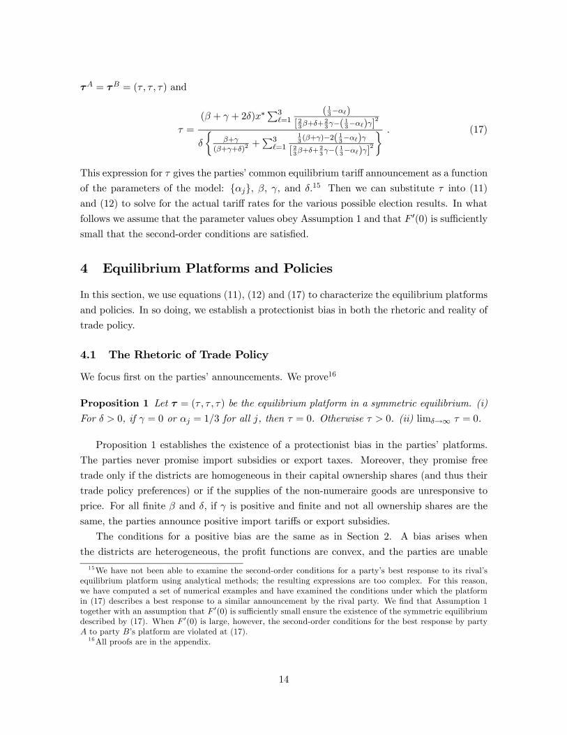
Figure 1: Negative protection for some industries

In Figure 1, we show the relationship between the equilibrium platforms and policies and

our measure of party discipline for one set of parameter values. In drawing the figure, we

have assumed that, for each industry g, all capital is owned by residents of a single district

(i.e., α1 = 1; α2 = α3 = 0) and that β = 2, γ = 1, and x∗ = 1. The top panel in the figureshows that, for these parameter values, the tariff on good 1 is positive whenever district 1

is included in the majority delegation (i.e., t{1,2,3},1 > 0 and t{1,2},1 = t{1,3},1 > 0) but the

tariff on good 1 is negative when the representative of district 1 is in the minority party

(i.e., t{2,3},1 < 0). The policy outcomes are most extreme when party discipline is totally

lacking and converge to free trade as discipline becomes perfect. The bottom panel shows

the equilibrium platform and the expected tariff for industry 1, both of which are positive

and monotonically decreasing, as is generally the case.

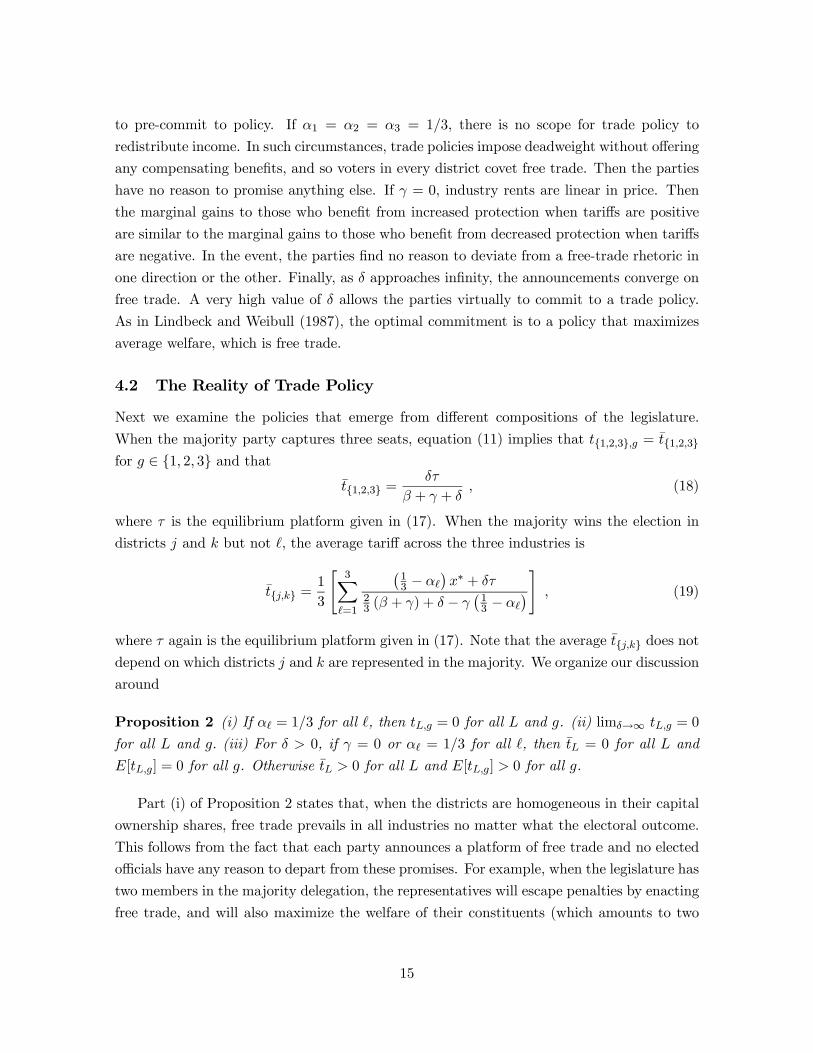
Figure 2 depicts another possibility.20 Here the parameter values are the same as for

Figure 1, except that the supply functions are flatter (γ = 2 instead of γ = 1). Now the tariff

on good 1 is positive no matter what the electoral outcome, although smallest (for given δ)

20Still another possibility is that the actual tariff on a good is positive only when the two districts with thelargest capital shares are both included in the majority delegation. For example, when β = 2, γ = 1, x∗ = 1,and α1 = 0.4, α2 = 0.4, and α3 = 0.2, t{1,2},1 > 0 and t{1,2,3},g > 0 for all finite δ, but t{1,2},2 = t{1,2},3 < 0for all finite δ.

18

when the representative of district 1 is not a member of the majority delegation. Again the

tariff levels, and also the platform and the expected tariffs, converge monotonically to zero.

We turn next to the distribution of the capital stock. If the districts are homogeneous

in their capital ownerships (and hence their industrial structures), tariffs cannot be used to

redistribute income and their is no political gain to be had from protection. The more uneven

the distribution, the greater is the scope for tyranny of the majority. This suggests loosely

that the protectionist bias may grow with a spread in ownership shares. In fact, we have

53.752.51.250

1

0.75

0.5

0.25

0

53.752.51.250

0.6

0.4

0.2

0

-0.2aPanel

bPanelδ

δ

tt 1},3,1{1},2,1{ =

t 1},3,2,1{

t 1},3,2{

τ

][ 1,LtE

Figure 2: Positive protection for all industries

Proposition 4 (i) ∂τ/∂αj > ∂τ/∂αk iff αj > αk. (ii) For all L, ∂t̄L/∂αj > ∂t̄L/∂αk iff

αj > αk. (iii) For all g, ∂E[tL,g]/∂αj > ∂E[tL,g]/∂αk iff αj > αk.

The proposition has the following implication. Fix any one of the capital ownership

parameters, say α3. Suppose α1 > α2. Now let α1 grow. Then α2 shrinks by the same

amount, because the two must sum to 1−α3. Part (i) states that this spread of the distributionof capital ownership results in a more protectionist policy announcement. Part (ii) says the

spread in ownership shares increases the average tariff for any electoral outcome. Part (iii)

states that the expected protection of every industry also rises. Evidently, the protectionist

bias is most severe when the ownership of each industry is concentrated in a single district.

19

200150100500

0.14

0.1375

0.135

0.1325

0.13γ

τ

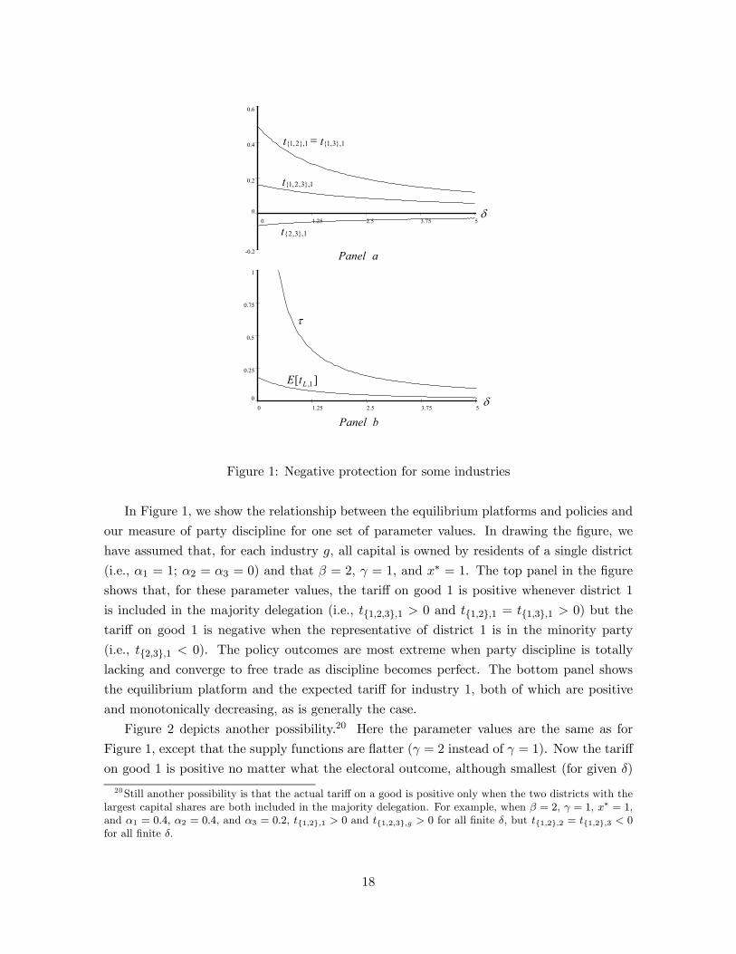
Figure 3: Platform rises and declines with γ

Finally, consider the slopes of the demand and supply curves. As β rises, the marginal

deadweight loss associated with any movement away from free trade grows. From (11) and

(12) it is clear that the elected representatives will choose a smaller deviation from free trade

in every industry for given τ the larger is β. It stands to reason that the announcement will

involve less of a protectionist bias, too, because there is less political appeal of using tariffs to

redistributive income when the excess burden is large. Indeed, we have found ∂τ/∂β < 0 in

all of our (many) numerical examples, although we have been unable to prove an analytical

result. We do know, however, that limβ→∞ τ = 0, as is apparent from equation (17). If

∂τ/∂β < 0, it follows that all positive tariff rates are monotonically decreasing in β, while

the negative rates may increase monotonically or fall first and then rise. In any case, all

tariffs approach zero as β grows large.

In contrast to an increase in β, an increase in the responsiveness of output to price has

offsetting political implications. On the one hand, an increase in γ exacerbates the marginal

deadweight loss associated with any movement of the trade policy variable away from free

trade. On the other hand, trade policy becomes a more effective redistributive tool as γ

grows larger. We find that a change in γ holding x∗ constant has an ambiguous effect on thetariff announcement.21 For example, Figure 3 depicts the relationship between the platform

and γ when β = 0, δ = 10, x∗ = 100 and α1 = 0.4, α2 = 0.3 and α3 = 0.3. Clearly, the

announcement becomes more protectionist with γ when γ is small, but it tends toward free

trade when γ is large. Even if the announced τ falls monotonically to zero–as it does for

21An increase in γ with x∗ constant corresponds to a rotation of the supply curve around the free-tradeproduction level.

20

many parameter values–the realized tariffs may display a non-monotonic relationship to the

supply responsiveness. It is even possible that a majority delegation representing the two

districts with the smallest ownership shares in an industry will set a negative tariff for that

good if γ is small but a positive tariff if γ is large, such that the tariff rises, then falls, then

asymptotes to zero, as γ ranges from zero to infinity.22

6 Conclusions

We have developed a novel model of campaigns, elections, and the policymaking process.

In our model, national political parties aim to maximize their probability of controlling the

legislature, while elected legislators seek to serve the interests of voters in their own districts.

The parties announce policy platforms as in a Downsian world, but these do not fully commit

the elected representatives. The legislators can deviate from their parties’ position in order

to serve their constituents, but they pay a political cost that varies with the size of any such

deviation. Thus, the model distinguishes “policy rhetoric” from “policy reality.”

When we apply the model to trade policy formation, we find a protectionist bias in the

equilibrium outcome of majoritarian systems. We define protection as a policy that raises

the domestic price of a tradeable good above the international price level. Thus, protection

involves positive import tariffs or export subsidies. We find that announced trade policies

always involve non-negative tariffs or export subsidies, and that the random electoral process

yields an expected policy with similar properties. Both positions and expected outcomes

involve positive protection whenever output responds positively to price, districts differ in

their ownership shares of the industry-specific capital stocks and party discipline is less than

perfect. The protectionist bias reflects the convexity of industry profits as a function of price,

and it arises whenever national parties cannot pre-commit to a policy and when the majority

delegation does not fully incorporate the preferences of the minority in its policy deliberations.

The protectionist bias is larger the more unequal the distribution of industry-specific capital

stocks. Under these circumstances one expects a smaller protectionist bias in countries with

better capital markets, which allow individuals to better diversify asset holdings and thereby

reduce their exposure to electoral risks.

Our analysis provides yet another demonstration of the importance of political institutions

for economic policy outcomes. We have focused here on differences in “party discipline,”

which we associate with the size of penalties that a national party can impose on individual

legislators if the latter choose to deviate from the parties’ announced positions when they are

in a position to set policy. We do not model the instruments of party discipline, but rather

treat this institutional feature of the political system parametrically. A strengthening of party

22This is true, for example, when β = 2, δ = 1, α1 = 0.65, α2 = 0.35, and α3 = 0.05.

21

discipline causes both the tariff (or export subsidy) announcements and the expected tariff

outcome to converge toward free trade. Thus, among countries with majoritarian electoral

systems, we would expected on average to find outcomes closer to free trade in those with

institutions that impose greater party discipline.

Our paper joins a very small literature on the comparative politics of trade policy. We

hope that future research by us and others will elaborate on the determinants of party dis-

cipline, and introduce other important differences in political institutions, such as between

presidential and parliamentary regimes and between systems with majoritarian elections ver-

sus some form of proportional representation. If, for example, one takes the view that pro-

portional representation leads to the election of legislators who maximize aggregate welfare,

because their election is not tied to particular geographic or economic interests, then our

model predicts higher average rates of protection in countries with majoritarian elections

than in countries with proportional representation.23 By introducing political features such

as these, we can gain a better understanding of cross-country differences in trade policies.

23We believe, however, that it is necessary to model explicitly the construction of party lists in systems withproportional representation in order to make an informed comparison between majoritarian and proportionalrepresentation, because some procedures for constructing party lists generate biases of their own. In Israel,for example, the lists of the large parties are determined by internal elections. As a result, those who areselected for the party list represent disproportionately the interests of those citizens who were responsible fortheir victory in the internal party election.

22

References

[1] Besley, Tim and Coate, Stephen (1997), “An Economic Model of Representative Democ-

racy,” Quarterly Journal of Economics, 112, 85-114.

[2] Dixit, Avinash K., Grossman, Gene M. and Gul, Faruk (2000), “The Dynamics of Po-

litical Compromise,” Journal of Political Economy, 108, 531-568.

[3] Grossman, Gene M. and Helpman, Elhanan (2005), “Party Discipline and the Provision

of Local Public Goods,” in progress.

[4] Lindbeck, Assar and Weibull, Jörgen (1987), “Balanced Budget Redistribution ad the

Outcome of Political Competition,” Public Choice, 52, 273-297.

[5] McCarty, Nolan, Poole, Keith T. and Rosenthal, Howard (2001), “The Hunt for Party

Discipline in Congress,” American Political Science Review, 95, 673-687.

[6] McGillivray, Fiona (1997), “Party Discipline as a Determinant of the Endogenous For-

mation of Tariffs,” American Journal of Political Science, 41, 584-607.

[7] McGillivray, Fiona (2004), Privileging Industry: The Comparative Politics of Trade and

Industrial Policy (Princeton NJ: Princeton University Press).

[8] McGillivray, Fiona and Smith, Alastair (1997), “Institutional Determinants of Trade

Policy,” International Interactions, 23, 119-143.

[9] Milesi-Ferretti, Gian Maria, Perotti, Roberto, and Rostagno, Massimo (2002), “Electoral

Systems and Public Spending,” The Quarterly Journal of Economics 117, 609-657.

[10] Persson, Torsten, Roland, Gerard, and Tabellini, Guido (2000), “Comparative Politics

and Public Finance,” Journal of Political Economy 108, 1121-1161.

[11] Osborne, Martin J. and Slivinski, Al (1996), “A Model of Political Competition with

Citizen-Candidates,” Quarterly Journal of Economics, 111, 65-96.

[12] Snyder, James M. and Groseclose, Tim (2000), “Estimating Party Influence in Congres-

sional Role-Call Voting,” American Journal of Political Science, 44, 193-211.

[13] Willmann, Gerald (2004), “Why Legislators are Protectionists: The Role of Majoritarian

Voting in Setting Tariffs,” Christian-Albrechts-Universität zu Kiel, manuscript.

23

Appendix

First-Order ConditionsWe first derive equations that hold if and only if the first-order conditions (15) are satisfied.

These equations will be used to show that the equilibrium platform is given by (17). To this

end first note that we can use (13) together with (11) and (12) to derive ∆j as a function of¡ρk, ρ , τA, τB

¢. Denote this functional relationship as ∆j

¡ρk, ρ , τA, τB

¢. Substituting this

function into (14) gives

ρj = F

"∆j

¡ρk, ρ , τA, τB

¢ρk(1− ρ ) + ρ (1− ρk)

#, for j, k, different from each other.

This is the system from which we can calculate ∂ρj/∂τAg and ∂ρj/∂τ

Bg . For a symmetric

equilibrium it is enough to calculate ∂ρj/∂τAg .

Differentiating this system of three equations with respect to the probabilities ρ1, ρ2, ρ3and with respect to τAg , and evaluating the result at the symmetric equilibrium point τ

Kg = τ

for all K and g, and ρj = 1/2 for all j, we obtain

E

∂ρ1∂τAg∂ρ2∂τAg∂ρ3∂τAg

= 2F 0 (0)

∂∆1

∂τAg∂∆2

∂τAg∂∆3

∂τAg

, (A1)

where E is the matrix

E =

1 −2F 0 (0) ∂∆1

∂ρ2−2F 0 (0) ∂∆1

∂ρ3

−2F 0 (0) ∂∆2∂ρ1

1 −2F 0 (0) ∂∆2∂ρ3

−2F 0 (0) ∂∆3∂ρ1

−2F 0 (0) ∂∆3∂ρ2

1

.

Next note that at the equilibrium point

∂∆j

∂ρk=

h3Vj(t

A{1,2,3})− 3Vj(tA{k, })

i+h3Vj(t

A{j,k})− 3Vj(tA{j, })

i= Q (τ) + 3

3Xg=1

αjgΠ

Ãp∗ +

¡13 − α g

¢x∗ + δτ

23(β + γ) + δ − γ

¡13 − α g

¢!

−33X

g=1

αjgΠ

Ãp∗ +

¡13 − αkg

¢x∗ + δτ

23(β + γ) + δ − γ

¡13 − αkg

¢! , j /∈ {k, } ,

24

where

Q (τ) = 3Π

µp∗ +

δτ

β + γ + δ

¶+ 3Z

µδτ

β + γ + δ

¶−3

3Xg=1

αgΠ

Ãp∗ +

¡13 − αg

¢x∗ + δτ

23(β + γ) + δ − γ

¡13 − αg

¢!

−3X

g=1

Z

à ¡13 − αg

¢x∗ + δτ

23(β + γ) + δ − γ

¡13 − αg

¢!

and

Z (t) = S (p∗ + t) + tm (p∗ + t) .

We calculate

∂∆2∂ρ1

+∂∆3∂ρ1

= 2Q (τ) + 33X

g=1

α2gΠ

Ãp∗ +

¡13 − α3g

¢x∗ + δτ

23(β + γ) + δ − γ

¡13 − α3g

¢!

−33X

g=1

α2gΠ

Ãp∗ +

¡13 − α1g

¢x∗ + δτ

23(β + γ) + δ − γ

¡13 − α1g

¢!

+33X

g=1

α3gΠ

Ãp∗ +

¡13 − α2g

¢x∗ + δτ

23(β + γ) + δ − γ

¡13 − α2g

¢!

−33X

g=1

α3gΠ

Ãp∗ +

¡13 − α1g

¢x∗ + δτ

23(β + γ) + δ − γ

¡13 − α1g

¢! ,

or

∂∆2∂ρ1

+∂∆3∂ρ1

= 2Q (τ)− 33X

g=1

(1− αg)Π

Ãp∗ +

¡13 − αg

¢x∗ + δτ

23(β + γ) + δ − γ

¡13 − αg

¢!

+33X

g=1

α2gΠ

Ãp∗ +

¡13 − α3g

¢x∗ + δτ

23(β + γ) + δ − γ

¡13 − α3g

¢!

+33X

g=1

α3gΠ

Ãp∗ +

¡13 − α2g

¢x∗ + δτ

23(β + γ) + δ − γ

¡13 − α2g

¢! .

25

Since

3Xg=1

α2gΠ

Ãp∗ +

¡13 − α3g

¢x∗ + δτ

23(β + γ) + δ − γ

¡13 − α3g

¢!

+3X

g=1

α3gΠ

Ãp∗ +

¡13 − α2g

¢x∗ + δτ

23(β + γ) + δ − γ

¡13 − α2g

¢!

= α2Π

Ãp∗ +

¡13 − α3

¢x∗ + δτ

23(β + γ) + δ − γ

¡13 − α3

¢!+ α1Π

Ãp∗ +

¡13 − α2

¢x∗ + δτ

23(β + γ) + δ − γ

¡13 − α2

¢!

α3Π

Ãp∗ +

¡13 − α1

¢x∗ + δτ

23(β + γ) + δ − γ

¡13 − α1

¢!

+α3Π

Ãp∗ +

¡13 − α2

¢x∗ + δτ

23(β + γ) + δ − γ

¡13 − α2

¢!+ α2Π

Ãp∗ +

¡13 − α1

¢x∗ + δτ

23(β + γ) + δ − γ

¡13 − α1

¢!

+α1Π

Ãp∗ +

¡13 − α3

¢x∗ + δτ

23(β + γ) + δ − γ

¡13 − α3

¢!

=3X

g=1

(1− αg)Π

Ãp∗ +

¡13 − αg

¢x∗ + δτ

23(β + γ) + δ − γ

¡13 − αg

¢! ,

we find that ∂∆2∂ρ1

+ ∂∆3∂ρ1

= 2Q (τ). Similarly, ∂∆j

∂ρ + ∂∆k∂ρ = 2Q (τ), for other j, k, that are

different from one another. This implies that 1TE = [1− 4F 0 (0)Q (τ)] (1, 1, 1), where 1 is acolumn vector of ones, and therefore 1T = (1, 1, 1). We assume that 0 < F 0 (0) < 1/4Q (τ),

where τ is given by (17). That is, F 0 (0) is small enough, and its upper limit is a function ofthe model’s parameters.24 In this event we can multiply (A1) by 1T from the left to obtain

3Xj=1

∂ρj∂τAg

=2F 0 (0)

1− 4F 0 (0)Q (τ)3X

j=1

∂∆j

∂τAgfor every g.

This equation, together with the restriction 0 < F 0 (0) < 1/4Q (τ), implies that the first-orderconditions (15) are satisfied if and only if

3Xj=1

∂∆j

∂τAg= 0 for all g. (A2)

We now use this condition to derive the equilibrium announcement τ .

24Our simulations indicate that F 0(0) has to be small for the symmetric equilibrium to exist. When F 0(0)is large, the second order conditions of the best response of party A to B’s platform are not satisfied at theproposed symmetric equilibrium point.

26

At the equilibrium point, where τAg = τBg = τ for all g and ρj = 1/2 for all j,

4

3

∂∆j

∂τAg=

·µαjg − 1

3

¶µx∗ + γ

δτ

β + γ + δ

¶− 13(β + γ)

δτ

β + γ + δ

¸δ

β + γ + δ

−"µ

αjg − 13

¶Ãx∗ + γ

¡13 − αjg

¢x∗ + δτ

23(β + γ) + δ − γ

¡13 − αjg

¢!− 13(β + γ)

¡13 − αjg

¢x∗ + δτ

23(β + γ) + δ − γ

¡13 − αjg

¢#

× δ23(β + γ) + δ − γ

¡13 − αjg

¢+

"µαjg − 1

3

¶Ãx∗ + γ

¡13 − α g

¢x∗ + δτ

23(β + γ) + δ − γ

¡13 − α g

¢!− 13(β + γ)

¡13 − α g

¢x∗ + δτ

23(β + γ) + δ − γ

¡13 − α g

¢#

× δ23(β + γ) + δ − γ

¡13 − α g

¢+

"µαjg − 1

3

¶Ãx∗ + γ

¡13 − αkg

¢x∗ + δτ

23(β + γ) + δ − γ

¡13 − αkg

¢!− 13(β + γ)

¡13 − αkg

¢x∗ + δτ

23(β + γ) + δ − γ

¡13 − αkg

¢#

× δ23(β + γ) + δ − γ

¡13 − αkg

¢=

·µαjg − 1

3

¶µx∗ + γ

δτ

β + γ + δ

¶− 13(β + γ)

δτ

β + γ + δ

¸δ

β + γ + δ

−"µ

αjg − 13

¶Ãx∗ + γ

¡13 − αjg

¢x∗ + δτ

23(β + γ) + δ − γ

¡13 − αjg

¢!− 13(β + γ)

¡13 − αjg

¢x∗ + δτ

23(β + γ) + δ − γ

¡13 − αjg

¢#

× 2δ23(β + γ) + δ − γ

¡13 − αjg

¢+

µαjg − 1

3

¶ 3Xh=1

Ãx∗ + γ

¡13 − αh

¢x∗ + δτ

23(β + γ) + δ − γ

¡13 − αh

¢! δ23(β + γ) + δ − γ

¡13 − αh

¢− 13δ (β + γ)

3Xh=1

¡13 − αh

¢x∗ + δτ£

23(β + γ) + δ − γ

¡13 − αh

¢¤2 .It follows that

P3j=1

∂∆j

∂τAg= 0 if and only if

3X=1

2

µ1

3− α

¶Ãx∗ + γ

¡13 − α

¢x∗ + δτ

23(β + γ) + δ − γ

¡13 − α

¢! δ23(β + γ) + δ − γ

¡13 − α

¢− 13(β + γ)

3X=1

£¡13 − α

¢x∗ + δτ

¤δ£

23(β + γ) + δ − γ

¡13 − α

¢¤2 − (β + γ) δ2τ

(β + γ + δ)2= 0.

This equation is the same as (16), because

tA{− },g =¡13 − α ,g

¢x∗ + δτAg

23(β + γ) + δ − γ

¡13 − α ,g

¢ ,27

∂tA{− },g∂τAg

=δ

23(β + γ) + δ − γ

¡13 − α ,g

¢ ,tA{1,2,3},g =

δτAgβ + γ + δ

,

and∂tA{1,2,3},g

∂τAg=

δ

β + γ + δ.

It follows from this equation that for δ > 0, the first-order condition is satisfied if and only

if (17) holds.

We now show that the denominator of (17) is positive when Assumption 1 is satisfied for

all δ ≥ 0. Let

D (δ) =β + γ

(β + γ + δ)2+

3X=1

13 (β + γ)− 2 ¡13 − α

¢γ£

23β + δ + 2

3γ −¡13 − α

¢γ¤2 (A3)

be the term in the curly brackets in the denominator of (17). We need to show that Assump-

tion 1 implies D(δ) > 0 for all δ > 0.

Suppose not; i.e., suppose D(δ) < 0 for some positive value of δ. Assumption 1 implies

that D(0) > 0. Since D (·) is continuous in δ, it can become negative for higher values of δ

only if there exists a δ̃ > 0 such that D(δ̃) = 0 and D0(δ̃) < 0. Let δ0 be the smallest δ̃ for

which this is true.

We calculate

D0 (δ) = −2"

β + γ

(β + γ + δ)3+

3X=1

13 (β + γ)− 2 ¡13 − α

¢γ£

23β + δ + 2

3γ −¡13 − α

¢γ¤3#. (A4)

Now note thatβ + γ

(β + γ + δ)3<

β + γ¡12β + δ + 1

2γ¢(β + γ + δ)2

,

and

13 (β + γ)− 2 ¡13 − α

¢γ£

23β + δ + 2

3γ −¡13 − α

¢γ¤3 − 1

3 (β + γ)− 2 ¡13 − α¢γ¡

12β + δ + 1

2γ¢ £

23β + δ + 2

3γ −¡13 − α

¢γ¤2

= −£13 (β + γ)− 2 ¡13 − α

¢γ¤2

2¡12β + δ + 1

2γ¢ £

23β + δ + 2

3γ −¡13 − α

¢γ¤3 < 0 for every .

Therefore

D0 (δ) > − 2D (δ)¡12β + δ + 1

2γ¢ (A5)

28

for every δ > 0. But since D (δ0) = 0, this inequality implies D0 (δ0) > 0, which contradicts

our supposition D0 (δ0) < 0. It follows that no such δ̃ exists and D(δ) > 0 for all δ > 0.

Proof of Proposition 1To prove part (i), first note that if α = 1/3 for all or γ = 0, then

3X=1

¡13 − α

¢£23β + δ + 2

3γ −¡13 − α

¢γ¤2 = 0

This implies, by (17), that τ = 0. Next note that if δ > 0, α 6= 1/3 for some and γ > 0,

then ¡13 − α

¢£23β + δ + 2

3γ −¡13 − α

¢γ¤2 >

¡13 − α

¢£23β + δ + 2

3γ −¡13 − 1

3

¢γ¤2 for α 6= 1

3

and ¡13 − α

¢£23β + δ + 2

3γ −¡13 − α

¢γ¤2 =

¡13 − α

¢£23β + δ + 2

3γ −¡13 − 1

3

¢γ¤2 for α =

1

3.

Therefore3X=1

¡13 − α

¢£23β + δ + 2

3γ −¡13 − α

¢γ¤2 >

3X=1

¡13 − α

¢¡23β + δ + 2

3γ¢2 = 0 .

Since the denominator of (17) is positive under Assumption 1, this inequality implies that

τ > 0.

To prove part (ii), note from (17) that

limδ→∞

τ =2x∗

P3=1

¡13 − α

¢β + γ +

P3=1

£13 (β + γ)− 2 ¡13 − α

¢γ¤ = 0.

Proof of Proposition 2To prove part (i), note from part (i) of Proposition 1 that α = 1/3 for all implies τ = 0.

It is then evident from (11) and (12) that tL,g = 0 for every majority L.

Next consider part (ii). Equations (11) and (12) imply that limδ→∞ tL,g = limδ→∞ τ

for every majority L. But limδ→∞ τ = 0 according to part (ii) of Proposition 1. Therefore

limδ→∞ tL,g = 0 for all majorities L.

Finally, consider part (iii). For finite δ > 0 the equilibrium platform is τ = 0 when either

α = 1/3 for all or γ = 0, as stated in part (i) of Proposition 1. Equations (18) and (19)

then implies that t̄L = 0 for all majorities L. Moreover, if α 6= 1/3 for some and γ > 0,

then τ > 0 by part (i) of Proposition 1. In this case, (18) implies that t̄{1,2,3} > 0 while (19)

29

implies that

t̄{j,k} >1

3

3X=1

¡13 − α

¢x∗

23 (β + γ) + δ − γ

¡13 − α

¢ > 1

3

3X=1

¡13 − α

¢x∗

23 (β + γ) + δ − γ

¡13 − 1

3

¢ = 0 .That is, t̄{j,k} > 0.

Proof of Proposition 3To prove part (i), note from (17) that if δ > 0, α 6= 1/3 for some , and γ > 0, then

∂

∂δlog τ = −D

0 (δ)D (δ)

+M 0 (δ)M (δ)

− (β + γ)

(β + γ + 2δ) δ, (A6)

where D (δ) is defined in (A3),

M (δ) =3X=1

¡13 − α

¢£23β + δ + 2

3γ −¡13 − α

¢γ¤2 (A7)

and

M 0 (δ) = −23X=1

¡13 − α

¢£23β + δ + 2

3γ −¡13 − α

¢γ¤3 . (A8)

Therefore M 0 (δ) /M (δ)−D0 (δ) /D (δ) < 0 is sufficient for ∂τ/∂δ < 0.Next note that (11), (12) and (17) imply that

4E [tL,g]

x∗=

(β + γ + 2δ)M

D

"1

β + γ + δ+

3X=1

123β + δ + 2

3γ −¡13 − α

¢γ

#

+3X=1

¡13 − α

¢23β + δ + 2

3γ −¡13 − α

¢γ

for g = 1, 2, 3,

where we have dropped the argument δ from the functions D andM , which are given in (A3)

and (A7). It follows that

4D

x∗M∂E [tL,g]

∂δ=

·2 + (β + γ + 2δ)

µM 0

M− D0

D

¶¸"1

β + γ + δ+

3X=1

123β + δ + 2

3γ −¡13 − α

¢γ

#

−D − (β + γ + 2δ)

"1

(β + γ + δ)2+

3X=1

1£23β + δ + 2

3γ −¡13 − α

¢γ¤2#

30

=

·2 + (β + γ + 2δ)

µM 0

M− D0

D

¶¸"1

β + γ + δ+

3X=1

123β + δ + 2

3γ −¡13 − α

¢γ

#

−2"

1

β + γ + δ+

3X=1

123β + δ + 2

3γ −¡13 − α

¢γ

#

= (β + γ + 2δ)

"1

β + γ + δ+

3X=1

123β + δ + 2

3γ −¡13 − α

¢γ

#µM 0

M− D0

D

¶,

where D0 and M 0 are given in in (A4) and (A8), respectively. Therefore ∂E [tL,g] /∂δ < 0 if

and only if M 0/M −D0/D < 0.

We now prove thatM 0/M−D0/D < 0, which is sufficient for ∂τ/∂δ < 0 and ∂E [tL,g] /∂δ <

0. To establish this inequality, note that

D0

D= −2 A3 + γM 0

A2 − 2γM , (A9)

where

A3 =β + γ

(β + γ + δ)3+

3X=1

13 (β + γ)£

23β + δ + 2

3γ −¡13 − α

¢γ¤3 ,

A2 =β + γ

(β + γ + δ)2+

3X=1

13 (β + γ)£

23β + δ + 2

3γ −¡13 − α

¢γ¤2 .

It follows from (A9) that

M 0

M− D0

D=

A2(A2 − 2γM)

µM 0

M+2A3A2

¶.

Therefore the sign of M 0/M −D0/D is the same as the sign of

B =M 0

M+2A3A2

,

because A2 − 2γM = D > 0. That is, we need to show that B < 0. But

1

2B =

1(β+γ+δ)3

+ 13

P3=1

1

[ 23β+δ+23γ−( 13−α )γ]

3

1(β+γ+δ)2

+ 13

P3=1

1

[ 23β+δ+23γ−( 13−α )γ]

2

−P3

=1( 13−α )

[ 23β+δ+23γ−( 13−α )γ]

3P3=1

( 13−α )[ 23β+δ+

23γ−( 13−α )γ]

2

,

31

which implies that the sign of B is the same as the sign of C, where

C =1

(β + γ + δ)3

3X=1

¡13 − α

¢£23β + δ + 2

3γ −¡13 − α

¢γ¤2

− 1

(β + γ + δ)2

3X=1

¡13 − α

¢£23β + δ + 2

3γ −¡13 − α

¢γ¤3

+1

3

Ã3X=1

1£23β + δ + 2

3γ −¡13 − α

¢γ¤3!Ã

3X=1

¡13 − α

¢£23β + δ + 2

3γ −¡13 − α

¢γ¤2!

−13

Ã3X=1

1£23β + δ + 2

3γ −¡13 − α

¢γ¤2!Ã

3X=1

¡13 − α

¢£23β + δ + 2

3γ −¡13 − α

¢γ¤3!.

Note, however, that

1

(β + γ + δ)3

3X=1

¡13 − α

¢£23β + δ + 2

3γ −¡13 − α

¢γ¤2

− 1

(β + γ + δ)2

3X=1

¡13 − α

¢£23β + δ + 2

3γ −¡13 − α

¢γ¤3

=1

(β + γ + δ)3

3X=1

¡13 − α

¢ £23β + δ + 2

3γ −¡13 − α

¢γ − (β + γ + δ)

¤£23β + δ + 2

3γ −¡13 − α

¢γ¤3

= − 1

(β + γ + δ)3

3X=1

γ¡13 − α

¢2+ 13 (β + γ)

¡13 − α

¢£23β + δ + 2

3γ −¡13 − α

¢γ¤3 < 0

and

1

3

Ã3X=1

1£23β + δ + 2

3γ −¡13 − α

¢γ¤3!Ã

3X=1

¡13 − α

¢£23β + δ + 2

3γ −¡13 − α

¢γ¤2!

−13

Ã3X=1

1£23β + δ + 2

3γ −¡13 − α

¢γ¤2!Ã

3X=1

¡13 − α

¢£23β + δ + 2

3γ −¡13 − α

¢γ¤3!

=1

3

3X=1

¡13 − α

¢£23β + δ + 2

3γ −¡13 − α

¢γ¤3

×3X

i=1

Ã23β + δ + 2

3γ −¡13 − α

¢γ£

23β + δ + 2

3γ −¡13 − αi

¢γ¤3 − 1£

23β + δ + 2

3γ −¡13 − αi

¢γ¤2!

=1

3

3X=1

¡13 − α

¢£23β + δ + 2

3γ −¡13 − α

¢γ¤3 3X

i=1

¡13 − αi

¢γ − ¡13 − α

¢γ£

23β + δ + 2

3γ −¡13 − αi

¢γ¤3

32

=1

3γ

Ã3X=1

¡13 − α

¢£23β + δ + 2

3γ −¡13 − α

¢γ¤3!2

−13γ

Ã3X=1

¡13 − α

¢2£23β + δ + 2

3γ −¡13 − α

¢γ¤3!Ã

3X=1

1£23β + δ + 2

3γ −¡13 − α

¢γ¤3!

= −13γ

Ã3X=1

1£23β + δ + 2

3γ −¡13 − α

¢γ¤3!2 3X

=1

ω

µ1

3− α

¶2−Ã

3X=1

ω

µ1

3− α

¶!2= −1

3γ

Ã3X=1

1£23β + δ + 2

3γ −¡13 − α

¢γ¤3!2 3X

=1

ω

µ13− α

¶−

3Xj=1

ωj

µ1

3− αj

¶2 < 0 ,where

ω =

1

[ 23β+δ+23γ−( 13−α )γ]

3P3j=1

1

[ 23β+δ+23γ−( 13−αj)γ]

3

.

It follows that C < 0, which implies M 0/M −D0/D < 0. This proves part (i).

For part (ii), first note that limδ→0 τ =∞ follows directly from (17). Next note that (17)

implies

limδ→0

δτ =

(β + γ)x∗P3

=1( 13−α )

[ 23β+23γ−( 13−α )γ]

2

1(β+γ) +

P3=1

13(β+γ)−2( 13−α )γ

[ 23βδ+23γ−( 13−α )γ]

2

,

which is finite. This result, together with (11) and (12), then imply that limδ→0 tL,g is finitefor every majority coalition L and every good g.

Finally, consider part (iii). We have shown in part (ii) of Proposition 1 that limδ→∞ τ = 0.

Using this result, it follows directly from equations (11) and (12) that limδ→∞ tL,g = 0 for all

L and g.

Proof of Proposition 4To prove part (i), note that–using (A3) and (A7)–we can represent (17) as

τ =(β + γ + 2δ)x∗M

δD.

In this representation, the capital shares α affect the platform only through their impact on

D and M . A direct calculation shows that

∂M

∂α= −

23β + δ + (1− α ) γ£

23β + δ + 2

3γ −¡13 − α

¢γ¤3 < 0 ,

33

and this expression is increasing in α . Therefore

0 >∂M

∂αj>

∂M

∂αkfor αj > αk .

Moreover,∂D

∂α= 2γ

13 (β + γ) +

¡13 − α

¢γ£

23β + δ + 2

3γ −¡13 − α

¢γ¤3 > 0 ,

and this expression declines in α . Therefore

0 <∂D

∂αj<

∂D

∂αkfor αj > αk .

It follows from these inequalities that

∂τ

∂αj>

∂τ

∂αkfor αj > αk .

For the proof of part (ii), first note from (18) that part (i) of this proposition immediately

implies∂t̄{1,2,3}∂αj

>∂t̄{1,2,3}∂αk

for αj > αk .

Next note that (19) implies that

3∂t̄{j,k}∂αi

=

"3X=1

δ23 (β + γ) + δ − γ

¡13 − α

¢# ∂τ

∂αi

−£23 (β + γ) + δ

¤x∗ + γδτ£

23 (β + γ) + δ − γ

¡13 − αi

¢¤2 ,

where the last term on the right-hand side is larger in districts with a larger αi. This

observation together with part (i) of the proposition imply that

∂t̄{j,k}∂αq

>∂t̄{j,k}∂αz

for all j 6= k and αq > αz .

Finally, for the proof of part (iii) note that (18) and (19) imply that

4∂E [tL,g]

∂αi=

µδ

β + γ + δ

¶∂τ

∂αi+

"3X=1

δ23 (β + γ) + δ − γ

¡13 − α

¢# ∂τ

∂αi

−£23 (β + γ) + δ

¤x∗ + γδτ£

23 (β + γ) + δ − γ

¡13 − αi

¢¤2 ,

where the last term on the right-hand side is larger in districts with a larger αi. This

34

observation together with part (i) of the proposition imply that

∂E [tL,g]

∂αj>

∂E [tL,g]

∂αkfor all g when αj > αk .

35