Multiobjective analysis of chaotic dynamic systems with sparse learning machines

Advances in Water Resources 29 (2006) 72–88

www.elsevier.com/locate/advwatres

Multiobjective analysis of chaotic dynamic systems withsparse learning machines

Abedalrazq F. Khalil *, Mac McKee, Mariush Kemblowski,Tirusew Asefa, Luis Bastidas

Department of Civil and Environmental Engineering and Utah Water Research Laboratory,

Utah State University, 1600 Canyon Road, Logan, Utah 84322-8200, USA

Received 8 December 2004Available online 26 July 2005

Abstract

Sparse learning machines provide a viable framework for modeling chaotic time-series systems. A powerful state-space recon-struction methodology using both support vector machines (SVM) and relevance vector machines (RVM) within a multiobjectiveoptimization framework is presented in this paper. The utility and practicality of the proposed approaches have been demonstratedon the time series of the Great Salt Lake (GSL) biweekly volumes from 1848 to 2004. A comparison of the two methods is madebased on their predictive power and robustness. The reconstruction of the dynamics of the Great Salt Lake volume time series isattained using the most relevant feature subset of the training data. In this paper, efforts are also made to assess the uncertaintyand robustness of the machines in learning and forecasting as a function of model structure, model parameters, and bootstrappingsamples. The resulting model will normally have a structure, including parameterization, that suits the information content of theavailable data, and can be used to develop time series forecasts for multiple lead times ranging from two weeks to several months.� 2005 Elsevier Ltd. All rights reserved.

Keywords: Bayesian; Probabilistic machines; Statistical learning theory; Chaotic theory; State-space reconstruction

1. Introduction

Chaotic systems are nonlinear, dynamic, fully deter-ministic, highly sensitive to initial conditions, and canbe modeled using state-space reconstruction via a timedelay embedding theorem [40]. Though Poincare de-scribed chaotic behavior in nonlinear systems in the late1880s, a resurgence in chaos theory arose with Lorenz[50] in his work with weather prediction models whereinhe discovered that nonlinear models could be exponen-tially divergent (i.e., sensitive to small differences in ini-tial conditions) [71,70,68,24]. Thus, unlike many other

0309-1708/$ - see front matter � 2005 Elsevier Ltd. All rights reserved.doi:10.1016/j.advwatres.2005.05.011

* Corresponding author. Tel.: +1 435 797 7176; fax: +1 435 7973663.

E-mail address: [email protected] (A.F. Khalil).

processes the erratic data produced from chaos aredue to complex outcome of a nonlinear system and ini-tial conditions that are identified from uncertain datarather than only intrinsic randomness. The behaviorsof many water resources systems have been observedto be chaotic and thus chaos has received significantattention in hydrology.

Chaos theory states that the time series itself carriesenough information about the behavior of the systemto carry out forecasting [50]. Therefore, a deterministic

chaotic system behaves in the future in a similar manneras in the past. The embedding theorem emerged in thelight of chaos theory, which states that given a recog-nized state-space representation of a chaotic time series,through estimation of the time delay and the embeddingdimension (i.e., state-space reconstruction) a fullknowledge of the system behavior is guaranteed [72].

mailto:[email protected]

A.F. Khalil et al. / Advances in Water Resources 29 (2006) 72–88 73

Nonetheless, the time series must: be sampled at suffi-cient resolution, not be corrupted by noise, and mea-sured over a long period of time [59] in order to avoidthe biases of many state-space reconstruction tech-niques. In addition, the state evolution of a chaotic sys-tem is dynamic and constitutes an inverse problem forwhich there is no unique solution, and for which theremight be no stable solution, either.

Capturing the behavior of a chaotic time series be-comes more complicated in the presence of noise (i.e.,background noise, or an inaccuracy of the measure-ments of system behavior) [67]. The process of measur-ing system states using physical sensors, in addition tothe lack or neglect of exogenous stresses, introducessome amount of noise [25]. This noise causes someuncertainties in both the model structure and, accord-ingly, in predictions about the future performance ofthe system. Contamination with noise is almost inherentin any hydrological time series. This, in essence, runscounter to many widely used methodologies that arebased on theories developed on assumptions of infiniteand noise-free time series [67]. Moreover, the structureof the hydrological processes exhibits temporal, spatial,and scale variability. A failure to account for the under-lying system structure limits the ability of the modelingapproaches to identify a unique mathematical represen-tation of the hydrological processes [67]. This translatedto an impediment to both traditional state-space fore-casting methodologies and learning machines to predictfuture system behaviors with confidence. In light ofthese modeling issues, a principal objective of this paperis to quantify the amount of uncertainty introduced inthe analysis of complex hydrological processes by thespecification of model structure.

From a pragmatic engineering point of view, state-space reconstruction techniques have shortcomings thatcan be attributed to the fact that their prediction accu-racy is often inadequate since the state-space parametersare not derived with the intention of minimizing the pre-diction error, but instead are developed to characterizethe nonlinear dynamic process in question [12,85,59].

In this sense, the other objective of this paper is tolink the powerful state-space reconstruction methodol-ogy via exploiting the appealing regularization conceptsof both support vector machines (SVM) and relevancevector machines (RVM) within a multiobjective optimi-zation framework. The parameters of chaos theory andthe unintuitive parameters of learning machines will beoptimized with the assistance of a multiobjective shufflecomplex evolution Metropolis algorithm (MOSCEM).The chosen objective functions will be optimized bothindependently and simultaneously. This will yield multi-ple feasible solutions accounting for the trade-off (e.g.,bias-variance trade-off; trade-offs between seepage, pre-cipitation, and evaporation induced signals) and more-over capture the uncertainty in the model structure.

In this manuscript, efforts will be made to assess theuncertainty and robustness of the machines in learningand forecasting as a function of model structure andbootstrapping samples. The proposed framework, usingsparse learning techniques, allows for compact represen-tations of system dynamics. In other words, models thatare developed from the learning machines used here nor-mally have a structure, including parameterization thatsuits the information content of the available data,and can be used to develop time series forecasts for mul-tiple lead times. The goal of this paper is to introducenew learning machines in a multiobjective frameworkthat identify a suite of model parameters and that con-sequently enable an ensemble forecast of time series. Atheoretical background is first described. Then theframework utility is demonstrated by applying it to aGreat Salt Lake (GSL) biweekly volume dataset.

2. Theoretical background

2.1. Chaotic and nonlinear time series

Chaos occurs as a feature of orbits x(t) arising fromsystems of differential equations of dx(t)/dt = F(x(t))with three or more degrees of freedom or invertiblemaps of x(t + 1) = F(x(t)). As a class of observable sig-nals, x(t), chaos lies logically between the well-studieddomain of predictable, regular, or quasi-periodic signaland the totally irregular stochastic signals [5]. In manysystems the interaction between the underlying physicalprocesses that are responsible for the evolution of sys-tem behavior are unknown. In addition, it is seldom thatone has information about all the relevant dynamic vari-ables. Instead, one usually tries to construct a multivar-iate state space in which the dynamics unfold usingsystem output measurements of a single variable. Thepurpose of state-space reconstruction is to representthe underlying system dynamics of a single time seriesby converting the time series to a multidimensionalstate-space. In state-space reconstruction, a scalar timeseries, Xj, where j = 1,2, . . .,N, with sampling time Dt,is converted to its state-space using the method of delays[72,30]:

xi ¼ ðxi; xiþs; xiþ2s; . . . ; xiþðd�1ÞsÞ ð1Þ

where i = 1,2, . . .,N � (d � 1)s/Dt, d is the embeddingdimension, and s is the delay time (i.e., some suitablemultiple of the sampling time Dt) [72,58,19,30]. In otherwords, state-space reconstruction techniques convert asingle scalar time series to a state-vector representationusing the embedding dimension (d) and delay time (s)(i.e., hereinafter called state-space parameters). Thisreconstruction is required for both characterizationand forecasting. In this study, recently celebrated learn-ing machines that are relatively new in water resources

74 A.F. Khalil et al. / Advances in Water Resources 29 (2006) 72–88

applications will be employed to capture the dynamicsdepicted in Eq. (1) with the purpose of producing reli-able predictions:

yi ¼ xiþs ¼ f ðxiÞ ð2Þwhere xi is the state variable vector, and yi is the output(i.e., future state) of the model. The learning machine isgiven M training pairs of data, [xi,yi], i = 1, . . .,M. Thetraining data consists of a d-dimensional vector, x 2 Rd,and the response or output, y 2 R. The goal of the learn-ing machine, then, is to estimate an unknown continu-ous, real-valued function f(x) that is capable ofmaking accurate predictions of an output, y, for previ-ously unseen values of x, thus utilizing informationabout the dynamics of system behavior in the state-space representation to make forecasts of future systemstates in observation space.

State-space estimation is needed to infer the para-meters of a chaotic process. The time delay coordinatemethod is one of the most popular techniques usedin state-space estimation [58,72,63,60,61,68,69,31,86].There are many techniques for estimating the state-spaceparameters, and Jayawardena and Gurung [31] have dis-cussed the merits and pitfalls of many of them. Theembedding dimension, d, is selected in order to suffi-ciently describe the evolution of the system. For instance,when d is very small the state-space is said to be not fullyunfolded, and when d is large, noise might occupy theembedding space. The minimum embedding dimensioncould be estimated utilizing the following techniques:(1) the point where the attractor invariant measure stopschanging with increasing dimension; (2) singular valuedecomposition, in which the singular values are estimatesof the variance projected on orthogonal directions of theembedding space; and (3) false nearest neighbors that isbased on the topological issue of the embedding process[35]. The delay time, s, could be estimated using any of anumber of widely plausible approaches. Some of theavailable estimation methods are: the average mutualinformation criterion [63] the pseudo-period of oscilla-tion; the complexity measure of the projected time series;the autocorrelation function method [63,80,67] and the

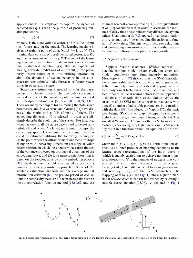
Fig. 1. Conceptual representation of the kernel transformation to the featu

minimal forecast error approach [11]. Rodriguez-Iturbeet al. [62] concluded that in order to ascertain the influ-ence of delay time one should employ different delay timevalues. Sivakumar et al. [68] reported an underestimationor overestimation of the embedding dimension as a func-tion of delay time. This interaction between delay timeand embedding dimension constitutes another reasonfor using a multiobjective optimization algorithm.

2.2. Support vector machine

Support vector machines (SVMs) represent amachine-learning model where prediction error andmodel complexity are simultaneously minimized.Mukherjee et al. [57] showed that the SVM algorithmhas a remarkable prediction capacity and it performedbetter than polynomial and rational approximations,local polynomial techniques, radial basis functions, andfeed-forward artificial neural networks when applied ona database of chaotic time series. Unlike ANNs, thestructure of the SVM model is not fixed in advance witha specific number of adjustable parameters, but can adaptwith the data [39]. Introduced by Vapnik [75], the basicidea behind SVMs is to map the input space into ahigh-dimensional feature space utilizing kernels [75]. Thisso-called ‘‘kernel-trick’’ enables the SVM to work withfeature spaces having very high dimensions. SVMs gener-ally result in a function estimation equation of the form:

f ðx;wÞ ¼Xmi¼1

wi � Kðxi; xÞ þ b ð3Þ

where the K(xi,x) = /(xi) Æ /(x) is a kernel function de-fined as an inner product of mapping functions to thefeature space representations of the input query x

(which is mainly carried out to achieve nonlinear trans-formation); m � M is the number of patterns that con-tain all the information necessary to solve a givenlearning task, hereinafter referred to as support vectors;and w = {w1, . . .,wm} are the SVM parameters. Themapping of x by /(x) (see Fig. 1) into a higher dimen-sional feature space is chosen in advance by selecting asuitable kernel function [75,76]. As depicted in Fig. 1

re space and the e-insensitive loss function in the linear SV machine.


by performing such a mapping the learning algorithmseeks to define a hyperplane that is necessary for apply-ing the linear regression in the SVM formulation [34].Now the problem is to determine w and the correspond-ing m support vectors from the training data. To avoidthe use of empirical risk minimization (e.g., quadraticresidual function), which may result in overfitting,Vapnik [75] proposed a structural risk minimization(SRM) in which one minimizes some empirical risk mea-sure regularized by a capacity term. SRM is a novelinductive rule for learning from a finite dataset andhas shown good performance with small samples [34].This is the most appealing advantage of SVMs, espe-cially when data scarcity is a limitation on the use ofprocess-based or ANNs models [4,42]. Consistent withSRM, therefore, the objective function of SVM formula-tion is to minimize the following:

EðwÞ ¼ 1

M

XMi¼1

jyi � f ðxi;wÞje þ1

2kwk2 ð4Þ

Vapnik [75] employed the e-insensitive loss function,jyi � f(xi,w)je, wherein those differences between esti-mated output, f(xi,w), and the observed output, yi, thatlie within the range of ±e do not contribute to the out-put error. The e-insensitive loss function shown in Fig. 1is defined as:

jyi � f ðxi;wÞje ¼ jeje ¼0 if jej 6 e

jej � e if jej > e

�ð5Þ

In order to address the possibility of infeasible con-straints in the primal formulation of the minimizationproblem that results from Eqs. (3) to (5) slack variablesn are introduced to penalize the points that lie outsidethe tube as shown in Fig. 1 analogous to Cortes andVapnik [13] and Scholkopf and Smola [65]. After intro-ducing a dual set of variables to construct a Lagrangefunction, and applying Karush–Kuhn–Tucker condi-tions, Vapnik [75] has shown that Eq. (2) is equivalentto the following in the dual form:

y ¼ f ðx; a�; aÞ ¼XMi¼1

ða�i � aiÞKðxi; xÞ þ b ð6Þ

where the Lagrange multipliers ai and a�i are required tobe greater than or equal to zero for i = 1, . . .,M. Typi-cally, the optimal parameters of Eqs. (4) and (6) arefound by solving the following dual formulation:

mina�;a

JDða�;aÞ ¼PMi¼1

yiðai � a�i Þ� ePMi¼1

ðai þ a�i Þ

� 12

PMi¼1

PMj¼1

ðai � a�i Þðaj � a�j ÞKðxi;xjÞ

such thatPMi¼1

ðai � a�i Þ ¼ 0

ai;a�i 2 ½0;c� 8i

266666666664

377777777775

ð7Þ

The parameter c is a user-defined constant that repre-sents the trade-off between model complexity and theapproximation error. Eq. (7) comprises a convex con-strained quadratic programming problem [75,76]. As aresult, the m-input vectors that correspond to nonzeroLagrangian multipliers, ai and a�i , are considered asthe support vectors. The SVM model thus formulated,then, is guaranteed to have a global, unique, and sparsesolution. Despite the mathematical simplicity and ele-gance of SVM training, experiments prove they are ableto deduce relationships of high complexity [49,85,84].For detailed description of SVM interested readers arereferred to [6,36,37].

2.3. Relevance vector machine

Relevance vector machines (RVMs) adopt a Bayesianextension of learning. RVMs allow computation of theprediction intervals taking into account uncertaintiesof both the parameters and the data [73]. RVMs evadecomplexity by producing models that have both a struc-ture and a parameterization process that, together, areappropriate to the information content of the data.RVMs have the identical functional form as SVMs, asin Eq. (3), but use kernel terms, f/iðxÞg

mi¼1 � Kðx; xiÞ,

that correspond to fixed nonlinear basis functions [74].The RVM model seeks to forecast y

_for any query x

according to y_ ¼ f ðx;wÞ þ en, where en � Nð0; r2Þ

and w = (w0, . . .,wM)T are a vector of weights. The like-lihood of the complete dataset can be written as:

pðyjw; r2Þ ¼ ð2pr2Þ�M=2 exp � 1

2r2ky�Uwk2

� �ð8Þ

whereU(xi) = [1,K(xi,x1),K(xi,x2), . . .,K(xi,xM)]T. Maxi-mum likelihood estimation of w and r2 in Eq. (6) oftenresults in severe overfitting. Therefore, Tipping [74] rec-ommended imposition of some prior constraints on theparameters, w, by adding a complexity penalty to thelikelihood or the error function. This a priori informa-tion controls the generalization ability of the learningsystem. Typically, new higher-level hyperparametersare used to constrain an explicit zero-mean Gaussianprior probability distribution over the weights, w [73]:

pðwjaÞ ¼YMi¼0

Nðwij0; a�1i Þ ð9Þ

where a is a hyperparameter vector that controls howfar from zero each weight is allowed to deviate [65].For completion of hierarchical prior specifications,hyperpriors over a and the noise variance, r2, are de-fined. Consequently, using Bayes� rule, the posterioroverall unknowns could be computed given the definednoninformative prior distributions:

pðw; a;r2jyÞ ¼ pðyjw; a; r2Þ � pðw; a; rÞRpðyjw; a; r2Þpðw; a; r2Þdwdadr2

ð10Þ


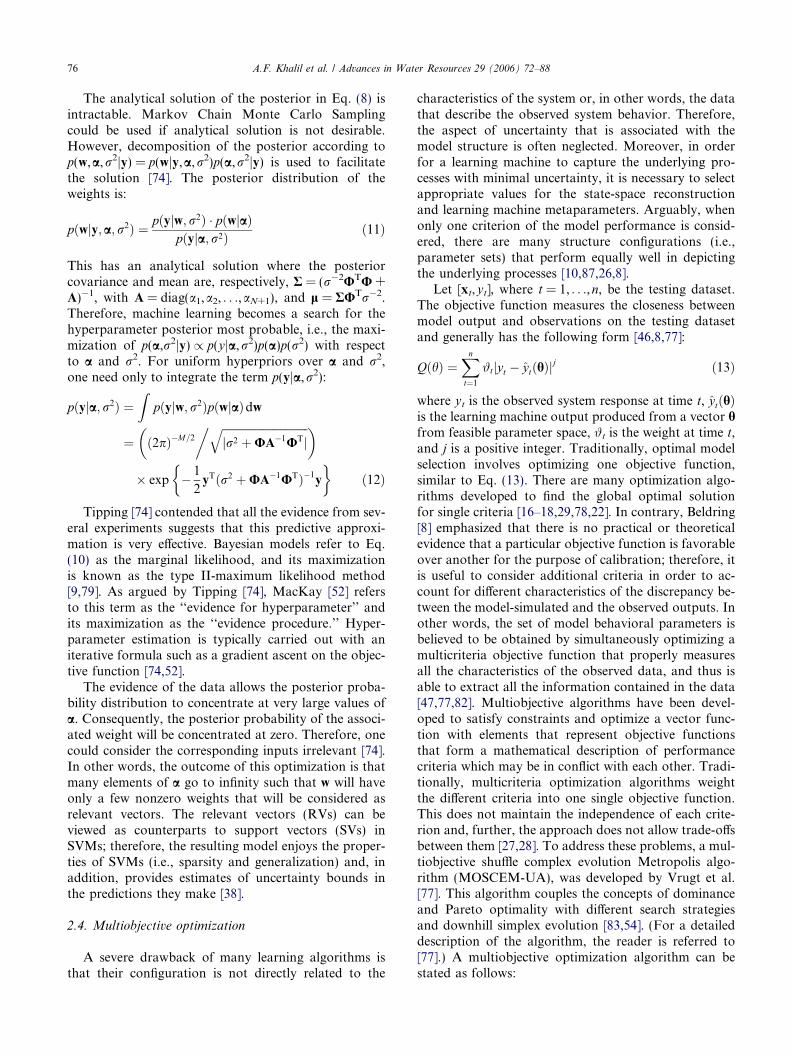
The analytical solution of the posterior in Eq. (8) isintractable. Markov Chain Monte Carlo Samplingcould be used if analytical solution is not desirable.However, decomposition of the posterior according top(w,a,r2jy) = p(wjy,a,r2)p(a,r2jy) is used to facilitatethe solution [74]. The posterior distribution of theweights is:

pðwjy; a; r2Þ ¼ pðyjw; r2Þ � pðwjaÞpðyja; r2Þ ð11Þ

This has an analytical solution where the posteriorcovariance and mean are, respectively, R = (r�2UTU +A)�1, with A = diag(a1,a2, . . .,aN+1), and l = RUTr�2.Therefore, machine learning becomes a search for thehyperparameter posterior most probable, i.e., the maxi-mization of p(a,r2jy) / p(yja,r2)p(a)p(r2) with respectto a and r2. For uniform hyperpriors over a and r2,one need only to integrate the term p(yja,r2):

pðyja; r2Þ ¼Z

pðyjw; r2ÞpðwjaÞdw

¼ ð2pÞ�M=2ffiffiffiffiffiffiffiffiffiffiffiffiffiffiffiffiffiffiffiffiffiffiffiffiffiffiffiffiffiffiffijr2 þUA�1UTj

q��

� exp � 1

2yTðr2 þUA�1UTÞ�1

y

� �ð12Þ

Tipping [74] contended that all the evidence from sev-eral experiments suggests that this predictive approxi-mation is very effective. Bayesian models refer to Eq.(10) as the marginal likelihood, and its maximizationis known as the type II-maximum likelihood method[9,79]. As argued by Tipping [74], MacKay [52] refersto this term as the ‘‘evidence for hyperparameter’’ andits maximization as the ‘‘evidence procedure.’’ Hyper-parameter estimation is typically carried out with aniterative formula such as a gradient ascent on the objec-tive function [74,52].

The evidence of the data allows the posterior proba-bility distribution to concentrate at very large values ofa. Consequently, the posterior probability of the associ-ated weight will be concentrated at zero. Therefore, onecould consider the corresponding inputs irrelevant [74].In other words, the outcome of this optimization is thatmany elements of a go to infinity such that w will haveonly a few nonzero weights that will be considered asrelevant vectors. The relevant vectors (RVs) can beviewed as counterparts to support vectors (SVs) inSVMs; therefore, the resulting model enjoys the proper-ties of SVMs (i.e., sparsity and generalization) and, inaddition, provides estimates of uncertainty bounds inthe predictions they make [38].

2.4. Multiobjective optimization

A severe drawback of many learning algorithms isthat their configuration is not directly related to the

characteristics of the system or, in other words, the datathat describe the observed system behavior. Therefore,the aspect of uncertainty that is associated with themodel structure is often neglected. Moreover, in orderfor a learning machine to capture the underlying pro-cesses with minimal uncertainty, it is necessary to selectappropriate values for the state-space reconstructionand learning machine metaparameters. Arguably, whenonly one criterion of the model performance is consid-ered, there are many structure configurations (i.e.,parameter sets) that perform equally well in depictingthe underlying processes [10,87,26,8].

Let [xt,yt], where t = 1, . . .,n, be the testing dataset.The objective function measures the closeness betweenmodel output and observations on the testing datasetand generally has the following form [46,8,77]:

QðhÞ ¼Xn

t¼1

#tjyt � ytðhÞjj ð13Þ

where yt is the observed system response at time t, ytðhÞis the learning machine output produced from a vector hfrom feasible parameter space, #t is the weight at time t,and j is a positive integer. Traditionally, optimal modelselection involves optimizing one objective function,similar to Eq. (13). There are many optimization algo-rithms developed to find the global optimal solutionfor single criteria [16–18,29,78,22]. In contrary, Beldring[8] emphasized that there is no practical or theoreticalevidence that a particular objective function is favorableover another for the purpose of calibration; therefore, itis useful to consider additional criteria in order to ac-count for different characteristics of the discrepancy be-tween the model-simulated and the observed outputs. Inother words, the set of model behavioral parameters isbelieved to be obtained by simultaneously optimizing amulticriteria objective function that properly measuresall the characteristics of the observed data, and thus isable to extract all the information contained in the data[47,77,82]. Multiobjective algorithms have been devel-oped to satisfy constraints and optimize a vector func-tion with elements that represent objective functionsthat form a mathematical description of performancecriteria which may be in conflict with each other. Tradi-tionally, multicriteria optimization algorithms weightthe different criteria into one single objective function.This does not maintain the independence of each crite-rion and, further, the approach does not allow trade-offsbetween them [27,28]. To address these problems, a mul-tiobjective shuffle complex evolution Metropolis algo-rithm (MOSCEM-UA), was developed by Vrugt et al.[77]. This algorithm couples the concepts of dominanceand Pareto optimality with different search strategiesand downhill simplex evolution [83,54]. (For a detaileddescription of the algorithm, the reader is referred to[77].) A multiobjective optimization algorithm can bestated as follows:


minh

QðhÞ ¼ ½Q1ðhÞ Q2ðhÞ � � � QN ðhÞ� ð14Þ

where Qi(h) is the ith objective function and i 2 [1,N].The purpose of the multicriteria optimization is to findthe values of h within the feasible set of parameters Hthat simultaneously optimize all criteria. Owing to thevarious competing trade-offs between the objective func-tions in conjunction with uncertainties in model struc-ture and data, one unique solution is not possible.Therefore, the Pareto set cannot be generated from asubjective weighting of the criteria whose relative impor-tance is a priori unknown. More straightforwardly, andfollowing Gupta et al. [28] and Demarty et al. [15], thePareto set has the following properties: the decision vec-tor hk is said to strictly dominate another hj ifQi(h

k) 6 Qi(hj) "i 2 {1,2, . . .,N} and Qi(h

k) Qi(hj) for

some i 2 {1,2, . . .,N}; less stringently hk is said to weaklydominate another hj if Qi(h

k) 6 Qi(hj) "i 2 {1,2, . . .,N}.

The Pareto set comprises parameters that result in feasi-ble, noninferior, or nondominated solutions. This im-

Fig. 2. Great Salt Lake basin and

plies each vector of the Pareto set will be able tocharacterize some regions in the simulated signal betterthan the others [83].

3. Application to Great Salt Lake volumes

3.1. Description of the study area

The Great Salt Lake (GSL) of Utah is the fourthlargest terminal (i.e., has no outlet) lake in the world(http://ut.water.usgs.gov/greatsaltlake/). The GSL basinencompasses a drainage area of 89,000 km2 includingmuch of Utah, parts of southeastern Idaho, and south-western Wyoming (Fig. 2) [32]. The three rivers thatdrain into the GSL are the Bear, the Weber, and the Jor-dan which, in total, comprise about 66% of the averageannual water inflow to the GSL; precipitation contrib-utes about 31%, and groundwater recharge about 3%of the annual flows to the lake [2,3].

its flow model (Source: [7]).

http://ut.water.usgs.gov/greatsaltlake/


Biweekly records for GSL levels and volumes were ob-tained from the Utah Geological Survey. These data,which date back to 1843, show dramatic rises and fallsin the GSL volumes throughout the historic period of re-cord. Such fluctuations represent the integrated effects ofprecipitation, evaporation, snow pack sublimation, andsubsurface transport over the watershed, in addition toglobal, regional, and local climatic variability [43–45,53,32]. The 1983–1987 rise of the GSL threatenedInterstate 80, the Salt Lake International Airport, theUnion Pacific Railroad, wastewater treatment facilities,wetlands, GSL minerals industries, migratory bird andother wildlife habitat, and tourism. As a result, the in-curred costs of that rise in the elevation of the GSL werea $150 million pumping project and $350 million in flooddamage [45,32]. The pumping project left 0.5 billion tonsof salt in the desert west of the lake; shortly after comple-tion of the pumping project, lakes levels underwent arapid retreat due to reduced annual inflows. The GSLencountered periods of prolonged drought in the 1930sand 1960s, and is currently at a very low level as the re-sult of another extended drought [38].

Johnson and Tarboton [32] noted that there is no cor-respondence between GSL long-term volume fluctua-tions and precipitation or streamflow. This indicatesthe possible influence of other nonlinear dynamic pro-cesses, and might partly explain the conclusion derivedby Lall et al. [45] that models based on traditional lineartime series analysis are insufficient to adequately de-scribe GSL volume fluctuation. Shun and Duffy [66]examined the GSL basin records of monthly precipita-tion, temperature, and runoff using multichannel singu-lar spectrum analysis in order to identify seasonal andlonger period oscillatory patterns in the time series inan effort to explain the strong low-frequency componentin streams entering the GSL.

3.2. Framework for optimal chaos reconstruction

Successful management of the GSL system necessi-tates a thorough understanding of its behavior, yet thecomplexities of the lake dynamics limit the forecastingability of its states. In addition, the underlying physicalprocesses that collectively produce changes in lake levelsoperate at different spatial and temporal scales. This fur-ther complicates the use of physical models to predict fu-ture system states. Therefore, we assume that there is aset of differential equations that collectively describethe generation of the GSL biweekly volume time series.This is a tenet of chaos theory. In essence, the behaviorof chaotic systems appears as random, complex, andunpredictable, but internally chaotic systems have defi-nite and unique relationships that are governed by lowdegrees of freedom.

It is worth mentioning that several studies havecontributed to the current understanding of the GSL

volume dynamics [64,44,56,1,53]. In addition, thesestudies provide evidence of low-dimensional chaos inGSL volumes via dimension calculations, estimates ofLyapunov exponents for predictability assessment, testsfor determinism, and tests for nonlinearity. Based onthis evidence, different forecasting methods involvingmultivariate adaptive regression splines [21,45] and localpolynomials [55] have been used by various authors topredict GSL short-term behavior.

The approaches proposed here are now applied to theGSL biweekly volume data. The biweekly volumes ofthe GSL have been identified to exhibit a low-dimen-sional chaotic attractor [63,64]. The low-dimensionalchaos exhibited by the data is a sufficient condition forthe application of the state-space reconstruction meth-ods we use. Yet, the methodologies and framework pre-sented in this manuscript could also be utilized for theprediction of nonlinear time series. In this paper, wereconstruct the dynamics of the GSL volume time series,thereby making it possible to develop forecasts of differ-ent lead times by ‘‘re-projecting’’ and unfolding thedynamics via representation of the data in multidimen-sional state-space.

The learning machines, RVMs and SVMs, are ap-plied on the state-space series of data. The reconstruc-tion parameters s and d, besides the learning machineparameters, are determined simultaneously to minimizethe prediction error. The prediction error is judged bythe multicriteria objective function. Traditionally, alearning machine is said to be optimally trained whenthe following conditions are satisfied: good agreementbetween the average simulated and the observed timeseries; good overall agreement of the shape of the timeseries, and good agreement in high-value measurements,low-value measurements, and peak measurements (i.e.,lag and shift in peak distortion). Therefore, three criteriawere used for quantifying these objectives.

The implementation of the framework is depicted inFig. 3. For both SVMs and RVMs, one seeks to opti-mize the following multiobjective function:

minh

QðhÞ ¼ ½Q1ðhÞ Q2ðhÞ Q3ðhÞ� ð15Þ

where Qi(h) are statistics of efficiency between the actualand predicted output, and are shown in Table 1; in thecase of RVMs, hr = [s d rr], and for of SVMs,hs = [s d e c rs]. Note that rr and rs are the scale param-eters of the Gaussian radial basis function that is used asthe kernel function for the RVM and SVM models,respectively. The selection of the objective functionshas taken into account some theoretical insight intothe problem of overfitting. Geman et al. [23] stated thatthe overfitting error can be estimated by decomposingthe error into the sum of bias and variance terms (i.e.,the ‘‘bias variance dilemma’’). On one hand, a modelwhich has liberal parameters and is too flexible will be

START

Generate population

Shuffle complex evolution

Evaluate model(RVM or SVM)

No

Competitive complexevolution process

NoYesOptimal

solutions

YesOptimizationCriteria met?

ConstraintsViolated?

Allocate trainingand testing

Calculate Kernel MatrixΦ(xi, xj)

Solve theoptimization problem

Obtain the functionapproximation

Evaluateobjective functions

Approximation functionestimation

Competitive complex evolution

Fig. 3. Framework structure and processes flow to achieve high-levelinference for chaotic systems.

Table 1Different efficiency measures used in the multiobjective optimization

Statistics Formulaa

RMSE Q1ðhÞ ¼ RMSE ¼ffiffiffiffiffiffiffiffiffiffiffiffiffiffiffiffiffiffiffiffiffiffiffiffiffiffiffiffiffiffiffiffiffiffiffiffiffiffiffiffiffiffiffin�1

Pnt¼1ðyt � ytðhÞÞ

2q

Mean absolute error Q2ðhÞ ¼ MAE ¼ n�1Pn

t¼1jðyt � ytðhÞÞj

Index of agreement Q3ðhÞ ¼ d ¼ 1�Pn

t¼1jyt�ytðhÞjPn

t¼1jyt�EðytðhÞÞjþjytðhÞ�EðytðhÞÞj

a The number of patterns used for testing is n, ytðhÞ is the predictedsignal using either of the learning machines, EðytðhÞÞ is an averagevalue of the predicted signal, and yt is the actual signal.


tuned to very specific details. As a consequence, it may‘‘learn’’ the noise in the particular dataset and hence givea high variance in prediction. On the other hand, anoverly sparse model that is inflexible will be unable torepresent the true structure in the underlying densityfunction, which gives rise to bias [33]. This discussionsuggests selection of objective functions that quantifythe ‘‘bias variance dilemma.’’ This ultimately enablesextraction of the useful information contained in thedata and transforms it into estimates for optimal param-eters. Therefore, three variance-based objective func-tions were selected: the root-mean-square-error, thecoefficient of efficiency, and the index of agreement(Table 1). Each is selected to emphasize different aspectsof variance. For instance, the index of agreement over-comes the insensitivity of other measures to differencesin the means and dispersions of observed and predictedvalues [81]. For bias evaluation, the mean absolute errorwas selected. The optimization framework will result inoptimal solutions in which a bias-variance trade-off isemphasized through specifying different objectives. Thusthe framework has the advantage to measure differentimportant aspects of the differences between the ob-served data and the model simulations. In other words,

the objective functions Q1(h), Q2(h), and Q3(h) will de-cide what is an appropriate selection of both the learn-ing machine and the state-space reconstructionparameters. In addition, the use of an optimization algo-rithm here is to avoid the use of a heuristic approach inthe nontrivial selection of such parameters. The multi-objective optimization framework begins by samplinga set of parameters from an a priori determined feasibleregion. The shuffled complex evolution algorithm willallocate this set into complexes (or communities) thatwill yield offspring while independently evolving. Per-forming population shuffling and reassigning of theparameter set to new complexes ensure informationsharing. The offspring evolution is conducted via the‘‘statistical reproduction process’’ in which the simplexgeometry and shape lead the search in a refined direc-tion. The competitive complex evolution procedure isdesigned to ensure that the response surface is thor-oughly exploited with efficacy. The parents with a higherprobability are favored in the generation of offspringmore than those with lower probability. Therefore, eachsimplex is evolved in an improvement direction using amulticriteria extension of the expansion, contraction,and reflection concepts of the downhill simplex tech-nique. A sufficiently large size of the population utilizingthese optimization techniques will essentially convergetowards the neighborhood of the global optima thatare the Pareto set [16].

In other words, The MOSCEM algorithm starts byevaluating the multiobjective vector Q(h) for an initialpopulation size. Thereafter, the population is rankedand sorted using the Pareto concept. This populationsize refers to the parameter vector hr = [s d rr] in caseof RVM and to the parameter vector hs = [s d e c rs]in case of SVM. The population is partitioned into com-plexes each of which perform independent search andgenerate candidate points that are accepted accordingto a Metropolis-acceptance rule that determines appro-priate evolution of offspring. After each candidate pointis generated, the SVM and RVM will be trained usingthis new parameter set, and the resulting multiobjectivevector will be evaluated. After a prescribed number ofiterations the complexes are fused and replaced, andnew complexes are formed through a process of shuf-fling. Iterative application of these steps guarantees con-vergence toward the Pareto set of solutions. Thisapproach improves upon the traditional method of pro-viding a single mean forecast by providing Pareto solu-tions which account for the uncertainty in modelstructure.

4. Results and discussion

Experience with the forecasting of complex dynami-cal processes has shown that the resulting predictions


always suffer from different sources of error. It is reason-able to speculate that any hydrological model can fallvictim to errors resulting from missing processes andparameters, limited knowledge of the governing equa-tions and laws underlying the processes (i.e., heuristicassumptions), errors in the measured data, approxima-tions in the computations (e.g., numerical discretiza-tion), temporal, spatial, and scale variability, and theoverall model structure. Therefore, one must acknowl-edge these uncertainties in order to attempt to quantifythe model predictability. The ultimate goal of hydro-logic modeling (physically based or data-driven) is toencapsulate the available knowledge of the underlyingdynamical processes, and the inherent uncertainties forthe sake of characterization and, finally, prediction.

4.1. Model selection

In the learning machine literature, substantial effort isexerted towards optimalmodel selection. This stems fromthe fact that a more complex machine will learn a trainingset better than a simpler one due to its higher flexibility.This is known as overfitting. However, a simpler modelmay actually be superior in the sense that it generalizesbetter in the case of new samples. Therefore, to obtainan optimal level of performance a considerable numberof design choices with respect to model structure mustbe performed. For instance, in RVMs and SVMs thereis a noticeable influence of kernel parameters (i.e., Gauss-ian RBF kernel is used for both RVM and SVMmodels)on the model performance in terms of model parsimony.In addition to the nontrivial aspect of model selection inlearningmachines, modeling of chaotic signals is sensitiveto small errors in the input data, regardless of their insig-nificance. These can yield extreme distortion in the sup-posedly optimal parameter sets. To reduce theseproblems, one could resort to a multiobjective optimiza-tion methodology and sparse learning machines that aresupposed to deal efficiently with noisy data. Because,one response function is not enough for model calibra-tion. In other words, it is not possible to retrieve uniqueparameters using a single objective function, especiallyin the presence of noise. Therefore, the MOSCOM-UAalgorithm, which has been proven to be robust against lo-cal nonlinearities in the solution space, is employed forthe selection of globally optimal parameters which aregenerally determined heuristically. A flowchart of theframework procedures is depicted in Fig. 3.

4.2. Model structure and performance evaluation

First, appropriate ranges of the parameters have tobe selected to form a feasible region for the parameterspace. For both RVMs and SVMs the state-spaceparameters were selected with the following in mind.The time delay, s, must be large enough that indepen-

dent information about the system is contained in eachcomponent of the vector, and s must not be so large thatthe components of the input vectors are independentwith respect to each other. In the case of a too short atime delay, the components of the reconstruction willbe independent enough and will not contain any newinformation. The most plausible rule for time delay esti-mation is to use the first minimum of the average mutualinformation [20,70]. In light of this, and based on theGSL modeling literature, the time delay was selectedto range between 4 and 10 time steps. The embeddingdimension d is the minimum number of time delay coor-dinates needed so that the trajectories of the input vectordo not intersect. In dimensions less than d, trajectoriescan intersect because of too few dimensions. Subsequentanalyses and predictions may then be corrupted. Solom-atine et al. [70] stated that too large a d yields noise andother contamination that later may corrupt the modelpredictability. Thus, while investigating the GSL dimen-sion, Sangoyomi et al. [63] used the correlation dimen-sion approach, the nearest neighbor method, and thegeometric estimation method, and concluded that thedimension of the GSL volume time should not be lessthan 4. In the literature, estimates of the GSL chaoticsignal embedding dimension have been selected to varyfrom 4 to 12 dimensions [5].

The feasible region of the parameters of the learningmachine is determined subjectively. For both SVMs andRVMs, the kernel parameters rs and rr feasible rangewere selected to vary between 1.0 and 10.0. The rangeon the SVM complexity cost, c, is selected to be between1.0 and 10.0, and the e-insensitive loss function para-meter varied between 0.01 and 0.05.

Having specified the feasible region of the para-meters, the next step is to allocate a ‘‘calibration’’ train-ing dataset. For this purpose a total of 1200 datapatterns (as shown in Eq. (1)) was assigned for the train-ing set. The remainder of the data patterns was used inthe testing phase (see Fig. 7 for more details about train-ing and testing data sets).

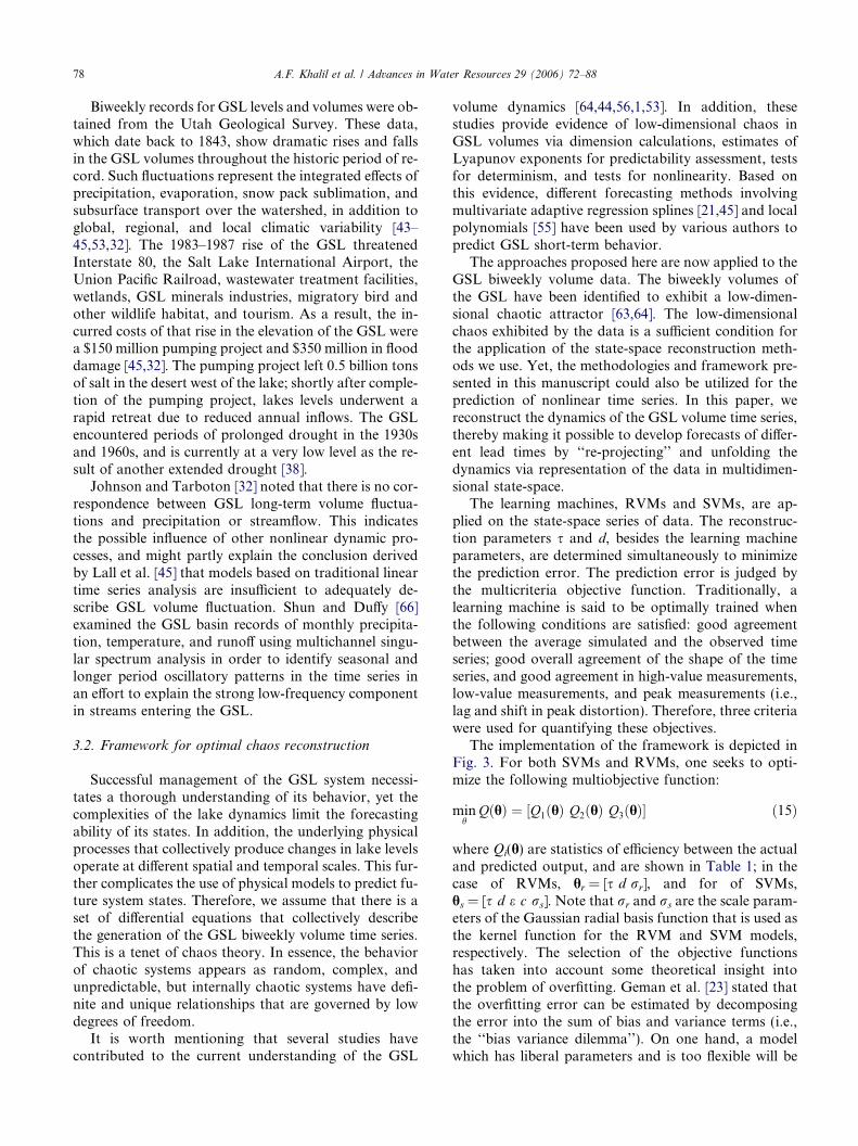
The MOSCEM algorithm generated approximately16 points in the Pareto solution in the case of SVM(Fig. 4a and b) and around 14 in the case of RVM(Fig. 4c and d). This Pareto optimal solution spacewas estimated using initial population size of 10,000(Fig. 4). The plots in Fig. 4 depicts two-dimensional pro-jections of the bicriterion tradeoff surface represented bythe total set of points generated by MOSCEM, with Par-eto frontier in these plots indicated by black dots. It isworth stating here that the correlation between someobjective functions (i.e., index of agreement and root-mean-square-error) does not limit the efficacy of MOS-CEM to identify optimal parameter values, but ratherit emphasizes different aspects of bias-variance trade-offs. There is less correlation between the variance mea-sures and the bias estimator, as shown in Fig. 4. Note

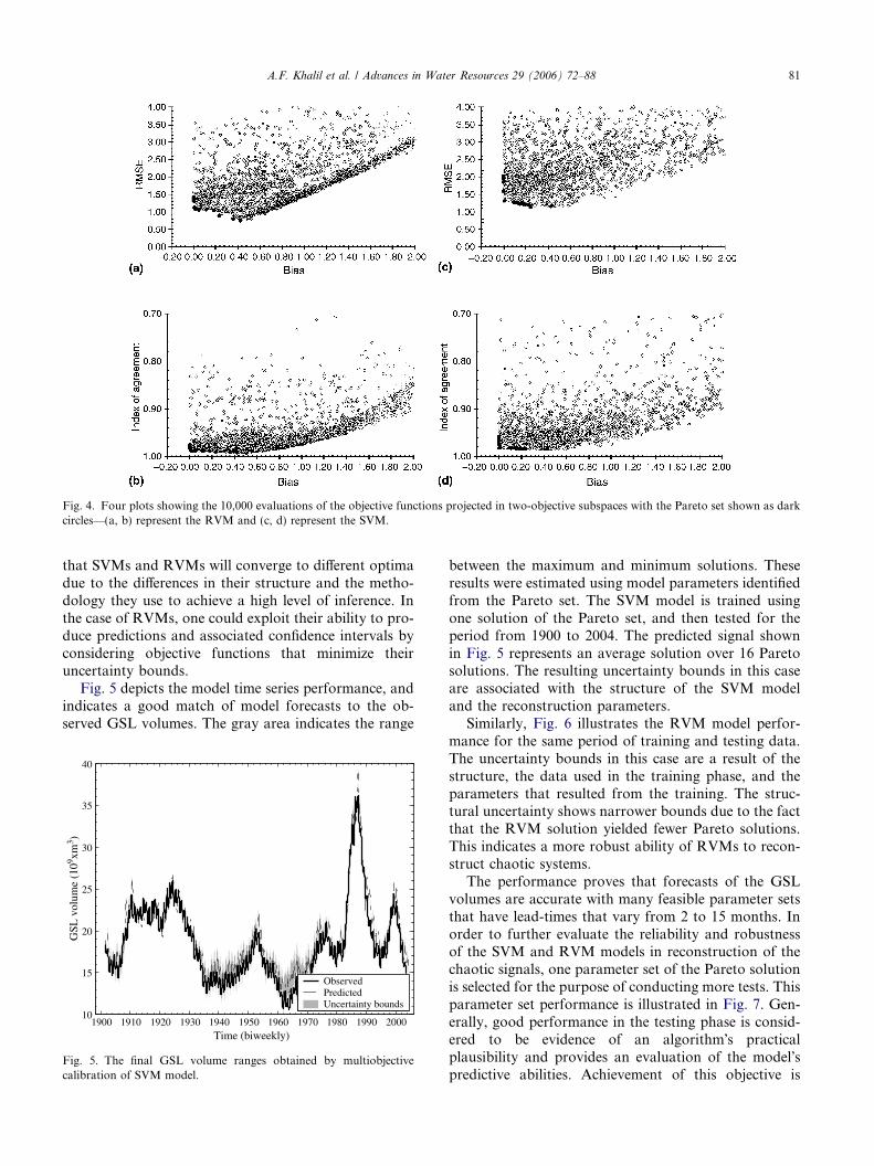
Fig. 4. Four plots showing the 10,000 evaluations of the objective functions projected in two-objective subspaces with the Pareto set shown as darkcircles—(a, b) represent the RVM and (c, d) represent the SVM.


that SVMs and RVMs will converge to different optimadue to the differences in their structure and the metho-dology they use to achieve a high level of inference. Inthe case of RVMs, one could exploit their ability to pro-duce predictions and associated confidence intervals byconsidering objective functions that minimize theiruncertainty bounds.

Fig. 5 depicts the model time series performance, andindicates a good match of model forecasts to the ob-served GSL volumes. The gray area indicates the range

1900 1910 1920 1930 1940 1950 1960 1970 1980 1990 200010

15

20

25

30

35

40

Time (biweekly)

GSL

vol

ume

(109 xm

3 )

ObservedPredictedUncertainty bounds

Fig. 5. The final GSL volume ranges obtained by multiobjectivecalibration of SVM model.

between the maximum and minimum solutions. Theseresults were estimated using model parameters identifiedfrom the Pareto set. The SVM model is trained usingone solution of the Pareto set, and then tested for theperiod from 1900 to 2004. The predicted signal shownin Fig. 5 represents an average solution over 16 Paretosolutions. The resulting uncertainty bounds in this caseare associated with the structure of the SVM modeland the reconstruction parameters.

Similarly, Fig. 6 illustrates the RVM model perfor-mance for the same period of training and testing data.The uncertainty bounds in this case are a result of thestructure, the data used in the training phase, and theparameters that resulted from the training. The struc-tural uncertainty shows narrower bounds due to the factthat the RVM solution yielded fewer Pareto solutions.This indicates a more robust ability of RVMs to recon-struct chaotic systems.

The performance proves that forecasts of the GSLvolumes are accurate with many feasible parameter setsthat have lead-times that vary from 2 to 15 months. Inorder to further evaluate the reliability and robustnessof the SVM and RVM models in reconstruction of thechaotic signals, one parameter set of the Pareto solutionis selected for the purpose of conducting more tests. Thisparameter set performance is illustrated in Fig. 7. Gen-erally, good performance in the testing phase is consid-ered to be evidence of an algorithm�s practicalplausibility and provides an evaluation of the model�spredictive abilities. Achievement of this objective is

1900 1910 1920 1930 1940 1950 1960 1970 1980 1990 20005

10

15

20

25

30

35

40

45

Time (biweekly)

GSL

vol

ume

(109 xm

3 )

ObservedPredictedUncertainty bounds

Fig. 6. The final GSL volume ranges obtained by multiobjectivecalibration of the RVM model.


quantified in Table 2, which provides key statistics forevaluating the efficiency of the two learning machinesin the training and testing phases. For more detailsregarding these goodness-of-fit measures, the interestedreader can refer to David and Gregory [14] and Will-mott [81]. For further details and discussions aboutthe key principles of SVM and RVM construction andapplication, readers are referred to Khalil et al. [37].Both SVMs and RVMs have better performance in thetraining phase than in the testing phase. The loss of per-formance with respect to the testing set addresses amachine�s susceptibility to overtraining. There is anoticeable reduction in performance on the testing data-set (i.e., there is a difference between machine perfor-mance on training and testing) for the SVM model incomparison to the RVM model. This relatively small de-cline of performance of the RVM model indicates itsability to avoid overtraining, and hence it can be ex-pected to generalize better. Performance of a feed-for-ward artificial neural network (ANN) is also reportedfor comparison purposes (Table 2). RVMs were foundto outperform ANNs, while the SVM model is shownto perform equivalent to the ANN. One may concludethat if the ANN model is cautiously structured againstoverfitting and is well-trained, it could be able to pro-vide competitive performance similar to SVMs andRVMs. However, when trained using a scarce data set,RVMs and SVMs are expected to provide better gener-alization capabilities. For more details about the com-parison between these learning machines, the reader isreferred to Khalil et al. [37].

4.3. Perspective on sparsity

Degrees of freedom are often used as a complexitymeasure in model selection. An important aspect in

machine learning, and more specifically model selection,is to avoid overparameterized models. In accordancewith the principle of Occam�s Razor, the most parsimo-nious model is the best [51,52]. SVMs and RVMs pro-vide functional formulations that produce a highdegree of generalization without resorting to the use ofa large number of parameters (i.e., degrees of freedom).According to Vapnik [76], generalization from finitedata is possible if and only if the estimator has limitedcapacity. This is called ‘‘enforced regularization.’’ TheSVM model is characterized by a highly effective mech-anism for avoiding overfitting that results in a modelwith good generalization capability. The SVM formula-tion leads to a sparse model dependent only on a subsetof training examples and their associated kernel func-tions [75]. Tipping [73] indicated that SVMs are notcapable of providing a probabilistic prediction that con-tains information about uncertainty (see Fig. 7). He alsonoted that SVMs suffer from the number of kernel func-tions that can grow steeply with the size of the trainingdataset, from the necessity to manually tune someparameters, and from the selection of kernel functionparameters (which also must satisfy Mercer�s condition[75,73]). Empirical results proved that RVMs areremarkable in producing an excellent generalization le-vel while maintaining the sparsest structure. For exam-ple, whereas the RVM model employs 1–0.4% of thetraining patterns as relevance vectors; the SVM modelutilized 10–15% of the training patterns as support vec-tors. For instance, as shown in Fig. 7, 123 patterns serveas support vectors and seven serve as relevance vectorsout of the 268 patterns of the training set. The supportvectors in the case of SVMs are a subset of the trainingdata set that is a associated with nonzero Lagrange mul-tipliers (and result from the solution of Eq. (7)). The rel-evance vectors are the queries of the training data setwhose associated weights are significant (i.e., the train-ing points where the distribution of the weight doesnot peak to infinity). Note that relevance and supportvectors and their corresponding parameters are the solerequirements to provide predictions for an incomingquery, as shown in Eq. (3).

It is worth mentioning here that the support vectorsin the SVM model represent decision boundaries, whilethe RVM relevance vectors represent prototypical exam-ples [48]. The prototypical examples exhibit the essentialfeatures of the information content of the data, and thusare able to transform the input data into the specifiedtargets. This feature of both RVMs and SVMs couldbe further utilized to build up a sparse representationof the processes such as might be useful in monitoringnetwork design. Practically speaking, this feature ofSVMs and RVMs was found to be essential for the mod-eling of GSL volumes, where much of the data that weremeasured before 1900 are subject to a greater level ofnoise, uncertainty, and inaccuracy due to the limited

Table 2Statistical measures of SVM and RVM ability to predict GSL volumes

Statistics RVM SVM ANN

Training Testing Confidencelimits (95%)



Lower Upper Lower Upper Lower Upper

Correlation coefficient 0.990 0.982 0.973 0.993 0.989 0.982 0.973 0.992 0.989 0.982 0.977 0.987Coefficient of efficiency 0.979 0.965 0.955 0.975 0.977 0.924 0.915 0.934 0.977 0.927 0.898 0.956Bias 0.000 0.451 0.441 0.461 �0.035 0.809 0.799 0.819 �0.005 0.757 0.558 0.956RMSE 0.749 0.869 0.859 0.879 0.785 1.290 1.280 1.300 0.786 1.256 1.048 1.463Mean absolute error 0.567 0.696 0.686 0.705 0.595 1.052 1.042 1.061 0.602 1.018 0.863 1.173Index of agreement 0.995 0.991 0.982 1.000 0.994 0.978 0.969 0.988 0.994 0.979 0.969 0.989

10.0

15.0

20.0

25.0

30.0

35.0

40.0

1840 1855 1870 1885 1900 1915 1930 1945 1960 1975 1990 2005

GSL

Vol

ume

(109 xm

3 )

RVM predictions

Relevance vectors

Observations

Training Testing

10.0

15.0

20.0

25.0

30.0

35.0

40.0

1840 1855 1870 1885 1900 1915 1930 1945 1960 1975 1990 2005

GSL

Vol

ume

(109 xm

3 )

ObservationsSVM PredictionsSupport vectors

Training Testing

10.0

15.0

20.0

25.0

30.0

35.0

40.0

1840 1855 1870 1885 1900 1915 1930 1945 1960 1975 1990 2005

GSL

Vol

ume

(109 xm

3 )

Observations

ANN Predictions

Training Testing

Fig. 7. Model performance for GSL volume prediction (data for the hydrological year 1847/2003 with two-week interval are used; 123 supportvectors and seven relevance vectors resulted out of 1200 samples used for training, embedded dimension = 10, time delay = 8 time steps). Note that inthe RVM case there is uncertainty bounds associated with each prediction.


capability of the instruments and measuring proceduresused in the 1800s. Given these data uncertainties, SVMs

and RVMs are particularly well suited for capturinginformation about the underlying GSL dynamics


because their formulation removes redundant featuresand noninformative patterns in the data, and thus theyare less susceptible to contamination by noise. On theother hand, since both SVMs and RVMs are formulatedto mitigate the influence of noise, they alleviate the sen-sitivity of the MOSCOM algorithm and Pareto set tosuch errors.

4.4. Bootstrapping performance

A very fundamental problem in chaotic reconstruc-tion and machine learning is one that deals with theill-posed nature of the problem: we are trying to inferparameters from a finite number of data points ratherthan from the entire distribution function. It is knownthat abundant data that accurately characterize theunderlined distribution provide robustness for applica-tions designed to specify model parameters. In forecast-ing models, there are infinitely many functions that mayprovide an accurate fit to the finite testing set. Notwith-standing this, SVM and RVM formulations do not tryto fit data. Instead, they try to capture underlying func-tions from which the data were generated irrespective ofthe presence of noise. For SVMs, this insensitivity tonoise in the data is attributed to the e-insensitive lossfunction in the model formulation. For RVMs, theimposition of hyperparameters, i.e., maximization ofthe type-II likelihood, removes much of the noise in

0.8 0.9 10

100

200

300

400

500

R20.50

100

200

300

400

500

COE

0 2 40

100

200

300

RMSE0 2

0

100

200

300

400

MAE

Fig. 8. Bootstrapped histogram of the coefficient of correlation, coefficienabsolute error (MAE), and index of agreement (IoA) associated with RVM

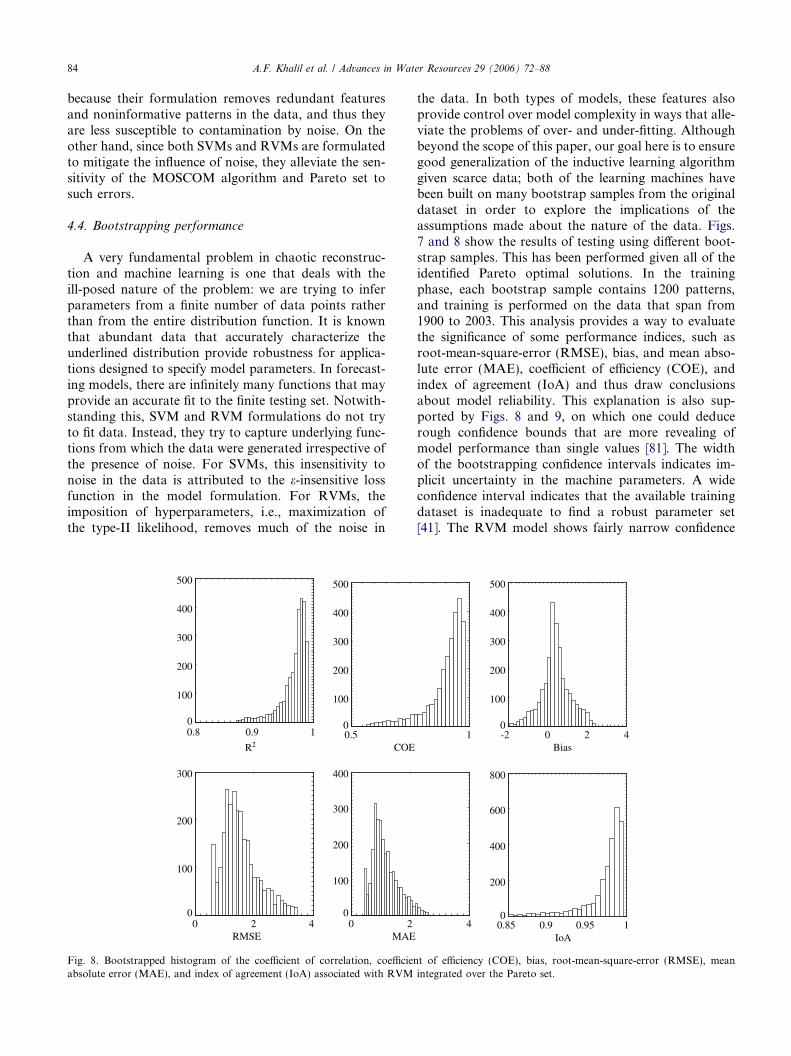
the data. In both types of models, these features alsoprovide control over model complexity in ways that alle-viate the problems of over- and under-fitting. Althoughbeyond the scope of this paper, our goal here is to ensuregood generalization of the inductive learning algorithmgiven scarce data; both of the learning machines havebeen built on many bootstrap samples from the originaldataset in order to explore the implications of theassumptions made about the nature of the data. Figs.7 and 8 show the results of testing using different boot-strap samples. This has been performed given all of theidentified Pareto optimal solutions. In the trainingphase, each bootstrap sample contains 1200 patterns,and training is performed on the data that span from1900 to 2003. This analysis provides a way to evaluatethe significance of some performance indices, such asroot-mean-square-error (RMSE), bias, and mean abso-lute error (MAE), coefficient of efficiency (COE), andindex of agreement (IoA) and thus draw conclusionsabout model reliability. This explanation is also sup-ported by Figs. 8 and 9, on which one could deducerough confidence bounds that are more revealing ofmodel performance than single values [81]. The widthof the bootstrapping confidence intervals indicates im-plicit uncertainty in the machine parameters. A wideconfidence interval indicates that the available trainingdataset is inadequate to find a robust parameter set[41]. The RVM model shows fairly narrow confidence

1 -2 0 2 40

100

200

300

400

500

Bias

4 0.85 0.9 0.95 10

200

400

600

800

IoA

t of efficiency (COE), bias, root-mean-square-error (RMSE), meanintegrated over the Pareto set.

0.8 0.9 10

100

200

300

400

R2

0.5 10

100

200

300

400

COE

-2 0 2 40

50

100

150

200

Bias

0 2 40

100

200

300

RMSE

0 2 40

100

200

300

MAE

0.85 0.9 0.95 10

200

400

600

IoA

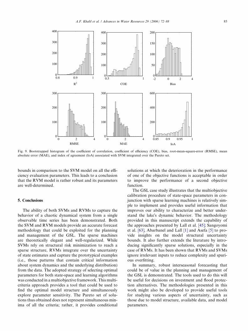
Fig. 9. Bootstrapped histogram of the coefficient of correlation, coefficient of efficiency (COE), bias, root-mean-square-error (RMSE), meanabsolute error (MAE), and index of agreement (IoA) associated with SVM integrated over the Pareto set.


bounds in comparison to the SVM model on all the effi-ciency evaluation parameters. This leads to a conclusionthat the RVM model is rather robust and its parametersare well-determined.

5. Conclusions

The ability of both SVMs and RVMs to capture thebehavior of a chaotic dynamical system from a singleobservable time series has been demonstrated. Boththe SVM and RVM models provide an accurate forecastmethodology that could be exploited for the planningand management of the GSL. The sparse machinesare theoretically elegant and well-regularized. WhileSVMs rely on structural risk minimization to reach asparse structure, RVMs integrate over the uncertaintyof state estimates and capture the prototypical examples(i.e., those patterns that contain critical informationabout system dynamics and the underlying distribution)from the data. The adopted strategy of selecting optimalparameters for both state-space and learning algorithmswas conducted in amultiobjective framework. Thismulti-criteria approach provides a tool that could be used tofind the optimal model structure and simultaneouslyexplore parameter sensitivity. The Pareto set of solu-tions thus obtained does not represent simultaneous min-ima of all the criteria; rather, it provides conditional

solutions at which the deterioration in the performanceof one of the objective functions is acceptable in orderto improve the performance of a second objectivefunction.

The GSL case study illustrates that the multiobjectivecalibration procedure of state-space parameters in con-junction with sparse learning machines is relatively sim-ple to implement and provides useful information thatimproves our ability to characterize and better under-stand the lake�s dynamic behavior. The methodologyprovided in this manuscript extends the capability ofthe approaches presented by Lall et al. [45]; Sangoyomiet al. [63], Abarbanel and Lall [1] and Asefa [5] to pro-vide insights on the model structural uncertaintybounds. It also further extends the literature by intro-ducing significantly sparse solutions, especially in thecase of RVMs. It has been shown that RVMs and SVMsignore irrelevant inputs to reduce complexity and spuri-ous overfitting.

In summary, robust interseasonal forecasting thatcould be of value in the planning and management ofthe GSL is demonstrated. The tools used to do this willbe useful for decisions on investment and flood protec-tion alternatives. The methodologies presented in thiswork might also be developed to provide useful toolsfor studying various aspects of uncertainty, such asthose due to model structure, available data, and modelparameters.


Acknowledgments

Portions of this work were supported by the UtahWater Research Laboratory, College of Engineering,Utah State University, and Utah Center for Water Re-sources Research. The authors would like to thank Dr.Wallace Gwynn of the Utah Geological Survey, UtahDepartment of Natural Resources, for providing thebiweekly GSL stage and volume data used in the study.Thanks are also due to anonymous reviewers for theirinsightful comments.

References

[1] Abarbanel HDL, Lall U. Nonlinear dynamics of the Great SaltLake: system identification and prediction. Climate Dyn1996;12:287–97.

[2] Arnow T. Water level and water quality changes in Great SaltLake, Utah, 1847–1983. Geological Survey Circular 913, USGeological Survey, 1984.

[3] Arnow T, Stephens D. Hydrologic characteristics of the GreatSalt Lake, Utah: 1847–1986. US Geological Survey Water-SupplyPaper 2332, Department of the Interior, US Geological Survey,Denver, CO, 1990.

[4] ASCE Task Committee on Application of the Artificial NeuralNetworks in Hydrology, Artificial neural networks in hydrology.II: Hydrologic applications. J Hydrol Eng, ASCE 2000;5(2):124–37.

[5] Asefa T. Statistical learning machine concepts and application inwater resources management. PhD dissertation. Department ofCivil and Environmental Engineering, Utah State University,Logan, UT, 2004.

[6] Asefa T, Kemblowski MW, Urroz G, McKee M, Khalil A.Support vectors-based groundwater head observation networksdesign. Water Resour Res 2004;40(11):W11509. doi:10.1029/2004WR003304.

[7] Baskin RL, Waddell KM, Thiros SA, Giddings EM, Hadley HK,Stephens DW, et al. Water-quality assessment of the Great SaltLake Basins, Utah, Idaho, and Wyoming—Environmental settingand study design. Water-Resources Investigations Report 02-4115, National Water Quality Assessment Program, USGS, SaltLake City. Available from: http://water.usgs.gov/pubs/wri/wri024115/, 2002.

[8] Beldring S. Multi-criteria validation of precipitation-runoff model.J Hydrol 2002;257:189–211.

[9] Berger JO. Statistical decision theory and Bayesian analysis. 2nded. New York: Springer; 1985.

[10] Beven K. Prophecy, reality, and uncertainty in distributedhydrologic modeling. Adv Water Resour 1993;16:41–55.

[11] Bezruchko BP, Karavaev AS, Ponomarenko VI, Prohhorov MD.Reconstruction of time-delay systems from chaotic time series.J Phys Rev E 2001;64(5):05621–7.

[12] Chun-Hua B, Xin-Bao N. Determining the minimum embeddingdimension of nonlinear time series based on prediction method.J Chin Phys 2004;13(5):633–7.

[13] Cortes C, Vapnik V. Support vector networks. J Mach Learning1995;20:273–97.

[14] David RL, Gregory MJ. Evaluating the use of ‘‘goodness-of-fit’’measures in hydrologic and hydroclimatic model validation.Water Resour Res 1999;35(1):233–41.

[15] Demarty J, Ottle C, Braud I, Olioso A, Frangi JP, Bastidas LA,et al. Using a multiobjective approach to retrieve information on

surface properties used in a SVAT model. J Hydrol 2004;287:214–36.

[16] Duan QA, Sorooshian S, Gupta VK. Optimal use of the SCE-UAglobal optimization method for calibrating watershed models.J Hydrol 1994;158:265–84.

[17] Duan QA, Gupta VK, Sorooshian S. Effective and efficient globaloptimization for conceptual rainfall-runoff models. Water ResourRes 1992;28(4):1015–31.

[18] Duan QA, Gupta VK, Sorooshian S. Shuffle complex evolutionapproach for effective and efficient global minimization. J OptimTheory Applic 1993;76(3):501–21.

[19] Farmer JD, Sidorowich JJ. Predicting chaotic time series. PhysRev Lett 1987;59(8):845–8.

[20] Frazer AM, Swinney HL. Independent coordinates for strangeattractors from mutual information. Phys Rev A 1996;33(2):1134–40.

[21] Friedman J. Multivariate adaptive regression splines. Ann Stat1991;19(1):1–141.

[22] Gan TY, Biftu GF. Automatic calibration of conceptual rainfall-runoff models: optimization algorithms, catchments condi-tions, and model structure. Water Resour Res 1996;32(12):3513–24.

[23] Geman S, Bienenstock E, Doursat R. Neural networks and thebias/variance dilemma. Neural Comput 1992;4:1–58.

[24] Gleick J. Chaos: making a new science. Viking HarmondsworthMiddlesex, England, 1987.

[25] Grewal MS, Andrews AP. Kalman filtering: theory and practiceusing MATLAB. 2nd ed. NY: Wiley; 2001.

[26] Gupta HV, Bastidas LA, Sorooshian S, Shuttleworth WJ, YangZL. Parameter estimation of land surface scheme usingmulti-criteria methods. J Geophys Res 1999;104(D16):19491–503.

[27] Gupta HV, Bastidas L, Vrugt JA, Sorooshian S. Multiple criteriaglobal optimization for watershed model calibration. In: Duan Qet al., editors. Calibration of watershed models. Water scienceapplied research, vol. 6. Washington, DC: AGU; 2003. p. 125–32.

[28] Gupta HV, Sorooshian S, Yapo PO. Toward improved calibra-tion of hydrologic models: multiple and noncommensurablemeasures of information. Water Resour Res 1998;34(4):751–63.

[29] Ibrahim Y, Liong SY. Calibration strategy for urban catchmentparameters. J Hydr Eng 1992;188(10):1150–70.

[30] Islam MN, Sivakumar B. Characterization and prediction ofrunoff dynamics: a nonlinear dynamical view. Adv Water Resour2002;25:179–90.

[31] Jayawardena AW, Gurung AB. Noise reduction and prediction ofhydrometeorological time series: dynamical system approach vs.stochastic approach. J Hydrol 2000;228:242–64.

[32] Johnson B, Tarboton DG. Great Salt Lake Basin hydrologicobservatory prospectus. Submitted to CUAHSI for considerationas a CUAHSI Hydrologic Observatory. Available from: http://greatsaltlake.utah.edu, 2004.

[33] Jordan MI, Bishop C. Neural networks. In: Tucker AB, editor.CRC handbook of computer science. Boca Raton, FL: CRCPress; 1997.

[34] Kecman V. Learning and soft computing: support vectormachines, neural networks, and fuzzy logic models. Cambridge,MA: MIT Press; 2001.

[35] Kennel MB, Brown R, Abarbanel HDL. Determining embeddingdimension for phase-space reconstruction using a geometricalconstruction. Phys Rev Lett A 1992;45(6):3403–11.

[36] Khadam IM, Kaluarachchi JJ. Use of soft information to describethe relative uncertainty of calibration data in hydrologic models.Water Resour Res 2004;40:W11505. doi:10.1029/2003WR002939.

[37] Khalil AF, Almasri MN, McKee M, Kaluarachchi JJ. Applica-bility of statistical learning algorithms in ground water quality

http://dx.doi.org/10.1029/2004WR003304

http://dx.doi.org/10.1029/2004WR003304

http://water.usgs.gov/pubs/wri/wri024115/

http://water.usgs.gov/pubs/wri/wri024115/

http://greatsaltlake.utah.edu

http://greatsaltlake.utah.edu

http://dx.doi.org/10.1029/2003WR002939


modeling. Water Resour Res 2005;41(5). doi:10.1029/2004WR003608.

[38] Khalil AF. Computational learning theory and data-drivenmodeling for ware resources management and hydrology. PhDdissertation, Utah State University, 2005. p. 161

[39] Khalil AF, McKee M, Kemblowski M, Asefa T. Basin-Scalewater management and forecasting using multisensor data andneutral networks. J Am Water Resour Assoc 2005;41(1):195–208.

[40] Koutsoyiannis D, Pachakis D. Deterministic chaos versus sto-chasticity in analysis and modeling of point rainfall series.J Geophys Res 1996;101(D21):26,441–51.

[41] Kuan MM, Lim CP, Harrison RF. On operating strategies of thefuzzy ARTMAP neural network: a comparative study. Int JComput Intell Appl 2003;3:23–43.

[42] Kunstmann H, Kinzelbach W, Siegfried T. Conditional first-ordersecond moment method and its application to the quantificationof uncertainty in groundwater modeling. Water Resour Res2002;38(4):1035.

[43] Lall U, Bosworth K. Multivariate kernel estimation of functionsof space and time hydrologic data. In: Hipel K, editor. Time seriesanalysis and forecasting. Kluwer; 1994.

[44] Lall U, Mann ME. The Great Salt Lake: a barometer of lowfrequency climatic variability. Water Resour Res 1995;31(10):2503–15.

[45] Lall U, Sangoyomi T, Abarbanel HDL. Nonlinear dynamics ofthe Great Salt Lake: nonparametric short term forecasting. WaterResour Res 1996;32(4):975–85.

[46] Legates DR, McCabe GJ. Evaluating the use of goodness-of-fitmeasures in hydrologic and hydroclimatic model validation.Water Resour Res 1999;35(1):233–41.

[47] Leplastrier M, Pitman AJ, Gupta HV, Xia Y. Exploring therelationship between complexity and performance in a landsurface model using the multi-criteria method. J Geophys Res2002;107(D20):4443. doi:10.1029/2002JD000931.

[48] Li Y, Campbell C, Tipping M. Bayesian automatic relevancedetermination algorithms for classifying gene expression data.Bioinformatics 2002;18(10):1332–9.

[49] Liong S, Sivapragasam C. Flood stage forecasting with supportvector machines. J Am Water Resour Assoc 2002;38(1):173–86.

[50] Lorenz EN. Deterministic non-periodic flow. J Atmos Sci1963;20:130–41.

[51] MacKay D. Bayesian interpolation. Neural Comput1992;4(3):415–47.

[52] MacKay D. Information theory, inference, and learning algo-rithms. Cambridge University Press 2003.

[53] Mann ME, Lall U, Saltzman B. Decadal-to-century scale climateverifiability: Insights into the rise and fall of the Great Salt Lake.Geophys Res Lett 1995;22:937–40.

[54] Meixner T, Bastidas LA, Gupta HV, Bales RC. Multicriteriaparameters estimation for models of stream chemical composi-tion. Water Resour Res 2002;38(3):9.1–9.

[55] Moon Y-I. Climate variability and dynamics of Great Salt Lakehydrology. Unpublished PhD dissertation. Utah State University,Logan, UT, 1993.

[56] Moon Y-I, Lall U. Large scale atmospheric indices and the GreatSalt Lake: interannual and interdecadal variability. J Hydrol Eng,ASCE 1996;1(2):55–62.

[57] Mukherjee S, Osuna E, Girosi F. Nonlinear prediction of chaotictime series using support vector machines. In: Proceedings ofIEEE workshops on neural network for signal processing, AmeliaIsland, FL, 1997.

[58] Packard NH, Crutchfield JP, Farmer JD, Shaw RS. Geometryfrom a time series. Phys Rev Lett 1980;45(9):712–6.

[59] Phoon KK, Islam MN, Liaw CY, Liong SY. Practical inverseapproach for forecasting nonlinear hydrological time series.J Hydrol Eng 2002;7(2):116–28.

[60] Porporato A, Ridolfi L. Clues to the existence of deterministicchaos in river flow. Int J Modern Phys B 1996(10):1821–62.

[61] Porporato A, Ridolfi L. Nonlinear analysis of river flow timesequences. Water Resour Res 1997;33(6):1353–67.

[62] Rodriguez-Iturbe I, DePower FB, Sharifi MB, Georgakakos KP.Chaos in rainfall. Water Resour Res 1989;25(7):1667–75.

[63] Sangoyomi TB, Lall U, Abarbanel HDL. Nonlinear dynamics ofthe Great Salt Lake: dimension estimation. Water Resour Res1996;32(1):149–59.

[64] Sangoyomi T, Climatic variability and dynamics of Great SaltLake hydrology. PhD dissertation. Department of Civil andEnvironmental Engineering, Utah State University, Logan, UT,1993.

[65] Schoolkopf B, Smola AJ. Learning with kernels: support vectormachines, regularization, optimization, and beyond. Cambridge,MA: MIT Press; 2002.

[66] Shun T, Duffy CJ. Low-frequency oscillations in precipitation,temperature, and runoff on a west facing mountain front: ahydrogeologic interpretation. Water Resour Res1999;35(1):191–220.

[67] Sivakumar B. Chaos theory in hydrology: important issues andinterpretations. J Hydrol 2000;227:1–20.

[68] Sivakumar B, Phoon KK, Liong SY, Liaw CY. A systematicapproach to noise reduction in chaotic hydrological time series.J Hydrol 1999;219:103–35.

[69] Sivakumar B, Liong SY, Liaw CY, Phoon KK. Singapore rainfallbehavior: chaotic? J Hydrol Eng 1999;4(1):38–48.

[70] Solomatine DP, Rojas C, Velickov S, Wust H. Chaos theory inpredicting surge water levels in the North Sea. In: Proceedings of4th international conference on hydroinformatics, Iowa, USA,2000.

[71] Solomatine DP, Velickov S, Rojas C, Wust H. Predictive datamining in predicting surge water levels. In: Proceedings ofhydroinformatics, Balkema, IA, 2000.

[72] Takens F. Detecting strange attractors in turbulence. In: RandDA, Young LS, editors. Dynamical systems and turbulence.Lecture notes in mathematics. Berlin: Springer-Verlag; 1980.p. 365–81.

[73] Tipping M. The relevance vector machine. In: Solla S, Leen T,Muller K-R, editors. Advances in neural information processingsystems, vol. 12. Cambridge, MA: MIT Press; 2000. p. 652–8.

[74] Tipping ME. Sparse Bayesian learning and the relevance vectormachine. J Mach Learning 2001;1:211–44.

[75] Vapnik V. The nature of statistical learning theory. NewYork: Springer; 1995.

[76] Vapnik V. Statistical learning theory. New York: Wiley; 1998.[77] Vrugt AJ, Gupta HV, Bastidas LA, Bouten W, Sorooshian S.

Effective and efficient algorithm for multiobjective optimization ofhydrologic models. Water Resour Res 2003;39(8):1214.doi:10.1029/2002WR001746.

[78] Wah BW, Chang S. Trace based methods for solving nonlinearglobal optimization and satisfiability problem. J Global Optim1997;10(2):107–41.

[79] Wahba G. A comparison of GCV and GML for choosing thesmoothing parameter in the generalized spline-smoothing prob-lem. Ann Stat 1985;4:1378–402.

[80] Wang Q, Gan TY. Basis of correlation dimension estimates ofstreamflow data in the Canadian prairies. Water Resour Res1998;34(9):2329–39.

[81] Willmott CJ. On the evaluation of model performance in physicalgeography. In: Gaile GL, Willmott CJ, editors. Spatial statisticsand models. Dordrecht: Holland; 1984. p. 443–60.

[82] Xia Y, Pitman AJ, Gupta HV, LplastrierLeplastrier M, Hender-son-Sellers A, Bastidas LA. Calibrating a land surface model ofvarying complexity using multi-criteria methods and the Cabauwdataset. J Hydrometeorol 2002;3(2):181–94.

http://dx.doi.org/10.1029/2004WR003608

http://dx.doi.org/10.1029/2004WR003608

http://dx.doi.org/10.1029/2002JD000931

http://dx.doi.org/10.1029/2002WR001746


[83] Yapo PO, Gupta HV, Sorooshian S. Multiobjective globaloptimization for hydrologic models. J Hydrol 1998;204:83–97.

[84] Yu XY. Support vector machine in chaotic hydrological timeseries forecasting. PhD dissertation. National University ofSingapore, Singapore, 2004.

[85] Yu XY, Liong SY, Babovic V. EC-SVM approach for real timehydrologic forecasting. J Hydroinform 2004;6:209–23.

[86] Zaldivar JM, Gutierrez E, Galvan IM, Strozzi F, Tomasin A.Forecasting high waters at Venice lagoon using chaotic time seriesanalysis and nonlinear neural networks. J Hydroinform2000;2:61–84.

[87] Zitzler E, Thiele L. Multiobjective evolutionary algorithms: acomparative case study and the strength Pareto approach. IEEETrans Evol Comput 1999;3(4):257–71.

Multiobjective analysis of chaotic dynamic systems with sparse learning machines

Documents

Transcript of Multiobjective analysis of chaotic dynamic systems with sparse learning machines