
Modeling River Flow using Artificial Neural Networks - Pertanika
Upload
khangminh22Category
view
2download
0
FINAL REPORT
MORPHOLOGICAL STUDY OF RAPTI RIVER USING REMOTE SENSING
TECHNIQUES
Prepared by
Indian Institute of Technology Roorkee
Uttarakhand
Prepared for
Morphology Directorate Central Water Commission
New Delhi
(ii)
PROJECT TEAM
Dr. Z. Ahmad, Professor (PI)
Dr. P.K. Garg, Professor
Dr. Deepak Kashyap, Professor
Dr. R.D. Garg, Assoc. Professor
Dr. P. K. Sharma, Assoc. Professor
Dr. Rajat Agarwal, Research Associate
Mr. Suresh S. Dodamani, Project Associate
Ms. Tanushree Mukherjee, Project Associate
Mr. Rajeev Ranjan, Project Associate
Mr. Sandeep Chauhan, Project Assistant
Department of Civil Engineering
INDIAN INSTITUTE OF TECHNOLOGY ROORKEE
ROORKEE
April 2018

(iii)
Executive Summary
1. River morphology deals with the plan form, cross-section and its dimension,
bed forms, aggradation, degradation etc. Such morphology changes due to
river hydrodynamics. Indian rivers experience large seasonal fluctuations in
discharge and sediment load resulting in significant changes in their
morphology. Shifting of the river course is generally accomplished by
erosion of habitated and pricey agricultural area that causes tremendous
losses. The sediments deposited and eroded in the river have a tremendous
effect on the river cross-section and its gradient, sediment transport rate,
discharge etc. Understanding of changes in the morphology of the rivers is
required in the engineering projects for their planning, design and
execution. With this in mind, CWC, New Delhi desires to carry out
morphological study of the major Indian rivers. In this direction, CWC
awarded a project entitled "Morphological study of rivers Ganga, Sharda
and Rapti using remote sensing techniques" to IIT Roorkee.
2. Following were broad objectives of the study
(i) Compilation of river drainage map in GIS; changes in Land use/Land
cover, flood affected areas, rainfall-runoff, geology etc.
(ii) Hydrological analysis: Probability curve and flow rates corresponding
to return period of 1.5 year and 2 year.
(iii) Decadal stream banks shifting and also changes in its Plan form
(Sinuosity & Plan-form Index) from the base year 1970 to 2010.
(iv) Work out erosion and siltation based on the banks shifting.
(v) Evaluate the impacts of major hydraulic structures on the river
morphology.
(vi) Identification of critical and other vulnerable reaches and to suggest
suitable river training/protection works.
(vii) Reconnaissance survey for ground validation of outcomes of the
study.
(viii) Recommendations in the respect of actionable points.
(ix) Suggestions for the further study.
3. Rapti river is the major tributary of Ghaghara river. The Rapti river basin
is diverse in its physiography. The lofty mountain, inner and outer Tarai
and undulating plain regions constitute the topography of the entire basin.
The reach of the Rapti river studied in this project work is from Nepalganj
to confluence point of Rapti and Ghaghra. Rapti river covers an area of
25,793 km2 out of which 44% (11,401 km2) lies in Nepal and 56% (14,392
km2) in Uttar Pradesh. Rapti River flows through the districts of Rukum,
Salyan, Rolpa, Gurmi, Arghakhanchi, Dang and Banke of Nepal territory;
(iv)
and Bahraich, Shrawasti, Balrampur, Siddharthnagar, Santkabinagar,
Gorakhpur and Deoria districts of the Eastern Uttar Pradesh. Important
tributaries of Rapti river in the study reach are Bhakia, Gaura, Kacna,
Kunhara, Sunawan. Various aspects of the Rapti river related to
topography, soil, climate, geology, meteorological stations, land use land
cover, flood map etc. are compiled in this report from the different sources,
like GSI, WRIS, NRSC.
4. Hydrological data of Rapti river that comprises of annual maximum and
minimum discharges and water levels; ten daily average discharge,
sediment, and gauge at different gauging stations, were obtained from
CWC, offices, while relevant satellite images were procured from the
National Remote Sensing Centre (NRSC), Hyderabad and downloaded from
United States Geological Survey (USGS) website. SOI toposheets were
obtained from SOI, Dehradun.
5.
6. Planform of the rivers may be described as straight, meandering or braided.
There is, in fact, a great range of channel patterns from straight through
meandering to braided. Straight and meandering channels are described by
sinuosity which is the ratio of channel length to valley length.
7. The computed sinuosity ratio of the Rapti river in the reach under
consideration is higher than 1.5 in the years 1970, 1980, 1990, 2000, and
2010, therefore, the Rapti is classified as meandering river. Almost whole
reach of the river has meandering pattern, however, it is prominent in the
reaches 25-50 km, 75-100 km, 300-375 km, 400-425 km and 450-475 km.
The meandering is characterized by acute bend with high amplitude,
however, they are relatively stable.
8. The plan form index (PFI) of Rapti River is calculated using the formula
given by Sharma (2004). It has been observed that the Rapti River always
flows in one channel, so negligible braiding is found in Rapti River.
9. For the computation of shifting of course of the river, center line of the river
as in year 2010 is perpendicularly bisected at a regular interval of 1.0 km
and shift of left bank, right bank and center line in either directions has
been computed for the years 1970, 1980, 1990 and 2000 with respect to year
2010 in GIS software. Remarkable shifting of the course of the Rapti river
from 1970 to 2010 has been noticed. The maximum shift is of the order of
2.7 km at some locations. The confluence point of Rapti and Gaghara rivers
has shifted 500 m towards left in year 2010 w.r.t. year 1970.
(v)
10. Major shifting of the river course in span of year 1970 to 2010 are in the
reaches 75 -100 km, 300-375 km, 400-485 km and 500-542 km. At Devpura,
Jamuha, Keshwapur, Nandnagar and Chitahari, shifting is from left to
right while at Gujarpurwa, Ikauna, Jyonar and Kanchalpur, the shifting is
from right to left. No progressive shifting of the course of the river with
respect to time has been noticed.
11. Width of the active channel of the river and river width based on the
extreme banks have been estimated using the satellite images of years
1970-2010. There is no definite progressive change in the width of the river
over the span of year 1970-2010 in the whole studied reach of the Rapti
river. From chainage zero to 450 km, the average width of the active
channel is almost constant and is equal to about 206 m, however, in the
upper reach i.e., Chainage 450 km to 542 km, the average width is about
290 m - which may be attributed to silting in upper reaches and spreading
of flow as the river descends from hilly areas.
12. Erosion and siltation studies have been carried out for the Rapti river from
Nepalganj to confluence point of Rapti and Ghaghra using SOI toposheets
and post-monsoon decadal satellite images from years 1970 to 2010. The
extreme left and right banks have been identified based on the sand deposit
and vegetation and based on the shifting of these banks, the erosion and
deposition are estimated for duration from year 1970 to 2010 and is
expressed in the terms of area in km2.
13. The total eroded, silted, eroded plus silted, and net eroded area in the Rapti
river during the period 1970 to 2010 are 79.04 km2, 57.24 km2, 107.35 km2
and 21.80 km2, respectively. It may be concluded that over a span of 40
years i.e, 1970 to 2010, about 21.80 km2 area of Rapti River has been eroded
by the flowing water.
14. Erosion has been noticed in the entire reach of Rapti River starting from
Nepalgunj to its confluence with Ghaghra River. Major erosion has occurred
during the period 1970 to 2010 in the upper reaches (chainage 450-542 km)
due to constant shifting of river course. At other locations, like Gorakhpur,
Balrampur, Utraula, and Domrianganj, the erosion is not so severe. Minor
deposition has taken place in the reaches 25 km - 50 km, 150 km - 175 km
and 425 km - 450 km that are near Ekauna, Bhaksa and Ikauna,
respectively.
15. Provision of embankments and other river training works in the Rapti river
has controlled the shifting of the river. There are natural water bodies in
the form of ox-bow lakes in vicinity of river due to its meandering nature.
16. Available measured cross sections of the Rapti river for different years at
gauging stations of Balrampur, Rigauli and Birdghat have been analysed.

(vi)
No remarkable changes in the historical cross-sections of the Rapti river at
Rigauli and Birdghat are noticed, however, river course has shifted towards
left side by about 40 m at Balrampur which has resulted in both erosion and
siltation at this location. Cross-section of the Rapti river is shallow at
Balrampur, however it is deep at Rigauli and Birdghat.
17. There is one barrage, named as Rapti barrage, in the reach of the river from
Nepalgunj to Patana Ghat (confluence point of Rapti and Ghaghra Rivers).
The river course has wandering behavior upstream of the barrage. However,
no shifting has been observed downstream of the barrage over the years.
The Rapti barrage was commissioned in year 2008. Since then no noticeable
silting upstream of the barrage has been observed. Nevertheless, river in
year 2015 was flowing in two channels upstream of the barrage.
18. There are about 22 bridges on the Rapti river from Nepalgunj to its
confluence with Ghaghra river at Patana ghat. Morphological changes have
noticed near the major bridges, however, proper river training works have
been provided which are working satisfactorily. Protection works are
suggested in the vicinity of the bridges at Chainages 160 km, 205 km, 212
km, 251.5 km, 272.5 km and 418 km to train the Rapti river.
19. Nine reaches of the Rapti river have been identified as critical. These
reaches are at Chainages 68-80 km (Chhithari), 138-156 km (Mirpur), 304-
322.5 km (Rasulabad), 326.5- 378 km (Utraula), 387-392 km
(Shankarnagar), 399-433 km (Jyonar), 438-466 km (Ikauna), 470-492 km
(Lakshmannagar) and 506-515 km (Jamnaha). In these reaches, river has
wandering behaviour in wide width. No progressive shifting in either
directions has been noticed over the years.
20. Methodology for the design of various river training works has been
discussed and based on the morphological changes of the river, it is
suggested to provide embankment/ levees/spurs in critical reaches of the
river.
a) Chainages 2-12.5 km Embankment on right side
b) Chainages 75-77 km Series of spurs on left side
c) Chainages 304-322.5 km Embankments on both sides
d) Chaianges 326.5-378 km Embankments on both sides
21. In the identified critical reaches, wherever river is striking to the existing
embankments, porcupine/ boulder revetment/geo tubes shall be provided to
avoid breach in the embankment.
22. Embankments are provided towards both sides of the river in its most of the
length, in particular in the lower reaches. In some reaches, embankments

(vii)
are not continuous and that are to be plugged by construction of new
embankment as suggested in this study.
23. Design methodology of conventional river training works and also flexible
system are described in the report that can be used for the design of a
particular work. A sample design of embankment/levees using flexible
system is also mentioned in the report.
24. Field reconnaissance survey was conducted at various locations, like Rapti
Barrage, Bansi Bridge, Birdghat, Patana ghat etc., to assess the present
condition of the river. The observations made during the site visits have
been examined in the perspective of the outcomes of the morphological
study carried out in this study.
Recommendations:
(i) It is recommended to implement the suggested measures in the identified
four critical reaches of the Rapti and in the vicinity of the identified bridges.
It is further suggested that such reaches/locations be studied in more details
based on ground survey and analysis of high resolution satellite data.
(ii) Suggested measures are prioritized as follow: a) Extension of the existing left guide bund of about 90 m downstream at Kodri ghat
(Chainage = 418 km, Fig.9.10) b) Provision of series of spurs towards left side at Dhani (Chainage = 205 km, Fig.
9.6) c) Boulder revetment/porcupine/series of spurs on right bank over a length of 700 m
upstream of the bridge at Peepeganj (Chainage = 160 km, Fig. 9.5) d) Provision of protection to the left embankment upstream of the bridge (SH5) in the
form of boulder revetment/short spurs at Rajendra Nagar (Chainage = 251.5 km, Fig. 9.8)
e) Provision of boulder revetment to the existing both sides embankments at Dhani (Chainage = 212 km)
f) Provision of boulder revetment to both the approach roads at Tighra (Chainage = 272.5 km)
g) Provision of series of spurs on left side in the reach at Chainages 75-77 km h) Provision of embankment on right side in the reach at Chainages 2-12.5 km i) Provision of embankment on both sides in the reach at Chainages 304-322.5 km j) Provision of embankment on both sides in the reach at Chainages 326.5-378 km
(iii) It is recommended to plan hydraulic structures, like barrage, bridge etc. at
the identified nodal points (wherein minimum morphology of the river has
occurred) on the Rapti river to avoid outflanking of the river and to
minimize the protection works.

(viii)
(iv) Large scale de-silting from the rivers are not recommended. Efforts shall be
made to manage the sediment in the river through deploying suitable river
training works. However, from the utility consideration like siltation at
water intake, minimum draft requirement for navigation, skewed
distribution of flow across bridges/barrages etc., it is recommended to desilt
the sediment from that location.
(v) River training works or any other structure shall be designed in such a way
that it should not encroach the flood plains of the river or it should not
delink the lakes, depressed areas, wetlands etc. as such bodies provide
additional storage to the river and that results in lowering the peak
discharge that controls the flood.
(vi) Sediment management in the vicinity of a barrage shall be explored by
operation of the barrage gates. For an example, gates of the barrages shall
be operated in such a way that incoming sediment can be passed
downstream during the flood time, to maintain the sediment equilibrium.
(vii) Detailed ground survey of the area and data collection/analysis is proposed
before implementing the recommendations, so as to incorporate the current
ground conditions and river behaviour.
Suggested Further Study:
(i) Unauthorized, unscientific and unplanned mining of sand and gravel from
the river has resulted in major morphological changes in river in the terms
of stream bank shifting, bed degradation, bank erosion, disrupting the
sediment mass balance, danger to the hydraulic structures etc. It is
suggested to carry out replenishment study so that quantity of the sand and
gravel to be mined can be estimated and morphological changes can be
controlled.
(ii) Erosion and siltation in the Rapti river has been studied herein on the basis
of the shifting of the banks of the river and analysis of satellite images. This
approach of the study is an indicative and does not provide the eroded/silted
sediment in the terms of volume/weight. In view of this, it is suggested that
the eroded/silted sediment shall be quantified on the basis of the sediment
mass balance study i.e., quantity of eroded/silted sediment in a reach of the
river is equal to mass of the sediment entered into the reach minus mass of
the sediment gone out from the reach during a period.
(iii) Flood zones of the river should be identified and delineated along both the
banks of river. Based on flood zone boundaries, habitation and development
activities may be prohibited in such areas.

(ix)
(iv) In future, morphological studies are required to be carried out using 3D
data of the terrain, as topography and slope of the region play an important
role to study the morphological behavior of the river.
For the dissemination of outcomes of the study carried out under the project to
the potential users, a workshop on Morphological Study of Rivers Ganga, Sharda
and Rapti Using Remote Sensing Technique was organized by Indian Institute of
Technology Roorkee in association with Central Water Commission at Library
building, CWC, New Delhi during 18-19 Sept. 2017. A brief note on the workshop
is given in Annexure-C,
Date:
Place: Roorkee
(Z. Ahmad)
Professor of Civil Engineering
IIT Roorkee
(x)
Acknowledgements
On behalf of the project team of IIT Roorkee, I would like to acknowledge the
support and help extended by the various organizations for carrying out this study.
It is worth mentioning some of them like Morphology and Climate Change
Directorate, CWC, New Delhi; Himalayan Ganga Division, CWC, Dehradun; Chief
Engineer (UGBO), CWC, Lucknow; Chief Engineer (LGBO), CWC, Patna; Water
Resources Dept., Patna; Irrigation Dept. UP; BSRDC, Patna; IWAI, Noida;
Irrigation Dept., UK; Chief Engineer (Sone), Irrigation Department, Varanasi;
General Manager and SE of Farakka barrage project; Director (R&D), MoWR, RD &
GR, New Delhi; Director, Remote Sensing Directorate, CWC, New Delhi; GFCC,
Patna; Brahmaputra Board; Executive Engineer, Irrigation Department, Roorkee.;
Survey of India, Dehradun; NRSC, Hyderabad; NIH, Roorkee; AHEC, Roorkee;
Faculty of Civil Eng., IIT Roorkee; Macafferri Pvt. Ltd.
Financial support received from Central Water Commission under the Plan Scheme
“Research & Development Program in Water Sector”, Ministry of Water Resources,
Govt. of India for carrying out this study is greatly acknowledged.
We would like to thank all members of the "Consultancy Evaluation cum Monitoring
Committee (CEMC)" whose valuable inputs and constructive comments improved
the contents of the project.
We indebted to Hon'ble Union Minister of State, Water Resources, River
Development & Ganga Rejuvenation and Parliamentary Affairs Shri Arjun Ram
Meghwal for inaugurating the workshop and delivering motivating lecture.
We heartily thank Prof. A K Chaturvedi, Director, Prof. M. Parida, Dean (SRIC),
and Prof. C S P Ojha, Prof. & Head, Dept. of Civil Eng, IIT Roorkee for their
encouragement and support.
We owe deep gratitude to Shri Narendra Kumar, Chairman, CWC; Shri Pradeep
Kumar, Member (RM); Shri N.K. Mathur, Member (D&R); Shri S Masood Husain,
Member, (WP&P); Shri Ravi Shankar, CE (P&D), Shri P N Singh, Project Director,
DRIP; Shri, Shri. A K Sinha, Director, Morphology & CC Directorate for their
encouragement, support and guidance. We would not forget to remember other
officials of CWC, New Delhi who helped us in carrying out this study.
We are grateful to Prof. M. K. Mittal, Retd. Prof., IIT Roorkee for his timely advice
for carrying out the study. Thanks to Shri Mahavir Prasad, Retired SE, UP
Irrigation who accompanied us during the visit to Rapi river at its various locations.
And finally, I would like to extend my sincere esteems to Prof. Deepak Kashyap,
Prof. P K Garg, Dr. R D Garg, Dr. P K Sharma and other project staff who assisted
me in timely completion of the project work.
Z. Ahmad & Project Team
Dept. of Civil Engineering
IIT Roorkee

(xi)
CONTENTS
Chapter Description Page No.
Executive Summary (iii)
Acknowledgment (x)
List of Figures (xiv)
List of Tables (xx)
1 INTRODUCTION 1.1 Introduction 1.1 1.2 Objectives & Terms of Reference 1.4 1.3 Need/Scope of Study 1.6
2 LITERATURE REVIEW 2.1 Literature Review 2.1 2.2 Concluding Remarks 2.9
3 RIVER BASIN 3.1 Rapti River Basin 3.1 3.2 Climate 3.2 3.3 Meteorological Stations 3.3 3.4 Basin Geology 3.3 3.5 Land Use & Land Cover 3.5 3.6 Flood Affected Areas 3.7 3.7 Concluding Remarks 3.9
4 STUDY REACH 4.1 The Study Area 4.1 4.2 Concluding Remarks 4.4
5 INPUT DATA AND METHODOLOGY 5.1 Hydro-Meteorological Data 5.1 5.2 Toposheets and Satellite Data 5.4 5.3 Software 5.5 5.4 Acquisition of Data and Geo-Referencing of Images 5.5 5.5 Methodology for Plan Form Changes 5.6 5.6 Flow Probability Curves 5.6 5.7 Concluding Remarks 5.9
6 HYDROLOGICAL DATA PROCESSING & ANALYSIS 6.1 Introduction 6.1 6.2 Hydro-Meteorological Data 6.1

(xii)
6.3 Temporal Variation of Maximum Discharge and Maximum Water Level
6.2
6.4 Flood Frequency Analysis 6.6 6.5 Probability Exceedance Curve 6.9 6.6 Concluding Remarks 6.9
7 RIVER MORPHOLOGY 7.1 Delineation/Digitization of River Bank Lines 7.1 7.2 Plan form Pattern of the River 7.4 7.3 Shifting of Main Course of the River 7.21 7.4 River Width 7.87 7.5 Discussions on River Course Shifting and Its Width 7.104 7.6 Nodal Points 7.107 7.7 Concluding Remarks 7.109
8 EROSION & SILTATION 8.1 Channel Evolution Analysis 8.1 8.2 Erosion & Deposition 8.1 8.3 Results and Analysis 8.2 8.4 Aggradation & Degradation 8.17 8.5 Discussion on the Results 8.19 8.6 Conclusions 8.21
9 MAJOR STRUCTURES & THEIR IMPACT ON THE MORPHOLOGY 9.1 Identification Of Major Structures 9.1 9.2 Barrages on the Rapti River
9.2.1 Impact of the Rapti barrage on the morphology of the river
9.2 9.4
9.3 Bridges on the Rapti River 9.7 9.4 Concluding Remarks 9.19
10 GROUND VALIDATION 10.1 Introduction 10.1 10.2 Visit to Rapti Barrage On 23 October, 2016 10.1 10.3 Visit to Bansi Bridge Site on 29/07/2016 10.3 10.4 Visit to Birdghat (Gorakhpur) and Patana Ghat
(Barhalganj) on 30/07/2016 10.3
11 RIVER TRAINING WORKS 11.1 Identification of the Critical Reaches 11.1 11.2 Proposed River Training Works for Restoration of
Critical and Important River Reach 11.13
11.3 Existing Embankments 11.24 11.4 Tentative Design of River Training Works 11.39 11.5 Conclusions 11.42

(xiii)
12 CONCLUSIONS & RECOMMENDATIONS 12.1 12.1 Conclusions 12.1 12.2 Recommendations 12.8 12.3 Suggested Further Studies 12.10 12.4 Acknowledgment 12.10
Bibliography R.1 Annexure-A A.1 Annexure-B B.1

(xiv)
List of Figures
Figure Description Page No.
1.1 Channel Patterns 1.4 3.1 River basin map of Rapti - Sharda - Ghaghra Basin (Source: WRIS) 3.1
3.2 Rapti river basic layers (Source: WRIS) 3.2 3.3 Rain gauge stations in Rapti Basin (Source: WRIS) 3.3
3.4 Geology of Rapti - Sharda - Ghaghra Basin (Source: GSI) 3.5 3.5 Land Use Land Cover Map of Rapti - Sharda - Ghaghra Basin
(Source: WRIS) 3.6
3.6 Land Use Land Cover Map of Rapti Basin (Source: WRIS) 3.6
3.7 Flood Hazard Zone Map of Rapti Sharda - Ghaghra Basin (Source: NRSC
3.8
3.8 Aggregated flood map of Rapti Basin from 2003-2013 (Source: NRSC)
3.8
4.1 River Rapti from Nepalgunj to confluence point of Rapti and Ghaghra 4.3 4.2 Confluence point of Rapti and Ghaghra river 4.2
4.3 Major water resources projects (Source: INDIA-WRIS, 2012) 4.4 5.1 Location of Gauging Sites 5.3
5.2 Flowchart of the methodology 5.7 6.1a-c Temporal variation of maximum observed discharge at gauging sites
a) Balrampur, b) Rigauli and c) Birdghat 6.4
6.2a-e Temporal variation of maximum observed water level at gauging sites (a) Kakardhari, (b) Balrampur, (c) Bansi, (d) Rigauli, and (e) Birdghat
6.6
7.1 Mosaic of SOI toposheets of Rapti river of year 1970 (Scale 1:50,000)
7.1
7.2 Mosaic of FCC of Rapti river of year 1980 (Landsat-MSS Images) 7.2
7.3 Mosaic of FCC of Rapti river of year 1990 (Landsat-TM Images) 7.2
7.4 Mosaic of FCC of Rapti river of year 2000 (IRS 1C LISS III Images) 7.3
7.5 Mosaic of FCC of Rapti river of year 2010 (IRS P6 LISS III Images) 7.3
7.6a Diagram representing the calculation of the sinuosity 7.6
7.6b Channel patterns for different Sinuosity ratio 7.6
7.7a Sinuosity ratio of Rapti River of year 1970, 1980, 1990, 2000 and 2010
7.9
7.7b Geometrical parameters of a river meander (Sinha 2012) 7.10
7.7c Meandering pattern of the Rapti river in the reach from chainage 5 km to 45 km
7.13
7.7d Meandering pattern of the Rapti river in the reach from chainage 80 km to 100 km
7.14
7.7e Meandering pattern of the Rapti river in the reach from chainage 300 km to 340 km
7.15

(xv)
7.7f Meandering pattern of the Rapti river in the reach from chainage 350 km to 390 km
7.16
7.7g Meandering pattern of the Rapti river in the reach from chainage 395 km to 430 km
7.17
7.7h Meandering pattern of the Rapti river in the reach from chainage 210 km to 240 km near Madho Tanda
7.18
7.8 Braiding indices 7.20
7.9 Definition sketch of PFI 7.21
7.10 Sample map of river shifting 7.22
7.11a Shifting of center line of Rapti river from chainage 0-50 km 7.43
7.11b Shifting of center line of Rapti river from chainage 0-50 km 7.44
7.11c Shifting of center line of Rapti river from chainage 50-100 km 7.45
7.12 Shifting of center line of Rapti river from chainage 50-100 km 7.46
7.13a Shifting of center line of Rapti river from chainage 100-150 km 7.47
7.13b Shifting of center line of Rapti river from chainage 100-150 km 7.48
7.14a Shifting of center line of Rapti river from chainage 150-200 km 7.49
7.14b Shifting of center line of Rapti river from chainage 150-200 km 7.50
7.15a Shifting of center line of Rapti river from chainage 200-250 km 7.51
7.15b Shifting of center line of Rapti river from chainage 200-250 km 7.52
7.16a Shifting of center line of Rapti river from chainage 250-300 km 7.53
7.16b Shifting of center line of Rapti river from chainage 250-300km 7.54
7.17a Shifting of center line of Rapti river from chainage 300-350 km 7.55
7.17b Shifting of center line of Rapti river from chainage 300-350 km 7.56
7.18a Shifting of center line of Rapti river from chainage 350-400 km 7.57
7.18b Shifting of center line of Rapti river from chainage 350-400 km 7.58
7.19a Shifting of center line of Rapti river from chainage 400-450 km 7.59
7.19b Shifting of center line of Rapti river from chainage 400-450 km 7.60
7.20a Shifting of center line of Rapti river from chainage 450-500 km 7.61
7.20b Shifting of center line of Rapti river from chainage 450-500 km 7.62
7.21a Shifting of center line of Rapti river from chainage 500-542 km 7.63
7.21b Shifting of center line of Rapti river from chainage 500-542 km 7.64
7.22a Decadal changes in the course of Rapti river from chainage 0-50 km 7.65
7.22b Changes in the course of Rapti river of year 1970 w.r.t. year 2010 from chainage 0-50 km
7.66
7.23a Decadal changes in the course of Rapti river from chainage 50-100 km
7.67
7.23b Changes in the course of Rapti river of year 1970 w.r.t. year 2010 from chainage 50-100 km
7.68

(xvi)
7.24a Decadal changes in the course of Rapti river from chainage 100-150 km
7.69
7.24b Changes in the course of Rapti river of Year 1970 w.r.t. year 2010 from chainage 100-150 km
7.70
7.25a Decadal changes in the course of Rapti river from chainage 150-200 km
7.71
7.25b Changes in the course of Rapti river of year 1970 w.r.t. year 2010 from chainage 150-200 km
7.72
7.26a Decadal changes in the course of Rapti river from chainage 200-250 km
7.73
7.26b Changes in the course of Rapti river of year 1970 w.r.t. year 2010 from chainage 200-250 km
7.74
7.27a Decadal changes in the course of Rapti river from chainage 250-300 km
7.75
7.27b Changes in the Course of Rapti river of year 1970 w.r.t. year 2010 from chainage 250-300 km
7.76
7.28a Decadal changes in the course of Rapti river from chainage 300-350 km
7.77
7.28b Changes in the course of Rapti river of year 1970 w.r.t. year 2010 from chainage 300-350 km
7.78
7.29a Decadal changes in the course of Rapti river from chainage 350-400 km
7.79
7.29b Changes in the course of Rapti river of year 1970 w.r.t. year 2010 from chainage 350-400 km
7.80
7.30a Decadal changes in the course of Rapti river from chainage 400-450 km
7.81
7.30b Changes in the course of Rapti river of year 1970 w.r.t. year 2010 from chainage 400-450 km
7.82
7.31a Decadal changes in the course of Rapti river from chainage 450-500 km
7.83
7.31b Changes in the course of Rapti river of year 1970 w.r.t. year 2010 from chainage 450-500 km
7.84
7.32a Decadal changes in the course of Rapti river from chainage 500-542 km
7.85
7.32b Changes in the course of Rapti river of year 1970 w.r.t. year 2010 from chainage 500-542 km
7.86
7.33 Sample map showing width of Rapti river for year 2010 7.88
7.34 Width of Rapti river in years 1970, 1980, 1990, 2000, and 2010 from chainage 0-50 km
7.92
7.35 Width of Rapti river in years 1970, 1980, 1990, 2000, and 2010 from chainage 50-100 km
7.93
7.36 Width of Rapti river in years 1970, 1980, 1990, 2000, and 2010 from chainage 100-150 km
7.94
7.37 Width of Rapti river in years 1970, 1980, 1990, 2000, and 2010 from chainage 150-200 km
7.95
7.38 Width of Rapti river in years 1970, 1980, 1990, 2000, and 2010 from chainage 200-250 km
7.96
7.39 Width of Rapti river in years 1970, 1980, 1990, 2000, and 2010 from chainage 250-300 km
7.97

(xvii)
7.40 Width of Rapti river in years 1970, 1980, 1990, 2000, and 2010 from chainage 300-350 km
7.98
7.41 Width of Rapti river in years 1970, 1980, 1990, 2000, and 2010 from chainage 350-400 km
7.99
7.42 Width of Rapti river in years 1970, 1980, 1990, 2000, and 2010 from chainage 400-450 km
7.100
7.43 Width of Rapti river in years 1970, 1980, 1990, 2000, and 2010 from chainage 450-500 km
7.101
7.44 Width of Rapti river in years 1970, 1980, 1990, 2000, and 2010 from chainage 500-542 km
7.102
7.45 Width of Rapti River in years 1970, 1980, 1990, 2000, and 2010 from chainage 0-542 km
7.103
8.1 Erosion and deposition in Rapti river based on shifting of extreme right and left banks during the period 1970 to 2010
8.4
8.2 Net erosion and deposition in Rapti river during the period 1970 to 2010 based on shifting of extreme right and left banks
8.5
8.3 Erosion and deposition map of Rapti river of period 1970-2010 from chainage 0-50 km
8.6
8.4 Erosion and deposition map of Rapti river of period 1970-2010 from chainage 50-100 km
8.6
8.5 Erosion and deposition map of Rapti river of period 1970-2010 from chainage 100-150 km
8.8
8.6 Erosion and deposition map of Rapti river of period 1970-2010 from chainage 150-200 km
8.9
8.7 Erosion and deposition map of Rapti river of period 1970-2010 from chainage 200-250 km
8.10
8.8 Erosion and deposition map of Rapti river of period 1970-2010 from chainage 250-300 km
8.11
8.9 Erosion and deposition map of Rapti river of period 1970-2010 from chainage 300-350 km
8.12
8.10 Erosion and deposition map of Rapti river of period 1970-2010 from chainage 350-400 km
8.13
8.11 Erosion and deposition map of Rapti river of period 1970-2010 from chainage 400-450 km
8.14
8.12 Erosion and deposition map of Rapti river of period 1970-2010 from chainage 450-500 km
8.15
8.13 Erosion and deposition map of Rapti river of period 1970-2010 from chainage 500-542 km
8.16
8.9 Historical cross-section of the Rapti river at a) Balrampur, b) Rigauli and c) Birdghat
8.18
9.1a Location of the Rapti barrage 9.3 9.2.1 A photogragh of the Rapti Barrage 9.4
9.2a GIS layer of the Rapti river of the year 1970, 1980, 1990, 2000 and 2010 on the satellite image of 2015
9.5
9.2b-g Images of Rapti river for the year 1970, 1980, 1990, 2000, 2010 and 2015
9.6
9.3 Courses of the Rapti river of year 1970, 1980, 1990, 2000, and 2010 on the image of year 2015 near road bridge at Patana ghat
9.14
9.4 Courses of the Rapti river of year 1970, 1980, 1990, 2000, and 2010 9.15

(xviii)
on the image of year 2015 near road bridge at Kaithwalia
9.5 Boulder revetment/porcupine/series of spurs on right bank over a length of 700 m upstream of the bridge at Peepeganj (Chainage = 160 km)
9.16
9.6 Provision of series of spurs towards left side at Dhani (Chainage = 205 km)
9.16
9.7 Boulder revetment to the existing both sides embankments at Dhani (Chainage = 212 km)
9.17
9.8 Provision of protection to the left embankment upstream of the bridge (SH5) in the form of boulder revetment/short spurs at Rajendra Nagar (Chainage = 251.5 km)
9.17
9.9 Provision of boulder revetment to both the approach roads at Tighra (Chainage 272.5 km )
9.18
9.10 Extension of the existing left guide bund of about 90 m downstream at Kodri ghat (chainage 418 km)
9.18
10.1 View of the Rapti river upstream of the barrage 10.2 10.2 Head regulator of the right channel 10.2
10.3 Upstream view of the Rapti Barrage 10.2 10.4 View of the Rapti river downstream of the Rapti barrage 10.3 10.5 Termination of the left canal system 10.3
10.6 Rapti river just upstream of its confluence with Ghaghra river (26.304926N, 83.668530E) and downstream of the bridge over it
10.5
10.7 Rapti river just upstream of its confluence with Ghaghra river (26.304926 N, 83.668530 E) and upstream of the bridge over it
10.5
10.8 Rapti river just upstream of its confluence with Ghaghra river (26.304926 N, 83.668530 E) and upstream of the bridge over it - left bank of the river is on higher elevation
10.5
10.9 Rapti river just upstream of its confluence with Ghaghra river (26.304926 N, 83.668530 E) and upstream of the bridge over it - right bank is flat and spurs are provided to protect the road SH-72
10.6
10.10 Rapti river downstream of NH29 (26.732984 N, 83.348470 E) - Left bank is elevated and right bank is flat, a bund is provided along right bank
10.6
10.11 Rapti river downstream of NH-29 (26.732984 N, 83.348470 E) - a bund is provided along right bank
10.6
10.12 Location of the sites of the Rapti river visited by the IIT Roorkee team
10.7
11.1a Critical reach of Rapti river from chainage 506- 515 km 11.4
11.1b Critical reach of Rapti river from chainage 470- 492 km 11.5 11.1c Critical reach of Rapti river from chainage 438-466 km 11.6
11.1d Critical reach of Rapti river from chainage 399- 433 km 11.7 11.1e Critical reach of Rapti river from chainage 387-392 km 11.8 11.1f Critical reach of Rapti river from chainage 326.5- 378 km 11.9 11.1g Critical reach of Rapti river from chainage 304- 322.5 km 11.10 11.1h Critical reach of Rapti river from chainage 138- 156 km 11.11
(xix)
11.1i Critical reach of Rapti river from chainage 68- 80 km 11.12
11.2a Extreme banks and 4P lines from chainage 138- 156 km 11.16 11.2b Extreme banks and 4P lines from chainage 399- 433 km 11.17
11.2c Extreme banks and 4P lines from chainage 470 - 492 km 11.18
11.2d Extreme banks and 4P lines from chainage 506 - 515 km 11.19
11.3a Extreme banks, 4P lines and location/alignment of the suggested works from chainage 2-12.5 km
11.20
11.3b Extreme banks, 4P lines and location/alignment of the suggested works from chainage 75-77 km
11.21
11.3c Extreme banks, 4P lines and location/alignment of the suggested works from chainage 304-322.5 km
11.22
11.3d Extreme banks, 4P lines and location/alignment of the suggested works from chainage 326.5-378 km
11.23
11.4a Existing embankments on Rapti river from chainage 0-50 km 11.25 11.4b Existing embankments on Rapti river from chainage 50-100 km 11.26 11.4c Existing embankments on Rapti river from chainage 100-150 km 11.27 11.4d Existing embankments on Rapti river from chainage 150-200 km 11.28 11.4e Existing embankments on Rapti river from chainage 200-250 km 11.29 11.4f Existing embankments on Rapti river from chainage 250-300 km 11.30 11.4g Existing embankments on Rapti river from chainage 300-350 km 11.31 11.4h Existing embankments on Rapti river from chainage 350-400 km 11.32 11.4i Existing embankments on Rapti river from chainage 400-450 km 11.33 11.4j Existing embankments on Rapti river from chainage 450-500 km 11.34 11.4k Existing embankments on Rapti river from chainage 500-542 km 11.35
11.5 Distance of the embankment from centreline of the river as in year 2015
11.39
11.6 Details of BioMac 11.40
11.7 A typical sketch of embankment & launching apron (conventional) 11.42

(xx)
List of Tables
Table Description Page No.
5.1 Hydro-meteorological data 5.1
5.2 Data used and their sources 5.4 5.3 Sensor specifications 5.5
6.1 Hydrological data of the Rapti river 6.1
6.2 Peak discharge of various return period from various distribution 6.8
7.1 Reaches of the Rapti River 7.4 7.2 Definition of sinuosity ratio 7.5
7.4a Sinuosity ratios of the Rapti river for different years 7.7
7.3 Sinuosity ratios for Rapti river of year 1970, 1980, 1990, 2000 and 2010
7.8
7.4b Geometrical parameters of the prominent meanders in the Rapti river
7.10
7.5 Changes in the course of Rapti river of year 1970, 1980, 1990 and 2000 with respect to year 2010
7.23
7.6 Width of Rapti river of Year 1970, 1980, 1990 and 2000 7.89
7.7 Nodal points of minimum morphological changes 7.107
9.1 Major Structures located on the Rapti River from Nepalgunj to Patana Ghat
9.1
9.2 Details of the bridges on Rapti river and morphology of the river near such bridges
9.7
11.1 Critical Reaches of the Rapti River 11.2
11.2 Design discharge of Rapti barage and 100 year return period estimated discharge at various gauging sites
11.13
11.3 River training works for the Critical Reaches of the Rapti River 11.9 11.4 Distance of the embankment from centreline of the river as in year
2015 11.36

(xxi)
Contact details
Zulfequar Ahmad, Ph.D. Professor of Civil Engineering Indian Institute of Technology Roorkee Roorkee – 247 667 |Uttarakhand |India Tel.: 91-1332-285423 (O) | 285469 (R) | Fax: 275568, 273560 Cell 919012223458 | email:[email protected] | [email protected]
DISCLAIMER
Utmost care has taken to process the toposheets, satellite images, hydrological data, estimation of erosion and siltation, identification of critical reaches, etc. to meet out the objectives
of the study in this report, however, possibility of errors, omissions, etc. cannot be precluded.

Chapter-1: Introduction
1-1 | P a g e
Chapter 1 INTRODUCTION
1.1 INTRODUCTION
The river morphology is concerned with the shapes of river channels and how they change
over time. The morphology of a river channel is a function of a number of processes and
environmental conditions on multiple spatial and temporal scales. Watershed features that
control river morphology include topography, discharge, sediment supply and vegetation.
River stability and response to changing environmental conditions are highly dependent on
local context i.e., channel type and associated degrees of freedom; the nature of the imposed
sediment, hydrologic and vegetation regimes; imposed anthropogenic constraints; and the
legacy of past natural and anthropogenic disturbances. Alluvial streams are dynamic
landforms subject to rapid change in channel shape and flow pattern. Water and sediment
discharges determine the dimensions of a stream channel (width, depth, and meander
wavelength and gradient). Characteristics of stream channels and types of pattern (braided,
meandering, straight) and sinuosity are significantly affected by changes in flow rate and
sediment discharge, and by the type of sediment load in terms of the ratio of suspended to bed
load. Dramatic changes in stream bank erosion within a short time period indicate changes in
sediment discharge.
River bank erosion is a natural geomorphic process which happens in all streams as
modifications of channel size and shape are made to carry the discharge and sediment
provided from the drainage basin. The sediments deposited and eroded in the river have a
tremendous impact on river cross-sectional area, gradient, intensity of water flow and its
discharge. Therefore, due to morphology change, there is overflow in river which causes
flood in the neighbourhood. With the remote sensing- GIS integrated approach,
morphological mapping of the river for the pre and post monsoon images can be easily done.
Data supplied by the optical and radar satellites can be employed to invoke maps of
morphological changes and flood inundation in a short period of time which is cost effective.

Chapter-1: Introduction
1-2 | P a g e
Radar images can be used in all type of weather conditions as they can penetrate clouds, they
are quite beneficial in mapping flood and are ideal for flood monitoring, especially in
complex hydraulic conditions.
Plan form of the rivers may be described as straight, meandering or braided. There is in fact a
great range of channel patterns from straight through meandering to braided. Straight and
meandering channels are described by sinuosity which is the ratio of channel length to valley
length or the ratio of valley slope or channel gradient as measured over the same length of
valley (Schumm, 1977). Braiding pattern of the rivers is characterized in different ways;
however, most common is Plan Form Index (PFI).
The river geomorphology is the knowledge and interpretation of river processes, which
generate and modify landscape’s shapes (Marchetti, 2000). By flowing in a river bed
composed of non-cohesive loose substances, the current modifies shape of the sections and its
planimetric and altitudinal structure, thus originating morpho-dynamics processes.
The preservation of morphological shape, the change of an already-existing balance or the
tendency to establish a new shape of the watercourse are the result of both varied and
different river processes (erosion/deposition, sedimentation) and geological, climatic,
hydrologic, hydraulic, vegetative and biological factors that could trigger, control or wipe out
various river phenomena. Such processes characterize every type of river bed, therefore are
not typical of any particular morphological configuration. In fact, there are in nature varied
river forms corresponding to different stability conditions of beds. The river beds are to be
modelled, in relation to the geometric characteristics of the valley and as a response to a
certain hydrometric status, to particular flow conditions and depending on the particle size of
material transported that forms the bed and on soil composition forming the banks (Lenzi et
al., 2000).
Indian rivers always divulge certain special features since they experience large seasonal
fluctuations in discharge and sediment load. The rivers are accustomed to a range of
discharges and most rivers exhibit morphologies that are related to high-magnitude floods.
The key themes in Indian river geomorphology includes the hydrology of monsoonal rivers,
and its forms and processes in alluvial channels; causes of avulsion, channel migration;
anomalous variations in channel patterns; dynamics of suspended sediments; and the
geomorphic impacts of floods. Researches indicate that the Himalayan Rivers are occupying
a highly dynamic environment with extreme variability in discharge and sediment load.

Chapter-1: Introduction
1-3 | P a g e
Earthquakes and landslides also have a great impact on these rivers from time to time.
Consequently, the rivers are characterized by frequent changes in shape, size, position and
planform.
There are no clear limits among the various morphological typologies but there is a
continuous shift from one form to the other. For this reason, in order to be able to define the
morphology of a watercourse and the typologies it is made of, one single parameter is not
enough, therefore different factors must be examined and taken into consideration, such as:
Sinuosity: it expresses the ratio between the length of the river and the length of the
valley axis (Leopold et al., 1964);
Grain distribution: it pertains to analyzing the particle size of the material forming
the bed;
Total sediment transportation: defined as the sum of two components, i.e. bed load
and suspended load transportation;
Braiding: it is the number of bars or islands situated along a given reach. It is defined
as the ratio between the main channel width under flood conditions (when bed
sediments are completely flooded) and its width under standard flow conditions;
Vertical running off: it specifies whether the stream flows deeply incised in the
valley’s plain or in its sediments. It is normally expressed by the ratio between the
width of the flooded area and the width of the open channel, which corresponds to the
bankfull discharge (Kellerhals et al., 1976; Rosgen, 1994);
Width-Depth ratio: it describes the size and the form factor as the ratio between bank
width of the channel, and the corresponding mean depth (Rosgen, 1994);
Planimetry: it explains how a watercourse flows into its drainage area;
Gradient: it is a very important aspect in the determination of the hydraulic,
morphological and biological characteristics relating to a watercourse;
Longitudinal section: it is the change in height of a stream which explains how the
river can be divided up into morphological categories according to the gradient;
Cross section: it indicates the incision degree of a channel and the extent of the most
important hydraulic variables.

Chapter-1: Introduction
1-4 | P a g e
A stream can have various channel patterns (as shown in Figure 1.1), such as braided
channels, meandering channels, and straight channels. These various patterns are a response
to the above variables, in particular the slope/gradient and the friction in the channel (related
to grain sizes).
Figure 1.1 Channel Patterns
1.2 OBJECTIVES & TERMS OF REFERENCE
The specific objectives of works are:
i. Compile complete river drainage map in GIS by integrating available secondary
maps in WRIS of CWC. Collect additional required information on major flood
protection structures, existing water resources projects, important cities/ towns,
CWC H.O. sites, airport, island etc., and to be integrated with final river drainage
maps.

Chapter-1: Introduction
1-5 | P a g e
ii. Study shifting of river course and also changes in its Plan form from the base year
(say 1970) till 2010, by collecting 4 sets of satellite imageries at 10 years interval
in addition to one set of Survey of India toposheets for the base year on a scale of
1:50,000. In case toposheets are available for older period say 1950, the base year
may be shifted accordingly.
iii. Compile Changes in Land Use/Land cover, and study of its impact on river
Morphology.
iv. Channel Evolution Analysis to describe the status of the river channel.
The analysis of the channel dimension, pattern, and longitudinal profile identifying
distinct river reaches i.e. channel in upper reaches, channel in flood plain with bank
erosion etc. This segregation of the reaches is to be determined by using Channel
Evolution Analysis.
v. Work out the rate of bank erosion/deposition in terms of erosion length & erosion
area w.r.t. base year at 50 km interval.
vi. The present condition of critical reaches of the main channel of river may be
assessed by conducting ground reconnaissance. Field recon trips may be taken, if
required.
vii. Evaluate the impacts of major hydraulic structures on morphological behavior of
river course and its impacts on river morphology.
viii. Evaluate braiding pattern of river by using Plan -Form Index (PFI) criteria along
with its threshold classifications.
ix. Compile information (if any) on flood affected areas in the vicinity of river course
prepared by NRSC using Multi-temporal satellite data of IRS WiFS (188 m) &
Radarsat ScanSAR Wide & Narrow (100 m & 50 m) for flood images of Bihar and
Assam.
x. Plot probability curve (Exceedance Probability vs. Flow rate) and show flow rates
corresponding to return period of 1.5 year and 2 years for different CWC H.O.
locations. The observed flows need to be normalized before using for analysis.
xi. Relate the morphological changes in river on the basis of available peak discharges
of different years in the time domain considered in this study. Study impact of

Chapter-1: Introduction
1-6 | P a g e
changes in annual rainfall in the basin on river morphology.
xii. Identify critical and other vulnerable reaches, locations. Analysis of respective rate
of river course shifting and based on it, future predication of river course behaviors.
xiii. Suggest suitable river training works for restoration of critical reaches depending on
site conditions.
1.3 NEED/SCOPE OF STUDY
Following are the scope of the intended study:
i. The required inventory of one set of Survey of India (SOI) toposheets in respect of
reference time datum on a scale of 1:50,000 are to be procured from SOI by the
Consultant. The inventory of satellite imageries having spatial resolution of 23.5
m , IRS LISS-I, LISS-II, LISS-III may be worked out covering the study area, and
to be procured from NRSC.
ii. One set of SOI toposheets (say year 1970) and digital satellite imageries of IRS
LISS-I, LISS-II and LISS-III sensors, comprising scenes for the years 1980, 1990,
2000 and 2010 are to be used for the present study. In case of non-availability of
above data, the foreign satellite data of similar resolution may also be used. The
maps and imagery are to be registered and geo-referenced with respect to Survey of
India (1:50,000 scale) toposheets w.r.t. to base year by using standard technique &
GIS tool.
iii. Delineation of River Bank Line, River Centre Line along with generation of
important GIS layers of river banks, major hydraulic structures,
embankments/levees, railway bridge line, island, airport, cities/towns/villages, and
important monuments etc. located in the vicinity of river banks for the selected
years of the studies are to be part of studies.
iv. Estimation of left & right banks shifting amount(s) w.r.t. base year & appropriate
graphical plotting of these shifting.
v. Evaluation of braiding of different river course reaches by using Plan Form Index
(PFI) criteria along with its threshold classification, wherever required.

Chapter-1: Introduction
1-7 | P a g e
vi. Estimation and comparison of each bank erosion for different reaches in term of
erosion length & erosion area of the river w.r.t. base year by using appropriate GIS
tool, accordingly vulnerability index for different reaches may be evolved &
prioritized along with causative factors detail for this erosion may be worked out.
vii. Comparison of delineated different river courses on the same graphical plot on A0
size, and all plots may be arranged in a separate volume.
viii. The most critical reaches may be shown separately with appropriate suitable stream
reach(s) restoration with a recommendation of suitable bank stabilization
technique(s) depending upon the channel planform and condition.
ix. The cross section data available may be used for identifying riffle locations, and
measure topography changes. The cross sectional data provided may be used to
extract necessary information to analyze the channel, which ultimately led to
identifying the channel stage or condition.
x. The plan view of various stream patterns may be used to define the geometric
relationship that may be quantitatively defined through measurement of meander
wavelength, radius of curvature, amplitude, and belt width. It may be done by
separating river reaches based on change in valley slopes into different RDs,
estimation of sinuosity, no. of bends for different RDs, average radius of curvature
for each segment of the rivers defined. Based on this channel pattern analysis,
proper interpretation may be given.
xi. River Channel Dimension; river channel width and the representative cross section
are a function of the channel hydrograph, suspended sediments, bed load, and bank
materials, etc. The future river channel dimensions may be evaluated based on the
available cross-section detail for vulnerable/critical reaches of the rivers.
xii. Maximum Flow Probability curves at CWC H.O. sites located on concern river,
may be developed to predict the channel discharge corresponding to 1.5 year and 2
year Return Interval (RI). These values i.e. 2 year Return Interval is widely
accepted as the “Channel Forming Discharge” or “Bankfull”. These are the flows
that contribute most to the channel dimension. These parameters may be used to
determine the Channel Evolution Stage based on the Channel Evolution Analysis.
Comparison of channel forming discharge and the maximum channel capacity may
Chapter-1: Introduction
1-8 | P a g e
be done; accordingly interpretation about the channel carrying capacity is to be
presented.
xiii. Channel profile; channel profile is commonly referred to channel slope or gradient.
The channel profile may be developed for river reach under consideration. The
proper interpretation w.r.t. bed formations, aggradations, degradation etc. may be
made part of studies.
xiv. Impaired stream analysis; as part of the scope of work, part of impaired streams to
be identified along with the causes and sources by the consultant. Based on the
causes of stream impairment, stream restoration mechanism/methods to be
recommended. While stream restoration and bank stabilization techniques do
improve water quality, land use practices may also be discussed, which is typically
the main culprit of chemical pollution.
xv. Results & Recommendations are to be separate chapters. A proper discussion about
results in respect of different reaches i.e. upper reach, middle reach & lower reach
of river along with appropriate suggestions to be given.
xvi. Collection of a dditional information like Topography, Climate, Soils, Geology and
Hydrology etc. required to be incorporated in the Morphological report.
xvii. Analysis of shifting of left and right banks of the rivers at about 50 kilometer
interval as well as covering critical reaches of the river irrespective of
river RDs interval.
xviii. Identification of flood affected areas in the vicinity of river course which have
experienced frequent flooding in the past and suggesting suitable remedial
measures for flood proofing for the river reaches. It was informed by NRSC
representatives that NRSC derived inundation from 10 years of multi-temporal
satellite data (1998-2007). Based on the frequency and extent of inundation, the
flood hazard is categorized into 5 classes - Very High, High, Moderate, Low and
Very Low. This helps the concerned authorities in planning developmental works
in these areas. NRSC used Multi-temporal satellite data of IRS WiFS (188 m) &
Radarsat ScanSAR Wide & Narrow (100 m & 50 m) for flood images. The flood
hazard along with flood annual layers mapping has been done for Assam & Bihar.
It includes complete flood hazard statistics district wise. This published
Chapter-1: Introduction
1-9 | P a g e
information can be utilized by IIT Roorkee to cover flood affected aspects in the
study.
xix. The entire satellite data used in the study by the IIT Roorkee, all analysis, results,
maps, charts etc. and the subsequent report prepared shall be the exclusive property
of CWC and the IIT Roorkee has no right whatsoever to divulge the
information/data to others without the specific written permission of CWC.
xx. In order to ensure the desired quality of the generated outputs as well as to ensure
that the GIS layers are hydrologically, hydraulically, and scientifically reasonable
approximations. It was decided that the standards used for WRIS, as well as
“Standards for Geomorphological Mapping Project” and “Standards for Land
Degradation Mapping Project” given in manuals of NRSC may be referred.
xxi. The compilation of Changes in Land Use/Land cover, and study of its impact on
river Morphology is to be incorporated in the study report. The NRSC’s published
information about land use and land cover maps under NRSC Bhuvan thematic
service on a scale of 1:50,000 as well as 1:2,50,000 for all states can be used for
this purpose.

Chapter- 2: Literature Review
2-1 | P a g e
Chapter 2 LITERATURE REVIEW
2.1 LITERATURE REVIEW
The dynamics of river and associated problems like erosion/deposition floods in particular
have been studied by many researchers around the world. The physical based research in the
area of river geomorphology has pointed out the historical trends in river processes and
flooding. Pioneering study in river geomorphology by Leopold and Wolman (1957) is the
most noteworthy along with the work of Schumm (1963), Chorley (1969), Gregory and
Walling (1973), Brice (1981) and Hooke (2006). The following section deals with the
literature survey to streamline the present work.
Leopold and Wolman (1957) grouped the alluvial rivers into straight, braided and
meandering on the basis of their plan form, and calculated the characteristics of each of these
patterns. Braided river was found to be the one that flows into two or more anastomosing
channels (anabranches) around alluvial island, and in a winding course. The continuum of
channel patterns from unbranched to highly braided has been quantified by the braiding index
introduced by Brice (1974), which is the ratio of twice of the channel length of the islands in
the reach of stream divided by the length of the reach.Channels have also been classified
based on the relative percentage of bed load and suspended load they transport (Schumm,
1969).
Brice (1981) studied the meandering pattern of three reaches of the white river, Indiana. He
demarcated the centroid of each bend to find out the movement in the meanders. To find out
the potential of erosion in each meander bend a plot was created between angular movements
of centroids and meander length. Further, he plotted the eroded area and the meander length
on a scatter diagram to find out the average meander length which triggers erosion. He
concluded that the erosion along straight segments of a highly sinuous channel is negligible.

Chapter- 2: Literature Review
2-2 | P a g e
Hooke (1987) stated that channel planform changes by erosion of the banks (growth of
meanders), by deposition within the channel (braiding), or by cutoffs and avulsions that
involve switching of channel position. Hooke (2006) elaborated the spatial pattern of
instability and the mechanism of change in an active meandering river, the Dane. Nearly 100
meandering bends of the Dane river have been analyzed using historical maps and aerial
photographs for the period 1981-2002. More than 20 years of monitoring of these bends
provided a unique insight into the link between erosion, deposition and maximum discharge.
Sarma and Phukan (2004) studied the origin and geomorphological changes of Majuli Island
of the Brahmaputra River in Assam, India using SOI toposheets (1917, 1966 and 1972) and
satellite data (IRS-1B LISS II data of 1996 and IRS-1D LISS III data of 2001). This study
reveals that erosion is predominant in the southern boundary of Majuli Island owing to the
river Brahmaputra while rate of erosion is more prominent in the south western part of the
island. Increase in rate of erosion is noticeable during 1917-2001 due to this Brahmaputra has
widened its channel by eroding both of its banks, particularly after the Great Assam
earthquake of 1950. An increase in channel width from 35.8% to 61.2% has been measured
around Majuli during the period from 1917 to 1996 due to overall northward migration of the
Brahmaputra.
Lauer and Parker (2008) stated that erosion from the banks of meandering rivers causes a
local influx of sediment to the river channel. Most of the eroded volume is usually replaced in
nearby point bars. However, the typical geometry of river bends precludes the local
replacement of all eroded material because (i) point bars tend to be built to a lower elevation
than cut-banks and (ii) point bars tend to be shorter than the eroding portion of cut-banks
because of channel curvature. In a floodplain that is in equilibrium (i.e., neither increasing
nor decreasing in volume), sediment eroded from cut banks must be replaced elsewhere on
the floodplain. The local imbalance caused by differences in bank height should be balanced
primarily by overbank deposition, while the local imbalance caused by curvature should be
balanced primarily by deposition in abandoned stream courses or oxbow lakes.
Nicoll and Hickin (2010) examined the planform geometry and migration behavior of
confined meandering rivers at 23 locations in Alberta and British Columbia. Relationships
among planform geometry variables are generally consistent with those described for freely
meandering rivers with small but significant differences because of the unique meander

Chapter- 2: Literature Review
2-3 | P a g e
pattern of confined meanders. Migrating confined meandering rivers do not develop cutoffs,
and meander bends appear to migrate downstream as a coherent waveform.
Luchi et al. (2010) stated that high spatial resolution of the topographical survey allows
capture of significant variations in the cross-sectional morphology at the meander wavelength
scale. The width-curvature behavior is correlated with the pattern of bed and banks
morphology, which is different in bend apices and in meander inflections. The survey shows
that the bed-form morphology can be characterized by a mid-channel bar pattern that is
initiated at the inflection section and that the bed-form dynamics can be closely associated
with channel width variations.
Rozo et al. (2014) stated that bank erosion is essential in the proper functioning of river
ecosystem and it also happens in densely forested system. The identification of pixel class-
change was carried out and the following changes were acknowledged: a) Deposition: when
there is formation of island or floodplain from water feature; b) Erosion: when floodplain or
island changes to water body; c) Erosion-Deposition: when there is change from floodplain or
island to water and again to recent deposition; d) Changes between various land forms; and e)
No change.
Ghosh (2014) quantifies planform of the river Teesta after Gazaldoba barrage using satellite
images of years 1997, 1990, 1999 and 2008 in the GIS environments and found that the river
braiding has drastically increased in the year 1999 just after the dam/barrage operation in
comparison of pre barrage operations year 1977 and 1990 where Plan Form Index (PFI)
values have shown an increasing trend in most of the reaches indicating less braiding of the
river planform. His study highlights that Gazaldoba barrage is not solely responsible for
altered river flow but several other upstream factors are also responsible for this changes.
Thus the river Teesta planform pattern has been changed from low braided to highly braided
after the human induced changes in the river.
Hazarika et al. (2015) quantified the planform and land use changes of Gai and Simen
tributaries of the Brahmaputra River, Assam, India for last 40 years using remote sensing and
GIS techniques. Quantification of bank line migration shows that the river courses are
unstable. A reversal in the rate of erosion and deposition is also observed. Land use change
shows that there is an increase in settlement and agriculture and a decrease in the grassland.
The area affected by erosion–deposition and river migration comprises primarily of the
agricultural land. Effect of river dynamics on settlements is also evident. Loss of agricultural

Chapter- 2: Literature Review
2-4 | P a g e
land and homestead led to the loss of livelihood and internal migration in the floodplains. The
observed pattern of river dynamics and the consequent land use change in the recent decades
have thrown newer environmental challenges at a pace and magnitude way beyond the
coping capabilities of the dwellers.
Dewan et al. (2016) used geospatial techniques to quantify the channel characteristics of two
major reaches of the Ganges system in Bangladesh over 38 years. It has covered the section
of the Ganges River, from the India–Bangladesh border and the Padma, from Aricha to
Chandpur. They also examined the nature and extent of bankline movements of the Ganges
and Padma rivers and estimated the volume and location of both erosion and deposition in the
river channel. Channel planform maps of the Ganges over 38 years revealed that the river
experienced contraction and expansion as well as adjustment to its planform. Analysis of the
left and right bank movement showed that each bank has particular stretches where
movement is high and low.
Fluvial geomorphological studies in India have mostly focused on the river response to
climate and tectonic force at Quaternary time scale (Chamyal et al., 2003; Juyal et al., 2006;
Sinha et al., 2007). Recently, studies of the hydro geomorphic behavior of river systems at
modern time scale have also been initiated to understand the impact of anthropogenic force
on geomorphic processes for some of the Indian river systems. Such studies at modern time
scale have not only highlighted anthropogenic impacts on river systems but have provided
significant insights to river hazards, particularly flooding and river dynamics.
Jain et al. (2012) reviewed the major geomorphic studies on the Indian rivers and highlighted
various research questions. One of the major research concerns is the development of
hydrology morphology ecology relationship in the river system and the assessment of the
anthropogenic disturbances on this or a part of this relationship. Anthropogenic disturbances
cause flux or slope variability in the channel, which alter the morphology and ecology of the
river system.
Channel morphology is a manifestation of the river characteristics and river behavior
(Gregory and Lewin, 2014). Its spatial variability not only represents the variability in
hydrology and channel processes but also governs the ecological diversity in the channel. In
order to understand the spatial variability, a geomorphic diversity framework has been
developed for the Ganga River and its tributaries (Sinha et al., 2016). The geomorphic

Chapter- 2: Literature Review
2-5 | P a g e
features at different spatial scales were used in a hierarchical framework to divide the Ganga
River system into different reach types.
Rivers support human population in villages and are therefore of significant interest to
different workers.
The Majuli Island has been shrinking with an average erosion rate of 3.2 km2/yr. A recent
study showed that the erosion trend closely correlates with the various geomorphic
parameters of the Brahmaputra River, which includes channel belt area (CHB), channel belt
width (W), braid bar area (BB), channel area (CH), thalweg changes and bank line migration,
which highlights the role of channel processes on the evolution and erosion of the island
(Lahiri and Sinha, 2014). It was also suggested that subsurface tectonic processes also
governed its evolutionary trajectory. This new understanding of the evolutionary trajectory of
the Majuli Island highlights the complexity in the management of this mega geomorphic
feature.
A recent study on the stream network connectivity structure in longitudinal and lateral
dimensions had shown its utility for the prediction of inundation areas in the scenario of
avulsion driven flooding (Sinha et al., 2013). The connectivity structure was quantified by a
connectivity index defined as a function of the length and slope properties of the channel
network. This topography-driven connectivity model was successfully used to simulate the
avulsion pathway of the Kosi River during the August 2008 breach (Sinha, 2009). In general,
avulsion prone reach of the Kosi River is characterised by different palaeo channels, which
makes it difficult to predict the inundation zone due to avulsion event. However, such an
approach provides a priori information about possible inundation zones and could be used to
predict flood risk in populated and vulnerable regions. This study demonstrated that the
mapping of connectivity structure for a stream network on a part of a fan surface can be used
as an important tool in the management of flood hazards.
Formation of various barriers across the rivers like dams and barrages has also caused
significant disconnectivity in the system. A number of major dams constructed on the
Himalayan and Peninsular rivers in India have disturbed the water and sediment fluxes. In the
Mahanadi River basin, the time series data of the rainfall at different monthly and seasonal
scales show that the rainfall trend is spatially variable (Panda et al., 2013).

Chapter- 2: Literature Review
2-6 | P a g e
Large dams have caused more pronounced disconnectivity on the sediment fluxes. The
Peninsular rivers were characterized by significant decrease in sediment supply during the
last few decades. Using hydrological data from 1986 to 2006, Panda et al. (2011) had shown
that all the Peninsular rivers were characterized by decrease in sediment supply to ocean in
response to decrease in rainfall and anthropogenic impact. The source-sink disconnectivity
was more explicit in the highly regulated Narmada and Krishna rivers, where climate (rainfall
variability) had no significant control on sediment flux variability. The sediment supply in the
ocean had decreased by 70% in these regulated river basins.
Gupta and Subramanian (1994 and 1998) analyzed water and sediment samples collected
from the Gomti river during the post-monsoon season. The results indicated almost
monotonous spatial distribution of various chemical species, especially because of uniform
presence of alluvium dun gravels throughout the basin. The river annually transports
0.34×10⁶ tonnes of total suspended material (TSM) and 3.0×10⁶ tonnes of total dissolved
solids (TDS), 69% of which is accounted for by bicarbonate ions only.
Shukla and Asthana (2005) studied the inter linking of river in India. The interlinking river
project was separated into two primary components i.e. Himalayan and Peninsular Rivers.
The Himalayan component proposes 14 canals and the Peninsular component 16. In the
Himalayan component, many dams are slated for construction on tributaries of the Ganga and
Brahmaputra in India, Nepal and Bhutan. The project intends to link the Brahmaputra and its
tributaries with the Ganga and the Ganga with the Mahanadi River to transfer surplus water
from east to west. The scheme envisages flood control in the Ganga and Brahmaputra basins
and a reduction in water deficits for many states. In the Peninsular component, river interlinks
were envisaged to benefit the states of Orissa, Karnataka, Tamil Nadu, Gujarat, Pondicherry
and Maharashtra. The linkage of the Mahanadi and Godavari rivers was proposed to feed the
Krishna, Pennar, Cauvery, and Vaigai rivers. Transfer of water from Godavari and
Krishnaentails pumping 1,200 cusecs of water over a crest of about 116 meters. Interlinking
the Ken with the Betwa, Parbati, Kalisindh and Chambal rivers was proposed to benefit
Madhya Pradesh and Rajasthan.
Latrubesse et al. (2005) presented an overview of tropical river systems around the world and
identifies major knowledge gaps. They focused particularly on the rivers draining the wet and
wet–dry tropics with annual rainfall of more than 700 mm/year. The size of the analyzed river
basins varies from 104 to 6×10⁶ km2. They also computed the intensity of floods and

Chapter- 2: Literature Review
2-7 | P a g e
discharge variability in tropical rivers. The relationship between sediment yield and average
water discharge for orogenic continental rivers of South America and Asia was also plotted.
Insular Asian rivers show lower values of sediment yield related to mean annual discharge
than continental orogenic rivers of Asia and South America. Rivers draining platforms or
cratonic areas in Savanna and wet tropical climates are characterized by low sediment yields.
Tropical rivers exhibit a large variety of channel form. In most cases, and particularly in large
basins, rivers exhibit a transition from one form to another so that traditional definitions of
straight, meandering and braided may be difficult to apply.
Schwenk et al. (2016) studied the planform changes of large, active meandering rivers at high
spatiotemporal resolutions. Through mapping of annual planforms at Landsat-pixel scale of
30 m, their results provided a basis for determining controlling factors on local planform
changes and contextualizing them within the broader reach. They also introduced the
RivMAP toolbox, which provides intuitive, easily-customized, and parallelizable Matlab
codes for analyzing meandering river masks derived from satellite imagery, aerial
photography. Based on estimates of uncertainty associated with classifying and compositing
Landsat data, their techniques can provide meaningful annual morphodynamic insights in
large rivers from Landsat imagery. With current Landsat data, over a dozen large, tropical
meandering rivers, e.g. the Mamoré, Beni, Juruá, Fly, and Sepik Rivers, were ideal
candidates for quantifying morphodynamic changes and identifying process controls on
planform adjustments from Landsat imagery.
Kumar et al. (2013) focused on the fluvial geomorphic features within the valley margin of
Rapti river. The study revealed that the floodplain was formed due to lateral migration of
channel and associated scroll bars in accordance with unit stream power varying from ~10
Wm-2 to 23 Wm-2. They also studied the hydrometeorological conditions of 2011 monsoon
season and its effect on channel instability. Lateral expansion, translation of meander and cut-
offs formation were responsible for altering the planform of the channel. Based on the
proportion of bar area to channel belt area and channel area, they identified reach-wise
aggradational and degradational processes.
Gautam and Phaiju (2013) presented an overview of flood problems in the West Rapti River
basin, causes and consequences of recent floods and the applicability and effectiveness of the
community based approach to flood early warning in Nepal. A community based flood early
warning system has been set up with a collaborative effort of the Department of Hydrology

Chapter- 2: Literature Review
2-8 | P a g e
and Meteorology, Practical Action, local government and non-governmental organisations.
Community level disaster management committees have been formed in each of the disaster
prone villages. These committees have been brought into a network of District Disaster Relief
Committee, local media, the Red Cross, local police, the military units and the flood
monitoring and forecasting station of the Department of Hydrology and Meteorology. The
disaster management committees have been equipped and trained for warning dissemination,
preparedness and immediate response. This proved to be a very effective mechanism to
disseminate flood warning and respond immediately during times of disaster.
Talchabhadel and Sharma (2014) presented an overview of flood problems in the West Rapti
River basin, causes and consequences of recent floods and the applicability and effectiveness
of the real time data to flood early warning in Nepal. The west Rapti River basin is one of the
most flood prone river basins in Nepal. The real-time flood early warning system together
with the development of water management and flood protection schemes play a crucial role
in reducing the loss of lives and properties and in overall development of the basin. The non-
structural mitigating measure places people away from flood. This method was designed to
reduce the impact of flooding to society and economy.
Singh et al. (2015) studied the threshold limits of discharge, sediment load and water level,
which creates the flood and helps to identify the recurrence interval, flood inundation map
and geomorphic features for flood forecasting and risk management in the Gorakhpur region.
The construction and preservation of retaining ponds should be popularized which would
mitigate the flood risk and also solve the problem of depleting ground water table in the
Gorakhpur region.
Shrestha (2016) focused on various storage project related to development of main course of
Rapti (West), Nepal. In the case of Nepal, river waters are the basic sources of all these
elements and are the only resources available indigenously in Nepal for these purposes. Rapti
(West), being medium size river of rain-fed nature, the dry spell continues long from
December up to the end of May; at the same time the flood waters available particularly in
July, August and September create havoc by flooding in the downstream reaches. The
Kapilvastu area which can be commanded by the Rapti (West) river does not have other
dependable sources for fulfilling its requirements. The only way to fulfill its requirements
without affecting downstream users is, thus, to capture a portion of flood water of Rapti
behind a storage dam aimed at diversion to Kapilvastu for use during dry season. An

Chapter- 2: Literature Review
2-9 | P a g e
appropriate site for such purpose is located at Bhalubang. Hence, this site needs to be
developed first to ensure the diversion to Kapilvastu and then a much higher storage dam site
at Naumore could, later at appropriate time but within 25 to 30 years after development of
Bhalubang site, be developed for increasing the flow regulation potential of the Rapti River
so that the hydropower generation, flood control and intensification of irrigated agriculture at
its commandable areas, could be maximized.
2.2 CONCLUDING REMARKS
Review of the available literature related to morphology of the rivers indicates that various
investigators have investigated the morphology of the rivers in the respect of its planform
change, river shifting, changes in land use and land pattern, erosion and siltation, impact of
the structures on the morphology, measures for training the rivers etc. However, a
comprehensive morphological study of Rapti river is not available in the literature. In view of
this gap, this study has been taken up.
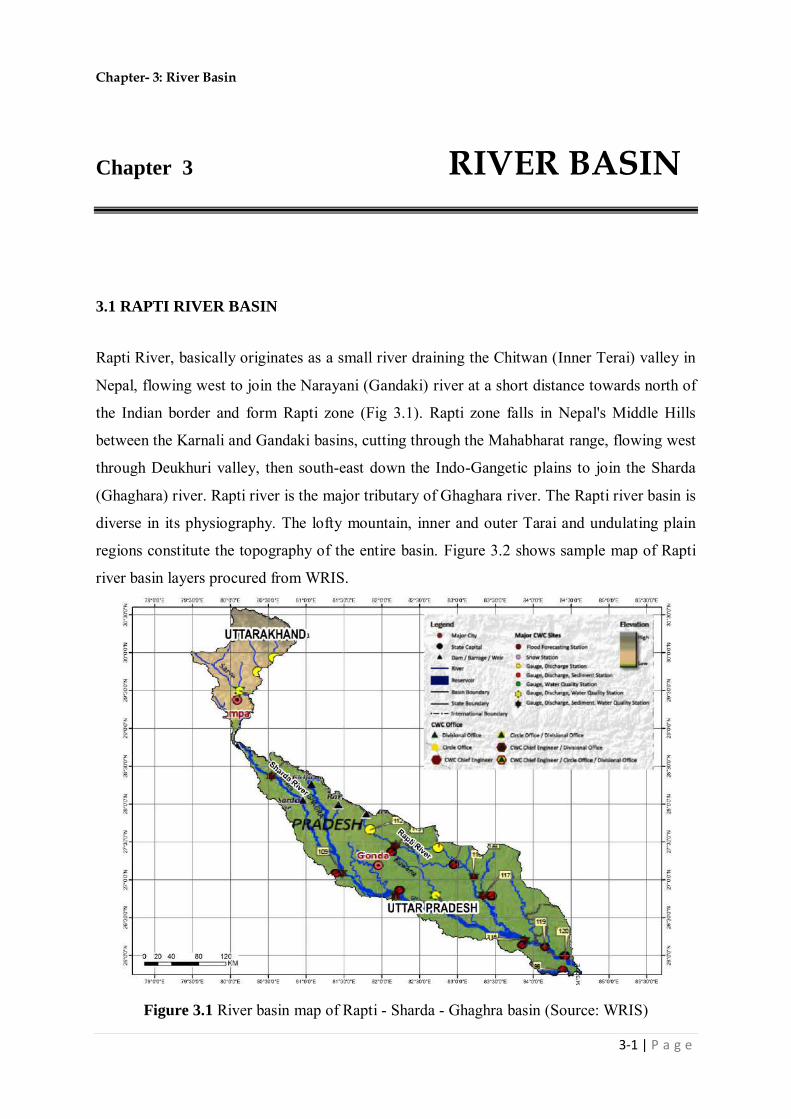
Chapter- 3: River Basin
3-1 | P a g e
Chapter 3 RIVER BASIN
3.1 RAPTI RIVER BASIN
Rapti River, basically originates as a small river draining the Chitwan (Inner Terai) valley in
Nepal, flowing west to join the Narayani (Gandaki) river at a short distance towards north of
the Indian border and form Rapti zone (Fig 3.1). Rapti zone falls in Nepal's Middle Hills
between the Karnali and Gandaki basins, cutting through the Mahabharat range, flowing west
through Deukhuri valley, then south-east down the Indo-Gangetic plains to join the Sharda
(Ghaghara) river. Rapti river is the major tributary of Ghaghara river. The Rapti river basin is
diverse in its physiography. The lofty mountain, inner and outer Tarai and undulating plain
regions constitute the topography of the entire basin. Figure 3.2 shows sample map of Rapti
river basin layers procured from WRIS.
Figure 3.1 River basin map of Rapti - Sharda - Ghaghra basin (Source: WRIS)
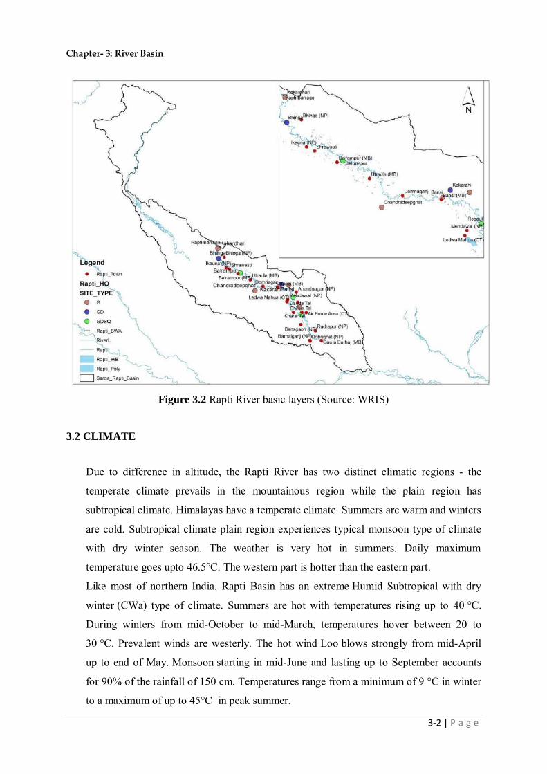
Chapter- 3: River Basin
3-2 | P a g e
Figure 3.2 Rapti River basic layers (Source: WRIS)
3.2 CLIMATE
Due to difference in altitude, the Rapti River has two distinct climatic regions - the
temperate climate prevails in the mountainous region while the plain region has
subtropical climate. Himalayas have a temperate climate. Summers are warm and winters
are cold. Subtropical climate plain region experiences typical monsoon type of climate
with dry winter season. The weather is very hot in summers. Daily maximum
temperature goes upto 46.5°C. The western part is hotter than the eastern part.
Like most of northern India, Rapti Basin has an extreme Humid Subtropical with dry
winter (CWa) type of climate. Summers are hot with temperatures rising up to 40 °C.
During winters from mid-October to mid-March, temperatures hover between 20 to
30 °C. Prevalent winds are westerly. The hot wind Loo blows strongly from mid-April
up to end of May. Monsoon starting in mid-June and lasting up to September accounts
for 90% of the rainfall of 150 cm. Temperatures range from a minimum of 9 °C in winter
to a maximum of up to 45°C in peak summer.

Chapter- 3: River Basin
3-3 | P a g e
3.3 METEOROLOGICAL STATIONS
Meteorological sites (Raingauge) of the Indian Meteorological Dept. located in the basin of
the Rapti river are shown in Fig. 3.3.
Figure 3.3 Rain gauge stations of Rapti basin (Source: WRIS)
3.4. BASIN GEOLOGY
Geologically, the Rapti river basin may be divided into three zones:
The northern mountain zone or Shiwalik Himalaya,
The tarai zone, and
The plain zone.
The Northern Mountain Zone or Shiwalik Himalaya: It forms the foothills of the
Himalayan Range and is essentially composed of Miocene to Pleistocene molassic sediments
derived from the erosion of the Himalaya. These molasse deposits, known as the Muree and
Siwaliks Formations, are internally folded and imbricated. The Sub Himalaya is thrust along
the Main Frontal Thrust over the Quaternary alluvium deposited by the rivers coming from

Chapter- 3: River Basin
3-4 | P a g e
the Himalaya (Ganga, Indus, Brahmaputra and others), which demonstrates that the Himalaya
is still a very active orogen.
The Tarai Zone: The Tarai is crossed by the large perennial Himalayan rivers Yamuna,
Ganga, Sharda, Karnali, Narayani and Kosi that have each built alluvial fans covering
thousands of square kilometres below their exits from the hills. Medium rivers such as
the Rapti rise in the Mahabharat Range. The geological structure of the region consists of old
and new alluvium, both of which constitute alluvial deposits mainly of sand, clay, silt, gravels
and coarse fragments. The new alluvium is renewed every year by fresh deposits brought
down by active streams, which engage themselves in fluvial action. Old alluvium is found
rather away from river courses, especially on uplands of the plain where silting is a rare
phenomenon.
The Plain Zone: The reduction in slope as rivers exit the hills and then transition from the
sloping Bhabhar to the nearly level Tarai causes current to slow and the heavy sediment load
to fall out of suspension. This deposition process creates multiple channels with shallow
beds, enabling massive floods as monsoon-swollen rivers overflow their low banks and shift
channels. Many areas show erosion such as gullies. This area consists of highly fertile and
arable land.
Geology of Rapti - Sharda - Ghaghra Basin as obtained from GSI is shown in Fig. 3.4.

Chapter- 3: River Basin
3-5 | P a g e
Figure 3.4 Geology of Rapti - Sharda - Ghaghra basin (Source: GSI)
3.5 LAND USE & LAND COVER
Land use land cover map of Rapti - Sharda - Ghaghra Basin as obtained from WRIS is shown
in Fig. 3.5, while Fig. 3.6 shows land use land cover map of Rapti basin explicitly.
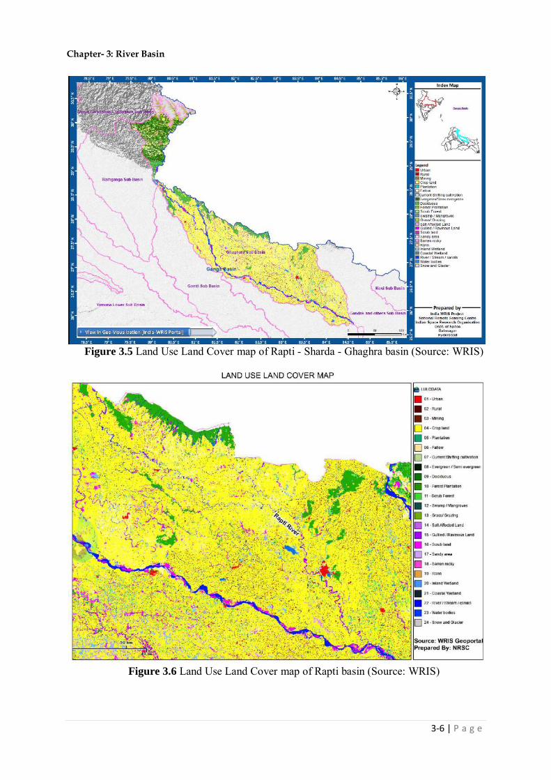
Chapter- 3: River Basin
3-6 | P a g e
Figure 3.5 Land Use Land Cover map of Rapti - Sharda - Ghaghra basin (Source: WRIS)
Figure 3.6 Land Use Land Cover map of Rapti basin (Source: WRIS)

Chapter- 3: River Basin
3-7 | P a g e
3.6 FLOOD AFFECTED AREA
The Indo-Gangetic and Brahmaputra river basins are the most chronic flood prone areas and
are regarded as the worst flood affected region in the world (Agarwal and Sunita, 1991).
Every year states like Assam located in Brahmaputra basin and Bihar, Uttar Pradesh and
West Bengal located in Indo-Gangetic basin face severe flood problems due to the huge
amount of discharge and large volume of sediments brought down from the Himalayan
Rivers and their tributaries during the monsoon season. The recurring floods cause loss of
life, destruction and damages to existing infrastructure, including roads, bridges,
embankments and agricultural land and stress the need for identification of flood prone areas
in the country. Identification of flood prone areas is one of the most important non-structural
measures for mitigation of floods (Jain et.al. 2005).
Flood hazard zonation facilitates appropriate regulation, and development of floodplains
thereby reducing the flood impact. The recurrent flood events at frequent intervals demand
the need for identification of flood hazard prone areas for prioritizing appropriate flood
control measures. In this context, satellite remote sensing plays an important role in
delineating such flood hazard zones.
Generation of the Flood hazard zones was done based on the analysis of multi-temporal
satellite data acquired during the floods of 2003-2013. Three major steps are involved in
preparation of flood hazard zonation maps.
i. Satellite data Planning and Acquisition: Data from Indian Remote Sensing
Satellites (IRS) and Landsat satellites was acquired during the floods. The water
levels observed at different gauge stations were closely monitored during floods and
attempts were made to program the satellite data during peak/near peak situations.
ii. Rectification: The acquired satellite datasets were geo-rectified to Lambert
Conformal Conic projection system with Modified Everest Datum for achieving
positional accuracy.
iii. Flood inundation layer preparation: Using image processing classification
algorithms, water layer was extracted from the satellite data and integrated with the
pre-flood river and water bodies layer to derive flood inundation layer.
Flood hazard zone map of Rapti - Sharda - Ghaghra Basin as obtained from NRSC is
shown in Fig. 3.7, while Fig. 3.8 shows flood hazard zone map of Rapti basin.

Chapter- 3: River Basin
3-8 | P a g e
Figure 3.7 Flood hazard zone map of Rapti - Sharda - Ghaghra basin (Source: NRSC)
Figure 3.8 Aggregated flood map of Rapti basin from 2003-2013 (Source: NRSC)

Chapter- 3: River Basin
3-9 | P a g e
3.7 CONCLUDING REMARKS
Various aspects of the Rapti basin related to topography, soil, climate, geology,
meteorological stations, land use land cover, flood map etc. are compiled in this chapter from
the different sources like GSI, WRIS and NRSC.

Chapter- 4: Study Reach
4-1 | P a g e
Chapter 4 STUDY REACH
4.1 THE STUDY AREA
The reach of the Rapti river studied in this project work is from Nepalganj to confluence
point of Rapti and Ghaghra which lies between longitudes 81°03'00" E to 83°45'06" E and
latitudes 26°18'00" N to 28°05'00" N as shown in Fig. 4.1. Rapti river covers an area of
25,793 km2 out of which 44% (11,401 km2) lies in Nepal and 56% (14,392 km2) in Uttar
Pradesh. A photograph of confluence point of Rapti and Ghaghra rivers is shown in Fig. 4.2.
The Rapti river flows in the sub-humid to humid monsoon region of the middle Ganga plain.
It is the largest tributary of river Ghaghra, which itself is one of the major tributaries of the
Ganga River. Rapti River flows through the districts of Rukum, Salyan, Rolpa, Gurmi,
Arghakhanchi, Dang and Banke of Nepal territory; and Bahraich, Shrawasti, Balrampur,
Siddharthnagar, Santkabinagar, Gorakhpur and Deoria districts of the Eastern Uttar Pradesh.
The Rapti river basin is diverse in its physiography. The lofty mountain, inner and outer tarai
and undulating plain regions constitute the topography of the entire basin. Due to difference
in altitude, the Rapti river has two distinct climatic regions, the temperate climate prevails in
the mountainous region while the plain has subtropical climate. Himalayas has a temperate
climate. Summers are warm and winters are cool to severe. Subtropical Climate plain region
experiences typical monsoon type of climate with dry winter season. The weather is very hot
in summers. Daily maximum temperature goes upto 46.5°C. The western part is hotter than
the eastern part.
The Rapti River was historically known as Iravati. The river originates in the Siwalik
Himalayas of Nepal at an elevation of 3050 m. After flowing through Nepal, it enters eastern
Uttar Pradesh in Chanda Pargana, east of the Kundwa village of Bahraich District. It flows in
a very sinuous course with shallow depth and causes heavy flooding in the districts of eastern
Uttar Pradesh. The Rapti River has a total length of about 776 km from its origin to its

Chapter- 4: Study Reach
4-2 | P a g e
confluence with the Ghaghra at Barha. Out of this, 290 km lie in Nepal territory. After the
hair pin bend just above the Indo-Nepal border, the river maintains a south-easterly direction
passing through a number of lakes and swamps and some abandoned water courses.
The course of the Rapti River can be divided into three sections. The first section is
mountainous, in this section, the river runs in a longitudinal valley. It receives the combined
waters of Madi, Lungi and Jhirmuk. The altitude drops from 3000 m to 1500 m and the slope
of this section is steep.
The second section of the river is called Rapti Dun. This section of the river flows up to
Nepalganj. Here, the river turns south presenting an elbow towards Nepalganj. The altitude of
this section varies from 300 m to 150 m.
In the third section, the Rapti River enters the tarai region of eastern Uttar Pradesh. In this
tarai region, the gradient is very low throughout its easterly. The altitude of this section varies
from 100 m to 80 m. Other salient features of the Rapti basin are as follow:
Drainage Area : 25,793 km2
Important Tributaries within Study Reach :Bhakia, Gaura, Kacna, Kunhara, Sunawan
Important Habitat :Gorakhpur, Bansi, Balrampur, Baharaich,
Water Resources Projects : Rapti Barrage, Rapti Sarayu Canal (Fig. 4.3)

Chapter- 4: Study Reach
4-3 | P a g e
Figure 4.1 River Rapti from Nepalgunj to confluence point of Rapti and Ghaghra
Figure 4.2 Confluence point of Rapti and Ghaghra river
Rapti River
Ghaghra River

Chapter- 4: Study Reach
4-4 | P a g e
Figure 4.3 Major water resources projects (Source: INDIA-WRIS, 2012)
4.2 CONCLUDING REMARKS
Morphological changes of the rivers are more pronounced in the plain area. Therefore
considered reach of the Rapti river in this study is relatively flat and varies from elevation
150 m to 80 m. It starts from Nepalganj and ends at Confluence point of Rapti river with
Ghaghra river.

Chapter- 5: Input Data & Methodology
5-1 | P a g e
Chapter 5 INPUT DATA & METHODOLOGY
5.1 HYDRO-METEOROLOGICAL DATA
The various gauging sites on Rapti River as given in Table 5.1 and shown in Fig. 5.1 were
identified and requisition was sent to concerned Chief Engineers of CWC for the
procurement of the data comprising of annual maximum and minimum discharge and water
level, 10-daily water level, discharge and silt data and also cross-section data.
Table 5.1 Hydro-meteorological data
S.
No.
Name
of River
Name of
G&D Sites District
Chainage
(km) Concerned Agency
1. Rapti Kakardhari Gonda, UP 517 CWC (MGD-I), Lucknow 2. Rapti Balrampur Gonda, UP 396 CWC (MGD-I), Lucknow 3. Rapti Bansi Basti, UP 250 CWC (MGD-I), Lucknow
4. Rapti Rigauli Gorakhpur, UP 183 CWC (MGD-I), Lucknow
5. Rapti Gorakhpur (Birdghat)
Gorakhpur, UP 120 CWC (MGD-I), Lucknow
Following data have been received:
a) Gauging Site: Kakardhari
Maximum water level from year 1971-2015
b) Gauging Site: Balrampur
Maximum water level from year 1971-2015
Maximum discharge from year 1971-2015
10-daily silt data year 1985-2015
Cross-sectional data: Pre-monsoon 2010 to 2014
Post-monsoon 2013 to 2014
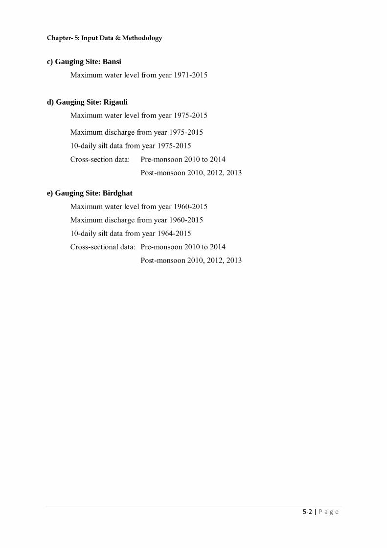
Chapter- 5: Input Data & Methodology
5-2 | P a g e
c) Gauging Site: Bansi
Maximum water level from year 1971-2015
d) Gauging Site: Rigauli
Maximum water level from year 1975-2015
Maximum discharge from year 1975-2015
10-daily silt data from year 1975-2015
Cross-section data: Pre-monsoon 2010 to 2014
Post-monsoon 2010, 2012, 2013
e) Gauging Site: Birdghat
Maximum water level from year 1960-2015
Maximum discharge from year 1960-2015
10-daily silt data from year 1964-2015
Cross-sectional data: Pre-monsoon 2010 to 2014
Post-monsoon 2010, 2012, 2013
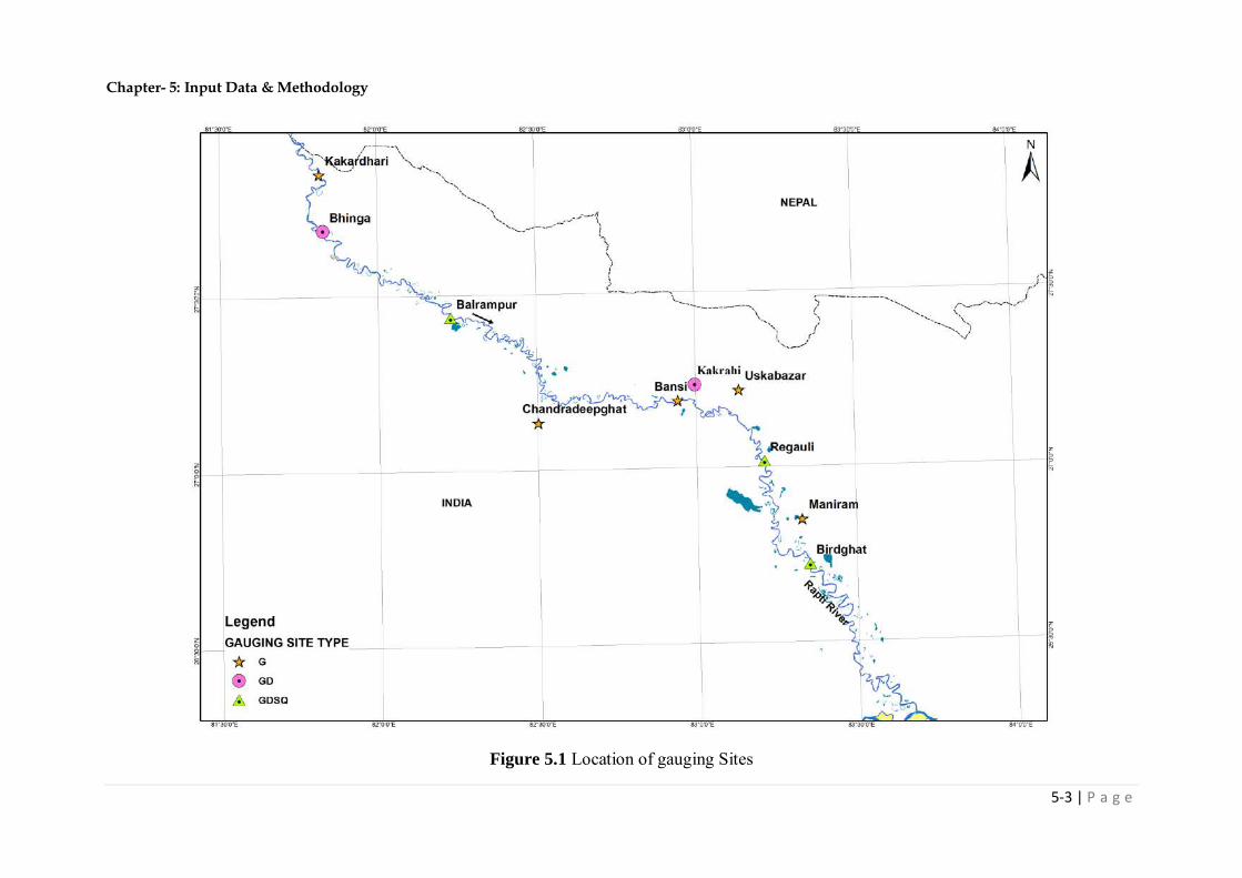
Chapter- 5: Input Data & Methodology
5-3 | P a g e
Figure 5.1 Location of gauging Sites
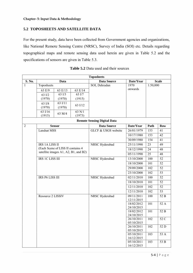
Chapter- 5: Input Data & Methodology
5-4 | P a g e
5.2 TOPOSHEETS AND SATELLITE DATA
For the present study, data have been collected from Government agencies and organizations,
like National Remote Sensing Centre (NRSC), Survey of India (SOI) etc. Details regarding
topographical maps and remote sensing data used herein are given in Table 5.2 and the
specifications of sensors are given in Table 5.3.
Table 5.2 Data used and their sources
Toposheets
S. No. Data Data Source Date/Year Scale
1 Toposheets SOI, Dehradun 1970 onwards
1:50,000 63 E/9 63 E/13 63 E/14 63 I/2 (1970)
63 I/3 (1970)
63 I/7 (1915)
63 I/8 (1970)
63 I/11 (1970) 63 I/12
63 I/16 (1915) 63 M/4 63 N/1
(1973) Remote Sensing Digital Data
2 Sensor Data Source Date/Year Path Row
Landsat MSS GLCF & USGS website 26/01/1979 153 41 10/17/1980 153 42 30/09/1980 154 41
IRS 1A LISS II (Each Scene of LISS II contains 4 satellite images A1, A2, B1, and B2)
NRSC Hyderabad 25/11/1990 23 49 18/12/1990 24 48 05/11/1990 25 48
IRS 1C LISS III NRSC Hyderabad 13/10/2000 100 52 18/10/2000 101 52 29/09/2000 102 52 23/10/2000 102 53
IRS P6 LISS III NRSC Hyderabad 02/11/2010 100 52 18/10/2010 101 52 12/11/2010 102 52 12/11/2010 102 53
Resource 2 LISSIV NRSC Hyderabad 09/11/2011 12/11/2015
100 52 B
18/02/2012 24/10/2015
101 52 A
18/02/2012 24/10/2015
101 52 B
26/10/2011 05/10/2015
102 52 C
26/10/2011 05/10/2015
102 52 D
05/10/2011 16/12/2015
103 53 A
05/10/201116/12/2015
103 53 B

Chapter- 5: Input Data & Methodology
5-5 | P a g e
Table 5.3 Sensors specifications
Specifications LANDSAT
MSS
IRS 1A
LISS II
IRS 1C
LISS III
IRS P6
LISS III
Spectral Bands 1-5 1-4 1-4 1-4 Spatial Resolution (m) 60 36.25 23.5 23.5 Swath Width (km) 185×185 141 141 141
Radiometric Resolution (bits) 8 7 7 7
5.3 SOFTWARE
The flowing softwares have been used in this study
ArcGIS 10.2
ERDAS Imagine 10.1
Microsoft Office & Excel
Sigma Plot
Matlab
5.4 ACQUISITION OF DATA AND GEO-REFERENCING OF IMAGES
Firstly, the Survey of India toposheets (1:50000 scale) which covers the area of interest are
procured. Then, these toposheets have been geo-referenced and ortho-rectified using first
order polynomial and Lambert Conformal Conic (LCC) projection type with the help of
ERDAS Imagine 2014 software, before initiating the analysis. After geo-referencing, clipping
and mosaicing have been done.
Relevant satellite images were procured from the NRSC (National Remote Sensing Centre),
Hyderabad or downloaded from United States Geological Survey (USGS) website. Pre-
processing of the satellite images have been carried out using filters such as histogram
equalization and matching etc. to improve and equalize the brightness levels of similar
features and provide uniform information. After mosaicing the toposheets, all the satellite
images were geo-referenced using image to image method by selecting several control points.
The RMS error has been kept below the half pixel size. After geo-referencing, images have
been mosaiced to cover the entire study area. For mosaicing feather option of the software
has been used to get the seamless boundaries between different images of the same year.
Chapter- 5: Input Data & Methodology
5-6 | P a g e
5.5 METHODOLOGY FOR PLAN FORM CHANGES
Plan form of the rivers may be described as straight, meandering or braided. There are in fact
a great range of channel patterns from straight through meandering to braid. Methodology
adopted to fulfil the objective in respect of planform changes of the river is shown in Fig. 5.2
in a form of a methological flowchart:
In the present study of morphology of Rapti River, sinuosity ratio and PFI index of the river
shall be estimated using the satellite images for different years. The temporal and spatial
variation of sinuosity ratio and PFI index for different reaches shall be shown graphically.
5.6 FLOW PROBABILITY CURVES
Flood frequency analysis shall be carried out for the recorded discharge data at various CWC
gauging sites on the river for the estimation of discharges for 1.5 to 2 year return periods.
Discharge for higher return periods shall also be estimated using frequency analysis to
correlate the peak discharges with the morphological parameters of the rivers. Details of the
frequency analysis are given below:
Frequency analysis of recorded maximum stream flow data is an important flood-runoff
analysis tool. The objective of flood frequency analysis is to infer the probability of
exceedance of all possible discharge values (the parent population) from observed discharge
values (a sample of the parent population). This process is accomplished by selecting a
statistical model that represents the relationship of discharge magnitude and exceedance
probability for the parent population. The parameters of the models are estimated from the
sample.
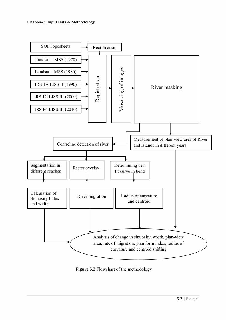
Chapter- 5: Input Data & Methodology
5-7 | P a g e
Figure 5.2 Flowchart of the methodology
SOI Toposheets
Landsat – MSS (1980)
IRS 1A LISS II (1990)
IRS 1C LISS III (2000)
IRS P6 LISS III (2010)
Rectification
Reg
istra
tion
Landsat – MSS (1970)
River masking
Mos
aici
ng o
f im
ages
Centreline detection of river
Segmentation in different reaches
Calculation of Sinuosity Index and width
Measurement of plan-view area of River and Islands in different years
Raster overlay
River migration
Determining best fit curve in bend
Radius of curvature and centroid
Analysis of change in sinuosity, width, plan-view area, rate of migration, plan form index, radius of
curvature and centroid shifting

Chapter- 5: Input Data & Methodology
5-8 | P a g e
Commonly used methods for the frequency analysis are
(a) Graphical methods
In this method, the annual maximum flood data are arranged in descending order and rank is
assigned to each data. The highest flood data is assigned a rank 1 second highest 2 and like-
wise others. This arrangement of data gives an estimate of the exceedance probability, that is,
the probability of a value being equal to or greater than the ranked value. The probability of a
data being equal to or exceeded is calculated by Weibull formula
1
N
mP
(5.1)
where m is the rank of the data and N is the total number of the data. The return period for the
event
T=1/P (5.2)
A plot of discharge Q vs time T yields the probability distribution. Return period for any
discharge can be read from the fitted data on the probability plot.
(b) Analytical methods
Commonly used frequency distribution functions for the prediction of extreme flood values
analytically are
i. Gumbel’s extreme value distribution method
ii. Log-Pearson Type-II distribution
iii. Log normal distribution
The best fitted probability distribution shall be used to estimate the discharge for higher
return period.
In addition to the above, hydraulic structures constructed across and along the rivers like
barrages, bridges etc shall be identified from Google Earth images and details of those
structures shall be collected from concerned department. The morphological changes of the
river in the vicinity of the structure shall be studied using high resolution images and changes
in morphology due to construction of the structure shall be assessed in the form of shifting of
banks and erosion/deposition of the sediments.

Chapter- 5: Input Data & Methodology
5-9 | P a g e
5.7 CONCLUDING REAMRKS
The following tasks shall be performed in this study
Reach-wise temporal analysis of main (deeper channel), left and right bank of river.
Estimation of eroded/deposited area of the river, and their presentation in a graphical
form, with length of the river on x-axis and erosion & deposition on y-axis.
Length-wise variation of sinuosity ratio and Plan Form Index (PFI) for the evaluation
of meandering and braiding patterns of the river.
Identification of levels of braiding using Plan Form Index threshold values.
Detailed analysis of the shifting of river in the critical reaches using high resolution
satellite images.
Plotting of probability curve for discharge at various gauging sites of the river using
the recorded flow data for 1.5 years and 2 years return period.
Flood discharge for higher return periods shall also be computed using the frequency
analysis.
After the identification of critical reaches, that will be characterized by major left and
right bank shifting inserting heavy erosion/deposition, river training works in the form
of flood walls, guide bunds, sparse submerged vanes, porcupines etc. shall be
suggested.
Reconnaissance survey shall be carried out near the major hydraulic structures and
also the critical reaches to assess the morphological changes of the river onset of the
construction of the hydraulic structures.
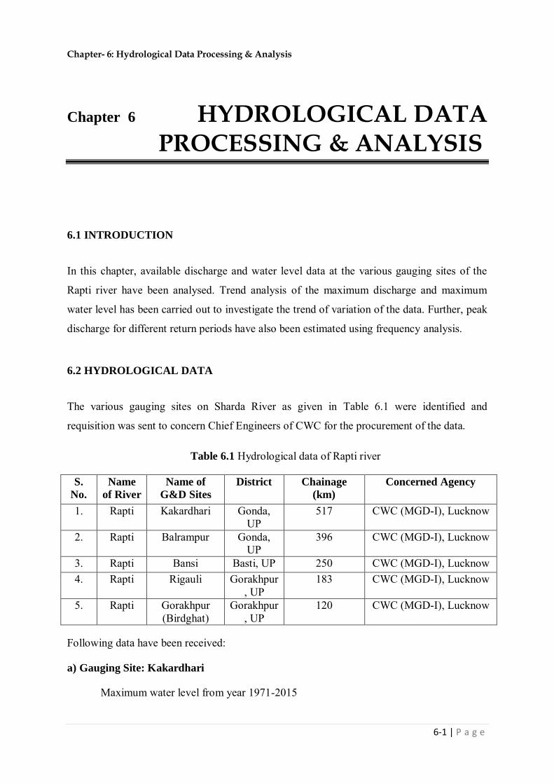
Chapter- 6: Hydrological Data Processing & Analysis
6-1 | P a g e
Chapter 6 HYDROLOGICAL DATA PROCESSING & ANALYSIS
6.1 INTRODUCTION
In this chapter, available discharge and water level data at the various gauging sites of the
Rapti river have been analysed. Trend analysis of the maximum discharge and maximum
water level has been carried out to investigate the trend of variation of the data. Further, peak
discharge for different return periods have also been estimated using frequency analysis.
6.2 HYDROLOGICAL DATA
The various gauging sites on Sharda River as given in Table 6.1 were identified and
requisition was sent to concern Chief Engineers of CWC for the procurement of the data.
Table 6.1 Hydrological data of Rapti river
S.
No.
Name
of River
Name of
G&D Sites
District Chainage
(km)
Concerned Agency
1. Rapti Kakardhari Gonda, UP
517 CWC (MGD-I), Lucknow
2. Rapti Balrampur Gonda, UP
396 CWC (MGD-I), Lucknow
3. Rapti Bansi Basti, UP 250 CWC (MGD-I), Lucknow 4. Rapti Rigauli Gorakhpur
, UP 183 CWC (MGD-I), Lucknow
5. Rapti Gorakhpur (Birdghat)
Gorakhpur, UP
120 CWC (MGD-I), Lucknow
Following data have been received:
a) Gauging Site: Kakardhari
Maximum water level from year 1971-2015

Chapter- 6: Hydrological Data Processing & Analysis
6-2 | P a g e
b) Gauging Site: Balrampur
Maximum water level from year 1971-2015
Maximum discharge from year 1971-2015
10-daily silt data year 1985-2015
Cross-sectional data: Pre-monsoon 2010 to 2014
Post-monsoon 2013 to 2014
c) Gauging Site: Bansi
Maximum water level from year 1971-2015
d) Gauging Site: Rigauli
Maximum water level from year 1975-2015
Maximum discharge from year 1975-2015
10-daily silt data year 1975-2015
Cross-section data: Pre-monsoon 2010 to 2014
Post-monsoon 2010, 2012, 2013
e) Gauging Site: Birdghat
Maximum water level from year 1960-2015
Maximum discharge from year 1960-2015
10-daily silt data year 1964-2015
Cross-sectional data: Pre-monsoon 2010 to 2014
Post-monsoon 2010, 2012, 2013
6.3 TEMPORAL VARIATION OF MAXIMUM DISCHARGE AND MAXIMUM
WATER LEVEL
Temporal variation of maximum observed discharge and maximum observed water level on
various gauging sites on Rapti river has been carried out using the available data. Temporal
variation of the maximum observed discharge during period 1971-2015 at Balrampur, during
1975-2015 at Rigauli, during 1960-2015 at Birdghat are shown in Figs. 6.1a-c, respectively.
It may be concluded that maximum discharge at Balrampur has decreasing trend, however,
no trend has been found at Rigauli and Birdghat gauging sites. Like-wise Figs 6.2a-e show
Chapter- 6: Hydrological Data Processing & Analysis
6-7 | P a g e
process is accomplished by selecting a statistical model that represents the relationship of
discharge magnitude and exceedance probability for the parent population. The parameters of
the models are estimated from the sample.
Annual maximum observed discharge data at gauging sites Balrampur (1971-2015), Rigauli
(1975-2015), Birdghat (1960-2015) on Rapti river have been used to estimate the flood
discharge for different return periods. Following distribution methods have been used herein.
(a) Gumbel’s Extreme Value Distribution method
The annual maximum discharge for T year returns period QT is defined as
KQQT
Where Q = average of annual maximum discharge
= standard deviation of available annual maximum discharge data
K = Frequency factor and expressed as
n
nT
S
yyK
yT = reduced variate and function of return period T
1ln.ln
T
TyT
ny = mean and function of sample size, N
Sn = reduced standard deviation and function of N
T = Return period in year
(b) Log-Pearson Type III Distribution method
In this method, the variate is first transformed into logarithmic form and the transformed data
is then analysed. For any return period T
zzT KZZ
and Z = log (Q)

Chapter- 6: Hydrological Data Processing & Analysis
6-8 | P a g e
Where Q = variate of available flood data
= standard deviation of the Z variate= 1
2
N
ZZ
Kz = Frequency factor and function of return period T and the coefficient of skewness, Cs of variate Z.
3
3
)2)(1( z
sNN
ZZNC
Z = mean of the variate Z
N = number of sample, i.e. discharge data
(c) Log Normal Distribution method
Log-Pearson Type III distribution reduces to Log normal distribution when the coefficient of
skewness of variate Z is zero, i.e., Cs =0. Procedure for estimation of peak discharge would
be same as the Log pearson Type III distribution method.
Estimated peak discharge at Palia kalan using different probability methods are given in
Table 6.2.
Table 6.2 Peak discharge of various return periods from various distributions
Method Station Peak Discharge (m3/s)
Return period
25 yr 50 yr 100 yr
Gumbel’s Extreme Value Birdghat Rigauli
Balrampur Log Normal Birdghat
Rigauli Balrampur
Log Pearson Type III
Birdghat Rigauli
Balrampur Average value--> Birdghat
Rigauli Balrampur

Chapter- 6: Hydrological Data Processing & Analysis
6-9 | P a g e
6.5 PROBABILITY EXCEEDANCE CURVE
Probability exceedance curve for estimation of the discharges for 1.5 to 2 year return periods
using 10-daily discharge data have not been carried out due to unavailability of the data.
6.6 CONCLUDING REMARKS
Analysis of maximum observed discharge and maximum observed water level at different
gauging sites on Rapti river using the available data indicates that there is no remarkable
trend of temporal variation of maximum discharge and maximum water level at the gauging
sites Kakardhari, Balrampur, Bansi, Rigauli and Birdghat over a long period of time.
However, maximum discharge at Balrampur has decreasing trend, however, no trend has
been found at Rigauli and Birdghat gauging sites. The maximum water level has increasing
trend at Kakardhari and Balrampur and decresing trend at Bansi, however, no trend was
found at gauging sites of Rigauli and Birdghat.

Chapter- 7: River Morphology
7-1 | P a g e
Chapter 7 RIVER MORPHOLOGY
7.1 DELINEATION/DIGITIZATION OF RIVER BANK LINES
The river bank lines have been identified and delineated from mosaics for all the satellite images
of year 1970, 1980, 1990, 2000 and 2010 as shown in Figs. 7.1 to 7.5. The identified river bank
lines for the left, right and center (main channel) have been digitized using ArcMap software.
The left bank, right bank and centerline have been prepared for the years 1970, 1980, 1990, 2000
and 2010. The length of arcs of the left bank, right bank and centerline for all the above years has
been calculated using GIS software. Shifting of centerline, left bank, right bank of the river has
been evaluated with respect to river course of year 2010.
Figure 7.1 Mosaic of SOI toposheets of Rapti river of year 1970 (Scale 1:50,000)

Chapter- 7: River Morphology
7-2 | P a g e
Figure 7.2 Mosaic of FCC of Rapti river of year 1980 (Landsat-MSS Images)
Figure 7.3 Mosaic of FCC of Rapti river of year 1990 (IRS 1A LISS II Images)
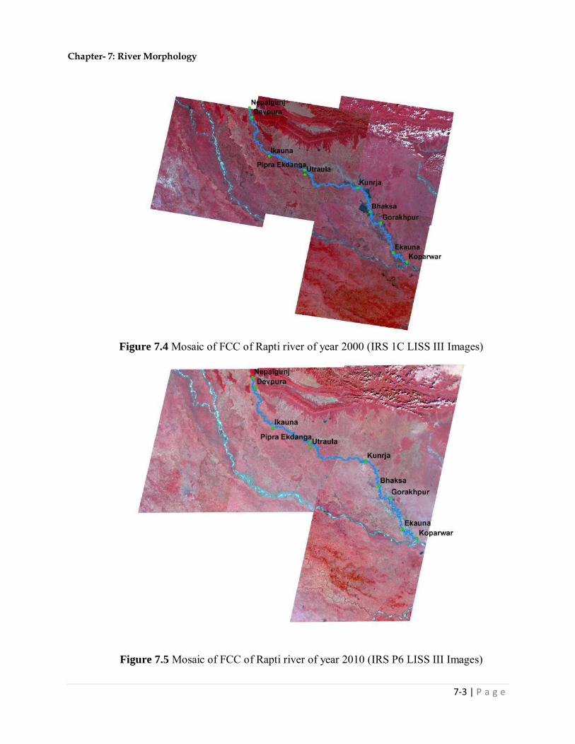
Chapter- 7: River Morphology
7-3 | P a g e
Figure 7.4 Mosaic of FCC of Rapti river of year 2000 (IRS 1C LISS III Images)
Figure 7.5 Mosaic of FCC of Rapti river of year 2010 (IRS P6 LISS III Images)
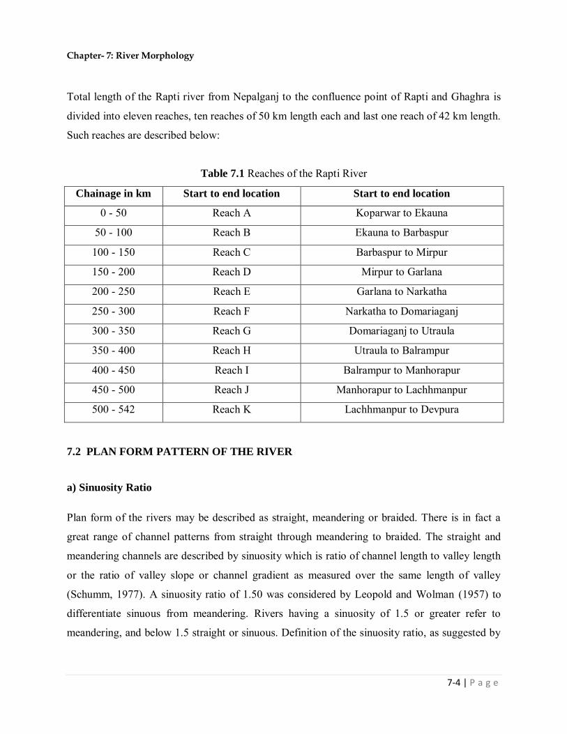
Chapter- 7: River Morphology
7-4 | P a g e
Total length of the Rapti river from Nepalganj to the confluence point of Rapti and Ghaghra is
divided into eleven reaches, ten reaches of 50 km length each and last one reach of 42 km length.
Such reaches are described below:
Table 7.1 Reaches of the Rapti River
Chainage in km Start to end location Start to end location
0 - 50 Reach A Koparwar to Ekauna
50 - 100 Reach B Ekauna to Barbaspur
100 - 150 Reach C Barbaspur to Mirpur
150 - 200 Reach D Mirpur to Garlana
200 - 250 Reach E Garlana to Narkatha
250 - 300 Reach F Narkatha to Domariaganj
300 - 350 Reach G Domariaganj to Utraula
350 - 400 Reach H Utraula to Balrampur
400 - 450 Reach I Balrampur to Manhorapur
450 - 500 Reach J Manhorapur to Lachhmanpur
500 - 542 Reach K Lachhmanpur to Devpura
7.2 PLAN FORM PATTERN OF THE RIVER
a) Sinuosity Ratio
Plan form of the rivers may be described as straight, meandering or braided. There is in fact a
great range of channel patterns from straight through meandering to braided. The straight and
meandering channels are described by sinuosity which is ratio of channel length to valley length
or the ratio of valley slope or channel gradient as measured over the same length of valley
(Schumm, 1977). A sinuosity ratio of 1.50 was considered by Leopold and Wolman (1957) to
differentiate sinuous from meandering. Rivers having a sinuosity of 1.5 or greater refer to
meandering, and below 1.5 straight or sinuous. Definition of the sinuosity ratio, as suggested by

Chapter- 7: River Morphology
7-5 | P a g e
various investigators, is given in the Table 7.2, however, definition proposed by Leopold and
Wolman (1957) is commonly used.
Table 7.2 Definition of sinuosity ratio
The modified sinuosity parameter, P, as defined by Friend and Sinha (1993) has been used for
this study.
P = Lcmax/LR (7.1)
Where, LR is overall length of the channel belt reach measured along a straight line, or the valley
length, and Lcmax is the mid channel length for the same reach or the stream length. The sample
map that depicts the computation of river sinuosity is shown in Fig. 7.6a. Fig 7.6b shows channel
patterns for different Sinuosity ratio.
It is apparent from Fig. 7.7 that there is no definite progressive change in the sinuosity ratio of
the Rapti river in the span of time 1970 to 2010 in the studied reach. High sinuosity ratio was
noticed in the reach of Chainage 25-50 km, 75-100 km and 300-425 km. Rapti river possess
lower sinuosity ratio in upper reaches.
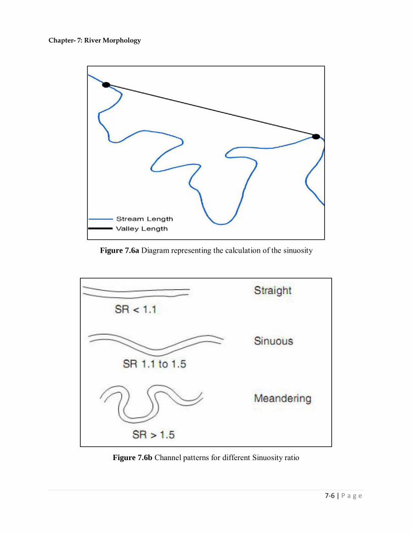
Chapter- 7: River Morphology
7-6 | P a g e
Figure 7.6a Diagram representing the calculation of the sinuosity
Figure 7.6b Channel patterns for different Sinuosity ratio

Chapter- 7: River Morphology
7-7 | P a g e
Rapti river with a length of 542 km has been divided into reaches 50 km each in length. For
calculating sinuosity ratios, the river reach has been further divided into 25 km long reaches. The
total length of the river has been subdivided into 21 reaches of 25 km length, the last one being
15.68 km. Equation (7.1) has been used for the computation of sinuosity ratio. The calculated
values of sinuosity ratio are given in Table 7.3 and graphically shown in Fig 7.7.
The following data as given in Table 7.4 have been extracted from the computed sinuosity ratio
of the Rapti river:
Table 7.4a Sinuosity ratios of the Rapti river for different years
S.No. Year Maximum Sinuosity Minimum Sinuosity Average Sinuosity
1. 1970 3 1.37 1.8
2. 1980 2.9 1.11 1.88
3. 1990 2.83 1.14 1.79
4. 2000 2.79 1.42 1.87
5. 2010 2.8 1.55 1.92
It is apparent from Table 7.3 & 7.4a and Fig. 7.7a that the sinuosity ratio of the Rapti river in the
reach under consideration is higher than 1.5 in the year 1970, 1980, 1990, 2000, and 2010,
therefore, the Rapti is classified as meandering river.

Chapter- 7: River Morphology
7-8 | P a g e
Table 7.3 Sinuosity ratios for Rapti river of year 1970, 1980, 1990, 2000 and 2010
Chainage (km)
Section 2010 2000 1990 1980 1970
Lmax LR Sinuosity Lmax LR Sinuosity Lmax LR Sinuosity Lmax LR Sinuosity Lmax LR Sinuosity
12.5 1 25.00 14.53 1.72 24.48 14.44 1.70 25.93 14.49 1.79 25.55 14.44 1.77 27.53 14.40 1.91
37.5 2 25.00 8.87 2.82 24.76 8.88 2.79 25.15 8.87 2.83 25.75 8.89 2.90 26.56 8.85 3.00
62.5 3 25.00 14.55 1.72 23.94 14.53 1.65 23.03 14.44 1.59 21.90 14.48 1.51 22.49 14.41 1.56
87.5 4 25.00 9.70 2.58 24.15 9.75 2.48 23.37 9.74 2.40 22.75 9.64 2.36 26.75 9.81 2.73
112.5 5 25.00 14.96 1.67 25.17 15.05 1.67 25.12 15.26 1.65 23.76 15.19 1.56 22.65 15.32 1.48
137.5 6 25.00 12.41 2.01 24.60 12.20 2.02 23.01 12.08 1.91 24.90 12.24 2.04 23.31 12.11 1.92
162.5 7 25.00 14.51 1.72 24.70 14.33 1.72 23.96 14.37 1.67 22.79 15.00 1.52 24.60 15.37 1.60
187.5 8 25.00 12.44 2.01 23.58 12.41 1.90 23.52 12.44 1.89 22.72 11.81 1.92 24.13 11.88 2.03
212.5 9 25.00 13.92 1.80 24.05 13.96 1.72 24.84 14.00 1.77 24.80 13.95 1.78 25.21 14.00 1.80
237.5 10 25.00 11.77 2.12 22.88 11.74 1.95 23.11 11.71 1.97 20.34 11.70 1.74 19.01 11.86 1.60
262.5 11 25.00 16.16 1.55 24.79 16.23 1.53 24.71 16.29 1.52 24.13 16.47 1.47 23.43 15.67 1.50
287.5 12 25.00 15.83 1.58 24.11 15.75 1.53 24.07 15.67 1.54 23.99 15.52 1.55 22.19 15.95 1.39
312.5 13 25.00 12.88 1.94 32.49 12.94 2.51 29.41 12.94 2.27 29.66 13.00 2.28 29.20 13.48 2.17
337.5 14 25.00 10.50 2.38 22.00 10.49 2.10 17.79 10.48 1.70 19.86 10.48 1.89 17.45 10.46 1.67
362.5 15 25.00 11.49 2.18 19.86 11.42 1.74 22.42 11.12 2.02 27.33 10.99 2.49 24.77 10.92 2.27
387.5 16 25.00 15.22 1.64 27.55 15.05 1.83 24.73 14.98 1.65 23.45 15.41 1.52 23.45 15.97 1.47
412.5 17 25.00 13.22 1.89 29.45 13.43 2.19 21.21 13.84 1.53 37.67 13.79 2.73 28.17 12.82 2.20
437.5 18 25.00 15.00 1.67 26.50 15.11 1.75 19.02 14.85 1.28 25.51 14.43 1.77 23.62 14.45 1.63
462.5 19 25.00 11.04 2.27 18.84 10.90 1.73 24.85 11.34 2.19 24.81 12.15 2.04 24.28 11.99 2.03
487.5 20 25.00 15.00 1.67 23.05 14.96 1.54 22.51 14.80 1.52 25.35 14.24 1.78 20.16 14.68 1.37
512.5 21 25.00 14.00 1.79 21.55 13.71 1.57 21.92 13.58 1.61 21.80 13.92 1.57 23.63 14.14 1.67
537.5 22 15.68 9.79 1.60 13.69 9.64 1.42 10.18 8.92 1.14 9.95 9.00 1.11 13.19 8.58 1.54
Maximum 2.82 2.79 2.83 2.90 3.00
Minimum 1.55 1.42 1.14 1.11 1.37
Average 1.92 1.87 1.79 1.88 1.84

Chapter- 7: River Morphology
7-9 | P a g e
Figure 7.7a Sinuosity ratio of Rapti river of year 1970, 1980, 1990, 2000 and 2010

Chapter- 7: River Morphology
7-10 | P a g e
Geometrical parameters of the prominent meanders such as axial wavelength, amplitude and
radius of curvature as shown in Fig. 7.7b have been calculated and listed in the Table 7.4b.
Prominent meanders are numbered as M-1 to M-16 and shown in Figures 7.7c-h.
Figure 7.7b Geometrical parameters of a river meander (Sinha 2012)
Table 7.4b Geometrical parameters of the prominent meanders in the Rapti river
Meander
No.
Chainage
(km)
Location Year Axis wave length
(km)
Amplitude
(km)
Radius of
Curvature (km)
M-1 8 Sareya
1970 1.5 2.8 0.8 1980 SR~1 1990 SR~1 2000 SR~1 2010 SR~1
M-2 35 Bahsua
1970 2 3.5 0.9 1980 2 3.5 0.9 1990 2 3.5 0.9 2000 2 3.5 0.9 2010 2 3.5 0.9
M-3 83 Kanail
1970 3.5 3.7 1.3 1980 3.3 3.5 1.3 1990 3.3 3.5 1.3 2000 3.3 3.5 1.3 2010 3.3 3.5 1.3

Chapter- 7: River Morphology
7-11 | P a g e
M-4 93 Choppra
1970 1.8 3.1 1.3 1980 2.1 3.5 1.3 1990 2.9 3.6 1.4 2000 2.9 3.6 1.4 2010 2.9 3.6 1.4
M-5 100 Barbaspur
1970 3.7 3.4 1.3 1980 3.7 3.4 1.3 1990 3.7 3.4 1.3 2000 3.7 3.4 1.3 2010 3.7 3.4 1.3
M-6 305 Rasulabad
1970 0.8 1.7 0.4 1980 1 2 0.6 1990 0.5 1.3 1.3 2000 0.5 1.3 1.3 2010 1.3 1.2 0.4
M-7 315 MahwaTerhwa
1970 SR~1 1980 1.2 1.3 0.5 1990 1.7 1.4 0.7 2000 0.7 1.3 0.5 2010 SR~1
M-8. 335 MahuaDhani
1970 3.6 1.8 1.7 1980 0.4 9.4 0.2 1990 0.6 1.7 0.4 2000 1.7 2.0 0.7 2010 1.7 2.1 0.7
M-9 350 Misraula
1970 0.5 1.1 0.5 1980 1.2 2.3 0.7 1990 1.3 2.0 0.5 2000 1.3 2.1 0.5 2010 1.1 1.9 0.5
M-10 375 Nandnagar
1970 1.3 2.4 0.5 1980 1.2 2.2 0.6 1990 1.1 1.6 0.4 2000 2.5 2.6 1.1 2010 2.3 2.9 1.0
M-11 390 Bilha
1970 1.8 1.6 0.5 1980 2.3 1.1 0.6 1990 2.5 1.3 0.8 2000 0.5 1.3 0.3 2010 1.1 1.1 0.4
M-12 400 Jyonar
1970 SR~1 1980 1.6 1.9 0.7 1990 1.7 3.0 1.3 2000 0.8 2.4 0.4 2010 0.7 3.0 0.6
M-13 413 KanlanderpurKhurd 1970 0.5 1.2 0.3 1980 1.2 2.4 0.6 1990 1.9 1.0 0.9

Chapter- 7: River Morphology
7-12 | P a g e
2000 0.9 1.7 0.4 2010 0.5 0.7 0.4
M-14 430 Shravasti
1970 2.0 2.6 0.8 1980 1.8 0.8 0.9 1990 2.2 1.4 1.0 2000 1.3 2.4 0.6 2010 1.9 1.3 0.6
M-15 450 Itwariya
1970 1.2 1.5 0.4 1980 2.0 0.8 0.7 1990 4.8 2.0 1.9 2000 2.0 2.0 0.8 2010 2.8 1.9 1.8
M-16 485 Lakshman Nagar
1970 3.1 1.6 1.5 1980 2.6 1.5 1.0 1990 2.0 1.6 0.8 2000 1.7 1.6 0.7 2010 1.9 1.6 0.8
From the Table 7.4b and Figures 7.7c-h, it may be concluded that in general the meanders are
relatively stable. Close examination of these figures indicate that almost whole reach of the river
has meandering pattern, however, it is prominent in the reaches 25-50 km, 75-100 km, 300-375
km, 400-425 km and 450-475 km. The meandering is characterised by acute bend with high
amplitude.
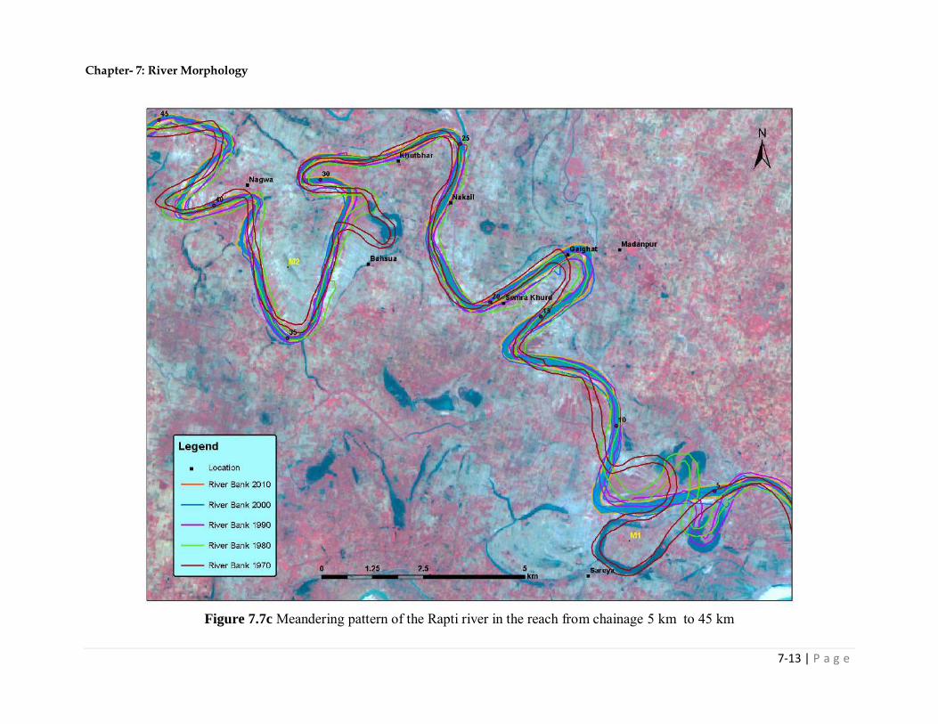
Chapter- 7: River Morphology
7-13 | P a g e
Figure 7.7c Meandering pattern of the Rapti river in the reach from chainage 5 km to 45 km
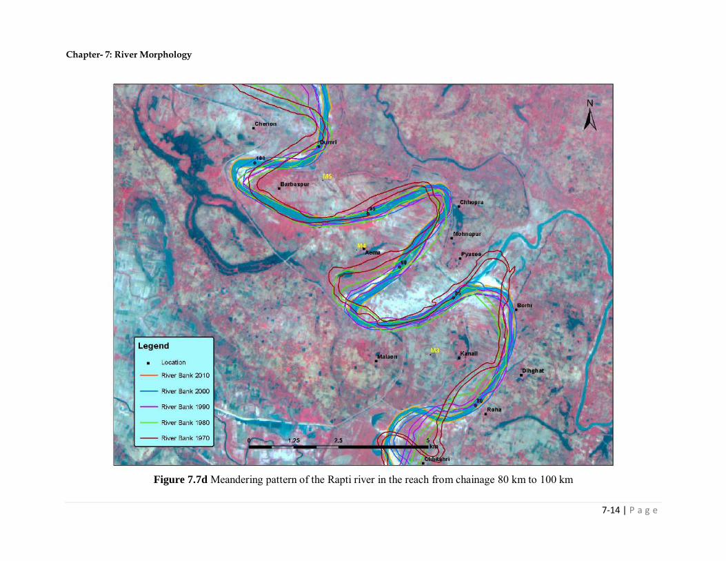
Chapter- 7: River Morphology
7-14 | P a g e
Figure 7.7d Meandering pattern of the Rapti river in the reach from chainage 80 km to 100 km
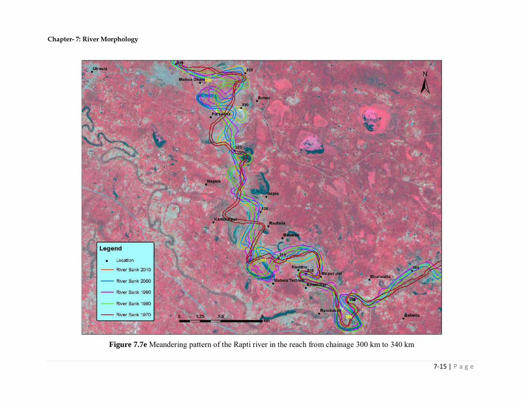
Chapter- 7: River Morphology
7-15 | P a g e
Figure 7.7e Meandering pattern of the Rapti river in the reach from chainage 300 km to 340 km

Chapter- 7: River Morphology
7-16 | P a g e
Figure 7.7f Meandering pattern of the Rapti river in the reach from chainage 350 km to 390 km

Chapter- 7: River Morphology
7-17 | P a g e
Figure 7.7g Meandering pattern of the Rapti river in the reach from chainage 395 km to 430 km

Chapter- 7: River Morphology
7-18 | P a g e
Figure 7.7h Meandering pattern of the Rapti river in the reach from chainage 210 km to 240 km near Madho Tanda

Chapter- 7: River Morphology
7-19 | P a g e
b) Planform Index
Braiding pattern of the rivers has been characterized in different ways. Three parameters which
are mentioned in the literature and commonly being used to characterize the braided pattern are
proposed by Brice (1964), Rust (1978) and Friend and Sinha (1993) (Fig 7.8).
Brice Index (BI) = 2 Li/Lr (7.2)
where Li is the length of the islands or bars in a reach and Lr is the reach measured midway
between the banks of the channel. The factor 2 in the Eq. (7.2) accounts for the total length of the
bars.
Braiding parameter as given by Rust (1968)
RI =2 Lb/Lm (7.3)
where Lb is the sum of the braid lengths between the channel thalweg divergences and
confluences in a reach, and Lm is the average of meander wave lengths in the reach. Friend and
Sinha (1993) proposed braid–channel ratio BR as
BR = Lctot/Lcmax (7.4)
where Lctot is the sum of mid-channel lengths of all the segments of primary channels in a reach,
and Lcmax is the mid-channel length of the widest channel through the reach. The ratio BR is a
measure of tendency of the channel belt to develop multiple channels in a reach. If the reach has
a single channel, BR will be unity.

Chapter- 7: River Morphology
7-20 | P a g e
Figure 7.8 Braiding indices
Sharma et al. (2004) introduced a Plan Form Index (PFI), cross-slope ratio and Flow Geometry
Index (FGI) for identifying the level of braiding in a highly braided river. The Plan Form Index,
Flow Geometric Index and Cross-Slope ratio can be expressed as (Fig 7.9)
Plan Form Index =N
B
T 100
(7.5)
Flow Geometry Index = NRT
xd ii ][ (7.6)
Cross-Slope ratio =).(
2levelbedAvlevelBank
BL
(7.7)
where, T = flow top width; B= overall width of the channel; N = number of braided channels; R
= hydraulic mean depth; di and xi are depth and width of submerged sub-channels. BL = transect
length across river width.

Chapter- 7: River Morphology
7-21 | P a g e
Figure 7.9 Definition sketch of PFI
PFI reflects the river landform disposition with respect to a given water level. Low value of PFI
indicates higher degree of braiding. For the classification of the braiding intensity, the following
threshold values for PFI are proposed by Sharma (2012).
Highly Braided: PFI < 4
Moderately Braided: 19 > PFI > 4
Low Braided: PFI > 19
The plan form index (PFI) of Rapti River is calculated using the formula given by Sharma
(2004). It has been observed that the Rapti River always runs bankfull, so no braiding is found in
Rapti river.
7.3 SHIFTING OF MAIN COURSE OF THE RIVER
Shifting of river is calculated on the basis of center line of year 2010. Center line of year 2010 is
perpendicularly bisected at a regular interval of 1 km and it’s further bisected at an interval of 0.5
km on the places where river taking sharp turn. The shift of left bank, right bank and center line
in left and right direction has been computed for the year 1970, 1980, 1990 and 2000 with
respect to base year 2010 in GIS software. The sample map of computation of river shifting is
shown in Fig 7.10 and results of the river shifting are given in Table 7.5.

Chapter- 7: River Morphology
7-22 | P a g e
Figure 7.10 Sample map of river shifting
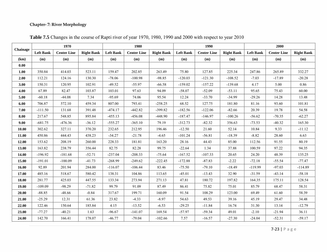
Chapter- 7: River Morphology
7-23 | P a g e
Table 7.5 Changes in the course of Rapti river of year 1970, 1980, 1990 and 2000 with respect to year 2010
Chainage 1970 1980 1990 2000
Left Bank Center Line Right Bank Left Bank Center Line Right Bank Left Bank Center Line Right Bank Left Bank Center Line Right Bank
(km) (m) (m) (m) (m) (m) (m) (m) (m) (m) (m) (m) (m)
0.00 1.00 350.84 414.03 523.11 159.47 202.85 263.49 75.80 127.85 225.34 247.86 265.89 332.27
2.00 112.21 124.16 130.30 -78.06 -100.98 -98.85 -120.03 -121.30 -108.52 -7.03 -17.89 -20.28
3.00 150.31 120.95 102.91 -49.52 -55.97 -66.58 -159.02 -157.22 -139.68 4.17 5.00 0.86
4.00 67.89 82.47 103.87 103.01 97.63 94.09 -58.07 -52.09 -53.11 95.65 75.43 60.00
5.00 -60.18 -44.08 7.34 -95.69 74.06 95.54 12.24 -33.70 -34.99 -29.26 14.28 13.48
6.00 706.87 572.10 459.34 807.00 793.41 -258.25 68.52 127.75 181.80 81.16 93.60 101.81
7.00 -111.50 131.68 391.48 -474.17 -442.82 -399.82 -182.56 -122.06 -82.66 20.39 19.78 54.58
8.00 217.67 548.85 895.84 -455.13 -456.08 -448.90 -187.47 -146.97 -100.26 -56.62 -70.35 -62.27
9.00 -681.75 -476.36 -36.12 -555.27 -365.10 79.19 -312.73 -82.32 356.63 -73.53 -40.32 165.30
10.00 302.62 327.11 370.20 232.65 212.95 196.46 -12.50 21.60 52.14 10.84 9.33 -11.12
11.00 450.86 444.43 438.23 -34.27 -21.78 -4.65 -101.24 -56.81 -18.39 -8.82 28.60 6.63
12.00 153.62 208.19 260.00 228.33 181.81 163.20 28.16 44.43 85.00 112.56 91.55 80.19
13.00 163.82 238.79 356.44 82.75 82.28 99.75 -22.64 1.34 37.88 100.59 97.22 94.35
14.00 -196.92 -181.68 -52.71 -237.04 -208.33 -75.64 -167.52 -107.33 20.65 24.20 48.39 135.25
15.00 -191.01 -100.09 -41.73 -268.99 -249.62 -222.45 -172.88 -87.83 -2.22 -72.18 -55.54 -77.47
16.00 92.89 201.94 284.00 -116.07 -106.44 83.46 -75.50 -79.10 -18.49 -119.99 -97.03 -114.89
17.00 485.16 518.67 580.42 138.31 104.86 113.65 -45.01 -13.43 32.90 -31.59 -43.14 -58.18
18.00 281.77 425.03 447.55 133.34 273.94 271.13 47.81 180.72 197.82 164.35 175.11 128.54
19.00 -109.09 -98.29 -71.82 99.79 91.09 87.49 86.41 75.82 75.01 85.79 68.47 58.31
20.00 -88.85 -48.66 -0.84 317.67 199.71 160.09 91.54 108.29 123.00 69.49 61.60 58.39
21.00 -25.29 12.31 61.36 23.82 -4.33 -8.97 54.63 49.53 39.16 45.19 29.47 34.48
22.00 122.46 150.64 185.84 4.15 -13.52 -6.53 -29.25 -11.84 16.74 31.30 13.14 -12.79
23.00 -77.27 -40.21 1.63 -96.67 -141.07 169.54 -57.97 -59.34 49.01 -2.10 -21.94 36.11
24.00 142.70 166.41 178.07 -46.77 -79.04 -102.66 7.57 -16.57 -27.30 -24.04 -52.31 -59.17

Chapter- 7: River Morphology
7-24 | P a g e
25.00 50.89 81.05 118.61 -118.24 -121.17 -118.89 -38.19 -50.24 37.83 -68.52 -47.45 -38.62
26.00 51.45 72.09 83.48 68.93 75.66 84.57 27.90 18.54 80.92 50.80 57.50 76.48
27.00 -43.42 -64.68 -71.22 89.59 74.72 44.09 52.34 40.51 22.31 80.75 51.66 24.17
28.00 7.31 33.32 79.77 129.00 88.66 58.38 60.50 55.13 69.13 73.86 52.37 30.26
29.00 58.13 84.02 113.20 109.82 94.50 92.89 54.27 68.05 74.64 66.21 72.81 79.51
30.00 -23.17 -2.23 26.07 145.21 -106.63 86.78 30.87 -6.54 50.72 -15.69 9.18 -15.50
31.00 -225.54 251.63 276.16 -177.59 298.05 420.65 -107.49 88.16 84.82 -92.08 108.89 127.29
31.50 488.37 -483.47 481.71 585.83 -545.02 489.29 104.19 -96.47 103.94 108.83 -26.43 -29.39
32.00 1322.49 -1324.82 1364.22 253.60 -211.32 175.83 86.23 -105.12 120.67 45.63 -37.97 35.02
33.00 62.49 -72.24 70.96 100.00 -129.85 133.68 -6.61 -55.00 90.05 -0.26 -11.88 -4.46
34.00 -35.27 63.27 -74.00 151.58 -101.63 52.21 0.00 -16.99 49.98 -17.52 5.41 6.74
35.00 -266.20 144.15 -169.08 45.91 -13.76 -17.08 42.45 -50.41 62.86 35.07 -18.30 -17.83
36.00 -196.64 153.32 -115.11 -90.95 -112.22 -144.14 -16.27 17.58 39.98 7.85 5.90 5.42
37.00 -6.12 23.24 45.97 -55.69 -57.46 -51.20 12.92 29.62 40.38 31.78 26.38 15.17
38.00 -280.01 -264.58 -260.43 -301.70 -310.77 -306.85 -178.86 -131.48 -90.79 -51.08 -24.65 -12.80
39.00 26.89 62.50 85.52 -167.52 -187.76 -192.11 -61.95 -46.08 -10.43 -21.97 -24.10 -39.20
40.00 -102.36 -117.46 -124.92 167.85 163.97 157.01 57.85 51.38 64.49 103.89 77.27 39.44
41.00 -84.57 -65.03 -33.87 113.11 53.41 6.49 73.68 77.40 89.07 61.35 43.35 36.26
41.50 428.35 388.60 307.55 320.06 233.21 140.00 14.52 -32.82 -60.90 -20.78 -64.13 -140.03
42.00 135.77 128.14 102.14 -119.35 -143.45 -146.14 -134.60 -125.93 -121.43 -104.27 -116.00 -130.84
43.00 -27.19 7.17 20.61 -225.52 -205.75 -170.91 -106.80 -74.17 -59.47 -89.73 -85.86 -87.03
44.00 15.99 15.46 15.74 -19.23 -27.18 -74.36 64.27 69.79 66.96 96.72 62.34 18.54
45.00 274.72 284.24 276.33 174.30 235.08 266.21 27.26 82.07 112.81 24.94 95.08 76.12
46.00 52.37 49.05 69.68 58.65 14.00 24.65 73.19 84.03 127.79 72.86 63.47 62.06
47.00 -258.80 -232.78 -193.37 -32.92 -11.25 -10.36 44.77 47.97 44.06 55.00 61.93 52.41
48.00 55.85 1.03 -38.59 -43.38 -61.14 -87.72 -178.64 -173.86 -177.51 -81.21 -93.45 -100.89
49.00 403.06 311.64 248.95 294.21 246.44 209.02 350.55 376.83 389.28 225.11 178.79 136.59
50.00 8.34 -7.84 -46.36 -88.97 -130.33 -144.07 -30.93 -58.62 -99.68 16.68 -18.15 -33.11
51.00 -67.30 -46.25 -51.48 30.82 8.61 -7.13 -20.50 -1.47 12.63 -24.30 -4.86 21.19

Chapter- 7: River Morphology
7-25 | P a g e
52.00 67.83 60.33 38.34 -21.15 -13.80 -17.59 -2.65 10.52 3.04 34.37 34.03 23.24
53.00 -112.57 -181.16 -236.67 -38.67 -90.33 -133.43 8.06 0.25 2.46 42.73 32.62 32.32
54.00 -36.68 11.72 65.29 4.64 2.98 -5.35 12.03 27.80 55.40 50.42 64.80 42.97
55.00 29.55 37.25 17.57 -115.77 -111.34 -115.92 -133.05 -110.97 -133.65 -80.34 -62.60 -46.03
56.00 132.50 -128.10 -144.27 120.93 -79.83 -45.08 -51.17 45.93 36.50 -12.23 24.68 33.03
57.00 123.84 178.75 215.39 -16.00 5.27 19.28 -23.48 8.65 36.03 -10.97 9.52 21.25
58.00 31.19 27.59 29.73 -140.01 -148.11 -155.14 -101.53 -100.06 -87.64 -54.26 -60.88 -77.59
59.00 -151.96 -142.98 -151.93 -131.65 -171.26 -215.56 -50.52 -21.99 16.37 -19.44 -45.82 -66.73
60.00 46.40 73.25 68.23 -22.46 -76.35 -147.41 -63.94 -42.38 -23.62 -53.45 -61.71 -112.65
61.00 48.42 92.69 135.54 -58.04 -75.94 -96.88 -22.51 -39.07 -52.46 -2.47 -19.80 -52.88
62.00 208.38 192.28 175.87 219.63 192.62 171.66 144.03 134.94 107.90 100.66 44.16 18.05
63.00 -89.59 -109.47 -94.75 -72.48 -97.40 -97.17 39.96 52.75 72.70 35.42 -27.18 -53.41
64.00 -72.10 -58.36 -56.37 84.86 65.63 42.97 43.65 147.05 157.89 18.40 3.92 -37.05
65.00 251.74 239.06 245.96 54.44 21.58 27.47 25.26 15.86 24.22 18.77 -6.83 -3.46
66.00 45.31 57.73 65.99 103.63 78.20 -41.63 22.18 14.42 9.39 83.40 52.49 0.04
66.50 -621.38 -1162.08 -1130.03 65.24 62.76 49.55 16.07 21.84 38.55 40.42 34.56 36.75
67.00 33.64 34.42 43.02 103.53 109.57 106.77 59.44 46.85 20.95 50.04 23.81 19.63
68.00 -251.69 -233.23 -227.92 -27.58 -51.90 -69.47 -12.66 -41.07 -95.05 44.46 30.98 43.29
69.00 -128.52 -104.05 -106.55 -499.71 -510.55 -535.37 -285.99 -301.43 -315.21 -235.70 -248.31 -274.19
70.00 360.06 462.04 588.20 243.55 273.24 333.74 -43.66 50.13 189.95 -51.03 -68.42 -31.00
71.00 1063.12 1098.88 1105.92 1035.93 1029.26 1019.29 592.74 596.33 571.94 143.31 163.53 173.61
72.00 910.81 970.80 996.24 885.12 930.62 950.85 555.33 559.32 549.53 264.27 288.58 299.29
73.00 289.85 338.69 379.08 299.89 312.26 293.69 35.45 55.09 87.95 38.16 20.97 12.35
74.00 -172.82 -126.21 -79.73 -13.32 -23.87 -44.04 17.33 3.41 -10.16 40.78 37.42 23.05
75.00 114.13 94.25 90.36 924.14 856.91 815.10 721.40 724.74 764.35 802.72 926.30 489.26
76.00 683.58 701.31 755.50 504.84 172.18 37.56 568.77 543.26 552.74 15.19 35.45 81.05
77.00 84.53 72.36 44.05 -767.76 -832.14 -883.61 -506.15 -501.84 -507.68 -326.88 -377.06 -419.22
78.00 -226.72 -1147.39 -1225.01 -125.98 -1080.70 -1162.07 -629.89 -663.02 -702.55 -141.89 -159.58 -172.70
79.00 -1313.52 -1278.14 -1253.55 -436.01 -462.69 -495.82 -95.57 -41.26 -7.95 65.46 99.28 103.71
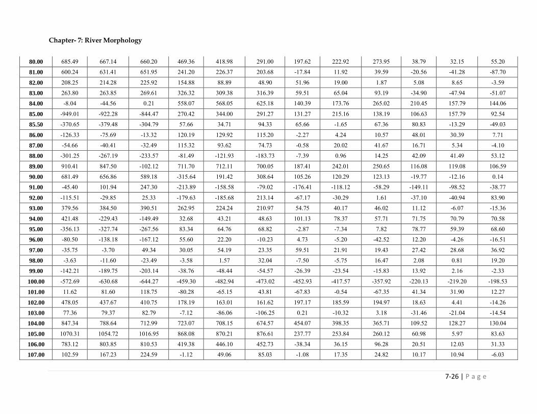
Chapter- 7: River Morphology
7-26 | P a g e
80.00 685.49 667.14 660.20 469.36 418.98 291.00 197.62 222.92 273.95 38.79 32.15 55.20
81.00 600.24 631.41 651.95 241.20 226.37 203.68 -17.84 11.92 39.59 -20.56 -41.28 -87.70
82.00 208.25 214.28 225.92 154.88 88.89 48.90 51.96 19.00 1.87 5.08 8.65 -3.59
83.00 263.80 263.85 269.61 326.32 309.38 316.39 59.51 65.04 93.19 -34.90 -47.94 -51.07
84.00 -8.04 -44.56 0.21 558.07 568.05 625.18 140.39 173.76 265.02 210.45 157.79 144.06
85.00 -949.01 -922.28 -844.47 270.42 344.00 291.27 131.27 215.16 138.19 106.63 157.79 92.54
85.50 -370.65 -379.48 -304.79 57.66 34.71 94.33 65.66 -1.65 67.36 80.83 -13.29 -49.03
86.00 -126.33 -75.69 -13.32 120.19 129.92 115.20 -2.27 4.24 10.57 48.01 30.39 7.71
87.00 -54.66 -40.41 -32.49 115.32 93.62 74.73 -0.58 20.02 41.67 16.71 5.34 -4.10
88.00 -301.25 -267.19 -233.57 -81.49 -121.93 -183.73 -7.39 0.96 14.25 42.09 41.49 53.12
89.00 910.41 847.50 -102.12 711.70 712.11 700.05 187.41 242.01 250.65 116.08 119.08 106.59
90.00 681.49 656.86 589.18 -315.64 191.42 308.64 105.26 120.29 123.13 -19.77 -12.16 0.14
91.00 -45.40 101.94 247.30 -213.89 -158.58 -79.02 -176.41 -118.12 -58.29 -149.11 -98.52 -38.77
92.00 -115.51 -29.85 25.33 -179.63 -185.68 213.14 -67.17 -30.29 1.61 -37.10 -40.94 83.90
93.00 379.56 384.50 390.51 262.95 224.24 210.97 54.75 40.17 46.02 11.12 -6.07 -15.36
94.00 421.48 -229.43 -149.49 32.68 43.21 48.63 101.13 78.37 57.71 71.75 70.79 70.58
95.00 -356.13 -327.74 -267.56 83.34 64.76 68.82 -2.87 -7.34 7.82 78.77 59.39 68.60
96.00 -80.50 -138.18 -167.12 55.60 22.20 -10.23 4.73 -5.20 -42.52 12.20 -4.26 -16.51
97.00 -35.75 -3.70 49.34 30.05 54.19 23.35 59.51 21.91 19.43 27.42 28.68 36.92
98.00 -3.63 -11.60 -23.49 -3.58 1.57 32.04 -7.50 -5.75 16.47 2.08 0.81 19.20
99.00 -142.21 -189.75 -203.14 -38.76 -48.44 -54.57 -26.39 -23.54 -15.83 13.92 2.16 -2.33
100.00 -572.69 -630.68 -644.27 -459.30 -482.94 -473.02 -452.93 -417.57 -357.92 -220.13 -219.20 -198.53
101.00 11.62 81.60 118.75 -80.28 -65.15 43.81 -67.83 -0.54 -67.35 41.34 31.90 12.27
102.00 478.05 437.67 410.75 178.19 163.01 161.62 197.17 185.59 194.97 18.63 4.41 -14.26
103.00 77.36 79.37 82.79 -7.12 -86.06 -106.25 0.21 -10.32 3.18 -31.46 -21.04 -14.54
104.00 847.34 788.64 712.99 723.07 708.15 674.57 454.07 398.35 365.71 109.52 128.27 130.04
105.00 1070.31 1054.72 1016.95 868.08 870.21 876.61 237.77 253.84 260.12 60.98 5.97 83.63
106.00 783.12 803.85 810.53 419.38 446.10 452.73 -38.34 36.15 96.28 20.51 12.03 31.33
107.00 102.59 167.23 224.59 -1.12 49.06 85.03 -1.08 17.35 24.82 10.17 10.94 -6.03

Chapter- 7: River Morphology
7-27 | P a g e
108.00 -196.17 -207.18 -179.20 -99.40 -77.13 -62.51 -98.75 -70.22 -30.03 -63.93 -55.61 -24.23
109.00 557.24 594.81 613.13 517.96 456.28 429.62 481.25 471.02 465.32 449.22 422.84 363.25
110.00 166.94 108.33 37.55 -212.38 -306.80 -336.89 -177.55 -195.88 -218.37 -199.02 -223.90 -255.08
111.00 -301.05 -281.59 -263.37 -445.74 -469.73 -492.83 -417.81 -450.19 -481.73 -58.24 -36.13 -9.01
112.00 645.16 649.18 584.51 20.62 85.02 103.95 27.17 79.78 87.33 10.51 65.05 61.28
113.00 1015.50 97.60 928.64 626.28 580.57 548.39 64.92 79.20 82.96 18.73 21.68 -19.01
114.00 469.55 1491.68 586.85 226.19 272.11 309.50 -58.54 -16.25 48.03 2.03 -29.41 -18.95
115.00 -225.35 -149.20 -71.78 -54.99 -18.70 -12.92 -89.86 -54.89 -19.59 -13.89 -26.89 -42.04
116.00 -264.73 -235.88 -211.32 33.62 44.55 19.66 7.35 26.24 18.02 7.52 12.31 8.68
119.00 221.61 298.81 108.00 2.88 -1.12 -164.13 -61.46 -35.22 154.64 -22.84 -25.54 16.60
120.00 3.84 68.43 328.76 -149.26 -145.00 165.35 -52.24 118.19 173.54 -12.83 -26.75 76.36
121.00 -103.28 -146.22 -157.34 -81.14 -100.07 -106.08 -109.77 -96.57 -68.77 -90.78 -113.06 -145.09
122.00 592.59 645.50 691.03 -363.23 -345.07 -316.93 -360.68 -313.95 -291.86 -107.36 -143.29 -204.00
122.50 856.35 888.45 919.47 -404.45 -415.15 -428.47 -133.58 -80.40 -40.18 -36.23 -87.46 -144.77
123.00 659.53 751.30 833.51 -128.36 -98.77 -97.28 111.04 124.58 110.07 2.66 1.57 7.22
124.00 632.14 613.76 675.18 -74.66 -71.95 -21.49 -131.08 -126.90 -56.70 -107.69 -153.59 -166.98
125.00 -530.65 -509.25 -502.17 -444.91 -493.47 -540.22 -404.54 -418.81 -435.04 -178.73 -257.23 -327.23
126.00 -405.99 -332.66 -232.19 -52.56 -16.63 25.86 -99.16 -162.05 -94.03 -51.21 -66.24 -61.99
127.00 -98.16 -49.25 -7.95 126.65 125.02 112.05 19.19 47.29 51.00 -5.18 21.46 44.55
128.00 541.22 646.72 728.91 667.85 720.19 768.89 723.63 756.90 766.87 695.46 698.87 659.60
129.00 1159.72 1182.78 1190.90 1129.92 1089.03 1046.27 1176.72 1158.04 1098.13 601.63 579.16 549.48
130.00 1004.15 1013.45 1006.14 922.81 887.25 839.41 959.14 947.96 912.05 312.64 306.90 265.08
131.00 150.98 376.38 632.26 -11.15 153.55 365.41 110.22 301.10 475.06 -451.11 -170.59 87.27
132.00 -1793.74 -1756.09 -1717.17 -1500.80 -1512.36 -1502.27 -1165.75 -1243.06 -1350.25 -334.05 -461.14 -665.63
133.00 -304.46 -257.76 -228.04 -129.64 -128.94 -141.59 -185.70 -151.56 -121.08 -112.59 -93.58 -66.63
134.00 119.76 -64.92 -29.46 74.46 84.45 55.05 38.16 54.38 74.15 -38.48 -35.12 -37.96
135.00 -171.73 -136.33 -193.50 -108.15 -99.40 -93.05 -47.02 -50.01 -62.19 -3.68 -11.07 -29.65
136.00 -21.98 -25.69 -13.45 -21.83 -37.24 -21.75 22.15 8.76 8.73 -4.48 -31.81 -56.79
137.00 27.20 4.24 -23.49 -90.00 -90.14 -101.98 -50.99 -66.97 -71.66 -7.69 -39.95 -67.12

Chapter- 7: River Morphology
7-28 | P a g e
138.00 -130.19 -281.76 -306.33 -58.43 -51.57 -76.80 82.68 83.89 53.30 -61.75 -84.80 -103.17
139.00 -566.41 -661.37 -743.10 8.41 -1.94 -5.51 -369.87 -386.15 -394.71 -203.89 -226.09 -257.89
140.00 16.79 1.55 -87.75 -528.43 -448.02 -438.26 -0.62 157.58 234.91 122.19 193.77 159.82
141.00 -407.95 -564.33 -685.18 -294.99 -299.69 -301.85 161.85 171.24 175.89 -36.26 -71.28 -130.16
142.00 -1132.25 -1132.92 -1138.94 -1442.67 -1491.21 -1515.84 319.86 293.98 282.06 106.23 63.77 24.68
143.00 453.07 440.15 447.65 565.80 469.53 359.52 258.45 309.68 349.52 124.27 88.90 74.70
144.00 1002.66 972.17 936.15 1136.39 1117.19 1101.89 615.47 606.16 563.27 66.36 49.85 26.30
145.00 748.11 507.41 706.78 953.91 924.28 986.51 231.07 167.17 202.17 -13.48 -56.03 -32.56
146.00 -204.88 -191.19 -125.85 -806.55 -827.71 -793.50 -553.11 -570.15 -513.86 -144.38 -228.38 -427.84
147.00 -532.66 -225.69 314.67 -1289.69 -997.77 -469.27 -173.06 146.06 697.95 -68.39 396.33 952.38
148.00 806.96 787.81 783.09 17.94 -75.01 -149.50 714.53 739.15 766.80 833.27 664.02 495.59
149.00 1202.11 1155.85 1149.04 478.44 460.12 418.81 148.48 96.45 81.16 81.37 68.14 18.60
150.00 1243.55 1321.12 1301.53 55.45 159.55 187.95 -125.49 -7.03 36.11 -203.51 -101.60 -83.25
151.50 -354.96 -462.27 -556.68 -967.33 -1018.26 -1071.39 -948.29 -1011.24 -1028.92 -482.05 -556.22 -614.70
152.00 -730.70 -786.52 -836.89 -1008.05 -1064.95 -1121.80 -806.61 -887.72 -928.23 -392.26 -439.38 -490.88
153.00 -177.38 -170.74 -154.90 -195.44 -223.02 -272.07 204.92 261.96 330.07 335.78 374.02 414.39
154.00 381.36 341.58 297.62 587.35 509.68 438.70 80.23 -20.60 -140.49 -168.99 -264.36 -351.40
155.00 1766.95 1699.31 1691.69 -570.94 -626.56 -596.16 -633.49 -591.02 -555.93 -706.85 -701.91 -685.46
156.00 -238.93 -284.83 -314.59 -581.45 -618.20 -649.53 -476.30 -463.21 -440.11 -345.23 -336.10 -309.82
157.00 72.45 48.82 36.98 -148.54 -170.71 -179.15 -72.52 -63.57 -34.42 -24.04 -22.67 -31.25
158.00 179.47 157.26 154.99 -36.58 -2.19 -16.29 -160.45 -147.12 -110.19 -61.68 -104.97 -149.34
159.00 -544.38 -537.75 -513.89 -527.16 -687.38 -733.05 -441.22 -455.84 -467.20 -138.96 -138.26 -122.42
160.00 -503.35 -531.94 -577.10 -634.28 -654.40 -664.23 -273.24 -285.18 -325.54 -60.27 -73.72 -88.54
161.00 89.28 52.69 27.29 138.84 48.38 -34.43 260.30 225.24 161.85 131.47 81.65 24.54
162.00 480.19 222.51 242.42 559.69 241.42 214.53 380.18 103.74 115.62 323.41 19.56 -5.48
163.00 301.83 220.41 152.29 -220.56 93.11 48.70 149.30 66.26 0.43 187.26 103.04 22.17
164.00 -517.60 -555.06 -523.83 -94.25 -124.78 -109.24 2.58 -34.75 -92.43 -0.44 -69.60 -79.65
165.00 -697.44 -771.38 -850.54 -323.39 -351.25 -396.20 -135.82 -97.94 -63.92 -517.60 -59.28 -141.91
166.00 232.71 226.05 219.44 -3.32 -48.12 -75.85 3.04 23.13 46.32 26.93 7.10 -14.29

Chapter- 7: River Morphology
7-29 | P a g e
167.00 222.71 189.56 141.86 84.36 21.67 -43.14 112.69 106.54 90.14 119.79 74.42 34.06
168.00 98.44 68.16 10.66 -160.16 -138.50 -8.83 7.48 23.00 30.81 6.75 -49.16 -101.07
169.00 201.94 201.63 153.67 10.56 12.57 7.91 25.12 25.73 15.17 -50.79 -36.71 -58.20
170.00 305.32 243.14 192.70 94.45 48.73 10.12 65.46 -97.45 -126.27 -54.11 -129.64 -204.97
171.00 38.72 -3.56 -63.89 -128.09 -174.00 -220.51 -47.56 -55.13 -68.12 -46.05 -129.97 -233.24
172.00 -16.49 -59.55 -101.77 29.93 10.41 5.62 14.86 11.48 27.38 -40.02 -44.46 -61.15
173.00 -77.15 -81.90 -71.43 -379.44 -397.07 -394.69 63.09 53.81 73.39 13.54 6.89 10.45
174.00 -234.02 -191.16 -130.18 -318.62 -328.20 -352.86 -77.52 -53.67 -9.08 45.14 41.85 41.03
175.00 579.38 564.10 472.33 478.66 445.43 392.34 159.20 139.95 133.29 225.68 145.48 66.52
176.00 786.70 730.66 703.00 780.27 703.78 655.82 94.59 77.07 79.11 143.33 76.34 41.31
177.00 558.65 502.73 443.13 347.32 214.82 158.03 -46.59 -38.46 -23.61 2.20 -23.84 -51.10
178.00 -246.00 -340.68 -424.88 126.99 51.10 -37.09 141.18 97.92 64.15 143.82 58.19 -29.34
179.00 -468.71 -492.90 -518.52 62.96 53.00 34.91 55.85 47.64 24.12 20.71 4.91 -15.00
180.00 -238.81 -338.50 -517.09 -132.15 -143.90 -157.87 50.68 29.78 9.01 -22.64 -30.42 -46.29
181.00 337.41 355.95 372.14 155.30 95.96 36.12 148.14 95.92 40.83 88.12 45.86 -4.30
182.00 113.62 138.70 159.68 12.97 -14.29 -46.19 114.24 86.38 79.32 21.76 11.76 -2.29
183.00 -175.12 -145.68 -136.52 -203.31 -177.19 -173.55 -55.25 -42.95 -67.53 -58.37 -78.85 -111.46
184.00 -34.08 -101.57 -87.18 -153.25 -175.95 -202.60 -62.99 -79.46 -86.21 -12.83 -41.36 -99.43
185.00 -615.87 -686.97 -673.05 -75.26 -66.82 -64.91 19.99 44.95 39.73 -53.34 -53.59 -52.19
186.00 18.04 84.76 107.34 75.80 110.78 91.90 76.61 101.08 65.92 41.07 12.14 -40.20
187.00 364.41 -328.29 -263.40 96.23 -113.22 -103.94 255.85 -257.22 -267.19 167.22 -170.94 -192.00
188.00 -291.73 -251.89 -218.70 -159.80 -202.02 -241.31 -41.05 -88.32 -114.94 -39.20 -75.00 -113.20
189.00 49.72 64.18 84.47 -89.11 -131.16 -172.30 1.09 -12.82 -9.04 25.24 17.11 -1.66
190.00 69.59 93.35 106.13 -104.65 -107.46 -117.37 -7.47 17.19 44.13 3.90 15.35 21.50
191.00 -39.62 -6.40 0.93 -71.25 -109.09 -136.27 49.50 15.45 -27.22 32.95 -24.65 -77.46
192.00 11.95 -4.13 -31.52 47.01 18.30 -19.12 83.90 44.55 -3.50 3.11 6.01 -13.28
193.00 -608.60 -648.38 -452.12 -567.12 -516.25 -340.63 -351.34 -237.76 -10.05 -247.44 -197.76 -18.80
194.00 26.62 40.12 22.66 -331.87 -384.72 -405.20 -35.75 -74.27 -117.76 -21.72 -115.00 -199.53
195.00 72.99 98.01 132.00 41.52 -23.92 -61.24 90.43 67.24 65.40 99.27 52.75 44.71
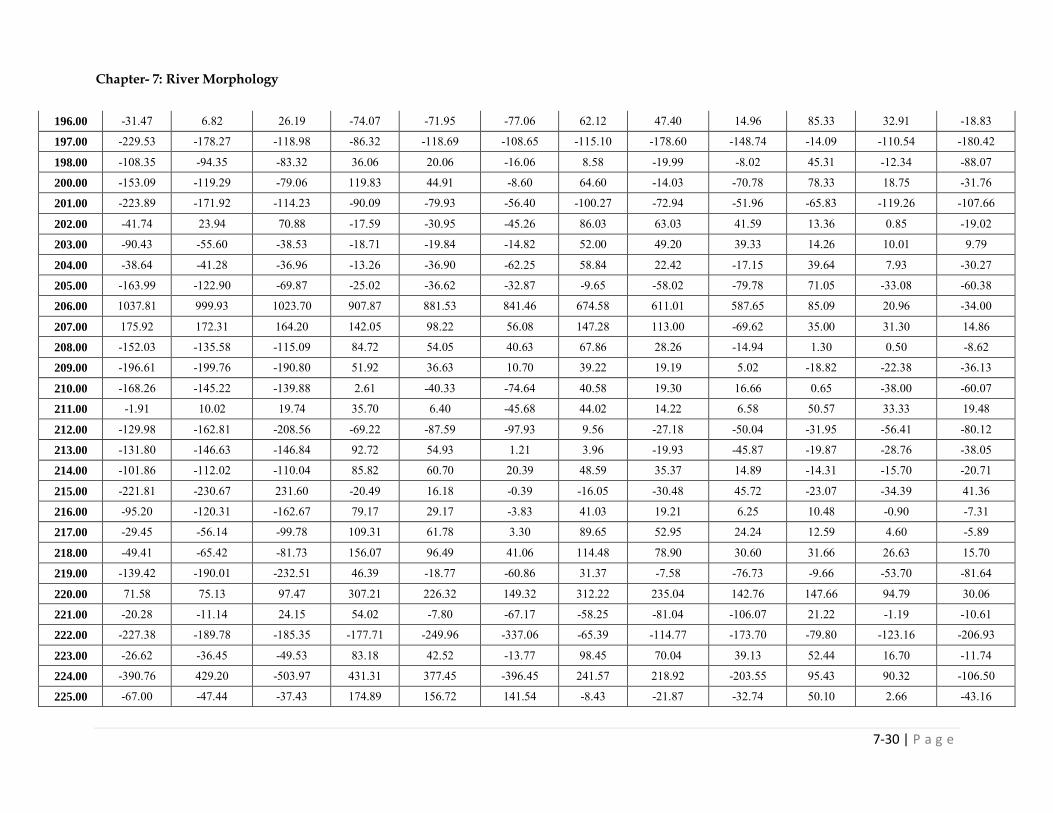
Chapter- 7: River Morphology
7-30 | P a g e
196.00 -31.47 6.82 26.19 -74.07 -71.95 -77.06 62.12 47.40 14.96 85.33 32.91 -18.83
197.00 -229.53 -178.27 -118.98 -86.32 -118.69 -108.65 -115.10 -178.60 -148.74 -14.09 -110.54 -180.42
198.00 -108.35 -94.35 -83.32 36.06 20.06 -16.06 8.58 -19.99 -8.02 45.31 -12.34 -88.07
200.00 -153.09 -119.29 -79.06 119.83 44.91 -8.60 64.60 -14.03 -70.78 78.33 18.75 -31.76
201.00 -223.89 -171.92 -114.23 -90.09 -79.93 -56.40 -100.27 -72.94 -51.96 -65.83 -119.26 -107.66
202.00 -41.74 23.94 70.88 -17.59 -30.95 -45.26 86.03 63.03 41.59 13.36 0.85 -19.02
203.00 -90.43 -55.60 -38.53 -18.71 -19.84 -14.82 52.00 49.20 39.33 14.26 10.01 9.79
204.00 -38.64 -41.28 -36.96 -13.26 -36.90 -62.25 58.84 22.42 -17.15 39.64 7.93 -30.27
205.00 -163.99 -122.90 -69.87 -25.02 -36.62 -32.87 -9.65 -58.02 -79.78 71.05 -33.08 -60.38
206.00 1037.81 999.93 1023.70 907.87 881.53 841.46 674.58 611.01 587.65 85.09 20.96 -34.00
207.00 175.92 172.31 164.20 142.05 98.22 56.08 147.28 113.00 -69.62 35.00 31.30 14.86
208.00 -152.03 -135.58 -115.09 84.72 54.05 40.63 67.86 28.26 -14.94 1.30 0.50 -8.62
209.00 -196.61 -199.76 -190.80 51.92 36.63 10.70 39.22 19.19 5.02 -18.82 -22.38 -36.13
210.00 -168.26 -145.22 -139.88 2.61 -40.33 -74.64 40.58 19.30 16.66 0.65 -38.00 -60.07
211.00 -1.91 10.02 19.74 35.70 6.40 -45.68 44.02 14.22 6.58 50.57 33.33 19.48
212.00 -129.98 -162.81 -208.56 -69.22 -87.59 -97.93 9.56 -27.18 -50.04 -31.95 -56.41 -80.12
213.00 -131.80 -146.63 -146.84 92.72 54.93 1.21 3.96 -19.93 -45.87 -19.87 -28.76 -38.05
214.00 -101.86 -112.02 -110.04 85.82 60.70 20.39 48.59 35.37 14.89 -14.31 -15.70 -20.71
215.00 -221.81 -230.67 231.60 -20.49 16.18 -0.39 -16.05 -30.48 45.72 -23.07 -34.39 41.36
216.00 -95.20 -120.31 -162.67 79.17 29.17 -3.83 41.03 19.21 6.25 10.48 -0.90 -7.31
217.00 -29.45 -56.14 -99.78 109.31 61.78 3.30 89.65 52.95 24.24 12.59 4.60 -5.89
218.00 -49.41 -65.42 -81.73 156.07 96.49 41.06 114.48 78.90 30.60 31.66 26.63 15.70
219.00 -139.42 -190.01 -232.51 46.39 -18.77 -60.86 31.37 -7.58 -76.73 -9.66 -53.70 -81.64
220.00 71.58 75.13 97.47 307.21 226.32 149.32 312.22 235.04 142.76 147.66 94.79 30.06
221.00 -20.28 -11.14 24.15 54.02 -7.80 -67.17 -58.25 -81.04 -106.07 21.22 -1.19 -10.61
222.00 -227.38 -189.78 -185.35 -177.71 -249.96 -337.06 -65.39 -114.77 -173.70 -79.80 -123.16 -206.93
223.00 -26.62 -36.45 -49.53 83.18 42.52 -13.77 98.45 70.04 39.13 52.44 16.70 -11.74
224.00 -390.76 429.20 -503.97 431.31 377.45 -396.45 241.57 218.92 -203.55 95.43 90.32 -106.50
225.00 -67.00 -47.44 -37.43 174.89 156.72 141.54 -8.43 -21.87 -32.74 50.10 2.66 -43.16

Chapter- 7: River Morphology
7-31 | P a g e
226.00 -270.70 -277.34 -280.29 -97.58 -133.64 -174.56 -76.88 -77.06 -91.09 -8.44 -23.82 -52.65
227.00 -76.22 -70.39 -60.94 412.95 360.63 297.20 444.97 384.48 344.07 308.75 209.25 144.22
228.00 -314.39 -257.47 -174.23 0.00 0.00 0.00 -55.34 -65.37 -92.94 -8.06 -39.02 -35.83
229.00 -447.04 -388.56 -342.56 -6.29 -909.71 -897.27 -275.07 -219.24 -174.87 -254.78 -211.23 -169.42
232.00 1241.05 529.02 1313.58 812.28 404.19 631.03 56.54 188.59 -56.80 146.73 139.92 -11.06
233.00 457.97 -188.05 599.16 414.03 59.61 378.26 278.31 6.90 181.58 197.07 -27.76 78.63
234.00 -214.10 -71.47 -134.78 119.85 38.12 26.33 104.24 14.39 2.91 7.70 -12.95 -39.26
235.00 -97.42 -71.47 -40.05 84.77 38.12 11.72 59.69 14.39 -21.33 14.67 -12.95 -24.36
236.00 -121.68 -88.65 -47.35 -7.08 -64.64 -134.12 17.97 -42.09 -78.04 19.28 -20.75 -38.27
237.00 32.53 115.69 218.61 -123.46 -38.49 70.36 -140.10 10.05 149.63 -53.81 13.98 41.78
238.00 -157.27 -136.73 -135.43 27.97 33.40 32.76 13.88 59.72 11.03 30.66 21.83 12.15
239.00 -56.46 -67.62 -86.05 109.75 51.77 15.82 99.47 55.11 7.57 29.84 2.33 -12.03
240.00 -148.06 -140.90 -117.16 90.85 51.49 27.13 31.94 38.63 -15.10 86.57 20.88 -30.52
241.00 -14.45 26.12 37.44 -17.44 -14.13 -51.17 85.49 43.48 34.32 35.89 50.07 38.35
242.00 -128.34 -79.95 -34.64 69.15 31.62 -23.30 4.08 -7.25 -33.78 33.87 4.01 -29.21
243.00 21.17 149.00 226.98 -84.47 -2.93 -54.95 65.13 60.42 29.75 19.88 4.31 -8.64
244.00 -125.11 -99.29 -69.47 138.94 92.72 49.81 28.72 8.54 -18.99 35.22 16.03 8.97
245.00 -59.09 -32.75 -3.31 115.45 85.42 59.26 24.88 6.82 -10.83 49.16 29.45 6.31
246.00 -337.37 -301.19 -268.30 142.59 100.91 38.81 -27.32 -36.69 -50.47 35.82 21.96 10.31
247.00 -219.83 -200.12 -184.81 60.52 3.66 -46.95 45.53 22.20 -69.13 32.08 -0.79 -47.29
248.00 117.68 141.33 175.83 46.96 -3.11 2.25 50.78 21.51 -11.41 82.21 34.98 5.00
249.00 54.21 82.79 117.34 151.46 124.13 110.81 1.28 -3.04 -8.72 39.04 24.78 10.31
250.00 19.78 -17.05 -13.06 65.97 50.73 81.14 -22.69 -36.20 -48.53 -7.03 -32.70 -47.78
251.00 -80.27 -55.13 -97.09 45.84 20.47 -32.52 30.44 35.08 -0.78 40.29 49.09 37.71
252.00 -130.97 -77.25 -34.52 47.37 10.89 -33.75 42.04 25.74 -2.26 23.64 30.49 22.84
253.00 -92.72 -58.92 -27.19 125.30 67.33 14.54 48.46 26.45 -5.31 43.55 44.36 36.99
254.00 -207.77 -152.66 -131.90 4.15 -5.52 -38.12 12.94 8.70 17.04 34.96 22.54 9.50
255.00 36.18 74.74 -87.31 -6.06 -21.20 -20.59 20.77 22.03 20.79 27.38 30.32 41.81
256.00 -132.03 -66.69 -18.91 35.52 22.82 1.02 0.94 28.13 38.19 51.95 63.04 64.22

Chapter- 7: River Morphology
7-32 | P a g e
257.00 -99.05 -53.38 10.42 79.90 41.55 22.56 -36.75 -28.56 -4.07 -11.17 -23.91 -25.26
258.00 -112.81 -92.11 -75.83 60.65 27.05 -10.07 0.00 0.00 0.00 -3.35 9.80 8.14
259.00 22.22 53.55 15.43 63.01 -40.81 -0.82 -8.46 -2.80 11.94 39.39 35.43 22.37
260.00 209.81 -248.05 121.66 47.50 -1.63 -13.00 -37.21 29.28 -19.96 -17.09 33.73 -47.47
261.00 32.14 -72.67 66.60 100.16 -69.48 55.06 -8.45 14.87 -6.39 -19.07 21.58 -9.84
262.00 -64.95 64.31 -86.82 182.34 -74.65 -26.09 9.75 23.30 -52.05 -31.90 31.66 -27.88
263.00 24.33 -20.50 -12.36 25.12 -7.80 -26.49 64.40 40.44 34.62 21.45 11.48 21.62
264.00 -85.28 -63.87 -66.63 80.71 62.73 52.04 12.35 22.02 19.76 -36.43 -21.62 0.95
265.00 36.91 33.35 34.20 82.91 51.88 28.10 54.82 55.40 57.90 9.12 21.01 16.89
266.00 -18.18 0.60 17.40 119.74 65.20 -9.83 -17.33 -18.51 -42.51 -12.90 -21.87 -56.66
267.00 -66.87 -71.57 -60.48 -36.70 -67.92 -87.72 0.99 19.14 29.13 53.43 27.87 6.98
268.00 7.60 32.82 26.75 146.61 93.22 49.47 39.74 20.39 8.98 29.77 14.45 -11.00
269.00 -138.08 -97.15 -319.25 51.61 -111.41 -251.67 -25.89 -15.34 9.22 1.58 1.95 10.93
270.00 110.56 106.97 90.13 -25.44 -56.18 -86.61 2.83 -23.28 -36.27 34.83 31.88 17.94
271.00 -140.59 -111.91 -93.79 88.03 75.93 42.93 4.53 -16.85 -44.30 -17.69 -12.38 -12.04
272.00 -5.76 -32.79 -57.61 -48.12 -64.65 -81.19 21.41 -35.35 -63.58 38.64 32.64 38.72
273.00 31.51 53.61 66.70 111.64 62.00 -0.32 97.19 78.84 73.09 53.37 50.69 43.00
274.00 113.84 114.22 102.62 235.23 168.92 107.94 118.93 77.02 52.50 43.54 35.06 38.85
275.00 -672.06 -732.66 -719.28 -8.21 -42.32 -96.10 48.93 38.41 5.99 28.37 2.37 -24.95
276.00 275.67 105.90 58.36 402.54 334.77 284.12 211.94 192.13 163.37 81.03 89.10 88.38
277.00 410.32 404.11 406.18 160.56 119.25 74.65 112.26 75.44 32.50 48.97 51.34 42.22
278.00 148.93 131.98 137.12 207.66 158.84 134.10 114.13 59.02 13.87 12.07 -6.18 18.59
279.00 65.78 90.07 104.69 115.29 63.96 32.75 93.54 68.03 54.90 72.43 50.80 44.79
280.00 -186.81 -182.14 -172.23 142.25 60.93 -0.78 -8.95 -27.96 -51.97 -5.03 -20.98 -22.03
281.00 85.59 126.31 168.33 -50.64 -56.68 -97.65 15.06 17.93 33.43 11.73 23.19 22.62
282.00 105.10 142.89 147.71 253.72 158.14 66.39 36.30 25.53 26.37 33.98 45.07 41.75
283.00 -155.46 -155.18 -151.26 135.86 117.26 109.79 7.18 16.76 6.01 -1.50 -6.17 -33.99
284.00 272.33 261.48 227.72 -0.45 -54.43 -110.45 -10.75 -17.60 -38.59 55.37 28.50 -8.14
285.00 387.68 412.65 449.86 333.64 215.89 232.42 230.03 68.49 45.20 110.71 63.73 -0.84

Chapter- 7: River Morphology
7-33 | P a g e
285.50 -321.97 -340.39 -385.69 179.43 123.02 62.48 151.62 109.66 50.88 41.29 29.10 7.00
286.00 -285.48 -276.29 -255.87 297.70 236.40 202.63 106.60 91.35 56.70 22.69 1.18 1.97
287.00 -182.61 -153.03 -114.87 126.22 59.87 20.12 -2.67 -36.06 -53.85 -44.43 -56.77 -43.09
288.00 -173.86 -193.93 -224.81 74.51 30.73 -16.64 52.26 28.25 -13.69 16.86 3.26 5.70
289.00 -63.92 -120.40 -115.34 157.59 79.75 6.72 65.41 61.53 33.81 -3.18 -22.08 -24.87
290.00 -64.76 -38.50 -22.01 125.63 82.01 32.09 47.27 54.05 18.52 8.48 11.06 7.38
291.00 -71.87 -68.63 -70.41 109.13 -46.34 -21.25 5.84 -28.67 -84.15 -7.90 -3.72 12.09
292.00 -20.36 9.00 4.11 -80.62 -88.12 -130.97 -29.04 -29.17 -66.41 -0.32 -5.40 -6.88
293.00 -30.25 38.45 88.99 88.74 22.49 -36.01 1.18 -12.01 -46.19 29.75 26.82 4.98
294.00 -63.30 -63.35 -83.48 9.98 -13.13 -39.62 -22.04 -81.71 -144.29 -17.16 15.12 20.52
295.00 383.66 358.89 268.07 115.80 80.18 45.46 76.71 -1.96 -56.57 32.53 19.39 2.86
296.00 -58.43 -46.71 -50.61 60.63 0.39 -94.85 -14.26 -105.69 -188.50 -120.63 -138.49 -181.10
297.00 -293.95 -307.71 -404.18 351.70 291.30 229.71 379.47 272.58 119.55 225.69 153.59 102.60
298.00 -797.52 -885.30 -926.78 -124.58 -164.97 -227.10 -132.58 -220.13 -643.03 -222.47 -262.96 -310.50
299.00 -237.34 -150.42 -153.86 -24.46 37.84 5.46 -5.26 14.94 -206.41 19.34 58.62 48.53
300.00 581.53 625.72 662.90 56.82 16.68 -9.79 20.66 12.60 -36.91 -10.74 -23.50 -26.10
301.00 558.67 534.03 493.90 98.43 86.44 65.69 56.80 14.60 -42.26 24.95 5.62 -30.83
302.00 395.25 376.83 391.27 158.69 118.23 70.94 157.13 94.18 40.52 -2.21 -6.67 -4.95
303.00 12.90 -81.31 -60.00 89.88 41.28 -19.19 61.86 -63.59 -157.12 26.36 -12.15 -43.72
304.00 100.13 125.54 -27.42 54.62 -4.17 -64.85 51.97 -21.04 -87.95 -10.42 -13.70 -17.37
305.00 -105.42 -73.50 -41.70 41.84 -1.18 -45.88 31.83 15.25 -178.24 88.31 84.36 90.68
306.00 -40.92 -53.42 -42.03 234.41 65.84 -29.22 -279.52 -381.68 -525.81 -457.00 -500.52 518.46
306.50 653.34 639.98 599.09 1435.19 1401.97 1324.14 1340.64 1285.74 1215.22 1279.77 1257.92 1219.02
306.75 668.17 601.71 477.32 1015.55 938.47 920.83 990.51 943.29 104.90 1005.06 966.33 981.54
307.00 -0.30 18.49 27.42 102.98 37.22 -14.41 107.49 88.33 -29.48 200.58 166.54 126.37
307.50 -53.62 -34.71 -31.50 38.37 -14.49 -69.33 9.01 14.70 16.22 109.38 85.21 56.61
308.50 -1.04 43.62 33.81 147.95 55.42 -32.07 237.49 38.19 -229.25 57.24 43.80 12.03
309.50 -35.63 -28.38 -31.30 81.87 67.40 50.46 -2.49 14.34 3.38 -16.66 -12.68 -19.59
310.50 -71.57 -41.91 -26.30 -9.19 -67.86 -110.06 -0.15 -31.60 -51.75 13.61 18.06 22.67

Chapter- 7: River Morphology
7-34 | P a g e
311.50 86.13 80.71 99.11 1.19 -25.18 -56.72 61.19 36.30 11.83 21.23 5.04 -2.40
312.50 94.81 132.41 169.43 123.90 136.65 146.87 134.68 84.57 15.90 102.26 85.82 68.23
313.50 18.79 64.31 114.27 44.54 16.26 24.12 8.21 -25.16 -30.78 -30.04 2.84 31.28
314.50 -434.38 -403.06 -365.17 -697.68 -718.75 -710.01 -781.75 -813.34 -822.60 -848.29 -821.12 -791.93
315.50 -105.28 -81.51 -47.24 -404.59 -455.04 -487.35 -478.82 -586.84 -698.69 -154.32 -162.28 -160.21
316.50 234.70 294.28 327.14 559.41 578.72 597.80 411.83 373.54 279.37 -34.98 -12.40 -9.68
317.00 543.75 544.95 438.95 1665.44 1617.40 1579.37 1873.92 1755.24 1604.33 97.94 69.52 36.51
317.50 889.19 894.66 917.98 184.09 71.49 -6.64 1527.08 1175.28 1095.31 1506.54 1508.57 1257.40
318.50 -1356.00 -1396.44 -1594.41 -876.76 -886.60 -920.97 -703.76 -757.28 -833.01 -287.09 -341.65 -394.83
319.50 -1180.43 -1084.35 -1002.15 -408.05 -400.72 -440.67 -422.57 -429.54 -431.27 -25.79 -29.65 -34.63
320.50 1098.73 991.09 778.03 74.85 108.44 151.01 -8.60 3.16 31.34 15.57 21.15 37.82
321.50 1883.78 1955.76 2009.99 474.83 530.73 597.47 110.37 174.68 239.18 16.52 31.35 105.68
322.50 1403.21 1414.65 1403.35 -223.55 -362.98 -378.47 -357.86 -416.89 -488.37 -240.17 -267.26 -287.99
323.50 36.69 54.35 78.85 66.60 -13.08 -93.60 479.45 244.32 82.21 276.70 118.21 67.06
324.50 -133.33 -109.92 -89.24 678.25 603.31 590.23 -81.56 -168.34 -194.08 -143.73 -126.98 -121.59
325.50 -652.75 -637.91 -624.74 -139.43 -258.54 -762.60 34.33 38.36 -153.28 64.10 76.95 94.42
326.50 439.68 427.75 395.48 45.61 19.46 -4.43 146.99 44.91 -51.17 129.27 119.85 102.84
327.50 200.91 137.48 34.06 -881.81 -922.74 -972.69 -1008.06 -1119.86 -1284.02 -548.20 -551.81 -563.38
328.50 851.86 880.46 894.88 -283.14 -293.85 -319.51 -366.11 -459.94 -570.49 -73.25 -41.41 -30.03
329.00 854.05 771.99 719.92 174.80 108.46 48.75 59.39 -10.06 -88.46 -133.48 -190.85 -213.15
331.00 1846.42 1767.27 1673.09 1362.65 1307.52 1261.30 1276.40 1211.09 1153.15 745.37 751.82 748.62
332.00 286.65 577.03 912.07 323.31 744.50 1125.45 262.01 712.98 1114.76 -430.83 6.56 409.95
333.00 -734.89 -779.73 -816.08 -220.67 -192.13 -156.85 -124.31 -155.43 -83.99 -701.56 -721.64 -759.67
334.00 -622.09 -542.94 -500.25 268.78 315.18 334.44 1051.54 871.73 823.14 1307.51 1382.57 1421.32
334.50 -252.63 -247.84 -244.12 925.30 908.88 902.52 1332.70 1312.18 102.78 103.81 56.34 -0.65
335.00 103.01 132.76 170.21 916.37 895.40 885.16 308.40 259.50 242.04 56.47 34.56 26.96
336.00 -38.67 -37.43 -39.49 560.49 65.90 -94.73 468.79 401.21 340.08 24.08 24.49 28.61
337.00 437.72 447.22 458.26 843.56 755.73 668.93 684.45 630.62 585.82 223.42 194.13 141.13
338.00 1.80 57.46 116.12 251.01 211.23 192.26 58.79 74.58 69.58 5.91 -1.30 17.82

Chapter- 7: River Morphology
7-35 | P a g e
339.00 -608.58 -580.08 -566.78 -125.33 -188.17 -279.35 26.35 -32.26 -69.06 39.45 25.18 2.67
340.00 -204.54 -204.90 -304.74 12.51 -56.84 -115.73 82.78 18.20 -48.07 52.75 33.36 23.22
341.00 -180.51 -254.61 -186.72 99.80 56.05 53.36 -152.81 -194.84 -188.22 12.25 9.05 26.25
341.50 -434.94 734.06 -397.14 -124.29 -69.32 10.32 -377.64 -402.73 -368.12 106.55 165.35 246.64
342.00 -38.31 -20.68 -13.65 185.24 177.91 169.32 132.91 107.67 28.36 197.35 135.92 119.52
343.00 700.26 734.05 775.90 41.89 -83.60 -124.75 742.81 697.95 656.22 48.25 55.92 47.09
344.00 -281.04 359.25 513.99 -979.87 -415.04 -308.60 -261.04 286.25 360.17 -559.51 68.34 208.38
345.00 -752.40 -902.26 -854.39 -54.86 -109.90 -138.34 -441.18 -426.58 -421.16 -528.18 -505.20 -489.62
346.00 250.64 604.34 441.89 922.69 1186.93 1166.24 165.52 496.26 524.06 51.84 368.31 400.12
347.00 801.63 839.14 859.36 1277.03 1244.40 1202.31 459.33 475.24 456.79 199.79 250.96 267.69
348.00 -78.53 147.02 -227.47 -142.23 179.90 -253.66 -175.49 230.21 -261.71 -148.18 -164.55 -176.54
349.00 -832.12 -846.75 -847.50 -318.60 -325.83 -325.88 95.70 -77.94 -176.37 -100.82 -149.38 -168.88
350.00 -423.08 -383.05 -319.27 307.79 356.25 431.17 -160.13 -197.75 -185.86 -214.23 -191.86 -140.83
351.00 272.86 317.49 355.66 377.24 292.01 216.10 51.58 23.45 3.34 131.59 111.49 64.49
352.00 800.25 828.46 355.66 175.01 165.39 216.10 -5.77 -27.03 3.34 35.82 23.29 64.49
353.00 87.29 209.72 854.53 446.32 416.90 155.83 887.29 460.77 -52.67 23.56 -36.66 12.26
354.00 132.49 -772.60 351.15 -755.70 -679.27 396.75 2.49 -17.88 227.41 -31.03 -13.12 -69.45
355.00 -400.63 -416.07 -758.86 -377.72 -424.22 -609.99 -29.69 -22.50 -94.08 -3.65 -22.50 -56.46
356.00 415.00 463.21 -445.31 415.00 1067.61 -506.34 61.14 33.21 -9.12 80.05 47.83 -51.30
357.00 743.73 790.54 524.03 94.22 73.74 -188.31 108.96 64.59 36.73 73.74 53.12 44.38
358.00 291.99 265.99 835.02 -480.47 -532.56 49.91 -525.75 -656.59 29.86 -382.17 -501.97 26.75
359.00 41.33 66.61 -23.91 478.25 467.67 -588.08 397.65 409.21 -757.80 -293.31 -298.26 -571.75
360.00 -259.66 -255.17 103.31 570.48 541.78 454.28 503.93 494.79 422.84 -323.15 -391.59 -336.29
361.00 -1131.32 -1094.90 -270.32 -177.74 -272.44 516.19 -802.92 -862.37 471.29 -510.41 -518.12 -558.89
362.00 -514.43 -379.45 -1077.64 287.89 308.08 -376.35 -329.79 -268.73 -925.99 136.67 224.01 -532.44
363.00 371.35 393.59 -284.38 568.47 422.27 300.55 955.07 897.46 -209.99 824.37 799.32 273.83
364.00 199.51 216.32 410.28 -92.16 -139.92 380.46 812.73 852.10 612.01 152.83 180.58 784.73
365.00 -704.38 -729.56 175.09 -103.43 -121.47 -170.31 -263.41 -701.79 795.62 -117.08 -157.84 203.50
366.00 -749.46 -759.12 -737.89 291.26 208.37 -129.94 148.47 91.57 -735.33 376.97 -327.49 -190.52

Chapter- 7: River Morphology
7-36 | P a g e
367.00 -1540.00 -1550.27 -763.06 -265.56 -387.67 163.63 -9.91 -77.36 -4.44 -624.16 -613.41 282.50
368.00 -1179.32 -1088.22 -562.23 -1233.65 164.24 -14.66 -90.63 -15.11 476.16 -559.46 -397.85 229.70
369.00 -24.04 -15.98 -100.23 -727.58 -725.00 -728.31 290.98 258.96 217.67 250.67 204.63 119.08
370.00 1014.65 980.84 1015.96 1104.08 1013.73 910.47 1137.55 1155.03 1129.15 354.38 384.21 401.57
371.00 682.21 720.52 756.73 995.62 993.93 975.42 919.55 898.73 870.73 154.42 184.50 217.35
373.50 -2003.33 -2790.68 -2771.62 -889.21 -946.87 -982.65 -2128.10 -2293.02 -2435.25 134.78 74.19 32.00
374.00 -740.09 -713.59 -704.96 1004.97 944.29 -27.35 -877.83 -946.27 -1027.68 -52.87 -91.12 133.23
374.50 -660.82 -654.92 -649.49 1022.94 990.32 944.64 -883.42 -982.39 -1080.11 -275.30 -280.70 -302.86
375.00 -562.97 -516.61 -458.44 589.79 465.13 207.50 -842.92 -898.64 -928.63 -341.93 -291.49 -228.22
376.00 -86.85 -53.02 -17.43 -150.53 -152.85 -163.32 -414.18 -447.46 -463.52 -25.97 -66.13 -110.54
377.00 -227.53 -147.00 -86.29 -348.08 -303.59 -284.86 -233.70 -204.70 -185.60 -24.17 -18.84 -64.36
378.00 251.16 291.14 319.23 192.22 193.07 201.50 50.27 36.18 2.21 52.89 32.27 -5.03
379.00 186.35 230.68 261.50 227.06 171.61 65.90 132.72 40.74 -48.33 62.68 58.74 43.75
380.00 28.07 57.98 81.33 260.83 259.09 254.62 164.87 121.33 53.19 53.40 37.42 16.18
381.00 -228.31 -194.44 -174.13 -94.19 -148.36 -167.17 13.66 -34.32 -66.41 56.54 19.35 24.46
382.00 63.40 47.39 31.85 243.72 153.19 84.80 23.56 12.71 -3.62 -12.33 -34.84 -36.86
383.00 -65.68 -111.66 -98.17 123.78 93.30 62.50 -21.86 -36.08 -65.20 -6.09 -22.60 -34.87
384.00 182.44 198.89 184.53 176.42 177.99 171.31 247.42 161.03 33.56 77.93 60.64 50.87
385.00 -81.54 -53.21 124.67 160.82 142.44 11.66 8.28 -4.22 -59.92 29.11 11.31 3.78
386.00 -190.95 -132.99 -62.21 109.53 133.17 152.60 34.59 -33.39 -62.47 24.34 9.52 -4.39
387.00 487.82 459.12 462.00 112.12 98.35 103.99 -86.86 -90.57 -88.05 -106.16 -98.62 -98.79
388.00 538.19 561.49 578.55 651.76 646.10 634.79 630.79 574.53 496.35 400.33 403.32 386.41
389.00 -30.60 27.82 4.51 351.84 370.28 386.66 239.63 243.87 247.09 -153.38 -115.79 -58.48
390.00 665.97 631.30 660.88 26.74 -54.07 -30.16 23.38 67.52 175.72 1375.85 1443.99 -1575.48
390.50 823.06 804.71 825.36 33.90 34.79 51.51 248.62 302.59 291.33 101.16 56.68 39.98
391.00 583.29 616.82 629.31 303.62 306.69 300.70 228.17 200.74 202.78 33.26 32.66 27.20
392.00 332.41 374.90 411.63 326.83 341.73 343.86 53.00 33.20 2.37 -1.72 -15.77 -36.24
393.00 -141.87 -97.64 -55.36 136.75 131.52 109.49 35.07 -20.10 -50.96 -5.97 -3.61 -9.70
394.00 -29.78 2.30 29.32 85.56 77.11 61.03 11.31 -18.62 -23.12 -9.33 -9.35 -7.89

Chapter- 7: River Morphology
7-37 | P a g e
395.00 -40.44 4.35 31.29 60.54 39.60 8.07 6.54 -9.56 -21.47 44.39 32.32 17.98
396.00 16.29 44.17 49.44 -27.94 -28.53 -37.95 41.51 11.64 9.43 37.87 32.66 19.55
397.00 -45.20 -50.84 -73.78 162.76 131.54 84.54 2.79 16.62 -103.66 36.49 12.10 -14.98
398.00 -80.25 -85.26 -89.71 106.67 68.30 57.77 12.33 -34.56 -86.96 -27.90 -27.25 -16.34
399.00 -61.99 -40.71 -10.32 68.40 70.12 70.66 -1.32 -10.46 -37.47 25.27 28.34 22.79
399.50 85.54 126.29 146.28 -96.55 95.68 -119.27 54.38 58.82 47.08 -6.13 2.38 11.82
400.00 -74.73 8.68 38.95 -1049.96 -1034.66 1039.79 -920.78 -900.66 999.66 -418.70 -328.40 -281.02
401.00 0.00 0.00 0.00 0.00 0.00 0.00 0.00 0.00 0.00 0.00 0.00 0.00
403.50 2892.85 190.98 2901.78 1693.30 -1046.04 1655.15 1208.99 -1684.85 984.82 480.87 -193.55 228.60
405.00 2005.55 2048.17 2087.69 813.42 834.79 832.37 334.87 253.80 151.38 297.43 25.42 88.07
406.00 1227.14 1222.58 1230.28 607.42 504.12 415.17 323.03 231.89 90.48 283.43 185.95 97.93
407.00 234.55 712.59 827.82 -212.41 230.90 297.81 -411.27 41.75 145.58 -447.05 -8.87 50.29
407.50 236.54 373.26 532.77 373.46 492.13 656.38 239.54 347.97 422.33 297.15 406.94 560.42
408.00 335.98 407.87 462.92 822.85 873.32 946.79 818.50 841.76 824.22 725.47 659.34 663.64
408.50 -210.26 -161.08 135.06 -1.42 -143.60 -256.58 -408.93 -457.71 -495.21 -146.22 -157.79 -202.89
409.00 -1009.29 -1011.48 -1109.73 -1309.00 -1297.51 -1289.44 -827.91 -833.47 896.72 -1218.64 -1390.96 -1432.31
410.00 -266.00 -190.38 -120.46 -325.06 -463.91 -421.17 -159.56 -126.14 -117.16 102.28 162.30 201.19
411.00 807.79 828.05 845.43 467.98 448.48 422.57 646.52 492.28 385.01 39.14 47.85 59.57
412.00 -846.84 -835.29 -875.75 -184.06 -146.68 -142.57 -293.63 -310.74 -329.02 -17.75 7.60 22.72
414.00 740.10 -910.23 1048.35 153.28 -461.54 695.53 16.14 -280.26 516.28 -692.39 525.02 -407.34
415.00 -511.70 -523.72 -515.67 -430.29 -531.96 -614.27 261.96 243.16 248.56 -678.65 -728.87 -754.11
415.50 -109.83 -259.13 -1696.86 -1010.04 -1051.83 -1143.64 376.84 313.94 247.94 -50.42 -143.75 -268.61
416.00 134.60 275.44 228.55 38.32 -113.15 -328.97 119.46 219.34 156.79 49.14 184.93 137.94
417.00 -37.63 -91.20 -158.19 142.52 128.50 129.75 -231.53 -324.44 -397.56 -19.69 -17.25 -126.81
418.00 -240.83 -245.24 -151.47 -216.07 -407.61 -578.39 -451.53 -464.41 -438.13 -231.22 -239.46 -213.59
419.00 311.59 422.77 527.75 -436.70 -308.29 -202.34 439.92 505.25 563.44 72.29 195.51 299.42
420.00 352.62 379.24 526.98 369.08 388.41 571.55 509.12 411.90 519.68 259.10 313.49 527.71
421.00 -1599.39 -1281.17 -1160.27 -798.14 -543.19 -2346.37 -1080.86 -1138.20 -1122.92 -506.38 -250.04 -184.21
422.00 -1927.58 -1726.10 -1382.98 -1169.56 -1451.86 -2434.16 -1785.70 -1667.44 -1391.01 -235.24 -47.61 298.78

Chapter- 7: River Morphology
7-38 | P a g e
423.00 -984.17 -1011.72 -1047.72 -618.43 0.63 -1541.05 -71.66 -225.14 -526.50 222.53 172.52 129.06
423.50 -1109.68 -1160.05 -1247.57 -2620.49 -2687.41 -2734.46 159.92 99.55 -0.89 -282.91 -299.54 -302.85
424.00 -1170.50 -1885.86 -1615.23 -317.62 -401.89 -822.57 634.57 606.61 811.11 -208.61 -169.14 82.54
425.00 -1041.42 -1134.36 -1173.09 342.98 323.50 -300.27 511.29 529.75 496.59 -266.38 -13.44 200.31
426.00 1011.18 1048.57 1049.27 1384.87 312.07 325.38 573.41 576.71 566.34 -390.41 -376.33 -398.33
427.00 1295.57 1296.34 1323.37 511.04 435.61 433.02 601.15 487.11 417.07 606.99 418.31 349.74
428.00 236.25 311.95 400.86 1019.14 1085.91 1179.44 1235.86 1279.61 1302.72 1418.50 1510.77 1606.41
429.00 1037.02 982.87 873.57 1693.89 1688.22 1674.25 2018.47 2036.55 2025.94 246.29 138.81 87.28
430.00 1311.61 1325.23 1325.29 1081.28 1074.72 1068.26 1736.74 85.71 -103.95 105.43 174.87 76.47
431.00 862.40 918.26 1637.96 -330.73 -167.39 653.90 -136.73 -1070.52 -388.70 152.63 552.21 9.38
432.00 1150.85 1152.74 1159.45 -973.64 -984.70 -939.25 -1233.90 -1289.98 -1296.19 153.28 374.52 705.09
432.50 1728.97 1818.94 1861.08 -512.67 -533.63 -584.51 -842.43 -863.11 -944.94 -258.13 -269.96 -368.87
433.00 87.61 -29.79 -110.74 799.51 801.91 775.91 -26.81 -251.34 -558.41 385.77 355.24 176.05
434.00 -623.06 -715.69 -748.04 286.75 260.73 276.59 324.49 266.16 260.66 279.95 263.30 299.38
435.00 -422.44 -417.28 -419.27 -123.18 -81.25 -53.64 193.75 178.13 115.13 285.57 345.66 357.09
436.00 188.64 233.85 230.76 697.74 739.32 761.51 487.18 484.86 433.75 644.21 698.51 707.80
437.00 -587.86 -654.72 -670.87 -72.71 -344.53 -462.79 -154.34 -218.83 -194.73 -367.50 -438.94 -442.13
438.00 -51.73 -154.62 -285.14 -64.92 -116.62 -175.15 459.60 354.36 233.35 697.18 625.92 567.96
438.50 -657.67 -489.20 -463.71 -497.59 -1401.21 -1376.71 -57.68 -9.69 43.61 356.00 498.10 537.57
439.00 -1091.49 -913.31 -628.67 -737.81 -559.81 -338.15 -713.65 -657.36 -493.10 -181.66 15.34 291.02
440.00 -1679.78 -1679.15 -1687.47 -410.17 -424.13 -463.11 -1494.66 -1617.47 -1707.62 -850.70 -850.82 -843.97
441.00 -1267.51 -1200.50 -1201.30 -654.90 -614.76 -621.26 -1481.87 -1501.75 -1530.30 -615.74 -553.90 -494.60
442.00 -232.49 -237.58 -326.76 -262.23 -219.17 -210.54 -653.43 -714.18 -797.50 33.99 -31.50 186.04
443.00 318.86 424.84 482.42 717.90 788.19 818.76 698.07 734.34 726.16 -131.72 -63.60 -74.48
444.00 906.35 943.76 992.77 17.06 28.00 24.36 897.34 846.85 830.48 233.34 242.54 263.41
445.00 698.79 721.75 737.26 854.59 779.14 716.14 383.06 357.35 343.25 -5.89 13.56 16.88
446.00 485.11 640.65 744.36 487.22 579.75 630.97 272.05 336.83 341.30 -138.89 -29.46 64.17
447.00 1901.24 1935.05 1934.73 80.63 48.15 20.83 811.39 673.05 501.82 -12.42 -75.30 -112.19
448.00 -106.84 -130.95 -196.66 491.50 459.68 418.47 -152.73 -202.40 -315.69 799.35 738.46 695.63

Chapter- 7: River Morphology
7-39 | P a g e
449.00 343.06 436.35 335.08 894.94 894.11 877.44 68.48 111.41 157.39 -237.21 -167.25 -107.60
450.00 2589.56 2644.74 2674.31 935.14 928.76 916.59 709.29 658.45 331.41 227.83 240.85 243.57
451.00 1886.15 2077.98 2301.25 231.75 323.07 441.99 147.12 280.97 467.38 -258.38 -153.61 10.70
452.00 -338.16 -285.75 -150.25 -210.08 -222.21 -129.89 -230.15 -268.00 -282.27 48.79 39.96 104.65
453.00 -694.07 -759.54 -817.44 -144.11 -231.83 -327.23 -332.68 -400.98 -442.17 -68.55 -103.31 -161.99
454.00 -10.63 92.71 184.42 588.89 647.71 671.97 485.54 564.12 618.60 574.11 618.75 587.67
455.00 795.89 826.80 827.93 766.42 610.72 319.05 606.04 579.76 522.47 -10.45 -88.40 -173.42
456.00 -236.12 -189.21 -155.74 -287.59 -330.22 -398.85 241.01 236.38 229.74 -491.96 -558.22 -671.30
457.00 242.07 281.99 301.60 119.37 56.69 -12.45 -747.36 -719.47 -697.32 549.67 539.07 521.89
458.00 172.30 278.88 313.24 29.11 92.20 113.17 744.40 786.73 730.86 793.17 928.02 994.58
459.00 -923.22 -964.85 -927.01 -1037.03 -1094.64 -1042.76 46.08 50.96 90.02 55.63 98.08 144.45
460.50 -2136.19 -2254.63 2234.58 -1578.60 -2235.94 2266.20 -1011.45 -1056.33 1089.59 -500.38 -490.63 499.25
462.00 280.52 -885.38 -694.47 797.98 1137.89 -150.43 -151.27 265.33 458.94 44.47 413.57 556.82
463.00 1254.71 1584.53 252.57 1874.17 2068.08 2549.32 554.66 876.21 1361.83 519.51 804.03 1285.02
464.00 2596.19 2604.93 2608.79 2832.97 2636.80 2383.39 1432.72 1370.66 1291.44 921.08 884.35 832.86
465.00 1376.73 1507.22 2055.51 938.71 847.52 1305.65 433.63 442.55 901.77 -172.83 -136.08 381.87
466.00 417.85 417.31 392.43 -108.75 -96.46 -71.23 -242.51 -257.19 -245.96 -498.04 -539.11 -570.52
467.00 -439.02 -368.20 -125.41 -222.99 -258.99 -112.26 -636.36 -615.62 -426.95 -300.28 -305.73 -110.23
468.00 -242.65 -184.77 308.07 -107.50 -108.72 334.73 -384.76 -384.96 31.52 -444.29 -420.07 51.30
469.00 -12.59 47.14 767.55 199.85 199.51 797.15 8.49 22.46 678.57 -612.18 -585.01 134.32
470.00 -146.44 138.32 742.47 -44.09 175.57 625.29 -6.66 313.49 209.24 -1091.72 -793.46 -190.36
471.00 1431.45 1477.96 1512.10 383.01 388.65 404.08 1.72 -59.17 -101.45 327.37 270.82 204.41
472.00 340.49 201.44 161.46 1086.24 955.39 799.58 787.79 354.57 208.79 418.51 358.88 282.62
473.00 896.86 1009.59 1098.22 633.26 378.68 277.58 1279.52 1369.51 1455.62 -69.36 -190.26 -318.85
474.00 -88.29 -87.20 -146.55 -46.34 -437.99 -450.25 -292.02 -313.94 -310.69 -464.83 -458.57 -451.94
475.00 -86.39 112.84 398.35 1288.62 1508.25 87.58 -194.18 5.28 300.25 -229.82 -79.50 176.14
476.00 1118.09 968.75 988.84 2180.11 2210.19 2221.65 738.08 716.22 720.78 67.11 74.82 83.30
477.00 925.07 938.52 955.36 1637.90 1682.84 1710.75 386.32 392.66 374.39 152.62 137.07 133.71
478.00 157.66 169.87 191.36 862.77 838.30 810.71 -209.21 -247.38 -272.42 -47.23 -167.00 -282.50

Chapter- 7: River Morphology
7-40 | P a g e
479.00 -1643.62 -1665.79 -1792.67 -943.72 -1085.07 -1417.50 86.61 67.77 -13.85 160.02 117.36 58.75
480.00 -1445.57 -1381.07 -1449.94 -244.17 -277.43 -317.61 210.67 180.02 148.71 211.96 172.29 195.41
481.00 -985.41 -946.16 -938.72 -143.71 -141.83 -193.67 -116.25 -394.60 -705.67 -323.17 -388.89 -795.57
482.00 -163.90 -187.06 -347.31 32.47 -281.22 -330.30 -261.19 -387.54 -516.38 -255.32 -399.80 -533.56
483.00 66.97 100.31 165.26 118.17 -15.98 -76.73 26.56 54.85 76.51 -113.27 -104.16 -106.06
484.00 100.39 186.28 689.53 -72.73 -154.52 243.34 66.75 71.72 182.36 14.59 27.75 -45.78
485.00 884.78 993.09 1054.65 203.38 122.82 95.40 148.36 173.04 161.33 -39.37 5.09 9.58
486.00 1070.54 1232.19 1352.53 507.11 605.00 643.09 122.26 92.27 59.53 -16.51 -17.63 -64.99
487.00 941.84 954.07 962.85 648.35 540.63 474.19 324.34 187.76 27.10 443.13 347.44 251.10
488.00 247.49 350.42 487.98 -84.17 -45.29 23.94 94.34 -3.97 -56.70 154.19 227.37 325.30
489.00 -99.10 -37.20 24.05 42.44 0.44 -61.17 -7.57 -40.54 -90.06 -7.53 6.63 24.02
490.00 -604.55 -610.51 -584.43 -50.35 -355.84 -423.28 -92.19 -87.28 -148.43 -264.28 -175.22 -132.61
491.00 -930.77 -684.13 -458.81 -533.63 -399.14 -266.14 -422.70 -321.59 -96.67 -728.33 -524.09 -342.76
492.00 262.78 570.53 703.50 600.37 886.60 809.68 319.09 586.28 600.50 -153.09 234.39 334.35
493.00 1064.02 1159.51 1161.00 1025.70 1034.08 1028.42 737.65 732.68 693.50 112.39 174.45 218.65
494.00 1038.91 1056.95 1086.62 325.52 211.67 148.27 263.91 225.34 189.54 83.06 65.46 53.36
495.00 358.51 436.42 558.83 -52.48 -145.36 -145.58 -124.65 -39.43 67.54 24.97 -37.85 -69.38
496.00 -586.72 -532.85 -534.39 167.70 147.52 79.35 113.60 85.65 -0.40 79.91 45.57 22.04
497.00 -321.22 -233.33 -182.87 537.02 548.63 187.25 430.03 383.10 356.00 111.91 92.25 73.80
498.00 277.35 357.30 429.43 -26.64 -47.57 -47.99 121.33 123.17 127.94 50.27 39.31 27.95
499.00 -5.36 51.29 13.31 -46.75 -85.59 -125.31 72.70 57.60 59.34 -1.04 6.22 18.28
500.00 42.61 106.96 153.28 -76.43 -52.43 -24.79 76.53 108.35 128.46 26.40 24.91 7.27
501.00 315.95 372.94 420.94 73.41 10.17 -77.12 187.46 164.40 104.54 22.16 28.69 25.80
502.00 107.66 177.43 281.74 4.95 -11.20 -5.67 -4.87 -21.58 -18.57 -62.70 -104.47 -133.34
503.00 -937.41 -1100.60 -1006.72 -456.32 -461.38 -449.46 -277.39 -376.87 -530.48 9.22 9.23 -11.44
504.00 -196.94 -57.58 104.24 -499.41 -488.63 -446.01 219.26 271.82 354.09 -386.86 -316.62 -228.98
505.00 -328.24 -114.52 150.62 294.35 313.92 331.98 328.10 311.39 269.55 -36.46 18.03 48.46
506.00 472.86 519.00 558.49 450.81 410.05 365.17 129.61 113.48 109.52 327.35 314.03 298.41
507.00 75.42 348.19 671.11 -549.53 -329.50 -159.94 -125.80 -51.73 103.03 -12.87 236.38 427.34

Chapter- 7: River Morphology
7-41 | P a g e
508.00 -455.27 -420.43 -391.75 -1276.06 -1281.14 -1309.59 -358.57 -501.52 -712.42 -391.68 -336.01 -285.06
509.00 193.64 272.73 402.83 -471.44 -601.88 -657.44 877.46 903.55 925.59 -304.82 -299.73 -274.89
510.00 739.11 592.52 -563.39 423.87 330.32 -320.91 -367.50 -483.73 554.19 -1375.35 -1483.00 1555.34
511.00 264.92 354.54 469.44 247.25 72.07 -41.18 -260.92 -390.10 -492.14 -750.65 -763.84 -781.71
512.00 413.00 700.94 921.30 -181.71 -63.88 -30.86 79.29 390.26 547.24 234.27 325.59 318.97
513.00 1311.94 1313.77 1317.76 212.66 147.90 101.06 1212.45 1147.94 960.21 1252.10 1124.40 993.03
514.00 977.39 1143.69 1271.30 160.71 306.29 405.54 1034.41 961.17 893.32 936.71 935.42 924.43
515.00 -37.59 361.68 782.67 -654.93 -341.71 -6.73 -305.85 -41.50 285.68 -351.36 -68.24 190.90
516.00 -295.39 -295.22 -312.72 -535.65 -599.79 -674.20 -675.68 -771.39 -823.83 -762.39 -792.14 -810.41
517.00 -627.40 -339.30 -156.91 -736.74 -601.64 -578.95 -893.81 -718.04 -639.73 -783.80 -641.99 -578.81
518.00 -293.69 19.13 87.48 -365.21 -122.93 -86.29 -429.80 -98.15 -3.12 -8.74 58.06 -78.30
519.00 38.19 71.66 61.78 125.37 -44.66 -55.48 -35.81 2.56 -26.77 57.55 26.22 -16.51
520.00 -738.80 -628.77 -162.29 -406.93 -535.06 -128.69 -703.69 -604.48 -101.58 -711.81 -690.11 -317.85
521.00 -1478.52 -1445.88 -1459.86 -711.83 -889.91 -1062.50 -1332.73 -1282.73 -1232.23 -1221.77 -1235.23 -1698.25
522.00 -3733.53 -2262.96 -2229.69 -1956.78 -679.71 -1068.17 -3071.60 -1698.61 -1772.73 -2280.38 -1043.45 -1257.39
523.00 -2426.30 -2439.42 -2452.58 341.40 295.65 242.85 -1625.01 -1629.28 -1653.54 -647.37 -725.61 -812.20
524.00 -1545.20 -1609.78 -1542.75 1116.02 1146.82 1178.19 -479.38 -683.13 -745.69 416.55 302.00 242.96
525.00 3.80 110.67 199.80 231.31 200.92 16.24 868.35 727.47 626.28 829.49 868.62 910.51
526.00 119.63 153.87 210.32 297.42 310.04 338.87 991.68 940.27 963.46 829.93 692.52 700.80
527.00 -841.21 -747.71 -674.92 -266.78 -375.51 -474.53 165.38 54.60 -211.37 -126.21 -127.77 -138.12
528.00 -419.15 -653.77 -602.80 -654.30 -717.85 -678.38 -384.87 -505.50 -503.46 -212.13 -185.47 -110.90
529.00 20.51 167.03 290.03 -76.08 -43.19 -9.96 -303.94 -254.50 -195.79 798.47 819.37 865.26
530.00 -1418.79 -1267.95 -1133.61 -561.10 -511.63 -841.86 -664.70 -683.09 -664.83 185.70 298.22 463.56
531.00 -1739.91 -1605.87 -1484.35 -1113.50 -1319.68 -1441.05 -806.58 -703.73 -618.46 -371.31 -512.02 -600.91
532.00 -1648.20 -1262.79 -860.45 -1442.53 -1147.29 -807.94 -806.53 -552.34 -271.16 -1206.98 -960.74 -737.13
533.00 -784.18 -619.10 -503.51 -408.17 -336.37 -399.64 116.20 22.17 -73.13 -689.19 -718.41 -785.20
534.00 -231.95 -202.88 -86.74 817.26 774.62 746.23 496.71 492.60 524.75 -431.99 -406.93 -343.68
535.00 -168.65 -56.10 -52.92 1546.11 1522.93 1451.20 837.24 876.93 849.38 609.05 481.82 200.11
536.00 -1678.98 -901.74 -739.84 -21.80 618.31 653.24 -784.25 -72.19 -54.86 -690.37 73.62 225.01

Chapter- 7: River Morphology
7-42 | P a g e
537.00 -1521.88 -1432.00 -741.14 -456.73 -597.68 -215.14 -1107.51 -1207.17 -687.66 -793.38 -729.19 -103.05
538.00 -1913.41 -1745.41 -1488.13 -1558.62 -1595.06 -1477.86 -1827.08 -1765.40 -1616.54 -1019.77 -994.71 -885.84
539.00 -2219.79 -2185.42 -2180.60 -2250.88 -2302.50 -2364.15 -2181.03 -2099.94 -2318.95 -46.75 -62.57 -140.35
540.00 -2578.01 -2573.85 -2550.21 -2524.20 -2582.74 -2600.92 -2395.54 -2413.63 -2498.94 -112.96 -132.83 -132.32
541.00 -2609.53 -2547.69 -2497.40 -2554.40 -2537.18 -2532.32 -2378.59 -2360.30 -2317.52 -279.68 -382.32 -488.56
542.00 -2238.91 -2182.73 -2231.63 -2171.40 -2233.49 -2376.52 -2061.42 -2015.46 -2125.55 -351.86 -345.28 -392.99
* positive (+) value indicates that the river course was towards right side and negative (-) value indicates it was towards left side with
respect to course of the river in year 2010
Figures 7.11 to 7.21 show the shifting of center line of river of year 1970, 1980, 1990 and 2000 with respect to year 2010 while Figs.
7.22a to 7.32a show decadal chnages in the course of river and Figs. 7.22b to 7.32b show change in river course for year 1970 with
respect to year 2010 in respect of shifting of centreline, right bank and left bank.
Figures 7.11 to 7.32 reveal that major shifting of the river course in span of year 1970 to 2010 is the reaches 75 -100 km, 300-375 km,
400-485 km and 500-542 km. The river has also high meadering pattern in the above reaches. High meandering and major shift in the
upper reaches may be attributed to aggradation of the river bed due to high sediment carried by the river from the hilly areas. Major
shifting from left to right has been noticed at Devpura, Jamuha, Keshwapur, Nandnagar and Chitahari while maximum shifting from
right to left are at Gujarpurwa, Ikauna, Jyonar and Kanchalpur. No progressive shifting of the course of the river with respect to time
has been noticed as evident from Figs. 7.13 to 7.32.

Chapter- 7: River Morphology
7-43 | P a g e
Figure 7.11a Shifting of center line of Rapti river from chainage 0-50 km

Chapter- 7: River Morphology
7-44 | P a g e
Figure 7.11b Shifting of center line of Rapti river from chainage 0-50 km

Chapter- 7: River Morphology
7-45 | P a g e
Figure 7.12a Shifting of center line of Rapti river from chainage 50-100 km
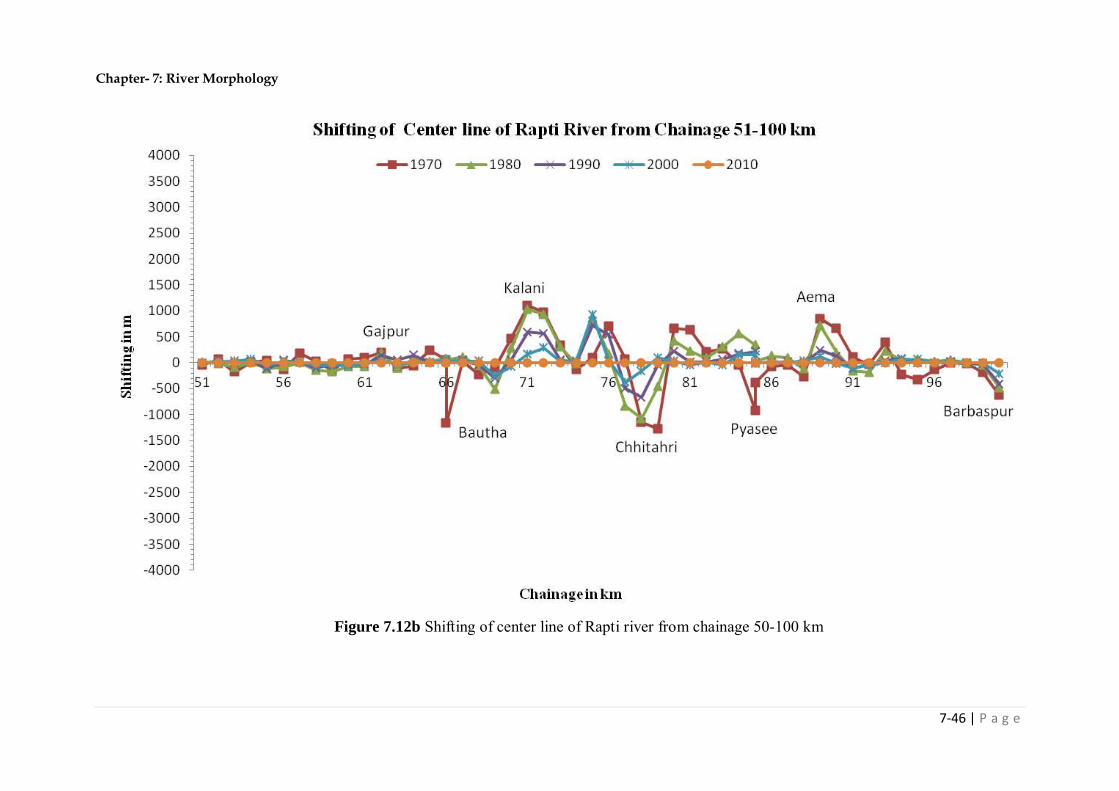
Chapter- 7: River Morphology
7-46 | P a g e
Figure 7.12b Shifting of center line of Rapti river from chainage 50-100 km

Chapter- 7: River Morphology
7-47 | P a g e
Figure 7.13a Shifting of center line of Rapti river from chainage 100-150 km

Chapter- 7: River Morphology
7-48 | P a g e
Figure 7.13b Shifting of center line of Rapti river from chainage 100-150 km
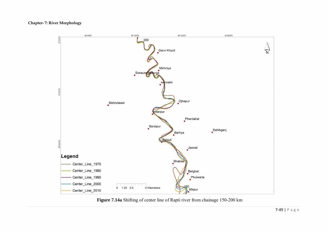
Chapter- 7: River Morphology
7-49 | P a g e
Figure 7.14a Shifting of center line of Rapti river from chainage 150-200 km

Chapter- 7: River Morphology
7-50 | P a g e
Figure 7.14b Shifting of center line of Rapti river from chainage 150-200 km

Chapter- 7: River Morphology
7-51 | P a g e
Figure 7.15a Shifting of center line of Rapti river from chainage 200-250 km

Chapter- 7: River Morphology
7-52 | P a g e
Figure 7.15b Shifting of center line of Rapti river from chainage 200-250 km

Chapter- 7: River Morphology
7-53 | P a g e
Figure 7.16a Shifting of center line of Rapti river from chainage 250-300 km

Chapter- 7: River Morphology
7-54 | P a g e
Figure 7.16b Shifting of center line of Rapti river from chainage 250-300 km

Chapter- 7: River Morphology
7-55 | P a g e
Figure 7.17a Shifting of center line of Rapti river from chainage 300-350 km

Chapter- 7: River Morphology
7-56 | P a g e
Figure 7.17b Shifting of center line of Rapti river from chainage 300-350 km

Chapter- 7: River Morphology
7-57 | P a g e
Figure 7.18a Shifting of center line of Rapti river from chainage 350-400 km

Chapter- 7: River Morphology
7-58 | P a g e
Figure 7.18b Shifting of center line of Rapti river from chainage 350-400 km
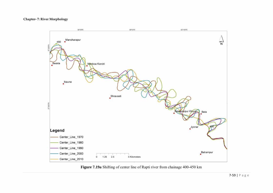
Chapter- 7: River Morphology
7-59 | P a g e
Figure 7.19a Shifting of center line of Rapti river from chainage 400-450 km

Chapter- 7: River Morphology
7-60 | P a g e
Figure 7.19b Shifting of center line of Rapti river from chainage 400-450 km

Chapter- 7: River Morphology
7-61 | P a g e
Figure 7.20a Shifting of center line of Rapti river from chainage 450-500 km

Chapter- 7: River Morphology
7-62 | P a g e
Figure 7.20b Shifting of center line of Rapti river from chainage 450-500 km

Chapter- 7: River Morphology
7-63 | P a g e
Figure 7.21a Shifting of center line of Rapti river from chainage 500-542 km
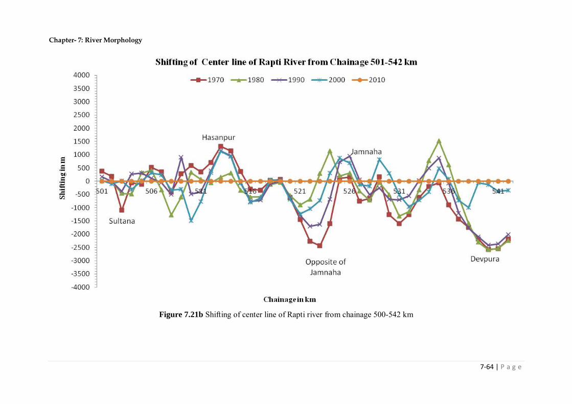
Chapter- 7: River Morphology
7-64 | P a g e
Figure 7.21b Shifting of center line of Rapti river from chainage 500-542 km

Chapter- 7: River Morphology
7-65 | P a g e
Figure 7.22a Decadal changes in the course of Rapti river from chainage 0-50 km
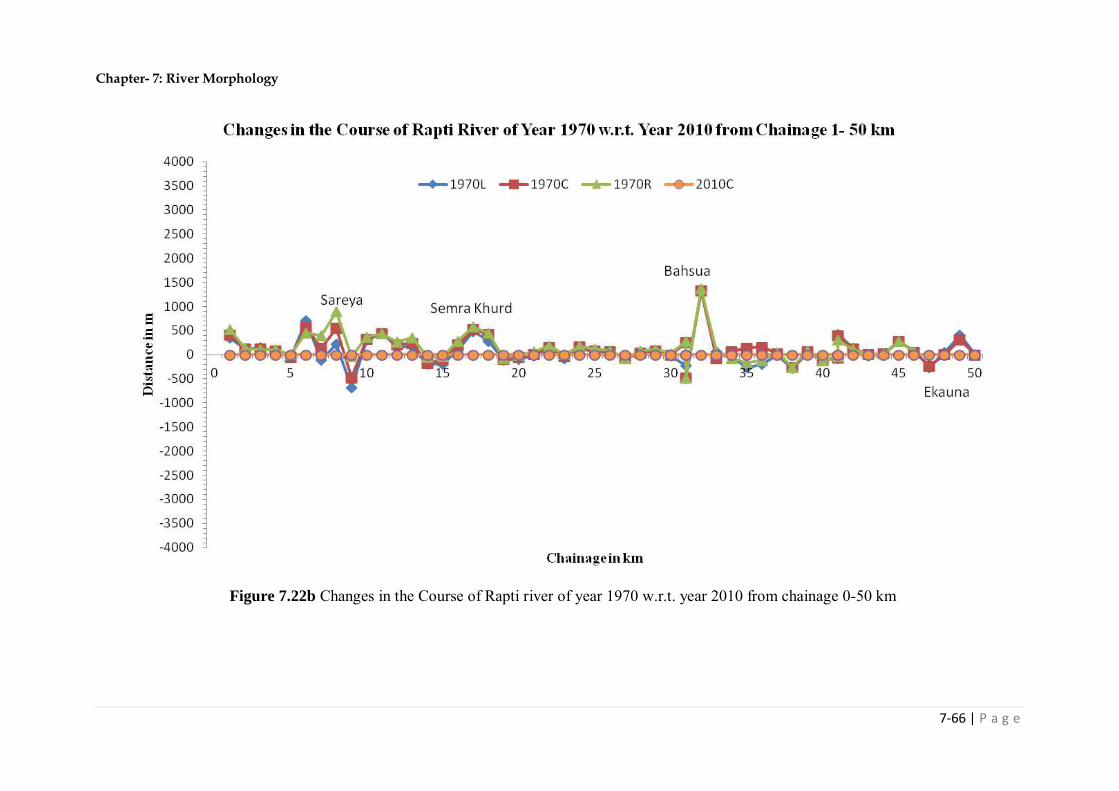
Chapter- 7: River Morphology
7-66 | P a g e
Figure 7.22b Changes in the Course of Rapti river of year 1970 w.r.t. year 2010 from chainage 0-50 km

Chapter- 7: River Morphology
7-67 | P a g e
Figure 7.23a Decadal changes in the course of Rapti river from chainage 50-100 km

Chapter- 7: River Morphology
7-68 | P a g e
Figure 7.23b Changes in the Course of Rapti river of year 1970 w.r.t. year 2010 from chainage 50-100 km

Chapter- 7: River Morphology
7-69 | P a g e
Figure 7.24a Decadal changes in the course of Rapti river from chainage 100-150 km
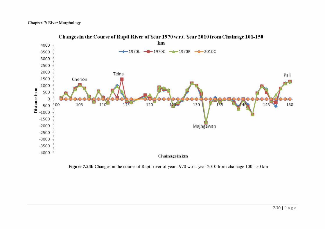
Chapter- 7: River Morphology
7-70 | P a g e
Figure 7.24b Changes in the course of Rapti river of year 1970 w.r.t. year 2010 from chainage 100-150 km

Chapter- 7: River Morphology
7-71 | P a g e
Figure 7.25a Decadal changes in the course of Rapti river from chainage 150-200 km

Chapter- 7: River Morphology
7-72 | P a g e
Figure 7.25b Changes in the Course of Rapti river of year 1970 w.r.t. year 2010 from chainage 150-200 km

Chapter- 7: River Morphology
7-73 | P a g e
Figure 7.26a Decadal changes in the course of Rapti river from chainage 200-250 km

Chapter- 7: River Morphology
7-74 | P a g e
Figure 7.26b Changes in the Course of Rapti river of year 1970 w.r.t. year 2010 from chainage 200-250 km

Chapter- 7: River Morphology
7-75 | P a g e
Figure 7.27a Decadal changes in the course of Rapti river from chainage 250-300 km
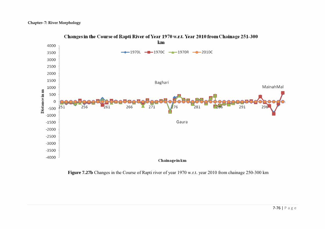
Chapter- 7: River Morphology
7-76 | P a g e
Figure 7.27b Changes in the Course of Rapti river of year 1970 w.r.t. year 2010 from chainage 250-300 km

Chapter- 7: River Morphology
7-77 | P a g e
Figure 7.28a Decadal changes in the course of Rapti river from chainage 300-350 km
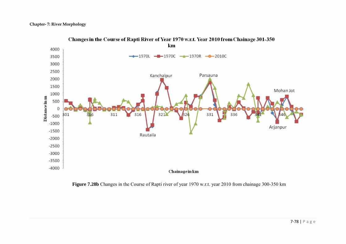
Chapter- 7: River Morphology
7-78 | P a g e
Figure 7.28b Changes in the Course of Rapti river of year 1970 w.r.t. year 2010 from chainage 300-350 km

Chapter- 7: River Morphology
7-79 | P a g e
Figure 7.29a Decadal changes in the course of Rapti river from chainage 350-400 km

Chapter- 7: River Morphology
7-80 | P a g e
Figure 7.29b Changes in the Course of Rapti river of year 1970 w.r.t. year 2010 from chainage 350-400 km

Chapter- 7: River Morphology
7-81 | P a g e
Figure 7.30a Decadal changes in the course of Rapti river from chainage 400-450 km

Chapter- 7: River Morphology
7-82 | P a g e
Figure 7.30b Changes in the Course of Rapti river of year 1970 w.r.t. year 2010 from chainage 400-450 km

Chapter- 7: River Morphology
7-83 | P a g e
Figure 7.31a Decadal changes in the course of Rapti river from chainage 450-500 km

Chapter- 7: River Morphology
7-84 | P a g e
Figure 7.31b Changes in the Course of Rapti river of year 1970 w.r.t. year 2010 from chainage 450-500 km

Chapter- 7: River Morphology
7-85 | P a g e
Figure 7.32a Decadal changes in the course of Rapti river from chainage 500-542 km

Chapter- 7: River Morphology
7-86 | P a g e
Figure 7.32b Changes in the Course of Rapti river of year 1970 w.r.t. year 2010 from chainage 500-542 km
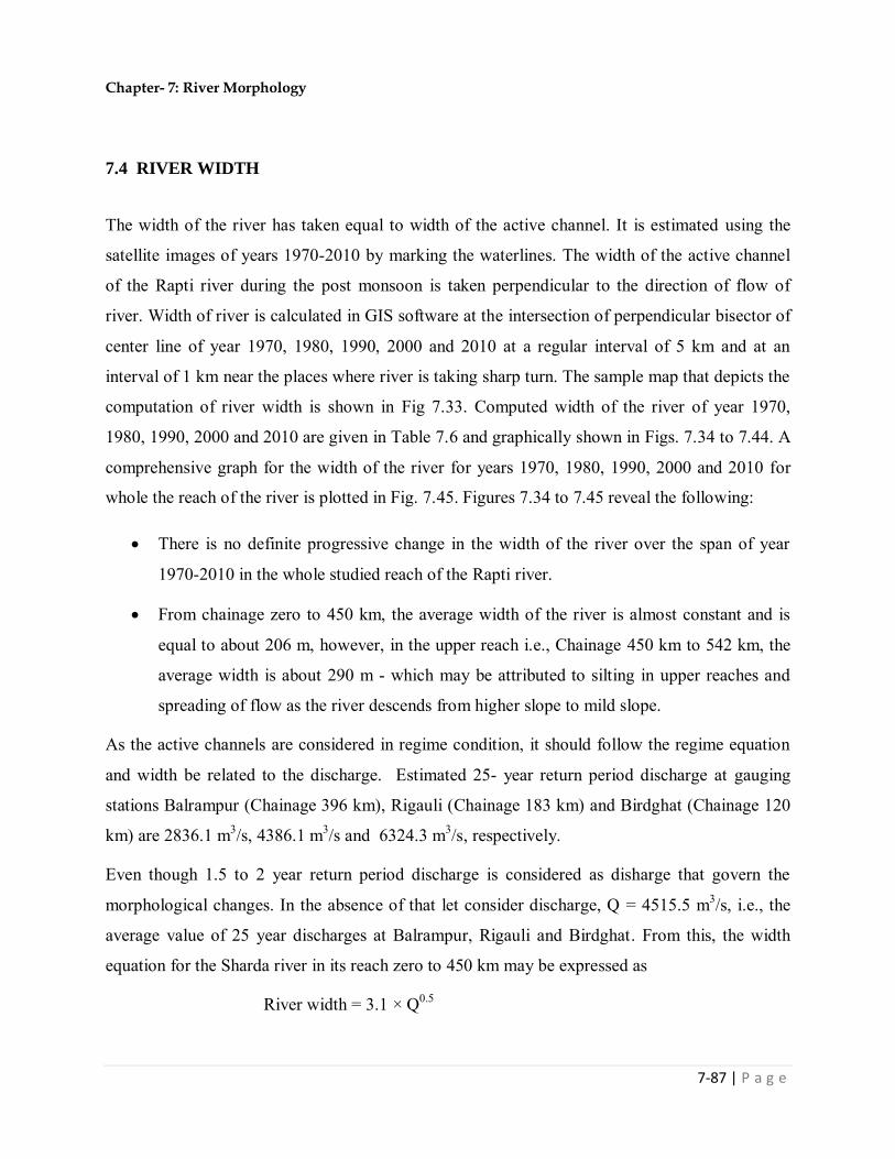
Chapter- 7: River Morphology
7-87 | P a g e
7.4 RIVER WIDTH
The width of the river has taken equal to width of the active channel. It is estimated using the
satellite images of years 1970-2010 by marking the waterlines. The width of the active channel
of the Rapti river during the post monsoon is taken perpendicular to the direction of flow of
river. Width of river is calculated in GIS software at the intersection of perpendicular bisector of
center line of year 1970, 1980, 1990, 2000 and 2010 at a regular interval of 5 km and at an
interval of 1 km near the places where river is taking sharp turn. The sample map that depicts the
computation of river width is shown in Fig 7.33. Computed width of the river of year 1970,
1980, 1990, 2000 and 2010 are given in Table 7.6 and graphically shown in Figs. 7.34 to 7.44. A
comprehensive graph for the width of the river for years 1970, 1980, 1990, 2000 and 2010 for
whole the reach of the river is plotted in Fig. 7.45. Figures 7.34 to 7.45 reveal the following:
There is no definite progressive change in the width of the river over the span of year
1970-2010 in the whole studied reach of the Rapti river.
From chainage zero to 450 km, the average width of the river is almost constant and is
equal to about 206 m, however, in the upper reach i.e., Chainage 450 km to 542 km, the
average width is about 290 m - which may be attributed to silting in upper reaches and
spreading of flow as the river descends from higher slope to mild slope.
As the active channels are considered in regime condition, it should follow the regime equation
and width be related to the discharge. Estimated 25- year return period discharge at gauging
stations Balrampur (Chainage 396 km), Rigauli (Chainage 183 km) and Birdghat (Chainage 120
km) are 2836.1 m3/s, 4386.1 m3/s and 6324.3 m3/s, respectively.
Even though 1.5 to 2 year return period discharge is considered as disharge that govern the
morphological changes. In the absence of that let consider discharge, Q = 4515.5 m3/s, i.e., the
average value of 25 year discharges at Balrampur, Rigauli and Birdghat. From this, the width
equation for the Sharda river in its reach zero to 450 km may be expressed as
River width = 3.1 × Q0.5

Chapter- 7: River Morphology
7-88 | P a g e
Here River width is in m and Q in m3/s. The multiplying coefficient of the above equation is
lower than the Lacey equation.
Figure 7.33 Sample map showing width of Rapti river for year 2010

Chapter- 7: River Morphology
7-89 | P a g e
Table 7.6 Width of Rapti river of year 1970, 1980, 1990, 2000 and 2010
Chainage
(km)
Width (m)
2010 2000 1990 1980 1970
0 357.61 281.95 205.35 251.71 206.63 5 242.36 336.34 261.95 254.13 185.49
10 258.67 284.02 192.68 299.01 206.18 15 276.79 283.42 150.27 278.69 192.94 20 291.49 301.28 261.24 394.16 167.86 25 199.11 173.05 199.79 209.49 140.38 30 139.34 152.62 132.57 195.85 111.09 35 168.86 239.58 134.97 214.33 227.83 40 196.33 265.13 195.85 215.18 231.70 45 209.38 170.79 137.87 127.52 212.34 50 156.02 197.57 217.74 208.13 214.16 55 189.71 152.13 186.74 189.21 196.44 60 220.05 274.02 178.42 294.75 240.09 65 180.09 206.87 195.56 219.61 171.73 70 122.44 186.67 109.08 212.11 92.90 75 168.44 480.68 127.44 280.80 194.56 80 178.26 155.16 86.35 360.47 254.56 85 180.30 190.50 161.62 170.53 86.58 90 281.70 237.18 217.31 204.84 290.22 95 278.36 290.71 274.47 326.64 185.54 100 222.05 236.44 256.99 439.71 290.61 105 238.99 210.09 199.99 207.73 286.15 110 151.27 207.36 192.46 276.33 278.70 115 250.72 278.85 174.61 203.90 88.09 120 251.57 273.92 250.45 248.86 120.06 125 127.64 321.87 165.78 306.75 102.91 130 174.37 222.08 222.56 259.86 173.77 135 207.26 232.37 226.14 194.38 231.83 140 450.99 432.75 151.57 209.99 298.51 145 253.38 277.74 262.60 199.47 214.16 150 277.45 222.20 221.68 251.64 203.82 155 178.33 185.54 156.51 328.58 335.63 160 193.28 215.97 232.74 209.18 262.24 165 214.29 339.89 138.73 311.85 273.69 170 146.59 302.89 225.45 212.55 257.48 175 129.82 290.12 161.20 237.18 260.12 180 140.29 168.36 210.28 196.80 203.77 185 219.79 220.91 201.34 209.56 147.83 190 188.40 171.52 140.67 199.07 157.24 195 138.60 189.79 175.13 273.49 97.12

Chapter- 7: River Morphology
7-90 | P a g e
200 153.84 282.28 288.77 304.76 74.01 205 202.69 334.29 272.86 210.62 108.64 210 140.48 196.53 161.28 228.26 115.52 215 139.99 114.38 99.40 112.55 114.85 220 95.55 170.56 240.87 271.55 86.97 225 165.83 269.35 183.41 208.70 126.00 230 309.55 264.97 140.36 221.52 79.17 235 159.74 198.50 244.04 241.22 102.46 240 126.11 245.08 186.52 185.60 90.10 245 125.28 168.59 161.15 181.49 69.55 250 189.85 240.88 222.43 185.25 234.43 255 190.97 173.39 184.54 201.21 129.27 260 172.07 196.67 147.61 237.19 245.68 265 164.45 151.84 166.32 216.99 173.42 270 121.29 141.08 163.08 184.42 143.23 275 132.34 174.54 150.42 257.91 235.63 280 180.71 205.02 194.94 320.06 161.25 285 160.06 233.21 262.70 262.61 136.95 290 175.27 170.89 192.53 251.70 131.17 295 127.47 158.16 268.39 202.05 285.19 300 176.49 197.71 245.68 233.47 99.84 305 190.83 176.91 415.65 287.54 118.25 310 118.60 112.46 172.91 220.59 76.72 315 127.72 129.76 337.68 201.27 62.96 320 226.46 199.83 223.81 186.66 223.77 325 156.84 154.78 380.24 239.52 153.87 330 188.02 121.03 302.86 263.98 219.58 335 149.51 178.06 222.54 165.69 113.06 340 131.13 159.80 258.52 263.50 242.26 345 144.82 186.03 197.26 212.48 93.55 350 210.51 168.94 220.93 127.30 172.05 355 127.84 178.57 104.58 201.27 147.51 360 123.58 131.76 158.02 197.99 88.13 365 168.73 278.01 209.57 169.30 103.27 370 142.90 145.31 213.52 187.31 189.51 375 185.79 98.57 283.44 359.05 115.52 380 213.06 231.10 296.93 184.34 127.44 385 167.11 193.06 235.65 203.91 94.99 390 342.76 143.80 191.09 399.55 94.19 395 138.10 163.28 165.50 188.69 66.93 400 270.43 136.53 328.88 254.08 160.14 405 156.96 198.90 240.31 198.65 137.78 410 201.57 206.66 314.42 354.28 253.89 415 169.85 171.34 185.95 346.06 174.75

Chapter- 7: River Morphology
7-91 | P a g e
420 381.28 123.86 409.03 185.65 234.85 425 269.14 119.76 263.37 192.56 316.24 430 205.86 470.04 254.19 186.03 253.99 435 175.47 153.77 334.53 164.43 201.50 440 198.77 159.68 328.94 199.65 240.48 445 199.99 193.57 229.38 301.99 175.61 450 181.78 162.51 550.21 199.85 92.16 455 226.73 386.38 308.02 351.67 169.60 460 132.93 157.11 236.23 401.83 139.01 465 142.03 276.10 362.98 305.62 150.51 470 156.55 172.70 122.20 372.45 185.19 475 623.19 269.85 190.04 198.64 198.75 480 236.21 248.78 282.99 351.22 302.85 485 212.95 199.94 220.88 230.13 129.92 490 287.90 126.85 339.48 685.97 253.75 495 364.08 457.68 168.30 461.23 148.24 500 228.64 248.95 179.88 184.65 122.14 505 264.99 179.03 319.92 229.46 213.81 510 206.03 389.09 410.95 289.01 391.56 515 197.02 465.03 403.71 656.54 234.51 520 271.53 371.19 220.81 635.39 179.19 525 301.38 204.21 480.62 442.51 114.32 530 480.54 218.93 508.06 350.58 214.80 535 479.87 358.80 290.40 415.18 181.84 540 271.41 280.50 359.47 321.60 217.68 542 286.67 277.18 307.61 452.17 210.13

Chapter- 7: River Morphology
7-92 | P a g e
Figure 7.34 Width of Rapti river in years 1970, 1980, 1990, 2000, and 2010 from chainage 0-50 km
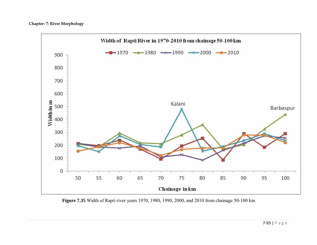
Chapter- 7: River Morphology
7-93 | P a g e
Figure 7.35 Width of Rapti river years 1970, 1980, 1990, 2000, and 2010 from chainage 50-100 km

Chapter- 7: River Morphology
7-94 | P a g e
Figure 7.36 Width of Rapti river in years 1970, 1980, 1990, 2000, and 2010 from chainage 100-150 km

Chapter- 7: River Morphology
7-95 | P a g e
Figure 7.37Width of Rapti river in years 1970, 1980, 1990, 2000, and 2010 from chainage 150-200 km
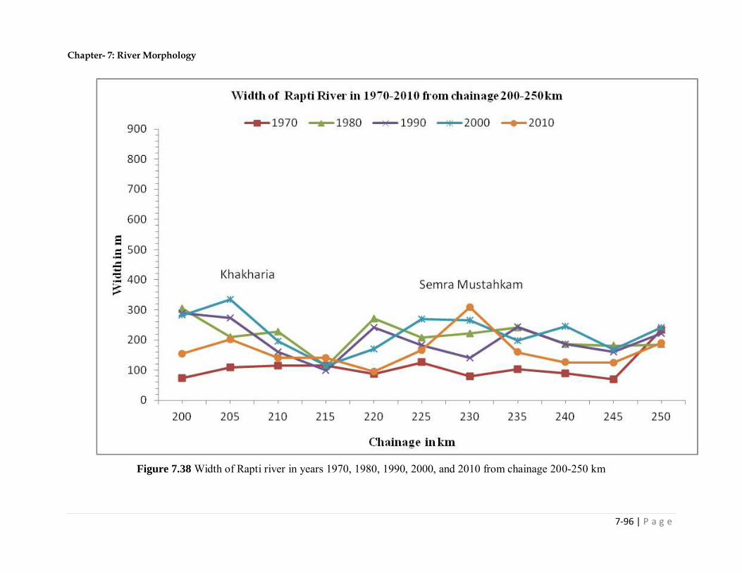
Chapter- 7: River Morphology
7-96 | P a g e
Figure 7.38 Width of Rapti river in years 1970, 1980, 1990, 2000, and 2010 from chainage 200-250 km

Chapter- 7: River Morphology
7-97 | P a g e
Figure 7.39 Width of Rapti river in years 1970, 1980, 1990, 2000, and 2010 from chainage 250-300 km

Chapter- 7: River Morphology
7-98 | P a g e
Figure 7.40 Width of Rapti River in years 1970, 1980, 1990, 2000, and 2010 from chainage 300-350 km

Chapter- 7: River Morphology
7-99 | P a g e
Figure 7.41 Width of Rapti River in years 1970, 1980, 1990, 2000, and 2010 from chainage 350-400 km
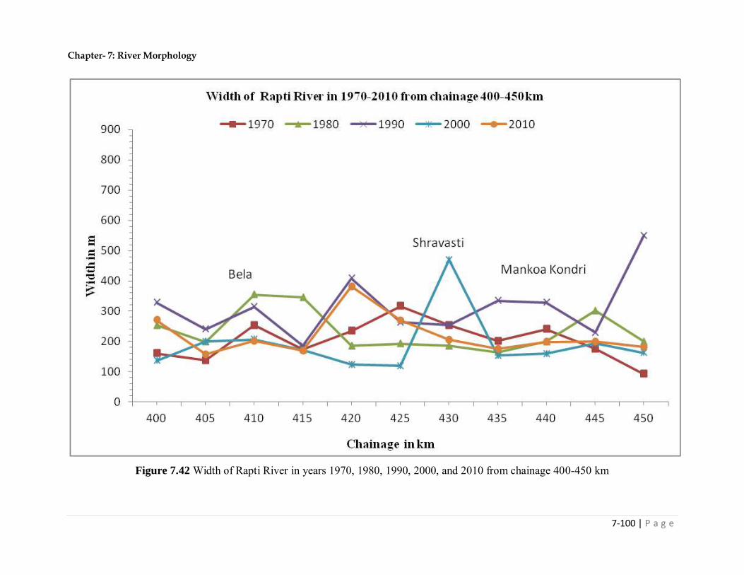
Chapter- 7: River Morphology
7-100 | P a g e
Figure 7.42 Width of Rapti River in years 1970, 1980, 1990, 2000, and 2010 from chainage 400-450 km
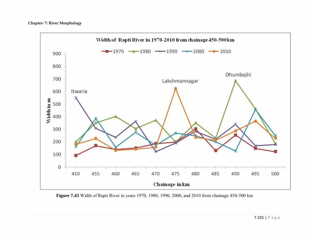
Chapter- 7: River Morphology
7-101 | P a g e
Figure 7.43 Width of Rapti River in years 1970, 1980, 1990, 2000, and 2010 from chainage 450-500 km

Chapter- 7: River Morphology
7-102 | P a g e
Figure 7.44 Width of Rapti River in years 1970, 1980, 1990, 2000, and 2010 from chainage 500-542 km

Chapter- 7: River Morphology
7-103 | P a g e
Figure 7.45 Width of Rapti River in years 1970, 1980, 1990, 2000, and 2010 from chainage 0-542 km
0
100
200
300
400
500
600
700
0 100 200 300 400 500
Wid
th (m
)
Chainage (km)
2010 2000 1990 1980 1970 Average
Chapter- 7: River Morphology
7-104 | P a g e
7.5 DISCUSSIONS ON RIVER COURSE SHIFTING AND ITS WIDTH
The following points may be noted from the analysis carried out in respect of shifting of course
of the river and the river width:
1. Reach 0-50 km: There is no any progressive change in the course of river in this reach in
the span of year 1970 to 2010. River is having meandering pattern in this reach. Major
changes in the course of river has been noticed near Sareya, Ghaighat and Bahsua. The
river has shifted from left to right at Sareya and Bahsua by 3 km and 2 km, respectively.
Average width of the active channel is about 200 m in this reach. There is no much
variation in the width over the years and along the channel except at Semra Khard, the
width of the river was 400 m in year 1980.
2. Reach 50-100 km: Major changes in the course of the river have been noticed in the upper
part of the reach. It is also meandering in this reach. There is no progressive shift in course
of the river in this reach. Major random shifting of the river has been noticed at Chhitarhri.
In the upper reaches, the course of river in year 1970 to 2010 was within a buffer of two
km.
The average width of the active channel of Rapti river is about 200 m. The maximum width
of the river is about 450 m at Bautha and Chhopra.
3. Reach 100-150 km: There is no any progressive shift of course of river in this reach.
Maximum random shift of the order of 2.5 km has been noticed at Bariarpur, Pali and
Mirpur. Major shift from left to right of the order of 1 km has been noticed at Surghana.
While the river course has shifted from right to left of the order of 1.5 km at Majhgawan
and Bariarpur.
Average width of the active channel in this reach is about 200 m with maximum width of
the order of 5 km at Pali. In general, the width of the river in this reach is varying from 100
m to 300 m.
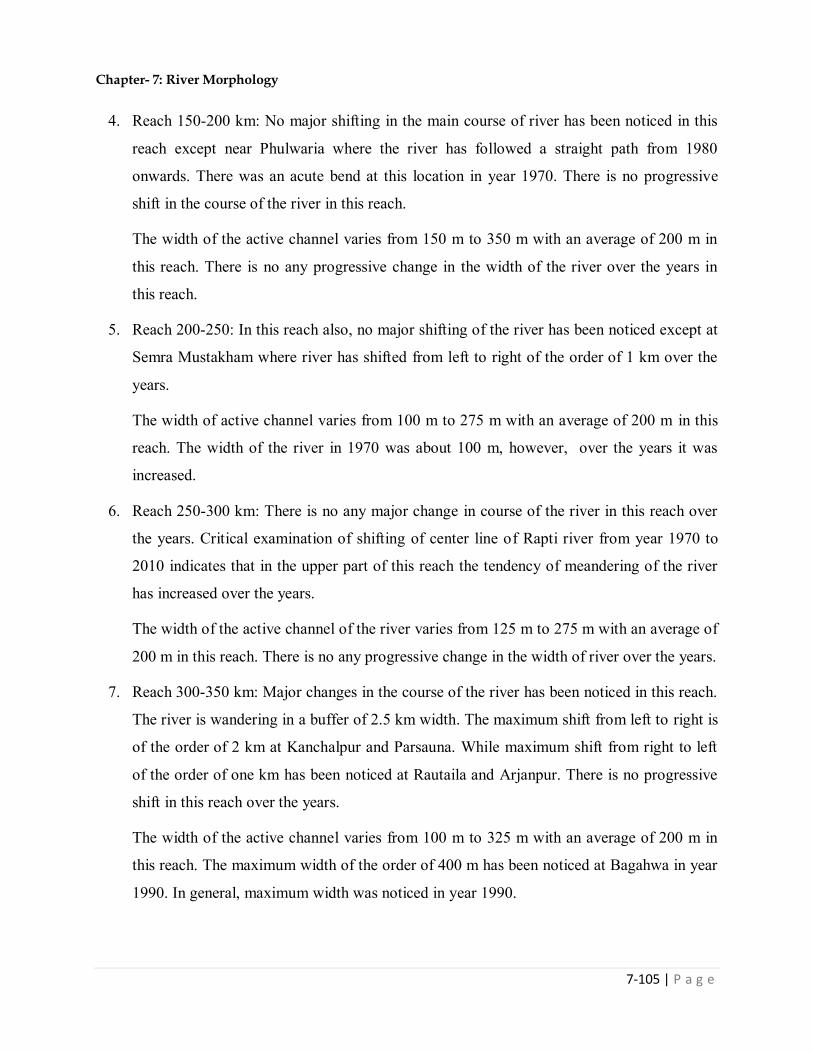
Chapter- 7: River Morphology
7-105 | P a g e
4. Reach 150-200 km: No major shifting in the main course of river has been noticed in this
reach except near Phulwaria where the river has followed a straight path from 1980
onwards. There was an acute bend at this location in year 1970. There is no progressive
shift in the course of the river in this reach.
The width of the active channel varies from 150 m to 350 m with an average of 200 m in
this reach. There is no any progressive change in the width of the river over the years in
this reach.
5. Reach 200-250: In this reach also, no major shifting of the river has been noticed except at
Semra Mustakham where river has shifted from left to right of the order of 1 km over the
years.
The width of active channel varies from 100 m to 275 m with an average of 200 m in this
reach. The width of the river in 1970 was about 100 m, however, over the years it was
increased.
6. Reach 250-300 km: There is no any major change in course of the river in this reach over
the years. Critical examination of shifting of center line of Rapti river from year 1970 to
2010 indicates that in the upper part of this reach the tendency of meandering of the river
has increased over the years.
The width of the active channel of the river varies from 125 m to 275 m with an average of
200 m in this reach. There is no any progressive change in the width of river over the years.
7. Reach 300-350 km: Major changes in the course of the river has been noticed in this reach.
The river is wandering in a buffer of 2.5 km width. The maximum shift from left to right is
of the order of 2 km at Kanchalpur and Parsauna. While maximum shift from right to left
of the order of one km has been noticed at Rautaila and Arjanpur. There is no progressive
shift in this reach over the years.
The width of the active channel varies from 100 m to 325 m with an average of 200 m in
this reach. The maximum width of the order of 400 m has been noticed at Bagahwa in year
1990. In general, maximum width was noticed in year 1990.

Chapter- 7: River Morphology
7-106 | P a g e
8. Reach 350-400 km: Major changes in the course of the river has been observed in the lower
part of this reach. In the upper part major changes in the course of the river has been
noticed only at Shankarnagar. River has meandering pattern in the lower part of this reach.
The maximum shift of the river course from right to left is of the order of 3 km at
Nandnagar from year 1970 to 2010. While river has shifted of the order of 1.5 km from left
to right at Shankarnagar.
Large variation in the width of active channel in this reach has been noticed. River has
widen over the years in this reach. In general, minimum width was found in year 1970 and
maximum in year 1980. Maximum width of the order of 400 m has been noticed at
Mirazapur.
9. Reach 400-450 km: River has remarkable wandering and meandering behavior in this
reach. The river course has wandered in a buffer of 3.5 km in this reach in the span of year
1970 to 2010. There is no any progressive change in the course of the river in this reach.
The maximum shift from left to right of the order of 2 km is found at Jyonar, Shravasti and
Ikauna from 1970 to 2010. However, maximum shift of the river course from right to left
of the order of 2 km can be seen at Mankoa Kondri.
Average width of the active channel in this reach is of the order of 225 m. In general, the
width has increased over the years. The maximum width of the order of 500 m was noticed
at Shravasti in year 2000 and of the order of 575 m at Itwaria in year 1990.
10. Reach 450-500 km: Major changes in the course of the river has been noticed in this reach.
However, no progressive change in the course of river has been noticed over the years. In
general, river has been wandering in a width of 3 km. It has acute meandering pattern in
this reach. River has maximum shift from left to right at Gujar Purwa and right to left at
Keshwapur of the order of 2.5 km in the span of year 1970 to 2010.
The average width of the active channel in this reach is of the order of 290 m. However, it
varies from 150 m to 400 m in this reach. River had maximum width of the order of 650 m
at chainage 475 km (Tribhaura) and 490 km (Lakshmannagar). The width of the active
channel has increased over the years in this reach.

Chapter- 7: River Morphology
7-107 | P a g e
11. Reach 500-542 km: This reach has also wandering and meandering behaviour of the river.
There is no progressive change in the course of river in this reach. However, river has
laterally shifted from left to right of the order of 3 km at Devpura and Jamnagar. At
Hansapur, river has shifted from right of the order of 1.25 km.
Average width of the active channel river is of the order of 290 m. The river width has
increased from 1970 onwards. The maximum width is found at Jamnaha.
7.6 NODAL POITNS
The nodal points along the reach of the river i.e. wherein minimum morphological changes
are seen, have been identified and given in Table 7.7 . This will be helpful in planning of
structures like bridge in the future.
Table 7.7 Nodal points of minimum morphological changes
Sl. No. Chainage (km) Latitude & Longitude Location 1. 0-4 83°40'18.92"E 26°17'29.873"N-
83°39'36.565"E 26°19'5.514"N Koparwar
2. 9-29 83°37'25.54"E 26°19'21.186"N-83°33'1.142"E 26°23'35.424"N
Madanpur
3. 32-40 83°33'22.75"E 26°22'33.243"N-83°31'33.763"E 26°23'0.247"N
Nagwa
4. 42 83°31'22.134"E 26°23'29.952"N Reaon 5. 47-48 83°30'0.387"E 26°24'15.162"N-
83°29'48.992"E 26°24'43.019"N Ekauna
6. 50-62 83°30'13.772"E 26°25'34.602"N-83°28'59.886"E 26°29'45.536"N
Gajpur
7. 64 83°28'57.49"E 26°30'22.389"N Sarar Majhgawan 8. 66-68 83°28'53.166"E 26°31'17.685"N-
83°28'3.749"E 26°32'2.589"N Bautha
9. 73 83°27'43.138"E 26°32'50.358"N Kalani 10. 82 83°28'47.148"E 26°35'19.634"N Dihghat 11. 85-87 83°27'49.889"E 26°36'3.832"N-
83°26'42.979"E 26°35'40.338"N Malaon
12. 91-98 83°27'16.318"E 26°36'59.329"N-83°24'38.482"E 26°37'37.829"N
Aema
13. 102 83°25'36.335"E 26°38'26.503"N Dumri 14. 107 83°23'49.381"E 26°39'31.469"N Cherion 15. 110 83°23'15.166"E 26°40'40.978"N Bhatwa 16. 114-120 83°22'27.782"E 26°41'50.767"N- Nausar
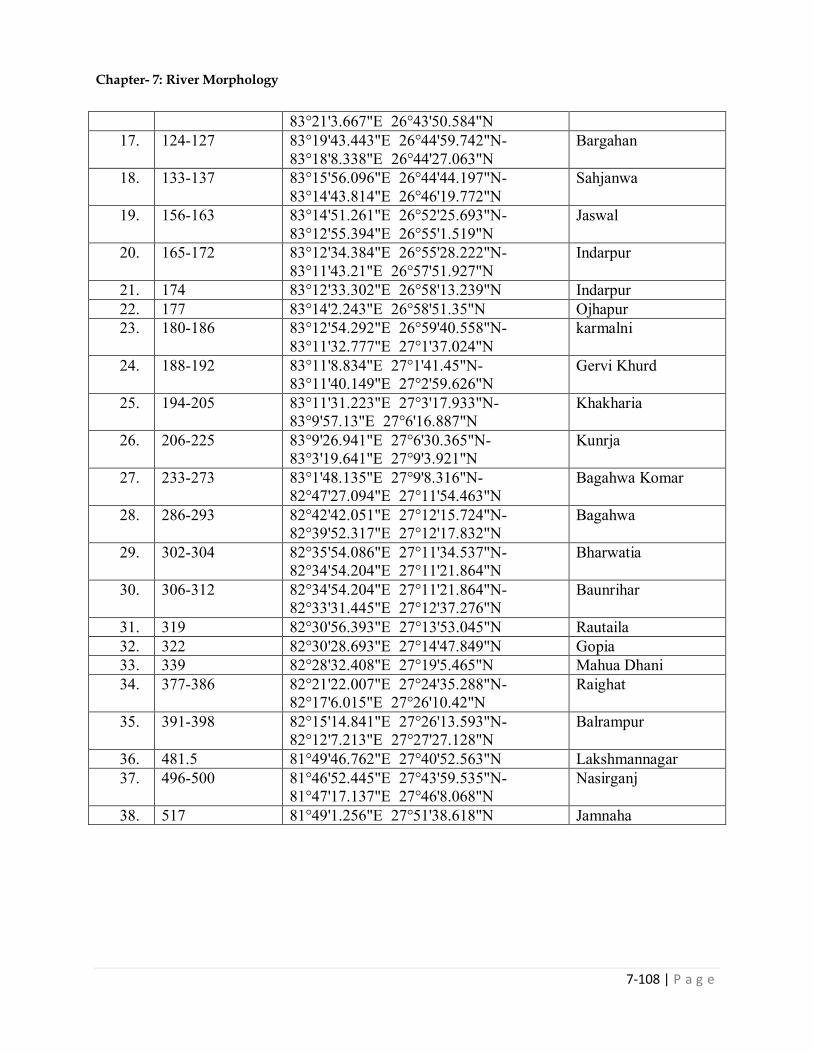
Chapter- 7: River Morphology
7-108 | P a g e
83°21'3.667"E 26°43'50.584"N 17. 124-127 83°19'43.443"E 26°44'59.742"N-
83°18'8.338"E 26°44'27.063"N Bargahan
18. 133-137 83°15'56.096"E 26°44'44.197"N-83°14'43.814"E 26°46'19.772"N
Sahjanwa
19. 156-163 83°14'51.261"E 26°52'25.693"N-83°12'55.394"E 26°55'1.519"N
Jaswal
20. 165-172 83°12'34.384"E 26°55'28.222"N-83°11'43.21"E 26°57'51.927"N
Indarpur
21. 174 83°12'33.302"E 26°58'13.239"N Indarpur 22. 177 83°14'2.243"E 26°58'51.35"N Ojhapur 23. 180-186 83°12'54.292"E 26°59'40.558"N-
83°11'32.777"E 27°1'37.024"N karmalni
24. 188-192 83°11'8.834"E 27°1'41.45"N- 83°11'40.149"E 27°2'59.626"N
Gervi Khurd
25. 194-205 83°11'31.223"E 27°3'17.933"N- 83°9'57.13"E 27°6'16.887"N
Khakharia
26. 206-225 83°9'26.941"E 27°6'30.365"N- 83°3'19.641"E 27°9'3.921"N
Kunrja
27. 233-273 83°1'48.135"E 27°9'8.316"N- 82°47'27.094"E 27°11'54.463"N
Bagahwa Komar
28. 286-293 82°42'42.051"E 27°12'15.724"N- 82°39'52.317"E 27°12'17.832"N
Bagahwa
29. 302-304 82°35'54.086"E 27°11'34.537"N-82°34'54.204"E 27°11'21.864"N
Bharwatia
30. 306-312 82°34'54.204"E 27°11'21.864"N-82°33'31.445"E 27°12'37.276"N
Baunrihar
31. 319 82°30'56.393"E 27°13'53.045"N Rautaila 32. 322 82°30'28.693"E 27°14'47.849"N Gopia 33. 339 82°28'32.408"E 27°19'5.465"N Mahua Dhani 34. 377-386 82°21'22.007"E 27°24'35.288"N-
82°17'6.015"E 27°26'10.42"N Raighat
35. 391-398 82°15'14.841"E 27°26'13.593"N-82°12'7.213"E 27°27'27.128"N
Balrampur
36. 481.5 81°49'46.762"E 27°40'52.563"N Lakshmannagar 37. 496-500 81°46'52.445"E 27°43'59.535"N-
81°47'17.137"E 27°46'8.068"N Nasirganj
38. 517 81°49'1.256"E 27°51'38.618"N Jamnaha

Chapter- 7: River Morphology
7-109 | P a g e
7.7 CONCLUDING REMARKS
1. The computed sinuosity ratio of the Rapti river in the reach under consideration is higher
than 1.5 in the year 1970, 1980, 1990, 2000, and 2010, therefore, the Rapti river is
classified as meandering river.
2. Almost whole reach of the river has meandering pattern, however, it is prominent in the
reaches 25-50 km, 75-100 km, 300-375 km, 400-425 km and 450-475 km. The
meandering is characterized by acute bend with high amplitude, however, they are
relatively stable.
3. The plan form index (PFI) of Rapti River is calculated using the formula given by
Sharma (2004). It has been observed that the Rapti River always runs bankfull, so no
braiding is found in Rapti River.
4. Remarkable shifting of the course of the Rapti river from 1970 to 2010 has been noticed.
The maximum shift is of the order of 2.7 km at some locations. The confluence point of
Rapti and Gaghara rivers has shifted 500 m towards left in year 2010 w.r.t. year 1970.
5. Major shifting of the river course in span of year 1970 to 2010 is in the reaches 75 -100
km, 300-375 km, 400-485 km and 500-542 km. At Devpura, Jamuha, Keshwapur,
Nandnagar and Chitahari shifting is from left to right while at Gujarpurwa, Ikauna,
Jyonar and Kanchalpur shifting is from right to left. No progressive shifting of the course
of the river with respect to time has been noticed.
6. Width of the active channel of the river and river width based on the extreme banks have
been estimated using the satellite images of years 1970-2010. There is no definite
progressive change in the width of the river over the span of year 1970-2010 in the whole
studied reach of the Rapti river. From chainage zero to 450 km, the average width of the
river is almost constant and is equal to about 206 m, however, in the upper reach i.e.,
Chainage 450 km to 542 km, the average width is about 290 m - which may be attributed
to silting in upper reaches and spreading of flow as the river descends from higher slope
to mild slope.

Chapter- 8: Erosion and Siltation
8-1 | P a g e
Chapter 8 EROSION AND SILTATION
8.1 CHANNEL EVOLUTION ANALYSIS
Channel evolution analysis describes the status of the river channel that includes channel
dimension, pattern and longitudinal profile identifying distinct river reaches i.e. channel in upper
reaches, channel in flood plain, aggradation and degradation, bank erosion etc. Such study is
carried out from a field reconnaissance.
The evolution sequence provides an understanding that reaches of a stream may differ in
appearance, but channel form in one reach is associated with other reaches by an evolving
process. The channel evolution analysis helps in understanding a stream’s response to
downstream as well as upstream disturbances in form of morphological changes.
In the present study, the quantification of bank erosion and siltation has been carried out from the
satellite images and toposheets. 1970 has been considered as base year and the changes have
been plotted graphically.
8.2 EROSION & DEPOSITION
Erosion and siltation studies have been carried out for the Rapti River from Nepalgunj to its
confluence point with Ghaghara i.e., near the Barhalganj, UP using the remote sensing
techniques. The toposheet and post-monsoon images of years 1970 and 2010 have been used,
and the study has been carried out to quantify sediment erosion and deposition for duration from
year 1970 to year 2010. The erosion and siltation have been expressed in the terms of area in
km2.

Chapter- 8: Erosion and Siltation
8-2 | P a g e
For estimation of erosion and deposition, extreme left and right banks have been identified based
on the sand deposit and vegetation. Based on the shifting of extreme left and right banks, the
erosion and deposition are determined.
8.3 RESULTS AND ANALYSIS
Estimation of erosion and deposition has been carried out in the view of shifting of extreme left
and right bank which are being identified on the basis of sand deposit and vegetation. Details of
the computed eroded and sited area and also area that were eroded and subsequently silted or
otherwise in the period 1970 to 2010 are given in Table 8.1, and also shown in Fig. 8.1. Net
erosion and deposition in each reach of 50 km are shown in Fig 8.2.
Table 8.1 Erosion and deposition in Rapti river based on shifting of extreme right and left banks
Chainage
(km)
Erosion
(ha)
Deposition
(ha)
Erosion+ Deposition
(ha)
Net Erosion/ Deposition
(ha)
0-50 617.48 549.55 501.37 -67.93
50-100 643.98 522.89 603.94 -121.09
100-150 869.24 663.53 1168.91 -205.71
150-200 625.93 668.49 491.20 42.56
200-250 519.18 343.79 220.31 -175.39
250-300 527.63 344.97 205.41 -182.65
300-350 581.51 463.79 952.34 -117.72
350-400 595.41 426.30 997.27 -169.11
400-450 836.24 770.37 1850.58 -65.87
450-500 996.64 513.39 1801.13 -483.26
500-542 1091.65 457.44 1942.98 -634.20
Total 7904.89 5724.51 10735.44 -2180.37
* '-' indicates erosion and '+' indicates deposition 1 ha = 0.01 km2

Chapter- 8: Erosion and Siltation
8-3 | P a g e
From the above table, it can be summarized that total eroded area is 7904.89 ha, total deposited
area is 5724.51 ha and total eroded plus deposited area is 10735.44 ha. Net eroded area is
2180.37 ha during the period 1970 to 2010.
Total Drainage area of Rapti River is 23,900 km2 for Indian part. Thus eroded area per km2
catchment area is 21.80/23900 (0.09%).
Based on shifting of extreme left and right banks during the period of year 1970-2010, erosion
deposition maps for each reach have been prepared and the same are shown in Figs. 8.3-8.13.
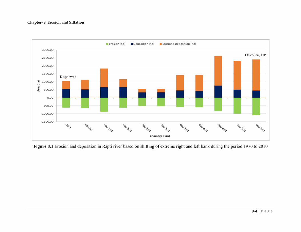
Chapter- 8: Erosion and Siltation
8-4 | P a g e
Figure 8.1 Erosion and deposition in Rapti river based on shifting of extreme right and left bank during the period 1970 to 2010

Chapter- 8: Erosion and Siltation
8-5 | P a g e
Figure 8.2 Net Erosion and deposition in Rapti River during the period 1970 to 2010 based on shifting of extreme right and left
bank during the period 1970 to 2010

Chapter- 8: Erosion and Siltation
8-6 | P a g e
Figure 8.3 Erosion and deposition map of Rapti river for period 1970-2010 from chainage 0-50 km

Chapter- 8: Erosion and Siltation
8-7 | P a g e
Figure 8.4 Erosion and deposition map of Rapti River for period 1970-2010 from chainage 50-100 km

Chapter- 8: Erosion and Siltation
8-8 | P a g e
Figure 8.5 Erosion and deposition map of Rapti River for period 1970-2010 from chainage 100-150 km
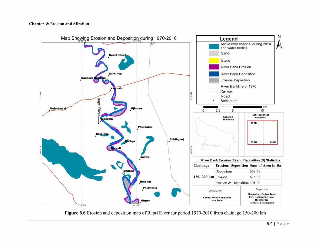
Chapter- 8: Erosion and Siltation
8-9 | P a g e
Figure 8.6 Erosion and deposition map of Rapti River for period 1970-2010 from chainage 150-200 km
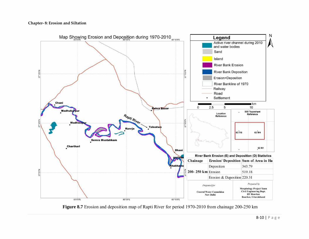
Chapter- 8: Erosion and Siltation
8-10 | P a g e
Figure 8.7 Erosion and deposition map of Rapti River for period 1970-2010 from chainage 200-250 km

Chapter- 8: Erosion and Siltation
8-11 | P a g e
Figure 8.8 Erosion and deposition map of Rapti River for period 1970-2010 from chainage 250-300 km

Chapter- 8: Erosion and Siltation
8-12 | P a g e
Figure 8.9 Erosion and deposition map of Rapti River for period 1970-2010 from chainage 300-350 km

Chapter- 8: Erosion and Siltation
8-13 | P a g e
Figure 8.10 Erosion and deposition map of Rapti River for period 1970-2010 from chainage 350-400 km

Chapter- 8: Erosion and Siltation
8-14 | P a g e
Figure 8.11 Erosion and deposition map of Rapti River for period 1970-2010 from chainage 400-450 km
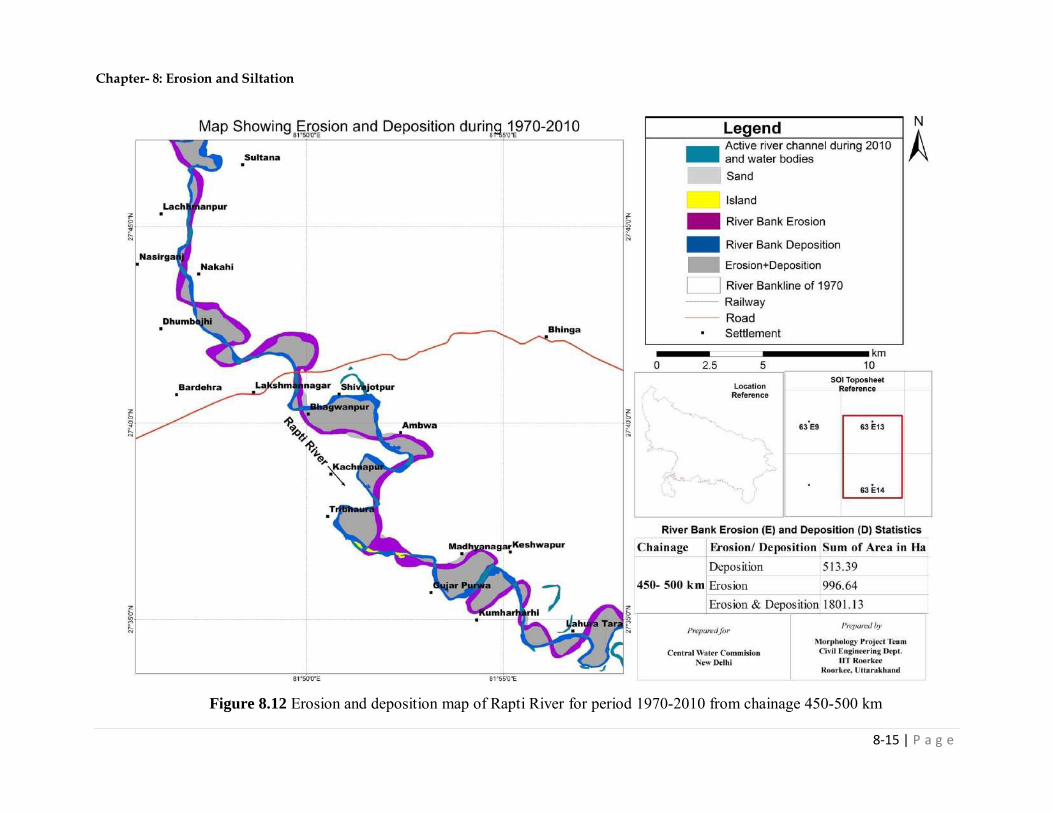
Chapter- 8: Erosion and Siltation
8-15 | P a g e
Figure 8.12 Erosion and deposition map of Rapti River for period 1970-2010 from chainage 450-500 km

Chapter- 8: Erosion and Siltation
8-16 | P a g e
Figure 8.13 Erosion and deposition map of Rapti River for period 1970-2010 from chainage 500-542 km
Chapter- 8: Erosion and Siltation
8-19 | P a g e
8.5 DISCUSSION ON THE RESULTS
The following points have been noted considering erosion and siltation based on the shifting of
extreme left and right banks.
In the reach 0-50 km, total eroded area, total deposited area and total eroded & deposited area
are 617.48 ha, 549.55 ha and 501.37 ha, respectively. Net erosion in this reach is 67.93 ha.
Erosion is observed on left bank near Gaighat and Ekauna and deposition near Sareya and
Bahssua on the right bank. The possible reason behind this is meandering nature of the river.
In the reach 50-100 km, total eroded area, total deposited area and total eroded plus deposited
area are 643.98 ha, 522.89 ha and 603.94 ha respectively. Net erosion in this reach is 121.09
ha. Erosion is observed on left bank near Chhithari, Dumri, Chhopra and Borhi while
deposition has occurred near Malaon & Jagdishpur on the right bank. The possible reason
behind this is meandering nature of the river and lateral shifting.
In the reach 100-150 km, total eroded area, total deposited area and total eroded & deposited
area are 869.24 ha, 663.23 ha and 1168.91 ha respectively. Net erosion in this reach is 205.71
ha. Erosion is observed towards left bank near Dumri, Gorakhpur, Mainabhagar and Mirpur,
on the other hand deposition was noticed near Bhauapur and Nausar on the right bank. The
possible reason behind this is meandering nature of the river and provision of river training
works.
In the reach 150-200 km, total eroded area, total deposited area and total eroded & deposited
area are 625.93 ha, 668.49 ha and 491.20 ha respectively. Net deposition in this reach is
42.56 ha. Erosion is observed towards left bank near Mirpur and Ojhapur, and on the other
hand deposition was found near Indarpur and Karmalini on the right bank. The possible
reason behind this is meandering nature of the river and lateral shifting. There are natural
lakes in this reach, and Bakhira taal is the largest among them.
In the reach 200-250 km, total eroded area, total deposited area and total eroded plus
deposited area are 519.18 ha, 343.79 ha and 220.31 ha respectively. Net erosion of this reach
is 175.39 ha. No major changes are visible in this reach during the period 1970-2010. Minor
erosion on left bank near Madhwapur and deposition near Charthari on the right bank has

Chapter- 8: Erosion and Siltation
8-20 | P a g e
been noticed. The possible reason behind this is meandering nature of the river and lateral
shifting.
In the reach 250-300 km, total eroded area, total deposited area and total eroded plus
deposited area are 527.63 ha, 344.97 ha and 205.41 ha respectively. Net erosion of this reach
is 182.65 ha. No major erosion and deposition are visible in this reach.
In the reach 300-350 km, total eroded area, total deposited area and total eroded plus
deposited area are 581.51 ha, 463.79 ha and 952.34 ha respectively. Net erosion in this reach
is 117.72 ha. Erosion is observed on left bank near Gopia, u/s of Arjanpur and Bharwatia on
the other hand deposition was found near Raasulabad, Mahua Dhani and Nagwa; on the right
bank. The possible reason behind this is meandering nature of the river and lateral shifting.
In the reach 350-400 km, total eroded area, total deposited area and total eroded plus
deposited area are 595.41 ha, 426.30 ha and 997.27 ha respectively. Net erosion in this reach
is 169.11 ha. Major changes in the form of erosion and deposition are visible in this reach.
There are erosion and deposition on both the banks. The possible reason behind this is
meandering nature of the river and existing river training methods.
In the reach 400-450 km, total eroded area, total deposited area and total eroded plus
deposited area are 836.24 ha, 770.37 ha and 1850.58 ha respectively. Net erosion in this
reach is 65.87 ha. River has eroded and deposited on both the banks. Erosion is observed on
left bank near Manoharpur, on the other hand deposition near Ikauna on the right bank was
noticed. Major changes are visible near Jyonar and Balrampur. The possible reason behind
this is meandering nature of the river, lateral shifting and constructed structures.
In the reach 450-500 km, total eroded area, total deposited area and total eroded plus
deposited area are 996.64 ha, 513.39 ha and 1801.13 ha respectively. Net erosion in this
reach is 483.26 ha. Noticeable amounts of erosion &deposition are visible in this reach,
especially on the upstream of the barrage. The possible reason behind this is construction of
barrages and braiding & meandering nature of the river due to topographical changes. Other
areas are suffered with huge erosion and deposition.
In the reach 500-542 km, total eroded area, total deposited area and total eroded plus
deposited area are 1091.65 ha. 457.44 ha and 1942.98 ha respectively. Net erosion in this
Chapter- 8: Erosion and Siltation
8-21 | P a g e
reach is 634.20 ha. Erosion is observed on right bank near Jamnaha and Kundwa. The
possible reason behind this is braiding & meandering nature of the river due to topographical
change.
8.6 CONCLUSIONS
Following conclusions may be drawn from the study of erosion and siltation in the Rapti river:
a) The total eroded, silted, eroded plus silted, and net eroded area in the Rapti river during
the period 1970 to 2010 are 79.04 km2, 57.24 km2, 107.35 km2 and 21.80 km2,
respectively. It may be concluded that over a span of 40 years i.e, 1970 to 2010, about
21.80 km2 area of Rapti River has been eroded by the flowing water.
b) Erosion has been noticed in the entire reach of Rapti River starting from Nepalgunj to its
confluence with Ghaghra River. Major erosion has occurred during the period 1970 to
2010 in the upper reaches (chainage 450-542 km) due to constant shifting of river course.
Minor deposition has taken place in the reaches 25 km - 50 km, 150 km - 175 km and 425
km - 450 km that are near Ekauna, Bhaksa and Ikauna, respectively. At other locations,
like Gorakhpur, Balrampur, Utraula, and Domrianganj, the erosion is not so severe.
c) There is not much shifting and deposition visible in Rapti river course due to provision of
embankments and river training works. There are natural water bodies in the form of ox-
bow lakes in vicinity of river due to its meandering nature.
d) Available measured cross sections of the Rapti river for different years at gauging
stations of Balrampur, Rigauli and Birdghat have been analysed. No remarkable changes
in the historical cross-sections of the Rapti river at Rigauli and Birdghat is noticed,
however, river course has shifted towards left side by about 40 m at Balrampur which has
resulted in both erosion and siltation at this location. Cross-section of the Rapti river is
shallow at Balrampur, however, it is deep at Rigauli and Birdghat.

Chapter- 9: Major Structures & Their Impact On The Morphology
9-1 | P a g e
Chapter 9 MAJOR STRUCTURES & THEIR IMPACT ON THE MORPHOLOGY
9.1 IDENTIFICATION OF MAJOR STRUCTURES
Major structures such as barrages and railway & road bridges located on Rapti River from
Nepalgunj to Patana Ghat (confluence point of Rapti and Ghaghra Rivers) have been
identified using Google Earth and WRIS website and the same are given in Table 9.1.
Table 9.1 Major structures located on the Rapti River from Nepalgunj to Patana Ghat
ID Name Nearby Place Length
(m) Type Long. Lat.
1 Road Bridge (SH-72) Patana Ghat (Barhalganj) 290 Road 83.671681 26.304840
2 Road Bridge Sonbah 330.67 Road 83.617588 26.367654
3 Road Bridge Gheorpar Ahatmali 390 Road 83.522142 26.382252
4 Road Bridge(Panchaldi road) Banspar 353.73 Road 83.488096 26.482628
5 Road Bridge (Under Construction) Kaithwalia 357.63 Road 83.453580 26.544960
6 Road Bridge (Gorakhpur bypass road)
Pipari 410 Road 83.350243 26.705609
7 Road Bridge (NH 28) Gorakhpur 420 Road 83.348608 26.732985
8 Railway Bridge Mohmadpur Mafi 420 Rail 83.244408 26.767676
9 Road Bridge (Pepeeganj- Sesai Ghar Road)
Peepeganj 294.89 Road 83.237861 26.893515
10 Road Bridge (SH 64) Karmaini 333 Road 83.214000 27.014072
11 Road Bridge (Bayurbyaas- Dhani Dhani Bazar 290.01 Road 83.167426 27.108387

Chapter- 9: Major Structures & Their Impact On The Morphology
9-2 | P a g e
Mag)
12 Road Bridge (Dhani- Bayurbyaas Marg) Tal Natawa 232.36 Road 83.126503 27.147096
13 Road Bridge (SH 5) Bansi 213.54 Road 82.932227 27.183164
14 Road Bridge Tighra 200 Road 82.796472 27.193603
15 Road Bridge (Dumriyanganj Road) Domariyaganj 170.81 Road 82.655010 27.213528
16 Road Bridge (Gagapur- Utraula Road) Kundi,Utraula 150 Road 82.478298 27.317368
17 Road Bridge (SH 1A) Durgapur 198.55 Road 82.228716 27.437506
18 Railway bridge (Gainjhawa) Gainjhawa 201.15 Railway 82.226470 27.441303
19 Railway bridge (Gainjhawa) Gainjhawa 230.09 Railway 82.226489 27.441152
20 Road Bridge Kodri Ghat 280 Road 82.138970 27.496591
21 Road Bridge (Under Construction) Andher Purwa 287 Road 81.952020 27.583987
22 Road Bridge(SH 96 A) Mankapur 160 Road 81.827075 27.688620
23 Road Bridge (Barrage) Dayali 285.04 Barrage/ Road
81.813558 27.864529
9.2 BARRAGES ON THE RAPTI RIVER
There is only one barrage namely Rapti Barrage on Rapti river near Baharaich at Chainage
519 km. The construction of the Rapti Barrage was started in the year 1977-78 and completed
in year 2008. This barrage is part of Sarayu Nahar Pariyojana. Uttar Pradesh Govt. took
initiative to provide irrigation to 12.0 Lacs h.a. area (C.C.A) of Baharaich, Shravasti, Gonda,
Balrampur, Basti, Siddharthnagar, Sant Kabir Nagar & Gorakhpur through this project.
Location of Rapti barrage on Goolge earth image is shown in Fig. 9.1a while a photograph of
the Barrage is shown in Fig. 9.1b.
Salient features of the barrage are as follows:

Chapter- 9: Major Structures & Their Impact On The Morphology
9-3 | P a g e
Figure 9.1a Location of Rapti barrage
Salient Features
Name of the Structure Rapti Barrage Nearest city Baharaich District Shrawasti State Uttar Pradesh Name of the River Rapti Basin Ganga Purpose Irrigation Design flood (cumecs) 4990 Length of Barrage and Anicut (m) 284.5 No. of bays (i.e. number of openings) 15 Width of Bay (m) 18 Type of spillway gate Others Thickness of Intermediate Plot (m) 2.5 Crest Level (m) 125 Pond level (m) 127.7 Under sluice bay- Number 4 Gates for under sluice- Size (m) 14 m×18 m×3 m Means for dissipating energy (Hydraulic) DENTATED SILL DEVICE Status of BWA Construction Completed

Chapter- 9: Major Structures & Their Impact On The Morphology
9-4 | P a g e
Figure 9.1b A photogragh of the Rapti barrage
9.2.1 Impact of the Rapti barrage on the morphology of the river
To study the impact of the barrage on the river morphology, decadal satellite images and
geospatial datasets are examined. Fig 9.2a shows the major course of the Rapti River of the
year 1970, 1980, 1990, 2000 and 2010 on the satellite image of the year 2015 while Figs 9.2
b-g show images of the year 1970, 1980, 1990, 2000, 2010 and 2015, respectively.
From the Fig. 9.2a, one can conclude that the river course has wandering behavior upstream
of the barrage. However, no shifting has been observed downstream of the barrage over the
years.
The barrage was commissioned in year 2008. Since then no noticeable silting upstream of the
barrage has been observed. Nevertheless, river in year 2015 was flowing in two channels
upstream of the barrage.
A site visit was undertaken on 23rd October 2016, to have the comprehensive idea of the
morphology of the river at the barrage site. The river has severe wandering behavior
upstream of the barrage. In the past, the river had come very close to the right approach road,
however, with the provision of series of spurs along the right approach road, it was protected
against the erosion - subsequnetly river shifted away from the right approach road.

Chapter- 9: Major Structures & Their Impact On The Morphology
9-5 | P a g e
Figure 9.2a GIS layer of the Rapti river of the year 1970, 1980, 1990, 2000 and 2010 on the satellite image of 2015

Chapter- 9: Major Structures & Their Impact On The Morphology
9-6 | P a g e
Figure 9.2b-g Images of Rapti river for the year 1970, 1980, 1990, 2000, 2010 and 2015
C B
D E
F G

Chapter- 9: Major Structures & Their Impact On The Morphology
9-7 | P a g e
9.3 BRIDGES ON THE RAPTI RIVER
Details of the bridges located on the Rapti River and morphology of the river near such bridges are given in Table 9.2.
Table 9.2 Details of the bridges on Rapti river and morphology of the river near such bridges
ID Name of the
Bridge/ Road Chainage
Length
(m)
Type of
Bridge
River
Width
(m)
Nearby
Place Remarks
1 Road Bridge 2 290 Road 230 Patana Ghat
* Located in relatively straight and stable reach of the river. * No protection works have been provided. * In past, river had come close to the right approach road of the bridge - spurs were provided to protect the approach road. * As such no measures are required for training the river at the bridge site. *Provision of embankment towards right side, upstream of the bridge (SH 72 Bridge) to control the spread of flood water is recommended. (see Fig. 9.3)
2 Road Bridge 17.5 330.67 Road 150 Sonbah
* No protection works are provided near the bridge, however, river has a 90o bend at about 450 m upstream of the bridge - the outer bank of the river is protected using series of spurs against erosion. *A pilot channel is excavated towards left side near the bend.

Chapter- 9: Major Structures & Their Impact On The Morphology
9-8 | P a g e
* In year 1970, the river was away from the bridge towards the right side. * As such not measures are required for training the river at the bridge site.
3 Road Bridge 41 390 Road 200 Gheorpar Ahatmali
* No protection works are provided near the bridge. * Located in a straight reach, however, in a meandering zone. * There is an acute bend at about 720 m upstream of the bridge -outer bank protected using series of spurs. * No measures are required for training the river at the bridge site.
4 Road Bridge
(Panchaldi road) 60 353.73 Road 200 Banspar
* No protection works are provided. * Located in relatively straight and stable reach of the river. * No measures are required for training the river at the bridge site.
5
Road Bridge (Under
Construction)
74 357.63 Road 140 Kaithwalia
*Located just downstream of an acute bend and major shifting of river towards its left side has been noticed upstream of the bend. *Recommended to provide series of spurs towards left side upstream of the bend to arrest such shifting so that out flanking of the bridge can be avoided. (see Fig. 9.4)
6 Road Bridge (Gorakhpur bypass road)
117.5 410 Road 250 Pipari
*Located in a relatively straight and stable reach of the river. *No protection works are provided. *No measures are required for training the river at the bridge site.
7 Road Bridge 121 420 Road 240 Gorakhpur *Currently located skewed in the respect of

Chapter- 9: Major Structures & Their Impact On The Morphology
9-9 | P a g e
(NH 28) direction of flow of the river. * Elliptical guide bund is provided towards right side which performance is satisfactory. * No damage to the guide bund has been noticed. * River is relatively stable near the bridge and requires no protection works.
8 Railway Bridge 137 420 Railway 210 Mohmadpur Mafi
* Jacketing of the river upto about 1 km upstream of the bridge using embankment and spurs. Performances of such structures are satisfactory. * Located in a straight and stable reach of the river. * No any other protection works are required.
9
Road Bridge (Peepeganj- Sesai Ghar
Road)
160 294.89 Road 230 Peepeganj
* Relatively in a straight and stable reach from year 2000 onwards, however, right bank over a length of 700 m upstream of the bridge is under erosion and the same is to be protected using boulder revetment/ porcupine/series of spurs. (see Fig. 9.5) * In the years 1970 to 2000, the river was away from the bridge towards the left side.
10 Road Bridge (SH 64) 183 333 Road 230 Karmaini
* Slightly skewed in the respect of direction of flow. * Series of short spurs are provided towards right side upstream of the bridge to control the erosion. * Except for erosion of right bank upstream of the bridge, the river is stable and no any other river raining or protection work is

Chapter- 9: Major Structures & Their Impact On The Morphology
9-10 | P a g e
required.
11 Road Bridge (Bayurbyaas- Dhani Mag)
205 290.01 Road 200 Dhani
* Located on meandering path of the river. * There is an acute bend upstream of the bridge and the river has come very close to the right side approach road upstream of the bridge. * Even though few spurs have been provided to deflect the course of river away from the road, however, it is strongly recommended to provide river training works in the vicinity of the bridge to guide the flow. (see Fig. 9.6)
12
Road Bridge (Dhani-
Bayurbyaas Marg)
212 232.36 Road 235 Dhani
Located in relatively stable reach of the river, however, it is recommended to protect the both banks near the bridge with boulder revetment to the existing both sides embankments. (see Fig. 9.7)
13 Road Bridge (SH 5) 251.5 213.54 Road 123
Rajendra
Nagar
*Located in straight and stable reach of the river. * Embankments are provided towards both the sides of the river at spacing of about 250 m near the bridge. * As river is flowing abutting the left embankment upstream of the bridge, it is recommended to provide protection to the left embankment upstream of the bridge in the form of boulder revetment/short spurs. (see Fig. 9.8)
14 Road Bridge 272.5 200 Road 160 Tighra
*Located in a straight and stable reach of the river. *As such, no river training/ protection works

Chapter- 9: Major Structures & Their Impact On The Morphology
9-11 | P a g e
are required, however, it is suggested to provide boulder revetment to the both approach roads of the bridge. (see Fig. 9.9)
15 Road Bridge
(Dumriyanganj Road)
295 170.81 Road 170 Domariyaganj
*Located in a relatively straight and stable reach of the river from year 1980 onwards. In the year 1970, the river was away from the bridge towards right side. * Embankments are provided towards both sides and near the bridge. * As such, no river training/protection measures are required.
16 Road Bridge (Gagapur-
Utraula Road) 340 150 Road 160 Kundi,Utraula
*Located in a relatively straight and stable reach, however there is an acute meandering of the river upstream of the bridge and remarkable changes in the morphology of the river have been noticed. * Embankments are provided towards both sides of the river. * As such no river training/protection works are required, however, the behavior of the river shall be watched in future and depending on its behavior, suitable measures be provided.
17 Road Bridge
(SH 1A) 395 198.55 Road 145 Balrampur
* Located in a relatively straight and stable reach of the river. * As such no river trainings /protection works are required.
18 Railway bridge
(Gainjhawa) 395.5 201.15 Railway 160 Gainjhawa *Located in a relatively straight and stable reach. * Right guide bund along with

Chapter- 9: Major Structures & Their Impact On The Morphology
9-12 | P a g e
19 Railway bridge (Gainjhawa) 395.5 230.09
embankments are provided towards right side upstream of the bridge. * The performances of such structures are satisfactory and no any other structures are required near the bridge side for training of the river and protection of the banks.
20 Road Bridge 418 280 Road 250 Kodri Ghat
* The river is highly unstable near the bridge as major planform changes have been noticed. *Currently provided truncated right guide bund and right embankment upstream of the bridge are in order, like wise provided left embankment upstream of the bridge is also working satisfactory. *It is recommended to extend the existing left guide bund of about 90 m downstream so that right approach road can be protected against the erosion. (see Fig. 9.10)
21 Road Bridge
(Under Construction)
451 287 Road 260 Andher Purwa
*Guide bund is provided towards left side while an embankment is provided towards right side. Their performances are satisfactory. * Presently the river is in a straight reach however, historical images indicate major changes in the morphology of the river near the bridge site. In 1970, the river was about 2 km away from the bridge towards right side. * Adequate river training /protection works have provided. No further are required.
22 Road Bridge 484 160 Road 225 Mankapur *Located just downstream of an acute bend

Chapter- 9: Major Structures & Their Impact On The Morphology
9-13 | P a g e
(SH 96 A) in the river. From 1970 onwards, the river has shifted towards left side upstream of the bridge. * River is widespread downstream of the bridge. * Two elliptical guide bunds each of length 160 m are provided towards both the sides. * Left bank of the river beyond the guide bund is protected with series of the spurs & boulder revetment and such arrangements are successfully protecting the bank against erosion. * Even though river near the bridge is having acute bends, however, adequate measures have been taken for training the river. No additional measures are required near the bridge.

Chapter- 9: Major Structures & Their Impact On The Morphology
9-14 | P a g e
Figure 9.3 Courses of the Rapti river of year 1970, 1980, 1990, 2000, and 2010 on the image of year 2015 near road bridge at
Patana ghat
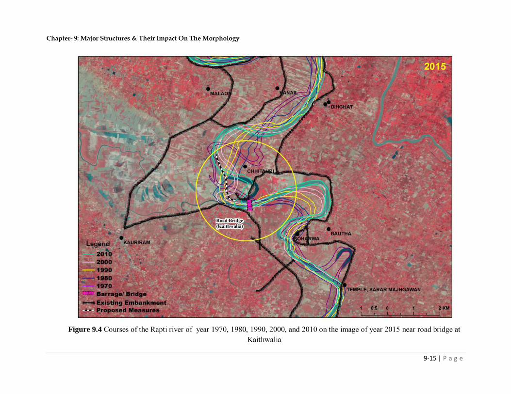
Chapter- 9: Major Structures & Their Impact On The Morphology
9-15 | P a g e
Figure 9.4 Courses of the Rapti river of year 1970, 1980, 1990, 2000, and 2010 on the image of year 2015 near road bridge at
Kaithwalia

Chapter- 9: Major Structures & Their Impact On The Morphology
9-16 | P a g e
Figure 9.5 Boulder revetment/porcupine/series of spurs on right bank over a length of 700 m
upstream of the bridge at Peepeganj (Chainage = 160 km)
Figure 9.6 Provision of series of spurs towards left side at Dhani (Chainage = 205 km)
Series of spurs
Boulder revetment/
Spurs/porcupine

Chapter- 9: Major Structures & Their Impact On The Morphology
9-17 | P a g e
Figure 9.7 Boulder revetment to the existing both sides embankments at Dhani
(Chainage = 212 km)
Figure 9.8 Provision of protection to the left embankment upstream of the bridge (SH5) in the form of
boulder revetment/short spurs at Rajendra Nagar (Chainage = 251.5 km)
Boulder revetment/Short spurs
Boulder revetment

Chapter- 9: Major Structures & Their Impact On The Morphology
9-18 | P a g e
Figure 9.9 Provision of boulder revetment to both the approach roads at Tighra
(Chainage 272.5 km )
Figure 9.10 Extension of the existing left guide bund of about 90 m downstream at Kodri ghat
(chainage 418 km)
Extension of guide bund
Boulder revetment to
both the approach roads

Chapter- 9: Major Structures & Their Impact On The Morphology
9-19 | P a g e
9.4 CONCLUDING REMARKS
Following conclusions may be drawn:
1. The river course has wandering behavior upstream of the barrage. However, no shifting has been observed downstream of the barrage over the years. The Rapti barrage was commissioned in year 2008. Since then no noticeable silting upstream of the barrage has been observed. Nevertheless, river in year 2015 was flowing in two channels upstream of the barrage.
2. There are about 22 bridges on the Rapti river from Nepalgunj to its confluence with Ghaghra river at Patana ghat. Morphological changes have noticed near the major bridges, however, proper river training works have been provided which are working satisfactorily.
3. Road bridge (SH 72, Patana Ghat) is located in relatively straight and stable reach of the Rapti river. In past, river had come close to the right approach road of the bridge - spurs were provided to protect the approach road. As such no measures are required for training the river at the bridge site. However, it is suggested to provide embankment towards right side, upstream of the bridge (SH 72 Bridge) to control the spread of flood water.
4. Road bridge (Kaithwalia) is located just downstream of an acute bend and major shifting of river towards its left side has been noticed upstream of the bend. It is suggested to provide series of spurs towards left side upstream of the bend to arrest such shifting so that out flanking of the bridge be avoided.
5. Protection works are suggested in the vicinity of the bridges at Chainages 160 km, 205 km, 212 km, 251.5 km, 272.5 km and 418 km to train the Rapti river as per detail below: a) Boulder revetment/porcupine/series of spurs on right bank over a length of 700 m
upstream of the bridge at Peepeganj (Chainage = 160 km, Fig. 9.5) b) Provision of series of spurs towards left side at Dhani (Chainage = 205 km, Fig. 9.6) c) Boulder revetment to the existing both sides embankments at Dhani (Chainage = 212
km, Fig. 9.7) d) Provision of protection to the left embankment upstream of the bridge (SH5) in the
form of boulder revetment/short spurs at Rajendra Nagar (Chainage = 251.5 km, Fig. 9.8)
e) Provision of boulder revetment to both the approach roads at Tighra (Chainage 272.5 km, Fig. 9.9)
f) Extension of the existing left guide bund of about 90 m downstream at Kodri ghat (Chainage 418 km, 9.10)
Chapter- 10: Ground Validation
10-1 | P a g e
Chapter 10 GROUND VALIDATION
10.1 INTRODUCTION
This chapter deals with details of the site visit undertaken to various locations of the Rapti
river by the team of IIT Roorkee. The observations made during the site visits have been
examined in the perspective of the outcomes of the morphological study carried out in this
study.
10.2 VISIT TO RAPTI BARRAGE ON 23 OCTOBER, 2016
A team of IIT Roorkee visited the Rapti barrage on 23rd October 2016 also had discussion
with the barrage authority. Two canals off-take from each side of the river upstream of the
barrage. The left canal terminates just after it's off-take from the barrage. However, the right
canal is functional and on the day of visit repair work of the canal was in progress. Guide
bunds are provided towards both sides of the river both upstream and downstream of the
barrage. Such bunds were intact and no major damage to the bunds was noticed during the
visit.
The length of barrage is 284.5 m and is designed for peak discharge of 4990 m³/s. Lacey
perimeter corresponding to this peak discharge is estimated as 335.5 m against the provided
length of barrage of 284.5 m. Thus the looseness factor of the barrage is 1.18.
Major changes in the course of Rapti River upstream of barrage have been noticed. The river
has wandering behavior at the barrage. On the day of visit, the river was flowing relatively
towards its left side.
No major silting was noticed in upstream and downstream of the barrage during the site visit.
Some of the photographs taken during the site visit are shown in Figs. 10.1 to 10.5.

Chapter- 10: Ground Validation
10-2 | P a g e
Figure 10.1 View of the Rapti river upstream of the barrage
Figure 10.2 Head regulator of the right channel
Figure 10.3 Upstream view of the Rapti Barrage
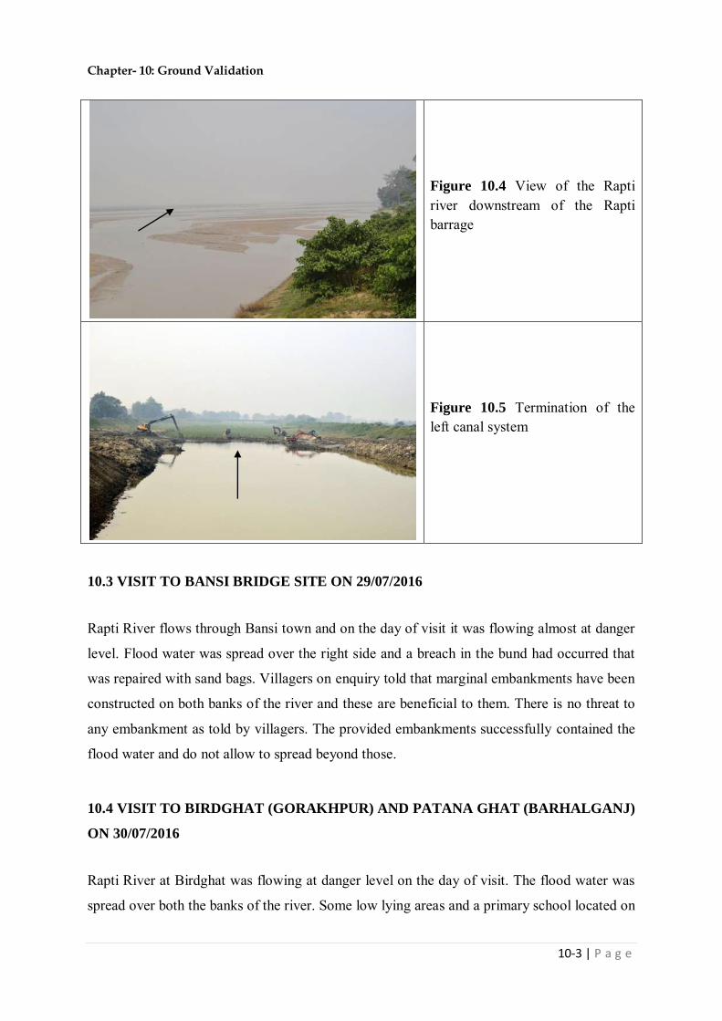
Chapter- 10: Ground Validation
10-3 | P a g e
Figure 10.4 View of the Rapti river downstream of the Rapti barrage
Figure 10.5 Termination of the left canal system
10.3 VISIT TO BANSI BRIDGE SITE ON 29/07/2016
Rapti River flows through Bansi town and on the day of visit it was flowing almost at danger
level. Flood water was spread over the right side and a breach in the bund had occurred that
was repaired with sand bags. Villagers on enquiry told that marginal embankments have been
constructed on both banks of the river and these are beneficial to them. There is no threat to
any embankment as told by villagers. The provided embankments successfully contained the
flood water and do not allow to spread beyond those.
10.4 VISIT TO BIRDGHAT (GORAKHPUR) AND PATANA GHAT (BARHALGANJ)
ON 30/07/2016
Rapti River at Birdghat was flowing at danger level on the day of visit. The flood water was
spread over both the banks of the river. Some low lying areas and a primary school located on

Chapter- 10: Ground Validation
10-4 | P a g e
the right bank and upstream of the bridge were submerged. After this, the visiting team
moved to Patana Ghat bridge on River Rapti located close to its influence with the Ghaghra
River near Barhalganj. In downstream of bridge, water was found to spread on both sides of
the river. There were no embankments on upstream and downstream sides of the bridge. The
left bank was higher and right bank was submerged with a vast area. In the meeting held with
the Officers of U.P. Irrigation Department, it was told that 6.1 km long bund is proposed to
be constructed towards right side on upstream of bridge.
In the afternoon, a meeting was held with Chief Engineer (Gandak) concerning
Superintendent Engineer and Executive Engineers of U.P. Irrigation Department. It was
requested to provide a map showing the existing bunds on either banks of Rapti river starting
from Nepal Boarder to Patana Ghat Bridge. It was also requested to provide details of the
protection works that were provided over and above the embankments. It was also requested
to provide threatening reaches and new works recently proposed to protect the bunds, so that
possible measures may be considered for the provision of protection works in the near future.
Department officers told that the existing bunds are constructed taking about two times the
Lacey's perimeter. The river has a tendency of attacking either of the embankments and
eroding them depending on flow condition and protection works provided. The Department
officers told that in the place of boulders revetments, provision of geobags and porcupines
have been found to be quite encouraging. This type of protection works have been executed
this year in river Rapti, and few years back in river Sharda. They were requested to provide
feedback in this respect after the monsoon, so that it may also be included in the report. Use
of geobag and porcupine has given better performance in lower discharge, like in Rapti and
Sharda. In Ghaghra River, these works have not been found to be successful. Some relevant
photographs taken during the site visits are shown in Figs. 10.6 to 10.11.
Figure 10.12 shows location of the sites of the Rapti river that were visited by the IIT Roorkee team.

Chapter- 10: Ground Validation
10-5 | P a g e
Figure 10.6 Rapti river just upstream of its confluence with Ghaghra river (26.304926N, 83.668530E) and downstream of the bridge over it
Figure 10.7 Rapti river just upstream of its confluence with Ghaghra river (26.304926 N, 83.668530 E) and upstream of the bridge over it
Figure 10.8 Rapti river just upstream of its confluence with Ghaghra river (26.304926 N, 83.668530 E) and upstream of the bridge over it - left bank of the river is on higher elevation

Chapter- 10: Ground Validation
10-6 | P a g e
Figure 10.9 Rapti river just upstream of its confluence with Ghaghra river (26.304926 N, 83.668530 E) and upstream of the bridge over it - right bank is flat and spurs are provided to protect the road SH-72
Figure 10.10 Rapti river downstream of NH29 (26.732984 N, 83.348470 E) - Left bank is elevated and right bank is flat, a bund is provided along right bank
Figure 10.11 Rapti river downstream of NH-29 (26.732984 N, 83.348470 E) - a bund is provided along right bank

Chapter- 10: Ground Validation
10-7 | P a g e
Figure 10.12 Location of the sites of the Rapti River visited by the IIT Roorkee team

Chapter- 11: Identification of the Critical Reaches & River Training Works
11-1 | P a g e
Chapter 11 IDENTIFICATION OF CRITICAL REACHES &
RIVER TRAINING WORKS
11.1 IDENTIFICATION OF THE CRITICAL REACHES
Discussion on the plan form changes of the river in the terms of bank line shifting, sinuosity,
plan form index etc. has been mentioned in the previous chapters. For fulfilling the objective
of the study regarding identification of the critical reaches and provision of river training
works thereof, suitable basis has been discussed here.
The proposed basis for the identification of the critical reaches is as follows:
a) The reach of the river that has been progressively shifting towards either sides from
the base year 1970 shall be considered as critical reaches. This is due to the fact that
such progressive shifting of the course of river causes severe erosion of the
agricultural areas, which results in loss of the agricultural land.
b) Localized erosion of the either banks in the habitated/ settlement areas, as such
erosion causes displacement of the houses to the new locations, inundation of pricey
areas etc.
(c) In agricultural land, where the river is wide and the width is much higher than regime
width of the channel even though there is no progressive shifting of river course in
either directions. Such frequent shifting of the river in wide width of the land causes
loss of the crops and agricultural land. Thus there is a need to confine the width of the
river so that spread of the flood water which is causing huge inundation can be
controlled.
The above basis has been adopted in this study for identification of critical reaches of the
Rapti river.

Chapter- 11: Identification of the Critical Reaches & River Training Works
11-2 | P a g e
As per the IS code 12094:2000, the spacing between the embankments/levees for the
containment of the river should not be less than 3 times Lacey’s wetted perimeter for the
design flood discharge. In no case, should an embankment be placed at distance less than
Lacey’s wetted perimeter from the river bank or one and a half times.
In the present study for the relatively straight reach, width of the river is kept 3 times of the
Lacey perimeter. However, at locations where sinuosity ratio of the river is higher, it is
proposed to place the embankments at 4 times the Lacey perimeter apart.
Lacey's perimeter for the alluvial river may be obtained by
𝑃 = 4.75 𝑄 (11.1)
Where P is in m and Q is discharge in cumecs.
Invoking the methodology/criteria discussed in the above section, the identified critical
reaches of the Rapti river are given in the Table 11.1 with justification. Nine reaches of the
Rapti river have been identified as critical.
In the reaches from 68-80 km, 138-156 km, 304-322.5 km, 326.5- 378 km, 387-392 km, 399-
433 km, 438-466 km, 470-492 km and 506-515 km, the historical images of the river indicate
its random wandering in wide width. These reaches are located near Chhithari, Mirpur,
Rasulabad, Utraula, Jyonar, Ikauna, Lakshmannagar and Jamnaha in Uttar Pradesh. The left
and right banks of the river of the year 1970, 1980, 1990, 2000 and 2010 are marked on the
LISS IV image of year 2015 and shown in the Figs. 11.1a to i. The land in this area is mostly
agricultural.
Table 11.1 Critical reaches of the Rapti River
Chainage (km)
Location Justification Figure
No.
506-515 Jamnaha, UP
Agricultural land on either sides of the river. Random wandering of the river in wide width. No progressive shifting in either directions.
11.1a
470-492 Lakshmannagar, UP Agricultural land on either sides of the river. Random wandering of the river in wide
11.1b

Chapter- 11: Identification of the Critical Reaches & River Training Works
11-3 | P a g e
width. No progressive shifting in either directions.
438-466 Ikauna, UP
Agricultural land on either sides of the river. Random wandering of the river in wide width. No progressive shifting in either directions.
11.1c
399-433 Jyonar, UP
Agricultural land on either sides of the river. Random wandering of the river in wide width. No progressive shifting in either directions.
11.1d
387-392 Shankarnagar, UP
Agricultural land on either sides of the river. Random wandering of the river in wide width. No progressive shifting in either directions.
11.1e
326.5-378 Utraula, UP
Agricultural land on either sides of the river. Random wandering of the river in wide width. No progressive shifting in either directions.
11.1f
304-322.5 Rasulabad, UP
Agricultural land on either sides of the river. Random wandering of the river in wide width. No progressive shifting in either directions.
11.1g
138-156 Mirpur, UP
Agricultural land on either sides of the river. Random wandering of the river in wide width. No progressive shifting
in either directions.
11.1h
68-80 Chhitahri, UP
Agricultural land on either sides of the river. Random wandering of the river in wide width. No progressive shifting in either directions.
11.1i

Chapter- 11: Identification of the Critical Reaches & River Training Works
11-4 | P a g e
Figure 11.1a Critical reach of Rapti river from chainage 506- 515 km

Chapter- 11: Identification of the Critical Reaches & River Training Works
11-5 | P a g e
Figure 11.1b Critical reach of Rapti river from chainage 470- 492 km
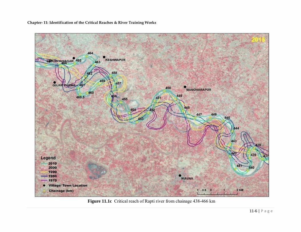
Chapter- 11: Identification of the Critical Reaches & River Training Works
11-6 | P a g e
Figure 11.1c Critical reach of Rapti river from chainage 438-466 km

Chapter- 11: Identification of the Critical Reaches & River Training Works
11-7 | P a g e
Figure 11.1d Critical reach of Rapti river from chainage 399- 433 km

Chapter- 11: Identification of the Critical Reaches & River Training Works
11-8 | P a g e
Figure 11.1e Critical reach of Rapti river from chainage 387-392 km

Chapter- 11: Identification of the Critical Reaches & River Training Works
11-9 | P a g e
Figure 11.1f Critical reach of Rapti river from chainage 326.5- 378 km

Chapter- 11: Identification of the Critical Reaches & River Training Works
11-10 | P a g e
Figure 11.1g Critical reach of Rapti river from chainage 304- 322.5 km
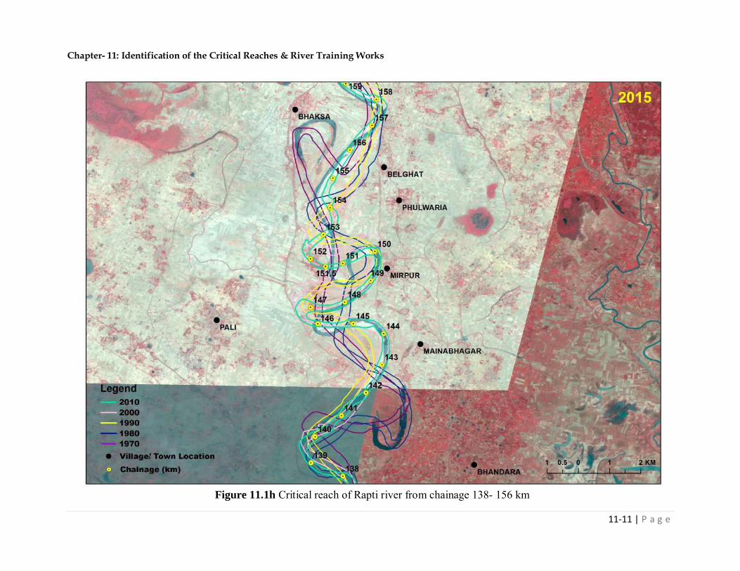
Chapter- 11: Identification of the Critical Reaches & River Training Works
11-11 | P a g e
Figure 11.1h Critical reach of Rapti river from chainage 138- 156 km

Chapter- 11: Identification of the Critical Reaches & River Training Works
11-12 | P a g e
Figure 11.1i Critical reach of Rapti river from chainage 68- 80 km

Chapter- 11: Identification of the Critical Reaches & River Training Works
11-13 | P a g e
11.2 PROPOSED RIVER TRAINING WORKS FOR RESTORATION OF CRITICAL
AND IMPORTANT RIVER REACHES
Design methodologies of various river training works like guide banks, spurs, pilot channels
etc., are given in Annexure - A. Such methodologies have been compiled from the relevant IS
and IRC codes and also from relevant literature.
For the containment of the flood water at the critical reaches, Lacey waterway has been
estimated using Eq. (11.1) and lines of the 4 times the Lacey waterway have been drawn and
shown in the Figs. 11.2a to 11.2d for the selected critical reaches for the illustrations. The
computed Lacey waterway corresponding to the design discharge of Rapti bararge and 100
year return period estimated discharge at various gauging sites are given in Table 11.2.
Table 11.2 Design discharge of Rapti barage and 100 year return period estimated discharge at various gauging sites
Barrage Chainage (km) Discharge
(m3/s)
P=4.75√Q (m)
Rapti Barrage 519 4990.00 335.54
Balrampur 396 3455.9 279.24
Rigauli 183 5288.9 345.44
Birdghat 120 7934.9 423.12
Average value 345.8
Proposed river training works for the various critical reaches are mentioned in the Table 11.3
with justification. For the positioning the levees/embankment, the extreme left and right
banks of the Rapti river attained during the period 1970-2010 have been marked along with
buffer of four times Lacey perimeter (P) on the satellite images of 2015 for different critical
reaches. The alignment of the levee has been marked such that it should be close to extreme
banks and 4P lines. As the variation in estimated Lacey perimeter in Table 11.2 from
Chainage 120 km to 519 km is not large, an average perimeter P=345.8 m is adopted in this
study. Figs. 11.2a-d show extreme banks and 4P lines in the four critical reaches for
illustrations, while suggested river training works at four locations i.e., Utrauli, Rasulabad
Chhitahri and Patana ghat are shown in Figs. 11.3a-d.

Chapter- 11: Identification of the Critical Reaches & River Training Works
11-14 | P a g e
In the critical reaches as shown in Figs. 11.1a to 11.1i, wherever river is striking to the
existing embankments, porcupine/ boulder revetment shall be provided to control breach in
the embankment.
Table 11.3 River training works for the critical reaches of the Rapti River
Critical Reaches (Chainage / Location)
Type of River Training Works
Justification
506-515 (Jamnaha, UP)
NIL
River course is wandering in wide width with maximum shift of 2.5 km. No measures required. No major habitation.
470-492 (Lakshmannagar, UP)
NIL
River course is wandering in wide width with maximum shift of 2.8 km. No Measures required. No major habitation.
438-466 (Ikauna, UP)
NIL
River course is wandering in wide width with maximum shift of 2.9 km. No measures required. No major habitation.
399-433 (Jyonar, UP)
NIL
River course is wandering in wide width with maximum shift of 3.4 km. No Measures required. No major habitation.
387-392 (Shankarnagar, UP)
NIL
River course is wandering in wide width with maximum shift of 1.7 km. No measures required. No major habitation. Embankments are provided towards both sides of the reach.
326.5-378 (Utraula, UP)
Embankment with boulder revetment
River course is wandering in wide width with maximum shift of 1.5 km. Partially provided embankments should be fully provided in this reach, preferrably at 4P. Boulder revetment is to be
provided where the deeper part
of the river is close to the
proposed embankments.
304-322.5 (Rasulabad, UP)
Embankment/ Levees
River course is wandering in wide width with maximum shift of 2.5 km. Recommended to provide
embankment towards both sides
at a spacing of 4 times Lacey
perimeter to control the spread
of flood water. It may be noted
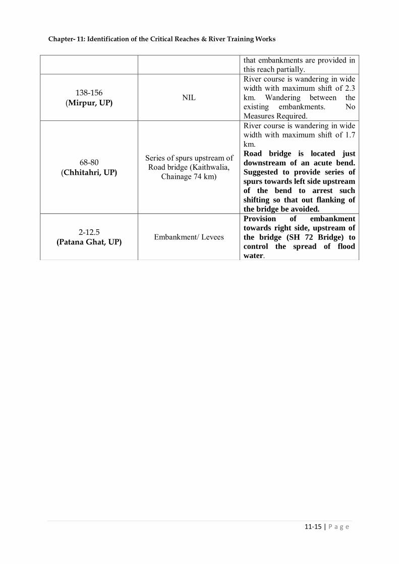
Chapter- 11: Identification of the Critical Reaches & River Training Works
11-15 | P a g e
that embankments are provided in this reach partially.
138-156 (Mirpur, UP)
NIL
River course is wandering in wide width with maximum shift of 2.3 km. Wandering between the existing embankments. No Measures Required.
68-80 (Chhitahri, UP)
Series of spurs upstream of Road bridge (Kaithwalia,
Chainage 74 km)
River course is wandering in wide width with maximum shift of 1.7 km. Road bridge is located just
downstream of an acute bend.
Suggested to provide series of
spurs towards left side upstream
of the bend to arrest such
shifting so that out flanking of
the bridge be avoided.
2-12.5 (Patana Ghat, UP)
Embankment/ Levees
Provision of embankment
towards right side, upstream of
the bridge (SH 72 Bridge) to
control the spread of flood
water.

Chapter- 11: Identification of the Critical Reaches & River Training Works
11-16 | P a g e
Figure 11.2a Extreme banks and 4P lines from chainage 138- 156 km
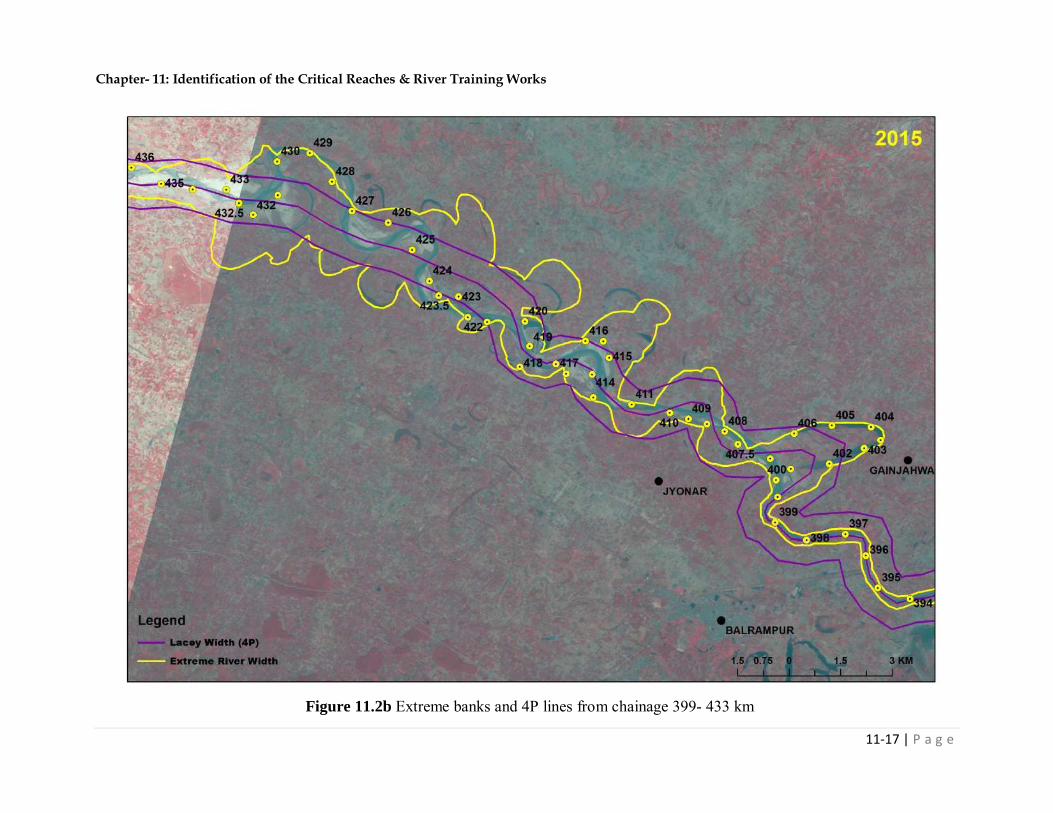
Chapter- 11: Identification of the Critical Reaches & River Training Works
11-17 | P a g e
Figure 11.2b Extreme banks and 4P lines from chainage 399- 433 km

Chapter- 11: Identification of the Critical Reaches & River Training Works
11-18 | P a g e
Figure 11.2c Extreme banks and 4P lines from chainage 470 - 492 km

Chapter- 11: Identification of the Critical Reaches & River Training Works
11-19 | P a g e
Figure 11.2d Extreme banks and 4P lines from chainage 506 - 515 km

Chapter- 11: Identification of the Critical Reaches & River Training Works
11-20 | P a g e
Figure 11.3a Extreme banks, 4P lines and location/alignment of the suggested works from chainage 2-12.5 km
Chapter- 11: Identification of the Critical Reaches & River Training Works
11-21 | P a g e
Figure 11.3b Extreme banks, 4P lines and location/alignment of the suggested works from chainage 75-77 km
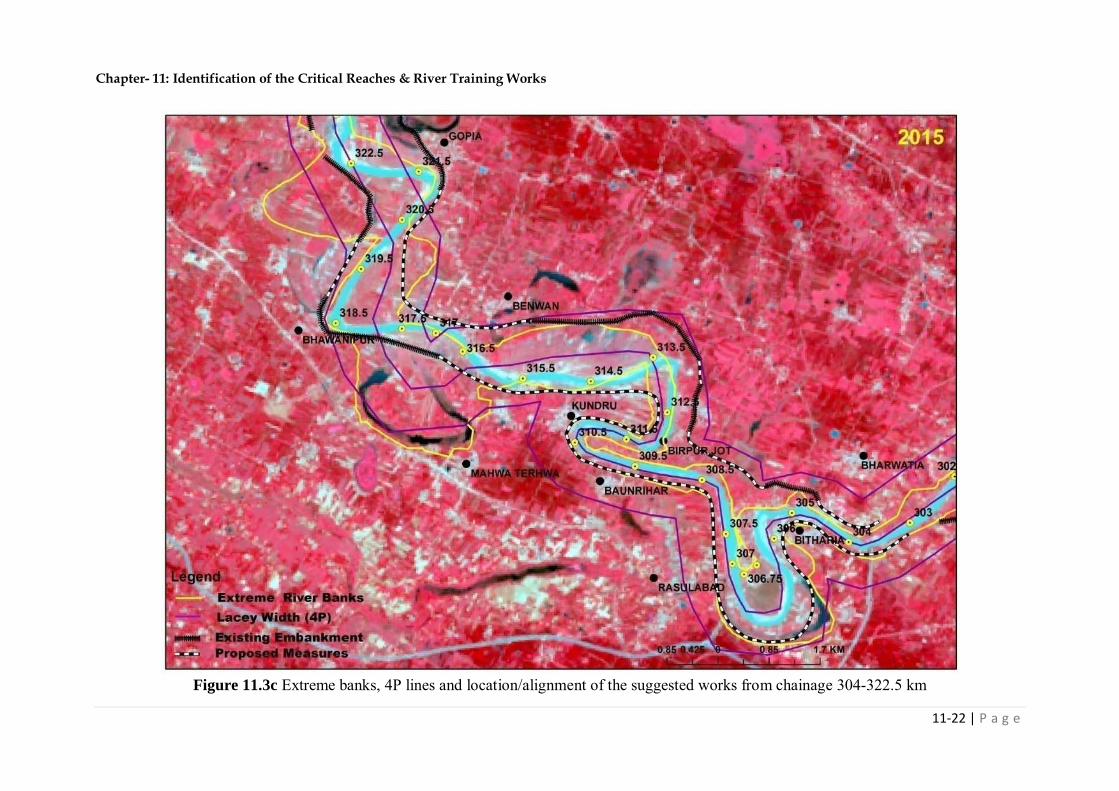
Chapter- 11: Identification of the Critical Reaches & River Training Works
11-22 | P a g e
Figure 11.3c Extreme banks, 4P lines and location/alignment of the suggested works from chainage 304-322.5 km

Chapter- 11: Identification of the Critical Reaches & River Training Works
11-23 | P a g e
Figure 11.3d Extreme banks, 4P lines and location/alignment of the suggested works from chainage 326.5-378 km

Chapter- 11: Identification of the Critical Reaches & River Training Works
11-24 | P a g e
11.3 EXISTING EMBANKMENTS
Embankments are provided towards both sides of the river in its most of the length in
particular in the lower reaches. Location of such embankments are shown in the Figs. 11.4a
to 11.4k. It may be noted that embankments are partially provided in the upper reaches.
Distances of the embankment at different chainages from the centreline of the river as in year
2015 are given in the Table 11.4 and also shown graphically in Fig. 11.5.
It may be noted that the proposed embankments, as mentioned in the section 11.2, are
suggested to be provided in the upper reach of the Rapti river on its both sides.

Chapter- 11: Identification of the Critical Reaches & River Training Works
11-25 | P a g e
Figure 11.4a Existing embankments on Rapti river from chainage 0-50 km
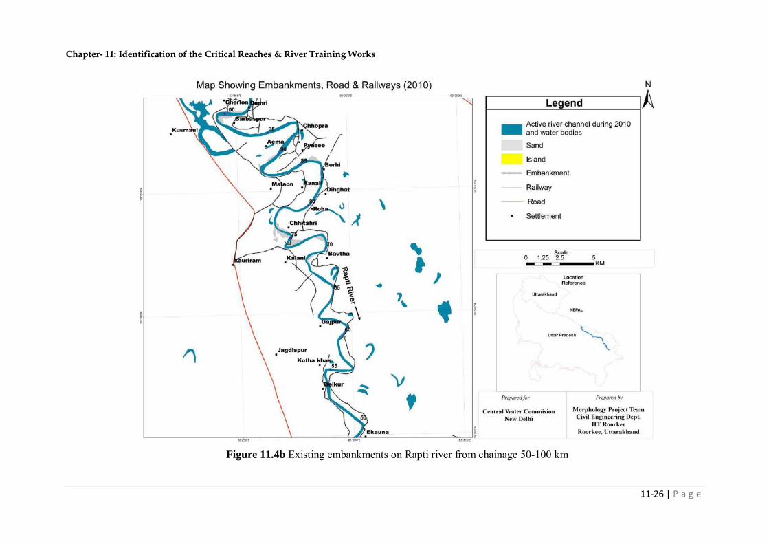
Chapter- 11: Identification of the Critical Reaches & River Training Works
11-26 | P a g e
Figure 11.4b Existing embankments on Rapti river from chainage 50-100 km
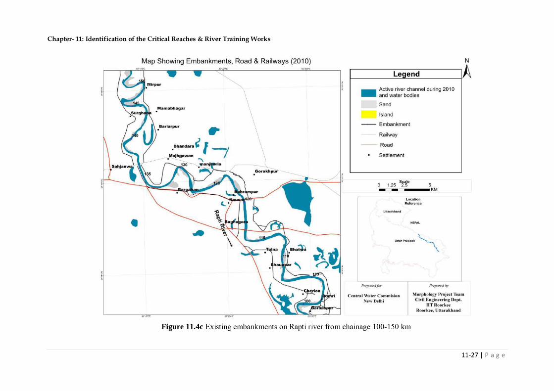
Chapter- 11: Identification of the Critical Reaches & River Training Works
11-27 | P a g e
Figure 11.4c Existing embankments on Rapti river from chainage 100-150 km
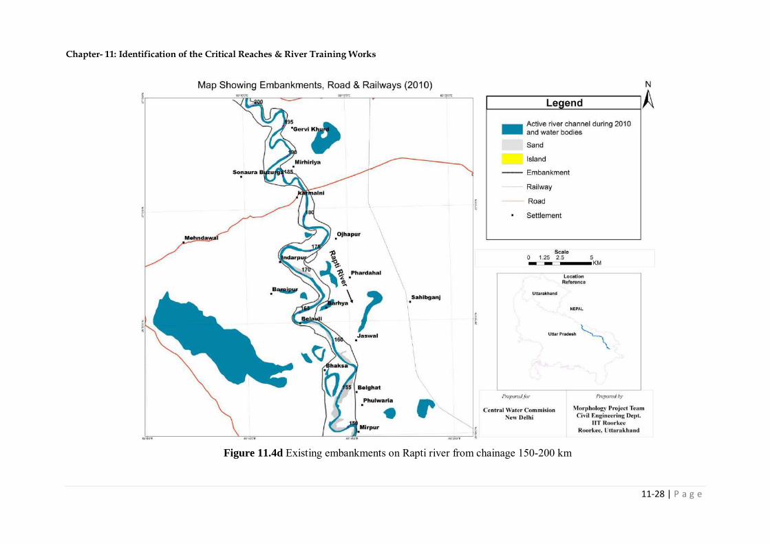
Chapter- 11: Identification of the Critical Reaches & River Training Works
11-28 | P a g e
Figure 11.4d Existing embankments on Rapti river from chainage 150-200 km

Chapter- 11: Identification of the Critical Reaches & River Training Works
11-29 | P a g e
Figure 11.4e Existing embankments on Rapti river from chainage 200-250 km

Chapter- 11: Identification of the Critical Reaches & River Training Works
11-30 | P a g e
Figure 11.4f Existing embankments on Rapti river from chainage 250-300 km

Chapter- 11: Identification of the Critical Reaches & River Training Works
11-31 | P a g e
Figure 11.4g Existing embankments on Rapti river from chainage 300-350 km

Chapter- 11: Identification of the Critical Reaches & River Training Works
11-32 | P a g e
Figure 11.4h Existing embankments on Rapti river from chainage 350-400 km

Chapter- 11: Identification of the Critical Reaches & River Training Works
11-33 | P a g e
Figure 11.4i Existing embankments on Rapti river from chainage 400-450 km
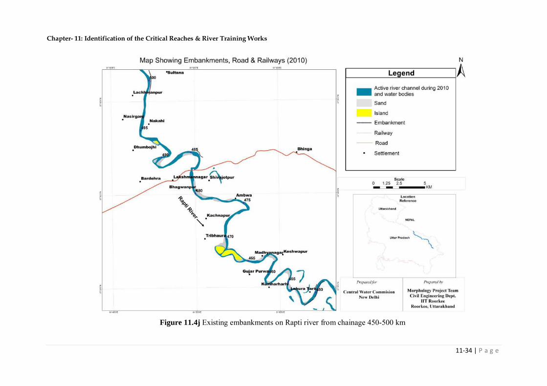
Chapter- 11: Identification of the Critical Reaches & River Training Works
11-34 | P a g e
Figure 11.4j Existing embankments on Rapti river from chainage 450-500 km

Chapter- 11: Identification of the Critical Reaches & River Training Works
11-35 | P a g e
Figure 11.4k Existing embankments on Rapti river from chainage 500-542 km
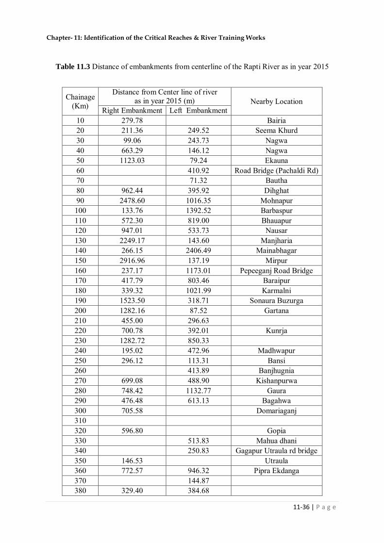
Chapter- 11: Identification of the Critical Reaches & River Training Works
11-36 | P a g e
Table 11.3 Distance of embankments from centerline of the Rapti River as in year 2015
Chainage (Km)
Distance from Center line of river as in year 2015 (m) Nearby Location
Right Embankment Left Embankment 10 279.78 Bairia 20 211.36 249.52 Seema Khurd 30 99.06 243.73 Nagwa 40 663.29 146.12 Nagwa 50 1123.03 79.24 Ekauna 60 410.92 Road Bridge (Pachaldi Rd) 70 71.32 Bautha 80 962.44 395.92 Dihghat 90 2478.60 1016.35 Mohnapur 100 133.76 1392.52 Barbaspur 110 572.30 819.00 Bhauapur 120 947.01 533.73 Nausar 130 2249.17 143.60 Manjharia 140 266.15 2406.49 Mainabhagar 150 2916.96 137.19 Mirpur 160 237.17 1173.01 Pepeeganj Road Bridge 170 417.79 803.46 Baraipur 180 339.32 1021.99 Karmalni 190 1523.50 318.71 Sonaura Buzurga 200 1282.16 87.52 Gartana 210 455.00 296.63 220 700.78 392.01 Kunrja 230 1282.72 850.33 240 195.02 472.96 Madhwapur 250 296.12 113.31 Bansi 260 413.89 Banjhugnia 270 699.08 488.90 Kishanpurwa 280 748.42 1132.77 Gaura 290 476.48 613.13 Bagahwa 300 705.58 Domariaganj 310 320 596.80 Gopia 330 513.83 Mahua dhani 340 250.83 Gagapur Utraula rd bridge 350 146.53 Utraula 360 772.57 946.32 Pipra Ekdanga 370 144.87 380 329.40 384.68

Chapter- 11: Identification of the Critical Reaches & River Training Works
11-37 | P a g e
390 1418.71 Raighat 400 410 420 298.23 Road Bridge 430 440 450 224.06 Manoharapur 460 470 480 490 500 320.70 Lachhmanpur 510 2499.67 520 2302.40 Rapti Barrage 530 4240.79 540 146.05 Nepalganj

Chapter- 11: Identification of the Critical Reaches & River Training Works
11-38 | P a g e
Fig 11.5 Distance of the embankment from centreline of the river as in year 20
-3,000
-2,000
-1,000
0
1,000
2,000
3,000
4,000
5,000
0 50 100 150 200 250 300 350 400 450 500 550Dis
tan
ce fr
om
cen
tre
line
(m)
Chainage (km)
Right embankment Left Embankment

Chapter- 11: Identification of the Critical Reaches & River Training Works
11-39 | P a g e
11.4 TENTATIVE DESIGN OF RIVER TRAINING WORKS
A sample design of Levees/embankment has been carried out in this section on the basis
of some assumed data. It is recommended that other suggested measures shall be
designed after acquiring required data and invoking the methodology described in the
Annexures-A and B.
A sample design of Levees/Embankment in the reach Chainage 326.5 - 378 km
It is proposed to keep the top width of the embankment of 3 m and side slope 1V: 2H. The
top level of the embankment shall be 1.5 m higher than the highest flood level. Further, it is
proposed to provide Biomac blankets which are also known as Rolled Erosion Control
Protection (RECPs) mats and are used for surface erosion protection (Fig. 11.6). Placed onto
top soiled and seeded slopes, Biomac supports the establishment of vegetation. As the mat
biodegrades over time, the protection function is maintained by the vegetation. The Biomac
are made with a mixture of fully biodegradable fibres properly integrated during
manufacturing. The fibre mat is reinforced with a fine polypropylene scrim netting securely
stitched on both sides during manufacturing.
Figure 11.6 Details of BioMac
Nearest hydrological station to the reach 326.5 km-378 km is Balrampur (Chainage 396 km).
Peak discharge for 25 years return period at Balrampur is estimated as 2836.1 m3/s and ever
maximum recorded water level at this station is 105.47 m. Let adopt these data for the design
of the embankment in the reach 326.5 km-378 km.
As such, no revetment on the sloping surface of the levees and launching apron are required,
however, it is suggested that river behaviour shall be watched and if river has tendency to
come close to levees, slope protection and launching apron be provided as per detail below:

Chapter- 11: Identification of the Critical Reaches & River Training Works
11-40 | P a g e
Slop protection
It is proposed to provide geo-bags for the control of erosion of the slope. Annexure-B may be
seen for the details of flexible system including geo-bags.
Size of Bags: Weight of bags shall be calculated by
(1)
(2)
where, W - weight in kg
V – velocity in m/s Ss - Specific Gravity of protection material (adopted between 1.5 to 1.8)
θ - Angle of sloping bank
φ - Angle of repose of protection material
The average velocity U during flood is given by Lacey equation
1/62
140QfU
(3)
For Q = 2836.1 m3/s and f = 1, the above equation yields V = 1.65 m/s
let assume φ = 300
θ = tan-1 (1/2) = 26.5650
K = 0.45
Let take Ss = 1.7
From Eq. (1), W = 5.16 kg, let provide bags of size 1.1m x 0.7m x 0.15m (weight around
126 kg) as per Nomograph given in IS-14262.
Thickness of Pitching: Thickness should be more than that calculated as under:
(4)
T - thickness in m
V – velocity in m/s
Ss - Specific Gravity of protection material (adopted between 1.5 to 1.8)
g - Acceleration due to gravity (9.81 m/s2)
For the data in the present case, Eq. (4) yields T =0.20 m

Chapter- 11: Identification of the Critical Reaches & River Training Works
11-41 | P a g e
Pitching may be provided in double layers of geo-bags (in loose).
Launching Apron
Figure 11.7 shows a general arrangement of a launching apron that is generally provided at
the toe of the embankment. It is assumed that the launching apron placed on the river bed
would launch into the scour hole to take a slope of 1V: 2H. This launching apron is placed on
the river bed over a length equal to 1.5 times D, where D is the scour depth measured below
the river bed.
Figure 11.7 A typical sketch of embankment & launching apron (conventional)
According to IS Code: 10751:1994, the maximum scour depth Dse measured from the high
flood level at the toe of straight part of the embankment 1.5R, in which R is Lacey’s normal
scour depth also measured from high flood level. The value of R is given by
R = 0.48(Q/f) 1/3 in SI units (5)
where f is Lacey’s silt factor, let assume f = 1.
For Q = 2836.10 m3/s i.e. discharge adopted for the scour computations as per IRC: 78-2000
and f = 1.0, Eq. (5) gives
R = 0.48(2836.1 /1.0) 1/3
= 6.8 m
Maximum scour depths Dse at the toe of the embankment measured from HFL at different
locations = 1.5R = 10.20 m
High flood level (HFL) =105.47 m
Deepest scour level = 105.47-10.20 = 95.27 m
Bed level of the river = 105 m (assumed)

Chapter- 11: Identification of the Critical Reaches & River Training Works
11-42 | P a g e
Scour below bed level D = 105-95.27 = 9.73 m
Length of the launching apron = 1.5D = 14.60 m , provide 14 m
Thickness of launching apron = 1.8T = 1.8×0.20 = 0.36 m, let provide 0.40 m thick geo-bags
in 2-3 layers.
Disclaimer: The above is a sample design and based on the gross assumed data. Thus this
should not executed in the present form. It is suggested to collect detailed data and design
shall be carried out as per the above procedure.
11.5 CONCLUSIONS
Following conclusions have been drawn from the study carried out in this report:
a) Nine reaches of the Rapti river have been identified as critical. These reaches are
Chainages 68-80 km (Chhithari), 138-156 km (Mirpur), 304-322.5 km (Rasulabad),
326.5- 378 km (Utraula), 387-392 km (Shankarnagar), 399-433 km (Jyonar), 438-466
km (Ikauna), 470-492 km (Lakshmannagar) and 506-515 km (Jamnaha). In these
reaches, river has wandering behaviour in wide width. No progressive shifting in either
directions has been noticed over the years.
b) Methodology for the design of various river training works has been discussed and
based on the morphological changes of the river, it is suggested to provide embankment
or levees in critical reaches of the river.
Chainages 2-12.5 km Embankment on right side
Chainages 75-77 km Series of spurs on left side
Chainages 304-322.5 km Embankments on both sides
Chaianges 326.5-378 km Embankments on both sides
In the identified critical reaches, wherever river is striking to the existing embankments,
porcupine/ boulder revetment shall be provided to avoid breach in the embankment.
c) Embankments are provided towards both sides of the river in its most of the length, in
particular in the lower reaches. In some reaches, embankments are not continuous and
that requires to be plugged by construction new embankment as suggested in this study.
Chapter-12: Conclusions & Recommendations
12-1 | P a g e
Chapter 12 CONCLUSIONS & RECOMMENDATIONS
12.1 CONCLUSIONS
Following conclusions have been drawn from the study carried out in this report:
a) Hydrological Analysis
1. Analysis of maximum observed discharge and maximum observed water level at different gauging sites on Rapti river using the available data indicates that there is no remarkable trend of temporal variation of maximum discharge and maximum water level at the gauging sites Kakardhari, Balrampur, Bansi, Rigauli and Birdghat over a long period of time.
2. The, maximum discharge at Balrampur has shown a decreasing trend, however, no trend has been found at Rigauli and Birdghat gauging sites. The maximum water level has an increasing trend at Kakardhari and Balrampur and decreasing trend at Bansi, however, no trend was found at gauging sites of Rigauli and Birdghat.
3. Estimated peak discharge at different gauging sites for 25, 50 and 100 years return periods has been estimated using various flood frequency methods. The estimated values indicate that peak discharge increases continuously in the downstream of the river.
b) Morphological Changes
1. Reach 0-50 km: There is no any progressive change in the course of river in this reach in the span 1970 to 2010. River is having meandering pattern in this reach. Major changes in the course of river have been noticed near Sareya, Ghaighat and Bahsua. The river has shifted from left to right at Sareya and Bahsua by 3 km and 2 km, respectively.
Average width of the active channel is about 200 m in this reach. There is no much variation in the width over the years and along the channel except at Semra Khard, where the width of the river was 400 m in year 1980.

Chapter-12: Conclusions & Recommendations
12-2 | P a g e
2. Reach 50-100 km: Major changes in the course of the river have been noticed in the upper part of the reach. It is also meandering in this reach. There is no progressive shift in course of the river in this reach. Major random shifting of the river has been noticed at Chhitarhri. In the upper reaches, the course of river in year 1970 to 2010 was within a buffer of 2.0 km.
The average width of the active channel of Rapti river is about 200 m. The maximum width of the river is about 450 m at Bautha and Chhopra.
3. Reach 100-150 km: There is no any progressive shift of course of river in this reach. Maximum random shift of the order of 2.5 km has been noticed at Bariarpur, Pali and Mirpur. Major shift from left to right of the order of 1 km has been noticed at Surghana. While the river course has shifted from right to left of the order of 1.5 km at Majhgawan and Bariarpur.
Average width of the active channel in this reach is about 200 m with maximum width of the order of 5 km at Pali. In general, the width of the river in this reach is varying from 100 m to 300 m.
4. Reach 150-200 km: No major shifting in the main course of river has been noticed in this reach, except near Phulwaria where the river has followed a straight path from 1980 onwards. There was an acute bend at this location in year 1970. There is no progressive shift in the course of the river in this reach.
The width of the active channel varies from 150 m to 350 m with an average of 200 m in this reach. There is no any progressive change in the width of the river over the years in this reach.
5. Reach 200-250: In this reach also, no major shifting of the river has been noticed except at Semra Mustakham where river has shifted from left to right of the order of 1 km over the years.
The width of active channel varies from 100 m to 275 m with an average of 200 m in this reach. The width of the river in 1970 was about 100 m, however, over the years it has increased.
6. Reach 250-300 km: There is no any major change in course of the river in this reach over the years. Critical examination of shifting of center line of Rapti river from year 1970 to 2010 indicates that in the upper part of this reach the tendency of meandering of the river has increased over the years.
The width of the active channel of the river varies from 125 m to 275 m with an average of 200 m in this reach. There is no any progressive change in the width of river over the years.
7. Reach 300-350 km: Major changes in the course of the river has been noticed in this reach. The river is wandering in a buffer of 2.5 km width. The maximum shift from left to right is of the order of 2 km at Kanchalpur and Parsauna. The maximum shift from
Chapter-12: Conclusions & Recommendations
12-3 | P a g e
right to left of the order of one km has been noticed at Rautaila and Arjanpur, and also there is no progressive shift in this reach over the years.
The width of the active channel varies from 100 m to 325 m with an average of 200 m in this reach. The maximum width of the order of 400 m has been noticed at Bagahwa in year 1990. In general, the maximum width was noticed in year 1990.
8. Reach 350-400 km: Major changes in the course of the river has been observed in the lower part of this reach. In the upper part, major changes in the course of the river has been noticed only at Shankarnagar. River has meandering pattern in the lower part of this reach. The maximum shift of the river course from right to left is of the order of 3 km at Nandnagar from year 1970 to 2010, while river has shifted of the order of 1.5 km from left to right at Shankarnagar.
Large variation in the width of active channel in this reach has been noticed. River has widened over the years in this reach. In general, minimum width was found in year 1970 and maximum in year 1980. Maximum width of the order of 400 m has been noticed at Mirazapur.
9. Reach 400-450 km: River has remarkable wandering and meandering behavior in this reach. The river course has wandered in a buffer of 3.5 km in this reach in the span of year 1970 to 2010. There is no any progressive change in the course of the river in this reach. The maximum shift from left to right of the order of 2 km is found at Jyonar, Shravasti and Ikauna from 1970 to 2010. However, maximum shift of the river course from right to left of the order of 2 km can be seen at Mankoa Kondri.
Average width of the active channel in this reach is of the order of 225 m. In general, the width has increased over the years. The maximum width of the order of 500 m was noticed at Shravasti in year 2000 and of the order of 575 m at Itwaria in year 1990.
10. Reach 450-500 km: Major changes in the course of the river has been noticed in this reach. However, no progressive change in the course of river has been noticed over the years. In general, river has been wandering in a width of 3 km. It has an acute meandering pattern in this reach. River has maximum shift from left to right at Gujar Purwa and right to left at Keshwapur of the order of 2.5 km in the span of year 1970 to 2010.
The average width of the active channel in this reach is of the order of 290 m. However, it varies from 150 m to 400 m in this reach. River had maximum width of the order of 650 m at chainage 475 km (Tribhaura) and 490 km (Lakshmannagar). The width of the active channel has increased over the years in this reach.
11. Reach 500-542 km: This reach has also wandering and meandering behaviour of the river. There is no progressive change in the course of river in this reach. However, river has laterally shifted from left to right of the order of 3 km at Devpura and Jamnagar. At Hansapur, river has shifted from right of the order of 1.25 km.

Chapter-12: Conclusions & Recommendations
12-4 | P a g e
Average width of the active channel river is of the order of 290 m. The river width has increased from 1970 onwards. The maximum width is found at Jamnaha.
12. The sinuosity of Rapti river is calculated using the formulation given by Friend and Sinha (1993). From the sinuosity plot of Rapti river, the following data were extracted:
Year Maximum Sinuosity Minimum Sinuosity
Average Sinuosity
1970 3 1.37 1.8 1980 2.9 1.11 1.88 1990 2.83 1.14 1.79 2000 2.79 1.42 1.87 2010 2.8 1.55 1.92
13. The computed sinuosity ratio of the Rapti river in the reach under consideration is higher than 1.5 in the years 1970, 1980, 1990, 2000, and 2010, therefore, the Rapti is classified as a meandering river.
14. Almost whole reach of the river has meandering pattern, however, it is prominent in the reaches 25-50 km, 75-100 km, 300-375 km, 400-425 km and 450-475 km. The meandering is characterized by acute bend with high amplitude, however, they are relatively stable.
15. The plan form index (PFI) of Rapti River is calculated using the formula given by Sharma (2004). It has been observed that the Rapti River always flows in one channel, so negligible braiding is found in the Rapti River.
16. Major shifting of the river course in span of year 1970 to 2010 is in the reaches 75 -100 km, 300-375 km, 400-485 km and 500-542 km. At Devpura, Jamuha, Keshwapur, Nandnagar and Chitahari shifting is from left to righ,t while at Gujarpurwa, Ikauna, Jyonar and Kanchalpur shifting is from right to left. No progressive shifting of the course of the river with respect to time has been noticed.
17. Width of the active channel of the river and river width based on the extreme banks have been estimated using the satellite images of years 1970-2010. There is no definite progressive change in the width of the river over the span 1970-2010 in the whole studied reach of the Rapti river. From chainage zero to 450 km, the average width of the active channel is almost constant and is equal to about 206 m, however, in the upper reach i.e., chainage 450 km to 542 km, the average width is about 290 m - which may be attributed to silting in upper reaches and spreading of flow as the river descends from hilly areas.
18. The nodal points along the reach of the river i.e. wherein minimum morphological changes are seen, have been identified. This will be helpful in planning of structures, like barrage and bridge in the future.

Chapter-12: Conclusions & Recommendations
12-5 | P a g e
c) Erosion and Siltation
The erosion and siltation are determined on the basis of shifting of extreme left and right banks and the following conclusions are drawn:
1. The total eroded, silted, eroded plus silted, and net eroded area in the Rapti river during the period 1970 to 2010 are 79.04 km2, 57.24 km2, 107.35 km2 and 21.80 km2, respectively. It may be concluded that over a span of 40 years i.e, 1970 to 2010, about 21.80 km2 area of Rapti River has been eroded by the flowing water.
2. Erosion has been noticed in the entire reach of Rapti River starting from Nepalgunj to its confluence with Ghaghra River. Major erosion has occurred during the period 1970 to 2010 in the upper reaches (chainage 450-542 km) due to constant shifting of river course. At other locations, like Gorakhpur, Balrampur, Utraula, and Domrianganj, the erosion is not so severe. Minor deposition has taken place in the reaches 25 km - 50 km, 150 km - 175 km and 425 km - 450 km that are near Ekauna, Bhaksa and Ikauna, respectively.
3. Provision of embankments and other river training works in the Rapti river has controlled the shifting of the river. There are natural water bodies in the form of ox-bow lakes in vicinity of river due to its meandering nature.
4. In the reach 0-50 km, total eroded area, total deposited area and total eroded & deposited area are 617.48 ha, 549.55 ha and 501.37 ha, respectively. Net erosion in this reach is 67.93 ha. Erosion is observed on left bank near Gaighat and Ekauna while deposition near Sareya and Bahssua on the right bank. The possible reason behind this is meandering nature of the river.
5. In the reach 50-100 km, total eroded area, total deposited area and total eroded plus deposited area are 643.98 ha, 522.89 ha and 603.94 ha, respectively. Net erosion in this reach is 121.09 ha. Erosion is observed on left bank near Chhithari, Dumri, Chhopra and Borhi, while deposition has occurred near Malaon and Jagdishpur on the right bank. The possible reason behind this is meandering nature of the river and lateral shifting.
6. In the reach 100-150 km, total eroded area, total deposited area and total eroded & deposited area are 869.24 ha, 663.23 ha and 1168.91 ha respectively. Net erosion in this reach is 205.71 ha. Erosion is observed towards left bank near Dumri, Gorakhpur, Mainabhagar and Mirpur, on the other hand deposition was noticed near Bhauapur and Nausar on the right bank. The possible reason behind this is meandering nature of the river and provision of river training works.
7. In the reach 150-200 km, total eroded area, total deposited area and total eroded & deposited area are 625.93 ha, 668.49 ha and 491.20 ha, respectively. Net deposition in this reach is 42.56 ha. Erosion is observed towards left bank near Mirpur and Ojhapur, and on the other hand deposition was found near Indarpur and Karmalini on the right bank. The possible reason behind this is meandering is the nature of the river and lateral

Chapter-12: Conclusions & Recommendations
12-6 | P a g e
shifting. There are natural lakes in this reach, and Bakhira taal is the largest among them.
8. In the reach 200-250 km, total eroded area, total deposited area and total eroded plus deposited area are 519.18 ha, 343.79 ha and 220.31 ha, respectively. Net erosion of this reach is 175.39 ha. No major changes are visible in this reach during the period 1970-2010. Minor erosion on left bank near Madhwapur and deposition near Charthari on the right bank has been noticed. The possible reason behind this is meandering nature of the river and lateral shifting.
9. In the reach 250-300 km, total eroded area, total deposited area and total eroded plus deposited area are 527.63 ha, 344.97 ha and 205.41 ha, respectively. Net erosion of this reach is 182.65 ha. No major erosion and deposition are visible in this reach.
10. In the reach 300-350 km, total eroded area, total deposited area and total eroded plus deposited area are 581.51 ha, 463.79 ha and 952.34 ha, respectively. Net erosion in this reach is 117.72 ha. Erosion is observed on left bank near Gopia, u/s of Arjanpur and Bharwatia on the other hand deposition was found near Raasulabad, Mahua Dhani and Nagwa; on the right bank. The possible reason behind this is meandering nature of the river and lateral shifting.
11. In the reach 350-400 km, total eroded area, total deposited area and total eroded plus deposited area are 595.41 ha, 426.30 ha and 997.27 ha, respectively. Net erosion in this reach is 169.11 ha. Major changes in the form of erosion and deposition are visible in this reach. There are erosion and deposition on both the banks. The possible reason behind this is meandering nature of the river and existing river training methods.
12. In the reach 400-450 km, total eroded area, total deposited area and total eroded plus deposited area are 836.24 ha, 770.37 ha and 1850.58 ha respectively. Net erosion in this reach is 65.87 ha. River has eroded and deposited on both the banks. Erosion is observed on left bank near Manoharpur, on the other hand deposition near Ikauna on the right bank was noticed. Major changes are visible near Jyonar and Balrampur. The possible reason behind this is meandering nature of the river, lateral shifting and constructed structures.
13. In the reach 450-500 km, total eroded area, total deposited area and total eroded plus deposited area are 996.64 ha, 513.39 ha and 1801.13 ha respectively. Net erosion in this reach is 483.26 ha. Noticeable amounts of erosion & deposition are visible in this reach, especially on the upstream of the barrage. The possible reason behind this is construction of barrages and braiding & meandering nature of the river due to topographical changes. Other areas are suffered with huge erosion and deposition.
14. In the reach 500-542 km, total eroded area, total deposited area and total eroded plus deposited area are 1091.65 ha. 457.44 ha and 1942.98 ha, respectively. Net erosion in this reach is 634.20 ha. Erosion is observed on right bank near Jamnaha and Kundwa. The possible reason behind this is braiding & meandering nature of the river due to topographical change.

Chapter-12: Conclusions & Recommendations
12-7 | P a g e
15. Available measured cross sections of the Rapti river for different years at gauging stations of Balrampur, Rigauli and Birdghat have been analysed. No remarkable changes in the historical cross-sections of the Rapti river at Rigauli and Birdghat are noticed, however, river course has shifted towards left side by about 40 m at Balrampur which has resulted in both erosion and siltation at this location. Cross-section of the Rapti river is shallow at Balrampur, however, it is deep at Rigauli and Birdghat.
d) Major Structures & their Impact on the Morphology
There is only one barrage, named as Rapti barrage, in the reach of the river from Nepalgunj to Patana Ghat (confluence point of Rapti and Ghaghra Rivers). Following points may be noted from the identification of major structures and their impact on the morphology.
1. The river course has wandering behavior upstream of the barrage. However, no shifting has been observed downstream of the barrage over the years. The Rapti barrage was commissioned in year 2008. Since then no noticeable silting upstream of the barrage has been observed. Nevertheless, river in year 2015 was flowing in two channels upstream of the barrage.
2. There are about 22 bridges on the Rapti river from Nepalgunj to its confluence with Ghaghra river at Patana ghat. Morphological changes are noticed near the major bridges, however, proper river training works have been provided which are working satisfactorily.
3. Road bridge (SH 72, Patana Ghat) is located in relatively straight and stable reach of the Rapti river. In past, river had come close to the right approach road of the bridge - spurs were provided to protect the approach road. As such no measures are required for training the river at the bridge site. However, it is suggested to provide embankment towards right side, upstream of the bridge (SH 72 Bridge) to control the spread of flood water.
4. Road bridge (Kaithwalia) is located just downstream of an acute bend and major shifting of river towards its left side has been noticed upstream of the bend. It is suggested to provide series of spurs towards left side upstream of the bend to arrest such shifting so that out flanking of the bridge may be avoided.
5. Protection works are suggested in the vicinity of the bridges at Chainages 160 km, 205 km, 212 km, 251.5 km, 272.5 km and 418 km to train the Rapti river, as per detail below:
a) Boulder revetment/porcupine/series of spurs on right bank over a length of 700 m upstream of the bridge at Peepeganj (Chainage = 160 km, Fig. 9.5)
b) Provision of series of spurs towards left side at Dhani (Chainage = 205 km, Fig. 9.6)
c) Boulder revetment to the existing both sides embankments at Dhani (Chainage = 212 km, Fig. 9.7)

Chapter-12: Conclusions & Recommendations
12-8 | P a g e
d) Provision of protection to the left embankment upstream of the bridge (SH5) in the form of boulder revetment/short spurs at Rajendra Nagar (Chainage = 251.5 km, Fig. 9.8)
e) Provision of boulder revetment to both the approach roads at Tighra (Chainage = 272.5 km, Fig. 9.9)
f) Extension of the existing left guide bund of about 90 m downstream at Kodri ghat (Chainage = 418 km, 9.10)
e) Critical Reaches and River Training Works
1. Nine reaches of the Rapti river have been identified as critical. These reaches are chainages 68-80 km (Chhithari), 138-156 km (Mirpur), 304-322.5 km (Rasulabad), 326.5- 378 km (Utraula), 387-392 km (Shankarnagar), 399-433 km (Jyonar), 438-466 km (Ikauna), 470-492 km (Lakshmannagar) and 506-515 km (Jamnaha). In these reaches, river has wandering behaviour in wide width. No progressive shifting in either directions has been noticed over the years.
2. Methodology for the design of various river training works has been discussed and based on the morphological changes of the river, it is suggested to provide embankment/levees/spurs in critical reaches of the river.
Chainages 2-12.5 km Embankment on right side Chainages 75-77 km Series of spurs on left side
Chainages 304-322.5 km Embankments on both sides Chaianges 326.5-378 km Embankments on both sides
In the identified critical reaches, wherever river is striking to the existing embankments, porcupine/ boulder revetment/geo tubes shall be provided to avoid breach in the embankment.
3. Embankments are provided towards both sides of the river in its most of the length, in particular in the lower reaches. In some reaches, embankments are not continuous and these require to be plugged by construction new embankment as suggested in this study.
12.2 RECOMMENDATIONS
(i) It is recommended to implement the suggested measures in the identified four critical reaches of the Rapti and in the vicinity of the identified bridges. It is further suggested that such reaches/locations be studied in more details based on ground survey and analysis of high resolution satellite data.
(ii) Suggested measures are prioritized as follow: a) Extension of the existing left guide bund of about 90 m downstream at Kodri
ghat (Chainage = 418 km, Fig.9.10)

Chapter-12: Conclusions & Recommendations
12-9 | P a g e
b) Provision of series of spurs towards left side at Dhani (Chainage = 205 km, Fig. 9.6)
c) Boulder revetment/porcupine/series of spurs on right bank over a length of 700 m upstream of the bridge at Peepeganj (Chainage = 160 km, Fig. 9.5)
d) Provision of protection to the left embankment upstream of the bridge (SH5) in the form of boulder revetment/short spurs at Rajendra Nagar (Chainage = 251.5 km, Fig. 9.8)
e) Provision of boulder revetment to the existing both sides embankments at Dhani (Chainage = 212 km, Fig. 9.7)
f) Provision of boulder revetment to both the approach roads at Tighra (Chainage = 272.5 km, Fig. 9.9)
g) Provision of series of spurs on left side in the reach at Chainages 75-77 km (Fig. 11.3b).
h) Provision of embankment on right side in the reach at Chainages 2-12.5 km (Fig. 11.3a)
i) Provision of embankment on both sides in the reach at Chainages 304-322.5 km (Fig. 11.3c)
j) Provision of embankment on both sides in the reach at Chainages 326.5-378 km (Fig. 11.3d)
(iii) It is recommended to plan hydraulic structures like barrage, bridge etc. at the identified nodal points (wherein minimum morphology of the river has occurred) on the Rapti river to avoid outflanking of the river and to minimize protection works.
(iv) Large scale de-silting from the rivers is not recommended. Efforts shall be made to manage the sediment in the river through deploying suitable river training works. However, from the utility consideration like siltation at water intake, minimum draft requirement for navigation, skewed distribution of flow across bridges/barrages etc., it is recommended to desilt the sediment from that location.
(v) River training works or any other structure shall be designed in such a way that it should not encroach the flood plains of the river or it should not delink the lakes, depressed areas, wetlands etc. as such bodies provide additional storage to the river and which results in lowering the peak discharge that controls the flood.
(vi) Sediment management in the vicinity of a barrage shall be explored by operation of the barrage gates. For an example, gates of the barrages shall be operated in such a way that incoming sediment can be passed downstream during the flood time, to maintain the sediment equilibrium.
(vii) Detailed ground survey of the area and data collection/analysis is proposed before implementing the recommendations, so as to incorporate the current ground conditions and river behaviour.

Chapter-12: Conclusions & Recommendations
12-10 | P a g e
12.3 SUGGESTED FURTHER STUDY
(i) Unauthorized, unscientific and unplanned mining of sand and gravel from the river has resulted in major morphological changes in river in the terms of stream bank shifting, bed degradation, bank erosion, disrupting the sediment mass balance, danger to the hydraulic structures etc. It is suggested to carry out replenishment study so that quantity of the sand and gravel to be mined can be estimated and morphological changes can be controlled.
(ii) Erosion and siltation in the River river has been studied herein on the basis of the shifting of the banks of the river as well as analysis of satellite images. This approach of the study is an indicative and does not provide the eroded/silted sediment in the terms of volume/weight. In view of this, it is suggested that the eroded/silted sediment may be quantified on the basis of the sediment mass balance study i.e., quantity of eroded/silted sediment in a reach of the river is equal to mass of the sediment entered into the reach minus mass of the sediment gone out from the reach during a period.
(iii) Flood zones of the river should be identified and delineated along both the banks of river. Based on flood zone boundaries, habitation and development activities may be prohibited in such areas.
(iv) In future, morphological studies are required to be carried out using 3D data of the terrain, as topography and slope of the region play an important role to study the morphological behavior of the river.
R-1
BIBLIOGRAPHY
1. Aswathy, M.V., Vijith, H. and Satheesh, R. (2008), “Factors influencing the sinuosity of Pannagon River, Kottayam, Kerala, India: An assessment using remote sensing and GIS”, Environmental monitoring and Assessment, Vol. 138, Issue 1-3, pp. 173-180.
2. Avtar, R., Singh, C.K., Shashtri, S. and Mukherjee, S. (2011), "Identification of erosional and inundation hazard zones in Ken–Betwa river linking area, India, using remote sensing and GIS", Environmental Monitoring and Assessment, Vol. 182, Issue.1-4, pp. 341-360.
3. Bagnold, R. (1960), “Some aspects of the shapes of river meanders”, U.S. Geological
Survey Professional Paper, vol. 282-E, pp. 135-144.
4. Bali, R., Agarwal, K.K., Nawaz Ali, S., Rastogi, S.K. and Krishnal, K. (2012), "Drainage morphometry of Himalayan Glacio-river basin, India: hydrologic and neotectonic implications", Environmental Earth Sciences, vol. 66 Issue 4, pp. 1163-1174.
5. Bawa, N., Jaina, V., Shekhar, S., Kumar, N. and Jyani, V. (2014), “Controls on morphological variability and role of stream power distribution pattern, Yamuna River, western India”. Geomorphology vol. 227, pp. 60–72.
6. Bhutiani, R., Khanna, D. R., Kulkarni, D.B., & Ruhela, M. (2014). Assessment of Ganga river ecosystem at Haridwar, Uttarakhand, India with reference to water quality indices. Applied Water Science, 1-7.
7. Bjerklie, D.M. (2007), “Estimating the bankfull velocity and discharge for rivers using remotely sensed river morphology information”, Journal of Hydrology, vol. 341, pp. 144-155.
8. Brice, J.C. (1974), “Evolution of meander loops”, Geological Society of America
Bulletin, vol.85, pp. 581-586.
9. Brice, J.C. (1981), "Meander Pattern of the White River in Indiana: A Analysis," in River
Geomorphology, edited by Morisawa, M., pp.178-200.
10. Chamyal, L.S, Maurya, D.M and Raj. R (2003)." Fluvial systems of the dry lands of western India: a synthesis of Late Quaternary environmental and tectonic changes Quaternary International104 69-86."
11. Chandra, A.M. and Ghosh, S. (2006), “Remote Sensing and Geographical Information System”, Narosa publication.
12. Chorley, R.J. (1969), “Water, Earth and Man: A Synthesis of Hydrology, Geomorphology
and Socio-economic Geography”, pp. 588, Methuen & co. Ltd., London.

R-2
13. Chu, Z.X., Sun, X.G., Zhai, S.K., Xu, K.H. (2006). “Changing pattern of accretion/erosion of the modern Yellow River (Huanghe) subaerial delta, China: Based on remote sensing images”. Marine Geology vol.227 pp.13– 30.
14. Clerici, A., Perego, S., Chelli, A. and Tellini, C. (2015). “Morphological changes of the floodplain reach of the Taro River (Northern Italy) in the last two centuries”. Journal of
Hydrology, vol. 527 pp. 1106–1122.
15. Das, K., Gupta, K., Swarnakar, S., & Talapatra, S. N. (2015). Biomonitoring tool: morphological anomalies in Zygnema sp. of Ganga River Bank. International Letters of
Natural Sciences, 47. 16. David, M. and Bjerklie (2007). “Estimating the bankfull velocity and discharge for rivers
using remotely sensed river morphology information”. Journal of Hydrology, vol.341, pp.144– 155.
17. Densmore, A. L., Sinha, R., Sinha, S., Tandon, S. K., & Jain, V. (2015). Sediment storage and release from Himalayan piggyback basins and implications for downstream river morphology and evolution. Basin research.
18. Devkota, R., Brant, S. V., & Loker, E. S. (2016). A genetically distinct Schistosoma from Radix luteola from Nepal related to Schistosoma turkestanicum: A phylogenetic study of schistosome and snail host. Acta Tropica, 164, 45-53.
19. Dewan, A., Corner, R., Saleem, A., Rahman, M. M., Haider, M. R., Rahman, M. M., & Sarker, M. H. (2017). Assessing channel changes of the Ganges-Padma River system in Bangladesh using Landsat and hydrological data. Geomorphology, 276, 257-279.
20. Dingle, E. H., Sinclair, H. D., Attal, M., Milodowski, D. T., & Singh, V. (2016). Subsidence control on river morphology and grain size in the Ganga Plain. American
Journal of Science, 316(8), 778-812.
21. Dubey, A.K., Gupta P.K., Dutta, S., Singh R.P. (2015). “An improved methodology to estimate river stage and discharge using Jason-2 satellite data”. Journal of Hydrology,
vol.529 pp.1776–1787. 22. Dutta, V., Srivastava, R. K., Yunus, M., Ahmed, S., Pathak, V. V., Rai, A., & Prasad, N.
(2011). Restoration plan of Gomti River with designated best use classification of surface water quality based on river expedition, monitoring and quality assessment. Earth Sci
India, 4(III), 80-104. 23. Eaking, H.M. (1910), “The Influence of the Earth’s Rotation upon the Lateral Erosion of
Streams”, Jour. Geol. Vol. 18, pp. 435-447. 24. Fan, H., Huang, H., Zeng, T. Q. and Wang, K.(2006), “River mouth bar formation,
riverbed aggradation and channel migration in the modern Huanghe (Yellow) River delta, China”, Geomorphology,vol.74, pp. 124– 136.
25. Florsheim, J. L., Jeffrey F. M. and Anne, C. (2008), “Bank erosion as a desirable attribute of rivers”, Bioscience, vol.58, Issue 6, pp. 519-529.
26. Garde, R. J. (2006) “River morphology”, New age International Publishers.

R-3
27. Gautam, D. K., and Phaiju, A. G. (2013). Community based approach to flood early warning in West Rapti River Basin of Nepal. IDRiM Journal, 3(1), 155-169.
28. Ghosh, K. (2014) “Planform Pattern of Teesta River after the Gazaldoba Barrage”. Indian
Journal of Geography & Environment. Vol.13, pp.127-137.
29. Gregory K J and Lewin J (2014) The Basics of Geomorhology: Key Concepts. Sage Publications.
30. Gregory, K.J. and Walling, D.E. (1973), Drainage Basin Form and Processes: A
Geomorphological Approach, Edward Arnold, London, pp. 447.
31. Griggs, R.F. (1906), “The Buffalo River: An Interesting Meandering Stream”, Bull. Geol.
Soc. Am.,Vol. 38, No. 3, pp. 168-177.
32. Gupta, L. P. and Subramanian, V. (1994). Environmental Geochemistry of the River Gomti: A Tributary of the Ganga River. Environmental Geology, vol. 24, pp. 235-243.
33. Gupta, L. P. and Subramanian,V. (1998). Geochemical factors controlling the chemical nature of water and sediments in the Gomti River, India. Environmental Geology, vol. 36(1/2), pp.102-108.
34. Harmar, O.P. and Clifford, N. J. (2006), “Planform dynamics of the Lower Mississippi River”, Earth Surface Processes Landforms, 31, pp. 825-843.
35. Hazarika, N., Das, A.K. and Borah, S.B. (2015), “Assessing land-use changes driven by river dynamics in chronically flood affected Upper Brahmaputra plains, India, using RS-GIS techniques”, The Egyptian Journal of Remote Sensing and Space Sciences 18, 107–118.
36. Heo, J., Due, T.A., Cho, H. and Choi, S. (2009) “Characterization and prediction of meandering channel migration in the GIS environment: A case study of the Sabine River in the USA”, Environ Monit. Assess, 152, pp. 155-165.
37. Hickin, E.J. (1974), “The development of meanders in natural river-channels”, American
Journal of Science, vol. 274, pp. 414-442.
38. Hjulstorm, F.A. (1957), “A Study of the Meander Problem”, Institute of Hydraulics,
Royal Institute of Technology, Stockholm, and Bull. No. 51.
39. Hooke, J.M., (1987), “Changes in meander morphology”, In: International Geomorphology 1986 Part I (ed. by V. Gardiner), pp. 591–609. Wiley, Chichester, UK.
40. Hooke, J.M., (2006), "Spatial Variability Mechanism and Propagation of Change in an Active Meandering River". Geomorphology, Vol. 84, Issues 3-4, pp.277-296.
41. Hossain, M.A., Gan, T.Y., Basar, A. and Baki, M. (2013) “Assessing morphological changes of the Ganges River using satellite images”. Quaternary International 304, pp.142-155.
42. Idris, S., Abdu, Y. A., & Saini, G. (2016). Assessment of Surface Water Quality Using Qual2k Software: A Case Study of River Yamuna, India. European Journal of Advances
in Engineering and Technology, 3(7), 16-23.
43. Inglis, C. C. (1947), “Meanders and Their Bearing on River Training”, ICE (London),
Maritime Paper No. 7, pp. 3-54.
R-4
44. Jain V, Tandon S K and Sinha R (2012) Application of modern geomorphic concepts for understanding the spatio-temporal complexity of the large Ganga river dispersal system Curr Sci 103 1300-1319
45. Juyal N, Chamyal L S, Bhandari S, Bhushan R and Singhvi A K (2006) Continental record of the southwest monsoon during the last 130 ka: evidence from the southern margin of the Thar Desert, India Quat Sci Rev 5 2632-2650
46. Kellerhals, R., Church, M., and Bray, D.I. (1976), “Classification and analysis of river processes”, Journal of Hydraulic Engineering, American Society of Civil Engineers, vol. 102, pp. 813-829.
47. Khadri, S. F. R. and Thakur, N. G. (2013), "Geomorphological investigations of Bore River Basin (Tributary of Pedi River) Amravati District, Maharashtra using Remote Sensing and GIS techniques", International Journal of Scientific & Engineering
Research, vol.4, pp. 1089-1098. 48. Kinoshita, R. (1961), “Investigation of Channel Migration of the Ishikari River”, (In
Japanese) Science and Technology Agency, Bureau of Resources, No. vol. 31, pp. 138. 49. Kumar, A., Narayana, A.C., Jayappa, K.S. (2010), “Shoreline changes and morphology
of spits along southern Karnataka, west coast of India: A remote sensing and statistics-based approach”, Geomorphology 120, pp. 133–152.
50. Kumar, A., Sarkar, S. A., & Sharma, N. (2015). Snowmelt Runoff Modeling in an Indian Himalayan River Basin using WinSRM, RS & GIS. Water and Energy
International, 58(1), 65-72. 51. Kumar, R., Kamal, V., & Singh, R. K. (2013). Geomorphic Effects of 2011 Floods on
Channel Belt Parameters of Rapti River: A Remote Sensing and GIS Approach. Corona. Journal of Science and Technology, Vol. 2, No. II (2013), pp. 4-12
52. Lahiri S K and Sinha R (2014) Morphotectonic evolution of the Majuli Island in the Brahmaputra valley of Assam, India inferred from geomorphic and geophysical analysis Geomorphology 227 101-111.
53. Lamadrid, A.J., and MacClume, K.L., (2010). Climate and hydrological modeling in the Hindu-Kush Himalaya region. Feasibility report for a Himalayan climate change impact and adaptation assessment. Centre for International Climate and Environment Research.
54. Langbein, W.B. (1964), “Geometry of River Channels”, JHD, Proc. ASCE, Vol. 90, No. HY2, March, pp. 301-347.
55. Latrubesse, E. (2008), “Patterns of anabranching channels: the ultimate end-member adjustments of mega-rivers”, Geomorphology, 101 pp. 130–145.
56. Latrubesse, E.M., Stevaux, J.C., and Sinha, R. (2005). Tropical rivers. Geomorphology, 70(3), 187-206.
57. Lauer, J.W. and Parker, G. (2008), “Net local removal of floodplain sediment by river meander migration”, Geomorphology, vol. 96, pp. 123–149.

R-5
58. Legleiter, C.J. and Roberts, D.A. (2005), “Effects of channel morphology and sensor spatial resolution on image-derived depth estimates”, Remote Sensing of Environment,
vol. 95, pp. 231–247. 59. Leliavsky, S. (1955), “An introduction to River Hydraulics”, Constable and Co. Ltd.,
London, pp. 115-120. 60. Leopold, L. B. and Wolman, M.G. (1970), “River channel patterns, in Dury, G. H., ed.,
Rivers and river terrances”, New York, Praeger”, pp. 197-238. 61. Leopold, L.B. and Maddock, T., (1953), “The hydraulic geometry of stream channels and
some physiographic implications”, United States Geological Survey Professional Paper, vol. 252, pp. 57.
62. Leopold, L.B. and Wolman, M.G. (1957), “River Channel Patterns: Braided, Meandering and Straight”, USGS Prof. Paper vol. 282-B, pp. 85.
63. Leopold, L.B., Wolman, M.G. and Miller, J.P. (1964), “River Processes in Geomorphology”, Freeman, San Francisco. pp. 522.
64. Luchi, R., Hooke, J. M., Zolezzi, G. and Bertoldi, W. (2010), “Width variations and mid-channel bar inception in meanders: River Bollin (UK)”, Geomorphology, 119, pp.1-8.
65. Marchetti, M. (2002), “Environmental changes in the central Po Plain (northern Italy) due to river modifications and anthropogenic activities”, Geomorphology, vol.44, pp.361-373.
66. Mehrotra, A., Mishra, A., Tripathi, R. M., and Shukla, N. (2016). Mapping of arsenic contamination severity in Bahraich district of Ghagra basin, Uttar Pradesh, India. Geomatics, Natural Hazards and Risk, 7(1), 101-112.
67. Midha, N., and Mathur, P.K. (2013). Channel Characteristics and Planform Dynamics in the Indian Terai, Sharda River. Environmental management, 53(1), 120-134.
68. Midha, N., and Mathur, P. K. (2010). Conservation implications of the channel changes in Sharda River on endangered swamp deer population and floodplain ecosystem in Kishanpur Wildlife Sanctuary, Uttar Pradesh, India. Current Science, 98(5), 665-672.
69. Neu, H.A. (1967), “Transverse Flow of a River Due to Earth’s Rotation”, JHD, Proc.
ASCE, Vol. 93, No. HY5, Sept. pp. 149-165.
70. Nicoll, T.J. and Hickin, E.J. (2010), “Planform geometry and channel migration of confined meandering rivers on the Canadian prairies”, Geomorphology, 116, pp. 37–47.
71. Pal, R. and Pani, P. (2016). Seasonality, barrage (Farakka) regulated hydrology and flood scenarios of the Ganga River: a study based on MNDWI and simple Gumbel model. Modeling Earth Systems and Environment, 2(2), 1-11.
72. Panda D.K. Kumar A, Ghosh S and Mohanty R K (2013) Streamflow trends in the Mahanadi River basin (India): Linkages to tropical climate variability. Journal of
Hydrology 495 135-149
73. Panda, D.K. Kumar, A., and Mohanty, S. (2011). Recent trends in sediment load of the tropical (Peninsular) river basins of India. Global and Planetary Change, 75(3), 108-118

R-6
74. Panda, S. and Bandyopadhyay, J. (2011), “Morphodynamic Changes of Bhagirathi River at Murshidabad District Using Geoinformatics”, Journal of Geographic Information
System, 3, pp. 85-97. 75. Prus-Chacinski, T.M. (1954), “Patterns of Motions in Open Channel Bends”, Assoc. Intl.
d’Hydrologie, Publ. 38, Vol. 3, pp. 311-318. 76. Rajendran, C. P., John, B., Rajendran, K., and Sanwal, J. (2016). Liquefaction record of
the great 1934 earthquake predecessors from the north Bihar alluvial plains of India. Journal of Seismology, 1-13.
77. Rosgen, D.L. (1994), “A classification of natural rivers”. Catena, 22, pp. 169-199. 78. Roy, P.K., Ray, D., Pal, S., Banerjee, G., Majumder, A., & Mazumdar, A. (2014).
Qualitative and Quantitative Assessment of Pollutional Load in River Ganga in West Bengal Using Statistical Technique. World Applied Sciences Journal, 29(5), 634-640.
79. Roy, S. and Sahu, A.S.,(2015), “Quaternary tectonic control on channel morphology over sedimentary low land: A case study in the Ajay-Damodar interfluve of Eastern India”, Geoscience Frontiers, vol.30, pp.1-20.
80. Rozo, M.G., and Castro, C.S. (2012), "Multitemporal Analysis of the Amazon River BetweenCorea Island (Colombia) and Aramosa Island (Brazil),"IngenieríaInvestigación y
Desarrollo, 9(2), pp. 13-17.
81. Rozo, M.G., Nogueira, A.C.R. and Castro, C.S. (2014), “Remote sensing-based analysis of the planform changes in the Upper Amazon River over the period 1986-2006”, Journal
of South American Earth Sciences, vol.51, pp. 28-44. 82. Rudra K (2010a) Banglar Nadikatha (Bengali). Sahitya Sanshad, Kolkata
83. Rudra. K. (2010b) Dynamics of the Ganga in West Bengal, India (1764–2007): implications for science policy interaction. Quatern Int 227:161–169
84. Saeedrashed, Y. and Guven, A. (2013), "Estimation of Geomorphological Parameters of Lower Zab River-Basin by Using GIS-Based Remotely Sensed Image", Water Resources
Management, 27(1), pp.209-219. 85. Sarkar A., Garg R.D. and Sharma N. (2012), "RS-GIS based assessment of river
dynamics of Brahmaputra river in India," Journal of Water Resource and Protection, vol.4, pp. 63-72.
86. Sarma, J.N. and Phukan, M.K. (2004). “Origin and some geomorphological changes of Majuli Island of the Brahmaputra River in Assam, India”. Geomorphology, vol.60 pp.1–19.
87. Schoklitsch, A. (1937), “Hydraulic Structures, Vol. 1”, Am. Soc. Mech. Engineers, pp. 504.
88. Schumm, S.A. (1963), “Sinuosity of alluvial rivers on the great plains”, Geological
Society of America Bulletin, vol. 74, pp. 1089-1100. 89. Schumm, S.A., (1969), “River metamorphoses”, Journal of the Hydraulics Division,
American Society of Civil Engineers, vol. 95, pp. 255-273.
R-7
90. Schwenk, J., Khandelwal, A., Fratkin, M., Kumar, V., and Foufoula‐Georgiou, E. (2016). High spatio‐temporal resolution of river planform dynamics from Landsat: the RivMAP toolbox and results from the Ucayali River. Earth and Space Science.
91. Sharma, N., Bakimchandra, O. and Parida, B.R. (2004) “Remote sensing based study on channel changes and wetland ecosystem dynamics of Brahmaputra River in India,"
Technical Report. IIT Roorkee, India. 92. Shilpakar, R.L., Bastiaanssen, W.G., and Molden, D.J. (2011). A remote sensing-based
approach for water accounting in the East Rapti River Basin, Nepal. Himalayan Journal
of Sciences, 7(9), 15-30.
93. Shrestha, H.M. (2016). Naumore Storage Project Should be the Last Resort of Development on the Main Course of Rapti (West), Nepal. Hydro Nepal: Journal of
Water, Energy and Environment, 18, 1-5. 94. Shukla, A.C., and Asthana, V. (2005). Anatomy of Interlinking Rivers in India: a decision
in doubt. Program in Arms Control, Disarmament, and International Security, University of Illinois at Urbana-Champaign.
95. Shukla, U.K., Srivastava, P. and Singh, I.B. (2012). “Migration of the Ganga River and development of cliffs in the Varanasi region, India during the late Quaternary: Role of active tectonics.” Geomorphology, vol. 171–172, pp. 101–113.
96. Singh. I.B. (2007). The Ganga River: geomorphology and management. In: Gupta A (ed) Large rivers. Wiley, London, pp 347–371
97. Singh. M, Singh I.B., Muller. G. (2007) Sediment characteristics and transportation dynamics of the Ganga River. Geomorphology, 86:144–175
98. Singh R (1971) India: a regional geography. National Geographical Society of India, Varanasi
99. Singh, D. S., Prajapati, S. K., Singh, P., Singh, K., and Kumar, D. (2015). Climatically induced levee break and flood risk management of the Gorakhpur region, Rapti River Basin, Ganga Plain, India. Journal of the Geological Society of India, 85(1), 79-86.
100. Singh, N., and Sharma, R. C. (2016). Assessment of Physico-chemical parameters of Mountain River Baldi, Garhwal Himalayas.
101. Singh, V.P. (1989), “Hydrologic Systems Watershed Modeling”, Vol. II, Prentice Hall,
Englewood Cliffs, New Jersey, pp. 107-135.
102. Sinha R (2009) The Great avulsion of Kosi on 18 August 2008 Current Science 97 429-433
103. Sinha R, Gaurav K, Chandra S and Tandon S K (2013) Exploring the channel connectivity structure of the August 2008 avulsion belt of the Kosi River, India: Application to flood risk assessment Geology 41 1099-1102
104. Sinha R, Kumar R, Sinha S, Tandon S K and Gibling M R (2007) Late Cenozoic fluvial successions in northern and western India: an overview and synthesis Quat Sci Rev 26 2801- 2822

R-8
105. Sinha R, Mohanta H, Basu L, Jain V, Chakraborty T, Ghosh P, Pandey A, Pati J K and Mukherjee S (2016) Geomorphology of the Ganga River. In Biodiversity of the Ganga River basin Springer (In Press) Social and Environment Transition.
106. Talchabhadel, R., and Sharma, R. (2014). Real Time Data Analysis of West Rapti River Basin of Nepal. Journal of Geoscience and Environment Protection, 2(05), 1.
107. Twidale, C. R. (2004), “River patterns and their meaning”. Earth-Science Reviews vol. 67, pp. 159–218.
108. Wandre, S. S. and Rank, H. D. (2013), "Assessment of morphometric characteristics of Shetrunji River basin using remote sensing and geographical information system (GIS)", African Journal of Agricultural Research, vol. 6 (3), pp.503-514.
109. Yang, C. and Ouchi, K. (2012), “Analysis of bar morphology using multi-temporal and multi-sensor satellite images: Example from the Han Estuary, Korea”, Marine Geology 311-314, 17–31.
110. Yao, Z., Wanquan T., Xiaopeng J. and Jianhua X. (2011). “Bank erosion and accretion along the Ningxia–Inner Mongolia reaches of the Yellow River from 1958 to 2008”. Geomorphology vol.127 pp. 99–106.
111. Zhang, S. and Mao, X. (2015), “Hydrology, sediment circulation and long-term morphological changes in highly urbanized Shenzhen River estuary, China: A combined field experimental and modeling approach”. Journal of Hydrology vol.529, pp. 1562–1577.

A-1
Annexure-A
DESIGN METHODOLOGY FOR VARIOUS RIVER TRAINING WORKS
A1. GUID BANKS (IS 10751:1994)
General
The alignment should be such that the pattern of flow is uniform with minimum return
currents. The guide banks can be straight or elliptical with a circular or multi-radii curved
head (Fig. A1). Elliptical guide banks have been found more suitable in case of wide flood
plain rivers for better hydraulic performance. In case of elliptical guide banks, the ratio of
major axis to the minor axis is generally in the range of 2 to 3.5.
Length of Guide Banks
Upstream Length
The general practice is to keep the upstream length of guide banks as 1.0 L to 1.5 L, where L
is the length of structure between the abutments. For elliptical guide banks, the upstream
length (that is semi major axis a) is generally kept as 1.0 L to l.25 L. This practice is
generally applicable where the waterway is within the close range of L that is, Lacey’s
waterway.
For wide alluvial belt, the length of guide banks should be decided from two important
considerations, namely (a) the maximum obliquity of current (it is desirable that obliquity of
flow to the river axis should not be more than 300), and (b) the limit to which the main
channel of the river can be allowed to flow near the approach embankment in the event of the
river developing excessive embayment behind the guide bank. The radius of worst possible
loop should be ascertained from the data of acute loops formed by the river during past. In
case of river where adequate past surveys are not available, the radius of worst loop can be
determined by dividing the average radius of loop worked out from the available surveys of
the river by 2.5 for river having a maximum discharge up to 5000 m3/s and by 2.0 for
discharging above 5000 m3/s. The above considerations are illustrated in Fig. A2. The limit to

A-2
which the main channel of the river can be allowed to flow near approach embankment has to
be decided based on importance of structure and local conditions.
Figure.A1 A) Straight guide bank, and B) Elliptical guide bank

A-3
Figure. A2 Typical layout of the guide bank
Downstream Length
On the downstream side the river tries to fan out to regain its natural width. The function of
guide bank is to ensure that the river action does not adversely affect the approach
embankment. The downstream length will therefore, has to be determined so that swirls and
turbulence likely to be caused by fanning out of the flow downstream the guide bank do not
endanger the structure and its approach. The length of 0.2L to 0.4L is recommended.
Radius of Curved Head and Tail
Radius of curve head equal to 0.45L has been found to be satisfactory. Radius of curved tail
may be 0.3 to 0.5 times the radius of curved head.
As per IRC: The radius of upstream mole head should not be less than 150 m nor more than
600 m unless indicated otherwise by model studies.
The radius of the upstream mole can also be estimated by
Q2.2R1 in SI units
in which Q is the design flood discharge.
The radius of the downstream mole head R2 is given by
A-4
Q1.1R 2 in SI units
Sweep Angle
The sweep angle is related to the loop formation. For curved head the angle of sweep may
range from 120o to145o according to river curvature. For curved tail it varies from 45o to
60o . As per IRC: 89-1997.
Design of Guide banks
Material
Guide banks may be made of locally available materials from river bed, preferably silt, sand
or sand-cum-gravel.
Top Width
The top width should be 6 to 9 m to permit transport of material. At the nose of guide banks,
the width may be increased suitably to enable vehicles to take turn and for stacking stones.
Free board
A free board of 1.0 m to 2.0 m may be provided above the design flood level. Where heavy
wave action is apprehended and/or aggravation is anticipated, a higher free board may be
provided. As per IRC: 89-1997: The minimum free board to top of guide bank above the
pond level is generally kept as 1.5 m to 1.8 m.
Side slope
It depends on the angle of repose of the material of guide banks and the height. Side slope of
2H:1V to 3H:1V are generally recommended.
Protection of structures
Curved head is prone to damage due to concentration of discharge caused by collection of
over bank flow and direct attack of current obliquely. The shank is subjected to attack by
parallel/oblique flow. The curved tail is subject to attack by fanning out of current.
Toe Protection
Launching apron should be provided for protection of toe and it should form a continuous flexible cover over the slope of the scour hole in continuation of pitching up to the point of deepest scour.

A-5
Bank Revetment
Thickness of pitching on slope should be equal to two layers of stones of size given by Eq.
(A1) in the case of free dumping of stones.
The weight of the stones required on sloping surface to withstand erosive action of flow may
be determined using following relationship
63
0.02323(G 1)
s
S
GW V
K
(A1)
1
2 2
2
sin1sin
K
(A2)
whereW = weight of stone in kg, sG = specific gravity of stones, = angle of repose of
protection material, = angle of sloping bank, and V = velocity in m/s.
Alternatively, the thickness of the bank revetment can be estimated by the following
empirical equation of Inglis (Garde and Ranga Raju, 2000):
T = 0.04 to 0.06 Q1/3 in SI units (A3)
As per IRC 89, the thickness of stone pitching computed from the above formula shall be
subject to an upper limit of 1.0 m and lower limit of 0.3 m.
In the case of crates, the thickness of crates be decided for negative head created due to
velocity from following formula:
2
2 1s
Vt
g G
(A4)
Where, t = thickness in m; V in m/s; g in m/s2. The crate openings should not be larger than
the smallest size of stone used. Shape of crates or blocks should be as far as possible cubical.
Crates may be made of G.I. wire or nylon ropes of adequate strength and should be with
double knots and close knits.
Size of stone
The stones used for slope protection and launching apron must be heavy enough to stay in
place against the force of the current. For stones of relative density 2.65, the minimum size of
stone is given by (Garde and Ranga Raju, 2000):
dmin = 0.023 to 0.046 2maxU (A5)

A-6
in which dmin is expressed in m, and Umax is the maximum velocity of flow (in m/s) in the
vicinity of the guide bund.
As per IRC 89, the size of stone required for slope protection and launching apron to resist
mean design velocity (average velocity) is given by the formula: V =4.893 d1/2 (A6)
Where, V = mean design velocity in m/s and d = equivalent diameter of stone in m.
For velocities up to 5.0 m/s, the size and weight of stone is given in Table A1 below.
Table A1. Minimum size and weight of stone for slope protection
Mean design
velocity in m/s
Minimum size and weight of stone
Slope 2:1 Slope 3:1
Diameter (cm) Weight (kg) Diameter (cm) Weight (kg)
Upto 2.5 30 40 30 40 3.0 30 40 30 40 3.5 35 59 30 40 4.0 45 126 35 59 4.5 57 257 55 118 5.0 71 497 54 218
Launching Apron
Figure A3 shows the general arrangement of a launching apron that is generally provided at
the mole head and the straight portion of the guide bund to prevent undermining of the bank
revetment and consequent failure of the guide bund. It is assumed that the launching apron
placed on the river bed would launch into the scour hole to take a slope of 1V: 2H with an
average thickness of 1.25T. The slope of launched apron may be taken as 1.5H:1V for
concrete blocks or stones in wire crates. To ensure this volume of boulder material, the
average thickness of the launching apron on the river bed comes to 1.86T. This launching
apron is placed on the river bed over a length equal to 1.5 times D, where D is the scour depth
measured below the river bed.
The design of the launching apron, therefore, requires the estimation of the maximum scour
below the river bed level that is likely to occur at the mole head and straight reach of the
guide bund. The extent of scour depends on angle of attack, discharge intensity, duration of
flood and silt concentration, etc.
The regime depth R may be determined as given below:

A-7
3/1
473.0
f
QR (A7)
Figure. A3 A typical sketch of guide bund & launching apron
For waterway equal to or more than Lacey’s waterway. In case where the waterway is less
than Lacey’s waterway and also the flow is non-uniform, D may be calculated as:
3/12
35.1
f
qR (A8)
Where R =scour depth in m, f = silt factor =1.76 d where d is the mean diameter of river
bed material in mm, Q = discharge in m3/s, q = intensity of discharge in m3/s/m.
The depth of design scour for different portions of the guide banks may be adopted as below:
Location Design Scour Depth to be adopted
(R×Scour factor)
Upstream curved head of guide bank 2.0 R to 2.5 R
Straight reach of guide bank to nose of downstream guide bank
1.5 R
Downstream curved tail of guide bank 1.5 R to 1.75 R
However, as per IRC: 89-1997
Location Maximum scour depth to be adopted
Upstream curved mole head of guide bank 2-2.5 R
Straight reach of guide bank including tail on the downstream of guide bank 1.5 R

A-8
Slope Protection
The river side earthen slope of guide banks are protected against river action by covering
them with dumped or hand placed stones and concrete blocks. This pitching is intended to
remain in its laid position.
The rear slopes of guide banks are not subjected to direct attack of river and may be protected
against wave splashing by 0.3-0.6 m thick cover of spawls or by turfing, In case however, a
parallel or back flow leading to erosive action is likely as evident from model studies at the
rear face, suitable pitching may be necessary.
The thickness of pitching should be equal to the size of stone determined from the velocity
consideration from Eq. (A1) for hand placed pitching. For dumped stone pitching the
thickness may be two times the size of stone. In general the following guidelines are
followed:
a) Brick on edge can be adopted up to an average velocity of 2 m/s,
b) Quarried stones of size 350 mm and/or weighing 40-70 kg should be used up to an
average velocity of 3.5 m/s, and
c) For higher velocity cement concrete blocks/crated stone could be used.
As per IRC 89, rear slopes of guide banks are not subjected to direct attack of the river and
may be protected against ordinary wave splashing by 0.3- 0.6 m thick cover of clayey or silty
earth and turfed. Where moderate to heavy wave action is expected slope pitching should be
laid up to a height of 1 m above the pond level.
Drainage Arrangement
A system of open paved drains (Chutes) along the sloping surface terminating in longitudinal
collecting drains at the junction of berm and slope should be constructed at 30 m center to
drain the rain water. The drains are to be formed of stone pitching or with precast concrete
section.
A2. DESIGN OF SPURS (IS 8408:1994)
General
Spurs may be aligned either normal to the dominant flow direction or at an angle pointing
upstream or downstream. Spurs serve one or more of the following functions:

A-9
(a) Training the river along the desired course to reduce the concentration of flow at the
point of attack,
(b) Protecting the bank by keeping the flow away from it,
(c) Creating a slack flow with the object of silting up the area in the vicinity of the river
bank, and
(d) Improving the depths for navigation purpose.
Classification of Spurs
(a) The methods and materials of construction, namely permeable, impermeable and
slotted;
(b) Height of spur with respect to water level, namely submerged, non-submerged and
sloping (partially and/or submerged);
(c) Action, namely deflecting, attracting and repelling (see Fig. A4); and
(d) Special shapes, namely T-headed, hockey type or Burma type, kinked type, etc.
For repelling spur the angle upstream varies from 60o to 80o with the bank while in
attracting spur the angle is usually 60o with the bank.
In case of deep and narrow rivers or rivers carrying considerable suspended sediment,
permeable spurs are preferred. Following type of permeable spurs are generally in use:
(a) Pile spurs
(b) Tree spurs
(c) Porcupine spurs
Design of spurs
The design discharge for the spur should be equal to that for which any structure in close
proximity is designed or 50 year flood whichever is higher.
Length and Spacing of spur
Normally the effective length of spur should not exceed 1/5th of width of the flow in the case
of single channel. In case of wide, shallow and braided rives, the protrusion of the spur in the
deep channel should not exceed the length over the bank. The spacing of the spur is normally
2 to 2.5 times its effective length.
Shorter length may also cause bank erosion upstream of the spur whereas too long spur may
dam up the river. Normally spur should not obstruct more than 20% of the channel width at
ordinary flood level.

A-10
As per IRC 89, in a straight reach the spacing is about 3 times the length of spur. Spurs are
spaced further apart (with respect to their length) in a wide river than in a narrow one, if their
discharges are nearly equal. In a curved reach a spacing of 2 to 3.5 times the length of spur is
recommended. Larger spacing (3 to 3.5 times) can be adopted for concave banks and smaller
spacing (2 to 3 times) can be adopted for convex banks.
Figure. A4 Types of spurs

A-11
Top level and Top width of spur
In case of non-submerged spurs the top level should be above design flood level with a free
board of 1 to 1.5 m. The top width of spur should be 3 to 6 m as per requirements.
Side slopes
Slopes of the sides and nose of the spurs would be between 2H:1V and 3H:1V depending
upon the material used.
A typical layout of the spur is shown in Fig. A5. Methodology for the bank protection and
Launching apron discussed in the design of Guide banks shall be adopted for the spur also.
However, scour depth at different locations of the spur shall be taken as
S.N. Location Maximum Scour Depth to be
Adopted
(i) Nose 2.0 R to 2.5 R
(ii) Transition from nose to shank and first 30 to 60 m in upstream 1.5 R
(iii) Next 30 to 60 m in upstream 1.0 R
(iv) Transition from nose to shank and first 15 to 30 m in downstream 1.0 R
A3. PILOT CHANNEL /ARTIFICIAL CUT OFF
In order to divert the flow and reduce pressure on the protection works, wherever feasible,
pilot channels are provided. It is made is initially constructed of small cross-section so as to
carry 8 to 10% of the flood discharge. This channel is then allowed to develop by itself and
sometimes such gradual development is assisted by dredging.
The following points are worth considering for the design and execution of the pilot channels
(Garde and Ranga Raju, 2000).
1. The pilot channel should be tangential to the main direction of river flow approaching
and leaving the cut.
2. The pilot channel is usually made on a slight curve, the curvature being less than the
dominant curvature of the river itself.

A-12
Figure. A5 Layout of a typical spur
A-13
3. Entrance of the pilot channel is made bell-mouthed. Such transition at the exit is
considered unnecessary because the cut develops first at the lower end and works
progressively upstream.
4. The cut, when unlikely to develop because of coarseness of the material or of low shear
stress, should be excavated to mean river cross-section.
5. The width of the pilot channel is unimportant as the cut ultimately widens due to
scouring, Hence, in practice, the width is determined by consideration of the type and
size of the dredging equipment used.
6. When a series of cutoff is to be made, the work should progress from downstream to
upstream.
It is desirable that the dimensions of this pilot channel should be such that with flow in it, the
actual shear stress is much more than the critical shear stress required to move the bed
material. It is hypothesized that with this excess shear stress, the channel will develop on its
own during the period when discharge increases in the main river.
Let consider a pilot channel having
Length = 1000 m
Upstream bed level = 97.0 m
Downstream bed level = 96.0
Channel slope =1/1000
Base width = 10 m
Side slopes = 1V:2H
For a depth of flow of 1.0 m provided in the pilot channel, the values of flow area, A and
hydraulic radius, R for this channel are 12.0 m2 and 0.829 m, respectively. Using Manning’s
equation with n = 0.025, the discharge in the pilot channel may be calculated as -
Q = 2/133/2 )10(829.012025.01 = 13.40 m3/s
The average shear stress o in this channel is given by
o = f R S = 9810 × 0.829 × 10-3 =8.132 N/m2
The critical shear stress c as per Yalin-Karahan (Garde and Ranga Raju, 2000) for the
average size of 0.32 mm comes out to be 0.19 N/m2.
A-14
Thus, the proposed pilot channel has an average shear stress on its boundary much more than
the critical shear stress and this would help in the development of this channel during the
flood. And once this happens, this channel would carry a much higher discharge than the
calculated discharge of 13.40 m3/s, giving relief to its tendency to move in bend.
A4. DESIGN OF RIVER EMBANKMENTS (LEVEES) (IS 12094:2000)
General
Embankments/Levees are used for the containment of spread of the flood water. These are
designed for a flood of 25 years frequency in the case of predominantly agricultural areas and
for flood of 100 years frequency for works pertaining to protection of town, important
industrial and other vital installations. It would better consider flood of a particular frequency
based on the benefit-cost ratio.
In general, embankment should be aligned on the high ridge of the natural banks of a river,
where land is high and soil suitable for the construction of embankments. Their alignment has
to be determined in such a way that the high velocity flow is sufficiently away from them.
Where it is not possible to avoid high velocity flow, protection in the form of spurs and
revetments is necessary.
Embankment should be aligned so that important towns and properties along the river bank
are left outside the embankment. Where it is not possible to set back embankments to avoid
the high velocity flow, some form of protection is necessary. Protrusions and sudden changes
in the alignments and forming kinks should be avoided as far as possible.
The spacing between the embankments in jacketed reach of river should not be less than 3
times Lacey’s wetted perimeter for the design flood discharge. In no case should an
embankment be placed at distance less than Lacey’s wetted perimeter from the river bank or
one and a half times the Lacey’s wetted perimeter from the midstream of the river.
Length of embankment directly depends upon the alignment. However, it is to be ensured that
both ends of the bund are tied up to some high-ground or existing highway or railway or any
other embankment nearby conforming to the design height of the embankment.
Design of Embankment
Embankments can be classified into two types as given below:

A-15
a) Homogeneous Embankment
b) Zoned Embankment
The essential requirements for design of the embankment are design high flood level (HFL),
hydraulic gradient, free board, side slopes, top width etc. The stability of the structure should
be checked under all stages of construction, condition of saturation and drawdown. Typical
cross-sections of the homogenous and Zoned embankments are shown in Figs. A6, and A7,
respectively.
Figure. A6 Typical cross-section of Homogeneous embankment
Figure. A7 Typical cross-section of Zoned embankment
Design discharge & HFL: To be obtained from the hydrological analysis.
Free Board: As a guideline, minimum free board of 1.5 m over design HFL including the
back water effect, if any, should be provided for the river carrying design discharge up to
3000 m3/s. For higher discharges or for flashy rivers, the minimum free board should be of
1.8 m. This should be checked also for ensuring a minimum of about 1.0m of free board over
HFL corresponding to 100 years frequency flood.

A-16
Top width : The top width of the embankment should be of 5.0 m. The turning platforms, 15
to 30 m long and 3.0 m wide with side slope 1:3 along the countryside of the embankment
should be provided at every km (Fig. A8).
Figure. A8 Typical cross-section showing turning platform
Hydraulic Gradient :
Type of fill Hydraulic Gradient
Clayey soil 1V: 4H
Clayey sand 1V:5H
Sandy soil 1V:6H
River Side Slope: The river side slope should be flatter than the underwater angle of repose
of the material used in fill. Up to an embankment height of 4.5 m, the slope should not be
steeper than 1 in 2 and in case of higher embankments slopes should not be steeper than 1 in
3, when soil is good and to be used in the most favorable condition of saturation and
drawdown.
a) In case of higher embankment protected by rip-rap, the slope of embankments up to 6
m high may be 1 in 2 or 1 in 2.5 depending upon type of slope protection.
b) If the construction material is sandy, the slope should be protected with a cover of 0.6
m thick good soil.
A-17
c) It is usually preferable to have more or less free draining material on the river side to
take care of sudden drawdown. In case of high and important embankment stone rip-
rap either dry dumped or hand placed and concrete pavements/ concrete blocks with
open joints are adopted to protect the embankment against drawdown and/or erosive
action of the river; in less important embankments where rip-rap is costly, willow
mattress can be used.
Countryside Slope: A minimum cover of 0.6 m over the hydraulic line should be provided.
a) For embankment up to 4.5 m height, the countryside slope should be 1 in 2 from the
top up to the point where the cover over HG line is 0.6 m after which a berm of
suitable width, with the countryside slope of 1 in 2 from the end of the berm up to
ground level should be provided.
b) For embankment of height between 4.5 to 6.0 m, the corresponding slopes with
respect to above point (a) should be 1 in 3. Berm should be of width of 1.5 m
normally.
c) For embankments of height more than 6.0 m detail design should be made.
A5. PITCHED ISLAND
The device of a pitched island is a recent innovation in the armoury of river training
hydraulics. The basic principle underlying the behavior of a pitched island, used as a river
training measure, is its ability to cause re-distribution of velocity and tractive force. The
tractive force near a pitched island begins to increase rapidly after the construction of the
island, with the result that deep scour begins to form round the island and gradually draws
the, main river channel into itself and ultimately holds it permanently. Because of this
property, the pitched island can be used, either singly or in series for the following purposes:
(i) Correcting oblique approach upstream of weirs, barrages and bridges by training the river to be axial.
(ii) Rectification of adverse curvature for effective sand exclusion.
(iii) Redistributing harmful concentration of flow for relieving attack on marginal bunds, guide banks and river bends.
(iv) Training the river in the reach away from control points.
(v) Improve channel for navigation.
A-18
Generally, pitched island consist of a sand core pitched with boulders along its side slopes
and protected at the toe by a falling boulder apron. As deep scour occurs round the pitched
island creating heavy concentration of flow in its vicinity, the boulder pitching and apron
have to be designed for the maximum scour under worst condition, generally taken equivalent
to 2R (Lacey).
The general shapes adopted are triangular, elliptical or egg-shaped. Scour at the toe of a
steeper slope is deeper that the toe of a flatter slope. The steeper slope, usually 2:1 is adopted
on the side on which a concentration of flow is desired, while the flatter slope is given on the
side where a throw-off becomes necessary.
A6. DESIGN OF PORCUPINES
According to IRC: 089-1997 and River Behavior Management and Training Volume-I
(CBIP, 1989), these is one particular type of permeable spurs which help to induce siltation
along the banks. These are made of steel, bamboo or timber and are provided on a scouring
bank in a line normal to the flow. These spurs increase the roughness of the channel thereby
deflecting the eroding current away from the bank. In course of time, vegetation within the
jacks and action of spur is enhanced further.
One type of porcupine, known as Kellner Jack comprises of three steel angles about 5 m long
bolted together at the center with the wire string between the legs (Fig. A9).

A-19
Figure. A9 Kellner Jack type porcupine
Other type of porcupine used for similar purpose is made of bamboo (Fig. A10). These are
made of 3 to 6 m long bamboo of 75 mm diameter tied together at the center in the form of a
space angle and are weighed down by tying boulder stones packed in wire cage at the center.
Figure. A10 Bamboo type porcupine

A-20
The spacing between the two consecutive units of porcupines will depend upon the desired
permeability varying from 30 to 50 %. The spacing of two consecutive rows of porcupines
varies from 3L to 4L, where L is the length of spur.
Cribs
These are similar to porcupines with the difference that the ballies/bamboos from a pyramid
type structure with a box at the bottom for holding stones for the stability of individual units.
The spacing between the consecutive cribs and the consecutive rows of cribs will be similar
to that of porcupines.
Balli/bamboo frames
A framed structure made with driven poles of bamboos/shawls with longitudinal, cross and
diagonal bracing is constructed across the flow.
Willow/brushwood spurs
Willow is a type of bush available in plenty across the country, has sufficient rigidity and
strength are not easily decomposed. These or other brushwood available locally are filled and
weighted by heavy stones in alternate layers within the framed structures. Such spurs,
however, entrap sediments and lose their initial permeability and eventually behave like
impermeable spurs with deep scour near their noses.
Submergence of spurs
Unlike impermeable spurs which are un-submerged with freeboard, permeable spurs may be
either un-submerged or submerged. The submergence up to 50% is acceptable for porcupines,
20% for cribs and 5% to 10% for tree and willow spurs with framed structure.
A7. SUBMERGED VANES
Introduction
Recently at Iowa Institute of Hydraulic Research (IIHR) a new technique using submerged
vanes has been suggested to alleviate the above sediment problems. The vanes are small
submerged flow-training structures or foils designed to modify the near-bed flow pattern and
redistribute the flow and sediment transport within the channel cross-section at relatively
lesser cost (Fig. A11). Number, size and layout of these vanes depend on the channel, flow
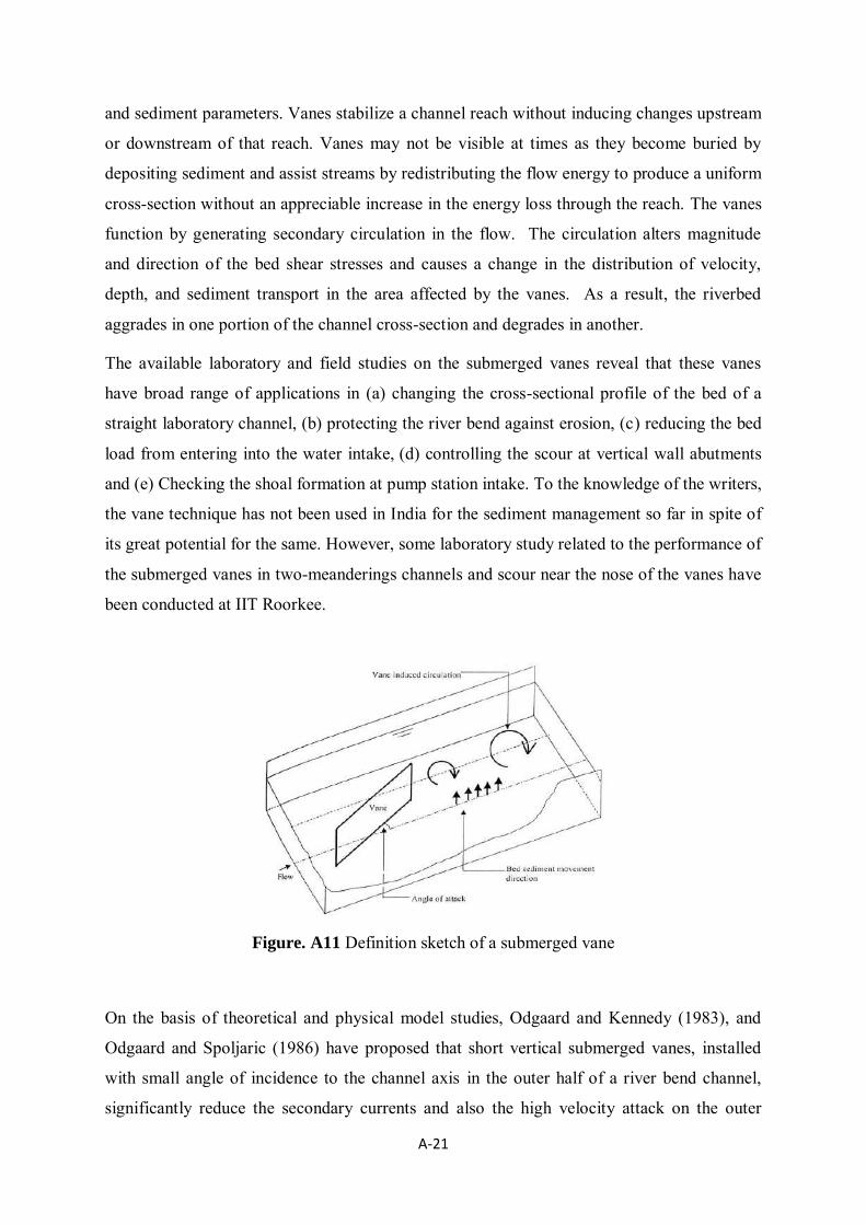
A-21
and sediment parameters. Vanes stabilize a channel reach without inducing changes upstream
or downstream of that reach. Vanes may not be visible at times as they become buried by
depositing sediment and assist streams by redistributing the flow energy to produce a uniform
cross-section without an appreciable increase in the energy loss through the reach. The vanes
function by generating secondary circulation in the flow. The circulation alters magnitude
and direction of the bed shear stresses and causes a change in the distribution of velocity,
depth, and sediment transport in the area affected by the vanes. As a result, the riverbed
aggrades in one portion of the channel cross-section and degrades in another.
The available laboratory and field studies on the submerged vanes reveal that these vanes
have broad range of applications in (a) changing the cross-sectional profile of the bed of a
straight laboratory channel, (b) protecting the river bend against erosion, (c) reducing the bed
load from entering into the water intake, (d) controlling the scour at vertical wall abutments
and (e) Checking the shoal formation at pump station intake. To the knowledge of the writers,
the vane technique has not been used in India for the sediment management so far in spite of
its great potential for the same. However, some laboratory study related to the performance of
the submerged vanes in two-meanderings channels and scour near the nose of the vanes have
been conducted at IIT Roorkee.
Figure. A11 Definition sketch of a submerged vane
On the basis of theoretical and physical model studies, Odgaard and Kennedy (1983), and
Odgaard and Spoljaric (1986) have proposed that short vertical submerged vanes, installed
with small angle of incidence to the channel axis in the outer half of a river bend channel,
significantly reduce the secondary currents and also the high velocity attack on the outer
A-22
bank. In addition, these vanes do not increase the local channel roughness as much as other
traditional methods do when used for reduction of near bank velocity. On the basis of
theoretical studies in a curved channel Odgaard and Wang (1991a, b) have shown that vanes
having height equal to 0.2–0.4 times the local water depth and installed at an angle of attack
within 150- 250 with the flow are quite successful in straight as well as meandering channels.
Their findings also reveal that by introducing relatively small changes in the bed shear
stresses, array of vanes could generate local changes in the bed elevation of the order of vane
height. Odgaard and Mosconi (1987) carried out laboratory tests and found that the vane
system does not interfere with the overall sediment balance and stability of channel while
protecting the bank. Experimental work of Johnson et al. (2001) using rock vanes, angled to
the flow and embedded into the stream bed such that the tip of the vane is submerged even
during low flow, also clearly demonstrates the effectiveness of vanes for preventing scour at
vertical wall abutments. Sinha and Marelius (2000) have shown that the optimal angle of
attack close to 400 produces strongest vane-induced circulation. Islam et al. (2003) carried out
experiments on both straight and curved reaches and have shown that for straight reach,
increasing the angle of attack in a vane array results in increasing the navigation depth.
Laboratory study of Barkdoll et al. (1999) shows that submerged vanes placed at the
diversion entrance admits only a negligible rate of bed-sediment entry into the water intake
when the ratio of unit discharge in the diversion to unit discharge in the main channel qr is
less than about 0.2. Beyond this value, the effectiveness of the vanes diminishes.
The performance of vanes for sediment control can be enhanced in several ways. One is to
use of a skimming wall in conjunction with the vanes and this is effective for values of qr up
to about 0.3. Another way is to widen the diversion entrance such that at the entrance qr does
not exceed about 0.3. Further enhancements like modified vane shape, uniformity of flow
distribution into the diversion, and increased flow velocity into the diversion are not
effective.
Figures A12a and A12b show a system of submerged vanes used by Odgaard and Mosconi
(1987) to protect the bank erosion of a bend of Wapsipinicon River, Iowa. Fig. A12(a) shows
vanes being installed in the bend in the summer of 1988 during low-flow, and the condition
of the same bend two years later; Fig. A12(b). Substantial deposition of sediment induced by
these vanes can be clearly seen in Fig. A12(b), thus demonstrating the capacity of these vanes
in preventing the scour along the river bend.

A-23
Figure. A12 Installation of Iowa Vanes in Wapsipinicon river bend
(a) During low flow in the Summer of 1988 (b) Low flow, May 10, 1990
Submerged vanes installed outside a water intake on Kosi River in Nepal is shown in Fig.
A13. The vane system prevents sediment from being entrained into the intake (left). Each
vane is 6 m long and 1.5 m-tall (with 0.8 m of vane below average bed level). Longitudinal
spacing varies between 30 m and 40 m; lateral spacing is 5 m.
2. Design of a Submerged Vane System
The design variables of a vane system are shown in Fig. A14. The design procedure generally
consists of selecting values of vane height H0, vane length L, angle of incidence vane
submergence T, vane spacings n and s, and vane-to-bank distance b using the following
known values: (a) the average depth of flow prior to the vane installation, d0; (b) the velocity
in the channel u0; (c) the resistance parameter m; (d) the channel’s width-depth ratio b/d0; (e)
the radius of bend-width ratio r/b; and (f) the sediment Froude number FD, defined as
gDuF 0D where g = acceleration due to gravity; and D = median grain diameter. The
resistance parameter, m is defined as f/8m , where f = friction factor and
=Karman’s constant taken as 0.4.
(a) (b)

A-24
Figure. A13 Vanes installed at a water intake on Kosi river, Nepal
To facilitate design, Odgaard and Wang (199a,b) prepared a number of graphs relating
maximum changes in depth of flow d0–dv, as a function of vane, flow and sediment
parameters where d0 = maximum pre-vane flow depth; and dv = vane induced flow depth.
These graphs were prepared for arrays with one, two, and three vanes arrangement; relative
vane submergence of T/d0=0.5, 0.7, and 1.0; Froude numbers FD = 5, 15, and 25; aspect ratio
of H0/L=0.3; angle of incidence = 200; and resistance parameter m = 4 and 3. Further these
graphs were for vane spacing ofn = 3H0 and s = 15H0 and 30H0, and for channels with
depth-width ratio of 0.03. In these graph the values of (d0–dv)/dv were shown as function of
width/radius of river bend (b/r). For a straight channel, radius of the bend can be considered
as infinity. Therefore, width/radius tends to zero. For this value of b/r ,i.e, for straight channel
the value of (d0–dv)/dv was found to be zero for T/d0 = 1. This shows that for straight
channels, vanes will not have any effect on bed level variation if relative submergence is
close to unity. The design chart as proposed by Odgaard and Wang (1991a) can be
reproduced in a tabular form as shown in Table A2.
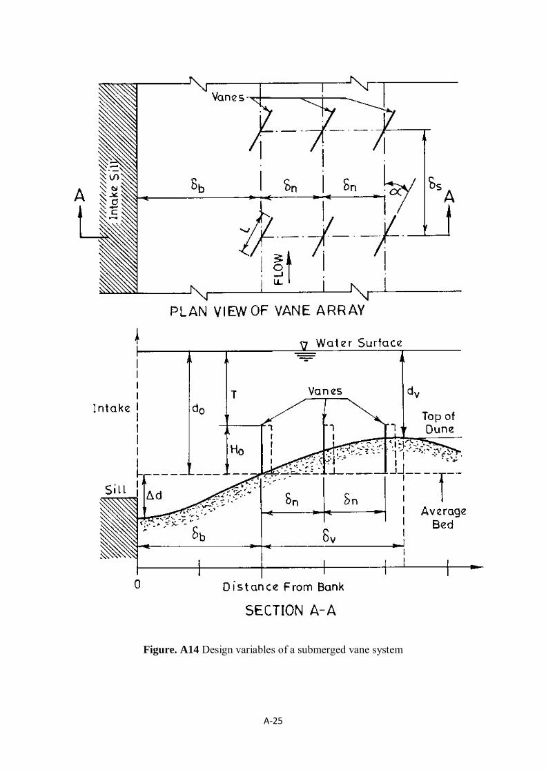
A-25
Figure. A14 Design variables of a submerged vane system

A-26
Table A2 Vane induced maximum increase in bed level along the bank of a stream.
FD m
(d0-dv)/d0
Three vanes array Two vanes array One vane array
T/do=0.5
s/Ho=15
0.5
30
0.7
15
0.7
30
0.5
15
0.5
30
0.7
15
0.7
30
0.5
15
0.5
30
0.7
15
0.7
30
5 4 0.20 0.20 0.18 0.15 0.16 0.15 0.12 0.10 0.10 0.09 0.07 0.05
5 3 0.25 0.20 0.20 0.16 0.20 0.16 0.14 0.11 0.12 0.10 0.08 0.05
15 4 0.46 0.40 0.30 0.27 0.36 0.34 0.25 0.23 0.24 0.2 0.17 0.13
15 3 0.50 0.45 0.30 0.28 0.45 0.38 0.30 0.25 0.26 0.22 0.2 0.15
25 4 0.50 0.50 0.30 0.28 0.50 0.45 0.30 0.30 0.4 0.34 0.25 0.22
25 3 0.50 0.50 0.30 0.28 0.50 0.50 0.30 0.30 0.41 0.35 0.30 0.30
3. Design Procedure
At the design stage, the depth of the flow d0, bed slope of the river S, velocity in the channel
u0, and median size of sediment D are known. If the vane system is to be designed for a river
bend, the radius of the bend r is also known. However, for the installation of vane in straight
channel like in the case of water intake, radius of the bend will be equal to infinity. Assuming
the channel to be wide, calculate oo gSd/uf/8 and then the channel’s resistance
parameter f/8m . Also calculate the sediment Froude number from the median
diameter of the sediment. Odgaard and Wang (1991a) and Odgaard and Kenedy (1983)
recommended that the height of vane H0 should be equal to 0.2 -0.4 times the depth of flow.
Choose some value of T/d0 out of 0.5, 0.7 and 1.0. Calculate the length of vane L keeping the
aspect ratio H0/L=0.3. Take n = 3H0 and s = 15H0 or 30H0. Now corresponds to known
values of T/d0, m,s/ H0, FD, b/r and number of vanes per array, read (d0–dv)/d0 from the Table
1. Finally, one can calculate the vane-induced depth of flow dv. It is to be noted that a number
of alternate designs are possible for a specific problem.

A-27
A8. FLOOD RETAINING WALL
There a several types of floodwalls, including gravity, cantilever, buttress and counter fort.
The gravity and cantilever floodwalls are the more commonly used types.
Gravity Floodwalls
As its name implies, a gravity floodwall depends upon its weight for stability. The gravity
wall’s structural stability is attained by effective positioning of the mass of the wall, rather
than the weight of the retained materials. The gravity wall resists overturning primarily by the
dead weight of the concrete and masonry construction.
Frictional forces between the concrete base and the soil foundation generally resist sliding of
the gravity wall. Soil foundation stability is achieved by ensuring that the structure neither
moves nor fails along possible failure surfaces. Gravity walls are appropriate for low walls or
lightly loaded walls. They are relatively easy to design and construct. The primary
disadvantage of a gravity floodwall is that a large volume of material is required. As he
required height of a gravity floodwall increases, it becomes more cost-effective to use
cantilever wall.
Cantilever Floodwall
A cantilever wall is reinforced-concrete wall that utilizes cantilever action to retain the mass
behind the wall. Stability of this type of wall is partially achieved from the weight of the soil
on the heel portion of the base. A comfortable safety factor is taken when considering the
unpredictability of the flood. Backfill can be placed along the outside face of the wall to keep
water away from the wall during flooding conditions.
Buttressed Floodwall
A buttressed wall is very similar to a counterfort wall. The only difference between the two is
that the transverse support walls are located on the side of the stem, opposite the retained
materials. The counterfort wall is more widely used than the buttress because the support
stem is hidden beneath the retained material, whereas the buttress occupies what may
otherwise be usable space in front of the wall.
Counterfort floodwall
A counterfort wall is similar to a cantilever retaining wall except that it can be used where the
cantilever is long or when very high pressures are exerted behind the wall. Counterforts or
A-28
intermediate traverse support bracing, are designed and built at intervals along the wall and
reduce the design forces.
Floodwall design
(i) Determine wall height and footing depth
(a) Determine wall height based on the highest flood level (HFL) plus 1.5 m of freeboard.
(b) Determine minimum footing depth based on the Lacey scour depth. Take depth of foundation at1.5 smd , where smd mean depth of scour
(ii) Assume dimensions
Based on the following guidelines or reference to engineering handbooks, assume dimensions for the wall thickness, footing width and footing thickness.
(a) The choice of wall thickness depends on the wall material, the strength of material and the height of the wall. Typical wall thicknesses are 8, 12 and 16 inches for masonry, concrete or masonry/concrete walls.
(b) The footing width depends on the magnitude of the lateral forces, allowable soil bearing capacity, dead load and wall height. Typically, the footing is located under the wall in such a manner that 1/3 of its width forms the toe and 2/3 of the width forms the heel of the wall. Typical footing thickness is based upon strength requirements.
(iii) Calculate forces
There are two types of forces acting on all and its footing: lateral and vertical.
(a) Vertical forces: The vertical forces are buoyancy and the various weights of the wall, footing, soil and water acting upward on the floodwall.
Lateral forces: These forces are mainly the hydrostatic and differential soil/water forces
on the heel side of the wall and the saturated soil force on the toe side of the wall.

B-1
Annexure-B
FLEXIBLE SYSTEM IN FLOOD CONTROL AND MITIGATION PLAN
I. Use of Geo-Textile Filters in Flood Management Works
For better performance of embankments, retaining walls, pavements and other structures, drains are provided to relieve hydrostatic pressure by allowing passage of water while preventing loss of soil. Traditionally granular filters are provided to serve these two functions. In last 25 years or so, geo-textile filters have emerged as a better alternative to traditional granular filter but since long term experience is limited, geo-textiles should not be used as a substitute for granular filter within or on the upstream face of earth dams or within any inaccessible portion of the dam embankment. Caution is advised in using geotextiles to wrap permanent peizometers and relief wells where they form part of the safety system of a water retaining structure. During monsoon period, rivers undergo bank and bed erosion at many stretches. Traditionally anti-erosion works to protect river bank and bed consists of a granular filter below the revetment and also below apron at Low Water Level (LWL). This anti-erosion work provides a good protection against erosion by preventing excessive migration of soil particles, while at the same time allowing water to flow freely through the filter layer. But this granular filter is often difficult to obtain, expensive to purchase, time consuming to install and segregates during placement, thus compromising its filtration ability. While the launching elements slide easily over the subsoil, they do not do so over each other. The falling apron, therefore, results in an about one-layer thick coverage. This layer is not stable and prone to loss of fines through the gaps in the protection. Many of the shortcomings of traditional filter can be overcome using geotextiles. Specially, a single layer of geo-textile fabric can replace a graded filter comprising of two or three layers. Geo-textiles are easy to install, especially, working underwater becomes much easier because the filter system can be assembled above the water and lowered into position. On negative side, geotextiles are sensitive to UV exposure and punching. Due care, therefore, must be taken while the installation of geo-textiles. Geo-textiles are comparatively costlier but more effective with longer serviceability.
Design of Bank Protection/ Anti-Erosion/ River Training works using Geo-textile Filters
Geo-textiles are frequently used in armoured erosion control and drainage applications. Geo-textiles are used to retain soil particles while allowing liquid topass freely. Designing with geo-textiles for filtration is essentially the same as designing graded granular filters.

B-2
Mechanism of Filtration
A filter should prevent excessive migration of soil particles, while at the same time allowing liquid to flow freely through the filter layer. Filtration is therefore summarized by two seemingly conflicting requirements: 1. The filter must retain soil, implying that the largest size of filter pore spaces or openings
should be smaller than a specified maximum value; and 2. The filter must be permeable enough to allow a relatively free flow through it, implying
that the openings of the geo-textile filter are sufficiently large enough and in large number to allow water flow while preventing clogging.
Design Philosophy
The design philosophy includes the estimation of scouring potential of river which is a function of the discharge intensity and Lacey’s scour depth. The fineness of riverbed material is indicated in terms of silt factor which along with discharge intensity governs the Lacey’s scour depth. The thickness of sloped bank pitching is determined on the basis of velocity of flow along the bank. Thickness and length of launching apron is determined once the scour depth, High Flood Level (HFL), and Low Water Level (LWL) are known. Proper drainage arrangement behind revetment is necessary. A suitable filter is also provided below the sloped pitching and launching apron to prevent fine soil particles from being removed. The provisions regarding Design of revetment and design of apron are available in IS 14262 and IS 10751, respectively.
Design of Geo-textile Filter
Before the introduction of geo-textiles, granular materials were widely used as filters for geotechnical engineering applications. Drainage criteria for geo-textile filters are largely derived from those for granular filters. The criteria for both are, therefore, similar. In addition to retention and permeability criteria, several other considerations are required for geo-textile filter design. Some considerations are noted below: 1. Retention: Ensures that the geo-textile openings are small enough to prevent excessive
migration of soil particles. 2. Permeability: Ensures that the geo-textile is permeable enough to allow liquids to pass
through without causing significant upstream pressure build up. 3. Anti-clogging: Ensures that the geo-textile has adequate openings, preventing trapped soil
from clogging openings and affecting permeability. 4. Survivability: Ensures that the geo-textile is strong enough to resist damage during
installation. 5. Durability: Ensures that the geo-textile is resilient to adverse chemical, biological and
ultraviolet (UV) light exposure for the design life of the project.

B-3
The specified numerical criteria for geo-textile filter requirements depends on the application of the filter, filter boundary conditions, properties of the soil being filtered, and construction methods used to install the filter. These factors are discussed in the following step-by-step geo-textile design methodology. Design Methodology
The proposed design methodology represents years of research and experience ingeo-textile filtration design. The approach presents a logical progression through seven steps.
Step 1: Determine Soil Retention Requirements Step 2: Define Boundary Conditions Step 3: Define the Application of Filter Requirements Step 4: Determine Permeability Requirements Step 5: Determine Anti-Clogging Requirements Step 6: Determine Survivability Requirements Step 7: Determine Durability Requirements
STEP 1: DETERMINE SOIL RETENTION REQUIREMENTS Analysis of the soil to be protected is critical to proper filtration design. The particle-size distribution of the soil to be protected should be determined using test method ASTM D 422. The grain size distribution curve is used to determine parameters necessary for the selection of numerical retention criteria. The maximum allowable opening size (O95) of the geo-textile is one that will provide adequate soil retention. It is also known as the geo-textile’s Apparent Opening Size (AOS) and is determined from test procedure ASTM D 4751. AOS can often be obtained from manufacturer’s literature. STEP 2: DEFINE BOUNDARY CONDITIONS Confining Stress: The confining pressure is important for several reasons: 1. High confining pressures tend to increase the relative density of coarse grained soil,
increasing the soil’s resistance to particle movement. This affects the selection of retention criteria.
2. High confining pressures decrease the hydraulic conductivity of fine grainedsoils, increasing the potential for soil to intrude into, or through, and thegeo-textile filter.
3. For all soil conditions, high confining pressures increase the potential for thegeo-textile and soil mass to intrude into the flow paths. This can reduce flow capacity within the drainage media, especially when geo-synthetic drainagecores are used.
Flow Conditions: Flow conditions can be either steady-state or dynamic. Defining these conditions is important because the retention criteria for each are different. Examples of applications with steady-state flow conditions include standard dewatering drains, wall drains

B-4
and leachate collection drains. Inland waterways and shoreline protection are typical examples of applications where waves or watercurrents cause dynamic flow conditions. STEP 3: DEFINE THE APPLICATION OF FILTER REQUIREMENTS Geo-textile filters are used between the soil and drainage or armoring medium. Typical drainage media include natural materials such as gravel and sand, as well as geo-synthetic materials such as geo-nets and cuspated drainage cores. Armoring material is often Revetment/ foundation or concrete blocks. Often, anarmoring system includes a sand bedding layer beneath the surface armour. The armoring system can be considered to act as a “drain” for water seeping from the protected slope. Drainage Material: The drainage medium adjacent to the geo-textile must be identified. The primary reasons for this include:
1. Large voids or high pore volume can influence the selection of the retention criterion 2. Sharp contact points such as highly angular gravel or rock will influence the
geosynthetic survivability requirements STEP 4: DETERMINE PERMEABILITY REQUIREMENTS Soil Permeability (ks): The soil permeability should be lab measured using representative field conditions in accordance with test procedure ASTM D 5084. Minimum Allowable Geo-textile Permeability (kg): The requirement of geotextile permeability can be affected by the filter application, flow conditions and soil type. The following equation can be used for all flow conditions to determine the minimum allowable geo-textile permeability (Giroud, 1988):
kg ≥ is.ks ; where:
kg= minimum allowable geo-textile permeability
ks= the soil permeability
is= desired hydraulic gradient (based upon the filtration application)
Permeability of the geo-textile can be calculated from the permittivity test procedure (ASTM D 4491). This value is often available from manufacturer’sliterature. Geo-textile permeability is defined as the product of the permittivity, Ψ, and the geo-textile thickness, tg:kg= Ψ.tg STEP 5: DETERMINE ANTI-CLOGGING REQUIREMENTS To minimize the risk of clogging, one should follow the provisions of IS 14262.

B-5
STEP 6: DETERMINE SURVIVABILITY REQUIREMENTS Minimum strength properties of the geo-textile fabric should be specified that fit with the severity of the installation procedure, to ensure construction survivability. STEP 7: DETERMINE DURABILITY REQUIREMENTS During installation, if the geo-textile filter is exposed to sunlight for extended periods, high carbon black content and UV stabilizers are recommended for added resistance to UV degradation. Polypropylene is one of the most durable geo-textiles today. It is inert to most naturally occurring chemicals in civil engineering applications. However, if it is known that the geo-textile may exposed to adverse chemicals (such as in waste containment landfill applications), use test method ASTM D5322 to determine its compatibility. BIS Specifications (IS 14262): Geo-textile filters may be recommended because of ease in installation and their proven effectiveness as an integral part of protection works. A 15 cm layer of sandis provided over filter fabric to avoid its mechanical rupture by protection material. The following criteria, depending on the gradation of bed material, may be used to select the correct filter fabric: a) For granular material containing 50 percent or less fines by weight, the following ratio
should be satisfied:
In order to reduce the chances of clogging, no fabric should be specified with an equivalent opening size smaller than 0.075 mm. Thus the equivalent opening size of fabric should not be smaller than 0.149 mm and should be equal to or less than 85 percent passing size of the bed material.
b) For bed material containing at least 50 percent but not more than 85 percent fines by
weight, the equivalent opening size of filter should not be smaller than 0.149 mm and should not be larger than 0.211 mm.
c) For bed material containing 85 percent or more of particles finer than 0.074 mm, it is
suggested that use of non-woven geo-fabric filter having opening sizeand permeability compatible to the equivalent values given in a) above may be used.
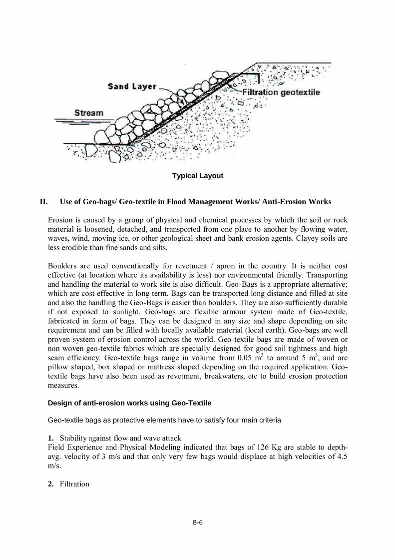
B-6
Typical Layout
II. Use of Geo-bags/ Geo-textile in Flood Management Works/ Anti-Erosion Works
Erosion is caused by a group of physical and chemical processes by which the soil or rock material is loosened, detached, and transported from one place to another by flowing water, waves, wind, moving ice, or other geological sheet and bank erosion agents. Clayey soils are less erodible than fine sands and silts. Boulders are used conventionally for revetment / apron in the country. It is neither cost effective (at location where its availability is less) nor environmental friendly. Transporting and handling the material to work site is also difficult. Geo-Bags is a appropriate alternative; which are cost effective in long term. Bags can be transported long distance and filled at site and also the handling the Geo-Bags is easier than boulders. They are also sufficiently durable if not exposed to sunlight. Geo-bags are flexible armour system made of Geo-textile, fabricated in form of bags. They can be designed in any size and shape depending on site requirement and can be filled with locally available material (local earth). Geo-bags are well proven system of erosion control across the world. Geo-textile bags are made of woven or non woven geo-textile fabrics which are specially designed for good soil tightness and high seam efficiency. Geo-textile bags range in volume from 0.05 m3 to around 5 m3, and are pillow shaped, box shaped or mattress shaped depending on the required application. Geo-textile bags have also been used as revetment, breakwaters, etc to build erosion protection measures. Design of anti-erosion works using Geo-Textile
Geo-textile bags as protective elements have to satisfy four main criteria
1. Stability against flow and wave attack Field Experience and Physical Modeling indicated that bags of 126 Kg are stable to depth-avg. velocity of 3 m/s and that only very few bags would displace at high velocities of 4.5 m/s. 2. Filtration

B-7
Geo-textile in the Bags also to act as filter for preventing loss of fines between bags, this type of failure is called as winnowing failure. This can be prevented by using multiple layer coverage. 3. Launching 4. Longevity
UV stability Abrasion resistance
Design steps
Application evaluation Obtain soil samples from the site Evaluate armor material and placement Calculate anticipated reverse flow through erosion control system. Determine geo-textile requirements
o Retention criteria o Permeability criteria o Clogging criteria
Estimate costs Prepare specifications Obtain samples of the geo-textile before acceptance. Monitor installation during construction and control drop height. Observeerosion
control systems during and after significant storm events.
The provisions regarding design of revetment and design of apron are available in IS 14262 and IS 10751 respectively. All structural parameter need to be designed similar to revetment/ spur using boulders. Size of Bags
For velocity up to 3 m/s, bags of size 1.1m x 0.7m x 0.15m (weight around 126 kg) may be used.
For higher velocity, weight should be more than that calculated as under:
where
W - weight in kg
V – velocity in m/sec
Ss - Specific Gravity of protection material (adopted between 1.5 to 1.8)
θ - Angle of sloping bank

B-8
φ - Angle of repose of protection material
The geo-synthetic material should be safe against the UV rays and abrasion. Thickness of Pitching
Thickness should be more than that calculated as under:
T - thickness in m
V – velocity in m/sec
Ss - Specific Gravity of protection material (adopted between 1.5 to 1.8)
g - Acceleration due to gravity (9.81 m/s2)
Pitching may be provided in double layers of geo-bags (in loose) and single layer (encased with nylon/polypropylene ropes)
Filter
A layer of Geo-textile filter may be provided under Geo-Bags.
III. Use of Geo-tubes/ Geo-textile in Flood Management Works/Embankments
Geo-tubes are basically containment systems in tubular forms filled with locally available sand which are formed in-situ on land or in water to protect shore and marine environments. It is in tubular shape made of geo-textile and is generally filled with sand or dredged material. These tubes are generally about 1 m to 3 m in diameter, though they can be customized to any size depending on their application. Today, geo-textile tubes ranging in diameters from 1.5 m to 5.0 m are used in many coastal and flood protection applications. Earthen embankments are constructed for Flood Protection. Availability of good quality earth is a major bottle neck in ensuring the quality of embankment. Embankment quality can be substantially improved by the use of geo-tubes. Use of geo-tubes also provides enhanced

B-9
security against breach and hence reduces investment on anti-erosion measures. Geo-tubes are very effective in breach closure without back shifting.
Quite often, conventional construction techniques will not allow dikes or levees to be constructed on very soft foundations because it may not be cost effective, operationally practical, or technically feasible. Nevertheless, geo-tube reinforced dikes have been designed and constructed. Geo-tubes used in those dikes alleviated many soft-ground foundation dike construction problems because they permit better equipment mobility, allow expedient construction, and allow construction to design elevation without failure. Embankments constructed on soft foundation soils have a tendency to spread laterally because of horizontal earth pressure acting within the embankment. These earth pressures cause horizontal shear stresses at the base of the embankment which must be resisted by the foundation soil. If the foundation soil doesn’t have adequate shear resistance, failure can result.
Design of Embankments using Geo-Tube
The cross section of the embankment made using Geo-tube is to be designed as per usual earthen embankment. The Geo-Tubes are placed in the core of such embankment generally in a pyramid shape. As with ordinary embankments on soft soils, the basic design approach for reinforced embankment is to design against failure. To successfully design a dike on a very soft foundation, three potential failure modes must be investigated:
Horizontal sliding and spreading of the embankment and foundation. Rotational slope and/or foundation failure. Excessive vertical foundation displacement.
The geo-tube must resist the unbalanced forces necessary for dike stability and must develop moderate-to-high tensile forces at relatively low-to moderate strains. It must exhibit enough soil fabric resistance to prevent pullout. The geo tube tensile forces resist the unbalanced forces, and its tensile modulus controls the vertical and horizontal displacement of dike and foundation. Adequate development of soil-geo-tube friction allows the transfer of dike load to the geo-tube. Developing geo-tube tensile stresses during construction at small material elongations or strains is essential. In addition, potential creep of the reinforcement must also be considered. Because the most critical condition for embankment stability is at the end of the construction, the reinforcement only has to function until the foundation soils gain sufficient strength to support the embankment.The cross section of the embankment made using Geo-Tube is to bedesigned as per usual earthen embankment. The Geo-Tubes are placed in the core of such embankment generally in a pyramid shape. Double layer of sheets of woven textiles is also used for added UV protection for a prolonged life and sufficient abrasion resistance. Design Steps
The following is a step-by-step procedure for design of reinforced embankments. STEP 1 Define embankment dimensions and loading conditions
A. Embankment height, H B. Embankment length C. Width of crest
B-10
D. Side slopes, b/H E. External loads
Surcharges Temporary (traffic) loads Dynamic loads
F. Environmental considerations Frost action Shrinkage and swelling Drainage, erosion and scour
G. Embankment construction rate Project constraints Anticipated or planned rate of construction
STEP 2 Establish the soil profile and determine the engineering properties of the
foundation soil
A. From a subsurface soils investigation, determine
Subsurface stratigraphy and soil profile. Groundwater table (location, fluctuation)
B. Engineering properties of the sub-soils
Undrained shear strength, cu, for end of construction Drained shear strength parameters, c’ and Φ’, for long-term conditions. Consolidation parameters (Cc, Cr, cv, σP ’)
Chemical and biological factors that may be detrimental to the reinforcement
C. Variation of properties with depth and areal extent. STEP 3 Obtain engineering properties of embankment fill materials
Classification properties Moisture-density relationships Shear strength properties Chemical and biological factors that may be detrimental to the reinforcement.
STEP 4 Establish minimum appropriate factors of safety and operational
settlement criteria for the embankment. Suggested minimum factors of
safety are as follows
Overall bearing capacity: 1.5 to 2 Global (rotational) shear stability at the end of construction: 1.3 Internal shear stability, long – term: 1.5 Lateral spreading (sliding): 1.5 Dynamic loading: 1.1 Settlement criteria: dependent upon project requirements
STEP 5 Check bearing capacity

B-11
A. When the thickness of the soft soil is much greater than the width of theembankment, use classical bearing capacity theory : qult= γfill*H = cuNc; Where Nc, the bearing capacity factor, is usually taken as 5.14 – the value for a strip footing on a cohesive soil of constant un-drained shear strength, cu, with depth.This approach underestimates the bearing capacity of reinforced embankments. B. When the soft soil is of limited depth, perform a lateral squeeze analysis. STEP 6 Check rotational shear stability
Perform a rotational slip surface analysis on the unreinforced embankment andfoundation to determine the critical failure surface and the factor of safety againstlocal shear instability. A. If the calculated factor of safety is greater than the minimum required, then reinforcement is not needed. Check lateral embankment spreading (Step 7). B. If the factor of safety is less than the required minimum, then calculate the required reinforcement strength, Tg, to provide an adequate factor of safety where :
STEP 7 Check lateral spreading (sliding) stability
Perform a lateral spreading or sliding wedge stability analysis
A. If the calculated factor of safety is greater than the minimum required, thenreinforcement is not needed for this failure possibility.
B. If the factor of safety is inadequate, then determine the lateral spreading strength of reinforcement, Tls required. Soil/geo-synthetic cohesion, Ca should be assumed equal to 0 for extremely soft soils and low embankments. A cohesionvalue should be included with placement of the second and subsequent fills in staged embankment construction.
C. Check sliding above the reinforcement. STEP 8 Establish tolerable geosynthetic deformation requirements and
calculatethe required reinforcement modulus, J, based on wide width
(ASTM D4595) tensile testing.
Reinforcement Modulus: J = Tls /Єgeosynthetic
Recommendations for strain limits, based on type of fill soil materials and for
construction over peats, are:
Cohesonless soils: Єgeosynthetic = 5 to 10%
Cohesive soils: Єgeosynthetic = 2%
Peats: Єgeosynthetic = 2 to 20%
STEP 9 Establish geosynthetic strength requirements in the embankment’s
longitudinal direction (i.e. direction of the embankment alignment).

B-12
A. Check bearing capacity and rotational slope stability at the ends of the embankment
(Steps 5 and 6)
B. Use strength and elongation determined from Steps 7 and 8 to control embankment
spreading during construction and to control bending following construction.
C. As the strength of the seams transverse to the embankment alignment control strength
requirements, seam strength requirements are the higher of thestrengths determined from
Steps 9A or 9B.
STEP 10 Establish geosynthetic properties.
A. Design strengths and modulus are based on the ASTM D 4595 wide width tensile test.
This test standard pewits definition of tensile modulus in terms of:
(i) initial tensile modulus; (ii) offset tensile modulus; or (iii) secant tensile modulus.
Furthermore, the secant modulus may be defined between any two strain points.
Geosynthetic modulus for design of embankments should be determined using a secant
modulus, defined with the zero strain point anddesign strain limit (i.e., 2 to 10%) point.
B. Seam strength is qualified with ASTM D 4884 test method, and is equal to the strength
required in the embankment’s longitudinal direction.
C. Soil-geosynthetic friction, Φsg , based on ASTM D 5321 with on-site soils. For preliminary
estimates, assume Φsg = 2/3Φ; for final design, testing is recommended.
D. Geo-textile stiffness based on site conditions and experience.
E. Select survivability and constructability requirements for the geosynthetic based on site
conditions, backfill materials, and equipment.
STEP 11 Estimate magnitude and rate of embankment settlement- Use
conventional geotechnical procedures and practices for this step.
STEP 12 Establish construction sequence and procedures.
STEP 13 Establish construction observation requirements.
STEP 14 Hold preconstruction meetings- Consider a partnering type contract with
a disputes resolution board.
STEP 15 Observe construction.
Geo-textile tubes fabric undergoes several stress cycles during its installation as well as during its life cycle. Theoretically the tube fabric is subjected to maximum stresses, both in circumferential and axial, directions at the time of filling. The Geo-textile skin of the Tube and it’s component parts should have adequate tensile strength to resist the various forces generated during filling as well as during the life time of the structure. The required Ultimate Tensile Strengthof the Geo-textile Tube Fabric is: [Tu]c>= FS [Tu]c The FS must account for factors such as Geotextile Tensions, Creep, seam factors and Durability. If any specific analysis is not undertaken a minimum FS of 4-5 shall be applied. With this the required fabric strength should be 150 N/mm2.
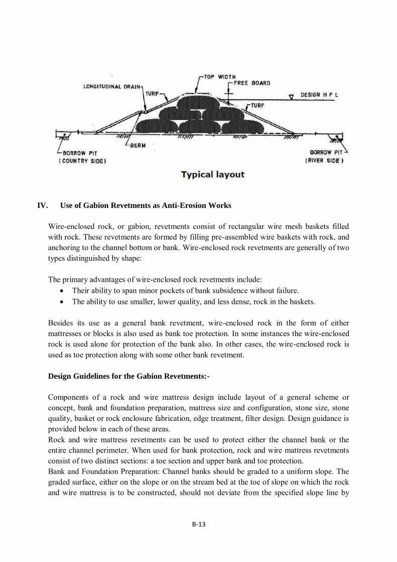
B-13
IV. Use of Gabion Revetments as Anti-Erosion Works
Wire-enclosed rock, or gabion, revetments consist of rectangular wire mesh baskets filled with rock. These revetments are formed by filling pre-assembled wire baskets with rock, and anchoring to the channel bottom or bank. Wire-enclosed rock revetments are generally of two types distinguished by shape: The primary advantages of wire-enclosed rock revetments include:
Their ability to span minor pockets of bank subsidence without failure. The ability to use smaller, lower quality, and less dense, rock in the baskets.
Besides its use as a general bank revetment, wire-enclosed rock in the form of either mattresses or blocks is also used as bank toe protection. In some instances the wire-enclosed rock is used alone for protection of the bank also. In other cases, the wire-enclosed rock is used as toe protection along with some other bank revetment. Design Guidelines for the Gabion Revetments:-
Components of a rock and wire mattress design include layout of a general scheme or concept, bank and foundation preparation, mattress size and configuration, stone size, stone quality, basket or rock enclosure fabrication, edge treatment, filter design. Design guidance is provided below in each of these areas. Rock and wire mattress revetments can be used to protect either the channel bank or the entire channel perimeter. When used for bank protection, rock and wire mattress revetments consist of two distinct sections: a toe section and upper bank and toe protection. Bank and Foundation Preparation: Channel banks should be graded to a uniform slope. The graded surface, either on the slope or on the stream bed at the toe of slope on which the rock and wire mattress is to be constructed, should not deviate from the specified slope line by

B-14
more than 150 mm. All blunt or sharp objects (such as rocks or tree roots) protruding from the graded surface should be removed. Large boulders near the outer edge of the toe and apron area should be removed. The thickness of the mattress is determined by three factors:
1. The erodability of the bank soil 2. The maximum velocity of the water, and 3. The bank slope.
The mattress thickness should be at least as thick as two overlapping layers of stone. The thickness of mattresses used as bank toe aprons should always exceed 150 mm. The typical range is 150 to 510 mm. The maximum size of stone should not exceed the thickness of individual mattress Units. The stone should be well graded within the sizes available and 70 percent of the stone, by weight, should be slightly larger than the wire-mesh opening.
Typical Layout
Note: This chapter is contributed by Mr. Dheeraj Kumar, Maccaferi Pvt. Ltd. and
edited by Prof. Z Ahmad

C-1
Annexure-C
A BRIEF REPORT ON WORKSHOP ON "MORPHOLOGICAL STUDY OF RIVERS
GANGA, SHARDA AND RAPTI USING REMOTE SENSING TECHNIQUE" HELD AT
LIBRARY BUILDING, CWC, NEW DELHI DURING 18-19 SEPT. 2017
Indian rivers experience large seasonal fluctuations in discharge and sediment load resulting in significant changes in their morphology. Shifting of the river course is generally accomplished by erosion of habitated and pricey agricultural area that causes tremendous losses. The sediments deposited and eroded in the river have a tremendous effect on river cross-section, gradient, intensity of water flow and its discharge. Understanding of changes in the morphology of the rivers is required in all engineering projects for their planning, design and execution. With this in mind, CWC, New Delhi desires to carry out morphological study of the major Indian rivers. In this direction, CWC awarded a project entitled "Morphological study of rivers Ganga, Sharda and Rapti using remote sensing techniques" to IIT Roorkee. Accordingly, IIT Roorkee carried out the morphological study of Ganga river from Devprayag to Farakka barrage; Sharda river from Tanakpur to its conflunece with Ghaghra river and Rapti river from Nepalgunj to Patana ghat near confluence of Ghaghra river for the period 1970 to 2010. The broad objectives of the study were hydrological aspects of flow and sediment; stream bank shifting; plan form changes; erosion & siltation; impacts of major hydraulic structures on the river morphology; vulnerable reaches and suggestion for training/protection works; morphology of islands; recommendations in the respect of actionable points & suggestions for the further study.
For the dissemination of outcomes of the study carried out under the cited project to the potential users, a workshop on Morphological Study of Rivers Ganga, Sharda and Rapti Using Remote
Sensing Technique was organized by Indian Institute of Technology Roorkee in association with Central Water Commission at Library building, CWC, New Delhi during 18-19 Sept. 2017.
The workshop was inaugurated by Hon'ble Union Minister of State, Water Resources, River Development & Ganga Rejuvenation and Parliamentary Affairs Shri Arjun Ram Meghwal. Prof. A K Chaturvedi, Director, IIT Roorkee; Shri Narendra Kumar, Chairman, CWC; Shri Pradeep Kumar, Member (RM); Shri N.K. Mathur, Member (D&R); Shri S Masood Husain, Member, (WP&P); Shri Ravi Shankar, CE (P&D), Prof. C S P Ojha, Head Civil Eng., IIT Roorkee; Prof. P K Garg, Professor, IIT Roorkee & Vice Chancellor, UTU; Shri P N Singh, Project Director, DRIP were also present.
Prof. Z Ahmad, Org. Secretary presented the gist of the study in the inaugural session. Shri Meghwal emphasizes the importance of water and its conservation. He also stressed upon the

C-2
study on morphology of the rivers prior to the independence subject to availability of the required data.
The workshop was attended by more than 160 participants from various Institutions, organizations, Public & private sectors, NGO etc. like CWC, New Delhi; IMD, New Delhi; IWAI, Noida; GFCC, Patna & Lucknow; NMCG, MoWR, RD & GR, New Delhi; NDMA, New Delhi; BSRDCL, Patna; CWPRS, Pune; RITES Ltd., New Delhi; DHI, India; C2S2, New Delhi; PWD, Uttarakhand; JNU, New Delhi; AMU, Aligarh; MANIT, Bhopal; Wildlife Inst. of India, Dehradun; Myway Education Charitable Trust, New Delhi; MGCGVV, Satna (MP); GEU, Dehradun.
Prof. Z. Ahmad, Prof. P K Garg, and Dr. R D Garg presented the outcomes of the morphology of the Ganga, Sharda and Rapti rivers before the participants which were well responded by them. Details of the delivered talks are as follow:
18 October 2017: Ganga River
Introduction covering scope of study, basin, study reach, data, methodology, geology, Land use land pattern, flood affected area, reconnaissance etc. : Prof. Z Ahmad
Analysis of hydrological data - Exceedance curve, Frequency Analysis, Trend Analysis : Prof. Z Ahmad
River Morphology : Planform (Meandering & Braiding), Shifting of course of river, Width of river & Shifting of confluence points : Prof. P K Garg, Dr. R D Garg & Prof. Z Ahmad
River Morphology - Islands in Ganga river : Prof. Z Ahmad Erosion and Siltation (including aggradation & degradation): Prof. P K Garg & Dr. R D Garg Major structures & their impacts on the morphology: Dr. R D Garg & Prof. Z Ahmad Critical reaches and suggested training works : Prof. Z Ahmad Panel discussion
19 October 2017: Rapti River
Introduction covering scope of study, basin, study reach, data, methodology, geology, Land use land pattern, flood affected area, reconnaissance etc. : Prof. Z. Ahmad
Presentation of outcomes of the hydrological data - Exceedance probability curves, peak discharge for different return periods & trend analysis: Prof. Z. Ahmad
River Morphology: Planform (Meandering & Braiding), Shifting of course of river & Width of river : Prof. P K Garg, Dr. R D Garg & Prof. Z Ahmad
Erosion and Siltation (including aggradation & degradation) : Prof. P K Garg & Dr. R D Garg Major structures & their impacts on the morphology: Prof. Z Ahmad
Critical reaches and suggested training works : Prof. Z Ahmad
19 October 2017: Sharda River
Introduction covering scope of study, basin, study reach, data, methodology, geology, Land use land pattern, flood affected area, reconnaissance etc. : Prof. Z. Ahmad
Presentation of outcomes of the hydrological data - Exceedance probability curves, peak discharge for different return periods & trend analysis: Prof. Z. Ahmad
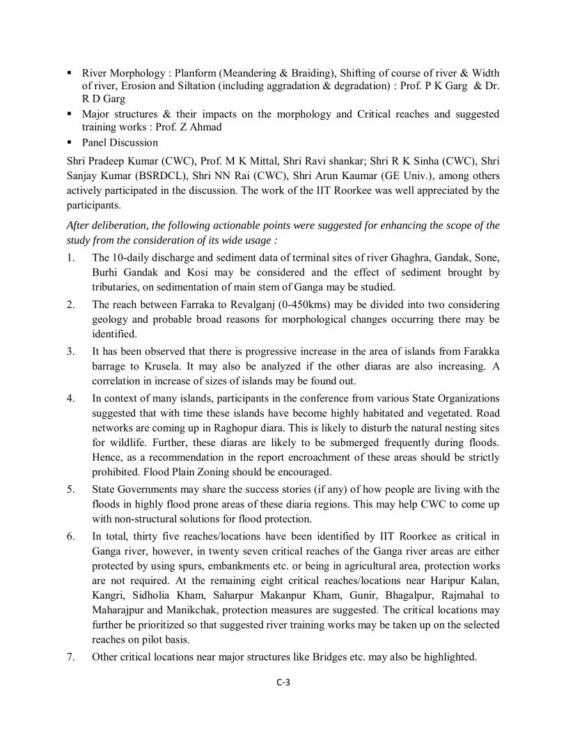
C-3
River Morphology : Planform (Meandering & Braiding), Shifting of course of river & Width of river, Erosion and Siltation (including aggradation & degradation) : Prof. P K Garg & Dr. R D Garg
Major structures & their impacts on the morphology and Critical reaches and suggested training works : Prof. Z Ahmad
Panel Discussion
Shri Pradeep Kumar (CWC), Prof. M K Mittal, Shri Ravi shankar; Shri R K Sinha (CWC), Shri Sanjay Kumar (BSRDCL), Shri NN Rai (CWC), Shri Arun Kaumar (GE Univ.), among others actively participated in the discussion. The work of the IIT Roorkee was well appreciated by the participants.
After deliberation, the following actionable points were suggested for enhancing the scope of the
study from the consideration of its wide usage :
1. The 10-daily discharge and sediment data of terminal sites of river Ghaghra, Gandak, Sone, Burhi Gandak and Kosi may be considered and the effect of sediment brought by tributaries, on sedimentation of main stem of Ganga may be studied.
2. The reach between Farraka to Revalganj (0-450kms) may be divided into two considering geology and probable broad reasons for morphological changes occurring there may be identified.
3. It has been observed that there is progressive increase in the area of islands from Farakka barrage to Krusela. It may also be analyzed if the other diaras are also increasing. A correlation in increase of sizes of islands may be found out.
4. In context of many islands, participants in the conference from various State Organizations suggested that with time these islands have become highly habitated and vegetated. Road networks are coming up in Raghopur diara. This is likely to disturb the natural nesting sites for wildlife. Further, these diaras are likely to be submerged frequently during floods. Hence, as a recommendation in the report encroachment of these areas should be strictly prohibited. Flood Plain Zoning should be encouraged.
5. State Governments may share the success stories (if any) of how people are living with the floods in highly flood prone areas of these diaria regions. This may help CWC to come up with non-structural solutions for flood protection.
6. In total, thirty five reaches/locations have been identified by IIT Roorkee as critical in Ganga river, however, in twenty seven critical reaches of the Ganga river areas are either protected by using spurs, embankments etc. or being in agricultural area, protection works are not required. At the remaining eight critical reaches/locations near Haripur Kalan, Kangri, Sidholia Kham, Saharpur Makanpur Kham, Gunir, Bhagalpur, Rajmahal to Maharajpur and Manikchak, protection measures are suggested. The critical locations may further be prioritized so that suggested river training works may be taken up on the selected reaches on pilot basis.
7. Other critical locations near major structures like Bridges etc. may also be highlighted.

C-4
8. Some key economical flood management structures which may be suitable for these reaches as available globally may also be indicated along with the report. An economical flood protection work scheme which may try to utilize locally available silt / sand in the river for protection through geo bags & geo tubes, etc. for immediate relief, a suitable design of this tentative proposal may also be included in the report. Similar globally adopted structures may also be indicated. Non conventional method of flood control in critical areas may also be discussed.
9. The trends of aggradations/degradation in the river may be established and certain conclusions be drawn from it.
10. The suggested future studies by IIT Roorkee may be prioritized according to the need and importance. Further, similar small studies if carried out by IIT Roorkee in past in form of Phd or M. Tech. thesis may be shared with CWC.
11. The dates corresponding to the remote sensing images used to determine the width of the river may be provided, so that discharge corresponding to the same day may be provided. The same may be used to infer, if possible some relationship between water level, discharge and the width of the river.
12. The existing embankments on the Ganga River may be marked in GIS environment and included in the final report.
13. The trend analysis of hydrological parameters like discharge etc. carried out by IIT Roorkee may result in wrong interpretations due to lack of complete daily hydrological data; hence the same may not be included in the final report. However frequency analysis may be published in the final report.
14. The nodal points along the reach of the river i.e. wherein minimum morphological changes are seen in the river be identified. This will be helpful in planning of structures like bridge in the future.
15. Where ever possible Disclaimers may be provided for more clarification. 16. Effect of vegetation on both sides of river and Existing Embankment on river morphology
may be discussed. Few photographs of the workshop are as follow:

C-5
Copyright © 2022 FDOKUMEN