Hydrol. Earth Syst. Sci., 19, 1293–1306, 2015

www.hydrol-earth-syst-sci.net/19/1293/2015/

doi:10.5194/hess-19-1293-2015

© Author(s) 2015. CC Attribution 3.0 License.

Modeling suspended sediment sources and transport

in the Ishikari River basin, Japan, using SPARROW

W. L. Duan1,2, B. He1, K. Takara2, P. P. Luo3,4, D. Nover5, and M. C. Hu2

1Key Laboratory of Watershed Geographic Sciences, Nanjing Institute of Geography and Limnology,

Chinese Academy of Sciences, Nanjing, 210008, China2Disaster Prevention Research Institute, Kyoto University, Kyoto, Japan3Institute of Hydraulic Structure Engineering and Water Environment, College of Civil Engineering and Architecture,

Zhejiang University, Hangzhou, Zhejiang, China4Institute for the Advanced Study of Sustainability, United Nations University, Shibuya, Tokyo, Japan5AAAS Science and Technology Policy Fellow, US Environmental Protection Agency, Global Change Research Group,

Washington, D.C., 20010, USA

Correspondence to: W. L. Duan (duan.scut.cn@gmail.com), B. He (hebin@niglas.ac.cn),

and P. P. Luo (luoping198121@gmail.com)

Received: 13 September 2014 – Published in Hydrol. Earth Syst. Sci. Discuss.: 6 October 2014

Revised: – – Accepted: 15 February 2015 – Published: 6 March 2015

Abstract. It is important to understand the mechanisms that

control the fate and transport of suspended sediment (SS)

in rivers, because high suspended sediment loads have sig-

nificant impacts on riverine hydroecology. In this study,

the SPARROW (SPAtially Referenced Regression on Wa-

tershed Attributes) watershed model was applied to esti-

mate the sources and transport of SS in surface waters

of the Ishikari River basin (14 330 km2), the largest water-

shed in Hokkaido, Japan. The final developed SPARROW

model has four source variables (developing lands, forest

lands, agricultural lands, and stream channels), three land-

scape delivery variables (slope, soil permeability, and pre-

cipitation), two in-stream loss coefficients, including small

streams (streams with drainage area< 200 km2) and large

streams, and reservoir attenuation. The model was calibrated

using measurements of SS from 31 monitoring sites of mixed

spatial data on topography, soils and stream hydrography.

Calibration results explain approximately 96 % (R2) of the

spatial variability in the natural logarithm mean annual SS

flux (kg yr−1) and display relatively small prediction er-

rors at the 31 monitoring stations. Results show that de-

veloping land is associated with the largest sediment yield

at around 1006 kg km−2 yr−1, followed by agricultural land

(234 kg km−2 yr−1). Estimation of incremental yields shows

that 35 % comes from agricultural lands, 23 % from forested

lands, 23 % from developing lands, and 19 % from stream

channels. The results of this study improve our understand-

ing of sediment production and transportation in the Ishikari

River basin in general, which will benefit both the scien-

tific and management communities in safeguarding water re-

sources.

1 Introduction

Suspended sediment (SS) is ubiquitous in aquatic ecosys-

tems and contributes to bottom material composition, water-

column turbidity, and chemical constituent transport. How-

ever, sediment is the largest water pollutant by volume, and

excessive sediment can have dramatic impacts on both wa-

ter quality and aquatic biota (Bilotta and Brazier, 2008).

High turbidity can significantly reduce or limit light pene-

tration into water, with implications for primary production

and for populations of fish and aquatic plants. In addition,

excessive sedimentation can bring more pollutants contain-

ing organic matter, animal or industrial wastes, nutrients, and

toxic chemicals, because sediment comes mainly from for-

est lands, agricultural fields, highway runoff, construction

Published by Copernicus Publications on behalf of the European Geosciences Union.

1294 W. L. Duan et al.: Modeling suspended sediment sources and transport in the Ishikari River basin

sites, and mining operations (Le et al., 2010; Srinivasa et al.,

2010), which always cause water quality deterioration and

therefore are a common and growing problem in rivers, lakes

and coastal estuaries (Dedkov and Mozzherin, 1992; Ishida

et al., 2010; Meade et al., 1985). Eutrophication due to nutri-

ent pollution, for example, is a widespread sediment-related

problem recognized at sites world-wide (Conley et al., 2009).

Also, in the US, approximately 25 % of the stream length

(167 092 miles) has been negatively impacted by excessive

sediment loads (USEPA, 2006).

Similarly, sediment accumulation can reduce the transport

capacity of roadside ditches, streams, rivers, and navigation

channels and the storage capabilities of reservoirs and lakes,

which cause more frequent flooding. For example, dams will

gradually lose their water storage capacity as sediment ac-

cumulates behind the dam (Fang et al., 2011); erosion of

river banks and increased sedimentation are also impacting

the Johnstone River catchment (Hunter and Walton, 2008)

and the estuary in the Tuross River catchment of coastal

southeastern Australia (Drewry et al., 2009) in clogging of

land and road drainage systems and river systems. There-

fore, as SS is fundamental to aquatic environments and im-

pairments due to enhanced sediment loads are increasingly

damaging water quality and water resource infrastructure, it

is extremely important to develop both monitoring systems

and technologies to track and to reduce the volume of SS in

order to safeguard freshwater systems.

Sediment sources can be separated into sediment originat-

ing in upland regions, sediment from urban areas, and sedi-

ment eroded from channel corridors (Langland and Cronin,

2003). Land use impacts are commonly seen as resulting in

increased sediment loads and therefore as an inadvertent con-

sequence of human activity. Moreover, land use and land use

change are also important factors influencing erosion and

sediment yields. For example, urbanization may ultimately

result in decreased local surface erosion rates when large ar-

eas are covered with impervious surfaces such as roadways,

rooftops, and parking lots (Wolman, 1967); because of the in-

creased exposure of the soil surface to erosive forces as a re-

sult of the removal of the native vegetative cover, agricultural

lands can drastically accelerate erosion rates (Lal, 2001). In

addition, stream channel erosion can be a major source of

sediment yield from urbanizing areas (Trimble, 1997).

In the Japanese context, high suspended sediment loads

are increasingly recognized as an important problem for

watershed management (Mizugaki et al., 2008; Somura et

al., 2012). For example, the Ishikari River basin has long

been plagued by high suspended sediment loads, generally

causing high turbidity along the river, including in Sapporo,

Hokkaido’s economic and government center. The pervasive-

ness of the problem has generated several sediment manage-

ment studies in the Ishikari River basin. Asahi et al. (2003)

found that it is necessary to consider tributary effects directly

and that sediment discharged from tributaries contributes

to the output sediment discharged from the river’s mouth.

Wongsa and Shimizu (2004) indicated that land use change

has a significant effect on soil eroded from hill slopes, but

no significant effect on flooding for the Ishikari River basin.

Ahn et al. (2009) concluded that sedimentation rate increased

in the Ishikari River floodplain because of agricultural devel-

opment on the floodplains. However, detailed accounting of

sediment sources (e.g., the type of land use) and transport in

the Ishikari River basin remains poorly understood.

Computer-based modeling is an essential exercise both for

organizing and understanding the complex data associated

with water quality conditions and for development of man-

agement strategies and decision support tools for water re-

source managers (Somura et al., 2012). Recent applications

of the GIS-based SPAtially Referenced Regression On Wa-

tershed attributes (SPARROW) (Smith et al., 1997) water-

shed model in the United States have advanced understand-

ing of nutrient sources and transport in large regions such

as the Mississippi River basin (Alexander et al., 2000, 2007)

and smaller watersheds such as the Chesapeake Bay water-

shed (Brakebill et al., 2010) and those draining to the North

Carolina coast (McMahon et al., 2003).

In this study, we use the SPARROW principle and frame-

work to develop a regional-scale sediment transport model

for the Ishikari River basin in Hokkaido, Japan. The con-

crete objectives are (1) to calibrate SS SPARROW for the

Ishikari River basin on the basis of 31 stations, (2) to use

the calibrated model to estimate mean annual SS condi-

tions, and (3) to quantify the relative contribution of different

SS sources to in-stream SS loads. These efforts are under-

taken with the ultimate goal of providing the information on

total and incremental sediment loads in different sub-basins

that will help resource managers identify priority sources of

pollution and mitigate this pollution in order to safeguard wa-

ter resources and protect aquatic ecosystems.

2 Materials and methods

2.1 Study area

The Ishikari River, the third longest river in Japan (Fig. 1),

originates from Mt. Ishikaridake (elevation 1967 m) in the

Taisetsu Mountains of central Hokkaido, passes through the

west of Hokkaido, and flows into the Sea of Japan, with a

total sediment discharge of around 14.8 km3 per year. The

river has the largest river basin, with a total drainage area

of 14 330 km2, the north–south and east–west distances of

which are about 170 and 200 km, respectively. The Ishikari

plain occupies most of the basin’s area, which is surrounded

by rolling hills and is the lowest land in Japan (the highest

elevation is less than 50 m) and consequently the best farm-

ing region in the country. The Ishikari River basin has cold

snowy winters and warm, non-humid summers. Sediment

load is very low in the cold winter except for the temporary

snowmelt at positive degree air temperature, and high in the

Hydrol. Earth Syst. Sci., 19, 1293–1306, 2015 www.hydrol-earth-syst-sci.net/19/1293/2015/

W. L. Duan et al.: Modeling suspended sediment sources and transport in the Ishikari River basin 1295

Figure 1. Study area, stream networks, and monitoring stations for the Ishikari River basin.

snowmelt season of mid-March to May and heavy rainfalls in

May–late November. In this basin, the regional average Au-

gust temperature ranges from 17 to 22 ◦C, while the average

January temperature ranges from −12 to −4 ◦C; the regional

annual precipitation was 850–1300 mm from 1980 to 2011.

2.2 Modeling tools

Based on the mechanistic mass transport components, in-

cluding surface-water flow paths (channel time of travel,

reservoirs), non-conservative transport processes (i.e., first-

order in-stream and reservoir decay), and mass-balance con-

straints on model inputs (sources), losses (terrestrial and

aquatic losses/storage), and outputs (riverine nutrient ex-

port), the SPARROW modeling approach performs a nonlin-

ear least-squares multiple regression to describe the relation

between spatially referenced watershed and channel charac-

teristics (predictors) and in-stream load (response) (Schwarz

et al., 2006). This allows nutrient supply and attenuation to

be tracked during water transport through streams and reser-

voirs and assesses the natural processes that attenuate con-

stituents as they are transported from land and upstream (Pre-

ston et al., 2009). Figure 2 gives a graphical description of the

SPARROW model components. Monitoring station flux esti-

mation refers to the estimates of long-term flux used as the

response variable in the model. Flux estimates at monitor-

ing stations are derived from station-specific models that re-

late contaminant concentrations from individual water qual-

ity samples to continuous records of streamflow time series.

To obtain reliable unbiased estimates, the Maintenance of

Variance-Extension type 3 (MOVE.3) and the Load Estima-

tor (LOADEST) regression model were applied to develop

regression equations and to estimate monitoring station flux

(for calculation details, see Duan et al., 2013a, b).

For the model-estimated flux, the SPARROW modeling

can generally be defined by the following equation (Alexan-

der et al., 2007):

F ∗i =

[( ∑j∈J (i)

F ′j

)A(ZSi ,Z

Ri ;θS,θR

)

+

(NS∑n=1

Sn,iαnDn

(ZDi ;θD

))A′(ZSi ,Z

Ri ;θS,θR

)]εi, (1)

where F ∗i is the model-estimated flux for contaminants leav-

ing reach i. The first summation term represents the sed-

iment flux that leaves upstream reaches and is delivered

downstream to reach i, where F ′j denotes measured sediment

www.hydrol-earth-syst-sci.net/19/1293/2015/ Hydrol. Earth Syst. Sci., 19, 1293–1306, 2015

1296 W. L. Duan et al.: Modeling suspended sediment sources and transport in the Ishikari River basin

Industrial / MunicipalPoint Sources

Diffuse Sources

Landscape Transport

Aquatic TransportStreams /Reservoirs

In-Stream Flux PredictionCalibration minimizes differences

between predicted and calculated mean-annual loads at the monitoring stations

Water-Quality and Flow DataPeriodic measurements at

monitoring stations

Rating Curve Model ofPollutant Flux

Station calibration to monitoringdata

Mean-Annual Pollutant FluxEstimation

Continuous FlowData

Evaluation of ModelParameters and Predictions

MonitoringStation FluxEstimation

SPARROWModel Components

Re-Estimate M

odel Parameters

Figure 2. Schematic of the major SPARROW model components (from Schwarz et al., 2006).

flux (FMj ) when upstream reach j is monitored and equals

the given model-estimated flux (F ∗j ) when it is not. A( q) is

the stream delivery function representing sediment loss pro-

cesses acting on flux as it travels along the reach pathway,

which defines the fraction of sediment flux entering reach i

at the upstream node that is delivered to the reach’s down-

stream node. ZS and ZR represent the function of measured

stream and reservoir characteristics, respectively, and θS and

θR are their corresponding coefficient vectors. Here, stream

reach and watershed characteristics such as stream length, di-

rection of water flow, connectivity, mean annual streamflow,

water travel time per unit length, reservoir characteristics like

surface area, and local and total drainage area, were present

in the digital stream network data set and reflect parameters

required by the model. The second summation term denotes

the amount of sediment flux introduced to the stream network

at reach i, which is composed of the flux originating from

specific sediment sources, indexed by n= 1, 2, . . . , NS. Each

source has a source variable, denoted Sn, and its correspond-

ing source-specific coefficient αn. This coefficient retains the

units that convert the source variable units to flux units. The

function Dn( q) represents the land-to-water delivery factor.

The land-to-water delivery factor is a source-specific func-

tion of a vector of delivery variables, denoted by Zθi , and

an associated vector of coefficients θD . The function A′( q)represents the fraction of flux originating in and delivered to

reach i that is transported to the reach’s downstream node and

is similar in form to the stream delivery factor defined in the

first summation term of the equation. If reach i is classified

as a stream (as opposed to a reservoir reach), the sediment

introduced to the reach from its incremental drainage area

receives the square root of the reach’s full in-stream delivery.

This assumption is consistent with the notion that contami-

nants are introduced to the reach network at the midpoint of

reach i and thus are subjected to only half of the reach’s time

of travel. Alternatively, for reaches classified as reservoirs,

we assume that the sediment mass receives the full attenu-

ation defined for the reach. The multiplicative error term in

Eq. (1), εi , is applicable in cases where reach i is a monitored

reach; the error is assumed to be independent and identically

distributed across independent sub-basins in the intervening

drainage between stream monitoring stations. This item can

also be used for unmonitored reaches.

The reach loss and reservoir loss are used as the me-

diating factors affecting the mobilization of sediment from

the stream network. The reach-loss variable is nonzero only

for stream reaches, and is defined for two separate classes,

shallow-flowing (small) streams versus deep-flowing (large)

streams. Since stream depth is not known, streams with

drainage area< 200 km2 are classified as shallow, small

streams. The reservoir loss is denoted by areal hydraulic load

of the reservoir, which is computed as the quotient of mean

annual impoundment outflow and surface area (Hoos and

McMahon, 2009). Sediment loss in streams is modeled ac-

cording to a first-order decay process (Chapra, 1997; Brake-

bill et al., 2010) in which the fraction of the sediment mass

originating from the upstream node and transported along

reach i to its downstream node is estimated as a continuous

function of the mean water time of travel (T Si ; units of time)

and mean water depth, Di , in reach i, such that

Hydrol. Earth Syst. Sci., 19, 1293–1306, 2015 www.hydrol-earth-syst-sci.net/19/1293/2015/

W. L. Duan et al.: Modeling suspended sediment sources and transport in the Ishikari River basin 1297

Table 1. Summary of input data and calibration parameters. References to data sources are in the main text.

Category Input data Data source

The stream Stream network, stream lengths, Automated catchment delineation based on

network sub-catchment boundaries, a 50 m DEM, with modification of flow

sub-catchment areas diversions

Stream Water quality monitoring station Thirty-one stations from the National

load data Land with Water Information

monitoring network from 1982 to 2010

Sediment Developing land, forest land, Land use data including developing

source data and agricultural land land, forest land, agricultural land from

the Ministry of Land, Infrastructure,

Transport and Tourism, Japan, 2006

Environmental Mean annual precipitation The 20-year (1990–2010) average from the

setting Japanese Meteorological Agency

data Catchment slope Mean value of local slope, obtained from

50 m DEM

Soil texture, soil permeability Obtained from the 1 : 5 000 000-scale

FAO/UNESCO Soil Map of the World

and the National and Regional Planning

Bureau, Japan

Reservoir (dam) loss The Japan Dam Foundation

(http://damnet.or.jp/)

A(ZSi ,Z

Ri ;θS,θR

)= exp

(−θS

T Si

Di

), (2)

where θS is an estimated mass-transfer flux-rate coefficient

in units of L T−1. The rate coefficient is independent of the

properties of the water volume that are proportional to water

volume, such as streamflow and depth (Eq. 3). The rate can

be re-expressed as a reaction rate coefficient (T−1) that is

dependent on water-column depth by dividing by the mean

water depth.

Sediment loss in lakes and reservoirs is modeled accord-

ing to a first-order process (Chapra, 1997; Brakebill et al.,

2010) in which the fraction of the sediment mass originating

from the upstream reach node and transported through the

reservoir segment of reach i to its downstream node is es-

timated as a function of the reciprocal of the areal hydraulic

load (qRi )−1 (units of T L−1) for the reservoir associated with

reach i and an apparent settling velocity coefficient (θR; units

of length T−1), such that

A(ZSi ,Z

Ri ;θS,θR

)=

1

1+ θR

(qRi

)−1. (3)

The areal hydraulic load is estimated as the quotient of the

outflow discharge to the surface area of the impoundment.

2.3 Input data

In this study, input data for building SPARROW models are

classified into (Table 1) (1) stream network data to define

stream reaches and catchments of the study area; (2) loading

data for many monitoring stations within the model bound-

aries (dependent variables); (3) sediment source data describ-

ing all of the sources of the sediment being modeled (inde-

pendent variables); and (4) data describing the environmen-

tal setting of the area being modeled that causes statistically

significant variability in the land-to-water delivery of sedi-

ment (independent variables). Input data types are described

in more detail below.

2.3.1 The stream network

The hydrologic network used for the SPARROW model

of the Ishikari River basin is derived from a 50 m digi-

tal elevation model (DEM) (Fig. 1), which has 900 stream

reaches, each with an associated sub-basin. The stream net-

work mainly contains stream reach and sub-basin character-

istics such as stream length, direction of water flow, reservoir

characteristics like surface area, and local and total drainage

areas. For example, the areas of the sub-basin range from

0.009 to 117 km2, with a median of 15.9 km2. However,

mean water flow is not reported for each stream reach, sug-

gesting that we cannot calculate the SS concentration at the

stream reach scale, but can calculate the total yield SS for

each associated sub-basin.

2.3.2 Stream load data

Suspended sediment concentration and daily flow data are

collected to calculate the long-term (from 1985 to 2010)

www.hydrol-earth-syst-sci.net/19/1293/2015/ Hydrol. Earth Syst. Sci., 19, 1293–1306, 2015

1298 W. L. Duan et al.: Modeling suspended sediment sources and transport in the Ishikari River basin

Figure 3. Schematic showing (a) the observed water flows (m3 s−1) and (b) the observed SS concentration (mg L−1) at 31 monitoring

stations.

mean SS flux at every monitoring station. Thirty-one mon-

itoring stations were chosen for model calibration in this

study (Fig. 1). SS concentration and daily flow data were col-

lected at each site for the period from 1985 to 2010 by the

National Land with Water Information (http://www1.river.

go.jp/) monitoring network (Fig. 3). However, some stream-

flow gaging stations have short periods of record or miss-

ing flow values, but do not over 10 % of the time periods.

A streamflow record extension method called the Mainte-

nance of Variance-Extension type 3 (MOVE.3) (Vogel and

Stedinger, 1985) is employed to estimate missing flow val-

ues or to extend the record at a short-record station on the

basis of daily streamflow values recorded at nearby, hydro-

logically similar index stations. On this basis, the FORTRAN

Load Estimator (LOADEST), which uses time-series stream-

flow data and constituent concentrations to calibrate a regres-

sion model that describes constituent loads in terms of vari-

ous functions of streamflow and time, is applied to estimate

SS loads. The output regression model equations take the fol-

lowing general form (Runkel et al., 2004):

ln(Li)= α+ b lnQ+ c lnQ2= dsin(2π · dtime)

+ ecos(2π · dtime)+ f · dtime+ g · dtime2+ ε, (4)

where Li is the calculated load for sample i;Q is stream dis-

charge; dtime is time in decimal years from the beginning of

the calibration period; ε is error; and a, b, cd, e, f , and g are

the fitted parameters in the multiple regression model. The

number of parameters may be different at different stations,

depending on the lowest Akaike information criterion (AIC)

values (for details, please see Duan et al., 2013a, b).

AIC= 2k− 2ln(L), (5)

where k is the number of parameters in the statistical model,

and L is the maximized value of the likelihood function for

the estimated model.

The mean annual load is normalized to the 2006 base

year at the 31 monitoring stations to address the problem

of incompatibility in periods of record by using normaliz-

ing or detrending methods (for the detailed process, please

see Schwarz et al., 2006).

2.3.3 Sediment source data

SS source variables tested in the Ishikari SPARROW model

include estimates of developing lands, forest lands, agricul-

tural lands, and stream channels. Estimates of land use were

developed using data derived from the Policy Bureau of

the Ministry of Land, Infrastructure, Transport and Tourism,

Japan, 2006, which mainly contains 11 types of land use

(see Fig. 4). It was then merged into four types: developing

land, forest land, agricultural land, and water land. Finally,

different lands are allocated to individual sub-basins using

GIS zonal processes. Arc Hydro Tools is employed to get the

reach length, which denotes the streambed source.

Hydrol. Earth Syst. Sci., 19, 1293–1306, 2015 www.hydrol-earth-syst-sci.net/19/1293/2015/

W. L. Duan et al.: Modeling suspended sediment sources and transport in the Ishikari River basin 1299

Figure 4. Land use of the Ishikari River basin, 2006.

2.3.4 Environmental setting data

Climatic and landscape characteristics considered candidates

for SS transport predictors include climate, topography and

soil (Duan et al., 2012; Asselman et al., 2003; Dedkov and

Mozzherin, 1992). Here, slope, soil permeability, and pre-

cipitation are used to evaluate the influences of “land-to-

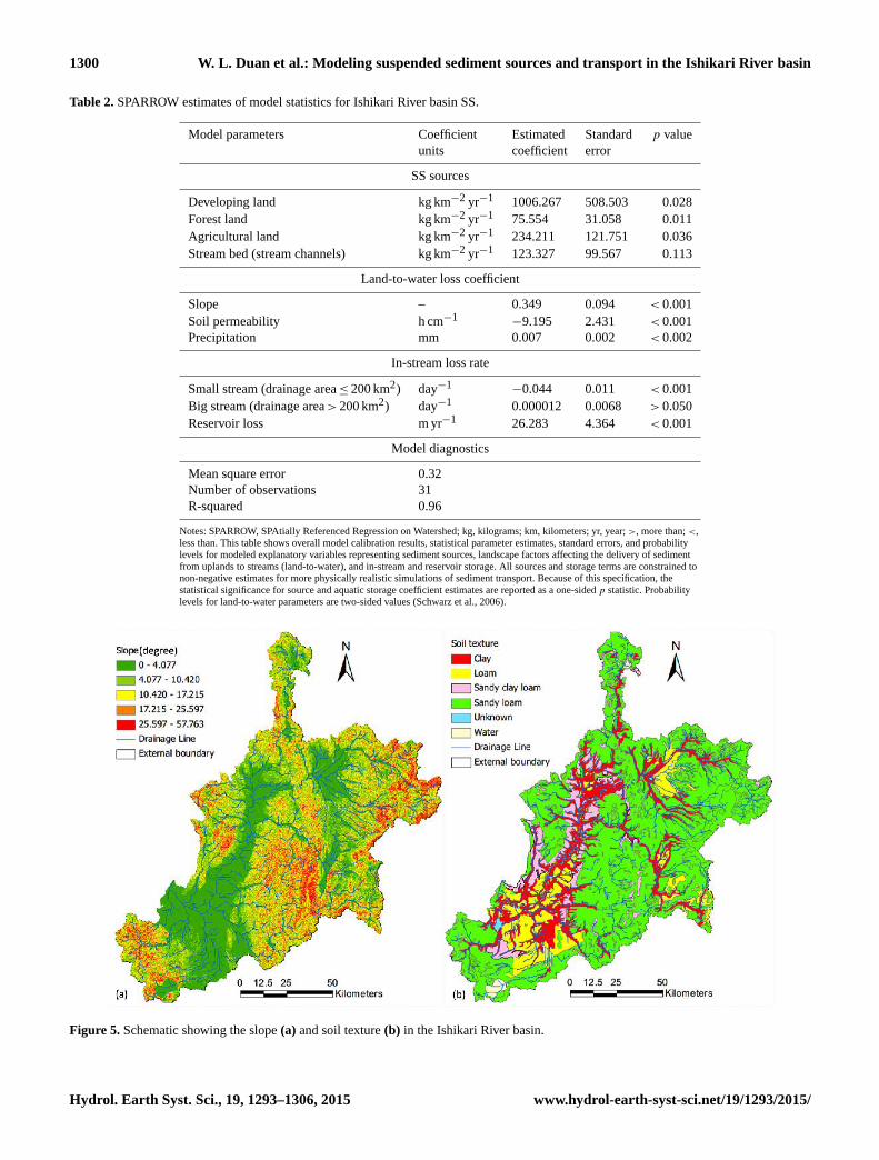
water” delivery terms. Basin slope is obtained using the GIS

surface tool (see Fig. 5a). Soil permeability and clay con-

tent (see Fig. 5b) are estimated using data derived from the

1 : 5 000 000-scale FAO/UNESCO Soil Map of the World

(FAO-UNESCO-ISRIC, 1988) and the National and Re-

gional Planning Bureau, Japan. Mean annual precipitation

data, representing the 20-year (1990–2010) average, were

obtained from daily precipitation data at 161 weather sta-

tions (see Fig. S1 in the Supplement) in Hokkaido from 1990

to 2010; that is, we first interpolated the mean annual pre-

cipitation over Hokkaido using a conventional Kriging tech-

nique on the basis of 161 stations, and then clipped the mean

annual precipitation distribution for the Ishikari River basin.

Finally, all these watershed average values were used to cal-

culate estimates for each sub-basin in the Ishikari model area

using the ZONALMEAN and ZONALSTATISTICAL func-

tions (zonal spatial analyst methods) of ArcGIS 10.

2.4 Model calibration and application

Considering that the calibration of the SPARROW model re-

quires long-term averaging and load adjustments for changes

in flow and sources, the final SPARROW model was statis-

tically calibrated using estimates of mean annual SS fluxes

at 31 monitoring stations (see input data). The explanatory

variables represented statistically significant or otherwise im-

portant geospatial variables, and the measures of statistically

significance are based on statistical evaluations of the t statis-

tics (ratio of the coefficient value to its standard error). The t

statistics are asymptotically distributed as a standard normal.

The statistical significance (α= 0.05) of the coefficients for

each of the SS source terms (which were constrained to be

positive) were determined by using a one-sided t test, and the

significance of the coefficients for each of the land-to-water

delivery terms (which were allowed to be positive or nega-

tive, reflecting either enhanced or attenuated delivery, respec-

tively) and the variables representing SS loss in free-flowing

streams and impoundments were determined by using a two-

sided t test (Schwarz et al., 2006). The yield R-squared (R2),

the root mean squared error (RMSE), and the residuals for

spatial patterns were the conventional statistical diagnostics

used to assess the overall SPARROW model accuracy and

performance.

According to the equations of SPARROW, the calibrated

model can be used to identify the largest local SS sources;

that is, the sediment source contributing the most to the in-

cremental SS yield for each catchment in the Ishikari River

basin can be calculated. In addition, the models can be used

to estimate the contribution from each sediment source to the

total SS loads predicted for each reach. Total loads were the

predicted load contributed from all upstream landscape sed-

iment sources. Finally, the factors that affect mean annual

transport in the Ishikari River basin can be identified.

3 Results and discussion

3.1 Model calibration

Model calibration results for the log transforms of the

summed quantities in Eq. (1) and nonlinear least-squares es-

timates are presented in Table 2, which explains approxi-

mately 96 % (R2) of the spatial variation in the natural loga-

rithm of mean annual SS flux (kg yr−1), with a mean square

error (MSE) of 0.323 kg yr−1, suggesting that the SS pre-

dicted by the model has litter error compared with the ob-

servation load.

The plot of predicted and observed SS flux is shown in

Fig. 6, demonstrating model accuracy over a wide range

of predicted flux and stream sizes. Generally, for a good

SPARROW model, the graphed points should exhibit an even

spread about the one-to-one line (the straight line in Fig. 6)

with no outliers. However, a common pattern expressed in

Fig. 6 for the final SPARROW SS model is the tendency

for larger scatter among observations with smaller predicted

fluxes – a pattern of heteroscedasticity. One likely cause

of this pattern is greater error in the measurement of flux

www.hydrol-earth-syst-sci.net/19/1293/2015/ Hydrol. Earth Syst. Sci., 19, 1293–1306, 2015

1300 W. L. Duan et al.: Modeling suspended sediment sources and transport in the Ishikari River basin

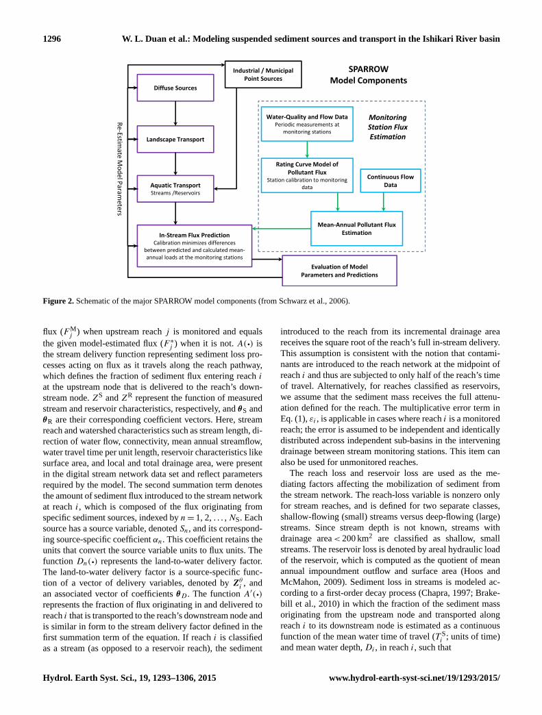
Table 2. SPARROW estimates of model statistics for Ishikari River basin SS.

Model parameters Coefficient Estimated Standard p value

units coefficient error

SS sources

Developing land kg km−2 yr−1 1006.267 508.503 0.028

Forest land kg km−2 yr−1 75.554 31.058 0.011

Agricultural land kg km−2 yr−1 234.211 121.751 0.036

Stream bed (stream channels) kg km−2 yr−1 123.327 99.567 0.113

Land-to-water loss coefficient

Slope – 0.349 0.094 < 0.001

Soil permeability h cm−1−9.195 2.431 < 0.001

Precipitation mm 0.007 0.002 < 0.002

In-stream loss rate

Small stream (drainage area≤ 200 km2) day−1−0.044 0.011 < 0.001

Big stream (drainage area> 200 km2) day−1 0.000012 0.0068 > 0.050

Reservoir loss m yr−1 26.283 4.364 < 0.001

Model diagnostics

Mean square error 0.32

Number of observations 31

R-squared 0.96

Notes: SPARROW, SPAtially Referenced Regression on Watershed; kg, kilograms; km, kilometers; yr, year; >, more than; <,

less than. This table shows overall model calibration results, statistical parameter estimates, standard errors, and probability

levels for modeled explanatory variables representing sediment sources, landscape factors affecting the delivery of sediment

from uplands to streams (land-to-water), and in-stream and reservoir storage. All sources and storage terms are constrained to

non-negative estimates for more physically realistic simulations of sediment transport. Because of this specification, the

statistical significance for source and aquatic storage coefficient estimates are reported as a one-sided p statistic. Probability

levels for land-to-water parameters are two-sided values (Schwarz et al., 2006).

Figure 5. Schematic showing the slope (a) and soil texture (b) in the Ishikari River basin.

Hydrol. Earth Syst. Sci., 19, 1293–1306, 2015 www.hydrol-earth-syst-sci.net/19/1293/2015/

W. L. Duan et al.: Modeling suspended sediment sources and transport in the Ishikari River basin 1301

Figure 6. Observed and predicted SS flux (kg yr−1) at 31 monitor-

ing sites included in the Ishikari SPARROW model (Natural loga-

rithm transformation applied to observed and predicted values; the

black line is the trend line, the green dashed line is a 1 : 1 line).

in small sub-basins due to greater variability in flow or to

greater relative inhomogeneity of sediment sources within

small sub-basins (Schwarz et al., 2006). Appropriate assign-

ment of weights reflecting the relative measurement error in

each observation (plus an additional common model error)

can improve the coefficient estimates and correct the infer-

ence of coefficient error if the heteroscedasticity is caused

by measurement error. On the other hand, the observations

can be weighted to improve the coefficient estimates and cor-

rect their estimates of error if the heteroscedasticity is due to

structural features of the SPARROW model. Figure 7 shows

the standardized residuals at the 31 monitoring sites. Mon-

itoring sites with overpredictions (< 0) mainly exist in the

middle area of the Ishikari River basin, and underpredic-

tions (> 0) exist in the upper and lower areas. The Studen-

tized residual is useful for identifying outliers and, if greater

than 3.6, is generally considered an outlier warranting further

investigation (Schwarz et al., 2006). Overall, the final model

does not show evidence of large prediction biases over the

monitoring sites.

With the exception of stream channels, all of the

source variables modeled are statistically significant

(p value< 0.05), with the estimated coefficient representing

an approximate estimate of mean sediment yield for the

associated land use (Table 2). The largest intrinsic sediment

yield is associated with developing land, the estimated value

of which is around 1006 kg km−2 yr−1. Land development,

including removing cover and developing cuts and fills, can

increase potential erosion and sediment hazards on-site by

changing water conveyance routes, soil compaction (both

planned and unplanned), longer slopes and more and faster

stormwater runoff. With the analysis of factors affecting

sediment transport from uplands to streams (mean basin

slope, reservoirs, physiography, and soil permeability),

developing land was also the largest sediment source

Figure 7. Model residuals for 31 monitoring stations used to cali-

brate the final Ishikari SPARROW model.

reported in Brakebill et al. (2010) and Schwarz (2008).

Agricultural land has the second highest sediment yield,

with an estimated value of around 234 kg km−2 yr−1, and

forest land has the lowest sediment yield, with an estimated

value of around 76 kg km−2 yr−1.

Land-to-water delivery for sediment land sources is pow-

erfully mediated by watershed slope, soil permeability, and

rainfall, all of which are statistically significant (Table 2). As

expected, Table 2 shows that sediment produced from land

transport to rivers is most efficient in areas with greater basin

slope, less permeable soils, and greater rainfall, which is con-

sistent with the results calculated by Brakebill et al. (2010).

The alteration of these factors can directly and indirectly

cause changes in sediment degradation and deposition, and,

finally, to the sediment yield (Luce and Black, 1999; Nel-

son and Booth, 2002). Increased rainfall amounts and inten-

sities can directly increase surface runoff, leading to greater

rates of soil erosion (Nearing et al., 2005; Ran et al., 2012)

with consequences for productivity of farmland (Julien and

Simons, 1985). Watershed slope and soil permeability have

a powerful influence on potential surface runoff as they af-

fect the magnitude and rate of eroded sediment that may be

transported to streams (Brakebill et al., 2010).

The coefficient for in-stream loss indicates that sediment

is removed from large streams (about 0.000012 day−1) and

accumulates in small streams (about −0.044 day−1). These

www.hydrol-earth-syst-sci.net/19/1293/2015/ Hydrol. Earth Syst. Sci., 19, 1293–1306, 2015

1302 W. L. Duan et al.: Modeling suspended sediment sources and transport in the Ishikari River basin

Figure 8. Map showing the spatial distribution of total suspended sediment yields (a) and incremental suspended sediment yields (b) esti-

mated by SPARROW.

results run contrary to several published examples. For ex-

ample, Schwarz (2008) argued that greater streamflow causes

an increase in the amount of sediment generated from stream

channels. The reasons for these results could be the crite-

rion of the two kinds of streams. In this study, streams with

drainage area< 200 km2 are shallow, small streams, which

tend to attenuate the sediments; on the contrary, streams with

drainage area> 200 km2 are big streams, which tend to cre-

ate the sediments. Sediment storage is statistically signifi-

cant in reservoirs (dams), the estimated value of which is

around 26 m yr−1. This value is much less than the coeffi-

cient of 235 m yr−1 reported for the Chesapeake Bay water-

shed (SPARROW model; Brakebill et al., 2010), one possible

reason for which maybe is that the reservoirs in the Ishikari

River basin have less storage capacity compared with the

reservoirs in Chesapeake Bay. However, the value is similar

to the 36 m yr−1 computed by the conterminous US SPAR-

ROW model (Schwarz, 2008).

3.2 Model application

Because data from sampling stream networks suffer from

sparseness of monitoring stations, spatial bias and basin het-

erogeneity, describing regional distributions and exploring

transport mechanism of sediment is one of the challenges of

sediment assessment programs. Through the stream network,

SPARROW can link in-stream water quality to spatially ref-

erenced information on contaminant sources and other wa-

tershed attributes relevant to contaminant transport (Smith et

al., 1997). After calibration, the SPARROW model of total

suspended sediment can be applied to evaluate the stream-

corridor sediment supply, storage, and transport properties

and processes in a regional context, which can inform a va-

riety of decisions relevant to resource managers. Here, in

order to further explore and manage sediment sources, we

predict and analyze the spatial distribution of total sediment

and incremental sediment yields, and estimate the amount of

sediment generated by source described in each incremental

basin.

The total yields (load per area) represent the amount of

sediment including upstream load and local catchment load

contributing to each stream reach, and the incremental yields

represent the amount of sediment generated locally indepen-

dent of upstream supply, and contributing to each stream

reach, normalized by the local catchment area (see Fig. S2)

(Ruddy et al., 2006). Figure 8a shows the spatial distribu-

tion of the total yields, describing the sediment mass en-

tering streams per unit area of the incremental drainages

of the Ishikari River basin associated with the stream net-

work (Fig. 1). It is mediated by climatic and landscape char-

acteristics and delivered to the Ishikari Gulf of the Sea of

Japan after accounting for the cumulative effect of aquatic

removal processes. Figure 8a shows that total yields, ranging

from 0.03 to 1190 kg ha−1 yr−1 (mean= 101 kg ha−1 yr−1),

concentrate in the sub-basin along the middle and lower

reaches of the Ishikari River. Like total yields, much of

the incremental sediment yields are distributed in similar

areas (see Fig. 8b), the largest of which is greater than

150 kg ha−1 yr−1. These two kinds of predictions provide lo-

calized estimates of sediment that are useful in evaluating

local contributions of sediment in addition to identifying ge-

Hydrol. Earth Syst. Sci., 19, 1293–1306, 2015 www.hydrol-earth-syst-sci.net/19/1293/2015/

W. L. Duan et al.: Modeling suspended sediment sources and transport in the Ishikari River basin 1303

Figure 9. Maps showing the spatial distributions of independent sediment sources generated in each incremental catchment for (a) agricul-

tural land, (b) developing land, (c) forested land, and (d) stream channels.

ographic areas of potential water quality degradation due to

excessive sedimentation.

Figure 9 shows the percent of total incremental flux

generated for (a) agricultural lands, (b) developing lands,

(c) forested lands, and (d) stream channels, suggesting the

relative contributions from the various sources at each sub-

basin. The contributions from these sources that go into the

sub-basin yield (Fig. 8) are assessed by comparing predicted

sub-basin yield with predicted yield from agricultural-land

sediment yield (Fig. 9a); predicted developing-land sedi-

ment yield (Fig. 9b); predicted forest-land sediment yield

(Fig. 9c); and predicted steam channel yield (Fig. 9d). Gen-

erally, the spatial distribution of these contributions from dif-

ferent sources is in accordance with land use (Fig. 4). On

average, we can see that 35 % of the incremental flux is from

agricultural lands, which is the largest of all sources; the

second largest is from forested lands, the value of which is

around 23 %, followed by developing lands (23 %); the least

is from stream channels, with a value of 19 %.

3.3 Uncertainty analysis

Uncertainty always exists in hydrological models such as

SPARROW and therefore cannot but imperfectly reflect real-

www.hydrol-earth-syst-sci.net/19/1293/2015/ Hydrol. Earth Syst. Sci., 19, 1293–1306, 2015

1304 W. L. Duan et al.: Modeling suspended sediment sources and transport in the Ishikari River basin

ity. The sources of uncertainty in this study include (1) reso-

lution of the geospatial data, (2) quality of the sediment loads

used to calibrate the model, and (3) limitations of the mod-

eling approach in representing the environmental processes

accurately (Alexander et al., 2007). First, the hydrologic

network was derived from a 50 m digital elevation model

(DEM), which potentially deviates from the actual stream

network, causing the discrepancy of stream reach and sub-

basin characteristics such as stream length and local and to-

tal drainage area. This will lead to spatial uncertainty, al-

though that uncertainty is generally reflected in the SPAR-

ROW model errors after the calibration process (Alexander

et al., 2007). Another cause of uncertainty is the suitability of

using SS grab samples at the 31 monitoring sites for model

calibration to reflect the normal conditions in-stream. Also,

the SS loads at some monitoring stations were estimated us-

ing the MOVE.3 and LOADEST techniques (Runkel et al.,

2004; Duan et al., 2013a, b), which also have some uncer-

tainties.

4 Conclusions

In this study, we developed a SPARROW-based sediment

model for surface waters in the Ishikari River basin, the

largest watershed in Hokkaido, Japan. This model is based on

stream water quality monitoring records collected at 31 sta-

tions for the period 1985 to 2010 and uses four source vari-

ables including developing lands, forest lands, agricultural

lands, and steam channels, three landscape delivery variables

including slope, soil permeability, and precipitation, two in-

stream loss coefficients including small streams (drainage

area≤ 200 km2) and big streams (drainage area> 200 km2),

and reservoir attenuation. Significant conclusions on the cali-

bration procedure and model application are summarized be-

low. Calibration results explain approximately 96 % of the

spatial variation in the natural logarithm of mean annual

SS flux (kg km−2 yr−1) and display relatively small predic-

tion errors on the basis of 31 monitoring stations. Devel-

oping land is associated with the largest intrinsic sediment

yield at around 1006 kg km−2 yr−1, followed by agricultural

land (234 kg km−2 yr−1). Greater basin slope, less perme-

able soils, and greater rainfall can directly and indirectly en-

able sediment transport from land into streams. Reservoir

attenuation (26 m yr−1) is statistically significant, suggest-

ing that reservoirs can play a dramatic role in sediment in-

terception. The percent of total incremental flux generated

for agricultural lands, developing lands, forested lands, and

stream channels is 35, 23, 23 and 19 %, respectively. Sedi-

ment total yields and incremental yields concentrate in the

sub-basin along the middle and lower reaches of the Ishikari

River, showing which sub-basin is most susceptible to ero-

sion. Combined with land use, management actions should

be designed to reduce sedimentation of agricultural lands and

developing lands in the sub-basin along the middle and lower

reaches of the Ishikari River. Our results suggest several ar-

eas for further research, including explicit representation of

flow and sediment discharge from each stream and in total to

the Sea of Japan, more accurate representation of spatial data

in SPARROW, and the design of pollutant reduction strate-

gies for local watersheds.

This study also has a number of shortcomings and suggests

several areas for future work. Some important model param-

eters lack statistical significance, for example, statistically

insignificant model components and inaccuracies associated

with river systems, which contain a source variable (stream

channels), and big streams with drainage area> 200 km2.

These findings are contrary to the findings of other stud-

ies (Brakebill et al., 2010). In addition, the predictions of

the model pertain to mean-annual conditions, not necessar-

ily critical conditions such as low-flow conditions. The rea-

son for these shortcomings derives from the following points:

(1) the hydrologic network was derived from a 50 m digital

elevation model (DEM), which potentially deviates from the

actual stream network; (2) due to a lack of water discharge in

all streams, stream velocity was replaced with the drainage

area to classify fast and slow streams; and (3) the calibra-

tion data only incorporate monitored load data from a limited

number of stations with long-term data.

Excessive sedimentation can have a variety of adverse ef-

fects on aquatic ecosystems and water resource infrastruc-

ture. Analysis of sediment production and transport mech-

anisms is therefore necessary to describe and evaluate a

basin’s water quality conditions in order to provide guid-

ance for development of water quality indicators and pol-

lution prevention measures (Buggy and Tobin, 2008; Meals

et al., 2010). As illustrated here, the SPARROW model is a

valuable tool that can be used by water resource managers in

water quality assessment and management activities to sup-

port regional management of sediment in large rivers and es-

tuaries.

The Supplement related to this article is available online

at doi:10.5194/hess-19-1293-2015-supplement.

Acknowledgements. This study is sponsored by National Natural

Science Foundation of China (No. 41471460) and “One Hundred

Talents Program” of Chinese Academy of Sciences, the Kyoto Uni-

versity Sustainability/Survivability Science for a Resilient Society

Adaptable to Extreme Weather Conditions Global COE program

and the Global Center for Education and Research on Human Se-

curity Engineering for Asian Megacities, the Postdoctoral fellow-

ship of Japan Society for the Promotion of Science (P12055), JSPS

KAKENHI grant number 24.02055 and the JSPS Grant-in-Aid for

Young Scientists (B) (KAKENHI Wakate B, 90569724). We also

wish to acknowledge Anne B. Hoos and John W. Brakebill of the

US Geological Survey for their help with the use of the SPARROW

model. The first author would like to thank the China Scholarship

Council (CSC) for his PhD scholarships.

Hydrol. Earth Syst. Sci., 19, 1293–1306, 2015 www.hydrol-earth-syst-sci.net/19/1293/2015/

W. L. Duan et al.: Modeling suspended sediment sources and transport in the Ishikari River basin 1305

Edited by: M. Mikos

References

Ahn, Y. S., Nakamura, F., Kizuka, T., and Nakamura, Y.: Elevated

sedimentation in lake records linked to agricultural activities in

the Ishikari River floodplain, northern Japan, Earth Surf. Proc.

Land, 34, 1650–1660, doi:10.1002/esp.1854, 2009.

Alexander, R. B., Smith, R. A., and Schwarz, G. E.: Effect of stream

channel size on the delivery of nitrogen to the Gulf of Mexico,

Nature, 403, 758–761, doi:10.1038/35001562, 2000.

Alexander, R. B., Smith, R. A., Schwarz, G. E., Boyer, E. W.,

Nolan, J. V., and Brakebill, J. W.: Differences in phospho-

rus and nitrogen delivery to the Gulf of Mexico from the

Mississippi River Basin, Environ. Sci. Technol., 42, 822–830,

doi:10.1021/es0716103, 2007.

Asahi, K., Kato, K., and Shimizu, Y.: Estimation of Sediment Dis-

charge Taking into Account Tributaries to the Ishikari River, J.

Nat. Disast. Sci., 25, 17–22, 2003.

Asselman, N. E. M., Middelkoop, H., and Van Dijk, P. M.: The im-

pact of changes in climate and land use on soil erosion, transport

and deposition of suspended sediment in the River Rhine, Hy-

drol. Process., 17, 3225–3244, doi:10.1002/hyp.1384, 2003.

Bilotta, G. S. and Brazier, R. E.: Understanding the influence of

suspended solids on water quality and aquatic biota, Water Res.,

42, 2849–2861, doi:10.1016/j.watres.2008.03.018, 2008.

Brakebill, J. W., Ator, S. W., and Schwarz, G. E.: Sources of Sus-

pended Sediment Flux in Streams of the Chesapeake Bay Wa-

tershed: A Regional Application of the SPARROW Modell, J.

Am. Water Resour. Assoc., 46, 757–776, doi:10.1111/j.1752-

1688.2010.00450.x, 2010.

Buggy, C. J. and Tobin, J. M.: Seasonal and spatial distribution of

metals in surface sediment of an urban estuary, Environ. Pollut.,

155, 308–319, doi:10.1016/j.envpol.2007.11.032, 2008.

Chapra, S. C.: Surface Water-Quality Modelling, McGraw-Hill,

New York, 1997.

Conley, D. J., Paerl, H. W., Howarth, R. W., Boesch, D. F.,

Seitzinger, S. P., Havens, K. E., Lancelot, C., and Likens, G. E.:

Controlling eutrophication: nitrogen and phosphorus, Science,

323, 1014–1015, doi:10.1126/science.1167755, 2009.

Dedkov, A. P. and Mozzherin, V. I.:. Erosion and sediment yield

in mountain regions of the world. Erosion, debris flows and en-

vironment in mountain regions, Proceedings of the International

Symposium, 5–9 July 1992, Chengdu, China, IAHS Publ., 209,

29–36, 1992.

Drewry, J. J., Newham, L., and Croke, B.: Suspended sediment, ni-

trogen and phosphorus concentrations and exports during storm-

events to the Tuross estuary, Australia, J. Environ. Manage., 90,

879–887, doi:10.1016/j.jenvman.2008.02.004, 2009.

Duan, W., He, B., Takara, K., Luo, P., and Yamashiki, Y.: Esti-

mating the Sources and Transport of Nitrogen Pollution in the

Ishikari River Basin, Japan, Adv. Mater. Res., 518, 3007–3010,

doi:10.4028/www.scientific.net/AMR.518-523.3007, 2012.

Duan, W., Takara, K., He, B., Luo, P., Nover, D., and Yamashiki,

Y.: Nutrients and Suspended Sediment Load Estimates for the

Ishikari River Basin, Japan, Over a Decade, Kyoto University,

Disast. Prevent. Res. Inst. Annu., 56, 59–64, 2013a.

Duan, W., Takara, K., He, B., Luo, P., Nover, D., and Ya-

mashiki, Y.: Spatial and temporal trends in estimates of nu-

trient and suspended sediment loads in the Ishikari River,

Japan, 1985 to 2010, Sci. Total Environ., 461, 499–508,

doi:10.1016/j.scitotenv.2013.05.022, 2013b.

Fang, N. F., Shi, Z. H., Li, L., and Jiang, C.: Rainfall, runoff, and

suspended sediment delivery relationships in a small agricultural

watershed of the Three Gorges area, China, Geomorphology,

135, 158–166, doi:10.1016/j.geomorph.2011.08.013, 2011.

FAO-UNESCO-ISRIC: FAO-UNESCO soil map of the world: re-

vised legend, FAO, Rome, Italy, 1988.

Hoos, A. B. and McMahon, G.: Spatial analysis of instream nitro-

gen loads and factors controlling nitrogen delivery to streams

in the southeastern United States using spatially referenced

regression on watershed attributes (SPARROW) and regional

classification frameworks, Hydrol. Process., 23, 2275–2294,

doi:10.1002/hyp.7323, 2009.

Hunter, H. M. and Walton, R. S.: Land-use effects on fluxes of sus-

pended sediment, nitrogen and phosphorus from a river catch-

ment of the Great Barrier Reef, Australia, J. Hydrol., 356, 131–

146, doi:10.1016/j.jhydrol.2008.04.003, 2008.

Ishida, T., Nakayama, K., Okada, T., Maruya, Y., Onishi, K., and

Omori, M.: Suspended sediment transport in a river basin esti-

mated by chemical composition analysis, Hydrol. Res. Lett., 4,

55–59, doi:10.3178/hrl.4.55, 2010, 2010.

Julien, P. Y. and Simons, D. B.: Sediment transport capacity of over-

land flow, Trans. Am. Soc. Agric. Eng., 28, 755–762, 1985.

Lal, R.: Soil degradation by erosion, Land Degrad. Dev., 12, 519–

539, doi:10.1002/ldr.472, 2001.

Langland, M. J. and Cronin, T. M.: A summary report of sediment

processes in Chesapeake Bay and watershed, Water-Resources

Investigations Report 03-4123, US Geological Survey, 109 pp.,

2003.

Le, C., Zha, Y., Li, Y., Sun, D., Lu, H., and Yin, B.: Eutrophica-

tion of lake waters in China: cost, causes, and control, Environ.

Manage., 45, 662–668, doi:10.1007/s00267-010-9440-3, 2010.

Luce, C. H. and Black, T. A.: Sediment production from forest

roads in western Oregon, Water Resour. Res., 35, 2561–2570,

doi:10.1029/1999WR900135, 1999.

McMahon, G., Alexander, R. B., and Qian, S.: Support of total

maximum daily load programs using spatially referenced re-

gression models, J. Water Resour. Pl. Manage., 129, 315–329,

doi:10.1061/(ASCE)0733-9496(2003)129:4(315), 2003.

Meade, R. H., Dunne, T., Richey, J. E., De M Santos, U., and

Salati, E.: Storage and remobilization of suspended sediment

in the lower Amazon River of Brazil, Science, 228, 488–490,

doi:10.1126/science.228.4698.488, 1985.

Meals, D. W., Dressing, S. A., and Davenport, T. E.: Lag time in

water quality response to best management practices: A review,

J. Environ. Qual., 39, 85–96, doi:10.2134/jeq2009.0108, 2010.

Mizugaki, S., Onda, Y., Fukuyama, T., Koga, S., Asai, H., and Hi-

ramatsu, S.: Estimation of suspended sediment sources using

137Cs and 210Pbex in unmanaged Japanese cypress plantation

watersheds in southern Japan, Hydrol. Process., 22, 4519–4531,

doi:10.1002/hyp.7053, 2008.

Nearing, M. A., Jetten, V., Baffaut, C., Cerdan, O., Couturier, A.,

Hernandez, M., Le Bissonnais, Y., Nichols, M. H., Nunes, J.

P., and Renschler, C. S.: Modeling response of soil erosion and

www.hydrol-earth-syst-sci.net/19/1293/2015/ Hydrol. Earth Syst. Sci., 19, 1293–1306, 2015

1306 W. L. Duan et al.: Modeling suspended sediment sources and transport in the Ishikari River basin

runoff to changes in precipitation and cover, Catena, 61, 131–

154, doi:10.1016/j.catena.2005.03.007, 2005.

Nelson, E. J. and Booth, D. B.: Sediment sources in an ur-

banizing, mixed land-use watershed, J. Hydrol., 264, 51–68,

doi:10.1016/S0022-1694(02)00059-8, 2002.

Preston, S. D., Alexander, R. B., Woodside, M. D., and Hamilton,

P. A.: SPARROW modeling: Enhancing understanding of the

nation’s water quality, US Geological Survey Fact Sheet 2009-

3019, US Geological Survey, Reston, VA, 2009.

Ran, Q., Su, D., Li, P., and He, Z.: Experimental study of the impact

of rainfall characteristics on runoff generation and soil erosion, J.

Hydrol., 424, 99–111, doi:10.1016/j.jhydrol.2011.12.035, 2012.

Ruddy, B. C., Lorenz, D. L., and Mueller, D. K.: County-level

estimates of nutrient inputs to the land surface of the conter-

minous United States, 1982–2001, US Geol. Surv. Sci. Invest.

Rep. 2006-5012, 17 pp., http://pubs.usgs.gov/sir/2006/5012/pdf/

sir2006_5012.pdf (last access: 9 April 2013), 2006.

Runkel, R. L., Crawford, C. G., and Cohn, T. A.: Load Estimator

(LOADEST): A FORTRAN Program for Estimating Constituent

Loads in Streams and Rivers, US Geological Survey, Reston, Vir-

ginia, 69 pp., 2004.

Schwarz, G. E.: A Preliminary SPARROW Model of Suspended

Sediment for the Conterminous United States, US Geologi-

cal Survey Open-File Report 2008-1205, US Geological Sur-

vey, Reston, VA, http://pubs.usgs.gov/of/2008/1205 (last access:

4 September 2013), 2008.

Schwartz, G. E., Hoos, A. B., Alexander, R. B., and Smith, R.

A.: The SPARROW surface water-quality model: Theory, ap-

plication, and user documentation, US Geological Survey Tech-

niques and Methods Report 6-B3, 248 pp., http://pubs.usgs.gov/

tm/2006/tm6b3/PDF.htm (last access: 9 April 2013), 2006.

Smith, R. A., Schwarz, G. E., and Alexander, R. B.: Regional inter-

pretation of water-quality monitoring data, Water Resour. Res.,

33, 2781–2798, doi:10.1029/97WR02171, 1997.

Somura, H., Takeda, I., Arnold, J. G., Mori, Y., Jeong, J.,

Kannan, N., and Hoffman, D.: Impact of suspended sedi-

ment and nutrient loading from land uses against water qual-

ity in the Hii River basin, Japan, J. Hydrol., 450, 25–35,

doi:10.1016/j.jhydrol.2012.05.032, 2012.

Srinivasa, G. S., Ramakrishna, R. M., and Govil, P. K.: As-

sessment of heavy metal contamination in soils at Jaj-

mau (Kanpur) and Unnao industrial areas of the Ganga

Plain, Uttar Pradesh, India, J. Hazard. Mater., 174, 113–121,

doi:10.1016/j.jhazmat.2009.09.024, 2010.

Trimble, S. W.: Contribution of stream channel erosion to sediment

yield from an urbanizing watershed, Science, 278, 1442–1444,

doi:10.1126/science.278.5342.1442, 1997.

USEPA – US Environmental Protection Agency: Wadeable streams

assessment: a collaborative survey of the nation’s streams, Wash-

ington, D.C., 98 pp., 2006.

Vogel, R. M. and Stedinger, J. R.: Minimum variance streamflow

record augmentation procedures, Water Resour. Res., 21, 715–

723, doi:10.1029/WR021i005p00715, 1985.

Wolman, M. G.: A cycle of sedimentation and erosion

in urban river channels, Geograf. Ann. A, 385–395,

doi:10.1177/0309133311414527, 1967.

Wongsa, S. and Shimizu, Y.: Modelling artificial channel and

land-use changes and their impact on floods and sediment

yield to the Ishikari basin, Hydrol. Process., 18, 1837–1852,

doi:10.1002/hyp.1450, 2004.

Hydrol. Earth Syst. Sci., 19, 1293–1306, 2015 www.hydrol-earth-syst-sci.net/19/1293/2015/