
Partly submerged crane suspended jacket - TU Delft ...
85
Partly submerged crane suspended jacket Koen Eijgenraam June 2020
-
Upload
khangminh22 -
Category
Documents
-
view
2 -
download
0
Transcript of Partly submerged crane suspended jacket - TU Delft ...

Partly submerged crane suspended jacket
Koen Eijgenraam
June 2020

DELFT UNIVERSITY OF TECHNOLOGYOFFSHORE & DREDGING ENGINEERING
Partly submerged crane suspended jacket
K.S. Eijgenraam4319125
June 3, 2020
Graduation committee TU DELFT:Dr.ir. S.A. MiedemaDr. -Ing. S. SchreierDr. ir. M.B. Duinkerken
Graduation committee HEEREMA MARINE
CONTRACTORS:Ir. J. BokhorstIr. P. Samudero
Department:Dredging EngineeringShip Hydromechanics
Transport Engineering Logistics
Position:Lead Specialist Engineer
Specialist Engineer

Abstract
This study is focused on the decommissioning of a jacket with a heavy lift vessel. During the transport thecrane suspended jacket hanging in air can start swinging due to swell waves. This can result in undesiredrisks such as a collision between the jacket and the vessel. To prevent this undesired risks from occurring asolution must be sought. A possible contingency scenario to prevent this risks from occurring is to (partly)submerge the jacket. The aim of this study is to investigate in which way the jacket motion response changesif it would be in the water. A research methodology will be derived to investigate this. This will be done byinvestigating a jacket transport with the Thialf.
As a starting point, and for later comparison, the behaviour of the jacket in air, while it is free hanging fromthe cranes of the Thialf, will be investigated in a frequency domain solver Liftdyn. The resulting modes andresponse between the model and measurements indicate a good starting point. Thereafter the jacket will belowered in to the water and the resulting forces will be determined.
The forces on the jacket will be determined using the linearised Morison equation. For the damping twoapproaches are investigated, i.e. the absolute velocity approach and the relative velocity approach. Subse-quently different submerged depths are investigated and the effect of adding tugger winches is investigated.
The operability for the different scenarios is derived and compared. It is observed that by submerging thejacket the pitch mode is limiting the operability for wind waves. This mode can be damped by adding tuggerwinches. By submerging the jacket deeper the operability improves. For swell waves the operability is im-proved when the jacket is submerged.
It is concluded that submerging the jacket can be used as a contingency scenario for a swell train, but it iscrucial to know the behaviour of the jacket. Because submerging it at the wrong depth could lead to largeresonant responses. And by understanding the behaviour of the jacket tugger winches can be used to dampout a specific modes.
i

Preface
In front of you lies the document resulting from my master thesis project, in partial fulfillment to obtain thedegree of Master of Science in Offshore and Dredging engineering at the Delft University of Technology. Theproject is a cooperation between the Delft University of Technology and Heerema Marine Contractors.
I would like to thank my supervisor from the university, Dr. -Ing. S. Schreier. I really appreciate the timeyou took to help me and guided me through the process.
Many thanks as well to Ir. J. Bokhorst and Ir. P. Samudero from Heerema for all their help during my researchand showing me around in the world of a the marine contractors. Also thanks to all the other colleagues atHeeerema, I appreciate the interest and knowledge you have invested in my project.
Dr. ir. M.B. Duinkerken thank you for taking the time to take part of the committee. And last but not leastthank you Dr.ir. S.A. Miedema for taking part in my committee as the chairman.
ii

Contents
Abstract i
Preface ii
List of Figures v
List of Tables vii
Acronyms viii
1 Introduction 11.1 Platform decommissioning . . . . . . . . . . . . . . . . . . . . . . . . . . . . . . . . . . . . 11.2 Decommissioning within Heerema . . . . . . . . . . . . . . . . . . . . . . . . . . . . . . . . 31.3 Relevance research topic . . . . . . . . . . . . . . . . . . . . . . . . . . . . . . . . . . . . . 41.4 Thesis outline . . . . . . . . . . . . . . . . . . . . . . . . . . . . . . . . . . . . . . . . . . . 6
2 Problem statement 72.1 Origin . . . . . . . . . . . . . . . . . . . . . . . . . . . . . . . . . . . . . . . . . . . . . . . 72.2 Problem statement . . . . . . . . . . . . . . . . . . . . . . . . . . . . . . . . . . . . . . . . 72.3 Objectives. . . . . . . . . . . . . . . . . . . . . . . . . . . . . . . . . . . . . . . . . . . . . 82.4 Scope definition . . . . . . . . . . . . . . . . . . . . . . . . . . . . . . . . . . . . . . . . . 82.5 Research question . . . . . . . . . . . . . . . . . . . . . . . . . . . . . . . . . . . . . . . . 9
3 Theory 103.1 Waves . . . . . . . . . . . . . . . . . . . . . . . . . . . . . . . . . . . . . . . . . . . . . . . 103.2 Wave forces on structures . . . . . . . . . . . . . . . . . . . . . . . . . . . . . . . . . . . . . 14
3.2.1 Dimensionless numbers . . . . . . . . . . . . . . . . . . . . . . . . . . . . . . . . . . 143.2.2 Morison equation . . . . . . . . . . . . . . . . . . . . . . . . . . . . . . . . . . . . . 163.2.3 Other theories . . . . . . . . . . . . . . . . . . . . . . . . . . . . . . . . . . . . . . . 20
3.3 Multi-body dynamics . . . . . . . . . . . . . . . . . . . . . . . . . . . . . . . . . . . . . . . 213.4 Operability . . . . . . . . . . . . . . . . . . . . . . . . . . . . . . . . . . . . . . . . . . . . 233.5 Theory analysis . . . . . . . . . . . . . . . . . . . . . . . . . . . . . . . . . . . . . . . . . . 25
4 Base model 294.1 Model description . . . . . . . . . . . . . . . . . . . . . . . . . . . . . . . . . . . . . . . . 294.2 Measurements . . . . . . . . . . . . . . . . . . . . . . . . . . . . . . . . . . . . . . . . . . 334.3 Measurements vs Liftdyn model . . . . . . . . . . . . . . . . . . . . . . . . . . . . . . . . . 36
5 Submerged Jacket Model 385.1 Model description . . . . . . . . . . . . . . . . . . . . . . . . . . . . . . . . . . . . . . . . 385.2 Adding influences on the jacket . . . . . . . . . . . . . . . . . . . . . . . . . . . . . . . . . . 40
5.2.1 Static effects . . . . . . . . . . . . . . . . . . . . . . . . . . . . . . . . . . . . . . . . 405.2.2 Hydrodynamic effects . . . . . . . . . . . . . . . . . . . . . . . . . . . . . . . . . . . 42
5.3 Relative velocity approach . . . . . . . . . . . . . . . . . . . . . . . . . . . . . . . . . . . . 465.4 Case study . . . . . . . . . . . . . . . . . . . . . . . . . . . . . . . . . . . . . . . . . . . . 50
6 Verification 526.1 Forces on leg . . . . . . . . . . . . . . . . . . . . . . . . . . . . . . . . . . . . . . . . . . . 546.2 Relative velocity approach . . . . . . . . . . . . . . . . . . . . . . . . . . . . . . . . . . . . 57
7 Results 58
8 Conclusion & Recommendations 638.1 Conclusions. . . . . . . . . . . . . . . . . . . . . . . . . . . . . . . . . . . . . . . . . . . . 638.2 Recommendations . . . . . . . . . . . . . . . . . . . . . . . . . . . . . . . . . . . . . . . . 64
iii

Contents iv
Bibliography 65
Appendices 67
A Appendix 68A.1 Diffraction theory . . . . . . . . . . . . . . . . . . . . . . . . . . . . . . . . . . . . . . . . . 68
B Appendix 70B.1 Software tools for dynamic analysis . . . . . . . . . . . . . . . . . . . . . . . . . . . . . . . . 70
C Appendix 71C.1 Freebody diagram. . . . . . . . . . . . . . . . . . . . . . . . . . . . . . . . . . . . . . . . . 71
D Appendix 72D.1 RAO’s absolute velocity approach . . . . . . . . . . . . . . . . . . . . . . . . . . . . . . . . . 72D.2 Wave force on jacket . . . . . . . . . . . . . . . . . . . . . . . . . . . . . . . . . . . . . . . 75

List of Figures
1.1 Bottom founded offshore structure components [4]. . . . . . . . . . . . . . . . . . . . . . . . . . . 11.2 Decommissioning phases . . . . . . . . . . . . . . . . . . . . . . . . . . . . . . . . . . . . . . . . . . 21.3 SSCV Thialf with the Jacket [28]. . . . . . . . . . . . . . . . . . . . . . . . . . . . . . . . . . . . . . . 31.4 Marin model tests S-7000 with Frigg QP jacket [2]. . . . . . . . . . . . . . . . . . . . . . . . . . . . . 41.5 Frigg QP jacket on wet transport [3]. . . . . . . . . . . . . . . . . . . . . . . . . . . . . . . . . . . . . 41.6 Workers dismantling ships in Alang, India [15] . . . . . . . . . . . . . . . . . . . . . . . . . . . . . . 51.7 Dismanteling yard AF Gruppe, Norway [9] . . . . . . . . . . . . . . . . . . . . . . . . . . . . . . . . 51.8 Rig-to-reef [25]. . . . . . . . . . . . . . . . . . . . . . . . . . . . . . . . . . . . . . . . . . . . . . . . . 6
3.1 Principle of super position of waves. [16]. . . . . . . . . . . . . . . . . . . . . . . . . . . . . . . . . . 103.2 Regular wave [16]. . . . . . . . . . . . . . . . . . . . . . . . . . . . . . . . . . . . . . . . . . . . . . . . 113.3 Linear wave particle trajectories [12]. . . . . . . . . . . . . . . . . . . . . . . . . . . . . . . . . . . . 123.4 Flow around a cylinder for various Reynolds numbers [16]. . . . . . . . . . . . . . . . . . . . . . . 143.5 Different wave force regimes [5]. . . . . . . . . . . . . . . . . . . . . . . . . . . . . . . . . . . . . . . 153.6 Inertia- and drag coefficients based on Sarpkaya [31]. . . . . . . . . . . . . . . . . . . . . . . . . . 193.7 Drag coefficients based on DNV [41]. . . . . . . . . . . . . . . . . . . . . . . . . . . . . . . . . . . . 203.8 The Degrees of Free of a ship [16]. . . . . . . . . . . . . . . . . . . . . . . . . . . . . . . . . . . . . . 213.9 Crane side-lead and off-lead [30]. . . . . . . . . . . . . . . . . . . . . . . . . . . . . . . . . . . . . . 243.10 Thialf(blue) and Jacket(red) in the Chakrabarti diagram [5]. . . . . . . . . . . . . . . . . . . . . . . 263.11 Equivalent energy drag linearisation [6] . . . . . . . . . . . . . . . . . . . . . . . . . . . . . . . . . . 27
4.1 SSCV Thialf with the unrestrained crane suspended jacket [30]. . . . . . . . . . . . . . . . . . . . . 304.2 Sling configuration . . . . . . . . . . . . . . . . . . . . . . . . . . . . . . . . . . . . . . . . . . . . . . 304.3 Response amplitude operators of the vessel. . . . . . . . . . . . . . . . . . . . . . . . . . . . . . . . 324.4 Mode shapes 8 and 9. . . . . . . . . . . . . . . . . . . . . . . . . . . . . . . . . . . . . . . . . . . . . . 324.5 Response amplitude operators of the vessel. . . . . . . . . . . . . . . . . . . . . . . . . . . . . . . . 334.6 Spectral response of the measured roll and pitch. . . . . . . . . . . . . . . . . . . . . . . . . . . . . 344.7 Measured wave spectrum and the corrected wave spectrum. . . . . . . . . . . . . . . . . . . . . . 354.8 Spectral roll response for the Thialf with waves coming from 150 deg. . . . . . . . . . . . . . . . . 364.9 Spectral pitch response for the Thialf with waves coming from 150 deg. . . . . . . . . . . . . . . . 36
5.1 Flowchart approach . . . . . . . . . . . . . . . . . . . . . . . . . . . . . . . . . . . . . . . . . . . . . 395.2 The jacket modelled in SACS [38]. . . . . . . . . . . . . . . . . . . . . . . . . . . . . . . . . . . . . . 395.3 Side view of the jacket 8.65m submerged. . . . . . . . . . . . . . . . . . . . . . . . . . . . . . . . . . 405.4 Influences on the jacket due to static effects. . . . . . . . . . . . . . . . . . . . . . . . . . . . . . . . 425.5 Wave force per meter wave height in horizontal directions on the jacket. . . . . . . . . . . . . . . 435.6 Influences on the jacket due to dynamic effects. With S the (hydro)static effects, A the added
mass, W the wave and D the damping. . . . . . . . . . . . . . . . . . . . . . . . . . . . . . . . . . . 455.7 The jacket in three parts and the whole jacket. . . . . . . . . . . . . . . . . . . . . . . . . . . . . . . 465.8 Flowchart relative velocity damping approach. . . . . . . . . . . . . . . . . . . . . . . . . . . . . . 475.9 Jacket motions RAO with relative velocity approach . . . . . . . . . . . . . . . . . . . . . . . . . . . 485.10 Side view of the jacket 18.65m submerged. . . . . . . . . . . . . . . . . . . . . . . . . . . . . . . . . 505.11 The effect of submerged depth on the jacket RAO’s. . . . . . . . . . . . . . . . . . . . . . . . . . . . 505.12 Tuggerlines attached to the mainblocks of the Thialf. . . . . . . . . . . . . . . . . . . . . . . . . . . 515.13 The effect of adding tuggerlines on the jacket pitch RAO. . . . . . . . . . . . . . . . . . . . . . . . . 51
6.1 Surge wave force in the jacket with waves coming from 0 deg. . . . . . . . . . . . . . . . . . . . . . 526.2 Bottom leg jacket. . . . . . . . . . . . . . . . . . . . . . . . . . . . . . . . . . . . . . . . . . . . . . . . 546.3 Drag coefficient based on Reynolds number[37]. . . . . . . . . . . . . . . . . . . . . . . . . . . . . 55
v

List of Figures vi
6.4 Wave force and moment comparison. . . . . . . . . . . . . . . . . . . . . . . . . . . . . . . . . . . . 56
7.1 JONSWAP specta and Thialf pitch RAO with jacket 8.65m submerged. . . . . . . . . . . . . . . . . 587.2 Thialf pitch response and operability with jacket 8.65m submerged. . . . . . . . . . . . . . . . . . 597.3 Operability curves for jacket in air vs. 8.65m. . . . . . . . . . . . . . . . . . . . . . . . . . . . . . . . 607.4 operability curves for jacket 8.65m vs. 18m submerged. . . . . . . . . . . . . . . . . . . . . . . . . 617.5 Operability curves with the jacket 18 meters submerged with tuggerlines for the limiting criteria. 62
C.1 Free body diagram jacket. Note that Fbuoy is 0 in this case. . . . . . . . . . . . . . . . . . . . . . . 71
D.1 Jacket RAO’s static influences . . . . . . . . . . . . . . . . . . . . . . . . . . . . . . . . . . . . . . . . 72D.2 Thialf RAO’s static influences . . . . . . . . . . . . . . . . . . . . . . . . . . . . . . . . . . . . . . . . 73D.3 Jacket RAO’s dynamic influences . . . . . . . . . . . . . . . . . . . . . . . . . . . . . . . . . . . . . . 73D.4 Thialf RAO’s dynamic influences . . . . . . . . . . . . . . . . . . . . . . . . . . . . . . . . . . . . . . 74D.5 Wave force on jacket per meter wave height. . . . . . . . . . . . . . . . . . . . . . . . . . . . . . . . 75

List of Tables
3.1 Marine growth thickness and weight based on Elevation Level (EL) [24]. Note that the weight isweight per volume. . . . . . . . . . . . . . . . . . . . . . . . . . . . . . . . . . . . . . . . . . . . . . . 16
3.2 Inertia- and drag coefficients based on the API [29]. . . . . . . . . . . . . . . . . . . . . . . . . . . . 193.3 Dimensions Thialf and North Sea jacket. . . . . . . . . . . . . . . . . . . . . . . . . . . . . . . . . . 253.4 KC Number and wave forcing parameters according to Chakarbarti [5]. . . . . . . . . . . . . . . . 25
4.1 Pretension slings . . . . . . . . . . . . . . . . . . . . . . . . . . . . . . . . . . . . . . . . . . . . . . . 314.2 Natural modes of the coupled Thialf-Jacket system . . . . . . . . . . . . . . . . . . . . . . . . . . . 314.3 Significant double amplitudes for roll and pitch. . . . . . . . . . . . . . . . . . . . . . . . . . . . . . 37
5.1 Pretension slings submerged jacket. . . . . . . . . . . . . . . . . . . . . . . . . . . . . . . . . . . . . 405.2 Hydrostatic stiffness of the jacket w.r.t. the center of buoyancy in kN/m. . . . . . . . . . . . . . . 415.3 Added mass matrix of the jacket w.r.t the center of buoyancy in t. . . . . . . . . . . . . . . . . . . . 435.4 Damping coefficients matrix w.r.t. center of buoyancy in kN.s/m and kN.m.s./rad. . . . . . . . . 44
6.1 Dimensions jacket leg. . . . . . . . . . . . . . . . . . . . . . . . . . . . . . . . . . . . . . . . . . . . . 546.2 Added mass calculation and comparison to Moses. . . . . . . . . . . . . . . . . . . . . . . . . . . . 546.3 Damping force calculation and comparison to Moses in kN. . . . . . . . . . . . . . . . . . . . . . . 556.4 Damping moments, around CoB, calculation compared to Moses. . . . . . . . . . . . . . . . . . . 556.5 A comparison of the horizontal and vertical damping forces. . . . . . . . . . . . . . . . . . . . . . 576.6 Applicability relative velocity approach. . . . . . . . . . . . . . . . . . . . . . . . . . . . . . . . . . . 57
vii

Acronyms
MME16 Motion Monitoring Equipment# 16
JONSWAP Joint North Sea Wave Project
HMC Heerema Marine Contractors
DP Dynamic Positioning
KC Keulegan Carpenter
Re Reynolds Number
SPAR Single Point Anchor Reservoir
TLP Tension Leg Platform
CFD Computational Fluid Dynamics
LAT Lowest Astronomical Tide
DAF Dynamic Amplification Factor
SDA Significant Double Ampltiude
SMPM Single Most Probable Maximum
PS Port side
SB Starboard
DNV Det Norske Veritas
Aux Auxiliary
CoB Center of Buoyancy
CoG Center of Gravity
SSCV Semi-Submersible Crane Vessel
RAO Response Amplitude Operator
OSPAR Oslo-Paris convention
viii

1Introduction
Figure 1.1: Bottom founded offshore structure components [4].
In this chapter the general introduction to the sub-ject, the company where this study is performed anddecommissioning is presented. Also the relevanceof the topic will be reasoned. Finally, a thesis out-line is presented.
1.1. Platform decommissioningBottom founded structuresThere is a wide variety of structures installed off-shore, ranging from monopiles (with a diameter of afew meters) to Floating Production, Storage and Of-floading units of almost 500 meters long. But mostof the offshore structures that are build are fixedbottom founded platforms. They usually consist of asteel truss structure known as a jacket which is con-nected on the seabed with foundation piles. On topof the jacket is the actual production facility, the top-side. The topside can consist of various modules.Usually there is a main deck, living quarters, a he-lideck, cranes, a power generation and productionfacilities. From this production facilities conductorsand risers reach down to the oil or gas field.
Decommissioning in the North SeaFrom the 1970s platforms in the North Sea havebeen producing large amounts of oil and gas. Dueto the discoveries of many oil and gas fields and thedevelopment of the oil price, the oil and gas industryhave deployed many offshore structures in the North Sea since than. Since the area is relatively shallow watermost of these structures are fixed steel jackets. After years of exploration and production many platforms inthe North Sea are now entering a new phase of life, namely decommissioning. This has led to a relative newbut big market for offshore contractors. They now have to remove the platforms which they installed yearsago.
The OSPAR convention is the current legislative instrument regarding the mandatory decommissioning ofplatforms and protection of the environment at sea in the North-East Atlantic [7]. It is was signed in 1992and it combines and updated the Oslo convention on dumping waste at sea and the Paris convention on landbased sources of marine pollution, hence the name OS(lo)PAR(is).
1

1.1. Platform decommissioning 2
According to the OSPAR legislation the following installations have to be removed. All installations have to beintegrally removed apart from, fixed concrete structures (decks only) and 41 large steel platforms (> 10.000 t)(only partial removal). All steel platforms installed as from 1999 have to be removed totally. And the concreteplatforms may only be installed if technical and safety considerations require their use and if removal at endof economic life is feasible. It is estimated by experts that around 600 installations will be decommissionedin the North Sea in the next 30 years [32].
Platform decommissioning phasesThe decommissioning of such a bottom founded offshore platform typically consists of six phases. It caneasily take several years of careful planning before the actual removal of a platform can begin. A lot of workneeds to be done between the initial plan and the closure of the project. The different phases that are usuallypresent are briefly described here [13].
Figure 1.2: Decommissioning phases
1. Planning - Develop, asses and select options. In this phase a global planning is made. Also the differentpossibilities of decommissioning are assessed and a preliminary option is selected.
2. Permits - Obtain approval and the necessary permits. Decommissioning activities are bound to na-tional and international rules and regulations, to which the operator must comply.
3. Stop production, P&A wells - Stop the production and plug and abandon the wells. Also the facilitiesneed to be cleaned so no oil or chemicals can spill in to the ocean.
4. Detailed engineering and preparations - In this phase the detailed engineering and preparations takeplace. A work plan needs to be drafted and approved and the specific parts prepared and/or made.
5. Removal - Removal of the structure, also known as decommissioning. This can be in parts or a onepiece. The (parts of the) structures are lifted by a crane of a semi-submersible, mono hull or a jacket up.They are then transported to shore to start the next phase.
6. Recycle - Reuse and/or disposal of removed parts.

1.2. Decommissioning within Heerema 3
1.2. Decommissioning within HeeremaIn this section the company profile will be given first. Thereafter the vessel and the jacket that are used in thisstudy are introduced.
Heerema Marine ContractorsHeerema Marine Contractors, hereafter described as Heerema, is a world leading marine construction com-pany for the oil, gas and the wind industry and is specialized in design, transportation, installation and re-moval of all types of fixed and floating offshore structures. Heerema owns and operates her own fleet in-cluding the world’s largest semi-submersible crane vessel (SSCV), the Sleipnir, anchor handling tugs/supplyvessels, cargo/launch barges and other equipment required for offshore activities e.g. pile driving hammers.
In this report the case study on the removal of a typical North Sea jacket with the Thialf is used. The Thialfand the North Sea jacket are briefly introduced here. The Thialf is a semi-submersible crane vessel operatedand owned by Heerema. It is the second largest crane vessel in the world, after Heerema’s other crane vesselthe Sleipnir. The Thialf can perform a tandem lift of 14,200 ton. It is customized for the installation and de-commissioning of jackets and topside, foundations, moorings, SPARs and TLP’s. The overall length is 201.6m,the width is 88.4m and the draught can vary between 11.8-31.6m and it is equipped with a class III DynamicPositioning system.
Figure 1.3: SSCV Thialf with the Jacket [28].
North Sea jacketThe platform was installed in the Norwegian sector of the North Sea. The details of this platform are givenhere. It was developed with a wellhead facility and a simple process plant. It was used to produce gas andgas condensate. It was remotely operated from another platform nearby. When the production was ceasedthe decommissioning contract was awarded to Heerema. Heerema removed the jacket, weighting approxi-mately 6000 t and 150 m in height, with the Thialf in 2019. The jacket was lifted from the seabed and tiltedhorizontally (also known as downending). In Figure: 1.3 the jacket is almost fully the downended and outof the water. New in this operation for Heerema was that they transported the jacket having it suspendedby the cranes only, instead of placing it on deck, a barge or restraining it to the SSCV. This method is calledunrestrained crane suspended or ’free-hanging’. Since this type of operation was new, a motion sensor wasplaced on the jacket in order to log/monitor the motions during the transport.

1.3. Relevance research topic 4
1.3. Relevance research topicIn this section the relevance of decommissioning the a platform or more general, the whole decommissioningindustry, is explained. It will be discussed from different angles, from an industrial, a social and a scientificpoint of view.
IndustrialFrom an industrial point of view it is the aim to decommission a platform as efficient, safe and cheap aspossible. Understanding and being able to predict the behaviour of the jacket once it is in the water is a con-tributing step towards that aim. To begin with the safety aspect, if the motions get damped when the jacketis partly submerged this could be included as contingency scenario for undesired dynamic behaviour dur-ing transport. The efficiency can be increased if the behaviour of the jacket in the water is known since itcould potentially widen the window in which the operation can be executed. Also the costs can be reducedby omitting the restraint since there is less offshore time needed and the restraint system does not have to bedesigned and manufactured.
If the results of this study are positive it creates the opportunity for further research. With the behaviourof the jacket in the water known the possibility of "wet transport" can be investigated. Transport in air is notalways possible due to the increasing dimensions, weight and complexity of the jacket. By partly submergingthe jacket these problems could potentially be solved:
• Change the dynamic behaviour due to having the jacket in water instead of air;
• Submerging the jacket reduces the hookload (due to buoyancy);
• By partly dragging the jacket through the water the height is less limiting.
Besides Heerema there are more companies looking in to the possibilities of wet transport. Saipem UK per-formed model tests at Marin to enhance its knowledge of the SSCV S-7000 and the jacket from Frigg QP plat-form during lifting and transporting it. They where interested in the sling loads, clearance and the globalmotions and accelerations [2]. The S-7000 decommissioned the jacket later in 2009.
Figure 1.4: Marin model tests S-7000 with Frigg QP jacket [2]. Figure 1.5: Frigg QP jacket on wet transport [3].
Apart from the Frigg QP jacket also other projects have been executed. Saipem performed at least two otherwet transports the last decade, the Ekofisk 2/4s jacket in 2014 and the Miller jacket in 2016 [34]. Other smallerscale projects have been carried out, like the Scaldis L6-B for example where they transported a tripod withthe tips of the bucket slightly submerged.
The further research possibility for Heerema, the examples and the studies done relating this topic showthat there is a larger interest in the effects of submerging jacket and possibly even wet transport it. This thesisprovides a necessary step in that direction.

1.3. Relevance research topic 5
SocietalFrom a societal point of view the challenge is mainly in what to do with all the thousands of tons of old steelthat is currently out in the North sea and in the other seas and oceans. Once a platform reaches the end of itslifetime there are three options, i.e. they will be scrapped, they will be relocated or they will be left in place.All three options will be explained in this section.
The first option, which is used for most of the offshore platforms, is that they will eventually be broughtto shore by their owner to be scrapped. This is where offshore really meets the society. Recycling is the mostenvironmentally-friendly solution. But recycling of a rig can be a heavy and a hazardous process. Workers,the environment and communities are exposed to a wide variety of risks such as toxic metal. There are twotypes of scrapping yards, the first one is on the beach and the second one is off the beach. In 2018 86% ofthe world end-of-life tonnage (not specifically oil & gas structures) where scrapped under rudimentary con-ditions on the beaches of South Asian countries according to Jenssen [15]. Since most beaching yards do nothave the right infrastructure, procedures and equipment in place they can not fully contain and control thepollution, the safe handling and disposal of hazardous waste. You may have reservations about environmen-tal friendliness in this case. But it can be done in a much more sustainable way, namely the second category,off the beach. The European Union made a list of around 45 facilities world wide that can recycle in a safeand sound way [40].
Figure 1.6: Workers dismantling ships in Alang, India [15] Figure 1.7: Dismanteling yard AF Gruppe, Norway [9]
The second option for a offshore platform is to be relocated. The options here are to put (parts) of the plat-form on sale in the market, reuse in own company or return it to manufacturer for refurbishment. An exampleof a whole platform relocation is the Ophir platform of Vestigo. SPT Offshore lifted the entire platform for ap-proximately 50 nautical miles where the platform was immediately reinstalled [27].
The third option is to leave the platform in the water. To just leave it in the water could cause potentialdangers. The platforms could break down in an uncontrolled manner eventually causing pollution and otherdangers. It could result in unknown obstacles for the shipping transport industry, which is highly undesired.A more viable option here is to clean the platform, decommission the topside and turn the jacket into a arti-ficial reef. This method is called rigs-to-reef. The jacket is placed on the seabed and creates an artificial reef.This method is not possible for all jacket and in all locations. But for the cases where it is possible it can attracta rich diversity of marine life. This can enhance the commercial and recreational fishing and diving activities.For the environment and operator it can also be beneficial since it saves fuel emissions for the transport andthe jacket does not have to be scraped [25].

1.4. Thesis outline 6
Figure 1.8: Rig-to-reef [25].
For all the three options lifting the platform or the jacket with a vessel is needed. Therefore it is, also from asocietal point of view, important to get a better understanding of the jacket motions while it is hanging fromthe cranes of a vessel. Because the more information known up front, the better the decision can be made ofwhat to do with the platform. Hereby keeping in mind that decommissioning of a platform is still not alwaysdone in an ethical and sustainable way.
ScientificA gap analysis will be performed in this literature study. The theory behind it is applicable for other casestoo. The methodology can also be used on a mono-hull or on an other jacket. The insights gained here couldalso be taken into consideration for the upending process of a jacket during installation or the transportationof a monopile of a wind turbine. For the upending process of a jacket the free hanging stage is usually muchshorter if the dynamics stay the same. For the long monopiles partly submerging them during transport couldhelp for the same reasons that submerging a jacket could help, as described in the industrial relevance sec-tion. In this case it might become possible then to transport long monopiles with less height requirement onthe cranes or to lift even longer monopiles with the current cranes.
1.4. Thesis outlineThis thesis is structured as follows. First a general introduction will be given in the first chapter. A general in-troduction in to the decommissioning of a platform will be given and the company at which this research wasconducted will be introduced. Also the relevance of the research will be treated. The problem statement is atthe centre of the second chapter. The scope definition and the research question will be presented. There-after the theoretical framework is given in Chapter 3.
The model of the crane suspended jacket decommissioning with the jacket hanging in air will be investi-gated in Chapter4. The measured data during the campaign is compared to the model predictions (based onHeerema’s current practice) of the free hanging jacket transport in air. It is the aim to determine how wellthe free hanging jacket motions are predicted by the model and it will later be used as comparison for thesubmerged jacket.
In Chapter 5 the jacket will be submerged by lowering the jacket in the model determined in the previouschapter. Since the jacket is now in the water the relevant forces and the impact on the resulting motionswill be determined. Based on the outcome of the first model with the absolute velocity approach and theliterature from section 3.5 a updated approach is investigated and implemented. The verification will be per-formed in Chapter 6.
The results of the models are given based on the operability in Chapter 7. For the different scenarios andmethods the operabilities are compared. Finally, the conclusions and recommendations are presented inChapter 8. The research question(s) are answered and recommendations are made.

2Problem statement
In this chapter the problem statement will be described. Where the problem originates from, what the prob-lem is that arises and what the different stakeholders have for objectives. In the scope it is defined what isgoing to be investigated and also what is not. From all of the above mentioned follows the research question.
2.1. OriginIn the summer of 2019 the Thialf removed and transported a jacket and a topside using the new ’free hanging’method for the first time. During these transportation HMC placed a motion sensor on the suspended loadin order to log/monitor the motions during the transportation. A new potential contingency scenario wasthough of during the campaign. In case of undesired dynamic behaviour of the jacket it could be partlylowered in to the water to introduce added damping into the system. Since it is unclear if, and if so how, itwould damp the behaviour of the jacket it was concluded that a detailed study into this scenario was neededbefore implementing or using it for a project.
2.2. Problem statementThere are approximately 600 platforms in the North Sea that are going to be decommissioned in the comingdecades. This creates a relatively new and big market for the offshore contractors. They now have to removethe platforms that they once installed. Although it sounds similar there are significant differences betweendecommissioning and installing a platform. The platforms have been out in the seas for many years whichcould lead to degradation of the structure, there can be damage and the exact drawings are not always avail-able. Furthermore the margins on the removal are much smaller than for installation. Since the value of theasset for the oil- or gas-company is much less then when it was being installed. Additionally the oil pricedropped in the economical crisis last decade, which reduces the overall margins in the offshore industry.
Due to the large number of platforms and the differences described above there is a desire to decommis-sion the platforms as efficient and cheap as possible without lowering the safety level of the operation.In the past jacket and topsides were decommissioned by the piece-small method or reverse installation. Inboth methods separate modules or pieces are lifted off the platform onto the deck of the lifting vessel or abarge. The downside of putting it on a barge is that the workability is low since there are two moving vessels.Also it requires the use of a barge (which costs money). There are three disadvantages to putting it on deck.Firstly, there is only very limited space available on the deck. Secondly, it is also not possible to lift somethingwith the two cranes and put it on deck. And thirdly, additional lift height is needed to be able to put it on thedeck. After that the heavy lifting vessels went on to single lifts, where the entire topside or jacket is lifted inone piece and restraint to the vessel or restraint on a barge. Deck space on the vessel is limited so lifting theentire structure on the deck is usually not possible. Due to the low workability putting it on a barge is not anpopular option. The restraints to the vessel are mainly applied with the objective of increasing the stability ofthe vessel. However, when the stability is considered to be sufficient, it is possible to save offshore time andcost by omitting the restraints. And therefore transport the jacket unrestrained or ‘free-hanging’.
7
2.3. Objectives 8
Unrestrained crane suspended transport is a relatively new way of working for Heerema. Although thismethod has advantages there are also additional criteria that must be considered compared to the restrainttransportation. The jacket is now able to move relative to the vessel. Undesired dynamic behaviour of thejacket can induce new risks to the operation.The prescribed vessel motion limits can be exceeded, the mo-tions and forces on the jacket can damage it, the sling dynamics change, the clearance between the jacketand the vessel can become insufficient and last but not least cranes (fatigue) damage could occur.
2.3. ObjectivesSince there are three stakeholders involved here there are multiple objectives. First there is Heerema, sec-ondly the Delft University of Technology and lastly the author of this report.
As one of the stakeholders Heerema wants to reduce the risks as described above and if possible increasethe range of jackets that can be decommissioned in a single piece. But there is currently no clear methodo-logy on how to model the behaviour of the jacket if it is partly in the water (during transport). It is desirablefor them to have such a methodology. It will be used to gain insight in the effect of lowering a jacket partly inthe water (during transport) on its hydrodynamic behaviour. This is of important for two reasons. Firstly, thesubmerging of the jacket could be a contingency scenario to suppress undesired dynamic behaviour of thejacket during transport in air. Secondly, it could be a solution for transporting jackets which could otherwisenot be transported in one piece. Free hanging transport in air is not always possible since jacket are becominglarger, heavier, more complex. Furthermore, not all jackets can be down-ended. If so, the clearance betweenthe crane tip and the waterline can be insufficient.
As the second stakeholder, Delft University of Technology, it is of interest to get a better understanding ofthe response of the system. Therefore the objective is to derive the methodology for the(hydro-)dynamic re-sponse for the multi body system consisting of the jacket, the vessel and the auxiliary equipment.
And the last stakeholder is the author of this report. Within this thesis the first part of Heerema’s objective isgoing to be addressed by setting up a methodology to derive the (hydro-)dynamic response for the multi bodysystem. And with that methodology determine whether or not submerging the jacket could work as a contin-gency scenario. And suggestions/recommendations will be made with respect to further research/methodsand the approach. The last objective of the author is to obtain the degree of Master of Science in Offshore andDredging engineering at the Delft University of Technology.
2.4. Scope definitionThis study focuses on how decommissioning of a jacket is done. On the free hanging transport of a jacketwith a SSCV. And within of this transport only a potential contingency scenario will be investigated. Wherethe vessel stopped sailing and the jacket is (partly) submerged. This is done to study what happens if a jacketis partly submerged and on how to submerge it. The submerging of the jacket is going to be investigated togain a better understanding in the effects at play. How the system changes once the jacket is submerged willbe investigated based on the resulting response and operability. The lift off (of the seabed) and set down(atthe yard) are not thoroughly investigated, but are considered for the boundary conditions. They determinethe minimum length between the spreaderbar and the jacket to be able to rotate it while lifting. Furthermorethe resulting fatigue on the crane can be determined based on the motions and loads but it is left outside ofthe scope of this thesis. Within this study the Thialf with the North Sea jacket are used, but the method thatis developed will also be applicable on other vessels and jackets.
The wind forces are neglected in this study. An in-house study from Heerema determined that the windforces are very small compared to the other forces [10]. The vessel in waves is considered, but without for-ward speed, as also stated above. Forward speed is usually modelled as an equivalent current. Thereforecurrent is not considered in the scope of this study. Also shielding of the jacket with the SSCV is not modelled,since waves are mostly coming from behind while sailing to the decommissioning yard during the NorthSea jacket campaign. If shielding would be considered it is expected that smaller displacements, mainly forshorter wave period, will be experienced according to Slyozkin [33].

2.5. Research question 9
When the project is executed offshore a decision needs to be made on quite a short notice. Therefore itis desirable to be able to quickly identify, based on existing tools, if submerging the jacket could solve thepotential problem.
2.5. Research questionFrom the problem statement and the associated objectives the following research question arises:
How does the response of a crane suspended jacket and the vessel change if the jacket is (partly) sub-merged in water compared to in air?
To answer this question the following sub-questions are formulated:
1. How does the free hanging jacket in air behave?
2. What are the relevant forces and how can they and the resulting motions be determined?
3. How should one submerge the jacket to reduce the motions as much as practically possible based on acase study of the North Sea jacket?

3Theory
In this chapter the theoretical framework will be presented. The theories will be presented generally first,in the last section they will be linked to the problem of this thesis. The framework will be presented by firstlooking in to how waves are characterized. Then it will be investigated how the resulting wave forces can bedetermined on a structure and how these forces can be translated in the motion of the structure. After all thetheory is presented it will be analysed how this theory is going to be used in this study and the reason why.
3.1. WavesIn this section the theory to characterize waves will be explained. The wind or a storm can generate wavesat open water. Those waves are typically irregular. But they can be seen as a superposition of many regularharmonic wave components. This is called the superposition principle and is given in Figure: 3.1.
Figure 3.1: Principle of super position of waves. [16].
To analyse a complicated wave system, it is necessary to know all the components of the regular wave com-ponents. The wave components can be described by (airy) linear wave theory [16]. Each wave with its ownheight (H), length(λ), period (T ) and direction. An example of such a regular wave is given in Fig: 3.2. Thewave, at a certain location in space (x) and time (t ), can be described by the wave elevation (ζ). The elevationdepends on space, time, the wave number (k), the wave frequency (ω) and the wave amplitude (ζa). The waveamplitude describes the distance between the wave peak or trough with respect to the still water level (SWL).
ζ= ζacos(kx −ωt ) (3.1)
10
3.1. Waves 11
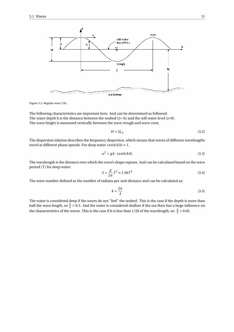
Figure 3.2: Regular wave [16].
The following characteristics are important here. And can be determined as followed:The water depth h is the distance between the seabed (z=-h) and the still water level (z=0).The wave height is measured vertically between the wave trough and wave crest.
H = 2ζa (3.2)
The dispersion relation describes the frequency dispersion, which means that waves of different wavelengthstravel at different phase speeds. For deep water t anh(kh) ≈ 1.
ω2 = g k · t anh(kh) (3.3)
The wavelength is the distance over which the wave’s shape repeats. And can be calculated based on the waveperiod (T) for deep water:
λ= g
2πT 2 ≈ 1.56T 2 (3.4)
The wave number defined as the number of radians per unit distance and can be calculated as:
k = 2π
λ(3.5)
The water is considered deep if the waves do not "feel" the seabed. This is the case if the depth is more thanhalf the wave length, so h
λ > 0.5. And the water is considered shallow if the sea floor has a large influence on
the characteristics of the waves. This is the case if h is less than 1/20 of the wavelength, so: hλ < 0.05.

3.1. Waves 12
The separate surface elevations ζ from Equation: 3.1 are used to calculate the water particle kinematics forwaves [16]. The kinematics of a water particle is found from the velocity components in x- and z- directions.It creates a circular trajectory for deep water waves and a more oval path for shallow water waves, as shownin Figure: 3.3. The horizontal and vertical velocities are calculated based on the velocity potential in wavesand the dispersion relation, Equation: 3.3, and are presented in the Equations: 3.6 and 3.7 respectively.
(a) Linear wave particle trajectories for deep water.(b) Linear wave particle trajectories for shallow water.
Figure 3.3: Linear wave particle trajectories [12].
u = ∂Φw
∂x= d x
d t= ζa
kg
ω
coshk(h + z)
coshkhcos(kx −w t ) (3.6)
w = ∂Φw
∂z= d z
d t= ζa
kg
ω
si nhk(h + z)
coshkhsi n(kx −w t ) (3.7)
In deep water, the wave particle velocities can be simplified and are given by:
u = ζaωekz cos(kx −ωt ) (3.8)
w = ζaωekz si n(kx −ωt ) (3.9)
The horizontal and vertical accelerations in deep water are obtained by differentiation of the velocity com-ponents with respect to time.
u =+ζaω2ekz si n(kx −ωt ) (3.10)
w =−ζaω2ekz cos(kx −ωt ) (3.11)
With the described theory above the individual wave components can be characterized. When describing anentire wave field the overall characteristics of the sea are usually more of interest. This is done with a wavespectrum as described below.

3.1. Waves 13
Wave spectrumIn 1969 an extensiv study was performed on young sea states in deep water with limited fetches. The researchwas named theJoint North Sea Wave Project (JONSWAP). The analysis of the data resulted in a JONSWAP wavespectrum, which is widely used for projects in the North sea. It is a modification of the Pierson-Moskowitzwave spectrum for fetch-limited(or coastal) wind generated seas. The following definition is advised in [16]:
Sζ(ω) = 320H 21/3
T 4p
·ω−5 ·exp
(−1950
T 4p
·ω−4
)·γA (3.12)
Where:
γ = 3.3 = Peakedness factor
H1/3 = Significant wave height
Tp = Peak period
ω = Wave frequency
A = exp
(−
( ωωp
−1
σp
2
)2)
ωp = 2πTp
= Wave peak frequency
σ = Spectral width parameter

3.2. Wave forces on structures 14
3.2. Wave forces on structuresIn this section the different theories and methods available to calculate the wave forces on a structure atsea are presented. Based on the wave theory described above different theories can be used. One can usethe Morison equation, a diffraction analysis, Computational Fluid Dynamics (hereafter described as CFD)or perform (scale)model tests. Each theory or method has its own range of applicability. Dimensionlessnumbers or charts are often used to identify the flow patterns and which theory is thus best suited to use.The dimensionless numbers will be described first after which the different theories are explained in thissection. The different theories are presented in this section. How these theories are going to be applied inthis thesis is elaborated on in Section 3.5.
3.2.1. Dimensionless numbers
Figure 3.4: Flow around a cylinder for variousReynolds numbers [16].
The Reynolds number (Re) is an important dimensionlessquantity that is used to help predict the flow patterns fordifferent fluid velocities. It indicates a flow regime from asmooth laminar flow, where viscous forces are dominant toa fully turbulent flow, which is dominated by inertial forces,see Figure: 3.4. The Reynolds number is calculated withEquation: 3.13. Another important dimensionless num-ber is the Keulegan Carpenter number (KC), see Equation:3.14, it is used for oscillating flows like waves. It assessthe relative importance of drag force compared to inertialforces.
For low values of KC (KC<3) the inertia force is dominant anddrag can be neglected. For the next range until drag becomessignificant (3<KC<15), drag can be linearised. And for the range15<KC<45 the components are equally important. For high val-ues of KC (KC>45) drag dominates and inertia can be neglected[5]. Sarpakaya carried out experiments and determined theSarpkaya beta,β. It is another way of plotting but it is not some-thing new since it can be rewritten as a function of the KC andReynolds number [31].
Re = uaD
ν(3.13)
KC = uaT
D(3.14)
β= D2
νT= Re
KC(3.15)
Where:
ua= Flow velocity
D= Diameter of cylinder
ν= Kinematic viscosity
T = Wave period
Chakrabarti defined regions of application for three types of hydrodynamic forcing, inertial, drag and theforces resulting from wave diffraction. The different regimes are defined and plotted with the correspondinglimits in Figure: 3.5, the Chakrabarti diagram [5]. The vertical axis is the equivalent to the KC number underthe assumption of deep water. On the horizontal axis is a diffraction parameter, πD
λ , it is a measure for thesize of the wave scattering from the structures. In the diagram are seven regions defined, region I through VIdescribed different combinations of forces and the last region is above the deep water breaking wave curve,it that region the waves break.

3.2. Wave forces on structures 15
For the first six regions, the higher the wave height becomes compared to the diameter the more importantthe drag forces are with respect to the inertia. The larger the structure becomes compared to the wave lengththe more important diffraction is. So to calculate the relevant forces on a structure the correct method mustbe chosen. For regions II a diffraction theory approach is eligible to calculate the hydrodynamic loads, whichwill be further on elaborated in Section 3.2.3.And for the regions III, V and VI a Morison equation approach issuitable, which will be further explained in Section 3.2.2. For region I the Morison equation or the diffractiontheory approach can be used, since both theories can calculate the inertia correctly.
Figure 3.5: Different wave force regimes [5].
The dimensionless numbers and the Chakrabarti diagram will be used for the selection from the differenttheories that are presented in this section. This is done in section 3.5. But before the different theories arepresented the marine growth is briefly explained. Since marine growth influences the outcome of all thedifferent theories involved.
Marine growthWithin the offshore industry "marine growth" is the collective term for species that grow on or are attachedto the structure below the waterline. One should think of mussels, barnacles, algae and seaweed for instance.This fouling of the surface has three influences. It changes the surface roughness, it changes the effectivediameter of the structure and it adds mass to the system. The surface roughness has a direct impact onthe drag and inertia coefficients as described in Section 3.2.2. Due to the fouling the vortex shedding fromstructure changes, the rougher the surface the more drag is experienced. Due to the layer of marine growththe effective diameter also changes. The layer thickest is highest near the surface and decreases with the waterdepth. The new diameter of the structure can be calculated by adding a layer to each side of the structure asDeq = D + 2∗ t . With the thickness as described by Norway Standards[24] and presented in Table 3.1. Themass of of the marine growth is to be added to the structural mass and added mass. The additional mass iscalculated with the volume and the weight per volume of the marine growth from Table 3.1. It is given fromthe mudline to two meter above the Lowest Astronomical Tide (LAT). Note that the weight per volume for thein-air condition is equal to 9.0 kN
m3 based on partial draining of the water from marine growth [10].

3.2. Wave forces on structures 16
Table 3.1: Marine growth thickness and weight based on Elevation Level (EL) [24]. Note that the weight is weight per volume.
Elevation [m] Thickness [mm] In-water weight [ kNm3 ] In-air weight [ kN
m3 ]
From mudline, to EL(-)100 10
11.00 9.00From EL(-) 100 to EL (-) 60 20
From EL(-) 60 to EL (-) 40 30
From EL(-) 40 to EL (-) 30 40
13.25 9.00From EL(-) 30 to EL (-) 15 50
From EL(-) 15 to LAT +2 60
Above LAT +2 0 - -
3.2.2. Morison equationThe Morison equation is derived to predict wave forces perpendicular to an exposed slender structure [22].It superimposes the linear inertia force and an adaptation of the quadratic drag force per unit length for a(fixed) structure in an oscillatory flow. The assumption of this equation is that the submerged members onwhich the load is calculated do not affect the waves. This is valid for waves that are relatively large comparedto the diameter of the member(s). According to Chakrabarti it is not valid to use Morison if πD
λ > 0.5. The
DNV defined this limit stricter than Chakrabarti as λD > 5 [41]. If the diameter becomes larger compared to
the wave length they start to affect the wave field, this is called diffraction. If that is the case the validity of theMorison equation can be compromised [39], since it is assumed that waves are not affected by the structure.
As stated above, the Morison equation is composed of a drag force and the inertial force. The drag forceis related to the velocity and is created by viscous effects. The inertia force is related to the acceleration ofwater particles. The Morison equation depends on which effects are studied, whether the cylinder (or struc-ture) is fixed, if there are waves and/or current and if the cylinder is oscillating in the water. First the originalMorison equation is described after which the various possibilities for an oscillating cylinder are described.And at last the required coefficients for the drag and inertia are described. As stated above first the originalMorison equation is given. The Morison force for a vertical fixed pile exposed to waves is given by Morison[22]:
FMor i son = FIner t i a +FDr ag = π
4ρD2 ∂u
∂t︸ ︷︷ ︸F r oude−K r i lov f or ce
+ π
4ρD2Ca
∂u
∂t︸ ︷︷ ︸Added mass f or ce
+ ρ
2CD D|u(t )|u(t )︸ ︷︷ ︸
Dr ag f or ce
(3.16)
Which can be simplified by combining the Froude-Krilov force and the added mass:
FM = π
4ρD2Cm u + ρ
2CD D|u(t )|u(t ) (3.17)
Where:
Ca= Added mass coefficient
Cm= Inertia coefficient, Cm = 1+C a
CD = Drag coefficient
ρ = Water density
u = Fluid velocity
∂u∂t = u= Fluid acceleration

3.2. Wave forces on structures 17
Oscillating cylinder in still waterThe Morison equation was derived for a fixed cylinder in waves. If a cylinder is oscillating in still water thehydrodynamic forces related to the inertia are different. The Froude-Krilov will be absent in this case sincethe water is standing still so the ambient pressure gradient is zero. The inertia force will be associated to Ca
and the Froude Krilov part from Equation: 3.16 is zero. The resulting Morison force will be depended on thebody velocity and acceleration and acts in opposite direction of the body movement [31].
FMSti l l =−π4ρD2Ca x − ρ
2CD D|x|x (3.18)
Where:
x = ∂x∂t = Body velocity
x = ∂2x∂2t
= Body acceleration
Oscillating cylinder in wavesIf the cylinder is moving in waves the total hydrodynamic forcing needs to be derived. This depends on thevelocity and acceleration of the wave particle and the cylinder. For the inertia this can be done by combiningthe inertia parts of Equation: 3.16 and 3.18. For the drag related part this is different. Due to the quadraticterm in the drag force a segregated treatment of the cylinder motion drag and the wave drag would lead todifferent forces, since :
u2 + x2 < (u + x)2 (3.19)
Since the inertia is not quadratic it can be determined according to Equation 3.20 for each of the comingapproaches. For the damping various approaches are proposed in the literature and will be discussed afterthe inertia.
FMIner t i a = ρV Cm u −ρV Ca x (3.20)
The two approaches for the damping will be discussed below. First the relative velocity approach and thenthe absolute velocity approach. The first, and an apparent, approach is the relative velocity approach. Itconsiders the relative velocity between the cylinder and the wave as [31]:
FMRel =ρ
2CD D|u − x|(u − x) (3.21)
Notice here that due to the quadratic nature of the drag force it is not possible to split the (unknown) cylindervelocity from the wave velocity when computing the drag force. Thus it is not possible to calculate the time-dependent force component from the wave velocity independent of the dynamic response of the cylinder.
Since the superimposed jacket velocity, x, is unknown, the solution must be obtained by iteration, for whichspecial algorithms are proposed, like Van Wingerden and Stettner did for the floating installations of a jacketand a monopile [43],[36]. A step-by-step solution of the differential equation in the time domain is needed.Additionally a loop within each step must be performed to successfully approximate the resulting cylindervelocity [16]. That makes this approach a relatively time-consuming computation in time domain. An imple-mentation of the relative velocity approach in frequency domain is not found during the literature study.
As the second approach the absolute velocity approach is considered. A strict interpolation of the the su-perposition principle is applied to the velocities. The forces resulting from the combined motions are treatedas if they are fully independent of each other proposed by e.g. Laya and Sunder [17].
FMAbs =ρ
2CD D|u|u − ρ
2C ′
D D|x|x (3.22)

3.2. Wave forces on structures 18
This approach ’neglects’ the cross term which one would get when writing out the quadratic velocity termfrom Equation: 3.21 (−2ux). Usually the motions of the cylinder are considerably less than those of the sur-round water and therefore the largest contribution to the drag comes from the wave term. The advantageof this approach is now that the damping due to the velocity of the cylinder and the wave can be calculatedseparately. The wave related part can be isolated and moved to the right hand side of the equation of motion.
In a test with an oscillating horizontal cylinder in a uniform current, Moe and Verley [21] measured the forceson the cylinder. With a Cd and Cd’ value. And they concluded that the relative velocity for the Morisonequation is quite unconservative and over predicts damping in the system. Sarpkaya [31], on the other hand,recommended the use of relative velocity was better. As Cd’ showed unrealistically high values.
Applicability of relative velocity formulationWhen applying the Morison equation to a structure with waves and a constant current, the relative velocityapproach is valid according to the DNV [41] if:
r
D> 1 (3.23)
Where r is the member displacement amplitude and D the diameter of the member. When rD < 1 the validity
depends on the following parameter: VR = vTnD as follows:
20 >VR Relative velocity recommended.
10 ≤VR < 20 Relative velocity may lead to an over-estimation of damping if the displacement is less than themember diameter.
VR < 10 It is recommended to discard the velocity of the structure when the displacement is less thanone diameter, and use the absolute velocity approach.
Where:
v = vc + πHsTz
= Approximate velocity
vc = Current velocity
Tn= Period of structural oscillations
Hs = Significant wave height
Tz = zero crossing-up period

3.2. Wave forces on structures 19
Inertia- and drag coefficientsThe Morison equation,as seen in Equation: 3.16, depends on hydrodynamic coefficients which must be tunedfor each specific case. The determination of these coefficients is based on measurements at full scale, modelscale or CFD. A lot of research has been performed on these coefficients for various shapes under various flowconditions. Due to these experiments the behaviour of these coefficients is well captured for varying non di-mensional numbers, like the KC and Reynolds number described in Section 3.2.1 or the surface roughness, ε(due to marine growth for example). Classification societies have determined standarized calculations to de-termine the inertia and drag coefficients. Depending on the design code or researcher different approachesare used.
Sarpkaya was one of the first researcher that described the dependency of the drag and inertia coefficienton the KC, Re and β. The results of the laboratory experiments using an U-tube are presented in Figure: 3.6.
Figure 3.6: Inertia- and drag coefficients based on Sarpkaya [31].
The DNV and the API code are the most widely accepted and used codes in the industry for this. The API isthe simplest approach of the two. It makes a difference for smooth or rough members, but does not considerthe Reynolds number or the amount of roughness. The DNV code does include this effect. The values thatDNV suggests are given in Figure: 3.7
Table 3.2: Inertia- and drag coefficients based on the API [29].
CD CM
Smooth 0.65 1.6
Rough 1.02 1.2

3.2. Wave forces on structures 20
Figure 3.7: Drag coefficients based on DNV [41].
The Morison equation is now described for various flows. Also different ways to determine the correspondingdrag and inertia coefficients are presented. An overview of the other theories is given below.
3.2.3. Other theoriesApart from the Morison equation there are other ways to calculate the wave forcing on a structure. Diffractiontheory, CFD, Model tests. CFD and model tests are boths option which can perform tests on a very high levelof detail. The downside of this is that they require very extensive preparation and are very time consuming.Therefore they are not considered in further detail in this study. Concerning the diffraction theory is, this willbe considered in more detail. How this theory is going to be used in this thesis will be elaborated on in Section3.5.
The diffraction theory is based on potential theory. A brief overview of the diffraction theory is given here.A more detailed explanation is given in Appendix A. It is assumed here that a rigid body is moving in anideal fluid with harmonic waves. With potential theory the hydrodynamic loads are evaluated. The potential,Φ(x, y, z, t ) is based on the superposition of:
• The undisturbed waves potential (Φw ), this is the wave field as if the vessel is not there;
• The diffraction potential (Φd ), these are the waves that reflect from the vessel;
• The radiated waves potential (Φr ), which are the waves that radiate from the vessel due to the motionsof the vessel. The waves that radiate are dissipating energy from the ship. This can also be referred toas potential damping.

3.3. Multi-body dynamics 21
3.3. Multi-body dynamicsIn this section the dynamics required to determine the response of a body are described. With the differenttheories known to determine the wave forcing now the way to calculate the resulting motions is determined.The problem in this study consists of two main bodies, the Thialf and the jacket and some auxiliary equip-ment (spreaderbars and hooks). The main bodies are both affected by the waves and the water and theyinfluence each other. Theories to calculate the wave forces are described in the section above. In this sec-tion the multi-body dynamics that are needed to understand how the bodies are influenced are described.Both bodies can move relative to each other but are connected, and thus influenced, by the crane cables,spreaderbars and hooks. In general each body can move in 6 degrees of freedom, three translations and threerotations. The convention with respect to the axes and the corresponding names and descriptions are givenin Figure: 3.8. To calculate the motion or rotation of each degree of freedom equations of motion are needed.These equations can be solved in time domain or frequency domain, which will be elaborated on in the nextsection.
Figure 3.8: The Degrees of Free of a ship [16].
Time domain vs. Frequency domainThe equations of motion can be solved in a Time domain or Frequency domain approach. Either method hasits advantages and its disadvantages, which will be elaborated on in this section.In the time domain the equation of motion is solved every time step δt. This has the large advantage that inprinciple this method can solve any dynamics problem one can think off. The result is a simulation of thebehaviour as we experience it in the real world. Since it solves the calculations at each time step the analysisitself is (very) time consuming and multiple simulation are required to obtain statistical reliable results. Thetime domain method is mainly applied for non-linear processes, with non linear differential equations. Suchas, but not limited to, transient events like ballasting of a vessel, impact loads and mooring analyses.
The frequency domain approach can be used if it is governed by linear differential equations. So steady stateharmonics where forces are linearly depending on the motion, velocity and acceleration. The advantages ofthe frequency domain approach is that it is very quick (time efficient) and easy to interpret the results. Dueto the linearity the superposition principle can be applied. It states that the response caused by two or morestimuli is the sum of the responses that would have been caused by each one individually. This means that alldifferent contributions that influence a multi-body system can be determined separately and then be addedtogether to solve the whole systems response. The main disadvantage of this approach is that all non-linearaspects must be linearised first before they can be implemented. Like the quadratic Morison damping term,which will be further elaborated on in Section 3.5.
Due to all the disadvantages of the time domain approach and the advantages of the frequency domain ap-proach and given the scope that a quick solver is desired and a frequency domain model is already available(for the jacket in air), the frequency domain approach is the preferred method.
In the frequency domain the response of a body will be with the same frequency as the excitation but usuallywith a phase angle between them. With the body motions x assumed as [16]:
x = xae iωt (3.24)

3.3. Multi-body dynamics 22
The equation of motion for a system is given in Equation: 3.25. It is assumed that the system can be describedby a set of mass-spring-damper system. Where in each body M is the mass matrix, A is the added mass matrix,B is the damping matrix, C the spring matrix and F the forcing vector [35]. The content of the matrices will bedetermined later.
(M+A)x +Bx +Cx = F (3.25)
Since the wave forcing factor is assumed harmonic it can also be written as [23]:
F = Re(Fae iωt ) (3.26)
With the complex amplitude,Fa depending on the wave amplitude, ζa and the complex wave transfer func-tion H f z , which depends on the the wave frequency, the angle of which the waves are coming from and theouter shape of the body. And can be written as [23]:
Fa = H f zζa (3.27)
When substituting the motions vector as well as the new wave formulation it yields:
(−ω2(M+A)+ iωB+C)xa = S xa = H f zζa (3.28)
The complex transfer function, also known as the Response Amplitude Operator(RAO) is based on this andgiven as [16]:
R AO(ω) = xa
H f zζa= S−1H f z (3.29)
From this the amplitude can be determined and the phase angle:
R AOampli tude =xa
ζa= abs(R AO) (3.30)
R AOphase = εx = ang l e(R AO) (3.31)
Mode shapes and Natural frequenciesMode shapes and their natural frequencies (also called eigenfrequencies) give a lot of insight in the behaviourof the model. They visualise what motions of the model are most important in different frequency regions.The natural frequency is a frequency at which a low amount of energy is required to oscillate the model. Whena body is excited at those frequencies it can lead to the severe motions, much larger than the wave amplitudethat triggered the motion. At every oscillation with a new excitation the amplitude of the motion increases,this is called resonance. The mode shapes and natural periods of the system are obtained by solving thefollowing eigenvalue problem [16].
det (−ω2(M+A)+C)x) = 0 (3.32)
3.4. Operability 23
3.4. OperabilityIn this section the operability will be explained based on the significant response, a wave spectrum and a set oflimiting criteria. With that the operability curve can be derived. The operability curve gives, for each wave pe-riod, limit and response, a maximum allowable wave height before the limit is exceeded. They are presentedin the Hs −Tp curve and give the allowable sea states. First the significant response will be determined. Thenthe limiting criteria will be described. And lastly it is explained how the operability is determined.
Significant responseTo determine the significant response the RAO of the response of interest is needed and a wave spectrum.In this study the JONSWAP spectrum is used. The wave spectrum is described in Section 3.1. From this thespectral response is determined which is used to calculate the significant double amplitude (SDA) [16].
S(ω)moti on = |R AO(ω)|2 ·S(ω)JON SW AP (3.33)
From the spectral response the zeroth spectral moment, m0. This is also the area under the curve of thespectral response.
m0(ω) =∫ ∞
0S(ω)moti on(ω) ·dω (3.34)
From the zeroth moment the significant double amplitude(SDA) can be determined [16]. Note that this is thedouble significant amplitude, provided that the wave spectrum is defined on the significant wave height, Hs ,(which is double the significant wave amplitude).
SD A(ω) = 4 ·√
m0(ω) (3.35)
With this SDA the Single Most Probable Maximum (SMPM) is determined. In this study the 3 hour SMPM isused, as suggested by DNV [42], in that period approximately a 1000 waves pass. For more details on the sta-tistical derivation of the SMPM it is advised to consult Journee & Massee [16]or Holthuijsen [12] for example.The 3 hour SMPM single amplitude is determined as:
SMP M3hour (ω) = 1
2·√
1
2l n(1000) ·SD A(ω) ≈ 1.86
2·SD A(ω) (3.36)
The SMPM for each of the responses will be used to determine the operability. But to determine the operabil-ity the operational limiting criteria are needed. And they will be explained next.
Operational limiting criteriaTo determine the operability the operational limits are defined. This is done to protect the safety of the op-eration. Some limits are hard limits, like the clearance between the load and the vessel, others are derivedbased on experience by experts or the manufacturer. They are listed below:
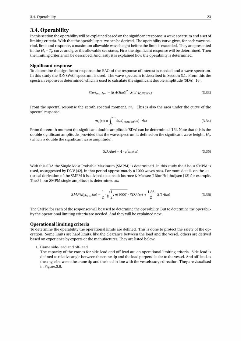
1. Crane side-lead and off-leadThe capacity of the cranes for side-lead and off-lead are an operational limiting criteria. Side-lead isdefined as relative angle between the crane tip and the load perpendicular to the vessel. And off-lead asthe angle between the crane tip and the load in line with the vessels surge direction. They are visualisedin Figure:3.9.

3.4. Operability 24
Figure 3.9: Crane side-lead and off-lead [30].
2. Clearance between the load and vesselA clearance between the load and the vessel must be preserved at all time. The minimal distance be-tween the jacket and the Thialf during the transport is 8.4m, between the boom of the crane and thepile sleeves[28]. Therefore the limit is set to 6 meter to have some redundancy.
3. Hookload fluctuationsThe hookload fluctuations are described according to the Dynamic Amplification Factor(DAF). It isdefined as described in Eq: 3.37. This is typically 1.1-1.3 during lifting operations in air and higher oncesubmerged [1]. But it must stay below 2 to assure that there is no slack in the slings, which could leadto high snap loads. A limit of 1.3 in air and 1.9 in water is chosen for this study. When rewriting Eq: 3.37it can be shown that this means that the Fd ynami c = 0.9 ·Fst ati c maximal.
D AF = Ftot al
Fst ati c= Fd ynami c +Fst ati c
Fst ati c(3.37)
4. Motions of vesselThis is an operational limit associated with experience rather than any physical limiting parameter. Theroll and pitch of the Thialf must be small.
These limits are used to determine the operability.
OperabilityThe operability is based on the limiting criteria, the response spectrum and the wave spectrum. It defines thelimiting combinations of significant wave height Hs and the peak period Tp for each wave direction and eachlimit. It is obtained from the limit and the response, as presented in Eq: 3.39.
Oper abi l i t y = Li mi t
Response(3.38)
So per limit and for each (peak) period the maximum allowable significant wave height is determined.
HSmax (Tp ,di r ) = Li mi t
SMP M(Tp ,di r )(3.39)
With the way to determine forces, the response from an equation of motion known and a way to gain moreinsight in the behaviour of the multi-body system an approach is made to choose which theory should beapplied where to determine the forces on the different bodies.

3.5. Theory analysis 25
3.5. Theory analysisIn this section the theory as presented in this chapter will be analysed. It will be determined how this theoryis going to be used in this study and the reason why. First it must be determined which theory should be usedto calculate the hydrodynamic loading on the bodies. The hydrodynamic loading on structures is composedof diffraction, inertia and drag forces. A way to characterise these forces is by the non-dimensional numberslike the KC number. Chakrabarti defined the different regions where different forces should be applied asdescribed in Section 3.2.1.
To determine which forces are dominant and should thus be taken into account for the hydrodynamic load-ing first the Thialf and jacket dimensions should be defined. The width of a floater is 30m and the total length201m as described in Table 3.3. The legs of the jacket are the thickest members with 2.2m in diameter andthe risers are the thinnest members with a diameter of 0.3m. A sea state of 1m to 3m wave height and periodsranging from 4 seconds to 16 seconds is considered. The wave length is determined using Equation: 3.4. Theresults are summarised in Table 3.3.
Table 3.3: Dimensions Thialf and North Sea jacket.
Thialf North Sea jacket
min max min max
D [m] 30 201 0.3 2.2
Hs [m] 1 3 1 3
Tp [s] 4 16 4 16
λ [m] 25 399 25 399
With the dimensions and the sea state the KC number, the equivalent KC number and the diffraction pa-rameter π D/λ are calculated and reported in Table 3.4 and visualised in the Chakrabarti diagram in Figure:3.10.
Table 3.4: KC Number and wave forcing parameters according to Chakarbarti [5].
Thialf North Sea jacket
min max min max
KC 0.01 0.31 0.71 31
πD/λ 0.24 25 0.002 0.28
H/D 0.002 0.10 0.23 10
3.5. Theory analysis 26
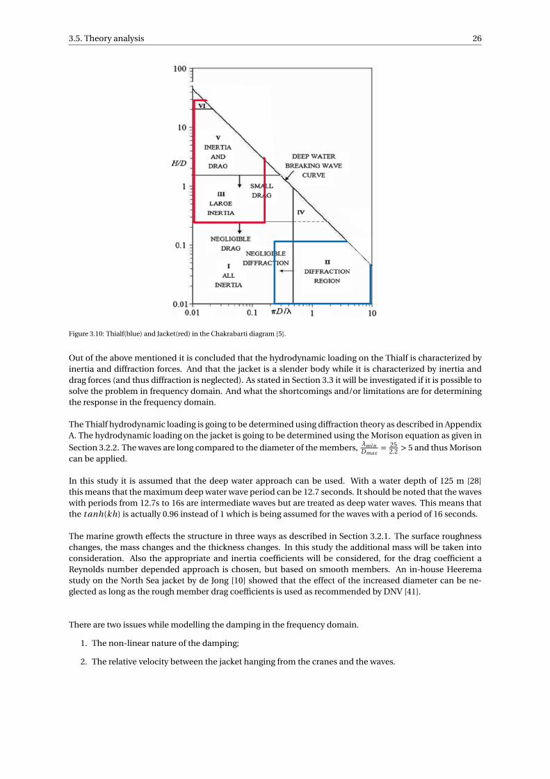
Figure 3.10: Thialf(blue) and Jacket(red) in the Chakrabarti diagram [5].
Out of the above mentioned it is concluded that the hydrodynamic loading on the Thialf is characterized byinertia and diffraction forces. And that the jacket is a slender body while it is characterized by inertia anddrag forces (and thus diffraction is neglected). As stated in Section 3.3 it will be investigated if it is possible tosolve the problem in frequency domain. And what the shortcomings and/or limitations are for determiningthe response in the frequency domain.
The Thialf hydrodynamic loading is going to be determined using diffraction theory as described in AppendixA. The hydrodynamic loading on the jacket is going to be determined using the Morison equation as given in
Section 3.2.2. The waves are long compared to the diameter of the members, λmi nDmax
= 252.2 > 5 and thus Morison
can be applied.
In this study it is assumed that the deep water approach can be used. With a water depth of 125 m [28]this means that the maximum deep water wave period can be 12.7 seconds. It should be noted that the waveswith periods from 12.7s to 16s are intermediate waves but are treated as deep water waves. This means thatthe t anh(kh) is actually 0.96 instead of 1 which is being assumed for the waves with a period of 16 seconds.
The marine growth effects the structure in three ways as described in Section 3.2.1. The surface roughnesschanges, the mass changes and the thickness changes. In this study the additional mass will be taken intoconsideration. Also the appropriate and inertia coefficients will be considered, for the drag coefficient aReynolds number depended approach is chosen, but based on smooth members. An in-house Heeremastudy on the North Sea jacket by de Jong [10] showed that the effect of the increased diameter can be ne-glected as long as the rough member drag coefficients is used as recommended by DNV [41].
There are two issues while modelling the damping in the frequency domain.
1. The non-linear nature of the damping;
2. The relative velocity between the jacket hanging from the cranes and the waves.

3.5. Theory analysis 27
In the frequency domain approach the quadratic damping term from the Morison equation must be lin-earised. The linearisation depends on the equivalent energy approach described by e.g. Clauss [6]. In thisapproach the amount of energy that is dissipated over a period must be the same for the linear and the non-linearised drag force.
For regular waves the velocity is u(t ) = uacos(ωt ). The drag related energy dissipated over a period for thelinear, FDL , and the non linear drag, FD , must be the same.
E =∫ 2π
0FD ·u ·d(ωt ) =
∫ 2π
0FDL ·u ·d(ωt ) (3.40)
With the nonlinear drag: FD = ρ2 CD D|u|u
And the linear drag: FDL = ρ2 CDLDu
With the regular wave velocity and Equation: 3.40 we obtain:
CD u3a
∫ 2π
0|cos(ωt )|cos2(ωt ) =CDLu2
a
∫ 2π
0cos2(ωt ) (3.41)
From this the linear drag coefficient can be found:
CDL = 8
3πCD ua (3.42)
The linearised drag is thus:
Fl i near dr ag = ρ
2CD D
(8
3∗πua
)u (3.43)
Figure 3.11: Equivalent energy drag linearisation [6]
The first problem of the frequency domain approach is solved, the drag is linearised. Now the second prob-lem is elaborated on. The second problem is related to the relative velocity between the jacket and the waves.The jacket will oscillate due to the waves and the motion of the Thialf. The damping is mainly important nearthe natural frequencies, since the other terms cancel each other out, as described in Section 3.3. For the abso-lute velocity approach the drag due to the velocity of the jacket and the drag due to the wave are determinedseparately, this is described in Section 3.2.2. First the jacket is moved through still water with a jacket velocityx, from this the damping force matrix, B, is derived. Then the jacket is fixed and waves are generated, fromthis the damping resulting from the wave velocity is determined for each frequency as a force vector, F.
To determine which kind of Morison equation approach to choose the resulting jacket velocity will be cal-culated first using the absolute velocity approach. From this it will be determined if this is the correct ap-proach or not. As a part of this the DNV code will be consulted, although it should be noted that it is derivedfor current plus waves. If the relative velocity approach is necessary it will be investigated how this can be
3.5. Theory analysis 28
implemented in the used software or otherwise be determined by an alternative approach. One should keepin mind that not only the relative velocity between the jacket and the waves is important here but also therelative velocity between the two legs. This differences is due to the phase difference w.r.t the wave betweenfor the two legs (since there is a physical distance between them). Through the steps as described above thegap will be filled in.
To summarise the theory analysis, as stated above, the following conclusions are formulated:
• Airy linear wave theory for deep water will be used;
• The Morison equation will be used for the jacket;
• The Diffraction theory will be used for the Thialf;
• A Frequency Domain approach will be made considering the:
– Non-linear damping in the Morison equation;
– With the absolute velocity damping approach and the relative velocity damping approach.
The theoretical background, the analysis and selection of the theory provides a good foundation for the studythat will be conducted in the next chapters. To get a better understanding of the behaviour of the jacketwhile it is free hanging from the cranes of the Thialf first a model will be made with the jacket in air. Thismodel can be compared with measured data of the North Sea jacket campaign. This way the forces on theThialf, determined with the diffraction theory, can be checked. If the model matches the behaviour of themeasurements it can be expanded by submerging the jacket. Also the in air case will be used for comparisonwith the submerged jacket later on. The additional forces on the jacket will remain the only unknowns. Thiswill be investigated in Chapter 5.

4Base model
In this chapter the model of the crane suspended jacket decommissioning with the jacket hanging in airwill be investigated. The measured data during the North Sea jacket campaign is compared to the modelpredictions (based on Heerema’s current practice) of the free hanging jacket transport in air. It is the aimto determine how well the free hanging jacket motions are predicted by the model and whether it is thus agood starting point to expand the model with the jacket in water. First the Liftdyn model will be described.Secondly it will be explained how the measurement data was obtained and how it is used. And lastly a com-parison between the measurements and the model is performed.
4.1. Model descriptionA model of the Thialf and the jacket is made in Liftdyn. Liftdyn is a in-house computer tool that is designed tomodel and solve general linear hydrodynamic problems in the frequency domain. Liftdyn can solve systemsconsisting of rigid bodies connected to each other or to the earth by springs, dampers and hinges. The bodymay have a frequency depended mass and damping, and frequency depended exciting forces resulting in afrequency depended response or RAO of the system. Due to the superposition principle the response is thesum of the responses that would have been caused by each body individually. This means that all differentcontributions that influence a multi-body system can be determined separately and then be added togetherto solve the whole systems response. The hydrodynamic properties for the Thialf are obtained via WAMITfor example, and are implemented in Liftdyn. For a more detailed description about Liftdyn and WAMIT, seeAppendix B.1.
The Thialf is modelled as rigid body to which properties are assigned. The properties are given in Table ??and a hydrodynamic database was imported. This database contains the coefficients for the added mass,damping, hydrostatic spring and the wave forces. The databases for the Thialf are derived by Heerema andare widely used within the company. The hoist wires are modeled as springs with a initial position and astiffness and a pretension. The stiffness of the spring is defined with an axial stiffness EA with A the effectivediameter of the sling/hoistwire and E the Young’s modulus of the wire. The wires are under pretension toequal out to the static load of the jacket, which is elaborated on in this section. This means that environmen-tal loads on the wires are not included. The spreaderbars and main hooks are modelled as rigid bodies. Thespreaderbar on port side weighs 299 t, the spreaderbar on starboard weighs 346 t and the main hooks weigh236 t each.
The jacket is also modelled as a rigid body which consists of various tubular structural members. The ge-ometry of the jacket is approximated by a square jacket of which the properties match the real jacket and arepresented in Table ??. The coordinates of the center of gravity are given with respect to the center of the baseof the jacket. The jacket that is shown in Figure: 4.1 is just for visualization with regards to the geometry. Ithas the correct height en width but the cross members and the diameters of the tubular members are notcorrect. But the center of gravity and the connection points to the hoist wires are in the correct location. Andall the relevant properties are assigned with respect to the center of gravity of the jacket so the calculationscan be performed in a correct way.
29

4.1. Model description 30
The global coordinate system is located at the stern of the Thialf, at the centerline of the keel. It coincideswith the local axis system of the Thialf and is shown in Figure: 4.1a. With a right-handed axis system wherethe x-axis is positive towards the bow of the Thialf, the y-axis positive towards portside and the z-axis pointingupwards. The local coordinate system of the jacket is located at the center of the base. With the x-axis pointingupwards, the y-axis parallel to the global x-axis and the z-axis positive towards the top of the jacket.
(a) View from the stern.
(b) View from above.
Figure 4.1: SSCV Thialf with the unrestrained crane suspended jacket [30].
The jacket is connected to the cranes by means of slings. For all these slings the pretensions needs to bedetermined so that the system is in static equilibrium, as stated earlier. It will later also be used to determinethe DAF during the operability calculations. To determine the hookload a free body diagram was made, asshown in Appendix C. The hookloads need to be the same as the total weight from the jacket and the auxiliaryequipment. With the hookloads and the sling configuration the required pretensions are determined andpresented in Table 4.1. The stiffness of the spring is the axial stiffness EA with A the effective diameter of thesling and E the Young’s modulus of the wire. And the angle is determined as the internal angle between theend of the sling and the beginning.
Figure 4.2: Sling configuration

4.1. Model description 31
Table 4.1: Pretension slings
LP Sling.No Angle [deg] Pretension [kN]
PS
1 SL 2987 90.00 12,949
2 SL 2986 90.00 12,949
3 SL 4545 56.71 17,247
4 SL 4544 56.52 17,247
SB5 SL 7142 65.88 20,368
6 SL 7581 67.37 20,141
All the different aspects for the setting up of the equation of motion are described above. The general equationof motion, given in Equation: 3.28, will be filled in with the values and the hydrodynamic database specifiedabove. This equation will be used to compile the RAO’s, according to Equation: 3.29. In Equation: 4.1 itis shown which effects are included in the combined equation of motion. Where MT is the mass matrix ofthe Thialf and Ahyd is the hydrodynamic (added) mass matrix of the vessel. MJ contains the mass matrixof the jacket that is hanging from the cranes. And
∑41 Maux contains the masses of the four other bodies
namely the two spreaderbars and the two main hooks . The hydrodynamic damping from WAMIT for thevessel is specified in Bhyd . To correct for the fact that the bodies are actually not completely rigid and sincea minimum value of damping is required for asserting damping presence in all of the modes of the system apercentage of 0.3% of the critical damping for each mode is determined and added in Bcr i t . Chyd containsthe hydrostatic spring terms of the vessel. The stiffness of the hoist wires that lift the jacket are representedin Cwi r e . The motion of each body for each of the degrees of freedom can be determined with Equation: 4.2.Fexc is the sum of all the excitation forces. In this case this will consist of the wave excitation force on thevessel ,Fa , which is determined in WAMIT.
S(ω) =−ω2 · (MT +Ahyd +MJ +4∑1
Maux )− i ·ω · (Bhyd +Bcr i t )+ (Chyd +Cwi r e ) (4.1)
x(ω) = S(ω)−1 ·Fexc (4.2)
Mode shapes and their natural period give a lot of insight in the behaviour of a model. They can be used tovisualise what motions of the model are most important in different frequency regions. The mode shapescan be determined as explained in Chapter 3.1 with Equation: 3.3. The first ten mode shapes are presentedin Table 4.2. Note that the motions are given w.r.t. the global coordinates (so not the local coordinates forthe jacket). An additional spring matrix is defined for the Thialf to mimic the effect of the DP system andconstrain the lowest three modes.
Table 4.2: Natural modes of the coupled Thialf-Jacket system
No. Thialf Jacket
1 Yaw -
2 Sway -
3 Surge -
4 Roll Sway in phase
5 Pitch Surge in phase
6 - Yaw
7 Heave-Pitch Surge antiphase
8 Pitch Heave Surge antiphase
9 Roll Sway antiphase
10 - Pitch
In Figure: 4.3 the RAO’s obtained via Liftdyn are presented. In this figure the roll and pitch motion of the

4.1. Model description 32
vessel are given for incoming waves of 145 degrees. The wave frequency is on the horizontal axis. On thevertical axis the amplitude is given for each frequency. The colour under the curve has no influence here,only the outer line of the curve is of interest.
(a) Roll RAO for the Thialf with waves coming from 145 deg. (b) Pitch RAO for the Thialf with waves coming from 145 deg.
Figure 4.3: Response amplitude operators of the vessel.
In Figure: 4.3a the peaks suggest that there are natural modes. The same holds for the two peaks in Figure:4.3b. They match with the calculated modes from Table 4.2. For the pitch and the roll RAO the mode whichis closed to the wave frequency range is visualised below. For the roll mode this is mode 9. In this mode theThialf is rolling and the jacket is swaying out of phase with the Thialf. The visualisation is given in Figure:4.4a . For the pitch mode this is mode 8. In this mode the Thialf is pitching and heaving and the jacket ismoving in surge direction out of phase with the vessel. It is visualised in Figure: 4.4b. Note that the motionsare exaggerated in the figures.
(a) Mode 9: Roll of the Thialf and surge of jacket in antiphase. (b) Mode 8: Pitch of the Thialf and surge of jacket in antiphase.
Figure 4.4: Mode shapes 8 and 9.

4.2. Measurements 33
4.2. MeasurementsWith the RAO’s from the model known it is time to study the measurements that were performed. This will bedone in the following order. First the measurement systems will be introduced, secondly the measurementsof the motion are obtained and filtered. And thirdly the wave spectrum will be obtained from the wave-riderbuoy.
On board the Thialf there are several monitoring systems installed and the collective term for all this equip-ment is Motion Monitoring Equipment#16 (MME16). There are systems to track the position of the Thialf, thecrane loads, the power consumption and the motions of the Thialf. This systems were also used during themeasurement campaign. The sensors that are used in this study are called Fiber Optical Gyroscopes sensorsby Octan [14]. They record the vessel motion in six degrees of freedom, within 5cm or 0.01 deg of accuracyat a sample rate of 16 Hz[14]. It is used to determine the heading of the vessel and the roll and pitch of theThialf. There was an additional measurement sensor installed on the jacket but unfortunately it did not work.Therefore only the Thialf motions are considered in this part.
The measurement campaign, from which the data is collected, started at 9.30 on May the 26th . The jacketwas lifted out of the water and the Thialf started the transport. The Thialf then started adjusting to the sailheading (150 deg), while simultaneously performed deballasting to the transit draf and connecting the bridalto the support tug. It sailed from the open sea to the more sheltered location in a fjord, at which the decom-missioning yard is located. It arrived in the fjord on 27 May at around 17.00, so the total transit duration wasabout 29 hours. Afterwards, it sailed for 40 NM inshore along the fjord to the decommissioning yard.
A good window of the measured data must be selected, to make sure that there are no transient effects presentsince the model does not capture this. So a sufficiently long window was needed in which the vessel was stillat the open sea but the heading, draft and the vessel speed are constant and the Thialf was not (de-)ballasting.
An adequate three hour window was found between 14.52 and 17.52 on the 26th of May. The transient opera-tions were completed and the the vessel was sailing in a constant direction and speed. More detailed outputof the operation is given in Appendix C. The measured roll and pitch of the Thialf is presented in Figure: 4.5a.To make sure that the offset and the noise in the roll and pitch is not influencing the results a band pass filterhas been applied. All the motions with periods above 60 seconds and below 2 seconds have been filtered out.Since the interest lies in the wave induced motions this is a valid assumption, motions outside that range arenot induced by waves. The filtered motions are presented in Figure: 4.5b.
(a) Time trace of the Thialf roll(red) and pitch (blue) unfiltered. (b) Time trace of the Thialf roll(red) and pitch(blue) filtered.
Figure 4.5: Response amplitude operators of the vessel.

4.2. Measurements 34
The filtered time traces are used to determine the spectral density. The spectral density describes how theenergy of the time trace is distributed with frequency. The spectral density is calculated with the Fouriertransform. The total amount of energy that is in the signal x(t) is transformed to x(ω):
x(ω) =∫ t=10800
t=0exp(−i ·ω · t ) · x(t )2d t (4.3)
And the spectral density can be defined as:
Sxx (ω) = |x(ω)|2 (4.4)
The resulting spectral density for the roll and pitch motions of the vessel are plotted below in Figure: 4.6. Withon the horizontal axis the frequency and on the vertical axis the spectral density in (r ad/s)2 · s.
Figure 4.6: Spectral response of the measured roll and pitch.
To be able to compare the measurements to the Liftdyn model the wave spectrum is needed. A wave riderbuoy was deployed near the original field. This wave buoy is fixed in one place. So the measured spectrumof the waves must be corrected for the fact that the Thialf is sailing with a certain speed in a given direction.The spectrum is corrected according to Journee [16] with a encounter frequency, as presented in Equation:4.5. Where V is the vessel velocity and µ= wave direction relative to the ship’s speed.
ωe =ω−k ·V · cos(µ) (4.5)
The vessel is sailing in almost the opposite direction of where the waves are coming from. As expected theenergy of the spectrum shifts to the lower wave frequencies. It can be seen in Figure: 4.7 that there are mainlywind included wave and a small peak of swell waves in the lower frequencies. Now that the spectral responseof the measured data is determined and the wave spectrum as well, it is time to determine the spectral re-sponse with of the model with the wave measurements and the RAO’s from Figure: 4.3. Afterwards these twocan be compared. This will be done in the next section.

4.2. Measurements 35
Figure 4.7: Measured wave spectrum and the corrected wave spectrum.

4.3. Measurements vs Liftdyn model 36
4.3. Measurements vs Liftdyn modelIn this section the model predictions for roll and pitch will be compared to the measured data. To check if in-formation got lost in translation from the time traces to the spectral response and the filtering the significantdouble amplitude (SDA) will be determined for each case.The spectral roll response is determined and shown in Figure: 4.8. With the measured spectral response (inred) and the modelled spectral response from Liftdyn, derived by the RAO from Liftdyn and the measured(encounter) wave spectrum (in black). The natural frequency of mode 9 is highlighted with a dotted redline. The spectral pitch response is shown in Figure: 4.9. With the measured spectrum in blue and modelledspectral response from Liftdyn (in black), derived by the RAO from Liftdyn and the measured (encounter)wave spectrum. The natural frequency of mode 8 is highlighted with a dotted red line.
Figure 4.8: Spectral roll response for the Thialf with waves coming from 150 deg.
Figure 4.9: Spectral pitch response for the Thialf with waves coming from 150 deg.

4.3. Measurements vs Liftdyn model 37
The SDA can be calculated according to Equation: 3.35 in the frequency domain. For the time trace the SDAwas calculated based on the standard deviation, σ, as:
SD At t = 4√σ2 (4.6)
The SDA is calculated for four cases, the unfiltered time trace measurements (1), the filtered time tracemeasurements (2), the filtered spectral response from the measurements (3) and the calculated spectral re-sponse(4). The results are presented in Table 4.3.
Table 4.3: Significant double amplitudes for roll and pitch.
Case Roll SDA [deg] Pitch SDA [deg]
1. Unfiltered 0.174 0.15
2. Filtered tt 0.159 0.076
3. Filtered FD 0.157 0.077
4. Calculated 0.143 0.088
Based on the results in this chapter the following observations are made and conclusions are drawn. Theweather was very good during the transport. This resulted in very low amplitude motions.
The model predicted the natural modes and the trend well. There is a very small offset when comparingthe natural peaks from mode 8 and mode 9 in Figure: 4.8 and 4.9. The models do seem to underestimatethe damping in the antiphase modes since both of the calculated peaks are higher. This could be due to the(double) pendulum motion of the jacket that is moving out of phase with the Thialf, but since the sensor onthe jacket did not work this is hard to verify.
When looking at the effect of filtering and processing the data the SDA was used. It can be seen that theoverall amplitudes where quite low, around 0.08 deg for pitch and 0.15 deg for roll. Where the limit was set to1 deg for both pitch and roll. Most of the energy that was discarded during the process was in the filtering ofthe pitch data, where the SDA is almost halved. This is due to the jump offset from around -0.6 deg to -0.45deg of the pitch.
In the low frequency part, there was no wave energy measured by the wavebuoy but a response was mea-sured by the sensors. Therefore there is no energy in the modelled response but there is in the measurementresponse. When looking at the frequencies of the roll peak and the pitch peak they do match with Thialfheave-pitch - jacket surge in phase, mode 7, and the Thialf roll - jacket sway, mode 4. The roll motion ofmode 4 is not likely triggered by waves due to the low frequency, it is expected that it is caused by DP inducedmotions.
Concluding this chapter, the Liftdyn model with the Thialf and the jacket is a good starting point to expandthe model and investigate what happens if the jacket is lowered through the waterline. In the next chapter itwill be investigated what influences should be added to the jacket once it is in the water.
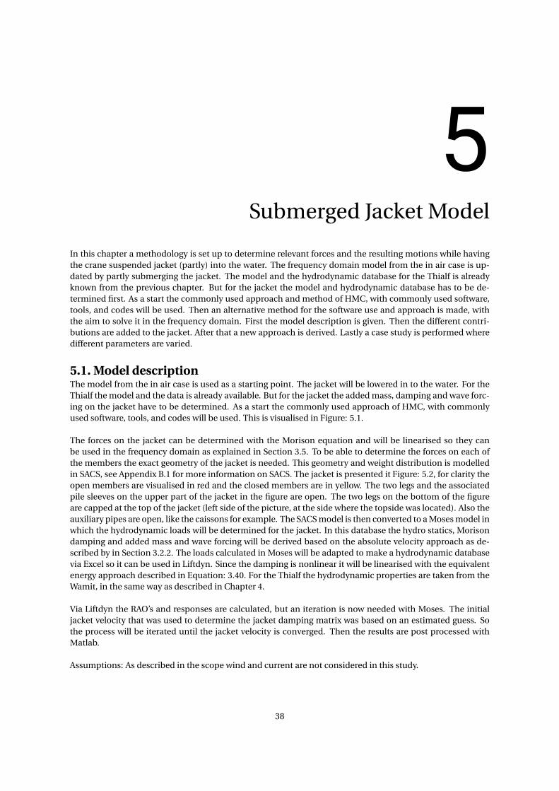
5Submerged Jacket Model
In this chapter a methodology is set up to determine relevant forces and the resulting motions while havingthe crane suspended jacket (partly) into the water. The frequency domain model from the in air case is up-dated by partly submerging the jacket. The model and the hydrodynamic database for the Thialf is alreadyknown from the previous chapter. But for the jacket the model and hydrodynamic database has to be de-termined first. As a start the commonly used approach and method of HMC, with commonly used software,tools, and codes will be used. Then an alternative method for the software use and approach is made, withthe aim to solve it in the frequency domain. First the model description is given. Then the different contri-butions are added to the jacket. After that a new approach is derived. Lastly a case study is performed wheredifferent parameters are varied.
5.1. Model descriptionThe model from the in air case is used as a starting point. The jacket will be lowered in to the water. For theThialf the model and the data is already available. But for the jacket the added mass, damping and wave forc-ing on the jacket have to be determined. As a start the commonly used approach of HMC, with commonlyused software, tools, and codes will be used. This is visualised in Figure: 5.1.
The forces on the jacket can be determined with the Morison equation and will be linearised so they canbe used in the frequency domain as explained in Section 3.5. To be able to determine the forces on each ofthe members the exact geometry of the jacket is needed. This geometry and weight distribution is modelledin SACS, see Appendix B.1 for more information on SACS. The jacket is presented it Figure: 5.2, for clarity theopen members are visualised in red and the closed members are in yellow. The two legs and the associatedpile sleeves on the upper part of the jacket in the figure are open. The two legs on the bottom of the figureare capped at the top of the jacket (left side of the picture, at the side where the topside was located). Also theauxiliary pipes are open, like the caissons for example. The SACS model is then converted to a Moses model inwhich the hydrodynamic loads will be determined for the jacket. In this database the hydro statics, Morisondamping and added mass and wave forcing will be derived based on the absolute velocity approach as de-scribed by in Section 3.2.2. The loads calculated in Moses will be adapted to make a hydrodynamic databasevia Excel so it can be used in Liftdyn. Since the damping is nonlinear it will be linearised with the equivalentenergy approach described in Equation: 3.40. For the Thialf the hydrodynamic properties are taken from theWamit, in the same way as described in Chapter 4.
Via Liftdyn the RAO’s and responses are calculated, but an iteration is now needed with Moses. The initialjacket velocity that was used to determine the jacket damping matrix was based on an estimated guess. Sothe process will be iterated until the jacket velocity is converged. Then the results are post processed withMatlab.
Assumptions: As described in the scope wind and current are not considered in this study.
38
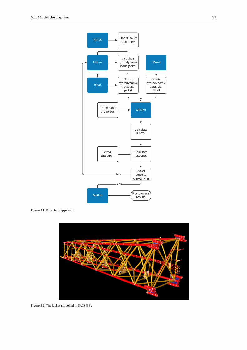
5.1. Model description 39
Figure 5.1: Flowchart approach
Figure 5.2: The jacket modelled in SACS [38].

5.2. Adding influences on the jacket 40
5.2. Adding influences on the jacketWith the approach explained in the previous section the additional influences on the jacket will be deter-mined in this section. First the effect of having the jacket lowered on the RAO will be investigated and thehydrostatic terms are determined. The added mass and the damping due to the jacket motions will be cal-culated. And lastly the wave forcing on the jacket, which consists of the added mass and damping due to thewave particle velocity will also be treated. The different effects due to the now partly submerged jacket willbe elaborated next. In this study waves from behind will be considered (0 degrees).Keep in mind that only the effects on the jacket are added one by one here. The effects on the Thialf, suchas wave forcing, are present in all the cases treated here!
5.2.1. Static effectsThree static effects are investigated here, firstly the effect of lowering the jacket, secondly the effect of buoy-ancy and thirdly the hydrostatic stiffness.
Effect of lowering jacketThe jacket is lowered sufficiently deep so the bottom legs of the jacket stay submerged. Therefore the jacketis lowered 20 meters down from the original position (as used in Chapter 4). The bottom legs are now 8.65munder the still water level, as visualised in Figure: 5.3. By lowering the jacket into the water the sling lengthof the hoist wires is increased by 20 meters. Due to this longer length the pendulum motion of the jacket willalso shift to a slightly higher period.
Figure 5.3: Side view of the jacket 8.65m submerged.
BuoyancySince the jacket is now partly submerged it will have buoyancy. In Figure: 5.2 it was shown which membersare open (red) or are closed and thus filled with air (yellow). The total buoyancy is a combination of theentrapped air and the displaced water due to the submerged structural volume. The total buoyancy force ofthe jacket is 1330 t. This leads to a weight reduction on the cranes since the load due to the jacket reducesfrom 5959 t to 4629 t, this is a reduction of 22%. Since the hookloads reduce the pretensions on the slingsalso reduces. They are determined in the same way as described in Section 4.1, but now with the buoyancyincluded.
Table 5.1: Pretension slings submerged jacket.
LP Sling.No Angle [deg]Pretension
in air [kN]
Pretension
8.65m sub [kN]
PS
1 SL 2987 90.00 12,949 8,152
2 SL 2986 90.00 12,949 8,152
3 SL 4545 56.71 17,247 11,507
4 SL 4544 56.52 17,247 11,507
SB5 SL 7142 65.88 20,368 17,156
6 SL 7581 67.37 20,141 16,964

5.2. Adding influences on the jacket 41
Hydrostatic stiffnessThe hydrostatic stiffness matrix describes how the buoyancy (and weight) loads on the jacket change due to(small) changes in the jacket position and orientation. The hydrostatic stiffness components are only spec-ified for the heave, roll and pitch degrees of freedom; for the other degrees of freedom of the jacket they arezero. The matrix is presented in Table 5.2.
Table 5.2: Hydrostatic stiffness of the jacket w.r.t. the center of buoyancy in kN/m.
Heave Roll Pitch
z 5.11E+02 1.11E+03 6.61E+01
rx 1.11E+03 1.04E+06 9.67E+03
ry 6.61E+01 9.67E+03 1.17E+05
The effects of lowering the jacket and the static effects due to the submerging are presented in Figure: 5.4.In this figure the relevant motion RAO’s of the jacket with waves coming from behind(0 deg) are presented.The following motion are considered and defined in the same direction as in Chapter 4.1: a) Surge, horizontalmotion inline with the Thialf b) Heave, the vertical motion and c) Pitch, rotation towards the Thialf. TheRAO’s of the Thialf and the other motions of the jacket are summarised in Appendix D.1. On the horizontalaxis are the different periods and on the vertical axis the response per meter wave height. Before going inon the different contributions it can be seen that there are two distinctive peaks in the figures. One peak ata high period and one at a low period. These peaks correspond with mode 8 and 10 from Table 4.2 and arethe Pitch-Heave of the Thialf with jacket surge antiphase and pitch of the jacket respectively. Looking at themotions of the jacket in air corresponding with the 8th mode (high period peak)) it can be seen that the jacketis also following the motion of the Thialf for heave and is also pitching while slinging back and forward inSurge direction. When comparing the RAO’s of the jacket in air with the ones where the jacket is lowered(but the effects of the water are not included) it can be seen that the peak from mode 8 shifts to a higherperiod, as expected for a longer sling length. It also amplifies a new mode, mode 11 surge of the spreaderbaron port side. By adding the static effects of buoyancy and the stiffness mode 11 is reduced significantly inamplitude. But the jacket pitch, mode 10, is triggered due to the low stiffness in pitch direction. The stiffnessis sufficient to reduce height of the peak at the higher period for surge and pitch. By lowering the jacket andadding the static effects the Thialf is only affected at the higher period modes, but less severe than the jacket,see Appendix D.2.

5.2. Adding influences on the jacket 42
Figure 5.4: Influences on the jacket due to static effects.
5.2.2. Hydrodynamic effectsAfter analysing the effects of having the jacket lowered and the (hydro-)static effects the hydrodynamic effectsare investigated. First the different components are discussed after which the effects on the jacket RAO’s arediscussed. Remember that the effects on the jacket are added step-by-step but the forces on the Thialf are allpresent.
Added massThe added mass is a combination of the due to the water that is in the flooded members and the Morisoninertia terms. For each member the inertia terms is determined according to the Morison Equation: 3.16presented in the equation below. And for the flooded members the entrapped water mass is added to theadded mass matrix. The resulting added mass matrix is given in Table 5.3. It can be seen that the addedmass in surge and heave direction are in the same order of magnitude, and they are about 60% of the mass ofthe jacket. The added mass in sway direction is much less than surge and heave, this is as expected as mostmembers are in line with this direction and thus do not contribute to the added mass.
FMIner t i a = π
4ρD2Cm x (5.1)

5.2. Adding influences on the jacket 43
Table 5.3: Added mass matrix of the jacket w.r.t the center of buoyancy in t.
Surge Sway Heave Roll Pitch Yaw
x 3.54E+03 6.70E+00 -1.46E+01 1.00E+03 2.02E+03 7.61E+04
y 6.70E+00 9.67E+02 -1.25E+00 8.44E+02 -1.75E+01 1.91E+02
z -1.46E+01 -1.25E+00 3.61E+03 -6.69E+04 -2.83E+01 -9.86E+02
rx 1.00E+03 8.44E+02 -6.69E+04 8.52E+06 1.24E+05 4.83E+04
ry 2.02E+03 -1.75E+01 -2.83E+01 1.24E+05 1.31E+06 1.76E+05
rz 7.61E+04 1.91E+02 -9.86E+02 4.83E+04 1.76E+05 9.03E+06
Wave force
The wave forcing on the jacket is caused by the water particle kinematics around the structure. From thewaves the velocities and accelerations perpendicular to a member cause a drag and inertia component. Theforces are calculated according to the Morison absolute velocity approach equation. The wave forces arecalculated according to Equation: 3.22.
FMW ave =√
(π
4ρD2Cm u)2 + (
ρ
2CD D|u(t )|u(t ))2 (5.2)
The resulting forces are summed in surge, sway and heave direction and give a resulting force (and a phaseangle w.r.t. to the wave) for each period and each direction. The forces are multiplied with their horizontaland vertical positions w.r.t. to the center of buoyancy for the resulting moments in roll, pitch and yaw direc-tion. The resulting surge and sway force are given in Figure: 5.5. The other directions are given in AppendixD.5. The forces and moments are used in the right-hand side of the equation of motion, as given in 4.1, as anexcitation force to the system.
Figure 5.5: Wave force per meter wave height in horizontal directions on the jacket.
Damping
The damping due to the jacket velocity is obtained via the absolute velocity approach of the Morison equa-tion. It is therefore treated as if the cylinder is oscillating in still water to the determine the jacket damping.This is done accordingly to the damping part of Equation: 3.18 which is linearised and is presented in Equa-tion: 5.3.

5.2. Adding influences on the jacket 44
FMDampi ng = ρ
2CD D|x|x = ρ
2CD D
8
3πxa︸ ︷︷ ︸
Dampi ng coe f f i ci ent
·x (5.3)
The damping coefficients matrix is obtained via iteration in Liftdyn and Moses, as explained in Figure: 5.1.The damping is linearised around the jacket velocity amplitude. Therefore the velocity is needed as inputfor determining the damping coefficients matrix. Thus an iteration is needed until the jacket velocity is con-verged for a given period and a direction, and the damping is linearised around the right value. The matrixpresented here is obtained by iterating the jacket velocity (for all six degrees of freedom) around the low pe-riod peak and 0 degrees wave heading. It can be seen that the damping in sway is much less than the dampingfor surge and heave in this case, this is as expected since the jacket is barely moving in sway when the wavesare coming from behind. It is also noted that the damping in pitch is about 2.5 times smaller than the damp-ing in the other rotational directions. This is in line with the expectations since the arm over which the jacketrotates is much smaller in this direction compared to rotating it in yaw or roll direction.
Table 5.4: Damping coefficients matrix w.r.t. center of buoyancy in kN.s/m and kN.m.s./rad.
Surge Sway Heave Roll Pitch Yaw
x 1.59E+02 0.00E+00 2.55E-01 7.48E+00 1.71E+01 -1.71E+03
y 1.74E+00 8.49E+00 2.55E-01 3.74E+01 -1.03E+01 -5.72E+00
z 1.00E+00 0.00E+00 1.02E+02 8.83E+02 -1.31E+02 -8.58E+00
rx 1.70E+01 0.00E+00 1.10E+02 2.63E+05 2.90E+03 -8.58E+02
ry 1.89E+01 0.00E+00 0.00E+00 3.37E+03 1.06E+05 -2.00E+03
rz -7.13E+02 0.00E+00 0.00E+00 -7.48E+02 1.42E+03 2.84E+05
With all the different dynamic contributions for the jacket determined they are now added one by one to theRAO’s calculations. The results are in Figure: 5.6, where the jacket RAO’s of the surge, heave and pitch arepresented again. As a starting point the RAO’s from the submerged case with the static effects from Figure:5.4 are used, with the static effects denoted with the black line and the "S". First the added mass is addedto the system, denoted with the blue line and the "A". Due to the added mass the natural frequencies shiftto higher periods, as expected from natural frequency Equation: 3.32, a higher (added) mass leads to highernatural periods. And when looking at the surge motion of the high period mode the peak reduces in heightdue to the added mass. The mass is increased but there is no extra force present and thus the accelerationof the jacket, and the resulting motion reduces. Next the wave force on the jacket, denoted with the red lineand the "W", is added. It can be seen that the wave force mainly influences the first peak, the pitch of thejacket mode. The natural period of the pitch mode almost coincides with the peak in wave force for pitchas well as surge. Outside this peak the influence of the wave force on the RAO’s is small. Lastly the dampingdue to the jacket velocity, denoted with the green line and the "D", is added. It can be seen that the damping,that is linearised around the velocities of the pitch peak, mainly has an effect at the pitch peak. It damps theheave motion almost completely and the pitch and surge RAO significantly. The effect outside this peak isvery limited, as it only slightly reduces the high period peak.

5.2. Adding influences on the jacket 45
Figure 5.6: Influences on the jacket due to dynamic effects. With S the (hydro)static effects, A the added mass, W the wave and D thedamping.

5.3. Relative velocity approach 46
5.3. Relative velocity approachIn this section another approach to determine the damping on the jacket is investigated. First it will be ex-plained why this has been done. Then the new approach will be elaborated on. After which the results andthe findings are presented.
In the approach explained in the previous section the standard way of working with the tools and programsfrom Heerema is used. The absolute velocity approach was used to calculate the damping due to the jacketvelocity and the wave particle velocities separately. In Section 3.2.2 it was shown that the damping can alsobe determined with the relative velocity approach, which uses the relative velocity between the waves andthe jacket to determine the damping. This might be a more realistic approach. Since the damping scales withthe velocity squared a different velocity could lead to a factor of four difference in the resulting damping. Asseen in Figure: 5.6 the damping has a major impact on the response of the jacket near the pitch mode. Whenlooking at waves from 0 deg, the jacket velocity in surge direction is in the same order of magnitude as thewave particle velocity (according to linear wave theory with 1m wave height at the low period peak). Thewave particle velocity is 0.52 m/s at still water level and it decreases to 0.21 m/s at the bottom of the jacket.Therefore a new approach is set up to capture the influence of relative velocity while calculating the dampingin the frequency domain. Since this approach is not affecting the other effects such as added mass and stiff-ness they are not further elaborated on here.
There are two things to keep in mind here concerning the relative velocity. Firstly, there is a relative velocitybetween the jacket motion and the wave. Secondly, there is a difference in relative velocity between the firstand the second legs due to the physical distance between them. Since Moses can only output one wave force(and phase) per period and dampings matrix per body the model is cut into three parts. This way the relativevelocity w.r.t. to the wave can be determined for each part. And the spatial difference is automatically takeninto consideration since it is modelled by three parts, the front leg, the back leg and the middle part. Therelative velocity between the wave and the jacket is captured by calculating the damping based on the rela-tive velocity instead of the two separately. This velocity is obtained by iterating the relative velocity until in isconverged. This is done via the following approach.The three parts of the jacket are presented in Figure: 5.7.
Figure 5.7: The jacket in three parts and the whole jacket.
The damping forces on the jacket is obtained as described in Figure: 5.8 per part. The damping matrix isdetermined by Moses and divided by the relative velocity. This coefficient matrix B will be used to deter-mine the damping. For each of the three parts a different damping file (hydrodynamic database) is made.This database consists of a frequency depended ,linearised, damping matrix and a linearised, frequency de-pended, wave damping force. After linearising the damping around the relative velocity the damping can besplit in two parts:
FMRel =ρ
2CD D|u − x|(x −u) = ρ
2CD D(
8
3 ·π ra)(x −u) (5.4)
Which can be split in a part related to the jacket velocity and a part related to the wave velocity.
Bd amp = (− 8
3 ·π )B · ra x (5.5)

5.3. Relative velocity approach 47
Fw aved amp = (8
3 ·π )B · ra ·uw ave (5.6)
The three different parts are connected to a dummy body of the jacket by a joint which slaves the motionsof the parts to the dummy. But via the joint the forces and moments from the different parts are transferredcorrectly to the system. This dummy body contains a hydrodynamic database with the mass, added mass,stiffness and wave inertia force. Each of the parts contain a damping file with a damping coefficients matrixand a wave damping force, based on Equations: 5.5 and 5.6 respectively.
Figure 5.8: Flowchart relative velocity damping approach.
The procedure to determine the Bd amp is similar to the way the damping coefficients matrix was determinedin Section 5.2.2 only the relative velocity is now used to linearise around and for the velocities in x,y and zdirection. For rx, ry and rz the jacket velocity was used since the wave velocity is described by a velocitycomponent in x and in z direction (with waves from behind). For the wave damping the velocity in x and z isused based on linear wave theory. It is assumed that the wave force in all other directions is zero.

5.3. Relative velocity approach 48
Figure 5.9: Jacket motions RAO with relative velocity approach

5.3. Relative velocity approach 49
It can be seen from Figure: 5.9 that by modelling the jacket in parts the damping decreases near the jacketpitch peak. Since this mode is highly undamped, a slight change could lead to a large change in response.But when comparing the response from the absolute velocity approach by parts with the relative velocityapproach by parts it is noted that the peak of the pitch mode is reduced by almost 30 %. Since the differencebetween cutting the jacket in three parts compared the jacket in one piece (’full’) is already large for theabsolute velocity approach, the relative velocity approach is not used for the rest of this study.
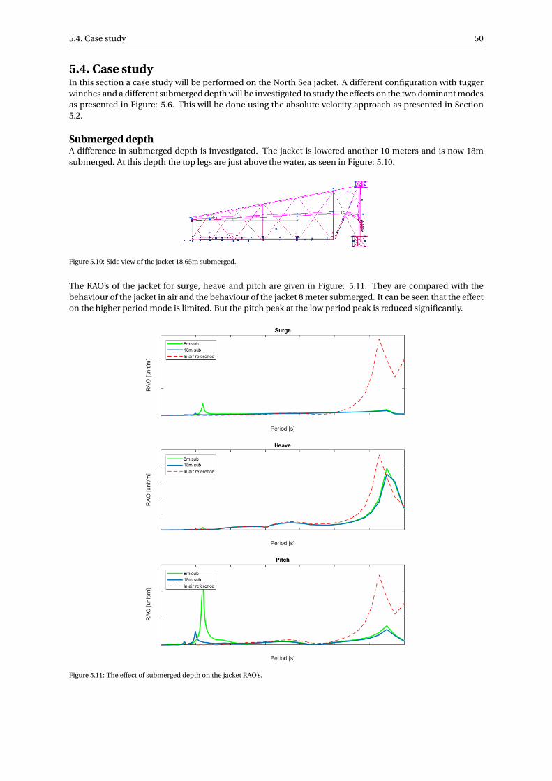
5.4. Case study 50
5.4. Case studyIn this section a case study will be performed on the North Sea jacket. A different configuration with tuggerwinches and a different submerged depth will be investigated to study the effects on the two dominant modesas presented in Figure: 5.6. This will be done using the absolute velocity approach as presented in Section5.2.
Submerged depthA difference in submerged depth is investigated. The jacket is lowered another 10 meters and is now 18msubmerged. At this depth the top legs are just above the water, as seen in Figure: 5.10.
Figure 5.10: Side view of the jacket 18.65m submerged.
The RAO’s of the jacket for surge, heave and pitch are given in Figure: 5.11. They are compared with thebehaviour of the jacket in air and the behaviour of the jacket 8 meter submerged. It can be seen that the effecton the higher period mode is limited. But the pitch peak at the low period peak is reduced significantly.
Figure 5.11: The effect of submerged depth on the jacket RAO’s.

5.4. Case study 51
Tugger winchesTugger winches are added at the bottom on the crane and are connected to the mainblocks. The goal is toreduce the pitch mode of the jacket. Two tuggerlines per mainblock are applied. This is visualised in Figure:5.12. A constant damping is set on each of the winches [19]. The result on the pitch RAO is given in Figure:5.13. It can be seen from the figure that the pitch mode peak is almost completely damped by the tuggerwinches.
Figure 5.12: Tuggerlines attached to the mainblocks of the Thialf.
Figure 5.13: The effect of adding tuggerlines on the jacket pitch RAO.

6Verification
In this section the verification of the submerged jacket model from 5.2, the absolute velocity approach is per-formed. It is investigated if the formulas are implemented correctly in Moses and the conversion between thedifferent programs is done properly. Comments about the order of magnitude are already made in the ex-planation of the different influences. But two aspects will be studied in greater detail here namely: the wavesurge force on the full jacket and the forces on one leg. Since this is a new method for Heerema there is nomeasurement data available to validate the model with. But the model of the in air behaviour is compared tomeasurements. And it proved to be a good starting point. The parts, which are new, are related to the forceof the water on the jacket. The formulas which are interned to determine these parts are widely validated. Soby verifying the model a first step is made towards validating the whole model. First the wave force will bestudied. And secondly the added mass, damping and wave force on one leg are investigated by performing ahand calculation and comparing them to the Moses output.
Concerning the surge wave force on the jacket it is determined where the peaks and trough of the wave forceare expected. The force is presented in Figure: 6.1, with the period on the horizontal axis, the amplitude onthe primary vertical axis and the phase angle w.r.t. the wave on the secondary axis. The distance between thetwo submerged legs is about 40 meters. With the use of linear wave theory it can be reasoned and calculatedat what periods the peaks and trough are expected in the wave force.
Figure 6.1: Surge wave force in the jacket with waves coming from 0 deg.
52
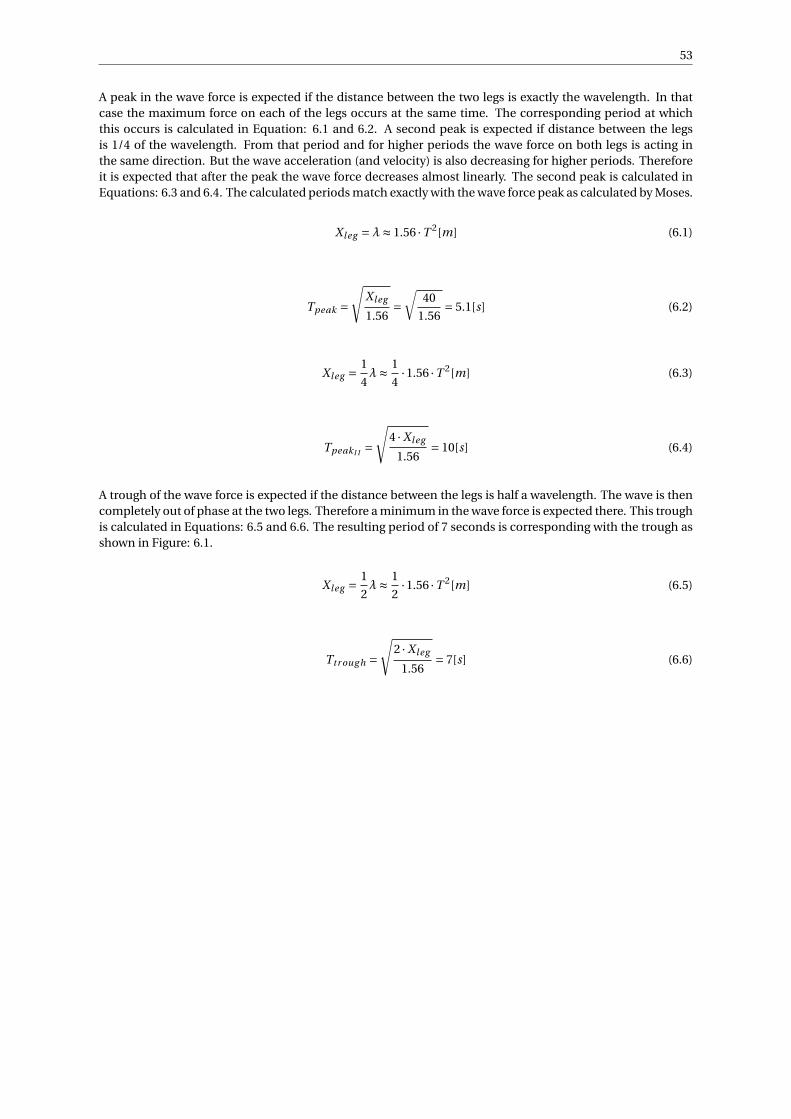
53
A peak in the wave force is expected if the distance between the two legs is exactly the wavelength. In thatcase the maximum force on each of the legs occurs at the same time. The corresponding period at whichthis occurs is calculated in Equation: 6.1 and 6.2. A second peak is expected if distance between the legsis 1/4 of the wavelength. From that period and for higher periods the wave force on both legs is acting inthe same direction. But the wave acceleration (and velocity) is also decreasing for higher periods. Thereforeit is expected that after the peak the wave force decreases almost linearly. The second peak is calculated inEquations: 6.3 and 6.4. The calculated periods match exactly with the wave force peak as calculated by Moses.
Xl eg =λ≈ 1.56 ·T 2[m] (6.1)
Tpeak =√
Xleg
1.56=
√40
1.56= 5.1[s] (6.2)
Xleg = 1
4λ≈ 1
4·1.56 ·T 2[m] (6.3)
TpeakI I =√
4 ·Xl eg
1.56= 10[s] (6.4)
A trough of the wave force is expected if the distance between the legs is half a wavelength. The wave is thencompletely out of phase at the two legs. Therefore a minimum in the wave force is expected there. This troughis calculated in Equations: 6.5 and 6.6. The resulting period of 7 seconds is corresponding with the trough asshown in Figure: 6.1.
Xleg = 1
2λ≈ 1
2·1.56 ·T 2[m] (6.5)
Ttr oug h =√
2 ·Xl eg
1.56= 7[s] (6.6)

6.1. Forces on leg 54
6.1. Forces on legTo verify the forces that Moses calculates the output of Moses for one leg will be compared to hand calcula-tions. The bottom leg of the jacket is modelled separately in SACS and then converted tot Moses in the sameway this is done for the entire jacket. The leg consists of three parts, with the largest diameter at the bottom ofthe leg and the smallest at the top of leg. The leg is 8.65m submerged and the origin is located at bottom of theleg and the axes system is shown in Figure: 6.2. The center of buoyancy is located at [x, y, z] = [0,63.93,0] fromthe origin. The dimensions of the leg are presented in Table 6.1. For the leg the added mass, the damping dueto the jacket velocity and the wave force are determined and compared to the output of Moses.
Table 6.1: Dimensions jacket leg.
D [m] L [m] t [m] CoB part to CoB Leg [m]
Part 1 1.30 46.3 0.08 57.92
Part 2 1.70 16.7 0.08 26.42
Part 3 2.20 82.0 0.08 22.93
Figure 6.2: Bottom leg jacket.
The added mass and the added mass due to the water that is in the flooded leg is determined. For the hor-izontal and vertical added mass Equation: 6.7 is used per part with Ca=1. And for the resulting added massmoment of inertia Equation: 6.8 is used. The arm to the CoB of the leg is determined for each point on thepart and then integrated per part. The total added mass in surge direction for the whole jacket, calculated inSection 5.6, is 3545 [t]. The added mass of two legs is 1414 [t], which means that the two legs account for 40%of the added mass in surge direction.
AF par t = π
4·ρw ·Ca · (D2
out +D2i n) ·Lpar t (6.7)
AM par t =∫ end−CoB
beg i n−CoBy2 · A ·d y = 1
3(y3
beg i n−CoB − y3end−CoB ) · π
4·ρw ·Ca · (D2
out +D2i n) (6.8)
Table 6.2: Added mass calculation and comparison to Moses.
Direction A1 A2 A2 Atot al [t ] and [t ·m2] AMoses [t ] and [t ·m2] % of Moses
x 111 71 594 776 777 1.00
y 0 0 0 0 0 1.00
z 111 71 594 776 777 1.00
rx 393728 51020 645393 1090141 1090421 1.00
ry 0 0 0 0 0 1.00
rz 393728 51020 645393 1090141 1090421 1.00

6.1. Forces on leg 55
The damping due to the jacket velocity is determined next. This is done by calculating the damping force perdirection and per part according to the Equations: 6.9 and 6.11. The following velocities are used during thiscalculation: [x, y, z]= [1, 2, 3] m/s and [ ˙r x, ˙r y , ˙r z]= [1, 2, 3,] deg/s. The drag coefficient is determined basedon smooth members and the Reynolds number per part, as shown in Figure: 6.3. The velocities at each pointon the leg are determined based on the the rotational velocity ( ˙r x) and the arm to the CoB of the leg (r). Withthis velocity and arm the drag coefficient and the resulting moment around the CoB can be determined. Theresulting forces and moments due to the (rotational) velocity are presented in Tables: 6.3 and 6.4 respectively.
FDpar t = 1
2·ρw ·CD |x|x ·Lpar t (6.9)
vpoi nt =ω · r = (π
180· ˙r x) · r (6.10)
MDx =y=145∑
y=0FDz · rpoi nt−CoB (6.11)
Figure 6.3: Drag coefficient based on Reynolds number[37].
Table 6.3: Damping force calculation and comparison to Moses in kN.
Part 1 Part 2 Part 3 Total
Re Cd Drag Re Cd Drag Re Cd Drag FDtot FDMoses %Moses
x 1.74E+06 0.50 -15.4 1.74E+06 0.50 -7.27 2.26E+06 0.57 -52.7 -75.4 -75.1 1.00
y 3.49E+06 0.57 0.00 3.49E+06 0.57 0.00 4.51E+06 0.57 0.00 0.0 0.0 1.00
z 5.23E+06 0.62 -158 5.23E+06 0.62 -81.2 6.77E+06 0.62 -515 -755 -764 0.99
Table 6.4: Damping moments, around CoB, calculation compared to Moses.
Total
Direction MDtot [kNm] MDMoses [kNm] % Moses
rx -22500 -22351 1.01
ry 0.0 0.0 1.00
rz -2163 -2101 1.03

6.1. Forces on leg 56
The wave force is calculated next. It consists of a drag and an inertia depended part. Due to symmetry of theleg the force in surge and heave direction are the same, so only the surge force is explained in this section.Since the leg is horizontally submerged the wave velocity and wave acceleration are constant over the lengthof the leg, but do vary per wave period. The wave velocity and acceleration are calculated based on Equation:3.6 and 3.10 for each period and Hs =1m. A constant drag coefficient of 1.2 and inertia coefficient of 2 areused. The wave force and moment per meter wave height are calculated according to Equation: 6.14 and 6.15and the results are presented in Figure: 6.4.
FDpar t
ζa= 1
2·ρw ·D ·C d ·u2 · Lpar t
ζa(6.12)
FI par t
ζa= π
4·D2 ·ρw ·C m · u · Lpar t
ζa(6.13)
Fw ave =√
(FD1 +FD2 +FD3)2 + (FI 1 +FI 2 +FI 3)2 (6.14)
Mw ave =√
(FD1 · r1 +FD2 · r2 +FD3 · r3)2 + (FI 1 · r1 +FI 2 · r2 +FI 3 · r3)2 (6.15)
(a) Morison wave force in surge direction. (b) Morison wave moment around CoB in yaw direction.
Figure 6.4: Wave force and moment comparison.
From all of the above mentioned it is concluded that Moses can be used to accurately determine the forces ofthe water and the waves on a structure based on the absolute velocity Morison approach. It has been verifiedthat the peaks/trough in the wave force are at the expected periods. And from the calculations on the leg itis shown that Moses can correctly calculate the added mass, including the effect of a flooded member. TheReynolds depended damping force due to the jacket (rotational) velocity matches the hand calculations. Andthe wave force and moment over a large range of periods correspond with the hand calculation as well.

6.2. Relative velocity approach 57
6.2. Relative velocity approachAs a check the damping force for the different parts in x, y and z are compared to the damping force for thewhole jacket. The results are given in the Table 6.5. It can be seen from the table that cutting the jacket intoparts does leads to a small change in force if the same velocities are used.
Table 6.5: A comparison of the horizontal and vertical damping forces.
Left Middle Right Total parts Whole jacket
Fx [kN] 28.12 42.54 29.99 100.7 98.2
Fy [kN] 0.02 0.12 0.02 0.2 0.2
Fz [kN] 2.74 6.84 2.87 12.5 12.4
It was noted from the RAO calculations in Section 5.2.2 that the damping has a large influence on the re-sponse of the jacket near the pitch mode at 6s. To determine the applicability of the relative velocity approachthe amplitude of the motion is compared to the diameter of the members. According to DNV the approach isvalid for r/D>1. The significant single amplitudes of the motion have been derived from the model made inSection 5.2.2 and are presented in Table 5.9 . Where Dlmax = 2.2m, Dlmi n = 1.3m and Dbr ace = 0.4m. It canbe seen that for the brace the relative velocity would be valid in heave direction. The approach is also validfor part of the leg and brace.
Table 6.6: Applicability relative velocity approach.
xa [m] r/Dlmax r/Dlmin r/Dbrace
x 0.28 0.1 0.2 0.7
y 0.05 0.0 0.0 0.1
z 0.75 0.3 0.6 1.9
rx 0.1 0.0 0.1 0.3
ry 1.8 0.8 1.4 4.5
rz 0.1 0.0 0.1 0.3

7Results
In this chapter the operability of the model is determined. The operability of the in air model is compared tothe submerged jacket model and the different submerged depths are compared. Lastly the affect of addingtuggerwinches on the operability is presented.
The operability is calculated based on the theory described in Section 3.4. The limits that are used are de-scribed in Section 3.4. As an input the different RAO’s are used, for in air they are determined with the modelfrom Section 4.1 and for the submerged case the RAO’s are determined from the models in Section 5.2. Withthis RAO’s the Significant Double Amplitudes are determined, based on a JONSWAP spectrum with 1m Hs,which are used to the determine the Single Most Probable Maximum for a 3 hour window. With the SMPMand the defined limits the operability is determined for waves coming from 0, 45 and 90 degrees. And theyare presented in Figure: 7.3 and 7.4.
The Thialf pitch operability, with the jacket 8.65m submerged and waves from 0 degrees, is determined asexample in Figure: 7.1 and Figure: 7.2. With each JONSWAP spectrum and the Thialf pitch RAO the corre-sponding SDA is determined. The results of which are plotted in Figure: 7. The SMPM is determined and thepitch limit is plotted as well. From Figure: 7.2a it can be seen that the Thialf pitch SMPM cross at a certainperiod. Therefore it can be seen in Figure: 7 that the operability limit at that period is 1m Hs. And for thelower periods a higher wave height is allowed, since the SMPM is less, and for higher periods the opposite.This operability curve is also shown in the top left plot of Figure: 7.3b.
(a) JONSWAP spectra with Hs=1m and Tp=4-20s.
(b) Thialf pitch RAO.
Figure 7.1: JONSWAP specta and Thialf pitch RAO with jacket 8.65m submerged.
58
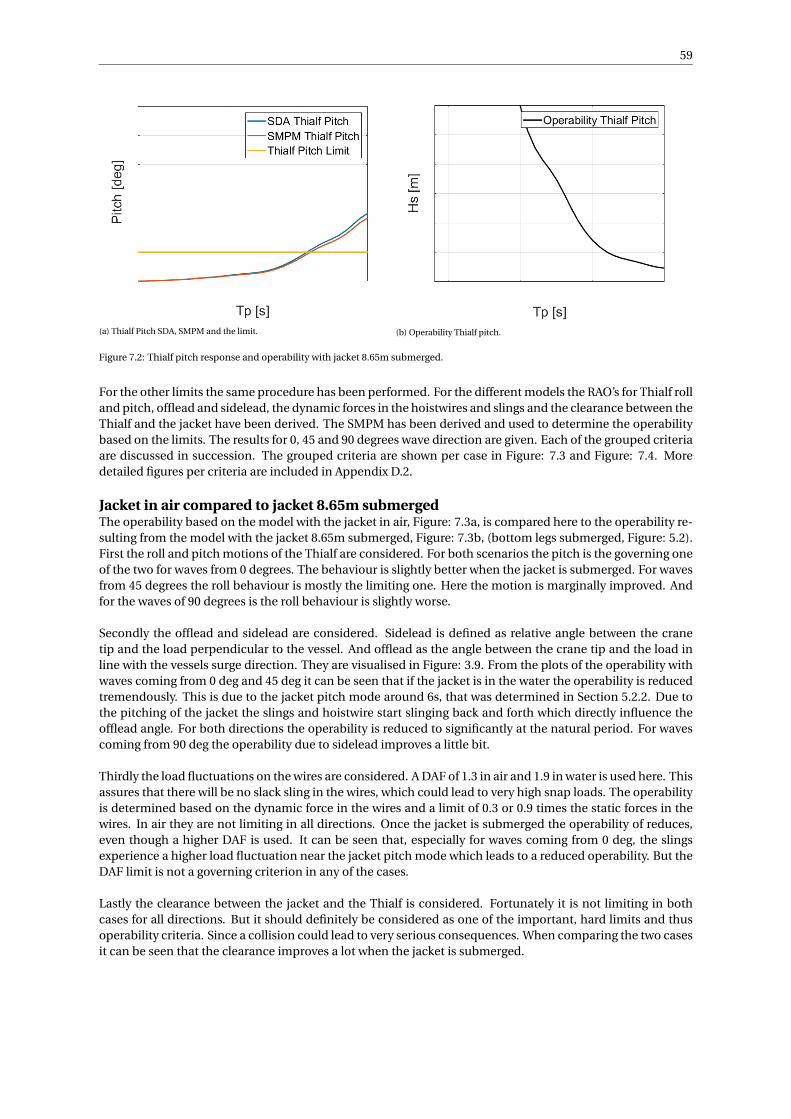
59
(a) Thialf Pitch SDA, SMPM and the limit. (b) Operability Thialf pitch.
Figure 7.2: Thialf pitch response and operability with jacket 8.65m submerged.
For the other limits the same procedure has been performed. For the different models the RAO’s for Thialf rolland pitch, offlead and sidelead, the dynamic forces in the hoistwires and slings and the clearance between theThialf and the jacket have been derived. The SMPM has been derived and used to determine the operabilitybased on the limits. The results for 0, 45 and 90 degrees wave direction are given. Each of the grouped criteriaare discussed in succession. The grouped criteria are shown per case in Figure: 7.3 and Figure: 7.4. Moredetailed figures per criteria are included in Appendix D.2.
Jacket in air compared to jacket 8.65m submergedThe operability based on the model with the jacket in air, Figure: 7.3a, is compared here to the operability re-sulting from the model with the jacket 8.65m submerged, Figure: 7.3b, (bottom legs submerged, Figure: 5.2).First the roll and pitch motions of the Thialf are considered. For both scenarios the pitch is the governing oneof the two for waves from 0 degrees. The behaviour is slightly better when the jacket is submerged. For wavesfrom 45 degrees the roll behaviour is mostly the limiting one. Here the motion is marginally improved. Andfor the waves of 90 degrees is the roll behaviour is slightly worse.
Secondly the offlead and sidelead are considered. Sidelead is defined as relative angle between the cranetip and the load perpendicular to the vessel. And offlead as the angle between the crane tip and the load inline with the vessels surge direction. They are visualised in Figure: 3.9. From the plots of the operability withwaves coming from 0 deg and 45 deg it can be seen that if the jacket is in the water the operability is reducedtremendously. This is due to the jacket pitch mode around 6s, that was determined in Section 5.2.2. Due tothe pitching of the jacket the slings and hoistwire start slinging back and forth which directly influence theofflead angle. For both directions the operability is reduced to significantly at the natural period. For wavescoming from 90 deg the operability due to sidelead improves a little bit.
Thirdly the load fluctuations on the wires are considered. A DAF of 1.3 in air and 1.9 in water is used here. Thisassures that there will be no slack sling in the wires, which could lead to very high snap loads. The operabilityis determined based on the dynamic force in the wires and a limit of 0.3 or 0.9 times the static forces in thewires. In air they are not limiting in all directions. Once the jacket is submerged the operability of reduces,even though a higher DAF is used. It can be seen that, especially for waves coming from 0 deg, the slingsexperience a higher load fluctuation near the jacket pitch mode which leads to a reduced operability. But theDAF limit is not a governing criterion in any of the cases.
Lastly the clearance between the jacket and the Thialf is considered. Fortunately it is not limiting in bothcases for all directions. But it should definitely be considered as one of the important, hard limits and thusoperability criteria. Since a collision could lead to very serious consequences. When comparing the two casesit can be seen that the clearance improves a lot when the jacket is submerged.

60
(a) Operability curves with the jacket in air for the limiting criteria.(b) Operability curves with the jacket 8.65 m submerged for the limiting cri-teria.
Figure 7.3: Operability curves for jacket in air vs. 8.65m.

61
Jacket 8.65m submerged compared to jacket 18.65m submergedThe operability of the two models made in Section 5.4 are presented in Figure: 7.4b and 7.5. By submergingthe jacket deeper in to the water the operability improves. The jacket gets more resistance to the pitch modedue to the increase in added mass and the reduction on the wave force on the bottom legs (since they aredeeper below the wave crest). This results in a higher limit for the offlead peak at the pitch mode. For wavecoming from 0 deg the operability for waves with lower periods is still governed by the pitch mode. For thewaves with longer periods and the other wave directions the operability improves significantly. The largestimprovement is with waves from 45 deg, the operability at the pitch peak period, the allowable wave heightmore than triples.
(a) Operability curves with the jacket 8.65 m submerged for the limiting crite-ria.
(b) Operability curves with the jacket 18 meters submerged for the limitingcriteria.
Figure 7.4: operability curves for jacket 8.65m vs. 18m submerged.

62
When adding tuggerlines to the mainblocks the operability can be improved further, as presented in Fig-ure: 7.5. The tuggerlines configuration is shown in Figure: 5.12. As expected they only influence the offleadand sidelead angle near the pitch mode. For the rest the influence on the other limits and higher periods ismarginal.
Figure 7.5: Operability curves with the jacket 18 meters submerged with tuggerlines for the limiting criteria.

8Conclusion & Recommendations
In this chapter the conclusions and recommendations are presented. The 3 sub-question and the main re-search question are answered first. Thereafter the recommendations are given for improving the research,general considerations and future research.
8.1. ConclusionsThe following research questions have been formulated in Chapter 2. They will be answered one by one inthis section. First all the sub-questions and after that the main research question. Eventually the additionalconclusion are formulated.
1. How does the free hanging jacket in air behave?
• The jacket behaviour is analysed by comparing the measured response to the model response. Itwas determined that there are several modes of interest when looking at the RAO’s.
• Although the Thialf’s response was low due to the nice weather during the measurements cam-paign the modes where captured accurately.
2. Which are the relevant forces and how can they and the resulting motions be determined?
• The relevant forces on the jacket are the wave forces. These forces can be determined by using theMorison equation.
• The impact of the wind force appeared to be minor when looking at the behaviour of the jacket inwater, and it can therefore be neglected.
3. How should one submerge the jacket to reduce the motions as much as practically possible based on acase study of the North Sea jacket?
• When the jacket is submerged it should be submerged more than a few meters. At first it willmainly attract wave loads. By submerging it deeper the damping and the added mass increases.
• The relative velocity approach leads to a decrease in damping. This is due to the effect of mod-elling the jacket in parts.
• Adding tugger winches to the jacket can improve the behaviour since it can be used to damp outa specific peak, the pitch peak of the jacket in this case.
How does the response of a crane suspended jacket and the vessel change if the jacket is (partly) sub-merged in water compared to in air?
• When the jacket is submerged in the water it attracts wave loading. This excitation force triggers thelow damped pitch mode of the jacket.
63

8.2. Recommendations 64
• By submerging the jacket only a few meters this lead to a large reduction in operability.
• If the jacket is being submerged deeper it gains additional damping and added mass. This reduces thepitch peak and improves the operability.
• The response to higher periods wave improves when submerging the jacket deeper in the water.
• Submerging the jacket can be used as a contingency scenario for (unexpected) swell waves. But it iscrucial to know the behaviour of the jacket. Because submerging it at the wrong depth could lead tolarge resonant responses. Based on the North Sea jacket case the jacket legs should be outside the wavedominant zone.
• The response with the jacket in the water can be modelled in the frequency domain. But estimating theright damping turned out to be quite difficult. A new approach has been developed.
8.2. RecommendationsThis study demonstrates the feasibility of submerging the jacket as a contingency scenario. To explore theother options with a submerged jacket or increase the accuracy of the model recommendations are made inthis section.
• Perform more measurements to get more reliable data of the movement of the free hanging jacket. Togain more insight in the behaviour while the jacket is in the water scale model tests can be performed.In that way the Thialf and the full size jacket are not put at risk.
• The jacket velocity values that are used by Heerema may not always be suited for the investigations ofthe submerged jacket case. It is therefore recommended that an iteration is performed until the jacketvelocity converges.
• To improve the relative velocity damping approach, while the jacket is just submerged, a way to accu-rately determine the forces on parts must be sought. By modelling it in parts the damping increases,although the relative velocity approach gives more damping than the absolute velocity approach. Forthis study it is more straightforward to submerge the jacket deeper and thereby increase the damping.
• It is recommended to study the affect of submerging a jacket vertically instead of horizontally. Otherbehaviour of the jacket is expected here. Whether or not this will be positive needs to be determined. Ifit is positive it could be expanded by investigating the feasibility of wet transport.
• It is recommended to continue this work by expanding the model to include forward speed. That wayit can be investigated if sailing with a partly submerged jacket is possible.
• If there is a strong current it could influence the behaviour of the jacket. It is recommended to investi-gate if this improves or worsens the operation.

Bibliography
[1] P Barclay, C. Schoenmaekers. Dual crane lift systems - sc 211. Heerema Marine Contractors: Inhouse,2016.
[2] J. van den Berg. Frigg qp jacket gets ’on the move’ at marin. MARIN Magazine, 2009.
[3] J.-C. Berger. The frigg cessation project. Society of Petroleum Engineers, 2011.
[4] A.S. Bull and Milton S.L. Worldwide oil and gas platform decommissioning: A review of practices andreefing options. Ocean Coastal Management, 168, 2019. URL http://www.sciencedirect.com/science/article/pii/S0964569118304484.
[5] S.K. Chakrabarti. Hydrodynamics of offshore structures. World Scientific Publishing Co., 1987.
[6] Lehmann E. Östergaard C. Clauss, G. Offshore Strucutres. Springer-Verlag London, 1994.
[7] OSPAR commission. Convention for the protection of the marine environment of the north-east atlantic.1992.
[8] Heerema Marine Contractors. Liftdyn theory manual, 2009.
[9] Heerema Marine Contractors. Multimedia gallery, 2020. URL https://hmc.heerema.com/news-media/multimedia-gallery/.
[10] J. de Jong. Basis of design for jacket removal, transport & offloading. Heerema Marine Contractors, 2000.
[11] O. Faltinsen. Sea loads on ships and offshore structures. Cambridge University Press., 1990.
[12] Leo Holthuijsen. Waves in oceanic and coastal waters. Cambridge University Press:, 2007.
[13] J. Hoving. Oe44095 bottom founded offshore structures 2019 tu delft, 2019. URL https://brightspace.tudelft.nl/d2l/le/content/50108/viewContent/711006/View.
[14] iXblue. Octans. 2019. URL https://www.ixblue.com/sites/default/files/2020-02/Octans_2019.pdf.
[15] Mork M. Jenssen, I. Recommended practice for planning, designing and constructing fixed offshoreplatforms. NGO Shipbreaking Platform, 2019.
[16] Massie W.W. Journee, J.M.J. Offshore Hydromechanics. Delft University of Technology, 2000.
[17] Connor J.J. Laya, E.J. and S.S. Sunder. Hydrodynamic forceson flexible offshore structures. J Eng Mech,ASCE, Vol 110, 1984.
[18] Mathworks. MATLAB documentation R2020a, 2020.
[19] G. Meskers and R. Van Dijk. A damping tugger system for offshore heavy lifts. 2012.
[20] Microsoft. Microsoft Excel Manual, 2015.
[21] G. Moe and R.L.P. Verley. Hydrodynamic damping of offshore structures in waves and currents. 12thAnnual Offshore Technology Conference Houston, 1980.
[22] J.W. Morison, J.R. Johnson. The force exerted by surface waves on piles. Journal of Petroleum Technology,2(05):149–154, 5, 1950.
[23] P Naaijen. Course notes on motions and loading of structures in waves. Delft University of Technology,2019.
65

Bibliography 66
[24] Standards Norway. Norsok n-003: Actions and action effects. 2017.
[25] Basuki R. Nugraha, B. Rigs-to-reef: A new initiative on re-utilization of abandoned offshore oil and gasplatforms in indonesia for marine and fisheries sectors. IOP Conference Series: Earth and EnvironmentalScience, 241, 2019.
[26] Massachusetts Institute of Technology. WAMIT Theory Manual, 1995.
[27] SPT Offshore. Relocation ophir wellhead platform, 2019. URL https://www.sptoffshore.com/news/malaysia-jitang-field-offshore/.
[28] Y. Rentoulis. Huldra facilities engineering, preparations and removal. Heerema Marine Contractors,2018.
[29] API RP2A-WSD. Recycling outlook decommissioning of north sea floating oil & gas units. Houston:American Petroleum Institute, 2000.
[30] Zoontjes R. Capurso V Samudero, P. Spe-199177-ms-crane suspended transportation – an effective wayto remove offshore platforms. SPE Symposium: Decommissioning and Abandonment, 2019.
[31] Isaacson M. Sarpkaya, T. Mechanics of wave forces on offshore structures. Van Nostrand Reinhold Co NewYork, 1981.
[32] Shell. Decommissioning in the uk, 2013. URL https://www.shell.co.uk/sustainability/decommissioning/brent-field-decommissioning/decommissioning-in-the-uk.html.
[33] A. Slyozkin. Hydrodynamic interaction between floating structures during heavy lift operations - is itworth analysing? Marine Heavy Transport Lift IV, 2014.
[34] Saipem S.p.A. Statoil 2/4s removal project, 2014. URL https://www.gassco.no/globalassets/saipem.pdf.
[35] Vrouwenvelder A.W.C.M. Klaver E.C. Spijkers, J.M.J. Lecture notes on structural dynamic. Delft Univer-sity of Technology, 2005.
[36] O. Stettner. Floating jacket installation. 2014. URL http://resolver.tudelft.nl/uuid:c3f0821c-9f1a-460e-bdb5-4a5aac3da95e.
[37] Bentley Systems. Reference manual for MOSES, 2017.
[38] Bentley Systems. Reference manual for SACS, 2018.
[39] J. Van Der Tempel, N.F.B. Diepeveen, W.E. De Vries, and D. Cerda Salzmann. Wind energy systems -offshore environmental loads and wind turbine design: impact of wind, wave, currents and ice. 2011.
[40] European Union. Requirements and procedure for inclusion of facilities located in third countries in theeuropean. Journal of the European Union, 2016.
[41] Det Norske Veritas. Dnv recommended practice dnv-rp-c205 on environmental conditions and envi-ronmental loads. 2006.
[42] Det Norske Veritas. Dnvgl-cg-0130 wave loads - rules and standards. 2018.
[43] W.T. van Wingerden. Floating jacket installation. 2019. URL http://resolver.tudelft.nl/uuid:dabf39be-c712-48f3-bd44-002f68770dc8.

Appendices
67

AAppendix
A.1. Diffraction theoryThe diffraction theory is based on potential theory. It is assumed here that a rigid body is moving in anideal fluid with harmonic waves. With potential theory the hydrodynamic loads are evaluated. The potentialΦ(x, y, z, t ) is based on the superposition of:
• The undisturbed waves potential (Φw ), this is the wave field as if the vessel is not there.
• The diffraction potential (Φd ), these are the waves that reflect from the vessel.
• The radiated waves potential (Φr ), which are the waves that radiate from the vessel due to the motionsof the vessel. The waves that radiate are dissipating energy from the ship. This can also be referred toas potential damping.
A brief overview of the theory is given here. For a more elaborate description it is advised to consult Faltinsen[11] or Journee and Massie [16].It is assumed that the water is incompressible, without viscosity and irrotational. The pressures and velocitiescan be written in terms of a potential flow. The potential function, Φ, describes the state of the fluid at eachpoint in the water. It has no physical meaning, it is a mathematical expression that can be used to calculatethe velocities at a certain point (x, y, z) at time t . The velocity can be obtained by taking the spatial derivativeof the potential function and is given in Equation: A.1.
V =∇Φ= ∂Φ
∂xi+ ∂Φ
∂yj+ ∂Φ
∂zk = ui+ vj+wk (A.1)
Within the fluid domain the potential function has to fulfil several requirements.
1. Continuity condition or Laplace EquationWith the incompressible flow assumption the velocity potential derived in Equation: A.1 has to satisfythe Laplace equation, as expressed in Equation: A.2.
∇V =∇2Φ= 0 (A.2)
2. Seabed boundary conditionThis condition allows no fluid to pass through the sea floor. The sea floor is impermeable, therefor thefollowing condition has to be satisfied:
∂Φ
∂z= 0 at the sea floor z =−h (A.3)
3. Boundary condition at the surfaceFor the free surface dynamic boundary condition the pressure at the free surface of the fluid (z = 0) isequal to the atmospheric pressure.
∂Φ
∂t+ gζ= 0 at z = 0 (A.4)
68

A.1. Diffraction theory 69
And the kinematic boundary condition states that at the free surface the vertical motion of the flow hasto be identical to the vertical velocity of the free surface itself. This assures that no particles can escapetrough the surface. With linearised free surface flow conditions this is given in Equation: A.5:
∂Φ
∂z= ∂ζ
∂tat z = 0 (A.5)
A differentiation of Equation: A.4 with respect to t and combined with the kinematic free surfaceboundary condition gives:
∂2Φ
∂t 2 + g∂Φ
∂z= 0 at z = 0 (A.6)
4. Kinematic Boundary Condition on the Oscillating Body SurfaceNo fluid can go through the surface of a body. Therefor the velocity normal to the vessel hull is set tothe same value as the velocity of the hull in this direction. This boundary condition is also referred toas the "no-leak" condition and is given by:
∂Φ
∂η= vηx, y, z, t (A.7)
5. Radiation condition The radiation condition states that the outgoing free surface wave decays appro-priately.
limR→∞
Φ= 0 (A.8)
The complex potential Φ can be written as a superposition of the undisturbed wave potential Φ0, the wavediffraction potentialΦ7 and the potentials which describe the body motions in all six directions.
Φ=−iω
[(Φ0 +Φ7)ζ0 +
6∑j=1Φ j ζ j
](A.9)
From the linearised Bernoulli equation the pressure of the fluid can be calculated:
p(x, y, z, t ) =−ρ ∂Φ∂t
(A.10)
The forces and moments follow from integration of the pressure p, over the submerged surface of the vesselS.
~F =−∫
S
∫(p ·~n)dS (A.11)
~M =−∫
S
∫(p · (~r ×~n)dS (A.12)

BAppendix
B.1. Software tools for dynamic analysisDifferent software tools are used in this study. Apart from the supposedly known Matlab [18] and Excel [20]more specialised software will be used. The different tools are summarised below.
LIFTDYN (Heerema Marine Contractors [8]). Liftdyn is a in-house computer tool that is designed to modeland solve general linear hydrodynamic problems in the frequency domain. Liftdyn can solve systems con-sisting of rigid bodies connected to each other or to the earth by springs, dampers and hinges. The bodymay have a frequency depended mass and damping, and frequency depended exciting forces resulting in afrequency depended response or RAO (response amplitude operator) of the system. The mass matrix M isdefined by a vessels mass and radii of gyration. The hydrodynamic database for the vessel or the load canbe inserted for each body. In case of the SSCV, a standard spring matrix which represents the stiffness ofthe DP system is added to the spring matrix. The resulting RAO can be post-processed to a motion, velocityor acceleration RAO at any desired point relative to any other point. A RAO of the force in a connector canalso be generated. A generated RAO can be used to produce the significant response in a specific sea state.Furthermore, limiting criteria can be defined to obtain operability curves indicating the maximum allowablewave height as a function of the spectral period.
MOSES (Bentley Systems[37]). MOSES is a program that can be used for the hydrostatic and hydrodynamicanalysis of offshore platforms and vessels. It can be used to design, simulate and analyse complex offshorestructures and installation projects. It is a frequency domain program that can computed the Morison equa-tion and diffraction theory.
WAMIT (Massachusetts Institute of Technology [26]). WAMIT is a program that can be used to analyse waveinteractions with offshore structures and vessels. It is a frequency domain program that uses potential wavetheory to calculate the inertial forces such as radiation and diffraction. It is based on linear and second orderpotential theory. It uses a panel method with a certain mesh of the panels to solve the velocity potential onthe submerged surfaces of the bodies.
SACS (Bentley Systems [38]). SACS is an integrated finite element structural analysis program. It is widelyused by structural engineers. It can be used to design and analyse offshore structures, perform fatigue anal-ysis, design check, grillage & sea fastening designs and structural integrity (e.g.ship impact analysis). Withinthe scope of the thesis SACS will only be used to get the detailed geometric model of the jacket.
70

CAppendix
C.1. Freebody diagram
Figure C.1: Free body diagram jacket. Note that Fbuoy is 0 in this case.
71
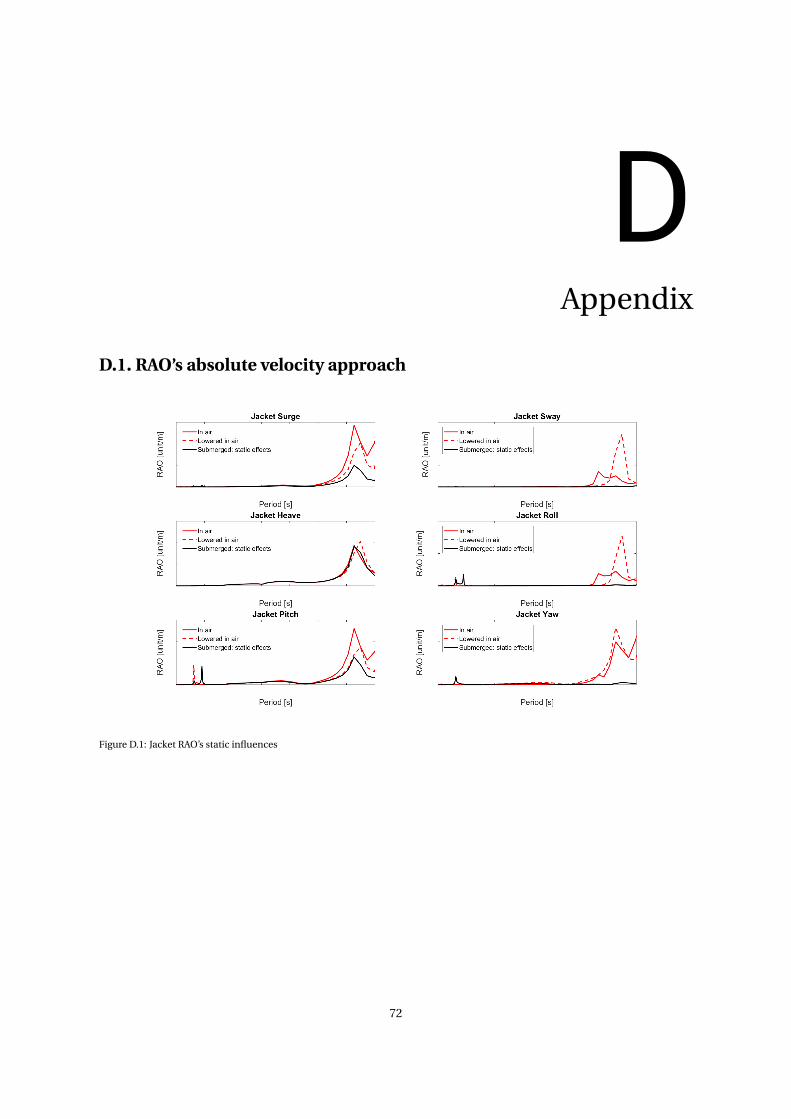
DAppendix
D.1. RAO’s absolute velocity approach
Figure D.1: Jacket RAO’s static influences
72

D.1. RAO’s absolute velocity approach 73
Figure D.2: Thialf RAO’s static influences
Figure D.3: Jacket RAO’s dynamic influences

D.1. RAO’s absolute velocity approach 74
Figure D.4: Thialf RAO’s dynamic influences

D.2. Wave force on jacket 75
D.2. Wave force on jacket
Figure D.5: Wave force on jacket per meter wave height.