1  

A single-layer model for average flow velocity with 1 

submerged rigid cylinders 2 

3 

Nian-Sheng Cheng 4 

5 

School of Civil and Environmental Engineering 6 

Nanyang Technological University, Nanyang Avenue, 639798, Singapore 7 

Email: cnscheng@ntu.edu.sg 8 

9 

Abstract A single-layer velocity model is proposed in this study to predict the cross-10 

sectional average velocity for open channel flows with submerged rigid cylinders. This model 11 

is preferable to previous two-layer models in that it does not involve evaluations of 12 

vegetation drag coefficient and hydrodynamic height of roughness elements. In the 13 

development of the single-layer model, the concept of the hydraulic radius is applied to 14 

determine the length scale of the entire cross section affected by the submerged vegetation. 15 

The resulting friction factor scales largely with the ratio of stem height to flow depth with 16 

exponent 3/2, and also decreases slightly with increasing Reynolds number. Comparisons of 17 

the single-layer model with experimental data show that its performance is comparable to the 18 

previous two-layer models, and the model is also applicable to open channel flows subject to 19 

submerged flexible vegetation. However, the proposed model cannot be extended to two 20 

extreme conditions including flows over a smooth channel bed without vegetation and flows 21 

passing through emergent vegetation. 22 

2  

Keywords: submerged vegetation; average flow velocity; resistance; friction factor; open 23 

channel; roughness height; hydraulic radius 24 

25 

26 

Introduction 27 

In the presence of submerged vegetation, an open channel flow is significantly affected by 28 

the discontinuous vegetation drag and a shear layer is generated across the vegetation-water 29 

interface. Similar to a plane mixing layer (Raupach et al. 1996), the shear layer is 30 

characterized by large-scale coherent vortex structures, which dominate momentum transport 31 

and mixing processes across the interface (Nepf and Vivoni 2000). However, the reduced 32 

flow velocity within the layer of submerged vegetation makes it substantially different from 33 

the flow over the vegetation. As a result, two flow layers can be proposed, i.e. surface layer 34 

above the vegetation and resistance layer passing through the vegetation. The flow analysis 35 

based on the two-layer division is called two-layer model, with which the average flow 36 

velocity in each layer is evaluated individually. For example, the average velocity in the 37 

surface layer can be estimated from the logarithmic velocity distribution (Baptist et al. 2007; 38 

Cheng et al. 2012; Nepf and Vivoni 2000; Yang and Choi 2010). In comparison, in the 39 

vegetation layer, the average flow velocity can be evaluated based on vegetation drag 40 

coefficient (Cheng 2011; Ghisalberti and Nepf 2004; Huthoff et al. 2007; Stone and Shen 41 

2002). 42 

With a two-layer model, important flow characteristics inherent in each layer can be 43 

included for analysis. However, whether the model performs well or not in the prediction of 44 

average flow velocity largely depends on how unknown constants involved in the model are 45 

3  

determined. At present, some details that are required for the development of a two-layer 46 

model are still not available because of complicated interactions between the two layers. For 47 

example, for the surface layer, it is not clear how to define the zero-plane displacement and 48 

the hydrodynamic roughness length theoretically when applying the logarithmic velocity 49 

distribution (Baptist et al. 2007; Okamoto and Nezu 2009). For the vegetation layer, the stem-50 

induced drag still remains a challenging task, in spite of the fact that the topic has been 51 

extensively investigated in the recent years (Cheng 2011; Ishikawa et al. 2000; James et al. 52 

2004; Kothyari et al. 2009; Tanino and Nepf 2008). For simplicity, the drag coefficient 53 

involved in the development of two-layer models is often taken to be a constant(Baptist et al. 54 

2007; Huthoff et al. 2007; Stone and Shen 2002; Yang and Choi 2010), which may not hold 55 

generally (Cheng 2013; Cheng and Nguyen 2011). All these uncertainties may cause 56 

difficulties in the practical implementation of a two-layer model. 57 

In this study, a single-layer model is proposed as an alternative to the two-layer model 58 

for the estimate of the average velocity in open channel flows with submerged vegetation. 59 

Such a model, though simpler than a two-layer model, has not been established in the 60 

literature. To develop the single-layer model, the traditional concept of hydraulic radius is 61 

first applied to determine the length scale of the entire cross section of an open channel flow 62 

obstructed by submerged vegetation. Then, the friction factor is redefined and correlated with 63 

relative vegetation height. The proposed single-layer model does not involve any partition of 64 

the flow domain and evaluation of vegetation drag coefficient, and thus facilitates practical 65 

applications. After calibration, the single-layer model is found comparable to two-layer 66 

models in the prediction of the bulk velocity for open channel flows subject to submerged 67 

vegetation. 68 

69 

4  

Hydraulic radius for flow obstructed by submerged vegetation 70 

For a regular open channel, the hydraulic radius describes the ratio of the cross-sectional area 71 

to the wetted perimeter. Cheng and Nguyen (2011) applied the concept of hydraulic radius 72 

for flows passing through vegetation stems, yielding a stem-related hydraulic radius. They 73 

also showed that in comparison with several other length scales including flow depth, stem 74 

diameter and stem spacing, the stem-related hydraulic radius performs much better in the 75 

quantification of the bulk flow velocity and vegetation resistance. In the present study, the 76 

concept of hydraulic radius is further applied to find the characteristic length for the entire 77 

cross section of open channel flow subject to submerged vegetation. Being consistent with 78 

most experimental setups reported in the literature, the vegetation is represented with rigid 79 

cylindrical rods. This should be considered as an approximation by noting that most natural 80 

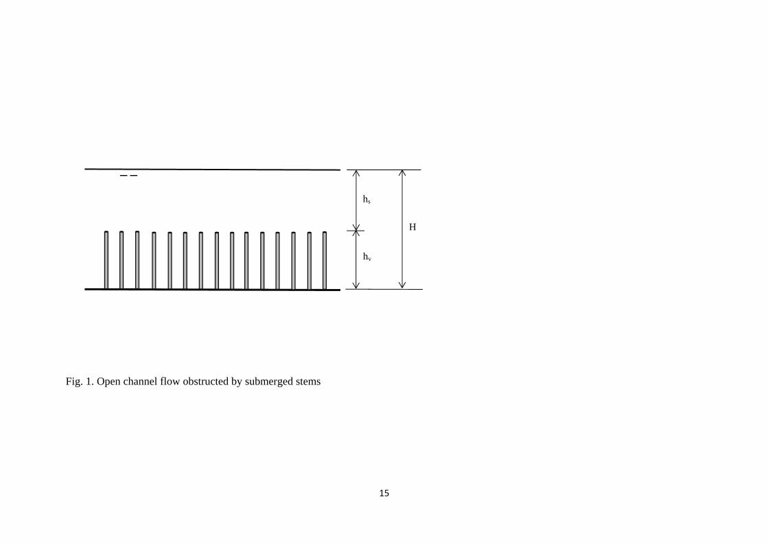
vegetation is flexible and has a different shape from cylinders. The stem diameter is d, and 81 

the stem density is λ, measured as the fraction of the bed area occupied by the stems. The 82 

vegetation height is hv, the thickness of the surface layer is hs, and the total flow depth is H (= 83 

hv+hs), as shown in Fig. 1. To define the hydraulic radius, a flow domain is considered, with a 84 

width of B (= channel width), a height of H and a unit channel length. Within this domain, 85 

the volume of fluid is Bhs+Bhv(1-λ) and the total area of the wetted boundary is B(1-86 

λ)+2H+NπBdhv, where N [= 4λ/(πd2)] is the total number of the stems per unit bed area. 87 

Then, the hydraulic radius r can be defined as the ratio of the volume of fluid to the area of 88 

the wetted boundary, 89 

( )s v

v

Bh Bh 1r

B(1 ) 2H 4 Bh / d+ − λ

=− λ + + λ

(1)

It is noted that Eq. (1) is valid only for a rectangular channel. 90 

91 

5  

Formula for cross-sectional average flow velocity 92 

With the hydraulic radius defined, the friction factor can be expressed as 93 

2

8grSfU

= (2)

where g is the gravitational acceleration, S is the energy gradient, and U is the cross-sectional 94 

average flow velocity calculated as Q/(BH) with Q being the flow rate. In the following, how 95 

f varies with the height of roughness element hv will be explored. 96 

Altogether 300 sets of data are used for analysis, which were collected previously by 97 

Shimizu et al. (1991), Dunn et al. (1996), Meijer and van Velzen (1999), Stone and Shen 98 

(2002), Murphy et al. (2007), Liu et al. (2008), Nezu and Sanjou (2008), Yan (2008), Yang 99 

(2008), Poggi et al. (2009) and Cheng (2011). In these studies, vegetation stems were 100 

simulated with rigid cylindrical rods, except for Nezu and Sanjou (2008) who used 101 

rectangular blocks. The relevant experiments were conducted in different sizes of rectangular 102 

open channels, e.g. the channel length ranging from 4.3 m (Liu et al. 2008) to over 100 m 103 

(Meijer and van Velzen 1999). The vegetation configuration also varied, with rods being 104 

arranged in staggered pattern (Cheng 2011; Dunn et al. 1996; Liu et al. 2008; Stone and Shen 105 

2002; Yang 2008), in linear or straight pattern (Liu et al. 2008; Nezu and Sanjou 2008; Poggi 106 

et al. 2009; Shimizu et al. 1991; Yan 2008), or even randomly (Murphy et al. 2007). 107 

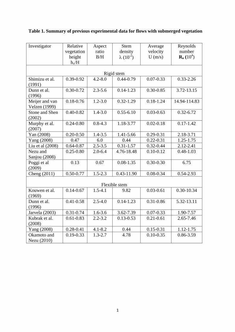
A summary of the data is given in Table 1, which covers different flow conditions and 108 

vegetation configurations, with vegetation density λ = 0.08%-18.48%, relative stem height 109 

hv/H = 0.13-0.92, channel aspect ratio B/H = 0.8-8.0, average flow velocity U = 0.02-1.24 110 

m/s, and Reynolds number Ro = 1.7×103-1.1×106. The Reynolds number is defined as Ro = 111 

Uro /ν, where ro [= BH/(B+2H)] is the hydraulic radius without considering vegetation effect, 112 

6  

and ν is the kinematic viscosity of fluid. For the rectangular blocks, the block width is taken 113 

as an equivalent stem diameter, and the equivalent vegetation density is calculated as πd2N/4. 114 

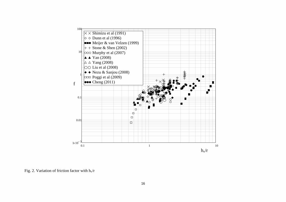
Fig. 2 shows the variation of f with hv normalized by r. For sand-roughened 115 

boundaries, f correlates with ks/r for fully rough turbulent flows, where ks is the equivalent 116 

roughness height. However the similar idea does not apply for vegetated flows, because the 117 

energy dissipation mechanism for vegetated flows is different from regular fully rough flows 118 

and hv cannot be taken as the equivalent roughness height. 119 

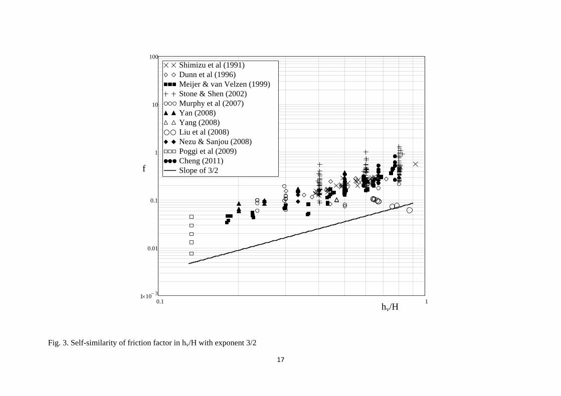
In Fig. 3, f is plotted against hv normalized by H. By comparing Figs. 2 to 3, it can be 120 

seen that f correlates with hv/H much better than hv/r, in spite of the data points spreading 121 

across almost an order of magnitude. The calculated Pearson's correlation coefficient is 0.56 122 

for the relation of log(f) to log(hv/r) and increases to 0.82 for the relation of log(f) to 123 

log(hv/H). This assessment is conducted based on all the data used. For some individual 124 

datasets, the deviation from the general data trend appears large. This implies that in addition 125 

to hv/H, there should be other factors that account for the variation of f. The spread of the data 126 

can also be associated with limitations of experimental setup such as the use of short 127 

vegetation zone (Liu et al. 2008). Furthermore, it can be observed from Fig. 3 that the 128 

average slope of the data trend is about 3/2. This suggests that f is broadly self-similar in hv/H 129 

with exponent 3/2, i.e. f ∼ (hv/H)3/2. It is interesting to note that this scaling is different from 130 

the friction factor for fully rough sediment beds, which scales with the roughness height with 131 

exponent 1/3 as implied by the Manning-Strickler formula. 132 

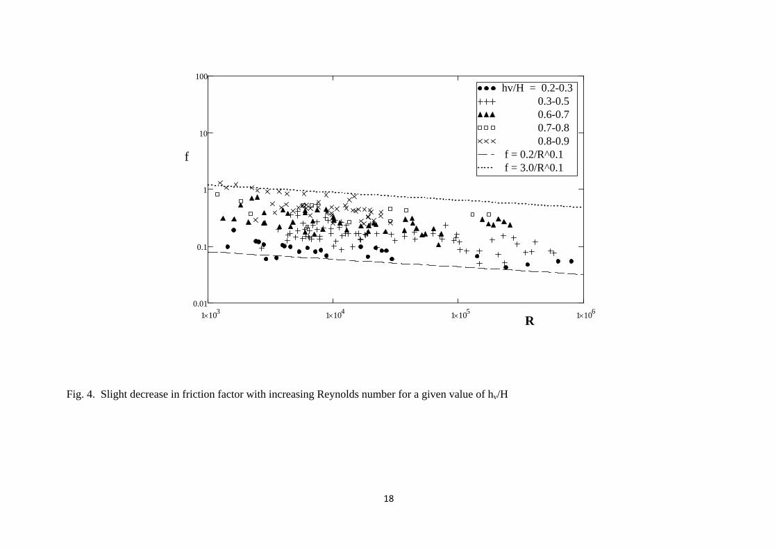
To further check if the fluid viscosity has any effect on the friction factor, f is plotted 133 

against the Reynolds number R (defined as Ur/ν) in Fig. 4. It can be seen that f slightly 134 

decreases with increasing R for a given value of hv/H. Such an f-R relation can also be 135 

observed for open channel flows in the presence of emergent vegetation even for high 136 

7  

Reynolds numbers in the range of 104 to 5×105 (Cheng and Nguyen 2011). Also plotted in Fig. 137 

4 are two straight lines that confined most of the data and approximate the deceasing slope of 138 

the friction factor. This suggests that f is proportional to Rm(hv/H)3/2 where m is a negative 139 

exponent. Since both f and R include U, it is inconvenient to find U with a relation of f 140 

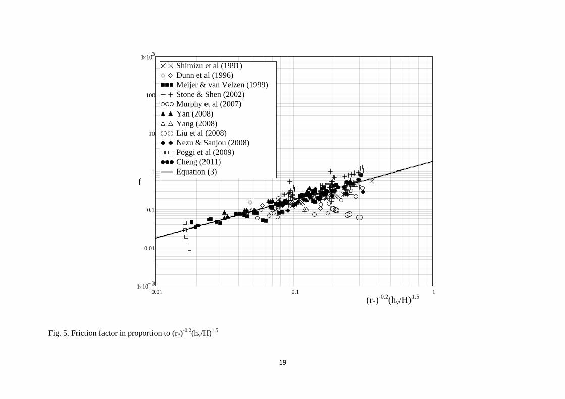
dependent on R. To avoid this problem, a dimensionless hydraulic radius is defined as r∗ = 141 

r(gS/ν2)1/3 by noting that R2f/8 = (Ur/ν)2 (grS/U2) = r3gS/ν2. Then f is related to r∗ and hv/H in 142 

the form of p 3/2* vr (h / H) , where p is an exponent. With the experimental data, the Pearson’s 143 

correlation coefficient was calculated. It optimizes when p = -0.2, and the coefficient of 144 

proportionality is 1.8 (see Fig. 5). Therefore, 145 

3/20.2 v

*hf 1.8rH

− ⎛ ⎞= ⎜ ⎟⎝ ⎠

(3)

Using Eq. (3) and noting that R2f/8 = r∗3, one can deduce that f is inversely proportional to 146 

R1/8. It is noted that a similar relation of proportionality can also be obtained for open channel 147 

flows in the presence of emergent vegetation for high Reynolds numbers (Cheng and Nguyen 148 

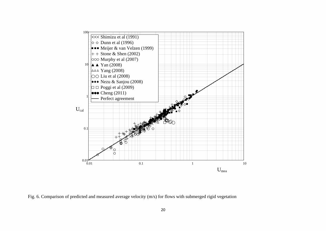
2011). With Eqs. (2) and (3), the cross-sectional average velocity can be expressed as 149 

0.750.1

*v

HU 2.1r grSh

⎛ ⎞= ⎜ ⎟

⎝ ⎠

(4)

Fig. 6 shows good agreement between the average velocities predicted using Eq. (4) and the 150 

measurements. However, the applicability of Eqs. (3) and Eq. (4) should be limited to the 151 

data used, which is in the range of hv/H = 0.13-0.92 and λ = 0.08-18.48%. The value of hv/H 152 

varies between the two extreme cases, flows over a smooth bed with hv/H = 0 and flows 153 

through emergent vegetation with hv/H = 1. For flow conditions close to the extreme cases, 154 

Eq. (4) could fail in the velocity prediction. For example, if the stem height is very small, the 155 

bed would become smooth, for which Eq. (4) predicts that U would approach infinity. A 156 

8  

similar failure could also occur for a river bed that is completely covered by vegetation, 157 

which results in an extremely large wetted perimeter and thus a minimal hydraulic radius. 158 

Therefore, future efforts are needed to extend Eq. (4) to the extreme conditions. 159 

160 

Comparison with two-layer models 161 

Employed for comparison are five two-layer flow models, which have been developed by 162 

Stone and Shen (2002), Baptist et al. (2007), Huthoff et al. (2007), Yang and Choi (2010) and 163 

Cheng (2011), as summarized in Table 2. Stone and Shen (2002) derived their model by 164 

partitioning the friction slope into bed and vegetation components and applying a constant 165 

drag coefficient for vegetation stems. Baptist et al.’s (2007) formula was developed by 166 

applying a machine learning technique that performs optimization with symbolic operations. 167 

With similarity considerations, Huthoff et al. (2007) proposed a scaling model for the average 168 

velocity, which was calibrated using a single set of data by Meijer and van Velzen (1999). 169 

Yang and Choi (2010) applied the logarithmic law to the surface layer and also assumed a 170 

constant drag coefficient for vegetation stems for the computation of the depth-averaged 171 

velocity. Cheng (2011) proposed a representative roughness height, which is proportional to 172 

both stem diameter and vegetation concentration, for the evaluation of submerged vegetation 173 

effect on the resistance and thus the average flow velocity. 174 

The cross-sectional average velocity predicted using Eq. (4) was found comparable to 175 

predictions obtained using the two-layer models. The prediction was assessed using the 176 

average of the prediction error that was calculated as |prediction – 177 

measurement|/measurement × 100 (%). The results are summarized in Table 2. Using the 178 

proposed single-layer model, the prediction error is 15.5%, which is slightly higher than the 179 

results (14-14.3%) from the two best models (Cheng 2011; Huthoff et al. 2007), but much 180 

9  

lower than those (18.9-24.2%) from the three others (Baptist et al. 2007; Stone and Shen 181 

2002; Yang and Choi 2010). By noting that the concept implemented in the present work is 182 

much simpler than the previous two-layer considerations, the proposed single-layer model 183 

can be considered as a good alternative to the existing two-layer models, in spite of its 184 

empirical nature. 185 

186 

Application to flows over flexible vegetation 187 

The present single-layer model is developed based only on the laboratory data collected from 188 

the experiments with rigid stems. In this section, Eq. (4) is further applied to calculate the 189 

cross-sectional average velocity of open channel flows subject to submerged flexible 190 

vegetation. Certainly, there is some difference in the resistance between rigid and flexible 191 

stems. However, Cheng (2011) shows that flow velocity models, which were originally 192 

developed for rigid stems, can be approximately applied for flexible stems provided that the 193 

deflected vegetation height is used. 194 

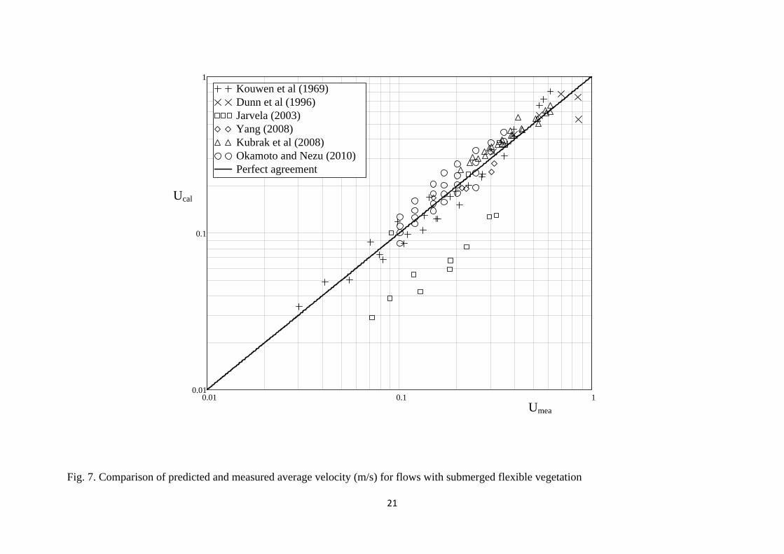
Comparisons were made with 103 sets of flexible stem data reported by Kouwen et al. 195 

(1969), Dunn et al. (1996), Järvelä (2003), Kubrak et al. (2008), Yang (2008) and Okamoto 196 

and Nezu (2010) (see Table 1). In these previous studies, different materials have been used 197 

to represent flexible vegetation, such as film strips (Kouwen et al. 1969; Okamoto and Nezu 198 

2010; Yang 2008), cylindrical stems (Dunn et al. 1996; Kubrak et al. 2008) and real plants 199 

(Järvelä 2003). In the prediction, hv is taken as the average value of deflected height. For 200 

film strips, the equivalent stem density λ is computed as πNd2/4, where d is the strip width 201 

and N is the total number of strips per unit bed area. Fig. 7 shows the computed flow 202 

velocities in comparison with the data. The agreement is generally acceptable and the average 203 

prediction error is 18.8%, which is comparable to the average errors (15.3%-27.1%) 204 

10  

associated with the five two-layer models (see Table 2). However, the difference appears 205 

very large between the prediction and measurement related to the only data measured with 206 

real plants by Järvelä (2003), who grew wheat in a 10-cm thick topsoil and installed it in the 207 

flume with metal boxes. The special experimental design, clearly different from the others, 208 

may partially explain the large difference. 209 

210 

Conclusions 211 

Several two-layer models have been reported in the literature to determine cross-sectional 212 

average velocity for open channel flows in the presence of submerged vegetation. These 213 

models evaluate the surface layer velocity and vegetation layer velocity separately, but they 214 

involve some arguments that have not been fully substantiated. Alternatively, a single-layer 215 

velocity model is proposed in the present study by defining friction factor with a new 216 

hydraulic radius, which quantifies the length scale of the cross section obstructed by 217 

submerged vegetation. The analysis of experimental data shows that the friction factor is 218 

broadly self-similar in vegetation height with exponent 3/2. A formula is then obtained for 219 

the calculation of the average velocity in the presence of submerged vegetation. The results 220 

show that the performance of the single-layer model is comparable to two-layer models 221 

published in the literature. However, the proposed model cannot be applied for two extreme 222 

conditions, flows over a smooth bed with hv/H = 0 and flows through emergent vegetation 223 

with hv/H = 1. 224 

225 

226 

Notation 227 

The following symbols are used in the paper: 228 

11  

B = channel width; 229 

Cb = bed-related Chezy coefficient; 230 

CD = drag coefficient; 231 

Cu = constant; 232 

d = stem width or diameter; 233 

f = friction factor = 8grS/U2; 234 

g = gravitational acceleration; 235 

H = total flow depth = hv+hs; 236 

hs = surface layer thickness; 237 

hv = vegetation height; 238 

ks = equivalent roughness height; 239 

m = exponent; 240 

N = the total number of stems per unit bed area; 241 

p = exponent; 242 

Q = flow rate; 243 

R = Reynolds number = Ur/ν; 244 

Ro = Reynolds number = Uro/ν; 245 

r = hydraulic radius or ratio of fluid volume to wetted boundary area; 246 

ro = hydraulic radius without considering vegetation = BH/(B+2H); 247 

rv = π(1-λ)d/(4λ); 248 

rv∗ = rv(gS/ν2)1/3; 249 

r∗ = dimensionless hydraulic radius = r(gS/ν2)1/3; 250 

S = energy gradient; 251 

U = cross-sectional average flow velocity = Q/(BH); 252 

λ = stem density = fraction of bed area occupied by stems; and 253 

12  

ν = kinematic viscosity of fluid. 254 

255 

256 

257 

13  

References 258 

Baptist, M. J., Babovic, V., Uthurburu, J. R., Keijzer, M., Uittenbogaard, R. E., Mynett, A., 259 and Verwey, A. (2007). "On inducing equations for vegetation resistance." Journal of 260 Hydraulic Research, 45(4), 435-450. 261 

 262 Cheng, N. S. (2011). "Representative roughness height of submerged vegetation." Water 263 Resources Research, 47, 10.1029/2011wr010590. 264 

 265 Cheng, N. S. (2013). "Calculation of drag coefficient for arrays of emergent circular cylinders 266 with pseudo-fluid model." Journal of Hydraulic Engineering-ASCE, 139(6), 602-611. 267 

 268 Cheng, N. S., and Nguyen, H. T. (2011). "Hydraulic Radius for Evaluating Resistance 269 Induced by Simulated Emergent Vegetation in Open-Channel Flows." Journal of Hydraulic 270 Engineering-ASCE, 137(9), 995-1004, 10.1061/(asce)hy.1943-7900.0000377. 271 

 272 Cheng, N. S., Nguyen, H. T., Tan, S. K., and Shao, S. D. (2012). "Scaling of Velocity 273 Profiles for Depth-Limited Open Channel Flows over Simulated Rigid Vegetation." Journal 274 of Hydraulic Engineering-ASCE, 138(8), 673-683, 10.1061/(asce)hy.1943-7900.0000562. 275 

 276 Dunn, C., Lopez, F., and Garcia, M. (1996). "Mean flow and turbulence in a laboratory 277 channel with simulated vegetation." Hydrosystem Lab., University of Illinois, Urbana. 278 

 279 Ghisalberti, M., and Nepf, H. (2004). "The limited growth of vegetated shear layers." Water 280 Resources Research, 40(W07502), 1-12, 10.1029/2003wr002776. 281 

 282 Huthoff, F., Augustijn, D. C. M., and Hulscher, S. J. M. H. (2007). "Analytical solution of the 283 depth-averaged flow velocity in case of submerged rigid cylindrical vegetation." Water 284 Resources Research, 43(W06413), 1-10. 285 

 286 Ishikawa, Y., Mizuhara, K., and Ashida, S. (2000). "Effect of density of trees on drag exerted 287 on trees in river channels." Journal of Forest Research, 5(4), 271-279. 288 

 289 James, C. S., Birkhead, A. L., Jordanova, A. A., and O'Sullivan, J. J. (2004). "Flow resistance 290 of emergent vegetation." Journal of Hydraulic Research, 42(4), 390-398. 291 

 292 Järvelä, J. (2003). "Influence of vegetation on flow structure in floodplains and wetlands." 293 Proceedings of the 3rd IAHR Symposium on River, Coastal and Estuarine Morphodynamics 294 (RCEM 2003), Madrid, 845-856. 295 

 296 Kothyari, U. C., Hayashi, K., and Hashimoto, H. (2009). "Drag coefficient of unsubmerged 297 rigid vegetation stems in open channel flows." Journal of Hydraulic Research, 47(6), 691-699, 298 10.3826/jhr.2009.3283. 299 

14  

 300 Kouwen, N., Unny, T. E., and Hill, H. M. (1969). "Flow retardance in vegetated channels." 301 Journal of Irrigation and Drainage Division-ASCE 95(IR2), 329-342. 302 

 303 Kubrak, E., Kubrak, J., and Rowinski, P. M. (2008). "Vertical velocity distributions through 304 and above submerged, flexible vegetation." Hydrological Sciences Journal-Journal Des 305 Sciences Hydrologiques, 53(4), 905-920. 306 

 307 Liu, D., Diplas, P., Fairbanks, J. D., and Hodges, C. C. (2008). "An experimental study of 308 flow through rigid vegetation." Journal of Geophysical Research-Earth Surface, 113(F04015), 309 1-16, F04015 310 

10.1029/2008jf001042. 311 

 312 Meijer, D. G., and van Velzen, E. H. (1999). "Prototype-scale flume experiments on 313 hydraulic roughness of submerged vegetation." XXVIII IAHR Conference, Graz, Austria, 6 314 (CD-ROM). 315 

 316 Murphy, E., Ghisalberti, M., and Nepf, H. (2007). "Model and laboratory study of dispersion 317 in flows with submerged vegetation." Water Resources Research, 43(5), W05438, 318 doi:10.1029/2006WR005229, 10.1029/2006wr005229. 319 

 320 Nepf, H. M., and Vivoni, E. R. (2000). "Flow structure in depth-limited, vegetated flow." 321 Journal of Geophysical Research-Oceans, 105(C12), 28547-28557. 322 

 323 Nezu, I., and Sanjou, M. (2008). "Turburence structure and coherent motion in vegetated 324 canopy open-channel flows." Journal of Hydro-Environment Research, 2(2), 62-90, 325 10.1016/j.jher.2008.05.003. 326 

 327 Okamoto, T., and Nezu, I. (2010). "Flow resistance law in open-channel flows with rigid and 328 flexible vegetation." River Flow 2010, A. Dittrich, K. Koll, J. Aberle, and P. Geisenhainer, 329 eds., Bundesanstalt für Wasserbau, Karlsruhe, Germany, 261-268. 330 

 331 Okamoto, T. A., and Nezu, I. (2009). "Turbulence structure and "Monami" phenomena in 332 flexible vegetated open-channel flows." Journal of Hydraulic Research, 47(6), 798-810, 333 10.3826/jhr.2009.3536. 334 

 335 Poggi, D., Krug, C., and Katul, G. G. (2009). "Hydraulic resistance of submerged rigid 336 vegetation derived from first-order closure models." Water Resources Research, 45(10). 337 

 338 Raupach, M. R., Finnigan, J. J., and Brunet, Y. (1996). "Coherent eddies and turbulence in 339 vegetation canopies: The mixing-layer analogy." Boundary-Layer Meteorology, 78(3-4), 351-340 382. 341 

15  

 342 Shimizu, Y., Tsujimoto, T., Nakagawa, H., and Kitamura, T. (1991). "Experimental study on 343 flow over rigid vegetation simulated by cylindrical with equi-spacing." Proceedings of the 344 Japan Society of Civil Engineers, 438/II-17, 31-40 (In Japanese). 345 

 346 Stone, B. M., and Shen, H. T. (2002). "Hydraulic resistance of flow in channels with 347 cylindrical roughness." Journal of Hydraulic Engineering-ASCE, 128(5), 500-506, 348 10.1061/(asce)0733-9429(2002)128:5(500). 349 

 350 Tanino, Y., and Nepf, H. M. (2008). "Laboratory investigation of mean drag in a random 351 array of rigid, emergent cylinders." Journal of Hydraulic Engineering-ASCE, 134(1), 34-41, 352 10.1061/(asce)0733-9429(2008)134:1(34). 353 

 354 Yan, J. (2008). "Experimental study of flow resistance and turbulence characteristics of open 355 channel flow with vegetation." PhD Thesis, Hohai University, China. 356 

 357 Yang, W. (2008). "Experimental study of turbulent open-channel flows with submerged 358 vegetation." PhD Thesis, Yonsei University, Korea. 359 

 360 Yang, W., and Choi, S. U. (2010). "A two-layer approach for depth-limited open-channel 361 flows with submerged vegetation." Journal of Hydraulic Research, 48(4), 466-475. 362 

 363 

364 

1  

Table 1. Summary of previous experimental data for flows with submerged vegetation

Investigator Relative vegetation

height hv/H

Aspect ratio B/H

Stem density λ (10-2)

Average velocity U (m/s)

Reynolds number Ro (104)

Rigid stem

Shimizu et al. (1991)

0.39-0.92 4.2-8.0 0.44-0.79 0.07-0.33 0.33-2.26

Dunn et al. (1996)

0.30-0.72 2.3-5.6 0.14-1.23 0.30-0.85 3.72-13.15

Meijer and van Velzen (1999)

0.18-0.76 1.2-3.0 0.32-1.29 0.18-1.24 14.94-114.83

Stone and Shen (2002)

0.40-0.82 1.4-3.0 0.55-6.10 0.03-0.63 0.32-6.72

Murphy et al. (2007)

0.24-0.80 0.8-4.3 1.18-3.77 0.02-0.18 0.17-1.42

Yan (2008) 0.20-0.50 1.4-3.5 1.41-5.66 0.29-0.31 2.18-3.71 Yang (2008) 0.47 6.0 0.44 0.22-0.31 1.25-1.75 Liu et al (2008) 0.64-0.87 2.5-3.5 0.31-1.57 0.32-0.44 2.12-2.41 Nezu and Sanjou (2008)

0.25-0.80 2.0-6.4 4.76-18.48 0.10-0.12 0.48-1.03

Poggi et al (2009)

0.13 0.67 0.08-1.35 0.30-0.30 6.75

Cheng (2011) 0.50-0.77 1.5-2.3 0.43-11.90 0.08-0.34 0.54-2.93

Flexible stem Kouwen et al. (1969)

0.14-0.67 1.5-4.1 9.82 0.03-0.61 0.30-10.34

Dunn et al. (1996)

0.41-0.58 2.5-4.0 0.14-1.23 0.31-0.86 5.32-13.11

Jarvela (2003) 0.31-0.74 1.6-3.6 3.62-7.39 0.07-0.33 1.90-7.57 Kubrak et al. (2008)

0.61-0.83 2.2-3.2 0.13-0.53 0.21-0.61 2.65-7.46

Yang (2008) 0.28-0.41 4.1-8.2 0.44 0.15-0.31 1.12-1.75 Okamoto and Nezu (2010)

0.19-0.33 1.3-2.7 4.78 0.10-0.35 0.86-3.59

  

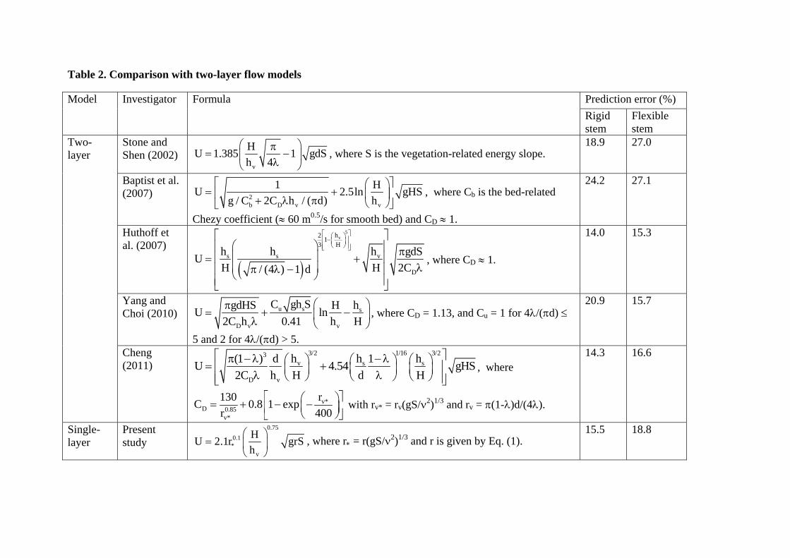
Table 2. Comparison with two-layer flow models

Model Investigator Formula Prediction error (%) Rigid stem

Flexible stem

Two-layer

Stone and Shen (2002)

v

HU 1.385 1 gdSh 4

⎛ ⎞π= −⎜ ⎟λ⎝ ⎠

, where S is the vegetation-related energy slope. 18.9 27.0

Baptist et al. (2007) 2

b D v v

1 HU 2.5ln gHSg / C 2C h / ( d) h

⎡ ⎤⎛ ⎞= +⎢ ⎥⎜ ⎟+ λ π ⎝ ⎠⎣ ⎦

, where Cb is the bed-related

Chezy coefficient (≈ 60 m0.5/s for smooth bed) and CD ≈ 1.

24.2 27.1

Huthoff et al. (2007)

( )

5vh2 1

3 H

s s v

D

h h h gdSUH H 2C/ (4 ) 1 d

⎡ ⎤⎛ ⎞−⎢ ⎥⎜ ⎟⎝ ⎠⎢ ⎥⎣ ⎦

⎡ ⎤⎛ ⎞⎢ ⎥ π⎜ ⎟⎢ ⎥= +

λ⎜ ⎟π λ −⎢ ⎥⎝ ⎠⎢ ⎥⎣ ⎦

, where CD ≈ 1.

14.0 15.3

Yang and Choi (2010) u s s

D v v

C gh SgdHS H hU ln2C h 0.41 h H

⎛ ⎞π= + −⎜ ⎟λ ⎝ ⎠

, where CD = 1.13, and Cu = 1 for 4λ/(πd) ≤

5 and 2 for 4λ/(πd) > 5.

20.9 15.7

Cheng (2011)

3/2 1/16 3/23v s s

D v

(1 ) d h h 1 hU 4.54 gHS2C h H d H

⎡ ⎤π −λ −λ⎛ ⎞ ⎛ ⎞ ⎛ ⎞= +⎢ ⎥⎜ ⎟ ⎜ ⎟ ⎜ ⎟λ λ⎝ ⎠ ⎝ ⎠ ⎝ ⎠⎢ ⎥⎣ ⎦, where

v*D 0.85

v*

130 rC 0.8 1 expr 400

⎡ ⎤⎛ ⎞= + − −⎜ ⎟⎢ ⎥⎝ ⎠⎣ ⎦ with rv* = rv(gS/ν2)1/3 and rv = π(1-λ)d/(4λ).

14.3 16.6

Single-layer

Present study

0.750.1

*v

HU 2.1r grSh

⎛ ⎞= ⎜ ⎟

⎝ ⎠, where r∗ = r(gS/ν2)1/3 and r is given by Eq. (1).

15.5 18.8

15  

Fig. 1. Open channel flow obstructed by submerged stems

hs

hv

H

16  

Fig. 2. Variation of friction factor with hv/r

0.1 1 101 10 3−×

0.01

0.1

1

10

100Shimizu et al (1991)Dunn et al (1996)Meijer & van Velzen (1999) Stone & Shen (2002)Murphy et al (2007)Yan (2008)Yang (2008) Liu et al (2008)Nezu & Sanjou (2008) Poggi et al (2009)Cheng (2011)f

hv/r

17  

Fig. 3. Self-similarity of friction factor in hv/H with exponent 3/2

0.1 11 10 3−×

0.01

0.1

1

10

100Shimizu et al (1991)Dunn et al (1996)Meijer & van Velzen (1999) Stone & Shen (2002)Murphy et al (2007)Yan (2008)Yang (2008) Liu et al (2008)Nezu & Sanjou (2008) Poggi et al (2009)Cheng (2011)Slope of 3/2f

hv/H

18  

Fig. 4. Slight decrease in friction factor with increasing Reynolds number for a given value of hv/H

1 103× 1 104× 1 105× 1 106×0.01

0.1

1

10

100 hv/H = 0.2-0.3 0.3-0.5 0.6-0.7 0.7-0.8 0.8-0.9 f = 0.2/R^0.1 f = 3.0/R^0.1

f

R

19  

Fig. 5. Friction factor in proportion to (r*)-0.2(hv/H)1.5

0.01 0.1 11 10 3−×

0.01

0.1

1

10

100

1 103×Shimizu et al (1991)Dunn et al (1996)Meijer & van Velzen (1999) Stone & Shen (2002)Murphy et al (2007)Yan (2008)Yang (2008) Liu et al (2008)Nezu & Sanjou (2008) Poggi et al (2009)Cheng (2011)Equation (3)

f

(r*)-0.2(hv/H)1.5

20  

Fig. 6. Comparison of predicted and measured average velocity (m/s) for flows with submerged rigid vegetation

0.01 0.1 1 100.01

0.1

1

10

100Shimizu et al (1991)Dunn et al (1996)Meijer & van Velzen (1999) Stone & Shen (2002)Murphy et al (2007)Yan (2008)Yang (2008) Liu et al (2008) Nezu & Sanjou (2008) Poggi et al (2009) Cheng (2011)Perfect agreement

Ucal

Umea

21  

Fig. 7. Comparison of predicted and measured average velocity (m/s) for flows with submerged flexible vegetation

0.01 0.1 10.01

0.1

1Kouwen et al (1969)Dunn et al (1996)Jarvela (2003)Yang (2008) Kubrak et al (2008) Okamoto and Nezu (2010) Perfect agreement

Ucal

Umea