Spectral estimates of bed shear stress using suspended-sediment concentrations in a wave-current...

Spectral estimates of bed shear stress using suspended-sediment

concentrations in a wave-current boundary layer

Guan-Hong Lee1 and W. Brian Dade2

Institute of Theoretical Geophysics, Cambridge University, Cambridge, UK

Carl T. FriedrichsVirginia Institute of Marine Science, College of William and Mary, Gloucester Point, Virginia, USA

Chris E. VincentSchool of Environmental Sciences, University of East Anglia, Norwich, UK

Received 27 December 2001; revised 29 July 2002; accepted 11 February 2003; published 1 July 2003.

[1] High-resolution time series of suspended-sediment profiles have been obtained usingan acoustic backscatter system at an inner shelf site (North Carolina) where flows aredominated by wind-driven currents and waves. We analyzed the spatial and temporalstructure of near-bed turbulence in particle-transporting flows and scalar-like fluctuationsof suspended-sediment concentrations. An important element of our analysis is a newinertial dissipation method for passive tracers to estimate the shear stress acting on theseabed, using the spectral properties of suspended sediment concentrations observed byacoustic backscatter sensors. In flows that provide adequate separation of the scales ofturbulence production and dissipation, a sufficiently thick constant stress wall layer, andsignificant sediment suspension, frequency (or associated wave number) spectra of near-bed sediment concentration exhibit a �5/3 slope in the inertial subrange that spansfrequencies of order 1 Hz. This observation suggests that the suspended sediment iseffectively a passive tracer of turbulent fluid motions. Inversion of the relevant,Kolmogorov scaling equations yields estimates of the shear velocity that agree reasonablywell with other, independent and widely used measures. High- and low-frequency limitson application of the inertial dissipation method to sediment concentration are related tothe inertial response time of sediment particles and the sediment settling timescale. Wepropose that, in future applications, the inertial dissipation method for passive tracers canbe used to estimate either the shear velocity, effective settling velocity of suspendedsediment (or equivalent particle size) or dynamic bed roughness if two of these threequantities are independently known. INDEX TERMS: 4211 Oceanography: General: Benthic

boundary layers; 4568 Oceanography: Physical: Turbulence, diffusion, and mixing processes; 4558

Oceanography: Physical: Sediment transport; KEYWORDS: turbulence, suspended sediment, inertial dissipation

method, eddy diffusivity

Citation: Lee, G.-H., W. B. Dade, C. T. Friedrichs, and C. E. Vincent, Spectral estimates of bed shear stress using suspended-

sediment concentrations in a wave-current boundary layer, J. Geophys. Res., 108(C7), 3208, doi:10.1029/2001JC001279, 2003.

1. Introduction

[2] The inner shelf comprises an important pathway for thewave- and current-driven transport of water, sediment andcontaminants in nearshore marine environments. Here weexamine a fundamental component of the transport processesat 13-m water depth in a micro-tidal environment wherecurrents are predominantly wind-driven and interact with

waves (Duck, North Carolina). Using data collected at thesite during the fall of 1996, we analyze the spatial andtemporal structure of near-bed turbulence in particle-trans-porting flows inferred from mean and fluctuating values ofsuspended-sediment concentration. An important element ofour analysis is a new method to estimate the shear stressacting on the seabed, using the spectral properties of sus-pended sediment concentrations observed just above the bed.[3] Our study is motivated by the recognition of Kolmo-

gorov scaling in spectra of observed suspended-sedimentconcentrations, in which the spectral power (or variance) ofsuspended sediment concentration varies with frequency (orassociated wave number) raised to the �5/3 power. Soulsbyet al. [1984] observed and applied Kolmogorov spectralscaling of suspended sediment flux in a tidal current in ways

JOURNAL OF GEOPHYSICAL RESEARCH, VOL. 108, NO. C7, 3208, doi:10.1029/2001JC001279, 2003

1Now at Korea Ocean Research and Development Institute, Ansan,South Korea.

2Now at Department of Earth Sciences, Dartmouth College, Hanover,New Hampshire, USA.

Copyright 2003 by the American Geophysical Union.0148-0227/03/2001JC001279

1 - 1

similar to that described here. In this study, however, weconsider measurements, acquired with a well-proven acous-tic backscatter system (ABS), of suspended-sediment con-centration in a wave-current boundary layer. Relative toopen channel flow, wave-current boundary layers providedistinct challenges for the application of spectral scaling ofturbulence because of the presence of intense oscillatorycurrents. Above the wave boundary layer, oscillatory cur-rents can dominate advection of turbulence associated withmean stress, while within the wave boundary layer, wavesgenerate instantaneous levels of turbulence which cangreatly exceed the mean turbulence level above the waveboundary layer.[4] An ABS, in contrast with earlier sampling technolo-

gies, provides the capability of noninvasively measuringsuspended-sediment concentration profiles at high temporal(multiple Hz sampling frequencies) and spatial resolution(1-cm intervals). With such measurements, the understand-ing of boundary layer dynamics of sediment transport undercurrents and waves has improved over the last decade,particularly with respect to boundary conditions, mecha-nisms for sediment suspension, and vertical distribution ofsuspended sediment [e.g., Vincent and Green, 1990; Hayand Bowen, 1994; Lee and Hanes, 1996; Traykovsky et al.,1999]. In this study, we exploit the advantages of ABSmeasurements to explore in detail the temporal and spatialcharacteristics of turbulence inferred from the spectra ofsuspended sediment concentrations. Moreover, we proposea new method, based on established relationships betweenthe wave number of turbulent motions, turbulent kineticenergy of a flow, and the observed variance of passivelytransported suspended sediment, to estimate shear stressacting on the seabed.[5] In the next section we present the key ideas about

sediment transport by turbulence that underpin and motivateour approach. This is followed by a description of the fieldstudies and a relevant analysis of the resulting observationsof nearshore sediment transport by waves and currents. Weconclude with a discussion of key findings and prospects forfurther work. A summary of the notation used in ouranalysis is given in section 7.

2. Analysis

2.1. Vertical Structure of Turbulent Eddy Diffusivityin Wave-Current Boundary Layers

[6] At the most fundamental level, many models ofsediment transport by boundary layer flows (including thoseof inherently unsteady, wave-current boundary layers) con-sider particle-suspending turbulence as a diffusional processcharacterized by a time-averaged eddy diffusivity of mag-nitude K. Over sufficiently long times, this process isbalanced by the tendency of individual particles to settledownward with average speed ws. This balance can beexpressed in terms of the time-averaged concentration ofsediment C at elevation z above the bed by the expression

wsCþ K@C=@z ¼ 0; ð1Þ

for which a lower boundary condition must be specified andis usually related to bed shear stress [e.g., Smith, 1977;Sleath, 1984; Glenn and Grant, 1987]. An important

challenge introduced with equation (1) is the delineationof the vertical structure of the time-averaged eddydiffusivity in wave-current boundary layers. Severaldifferent closure schemes for such settings have beenproposed [e.g., Sleath, 1990], but little effort has been madeto resolve their general applicability under field conditions.Important exceptions include studies by Vincent andDowning [1994] who, by examining equation (1) withABS data obtained in wave-current flows, inferred that eddydiffusivity increases linearly from the bed to about 20-cmelevation and decreases above that level. Subsequent studiesin different settings have supported this view [Sheng andHay, 1995; Vincent and Osborne, 1995; Lee et al., 2002].These findings are key to our subsequent application of theinertial dissipation method in that they support the presenceof a bottom boundary layer, which is approximately 20-cmthick, with mean properties consistent with constant stressand the law of the wall.[7] To further examine the structure of the wave-current

boundary layer, we consider near-bed observations of sedi-ment transport in the following terms. Upon rearrangementof equation (1) and introduction of the flow velocity scale u*and wave-boundary layer length scale dw, we obtain adimensionless measure of eddy diffusivity K+ which canbe evaluated directly from observations of suspended-sed-iment concentration and flow intensity in a wave-currentboundary layer. This expression is given by

Kþ ¼ � ws

ku*

C

�C

�z

dw; ð2Þ

where �C/�z is the discrete gradient in sediment concen-tration evaluated at spatial intervals �z, dw � 2u*cw/w is thethickness of the wave boundary layer associated withcharacteristic incident wave radian frequency w [Grant andMadsen, 1986] (hereinafter referred to as GM), and k � 0.4is von Karman’s constant associated with the law of the wall(compare equation (3) below). Depending on the specificapplication, the generalized shear velocity, u*, in equation(2) can be either u*cw, the shear velocity characterizing themaximum bed stress induced by currents plus waves (GM),or u*c, the shear velocity characterizing the mean stressabove the wave boundary layer. Normalizing eddy diffusivi-ty as indicated by equation (2) allows comparison ofestimates of K made from observations in dynamicallywide-ranging environments. In particular, if conditions ofthe simplest assumption of eddy diffusivity structure K �ku*z are met, then there should be a one-to-one, linearrelationship between K+ and relative elevation, z/dw. Thelinear relationship should apply more closely using u*cw oru*c for u* in equation (2) depending on whether waves orcurrents dominate sediment suspension at the height of theobservations. Implicit in equation (2) is the assumption thatthe buoyancy effect due to sediment suspension is minimal.The validity of these assumptions, coupled with the notionthat eddy diffusivities of mass and momentum areequivalent, underpin the following analysis.

2.2. Shear-Velocity Estimates From MeasuredVelocity Spectra

[8] The near-bed structure and intensity of turbulencecontrol the dynamics of sediment transport in marine

1 - 2 LEE ET AL.: SPECTRAL ESTIMATES OF BED SHEAR STRESS

boundary layers. A fundamental measure of boundary layerintensity is the mean shear stress tc imposed by a flow offluid with density r on the seabed, and the associated shearvelocity u*c � (tc/r)

1/2 introduced in equation (2). Accord-ingly, several methods to infer values of tc and u*c fromflow measurements have evolved during the last severaldecades. The key elements of the most widely used techni-ques, along with their strengths and weaknesses, arereviewed by, among others, Kim et al. [2000] and Dade etal. [2001]. Among these techniques, the inertial dissipationmethod (hereinafter referred to as IDM) involves the use ofspectra of the turbulent fluctuations to infer u*c values. It isuseful here to review the basis of this method as it is thestarting point for a new approach to estimate bed shearstress from suspended sediment concentration and outlinedin the next section.[9] Dimensional considerations, coupled with the assump-

tions that shear stress tc is uniform in z and arises solelyfrom turbulent fluid motions, requires that in the near-bedregion of a boundary layer flow [e.g., Tennekes and Lumley,1972; Kundu, 1990],

@uc=@z ¼ u*c=kz ð3Þ

K@uc=@z ¼ u2*c; ð4Þ

and hence

K ¼ ku*cz; ð5Þ

where uc is current velocity averaged over wave andturbulent timescales. Equations (3)–(5) are related state-ments of the ‘‘law of the wall.’’ These relations also assumethat the fluid is unstratified and that any vertical densitygradients due to the sediment suspension are dynamicallynegligible.[10] In neutral, locally isotropic, horizontally homoge-

neous and stationary boundary layer flows there exists arange of eddy sizes over which turbulent kinetic energy(TKE) is transmitted to ever smaller scales and, ultimately,to viscous dissipation. The inertial subrange is defined asthe domain of fluid motions over which the largest scales ofturbulent energy production are well separated from those ofviscous dissipation. Dimensional considerations require thatthis energy cascade on the inertial subrange results in acharacteristic, three-dimensional TKE spectrum that can bedescribed in terms of its spectral density fii(k) (with units ofL3 T�2 ), rate of TKE dissipation e (L2 T�3), and eddy wavenumber k (L�1), for which

fii kð Þ ¼ aie2=3k�5=3; ð6Þ

where ai is one dimensional Kolmogorov constant[Tennekes and Lumley, 1972]. In locally isotropic turbu-lence, a1 � 0.51 and a2 = a3 = 4/3a1 � 0.69 [Huntley,1988; Green, 1992], where a1 and a2 are horizontalcomponents parallel and transverse to the mean flow,respectively, and a3 is vertical component.[11] In practice, Eulerian estimates of TKE spectra are

obtained as functions of frequency f (T�1) rather than wave

number k. Taylor’s concept of ‘‘frozen turbulence’’ [e.g.,Tennekes and Lumley, 1972] specifies that

fii kð Þ ¼ Ufii fð Þ=2p; ð7Þ

where U is the dominant flow speed characteristic offrequencies below the spectrum of interest. Equation (7)holds if the characteristic lifetimes of turbulent eddies canbe reasonably assumed to be much larger than thecharacteristic time required for eddies to advect past thepoint or, equivalently, if

kfii kð Þ=U2 � 1: ð8Þ

Introduction of equation (7) and k = 2pf/U into equation (6)with subsequent rearrangement yield an expression for TKEfrequency spectra given by

fii fð Þ ¼ ai eU=2pð Þ2=3f�5=3: ð9Þ

Despite the seemingly restrictive assumptions underlyingthe derivation of equations (6) and (9), a range of wavenumbers or equivalent frequencies over which TKE spectraexhibit Kolmogorov scaling has been demonstrated in manybenthic boundary layers [e.g., Gross and Nowell, 1985;Huntley, 1988; Green, 1992].[12] Within the inertial subrange, and in the absence of

any other sources or sinks of energy, the rates of turbulentkinetic energy (TKE) production by mean-flow shear actingon turbulent eddies of intensity u*c and dissipation e byviscosity must be in balance. The balance between rates ofTKE production and dissipation can be expressed in termsof the mean-flow gradient @uc/@z and the shear velocity u*cas

e ¼ u2*c@uc=@z ¼ K @uc=@zð Þ2: ð10Þ

The relationships introduced in equations (3)–(5) and (10)jointly require that

e ¼ u3*c=kz: ð11Þ

Substitution of this result into equation (6) or (9) andsubsequent rearrangement yield, respectively,

u*c ¼ a�1i k5=3fii kð Þ kzð Þ2=3

h i1=2; ð12Þ

or

u*c ¼ a�1i f 5=3fii fð Þ 2pkz=Uð Þ2=3

h i1=2: ð13Þ

Thus, an estimate of u*c can be obtained from spectralanalysis of a boundary layer flow observed at a knownelevation z.[13] A potentially important complication addressed by

Huntley [1988] is that equations (6)–(13) will not be validunless two conditions are met. First, the measurements mustbe made within the constant stress layer. Second, a criticalReynolds number,

Recr ¼ ku*cz=n; ð14Þ

LEE ET AL.: SPECTRAL ESTIMATES OF BED SHEAR STRESS 1 - 3

must be exceeded to ensure separation between turbulenceproduction and dissipation, where n is the kinematicviscosity of the ambient fluid and 2500 < Recr < 4000.The corresponding critical height, zcr, above whichmeasurements must be made to ensure an inertial subrangeis then

zcr ¼ Recrn= ku*c� �

: ð15Þ

Huntley developed an empirical formula to correct shear-velocity estimates obtained from equation (12) or (13) forelevations less than zcr. This correction is given by

u*c ¼ Recru3

*cn=kz� �1=4

; ð16Þ

where u*c is the uncorrected estimate from equation (12) or(13), and u*c is a new estimate corrected for the effects ofsubcritical elevation. In our calculations, we set Recr = 3000[Huntley, 1988]. The physical significance of equation (16)is not well understood, but its essential role in usefulestimates of bed shear stress in many, diverse settings iswidely recognized [e.g., Huntley, 1988; Green, 1992; Kim etal., 2000].

2.3. A New Method of Estimating the Shear VelocityFrom Sediment Concentration Time Series

[14] Scalar quantities, such as measures of the concentra-tion of heat, solutes or other passive tracers, exhibit asimilar distribution of spectral density over an inertialsubrange of wave numbers or equivalent frequencies inwell-developed turbulent flows [Tennekes and Lumley,1972]. By taking the analogy between temperature andsuspended sediment measured in units of concentration Y,dimensional considerations yield general relationships anal-ogous to that introduced in equation (6) given by

fs kð Þ ¼ asese�1=3k�5=3; ð17Þ

or, equivalently, in terms of frequency spectra by theconcept of frozen turbulence (compare equation (7)),

fs fð Þ ¼ asese�1=3 U=2pð Þ2=3f�5=3; ð18Þ

where fs(k) and fs(f) represent the spectral energy density ofsediment concentration (with units of either Y2L or Y2T,respectively), es (Y2T�1) is the rate of dissipation offluctuating sediment concentration, and as is an empiricalconstant pertaining to the class of scalars of interest.Equations (17) and (18) are well established for heat andsolutes in atmospheric and marine boundary layers for whichas = 0.71 [Hicks and Dyer, 1972;McPhee, 1998; Sharples etal., 2001]. Soulsby et al. [1984] noted the similarity ofequations (9) and (18) when applied to coincident records ofvelocity and suspended sediment concentration in a tidalflow. Here we extend the analysis of Soulsby et al. [1984] byincorporating the sediment diffusion equation to solve forshear velocity. We end this section with a discussion oftheoretical limitations of applying IDM to suspendedsediment concentration in wave-current boundary layers.[15] Assuming a local balance between the production of

concentration variance and its dissipation, the dissipation

rate es of turbulence-driven fluctuations in scalar concen-tration C introduced in equations (17) and (18) is given by[e.g., Hicks and Dyer, 1972; Soulsby et al., 1984; McPhee,1998; Sharples et al., 2001]

es ¼ �w0c0@C

@z; ð19Þ

where c0 is the fluctuating part of the tracer concentration.Additionally, the vertical, turbulent flux of sediment isassumed to be well-described in terms of eddy diffusivityfor which

w0c0 ¼ �K@C

@z; ð20Þ

where eddy diffusivity is taken to be equal to eddy viscosity.In the case of a steady and horizontally uniform distributionof suspended sediment described by the time-averagedsediment diffusion equation (1),

@C=@z ¼ �wsC=K; ð21Þ

and thus

es ¼ wsCð Þ2=ku*cz: ð22Þ

Substitution of equations (11) and (22) into equations (17)and (18) and subsequent rearrangement of the result toisolate the shear velocity u*c yields, respectively,

u*c ¼ wsCð Þ as fs kð Þf g�1k�5=3 kzð Þ�2=3

h i1=2ð23Þ

and

u*c ¼ wsCð Þ as fs fð Þf g�1f�5=3 U=2pkzð Þ2=3

h i1=2: ð24Þ

Note that there is a dependence on elevation z in equations(23) and (24) not present in the analogous expressions forspectral estimates based on turbulence in equations (12) and(13). This difference accommodates nonuniform turbulentflux of sediment. The analogous constraint for turbulencespectral estimates, which eliminates z-dependence, is uni-form stress in the near-bed region.[16] Although temperature is a property of the fluid while

sediment suspension is essentially a two-phase system, thereare both theoretical [Snyder and Lumley, 1971; Lumley,1977] and experimental [Smith and McLean, 1977; Soulsbyet al., 1984;Glenn and Grant, 1987] grounds for making thisanalogy under certain conditions. For the turbulent motion ofa suspended particle to be indistinguishable from that of thesurrounding fluid, key ratios must be satisfied regarding theparticle’s (1) size, (2) inertia and (3) settling trajectory[Snyder and Lumley, 1971]. First, the particle diameter, d,must be small relative to the smallest length scale of fluidmotion, known as the Kolmogorov microscale (n3/e)1/4,where n is kinematic viscosity (�0.01cm2/s for seawater).If d (n3/e)1/4, distinct velocities will act on various portionsof the particle. Second, the particle’s inertial response time,as scaled by ws/g, where g is the acceleration of gravity(�980 cm/s2), must be much smaller than the Kolmogorov


time microscale, (n/e)1/2. If ws/g (n/e)1/2, then the particlewill not respond to small scale temporal changes in velocityas quickly as the fluid itself. Finally, the sediment fallvelocity must be small relative to the turbulent velocity(�u*), or the particle will fall from one eddy to anothermore quickly than the fluid is passed among eddies.[17] The two constraints related to the Kolmogorov

microscale limit the ability of suspended particle motionto represent turbulent fluid velocity at very short time andlength scales. If d > (n3/e)1/4 and/or ws/g > (n/e)1/2, then thesmallest velocity and timescales potentially resolved byobservations of sediment motion will be of order d andws/g, even if these are not the smallest turbulent scales. Forfine sand, these inherent resolution limits (d = �100–300 mm, ws/g = �1–3 ms) are smaller than the smallestscales typically used in the inertial dissipation method whenevaluating �5/3 spectra of velocity or passive tracers in theocean. In the extreme of ws � u*, violating the thirdconstraint above causes a settling particle to experience afrozen turbulence field as it rapidly cuts through the fluidturbulence [Snyder and Lumley, 1971]. This causes theautocorrelation of the turbulence seen by the particle todeviate from the true Lagrangian autocorrelation of the fluidturbulence. As long as the mean fall velocity is uncorrelatedto the turbulent field, however, the net effect of the settlingtrajectory on the �5/3 method applied to small scales isconsistent with the frozen turbulence assumption used totranslate f(k) to f(f) for any tracer. The additional error atshort time and space scales associated with neglecting ws isthen O(ws/U) and is relatively small.[18] Practically, however, the condition ws > u*, can still

be problematic because (1) relatively little sediment may bein suspension, undermining the assumption of a continuousfield, and (2) individual particles put into suspension willremain there for only a short while. For ws > u*, the typicalsuspension timescale is only on the order of ds/ws, where dsis a characteristic suspension height. If ds corresponds to theheight of the constant stress layer, approximately 20 cm, forexample, then the upper limit for turbulent timescales well-represented by 200 mm sand will be on the order of 10 s. Weaccordingly limit applications of sediment concentrationIDM to (1) bursts with significant suspension and (2)frequencies above ws/ds.[19] Given the above restrictions, we do not expect the

inherent decoupling of suspended sediment from fluid tur-bulence to further limit application of the �5/3 method.However, IDM may still be undermined by the same con-ditions which apply to any tracer of turbulence: (1) Measure-ments must be made within a steady, spatially uniform,unstratified constant stress layer; (2) sufficient separationmust exist in the inertial subrange between the scales ofturbulence production and dissipation; and (3) the charac-teristic lifetimes of turbulent eddies in the inertial subrangemust be much larger than the characteristic time required foreddies to advect past the point of Eulerian measurement.

2.4. Summary of Analysis

[20] In this section we have reviewed existing and newideas about sediment transport in the sea. In equation (2) weintroduce a dimensionless form of eddy diffusivity K thatcan be used to test the relevance of the law of the wall analogto observations of suspended-sediment concentrations in

wave-current boundary layers with wide-ranging dynamics.Equations (6)–(9) and (17)–(18) state the Kolmogorovscaling relationships between the spectral distribution ofvariance and wave number or frequency for time seriesobservations of boundary layer flow velocities and passiveconcentrations, respectively. The scaling relationships forflow velocity given by equations (6)–(9), in particular, arethe basis of well-proven expressions, given by equations(12) and (13), for estimating a fundamental measure ofboundary layer flow intensity, the shear velocity u*.[21] In equations (19)–(24), we advance a new method

for evaluating u*c based on the scaling relationships relevantto suspended-sediment concentration spectra as indicated inequations (17) and (18). Notable requirements for meaning-ful application of equations (19)–(24) include (1) signifi-cant sediment suspension, and (2) turbulent timescales thatfall within the range [ws/g, ds/ws]. In the following section,we describe a field experiment that validates these ideas.

3. Field Study

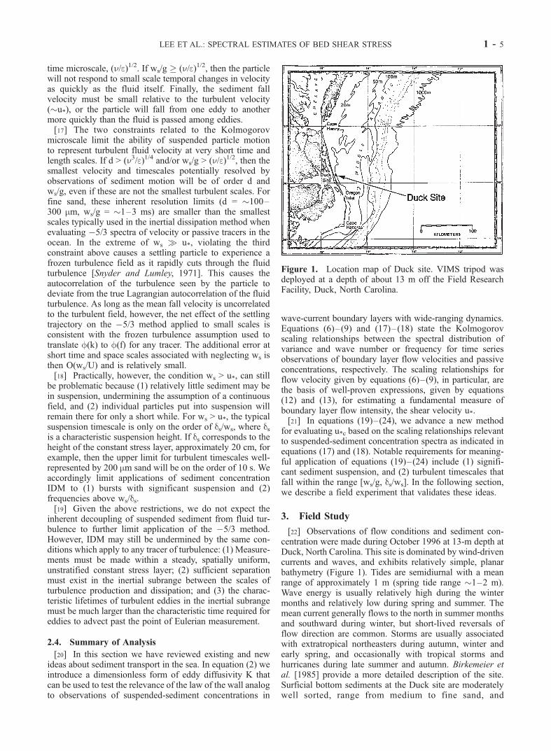
[22] Observations of flow conditions and sediment con-centration were made during October 1996 at 13-m depth atDuck, North Carolina. This site is dominated by wind-drivencurrents and waves, and exhibits relatively simple, planarbathymetry (Figure 1). Tides are semidiurnal with a meanrange of approximately 1 m (spring tide range �1–2 m).Wave energy is usually relatively high during the wintermonths and relatively low during spring and summer. Themean current generally flows to the north in summer monthsand southward during winter, but short-lived reversals offlow direction are common. Storms are usually associatedwith extratropical northeasters during autumn, winter andearly spring, and occasionally with tropical storms andhurricanes during late summer and autumn. Birkemeier etal. [1985] provide a more detailed description of the site.Surficial bottom sediments at the Duck site are moderatelywell sorted, range from medium to fine sand, and

Figure 1. Location map of Duck site. VIMS tripod wasdeployed at a depth of about 13 m off the Field ResearchFacility, Duck, North Carolina.


volumetrically comprise silts and clays to less than 10percent [Lee et al., 2002]. The median size, ds, of sedimentin samples collected by divers is 0.012 cm, for which therelative excess density s = 1.65, the settling velocity ws =1.0 cm/s in seawater of characteristic density and viscosity[Dietrichs, 1982]. Divers’ observations indicate that at thetime of deployment the seabed was weakly rippled.[23] Instrumentation deployed at Duck included five

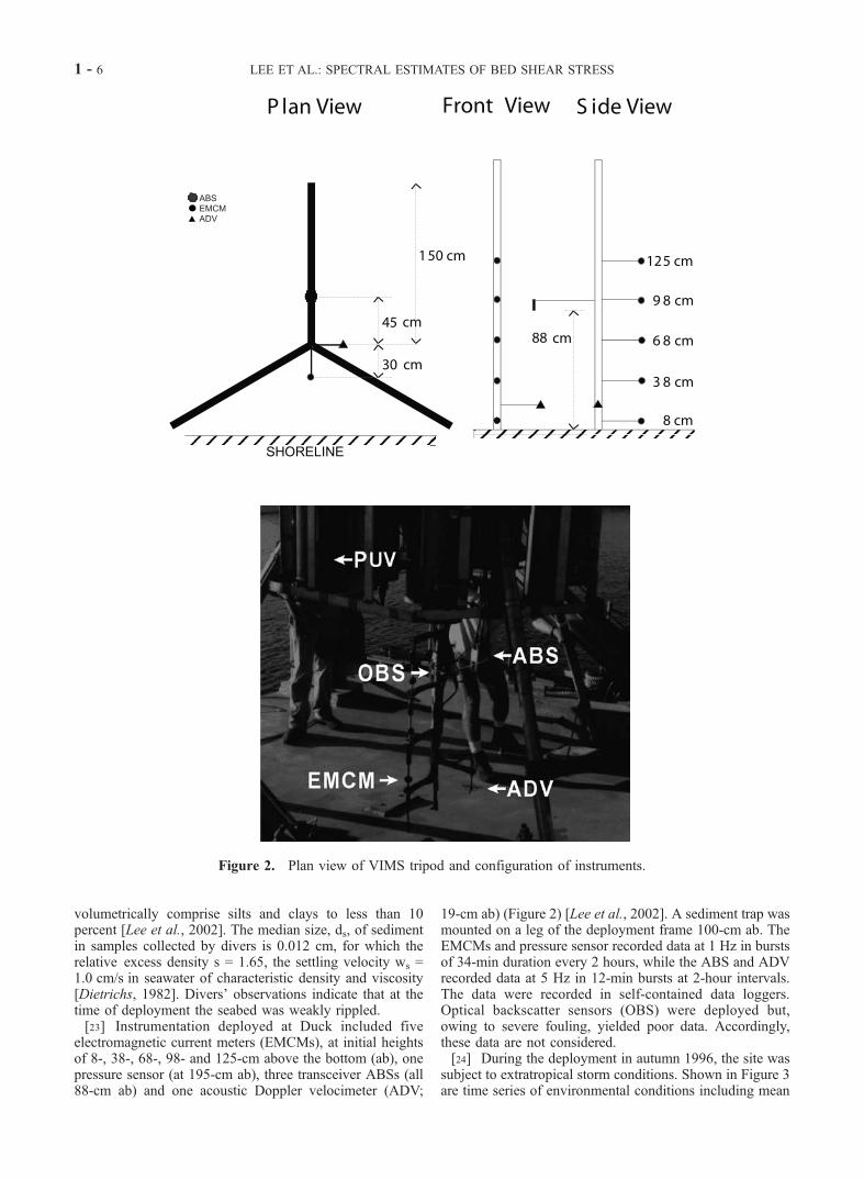
electromagnetic current meters (EMCMs), at initial heightsof 8-, 38-, 68-, 98- and 125-cm above the bottom (ab), onepressure sensor (at 195-cm ab), three transceiver ABSs (all88-cm ab) and one acoustic Doppler velocimeter (ADV;

19-cm ab) (Figure 2) [Lee et al., 2002]. A sediment trap wasmounted on a leg of the deployment frame 100-cm ab. TheEMCMs and pressure sensor recorded data at 1 Hz in burstsof 34-min duration every 2 hours, while the ABS and ADVrecorded data at 5 Hz in 12-min bursts at 2-hour intervals.The data were recorded in self-contained data loggers.Optical backscatter sensors (OBS) were deployed but,owing to severe fouling, yielded poor data. Accordingly,these data are not considered.[24] During the deployment in autumn 1996, the site was

subject to extratropical storm conditions. Shown in Figure 3are time series of environmental conditions including mean

Figure 2. Plan view of VIMS tripod and configuration of instruments.


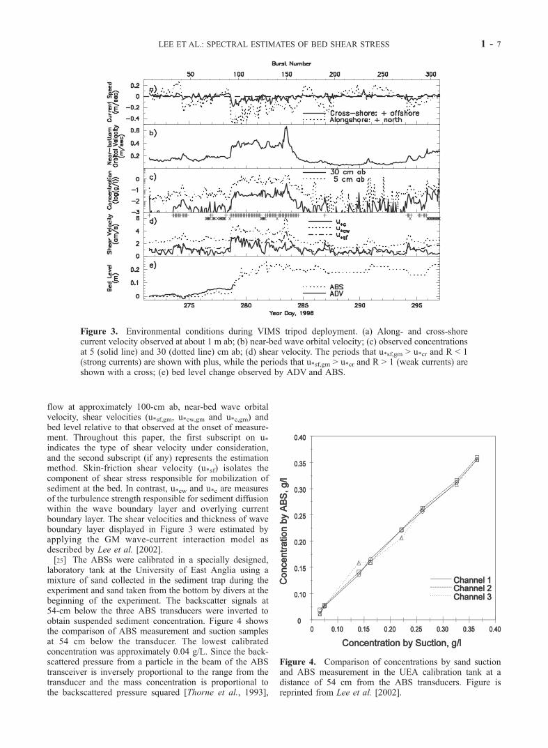
flow at approximately 100-cm ab, near-bed wave orbitalvelocity, shear velocities (u*sf,gm, u*cw,gm and u*c,gm) andbed level relative to that observed at the onset of measure-ment. Throughout this paper, the first subscript on u*indicates the type of shear velocity under consideration,and the second subscript (if any) represents the estimationmethod. Skin-friction shear velocity (u*sf) isolates thecomponent of shear stress responsible for mobilization ofsediment at the bed. In contrast, u*cw and u*c are measuresof the turbulence strength responsible for sediment diffusionwithin the wave boundary layer and overlying currentboundary layer. The shear velocities and thickness of waveboundary layer displayed in Figure 3 were estimated byapplying the GM wave-current interaction model asdescribed by Lee et al. [2002].[25] The ABSs were calibrated in a specially designed,

laboratory tank at the University of East Anglia using amixture of sand collected in the sediment trap during theexperiment and sand taken from the bottom by divers at thebeginning of the experiment. The backscatter signals at54-cm below the three ABS transducers were inverted toobtain suspended sediment concentration. Figure 4 showsthe comparison of ABS measurement and suction samplesat 54 cm below the transducer. The lowest calibratedconcentration was approximately 0.04 g/L. Since the back-scattered pressure from a particle in the beam of the ABStransceiver is inversely proportional to the range from thetransducer and the mass concentration is proportional tothe backscattered pressure squared [Thorne et al., 1993],

Figure 3. Environmental conditions during VIMS tripod deployment. (a) Along- and cross-shorecurrent velocity observed at about 1 m ab; (b) near-bed wave orbital velocity; (c) observed concentrationsat 5 (solid line) and 30 (dotted line) cm ab; (d) shear velocity. The periods that u*sf,gm > u*cr and R < 1(strong currents) are shown with plus, while the periods that u*sf,gm > u*cr and R > 1 (weak currents) areshown with a cross; (e) bed level change observed by ADV and ABS.

Figure 4. Comparison of concentrations by sand suctionand ABS measurement in the UEA calibration tank at adistance of 54 cm from the ABS transducers. Figure isreprinted from Lee et al. [2002].


the accuracy of the ABSs corresponds to �0.005 g/L at adistance of 20 cm from the transducer.

4. Data Analysis

[26] The following analysis was applied to ADV data(sampling bursts 1–90) recorded before the onset of a stormin early October 1996 (calendar day 279), after which thereliability of the ADV data came into question owing tosensor proximity (to within 3 cm) to an accreting bed. Errorsin near-bed flow measurements associated with bed prox-imity have been noted elsewhere and attributed to significantincreases in random motion of scattering targets and meanvelocity shear within the sampling volume [Voulgaris andTrowbridge, 1998]. For bursts 1–90 the ADV samplingvolume was an average distance of 16.5 cm from the bed.Although all 309 bursts of ABS data were analyzed, resultsof ABS data analysis are only presented for bursts whereenergy conditions were sufficient to suspend sand. Thecritical condition is determined as u*sf,gm > u*cr (criticalshear velocity for initiation of motion) because for mediangrain size (120 mm) of bed sediment at Duck critical shearvelocity for initiation of motion (u*cr = 1.22 cm/s) is greaterthan critical shear velocity for suspension (ws = 1.01 cm/s).During the period of u*sf,gm > u*cr, concentration at 30 cm abin general exceeds the calibrated ABS accuracy, 0.005 g/l(Figure 3). These bursts are indicated in Figure 3d.[27] Standard transformations of time series observations

of flow velocities and suspended sediment concentrationswere used to obtain their Fourier spectra [e.g., Bendat andPiersol, 1986]. Original time series of velocities and ABSconcentration measurements comprised 3072 and 2048records, respectively, and, following conventional prewhit-ening of the series, were partitioned into segments of equallength (each 512 records) and with 50 percent overlap withadjoining segments. A Hanning window was applied to eachsegment before Fourier transformation. The resulting spectrawere arithmetically averaged, thus the 95 percent confidenceintervals correspond to 0.61–1.94 times and 0.54–2.48times the smoothed spectral estimates of velocity and con-centration data, respectively. The resulting estimates of u*care proportional to the square root of the power density of thevelocity and concentration spectra. At the 95 percent confi-dence level, therefore, uncertainty on estimates at eachfrequency amounts to approximately 40 percent and 60percent for flow- and sediment-spectral values, respectively.Standard errors of u*c estimates, obtained by averaging overan inertial subrange of frequencies, amount to no more thanabout 10 percent of the reported values. The criteria used toidentify the inertial subranges are described below.[28] The inertial dissipation method has been criticized as

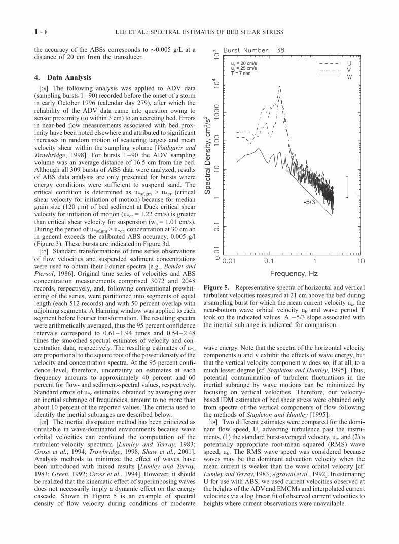
unreliable in wave-dominated environments because waveorbital velocities can confound the computation of theturbulent-velocity spectrum [Lumley and Terray, 1983;Gross et al., 1994; Trowbridge, 1998; Shaw et al., 2001].Analysis methods to minimize the effect of waves havebeen introduced with mixed results [Lumley and Terray,1983; Green, 1992; Gross et al., 1994]. However, it shouldbe realized that the kinematic effect of superimposing wavesdoes not necessarily imply a dynamic effect on the energycascade. Shown in Figure 5 is an example of spectraldensity of flow velocity during conditions of moderate

wave energy. Note that the spectra of the horizontal velocitycomponents u and v exhibit the effects of wave energy, butthat the vertical velocity component w does so, if at all, to amuch lesser degree [cf. Stapleton and Huntley, 1995]. Thus,potential contamination of turbulent fluctuations in theinertial subrange by wave motions can be minimized byfocusing on vertical velocities. Therefore, our velocity-based IDM estimates of bed shear stress were obtained onlyfrom spectra of the vertical components of flow followingthe methods of Stapleton and Huntley [1995].[29] Two different estimates were compared for the domi-

nant flow speed, U, advecting turbulence past the instru-ments, (1) the standard burst-averaged velocity, uc, and (2) apotentially appropriate root-mean squared (RMS) wavespeed, ub. The RMS wave speed was considered becausewaves may be the dominant advection velocity when themean current is weaker than the wave orbital velocity [cf.Lumley and Terray, 1983;Agrawal et al., 1992]. In estimatingU for use with ABS, we used current velocities observed atthe heights of the ADVand EMCMs and interpolated currentvelocities via a log linear fit of observed current velocities toheights where current observations were unavailable.

Figure 5. Representative spectra of horizontal and verticalturbulent velocities measured at 21 cm above the bed duringa sampling burst for which the mean current velocity uc, thenear-bottom wave orbital velocity ub and wave period Ttook on the indicated values. A �5/3 slope associated withthe inertial subrange is indicated for comparison.


[30] In estimating bed shear stress from velocity, weconsider the inertial spectral subrange to be bounded bylower wave number and frequency limits of 2p/z and U(z)/z,respectively [Green, 1992; Stapleton and Huntley, 1995],and by upper wave number and frequency limits of 2p/l0and U(z)/l0, respectively, where l0 corresponds to the largervalue of either the sensor averaging length or U(z)/f0 forwhich f0 is the sampling Nyquist frequency. For concentra-tion, the practical upper limits are given by the sameformulae, but the lower limiting frequency due to particlesettling can be ws/ds (see section 2.3), corresponding to alimiting wave number of (2p/U)(ws/ds). For the ADVmeasurements (10 MHz, sampling 10 cm below probe),the averaging length is 1 cm; for ABS settings duringthe Duck deployment (a transmission half angle of 2.5�;2 MHz), the length scale associated with the far-fieldsampling volume at 50 cm from the acoustic source is about4.4 cm [c.f. Hay, 1991]. In general, flow speeds associatedwith marked sediment transport were 5 cm/s or greater forwhich lower-limiting inertial frequencies at 10-cm ab werethus of order 0.5 Hz. For a conservatively low sedimentsuspension height of ds = 10 cm, ws/ds is of order 0.1 Hz,which is a less stringent constraint than U(z)/l0. The upperlimits of the inertial subrange in the ABS spectra typicallycorresponded to the Nyquist frequency of 2.5 Hz.

5. Results

5.1. Vertical Structure of Eddy Diffusivity FromSuspended Sediment Concentrations

[31] In calculating dimensionless eddy diffusivity fromsuspended sediment concentrations, only cases for which

u*sf,gm exceeded the critical value for initiation of motion u*crwere considered; the number of bursts was thus 133 out of atotal of 309. The selected bursts were grouped into strong andweak current cases according to a scaling parameter, R. Thescaling parameter, R, is the ratio of the vertical advectionvelocity relative to the mean current at the top of the GMwave boundary layer [Lee et al., 2002]. The vertical advec-tion or ‘‘jet’’ velocity is defined as (h/l)ub where h and l arethe modeled ripple height and ripple length [Wiberg andHarris, 1994], respectively. Periods with R < 1 correspond tostrong current conditions for which the dominant suspensionprocess is assumed to be turbulent diffusion associated withcurrent-generated turbulence outside the wave boundarylayer. There were 95 cases out of 133 with strong currents.These cases are shown with an asterisk in Figure 3c. Caseswith R > 1 generally correspond to weak currents, but wavesstrong enough to suspend sediment from the bed. For R > 1,the dominant mechanism for initial sediment suspension isnot near-bed turbulent diffusion, but wave-generated shed-ding vortices [Lee et al., 2002]. There were 38 bursts forweak currents; these are shown with a cross in Figure 3c.[32] Two pairs of median and quartile estimates of non-

dimensionalized eddy diffusivity K+, defined in equation(2), are shown in Figure 6 as a function of relative heightz/dw, where dw = 2u*cw,gm/w. Strong current cases are shownin Figures 6a and 6b, while weak current cases are presentedin Figures 6c and 6d. For each of the two pairs, one of thepair was normalized by u*c,gm (i.e., K+c, Figures 6a and 6c)and the other by u*cw,gm (i.e., K+cw, Figures 6b and 6d). Forcomparison, K+ normalized by u*c,fit, where u*c,fit wasdetermined by a best fit to observed current log-profiles(equation (3)), is also shown in Figure 6a by the solid circles

Figure 6. Inferred values of nondimensional eddy diffusivity K+ as a function of relative elevationz/dw in flows for which u*sf exceeds the critical value for initiation of motion u*cr. Under strong currents(R < 1), eddy diffusivity was scaled with u*c as shown in Figure 6a, while under weak currents, eddydiffusivities were scales with u*cw as shown in Figure 6d. Figures 6b and 6d are plotted for comparisonwith Figures 6a and 6c with u*cw and u*c, respectively.


and dashed error bars. Note that nondimensionalized eddydiffusivities for each burst were interpolated into z/dw spacebefore obtaining median and quartile estimates.[33] In general, eddy diffusivity increases linearly with

elevation and u* to a height of about five times the waveboundary layer thickness dw. From Figures 6a and 6d, it isevident that eddy diffusivities for strong currents are scaledby u*c, while eddy diffusivities for weak currents are scaledby u*cw. For cases of strong currents, Figure 6a validatestwo fundamental assumptions necessary for the analyticaldevelopment of the inertial dissipation method in sections2.2 and 2.3: (1) K � ku*z and (2) the equality of eddydiffusivities for mass and momentum. The first assumptionfurther implies that stratification due to sediment suspensionis dynamically unimportant. For cases of weak currents,Figure 6d suggests that wave-induced turbulence in theabsence of currents often penetrates much higher thanpredicted by the classical value for dw. This further suggeststhe likelihood that the spectral methods developed abovewill be influenced by u*cw if applied at z < �6dw for casesof weak currents.

5.2. Bed Shear Stress Estimation FromVelocity Measurements

[34] An example of spectral density of flow velocityduring conditions of moderate wave energy is shown inFigure 5. The inertial subrange is clearly marked with a�5/3slope. For the 90 sampling bursts considered here, the meanslope of the spectra of vertical velocities in the frequencyrange 0.3–2 Hz is �1.51 ± 0.16 SE (95% standard error).This value is only slightly smaller than the value of �5/3expected for Kolmogorov scaling in the inertial subrange.[35] Figure 7 shows ratios of IDM shear velocity esti-

mates obtained from the w-velocity spectra (u*c,ADV) andGM shear velocity estimates (u*c,gm) as a function of u*c,gm/ws and uc/ub. Estimates with (without) Huntley’s correctiongiven by equation (16), which used uc as the advectionvelocity, are shown as open circles (solid squares) inFigure 7a. Under conditions of relatively small values ofu*c,gm/ws (<1), the spectral estimates of the shear velocityare consistently larger than those yielded by the GM model.The overestimation of u*c,ADV at small values of u*c,gm/ws

(<1) may be due to a poorly developed region of constantstress in the wave-current boundary layer for which theinertial dissipation method is not likely to apply. It is notedthat a u*c value of �0.7 cm/s (equivalent u*c,gm/ws � 1) issimilar to the minimum value (u*c = 0.8 ± 0.2 cm/s) thatHuntley [1988] identified below which the inertial dissipa-tion method is not likely to apply.[36] In contrast, under conditions of intense flow for which

u*c,gm/ws is relatively large, spectral estimates using equation(13) subject to Huntley’s correction are in good agreement(Figure 7a). The ratio of u*c,ADV to u*c,gm estimates has amean value of 1.09 ± 0.05 SE (0.67 ± 0.04 SE) for with(without) the Huntley correction. Assuming Gaussian statis-tics, this mean value with the Huntley correction is notstatistically different from unity. Overall, the significanceof the Huntley correction is indicated by the consistent lack ofagreement between GM and uncorrected IDM estimates.[37] Estimates of Huntley-corrected u*c,ADV/u*c,gm with uc

and ub as the advection velocity are shown in Figure 7b as afunction of uc/ub. The absolute differences, abs u*c;ADV ub�

�

u*c;ADV ucÞ=u*c;ADV ub , between the two estimates with ucand ub are also shown in Figure 7b. The differencesbetween two estimates are less than 10% during the periodswhen waves and currents have similar strength (uc/ub > 0.7).As the RMS wave velocity increases relative to the meancurrent (uc/ub < 0.7), the spectral estimates of shear stresswith ub reduce the overestimation significantly (up to 100percent at the lowest ratio of uc/ub). Nonetheless, theestimates still significantly deviate from the actual shearstress. The systematic overestimate of shear velocity rela-tive to u*c,gm for small uc/ub in Figure 7b may indicate theinfluence of u*cw on u*c,ADV for cases such as those inFigure 6d where periodic wave-generated turbulenceappears to penetrate well beyond the traditional waveboundary layer.

Figure 7. (a) Shear velocity estimates from the conven-tional inertial dissipation method as a function of u*c,gm/ws.The estimates are normalized by the corresponding u*,gm.Circles and squares indicate estimates with and withoutHuntley’s correction, respectively. Mean current velocity isused as the advection velocity. (b) Normalized shearvelocity estimates by u*,gm as a function of uc/ub. Circlesand asterisks indicate estimates with uc and ub as theadvection velocity, respectively. Triangles represent theabsolute difference between two estimates.


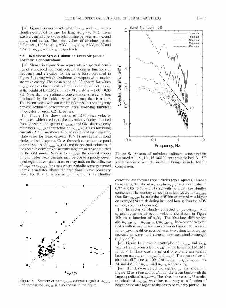
[38] Figure 8 shows a scatterplot of u*c,gm and u*c,fit versusHuntley-corrected u*c,ADV for large u*c,gm/ws (>1). Thereexists a general one-to-one relationship between u*c,ADVandu*c,gm (and u*c,fit). The mean values of absolute percentdifferences, 100* abs u*c;ADV� u*cð Þ=u*c;ADV, are 37 and35% for u*c,gm and u*c,fit, respectively.

5.3. Bed Shear Stress Estimation From SuspendedSediment Concentrations

[39] Shown in Figure 9 are representative spectral densi-ties of suspended sediment concentrations as functions offrequency and elevation for the same burst portrayed inFigure 5, during which conditions corresponded to moder-ate wave energy. The mean slope of 133 spectra for whichu*sf,gm exceeds the critical value for initiation of motion u*crat the height of EMCM2 (initially 38 cm ab) is �1.60 ± 0.05SE. Note that the sediment concentration spectra is lessdominated by the incident wave frequency than is u or v.This is consistent with our earlier inference that settling mayprevent sediment concentration from resolving turbulenttime-scales of order 0.2 Hz or less.[40] Figure 10a shows ratios of IDM shear velocity

estimates, which used uc as the advection velocity, obtainedfrom concentration spectra (u*c,ABS) and GM shear velocityestimates (u*c,gm) as a function of u*c,gm/ws. Cases for strongcurrents (R < 1) are shown as open circles and open squares,while cases for weak currents (R > 1) are shown as solidcircles and solid squares. Cases for weak currents correspondto small values of u*c,gm/ws (<1) and the spectral estimates ofthe shear velocity are consistently larger than those predictedby the GM model. Similar to u*c,ADV, the overestimationu*c,ABS under weak currents may be due to a poorly devel-oped region of constant stress or may indicate the influenceof u*cw on u*c,ABS for cases where periodic wave-generatedvortex penetrates above the traditional wave boundarylayer. For R < 1, estimates with (without) the Huntley

correction are shown as open circles (open squares). Amongthese cases, the ratio of u*c,ABS to u*c,gm has a mean value of0.87 ± 0.05 (0.60 ± 0.03) SE with (without) the Huntleycorrection. The Huntley correction is less severe for u*c,ABSthan for u*c,ADV because the ABS bin examined was higheron average (24 cm ab during included bursts) than the ADVsensing volume (17 cm ab).[41] Estimates of Huntley-corrected u*c,ADV/u*c,gm with

uc and ub as the advection velocity are shown in Figure10b as a function of uc/ub. The absolute differences,abs u*c;ABS ub � u*c;ABS uc

� �=u*c;ABS ub , between the two esti-

mates with uc and ub are also shown in Figure 10b. As seenfor u*c,ADV, the differences between two estimates of u*c,ABSdecrease as waves and currents approach similar strength(uc/ub > 0.7).[42] Figure 11 shows a scatterplot of u*c,gm and u*c,fit

versus Huntley-corrected u*c,ABS (at the height of EMCM2)for R < 1. There exists a general one-to-one relationshipbetween u*c,ABS and u*c,gm (and u*c,fit). The mean values ofabsolute differences, 100*abs u*c;ABS � u*c

� �=u*c;ABS, are

34 and 43% for u*c,gm and u*c,fit, respectively.[43] Huntley-corrected u*c,ABS/u*c,gm are shown in

Figure 12 as a function of z/dw for the seven bursts with thelargest predicted u*c,gm/ws. The advection velocity U neededto calculated u*c,ABS was chosen to vary as a function ofheight based on a log-fit to the observed velocity profile. The

Figure 8. Scatterplot of u*c,ADV estimates against u*c,gm.For comparison, u*c,fit is also shown in the figure.

Figure 9. Spectra of turbulent sediment concentrationsmeasured at 1-, 5-, 10-, 15- and 20-cm above the bed. A�5/3slope associated with the inertial subrange is indicated forcomparison.


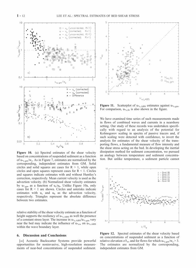
relative stability of the shear velocity estimate as a function ofheight supports the resiliency of u*c,ABS as well the presenceof a constant stress layer. The increase in u*c,ABS/u*c,gm verynear the bed may indicate the influence of u*cw on u*c,ABSwithin the wave boundary layer.

6. Discussion and Conclusions

[44] Acoustic Backscatter Systems provide powerfulopportunities for noninvasive, high-resolution measure-ments of near-bed concentrations of suspended sediment.

We have examined time series of such measurements madein flows of combined waves and currents in a nearshoresetting. Our study of these records was undertaken specifi-cally with regard to an analysis of the potential forKolmogorov scaling in spectra of passive tracers and, ifsuch scaling were detected with confidence, to invert theanalysis for estimates of the shear velocity of the trans-porting flows, a fundamental measure of flow intensity andthe shear stress acting on the bed. In developing the inertialdissipation method for sediment concentration, we pursuedan analogy between temperature and sediment concentra-tion. But unlike temperature, a sediment particle cannot

Figure 10. (a) Spectral estimates of the shear velocitybased on concentrations of suspended sediment as a functionof u*c,gm/ws. As in Figure 7, estimates are normalized by thecorresponding, independent estimates from GM. Solidcircles and solid squares are cases for R > 1, while opencircles and open squares represent cases for R < 1. Circlesand squares indicate estimates with and without Huntley’scorrection, respectively. Mean current velocity is used as theadvection velocity. (b) Normalized shear velocity estimatesby u*,gm as a function of uc/ub. Unlike Figure 10a, onlycases for R < 1 are shown. Circles and asterisks indicateestimates with uc and ub as the advection velocity,respectively. Triangles represent the absolute differencebetween two estimates.

Figure 11. Scatterplot of u*c,ABS estimates against u*c,gm.For comparison, u*c,fit is also shown in the figure.

Figure 12. Spectral estimates of the shear velocity basedon concentrations of suspended sediment as a function ofrelative elevation z/dw, and for flows for which u*c,gm/ws > 3.The estimates are normalized by the corresponding,independent estimates from GM.


resolve the shortest scales of turbulent fluid motion if itssize or inertial response time is greater than the Kolmo-gorov microscales. For fine sand, these ultimate resolutionlimits are still much smaller than the sampling volumes andresponse times of field instrumentation typically applied toIDM.[45] An analysis of the observed vertical structure of

suspended sediment in terms of the conventional Rouseequation indicate an approximately linear relationshipbetween eddy diffusivity of mass and height above thebed to elevations of at least 20 cm or equivalently, for theflow conditions observed, more than 4–5 times the waveboundary layer thickness. In particular, eddy diffusivityprofiles were scaled with u*c under strong currents. Duringweak currents, eddy diffusivity profiles were scaled withu*cw and the vertical length scale extended about 5 times theclassical wave boundary layer (Figure 6). The implicationfrom these results is clear in that u*cw must be used for weakcurrents even above the classical wave boundary layer in theRouse-type equation as suggested by Lee et al. [2002] or anapproach other than a diffusion model must be adopted formodeling sediment suspension under weak current condi-tions. Although the finding that eddy diffusivity follows alaw-of-the-wall formulation equivalent to eddy viscosity isnot surprising, its confirmation is fundamental to manytransport models and indeed, underpins the followingcomponents of our analysis. Furthermore, the agreementbetween eddy diffusivity and an unstratified model for eddyviscosity during strong currents suggests that density strati-fication due to suspended sediment is not dynamicallyimportant.[46] Dimensional analysis predicts and we observe Kol-

mogorov scaling in the inertial subrange, spanning frequen-cies of order 1 Hz, of power spectra of not only the flowitself, but also of concentrations of suspended sediment nearthe bed. The existence of �5/3 slope observed fromconcentration spectra within appropriate frequency boundsindicates that sand particles are effectively passive tracers ofthe turbulent motions of the suspending fluid, and thus canbe used to study the structure and intensity of marineboundary layers over mobile beds. However, our earlierfinding that u*cw dominates the Rouse profile above thetraditional wave boundary layer during weak current con-ditions suggests that the application of inertial dissipationtechnique for determining u*c should be limited to caseswith relatively strong currents. Furthermore, in relativelyslow flows for which the shear velocity was less than about0.8, spectral estimates of the flow shear velocity u* wereconsistently larger than estimates inferred from GM. This istrue for spectral estimates based on flow and sedimentconcentration observations alike.[47] In applying this method to sufficiently intense mean

flows, we find that at elevations between one and four timesthe thickness of the wave boundary layer, estimates of theshear velocity obtained from Kolmogorov scaling in thesuspended sediment spectra consistently agree to within afactor of 2 with similar estimates from flow spectra andindependent estimates from log-fits to the velocity profile aswell as a widely used wave-current model [Grant andMadsen, 1986]. In addition, we note that an importantaspect of conventional and new spectral analyses alike isthe correction introduced by Huntley [1988] for observa-

tions made in near-bed flows characterized by insufficientseparation of the scales of turbulence production anddissipation. The physical meaning of the correction is stillunclear and the significance of this correction for suspendedsediment concentration spectra is still a focus of study.[48] Sources of the discrepancies up to a factor of 1 or 2

which do exist between the various estimates at this timeinclude poor constraints on empirical model parameters(e.g.,as introduced in equations (7) and (8), for which thevalue of 0.71 used here, well-established for scalar quanti-ties, may not be strictly applicable for suspended sediment).Another source of significant error may be the characteristicsettling velocity, ws, which we set to be constant in time andwith height above the bed. It is widely known that gradingof sediment suspensions occur with elevation. More accu-rate, time and/or elevation-varying settling velocity mayimprove shear velocity estimates made in the future. Wealso acknowledge that the sampling rate of 5 Hz limited ourresolution of the entire inertial subrange and thus our abilityto confidently estimate shear velocity. In order to improvefuture estimation, a higher sampling rate is desirable.[49] We have advanced here the development and appli-

cation of a theory for spectral scaling in suspended sedimentconcentrations observed near the seabed. One application ofthe analysis focuses on an inversion of the theory forestimates of bed shear stress. We conclude that the approachshows significant promise. In this regard, we also note thatif bed shear stress is known independently, one can usespectral scaling relationships for suspended sediment con-centrations to estimate either the characteristic settlingvelocity (or equivalent sediment size) of the material insuspension or bed roughness, provided one or the otherquantity is known. Such applications could provide power-ful, new noninvasive tools to resolve, for example, fre-quently encountered discrepancies between the inferredcaliber of materials comprising the bed and in suspension[e.g., Lee et al., 2002]. Work on extending the analysisdeveloped here is currently underway.

NotationGeneral

c0 fluctuating part of sediment concentration.C time-averaged sediment concentration (g/L).d suspended sediment particle size.f frequency.fo Nyquist frequency.k wave number.K eddy diffusivity (cm2/s).K+ dimensionless eddy diffusivity.K+c dimensionless eddy diffusivity scaled with shear

velocity due to currents.K+cw dimensionless eddy diffusivity scaled with shear

velocity due to the combined effect of waves andcurrents.

lo sensor averaging length.R scaling parameter.

Recr critical Reynolds number.U dominant flow speed.u total instantaneous flow velocity.ub root-mean squared wave speed.uc time-averaged current velocity.


u* characteristic shear velocity.u*c shear velocity due to currents.u*cr critical shear velocity.u*cw shear velocity due to the combined effect of waves

and currents.u*sf skin-friction shear velocity.u*c shear velocity corrected by using the Huntley’s

correction.ws settling velocity of sediment grains (cm/s).z height above the bed.

zcr critical height above which measurements must bemade to ensure an inertial subrange.

aii empirical constant in equations (6) and (9).as empirical constant in equations (17) and (18).ds characteristic sediment suspension heightdw thickness of wave boundary layer.e rate of TKE dissipation.es rate of dissipation of sediment fluctuation.fii TKE spectrum.fs spectrum of sediment concentration.h ripple height.k von Karman’s constant.l ripple length.n kinematic viscosity of seawater.r density of seawater.tc bed shear stress associated with currents.w wave radian frequency.

Subscript

ABS shear velocity measured by inertial dissipationmethod of sediment concentration.

ADV shear velocity measured by inertial dissipationmethod of flow.

gm shear velocity measure by the GM wave-currentinteraction model.

ub rms wave speed was used as characteristic advectionvelocity for IDM.

uc time-averaged current speed was used as character-istic advection velocity for IDM.

[50] Acknowledgments. G.L. and W.B.D. gratefully acknowledgethe support of the (UK) Atomic Energy Authority and the (UK) NaturalEnvironmental Research Council. Participation by C.T.F. and field studiesat Duck, N. C., were supported by the (U.S.) National Science Foundation.

ReferencesAgrawal, Y. C., E. A. Terray, M. A. Donelan, P. A. Hwang, A. J. WilliamsIII, W. M. Drennan, K. K. Kahma, and S. A. Kitaigorodskii, Enhanceddissipation of kinetic energy beneath surface waves, Nature, 359, 219–220, 1992.

Bendat, J. S., and A. G. Piersol, Random Data: Analysis and MeasurementProcedures, 566 pp., John Wiley, New York, 1986.

Birkemeier, W. A., H. C. Miller, S. D. Wilhelm, A. E. DeWall, and C. S.Gorbics, A user’s guide to the Coastal Engineering Research Center’sField Research Facility, Instruct. Rep. CERC-85-1, Coastal Eng. Res.Cent., U.S. Army Corps of Eng., Vicksburg, Miss., 1985.

Dade, W. A., A. J. Hogg, and B. P. Bourdreau, Hydrodynamics of thebenthic boundary layer, in The Benthic Boundary Layer, edited by B. P.Boudreau and B. B. Jorgensen, pp. 4–43, Oxford Univ. Press, New York,2001.

Dietrichs, W. E., Settling velocity of natural particles, Water Resour. Res.,18, 1615–1621, 1982.

Glenn, S. M., and W. D. Grant, A suspended sediment stratification correc-tion for combined wave and current flow, J. Geophys. Res., 92, 8244–8264, 1987.

Grant, W. D., and O. S. Madsen, The continental shelf bottom boundarylayer, Ann. Rev. Fluid Mech., 18, 265–305, 1986.

Green, M. O., Spectral estimates of bed stress at subcritical Reynoldsnumbers in a tidal boundary layer, J. Phys. Oceanogr., 22, 903–917,1992.

Gross, T. F., and A. R. M. Nowell, Spectral scaling in a tidal boundarylayer, J. Phys. Oceanogr., 15, 496–508, 1985.

Gross, T. F., A. J. Williams III, and E. A. Terray, Bottom boundary layerspectral dissipation estimates in the presence of wave motions, Cont.Shelf Res., 14, 1239–1256, 1994.

Hay, A. E., Sound scattering from a particle-laden, turbulent jet, J. Acoust.Soc. Am., 90, 2055–2074, 1991.

Hay, A. E., and A. J. Bowen, Coherence scales of wave-induced suspendedsand concentration fluctuations, J. Geophys. Res., 99, 12,749–12,765,1994.

Hicks, B. B., and A. J. Dyer, The spectral density technique for thedetermination of eddy flux, Q. J. R. Meteorol. Soc., 98, 838–844,1972.

Huntley, D. A., A modified inertial dissipation method for estimatingseabed stresses at low Reynolds numbers, with applications to wave/current boundary layer measurements, J. Phys. Oceanogr., 18, 339–346, 1988.

Kim, S.-C., C. T. Friedrichs, J. P.-Y. Maa, and L. D. Wright, Estimatingbottom stress in tidal boundary layer from Acoustic Doppler Velocimeterdata, J. Hydraul. Eng., 126, 399–406, 2000.

Kundu, P. K., Fluid Mechanics, 638 pp., Academic Press, San Diego,Calif., 1990.

Lee, G., C. T. Friedrichs, and C. E. Vincent, Examination of diffusionversus advection dominated sediment suspension on the inner shelf understorm and swell condition, Duck, North Carolina, J. Geophys. Res., 107,3084, doi:10.1029/2001JC000918, 2002.

Lee, T. H., and D. M. Hanes, Comparison of field observations of thevertical distribution of suspended sand and its prediction by models, J.Geophys. Res., 101, 3561–3572, 1996.

Lumley, J. L., Two-phase and non-Newtonian flows, in Topics in AppliedPhysics, vol. 24, edited by P. Bradshaw, pp. 507–527, Springer-Verlag,New York, 1977.

Lumley, J. L., and E. A. Terray, Kinematics of turbulence convected by arandom wave field, J. Phys. Oceanogr., 10, 208–219, 1983.

McPhee, M. G., An inertial-dissipation method for estimating turbulent fluxin buoyancy-driven, convective boundary layers, J. Geophys. Res., 103,3249–3255, 1998.

Sharples, J., C. M. Moore, and E. R. Abraham, Internal tide dissipation,mixing, and vertical nitrate flux at the shelf edge of NE New Zealand,J. Geophys. Res., 106, 14,069–14,082, 2001.

Shaw, W. J., J. H. Trowbridge, and A. J. Williams III, Budgets of turbulentkinetic energy and scalar variance in the continental shelf bottom bound-ary layer, J. Geophys. Res., 106, 9551–9564, 2001.

Sheng, J., and A. E. Hay, Sediment eddy diffusivities in the nearshore zone,from multifrequency acoustic backscatter, Cont. Shelf Res., 15, 129–147,1995.

Sleath, J. F. A., Seabed Mechanics, 355 pp., John Wiley, New York,1984.

Sleath, J. F. A., Seabed boundary layers, in The Sea, vol. 9B, edited byB. Le Mehaute and D. M. Hanes, pp. 693–728, John Wiley, New York,1990.

Smith, J. D., Modeling of sediment transport on continental shelves, in TheSea, vol. 6, edited by E. D. Goldberg et al., pp. 539–577, John Wiley,New York, 1977.

Smith, J. D., and S. R. McLean, Spatially averaged flow over a wavysurface, J. Geophys. Res., 82, 1735–1746, 1977.

Snyder, W. H., and J. L. Lumley, Some measurements of particle velocityautocorrelation functions in a turbulent flow, J. Fluid Mech., 48, 41–71,1971.

Soulsby, R. L., A. P. Salkield, and G. P. Le Good, Measurements of theturbulence characteristics of sand suspended by a tidal current, Cont.Shelf Res., 3, 439–454, 1984.

Stapleton, K. R., and D. A. Huntley, Seabed stress determinations using theinertial dissipation method and the turbulent kinetic energy method,Earth Surf. Processes Landforms, 20, 807–815, 1995.

Tennekes, H., and J. L. Lumley, A First Course in Turbulence, 300 pp.,MIT Press, Cambridge, Mass., 1972.

Thorne, P. D., P. J. Hardcastle, and R. L. Soulsby, Analysis of acousticmeasurements of suspended sediments, J. Geophys. Res., 98, 899–910,1993.

Traykovski, P., A. E. Hay, J. D. Irish, and J. F. Lynch, Geometry, migrationand evolution of wave orbital ripples at LEO-15, J. Geophys. Res., 104,1505–1524, 1999.

Trowbridge, J. H., On a technique for measurement of turbulent shear stressin the presence of surface waves, J. Atmos. Oceanic Technol., 15, 290–298, 1998.


Vincent, C. E., and A. Downing, Variability of suspended sand concentra-tions, transport and eddy diffusivity under non-breaking waves on theshoreface, Cont. Shelf Res., 14, 223–250, 1994.

Vincent, C. E., and M. O. Green, Field measurements of the suspendedsand concentration profiles and fluxes and of the resuspension coeffi-cient go over a rippled bed, J. Geophys. Res., 95, 11,591–11,601,1990.

Vincent, C. E., and P. D. Osborne, Predicting suspended sand concentra-tion profiles on a macro-tidal beach, Cont. Shelf Res., 15, 1497–1514,1995.

Voulgaris, B., and J. H. Trowbridge, Evaluation of the Acoustic DopplerVelocimeter (ADV) for turbulence measurements, J. Atmos. OceanicTechnol., 15, 272–289, 1998.

Wiberg, P. L., and C. K. Harris, Ripple geometry in wave-dominated en-vironments, J. Geophys. Res., 99, 775–789, 1994.

��W. B. Dade, Department of Earth Sciences, Dartmouth College, Hanover,

NH 03755, USA. ([email protected])C. T. Friedrichs, Virginia Institute of Marine Science, College of William

and Mary, Gloucester Point, VA 23062, USA. ([email protected])G.-H. Lee, Korea Ocean Research and Development Institute, 1270

Sadong, Ansan 425-744, South Korea. ([email protected])C. E. Vincent, School of Environmental Sciences, University of East

Anglia, Norwich, NR4 6TJ, UK. ([email protected])


Spectral estimates of bed shear stress using suspended-sediment concentrations in a wave-current...

Documents

Transcript of Spectral estimates of bed shear stress using suspended-sediment concentrations in a wave-current...