ww.sciencedirect.com

wat e r r e s e a r c h 6 4 ( 2 0 1 4 ) 2 6 5e2 7 7

Available online at w

ScienceDirect

journal homepage: www.elsevier .com/locate/watres

Surrogate measures for providing high frequencyestimates of total phosphorus concentrations inurban watersheds

Gaetano Viviano, Franco Salerno*, Emanuela Chiara Manfredi,Stefano Polesello, Sara Valsecchi, Gianni Tartari

CNR e Water Research Institute (IRSA), Via del Mulino 19, Brugherio (MB) 20861, Italy

a r t i c l e i n f o

Article history:

Received 28 February 2014

Received in revised form

30 June 2014

Accepted 3 July 2014

Available online 11 July 2014

Keywords:

Surrogate measures

Total phosphorus

Turbidity

Caffeine

Urban water quality

Combined sewer overflows

* Corresponding author. IRSA-CNR, Via Del M2004692.

E-mail address: salerno@irsa.cnr.it (F. Sahttp://dx.doi.org/10.1016/j.watres.2014.07.0090043-1354/© 2014 Elsevier Ltd. All rights rese

a b s t r a c t

Until robust in situ sensors for total phosphorus (TP) are developed, continuouswater quality

measurements have the potential to be used as surrogates for generating high frequency

estimates. Their use haswidespread implications for water qualitymonitoring programmes

considering that TP, in particular, is generally recognised as the limiting factor in the process

of eutrophication. Surrogate measures for TP concentration, such as turbidity, have proved

useful within natural and agricultural contexts, but their predictive capability for urban

watersheds is considered more difficult, due to the different sources of TP, though a strict

relationship with turbidity/suspended matter has been clearly described even for these

environments. In this context, we investigated this still unresolved problem for high fre-

quency estimation of TP concentration in urban environments by monitoring a medium-

sized (71 km2) urban watershed (Lambro River watershed, north Italy) in which we detec-

ted 60 active combined sewer overflows, and an its natural sub-basin for comparison. We

found twodifferent relationships between turbidity andTP concentration in the investigated

urbanwatershed that differently describe the prevalence of TP frompoint sources (domestic

wastewaters) or diffuse origin (surface runoff). In this regard, we first characterise the pre-

vailing sources of TP by using a marker for detecting domestic wastewater contamination

(caffeine), then we describe the mutual relationships amongst the continuously monitored

variables (in our case the occurrence of the First Flush and the clockwise turbidity/discharge

hysteresis). Afterwards we discriminate, by observing variables that are continuously

monitored (in our case, the discharge and the turbidity), amongst the continuous surrogate

records according to their sources. In conclusion, we are able to apply the relevant turbidity/

TP regression equations to each turbidity record and, thus, estimate the respective TP con-

centrationswithhigh frequency. If traditional grab sampling techniqueshadbeenemployed,

the contributions of point sources (up to 34% across 237 monitored days) to the total esti-

mated loads would not have been correctly evaluated, whilst the high frequencymonitoring

is able to catch the dynamics that occur over time scales of a fewhours.We conclude that the

reasonable uncertainty obtained in this study can be achieved in other urban watersheds,

but further studies are required forwatershedsof differing sizes anddegrees of urbanisation.

© 2014 Elsevier Ltd. All rights reserved.

ulino 19, Localit�a Occhiate, 20861 Brugherio (MB), Italy. Tel.: þ39 039 21694221; fax: þ39 039

lerno).

rved.

wat e r r e s e a r c h 6 4 ( 2 0 1 4 ) 2 6 5e2 7 7266

1. Introduction

Phosphorus is generally recognised as the limiting factor in

the process of eutrophication and, therefore, is widely used as

an indicator of the trophic conditions of lakes (OECD, 1982;

Schindler et al., 2008). Restoration efforts that aim to control

inputs from sources of phosphorus into watersheds (Goldman

et al., 1993; Elser et al., 2007; Carraro et al., 2012a) are

considered to be important strategies for decreasing the risk

of cyanobacterial blooms in lakes (Carraro et al., 2012a,b).

Determinations of nutrient loads are typically based on the

collection and analysis of grab samples in combination with

instantaneous estimates of discharge, but the frequency and

regularity of traditional sampling methods may not provide a

good representation of the variations in constituent loading of

P. This is particularly relevant in small watershed and in

systems with flashy hydrology (Scholefield et al., 2005; Jones

et al., 2012). For most water quality monitoring programmes,

the frequency of grab sampling is determined by the balance

between the resolution necessary to estimate accurate loads

and the resource costs of sampling (e.g., Jones et al., 2012).

Several Authors recommend high frequency, continuous

monitoring to reduce the uncertainties in load calculations

that result from infrequent sampling efforts and biased esti-

mation methods (Quilbe et al., 2006; Johnes, 2007; Jones et al.,

2012). A large proportion of annual phosphorus loads may be

exported during short periods of high flows (Grayson et al.,

1996; Demars et al., 2005). Moreover, whilst these research

and monitoring efforts are episodically intensive, they

generally have been too limited in their temporal and spatial

scales to adequately address the factors that influence the

development of detrimental events such as harmful algal

blooms, oxygen depletion and fish kills (Glasgow et al., 2004).

In many situations, turbidity (TURB) has been used as a

surrogate measure for the concentration of suspended solids

as well as constituents such as total phosphorus (TP) thatmay

be associated with suspended matter. The justification for the

choice of this proxy is that: (i) the attenuation of light by a

sample of water should be related to the amount of fine sus-

pended material in the water, and (ii) most of the TP trans-

ported in streams is in a particulate form and attached to fine

suspended material (Grayson et al., 1996; Stubblefield et al.,

2007). However, these surrogate relationships are site-

specific (Grayson et al., 1996; Tomlinson and De Carlo, 2003)

and depend greatly on the source of sediment. Grayson et al.

(1996), Kronvang et al. (1997), Stubblefield et al. (2007) and

Jones et al. (2011) reported significant and high TURB/TP cor-

relations both in natural and agricultural watersheds.

Rasmussen et al. (2008) observed that non-urban sites present

the highest correlations, whilst Miguntanna et al. (2010)

highlighted a direct TURB/TP correlation for an urban water-

shed. Grayson et al. (1996) suggested that some of the outliers

in the TURB/TP relationship could be attributed to “First Flush”

events of urban stormwater. According to these studies, the

TURB/TP relationship for an urban watershed seems more

complex because it is influenced by additive factors (mainly

organic matter of anthropogenic origin) than for a natural

watershed (mainly mineral particles as clay, amorphous ox-

ides as iron oxo-hydroxide, etc.), as described by Oliver et al.

(1999). In summary, whilst in literature TURB has been

found to be a suitable proxy for TP concentration in some

natural and agricultural watersheds, its adequacy for urban

environments still requires further insights. Furthermore,

considering that nearly all European rivers drain populated

areas, the need to understand the contributions from both

diffuse and point source pollution has long been recognised

(e.g., Demars et al., 2005).

The objective of this study is to develop a method for

estimating TP concentrations with a high frequency in ur-

banized watersheds. A completely forested watershed and

one urbanized have been continuously monitored with the

same experimental design to evaluate potential discrepancies

in the behaviour of surrogatemeasures in the estimation of TP

concentration between these two environments. The suit-

ability of potential explanatory variables that have been

continuously monitored as surrogate measures for TP con-

centration in the Lambro River, Northern Italy is evaluated.

We first evaluate the effectiveness of surrogate relationships

for TP concentrations. Then, we investigate the different

sources of particulate matter (using Principal Component

Analysis) and attempt to classify samples according to their

source (using Quadratic Discriminant Analysis and the Sup-

port Vector Machines). We conclude by discussing the appli-

cability of this surrogate method to urban systems and

suggesting potential improvements to our approach.

2. Material and Methods

2.1. Site description

The Lambrone watershed (71 km2) is situated on the southern

edge of the Alps (northern Italy) between the two branches of

Lake Como (Lombardy Region) (Fig. 1). The main watercourse

is the Lambro River, which is also the main tributary of

Pusiano Lake. This is amedium-sized subalpine lake (Buraschi

et al., 2005). The lake TP concentration increased until the

mid-1980s (0.2 mg P/L at the 1984 winter overturn) and has

progressively decreased towards the mesotrophic conditions

(TP concentration 0.039 mg P/L at the 2013 winter overturn)

since the construction of a wastewater treatment plant

(WWTP) in 1985. Despite the improvement in the lake's trophicconditions, several cyanobacterial blooms have caused

ecological problems, particularly those of the filamentous

cyanobacterium Planktothrix rubescens (Carraro et al., 2012a,b).

The precipitation in this area is concentrated in spring and

autumn and tends to increase progressively, from 1500mm/yr

to 2000 mm/yr, from south to north along the altitudinal

gradient of thewatershed (Salerno and Tartari, 2009). The soils

of the Pusiano watershed belong to the following 4 groups in

accordance with the WRB1998 classification system (FAO,

ISRIC, ISSS, 1998): Leptosols, Regosols, Cambisols and Phaeo-

zems (Salerno et al., 2014a,b). The elevation ranges from 282 to

1450 m a.s.l. (above sea level), with a mean slope of 24.2�. Thebasin's corrivation time, indicating the susceptibility of the

basin on a temporal scale to a flash flood response (i.e., the

hydrological response), is 4 h. The mean discharge calculated

over the last 10 years is 1.6 m3/s (Salerno and Tartari, 2009).

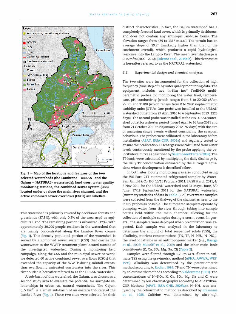
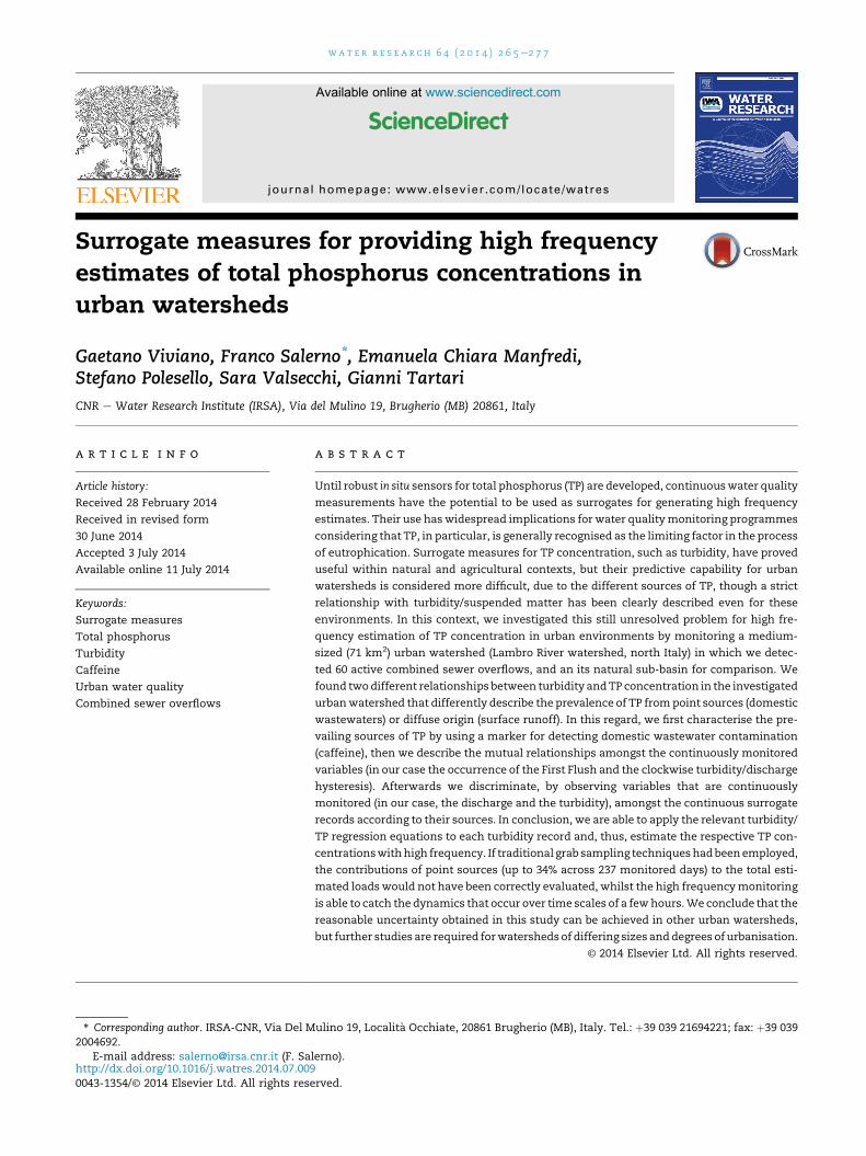
Fig. 1 e Map of the locations and features of the two

selected watersheds (the Lambrone eURBAN- and the

Gajum e NATURAL- watersheds): land uses, water quality

monitoring stations, the combined sewer system (CSS)

located under or close the main river channel, and the

active combined sewer overflows (CSOs) are labelled.

wat e r r e s e a r c h 6 4 ( 2 0 1 4 ) 2 6 5e2 7 7 267

This watershed is primarily covered by deciduous forests and

grasslands (87.5%), with only 0.5% of the area used as agri-

cultural land. The remaining portion is urbanized (12%), with

approximately 30,000 people resident in the watershed that

are mainly concentrated along the Lambro River course

(Fig. 1). This densely populated portion of the watershed is

served by a combined sewer system (CSS) that carries the

wastewater to the WWTP treatment plant located outside of

the investigated watershed. During a monitoring field

campaign, along the CSS and the municipal sewer network,

we detected 60 active combined sewer overflows (CSOs) that

exceeded the capacity of the WWTP during rainfall events,

thus overflowing untreated wastewater into the river. This

river outlet is hereafter referred to as the URBAN watershed.

A sub-basin of this watershed, the Gajum, was chosen as a

second study area to evaluate the potential for surrogate re-

lationships in urban vs. natural watersheds. The Gajum

(5.5 km2) is a small sub-basin of an eastern tributary of the

Lambro River (Fig. 1). These two sites were selected for their

distinct characteristics. In fact, the Gajum watershed has a

completely forested land cover, which is primarily deciduous,

and does not contain any anthropic land-use forms. The

elevation ranges from 489 to 1367 m a.s.l. The terrain has an

average slope of 29.2� (markedly higher than that of the

catchment overall), which produces a rapid hydrological

response into the Lambro River. The mean river discharge is

0.15m3/s (2000e2010) (Salerno et al., 2014a,b). This river outlet

is hereafter referred to as the NATURAL watershed.

2.2. Experimental design and chemical analyses

The two sites were instrumented for the collection of high

frequency (time step of 1 h) water qualitymonitoring data. The

equipment includes two In-Situ Inc© Troll9500 multi-

parametric probes for monitoring the water level, tempera-

ture, pH, conductivity (which ranges from 5 to 20,000 mS/cm

25 �C) and TURB (which ranges from 0 to 2830 nephelometric

turbidity units (NTU)). One probe was installed at the URBAN

watershed outlet from 29 April 2010 to 4 September 2013 (1225

days). The second probe was installed at the NATURAL water-

shedoutlet for a shorter period (from4April to 16 June 2011 and

from 21 October 2011 to 20 January 2012e92 days) with the aim

of analysing single events without considering the seasonal

behaviour. The probes were calibrated in the laboratory before

installation (APAT, IRSA-CNR, 2003a) and regularly tested to

ensure their calibration.Dischargeswere calculated fromwater

levels continuously monitored by the probe applying the ve-

locity/level curveasdescribedbySalernoandTartari (2009).The

TP loads were calculated by multiplying the daily discharge by

the daily TP concentration estimated by the surrogate equa-

tions whose development is described below.

In both sites, hourly monitoring was also conducted using

the WS Porti 24T automated refrigerated sampler by Water-

SamGmbH&Co. KG: 15/16 February 2011, 27/28March 2011, 4/

5 Nov 2011 for the URBAN watershed and 31 May/1 June, 8/9

June, 17/18 September 2011 for the NATURAL watershed

(summary statistics of data in Table 1). All river water samples

were collected from the thalweg of the channel as near to the

in situ probes as possible. The automated samplers operate by

pumping water from the river through tubing into sample

bottles held within the main chamber, allowing for the

collection of multiple samples during a storm event. In gen-

eral, the samplers were deployed when precipitation was ex-

pected. Each sample was analysed in the laboratory to

determine the amount of total suspended solids (TSS), the

alkalinity, nutrient concentrations (TN, TP, NeNH4, NeNO3),

the level of caffeine as an anthropogenic marker (e.g., Buerge

et al., 2003; Musolff et al., 2009) and the other main ionic

constituents (K, Ca, SO4, Mg, Na, Cl) (Table 2).

Samples were filtered through 1.2 mm GF/C filters to esti-

mate TSS using the gravimetric method (APHA, AWWA, WEF,

1995). Alkalinity was determined by the potentiometric

method according to Rodier, 1984. TP and TNwere determined

by colourimetricmethods according to Valderrama (1981). The

concentrations of NeNO3, K, Ca, SO4, Mg, Na and Cl were

determined by ion chromatography according to APAT/IRSA-

CNR Methods (APAT, IRSA-CNR, 2003b,c). NeNH4 was ana-

lysed by the colourimetric method as described by Fresenius

et al., 1988. Caffeine was determined by ultra-high

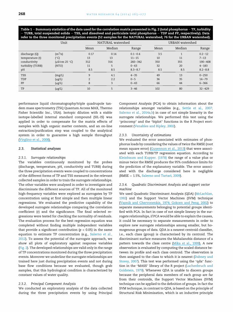
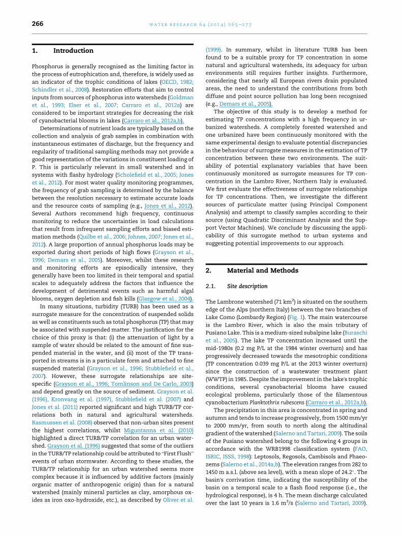
Table 1e Summary statistics of the data used for the correlationmatrix presented in Fig. 2 (total phosphoruseTP, turbiditye TURB, total suspended solids e TSS, and dissolved and particulate total phosphorus e TDP and PP, respectively). Datarefer to the three monitored precipitation events (52 samples for the NATURAL watershed; 76 for the URBAN watershed).

Unit NATURAL watershed URBAN watershed

Mean Median Range Mean Median Range

discharge (Q) (m3/s) 0.17 0.14 0.1e0.4 3.5 1 0.2e12

temperature (t) (�C) 13 13 11e15 10 11 7e13

conductivity (mS/cm 25 �C) 312 316 260e342 350 355 190e408

turbidity (TURB) (NTU) 11 5 0e63 32 20 4e183

pH 8.5 8.5 8.3e8.7 8.5 8.5 8.2e8.8

TSS (mg/L) 9 4.1 4e35 49 13 0e250

TDP (mg/L) 2 2.2 0e5 36 35 14e79

PP (mg/L) 8 3 0e43 66 44 6e366

TP (mg/L) 10 5 3e46 102 80 32e429

wat e r r e s e a r c h 6 4 ( 2 0 1 4 ) 2 6 5e2 7 7268

performance liquid chromatography/triple quadrupole tan-

dem mass spectrometry (TSQ Quantum Access MAX, Thermo

Fisher Scientific Inc., USA). Isotopic dilution with a stable

isotope-labelled internal standard compound (SIL-IS) was

applied in order to compensate for the matrix effects of

samples with high organic matter contents, and an on-line

extraction/purification step was coupled to the analytical

system in order to guarantee a high sample throughput

(Virglino et al., 2008).

2.3. Statistical analyses

2.3.1. Surrogate relationshipsThe variables continuously monitored by the probes

(discharge, temperature, pH, conductivity and TURB) during

the three precipitation events were coupled to concentrations

of the different forms of TP and TSS measured in the relevant

collected samples in order to train the surrogate relationships.

The other variables were analysed in order to investigate and

discriminate the different sources of TP. All of the monitored

high-frequency variables were explored as surrogates by TP

concentration using at first simple and then multiple linear

regressions. We evaluated the predictive capability of the

developed surrogate relationships comparing the correlation

coefficient (r) and the significance. The final selected re-

gressions were tested for checking the normality of residuals.

The evaluation process for the best regression equation was

completed without finding multiple independent variables

that provide a significant contribution (p < 0.05) in the same

equation to estimate TP concentration (e.g., Salerno et al.,

2012). To assess the potential of the surrogate approach, we

show all plots of exploratory against response variables

(Fig. 2). The developed relationships are valid only in the range

of TP concentrations monitored during the three precipitation

events. Moreover we underline the surrogate relationships are

trained here just during precipitation events and not during

base flow conditions because we evaluated, though grab

samples, that this hydrological condition is characterized by

constant values of water quality.

2.3.2. Principal Component AnalysisWe conducted an exploratory analysis of the data collected

during the three precipitation events by using Principal

Component Analysis (PCA) to obtain information about the

relationships amongst variables (e.g., Settle et al., 2007;

Salerno et al., 2014a,b) in case of not simple linearity in the

surrogate relationships. We performed this test using the

“princomp” and the “biplot” functions in the R Project envi-

ronment (Venables and Ripley, 2002).

2.3.3. Uncertainty of estimationsWe evaluated the error associated with estimates of phos-

phorus loads by considering the values of twice the RMSE (root

mean square error) (Guyennon et al., 2013) that were associ-

ated with each TURB/TP regression equation. According to

Kleinbaum and Kupper. (1978) the range of a value plus or

minus twice the RMSE produces the 95% confidence limits for

the prediction of the explanatory variable. The error associ-

ated with the discharge considered here is negligible

(RMSE ¼ 1.5%, Salerno and Tartari, 2009).

2.3.4. Quadratic Discriminant Analysis and support vectormachineWe used Quadratic Discriminant Analysis (QDA) (McLachlan,

1992) and the Support Vector Machines (SVM) technique

(Vapnik and Chervonenkis, 1974; Gokcen and Peng, 2002) to

separate measurements belonging to potential groups identi-

fied with PCA. In fact in case of not simple lineary in the sur-

rogate relationships, if PCAwouldbe able to explain the causes,

it could be necessary to separate measurements in order to

explore new surrogate relationships among smaller, but ho-

mogenous groups of data. QDA is a nearest centroid classifier,

i.e., each class (group) is characterised by its centroid. The

discriminant surface measures the Mahalanobis distance of a

pattern towards the class centre (Mika et al., 1999). A new

observation is evaluated by computing the scaled distance be-

tween its profile and each class centroid. The observation is

then assigned to the class to which it is nearest (Dabney and

Storey, 2007). This test was performed using the “qda” func-

tion in the “MASS” library of the R project (Lachenbruch and

Goldstein, 1979). Whenever QDA is unable to discern groups

because the peripheral data members of each group are far

from their centroids, the Support Vector Machines (SVM)

technique can be applied to the definition of groups. In fact the

SVM technique, in contrast to QDA, is based on the principle of

Structural Risk Minimisation, which is an inductive principle

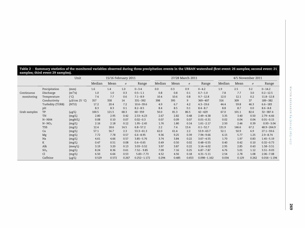
Table 2 e Summary statistics of the monitored variables observed during three precipitation events in the URBAN watershed (first event: 26 samples; second event: 21samples; third event 29 samples).

Unit 15/16 February 2011 27/28 March 2011 4/5 November 2011

Median Mean s Range Median Mean s Range Median Mean s Range

Precipitation (mm) 1.6 1.4 1.0 0e3.4 0.0 0.3 0.9 0e4.2 1.9 2.5 3.2 0e14.2

Continuous

monitoring

Discharge (m3/s) 1.0 1.0 0.3 0.5e1.1 0.8 0.8 0.1 0.7e1.0 7.8 7.7 3.0 0.2e12.5

Temperature (�C) 7.4 7.7 0.6 7.1e8.9 10.4 10.6 0.8 9.7e12.8 12.0 12.1 0.2 11.8e12.8

Conductivity (mS/cm 25 �C) 357 358 14 331e392 398 395 9 369e407 316 309 37 189e382

Turbidity (TURB) (NTU) 17.2 20.4 7.2 10.6e39.6 4.9 6.7 4.2 4.3e19.6 44.4 59.8 46.3 6.6e183

pH 8.3 8.3 0.1 8.2e8.5 8.4 8.5 0.1 8.4e8.7 8.8 8.7 0.0 8.6e8.8

Grab samples TP (mg/L) 100.5 121.5 68.3 60e359 50.0 81.3 86.5 42e429 67.0 101.1 82.6 32e387.4

TN (mg/L) 2.80 2.95 0.42 2.53e4.23 2.67 2.82 0.48 2.49e4.38 3.35 3.40 0.50 2.79e4.66

NeNH4 (mgN/L) 0.08 0.10 0.07 0.02e0.3 0.07 0.09 0.07 0.01e0.31 0.02 0.04 0.04 0.01e0.15

NeNO3 (mg/L) 2.16 2.18 0.12 1.95e2.45 1.76 1.80 0.14 1.61e2.17 2.50 2.46 0.39 0.93e3.04

TSS (mg/L) 12.4 18.6 14.5 6.8e57.2 2.2 7.4 13.4 0.1e52.7 131.9 146.6 67.2 48.9e264.9

Ca (mg/L) 57.1 56.7 2.3 53.3e61.3 62.0 61.4 2.2 53.9e63.7 52.1 50.9 6.9 27.1e59.6

Mg (mg/L) 7.72 7.78 0.57 6.6e8.95 9.36 9.25 0.39 7.94e9.66 6.15 5.77 1.25 2.9e8.74

Na (mg/L) 4.61 4.66 0.57 3.85e5.76 3.74 3.84 0.22 3.67e4.55 1.70 1.97 0.83 1.45e5.19

K (mg/L) 0.47 0.51 0.08 0.4e0.65 0.49 0.50 0.02 0.48e0.55 0.40 0.42 0.10 0.32e0.73

Alk (meq/L) 3.19 3.20 0.13 3.03e3.52 3.97 3.87 0.22 3.14e4.02 2.95 2.85 0.43 1.58e3.51

SO4 (mg/L) 8.24 8.36 0.61 7.52e 9.85 7.09 7.16 0.25 6.87e7.87 4.76 5.01 1.12 3.51e9.03

Cl (mg/L) 6.50 6.66 0.53 5.83e7.73 4.52 4.56 0.18 4.31e5.11 2.54 2.78 1.08 2.06e7.08

Caffeine (mg/L) 0.529 0.572 0.267 0.252e1.172 0.294 0.485 0.653 0.098e1.162 0.034 0.129 0.262 0.016e1.194

water

research

64

(2014)265e277

269

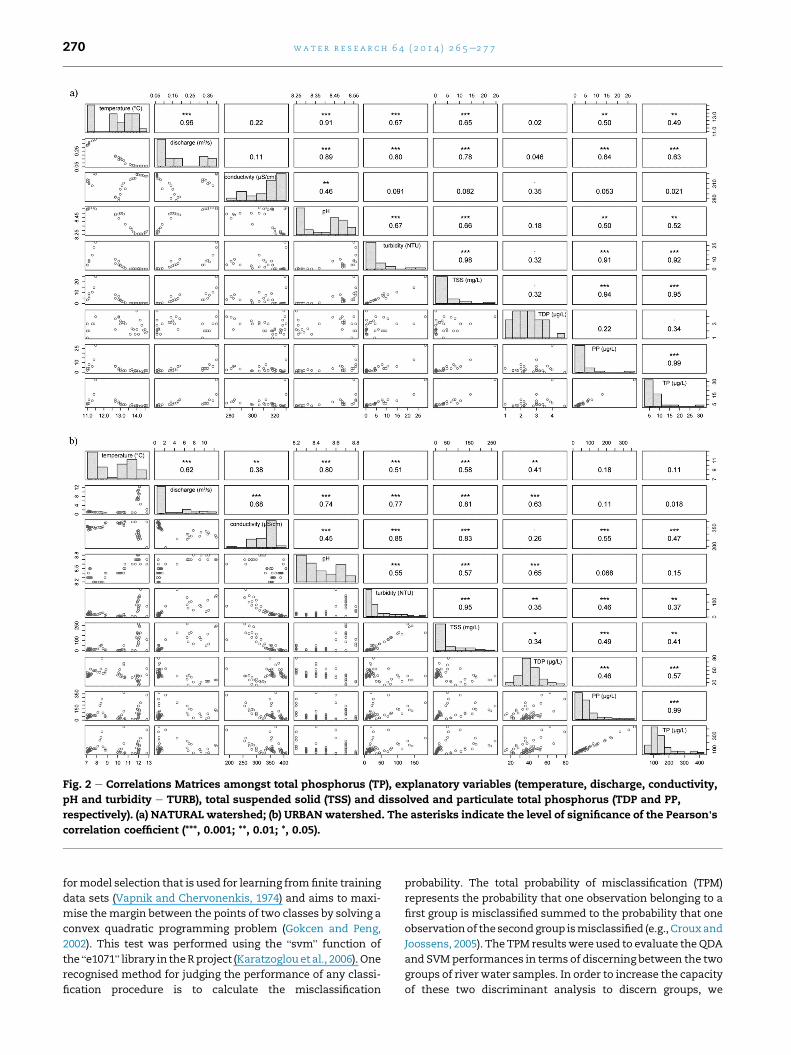
Fig. 2 e Correlations Matrices amongst total phosphorus (TP), explanatory variables (temperature, discharge, conductivity,

pH and turbidity e TURB), total suspended solid (TSS) and dissolved and particulate total phosphorus (TDP and PP,

respectively). (a) NATURAL watershed; (b) URBANwatershed. The asterisks indicate the level of significance of the Pearson'scorrelation coefficient (***, 0.001; **, 0.01; *, 0.05).

wat e r r e s e a r c h 6 4 ( 2 0 1 4 ) 2 6 5e2 7 7270

formodel selection that is used for learning fromfinite training

data sets (Vapnik and Chervonenkis, 1974) and aims to maxi-

mise themargin between the points of two classes by solving a

convex quadratic programming problem (Gokcen and Peng,

2002). This test was performed using the “svm” function of

the “e1071” library in theRproject (Karatzoglouet al., 2006). One

recognised method for judging the performance of any classi-

fication procedure is to calculate the misclassification

probability. The total probability of misclassification (TPM)

represents the probability that one observation belonging to a

first group is misclassified summed to the probability that one

observationof thesecondgroup ismisclassified (e.g., Crouxand

Joossens, 2005). The TPM resultswere used to evaluate theQDA

and SVMperformances in terms of discerning between the two

groups of river water samples. In order to increase the capacity

of these two discriminant analysis to discern groups, we

wat e r r e s e a r c h 6 4 ( 2 0 1 4 ) 2 6 5e2 7 7 271

included some records registered by the multi-parametric

probe whose origin can be attributed with certainty, i.e., we

considered 839hourly records registered either before a rainfall

event or after 24 h after a rainfall event and added 96 hourly

records registered during precipitation events for which grab

water samples shown caffeine values >0.1 mg/L.

3. Results

3.1. Relationships between TP concentrations andpotential explanatory variables

As mentioned above, all of the monitored high-frequency

variables were explored as surrogates for TP concentration.

Moreover, we investigated their relationships with TSS, and

the dissolved (TDP) and particulate (PP ¼ TP � TDP) forms of

phosphorus (Fig. 2). The data discussed below are the mea-

surements collected during the three rain events forwhich the

high-frequency monitoring efforts were coupled with the

automated (hourly collected) water samplings (Table 1).

For the NATURAL watershed (Fig. 2a), TP is strongly

correlated with TURB (r ¼ 0.92, p < 0.001) and had significant

but weaker relationships with discharge and temperature

(r ¼ 0.63, 0.49, respectively). Moreover, we observe that TSS is

strongly correlated with both TURB and TP (r ¼ 0.98, p < 0.001;

r ¼ 0.95, p < 0.001, respectively). The observed tight relation-

ship between TSS and TP is attributed to the fact that most of

the phosphorus transported in streams is bound to suspended

particles (Grayson et al., 1996; Stubblefield et al., 2007). Indeed,

we observe strong correlations for TSS/PP and PP/TP (r ¼ 0.94,

p< 0.001; r¼ 0.99, p< 0.001, respectively; Fig. 2a), and the PP/TP

ratio is very high on average: 80% (PP¼ 8 mg P/L and TP 10 mg P/

L; Table 1). This fraction or PP is comparable with those re-

ported by Johnes (2007) and Jones et al. (2011). The resulting

surrogate equations are reported in Table 3, the cross-

validated correlation coefficient (Aitkin et al., 2009) is 0.92,

p < 0.001 with an RMSE equal to 4 mg P/L (range: 3e46 mg P/L).

In contrast, for the URBAN watershed (Fig. 2b), the corre-

lation coefficients are much weaker than those for the NAT-

URALwatershed for all of the explanatory variablesmeasured.

In particular, the relationships for TURB/TP and discharge/TP

are r¼ 0.37, p < 0.01 and 0.02, p > 0.05, respectively. However, it

is very interesting to note that while there is still a strong

relationship between TSS and TURB (r ¼ 0.95, p < 0.001), the

relationship between TSS and TP is much weaker (r ¼ 0.41,

p < 0.01). In this case, the relationship PP/TP is also very high

(r¼ 0.99, p< 0.001), although the PP/TP ratio (Table 1) is slightly

lower than that of the NATURALwatershed: 65% (PP¼ 66 mg P/

L and TP 102 mg P/L). If we look carefully at the scatter-plots for

Table 3 e Surrogate equations for estimating high frequency T

Site Equation

NATURAL watershed TP ¼ 0.73* TURB þ 1.88

URBAN watershed (non point sources) TP ¼ 1.38* TURB þ 9.51

URBAN watershed (point sources) TP ¼ 4.36* TURB þ 34.4

TURB: turbidity (NTU); TP: total phosphorus (mg/L).a Leave-one-out cross validated correlation coefficient (Aitkin et al., 2009

TURB/TP and TSS/TP for both the NATURAL and URBAN wa-

tersheds, we observe that in the first NATURAL case (Fig. 2a)

the two relationships are biunivocal (one-to-one), whilst in

the URBAN case they exhibit “one-to-two” correspondences,

i.e., each independent variable corresponds to two different

dependent variables (Fig. 2b).

These results raise the question ofwhat the reasons for this

dual behaviour between TSS and TP are in the URBAN water-

shed. To answer this question, we analysed the temporal

behaviour of selected variables for the URBAN watershed

during the three monitored precipitation events for which the

multi-parametric probe data were coupled with hourly auto-

mated water sampling. These results are discussed hereafter.

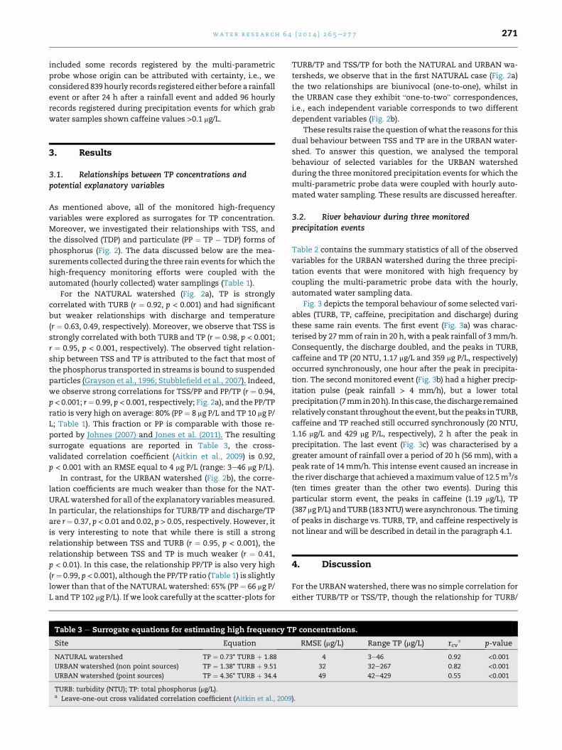
3.2. River behaviour during three monitoredprecipitation events

Table 2 contains the summary statistics of all of the observed

variables for the URBAN watershed during the three precipi-

tation events that were monitored with high frequency by

coupling the multi-parametric probe data with the hourly,

automated water sampling data.

Fig. 3 depicts the temporal behaviour of some selected vari-

ables (TURB, TP, caffeine, precipitation and discharge) during

these same rain events. The first event (Fig. 3a) was charac-

terised by 27mmof rain in 20 h, with a peak rainfall of 3mm/h.

Consequently, the discharge doubled, and the peaks in TURB,

caffeine and TP (20 NTU, 1.17 mg/L and 359 mg P/L, respectively)

occurred synchronously, one hour after the peak in precipita-

tion. The secondmonitored event (Fig. 3b) had a higher precip-

itation pulse (peak rainfall > 4 mm/h), but a lower total

precipitation (7mmin20h). In thiscase, thedischargeremained

relatively constant throughout theevent, but thepeaks inTURB,

caffeine and TP reached still occurred synchronously (20 NTU,

1.16 mg/L and 429 mg P/L, respectively), 2 h after the peak in

precipitation. The last event (Fig. 3c) was characterised by a

greater amount of rainfall over a period of 20 h (56 mm), with a

peak rate of 14mm/h. This intense event caused an increase in

the river discharge that achieved amaximumvalue of 12.5m3/s

(ten times greater than the other two events). During this

particular storm event, the peaks in caffeine (1.19 mg/L), TP

(387 mg P/L) andTURB (183NTU)were asynchronous. The timing

of peaks in discharge vs. TURB, TP, and caffeine respectively is

not linear and will be described in detail in the paragraph 4.1.

4. Discussion

For the URBANwatershed, there was no simple correlation for

either TURB/TP or TSS/TP, though the relationship for TURB/

P concentrations.

RMSE (mg/L) Range TP (mg/L) rcva p-value

4 3e46 0.92 <0.00132 32e267 0.82 <0.00149 42e429 0.55 <0.001

).

Fig. 3 e Temporal behaviour of some selected variables (turbidity, TP concentration, caffeine, precipitation and discharge -Q-

) monitored in the URBAN watershed during three precipitation events for which the multi-parametric probe measurement

were coupled with the hourly automated collection of water samples. a) 15/16 February 2011; b) 27/28 March 2011; c) 4/5

November 2011. Note that the y-axes have different scales in the three figures.

wat e r r e s e a r c h 6 4 ( 2 0 1 4 ) 2 6 5e2 7 7272

TSSwas similar to that of the NATURALwatershed. Hence, we

attempted to determine whether the “one-to-two” behaviour

observed for the TURB/TP relationship for the URBAN water-

shed (Fig. 2b) represents two distinct groups of data that differ

in the relevant chemical characteristics of the suspended

solids because they are from different sources. In this regard,

we observed that there was a loss of synchrony between the

peaks in TURB and TP during the most intense precipitation

event (Fig. 3c); there is a lag of one hour between the peak in

precipitation and the peak in TP, which is then followed by a

peak in TURB another hour later. This loss of synchrony be-

tween TURB and TP demonstrates that, during this particular

storm event, low TURB levels (and, therefore, low TSS levels,

considering the high TURB/TSS correlation) corresponded to

high TP levels.

This result explains the duality observed in the TURB/TP

relationship at the URBAN watershed, but other questions

remain: What do the two groups of TSS represent? Is it

possible to discriminate between these two groups in order to

improve high frequency estimates of TP for urbanised

watersheds?

4.1. Different sources of suspended solids

The above-mentioned questions can be answered by per-

forming an exploratory analysis of the relationships amongst

the variables measured during the three precipitation events

by Principal Component Analysis (PCA) (Table 2). Fig. 4a shows

that the first Principal Component (PC1) explains 61% of the

variance, while the second Principal Component (PC2)

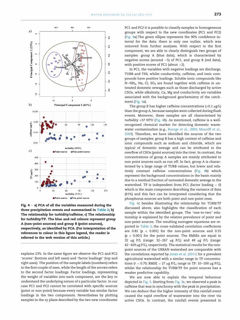
Fig. 4 e a) PCA of all the variables measured during the

three precipitation events and summarised in Table 2; b)

The relationship for turbidity/caffeine; c) The relationship

for turbidity/TP. The blue and red colours represent group

A (non-point sources) and group B (point sources),

respectively, as identified by PCA. (For interpretation of the

references to colour in this figure legend, the reader is

referred to the web version of this article.)

wat e r r e s e a r c h 6 4 ( 2 0 1 4 ) 2 6 5e2 7 7 273

explains 23%. In the same figure we observe the PC1 and PC2

“scores” (bottom and left axes) and “factor loadings” (top and

right axes). The position of the sample labels (numbers) refers

to the first couple of axes, while the length of the arrows refers

to the second factor loadings. Factor loadings, representing

the weight of variables into each component, are the key to

understand the underlying nature of a particular factor. In our

case PC1 and PC2 cannot be correlated with specific sources

(point or non-point) because every variable has similar factor

loadings in the two components. Nevertheless by plotting

samples in the xy plane described by the two new coordinates

PC1 and PC2 it is possible to classify samples in homogeneous

groups with respect to the new coordinates (PC1 and PC2)

(Fig. 4a).The green ellipse represents the 90% confidence in-

terval for the data: there is only one outlier, which was

removed from further analyses. With respect to the first

component, we are able to clearly distinguish two groups of

samples: group A (blue data), which is characterised by

negative scores (around �5) of PC1, and group B (red data),

with positive scores of PC1 (about þ2).

In PC1, the variables with negative loadings are discharge,

TURB and TSS, whilst conductivity, caffeine, and ionic com-

pounds have positive loadings. Soluble ionic compounds like

NeNH4, Na, Cl, SO4 are found together with caffeine in un-

treated domestic sewages such as those discharged by active

CSOs, while alkalinity, Ca, Mg and conductivity are variables

associated with the background geochemistry of the catch-

ment (Fig. 4a).

The group B has higher caffeine concentrations (>0.1 mg/L)

than the groupA, because sampleswere collected during flush

events. Moreover, these samples are all characterised by

turbidity <37 NTU (Fig. 4b). As mentioned, caffeine is a well-

recognised chemical marker for detecting domestic waste-

water contamination (e.g., Buerge et al., 2003; Musolff et al.,

2009). Therefore, we have identified the sources of the two

groups of samples: group B has a high content of caffeine and

ionic compounds such as sodium and chloride, which are

typical of domestic sewage and can be attributed to the

overflow of CSOs (point sources) into the river. In contrast, the

concentrations of group A samples are mainly attributed to

non point sources such as run off. In fact, group A is charac-

terised by a large range of TURB values, but lower and rela-

tively constant caffeine concentrations (Fig. 4b) which

represent the background concentrations in the basin mainly

due to a residual fraction of untreated domestic sewage in the

watershed. TP is independent from PC1 (factor loading ¼ 0)

which is the main component describing the variance of data

(61%) and this fact can be interpreted considering that the

phosphorus sources are both point and non-point ones.

Fig. 4c besides illustrating the relationship for TURB/TP

discussed above, also highlights the classification of each

sample within the identified groups. The “one-to-two” rela-

tionship is explained by the relative prevalence of point and

non-point sources. The resulting surrogate equations are re-

ported in Table 3, the cross-validated correlation coefficients

are 0.82 (p < 0.001) for the non-point sources and 0.55

(p < 0.001) for the point sources. The RMSEs are equal to

32 mg P/L (range: 32e267 mg P/L) and 49 mg P/L (range:

42e429 mg P/L), respectively. The statistical results for the non-

point sources of the URBAN watershed are comparable with

the correlations reported by Jones et al. (2011) for a prevalent

agricultural watershed with a similar range in TP concentra-

tions (r ¼ 0.70; RMSE ¼ 27 mg P/L; range in TP: 10e200 mg P/L),

whilst the relationship for TURB/TP for point sources has a

weaker predictive capability.

We are now able to explain the temporal behaviour

depicted in Fig. 3. Starting from Fig. 3c, we observed a peak in

caffeine that was in synchrony with the peak in precipitation.

We can deduce that the higher intensity of this rainfall event

caused the rapid overflow of wastewater into the river via

active CSOs. In contrast, the rainfall events presented in

wat e r r e s e a r c h 6 4 ( 2 0 1 4 ) 2 6 5e2 7 7274

Fig. 3a and b, which were characterised by a lower intensity of

precipitation, did not activate the overflows until an hour

later. However, in all the three cases, the overflow spills are

characterised by a modest amount of suspended matter

(reduced levels of turbidity) with high phosphorus content

(most likely organic matter of anthropogenic origin). The

event described by Fig. 3c also differed from the other two in

terms of the lack of synchrony between TP and TURB. In this

case, the large amount of precipitation, after inducing the

activation of the CSOs (detected by the peak in caffeine),

caused an intensive removal of suspended solids from the

basin, but was characterised by a lower TP content than that

observed for the point sources.

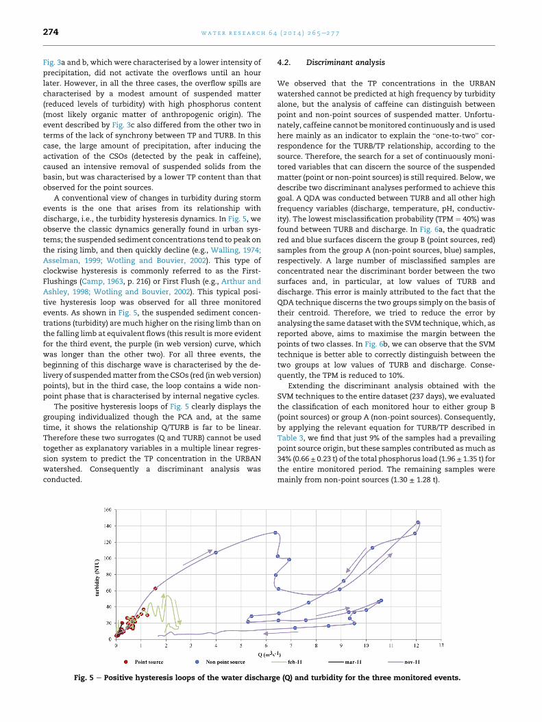
A conventional view of changes in turbidity during storm

events is the one that arises from its relationship with

discharge, i.e., the turbidity hysteresis dynamics. In Fig. 5, we

observe the classic dynamics generally found in urban sys-

tems; the suspended sediment concentrations tend to peak on

the rising limb, and then quickly decline (e.g., Walling, 1974;

Asselman, 1999; Wotling and Bouvier, 2002). This type of

clockwise hysteresis is commonly referred to as the First-

Flushings (Camp, 1963, p. 216) or First Flush (e.g., Arthur and

Ashley, 1998; Wotling and Bouvier, 2002). This typical posi-

tive hysteresis loop was observed for all three monitored

events. As shown in Fig. 5, the suspended sediment concen-

trations (turbidity) are much higher on the rising limb than on

the falling limb at equivalent flows (this result is more evident

for the third event, the purple (in web version) curve, which

was longer than the other two). For all three events, the

beginning of this discharge wave is characterised by the de-

livery of suspendedmatter from the CSOs (red (inweb version)

points), but in the third case, the loop contains a wide non-

point phase that is characterised by internal negative cycles.

The positive hysteresis loops of Fig. 5 clearly displays the

grouping individualized though the PCA and, at the same

time, it shows the relationship Q/TURB is far to be linear.

Therefore these two surrogates (Q and TURB) cannot be used

together as explanatory variables in a multiple linear regres-

sion system to predict the TP concentration in the URBAN

watershed. Consequently a discriminant analysis was

conducted.

Fig. 5 e Positive hysteresis loops of the water discharg

4.2. Discriminant analysis

We observed that the TP concentrations in the URBAN

watershed cannot be predicted at high frequency by turbidity

alone, but the analysis of caffeine can distinguish between

point and non-point sources of suspended matter. Unfortu-

nately, caffeine cannot bemonitored continuously and is used

here mainly as an indicator to explain the “one-to-two” cor-

respondence for the TURB/TP relationship, according to the

source. Therefore, the search for a set of continuously moni-

tored variables that can discern the source of the suspended

matter (point or non-point sources) is still required. Below, we

describe two discriminant analyses performed to achieve this

goal. A QDA was conducted between TURB and all other high

frequency variables (discharge, temperature, pH, conductiv-

ity). The lowest misclassification probability (TPM ¼ 40%) was

found between TURB and discharge. In Fig. 6a, the quadratic

red and blue surfaces discern the group B (point sources, red)

samples from the group A (non-point sources, blue) samples,

respectively. A large number of misclassified samples are

concentrated near the discriminant border between the two

surfaces and, in particular, at low values of TURB and

discharge. This error is mainly attributed to the fact that the

QDA technique discerns the two groups simply on the basis of

their centroid. Therefore, we tried to reduce the error by

analysing the same dataset with the SVM technique, which, as

reported above, aims to maximise the margin between the

points of two classes. In Fig. 6b, we can observe that the SVM

technique is better able to correctly distinguish between the

two groups at low values of TURB and discharge. Conse-

quently, the TPM is reduced to 10%.

Extending the discriminant analysis obtained with the

SVM techniques to the entire dataset (237 days), we evaluated

the classification of each monitored hour to either group B

(point sources) or group A (non-point sources). Consequently,

by applying the relevant equation for TURB/TP described in

Table 3, we find that just 9% of the samples had a prevailing

point source origin, but these samples contributed asmuch as

34% (0.66± 0.23 t) of the total phosphorus load (1.96± 1.35 t) for

the entire monitored period. The remaining samples were

mainly from non-point sources (1.30 ± 1.28 t).

e (Q) and turbidity for the three monitored events.

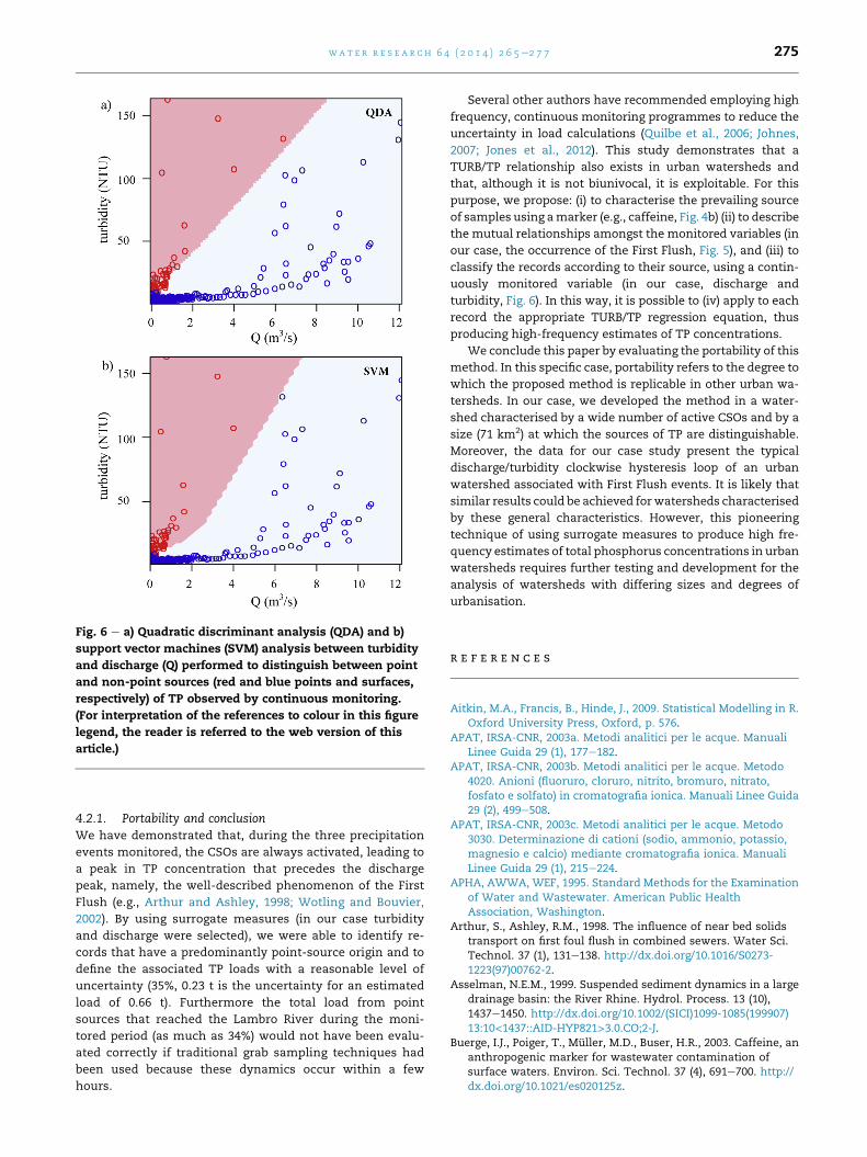
Fig. 6 e a) Quadratic discriminant analysis (QDA) and b)

support vector machines (SVM) analysis between turbidity

and discharge (Q) performed to distinguish between point

and non-point sources (red and blue points and surfaces,

respectively) of TP observed by continuous monitoring.

(For interpretation of the references to colour in this figure

legend, the reader is referred to the web version of this

article.)

wat e r r e s e a r c h 6 4 ( 2 0 1 4 ) 2 6 5e2 7 7 275

4.2.1. Portability and conclusionWe have demonstrated that, during the three precipitation

events monitored, the CSOs are always activated, leading to

a peak in TP concentration that precedes the discharge

peak, namely, the well-described phenomenon of the First

Flush (e.g., Arthur and Ashley, 1998; Wotling and Bouvier,

2002). By using surrogate measures (in our case turbidity

and discharge were selected), we were able to identify re-

cords that have a predominantly point-source origin and to

define the associated TP loads with a reasonable level of

uncertainty (35%, 0.23 t is the uncertainty for an estimated

load of 0.66 t). Furthermore the total load from point

sources that reached the Lambro River during the moni-

tored period (as much as 34%) would not have been evalu-

ated correctly if traditional grab sampling techniques had

been used because these dynamics occur within a few

hours.

Several other authors have recommended employing high

frequency, continuous monitoring programmes to reduce the

uncertainty in load calculations (Quilbe et al., 2006; Johnes,

2007; Jones et al., 2012). This study demonstrates that a

TURB/TP relationship also exists in urban watersheds and

that, although it is not biunivocal, it is exploitable. For this

purpose, we propose: (i) to characterise the prevailing source

of samples using amarker (e.g., caffeine, Fig. 4b) (ii) to describe

the mutual relationships amongst the monitored variables (in

our case, the occurrence of the First Flush, Fig. 5), and (iii) to

classify the records according to their source, using a contin-

uously monitored variable (in our case, discharge and

turbidity, Fig. 6). In this way, it is possible to (iv) apply to each

record the appropriate TURB/TP regression equation, thus

producing high-frequency estimates of TP concentrations.

We conclude this paper by evaluating the portability of this

method. In this specific case, portability refers to the degree to

which the proposed method is replicable in other urban wa-

tersheds. In our case, we developed the method in a water-

shed characterised by a wide number of active CSOs and by a

size (71 km2) at which the sources of TP are distinguishable.

Moreover, the data for our case study present the typical

discharge/turbidity clockwise hysteresis loop of an urban

watershed associated with First Flush events. It is likely that

similar results could be achieved forwatersheds characterised

by these general characteristics. However, this pioneering

technique of using surrogate measures to produce high fre-

quency estimates of total phosphorus concentrations in urban

watersheds requires further testing and development for the

analysis of watersheds with differing sizes and degrees of

urbanisation.

r e f e r e n c e s

Aitkin, M.A., Francis, B., Hinde, J., 2009. Statistical Modelling in R.Oxford University Press, Oxford, p. 576.

APAT, IRSA-CNR, 2003a. Metodi analitici per le acque. ManualiLinee Guida 29 (1), 177e182.

APAT, IRSA-CNR, 2003b. Metodi analitici per le acque. Metodo4020. Anioni (fluoruro, cloruro, nitrito, bromuro, nitrato,fosfato e solfato) in cromatografia ionica. Manuali Linee Guida29 (2), 499e508.

APAT, IRSA-CNR, 2003c. Metodi analitici per le acque. Metodo3030. Determinazione di cationi (sodio, ammonio, potassio,magnesio e calcio) mediante cromatografia ionica. ManualiLinee Guida 29 (1), 215e224.

APHA, AWWA, WEF, 1995. Standard Methods for the Examinationof Water and Wastewater. American Public HealthAssociation, Washington.

Arthur, S., Ashley, R.M., 1998. The influence of near bed solidstransport on first foul flush in combined sewers. Water Sci.Technol. 37 (1), 131e138. http://dx.doi.org/10.1016/S0273-1223(97)00762-2.

Asselman, N.E.M., 1999. Suspended sediment dynamics in a largedrainage basin: the River Rhine. Hydrol. Process. 13 (10),1437e1450. http://dx.doi.org/10.1002/(SICI)1099-1085(199907)13:10<1437::AID-HYP821>3.0.CO;2-J.

Buerge, I.J., Poiger, T., Muller, M.D., Buser, H.R., 2003. Caffeine, ananthropogenic marker for wastewater contamination ofsurface waters. Environ. Sci. Technol. 37 (4), 691e700. http://dx.doi.org/10.1021/es020125z.

wat e r r e s e a r c h 6 4 ( 2 0 1 4 ) 2 6 5e2 7 7276

Buraschi, E., Salerno, F., Monguzzi, C., Barbiero, G., Tartari, G.,2005. Characterization of the Italian lake-types andidentification of their reference sites using anthropogenicpressure factors. J. Limnol. 64 (1), 75e84. http://dx.doi.org/10.4081/jlimnol.2005.75.

Camp, T.R., 1963. Water and its Impurities. Reinhold PublishingCorporation, New York.

Carraro, E., Guyennon, N., Hamilton, D., Valsecchi, L.,Manfredi, E.C., Viviano, G., Salerno, F., Tartari, G., Copetti, D.,2012a. Coupling high-resolution measurements to a three-dimensional lake model to assess the spatial and temporaldynamics of the cyanobacterium Planktothrix rubescens in amedium-sized lake. Hydrobiologia 698 (1), 77e95. http://dx.doi.org/10.1007/s10750-012-1096-y.

Carraro, E., Guyennon, N., Viviano, G., Manfredi, E.C.,Valsecchi, L., Salerno, F., Tartari, G., Copetti, D., 2012b. Impactof global and local pressures on the ecology of a medium-sizedPre-Alpine Lake. In: Jordan, F., Jorgensen, S.E. (Eds.), Models ofthe Ecological Hierarchy. Elsevier B.V, pp. 259e274. http://dx.doi.org/10.1016/B978-0-444-59396-2.00016-X.

Croux, C., Joossens, K., 2005. Influence of observations on themisclassification probability in quadratic discriminantanalysis. J. Multivar. Anal. 96 (2), 384e403. http://dx.doi.org/10.1016/j.jmva.2004.11.001.

Dabney, A.R., Storey, J.D., 2007. Optimality driven nearestcentroid classification from genomic data. PLoS One 2 (10),e1002. http://dx.doi.org/10.1371/journal.pone.0001002.

Demars, B.O.L., Harper, D.M., Pitt, J.-A., Slaughter, R., 2005. Impactof phosphorus control measures on in-river phosphorusretention associated with point source pollution. Hydrol. EarthSyst. Sci. Discuss. 2, 37e72. http://dx.doi.org/10.5194/hessd-2-37-2005.

Elser, J.J., Bracken, M.E.S., Cleland, E.E., Gruner, D.S., StanleyHarpole, W., Hillebrand, H., Ngai, J.T., Seabloom, E.W.,Shurin, J.B., Smith, J.E., 2007. Global analysis of nitrogen andphosphorus limitation of primary producers in freshwater,marine and terrestrial ecosystems. Ecol. Lett. 10 (12),1135e1142. http://dx.doi.org/10.1111/j.1461-0248.2007.01113.x.

FAO, ISRIC, ISSS, 1998. World Reference Base for Soil Resources.World Society of Soil Science, Rome, 84.

Fresenius, W., Quentin, K.E., Schneider, W. (Eds.), 1988. WaterAnalysis. Springer-Verlag, Berlin.

Glasgow, H.B., Burkholder, J.M., Reed, R.E., Lewitus, A.J.,Kleinman, J.E., 2004. Real-time remote monitoring of waterquality: a review of current applications, and advancements insensor, telemetry, and computing technologies. J. Exp. Mar.Biol. Ecol. 300 (1e2), 409e448. http://dx.doi.org/10.1016/j.jembe.2004.02.022.

Gokcen, I., Peng, J., 2002. Comparing linear discriminant analysisand support vector machines. In: Yakhno, T. (Ed.), Advances inInformation Systems, Lecture Notes in Computer Science,2457. Springer, pp. 104e113. http://dx.doi.org/10.1007/3-540-36077-8_10.

Goldman, C.R., Jassby, A.D., Hackely, S.H., 1993. Decadal,interannual, and seasonal variability in enrichment bioassaysat Lake Tahoe, CaliforniaeNevada, U.S.A. Can. J. Fish. Aquat.Sci. 50 (7), 1489e1496. http://dx.doi.org/10.1139/f93-170.

Grayson, R.B., Finlayson, B.L., Gippel, C.J., Hart, B.T., 1996. Thepotential of field turbidity measurements for the computationof total phosphorus and suspended solids loads. J. Environ.Manag. 47 (3), 257e267. http://dx.doi.org/10.1006/jema.1996.0051.

Guyennon, N., Romano, E., Portoghese, I., Salerno, F., Calmanti, S.,Petrangeli, A.B., Tartari, G., Copetti, D., 2013. Benefits fromusing combined dynamical-statistical downscalingapproaches e lessons from a case study in the Mediterraneanregion. Hydrol. Earth Syst. Sci. 17, 705e720. http://dx.doi.org/10.5194/hess-17-705-2013.

Johnes, P.J., 2007. Uncertainties in annual riverine phosphorusload estimation: impact of load estimation methodology,sampling frequency, baseflow index and catchmentpopulation density. J. Hydrol. 332 (1e2), 241e258. http://dx.doi.org/10.1016/j.jhydrol.2006.07.006.

Jones, A.S., Horsburgh, J.S., Mesner, N.O., Ryel, R.J., Stevens, D.K.,2012. Influence of sampling frequency on estimation of annualtotal phosphorus and total suspended solids loads. J. Am.Water Resour. Assoc. 48 (6), 1258e1275. http://dx.doi.org/10.1111/j.1752-1688.2012.00684.x.

Jones, A.S., Stevens, D.K., Horsburgh, J.S., Mesner, N.O., 2011.Surrogate measures for providing high frequency estimates oftotal suspended solids and total phosphorus concentrations. J.Am. Water Resour. Assoc. 47 (2), 239e253. http://dx.doi.org/10.1111/j.1752-1688.2010.00505.x.

Karatzoglou, A., Meyer, D., Hornik, K., 2006. Support vectormachines in r. J. Stat. Softw. 15 (9).

Kleinbaum, D.G., Kupper, L.L., 1978. Applied Regression Analysisand Other Multivariate Methods. Duxbury Press, NorthScituate (MA), p. 556.

Kronvang, B., Laubel, A., Grant, R., 1997. Suspended sedimentand particulate phosphorus transport and deliverypathways in an Arable Catchment, Gelbaek Stream,Denmark. Hydrol. Process. 11 (6), 627e642. http://dx.doi.org/10.1002/(SICI)1099-1085(199705)11:6<627::AID-HYP481>3.0.CO;2-E.

Lachenbruch, P.A., Goldstein, M., 1979. Discriminant analysis. In:Biometrics, vol. 35(1). International Biometric Society,pp. 69e85. URL: http://www.jstor.org/stable/2529937.

McLachlan, G.J., 1992. Discriminant Analysis and StatisticalPattern Recognition. Wiley-Interscience Publication, NewYork, p. 526.

Miguntanna, N.S., Egodawatta, P., Kokot, S., Goonetilleke, A.,2010. Determination of a set of surrogate parameters to assessurban stormwater quality. Sci. Total Environ. 408 (24),6251e6259. http://dx.doi.org/10.1016/j.scitotenv.2010.09.015.

Mika, S., Ratsch, G., Weston, J., Scholkopf, B., Muller, K., 1999.Fisher discriminant analysis with kernels. In: NeuralNetworks for Signal Processing IX, 1999. Proceedings of the1999 IEEE Signal Processing Society Workshop, pp. 41e48.http://dx.doi.org/10.1109/NNSP.1999.788121.

Musolff, A., Leschik, S., M€oder, M., Strauch, G., Reinstorf, F.,Schirmer, M., 2009. Temporal and spatial patterns ofmicropollutants in urban receiving waters. Environ. Pollut. 157(11), 3069e3077. http://dx.doi.org/10.1016/j.envpol.2009.05.037.

OECD, 1982. Eutrophication of Waters Monitoring Assessmentand Control. Organization for Economic Co-operation andDevelopment, Paris.

Oliver, R.L., Hart, B.T., Olley, J., Grace, M., Rees, C.,Caitcheon, G., 1999. The Darling River: Algal Growth and theCycling and Sources of Nutrients. In: Murray Darling BasinCommission, Project M386, p. 201. Final Report, Camberra,Australia.

Quilbe, R., Rousseau, A.N., Duchemin, M., Poulin, A.,Gangbazo, G., Villeneuve, J.P., 2006. Selecting a calculationmethod to estimate sediment and nutrient loads in streams:application to the Beaurivage River (Quebec, Canada). J.Hydrol. 326 (1e4), 295e310. http://dx.doi.org/10.1016/j.jhydrol.2005.11.008.

Rasmussen, T.J., Lee, C.J., Ziegler, A.C., 2008. Estimation ofConstituent Concentrations, Loads, and Yields in Streams ofJohnson County, Northeast Kansas, Using Continuous Water-quality Monitoring and Regression Models, October 2002through December 2006, p. 103. U.S. Geological SurveyScientific Investigation Report 2008-5014. Reston, Virginia.

Rodier, J., 1984. L'analyse de l'eau: eaux naturelles, eauxr�esiduaires, eau de mer, seventh ed. Dunod, Bordas (�Editeurs),Paris, p. 1365.

wat e r r e s e a r c h 6 4 ( 2 0 1 4 ) 2 6 5e2 7 7 277

Salerno, F., Gambelli, S., Viviano, G., Thakuri, S., Guyennon, N.,D’Agata, C., Diolaiuti, G., Smiraglia, C., Stefani, F.,Bochhiola, D., Tartari, G., 2014a. High alpine ponds shiftupwards as average temperature increase: a case study of theOrtles-Cevedale mountain group (Southern alps, Italy) overthe last 50 years. Glob. Planet. Change 120, 81e91. http://dx.doi.org/10.1016/j.gloplacha.2014.06.003.

Salerno, F., Tartari, G., 2009. A coupled approach of surfacehydrological modelling and Wavelet Analysis forunderstanding the baseflow components of river discharge inkarst Environments. J. Hydrol. 376 (1e2), 295e306. http://dx.doi.org/10.1016/j.jhydrol.2009.07.042.

Salerno, F., Thakuri, S., D'Agata, C., Smiraglia, C., Manfredi, E.C.,Viviano, G., Tartari, G., 2012. Glacial lake distribution in theMount Everest region: uncertainty of measurement andconditions of formation. Glob. Planet. Change 92e93, 30e39.http://dx.doi.org/10.1016/j.gloplacha.2012.04.001.

Salerno, F., Viviano, G., Carraro, E., Manfredi, E.C., Lami, A.,Musazzi, S., Marchetto, A., Guyennon, N., Tartari, G.,Copetti, D., 2014b. Total phosphorus reference condition forsubalpine lakes: comparison among traditional methods and anew process based and dynamic lake-basin approach. J.Environ. Manag. 145, 94e105. http://dx.doi.org/10.1016/j.jenvman.2014.06.011.

Schindler, D.W., Hecky, R.E., Findlay, D.L., Stainton, M.P.,Parker, B.R., Paterson, M.J., Beaty, K.G., Lyng, M.,Kasian, S.E.M., 2008. Eutrophication of lakes cannot becontrolled by reducing nitrogen input: results of a 37-yearwhole-ecosystem experiment. Proc. Natl. Acad. Sci. U. S. A.105 (2), 11254e11258. http://dx.doi.org/10.1073/pnas.0805108105.

Scholefield, D., Le Goff, T., Braven, J., Ebdon, L., Long, T.,Butler, M., 2005. Concerted diurnal patterns in riverinenutrient concentrations and physical conditions. Sci. TotalEnviron. 344 (1e3), 201e210. http://dx.doi.org/10.1016/j.scitotenv.2005.02.014.

Settle, S., Goonetilleke, S.A., Ayoko, G.A., 2007. Determination ofsurrogate indicators for phosphorus and solids in urbanstormwater: application of multivariate data analysistechniques. Water Air Soil. Pollut. 182 (1e4), 149e161. http://dx.doi.org/10.1007/s11270-006-9328-2.

Stubblefield, A.P., Reuter, J.E., Dahlgren, R.A., Goldman, C.R., 2007.Use of turbidometry to characterize suspended sediment andphosphorus fluxes in the Lake Tahoe basin, California, USA.Hydrol. Process. 21 (3), 281e291. http://dx.doi.org/10.1002/hyp.6234.

Tomlinson, M.S., De Carlo, E.H., 2003. The need for highresolution time series data to characterize Hawaiian streams.J. Am. Water Resour. Assoc. 39 (1), 113e123. http://dx.doi.org/10.1111/j.1752-1688.2003.tb01565.x.

Valderrama, J.C., 1981. The simultaneous analysis of totalnitrogen and total phosphorus in natural waters. Mar. Chem.10, 109e122. http://dx.doi.org/10.1016/0304-4203(81)90027-X.

Vapnik, V.N., Chervonenkis, A.Ya, 1974. Theory of PatternRecognition. Nauka, Moscow (in Russian).

Venables, W.N., Ripley, B.D., 2002. Modern Applied Statistics withS, fourth ed. Springer, New York.

Virglino, L., Aboulfald, K., Mahvelat, A.D., Pr�evost, M., Sauv�e, S.,2008. On-line solid phase extraction and liquidchromatography/tandem mass spectrometry to quantifypharmaceuticals, pesticides and some metabolites inwastewaters, drinking, and surface waters. J. Environ. Monit.10 (4), 482e489. http://dx.doi.org/10.1039/b800861b.

Walling, D.E., 1974. Suspended sediment and solute yields from asmall catchment prior to urbanization. In: Gregory, K.J.,Walling, D.E. (Eds.), Fluvial Processes in InstrumentedWatersheds, vol. 6. Institute of British Geographers SpecialPublication, pp. 169e192.

Wotling, G., Bouvier, C., 2002. Impact of urbanization onsuspended sediment and organic matter fluxes from smallcatchments in Tahiti. Hydrol. Process. 16 (9), 1745e1756.http://dx.doi.org/10.1002/hyp.393.