Monthly averages of aerosol properties: A global comparison among models, satellite data, and...
42
Monthly averages of aerosol properties: A global comparison among models, satellite data, and AERONET ground data S. Kinne, 1 U. Lohmann, 2 J. Feichter, 1 M. Schulz, 3 C. Timmreck, 1 S. Ghan, 4 R. Easter, 4 M. Chin, 5 P. Ginoux, 6 T. Takemura, 7 I. Tegen, 8 D. Koch, 9 M. Herzog, 10 J. Penner, 10 G. Pitari, 11 B. Holben, 5 T. Eck, 12 A. Smirnov, 12 O. Dubovik, 12 I. Slutsker, 12 D. Tanre, 13 O. Torres, 14 M. Mishchenko, 15 I. Geogdzhayev, 9 D. A. Chu, 12 and Y. Kaufman 5 Received 29 August 2001; revised 18 March 2002; accepted 12 March 2003; published 21 October 2003. [1] New aerosol modules of global (circulation and chemical transport) models are evaluated. These new modules distinguish among at least five aerosol components: sulfate, organic carbon, black carbon, sea salt, and dust. Monthly and regionally averaged predictions for aerosol mass and aerosol optical depth are compared. Differences among models are significant for all aerosol types. The largest differences were found near expected source regions of biomass burning (carbon) and dust. Assumptions for the permitted water uptake also contribute to optical depth differences (of sulfate, organic carbon, and sea salt) at higher latitudes. The decline of mass or optical depth away from recognized sources reveals strong differences in aerosol transport or removal among models. These differences are also a function of altitude, as transport biases of dust do not always extend to other aerosol types. Ratios of optical depth and mass demonstrate large differences in the mass extinction efficiency, even for hydrophobic aerosol. This suggests that efforts of good mass simulations could be wasted or that conversions are misused to cover for poor mass simulations. In an attempt to provide an absolute measure for model skill, simulated total optical depths (when adding contributions from all five aerosol types) are compared to measurements from ground and space. Comparisons to the Aerosol Robotic Network (AERONET) suggest a source strength underestimate in many models, most frequently for (subtropical) tropical biomass or dust. Comparisons to the combined best of Moderate-Resolution Imaging Spectroradiometer (MODIS) and Total Ozone Mapping Spectrometer (TOMS) indicate that away from sources, model simulations are usually smaller. Particularly large are discrepancies over tropical oceans and oceans of the Southern Hemisphere, raising issues on the treatment of sea salt in models. Totals for mass or optical depth in many models are defined by the absence or dominance of only one aerosol component. With appropriate corrections to that component (e.g., to removal, to source strength, or to seasonality) a much better model performance can be expected. Still, many important modeling issues remain inconclusive as the combined result of poor coordination (different emissions and meteorology), insufficient model output (vertical distributions, water uptake by aerosol type), and unresolved measurement issues (retrieval assumptions and temporal or spatial sampling biases). INDEX TERMS: 1610 Global Change: Atmosphere (0315, 0325); 1615 Global Change: Biogeochemical processes (4805); 3319 Meteorology and Atmospheric Dynamics: General circulation; 9 Department of Applied Physics and Applied Mathematics, Columbia University-NASA Goddard Institute for Space Studies, New York, USA. 10 Department of Atmospheric, Oceanic and Space Sciences, University of Michigan, Ann Arbor, Michigan, USA. 11 Dipartimento di Fisica, Universita ` degli Studi dell’Aquila, L’Aquila, Italy. 12 Goddard Earth Sciences and Technology Center, University of Maryland Baltimore County-NASA Goddard Space Flight Center, Green- belt, Maryland, USA. 13 Laboratoire d’Optique Atmosphe ´rique, Universite ´ des Sciences et Technologies de Lille 1, Lille, France. 14 Joint Center for Earth Systems Technology, University of Maryland Baltimore County-NASA Goddard Space Flight Center, Greenbelt, Mary- land, USA. 15 NASA Goddard Institute for Space Studies, New York, USA. JOURNAL OF GEOPHYSICAL RESEARCH, VOL. 108, NO. D20, 4634, doi:10.1029/2001JD001253, 2003 1 Max-Planck-Institut fu ¨r Meteorologie, Hamburg, Germany. 2 Department of Physics, Dalhousie University, Halifax, Nova Scotia, Canada. 3 Laboratoire des Sciences du Climat et l’Environnement, Gif-sur- Yvette, France. 4 Pacific Northwest National Laboratory, Battelle, Richland, Washington, USA. 5 NASA Goddard Space Flight Center, Greenbelt, Maryland, USA. 6 Geophysical Fluid Dynamics Laboratory, NOAA, Princeton, New Jersey, USA. 7 Research Institute for Applied Mechanics, Kyushu University, Fukuoka, Japan. 8 Max-Planck-Institut fu ¨r Biogeochemie, Jena, Germany. Copyright 2003 by the American Geophysical Union. 0148-0227/03/2001JD001253 AAC 3 - 1
-
Upload
independent -
Category
Documents
-
view
0 -
download
0
Transcript of Monthly averages of aerosol properties: A global comparison among models, satellite data, and...
Monthly averages of aerosol properties: A global comparison among
models, satellite data, and AERONET ground data
S. Kinne,1 U. Lohmann,2 J. Feichter,1 M. Schulz,3 C. Timmreck,1 S. Ghan,4 R. Easter,4
M. Chin,5 P. Ginoux,6 T. Takemura,7 I. Tegen,8 D. Koch,9 M. Herzog,10 J. Penner,10
G. Pitari,11 B. Holben,5 T. Eck,12 A. Smirnov,12 O. Dubovik,12 I. Slutsker,12 D. Tanre,13
O. Torres,14 M. Mishchenko,15 I. Geogdzhayev,9 D. A. Chu,12 and Y. Kaufman5
Received 29 August 2001; revised 18 March 2002; accepted 12 March 2003; published 21 October 2003.
[1] New aerosol modules of global (circulation and chemical transport) models areevaluated. These new modules distinguish among at least five aerosol components:sulfate, organic carbon, black carbon, sea salt, and dust. Monthly and regionally averagedpredictions for aerosol mass and aerosol optical depth are compared. Differences amongmodels are significant for all aerosol types. The largest differences were found nearexpected source regions of biomass burning (carbon) and dust. Assumptions for thepermitted water uptake also contribute to optical depth differences (of sulfate, organiccarbon, and sea salt) at higher latitudes. The decline of mass or optical depth away fromrecognized sources reveals strong differences in aerosol transport or removal amongmodels. These differences are also a function of altitude, as transport biases of dust do notalways extend to other aerosol types. Ratios of optical depth and mass demonstrate largedifferences in the mass extinction efficiency, even for hydrophobic aerosol. Thissuggests that efforts of good mass simulations could be wasted or that conversions aremisused to cover for poor mass simulations. In an attempt to provide an absolute measurefor model skill, simulated total optical depths (when adding contributions from all fiveaerosol types) are compared to measurements from ground and space. Comparisons to theAerosol Robotic Network (AERONET) suggest a source strength underestimate inmany models, most frequently for (subtropical) tropical biomass or dust. Comparisons tothe combined best of Moderate-Resolution Imaging Spectroradiometer (MODIS) andTotal Ozone Mapping Spectrometer (TOMS) indicate that away from sources, modelsimulations are usually smaller. Particularly large are discrepancies over tropical oceansand oceans of the Southern Hemisphere, raising issues on the treatment of sea salt inmodels. Totals for mass or optical depth in many models are defined by the absence ordominance of only one aerosol component. With appropriate corrections to thatcomponent (e.g., to removal, to source strength, or to seasonality) a much better modelperformance can be expected. Still, many important modeling issues remain inconclusiveas the combined result of poor coordination (different emissions and meteorology),insufficient model output (vertical distributions, water uptake by aerosol type), andunresolved measurement issues (retrieval assumptions and temporal or spatial samplingbiases). INDEX TERMS: 1610 Global Change: Atmosphere (0315, 0325); 1615 Global Change:
Biogeochemical processes (4805); 3319 Meteorology and Atmospheric Dynamics: General circulation;
9Department of Applied Physics and Applied Mathematics, ColumbiaUniversity-NASA Goddard Institute for Space Studies, New York, USA.
10Department of Atmospheric, Oceanic and Space Sciences, Universityof Michigan, Ann Arbor, Michigan, USA.
11Dipartimento di Fisica, Universita degli Studi dell’Aquila, L’Aquila,Italy.
12Goddard Earth Sciences and Technology Center, University ofMaryland Baltimore County-NASA Goddard Space Flight Center, Green-belt, Maryland, USA.
13Laboratoire d’Optique Atmospherique, Universite des Sciences etTechnologies de Lille 1, Lille, France.
14Joint Center for Earth Systems Technology, University of MarylandBaltimore County-NASA Goddard Space Flight Center, Greenbelt, Mary-land, USA.
15NASA Goddard Institute for Space Studies, New York, USA.
JOURNAL OF GEOPHYSICAL RESEARCH, VOL. 108, NO. D20, 4634, doi:10.1029/2001JD001253, 2003
1Max-Planck-Institut fur Meteorologie, Hamburg, Germany.2Department of Physics, Dalhousie University, Halifax, Nova Scotia,
Canada.3Laboratoire des Sciences du Climat et l’Environnement, Gif-sur-
Yvette, France.4Pacific Northwest National Laboratory, Battelle, Richland, Washington,
USA.5NASA Goddard Space Flight Center, Greenbelt, Maryland, USA.6Geophysical Fluid Dynamics Laboratory, NOAA, Princeton, New
Jersey, USA.7Research Institute for Applied Mechanics, Kyushu University,
Fukuoka, Japan.8Max-Planck-Institut fur Biogeochemie, Jena, Germany.
Copyright 2003 by the American Geophysical Union.0148-0227/03/2001JD001253
AAC 3 - 1
KEYWORDS: tropospheric aerosol, aerosol component modeling, aerosol module evaluation, direct aerosol
radiative forcing, regional comparisons
Citation: Kinne, S., et al., Monthly averages of aerosol properties: A global comparison among models, satellite data, and
AERONET ground data, J. Geophys. Res., 108(D20), 4634, doi:10.1029/2001JD001253, 2003.
1. Introduction
[2] Aerosol introduces one of the largest uncertainties inmodel-based estimates of anthropogenic forcing on climate[Houghton et al., 1995, 2001]. Thus an adequate repre-sentation of aerosol properties in these climate models isessential. To improve the characterization for concentra-tion, size and absorption of aerosol on regional andseasonal scales, new aerosol modules were developed. Incontrast to prior schemes, these new modules distinguishamong different aerosol types or components. Componentshave their individual sources and their individual proper-ties for size, (spectral) absorption and humidification (theirability to swell in size with increases to the ambientrelative humidity). In separate processes, sources of eachaerosol type are translated into aerosol mass, then con-verted into optical depth and eventually associated with aforcing. And it is the sum of aerosol component forcingsthat defines the aerosol impact on climate. To trust theseclimate assessments, the new aerosol modules must betested.[3] The validation of aerosol modules, however, is
extremely difficult. Measurements of aerosol properties(e.g., optical depth) from ground or space exist. Particu-larly complete are data of the Aerosol Robotic Network(AERONET). However, all these remote sensing measure-ments are highly integrated: not only over the atmosphericcolumn but also over all aerosol components. Thusinvestigations for the treatment of a particular aerosoltype may be limited to seasons and regions, when orwhere that aerosol type dominates the aerosol composi-tion. To make matters worse, many measurements arelocal in nature and/or temporally sparse or already con-taminated by a-priori assumptions. With these limitationsin mind only general evaluations of the new aerosolmodules are possible. In this study, based on a comparisonof monthly averages for a complete yearly cycle, regionalmodel tendencies are explored. This is done in consistencytests among models and in comparisons to data fromground and space.[4] First, the models are introduced. This includes a
review of assumptions for aerosol type properties. Thenmodel biases are identified on the basis of regionalmonthly averages. Finally, aerosol data sets of multiyearmeasurements from ground and space are introduced andcomparisons to model simulations are examined andevaluated.
2. Models
[5] Our understanding of climatic impacts resulting fromchanges to atmospheric properties is largely based onsimulations with global models. For aerosol, many uncer-tainties regarding its climatic impact are a direct conse-quence of simplifications to the variable nature of aerosolon regional and seasonal scales. Thus, for a better repre-
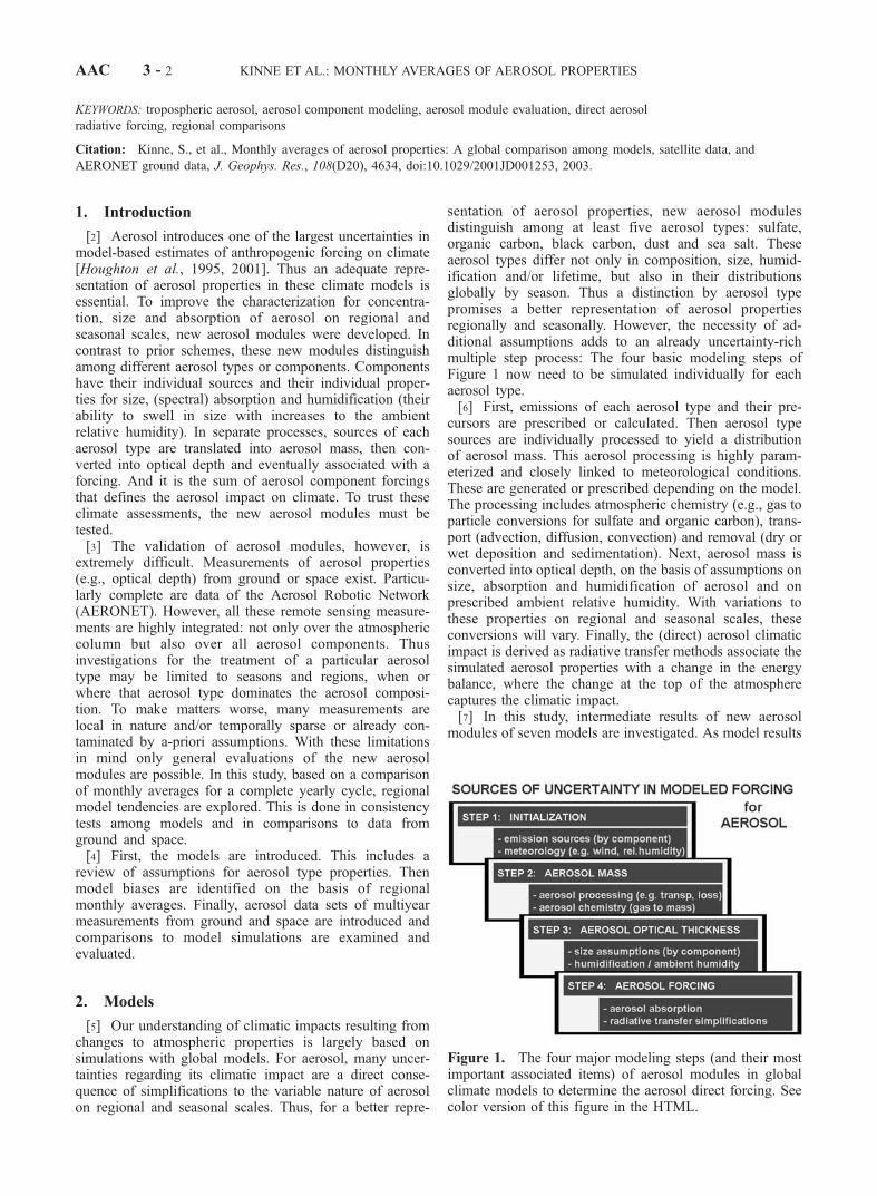
sentation of aerosol properties, new aerosol modulesdistinguish among at least five aerosol types: sulfate,organic carbon, black carbon, dust and sea salt. Theseaerosol types differ not only in composition, size, humid-ification and/or lifetime, but also in their distributionsglobally by season. Thus a distinction by aerosol typepromises a better representation of aerosol propertiesregionally and seasonally. However, the necessity of ad-ditional assumptions adds to an already uncertainty-richmultiple step process: The four basic modeling steps ofFigure 1 now need to be simulated individually for eachaerosol type.[6] First, emissions of each aerosol type and their pre-
cursors are prescribed or calculated. Then aerosol typesources are individually processed to yield a distributionof aerosol mass. This aerosol processing is highly param-eterized and closely linked to meteorological conditions.These are generated or prescribed depending on the model.The processing includes atmospheric chemistry (e.g., gas toparticle conversions for sulfate and organic carbon), trans-port (advection, diffusion, convection) and removal (dry orwet deposition and sedimentation). Next, aerosol mass isconverted into optical depth, on the basis of assumptions onsize, absorption and humidification of aerosol and onprescribed ambient relative humidity. With variations tothese properties on regional and seasonal scales, theseconversions will vary. Finally, the (direct) aerosol climaticimpact is derived as radiative transfer methods associate thesimulated aerosol properties with a change in the energybalance, where the change at the top of the atmospherecaptures the climatic impact.[7] In this study, intermediate results of new aerosol
modules of seven models are investigated. As model results
Figure 1. The four major modeling steps (and their mostimportant associated items) of aerosol modules in globalclimate models to determine the aerosol direct forcing. Seecolor version of this figure in the HTML.
AAC 3 - 2 KINNE ET AL.: MONTHLY AVERAGES OF AEROSOL PROPERTIES
depend on model specific assumptions, model details areintroduced first. Special attention was given to assumptionsfor the conversion of aerosol mass into aerosol opticaldepth.
2.1. Model Specifications
[8] Aerosol modules of seven global models are com-pared. The models primarily simulate tropospheric processesat horizontal resolutions of about 300 � 300 km. Themodels can be divided into two classes: Global circulationmodels (GCMs), which generate their own meteorology,and chemical transport models (CTMs), which adopt mete-orological data (usually for a particular year). For GCMs thelink to a particular year can be accomplished throughnudging, an elementary form of data assimilation. Nudgingin GCMs reduces biases of simulated circulation andsimulated winds.[9] 1. ECHAM4 (EC) is a global circulation model
[Roeckner et al., 1996; Lohmann et al., 1999], whichoriginated at the Max-Planck-Institute for Meteorology(Hamburg, Germany). Wind, temperature and pressurefields are generated without a link to a particular year(50 year simulation). (Successful nudging to ECMWF datafrom 1993 to 1997 has been demonstrated, though it is notconsidered here.)[10] 2. MIRAGE (MI) is a chemical transport model of
PNNL (Richland, Washington, United States), which iscoupled on-line with a global circulation model [Ghan etal., 2001a, 2001b]. To improve agreement on time-scales ofdays nudging has been applied. Results are based onECMWF assimilated wind, temperature and sea-surfacetemperature fields from June 1994 to May 1995.[11] 3. GOCART (GO), from Georgia Institute of Tech-
nology and NASA-Goddard (Atlanta, Georgia/Greenbelt,Maryland, United States), is a chemical transport model[Chin et al., 2000, 2002; Ginoux et al., 2001] driven byassimilated meteorological fields from the GEOS DAS(Goddard Earth Observing System Data Assimilation Sys-tem). Simulations usually refer to 1990. Additional simu-lations with meteorological data for 1996 and 1997 wereused to demonstrate year-to-year variability.
[12] 4. CCSR (CC) (or SPRINTARS) from the Center forClimate System Research at the University of Tokyo andfrom Kyushu University (Tokyo and Kyushu, Japan), is achemical transport model [Takemura et al., 2000, 2002].The model is coupled with the CCSR/NIES (NationalInstitute for Environmental Studies) atmospheric generalcirculation model. Here, results are based on nudged wind,temperature and pressure fields of the NCEP/NCAR(National Center for Environmental Predictions/NationalCenter for Atmospheric Research) reanalysis for 1990.[13] 5. GISS (GI), the community model of NASA-GISS
(New York City, United States) is a global circulation model[Tegen et al., 1997, 2000; Koch et al., 1999; Koch, 2001].Fields for wind, temperature and pressure are generatedwithout a link to a particular year (3 year simulation).[14] 6. Grantour (Gr), from the University of Michigan
(Ann Arbor, Michigan, United States), is a Lagrangianmodel that treats the global scale transport, transformationand removal of trace species in the atmosphere [Walton etal., 1988]. Wind, temperature and pressure fields are gen-erated without a link to a particular year (1 year simulation).[15] 7. ULAQ (UL) is a coarse resolution chemical
transport model [Pitari et al., 2002] from the Universityof L’Aquila (Italy). Meteorological variables are generatedin a coupled GCM model (5 year simulation).[16] Next, individual model assumptions with respect to
the four steps of Figure 1 are explored in more detail.2.1.1. Initialization[17] The meteorological data provide the background in
model simulations. The meteorology is either generated(GCM) or prescribed (CTM) by observed meteorologicaldata (e.g., wind, temperature, pressure). Meteorological dataof all models differed, because even when identical years inCTMs were selected, the sources of assimilation datadiffered. Model characteristics parameters, includingchoices for meteorology are summarized in Table 1.[18] One of the more important reasons to explain differ-
ences in simulated aerosol properties are adopted data foraerosol emissions. The IPCC report [Houghton et al., 2001]provides a comprehensive overview on current data sets foraerosol components. For the seven evaluated models the
Table 1. Comparison of Model Resolution, Meteorology, and References for Emission Sourcesa
ECECHAM4
GOGOCART
MIMIRAGE
GIGISS
CCSprintars
GRGrantour
ULULAQ
Origin MPI,ger NASA,us PNNL,us NASA,us Kyushu,jap U.Mich,us U.Aquila,itGrid (lon/lat) 3.8 � 3.8 2.5 � 2.0 2.8 � 2.8 4.0 � 5.0 1.1 � 1.1 5.6 � 5.6 10 � 22.5Vert.layers 19 20 (26) 24 9 11 19 25Simulation 50 years 090096097 6094-5095 3 years 090 1 year 5 yearsMet-data generated geos/das ECMWF generated ncar/ncep echam3.6 from gcmClouds prognostic diagnostic prognostic prognostic prognostic prognostic diagnosticHum.growth r1 r1 r2 r3 r2Emis: dust r4 r5 r6 r7 r8 r5 r5Emis: carb. r9, r10 r11, r12 r9, r10 r9 r9, r13, r10 r9, r10 r9, r12Emis: salt r14 r15 r16 r15 r17Surf. winds prognostic SSM/I ECMWF r18 prognostic r18 r18Emis: sulf. r19 r20 r19 r19 r19 r19 r19Sulf.oxidant imported imported co-ch4 ch. semi-prog imported imported imported
aMIRAGE: Water-uptake is based on ECMWF relative humidity and nudges towards ECMWF winds and temperatures. GISS: Oxidant precursors areimported rather than oxidants (H2O2 is carried as a prognostic species). References: r1, Koepke et al. [1997]; r2, Koehler [1936]; r3, Hobbs et al. [1997];r4, Schulz et al. [1998]; r5, Ginoux et al. [2001]; r6, Gillette and Passi [1988]; r7, Tegen and Fung [1995]; r8, Gillette [1978]; r9, Liousse et al. [1996];r10, Cooke and Wilson [1996]; r11, Duncan et al. [2003]; r12, Cooke et al. [1999]; r13, Guenther et al. [1995]; r14, Guelle et al. [2001]; r15, Monahan etal. [1986]; r16, O’Dowd et al. [1997]; r17, Erickson et al. [1986]; r18, Gong et al. [1997]; r19, Benkowitz et al. [1996]; r20, Olivier et al. [1996].
KINNE ET AL.: MONTHLY AVERAGES OF AEROSOL PROPERTIES AAC 3 - 3
primary references for each aerosol type are listed in Table 1.Even when the same primary reference is given, manyuncertainties regarding the comparability of source strengthamong models remain. Differences in data implementation(daily or monthly averages), a dependence on meteorology(near surface winds) and the use of secondary data dilute aclear picture of source strength. Future model evaluationsneed to focus on assumptions for source strength andseasonality as not to attribute their differences to aerosolprocessing.2.1.2. Toward Aerosol Mass[19] The processing of emission sources toward a distri-
bution of 3-D mass fields for each aerosol type involvesmany processes. All models address the major aerosolmechanisms, including sulfate chemistry (gas to particleconversion), transport (advection, diffusion and convec-tion) and aerosol processing: (1) dry deposition: aerosolclustering from turbulent mixing; (2) in-cloud scavenging:(a) aerosol can act as cloud condensation nucleusand (b) aerosol can diffuse in cloud drops with subsequentremoval via precipitation; (3) below-cloud scavenging:aerosol capture and removal by rain; (4) aerosol re-emis-sion: by evaporation of rain or cloud drops; (5) gravitationalsettling.[20] Most of these processes are highly parameterized and
tuned to model resolution. Thus aerosol processing to masshas one of the largest potentials for errors. More detailedmodel comparisons in the future have to include tests ofparticular processes (e.g., tracer studies to understand trans-port biases or comparisons of near surface wind fields). Inaddition, control experiments linked to a particular aerosoltype are very much needed, similar to a recently concludedcomparison of simulated (near surface) sulfate mass to localmeasurements in COSAM [Lohmann et al., 2001; Barrie etal., 2001; Roelofs et al., 2001].2.1.3. Toward Aerosol Optical Depth[21] In the new aerosol modules the (dry) aerosol mass m
is converted to aerosol optical depth t, separately for eachaerosol type. The conversion factor, as the ratio betweenoptical depth and dry mass, is called the mass extinctionefficiency b (units in m2/g). For a distribution of spheres, b isdefined by
b ¼ t=m ¼ 0:75 Q= r reð ÞH
where Q is the extinction efficiency, r is the density, re is theeffective radius (�r3/�r2), and H is the humidificationfactor.[22] The extinction efficiency Q is the ratio between
extinction cross-section and the geometric cross-section. Qdepends on aerosol size and composition. Q is largest, ifparticle radius and interacting wavelength have similarvalues. Maximum values for Q near values of 3 are commonfor size-distributions with effective radii of about 0.5 mm atmid-visible wavelengths. Q converges towards 2 forincreasingly larger radius-to-wavelength ratios (geometricallimit). For increasingly smaller radius-to-wavelength ratios,Q decreases sharply (inverse proportional to 4th power) forscattering aerosol but only moderately (inverse propor-tional) for absorbing aerosol. For hydrophilic aerosolcomponents (e.g., sulfate, sea salt and organic carbon) wateruptake impacts Q in two ways: Water uptake increases the
aerosol size, thereby increasing the radius-to-wavelengthratio. And water uptake decreases the aerosol absorption,which is less important if the effective aerosol radius islarger than the wavelength.[23] The humidification factor H accounts for effects of
water uptake by hydrophilic aerosol types.
H ¼ 1 for hydrophobic aerosol
H ¼ Q; hum=Q� �
re;hum=re� �2
for hydrophilic aerosol
The subscript (hum) indicates values at ambient (moist)conditions as compared to completely dry conditions. Thusthe radius ratio (re,hum/re) captures aerosol swelling. Thisswelling is nonlinear, as a function of the ambient relativehumidity, which can vary strongly within the region of amodel grid point. Thus choices for the regional effectiveambient relative humidity become a critical issue for thesizing of hydrophilic aerosol types.[24] Given the multiparameter influence for m-to-t con-
versions, model assumptions for size, humidification, den-sity and composition (refractive index influences valuesfor Q) are compared next.2.1.3.1. Size Assumptions[25] Larger mass extinctions efficiencies are associated
with smaller (and especially absorbing) aerosol and withmore humid environments. Table 2 provides a summary ofsize-assumptions.[26] A higher number of size-classes (or size modes) can
better represent the observed aerosol size distributions. Thisis particularly important when super-micrometer sizes areinvolved, and recognized with 2 to 10 size-classes for dustand sea salt. In contrast, for sulfate and carbon aerosol mostmodels consider only a single (submicrometer) size class.Such simplification permits a direct comparison amongmodels. For sulfate, the dry size is large in GISS and smallin Grantour, relative to other models. For both carbon types,the dry sizes in GISS and also CCSR are large, whereas drysizes in ECHAM4 and GOCART are small (although theirassumed wide distribution permits few larger sizes tocontribute).2.1.3.2. Humidification Assumptions[27] The mass extinction efficiency is also a function of
environmental conditions. The ambient relative humiditymoderates the size of hydrophilic aerosol. Most modelsallow water uptake only for sulfate, sea salt and organiccarbon. Size and relative humidity relationships are sum-marized in Table 3.[28] Most models recognize the nonlinear relationship
between size and humidity. However, there are significantdifferences already at intermediate relative humidities (50–80%). With respect to aerosol size, the assumed swelling (orradius increase) is usually stronger for larger aerosol (e.g.,sea salt versus sulfate). With respect to aerosol type theassumed swelling is usually stronger for sulfate than forcarbon. This is in agreement with observed correlationsbetween size and ambient relative humidity at severalU.S. National Park sites [Malm et al., 1994; D. Day andW. Malm, private communication, 2000]. In Table 3, thelocations of Grand Canyon, Arizona, and Big Bend, Texas,provide data for carbon-dominated aerosol, whereas Great
AAC 3 - 4 KINNE ET AL.: MONTHLY AVERAGES OF AEROSOL PROPERTIES

Smoky, Kentucky, provides data for sulfate-dominatedaerosol.[29] The water uptake in hydrophilic aerosol types
depends not only on the prescribed humidification (strength,see Table 3) but also on the prescribed ambient relativehumidity, which may be in error. Because of the increasedsensitivity at higher ambient relative humidities, small
humidity errors can have a strong impact on aerosol sizeand the derived aerosol forcing. Therefore many modelsintroduce less physical but ‘more stable’ simplifications.These include the replacement of the predicted by(re-analysis) prescribed ambient relative humidities (e.g.,MIRAGE), the assumption of a maximum growth factor farbefore saturation (e.g., sulfate in GISS or sea salt in ULAQ),
Table 2. Comparison of Assumed Dry Aerosol Sizes in Modelsa
EC GO MI GI CC Gr UL
DU 2 sizesvariablesmaller awayfrom sources
7 sizes.14, .24,.45, .80,1.4, 2.4,4.5
2 sizes.16, .75
8 sizes.15, .25,.40, .80,1.5, 2.5,4.0, 8.0
10 sizes.13, .20,.33, .52,.82, 1.3,2.0, 3.2,5.1, 8.0
2 sizes.88, 1.91
5 sizes.01 � 2n, n = 5,.,9
OC 1 size.11
1 size.10
2 sizes.02, .16
1 size.50
1 size.24
1 size.17
5 sizes.01 � 2n, n = 2,.,5
BC 1 size.04
1 size.04
2 sizes.02, .16
1 size.10
1 size.067
(in OC) 5 sizes.01 � 2n, n = 1,.,4
SS 2 sizesvariablefunction ofsurface winds
2 sizes.80, 5.7data fromfour sizebins
2 sizes.16, 2.7
1 size2.0datafrom sixsize bins
10 sizes.13, .20,.32, .50,.79, 1.3,2.0, 3.2,5.0, 7.9
2 sizes.79, 1.6
6 sizes.01 � 2n, n = 5,.,10
SU 1 size.24
1 size.24
4 sizes.02, .16,.75, 2.7
1 size.30
1 size.24
1 size.12
16 sizes.01 � 2n, n = �5,.,10
aFor each aerosol type the number of size classes is listed. In addition, mean radii of assumed size-bins or effective radii re (third moment to secondmoment ratio) of assumed lognormal size-distributions are provided (in units of mm). ECHAM4 and GOCART fixed aerosol size modes are based on theGADS data set [Koepke et al., 1997]. MIRAGE assumes internal mixing of components (only model) and predicts number and mass for each of the4 modes. CCSR assumes for transport processes an internal mixture of organic and black carbon (except for 50% of the black carbon mass originating fromfossil fuel) with different oc/bc mass ratios according to the source.
Table 3. Comparison of Assumed Humidificationsa
RH, % EC GO MI GI CC Gr UL ‘‘Observed’’
OC0 1.00 1.00 1.00 1.00 1.00 1.00 1.0050 1.24 1.24 1.06 1.00 1.08 1.00 1.01 1.01–1.0570 1.35 1.35 1.11 1.00 1.10 1.00 1.03 1.15–1.3080 1.45 1.45 1.17 1.00 1.44 1.00 1.05 1.25–1.5090 1.65 1.65 1.31 1.00 1.69 1.00 1.09 1.40–1.9095 1.89 1.89 1.51 1.00 1.96 1.00 1.18
SS0 1.00 1.00 1.00 1.00 1.43 1.00 1.0050 1.30 1.60 1.38 1.00 1.43 1.0570 1.49 1.81 1.62 1.00 1.43 1.1880 1.57 1.99 1.83 1.00 1.43 1.67 1.4590 2.06 2.38 2.27 1.00 1.43 1.5295 2.57 2.89 2.84 1.00 1.43 1.55
SU0 1.00 1.00 1.00 1.00 1.00 1.00 1.0050 1.41 1.40 1.20 1.00 1.22 1.28 1.30 1.05–1.2070 1.57 1.50 1.34 1.06 1.37 1.41 1.52 1.15–1.3580 1.70 1.60 1.47 1.20 1.48 1.53 1.67 1.20–1.5090 1.94 1.80 1.77 1.60 1.76 1.75 1.84 1.45–1.8095 2.27 1.90 2.16 1.60 2.26 2.05 1.92 1.70–2.05aPrescribed size increases for organic carbon (OC), sea-salt (SS) and sulfate size (SU), with respect to their dry size, are compared for
ambient relative humidities (RH) of 50, 70, 80, 90 and 95%. Estimates from measured relationships between size (via scattering) andrelative humidity are given as well. ULAQ and GISS values are derived from permitted optical depth t increases, �(re,hum/re) � SQRT(�t). CCSR sea-salt aerosols consist of 70% of salt and 30% of water in mass. GOCART permits limited humidification for blackcarbon on a time delay basis. GISS uses a growth cap for sulfate at 85% ambient relative humidity (rh). ‘‘Observed’’ surface statistics arefrom three U.S. National Park sites, �(re,hum/re) � SQRT (�scattering coefficient).
KINNE ET AL.: MONTHLY AVERAGES OF AEROSOL PROPERTIES AAC 3 - 5

the prescription of an average swell-factor (e.g., sea salt inCCSR), the omission of swelling altogether (e.g., carbon inGrantour) (if not understood) or worse, the assumption of aconstant for the conversion of component mass into opticaldepth (e.g., carbon and sea salt in GISS) which also rejectsall other (e.g., temporal) dependences. In what way thesesimplifications can be justified is unclear, since neithermodel provided data on their applied 3-dimensional ambientrelative humidity fields. Meaningful future model compar-isons have to explore the water uptake for each aerosol type,which may require simulations with prescribed relativehumidity fields.2.1.3.3. Density Assumptions[30] The dry mass density is inversely proportional to the
mass extinction efficiency. Assumed dry mass densities arecompared in Table 4. The largest differences among modelsare for organic carbon. However, the suggested uncertaintyof up to 2 only applies to dry aerosol, and the likely wateruptake reduces uncertainties (as densities decrease toward1g/cm3). For dust, sulfate and sea-salt aerosol componentsmodel assumptions are similar, except for the low sea-saltvalue of MIRAGE. However, also this difference will bewashed out with likely water uptake.2.1.3.4. Composition Assumptions[31] Mass extinction efficiency is also affected by
assumptions to aerosol composition (and absorption) viathe extinction efficiency Q. Especially at small size param-eters (when aerosol size is small compared to the wave-length) absorption can increase mass extinction efficiencies(e.g., black carbon type in the visible). Absorption byaerosol is a critical parameter in radiative forcing simula-tions. In fact, a better representation of aerosol absorption isa major reason for the separate treatment of aerosol types innew aerosol modules. Absorption is defined by the refrac-tive index’s imaginary part (roughly: >0.1 strong /0.1>
moderate >0.001 / <0.001 weak). Its selection for tropo-spheric aerosol is particularly important at mid-visiblewavelengths, because of (weight-) maxima for the productof aerosol extinction and available radiative energy.Assumed refractive indices at a visible and an infraredwavelength for the five aerosol types are compared inTable 5.[32] The data of Table 5 are for ‘dry’ aerosol and the
addition of water will reduce real and imaginary partstoward the refractive index of water (1.34/0.1e-8). Anysimilarity among choices in models originates largely fromthe limited number of catalogued values. However, thereare some noteworthy differences.[33] At visible wavelengths, differences are larger for the
imaginary parts of organic carbon and dust:[34] 1. For dust (vis) the lowest model assumption of
0.002 is supported by statistics from inversions of skyradiances [Dubovik and King, 2000] at dust-dominatedsites. On the other hand, the largest values of 0.008 are inline with diffuse reflectance measurements [Patterson et al.,1976]. As large optical depths for dust are found in manyregions of the world, this difference is significant forsimulations of the aerosol radiative forcing. Weaker dustabsorption at solar wavelengths reduces the warming of theaerosol layers and increases solar energy losses to space[Kaufman et al., 2001], resulting in a more negative ToAforcing. Absorption of dust increases toward shorter wave-lengths (UV) and decreases toward longer wavelengths(near-IR). It is unclear, if and to what degree this importantspectral dependence is considered in models with limita-tions to spectral resolution in their (solar) radiative transferschemes.[35] 2. For carbon (vis), absorption is largely determined
by the fraction of black carbon. All models agree on strongabsorption for black carbon, assuming large refractive indeximaginary parts of about 0.5. Less understood is theabsorption of organic carbon. Estimates [Novakov et al.,1997] suggest light to moderate absorption with a refractiveindex imaginary part of near 0.005 at visible wavelengths.However, uncertainties are so large that some models ignoreabsorption by organic carbon completely. This is not a goodchoice, even though black carbon is expected to dominatecarbon absorption. It should be kept in mind that blackcarbon only accounts for a small portion of the total carbon
Table 4. Comparison of Assumed Dry Mass Densitiesa
EC GO MI GI CC Gr UL
DU: dust 2.65 2.6 2.6 2.5 2.5 2.5 2.5OC: organic carbon 1.9 1.8 1.7 1.0 1.47 1.0 2.0BC: black carbon 1.0 1.0 1.0 1.0 1.25 1.0 1.0SS: sea salt 2.17 2.2 1.9 2.16 2.25 2.17 2.2SU: sulfate 1.7 1.7 1.77 1.7 1.77 1.77 1.7
aValues are given in g/cm3.
Table 5. Comparison of Assumed Dry Component Refractive Indices at 0.55 and 10 mm (Real Part, Imaginary
Part)
EC GO MI GI CC Gr UL
Visible 0.55 mmDU 1.5, .0055 1.5, .0078 1.5, .002 1.56, .005 1.53, .008 1.53, .008 1.56, .006OC 1.53, .006 1.53, .006 1.55, 0 1.53, .005 1.53, .006 1.53, 0 1.6, .0035BC 1.75, .44 1.75, .44 1.9, .6 1.57, .5 1.75, .44 1.75, .44 2.07, .6SS 1.5, 0 1.5, 0 1.5, 0 1.45, 0 1.38, 0 1.38, 0 1.50, 0SU + MSAa 1.43, 0 1.43, 0 1.53, 0 1.43, 0 1.43, 0 1.43, 0 1.45, 0
Infrared 10 mmDU 2.9, .7 2.57, .5 1.62, .12 3.0, 1.0 1.75, .162 1.75, .162OC 1.9, .1 1.82, .09 1.7, .07 2.19, .13 1.82, .09 2.19, .13BC 2.2, .73 2.21, .72 2.22, .73 2.3, 1.29 2.21, .72 2.21, .72SS 1.55, .02 1.5, .014 1.5, 0 1.53, .016 1.31, .04 1.31, .04SU + MSAa 1.95, .455 1.89, .455 1.98, .06 1.95, .455 1.89, .455 1.89, .455aSulfate: usually based on 75% sulfuric acid solution (MIRAGE data are based on ammonium sulfate).
AAC 3 - 6 KINNE ET AL.: MONTHLY AVERAGES OF AEROSOL PROPERTIES

mass, and that smaller black carbon sizes (compared toorganic carbon) have a reduced impact on total carbonproperties toward longer wavelengths. Thus good estimatesfor the absorption properties of organic carbon matter andare needed.[36] At far-infrared wavelength, the choices for refractive
indices are usually less important, because of a lack inextinction and in temperature contrast to the ground.Choices, however, are important for elevated larger aerosolsizes. This mainly applies to dust. Yet with respect to dustmany uncertainties regarding their composition and associ-ated infrared absorption features remain [Sokolik and Toon,1999].2.1.4. Toward Radiative Forcing[37] To relate aerosol properties to climate, simulations
with spectral broadband radiative transfer methods areperformed. Necessary input data, in terms of aerosolproperties, are (type combined) measures for amount(optical depth), absorption (single scattering albedos) andscattering behavior (phase-function) as function of wave-length. Radiative transfer is well understood, and scheme-related errors should be small. However, time-efficiencyrequirements in global models (evaluation at each grid pointin frequent time steps) require simplifications to the radia-tive transfer method and more importantly to the spectralresolution. These approximations can compromise priormodeling efforts. Table 6 provides an overview of thenumber of assumed spectral bands and the adopted radia-tive transfer method.
[38] Rather than judging radiative transfer choices ofindividual models, potential errors from common simplifi-cations are explored for different aerosol types. As to relateto the climate-predicting nature of these models, results ofsensitivity studies over cloud-free ocean scenes areexpressed in ‘cooling’ or ‘warming’ (these are terms thatcapture the changes to the radiative net-flux at the top of theatmosphere, where energy gain to the Earth-atmospheresystem is referred to as ‘warming’ and an energy loss as‘cooling’). With respect to the radiative transfer method, theuse of the widely used two-stream scattering approximationtends to overestimate (solar) cooling by about 5%. Com-mon spectral simplifications can even lead to larger errors.For example, a solar two-band approach (with 1 visibleband (0.55 mm) and 1 near-IR band (1.6 mm)) largelyignores the solar spectral variability of aerosol properties.This leads to an underestimate of (solar) cooling by about15% for dust and by about 25% for biomass and urbanaerosol. Another common simplification is the neglect ofaerosol forcing in the far-IR. While this may be justifiablefor near surface aerosol (e.g., urban pollution), the effect of(IR) warming is nonnegligible if aerosol is elevated (e.g.,biomass and dust) and characteristic aerosol sizes exceed1 mm in size (e.g., dust). The neglect of IR (greenhouse)-effects for dust can introduce errors comparable in magni-tude (though opposite in sign) to that of a solar two-bandapproximation. In summary, simplifications of currentradiative transfer schemes can easily lead to forcing errorson the order of 20%.2.1.5. Summary[39] All four modeling steps (see Figure 1) are potential
sources for errors. The largest uncertainties are associatedwith the initial two steps (initialization and aerosol process-ing for mass fields), because of complex assumptions andparameterizations, which were not examined in this study.In contrast, model differences during the last two modelingsteps (mass to optical depth conversions and radiativetransfer calculations) result from assumptions or simplifica-tions that can be tested. Particularly useful is an understand-ing of conversion biases, because models are usuallyevaluated in comparisons to optical depth. Critical aerosol
Table 6. Comparison of Radiative Transfer Schemes: Choices of Models for Spectral Resolution and Methoda
Micrometers EC GO MI GI CC Gr UL
visible .2– .7 1 (sp-t) 1 + 7 (sp-a) 9 (sp-t) 1(sp-a) 7 (sp-a) 4 (sp) (sp)*near-IR .7–4 1 (sp-t) 3 (sp-a) 10 (sp-t) 1(sp-a) 1 (sp-a) 5 (sp) (sp)*far-IR 4–50 6 (sp) 10 (sp-a) 1 (10 mm) 4(sp-a) 10 (sp-t) 14 (sp) (em)*
aHere, sp, spectral sub-bands; em, emissivity approach; �a, adding doubling; �t, two-stream; asterisk, external option.
Figure 2. Location of selected regions and AERONETsites for model evaluations. Data at three AERONET sitesare investigated in more detail. These sites are marked by across: GSFC (USA), Capo_Verde (off Africa) and Mongu(southern Africa). See color version of this figure in theHTML.
Table 7. Classification for Regions of Figure 2 by Type and
Source Strength
Class Regions in Figure 2
Urban sources E. Europe, E. AsiaUrban outflow regions 1, 7 and 9Dust sources N. Africa, AsiaDust outflow region 2Biomass sources Africa, S. AmericaBiomass outflow regions 3, 4 and 8Remote, tropical regions 6 and 10Remote, S. Hemis. regions 5 and 11Unclassified regions 12 and 13, N. America
KINNE ET AL.: MONTHLY AVERAGES OF AEROSOL PROPERTIES AAC 3 - 7

properties for the mass conversion are the prescribedambient relative humidity and assumptions to aerosol size,humidification, density and composition. Although aerosolassumptions of all tested models were presented in Tables2–5, firm conclusions on biases are not possible, withoutdata on ambient relative humidity fields and relative weightsfor sizes classes of multibinned aerosol types. This illus-trates the need for additional model output (water uptake)and for control runs (e.g., prescribing identical ambientrelative humidity fields for size swelling) in future modelevaluation efforts. Nonetheless, demonstrated dependenciesand listed model assumptions provide a useful backgroundfor the understanding of differences among models, wheneffective mass conversions are derived (below) from simu-lated mass and optical depth data for each aerosol type on aregional and seasonal basis.
2.2. Simulated Monthly Averages
[40] The evaluation of general model tendencies is basedon monthly averages. Individually for each aerosol type,model results are compared. Comparisons focus on aerosolmass and aerosol optical depth, intermediate properties inglobal aerosol forcing simulations. Combining both prop-erties and also conversions of mass into optical depth areexplored. In addition, compositional mixture and absorptionare addressed.[41] Comparisons are conducted on a regional basis.
These regions are small enough to accommodate distinctdifferences in sources and transport but large enoughminimize effects from differences in spatial resolution (ofmodels). The regional choices include 13 ocean regions andthe 7 land regions. All regions plus locations of 20 AerosolRobotic Network (AERONET) ground sites with yearlongaerosol statistics are displayed in Figure 2.[42] The huge number of comparisons (each month, each
aerosol type, each regions and different properties) neces-sitated a more compact approach. Therefore simulatedmonthly averages are summarized by ‘‘yearly average’’and ‘‘seasonality’’. Seasonality is defined as the yearlyrange of the three-month running mean relative to the yearlyaverage [(avg3mo_MAX � avg3mo_MIN)/(� avgmo/12)]. Inaddition, regions of Figure 2 were combined according todominant aerosol type (urban, dust or biomass) and accord-ing to source distance, as outlined in Table 7.[43] For the eight regional aerosol classes of Table 7 yearly
average and seasonality were compared for aerosol mass,aerosol optical depth and mass extinction efficiency. Modeltendency were identified for each aerosol type by comparingindividual model simulations to that of the median model(the model ranked fourth among the seven models).2.2.1. Aerosol Mass[44] All models display the expected decrease in aerosol
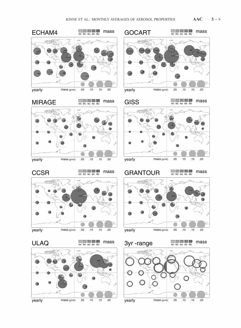
mass from sources toward remote regions. However, thereare differences in source strength, in decay rate (toward
remote regions) and in seasonality among the sevenmodels. Mass simulations of all seven models are dis-played in Figure 3 and quantified in Table 8. Table 8 alsoidentifies models with extreme behavior, and uncommonmodel tendencies are summarized in Figure 4. Figure 3also illustrates that for yearly averages the variability fromsimulations for three different years with the same modelis small compared to differences (disk size in Figure 3)among models. Thus, to explain model differences, thechoice of meteorological data appears of secondaryimportance.[45] Despite some common general trends, mass differ-
ences among models are large. Not only type-combinedtotals (disk sizes in Figure 3) but also contributions ofindividual aerosol types (pie sections of disks in Figure 3)vary, when comparing simulated mass of different modelsfor the same region. Models with extreme mass simula-tions are identified for each aerosol class and each aerosoltype in Table 8 for yearly average and for seasonalitystrength. For more detailed information on mass simula-tions, the individual model values (yearly average, sea-sonality strength and seasonality phase) for each of the20 regions of Figure 2 are compared in Appendix B. Tosimplify a comparison of the yearly average mediansamong aerosol types, the average compositional mixtureaerosol class is summarized in Table 9, which also showsmass ratios between organic and black carbon.[46] Model simulations identify dust and sea salt as
leading contributors to aerosol mass, which at least inpart reflects their relative large particles sizes (m � r3).Over continents dust dominates by mass. Even for urbanand biomass source regions dust mass matches the com-bined mass contributions from carbon and sulfate. Overoceans, sea salt usually dominates by mass, except fordust outflow regions (e.g., west off Africa). As yearlyaverages and seasonality for dust and sea salt displayhigher variability than for other aerosol types, the largedifferences in simulated total mass among models are notsurprising.[47] Larger differences are also found for simulated car-
bon mass away from urban sources. Although carbon is lessimportant in terms of total mass, the mass ratio betweenorganic and black carbon varies by almost one order ofmagnitude (GISS �12 and Grantour �1.5), even afterexcluding very large values in excess of 20 by the ULAQmodel. Different choices for carbon sources are certainly acontributing factor as ob/bc ratios from biomass burning areusually larger than ratios from fossil fuel burning.2.2.2. Aerosol Optical Depth[48] Aerosol optical depth (or aerosol optical thickness,
thus AOT) is derived from simulated aerosol mass fields.Thus a somewhat similar behavior is expected. However,while the decrease away from sources toward remoteregions is maintained, there are differences, due to increased
Figure 3. (opposite) Simulated aerosol mass averaged for the regions of Figure 2. Yearly averages (disks) and seasonality(rings) of each model are presented. Over each region the size of disks or rings indicates the amount (according to the scalein the lower right), and the detail on disks or rings indicates fractional contributions by aerosol type (following the key inthe upper right). Also shown is the impact of different meteorological data (1990, 1996, and 1997 simulations with theGOCART model) on the yearly average and a model composite with 4th-ranked aerosol component properties. See colorversion of this figure in the HTML.
AAC 3 - 8 KINNE ET AL.: MONTHLY AVERAGES OF AEROSOL PROPERTIES
KINNE ET AL.: MONTHLY AVERAGES OF AEROSOL PROPERTIES AAC 3 - 9

Figure 3. (continued)
AAC 3 - 10 KINNE ET AL.: MONTHLY AVERAGES OF AEROSOL PROPERTIES

Table 8. Simulated Component Mass: Values of the Median Model and Models With Extreme Tendenciesa
Yearly Average Component Mass, mg/m2
OC BC SU SS DU
Avg. Max/Min Avg. Max/Min Avg. Max/Min Avg. Max/Min Avg. Max/Min
Urban sources 9.8 UL/GO 2.3 UL 12.9 UL, MI 11.1 EC, GO/GI, MI 48.4 GO, UL/MIUrban outflow 1.1 MI, GI .4 UL 5.3 MI 28.2 EC, GO/GI, MI 16.9 GO, EC/MIDust sources 3.2 UL .8 9.6 Gr 2.9 UL, EC/MI 253. GO, CC/MI, GIDust outflow 2.9 CC/UL .7 UL, GI 3.2 MI 17.6 UL, EC/GI 99.0 EC, GO/MI, GIBiomass sources 13.3 1.5 EC 3.6 UL, MI 3.4 EC/GI, MI 26.7 GO/MI, CCBiomass outflow 2.9 CC .4 CC/UL 2.1 MI 17.1 EC/GI 14.8 UL, GO/MI, CCRemote, tropics 1.0 UL .1 Gr, GO/UL 1.8 MI 18.7 EC/GI 7.5 GO/UL, MIRemote, S. Hemis. .5 MI, GO/Gr, UL .1 GO, MI/UL, GI 1.7 MI/CC,Gr 30.7 EC, GO/GI, MI 4.1 GO
Seasonality for Component Mass
OC BC SU SS DU
Var Max/Min Var Max/Min Var Max/Min Var Max/Min Var Max/Min
Urban sources 0.3 GO .3 .8 Gr/MI, CC 1.3 MI 1.2Urban outflow .7 UL .5 GO .5 CC 1.3 EC/MI 1.3Dust sources .6 EC/MI .5 EC/UL 1.0 CC/MI .8 GO, EC 1.0 ECDust outflow 1.7 1.3 MI .6 CCUL .8 MI 1.1 ULBiomass sources 1.5 1.7 .3 GO, EC .6 MI 1.0 ECBiomass outflow 1.0 UL 1.2 UL .3 CC .3 EC, GI/MI .7 ECRemote, tropics 1.5 MI 1.2 UL .4 MI .5 EC/MI 1.0 CC/GrRemote, S. Hemis. 1.5 1.4 .9 GO, UL .7 MI 1.2 CC/GI
aFor class-combined regions (see Table 7), yearly averages (Avg) and seasonality (Var) of the median model (4th-ranked among all models) arepresented. Seasonality is the ratio of the 3-month running mean range during a year and the yearly average. In addition, models are displayed whose valuesfor Avg or Var exceed (italic-bold) or fail (italic) that of the median model by more than 50%.
Figure 4. Component aerosol mass tendencies with respect to the median model.
Table 9. Simulated Fractional Component Contributions to Aerosol Mass, oc/bc Mass Ratios, and Models With Extreme Tendenciesa
Mass
OC + BC SU SS DUoc/bcRatio
oc/bc RatioMax/MinModelsPercent Max Model Percent Max Model Percent Max Model Percent Max Model
Urban sources 17 MI 22 MI 15 EC 46 GO 4 MI/GOUrban outflow 4 MI 14 MI 48 EC 34 GO 4.5 GI/GrDust sources 3 MI 7 MI 4 EC 86 GO 4.5 MI/GrDust outflow 4 MI 6 MI 20 UL 70 EC 6.5 GI/GrBiomass sources 31 CC 13 MI 9 Gr 47 GO h10i MI/GOBiomass outflow 9 GI 8 MI 47 CC 36 GO h8i GI/GrRemote, tropics 4 GI 9 MI 64 UL 25 GI 7 GI/GrRemote, S. Hemis. 2 GI 7 MI 77 EC 14 GO 7 GI/Gr
aFor class-combined regions (see Table 7), yearly averages of aerosol component fractional contributions (in percent) and of oc/bc mass ratios arepresented. In addition, models with the largest fractional contribution (italic-bold) and models with the largest (italic-bold) and smallest (italic) oc/bc massratio are listed. Very high oc/bc ratios of the ULAQ models (caused by strong BC removal) were ignored.
KINNE ET AL.: MONTHLY AVERAGES OF AEROSOL PROPERTIES AAC 3 - 11
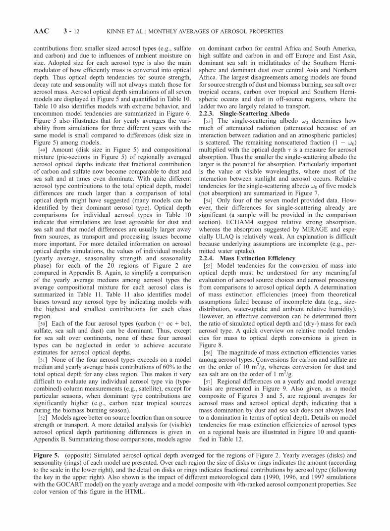
contributions from smaller sized aerosol types (e.g., sulfateand carbon) and due to influences of ambient moisture onsize. Adopted size for each aerosol type is also the mainmodulator of how efficiently mass is converted into opticaldepth. Thus optical depth tendencies for source strength,decay rate and seasonality will not always match those foraerosol mass. Aerosol optical depth simulations of all sevenmodels are displayed in Figure 5 and quantified in Table 10.Table 10 also identifies models with extreme behavior, anduncommon model tendencies are summarized in Figure 6.Figure 5 also illustrates that for yearly averages the vari-ability from simulations for three different years with thesame model is small compared to differences (disk size inFigure 5) among models.[49] Amount (disk size in Figure 5) and compositional
mixture (pie-sections in Figure 5) of regionally averagedaerosol optical depths indicate that fractional contributionof carbon and sulfate now become comparable to dust andsea salt and at times even dominate. With quite differentaerosol type contributions to the total optical depth, modeldifferences are much larger than a comparison of totaloptical depth might have suggested (many models can beidentified by their dominant aerosol type). Optical depthcomparisons for individual aerosol types in Table 10indicate that simulations are least agreeable for dust andsea salt and that model differences are usually larger awayfrom sources, as transport and processing issues becomemore important. For more detailed information on aerosoloptical depths simulations, the values of individual models(yearly average, seasonality strength and seasonalityphase) for each of the 20 regions of Figure 2 arecompared in Appendix B. Again, to simplify a comparisonof the yearly average medians among aerosol types theaverage compositional mixture for each aerosol class issummarized in Table 11. Table 11 also identifies modelbiases toward any aerosol type by indicating models withthe highest and smallest contributions for each classregion.[50] Each of the four aerosol types (carbon (= oc + bc),
sulfate, sea salt and dust) can be dominant. Thus, exceptfor sea salt over continents, none of these four aerosoltypes can be neglected in order to achieve accurateestimates for aerosol optical depths.[51] None of the four aerosol types exceeds on a model
median and yearly average basis contributions of 60% to thetotal optical depth for any class region. This makes it verydifficult to evaluate any individual aerosol type via (type-combined) column measurements (e.g., satellite), except forparticular seasons, when dominant type contributions aresignificantly higher (e.g., carbon near tropical sourcesduring the biomass burning season).[52] Models agree better on source location than on source
strength or transport. A more detailed analysis for (visible)aerosol optical depth partitioning differences is given inAppendix B. Summarizing those comparisons, models agree
on dominant carbon for central Africa and South America,high sulfate and carbon in and off Europe and East Asia,dominant sea salt in midlatitudes of the Southern Hemi-sphere and dominant dust over central Asia and NorthernAfrica. The largest disagreements among models are foundfor source strength of dust and biomass burning, sea salt overtropical oceans, carbon over tropical and Southern Hemi-spheric oceans and dust in off-source regions, where theladder two are largely related to transport.2.2.3. Single-Scattering Albedo[53] The single-scattering albedo w0 determines how
much of attenuated radiation (attenuated because of aninteraction between radiation and an atmospheric particles)is scattered. The remaining nonscattered fraction (1 � w0)multiplied with the optical depth t is a measure for aerosolabsorption. Thus the smaller the single-scattering albedo thelarger is the potential for absorption. Particularly importantis the value at visible wavelengths, where most of theinteraction between sunlight and aerosol occurs. Relativetendencies for the single-scattering albedo w0 of five models(not absorption) are summarized in Figure 7.[54] Only four of the seven model provided data. How-
ever, their differences for single-scattering already aresignificant (a sample will be provided in the comparisonsection). ECHAM4 suggest relative strong absorption,whereas the absorption suggested by MIRAGE and espe-cially ULAQ is relatively weak. An explanation is difficultbecause underlying assumptions are incomplete (e.g., per-mitted water uptake).2.2.4. Mass Extinction Efficiency[55] Model tendencies for the conversion of mass into
optical depth must be understood for any meaningfulevaluation of aerosol source choices and aerosol processingfrom comparisons to aerosol optical depth. A determinationof mass extinction efficiencies (mee) from theoreticalassumptions failed because of incomplete data (e.g., size-distribution, water-uptake and ambient relative humidity).However, an effective conversion can be determined fromthe ratio of simulated optical depth and (dry-) mass for eachaerosol type. A quick overview on relative model tenden-cies for mass to optical depth conversions is given inFigure 8.[56] The magnitude of mass extinction efficiencies varies
among aerosol types. Conversions for carbon and sulfate areon the order of 10 m2/g, whereas conversion for dust andsea salt are on the order of 1 m2/g.[57] Regional differences on a yearly and model average
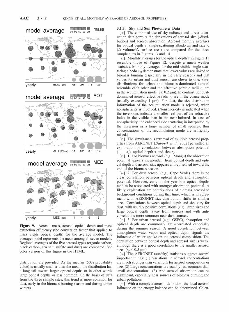
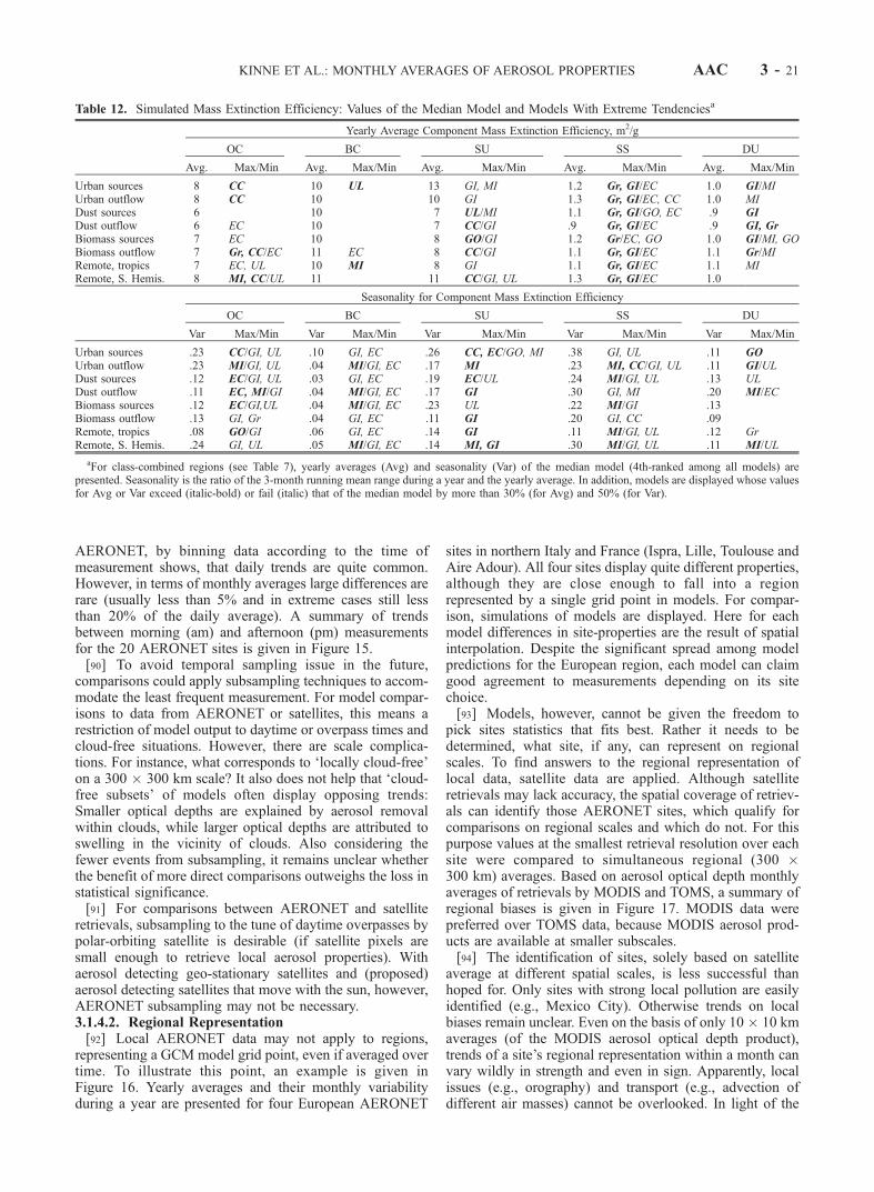
basis are presented in Figure 9. Also given, as a modelcomposite of Figures 3 and 5, are regional averages foraerosol mass and aerosol optical depth, indicating that amass domination by dust and sea salt does not always leadto a domination in terms of optical depth. Details on modeltendencies for mass extinction efficiencies of aerosol typeson a regional basis are illustrated in Figure 10 and quanti-fied in Table 12.
Figure 5. (opposite) Simulated aerosol optical depth averaged for the regions of Figure 2. Yearly averages (disks) andseasonality (rings) of each model are presented. Over each region the size of disks or rings indicates the amount (accordingto the scale in the lower right), and the detail on disks or rings indicates fractional contributions by aerosol type (followingthe key in the upper right). Also shown is the impact of different meteorological data (1990, 1996, and 1997 simulationswith the GOCART model) on the yearly average and a model composite with 4th-ranked aerosol component properties. Seecolor version of this figure in the HTML.
AAC 3 - 12 KINNE ET AL.: MONTHLY AVERAGES OF AEROSOL PROPERTIES

KINNE ET AL.: MONTHLY AVERAGES OF AEROSOL PROPERTIES AAC 3 - 13

Figure 5. (continued)
AAC 3 - 14 KINNE ET AL.: MONTHLY AVERAGES OF AEROSOL PROPERTIES

Table 10. Simulated Aerosol Optical Depth: Values of the Median Model and Models With Extreme Tendenciesa
Yearly Average Component Aerosol Optical Thickness
OC BC SU SS DU
Avg. Max/Min Avg. Max/Min Avg. Max/Min Avg. Max/Min Avg. Max/Min
Urban sources .073 UL, CC/GO .025 UL .158 UL .010 Gr/MI .045 GO, UL/MIUrban outflow .011 MI .003 GO, MI/UL .044 MI .028 Gr, UL/GI 0.22 GO/MI, CCDust sources .020 UL .007 .058 UL/Gr .003 UL, EC/MI .218 MIDust outflow .021 EC .006 GO/UL .023 MI, GO .014 Gr, UL/EC .127 EC/MI, GIBiomass sources .065 UL, CC .025 UL .026 UL .004 Gr/MI .028 MI, CCBiomass outflow .022 CC/EC .003 GO, Gr .020 MI .019 Gr/GI .015 UL, Gr/MI, CCRemote, tropics .006 CC/UL .001 MI, GO/UL .014 MI .016 Gr/GI .008 GO/UL, MIRemote, S. Hemis. .004 MI, GO/UL, Gr .001 GO, Gr/UL .012 MI/CC .050 MI, Gr/CC, GI .005 GO/MI
Seasonality for Component Aerosol Optical Thickness
OC BC SU SS DU
Var Max/Min Var Max/Min Var Max/Min Var Max/Min Var Max/Min
Urban sources .4 GO/MI, UL .3 .4 Gr, UL 1.3 MI 1.2Urban outflow .7 GO/UL .6 GO/UL .5 CC 1.4 MI/CC 1.3Dust sources .7 MI .4 EC 1.0 MI .9 GO, EC 1.0 ECDust outflow 1.5 UL, GI 1.5 .7 CC/MI .7 CC, MI 1.1 ULBiomass sources 1.5 MI 1.5 .4 .6 EC 1.0 ECBiomass outflow 1.0 UL .9 UL .3 .2 EC .7 ECRemote, tropics 1.3 MI 1.1 UL .3 .4 MI/CC 1.0 CC/GrRemote, S. Hemis. 1.6 1.6 .9 Gr/GO .9 MI/GI, UL 1.2 CC/GI
aFor class-combined regions (see Table 7), yearly averages (Avg) and seasonality (Var) of the median model (4th-ranked among all models) arepresented. Seasonality is the ratio of the 3-month running mean range during a year and the yearly average. In addition, models are displayed whose valuesfor Avg or Var exceed (italic-bold) or fail (italic) that of the median model by more than 50%.
Figure 6. Component aerosol optical depth tendencies with respect to the median model.
Table 11. Simulated Fractional Component Contributions to Aerosol Optical Depth and Models With Extreme Tendenciesa
Aerosol Optical Thickness
OC BC SU SS DU
Percent Max/Min Percent Max/Min Percent Max/Min Percent Max/Min Percent Max/Min
Urban sources 28 CC/GO 7 Gr/EC 47 MI/Gr 4 Gr/MI 14 GO/MIUrban outflow 10 CC/Gr 2 GO/UL 42 MI/Gr 27 Gr/GI 19 GO/MIDust sources 11 CC/UL 3 MI/UL 25 MI/Gr 2 EC/MI 59 Gr/MIDust outflow 14 CC/EC 3 MI/UL 19 MI/EC 13 UL/EC 51 EC/MIBiomass sources 48 CC/UL 7 GO/UL 27 UL/Gr 3 Gr/MI 15 GI/MIBiomass outflow 23 GI/Gr 3 GO/UL 28 MI/Gr 26 Gr/GI 19 GO/MIRemote, tropics 14 GI/UL 3 GO/UL 31 MI/CC 38 Gr/GI 14 GO/ULRemote, S. Hemis. 8 CC/Gr 1 GO/UL 23 MI/Gr 60 Gr/MI 8 CC/MI
aFor class-combined regions (see Table 7), yearly averages of aerosol component fractional contributions (in percent) are presented. In addition, modelswith the largest (italic-bold) and smallest (italic) fractional contribution are listed.
KINNE ET AL.: MONTHLY AVERAGES OF AEROSOL PROPERTIES AAC 3 - 15

[58] Mass extinction efficiencies for sulfate, sea salt andorganic carbon are higher at midlatitudes. This can beexplained by on average higher ambient relative humidities.Mass extinction efficiencies for dust are smallest near dustsources, because of the presence of larger aerosol, which isotherwise lost to gravity.[59] Differences among models for the mass extinction
efficiency are largest for sea salt. Surprisingly large are alsodifferences for dust, since mass conversions are not affectedby the ambient moisture. The seasonality for mass extinc-tion efficiency is weak compared to that of mass and opticaldepth. Seasonality differences among models are largelylimited to hydrophilic aerosol, especially at higher latitudes,and therefore most likely caused by differences in therelative humidity fields.[60] The large disagreement for the mass extinction
efficiencies of any aerosol type is disturbing. A closeagreement is highly desirable, as to avoid biases for derivedcomponent aerosol optical depths. As of now, many modelshave relatively large conversions for one type and relativelysmall conversions for another type. Thus there is a dangerthat type-combined totals of optical depth often appear inbetter agreement to measurements (e.g., satellites) than theyshould (as biases of different aerosol types offset eachother). Tools for constraints on mass conversions are nowbecoming available with size-information from remotesensing data by satellites (e.g., Angstrom parameter) orground data (e.g., AERONET size-distributions). Anotherpossibility to avoid conversions biases at least for dust andsea salt is a direct comparison of aerosol (‘wet’) mass withcolumn size-distribution retrievals from AERONET.2.2.5. Summary[61] The intercomparison of models revealed many differ-
ences for simulated mass and optical depth. With manyopposing (thus partially offsetting) trends for differentaerosol types, differences among models were often muchlarger than a comparison of (aerosol type-combined) totalswould have suggested. In an effort to provide a quickoverview of the peculiarities of particular models, unusualtendencies are summarized in Figure 11. For yearly averageand seasonality of aerosol optical depth and aerosol mass,following the regional classification of Table 2, modeldeviations in excess of 30% with respect to the median(or fourth-ranked) model and with respect to MODISretrievals (introduced later) are summarized. In addition,the most unusual overall model tendencies and tendencieson a component basis are as follows:[62] 1. ECHAM4 has high MASS and AOT for dust,
especially in spring near the Azores. Uncommon modelbehaviors by component are (a) for sulfate: high mass and
seasonality, low mee; (b) for dust: strong (out of phase)seasonality for mass and aot; (c) for sea-salt: high mass,very low mee (size overestimate), low aot; (d) for carbon:low mee.[63] 2. GOCART has strong transport (or weak removal).
Uncommon model behaviors by component are (a) forsulfate: dust: high mass, lower mee; (b) for sea-salt: highmass at high latitudes; (c) for carbon: high bc-mee andbc-aot, low urban mass and aot, low oc/bc ratio.[64] 3. MIRAGE has very strong NH sulfate MASS and
AOT and weak tropical sources. Uncommon model behav-iors by component are (a) for sulfate: high mass and highaot (esp. in NH); (b) for dust: low mass, mee and aot, weakseasonality; (c) for sea-salt: low mass, high mee seasonality;(d) for carbon: high mass and aot at higher latitudes, low inthe tropics.[65] 4. GISS has low MASS and AOT, except for sulfate.
Uncommon model behaviors by component are (a) forsulfate: low mee but strong mee-seasonality; (b) for dust:low source mass is offset by high mee; (c) for sea-salt: lowmass, high mee but still low aot; (d) for carbon: low mass,low aot.[66] 5. CCSR has strong sources for dust and carbon but a
weak transport. Uncommon model behaviors by componentare (a) for sulfate: strong mee; (b) for dust: high sourcemass, weak transport, strong seasonality; (c) for sea-salt:strong seasonality for mass; (d) for carbon: high sourcemass, high mee and aot, weak transport, low oc/bc ratio.[67] 6. Grantour has the strongest (sea-salt) AOT in
remote regions. Uncommon model behaviors by componentare (a) for sea-salt: high mee, high aot; (b) for carbon: highmass and aot in urban regions, very low oc/bc ratio.[68] 7. ULAQ has strong MASS and AOT for sulfate and
carbon near (urban) sources, transport is weak. Uncommonmodel behaviors by component are (a) for sulfate: highmass and aot near sources; (b) for dust: weak mee season-ality; (c) for sea-salt: weak mee seasonality; (d) for carbon:high urban mass and aot, weak transport, oc/bc ratio that isvery large away from sources (fast bc removal).[69] On a final note, it should be emphasized that
uncommon tendencies or the lack of them (among models)are not a measure of modeling skill. Model skill can only bedetermined in comparisons to quality data.
3. Comparisons
[70] To evaluate models on an absolute scale the agree-ment of simulated aerosol properties to measurements wasexplored. The data had to cover an entire year to addressseasonality issues, although multiyear data sets were pre-
Figure 7. Aerosol single scattering albedo tendencies with respect to the median model.
AAC 3 - 16 KINNE ET AL.: MONTHLY AVERAGES OF AEROSOL PROPERTIES

ferred to minimize biases from a particular year. Onlymonthly or seasonal statistics were compared in order tominimize sampling biases of data sets. The comparedaerosol property is primarily the mid-visible aerosol opticaldepth. Easily imagined (it captures the aerosol impact on theattenuation of direct sunlight), it is one of the standardretrieved aerosol properties in remote sensing. Remotesensing measurements from ground (AERONET) and space(AVHRR, TOMS, MODIS) are used. Their retrieved aerosolproperties, however, are vertically (column-) integrated andtype-combined. Thus evaluations of particular aerosol typeswill be largely limited to regions or seasons, where theseaerosol types dominate. With currently diverse assumptionsfor size and water uptake among models, conclusions onaerosol source strength and processing from optical depthcomparisons will be limited. Next, the measurement datasets are always introduced first before comparisons to modelsimulation are presented.
3.1. AERONET
[71] AERONET is a federated worldwide network ofCIMEL sun-/sky-photometers that are monitored and main-tained at the NASA-Goddard Space-Flight Center [Holbenet al., 1998]. Data have been collected since 1993. The sun-/sky-photometers have a 1.2 degree field of view and samplesequentially at (up to) eight solar spectral subbands (.34,.38, .44, .50, .67, .87, .94 and 1.02 mm). Weather andinstrument status permitting, up to 50 attenuation (4/hr)and 10 sky-radiance (1/hr) measurements can be takenduring a day.[72] Attenuation measurements of direct sunlight are
always repeated twice (three consecutive measurements)for quality purposes. Sharp discontinuities among tripletdata and among consecutive triplet averages indicate pooror cloud-contaminated data, which were removed in ‘qualitycontrolled’ attenuation data sets [Smirnov et al., 2000].[73] Sky-radiance measurements involve an upward solar
principal scan and a complete azimuthal scan. The addedinformation from the scanning modes enables via radiativetransfer inversion techniques [Dubovik and King, 2000;Dubovik et al., 2000] usually reliable estimates for aerosolsize-distribution, aerosol absorption and the presence ofnonspherical shapes. Without a consistent quality algorithmin place only sky-radiance scans within minutes of ‘qualitycontrolled’ attenuation data are considered.3.1.1. Selected Sites[74] Twenty AERONET sites were picked for local com-
parisons. The pick selection was based on aerosol typediversity and data volume. Table 13 summarizes the geo-
graphical coordinates, dominant aerosol type and data totals(prior to the year 2000). Particularly important is thenumber of quality sky data (Sky-g), because these datacompletely define the aerosol properties: absorption, sizeand optical depth.[75] To better illustrate the derived AERONET properties
[Holben et al., 2000; Dubovik et al., 2002], monthlystatistics from three samples sites are introduced. Thesethree sites, Goddard or GSFC, Cape Verde and Mongu arespecially marked in Figure 2. GSFC located east of Wash-ington, D. C., is dominated by urban aerosol, Cape Verdeoff the African west coast is dominated by dust aerosol andMongu in central southern Africa, is dominated by biomassaerosol during the biomass burning season from July toNovember.3.1.2. Sun Photometer Data[76] Measurements of the direct attenuation of sunlight
provide data on aerosol optical depth t and Angstromparameter a (‘alpha-slope’). Averages for the three samplesites are compared in Figure 12.[77] The aerosol optical depth t at 0.55 mm wavelength
(a measure for the attenuation of visible light) displaysstrong seasonal variations at all three sites: A strongmaximum during the height of the biomass season fromAugust to October in (subtropical and) tropical regions ofthe Southern Hemisphere (e.g., Mongu), early spring andmid-year summer maxima of Saharan dust outflow offwestern Africa (e.g., Cape Verde) and a summer maximumfor urban(-industrial) areas of the Northern Hemisphere(e.g., GSFC or Goddard).[78] The Angstrom parameter a captures the spectral
change in optical depth, here between 0.44 mm and0.87 mm wavelength. a is defined as the negative slope ina log {optical depth}/log {wavelength}-space. For thespectral region of the Sun photometer, the Angstrom pa-rameter is sensitive to size of submicrometer aerosol. Valuesbetween 1.5 and 2.0 indicate particles sizes of the ‘accu-mulation mode’ with a few tenth of a micrometer in size.These aerosol sizes are characteristic for biomass-burning-dominated aerosol (July to November at Mongu) and urbaninfluenced aerosol (GSFC) [Eck et al., 1999]. Sites domi-nated by larger ‘coarse mode’ particles (e.g., dust at CapeVerde) display smaller Angstrom parameters. Values below0.4 almost resemble the spectrally neutral behavior ofclouds (thus are often a cause of mistaken identity inAngstrom based cloud-screens of aerosol retrievals).[79] The variability during a month is much larger for t
than for a. Thus, only for the optical depth (in the upperpanel of Figure 12), sectional averages of the probability
Figure 8. Component aerosol mass extinction efficiencies with respect to the median model.
KINNE ET AL.: MONTHLY AVERAGES OF AEROSOL PROPERTIES AAC 3 - 17
distribution are provided. As the median (50% probabilityvalue) is usually smaller than the mean, the distribution hasa long tail toward larger optical depths or in other wordslarge optical depths or less common. On the basis of datafrom the three sample sites, this trend is more common fordust, early in the biomass burning season and during urbanwinters.
3.1.3. Sky and Sun Photometer Data[80] The combined use of sky-radiance and direct atten-
uation data permits the derivations of aerosol size (-distri-bution) and aerosol absorption. Aerosol monthly averagesfor optical depth t, single-scattering albedo w0 and size re(� volume/� surface area) are compared for the threesample sites in Figures 13 and 14.[81] Monthly averages for the optical depth t in Figure 13
resemble those of Figure 12, despite a much weakerstatistics. Monthly averages for the mid-visible single-scat-tering albedo w0 demonstrate that lower values are linked tobiomass burning (especially in the early season) and thatvalues for urban and dust aerosol are closer to one. Size-distributions for urban and biomass-dominated aerosolresemble each other and the effective particle radii re arein the accumulation mode (ca. 0.2 mm). In contrast, for dust-dominated aerosol effective radii re are in the coarse mode(usually exceeding 1 mm). For dust, the size-distributioninformation of the accumulation mode is rejected, whennonsphericity is involved. (Nonsphericity is indicated whenthe inversions indicate a smaller real part of the refractiveindex in the visible than in the near-infrared. In case ofnonsphericity, the enhanced side scattering in interpreted bythe inversion as a large number of small spheres, thusconcentrations of the accumulation mode are artificiallyraised.)[82] The simultaneous retrieval of multiple aerosol prop-
erties from AERONET [Dubovik et al., 2002] permitted anexploration of correlations between absorption potential(1 � w0), optical depth t and size re:[83] 1. For biomass aerosol (e.g., Mongu) the absorption
potential appears independent from optical depth and opti-cal depth and aerosol size appears anti-correlated toward theend of the biomass season.[84] 2. For dust aerosol (e.g., Cape Verde) there is no
clear correlation between optical depth and absorptionpotential. However, early in the year low optical depthstend to be associated with stronger absorption potential. Alikely explanation are contributions of biomass aerosol tobackground conditions during that time, which is in agree-ment with AERONET size-distribution shifts to smallersizes. Correlations between optical depth and size vary fordust, with usually positive correlations (e.g., large sizes andlarge optical depth) away from sources and with anti-correlations more common near dust sources.[85] 3. For urban aerosol (e.g., GSFC), absorption and
optical depth are commonly anti-correlated especiallyduring the summer season. A good correlation betweenatmospheric water vapor and optical depth signals theinfluence of water uptake on the aerosol composition. Thecorrelation between optical depth and aerosol size is weak,although there is a good correlation to the smaller aerosolsizes (re < 0.5 mm).[86] The AERONET (sun/sky) statistics suggests several
important things: (1) Variations in aerosol concentrationsare much stronger than variations for aerosol composition orsize. (2) Large concentrations are usually less common thansmall concentrations. (3) And aerosol absorption can besignificant, especially near sources of biomass burning andurban pollution.[87] With a complete aerosol definition, the local aerosol
influence on the energy balance can be determined. Calcu-
Figure 9. Aerosol mass, aerosol optical depth and massextinction efficiency (the conversion factor that applied tomass yields optical depth) for the average model. Theaverage model represents the mean among all seven models.Regional averages of the five aerosol types (organic carbon,black carbon, sea salt, sulfate and dust) are compared. Seecolor version of this figure in the HTML.
AAC 3 - 18 KINNE ET AL.: MONTHLY AVERAGES OF AEROSOL PROPERTIES
lated (local) estimates of the seasonal direct aerosol forcingat the 20 AERONET sites of Table 13 are provided inAppendix A.3.1.4. Comparison Issues[88] AERONET statistics is based on local measurements
samples. Their usefulness, when comparing to simulationsof global models, depends largely on indifferences to(daytime and clear-sky) sampling and on the ability to
represent on regional scales. Thus potential biases ofmonthly averages of AERONET data are explored next.3.1.4.1. Temporal Representation[89] Data sampling at particular daylight times or partic-
ular days can bias long-term averages. AERONET data aresampled only during daylight hours in the absence ofclouds. The sampling is usually irregular because of therequirement of cloud-free conditions. An evaluation of
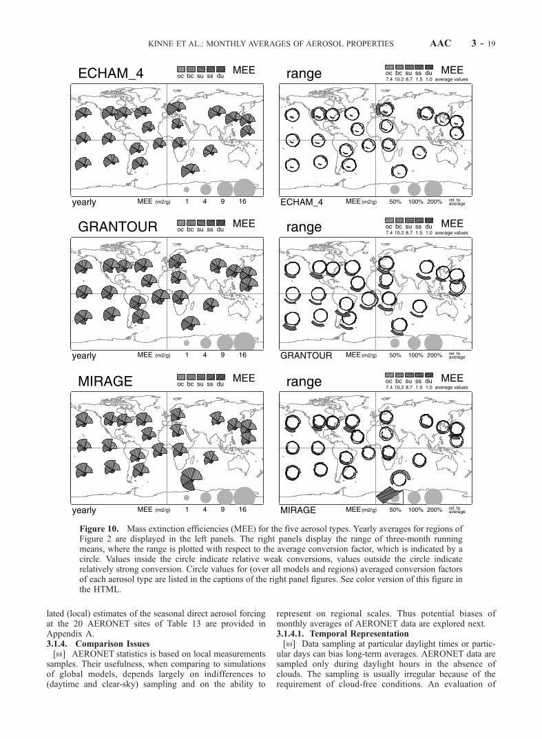
Figure 10. Mass extinction efficiencies (MEE) for the five aerosol types. Yearly averages for regions ofFigure 2 are displayed in the left panels. The right panels display the range of three-month runningmeans, where the range is plotted with respect to the average conversion factor, which is indicated by acircle. Values inside the circle indicate relative weak conversions, values outside the circle indicaterelatively strong conversion. Circle values for (over all models and regions) averaged conversion factorsof each aerosol type are listed in the captions of the right panel figures. See color version of this figure inthe HTML.
KINNE ET AL.: MONTHLY AVERAGES OF AEROSOL PROPERTIES AAC 3 - 19
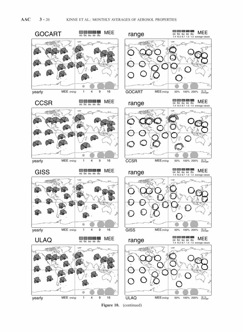
Figure 10. (continued)
AAC 3 - 20 KINNE ET AL.: MONTHLY AVERAGES OF AEROSOL PROPERTIES
AERONET, by binning data according to the time ofmeasurement shows, that daily trends are quite common.However, in terms of monthly averages large differences arerare (usually less than 5% and in extreme cases still lessthan 20% of the daily average). A summary of trendsbetween morning (am) and afternoon (pm) measurementsfor the 20 AERONET sites is given in Figure 15.[90] To avoid temporal sampling issue in the future,
comparisons could apply subsampling techniques to accom-modate the least frequent measurement. For model compar-isons to data from AERONET or satellites, this means arestriction of model output to daytime or overpass times andcloud-free situations. However, there are scale complica-tions. For instance, what corresponds to ‘locally cloud-free’on a 300 � 300 km scale? It also does not help that ‘cloud-free subsets’ of models often display opposing trends:Smaller optical depths are explained by aerosol removalwithin clouds, while larger optical depths are attributed toswelling in the vicinity of clouds. Also considering thefewer events from subsampling, it remains unclear whetherthe benefit of more direct comparisons outweighs the loss instatistical significance.[91] For comparisons between AERONET and satellite
retrievals, subsampling to the tune of daytime overpasses bypolar-orbiting satellite is desirable (if satellite pixels aresmall enough to retrieve local aerosol properties). Withaerosol detecting geo-stationary satellites and (proposed)aerosol detecting satellites that move with the sun, however,AERONET subsampling may not be necessary.3.1.4.2. Regional Representation[92] Local AERONET data may not apply to regions,
representing a GCM model grid point, even if averaged overtime. To illustrate this point, an example is given inFigure 16. Yearly averages and their monthly variabilityduring a year are presented for four European AERONET
sites in northern Italy and France (Ispra, Lille, Toulouse andAire Adour). All four sites display quite different properties,although they are close enough to fall into a regionrepresented by a single grid point in models. For compar-ison, simulations of models are displayed. Here for eachmodel differences in site-properties are the result of spatialinterpolation. Despite the significant spread among modelpredictions for the European region, each model can claimgood agreement to measurements depending on its sitechoice.[93] Models, however, cannot be given the freedom to
pick sites statistics that fits best. Rather it needs to bedetermined, what site, if any, can represent on regionalscales. To find answers to the regional representation oflocal data, satellite data are applied. Although satelliteretrievals may lack accuracy, the spatial coverage of retriev-als can identify those AERONET sites, which qualify forcomparisons on regional scales and which do not. For thispurpose values at the smallest retrieval resolution over eachsite were compared to simultaneous regional (300 �300 km) averages. Based on aerosol optical depth monthlyaverages of retrievals by MODIS and TOMS, a summary ofregional biases is given in Figure 17. MODIS data werepreferred over TOMS data, because MODIS aerosol prod-ucts are available at smaller subscales.[94] The identification of sites, solely based on satellite
average at different spatial scales, is less successful thanhoped for. Only sites with strong local pollution are easilyidentified (e.g., Mexico City). Otherwise trends on localbiases remain unclear. Even on the basis of only 10 � 10 kmaverages (of the MODIS aerosol optical depth product),trends of a site’s regional representation within a month canvary wildly in strength and even in sign. Apparently, localissues (e.g., orography) and transport (e.g., advection ofdifferent air masses) cannot be overlooked. In light of the
Table 12. Simulated Mass Extinction Efficiency: Values of the Median Model and Models With Extreme Tendenciesa
Yearly Average Component Mass Extinction Efficiency, m2/g
OC BC SU SS DU
Avg. Max/Min Avg. Max/Min Avg. Max/Min Avg. Max/Min Avg. Max/Min
Urban sources 8 CC 10 UL 13 GI, MI 1.2 Gr, GI/EC 1.0 GI/MIUrban outflow 8 CC 10 10 GI 1.3 Gr, GI/EC, CC 1.0 MIDust sources 6 10 7 UL/MI 1.1 Gr, GI/GO, EC .9 GIDust outflow 6 EC 10 7 CC/GI .9 Gr, GI/EC .9 GI, GrBiomass sources 7 EC 10 8 GO/GI 1.2 Gr/EC, GO 1.0 GI/MI, GOBiomass outflow 7 Gr, CC/EC 11 EC 8 CC/GI 1.1 Gr, GI/EC 1.1 Gr/MIRemote, tropics 7 EC, UL 10 MI 8 GI 1.1 Gr, GI/EC 1.1 MIRemote, S. Hemis. 8 MI, CC/UL 11 11 CC/GI, UL 1.3 Gr, GI/EC 1.0
Seasonality for Component Mass Extinction Efficiency
OC BC SU SS DU
Var Max/Min Var Max/Min Var Max/Min Var Max/Min Var Max/Min
Urban sources .23 CC/GI, UL .10 GI, EC .26 CC, EC/GO, MI .38 GI, UL .11 GOUrban outflow .23 MI/GI, UL .04 MI/GI, EC .17 MI .23 MI, CC/GI, UL .11 GI/ULDust sources .12 EC/GI, UL .03 GI, EC .19 EC/UL .24 MI/GI, UL .13 ULDust outflow .11 EC, MI/GI .04 MI/GI, EC .17 GI .30 GI, MI .20 MI/ECBiomass sources .12 EC/GI,UL .04 MI/GI, EC .23 UL .22 MI/GI .13Biomass outflow .13 GI, Gr .04 GI, EC .11 GI .20 GI, CC .09Remote, tropics .08 GO/GI .06 GI, EC .14 GI .11 MI/GI, UL .12 GrRemote, S. Hemis. .24 GI, UL .05 MI/GI, EC .14 MI, GI .30 MI/GI, UL .11 MI/UL
aFor class-combined regions (see Table 7), yearly averages (Avg) and seasonality (Var) of the median model (4th-ranked among all models) arepresented. Seasonality is the ratio of the 3-month running mean range during a year and the yearly average. In addition, models are displayed whose valuesfor Avg or Var exceed (italic-bold) or fail (italic) that of the median model by more than 30% (for Avg) and 50% (for Var).
KINNE ET AL.: MONTHLY AVERAGES OF AEROSOL PROPERTIES AAC 3 - 21

variability, much stronger statistical samples are neededthan those provided by the limited number of successfullocal MODIS aerosol retrievals during one month over land.In summary, a much more detailed analysis and a betterstatistical sample are necessary to identify regional trendsfor many sites.[95] Thus, for the model evaluation with AERONET
data, only three sites with known local pollution wereremoved: Mexico City, Arica and Goddard. In additionthree other sites were removed because of a relative closegeographical proximity to other AERONET sites: Bani-zoumbou, Cuiaba and Conception. To maintain the num-ber of AERONET sites at 20 for the model evaluations,six additional sites were added and are introduced inTable 14.
3.1.5. Comparison of Aerosol Optical Depths[96] Model simulated aerosol optical depths t are evalu-
ated by comparing yearly mean, seasonality strength andseasonality phase. Comparisons at 20 AERONET sites areillustrated in Figure 18, quantified in more detail in Appen-dix C and summarized in Table 15.[97] The combined average of all models (see ‘model
average’ in Figure 18) illustrates in general terms differencesbetween simulated aerosol optical depths and AERONETdata. There is a tendency by models to underestimate inthe tropics, especially in regions of biomass burning, andthere is a tendency by models to overestimate from theMideast or Asia, in regions with significant dust contribu-tions. Agreement seems best near and off urban industrialregions of the Northern Hemisphere. This could suggest that
Figure 11. Model tendencies for yearly average and seasonality for component combined optical depth tand mass m with respect to the median model and with respect to satellite data.
AAC 3 - 22 KINNE ET AL.: MONTHLY AVERAGES OF AEROSOL PROPERTIES
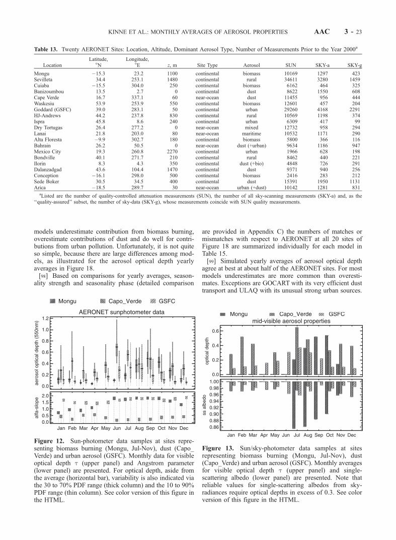
models underestimate contribution from biomass burning,overestimate contributions of dust and do well for contri-butions from urban pollution. Unfortunately, it is not quiteso simple, because there are large differences among mod-els, as illustrated for the aerosol optical depth yearlyaverages in Figure 18.[98] Based on comparisons for yearly averages, season-
ality strength and seasonality phase (detailed comparison
are provided in Appendix C) the numbers of matches ormismatches with respect to AERONET at all 20 sites ofFigure 18 are summarized individually for each model inTable 15.[99] Simulated yearly averages of aerosol optical depth
agree at best at about half of the AERONET sites. For mostmodels underestimates are more common than overesti-mates. Exceptions are GOCART with its very efficient dusttransport and ULAQ with its unusual strong urban sources.
Table 13. Twenty AERONET Sites: Location, Altitude, Dominant Aerosol Type, Number of Measurements Prior to the Year 2000a
LocationLatitude,
�NLongitude,
�E z, m Site Type Aerosol SUN SKY-a SKY-g
Mongu �15.3 23.2 1100 continental biomass 10169 1297 423Sevilleta 34.4 253.1 1480 continental rural 34611 3280 1459Cuiaba �15.5 304.0 250 continental biomass 6162 464 325Banizoumbou 13.5 2.7 0 continental dust 8622 1550 608Cape Verde 16.7 337.1 60 near-ocean dust 11455 956 444Waskesiu 53.9 253.9 550 continental biomass 12601 457 204Goddard (GSFC) 39.0 283.1 50 continental urban 29260 4168 2291HJ-Andrews 44.2 237.8 830 continental rural 10569 1198 374Ispra 45.8 8.6 240 continental urban 6309 417 99Dry Tortugas 26.4 277.2 0 near-ocean mixed 12732 958 294Lanai 21.8 203.0 80 near-ocean maritime 10532 1171 290Alta Floresta �9.9 302.7 180 continental biomass 5800 366 116Bahrain 26.2 50.5 0 near-ocean dust (+urban) 9634 1186 947Mexico City 19.3 260.8 2270 continental urban 1966 628 198Bondville 40.1 271.7 210 continental rural 8462 440 221Ilorin 8.3 4.3 350 continental dust (+bio) 4848 726 291Dalanzadgad 43.6 104.4 1470 continental dust 9371 940 256Conception �16.1 298.0 500 continental biomass 2416 283 212Sede Boker 30.5 34.5 400 continental dust 15391 1950 1131Arica �18.5 289.7 30 near-ocean urban (+dust) 10142 1281 831
aListed are the number of quality-controlled attenuation measurements (SUN), the number of all sky-scanning measurements (SKY-a) and, as the‘‘quality-assured’’ subset, the number of sky-data (SKY-g), whose measurements coincide with SUN quality measurements.
Figure 12. Sun-photometer data samples at sites repre-senting biomass burning (Mongu, Jul-Nov), dust (Capo_Verde) and urban aerosol (GSFC). Monthly data for visibleoptical depth t (upper panel) and Angstrom parameter(lower panel) are presented. For optical depth, aside fromthe average (horizontal bar), variability is also indicated viathe 30 to 70% PDF range (thick column) and the 10 to 90%PDF range (thin column). See color version of this figure inthe HTML.
Figure 13. Sun/sky-photometer data samples at sitesrepresenting biomass burning (Mongu, Jul-Nov), dust(Capo_Verde) and urban aerosol (GSFC). Monthly averagesfor visible optical depth t (upper panel) and single-scattering albedo (lower panel) are presented. Note thatreliable values for single-scattering albedos from sky-radiances require optical depths in excess of 0.3. See colorversion of this figure in the HTML.
KINNE ET AL.: MONTHLY AVERAGES OF AEROSOL PROPERTIES AAC 3 - 23

Simulated seasonality strength for aerosol optical depth isusually stronger near dust sources, but weaker at midlatitudesites of the Northern Hemisphere (AERONET minima arelower) and also weaker at biomass burning sites in the
tropics (AERONET maxima are higher). Simulated season-ality maxima (phase) are correct at about half of theAERONET sites. Matches of all three aerosol properties(yearly average, seasonality strength and seasonality phase)occur only at a rate of about 1 in 4 (AERONET sites).Although this disappoints, complete matches betweenAERONET and MODIS satellite data are also only of thesame order.[100] The location of the matches is also indicative of the
strength of particular models: Grantour does usually well inall outflow regions, ECHAM4 does best in the N. Pacific,CCSR does best over Europe, GISS does best over thecontinental United States and GOCART is best near dustand biomass sources.[101] Another approach to evaluate models with
AERONET data is the comparison of seasonal averages.For the central month of each season (January, April,July and October) comparisons are presented in Figure 19and a statistical summary from seasonal comparisons(which are provided in Appendix C) for the 20 sitesof Figures 18 or 19 are given in Table 16.[102] On the basis of larger deviations to AERONET data,
overall seasonal trends were derived. These trends are con-sistent with earlier results that only GOCART and ULAQhave usually larger optical depths thanAERONET. However,there are now two models that display overestimates as well,although only for one or two seasons: In ECHAM4 theoverestimates relate in to a very strong dust component offAfrica around April (in conjunction with the ‘Azores HIGH’)and in CCSR the overestimates relate to an unusual early(June rather than August) onset of the tropical biomassseason.[103] The comparisons for particular months indicate that
differences with AERONET and among models are more
Figure 14. Aerosol size data from Sun/sky-photometermeasurements at sites representing biomass burning (Mongu,Jul-Nov), dust (Capo_Verde) and urban aerosol (GSFC).Monthly averages for effective radius (upper panel) andyearly averages for size-distribution (lower left) and for sizeswith maxima in surface area contribution (lower right) aregiven. The amplified concentration for dust at radii below0.1 mm due to nonsphericity has been removed for thedetermination of the effective radius. See color version of thisfigure in the HTML.
Figure 15. Daytime trends for aerosol optical depths between morning and evening at 20 AERONETsites.
AAC 3 - 24 KINNE ET AL.: MONTHLY AVERAGES OF AEROSOL PROPERTIES
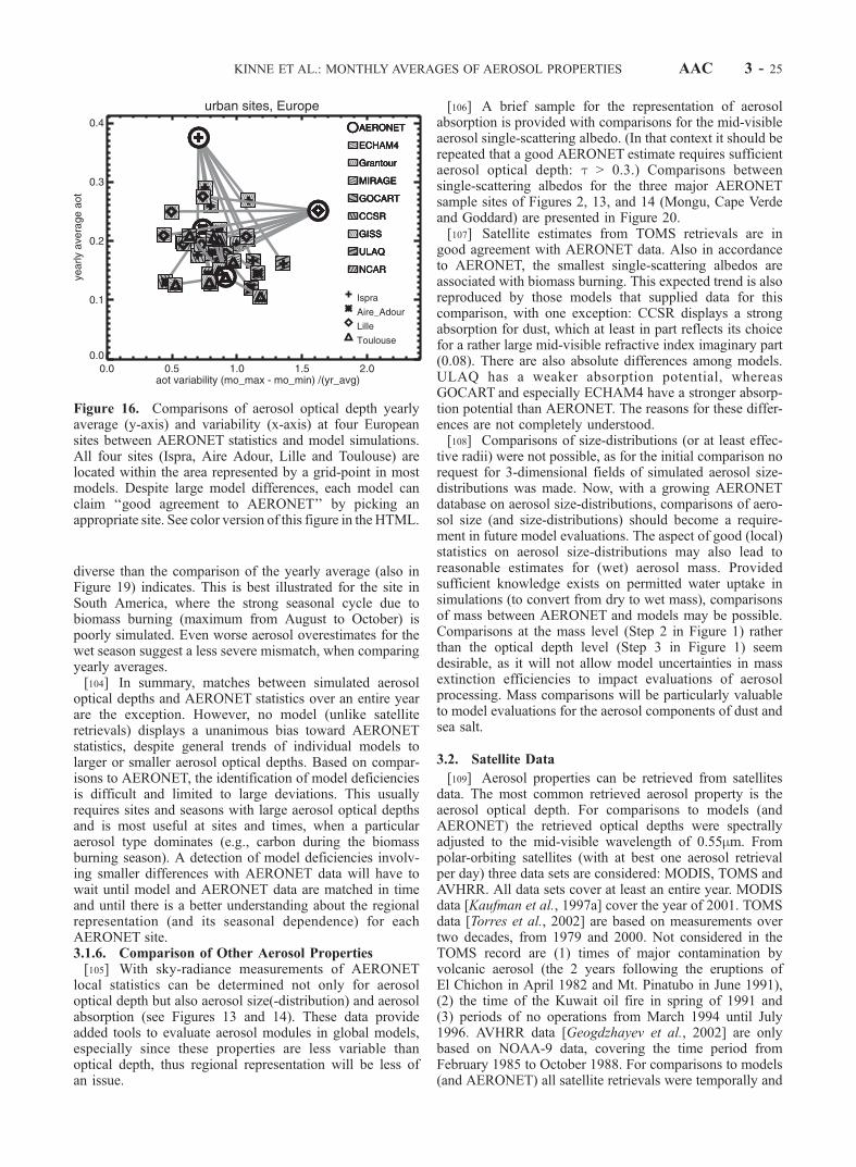
diverse than the comparison of the yearly average (also inFigure 19) indicates. This is best illustrated for the site inSouth America, where the strong seasonal cycle due tobiomass burning (maximum from August to October) ispoorly simulated. Even worse aerosol overestimates for thewet season suggest a less severe mismatch, when comparingyearly averages.[104] In summary, matches between simulated aerosol
optical depths and AERONET statistics over an entire yearare the exception. However, no model (unlike satelliteretrievals) displays a unanimous bias toward AERONETstatistics, despite general trends of individual models tolarger or smaller aerosol optical depths. Based on compar-isons to AERONET, the identification of model deficienciesis difficult and limited to large deviations. This usuallyrequires sites and seasons with large aerosol optical depthsand is most useful at sites and times, when a particularaerosol type dominates (e.g., carbon during the biomassburning season). A detection of model deficiencies involv-ing smaller differences with AERONET data will have towait until model and AERONET data are matched in timeand until there is a better understanding about the regionalrepresentation (and its seasonal dependence) for eachAERONET site.3.1.6. Comparison of Other Aerosol Properties[105] With sky-radiance measurements of AERONET
local statistics can be determined not only for aerosoloptical depth but also aerosol size(-distribution) and aerosolabsorption (see Figures 13 and 14). These data provideadded tools to evaluate aerosol modules in global models,especially since these properties are less variable thanoptical depth, thus regional representation will be less ofan issue.
[106] A brief sample for the representation of aerosolabsorption is provided with comparisons for the mid-visibleaerosol single-scattering albedo. (In that context it should berepeated that a good AERONET estimate requires sufficientaerosol optical depth: t > 0.3.) Comparisons betweensingle-scattering albedos for the three major AERONETsample sites of Figures 2, 13, and 14 (Mongu, Cape Verdeand Goddard) are presented in Figure 20.[107] Satellite estimates from TOMS retrievals are in
good agreement with AERONET data. Also in accordanceto AERONET, the smallest single-scattering albedos areassociated with biomass burning. This expected trend is alsoreproduced by those models that supplied data for thiscomparison, with one exception: CCSR displays a strongabsorption for dust, which at least in part reflects its choicefor a rather large mid-visible refractive index imaginary part(0.08). There are also absolute differences among models.ULAQ has a weaker absorption potential, whereasGOCART and especially ECHAM4 have a stronger absorp-tion potential than AERONET. The reasons for these differ-ences are not completely understood.[108] Comparisons of size-distributions (or at least effec-
tive radii) were not possible, as for the initial comparison norequest for 3-dimensional fields of simulated aerosol size-distributions was made. Now, with a growing AERONETdatabase on aerosol size-distributions, comparisons of aero-sol size (and size-distributions) should become a require-ment in future model evaluations. The aspect of good (local)statistics on aerosol size-distributions may also lead toreasonable estimates for (wet) aerosol mass. Providedsufficient knowledge exists on permitted water uptake insimulations (to convert from dry to wet mass), comparisonsof mass between AERONET and models may be possible.Comparisons at the mass level (Step 2 in Figure 1) ratherthan the optical depth level (Step 3 in Figure 1) seemdesirable, as it will not allow model uncertainties in massextinction efficiencies to impact evaluations of aerosolprocessing. Mass comparisons will be particularly valuableto model evaluations for the aerosol components of dust andsea salt.
3.2. Satellite Data
[109] Aerosol properties can be retrieved from satellitesdata. The most common retrieved aerosol property is theaerosol optical depth. For comparisons to models (andAERONET) the retrieved optical depths were spectrallyadjusted to the mid-visible wavelength of 0.55mm. Frompolar-orbiting satellites (with at best one aerosol retrievalper day) three data sets are considered: MODIS, TOMS andAVHRR. All data sets cover at least an entire year. MODISdata [Kaufman et al., 1997a] cover the year of 2001. TOMSdata [Torres et al., 2002] are based on measurements overtwo decades, from 1979 and 2000. Not considered in theTOMS record are (1) times of major contamination byvolcanic aerosol (the 2 years following the eruptions ofEl Chichon in April 1982 and Mt. Pinatubo in June 1991),(2) the time of the Kuwait oil fire in spring of 1991 and(3) periods of no operations from March 1994 until July1996. AVHRR data [Geogdzhayev et al., 2002] are onlybased on NOAA-9 data, covering the time period fromFebruary 1985 to October 1988. For comparisons to models(and AERONET) all satellite retrievals were temporally and
Figure 16. Comparisons of aerosol optical depth yearlyaverage (y-axis) and variability (x-axis) at four Europeansites between AERONET statistics and model simulations.All four sites (Ispra, Aire Adour, Lille and Toulouse) arelocated within the area represented by a grid-point in mostmodels. Despite large model differences, each model canclaim ‘‘good agreement to AERONET’’ by picking anappropriate site. See color version of this figure in the HTML.
KINNE ET AL.: MONTHLY AVERAGES OF AEROSOL PROPERTIES AAC 3 - 25
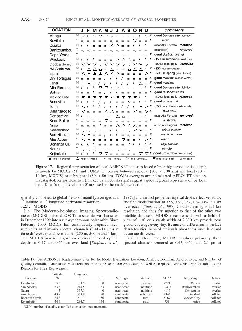
spatially combined to global fields of monthly averages at a1� latitude � 1� longitude horizontal resolution.3.2.1. MODIS[110] The Moderate-Resolution Imaging Spectroradio-
meter (MODIS) onboard EOS-Terra satellite was launchedin December 1999 into a sun-synchronous polar orbit. SinceFebruary 2000, MODIS has continuously acquired mea-surements at thirty-six spectral channels (0.41–14 mm) atthree different spatial resolutions (250 m, 500 m and 1 km).The MODIS aerosol algorithm derives aerosol opticaldepths at 0.47 and 0.66 mm over land [Kaufman et al.,
1997a] and aerosol properties (optical depth, effective radius,and fine-mode fraction) at 0.55, 0.67, 0.87, 1.24, 1.64, 2.1 mmover ocean [Tanre et al., 1997]. Cloud screening is at 1 kmresolution and thus far superior to that of the other twosatellite data sets. MODIS measurements with a field-of-view of 110� or a swath width of 2,330 km provide nearglobal coverage every day. Because of differences in surfacecharacteristics, aerosol retrievals algorithms over land andocean are different.[111] 1. Over land, MODIS employs primarily three
spectral channels centered at 0.47, 0.66, and 2.1 mm at
Figure 17. Regional representation of local AERONET statistics based of monthly aerosol optical depthretrievals by MODIS (M) and TOMS (T). Ratios between regional (300 � 300 km) and local (10 �10 km, MODIS) or subregional (80 � 80 km, TOMS) averages around selected AERONET sites areinvestigated. Ratios close to 1 (marked by an equals sign) suggest a good regional representation by localdata. Data from sites with an X are used in the model evaluations.
Table 14. Six AERONET Replacement Sites for the Model Evaluation: Location, Altitude, Dominant Aerosol Type, and Number of
Quality-Controlled Attenuation Measurements Prior to the Year 2000 Are Listed, As Well As Replaced AERONET Sites of Table 13 and
Reasons for Their Replacement
LocationLatitude,
�NLongitude,
�E z, m Site Type Aerosol SUNa Replacing Reason
Kaashidhoo 5.0 73.5 0 near-ocean biomass 4724 Cuiaba overlapSan Nicolas 33.3 240.5 133 near-ocean maritime 10437 Banizoumbou overlapNauru �.5 337.1 0 near-ocean maritime 4119 Conception overlapAire Adour 43.7 359.8 80 continental off-urban 4343 Goddard pollutedBonanza Creek 64.8 211.7 150 continental rural 5169 Mexico City pollutedKejimkujik 44.4 294.7 154 continental rural 738 Arica polluted
aSUN, number of quality-controlled attenuation measurements.
AAC 3 - 26 KINNE ET AL.: MONTHLY AVERAGES OF AEROSOL PROPERTIES

KINNE ET AL.: MONTHLY AVERAGES OF AEROSOL PROPERTIES AAC 3 - 27

500 m resolution. The dark target approach developed overvegetated surfaces (e.g., forest, grassland) is used to esti-mate the surface reflectances (rs) at 0.47 mm and at 0.66 mmfrom themeasurements at 2.1 mmassuming rs
0.47 mm/rs2.1 mm =
0.25 and rs0.66 mm/rs
2.1 mm = 0.5 [Kaufman et al., 1997b].Snow/ice and water covered surfaces are excluded, becausethere this empirical relationship becomes invalid. Aerosoloptical depths are derived from averaged reflectance of anensemble of cloud-free pixels on a 10 km � 10 km grid.[112] 2. Over oceans, the algorithm inverts the spectral
measurements (0.55–2.l mm) to derive the spectral aerosolproperties from cloud-free and glint-free measurements inon a 10 km � 10 km grid.[113] MODIS-derived aerosol properties were validated
against AERONET Sun photometer measurements with theerrors of �ta = ±0.05 ± 0.20ta over land [Chu et al., 2002],and with the errors of �ta = ±0.03 ± 0.05ta over ocean[Remer et al., 2002]. In addition to the mid-visible aerosoloptical depth, MODIS also provides information on par-ticles size, deriving ratios of prescribed size modes fromvariations in spectral extinction. This size information is notused in this study but will certainly be of value in futuremodel evaluations.3.2.2. TOMS[114] The Total Ozone Mapping Spectrometer (TOMS)
is a 6-band (UV: 6) cross track scanning radiometer flownon many different polar-orbiting satellites (NIMBUS-7,Meteor-3, Earth Probe, ADEOS) since 1979. Swath widthand spatial resolution are about 3000 km and 50 km.Although primarily designed to monitor ozone, measure-ments in channels with weak (0.34 mm) or no ozoneabsorption (0.38 mm) permit the retrieval of aerosolproperties [Torres et al., 1998]. The optical depth ofscattering aerosol is derived from enhancements in molec-ular backscatter at 0.38 mm. Optical depth of absorbingaerosol and aerosol single-scattering albedo are derivedfrom changes to the background spectral dependence ofmolecular scattering between 0.34 mm and 0.38 mm. Thesechanges are a function of aerosol altitude. Thus not onlyappropriate assumptions of aerosol size (and shape) butalso appropriate assumptions of aerosol elevations areessential. Altitude underestimates lead to aerosol opticaldepth overestimates and vice versa. For absorbing aerosol
the current retrieval assumes an average altitude of 3 km.Also without sufficient background signal below theaerosol layer the detection of absorbing aerosol near thesurface is difficult. The retrieval assumes surfaces at sealevel, which causes overestimates for absorbing aerosoloptical depths at high-altitude regions. The large 50 km �50 km pixel size of a TOMS image makes it difficult toavoid contamination by clouds, which can have a strongimpact on the retrieval of absorbing aerosol. A reflectionthreshold technique is assumed to remove clouds. Surfacereflections, although small both over water and land in theultraviolet, are based on minimum reflections for cases,where the spectral dependency of molecular scattering didnot change.3.2.3. AVHRR[115] The Advanced Very High Resolution Radiometer
AVHRR is a 5 band (vis: 1, near-IR: 2, IR: 2) cross trackscanning radiometer flown on many NOAA polar-orbitingsatellites since 1978. Swath width and spatial resolution areabout 2800 km and 1 km. Aerosol optical depths arederived from visible (0.63 mm, as the nominal value forthe 0.58–0.68 mm band) and near-infrared (0.83 mm, as thenominal value for the 0.72–1.1 mm band) reflection anoma-lies for cloud-free 1 � 4 km GAC (global area coverage)pixels over sun-glint free ocean scenes. For accuracy con-cerns, here AVHRR monthly averages are only based onNOAA-9 data (for the period from February 1985 toOctober 1988). These data had fewer calibration drifts thanAVHRR sensors on other NOAA satellites. In addition, nomajor contamination by stratospheric aerosol from volcaniceruptions occurred during that time. Monthly averagesinclude data from all four years. Retrieved optical depthsof the visible band (0.63 mm) were extrapolated to valuesat 0.55 mm wavelength with the Angstrom parameter.The Angstrom statistics is based on a power law size-distribution, whose power exponent is inferred from theoptical depth ratios of the visible and the near-infrared band.Other retrieval assumptions are moderate absorption (0.97 <w0 < 0.99) and a spherical aerosol shape [Mishchenko et al.,1999]. Cloud screening is based on the ISCCP data set[Rossow et al., 1993], with the additional constraints, as toinclude only the warmest pixels (only retaining pixels withIR temperatures warmer than the composite value).
Figure 18. (opposite) Local comparisons of yearly average aerosol optical depth. Interpolated model simulations (disks)are compared to AERONET data (circles). Dark circles indicate model underestimates, and white circles indicate modeloverestimates. See color version of this figure in the HTML.
Table 15. Local Agreement at 20 AERONET Sites: Matches in Terms of Yearly Average and Seasonality for Aerosol Optical Deptha
AOT Versus AERONET
EC(>, �, <)
GO(>, �, <)
MI(>, �, <)
GI(>, �, <)
CC(>, �, <)
Gr(>, �, <)
UL(>, �, <)
MO(>, �, <)
TO(>, �, <)
Yearly average 2, 10, 8 7, 9, 4 3, 7, 10 3, 7, 10 3, 11, 6 3, 12, 5 5, 12, 3 9, 9, 1 14, 6, -Season strength 4, 12, 4 1, 14, 5 3, 9, 8 4, 15, 1 3, 13, 4 1, 14, 5 2, 12, 6 2, 15, 2 2, 7, 14Season phase 13 13 8 14 11 10 10 11 7Avg +s-str. +s-ph 4 3 1 3 4 6 2 5 1
aWhen possible, a distinction was made between clearly larger values (>), clearly smaller values (<), and close agreement (�). Yearly averages wereconsidered agreeable when the simulated optical depth remained within 30% of the AERONET value. Seasonality strength was considered agreeable forvariations within 50% of the AERONET value. Seasonality phase was considered agreeable when the month with the maximum of the three-month runningaverage for optical depths had not shifted by more than one month from the month of the AERONET maximum. The last line indicates at how many sites(out of 20) all three aerosol properties matched the AERONET statistics.
AAC 3 - 28 KINNE ET AL.: MONTHLY AVERAGES OF AEROSOL PROPERTIES

3.2.4. Comparisons[116] Evaluations of models with satellite data are con-
ducted by comparing averages of regions. These regions,which were already introduced in Figure 2, are much largerthan regions associated with a particular model grid point.In Figure 21, yearly and regionally averaged aerosol opticaldepths of satellite retrievals and models are compared.Separate comparisons are given with respect to individualmodels and to the ‘average’ model. The initial focus,
however, will be on a comparison of satellite retrievals byaerosol class (see Table 7) to determine which satellite datashould best be used in model evaluations.[117] 1. In urban source regions, MODIS averages are
larger than TOMS for East Asia, but smaller than TOMS forEurope and North America. In comparisons to AERONET(see Appendix C) TOMS more than MODIS, lacks onseasonality (in particular seasonal minima) and tends tooverestimate. Choice is MODIS.
Figure 19. Local comparisons of simulated (outer pie-section border) and measured (circle) aerosoloptical depths at 20 AERONET sites. Aside from yearly averages in the top panel, averages for themonths of January, April, July and October are presented, to illustrate seasonal differences. See colorversion of this figure in the HTML.
KINNE ET AL.: MONTHLY AVERAGES OF AEROSOL PROPERTIES AAC 3 - 29
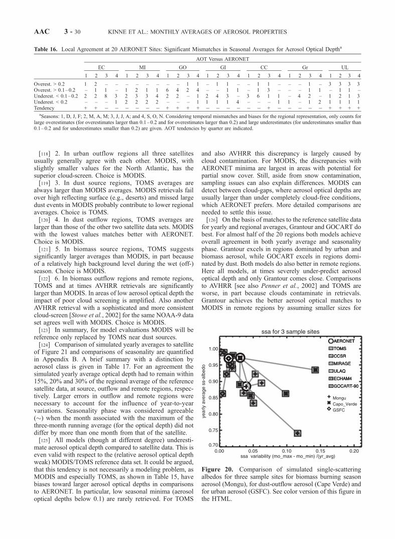
[118] 2. In urban outflow regions all three satellitesusually generally agree with each other. MODIS, withslightly smaller values for the North Atlantic, has thesuperior cloud-screen. Choice is MODIS.[119] 3. In dust source regions, TOMS averages are
always larger than MODIS averages. MODIS retrievals failover high reflecting surface (e.g., deserts) and missed largedust events in MODIS probably contribute to lower regionalaverages. Choice is TOMS.[120] 4. In dust outflow regions, TOMS averages are
larger than those of the other two satellite data sets. MODISwith the lowest values matches better with AERONET.Choice is MODIS.[121] 5. In biomass source regions, TOMS suggests
significantly larger averages than MODIS, in part becauseof a relatively high background level during the wet (off-)season. Choice is MODIS.[122] 6. In biomass outflow regions and remote regions,
TOMS and at times AVHRR retrievals are significantlylarger than MODIS. In areas of low aerosol optical depth theimpact of poor cloud screening is amplified. Also anotherAVHRR retrieval with a sophisticated and more consistentcloud-screen [Stowe et al., 2002] for the same NOAA-9 dataset agrees well with MODIS. Choice is MODIS.[123] In summary, for model evaluations MODIS will be
reference only replaced by TOMS near dust sources.[124] Comparison of simulated yearly averages to satellite
of Figure 21 and comparisons of seasonality are quantifiedin Appendix B. A brief summary with a distinction byaerosol class is given in Table 17. For an agreement thesimulated yearly average optical depth had to remain within15%, 20% and 30% of the regional average of the referencesatellite data, at source, outflow and remote regions, respec-tively. Larger errors in outflow and remote regions werenecessary to account for the influence of year-to-yearvariations. Seasonality phase was considered agreeable(�) when the month associated with the maximum of thethree-month running average (for the optical depth) did notdiffer by more than one month from that of the satellite.[125] All models (though at different degree) underesti-
mate aerosol optical depth compared to satellite data. This iseven valid with respect to the (relative aerosol optical depthweak) MODIS/TOMS reference data set. It could be argued,that this tendency is not necessarily a modeling problem, asMODIS and especially TOMS, as shown in Table 15, havebiases toward larger aerosol optical depths in comparisonsto AERONET. In particular, low seasonal minima (aerosoloptical depths below 0.1) are rarely retrieved. For TOMS
and also AVHRR this discrepancy is largely caused bycloud contamination. For MODIS, the discrepancies withAERONET minima are largest in areas with potential forpartial snow cover. Still, aside from snow contamination,sampling issues can also explain differences. MODIS candetect between cloud-gaps, where aerosol optical depths areusually larger than under completely cloud-free conditions,which AERONET prefers. More detailed comparisons areneeded to settle this issue.[126] On the basis of matches to the reference satellite data
for yearly and regional averages, Grantour and GOCART dobest. For almost half of the 20 regions both models achieveoverall agreement in both yearly average and seasonalityphase. Grantour excels in regions dominated by urban andbiomass aerosol, while GOCART excels in regions domi-nated by dust. Both models do also better in remote regions.Here all models, at times severely under-predict aerosoloptical depth and only Grantour comes close. Comparisonsto AVHRR [see also Penner et al., 2002] and TOMS areworse, in part because clouds contaminate in retrievals.Grantour achieves the better aerosol optical matches toMODIS in remote regions by assuming smaller sizes for
Figure 20. Comparison of simulated single-scatteringalbedos for three sample sites for biomass burning seasonaerosol (Mongu), for dust-outflow aerosol (Cape Verde) andfor urban aerosol (GSFC). See color version of this figure inthe HTML.
Table 16. Local Agreement at 20 AERONET Sites: Significant Mismatches in Seasonal Averages for Aerosol Optical Deptha
AOT Versus AERONET
EC MI GO GI CC Gr UL
1 2 3 4 1 2 3 4 1 2 3 4 1 2 3 4 1 2 3 4 1 2 3 4 1 2 3 4
Overest. > 0.2 1 2 – – – – – – – – 1 1 – 1 1 – – 1 1 – – – 1 – 3 3 3 3Overest. > 0.1–0.2 – 1 1 – 1 2 1 1 6 4 2 4 – – 1 1 – 1 3 – – – 1 1 – 1 1 –Underest. < 0.1–0.2 2 2 8 3 2 3 3 4 2 2 – 1 2 4 3 – 3 6 1 1 – 4 2 – 1 2 1 3Underest. < 0.2 – – – 1 2 2 2 2 – – – 1 1 1 1 4 – – – 1 1 – 1 2 1 1 1 1Tendency + + � � � � � � + + + + � � � � � � + � � � � � + + + +
aSeasons: 1, D, J, F; 2, M, A, M; 3, J, J, A; and 4, S, O, N. Considering temporal mismatches and biases for the regional representation, only counts forlarge overestimates (for overestimates larger than 0.1–0.2 and for overestimates larger than 0.2) and large underestimates (for underestimates smaller than0.1–0.2 and for underestimates smaller than 0.2) are given. AOT tendencies by quarter are indicated.
AAC 3 - 30 KINNE ET AL.: MONTHLY AVERAGES OF AEROSOL PROPERTIES
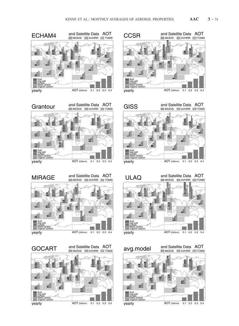
KINNE ET AL.: MONTHLY AVERAGES OF AEROSOL PROPERTIES AAC 3 - 31
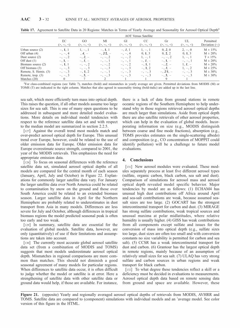
sea salt, which more efficiently turn mass into optical depth.This raises the question, if all other models assume too largesizes for sea salt. This is one of many open questions to beaddressed in subsequent and more detailed model evalua-tions. More details on individual model tendencies withrespect to the reference satellite data set and with respectto the median model are summarized in section 2.2.5.[127] Against the overall trend most models match and
over-predict aerosol optical depth for Europe. This unusualtrend over Europe, however, could be related to the use ofolder emission data for Europe. Older emission data forEurope overestimate source strength, compared to 2001, theyear of the MODIS retrievals. This emphasizes the need forappropriate emission data.[128] To focus on seasonal differences with the reference
satellite data set, simulated aerosol optical depths of allmodels are compared for the central month of each season(January, April, July and October) in Figure 22. Explan-ations for commonly larger satellite data vary. For Januarythe larger satellite data over North America could be relatedto contamination by snow on the ground and those overSouth America could be related to an extended biomassseason. Larger satellite data in April for the NorthernHemisphere are probably related to underestimates in dusttransport from Asia in many models. Differences are lesssevere for July and October, although differences in tropicalbiomass regions the model predicted seasonal peak is oftentoo early and too weak.[129] In summary, satellite data are essential for the
evaluation of global models. Satellite data, however, areonly (quantitatively) of use if their limitations and assump-tions are taken into account.[130] The currently most accurate global aerosol satellite
data set (from a combination of MODIS and TOMS)suggests that most models underestimate aerosol opticaldepth. Mismatches in regional comparisons are more com-mon than matches. This should not diminish a goodseasonal agreement of many models for particular regions.When differences to satellite data occur, it is often difficultto judge whether the model or satellite is at error. Here astrengthening of satellite data with other satellite data orground data would help, if those are available. For instance,
there is a lack of data from ground stations in remoteoceanic regions of the Southern Hemisphere to help under-stand why in those regions retrieved aerosol optical depthsare much larger than simulations. Aside from optical depththere are also satellite retrievals of other aerosol properties,which can help in the evaluation of global models. Incor-porating information on size (e.g., MODIS distinguishbetween coarse and fine mode fractions), absorption (e.g.,TOMS provides estimates on the single-scattering albedo)and composition (e.g., CO concentration of MOPPIT couldidentify pollution) will be a challenge to future modelevaluations.
4. Conclusions
[131] New aerosol modules were evaluated. These mod-ules separately process at least five different aerosol types(sulfate, organic carbon, black carbon, sea salt and dust).Comparison of simulations for aerosol mass and aerosoloptical depth revealed model specific behavior. Majortendencies by model are as follows: (1) ECHAM4 hasunusual high dust contributions off Africa around Apriland sea-salt contributions are weak, because assumed sea-salt sizes are too large. (2) GOCART has the strongestintercontinental transport for carbon and dust. (3) MIRAGEhas strong sulfate contributions, weak tropical sources andunusual maxima at polar midlatitudes, where relativehumidity is usually higher. (4) GISS has weak contributionsfrom all components except sulfate and issues for theconversion of mass into optical depth (e.g., sulfate sizestoo large, dust sizes are often too small and with conversionconstants no size variability is permitted for carbon and seasalt). (5) CCSR has a weak intercontinental transport fordust and carbon. (6) Grantour has the largest optical depthin remote regions, mainly because of an assumption ofrelatively small sizes for sea salt. (7) ULAQ has very strongsulfate and carbon sources in urban regions and weaktransport for black carbon.[132] To what degree these tendencies reflect a skill or a
deficiency must be decided in evaluations to measurements.Aerosol optical depth data based on remote sensing datafrom ground and space are available. However, these
Figure 21. (opposite) Yearly and regionally averaged aerosol optical depths of retrievals from MODIS, AVHRR andTOMS. Satellite data are compared to (component) simulations with individual models and an ’average model. See colorversion of this figure in the HTML.
Table 17. Agreement to Satellite Data in 20 Regions: Matches in Terms of Yearly Average and Seasonality for Aerosol Optical Deptha
AOT Versus Satellite
EC(>, �, <)
GO(>, �, <)
MI(>, �, <)
GI(>, �, <)
CC(>, �, <)
Gr(>, �, <)
UL(>, �, <)
PermittedDeviation (�)
Urban source (2) – , 1, 1 1, – , 1 – , 1, 1 – , 1, 1 1, – , 1 0, 2, 0 2, �, 0 M ± 15%Off urban (4) – , – , 4 , 4, – – , 2/2, – – , – , 4 0, 1, 3 0, 2, 2 0, 1, 3 M ± 20%Dust source (2) – , – , 2 – , 2, – – , – , 2 – , – , 2 1, – , 1 – , – , 2 1, – , 1 T ± 15%Off dust (1) – , 1, – – , 1, – – , – , 1 – , – , 1 – , 1, – – , 1, – – , – , 1 M ± 20%Biomass source (2) – , 1, 1 – , – , 2 – , – , 2 – , – , 2 – , 1, 1 – , 2, – 1, 1, – M ± 20%Off biomass (3) – , – , 3 – , – , 3 – , – , 3 – , – , 3 – , 1, 2 – , 3, – 1, – , 2 M ± 25%Remote, S. Hemis. (3) – , – , 3 – , 1, 2 – , – , 1 – , – , 3 – , – , 3 – , 2/1, – – , – , 3 M ± 30%Remote, trop. (3) – , – , 3 – , 3, – – , – , 3 – , – , 3 – , – , 3 – , 3, – – , – , 3 M ± 30%Matches (20) 0 7 2 1 1 9 1
aFor class-combined regions (see Table 7), matches (bold) and mismatches in yearly average are given. Permitted deviations from MODIS (M) orTOMS (T) are indicated in the right column. Matches that also agreed in seasonality timing (bold-italic) are added up in the last line.
AAC 3 - 32 KINNE ET AL.: MONTHLY AVERAGES OF AEROSOL PROPERTIES
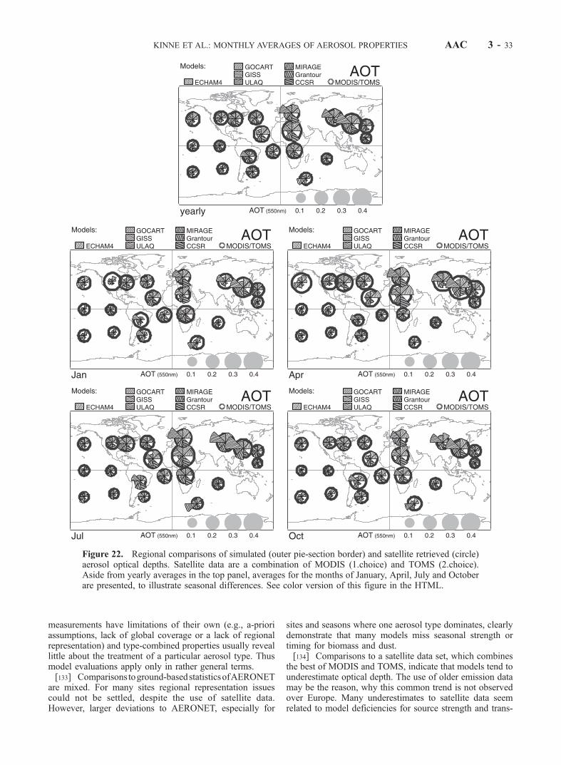
measurements have limitations of their own (e.g., a-prioriassumptions, lack of global coverage or a lack of regionalrepresentation) and type-combined properties usually reveallittle about the treatment of a particular aerosol type. Thusmodel evaluations apply only in rather general terms.[133] Comparisons toground-basedstatisticsofAERONET
are mixed. For many sites regional representation issuescould not be settled, despite the use of satellite data.However, larger deviations to AERONET, especially for
sites and seasons where one aerosol type dominates, clearlydemonstrate that many models miss seasonal strength ortiming for biomass and dust.[134] Comparisons to a satellite data set, which combines
the best of MODIS and TOMS, indicate that models tend tounderestimate optical depth. The use of older emission datamay be the reason, why this common trend is not observedover Europe. Many underestimates to satellite data seemrelated to model deficiencies for source strength and trans-
Figure 22. Regional comparisons of simulated (outer pie-section border) and satellite retrieved (circle)aerosol optical depths. Satellite data are a combination of MODIS (1.choice) and TOMS (2.choice).Aside from yearly averages in the top panel, averages for the months of January, April, July and Octoberare presented, to illustrate seasonal differences. See color version of this figure in the HTML.
KINNE ET AL.: MONTHLY AVERAGES OF AEROSOL PROPERTIES AAC 3 - 33

port. Less clear are reasons for consistently lower modelsimulations for remote regions of the tropics and theSouthern Hemisphere.[135] This study served two purposes. It was intended to
provide a glimpse into the problems and uncertainties ofclimate simulations with aerosol and to convey the messagefor the need of measurements, on which the skill of thesemodels can be tested. On the other hand this study providesfeedback to the models that have participated in thiscomparison. In fact, as a result of this comparison, severalassumptions regarding the representation of aerosol in somemodels were or are currently modified. As biases often canbe traced back to one aerosol type, it can be expected thatperformances of some models could drastically improvedwith few modifications. Still, many model tendencies aredifficult to explain. For more insights on model behavior, amore coordinated approach is needed. This includes anstepped up effort for identical background data (assimilatedmeteorology and emission), added intermediate model out-put (e.g., surface winds, water uptake by type, verticaldistributions, subsampling for time-matches to data), awillingness to perform sensitivity tests (e.g., tracer transportsimulations, humidification with prescribed humidityfields), a consensus on assumptions for aerosol (e.g.,absorption of dust and organic carbon, dust-size) and areview of radiative transfer schemes as to their appropriate-ness for aerosol studies.
Appendix A: Direct Aerosol Forcing
[136] AERONET sky data completely define the aerosoloptical properties (see Figures 13 and 14). Combining thesedata with smart choices to other atmospheric properties (asinput to radiative transfer codes) the associated local directradiative forcing for aerosol can be determined. Here,additional input to the model included monthly statisticsfor solar surface albedo from MODIS [Schaaf et al., 2002]and for cloud cover from ISCCP [Rossow et al., 1993]. Forthe three major AERONET sites of Figure 2 the calculatednet-flux changes at the top of the atmosphere (ToA) and atthe surface is presented in Figure A1.[137] The aerosol radiative forcing at the top of the
atmosphere (ToA) is always less negative than the associatedforcing at the surface. This difference is mainly an indicatorfor the aerosol solar absorption (which is particularly largefor aerosol from biomass burning). The consideration ofclouds (versus a cloud-free scenario) usually reduces theaerosol forcing strength. Particularly important for the ‘cli-mate impact indicating’ ToA forcing is the relative altitudeplacement between cloud and aerosol. Clouds below aerosolbrighten the aerosol’s underlying surface, similar to switch-ing from ocean to desert or snow surfaces. Such brighteningcan change the sign of aerosol ToA forcing from a net fluxloss (cooling) to a net flux gain (warming).[138] Calculated aerosol forcing for all 20 AERONET
sites of Table 13 and Figure 2 are summarized in Tables A1and A2 for (ISCCP-) cloudy conditions. Three-month(seasonal) averages are usually presented. At sites stronglyinfluenced by biomass burning, only monthly averages ofthe biomass peak season are given.[139] The direct aerosol forcing at AERONET sites is
usually larger than global forcing averages because of the
proximity of AERONET sites to aerosol sources. In addi-tion, when comparing to values of IPCC studies [e.g.,Houghton et al., 2001], it must be kept in mind that IPCConly addresses forcing from anthropogenic aerosol, whereasthe results here include effects from natural aerosol. Allcalculated forcings carry some uncertainty with year-to-yearvariations in aerosol concentration (e.g., common occur-rence of episodic events such as dust storms and shifts inonset and/or intensity of seasonal events such as a biomassburning seasons).[140] At all 20 evaluated AERONET sites, aerosol
reduces (on a seasonal basis) the available energy tothe Earth-atmosphere system (negative ToA forcing). Asso-ciated reductions of surface net-fluxes are always larger,because of aerosol absorption. This atmospheric forcingheats aerosol layers and is particularly large for biomass andpolluted urban aerosol. To what degree this added heating inthe atmosphere influences the dynamics (less instabilityand/or suppressed convection and precipitation) is notcompletely understood.
Appendix B: Regional Comparisons
[141] Here, differences among models and to satellite dataare compared individually for each region. Such comparisonprovides more detail than comparing averages of type-similar regions, as it was done in the text above for brevity(according to Table 7). Aerosol properties of mass, opticaldepth and optical depth compositional partition are com-pared for the 20 regions of Figure 2. Investigated propertiesare yearly average, seasonality strength and seasonalityphase. Their definition is the same as in the text: Seasonalitystrength is the ratio between the (maximum-minimum)range of the three-month running average during a year
Figure A1. AERONET-derived aerosol forcing at sitesrepresenting biomass burning (Mongu, Jul-Nov), dust(Capo_Verde) and urban aerosol (GSFC). Radiative forcingmonthly averages are given at the top of the atmosphere(upper panel) and at the surface (lower panel) for clear-skyconditions (grey bars) and under cloudy conditions (stripedor colored bars). See color version of this figure in theHTML.
AAC 3 - 34 KINNE ET AL.: MONTHLY AVERAGES OF AEROSOL PROPERTIES

and the yearly average. Seasonality phase is identified bythe (center-) months associated with the maximum andminimum of a three-month running average during a year.
B1. Aerosol Mass
[142] Regional mass comparisons of Table B1 quantify thecomparisons of Figure 3 for yearly average and seasonalitystrength (or range). Table B2 compares the correspondingseasonality phase.
B2. Aerosol Optical Depth
[143] Regional aerosol optical depth comparisons ofTable B3 quantify the comparisons of Figure 5 for yearlyaverage and seasonality strength (or range). Table B4compares the corresponding seasonality phase indicatingcentral months, when the three-month running mean is at itsmaximum or minimum, respectively.[144] Tables B3 and B4 also display statistics of three
satellite data sets: MODIS, TOMS and AVHRR. To whatdegree these ‘measured’ aerosol optical depths can be usedfor model evaluations of aerosol modules depends largely onthe accuracy in those satellite retrievals. At issue are theappropriateness of retrieval assumptions and the skill to
remove scenes with clouds. Cloud-contamination issuesare likely explanations for the relatively high aerosol opticaldepths in remote regions of TOMS (large pixel size) and ofAVHRR (ISCCP climatology threshold). In contrast, multi-spectral data at subkilometer pixel size of MODIS are thebasis of a superior cloud screen. Thus MODIS is the selectedreference for model evaluations, except for dust sourceregions, where TOMS statistics replaces MODIS as refer-ence. This is because MODIS retrievals fail over continentalregions with relatively high solar surface reflectance (e.g.,deserts). In addition, large dust events in MODIS retrievalsare frequently mistaken as clouds and removed, leading toregional underestimates near dust sources.[145] Compared to the best satellite product (MODIS with
TOMS) all models tend to underestimate aerosol opticaldepth, as illustrated in Table B5. Particularly common areunderestimates for outflow and remote regions. Less com-mon are underestimates for source regions. Here manymodels match up quite well to satellite data and even afew model overestimates occur. In fact, over Europe almostall models suggest larger values than the satellite data. Thisunusual trend over Europe, however, could be related to theuse of older emission data for Europe. Older emission data
Table A1. Direct (All-Sky) Aerosol Forcing at AERONET Sites on a Seasonal Basis
Lat,N
Lon,E
Forcing, W/m2
Top of Atmosphere Surface Atmosphere
DJF MAM JJA SON DJF MAM JJA SON DJF MAM JJA SON
DustCape Verde 17 337 �11 �11 �13 �11 �20 �19 �25 �19 9 8 12 8Banizoumbou 14 3 �6 �9 �4 �8 �14 �27 �21 �18 8 18 17 10Ilorin 8 4 �12 �10 �7 �9 �55b �24 �21 �17 43b 14 14 8Sede Boker 31 34 �4 �6 �5 �5 �6 �11 �9 �9 2 5 4 4Bahrain 26 50 �5 �11 �11 �8 �8 �19 �23 �12 3 8 12 4Dalanzadgad 44 104 0 �8 �2 �1 �14 �20 �8 �11 14 12 6 10
Urban/RuralGSFC 39 283 �2 �5 �9 �4 �3 �7 �13 �6 1 2 4 2Ispra 46 9 �3 — �6 �8 �4 — �14 �15 1 — 8 7Mexico City 19 261 — �5 �3 — — �23 �14 — — 18 12 —Bondville 40 272 �1 �4 �9 �4 �2 �7 �13 �6 1 3 4 2Sevilleta 24 253 �1 �3 �2 �1 �3 �6 �7 �7 2 3 5 6Arica 18 310 �6 �5 �5 �5 �10 �9 �8 �8 4 4 3 3
MaritimeLanai 21 203 �3 �5 �2 �2 �4 �7 �4 �3 1 2 2 1Dry Tortugas 25 277 �5 �8 �6 �2 �8 �12 �9 �6 3 4 3 2
aDJF, Dec/Jan/Feb; MAM, Mar/Apr/May; JJA, Jun/Jul/Aug; SON, Sep/Oct/Nov. Dashes indicate insufficient statistics.bDuring DJF, ‘‘Ilorin’’ is strongly influenced by biomass aerosol (causing strong surface cooling and atmospheric forcing).
Table A2. Direct (All-Sky) Aerosol Forcing at AERONET Sites During Months of Biomass Burning
Lat,N
Lon,E
Forcing for Biomass, W/m2
Top of Atmosphere Surface Atmosphere
July Aug. Sept. Oct. July Aug. Sept. Oct. July Aug. Sept. Oct.
Mongu �15 23 �5 �7 �9 �8 �14 �25 �35 �34 9 18 26 26Cuiaba �15 304 �5 �9 �11 �6 �11 �34 �49 �19 6 25 38 13Alta Floresta �10 303 �5 �16 �17 �10 �8 �30 �48 �19 3 14 31 9Conception �16 298 �5 �12 �10 �10 �8 �26 �24 �18 3 14 14 8
Lat,N
Lon,E
Forcing for High Latitude, W/m2
Top of Atmosphere Surface Atmosphere
May June July Aug. May June July Aug. May June July Aug.
Waskesiu 54 254 �9 �16 �12 �7 �14 �34 �19 �9 5 18 7 2HJ Andrews 44 238 �3 �4 �4 �3 �6 �7 �7 �5 3 3 3 2
KINNE ET AL.: MONTHLY AVERAGES OF AEROSOL PROPERTIES AAC 3 - 35

Table B1. Simulations of Aerosol Mass for Regions of Figure 2: Yearly Average and Seasonality Strengtha
Mass (Yearly Average in g/m2, Seasonality-Strength)
EC GO MI GI CC Gr UL
Urban sourceE. Asia .11, 0.5 .20, 0.7 .06, 0.4 .06, 0.4 .06, 0.4 .13, 1.0 .26, 0.7Europe .11, 0.6 .15, 0.3 .05, 0.5 .05, 0.8 .06, 0.5 .05, 0.9 .09, 0.3
Urban outflowNWAtlantic .13, 1.1 .12, 0.3 .04, 0.4 .03, 0.6 .05, 0.7 .05, 0.6 .05, 0.8NW Pacific .13, 0.8 .13, 0.5 .04, 0.6 .04, 0.6 .04, 0.5 .06, 0.5 .05, 0.3N. Pacific .15, 1.3 .44, 0.4 .04, 0.5 .04, 0.6 .03, 0.4 .04, 0.3 .05, 0.7
Dust sourceN. Africa .34, 1.6 .58, 0.6 .06, 0.6 .15, 0.6 .73, 1.6 .30, 0.8 .24, 0.6Asia .09, 1.3 .32, 0.6 .08, 0.9 .11, 1.3 .10, 1.7 .22, 1.4 .53, 1.1
Dust outflowE. Atlantic .29, 0.8 .21, 0.9 .04, 0.6 .05, 0.8 .18, 1.3 .12, 0.6 .10, 0.9
Biomass sourceAfrica .10, 1.3 .07, 1.1 .02, 0.7 .03, 1.0 .05, 1.1 .06, 0.5 .04, 1.1S. America .04, 1.3 .05, 1.0 .02, 0.8 .02, 0.9 .02, 1.6 .04, 0.7 .09, 0.6
Biomass outflowSE Atlantic .06, 0.8 .07, 1.0 .03, 0.3 .02, 0.7 .05, 0.6 .03, 0.5 .04, 1.1SW Atlantic .11, 1.0 .05, 0.5 .03, 0.3 .03, 0.1 .02, 0.6 .07, 0.6 .23, 0.7W. Pacific .07, 0.5 .05, 0.3 .02, 0.4 .01, 0.5 .03, 0.4 .03, 0.4 .02, 0.9
Remote, S. Hemis.S. Atlantic .19, 1.0 .08, 0.6 .03, 0.1 .02, 0.6 .02, 0.8 .04, 0.6 .06, 0.7S. Pacific .13, 1.3 .06, 0.6 .02, 0.2 .02, 0.5 .03, 1.0 .03, 0.6 .03, 0.5
Remote, tropicsIndian O. .08, 1.2 .05, 0.8 .02, 0.1 .02, 0.5 .04, 1.1 .02, 0.6 .03, 0.7Mid-Pacific .04, 0.5 .06, 0.6 .02, 0.2 .02, 0.5 .03, 1.1 .03, 0.4 .03, 0.5
Other regionsE. Pacific .04, 0.5 .04, 0.4 .02, 0.2 .01, 0.2 .03, 0.2 .02, 0.3 .02, 0.2SE Pacific .34, 1.6 .58, 0.6 .06, 0.6 .15, 0.9 .73, 1.6 .30, 0.8 .24, 0.6N. America .06, 0.4 .09, 0.3 .05, 0.7 .04, 0.8 .03, 0.5 .04, 0.8 .06, 1.1aData pairs by region indicate the yearly average in g/m2 (first value, in bold) and the seasonality (second value, in italics) of each model. Models:
ECHAM4, GOCART, MIRAGE, GISS, CCSR, Grantour, ULAQ.
Table B2. Simulations of Aerosol Mass for Regions of Figure 2: Seasonality Phase (Months of Maxima and Minima)a
Mass (Seasonal Maximum–Seasonal Minimum)
EC GO MI GI CC Gr UL
Urban sourceE. Asia Jan–Nov Jun–Feb Apr–Jul Apr–Jan Jun–Feb Jun–Jan Jun–FebEurope Mar–Sep Mar–Sep May–Jan May–Dec Jun–Jan Jul–Jan Jul–Oct
Urban outflowNWAtlantic Jan–Aug Mar–Jul Apr–Nov Mar–Aug Jan–Sep Feb–Jul Feb–SepNW Pacific Jan–Aug May–Oct Apr–Jul May–Sep Dec–Aug Jun–Oct Feb–SepN. Pacific Jan–Aug May–Sep Apr–Jul Mar–Dec Feb–Jul Feb–Jul Jan–Aug
Dust sourceN. Africa May–Dec May–Jan May–Jan Jun–Dec May–Dec Jul–Jan Jul–DecAsia May–Dec Jun–Jan Jun–Jan Jun–Jan Aug–Feb Jul–Jan Jul–Feb
Dust outflowE. Atlantic Mar–Oct Jul–Dec Jan–Oct Mar–Oct Jul–Dec Aug–May Jul–Nov
Biomass sourceAfrica Feb–Nov Aug–May Jan–May Jul–Apr Jul–Apr Feb–May Sep–AprS. America Aug–Jan Sep–Apr Jul–Mar Aug–Feb Jul–Feb Aug–Apr Oct–Apr
Biomass outflowSE Atlantic Mar–Nov Aug–Dec Jul–Apr Aug–Apr Jul–Apr Aug–Oct Jul–MarSW Atlantic Jul–Jan Oct–Mar Dec–May Nov–Feb Jul–Feb Dec–Jun Dec–JulW. Pacific Jan–Sep Jul–Nov Apr–Aug Mar–Aug Jan–Sep Jan–Oct Feb–Jul
Remote, S. Hemis.S. Atlantic Jul–Jan Aug–Jan Aug–Jun Jul–Nov Jul–Feb Aug–Nov Jul–DecS. Pacific Jul–Jan Aug–Feb Jan–Jul Aug–Apr Oct–Feb Aug–Apr Aug–Dec
Remote, tropicsIndian O. Jul–Jan Aug–Mar Aug–May Oct–May Oct–Feb Jul–Dec Aug–DecMid–Pacific Jul–Oct Aug–Nov Jan–Oct Mar–May Jul–Mar Aug–Nov Sep–Dec
Other regionsE. Pacific Jul–Dec Aug–Jan Jul–Nov Mar–Dec Aug–Jan Aug–Nov Jan–JulSE Pacific May–Dec May–Jan May–Jan Jun–Dec May–Dec Jul–Jan Jul–DecN. America May–Nov May–Sep May–Jan Jun–Jan Jul–Jan Jul–Mar Nov–ApraItalics indicate the regional maxima and minima among all models. Models: ECHAM4, GOCART, MIRAGE, GISS, CCSR, Grantour, ULAQ.
AAC 3 - 36 KINNE ET AL.: MONTHLY AVERAGES OF AEROSOL PROPERTIES

Table B3. Simulations of Aerosol Optical Depth for Regions of Figure 2: Yearly Average and Seasonality Strengtha
Aerosol Optical Thickness (Yearly Average in g/m2, Seasonality-Strength)
EC GO MI GI CC Gr UL MO TO AV
Urban sourceE. Asia .29, 0.4 .33, 0.4 .28, 0.2 .22, 0.2 .28, 0.3 .37, 0.8 .97, 0.6 .41, 0.5 .27, 0.3Europe .27, 0.4 .33, 0.5 .25, 0.4 .25, 0.8 .42, 0.3 .22, 0.7 .63, 0.7 .23, 0.6 .30, 0.2
Urban outflowNWAtlantic .09, 0.4 .17, 0.4 .20, 0.6 .09, 0.3 .09, 0.6 .16, 0.6 .13, 0.3 .19, 0.5 .24, 0.3 .20, 0.3NW Pacific .10, 0.7 .17, 0.6 .18, 0.8 .10, 0.6 .08, 0.4 .15, 0.5 .15, 0.1 .19, 0.8 .18, 0.2 .19, 0.5N. Pacific .08, 0.6 .18, 0.4 .19, 0.6 .10, 0.9 .04, 0.5 .12, 0.5 .09, 0.5 .19, 0.9 .18, 0.3 .20, 0.4
Dust sourceN. Africa .33, 1.5 .44, 0.5 .09, 0.5 .23, 0.8 .52, 1.3 .31, 0.7 .33, 0.5 .28, 0.7 .40, 0.9Asia .16, 0.8 .30, 0.6 .14, 0.4 .22, 0.1 .12, 1.3 .23, 1.3 .62, 0.9 .28, 0.4 .30, 0.9
Dust outflowE. Atlantic .26, 0.8 .24, 0.6 .09, 0.6 .10, 0.8 .22, 0.8 .22, 0.5 .13, 0.9 .26, 0.5 .36, 0.7 .27, 0.2
Biomass sourceAfrica .21, 0.7 .18, 1.2 .02, 0.8 .12, 1.0 .21, 1.2 .20, 0.7 .24, 1.1 .25, 0.8 .28, 0.2S. America .10, 1.4 .10, 1.5 .11, 0.8 .10, 1.3 .10, 1.8 .18, 1.0 .30, 0.6 .18, 1.0 .25, 0.5
Biomass outflowSE Atlantic .07, 0.7 .13, 1.3 .08, 0.6 .08, 0.9 .17, 1.2 .14, 0.5 .13, 1.1 .19, 0.5 .23, 0.3 .22, 0.2SW Atlantic .07, 0.8 .08, 0.5 .09, 0.6 .06, 0.4 .05, 0.5 .16, 0.2 .19, 0.6 .14, 0.5 .21, 0.2 .16, 0.2W. Pacific .04, 0.6 .06, 0.6 .05, 0.4 .03, 0.5 .05, 0.2 .10, 0.5 .03, 0.5 .11, 0.4 .16, 0.1 .18, 0.3
Remote, S. Hemis.S. Atlantic .06, 0.6 .12, 0.5 .33, 1.3 .05, 0.6 .03, 1.1 .13, 0.4 .08, 0.7 .15, 0.6 .21, 0.2 .20, 0.3S. Pacific .05, 0.9 .08, 0.5 .07, 0.5 .04, 0.4 .03, 1.0 .13, 0.6 .05, 0.4 .13, 0.6 .17, 0.1 .17, 0.2
Remote, tropicsIndian O. .04, 0.8 .06, 0.8 .05, 0.3 .04, 0.6 .07, 0.9 .09, 0.5 .04, 0.4 .12, 0.4 .20, 0.2 .17, 0.1Mid-Pacific .03, 0.5 .05, 0.6 .03, 0.2 .02, 0.3 .05, 1.1 .09, 0.2 .03, 0.1 .12, 0.2 .19, 0.1 .18, 0.3
Other regionsE. Pacific .04, 0.7 .07, 0.4 .06, 0.2 .04, 0.8 .06, 0.7 .11, 0.4 .04, 0.2 .12, 0.3 .19, 0.1 .18, 0.1SE Pacific .04, 0.7 .07, 0.6 .06, 0.5 .03, 0.5 .03, 0.7 .10, 0.6 .03, 0.7 .11, 0.4 .16, 0.1 .17, 0.1N. America .16, 0.5 .18, 0.4 .24, 0.7 .14, 0.6 .22, 0.5 .13, 0.8 .29, 0.7 .22, 0.5 .31, 0.3aData pairs by region for model or satellite indicate the yearly average (first value, in bold) and the seasonality (second value, in italics). Models:
ECHAM4, GOCART, MIRAGE, GISS, CCSR, Grantour, ULAQ; Satellites: MODIS, TOMS, AVHRR (oceans only).
Table B4. Simulations of Aerosol Optical Depth for Regions of Figure 2: Seasonality Phase (Months of Maxima and Minima)a
Aerosol Optical Thickness (Seasonal Maximum–Seasonal Minimum)
EC GO MI GI CC Gr UL MO TO AV
Urban sourceE. Asia Apr–Nov Mar–Jul Oct– Jun Apr–Feb Jun–Nov Jun–Jan Jun–Jan May–Nov Apr–DecEurope May–Jan Aug–Jan May–Jan Jun–Dec Dec–Jul Jul–Jan Jul–Nov Jul–Jan Dec–Oct
Urban outflowNWAtlantic Apr–Sep Mar–Jul Mar–Sep May–Aug Jun–Jan Feb–Aug Feb–Oct Apr–Sep Mar–Nov Mar–DecNW Pacific Apr–Oct Apr–Sep Feb–Aug May–Sep May–Oct Jun–Sep Dec–Mar Apr–Sep Mar–Oct Mar–AugN. Pacific May–Aug Apr–Aug Apr–Aug May–Dec Jun–Jan Dec–Aug Jan–Jul Apr–Jul Apr–Jan Apr–Aug
Dust sourceN. Africa May–Dec Aug–Jan Jul–Nov Jul–Dec May–Dec Jul–Jan Jul–Dec Aug–Dec Jun–DecAsia May–Dec Jun–Jan Jun–Dec Jun–Jan Aug–Jan Jul– Jan Jul– Jan Sep–Nov May–Dec
Dust outflowE. Atlantic Mar–Oct Jul–Dec Jan–Oct Mar–Oct Jul–Dec Feb–May Jul–Dec Jul–Nov Jul–Nov Jun–Feb
Biomass sourceAfrica Feb–Jul Sep–Apr Jan–May Aug–Apr Jul–Apr Aug–May Aug–Mar Sep–May Feb–MayS. America Sep–Feb Sep–Mar Jul–Mar Aug–Mar Jul–Mar Aug–Dec Sep–Apr Sep–Jun Sep–Jun
Biomass outflowSE Atlantic Feb–Nov Aug–Apr Jan–Oct Aug–Apr Aug–Apr Feb–Oct Aug–Mar Jan–May Jan–May Aug–AprSW Atlantic Sep–Jan Sep–Feb Aug–Apr Jul–Apr Jul–Feb Sep–Mar Dec–Jul Oct–Jun Sep–May Oct– JulW. Pacific May–Nov Mar–Oct Apr–Sep Mar–Sep Mar–Oct Feb–Oct Jan–Jul Jan–Jun Jul–Mar Jan–Aug
Remote, S. Hemis.S. Atlantic Aug–Jan Aug–Feb Aug–Apr Jul–Nov Jul–Feb Feb–Nov Jul–Dec Nov–May Jun–Apr Jan–JulS. Pacific Sep–Jan Aug–Feb Dec–Apr Aug–Apr Oct–Jun Jul– Jan Aug–Dec Oct–Jun Oct–May Oct– Jul
Remote, tropicsIndian O. Aug–Dec Sep–Feb Dec–May Aug–Apr Oct–Feb Aug–Nov Aug–Dec Sep–May Aug–Jan Sep–JanMid-Pacific Jul–Nov Aug–May Jan–Sep Aug–Dec Aug–Feb Feb–Nov Aug–Nov Jan–Aug Jun–Feb Jan–Sep
Other regionsE. Pacific Aug–Nov Aug–Mar Jan –Oct Aug–Dec Jul–Dec Aug–Nov Jan–Jun May–Oct Apr–Sep May–NovSE Pacific Aug–Jan Sep–Feb Dec–May Aug–Apr Nov–May Jul–Dec Aug–Dec Nov–Jun Aug–May Oct– JunN. America Jul– Jan Apr–Jan Jul–Nov Jun–Jan Aug–Nov Jul– Jan Jul–Feb May–Nov Aug–DecaFor the 20 regions of Figure 2, months of maximum (left) and minimum (right) aerosol optical depth are displayed. Bold type indicates model
simulations whose maxima (or maxima and minima) differ by less than two months from extremes (bold, italic type) of the ‘‘best’’ satellite data (MODIS,except for TOMS over dust sources). Models: ECHAM4, GOCART, MIRAGE, GISS, CCSR, Grantour, ULAQ; Satellites: MODIS, TOMS, AVHRR.
KINNE ET AL.: MONTHLY AVERAGES OF AEROSOL PROPERTIES AAC 3 - 37

for Europe overestimate source strength, compared to 2001,the year of the MODIS retrievals.[146] Looking for matches to satellite data in terms of all
three optical depth properties (yearly average, seasonalitystrength and seasonality phase) we find on a model-by-modelbasis: (1) ECHAM4 has no regional matches (dust outflowaverage match has incorrect seasonality). (2) GOCART hasregional matches at dust sources, dust outflow and urbanoutflow regions. (3) MIRAGE has regional matches only athigher-latitude regions of the Northern Hemisphere. (4) GISShas a regional match only for Europe. (5) CCSR has noregional match (biomass outflow averagematch has incorrectseasonality). (6) Grantour has regional matches for biomasssource, urban source and urban outflow regions. (7) ULAQhas a regional for N. Africa (but only because of high sulfateand carbon contributions).
B3. Aerosol Composition
[147] Regional aerosol optical depth partitioning varies bymodel, region and season. For a general overview yearlyaverages are compared in Table B6. Particularly insightful isthe central range, which already excluded extremes of the(indicated) maximum and minimum models.
[148] Models agree on the following: (1) dominant carboncontributions for central Africa and South America, (2) highsulfate and carbon contributions in and off Europe and Asia,(3) dominant sea-salt contributions in midlatitudes of theSouthern Hemisphere, and (4) dominant dust contributionsover central Asia and Northern Africa.[149] Models disagree on the following: (1) source
strength for dust and tropical biomass burning, (2) sea-saltcontributions over tropical oceans, (3) carbon contributionsover tropical and Southern Hemispheric oceans, and (4) dustcontributions, especially for off-source regions.
Appendix C: Local Comparisons of AerosolOptical Depths
[150] Here,model and satellite data are compared to groundstatistics at 20 AERONET sites. The coarse horizontalresolution of models (coarser than 2�lat � 2�lon) and ofsatellite data sets (1�lat� 1�lon) required interpolations. Onlydata of the four closest grid points was considered. Compar-isons are limited to aerosol optical depth properties of yearlyaverage, seasonality strength and seasonality phase. Season-ality strength is the ratio between the (maximum-minimum)
Table B5. Agreement to Satellite Data in 20 Regions (of Figure 2): Simulated Aerosol Optical Depthsa
AOT Versus Satellite Data
EC(>, �, <)
GO(>, �, <)
MI(>, �, <)
GI(>, �, <)
CC(>, �, <)
Gr(>, �, <)
UL(>, �, <)
Yearly average 0, 2, 18 1, 8, 11 1, 5, 14 0, 1, 19 2, 4, 14 0, 16, 4 6, 2, 12Seasonality phase (max) 9 13 7 11 6 10 8Average + phase 0 7 2 1 1 9 1
aInvestigated properties are yearly average and seasonality phase. For the comparison of yearly averages a distinction was made between clearly largervalues (>), clearly smaller values (<) and general agreement (�). For general agreement the simulated optical depths had to remain within 15%, 20% and30% of the regional average of the satellite data, at source, outflow, and remote regions, respectively. Larger errors in outflow and remote regions werenecessary to account for the influence of year-to-year variations. Seasonality phase was considered agreeable (�) when the month with the maximum thethree-month running average (for the optical depth) did not differ by more than one month from that of the satellite. Here, satellite data refer to MODISretrievals, except for dust source regions, where TOMS data fill in. Also given is the count of 20 regions where both properties matched satellite data.
Table B6. Contributions to Total Aerosol Optical Depth for the 20 Regions of Figure 2a
Aerosol Optical Thickness
Carbon Sulfate Sea Salt Dust
t, % Max/Min Range, % t, % Max/Min Range, % t, % Max/Min Range, % t, % Max/Min Range, %
1: NW Atlantic 10 CC/UL 16–6 47 MI/Gr 52–32 28 Gr/MI 38–20 15 GO/MI 31–52: E. Atlantic 16 GI/UL 26–5 19 MI/EC 20–10 13 UL/EC 19–7 51 EC/MI 62–413: SE Atlantic 46 CC/EC 58–36 22 MI/Gr 33–16 13 Gr/GI 15–10 18 EC/UL 30–44: SW Atlantic 19 CC/UL 27–13 27 MI/UL 37–11 31 Gr/MI 38–19 24 UL/EC 31–65: S. Atlantic 8 CC/UL 8–2 20 MI/Gr 25–14 66 Gr/CC 80–61 5 GO/MI 7–36: Indian O. 20 GI/Gr 30–10 28 MI/CC 38–21 37 Gr/CC 48–18 16 GI/UL 24–57: NW Pacific 15 GI/UL 21–11 41 MI/Gr 57–30 21 Gr/GI 27–13 22 GO/MI 35–128: W. Pacific 15 GI/EC 16–7 35 MI/CC 45–25 36 Gr/GI 56–23 14 GO/UL 30–39: N. Pacific 10 GI/Gr 15–6 38 MI/Gr 53–28 30 Gr/GI 45–23 21 GO/MI 35–1210: mid–Pacific 13 GI/UL 15–5 34 MI/CC 39–23 42 CC/GI 63–26 11 GO/UL 24–211: S. Pacific 9 MI/Gr 14–3 26 MI/Gr 29–18 54 Gr/MI 65–47 11 CC/MI 17–312: E. Pacific 22 GI/UL 29–15 37 MI/Gr 40–26 28 UL/GI 41–16 13 GO/MI 21–313: SE Pacific 8 GI/Gr 14–2 28 MI/Gr 34–18 54 Gr/MI 61–45 10 GO/MI 15–3N. Africa 11 MI/EC 13–8 20 MI/CC 34–8 3 UL/GO 4–1 66 Gr/MI 77–48Asia 15 CC/GO 16–11 31 MI/Gr 44–22 2 EC/GI 2–1 52 Gr/EC 68–32E. Asia 30 GI/GO 37–25 49 UL/Gr 54–36 3 Gr/UL 4–1 18 GO/MI 25–10Europe 39 GI/GO 46–35 46 MI/Gr 48–40 5 Gr/MI 9–2 10 GO/MI 15–1Africa 57 CC/EC 64–52 23 UL/Gr 31–16 2 Gr/MI 3–1 17 GI/MI 27–6S. America 52 CC/UL 59–41 30 UL/Gr 37–21 5 Gr/MI 6–2 14 GO/MI 20–3N. America 19 CC/GI 21–14 48 MI/Gr 56–41 6 EC/MI 10–1 27 Gr/MI 34–10
aListed by aerosol type are the yearly average, models with the highest (‘‘Max’’; italic-bold) and lowest fraction (‘‘Min’’; italic) and the central range offractional contributions (after removing the identified models with the highest and lowest fraction). Models: EC, ECHAM4; GO, GOCART; MI, MIRAGE;GI, GISS; CC, CCSR; Gr, Grantour; UL, ULAQ.
AAC 3 - 38 KINNE ET AL.: MONTHLY AVERAGES OF AEROSOL PROPERTIES

range of the three-month running average during a year andthe yearly average. Seasonality phase is identified by the(center-) months associated with the maximum andminimumof a three-month running average during a year.[151] Local comparisons of Table C1 compare yearly
average and seasonality strength (or range). Table C2
compares the seasonality phase and Table C3 statisticallyquantifies the matches to AERONET from comparisons inTables C1 and C2. Requirements for local matches wereusually less stringent than for regional comparisons (inTable B3), because of uncertainties with the regionalrepresentation of many AERONET sites.
Table C2. Simulations of Aerosol Optical Depth at 20 AERONET Sites: Seasonality Phase (Months of Maxima and Minima)a
Aerosol Optical Thickness (Seasonal Maximum–Seasonal Minimum)
AER EC GO MI GI CC Gr UL MO TO
Urban outflowIspra Apr–Dec May–Jan Sep–Jan Jul–Feb Jun–Dec Apr–Oct Jul–Feb Jul–Nov Jun–Nov May–OctBondville Aug–Jan Aug–Jan Aug–Jan May–Jan Jul–Jan Aug–Dec Sep–Jan Aug–Mar Feb–Nov Aug–AprKeiimkujik Jun–Nov Jul–Jan Apr–Jul Jul–Jan May–Jan Jul–Apr Jul–Dec Jul–Jan Jul–Jan Jan–Nov
Dust outflowCape Verde Jul–Apr Mar–Aug Jul–Dec Jan–Apr Mar–Oct Jul–Dec Aug–May Jul–Dec Jul–Dec Jul–NovBahrain Aug–Dec May–Dec Jun–Dec Aug–Dec Jul–Dec Jul–Dec Jul–Jan Jul–Jan Aug–Dec Jun–NovSede Boker Aug–Jan May–Dec Apr–Feb May–Sep Aug–Dec May–Feb Jul–Jan Jul–Dec May–Dec May–DecDalanzadgad Apr–Dec May–Dec Jul– Jan Jun–Feb May–Jan Jul– Jan Jul– Jan Jul– Jan – Jun–Oct
Biomass outflowMongu Sep–Apr Oct–Mar Oct–Feb Nov–May Aug–Mar Jul–Mar Aug–Apr Aug–Mar Sep–Jun Oct–MayAlta Floresta Sep–Apr Sep–Jan Aug–Jan Jun–Nov Jul–Mar Jul–Mar Aug–Dec Aug–Feb Oct–Jun Sep–JunIlorin Jan–Aug Feb–Jul Jan–Aug Feb–Sep Feb–Sep Jan–Aug Feb–Oct Feb–Aug Feb–Aug Mar–Sep
RuralSevilletta Jul–Jan May–Jan Jun–Dec Apr–Dec Jul–Feb Aug–Jan Sep–Dec Jul–Feb Jan–Oct Jun–DecWaskesiu May–Jan May–Jan May–Jan Apr–Jan May–Dec May–Jan Jul– Jan Aug–Apr Apr–Nov Aug–NovHJ Andrews Apr–Dec May–Dec May–Nov Apr–Aug May–Jan Aug–Jan Nov–Aug Aug–Jan Apr–Nov Apr–NovBonanza Cr. Jun–Oct May–Nov May–Sep Nov–Aug May–Nov Jul–Mar Nov–May Aug–Mar May–Oct Mar–Aug
MaritimeKaashidhoo Feb–Aug Jun–Nov Jul–Nov Feb–Sep Feb–Oct Jul–Nov Jul–Nov Aug–Apr Jul–Apr Dec–FebNauru Feb–Sep Jul–Nov Feb–Jun Jan–Jun Mar–Nov Nov–Jun Feb–Oct Aug–May Feb–Aug Oct–JanLanai Apr–Oct May–Dec May–Oct Apr–Oct May–Oct Jul– Jan Feb–Sep Dec–Jun May–Dec Jun–Sep
CoastalSan Nicolas Apr–Dec May–Jan Jun–Dec Aug–Dec Jul–Feb Aug–Jan Aug–Dec Jul–Feb May–Jan Aug–DecDry Tortugas Jun–Nov Apr–Dec Jun–Jan Apr–Dec Mar–Dec Jul–Jan Jul–Nov Jul–Jan Apr–Dec Feb–SepAire Adour May–Nov Apr–Dec Aug–Dec Jul– Jan Jun–Mar Apr–Oct Jul–Oct Jul–Oct Jul–Oct Jul– JanaBold indicates model simulations or satellite data whose maxima (or maxima and minima) differ by less than two months from extremes of AERONET.
Ground data: AERONET; Models: ECHAM4, GOCART, MIRAGE, GISS, CCSR, Grantour, ULAQ; Satellites: MODIS, TOMS.
Table C1. Simulations of Aerosol Optical Depth at 20 AERONET Sites: Yearly Average and Seasonality Strengtha
Aerosol Optical Thickness (Yearly Average in g/m2, Seasonality-Strength)
AER EC GO MI GI CC Gr UL MO TO
Urban outflowIspra .38, 0.5 .18, 0.6 .27, 0.7 .17, 0.9 .20, 0.9 .29, 0.4 .19, 0.5 .26, 0.6 .25, 0.6 .34, 1.0Bondville .16, 1.5 .14, 0.5 .17, 0.3 .24, 0.4 .16, 1.0 .17, 0.6 .13, 1.1 .18, 0.7 .24, 0.7 .25, 0.3Keiimkujik .13, 0.3 .13, 0.7 .16, 0.3 .22, 0.6 .11, 0.7 .17, 0.4 .14, 0.5 .16, 0.6 .20, 0.7 .34, 0.3
Dust outflowCape Verde .39, 0.6 .61, 1.0 .39, 0.7 .11, 0.6 .16, 0.8 .36, 1.1 .30, 0.5 .22, 0.8 .40, 0.9 .46, 1.0Bahrain .27, 0.7 .20, 1.1 .28, 0.6 .10, 0.6 .28, 1.2 .45, 1.4 .31, 1.3 .77, 0.8 .32, 0.5 .45, 0.8Sede Boker .17, 0.5 .21, 1.1 .27, 0.6 .10, 0.3 .20, 0.9 .26, 1.2 .21, 0.7 .64, 1.1 .30, 0.6 .31, 0.1Dalanzadgad .10, 1.3 .15, 0.8 .30, 0.7 .12, 0.5 .29, 1.1 .09, 1.4 .23, 1.1 .63, 0.9 – .19, 0.7
Biomass outflowMongu .20, 1.9 .11, 1.2 .14, 2.1 .08, 0.6 .11, 1.4 .21, 1.3 .14, 1.3 .19, 1.0 .19, 1.4 .22, 0.7Alta Floresta .35, 2.2 .13, 1.9 .15, 2.5 .14, 1.0 .13, 1.8 .14, 2.6 .23, 1.1 .33, 1.2 .22, 1.6 .40, 1.1Ilorin .47, 1.1 .48, 1.6 .35, 1.0 .17, 1.2 .16, 1.1 .42, 0.9 .41, 0.5 .21, 1.0 .38, 0.6 .51, 0.5
RuralSevilletta .06, 1.0 .06, 0.7 .11, 0.7 .08, 0.6 .11, 1.0 .06, 1.2 .09, 0.7 .12, 0.4 .19, 1.0 .24, 1.0Waskesiu .12, 1.4 .07, 0.5 .14, 0.3 .11, 0.5 .09, 0.9 .03, 0.8 .06, 1.0 .12, 0.6 .16, 1.4 .28, 0.4HJ Andrews .08, 1.4 .06, 0.7 .15, 0.3 .10, 0.4 .09, 0.8 .03, 0.5 .07, 0.2 .08, 0.3 .14, 0.7 .21, 0.3Bonanza Cr. .07, 0.7 .08, 0.3 .16, 0.2 .15, 1.0 .13, 0.5 .02, 0.6 .04, 0.5 .12, 0.4 .16, 1.0 .31, 0.5
MaritimeKaashidhoo .16, 0.9 .08, 0.4 .09, 1.3 .04, 0.4 .04, 0.3 .16, 1.3 .13, 0.6 .12, 0.6 .21, 0.4 .21, 0.2Nauru .07, 0.4 .02, 0.4 .03, 0.5 .03, 0.3 .02, 0.2 .04, 0.3 .07, 0.3 .04, 0.2 .08, 0.7 .21, 0.1Lanai .07, 0.8 .06, 0.9 .12, 0.5 .07, 0.6 .04, 0.7 .05, 0.3 .11, 0.3 .06, 0.3 .15, 0.6 .19, 0.2
CoastalSan Nicolas .07, 1.1 .06, 0.8 .12, 0.5 .09, 0.5 .09, 0.8 .06, 0.5 .07, 0.2 .09, 0.2 .19, 0.7 .25, 0.3Dry Tortugas .15, 0.8 .10, 0.5 .10, 0.4 .11, 0.4 .08, 0.7 .09, 0.7 .17, 0.3 .19, 0.4 .17, 0.5 .23, 0.2Aire Adour .23, 0.4 .13, 0.5 .22, 0.7 .14, 0.7 .13, 0.3 .18, 0.6 .14, 0.3 .20, 0.4 .23, 0.6 .26, 0.5aData of models and satellite data spatially interpolated. Data pairs indicate the yearly average (first value, in bold) and the seasonality (second value, in
italics). Ground-data: Aeronet; Models: ECHAM4, GOCART, MIRAGE, GISS, CCSR, Grantour, ULAQ; Satellites: MODIS, TOMS.
KINNE ET AL.: MONTHLY AVERAGES OF AEROSOL PROPERTIES AAC 3 - 39

[152] For models the yearly average of simulated aerosoloptical depth agrees at 35 to 60% of the AERONET sites.Underestimates are more common than overestimates,except in GOCART (very efficient transport) and ULAQ(strong urban sources). Simulated seasonality strength foraerosol optical depth is usually stronger near dust sources,but weaker at midlatitude sites of the Northern Hemisphere(AERONET minima are lower) and also weaker at biomassburning sites in the tropics (AERONET maxima are higher).
Simulated seasonality maxima (phase) are correct at 40 to70% of the AERONET sites. Matches of all three aerosolproperties (yearly average, seasonality strength and season-ality phase) occur only at a rate of about 1 in 4.[153] For more temporal detail seasonal comparisons are
provided in Figure C1, where seasonal biases with respectto AERONET statistics can be explored.[154] For satellites, there is a clear bias toward larger
yearly averages. In particular, low seasonal minima (aerosol
Table C3. Agreement to Data at 20 AERONET Sites: Simulated and Retrieved Aerosol Optical Depthsa
Aerosol Optical Thickness Versus AERONET
EC(>, �, <)
GO(>, �, <)
MI(>, �, <)
GI(>, �, <)
CC(>, �, <)
Gr(>, �, <)
UL(>, �, <)
MO(>, �, <)
TO(>, �, <)
Yearly average 2, 10, 8 7, 9, 4 3, 7, 10 3, 7, 10 3, 11, 6 3, 12, 5 5, 12, 3 9, 9, 1 14, 6, –Season strength 4, 12, 4 1, 14, 5 3, 9, 8 4, 15, 1 3, 13, 4 1, 14, 5 2, 12, 6 2, 15, 2 2, 7, 14Avg + s-str. 5 6 3 4 7 7 5 8 1Season phase 13 13 8 14 11 10 10 11 7Avg + s-str. + s-ph 4 3 1 3 4 6 2 5 1
aHere, avg, yearly average; s-str., seasonality strength; and s-phase, phase. Often a distinction was made between clearly larger values (>), clearly smallervalues (<) and general agreement (�). Yearly averages were considered agreeable, when the simulated optical depth remained within 30% of the AERONETvalue. Seasonality strength was considered agreeable for variations within 50% of the AERONET value. Seasonality phase was considered agreeable phasewhen the month of with the maximum the three-month running average for optical depths had not shifted by more than one month from the month of theAERONET maximum. The last line indicates out of 20 the number of sites, where all three aerosol properties matches with AERONET statistics.
Figure C1. Model-based deviations with respect to multiyear statistics at 26 AERONET sites forseasonally averaged aerosol optical depth (1, Dec–Jan–Feb; 2, Mar–April–May; 3, June–July–Aug;4, Sept–Oct–Nov). Results for all seven models are displayed and more meaningful deviations in excessof ±0.1 for optical depth are indicated by solid arrows. Because of a characterization by local pollution atMexico City and Arica, model underestimates are expected at these sites.
AAC 3 - 40 KINNE ET AL.: MONTHLY AVERAGES OF AEROSOL PROPERTIES

optical depths below 0.1) are rarely reproduced. Thistendency is particularly strong for TOMS in remote regions.In those regions, where cloud contamination issues gain inimportance, yearly average values are larger and seasonalitystrength is weaker than AERONET. Near aerosol sourceregions (as aerosol optical depths exceed 0.3) TOMS dis-plays better skill. MODIS shows numerous matches at avariety of AERONET sites, but not more frequent than thebetter models. This is disappointing but may in part berelated to sampling biases. MODIS can detect near clouds,whereas AERONET prefers completely cloud-free environ-ments. Since aerosol optical depths near-clouds are usuallylarger, MODIS averages are expected to exceed AERONET.Thus it remains an open question, to what degree theMODIS tendency toward larger optical depth averages inreference AERONET is real or a sampling artifact.
ReferencesBarrie, L., et al., A comparison of large scale atmospheric sulphate aerosolmodels (COSAM): Overview and highlights, Tellus, Ser. B, 53, 615–645,2001.
Benkowitz, C., M. Scholtz, J. Pacyna, L. Tarrason, J. Dignon, E. Voldner,P. Spiro, J. Logan, and T. Graedel, Global gridded inventories of anthro-pogenic emissions of sulfur and nitrogen, J. Geophys. Res., 101, 29,239–29,253, 1996.
Chin, M., R. Rood, S.-J. Lin, J.-F. Muller, and A. Thompson, Atmo-spheric sulfur cycle simulated in the global model GOCART: Modeldescription and global properties, J. Geophys. Res., 105, 24,671–24,687, 2000.
Chin, M., P. Ginoux, S. Kinne, O. Torres, B. Holben, B. Duncan, R. Martin,J. Logan, A. Hiragushi, and T. Nakajima, Tropospheric aerosol opticalthickness from the GOCART model and comparisons with satellite andsunphotometer measurements, J. Atmos. Sci., 59, 461–483, 2002.
Chu, D. A., Y. Kaufman, C. Ichoku, L. Remer, D. Tanre, and B. Holben,Validation of MODIS aerosol optical depth retrieval over land, Geophys.Res. Lett., 29(12), 8007, doi:10.1029/2001GL013205, 2002.
Cooke, W., and J. Wilson, A global black carbon aerosol model, J. Geo-phys. Res., 101, 19,395–19,409, 1996.
Cooke, W., C. Liousse, H. Cachier, and J. Feichter, Construction of 1� � 1�fossil fuel emission data set for carbonaceous aerosol and implementationand radiative impact in the ECHAM4 model, J. Geophys. Res., 104,22,137–22,162, 1999.
Dubovik, O., and M. King, A flexible inversion algorithm for the retrievalof aerosol optical properties from Sun and sky radiance measurements,J. Geophys. Res., 105, 20,673–20,696, 2000.
Dubovik, O., A. Smirnov, B. Holben, M. King, Y. Kaufman, T. Eck, andI. Slutsker, Accuracy assessments of aerosol optical properties retrievedfrom AERONET Sun and sky radiance measurements, J. Geophys. Res.,105, 9791–9806, 2000.
Dubovik, O., B. Holben, T. Eck, A. Smirnov, Y. Kaufman, M. King,D. Tanre, and I. Slutsker, Variability of absorption and optical propertiesof key aerosol types observed in worldwide locations, J. Atmos. Sci., 59,590–608, 2002.
Duncan, B., R. Martin, A. Standt, R. Yevich, and J. Logan, Interannualand seasonal variability of biomass burning emissions constrained bysatellite observations, J. Geophys. Res., 108(D2), 4100, doi:10.1029/2002JD002378, 2003.
Eck, T., B. Holben, J. Reid, O. Dubovik, A. Smirnov, N. O’Neill, I. Slutsker,and S. Kinne, Wavelength dependence of the optical depth of biomassburning, urban and desert dust aerosols, J. Geophys. Res., 104, 31,333–31,349, 1999.
Erickson, D., J. Merill, and R. Duce, Seasonal estimates of global atmo-spheric sea-salt contribution, J. Geophys. Res., 91, 1067–1072, 1986.
Geogdzhayev, I., M. Mishchenko, W. Rossow, B. Cairns, and A. Lacis,Global 2-channel AVHRR retrieval of aerosol properties over theocean for the period of NOAA-9 observations and preliminaryretrievals using NOAA-7 and NOAA-11 data, J. Atmos. Sci., 59,262–278, 2002.
Ghan, S., R. Easter, E. Chapman, H. Abdul-Razzak, Y. Zhang, L. Leung,N. Laulainen, R. Saylor, and R. Zaveri, A physically based estimate ofradiative forcing by anthropogenic sulfate aerosol, J. Geophys. Res., 106,5279–5293, 2001a.
Ghan, S., N. Laulainen, R. Easter, R. Wagener, S. Nemesure, E. Chapman,Y. Zhang, and R. Leung, Evaluation of aerosol direct forcing inMIRAGE, J. Geophys. Res., 106, 5295–5316, 2001b.
Gillette, D., A wind tunnel simulation of the erosion of soil: Effect of soiltexture, sandblasting, wind-speed, and soil consolidation, Atmos.Environ., 12, 1735–1743, 1978.
Gillette, D., and R. Passi, Modeling dust emission caused by wind erosion,J. Geophys. Res., 93, 14,233–14,242, 1988.
Ginoux, P., M. Chin, I. Tegen, J. Prospero, B. Holben, O. Dubovik, andS.-J.Lin, Sources and distributions of dust aerosol simulated with theGOCART model, J. Geophys. Res., 106, 20,255–20,273, 2001.
Gong, S., L. Barrie, J. Prospero, D. Savoie, G. Ayers, J.-P. Blanchet, andL. Spacek, Modeling sea-salt in the atmosphere, atmospheric concentra-tion and fluxes, J. Geophys. Res., 102, 3819–3830, 1997.
Guelle, W., M. Schulz, Y. Balkanski, and F. Dentener, Influence of thesource formulation on modeling the atmospheric global distribution ofsea-salt aerosol, J. Geophys. Res., 106, 27,509–27,524, 2001.
Guenther, A., et al., A global model for natural volatile organic compoundemissions, J. Geophys. Res., 100, 8873–8892, 1995.
Hobbs, P., J. Reid, A. Kotchenruther, R. Ferek, and R. Weiss, Direct radia-tive forcing by smoke from biomass burning, Science, 275, 1776–1777,1997.
Holben, B., et al., AERONET: A federated instrument network and data-archive for aerosol characterization, Remote Sens. Environ., 66, 1–16,1998.
Holben, B., et al., An emerging ground-based aerosol climatology: Aerosoloptical depth from AERONET, J. Geophys. Res., 106, 12,067–12,097,2000.
Houghton, J., L. Meira Filho, J. Bruce, H. Lee, B. Callander, E. Haites,N. Harris, and K. Maskell, Climate Change 1994: Radiative Forcing andClimate Change and an Evaluation of the IPCC (International Panel onClimate Change) IS 92 Emission Scenarios, Cambridge Univ. Press, NewYork, 1995.
Houghton, J., et al., Climate Change 2001: The Scientific Basis, An Eva-luation of the IPCC (International Panel on Climate Change), Cam-bridge Univ. Press, New York, 2001.
Kaufman, Y., D. Tanre, L. Remer, E. Vermote, D. Chu, and B. Holben,Operational remote sensing of tropospheric aerosol over the land fromEOS-MODIS, J. Geophys. Res., 102, 17,051–17,061, 1997a.
Kaufman, Y., et al., The MODIS 2.1 mm channel: Correlation with visiblereflectance for use in remote sensing of aerosol, IEEE Trans. Geosci.Remote Sens., 35(5), 1286–1298, 1997b.
Kaufman, Y., D. Tanre, O. Dubovik, A. Karnieli, and L. Remer, Absorptionof sunlight by dust as inferred from satellite and groundbased remotesensing, Geophys. Res. Lett., 28, 1479–1482, 2001.
Koch, D., The transport and direct radiative forcing of carbonaceous andsulfate aerosol in the GISS GCM, J. Geophys. Res., 106, 20,311–20,332,2001.
Koch, D., D. Jacob, I. Tegen, D. Rind, and M. Chin, Tropospheric sulfursimulation and sulfate direct forcing in the Goddard Institute for SpaceStudies (GISS) general circulation model, J. Geophys. Res., 104,23,799–23,822, 1999.
Koehler, H., The nucleus in the growth of hygroscopic droplets, Trans.Faraday Soc., 32, 1152–1161, 1936.
Koepke, P., M. Hess, I. Schult, and E. P. Shettle, Global aerosol data set, Tech.Rep. 243, Max-Planck-Inst. fur Meteorol., Hamburg, Germany, 1997.
Liousse, C., J. Penner, C. Chuang, J. Walton, H. Eddleman, and H. Cachier,A global three-dimensional model study of carbonaceous aerosol,J. Geophys. Res., 101, 19,411–19,432, 1996.
Lohmann, U., J. Feichter, C. Chuang, and J. Penner, Predicting the numberof cloud droplets in the ECHAM GCM, J. Geophys. Res., 104, 24,557–24,563, 1999.
Lohmann, U., et al., Vertical distributions of sulfur species simulated bylarge scale atmospheric models in COSAM: Comparison with observa-tions, Tellus, Ser. B, 53, 646–672, 2001.
Malm, W., J. F. Sisler, D. Hoffmann, R. Eldred, and T. Cahill, Spatial andseasonal trends in particle concentration and optical extinction in theUnited States, J. Geophys. Res., 99, 1347–1370, 1994.
Mishchenko, M., I. Geogdzhayev, B. Cairns, W. Rossow, and A. Lacis,Aerosol retrievals over ocean using channel 1 and 2 AVHRR data: Asensitivity study and preliminary results, Appl. Opt., 36, 7325–7341,1999.
Monahan, E., D. Spiel, and K. Davidson, A model of marine aerosol gen-eration via whitecaps and wave-disruptions, in Oceanic Whitecaps,pp. 167–174, D. Reidel, Norwell, Mass., 1986.
Novakov, T., D. Hegg, and P. Hobbs, Airborne measurements of carbo-naceous aerosols on the east coast of the United States, J. Geophys. Res.,102, 30,023–30,030, 1997.
O’Dowd, C. D., M. H. Smith, I. E. Consterdine, and J. A. Lowe, Marineaerosols, sea-salt, and the marine sulfur cycle: A short review, Atmos.Environ., 31, 73–80, 1997.
Olivier, J., A. Bouwan, C. Van der Mass, J. Berdowski, C. Veldt, J. Bloss,A. Vesschedijk, P. Znaweld, and J. Haverlag, Description of EDGAR
KINNE ET AL.: MONTHLY AVERAGES OF AEROSOL PROPERTIES AAC 3 - 41
version 2.0: A set of global emission inventories of greenhouse gases andozone depleting substances for all anthropogenic and most naturalsources on a per country basis on a 1 � 1 grid, RIVM/TNO Rep.771060 002, RIVM, Bilthoven, Netherlands, Dec. 1996.
Patterson, E., D. Gilette, and B. Stockton, complex index of refractionbetween 300 and 700nm for Saharan aerosol, J. Geophys. Res., 81,5733–5748, 1976.
Penner, J., et al., A comparison of model- and satellite-derived aerosoloptical depth and reflectivity, J. Atmos. Sci., 59, 441–460, 2002.
Pitari, G., E. Mancini, V. Rizi, and D. Shindell, Impact of future climatesand emission changes on stratospheric aerosol and climate, J. Atmos.Sci., 59, 414–440, 2002.
Remer, L., et al., Validation of MODIS aerosol retrieval over ocean, Geo-phys. Res. Lett., 29(12), 8008, doi:10.1029/2001GL013204, 2002.
Roeckner, E., K. Arpe, L. Bengtsson, M. Christoph, M. Claussen,L. Duemenil, M. Esch, M. Giorgetta, U. Schlese, and U. Schulzweida,The atmospheric general circulation model ECHAM-4: Model descrip-tion and simulation of present-day climate, Tech. Rep. 218, Max-Planck-Inst. fur Meteorol., Hamburg, Germany, 1996.
Roelofs, G.-J., et al., Analysis of regional budgets of sulfur species mod-elled for the COSAM exercise, Tellus, Ser. B, 53, 673–694, 2001.
Rossow, W., A. Walker, and C. Garder, Comparison of ISCCP and othercloud amounts, J. Clim., 6, 2394–2418, 1993.
Schaaf, C., et al., First observational BRDF, albedo and nadir reflectancefrom MODIS, Remote Sens. Environ., 83, 135–148, 2002.
Schulz, M., Y. Balkanski, F. Dulac, and W. Guelle, Role of aerosol sizedistribution and source location in a three-dimensional simulation of aSaharan dust episode tested against satellite derived optical thickness,J. Geophys. Res., 103, 10,579–10,592, 1998.
Smirnov, A., B. Holben, T. Eck, O. Dubovik, and I. Slutsker, Cloud screen-ing and quality control algorithms for the AERONET database, RemoteSens. Environ., 73, 337–349, 2000.
Sokolik, I., and O. B. Toon, incorporation of mineral composition intomodels of the radiative properties of mineral aerosol from UV to IRwavelengths, J. Geophys. Res., 104, 9423–9444, 1999.
Stowe, L., H. Jacobowitz, G. Ohring, K. Knapp, and N. Nalli, Theadvanced very high resolution radiometer Pathfinder Atmosphere(PATMOS) data set: Initial analyses and evaluations, J. Clim., 15,1243–1260, 2002.
Takemura, T., H. Okamoto, Y. Maruyama, A. Numaguti, A. Hiragushi, andT. Nakajima, Global three dimensional simulation of aerosol opticalthickness distribution of various origins, J. Geophys. Res., 105,17,853–17,873, 2000.
Takemura, T., T. Nakajima, O. Dubovik, B. Holben, and S. Kinne, Singlescattering albedo and radiative forcing of various aerosol species with aglobal three-dimensional model, J. Clim., 4, 333–352, 2002.
Tanre, D., et al., Remote sensing of aerosol properties over ocean using theMODIS/EOS spectral radiances, J. Geophys. Res., 102, 16,971–16,988,1997.
Tegen, I., and I. Fung, Contributions to the atmospheric mineral loadfrom land-surface modification, J. Geophys. Res., 100, 18,707 –18,726, 1995.
Tegen, I., P. Hollrig, M. Chin, I. Fung, D. Jacob, and J. Penner, Contribu-tion of different aerosol species to the global aerosol extinction opticalthickness: Estimates from model results, J. Geophys. Res., 102, 23,895–23,915, 1997.
Tegen, I., D. Koch, A. Lacis, and M. Sato, Trends in tropospheric aerosolloads and corresponding impact on direct radiative forcing between 1950and 1990: A model study, J. Geophys. Res., 105, 26,971–26,989, 2000.
Torres, O., P. Barthia, J. Herman, Z. Ahmad, and J. Gleason, Derivation ofoptical properties from satellite measurements of backscattered ultravioletradiation: Theoretical basis, J. Geophys. Res., 103, 17,099–17,110, 1998.
Torres, O., P. Barthia, J. Herman, A. Sinyuk, P. Ginoux, and B. Holben, Along-term record of aerosol optical depth from TOMS observations andcomparison to AERONET measurements, J. Atmos. Sci., 59, 398–413,2002.
Walton, J., M. MacCracken, and S. Ghan, A global-scale Lagrangian tracespecies model of transport, transformation, and removal processes,J. Geophys. Res., 93, 8339–8354, 1988.
�����������������������M. Chin, GIT/NASA Goddard Space Flight Center, M.S. 916.0, Building
21, Room C217, Greenbelt, MD 20771, USA. ([email protected])D. A. Chu, O. Dubovik, T. Eck, I. Slutsker, and A. Smirnov, Goddard
Earth Sciences and Technology Center, University of Maryland BaltimoreCounty-NASA Goddard Space Flight Center, Greenbelt, MD 20771, USA.([email protected]; [email protected]; [email protected]; [email protected]; [email protected])R. Easter and S. Ghan, Pacific Northwest National Laboratory, Battelle,
6th & P Street, Building 790, Richland, WA 99352, USA. ([email protected]; [email protected])J. Feichter, S. Kinne, and C. Timmreck, Max-Planck-Institut fur
Meteorologie, Bundesstraße 55, D-20146 Hamburg, Germany. ([email protected]; [email protected]; [email protected])I. Geogdzhayev, D. Koch, and M. Mishchenko, NASA Goddard Institute
for Space Studies, 2880 Broadway, New York, NY 10025, USA.([email protected]; [email protected]; [email protected])P. Ginoux, Geophysical Fluid Dynamics Laboratory, NOAA, Princeton
Forrestal Campus Route 1, P. O. Box 308, Princeton, NJ 08542-0308, USA.([email protected])M. Herzog and J. Penner, Department of Atmospheric, Oceanic and
Space Sciences, University of Michigan, 2455 Hayward Street, Ann Arbor,MI 48109, USA. ([email protected]; [email protected])B. Holben and Y. Kaufman, NASA Goddard Space Flight Center,
Code 923, Greenbelt, MD 20771, USA. ([email protected];[email protected])G. Pitari, Dipartimento di Fisica, Universita degli Studi dell’Aquila,
I-67010, Coppito L’Aquila, Italy. ([email protected])U. Lohmann, Atmospheric Sciences Program, Department of Physics,
Dalhousie University, Halifax, Nova Scotia, Canada B3H 3J5. ([email protected])M. Schulz, Laboratoire des Sciences du Climat et l’Environnement, CEA/
CNRS-LSCE, L’Orme des Merisiers, Bat. 709, F-91191, Gif-sur-YvetteCedex, France. ([email protected])T. Takemura, Research Institute for Applied Mechanics, Kyushu
University, 6-1 Kasuga-koen, Kasuga, Fukuoka 816-8580, Japan. ([email protected])D. Tanre, Laboratoire d’Optique Atmospherique, Universite des Sciences
et Technologies de Lille 1, Batiment P5, F-59655 Villeneuve d’AscqCedex, France. ([email protected])I. Tegen, Max-Planck-Institut fur Biogeochemie, P. O. Box 100164,
Tatzendpromenade 1a, D-07745 Jena, Germany. ([email protected])O. Torres, Joint Center for Earth Systems Technology, University of
Maryland Baltimore County-NASA Goddard Space Flight Center, Green-belt, MD 20771, USA. ([email protected])
AAC 3 - 42 KINNE ET AL.: MONTHLY AVERAGES OF AEROSOL PROPERTIES