Data Exchange with Data-Metadata Translations

Data Exchange with Data-Metadata Translations

Mauricio A. Hernandez∗

IBM Almaden Research [email protected]

Paolo Papotti† ‡

Universita Roma [email protected]

Wang-Chiew Tan‡

UC Santa [email protected]

ABSTRACTData exchange is the process of converting an instance of one schemainto an instance of a different schema according to a given speci-fication. Recent data exchange systems have largely dealt with thecase where the schemas are given a priori and transformations canonly migrate data from the first schema to an instance of the sec-ond schema. In particular, the ability to perform data-metadatatranslations, transformation in which data is converted into meta-data or metadata is converted into data, is largely ignored. Thispaper provides a systematic study of the data exchange problemwith data-metadata translation capabilities. We describe the prob-lem, our solution, implementation and experiments. Our solution isa principled and systematic extension of the existing data exchangeframework; all the way from the constructs required in the visualinterface to specify data-metadata correspondences, which natu-rally extend the traditional value correspondences, to constructs re-quired for the mapping language to specify data-metadata transla-tions, and algorithms required for generating mappings and queriesthat perform the exchange.

1. INTRODUCTIONData exchange is the process of converting an instance of one

schema, called the source schema, into an instance of a differentschema, called the target schema, according to a given specifica-tion. This is an old problem that has renewed interests in recentyears. Many data exchange related research problems were inves-tigated in the context where the relation between source and targetinstances is described in a high-level declarative formalism calledschema mappings (or mappings) [10, 16]. A language for map-pings of relational schemas that is widely used in data exchange, aswell as data integration and peer data management systems, is that

∗Work partly funded by U.S. Air Force Office for Scientific Re-search under contract FA9550-07-1-0223.†Work done while visiting UC Santa Cruz, partly funded by anIBM Faculty Award.‡Work partly funded by NSF CAREER Award IIS-0347065 andNSF grant IIS-0430994.

Permission to copy without fee all or part of this material is granted providedthat the copies are not made or distributed for direct commercial advantage,the VLDB copyright notice and the title of the publication and its date appear,and notice is given that copying is by permission of the Very Large DataBase Endowment. To copy otherwise, or to republish, to post on serversor to redistribute to lists, requires a fee and/or special permission from thepublisher, ACM.VLDB ‘08, August 24-30, 2008, Auckland, New ZealandCopyright 2008 VLDB Endowment, ACM 000-0-00000-000-0/00/00.

of source-to-target tuple generating dependencies (s-t tgds) [6] or(Global-and-Local-As-View) GLAV mappings [7, 12]. They havealso been extended to specify the relation of pairs of instances ofnested schemas in [8, 18].

Data exchange systems [9, 13, 14, 21, 22] have been developedto (semi-) automatically generate the mappings and the transfor-mation code in the desired language by mapping schema elementsin a visual interface. These frameworks alleviate the need to fullyunderstand the underlying transformation language (e.g. XQuery)and language-specific visual editor (e.g. XQuery editor). Further-more, some of these systems allow the same visual specification ofmapping schema elements to be used to generate a skeleton of thetransformation code in diverse languages (e.g., Java, XSLT).

Past research on data exchange, as well as commercial data ex-change systems , have largely dealt with the case where the schemasare given a priori and transformations can only migrate data fromthe first instance to an instance of the second schema. In partic-ular, data-metadata translations are not supported by these sys-tems. Data-metadata translations are transformations that convertdata/metadata in the source instance or schema to data/metadata inthe target instance or schema. Such capabilities are needed in manygenuine data exchange scenarios that we have encountered, as wellas in data visualization tools, where data are reorganized in differ-ent ways in order to expose patterns or trends that would be easierfor subsequent data analysis.

A simple example that is commonly used in the relational settingto motivate and illustrate data-metadata translations is to “flip” theStockTicker(Time, Company, Price) table so that company namesappear as column names of the resulting table [15]. This is akin tothe pivot operation [23] used in spreadsheets such as Excel. Aftera pivot on the company name and a sort on the time column, itbecomes easier to see the variation of a company’s stock prices andalso compare against other companies’ performance throughout theday (see the table on the right below).

Time Symbol Price0900 MSFT 27.200900 IBM 120.000905 MSFT 27.30

Time MSFT IBM0900 27.20 -0900 - 120.000905 27.30 -

Observe that the second schema cannot be determined a priorisince it depends on the first instance and the defined transformation.Such schemas are called dynamic output schemas in [11]. Con-ceivably, one might also wish to unpivot the right table to obtainthe left one. Although operations for data-metadata translationshave been investigated extensively in the relational setting (see, forinstance, [24] for a comprehensive overview of related work), thissubject is relatively unexplored for data exchange systems in whichsource or target instances are no longer “flat” relations and the re-lationship between the schemas is specified with mappings.

Extending the data exchange framework with data-metadata trans-lation capabilities for hierarchical or XML instances is a highlynon-trivial task. To understand why, we first need to explain thedata exchange framework of [18], which essentially consists ofthree components:• A visual interface where value correspondences, i.e., the re-

lation between elements of the source and target schema canbe manually specified or (semi-)automatically derived with aschema matcher. Value correspondences are depicted as linesbetween schema element in the visual interface and it providesan intuitive description of the underlying mappings.

• A mapping generation algorithm that interprets the schemasand values correspondences into mappings.

• A query generation algorithm that generates a query in somelanguage (e.g., XQuery) from the mappings that are generatedin the previous step. The generated query implements the spec-ification according to the mappings and is used to derive thetarget instance from a given source instance. (Note that theframework of [14] is similar and essentially consists of only thesecond and third components.)

Adding data-metadata translation capabilities to the existing dataexchange framework requires a careful and systematic extension toall three components described above. The extension must capturetraditional data exchange as a special case. It is worth pointing outthat the visual interface component described above is not peculiarto [18] alone. Relationship-based mapping systems [20] consist ofa visual interface in which value correspondences are used to in-tuitively describe the transformation between a source and targetschema and in addition to [18], commercial mapping systems suchas [13, 21, 22] all fall under this category. Hence, our proposed ex-tensions to the visual interface could also be applied to these map-ping systems as well. The difference between mapping systemssuch as [13, 21, 22] and [18] is, essentially, the second componentof the data exchange framework described above; these commer-cial systems do not generate mappings, they generate queries (orexecutable code) directly.

Our solution is a principled extension to all the three compo-nents, from constructs required in the visual interface to depictdata-metadata relationships, new constructs for mappings to de-scribe data-metadata translations, to a redesign of mapping andquery generation algorithms. A novelty of our work is the abilityto handle data-to-metadata translations with nested dynamic out-put schemas (ndos). This is a major extension of dynamic outputschemas where, intuitively, multiple parts of the output (nested)schema may be fully-defined only at runtime and is dependent onthe source instance. Ndos schemas capture relational dynamic out-put schemas as a special case where there is only one level of nest-ing and only the number of output columns are dynamic. It alsocaptures relational output schemas as a special case where there isonly one level of nesting and none of the output columns are dy-namic.

In what follows, we describe a series of data-metadata transla-tion examples to exemplify our contributions, and introduce back-ground and related work. We detail our mapping and query gener-ation algorithms in Sections 4 and 5, respectively, and describe ourexperimental results in Section 6.

2. DATA-METADATA TRANSLATIONSIn this section, we give examples of data/metadata to data/metadata

translations to exemplify our contributions. We start by describingsome background through an example of data-to-data translation.

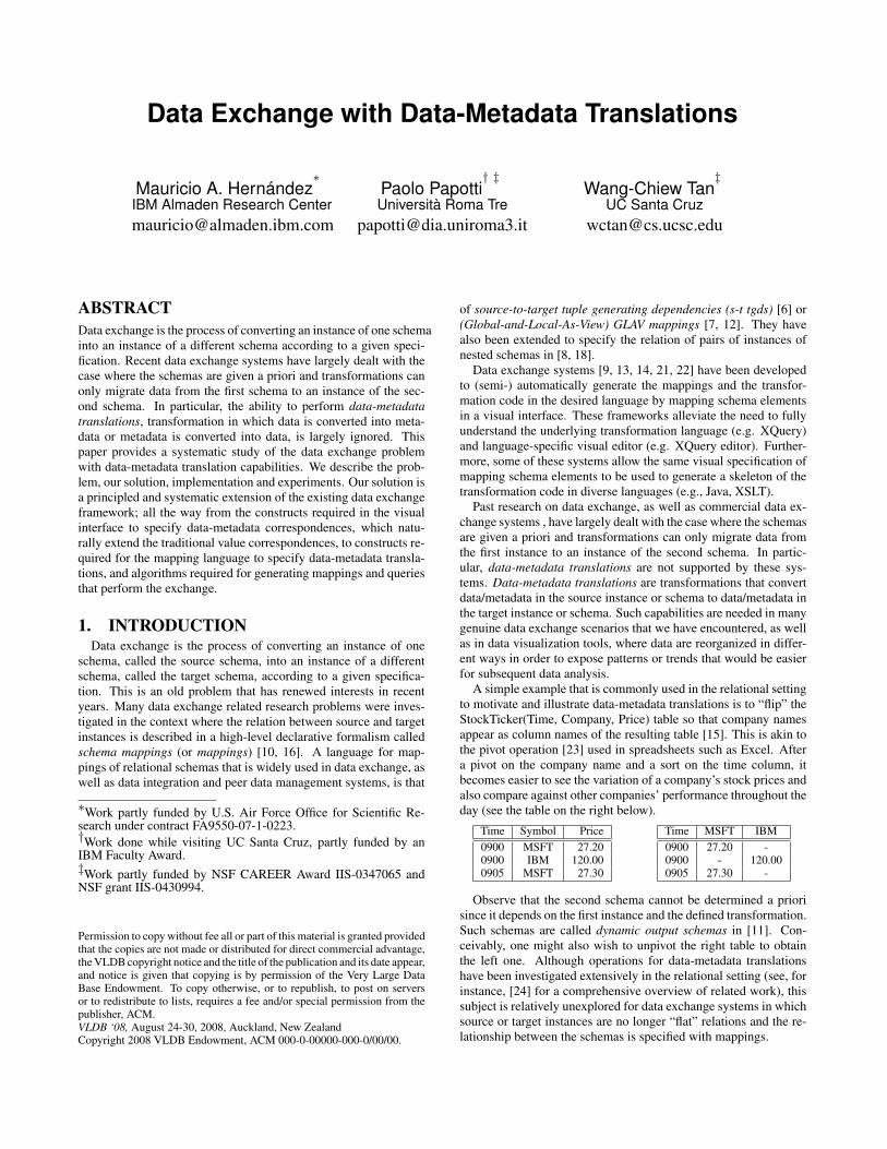
Source: RcdSales: SetOf Rcdcountryregionstyleshipdateunitsprice

Target: RcdCountrySales: SetOf Rcd

countrySales: SetOf Rcdstyleshipdateunitsid

for $s in Source.Salesexists $c in Target.CountrySales, $cs in $c.Saleswhere $c.country = $s.country and $cs.style = $s.style and

$cs.shipdate = $s.shipdate and $cs.units = $s.units and$c.Sales = SK[$s.country]

Salescountry region style shipdate units priceUSA East Tee 12/07 11 1200 USA East Elec. 12/07 12 3600USA West Tee 01/08 10 1600UK West Tee 02/08 12 2000

CountrySalescountry SalesUSA style shipdate units id

Tee 12/07 11 ID1Elec. 12/07 12 ID2Tee 01/08 10 ID3country Sales

UK style shipdate units idTee 02/08 12 ID4

“For every Sales tuple, map it to a CountrySales tuple where Sales are grouped by country in that tuple.”

(a)

(b)

(c)

Figure 1: Data-to-Data Exchange

2.1 Data-to-Data Translation (Data Exchange)Data-to-data translation corresponds to the traditional data ex-

change where the goal is to materialize a target instance accordingto the specified mappings when given a source instance. In data-to-data translation, the source and target schemas are given a priori.

Figure 1 shows a typical data-to-data translation scenario. Here,users have mapped the source-side schema entities into some tar-get side entities, which are depicted as lines in the visual interface.The lines are called value correspondences. The schemas are rep-resented using the Nested Relational (NR) Model of [18], wherea relation is modeled as a set of records and relations may be arbi-trarily nested. In the source schema, Sales is a set of records whereeach record has six atomic elements: country, region, style, ship-date, units, and price. The target is a slight reorganization of thesource. CountrySales is a set of records, where each record has twolabels, country and Sales. Country is associated to an atomic type(atomic types are not shown in the figure), whereas Sales is a set ofrecords. The intention is to group Sales records as nested sets bycountry, regardless of region.

Formally, a NR schema is a set of labels {R1,...,Rk}, calledroots, where each root is associated with a type τ , defined by thefollowing grammar: τ ::= String | Int | SetOf τ |Rcd[l1 : τ1, ..., ln :τn] | Choice[l1 : τ1, ..., ln : τn]. The types String and Int areatomic types (not shown in Figure 1)1. Rcd and Choice are com-plex types. A value of type Rcd[l1 : τ1, ..., ln : τn] is a set oflabel-value pairs [l1 : a1, ..., ln : an], where a1, ..., an are of typesτ1, ..., τn, respectively. A value of type Choice[l1 : τ1, ..., ln : τn]is a single label-value pair [lk : ak], where ak is of type τk and1 ≤ k ≤ n. The labels l1, ..., ln are pairwise distinct. The set typeSetOf τ (where τ is a complex type) is used to model repeatableelements modulo order.

In [18], mappings are generated from the visual specificationwith a mapping generation algorithm. For example, the visual spec-ification of Figure 1(a) will be interpreted into the mapping expres-sion that is written in a query-like notation shown on Figure 1(b).

1We use only String and Int as explicit examples of atomic types.Our implementation supports more than String and Int.

Source: RcdSalesByCountries: SetOf RcdmonthUSAUK Italy

Target: RcdSales: SetOf Rcdmonthcountryunits

for $s in Source.SalesByCountries, $c in {“USA”, “UK”, “Italy”}exists $t in Target.Saleswhere $t.month = $s.month and $t.country = $c and $t.units = $s.($c)

SalesByCountriesmonth USA UK ItalyJan 120 223 89Feb 83 168 56

Salesmonth country unitsJan USA 120Jan UK 223Jan Italy 89Feb USA 83Feb UK 168Feb Italy 56

<<countries>>labelvalue

“For every SalesByCountries tuple, map it to a Sales tuple where Sales are listed by month and country names.”

(a)

(b)

(c)

Figure 2: Metadata-to-Data Exchange

The mapping language is essentially a for . . . where . . . exists. . . where . . . clause. Intuitively, the for clause binds variables totuples in the source, and the first where clause describes the sourceconstraints that are to be satisfied by the source tuples declared inthe for clause (e.g., filter or join conditions)2. The exists clausedescribes the tuples that are expected in the target, and the secondwhere clause describes the target constraints that are to be satisfiedby the target tuples as well as the content of these target tuples.

The mapping in Figure 1 states that for every Sales record inthe source instance that binds to $s, a record is created in theCountrySales relation together with a nested set Sales. For exam-ple, when $s binds to the first tuple in Sales, a record in Coun-trySales must exists whose country value is “USA” and Sales valueis a record (style=“Tee”, shipdate=“12/07”, units=“11”, id=ID1”).Since the value of id label is not specified, a null “ID1” is created asits value. Records in Target.Sales are grouped by country, which isspecified by the grouping expression “$c.Sales = SK[$s.country]”.The term SK[$s.country] is essentially the identifier of the nestedset $c.Sales in the target. For the current record that is boundto $s, the identifier of $c.Sales in the target is SK[USA]. When$s binds to the second tuple in Source.Sales, an additional record(style=“Elec.”, shipdate=“12/07”, units=“11”, id=“ID2”) with thesame Sales set identifier, SK[USA], must exist in the target. Givena source instance shown on the bottom-left of Figure 1, a targetinstance that satisfies the mapping is shown on the bottom-right.Such mappings are called as basic mappings.

Although mappings describe what is expected of a target in-stance, they are not used to materialize a target instance in the dataexchange framework of [18]. Instead, a query is generated fromthe mappings, and the generated query is used to perform the dataexchange.

2.2 Metadata-to-Data TranslationAn example of metadata-to-data translation is shown in Figure 2.

This example is similar to that of unpivoting the second relationinto the first in the StockTicker example described in Section 1.Like data-to-data translations, both the source and target schemasare given a priori in metadata-to-data translations. The goal of theexchange in Figure 2 is to tabulate, for every month and country,

2The example in Figure 1(b) does not use the first where clause.

the number of units sold. Hence, the mapping has to specify thatthe element names, “USA”, “UK” and “Italy”, in the source schemaare to be translated into data in the target instance.Placeholders in the source schema Our visual interface allows thespecification of metadata-to-data transformations by first selectingthe set of element names (i.e., metadata) of interest in the source.In Figure 2, “USA”, “UK” and “Italy” are selected and grouped to-gether under the placeholder 〈〈countries〉〉, shown in the middle ofthe visual specification in Figure 2. The placeholder 〈〈countries〉〉exposes two attributes, label and value, which are shown under-neath 〈〈countries〉〉. Intuitively, the contents of label correspond toan element of the set {“USA”, “UK” and “Italy”}, while the con-tents of value correspond to value of the corresponding label (e.g.,the value of “USA”, “UK”, or “Italy” in a record of the set Sales-ByCountries). To specify metadata-to-data transformation, a valuecorrespondence is used to associate a label in the source schemato an element in the target schema. In this case, the label under〈〈countries〉〉 in the source schema is associated with country in thetarget schema. Intuitively, this specifies that the element names“USA”, “UK” and “Italy” will become values of the country ele-ment in the target instance. It is worth remarking that label under〈〈countries〉〉 essentially turns metadata into data, thus allowing tra-ditional value correspondences to be used to specify metadata-to-data translations. Another value correspondence, which associatesvalue to units, will migrate the sales of the corresponding coun-tries to units in the target. A placeholder is an elegant extension tothe visual interface. Without placeholders, different types of lineswill need to be introduced on the visual interface to denote differ-ent types of intended translations. We believe placeholders providean intuitive descriptions of the intended translation with minimalextensions to the visual interface without cluttering the visual in-terface with different types of lines. As we shall see in Section 2.3,a similar idea is used to represent data-to-metadata translations.

The precise mapping that describes this transformation is shownon Figure 2(b). The mapping states that for every combination of atuple, denoted by $s, in SalesByCountries and an element $c in theset {“USA”, “UK”, “Italy”}, generate a tuple in Sales in the targetwith the values as specified in the where clause of the mapping.Observe that the record projection operation $s.($c) depends of thevalue that $c is currently bound to. For example, if $c is boundto the value “USA”, then $s.($c) has the same effect as writing$s.USA. Such a construct for projecting records “dynamically” isactually not needed for metadata-to-data translations. Indeed, thesame transformation could be achieved by writing the followingmapping:

for $s in Source.SalesByCountriesexists $t1 in Target.Sales, $t2 in Target.Sales, $t3 in Target.Saleswhere $t1.month = $s.month and $t2.month = $s.month and

$t3.month = $s.month and$t1.country = “USA” and $t2.country = “UK” and$t3.country = “Italy” and$t1.units = $s.USA and $t2.units = $s.UK and$t3.units = $s.Italy

The above mapping states that for every tuple $s in SalesBy-Countries, there exists three tuples $t1, $t2 and $t3 in Sales, onefor each country “USA”, “UK” and “Italy”, with the appropriatevalues for month, country and units.

Since our placeholders are used strictly to pivot metadata intodata values, we can only use them in the source schema duringmetadata-to-data translations. Our current implementation allowsplaceholders to be created for element names at the same level ofnesting and of the same type. For example, a placeholder couldbe created for “USA”, “UK” and “Italy” because they belong to

the same record and have the same atomic type, say Int. If “USA”occurs in some other record or, if “USA” is a complex type while“UK” and “Italy” are atomic types, then it is not possible to cre-ate a placeholder for these elements. Although it is conceivable toallow placeholders for the latter case by generating different map-pings according to types of elements in the placeholder, we do notelaborate on that option here.

Just as in the relational metadata-to-data translations where SQLdoes not need to be extended to handle metadata-to-data transla-tions [25], the existing mapping language does not need to be ex-tended to handle metadata-to-data translations as well. As a mat-ter of fact, in Section 4 we will discuss how mapping expressionscontaining our placeholders are re-written into the notation used inFigure 2. In contrast, the situation is rather different with data-to-metadata translations, which we shall describe in the next section.

2.3 Data-to-Metadata TranslationTo illustrate data exchange with data-to-metadata translation, we

first revisit the example that was described in Section 1. The map-ping below illustrates the exchange where the source schema is aset of records with three attributes (time, symbol and price) andthe target is a set of records with a time attribute and a dynamicelement, shown as a label and value pair. Schemas with dynamicelements are called nested dynamic output schemas (ndos).

Source: RcdStockTicker: SetOf Rcd

timesymbolprice

Target: RcdStockquotes: SetOf Rcd

timelabelvalue

Nested Dynamic Output Schema (ndos) A ndos schema is simi-lar to an NR schema except that it can contain dynamic elements.Like NR schemas, a ndos schema is a set of labels {R1,...,Rk},called roots, where each root is associated with a type τ , definedby the following grammar: τ ::= String | Int | SetOf τ | Rcd[l1 :τ1, ..., lm : τm, $d : τ ] | Choice[l1 : τ1, ..., lm : τm, $d : τ ].Observe that the grammar is very similar to that defined for a NRschema except that Rcd and Choice types can each contain a dy-namic element, denoted by $d. A dynamic element has type τwhich may contain dynamic elements within. Intuitively, a dy-namic element may be instantiated to one or more element names atruntime (i.e., during the exchange process). If $d is instantiated tovalues p1, ..., pn at runtime, then all values of p1, ..., pn must havethe same type τ . Ndos schemas can only be defined in the target.Note that they are different from source schemas with placeholders.Dynamic elements are not placeholders since they do not representa set of element names that exists in the schema but rather, they areintended to represent element names that are only determined atruntime. Our implementation supports the specification of multipledynamic elements within a record or choice type although we donot elaborate on this possibility here.

The visual specification of the figure above is interpreted into thefollowing mappings by our mapping generation algorithm:

m : for $s in Source.StockTickerexists $t in Target.Stockquoteswhere $t.time = $s.time and $t.($s.Symbol) = $s.Price

c : for $t1 in Target.Stockquotes, $t2 in Target.Stockquotes, l ∈ dom($t1)exists $l′in dom($t2)where l = l′

Mapping m asserts that for every record $s in StockTicker, theremust be a record $t in Stockquotes whose time value is the same asthe time value of $s and there is an attribute in $t named $s.Symbol

whose value is $s.Price. It is worth noting that the term $t.($s.Symbol)projects on the record $t dynamically. The attribute on which toproject the record $t is $s.Symbol which can only be determinedduring the exchange. This is similar to the dynamic projection ofrecords that was described in Section 2.1. However, unlike theexample in Section 2.1, the ability to dynamically project recordsis crucial for data-to-metadata translations. Since the attribute onwhich to project the record $t is determined by the source instance,the mapping cannot be rewritten into one that does not use suchdynamic constructs. The assertions described by the mapping pro-duce, conceptually, the following data:

Rcd[Time:0900, MSFT:27.20]Rcd[Time:0900, IBM:120]Rcd[Time:0905, MSFT:27.30]

Since Stockquotes is a set of records and all records in the sameset must be homogeneous, we obtain the result that is shown inthe Section 1, where each record has three fields, time, MSFTand IBM. Indeed, the above homogeneity constraint is capturedby the mapping c. This mapping states that all records in Tar-get.Stockquotes must have the same set of labels.

Our mapping and query generation algorithms can also accountfor key constraints. For example, if time is the key of Stockquotes,then there will be an additional mapping that essentially enforcethat every pair of tuples with the same time value must have thesame MSFT and IBM values. The key constraint is enforced as apost-processing step on the instance obtained in Section 1. Hence,there will only be two tuples in the output, corresponding to (0900,27.20, 120.00) and (0905, 27.30, -) after the post-processing. Notethat inclusion dependencies, such as key/foreign key constraints,are automatically enforced prior to the post-processing step.

If the desired output is to have three records of possibly hetero-geneous types as shown above, then one solution is to specify thedynamic element in Stockquotes as a Choice type. We shall de-scribe in Sections 4 and 5 how types in an ndos schema are used inthe mapping and query generation process to generate the correctmapping specification and transformation.

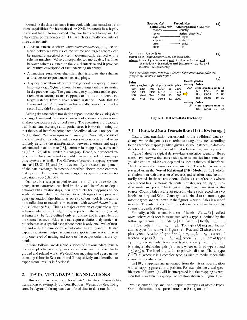
A novelty of our work is that ndos schemas can contain many dy-namic elements, which may be arbitrarily nested. This is a majorextension to dynamic output schemas of [11] for the relational case.We illustrate this with the example in Figure 3. The source schemais identical to that of Figure 1 and the target is a ndos schema.It contains two dynamic elements (denoted as label1, value1 andlabel2, value2, respectively, in the figure), where one is nestedunder the other. Target.ByShipdateCountry is a SetOf Choicetypes. This means that every tuple in Target.ByShipdateCountryis a choice between many different label-value pairs. The set oflabel-value pairs is determined at runtime, where the labels in theset are all the shipdates (e.g., 12/07, 01/08, and 02/08 accordingto the source instance shown on the bottom-left of the same fig-ure) and the value associated with each label is a record with adynamic element. The set of labels in each record is determined bythe countries in the source instance (e.g., USA, UK) and the valueassociated with each label is a set of records of a fixed type (style,units, price).

The visual specification is interpreted into the mapping shownon Figure 3(b). The mapping is a constraint that states that forevery Source.Sales tuple $s, there must exists a tuple $t in theset Target.ByShipdateCountry where a case (or choice) of this tu-ple has label $s.shipdate and the value is bound to the variable$u. From the ndos schema, we know that $u is a record. Theterm $u.($s.country) states that $u has an attribute $s.country andfrom the ndos schema, we know that $u.($s.country) is a set of

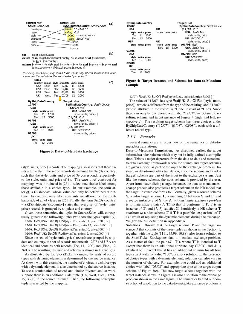
Source: RcdSales: SetOf Rcd

countryregionstyleshipdateunitsprice

Target: RcdByShipdateCountry: SetOf Choice

label1value1: Rcdlabel2value2: SetOf Rcd

styleunitsprice

“For every Sales tuple, map it to a tuple whose only label is shipdate and value is a record that tabulates the set of sales by country.”

for $s in Source.Salesexists $t in Target.ByShipdateCountry, $u in case $t of $s.shipdate,

$v in $u.($s.country) where $v.style = $s.style and $v.units = $s.units and $v.price = $s.price and

$u.($s.country) = SK[$s.shipdate,$s.country]

(a)

(b)

(c)

<<dates>>

<<countries>>

Salescountry region style shipdate units price

USA East Tee 12/07 11 1200 USA East Elec. 12/07 12 3600USA West Tee 01/08 10 1600UK West Tee 02/08 12 2000

ByShipDateCountry12/07USA

style units priceTee 11 1200 Elec. 12 3600

01/08USA

style units priceTee 10 1600

02/08UK


Target: RcdByShipDateCountry: SetOf Choice

(12/07: RcdUSA: SetOf Rcd

style, units, price) |(01/08: Rcd

USA: SetOf Rcdstyle, units, price) |

(02/08: RcdUK: SetOf Rcd

style, units, price)

Figure 3: Data-to-Metadata Exchange

(style, units, price) records. The mapping also asserts that there ex-ists a tuple $v in the set of records determined by $u.($s.country)such that the style, units and price of $v correspond, respectively,to the style, units and price of $s. The case . . . of construct formappings was introduced in [26] to select one choice label amongthose available in a choice type. In our example, the term af-ter of is $s.shipdate, whose value can only be determined at run-time. In contrast, only label constants are allowed on the right-hand-side of an of clause in [26]. Finally, the term $u.($s.country)= SK[$s.shipdate,$s.country] states that every set of (style, units,price) records is grouped by shipdate and country.

Given these semantics, the tuples in Source.Sales will, concep-tually, generate the following tuples (we show the types explicitly):

12/07: Rcd[USA: SetOf{ Rcd[style:Tee, units:11, price:1200] } ]12/07: Rcd[USA: SetOf{ Rcd[style:Elec., units:12, price:3600] } ]01/08: Rcd[USA: SetOf{ Rcd[style:Tee, units:10, price:1600] } ]02/08: Rcd[ UK: SetOf{ Rcd[style:Tee, units:12, price:2000] } ]Since the sets of (style, units, price) records are grouped by ship-

date and country, the set of records underneath 12/07 and USA areidentical and contains both records (Tee, 11, 1200) and (Elec., 12,3600). The resulting instance and schema is shown in Figure 3(c).

As illustrated by the StockTicker example, the arity of recordtypes with dynamic elements is determined by the source instance.As shown with this example, the number of choices in a choice typewith a dynamic element is also determined by the source instance.To see a combination of record and choice “dynamism” at work,suppose there is an additional Sale tuple (UK, West, Elec., 12/07,15, 3390) in the source instance. Then, the following conceptualtuple is asserted by the mapping:

Target: RcdByShipDateCountry: SetOf Choice

(12/07: RcdUSA: SetOf Rcd

style, units, priceUK: SetOf Rcd

style, units, price) |(01/08: Rcd

USA: SetOf Rcdstyle, units, price) |

(02/08: RcdUK: SetOf Rcd

style, units, price)

ByShipDateCountry12/07

USA UKstyle units price style units priceTee 11 1200 Elec. 12 3600

USA UKstyle units price style units price

Elec. 15 3390 01/08

USAstyle units priceTee 10 1600

02/08UK


Figure 4: Target Instance and Schema for Data-to-Metadataexample

12/07: Rcd[UK: SetOf{ Rcd[style:Elec., units:15, price:3390] } ]The value of “12/07” has type Rcd[UK: SetOf Rcd[style, units,

price]], which is different from the type of the existing label “12/07”(whose attribute in the record is “USA” instead of “UK”). Sincethere can only be one choice with label “12/07”, we obtain the re-sulting schema and target instance of Figure 4 (right and left, re-spectively). The resulting target schema has three choices underByShipDateCountry (“12/07”, “01/08”, “02/08”), each with a dif-ferent record type.

2.3.1 RemarksSeveral remarks are in order now on the semantics of data-to-

metadata translations.Data-to-Metadata Translation. As discussed earlier, the targetschema is a ndos schema which may not be fully-defined at compile-time. This is a major departure from the data-to-data and metadata-to-data exchange framework where the source and target schemasare given a priori as part of the input to the exchange problem. In-stead, in data-to-metadata translation, a source schema and a ndos(target) schema are part of the input to the exchange system. Justlike the source schema, the ndos schema is provided by the user.Apart from materializing a target instance, the data-to-metadata ex-change process also produces a target schema in the NR model thatthe target instance conforms to. Formally, given a source schemaS, a ndos target schema Γ, a mapping Σ between S and Γ, anda source instance I of S, the data-to-metadata exchange problemis to materialize a pair (J , T) so that T conforms to Γ, J is aninstance of T, and (I, J) satisfies Σ. Intuitively, a NR schema Tconforms to a ndos schema Γ if T is a possible “expansion” of Γas a result of replacing the dynamic elements during the exchange.We give the full definition in Appendix A.Solutions. Observe that the target schema T and the target in-stance J that consists of the three tuples as shown in the Section 1,together with the tuple (1111, 35.99, 10.88), also form a solution tothe StockTicker-Stockquotes data-to-metadata exchange problem.As a matter of fact, the pair (J ′, T′), where T′ is identical to Texcept that there is an additional attribute, say CISCO, and J ′ isidentical to J except that it has an additional column for all fourtuples in J with the value “100”, is also a solution. In the presenceof choice types with a dynamic element, solutions can also vary inthe number of choices. For example, one could add an additionalchoice with label “03/08” and appropriate type to the target outputschema of Figure 3(c). This new target schema together with thetarget instance shown in Figure 3 is also a solution to the exchangeproblem shown in the same figure. The semantics behind our con-struction of a solution to the data-to-metadata exchange problem is

based on an analysis of the assertions given by the mappings and in-put schemas, much like the chase procedure used in [8]. We believethat query generates the most natural solution amongst all possiblesolutions. A formal justification of this semantics is an interestingproblem on its own and part of our future work.

We detail an interesting metadata-to-metadata translation exam-ple in Appendix B.

3. MAD MAPPINGSIn Section 2, we have informally described the constructs that

are needed for mappings that specify data-metadata translations.We call such mappings, MAD mappings (short for MetadatA-Datamappings). The precise syntax of MAD mappings (MM) is de-scribed next.

for $x1 in g1, . . . , $xn in gn

where ρ($x1, . . . , $xn)exists $y1 in h1, . . . , $ym in hm

where υ($x1, . . . , $xn, $y1, . . . $ym) and MM1and . . . and MMk

Each gi in the for clause is an expression that either has a SetOfτ type or a τ type under the label l from the Choice [..., l : τ , ...].In the former case, the variable $xi will bind to an element in theset while in the latter case, $xi will bind to the value of the choiceunder label l. More precisely, gi is an expression of the form:E ::= S | $x |E.L | case E of L | 〈〈d〉〉 | {V1, . . . , Vz} | dom($x)

L ::= l | (E)

where $x is a variable, S is a schema root (e.g., Source in the sourceschema of Figure 1(a)) and E.L represents a projection of recordE on label L. The case E of L expression represents the selec-tion of label L under the choice type E. The label L is either asimple label or an expression. The latter case allows one to modeldynamic projections or dynamic elements under Choice types (e.g.,see Figure 3(b)). The expression 〈〈d〉〉 is a placeholder as describedin Section 2.2. As we shall discuss in the next section, placehold-ers can always be rewritten as a set of literal values {V1, . . . , Vz}.However, we have introduced placeholders in MAD mappings inorder to directly model the visual specification of grouping multi-ple schema elements (e.g., see 〈〈countries〉〉 in Figure 2(a)) in ourmapping generation algorithm. The expression dom($x) denotesthe set of labels in the domain of a record $x. Naturally, a variable$x that is used in an expression gi needs to be declared prior toits use, i.e., among x1, ..., xi−1 or in the for clause of some outermapping, in order for the mapping to be well-formed.

The expressions ρ($x1, . . ., $xn) and υ($x1, . . ., $xn, $y1, . . .$ym) are boolean expressions over the variables $x1, ..., $xn and$x1, ..., $xn, $y1, ..., $ym respectively. As illustrated in Section2, the expression in υ can also includes grouping conditions. Thehi expressions in the exists clause are similar to gis except that a〈〈d〉〉 expression in hi represents a dynamic element, and not place-holders. Finally, MAD mappings can be nested. Just like nestedmappings in [8], nested MAD mappings are not arbitrarily nested.The for clause of a MAD mapping can only extend expressionsbound to variables defined in the for clause of its parent mapping.Similarly, the exists clause can only extend expressions bound tovariables defined in the exists clause of an ancestor mapping. Notethat MAD mappings captures nested mappings of [8] as a specialcase.

4. MAD MAPPING GENERATIONIn this section, we describe how MAD mappings are generated

when given a source schema S, a target ndos schema Γ, and a set of

value correspondences that connect elements of the two schemas.This problem is first explored in Clio [18] for the case when Γ is anNR schema T and no placeholders are allowed in the source or tar-get schema. Here, we extend the mapping generation algorithm ofClio to generate MAD mappings that support data-metadata trans-lations.

The method by which data-metadata translations are specifiedin our visual interface is similar to Clio’s. A source and a targetschema are loaded into the visual interface and are rendered as twotrees of elements and attributes, and are shown side-by-side on thescreen. Users enter value correspondences by drawing lines be-tween schema elements. After this, the value correspondences canbe refined with transformation functions that define how source val-ues are to be converted to target values. As value correspondencesare entered, the mapping generation algorithm of Clio incremen-tally creates the mapping expressions that capture the transforma-tion semantics implied by the visual specification.

There are, however, significant differences between Clio’s visualinterface and our visual interface. First, users can create placehold-ers in the source and target schema. (e.g., see Figure 2(a)). Second,users can load ndos schemas on the target side of our visual inter-face and further edit it. Third, users can add value correspondencesthat connect placeholders or schema elements in the source schemawith placeholders, dynamic elements, or schema elements in thetarget schema.

4.1 Generation of Basic MappingsA general mapping generation algorithm that produces basic map-

pings was first described in [18] and subsequently refined in [8] toproduce mappings that can be nested within another. In what fol-lows, we describe briefly the basic mapping generation algorithmof [18]. Step 1. Tableaux: The generation of basic mappingsstarts by compiling the source and target schemas into a set ofsource and target tableaux. Let X = 〈x1, . . . , xn〉 be a sequenceof variables over expressions g1, . . . , gn of set or choice type. Atableaux is an expression of the form

T ::= {$x1 ∈ g1, . . . , $xn ∈ gn; E}where E is a (possibly empty) conjunction of equalities over the val-ues bounded to the variables in X . Informally, a a tableau capture arelationship or “concept” represented in the schema. Obvious rela-tionship such as all atomic attributes under a SetOf Rcd or SetOfChoice type, form “basic” tableaux. Basic tableaux are enhancedby chasing either the constraints (e.g., referential constraints) thatexist in the schema or the structural constraints in the schema (e.g.,parent-child relationship).

For example, we can derive two basic tableaux from the targetschema of Figure 1(a): {$x1 ∈ CountrySales} and {$x1 ∈ Coun-trySales.Sales}. Since CountrySales.Sales is nested under Coun-trySales, we obtain two tableaux after chasing: {$x1 ∈ Country-Sales} and {$x1 ∈ CountrySales, $x2 ∈ $x1.Sales}. As anotherexample, suppose we have a relational schema that contains twotables, Department and Employee, and a referential constraint fromEmployee into Department. In this case, there are two trivial tableaux,{$x1 ∈ Department} and {$x1 ∈ Employee}. After chasing overthe constraint, the resulting tableaux are {$x1 ∈ Department} and{$x1 ∈ Department, $x2 ∈ Employee; $x1.did=$x2.did}. Ob-serve that the Employee tableau is not in the final list because therecannot be Employee tuples without a related Department tuple, ac-cording to the referential constraint.

The output of the tableaux generation step is thus a set of sourcetableaux {s1, ..., sn} and a set of target tableaux {t1, ..., tm}.Step 2. Skeletons: Next, a n × m matrix of skeletons is con-

structed for the set of source tableaux {s1, ..., sn} and the set oftarget tableaux {t1, ..., tm}. Conceptually, each entry (i, j) in thematrix is a skeleton of a potential mapping. This means that everyentry provides some information towards the creation of a basicmapping. Specifically, the skeleton at (i, j) represents the mappingbetween source tuples of the form of the tableau si and target tuplesof the form of the tableau tj . Once the skeletons are created, themapping system is ready to accept value correspondences.

Observe that both the creation of tableaux and skeletons occursduring the loading of schemas. As long as the schemas do notchange after being loaded, there is not need to recompute its tableauxor update the skeleton matrix.Step 3. Creating Basic Mappings: For each value correspon-dence that is given by a user (or discovered using a schema match-ing method [19]), the source side of the correspondence is matchedagainst one or more source tableaux while the target side is matchedto one or more target tableaux. For every pair of matched sourceand target tableaux, we add the value correspondence to the skele-ton and mark the skeleton as “active”.

The next step involves an analysis of possible relationships (sub-sumed or implied by) among all “active” skeletons. Through thisrelationship, we avoid the generation of redundant mappings. Weomit the details of how and when skeletons are considered sub-sumed or implied by another, which are explained in [8, 18].

Any active skeleton that is not implied or subsumed by another,is reported as a mapping. The construction of a mapping from anactive skeleton is relatively straightforward: essentially, the sourcetableau expression becomes the for clause and the first where clausesof the mapping. The target tableau becomes the exists and secondwhere clause. Finally, the value correspondences that are associ-ated with the skeleton are added to the second where clause.

4.2 Generation of MAD mappingsWe are now ready to explain how MAD mappings are generated

from our visual specification that consists of a source schema, atarget ndos schema, and value correspondences between the two.Step 1. Tableaux: We start by compiling the given schemas intosource and target tableaux. This step is similar to Step 1 of the basicmapping generation algorithm, except that our representation of atableau is more elaborate and takes into account placeholders anddynamic elements:

T ′ ::= {$x1 ∈ g1, . . . , $xt ∈ gt; $xt+1 := gt+1, . . . ; E}The “assignments” at the end of our tableau representation are onlygenerated when placeholders or dynamic elements appear in theschema. In our subsequent discussions, we uniformly denote place-holders and dynamic elements with 〈〈D〉〉.

For every 〈〈D〉〉, we find the set P(D) of all tableaux that includethe context element of 〈〈D〉〉. The context element of 〈〈D〉〉 is therecord or choice in the schema in which 〈〈D〉〉 occurs. For example,SalesByCountry is the context element of 〈〈countries〉〉 in the sourceschema of Figure 2(a). Next, we extend each tableaux p ∈ P(D)by adding two path expressions corresponding to: (a) the metadatalabel of 〈〈D〉〉, and (b) the value label of 〈〈D〉〉. Specifically, let $x bethe variable that ranges over the context elements of 〈〈D〉〉. We firstadd to p an expression “$l ∈ 〈〈D〉〉” to represent an iteration overall the metadata values in 〈〈D〉〉3. After this, we examine the type ofthe values under the labels in 〈〈D〉〉. If the values are a set type, weadd to p an expression “$x′ ∈ $x.($l)”. The new variable $x′ willrange over the elements in the set represented by $x.($l). (If the

3Recall that 〈〈D〉〉 denotes a set of (label, value) pairs. The expres-sion “$l ∈ 〈〈D〉〉” ranges $l over the labels of 〈〈D〉〉.

values are a choice type, we add “$x′ ∈ case $x of ($l)”.) Other-wise, if the values under labels in 〈〈D〉〉 is a non-repeating type (e.g.,record or atomic), we add an assignment: “$x′ := $x.($l)”. Inother words, x′ is assigned the value (record or atomic value) underthe current metadata label $l. As an example, the source schemaof Figure 2(a) will be compiled into a single source tableau {$x0∈Source.SalesByCountries, $x1∈〈〈countries〉〉; $x2 := $x0.($x1) }Step 2. Skeletons: The generation of skeletons proceeds in thesame manner as described in the previous section. A skeleton of apotential mapping is created for every possible pair of source andtarget tableau.Step 3. Creating MAD Mappings: At this stage, the value corre-spondences need to be matched against the tableaux in order to fac-tor them into the appropriate skeletons. To explain how we match,consider the first two value correspondences in Figure 1(a), whichare represented internally by a pair of sequence of labels.Source.Sales.country→ Target.CountrySales.countrySource.Sales.style→ Target.CountrySales.Sales.style

In order to compare the above path expressions with expressionsin the tableaux, each variable binding in a tableau expression isfirst expanded into an absolute path. For example, recall that atarget tableau for Figure 1(a) is {$y0 ∈ Target.CountrySales, y1 ∈$y0.Sales}. The absolute path of y1 is Target.CountrySales.Sales.

For each value correspondence, the path on the left (resp. right)(called correspondence path) is matched against absolute paths ofsource (resp. target) tableaux. A correspondence path p1 is saidto match an absolute path p2 if p2 is a prefix of p1. Observe thata match of the left and right correspondence paths of a value cor-respondence into a source and target tableau corresponds to a se-lection of a skeleton in the matrix. After a match has been found,we then replace the longest possible suffix of the correspondencepath with a variable in the tableau. For example, the right corre-spondence path of the second value correspondence above matchesagainst the absolute path of the tableau {$y0 ∈ Target.CountrySales,y1 ∈ $y0.Sales}. The expression “$y1.style” is generated as a re-sult. The left correspondence of the same value correspondenceis matched against the only source tableau { $x ∈ Source.Sales }and the expression “$x.style” is generated. The result of matchinga value correspondence to a source and target tableau is an equal-ity expression (e.g., “$x.style = $y1.style”) which is added to thecorresponding skeleton in the matrix.

Matching correspondences paths in the presence of dynamic el-ements or placeholders to tableaux proceeds in a similar manner.Our translation of value correspondences, that starts or ends at place-holders or dynamic elements, into path expressions is slightly dif-ferent in order to faciliate the subsequent matching process. Whena value correspondence starts or ends with the label part of a place-holder, the element name corresponding to this label is the nameof the placeholder (i.e., 〈〈D〉〉). If a value correspondence starts orends with the value part of a placeholder, the element name corre-sponding to this value is “&〈〈D〉〉”, where 〈〈D〉〉 is the name of theplaceholder and &〈〈D〉〉 represents the value part of 〈〈D〉〉.

We explain the complete MAD mapping generation process throughtwo examples next. More details about the mapping generation al-gorithm are presented in Appendix C.

4.2.1 ExamplesConsider the example in Figure 2. When the schemas are loaded,

the system creates one source tableau, {$x1 ∈ Source.SalesBy-Country}, and one target tableau {$y1 ∈ Target.Sales}. This re-sults in only one mapping skeleton.

Now the user creates the source placeholder 〈〈countries〉〉. In-ternally, our system replaces the three selected source labels with a

new element, named 〈〈countries〉〉 and whose type is SetOf Record[label: String, value: String]. This change in the schema triggers arecompilation of the source tableau into: {$x1 ∈ Source.SalesBy-Country, $x2 ∈ 〈〈countries〉〉; $x3 := $x1.($x2)} A new skeletonusing this new source tableau is thus created.

The user then enters the three value correspondences of Figure 2.Of particular interests to this discussion are the value correspon-dences that map the placeholder 〈〈countries〉〉:

Source.SalesByCountries.〈〈countries〉〉 → Target.Sales.countrySource.SalesByCountries.&〈〈countries〉〉 → Target.Sales.units

These two value correspondences match the new source tableauand the only target tableau. Hence, the expressions $x2 = $y1.countryand $x3 = $y1.units are compiled into the skeleton. Since $x3 isan assignment in the source tableau, we rewrite the second corre-spondence as $x1.($x2) = $y1.units and can redact the $x3 as-signment from the mapping.

The following MAD mapping is constructed from that skeleton,using its source and target tableaux and the matched value corre-spondences:

(a) for $x1 in Source.SalesByCountry, $x2 ∈ 〈〈countries〉〉exists $y1 in Target.Saleswhere $y1.month = $x1.month and

$y1.country = $x2 and $y1.units = $x1.($x2)

As a final rewrite, we replace the 〈〈countries〉〉 placeholder in the forclause with the set of labels wrapped by the placeholder, to capturethe actual label values in the mapping expression. The resultingmapping is exactly the one illustrated in Figure 2(b).

Next, consider the more complex example of Figure 3. Herethere is only one source tableau and one dynamic target tableau.After the value correspondences are entered, the system emits thefollowing MAD mapping:

(b) for $x1 in Source.Salesexists $y1 in Target.ByShipdateCountry,

$y2 in 〈〈dates〉〉, $y3 in case $y1of $y2,$y4 in 〈〈countries〉〉, $y5 in $y3.($y4)

where $y2 = $x1.shipdate and $y4 = $x1.country and$y5.style = $x1.style and $y5.units = $x1.units and$y5.price = $x1.price

We rewrite this expression by first replacing all usages of $y2 and$y4 in the exists clause with their assignment from the whereclause. Since these assignments are redundant after the replace-ments, they are redacted from the where clause. Further, since alluses of $y2 and $y4 were removed from the where clause, theirdeclarations in the exists clause are also redundant and, therefore,removed. The resulting MAD mapping is reduced to the mappingexpression presented below:

(c) for $x1 in Source.Salesexists $y1 in Target.ByShipdateCountry,

$y3 in case $y1of $x1.shipdate,$y5 in $y3.($x1.country)

where $y5.style = $x1.style and $y5.units = $x1.units and$y5.price = $x1.price

Observe that this mapping differs from the one in Figure 3(b)in that the grouping condition “$u.($s.country)=SK[$s.shipdate,$s.country]” is missing here. We assume that the user has explicitlyadded the grouping function in Figure 3(b), after the value corre-spondences are entered (i.e., after the mapping above is obtained).

Q2

I J

S

S1

T

T1 T2

T3

Q1 rr

rr

Q3

ndos

T1 T2

T3

Q4

Phase 1: Q1 shreds the source instance I over relational views of the target ndos

Phase 2: Q2 assembles the target instance J from the relational views

Q3 computes the target schema T

Q4 is the optional post -processing T4

conforms-to

conforms-to

conforms-to

Figure 5: The architecture of the two-phase query generation.

5. QUERY GENERATIONMappings have an executable semantics that can be expressed

in many different data manipulation languages. In this section, wedescribe how queries are generated from MAD mappings (and theassociated source and target schemas) to translate a source instanceinto a target instance according to the semantics of the MAD map-pings. Previous works [8, 18] have described algorithms for gen-erating queries from (data-to-data) mappings. Here, we generalizethose algorithms to MAD mappings, which include constructs fordata-metadata transformations. If the visual specification involvesa target ndos schema, the MAD mappings that are generated fromour mapping generation algorithm (described in Section 4) includeconstructs for specifying data-to-metadata translations. In this case,our algorithm is also able to generate a query that outputs a targetschema which conforms to the ndos schema, when executed againsta source instance.

In order to distinguish between the two types of queries gen-erated by our algorithm, we call the first type of queries whichgenerates a target instance, instance queries, and the second typeof queries which generates a target schema, schema queries. Fig-ure 5 shows where the different kind of queries are used in MAD.Queries Q1, Q2, and Q4 represent our instance queries, and Q3

represent the schema queries. As will discuss shortly, Q2 and Q3

work form the data produced by the first query Q1.

5.1 Instance Query GenerationOur instance query generation algorithm produces a query script

that, conceptually, constructs the target instance with a two-phaseprocess. In the first phase, source data is “shredded” into viewsthat form a relational representation of the target schema (Q1 inFigure 5). The second phase restructures the data in the relationalviews to conform to the actual target schema (Q2). We now de-scribe these two stages in details.

The instance query generation algorithm takes as input the com-piled source and target schemas and the mapping skeletons thatwere used to produce the MAD mappings. Recall that a mappingskeleton contains a pair of a source and a target tableau, and a setof compiled value correspondences.

Our first step is to find a suitable ”shredding” of the target schema.All the information needed to construct these views is in the map-ping expression and the target schema. In particular, the existsclause of the mapping dictates the part of the target schema beinggenerated. We start by breaking each mapping into one or more“single-headed” mappings; we create one single-headed mapping

let ByShipdateCountry := for s in Salesreturn [ datesID = SK1[s.shipdate, s.country, s.style, s.units, s.price] ], «dates» := for s in Salesreturn [ setID = SK1[s.shipdate, s.country, s.style, s.units, s.price],

label = s.shipdate, value = SK2[s.shipdate, s.country, s.style, s.units, s.price],countriesID = SK2[s.shipdate, s.country, s.style, s.units, s.price] ],

«countries» := for s in Salesreturn [ setID = SK2[s.shipdate, s.country, s.style, s.units, s.price],

label = s.country, value = SK3[s.shipdate, s.country],SetOfRecords1_ID = SK3[s.shipdate, s.country] ],

SetOfRecords1 := for s in Salesreturn [ setID = SK3[s.shipdate, s.country],

style = s.style, units = s.units, price = s.price ]

Figure 6: First-phase query (Q1)

for each variable in the exists clause of the mapping bounded toa set type or a dynamic expression. Each single-headed mappingdefines how to populate a region of the target instance and is usedto define a target view. To maintain the parent-child relationshipbetween these views, we compute a parent “setID” for each tuplein a view. This setID tells us under which tuple (or tuples) on theparent view each tuple on a child view belongs to.

The setID are actually computed by “Skolemizing” each variablein the exists clause of the mapping4. The Skolemization replaceseach variable in the exists clause with a Skolem function that de-pends on all the source columns appear in the where clause.

For example, consider the mapping labeled (b) in Section 2 (themapping we compute internally for the example in Figure 3). Theexists clause of the mapping defines four set type or dynamic ex-pressions. Thus, we construct the following views of the targetinstance:

ByShipdateCountry ( DatesID )〈〈 dates 〉〉 ( setID, label, value, CountriesID )

〈〈 countries 〉〉 ( setID, label, value, SetOfRecords 1ID )SetOfRecord 1 ( setID, style, units, price )

Every view contains the atomic elements that are directly nestedunder the set type it represents. A view that represents a set typethat is not top-level has a generated setID column that containsthe defined Skolem function. Observe that Skolem functions areessentially set identifiers which can be used to reconstruct data inthe views according to the structure of the target schema by join-ing on the appropriate ID fields. For example, the set identifierfor 〈〈countries〉〉 is SK[$s.shipdate, $s.country, $s.style, $s.units,$s.price] and the set identifier for SetOfRecords 1 is SK[$s.shipdate,$s.country]. The latter is obtained directly from the mapping sinceit is defined by the user in Figure 3(b).

Figure 6 depicts the generated queries that define each view.These queries are constructed using the source tableau and the valuecorrespondences from the skeleton that produced the mapping. No-tice that in more complex mappings, multiple mappings can con-tribute data to the same target element. The query generation algo-rithm can detect such cases and create a union of queries that aregenerated from all mappings contributing data to the same targetelement.

The next step is to create a query that constructs the actual tar-get instance using the views. The generation algorithm visits thetarget schema. At each set element, it figures which view producesdata that belongs in this set. A query that iterates over the view

4We can also use only the key columns, if available.

Target = for b in ByShipdateCountryreturn [

for s in «dates»where s.setID = b.datesID

return [s.label = for c in «countries»

where c.setID = s.countriesIDreturn [

c.label = for r in SetOfRecord_1where r.setID = c.SetOfRecord_1return [ style = r.style,

units = r.unitsprice = r.price ] ] ] ]

Figure 7: Second-phase query (Q2)

is created and the appropriate values are copied into each producedtarget tuple. To reconstruct the structure of the target schema, viewsare joined on the appropriate fields. For example, SetOfRecord 1is joined with 〈〈countries〉〉 on setID and SetOfRecords ID fields inorder to nest all (style, units, price) records under the appropriate〈〈countries〉〉 element. The query that produces the nested data is inFigure 7. Notice how the label values of the dynamic elements (sand c) become the set names in the target instance.

While there are simpler and more efficient query strategies thatwork for a large class of examples, it is not possible to apply themin general settings. This two-phase generation strategy allows us tosupport user-defined grouping in target schemas with nested sets.Also, it allows us to implement grouping over target languages thatdo not natively support group-by operations (e.g., XQuery 1.0).

5.2 Schema Query GenerationWe can also generate a schema query (Q3) when the target schema

is a ndos. Continuing with our example, we produce the followingquery:Schema = Target: Rcd

ByShipdateCountry: SetOf Choicelet dates := distinct-values («dates».label)for d in dateswhere valid(d)return [

d: Rcdlet cIDs := distinct-values («dates»[.label=d].CountriesID)for ci in cIDsreturn [

let countries := distinct-values («countries»[.setID=ci].label)for c in countrieswhere valid(c)return [

c: SetOf Rcdstyle, units, price ] ] ]

The schema query follows the structure of the ndos schema closely.Explicit schema elements, those that are statically defined in thendos, appear in the query as-is (e.g., Target and ByShipdateCoun-try). Dynamic elements, on the other hand, are replaced with a sub-query that retrieves the label data from the appropriate relationalview computed by Q1. Notice that we use distinct-value() whencreating the dynamic target labels. This avoids the invalid gener-ation of duplicate labels under the same Record or Choice type.Also, we call a user-defined function valid() to make sure we onlyuse valid strings as labels in the resulting schema. Many schemamodels do not support numbers, certain special characters, or mayhave length restrictions on their metadata labels. used in the targetas metadata.

5.3 Post-processingWe have an additional module that generates post-processing

scripts that execute over the data produced by the instance query.

Post-processing is needed when there is a need to enforce the ho-mogeneity (or relational) constraint, or a key constraint.

An example where both the homogeneity and key constraints areused is the StockTicker-Stockquotes example (described in Sec-tion 2.3 with the homogeneity constraint labeled c). The trans-formation that implements the homogeneity constraint is a rela-tively straightforward rewriting where an important function is in-troduced to implement the dom operator.

In our implementation, it is possible to generate a post-processingscript that enforces both homogeneity and key constraints simulta-neously. The script that does this for the StockTicker-Stockquotesexample is shown below:

Target’ = let times := Target.Stockquotes.time,attributes := dom (Target.Stockquotes)

for t in timesreturn [

Stockquotes= let elements := Target.Stockquotes[time=t]for a in attributesreturn [

if is-not-in (a, elements)then a = null else a = elements.a ] ]

The query above first defines two sets. The first set times is theset of all values under the key attribute time. The second set at-tributes is the set of all the attributes names in the target instanceStockquotes. For each key value in times, all tuples in the targetinstance with this key value are collected under a third set calledelements. At this point, the query iterates over all attribute namesin attributes. For each attribute a in attributes, it checks whetherthere is a tuple t in elements with attribute a. If yes, the output tuplewill contain attribute a with value as determined by t.a. Otherwise,the value is null. It is possible that there is more than one tuple inelements with different a values. In this case, a conflict occurs andno target instance can be constructed.

5.4 Implementation RemarksIn our current prototype implementation, we produce instance

and schema queries in XQuery. It is worth pointing out that XQuery,as well as other XML query languages such as XSLT, support query-ing of XML data and metadata, and the construction of XML dataand metadata.

In contrast, relational query languages such as SQL do not al-low us to uniformly query data and metadata. Even though manyRDBMS store catalog information as relations and allow users toaccess it using SQL, the catalog schema varies from vendor-to-vendor. Furthermore, to update or create catalog information, wewould need to use DDL scripts (not SQL). Languages that allowone to uniformly manipulate relational data-metadata do exists (e.g.,SchemaSQL [11] and FISQL [25]). It is possible, for e.g., to imple-ment our relational data-metadata translations as FISQL queries.

6. EXPERIMENTSWe conducted a number of experiments to understand the per-

formance of the queries generated from MAD mappings and com-pared them with those produced by existing schema mappings tools.Our prototype is implemented entirely in Java and all the experi-ments were performed on a PC-compatible machine, with a single1.4GHz P4 CPU and 760MB RAM, running Windows XP (SP2)and JRE 1.5.0. The prototype generates XQuery scripts from themappings and we used the Saxon-B 9.05 engine to run them. Eachexperiment was repeated three times, and the average of the three

5http://saxon.sourceforge.net/

1

10

100

1000

10000

100000

0 100 200 300 400 500 600

Number of distinct labels

Que

ry e

xecu

tion

time

[s]

Traditional mappingsMAD mappingsOptimized from MAD mapping

Figure 8: Impact of MAD mappings for Metadata-to-Data ex-change.

trials is reported. Datasets were generated using ToXgene6.

6.1 Metadata-to-DataWe use the simple mapping in Figure 2 to test the performance

of the generated instance queries. This simple mapping, with oneplaceholder, allows to clearly study the effect of varying the num-ber of labels assigned to the placeholder. We compare the perfor-mance of three XQuery scripts. The first one was generated usinga traditional schema mappings and the query generation algorithmin [18]. For each label value in the source, a separate query over thesource data is generated by [18] and the resulting target instance isthe union of the result of all those queries. The second query scriptis our two-phase instance query. The third query script is an opti-mized version of our instance query. If we only use source place-holders, we know at compile-time the values of the source labelsthat will appear as data in the target. When this happens, we canremove the iteration over the labels in the source and directly writeas many return clauses as needed to handle each value.

We ran the queries and increased the input file sizes, from 69KB to 110 MB, and a number of distinct labels from 3 to 600.The generated Input data varied from 600 to 10,000 distinct tuples.Figure 8 shows the query execution time for the three queries whenthe input had 10,000 tuples (the results using smaller input sizedshowed the same behavior).

The chart shows that classical mapping queries are outperformedby MAD mapping queries by an order of magnitude, while the op-timized queries are faster by two orders of magnitude. Again, theexample in Figure 2 presents minimal manipulation of data, but ef-fectively shows that one dynamic element in the mapping is enoughto generate better queries than existing solutions for mapping andquery generation. The graph also shows the effect of increasing thenumber of distinct labels encoded in the placeholder. Even withonly 3 distinct labels in the placeholder, the optimized query isfaster than the union of traditional mapping queries: translating10,000 tuples it took 1 second vs 2.5 seconds. Notice that when thenumber of distinct labels mapped from the source are more thana dozen, a scenario not unusual when using data exported fromspreadsheets, the traditional mapping queries take minutes to hoursto complete. Our optimized queries can take less than two minutesto complete the same task.

6.2 Data-to-MetadataTo understand the performance of instance queries for data-to-

6http://www.cs.toronto.edu/tox/toxgene

1

10

100

1000

10000

100000

1000 3000 6000 12000 24000 44000 60000 120000

Number of tuples

Que

ry e

xecu

tion

time

[s]

Data exchange (1)Make hom. (1)Make hom.+merge (1)Data exchange w/Merge (2)Make Hom (2)

Figure 9: Data exchange and post processing performance.

metadata mappings, we used the simple StockTicker - Stockquotesexample from Section 2.3. In this example, the target schema useda single ndos construct. To compare our instance queries with thoseproduced by a data-data mapping tools, we manually constructeda concrete version of the target schema (with increasing numbersof distinct symbol labels). Given n such labels, we created nsimple mappings, one per target label, and produced n data-to-datamappings. The result is the union of the result of these queries.The manually created data-to-data mappings performed as well asour data-to-metadata instance query. Notice, however, that usingMAD we were able to express the same result with only three valuecorrespondences.

We now discuss the performance of the queries we use to dopost-processing into homogeneous records and merging data usingspecial Skolem values. In this set of experiments, we used sourceinstances with increasing number of StockTicker elements (from720 to 120,000 tuples), and a domain of 12 distinct values for thesymbol attribute. We generated from 60 to 10,000 different timevalues, and each time value is repeated in the source in combina-tion with each possible symbol. We left a fraction (10%) of timevalues with less than 12 tuples to test the performance of the post-processing queries that make the records homogeneous. The gen-erated input files range in sizes from 58 KB to 100 MB.

Figures 9 and 10 show the results for two sets of queries, iden-tified as (1) and (2). The set (1) includes the instance queries (Q1

and Q2 in Figure 5 and labeled “Data exchange” in Figure 9), andtwo post-processing queries (Q4): one that makes the target recordhomogeneous (labeled “Make hom”), and another that merges thehomogeneous tuples when they share the same key value (labeled“Make hom.+merge”). Set (2) contains the same set of queries as(1) except that the instance queries use a user-defined Skolem func-tion that groups the dynamic content by the value of time. Theinstance queries in (1) use a default Skolem function that dependson the values of time and symbol.

Figure 9 shows the execution time of the queries in the two testsets as the number of input tuples increase. We first note thatthe instance query using the default Skolem function (“Data ex-change”) takes more time to complete than the instance query thatuses the more refined, user entered, Skolem function (“Data ex-change w/Merge”). This is expected, since, in the second phase,the data exchange with merge compute only 1 join for each keyvalue, while the simple data exchange computes a join for each pairof (time, symbol) values. It is also interesting to point out that thescripts to make the record homogeneous are extremely fast for bothsets, while the merging of the tuple produced by the data exchangeis expensive since a self join over the output data is required.

1

10

100

1000

10000

100000

0 20000 40000 60000 80000 100000 120000

Number of tuples

Que

ry E

xecu

tion

Tim

e [s

]

Data exchange + merge + hom. (1)

Data exchange w/merge + hom. (2)

Figure 10: Performance of MAD mappings for Data-to-Metadata exchange.

Figure 10 compares the total execution times of sets (1) and (2).The time includes the query to generate the target instance and theneeded time to make the record homogeneous and merge the re-sult. The results show that optimized queries are faster than defaultqueries by an order of magnitude. Notice that queries in set (1)took more than two minutes to process 12,000 tuples, while theoptimized queries in set (2) needed less than 25 seconds.

7. RELATED WORKTo the best of our knowledge, there are no mapping or exchange

systems that support data-metadata translations between hierarchi-cal schemas, except for HePToX [3]. Research prototypes, such as[9, 14], and commercial mapping systems, such as [5, 13, 21, 22],fully support only data-to-data translations. Some tools [13, 21] dohave partial support for metadata-to-data transformations, exposingXQuery or XSLT functions to query node names. However, thesetools do not offer constructs equivalent to our placeholder and usersneed to create a separate mapping for each metadata value that istransformed into data (as illustrated in Section 2.2).

In contrast to the XML setting, data exchange between rela-tional schemas that also support data-metadata translations havebeen studied extensively. (See [24] for a comprehensive overviewof related work.) Perhaps the most notable work on data-metadatatranslations in the relational setting are SchemaSQL [11] and, morerecently, FIRA / FISQL [24, 25]. [15] demonstrated the practi-cal importance of extending traditional query languages with data-metadata by illustrating some real data integration scenarios involv-ing legacy systems and publishing.

Our MAD mapping language is similar to SchemaSQL. Schema-SQL allows terms of the form “relation → x” in the FROM clauseof an SQL query. This means x ranges over the attributes of rela-tion. This is similar to our concept of placeholders, where one cangroup all attributes of relation under a placeholder, say 〈〈allAttrs〉〉,and range a variable $x over elements in 〈〈allAttrs〉〉 by stating“$x in 〈〈allAttrs〉〉” in the for clause of a MAD mapping. Alter-natively, one can also write “$x in dom(relation)” to range $xover all attributes of relation or, write “$x in {A1, ..., An}”, wherethe attributes A1, ..., An of relation are stated explicitly. One canalso define dynamic output schemas through a view definition inSchemaSQL. For example, the following SchemaSQL view defini-tion translates StockTicker to Stockquotes (as described inSection 1). The variable D is essentially a dynamic element thatbinds to the value symbol in tuple s and this value is “lifted” tobecome an attribute of the output schema.

create view DB::Stockquotes(time, D) asselect s.time, s.pricefrom Source::StockTicker s, s.symbol D

This view definition is similar to the MAD mappings m and cthat was described in Section 2.3. (Recall that the mapping m de-scribes the data-to-metadata translation and c is used to enforce thehomogeneity/relational model.) A major difference, however, isthat the SchemaSQL query above produces only two tuples in theoutput where tuples are merged based on time. On the other hand,mappings m and c will generate queries that produce three tuplesas shown in Section 1. It is only in the presence of an additionalkey constraint on time that two tuples will be produced.

FISQL is a successor of SchemaSQL that allows more generalrelational data-metadata translations. In particular, while Schema-SQL allows only one column of data to be translated into meta-data in one query, FISQL has no such restriction. In contrast toSchemaSQL which is may be non-deterministic in the set of outputtuples it produces due to the implicit merge semantics, FISQL doesnot merge output tuples implicitly. MAD mappings are similar toFISQL in this aspect. However, unlike FISQL which has an equiv-alent algebra called FIRA, we do not have an equivalent algebrafor MAD mappings. Recall, however, that the purpose of MAD isto automatically generate mapping expressions that encode thesedata-metadata transformation starting from simple lines. In Sec-tions 5 we described how the generated mappings are translatedinto a query. If our source and target schemas are relational, wecould translate those queries into SchemaSQL or FISQL.

HePToX [3, 4] is a P2P XML database system that uses a frame-work that has components that are similar to the first two compo-nents of data exchange, as described in Section 1. A peer joinsa network by drawing lines between the peer Document Type De-scriptor (DTD) and some existing DTDs in the network. The visualspecification is then compiled into mappings that are expressed asDatalog-like rules. Hence, these two components of HePToX aresimilar to the visual interface and, respectively, mapping generationcomponents of the data exchange framework. Although HePToX’sDatalog-like language, TreeLog, can describe data-to-metadata andmetadata-to-data translations, HePToX does not allow target dy-namic elements. I.e., neither HePToX’s GUI nor its mapping gen-eration algorithm support nested dynamic output schemas.

Lastly, the problem of generating a target schema using map-pings from a source schema (i.e., metadata-to-metadata transla-tions) is also known as schema translation [17]. The ModelGenoperator of Model Management [2] (see Section 3.2 of [1] for asurvey of ModelGen work) relies on a library of pre-defined trans-formations (or rules) that convert the source schema into a targetschema. Alternatively, [17] uses mappings between meta-meta-models to transform metadata. None of these approaches, however,allow for data-to-metadata transformations.

8. CONCLUSIONWe have presented the problem of data exchange with data-metadata

translation capabilities and presented our solution, implementationand experiments. We have also introduced the novel concept ofnested dynamic output schemas, which are nested schemas thatmay only be partially defined at compile time. Data exchangewith nested dynamic output schemas involves the materializationof a target instance and additionally, the materialization of a tar-get schema that conforms to the structure dictated by the nesteddynamic output schema. Our general framework captures rela-tional data-metadata translations and data-to-data exchange as spe-cial cases. Our solution is a complete package that covers the entiremapping design process: we introduce the new (minimal) graphi-cal constructs to the visual interface for specifying data-metadatatranslations, extend the existing schema mapping language to han-dle data-metadata specifications, and extend the algorithms to gen-

erate the mappings and the corresponding queries that perform theexchange.

Acknowledgments We thank Lucian Popa and Cathy M. Wyssfor insightful comments on the subject of the paper.

9. REFERENCES[1] P. Bernstein and S. Melnik. Model Management 2.0: Manipulating

Richer Mappings. In SIGMOD, pages 1–12, 2007.[2] P. A. Bernstein. Applying Model Management to Classical Meta

Data Problems. In CIDR, pages 209–220, 2003.[3] A. Bonifati, E. Q. Chang, T. Ho, and L. V. S. Lakshmanan. HepToX:

Heterogeneous Peer to Peer XML Databases. Technical ReportCoRR cs.DB/0506002, arXiv.org, 2005.

[4] A. Bonifati, E. Q. Chang, T. Ho, L. V. S. Lakshmanan, andR. Pottinger. HePToX: Marrying XML and Heterogeneity in YourP2P Databases. In VLDB(demo), pages 1267–1270, 2005.

[5] M. J. Carey. Data delivery in a service-oriented world: the BEAaquaLogic data services platform. In SIGMOD, pages 695–705,2006.

[6] R. Fagin, P. G. Kolaitis, R. J. Miller, and L. Popa. Data Exchange:Semantics and Query Answering. TCS, 336(1):89–124, 2005.

[7] M. Friedman, A. Y. Levy, and T. D. Millstein. Navigational Plans ForData Integration. In AAAI/IAAI, pages 67–73, 1999.

[8] A. Fuxman, M. A. Hernandez, H. Ho, R. J. Miller, P. Papotti, andL. Popa. Nested Mappings: Schema Mapping Reloaded. In VLDB,pages 67–78, 2006.

[9] L. M. Haas, M. A. Hernandez, H. Ho, L. Popa, and M. Roth. ClioGrows Up: From Research Prototype to Industrial Tool. In SIGMOD,pages 805–810, 2005.

[10] P. G. Kolaitis. Schema mappings, data exchange, and metadatamanagement. In PODS, pages 61–75, 2005.

[11] L. V. S. Lakshmanan, F. Sadri, and I. N. Subramanian. SchemaSQL -A Language for Interoperability in Relational Multi-DatabaseSystems. In VLDB, pages 239–250, 1996.

[12] M. Lenzerini. Data Integration: A Theoretical Perspective. In PODS,pages 233–246, 2002.

[13] Altova MapForce Professional Edition, Version 2008.http://www.altova.com.

[14] S. Melnik, P. A. Bernstein, A. Halevy, and E. Rahm. SupportingExecutable Mappings in Model Management. In SIGMOD, pages167–178, 2005.

[15] R. J. Miller. Using Schematically Heterogeneous Structures. InSIGMOD, pages 189–200, 1998.

[16] R. J. Miller, L. M. Haas, and M. A. Hernandez. Schema Mapping asQuery Discovery. In VLDB, pages 77–88, 2000.

[17] P. Papotti and R. Torlone. Schema exchange: A template-basedapproach to data and metadata translation. In ER, pages 323–337,2007.

[18] L. Popa, Y. Velegrakis, R. J. Miller, M. A. Hernandez, and R. Fagin.Translating Web Data. In VLDB, pages 598–609, 2002.

[19] E. Rahm and P. A. Bernstein. A survey of approaches to automaticschema matching. VLDB J., 10(4):334–350, 2001.

[20] M. Roth, M. A. Hernandez, P. Coulthard, L. Yan, L. Popa, H. C.-T.Ho, and C. C. Salter. XML mapping technology:Making connectionsin an XML-centric world. IBM Sys. Journal, 45(2):389–410, 2006.

[21] Stylus Studio 2008, XML Enterprise Suite, Release 2.http://www.stylusstudio.com.

[22] Microsoft BizTalk Server 2006 R2.http://www.microsoft.com/biztalk/.

[23] C. M. Wyss and E. L. Robertson. A Formal Characterization ofPIVOT/UNPIVOT. In CIKM, pages 602–608, 2005.

[24] C. M. Wyss and E. L. Robertson. Relational Languages for MetadataIntegration. ACM TODS, 30(2):624–660, 2005.

[25] C. M. Wyss and F. I. Wyss. Extending Relational Query Optimizationto Dynamic Schemas for Information Integration in Multidatabases.In SIGMOD, pages 473–484, 2007.

[26] C. Yu and L. Popa. Semantic adaptation of schema mappings whenschemas evolve. In VLDB, pages 1006–1017, 2005.

APPENDIXA. DEFINITION OF “CONFORMS TO”

A NR schema T with roots T ′1, ..., T′k conforms to a ndos schema

Γ with roots R1, ..., Rk if there is a permutation of T ′1, ..., T′k into

T1, ..., Tk such that Ti conforms to Ri, 1 ≤ i ≤ k.

1. If R is of String type, then T conforms to R if T is of typeString.

2. If R is of Int type, then T conforms to R if T is of type Int.

3. If R is of Rcd[l1 : τ1, ..., lm : τm, $d : τ ] type, then Tconforms to R if T is of type Rcd[l1 : τ ′1, ..., lm : τ ′m, lm+1 :τ ′m+1, ..., ln : τ ′n] and τ ′i conforms to τi, 1 ≤ i ≤ m, andτ ′m+j conforms to τ , 1 ≤ j ≤ n.

4. If R is of Choice[l1 : τ1, ..., lm : τm, $d : τ ] type, thenT conforms to R if T is of type Choice[l1 : τ ′1, ..., lm :τ ′m, lm+1 : τ ′m+1, ..., ln : τ ′n] and τ ′i conforms to τi, 1 ≤ i ≤m, and τ ′m+j conforms to τ , 1 ≤ j ≤ n.

B. METADATA-TO-METADATA TRANSLA-TION EXAMPLE

Unlike data-to-data, metadata-to-data, or data-to-metadata trans-lations, metadata-to-metadata translations are not as interesting asthey can always be implemented with the traditional data-to-datatranslation framework. To see this, consider the example shownbelow on the left which, essentially, generates a copy of the sourceschema and instance. This is no different from specifying the ex-change as shown on the bottom right.Source: RcdSales: SetOf Rcdmonth

USA

UK

Italy

Target: RcdSales: SetOf Rcdmonth

labelvalue<<countries>>

labelvalue

Source: RcdSales: SetOf RcdmonthUSA

UK

Italy

Target: RcdSales: SetOf Rcdmonth

USA

UK

Italy

However, when combined with other data-metadata constructs,we can accomplish complicated mappings with just a few lines.Consider the example in Figure 11. This kind of transformationsare not uncommon in many data exchange situations.

Source: Rcdproperties: SetOf Rcd

property: Rcd@name@lang@date…@formatpval

<properties>...<property name=“price”

lang=“en-us”date=“01-01-2008”... >

<pval>48.15</pval>...

</properties>

(a)

(b)

<<@attrs>>labelvalue

Target: Rcdproperties: SetOf Rcdlabel1value1: Rcd@amount

label2value2

<<names>>

<<@elems>>

...<price amount=“48.15”

lang=“en-us”date=“01-01-2008”... />

...

Figure 11: A more complex example

This mapping is expressed with a data-to-meta data combinedwith a metadata-to-metadata mapping, whose only (but crucial)

role is to copy the attributes as elements on the target. MAD pro-duces the following mapping for this specification:

for $x1 in Source.properties, $x2 in 〈〈attrs〉〉let $x3 := $x1.property.($x2)exists $y1 in Target.properties, $y2 in 〈〈names〉〉, $y3 in 〈〈elems〉〉let $y4 := $y1.($y2), $y5 := $y1.($y3)where$y2 = $x1.property.@name and

$y4.@amount = $x1.property.pval and$y3 = $x2 and$y5 = $x3

Replacing x2 with a set of literal values, and rewriting to remove$x3, and $y2, . . . , $y5, we obtain a simplified mapping expression:

for $x1 in Source.properties, $x2 in {‘@lang’,‘@data’,...,‘@format’}exists $y1 in Target.propertieswhere$y1.($x1.property.@name).@amount = $x1.property.pval and

$y1.($x1.property.@name).($x2) = $x1.property.($x2)

C. MAD MAPPING GENERATIONThis section uses pseudo-code to summarize the MAD mapping

generation algorithm discussed in Section 4.Algorithm 1 shows how we prepare the tableaux and skeletons

when dynamic placeholders are present in the source and targetschemas. The main difference between this algorithm and the map-ping generation algorithm of Clio [18] are steps 3–6 and 15–22.

Algorithm 2 shows how we process value correspondences andcreate MAD mappings using the tableaux and skeletons preparedby Algorithm 1. This procedure is similar to the one used by Clio.The main differences are that the MAD mapping generation algo-rithm 1) needs to take into account the let clauses in the tableaux,and 2) needs to take into account the value correspondences map-ping labels and values to and from dynamic placeholders. This isdone in steps 20–22.

The optional step 23 in Algorithm 2 uses the rewrite methoddescribed in Algorithm 3 to obtain the simplified MAD mappingexpressions we presented in this paper. The simplification removesall let clauses by in-lining the assignments in the where clauses.Any assignment in the where clause to the label part of a tar-get dynamic placeholder can be moved to a let clause and, thus,in-lined too. Finally, the set of labels represented by source-sideplaceholder replaces the placeholder name in the for clause.

Algorithm 1 Prepare Mapping SkeletonsRequire: a source schema S and a target ndos T .Ensure: a set of mapping skeletons.

{Compute a set of source tableaux τS .}1: Visit the schema tree S starting from the root2: for each set type, choice type, or dynamic placeholder do3: if visiting a dynamic placeholder 〈〈D〉〉 then4: Let xi−1 be the variable used in the context tableau ex-

pression.5: Create a {xi ∈ 〈〈D〉〉} tableau expression.6: Add xi+1 := xi−1.(xi) to the let clause of the tableau.7: else8: if visiting a set or choice type expression gi then9: Create a {xi ∈ gi} or a {xi ∈ choice giofL} tableau

expression as in Clio [18].10: end if11: end if12: end for

{Compute a set of target tableaux τT .}13: Visit the schema tree T starting from the root14: for each set type, choice type, or dynamic placeholder do15: if visiting a dynamic placeholder 〈〈D〉〉 then16: Let yi−1 be the variable used in the context tableau ex-

pression.17: Create a {yi ∈ 〈〈D〉〉} tableau expression.18: if the type of 〈〈D〉〉.value is a set type then19: Add xi+1 ∈ xi−1.(xi) to the tableau expression.20: else21: Add xi+1 := xi−1.(xi) to the let clause of the tableau.22: end if23: else24: if visiting a set or choice type expression gi then25: Create a {xi ∈ gi} or a {xi ∈ choice giofL} tableau

expression as in Clio [18].26: end if27: end if28: end for29: Enhance the source and target tableau by chasing over the

parent-child relationships and foreign key constraints (detailsof this step are in [18]).{Prepare the skeletons.}

30: Create a set of skeletons K = {(ti, tj) | ti ∈ τS , tj ∈ τT }.31: return τS , τT , K

Algorithm 2 MAD mapping generationRequire: a set of skeletons K and a set of correspondences VEnsure: a set of MAD mappings M1: M = ∅;{For each value correspondence in V }

2: for v ∈ V do3: {Find all matching skeletons.}4: for k = (ti, tj) ∈ K do5: if source(v) matches ti and target(v) matches tj then6: Add v to the set of correspondences matched to k.7: Mark k as “active”.8: end if9: end for

10: end for{Remove implied and subsumed mappings}

11: for k = (ti, tj) ∈ K do12: {The definition of “subsumed” and “implied” is in [8].}13: if k is “active” and is subsumed or implied by another active

skeleton then14: Mark k as “inactive”.15: end if16: end for

{Emit the mappings}17: for k = (ti, tj) ∈ K do18: if k is “active” then19: m ← a new mapping for skeleton (ti, tj).20: Add the expressions in ti to the for, let, and where clauses

of m.21: Add the expressions in tj to the exists, let, and where

clauses of m.22: Use the value correspondences matched to k to create the

s-t conditions in the last where clause of m.{An optional simplification of the mappings}

23: m ← rewrite(m)24: M ← M ∪m25: end if26: end for

Algorithm 3 rewriteRequire: a mapping m.Ensure: a simplified version of m.1: {Remove the let clauses.}2: for each let clause of the form x := E in m do3: Replace occurrences of x with E in the where clause.4: Remove x := E from the let clause.5: end for{Replace the target-side dynamic placeholders.}

6: for each “x in 〈〈D〉〉” in the exists clause of m do7: Find an expression x = E in the where clause.8: Remove that expression from the where clause.9: Remove “x in 〈〈D〉〉” from the exists clause.

10: Replace x with E in the where clause.11: end for

{Replace the source-side placeholders.}12: for each “x in 〈〈D〉〉” in the for clause of m do13: Replace 〈〈D〉〉 with a set of literal values {d1, . . . , dm}.14: end for15: return m.

Data Exchange with Data-Metadata Translations

Documents

Transcript of Data Exchange with Data-Metadata Translations