
Modelling and Simulation of Electrical Energy Systems
202
-
Upload
khangminh22 -
Category
Documents
-
view
1 -
download
0
Transcript of Modelling and Simulation of Electrical Energy Systems


Enrique Kremers
Modelling and Simulation of Electrical Energy Systems through a Complex Systems Approach using Agent-Based Models


Modelling and Simulation of Electrical Energy Systems through a Complex Systems Approach using Agent-Based Models
by Enrique Kremers

Diese Veröffentlichung ist im Internet unter folgender Creative Commons-Lizenz publiziert: http://creativecommons.org/licenses/by-nc-nd/3.0/de/
KIT Scientific Publishing 2013Print on Demand
ISBN 978-3-86644-946-6
This thesis was supervised by Dr. Oscar Barambones Caramazana, Automatic Control and System Engineering Department at Universidad del País Vasco (UPV/EHU) in Spain as an International Doctorate (Doctor Internacional). This modality prescribes a research stay abroad and the composition of the dissertation or a part of it in a foreign language.The international doctorate was elaborated in collaboration with the European Institute for Energy Research (EIFER) in Karlsruhe, Germany, which is a joint institute founded by both Karlsruhe Institute of Technology (KIT) and Electricité de France (EDF).
Acta de Grado de DoctorActa de Defensa de Tesis Doctoral
El Tribunal designado por la Subcomisión de Doctorado de la UPV/EHU paracalificar la Tesis Doctoral arriba indicada y reunido en el dia de la fecha,una vez efectuada la defensa por el doctorando y contestadas las objeciones y/osugerencias que se le han formulado, ha otorgado por unanimidad la calificación de: APTO CUM LAUDE.
En Vitoria-Gasteiz, a 27 de Julio de 2012.
El Presidente: Dr. Manuel de la SenEl Secretario: Dr. José María González de DuranaVocal 1°: Dr. Francisco Maciá PérezVocal 2°: Dr. José Manuel Andújar MárquezVocal 3°: Dr. Kevin McKoen
Dissertation, Universidad del Pais Vasco Escuela Universitaria de Ingeniería de VitoriaDepartamento Ingeniería de Sistemas y Automática, 2012
Impressum
Karlsruher Institut für Technologie (KIT), KIT Scientific PublishingStraße am Forum 2, D-76131 Karlsruhewww.ksp.kit.edu
KIT – Universität des Landes Baden-Württemberg und nationales Forschungszentrum in der Helmholtz-Gemeinschaft

Abstract
Our world is facing a significant challenge from climate change and global warming, cou-pled with an increased awareness about the importance of preserving the environment.This challenge calls for optimising our resources and developing in a more sustainableway. Energy, as one of the main contributors to air emissions and pollution, holds greatpotential for improving this area. One of the results of moving towards sustainability isthe general trend of introducing renewable energy sources in industrialised countries. Thisimplies a great change in the structure of energy systems, moving away from a centralisedand hierarchical energy system towards a new system influenced by diverse actors. Alongwith political decisions, such as the deregulation of the energy sector a paradigm shift inthe energy system has been initiated.
The electrical energy system is traditionally an interconnected, large scale system withdynamic behaviour over time; it is composed of networks at different levels spread overvast geographical areas. Different participants from these areas, each with their own rangeof local interests and objectives, all interact with the energy system. These factors indicatethat the energy system can be approached as a complex system. Complexity science isan emerging interdisciplinary field of research that has been mainly studied in the socialsciences, biology and physics. However, complexity, as such, is not restricted to theseareas as a subject of research. It aims to better understand and analyse the processes ofboth natural and man-made systems which are composed of many interacting entities atdifferent scales. Complexity can be found in the collective behaviour of large number ofentities at a system level, swarms of birds or ant trails for example. This behaviour at thecollective level, cannot, however, be directly inferred from the behaviour of the individualparts of the system. Complexity science is also closely related to network theory, which isused to describe relations or interactions among the entities. So, for example, the topologyof an electrical system is found to be scale-free, which means that there are many nodeswith few connections, but only some very well connected ones. Another application ofcomplexity related to electrical energy systems is the study of resilience of the networkagainst targeted attacks, based on its topology. However, a complex approach in the energydomain is still marginal. In this thesis, the relevance and interest of a complex systemsapproach is discussed, as there seem to be many parallels to other systems already studied.
i
ii
The hypothesis of how such an approach could help to better understand the behaviourof energy systems is initially treated from a theoretical point of view. In a second stage,the application of the approach is illustrated through some examples of modelling andsimulation.
One of the ways of studying complex systems is through modelling and simulation, whichare used as tools to represent these systems in a virtual environment. Current advancesin computing performance (which has been a major constraint in this field for some time)allow for the simulation these kinds of systems within reasonable time horizons.
One of the tools for simulating complex systems is agent-based models. This individual-centric approach is based on autonomous entities that can interact with each other, thusmodelling the system in a disaggregated way. Agent-based models can be coupled withother modelling methods, such as continuous models and discrete events, which can beembedded or run in parallel to the multi-agent system. When representing the electrical en-ergy system in a systemic and multi-layered way, it is treated as a true socio-technical sys-tem, in which not only technical models are taken into account, but also socio-behaviouralones. In this work, a number of different models for the parts of an electrical system arepresented, related to production, demand and storage. The models are intended to be assimple as possible in order to be simulated in an integrated framework representing thesystem as a whole. Furthermore, the models allow the inclusion of social behaviour andother, not purely engineering-related aspects of the system, which have to be consideredfrom a complex point of view.
Models that have been created as individual agents to represent specific components canbe combined and integrated to represent the energy system. Putting the models togetherallows the system to be represented by aggregating these models like building blocks in amodular way. In this thesis, the production side is addressed first, through the example of awind farm. This example allows us to show the behaviour of the wind farm at different timescales and shows the relation of individual wind turbines and the aggregated wind farm.Furthermore, it illustrates the importance of modelling agents in a heterogeneous way, e.g.by parameterising them differently, and including failure behaviour in order to representthe system more realistically. The representation through an agent-based approach is wellsuited in this case.
After showing the production side, a second example illustrating the demand side is pre-sented. It employs a multi-level model that couples the simulation of individually modelledconsumers with a simplified grid model, representing frequency behaviour. Refrigeratorswere chosen as consumers, because of their availability and thermal storage abilities. Twomain findings were made:
The aggregation effect, which describes why and how a load curve flattens when aggre-gating different number of consumers, was introduced. It was found that the standarddeviation is a power law of the number of consumers. This means that for only a few
iii
refrigerator agents, fluctuations in the curve are high, whereas for large numbers, the ag-gregated load curve does not change significantly and its shape is much smoother. Thispower-law relation is typical for complex systems with many interactions and processes.Even if only tested with the refrigerator model, it can be assumed to hold true for otherelectrical use and will be investigated further.
The second finding in this work is an emergent phenomenon observed in some of the sim-ulations in which, an under-frequency load shedding (UFLS) was applied. Disconnectingthe refrigerators at a frequency drop can improve the stability of the grid, and thereforeUFLS mechanisms are used. With a simple UFLS strategy, a rebound effect was observed,which can lead to synchronisation of the working cycles among different refrigerators,which individually have a pulsing load curve. The synchronisation of a large number ofthem can have fatal effects on the system, as an oscillation of loads and frequency was de-tected. This phase transition from a stable towards an oscillating system has shown manyparallels with synchronisation effects, that have been thoroughly studied in complexity sci-ence, such as hands clapping or firefly lightning. The model allowed us to understand andanalyse the origins of this phenomena. This was possible through the exploration of indi-vidual behaviour of the agents, as well as by using statistical methods such as Monte-Carlosimulations to analyse the behaviour of this non-deterministic model over several cases.
It can be said that, overall, complex systems can be very helpful in approaching the electri-cal energy system from an integral point of view, where interactions among different scalesand levels of the system are important. This is exactly the case in upcoming, distributed andcommunicating energy systems, or smart grids. Using techniques like agent-based mod-elling as simulation tools for complex systems, allows for simulating effects like emergentphenomena, which can have important effects on current and future systems. These ef-fects are not restricted only to oscillations and synchronisations, as illustrated by cascadeeffects during blackouts. The complex system approach opens new research topics that areproposed in the outlook of this thesis.
We can conclude in this thesis that complexity theory can help in the improvement anddesign of future energy grids, as well as in acquiring a better understanding of the operationof the system itself from an interdisciplinary perspective.

Sıntesis
Debido al cambio climatico y el calentamiento global, ası como la preservacion del medioambiente, nuestro mundo se enfrenta a un importante desafıo, que exige un uso massostenible y optimo de los recursos naturales. La energıa es uno de los principales con-tribuyentes a las emisiones y por tanto existe un gran potencial de mejora en este campo.Una de las consecuencias de la necesidad de sostenibilidad es la tendencia general haciala introduccion de fuentes de energıa renovables en los paıses industrializados. Esto im-plica uno de los mayores cambios en la estructura de los sistemas energeticos, alejandosede un sistema energetico centralizado y jerarquico hacia un nuevo sistema en el que di-versos actores, a distintas escalas, influyen en su comportamiento. Ademas, decisionespolıticas como la liberalizacion del sector, han creado lo que puede llamarse un cambio deparadigma en el sistema energetico.
Los sistemas de energıa electrica suelen ser de gran escala, estar interconectados, com-puestos por redes a distintos niveles, y con gran extension geografica. Ademas, el sistemaelectrico muestra un comportamiento dinamico en el tiempo e integra muchos participantescon diferentes intereses y objetivos locales, que interactuan entre ellos y con el sistema.Basandose en estas suposiciones, podemos asumir que se trata de un verdadero sistemacomplejo. La ciencia de la complejidad es un campo de investigacion emergente e inter-disciplinario, que ha sido investigado principalmente en los ambitos biologico, social yfısico. La complejidad, como tal, es objeto de investigacion no solo en estos ambitos. Suobjetivo es comprender mejor y analizar los procesos, tanto en los sistemas naturales comoen los creados por el hombre que estan compuestos de muchas entidades que interactuan,en diferentes niveles o escalas. Esto puede llevar a comportamientos colectivos a nivel desistema, que no pueden deducirse directamente de la conducta de los individuos; como porejemplo, bandadas de pajaros volando en formacion, o caminos de hormigas. La cienciade la complejidad tambien esta estrechamente relacionado con la teorıa de redes, que seutiliza para describir las relaciones o interacciones entre las entidades. Ası, por ejemplo, latopologıa de un sistema electrico es de tipo libre de escala (o scale-free), lo que significaque hay muchos nodos con pocas conexiones, pero solo algunos con una gran cantidad deconexiones. Otra de las aplicaciones de la teoria de la complejidad en relacion con los sis-temas electricos es el estudio de su resiliencia (que describe la elasticidad o resistencia de
v

vi
Generation Demand
Generation Demand‐side
Storage
(a) Sistema electrico clasico
Generation Demand
Generation Demand‐side
Storage
(b) Sistema electrico moderno
Figure 1: Cambio de paradigma en los sistemas energeticos electricos: (a) muestra los flujos unidirec-cionales de una red clasica, mientras que en (b) se puede observar un sistema moderno que incluyeproductores en el lado de la demanda, al igual que almacenamiento de energia. En este ultimo, los flujos
pueden ser en varios sentidos.
un sistema) frente a ataques o sabotajes localizados en su red, en relacion a su topologıa.Sin embargo, en el ambito de la energıa las aplicacions de la teoria de la complejidadaun siguen siendo marginales. En esta tesis, intentaremos recalcar y demostrar la impor-tancia de un enfoque desde el punto de vista desde la cienca de la complejidad, ya queaparentemente hay muchos paralelismos con otros sistemas estudiados ya por esta cien-cia. La hipotesis de como este enfoque podrıa ayudar a entender mejor el comportamientode los sistemas de energıa se trata desde un punto de vista teorico, en primer lugar. Enuna segunda etapa, la aplicacion del enfoque se ilustra a traves de algunos ejemplos demodelizacion y simulacion.
Una de las maneras de estudiar los sistemas complejos es a traves de su modelizacion ysimulacion, la cual se utiliza como una herramienta para recrear estos sistemas en un en-torno virtual. Los avances actuales en potencia de calculo computacional (que ha sidouna limitacion importante en este campo hace algunas decadas), permiten la simulacion deeste tipo de sistemas dentro de margenes de tiempo razonables. Una de las herramientaspara la simulacion de sistemas complejos son los modelos basados en agentes. Este tipode modelo, centrado en los individuos del sistema, se basa en entidades autonomas quepueden interactuar entre sı. Eso representa el sistema de una manera mas natural, de formadesagregada. Los modelos basados en agentes pueden ser acoplados a otros metodos de
vii
environment
Agent 2
Agent 1
Agent 3
Agent 4
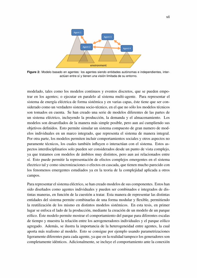
Figure 2: Modelo basado en agentes: los agentes siendo entidades autonomas e independientes, inter-actuan entre sı y tienen una vision limitada de su entorno.
modelado, tales como los modelos continuos y eventos discretos, que se pueden empo-trar en los agentes; o ejecutar en paralelo al sistema multi-agente. Para representar elsistema de energıa electrica de forma sistemica y en varias capas, este tiene que ser con-siderado como un verdadero sistema socio-tecnico, en el que no solo los modelos tecnicosson tomados en cuenta. Se han creado una serie de modelos diferentes de las partes deun sistema electrico, incluyendo la produccion, la demanda y el almacenamiento. Losmodelos son desarollados de la manera mas simple posible, pero aun ası cumpliendo susobjetivos definidos. Esto permite simular un sistema compuesto de gran numero de mod-elos individuales en un marco integrado, que representa el sistema de manera integral.Por otra parte, los modelos permiten incluir comportamientos sociales y otros aspectos nopuramente tecnicos, los cuales tambien influyen o interactuan con el sistema. Estos as-pectos interdisciplinarios solo pueden ser considerados desde un punto de vista complejo,ya que tratamos con modelos de ambitos muy distintos, pero aun asi relacionados entresı. Esto puede permitir la representacion de efectos complejos emergentes en el sistemaelectrico tal y como sincronizaciones o efectos en cascada, que tienen mucho parecido conlos fenomenos emergentes estudiados ya en la teoria de la complejidad aplicada a otroscampos.
Para representar el sistema electrico, se han creado modelos de sus componentes. Estos hansido disenados como agentes individuales y pueden ser combinados e integrados de dis-tintas maneras, en funcion de la cuestion a tratar. Esta manera de representar las distintasentidades del sistema permite combinarlas de una forma modular y flexible, permitiendola reutilizacion de los mismo en distintos modelos sistemicos. En esta tesis, en primerlugar se enfoca el lado de la produccion, mediante la creacion de un modelo de un parqueeolico. Este modelo permite mostrar el comportamiento del parque para diferentes escalasde tiempo y muestra la relacion entre los aerogeneradores individuales y el parque eolicoagregado. Ademas, se ilustra la importancia de la heterogeneidad entre agentes, la cualaporta mas realismo al modelo. Esto se consigue por ejemplo usando parametrizacionesligeramente diferentes para cada agente, ya que en la realidad tampoco los generadores soncompletamente identicos. Adicionalmente, se incluye el comportamiento ante la conexion
viii
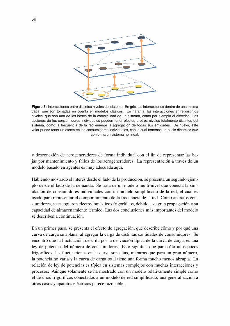
Figure 3: Interacciones entre distintos niveles del sistema. En gris, las interacciones dentro de una mismacapa, que son tomadas en cuenta en modelos clasicos. En naranja, las interacciones entre distintosniveles, que son una de las bases de la complejidad de un sistema, como por ejemplo el electrico. Lasacciones de los consumidores individuales pueden tener efectos a otros niveles totalmente distintos delsistema, como la frecuencia de la red emerge la agregacion de todas sus entidades. De nuevo, estevalor puede tener un efecto en los consumidores individuales, con lo cual tenemos un bucle dinamico que
conforma un sistema no lineal.
y desconexion de aerogeneradores de forma individual con el fin de representar las ba-jas por mantenimiento y fallos de los aerogeneradores. La representacion a traves de unmodelo basado en agentes es muy adecuada aquı.
Habiendo mostrado el interes desde el lado de la produccion, se presenta un segundo ejem-plo desde el lado de la demanda. Se trata de un modelo multi-nivel que conecta la sim-ulacion de consumidores individuales con un modelo simplificado de la red, el cual esusado para representar el comportamiento de la frecuencia de la red. Como aparatos con-sumidores, se escogieron electrodomesticos frigorıficos, debido a su gran propagacion y sucapacidad de almacenamiento termico. Las dos conclusiones mas importantes del modelose describen a continuacion.
En un primer paso, se presenta el efecto de agregacion, que describe como y por que unacurva de carga se aplana, al agregar la carga de distintas cantidades de consumidores. Seencontro que la fluctuacion, descrita por la desviacion tıpica de la curva de carga, es unaley de potencia del numero de consumidores. Esto significa que para solo unos pocosfrigorıficos, las fluctuaciones en la curva son altas, mientras que para un gran numero,la potencia no varia y la curva de carga total tiene una forma mucho menos abrupta. Larelacion de ley de potencias es tıpica en sistemas complejos con muchas interacciones yprocesos. Aunque solamente se ha mostrado con un modelo relativamente simple comoel de unos frigorıficos conectados a un modelo de red simplificado, una generalizacion aotros casos y aparatos electricos parece razonable.
ix
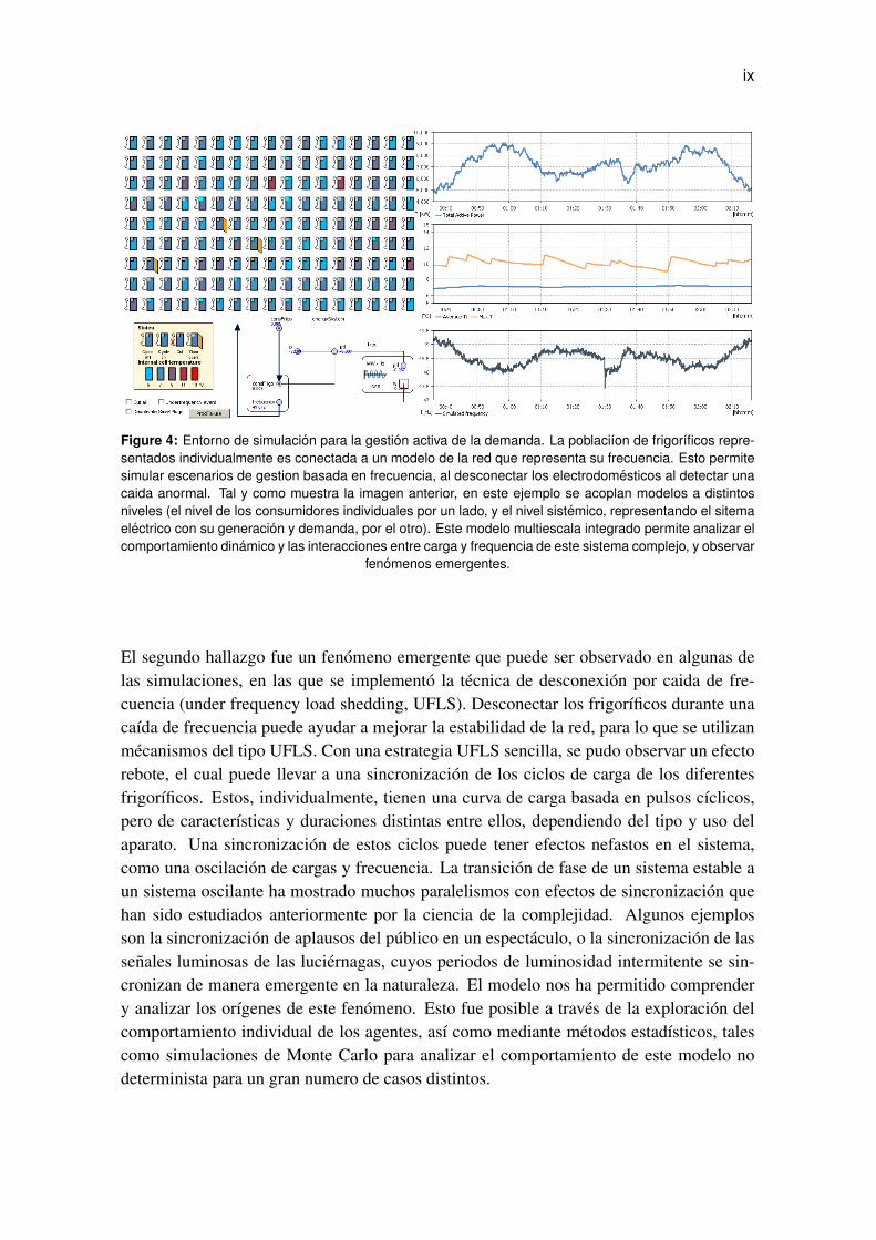
Figure 4: Entorno de simulacion para la gestion activa de la demanda. La poblaciıon de frigorıficos repre-sentados individualmente es conectada a un modelo de la red que representa su frecuencia. Esto permitesimular escenarios de gestion basada en frecuencia, al desconectar los electrodomesticos al detectar unacaida anormal. Tal y como muestra la imagen anterior, en este ejemplo se acoplan modelos a distintosniveles (el nivel de los consumidores individuales por un lado, y el nivel sistemico, representando el sitemaelectrico con su generacion y demanda, por el otro). Este modelo multiescala integrado permite analizar elcomportamiento dinamico y las interacciones entre carga y frequencia de este sistema complejo, y observar
fenomenos emergentes.
El segundo hallazgo fue un fenomeno emergente que puede ser observado en algunas delas simulaciones, en las que se implemento la tecnica de desconexion por caida de fre-cuencia (under frequency load shedding, UFLS). Desconectar los frigorıficos durante unacaıda de frecuencia puede ayudar a mejorar la estabilidad de la red, para lo que se utilizanmecanismos del tipo UFLS. Con una estrategia UFLS sencilla, se pudo observar un efectorebote, el cual puede llevar a una sincronizacion de los ciclos de carga de los diferentesfrigorıficos. Estos, individualmente, tienen una curva de carga basada en pulsos cıclicos,pero de caracterısticas y duraciones distintas entre ellos, dependiendo del tipo y uso delaparato. Una sincronizacion de estos ciclos puede tener efectos nefastos en el sistema,como una oscilacion de cargas y frecuencia. La transicion de fase de un sistema estable aun sistema oscilante ha mostrado muchos paralelismos con efectos de sincronizacion quehan sido estudiados anteriormente por la ciencia de la complejidad. Algunos ejemplosson la sincronizacion de aplausos del publico en un espectaculo, o la sincronizacion de lassenales luminosas de las luciernagas, cuyos periodos de luminosidad intermitente se sin-cronizan de manera emergente en la naturaleza. El modelo nos ha permitido comprendery analizar los orıgenes de este fenomeno. Esto fue posible a traves de la exploracion delcomportamiento individual de los agentes, ası como mediante metodos estadısticos, talescomo simulaciones de Monte Carlo para analizar el comportamiento de este modelo nodeterminista para un gran numero de casos distintos.

x
40%
60%
80%
100%
rige
rato
r st
ate
s
ON UFLS OFF
0%
20%
0 500 1000 1500 2000
Re
fr
Time [s]
(a) Sincronizacion de una poblacion de frigorıficos
40%
60%
80%
100%
Pro
bab
ility
Stable Partial oscillation Complete oscillation
0%
20%
6000 6500 7000 7500 8000 8500 9000 9500 10000 10500
Scale factor sf
(b) Cambio de fase de un sistema estable a uno oscilante
Figure 5: Sincronizacion y oscilacion de una poblacion de frigorıficos: Usando un sistema de gestion decarga basado en frecuencia (UFLS) se pueden observar sincronozaciones emergentes (a). La aparicionde estas oscilaciones se cuantifico mediante una probabilidad al tratarse de simulaciones no deterministas.La probabilidad se analizo variando el grado de influencia de los frigorıficos en el sitema electrico global.En (b) se puede observar un cambio de fase, que sigue una curva en forma de -S ,, tıpica en sistemas
complejos.
En general se puede decir que un enfoque desde los sistemas complejos puede ser muyutil para representar el sistema electrico desde un punto de vista integral, donde las in-teracciones entre diferentes escalas y niveles del sistema son fundamentales para la com-prension de causas y efectos. Este tipo de interacciones seran de especial importancia enel caso de sistemas distribuidos y comunicantes, tal y como sera el caso en la proxima gen-eracion de sistemas electricos, las smart grid o redes inteligentes. El uso de tecnicas parasimular sistemas complejos, como por ejemplo la modelazacion basada en agentes, per-miten la simulacion de efectos como los fenomenos emergentes, que pueden tener efectosimportantes en los sistemas actuales y futuros. Estos efectos no se limitan a oscilaciones ysincronizaciones solamente, sino que tambien engloban otros fenomenos como por ejem-plo los efectos en cascada como muestran algunos apagones electricos. El enfoque desdeel punto de vista de la complejidad abre nuevas lineas de investigacion que son propuestasen las perspectivas finales de esta tesis. Podemos concluir que la teorıa de la compleji-dad puede ayudar a la mejora y el diseno de los sistemas electricos venideros, ası como

xi
la adquisicion de un mejor conocimiento del funcionamiento del propio sistema, desde unpunto de vista interdisciplinario.


AcknowledgementsThis thesis would not have been possible without the support of many people. First andforemost I offer my sincerest gratitude to my supervisor, Oscar Barambones, who has sup-ported and guided me throughout this time, with his help and advice, whilst also allowingme the room to work in my own way. My sincere thanks also goes to Jose Marıa Gonzalezde Durana, for his patience and valuable knowledge which contributed to this work, as wellas for his continuous support in almost any aspect; and for being always available for veryfruitful exchanges and discussions.
I wish to especially thank Pablo Viejo, who introduced me to this fascinating topic almostfive years ago already, and without his support this thesis would not have been possible.He has made available this support in a number of ways, through always inspiring andmotivating discussions, valuable assistance and suggestions.
I would like to express my gratitude towards my numerous colleagues at EIFER and EDF,for their daily motivation and aid. I especially thank Fabrice Casciani, Kevin McKoen andPatrice Nogues for offering me the possibility to contribute to their projects through thiswork. I also would like to thank Carolina Tranchita for her comments on the manuscript.Furthermore, I would like to thank Andre Lachaud for his valuable support with the refrig-erator measurements.
Also I would like to thank the colleagues from SIANI - University of Las Palmas, es-pecially Jose Juan Hernandez and Mario Hernandez for the fruitful discussions. I wouldlike to show my gratitude to all the students, among them Alvaro, David, Nicola, Jen-nifer, Izaskun, Jose, Irantzu, Susana, Thibault, Sergio and Johannes, who worked with methroughout this time, and contributed in one way or another to this thesis. Besides I wouldlike to thank Caroline McKoen for her patience while proofreading, which not only con-tributed to improve grammar and spelling, but also served to clarify many ideas throughintense discussions. I also thank my friends who supported me during this time.
Finally, I thank my parents and sister for supporting me throughout all my studies and thisthesis.
Enrique Kremers, May 2012.
This thesis was possible through the support of the European Institute for Energy Research,EIFER (EDF & KIT), which gave me the opportunity to do this work in a multi-disciplinaryatmosphere. I would explicitly like to acknowledge the financial, academic and technicalsupport of EIFER and EDF.

Contents
Contents xv
1 Introduction 1
2 Complex Systems in the Context of Energy 72.1 Defintion: What are Complex Systems? . . . . . . . . . . . . . . . . . . . . . 92.2 Properties and Features of Complex Systems . . . . . . . . . . . . . . . . . . 10
2.2.1 Emergence . . . . . . . . . . . . . . . . . . . . . . . . . . . . . . . . . 102.2.2 Complex Networks . . . . . . . . . . . . . . . . . . . . . . . . . . . . 142.2.3 Power Laws . . . . . . . . . . . . . . . . . . . . . . . . . . . . . . . . 252.2.4 Resilience . . . . . . . . . . . . . . . . . . . . . . . . . . . . . . . . . 262.2.5 Controllability . . . . . . . . . . . . . . . . . . . . . . . . . . . . . . . 27
2.3 Electrical Energy Systems . . . . . . . . . . . . . . . . . . . . . . . . . . . . . 282.3.1 Electricity Generation . . . . . . . . . . . . . . . . . . . . . . . . . . . 292.3.2 Electrical Energy Consumption . . . . . . . . . . . . . . . . . . . . . 322.3.3 Modern Energy Systems . . . . . . . . . . . . . . . . . . . . . . . . . 362.3.4 Storage Systems . . . . . . . . . . . . . . . . . . . . . . . . . . . . . . 42
2.4 Energy Systems as Complex Systems? . . . . . . . . . . . . . . . . . . . . . 44
3 Modelling and Simulation of Complex Systems 473.1 Representation of Simulation Models . . . . . . . . . . . . . . . . . . . . . . 493.2 Agent Systems, Models and Simulations . . . . . . . . . . . . . . . . . . . . 51
3.2.1 Multi-Agent Systems . . . . . . . . . . . . . . . . . . . . . . . . . . . 513.2.2 Agent-Based Models . . . . . . . . . . . . . . . . . . . . . . . . . . . 523.2.3 MAS or ABM? . . . . . . . . . . . . . . . . . . . . . . . . . . . . . . 543.2.4 The Agent: a Definition . . . . . . . . . . . . . . . . . . . . . . . . . . 543.2.5 The Environment and its Interaction with the Agents . . . . . . . . . 563.2.6 Agent Networks and Social Ability . . . . . . . . . . . . . . . . . . . 573.2.7 Proactivity . . . . . . . . . . . . . . . . . . . . . . . . . . . . . . . . . 573.2.8 Agent-Based Simulations . . . . . . . . . . . . . . . . . . . . . . . . . 58
xv
xvi CONTENTS
3.2.9 Agents and Objects . . . . . . . . . . . . . . . . . . . . . . . . . . . . 593.2.10 Drawbacks and Benefits of ABM . . . . . . . . . . . . . . . . . . . . 60
3.3 System Dynamics . . . . . . . . . . . . . . . . . . . . . . . . . . . . . . . . . 623.3.1 Casual Loop Diagrams . . . . . . . . . . . . . . . . . . . . . . . . . . 623.3.2 Stock and Flow Diagrams . . . . . . . . . . . . . . . . . . . . . . . . 633.3.3 When to use System Dynamics . . . . . . . . . . . . . . . . . . . . . 64
3.4 Discrete Event Modelling . . . . . . . . . . . . . . . . . . . . . . . . . . . . . 643.5 Multi-Approach Modelling . . . . . . . . . . . . . . . . . . . . . . . . . . . . 653.6 Systems-of-Systems . . . . . . . . . . . . . . . . . . . . . . . . . . . . . . . . 673.7 Calibration and Validation of Agent-Based Models . . . . . . . . . . . . . . 673.8 Complex System Modelling – also in the Energy Field? . . . . . . . . . . . . 68
4 Electrical Energy System Modelling 714.1 Agent-Based Models for Energy Systems: A Review . . . . . . . . . . . . . 724.2 Modelling Approach . . . . . . . . . . . . . . . . . . . . . . . . . . . . . . . . 74
4.2.1 Challenges of the Electrical System . . . . . . . . . . . . . . . . . . . 754.2.2 Multi-Scale System Modelling . . . . . . . . . . . . . . . . . . . . . 76
4.3 Socio-Technical System Models . . . . . . . . . . . . . . . . . . . . . . . . . 784.4 Simulation and Modelling Tools used . . . . . . . . . . . . . . . . . . . . . . 804.5 Environmental and Production Models . . . . . . . . . . . . . . . . . . . . . 81
4.5.1 Wind Power Generation Model . . . . . . . . . . . . . . . . . . . . . 824.6 Consumption Models . . . . . . . . . . . . . . . . . . . . . . . . . . . . . . . 85
4.6.1 Modelling a Refrigerator . . . . . . . . . . . . . . . . . . . . . . . . . 864.6.2 Inclusion of Social Behaviour through Door Opening . . . . . . . . 89
4.7 Storage and Smart Grid measures . . . . . . . . . . . . . . . . . . . . . . . . 904.7.1 Generic Storage Model . . . . . . . . . . . . . . . . . . . . . . . . . . 904.7.2 Frequency-Based Load Control . . . . . . . . . . . . . . . . . . . . . 91
4.8 Grid Models . . . . . . . . . . . . . . . . . . . . . . . . . . . . . . . . . . . . . 924.8.1 Load Flow . . . . . . . . . . . . . . . . . . . . . . . . . . . . . . . . . 924.8.2 Grid Frequency Model . . . . . . . . . . . . . . . . . . . . . . . . . . 93
4.9 Towards Electrical Energy models as a Whole . . . . . . . . . . . . . . . . . 94
5 Integral Multi-Scale Case Study Models 955.1 Wind Farm Case Study . . . . . . . . . . . . . . . . . . . . . . . . . . . . . . 95
5.1.1 Wind Simulator Implementation . . . . . . . . . . . . . . . . . . . . . 955.1.2 Turbine Implementation . . . . . . . . . . . . . . . . . . . . . . . . . 975.1.3 Implementation of a Wind Farm . . . . . . . . . . . . . . . . . . . . . 99
5.2 Frequency-Controlled Refrigerator Case Study . . . . . . . . . . . . . . . . . 1005.2.1 Implementation of the Refrigerator Model . . . . . . . . . . . . . . . 1005.2.2 Implementation of the Social Behaviour: Door Openings . . . . . . 1005.2.3 Demand Side Management Implementation through UFLS . . . . . 102

CONTENTS xvii
5.2.4 Measurement and Calibration of the Refrigerator Model . . . . . . . 1025.2.5 Integration of the SFR Grid Model . . . . . . . . . . . . . . . . . . . 1035.2.6 Implementation of the Systemic Model . . . . . . . . . . . . . . . . . 1055.2.7 The Integrated Simulation Model . . . . . . . . . . . . . . . . . . . . 107
6 Simulation Results and Discussion 1096.1 Multi-Timescale Simulation of a Wind Farm . . . . . . . . . . . . . . . . . . 109
6.1.1 Low Wind Speed Day . . . . . . . . . . . . . . . . . . . . . . . . . . . 1096.1.2 High Wind Speed Day . . . . . . . . . . . . . . . . . . . . . . . . . . 1116.1.3 Simulation Over a Week . . . . . . . . . . . . . . . . . . . . . . . . . 1126.1.4 Comparison of the Simulations . . . . . . . . . . . . . . . . . . . . . 1136.1.5 Failure Behaviour of the Turbine Units . . . . . . . . . . . . . . . . . 1146.1.6 Heterogeneous Parameterisation of the Agents . . . . . . . . . . . . 1146.1.7 Discussion of the Results . . . . . . . . . . . . . . . . . . . . . . . . . 116
6.2 Frequency-Controlled Refrigerator Simulation . . . . . . . . . . . . . . . . . 1176.2.1 Simulation of a Refrigerator Population . . . . . . . . . . . . . . . . 1186.2.2 Variation of the Population Size: the Aggregation Effect . . . . . . . 1206.2.3 Simulation Settings for UFLS . . . . . . . . . . . . . . . . . . . . . . 1246.2.4 An UFLS Scenario . . . . . . . . . . . . . . . . . . . . . . . . . . . . 1246.2.5 The Rebound Effect . . . . . . . . . . . . . . . . . . . . . . . . . . . . 1256.2.6 Synchronisation and Emergent Phenomena in the Simulations . . . 1276.2.7 Conditions for an Emergent Oscillation . . . . . . . . . . . . . . . . 1296.2.8 Discussion of the Results . . . . . . . . . . . . . . . . . . . . . . . . . 130
7 Conclusions and Outlook 133
References 139
Author’s publications 151
Appendices 153
A Complexity science map 155
B Technology Comparison for Storage Systems 157
C Other Models 159C.1 Thermodynamic model of a household . . . . . . . . . . . . . . . . . . . . . 159
D Modelling Agents using SD 163D.1 Numerical ODE Solution using an SD model . . . . . . . . . . . . . . . . . . 165
D.1.1 First Order System . . . . . . . . . . . . . . . . . . . . . . . . . . . . 165D.2 SD Models in the Energy Sector . . . . . . . . . . . . . . . . . . . . . . . . . 166

xviii CONTENTS
E Calibration of the Refrigerator Model 167
List of Symbols and Abbreviations 171
List of Figures 173
List of Tables 176

Chapter 1
Introduction
Our society is facing major challenges in achieving and maintaining a sustainable andenvironmentally friendly energy supply. The demand for energy is constantly growing,and electrical energy, especially, has escalated in importance during the last century with acontinuous increase in electrical devices. Independent of efforts to reduce consumption andimprove efficiency, the growing use and quantity of electrical equipment has contributedto, and encouraged, a rise in energy demand.
In parallel with this increase in consumption, global issues have arisen which do not allowthe uncontrolled or unlimited expansion of power generation, needed to cover demand.Fossil fuels are limited and impose a natural constraint, however their use during the lastcenturies has had a negative impact on the environment. Global warming, which is partiallydue to the greenhouse effect and is related to increased CO2 emissions (which are alsoproduced by burning fossil resources), further constrains the expansion of the classicalgeneration system. In addition to this, fossil fuels also contribute to the pollution levelsthrough inefficient and unsustainable energy generation.
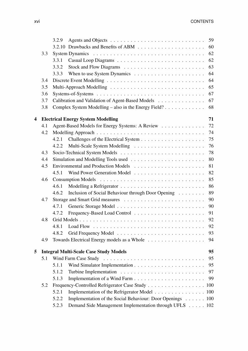
These issues are forcing policy makers to find solutions and improve the sustainability ofthe energy supply system. At the same time, they must guarantee it is both economicallyaffordable and technically secure. Thus, decision makers, often at governmental level, havean influence on energy stakeholders.
Since the deregulation of the energy markets, which began in the late nineties and has beenpromoted by the European Union, the number of actors has increased considerably. Formerstate-owned utilities have been transformed into profit making companies. These utilitiesand operators along with and other actors are constrained by the European Commission’slegislative framework and by individual national initiatives. Their drive to achieve eco-nomic benefit is limited by this legal framework which, for example, currently proposes toreduce CO2 emissions, by the introduction of emission certificates and incentives promot-ing renewable and sustainable energy sources.
1
2 CHAPTER 1. INTRODUCTION
Global issues
find
• Global warming & climate change
• Finite (fossil) resources • Pollution and environment
Energy industry (utilities, operators)
Policy and decision
makers
Solutions
Policies, directives
Individuals, collectives
act
Economic benefit
Energy System
impact
implement
condition
Figure 1.1: Global framework of the energy system.
This is leading to a paradigm shift in the electrical system. We are at a turning point,mainly because of the deregulation of the sector, environmental constraints and becauseof the introduction of renewable and distributed energy sources. Based on these trends,buzzwords such as the smart grid are common. Considering the future system as a smartelectricity system (whatever might be meant by smart at this point), it can be said that thereis a movement towards a modified system which is challenging the energy industry as wellas the current power system itself.
What the future system will look like is difficult to predict. However, given the frame-work above it can be said that it will have to be able to achieve a number of objectives.Possibly, its rather hierarchical, unidirectional structure will be largely affected through anincreased number of distributed resources being integrated. Furthermore, the use of renew-able energy sources will increase. The significant and sometimes unpredictable fluctuationof renewable energy production means that these sources cannot be controlled in the sameway as classical production stations. An increase in supply from renewable sources resultsin the need to develop new systems for production control and a growing need for effectiveand flexible generation units to compensate for this variability in supply.
There are many solutions and ways towards the smart electricity system and these dependon many factors. Location and local conditions may affect this process, as well as differentnational or regional policies. The much discussed question of the optimal energy mix orimplementation of concrete technologies such as smart metering or electric vehicles areonly some examples.
In order to address these and other issues, modelling and simulation can support and fa-cilitate the transition towards a smarter electrical system. Simulation is a procedure in

3
which (usually dynamic) systems can be analysed through running experiments on a modelspecifically designed for this purpose. Exploring different ways of tackling the challengesof the future system through simulation supports decision-making on complex questions.
Classical electrical system
Liberalization of the markets
Current electrical system
Smart electrical system
Introduction of renewable energy sources
?
?
?
Decentralization and distribution of the system
Simulation
Figure 1.2: Evolution of the electrial system.
Many different tools have been used for simulating electrical systems. However, theparadigm shift towards the smart grid now raises the question of whether there is a need fornew approaches considering that new issues are, and will be, arising. The classical elec-trical system (see Figure 1.2) is a rather hierarchical and one-directional system, whereproduction is centralised and injects on the one side, and demand is distributed and con-sumes on the other. Production only needs to guarantee to meet demand.
This operating principle is no longer valid. The inclusion of distributed production at lowerlevels of the system has created the possibility of local production, which can invert, or atleast reduce, the classical, one directional flow from big stations towards the final end user.As many demonstration projects show, in the future grid it will be possible to manage thedemand side. Demand is no longer regarded as a static, unmanageable part of the system,but rather it will support balancing and stability processes. Managing and controlling theseprocesses will require distributed control and communication mechanisms.
In order to correctly represent this system in an integrated, systemic approach, it is firstnecessary to create a model of the existing physical system. The representation of the clas-sical system will be achieved by taking into account both current and future possibilities;this will allow for it to be continually extended. Completing the model with current tech-nologies such as smart metering, distributed and renewable generation, etc. will allow forthe representation of the state-of-the-art.
The inclusion of a communication layer already seems reasonable; it is needed to handlecontrol and management processes over the distributed entities of the system. The cur-

4 CHAPTER 1. INTRODUCTION
rent system model can be modified for possible future scenarios by including prospectivetechnologies and implementations. The analysis of this virtual system will allow us toextrapolate and identify future challenges. The model will enable the simulation of con-crete case studies relating to real-world sets of problems in the transition to a smart powersystem.
The detailed knowledge required to accurately model a system is challenging to gather.This thesis explores modeling the electricity system however, this term is not simply de-fined. The different networks in different countries, each made with different technologiescreate a complex overall system. So how can we make a model of a system that is not fullyknown?
The solution adopted in this thesis uses a design that models the system in a simplified way,rather than initially focusing on details. The aim is to create a systemic model, rather thandetailed models of a part of it. Furthermore, the objective is to create an individual-centricrather than a system level model. This means that individual parts of the system will berepresented as such, and not by aggregated models.
This will help to define a new, hypothetical smart grid. The model of the energy system,has been designed for the minimum structure and components needed to emulate the es-sential behaviour of the current and future grids. It will serve to make virtual experiments(simulations) of the current energy system and also of potential future scenarios which arenot yet possible in current networks, or which would require great expense or risk.
In the first part of this thesis, complex system theory is presented. There are only fewexamples in which this relatively new field of research has been applied to energy systems.As we will see however, there is great potential to describe an energy system through itscomplexity. Therefore, we will analyse some of the main aspects of an electrical energysystem relevant to this task. Afterwards, the question of why we should treat this systemas a complex one is discussed.
In the third chapter, the subject of modelling and simulation of complex systems is ad-dressed. Varied approaches to this field are presented as well as a combination of differentmethods. This serves as a basis for the models which follow.
The chosen approach, along with its related challenges, is presented in chapter four. Thetools and models used are shown, for both the production and demand sides, as well as thenetwork itself. In this way, a minimal energy system with all of its basic components isrepresented.
The fifth chapter presents two case studies and demonstrates how they are integrated usingthe models previously described. The first case study addresses the production of renew-able energy by representing a wind farm. It is based on individual and heterogeneous windturbine models. The second case study proposes a more systemic model, which includes

5
refrigerator appliances as consumers, and a grid model to represent the complete systembehaviour.
In the last chapter, the simulation results of the two case studies are presented and dis-cussed. Some relevant findings are included to illustrate the advantages of using the se-lected approach. Scale effects, as well as interactions and emergent phenomena found inthe simulation, are discussed. Finally, the conclusions drawn from these studies are pre-sented, as well as a look at future possibilities for research.

Chapter 2
Complex Systems in the Context ofEnergy
The whole is more than the sum of its parts.
Aristotle, around 350 BC.
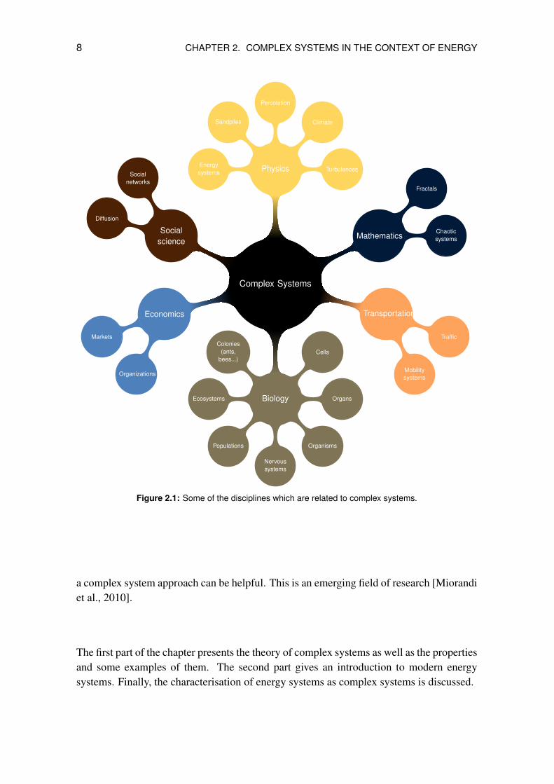
Complex systems are characterised not only by a large number of components, but also bythe diversity of these components, their relationships and interactions. In these systems,the relationship between the components can lead to collective behaviour at a system level.This is a subject of research in what is called complexity science. In the 1940’s and 1950’sinitial approaches were made towards systems theory and artificial intelligence. Duringthe 1960’s and 1970’s, formulations on what is now known as complexity science weremade on phenomena on order patterns in market systems. A phenomenon is emergent inthe sense that it results from human actions, but is not of human design [Hayek, 1967].Later on, other fields such as network theory, game theory, agent-based modelling, fractalsand chaos theory where found to be closely related to complexity science. Since then,this interdisciplinary field has been a focus of research into different domains, mainlystatistical physics as well as in social, biological and computer sciences, sometimes withquite diverse scopes. Some examples on current application of complex systems theory areshown in Figure 2.1 and are classified into different disciplines.
Energy systems are composed of many components at different levels connected to eachother, at a physical level, through a network infrastructure. The paradigm shift in theenergy sector characterised by the deregulation of markets, the introduction of renewableenergy sources and system decentralisation, has increased its degree of complexity. Forinstance, the introduction of smart grids will result in new communication means usedwithin the system. This will make an already large system much more dynamic in terms ofinteractions and communications. Therefore, we will see in the course of this chapter, that
7
8 CHAPTER 2. COMPLEX SYSTEMS IN THE CONTEXT OF ENERGY
Complex Systems
MathematicsChaoticsystems
Fractals
Physics Turbulences
Climate
Percolation
Sandpiles
Energysystems
Socialscience
Socialnetworks
Diffusion
Economics
Markets
Organizations
Biology
Cells
Organs
Organisms
Nervoussystems
Populations
Ecosystems
Colonies(ants,
bees...)
Transportation
Traffic
Mobilitysystems
Figure 2.1: Some of the disciplines which are related to complex systems.
a complex system approach can be helpful. This is an emerging field of research [Miorandiet al., 2010].
The first part of the chapter presents the theory of complex systems as well as the propertiesand some examples of them. The second part gives an introduction to modern energysystems. Finally, the characterisation of energy systems as complex systems is discussed.
2.1. DEFINTION: WHAT ARE COMPLEX SYSTEMS? 9
2.1 Defintion: What are Complex Systems?
Complex systems are studied by complexity science, an interdisciplinary field that consid-ers all kind of systems which are constituted by many parts with numberous interactions,and investigates their behaviour.
To explain phenomena concerning complex systems, their close relationship with net-works, swarm intelligence, game theory and mathematical and stochastic systems mustbe considered. Regarding complexity from a multi-disciplinary perspective can help us tounderstand the behaviour of these systems. A common definition for complexity scienceremains an open question, as is appears in many different disciplines and encompassesmany different views. These perspectives reach from complex mathematical systems tosocial sciences, passing by biological and technological systems. Despite conceptual ad-vances in concrete fields like chaos theory or emergence in non-linear or self-organisedsystem, which were studied in the previous decades, a complete theory of complexity doesnot yet exist [Barabasi, 2007].
Number of components
Rand
omne
ss
Chaotic systems
Organised simplicity
Complex systems
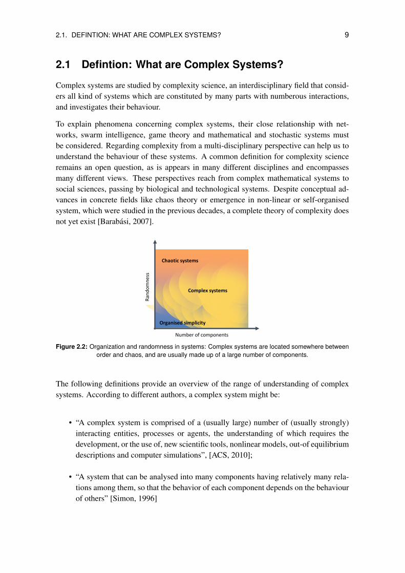
Figure 2.2: Organization and randomness in systems: Complex systems are located somewhere betweenorder and chaos, and are usually made up of a large number of components.
The following definitions provide an overview of the range of understanding of complexsystems. According to different authors, a complex system might be:
• “A complex system is comprised of a (usually large) number of (usually strongly)interacting entities, processes or agents, the understanding of which requires thedevelopment, or the use of, new scientific tools, nonlinear models, out-of equilibriumdescriptions and computer simulations”, [ACS, 2010];
• “A system that can be analysed into many components having relatively many rela-tions among them, so that the behavior of each component depends on the behaviourof others” [Simon, 1996]
10 CHAPTER 2. COMPLEX SYSTEMS IN THE CONTEXT OF ENERGY
• “A system that involves numerous interacting agents whose aggregate behavioursare to be understood. Such aggregate activity is nonlinear, hence it cannot simply bederived from summation of individual components behaviour.” [Singer, 1995]
Simon’s definition of complex systems is therefore, rather, a description in the structuralsense, whereas Singer’s definition is concerned more with the dynamics or functional rela-tions of the system. Furthermore, the concept of organisation or structural order plays animportant role: “Complexity is neither simple order nor a complete mess. It is somethingbetween order and chaos, and it grows at the edge of chaos. A complete mess or chaoscannot be represented in any shorter or more compact way than the mess itself. A simpleand static order on the contrary can be represented as a short formula. Complexity is dif-ferent from both of these, and although it often is a result of rather simple formulas too, itincludes iterations, the repetition of patterns - taking part of the result of the former roundas the input to the next - and most often also adding some randomness to the process. Thismeans that complexity is a result of a process unfolded in time.” [Gronlund, 1993]
A historical overview of complexity science is shown in Appendix A.
2.2 Properties and Features of Complex Systems
2.2.1 Emergence
One of the best known quotations related to complex is from a famous ancient Greekphilosopher: “The whole is more than the sum of its parts” [Aristotle, around 350 BC].Complex systems often behave in unexpected ways that cannot directly be inferred fromthe behaviour of their components; this is known as emergent behaviour. This is oneof the most important particularities when regarding a system from a complex point ofview. In classical approaches the system is usually deterministic or at least predictable(stochastically) in a large sense. Emergence describes how complex behaviours at themacro-level of a system arise out of more simple ones. These behaviours entail emergenceof properties that can hardly, if at all, be inferred from the properties of the individual parts.
Aristotle doesn’t suggest that complex systems are completely unpredictable. Complexsystems behave in a way that has to be studied, taking into account these particularities, inorder to better understand their operation and dynamics. In real systems, emergence caneither be a desired or undesired effect. If, in a real system, emergence is found, it can beinfluenced to avoid unwanted effects and can make the system evolve in the desired direc-tion. Therefore, a better understanding of emergent phenomena can help us in designingor managing those systems.
In the following, some examples of emergence in different fields are shown.
2.2. PROPERTIES AND FEATURES OF COMPLEX SYSTEMS 11
Step 0
Step 152
Step 156
Step 4
Step 153
Step 157
Step 7
Step 154
Step 161
Step 16
Step 155
Step 239
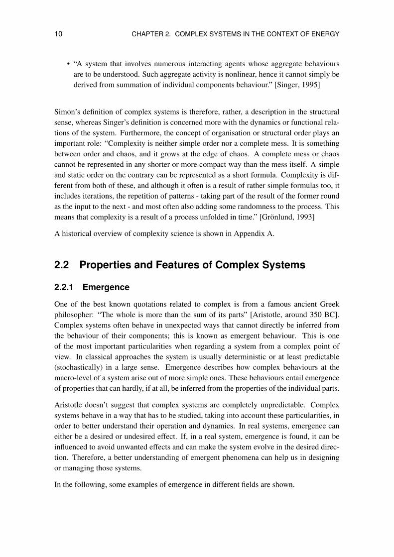
Figure 2.3: Sequence of some generations of the Game of Life. Starting from a random setup (step 0) itcan be seen how the system evolves into emergent structures, such as symmetrical, pulsating or movingpatterns (steps 152-157), which cannot be inferred by the rules of the individual cells. The sequence was
created using NetLogo [Wilensky, 2005]
Mathematics: Cellular Automata
Conaway’s Game of Life is a two-dimensional cellular automaton, whose cells can eitherbe alive or dead. Simple rules for each cell determine their change of state (dead/alive).Depending on the initial conditions, the whole system of cells can show an extraordinarycomplex, ordered behaviour, which does not allow the inference of the primitive rules ofthe individual cells. These rules are simple, for example that a new cell is born if thenumber of living neighbours is in a specified range, or that it dies when there are too manyor too few living neighbours [Packard and Wolfram, 1985]. The Game of Life is one, andprobably the best known, of several cellular automata. Changing rules and dimensionsallows for the creation of other automata of any complexity [Von Neumann and Burks,1966].

12 CHAPTER 2. COMPLEX SYSTEMS IN THE CONTEXT OF ENERGY
Physics: Percolation
The phenomena of percolation describes the behaviour of subgraphs in a random graph1
and how they form components or clusters.
(a) p << pC (b) p < pC (c) p = pC
Figure 2.4: Percolation of oil in a porous soil showed using a Netlogo model [Wilensky, 1998, 1999]. Theprobability p represents the porosity of the soil. With increasing p, it is more likely that the oil reachesthe bottom. However, the percolation probability θ(p) is not linear, but rather a phase shift. From a giventhreshold onwards, it is very probable that the oil will reach the bottom - but before this threshold, it is very
unlikely.
pc
p
(p)
1
1
Figure 2.5: θ(p), the probability that there is a uninterrupted path from the top to the bottom of the graph,indicates that above the critical probability pc there is a high probability of percolation. The function θ is
continuous except possibly at pc [Grimmett, 1999]
Percolation models can be used to represent the flow of fluid in a porous medium withrandomly blocked channels [Bollobas and Riordan, 2006]. The effect is described in the
1A random graph is generated by a random process, such as adding edges with a probability p (seeSection 2.2.2).

2.2. PROPERTIES AND FEATURES OF COMPLEX SYSTEMS 13
following way: if for a given probability p (which describes whether an an edge betweentwo nodes exists and permits passage) there is an open path from the top to the bottom ofthe network, and at which probability this path would exist. There is a critical value pc atwhich the probability of the existence of a path increases sharply, this means that below pcthere is no path, but it is likely that above this value such a path exists, as can be seen inFigure 2.4. This almost discrete effect, which happens suddenly, cannot be inferred from acontinuously growing probability p without taking into account the complexity of randomnetworks; this is another example of emergence. The percolation function is also relatedto power laws, another typical relationship appearing in complex system [Austin, 2011].
Biology: Honeybee Hives
In bee colonies, the phenomenon of thermoregulation can be observed. The brood nestneeds to maintain the same temperature over a long period to develop the brood; this tem-perature is also optimal for the creation of wax. A complex mechanism involving largenumbers of bees is used to maintain a stable temperature inside the hive [Jones et al., 2004].The individual bees have no knowledge of the overall hive conditions, and only sense theirimmediate environment. Each bee has different methods to regulate its temperature, suchas wing fanning, building isolating wax layers, evaporative cooling, etc. The thermoreg-ulatory mechanism of the hive is self-organised and arises from simple rules followed byeach bee. In very extreme conditions, even bee corpses fulfil an insulating function.
Computer Science & Biology: Swarms
Swarming or flocking is a typical example of a collective behaviour in which emergencearises. Swarming in nature is a collective animal behaviour exhibited by a large number ofinsects or other animals. As a swarm is not a static phenomenon, the individuals adapt theirdirection of movement and have to avoid collision. This creates the swarm, a collection ofindividual animals or units moving together as a group.
A typical swarm can be seen in Figure 2.6. The emergence of swarming has been anobject of research and modelled and simulated in order to understand, at macro levels, theunderlying rules which govern swarms. A swarm can be simulated by modelling individualentities maintaining a certain distance from each other, among other rules.
Architecture & Engineering: The Millennium Bridge
The Millennium bridge was opened in London in the year 2000 and was intended to be“a pure expression of engineering structure” by its designers. However, as thousands ofpedestrians began walking over it, the bridge began to sway slightly. Then, suddenly,the bridge began to oscillate and the people began to walk side-ways, but in a perfectlysynchronised manner. The oscillating bridge and the walking patterns of the pedestrianscaused a positive feedback, each one reinforcing the other. The bridge had to be closed

14 CHAPTER 2. COMPLEX SYSTEMS IN THE CONTEXT OF ENERGY
(a) Flock of birds (b) Flock of boids
Figure 2.6: Swarming: On the left, a flock is formed by the behavioural rules of individual birds and changesdynamically over space through time. Even so, the flock keeps a coherent and organised structure whenzooming out from the individual bird level. On the right we can see a flock simulation. Each bird (or boid,from the name of an artificial life simulation program [Reynolds, 1987]) is able to see the other birds andobstacles in a fixed radius in front of it. The bird adjusts its velocity based on a set of simple rules. Thisimplementation also features trees (white circles), which the birds will avoid flying into. The birds form tightflocks and navigate around obstacles as an emergent behaviour. Source: Occoids simulation by Cosmos
Research, http://www.cosmos-research.org/demos/occoids/
immediately, and redesigned in order to avoid oscillation. This is an example of a costlydesign where an emergent phenomenon appeared which had not been taken into accountthrough classical design and calculation methods. It was subject of an article of researchby Strogatz et al. [2005].
As we see, emergence can occur in very different areas, related to completely differentsubjects. However, the principles on which it relies are similar across disciplines, and areone of the main topics of research in complexity science.
2.2.2 Complex Networks
Complex systems are composed of many non-identical components connected through di-verse interactions. If we formalise these interactions, we end up with a mathematical graphor, more generally, a network. Complex networks are one of the fields of study in com-plexity science. They deal with the non-trivial, topological features of simple networks, butwhich can be observed in reality. These include patterns, which are neither completely reg-ular nor completely random. The study of complex networks is inspired by real networks,mainly computer, social and biological. Studies in relation to energy systems are stillmarginal, however.complex systems are very relevant to energy systems, which are mainlybased on a network infrastructure - the power grid. An overview of this field follows.
Complex networks have been object of several scientific studies. The first approach datesback to 1959, when [Erdos and Renyi, 1959] suggested modelling networks as random

2.2. PROPERTIES AND FEATURES OF COMPLEX SYSTEMS 15
graphs. In a random graph, the nodes are connected randomly by a placing a number oflinks among them. Random graphs allow the representation of generic random networksand permit the study of many properties of real systems. However, these assumptions maynot be appropriate for modelling phenomena in the real world.
Watts and Strogatz [Watts and Strogatz, 1998] defined p as the probability of rewiring anedge of a regular lattice graph. They analysed networks with wiring probability valuesbetween zero and one and found that these systems can be highly clustered and have smallcharacteristic path lengths. Networks with short average path lengths are considered smallworld networks. This is the case in many (real) networks with a large number of connec-tions. The Watts-Strogatz model first stated that special small world networks exist andare highly clustered. However they don’t have as many connections as regular or randomgraphs but still have short average path lengths.
However, analysing real-life networks has shown that there are also many examples inwhich the distribution of the number of connections per node is not bell-shaped. Barabasiand Albert [1999] found that many real networks have a common property: a power lawdistribution, which states that the number of nodes with many links is small whereas anexponential growth exists when moving towards nodes with fewer connections. Thesenetworks are called scale-free and they are located in between the range of random andcompletely regular wired networks.
Networks exist everywhere and at every scale [Barabasi, 2007]. The human brain, societiesor ecosystems are only a few examples of what can be represented as a complex network.Many systems in the real world fulfil the properties described above: neural networks,social networks and also the power grid. For the power grid, generators, transformers andsubstations were taken as vertices and high-voltage lines as edges.
Metrics of Complex Networks
A complex network can be represented as a directed or undirected graph. In order tocharacterise complex networks, different metrics have been defined. To explain the mostimportant metrics, a complex network will be represented as a directed or undirected graphG = {V,E}, where V is the set of vertices or nodes andE is the set of edges or connections.The total number of vertices is ∣V ∣, and the total number of edges is ∣E∣.
• Degree distribution:
The degree d(v) of a node or vertex v is the number ∣E(v)∣ of edges at v; this isequal to the number of connecting edges or neighbours. The average degree d(G) ofa network G is given by
d(G) =1
∣V ∣∑v∈V
d(v) (2.1)
16 CHAPTER 2. COMPLEX SYSTEMS IN THE CONTEXT OF ENERGY
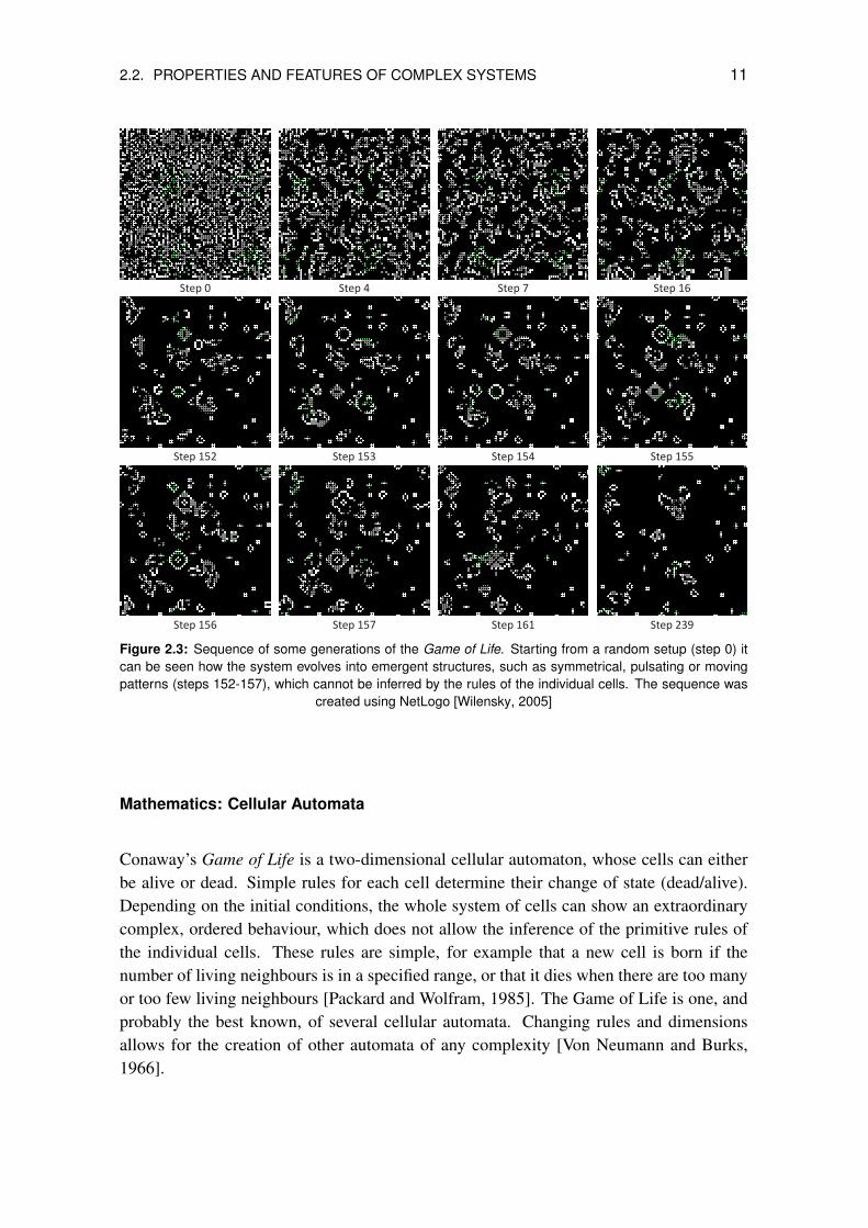
The degree distribution P (d) of a network is defined to be the fraction of nodes inthe network with degree d. The distribution can be plotted as a histogram and showsthe number of nodes with a given degree.
K P(d)
Degree
Num
ber
of n
odes
Figure 2.7: Example of a degree distribution P (d) with average degree d(G) =K
The average degree is a measure for how many connections a node has on aver-age. A large d(G) implies many connections per node. However, it does not revealhow closely nodes are clustered or how well they are connected to each other (forexample, if you wanted to travel around them and find a shortest path, etc.). Thedistribution of the degrees of the nodes gives us an idea of the spread of connections.If most of the nodes have a similar number of connections this will lead to a peakdistribution, whereas if we have heterogeneous numbers of connections among thenodes, exponential or other kinds of distributions emerge.
• Average path length:
The path length or distance l(v,w) between two nodes v,w ∈ V is the shortest pathbetween them, measured in number of edges. The average path length l(G) of agraph is calculated over all possible pairs of nodes.
l(G) =2
∣V ∣(∣V ∣ − 1)∑
v,w∈Vl(v,w) (2.2)
The network diameter lD(G) is the maximal path length of the network over all pairsof nodes of G.
lD(G) = maxv,w∈V
l(v,w) (2.3)
The path length between to nodes is an essential measure in graph theory, whichis fundamental to solving the shortest-path problem, for example for finding theshortest route on a road-map from one point to another. The average path length of agraph indicates how well connected the network is in terms of distances on average.A network with a low average path is likely to be travelled with short distances fromany point to another. This plays an important role in small networks, where shortaverage path lengths are the case.

2.2. PROPERTIES AND FEATURES OF COMPLEX SYSTEMS 17
• Clustering coefficient:
The neighbourhood of a node v are the d(v) nodes that are at distance 1 from A. If vhas d(v) neighbours, the number of pairs of those neighbours is
h(v) =d(v) ⋅ (d(v) − 1)
2(2.4)
The number of pairs which are connected to each other is f(v). The clusteringcoefficient of node v is then calculated as
c(v) =f(v)
h(v)(2.5)
If a node has a high clustering coefficient, this means that it is likely that its neigh-bours are connected to each other. c(v) can also be interpreted as the probability thattwo neighbours are connected.
For a graph G with ∣V ∣ nodes, we define the clustering coefficient of the networkc(G) as
c(G) =1
∣V ∣∑v∈V c(v)(2.6)
If most of the nodes of a network have high clustering coefficients, there are probablymany edges connecting nodes together. The network clustering coefficient is a metricthat describes if there are many well connected components (clusters) in the graph.However, it does not tell how well these clusters are connected to each other, as agraph with isolated components may have a large clustering coefficient, even withoutshortcuts from one to another cluster.
Types of Complex Networks
When analysing complex networks in the real world, recurrent types of networks wereidentified among different disciplines and fields. Creating a general classification of net-works allows us to find common properties, problems and solutions among these networks,and treat them independently of their original field. In the following section, the mosttypical networks are presented; these have been identified by different scientists and aregenerally accepted. The network types can be characterized by the metrics defined above,as well as by other, additional properties.
• Fully connected networks
Fully connected networks are homogeneous networks in which every node is con-nected to all the other nodes. If F = {V,E} is a fully connected network, the maxi-mal path length lD(F ) = l(F ) = 1 is equal to the average path length; i.e. every nodecan be reached from another in only one step. However, the number of connections
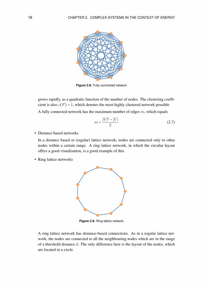
18 CHAPTER 2. COMPLEX SYSTEMS IN THE CONTEXT OF ENERGY
Figure 2.8: Fully connected network
grows rapidly, as a quadratic function of the number of nodes. The clustering coeffi-cient is also c(F ) = 1, which denotes the most highly clustered network possible.
A fully connected network has the maximum number of edges m, which equals
m =∣V ∣2 − ∣V ∣
2(2.7)
• Distance based networks
In a distance based or (regular) lattice network, nodes are connected only to othernodes within a certain range. A ring lattice network, in which the circular layoutoffers a good visualisation, is a good example of this.
• Ring lattice networks
Figure 2.9: Ring lattice network
A ring lattice network has distance-based connections. As in a regular lattice net-work, the nodes are connected to all the neighbouring nodes which are in the rangeof a threshold distance d. The only difference here is the layout of the nodes, whichare located in a circle.

2.2. PROPERTIES AND FEATURES OF COMPLEX SYSTEMS 19
• Random networks
Figure 2.10: Random network
In a random network, the nodes are wired with certain probability p. Each edge,independent of every other edge, is included in the graph with probability p. Forp = 1 therefore we would have a fully connected network, for p = 0 a network withoutconnections. Random networks are located in between. Wiring edges randomlyleads to a bell shaped Poisson distribution of the numbers of connections of eachnode, thus there are many nodes with a similar number of links. These networkswere identified by Erdos and Renyi [1959]. The Erdos-Renyi Model was the firstalgorithm proposed to generate a random graph and we will refer to them as ERnetworks, too.
• Small world networks
Figure 2.11: Watts-Strogatz small world network: the rewired edges can be seen as shortcuts whichdrastically reduce the average path length but still maintain a highly clustered network, which can be inferred
from the originating ring lattice
In 1998, Watts and Strogatz found a new type of complex network. Having latticenetworks which are distance based and show long path lengths, they began to rewire

20 CHAPTER 2. COMPLEX SYSTEMS IN THE CONTEXT OF ENERGY
some edges, taking them out from the lattice network and replacing them with a ran-dom edge. If this is done enough times, it results in a random, ER-network. However,if only some edges are rewired, some shortcuts are created, which drastically reducethe path length among the nodes. The study of these kinds of networks leads to thecommonly used term small world. A small world is a system in which some individ-uals within strongly clustered, but rather isolated, groups are connected with eachother. This provides both highly clustered and also well connected systems. Anysystem with small average path lengths and high clustering coefficient can be calleda small world.
The Watts-Strogatz (WS) model is an algorithm which generates a small world net-work. We start from a ring lattice network and begin to rewire random edges. As arandom edge is selected, the end node is rejected and a new, randomly chosen nodeis selected. This rewired edge represents a shortcut to a usually remotely locatedpart of the network part of the network. As the original edges are highly clustereddue to their lattice character (they are distance based wired, so they form so calledcliques, fully connected subgraphs), the connections among these clusters is not sig-nificantly affected by replacing the end node of one of the edges. On the other hand,the rewired edge connects over a short path the entire cluster to another, remotelylocated part of the network.
• Scale free networks
Figure 2.12: Scale-free network: Hubs are colored in yellow and have a large number of connections.
In real systems, for example in social networks, properties of random networks andsmall world networks were identified. However, at the end of the 1990’s, Albert Las-zlo Barabasi and Reka Albert found that many real world networks could not be fullymodelled by using these approaches. ER and WS networks have a Poisson degreedistribution in common, which generally means that there are many nodes with thesame number of connections, and few with large or small numbers of connections.
2.2. PROPERTIES AND FEATURES OF COMPLEX SYSTEMS 21
Barabasi and Albert identified many systems with networks that have only a fewnodes with a high number of connections, and many nodes with low number ofconnections. This is the case, for example, in the airport system: only some bigairports offer a large number of destinations, whereas many local airports often serveonly a low number of destinations. Another example is the western US electricitynetwork, where a few big stations connect many lines, and there are a lot of stationswith only a few connections.
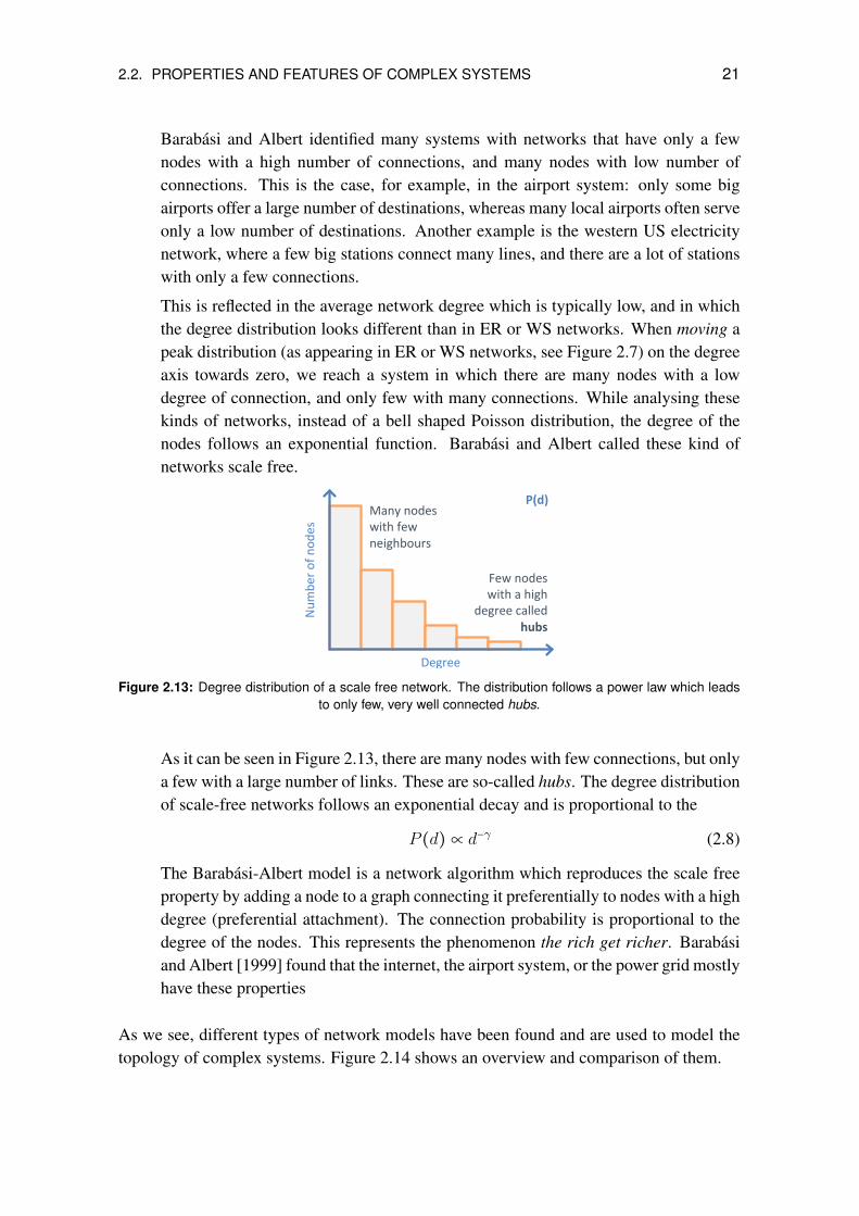
This is reflected in the average network degree which is typically low, and in whichthe degree distribution looks different than in ER or WS networks. When moving apeak distribution (as appearing in ER or WS networks, see Figure 2.7) on the degreeaxis towards zero, we reach a system in which there are many nodes with a lowdegree of connection, and only few with many connections. While analysing thesekinds of networks, instead of a bell shaped Poisson distribution, the degree of thenodes follows an exponential function. Barabasi and Albert called these kind ofnetworks scale free.
P(d)
Degree
Num
ber
of n
odes
Many nodes with few neighbours
Few nodes with a high
degree called hubs
Figure 2.13: Degree distribution of a scale free network. The distribution follows a power law which leadsto only few, very well connected hubs.
As it can be seen in Figure 2.13, there are many nodes with few connections, but onlya few with a large number of links. These are so-called hubs. The degree distributionof scale-free networks follows an exponential decay and is proportional to the
P (d)∝ d−γ (2.8)
The Barabasi-Albert model is a network algorithm which reproduces the scale freeproperty by adding a node to a graph connecting it preferentially to nodes with a highdegree (preferential attachment). The connection probability is proportional to thedegree of the nodes. This represents the phenomenon the rich get richer. Barabasiand Albert [1999] found that the internet, the airport system, or the power grid mostlyhave these properties
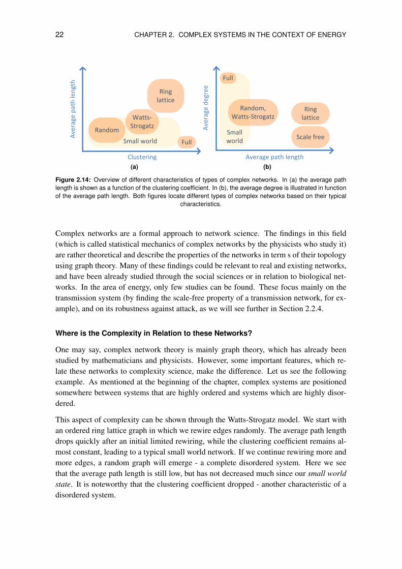
As we see, different types of network models have been found and are used to model thetopology of complex systems. Figure 2.14 shows an overview and comparison of them.
22 CHAPTER 2. COMPLEX SYSTEMS IN THE CONTEXT OF ENERGY
Small world
Ave
rage
pat
h le
ngt
h
Watts-Strogatz
Random
Ring lattice
Full
Clustering
(a)
Small world
Ringlattice
Average path length
Full
Ave
rage
deg
ree
Scale free
Random,Watts-Strogatz
(b)
Figure 2.14: Overview of different characteristics of types of complex networks. In (a) the average pathlength is shown as a function of the clustering coefficient. In (b), the average degree is illustrated in functionof the average path length. Both figures locate different types of complex networks based on their typical
characteristics.
Complex networks are a formal approach to network science. The findings in this field(which is called statistical mechanics of complex networks by the physicists who study it)are rather theoretical and describe the properties of the networks in term s of their topologyusing graph theory. Many of these findings could be relevant to real and existing networks,and have been already studied through the social sciences or in relation to biological net-works. In the area of energy, only few studies can be found. These focus mainly on thetransmission system (by finding the scale-free property of a transmission network, for ex-ample), and on its robustness against attack, as we will see further in Section 2.2.4.
Where is the Complexity in Relation to these Networks?
One may say, complex network theory is mainly graph theory, which has already beenstudied by mathematicians and physicists. However, some important features, which re-late these networks to complexity science, make the difference. Let us see the followingexample. As mentioned at the beginning of the chapter, complex systems are positionedsomewhere between systems that are highly ordered and systems which are highly disor-dered.
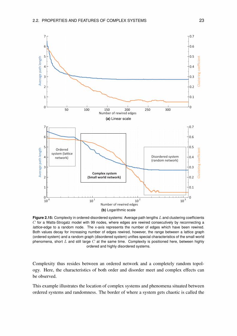
This aspect of complexity can be shown through the Watts-Strogatz model. We start withan ordered ring lattice graph in which we rewire edges randomly. The average path lengthdrops quickly after an initial limited rewiring, while the clustering coefficient remains al-most constant, leading to a typical small world network. If we continue rewiring more andmore edges, a random graph will emerge - a complete disordered system. Here we seethat the average path length is still low, but has not decreased much since our small worldstate. It is noteworthy that the clustering coefficient dropped - another characteristic of adisordered system.
2.2. PROPERTIES AND FEATURES OF COMPLEX SYSTEMS 23
50 100 150 200 250 3000
1
2
3
4
5
6
7
Number of rewired edges
Ave
rage
pat
h le
ngth
50 100 150 200 250 3000
0.1
0.2
0.3
0.4
0.5
0.6
0.7
Clus
teri
ng c
oeffi
cien
t
(a) Linear scale
10 0 10 1 10 2 10 30
1
2
3
4
5
6
7
Number of rewired edges
Ave
rage
pat
h le
ngth
10 0 10 1 10 2 10 30
0.1
0.2
0.3
0.4
0.5
0.6
0.7
Clus
teri
ng c
oeffi
cien
t
Disordered system(random network)
Complex system
(Small world network)
Orderedsystem (la�ce
network)
(b) Logarithmic scale
Figure 2.15: Complexity in ordered-disordered systems: Average path lengths L and clustering coefficientsC for a Watts-Strogatz model with 99 nodes, where edges are rewired consecutively by reconnecting alattice-edge to a random node. The x-axis represents the number of edges which have been rewired.Both values decay for increasing number of edges rewired, however, the range between a lattice graph(ordered system) and a random graph (disordered system) unifies special characteristics of the small worldphenomena, short L and still large C at the same time. Complexity is positioned here, between highly
ordered and highly disordered systems.
Complexity thus resides between an ordered network and a completely random topol-ogy. Here, the characteristics of both order and disorder meet and complex effects canbe observed.
This example illustrates the location of complex systems and phenomena situated betweenordered systems and randomness. The border of where a system gets chaotic is called the
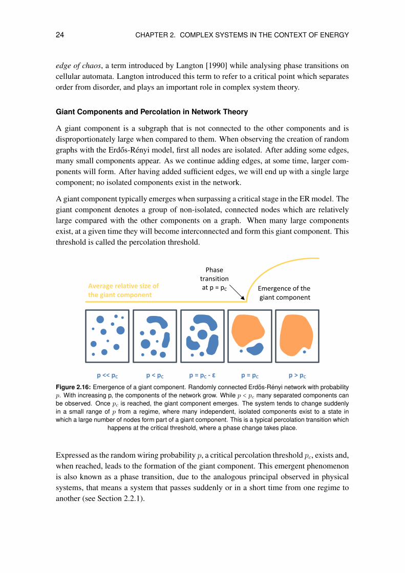
24 CHAPTER 2. COMPLEX SYSTEMS IN THE CONTEXT OF ENERGY
edge of chaos, a term introduced by Langton [1990] while analysing phase transitions oncellular automata. Langton introduced this term to refer to a critical point which separatesorder from disorder, and plays an important role in complex system theory.
Giant Components and Percolation in Network Theory
A giant component is a subgraph that is not connected to the other components and isdisproportionately large when compared to them. When observing the creation of randomgraphs with the Erdos-Renyi model, first all nodes are isolated. After adding some edges,many small components appear. As we continue adding edges, at some time, larger com-ponents will form. After having added sufficient edges, we will end up with a single largecomponent; no isolated components exist in the network.
A giant component typically emerges when surpassing a critical stage in the ER model. Thegiant component denotes a group of non-isolated, connected nodes which are relativelylarge compared with the other components on a graph. When many large componentsexist, at a given time they will become interconnected and form this giant component. Thisthreshold is called the percolation threshold.
Average relative size of the giant component
p << pC p < pC p = pC ‐ ε p = pC p > pC
Emergence of the giant component
Phasetransition at p = pC
Figure 2.16: Emergence of a giant component. Randomly connected Erdos-Renyi network with probabilityp. With increasing p, the components of the network grow. While p < pc many separated components canbe observed. Once pc is reached, the giant component emerges. The system tends to change suddenlyin a small range of p from a regime, where many independent, isolated components exist to a state inwhich a large number of nodes form part of a giant component. This is a typical percolation transition which
happens at the critical threshold, where a phase change takes place.
Expressed as the random wiring probability p, a critical percolation threshold pc, exists and,when reached, leads to the formation of the giant component. This emergent phenomenonis also known as a phase transition, due to the analogous principal observed in physicalsystems, that means a system that passes suddenly or in a short time from one regime toanother (see Section 2.2.1).

2.2. PROPERTIES AND FEATURES OF COMPLEX SYSTEMS 25
An analog parallel can be traced with electrical or railway networks. Historically, whenfirst introduced, those networks were small and isolated. Through time, they grew andexpanded, and some of them were connected, for example to national grids. As they grew,a giant component emerged. An example of this is the European UCTE network, whichinterconnects a power system through a whole continent.
2.2.3 Power Laws
As can be seen, power laws seem to play an important role in complex systems. In the caseof scale free networks, degree distribution follows a similar law. The percolation functionis also related to a power law, as well as to city sizes, where there are only a few mega-cities with many millions of inhabitants, but a large number of smaller towns. If we drawthe frequency of words in a novel or another lengthy piece of writing, we will see thatsome words appear very frequently and many others that are very rare. This is describedby Zipf’s law which is a special case of a power law distribution [Adamic, 2011].
Figure 2.17: Word frequencies in this thesis. The words are sized in proportion to their frequency ofappearance in this document. Very common words such as “the” or “a” where removed. We can see thatthere are few very frequent words, but a large number of words which appear only once or very few times.
The distribution follows a power law. [Created with wordle.net]
In Figure 2.17 the word frequencies of this thesis are shown. So, for instance, the words“system” or “model” appear over 300 times each, whereas words such as “experiment”or “computer” appear less than ten times. However, the amount of words that appear lessfrequently is much higher: there are over 5 000 words that appear less than ten times. InFigure 2.18 the word frequencies of this thesis are plotted in linear, half-log and log-logplanes. The power law can be clearly observed.
In any case, power laws are being studied in many fields of science in order to know moreabout their origins and appearance in the real world. One of the main points of interest inpower laws is their scale invariability: whereas other probability distributions change their
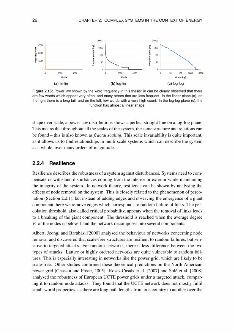
26 CHAPTER 2. COMPLEX SYSTEMS IN THE CONTEXT OF ENERGY
2000
3000
qu
en
cy c
ou
nt
0
1000
0 2000 4000
Fre
q
Words
(a) lin-lin
100
1000
10000
en
cy c
ou
nt
(lo
g)
1
10
0 2000 4000
Fre
qu
e
Words
(b) log-lin
100
1000
10000
en
cy c
ou
nt
(lo
g)
1
10
1 10 100 1000 10000
Fre
qu
e
Words (log)
(c) log-log
Figure 2.18: Power law shown by the word frequency in this thesis: in can be clearly observed that thereare few words which appear very often, and many others that are less frequent. In the linear plane (a), onthe right there is a long tail, and on the left, few words with a very high count. In the log-log plane (c), the
function has almost a linear shape.
shape over scale, a power law distributions shows a perfect straight line on a log-log plane.This means that throughout all the scales of the system, the same structure and relations canbe found – this is also known as fractal scaling. This scale invariability is quite important,as it allows us to find relationships in multi-scale systems which can describe the systemas a whole, over many orders of magnitude.
2.2.4 Resilience
Resilience describes the robustness of a system against disturbances. Systems need to com-pensate or withstand disturbances coming from the interior or exterior while maintainingthe integrity of the system. In network theory, resilience can be shown by analysing theeffects of node removal on the system. This is closely related to the phenomenon of perco-lation (Section 2.2.1), but instead of adding edges and observing the emergence of a giantcomponent, here we remove edges which corresponds to random failure of links. The per-colation threshold, also called critical probability, appears when the removal of links leadsto a breaking of the giant component. The threshold is reached when the average degreeK of the nodes is below 1 and the network decomposes into several components.
Albert, Jeong, and Barabasi [2000] analysed the behaviour of networks concerning noderemoval and discovered that scale-free structures are resilient to random failures, but sen-sitive to targeted attacks. For random networks, there is less difference between the twotypes of attacks. Lattice or highly ordered networks are quite vulnerable to random fail-ures. This is especially interesting in networks like the power grid, which are likely to bescale-free. Other studies confirmed these theoretical predictions on the North Americanpower grid [Chassin and Posse, 2005]. Rosas-Casals et al. [2007] and Sole et al. [2008]analysed the robustness of European UCTE power grids under a targeted attack, compar-ing it to random node attacks. They found that the UCTE network does not mostly fulfilsmall-world properties, as there are long path lengths from one country to another over the
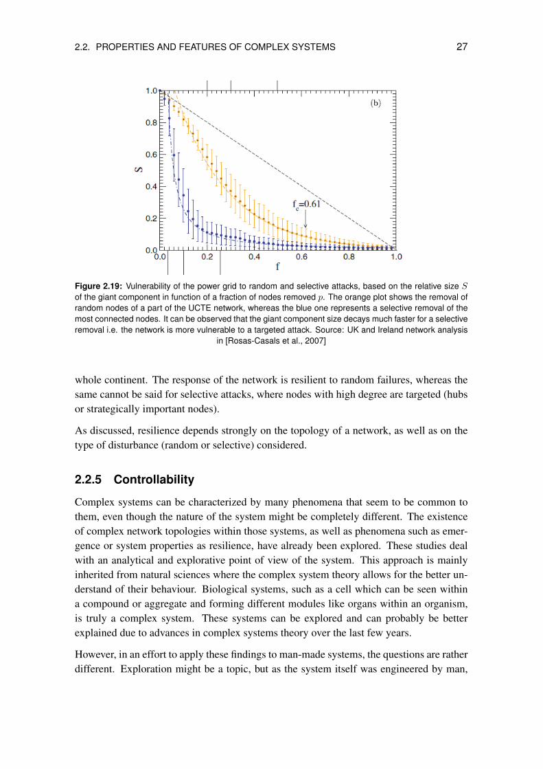
2.2. PROPERTIES AND FEATURES OF COMPLEX SYSTEMS 27
Figure 2.19: Vulnerability of the power grid to random and selective attacks, based on the relative size Sof the giant component in function of a fraction of nodes removed p. The orange plot shows the removal ofrandom nodes of a part of the UCTE network, whereas the blue one represents a selective removal of themost connected nodes. It can be observed that the giant component size decays much faster for a selectiveremoval i.e. the network is more vulnerable to a targeted attack. Source: UK and Ireland network analysis
in [Rosas-Casals et al., 2007]
whole continent. The response of the network is resilient to random failures, whereas thesame cannot be said for selective attacks, where nodes with high degree are targeted (hubsor strategically important nodes).
As discussed, resilience depends strongly on the topology of a network, as well as on thetype of disturbance (random or selective) considered.
2.2.5 Controllability
Complex systems can be characterized by many phenomena that seem to be common tothem, even though the nature of the system might be completely different. The existenceof complex network topologies within those systems, as well as phenomena such as emer-gence or system properties as resilience, have already been explored. These studies dealwith an analytical and explorative point of view of the system. This approach is mainlyinherited from natural sciences where the complex system theory allows for the better un-derstand of their behaviour. Biological systems, such as a cell which can be seen withina compound or aggregate and forming different modules like organs within an organism,is truly a complex system. These systems can be explored and can probably be betterexplained due to advances in complex systems theory over the last few years.
However, in an effort to apply these findings to man-made systems, the questions are ratherdifferent. Exploration might be a topic, but as the system itself was engineered by man,
28 CHAPTER 2. COMPLEX SYSTEMS IN THE CONTEXT OF ENERGY
its fundamental mode of operation and its structure is well known. This is not the casein biology. In addition, man-made systems are conceived to pursuit an aim. Therefore, itseems important to ask how the system works, and also how we can influence its operationin order to better fulfil the goals for which the system was created.
Recent studies have shown that there seems to be a common set of findings related tocontrollability throughout a diversity of complex systems [Liu et al., 2011]. Control theorydefines that a system is controllable if it is possible to drive it from any initial state to anydesired state within a finite time. In the case of a complex network, the time dimension hasto be introduced to allow the description of the state variation of the nodes. This meansthat the network evolves over time and that this involves a change in state for the nodes.In order to control the system, a signal is applied to a specific node. To control the wholesystem one must be able to influence all of the nodes. If we can identify the set nodes thatfulfil this property, we will be able to take control of the system by only acting on thesenodes. Liu et al. have called them driver nodes. They analysed different properties ofthese nodes and found, for example, that the amount of driver nodes can vary significantlydepending on the type of network. Social networks seem to have few of them, suggestingthat only a few individuals could control the system, whereas in gene regulatory networksa high number of nodes (around 80%) are driver nodes, and thus needed to be controlledin order to manage the whole system.
2.3 Electrical Energy Systems
The electrical energy system is composed of different electrical components that allow forthe production, transmission and consumption of electric power. Production or generationof electrical power is the process in which other energy sources are converted into electricalenergy. For transmission, different kinds of electrical networks are used. These networksare generally classified by their nominal voltage at each level. Long range transmissionover hundreds of kilometres is performed at high voltages of several hundreds of kilovolts(kV). These networks are called transmission systems. Transformer stations (substations),can reduce the voltage at a given point in order to feed electricity to the so-called dis-tribution system. The distribution system carries the electricity to the consumer. Thesenetworks operate at medium voltage levels, usually between 1-50 kV. In a final stage, dis-tribution transformers can convert from medium voltage to low voltage (less than 1 kV)which is the typical voltage level found at residential or tertiary customers. Some specificcustomers (such as industries) may have direct connections at the medium voltage level.
In a classical energy system, generation is injected at high or medium voltage levels andconsumed in the distribution system. Due to the introduction of renewable energy sourcesand distributed generation, energy can be injected at almost any level of the system. Also,and in order to better match the fluctuating production introduced to the system, Demand
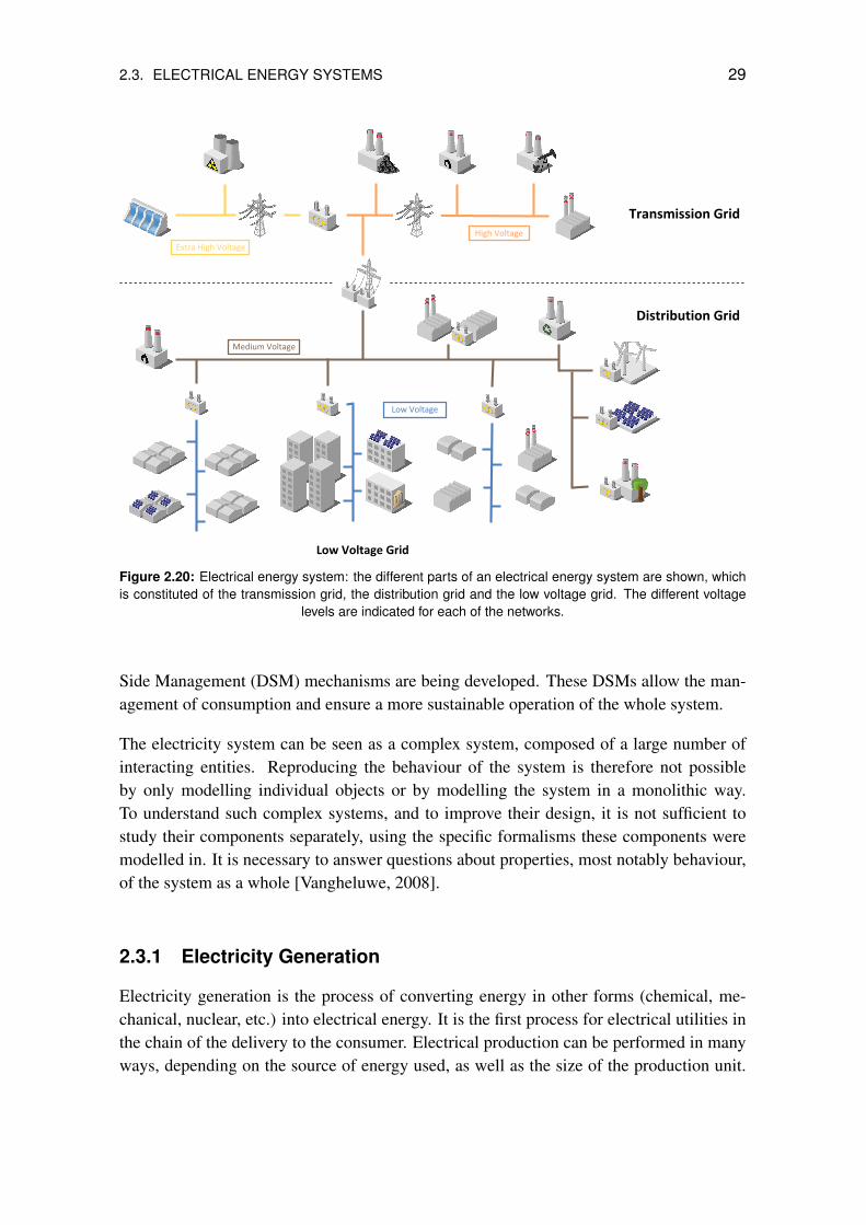
2.3. ELECTRICAL ENERGY SYSTEMS 29
Extra High Voltage
High Voltage
Medium Voltage
Low Voltage
Transmission Grid
Distribution Grid
Low Voltage Grid
Figure 2.20: Electrical energy system: the different parts of an electrical energy system are shown, whichis constituted of the transmission grid, the distribution grid and the low voltage grid. The different voltage
levels are indicated for each of the networks.
Side Management (DSM) mechanisms are being developed. These DSMs allow the man-agement of consumption and ensure a more sustainable operation of the whole system.
The electricity system can be seen as a complex system, composed of a large number ofinteracting entities. Reproducing the behaviour of the system is therefore not possibleby only modelling individual objects or by modelling the system in a monolithic way.To understand such complex systems, and to improve their design, it is not sufficient tostudy their components separately, using the specific formalisms these components weremodelled in. It is necessary to answer questions about properties, most notably behaviour,of the system as a whole [Vangheluwe, 2008].
2.3.1 Electricity Generation
Electricity generation is the process of converting energy in other forms (chemical, me-chanical, nuclear, etc.) into electrical energy. It is the first process for electrical utilities inthe chain of the delivery to the consumer. Electrical production can be performed in manyways, depending on the source of energy used, as well as the size of the production unit.

30 CHAPTER 2. COMPLEX SYSTEMS IN THE CONTEXT OF ENERGY
Two mayor classifications of electricity generation, must be considered when looking atthe current state of the energy system.
The first characterisation is related to their size and hierarchical grade in the system. Cen-tralised power plants tend to be located in remote areas with suitable conditions for theirdeployment (riverside for cooling, well connected to primary resource supply, etc.). This isthe traditional way of production that has been the foundation of the system since electri-fication. Classical production relies on large production units, feeding into a transmissiongrid to transport energy over long distances and distribute it to the final consumer, in atree-like structure. The leaves would be the final consumers, which are fed from a centralsource in the roots. In this configuration, flows are almost only uni-directional, from thesource to the sinks of energy – from the roots to the leaves.
The first distributed systems date back to the 1950s, when local generation was first con-sidered as an alternative to centralised structures. Distributed Generation (DG) avoidstransmission costs and losses, by producing the energy close to its point of consumption.However, this isn’t possible with all types of energy sources. In the classical paradigm,the location of coal plants outside an urban area was to avoid local pollution. Renewableenergy sources first began to be integrated as they are environmental-friendly and can bedeployed as small DER. Table 2.1 shows an overview of the different types of generationclassified by their degree of hierarchy.
Centralised Distributed
• Power stations managed by utility
• Large installed power capacity
• Few production plants
• Can be far away from consumer
• Classical production follows thisstructure
• Energy production based on inter-connected little and medium sizepower generators and/or renewableenergy plants
• Small or medium installed powercapacities
• Large number of production units
• Local production for local con-sumers
Table 2.1: Centralised vs. distributed generation
With a distributed generation, electric energy is produced close to the consumer, withinor near residential areas and industrial plants, through small production units. The dimen-sioning of the power generation equipment is usually only designed to meet the energyneeds of locally connected consumers. Excess energy can be fed into the distribution ortransmission grid. The transition to a smart grid will first involve the introduction and thenthe expansion of distributed generation which will result in massive use.

2.3. ELECTRICAL ENERGY SYSTEMS 31
The second aspect which allows us to characterise generation is the primary energy sourcetype. Here we distinguish between conventional and renewable energy sources. Conven-tional sources have been used since the beginning of electrical energy generation. Theyusually include fossil fuels and, more recently nuclear fuels, to power thermal plants. Theprocess is based on steam generation moving a turbine converting energy from mechani-cal into electrical form. Renewable energy sources have gained more and more importanceduring the past decades mainly because of environmental reasons and because of finite fos-sil fuel reserves. They include thermal generation through sustainable fuels, which operatesimilarly to conventional plants, and other generation methods, such as wind power wherewind turbines directly convert wind into electrical energy. Other means of generation usediverse methods, such as solar photovoltaic panels through the photovoltaic effect convert-ing radiation into electricity, or the use of tidal energy to generate electrical power. Table2.2 shows a synthesis of the generation types by primary energy source.
Conventional Renewable
• Thermal production based on fossilfuels (usually coal, petrol, gas, etc.)
• Thermal production based on nu-clear fuels
• Thermal production from sustain-able fuels (biomass, biofuel, bio-gas, etc.)
• Wind power
• Hydropower
• Solar power
• Geothermal power
Table 2.2: Generation by primary energy source: examples.
Renewable energy sources (RES) must not be confused with distributed generation. Re-newable energy is usually associated with distributed plants. However more and morelarge, centralised renewable production plants are being built (large wind farms, solarfarms, etc.). On the other hand, there are also conventional production systems whichare distributed (e.g. micro CHPs).
The introduction and, particularly, the expansion of renewable energy sources leads to im-portant questions. Is the necessity of covering the demand assured, as RES tend to fluctuate(e.g. wind) or may only be periodically available (e.g. solar, only during daylight)?
Again a trend towards the smart grid can be recognised in this classification. Generally, theintroduction and achievement of larger penetration rates of renewable production units canbe observed. For example, in Spain in the year 2009 already half of electrical consumptionat a specific moment was covered by wind power energy [Red Electrica Espanola, 2009].
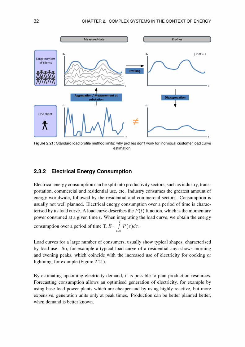
32 CHAPTER 2. COMPLEX SYSTEMS IN THE CONTEXT OF ENERGY
P
t
P
t
P
t
P
t
Aggregation / Measurement at substation
Profiling
One client
Large number of clients
Disaggregation
Measured data Profiles
∫ P dt = 1
Figure 2.21: Standard load profile method limits: why profiles don’t work for individual customer load curveestimation.
2.3.2 Electrical Energy Consumption
Electrical energy consumption can be split into productivity sectors, such as industry, trans-portation, commercial and residential use, etc. Industry consumes the greatest amount ofenergy worldwide, followed by the residential and commercial sectors. Consumption isusually not well planned. Electrical energy consumption over a period of time is charac-terised by its load curve. A load curve describes the P (t) function, which is the momentarypower consumed at a given time t. When integrating the load curve, we obtain the energy
consumption over a period of time T, E =T
∫t=0
P (τ)dτ .
Load curves for a large number of consumers, usually show typical shapes, characterisedby load-use. So, for example a typical load curve of a residential area shows morningand evening peaks, which coincide with the increased use of electricity for cooking orlightning, for example (Figure 2.21).
By estimating upcoming electricity demand, it is possible to plan production resources.Forecasting consumption allows an optimised generation of electricity, for example byusing base-load power plants which are cheaper and by using highly reactive, but moreexpensive, generation units only at peak times. Production can be better planned better,when demand is better known.

2.3. ELECTRICAL ENERGY SYSTEMS 33
Prediction of Electrical Consumption
The standard load profile method is commonly used for aggregated prediction. It relieson load profiles measured, or estimated, for specific consumers. These can be scaled formodelling demand. This approach was chosen for industry/business and the public sector,as most of the available data was aggregated and the behaviour of these sectors is basedon similar patterns. Synthetic load profiles are the result of a statistical analysis based onrepresentative samples from different consumer groups [Palensky et al., 2008].
A standard load profile is a representative load profile that is used to predict the demandof a user without making use of measurement. The profile is a normalised curve for aspecific consumer, consumer group or appliance that was obtained from measurements orestimations of many of these consumers. It represents the demand behaviour of a largeand aggregated group of users that is to be considered. This is especially helpful for cre-ating universal profiles for consumers that have heterogeneous behaviour and cannot bedescribed by aggregating the same individual entity many times over. This represents theaverage demand behaviour of this consumer group. By the normalisation of the curve, itcan be scaled further and customised for the model in which it is applied.
Load profiles are normally provided in normalised form, and the user has to multiply themby the total amount of energy resulting from the profile. This is normally daily, or yearlyconsumption, for example. As energy amounts for electrical use usually result from sur-veys and studies, having the profile is a practical way to obtain an approximate load curve.The approach is applicable in a broad range of uses and does not involve too many complexmodels. This makes it quick and results in good estimates at aggregated levels. Neverthe-less, it has to be kept in mind that these curves can only reflect aggregated behaviour andare not representative if individual users or small groups of users are considered [Willisand Scott, 2000; Paatero, 2009].
A further issue of current demand prediction or simulation models is that they mostly relyon low resolution data (e.g hourly sample rates). Hourly averages are suitable for mod-elling the demand at a high and aggregate level. However, when dealing with individualconsumers, there is a need for high resolution data [Wright and Firth, 2007]. Only a fewhigh resolution studies and models exist on domestic demand Wright and Firth [2007];Widen et al. [2009], and they are not coupled to an energy system model.
These curves are not suitable for planning and control at the distribution level. They onlyapply to a large number of consumers as they describe the average use of energy over time[Willis and Scott, 2000; Paatero, 2009]. Also, when considering distributed generation orrenewable energy sources, production cannot be accurately represented by this method.Diversified profiles are only applicable to community generation with a single point ofimport and export upstream of a large number of houses and the generator - but standardprofiles are unlikely to apply to a particular community [Wright and Firth, 2007].
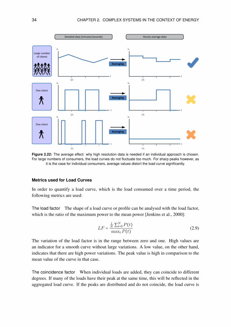
34 CHAPTER 2. COMPLEX SYSTEMS IN THE CONTEXT OF ENERGY
P
t
P
t
P
t
P
t
Averaging
One client
Large number of clients
Detailed data (minutes/seconds) Hourly average data
P
t
P
t
Averaging
One client
Averaging
1h1h
1h
1h 1h
1h
Figure 2.22: The average effect: why high resolution data is needed if an individual approach is chosen.For large numbers of consumers, the load curves do not fluctuate too much. For sharp peaks however, as
it is the case for individual consumers, average values distort the load curve significantly.
Metrics used for Load Curves
In order to quantify a load curve, which is the load consumed over a time period, thefollowing metrics are used:
The load factor The shape of a load curve or profile can be analysed with the load factor,which is the ratio of the maximum power to the mean power [Jenkins et al., 2000]:
LF =
1N ∑
Nt=0P (t)
maxtP (t)(2.9)
The variation of the load factor is in the range between zero and one. High values arean indicator for a smooth curve without large variations. A low value, on the other hand,indicates that there are high power variations. The peak value is high in comparison to themean value of the curve in that case.
The coincidence factor When individual loads are added, they can coincide to differentdegrees. If many of the loads have their peak at the same time, this will be reflected in theaggregated load curve. If the peaks are distributed and do not coincide, the load curve is

2.3. ELECTRICAL ENERGY SYSTEMS 35
smoother. This effect can be described and quantified by the coincidence factor [Jenkinset al., 2000]:
CF =maxtP (t)
∑i maxk Pi(k)(2.10)
where an aggregated curve P (t) is contemplated, which is formed by P (t) = ∑iPi(t)
where Pi are the individual loads. If the individual maxima of the loads occur at the sametime, the coincidence factor equals one, thus having a high coincidence or synchronisation.If the peaks of the individual loads are distributed over time, the coincidence factor is lower,indicating a smoother curve.
The coincidence factor is a measure over a load curve. To define the coincidence of loadsat a given time t we define the coincidence
c(t) =P (t)
Pinst(2.11)
where P (t) is the instantaneous load and Pinst the total installed load (maximum possibleload if all individual loads would coincide).
Demand Side Management (DSM)
In the future, smart electrical system, the demand side will have an active role. By regu-lating demand within certain limits, not only is production governed but it also allows fora more flexible balancing of the system. The use of demand side management (DSM) hasbeen widely discussed for different purposes in enhancing performance and avoid criticalsituations for the power grid Palensky and Dietrich [2011]; Albadi and El-Saadany [2007].Management of the demand side would allow for:
1. Improving energy efficiency
2. Reducing peak loads
3. Shifting loads over time
4. Increasing valley loads
5. Stabilising grid frequency
The first possibility represents a lasting improvement to the demand side (for example,permanently reducing demand through increased energy efficiency, by, for instance, usingenergy-saving lights). Points 2-4 focus more on load curve shaving, acting in a mediumterm (daily or at most hourly) view, which is also called demand response (DR). Thesemechanisms can support the integration of fluctuating renewable energy sources such aswind power or solar generation. The last possibility allows the support of the primary
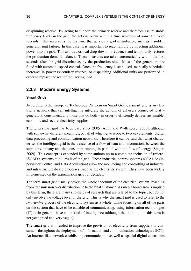
36 CHAPTER 2. COMPLEX SYSTEMS IN THE CONTEXT OF ENERGY
or spinning reserve. By acting to support the primary reserve and therefore assure stablefrequency levels in the grid, the actions occur within a time windows of some tenths ofseconds. This reserve is the first one that acts on a grid disturbance, such as a suddengenerator unit failure. In this case, it is important to react rapidly by injecting additionalpower into the grid. This avoids a critical drop-down in frequency and temporarily restoresthe production-demand balance. These measures are taken automatically within the firstseconds after the grid disturbance, by the production side. Most of the generators arefitted with automatic speed control. Once the frequency is stabilised, manually scheduledincreases in power (secondary reserve) or dispatching additional units are performed inorder to replace the rest of the lacking load.
2.3.3 Modern Energy Systems
Smart Grids
According to the European Technology Platform on Smart Grids, a smart grid is an elec-tricity network that can intelligently integrate the actions of all users connected to it –generators, consumers, and those that do both – in order to efficiently deliver sustainable,economic and secure electricity supplies.
The term smart grid has been used since 2005 [Amin and Wollenberg, 2005], althoughwith somewhat different meanings, but all of which give scope to two key elements: digitaldata processing and communication networks. Therefore it can be said that what charac-terises the intelligent grid is the existence of a flow of data and information, between thesupplier company and the consumer, running in parallel with the flow of energy [Singer,2009]. This concept is expanded by some authors up to a complete inclusion of (micro-)SCADA systems at all levels of the grid. These industrial control systems (SCADA: Su-pervisory Control and Data Acquisition) allow the monitoring and controlling of industrialand infrastructure-based processes, such as the electricity system. They have been widelyimplemented on the transmission grid for decades.
The term smart grid usually covers the whole spectrum of the electrical system, reachingfrom transmission over distribution up to the final customer. As such a broad area is impliedby this term, there are many sub-fields of research that are related to the topic, but do notonly involve the voltage level of the grid. This is why the smart grid is used to refer to thesmartening process of the electricity system as a whole, while focusing on all of the partson the system that have to be capable of communicating, using information technologies(IT) or in general, have some kind of intelligence (although the definition of this term isnot yet agreed and very vague).
The smart grid is intended to improve the provision of electricity from suppliers to con-sumers throughout the deployment of information and communication technologies (ICT).An internet like network establishing communication as well as special digital electronics

2.3. ELECTRICAL ENERGY SYSTEMS 37
to control energy generation and consumer demand are needed to set up this true complexsystem. It will allow suppliers to remotely monitor client power consumption, implementvariable energy costs, and in this way avoid long peak load periods or circuit overload situ-ations. Also, consumers will be able to monitor their real time power consumption, whichcould be used to load control by controlling their own peak and off-peak use in order tobenefit from lower tariffs.
With today’s smart grid goals in mind, energy supply companies are in a transition be-tween the existing electricity grid and the future smart grid. They seek to improve theconventional network infrastructure, and establish a digital level (essence of the intelli-gent network) and also create new business processes to carry out the capitalisation andcommercialisation of the intelligent network.
Generally, it can be said that the introduction of the smart grid involves an introductionof SCADA at almost all levels of the grid. SCADA systems have existed for years in thetransport network. In order to allow effective system management at all levels, includingtechnologies like SCADA into the distribution grid is necessary.
Other relevant technologies and mechanisms which are commonly mentioned in relationto smart grids are:
• Smart metering
• Electric vehicles
• Distributed generation
• Demand side management
• Energy storage
• Dynamic pricing
All these could be part of a future power grid, but non of them alone should be consideredas an integral smart grid. The introduction of ICT will allow the management and controlof most of these technologies. These technologies can also support the ICT infrastructure,for instance smart meters.
Smart Grid Demonstration Projects
Several demonstration projects are already running or are in preparation to show the possi-bilities of smart grids. A large catalogue of more than 200 smart grid related projects inthe EU is presented in [Giordano et al., 2011]. The distribution of projects across Europeis not uniform. Most of the projects and investments are located in old EU-15 countries,while the newer EU-12 member states still lag behind. These projects have some common
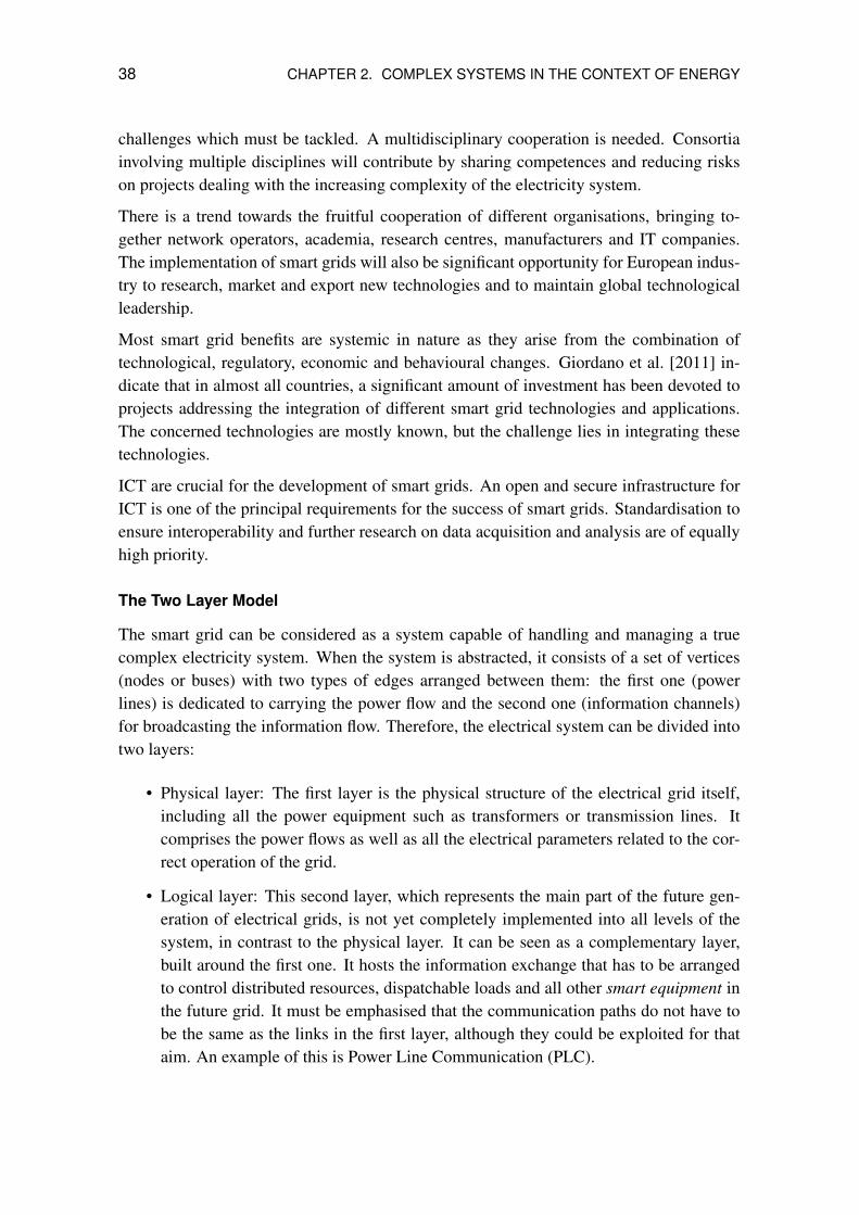
38 CHAPTER 2. COMPLEX SYSTEMS IN THE CONTEXT OF ENERGY
challenges which must be tackled. A multidisciplinary cooperation is needed. Consortiainvolving multiple disciplines will contribute by sharing competences and reducing riskson projects dealing with the increasing complexity of the electricity system.
There is a trend towards the fruitful cooperation of different organisations, bringing to-gether network operators, academia, research centres, manufacturers and IT companies.The implementation of smart grids will also be significant opportunity for European indus-try to research, market and export new technologies and to maintain global technologicalleadership.
Most smart grid benefits are systemic in nature as they arise from the combination oftechnological, regulatory, economic and behavioural changes. Giordano et al. [2011] in-dicate that in almost all countries, a significant amount of investment has been devoted toprojects addressing the integration of different smart grid technologies and applications.The concerned technologies are mostly known, but the challenge lies in integrating thesetechnologies.
ICT are crucial for the development of smart grids. An open and secure infrastructure forICT is one of the principal requirements for the success of smart grids. Standardisation toensure interoperability and further research on data acquisition and analysis are of equallyhigh priority.
The Two Layer Model
The smart grid can be considered as a system capable of handling and managing a truecomplex electricity system. When the system is abstracted, it consists of a set of vertices(nodes or buses) with two types of edges arranged between them: the first one (powerlines) is dedicated to carrying the power flow and the second one (information channels)for broadcasting the information flow. Therefore, the electrical system can be divided intotwo layers:
• Physical layer: The first layer is the physical structure of the electrical grid itself,including all the power equipment such as transformers or transmission lines. Itcomprises the power flows as well as all the electrical parameters related to the cor-rect operation of the grid.
• Logical layer: This second layer, which represents the main part of the future gen-eration of electrical grids, is not yet completely implemented into all levels of thesystem, in contrast to the physical layer. It can be seen as a complementary layer,built around the first one. It hosts the information exchange that has to be arrangedto control distributed resources, dispatchable loads and all other smart equipment inthe future grid. It must be emphasised that the communication paths do not have tobe the same as the links in the first layer, although they could be exploited for thataim. An example of this is Power Line Communication (PLC).
2.3. ELECTRICAL ENERGY SYSTEMS 39
Figure 2.23: The two layer model of a smart grid
There are several implementation possibilities for the second layer due to the wide spec-trum of communication technologies available. It is assumed that this layer will implementa system that allows real-time communication between the elements of the grid. In theGerman E-Energie project2, an Internet of Energy is suggested as an analogy to computernetworks. This medium could itself serve as a communication platform. More examplesof the network implementations for the logical layer are:
• Wired technologies
– Using the power grid infrastructure: PLC
– Internet infrastructure: over existing networks such as telephone or cable net-works
– Wired solutions on a (new) dedicated network
• Wireless technologies
– Internet related technologies: WLAN, WMAN or WiMax
– Mobile technologies: GSM/GPRS or third generation networks such as 3G/UMTS
– Lower range technologies: Bluetooth or Zigbee for local communication
The communication layer also supports other smart grid relevant topics such as geographicnetwork localisation, distribution of processing and databases, interaction with humans,and unpredictability of system reactions to unexpected external events, among others.
2http://www.e-energy.de/
40 CHAPTER 2. COMPLEX SYSTEMS IN THE CONTEXT OF ENERGY
Microgrids
A microgrid is an integrated energy system consisting of interconnected loads and dis-tributed energy resources which, as an integrated system, can operate in parallel with thegrid or in an intentional island mode [Navigant Consulting, 2006]. A microgrid is alsoa set of small energy generators arranged in order to supply energy for a community ofusers in close proximity. It is a combination of generation sources, loads and energy stor-age, interfaced through fast-acting power electronics. Emerging from the general trend ofthe introduction of renewable energy sources (RES), microgrids will mostly include thistype of generation, so they form part of the hybrid renewable energy systems (HRES).These systems combine two or more energy conversion devices, or two or more fuels forthe same device, that when integrated, overcome limitations inherent in either. Micro-grids represent a form of decentralisation of electrical networks. They comprise low- ormedium-voltage distribution systems with distributed energy sources, storage devices andcontrollable loads.
The European Commission [2011] defines microgrids as small electrical distribution sys-tems that connect multiple customers to multiple distributed sources of generation andstorage. It also states that microgrids can typically provide power to communities of up to500 households at low voltage level. This shows that this technology is not only suitablefor the electrification of small remote islands or remote zones in developing countries, butalso for integration into existing high voltage transmission grids. Therefore microgridscould have a wide application spectrum in the near future.
During disturbances, generation and corresponding loads can autonomously disconnectfrom the distribution system. This allows for the isolation of the microgrid load from thedisturbance without damaging the integrity of the transmission grid. This mode is calledthe islanding mode. From the customer’s perspective, it can be seen as a low voltage distri-bution service with additional features like an increase in local reliability, the improvementof voltage and power quality, the reduction of emissions, a decrease in the cost of energysupply, etc. A microgrid is connected to the distribution network through a single Point ofCommon Coupling (PCC) and appears as a single unit in the power transmission network.Power electronics will be a crucial feature for microgrids since most of the power micro-sources must be electronically controlled to gain the characteristics required of the system.The microgrid is therefore not only a more or less autonomous part of the power system,but also has to be a smart system itself. It has to be able to cope with multiple issues, asdescribed below.
The introduction of smart grids involves a change from manual operations towards anintelligent, ICT-based and controlled network. These changes will especially affect thedistribution grid [Jiyuan and Borlase, 2009]. Microgrids can support this change, by beinga flexible and autonomous module of the smart grid. The challenges of implementing

2.3. ELECTRICAL ENERGY SYSTEMS 41
microgrids mean that they are implicitly considered to be smart grids, or at least to be partof a smart grid.
The operation of a smart electrical system will involve a higher degree of complexity thanthe operation of the conventional power grid. In order to function, components like au-tomation, sensors, remote controlled switching devices and communication networks arenecessary. For example, the current power grid is still not ready to permit microgrid con-nections. Connections made at present are experimental and almost always performedmanually, by ensuring that a number of factors are fulfilled, for instance before completinga connection.
Microgrid Architectures In terms of their architecture, microgrids can be classified in fourdifferent types [Navigant Consulting, 2006]:
• Single facility microgrids
These microgrids include installations such as industrial and commercial buildings,residential buildings and hospitals, with loads typically under 2 MW.
• Multiple facility microgrids
This category includes microgrids spanning multiple buildings or structures, withloads typically ranging between 2 and 5 MW. Examples include campuses (medical,academic, municipal, etc), military bases, industrial and commercial complexes.
• Feeder microgrids
The feeder microgrid manages the generation and/or load of all entities within a dis-tribution feeder, which can encompass 5-10 MW. These microgrids may incorporatesmaller microgrids – single or multiple facility microgrids- – within them.
• Substation microgrids
The substation microgrid manages the generation and/or load of all entities con-nected to a distribution substation, which can encompass 5-10+ MW.
Island Systems
Interconnected continental power grids such as the UCTE or the North-American powergrid offer a large degree of resilience due to their extension and number of control mecha-nisms. Further, generators and loads are geographically and topologically distributed overthousands of kilometres. The frequency of these grids is usually largely stable and onlysmall variations occur during regular operation. For example, the effect of a failure ina production unit is low when compared to the overall production of the whole system.Thus, its effect on the frequency can be almost neglected. In addition to that, the usuallysufficient reserve units are available to rapidly compensate for the dropped power station.
42 CHAPTER 2. COMPLEX SYSTEMS IN THE CONTEXT OF ENERGY
On island systems however, the resilience is drastically reduced. Small, self-sufficient elec-trical systems have been traditionally supplied with highly reactive, rather small or mediumsized production units, such as gas or diesel plants (combined cycle), or even diesel mo-tors. The smaller the system, the more difficult it becomes to control, as the shaving andsmoothing effects of large systems are not present. Usually, a failure of one plant sup-poses an already large reduction relative to the total power consumed by the system. Onthe other hand, connecting large consumers, such as an industrial plant can cause similarimbalances.
Following the general trend of introducing renewable energy sources, fluctuating producersare being installed on island systems [Tarkowski and Uliasz-Misiak, 2003]. These systemsare usually suitable, as their climate condition allows significant exploitation, for exampledue to their wind characteristics. The inclusion of fluctuating energy sources adds anadditional variable to the system, which impacts directly on its stability.
Modern island systems are currently being used as a kind of experimental labs. They havespecific issues, but they also offer an isolated, autarkic grid, which can be used as a testbench for new technologies. Some of these systems offer the opportunity to test largepenetration rates of RES. The first island totally supplied by RES will implemented in ElHierro, Spain, where wind power coupled with a pumped hydro storage plant will allowindependent and completely autonomous generation.
2.3.4 Storage Systems
The implementation of storage systems in energy networks offers new paths to explore.Storage systems offer flexibility in a system that has previously been mainly characterizedby unidirectional units, which were, on the one hand generation units and on the other con-sumption units. In a power system, generation must always cover demand. Furthermore,not only must demand be covered, but no additional energy should be produced to avoidovercharging. A balance between production and demand must be assured at all times toguarantee a stable system.
Generation sources in conventional power systems are dispatchable (they can be controlledto gain a certain level of power output). They use different types of plants, like base, mid-dle and peak load plants, in order to meet current demand. For new emerging systems,which include several types of fluctuating renewable energy sources, as well as distributedgeneration, this task becomes more complicated. New measures are needed to assure sys-tem stability. Intermittent energy sources cannot be or can only be partially, forecasted.Sufficient reserve power must be available at conventional or dispatchable plants to main-tain production in case of abrupt drop-downs in the intermittent sources. But also, theremight be overproduction periods, where too much renewable energy is generated withouthaving a consumer to use it when available. Therefore, storage systems have gained in im-portance. They can be used to react to short term, transient effects caused by intermittent
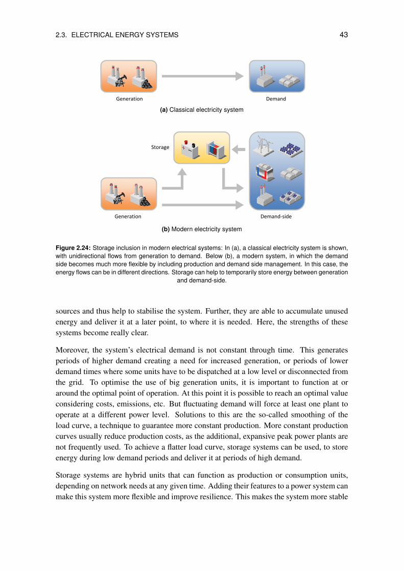
2.3. ELECTRICAL ENERGY SYSTEMS 43
Generation Demand
Generation Demand‐side
Storage
(a) Classical electricity system
Generation Demand
Generation Demand‐side
Storage
(b) Modern electricity system
Figure 2.24: Storage inclusion in modern electrical systems: In (a), a classical electricity system is shown,with unidirectional flows from generation to demand. Below (b), a modern system, in which the demandside becomes much more flexible by including production and demand side management. In this case, theenergy flows can be in different directions. Storage can help to temporarily store energy between generation
and demand-side.
sources and thus help to stabilise the system. Further, they are able to accumulate unusedenergy and deliver it at a later point, to where it is needed. Here, the strengths of thesesystems become really clear.
Moreover, the system’s electrical demand is not constant through time. This generatesperiods of higher demand creating a need for increased generation, or periods of lowerdemand times where some units have to be dispatched at a low level or disconnected fromthe grid. To optimise the use of big generation units, it is important to function at oraround the optimal point of operation. At this point it is possible to reach an optimal valueconsidering costs, emissions, etc. But fluctuating demand will force at least one plant tooperate at a different power level. Solutions to this are the so-called smoothing of theload curve, a technique to guarantee more constant production. More constant productioncurves usually reduce production costs, as the additional, expansive peak power plants arenot frequently used. To achieve a flatter load curve, storage systems can be used, to storeenergy during low demand periods and deliver it at periods of high demand.
Storage systems are hybrid units that can function as production or consumption units,depending on network needs at any given time. Adding their features to a power system canmake this system more flexible and improve resilience. This makes the system more stable

44 CHAPTER 2. COMPLEX SYSTEMS IN THE CONTEXT OF ENERGY
when facing unpredictable changes and exterior influences of any kind. Electrical energycan only be stored in electrical form with difficulty. This is only possible in capacitorsor supra-conducting coils, also called superconducting magnetic energy storage (SMES).Usually it is more economical to convert it into other forms of energy and then convertit back when needed. Each conversion involves losses, and the energy is lost over timeduring storage, too. The sum of all individual losses may be significant and make theprocess uneconomical. In Appendix B an overview of different storage technologies aswell as typical values for their performance, capacity and other factors, is shown.
2.4 Energy Systems: a Complex Systems Approach?
Complexity science is a new field of science, which aims to understand our complex worldfrom a new perspective. It can describe phenomena and effects that are common in manyreal systems, which at a first glance seem to be completely isolated from each other (emer-gent phenomena, for instance). A complex system approach allows the detection of com-mon patterns, such as networks or interactions, which, independent of the system, willshow recurrent properties. Studying phenomena at this level permits understanding ourworld from a more systemic perspective, rather than from the perspective of one givenfield.
Once at this point, one may say: what do complex systems really have to do with anelectrical grid? What does temperature variation in a honeybee hive have to do with gridfrequency? Why should modelling and simulation take into account this relatively newapproach? Isn’t it just possible to continue using classical engineering tools for the samepurpose?
Energy systems have been traditionally designed, developed and managed by electricalengineers for decades. The classical energy system is a hierarchically well-defined, top-down system, intended to work in one direction only. Centralised production using largeplants for the economical generation of energy, the only possible way at the beginning ofthe 20th century, feed electricity into the high voltage grid, where it is transported over longdistances to the origin of demand. Once there, a regional distribution grid approaches theenergy to large industrial consumers and low voltage transformers for final end customers.This system worked well before deregulation of the energy markets because almost allthese steps were covered by the same actor. Deregulation, along with the introductionof distributed and renewable energy sources, lead to a real paradigm shift in which theclassical system was no longer sustainable. Introducing production units at lower levelsfirstly allowed the inversion of energy flows. Concepts like prosumers (consumers whichare capable of producing energy as well) as well as new technologies in the field (smartmetering, ICT on energy systems) etc. and especially active management of the demandside (through DSM or DR), are now leading to what is called the smart grid.

2.4. ENERGY SYSTEMS AS COMPLEX SYSTEMS? 45
Complex systems aim to reflect the complex processes and dynamics of real systems, rely-ing on a cross-disciplinary approach. In the course of this work we will see how the energysystem is a real socio-technical system, which combines technical, automated processeswith human behaviour and social factors. If we want to understand many of the processesof an energy system, only by taking into account both aspects can we draw an integrativepicture.
Moreover, current methods, such as the standard profile method or other methods usinglow-resolution data, seem to have reached their limits. As we have seen, high-resolutionmodels can be helpful and are necessary. Individual-centric approaches, which are acommon tool in complex systems theory, can address the new challenges of using high-resolution models.
It must be said that the complex system approach does not aim to substitute any of the clas-sical tools and approaches already existing in the field. Power flow questions, grid stabilityissues, and many other engineering questions have been correctly addressed and should notbe represented by using overly-simplified models. However, the complex system approachaims to look at the system from a new perspective, taking it into account as a whole andbeing able to capture, for example, emergent phenomena, which can barely, if at all, berepresented with other tools.

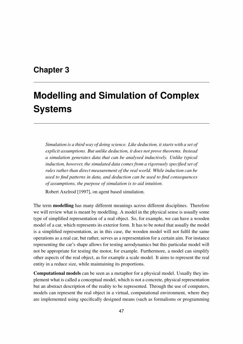
Chapter 3
Modelling and Simulation of ComplexSystems
Simulation is a third way of doing science. Like deduction, it starts with a set ofexplicit assumptions. But unlike deduction, it does not prove theorems. Insteada simulation generates data that can be analysed inductively. Unlike typicalinduction, however, the simulated data comes from a rigorously specified set ofrules rather than direct measurement of the real world. While induction can beused to find patterns in data, and deduction can be used to find consequencesof assumptions, the purpose of simulation is to aid intuition.
Robert Axelrod [1997], on agent based simulation.
The term modelling has many different meanings across different disciplines. Thereforewe will review what is meant by modelling. A model in the physical sense is usually sometype of simplified representation of a real object. So, for example, we can have a woodenmodel of a car, which represents its exterior form. It has to be noted that usually the modelis a simplified representation, as in this case, the wooden model will not fulfil the sameoperations as a real car, but rather, serves as a representation for a certain aim. For instancerepresenting the car’s shape allows for testing aerodynamics but this particular model willnot be appropriate for testing the motor, for example. Furthermore, a model can simplifyother aspects of the real object, as for example a scale model. It aims to represent the realentity in a reduce size, while maintaining its proportions.
Computational models can be seen as a metaphor for a physical model. Usually they im-plement what is called a conceptual model, which is not a concrete, physical representationbut an abstract description of the reality to be represented. Through the use of computers,models can represent the real object in a virtual, computational environment, where theyare implemented using specifically designed means (such as formalisms or programming
47
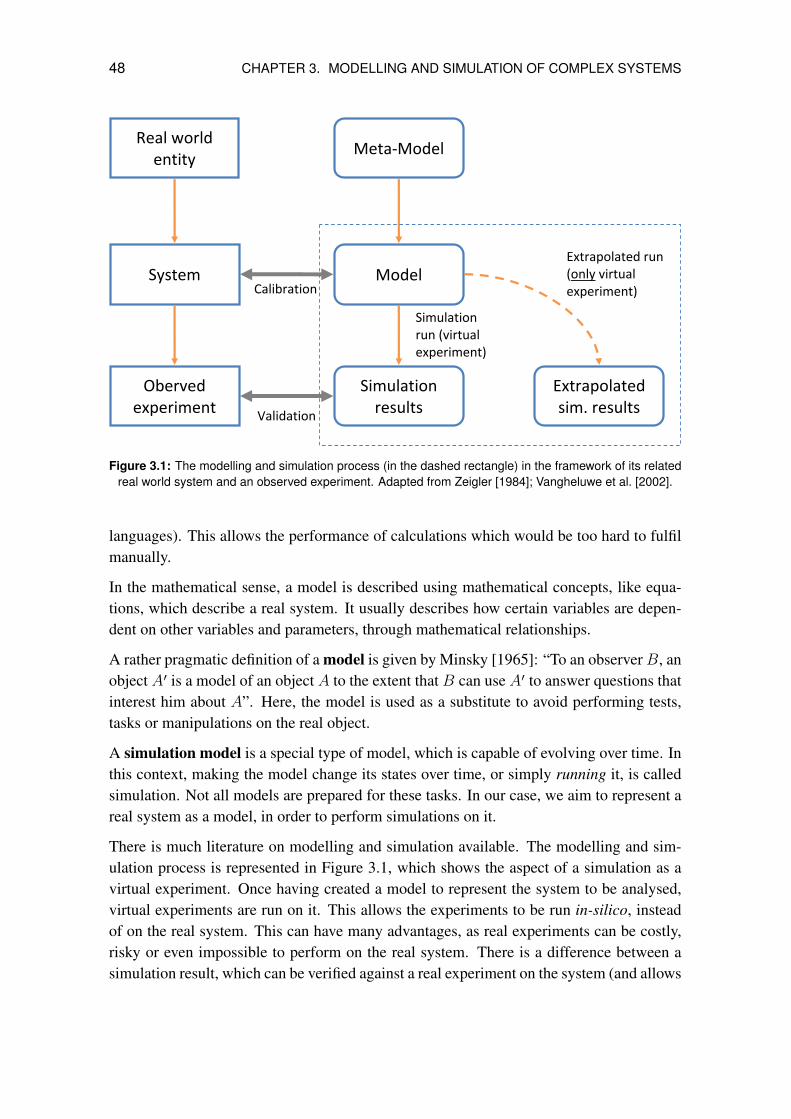
48 CHAPTER 3. MODELLING AND SIMULATION OF COMPLEX SYSTEMS
System
Meta‐Model Real world
entity
Oberved experiment
Model
Simulation results Validation
Calibration
Simulation run (virtual experiment)
Extrapolated sim. results
Extrapolated run(only virtual experiment)
Modelling and Simulation Process (1) Figure 3.1: The modelling and simulation process (in the dashed rectangle) in the framework of its relatedreal world system and an observed experiment. Adapted from Zeigler [1984]; Vangheluwe et al. [2002].
languages). This allows the performance of calculations which would be too hard to fulfilmanually.
In the mathematical sense, a model is described using mathematical concepts, like equa-tions, which describe a real system. It usually describes how certain variables are depen-dent on other variables and parameters, through mathematical relationships.
A rather pragmatic definition of a model is given by Minsky [1965]: “To an observerB, anobject A′ is a model of an object A to the extent that B can use A′ to answer questions thatinterest him about A”. Here, the model is used as a substitute to avoid performing tests,tasks or manipulations on the real object.
A simulation model is a special type of model, which is capable of evolving over time. Inthis context, making the model change its states over time, or simply running it, is calledsimulation. Not all models are prepared for these tasks. In our case, we aim to represent areal system as a model, in order to perform simulations on it.
There is much literature on modelling and simulation available. The modelling and sim-ulation process is represented in Figure 3.1, which shows the aspect of a simulation as avirtual experiment. Once having created a model to represent the system to be analysed,virtual experiments are run on it. This allows the experiments to be run in-silico, insteadof on the real system. This can have many advantages, as real experiments can be costly,risky or even impossible to perform on the real system. There is a difference between asimulation result, which can be verified against a real experiment on the system (and allows
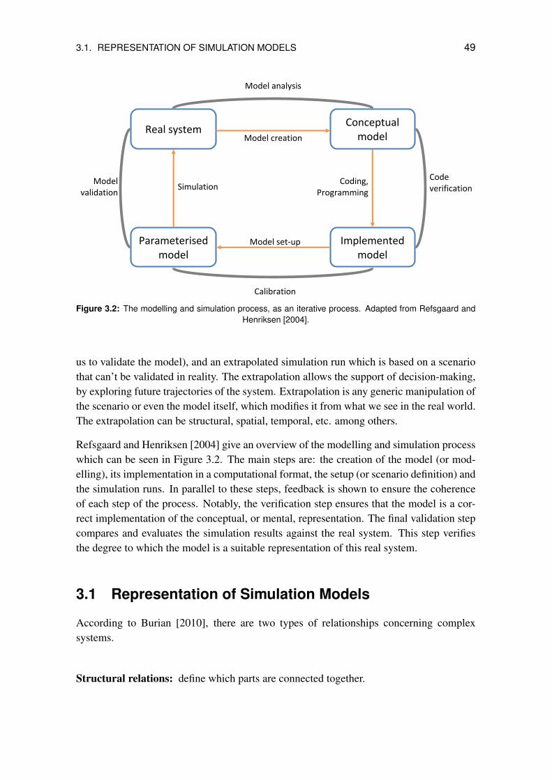
3.1. REPRESENTATION OF SIMULATION MODELS 49
Real system
Implemented model
Calibration
Model analysis
Model creation
Conceptual model
Parameterised model
Coding,Programming
Model set‐up
SimulationCode verification
Model validation
Figure 3.2: The modelling and simulation process, as an iterative process. Adapted from Refsgaard andHenriksen [2004].
us to validate the model), and an extrapolated simulation run which is based on a scenariothat can’t be validated in reality. The extrapolation allows the support of decision-making,by exploring future trajectories of the system. Extrapolation is any generic manipulation ofthe scenario or even the model itself, which modifies it from what we see in the real world.The extrapolation can be structural, spatial, temporal, etc. among others.
Refsgaard and Henriksen [2004] give an overview of the modelling and simulation processwhich can be seen in Figure 3.2. The main steps are: the creation of the model (or mod-elling), its implementation in a computational format, the setup (or scenario definition) andthe simulation runs. In parallel to these steps, feedback is shown to ensure the coherenceof each step of the process. Notably, the verification step ensures that the model is a cor-rect implementation of the conceptual, or mental, representation. The final validation stepcompares and evaluates the simulation results against the real system. This step verifiesthe degree to which the model is a suitable representation of this real system.
3.1 Representation of Simulation Models
According to Burian [2010], there are two types of relationships concerning complexsystems.
Structural relations: define which parts are connected together.

50 CHAPTER 3. MODELLING AND SIMULATION OF COMPLEX SYSTEMS
Functional relations: define the behaviour or dynamics of the system - how does thechange of state of one part influence the state of other connected parts.
The separation of these two concepts: structural and functional, plays an important rolein an initial stage of the analysis and understanding of complex systems. Furthermore,such a differentiation is advantageous when modelling and simulating complex systems.To describe a simulation model, it makes sense to distinguish between a structural and abehavioural representation.
Structural representation The structural description of the model shows only the nameand type of attributes (parameters, variables) and functions (or methods) of the model. Itcan be seen as a black box as it defines the interfaces and internal attributes, but not themode of operation of the model.
Behavioural representation The behavioural representation describes how a model evolvesover time, i.e. how the variables defined above change according to given rules such asmathematical expressions, algorithms, or any other kind of relations. The behavioural de-scription is always based on a structural description as it uses its elements as inputs andoutputs (for instance, the value of a variable is updated according to the values of certainparameters by evaluating an equation).
Simulation models have different types of properties to characterise the model. Even ifthey both describe a value of the model at a given time, we differentiate between variablesand parameters.
Variables Variables, as their name indicates, are able to vary their value throughout thesimulation. They are usually used for outputs or intermediate results or states. Their valuescan be read or evaluated, but are usually not changed from outside the model.
Parameters On the other hand, parameter values are fixed for an entire simulation. Aparameter is used to describe a certain state that is intentionally fixed before running thesimulation. It is usually constant throughout. However, the value can differ from simula-tion to simulation, for example through different instantiations of the same model.
Scenarios A set of parameters describes the characteristics of a simulation run, which wecall a scenario. A scenario is a specific, initial configuration of the model. We can furtherexpand a scenario which will also describe specific actions. A scenario can describe eventsthat might affect the model-run at a given time. These can be discrete events, such as asudden change of value or state, induced intentionally (which are not a result of the modelbehaviour itself). A continuous variation of a value can be part of the scenario description,too, such as the evolution of a temperature or a population over time.
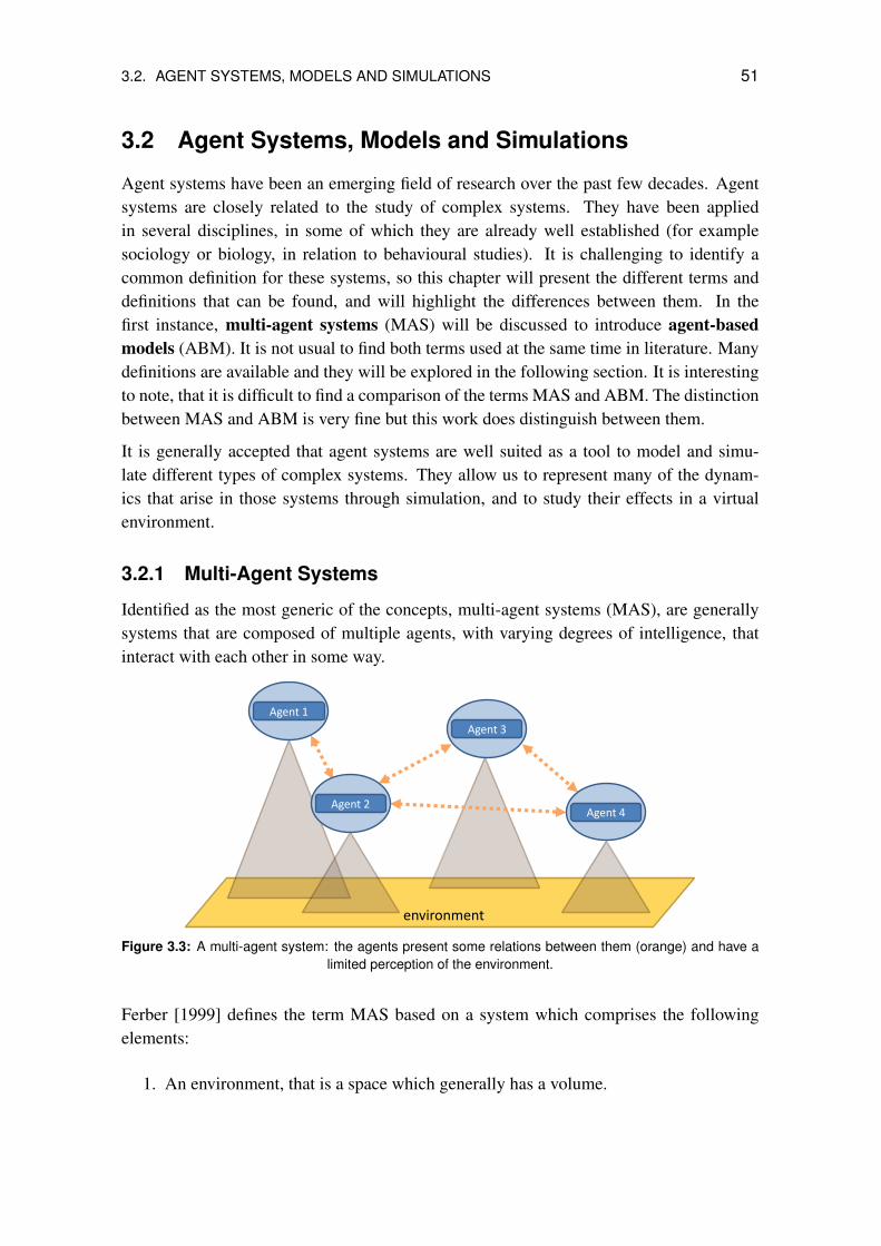
3.2. AGENT SYSTEMS, MODELS AND SIMULATIONS 51
3.2 Agent Systems, Models and Simulations
Agent systems have been an emerging field of research over the past few decades. Agentsystems are closely related to the study of complex systems. They have been appliedin several disciplines, in some of which they are already well established (for examplesociology or biology, in relation to behavioural studies). It is challenging to identify acommon definition for these systems, so this chapter will present the different terms anddefinitions that can be found, and will highlight the differences between them. In thefirst instance, multi-agent systems (MAS) will be discussed to introduce agent-basedmodels (ABM). It is not usual to find both terms used at the same time in literature. Manydefinitions are available and they will be explored in the following section. It is interestingto note, that it is difficult to find a comparison of the terms MAS and ABM. The distinctionbetween MAS and ABM is very fine but this work does distinguish between them.
It is generally accepted that agent systems are well suited as a tool to model and simu-late different types of complex systems. They allow us to represent many of the dynam-ics that arise in those systems through simulation, and to study their effects in a virtualenvironment.
3.2.1 Multi-Agent Systems
Identified as the most generic of the concepts, multi-agent systems (MAS), are generallysystems that are composed of multiple agents, with varying degrees of intelligence, thatinteract with each other in some way.
environment
Agent 1
Agent 2
Agent 3
Agent 4
Figure 3.3: A multi-agent system: the agents present some relations between them (orange) and have alimited perception of the environment.
Ferber [1999] defines the term MAS based on a system which comprises the followingelements:
1. An environment, that is a space which generally has a volume.

52 CHAPTER 3. MODELLING AND SIMULATION OF COMPLEX SYSTEMS
2. A set of objects. These objects are situated, that is to say, it is possible, at a givenmoment to associate any object with a position in the environment. These objectsare passive, that is, they can be perceived, created, destroyed and modified by theagents.
3. An assembly of agents, which are specific objects, representing the active entities ofthe system.
4. An assembly of relations, which link objects (and thus agents) to each other.
5. An assembly of operations, making it possible for the agents to perceive, produce,consume, transform and manipulate objects.
6. Operators with the task of representing the application of these operations and thereaction of the world to this attempt at modification, which we shall call the laws ofthe universe.
These characteristics show that MAS are directly related to complex systems, by sharingmany of their properties. It should be noted that, when referring to a MAS, we are referringto the system, independently whether a real or a virtual system is meant. Furthermore, themodelling aspect is not yet considered at this stage. The term multi indicates that heremultiple agents are considered in the system, usually a large number of them.
3.2.2 Agent-Based Models
Agent-based models(ABM) (also known as multi-agent models or individual based mod-els) are the foundation of a software development approach for the simulation of complexsystems. They are independent of the area of knowledge that they refer to. Agent-basedmodels have been increasingly used over the past few years in, and for systems whichare composed of large number of units that take decisions autonomously, and are there-fore, heterogeneous in nature and unpredictable in essence. These systems are generallycalled complex systems, although this is not a universally agreed term throughout differentdisciplines.
The following definitions can be found in literature:
• “Agent-based modeling (ABM) is a way to model the dynamics of complex systemsand complex adaptive systems. Such systems often self-organize themselves andcreate emergent order. Agent-based models also include models of behavior (humanor otherwise) and are used to observe the collective effects of agent behaviors andinteractions. The development of agent modeling tools, the availability of micro-data, and advances in computation have made possible a growing number of agent-based applications across a variety of domains and disciplines.” [Macal and North,2010]

3.2. AGENT SYSTEMS, MODELS AND SIMULATIONS 53
• “The ABM approach consists of a decentralized collection of agents acting au-tonomously in various contexts. The massively parallel and local interactions cangive rise to path dependencies, dynamic returns and their interaction. In such anenvironment global phenomena such as the development and diffusion of technolo-gies, the emergence of networks, herd-behavior etc. which cause the transformationof the observed system can be modeled adequately. This modeling approach focuseson depicting the agents, their relationships and the processes governing the transfor-mation.” [Pyka and Grebel, 2006]
• “Formally, agent-based modeling is a computational method that enables a researcherto create, analyze, and experiment with models composed of agents that interactwithin an environment.” [Gilbert, 2007]
Basically, ABM focuses on the modeling of systems at a local level through the definitionof their elementary units (called agents), as well as through their interactions. In this sense,it can be said that ABM is a form of modelling MAS. The elementary units are intended tobe modelled in a simple way, while the complexity of the system is an emergent propertyof their interactions. There are three main groups of actions that must be modelled:
1. Sensing the environment: Agents are capable of acquiring information on the localenvironment through sensors.
2. Taking decisions: Each agent can autonomously decide what action should be takenregarding its local information in order to fulfill its objectives.
3. Reaction to the environment: Agents decisions are effected on the environmentthrough actuators. Therefore, a feedback loop exists between the environment andthe agents.
Because agents are defined through local information, an important difference betweenthem and other models is their heterogeneity. Each agent is modelled in the same way,but the input parameters and the local environment can be different. Therefore, decisionstaken by the agents can differ, even when the reasoning process and objectives remain thesame. This is an important difference from traditional models, where several objects of thesame type usually share the same inputs.
Through the agents interaction, emergent phenomena can appear at higher levels. Theseemergent phenomena are not necessarily predictable from their behaviour at an individuallevel. Typical examples in engineering systems are synchronization or de-synchronizationprocesses. Another emergent behavior that is a focus of research through ABM is self-organization. Traditional models are not able to reproduce emergent processes and there-fore they are predictable, from the modeling stage.

54 CHAPTER 3. MODELLING AND SIMULATION OF COMPLEX SYSTEMS
ABM intends to define the individual agents in a simple way, in order to be massivelyand easily replicated. The structure of the system can therefore be dynamically changedthrough the addition or elimination of individual agents, even in simulation time. It ispossible, therefore, to represent long term scenarios, where the structure of the system isin the process of continuous change.
3.2.3 MAS or ABM?
There are no generally accepted definitions for MAS or ABM. Though, we can note somedifferences between these terms. These differences seem to be common according to themajority of the definitions and scope given above.
• MAS refers to a system, where many agents are interacting with each another, insome way, and mostly communicating. Those systems usually are related to largenumbers of agents in an environment. They can be real or virtual.
• ABM refers to a modeling paradigm (class of computational model) which is basedon ”the theory of” agents. It can be certainly used to model a MAS. It refers ratherto the way of modeling entities as agents, giving them the capability to interact.
• ABM is usually conceived in order to perform simulations (as a simulation model).Here, usually the terms agent based simulation (ABS) can be found. ABS are simu-lations performed by ABMs. A MAS is not exclusively a simulation model, but canbe used as one.
In different languages, terms are being literally translated and used different ways. InFrance, for example, it is common to talk about Systemes Multi-Agent referring in generalto agent-based systems, models and often also to simulation. In English, multi-agent sys-tem is not directly linked to the modelling and simulation fields. It is used, rather, for asystem that makes use of autonomous, distributed decision making processes.
3.2.4 The Agent: a Definition
Agents are the most important part of MAS and ABMs, especially when in relation toother, not individual-centric approaches. A commonly accepted definition of an agent isdifficult to find. The most generally accepted definitions are from Weiss and Wooldridge.
Weiss [1999] states that “agents are autonomous, computational entities that can be viewedas perceiving their environment through sensors and acting upon their environment throughits effectors”.
For Wooldridge [2009], “an agent is a computer system that is situated in some environ-ment, and that is capable of autonomous action in this environment in order to meet its
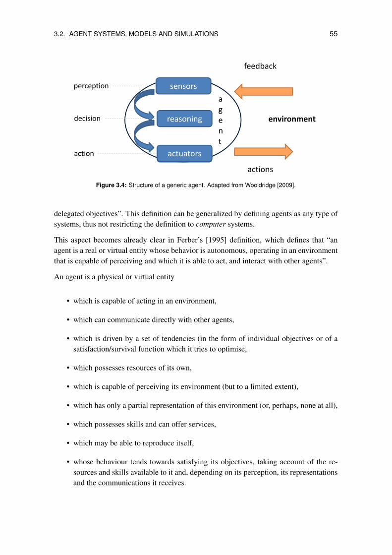
3.2. AGENT SYSTEMS, MODELS AND SIMULATIONS 55
sensorsperception
feedback
reasoning
p p
environment
agedecision reasoning environmentent
decision
actuators
actions
action
Figure 3.4: Structure of a generic agent. Adapted from Wooldridge [2009].
delegated objectives”. This definition can be generalized by defining agents as any type ofsystems, thus not restricting the definition to computer systems.
This aspect becomes already clear in Ferber’s [1995] definition, which defines that “anagent is a real or virtual entity whose behavior is autonomous, operating in an environmentthat is capable of perceiving and which it is able to act, and interact with other agents”.
An agent is a physical or virtual entity
• which is capable of acting in an environment,
• which can communicate directly with other agents,
• which is driven by a set of tendencies (in the form of individual objectives or of asatisfaction/survival function which it tries to optimise,
• which possesses resources of its own,
• which is capable of perceiving its environment (but to a limited extent),
• which has only a partial representation of this environment (or, perhaps, none at all),
• which possesses skills and can offer services,
• which may be able to reproduce itself,
• whose behaviour tends towards satisfying its objectives, taking account of the re-sources and skills available to it and, depending on its perception, its representationsand the communications it receives.

56 CHAPTER 3. MODELLING AND SIMULATION OF COMPLEX SYSTEMS
The definition includes several significant aspects such as, for example, that the agentcan be a physical entity, such as a robot or a machine, which is acting in the real world.However, it can be also a completely virtual entity, such as a computer program that doesnot have any physical existence at all and does not need to interact with the real world.
Characteristics of the Agent
Ferber and Perrot [1995] believe that autonomy is the most fundamental characteristic ofthe agent. Agents seek to meet individual goals in order to jointly achieve a particularobjective that their system should achieve. Autonomy allows the agent to answer or ignorerequests from other agents. Each agent therefore has some degree of freedom to act, whichdifferentiates it from other similar concepts, such as objects, or processes. The agent isthus both an open system because it needs external elements, and a closed system becauseit organises itself. Agents, like classical AI systems are capable of reasoning. They canalso, however, perform actions which can alter their environment. The agents’ environmentcan be defined as everything (that is not an agent) but that interacts with the agent. Agentscan also communicate with each other and this is one of the main modes of interactionbetween agents [Demazeau and Costa, 1996; Abras, 2009].
In order to call something an agent, it should at least fulfill some basic properties: theseare autonomy in its actions (the decision for acting is taken by the agent himself and notdetermined from the exterior), and the agent is able to interact in some way with its en-vironment or with other agents. Moreover, an agent disposes only on local information,which is coupled in some way with the environment. Further properties such as pro-activityor intelligence are typical for agents, but not obligatory. What is important is that the agenthas been conceived with the intention of being able to fulfil these extended functions. It isimportant to enlarge the definition in this way, as it permits a representation of large realobjects as agents, event if they only fulfil rather simple tasks.
3.2.5 The Environment and its Interaction with the Agents
The environment is defined as the part of the system within which the agent operates. It isnot the agent itself nor is it any of the other agents, but rather it is everything that has an(external) influence upon it. As visualised in Figure 3.5, different types of environmentscan be identified. They can be simple, multi-layered, or even change over time. Certainly,an environment can be sufficiently described by one single layer. Even complex stimulican, under certain conditions, be aggregated into one single stimulus to causes one certainreaction. Still, there are some situations where different stimuli cannot be satisfactorilycombined, so that the independent layers for an environment need to be defined.
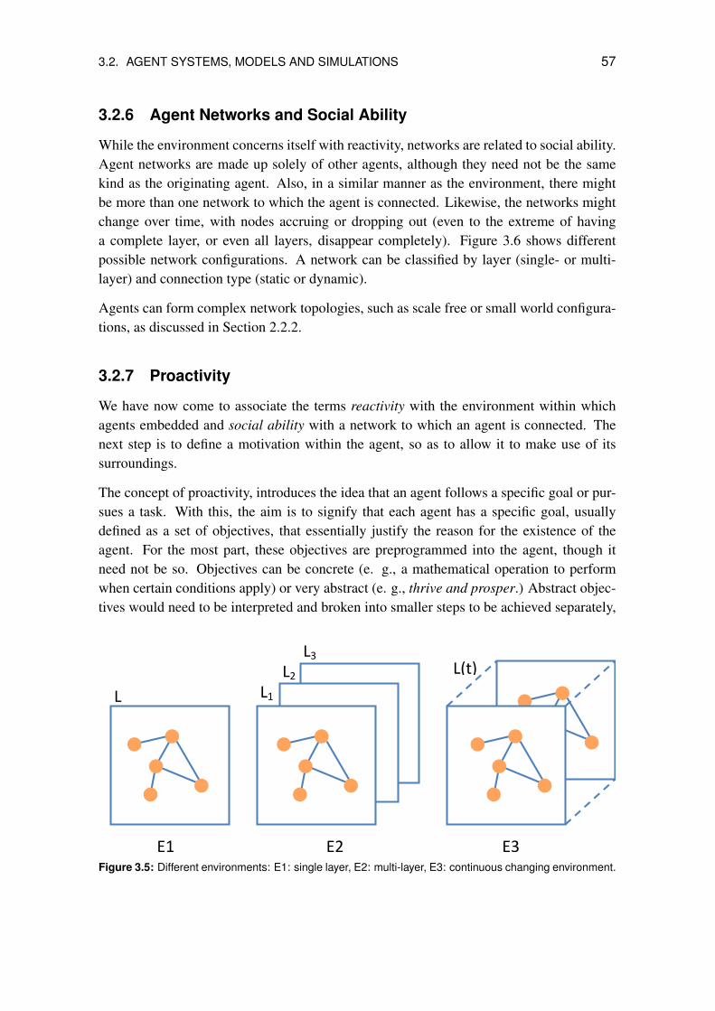
3.2. AGENT SYSTEMS, MODELS AND SIMULATIONS 57
3.2.6 Agent Networks and Social Ability
While the environment concerns itself with reactivity, networks are related to social ability.Agent networks are made up solely of other agents, although they need not be the samekind as the originating agent. Also, in a similar manner as the environment, there mightbe more than one network to which the agent is connected. Likewise, the networks mightchange over time, with nodes accruing or dropping out (even to the extreme of havinga complete layer, or even all layers, disappear completely). Figure 3.6 shows differentpossible network configurations. A network can be classified by layer (single- or multi-layer) and connection type (static or dynamic).
Agents can form complex network topologies, such as scale free or small world configura-tions, as discussed in Section 2.2.2.
3.2.7 Proactivity
We have now come to associate the terms reactivity with the environment within whichagents embedded and social ability with a network to which an agent is connected. Thenext step is to define a motivation within the agent, so as to allow it to make use of itssurroundings.
The concept of proactivity, introduces the idea that an agent follows a specific goal or pur-sues a task. With this, the aim is to signify that each agent has a specific goal, usuallydefined as a set of objectives, that essentially justify the reason for the existence of theagent. For the most part, these objectives are preprogrammed into the agent, though itneed not be so. Objectives can be concrete (e. g., a mathematical operation to performwhen certain conditions apply) or very abstract (e. g., thrive and prosper.) Abstract objec-tives would need to be interpreted and broken into smaller steps to be achieved separately,
E1 E2 E3
L L1
L2
L3 L(t)
Figure 3.5: Different environments: E1: single layer, E2: multi-layer, E3: continuous changing environment.
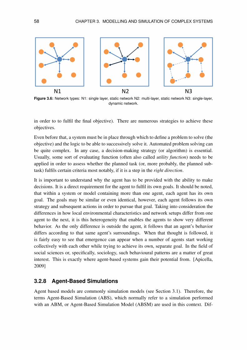
58 CHAPTER 3. MODELLING AND SIMULATION OF COMPLEX SYSTEMS
N1 N2 N3Figure 3.6: Network types: N1: single layer, static network N2: multi-layer, static network N3: single-layer,
dynamic network.
in order to to fulfil the final objective). There are numerous strategies to achieve theseobjectives.
Even before that, a system must be in place through which to define a problem to solve (theobjective) and the logic to be able to successively solve it. Automated problem solving canbe quite complex. In any case, a decision-making strategy (or algorithm) is essential.Usually, some sort of evaluating function (often also called utility function) needs to beapplied in order to assess whether the planned task (or, more probably, the planned sub-task) fulfils certain criteria most notably, if it is a step in the right direction.
It is important to understand why the agent has to be provided with the ability to makedecisions. It is a direct requirement for the agent to fulfil its own goals. It should be noted,that within a system or model containing more than one agent, each agent has its owngoal. The goals may be similar or even identical, however, each agent follows its ownstrategy and subsequent actions in order to pursue that goal. Taking into consideration thedifferences in how local environmental characteristics and network setups differ from oneagent to the next, it is this heterogeneity that enables the agents to show very differentbehavior. As the only difference is outside the agent, it follows that an agent’s behaviordiffers according to that same agent’s surroundings. When that thought is followed, itis fairly easy to see that emergence can appear when a number of agents start workingcollectively with each other while trying to achieve its own, separate goal. In the field ofsocial sciences or, specifically, sociology, such behavioural patterns are a matter of greatinterest. This is exactly where agent-based systems gain their potential from. [Apicella,2009]
3.2.8 Agent-Based Simulations
Agent based models are commonly simulation models (see Section 3.1). Therefore, theterms Agent-Based Simulation (ABS), which normally refer to a simulation performedwith an ABM, or Agent-Based Simulation Model (ABSM) are used in this context. Dif-
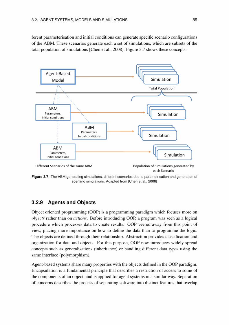
3.2. AGENT SYSTEMS, MODELS AND SIMULATIONS 59
ferent parameterisation and initial conditions can generate specific scenario configurationsof the ABM. These scenarios generate each a set of simulations, which are subsets of thetotal population of simulations [Chen et al., 2008]. Figure 3.7 shows these concepts.
Agent‐Based Model
Total Population
Different Scenarios of the same ABM
ABM Parameters,
Initial conditions
Simulation Simulation Simulation Simulation Simulation
ABM Parameters,
Initial conditions
ABM Parameters,
Initial conditions
Simulation Simulation Simulation
Simulation Simulation Simulation
Simulation Simulation Simulation
Population of Simulations generated by each Scenario
Figure 3.7: The ABM generating simulations, different scenarios due to parametrisation and generation ofscenario simulations. Adapted from [Chen et al., 2008]
3.2.9 Agents and Objects
Object oriented programming (OOP) is a programming paradigm which focuses more onobjects rather than on actions. Before introducing OOP, a program was seen as a logicalprocedure which processes data to create results. OOP veered away from this point ofview, placing more importance on how to define the data than to programme the logic.The objects are defined through their relationship. Abstraction provides classification andorganization for data and objects. For this purpose, OOP now introduces widely spreadconcepts such as generalisations (inheritance) or handling different data types using thesame interface (polymorphism).
Agent-based systems share many properties with the objects defined in the OOP paradigm.Encapsulation is a fundamental principle that describes a restriction of access to some ofthe components of an object, and is applied for agent systems in a similar way. Separationof concerns describes the process of separating software into distinct features that overlap
60 CHAPTER 3. MODELLING AND SIMULATION OF COMPLEX SYSTEMS
in their functionality as little as possible. In agent based systems, an agent has specificobjectives and for different concerns usually different agents are used.
Object oriented programming (OOP) exists as a formalism however, the agent-based sys-tem paradigm does not yet exist, and is not yet as well defined as OOP. There is a certaintendency that agents somehow represent more intelligent objects. According to our def-initions given in Section 3.2.4, an important point is that agents have a proactive role onclearly defined objectives. These aspects, combined with a certain amount of autonomy,differ from the more static objects. Classes in OOP usually have clearly defined goals, butthere is no need for a proactive role.
Wooldridge [2009] sums up the differences in a single phrase:
Objects do it for free, agents do it because they want to.
Interactions between agents are usually more complex than between objects. Messagepassing is a good example of this difference. In OOP, methods are usually called on theobjects, which perform some operations and are pre-programmed to return a given result(usually defined as a result type, such as a primitive type (double, integer) or a type ofobject). Message passing, which is used to communicate between agents, is a more naturalway of communicating, in the sense that messages are sent to a recipient. So far, thisis similar to a method call. However, when a message is sent, the recipient is the oneresponsible for reacting to it, and can decide locally what action to take. In the case ofa method, a predefined code will be run, and is implicitly considered in the method call.Sending messages also allows for communication mechanisms like broadcasting, where amessage is sent to the whole network, and only the agents which feel concerned will reactto it, depending on their local criteria, rules or state.
Message passing, from the implementation point of view, is also a more complex com-munication method. However, it clearly offers more flexibility and is a better adaptedrepresentation of reality in modelling a real system.
3.2.10 Drawbacks and Benefits of ABM
Although there are many examples of applied ABMs, only few evaluations of the methodcan be found. Usually the applications are not compared to other approaches, and theABM community tends to be quite enthusiastic in its approach and avoids confrontationwith other methods. However, the recognition of the method in other areas is a crucialpoint in establishing the foundations of a generally accepted theory on agent systems.
Jennings [2000] states that against this background, there are two major drawbacks asso-ciated with the very essence of an agent-based approach: the patterns and the outcomes ofthe interactions are inherently unpredictable; predicting the behavior of the overall system
3.2. AGENT SYSTEMS, MODELS AND SIMULATIONS 61
based on its constituent components is extremely difficult (sometimes impossible) becauseof the strong possibility of emergent behavior.
In the course of this thesis, there has been an effort to identify relevant drawbacks andbenefits of ABM.
Drawbacks Firstly, due to their individual-centric approach, in which agents can repre-sent large numbers of real entities, a large number of data is necessary to parametrise thesemodels. Also, large datasets are available as output of the models, and have to be correctlyhandled and interpreted. This involves voluminous databases on input and output. Forinput, the existence of large input datasets is presupposed. This is one of the major draw-backs, as in many cases the data is unavailable. However, methods to generate syntheticdata based on real populations are in development [Thiriot and Kant, 2008].
The calibration and validation of these models is difficult, as we deal with a large num-ber of entities, in most cases, which cannot be individually verified. Statistical methodscan be used to assure accuracy at a statistically representative level, however they do notguarantee correctness at the individual level. Therefore, different calibration and valida-tion phases are needed, usually at different levels. ABMs can grow rapidly thus needlarge computational power, as they are scalable and usually large numbers of agents haveto be simulated along with their interactions. Parallelising these types of models is alsoa rather hard task, due to the large number of interactions. Moreover, especially due totheir non-determinism, ABM results have to be correctly interpreted in order to identifyand understand, for instance, emergent phenomena.. Finally, because of their ability tosimulate unexpected behaviours, it is difficult to distinguish between bugs and the desiredbehaviour.
Benefits The modelling approach is based on simple, but heterogeneous, entities (withheterogeneous, autonomous behaviours), which allow a detailed and more realistic repre-sentation of complex systems. ABMs are capable of evolving over time, so it is possibleto add or remove agents and even change the structure of the system during the simula-tion. Agents are represented in a simplified but intuitive way, as they are described by realentities of the system, often located in a concrete environment. ABMs provide integrativesolutions that embed many simplified models in order to represent a complex system witha large number of components and interactions. The visualisation and representation of thesimulated phenomena can significantly improve exploration, discussion and informationexchange on the models. ABMs allow the extraction of high resolution data, even for mid-and long term scenarios. Because of their stochastic, non-deterministic nature, results canbe given in the form of solution spaces instead of deterministic results (for example usingmethods like Monte-Carlo). An agent-based approach allows us to represent, in a more in-tuitive way, the relationship between causes and effects. As we will see in the case studiespresented in the previous chapters, ABMs allow us to better understand the behaviour of
62 CHAPTER 3. MODELLING AND SIMULATION OF COMPLEX SYSTEMS
complex systems and their phenomena, through an exploration of the modelled system. Wewill see how an ABM helps us to understand complex, emergent phenomena and explaintheir causes at an individual level.
3.3 System Dynamics
System Dynamics (SD) is a method which was developed by J. Forrester in the 1950’s atthe Massachusetts Institute of Technology [Forrester, 1961]. It is intended to analyse andsimulate (through modelling) complex and dynamic systems at system level. It is basedon a representation using stocks and flows and characterized by using internal feedbackloops. These loops affect the behavior of the entire system, as they are able to reproducethe non-linearities of complex systems.
System dynamics falls under the so-called macro-simulation approaches, which describethe behavior at a high, aggregated system level. SD is applied where a behavior of indi-vidual entities is not directly regarded and does not have to be differentiated. However,knowledge at the aggregated level must be available. Meaningful variables defining thesystem behavior must be identified. They are then related to each other through differen-tial equations.
Being originally developed to understand the complexity in industrial processes, SD is nowapplied to a wide variety of fields. Most of the applications are related to policy making andanalysis. Qualitative approaches and models are common. However, the many soft vari-ables in the models, which sometimes make it difficult to estimate parameters for a quan-titative application, have resulted in this kind of application being less well established.
The simulation of SD models is run computationally on small step calculations (numericalapproach solving methods) that update all the variables at each time step. These meth-ods are needed to correctly represent the feedback effects, as the resulting mathematicalsystems which need to be solved are also usually of a non-linear nature. A SD model ad-dresses the values of the state of the system, which varies over time. SD defines severalformalisms in order to represent its models. There are two types of diagrams: casual loopdiagrams and stock and flow diagrams.
3.3.1 Casual Loop Diagrams
Casual Loop Diagrams (CLD) show the casual relationships of the system in a graphic way.They help visualise the causes and effects that appear among the interrelated variables ofthe system. The CLD diagram is constructed by connecting different nodes. It is a directedgraph with nodes representing system variables and directed arcs representing the binaryrelationships between these variables.
We can distinguish between two types of feedback loops:
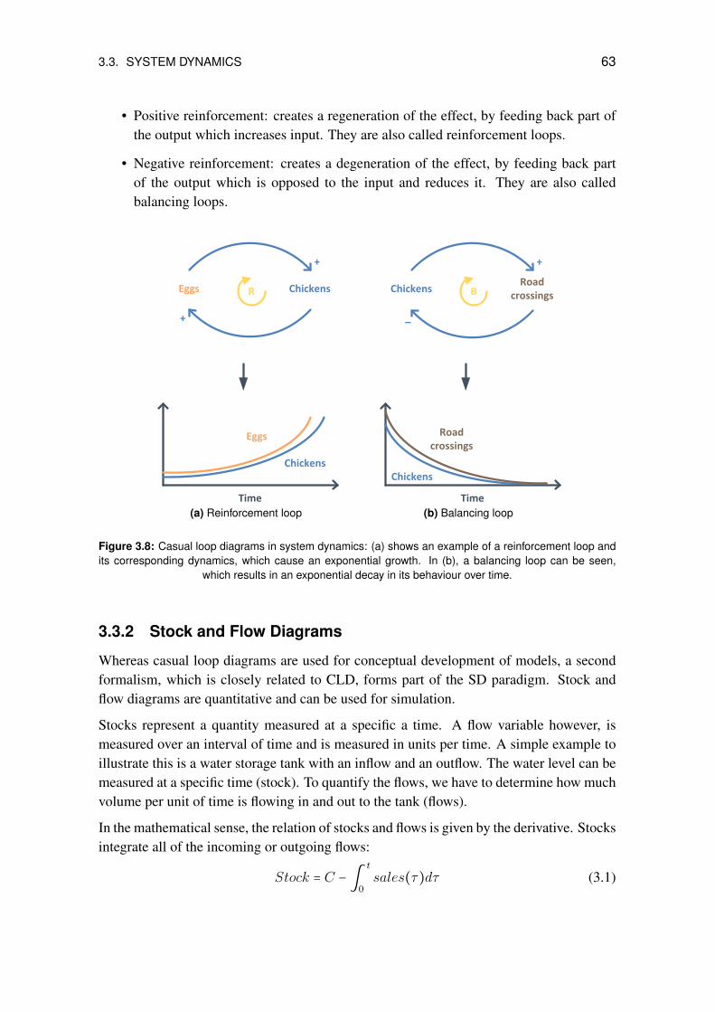
3.3. SYSTEM DYNAMICS 63
• Positive reinforcement: creates a regeneration of the effect, by feeding back part ofthe output which increases input. They are also called reinforcement loops.
• Negative reinforcement: creates a degeneration of the effect, by feeding back partof the output which is opposed to the input and reduces it. They are also calledbalancing loops.
Time
Eggs Chickens
+
+
R
Chickens
Eggs
(a) Reinforcement loop
Road crossings
+
BChickens
Time
Road crossings
Chickens
–
(b) Balancing loop
Figure 3.8: Casual loop diagrams in system dynamics: (a) shows an example of a reinforcement loop andits corresponding dynamics, which cause an exponential growth. In (b), a balancing loop can be seen,
which results in an exponential decay in its behaviour over time.
3.3.2 Stock and Flow Diagrams
Whereas casual loop diagrams are used for conceptual development of models, a secondformalism, which is closely related to CLD, forms part of the SD paradigm. Stock andflow diagrams are quantitative and can be used for simulation.
Stocks represent a quantity measured at a specific a time. A flow variable however, ismeasured over an interval of time and is measured in units per time. A simple example toillustrate this is a water storage tank with an inflow and an outflow. The water level can bemeasured at a specific time (stock). To quantify the flows, we have to determine how muchvolume per unit of time is flowing in and out to the tank (flows).
In the mathematical sense, the relation of stocks and flows is given by the derivative. Stocksintegrate all of the incoming or outgoing flows:
Stock = C − ∫
t
0sales(τ)dτ (3.1)
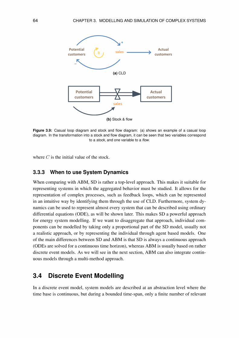
64 CHAPTER 3. MODELLING AND SIMULATION OF COMPLEX SYSTEMS
Potential customers
sales
+
B
–
Actual customers
(a) CLD
Actual customers
Potential customers
sales
(b) Stock & flow
Figure 3.9: Casual loop diagram and stock and flow diagram: (a) shows an example of a casual loopdiagram. In the transformation into a stock and flow diagram, it can be seen that two variables correspond
to a stock, and one variable to a flow.
where C is the initial value of the stock.
3.3.3 When to use System Dynamics
When comparing with ABM, SD is rather a top-level approach. This makes it suitable forrepresenting systems in which the aggregated behavior must be studied. It allows for therepresentation of complex processes, such as feedback loops, which can be representedin an intuitive way by identifying them through the use of CLD. Furthermore, system dy-namics can be used to represent almost every system that can be described using ordinarydifferential equations (ODE), as will be shown later. This makes SD a powerful approachfor energy system modelling. If we want to disaggregate that approach, individual com-ponents can be modelled by taking only a proportional part of the SD model, usually nota realistic approach, or by representing the individual through agent based models. Oneof the main differences between SD and ABM is that SD is always a continuous approach(ODEs are solved for a continuous time horizon), whereas ABM is usually based on ratherdiscrete event models. As we will see in the next section, ABM can also integrate contin-uous models through a multi-method approach.
3.4 Discrete Event Modelling
In a discrete event model, system models are described at an abstraction level where thetime base is continuous, but during a bounded time-span, only a finite number of relevant

3.5. MULTI-APPROACH MODELLING 65
events occur. The state of the system can change due to these events. In between events,the state of the system is not allowed to change. This is unlike the continuous models inwhich the state of the system may change continuously over time Vangheluwe et al. [2002].
One of the formalisms which is based on discrete events is the state-chart. State-chartswere firstly unified by Harel [1987], who proposed a notation which is now generallyaccepted throughout different fields. For example, it is the base for the normalisation ofstate-charts in the Unified Modelling Language (UML). State-charts are representations offinite state automata (as they are known in computer science). This formalism allows therepresentation of the complexity of these automata in a manageable way.
3.5 Multi-Approach Modelling
Models of system behaviour can be represented at different levels of abstraction or detailas well as through different modelling methods and formalisms. The particular methodand level of abstraction depends on the background and goals of the modeller, as well ason the system which is to be modelled [Vangheluwe et al., 2002].
Decision-making for a complex system requires an understanding of the behaviour of theoverall system. Studying the individual components of the system will usually not beenough. The complexity of this system and its model is due to several factors.
• The number of interacting, coupled, concurrent components.
• The variety of component formalisms. Often, a mix of continuous and discrete com-ponents occurs.
• The variety of views, at different levels of abstraction.
Complex behaviour is often a consequence of a large number of interactions. These inter-actions can also create feedback loops which reinforce this complex behaviour. In orderto represent these aspects, one formalism or modelling paradigm is usually not enough,as it will reduce the point of view to a certain level of abstraction or to a specific compo-nent; or will neglect the interactions between them. Also, depending on the questions tobe answered by the model, different abstraction levels have to be chosen. Components ofthe system itself may require different levels of abstractions, depending on their role in thesystem. The choice of the modellings paradigm is usually related to:
• the results that need to be provided by the model,
• the abstraction level,
• the amount and quality of data available for calibration and validation and
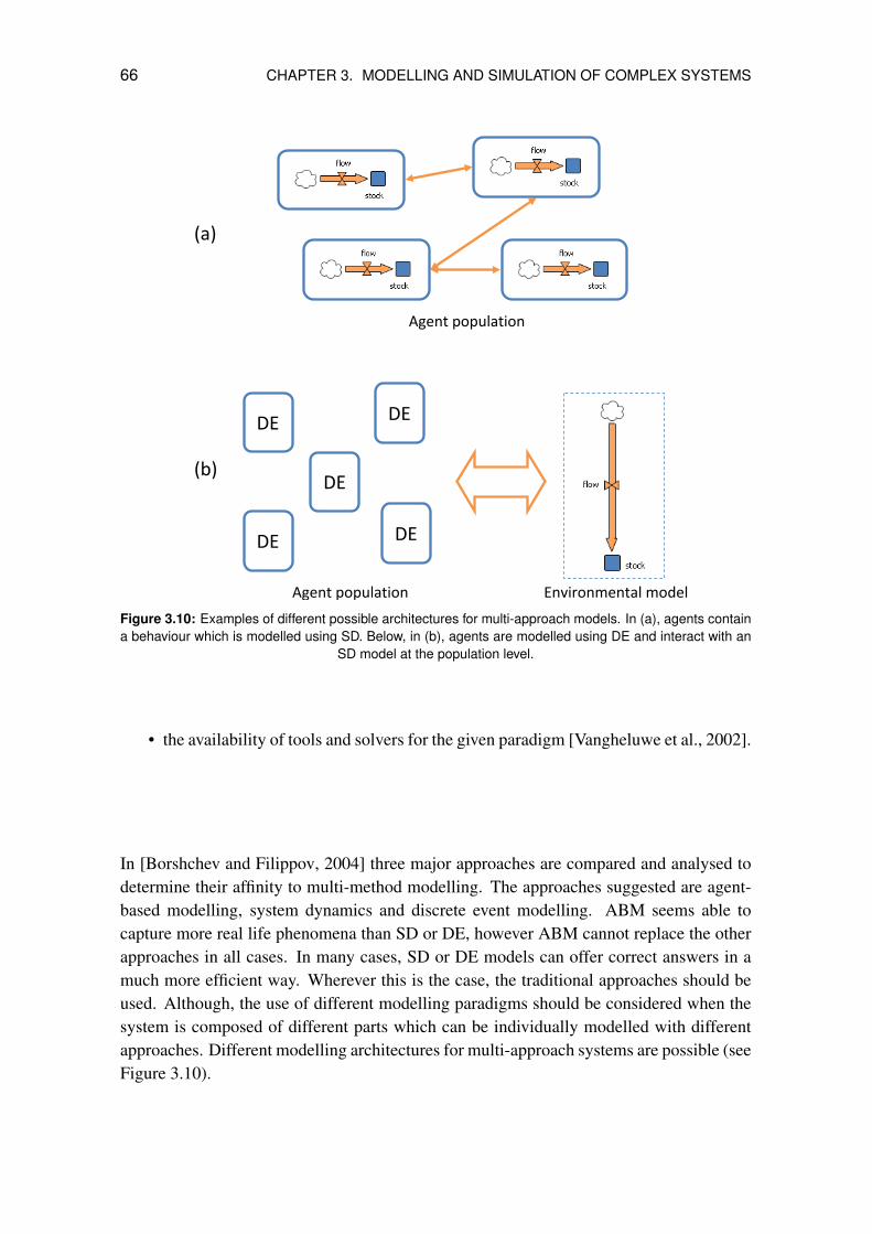
66 CHAPTER 3. MODELLING AND SIMULATION OF COMPLEX SYSTEMS
Agent population
DE
Environmental model
DE
DE
DE DE
Agent population
(a)
(b)
Figure 3.10: Examples of different possible architectures for multi-approach models. In (a), agents containa behaviour which is modelled using SD. Below, in (b), agents are modelled using DE and interact with an
SD model at the population level.
• the availability of tools and solvers for the given paradigm [Vangheluwe et al., 2002].
In [Borshchev and Filippov, 2004] three major approaches are compared and analysed todetermine their affinity to multi-method modelling. The approaches suggested are agent-based modelling, system dynamics and discrete event modelling. ABM seems able tocapture more real life phenomena than SD or DE, however ABM cannot replace the otherapproaches in all cases. In many cases, SD or DE models can offer correct answers in amuch more efficient way. Wherever this is the case, the traditional approaches should beused. Although, the use of different modelling paradigms should be considered when thesystem is composed of different parts which can be individually modelled with differentapproaches. Different modelling architectures for multi-approach systems are possible (seeFigure 3.10).

3.6. SYSTEMS-OF-SYSTEMS 67
3.6 Systems-of-Systems
The term system-of-systems (SoS) is a collection of task-oriented or dedicated systems thatpool their resources and capabilities together to achieve a new, more complex meta-system.This meta-system itself offers more functionality and performance than simply the sum ofthe individual systems from which it is constituted [Markarian et al., 2011].
One can easily argue [Kremers et al., 2010] that energy systems, and especially smartenergy systems, which tend to be more distributed and decentralised, mostly satisfy thefive principal characteristics that distinguish them as true systems-of-systems, as definedby Maier [1998]:
1. Operational independence of the elements: The elements of the energy systems areable to operate independently and usefully while fulfilling autonomous goals. Pro-ducers, consumers and other elements can work properly when they are not con-nected to the energy system as a whole, or can work as independent and autonomoussystems themselves (for example microgrids).
2. Managerial independence of the elements: energy systems not only can operate in-dependently, they do operate independently. They maintain a continuing operationalexistence independent of the SoS.
3. Evolutionary development: The energy system does not appear fully formed. Its fu-ture development and existence is evolutionary and depends of other environmentalagents.
4. Emergent behaviour: The energy system performs functions and carries out purposesthat do not reside in any component system. These behaviours are emergent proper-ties of the entire SoS and cannot be localised to any component system. The maingoals of the electrical system are given by these behaviours.
5. Geographic distribution: The geographic extent of the energy system is large. Thecomponents of the energy system can readily exchange information (and, in thiscase, can also exchange energy).
3.7 Calibration and Validation of Agent-Based Models
Calibration describes the process of adjusting the model and its parameters in order toobtain desired results. A validation is usually an evaluation of those results through com-parison with real data. The validation of agent-based models is, itself, a complex subject.Scepticism about ABM is because the validation process is not easy and cannot be per-formed in the same way as in deterministic models. As agent-based models usually cover
68 CHAPTER 3. MODELLING AND SIMULATION OF COMPLEX SYSTEMS
different scales of the system (at least two, the individual and the systemic one), a vali-dation should be performed at these two scales, at a minimum. An individual validationis possible by the comparison of individual agents with real data or measurements. In thecase of energy systems, an individual power plant or a specific consumer can be parame-terized and compared with real data. The validity of an individual model can therefore beconfirmed, as in classical validations.
However, when aggregating a population of replicated agents, the results at populationlevel are also relevant (usually more relevant than the individual ones). Once having cali-brated the individual agents, a calibration of the model at an aggregated level should takeplace. This is usually possible through the available macro-data (in the case of energysystems, measurements at an aggregated scale such as a transformer or substation).
This second validation has to performed in consistence with the first one. Aggregatedvalidations are closely related to the statistical effects of the system. Heterogeneity amongdifferent agents can impact the stability of the results. Therefore, probabilistic methodssuch as Monte-Carlo simulations should be used. However, a second validation at systemlevel does not ensure, that the representation of the system at intermediate levels will becorrect. In only confirms that, at an aggregated level, the results are correct. It does notreveal anything about intermediate aggregations of parts of the population or effects inlocal clusters. In either case, a two step validation already ensures consistency betweentwo levels of the system. This might suggest that intermediate levels will not suffer atoo large degree of incorrectness. If enough data is available, additional calibrations canbe performed. These will, however, increase the degree of complexity of the process,as consistence between all the calibrated levels should be maintained. Furthermore, ifdealing with multi-scale models, a validation at each main scale should be performed at aminimum.
It is unlikely that a complete validation of an agent-based model could be achieved becauseof the large amount of data and the complexity of the model itself. Additional expertvalidations are very important in order to ensure the validity of the models.
3.8 Complex System Modelling – also in the Energy Field?
Once we have given an overview of modelling and simulation of complex systems in gen-eral, one may ask what this approach can add to the modelling of complex systems. Thecomplex modelling approach does not aim to substitute current modelling tools, but rathermodel the system from a new point of view. In order to model a system such as the elec-trical energy system using a complex approach, agent-based modelling seems a reasonablerepresentation of the system from an individual perspective. This considers its different,single components. Furthermore, it could be interesting to include non-technical aspectsinto the model, as the complexity approach is inherently interdisciplinary and considers

3.8. COMPLEX SYSTEM MODELLING – ALSO IN THE ENERGY FIELD? 69
not only one domain. This could enrich the models by including human behavioural orenvironmental aspects such as meteorology. Of course, this is not an easy task. Manyquestions arise, such as:
• How can we be sure that an individual model of an entity will be correct?
• How can we represent different objects of the same entity in a realistic way (thinkabout TV, which might be the same concept but have many different technologicalimplementations (cathod ray, LCD, plasma, etc.)?
• How do we know that a population of individual models correctly represents the realpopulation?
• Is it worth the effort to model individually when averaged models already give goodanswers?
• And last but not least: What is the real added value of this approach?
These questions will be addressed in the following chapters. At this stage, it is clear that theincreasing complexity of the electrical system, such as the trend towards a smart grid, callsmany traditional methods into question. The classical approaches are not able to handlesystemic issues however, modelling the system from a complex point of view can possiblyovercome some of these limitations. The need for coupling technical and social behaviormodels seems to be essential to capture systemic behaviours in complex infrastructuresystems as the electrical grid.


Chapter 4
Electrical Energy System Modelling
It can scarcely be denied that the supreme goal of all theory is to make theirreducible basic elements as simple and as few as possible without having tosurrender the adequate representation of a single datum of experience.
Albert Einstein [1934].
In order to represent an energy system as a complex system through an agent-based ap-proach, it is necessary to individually model the components. Therefore, a special focusis put on modelling the components, or entities of the system, as they behave rather thantaking a macro-system approach of using statistical models or averaged, high level repre-sentations. Entities of the electrical system need to be modelled by taking into accounttheir individual states and modes of operation. This can also be called micro-modelling, asfor example, the objective is not to model a consumer by statistical means, representing anaggregated, averaged and typical behaviour. Rather, each individual household should bemodelled, parameterized by information which can be taken from statistical datasets, andthen recreating each household as an individual entity generating a power curve.
It is important to note that a very deep and detailed approach is an ambitious challenge.As Albert Einstein’s quotation indicates, the models should be made as simple as possible,but no simpler. There are already a large number of energy system models, each veryspecific and detailed for their concrete area of application. This is the case for classicalengineering models. which represent the technical aspects of the power grid. These couldbe the representation of the physical processes of the system, such as electrical, magneticor charge effects, by using the laws of Ohm, Joule, Gauss, or the Maxwell equations. Ofcourse, for technical analysis, these forms of representation are very important. However,when representing the energy system as a whole by modelling its individual components,the representation of a large number of entities in this way can consume a lot of resources.Possibly, depending on the questions to be solved, this might not even be needed. So,
71
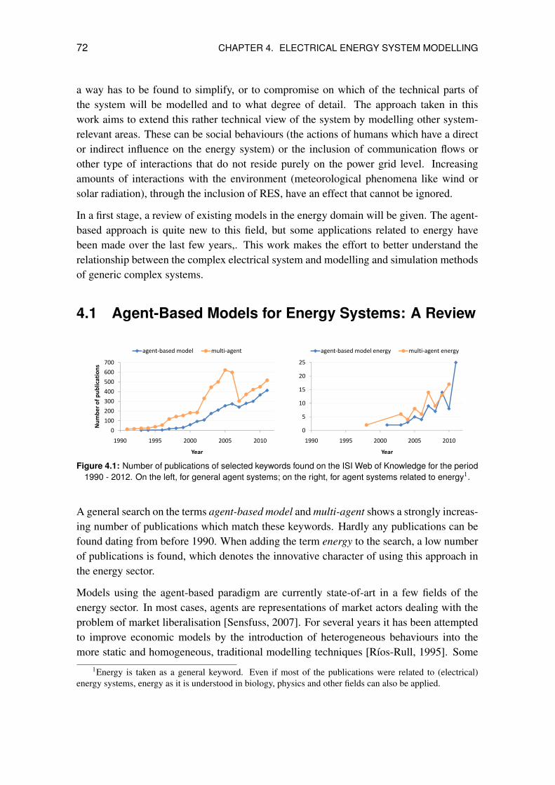
72 CHAPTER 4. ELECTRICAL ENERGY SYSTEM MODELLING
a way has to be found to simplify, or to compromise on which of the technical parts ofthe system will be modelled and to what degree of detail. The approach taken in thiswork aims to extend this rather technical view of the system by modelling other system-relevant areas. These can be social behaviours (the actions of humans which have a director indirect influence on the energy system) or the inclusion of communication flows orother type of interactions that do not reside purely on the power grid level. Increasingamounts of interactions with the environment (meteorological phenomena like wind orsolar radiation), through the inclusion of RES, have an effect that cannot be ignored.
In a first stage, a review of existing models in the energy domain will be given. The agent-based approach is quite new to this field, but some applications related to energy havebeen made over the last few years,. This work makes the effort to better understand therelationship between the complex electrical system and modelling and simulation methodsof generic complex systems.
4.1 Agent-Based Models for Energy Systems: A Review
300
400
500
600
700
r o
f p
ub
licat
ion
s
agent‐based model multi‐agent
0
100
200
1990 1995 2000 2005 2010
Nu
mb
er
Year
10
15
20
25
agent‐based model energy multi‐agent energy
0
5
1990 1995 2000 2005 2010
Year
Figure 4.1: Number of publications of selected keywords found on the ISI Web of Knowledge for the period1990 - 2012. On the left, for general agent systems; on the right, for agent systems related to energy1.
A general search on the terms agent-based model and multi-agent shows a strongly increas-ing number of publications which match these keywords. Hardly any publications can befound dating from before 1990. When adding the term energy to the search, a low numberof publications is found, which denotes the innovative character of using this approach inthe energy sector.
Models using the agent-based paradigm are currently state-of-art in a few fields of theenergy sector. In most cases, agents are representations of market actors dealing with theproblem of market liberalisation [Sensfuss, 2007]. For several years it has been attemptedto improve economic models by the introduction of heterogeneous behaviours into themore static and homogeneous, traditional modelling techniques [Rıos-Rull, 1995]. Some
1Energy is taken as a general keyword. Even if most of the publications were related to (electrical)energy systems, energy as it is understood in biology, physics and other fields can also be applied.

4.1. AGENT-BASED MODELS FOR ENERGY SYSTEMS: A REVIEW 73
agent-based models like Sugarscape by [Epstein and Axtell, 1996; Epstein, 2006] showthe emergence of counter-intuitive behaviours related to distributed decision-making fromheterogeneous agents. These approaches show that the more spatially distributed a systemis, the more important it is to take care of local interactions and the differences betweenagents. In energy systems, the spatial component is essential, especially if taking intoaccount distributed measures, which are applied locally, such as is the case in the smartgrid.
McArthur et al. [2007a,b] identify that the stumbling block for multi-agent systems in thepower engineering domain is mainly a lack of experience with these types of systems inthe industrial context, as well as the lack of standards. This is one of the reasons for arather slow introduction of agent-based approaches in the sector, in comparison to otherdisciplines such as biology or social sciences, where standards and the development of realsystems is not that relevant.
Chappin and Dijkema [2007] elucidate the impact of CO2 emission trading on Europeanelectricity production through a specifically created agent-based model. The model emu-lates the long-term evolution of European electricity production as a series of investmentdecisions by independent agents. The results underpin recommendations for CO2-policy.
Quite a number of ABMs exist on the energy market. They mainly focus on the economiceffects of energy systems. Agents usually represent actors in the market, which behaveautonomously and have some kind of influence on the market. In [Sensfuss, 2007], ABMsdealing primarily with energy markets are reviewed. Furthermore, an agent-based modelof the German electricity sector has been developed. For this purpose, electricity demandand generation, as well as the electricity market were modelled through agent-based ap-proaches. This work focuses on the economic effects of the introduction of renewableenergy sources such as the effect on spot market prices of electricity. Other examples ofenergy markets can be found in [Jacobo et al., 2008], which models the electricity marketof the United Kingdom; in [Tellidou and Bakirtzis, 2009] and [Chan et al., 2010].
Agent-based approaches have also been made on technical design and electrical and controlengineering. Notably, models dealing with the control of small autonomous grids, calledmini- or microgrid control can be found. First approaches on applying MAS for controlof mini- or microgrids date back to Tolbert et al. [2001]. Hatziargyriou et al. [2005] applyMAS to the centralised and decentralised control of microgrids. Dimeas and Hatziargyriou[2005] propose a MAS based framework for the control of microgrids. The main objectiveis to present a system capable of integrating several functionalities and to propose a gen-eral scheme for the control of microgrids. Dimeas and Hatziargyriou [2007] present theadvantages of using agents for Virtual Power Plant (VPP) control. More specifically thispaper, through examples and case studies, explains how local intelligence and the socialability of the agents could provide solutions for the optimal and effective control of a VPP.

74 CHAPTER 4. ELECTRICAL ENERGY SYSTEM MODELLING
Other agent based models for microgrid control can be found in [Jiang, 2006; Oyarzabalet al., 2007; Pipattanasomporn et al., 2009]
In relation to the smart grid and future information and communication on a trans-nationalinterconnected power grid, Tranchita et al. [2010] propose different suitable modellingapproaches, among them ABM, which could help acquire a better understanding of thenewly identified risks of including ICT into the energy system.
The author has contributed to the development of several agent-based models for energysystem analysis over the past few years. In [Evora et al., 2011] the Tafat framework for sim-ulating complex energy systems is presented, which includes important software engineer-ing techniques like Model Driven Engineering. Based on a metamodel, models includingdifferent behaviours can be automatically created. To model domestic demand, a disag-gregated model of electricity consumers is created. A case study simulating the load curveof 1 000 households, composed of five different social groups, is discussed and comparedwith an aggregated curve. The model represents the load curve of a sample of householdsusing a bottom-up approach and is a promising, powerful and high performance tool forenergy system modelling.
In [Gonzalez de Durana et al., 2009] an example of a simple Hybrid Renewable EnergySystems (HRES) is presented and an ABM for such systems, a microgrid, oriented todesigning a decentralised supervisory control was developed. In [Kremers et al., 2009]and [Kremers et al., 2011], an agent-based, multi-scale wind generation model is presented.This model will be discussed further in the next chapters. Viejo and Kremers [2009] presentan ABM of an integral island energy system, which represents the high voltage grid and canbe used for decision making on regional planning scenarios. Modelling microgrids throughan initial complex system approach, based on agents is presented in [Kremers et al., 2010],where some first simulation results from an integrated load flow algorithm were shown.In [Gonzalez de Durana et al., 2010] the importance of interaction among different layersof the systems was identified, as well as the need for systemic models which are able todeal with different layers and scales. The models presented in these publications serve asa basis for this work.
4.2 Modelling Approach
Agent-based modelling tools are able to capture complex system behaviour such as wantedand unwanted emergent behaviour in these systems, internal and external events, communi-cations within the system, etc. In particular, local effects of the single units comprising thesystem can be modelled and their effects can be analysed at the system level. On the otherhand, technical models of the single agents are necessary. Therefore, dynamic systemshave to be represented in the form of the physical and mathematical models of the devices.
4.2. MODELLING APPROACH 75
Furthermore, the large amounts of interactions and feedback appearing in distributed en-ergy systems make linear simulation models inappropriate for systemic simulations.
Therefore, an agent-based approach has been chosen. This approach is combined withother complex-system-relevant tools, such as system dynamics and discrete event simu-lation. The agent-based approach allows the inclusion of other modelling methods, forexample modelling the reasoning of an agent. They can also be coupled either at a parallellevel or embedded in a hierarchical structure.
The agent-based approach was chosen because it is able to represent autonomous entities,which interact with their environment. While retaining a broad definition of what an agentcan be, we can imagine representing even very simple entities of the energy system throughagents. So, for example, an electrical heater has a constant operating power, which can beswitched on and off. It interacts with the environment through heat dissipation and powerconsumption. Its behaviour is defined simply by a constant consumption. Modelling theentities of the system in this way, also allows an encapsulated and hierarchically structuredrepresentation, as we suppose that an agent (as an extension of objects in object orientedprogramming, and inheriting their properties) can have one or more other agents nestedinside itself. What is important to remark is that, even if the agents are modelled in asimple way, the modular structure of an agent based model allows for the improvementof the behaviour of the entities at any stage. This enables the addition of extra features,such as an intelligent control, to the previously mentioned heating system. The degreeof intelligence is not limited, so an agent can include any kind of decision algorithm,from the most simple to the most complex. The advantage is that the modelling systemprovides the potential for this from the beginning. This is because it has been conceivedwith these features in mind, and to overcome issues of non-modular or difficultly extensibleapproaches.
Using this type of approach allows the modelling of energy systems from a complex sys-tems point of view (as proposed in Section 2.4). It also means that the design of the modelhas to be carefully chosen.
A classical, top-down approach is not sufficient to model a complex system. The represen-tation of complex phenomena like emergence, requires that the system should be based onindividual rules which describe it in a bottom-up approach. These kinds of models enableemergence. It should be ensured that these phenomena emerge from the model, and arenot explicitly programmed into it.
4.2.1 Challenges of the Electrical System
Some of the challenges of future energy systems that could be tackled using a complexsystem approach through simulation with agent-based models are:

76 CHAPTER 4. ELECTRICAL ENERGY SYSTEM MODELLING
Extrapolation of results Dealing with smart grid demonstrators opens new research ques-tions which were not addressed some years ago. When testing new smart grid technologieson pilot demonstrators or individual experiments, large-scale penetration is not contem-plated. Results, based on small amounts of data should be extrapolated to a larger scale,on at least two levels:
• Larger penetration scales of a given territory (higher density of installations)
• Larger geographical spread (extrapolation to a geographically larger territory)
Furthermore, the capacity of ABM representing different scales simultaneously can helpto solve the uncertainties of changing the scale of applications.
Centralisation - decentralisation Using a bottom-up approach allows the modelling ofdecentralised decision making and, at the same time, the connectivity of agents enables acentralised control. Therefore, ABMs are suitable for the comparison of both centralisedand decentralised control strategies on the same energy system.
Adaption and evolution in dynamical systems Models based on agents are easily mod-ified on a unit basis, and therefore can truly reproduce adaptive and evolutionary mecha-nisms. Modelling based on agents focuses on individual units and therefore these units canbe hybrid and don’t have to be totally homogeneous, as it is the case in energy systems.Through their reactivity to the environment, these models are dynamic in an unstable equi-librium. This characteristic of ABMs can reproduce unexpected behaviour on the system,like snowball effects.
Representation of technical as well as social models The use of agents as encapsulat-ing units in a general sense, allows the inclusion of many types of models from differentfields. Through standardized interfaces it is possible to combine these models in the sameframework. This, for example, permits an interaction between sociological and technicalmodels.
Behavioural changes The reactivity of ABM and the possibility of evolution over timeallow the implementation of models that take into account different behaviours on the sameenvironment. Therefore they are suitable for models where behavioural changes have astrong impact.
4.2.2 Multi-Scale System Modelling
Multi-scale modelling is an emerging subject of research and development, in which sys-tems are represented in different structural, spatial and temporal scales. These systems
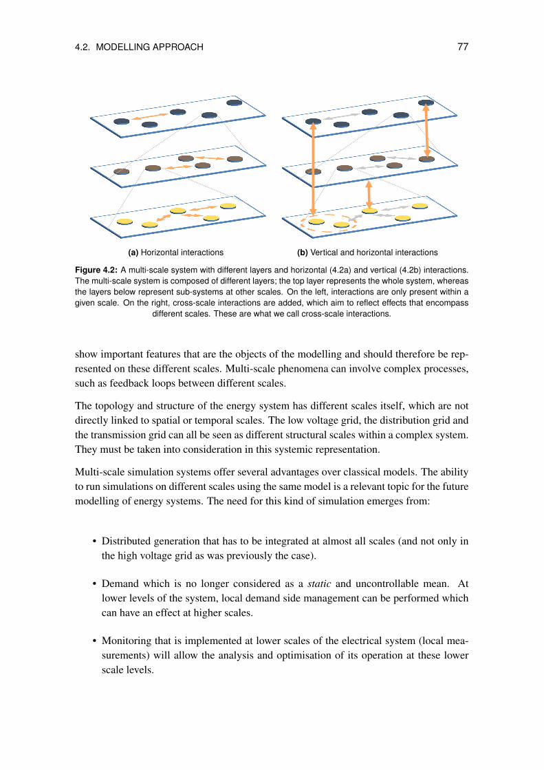
4.2. MODELLING APPROACH 77
(a) Horizontal interactions (b) Vertical and horizontal interactions
Figure 4.2: A multi-scale system with different layers and horizontal (4.2a) and vertical (4.2b) interactions.The multi-scale system is composed of different layers; the top layer represents the whole system, whereasthe layers below represent sub-systems at other scales. On the left, interactions are only present within agiven scale. On the right, cross-scale interactions are added, which aim to reflect effects that encompass
different scales. These are what we call cross-scale interactions.
show important features that are the objects of the modelling and should therefore be rep-resented on these different scales. Multi-scale phenomena can involve complex processes,such as feedback loops between different scales.
The topology and structure of the energy system has different scales itself, which are notdirectly linked to spatial or temporal scales. The low voltage grid, the distribution grid andthe transmission grid can all be seen as different structural scales within a complex system.They must be taken into consideration in this systemic representation.
Multi-scale simulation systems offer several advantages over classical models. The abilityto run simulations on different scales using the same model is a relevant topic for the futuremodelling of energy systems. The need for this kind of simulation emerges from:
• Distributed generation that has to be integrated at almost all scales (and not only inthe high voltage grid as was previously the case).
• Demand which is no longer considered as a static and uncontrollable mean. Atlower levels of the system, local demand side management can be performed whichcan have an effect at higher scales.
• Monitoring that is implemented at lower scales of the electrical system (local mea-surements) will allow the analysis and optimisation of its operation at these lowerscale levels.
78 CHAPTER 4. ELECTRICAL ENERGY SYSTEM MODELLING
Furthermore, simulating several scales in the same model has the advantage that there arefewer models and no need to port data between platforms. This leads to a more efficientsimulation run and decision-making support. The challenges of these kinds of simulationsare that a multi-scale model, at present, is not as accurate as a purpose-built model. So, themodelling method, the parameters, etc. included must be carefully chosen to ensure bothflexibility and accuracy. Further attention has to be put on the inter-scale interactions. Thisis a complex issue, as multi-scale systems require both horizontal and vertical interactions.Horizontal interactions should be easily managed, as they take place within the same scale.Vertical, cross-scale interactions enable the representation of complex system phenomena.These cross-scale interactions must be modelled carefully to a design that that enablesthem. This is not an easy task.
Figure 4.2 shows these interactions in a multi-scale system. Current agent-based modelsusually take place only at a fixed scale and in general do not encompass different scales orlayers. Adding multiple scales to the representation of the system increases the degree ofcomplexity. However, only in this way can complex interactions at different levels of thesystem be represented.
Multi-scale models usually also have to deal with different spatial and time resolutions,which should be adapted to each scale. When modelling cross-scale interactions, differentrepresentations have to be considered. Geographical information systems (GIS) can beused to represent different spatial resolutions and the location of the entities,.
4.3 Socio-Technical System Models
Social sciences use simulation modelling as a tool in order to analyse and understand phe-nomena related to human behaviour. Behavioural models include a large degree of uncer-tainty, as their aim is to represent difficulty predictable, or only statistically characterisable,actions. These models have therefore to be non-deterministic in order to capture the het-erogeneity of the actors. Behavioural models can only be validated with difficulty, due totheir complex decision making processes.
On the other hand, technical models aim to represent the operation of technical systems.These systems (in the real world) are usually intended to be deterministic, or at least, theirmode of operation is completely known as these systems are, in fact, man-made. Modelsrepresenting those systems are directly aimed to recreate the system’s mode of operation,for example based on its physical laws or discrete states. Their operation can be usuallymodelled in an unequivocal, predictable way and is deterministic.
Socio-technical systems are present in the real world everywhere in which a technicalsystem interacts with human behaviour. This is the case for almost all technical systems.In order to model the ”whole” behaviour, human behaviour has to be added to technicalmodels. Coupling social with technical models is therefore a requirement for modelling
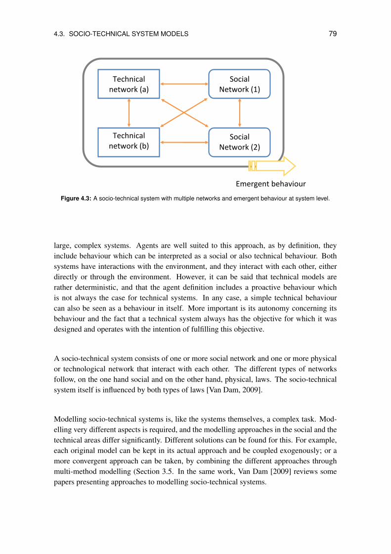
4.3. SOCIO-TECHNICAL SYSTEM MODELS 79
Technical network (a)
Technical network (b)
Social Network (1)
Social Network (2)
Emergent behaviour
Figure 4.3: A socio-technical system with multiple networks and emergent behaviour at system level.
large, complex systems. Agents are well suited to this approach, as by definition, theyinclude behaviour which can be interpreted as a social or also technical behaviour. Bothsystems have interactions with the environment, and they interact with each other, eitherdirectly or through the environment. However, it can be said that technical models arerather deterministic, and that the agent definition includes a proactive behaviour whichis not always the case for technical systems. In any case, a simple technical behaviourcan also be seen as a behaviour in itself. More important is its autonomy concerning itsbehaviour and the fact that a technical system always has the objective for which it wasdesigned and operates with the intention of fulfilling this objective.
A socio-technical system consists of one or more social network and one or more physicalor technological network that interact with each other. The different types of networksfollow, on the one hand social and on the other hand, physical, laws. The socio-technicalsystem itself is influenced by both types of laws [Van Dam, 2009].
Modelling socio-technical systems is, like the systems themselves, a complex task. Mod-elling very different aspects is required, and the modelling approaches in the social and thetechnical areas differ significantly. Different solutions can be found for this. For example,each original model can be kept in its actual approach and be coupled exogenously; or amore convergent approach can be taken, by combining the different approaches throughmulti-method modelling (Section 3.5. In the same work, Van Dam [2009] reviews somepapers presenting approaches to modelling socio-technical systems.
80 CHAPTER 4. ELECTRICAL ENERGY SYSTEM MODELLING
4.4 Simulation and Modelling Tools used
The paradigm shift in the energy sector involves new challenges for the modelling and sim-ulation of energy systems. More decentralised models that can reproduce the autonomousbehaviour of the different units of the system are needed. The models currently used relylargely on experiences gained over the last decades, and are thus suited to hierarchicallycontrolled one-way systems. A review of tools is presented in Valov and Heier [2006].This includes several commercial tools used in power engineering, such as Eurostag orPSS/E and a number of non-proprietary tools, such as several toolboxes based on Mat-lab/Simulink, for example Matpower Zimmerman et al. [2011] or PSAT Milano [2009].
Matlab is probably the most widely used simulation program for control systems at theacademic level, although there are many other programs like Maple, Mathematica, Octave,Scilab, etc. that are also very common. With Matlab, simulations are possible in a mathe-matical sense, i.e. to apply numerical methods to solve differential equations representingthe system. However, as it is designed using technologies from the 1950’s-60’s, it lacksthe advantages of more modern object-oriented software. These advantages are evidentif the system to model is of discrete event type and even more so if it is a hybrid or anagent-based system.
Taking this approach, we will look at the problem from a new perspective, trying to of-fer new solutions with an innovative approach based on multi-method modelling. Thiswork presents the opportunities and possibilities of a complex system approach to energysystems, as well as being an example of how modelling and simulation can help to exam-ine and analyse potential smart grid architectures, configurations, and strategies prior toimplementation.
Other agent-based tools are:
• Swarm
• Repast
• Netlogo
Anylogic is a well-regarded program in the community of multi-approach simulations, butlittle known in the areas of automation and control engineering. Anylogic is based on thelatest advances in object-oriented modelling applied to complex systems [Borshchev andFilippov, 2004]. It currently supports three approaches or modelling paradigms:
• System Dynamics (SD)
• Discrete Events (DE)

4.5. ENVIRONMENTAL AND PRODUCTION MODELS 81
• Agent Based Models (ABM)
These three approaches are mutually compatible, so that for example, in modelling a hybridsystem we might use the SD method for the continuous part of the differential equationsand the DE method for modelling the events. Anylogic models are multiplatform, portableJava applications that can run on their own anywhere a Java Runtime Environment (JRE)is installed. The models can be also run in a web browser as a Java Applet, which isan easy way of publishing the models. Moreover, Anylogic allows the development ofanimations of active objects: the assembly of the image is done automatically. In this waythe animations are highly reusable and can be displayed on applets.
In Anylogic, scalable models can be easily created, because it is possible to define arraysof objects whose size is a parameter of the model. It is possible to even reflect the dynamicchanges that can occur in a real system, by adding or deleting items, or changing theirinterconnection, during run time. Some of the simulation algorithms have been modifiedto work in hybrid environments (hybrid state machines) combining both continuous anddiscrete systems.
For continuous systems, we use the SD approach. This approach allows us to directlyinsert differential equations into the models, which are solved in Anylogic. As it usesthe SD formalism there is a clear overview of the dependencies of stocks and flows. InAppendix D how to model differential equations in SD in Anylogic is shown.
Furthermore, Anylogic includes an optimization engine based on the OptQuest packagefrom OptTek Systems. These tools allow a framework for simulation model runs which in-cludes parameter variation experiments, calibration (through optimisation) of parameters,optimisation, and Monte-Carlo runs.
4.5 Environmental and Production Models
Production of electricity can be mainly classified as conventional or renewable, from thepoint of view of the primary energy source used. In the following section, we will addressrenewable energy sources (RES), as they are especially relevant for modern grids.
Some of the RES are strongly correlated to environmental conditions. This is particularlythe case with wind and solar power; although other RES might also be affected by me-teorological effects. In the following example, the production models shown are used,making a special focus on RES. This has allowed greater focus on the fluctuating RES,which introduce stochastic and unpredictable magnitudes into the energy system.

82 CHAPTER 4. ELECTRICAL ENERGY SYSTEM MODELLING
4.5.1 Wind Power Generation Model
This model2 aims to represent wind power production by modelling wind farms consistingof wind turbine units on different time scales, ranging from short (minutes) to long-termsimulations (months). The model takes into account fluctuating wind speeds and technicalreliability. It can compute the aggregated output power of the wind farm influenced bydifferent random factors and can, thus, recreate a realistic power unit for integral energysystem simulations. The simulation of this data is performed in real time, so that poweroutput at a specific time can be reproduced and injected into the energy system simulation.
Stochastic Wind Speed Simulation
Generating realistic wind speeds is an important task for analysing the effects of windproduction in an electricity system. Fluctuating wind speed is the origin of the tempo-ral variation of power injected by this production type and thus has direct effects on theproduction-demand balance and grid stability. One of the challenges of wind speed simu-lators is to reproduce the different scale term fluctuations, as described in [Nichita et al.,2002]. To this end, different models have been developed. The model chosen here is builtup in two steps, comprising slow and fast components, [Bayem et al., 2008] with someminor modifications. More accurate wind models (that take into consideration e.g. long-term [Billinton et al., 1996] or cross-correlations [Allerton, 2008]) are available, but thisone is sufficient for the purposes of this work. An overview of some more approaches canbe found in [Aksoy et al., 2004]. It is important to add that to get a realistic simulation ofa specific site, records of historical data are needed to obtain the parameters of the model,as even the best model is useless if not accurately fitted.
The slow component The first part, which is used in previous works of the author [Kre-mers et al., 2009; Viejo and Kremers, 2009] is a generator of hourly mean wind speeds.This time series model is based on an ARMA (Auto-Regressive Moving-Average modelwhich is given by
yt = φ1 yt−1 + φ2 yt−2 + . . . + φn yt−n+ αt + θ1αt−1 + θ2αt−2 + . . . + θmαt−m
(4.1)
The data series yt is used to build the model, i.e. to calculate the auto-regressive φi; i =
1,2, . . . , n and the moving average parameters θj; j = 1,2, . . . ,m. {αt} is a Gaussianwhite noise process with zero mean and standard deviation of σα which is part of themoving average (MA) part of the model. Considering the orders, the process is referredto as ARMA(n,m). The parameters used in this work were chosen from an ARMA(3,2)approach, but the model was developed up to ARMA(4,3) and can be easily adapted to
2The following sections are inspired on the works published by the author in [Kremers et al., 2009] andthe book chapter [Kremers et al., 2011].
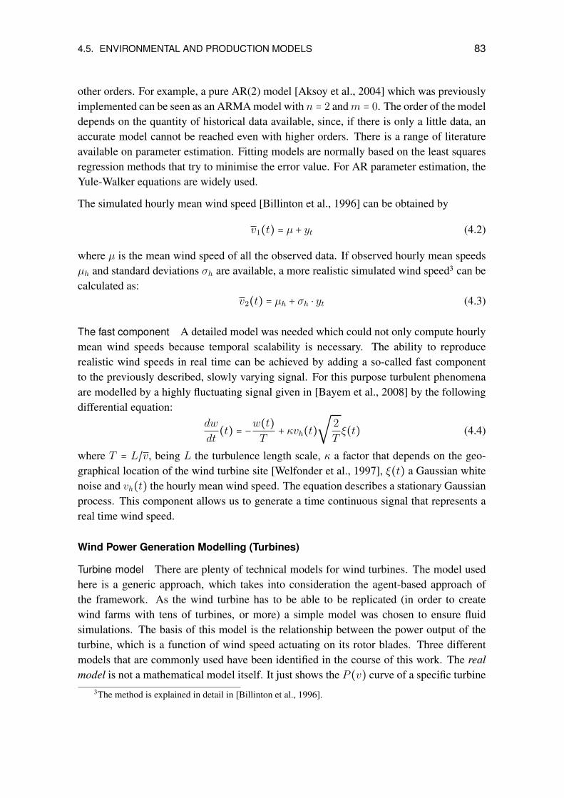
4.5. ENVIRONMENTAL AND PRODUCTION MODELS 83
other orders. For example, a pure AR(2) model [Aksoy et al., 2004] which was previouslyimplemented can be seen as an ARMA model with n = 2 andm = 0. The order of the modeldepends on the quantity of historical data available, since, if there is only a little data, anaccurate model cannot be reached even with higher orders. There is a range of literatureavailable on parameter estimation. Fitting models are normally based on the least squaresregression methods that try to minimise the error value. For AR parameter estimation, theYule-Walker equations are widely used.
The simulated hourly mean wind speed [Billinton et al., 1996] can be obtained by
v1(t) = µ + yt (4.2)
where µ is the mean wind speed of all the observed data. If observed hourly mean speedsµh and standard deviations σh are available, a more realistic simulated wind speed3 can becalculated as:
v2(t) = µh + σh ⋅ yt (4.3)
The fast component A detailed model was needed which could not only compute hourlymean wind speeds because temporal scalability is necessary. The ability to reproducerealistic wind speeds in real time can be achieved by adding a so-called fast componentto the previously described, slowly varying signal. For this purpose turbulent phenomenaare modelled by a highly fluctuating signal given in [Bayem et al., 2008] by the followingdifferential equation:
dw
dt(t) = −
w(t)
T+ κvh(t)
√2
Tξ(t) (4.4)
where T = L/v, being L the turbulence length scale, κ a factor that depends on the geo-graphical location of the wind turbine site [Welfonder et al., 1997], ξ(t) a Gaussian whitenoise and vh(t) the hourly mean wind speed. The equation describes a stationary Gaussianprocess. This component allows us to generate a time continuous signal that represents areal time wind speed.
Wind Power Generation Modelling (Turbines)
Turbine model There are plenty of technical models for wind turbines. The model usedhere is a generic approach, which takes into consideration the agent-based approach ofthe framework. As the wind turbine has to be able to be replicated (in order to createwind farms with tens of turbines, or more) a simple model was chosen to ensure fluidsimulations. The basis of this model is the relationship between the power output of theturbine, which is a function of wind speed actuating on its rotor blades. Three differentmodels that are commonly used have been identified in the course of this work. The realmodel is not a mathematical model itself. It just shows the P (v) curve of a specific turbine
3The method is explained in detail in [Billinton et al., 1996].
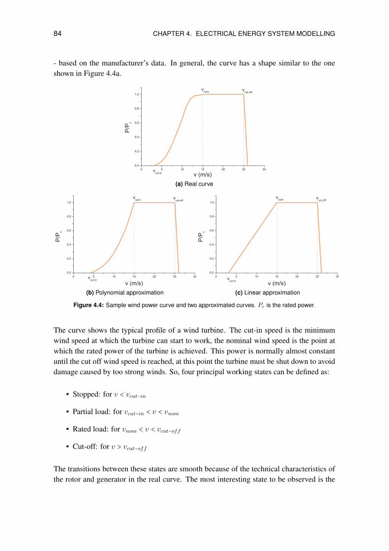
84 CHAPTER 4. ELECTRICAL ENERGY SYSTEM MODELLING
- based on the manufacturer’s data. In general, the curve has a shape similar to the oneshown in Figure 4.4a.
(a) Real curve
(b) Polynomial approximation (c) Linear approximation
Figure 4.4: Sample wind power curve and two approximated curves. Pr is the rated power.
The curve shows the typical profile of a wind turbine. The cut-in speed is the minimumwind speed at which the turbine can start to work, the nominal wind speed is the point atwhich the rated power of the turbine is achieved. This power is normally almost constantuntil the cut off wind speed is reached, at this point the turbine must be shut down to avoiddamage caused by too strong winds. So, four principal working states can be defined as:
• Stopped: for v < vcut−in
• Partial load: for vcut−in < v < vnom
• Rated load: for vnom < v < vcut−off
• Cut-off: for v > vcut−off
The transitions between these states are smooth because of the technical characteristics ofthe rotor and generator in the real curve. The most interesting state to be observed is the
4.6. CONSUMPTION MODELS 85
partially loaded state, where the turbine shows a non-linear P (v) dependence. Here thestart dynamics of the turbine, as well as the adaptation to the fully loaded capacity at ratedspeed, can be observed. This phase can be approximated by a polynomial term as shownin Figure 4.4b. The polynomial model assures the curved shape of the curve, but the tracejust before achieving the nominal wind speed is idealised. The linear approximation of thecurve, which is used in more simplified models, can be defined by a linear interpolationof the values for vcut−in and vnom. It can be seen in Figure 4.4c. The last model mightbe used only when the characteristic wind speeds of the turbine (and no power curve) areavailable. Though, the polynomial approach can be also be used as an approximation byusing a polynomial of degree three as described in [Chedid et al., 1998].
The cut-off state is reached when the turbine gets shut down because of exceeding vcut−off .Further, a vcut−back−in parameter can be defined for the model. Its value denotes the windspeed at which the turbine restarts after being in the cut-off state. This value describes therestart process of the machines after strong wind periods.
Being MTBF the Mean Time Between Failures of a unit defined by
MTBF =1
λ=
operational time
number of failures(4.5)
where λ is the failure rate. Using MTBF allows modelling the availability of a windturbine over time. The equation describing the Mean Time To Recover
MTTR =down time
number of failures(4.6)
is also included, where down time is the time when the turbine is inactive because of afailure, maintenance or reparations. The MTTR is therefore an indicator for the averagedown-time between an incident and the following start up. A failure model is integratedinto the turbine model which takes into account these two parameters. The rates (inversevalues of them) are used to determine failure probability used in the transition betweenstates.
4.6 Consumption Models
As we have seen in previous chapters (Section 2.3.2, there are different methods for mod-elling electrical consumption. As discussed, there is a need for high-resolution mod-els in order to clearly understand the composition of a load curve. Aggregated models,like standard load profiles, can approximate the load curve for a large number of con-sumers, but might be wrong for a particular population or region. In order to have a high-resolution model of domestic demand, several models of household appliances were devel-oped [Costa Gomez, 2011]. Called technical models they represent the device’s consump-tion load curve. However, in many cases this is not enough to represent the consumption

86 CHAPTER 4. ELECTRICAL ENERGY SYSTEM MODELLING
of a household, as these technical models do not include the associated human behaviour.They are therefore, like an unused appliance. Additionally, we need a social behaviouragent which controls the devices. This agent is the most complex part of the model. Thesocial behaviour agent will decide when to switch on or off certain devices, as a humanbeing would do. However, the more device there are in a household, and the more personsliving within, the more complex the different dependencies and correlations of the usageof the devices will become. Initial approaches to this were made in [Evora et al., 2011] inwhich 1000 households were simulated by using a simplified model of social behaviour.
As we can see, the micro-modelling of domestic demand is a quite complex task. In thegiven context, we will address one appliance, a refrigerator, in order to be able to illustratea concrete case study where the impact of the given appliance can be clearly observed. Asimple, social behaviour is included to represent the use of the refrigerator; it is conditionedby door openings followed by the insertion and extraction of items.
4.6.1 Modelling a Refrigerator
A refrigerator was chosen as an example of consumption device. Refrigerators offer amore complex behaviour than static loads that do not vary over time (like lighting or en-tertainment devices), but are continuously connected to the energy supply. Therefore, re-frigerators offer an interesting potential for demand side management. Acting as thermalstorage, a refrigerator is capable of being disconnected for some time, and then can laterrecover the lost energy, without having a high impact on the quality of the service it offers.In order to study and analyse a refrigerator’s potential for load shedding, a detailed model
SD refrigerator
model
DSM device Frequency
Load curveShedding
Door opening
agent
Environmental conditions
Figure 4.5: Overview of the refrigerator model: the core thermal model (called SD refrigerator model) iscoupled with a DSM device which permits load shedding, and additionally with an environment and a door
opening agent. Finally, the electrical part of the model is coupled with the energy system.
is described which will later be implemented in simulation. The structure of the model isbased on a thermal model that describes the thermal processes in the refrigerator (calledSD refrigerator model). It is coupled with a DSM device to unplug the refrigerator under
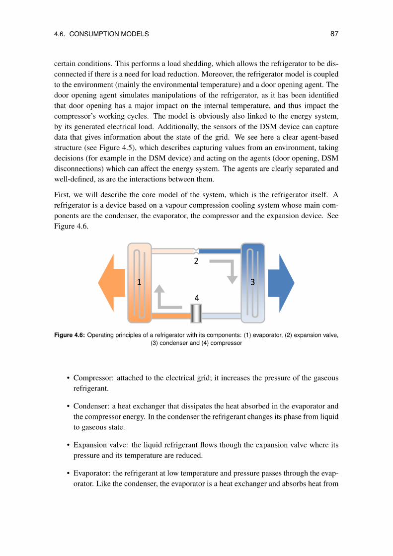
4.6. CONSUMPTION MODELS 87
certain conditions. This performs a load shedding, which allows the refrigerator to be dis-connected if there is a need for load reduction. Moreover, the refrigerator model is coupledto the environment (mainly the environmental temperature) and a door opening agent. Thedoor opening agent simulates manipulations of the refrigerator, as it has been identifiedthat door opening has a major impact on the internal temperature, and thus impact thecompressor’s working cycles. The model is obviously also linked to the energy system,by its generated electrical load. Additionally, the sensors of the DSM device can capturedata that gives information about the state of the grid. We see here a clear agent-basedstructure (see Figure 4.5), which describes capturing values from an environment, takingdecisions (for example in the DSM device) and acting on the agents (door opening, DSMdisconnections) which can affect the energy system. The agents are clearly separated andwell-defined, as are the interactions between them.
First, we will describe the core model of the system, which is the refrigerator itself. Arefrigerator is a device based on a vapour compression cooling system whose main com-ponents are the condenser, the evaporator, the compressor and the expansion device. SeeFigure 4.6.
2
4
3 1
Figure 4.6: Operating principles of a refrigerator with its components: (1) evaporator, (2) expansion valve,(3) condenser and (4) compressor
• Compressor: attached to the electrical grid; it increases the pressure of the gaseousrefrigerant.
• Condenser: a heat exchanger that dissipates the heat absorbed in the evaporator andthe compressor energy. In the condenser the refrigerant changes its phase from liquidto gaseous state.
• Expansion valve: the liquid refrigerant flows though the expansion valve where itspressure and its temperature are reduced.
• Evaporator: the refrigerant at low temperature and pressure passes through the evap-orator. Like the condenser, the evaporator is a heat exchanger and absorbs heat from
88 CHAPTER 4. ELECTRICAL ENERGY SYSTEM MODELLING
its environment. The liquid refrigerant, which flows into the evaporator, is trans-formed into gas by absorbing heat from inside.
The refrigerator model used in this study is based on the heat fluxes of its internal cell, theevaporator and the exterior. These fluxes are described by a set of differential equationswhich characterise the heat transfer processes. The principles of the models are describe in[Cerri et al., 2003]. This model was extended to include door opening and charge effects.Door opening has a significant impact on the internal air temperature, especially when therefrigerator is situated in a warm environment. The food and drinks in the refrigeratoralso are relevant for the dynamics and inertia of the inner cell temperature, and function asheat storage. The evolution of internal temperature is described by a differential equationthat takes into account the heat transfer process between the external environment and therefrigerator cell and the cooling contributions by the evaporator plate, as well as direct airexchanges due to door opening and heat exchanges with the contents:
dTidt
=Te − Tiτe−i
+Tp − Tiτp−i
+Tl − Tiτl−i
+Qdoor (4.7)
where Ti is the internal cell temperature, Te the temperature of the environment, Tp thetemperature of the evaporator plate. τe−i is a time constant describing the heat transferbetween the internal cell temperature and the environment. This constant depends on thethermal capacity of the cell, the surface of the walls in contact with the exterior and theheat transfer coefficient of the insulation of the cell. τp−i is the time constant for the heattransfer process between the evaporator and the inner cell. This constant depends on thethermal capacity of the inner volume, the surface of the evaporator and the heat transfercoefficient between the evaporator and the inner cell. Tl is the average temperature of theassumed content in the refrigerator. τl−i describes the heat transfer time constant betweenthe charge and the internal air temperature, and will depend on the surface and type ofcontent. Qdoor describes the effect of a door opening.
The variation of the temperature of the evaporator plate is obtained by
dTpdt
=Ti − Tpτi−p
−δc⋅Qf +Qext
Cp(4.8)
where τi−p is a time constant describing the heat fluxes from the plate to the inner cell,depending on the thermal capacity of the plate, its surface and the heat transfer coefficientbetween the plate and the inner cell. Qf is the cooling capacity of the plate, which ismultiplied by a switching variable δc to denote that this capacity only affects the systemwhen the compressor is working. The value is δc = 1 for the working phase and δc = 0
when the compressor is idle. Cp is the thermal heat capacity of the evaporator fluid andQext an exponential function of time which describes the effect of released thermal powerafter the compressor switches off and is explained in detail in [Cerri et al., 2003].
4.6. CONSUMPTION MODELS 89
The thermostat controlling the compressor turns it on when the temperature drops aboveTp,max, but doesn’t turn it off again until the temperature falls below Tp,min. Hence, thevalue of δc is triggered by two temperature thresholds in a hysteresis process, where:
δc =
⎧⎪⎪⎨⎪⎪⎩
0 if Tp < Tp,min1 if Tp > Tp,max until Tp < Tp,min.
(4.9)
When the compressor switches off after a refrigeration cycle, the thermal power is releasedwith the cooling fluid, passing from the condenser to the evaporator plate through theexpansion valve. This phenomena is described in Cerri et al. [2003] as an exponentialfunction of time.
The opening of the refrigerator door creates an immediate heat exchange between the envi-ronment air temperature and the interior, usually by warmer air flowing into the cell. Thisheat exchange is added to Equation 4.7 as an additional term:
Qdoor =δd ⋅ (Te − Ti)
τd(4.10)
The term is characterized by δd which expresses the heat exchange due to door openings.δd = 1 only if the door is open; if it is closed it equals zero. The time constant τd representsthe heat transfer by air exchange between the environment and the inner cell.
The effect of the load contained in the cell can be described as a heat transfer processbetween the internal cell temperature and the temperature of the contents.
dTldt
=Ti − Tlτi−l
(4.11)
where τi−l is a time constant depending on the type of contents (food, drinks, etc.), itsthermal capacity and its surface in contact with the air of the inner cell.
Finally, the electrical power Pel is described by the coefficient of performance and thecooling capacity of the plate:
Pel =Qf
COP(4.12)
4.6.2 Inclusion of Social Behaviour through Door Opening
In addition to the technical behaviour of the refrigerator, the operation of the compressorcycles is strongly effected by the refrigerator’s use. Door opening and (warm) contentsplaced into it can prolong refrigeration cycles and thus prolong consumption. In order torecreate and include these uncertainties, a stochastic model has been included to represent

90 CHAPTER 4. ELECTRICAL ENERGY SYSTEM MODELLING
the human behaviour that causes door opening. This door opening agent controls the re-frigerator door and is embedded in the refrigerator. The model is based on a discrete eventstate-chart, which triggers the δd values of the differential Equation (4.10).
The agent implements a random door opening, based on an average daily rate. The averagenumber of daily door opening n is defined by µn. The agent opens the door randomly,according to an exponential distribution, with a mean according to the given parameter. Sofor example, the mean of random openings per day will have a certain value, which can behigher or lower in a particular case, as this is a non-deterministic model. In any, case, overa longer period or several refrigerators, the average will tend to n→ µopeningsPerDay.
The second set of parameters defines the duration of each opening. This is calculated bya random number, which is taken from a normal distribution with the mean defined by themean time µdoDuration and the standard deviation σdoDuration of the door opening.
4.7 Storage and Smart Grid measures
Electrical storage plays an important role in smart grid technologies. Being able to storeenergy and release it at another time allows a more flexible use, and control, of resources.
4.7.1 Generic Storage Model
The term storage systems is intentionally used to describe the variety of implementingstorage in an energy network. The different technologies within which the systems arerealised (batteries, compressed air, etc.) are not relevant in this model. An abstract modelof a storage system will be used to make a generic approach to the problem, rather thanattempting to solve it using developing technologies with all their constraints .
The main model is described by the following equation,
dE(t)
dt= Pin(t) − Pout(t) − Ploss (4.13)
where E is the energy content of the storage, Pin the effective in-flowing power, Pout theeffective out-flowing power, and Ploss the power lost in storage. These describe the lossesover time when storage is in the static mode (no in- or out-flows), but in which the amountof energy gets reduced over time. Usually they are given in units like kWh per month, forinstance. It can be a function of E, in a detailed model. Conversion losses are added by anefficiency ηin
Pin = ηinP′in (4.14)
which describes the relationship between the real in-flow power P ′in and the effective in-
flow. Analogously this can is defined for the real output power P ′out
P ′out = ηoutPout. (4.15)
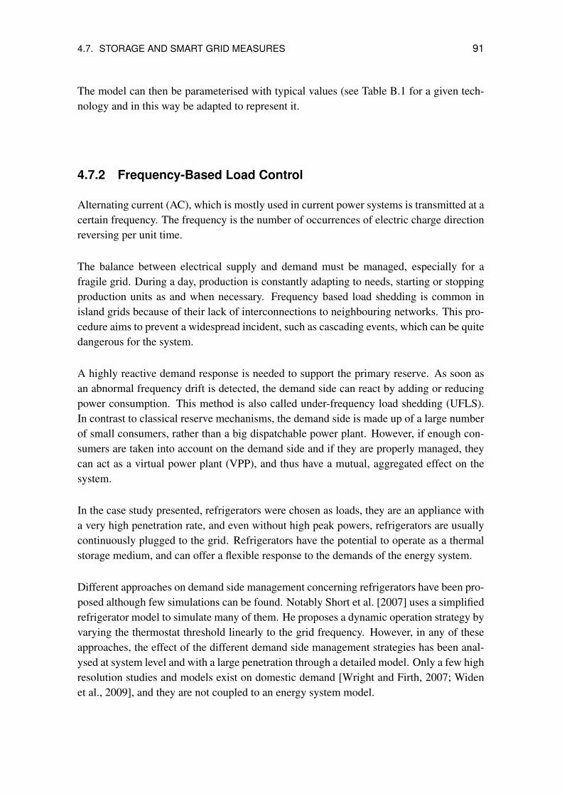
4.7. STORAGE AND SMART GRID MEASURES 91
The model can then be parameterised with typical values (see Table B.1 for a given tech-nology and in this way be adapted to represent it.
4.7.2 Frequency-Based Load Control
Alternating current (AC), which is mostly used in current power systems is transmitted at acertain frequency. The frequency is the number of occurrences of electric charge directionreversing per unit time.
The balance between electrical supply and demand must be managed, especially for afragile grid. During a day, production is constantly adapting to needs, starting or stoppingproduction units as and when necessary. Frequency based load shedding is common inisland grids because of their lack of interconnections to neighbouring networks. This pro-cedure aims to prevent a widespread incident, such as cascading events, which can be quitedangerous for the system.
A highly reactive demand response is needed to support the primary reserve. As soon asan abnormal frequency drift is detected, the demand side can react by adding or reducingpower consumption. This method is also called under-frequency load shedding (UFLS).In contrast to classical reserve mechanisms, the demand side is made up of a large numberof small consumers, rather than a big dispatchable power plant. However, if enough con-sumers are taken into account on the demand side and if they are properly managed, theycan act as a virtual power plant (VPP), and thus have a mutual, aggregated effect on thesystem.
In the case study presented, refrigerators were chosen as loads, they are an appliance witha very high penetration rate, and even without high peak powers, refrigerators are usuallycontinuously plugged to the grid. Refrigerators have the potential to operate as a thermalstorage medium, and can offer a flexible response to the demands of the energy system.
Different approaches on demand side management concerning refrigerators have been pro-posed although few simulations can be found. Notably Short et al. [2007] uses a simplifiedrefrigerator model to simulate many of them. He proposes a dynamic operation strategy byvarying the thermostat threshold linearly to the grid frequency. However, in any of theseapproaches, the effect of the different demand side management strategies has been anal-ysed at system level and with a large penetration through a detailed model. Only a few highresolution studies and models exist on domestic demand [Wright and Firth, 2007; Widenet al., 2009], and they are not coupled to an energy system model.
92 CHAPTER 4. ELECTRICAL ENERGY SYSTEM MODELLING
4.8 Grid Models
4.8.1 Load Flow
To design an electrical network, engineers need to be able to estimate the voltages and cur-rents at any place within the circuit. Usually, an undirected graph shows the grid topology,and mesh or nodal analysis is often used to set up an equation system and solve it for thevoltage and current at any place in the circuit. Standard linear algebra methods are suitablefor linear systems, but other nonlinear circuits can only be solved using estimation tech-niques or specialised software programs. The most common method used here is a loadflow analysis.
In an electrical network with n nodes, each one is associated with a pair of complex num-bers, V (voltage) and S = P +Qi (apparent power).
The given variables are:
• ∣V ∣ and ∠V = 0 are given at the reference node
• ∣V ∣ and P are given at control nodes
• P and Q are given at load nodes (the other nodes)
Applying the electrical laws results in a nonlinear system of 2n equations with 2n realunknowns,
g(x) = 0, (4.16)
where x, g(x) ∈ R2n, with the unknowns:
• P and Q for the reference or slack bus
• ∠V and Q for control buses
• ∣V ∣ and ∠V for load buses
To solve the system, the most common approach in the literature is to apply the Gauss-Jordan (iterative, of slow convergence) or the Newton-Raphson method, which is faster,but requires that the Jacobian matrix is calculated and inverted.
When talking about load flows [Bergen and Vittal, 2000], it is often assumed that theelectrical network is static. In fact, it is assumed that all data values are known constantsand the effect of actual load variations over time is studied through considering a numberof different cases for which steady-state conditions are assumed.
Still, to analyse transient effects after a value change in some nodes (e.g. in case of connec-tion and disconnection of loads or sources), the values of the unknowns have to be updated

4.8. GRID MODELS 93
quickly. It is these values that are used for the control of the network or for its simulation.The implementation of the algorithm in Anylogic [Kremers et al., 2010] was successfullyvalidated against a load flow calculation performed by PSAT [Milano, 2009].
4.8.2 Grid Frequency Model
The System Frequency Response (SFR) model [Anderson and Mirheydar, 1990] is a sim-plified model which describes the behaviour of an interconnected system when dealingwith a large disturbance. This model omits many details and ignores small time constants,providing a model that is useful in approximating the system frequency performance andhas been used by different authors in the field [Kottick et al., 1993; Lee Hau Aik, 2006].Despite of the model’s simplicity, the comparison with other system disturbances and de-tailed simulations, as shown by Anderson and Mirheydar [1990] are rather encouraging.
The model is represented in 4.7 in a block diagram in the Laplace domain, as is usual incontrol theory. It is composed of two main blocks in a typical feedback loop configuration,where the lower block balances the system. The upper block describes the initial responseδω of the system to a disturbance in the production-demand balance, Pd, taking into ac-count the inertia and damping factor of the system. The lower block feeds a negative powerPm at the input of the system representing the simplified response of the production system(primary reserve).
The SFR model allows further understanding of how the system parameters affect thefrequency response. In a detailed model of the electrical system, this is more difficultbecause there, frequency response is a very complex function of many system variables.
The effect of a sudden load disturbance on grid frequency can be summarised in two pointsby the given model [Anderson and Mirheydar, 1990; Terzija, 2006]:
• The initial slope of frequency change is proportional to the power imbalance, andalso depends on the inertia of the power system.
• The values of the minimum frequency, and the new steady-state frequency, reachedduring the following transient process are proportional to the power imbalance anddepend on the dynamic properties of turbines, governors, loads, and other systemcontrol devices.
The parameters of the SFR models are:
• H: inertial constant [s]
• D: damping factor [1]
• Km: mechanical power gain factor [1]

94 CHAPTER 4. ELECTRICAL ENERGY SYSTEM MODELLING
12
Pa
11
Δω
‐
+
Pm
Pd
Figure 4.7: Simplified system frequency response model
• FH : fraction of total power generated by the HP turbine [1]
• TR: reheat time constant [s]
• R: governor regulation [1]
The inertial storage capacity of a power system is measured by the inertial constant, H,which is the number of full-output seconds of energy stored (assuming nominal frequency)typically varies between 2 and 8 s [Short et al., 2007].
4.9 Towards Electrical Energy models as a Whole
We have seen that is possible to represent many of the entities of an electrical energy sys-tem through simplified, technical and non-technical models. Production was exemplifiedby wind power, a renewable energy source. In this case, we saw the need for an envi-ronmental model representing wind speeds, because a purely technical model of a turbineis not enough to simulate wind power. Demand was exemplified by a domestic refriger-ator. This appliance was chosen because of its high penetration rate and its continuousoperation (continuously connected to the power grid). This device can be managed by aDSM. A simple model for under frequency based load shedding was created and a simplenon-technical model represented the human behaviour of door opening was also used. Theinfrastructure, or network, can be represented by different models such as load flow or asimplified frequency response model.
These different modules, such as a wind turbine or a refrigerator, have been representedindividually, following the agent-based philosophy. They were conceived to interact witheach other: for example, the obtained wind speed can be used as an input for a windturbine, or the generated load of a refrigerator is used in the grid model. Now, as a nextstep, the different modules can be plugged together, in order to create electrical energysystem models, and run in simulation, in an interconnected way, at the same time.

Chapter 5
Integral Multi-Scale Case Study Models
After having identified and explored some of the models that describe different componentsof an energy system, an implementation in a modelling engine is performed in order to runsimulations. Two case studies show the application of the models in a complex systemenvironment. The first one focuses on production and the second example shows a demandmodel, which includes Demand Side Management (DSM) coupled to an energy systemmodel. Both models show behaviours at different scales, on both the individual scaleand on the systemic scale. The systemic scale shows a coupled model at a higher scale,interacting with the individual agents from the first model. Their implementation is basedon the components that were developed in the previous chapter.
5.1 Wind Farm Case Study
The first case study addresses one of the most commonly used forms of renewable energy.Wind energy allows for efficient generation, through turbines located close to the rotorwhich directly convert mechanical into electrical energy. This case study presents an agent-based model of a wind farm, in which each turbine is modelled individually. Furthermore,failure behaviour is included to make the model more realistic. The model is coupled toa multi-timescale wind simulator, that allows for representing wind speeds with differentaccuracy.
5.1.1 Wind Simulator Implementation
Different modules were developed in Anylogic to build the wind simulator. Each modulewas encapsulated to work independently and has well-defined interfaces. This allows fordifferent releases of the same module, which can be easily replaced.
The wind simulator modules as follows:
95
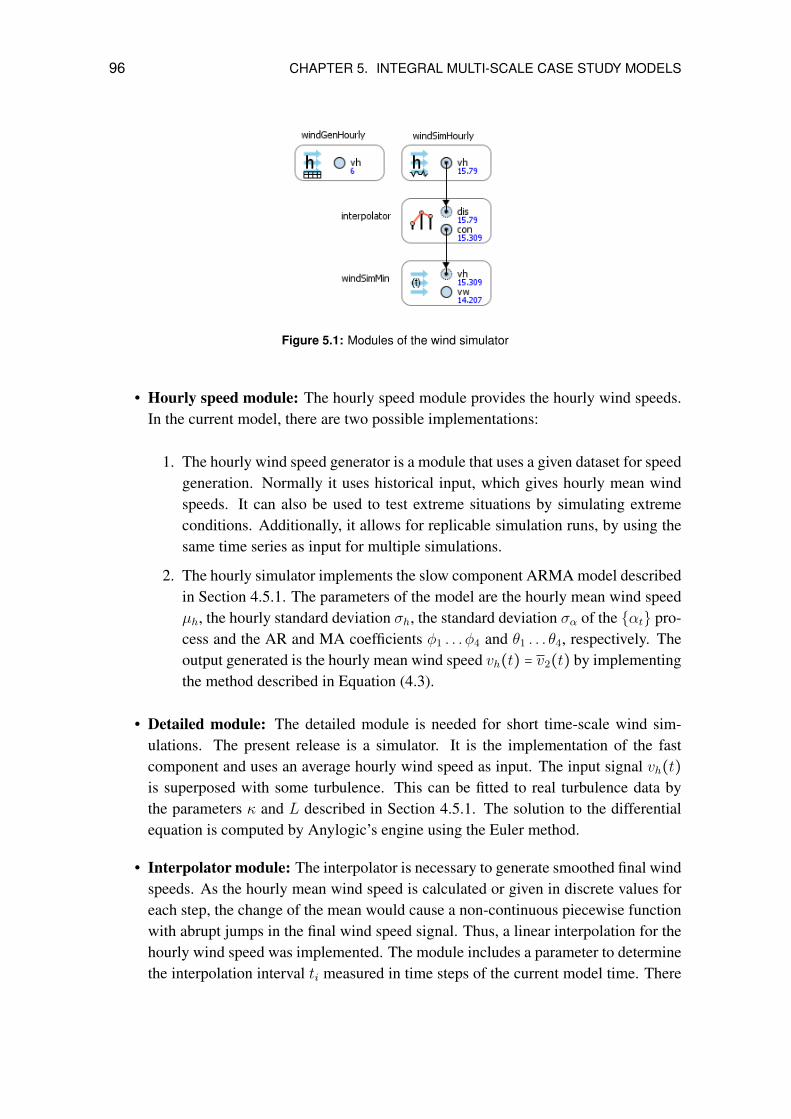
96 CHAPTER 5. INTEGRAL MULTI-SCALE CASE STUDY MODELS
Figure 5.1: Modules of the wind simulator
• Hourly speed module: The hourly speed module provides the hourly wind speeds.In the current model, there are two possible implementations:
1. The hourly wind speed generator is a module that uses a given dataset for speedgeneration. Normally it uses historical input, which gives hourly mean windspeeds. It can also be used to test extreme situations by simulating extremeconditions. Additionally, it allows for replicable simulation runs, by using thesame time series as input for multiple simulations.
2. The hourly simulator implements the slow component ARMA model describedin Section 4.5.1. The parameters of the model are the hourly mean wind speedµh, the hourly standard deviation σh, the standard deviation σα of the {αt} pro-cess and the AR and MA coefficients φ1 . . . φ4 and θ1 . . . θ4, respectively. Theoutput generated is the hourly mean wind speed vh(t) = v2(t) by implementingthe method described in Equation (4.3).
• Detailed module: The detailed module is needed for short time-scale wind sim-ulations. The present release is a simulator. It is the implementation of the fastcomponent and uses an average hourly wind speed as input. The input signal vh(t)is superposed with some turbulence. This can be fitted to real turbulence data bythe parameters κ and L described in Section 4.5.1. The solution to the differentialequation is computed by Anylogic’s engine using the Euler method.
• Interpolator module: The interpolator is necessary to generate smoothed final windspeeds. As the hourly mean wind speed is calculated or given in discrete values foreach step, the change of the mean would cause a non-continuous piecewise functionwith abrupt jumps in the final wind speed signal. Thus, a linear interpolation for thehourly wind speed was implemented. The module includes a parameter to determinethe interpolation interval ti measured in time steps of the current model time. There
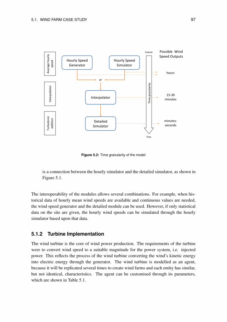
5.1. WIND FARM CASE STUDY 97
Hourly Speed Generator
Hourly Speed Simulator
Interpolator
Detailed Simulator
Coarse
hours
15‐30 minutes
minutes‐seconds
Ave
rage h
ourl
y sp
eed
Inte
rpol
atio
n Tu
rbul
ence
addi
tion
Tim
e gr
anul
arity
Fine
Possible Wind Speed Outputs
or
Figure 5.2: Time granularity of the model
is a connection between the hourly simulator and the detailed simulator, as shown inFigure 5.1.
The interoperability of the modules allows several combinations. For example, when his-torical data of hourly mean wind speeds are available and continuous values are needed,the wind speed generator and the detailed module can be used. However, if only statisticaldata on the site are given, the hourly wind speeds can be simulated through the hourlysimulator based upon that data.
5.1.2 Turbine Implementation
The wind turbine is the core of wind power production. The requirements of the turbinewere to convert wind speed to a suitable magnitude for the power system, i.e. injectedpower. This reflects the process of the wind turbine converting the wind’s kinetic energyinto electric energy through the generator. The wind turbine is modelled as an agent,because it will be replicated several times to create wind farms and each entity has similar,but not identical, characteristics. The agent can be customised through its parameters,which are shown in Table 5.1.

98 CHAPTER 5. INTEGRAL MULTI-SCALE CASE STUDY MODELS
Making use of Anylogic’s features to create hybrid models [Borshchev and Filippov, 2004],the turbine was modelled using the power curve model of the P (v) relationship describedin Section 4.5.1 in combination with UML state-charts. The power curve model was chosento ensure flexibility in the application of the model. It is assumed that when modelling awind farm, detailed information is available on the turbines used. This way, it is possible tocustomise each turbine with its corresponding power curve. The model of the wind turbineagent remains the same in any case.
The state-chart elaborated here is classified in states dependent on the output power andfailure state. The three working states of the turbine are as follows:
• OFF: this state is active when the turbine is not producing any output power, regard-less of the cause (no wind, overly strong wind speeds, etc.) except in the case of afailure
• FAILURE: this state is achieved when there is a failure or shutdown of the turbinedue to maintenance.
• ON: the turbine is in this state when producing output power, regardless if the ratedpower is gained or the turbine is only partially loaded.
The transition conditions between the states are defined by the wind speed for the transi-tions between the ON and OFF states, and by the corresponding rates of the MTBF andMTTR in the case of transitions to and from the FAILURE state, respectively. The MTBFis used for both transitions from the ON and OFF states. The rates are always adaptedto the current timescale by a factor that is proportional to it and set automatically by themodel as a function of the scale chosen.
For the computation of output power, Anylogic’s so-called action chart is used to link boththe discrete state-chart approach and the continuous power curve. The output power is onlytaken from the power curve if the current state is set to ON. The state-chart and the actionchart are shown in Figure 5.3.
Parameter Description ValuePnom Nominal power 275 kWvcut−in Cut-in wind speed 3 m/svcut−off Cut-off wind speed 20 m/svcut−back−in Cut-back-in wind speed 18 m/sMTBF Mean Time Between Failures 1900 hMTTR Mean Time To Recover 80 h
Table 5.1: Wind turbine parameters
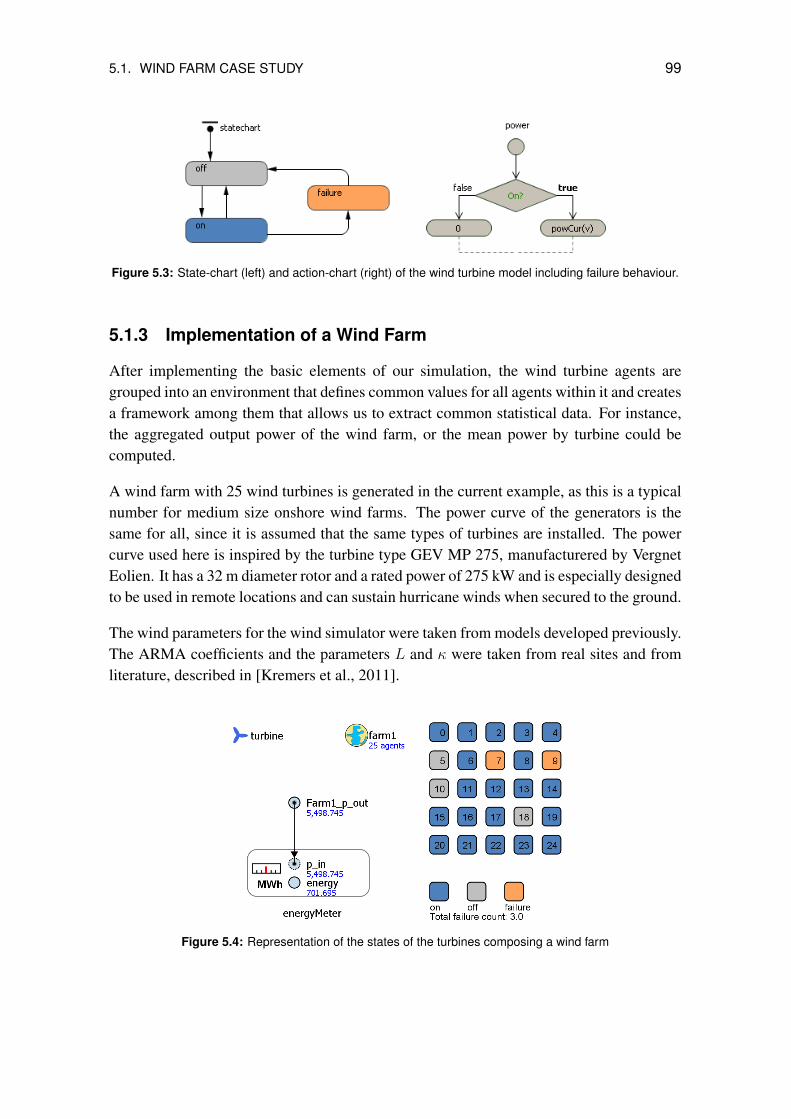
5.1. WIND FARM CASE STUDY 99
Figure 5.3: State-chart (left) and action-chart (right) of the wind turbine model including failure behaviour.
5.1.3 Implementation of a Wind Farm
After implementing the basic elements of our simulation, the wind turbine agents aregrouped into an environment that defines common values for all agents within it and createsa framework among them that allows us to extract common statistical data. For instance,the aggregated output power of the wind farm, or the mean power by turbine could becomputed.
A wind farm with 25 wind turbines is generated in the current example, as this is a typicalnumber for medium size onshore wind farms. The power curve of the generators is thesame for all, since it is assumed that the same types of turbines are installed. The powercurve used here is inspired by the turbine type GEV MP 275, manufacturered by VergnetEolien. It has a 32 m diameter rotor and a rated power of 275 kW and is especially designedto be used in remote locations and can sustain hurricane winds when secured to the ground.
The wind parameters for the wind simulator were taken from models developed previously.The ARMA coefficients and the parameters L and κ were taken from real sites and fromliterature, described in [Kremers et al., 2011].
Figure 5.4: Representation of the states of the turbines composing a wind farm
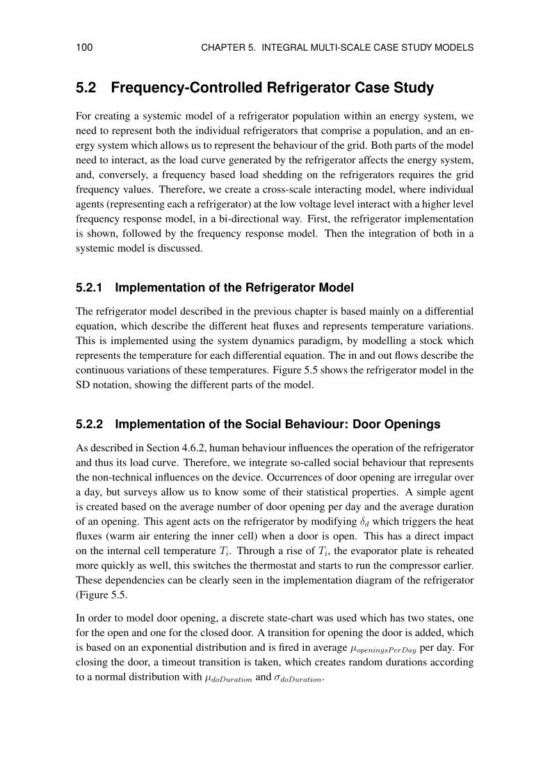
100 CHAPTER 5. INTEGRAL MULTI-SCALE CASE STUDY MODELS
5.2 Frequency-Controlled Refrigerator Case Study
For creating a systemic model of a refrigerator population within an energy system, weneed to represent both the individual refrigerators that comprise a population, and an en-ergy system which allows us to represent the behaviour of the grid. Both parts of the modelneed to interact, as the load curve generated by the refrigerator affects the energy system,and, conversely, a frequency based load shedding on the refrigerators requires the gridfrequency values. Therefore, we create a cross-scale interacting model, where individualagents (representing each a refrigerator) at the low voltage level interact with a higher levelfrequency response model, in a bi-directional way. First, the refrigerator implementationis shown, followed by the frequency response model. Then the integration of both in asystemic model is discussed.
5.2.1 Implementation of the Refrigerator Model
The refrigerator model described in the previous chapter is based mainly on a differentialequation, which describe the different heat fluxes and represents temperature variations.This is implemented using the system dynamics paradigm, by modelling a stock whichrepresents the temperature for each differential equation. The in and out flows describe thecontinuous variations of these temperatures. Figure 5.5 shows the refrigerator model in theSD notation, showing the different parts of the model.
5.2.2 Implementation of the Social Behaviour: Door Openings
As described in Section 4.6.2, human behaviour influences the operation of the refrigeratorand thus its load curve. Therefore, we integrate so-called social behaviour that representsthe non-technical influences on the device. Occurrences of door opening are irregular overa day, but surveys allow us to know some of their statistical properties. A simple agentis created based on the average number of door opening per day and the average durationof an opening. This agent acts on the refrigerator by modifying δd which triggers the heatfluxes (warm air entering the inner cell) when a door is open. This has a direct impacton the internal cell temperature Ti. Through a rise of Ti, the evaporator plate is reheatedmore quickly as well, this switches the thermostat and starts to run the compressor earlier.These dependencies can be clearly seen in the implementation diagram of the refrigerator(Figure 5.5.
In order to model door opening, a discrete state-chart was used which has two states, onefor the open and one for the closed door. A transition for opening the door is added, whichis based on an exponential distribution and is fired in average µopeningsPerDay per day. Forclosing the door, a timeout transition is taken, which creates random durations accordingto a normal distribution with µdoDuration and σdoDuration.
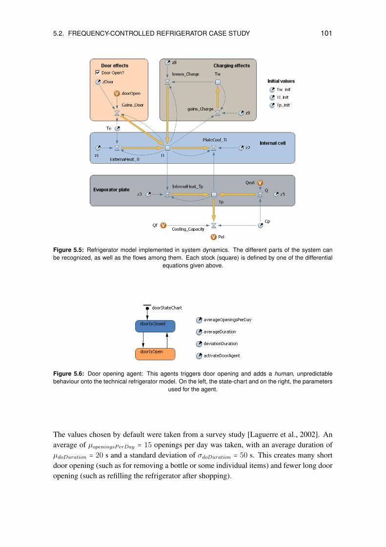
5.2. FREQUENCY-CONTROLLED REFRIGERATOR CASE STUDY 101
Figure 5.5: Refrigerator model implemented in system dynamics. The different parts of the system canbe recognized, as well as the flows among them. Each stock (square) is defined by one of the differential
equations given above.
Figure 5.6: Door opening agent: This agents triggers door opening and adds a human, unpredictablebehaviour onto the technical refrigerator model. On the left, the state-chart and on the right, the parameters
used for the agent.
The values chosen by default were taken from a survey study [Laguerre et al., 2002]. Anaverage of µopeningsPerDay = 15 openings per day was taken, with an average duration ofµdoDuration = 20 s and a standard deviation of σdoDuration = 50 s. This creates many shortdoor opening (such as for removing a bottle or some individual items) and fewer long dooropening (such as refilling the refrigerator after shopping).
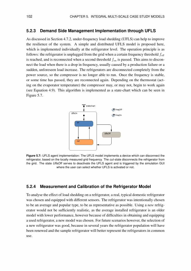
102 CHAPTER 5. INTEGRAL MULTI-SCALE CASE STUDY MODELS
5.2.3 Demand Side Management Implementation through UFLS
As discussed in Section 4.7.2, under-frequency load shedding (UFLS) can help to improvethe resilience of the system. A simple and distributed UFLS model is proposed here,which is implemented individually at the refrigerator level. The operation principle is asfollows: the refrigerator is unplugged from the grid when a certain frequency threshold foff
is reached, and is reconnected when a second threshold fon is passed. This aims to discon-nect the load when there is a drop in frequency, usually caused by a production failure or asudden, unforeseen load increase. The refrigerators are disconnected completely from thepower source, so the compressor is no longer able to run. Once the frequency is stable,or some time has passed, they are reconnected again. Depending on the thermostat (act-ing on the evaporator temperature) the compressor may, or may not, begin to work again(see Equation 4.9). This algorithm is implemented as a state-chart which can be seen inFigure 5.7.
Figure 5.7: UFLS agent implementation: The UFLS model implements a device which can disconnect therefrigerator, based on the locally measured grid frequency. The cut-state disconnects the refrigerator fromthe grid. The state UflsOff serves to deactivate the UFLS agent and is triggered by the simulation GUI
where the user can select whether UFLS is activated or not.
5.2.4 Measurement and Calibration of the Refrigerator Model
To analyse the effect of load shedding on a refrigerator, a real, typical domestic refrigeratorwas chosen and equipped with different sensors. The refrigerator was intentionally chosento be an average and popular type, to be as representative as possible. Using a new refrig-erator would not be sufficiently realistic, as the average installed refrigerator is an oldermodel with lower performance, however because of difficulties in obtaining and equippinga used refrigerator, a new model was chosen. For future scenarios however, the selection ofa new refrigerator was good, because in several years the refrigerator population will havebeen renewed and the sample refrigerator will better represent the refrigerators in commonuse.
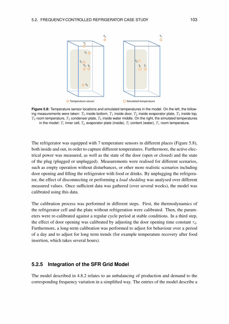
5.2. FREQUENCY-CONTROLLED REFRIGERATOR CASE STUDY 103
T0 = inside bottom T1 = inside door T2 = inside evaporator plate T3 = inside top T4 = room temperature T5 = condenser T6 = inside water middle
Ti = inside Tp = inside evaporator plate Tc = content (water) Te = room temperature
T4
T0
T2 T6 T1
T5
T3
Te
Tl Ti
Tp
Temperature sensor Simulated temperature
Figure 5.8: Temperature sensor locations and simulated temperatures in the model. On the left, the follow-ing measurements were taken: T0 inside bottom, T1 inside door, T2 inside evaporator plate, T3 inside top,T4 room temperature, T5 condenser plate, T6 inside water middle. On the right, the simulated temperatures
in the model: Ti inner cell, Tp evaporator plate (inside), Tl content (water), Te room temperature.
The refrigerator was equipped with 7 temperature sensors in different places (Figure 5.8),both inside and out, in order to capture different temperatures. Furthermore, the active elec-trical power was measured, as well as the state of the door (open or closed) and the stateof the plug (plugged or unplugged). Measurements were realised for different scenarios,such as empty operation without disturbances, or other more realistic scenarios includingdoor opening and filling the refrigerator with food or drinks. By unplugging the refrigera-tor, the effect of disconnecting or performing a load shedding was analysed over differentmeasured values. Once sufficient data was gathered (over several weeks), the model wascalibrated using this data.
The calibration process was performed in different steps. First, the thermodynamics ofthe refrigerator cell and the plate without refrigeration were calibrated. Then, the param-eters were re-calibrated against a regular cycle period at stable conditions. In a third step,the effect of door opening was calibrated by adjusting the door opening time constant τd.Furthermore, a long-term calibration was performed to adjust for behaviour over a periodof a day and to adjust for long term trends (for example temperature recovery after foodinsertion, which takes several hours).
5.2.5 Integration of the SFR Grid Model
The model described in 4.8.2 relates to an unbalancing of production and demand to thecorresponding frequency variation in a simplified way. The entries of the model describe a

104 CHAPTER 5. INTEGRAL MULTI-SCALE CASE STUDY MODELS
delta between actual production and the demand of the overall system, at a given point; itis called disturbance power. We define it generically as
∆P (t) = Pg(t) − Pd(t) (5.1)
where Pg is the total generated power and Pd is the total demanded power. The originalmodel is described in the block diagram formalism in the Laplace domain. This formal-ism can be directly implemented in, for example, Simulink; however, Anylogic, the mod-elling environment used here, includes the system dynamics paradigm. By transformingthe equations back to the time domain, the equivalent differential equations can be foundand implemented in SD as described in Appendix E.
The implementation of the SFR model in system dynamics can be seen in Figure 5.9.
Figure 5.9: Representation of SFR model as a system dynamics stock and flow diagram
The two blocks of the original model (see Figure 4.7 on page 94) are translated into thetwo flows in SD which represent a first order differential equation. For the parameters, thefollowing set was used (see Table 5.2. The two stocks ω and Pm represent the frequencyvariation and the mechanical turbine power, respectively.
Parameter Description ValueH Inertial constant 4 sD Damping factor 1Km Mechanical power gain factor 0.95FH Fraction of total power generated by the HP turbine 0.05TR Reheat time constant 8 sR Governor regulation 0.2
Table 5.2: SFR model parameters
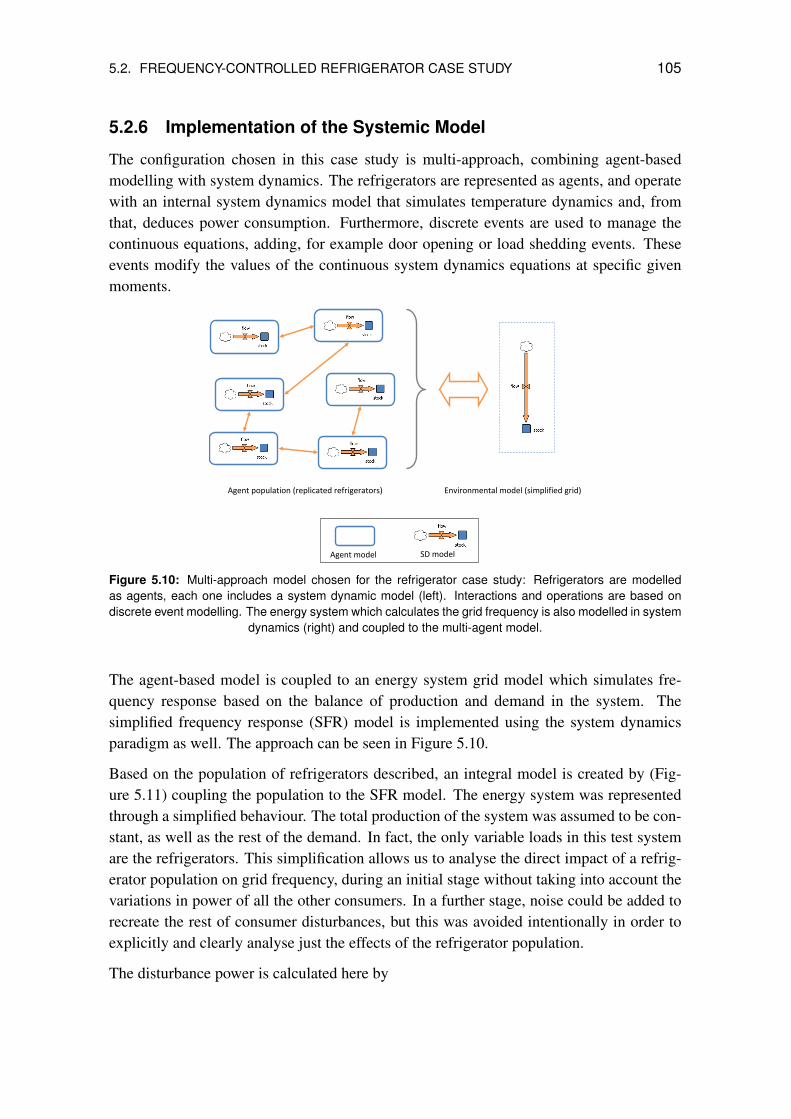
5.2. FREQUENCY-CONTROLLED REFRIGERATOR CASE STUDY 105
5.2.6 Implementation of the Systemic Model
The configuration chosen in this case study is multi-approach, combining agent-basedmodelling with system dynamics. The refrigerators are represented as agents, and operatewith an internal system dynamics model that simulates temperature dynamics and, fromthat, deduces power consumption. Furthermore, discrete events are used to manage thecontinuous equations, adding, for example door opening or load shedding events. Theseevents modify the values of the continuous system dynamics equations at specific givenmoments.
Agent population (replicated refrigerators)
Environmental model (simplified grid)
Agent model SD model
Figure 5.10: Multi-approach model chosen for the refrigerator case study: Refrigerators are modelledas agents, each one includes a system dynamic model (left). Interactions and operations are based ondiscrete event modelling. The energy system which calculates the grid frequency is also modelled in system
dynamics (right) and coupled to the multi-agent model.
The agent-based model is coupled to an energy system grid model which simulates fre-quency response based on the balance of production and demand in the system. Thesimplified frequency response (SFR) model is implemented using the system dynamicsparadigm as well. The approach can be seen in Figure 5.10.
Based on the population of refrigerators described, an integral model is created by (Fig-ure 5.11) coupling the population to the SFR model. The energy system was representedthrough a simplified behaviour. The total production of the system was assumed to be con-stant, as well as the rest of the demand. In fact, the only variable loads in this test systemare the refrigerators. This simplification allows us to analyse the direct impact of a refrig-erator population on grid frequency, during an initial stage without taking into account thevariations in power of all the other consumers. In a further stage, noise could be added torecreate the rest of consumer disturbances, but this was avoided intentionally in order toexplicitly and clearly analyse just the effects of the refrigerator population.
The disturbance power is calculated here by
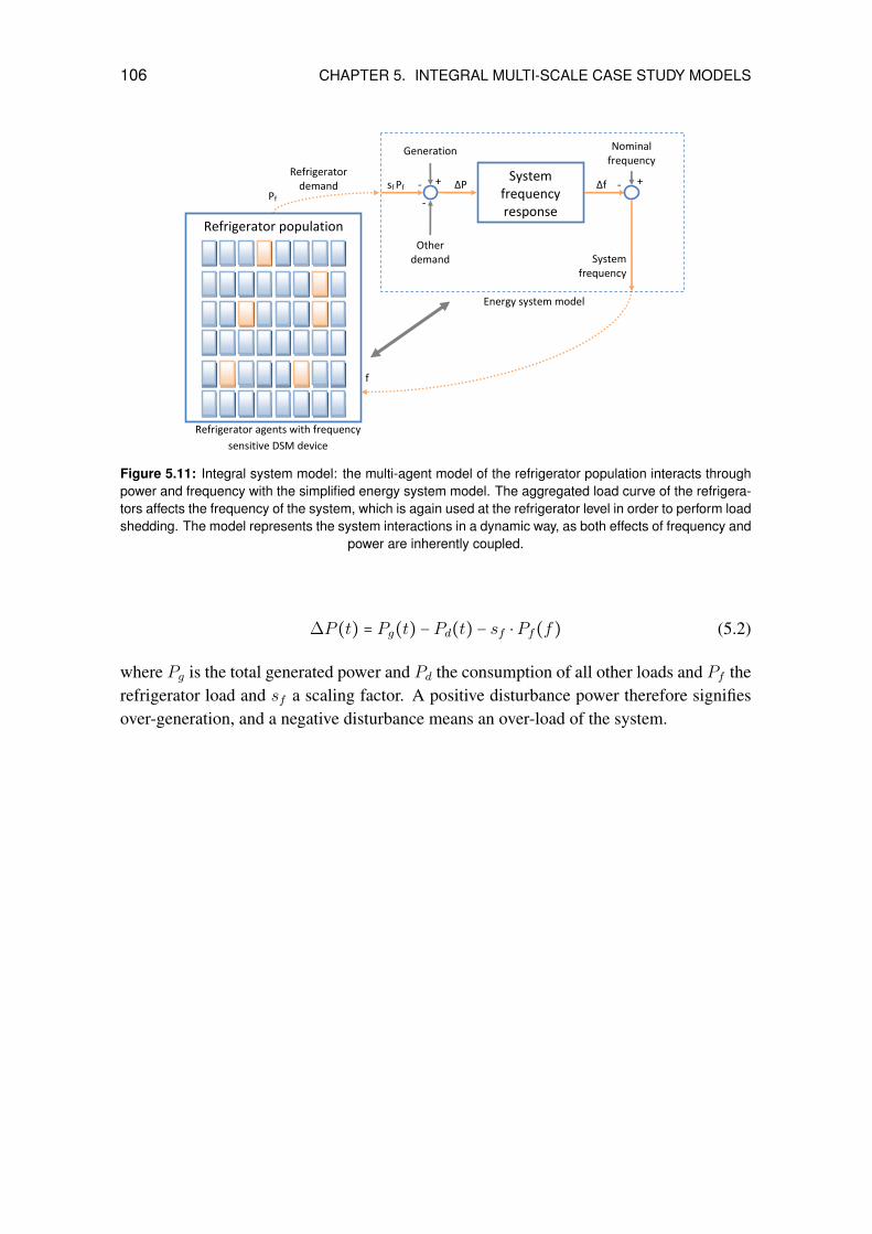
106 CHAPTER 5. INTEGRAL MULTI-SCALE CASE STUDY MODELS
System frequency response
Nominal frequency
Δf ‐ ++ ∆P
Generation
Other demand
‐‐
f
Refrigerator demand
System frequency
Pf
Refrigerator agents with frequency sensitive DSM device
Energy system model
Refrigerator population
sf Pf
Figure 5.11: Integral system model: the multi-agent model of the refrigerator population interacts throughpower and frequency with the simplified energy system model. The aggregated load curve of the refrigera-tors affects the frequency of the system, which is again used at the refrigerator level in order to perform loadshedding. The model represents the system interactions in a dynamic way, as both effects of frequency and
power are inherently coupled.
∆P (t) = Pg(t) − Pd(t) − sf ⋅ Pf(f) (5.2)
where Pg is the total generated power and Pd the consumption of all other loads and Pf therefrigerator load and sf a scaling factor. A positive disturbance power therefore signifiesover-generation, and a negative disturbance means an over-load of the system.
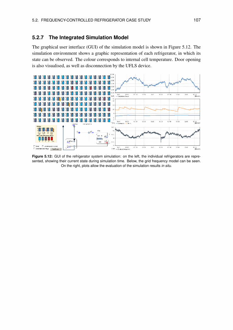
5.2. FREQUENCY-CONTROLLED REFRIGERATOR CASE STUDY 107
5.2.7 The Integrated Simulation Model
The graphical user interface (GUI) of the simulation model is shown in Figure 5.12. Thesimulation environment shows a graphic representation of each refrigerator, in which itsstate can be observed. The colour corresponds to internal cell temperature. Door openingis also visualised, as well as disconnection by the UFLS device.
Figure 5.12: GUI of the refrigerator system simulation: on the left, the individual refrigerators are repre-sented, showing their current state during simulation time. Below, the grid frequency model can be seen.
On the right, plots allow the evaluation of the simulation results in situ.

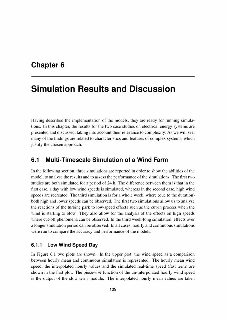
Chapter 6
Simulation Results and Discussion
Having described the implementation of the models, they are ready for running simula-tions. In this chapter, the results for the two case studies on electrical energy systems arepresented and discussed, taking into account their relevance to complexity. As we will see,many of the findings are related to characteristics and features of complex systems, whichjustify the chosen approach.
6.1 Multi-Timescale Simulation of a Wind Farm
In the following section, three simulations are reported in order to show the abilities of themodel, to analyse the results and to assess the performance of the simulations. The first twostudies are both simulated for a period of 24 h. The difference between them is that in thefirst case, a day with low wind speeds is simulated, whereas in the second case, high windspeeds are recreated. The third simulation is for a whole week, where (due to the duration)both high and lower speeds can be observed. The first two simulations allow us to analysethe reactions of the turbine park to low-speed effects such as the cut-in process when thewind is starting to blow. They also allow for the analysis of the effects on high speedswhere cut-off phenomena can be observed. In the third week-long simulation, effects overa longer simulation period can be observed. In all cases, hourly and continuous simulationswere run to compare the accuracy and performance of the models.
6.1.1 Low Wind Speed Day
In Figure 6.1 two plots are shown. In the upper plot, the wind speed as a comparisonbetween hourly mean and continuous simulation is represented. The hourly mean windspeed, the interpolated hourly values and the simulated real-time speed (fast term) areshown in the first plot. The piecewise function of the un-interpolated hourly wind speedis the output of the slow term module. The interpolated hourly mean values are taken
109

110 CHAPTER 6. SIMULATION RESULTS AND DISCUSSION
5
10
15
20v
[m/s
]
Wind Speed (hourly) Wind Speed (hourly interpolated) Wind Speed (continuous)
0
5
0 2 4 6 8 10 12 14 16 18 20 22 24
2000
4000
6000
8000
P [
kW]
Farm Power Output (hourly) Farm Power Output (continuous)
0
2000
0 2 4 6 8 10 12 14 16 18 20 22 24
Time [h]
Figure 6.1: Comparison hourly and continuous power outputs (bottom) and corresponding wind speeds(top) for a day with low wind speeds.
from the linear interpolator. These are again used as input for the fast term module. Theoutput curves of the wind farms are plotted below. Two curves are shown, one using theinterpolated hourly mean speeds as inputs, and the second using the real-time, continuouswind speed output.
This first simulation shows a period of 24 h where wind speeds are relatively low, thatmeans not exceeding 18 m/s. In particular, there are periods with low speeds, below 10m/s, where a significant decrease of the output power of the turbines can be observed.Falling under the cut-in speed, they can even stop completely. The simulated wind farmsare identical. The difference between them is the wind speed input data. The first farmtakes the interpolated hourly mean wind speeds, the second one the real time speeds.
In Figure 6.1 we can see that the hourly computed power output of the farm follows more orless what could be a hourly mean of the continuous values. There are no great deviations,except a small one around 21h, due to a drop in the continuous wind speed caused byturbulence in the fast term.
Due to random failure behaviour, some differences caused by turbines in failure status canbe observed (e.g. less total power in the last 2 hours of the day in the continuous simu-lation). It can be seen that the hourly power output approximately follows the continuous
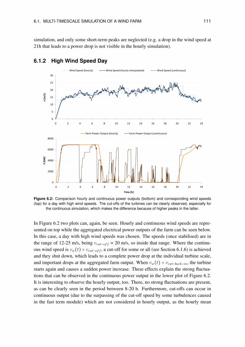
6.1. MULTI-TIMESCALE SIMULATION OF A WIND FARM 111
simulation, and only some short-term peaks are neglected (e.g. a drop in the wind speed at21h that leads to a power drop is not visible in the hourly simulation).
6.1.2 High Wind Speed Day
10
15
20
25
30
v [m
/s]
Wind Speed (hourly) Wind Speed (hourly interpolated) Wind Speed (continuous)
0
5
0 2 4 6 8 10 12 14 16 18 20 22 24
2000
4000
6000
8000
P [
kW]
Farm Power Output (hourly) Farm Power Output (continuous)
0
2000
0 2 4 6 8 10 12 14 16 18 20 22 24
Time [h]
Figure 6.2: Comparison hourly and continuous power outputs (bottom) and corresponding wind speeds(top) for a day with high wind speeds. The cut-offs of the turbines can be clearly observed, especially for
the continuous simulation, which makes the difference because of higher peaks in the latter.
In Figure 6.2 two plots can, again, be seen. Hourly and continuous wind speeds are repre-sented on top while the aggregated electrical power outputs of the farm can be seen below.In this case, a day with high wind speeds was chosen. The speeds (once stabilised) are inthe range of 12-25 m/s, being vcut−off = 20 m/s, so inside that range. Where the continu-ous wind speed is vw(t) > vcut−off , a cut-off for some or all (see Section 6.1.6) is achievedand they shut down, which leads to a complete power drop at the individual turbine scale,and important drops at the aggregated farm output. When vw(t) < vcut−back−in, the turbinestarts again and causes a sudden power increase. These effects explain the strong fluctua-tions that can be observed in the continuous power output in the lower plot of Figure 6.2.It is interesting to observe the hourly output, too. There, no strong fluctuations are present,as can be clearly seen in the period between 8-20 h. Furthermore, cut-offs can occur incontinuous output (due to the surpassing of the cut-off speed by some turbulences causedin the fast term module) which are not considered in hourly output, as the hourly mean

112 CHAPTER 6. SIMULATION RESULTS AND DISCUSSION
remains vh(t) < vcut−off . This can be seen in the power drop between 4-5 h, while thehourly output stays at the nominal farm output. Thus, when dealing with fast speeds, thecontinuous model reflects strong fluctuations much better; these are neglected in the hourlysimulation.
6.1.3 Simulation Over a Week
2000
4000
6000
8000
P [
kW]
Farm Power Output (hourly simulation)
0
2000
0 20 40 60 80 100 120 140 160
2000
4000
6000
8000
P [
kW]
Farm Power Output (continuous simulation)
0
2000
0 20 40 60 80 100 120 140 160
Time [h]
Figure 6.3: Comparison of a hourly (top) and a continuous (bottom) simulation for one week. It can beseen that the general trend is similar, but the continuous simulation shows some peaks and cut-offs that are
not present in the hourly one.
In this case, a complete week was simulated. Figure 6.3 shows two plots of the poweroutput for a 25 turbine wind farm (the same as in the previous examples), for hourly andcontinuous outputs, at top and bottom, respectively. As can be seen on the plots, over7 days the output of each method differs strongly only in some cases. There are somepoints where vw(t) > vcut−off . The turbines shut down due to excessive wind speeds inthis case, but looking at the same point in the hourly mean simulation, there is no suchpower drop. This is because vw(t) surpasses the hourly mean vh(t) punctually. To reacha power drop in the hourly simulation, vh(t) > vcut−off is needed. These drops are aproblem for grid stability, as they are very significant and occur in a short time frame.Indeed, control mechanisms for wind farms, to proactively shut down turbines based onwind speed forecasts or similar, in order to prevent such abrupt drops have not yet been
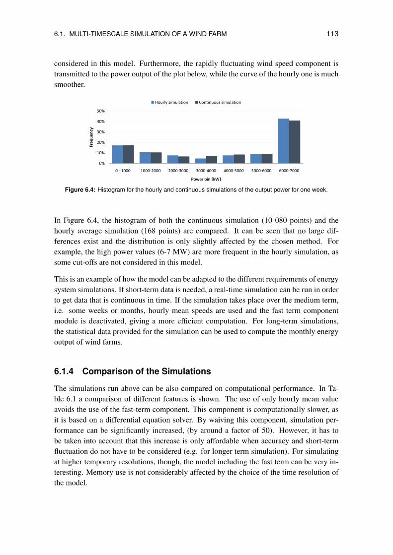
6.1. MULTI-TIMESCALE SIMULATION OF A WIND FARM 113
considered in this model. Furthermore, the rapidly fluctuating wind speed component istransmitted to the power output of the plot below, while the curve of the hourly one is muchsmoother.
20%
30%
40%
50%
Fre
qu
en
cy
Hourly simulation Continuous simulation
0%
10%
0 ‐ 1000 1000‐2000 2000‐3000 3000‐4000 4000‐5000 5000‐6000 6000‐7000
Power bin [kW]
Figure 6.4: Histogram for the hourly and continuous simulations of the output power for one week.
In Figure 6.4, the histogram of both the continuous simulation (10 080 points) and thehourly average simulation (168 points) are compared. It can be seen that no large dif-ferences exist and the distribution is only slightly affected by the chosen method. Forexample, the high power values (6-7 MW) are more frequent in the hourly simulation, assome cut-offs are not considered in this model.
This is an example of how the model can be adapted to the different requirements of energysystem simulations. If short-term data is needed, a real-time simulation can be run in orderto get data that is continuous in time. If the simulation takes place over the medium term,i.e. some weeks or months, hourly mean speeds are used and the fast term componentmodule is deactivated, giving a more efficient computation. For long-term simulations,the statistical data provided for the simulation can be used to compute the monthly energyoutput of wind farms.
6.1.4 Comparison of the Simulations
The simulations run above can be also compared on computational performance. In Ta-ble 6.1 a comparison of different features is shown. The use of only hourly mean valueavoids the use of the fast-term component. This component is computationally slower, asit is based on a differential equation solver. By waiving this component, simulation per-formance can be significantly increased, (by around a factor of 50). However, it has tobe taken into account that this increase is only affordable when accuracy and short-termfluctuation do not have to be considered (e.g. for longer term simulation). For simulatingat higher temporary resolutions, though, the model including the fast term can be very in-teresting. Memory use is not considerably affected by the choice of the time resolution ofthe model.
114 CHAPTER 6. SIMULATION RESULTS AND DISCUSSION
Simulation period 24 h 168 h (1 week)Resolution Continuous Hourly Continuous HourlyNumber of turbines 25 25Execution time 122,0 s 2,3 s 753,8 s 14,5 sMemory used 16 MB 16 MB 21 MB 15 MB
Table 6.1: Simulation run comparison
6.1.5 Failure Behaviour of the Turbine Units
As explained previously, the turbine model is provided with a failure function that allowsus to simulate technical failures using specific parameters that can be obtained empirically.In this way, failures of individual units are randomly simulated over time. The averagetime to restart the turbines after such a failure is also considered.
Randomly driven timeouts are used to represent the transition to the failure state, whichis triggered according to a rate. This rate is the inverse value of the MTBF. In order toget back to the working state, the rate corresponding to the MTTR is used. To triggerthe transitions, exponentially distributed random numbers are used. The distribution isparametrised by this rate.
In Figure 5.4 the representation of the turbines and their current state is shown. The modelcan easily show the state of each turbine and the aggregated current output and energyproduction. The state of an individual generator and its production values can also beobserved. The inclusion of failure behaviour in real time allows us to consider its directinfluence on the power output of the farm, within the same model.
6.1.6 Heterogeneous Parameterisation of the Agents
All turbine manufacturers provide technical specifications that document their character-istics in detail. The values shown in these documents are not normally specified for eachunit individually, as they are obtained using average values for all units of the same type.Although the units are supposed to be identical in construction, small differences cannotbe avoided.
To model this heterogeneity, the turbine parameters were varied slightly within the pop-ulation of turbines. The distribution used was a Normal distribution with a mean µ[value]corresponding to the indicated value and a small standard deviation of σ[value] = 0.1µ[value].Further studies could obtain exact values for the variation of parameters among differentunits. This leads to small variations in the behaviour of each unit, that can result in aggre-gated effects on the wind farm output, and which are not usually considered in classicalmodels. One of the strengths of the model is that it relies on the heterogeneous modellingof the individual agents.
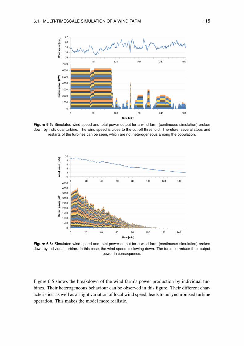
6.1. MULTI-TIMESCALE SIMULATION OF A WIND FARM 115
16
18
20
22
d s
pe
ed [
m/s
]14
16
0 60 120 180 240 300W
ind
2000
3000
4000
5000
6000
7000
utp
ut
po
we
r [k
W]
0
1000
2000
0 60 120 180 240 300
O
Time [min]
Figure 6.5: Simulated wind speed and total power output for a wind farm (continuous simulation) brokendown by individual turbine. The wind speed is close to the cut-off threshold. Therefore, several stops and
restarts of the turbines can be seen, which are not heterogeneous among the population.
2
4
6
8
10
d s
pe
ed [
m/s
]
0
2
0 20 40 60 80 100 120 140
Win
d
1500
2000
2500
3000
3500
4000
4500
utp
ut
po
we
r [k
W]
0
500
1000
0 20 40 60 80 100 120 140
O
Time [min]
Figure 6.6: Simulated wind speed and total power output for a wind farm (continuous simulation) brokendown by individual turbine. In this case, the wind speed is slowing down. The turbines reduce their output
power in consequence.
Figure 6.5 shows the breakdown of the wind farm’s power production by individual tur-bines. Their heterogeneous behaviour can be observed in this figure. Their different char-acteristics, as well as a slight variation of local wind speed, leads to unsynchronised turbineoperation. This makes the model more realistic.

116 CHAPTER 6. SIMULATION RESULTS AND DISCUSSION
6.1.7 Discussion of the Results
Modelling the power output of wind farms at different time scales can be quite a complexactivity. This case study presented a model for simulating a wind power system on multipletime scales. The multi-method approach was chosen in order to satisfy the various needsof the model, which integrates not only the pure generator but also failure behaviour andthe consideration of a wind farm as a whole. Furthermore, the model was conceived toallow for simulation at different time scales, looking for the best computational efficiencyin each case. The scalability included in this model allows the integration of different timescale simulations into the same module and the reduction of the number of total modules.
The model allows us to simulate wind power generation at different scales using the samemodel, by only switching between the different modules. The characteristics of the modelare maintained at the different scales. So, for example, failure behaviour is modelled andcan also be applied to short-term simulations, if needed. The following scope was made:
• The primary aim of the model is to simulate real time power outputs for energysystem simulations rather than to estimate the accumulated energy productions overa period (used for example for the dimensioning of wind farms) .
• At high speeds, cut-off effects are better reflected in a high resolution (continuoussimulation) model.
• The hourly model, though, can effectively approximate the hourly mean well in lowspeed periods.
• The model is sufficiently flexible to cover different needs arising from different timescales in integrated energy systems simulation.
This model brings together different modelling approaches, unifying continuous models,(differential equations, e.g. Equation (4.4), etc.) with discrete events (hourly changingmean speeds, state-chart modelling within the turbines) and agent-based modelling (e.g.of the failure behaviour and for the integration of the turbines into the wind farm). Theuse of different approaches allows for the creation of more realistic models that can takeadvantage of the different strengths of each approach. The agent-based approach, enablesdistributed parameters to be set to individual turbines, creating a heterogeneous park whichrecreates a more realistic behavior, both at the individual and at the aggregated scale. Fur-thermore, each turbine can be customised with real data (e.g. power curves, etc.). In thisway, it is possible to simulate the realistic behaviour of wind farms in contrast to the static,homogeneous multiplication of identical objects.
A compromise between accuracy of the output powers and performance of the model mustbe determined depending on the application scope of the model. In large time-scale energysystems simulations, over several months or years, estimating wind speeds through the low
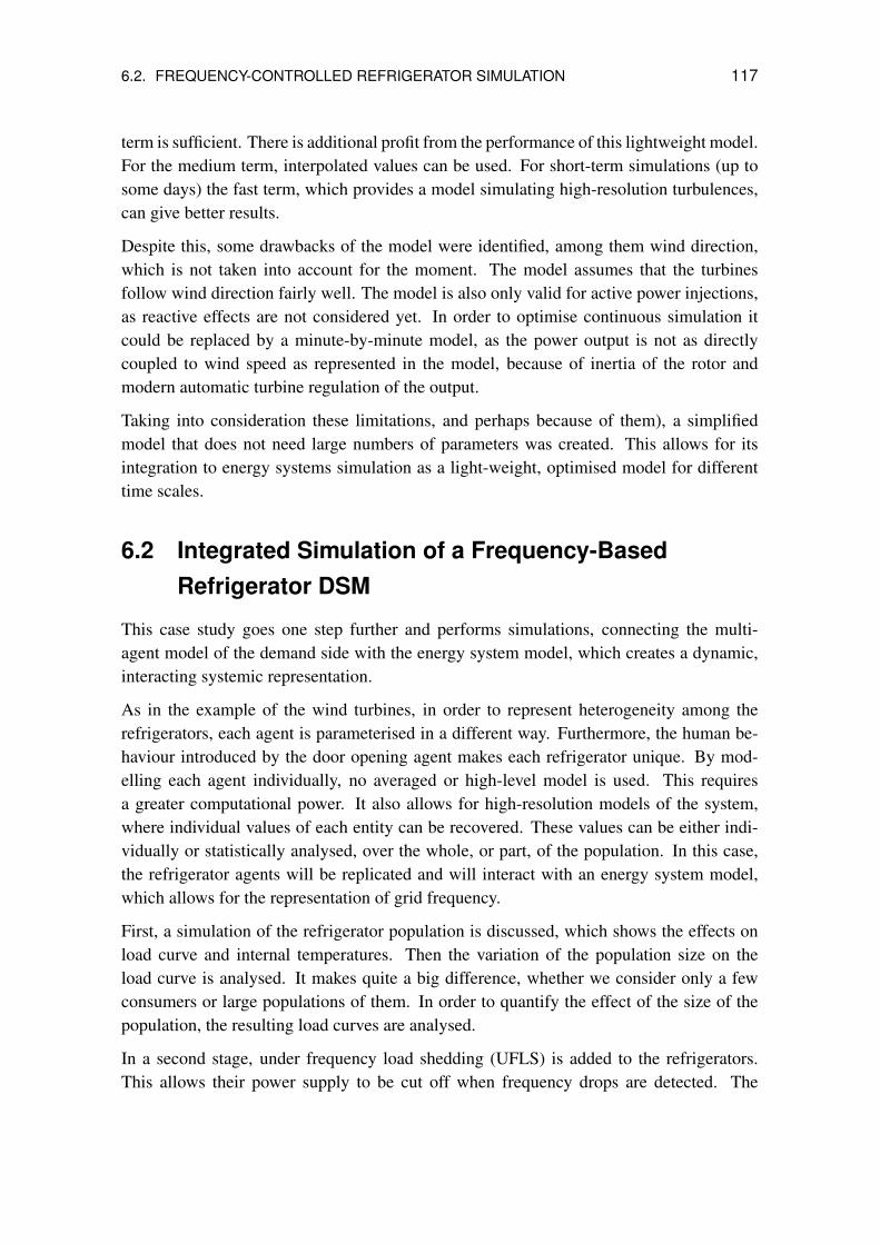
6.2. FREQUENCY-CONTROLLED REFRIGERATOR SIMULATION 117
term is sufficient. There is additional profit from the performance of this lightweight model.For the medium term, interpolated values can be used. For short-term simulations (up tosome days) the fast term, which provides a model simulating high-resolution turbulences,can give better results.
Despite this, some drawbacks of the model were identified, among them wind direction,which is not taken into account for the moment. The model assumes that the turbinesfollow wind direction fairly well. The model is also only valid for active power injections,as reactive effects are not considered yet. In order to optimise continuous simulation itcould be replaced by a minute-by-minute model, as the power output is not as directlycoupled to wind speed as represented in the model, because of inertia of the rotor andmodern automatic turbine regulation of the output.
Taking into consideration these limitations, and perhaps because of them), a simplifiedmodel that does not need large numbers of parameters was created. This allows for itsintegration to energy systems simulation as a light-weight, optimised model for differenttime scales.
6.2 Integrated Simulation of a Frequency-BasedRefrigerator DSM
This case study goes one step further and performs simulations, connecting the multi-agent model of the demand side with the energy system model, which creates a dynamic,interacting systemic representation.
As in the example of the wind turbines, in order to represent heterogeneity among therefrigerators, each agent is parameterised in a different way. Furthermore, the human be-haviour introduced by the door opening agent makes each refrigerator unique. By mod-elling each agent individually, no averaged or high-level model is used. This requiresa greater computational power. It also allows for high-resolution models of the system,where individual values of each entity can be recovered. These values can be either indi-vidually or statistically analysed, over the whole, or part, of the population. In this case,the refrigerator agents will be replicated and will interact with an energy system model,which allows for the representation of grid frequency.
First, a simulation of the refrigerator population is discussed, which shows the effects onload curve and internal temperatures. Then the variation of the population size on theload curve is analysed. It makes quite a big difference, whether we consider only a fewconsumers or large populations of them. In order to quantify the effect of the size of thepopulation, the resulting load curves are analysed.
In a second stage, under frequency load shedding (UFLS) is added to the refrigerators.This allows their power supply to be cut off when frequency drops are detected. The

118 CHAPTER 6. SIMULATION RESULTS AND DISCUSSION
UFLS strategy causes a rebound effect and a further synchronisation of the loads. Thisis analysed because complex system patterns were detected. Using the proposed UFLSstrategy, oscillation emerges in the system. In a last step, the conditions for these emergentphenomena found in the simulations are determined. The phase transition, typical forcomplex systems, from a stable to an oscillating regime is discussed.
6.2.1 Simulation of a Refrigerator Population
In this simulation, normal operation of the refrigerator population is shown. 250 refrig-erators are simulated with an installed power of 120 W each. All the parameters of therefrigerators are varied by 5% in order to recreate a realistic population in which eachrefrigerator has a slightly different configuration, as well as different initial conditions(internal temperature, etc.). This creates a heterogeneous population in which each refrig-erator has its own state and therefore the individual load curves are particular to each agent.This is necessary for recreating the aggregated load curve, which is a composition of manyindividual peaks which, however, do not coincide. The average total load of the populationis Pf = 11.5 kW during normal operation, which corresponds to a coincidence of aroundc = 40%.
40
80
120
ota
l lo
ad P [
W]
Single refrigerator electrical load
0
0 200 400 600 800 1000 1200 1400
To
Time [min]
7
8
9
10
mp
era
ture [
°C]
Single refrigerator internal cell temperature
5
6
0 200 400 600 800 1000 1200 1400
Tem
Time [min]
Figure 6.7: Simulation results for one randomly selected refrigerator of the population for one day. Theload curve follows rectangular pulses due to the cyclic operation of the refrigerator. The temperature of theinner cell is maintained at around 7 - 9°C. The sharp increases in temperature are due to simulated door
opening.
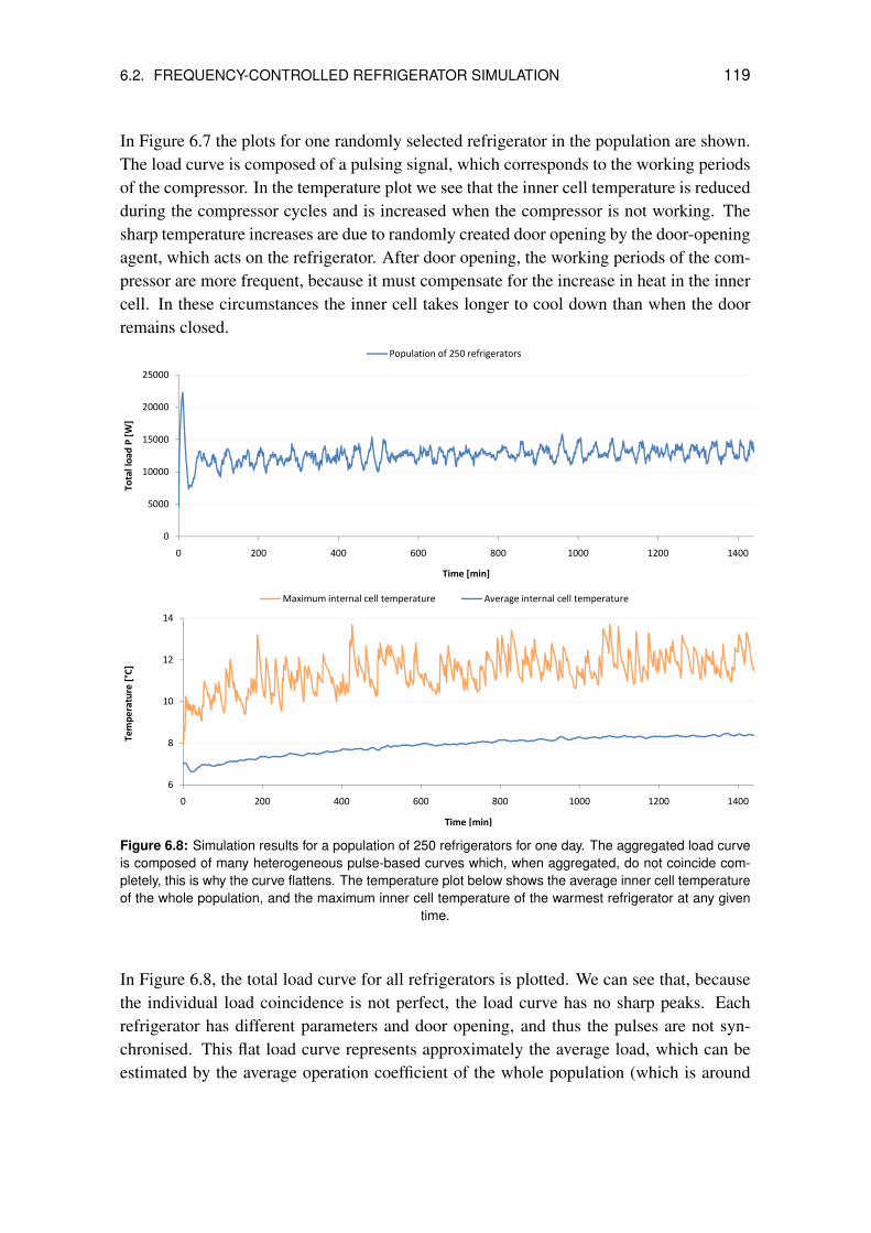
6.2. FREQUENCY-CONTROLLED REFRIGERATOR SIMULATION 119
In Figure 6.7 the plots for one randomly selected refrigerator in the population are shown.The load curve is composed of a pulsing signal, which corresponds to the working periodsof the compressor. In the temperature plot we see that the inner cell temperature is reducedduring the compressor cycles and is increased when the compressor is not working. Thesharp temperature increases are due to randomly created door opening by the door-openingagent, which acts on the refrigerator. After door opening, the working periods of the com-pressor are more frequent, because it must compensate for the increase in heat in the innercell. In these circumstances the inner cell takes longer to cool down than when the doorremains closed.
10000
15000
20000
25000
ota
l lo
ad P [
W]
Population of 250 refrigerators
0
5000
0 200 400 600 800 1000 1200 1400
To
Time [min]
10
12
14
mp
era
ture [
°C]
Maximum internal cell temperature Average internal cell temperature
6
8
0 200 400 600 800 1000 1200 1400
Tem
Time [min]
Figure 6.8: Simulation results for a population of 250 refrigerators for one day. The aggregated load curveis composed of many heterogeneous pulse-based curves which, when aggregated, do not coincide com-pletely, this is why the curve flattens. The temperature plot below shows the average inner cell temperatureof the whole population, and the maximum inner cell temperature of the warmest refrigerator at any given
time.
In Figure 6.8, the total load curve for all refrigerators is plotted. We can see that, becausethe individual load coincidence is not perfect, the load curve has no sharp peaks. Eachrefrigerator has different parameters and door opening, and thus the pulses are not syn-chronised. This flat load curve represents approximately the average load, which can beestimated by the average operation coefficient of the whole population (which is around

120 CHAPTER 6. SIMULATION RESULTS AND DISCUSSION
40%) times the installed power. The temperatures shown are the average temperature ofthe inner cells of the whole population; this slightly increases over the day due to dooropening. Door opening was not taken into account in the initial conditions. The maximumtemperature is derived from the whole refrigerator population and represents the warmestrefrigerator at any given time. This fluctuates significantly because door opening causessudden increases in temperature.
6.2.2 Variation of the Population Size: the Aggregation Effect
Obtaining real world data for different population sizes in order to analyse aggregationeffects of individual loads is quite a difficult task. In order to analyse many differentscales of aggregation, the load curves of different sizes of populations have to be acquired.This requires significant effort because the analysis of many different scales necessitatesindividual load monitoring. This can be done with small-scale populations or, in the future,through the deployment of smart meters or similar technology, which allow data capturefrom individual consumers.
However, an agent-based simulation approach allows us to easily vary the size of the pop-ulation and run many different experiments in-silico. In this case study, the effect of thevariation of the population size of fluctuating consumers will be analysed on the aggregatedcurve. The refrigerators have a characteristic consumption based on periodic pulses, dueto the compressor’s intermittent mode of operation. An irregular consumption is a goodexample for exploring the aggregation effect, as continuous loads are easy to predict anddo not present complex aggregation characteristics.
Having implemented the multi-agent simulation of a population of n refrigerators, differentruns with different populations sizes were simulated. A larger number of refrigeratorsusually smooths the curve, as the coincidence of individual peaks is lower.
Figure 6.9 represents a simulation run for one day, for different sizes n of the population.It can be seen that the curve fluctuates less and is smoother as n gets larger. The causeof this is the dispersion of individual pulses that do not coincide and are better distributedin time. The effect that is observed between different number of agents will be called theaggregation effect in this work.
The population size was varied from n = 5...50 (in steps of 5) and n = 50...250 (in steps of50) units. The load curve was analysed on the following features:
• Average load P
• Standard deviation s
• Maximum load Pmax per installed load Pinst
• Minimum load Pmin per installed load Pinst
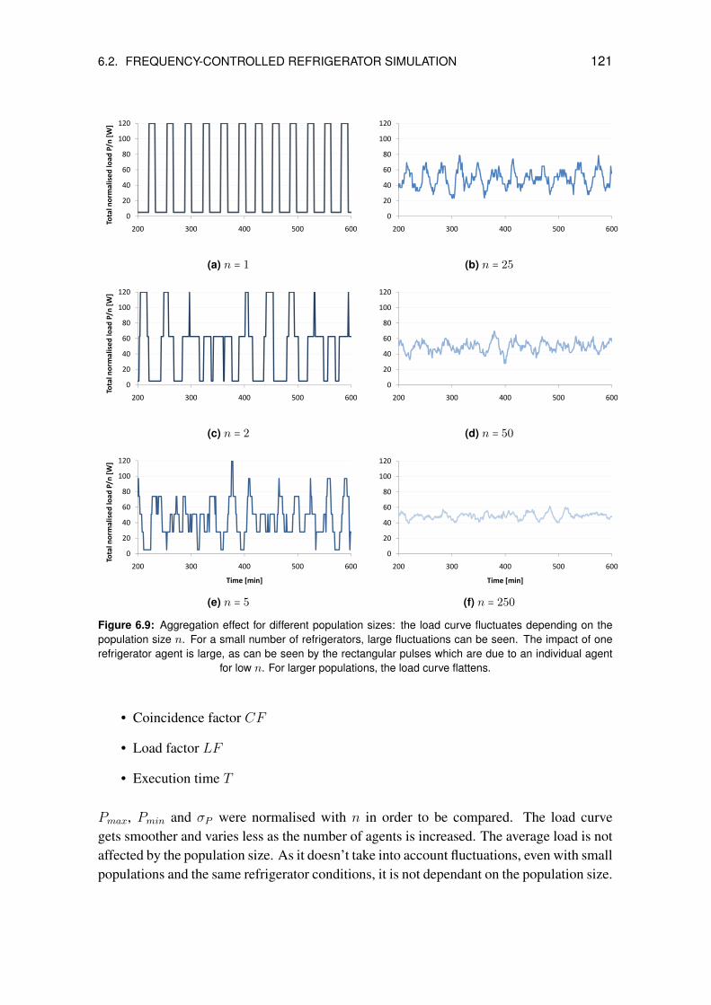
6.2. FREQUENCY-CONTROLLED REFRIGERATOR SIMULATION 121
40
60
80
100
120
mal
ised
load
P/n
[W
]
0
20
200 300 400 500 600
Tota
l no
rm
(a) n = 1
40
60
80
100
120
0
20
200 300 400 500 600
(b) n = 25
40
60
80
100
120
ma
lise
d lo
ad P
/n [
W]
0
20
200 300 400 500 600
Tota
l no
rm
(c) n = 2
40
60
80
100
120
0
20
200 300 400 500 600
(d) n = 50
40
60
80
100
120
mal
ise
d lo
ad P
/n [
W]
0
20
200 300 400 500 600
Tota
l no
rm
Time [min]
(e) n = 5
40
60
80
100
120
0
20
200 300 400 500 600
Time [min]
(f) n = 250
Figure 6.9: Aggregation effect for different population sizes: the load curve fluctuates depending on thepopulation size n. For a small number of refrigerators, large fluctuations can be seen. The impact of onerefrigerator agent is large, as can be seen by the rectangular pulses which are due to an individual agent
for low n. For larger populations, the load curve flattens.
• Coincidence factor CF
• Load factor LF
• Execution time T
Pmax, Pmin and σP were normalised with n in order to be compared. The load curvegets smoother and varies less as the number of agents is increased. The average load is notaffected by the population size. As it doesn’t take into account fluctuations, even with smallpopulations and the same refrigerator conditions, it is not dependant on the population size.

122 CHAPTER 6. SIMULATION RESULTS AND DISCUSSION
The standard deviation, or in this case, the coefficient of variation of the load curve de-creases when the population grows. This is because, in small populations, the impact ofone individual on the load curve is significant, and much sharper peaks appear than withlarger populations. The standard deviation apparently follows a power law (see interpolatedpower-law trend line, which is quite well-matched to the simulation values). The standarddeviation s thus seems clearly to be related to the population size. It can be approximatedby:
s = a ⋅ x(−b) with a ≈ 50 and b ≈ 0.5 (6.1)
for the described case, with a coefficient of determination of R2 = 0.9819. Similar findingsappear when observing the evolution of the coincidence and load factors CF and LF ,respectively. CF = 1 for very small populations, when the maximum load equals thetotal installed load. This means that there are moments where all single refrigerators areworking at the same time. As we increase the number of refrigerators, the coincidence islower, as it is much less likely that this occurs. The more refrigerators we have, the largerthe difference becomes between the maximum reached power and the installed power.Again, we seem to be confronted with a power law function of n. The fluctuations are dueto the stochastic nature of the model, which is important for small populations.
The load factor is a metric that relates the maximum load to the mean load. A low valueindicates that the ratio of the maximum to the mean load is high, thus that it is far awayfrom it. The value tends towards 1 as the curve gets flatter, which is the case for largerpopulations.
Indeed, CF and LF are closely related, as they both take into account the relationship ofthe maximum load to the total installed power and the mean, respectively. The mean power(which can be also obtained by the product of operation coefficient and installed individualpower) is not dependant on the size of the population. The operation coefficient dependson the characteristics of the refrigerators, and again, not on its size. So, finally we canconclude that the variation of maximum power (or minimum power) to the mean follows apower law function of n.
The standard deviation is a measure of how widely values are dispersed from the averagevalue (the mean). The standard deviation is also related but, as it is not calculated onone maximum but on the distances of all values from the mean, its statistical assertionis smoother. The maximum depends strongly on the non-determinism of the model, andvaries more among simulation runs than the sum of the distances. As an average, though,and if repeating the same experiment many times, the coincidence and load factors shouldalso remain stable and follow the power law.
The probability of extreme events, such as the coincidence of a large number of loads,should be further analysed. These events will strongly influence the load factor and co-
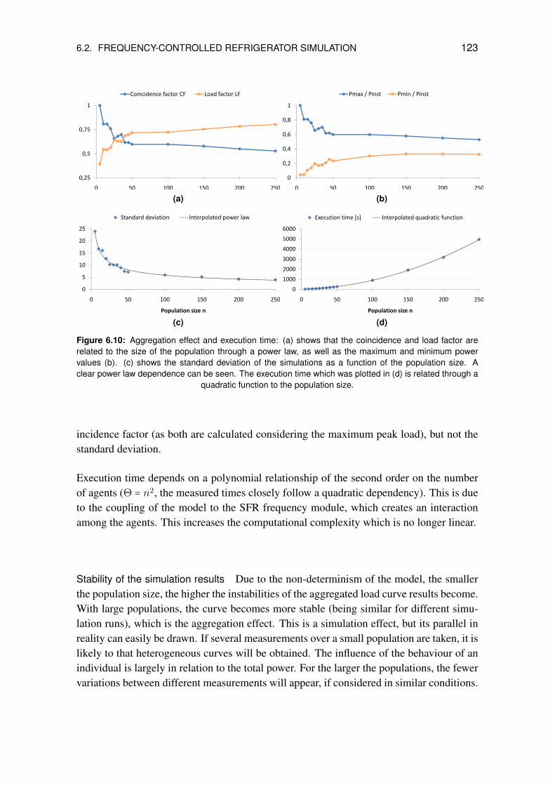
6.2. FREQUENCY-CONTROLLED REFRIGERATOR SIMULATION 123
0,75
1
Coincidence factor CF Load factor LF
0,25
0,5
0 50 100 150 200 250
(a)
0 4
0,6
0,8
1
Pmax / Pinst Pmin / Pinst
0
0,2
0,4
0 50 100 150 200 250
(b)
10
15
20
25
Standard deviation Interpolated power law
0
5
0 50 100 150 200 250
Population size n
(c)
2000
3000
4000
5000
6000
Execution time [s] Interpolated quadratic function
0
1000
2000
0 50 100 150 200 250
Population size n
(d)
Figure 6.10: Aggregation effect and execution time: (a) shows that the coincidence and load factor arerelated to the size of the population through a power law, as well as the maximum and minimum powervalues (b). (c) shows the standard deviation of the simulations as a function of the population size. Aclear power law dependence can be seen. The execution time which was plotted in (d) is related through a
quadratic function to the population size.
incidence factor (as both are calculated considering the maximum peak load), but not thestandard deviation.
Execution time depends on a polynomial relationship of the second order on the numberof agents (Θ = n2, the measured times closely follow a quadratic dependency). This is dueto the coupling of the model to the SFR frequency module, which creates an interactionamong the agents. This increases the computational complexity which is no longer linear.
Stability of the simulation results Due to the non-determinism of the model, the smallerthe population size, the higher the instabilities of the aggregated load curve results become.With large populations, the curve becomes more stable (being similar for different simu-lation runs), which is the aggregation effect. This is a simulation effect, but its parallel inreality can easily be drawn. If several measurements over a small population are taken, it islikely to that heterogeneous curves will be obtained. The influence of the behaviour of anindividual is largely in relation to the total power. For the larger the populations, the fewervariations between different measurements will appear, if considered in similar conditions.
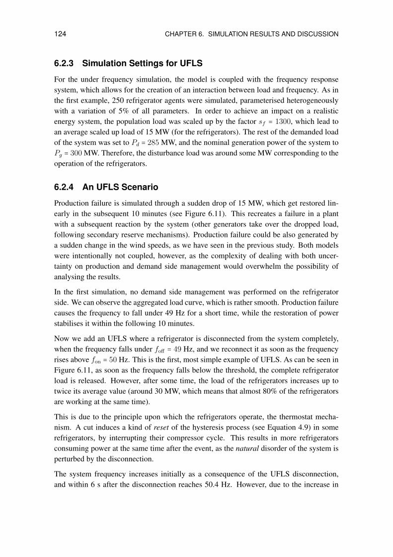
124 CHAPTER 6. SIMULATION RESULTS AND DISCUSSION
6.2.3 Simulation Settings for UFLS
For the under frequency simulation, the model is coupled with the frequency responsesystem, which allows for the creation of an interaction between load and frequency. As inthe first example, 250 refrigerator agents were simulated, parameterised heterogeneouslywith a variation of 5% of all parameters. In order to achieve an impact on a realisticenergy system, the population load was scaled up by the factor sf = 1300, which lead toan average scaled up load of 15 MW (for the refrigerators). The rest of the demanded loadof the system was set to Pd = 285 MW, and the nominal generation power of the system toPg = 300 MW. Therefore, the disturbance load was around some MW corresponding to theoperation of the refrigerators.
6.2.4 An UFLS Scenario
Production failure is simulated through a sudden drop of 15 MW, which get restored lin-early in the subsequent 10 minutes (see Figure 6.11). This recreates a failure in a plantwith a subsequent reaction by the system (other generators take over the dropped load,following secondary reserve mechanisms). Production failure could be also generated bya sudden change in the wind speeds, as we have seen in the previous study. Both modelswere intentionally not coupled, however, as the complexity of dealing with both uncer-tainty on production and demand side management would overwhelm the possibility ofanalysing the results.
In the first simulation, no demand side management was performed on the refrigeratorside. We can observe the aggregated load curve, which is rather smooth. Production failurecauses the frequency to fall under 49 Hz for a short time, while the restoration of powerstabilises it within the following 10 minutes.
Now we add an UFLS where a refrigerator is disconnected from the system completely,when the frequency falls under foff = 49 Hz, and we reconnect it as soon as the frequencyrises above fon = 50 Hz. This is the first, most simple example of UFLS. As can be seen inFigure 6.11, as soon as the frequency falls below the threshold, the complete refrigeratorload is released. However, after some time, the load of the refrigerators increases up totwice its average value (around 30 MW, which means that almost 80% of the refrigeratorsare working at the same time).
This is due to the principle upon which the refrigerators operate, the thermostat mecha-nism. A cut induces a kind of reset of the hysteresis process (see Equation 4.9) in somerefrigerators, by interrupting their compressor cycle. This results in more refrigeratorsconsuming power at the same time after the event, as the natural disorder of the system isperturbed by the disconnection.
The system frequency increases initially as a consequence of the UFLS disconnection,and within 6 s after the disconnection reaches 50.4 Hz. However, due to the increase in

6.2. FREQUENCY-CONTROLLED REFRIGERATOR SIMULATION 125
300
310
320
ctio
n [
MW
]
normal operation UFLS
280
290
0 200 400 600 800 1000 1200
Tota
l pro
du
c
295
300
305
310
315
320
eman
d p
ow
er
[MW
]
280
285
290
0 200 400 600 800 1000 1200
Tota
l de
49,4
49,6
49,8
50
50,2
50,4
50,6
stem
fre
qu
en
cy [
Hz]
48,8
49
49,2
0 200 400 600 800 1000 1200
Sys
Time [s]
Figure 6.11: Simulation results for a production failure scenario with and without UFLS. In the simulationwith UFLS, it can be seen how the demand drops down due to the shedding mechanisms of the refrigerators.Shortly after, frequency rises. Later, a rebound effect on the loads can be observed by the increase in power,in comparison to the normal case. The rebound lasts even after complete restoration of the generation side.
refrigerator consumption (in comparison to normal operation), the frequency recovery isslower and may even decrease again.
A very simple UFLS strategy based only on frequency thresholds can help to quickly re-store frequency after an event, but it can also create a rebound effect due to the coinci-dence of loads after disconnection. This load increase is counter-productive to frequencystabilisation.
6.2.5 The Rebound Effect
As we have seen with UFLS, after the first reconnection, an increase in total load can beobserved. This is usually called a rebound, which is characterised by a counteractive effect
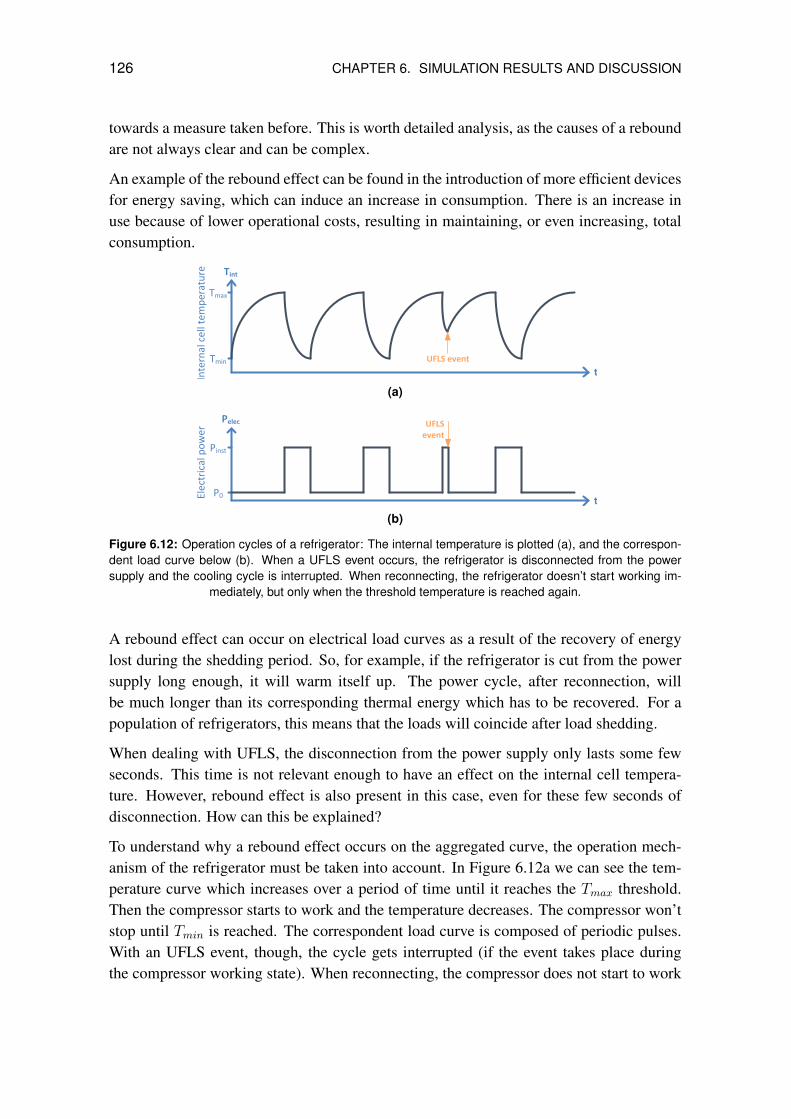
126 CHAPTER 6. SIMULATION RESULTS AND DISCUSSION
towards a measure taken before. This is worth detailed analysis, as the causes of a reboundare not always clear and can be complex.
An example of the rebound effect can be found in the introduction of more efficient devicesfor energy saving, which can induce an increase in consumption. There is an increase inuse because of lower operational costs, resulting in maintaining, or even increasing, totalconsumption.
Inte
rnal
cel
l tem
pera
ture
Tmax
Tmin UFLS event
t
Tint
(a)
P0
Pinst
Elec
tric
al p
ower
UFLS event
t
Pelec
(b)
Figure 6.12: Operation cycles of a refrigerator: The internal temperature is plotted (a), and the correspon-dent load curve below (b). When a UFLS event occurs, the refrigerator is disconnected from the powersupply and the cooling cycle is interrupted. When reconnecting, the refrigerator doesn’t start working im-
mediately, but only when the threshold temperature is reached again.
A rebound effect can occur on electrical load curves as a result of the recovery of energylost during the shedding period. So, for example, if the refrigerator is cut from the powersupply long enough, it will warm itself up. The power cycle, after reconnection, willbe much longer than its corresponding thermal energy which has to be recovered. For apopulation of refrigerators, this means that the loads will coincide after load shedding.
When dealing with UFLS, the disconnection from the power supply only lasts some fewseconds. This time is not relevant enough to have an effect on the internal cell tempera-ture. However, rebound effect is also present in this case, even for these few seconds ofdisconnection. How can this be explained?
To understand why a rebound effect occurs on the aggregated curve, the operation mech-anism of the refrigerator must be taken into account. In Figure 6.12a we can see the tem-perature curve which increases over a period of time until it reaches the Tmax threshold.Then the compressor starts to work and the temperature decreases. The compressor won’tstop until Tmin is reached. The correspondent load curve is composed of periodic pulses.With an UFLS event, though, the cycle gets interrupted (if the event takes place duringthe compressor working state). When reconnecting, the compressor does not start to work
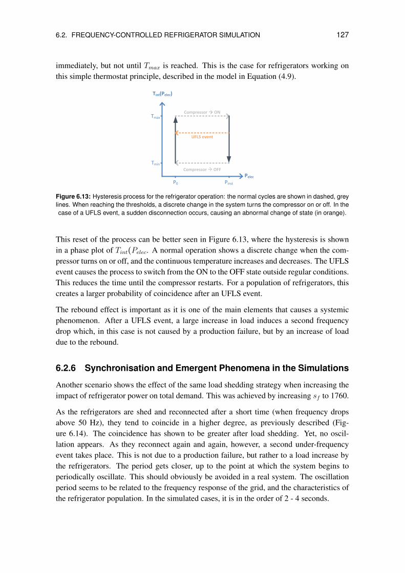
6.2. FREQUENCY-CONTROLLED REFRIGERATOR SIMULATION 127
immediately, but not until Tmax is reached. This is the case for refrigerators working onthis simple thermostat principle, described in the model in Equation (4.9).
Tmax
Tmin
P0 Pinst
Compressor ON
Compressor OFF
UFLS event
Tint(Pelec)
Pelec
Figure 6.13: Hysteresis process for the refrigerator operation: the normal cycles are shown in dashed, greylines. When reaching the thresholds, a discrete change in the system turns the compressor on or off. In thecase of a UFLS event, a sudden disconnection occurs, causing an abnormal change of state (in orange).
This reset of the process can be better seen in Figure 6.13, where the hysteresis is shownin a phase plot of Tint(Pelec. A normal operation shows a discrete change when the com-pressor turns on or off, and the continuous temperature increases and decreases. The UFLSevent causes the process to switch from the ON to the OFF state outside regular conditions.This reduces the time until the compressor restarts. For a population of refrigerators, thiscreates a larger probability of coincidence after an UFLS event.
The rebound effect is important as it is one of the main elements that causes a systemicphenomenon. After a UFLS event, a large increase in load induces a second frequencydrop which, in this case is not caused by a production failure, but by an increase of loaddue to the rebound.
6.2.6 Synchronisation and Emergent Phenomena in the Simulations
Another scenario shows the effect of the same load shedding strategy when increasing theimpact of refrigerator power on total demand. This was achieved by increasing sf to 1760.
As the refrigerators are shed and reconnected after a short time (when frequency dropsabove 50 Hz), they tend to coincide in a higher degree, as previously described (Fig-ure 6.14). The coincidence has shown to be greater after load shedding. Yet, no oscil-lation appears. As they reconnect again and again, however, a second under-frequencyevent takes place. This is not due to a production failure, but rather to a load increase bythe refrigerators. The period gets closer, up to the point at which the system begins toperiodically oscillate. This should obviously be avoided in a real system. The oscillationperiod seems to be related to the frequency response of the grid, and the characteristics ofthe refrigerator population. In the simulated cases, it is in the order of 2 - 4 seconds.
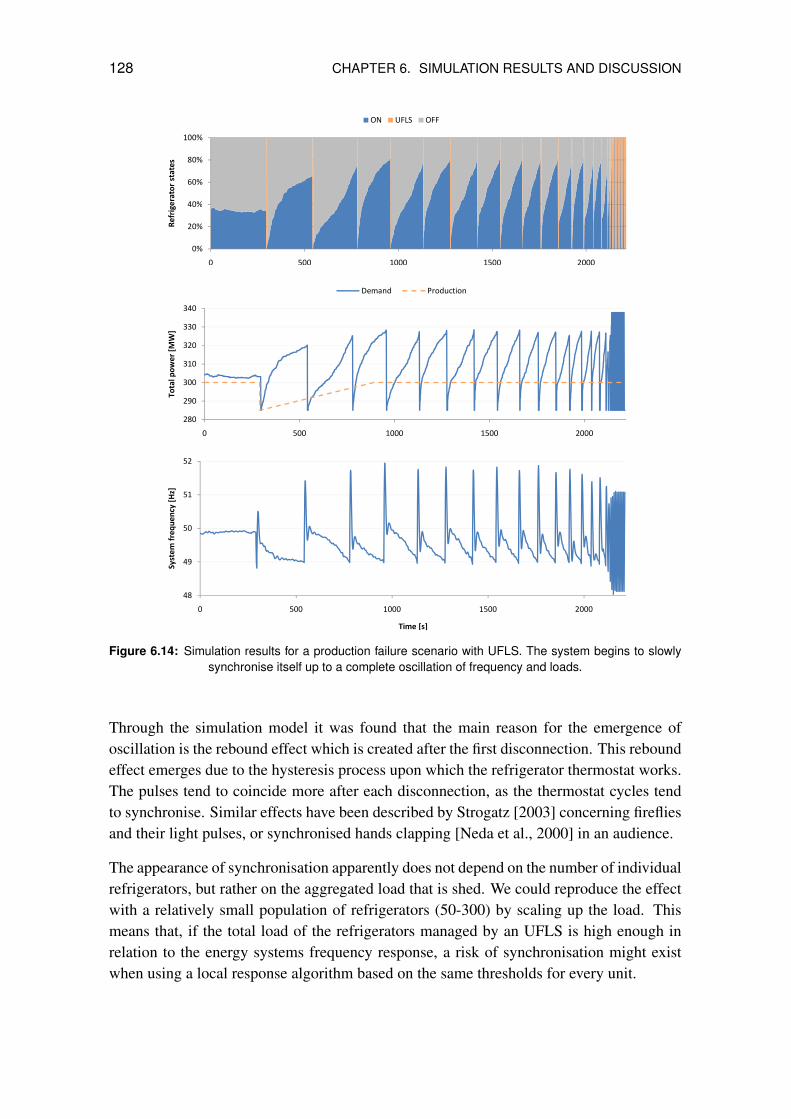
128 CHAPTER 6. SIMULATION RESULTS AND DISCUSSION
40%
60%
80%
100%
era
tor
stat
es
ON UFLS OFF
0%
20%
40%
0 500 1000 1500 2000
Re
frig
e
310
320
330
340
po
we
r [M
W]
Demand Production
280
290
300
0 500 1000 1500 2000
To
tal p
49
50
51
52
ste
m f
req
ue
ncy [
Hz]
48
49
0 500 1000 1500 2000
Sys
Time [s]
Figure 6.14: Simulation results for a production failure scenario with UFLS. The system begins to slowlysynchronise itself up to a complete oscillation of frequency and loads.
Through the simulation model it was found that the main reason for the emergence ofoscillation is the rebound effect which is created after the first disconnection. This reboundeffect emerges due to the hysteresis process upon which the refrigerator thermostat works.The pulses tend to coincide more after each disconnection, as the thermostat cycles tendto synchronise. Similar effects have been described by Strogatz [2003] concerning firefliesand their light pulses, or synchronised hands clapping [Neda et al., 2000] in an audience.
The appearance of synchronisation apparently does not depend on the number of individualrefrigerators, but rather on the aggregated load that is shed. We could reproduce the effectwith a relatively small population of refrigerators (50-300) by scaling up the load. Thismeans that, if the total load of the refrigerators managed by an UFLS is high enough inrelation to the energy systems frequency response, a risk of synchronisation might existwhen using a local response algorithm based on the same thresholds for every unit.
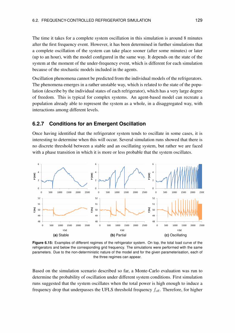
6.2. FREQUENCY-CONTROLLED REFRIGERATOR SIMULATION 129
The time it takes for a complete system oscillation in this simulation is around 8 minutesafter the first frequency event. However, it has been determined in further simulations thata complete oscillation of the system can take place sooner (after some minutes) or later(up to an hour), with the model configured in the same way. It depends on the state of thesystem at the moment of the under-frequency event, which is different for each simulationbecause of the stochastic models included in the agents.
Oscillation phenomena cannot be predicted from the individual models of the refrigerators.The phenomena emerges in a rather unstable way, which is related to the state of the popu-lation (describe by the individual states of each refrigerator), which has a very large degreeof freedom. This is typical for complex systems. An agent-based model can recreate apopulation already able to represent the system as a whole, in a disaggregated way, withinteractions among different levels.
6.2.7 Conditions for an Emergent Oscillation
Once having identified that the refrigerator system tends to oscillate in some cases, it isinteresting to determine when this will occur. Several simulation runs showed that there isno discrete threshold between a stable and an oscillating system, but rather we are facedwith a phase transition in which it is more or less probable that the system oscillates.
2
4
6
P [
kW]
0
2
0 500 1000 1500 2000 2500
2
4
6
P [
kW]
0
2
0 500 1000 1500 2000 2500
2
4
6
P [
kW]
0
2
0 500 1000 1500 2000 2500
49
50
51
52
f [H
z]
48
0 500 1000 1500 2000 2500
t [s]
(a) Stable
49
50
51
52
f [H
z]
48
0 500 1000 1500 2000 2500
t [s]
(b) Partial
49
50
51
52
f [H
z]
48
0 500 1000 1500 2000 2500
t [s]
(c) Oscillating
Figure 6.15: Examples of different regimes of the refrigerator system. On top, the total load curve of therefrigerators and below the corresponding grid frequency. The simulations were performed with the sameparameters. Due to the non-deterministic nature of the model and for the given parameterisation, each of
the three regimes can appear.
Based on the simulation scenario described so far, a Monte-Carlo evaluation was run todetermine the probability of oscillation under different system conditions. First simulationruns suggested that the system oscillates when the total power is high enough to induce afrequency drop that underpasses the UFLS threshold frequency foff . Therefore, for higher
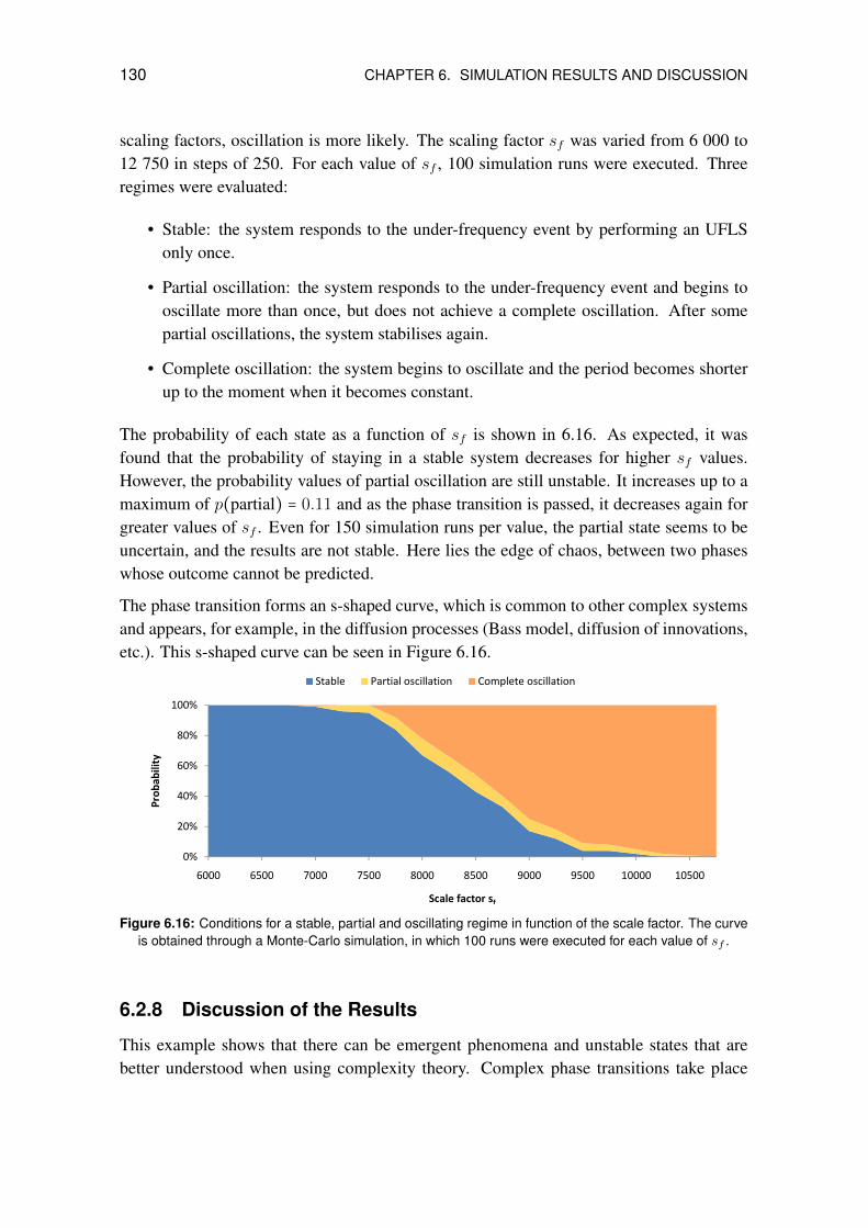
130 CHAPTER 6. SIMULATION RESULTS AND DISCUSSION
scaling factors, oscillation is more likely. The scaling factor sf was varied from 6 000 to12 750 in steps of 250. For each value of sf , 100 simulation runs were executed. Threeregimes were evaluated:
• Stable: the system responds to the under-frequency event by performing an UFLSonly once.
• Partial oscillation: the system responds to the under-frequency event and begins tooscillate more than once, but does not achieve a complete oscillation. After somepartial oscillations, the system stabilises again.
• Complete oscillation: the system begins to oscillate and the period becomes shorterup to the moment when it becomes constant.
The probability of each state as a function of sf is shown in 6.16. As expected, it wasfound that the probability of staying in a stable system decreases for higher sf values.However, the probability values of partial oscillation are still unstable. It increases up to amaximum of p(partial) = 0.11 and as the phase transition is passed, it decreases again forgreater values of sf . Even for 150 simulation runs per value, the partial state seems to beuncertain, and the results are not stable. Here lies the edge of chaos, between two phaseswhose outcome cannot be predicted.
The phase transition forms an s-shaped curve, which is common to other complex systemsand appears, for example, in the diffusion processes (Bass model, diffusion of innovations,etc.). This s-shaped curve can be seen in Figure 6.16.
40%
60%
80%
100%
Pro
bab
ility
Stable Partial oscillation Complete oscillation
0%
20%
6000 6500 7000 7500 8000 8500 9000 9500 10000 10500
Scale factor sf
Figure 6.16: Conditions for a stable, partial and oscillating regime in function of the scale factor. The curveis obtained through a Monte-Carlo simulation, in which 100 runs were executed for each value of sf .
6.2.8 Discussion of the Results
This example shows that there can be emergent phenomena and unstable states that arebetter understood when using complexity theory. Complex phase transitions take place
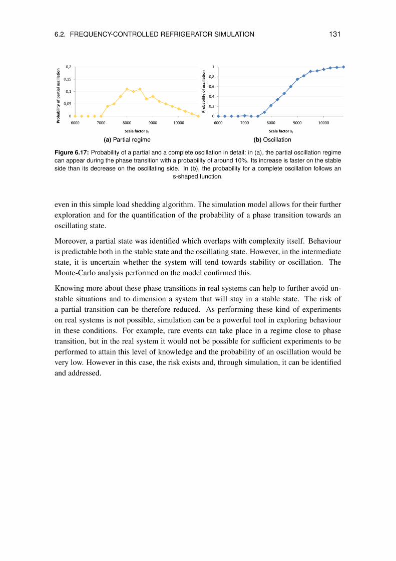
6.2. FREQUENCY-CONTROLLED REFRIGERATOR SIMULATION 131
0,05
0,1
0,15
0,2
y o
f p
arti
al o
scill
atio
n
0
0,05
6000 7000 8000 9000 10000Pro
bab
ility
Scale factor sf
(a) Partial regime
0 2
0,4
0,6
0,8
1
bab
ility o
f o
scill
atio
n
0
0,2
6000 7000 8000 9000 10000
Pro
b
Scale factor sf
(b) Oscillation
Figure 6.17: Probability of a partial and a complete oscillation in detail: in (a), the partial oscillation regimecan appear during the phase transition with a probability of around 10%. Its increase is faster on the stableside than its decrease on the oscillating side. In (b), the probability for a complete oscillation follows an
s-shaped function.
even in this simple load shedding algorithm. The simulation model allows for their furtherexploration and for the quantification of the probability of a phase transition towards anoscillating state.
Moreover, a partial state was identified which overlaps with complexity itself. Behaviouris predictable both in the stable state and the oscillating state. However, in the intermediatestate, it is uncertain whether the system will tend towards stability or oscillation. TheMonte-Carlo analysis performed on the model confirmed this.
Knowing more about these phase transitions in real systems can help to further avoid un-stable situations and to dimension a system that will stay in a stable state. The risk ofa partial transition can be therefore reduced. As performing these kind of experimentson real systems is not possible, simulation can be a powerful tool in exploring behaviourin these conditions. For example, rare events can take place in a regime close to phasetransition, but in the real system it would not be possible for sufficient experiments to beperformed to attain this level of knowledge and the probability of an oscillation would bevery low. However in this case, the risk exists and, through simulation, it can be identifiedand addressed.

Chapter 7
Conclusions and Outlook
The objective of this thesis was to show the interest and potential of a complex systemsapproach to the modelling and simulation of energy systems. This was first discussed froma theoretical point of view, presenting the fundamentals of complex systems, which arelittle known in the field of engineering. Complexity as an interdisciplinary science hasbeen shown to help to understand complex processes in biological, sociological and othersystems. Its application in the field of energy seems promising as similar patterns can befound, and as future energy systems will be more distributive in nature and include plentyof dynamic interactions, mainly because of the strong tendency to increase communication.Additionally, the energy system is multi-layered and is coupled to other non-technical as-pects such as human behaviour, which requires a socio-technical approach.
The energy system has to be considered as a socio-technical system. However, this di-mension is not yet part of many of the current simulation models. Including consumerbehaviour in models is becoming more and more important as changes have to be correctlyhandled and can be handled at local levels. Behavioural changes can also be induced (byincentives) in order to drive the system into a particular trajectory (for example, incentivebased DSM). Producer behaviour is also dependant on individual human decisions, such asthe installation of domestic distributed generation, significant penetration of which couldhave a major impact on the whole system. Therefore, the inclusion of sociological aspectsinto systemic models is quite important.
The energy system is a true system-of-systems, made-up of a large number of subsystemsthat can act independently. This becomes even more relevant in the move towards a smarter,more distributed and decentralised grid that includes an intelligent control of subsystemsand aggregators. The different subsystems are related to each other, by horizontal (withinthe same subsystem) and vertical (among different subsystems and scales) interactions.
Because of the need to represent a socio-technical, multi-scale system, a complex mod-elling approach was chosen. This is agent-based and allows for coupling with other mod-
133
134 CHAPTER 7. CONCLUSIONS AND OUTLOOK
elling tools. Agents as autonomous, proactive and interacting entities can be describedby continuous or discrete event models. The agent-based modelling approach allows abetter understanding of a complex energy system. The chosen approach has an importantexplorative character. This means, that agent-based models can help explore many of thepossible trajectories of a system before actually implementing it. Testing strategies be-forehand and foreseeing potential future problems allows a more efficient conception andplanning of future smart grids. The importance of the potential to include almost any kindof (inter and cross-scale) interactions should be underlined here. Agent-based models arenaturally conceived in order to allow these kinds of interactions. Even if not already in thesystem, they can be easily added to the model and tested in simulation. This is especiallyimportant when considering an increasing degree of decentralisation and distribution of theenergy system, which will encompass a larger number of interactions among its entities.
Using multi-approach modelling, in which agent-based models are coupled with contin-uous models, such as system dynamics or other differential equation modelling, seemspromising. This approach is the only way to represent the complex electrical system in adisaggregated way. It allows for the representation of interactions between the individualentities of the system. These are important effects that cannot be captured by linear modelsso it is especially important to model the system with numerous interactions, according tothe real system, in and between scales. Multi-scale modelling has been chosen as a fun-damental approach, in which cross-scale relationships are represented. There are currentlymany models at different scales, which implement only horizontal interactions (among en-tities of the same scale). However, pertinent vertical interactions have to be identified andmodelled too. This has been shown in the refrigerator case study, where individual loadscan have effects at a system level (grid frequency) and create feedback loops. The indica-tors at a system level have a further effect at a lower scale of the system, which can createnon-intuitive rebound effects, for instance.
The effects of topology and the relationship of complex network theory with electricalsystems should be analysed further. As identified before, some transmission grids wereshown to fulfil scale-free properties. An analysis of the distribution grid or other systemscould reveal other interesting complex network properties. Furthermore, the analysis ofnetworks in the communication layer and their relationship to the electrical layer shouldbe considered. It seems obvious that topology plays a role in the design and operation ofsmart grids.
A number of different models of the electrical system were created. Following the phi-losophy of the method, these models are intended to be as simple as possible, in order tocover the needs of smart electrical systems simulation, but not more than that. During themodelling works, the importance of this step to simplify the models must be noted. Thereare many very good and detailed models on one hand, and, on the other, very simplisticmodels, which would be too inaccurate for our purpose. The process of taking a detailed
135
model and reducing its degree of detail, in order to create a more simple one, is remark-ably complex. It is important to know exactly the aim of the model in order to prepare itfor that purpose. Furthermore, parameter reduction, in order to only take into account thereally relevant values of the model, is not a trivial task. Therefore, real expertise in the areais needed. As we are dealing with many different fields, including electrical, mechanical,thermal, environmental and other disciplines, many discussions with different experts wereneeded in an atmosphere of interdisciplinary cooperation.
It should be underlined that the effort that is needed for the processes of simplifying modelsis commonly underestimated. This is especially so because of the perception that currenttools, which implement detailed, non-systemic models are already sufficient and effectiveand need not be reduced. However, the need for a systemic approach in order to rep-resent the system and its interactions requires exactly these type of models. They mustbe representative enough for the purpose, but also lightweight enough to allow large-scalesimulations, in which many entities are executed in parallel and must allow for interactions.
Classical methods and models can also be combined with innovative approaches. The loadprofile method can complement agent-based models aiming to represent the demand sideto complete or facilitate whole system modelling. Modelling each and every consumerindividually might make sense in some cases, but might not be needed in others. Forexample, if only a specific electrical use is managed to perform DSM, it makes senseto represent this use in an agent-based form. For efficiency, the rest of the uses can bemodelled by standard load profiles, as they will not be affected by the DSM measures.This still allows for the representation of total consumption. This is a good example ofthe importance of the level of detail necessary to describe a certain phenomena. Complexmodels of a modular nature allow for the different representation of the same reality, indifferent levels of detail. By using a modular approach as the one presented, dependingon the question that has to be solved, an appropriate model for the considered entity canbe chosen. Wherever possible, modular approaches were used. Modular properties areessential for creating large-scale systemic models which are easily extendable. In addition,on-the-fly modifications that allow dynamic change to the structure of the models duringsimulation time, must be possible.
There is still a significant need for standardisation in order to allow interactions betweenmodels. A framework is necessary to develop models to represent such a large and complexsystem as energy. A framework was developed (Tafat), in parallel to this work in coop-eration with the University of Las Palmas, which aims to ensure compatibility betweenmodules by defining the interfaces and structure of the models through a model drivenengineering approach.
Another important point which was identified in the course of the work is validation. Val-idation of agent-based models of large-scale systems is a complex topic itself. It is toolarge a task to validate all the entities in these kinds of systems (and usually not all of the
136 CHAPTER 7. CONCLUSIONS AND OUTLOOK
data needed is available). Calibration at one scale is not sufficient, as this only ensuresvalidity at that scale, neglecting possible cross-scale effects. A calibration of the model isrecommended at a minimum of two scales, in order to ensure validity of ABMs. Coherencebetween the two calibrations should be considered.
The two case studies presented in this work address these topics and illustrate, from apractical point of view, the aforementioned points. Based on these, the relevance of theapproach is shown. Furthermore, some non-intuitive results were obtained which underlinethe interest of this modelling approach. Both the wind farm and the refrigerator case studyrepresent multi-scale models. In the case of the wind farm study, multiple time scaleswere treated. A model with the possibility of switching the accuracy of its outputs waspresented, which is modular and which can be used in different time-horizons for energysystem modelling. The importance of heterogeneous behaviour and parameterisation washighlighted. If all the turbine agents are modelled identically, the output doesn’t correspondto a real wind farm. Adding heterogeneous parameters and stochastic behaviour makes thesimulation results more realistic.
In the second case study a multi-agent population of refrigerators is coupled with a sim-plified grid model, which allows the recreation of the behaviour of the production-demandbalance on the frequency. The two scales are interacting dynamically with each other: thegenerated load from the refrigerators feeds the grid frequency model, and the frequency isthen used to manage the refrigerators. A calibrated and individually validated refrigeratormodel was taken as a base. Using frequency-based demand side management allows therefrigerator to be unplugged at under frequency events marked by a threshold, and to bereconnected when the frequency surpasses a second threshold.
Some important and unexpected findings were made with this model. Firstly, the aggre-gation effect was analysed. This effect describes how a load curve varies according to thenumber of consumers. It explains why we obtain different load curves when measuring atan individual level, or at a low voltage transformer or substation level. As load behaviourover time is heterogeneous among individual consumers, the peaks do not coincide at thesame time. Therefore, a flattening of the load curve occurs. However, up to this stage,very little is known about how loads aggregate and at which scale or number of consumerswe obtain a representative, flattened load curve. Through the refrigerator example it wasfound that the standard deviation of the load curve follows a power-law, this means thatthere are high numbers of fluctuations for a small number of consumers, but for large num-bers of consumers the deviation of the load curve is low. This relationship can be used todetermine when the load curve is representative. Of course, we only studied the effect onrefrigerators, but as power laws are common in complex systems it is likely that this typeof relationship is valid for other cases also. This should be explored further.
The model allowed the testing of an under frequency load shedding strategy on a refriger-ator population, and at the same time, the observation of the effects at a system scale. So,
137
grid frequency was calculated in real time according to the consumption of the refrigera-tors. The frequency was used again to control load shedding at the individual scale. Whenusing a simple load management strategy a rebound effect appears. Detailed analysis at theindividual level indicates that this effect is due to the hysteresis process of the refrigeratorthermostat and is not a result of the warming-up of the refrigerators during disconnection,as was first suspected. The model allowed us to explore these effects in detail. If required,a simulation can be stopped, and any of the values of the system (temperatures, DSM-state,thermostat state) observed and evaluated.
Furthermore, in some situations an emergent synchronisation appeared because the re-bound effect caused another frequency drop. This synchronisation lead to a complete os-cillation of loads and frequency, which would have been fatal in a real environment. Thiseffect could only be observed due to the replication and simulation of a large and hetero-geneous population of refrigerators, which for a real test bench would have been far tooexpensive. Emergent synchronisation has been studied in many other disciplines, and canbe exemplified by firefly lightning or hands clapping. The effects found in the refrigeratorpopulation show many parallels to these studies and are worthy of further study. So, forexample, we found certain values of parameters, which determine if the system remainsstable if it synchronised partially or oscillates completely. This phase transition from oneregime to another is typical for complex systems. In the intermediate stage, it is uncer-tain if the system will remain stable or if it will oscillate. This can be characterised by aprobability, which follows an s-shaped curve and includes an unstable transitory state in-between. Knowing more about these phase transitions can help to avoid getting even closeto a regime where a synchronisation would be possible (even with a very low probability),and occur as an extreme event. Systemic, cross-scale models like this can help to betterunderstand emergent phenomena such as synchronisation or cascade effects in electricalenergy systems.
A proposed simulation scenario would be to consider coupling both case studies presentedin this work. The first and the second case studies could be coupled and disturbances to thesystem could be produced by wind generation. This would enable analysis of the reactionto a sudden drop in power caused by the wind speed. Furthermore, the strategies used forUFLS have to be improved, first to reduce the rebound effect and second to ensure a betterfrequency stabilisation and restoration. Therefore, different or slightly varied thresholdscould be used.
Unlike in the biological or social fields, a much greater weight on controllability of emer-gence must be applied in energy systems. This is important because the other fields whichuse this type of approach are mostly interested only in greater analysis and understandingof the system’s behaviour. However, in the case of a man-made energy system, whichhas been designed for a certain purpose, a deep understanding of its operation is needed;control and management of the system, including forecasting its behaviour are really fun-

138 CHAPTER 7. CONCLUSIONS AND OUTLOOK
damental. The complex systems approach allows an understanding of the operation of apotential future system. Experiences gained through simulation benefit the developmentof future systems. This approach offers an in-silico lab where upcoming technologies andstrategies can be tested, in order to better manage the system, avoiding the costs and risksof real testing procedures. This is especially interesting in relation to distributed systems,in which large scale deployment would be necessary for testing. Strategies on how to man-age these systems can be explored through a complexity-based approach. This approachenables the simulation of complex phenomena and interactions within the system, throughdifferent scales and with dynamic, heterogeneous entities evolving over time.

References
Advances in Complex Systems, Journal. 2010.URL http://www.worldscinet.com/acs/mkt/aims_scope.shtml [cited on page 9]
ABRAS S. Systeme domotique Multi-Agents pour la gestion de l’energie dans l’habitat.PhD thesis, 2009. [cited on page 56]
ADAMIC L. Complex systems: Unzipping Zipf’s law. Nature, volume 474(7350):pages164–165, 2011. 10.1038/474164a. [cited on page 25]
AKSOY H., FUAT TOPRAK Z., AYTEK A., and ERDEM NAL N. Stochastic generationof hourly mean wind speed data. Renewable Energy, volume 29(14):pages 2111–2131,2004. [cited on pages 82 and 83]
ALBADI M.H. and EL-SAADANY E.F. Demand Response in Electricity Markets: AnOverview. In Power Engineering Society General Meeting, 2007. IEEE, pages 1–5.2007. [cited on page 35]
ALBERT R., JEONG H., and BARABASI A.L. Error and attack tolerance of com-plex networks. Nature, volume 406(6794):pages 378–382, 2000. 10.1038/35019019.[cited on page 26]
ALLERTON T. Simulating the distribution and cross-correlation of wind farm output. Tech-nical report, EON and The Heriott-Watt University, 2008. [cited on page 82]
AMIN S.M. and WOLLENBERG B.F. Toward a smart grid: power delivery for the 21stcentury. Power and Energy Magazine, IEEE, volume 3(5):pages 34–41, 2005. 1540-7977. [cited on page 36]
ANDERSON P.M. and MIRHEYDAR M. A low-order system frequency response model.Power Systems, IEEE Transactions on, volume 5(3):pages 720–729, 1990. [cited on page 93]
APICELLA N. A Library for Decision-Making in Agent-Based Models. Fakultat fur In-formatik, Universitat Karlsruhe (TH), 2009. [cited on page 58]
139

140 REFERENCES
AUSTIN D. Percolation: Slipping through the Cracks. 2011.URL http://www.ams.org/samplings/feature-column/fcarc-percolation
[cited on page 13]
AXELROD R. The complexity of cooperation: agent-based models of competition andcollaboration. Princeton University Press, 1997. [cited on page 47]
BARABASI A.L. The Architecture of Complexity. Control Systems Magazine, IEEE,volume 27(4):pages 33–42, 2007. 0272-1708. [cited on pages 9 and 15]
BARABASI A.L. and ALBERT R. Emergence of Scaling in Random Networks. Science,volume 286(5439):pages 509–512, 1999. [cited on pages 15 and 21]
BAYEM H., PHULPIN Y., DESSANTE P., and BECT J. Probabilistic computation of windfarm power generation based on wind turbine dynamic modeling. In 10th InternationalConference on Probabilistic Methods Applied to Power Systems - PMAPS 2008, pages1–6. Porto Rico, 2008. [cited on pages 82 and 83]
BERGEN A.R. and VITTAL V. Power System Analysis. Prentice-Hall, New Jersey, 2000.[cited on page 92]
BILLINTON R., CHEN H., and GHAJAR R. Time-series models for reliability evalua-tion of power systems including wind energy. Microelectronics and Reliability, vol-ume 36(9):pages 1253–1261, 1996. [cited on pages 82 and 83]
BOLLOBAS B. and RIORDAN O. Percolation. Cambridge University Press, 2006.[cited on page 12]
BORSHCHEV A. and FILIPPOV A. From system dynamics and discrete event to practicalagent based modeling: Reasons, techniques, tools. In The 22nd International Confer-ence of the System Dynamics Society. The System Dynamics Society, Oxford, England,2004. [cited on pages 66, 80, and 98]
BURIAN J. Complex Systems Tutorial. 2010.URL http://eldar.cz/cognition/complex/ [cited on page 49]
BURROUGH P.A. Principles of geographical information systems for land resources as-sessment. Monographs on soil and resource surveys ; no. 12. Clarendon Press, Oxford,England, 1986. Includes bibliographies and indexes.
CASTELLANI B. Art & Science Factory. 2012.URL http://www.art-sciencefactory.com/about-factory.html
[cited on page 155]

REFERENCES 141
CERRI G., PALMIERI A., MONTICELLI E., and PEZZOLI D. Identification of domesticrefrigerator models including cool storage. In International Congress of Refrigeration2003. Washington D.C., USA, 2003. [cited on pages 88 and 89]
CHAN W.K.V., YOUNG-JUN S., and MACAL C.M. Agent-based simulation tutorial -simulation of emergent behavior and differences between agent-based simulation anddiscrete-event simulation. In Winter Simulation Conference (WSC), Proceedings of the2010, pages 135–150. 2010. [cited on page 73]
CHAPPIN E.J.L. and DIJKEMA G.P.J. An Agent Based Model of the System of ElectricityProduction Systems: Exploring the Impact of CO2 Emission-Trading. In System ofSystems Engineering, 2007. SoSE ’07. IEEE International Conference on, pages 1–5.2007. [cited on page 73]
CHASSIN D.P. and POSSE C. Evaluating North American electric grid reliabilityusing the Barabsi-Albert network model. Physica A: Statistical Mechanics andits Applications, volume 355(2-4):pages 667–677, 2005. 0378-4371 doi: DOI:10.1016/j.physa.2005.02.051. [cited on page 26]
CHEDID R., AKIKI H., and RAHMAN S. A decision support technique for the designof hybrid solar-wind power systems. Energy conversion, ieee transactions on, vol-ume 13(1):pages 76–83, 1998. [cited on page 85]
CHEN C.C., NAGL S., and CLACK C. A Method for Validating and Discovering As-sociations between Multi-level Emergent Behaviours in Agent-Based Simulations. InN. Nguyen, G. Jo, R. Howlett, and L. Jain, editors, Agent and Multi-Agent Systems:Technologies and Applications, volume 4953 of Lecture Notes in Computer Science,pages 1–10. Springer Berlin / Heidelberg, 2008. [cited on page 59]
COSTA GOMEZ J. Desarrollo de modelos de demanda electrica en el hogar. Diplomathesis, 2011. [cited on page 85]
DEMAZEAU Y. and COSTA A. Populations and organizations in open multi-agent systems.In 1st National Symposium on Parallel and Distributed AI (PDAI96). Hyderabad, India,1996. [cited on page 56]
DIMEAS A.L. and HATZIARGYRIOU N.D. A MAS architecture for Microgrids control.In Intelligent Systems Application to Power Systems, 2005. Proceedings of the 13th In-ternational Conference on, page 5. 2005. [cited on page 73]
DIMEAS A.L. and HATZIARGYRIOU N.D. Agent based control of Virtual Power Plants.In Intelligent Systems Applications to Power Systems, 2007. ISAP 2007. InternationalConference on, pages 1–6. 2007. [cited on page 73]

142 REFERENCES
GONZALEZ DE DURANA J., BARAMBONES O., KREMERS E., and VIEJO P. CompleteAgent based Simulation of Mini-Grids. In The Ninth IASTED European Conferenceon Power and Engineering Systems, EuroPES 2009, volume 681, pages 046–188. ActaPress, Palma de Mallorca, Spain, 2009. [cited on page 74]
GONZALEZ DE DURANA J.M., BARAMBONES O., KREMERS E., and VIEJO P. Mod-elling Smart Grids As Complex Systems Through The Implementation Of IntelligentHubs. In Proceedings of the 7th International Conference on Informatics in Control,Automation and Robotics ICINCO 2010, volume 3, pages 146–151. INSTICC Press2010, Funchal, 2010. [cited on page 74]
EHRENTREICH N. Agent-Based Modeling : The Santa Fe Institute Artificial Stock Mar-ket Model Revisited. Lecture Notes in Economics and Mathematical Systems ; 602.Springer-Verlag Berlin Heidelberg, Berlin, Heidelberg, 2008. In: Springer-Online.
EINSTEIN A. On the method of theoretical physics. Philosophy of science, vol-ume 1(2):page 7, 1934. [cited on page 71]
EPSTEIN J. Generative social science: Studies in agent-based computational modeling.Princeton University Press, Princeton, USA, 2006. [cited on page 73]
EPSTEIN J.M. and AXTELL R. Growing artificial societies: social science from the bottomup. The Brookings Institution, Washington, DC, USA, 1996. ISBN 0-262-55025-3.[cited on page 73]
ERDOS P. and RENYI A. On random graphs, I. Publicationes Mathematicae (Debrecen),volume 6:pages 290–297, 1959. [cited on pages 14 and 19]
EUROPEAN COMMISSION. Microgrids Project. 2011.URL http://www.microgrids.eu [cited on page 40]
EVORA J., KREMERS E., CUEVA S., HERNANDEZ M., HERNANDEZ J., and VIEJO P.Agent-based modelling of electrical load at household level. In S. Stepney, P.H. Welch,and P.S. Andrews, editors, ECAL 2011: CoSMoS - Proceedings of the 2011 Workshopon Complex Systems Modelling and Simulation, page 15. Paris, 2011. [cited on pages 74
and 86]
FERBER J. Multi-agent systems: an introduction to distributed artificial intelligence, vol-ume 222. Addison-Wesley, 1999. [cited on page 51]
FERBER J. and PERROT J. Les systemes multi-agents: vers une intelligence collective.InterEditions, 1995. [cited on pages 55 and 56]
FORD A. System Dynamics and the Electric Power Industry. System Dynamics Review,volume 13(1):pages 57–85, 1997. [cited on page 166]
REFERENCES 143
FORRESTER J. Industrial dynamics. M.I.T. Press, 1961. [cited on page 62]
GILBERT N. Agent-Based Models (Quantitative Applications in the Social Sciences). SagePublications, Inc, 2007. [cited on page 53]
GIORDANO V., GANGALE F., FULLI G., and SANCHEZ JIMENEZ M. Smart Grid projectsin Europe: lessons learned and current developments. Technical Report EUR 24856 EN,Joint Research Centre - Institute for Energy, 2011. [cited on pages 37 and 38]
GRIMMETT G. Percolation, volume 321. Springer Verlag, 1999. [cited on page 12]
GRONLUND B. Life and Complexity in Urban Space. 1993.URL http://homepage.mac.com/bogronlund/get2net/Life_and_complexity.
html [cited on page 10]
HAREL D. Statecharts: a visual formalism for complex systems. Science of ComputerProgramming, volume 8(3):pages 231–274, 1987. [cited on page 65]
HATZIARGYRIOU N., DIMEAS A., and TSIKALAKIS A. Centralized and decentralizedcontrol of microgrids. International Journal of Distributed Energy Resources, vol-ume 1(3):pages 197–212, 2005. [cited on page 73]
HAYEK F. The results of human action but not of human design. Studies in philosophy,politics and economics, pages 96–105, 1967. [cited on page 7]
JACOBO J.C., ROURE D.D., and GERDING E.H. An agent-based electrical power market.2008. 14027501655-1656. [cited on page 73]
JENKINS N., ALLAN R., CROSSLEY P., KIRSCHEN D., and STRBAC G. Embeddedgeneration. Institution of Electrical Engineers, 2000. (Power and Energy Ser. 31).[cited on pages 34 and 35]
JENNINGS N.R. On agent-based software engineering. Artificial Intelligence, volume117(2):pages 277–296, 2000. [cited on page 60]
JIANG Z. Agent-Based Control Framework for Distributed Energy Resources Microgrids.In Intelligent Agent Technology, 2006. IAT ’06. IEEE/WIC/ACM International Confer-ence on. IEEE, 2006. [cited on page 74]
JIYUAN F. and BORLASE S. The evolution of distribution. Power and Energy Magazine,IEEE, volume 7(2):pages 63–68, 2009. 1540-7977. [cited on page 40]
JONES J.C., MYERSCOUGH M.R., GRAHAM S., and OLDROYD B.P. Honey Bee NestThermoregulation: Diversity Promotes Stability. Science, volume 305(5682):pages 402–404, 2004. [cited on page 13]
144 REFERENCES
KOTTICK D., BLAU M., and EDELSTEIN D. Battery energy storage for frequency reg-ulation in an island power system. Energy Conversion, IEEE Transactions on, vol-ume 8(3):pages 455–459, 1993. [cited on page 93]
KREMERS E., LEWALD N., BARAMBONES O., and GONZALEZ DE DURANA J.M. AnAgent-based Multi-Scale Wind Generation Model. In The Ninth IASTED EuropeanConference on Power and Engineering Systems, EuroPES 2009, volume 681, pages064–166. Acta Press, Palma de Mallorca, Spain, 2009. [cited on pages 74 and 82]
KREMERS E., VIEJO P., GONZALEZ DE DURANA J.M., and BARAMBONES O. A Com-plex Systems Modelling Approach for Decentralized Simulation of Electrical Micro-grids. In 15th IEEE International Conference on Engineering of Complex ComputerSystems, page 8. Oxford, 2010. [cited on pages 67, 74, and 93]
KREMERS E., VIEJO P., LEWALD N., GONZALEZ DE DURANA J.M., and BARAMBONES
O. Agent-Based Simulation of Wind Farm Generation at Multiple Time Scales. In G.O.Suvire, editor, Wind Farm / Book 2, volume 2. Intech, 2011. [cited on pages 74, 82, and 99]
LAGUERRE O., DERENS E., and PALAGOS B. Study of domestic refrigerator temperatureand analysis of factors affecting temperature: a French survey. International Journal ofRefrigeration, volume 25(5):pages 653–659, 2002. [cited on page 101]
LANGTON C.G. Computation at the edge of chaos: Phase transitions and emergentcomputation. Physica D: Nonlinear Phenomena, volume 42(1-3):pages 12–37, 1990.[cited on page 24]
LEE HAU AIK D. A general-order system frequency response model incorporating loadshedding: analytic modeling and applications. Power Systems, IEEE Transactions on,volume 21(2):pages 709–717, 2006. [cited on page 93]
LIU Y.Y., SLOTINE J.J., and BARABASI A.L. Controllability of complex networks. Na-ture, volume 473(7346):pages 167–173, 2011. 10.1038/nature10011. [cited on page 28]
MACAL C.M. and NORTH M.J. Tutorial on agent-based modelling and simulation. Jour-nal of Simulation, volume 4(3):pages 151–162, 2010. [cited on page 52]
MAIER M.W. Architecting principles for systems-of-systems. Systems Engineering, vol-ume 1(4):pages 267–284, 1998. [cited on page 67]
MARKARIAN G., KOLLE R., and TARTER A. Aviation Security Engineering: A HolisticApproach. Artech House Publishers, 2011. [cited on page 67]
MCARTHUR S.D.J., DAVIDSON E.M., CATTERSON V.M., DIMEAS A.L., HATZIAR-GYRIOU N.D., PONCI F., and FUNABASHI T. Multi-Agent Systems for Power Engi-neering Applications - Part I: Concepts, Approaches, and Technical Challenges. Power

REFERENCES 145
Systems, IEEE Transactions on, volume 22(4):pages 1743–1752, 2007a. 0885-8950.[cited on page 73]
MCARTHUR S.D.J., DAVIDSON E.M., CATTERSON V.M., DIMEAS A.L., HATZIAR-GYRIOU N.D., PONCI F., and FUNABASHI T. Multi-Agent Systems for Power Engi-neering Applications - Part II: Technologies, Standards, and Tools for Building Multi-agent Systems. Power Systems, IEEE Transactions on, volume 22(4):pages 1753–1759,2007b. 0885-8950. [cited on page 73]
MILANO F. Power System Analysis Toolbox. 2009.URL http://www.power.uwaterloo.ca/~fmilano/psat.htm [cited on pages 80 and 93]
MINSKY M. Matter, mind and models. Proceedings of IFIP Congress, pages 45–49, 1965.[cited on page 48]
MIORANDI D., ZANIN M., CRISTOBAL S., HERRANZ R., and BALBAS M. ComplexSystems for an ICT-enabled Energy System (ComplexEnergy White Paper). Technicalreport, Innaxis Foundation, Create-Net, 2010. [cited on page 8]
NAVIGANT CONSULTING. Microgrids Research Assessment: Phase 2 Final Report. Tech-nical report, 2006. [cited on pages 40 and 41]
NEDA Z., RAVASZ E., BRECHET Y., VICSEK T., and BARABASI A.L. Self-organizingprocesses: The sound of many hands clapping. Nature, volume 403(6772):pages 849–850, 2000. 10.1038/35002660. [cited on page 128]
NICHITA C., LUCA D., DAKYO B., and CEANGA E. Large Band Simulation of theWind Speed for Real-Time Wind Turbine Simulators. Power Engineering Review, IEEE,volume 22(8):pages 63–63, 2002. 0272-1724. [cited on page 82]
OYARZABAL J., JIMENO J., RUELA J., ENGLER A., and HARDT C. Agent based MicroGrid Management System. Power Engineering Society General Meeting, 2007. IEEE,page 5, 2007. [cited on page 74]
PAATERO J.V. Computational Studies on Variable Distributed Energy Systems. PhD thesis,Helsinki University of Technology, 2009. [cited on page 33]
PACKARD N.H. and WOLFRAM S. Two-dimensional cellular automata. Journal of Sta-tistical Physics, volume 38(5):pages 901–946, 1985. [cited on page 11]
PALENSKY P. and DIETRICH D. Demand Side Management: Demand Response, Intelli-gent Energy Systems, and Smart Loads. Industrial Informatics, IEEE Transactions on,volume 7(3):pages 381–388, 2011. [cited on page 35]

146 REFERENCES
PALENSKY P., KUPZOG F., ZAIDI A.A., and KAI Z. Modeling domestic housing loadsfor demand response. In Industrial Electronics, 2008. IECON 2008. 34th Annual Con-ference of IEEE, pages 2742–2747. 2008. [cited on page 33]
PIPATTANASOMPORN M., FEROZE H., and RAHMAN S. Multi-agent systems in a dis-tributed smart grid: Design and implementation. In Power Systems Conference andExposition, 2009. PSCE ’09. IEEE/PES, pages 1–8. 2009. [cited on page 74]
PYKA A. and GREBEL T. Agent-Based Modelling A Methodology for the Analysis ofQualitative Development Processes. pages 17–35. 2006. [cited on page 53]
RED ELECTRICA ESPANOLA. Wind power produced more than half the electricity inSpain during the early morning hours. 2009.URL http://www.ree.es/ingles/sala_prensa/web/notas_detalle.aspx?id_
nota=117 [cited on page 31]
REFSGAARD J.C. and HENRIKSEN H.J. Modelling guidelines–terminology and guid-ing principles. Advances in Water Resources, volume 27(1):pages 71–82, 2004.[cited on page 49]
REYNOLDS C.W. Flocks, herds and schools: A distributed behavioral model. SIGGRAPHComput. Graph., volume 21(4):pages 25–34, 1987. [cited on page 14]
R IOS-RULL J. Models with heterogeneous agents. Frontiers of business cycle research,pages 98–125, 1995. [cited on page 72]
ROCHA L. Complex Systems Modeling: Using Metaphors From Nature in Simulation andScientific Models. 2003.
ROSAS-CASALS M., VALVERDE S., and SOLE R.V. Topological vulnerability of theEuropean power grid under errors and attacks. International Journal of Bifurcationsand Chaos, volume 17(7):pages 2465–2475, 2007. [cited on pages 26 and 27]
SENSFUSS F. Assessment of the impact of renewable electricity generation on the Germanelectricity sector: an agent-based simulation approach. Doctoral thesis, UniversitatKarlsruhe (TH), 2007. [cited on pages 72 and 73]
SHORT J.A., INFIELD D.G., and FRERIS L.L. Stabilization of Grid Frequency ThroughDynamic Demand Control. Power Systems, IEEE Transactions on, volume 22(3):pages1284–1293, 2007. [cited on pages 91 and 94]
SIMON H. The Sciences of the Artificial - 3rd Edition. The MIT Press, 1996. [cited on page 9]
SINGER J. Mental processes and brain architecture: Confronting the complex adaptivesystems of human thought. volume 22, pages 1–1. Addison-Wesley Publishing Co.,1995. [cited on page 10]
REFERENCES 147
SINGER J. Enabling Tomorrow’s Electricity System - Report of the Ontario Smart GridForum. 2009. [cited on page 36]
SOLE R.V., ROSAS-CASALS M., COROMINAS-MURTRA B., and VALVERDE S. Ro-bustness of the European power grids under intentional attack. Physical Review E, vol-ume 77(2):page 026 102, 2008. PRE. [cited on page 26]
STROGATZ S. Sync: The Emerging Science of Spontaneous Order. Hyperion, 2003.[cited on page 128]
STROGATZ S.H., ABRAMS D.M., MCROBIE A., ECKHARDT B., and OTT E. The-oretical mechanics: Crowd synchrony on the Millennium Bridge. Nature, volume438(7064):pages 43–44, 2005. 10.1038/43843a. [cited on page 14]
TARKOWSKI R. and ULIASZ-MISIAK B. Renewable energy sources in Guadeloupe. Ap-plied Energy, volume 74:pages 221–228, 2003. [cited on page 42]
TELLIDOU A.C. and BAKIRTZIS A.G. Demand Response in Electricity Markets. InIntelligent System Applications to Power Systems, 2009. ISAP ’09. 15th InternationalConference on, pages 1–6. 2009. [cited on page 73]
TERZIJA V.V. Adaptive underfrequency load shedding based on the magnitude of the dis-turbance estimation. Power Systems, IEEE Transactions on, volume 21(3):pages 1260–1266, 2006. [cited on page 93]
THIRIOT S. and KANT J. Generate country-scale networks of interaction from scatteredstatistics. In Fifth Conference of the European Social Simulation Association (ESSA08).University of Brescia, Italy, 2008. [cited on page 61]
TOLBERT L.M., HAIRONG Q., and PENG F.Z. Scalable multi-agent system for real-timeelectric power management. In Power Engineering Society Summer Meeting, 2001.IEEE, volume 3, pages 1676–1679 vol.3. 2001. [cited on page 73]
TRANCHITA C., HADJSAID N., VIZITEU M., ROZEL B., and CAIRE R. ICT and PowersSystems: An Integrated Approach. In Z. Lukszo, G. Deconinck, and M.P.C. Weijnen,editors, Securing Electricity Supply in the Cyber Age, volume 15 of Topics in Safety,Risk, Reliability and Quality, pages 71–109. Springer Netherlands, 2010. [cited on page 74]
VALOV B. and HEIER S. Software for Analysis of Integration possibility of renewable en-ergy units into electrical networks. In The 5th International Conference Electric PowerQuality and Supply Reliability. Proceedings Tallin University of Technology pp 173-177., Viimsi, Estonia, 2006. [cited on page 80]
VAN DAM K. Capturing socio-technical systems with agent-based modelling. PhDthesis,Next Generation Infrastructures Foundation, 2009. [cited on page 79]
148 REFERENCES
VANGHELUWE H. Foundations of modelling and simulation of complex systems. Elec-tronic Communications of the EASST, volume 10(0), 2008. [cited on page 29]
VANGHELUWE H., DE LARA J., and MOSTERMAN P.J. An Introduction To Multi-Paradigm Modelling And Simulation. 2002. [cited on pages 48, 65, and 66]
VIEJO P. and KREMERS E. Simulation of energy system scenarios for regional plan-ning decision-making using agent-based modeling. In 11th International Conferenceon Computers in Urban Planning and Urban Management CUPUM. Hong Kong, 2009.[cited on pages 74 and 82]
VIEJO GARCIA P., GONZALEZ DE DURANA J., BARAMBONES O., and KREMERS E.Quantitative system dynamics: Comparison of modeling techniques for the simulationof electro-mechanical systems. In International System Dynamics Conference. Wash-ington, 2011. [cited on page 166]
VON NEUMANN J. and BURKS A.W. Theory of Self-Reproducing Automata. Technicalreport, University of Illinois Press, 1966. [cited on page 11]
WATTS D.J. and STROGATZ S.H. Collective dynamics of ’small-world’ networks. Nature,volume 393(6684):pages 440–442, 1998. 0028-0836 10.1038/30918 10.1038/30918.[cited on pages 15 and 19]
WEISS G. Multiagent systems: a modern approach to distributed artificial intelligence.The MIT press, 1999. [cited on page 54]
WELFONDER E., NEIFER R., and SPANNER M. Development and experimental iden-tification of dynamic models for wind turbines. Control Engineering Practice, vol-ume 5(1):pages 63–73, 1997. [cited on page 83]
WIDEN J., LUNDH M., VASSILEVA I., DAHLQUIST E., ELLEGARD K., and WACKEL-GARD E. Constructing load profiles for household electricity and hot water from time-use data–Modelling approach and validation. Energy and Buildings, volume 41(7):pages753–768, 2009. [cited on pages 33 and 91]
WIDEN J. and WACKELGARD E. A high-resolution stochastic model of domestic activitypatterns and electricity demand. Applied Energy, volume 87(6):pages 1880–1892, 2010.
WILENSKY U. NetLogo Percolation model. 1998. Center for Connected Learning andComputer-Based Modeling, Northwestern University, Evanston, IL. [cited on page 12]
WILENSKY U. NetLogo. 1999. Center for Connected Learning and Computer-BasedModeling, Northwestern University, Evanston, IL. [cited on page 12]
WILENSKY U. NetLogo Life Turtle-Based model. 2005. Center for Connected Learningand Computer-Based Modeling, Northwestern University, Evanston, IL. [cited on page 11]

REFERENCES 149
WILLIS H.L. and SCOTT W.G. Distributed power generation: planning and evaluation.Marcel Dekker, New York, 2000. [cited on page 33]
WOOLDRIDGE M.J. An introduction to multiagent systems. Wiley, Chichester, WestSussex, United Kingdom, 2009. [cited on pages 54, 55, and 60]
WRIGHT A. and FIRTH S. The nature of domestic electricity-loads and effects oftime averaging on statistics and on-site generation calculations. Applied Energy, vol-ume 84(4):pages 389–403, 2007. [cited on pages 33 and 91]
ZEIGLER B. Multifacetted modelling and discrete event simulation. Academic Press Pro-fessional, Inc. San Diego, CA, USA, 1984. [cited on page 48]
ZIMMERMAN R.D., MURILLO S., X, NCHEZ C.E., and THOMAS R.J. MATPOWER:Steady-State Operations, Planning, and Analysis Tools for Power Systems Research andEducation. Power Systems, IEEE Transactions on, volume 26(1):pages 12–19, 2011.[cited on page 80]


Author’s publications
APICELLA N., KREMERS E., and VIEJO P. A library of agent-based artificial intelligence inAnylogic modelling environment. In 23rd European Conference on Operational Research,EURO2009. Bonn, Germany, 2009. Oral presentation. [cited on page 58]
BARAMBONES O., ALKORTA P., GONZALEZ DE DURANA J.M., and KREMERS E. A Robust Po-sition Control for Induction Motors using a Load Torque Observer. In IEEE 20th MediterraneanConference on Control and Automation, MED’12. Barcelona, Spain, 2012.
GONZALEZ DE DURANA J., BARAMBONES O., KREMERS E., and VIEJO P. Complete Agentbased Simulation of Mini-Grids. In The Ninth IASTED European Conference on Power and En-gineering Systems, EuroPES 2009, volume 681, pages 046–188. Acta Press, Palma de Mallorca,Spain, 2009. [cited on page 74]
GONZALEZ DE DURANA J.M., BARAMBONES O., KREMERS E., and VIEJO P. Modelling SmartGrids As Complex Systems Through The Implementation Of Intelligent Hubs. In Proceedings ofthe 7th International Conference on Informatics in Control, Automation and Robotics ICINCO2010, volume 3, pages 146–151. INSTICC Press 2010, Funchal, Portugal, 2010a. [cited on page 74]
GONZALEZ DE DURANA J.M., BARAMBONES O., KREMERS E., and VIEJO P. Using The Sys-tem Dynamics Paradigm In Teaching And Learning Technological University Subjets. In In-ternational Conference on Education and New Learning Technologies EDULEARN 2010, ED-ULEARN10 Proceedings, pages 2897–2906. IATED, Barcelona, Spain, 2010b.
EVORA J., KREMERS E., CUEVA S., HERNANDEZ M., HERNANDEZ J., and VIEJO P. Agent-based modelling of electrical load at household level. In S. Stepney, P.H. Welch, and P.S. An-drews, editors, ECAL 2011: CoSMoS - Proceedings of the 2011 Workshop on Complex SystemsModelling and Simulation, page 15. Paris, France, 2011. [cited on pages 74 and 86]
KREMERS E. Untersuchung des Einsatzes von agentenbasierten Modellen fur die Simulationdezentraler Energiesysteme am Beispiel von Guadeloupe. Diploma thesis, Institut fur Elek-troenergiesysteme und Hochspannungstechnik, Universitat Karlsruhe, 2008.
KREMERS E. An agent based approach for the modelling of integral energy systems. In KIT PhDSymposium. Karlsruhe Institute of Technology (KIT), Karlsruhe, Germany, 2009. Poster.
151

152 AUTHOR’S PUBLICATIONS
KREMERS E., GONZALEZ DE DURANA J.M., and BARAMBONES O. Emergent synchronizationproperties of a refrigerator demand side management system. Applied Energy, 2012a. Acceptedon 18.07.2012. In press.
KREMERS E., GONZALEZ DE DURANA J.M., and BARAMBONES O. Synchronization phenom-ena in electrical systems: emergent oscillation in a refrigerator population. In Complex SystemDesign and Management, CSDM 2012. Paris, France, 2012b. Accepted on 29.06.2012.
KREMERS E., LEWALD N., BARAMBONES O., and GONZALEZ DE DURANA J.M. An Agent-based Multi-Scale Wind Generation Model. In The Ninth IASTED European Conference onPower and Engineering Systems, EuroPES 2009, volume 681, pages 064–166. Acta Press, Palmade Mallorca, Spain, 2009. [cited on pages 74 and 82]
KREMERS E. and VIEJO P. Untersuchung des Einsatzes von agentenbasierten Modellen zur Sim-ulation dezentraler Energiesysteme am Beispiel von Guadeloupe. In D. Most, W. Fichtner,and A. Grunwald, editors, Energiesystemanalyse, pages 169–182. Universitatsverlag Karlsruhe,Karlsruhe, Germany, 2009.
KREMERS E. and VIEJO P. An agent based electricity demand model for the distribution grid.In 24th European Conference on Operational Research, EURO2010. Lissabon, Portugal, 2010.Oral presentation.
KREMERS E., VIEJO P., GONZALEZ DE DURANA J.M., and BARAMBONES O. A ComplexSystems Modelling Approach for Decentralized Simulation of Electrical Microgrids. In 15thIEEE International Conference on Engineering of Complex Computer Systems, page 8. Oxford,UK, 2010. [cited on pages 67, 74, and 93]
KREMERS E., VIEJO P., LEWALD N., GONZALEZ DE DURANA J.M., and BARAMBONES O.Agent-Based Simulation of Wind Farm Generation at Multiple Time Scales. In G.O. Suvire,editor, Wind Farm / Book 2, volume 2. Intech, 2011. [cited on pages 74, 82, and 99]
VIEJO P. and KREMERS E. Simulation of energy system scenarios for regional planning decision-making using agent-based modeling. In 11th International Conference on Computers in UrbanPlanning and Urban Management CUPUM. Hong Kong, 2009. [cited on pages 74 and 82]
VIEJO P., KREMERS E., TEJERA M.H., HERNANDEZ J., EVORA J., LANGLOIS P., DAUDE E.,DURANA J.M.G.D., and BARAMBONES O. Towards an interdisciplinary approach for the sim-ulation of future smart grid architectures from a complex systems science point of view. InEuropean Conference on Complex Systems (ECCS). Vienna, Austria, 2011.
VIEJO GARCIA P., GONZALEZ DE DURANA J., BARAMBONES O., and KREMERS E. Quan-titative system dynamics: Comparison of modeling techniques for the simulation of electro-mechanical systems. In International System Dynamics Conference. Washington, USA, 2011.[cited on page 166]

Appendices
153


Appendix A
Complexity science map
Figure A.1 shows a map of complexity. It aims to represent a conceptual and historicalevolution of complexity science and theory. The map is rough historical timeline dividedinto six major periods.
Each field of study is represented by a double-lined circle, with a double lined arrow mov-ing from left to right. The double lined arrows represent the trajectory of each field ofstudy. Areas of research identified for each field of study are represented with a bold,single-lined arrow. Leading scholars are included for each area of research. The font sizedemonstrates the relative importance of the authors within complexity science, accordingto Castellani [2012].
155

156 APPENDIX A. COMPLEXITY SCIENCE MAP
Figu
reA
.1:
Map
ofco
mpl
exity
scie
nce,
rela
ted
toso
cial
scie
nces
.Th
efig
ure
repr
esen
tsa
conc
eptu
alan
dhi
stor
ical
over
view
ofco
mpl
exity
scie
nce
and
theo
ry.
Sou
rce:
http://www.art-sciencefactory.com/complexity-map_feb09.html

Appendix B
Technology Comparison for StorageSystems
Technology Max Power [kW] Ch./Disch. Time E Density [Wh/kg] Efficiency Standby losses Life time [cycles]
Supercapacitor 10 10‐6‐1s 1‐6 90% 0,1‐0,2% / h >1.000.00060? 95%
SMES 7.000 1‐20s 1,4 90% 10‐12% / day 1.000.000
95%
Flywheel 15.000 10‐30s 4‐60 85‐90% 3‐20% / h 1.000.00050.000 20‐500s 12‐140 90‐95% 1‐10% / h
Battery 17.000 20‐160 70‐90% 5‐30% / month 100‐2.000 Pb‐Acid 17.000 20‐50 5% / month 200‐300
NiCd 25‐80 5‐20% / month 1000‐2000
NiMH 55‐120 30% / month 100‐800
Li‐Ion 90‐160 70‐90% 5‐10% / month 300‐1200
CAES 290 MW 2h 9 50‐55%70‐75%
Pumped Hydro 1.060MW 8,33h 8480MWh 70‐80%1kWh/m3
Fuel Cell 100MW 6.000 40‐70%
Hydrogen Storage 0,5h 10.000 30% 0,3‐1% / day46%
Table B.1: Comparison of typical values for different storage technologies. Values in black are current,state-of-the art values; the values below in blue are expected values for technologies with a potential for
improvement1.
1Sources: Umwelt Bundesamt: Zukunftsmarkt Elektrische Energiespeicherung (2007), TAB: Energiespe-icher - Stand und Perspektiven (2008), BINE projektInfo (2003), FZ Jullich, http://www.elektroniknet.de and http://www.cap-xx.com/resources/reviews/strge_cmprsn.htm
157

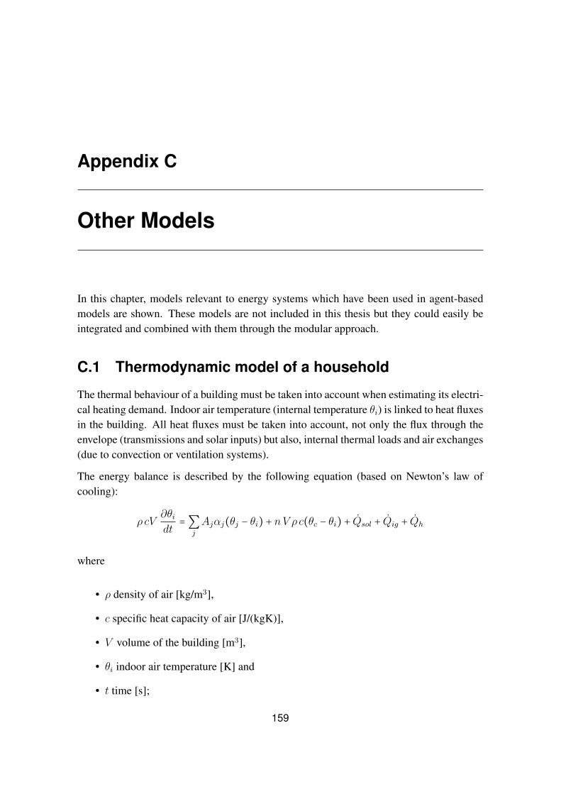
Appendix C
Other Models
In this chapter, models relevant to energy systems which have been used in agent-basedmodels are shown. These models are not included in this thesis but they could easily beintegrated and combined with them through the modular approach.
C.1 Thermodynamic model of a household
The thermal behaviour of a building must be taken into account when estimating its electri-cal heating demand. Indoor air temperature (internal temperature θi) is linked to heat fluxesin the building. All heat fluxes must be taken into account, not only the flux through theenvelope (transmissions and solar inputs) but also, internal thermal loads and air exchanges(due to convection or ventilation systems).
The energy balance is described by the following equation (based on Newton’s law ofcooling):
ρ cV∂θidt
=∑j
Ajαj(θj − θi) + nV ρ c(θc − θi) + Qsol + Qig + Qh
where
• ρ density of air [kg/m3],
• c specific heat capacity of air [J/(kgK)],
• V volume of the building [m3],
• θi indoor air temperature [K] and
• t time [s];
159

160 APPENDIX C. OTHER MODELS
the sum term corresponds to heat transmissions through the envelope of the building wherefor each surface j
• Aj surface area [m2],
• αj heat transfer coefficient [W/(m2K)] and
• θj interior wall temperature of the surface [K];
the next term describes the air exchange due to air infiltration through leakage, the windowand door frames or through intentional air exchange with the exterior (opening of windowsor doors), where
• n air exchange rate [h−1] and
• outdoor air temperature [K];
and the remaining terms represent other heat transfer rates due to
• Qsol solar radiation input incident on the window surfaces which directly leads to anincrease in temperature,
• Qig internal gains such as electrical appliances, human beings or lighting and
• Qh heat contribution due to electrical heating.
This equation represents one thermal zone. Several zones could be represented in a build-ing, but for simplicity’s sake and, as the model will be reproduced in large scale simulation,the equation is considered once for the whole building (one zone model), thus disregardingdifferent temperatures at different rooms and the heat transmissions between them.
The interior surface temperature was assumed at θj = θi − 1oC due to empirical data1. Thesolar radiation input was calculated according to the following equation.
Qsol = 0.8I ⋅ 0.1Aw
where
• I solar irrandiance [W/m2] and1The exterior surface of the wall can also be taken into account by considering the heat transmissions:
(interior air) - (interior surface); (interior surface) - (exterior surface); and (exterior surface) - (outdoor air).Therefore, the exterior surface temperature was assumed at θje = θe + 2
o due to empirical data.

C.1. THERMODYNAMIC MODEL OF A HOUSEHOLD 161
• Aw window surface area [m2]
The correction factors 0.8 and 0.1 consider a partial coverage and/or reflection effects, andthe fact that only a portion of the windows are exposed to the sunlight at any given time. Itis provided by a radiation simulator or a historical dataset.
Outdoor temperature θe can be taken from a random simulator or from historic data. Inter-nal gains can be calculated in several ways, in great detail, through using technical modelsof appliances that contribute heat to the interior temperature, or more broadly by takingstatic curves determined by measurements or other models. It is important to say that in-ternal gains are strongly correlated to household size, the total number of persons living inthe building, the number of persons currently present, weather conditions, etc.
Heat contributions will be explained in the next section as they are controlled to manageand keep reasonable levels for θi.
In this model, the differential equation which describes the heat flows is modelled usingsystem dynamics, based on the approach presented in Appendix D.


Appendix D
Modelling Agents using SD
The increasing computational power, as well as the rapid development of software andsimulation programs now allows for the creation of models of complex technical systemsin areas such as architecture, engineering, economics and business, telecommunications,networks and the Internet. The development of these complex models is expensive andrequires the cooperation of groups of people from different disciplines, often with differentacademic backgrounds. What is required is to employ a methodology that allows for theeasy and fast exchange of models and ideas.
On the one hand, traditional education in engineering schools is based on the use of math-ematical equations which will be referred to as Dynamic Systems (DS). These systems areprecise and usually deterministic, purely quantitative, according to the needs of engineer-ing sciences. The objective of these models is to be able to give a concrete answer to aproblem, unrelated to planning or strategic purposes.
On the other hand, System Dynamics (SD), is a modeling techniques which was originallycreated to better understand complex industrial processes. SD models are based on stockand flows and are more visual and intuitive, and were introduced in Section 3.3.Quali-tative approaches are mainly, but not exclusively found in SD. It is also possible to findquantitative approaches, as will be explained.
When multidisciplinary teams are working on models, communication problems arise thatmay hinder team integration and result in a drop in performance. This is mainly due totraining differences between the team members. So, while people coming from hard sci-ences like physicists, mathematicians or engineers, are used to addressing the problems ofdynamic systems in terms of differential equations (initial value problem (IVP)), people ineconomics, biology, architecture and philosophy, feel more comfortable when reasoningusing Forrester diagrams, system thinking and stock & flow diagrams. These two groups
163

164 APPENDIX D. MODELLING AGENTS USING SD
of people have been working for decades in completely disjointed fields; SD people rarelyexchange their views with DS people because they simply speak different languages.
Regarding methodology, DS people mainly use block-based tools like Matlab/Simulinkand physical modeling tools that allow two-way connections, such as Dymola. SD peopletypically employ System Dynamics modeling software such as Stella, Vensim, etc. Clearly,an important step to improve the effectiveness of model building in multidisciplinary teamsis to try to find a working methodology in which both DS and SD people feel comfortable.Methods used by the SD people are better positioned than DS methods to become thecommon methodology, some reasons for this are:
1. SD methods are easier to use for those familiar with DS methods than the reverse.
2. SD systems are depicted as SD diagrams (Forrester diagrams) representing explicitdifferential equations (with derivatives appearing only in the left hand side of theequations). They can easily be resolved by numerical calculation solvers. DS sys-tems usually show implicit differential equations which result in a set of differentialalgebraic equations, which are not so easy to solve, particularly for multidimen-sional, discontinuous and discrete systems.
3. There are significant difficulties in adapting DS to allow more freedom in buildingmodels (blocks, bond-graphs and sophisticated components). For example algebraicloops arise very frequently when modeling systems in Matlab/Simulink. This is no-ticeable especially in hybrid systems modeling (discontinuous ordinary differentialequations) where the SD method clearly offers many advantages.
4. A main advantage is the existence of high quality object-oriented software, that in-tegrates SD as well as other modeling approaches, and allows for multi-approachmodeling and team integration tasks.
Approach + –conciseness limitations in: space, compre-
DS reproducibility hension, notationpreciseness non scalablecomprehension not classical
SD scalability lack of standardsmultidimensionality unusual representation
Table D.1: Advantages and disadvantages of the approaches
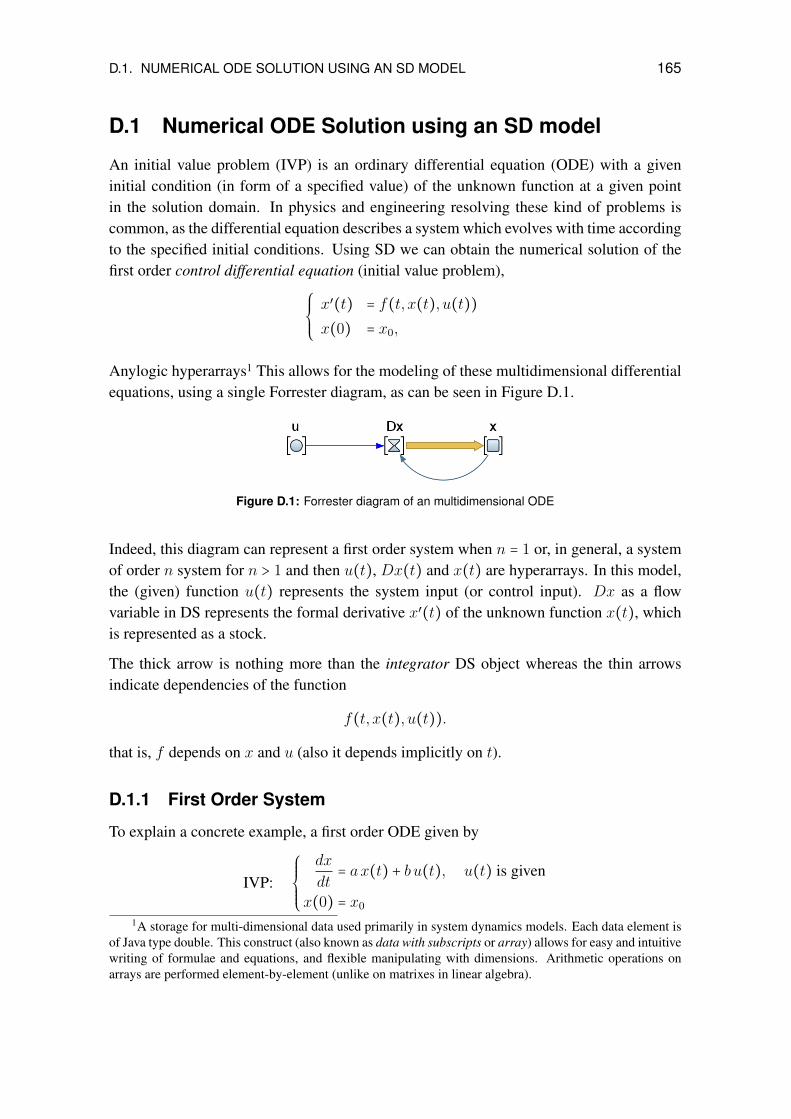
D.1. NUMERICAL ODE SOLUTION USING AN SD MODEL 165
D.1 Numerical ODE Solution using an SD model
An initial value problem (IVP) is an ordinary differential equation (ODE) with a giveninitial condition (in form of a specified value) of the unknown function at a given pointin the solution domain. In physics and engineering resolving these kind of problems iscommon, as the differential equation describes a system which evolves with time accordingto the specified initial conditions. Using SD we can obtain the numerical solution of thefirst order control differential equation (initial value problem),
⎧⎪⎪⎨⎪⎪⎩
x′(t) = f(t, x(t), u(t))
x(0) = x0,
Anylogic hyperarrays1 This allows for the modeling of these multidimensional differentialequations, using a single Forrester diagram, as can be seen in Figure D.1.
Figure D.1: Forrester diagram of an multidimensional ODE
Indeed, this diagram can represent a first order system when n = 1 or, in general, a systemof order n system for n > 1 and then u(t), Dx(t) and x(t) are hyperarrays. In this model,the (given) function u(t) represents the system input (or control input). Dx as a flowvariable in DS represents the formal derivative x′(t) of the unknown function x(t), whichis represented as a stock.
The thick arrow is nothing more than the integrator DS object whereas the thin arrowsindicate dependencies of the function
f(t, x(t), u(t)).
that is, f depends on x and u (also it depends implicitly on t).
D.1.1 First Order System
To explain a concrete example, a first order ODE given by
IVP:
⎧⎪⎪⎪⎨⎪⎪⎪⎩
dx
dt= ax(t) + bu(t), u(t) is given
x(0) = x0
1A storage for multi-dimensional data used primarily in system dynamics models. Each data element isof Java type double. This construct (also known as data with subscripts or array) allows for easy and intuitivewriting of formulae and equations, and flexible manipulating with dimensions. Arithmetic operations onarrays are performed element-by-element (unlike on matrixes in linear algebra).

166 APPENDIX D. MODELLING AGENTS USING SD
where parameters a, b and control input are given. The following example is a special casefrom the previous example as its Forrester diagram is the same (but without array variablesettings). The stock x variable properties are defined by
dx(t)
dt=Dx
as well as its initial value x0. The Dx flow variable is described by the following function:
ax + bu
where a and b are Java variables of type double, declared within the Main window proper-ties. Another double variable x0 should be declared here.
D.2 SD Models in the Energy Sector
As shown previously, SD can help us to model basic engineering blocks for energy systems,for example RC or LC circuits which can be used to model power lines, or other basicelements of power systems, at a technical level. This application of SD is not the mostcommon, and has been presented by the author in [Viejo Garcia et al., 2011]. It offers theadvantage of using simple and schematic block representation to model technical systemsin an environment like Anylogic. Also, the combination high and low level behavior byusing the same formalism is advantageous. As seen in Section 3.3, SD is commonly usedto represent systemic behavior at a higher level. At this level, a number of applications ofSD in the energy sector can be found. [Ford, 1997] gives a review of existing models inthe electric power industry. System dynamics has been used extensively to aid resourceplanning in this context.

Appendix E
Calibration of the Refrigerator Model
‐4
0
4
8
mp
era
ture [
°C]
Evaporator plate
‐16
‐12
‐8
0 10 20 30 40 50 60
Tem
(a) Evaporator
8
10
12
mp
era
ture [
°C]
Bottom Door Top Water
4
6
0 10 20 30 40 50 60
Tem
(b) Internal
6080
100120140
en
t p
ow
er
[VA
]
Electrical power
02040
0 10 20 30 40 50 60
Ap
par
Time [min]
(c) Power
26
28
30
32
em
per
atu
re [
°C]
Room Condenser plate
22
24
0 10 20 30 40 50 60
Te
Time [min]
(d) External
Figure E.1: Measured data for a stable cycle. The curves show the typical behaviour of the refrigeratorin stable conditions, this means without door opening or changes of the contents. A periodic cycle can beseen, which consists on a warming-up phase, in which the compressor is off and the apparent power isalmost zero, followed by a cooling-down phase in which the compressor is working and an almost constant
apparent power can be observed.
The calibration of the refrigerator model is preformed in two major steps. First, the ther-modynamics of the refrigerator cell and the plate, without refrigeration, are calibrated.Starting from a steady state after a refrigeration cycle, the evaporator plate is at its coolesttemperature (around -13°C). Now, the refrigerator is unplugged and the dynamics of the
167
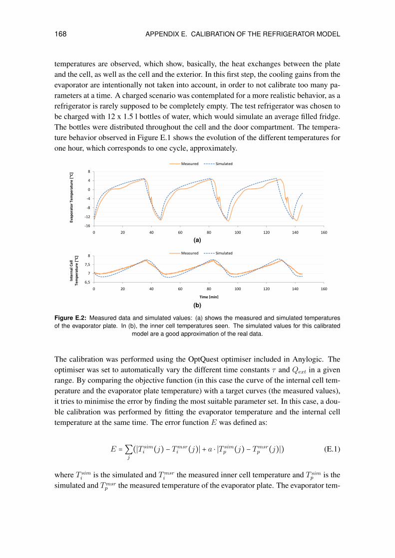
168 APPENDIX E. CALIBRATION OF THE REFRIGERATOR MODEL
temperatures are observed, which show, basically, the heat exchanges between the plateand the cell, as well as the cell and the exterior. In this first step, the cooling gains from theevaporator are intentionally not taken into account, in order to not calibrate too many pa-rameters at a time. A charged scenario was contemplated for a more realistic behavior, as arefrigerator is rarely supposed to be completely empty. The test refrigerator was chosen tobe charged with 12 x 1.5 l bottles of water, which would simulate an average filled fridge.The bottles were distributed throughout the cell and the door compartment. The tempera-ture behavior observed in Figure E.1 shows the evolution of the different temperatures forone hour, which corresponds to one cycle, approximately.
8
‐4
0
4
8
or
Tem
pe
ratu
re [
°C]
Measured Simulated
‐16
‐12
‐8
0 20 40 60 80 100 120 140 160
Evap
ora
t
(a)
7
7,5
8
Inte
rnal C
ell
mp
era
ture [
°C]
Measured Simulated
6,5
0 20 40 60 80 100 120 140 160
ITe
m
Time [min]
(b)
Figure E.2: Measured data and simulated values: (a) shows the measured and simulated temperaturesof the evaporator plate. In (b), the inner cell temperatures seen. The simulated values for this calibrated
model are a good approximation of the real data.
The calibration was performed using the OptQuest optimiser included in Anylogic. Theoptimiser was set to automatically vary the different time constants τ and Qext in a givenrange. By comparing the objective function (in this case the curve of the internal cell tem-perature and the evaporator plate temperature) with a target curves (the measured values),it tries to minimise the error by finding the most suitable parameter set. In this case, a dou-ble calibration was performed by fitting the evaporator temperature and the internal celltemperature at the same time. The error function E was defined as:
E =∑j
(∣T simi (j) − Tmsri (j)∣ + a ⋅ ∣T simp (j) − Tmsrp (j)∣) (E.1)
where T simi is the simulated and Tmsri the measured inner cell temperature and T simp is thesimulated and Tmsrp the measured temperature of the evaporator plate. The evaporator tem-

169
perature varies around 16°C, the internal temperature around 2°C, therefore the evaporatorerror was weighted down by a factor a = 0.2.
In Figure E.2, the measured and simulated values can be seen, after calibration.

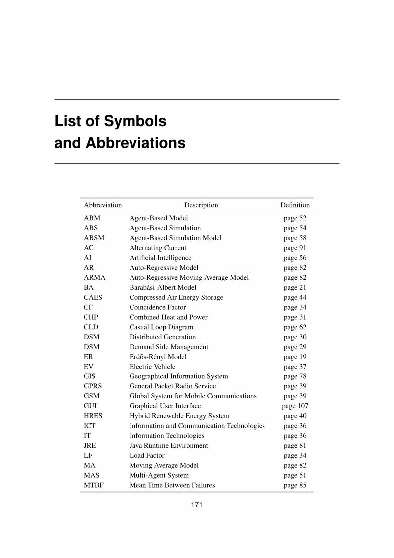
List of Symbolsand Abbreviations
Abbreviation Description Definition
ABM Agent-Based Model page 52ABS Agent-Based Simulation page 54ABSM Agent-Based Simulation Model page 58AC Alternating Current page 91AI Artificial Intelligence page 56AR Auto-Regressive Model page 82ARMA Auto-Regressive Moving Average Model page 82BA Barabasi-Albert Model page 21CAES Compressed Air Energy Storage page 44CF Coincidence Factor page 34CHP Combined Heat and Power page 31CLD Casual Loop Diagram page 62DSM Distributed Generation page 30DSM Demand Side Management page 29ER Erdos-Renyi Model page 19EV Electric Vehicle page 37GIS Geographical Information System page 78GPRS General Packet Radio Service page 39GSM Global System for Mobile Communications page 39GUI Graphical User Interface page 107HRES Hybrid Renewable Energy System page 40ICT Information and Communication Technologies page 36IT Information Technologies page 36JRE Java Runtime Environment page 81LF Load Factor page 34MA Moving Average Model page 82MAS Multi-Agent System page 51MTBF Mean Time Between Failures page 85
171

172 LIST OF SYMBOLS AND ABBREVIATIONS
Abbreviation Description Definition
MTTR Mean Time To Recover page 85ODE Ordinary Differential Equation page 64OOP Object Oriented Programming page 59PCC Point of Common Coupling page 40RES Renewable Energy Source page 31SCADA Supervisory Control and Data Adquisition page 36SD System Dynamics page 62SFR System Frequency Response page 93SMA Systeme Multi-Agent (French for MAS) page 54SMES Superconducting Magnetic Energy Storage page 44SOS System of Systems page 67UCTE Union for the Coordination of Transmission of
Electricitypage 26
UFLS Under Frequency Load Shedding page 91UMTS Universal Mobile Telecommunications System page 39VPP Virtual Power Plant page 73WMAN Wireless Metropolitan Area Networks page 39WLAN Wireless Local Area Networks page 39WS Watts-Strogatz Model page 20

List of Figures
2 Modelo basado en agentes . . . . . . . . . . . . . . . . . . . . . . . . . . . . . . . vii3 Interacciones entre distintos niveles . . . . . . . . . . . . . . . . . . . . . . . . . viii4 Entorno de simulacion para la gestion activa de la demanda . . . . . . . . . . . . ix
1.1 Global framework of the energy system . . . . . . . . . . . . . . . . . . . . . . . 21.2 Evolution of the electrial system . . . . . . . . . . . . . . . . . . . . . . . . . . . 3
2.1 Complex system disciplines . . . . . . . . . . . . . . . . . . . . . . . . . . . . . . 82.2 Organization and complex systems . . . . . . . . . . . . . . . . . . . . . . . . . . 92.3 Sequence of generations of the Game of Life . . . . . . . . . . . . . . . . . . . . 112.4 Percolation of oil in a porous soil . . . . . . . . . . . . . . . . . . . . . . . . . . . 122.5 Percolation probability . . . . . . . . . . . . . . . . . . . . . . . . . . . . . . . . . 122.6 Swarming: flock of birds and simulated swarm . . . . . . . . . . . . . . . . . . . 142.7 Example of a degree distribution P (d) with average degree d(G) =K . . . . . 162.8 Fully connected network . . . . . . . . . . . . . . . . . . . . . . . . . . . . . . . . 182.9 Ring lattice network . . . . . . . . . . . . . . . . . . . . . . . . . . . . . . . . . . 182.10 Random network . . . . . . . . . . . . . . . . . . . . . . . . . . . . . . . . . . . . 192.11 Watts-Strogatz small world network . . . . . . . . . . . . . . . . . . . . . . . . . 192.12 Scale-free network . . . . . . . . . . . . . . . . . . . . . . . . . . . . . . . . . . . 202.13 Degree distribution of a scale free network . . . . . . . . . . . . . . . . . . . . . 212.14 Overview of complex network characteristics . . . . . . . . . . . . . . . . . . . . 222.15 Complexity in ordered-disordered systems . . . . . . . . . . . . . . . . . . . . . 232.16 Emergence of a giant component . . . . . . . . . . . . . . . . . . . . . . . . . . . 242.17 Word frequency in this thesis . . . . . . . . . . . . . . . . . . . . . . . . . . . . . 252.18 Power law shown by word frequency . . . . . . . . . . . . . . . . . . . . . . . . . 262.19 Vulnerability of the power grid . . . . . . . . . . . . . . . . . . . . . . . . . . . . 272.20 Electrical energy system . . . . . . . . . . . . . . . . . . . . . . . . . . . . . . . . 292.21 Standard load profile method limits . . . . . . . . . . . . . . . . . . . . . . . . . . 322.22 The average effect . . . . . . . . . . . . . . . . . . . . . . . . . . . . . . . . . . . 342.23 The two layer model of a smart grid . . . . . . . . . . . . . . . . . . . . . . . . . 392.24 Storage inclusion in modern electrical systems . . . . . . . . . . . . . . . . . . . 43
173

174 LIST OF FIGURES
3.1 Modelling and simulation process (1) . . . . . . . . . . . . . . . . . . . . . . . . 483.2 Modelling and simulation process (2) . . . . . . . . . . . . . . . . . . . . . . . . 493.3 A multi-agent system . . . . . . . . . . . . . . . . . . . . . . . . . . . . . . . . . . 513.4 A generic agent . . . . . . . . . . . . . . . . . . . . . . . . . . . . . . . . . . . . . 553.5 Different environments . . . . . . . . . . . . . . . . . . . . . . . . . . . . . . . . . 573.6 Network types . . . . . . . . . . . . . . . . . . . . . . . . . . . . . . . . . . . . . . 583.7 ABM, parametrisation and simulations . . . . . . . . . . . . . . . . . . . . . . . . 593.8 Casual loop diagrams in system dynamics . . . . . . . . . . . . . . . . . . . . . . 633.9 Casual loop and stock and flow diagram . . . . . . . . . . . . . . . . . . . . . . . 643.10 Multi-approach modelling architectures . . . . . . . . . . . . . . . . . . . . . . . 66
4.1 Number of publications for selected keywords . . . . . . . . . . . . . . . . . . . 724.2 Interactions in multi-scale systems . . . . . . . . . . . . . . . . . . . . . . . . . . 774.3 Socio-technical system . . . . . . . . . . . . . . . . . . . . . . . . . . . . . . . . . 794.4 Sample wind power curve and two approximated curves. . . . . . . . . . . . . . 844.5 Overview of the refrigerator model . . . . . . . . . . . . . . . . . . . . . . . . . . 864.6 Operating principles of a refrigerator . . . . . . . . . . . . . . . . . . . . . . . . . 874.7 Simplified SFR model . . . . . . . . . . . . . . . . . . . . . . . . . . . . . . . . . 94
5.1 Modules of the wind simulator . . . . . . . . . . . . . . . . . . . . . . . . . . . . 965.2 Time granularity of the model . . . . . . . . . . . . . . . . . . . . . . . . . . . . . 975.3 State-chart of a wind turbine . . . . . . . . . . . . . . . . . . . . . . . . . . . . . . 995.4 Representation of the states of the turbines composing a wind farm . . . . . . . 995.5 Refrigerator model implemented in system dynamics . . . . . . . . . . . . . . . 1015.6 Door opening agent . . . . . . . . . . . . . . . . . . . . . . . . . . . . . . . . . . . 1015.7 UFLS agent implementation . . . . . . . . . . . . . . . . . . . . . . . . . . . . . . 1025.8 Temperature sensor locations . . . . . . . . . . . . . . . . . . . . . . . . . . . . . 1035.9 SFR model in system dynamics . . . . . . . . . . . . . . . . . . . . . . . . . . . . 1045.10 Multi-paradigm approach chosen for the refrigerator system model . . . . . . . 1055.11 Integral system model . . . . . . . . . . . . . . . . . . . . . . . . . . . . . . . . . 1065.12 GUI of the refrigerator simulation model . . . . . . . . . . . . . . . . . . . . . . 107
6.1 Low wind speed simulation . . . . . . . . . . . . . . . . . . . . . . . . . . . . . . 1106.2 High wind speed simulation . . . . . . . . . . . . . . . . . . . . . . . . . . . . . . 1116.3 Weekly simulation results for the wind output power . . . . . . . . . . . . . . . . 1126.4 Histogram comparison for hourly and continuous simulations . . . . . . . . . . 1136.5 Individual power outputs for a wind farm: cut-off case . . . . . . . . . . . . . . 1156.6 Individual power outputs for a wind farm: slowing down case . . . . . . . . . . 1156.7 Randomly selected refrigerator results . . . . . . . . . . . . . . . . . . . . . . . . 1186.8 Simulation results for 250 refrigerators . . . . . . . . . . . . . . . . . . . . . . . 1196.9 Aggregation effect for different population sizes . . . . . . . . . . . . . . . . . . 1216.10 Aggregation effect and execution time . . . . . . . . . . . . . . . . . . . . . . . . 123

LIST OF FIGURES 175
6.11 Simulation for normal operation and UFLS scenario . . . . . . . . . . . . . . . . 1256.12 Operation of a refrigerator . . . . . . . . . . . . . . . . . . . . . . . . . . . . . . . 1266.13 Hysteresis process for the refrigerator operation . . . . . . . . . . . . . . . . . . 1276.14 Simulation with UFLS and emergent oscillation . . . . . . . . . . . . . . . . . . 1286.15 Different regimes of the system . . . . . . . . . . . . . . . . . . . . . . . . . . . . 1296.16 Conditions for stable and oscillating regimes . . . . . . . . . . . . . . . . . . . . 1306.17 Probability of a partial and a complete oscillation . . . . . . . . . . . . . . . . . 131
A.1 Map of complexity science . . . . . . . . . . . . . . . . . . . . . . . . . . . . . . 156
D.1 Forrester diagram of an multidimensional ODE . . . . . . . . . . . . . . . . . . . 165
E.1 Measured data for a stable cycle . . . . . . . . . . . . . . . . . . . . . . . . . . . 167E.2 Measured data and simulated values . . . . . . . . . . . . . . . . . . . . . . . . . 168

List of Tables
2.1 Centralised vs. distributed generation . . . . . . . . . . . . . . . . . . . . . . . . 302.2 Generation by primary energy source: examples. . . . . . . . . . . . . . . . . . . 31
5.1 Wind turbine parameters . . . . . . . . . . . . . . . . . . . . . . . . . . . . . . . . 985.2 SFR model parameters . . . . . . . . . . . . . . . . . . . . . . . . . . . . . . . . . 104
6.1 Simulation run comparison . . . . . . . . . . . . . . . . . . . . . . . . . . . . . . 114
B.1 Comparison of typical values for different storage technologies . . . . . . . . . 157
D.1 Advantages and disadvantages of the approaches . . . . . . . . . . . . . . . . . . 164