
Stochastic modelling and simulation in cell biology
212
Stochastic modelling and simulation in cell biology Tam´ as Sz´ ekely Jr. St. Edmund Hall Computational Biology Research Group Department of Computer Science University of Oxford supervised by Professor Kevin Burrage (Department of Computer Science) Dr Radek Erban (Mathematical Institute) Hilary Term 2014 This dissertation is submitted for the degree of Doctor of Philosophy
-
Upload
khangminh22 -
Category
Documents
-
view
2 -
download
0
Transcript of Stochastic modelling and simulation in cell biology
Stochastic modelling andsimulation in cell biology
Tamas Szekely Jr.
St. Edmund Hall
Computational Biology Research GroupDepartment of Computer Science
University of Oxford
supervised byProfessor Kevin Burrage (Department of Computer Science)
Dr Radek Erban (Mathematical Institute)
Hilary Term 2014
This dissertation is submitted for the degree of Doctor of Philosophy

Abstract
Modelling and simulation are essential to modern research in cell biology. This the-sis follows a journey starting from the construction of new stochastic methods fordiscrete biochemical systems to using them to simulate a population of interactinghaematopoietic stem cell lineages.
The first part of this thesis is on discrete stochastic methods. We develop two newmethods, the stochastic extrapolation framework and the Stochastic Bulirsch-Stoermethods. These are based on the Richardson extrapolation technique, which is widelyused in ordinary differential equation solvers. We believed that it would also be usefulin the stochastic regime, and this turned out to be true.
The stochastic extrapolation framework is a scheme that admits any stochasticmethod with a fixed stepsize and known global error expansion. It can improve theweak order of the moments of these methods by cancelling the leading terms in theglobal error. Using numerical simulations, we demonstrate that this is the case up tosecond order, and postulate that this also follows for higher order. Our simulationsshow that extrapolation can greatly improve the accuracy of a numerical method.
The Stochastic Bulirsch-Stoer method is another highly accurate stochastic solver.Furthermore, using numerical simulations we find that it is able to better retainits high accuracy for larger timesteps than competing methods, meaning it remainsaccurate even when simulation time is speeded up. This is a useful property forsimulating the complex systems that researchers are often interested in today.
The second part of the thesis is concerned with modelling a haematopoietic stemcell system, which consists of many interacting niche lineages. We use a vectorisedτ -leap method to examine the differences between a deterministic and a stochasticmodel of the system, and investigate how coupling niche lineages affects the dynamicsof the system at the homeostatic state as well as after a perturbation. We find thatlarger coupling allows the system to find the optimal steady state blood cell levels.In addition, when the perturbation is applied randomly to the entire system, largercoupling also results in smaller post-perturbation cell fluctuations compared to non-coupled cells.
In brief, this thesis contains four main sets of contributions: two new high-accuracydiscrete stochastic methods that have been numerically tested, an improvement thatcan be used with any leaping method that introduces vectorisation as well as how touse a common stepsize adapting scheme, and an investigation of the effects of couplinglineages in a heterogeneous population of haematopoietic stem cell niche lineages.

Acknowledgements
I have had the privilege of meeting some excellent people throughout my DPhil, andI count myself lucky to be able to acknowledge so many of them as my collaborators.I would like to say a huge thank you to all of them for the thoroughly agreeableinteractions we have had, and I look forward to working with them in the future.
First and foremost, I am especially indebted to my supervisor Kevin Burrage, whointroduced me to Australia, helped me develop as an academic, and gave me directionwhen I needed it, but also supported me working on my own initiative rather thanrushing me to finish. Thank you for all your effort and patience.
I also thank Radek Erban, my co-supervisor, for always being responsive, verythorough and ready to help at short notice. I am very grateful to Konstantinos Zy-galakis, who patiently guided me through my mathematical bumblings and effectivelyco-supervised half of my DPhil. I am grateful to Manuel Barrio, with whom I startedcollaborating on a productive and enjoyable stay in Valladolid. I also thank MichaelBonsall and Marc Mangel, who have been extremely supportive despite only gettingto know me not much over a year ago.
I thank the EPSRC, who funded my DPhil via the Systems Biology DTC.From Computer Science, I thank Julie Sheppard, who has been of constant help
with my admin nightmares.From the DTC, I thank Samantha Miles. I have some great memories from that
first year. I also thank my friends and colleagues from Teddy Hall, the DTC and theComputational Biology group, who have made my time at Oxford such a fun one.
I am indebted to Aisi Li, who has been through most of my DPhil years withme, for her enduring understanding and support. Finally, I am very grateful to myfamily, especially my parents, who have supported me with their love and constantencouragement, never hesitating to help whenever they can. This thesis would nothave been possible without them.
i

Contents
1 Introduction 11.1 Background . . . . . . . . . . . . . . . . . . . . . . . . . . . . . . . . 11.2 Motivation . . . . . . . . . . . . . . . . . . . . . . . . . . . . . . . . . 21.3 Aim . . . . . . . . . . . . . . . . . . . . . . . . . . . . . . . . . . . . 31.4 Introduction to models in cell biology . . . . . . . . . . . . . . . . . . 3
1.4.1 Noise in cell biology . . . . . . . . . . . . . . . . . . . . . . . 61.4.2 Modelling regimes . . . . . . . . . . . . . . . . . . . . . . . . . 81.4.3 An example problem . . . . . . . . . . . . . . . . . . . . . . . 9
1.5 Thesis structure . . . . . . . . . . . . . . . . . . . . . . . . . . . . . . 131.6 Contributions . . . . . . . . . . . . . . . . . . . . . . . . . . . . . . . 151.7 Notation . . . . . . . . . . . . . . . . . . . . . . . . . . . . . . . . . . 17
2 Deterministic modelling and simulation 192.1 Introduction . . . . . . . . . . . . . . . . . . . . . . . . . . . . . . . . 19
2.1.1 Convergence and order of accuracy . . . . . . . . . . . . . . . 202.2 Deterministic methods . . . . . . . . . . . . . . . . . . . . . . . . . . 23
2.2.1 One-step methods . . . . . . . . . . . . . . . . . . . . . . . . . 232.2.2 Multistep methods . . . . . . . . . . . . . . . . . . . . . . . . 25
2.3 Richardson extrapolation . . . . . . . . . . . . . . . . . . . . . . . . . 252.4 Extrapolated deterministic methods . . . . . . . . . . . . . . . . . . . 29
2.4.1 Romberg integration . . . . . . . . . . . . . . . . . . . . . . . 292.4.2 Bulirsh-Stoer method . . . . . . . . . . . . . . . . . . . . . . . 29
3 Stochastic modelling and simulation 323.1 Strong and weak order . . . . . . . . . . . . . . . . . . . . . . . . . . 333.2 Continuous stochastic methods . . . . . . . . . . . . . . . . . . . . . 343.3 Discrete stochastic methods . . . . . . . . . . . . . . . . . . . . . . . 36
3.3.1 Chemical Master Equation . . . . . . . . . . . . . . . . . . . . 393.3.2 Stochastic simulation algorithm . . . . . . . . . . . . . . . . . 403.3.3 τ -leap method . . . . . . . . . . . . . . . . . . . . . . . . . . . 433.3.4 Higher-order leaping methods . . . . . . . . . . . . . . . . . . 473.3.5 Multiscale methods . . . . . . . . . . . . . . . . . . . . . . . . 533.3.6 Crossing regimes: from the τ -leap to the ODE . . . . . . . . . 55
ii

CONTENTS iii
4 Stochastic extrapolation 574.1 Extrapolation for SDEs . . . . . . . . . . . . . . . . . . . . . . . . . . 574.2 Discrete stochastic extrapolation . . . . . . . . . . . . . . . . . . . . 604.3 Theoretical analysis . . . . . . . . . . . . . . . . . . . . . . . . . . . . 62
4.3.1 Derivation for zeroth- and first-order reactions . . . . . . . . . 624.3.2 Global error expansion . . . . . . . . . . . . . . . . . . . . . . 684.3.3 Example explicit calculation of the global error . . . . . . . . 72
4.4 Numerical results . . . . . . . . . . . . . . . . . . . . . . . . . . . . . 734.4.1 Particle decay system . . . . . . . . . . . . . . . . . . . . . . . 744.4.2 Chain decay system . . . . . . . . . . . . . . . . . . . . . . . . 774.4.3 Michaelis-Menten system . . . . . . . . . . . . . . . . . . . . . 784.4.4 Mutually inhibiting enzymes system . . . . . . . . . . . . . . . 804.4.5 Schlogl system . . . . . . . . . . . . . . . . . . . . . . . . . . . 814.4.6 Higher extrapolation . . . . . . . . . . . . . . . . . . . . . . . 85
4.5 Monte Carlo error . . . . . . . . . . . . . . . . . . . . . . . . . . . . . 864.6 Discussion . . . . . . . . . . . . . . . . . . . . . . . . . . . . . . . . . 894.7 Conclusions . . . . . . . . . . . . . . . . . . . . . . . . . . . . . . . . 92
5 Stochastic Bulirsch-Stoer method 945.1 Introduction . . . . . . . . . . . . . . . . . . . . . . . . . . . . . . . . 945.2 Implementation . . . . . . . . . . . . . . . . . . . . . . . . . . . . . . 985.3 Extension: SBS-DA . . . . . . . . . . . . . . . . . . . . . . . . . . . . 1025.4 Numerical results . . . . . . . . . . . . . . . . . . . . . . . . . . . . . 104
5.4.1 Chain decay system . . . . . . . . . . . . . . . . . . . . . . . . 1065.4.2 Michaelis-Menten system . . . . . . . . . . . . . . . . . . . . . 1075.4.3 Schlogl system . . . . . . . . . . . . . . . . . . . . . . . . . . . 1085.4.4 Mutually inhibiting enzymes system . . . . . . . . . . . . . . . 1095.4.5 Further comparisons . . . . . . . . . . . . . . . . . . . . . . . 109
5.5 Higher order of accuracy and robustness . . . . . . . . . . . . . . . . 1135.6 Implementation issues . . . . . . . . . . . . . . . . . . . . . . . . . . 1185.7 Discussion . . . . . . . . . . . . . . . . . . . . . . . . . . . . . . . . . 1215.8 Conclusions . . . . . . . . . . . . . . . . . . . . . . . . . . . . . . . . 122
6 Haematopoietic stem cell modelling 1246.1 Introduction . . . . . . . . . . . . . . . . . . . . . . . . . . . . . . . . 1256.2 HSC model . . . . . . . . . . . . . . . . . . . . . . . . . . . . . . . . 1296.3 Stochastic HSC method . . . . . . . . . . . . . . . . . . . . . . . . . 135
6.3.1 Simulating a population of niches . . . . . . . . . . . . . . . . 1356.3.2 Coupling niches . . . . . . . . . . . . . . . . . . . . . . . . . . 138
6.4 Results . . . . . . . . . . . . . . . . . . . . . . . . . . . . . . . . . . . 1416.4.1 Stochastic model dynamics . . . . . . . . . . . . . . . . . . . . 1426.4.2 Fast stochastic simulations . . . . . . . . . . . . . . . . . . . . 1456.4.3 HSC steady state distributions . . . . . . . . . . . . . . . . . . 1476.4.4 Perturbation analysis . . . . . . . . . . . . . . . . . . . . . . . 154
6.5 Discussion . . . . . . . . . . . . . . . . . . . . . . . . . . . . . . . . . 1596.6 Conclusions . . . . . . . . . . . . . . . . . . . . . . . . . . . . . . . . 164

CONTENTS iv
7 Conclusions and future directions 167
A HSC model supporting information 172A.1 Deterministic model of HSC system . . . . . . . . . . . . . . . . . . . 172A.2 MPCR parameters and system steady states . . . . . . . . . . . . . . 173A.3 Optimal homeostatic cell levels . . . . . . . . . . . . . . . . . . . . . 175

List of Figures
1.1 Comparison of deterministic and stochastic simulations of the Schloglreactions . . . . . . . . . . . . . . . . . . . . . . . . . . . . . . . . . . 12
2.1 Comparison of one-step and multistep numerical integration methods 242.2 Graphical explanation of Richardson extrapolation I . . . . . . . . . . 262.3 Graphical explanation of Richardson extrapolation II . . . . . . . . . 27
4.1 Stochastic extrapolation: representation of the local error using theKolmogorov backward equations . . . . . . . . . . . . . . . . . . . . . 71
4.2 Stochastic extrapolation: particle decay system error . . . . . . . . . 764.3 Stochastic extrapolation: constructing a full PDF of the particle decay
system . . . . . . . . . . . . . . . . . . . . . . . . . . . . . . . . . . . 774.4 Stochastic extrapolation: chain decay system error . . . . . . . . . . . 784.5 Stochastic extrapolation: Michaelis-Menten system error . . . . . . . 794.6 Stochastic extrapolation: mutually inhibiting enzymes system error . 824.7 Stochastic extrapolation: Schlogl system low peak error . . . . . . . . 834.8 Stochastic extrapolation: Schlogl system high peak error . . . . . . . 844.9 Stochastic extrapolation: Schlogl system distribution . . . . . . . . . 854.10 Stochastic extrapolation: chain decay system double-extrapolated error 864.11 Stochastic extrapolation: Michaelis-Menten system double-extrapolated
error . . . . . . . . . . . . . . . . . . . . . . . . . . . . . . . . . . . . 874.12 Stochastic extrapolation: particle decay system total error split into
bias plus Monte Carlo error . . . . . . . . . . . . . . . . . . . . . . . 88
5.1 Stochastic Bulirsch-Stoer: chain decay system distribution and error ofX1 . . . . . . . . . . . . . . . . . . . . . . . . . . . . . . . . . . . . . 107
5.2 Stochastic Bulirsch-Stoer: Michaelis-Menten system distribution anderror of X1 . . . . . . . . . . . . . . . . . . . . . . . . . . . . . . . . . 108
5.3 Stochastic Bulirsch-Stoer: Schlogl system distribution and error of X 1095.4 Stochastic Bulirsch-Stoer: mutually inhibiting enzymes system distri-
bution and error of X1 . . . . . . . . . . . . . . . . . . . . . . . . . . 1105.5 Stochastic Bulirsch-Stoer: chain decay system error for all species . . 1115.6 Stochastic Bulirsch-Stoer: Michaelis-Menten system error for all species 1125.7 Stochastic Bulirsch-Stoer: mutually inhibiting enzymes system error
for all species . . . . . . . . . . . . . . . . . . . . . . . . . . . . . . . 1135.8 Stochastic Bulirsch-Stoer: order of accuracy of mean and variance for
a first-order reaction . . . . . . . . . . . . . . . . . . . . . . . . . . . 115
v

LIST OF FIGURES vi
5.9 Stochastic Bulirsch-Stoer: order of accuracy of mean and variance fora bimolecular reaction . . . . . . . . . . . . . . . . . . . . . . . . . . 116
5.10 Stochastic Bulirsch-Stoer: Michaelis-Menten system stepsizes with time 1195.11 Stochastic Bulirsch-Stoer: SBS method stepsize regimes for chain decay
system . . . . . . . . . . . . . . . . . . . . . . . . . . . . . . . . . . . 120
6.1 HSC model: overview of the model . . . . . . . . . . . . . . . . . . . 1306.2 HSC model: illustration of niche lineage coupling . . . . . . . . . . . 1406.3 HSC model: single stochastic simulation results . . . . . . . . . . . . 1416.4 HSC model: multiple stochastic simulation results I . . . . . . . . . . 1436.5 HSC model: multiple stochastic simulation results II . . . . . . . . . 1446.6 HSC model: multiple stochastic simulation results III . . . . . . . . . 1456.7 HSC model: myeloid cell steady-state distributions for various MPCR
parameters . . . . . . . . . . . . . . . . . . . . . . . . . . . . . . . . . 1476.8 HSC model: stem cell steady-state distributions for various MPCR
parameters . . . . . . . . . . . . . . . . . . . . . . . . . . . . . . . . . 1486.9 HSC model: lymphoid cell steady-state distributions for various MPCR
parameters . . . . . . . . . . . . . . . . . . . . . . . . . . . . . . . . . 1496.10 HSC model: means and variances of cell steady-state distributions for
various MPCR parameters . . . . . . . . . . . . . . . . . . . . . . . . 1506.11 HSC model: MPCR feedback steady-state distributions for various
MPCR parameters . . . . . . . . . . . . . . . . . . . . . . . . . . . . 1516.12 HSC model: means and variances of feedback steady-state distributions
for various MPCR parameters . . . . . . . . . . . . . . . . . . . . . . 1516.13 HSC model: cell and feedback level steady-state distributions for vari-
ous niche group sizes . . . . . . . . . . . . . . . . . . . . . . . . . . . 1526.14 HSC model: lymphoid cell steady-state distributions for various niche
group sizes . . . . . . . . . . . . . . . . . . . . . . . . . . . . . . . . . 1536.15 HSC model: feedback level steady-state distributions for various niche
group sizes . . . . . . . . . . . . . . . . . . . . . . . . . . . . . . . . . 1546.16 HSC model: mean cell and feedback levels over time for various MPCR
parameters . . . . . . . . . . . . . . . . . . . . . . . . . . . . . . . . . 1566.17 HSC model: mean cell levels over time and evolution of cell distribu-
tions around a perturbation for various niche group sizes . . . . . . . 1576.18 HSC model: mean feedback levels over time and evolution of feedback
distributions around a perturbation for various niche group sizes . . . 1586.19 HSC model: post-perturbation cell and feedback level overshoots for
three perturbation types . . . . . . . . . . . . . . . . . . . . . . . . . 160
A.1 HSC model: ODE model solutions for various MPCR parameters . . 174A.2 HSC model: symmetric ODE model solutions for various MPCR pa-
rameters . . . . . . . . . . . . . . . . . . . . . . . . . . . . . . . . . . 175A.3 HSC model: symmetric model lymphoid cell steady-state distributions
for various MPCR parameters I . . . . . . . . . . . . . . . . . . . . . 178A.4 HSC model: symmetric model lymphoid cell steady-state distributions
for various MPCR parameters II . . . . . . . . . . . . . . . . . . . . . 178

LIST OF FIGURES vii
A.5 HSC model: symmetric model myeloid cell steady-state distributionsfor various MPCR parameters I . . . . . . . . . . . . . . . . . . . . . 179
A.6 HSC model: symmetric model myeloid cell steady-state distributionsfor various MPCR parameters II . . . . . . . . . . . . . . . . . . . . . 179
A.7 HSC model: symmetric model MPCR feedback steady-state distribu-tions for various MPCR parameters I . . . . . . . . . . . . . . . . . . 180
A.8 HSC model: mean steady-state cell levels for various MPCR parameters180A.9 HSC model: symmetric model MPCR feedback steady-state distribu-
tions for various MPCR parameters II . . . . . . . . . . . . . . . . . 181

List of Tables
2.1 Neville table . . . . . . . . . . . . . . . . . . . . . . . . . . . . . . . . 28
4.1 Stochastic extrapolation: gradients estimated from log-log plots of theerror in the mean . . . . . . . . . . . . . . . . . . . . . . . . . . . . . 75
4.2 Stochastic extrapolation: gradients estimated from log-log plots of theerror in the second moments . . . . . . . . . . . . . . . . . . . . . . . 75
4.3 Stochastic extrapolation: splitting the Schlogl system distribution . . 844.4 Stochastic extrapolation: particle decay system processing times . . . 894.5 Stochastic extrapolation: mutually inhibiting enzymes system process-
ing times . . . . . . . . . . . . . . . . . . . . . . . . . . . . . . . . . . 90
5.1 Stochastic Bulirsch-Stoer: parameters for example systems . . . . . . 1065.2 Stochastic Bulirsch-Stoer: overall efficiency of methods for each example111
6.1 HSC model: transitions in the stochastic model . . . . . . . . . . . . 1316.2 HSC model: constants and parameters in the stochastic model . . . . 1336.3 HSC model: vectorised τ -leap method runtimes and errors . . . . . . 146
viii

List of abbreviations
PDF: Probability density functionODE: Ordinary differential equationMMP: Modified midpoint methodRRE: Reaction rate equationsSDE: Stochastic differential equationCLE: Chemical Langevin equationCME: Chemical Master EquationSSA: Stochastic simulation algorithmETL: Euler τ -leapMPTL: Midpoint τ -leapTTTL: θ-trapezoidal τ -leapUBTL: Unbiased τ -leapSBS: Stochastic Bulirsch-StoerHSC: Haematopoietic stem cellMPCR: Multipotent Progenitor Commitment Response
ix
1Introduction
1.1 Background
Mathematical modelling and computational simulation are essential components of
biology (Gunawardena, 2014). Theoretical results guide experimentalists, help us to
understand experimental results, and can explore scenarios that are not possible ex-
perimentally (Mangel, 2006). In recent years, especially since the turn of this century,
the field of stochastic modelling has experienced an explosion of interest. Worldwide,
there are now many groups in engineering, computer science, mathematics, physics
and chemistry, as well as biology, working on such methods.
In large part, this has come about because of concurrent advances in imaging
and experimental techniques. We can now see more of the microscopic world than
ever before. Whereas with a basic light microscope it is possible to see down to the
resolution of an entire cell and make out individual intracellular components, there
are now techniques that allow us to look at single proteins in real-time, as well as even
higher-resolution methods to image individual atoms (Kherlopian et al., 2008). At
such microscopic scales, noise dominates. Indeed, this is true for many, if not most,
problems in cell biology. Although this noise has been common knowledge in physics
1

CHAPTER 1. INTRODUCTION 2
for over a century as Brownian motion, or thermal diffusion, it has only recent come
to the forefront in biology (Fedoroff and Fontana, 2002). With this observation has
come the realisation that stochastic, that is random, effects should be accounted for in
the mathematical models and computer simulations that theorists employ (Wilkinson,
2011).
However, classical deterministic methods, such as ordinary differential equation
models, which theoretical biologists have relied on for decades, are unable to account
for stochasticity: indeed one of their key assumptions is to ignore it (Wilkinson, 2009).
This is why stochastic methods are important. They are, as the name suggests,
mathematical and computational methods that are based directly on the assumption
that noise exists, and plays an important role in the system.
1.2 Motivation
These days, stochastic methods are becoming widespread in biology, and have been
applied to many research questions, such as gene and protein expression (Barrio et al.,
2006; McAdams and Arkin, 1997), intracellular signal transduction networks (Shimizu
et al., 2003; Tian et al., 2007) and cell dynamics (Rodriguez-Brenes et al., 2013). In-
deed, as they are increasingly being applied to more and more complex systems, it has
become apparent that their strength also leads to one key weakness: slow computa-
tional performance. Because of their inherent randomness, stochastic methods must
generate many random numbers, which is computationally expensive. In systems with
many frequent reactions, simulating these can slow down the method considerably,
making it prohibitively slow (Gillespie, 2007). This is often the case in systems of
biological relevance. For instance in a gene expression model, the number of genes
would be small, hence the necessity for a stochastic method; however, there could be
thousands of proteins, slowing down the performance of the simulations.
For this reason, it is important to develop new stochastic methods that are able to
CHAPTER 1. INTRODUCTION 3
cope with such systems. There are many possible ways of attacking this problem, and
indeed, many different types of new methods have been proposed: for instance, faster
variants of known methods (e.g., improvements to Gillespie’s stochastic simulation
algorithm), more accurate methods (e.g., the τ -leap and higher-order leap methods),
methods with better stability (e.g., the Runge-Kutta τ -leap), and multiscale methods
that can simulate such disparate populations simultaneously (reviewed in Chapter 3,
as well as by Szekely and Burrage, 2014; Wilkinson, 2011 and Goutsias and Jenkinson,
2013).
1.3 Aim
This leads on to the research aims at the heart of this thesis:
1. the construction of new stochastic methods to address the gaps in
current methods;
2. the application of such methods to an important current problem
in cell biology, namely the investigation of haematopoietic stem cell
population dynamics.
1.4 Introduction to models in cell biology
What are cells composed of? How long do they live? How do they regulate their
inner workings? These are some of the questions cell biology attempts to answer.
Cells are the fundamental building block of every living creature. The smallest, such
as bacteria and other prokaryotes, are just composed of one cell; the most complex
contain many trillions (that is, 1012; Faller and Schunke, 2004). Nevertheless, even
the simplest cells have remarkable abilities; a classic and well-investigated example
is bacterial chemotaxis, the ability of bacterial cells to sense chemical gradients and
move towards favourable locations and away from unfavourable ones (Wadhams and

CHAPTER 1. INTRODUCTION 4
Armitage, 2004). The cell regulates its many functions and senses and responds to
its environment via signal transduction pathways, which can often interact with gene
regulatory networks that control the process of gene expression. These two complex
and interconnected processes perform many of the key functions of the cell (Cooper
and Hausman, 2009).
Signal transduction pathways, biochemical reactions initiated by a signal to a re-
ceptor on the cell’s surface that successively activate each other, mediate the responses
of the cell to a stimulus in order to produce a desired change in the cell (Gomperts
et al., 2009). Many signal transduction pathways exist, each controlling a different
aspect of the cell’s response. They are typically very complex and consist of many
reactions, some of which can feed back on to their own or another signalling pathway.
They can affect the cell in various ways, such as altering its life cycle, metabolism and
locomotion.
Gene expression starts at the level of the genome and can result in complex changes
to the cell, as it dictates the levels of proteins, many of which control physiological
processes in the cell. It involves two major steps: transcription, the copying of a
length of DNA to mRNA, and translation, the production of a chain of amino acids
from the mRNA, which then folds into its final form as a protein. This sequence
of information transfer is known as the central dogma of molecular genetics (Crick,
1958, 1970). In the decades since its conception, this original concept of a one-way
flow of information has been supplemented and revised, and we now know that the
picture is far more complicated, with for instance, feedback from proteins on to both
genes and RNA, as well as the discovery and mainstream acceptance of epigenetic
inheritance, non-coding RNA and prions (Ball, 2013; Shapiro, 2009). The numbers
of genes that initiate the process of gene expression are very low (typically one copy
per cell); mRNA numbers are higher, as many genes are transcribed continuously,
but still of a similar order (several mRNA molecules per gene; Alberts et al., 2002)
and protein numbers are higher still, as each section of mRNA can be translated

CHAPTER 1. INTRODUCTION 5
many times (resulting in many identical proteins). The numbers of different species
of proteins can vary: for instance, in cells of the bacterium Escherichia coli, 90%
of the total protein numbers are made up by about 15% of the protein species, as
these species produce many proteins each (O’Farrell, 1975; Pedersen et al., 1978).
The rest of the proteins are present in lower abundances, of under 100 proteins per
species. Proteins interact with each other and with the other components of the gene
expression process.
One well-known gene regulatory model is that of the bacteriophage λ. This is
a virus that infects cells of the bacterium Escherichia coli. Normally, once inside
the bacterium it releases and copies its DNA many times over and uses the gene
expression pathway of the host cell to construct many copies of the virus. Then it
breaks out of the bacterium, destroying it in the process, and releases new virions.
This is known as the lytic pathway (Dodd et al., 2005). However, upon infecting
a bacterium, sometimes it will enter the lysogenic pathway. In this case, the virus
incorporates its DNA into the bacterial cell’s own DNA and lies dormant until the
host cell encounters some form of damage, when it switches to its lytic phase. This
behaviour is governed by its gene regulatory network: upon entering the host cell,
the virus ‘decides’ which pathway to follow depending on the host cell’s condition
(McGrath and van Sinderen, 2007) (although, of course, this is affected by intrinsic
noise; Kaern et al., 2005). If it enters this lysogenic pathway, the virus forces the
host cell to make proteins that repress the expression of the genes for the lytic phase.
When the host cell encounters a stressor, these repressor proteins are broken down
and the phage enters the lytic phase. The λ phage is a good example of how a simple
gene regulation network can demonstrate the ability to make decisions, in this case
between lysis or lysogeny.
In short, although the cell is often regarded as the building block of life, it consti-
tutes an entire environment, full of intracellular machinery that have complex inter-
actions with each other. These machinery often have low numbers and, being inside

CHAPTER 1. INTRODUCTION 6
the cell, are also generally very small, and as such subject to noise. Thus the inside
of the cell is a noisy environment.
1.4.1 Noise in cell biology
The presence of noise inside the cell can give rise to heterogeneity in cell populations:
for instance, even populations of genetically identical cells can be phenotypically dif-
ferent (Blake et al., 2003; Spudich and Koshland, 1976). There are three sources of
heterogeneity affecting natural systems such as cell populations: genetic, environmen-
tal and random (or stochastic) (Huang, 2009; Szekely and Burrage, 2014). In clonal
populations and at the level of the individual cell, there is no genetic heterogeneity
so we are left with non-genetic contributions. When talking about gene expression,
these two contributions are usually labelled extrinsic and intrinsic, respectively (that
is, either the heterogeneity is caused by other sources, or it is due to the random
fluctuations intrinsic to any physical process; Elowitz et al., 2002; Pedraza and van
Oudenaarden, 2005).
Extrinsic heterogeneity arises due to differences in the state of the system (that is, a
cell): for instance, different quantities, locations and activities of various intracellular
components that carry out gene expression, or other factors from outside the cell such
as chemical signals. In contrast, there is also variation arising even when all of these
factors are identical in each cell, and the cells in a clonal population can still end up
different (known as phenotypic heterogeneity). This is because they are affected by
thermal fluctuations, altering the order and timing of the biochemical reactions inside
the cell. This “noise that cannot be controlled for” (Wilkinson, 2009) is known as
intrinsic heterogeneity.
The difference between the two sources of noise is shown clearly by Elowitz et al.
(2002). They inserted the reporter genes for the fluorescent proteins cfp and yfp (cyan
and yellow, respectively) into cells of the bacteria Escherichia coli so both of them
would be transcribed together. The colour of the cells then reveals the sources of noise
CHAPTER 1. INTRODUCTION 7
that are present: with no intrinsic noise to introduce variation in gene expression, the
cells should all be the same colour as extrinsic noise affects the levels of both proteins
equally. However, in the presense of intrisic noise the variation in protein levels is
different in each cell, leading to them being different colours. Elowitz et al. (2002)
found that the cells’ colours varied considerably, confirming that both intrinsic and
extrinsic noise have an effect on gene expression. This technique is known as a two-
reporter assay, and is a useful tool to estimate the magnitude of intrinsic versus
extrinsic noise (Swain et al., 2002).
Intrinsic noise is often ignored, as its direct effects tend to be weak at higher
particle numbers, concentrations and temperatures, and can be averaged out (Rosen-
feld et al., 2005). However, small variations in critical microscopic particles, such as
key genes or transcription factors in a gene regulatory network, can create dramatic
changes at macroscopic levels (Elowitz et al., 2002; Raser and O’Shea, 2005).
This stochasticity is generally detrimental to the proper functioning of a cell be-
cause of its interference with regulatory and signalling pathways (Barkai and Leibler,
2000; Rosenfeld et al., 2005), hence its alternative name of ‘noise’, borrowed from
engineering. This is confirmed by the fact that (at least in yeast) natural selection to
reduce noise is stronger on genes which encode critical proteins (Fraser et al., 2004;
Lehner, 2008). However, it has now been demonstrated that sometimes noise can
also be useful to the cell (Avery, 2006; Fraser and Kaern, 2009). Intrinsic noise en-
ables phenotypic heterogeneity to arise at the population level (Blake et al., 2003).
In microbial populations, this is particularly important as phenotypic heterogeneity
allows the population to survive rapidly changing environments (Arkin et al., 1998;
Thattai and van Oudenaarden, 2004). With several different phenotypes present in
a single microbial culture with the same genetic code, the population has effectively
multiplied its chances of surviving (Kaern et al., 2005). This is favourable compared
to evolutionarily adapting to a specific environment, as evolution is a slow and costly
process and microbial environments can change rapidly.
CHAPTER 1. INTRODUCTION 8
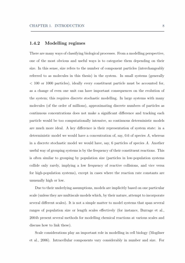
1.4.2 Modelling regimes
There are many ways of classifying biological processes. From a modelling perspective,
one of the most obvious and useful ways is to categorise them depending on their
size. In this sense, size refers to the number of component particles (interchangeably
referred to as molecules in this thesis) in the system. In small systems (generally
< 100 or 1000 particles), ideally every constituent particle must be accounted for,
as a change of even one unit can have important consequences on the evolution of
the system; this requires discrete stochastic modelling. In large systems with many
molecules (of the order of millions), approximating discrete numbers of particles as
continuous concentrations does not make a significant difference and tracking each
particle would be too computationally intensive, so continuous deterministic models
are much more ideal. A key difference is their representation of system state: in a
deterministic model we would have a concentration of, say, 0.6 of species A, whereas
in a discrete stochastic model we would have, say, 6 particles of species A. Another
useful way of grouping systems is by the frequency of their constituent reactions. This
is often similar to grouping by population size (particles in low-population systems
collide only rarely, implying a low frequency of reactive collisions, and vice versa
for high-population systems), except in cases where the reaction rate constants are
unusually high or low.
Due to their underlying assumptions, models are implicitly based on one particular
scale (unless they are multiscale models which, by their nature, attempt to incorporate
several different scales). It is not a simple matter to model systems that span several
ranges of population size or length scales effectively (for instance, Burrage et al.,
2004b present several methods for modelling chemical reactions at various scales and
discuss how to link these).
Scale considerations play an important role in modelling in cell biology (Mogilner
et al., 2006). Intracellular components vary considerably in number and size. For
CHAPTER 1. INTRODUCTION 9
instance, genes, mRNA and membrane proteins tend to be rare. Even small changes
in these critical components can have dramatic effects on the entire system (such as
a gene switching on or off), thus the effects of noise on the system must be accounted
for (McAdams and Arkin, 1997). In contrast, cytoplasmic proteins and chemicals
tend to be relatively abundant and in this case stochasticity can usually be ignored
by looking only at their average behaviour (Kaern et al., 2005). However, there are
examples where, at least over certain scales, increasing particle numbers do not imply
decreasing noise (Grima, 2014).
We can classify biochemical modelling/simulation approaches into three groups:
continuous deterministic, continuous stochastic and discrete stochastic, which ap-
proximately correspond to the hierarchy of scales of natural systems and their models
(large to medium to small, respectively). Wilkinson (2009) gives a nice introduction
to these regimes and their respective modelling/simulation techniques, and discusses
the differences between them. We also describe them in further detail in Chapters
2 and 3. There are also discrete deterministic models (Geritz and Kisdi, 2004), typ-
ically used in population dynamics and ecology to model populations with distinct
generations such as fish; however, they discretise time rather than populations, and
so in the above hierarchy they would also fall in the same category as continuous
deterministic models (which are also continuous in the populations). To start, in the
following section we use a simple example to graphically illustrate these ideas.
1.4.3 An example problem
A useful system to demonstrate the differences between modelling methods based
on the deterministic and stochastic regimes is the Schlogl system (Schlogl, 1972),
consisting of four reactions which take the form
A+ 2Xc1c2
3X
Bc3c4X
(1.1)

CHAPTER 1. INTRODUCTION 10
where A,B and X are three chemical species and the concentrations of A and B
are held constant at 105 and 2 × 10⁵ respectively, so only the concentration of X
can change. The rate constants we used are c = [3 × 10⁻⁷, 10−4, 10−3, 3.5]. The
units used here, and in the rest of this thesis, are non-dimensional. Note that one
of the reactions is third-order, and so follows a third-order mass-action rate law.
Actual third-order reactions are very rare, as they require three particles to collide in
order for the reaction to occur; more often, they are an approximate representation
of multiple elementary reactions (Clayden et al., 2012). That said, the distinction
does not especially matter here as the above reactions are intended only as model
reaction set for illustrative purposes. Indeed, this is a common benchmark system
for computational algorithms, and is also used later in this thesis for testing the
performance of the new stochastic methods we have worked on.
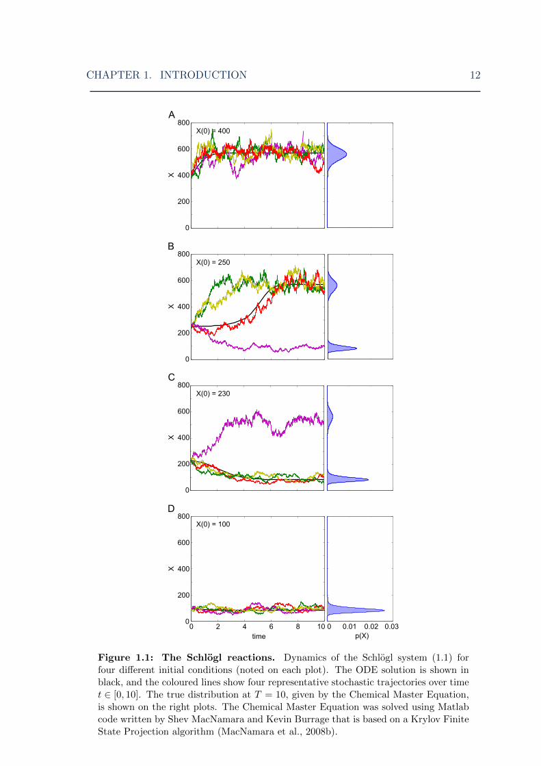
Under certain parameter configurations, this system has two stable states at finite
time, one high and one low (their exact values depend on the parameter values used).
We perform simulations using both a stochastic simulation algorithm (see Section
3.3.2) and an ordinary differential equation (ODE; see Section 2.2). Using a stochas-
tic algorithm yields probabilistic results: the system behaves differently during each
simulation run (Fig. 1.1, coloured lines). When the initial population of X (X0) is
small, the system usually settles in the lower state, and vice versa when X0 is large.
However, the system often finishes in the other state to that found by the deterministic
solution, especially when X0 is between the two states (Fig. 1.1B,C). In contrast, the
ODE model is deterministic: each X0 always produces the same final concentration
of X (Fig. 1.1 black lines). In the bistable parameter configuration, the system also
has a third equilibrium state: an unstable state between the two stable ones (around
X0 = 250 for our parameters). If the ODE solution was started in this state exactly,
it would remain in this state indefinitely. However, in practice we can never set X0
exactly to this value, and as X0 approaches it, the ODE trajectory stays constant for
longer and longer periods of time, but always eventually goes to either the high or
CHAPTER 1. INTRODUCTION 11
low stable state. This unstable state is also the point at which the ODE solution flips
from going to one steady state to the other. Note that in our example we look at
T = 10, i.e. a finite time. The number and position of peaks (stable states) is given
by the parameters, not X0, and if the stochastic simulations were run for a very long
time, the resulting PDF would look something like Figs. 1.1B,C and be identical for
all X0.
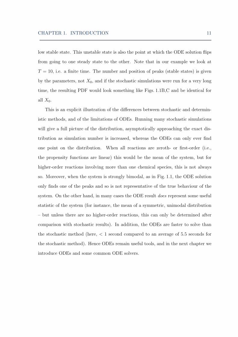
This is an explicit illustration of the differences between stochastic and determin-
istic methods, and of the limitations of ODEs. Running many stochastic simulations
will give a full picture of the distribution, asymptotically approaching the exact dis-
tribution as simulation number is increased, whereas the ODEs can only ever find
one point on the distribution. When all reactions are zeroth- or first-order (i.e.,
the propensity functions are linear) this would be the mean of the system, but for
higher-order reactions involving more than one chemical species, this is not always
so. Moreover, when the system is strongly bimodal, as in Fig. 1.1, the ODE solution
only finds one of the peaks and so is not representative of the true behaviour of the
system. On the other hand, in many cases the ODE result does represent some useful
statistic of the system (for instance, the mean of a symmetric, unimodal distribution
– but unless there are no higher-order reactions, this can only be determined after
comparison with stochastic results). In addition, the ODEs are faster to solve than
the stochastic method (here, < 1 second compared to an average of 5.5 seconds for
the stochastic method). Hence ODEs remain useful tools, and in the next chapter we
introduce ODEs and some common ODE solvers.
CHAPTER 1. INTRODUCTION 12
Figure 1.1: The Schlogl reactions. Dynamics of the Schlogl system (1.1) forfour different initial conditions (noted on each plot). The ODE solution is shown inblack, and the coloured lines show four representative stochastic trajectories over timet ∈ [0, 10]. The true distribution at T = 10, given by the Chemical Master Equation,is shown on the right plots. The Chemical Master Equation was solved using Matlabcode written by Shev MacNamara and Kevin Burrage that is based on a Krylov FiniteState Projection algorithm (MacNamara et al., 2008b).

CHAPTER 1. INTRODUCTION 13
1.5 Thesis structure
This thesis is structured as follows.
Chapter 2 gives the deterministic modelling background. We describe some de-
terministic concepts as well as some common numerical methods. We also introduce
the powerful idea of Richardson extrapolation in a deterministic setting, and describe
two common solvers that rely on it: the Romberg integration method for evaluat-
ing definite integrals, and the Bulirsch-Stoer method for solving ordinary differential
equations. Both of these will be built upon later in this thesis.
Chapter 3 is the stochastic modelling background chapter. We briefly cover
stochastic differential equations before moving on to discrete stochastic simulation
methods. We focus on discrete stochastic methods that track the biochemical popu-
lations of the system over time. We give a reasonable level of detail, as some of these
methods will also be built upon later in this thesis.
Chapter 4 details the first stochastic method we developed, the extrapolated τ -
leap, and the wider stochastic extrapolation framework. We perform a basic numerical
analysis of the mean and second moment of the Euler τ -leap of a linear system to
show that even in the stochastic case, extrapolation also increases the weak order of
a method. The global error expansion of a weak first order method is also found,
and it is demonstrated how to apply this in practice. We then show numerically that
for several example systems, stochastic extrapolation decreases the error of the Euler
τ -leap, midpoint τ -leap and θ-trapezoidal τ -leap methods in every instance, and in
cases where the Monte Carlo error is not too high, we can also see the improvement
in weak order.
Chapter 5 describes the Stochastic Bulirsch-Stoer (SBS) method, a powerful stochas-
tic method inspired by its deterministic namesake. It also incorporates the idea of
extrapolation, but this happens at every step. This allows it to generate a Poisson
random number of reactions at each step, and when enough simulations are run, re-

CHAPTER 1. INTRODUCTION 14
turn a full probability density function (PDF). It also allows for adaptive stepsize,
and this is an area where the SBS excels. It chooses large stepsizes, thus speeding up
simulations. We also introduce a second variant of the SBS called the SBS-DA. We
again show using numerical tests that the SBS has excellent accuracy; what is more,
it retains this accuracy well even as timesteps are increased, implying that it has high
efficiency. By quantifying the efficiency, we show that this is the case for both the
SBS and SBS-DA, and one or other variant has the highest efficiency in every test.
Chapter 6 focusses on a haematopoietic stem cell model. We first describe a
computational method to efficiently run a large number of SSA or leaping method
simulations at once. It involves running them simultaneously, using a state matrix
rather than a set of state vectors simulated in series. In the software package Matlab,
the matrix method is far more efficient, as it is optimised for matrix calculations.
Although this is not necessarily the case in other programming languages, the inherent
simplicity of the technique is still an advantage. This is even more so when the
individual simulations (that is, state vectors) interact with each other, as is the case
in the stem cell model. To our knowledge, so far this state matrix framework has only
been used with a fixed timestep; adaptively calculating the timestep for an entire set
of simulations at once would be too computationally difficult. However, we introduce
a simple idea: the entire set of simulations can evolve at the same pace by all using
the same adaptive timestep. This step is calculated from the simulation with largest
total propensity, that is, the one most likely to serve as a bottleneck for the entire
system. Once the step is calculated, the entire system can be evolved simultaneously.
In fact, this idea can be fitted into any scheme that adaptively selects the timestep.
Using this methodology, we synchronously simulate a heterogeneous metapopulation
of haematopoietic stem cell niche lineages that differentiate from stem to progenitor
to blood cells. We examine whether coupling the niche lineages has any effect on the
dynamics of the system, as well as its response to three different perturbation types:
even, uneven and random. We find that coupling lineages allows each individual

CHAPTER 1. INTRODUCTION 15
lineage greater variation in its blood cell levels. However, the distribution of the
entire group is centred on the optimal homeostatic state. In addition, there is a
difference in the response to a perturbation between coupled and uncoupled niche
lineages. For a random perturbation, which is spread across all blood cells, we find
that the more lineages are coupled, the better the response.
Finally, we summarise our work in Chapter 7 and highlight some promising direc-
tions for further work.
1.6 Contributions
The contributions from this DPhil, listed explicitly, are:
1. (Chapter 4) Development of a high-order stochastic simulation frame-
work, the extrapolated τ-leap/stochastic extrapolation. The power of
this framework is that any method with a known weak order can be extrap-
olated and its order increased. Moreover, the extrapolation is very simple to
carry out. Its drawbacks are that this can only be done for the moments, and
fixed timesteps must be used.
2. (Chapter 5) Development of a highly efficient stochastic simulation
method, the Stochastic Bulirsch-Stoer method. This is a complementary
method to the stochastic extrapolation. It overcomes both the drawbacks of the
latter, as it uses an optimised adaptive stepsize, as well as being able to give a
full PDF (if run multiple times, of course). In some situations, it is also able to
achieve higher weak order in the moments. Its only drawback, as far as we can
tell, is its complexity.
3. (Chapter 6) Introduction of an efficient and conceptually simple way,
using a state matrix rather than individual state vectors, of simulating
an entire set of τ-leaps. This is akin to running a τ -leap in series that many
CHAPTER 1. INTRODUCTION 16
times, and can be used to generate a full PDF of the system. When used in
an alternative way (explained in Section 6.3), it can be regarded as simulating
an entire heterogeneous metapopulation of interacting systems. In addition,
we introduce a simple way of adaptively selecting a timestep for this
entire matrix of simulations.
4. (Chapter 6) Finally, we use the above state matrix formulation to
simulate a population of interacting haematopoietic stem cell niche
lineages. We investigate the effects of varying the feedback parameters, and of
coupling niche lineages together, and how this varies for three different types of
perturbation.
All of the work that forms the core of this thesis has been written up into journal
papers, referenced in this thesis as Szekely et al. (2012, 2013a,b). Naturally, much of
it has been of a collaborative nature, and this is reflected in the multiple authorship
of the papers. We detail below the supervisors and collaborators for each chapter,
including their roles, any joint work, and any explicit contributions of others (all other
aspects of the research were performed by this author).
1. Chapter 4: This work was jointly supervised by Konstantinos Zygalakis, Kevin
Burrage and Radek Erban. The main ideas in this chapter were jointly dis-
cussed and developed by all four authors. The calculations in Section 4.3.1 were
performed with the help of Kevin Burrage, Konstantinos Zygalakis and Radek
Erban. Sections 4.3.2 and 4.3.3 were the work of Konstantinos Zygalakis, with
help from Kevin Burrage and Radek Erban. In addition, the calculations in
Section 4.5 were performed jointly with Konstantinos Zygalakis.
2. Chapter 5: this work was supervised by Manuel Barrio, with collaboration from
Kevin Burrage and Konstantinos Zygalakis. The SBS method described in Sec-
tions 5.1 and 5.2 was jointly developed by Manuel Barrio and Tamas Szekely Jr.

CHAPTER 1. INTRODUCTION 17
3. Chapter 6: this work was supervised by Michael Bonsall and Marc Mangel,
with collaboration from Kevin Burrage. Michael Bonsall, Marc Mangel and
Tamas Szekely Jr. conceived the work. Kevin Burrage and Tamas Szekely Jr.
developed the simulation methods.
1.7 Notation
In this thesis, we have attempted to use consistent notation wherever possible. The
following are standard conventions observed throughout this thesis:
• Bold font indicates any vector or matrix-valued function.
• Y refers to a species-indexed deterministic function, that is Y ≡ Yi, i = 1, . . . , N .
• In contrast, X denotes a species-indexed stochastic function, i.e. a random
variable. x ≡X(t) indicates a specific instance of this random variable.
• Y (t) and X(t) indicate true solutions of those functions at time t.
• Y hm and Xτ
m (also with the stepsize sometimes omitted as Ym and Xm) denote
approximate solutions of a solver using stepsize h or τ to the true solution at
time tm. Y hT andXτ
T are approximate solutions at time T . This notation ensures
there is no confusion between n and m subscripts.
• Time t and tm = mh or tm = mτ (we set t(0) = 0) indicate some unspecified
time, whereas time T = nh or T = nτ refer to the end of the simulation time.
• Unless otherwise indicated, N refers to number of chemical species, M refers to
number of chemical reactions, and i = 1, . . . , N , j = 1, . . . ,M .
• h always denotes a timestep for a continuous solver, i.e. differential equations.
• τ always denotes a timestep for a discrete stochastic method.

CHAPTER 1. INTRODUCTION 18
As sometimes different regimes must be discussed in the same chapter, or even sen-
tence, we switch between Y and X, as well as h and τ regardless of chapter, and
usage is dictated purely by the context of the method to which reference is being
made; each of these variables always sticks to the definition above.
2Deterministic modelling and simulation
2.1 Introduction
Large systems with frequent reactions are usually modelled using ODEs. They are a
very common modelling tool and are used for a vast array of different applications.
Historically, there has been much work on ODE analysis and numerical methods, and
today there are very fast and accurate solvers readily available for ODE systems, such
as the ubiquitous Runge-Kutta methods, linear multistep methods and the highly-
accurate Bulirsch-Stoer method. ODEs are deterministic and continuous, that is they
ignore fluctuations and regard their variables as continuous concentrations, rather
than actual particle numbers. To represent a biochemical system with an ODE model,
two assumptions must be made:
1. particle populations are very large compared to integral changes of a few parti-
cles and
2. reactions are very frequent.
When both these assumptions are fulfilled, to a close approximation the system is
continuous and deterministic (Arkin et al., 1998). Otherwise, although ODE models
19
CHAPTER 2. DETERMINISTIC MODELLING AND SIMULATION 20
can in some cases be used to give a qualitative idea of the mean behaviour of the
system, this is not always the case. This is especially so in systems whose distributions
do not have a monostable and symmetrical shape. For instance in a bistable system,
the ODE solution may not be representative of either of the stable states the system
actually adopts, or may only find one of them, as demonstrated by Fig. 1.1.
ODEs are equations of the form
dY (t)
dt= f(t,Y (t)), Y (0) = Y0. (2.1)
Here f(t,Y (t)) is an N × 1 vector-valued function. ODEs have been extensively
studied for many years, so there exist many methods for analysing and numerically
solving them (Kincaid and Cheney, 2002). Here we only give an overview of ODE
numerical solvers; their analysis is outside the scope of this thesis. The simplest nu-
merical methods are one-step first-order methods such as the Euler method, but many
more complicated schemes have been developed. ODEs are ubiquitous in mathemat-
ical and computational modelling, and are used for diverse applications ranging from
modelling oil fields to weather prediction (Braun, 1993).
2.1.1 Convergence and order of accuracy
A general method for solving ODEs calculates a solution to the equation at each step
t1, t2, . . . , tn. By definition, this solution is not exact for any step after the initial
value. However, a solver will converge to the true solution of Eq. (2.1) as h→ 0 if it
is both consistent and stable. We use the Euler method to illustrate these ideas.
The forward Euler method is probably the simplest ODE solver, and its solution
at step m+ 1 depends only on the solution at step m:
Y hm+1 = Y h
m + hf(tm,Yhm). (2.2)
CHAPTER 2. DETERMINISTIC MODELLING AND SIMULATION 21
Here, Y hm is the approximate solution to Eq. (2.1) at timestep m with stepsize h, and
tm = mh. Eq. (2.2) is a one-step, one-stage explicit solver, meaning that it takes
only a single sample of the gradient f to calculate the next step, and Ym+1 does not
depend on itself, but only on Ym.
The local truncation error of the Euler method, the difference between the true
solution and the numerical approximation over one timestep, is
ε(tm+1 − tm, h) = Y (tm+1)− Y hm+1
= Y (tm+1)− Y (tm)− hf(tm,Yhm), (2.3)
as by definition, at the start of the step, Y (tm) = Y hm. Taylor expanding Y (t) about
tm, we can write
Y (tm+1) = Y (tm) + hdY (tm)
dt+h2
2
d2Y (tm)
dt2+ . . .
This leaves us with the one-step error expansion of the Euler method,
ε(tm+1 − tm, h) =h2
2
d2Y (tm)
dt2+ . . . (2.4)
Thus the Euler method has a local error of O(h2).
A method can be said to be consistent if its local error tends to zero as the stepsize
is decreased,
limh→0|ε(tm+1 − tm, h)| = 0.
In addition, it is said to be (zero-)stable if
|Y hm − Y h
m| ≤ Cδ,
for all steps m, where C is a constant and Y hm is a numerical solution using the
same method and stepsize as Y hm but whose initial condition was Y (0) = Y0 + δ. In
CHAPTER 2. DETERMINISTIC MODELLING AND SIMULATION 22
other words, an initial perturbation to the numerical solution must only increase in a
controlled fashion over [0, T ]. Depending on the problem and the solver, small errors
in the numerical solution can be amplified, leading to large errors. In general this
places a limitation on the stepsize of the solver to avoid instability. Stability issues
are avoided by implicit methods such as the implicit (or backward) Euler method,
but they are more difficult and computationally intensive to solve.
If a method is both consistent and stable, then it is also convergent, defined as
limh→0
maxm|Y (tm)− Y h
m| = 0.
Such a method has global order of accuracy w, i.e. converges with order w, if
|Y (T )− Y hT | ≤ Chw, (2.5)
where C is again a constant, and T = nh is the final time. The global error of a
convergent method is one power of h less than its local error: a rough way of thinking
about this is that the local error is O(hw+1) at each step, and there are n = Th
steps
over [0, T ]. More rigorously, a limit on the global error can be calculated by backward
iteration, using the local error at each step, a bound for the maximum local error and
the assumption that the function f(t,Y (t)) is Lipschitz continuous. For instance, we
know that the local error of the Euler method is O(h2) (Eq. (2.4)), so if the Lipschitz
assumption holds for the function f(t,Y (t)), we also know that its global error is
O(h) and thus its order is one.
The order of accuracy is an important property of a numerical method, as it
dictates how fast its solutions converge to the true solution. An order of accuracy of
one indicates that halving the stepsize also halves the global error, whereas with an
order of two halving the stepsize reduces the error by a factor of four, and so on. Thus
it is desirable to use higher-order methods whenever possible, as a small reduction in
stepsize can reap large rewards in error reduction.
CHAPTER 2. DETERMINISTIC MODELLING AND SIMULATION 23
While it is a useful concept, one must be careful to bear in mind that the order of
accuracy is only an idealised mathematical property of a computational method: it
only truly exists in the limit h→ 0, which is clearly never reached. Thus when used
with practical stepsizes, a method may not achieve its theoretical order of accuracy,
and the concept becomes meaningless once large enough stepsizes are used.
2.2 Deterministic methods
Although it is simple and fast to run, the Euler method is not often used in practice
because of its low accuracy. To achieve a higher accuracy, the solution for each step
should sample the function more times. There are two obvious ways of doing this: to
find Ym+1 we can either evaluate the function Y and its derivatives at several points
between Ym+1 and Ym (such as Ym+h/2,Ym+h/4, etc) (one-step multistage method),
or use the solutions and derivatives of previous steps, e.g. Ym−1,Ym−2 (multistep
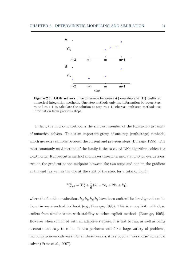
method). The difference between the two approaches is illustrated in Fig. 2.1.
2.2.1 One-step methods
Although one-step methods such as the Euler method use information from only a
single previous step, they can also take additional samples within that step; these are
called multistage methods (Fig. 2.1). The simplest multistage method is the midpoint
method. The form of the midpoint method is similar to Eq. (2.2), but the gradient is
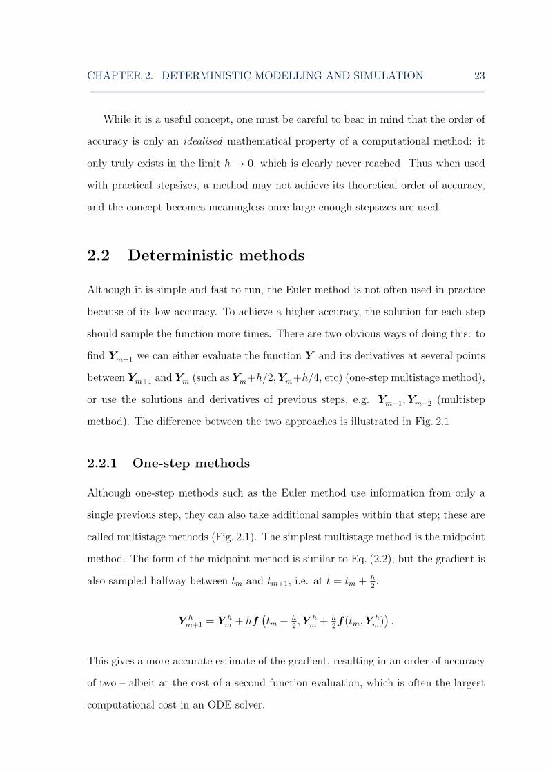
also sampled halfway between tm and tm+1, i.e. at t = tm + h2:
Y hm+1 = Y h
m + hf(tm + h
2,Y h
m + h2f(tm,Y
hm)).
This gives a more accurate estimate of the gradient, resulting in an order of accuracy
of two – albeit at the cost of a second function evaluation, which is often the largest
computational cost in an ODE solver.
CHAPTER 2. DETERMINISTIC MODELLING AND SIMULATION 24
Figure 2.1: ODE solvers. The difference between (A) one-step and (B) multistepnumerical integration methods. One-step methods only use information between stepsm and m+ 1 to calculate the solution at step m+ 1, whereas multistep methods useinformation from previous steps.
In fact, the midpoint method is the simplest member of the Runge-Kutta family
of numerical solvers. This is an important group of one-step (multistage) methods,
which use extra samples between the current and previous steps (Burrage, 1995). The
most commonly-used method of the family is the so-called RK4 algorithm, which is a
fourth order Runge-Kutta method and makes three intermediate function evaluations,
two on the gradient at the midpoint between the two steps and one on the gradient
at the end (as well as the one at the start of the step, for a total of four):
Y hm+1 = Y h
m +1
6(k1 + 2k2 + 2k3 + k4) ,
where the function evaluations k1, k2, k3, k4 have been omitted for brevity and can be
found in any standard textbook (e.g., Burrage, 1995). This is an explicit method, so
suffers from similar issues with stability as other explicit methods (Burrage, 1995).
However when combined with an adaptive stepsize, it is fast to run, as well as being
accurate and easy to code. It also performs well for a large variety of problems,
including non-smooth ones. For all these reasons, it is a popular ‘workhorse’ numerical
solver (Press et al., 2007).

CHAPTER 2. DETERMINISTIC MODELLING AND SIMULATION 25
2.2.2 Multistep methods
One problem with one-step methods is that they carry out several evaluations at each
step, which they then discard for the next step. Intuitively, if an algorithm keeps the
solutions it has calculated at previous steps and uses those at the next step instead
of doing several new calculations, it should be more efficient. Methods of this kind
are called multistep methods. They store the values from previous steps to use for
the current step (Fig. 2.1). For example, an obvious extension of the one-step Euler
method is the two-step Adams-Bashforth method, which is explicit and has order of
accuracy two (Burrage, 1995). Using more previous solutions increases the order of
the method. In addition, explicit and implicit solvers can be combined into predictor-
corrector methods: the explicit method gives a prediction for Y hm+1 and the implicit
corrector then uses that to interpolate a more accurate solution. However, multistep
methods do not have as good stability properties as one-step methods and they also
experience problems when the stepsize is varied.
2.3 Richardson extrapolation
Richardson extrapolation is a technique for increasing the order of accuracy of a de-
terministic numerical method by eliminating the leading term(s) in its error expansion
(Hairer et al., 1993; Richardson, 1911). It involves numerically solving some deter-
ministic function Y (t) at a given time T = nh using the same solver with different
stepsizes, where as usual we define Y hT as an approximation to Y (T ) at time T using
stepsize h. Y (T ) can be written as
Y (T ) = Y hT + ε(T, h),
where ε(T, h) is the (global) error of the approximate solution compared to the true
one. For a general numerical solver, ε(T, h) can be written in terms of powers of the
CHAPTER 2. DETERMINISTIC MODELLING AND SIMULATION 26
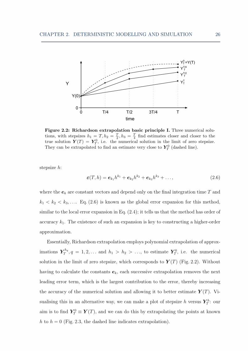
Figure 2.2: Richardson extrapolation basic principle I. Three numerical solu-tions, with stepsizes h1 = T, h2 = T
2 , h3 = T4 find estimates closer and closer to the
true solution Y (T ) = Y 0T , i.e. the numerical solution in the limit of zero stepsize.
They can be extrapolated to find an estimate very close to Y 0T (dashed line).
stepsize h:
ε(T, h) = ek1hk1 + ek2h
k2 + ek3hk3 + . . . , (2.6)
where the ek are constant vectors and depend only on the final integration time T and
k1 < k2 < k3, . . .. Eq. (2.6) is known as the global error expansion for this method,
similar to the local error expansion in Eq. (2.4); it tells us that the method has order of
accuracy k1. The existence of such an expansion is key to constructing a higher-order
approximation.
Essentially, Richardson extrapolation employs polynomial extrapolation of approx-
imations YhqT , q = 1, 2, . . . and h1 > h2 > . . ., to estimate Y 0
T , i.e. the numerical
solution in the limit of zero stepsize, which corresponds to Y (T ) (Fig. 2.2). Without
having to calculate the constants ek, each successive extrapolation removes the next
leading error term, which is the largest contribution to the error, thereby increasing
the accuracy of the numerical solution and allowing it to better estimate Y (T ). Vi-
sualising this in an alternative way, we can make a plot of stepsize h versus Y hT : our
aim is to find Y 0T ≡ Y (T ), and we can do this by extrapolating the points at known
h to h = 0 (Fig. 2.3, the dashed line indicates extrapolation).

CHAPTER 2. DETERMINISTIC MODELLING AND SIMULATION 27
Figure 2.3: Richardson extrapolation basic principle II. Four numerical so-lutions, with stepsizes h, h2 ,
h4 ,
h8 find estimates closer and closer to the true solution
Y (T ) = Y 0T , i.e. the numerical solution in the limit of zero stepsize. They can be
extrapolated to find an estimate very close to Y 0T (dashed line section). The axes are
chosen to highlight the dependence of the approximate solution on the stepsize.
To demonstrate, we take a numerical solver with stepsize h and global error ex-
pansion
Y (T )− Y hT = e1h+ e2h
2 +O(h3) + . . .
For instance, the Euler method has such an error expansion. Now instead of h, if we
use a stepsize h/2, the error expansion is
Y (T )− Y h/2T = e1
h
2+ e2
h2
4+O(h3) + . . . (2.7)
We can take Yh,h/2T = 2Y
h/2T − Y h
T , giving
Y (T )− Y h,h/2T = −e2
h2
2+O(h3) + . . . (2.8)
The leading error term has been removed, resulting in a higher-order approximation.
This can be repeated to obtain an even higher order of accuracy by using more initial
approximations Y h1T , . . .Y
hqT , where q can be any integer and h1 > h2 > . . . hq. We
define Yh1,hqT as the extrapolated solution using initial approximations Y h1
T , . . .YhqT .
The easiest way of visualising this is to build a Neville table (also called a Romberg
CHAPTER 2. DETERMINISTIC MODELLING AND SIMULATION 28
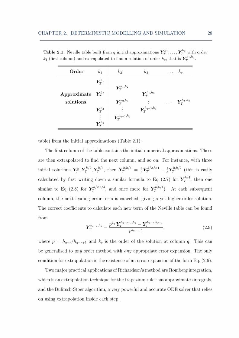
Table 2.1: Neville table built from q initial approximations Y h1T , . . . ,Y
hqT with order
k1 (first column) and extrapolated to find a solution of order kq, that is Yh1,hqT .
Order k1 k2 k3 . . . kq
Y h1T
Y h1,h2T
Approximate Y h2T Y h1,h3
T
solutions Y h2,h3T
... . . . Yh1,hqT
Y h3T
... Yhq−2,hqT
... Yhq−1,hqT
YhqT
table) from the initial approximations (Table 2.1).
The first column of the table contains the initial numerical approximations. These
are then extrapolated to find the next column, and so on. For instance, with three
initial solutions Y hT ,Y
h/2T ,Y
h/4T , then Y
h,h/4T = 4
3Y
h/2,h/4T − 1
3Y
h,h/2T (this is easily
calculated by first writing down a similar formula to Eq. (2.7) for Yh/4T , then one
similar to Eq. (2.8) for Yh/2,h/4T , and once more for Y
h,h/4T ). At each subsequent
column, the next leading error term is cancelled, giving a yet higher-order solution.
The correct coefficients to calculate each new term of the Neville table can be found
from
Yhq−r,hqT =
pkq Yhq−r+1,hqT − Y hq−r,hq−1
T
pkq − 1, (2.9)
where p = hq−r/hq−r+1 and kq is the order of the solution at column q. This can
be generalised to any order method with any appropriate error expansion. The only
condition for extrapolation is the existence of an error expansion of the form Eq. (2.6).
Two major practical applications of Richardson’s method are Romberg integration,
which is an extrapolation technique for the trapezium rule that approximates integrals,
and the Bulirsch-Stoer algorithm, a very powerful and accurate ODE solver that relies
on using extrapolation inside each step.

CHAPTER 2. DETERMINISTIC MODELLING AND SIMULATION 29
2.4 Extrapolated deterministic methods
2.4.1 Romberg integration
Suppose that we want to find the value of the integral
∫ b
a
f(t)dt. (2.10)
One common method for evaluating this is the composite trapezium rule. With
P = b−ah
intervals, the integral can be approximated as
∫ b
a
f(t)dt = h
(f(a) + f(b)
2+
P−1∑p=1
f(a+ ph)
)+O(h2).
We can repeat this using 2P intervals, 4P intervals, etc. to get successively more
accurate solutions, just as in the previous section, and then extrapolate them exactly
as before. This is known as Romberg integration. A key property of the composite
trapezoidal rule is that its error expansion has the form∑
kO(h2k), k = 1, 2, . . ., that
is it only contains terms with even powers of h (Gragg, 1965; Romberg, 1955). Thus,
putting the successive solutions into a table of the form Table 2.1 (a Romberg table,
in this case) allows us to remove two orders of accuracy per extrapolation, to very
quickly converge to the true solution to the integral in Eq. (2.10).
2.4.2 Bulirsh-Stoer method
The Bulirsch-Stoer method is an accurate ODE solver based on Richardson extrapola-
tion (Bulirsch and Stoer, 1966; Deuflhard, 1985). A Neville table is built by repeated
extrapolation of a set of initial approximations with stepsizes that are different subin-
tervals of a larger overall step h, and is then used to find a very accurate solution.
This happens inside each timestep, allowing h to be varied between steps. A modified

CHAPTER 2. DETERMINISTIC MODELLING AND SIMULATION 30
midpoint method (MMP, Algorithm 2.1) is used to generate the initial approximations
in the first column of the table. This lends itself well to an extrapolation framework,
as the MMP subdivides each step h into m substeps h = h/m. Furthermore, just as
the composite trapezoidal rule, the error expansion of the MMP contains only even
powers of h, resulting in fast convergence (Gragg, 1965).
Algorithm 2.1. Modified midpoint method (MMP)
With f(t,Y (t)) = dY (t)dt
and Y (0) = y0, assuming the system is in state ym = Y (tm)
at time tm, and a substep h = h/m:
1. Set z0 = ym.
2. Calculate first intermediate stage z1 = z0 + hf(tm, z0).
3. Evaluate next intermediate stages zl+1 = zl−1+2hf(tm+lh, zl), l = 1, . . . , m−1.
4. Update ym+1 =1
2
(zm + zm−1 + hf(tm + h, zm)
)and tm+1 = tm + h.
At each step, a column of the Neville table, k, in which we expect the approximate
solutions to have converged, as well as an overall stepsize h are selected (see Chapter 5
for full details). The Neville table is then built by running k MMPs, with stepsizes
h1 = h/2, . . . , hq = h/mq, where mq = 2q, q = 1, 2, . . . , k and successively extrapo-
lating the appropriate numerical approximations. The convergence of the solutions is
evaluated based on the internal consistency of the Neville table, that is, the difference
between the most accurate solution in column k and that in column k−1: from Table
2.1, this is ∆Y (k, k − 1) = Y h1,hkh − Y h2,hk
h . As successive initial approximations Yhqh
are added to the first column, the extrapolated results in each new column converge
to the true solution and ∆Y (k, k−1) shrinks. The final approximation at column k is
acceptable if errk ≤ 1, where errk is a scaled version of ∆Y (k, k − 1) (see Algorithm
5.2 for more detail). If errk > 1, the step is rejected and redone with h = h2.
In a practical implementation, the first step of the simulation tests over q =
1, . . . , kmax, where kmax is usually set as eight, in order to establish the k necessary

CHAPTER 2. DETERMINISTIC MODELLING AND SIMULATION 31
to achieve the required accuracy and ensure the stepsize is reasonable; subsequent
steps then test for convergence only in columns k− 1, k and k+ 1 (Press et al., 2007).
Because of its accuracy, the steps taken by the Bulirsch-Stoer method can be relatively
large compared to other numerical solvers. h is changed adaptively at each step, and
is chosen to minimise the amount of work done (i.e. function evaluations m+ 1 of the
MMP) per unit stepsize. In this way the Bulirsch-Stoer method adapts its order and
stepsize to maximise both accuracy and computational efficiency.
In this chapter, we have given an introduction to ODEs and ODE methods in
general. We have also covered Richardson extrapolation, one of the key ideas in this
thesis that will be applied later to the discrete stochastic regime. Finally, we gave
a brief overview of the Bulirsch-Stoer method, which we will adapt into an efficient
stochastic method in Chapter 5.

3Stochastic modelling and simulation
ODEs are used widely in biological and physical modelling, and have many advantages.
They are intuitive and easy to set up, very fast to solve computationally and have been
studied extensively, so the techniques for solving them are well-known. For problems
where noise has a negligible effect they are very useful.
However, it is often necessary to take proper account of the stochasticity in a
system. For instance, when close to a bifurcation regime, ODE approximations cannot
reproduce the behaviour of the system for some parameter values (Erban et al., 2009).
In such cases, stochastic modelling and simulation methods must be used. Because
of the presence of noise, the functions X(t) are random variables instead of the
deterministic variables Y (t). In this notation, X indicates the variable itself, whereas
a specific instance of it is written x ≡ X(t). Another notation change is the re-
labelling of the continuous method timestep h to the discrete one, τ .
ODEs (also known as reaction rate equations, RRE, in a chemical kinetics context)
and stochastic models are inherently linked: a useful way to think about ODEs is as
one type of conditioned mean of the stochastic process. In fact, they can be called
the continuously-conditioned average of the random process X, that is, the mean
of X(t) assuming that the value of X at all previous steps was its mean value and
32
CHAPTER 3. STOCHASTIC MODELLING AND SIMULATION 33
X(0) = x0 (Gillespie and Mangel, 1981). In contrast, what we would usually call the
mean of X, E(X(t)), is the initially-conditioned average of X, i.e. it is conditioned
only upon the requirement X(0) = x0. The ODE reaction rates, which have of-
ten been found phenomenologically, actually arise from the stochastic rate constants,
which are based on microphysical principles (Gillespie, 2007). The relationship be-
tween the RREs and stochastic approaches is further discussed by Higham (2008). In
addition, this direct link between the microscopic (master equation-based) individual
models and macroscopic (differential equation-based) population model approaches
was nicely illustrated by Erban and Othmer (2004) and Erban and Othmer (2005)
(and generalised further by Xue and Othmer, 2009). Using the bacterial chemotaxis
model as an example, they showed that by deriving the macroscopic model from its
microscopic basis, the ad-hoc macroscopic parameters could be linked to known mi-
croscopic properties of the bacteria. These papers highlight that the individual-based,
microscopic, exact approach gives rise to the approximate, macroscopic, population-
based equations that have been known for a long time. It is comforting to see that the
two approaches can be reconciled in the limit of large populations. In Section 3.3.6,
we show how, in a similar fashion, we can transition between models for the discrete
stochastic and deterministic regimes in the case of chemical kinetics.
3.1 Strong and weak order
In a stochastic setting, the term ‘order’ must be redefined; the presence of noise means
that two simulations started in the same initial state will often end in different states.
Thus, rather than a single unique solution, we must compare different properties of
the simulation to the true solution. We can define two different concepts of order:
strong and weak (Kloeden and Platen, 1999).
Strong order compares the trajectories of simulations to the true solution. For a
CHAPTER 3. STOCHASTIC MODELLING AND SIMULATION 34
sample stochastic trajectory XhT of X(T ) at time T = nh,
E|X(T )−XhT | ≤ Chγ
gives the strong order γ > 0 of the simulation method.
As the name implies, weak order requires a weaker connection between the true
solution and the approximate one than strong order. When looking at weak order,
it is only the distribution of the solution (i.e. its moments) that matters. We say
that the approximation XhT converges weakly with order β > 0 to the solution X(T )
if for any suitably smooth functional f(X(T )) up to an appropriate order there is a
positive constant D such that
|E(f(X(T )))− E(f(XhT ))| ≤ Dhβ.
Together, these two definitions are the equivalents to the concept of order in the
deterministic sense. Every stochastic method has both a strong and weak order. Most
have low strong order (for instance, one half for the Euler-Maruyama and Euler τ -
leap methods, described later) but weak order varies more, starting at one (again, the
Euler-Maruyama and Euler τ -leap methods), increasing to two (some τ -leap variants,
see Section 3.3.4) and possibly higher (extrapolated τ -leap), although this has not
been proved analytically.
3.2 Continuous stochastic methods
Systems with fewer particles (typically of the order of thousands to tens of thousands)
are affected correspondingly more by fluctuations. Particle populations are still large
enough to be approximated as concentrations; however, they are not large enough
that stochasticity can be neglected.
A useful way of representing such systems is with stochastic differential equa-

CHAPTER 3. STOCHASTIC MODELLING AND SIMULATION 35
tions (SDEs). These are based on the assumption that the underlying Markov jump
process governing the behaviour of the system can be approximated by a continu-
ous Markov process that is equivalent to certain diffusion processes described by the
chemical Langevin equation (CLE, a class of SDEs; Gillespie, 2000). This ‘diffusion
approximation’ is reasonable in a system with relatively frequent reactions.
A general SDE is identical in form to an ODE with an added noise term (in its
Ito formulation, shown here; Kloeden and Platen, 1989):
dX(t) = a(t,X(t))dt+ b(t,X(t))dW (t), X(0) = X0. (3.1)
Here a is an N × 1 vector-valued function, b is an N ×M matrix-valued function and
dW (t) is a vector of M independent Wiener noise terms. Each Wiener increment from
step n to n+1 is a sample from a Gaussian distribution, given by Wj(t+h)−Wj(t) =
N (0, h), j = 1, . . .M . Eq. (3.1) consists of a deterministic (drift) term that governs
the mean behaviour of the system, and a stochastic (diffusion) term that accounts
for the effects of noise. The diffusion term represents variables not explicitly taken
into account by the drift term, but which nonetheless contribute to the state of the
system.
SDEs form an intermediate regime between the discrete stochastic and determin-
istic regimes (Burrage et al., 2004b; Melykuti et al., 2010). In the limit of large
population, a discrete stochastic method can converge to an SDE. Furthermore, when
the populations are very large, the deterministic part of the SDE is much larger than
the stochastic part, and the diffusion term can be ignored, leaving an ODE, i.e. a
purely deterministic description of the system (Gillespie, 2000, 2001).
How do we numerically solve an SDE? One way is to take the Ito stochastic Taylor
expansion and truncate it at various points. The easiest place to start is by using

CHAPTER 3. STOCHASTIC MODELLING AND SIMULATION 36
only the first term. This gives the Euler-Maruyama method (Maruyama, 1955):
Xhm+1 = Xh
m + ha(tm,Xhm) + ∆Wmb(tm,X
hm),
where ∆Wm = Wm+1 −Wm and Wm is a sample from the normal distribution
N (0, hI), with I the M × 1 identity matrix. We notice that this is just the Euler
method of Eq. (2.2) with an added noise term. The Euler-Maruyama scheme has
strong order one half and weak order one.
In many cases, the trajectories of the individual simulations need to closely ap-
proximate the true solution. This is important in many applications, such as the
dynamics of physical systems with phase transitions and cell biology (Burrage et al.,
2004a). One method that presents considerable improvement on the Euler-Maruyama
method is the stochastic Runge-Kutta algorithm. This family of algorithms is partic-
ularly good at getting high strong order (in general, one to two) approximations; thus
they are particularly suitable for modelling the types of problems described above.
Burrage and Burrage (1996) developed several new classes of stochastic Runge-Kutta
methods, in particular one with strong order two. Abdulle and Cirilli (2007) and
Rue et al. (2010) have also constructed new stochastic Runge-Kutta methods. These
have strong order one, but have good stability, allowing for large timesteps, and are
especially useful for stiff systems that would otherwise be very computationally costly
to simulate.
3.3 Discrete stochastic methods
Going down to the smallest scales, small systems that contain few individual compo-
nents compared to their containing volume, reactions are rare. It is obvious that in
such systems we must account for every single particle, as changes in the molecular
populations are always by integer amounts – i.e. they are discrete. Since there are so
few particles, any change in their numbers is noticeable with respect to the popula-

CHAPTER 3. STOCHASTIC MODELLING AND SIMULATION 37
tion size. Thus they are highly stochastic systems: the states of two initially identical
systems may diverge significantly.
Two popular approaches to simulating stochastic chemical systems are the chem-
ical master equation and stochastic simulation algorithms. We focus on these non-
spatial methods that only count the populations of molecular species over time. There
are many other types of stochastic methods that we do not describe here. For instance,
popular methods such as molecular dynamics and Brownian dynamics simulations,
and compartment-based algorithms that include both time and space considerations.
Some of these approaches are introduced by Erban et al. (2007) (and further com-
pared by Erban and Chapman (2007, 2009)). Specifically, the group of methods we
focus on in this thesis assumes that:
1. individual molecules in the system are not explicitly tracked, only the number
of each chemical species, and
2. non-reactive collisions occur between particles much more often than reactive
ones.
As a consequence, we can assume that the system is well-mixed and spatially ho-
mogeneous (uniformly-distributed). The waiting time between reactive collisions is
exponentially-distributed. The chain of reasoning for this is as follows:
Frequent non-reactive collisions imply that the system is well-mixed;
→ This implies that we can write the probability of a reaction j occurring in
infinitesimal time dt as aj(x)dt = cjhj(x)dt+ o(dt) (see below);
→ The probability of a reaction j occurring over time [t, t + τ + dt) is given
by the probability of no reactions over [t, t + τ), then one reaction j over
[t+ τ, t+ τ + dt); from above this is (1−∑aj(x)dt+ o(dt))
τdt · (aj(x)dt+ o(dt));
→ In the limit dt→ 0, this gives Eq. (3.3), which is exponentially-distributed.
CHAPTER 3. STOCHASTIC MODELLING AND SIMULATION 38
The above justifies our assumption of exponentially-distributed waiting times (the
notation is set out below). This assumption, as well as the fact that particles are not
individually tracked, in turn implies that such systems can be modelled by Markov
jump processes (Gillespie, 1992a). This group of stochastic simulation methods de-
scribes the evolution of the chemical populations through time, where only the state
of the system is recorded as it undergoes a number of chemical reactions. Wilkinson
(2011) provides an accessible introduction to such stochastic methods.
We are interested in a system of biochemical reactions with N species and M reac-
tions inside some fixed volume V , each of which can involve different species and occur
at different rates. The populations of chemical species are represented as state vectors
X(t) ≡ Xi(t), i = 1, . . . , N ; crucially, these values are actual numbers of molecules
and not concentrations as in ODE methods. The reactions are represented by a sto-
ichiometric matrix ν ≡ νij, i = 1, . . . , N, j = 1, . . . ,M , composed of the individual
stoichiometric vectors νj. νj represents the change in state due to j occurring and
the system going from Xm to Xm+1, that is X(t) to X(t+ τ). Each reaction occurs
with probability aj(x)dt+o(dt) in the infinitesimal time interval dt, given that it is in
state x; this is known as the fundamental hypothesis of the stochastic formulation of
chemical kinetics (Gillespie, 1976). It represents a key difference between the stochas-
tic and deterministic approaches to chemical kinetics: ODEs assume that reactions
happen with a certain rate, whereas stochastic methods consider the probability of
reactions occurring. This is also the factor that allows stochastic methods to be ex-
act, whereas ODE methods are by definition approximations. aj(x) is known as the
propensity function of reaction j. Propensity functions are given by the mass-action
kinetics of the reactant chemical species. For instance in the reaction X1 +X2c→X3,
a = cX1X2 and ν = [−1,−1, 1]T , and for X1 + X1c→X2, a = cX1(X1 − 1)/2 (the
factor of 12
arises because we are effectively choosing two particles from a total of X1
without replacement) and ν = [−2, 1]T . X(t),ν and a(X(t)) fully characterise the
system at each time point t.

CHAPTER 3. STOCHASTIC MODELLING AND SIMULATION 39
3.3.1 Chemical Master Equation
The chemical master equation (CME) (Gillespie, 1992b) takes a ‘distribution’ view
of the system, keeping track of every possible state at once. It is an exact method
for tracking the behaviour of a stochastic system over time by enumerating all the
possible states in which the system can be at any time. For a system in state x at
time t,
P (x; t+ dt) = P (x; t)
(1−
M∑j=1
aj(x)dt
)+
M∑j=1
aj(x− νj)P (x− νj; t)dt+ o(dt),
where dt is sufficiently small that, to first order, at most one reaction takes place in
the time interval [t, t+ dt). In words, this states that the probability that the system
is in state x at time t+dt is given by the probability that it is in state x at time t and
does not change (first term), plus the probability that it is in another state at time t
and changes to state x during [t, t+ dt) (second term). Rearranging then taking the
limit dt→ 0, this can be written as a system of ODEs,
dP (x; t)
dt=
M∑j=1
aj(x− νj)P (x− νj; t)− P (x; t)M∑j=1
aj(x). (3.2)
The main difference between the CME and a deterministic model is that the CME
is based on probabilities, rather than rates of change. It describes the probabilities
of the system being in each state at different time points. Solving the CME consists
of evaluating Eq. (3.2) at certain time points, somewhat like an ODE; however, the
CME solution is an entire PDF.
Thus the CME seems to be the ideal way of finding the evolution in time of a
stochastic system: it is exact and returns the full PDF of the system. However, only
in the case of very simple systems can it be analytically solved; for the vast majority
of cases, a numerical approach is necessary. For this reason, in practice, solutions of
the CME are generally not actually exact. In addition, as each possible state has to

CHAPTER 3. STOCHASTIC MODELLING AND SIMULATION 40
be evaluated at each time point and the number of states can grow non-linearly, each
solution is very computationally-intensive. This can be an obstacle, and the CME
approach could initially only be effectively used to simulate simple systems for short
periods of time. However, in recent years there has been considerable progress on CME
solver methods: for instance MacNamara et al. (2008b) used an adapted finite state
projection algorithm (originally introduced by Munsky and Khammash, 2006) that
could detect when the system was at equilibrium to show that for some problems the
CME approach was faster at computing moments than both the stochastic simulation
algorithm and even the much faster τ -leap. By using the total quasi-steady-state
approximation with a CME solver, they were able to speed up the CME solver even
more (MacNamara et al., 2008a; MacNamara and Burrage, 2009). More recently,
MacNamara and Burrage (2010) were able to solve the CME for even larger systems,
as well as for time-dependent rate constants. This shows that the CME is now a useful
tool for finding exact distributions of stochastic systems. Comparatively, even the
stochastic simulation algorithm is less accurate, as it generally needs many simulations
before its distribution is close enough to the true one. Nevertheless, when populations
and propensities grow too large to be calculated using the CME, trajectory-based
simulations must be used instead.
3.3.2 Stochastic simulation algorithm
The most basic trajectory-based approach that exactly simulates individual paths
from the full distribution given by the CME is the stochastic simulation algorithm
(SSA; Gillespie, 1977). The SSA is a statistically exact method for generating Monte
Carlo paths; that is, a PDF built up from an infinite number of simulations of the
SSA will be identical to the true distribution of the system, as given by the CME.
Clearly this limit is never reached, but a satisfactorily accurate PDF can be achieved
by a moderately high number of repeats of the SSA: between 104 and 108, depending
on the system and the type of application.
CHAPTER 3. STOCHASTIC MODELLING AND SIMULATION 41
The SSA steps along in time reaction-by-reaction, governed by the reaction prob-
ability density function (Gillespie, 1976)
P (τ, µ) = aµ(x)exp(−a0(x)τ), (3.3)
for time 0 ≤ τ < ∞ and reaction types 1 ≤ µ ≤ M and a0(x) =∑M
j=1 aj(x). Note
that here and below, we now do not explicitly state the o(dt) term, as it is typically
assumed to be negligible; however it is worth keeping this in mind. Eq. (3.3) is a
joint probability density of the variables τ and µ: P (τ, µ)dt gives the probability of
when the next reaction will occur (in the infinitesimal time interval between t+ τ and
t+τ +dt) and what type of reaction it will be (type µ). In order to determine specific
quantities for these variables at each step, we can write
P (τ, µ) = P1(τ) · P2(µ|τ). (3.4)
P1(τ), which gives the time until next reaction regardless of reaction type, can be
found by summing P (τ, µ) over all µ, and then substituted into Eq. (3.4) to find
P2(µ|τ), which gives the reaction type given that the reaction occurs at t + τ . This
leads us to the simplest SSA scheme, the direct method, which samples one new
random number each from P1(τ) and P2(µ|τ) and thus calculates the time until the
next reaction τ , and the reaction j′ that will occur (Gillespie, 1976). The time until
the next reaction is given by
τ =1
a0(x)ln
(1
r1
), (3.5)
where r1 is a uniform random number on [0, 1]. Eq. (3.5) generates a random number
from the probability distribution P (τ) = a0(x)exp(−a0(x)τ) (Gillespie, 1976). This
is actually the minimum time until the next reaction over the entire set of reactions.
The separate probability of each reaction j occurring is P (τ) = aj(x)exp(−aj(x)τ),

CHAPTER 3. STOCHASTIC MODELLING AND SIMULATION 42
but the direct method finds the one that happens first, hence the sum over aj(x).
Notice that P (τ) has an exponential distribution with parameter a0(x), confirming
that the reaction times are exponentially-distributed as assumed. The index j′ of the
next reaction is given byj′−1∑m=1
am < a0r2 ≤M∑
m=j′
am, (3.6)
where r2 is a uniform random number on [0, 1]. Thus the relative probability of each
reaction j occurring isaj(x)
a0(x). The state vector is evolved in time according to the
update equation
Xm+1 = Xm +M∑j=1
νjKj, Kj =
1 if j = j′,
0 otherwise.
(3.7)
Algorithm 3.1. SSA (Direct method)
With the system in state Xm at time tm:
1. Sample r1 and r2 from the unit-interval uniform distribution.
2. Find time until next reaction τ = 1a0(Xm)
ln(
1r1
), where a0(Xm) =
∑Mj=1 aj(Xm).
3. Next reaction j′ is the smallest integer such that r2 a0(Xm) ≤∑j′
j=1 aj(Xm).
4. Update tm+1 = tm + τ and Xm+1 = Xm + νj′ .
The SSA is derived directly from microphysical principles; this is its key advantage,
and it is a very important factor. It also has several other, less significant, advantages.
For instance, it is very easy to program and can be run in parallel across simulations
or on the graphical processing units of modern graphics cards.
Its main drawback is the time it takes for simulations of more complicated systems
to run. For instance, a single simulation in the software package Matlab on a complex
problem can sometimes take of the order of a day to run. This is clearly not ideal.
Moreover, in order to learn about the typical behaviour of the system, for instance to

CHAPTER 3. STOCHASTIC MODELLING AND SIMULATION 43
find accurate values for statistical quantities such as the mean and standard deviation,
many simulations are necessary. This may take a prohibitively long time. Several
variants of the SSA have been proposed that attempt to speed up the simulations. The
first reaction method, also proposed by Gillespie (1976) instead found a ‘tentative’
waiting time for each reaction and then chose the one that occurred soonest. The
next reaction method (Gibson and Bruck, 2000) built upon this by recycling random
variables and by only updating those propensity functions that have changed over
each step. The optimised direct method improved the original direct method to be
competitive with the next reaction method (Cao et al., 2004). More recently, Yates
and Klingbeil (2013) introduced the concept of recycling random numbers to the
direct method to give significant gains in efficiency, whilst minimising changes to the
implementation by adding only one new line of code.
3.3.3 τ-leap method
Despite these advances, in many cases even the fastest SSA implementations are not
fast enough, and in these circumstances an approximate method must be used. The
first method to attempt to speed up the SSA by sacrificing its exactness was the
τ -leap method (Gillespie, 2001). As with the SSA, it evolves the state vector of the
system through time by simulating a series of chemical reactions. However, at each
step it computes the effects of many reactions at once. This allows each timestep to be
longer, resulting in fewer calculations over the length of the simulation. Using a τ -leap
method can dramatically reduce the number of calculations, and so the computational
time, as compared to the SSA. For instance, a simple decay process with 105 initial
particles obviously took an SSA 105 steps to reach zero population. In contrast, it took
a τ -leap of the order of one to several hundred steps, whilst maintaining reasonable
accuracy (Gillespie, 2001). This can often translate into a reduction in computational
time of several orders of magnitude, although this varies for each system.
The obvious problem is that the accuracy of our simulation is compromised: we
CHAPTER 3. STOCHASTIC MODELLING AND SIMULATION 44
can no longer tell exactly when each reaction occurs, only in which timestep; moreover,
we can only estimate the number of reactions itself. A careful balance must be struck
between this loss of information and the gain in speed. If we choose the timestep to
be too large, the results are useless because of the loss of accuracy. If, on the other
hand, the step size is too small, we are essentially reverting back to the SSA and
losing computational time.
What is the best way to ensure this balance? We can require that the timestep τ
is so small that the propensities do not change ‘significantly’ during one step. This
is known as the leap condition, and is another way of saying that the change in the
probability of each reaction occuring is infinitesimal (Gillespie, 2001). The number
of times Kj each reaction occurs during every timestep is drawn from a Poisson
distribution, and approximated by the τ -leap as (Gillespie, 2001)
Kj(τ ;x, t) = P(aj(x)τ), (3.8)
and the τ -leap algorithm evolves the system through time as
Xm+1 = Xm +M∑j=1
νjKj. (3.9)
This is identical to the SSA except for the form of K, which is given for the τ -leap
by Eq. (3.8) and Eq. (3.7) for the SSA.
Algorithm 3.2. Euler τ -leap method (ETL)
With the system in state Xm at time tm, and a timestep τ :
1. Generate M Poisson random numbers Kj = P(aj(Xm)τ), j = 1, . . . ,M .
2. Update tm+1 = tm + τ and Xm+1 = Xm +∑M
j=1 νjKj.
This most basic τ -leap method is also known as the Euler τ -leap method (ETL),
as the form of Eq. (3.9) resembles the Euler method for solving ODEs. Similar to the
Euler method, the ETL has weak order one, as well as strong order half (Li, 2007).
CHAPTER 3. STOCHASTIC MODELLING AND SIMULATION 45
Algorithm 3.2 does not specify how to choose τ , and an obvious first choice is to
manually set it to a fixed value. However, this is yet another trade-off between speed
(large timesteps, possibly even resulting in negative populations and thus simulation
failure) and accuracy (small timesteps, possibly resulting in slow simulations like
the SSA), and is of no real practical use unless simplicity is the most important
consideration or τ must be fixed, as is the case when used in the context of Richardson
extrapolation (see Chapter 4 and Szekely et al. (2012)) or the multilevel Monte Carlo
method (Anderson and Higham, 2012). Adaptively changing τ at each step can give
far greater gains in speed and accuracy: τ can be made as large as possible given the
state of the system at that point, resulting in faster computational times. Moreover,
higher accuracy is obtained as τ can also be kept small enough to adhere to the leap
condition. When τ has a similar size to the expected SSA step, 1a0(x)
, a good simulation
algorithm should temporarily switch to the SSA, for two reasons: firstly, there is
computational overhead involved in calculating τ ; secondly, and more importantly,
the SSA only needs one or two uniform random numbers per step (depending on the
implementation), but the τ -leap needs M Poisson random numbers, requiring much
more computational effort.
One way of enforcing the leap condition is to bound the change in propensity
functions over each step by a small percentage of their sum. Of course, we cannot know
in advance how the propensities will vary, so we must take the change in propensities
assuming the system changes by its expectation over that step (Gillespie, 2001), i.e.
|aj(x+ τνjaj(x))− aj(x)| ≤ εa0(x),
where ε � 1, usually somewhere around 0.01 to 0.05. But when the propensities
for each reaction have different sizes, the τ selected in this way could be suitable
for one reaction channel but far too large for another, and the leap condition is not
always obeyed closely enough. This was noted by Gillespie and Petzold (2003), who
CHAPTER 3. STOCHASTIC MODELLING AND SIMULATION 46
also introduced the size of the variance of the change in propensities, on top of their
mean, as a restriction upon τ . Ideally, we would calculate the optimal τ for each
reaction channel,
|aj(x+ τνjaj(x))− aj(x)| ≤ εaj(x),
then choose the smallest one, as this is where substantial accuracy can be lost. The
reason this solution is not practical is that when one of the species goes to zero,
the chosen τ would also go to zero, stopping the simulation prematurely. However,
we know that aj(x) = cjf(xi), i = 1, . . . , N , where f is a smooth function of the
species, for example xi (unimolecular reactions), xixi′ or xi(xi−1)/2 (both bimolecular
reactions). Since the smallest change in xi is one, the smallest possible change in aj(x)
is cj. As outlined by Cao et al. (2006), we can now take
|aj(x+ τνjaj(x))− aj(x)| ≤ max{εaj(x), cj},
i.e. the minimum τ chosen will always be greater than zero. However, this method
can still be improved, by employing a further approximation. This time the change
in propensities from one step to the next is approximated by the change in molecular
populations instead. Since this involves some complications, we do not discuss the
procedure further here, and leave it to Cao et al. (2006). The accuracy of this last
procedure is similar to the previous one, but its computational cost is lower: the num-
ber of calculations of earlier τ -leaping schemes increases quadratically with chemical
species, but is linear for this version of the algorithm (Cao et al., 2006).
There is an additional problem with the initial formulation of the τ -leap: when the
stepsize is chosen too large, the molecular species can sometimes go negative. Tian
and Burrage (2004) and Chatterjee et al. (2005) addressed this problem by sampling
Kj from a binomial distribution. The binomial distribution is bounded on [0,S] (where
S is sample size), so as long as S is set to the number of particles in the least populous
species the problem of negativity is avoided. The most recent method of Cao et al.

CHAPTER 3. STOCHASTIC MODELLING AND SIMULATION 47
(2006) also alleviates this problem by using a critical reaction parameter nc which is
set to a low integer value. Any reaction channel whose reacting populations are less
than nc switches to using a modified SSA for that timestep. There have been two more
recent variations of the binomial τ -leap: a new binomial τ -leap method (Peng et al.,
2007), which changes the restrictions on the sampling of binomial numbers to allow
larger steps whilst still retaining accuracy, and one that uses multinomial random
variables (Pettigrew and Resat, 2007), which has improved efficiency by both grouping
reactions together into larger groups and using a different stepsize selection scheme
to the one proposed by Gillespie and colleagues. Even more recently, also sampling
Poisson random variables, Yates and Burrage (2011) developed a method that is
somewhat similar to that of Cao et al. (2006), but more robust and efficient. Instead
of using a critical reaction parameter, they calculate the probability of each chemical
species becoming negative in the next step. This improves efficiency by ensuring that
species that are unlikely to become negative are not overcautiously classed as critical
and do not unnecessarily slow down simulations. Moreover, robustness is improved
as chemical species with populations above nc that may undergo many reactions can
thus possibly go negative in the standard τ -leap; in contrast, the formulation of Yates
and Burrage (2011) can catch this by noticing that that species has a high probability
of becoming negative.
3.3.4 Higher-order leaping methods
In recent years, there has been an effort to improve the τ -leap by formulating higher-
order leaping methods, rather than improving the stepsize selection itself. This is
somewhat inspired by higher-order methods for ODEs, such as the popular Runge-
Kutta (see Section 2.2.1) and Bulirsch-Stoer (see Section 2.4.2) methods. These meth-
ods are useful for the same reason as with ODEs: in theory, they reduce the error of
the results for a given stepsize. Because of this, they can use larger timesteps for a
desired error level, reducing processing time.
CHAPTER 3. STOCHASTIC MODELLING AND SIMULATION 48
We will refer to two different approaches for finding the order of these methods: the
‘classical’ scaling τ → 0 and the ‘large-volume’ scaling V → ∞. We introduce these
concepts here. Rathinam et al. (2005) were the first to analyse the order properties
of τ -leap methods. They showed that for linear propensity functions (that is, at most
first-order reactions), the ETL has weak order of accuracy one in the moments under
the scaling τ → 0. This is the scaling traditionally used in ODE analysis to find order
of accuracy. This analysis was extended to non-linear propensities by Li (2007), by
considering τ -leap methods as SDEs driven by Poisson random measures (see also
Burrage and Tian (2004)). He showed that the ETL is precisely the Euler method
applied to this SDE and hence inherits the properties of strong order half and weak
order one. However, the problem with using the scaling condition τ → 0 for τ -leaping
methods is that this is directly at odds with the regime under which τ -leaping is useful:
the stepsize should be large compared to the waiting time between each reaction, or
more precisely, a0(x)τ � 1, otherwise one loses efficiency compared to the SSA.
Anderson et al. (2011) got around this by considering order under a large-volume
scaling V → ∞. Here, one normalises the populations by the volume V such that
X/V = O(1) and sets τ = V −β, 0 < β < 1. Then in the limit V →∞, global strong
and weak order convergence can be established, both of which they found to be one for
the ETL. Hu et al. (2011a) investigate these issues in greater detail through the use of
rooted tree expansions of the local truncation errors for the moments and covariance,
thus generalising the approach first applied to SDEs by Burrage and Burrage (2000).
They note that the large-volume scaling also has its own problem, in that the system
size should not need to change as stepsize is varied to find order of convergence. Thus
the classical and large-volume scalings approach the problem of finding convergence
from two different angles. Their analysis shows that while some τ -leap methods may
have higher-order moments (for instance, the midpoint τ -leap method has order two
moments for linear systems), their covariance is invariably of unit order, unless this is
specially taken into consideration (as with the θ-trapezoidal τ -leap method, which has

CHAPTER 3. STOCHASTIC MODELLING AND SIMULATION 49
order two moments and covariance). As Hu et al. (2011a) point out, these issues arise
as a consequence of the differences between the infinitesimal generators for ODEs and
jump processes.
Gillespie proposed the first higher-order τ -leaping method, the midpoint τ -leap
(MPTL), in his seminal paper (Gillespie, 2001). He based it directly on the well-
known midpoint method for ODEs, a second-order Runge-Kutta method. Instead
of using the gradient at time t to estimate X(t + τ), as the Euler method does,
the midpoint method uses it to find X(t + τ2), and then uses the gradient at this
‘midpoint’ to find X(t + τ). In its τ -leap incarnation, the actual change in X is, of
course, a random variable, so Gillespie suggested using the expected midpoint value,
X ′, instead. Then the Poisson update becomes K = P(a(X ′)τ).
Algorithm 3.3. Midpoint τ -leap method (MPTL)
With the system in state Xm at time tm, and a timestep τ :
1. Calculate expected midpoint value X ′ = Xm + 12τ∑M
j=1 νjaj(Xm).
2. Generate M Poisson random numbers Kj = P(aj(X′)τ), j = 1, . . . ,M .
3. Update tm+1 = tm + τ and Xm+1 = Xm +∑M
j=1 νjKj.
It was subsequently found that the MPTL is not fully weak order two, unlike its
ODE cousin. It has weak order two moments in the large-volume scaling, but in the
classical scaling they have weak order one, like the ETL (Anderson et al., 2011; Hu
et al., 2011b). Its variance also has weak order one, again as the ETL.
Two more recent higher-order methods are the random-corrected τ -leap, which has
no deterministic analogue, and the θ-trapezoidal τ -leap, which is similar to Heun’s
method for ODEs. The random-corrected τ -leap method is based on the ETL, with a
(randomly-sampled) correction term applied at each step (Hu and Li, 2009). If chosen
properly, this has the effect of increasing the order of the method, as the correction
terms cancel with the leading terms in the local truncation error. Hu and Li (2009)

CHAPTER 3. STOCHASTIC MODELLING AND SIMULATION 50
introduce a Poisson correction, as well as two types of Gaussian corrections; the former
is able to achieve weak second order in the mean but only first order in the variance,
while the latter two achieve weak second order in both the mean and the variance.
The θ-trapezoidal τ -leap method (TTTL) is based on the similarly-named SDE
method of Anderson and Mattingly (2011), and has both higher-order moments and
covariance (Anderson and Koyama, 2012; Hu et al., 2011b). The method consists of
two steps, a predictor step with stepsize θτ and a corrector step with stepsize (1−θ)τ
that aims to cancel any errors made in the first step. In a general sense, its form is
similar to the random-corrected τ -leap, as the update formula of both can be written
Xm+1 = Xm +M∑j=1
νjK∗j , K∗ = K + K,
where K is the usual τ -leap update, i.e. the predictor, and K is the corrector term.
The main difference is that the random-corrected τ -leap takes a full step and attempts
to correct for the error at the end, whereas the TTTL only uses the initial predictor
stage to solve for a fraction of the timestep, θτ . The corrector stage then attempts
to correct the error in the predictor stage until τ is reached (Hu et al., 2011b).
Algorithm 3.4. θ-trapezoidal τ -leap method (TTTL)
For a specified θ ∈ (0, 1), α1 = 12(1−θ)θ , α2 = (1−θ)2+θ2
2(1−θ)θ . With the system in state Xm
at time tm, and a timestep τ :
1. Generate M Poisson random numbers K ′j = P(aj(Xm)θτ), j = 1, . . . ,M .
2. Calculate predicting step X ′ = Xm +∑M
j=1 νjK′j.
3. Calculate lj = max (α1aj(X′)− α2aj(Xm), 0).
4. Generate M Poisson random numbers Kj = P(lj(1− θ)τ), j = 1, . . . ,M .
5. Update tm+1 = tm + τ and Xm+1 = X ′ +∑M
j=1 νjKj.
CHAPTER 3. STOCHASTIC MODELLING AND SIMULATION 51
The moments of the TTTL were shown to have weak order of convergence two,
and its covariance has local truncation error O(τ 3V −1). τ = V −β, 0 < β < 1 and
in the analysis V →∞, but in simulations the system volume is kept constant; thus
it seems that in practice this also results in weak second-order convergence in the
covariance (Anderson and Koyama, 2012; Hu et al., 2011b).
The unbiased τ -leap method (UBTL), in theory, should not fit into this section, as
the idea is that it has zero bias error, and therefore should not have a defined order of
accuracy (Xu and Cai, 2008). In order to construct such a method, the authors begin
with a CME for K, the number of reactions occurring per step, rather than the usual
one for X. They then find an expression for the mean of this CME, which constitues
the Poisson parameter for the step, as well as its variance (explained further below).
At this point the method is indeed unbiased. Unfortunately, in general, the moment
equations derived from the CME contain higher moments, except in the case where
all the reactions are zeroth- or first-order, meaning the propensities are linear and
E(aj(x)) ≡ aj(E(x)). The ODEs for the higher moments contain yet higher moments,
and so on ad infinitum. Thus it is not possible to solve for the mean and variance
in the general case of non-linear propensities, and a moment closure approximation
must be made. For instance, the equation for the mean of K is dE(K)dt
= E(a(K)). To
be applicable in the general case, we can Taylor expand the propensities and truncate
the expansion at first order, that is a(K) = a(0) + FK, where F is defined below.
Taking a similar approach for the variance, we get Eqs. (3.10) and (3.11) (Xu and Cai,
2008). This clearly introduces a bias error into the method, which one would expect
to then be weak first order.
The method involves solving, at each timestep, two ODEs for the quantities µ(t)

CHAPTER 3. STOCHASTIC MODELLING AND SIMULATION 52
and C(t), the mean and variance of K, respectively:
dµj(s)
ds=
M∑j′=1
fjj′(x)µj′(s) + aj(x), µj(t) = 0, (3.10)
dCj(s)
ds= 2fjjCj(s) +
dµj(s)
ds, Cj(t) = 0, (3.11)
where s ∈ [t, t + τ), x ≡ X(t) is the value of the state vector at the start of the
step and fjj′(x) =N∑i=1
∂aj(x)
∂xiνij′ , j, j
′ = 1, . . . ,M are the elements of the M ×M
matrix F . Note that Eq. (3.11) only contains the diagonal elements fjj and C is
the variance of K, as we assume that the reactions are independent and so the non-
diagonal elements of the covariance matrix are zero. Eqs. (3.10) and (3.11) must be
solved simultaneously with initial conditions µ(t) = C(t) = 0 to find µ(t + τ) and
C(t+ τ).
In Section 5.5, we run numerical tests to find the order of a restricted SBS-DA
method, which uses Eqs. (3.10) and (3.11) to find the number of reactions at each
step. As this implementation was purposely restricted to both fixed stepsize and zero
(or one) extrapolations, in effect it reduced down to the UBTL with fixed stepsize.
Unexpectedly, we found that it actually has weak second order in the moments and
first order in the variance for the stepsizes used, which were chosen to be large to
avoid Monte Carlo error. Although the large stepsizes could also affect the order of
the method (see Section 5.5 for a discussion), the order would either be unaffected or
reduced; this shows that the maximum weak order one can probably obtain from the
UBTL with a first-order truncation of the Taylor series of the propensity functions is
two.
Algorithm 3.5. Unbiased τ -leap method (UBTL)
With the system in state Xm at time tm, and a timestep τ :
1. Solve Eqs. (3.10) and (3.11) using a standard ODE solver to find mean and
variance of number of reactions at time t+ τ .
CHAPTER 3. STOCHASTIC MODELLING AND SIMULATION 53
2. Choose K as given by Eq. (3.12).
3. Update tm+1 = tm + τ and Xm+1 = Xm +∑M
j=1 νjKj.
In fact, Eq. (3.11) is only necessary because Eq. (3.10) is not exact in the general
case; when all propensities are linear, only Eq. (3.10) is necessary to find an exact
value for the Poisson parameter. For larger timesteps, the loss of exactness may lead
to a sizeable error, so we must approximate the true, Poisson, distribution of K with
a Gaussian whose variance has been corrected. This leads to the update scheme
Kj(µj(t+τ), Cj(t+τ)) =
P(µj(t+ τ)) if µj(t+ τ) < 10,⌊N(µj(t+ τ),
√Cj(t+ τ)
)⌉if µj(t+ τ) ≥ 10,
(3.12)
where b e denote rounding to the nearest integer (this is done to keep particle numbers
as integers, and since the normal sample is taken when µj > 10, it should not introduce
excessive error). Here the value ten has been chosen heuristically as above this value
a Poisson sample can be well-represented by a Gaussian sample with the appropriate
mean and variance. Moreover, Xu and Cai (2008) also introduce a switch to binomial
variables when µj(t) is small and differs significantly from Cj(t).
3.3.5 Multiscale methods
Lastly, we will briefly cover multiscale methods. These are useful for simulating sys-
tems that have large differences in the frequency of their reactions (i.e. propensities),
due to large variations in the populations of their various species and/or their fast re-
action rates. In practice, this occurs in many systems, but standard leaping methods
are often able to satisfactorily simulate them. In the more extreme cases, specialised
multiscale methods must be used. The general form of the implementation is often
similar between these methods: a set of approximate equations, usually ODEs, CME
moment equations, or SDEs, is coupled with a stochastic method, either a set of
CHAPTER 3. STOCHASTIC MODELLING AND SIMULATION 54
SDEs or a Monte Carlo simulator, each representing different scales. The fast (high-
propensity) reactions are simulated approximately, and separately from the slower
reactions, potentially resulting in a large increase in speed: it is the frequent reac-
tions that slow down stochastic simulations, as they require small timesteps and thus
many computations. Additionally, these fast reactions are often not even important,
as they introduce transient dynamics that settle down very quickly.
The main problem is that often, the two sets of reactions both involve the same
chemical species, making them dependent on each other. Each method differs slightly
in its solution to this problem. As there are too many multiscale methods to detail
individually, we merely stick to general descriptions here. One group of methods uses
CME equations for the fast states, and calculates the slow timestep by drawing random
numbers like the SSA (Cao et al., 2005; Goutsias, 2005; Haseltine and Rawlings, 2002;
Rao and Arkin, 2003). These make the assumption that the fast species settle very
quickly to a steady state, on a time-scale very much shorter than the slow species.
Kiehl et al. (2004) instead approximate the fast reactions with ODEs, and select the
slow timesteps as above. Attempting to retain even more accuracy, E et al. (2005)
use an SSA for both fast and slow reactions, with one nested inside the other. Finally,
Salis and Kaznessis (2005) use a chemical Langevin equation, an SDE, for the fast
reactions, that they couple to jump equations to find the slow-scale timesteps.
Thus the idea behind all of these methods is somewhat similar: simulate the fast
reactions separately and approximately, while the slow ones are generally simulated
using a Monte-Carlo-type method. This has the effect of speeding up simulations, as
fast reactions are the bottleneck for a standard stochastic method that must simulate
all reactions. In contrast to these approaches, the method of Cotter et al. (2011)
simulates the fast reactions with a constrained SSA and uses this to then estimate
the parameters of a Fokker-Planck equation (which returns a full probability density)
to approximate the dynamics of the slow reactions. The reason this improves compu-
tational time is that only one SSA must be run to obtain the Fokker-Planck equation
CHAPTER 3. STOCHASTIC MODELLING AND SIMULATION 55
parameters for each value of the slow variable, rather than the many SSA simulations
typically used in multiscale methods.
3.3.6 Crossing regimes: from the τ-leap to the ODE
Finally, we end this section with a nice observation by Gillespie (2001, 2007). The
τ -leap method exists in an intermediate regime, somewhere between the SSA and the
SDE approach to chemical reactions. Gillespie shows how, as the populations under
consideration are increased, the τ -leap segues smoothly into the SDE regime, which,
as the populations tend to infinity, then transitions to an ODE.
We start with the τ -leap formula
Xm+1 = Xm +M∑j=1
νjP(aj(Xm)τ). (3.13)
We know that P(aj(x)τ) has mean and variance aj(x)τ . As we increase the pop-
ulations and∑
j aj(x)τ � 1, a well-known result in probability theory says that
P(aj(x)τ) ≈ N (aj(x)τ, aj(x)τ). Since a normal variable N (µ, σ2) = µ + σN (0, 1),
this can be written as
N (aj(x)τ, aj(x)τ) = aj(x)τ +√aj(x)τN (0, 1).
We can write the last term as√aj(x)τ∆Wj, where ∆Wj is a sample from N (0, 1).
Substituting back into Eq. (3.13), we arrive at a τ -leap method for large propensities
(which is valid as long as the leap condition is satisfied, as well as∑
j aj(x)τ � 1),
Xm+1 = Xm +M∑j=1
νjaj(Xm)τ +M∑j=1
νj
√aj(Xm)τ∆Wj.

CHAPTER 3. STOCHASTIC MODELLING AND SIMULATION 56
But this is just the Euler-Maruyama method applied to the CLE,
dX(t) =M∑j=1
νjaj(X(t)))dt+M∑j=1
νj
√aj(X(t))dWj. (3.14)
Thus when the propensities are large, the τ -leap is equivalent to the CLE. The next
step is obvious: what happens when we increase the populations even further? This
is known as the thermodynamic limit as X →∞ (as well as the volume V →∞, thus
ensuring X/V does not change). In this case, the first term on the right-hand side of
Eq. (3.14) grows faster than the square root term, meaning that Eq. (3.14) reduces to
simply
dX(t) =M∑j=1
νjaj(X(t)))dt. (3.15)
Eq. (3.15) should be easily recognisable as the ODE form of chemical kinetics, the
RRE, comparable to Eq. (2.1). This section has demonstrated, using the reasoning of
Gillespie (2001, 2007), that the CLE and RRE formulations of chemical kinetics arise
naturally as large-population limits of the τ -leap, which is formulated based on the
fundamental hypothesis of stochastic chemical kinetics.
We have now covered both deterministic and stochastic methods in enough detail
to establish the background, as well as to put the work in the following chapters into
context. Next, we build on and draw together both the deterministic and stochastic
branches of methods described thus far.
4Stochastic extrapolation
In this chapter, we now synthesise the ideas from the previous chapters to develop
the stochastic extrapolation framework. This is an important advance, as 1) it shows
that we can adapt techniques from the deterministic regime to work in the discrete
stochastic regime, 2) it allows us to increase the weak order of an approximation with
minimal effort, something that up to this point methods had to be specifically and
painstakingly designed to do, and 3) in theory it can be applied to any method any
number of times, thus raising the possibility of extremely accurate methods. We begin
with a short review of extrapolation for SDEs, as some of the ideas will be useful later,
then progress on to the work we have done on τ -leap extrapolation.
4.1 Extrapolation for SDEs
The ideas in Section 2.3 can be extended to the stochastic regime. This is more
complicated than the deterministic case: the main problem is that in the stochastic
Taylor expansion of the error, there are additional cross-terms. It is not clear that
these will cancel fully when extrapolated, as in the deterministic case. This did not
present a problem in the analysis of Talay and Tubaro (1990), although they ignored
57

CHAPTER 4. STOCHASTIC EXTRAPOLATION 58
third-order and higher terms in the expansion. In this section, we give an overview
of the work of Talay and Tubaro (1990) on SDE extrapolation. We again define the
global weak error of a stochastic numerical scheme to be
ε(T, h, f) = E(f(X(T )))− E(f(XhT )), (4.1)
where XhT is our approximation to the true solution X(T ) at time T = nh with
stepsize h. Note that the error expansion depends on the suitable smooth function f ,
although the order itself does not. To extrapolate this scheme, we want to obtain an
expression of the form
ε(T, h, f) = ek1hk1 + ek2h
k2 + ek3hk3 + . . .
Talay and Tubaro (1990) do this by using the scalar-valued function u in the equations
(known as the Kolmogorov backward equation)
∂u
∂t+ Lu = 0
u(T,x) = f(x),
(4.2)
where f is a homogeneous scalar-valued function and
u(t,x) = E(f(X(T ))|X(t) = x), (4.3)
i.e. u is (one component of) the expectation of the true solutions X at final time T ,
given that at time t, the system was in state x, and X is the solution of Eq. (3.1)
with initial conditions X(0) = X0. L is the generator of the general SDE Eq. (3.1),
L ≡ a(t,X) · ∇X +1
2b(t,X)bT (t,X) : ∇X∇X ,

CHAPTER 4. STOCHASTIC EXTRAPOLATION 59
with A : B =∑
i,j AijBij. Using Eq. (4.3), we rewrite Eq. (4.1) as
ε(T, h, f) = Eu(0,x0)− Eu(T,xhT ). (4.4)
The first term is known. To find the second, we first perform a stochastic Taylor
expansion of u about the point ((n− 1)h,xhn−1), to find
Eu(T,xhT ) = Eu((n− 1)h,xhn−1) + h2Eψe((n− 1)h,xhn−1) + h3RhT ,
where ψe(t,x) is an error function that is well-behaved and specific to each nu-
merical method, and |RhT | ≤ C(T ), with C a constant. We can now, in a simi-
lar way, recursively calculate the error between u evaluated at adjacent timesteps
(n− 1)h, (n− 2)h, . . .. Doing this for all steps gives
Eu(T,xhT ) = Eu(0,x0) + h2n−1∑k=0
Eψe(kh,xhk) + h2RhT .
For the case of the Euler-Maruyama and Milstein methods, the second term actually
evaluates to O(h). Now substituting back into Eq. (4.4), we find the global weak error
of these two methods to be (Talay and Tubaro, 1990)
ε(T, h, f) = −h∫ T
0
Eψe(t,x(s))ds+O(h2), (4.5)
where ψe(t,x) is a long expression, independent of h, containing several of the Taylor
expansion terms (Talay and Tubaro, 1990). Eq. (4.5) contains the first term of the
global error expansion of the Euler-Maruyama and Milstein methods; it confirms that
both have global weak order one. From here, extrapolation is a simple matter of
applying the ideas in Section 2.3, and it is clear that extrapolating the two methods
leads to solutions with global weak order two.
CHAPTER 4. STOCHASTIC EXTRAPOLATION 60
4.2 Discrete stochastic extrapolation
The extrapolation framework can be now be extended further, to the τ -leaping meth-
ods of the discrete stochastic regime. Since it requires two or more sets of approxi-
mations with given stepsizes (e.g. τ and τ/2), extrapolation can only be used with a
fixed-step method: as more complex τ -leap methods vary τ at each step, it is not clear
how to extrapolate them. However, this has the advantage of making the method very
easy to program, as there is no complex programming overhead. We use extrapola-
tion to obtain higher-order approximations to the moments of the system (or their
combinations, such as the covariance). In principle, given enough of the moments, the
full probability distribution at some given time could be constructed. This is known
as the Hamburger moment problem (Shohat and Tamarkin, 1943) and in general is a
difficult problem to solve, as it might admit an infinite number of solutions. However,
in some cases it is possible to reconstruct the full distribution from the extrapolated
moments, as we have a priori knowledge about its shape. For instance, when the
final distribution of states is known to be binomial, only the mean and variance are
necessary for constructing the full extrapolated distribution (see Section 4.4.1).
We first focus on the ETL, since this choice simplifies the explanation and basic
analysis, but in principle, any fixed-stepsize method can be extrapolated. The only
requirement for a single extrapolation is knowledge of the weak order of the method
(that is, the leading error term in the global error expansion); each successive extrap-
olation requires knowledge of the corresponding error terms in line. We later show
numerical results for the ETL, MPTL and TTTL methods. Extrapolating the ETL
is very similar to extrapolating an ODE solver. The extrapolated ETL, which we call
xETL from here on, involves running two sets of S ETL simulations for time T = nτ .
CHAPTER 4. STOCHASTIC EXTRAPOLATION 61
Algorithm 4.1. Extrapolated Euler τ -leap method (xETL)
1. Run S ETL simulations with stepsize τ , to get sXτT , s = 1, . . . , S.
2. Calculate desired moments ES(f(XτT )) = 1
S
∑Ss=1 f(sX
τT ).
3. Repeat steps 1 and 2 using stepsize τ/2 to get ES(f(Xτ/2T )).
4. Take(
2ES(f(Xτ/2T ))− ES(f(Xτ
T )))
as the extrapolated approximation to the
desired moment.
Note that Step 4 is a linear extrapolation to cancel the leading term of the error
expansion. Algorithm 4.1 can be easily modified for use with any other fixed-step
method, by replacing the ETL in Step 1 with the chosen method, and by choosing
appropriate coefficients in Step 4 (given by Eq. (2.9)). As discussed before, one limi-
tation of our approach is that only specific characteristics of the particle distribution
can be extrapolated, rather than the full distribution. Typically these are chosen to be
the first and second moments, as for many systems these are the quantities of interest.
However, in some cases the moments do not take values relevant to the actual dy-
namics of the system (Marquez-Lago and Stelling, 2010; Shahrezaei and Swain, 2008).
This occurs, for instance, in bimodal or multimodal systems, which have two or more
stable states. Nevertheless, the method can be easily generalised to accommodate
multimodal distributions as follows.
Algorithm 4.2. Extrapolated Euler τ -leap method (xETL) for multimodal systems
1. Run S ETL simulations with stepsize τ , to get sXτT , s = 1, . . . , S.
2. Plot histograms of the particle populations at time T and identify the stable
states.
3. Choose point(s) at which to partition the S simulations into p subsets of Si, . . . , Sp
simulations clustered around each stable state, where p is the number of stable
states.

CHAPTER 4. STOCHASTIC EXTRAPOLATION 62
4. Calculate desired moments over the subsets of simulations,
ESi(f(Xτ
T )) = 1Si
∑Si
s=1 f(sXτT ), i = 1, . . . , p.
5. Repeat steps 1 and 4 using stepsize τ/2 to get ESi(f(X
τ/2T )), i = 1, . . . , p.
6. Take(
2ESi(f(X
τ/2T ))− ESi
(f(XτT ))), i = 1, . . . , p as the extrapolated approx-
imation to the desired moment for each of the p subsets of simulations.
Algorithm 4.2 is also simple to code and does not require significant extra com-
putational time compared to Algorithm 4.1 because the dynamics of the system are
found from the original simulations that are necessary for the extrapolation anyway.
The point(s) at which the simulations are split into subsets can affect the accuracy
of the results, so must be chosen with some care. In Section 4.4.5, we apply Algo-
rithm 4.2 to the Schlogl system, a bimodal system, and investigate the effects of the
choice of splitting point. We have done this manually for an example with clearly-
separated peaks. However in practice, the distribution could in many cases involve
peaks very close together or even indistinguishable from each other, for instance given
by a mixture distribution. In such cases a manual approach is clearly inappropriate,
and clustering methods developed specifically for discriminating such datasets must
be used to find the splitting point(s) (e.g., Fraley and Raftery, 1998; Press et al.,
2007).
4.3 Theoretical analysis
4.3.1 Derivation for zeroth- and first-order reactions
It is instructive to use a simple example to see analytically the effects of extrap-
olating the ETL. When the propensity functions are linear (i.e. the system only
contains zeroth-order and first-order reactions), the equations for the moments are
closed (Gadgil et al., 2005; Jahnke and Huisinga, 2007) and we can find explicitly

CHAPTER 4. STOCHASTIC EXTRAPOLATION 63
the global error expansion for the first moment of our numerical solution (i.e. choose
f(x) = x). The propensity functions can be written as
a(x) = Cx+ d, (4.6)
where C is an M ×N matrix and d is an M × 1 vector, and we define W = νC, i.e.
W is an N ×N matrix. Thus at some timestep m,mτ < T , the ETL gives
Xτm+1 = Xτ
m + νP(τ(CXτm + d)).
Here, and for the rest of this chapter, we switch to matrix notation to avoid writing
out the numerous sum symbols. Taking the expectation of both sides, the ETL evolves
the mean over one step as
E(Xτm+1) = E(Xτ
m) + νE(P(τ(CXτm + d)))
= E(Xτm) + νE(E(P(τ(CXτ
m + d))|Xτm)) (4.7)
= (I + τW )E(Xτm) + τνd,
where I is the N × N identity matrix. Note that we cannot take the expectation
of P(τ(CXτm + d)) directly, because Xτ
m is a random variable and an expectation
cannot be equal to a random variable. To get around this, we use the law of total
expectation and condition on Xτm taking a specific value, thus ending up with the
expectation of a random variable.
The PDF of the SSA at time t is given by the CME (Gillespie, 1992b; McQuarrie,
1967). The mean µ(t) = E(X(t)) can be found from the CME (van Kampen, 2007);
it evolves as
dµ(t)
dt= Wµ(t) + νd.
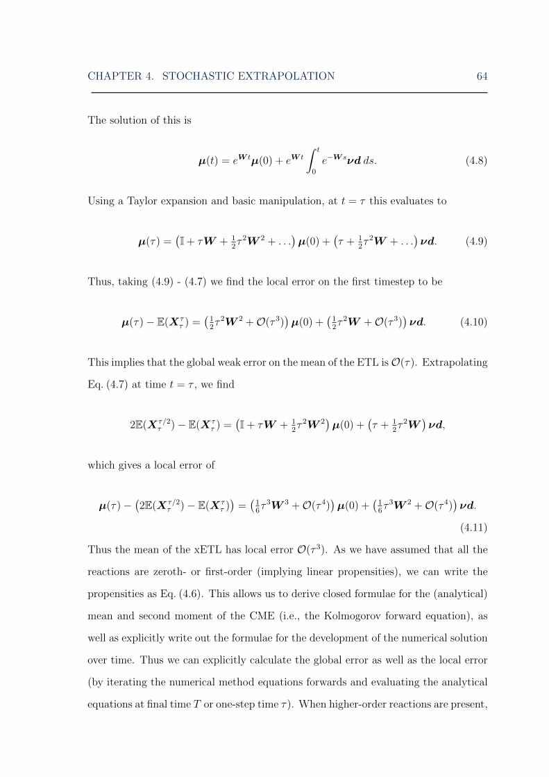
CHAPTER 4. STOCHASTIC EXTRAPOLATION 64
The solution of this is
µ(t) = eW tµ(0) + eW t
∫ t
0
e−W sνd ds. (4.8)
Using a Taylor expansion and basic manipulation, at t = τ this evaluates to
µ(τ) =(I + τW + 1
2τ 2W 2 + . . .
)µ(0) +
(τ + 1
2τ 2W + . . .
)νd. (4.9)
Thus, taking (4.9) - (4.7) we find the local error on the first timestep to be
µ(τ)− E(Xττ ) =
(12τ 2W 2 +O(τ 3)
)µ(0) +
(12τ 2W +O(τ 3)
)νd. (4.10)
This implies that the global weak error on the mean of the ETL isO(τ). Extrapolating
Eq. (4.7) at time t = τ , we find
2E(Xτ/2τ )− E(Xτ
τ ) =(I + τW + 1
2τ 2W 2
)µ(0) +
(τ + 1
2τ 2W
)νd,
which gives a local error of
µ(τ)−(2E(Xτ/2
τ )− E(Xττ ))
=(16τ 3W 3 +O(τ 4)
)µ(0) +
(16τ 3W 2 +O(τ 4)
)νd.
(4.11)
Thus the mean of the xETL has local error O(τ 3). As we have assumed that all the
reactions are zeroth- or first-order (implying linear propensities), we can write the
propensities as Eq. (4.6). This allows us to derive closed formulae for the (analytical)
mean and second moment of the CME (i.e., the Kolmogorov forward equation), as
well as explicitly write out the formulae for the development of the numerical solution
over time. Thus we can explicitly calculate the global error as well as the local error
(by iterating the numerical method equations forwards and evaluating the analytical
equations at final time T or one-step time τ). When higher-order reactions are present,

CHAPTER 4. STOCHASTIC EXTRAPOLATION 65
the propensities are non-linear and this cannot be done, so we must resort to backward
iteration of the local errors to find the global error using the Kolmogorov backward
equation (see Section 4.3.2).
Eq. (4.11) implies that the global error of the xETL is O(τ 2). In the linear case
we can verify this analytically. Taylor expanding Eq. (4.8) again, the true mean at
time t = T is
µ(T ) =(I + TW + 1
2T 2W 2 + 1
6T 3W 3 . . .
)µ(0) +
(T + 1
2T 2W + 1
6T 3W 2 . . .
)νd.
(4.12)
Iterating (4.7), we see that at time T = nτ the mean of the ETL is
E(XτT ) = (I + τW )nµ(0) + (I− (I + τW )n)νdW−1. (4.13)
Both of the brackets can be expanded out using the binomial theorem. However,
because each yields n + 1 terms, which themselves can be expanded further, this is
a long expression consisting of many terms. In particular, with an unspecified n, we
can expect there to be n− 3 (un-expanded) terms that each contribute an O(τ ) term
when expanded. Thus we have
E(XτT ) =
(I + nτW +
(n
2
)τ 2W 2 + . . .
)µ(0) + (nτ +
(n
2
)τ 2W + . . .)νd. (4.14)
Now taking (4.12) - (4.14), we see that the global error is
µ(T )− E(XτT )
=(−1
2τTW 2 − 1
2τT 2W 3 + . . .
)µ(0) +
(−1
2τTW +−1
2τT 2W 2 + . . .
)νd,
(4.15)
where only the leading two O(τ ) terms have been written out for convenience. Of
course, this does not affect the fact that the global error is O(τ ).
Furthermore, extrapolating as usual, the O(τ ) terms in Eq. (4.14) are cancelled,
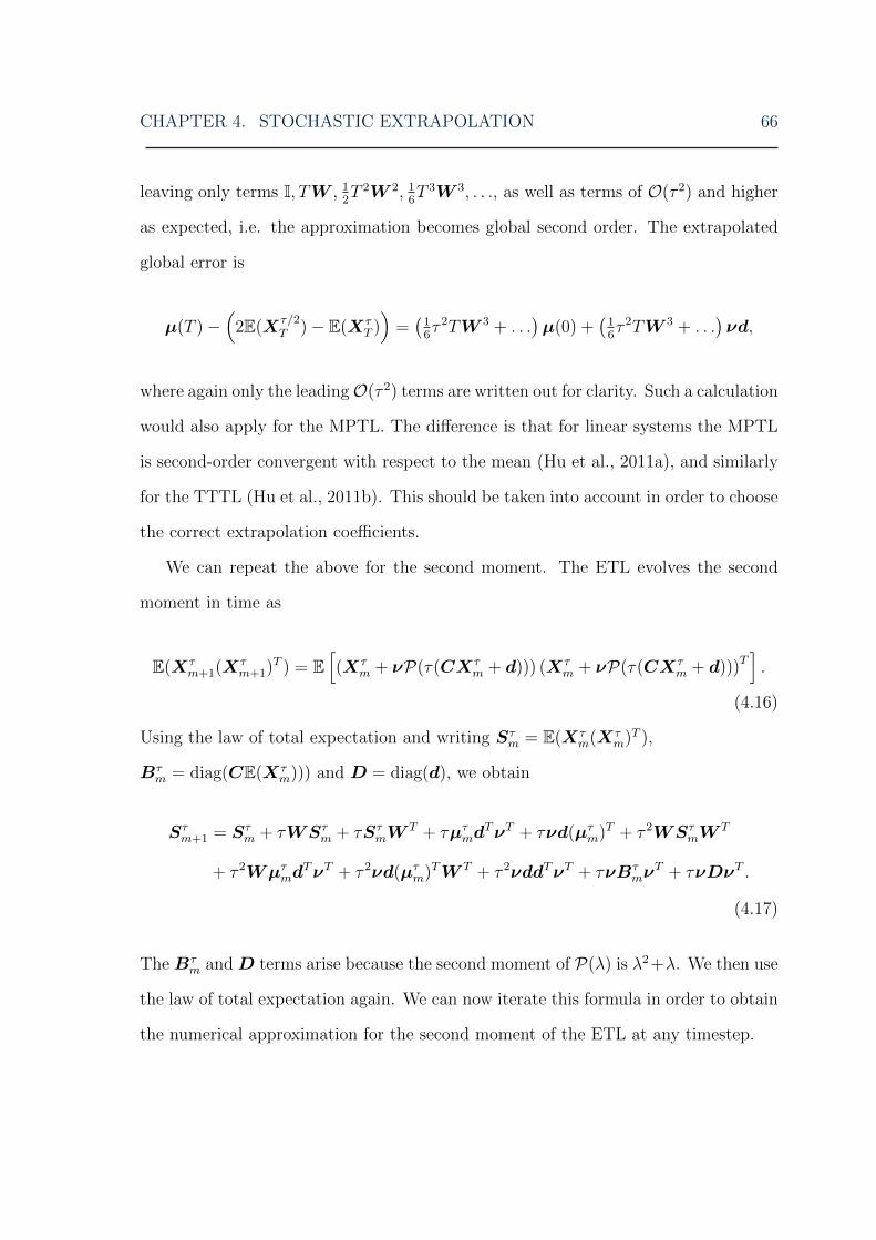
CHAPTER 4. STOCHASTIC EXTRAPOLATION 66
leaving only terms I, TW , 12T 2W 2, 1
6T 3W 3, . . ., as well as terms of O(τ 2) and higher
as expected, i.e. the approximation becomes global second order. The extrapolated
global error is
µ(T )−(
2E(Xτ/2T )− E(Xτ
T ))
=(16τ 2TW 3 + . . .
)µ(0) +
(16τ 2TW 3 + . . .
)νd,
where again only the leadingO(τ 2) terms are written out for clarity. Such a calculation
would also apply for the MPTL. The difference is that for linear systems the MPTL
is second-order convergent with respect to the mean (Hu et al., 2011a), and similarly
for the TTTL (Hu et al., 2011b). This should be taken into account in order to choose
the correct extrapolation coefficients.
We can repeat the above for the second moment. The ETL evolves the second
moment in time as
E(Xτm+1(X
τm+1)
T ) = E[(Xτ
m + νP(τ(CXτm + d))) (Xτ
m + νP(τ(CXτm + d)))T
].
(4.16)
Using the law of total expectation and writing Sτm = E(Xτm(Xτ
m)T ),
Bτm = diag(CE(Xτ
m))) and D = diag(d), we obtain
Sτm+1 = Sτm + τWSτm + τSτmWT + τµτmd
TνT + τνd(µτm)T + τ 2WSτmWT
+ τ 2WµτmdTνT + τ 2νd(µτm)TW T + τ 2νddTνT + τνBτ
mνT + τνDνT .
(4.17)
TheBτm andD terms arise because the second moment of P(λ) is λ2+λ. We then use
the law of total expectation again. We can now iterate this formula in order to obtain
the numerical approximation for the second moment of the ETL at any timestep.
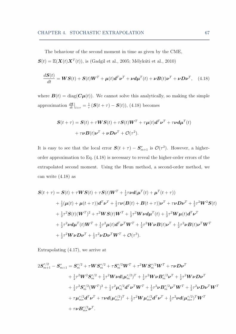
CHAPTER 4. STOCHASTIC EXTRAPOLATION 67
The behaviour of the second moment in time as given by the CME,
S(t) = E(X(t)XT (t)), is (Gadgil et al., 2005; Melykuti et al., 2010)
dS(t)
dt= WS(t) + S(t)W T + µ(t)dTνT + νdµT (t) + νB(t)νT + νDνT , (4.18)
where B(t) = diag(Cµ(t)). We cannot solve this analytically, so making the simple
approximation dSdt
∣∣t+τ
= 1τ
(S(t+ τ)− S(t)), (4.18) becomes
S(t+ τ) = S(t) + τWS(t) + τS(t)W T + τµ(t)dTνT + τνdµT (t)
+ τνB(t)νT + νDνT +O(τ 2).
It is easy to see that the local error S(t + τ) − Sτm+1 is O(τ 2). However, a higher-
order approximation to Eq. (4.18) is necessary to reveal the higher-order errors of the
extrapolated second moment. Using the Heun method, a second-order method, we
can write (4.18) as
S(t+ τ) = S(t) + τWS(t) + τS(t)W T + 12τνd(µT (t) + µT (t+ τ))
+ 12(µ(t) + µ(t+ τ))dTνT + 1
2τν(B(t) +B(t+ τ))νT + τνDνT + 1
2τ 2W 2S(t)
+ 12τ 2S(t)(W T )2 + τ 2WS(t)W T + 1
2τ 2WνdµT (t) + 1
2τ 2Wµ(t)dTνT
+ 12τ 2νdµT (t)W T + 1
2τ 2µ(t)dTνTW T + 1
2τ 2WνB(t)νT + 1
2τ 2νB(t)νTW T
+ 12τ 2WνDνT + 1
2τ 2νDνTW T +O(τ 3).
Extrapolating (4.17), we arrive at
2Sτ/2m+1 − Sτm+1 = Sτ/2m + τWSτ/2m + τSτ/2m W T + τ 2WSτ/2m W T + τνDνT
+ 12τ 2W 2Sτ/2m + 1
2τ 2Wνd(µτ/2m )T + 1
2τ 2WνBτ/2
m νT + 12τ 2WνDνT
+ 12τ 2Sτ/2m (W T )2 + 1
2τ 2µτ/2m dTνTW T + 1
2τ 2νBτ/2
m νTW T + 12τ 2νDνTW T
+ τµτ/2m∗dTνT + τνd(µτ/2m∗ )
T + 12τ 2Wµτ/2m∗d
TνT + 12τ 2νd(µτ/2m∗ )
TW T
+ τνBτ/2m∗ ν
T .

CHAPTER 4. STOCHASTIC EXTRAPOLATION 68
Here the subscript m∗ indicates time tm∗ = tm + τ2
that is only reached by the
approximation with stepsize τ2. The local error is S(t + τ) −
(2S
τ/2m − Sτm
). For
simplicity, we evaluate it at time t = τ . Most of the terms cancel, leaving
τνd(
12(µT (0) + µT (τ))− (µ
τ/21 )T
)+ τ
(12(µ(0) + µ(τ))− (µ
τ/21 ))dTνT
+ τν(
12(B(0) +B(τ))−Bτ/2
1
)νT + 1
2τ 2W (µ(0)− µτ/21 )dTνT
+ 12τ 2νd(µT (0)− (µ
τ/21 )T )W T +O(τ 3).
The first term equals τνd(µT (0)(1
4τ 2W 2 +O(τ 3)) + dTνT (1
4τ 2W +O(τ 3))
)and sim-
ilarly for the next two. The last two terms equal −12τ 2W (1
2τWµ(0) + 1
2τνd)dTνT .
Thus all terms in the local error are O(τ 3). Using a similar argument as before, this
implies a global weak error ofO(τ 2) in the case of zeroth- and first-order reactions. We
believe that this result also applies in the case of higher-order reactions, as we showed
for the mean above. However, we have stopped short of showing this analytically.
4.3.2 Global error expansion
The analysis in the previous section only applies for the mean and second moment of
the ETL for a linear system, a very restricted case, but it is useful for demonstrating
the basic principles of stochastic extrapolation. In this section, a similar approach to
Talay and Tubaro (1990) and Liu and Li (2000) is employed to derive a global error
expansion like Eq. (2.6) for the numerical approximation of the moments of a weak
first-order discrete stochastic method, such as the ETL and MPTL. Once the form of
the error expansion is known, it is clear which extrapolation coefficients can be used
and extrapolation is simple. In Section 4.3.3 this is evaluated explicitly for a particle
decay system, and it is shown that it is equivalent to Eq. (4.15) in this case.

CHAPTER 4. STOCHASTIC EXTRAPOLATION 69
As in the case of SDEs, we start with the Kolmogorov backward equation
∂u
∂t+ Lu = 0 in ZN+ × [0, T ), (4.19a)
u(T,x) = f(x) on ZN+ × {T}. (4.19b)
Here
Lu ≡M∑j=1
aj(x) (u(x+ νj)− u(x))
and
u(t,x) = E (f(X(T ))|X(t) = x) .
Using semigroup notation it is possible to formally denote the solution of (4.19) as
u(t,x) = e(T−t)Lf(x),
which can be useful for quantifying the local error of a numerical approximation. By
applying a stochastic Taylor expansion (Roßler, 2004) to jump processes (Hu et al.,
2011a), the one-step expansion for the expectation of f calculated with a first-order
numerical method should satisfy
E(f(Xττ )|Xτ
0 = x) = Aτf(x) = f(x) + τLf(x) +∞∑j=2
τ j
j!Ajf(x), (4.20)
where Aj are difference operators associated with the numerical method in hand.
Furthermore we have for the true one-step expansion
E(f(X(τ)|Xτ0 = x) = eLτf(x) = f(x) + τLf(x) +
∞∑j=2
τ j
j!Ljf(x). (4.21)
An important element in our derivation of a global error expansion relates to the
boundedness of u(t,x), and its discrete derivative. This boundedess is guaranteed (Li,
2007) when the number of molecules in the chemical system is conserved or decreases

CHAPTER 4. STOCHASTIC EXTRAPOLATION 70
with time. Proving this in the general case where zeroth-order reactions can add
molecules to the system is a non-trivial task. One way around this problem is to set
the propensity functions aj(x) to zero outside a large but finite domain (Li, 2007);
this is the approach followed here.
Now if we let ε(T, τ, f) define the global error in the numerical approximation of
E(f(X(T ))) at time T = nτ by a first-order numerical method with timestep τ ,
ε(T, τ, f) = E(f(X(T ))|X(0) = x)− E(f(XτT )|Xτ
0 = x)
= u(0,x)− E(u(T,XτT )|Xτ
0 = x)
=n∑
m=1
E(u((m− 1)τ,Xτ(m−1)τ ))− E(u(mτ,Xτ
mτ ))
=n∑
m=1
E(u(mτ,X∗mτ ))− E(u(mτ,Xτmτ )),
where we have used the result in Fig. 4.1, and for simplicity omitted the dependence of
the expectations on the initial conditions. Taking gm(y) = u(mτ,y) = eL(T−mτ)f(y),
E(u(mτ,X∗mτ ))− E(u(mτ,Xτmτ )) = E(gm(X∗mτ ))− E(gm(Xτ
mτ )).
Applying Eqs. (4.20) and (4.21) to gm,
ε(T, τ, f) =n∑
m=1
E[τ 2
2(L2 − A2)gm(Xτ
(m−1)τ ) + τ 3Rτm
]=
n∑m=1
E[τ 2
2(L2 − A2)e
−τLgm−1(Xτ(m−1)τ )
]+ τ 3E(Rτ
m)
=n∑
m=1
τ 2
2E[(L2 − A2)e
−τLu((m− 1)τ,Xτ(m−1)τ )
]+ τ 3E(Rτ
m),
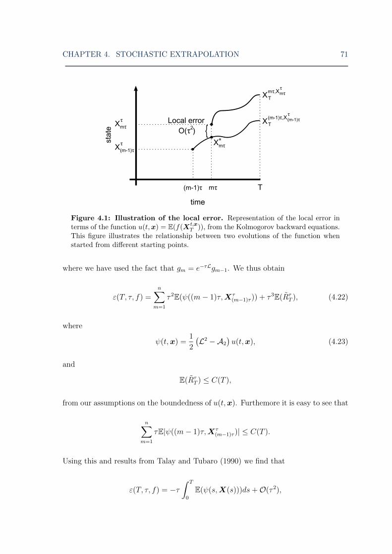
CHAPTER 4. STOCHASTIC EXTRAPOLATION 71
Figure 4.1: Illustration of the local error. Representation of the local error interms of the function u(t,x) = E(f(Xt,x
T )), from the Kolmogorov backward equations.This figure illustrates the relationship between two evolutions of the function whenstarted from different starting points.
where we have used the fact that gm = e−τLgm−1. We thus obtain
ε(T, τ, f) =n∑
m=1
τ 2E(ψ((m− 1)τ,Xτ(m−1)τ )) + τ 3E(Rτ
T ), (4.22)
where
ψ(t,x) =1
2
(L2 −A2
)u(t,x), (4.23)
and
E(RτT ) ≤ C(T ),
from our assumptions on the boundedness of u(t,x). Furthemore it is easy to see that
n∑m=1
τE|ψ((m− 1)τ,Xτ(m−1)τ )| ≤ C(T ).
Using this and results from Talay and Tubaro (1990) we find that
ε(T, τ, f) = −τ∫ T
0
E(ψ(s,X(s)))ds+O(τ 2),
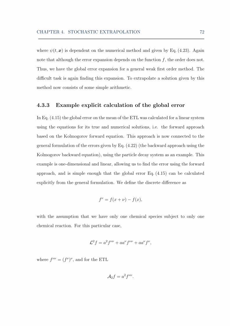
CHAPTER 4. STOCHASTIC EXTRAPOLATION 72
where ψ(t,x) is dependent on the numerical method and given by Eq. (4.23). Again
note that although the error expansion depends on the function f , the order does not.
Thus, we have the global error expansion for a general weak first order method. The
difficult task is again finding this expansion. To extrapolate a solution given by this
method now consists of some simple arithmetic.
4.3.3 Example explicit calculation of the global error
In Eq. (4.15) the global error on the mean of the ETL was calculated for a linear system
using the equations for its true and numerical solutions, i.e. the forward approach
based on the Kolmogorov forward equation. This approach is now connected to the
general formulation of the errors given by Eq. (4.22) (the backward approach using the
Kolmogorov backward equation), using the particle decay system as an example. This
example is one-dimensional and linear, allowing us to find the error using the forward
approach, and is simple enough that the global error Eq. (4.15) can be calculated
explicitly from the general formulation. We define the discrete difference as
f ν = f(x+ ν)− f(x),
with the assumption that we have only one chemical species subject to only one
chemical reaction. For this particular case,
L2f = a2f νν + aaνf νν + aaνf ν ,
where f νν = (f ν)ν , and for the ETL
A2f = a2f νν .

CHAPTER 4. STOCHASTIC EXTRAPOLATION 73
We want to find ψ(t, x) from Eq. (4.23), i.e. the first term of the local error. This is
ψ(t, x) =1
2(a(x)(a(x+ ν)− a(x))(u(t, x+ 2ν)− 2u(t, x+ ν) + u(t, x))
+1
2a(x)(a(x+ ν)− a(x))(u(t, x+ ν)− u(t, x)).
(4.24)
For particle decay, ν = −1 and a(x) = κx. For g(x) = x, the solution to (4.19) is
u(t, x) = xe−κ(T−t),
so (4.24) becomes
ψ(t, x) =1
2κ2xe−κ(T−t).
Thus the global error given by the general formulation is
N∑i=1
τ 2E(ψ((i− 1)τ,Xτ(i−1)τ )) =
κ2τ 2
2
N∑i=1
E(Xτ(i−1)τ )e
−κ(T−(i−1)τ)
=κ2τ 2
2
N∑i=1
[(1− κτ)eκτ ]i−1 e−κTE(Xτ0 )
=κ2Tτ
2
([(1− κτ)eκτ ]N − 1
(1− κτ)eκτ − 1
)e−κT
NE(Xτ
0 )
=κ2Tτ
2E(Xτ
0 ) +O(τ 2),
which agrees exactly with the result obtained by calculating Eq. (4.15) for the particle
decay problem (i.e. setting d = 0,W = −κ).
4.4 Numerical results
To numerically verify the stochastic extrapolation method, we simulate some exam-
ple systems for various stepsizes over time t = [0, T ] using three fixed-step numerical
methods: the ETL, MPTL and TTTL methods (with θ = 0.55), and their extrapo-
lated versions, the xETL, xMPTL and xTTTL. We plot the absolute weak errors in
CHAPTER 4. STOCHASTIC EXTRAPOLATION 74
the mean and second moment, that is,
|E(X(T ))− ES(XτT )|, |E(X(T )X†(T ))− ES(Xτ
T (XτT )†)| (4.25a)
for the ETL, MPTL and TTTL methods and
|E(X(T ))− 2ES(Xτ/2T ) + ES(Xτ
T )|,
|E(X(T )X†(T ))− 2ES(Xτ/2T (X
τ/2T )†) + ES(Xτ
T (XτT )†)|
(4.25b)
for the extrapolated methods. Here X(T ) is the analytical solution at time T and
ES(f(XτT )) are the moments of its approximations given by S simulations of a fixed-
step method with stepsize τ run for n steps. In addition, to avoid confusing notation,
we have temporarily relabelled the matrix transpose XT as X† for the rest of this
chapter. For the linear systems, the true solution is calculated analytically; for the
non-linear systems we use the value given by 106 or 107 repeats of the SSA, depending
on the system. The error of a weak order α method with stepsize τ is approximately
Cτα, where C is an unknown constant. We plot all the errors versus timesteps on
log-log plots so the order of accuracy can be read off as the gradient. Gradients are
calculated using a least squares fit through the points. The highest level of Monte
Carlo error, which can be calculated for the linear systems, is marked on the appro-
priate plots as a straight black line. Below this level, the absolute error results are, at
least in part, essentially random (see Section 4.5). Note that in all example systems,
the timesteps used were all in the useful τ -leaping regime: Poisson counts for each
reaction channel varied between tens to hundreds.
4.4.1 Particle decay system
A simple example is a particle decay,
Xk−→ ∅, k = 0.1.
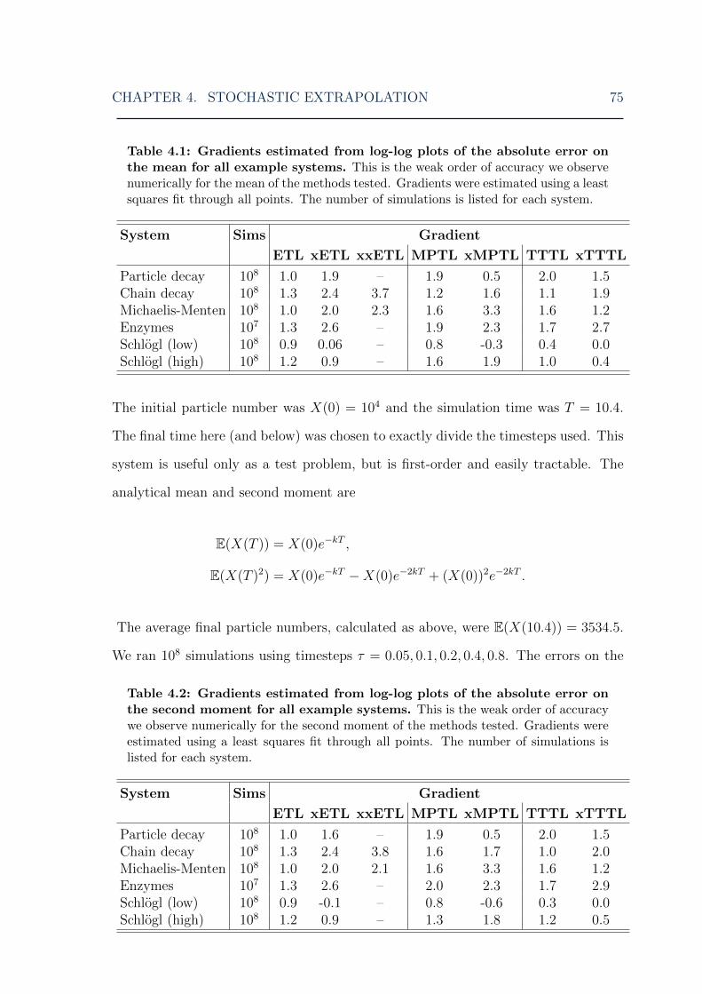
CHAPTER 4. STOCHASTIC EXTRAPOLATION 75
Table 4.1: Gradients estimated from log-log plots of the absolute error onthe mean for all example systems. This is the weak order of accuracy we observenumerically for the mean of the methods tested. Gradients were estimated using a leastsquares fit through all points. The number of simulations is listed for each system.
System Sims Gradient
ETL xETL xxETL MPTL xMPTL TTTL xTTTL
Particle decay 108 1.0 1.9 – 1.9 0.5 2.0 1.5Chain decay 108 1.3 2.4 3.7 1.2 1.6 1.1 1.9Michaelis-Menten 108 1.0 2.0 2.3 1.6 3.3 1.6 1.2Enzymes 107 1.3 2.6 – 1.9 2.3 1.7 2.7Schlogl (low) 108 0.9 0.06 – 0.8 -0.3 0.4 0.0Schlogl (high) 108 1.2 0.9 – 1.6 1.9 1.0 0.4
The initial particle number was X(0) = 104 and the simulation time was T = 10.4.
The final time here (and below) was chosen to exactly divide the timesteps used. This
system is useful only as a test problem, but is first-order and easily tractable. The
analytical mean and second moment are
E(X(T )) = X(0)e−kT ,
E(X(T )2) = X(0)e−kT −X(0)e−2kT + (X(0))2e−2kT .
The average final particle numbers, calculated as above, were E(X(10.4)) = 3534.5.
We ran 108 simulations using timesteps τ = 0.05, 0.1, 0.2, 0.4, 0.8. The errors on the
Table 4.2: Gradients estimated from log-log plots of the absolute error onthe second moment for all example systems. This is the weak order of accuracywe observe numerically for the second moment of the methods tested. Gradients wereestimated using a least squares fit through all points. The number of simulations islisted for each system.
System Sims Gradient
ETL xETL xxETL MPTL xMPTL TTTL xTTTL
Particle decay 108 1.0 1.6 – 1.9 0.5 2.0 1.5Chain decay 108 1.3 2.4 3.8 1.6 1.7 1.0 2.0Michaelis-Menten 108 1.0 2.0 2.1 1.6 3.3 1.6 1.2Enzymes 107 1.3 2.6 – 2.0 2.3 1.7 2.9Schlogl (low) 108 0.9 -0.1 – 0.8 -0.6 0.3 0.0Schlogl (high) 108 1.2 0.9 – 1.3 1.8 1.2 0.5
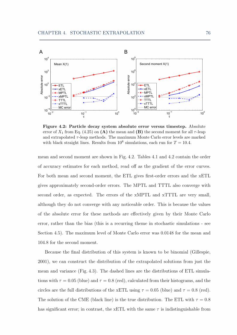
CHAPTER 4. STOCHASTIC EXTRAPOLATION 76
Figure 4.2: Particle decay system absolute error versus timestep. Absoluteerror of X1 from Eq. (4.25) on (A) the mean and (B) the second moment for all τ -leapand extrapolated τ -leap methods. The maximum Monte Carlo error levels are markedwith black straight lines. Results from 108 simulations, each run for T = 10.4.
mean and second moment are shown in Fig. 4.2. Tables 4.1 and 4.2 contain the order
of accuracy estimates for each method, read off as the gradient of the error curves.
For both mean and second moment, the ETL gives first-order errors and the xETL
gives approximately second-order errors. The MPTL and TTTL also converge with
second order, as expected. The errors of the xMPTL and xTTTL are very small,
although they do not converge with any noticeable order. This is because the values
of the absolute error for these methods are effectively given by their Monte Carlo
error, rather than the bias (this is a recurring theme in stochastic simulations - see
Section 4.5). The maximum level of Monte Carlo error was 0.0148 for the mean and
104.8 for the second moment.
Because the final distribution of this system is known to be binomial (Gillespie,
2001), we can construct the distribution of the extrapolated solutions from just the
mean and variance (Fig. 4.3). The dashed lines are the distributions of ETL simula-
tions with τ = 0.05 (blue) and τ = 0.8 (red), calculated from their histograms, and the
circles are the full distributions of the xETL using τ = 0.05 (blue) and τ = 0.8 (red).
The solution of the CME (black line) is the true distribution. The ETL with τ = 0.8
has significant error; in contrast, the xETL with the same τ is indistinguishable from

CHAPTER 4. STOCHASTIC EXTRAPOLATION 77
Figure 4.3: Constructing full extrapolated distributions of the particle de-cay system. Distribution of states at time T = 10.4 for ETL with τ = 0.05, 0.8 andxETL with τ = 0.05, 0.8. The analytical solution is given by the CME (black line).
the true PDF, with similar accuracy to the ETL (and xETL) with τ = 0.05. This
shows that, regardless of whether the order itself is improved, extrapolation greatly
improves the accuracy of the solutions.
4.4.2 Chain decay system
This system consists of five chemical species, each undergoing a first-order reaction.
It forms a closed chain of linear reactions, and is intended as a more complicated, but
still linear, example system.
X1c1−→ X2
c2−→ X3c3−→ X4
c4−→ X5c5−→ X1, cj = 0.3, j = 1, . . . , 5.
The initial populations were X(0) = [2500, 1875, 1875, 1875, 1875]† and simulation
time was T = 16. Since this system is linear, its mean and variance can be calculated
analytically, as shown by Jahnke and Huisinga (2007); these were used to calculate
the true second moment. The average final particle numbers, given by the analytical
mean, were E(X(16)) = [1971.3, 1996.7, 2025.1, 2020.9, 1986.1]†. We ran 108 simula-
tions with τ = 0.1, 0.2, 0.4, 0.8, 1.6. Fig. 4.4 shows the absolute errors for the mean
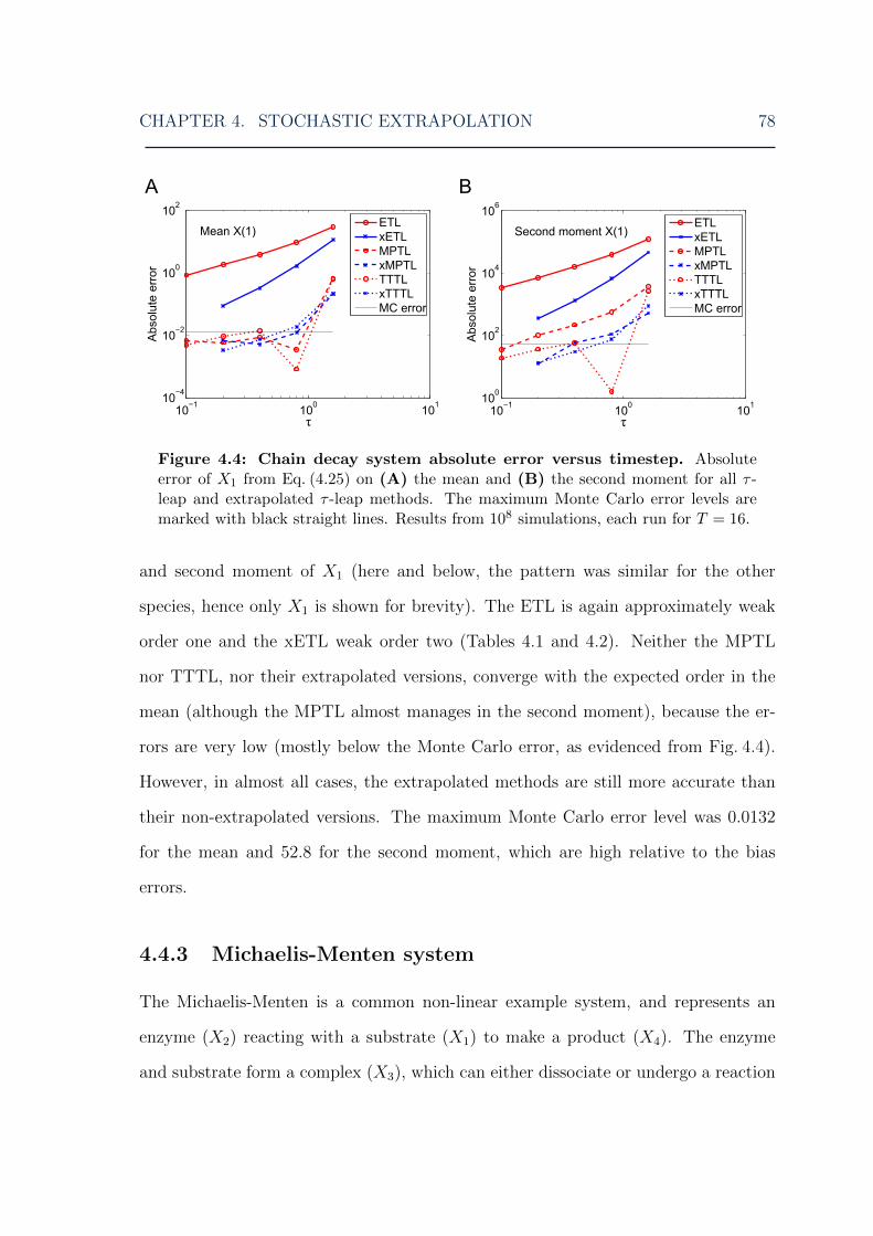
CHAPTER 4. STOCHASTIC EXTRAPOLATION 78
Figure 4.4: Chain decay system absolute error versus timestep. Absoluteerror of X1 from Eq. (4.25) on (A) the mean and (B) the second moment for all τ -leap and extrapolated τ -leap methods. The maximum Monte Carlo error levels aremarked with black straight lines. Results from 108 simulations, each run for T = 16.
and second moment of X1 (here and below, the pattern was similar for the other
species, hence only X1 is shown for brevity). The ETL is again approximately weak
order one and the xETL weak order two (Tables 4.1 and 4.2). Neither the MPTL
nor TTTL, nor their extrapolated versions, converge with the expected order in the
mean (although the MPTL almost manages in the second moment), because the er-
rors are very low (mostly below the Monte Carlo error, as evidenced from Fig. 4.4).
However, in almost all cases, the extrapolated methods are still more accurate than
their non-extrapolated versions. The maximum Monte Carlo error level was 0.0132
for the mean and 52.8 for the second moment, which are high relative to the bias
errors.
4.4.3 Michaelis-Menten system
The Michaelis-Menten is a common non-linear example system, and represents an
enzyme (X2) reacting with a substrate (X1) to make a product (X4). The enzyme
and substrate form a complex (X3), which can either dissociate or undergo a reaction
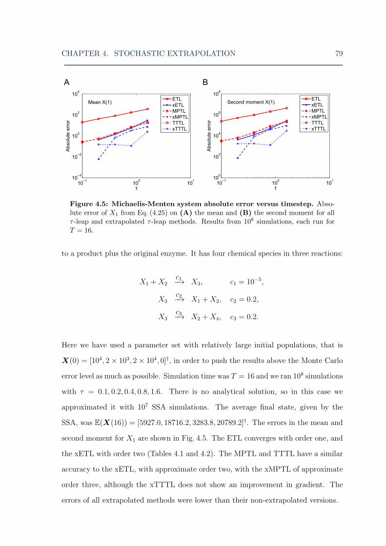
CHAPTER 4. STOCHASTIC EXTRAPOLATION 79
Figure 4.5: Michaelis-Menten system absolute error versus timestep. Abso-lute error of X1 from Eq. (4.25) on (A) the mean and (B) the second moment for allτ -leap and extrapolated τ -leap methods. Results from 108 simulations, each run forT = 16.
to a product plus the original enzyme. It has four chemical species in three reactions:
X1 +X2c1−→ X3, c1 = 10−5,
X3c2−→ X1 +X2, c2 = 0.2,
X3c3−→ X2 +X4, c3 = 0.2.
Here we have used a parameter set with relatively large initial populations, that is
X(0) = [104, 2× 10³, 2× 10⁴, 0]†, in order to push the results above the Monte Carlo
error level as much as possible. Simulation time was T = 16 and we ran 108 simulations
with τ = 0.1, 0.2, 0.4, 0.8, 1.6. There is no analytical solution, so in this case we
approximated it with 107 SSA simulations. The average final state, given by the
SSA, was E(X(16)) = [5927.0, 18716.2, 3283.8, 20789.2]†. The errors in the mean and
second moment for X1 are shown in Fig. 4.5. The ETL converges with order one, and
the xETL with order two (Tables 4.1 and 4.2). The MPTL and TTTL have a similar
accuracy to the xETL, with approximate order two, with the xMPTL of approximate
order three, although the xTTTL does not show an improvement in gradient. The
errors of all extrapolated methods were lower than their non-extrapolated versions.

CHAPTER 4. STOCHASTIC EXTRAPOLATION 80
We investigated the effects of the coefficient of variation (CV, standard deviation
divided by mean) on this system. The CVs of each species, averaged across all τ ,
in Michaelis-Menten system at T = 16 were CV(X(16)) = [0.01, 0.003, 0.02, 0.004]†.
In general, a higher CV indicates that the system is more noisy. We chose a new
set of parameters for the Michaelis-Menten system to give higher CVs: Xnew(0) =
[100, 50, 200, 0]† and rate constants cnew = [10−4, 0.05, 0.07]†. The CVs using these
parameters were CV(Xnew(16)) = [0.05, 0.03, 0.1, 0.07]†, very different from the orig-
inal CVs. However the relative errors (absolute error divided by average SSA state)
at τ = 0.1 were very similar: errorrel(X(16)) = [0.004, 0.0005, 0.003, 0.001]† for the
original system and errorrel(Xnew(16)) = [0.001, 0.0002, 0.0007, 0.002]† with the new
parameters (note that it is not useful to average the errors across all τ). This shows
that higher CV does not necessarily mean higher errors, and the two are indicators of
different characteristics of the system. We have focussed on the errors as this is the
characteristic that we want to improve.
4.4.4 Mutually inhibiting enzymes system
This is a more realistic system involving 8 chemical species and 12 reactions (Elf and
Ehrenberg, 2004; Marquez-Lago and Burrage, 2007). It represents two enzymes, EA
and EB, which catalyse the production of compounds A and B, respectively. In a
classic example of double-negative feedback, each product inhibits the activity of the
other enzyme. For this reason, the system is bistable in A and B: when there are
many particles of A, few particles of B can be produced, and vice versa. The reactions
CHAPTER 4. STOCHASTIC EXTRAPOLATION 81
are
EAc1→ EA + A, c1 = 15,
EBc2→ EB +B, c2 = 15,
EA +Bc3c4
EAB, c3 = 5× 10⁻⁴, c4 = 2,
EAB +Bc5c6
EAB2, c5 = 10−3, c6 = 6,
Ac7→ ∅, c7 = 5,
EB + Ac8c9
EBA, c8 = 5× 10⁻⁴, c9 = 2,
EBA+ Ac10c11
EBA2, c10 = 10−3, c11 = 6,
Bc12→ ∅, c12 = 5.
Using this parameter set, the system is actually unimodal. However, these param-
eters were necessary to again attempt to push the levels of total error far above
the Monte Carlo error. We simulated this system for T = 3.2 using initial popu-
lations of X(0) = [2 × 10⁴, 1.5 × 10⁴, 9500, 9500, 2000, 500, 2000, 500]†, where X =
[A,B,EA, EB, EAB,EAB2, EBA,EBA2]†. We ran 107 simulations of the τ -leap using
τ = 0.005, 0.01, 0.02, 0.04, 0.08. 106 SSA simulations were used as an approximation
to the analytical values. The final state of the system as given by the SSA mean was
E(X(3.2)) = [10420.5, 4884.4, 3594.7, 1528.0, 4592.7, 3812.6, 3853.8, 6618.2]†. The er-
rors for species A are shown in Fig. 4.6. The ETL and xETL were approximate order
one and two, respectively (Tables 4.1 and 4.2). The MPTL and TTTL were again
approximate order two; the xMPTL had errors very similar to those of the xETL,
and the xTTTL had very low errors and approximate order 2.5.
4.4.5 Schlogl system
The last example illustrates how the stochastic extrapolation method could work
for systems that have multimodal distributions. The Schlogl system consists of four

CHAPTER 4. STOCHASTIC EXTRAPOLATION 82
Figure 4.6: Mutually inhibiting enzymes system absolute error versustimestep. Absolute error of A from Eq. (4.25) on (A) the mean and (B) the secondmoment for all τ -leap and extrapolated τ -leap methods. Results from 107 simulations,each run for T = 3.2.
reactions (Schlogl, 1972) and is bimodal:
A+ 2Xc1c2
3X, c1 = 3× 10⁻⁷, c2 = 10−4
Bc3c4
X, c3 = 10−3, c4 = 3.5,
where the populations of species A and B are held constant at 105 and 2×10⁵ respec-
tively, so only the numbers of X can change. Under certain parameter configurations,
this system has two stable states for X, one high and one low (Figs. 1.1 and 4.9).
When X(0) is low, the system usually settles in the lower stable state, and vice versa
for high X(0). We used X(0) = 250, an intermediate value. We ran 108 simulations
until T = 5 using τ = 0.0125, 0.025, 0.05, 0.1, 0.2. Because of the bimodality, we sep-
arated the data into two sets. As the Schlogl system is simple enough to be solved
using a CME solver (see e.g. MacNamara et al., 2008b), we could calculate the PDF
of X at T = 5. When simulating more complicated systems, this can be approximated
by a normalised histogram at T calculated from the initial ETL simulations to get a
reasonable idea of its shape. Average final particle number was calculated from the
CME to be E(X(5)) = 101.3 for the low peak (stable state) and E(X(5)) = 546.2 for

CHAPTER 4. STOCHASTIC EXTRAPOLATION 83
Figure 4.7: Shlogl system low peak absolute error versus timestep. Absoluteerror of X from Eq. (4.25) on (A) the mean and (B) the second moment for all τ -leapand extrapolated τ -leap methods. Results from 108 simulations, each run for T = 5.
the high peak. Figs. 4.7 and 4.8 show the absolute errors for this system (low and
high peaks, respectively). The error levels seem to be roughly similar in both cases,
with those of the high peak being lower. The ETL converges with order one, and
the MPTL with one or higher (see next paragraph; Tables 4.1 and 4.2). The TTTL
errors in particular are very low, and its reported order is lower than expected for
this reason. The errors of the extrapolated methods are also very low for both high
and low peaks, although again we cannot make out a clear order of convergence. It
is clear that in this case also, the Monte Carlo error is interfering with our ability to
see a clear order of convergence.
The gradient of the MPTL mean error seems to change from around one (Fig. 4.7)
to 1.5 (Fig. 4.8). It is unlikely that this is due to Monte Carlo error, as even for the
high peak, the top of the MPTL error curve is large enough that this should not be
an issue (although this is not the case for the lower half). In fact, this may be due
to the large volume limit behaviour of the MPTL, discussed after Algorithm 3.3. As
the mean of the high peak is several times higher than the mean of the low peak, the
system is closer to the large volume limit and the weak order of the MPTL increases.
Once in the large volume limit, the gradient is expected to be two.
The point at which the data is separated must be chosen carefully, as it can

CHAPTER 4. STOCHASTIC EXTRAPOLATION 84
Figure 4.8: Shlogl system high peak absolute error versus timestep. Absoluteerror of X from Eq. (4.25) on (A) the mean and (B) the second moment for all τ -leapand extrapolated τ -leap methods. Results from 108 simulations, each run for T = 5.
influence the error results. Fig. 4.9 shows the distribution of X at T = 5 calculated
using a CME solver, marked with the three choices of splitting points that we compare.
We chose X = 300; this is a fairly obvious splitting point in our case. To support
this, we tested the effects of splitting the data given by the ETL at X = 250 and
X = 350. We calculated the relative change in mean, second moment and variance
between these two splitting values, averaged over all simulations of the ETL and all
five timesteps: Table 4.3 shows that the percentage difference is relatively small for
the mean, becomes larger for the second moment, and is very high for the variance.
This implies that the choice of splitting point is important in the case of the Schlogl
system, and should be carefully considered.
Table 4.3: Relative differences in moments for different splitting values ofSchlogl system. Relative differences in moments E(f(X)) for data split at X = 250and X = 350 for the Schlogl system as percentages of their values when split atX = 300, i.e. 100× |E(f(X))split350 − E(f(X))split250|/E(f(X))split300.
Moment Low peak High peak
Mean 6.4% 1.6%Second moment 21.8% 2.5%
Variance 81.6% 50.5%
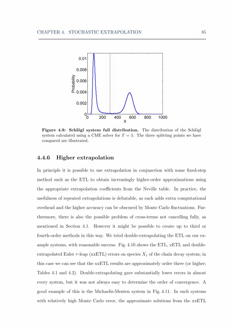
CHAPTER 4. STOCHASTIC EXTRAPOLATION 85
Figure 4.9: Schlogl system full distribution. The distribution of the Schloglsystem calculated using a CME solver for T = 5. The three splitting points we havecompared are illustrated.
4.4.6 Higher extrapolation
In principle it is possible to use extrapolation in conjunction with some fixed-step
method such as the ETL to obtain increasingly higher-order approximations using
the appropriate extrapolation coefficients from the Neville table. In practice, the
usefulness of repeated extrapolations is debatable, as each adds extra computational
overhead and the higher accuracy can be obscured by Monte Carlo fluctuations. Fur-
thermore, there is also the possible problem of cross-terms not cancelling fully, as
mentioned in Section 4.1. However it might be possible to create up to third or
fourth-order methods in this way. We tried double-extrapolating the ETL on our ex-
ample systems, with reasonable success. Fig. 4.10 shows the ETL, xETL and double-
extrapolated Euler τ -leap (xxETL) errors on species X1 of the chain decay system; in
this case we can see that the xxETL results are approximately order three (or higher;
Tables 4.1 and 4.2). Double-extrapolating gave substantially lower errors in almost
every system, but it was not always easy to determine the order of convergence. A
good example of this is the Michaelis-Menten system in Fig. 4.11. In such systems
with relatively high Monte Carlo error, the approximate solutions from the xxETL

CHAPTER 4. STOCHASTIC EXTRAPOLATION 86
Figure 4.10: Chain decay system, double-extrapolated absolute error versustimestep. Absolute error of X1 on (A) the mean and (B) the second moment of ETL,xETL and xxETL methods. Results from 108 simulations.
were obscured by these fluctuations. The order of accuracy of the xxETL could be
successfully seen for most molecular species of the chain decay system, but it was
not possible for the other systems as this would require a significant increase in the
number of simulations, in order to further reduce the Monte Carlo error.
4.5 Monte Carlo error
We have repeatedly mentioned the Monte Carlo error in the last few sections, so here
we discuss this subject in more detail. The weak error we calculate numerically is
|E(f(X(T )))− ES(f(XτT ))|. (4.26)
This error can be separated into two parts
[E(f(X(T )))− E∞(f(XτT ))] + [E∞(f(Xτ
T ))− ES(f(XτT ))] , (4.27)
where E∞(f(XτT )) are the theoretical values of the moments calculated by an infinite
number of simulations with stepsize τ . The first term is the truncation error of the

CHAPTER 4. STOCHASTIC EXTRAPOLATION 87
Figure 4.11: Michaelis-Menten system, double-extrapolated absolute errorversus timestep. Absolute error of X1 on (A) the mean and (B) the second momentof ETL, xETL and xxETL methods. Results from 108 simulations.
moments from their analytical solutions, i.e. the bias of the numerical method, which
depends only on the choice of timestep. The second term is the Monte Carlo error,
which depends only on the number of simulations and is given by C√S
, where C is some
constant and S the number of simulations. The Monte Carlo error can be so large
that it overwhelms the bias of the underlying numerical method completely; in this
case all of the numerical results are due to random fluctuations, as we have observed
in some of our error plots. This is not necessarily a bad thing – all it means is that
the numerical method is so accurate that its error is smaller than that arising from
the randomness inherent in stochastic simulations, that is, the Monte Carlo error.
The formulation in Eq. (4.27) is useful when the propensity functions are linear.
In this case, the moment equations are closed, so E∞(f(XτT )) can be calculated for
the appropriate numerical method. As an example, consider the mean of the ETL: its
true value is given by Eq. (4.8) and the value of its numerical approximation can be
found by iterating Eq. (4.7). Unfortunately, this is not possible for non-linear systems,
since in this case the equations describing the evolution of the moments are not closed
any more (e.g., Melykuti et al., 2010). In such cases, though, we can still make an
educated guess about the Monte Carlo error level based on when the absolute error
curves start losing their convergence.
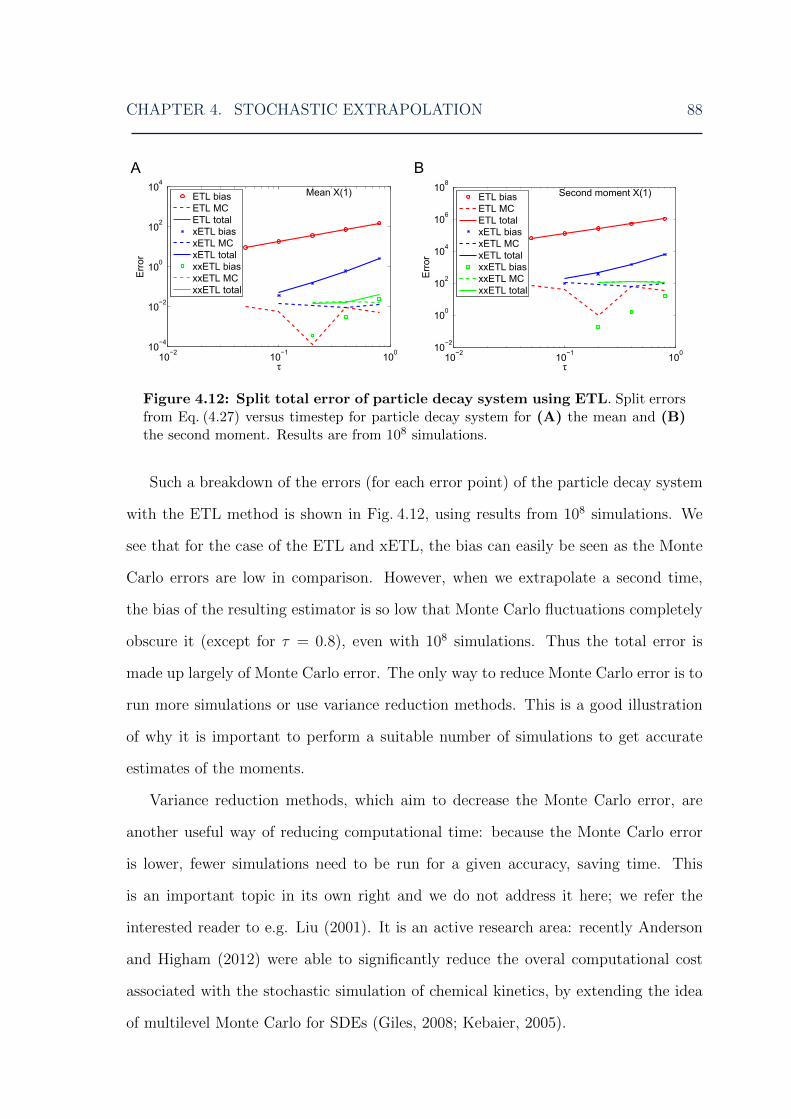
CHAPTER 4. STOCHASTIC EXTRAPOLATION 88
Figure 4.12: Split total error of particle decay system using ETL. Split errorsfrom Eq. (4.27) versus timestep for particle decay system for (A) the mean and (B)the second moment. Results are from 108 simulations.
Such a breakdown of the errors (for each error point) of the particle decay system
with the ETL method is shown in Fig. 4.12, using results from 108 simulations. We
see that for the case of the ETL and xETL, the bias can easily be seen as the Monte
Carlo errors are low in comparison. However, when we extrapolate a second time,
the bias of the resulting estimator is so low that Monte Carlo fluctuations completely
obscure it (except for τ = 0.8), even with 108 simulations. Thus the total error is
made up largely of Monte Carlo error. The only way to reduce Monte Carlo error is to
run more simulations or use variance reduction methods. This is a good illustration
of why it is important to perform a suitable number of simulations to get accurate
estimates of the moments.
Variance reduction methods, which aim to decrease the Monte Carlo error, are
another useful way of reducing computational time: because the Monte Carlo error
is lower, fewer simulations need to be run for a given accuracy, saving time. This
is an important topic in its own right and we do not address it here; we refer the
interested reader to e.g. Liu (2001). It is an active research area: recently Anderson
and Higham (2012) were able to significantly reduce the overal computational cost
associated with the stochastic simulation of chemical kinetics, by extending the idea
of multilevel Monte Carlo for SDEs (Giles, 2008; Kebaier, 2005).
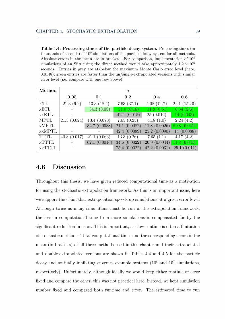
CHAPTER 4. STOCHASTIC EXTRAPOLATION 89
Table 4.4: Processing times of the particle decay system. Processing times (inthousands of seconds) of 108 simulations of the particle decay system for all methods.Absolute errors in the mean are in brackets. For comparison, implementation of 108
simulations of an SSA using the direct method would take approximately 1.2 × 10⁵
seconds. Entries in grey are at/below the maximum Monte Carlo error level (here,0.0148); green entries are faster than the un/single-extrapolated versions with similarerror level (i.e. compare with one row above).
Method τ
0.05 0.1 0.2 0.4 0.8
ETL 21.3 (9.2) 13.3 (18.4) 7.63 (37.1) 4.08 (74.7) 2.21 (152.0)xETL – 34.3 (0.05) 21.0 (0.16) 11.8 (0.61) 6.34 (2.6)xxETL – – 42.1 (0.015) 25 (0.016) 14 (0.043)MPTL 21.3 (0.024) 13.4 (0.070) 7.65 (0.25) 4.18 (1.0) 2.24 (4.2)xMPTL – 34.7 (0.0088) 21.1 (0.0082) 11.8 (0.0026) 6.38 (0.041)xxMPTL – – 42.4 (0.0089) 25.2 (0.0090) 14 (0.0088)TTTL 40.8 (0.017) 21.1 (0.063) 13.3 (0.26) 7.65 (1.1) 4.17 (4.2)xTTTL – 62.1 (0.0016) 34.6 (0.0022) 20.9 (0.0044) 11.8 (0.041)xxTTTL – – 75.4 (0.0022) 42.2 (0.0031) 25.1 (0.011)
4.6 Discussion
Throughout this thesis, we have given reduced computational time as a motivation
for using the stochastic extrapolation framework. As this is an important issue, here
we support the claim that extrapolation speeds up simulations at a given error level.
Although twice as many simulations must be run in the extrapolation framework,
the loss in computational time from more simulations is compensated for by the
significant reduction in error. This is important, as slow runtime is often a limitation
of stochastic methods. Total computational times and the corresponding errors in the
mean (in brackets) of all three methods used in this chapter and their extrapolated
and double-extrapolated versions are shown in Tables 4.4 and 4.5 for the particle
decay and mutually inhibiting enzymes example systems (108 and 107 simulations,
respectively). Unfortunately, although ideally we would keep either runtime or error
fixed and compare the other, this was not practical here; instead, we kept simulation
number fixed and compared both runtime and error. The estimated time to run

CHAPTER 4. STOCHASTIC EXTRAPOLATION 90
Table 4.5: Processing times of mutually inhibiting enzymes system. Pro-cessing times (in thousands of seconds) of 107 simulations of the mutually inhibitingenzymes system for all methods. Absolute errors in the mean of X1 in brackets. Run-ning 107 simulations of an SSA using the direct method would take approximately1.47 × 107 seconds. Entries in grey are thought to be below the Monte Carlo errorlevel; green entries are faster than the un/single-extrapolated versions with similarerror level (i.e. compare with one row above), and red entries are slower.
Method τ
0.005 0.01 0.02 0.04 0.08
ETL 191 (16.7) 82.3 (34.5) 46 (76.1) 32.6 (188.5) 19.7 (630.1)xETL – 293 (1.1) 123 (7.2) 66.4 (36.3) 35.1 (253.1)xxETL – – 279 (0.93) 152 (2.5) 80.1 (36.0)MPTL 165 (1.3) 84 (3.6) 44.9 (15.0) 24.1 (65.5) 12.3 (257.1)xMPTL – 244 (1.0) 129 (7.7) 69.1 (35.5) 36.3 (126.2)xxMPTL – – 289 (1.2) 153 (1.5) 81.3 (5.3)TTTL 277 (1.2) 155 (3.5) 82.4 (13.5) 44.6 (58.1) 23.3 (90.0)xTTTL – 430 (0.41) 239 (0.15) 128 (1.4) 68 (107.5)xxTTTL – – 515 (0.45) 283 (0.37) 151 (16.9)
the same number of SSA simulations is given for comparison. It should be noted
that all the extrapolated and double-extrapolated τ -leap times are estimates: the
time-consuming part of the extrapolation method is the two sets of simulations of
the original method that must be run (and possibly the operation of finding the
moments, but this must be performed whether or not extrapolation is used); the
extrapolation itself is a fast arithmetic operation. The times for an extrapolation are
calculated as[runtime(τ1 = τ) + runtime(τ2 = τ
2)], and for a double-extrapolation as[
runtime(τ1 = τ) + runtime(τ2 = τ2) + runtime(τ3 = τ
4)]. The extrapolated methods
take several times longer to run, but the errors they give are several to hundreds of
times lower. Most of the exceptions are where the error has clearly reached the Monte
Carlo level (Tables 4.4 and 4.5, grey entries). Besides extrapolation, the other obvious
way to reduce error is to use a smaller timestep, so the real test for the effectiveness
of extrapolation is to compare the runtimes of cases with similar error values. In
Tables 4.4 and 4.5, we have marked in green the extrapolated errors that can be
directly compared to the base method (i.e. read up one row) and take less time to
CHAPTER 4. STOCHASTIC EXTRAPOLATION 91
run and in red the ones that take longer, and similarly for double-extrapolated errors
as compared to single-extrapolated ones. The rest are either suspected to be faster
(light green) or slower (light red) but lack unequivocal verification, not comparable to
any other results (unextrapolated methods), or have too high a level of Monte Carlo
error to say anything useful about (grey). Although there is considerable variation for
each system and simulation method, adding up the greens and reds shows that the
general trend is that extrapolation takes less time to give a similar level of error (this
pattern was similar for our other example systems). Thus we found that in general,
extrapolation is a worthwhile procedure.
Monte Carlo error is an unavoidable problem when using stochastic simulations.
The statistical fluctuations inherent in stochastic systems can obscure the bias error
(i.e. order of convergence) of the numerical method if their size relative to the bias is
large, as the total error is made up of these two contributions. A large number S of
simulations must be run, as the Monte Carlo error scales as 1√S
. This error varies for
each system. Figs. 4.10 and 4.11, and especially 4.12, show this clearly: both of the
xxETLs have total errors of similar size for the same τ , but the chain decay system
has relatively low Monte Carlo error, allowing us to see the bias of the xxETL for
that system. However, Fig. 4.11 seems to indicate that the Michaelis-Menten system
has relatively high Monte Carlo error compared to the bias of the xxETL, implying
that the xxETL errors we see in the figure could be completely due to statistical
fluctuations. It should be noted that this also happens to varying degrees for the
other example problems we use. The reason for this is that the extrapolated methods
(and even the MPTL and TTTL, in some cases) have very high accuracy (i.e. low
bias error). Since it is only possible to run a limited number of simulations, when the
bias is very small, the total error will be given almost completely by the contribution
from the Monte Carlo error.
A contrasting approach to reducing numerical errors is the multilevel Monte Carlo
method. Originally developed for SDEs (Giles, 2008; Kebaier, 2005), it has recently
CHAPTER 4. STOCHASTIC EXTRAPOLATION 92
been extended to discrete chemical kinetics (Anderson and Higham, 2012). By consid-
ering a formulation of the total error similar to Eq. (4.27), the multilevel Monte-Carlo
method aims to reduce it by decreasing the Monte Carlo error. Here also many approx-
imate solutions are generated with a variety of different timesteps. By intelligently
combining many coarse-grained simulations with few fine-grained ones, it is possible
to find a similar level of accuracy to just using fine-grained simulations. In contrast,
extrapolation uses the same number of coarse and fine-scale solutions and gives results
that are more accurate than the fine-scale solution, by reducing the bias instead of
the Monte Carlo error. In cases where the bias is obscured by statistical errors, using
a combination of both extrapolation and the multilevel Monte Carlo method would
be ideal, as it would reduce both sources of error. This is an interesting possibility
for further work.
4.7 Conclusions
In this chapter, we have extended the extrapolation framework, which can increase
the weak order of accuracy of existing numerical methods, to the discrete stochastic
regime. To demonstrate the concept, we have applied it to three fixed-step τ -leap
methods, the ETL, MPTL and TTTL methods. We found that extrapolation reduced
the total error of the moments in all cases, except where both the original method and
the extrapolated method clearly had errors below the Monte Carlo error level. The
extrapolated methods had very low errors; in the rare cases where they were above the
Monte Carlo error level, extrapolating seems to have increased the weak order of the
solutions. Thus we have demonstrated numerically the effectiveness of extrapolation
on a range of discrete stochastic numerical methods with different orders of accuracy
for a variety of problems.
The main requirement to use extrapolation with a numerical method is the exis-
tence of an expression for the global error in terms of the stepsize. To extrapolate

CHAPTER 4. STOCHASTIC EXTRAPOLATION 93
once, only the leading error term need be known; further extrapolation requires knowl-
edge of higher-order terms. This is the real power of this approach: it can be applied
to any fixed-step numerical method. Moreover, further extrapolations may be able
to raise the order of accuracy of the method indefinitely, although there is a possible
problem with the Taylor expansion cross terms, plus beyond a certain point the lower
bias errors will be overtaken by Monte Carlo errors. We expect this method to be
useful for more complex biochemical systems, for instance where frequent reactions
must be simulated fast but accuracy is still important.
5Stochastic Bulirsch-Stoer method
5.1 Introduction
Stochastic extrapolation is a powerful framework for increasing the weak order of
accuracy of any method. Despite this, it has its limitations: only fixed-step methods
can be used, and only moments can be extrapolated. In this chapter, we develop
a sister method that complements the extrapolated τ -leap methods and overcomes
these limitations. Furthermore, it is both very accurate, capable of reaching a higher
deterministic order of accuracy that translates to higher weak order in the moments
in low-noise settings, as well as efficient, retaining its accuracy even as stepsize is
increased. This is the Stochastic Bulirsch-Stoer method (SBS).
The SBS is based on its deterministic counterpart described in Section 2.4.2. There
are some key issues that must be addressed in order to successfully adapt it into a
stochastic method. The two most important ones are interlinked: first, what quantity
should be calculated at each step, and second, how can stochasticity be introduced
into the picture? The deterministic Bulirsch-Stoer method calculates Xm+1 from Xm
using the MMP to find the intermediate stages over [t, t+ τ). However, stochasticity
cannot simply be added to this scheme either inside or outside the MMP, as this would
94

CHAPTER 5. STOCHASTIC BULIRSCH-STOER METHOD 95
interfere with the extrapolation necessary for the Neville table. In order to update
the state vector as in Eq. (3.7), we must find the number of reactions per step.
Looking at the formula for the evolution of the underlying Markov jump process
(known as the random time-change representation; Kurtz, 1978),
Xm+1 = Xm + νP(∫ tm+τ
tm
a(X(t))dt
), (5.1)
it is clear that the quantity we must calculate is∫ tm+τ
tma(X(t))dt, in order to then
take a Poisson sample for the state vector update (the τ -leap method approximates
this as a(X(tm))τ). Thus, rather than calculating Xm+1 directly using the MMP, we
need an accurate way to find the integral of the propensity functions over each step.
Proceeding in a somewhat similar way to the MMP (Algorithm 2.1), we arrive at
Algorithm 5.1, which is actually a Romberg-integrated approximation of the desired
integral above: the intermediate stages of the state are found using the MMP, and
the propensities calculated at each stage. These intermediate propensities are then
fed into a composite trapezoidal method to give an accurate estimate of the integral
over the timestep τ . The order of accuracy of this integral is identical to that of
the deterministic Bulirsch-Stoer method, as the composite trapezoidal rule has an
error expansion that starts with τ 2 and only contains even powers of τ , where τ = τm
,
m = 2, 4, 6, . . . is the stochastic equivalent of h (Section 2.4.1).
The intermediate stages are given by the reaction rate equations (Steps 1, 3, 5 of
Algorithm 5.1), which are equivalent to the expectation of the stochastic trajectories
over each step provided both are started in state Xm at time tm and the reactions
are zeroth- or first-order (in the case of higher-order reactions, i.e. non-linear aj(x),
there may be some error introduced by the fact that E(aj(x)) 6= aj(E(x))). Thus we
find the expected∫ tm+τ
tma(X(t))dt using Romberg integration, and use this to sample
a Poisson distribution in order to increment Xm. This method is both extremely
accurate at finding the mean and fully stochastic, that is each simulation gives a

CHAPTER 5. STOCHASTIC BULIRSCH-STOER METHOD 96
different stochastic realisation and the full probability density can be found from a
histogram of many simulations. There is still the question of whether the higher order
of accuracy from the Romberg integral for the Poisson parameter also translates into
higher weak order. Although our numerical simulations showed that this is the case
for large τ and X (see Section 5.5), this issue still needs further investigation in the
general case.
Algorithm 5.1. Integration of propensities over each step using composite trape-
zoidal rule
Assuming the system is in state Xm at time tm, and a substep τ = τ/m:
1. Set z0 = xm.
2. Calculate initial propensity, a′0 = a(z0).
3. Calculate first intermediate stage z1 = z0 + τνa′0.
4. Calculate first intermediate propensity, a′1 = a(z1).
5. Calculate next intermediate stages zl+1 = zl−1 + 2τνa′l, l = 1, . . . , m− 1.
6. Calculate next intermediate propensities a′l+1 = a(zl+1), l = 1, . . . , m− 1.
7. Calculate integral of propensities using the composite trapezoidal rule,
∆aτ (tm, tm + τ) = 12
(a′0 +
∑m−1l=1 2a′l + a′m
)≈∫ tm+τ
tma(X(t))dt
8. Update tm+1 = tm + τ .
We have now arrived at the implementation of the SBS. First, we must calculate
∆a(tm, tm + τ), the expected integral of the propensities over [tm, tm + τ) (with the
intermediate stages calculated using the reaction rate equations), using Algorithm 5.1
with multiple stepsizes τ1, τ2, . . .. Next, we Romberg integrate these using the Neville
(Romberg) table to arrive at the extrapolated solutions ∆aextr(tm, tm+τ). Once these

CHAPTER 5. STOCHASTIC BULIRSCH-STOER METHOD 97
are sufficiently accurate, we sample the number of reactions as
Xm+1 = Xm + νP(∆aextr(tm, tm + τ)
). (5.2)
This is our approximation to the Markov jump process at each step. Combined with
the extrapolation mechanism described previously and a way to adapt the stepsize,
we have the full SBS method.
The stepsize is chosen by calculating the quantity
τq = τ S1
(S2
errq
) 12(q−1)+1
, (5.3)
where τ is current timestep, τq is a hypothetical candidate next timestep necessary for
convergence in Romberg table column kq (τq is the full step, which is then divided into
substeps of size τq = τqm
; as the Romberg table is constructed locally, it is the substeps
τq that are comparable to hq in Table 2.1) and S1 and S2 are safety parameters,
introduced in the next paragraph. Here errq is the local error relative to a mixed
tolerance, with order O(τ 2(q−1)+1). Its ideal value is exactly one: if it is any smaller
than this the step could have been made bigger, and if it is any larger it means our
error bound is exceeded and the step must be redone using a smaller τ . At each step,
a candidate next timestep is selected for each Romberg table column kq according
to Eq. (5.3). As we know some measure of the work done for each kq (the number
of function evaluations of the MMP), we can calculate the efficiency of each of the
q candidate timesteps as the work per unit τ . We then select the candidate τq that
gives the highest efficiency. We leave the detailed step-by-step implementation until
the next section in order to first finish the current discussion.
The SBS uses several different parameters (see Algorithm 5.2), all of which have
some effect on the results. S1 and S2 are both safety factors that resize the next
timestep by some amount: the smaller they are, the smaller the timestep and the more

CHAPTER 5. STOCHASTIC BULIRSCH-STOER METHOD 98
accurate the solution. As always, however, there is a compromise between stepsize
and speed, so one must be careful to optimise the parameters for maximum efficiency.
The same is also true for the error tolerances atol, the absolute error tolerance, and rtol,
the relative error tolerance. These are used to scale the error that is calculated from
the internal consistency of the Romberg table. They are usually set fairly low: around
10−6 is common. They can be vectors, with a different tolerance for each reaction, but
for simplicity we always refer to them as scalars. There is an additional consideration
with the SBS, namely that of the column of convergence, k. Even when the safety
factors are set high (implying larger timesteps), the SBS can still achieve very high
accuracy by simply doing another extrapolation, and going to a higher Romberg table
column. For this reason, the relationship between the safety factors and accuracy is
not a direct one, and it is advisable to check the timesteps and column of convergence
for each new set of parameters.
5.2 Implementation
Here we give a detailed description of the SBS and its implementation. The aim of
the stepsize-adapting mechanism of the SBS (shared with the deterministic Bulirsch-
Stoer method) is to select the optimal column k of the Romberg table (Table 2.1)
that will give an acceptably low error while requiring as little computational work as
possible. We define the error of each Romberg table column q as
errq =
∣∣∣∣ ∆aτ1,τq −∆aτ2,τq
atol + rtol ×∆aτ1,τq
∣∣∣∣ , (5.4)
where ∆aτ ≡ ∆aτ (tm, tm + τ) as given in Algorithm 5.1 and ∆aτ1,τ2 is extrapolated
using stepsizes τ1 and τ2, as explained in Section 2.3, and | | denote the L2 norm.
The most ideal situation is if the error of the k-th column, errk = 1: if it is larger
than one, accuracy has been lost because τ was too large; if it is smaller than one,
computational time has been lost because τ was unnecessarily small. Below, we follow

CHAPTER 5. STOCHASTIC BULIRSCH-STOER METHOD 99
Press et al. (2007) and Hairer et al. (1993) in our exposition. An idea of how τ can
be adjusted to its optimal value for the next step is given by
τq = τ S1
(S2
errq
) 12(q−1)+1
, q = 1, . . . , k,
where τq is a set of hypothetical new stepsizes adjusted from the current stepsize τ .
S1 and S2 are safety factors 0 < S1, S2 < 1, that ensure τ is not set too large because
of errors in the MMP and composite trapezoidal rule approximations.
We want the column that minimises the work done per unit step. This is defined
for column q as
Wq =Aqτq, q = 1, 2, . . . ,
where Aq is the work done in computing the q-th Romberg table row and is assumed
to be the number of function evaluations inside the MMP. An MMP with stepsize
τ = τ/2 needs three evaluations, i.e. A1 = 3 using our scheme; this can be generalised
to
Aq+1 = Aq + nq+1,
where nq = 2q. The optimal column k for the next timestep is given by the lowest Wq,
and the optimal stepsize by the corresponding τq. In reality, after the initial step only
columns k−1, k and k+ 1 are tested for convergence, as otherwise the convergence is
likely to be an artifact or the timestep is far off its optimal size. This helps reduce the
runtime but makes the implementation more complicated. Now that the reasoning
behind the adaptive mechanism is clear, we set out a detailed algorithm for a practical
implementation of the SBS method.
Algorithm 5.2. Stochastic Bulirsch-Stoer method (SBS)
With the system in state Xm at time tm, set values for S1, S2, atol and rtol, and q = 0:
1. Compute up to Romberg table column k − 1:
(a) Set q = q + 1.
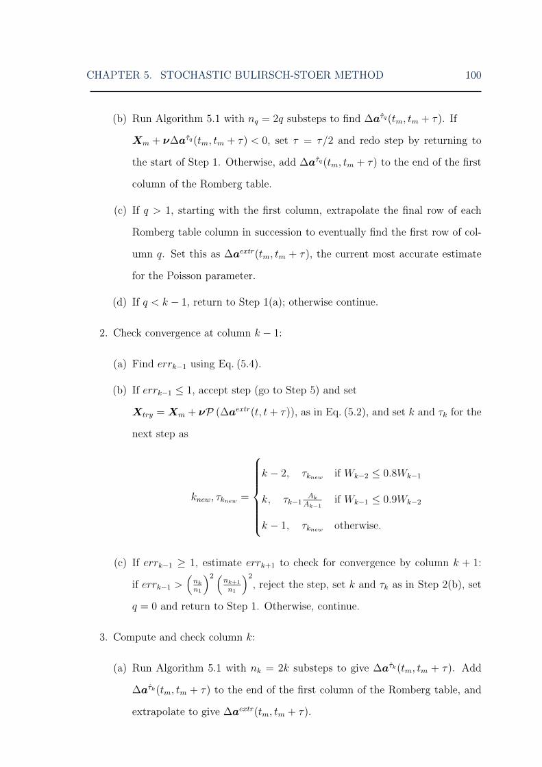
CHAPTER 5. STOCHASTIC BULIRSCH-STOER METHOD 100
(b) Run Algorithm 5.1 with nq = 2q substeps to find ∆aτq(tm, tm + τ). If
Xm + ν∆aτq(tm, tm + τ) < 0, set τ = τ/2 and redo step by returning to
the start of Step 1. Otherwise, add ∆aτq(tm, tm + τ) to the end of the first
column of the Romberg table.
(c) If q > 1, starting with the first column, extrapolate the final row of each
Romberg table column in succession to eventually find the first row of col-
umn q. Set this as ∆aextr(tm, tm + τ), the current most accurate estimate
for the Poisson parameter.
(d) If q < k − 1, return to Step 1(a); otherwise continue.
2. Check convergence at column k − 1:
(a) Find errk−1 using Eq. (5.4).
(b) If errk−1 ≤ 1, accept step (go to Step 5) and set
Xtry = Xm + νP (∆aextr(t, t+ τ)), as in Eq. (5.2), and set k and τk for the
next step as
knew, τknew =
k − 2, τknew if Wk−2 ≤ 0.8Wk−1
k, τk−1Ak
Ak−1if Wk−1 ≤ 0.9Wk−2
k − 1, τknew otherwise.
(c) If errk−1 ≥ 1, estimate errk+1 to check for convergence by column k + 1:
if errk−1 >(nk
n1
)2 (nk+1
n1
)2, reject the step, set k and τk as in Step 2(b), set
q = 0 and return to Step 1. Otherwise, continue.
3. Compute and check column k:
(a) Run Algorithm 5.1 with nk = 2k substeps to give ∆aτk(tm, tm + τ). Add
∆aτk(tm, tm + τ) to the end of the first column of the Romberg table, and
extrapolate to give ∆aextr(tm, tm + τ).
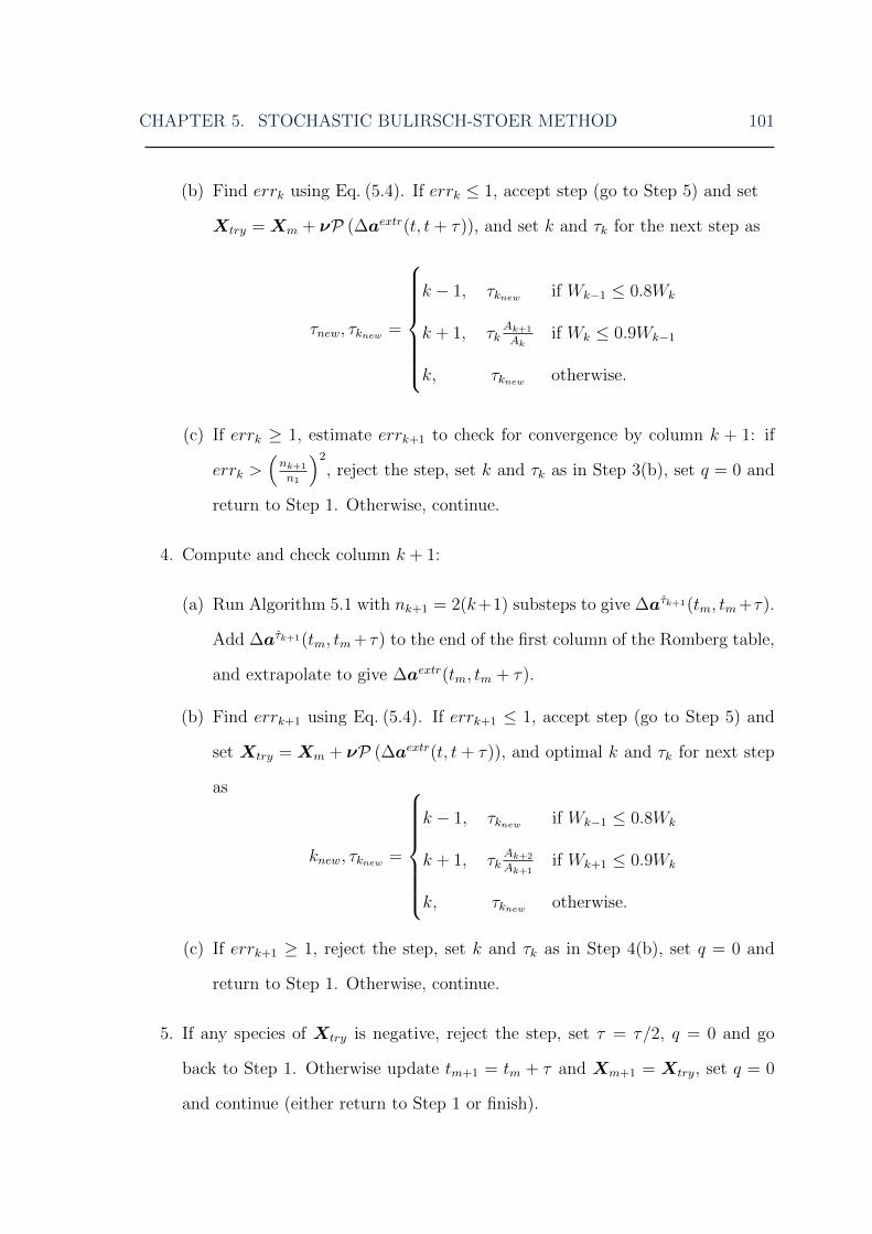
CHAPTER 5. STOCHASTIC BULIRSCH-STOER METHOD 101
(b) Find errk using Eq. (5.4). If errk ≤ 1, accept step (go to Step 5) and set
Xtry = Xm + νP (∆aextr(t, t+ τ)), and set k and τk for the next step as
τnew, τknew =
k − 1, τknew if Wk−1 ≤ 0.8Wk
k + 1, τkAk+1
Akif Wk ≤ 0.9Wk−1
k, τknew otherwise.
(c) If errk ≥ 1, estimate errk+1 to check for convergence by column k + 1: if
errk >(nk+1
n1
)2, reject the step, set k and τk as in Step 3(b), set q = 0 and
return to Step 1. Otherwise, continue.
4. Compute and check column k + 1:
(a) Run Algorithm 5.1 with nk+1 = 2(k+1) substeps to give ∆aτk+1(tm, tm+τ).
Add ∆aτk+1(tm, tm+ τ) to the end of the first column of the Romberg table,
and extrapolate to give ∆aextr(tm, tm + τ).
(b) Find errk+1 using Eq. (5.4). If errk+1 ≤ 1, accept step (go to Step 5) and
set Xtry = Xm + νP (∆aextr(t, t+ τ)), and optimal k and τk for next step
as
knew, τknew =
k − 1, τknew if Wk−1 ≤ 0.8Wk
k + 1, τkAk+2
Ak+1if Wk+1 ≤ 0.9Wk
k, τknew otherwise.
(c) If errk+1 ≥ 1, reject the step, set k and τk as in Step 4(b), set q = 0 and
return to Step 1. Otherwise, continue.
5. If any species of Xtry is negative, reject the step, set τ = τ/2, q = 0 and go
back to Step 1. Otherwise update tm+1 = tm + τ and Xm+1 = Xtry, set q = 0
and continue (either return to Step 1 or finish).

CHAPTER 5. STOCHASTIC BULIRSCH-STOER METHOD 102
5.3 Extension: SBS-DA
There is an alternative scheme to Eq. (5.2) for finding the stochastic update to the
state vector: this is the ‘degree of advancement’, or DA approach, and we call the
resulting method the SBS-DA. Its focus is the M×1 random process Z(t) ≡ Zj(t), j =
1, . . . ,M , the number of times that each reaction occurs over [0, t) (Goutsias and
Jenkinson, 2013; van Kampen, 2007). Z(t) is related to the state vector X(t) by
X(t) = X(0) +M∑j=1
νjZj(t).
In fact, X(t) is uniquely determined by Z(t) (Goutsias and Jenkinson, 2013). This
allows us to use the DA approach to calculate the number of reactions per step, then
return to the population approach to update the state vector, using
X(t+ τ) = X(t) +M∑j=1
νjZj([t, t+ τ)), (5.5)
where we define Zj([t, t + τ)) as the number of reactions of type j occurring over
[t, t + τ). Notice that Eq. (5.5) has the same form as Eq. (3.7),(3.9) and (5.2). In
fact, Kj = Zj([t, t + τ)): in the case of the SSA, the timestep tends to be very small
and only one reaction occurs, but for the τ -leap and SBS it is much larger so more
reactions can occur. Similarly to Eq. (5.1), we know that (Kurtz, 1980)
K = P(∫ t+τ
t
a(Z(s))ds
). (5.6)
In order to find the update of the state vector, we must solve for the mean (and
variance, see below) ofK, and sample according to Eq. (5.6). The τ -leap approximates
the mean relatively inaccurately as a(Z(t))τ , but the SBS aims to calculate a far
more accurate estimate. The equations for the evolution of the mean and variance of
K,µ(s) and C(s), respectively (where s runs only over one step [tm, tm + τ)), can be
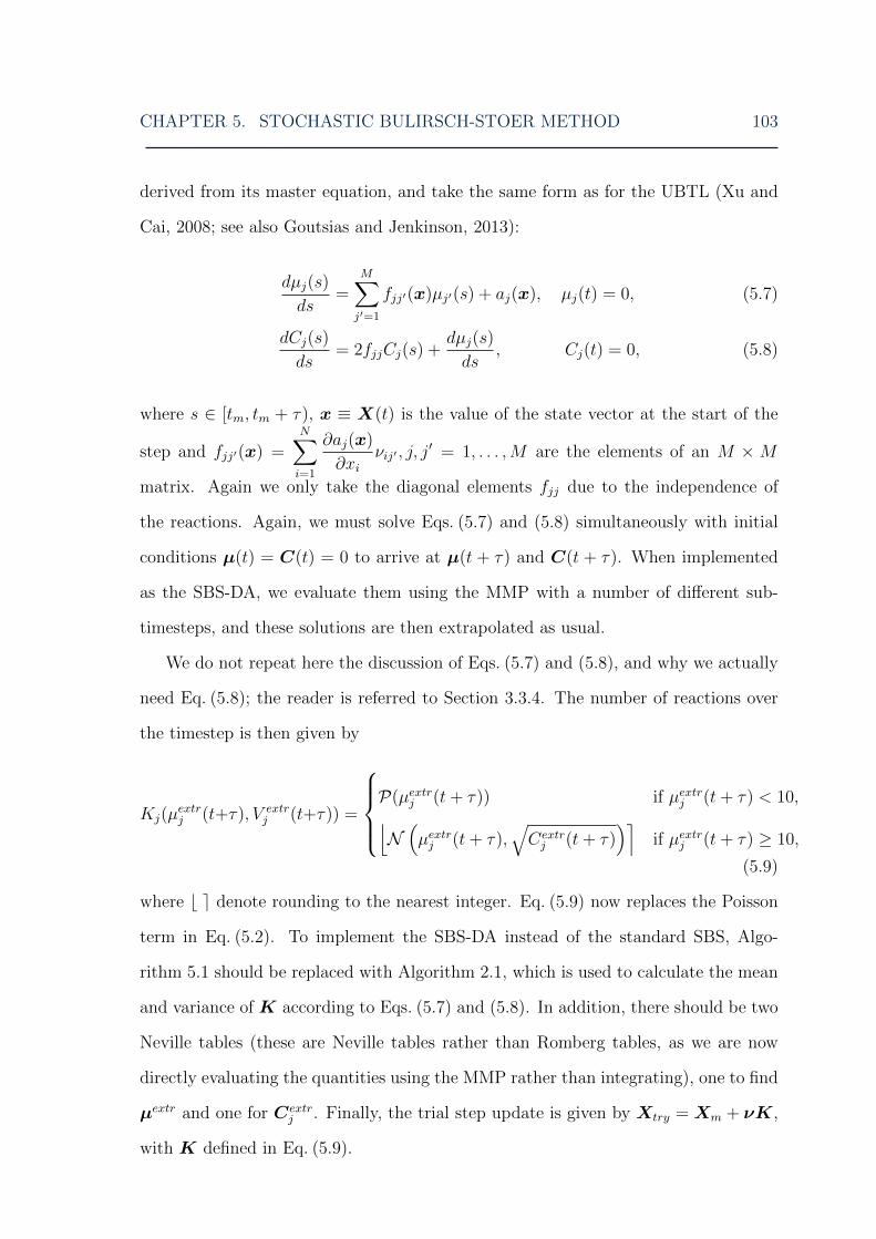
CHAPTER 5. STOCHASTIC BULIRSCH-STOER METHOD 103
derived from its master equation, and take the same form as for the UBTL (Xu and
Cai, 2008; see also Goutsias and Jenkinson, 2013):
dµj(s)
ds=
M∑j′=1
fjj′(x)µj′(s) + aj(x), µj(t) = 0, (5.7)
dCj(s)
ds= 2fjjCj(s) +
dµj(s)
ds, Cj(t) = 0, (5.8)
where s ∈ [tm, tm + τ), x ≡ X(t) is the value of the state vector at the start of the
step and fjj′(x) =N∑i=1
∂aj(x)
∂xiνij′ , j, j
′ = 1, . . . ,M are the elements of an M × M
matrix. Again we only take the diagonal elements fjj due to the independence of
the reactions. Again, we must solve Eqs. (5.7) and (5.8) simultaneously with initial
conditions µ(t) = C(t) = 0 to arrive at µ(t + τ) and C(t + τ). When implemented
as the SBS-DA, we evaluate them using the MMP with a number of different sub-
timesteps, and these solutions are then extrapolated as usual.
We do not repeat here the discussion of Eqs. (5.7) and (5.8), and why we actually
need Eq. (5.8); the reader is referred to Section 3.3.4. The number of reactions over
the timestep is then given by
Kj(µextrj (t+τ), V extr
j (t+τ)) =
P(µextrj (t+ τ)) if µextrj (t+ τ) < 10,⌊N(µextrj (t+ τ),
√Cextrj (t+ τ)
)⌉if µextrj (t+ τ) ≥ 10,
(5.9)
where b e denote rounding to the nearest integer. Eq. (5.9) now replaces the Poisson
term in Eq. (5.2). To implement the SBS-DA instead of the standard SBS, Algo-
rithm 5.1 should be replaced with Algorithm 2.1, which is used to calculate the mean
and variance of K according to Eqs. (5.7) and (5.8). In addition, there should be two
Neville tables (these are Neville tables rather than Romberg tables, as we are now
directly evaluating the quantities using the MMP rather than integrating), one to find
µextr and one for Cextrj . Finally, the trial step update is given by Xtry = Xm + νK,
with K defined in Eq. (5.9).
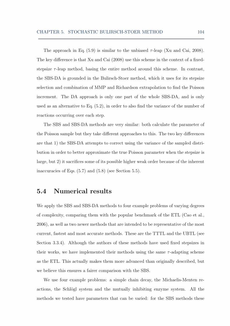
CHAPTER 5. STOCHASTIC BULIRSCH-STOER METHOD 104
The approach in Eq. (5.9) is similar to the unbiased τ -leap (Xu and Cai, 2008).
The key difference is that Xu and Cai (2008) use this scheme in the context of a fixed-
stepsize τ -leap method, basing the entire method around this scheme. In contrast,
the SBS-DA is grounded in the Bulirsch-Stoer method, which it uses for its stepsize
selection and combination of MMP and Richardson extrapolation to find the Poisson
increment. The DA approach is only one part of the whole SBS-DA, and is only
used as an alternative to Eq. (5.2), in order to also find the variance of the number of
reactions occurring over each step.
The SBS and SBS-DA methods are very similar: both calculate the parameter of
the Poisson sample but they take different approaches to this. The two key differences
are that 1) the SBS-DA attempts to correct using the variance of the sampled distri-
bution in order to better approximate the true Poisson parameter when the stepsize is
large, but 2) it sacrifices some of its possible higher weak order because of the inherent
inaccuracies of Eqs. (5.7) and (5.8) (see Section 5.5).
5.4 Numerical results
We apply the SBS and SBS-DA methods to four example problems of varying degrees
of complexity, comparing them with the popular benchmark of the ETL (Cao et al.,
2006), as well as two newer methods that are intended to be representative of the most
current, fastest and most accurate methods. These are the TTTL and the UBTL (see
Section 3.3.4). Although the authors of these methods have used fixed stepsizes in
their works, we have implemented their methods using the same τ -adapting scheme
as the ETL. This actually makes them more advanced than originally described, but
we believe this ensures a fairer comparison with the SBS.
We use four example problems: a simple chain decay, the Michaelis-Menten re-
actions, the Schlogl system and the mutually inhibiting enzyme system. All the
methods we tested have parameters that can be varied: for the SBS methods these
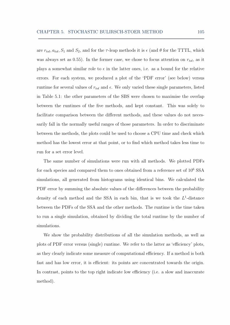
CHAPTER 5. STOCHASTIC BULIRSCH-STOER METHOD 105
are rtol, atol, S1 and S2, and for the τ -leap methods it is ε (and θ for the TTTL, which
was always set as 0.55). In the former case, we chose to focus attention on rtol, as it
plays a somewhat similar role to ε in the latter ones, i.e. as a bound for the relative
errors. For each system, we produced a plot of the ‘PDF error’ (see below) versus
runtime for several values of rtol and ε. We only varied these single parameters, listed
in Table 5.1: the other parameters of the SBS were chosen to maximise the overlap
between the runtimes of the five methods, and kept constant. This was solely to
facilitate comparison between the different methods, and these values do not neces-
sarily fall in the normally useful ranges of those parameters. In order to discriminate
between the methods, the plots could be used to choose a CPU time and check which
method has the lowest error at that point, or to find which method takes less time to
run for a set error level.
The same number of simulations were run with all methods. We plotted PDFs
for each species and compared them to ones obtained from a reference set of 106 SSA
simulations, all generated from histograms using identical bins. We calculated the
PDF error by summing the absolute values of the differences between the probability
density of each method and the SSA in each bin, that is we took the L1-distance
between the PDFs of the SSA and the other methods. The runtime is the time taken
to run a single simulation, obtained by dividing the total runtime by the number of
simulations.
We show the probability distributions of all the simulation methods, as well as
plots of PDF error versus (single) runtime. We refer to the latter as ‘efficiency’ plots,
as they clearly indicate some measure of computational efficiency. If a method is both
fast and has low error, it is efficient: its points are concentrated towards the origin.
In contrast, points to the top right indicate low efficiency (i.e. a slow and inaccurate
method).

CHAPTER 5. STOCHASTIC BULIRSCH-STOER METHOD 106
Table 5.1: Error tolerance parameters used in each method. Parametersvaried for SBS, SBS-DA, ETL, TTTL and UBTL for each example system in order fromfastest to slowest (left to right in efficiency plots). For SBS methods, the parameter isrtol; for τ -leap methods it is ε.
System Method Parameters
SBS 10−5 5× 10⁻⁶ 10−6 5× 10⁻⁷ 2.5× 10⁻⁷ 10−7
ChainSBS-DA 10−5 5× 10⁻⁶ 10−6 5× 10⁻⁷ 10−7 10−8
decayETL 0.125 0.1 0.075 0.05 0.04 0.03
TTTL 0.2 0.15 0.1 0.075 0.05 0.04UBTL 4 2 1 0.8 0.6 0.5
SBS 10−2 10−3 10−4 10−5 10−6 10−7
Michaelis-SBS-DA 10−3 10−4 10−5 10−6 10−7 10−8
MentenETL 0.2 0.15 0.1 0.07 0.05 0.04
TTTL 0.3 0.25 0.2 0.1 0.075 0.06UBTL 7 5 3 2 1.5 1
SBS 10−5 8× 10⁻⁶ 4× 10⁻⁶ 10−6 5× 10⁻⁷ 10−7
SBS-DA 2× 10⁻⁴ 1.5× 10⁻⁴ 10−4 9× 10⁻⁵ 8× 10⁻⁵ 6× 10⁻⁵
Schlogl ETL 0.046 0.044 0.042 0.04 0.0375 0.035TTTL 0.06 0.056 0.052 0.048 0.046 0.044UBTL 0.3 0.28 0.26 0.24 0.22 0.2
SBS 10−5 10−6 10−7 10−8 10−9 10−10
SBS-DA 10−5 10−6 10−7 10−8 10−9 10−10
Enzymes ETL 0.15 0.1 0.07 0.05 0.03 0.02TTTL 0.3 0.2 0.12 0.08 0.06 0.04UBTL 5 3 1.5 0.8 0.4 0.3
5.4.1 Chain decay system
We start with a variant of the chain decay system from Section 4.4.2. This system
was chosen to be identical to one of the examples used by Cao et al. (2006). It has
three species that are converted into each other by the reactions
X1k1−→ X2, c1 = 1,
X2k2−→ X3, c2 = 1.
The simulations were started in initial stateX(0) = [10000, 1, 0]T and simulation time
was T = 5. We ran 5×10⁵ simulations. The SBS safety factors were S1 = 0.2, S2 = 0.4,
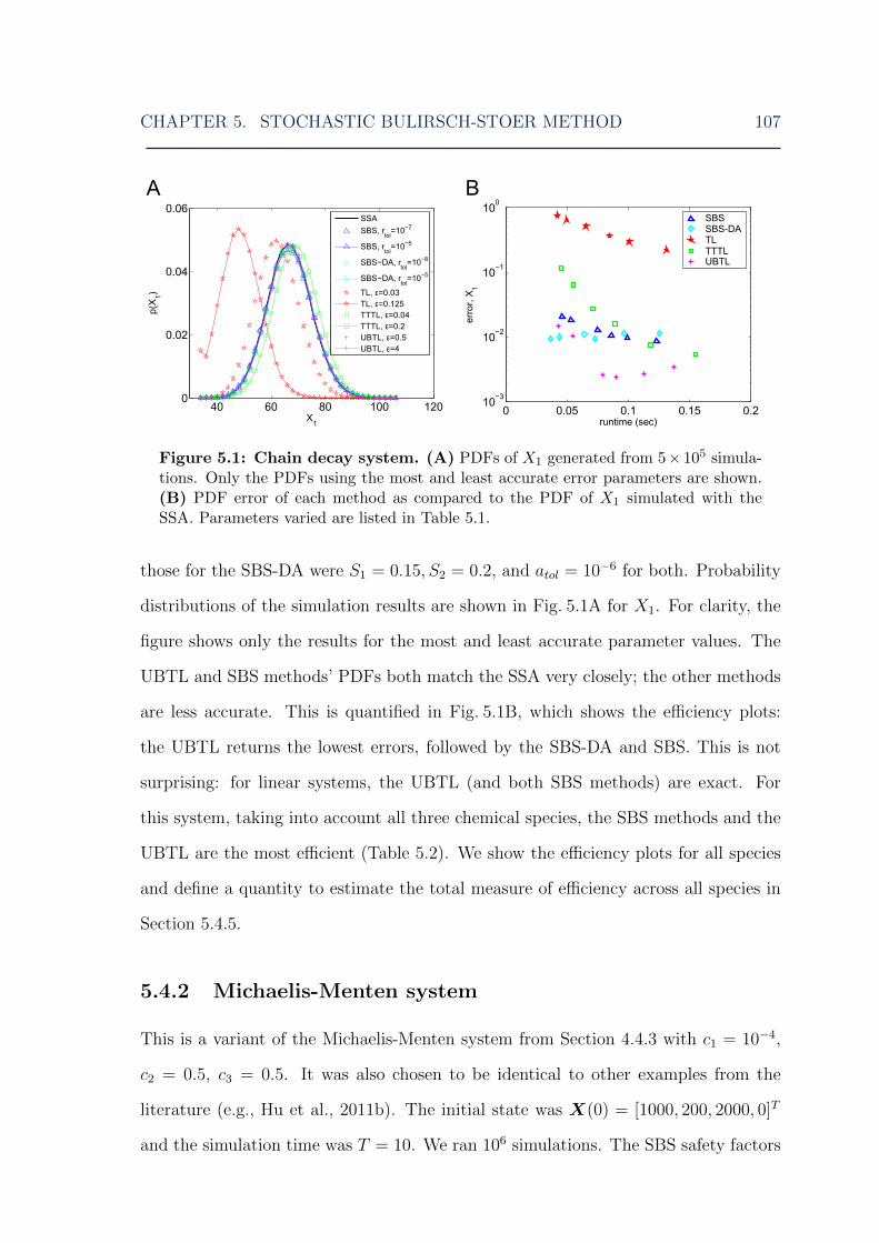
CHAPTER 5. STOCHASTIC BULIRSCH-STOER METHOD 107
Figure 5.1: Chain decay system. (A) PDFs of X1 generated from 5× 10⁵ simula-tions. Only the PDFs using the most and least accurate error parameters are shown.(B) PDF error of each method as compared to the PDF of X1 simulated with theSSA. Parameters varied are listed in Table 5.1.
those for the SBS-DA were S1 = 0.15, S2 = 0.2, and atol = 10−6 for both. Probability
distributions of the simulation results are shown in Fig. 5.1A for X1. For clarity, the
figure shows only the results for the most and least accurate parameter values. The
UBTL and SBS methods’ PDFs both match the SSA very closely; the other methods
are less accurate. This is quantified in Fig. 5.1B, which shows the efficiency plots:
the UBTL returns the lowest errors, followed by the SBS-DA and SBS. This is not
surprising: for linear systems, the UBTL (and both SBS methods) are exact. For
this system, taking into account all three chemical species, the SBS methods and the
UBTL are the most efficient (Table 5.2). We show the efficiency plots for all species
and define a quantity to estimate the total measure of efficiency across all species in
Section 5.4.5.
5.4.2 Michaelis-Menten system
This is a variant of the Michaelis-Menten system from Section 4.4.3 with c1 = 10−4,
c2 = 0.5, c3 = 0.5. It was also chosen to be identical to other examples from the
literature (e.g., Hu et al., 2011b). The initial state was X(0) = [1000, 200, 2000, 0]T
and the simulation time was T = 10. We ran 106 simulations. The SBS safety factors

CHAPTER 5. STOCHASTIC BULIRSCH-STOER METHOD 108
Figure 5.2: Michaelis-Menten system. (A) PDFs of X1 generated from 106 sim-ulations, and (B) PDF error of each method as compared to the PDF of X1 simulatedwith the SSA. Parameters varied are listed in Table 5.1.
were set as S1 = S2 = 0.35, and those of the SBS-DA as S1 = S2 = 0.33, with
atol = 10−6 for both. The PDFs and efficiency plot for X1 are shown in Fig. 5.2.
The SBS, SBS-DA and TTTL all achieve high accuracy. The TTTL becomes more
accurate than the SBS methods at higher runtimes, but the SBS methods have the
advantage at shorter runtimes. Thus when it is important to minimise runtime, the
SBS methods are preferable. Overall, the SBS-DA has the highest efficiency, with the
TTTL second and SBS a close third (Table 5.2).
5.4.3 Schlogl system
The Schlogl system is useful as an example system that is both bimodal and non-
linear, while at the same time being very simple. It is detailed in Section 4.4.5. As
before, parameters A and B are held constant at 105 and 2× 10⁵ units, respectively,
and we used the initial condition X(0) = 250. The simulation time was T = 10, and
we ran 105 simulations for each method. The SBS safety factors were S1 = S2 = 0.05,
those for the SBS-DA as S1 = S2 = 0.125, and atol = 10−6 for both.
The PDFs and efficiencies of each method are shown in Fig. 5.3 for X. For this
system, the ETL is surprisingly accurate compared to the other methods. The SBS
and TTTL have approximately the same efficiency as the ETL, with the SBS-DA
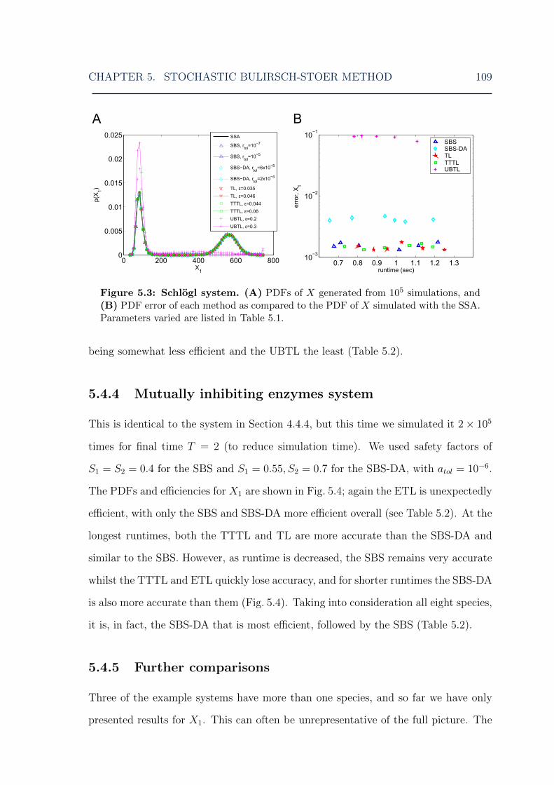
CHAPTER 5. STOCHASTIC BULIRSCH-STOER METHOD 109
Figure 5.3: Schlogl system. (A) PDFs of X generated from 105 simulations, and(B) PDF error of each method as compared to the PDF of X simulated with the SSA.Parameters varied are listed in Table 5.1.
being somewhat less efficient and the UBTL the least (Table 5.2).
5.4.4 Mutually inhibiting enzymes system
This is identical to the system in Section 4.4.4, but this time we simulated it 2× 10⁵
times for final time T = 2 (to reduce simulation time). We used safety factors of
S1 = S2 = 0.4 for the SBS and S1 = 0.55, S2 = 0.7 for the SBS-DA, with atol = 10−6.
The PDFs and efficiencies for X1 are shown in Fig. 5.4; again the ETL is unexpectedly
efficient, with only the SBS and SBS-DA more efficient overall (see Table 5.2). At the
longest runtimes, both the TTTL and TL are more accurate than the SBS-DA and
similar to the SBS. However, as runtime is decreased, the SBS remains very accurate
whilst the TTTL and ETL quickly lose accuracy, and for shorter runtimes the SBS-DA
is also more accurate than them (Fig. 5.4). Taking into consideration all eight species,
it is, in fact, the SBS-DA that is most efficient, followed by the SBS (Table 5.2).
5.4.5 Further comparisons
Three of the example systems have more than one species, and so far we have only
presented results for X1. This can often be unrepresentative of the full picture. The

CHAPTER 5. STOCHASTIC BULIRSCH-STOER METHOD 110
Figure 5.4: Mutually inhibiting enzymes system. (A) PDFs of X1 generatedfrom 2× 10⁵ simulations, (B) PDF error of each method as compared to the PDF ofX1 simulated with the SSA. Parameters varied are listed in Table 5.1.
chain decay system is a clear example of this. Fig. 5.5 shows the efficiency plots for all
three species. Only looking at X1 could lead one to think that the UBTL is the most
efficient method for simulating this system. But including the other two species reveals
that the SBS-DA is, in fact, the most efficient overall. This is important, because it is
clear that factors such as linear/non-linear propensities, population size and stiffness
all affect each reaction and species in a different way. It is overall performance we are
interested in.
To overcome this problem, we came up with a way of quantifying the overall
efficiency of each method over all species. This follows directly on from the previous
definition of efficiency: low error and low runtime implies an efficient method, high
error and high runtime implies an inefficient method, and a combination of the two,
for instance high error but low runtime, clearly lies somewhere between the two. We
define ‘efficiency’ η as
η =(sum(total error over all histogram bins and all species))−1
sum(single-simulation runtime over all error parameters). (5.10)
This varies for each system, and is comparable only when the bins used to calculate
errors are identical. In other words, the values are a direct comparison of the efficiency
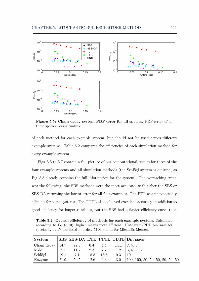
CHAPTER 5. STOCHASTIC BULIRSCH-STOER METHOD 111
Figure 5.5: Chain decay system PDF error for all species. PDF errors of allthree species versus runtime.
of each method for each example system, but should not be used across different
example systems. Table 5.2 compares the efficiencies of each simulation method for
every example system.
Figs. 5.5 to 5.7 contain a full picture of our computational results for three of the
four example systems and all simulation methods (the Schlogl system is omitted, as
Fig. 5.3 already contains the full information for the system). The overarching trend
was the following: the SBS methods were the most accurate, with either the SBS or
SBS-DA returning the lowest error for all four examples. The ETL was unexpectedly
efficient for some systems. The TTTL also achieved excellent accuracy in addition to
good efficiency for longer runtimes, but the SBS had a flatter efficiency curve than
Table 5.2: Overall efficiency of methods for each example system. Calculatedaccording to Eq. (5.10); higher means more efficient. Histogram/PDF bin sizes forspecies 1, . . . , N are listed in order. M-M stands for Michaelis-Menten.
System SBS SBS-DA ETL TTTL UBTL Bin sizes
Chain decay 14.7 22.3 0.4 4.4 14.1 2, 5, 5M-M 7.1 11.7 2.3 7.7 1.2 5, 5, 5, 5Schlogl 19.1 7.1 18.8 18.8 0.3 10Enzymes 21.9 50.5 12.6 6.3 3.0 100, 100, 50, 50, 50, 50, 50, 50

CHAPTER 5. STOCHASTIC BULIRSCH-STOER METHOD 112
Figure 5.6: Michaelis-Menten system PDF error for all species. PDF errorsof all four species versus runtime.
the TTTL, with the TTTL quickly losing accuracy at lower runtimes even when it
was more accurate than the SBS at higher runtimes. Thus we have shown that the
SBS is a very accurate method. More importantly, it is the most efficient method we
tested, maintaining its accuracy well even at low runtimes.
SBS methods excel when we want a short runtime with high accuracy. In this case,
we can set the safety factors high, allowing large steps and a corresponding increase
in extrapolations. This retains a high accuracy, whilst reducing runtime because of
the large timesteps. In contrast, when we allow a longer runtime, we set the safety
factors low, restricting the stepsize and removing the need for higher extrapolation. In
most of our examples, we have seen the SBS only using one extrapolation throughout
the simulation. This is a waste of the extrapolation capability of the SBS, and it is
no surprise that in these cases it loses efficiency, especially as the complex stepsize
adaptation scheme adds extra overhead to each step.

CHAPTER 5. STOCHASTIC BULIRSCH-STOER METHOD 113
Figure 5.7: Mutually inhibiting enzymes system PDF error for all species.PDF errors of all eight species versus runtime.
5.5 Higher order of accuracy and robustness
It is well-known that the Bulirsch-Stoer method has a high order of accuracy: this
is the reason it is able to use large steps whilst still finding very accurate solutions.
This is because of the Richardson extrapolation that is used at each step on the MMP
solutions (which themselves have order two as well as an error expansion containing
only even powers of τ , resulting in very high order solutions with little work). In
contrast, rather than the MMP solutions for X, the SBS instead extrapolates at each

CHAPTER 5. STOCHASTIC BULIRSCH-STOER METHOD 114
step the deterministic quantity ∆a(t, t + τ) (or the mean and variance of K given
by Eqs. (5.7) and (5.8) in the case of the SBS-DA), calculated using the composite
trapezoidal rule, which also has a known error expansion. Thus the extrapolation is
performed on a deterministic variable, the mean of the Poisson update, and it is not
clear how its higher order translates into the stochastic sense.
We explored the behaviour of the SBS and SBS-DA methods using numerical
simulations of two simple systems: a first-order chemical reaction X → 2X, with
X(0) = 1000, and a bimolecular reaction X + Y → ∅, X(0) = Y (0) = 10000. As
the SBS changes both stepsize and Romberg table column k adaptively, we used
a restricted version that fixed stepsize and k. We ran simulations with both SBS
and SBS-DA, for k = 1 and k = 2, that is no extrapolation and one extrapolation,
respectively. In addition, we also used the ETL and TTTL methods for comparison, as
they have known weak orders of accuracy (one and two, respectively). The relatively
large values that we have taken for τ are due to the fact that we do not want the results
to be contaminated by the Monte Carlo error. As only a finite number of simulations
is possible, we chose to use a large stepsize to stay above this level. The gradients
of the errors for the different methods are computed based on a linear least-squares
regression of all the data points.
Figs. 5.8 and 5.9 confirm that both the SBS and SBS-DA are able to reach high
weak order in the mean and higher-order moments in some settings (such as large
timesteps and populations, as discussed below). For the first-order reaction, both
methods have weak order approximately two and four in both the mean and the second
moment (not shown) for k = 1 and k = 2, respectively (Fig. 5.8A). However, there is
a difference in behaviour between the SBS and SBS-DA for the bimolecular reaction
(Fig. 5.9A). Here, the SBS-DA only has weak order two in the first two moments, even
when extrapolated. In contrast, the SBS increases its order to four when extrapolated.
This shows the limitations of Eqs. (5.7) and (5.8): for non-linear systems, they limit
the maximum order of accuracy of the first two (and likely higher) moments of the

CHAPTER 5. STOCHASTIC BULIRSCH-STOER METHOD 115
Figure 5.8: Order of accuracy for first-order reaction. Error versus stepsizefor (A) the mean, and (B) variance of the first-order reaction X → 2X, with c = 0.2,X(0) = 1000, T = 12. The gra dients of linear regression lines fitted to the points areshown in the legend. Note that in these figures, the SBS (blue triangles) and SBS-DAresults (cyan diamonds) cover each other.
SBS-DA to two. This is not the case for linear systems, as here Eq. (5.7) is exact, so
the order of the SBS and SBS-DA is identical.
Thus the message from Figs. 5.8 and 5.9 seems to be that under ideal conditions,
the SBS can indeed achieve higher-order (in the moments), and this order increases
as the Romberg table column (that is, number of extrapolations) is increased. It is
not possible to tell whether this trend continues to higher extrapolations as these are
so accurate that Monte Carlo error interferes with our ability to find the order. The
SBS-DA has at most weak order two in the mean for non-linear systems, but this
restriction in weak order is compensated for by the use of an appropriate Gaussian
sample when the Poisson parameter is large, and generally it is similarly, or even more,
efficient than the SBS. It is also worth noting that in the case of neither reaction does
extrapolation increase the weak order of the variance beyond one (Figs. 5.8B, 5.9B).
This seems to be an issue inherent to the SBS formulation.
However, it is important to clarify that the behaviour we have observed in Figs. 5.8
and 5.9 should not be generalised to all systems, and in many cases the SBS will not
be able to achieve such a high weak order in practice. To try to explain this, let us
briefly consider SDEs again. Talay and Tubaro (1990) derived the global weak error
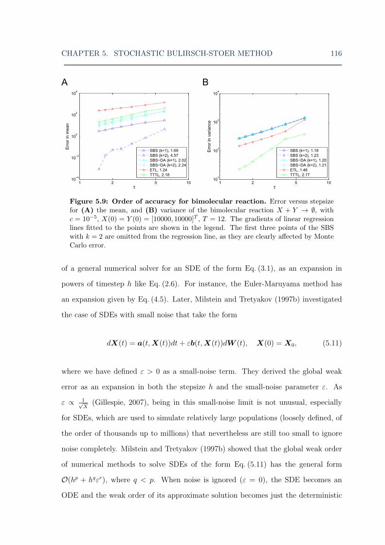
CHAPTER 5. STOCHASTIC BULIRSCH-STOER METHOD 116
Figure 5.9: Order of accuracy for bimolecular reaction. Error versus stepsizefor (A) the mean, and (B) variance of the bimolecular reaction X + Y → ∅, withc = 10−5, X(0) = Y (0) = [10000, 10000]T , T = 12. The gradients of linear regressionlines fitted to the points are shown in the legend. The first three points of the SBSwith k = 2 are omitted from the regression line, as they are clearly affected by MonteCarlo error.
of a general numerical solver for an SDE of the form Eq. (3.1), as an expansion in
powers of timestep h like Eq. (2.6). For instance, the Euler-Maruyama method has
an expansion given by Eq. (4.5). Later, Milstein and Tretyakov (1997b) investigated
the case of SDEs with small noise that take the form
dX(t) = a(t,X(t))dt+ εb(t,X(t))dW (t), X(0) = X0, (5.11)
where we have defined ε > 0 as a small-noise term. They derived the global weak
error as an expansion in both the stepsize h and the small-noise parameter ε. As
ε ∝ 1√X
(Gillespie, 2007), being in this small-noise limit is not unusual, especially
for SDEs, which are used to simulate relatively large populations (loosely defined, of
the order of thousands up to millions) that nevertheless are still too small to ignore
noise completely. Milstein and Tretyakov (1997b) showed that the global weak order
of numerical methods to solve SDEs of the form Eq. (5.11) has the general form
O(hp + hqεr), where q < p. When noise is ignored (ε = 0), the SDE becomes an
ODE and the weak order of its approximate solution becomes just the deterministic

CHAPTER 5. STOCHASTIC BULIRSCH-STOER METHOD 117
order term O(hp). Milstein and Tretyakov (1997a) also performed such an analysis
in the strong sense, and again found the general form of the global strong error to
be O(hp + hqεr), q < p. In addition, Buckwar et al. (2010) also examined small-
noise SDEs in a strong sense. They found that varying ε and h also varied the order
behaviour of the methods they examined.
The implication of the extra term in the stochastic order is that although the
underlying deterministic order of the method may be high, the stochastic order is
restricted by the noise term. However, when the noise is small, this term will also
become small, thus allowing the order to increase, possibly even up to O(hp). This
is also the case if the stepsize is large. In fact, it occurs over a range of values of h
and ε; it is trivial to see that the condition for the deterministic term to dominate is
h� εrp−q .
It is well-known that SDEs form an intermediate regime between the discrete
stochastic and the deterministic regimes. Indeed, a standard way of mathematically
investigating discrete stochastic methods is to look at SDEs with jumps; this is the
approach of Li (2007), as well as Liu and Li (2000). In particular, Li (2007) shows that
the Euler discretisation of such an SDE is the ETL method. Our hypothesis is that
the analysis of Milstein and Tretyakov (1997b) is also applicable to SDEs with jumps.
The SBS is especially useful for systems that include larger populations, even up to
similar levels as SDEs; otherwise, if all molecular populations are low, it would be
preferable to use an SSA, which can simulate such small numbers quickly and exactly.
Thus it is not unreasonable to expect that many of the systems simulated by the SBS
would, in fact, have medium or small levels of noise. Although we have not performed
similar analysis to Milstein and Tretyakov (1997b) for the SBS, we conjecture that
their small-noise error expansion with both τ and ε terms also exists for the SBS
when noise is relatively low. Combined with the fact that the SBS often uses large
stepsizes, this implies that in many systems of interest, the weak order of the SBS
may, in fact, not be far from its deterministic (high) order. This also explains the
CHAPTER 5. STOCHASTIC BULIRSCH-STOER METHOD 118
behaviour of the SBS in our numerical tests (Figs. 5.8 and 5.9). Here, we used large
timesteps to ensure that the total errors would be above the Monte Carlo error level;
an unintentional consequence was that in this regime, it is very likely that the weak
order was dominated by the high deterministic order of the SBS. In the general case,
the SBS would not necessarily behave like this, and its overall order would possibly
be reduced by the presence of sufficient noise in the system.
Thus one can legitimately ask whether our approach offers any advantage over,
for example, the TTTL, which has been analytically shown to have weak order two
in both the moments and the variance. This can be addressed by perusal of Figs. 5.1
to 5.4, where we compare the distances of the PDFs of the numerical methods and
the exact solution (as computed by the SSA) as a function of the runtime. Of the
methods tested, the SBS appears to be the most robust and efficient, even though
the TTTL has weak order two in the variance, which is higher than our numerical
results indicate for the SBS. It is the criteria of efficiency and robustness that are the
most important properties of any good numerical method. This property of the SBS
may be a consequence of the higher deterministic order of the moments, as well as
the ability to adaptively select the timestep and number of extrapolations to carry
out, thus maximising efficiency whilst keeping accuracy high.
5.6 Implementation issues
The speed of the SBS is due to the large steps it takes compared to other solvers. It
can do this as the extrapolation finds accurate estimates for the mean and variance
of Kj. We compare the stepsizes for all five methods used in this chapter on the
Michaelis-Menten system (Fig. 5.10). Clearly, the stepsizes are influenced by our
choice of error parameters. We attempted to control for this by using parameters
that gave similar (or as close as possible) error levels, regardless of runtime. Fig. 5.10
shows that the largest steps were taken by the SBS methods and the UBTL, with

CHAPTER 5. STOCHASTIC BULIRSCH-STOER METHOD 119
Figure 5.10: Stepsizes over time. Evolution in time of stepsizes of all the stochasticsolvers we have compared in the case of the Michaelis-Menten system. Parameters usedwere: S1 = S2 = 0.8, atol = 10−6, rtol = 10−4 for the SBS methods, and ε = 0.04, 0.1, 1for the ETL, TTTL and UBTL, respectively.
the stepsizes being very similar, followed by the other two methods. This is not very
surprising: the UBTL is in some respects similar to the SBS-DA, in that it also finds
very accurate solutions for the moments of K at each step. However, the stepsize is
controlled using a completely different mechanism, so it is interesting to see that both
employ a similar stepsize for a similar error level in this case.
One peculiarity of the SBS is that it can settle into one of several different ‘regimes’:
because it builds the Romberg table adaptively, it can achieve the same accuracy using
a larger step and higher extrapolation (i.e. higher Romberg table column) or smaller
step and lower extrapolation. The regime into which the particular simulation falls is
strongly influenced by the initial stepsize τ(0), but often changes mid-simulation. For
instance, a smaller τ(0) is more likely to fall into the smaller-τ (and lower extrapola-
tion) regime, and vice versa. Fig. 5.11 shows how τ changes with time in chain decay
system simulations using several different τ(0). It is clear that there are two regimes,
one high-τ and one low-τ . When τ(0) is very small, τ settles down to the low regime,
and only the second Romberg table column is used; as τ(0) is increased, τ settles in

CHAPTER 5. STOCHASTIC BULIRSCH-STOER METHOD 120
Figure 5.11: SBS stepsize regimes for chain decay example. Evolution intime of (A) stepsize using different initial stepsizes τ(0), and (B) the column of theRomberg table at which the solutions converge sufficiently (this is not necessarily k,as the error level could be accepted at only k − 1 or even k + 1). SBS parameters areS1 = S2 = 0.5, atol = rtol = 10−6. For clarity not every point has been given a marker.
the high regime and uses the third column. When τ(0) = 1, τ initially enters an even
higher-τ regime using the fourth column, but eventually settles into the high regime
with the third column. In practice, it is advisable to bear this in mind, and choose
τ(0) accordingly: low-τ , low-k simulations are more computationally expensive and
if the same accuracy can be achieved with a larger timestep then efficiency can be
improved even further.
There are two distinct approaches to determining τ(0): first, as described previ-
ously, we could set τ(0) to an arbitrary value and run the initial step through as many
columns as necessary (up to kmax) until it finds the required accuracy. Should τ(0) be
so large that it drives the populations negative, it would also be reduced here until it
reaches a more suitable size for the given problem. In addition, if τ(0) is still larger
than its optimum value, it is reduced over the next several steps until it has reached
this optimum value (and vice versa if it is too small). This is the standard approach
for the deterministic Bulirsch-Stoer method, and it is the one we have taken in the
simulations. However, in the stochastic regime there is another approach: we could
set τ(0) as some multiple of 1a0(X(0))
(the expected size of an SSA step in state X(0)
(Gillespie, 2001)), along with an initial guess of the Romberg table column to aim

CHAPTER 5. STOCHASTIC BULIRSCH-STOER METHOD 121
for. As 1a0(X(0))
is very small, this is a more conservative approach, but τ is increased
to its optimum value over the first few steps. It could be useful for systems that are
stiff, or that oscillate, whose timestep must be very small at certain parts of the so-
lution domain and larger timesteps could result in large errors. There seems to be no
substantial difference in accuracy between the two approaches, and we believe both
are equally valid.
5.7 Discussion
Our results have shown that the SBS is, under ideal stepsize and noise level conditions,
able to achieve a high order of accuracy in the mean and higher moments, at least
comparable to or, in most cases, better than its competitors. In practice, we have
observed that this translates into good accuracy for our example problems. While its
variance remains order one, the real strength of the SBS is this accuracy, combined
with the fact that its efficiency curve has a low gradient; in other words, it is an
accurate method that loses little of its accuracy as it is speeded up, allowing for fast,
robust and accurate simulations. This is because as runtime is shortened, the SBS
uses more and more extrapolations to maintain its accuracy. At the same time, the use
of larger timesteps means less overhead overall, allowing the SBS to be very efficient.
It is in such parameter regimes that the SBS can achieve its full potential.
As the SBS is an explicit method, it is not necessarily suited for solving especially
stiff problems. In such cases, Runge-Kutta methods with larger regions of stability,
such as the stochastic Runge-Kutta method (Rue et al., 2010), are more ideal, as well
as implicit or multiscale methods (Cao et al., 2007; Goutsias, 2005; MacNamara et al.,
2008b). The initial stepsize of the SBS should be chosen appropriately, as it may be
possible for the SBS to settle in a higher-stepsize regime, which could affect accuracy,
or a low-stepsize regime, which could affect runtime. In addition, τ(0) should be
chosen such that it is within the stability region of the modified midpoint method.
CHAPTER 5. STOCHASTIC BULIRSCH-STOER METHOD 122
Running a few preliminary simulations can help choose τ(0).
In previous work, we have extended Richardson extrapolation into the discrete
stochastic regime (Chapter 4 and Szekely et al., 2012). In this framework, full simu-
lations with fixed stepsize are run over t = [0, T ], and their moments are extrapolated
to find accurate approximations to the moments at time T . In contrast, the SBS uses
extrapolation within each timestep and varies τ to optimise efficiency. Thus the SBS
is a complementary approach to extrapolated τ -leap methods that has two advan-
tages: first, the stepsize can be adapted to lower runtime and eliminate the need for
manually finding a suitable range of fixed stepsizes; second, the SBS returns an entire
PDF, rather than just the moments. This can be desirable in many cases, especially
if the solutions do not follow a simple distribution such as a Gaussian or Poisson, or
have multiple stable states.
5.8 Conclusions
In this chapter, we have introduced a second new method for simulating discrete chem-
ical kinetics, the Stochastic Bulirsch-Stoer method. It is inspired by the deterministic
method of the same name, and as such it also boasts the two main advantages of that
method: its speed and its high accuracy. Using numerical tests, we have shown that
it and its variant, the SBS-DA, are at least as accurate as three other methods that
were chosen to be the current state-of-the-art, and robustly maintain this accuracy
even using larger steps.
As the deterministic Bulirsch-Stoer method has higher order, we expect this prop-
erty to be passed on to its stochastic cousin, to some degree. Indeed, we showed
using numerical simulations that this is certainly a possibility, at least for the simple
systems and large stepsizes used. Unfortunately, this need not be the case in general,
as analysis on SDEs with small noise has shown that their weak order consists of both
a deterministic and a noise term, which gives a lower overall order than just the deter-

CHAPTER 5. STOCHASTIC BULIRSCH-STOER METHOD 123
ministic term. Thus when the noise on the system is large compared to the stepsize,
the weak order is dominated by the noise term. On the other hand, when the noise
is small or the stepsize is large, it is the deterministic order term that dominates. It
is likely that our numerical simulations revealed this deterministic scenario, as the
stepsizes were large. Nevertheless, we believe that the SBS could indeed have higher
weak order in many practical problems. This is especially the case as the SBS is ideal
for larger systems for which the SSA is too slow (thus noise is likely to be lower), and
it also often uses a large stepsize.
Finally, even if the weak order of the SBS is not higher, our results have shown that
the SBS is just as, if not more, accurate than the comparison methods. Furthermore,
and most importantly, this accuracy is maintained well even when the stepsize is
increased, allowing for high computational efficiency. Thus the SBS is a promising
new method to address the need for fast and efficient discrete stochastic methods.

6Haematopoietic stem cell modelling
This chapter is somewhat different from the previous two, which were on constructing
new discrete stochastic methods. Here we focus on a biological problem, simulating
the dynamics of a population of haematopoietic stem cell niche lineages, which we
approach using the ideas and knowledge developed in the previous chapters. In order
to do this, we first devised a vectorised leaping method that can use adaptive stepsizes.
This method solves two problems in one go: it gives a large improvement in runtime
as compared to an SSA, and furthermore it allows the inclusion of interactions in the
population that is simulated. This second point is essential for the biological focus of
this work, which we discuss later.
To begin, we justify the reasons why we used a vectorised τ -leap, rather than the
extrapolated τ -leap or SBS from the previous chapters. First, we needed a full PDF,
so the extrapolated τ -leap was not an option. The SBS would have been ideal for just
such a system, where some of the species go into the tends of thousands. We originally
experimented with it, but encountered problems with the extrapolation during each
step. The main reason for this seemed to be the variable rate ‘constants’, which do
not occur in chemical kinetics. In addition, we needed many simulations to be run
fast, as we were simulating an entire population of niche lineages. Furthermore, we
124
CHAPTER 6. HAEMATOPOIETIC STEM CELL MODELLING 125
wanted each member of the population (that is, each individual simulation) to stay
in step, in order to add interactions between them.
Finally, we needed the method to be simple, since we were introducing extra
complexity (in the form of couplings) to an already non-trivial system. The logical
choice was therefore a τ -leap method, and the simulations were actually performed
with a much-simplified τ -leap that used only a few lines of code to select τ . Initial
simulations showed that it would give good accuracy without taking too long to run.
However, it is important to bear in mind that this vectorised scheme can be used in
conjunction with any solver, because the timestep is found using only one member of
the population. Accordingly, it can easily be slotted into existing non-vectorised code
if even higher computational efficiency is important.
6.1 Introduction
Stem cells offer exciting potential for regenerative therapy, with ultimate possibilities
being the ability to regenerate limbs and heal genetic diseases (Mason and Dunnill,
2008; Wagers, 2012). Although we have already begun the long journey to reach
these goals, much work remains to be done (Gurtner et al., 2007; Weissman, 2000b).
Indeed, much of our knowledge of stem cells is derived from in vitro experiments,
where the stem cells have been relocated from their native environment. For instance,
in haematopoietic (blood-producing) stem cell experiments the stem cells are often
isolated from a donor, expanded in vitro, and transplanted into a lethally irradiated
host, with the question of interest being how the stem cells respond to this new
environment (e.g., Till et al., 1964). However, it is difficult to draw conclusions about
the role and behaviour of stem cells in their native environments when we must
investigate them in foreign ones (Fuchs et al., 2004; Metcalf, 2007).
In vivo, stem cells are generally found in special microenvironments, or niches,
which are defined by a complex set of biochemical and physical conditions that feed

CHAPTER 6. HAEMATOPOIETIC STEM CELL MODELLING 126
back on each other (Scadden, 2006; Wagers, 2012). Niches play a critical role in the
function and behaviour of stem cells and their role should not be underestimated
(Lander, 2009; Wagers, 2012). For instance, experimentally changing certain niche
attributes affects the dynamics of the resident stem cells (Peerani et al., 2007). Indeed,
Moore and Lemischka (2006) noted that an important step for the future is “the
development of in vitro systems that accurately recapitulate the in vivo functions of
niches”. In addition, stem cells are often not single entities that exist independently
of each other, instead forming an interacting population that includes stem cells and
their more differentiated products, both within and outside the niche (Hsu and Fuchs,
2012; Stine and Matunis, 2013). Moreover, even separate niches can affect each other,
through the effects of their daughter cells or migration (e.g., Takeda et al., 2011).
We focus on the haematopoietic stem cell system, for two reasons: first, it is prob-
ably the most well-characterised stem cell system. Second, it is representative of stem
cell systems in general, incorporating their essential properties such as self-renewal,
differentiation, multiple lineage choices and feedbacks to regulate cell levels (Lander,
2009; Orkin and Zon, 2008). This allows us to start thinking about heterogeneity and
the introduction of population interactions in a comparatively simple setting. The
haematopoietic system consists of the bone marrow, blood, spleen, liver and lymph
nodes, with haematopoietic stem cells (HSCs) mostly located in the bone marrow.
So far, two niche types have been observed in bone marrow, although their relation-
ship to each other and to HSCs is not clear, and it is possible that there is further
complexity to come (Kiel and Morrison, 208; Lo Celso and Scadden, 2011; Morrison
and Spradling, 2008; Yin and Li, 2006). Spatially, however, it is likely that the HSCs
themselves are spread throughout the bone marrow, each in its own individual ‘facul-
tative niche’ (Hawkins and Lo Celso, 2013; Kiel et al., 2005; Morrison and Spradling,
2008; Sugiyama et al., 2006; Wang et al., 2013). To be precise in our definition,
henceforth we refer only to these facultative niches as ‘niches’. Bone marrow thus
contains an entire population of niches, each niche containing small numbers of HSC,

CHAPTER 6. HAEMATOPOIETIC STEM CELL MODELLING 127
and inside each niche, the stem cell differentiates into blood cells, which eventually
join the bloodstream.
The haematopoietic system operates by demand control: there is a target level
of differentiated blood cells, the homeostatic level, which is set by natural selection
(Mangel and Bonsall, 2007, 2008, 2013), and which the organism attains by differen-
tiation of the HSC and blood progenitor cells into appropriate lineages (Lander et al.,
2009; Mangel and Bonsall, 2013). This seems to be achieved by feedback from the
fully-differentiated progeny of the HSC in the bloodstream (e.g., Cheshier et al., 2007;
de Graaf et al., 2010; Lander et al., 2009). In addition, there is also feedback from
differentiated progeny that have not entered the bloodstream, but remain localised to
the niche (Hsu and Fuchs, 2012). The HSC system must respond rapidly to pertur-
bations such as wounding or infection, and even under normal conditions the blood
cell turnover of an average human being is around one trillion cells per day (Ogawa,
1993). Such enormous numbers mean that it is important to have a robust feedback
mechanism for proper functioning of the system.
The complex nature of the HSC system, with many different feedbacks and lineage
choices, as well as many spatially separate niches, means that it is very difficult to
model. In general, current models of stem cell dynamics involve either only one focal
stem cell, or a homogeneous population of each cell type, and are modelled using
ODEs (Mangel and Bonsall, 2007). Although such models can give useful results,
it is important to include heterogeneity in the picture (Huang, 2011). For example,
there is considerable heterogeneity between individual stem cell clones (Osafune et al.,
2008; Sieburg et al., 2011); this heterogeneity is also present within clonal cell lines
(Huang, 2009; Lander, 2011), and was even observed many years ago by Till et al.
(1964), as well as by Suda et al. (1983). However, in the intervening decades the
deterministic view of stem cell differentiation has taken hold with great success and has
led towards understanding the feedback between differentiated and stem/progenitor
cells (Lander et al., 2009; Marciniak-Czochra et al., 2009). More recently there has
CHAPTER 6. HAEMATOPOIETIC STEM CELL MODELLING 128
been a shift in emphasis, with stochastic models being used to examine the dynamics
and the evolution of mutations in a stem cell population (Dingli and Pacheco, 2011),
phenotypic equilibrium in a population of cancer cells (Gupta et al., 2011), and the
effects of different control mechanisms on stem cell populations (Komarova, 2013; Sun
and Komarova, 2012),
Mangel and Bonsall (2008, 2013) have already proposed a population biology
framework for stem cell dynamics, with the theme “stem cell biology is population
biology”. They used a differential equation model of one niche lineage to show how
evolution affects the decision of whether to differentiate into myeloid or lymphoid
cells. In addition, they started to explore how stochasticity enters the picture. Here,
we further expand on this framework by considering the stochastic evolution of a
heterogeneous metapopulation of niche lineages, comprised of stem, progenitor and
differentiated blood cells. We also take into account the further consideration that
while the niches (containing the primitive cells) may be distinct, the blood cells are
mixed in the bloodstream, and the niche lineages could be controlled by feedback
from the entire bloodstream rather than just their own, possibly localised, descen-
dants. Thus, the separate lineages in the population are coupled together through
their differentiated progeny. Our main aims here are to 1) establish the stochas-
tic framework, 2) investigate the dynamics of the stochastic system, 3) explore how
coupling niche lineages together into niche groups affects the system dynamics, and
4) whether it has any effect on the response of the entire system to a perturbation.
We first develop the stochastic modelling framework. Since stochastic simulations
can be slow, especially for complicated models such as ours, we introduce a fast,
approximate method for simulating an entire metapopulation of HSC niche lineages
(each of which forms a population itself). We then describe how to take into account
the interactions from the blood cells on to the primitive cells in the niche in our sim-
ulations. We simulate a metapopulation of lineages, which first settles to homeostasis
and is then perturbed by reducing blood cell numbers. After the perturbation, there

CHAPTER 6. HAEMATOPOIETIC STEM CELL MODELLING 129
is a peak in blood cell numbers as the stem and progenitor cells replenish them. We
investigate the effects of coupling niche lineages together: that is, what happens when
the feedbacks are averaged across many niche lineages. We find that 1) coupling niche
lineages shifts the mean cell populations at steady state, and changes the shape of the
cells’ distributions; 2) as more lineages are coupled together, the total blood cells in
each coupled niche group approach the target steady state of the system; 3) different
perturbation types elicit a different response from the system, and when blood cells
are perturbed randomly, niche lineages coupled into larger groups respond better than
smaller groups and uncoupled lineages. Taken together, these results imply that for
the organism, connecting the individual niche lineages into larger niche groups is ad-
vantageous, both for attaining homeostasis of the overall system and for responding
to random perturbations.
6.2 HSC model
We start with the model of the HSC system as developed by Mangel and Bonsall
(2013), which characterises the stem cell niche and its products as a control system
driven ultimately by demand from the organism (Fig. 6.1 and Appendix A.1). The
system consists of one niche lineage: an HSC niche and its fully-differentiated product
cells in the bloodstream. The demand from the organism occurs via changes in the
levels of differentiated blood cells, which feed back this demand to the primitive cells
(that is, stem and progenitor cells).
Specifically, the model is comprised of the populations of stem cells (S), multi-
potent progenitor cells (MPP), common lymphoid and common myeloid progenitor
cells (CLP,CMP, respectively) and their fully-differentiated products, lymphoid and
myeloid blood cells (L,M , respectively). Although clearly there are many blood cell
types (more details in, e.g., Orkin and Zon, 2008), here they have all been classi-
fied under myeloid and lymphoid types for the sake of simplicity. Thus our model
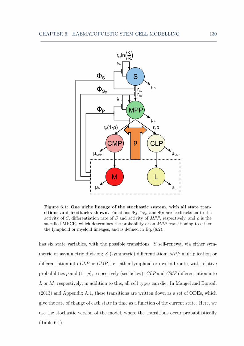
CHAPTER 6. HAEMATOPOIETIC STEM CELL MODELLING 130
Figure 6.1: One niche lineage of the stochastic system, with all state tran-sitions and feedbacks shown. Functions ΦS ,ΦSD
and ΦP are feedbacks on to theactivity of S, differentiation rate of S and activity of MPP, respectively, and ρ is theso-called MPCR, which determines the probability of an MPP transitioning to eitherthe lymphoid or myeloid lineages, and is defined in Eq. (6.2).
has six state variables, with the possible transitions: S self-renewal via either sym-
metric or asymmetric division; S (symmetric) differentiation; MPP multiplication or
differentiation into CLP or CMP, i.e. either lymphoid or myeloid route, with relative
probabilities ρ and (1−ρ), respectively (see below); CLP and CMP differentiation into
L or M , respectively; in addition to this, all cell types can die. In Mangel and Bonsall
(2013) and Appendix A.1, these transitions are written down as a set of ODEs, which
give the rate of change of each state in time as a function of the current state. Here, we
use the stochastic version of the model, where the transitions occur probabilistically
(Table 6.1).

CHAPTER 6. HAEMATOPOIETIC STEM CELL MODELLING 131
The model also incorporates four different feedbacks from the blood cells L,M on
to the S and MPP cells. Three of these, ΦS,ΦSD,ΦP take the form
ΦS(L(t),M(t)) =1
(1 + βLSL(t) + βMSM(t)), (6.1)
with their respective parameters β defined in Table 6.2. These inhibit the activity of S
and MPP when blood cell levels are high. Specifically, ΦS inhibits all S activity (both
self-renewal and differentiation), ΦSDinhibits S differentiation only and ΦP inhibits
all MPP activity. The form of Eq. (6.1) is deliberately general to make no assumptions
about the underlying mechanisms and is based on earlier studies (Lander et al., 2009;
Marciniak-Czochra et al., 2009); it conforms to the assumptions that: 1) numbers
of both blood cell types have an effect on S and MPP activity, 2) their effects are
additive, 3) its strength is different for L,M cells, and 4) when numbers of either fall,
the activity of S and MPP increases again. Note that feedbacks Φ always take values
on (0, 1].
The last feedback is perhaps the most interesting, and is one aspect that differen-
Table 6.1: Transitions in the stochastic HSC model
# Transition Transition probability Process
1 S → 2S rSSln(K
S)ΦS(L,M)S S symmetric division (self-renewal)
2 S → S + MPP rSAΦS(L,M)S S asymmetric division (self-renewal)
3 S → 2MPP rSDΦSD
(L,M)ΦS(L,M)S S symmetric differentiation4 S → ∅ µSS S death
5 MPP → 2MPP λPΦP (L,M)MPP MPP renewal6 MPP → CLP rPΦP (L,M)ρMPP MPP differentiation to CLP7 MPP → CMP rPΦP (L,M)(1− ρ)MPP MPP differentiation to CMP8 MPP → ∅ µPMPP MPP death
9 CLP → L rCLPCLP CLP differentiation10 CLP → ∅ µCLPCLP CLP death11 CMP → M rCMPCMP CMP differentiation12 CMP → ∅ µCMPCMP CMP death
13 L → ∅ µLL L death14 M → ∅ µMM M death
CHAPTER 6. HAEMATOPOIETIC STEM CELL MODELLING 132
tiates this model from previous work. We refer to it as the Multipotent Progenitor
Commitment Response, or MPCR (Mangel and Bonsall, 2013). This feedback de-
termines the probability of an MPP cell differentiating into either the lymphoid or
myeloid routes (see Eq. (6.2)). The idea behind this is that when blood cell numbers
are not at their homeostatic levels (defined as a specific desired value of ρ), and S
and MPP activity is high, the MPCR aims to shift the production of new blood cells
to the appropriate cell type. We model the MPCR as
ρ(L(t),M(t)) =α(M(t)L(t)
)γ1 + α
(M(t)L(t)
)γ , (6.2)
where α and γ are positive parameters. When either L(t) or M(t) = 0, they are
simply set to 1 instead; this has the advantage of affecting the value of ρ by only a
small amount whilst keeping the MPCR pressure towards the correct cell type.
We set the MPCR parameters γ, α to give a desired homeostatic blood cell ratio,
which here is 1L : 1000M to loosely correspond to that in humans. As ρ is defined as
the probability of an MPP differentiating to a CLP, and we know that on average there
will be one CLP produced for every 1000 CMP at homeostasis, then ρh = 11+1000
=
9.99 × 10⁻⁴. We can now substitute these values into Eq. (6.2), choose a value for γ
and so calculate the corresponding α. We can do this for different combinations of
γ, α, thus varying the strength of the response whilst sticking to the same cell ratio
ρh.
Although many combinations of γ, α can give the same homeostatic ratio of L :M ,
they strongly affect the sensitivity of the MPCR to changes in cell levels and its
response to perturbations. Mangel and Bonsall (2013) used this model to examine the
behaviour of the haematopoietic system from an evolutionary perspective. Treating it
as a demand control system, where the demand comes from the entire organism, they
showed that there is varying selection on organisms with different MPCR parameters
γ, α. Different organisms can thus evolve a range of parameters as their environments
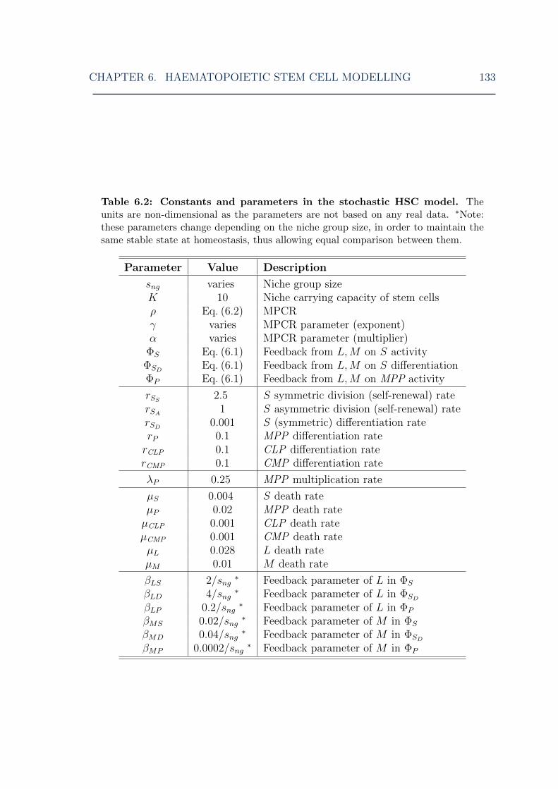
CHAPTER 6. HAEMATOPOIETIC STEM CELL MODELLING 133
Table 6.2: Constants and parameters in the stochastic HSC model. Theunits are non-dimensional as the parameters are not based on any real data. ∗Note:these parameters change depending on the niche group size, in order to maintain thesame stable state at homeostasis, thus allowing equal comparison between them.
Parameter Value Description
sng varies Niche group sizeK 10 Niche carrying capacity of stem cellsρ Eq. (6.2) MPCRγ varies MPCR parameter (exponent)α varies MPCR parameter (multiplier)
ΦS Eq. (6.1) Feedback from L,M on S activityΦSD
Eq. (6.1) Feedback from L,M on S differentiationΦP Eq. (6.1) Feedback from L,M on MPP activity
rSS2.5 S symmetric division (self-renewal) rate
rSA1 S asymmetric division (self-renewal) rate
rSD0.001 S (symmetric) differentiation rate
rP 0.1 MPP differentiation raterCLP 0.1 CLP differentiation raterCMP 0.1 CMP differentiation rate
λP 0.25 MPP multiplication rate
µS 0.004 S death rateµP 0.02 MPP death rateµCLP 0.001 CLP death rateµCMP 0.001 CMP death rateµL 0.028 L death rateµM 0.01 M death rate
βLS 2/sng∗ Feedback parameter of L in ΦS
βLD 4/sng∗ Feedback parameter of L in ΦSD
βLP 0.2/sng∗ Feedback parameter of L in ΦP
βMS 0.02/sng∗ Feedback parameter of M in ΦS
βMD 0.04/sng∗ Feedback parameter of M in ΦSD
βMP 0.0002/sng∗ Feedback parameter of M in ΦP
CHAPTER 6. HAEMATOPOIETIC STEM CELL MODELLING 134
vary, and this affects the dynamics of their haematopoietic system as well as its
response to perturbations. This implies that it is important to take into account
the evolutionary background of an organism when examining the dynamics of the
haematopoietic system, and stem cell systems in general. This is consistent with the
idea that stem cells are units of evolution (Laird et al., 2005; Weissman, 2000a).
It is now well-known that ODE models are not able to account for the full range
of dynamics of highly stochastic systems (Goutsias, 2007; Wilkinson, 2009). Thus the
next step is the stochastic formulation of this HSC model. This is similar to the ODE
formulation, with six states and fourteen reactions, i.e. types of transition between
the states. However, rather than occurring with deterministic rates, these transitions
now occur with particular propensities at each step of the simulation. We now adopt
the formulation of discrete stochastic kinetics described in Section 3.3.
This formulation was developed to simulate the interactions of different chemical
species in a dilute gas, and has since been extended to dilute solutions (Gillespie,
2009). Both of these scenarios assume that the system is macroscopically well-stirred
and homogeneous and the usual (mass-action) forms of its propensity functions are
formulated based on these assumptions. In order to use this formulation with the HSC
system, which does not necessarily obey either assumption, we adopt instead a phe-
nomenological approach to definining the propensity functions, as is the custom when
constructing ODE population models. In effect, we simply convert the transition rates
of the ODE system into transition propensities. The form of the propensities depends
on our assumptions regarding the processes involved: thus, the propensities are depen-
dent upon a rate constant, the population of the transitioning cell type, and in the case
of stem and progenitor cells, also the feedbacks that we have assumed exist (Table 6.1).
Note that the propensities give the probability of a reaction occurring per unit time,
and therefore are not required to remain on [0, 1]. For our HSC model simulations,
we define the state vector as X(t) = [S(t),MPP(t),CLP(t),CMP(t), L(t),M(t)]T .

CHAPTER 6. HAEMATOPOIETIC STEM CELL MODELLING 135
6.3 Stochastic HSC method
6.3.1 Simulating a population of niches
In order to simulate a large number of niche lineages, we now expand the Gillespie
SSA/τ -leap approach from just one compartment to many. By including interaction
terms between each individual niche lineage, we can easily simulate an entire inter-
acting heterogeneous metapopulation of niche lineages. The heterogeneity results
from the different stochastic time evolution of each individual niche lineage (i.e., it
is intrinsic heterogeneity). Strictly speaking, we simulate through time a metapop-
ulation of separate, spatially distinct but interacting, isogenic cell populations in an
identical environment that are affected by intrinsic noise only. Thus our method is
somewhat of a mix between the usual SSA method, which does not take into account
spatial considerations and simulates only a single niche lineage, and an individual-
based model, which can include spatial movement as well as allowing each individual
different properties, scaled up to the level of populations.
We take advantage of the native matrix structures of the Matlab programming
language to form a state matrix, with the state vector of each niche lineage forming
one column of the overall state matrix: thus, if there are F separate niche lineages,
instead of an N × 1 state vector, we now manipulate an N × F state matrix. This
approach is conceptually simple, easily allows for the addition of interactions, and is
especially fast (as Matlab is optimised for matrix calculations, calculating each step
of the SSA scheme on a matrix rather than a vector has little effect on the speed,
whereas doing the same for each niche in turn would be very much slower). This state
matrix approach could easily be implemented in other programming languages, and
although it would not necessarily result in a computational speedup (for instance,
this is likely to be the case in the popular C and C++ languages), we argue that it is
favourable even for its inherent simplicity alone.

CHAPTER 6. HAEMATOPOIETIC STEM CELL MODELLING 136
This matrix scheme can also be used to quickly generate many repeat simulations
of the same system, which is necessary when we are interested in the overall distri-
bution of results at some given time. The difference here is the following: instead of
simulating many repeat trajectories of a single niche lineage, here we simulate a single
trajectory of the entire metapopulation of niche lineages. The aim of the former is to
show the spectrum of possible results (and their probabilities) of a single niche lineage
at some given time, whereas the aim of the latter is to find one instance of the whole
system of sub-populations, allowing the introduction of interactions between them.
Since the SSA chooses timesteps randomly, the metapopulation of niche lineages
will not be simulated in time synchronously, akin to a running race where some
runners are ahead and some lag behind. If we were interested in repeat simulations
of a single lineage this would not be a problem, but since here we are simulating an
interacting metapopulation, all lineages must stay in step otherwise the interactions
would effectively be averaging over time. The solution to this problem is to switch to
the τ -leap method, use it to choose a suitable timestep and evolve every niche lineage
according to one common time frame. It is important to note that this does not bias
our results in any way: we are only selecting a common timestep for all the lineages,
but the reactions that occur in each lineage are then chosen according to the true
Markov process.
To explain this, let us go back to basics: the evolution of each lineage is governed by
a Markov jump process (Kurtz, 1978), which is approximated by the τ -leap method.
If we wanted to simulate a population of F niche lineages using a standard τ -leap, we
would run F repeat simulations of a single lineage. This could be done with either a
fixed or an adaptive timestep, and we would sample the Markov process (carry out
the τ -leap update) at the time points given by those timesteps. However, the process
itself is independent of the times at which we sample it (although, of course, the
same cannot be said for the solution of our τ -leap method, which approaches the true
Markov process as the timesteps decrease). Thus we are free to sample the Markov

CHAPTER 6. HAEMATOPOIETIC STEM CELL MODELLING 137
process at whatever time points we choose, provided we remember the condition on
our approximate solution. Now, a reasonable part of the computational time of a
leaping method is taken up with the overhead of calculating the timestep adaptively.
By simulating the metapopulation simultaneously, our method allows us to choose
just one timestep for all F niche lineages, reducing this overhead considerably. The
only disadvantage is that if one lineage contains unusually large populations, this
would pose as a bottleneck on the common stepsize.
We must thus find the limiting timestep from the whole metapopulation. First,
the propensities of each transition in each niche lineage are calculated. Then, we
find the one with the largest a0(x), that is the sum of the propensities. Now, we
simply continue with the stepsize selection as if we were only simulating a single niche
lineage, and its propensities were those of the selected one. Once the stepsize has
been chosen, the entire population is evolved over that step using the standard τ -leap
update formula Eq. (3.9). This is described more precisely in Algorithm 6.1.
Algorithm 6.1. Vectorised τ -leap
At time t = 0, with a metapopulation of niche lineages of size F , each taking initial
states of Xf (0), f=1,. . . ,F:
0. Initialise state matrix containing F niche lineages, each with N distinct cell
types: this is an N × F matrix containing the initial state vectors
X(0) =[X1(0), . . . , XF (0)
].
With the system in state X(tm) =[X1(tm), . . . , XF (tm)
]at time tm:
1. Calculate propensities of each niche lineage to get an M × F matrix of propen-
sities, a(X(tm)) =[aj(X
1(tm)), . . . , aj(XF (tm))
], j = 1, . . . ,M .
2. Find a0(X(tm)) =[∑M
j=1 aj(X1(tm)), . . . ,
∑Mj=1 aj(X
F (tm))]
3. Find maxf[a0(X
f (tm))], f = 1, . . . , F , i.e. the niche lineage with highest total
propensity, and assign its lineage index to f ′.
CHAPTER 6. HAEMATOPOIETIC STEM CELL MODELLING 138
4. Calculate τ as described by Cao et al. (2006), using the propensities a(Xf ′(tm))).
5. Update state matrix asX(tm+1) = X(tm)+νP(a(X(tm))τ), and tm+1 = tm+τ .
If any cell population in any niche lineage goes negative, redo step using τ = τ2.
Otherwise, return to Step 1.
We select the lineage index of the highest total propensity, as this is the niche
lineage with the most frequent transitions, and thus the limiting factor on the stepsize.
Of course, the actual number of transitions at each step is probabilistic, so if by
chance too many transitions occur for any cell type in any niche and its population
goes negative, the step should be redone with τ = τ/2. For even tighter control of the
stepsize, instead of selecting a single niche lineage f ′ and taking its total propensity as
the limiting factor, we could instead find the lineage index of the maximum propensity
of each transition. This would set a tighter bound on τ , as each transition would
partake in the stepsize-selection process. However we found the current method to be
satisfactory.
Although in this chapter we have used a procedure from Cao et al. (2006) to find
the timestep, we are not restricted to this particular method. The matrix scheme
we have described above is flexible, in that it can easily be fitted into any procedure
for adapting τ , including advanced and efficient methods such as the SBS method
(Szekely et al., 2013b) or TTTL method (Hu et al., 2011b). As long as we find
the niche lineage (or simulation index, depending on context) with the most frequent
reactions, we can choose a timestep based on this lineage for the entire metapopulation
using any τ -adapting scheme.
6.3.2 Coupling niches
Each HSC niche does not exist in isolation in the bone marrow; in fact, HSC of-
ten circulate around the bone marrow and bloodstream (Adams and Scadden, 2006;
Wright et al., 2001). Differentiated blood cells are also, in general, ejected from the

CHAPTER 6. HAEMATOPOIETIC STEM CELL MODELLING 139
niche and enter the bloodstream, although certain differentiated cell types can remain
localised to the niche (Hsu and Fuchs, 2012). Thus most cells from each niche are,
to some degree, mixed after they have fully differentiated and leave the niche. To
investigate the dynamics of coupling together separate niche lineages, we introduce
the implementation of the coupling.
We assume that there is no interaction between cells that are not fully differenti-
ated (that is, any cell type except for L and M). The coupling comes into effect only
through the feedback functions of the L, M cells on to S and MPP cells. To capture
this, we create ‘niche groups’, where the feedbacks on the stem and progenitor cells
in each niche lineage depend on the total levels of L,M in the entire niche group of
that lineage. In practice, this means that the blood cells L,M in each lineage of a
niche group are replaced in the feedback equations by the total L,M in that niche
group (whilst normalising the parameters by the niche group size). The propensities
for each niche lineage are then calculated as described in the previous section and the
populations of each niche lineage updated separately.
To aid in visualising this, we give an example using a population of four niche
lineages coupled into niche groups of size two, i.e. F = 4, G = 2 (Fig. 6.2). When the
lineages are coupled, the feedbacks are taken over the total L,M in the respective niche
group. Then, denoting by Lf the population of L from niche lineage f , and similarly
for M , the feedbacks of the first two niche lineages would be Φ(L1(t)+L2(t)
2, M
1(t)+M2(t)2
),
and the last two would be Φ(L3(t)+L4(t)
2, M
3(t)+M4(t)2
). This is the case for all feedback
functions, including the MPCR. The factor of one half is necessary to normalise the
steady states to be directly comparable, regardless of niche group size.
Algorithm 6.2. Coupled vectorised τ -leap
With the system in state X(tm) =[X1(tm), . . . , XF (tm)
]at time tm, and F niche
lineages coupled into G niche groups, i.e. niche group size sng = F/G:
1. Find total L,M for each niche group, Lg =
gsng∑g′=1+(g−1)sng
Lg′/sng, g = 1, . . . , G,
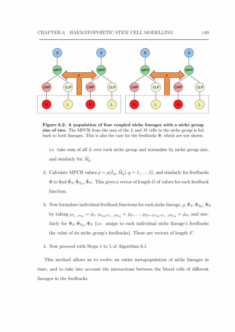
CHAPTER 6. HAEMATOPOIETIC STEM CELL MODELLING 140
Figure 6.2: A population of four coupled niche lineages with a niche groupsize of two. The MPCR from the sum of the L and M cells in the niche group is fedback to both lineages. This is also the case for the feedbacks Φ, which are not shown.
i.e. take sum of all L over each niche group and normalise by niche group size,
and similarly for Mg.
2. Calculate MPCR values ρ = ρ(Lg, Mg), g = 1, . . . , G, and similarly for feedbacks
Φ to find ΦS, ΦSD, ΦP . This gives a vector of length G of values for each feedback
function.
3. Now formulate individual feedback functions for each niche lineage, ρ,ΦS,ΦSD,ΦP
by taking ρ1,...,sng = ρ1, ρsng+1,...,2sng = ρ2,. . . , ρ(G−1)sng+1,...,Gsng = ρG, and sim-
ilarly for ΦS,ΦSD,ΦP (i.e. assign to each individual niche lineage’s feedbacks
the value of its niche group’s feedbacks). These are vectors of length F .
4. Now proceed with Steps 1 to 5 of Algorithm 6.1.
This method allows us to evolve an entire metapopulation of niche lineages in
time, and to take into account the interactions between the blood cells of different
lineages in the feedbacks.
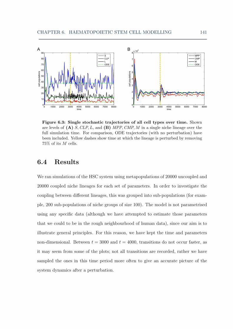
CHAPTER 6. HAEMATOPOIETIC STEM CELL MODELLING 141
Figure 6.3: Single stochastic trajectories of all cell types over time. Shownare levels of (A) S,CLP, L, and (B) MPP,CMP,M in a single niche lineage over thefull simulation time. For comparison, ODE trajectories (with no perturbation) havebeen included. Yellow dashes show time at which the lineage is perturbed by removing75% of its M cells.
6.4 Results
We ran simulations of the HSC system using metapopulations of 20000 uncoupled and
20000 coupled niche lineages for each set of parameters. In order to investigate the
coupling between different lineages, this was grouped into sub-populations (for exam-
ple, 200 sub-populations of niche groups of size 100). The model is not parametrised
using any specific data (although we have attempted to estimate those parameters
that we could to be in the rough neighbourhood of human data), since our aim is to
illustrate general principles. For this reason, we have kept the time and parameters
non-dimensional. Between t = 3000 and t = 4000, transitions do not occur faster, as
it may seem from some of the plots; not all transitions are recorded, rather we have
sampled the ones in this time period more often to give an accurate picture of the
system dynamics after a perturbation.
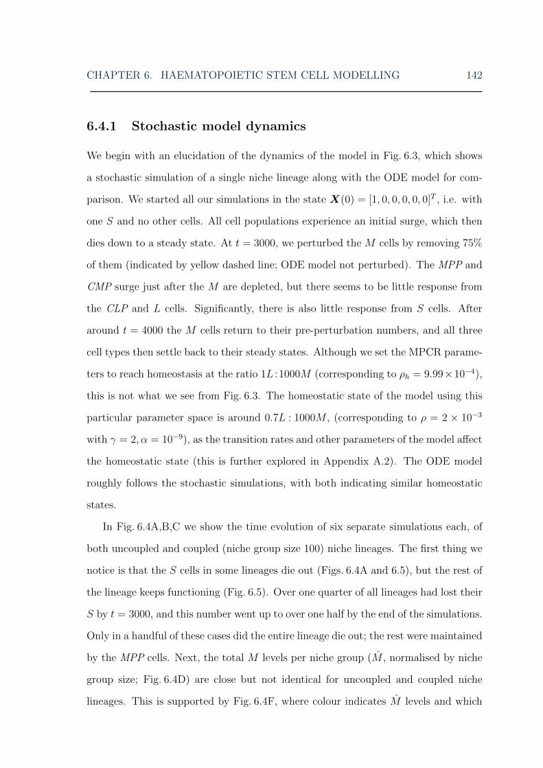
CHAPTER 6. HAEMATOPOIETIC STEM CELL MODELLING 142
6.4.1 Stochastic model dynamics
We begin with an elucidation of the dynamics of the model in Fig. 6.3, which shows
a stochastic simulation of a single niche lineage along with the ODE model for com-
parison. We started all our simulations in the state X(0) = [1, 0, 0, 0, 0, 0]T , i.e. with
one S and no other cells. All cell populations experience an initial surge, which then
dies down to a steady state. At t = 3000, we perturbed the M cells by removing 75%
of them (indicated by yellow dashed line; ODE model not perturbed). The MPP and
CMP surge just after the M are depleted, but there seems to be little response from
the CLP and L cells. Significantly, there is also little response from S cells. After
around t = 4000 the M cells return to their pre-perturbation numbers, and all three
cell types then settle back to their steady states. Although we set the MPCR parame-
ters to reach homeostasis at the ratio 1L : 1000M (corresponding to ρh = 9.99×10⁻⁴),
this is not what we see from Fig. 6.3. The homeostatic state of the model using this
particular parameter space is around 0.7L : 1000M , (corresponding to ρ = 2 × 10⁻³
with γ = 2, α = 10−9), as the transition rates and other parameters of the model affect
the homeostatic state (this is further explored in Appendix A.2). The ODE model
roughly follows the stochastic simulations, with both indicating similar homeostatic
states.
In Fig. 6.4A,B,C we show the time evolution of six separate simulations each, of
both uncoupled and coupled (niche group size 100) niche lineages. The first thing we
notice is that the S cells in some lineages die out (Figs. 6.4A and 6.5), but the rest of
the lineage keeps functioning (Fig. 6.5). Over one quarter of all lineages had lost their
S by t = 3000, and this number went up to over one half by the end of the simulations.
Only in a handful of these cases did the entire lineage die out; the rest were maintained
by the MPP cells. Next, the total M levels per niche group (M , normalised by niche
group size; Fig. 6.4D) are close but not identical for uncoupled and coupled niche
lineages. This is supported by Fig. 6.4F, where colour indicates M levels and which
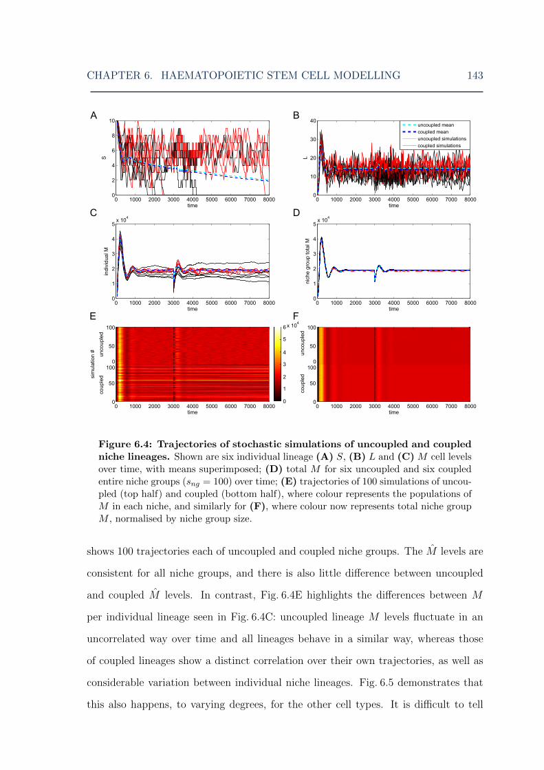
CHAPTER 6. HAEMATOPOIETIC STEM CELL MODELLING 143
Figure 6.4: Trajectories of stochastic simulations of uncoupled and coupledniche lineages. Shown are six individual lineage (A) S, (B) L and (C) M cell levelsover time, with means superimposed; (D) total M for six uncoupled and six coupledentire niche groups (sng = 100) over time; (E) trajectories of 100 simulations of uncou-pled (top half) and coupled (bottom half), where colour represents the populations ofM in each niche, and similarly for (F), where colour now represents total niche groupM , normalised by niche group size.
shows 100 trajectories each of uncoupled and coupled niche groups. The M levels are
consistent for all niche groups, and there is also little difference between uncoupled
and coupled M levels. In contrast, Fig. 6.4E highlights the differences between M
per individual lineage seen in Fig. 6.4C: uncoupled lineage M levels fluctuate in an
uncorrelated way over time and all lineages behave in a similar way, whereas those
of coupled lineages show a distinct correlation over their own trajectories, as well as
considerable variation between individual niche lineages. Fig. 6.5 demonstrates that
this also happens, to varying degrees, for the other cell types. It is difficult to tell

CHAPTER 6. HAEMATOPOIETIC STEM CELL MODELLING 144
Figure 6.5: Trajectories of stochastic simulations of all cell species, with sixuncoupled and six coupled niche lineages. Plots start from t = 2000 to omit theinitial cell level fluctuations. Plots for S, L and M correspond to Fig. 6.4A,B,C.
whether this is also the case for L, where stochastic fluctuations are large compared to
cell numbers, but Fig. 6.6 helps to clarify the issue: the steady states of the uncoupled
and coupled L are also fairly close but not identical (Fig. 6.6A,C), and in Fig. 6.6B we
can make out the distinct lines made by the coupled lineage L levels, implying their
fluctuations are correlated compared to the uncoupled lineages. To sum up so far,
Figs. 6.4, 6.5 and 6.6 tell us that 1) although the MPP have a large surge in numbers,
there is a smaller relative response in numbers of S; 2) there is also a large surge in
CMP numbers to replenish the lost M , which corresponds to a modest drop in CLP
and L numbers followed by a small surge to return to their steady states; 3) cell levels
in individual uncoupled niche lineages fluctuate considerably with time, whereas those
of coupled niche lineages less so; 4) however, cell levels between individual coupled
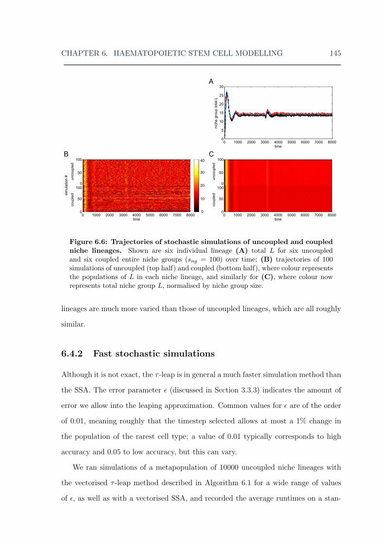
CHAPTER 6. HAEMATOPOIETIC STEM CELL MODELLING 145
Figure 6.6: Trajectories of stochastic simulations of uncoupled and coupledniche lineages. Shown are six individual lineage (A) total L for six uncoupledand six coupled entire niche groups (sng = 100) over time; (B) trajectories of 100simulations of uncoupled (top half) and coupled (bottom half), where colour representsthe populations of L in each niche lineage, and similarly for (C), where colour nowrepresents total niche group L, normalised by niche group size.
lineages are much more varied than those of uncoupled lineages, which are all roughly
similar.
6.4.2 Fast stochastic simulations
Although it is not exact, the τ -leap is in general a much faster simulation method than
the SSA. The error parameter ε (discussed in Section 3.3.3) indicates the amount of
error we allow into the leaping approximation. Common values for ε are of the order
of 0.01, meaning roughly that the timestep selected allows at most a 1% change in
the population of the rarest cell type; a value of 0.01 typically corresponds to high
accuracy and 0.05 to low accuracy, but this can vary.
We ran simulations of a metapopulation of 10000 uncoupled niche lineages with
the vectorised τ -leap method described in Algorithm 6.1 for a wide range of values
of ε, as well as with a vectorised SSA, and recorded the average runtimes on a stan-

CHAPTER 6. HAEMATOPOIETIC STEM CELL MODELLING 146
dard desktop computer. The SSA can be regarded as finding the exact solution (for
uncoupled niche lineages only – it loses this exactness when the lineages are coupled,
see Section 6.3.1). Therefore we compared the probability density functions (PDFs)
returned by the τ -leap to the exact PDF given by the SSA to get an idea of how the
errors of the τ -leap simulations changed as the error parameter was varied.
Table 6.3: Runtimes and errors of the vectorised τ-leap method in Algo-rithm 6.1 compared to the SSA. The errors are calculated by taking the L1-distance of the weight of each point of the τ -leap PDF (that is, value multiplied bybin width) from the SSA PDF. The error in the SSA row is the SSA self-distance, i.e.the error between two different SSA simulations. These simulations are of uncoupledniche lineages only, hence the SSA can be regarded as the true solution.
Simulation method Runtime (hours) Total error
SSA 67.4 0.201τ -leap, ε = 0.001 44.6 0.173τ -leap, ε = 0.005 6.7 0.175τ -leap, ε = 0.01 2.9 0.189τ -leap, ε = 0.05 0.9 0.214τ -leap, ε = 0.1 0.7 0.312
The simulation runtimes are listed in Table 6.3, as is the total error of the τ -leap
results. We calculated these by summing the absolute values of the difference between
the weight of each bin of the τ -leap PDFs (that is, probability density multiplied by
bin width) as compared to the PDF of the SSA, i.e. we took the L1-distance between
the weights of the τ -leap and SSA PDF bins. The runtimes decrease as the error
parameters increase, with the SSA taking the longest, as expected. The self-distance
of two different SSA simulations is relatively large (Table 6.3, row 1), indicating that
the differences in errors between the τ -leap with ε = 0.001,0.005 and 0.01 may be
due to Monte Carlo error. This means that the vectorised τ -leap with these error
parameters is about as accurate as the SSA. With ε = 0.05 and 0.1, however, the τ -
leap does become substantially less accurate. The difference in runtime between using
ε = 0.01 and 0.05 is around 2 hours for some gain in accuracy, meaning that the former
is probably the most efficient error parameter in this case. Accordingly, in the rest of
our simulations, we used ε = 0.01. Table 6.3 confirms that the τ -leap is indeed faster
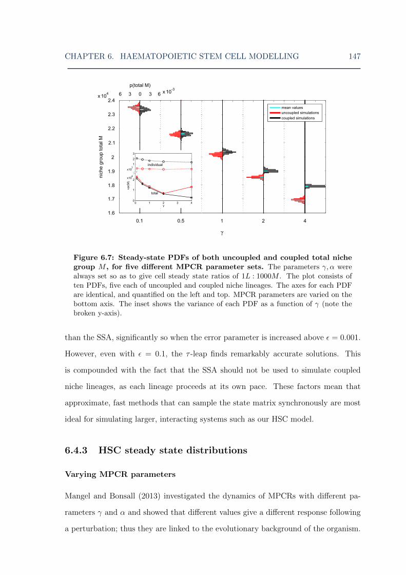
CHAPTER 6. HAEMATOPOIETIC STEM CELL MODELLING 147
Figure 6.7: Steady-state PDFs of both uncoupled and coupled total nichegroup M , for five different MPCR parameter sets. The parameters γ, α werealways set so as to give cell steady state ratios of 1L : 1000M . The plot consists often PDFs, five each of uncoupled and coupled niche lineages. The axes for each PDFare identical, and quantified on the left and top. MPCR parameters are varied on thebottom axis. The inset shows the variance of each PDF as a function of γ (note thebroken y-axis).
than the SSA, significantly so when the error parameter is increased above ε = 0.001.
However, even with ε = 0.1, the τ -leap finds remarkably accurate solutions. This
is compounded with the fact that the SSA should not be used to simulate coupled
niche lineages, as each lineage proceeds at its own pace. These factors mean that
approximate, fast methods that can sample the state matrix synchronously are most
ideal for simulating larger, interacting systems such as our HSC model.
6.4.3 HSC steady state distributions
Varying MPCR parameters
Mangel and Bonsall (2013) investigated the dynamics of MPCRs with different pa-
rameters γ and α and showed that different values give a different response following
a perturbation; thus they are linked to the evolutionary background of the organism.
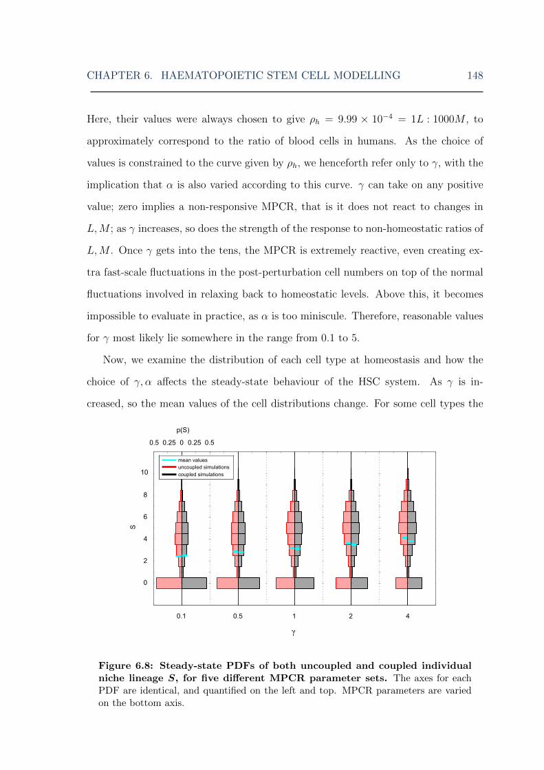
CHAPTER 6. HAEMATOPOIETIC STEM CELL MODELLING 148
Here, their values were always chosen to give ρh = 9.99 × 10−4 = 1L : 1000M , to
approximately correspond to the ratio of blood cells in humans. As the choice of
values is constrained to the curve given by ρh, we henceforth refer only to γ, with the
implication that α is also varied according to this curve. γ can take on any positive
value; zero implies a non-responsive MPCR, that is it does not react to changes in
L,M ; as γ increases, so does the strength of the response to non-homeostatic ratios of
L,M . Once γ gets into the tens, the MPCR is extremely reactive, even creating ex-
tra fast-scale fluctuations in the post-perturbation cell numbers on top of the normal
fluctuations involved in relaxing back to homeostatic levels. Above this, it becomes
impossible to evaluate in practice, as α is too miniscule. Therefore, reasonable values
for γ most likely lie somewhere in the range from 0.1 to 5.
Now, we examine the distribution of each cell type at homeostasis and how the
choice of γ, α affects the steady-state behaviour of the HSC system. As γ is in-
creased, so the mean values of the cell distributions change. For some cell types the
Figure 6.8: Steady-state PDFs of both uncoupled and coupled individualniche lineage S, for five different MPCR parameter sets. The axes for eachPDF are identical, and quantified on the left and top. MPCR parameters are variedon the bottom axis.
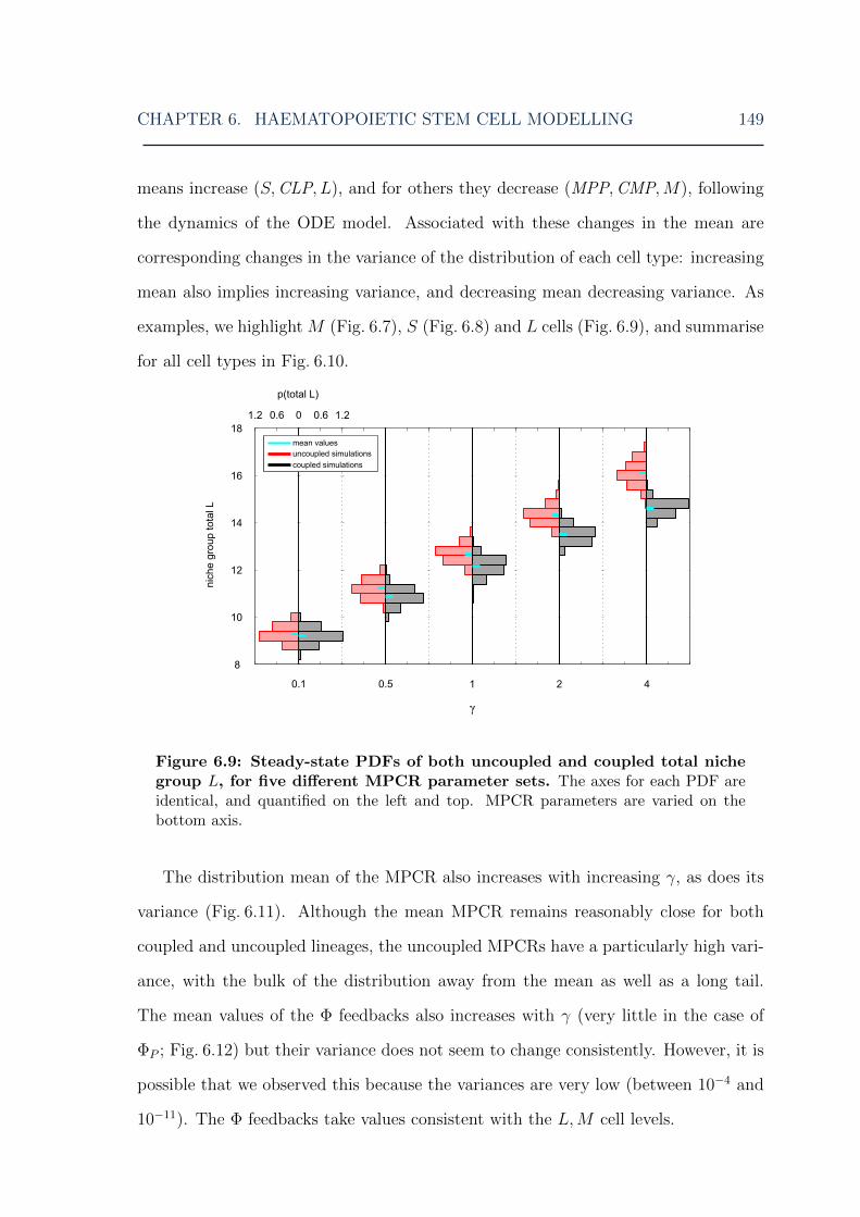
CHAPTER 6. HAEMATOPOIETIC STEM CELL MODELLING 149
means increase (S,CLP, L), and for others they decrease (MPP,CMP,M), following
the dynamics of the ODE model. Associated with these changes in the mean are
corresponding changes in the variance of the distribution of each cell type: increasing
mean also implies increasing variance, and decreasing mean decreasing variance. As
examples, we highlight M (Fig. 6.7), S (Fig. 6.8) and L cells (Fig. 6.9), and summarise
for all cell types in Fig. 6.10.
Figure 6.9: Steady-state PDFs of both uncoupled and coupled total nichegroup L, for five different MPCR parameter sets. The axes for each PDF areidentical, and quantified on the left and top. MPCR parameters are varied on thebottom axis.
The distribution mean of the MPCR also increases with increasing γ, as does its
variance (Fig. 6.11). Although the mean MPCR remains reasonably close for both
coupled and uncoupled lineages, the uncoupled MPCRs have a particularly high vari-
ance, with the bulk of the distribution away from the mean as well as a long tail.
The mean values of the Φ feedbacks also increases with γ (very little in the case of
ΦP ; Fig. 6.12) but their variance does not seem to change consistently. However, it is
possible that we observed this because the variances are very low (between 10−4 and
10−11). The Φ feedbacks take values consistent with the L,M cell levels.
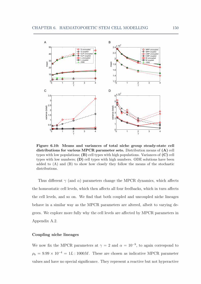
CHAPTER 6. HAEMATOPOIETIC STEM CELL MODELLING 150
Figure 6.10: Means and variances of total niche group steady-state celldistributions for various MPCR parameter sets. Distribution means of (A) celltypes with low populations; (B) cell types with high populations. Variances of (C) celltypes with low numbers; (D) cell types with high numbers. ODE solutions have beenadded to (A) and (B) to show how closely they follow the means of the stochasticdistributions.
Thus different γ (and α) parameters change the MPCR dynamics, which affects
the homeostatic cell levels, which then affects all four feedbacks, which in turn affects
the cell levels, and so on. We find that both coupled and uncoupled niche lineages
behave in a similar way as the MPCR parameters are altered, albeit to varying de-
grees. We explore more fully why the cell levels are affected by MPCR parameters in
Appendix A.2.
Coupling niche lineages
We now fix the MPCR parameters at γ = 2 and α = 10−9, to again correspond to
ρh = 9.99 × 10−4 = 1L : 1000M . These are chosen as indicative MPCR parameter
values and have no special significance. They represent a reactive but not hyperactive

CHAPTER 6. HAEMATOPOIETIC STEM CELL MODELLING 151
Figure 6.11: Steady-state PDFs of both uncoupled and coupled MPCRvalues in each individual niche lineage, for five different MPCR parametersets. The axes for each PDF are identical, and quantified on the left and top. MPCRparameters are varied on the bottom axis.
MPCR intended to highlight any dynamics arising from varying the niche grouping
size, which we now turn our attention to. When taken individually, it is the uncoupled
niche lineages that are regulated more tightly, with theM levels of the coupled lineages
having a much wider distribution (Fig. 6.13A). In contrast, from a systemic view the
situation is the opposite: when looking at total cell levels per niche group (normalised
Figure 6.12: Means and variances of total niche group feedback distribu-tions for various MPCR parameter sets. (A) Distribution means, and (B) vari-ances for different MPCR parameter sets.
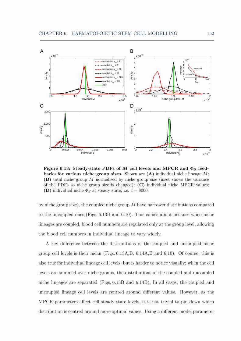
CHAPTER 6. HAEMATOPOIETIC STEM CELL MODELLING 152
Figure 6.13: Steady-state PDFs of M cell levels and MPCR and ΦS feed-backs for various niche group sizes. Shown are (A) individual niche lineage M ;(B) total niche group M normalised by niche group size (inset shows the varianceof the PDFs as niche group size is changed); (C) individual niche MPCR values;(D) individual niche ΦS at steady state, i.e. t = 8000.
by niche group size), the coupled niche group M have narrower distributions compared
to the uncoupled ones (Figs. 6.13B and 6.10). This comes about because when niche
lineages are coupled, blood cell numbers are regulated only at the group level, allowing
the blood cell numbers in individual lineage to vary widely.
A key difference between the distributions of the coupled and uncoupled niche
group cell levels is their mean (Figs. 6.13A,B, 6.14A,B and 6.10). Of course, this is
also true for individual lineage cell levels, but is harder to notice visually; when the cell
levels are summed over niche groups, the distributions of the coupled and uncoupled
niche lineages are separated (Figs. 6.13B and 6.14B). In all cases, the coupled and
uncoupled lineage cell levels are centred around different values. However, as the
MPCR parameters affect cell steady state levels, it is not trivial to pin down which
distribution is centred around more optimal values. Using a different model parameter

CHAPTER 6. HAEMATOPOIETIC STEM CELL MODELLING 153
Figure 6.14: Steady-state distributions of L cell numbers for various nichegroup sizes. PDFs of (A) individual niche lineage L and (B) niche group total L,normalised by niche group size, at t = 8000 for various niche group sizes. Inset showsthe variance of niche group total L PDFs as a function of niche group size.
setup to investigate, we found that it was indeed the coupled niche lineages that
regulated their cell levels to be closer to ρh (Appendix A.3).
The corresponding homeostatic distributions of two of the feedback functions are
shown in Fig. 6.13C,D. In contrast to the cell levels, it is the feedbacks of individ-
ual coupled niche lineages that are more tightly-distributed, and this effect becomes
stronger as niche group size is increased. This suggests that it may be due to the
niche lineage grouping, because within each niche group the feedbacks are identical.
To check this, we next calculated the mean feedbacks in each niche group. It turns
out that the distribution of the feedbacks is indeed controlled by the coupling, and the
mean feedbacks per niche group have similar distributions, whether they are coupled
or uncoupled (Fig. 6.15). The figure also shows that the niche group size changes the
feedbacks’ distribution means. This is again a case of the coupled MPCRs affecting
the mean cell levels in each niche group, which then affect the Φ feedbacks, which in
turn affect the cell levels.
We find that coupling individual niche lineages together into niche groups, by
pooling the blood cells of the group in the feedbacks, has an effect on the distributions
of the cells as well as of the feedbacks. This effect is positive, in that it allows the
blood cell numbers to be regulated more closely to the homeostatic levels dictated by
the model.

CHAPTER 6. HAEMATOPOIETIC STEM CELL MODELLING 154
Figure 6.15: Steady-state distributions of feedbacks for various niche groupsizes. PDFs of (A) niche group mean MPCR and (B) niche group mean ΦS att = 8000 for various niche group sizes.
6.4.4 Perturbation analysis
Next, we look more closely at the response of the system to perturbations. We examine
three types of perturbation: even perturbations (37.5% reduction of M from every
niche lineage), uneven perturbations (75% reduction of M from every second lineage
only), and random, or more precisely, probabilistic, where each lineage has a 50%
chance that its M are reduced by 75%. The perturbations were chosen to cause,
on average, an identical change in cell levels across the entire population of niche
lineages, that is the removal of 37.5% of the entire population of M . The actual
values of 37.5% and 75% are illustrative in nature, rather than realistic examples
of blood loss from injury. In the interest of brevity, we first restrict ourselves to a
random-type perturbation only.
The response of the system to perturbations is given by two main indicators: return
time to homeostatic levels, and overshoot/oscillation size, defined as the difference
between the maximum of the post-perturbation spike in cell numbers (and feedbacks)
and their steady states. Return time, much like the homeostatic levels of the system,
is dictated by the model parameters. Moreover, it is difficult to accurately measure,
as even in homeostasis, there is a continuous turnover of cells, leading to fluctuations
in the cell levels. We did not find a substantial difference in return time between

CHAPTER 6. HAEMATOPOIETIC STEM CELL MODELLING 155
uncoupled and coupled niche lineages for any type of perturbation, and the ODE
model and the mean of the stochastic system closely matched in this respect.
Varying MPCR parameters
Plotting the trajectories of the mean cell levels in time allows us to easily quantify
the recovery of the entire metapopulation after a perturbation, as opposed to the
complications arising from comparing many PDFs. Fig. 6.16 shows the response of
mean L and M levels, as well as the MPCR and ΦS feedbacks for various values
of γ. As discussed above, the steady states are influenced by the choice of γ. The
post-perturbation fluctuations of both cell levels and feedbacks are also affected, with
no clear trend in overshoot of L but an increase in overshoot of M as γ is increased;
the overshoot of the MPCR also increases with γ, in contrast to the Φ feedbacks,
whose overshoot decreases (Fig. 6.16 insets). As γ is increased, the MPCR becomes
more responsive, implying a larger overshoot after changes in cell levels. However,
contrary to expectations, this seems to affect the levels of L and M in a complicated
way. Finally, the one factor that is consistent in Fig. 6.16 is that the coupled lineages
have smaller overshoot than uncoupled ones, both for cell and feedback levels.
Coupling niche lineages
We again fix γ = 2 and α = 10−9, and focus on niche group size. We have already
seen that the distribution means of both coupled L and M more closely approached
the desired ρh as niche group size was increased; this is supported by Fig. 6.17A,B,
which show the mean L and M over time. It is important to realise that this is not a
result of the summing process to calculate total niche group L and M . As a control,
we also plot the distribution means of the uncoupled niche lineages, each of which
were summed over niche groups as with their coupled counterparts; their mean levels
are so similar that they are almost indistinguishable from each other in the figures.
In Appendix A.3 we show that the ODE model does give a good indication of the
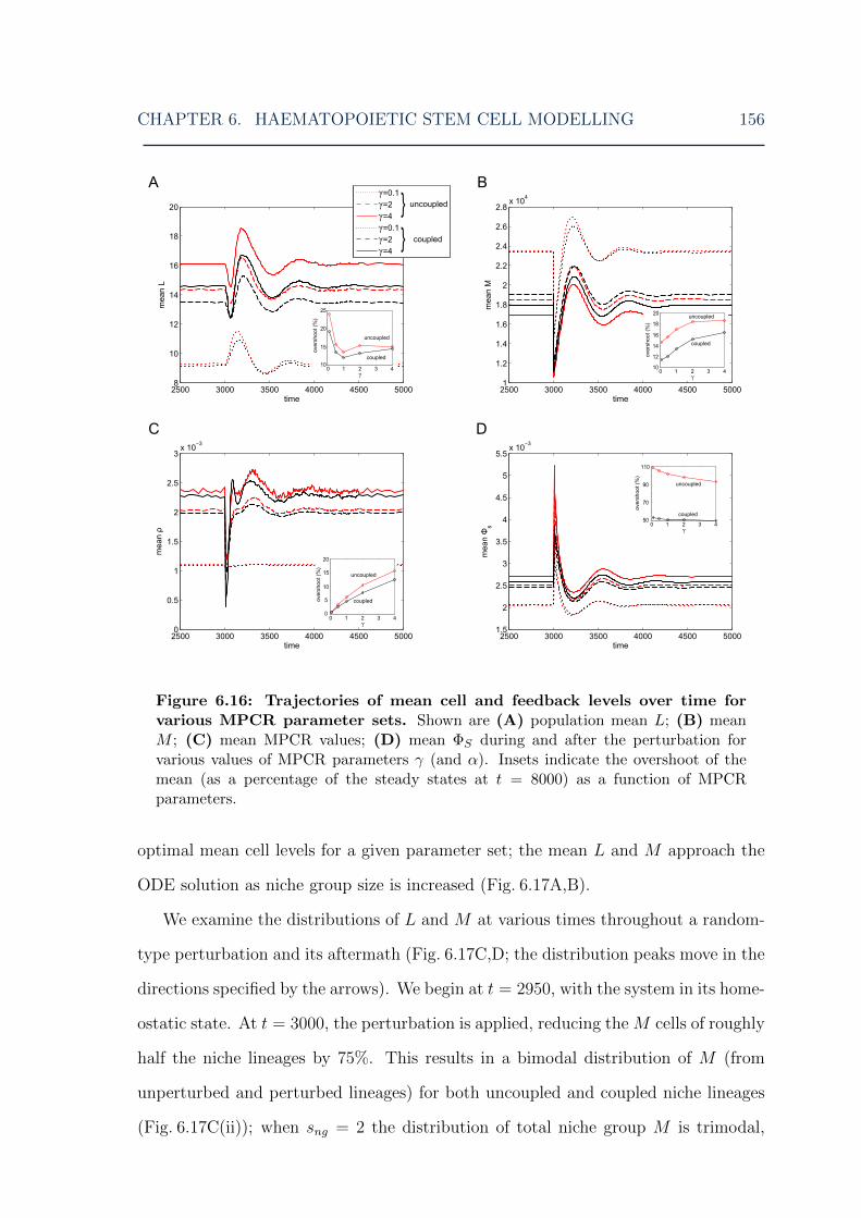
CHAPTER 6. HAEMATOPOIETIC STEM CELL MODELLING 156
Figure 6.16: Trajectories of mean cell and feedback levels over time forvarious MPCR parameter sets. Shown are (A) population mean L; (B) meanM ; (C) mean MPCR values; (D) mean ΦS during and after the perturbation forvarious values of MPCR parameters γ (and α). Insets indicate the overshoot of themean (as a percentage of the steady states at t = 8000) as a function of MPCRparameters.
optimal mean cell levels for a given parameter set; the mean L and M approach the
ODE solution as niche group size is increased (Fig. 6.17A,B).
We examine the distributions of L and M at various times throughout a random-
type perturbation and its aftermath (Fig. 6.17C,D; the distribution peaks move in the
directions specified by the arrows). We begin at t = 2950, with the system in its home-
ostatic state. At t = 3000, the perturbation is applied, reducing the M cells of roughly
half the niche lineages by 75%. This results in a bimodal distribution of M (from
unperturbed and perturbed lineages) for both uncoupled and coupled niche lineages
(Fig. 6.17C(ii)); when sng = 2 the distribution of total niche group M is trimodal,

CHAPTER 6. HAEMATOPOIETIC STEM CELL MODELLING 157
Figure 6.17: Evolution of population means and distributions of cell levelsaround the perturbation. Population means of (A) L; (B) M for various nichegroup sizes during and after the perturbation. In addition, we plot PDFs of (C)individual lineage M and (D) total niche group M at the time points labelled withblue arrows in (B). Arrows indicate which direction the peaks are moving with time.
since the possibilities are either zero, one or two perturbed niches per niche group
(Fig. 6.17D(ii)). By t = 3175, the individual coupled lineages’ M cells had resumed
their previous unimodal shape, but the uncoupled niches retained their bimodality
(Fig. 6.17C(iii)). By t = 3560, the individual uncoupled lineages’ M cells were also
starting to coalesce into a unimodal distribution again (Fig. 6.17C(v)). Throughout,
except for very close to the perturbation time, the distributions of the total niche
group M with sng = 100 kept their shape, with the coupled niches remaining centred
closer to the optimal homeostatic state (Fig. 6.17D).
Repeating this for the MPCR and ΦS feedbacks, we see that the response of the
feedbacks after the perturbation is approximately similar, albeit again with small
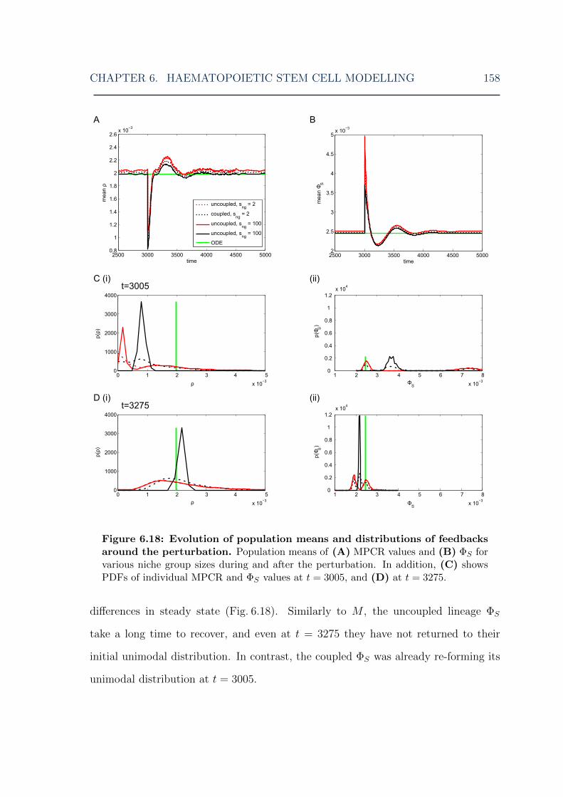
CHAPTER 6. HAEMATOPOIETIC STEM CELL MODELLING 158
Figure 6.18: Evolution of population means and distributions of feedbacksaround the perturbation. Population means of (A) MPCR values and (B) ΦS forvarious niche group sizes during and after the perturbation. In addition, (C) showsPDFs of individual MPCR and ΦS values at t = 3005, and (D) at t = 3275.
differences in steady state (Fig. 6.18). Similarly to M , the uncoupled lineage ΦS
take a long time to recover, and even at t = 3275 they have not returned to their
initial unimodal distribution. In contrast, the coupled ΦS was already re-forming its
unimodal distribution at t = 3005.
CHAPTER 6. HAEMATOPOIETIC STEM CELL MODELLING 159
Different perturbation types
Finally, for an overview of the response of the system, we investigate how the over-
shoot of the mean cell/feedback levels change for all three different perturbation types:
even, uneven and random (Fig. 6.19). The overshoot response of the cell levels is dif-
ferent for each perturbation type (Fig. 6.19A,B): even perturbations affect all lineages
equally, with the overshoots of uncoupled lineages slightly lower than coupled ones.
Uneven perturbations, where the M of every second niche lineage are perturbed, re-
sult in a smaller overshoot for coupled lineages than uncoupled ones, but this does
not vary with niche grouping size. In contrast, random perturbations result in both
a difference in overshoot between coupled and uncoupled lineages, with coupled ones
having smaller overshoot, as well as a further decrease in the overshoot of the coupled
lineages as niche grouping size is increased. The feedbacks also respond in a very
similar way (Fig. 6.19C,D). Thus, we see that the response of the system is strongly
dependent on perturbation type, with niche group size having no effect in the case of
even and uneven perturbations, but random perturbations eliciting a more optimal
response when the niches are coupled in larger groups.
6.5 Discussion
A large niche group size indicates that the feedback from the blood cells (L,M) to
the primitive cells (S,MPP) is regulated by a large fraction of the overall blood cell
numbers in the organism. We found that as niche group size was increased, the
mean levels of L,M moved closer to the ODE model solutions. This is not a surprise:
summing the blood cells in each niche group and normalising is equivalent to averaging
over niche groups; the larger the niche group, therefore, the less noise in total cells
per niche group, and the closer the system is to the ODE model. However, the
question remained of whether it was the uncoupled lineages or the coupled ones (and
the ODEs) that represented the more optimal cell levels. From the control system

CHAPTER 6. HAEMATOPOIETIC STEM CELL MODELLING 160
Figure 6.19: Overshoots of mean cell levels and feedbacks for variousniche group sizes and perturbation types. Overshoots of mean (A) L; (B) M ;(C) MPCR; (D) ΦS for various values niche group sizes and three perturbation types.An even perturbation signifies a 37.5% reduction in M in every niche lineage, unevena 75% reduction of M in every second lineage and random is a 50% chance of eachlineage losing 75% of its M .
perspective that we have taken, optimality is defined as regulation of the cell levels
to the desired ratio 1L : 1000M . Given the interactions of the MPCR parameters and
this ratio in setting the cell steady states (see Appendix A.3), the ODE solutions, and
therefore the coupled niche lineages, followed the desired cell levels more closely than
the uncoupled ones. Thus, it seems that on a systemic level, it is advantageous to
connect the feedbacks from the blood cells. This hints at some intriguing possibilities
for understanding the emergence of tissues, which are interacting populations of single
cells.
The difference between the overshoots for the three perturbation types can be

CHAPTER 6. HAEMATOPOIETIC STEM CELL MODELLING 161
understood as follows. The even perturbation should result in a similar overshoot
from both uncoupled and coupled niche lineages, since it affects all niches equally.
This is consistent with our results for M , but it is unclear why the overshoot of
the uncoupled L is lower. The uneven perturbation affects uncoupled and coupled
lineages differently, with coupled niches having smaller overshoot, but there is no
variation with niche group size. Because it is a regular perturbation, coupling lineages
(into even-sized groups) reduces the niche group overshoot, and it does not change
with niche group size as in every case 37.5% of the cells in each niche group are lost.
However, random perturbations elicited yet another response. With smaller groups, or
individual lineages, it is more likely that the entire niche group is perturbed, resulting
in a larger overshoot. At the extreme end of the scale, one could conceivably have one
niche group with all niche lineages perturbed, and another with none. As niche group
size is increased the chances of this decrease and the percentage of total niche group M
that is lost tends asymptotically to 37.5%, with the overshoot declining to the same
levels as for an uneven perturbation. This shows that in environments with even
perturbations, it may be advantageous to not couple niche lineages – however such an
environment is unlikely to occur in nature. In contrast, in natural environments with
random perturbations, coupling niche lineages results in a more favourable response.
In previous work, Mangel and Bonsall (2008, 2013) modelled both a general stem
cell system and the haematopoietic system in particular. They employed both ODE
models, to illustrate mean behaviour, as well as stochastic simulations to find the
variation around this mean. In a general setting, they showed that the overdispersed
cell cycle times found by Till et al. (1964) could be reproduced in a stochastic model,
and considered competition within a stem cell niche to find when a resident stem
cell population is replaced by an invading one (Mangel and Bonsall, 2008). In the
HSC setting, they introduced the concept of the MPCR, which sets the probability
of a progenitor cell differentiating into either a myeloid or lymphoid route, and is
controlled by demand from the organism as a whole. They showed that the MPCR
CHAPTER 6. HAEMATOPOIETIC STEM CELL MODELLING 162
parameters affect the fitness of the organism in specific environments, and could be a
result of evolution of that organism to its environment (Mangel and Bonsall, 2013).
Here, we have started with this framework and concerned ourselves with simulations
of an entire metapopulation of HSC niche lineages in order to elucidate the stochastic
dynamics of the system as well as how introducing interactions into the feedback from
the differentiated blood cells affects the dynamics of the population.
One interesting result from our model is the large variation we see in cell levels of
coupled lineages between different lineages in the same niche group, and the relatively
low variation over time of the levels in each lineage. This indicates that the activity
of the primitive cells of each lineage varies, with some inactive/less active and others
continuously differentiating to produce more cells, in order to achieve the correct
homeostatic cell levels, somewhat akin to the HSC subsets found by Sieburg et al.
(2006). Although we have not explicitly considered it here, our model naturally
captures the cycling behaviour of HSCs, with periods of quiescence and activity in
each lineage (Cheshier et al., 1999). In addition, after a perturbation, our model finds
a response from both stem and progenitor cells. This is in agreement with studies
finding stem cell activation after injury (e.g., Cheshier et al., 2007), but also supports
the suggestion that at least part of the response is from progenitor cells (Morrison
and Kimble, 2006).
Our results indicate that, in order to regulate blood cell levels tightly and for a less
severe response following random perturbations, it is advantageous to the organism
to couple haematopoietic lineages together via the feedbacks from blood cells on to
primitive cells. There are three biologically-viable possibilities for the nature of this
feedback mechanism: lineage-dependent feedback, where the primitive cells in one
lineage can only sense numbers of their own differentiated progeny; local feedback,
where the primitive cells can sense blood cells of any lineage in proximity to them;
global feedback, where all primitive cells can sense all blood cells in the organism.
Lineage-dependent feedback would require a biochemical mechanism in which niche

CHAPTER 6. HAEMATOPOIETIC STEM CELL MODELLING 163
lineages (or niche groups) can identify signals from their descendants and respond
to the demand control from those cells, but not others in the blood; this implies
an epigenetic process. Indeed, studies have found that stem cell daughters of HSCs
have a similar lifetime to their parents (Sieburg et al., 2011), and such an epigenetic
mechanism could also exist in non-primitive progeny to regulate their feedback. Local
feedback implies a spatial constraint on the feedbacks; although this has already been
found to exist in the case of certain HSC progeny as well as other niche cells (Hsu
and Fuchs, 2012), it is unlikely to be a universal mechanism for the haematopoietic
system because most blood cells enter the bloodstream rather than localising around
the niche. However, in other stem cell systems it is a plausible mode of feedback, and
remains to be investigated (O’Brien and Bilder, 2013). In contrast, global feedback
would require the HSC to sense every blood cell in the bloodstream. Since it is likely
that the feedbacks from the blood cells occur via growth factors (Lander et al., 2009),
which naturally have a limit on their range of action, it does not seem likely that the
HSC system incorporates global feedbacks from all blood cells. More likely is some
combination of the above mechanisms, with HSCs sensing either their own progeny
or all blood cells within some limited spatial range. Looking for groups of epigenetic
markers shared by HSC, progenitor cells and differentiated blood cells could be a
useful avenue for further experimental work. Finally, as evidenced by the dynamics
of our model, the feedbacks are essential for achieving homeostatic cell rates (Lander
et al., 2009). Although we have not explored this issue further, our results also support
the idea that cancers may be a failure of the signalling mechanism and the associated
feedback control (Rodriguez-Brenes et al., 2011).
In ODE models, one can only account for a single, or at best an identical set of
deterministic niche lineages, so that the interactions between a heterogeneous metapop-
ulation of lineages is underexplored theoretically. This is important for two reasons:
first, the dynamics of the entire system cannot be determined just by looking at its
parts, and second, we can take a much broader point of view by looking at an entire

CHAPTER 6. HAEMATOPOIETIC STEM CELL MODELLING 164
population (Mangel and Bonsall, 2007). Indeed, Huang (2011) suggests that this is
one of three as-yet-neglected perspectives that should be adopted in stem cell mod-
elling. For example, maintaining homeostasis at the population level can be achieved
by several possible strategies (Morrison and Kimble, 2006); just modelling a single
stem cell restricts consideration to just one strategy, asymmetric division, which does
not reveal the full picture. A stochastic treatment is needed to be able to incorporate
population-level strategies such as a combination of both asymmetric and symmetric
division and differentiation. Our work also links with the idea of a potential land-
scape of cell states (e.g., Wang et al., 2010): one simulation represents a niche lineage
moving along the landscape and falling into a stable state, and many simulations,
as we have done, could allow us to reconstruct the potential landscape by randomly
generating trajectories until we can see its full shape. Thus Monte Carlo simulations
offer a computational way to explore the potential landscape.
6.6 Conclusions
In this chapter, we first introduced a fast method of simulating an entire metapop-
ulation of interacting niche lineages (or cells or biochemical species) synchronously
through time. This is based on a version of the τ -leap method (Gillespie, 2001) and
then generalised to the population level. It compares favourably with the popular
SSA (Gillespie, 1977), both in terms of speed and accuracy – when interactions are
to be included, the stochastic simulation algorithm averages them over time, as each
member of the population proceeds through time at a different pace. The computa-
tional method we have proposed here can be combined with many stochastic method-
ologies in order to allow one to quickly and easily simulate whole metapopulations.
Naturally, it is not limited to HSC metapopulations, and can be used in any con-
text where we would otherwise use Gillespie’s standard SSA to simulate biochemical
populations without tracking individual particles. For instance, with no interactions

CHAPTER 6. HAEMATOPOIETIC STEM CELL MODELLING 165
specified, it can be used to simultaneously run many repeat simulations of the same
chemical reaction system (by regarding each state vector as a separate simulation), in
order to find the full distribution possible states, arising from intrinsic noise, at some
time. However, it is especially useful when we are interested in interacting popula-
tions/metapopulations; for instance, this is often the case in ecological systems. It
could also be used in condensed matter and chemical physics and in any biochemical
context with spatial homogeneity. Finally, it is a very short logical step away from a
spatial stochastic model made up of separate compartments (e.g., Hattne et al., 2005;
Marquez-Lago and Burrage, 2007), and this is one obvious extension.
We used this method to build upon the haematopoietic stem cell model intro-
duced by Mangel and Bonsall (2013), to simulate a heterogeneous metapopulation
of haematopoietic stem cell lineages in time. Using this model, we considered the
coupling of individual niche lineages into niche groups. We found that the more niche
lineages are coupled, the more closely the mean blood cell numbers approached the
target cell ratio. Moreover, when perturbations affected each lineage randomly, as
would be the case in a natural environment, the more niche lineages are coupled, the
smaller the overshoot in cell numbers, implying a more ideal response. This suggests
that it is advantageous for an organism to couple haematopoietic lineages in order to
better regulate homeostasis in the haematopoietic system, as well as respond better
to natural perturbations.
This work leads naturally on to questions about linking cells into whole tissues
(O’Brien and Bilder, 2013); for instance, an obvious question is whether these are
evolutionarily favourable compared to single niche lineages (or cells). One advantage
might be the ability of larger systems to ‘average out’ excessive noise, as is the case
with our coupled niche groups. So far, there are few studies investigating whole
populations of stem cells, and even fewer on the consequences of linking them into
tissues. It is well-known that HSCs routinely leave the niche and migrate in the
bloodstream (Bhattacharya et al., 2009; Wright et al., 2001; Yin and Li, 2006). Using

CHAPTER 6. HAEMATOPOIETIC STEM CELL MODELLING 166
our current model, an easy modification is to allow for this migration into and out
of the niches (which might mitigate the instances of all stem cells in one lineage
dying out, as we observed). Another obvious extension of our work is to introduce
environmental or even genetic heterogeneity into the picture. Then it becomes possible
to investigate the effects of mutations, for instance by introducing niche lineages with
different parameters, in a similar way to evolutionary invasion analysis.

7Conclusions and future directions
This thesis has followed the academic trajectory of the author’s DPhil research. We
started out working on discrete stochastic methodology, constructing new stochastic
methods using the powerful Richardson extrapolation technique for differential equa-
tions. We then transitioned to applying the methods and knowledge we had gained
from this to a current problem in cell biology: stem cell modelling. This follows a
natural progression from constructing a new method to using it in a new setting.
We have discussed the results of our work in each chapter separately. Here, we
briefly review our work and summarise our contributions. The first part of this DPhil
was concerned with constructing new discrete stochastic methods. We have worked
on two: the stochastic extrapolation framework and the Stochastic Bulirsch-Stoer
method. These are important contributions as current stochastic methods are not
fast enough to accurately solve complicated biochemical systems. These two methods
will hopefully help in advancing the field towards this goal.
The stochastic extrapolation framework is a simple yet powerful way of improving
the accuracy of the moments of a set of stochastic simulations. It builds on Richard-
son extrapolation, and involves running several sets of stochastic simulations and
combining their moments intelligently to end up with a very accurate solution. We
167

CHAPTER 7. CONCLUSIONS AND FUTURE DIRECTIONS 168
demonstrated that it considerably improves the accuracy of any discrete stochastic
method, and provided the first term of the global error expansion is known (and the
Monte Carlo error level is not too high), is able to improve the weak order to at least
second order. We believe this is also possible for higher orders, but this is difficult
to show numerically due to Monte Carlo error. For this reason it may not even be
useful to extrapolate higher, as the results would be flooded by Monte Carlo error
unless a large number of simulations were carried out. We have shown that in general,
although stochastic extrapolation requires extra simulations to be run, it seems to be
worthwhile in terms of improving accuracy for a given runtime.
The Stochastic Bulirsch-Stoer method is a somewhat related discrete stochastic
solver. In contrast, it uses extrapolation within each timestep. This allows it to
both generate full PDFs (when many simulations are run) and use an adaptive step-
size. This greatly increases the efficiency of the SBS. We showed using numerical
simulations that the SBS has very high accuracy and efficiency, and importantly, can
often retain this accuracy when large timesteps are used, meaning it becomes more
efficient. With further numerical simulations, we demonstrated that it can indeed
achieve a higher order of accuracy as a result of its high deterministic order, which
can also translate to higher weak order in the stochastic sense when the noise is small
compared to the timestep. However, this is difficult to show analytically because of
its adaptive stepsize and extrapolation scheme.
The second part of this DPhil is centred on haematopoietic stem cells. The study
of stem cells has exploded in recent years (Lander, 2011), but many questions still
remain, even ones about the very basic properties of stem cells. Modelling such
systems is not trivial, as stem cell systems can consist of many different routes for
differentiation and often have complex feedbacks. Most modelling work to date has
used deterministic methods, thus ruling out many questions that are only accessible
via a stochastic approach, for instance looking at stem cell systems as heterogeneous
populations. Research is sorely lacking in this area, and this is what our work has

CHAPTER 7. CONCLUSIONS AND FUTURE DIRECTIONS 169
hoped to achieve. We simulate a haematopoietic stem cell system as a heterogeneous
metapopulation of niche lineages, each of which is a population in itself. We show that
coupling niche lineages together affects the distributions of the cells as well as their re-
sponse after a perturbation such as wounding. Thus, incorporating heterogeneity into
the picture introduces more complex dynamics than could previously be investigated
using a deterministic approach. Although we have focussed on the haematopoietic
system, the results are intended to indicate general ideas. In other stem cell settings,
for instance the skin or gut, the coupling could very easily be interpreted as spatial
proximity, with coupled groups being spatially close together.
There are numerous avenues for further work arising from this DPhil. Starting
with stochastic methodology, the three most obvious areas are: 1) show higher-order
convergence analytically, for both the extrapolated τ -leap as well as the SBS. Ex-
tending our global error analysis to higher-order methods would be a possible way
of investigating analytically whether higher extrapolation is possible. In addition, an
analysis of the order of convergence of the SBS would be very useful to improving
our knowledge of the method itself. Currently, we know only that it gives accurate
and efficient solutions numerically in the parameter ranges investigated; the conver-
gence analysis would tell us more about its behaviour in general. However, this is a
complicated issue to consider because of its adaptive stepsize and number of extrap-
olations. 2) Improve the covariance of these methods, or investigate other methods
with improved covariance. Both the extrapolated τ -leap framework that we developed
and the SBS have weak order of one for the covariance. This could be, for instance,
why in some cases the SBS is not able to fully reproduce the width of the target
distribution (see e.g., Fig. 5.2A). Improving its covariance would be useful for making
its approximation to the PDF more accurate, especially if not too much extra com-
putational effort is involved. 3) Investigate variance reduction methods. These were
briefly mentioned in Chapter 4 but no detail was given. They work by reducing the
Monte Carlo error, which was the biggest problem we faced when attempting to show
CHAPTER 7. CONCLUSIONS AND FUTURE DIRECTIONS 170
the accuracy of the extrapolated τ -leap methods. This is also a problem in general.
If somehow, for instance, a multilevel Monte Carlo method could be combined with
extrapolation, this would make a very popular method indeed. At this point, it is
not clear that this can be done, as the multilevel Monte Carlo relies on a strong order
approach, whereas extrapolation is based on a weak order approach.
Our haematopoietic stem cell work raises many interesting questions. The most
obvious avenues for further work are: 1) as it is well-known that HSCs leave their
niches and migrate around the bloodstream (Bhattacharya et al., 2009; Wright et al.,
2001; Yin and Li, 2006), it would be interesting to introduce migration into the system.
This would be a simple matter using the vectorised approach that we have taken. 2) In
our current model, the individual niches and their cell lines are heterogeneous due to
intrinsic noise only. This restricts possible analogies with real stem cell systems, which
are also affected by environmental heterogeneity (at the very least from intracellular
phenotypic differences), and quite possibly also genetic heterogeneity. Taking our
work to the next logical level would involve incorporating these other two sources
of heterogeneity: in practice, this could be done by giving each lineage different
parameters or allowing them to vary over time. This would effectively turn the model
into something similar to an individual-based model, where each ‘individual’ is now
a population of cells. This could potentially reveal some interesting dynamics: for
instance, do certain parameter regimes dominate over others, akin to an invasion by
a new phenotype or an alien species. It also links very clearly to investigations of
how cancer arises (Rodriguez-Brenes et al., 2013). 3) Explicitly introduce spatial
location into our simulations. We know that the feedback between differentiated
and primitive cells is at least partly based on growth factors (Lander et al., 2009).
However, it is clear that stem cells cannot sense every blood cell in the body, so it is
likely that this is just one facet of a more complex interaction. Further experiments
to investigate the relationship between local and global feedback may reveal more
about this mechanism. It is only a short leap of the imagination to regard each

CHAPTER 7. CONCLUSIONS AND FUTURE DIRECTIONS 171
sub-simulation in our state matrix as a spatial sub-volume (e.g., Elf and Ehrenberg,
2004; Marquez-Lago and Burrage, 2007); although this is unlikely to be useful for
the haematopoietic system (as the blood cells enter the bloodstream, rather than
localising around the niches), in other stem cell systems it can be a useful modelling
approach. 4) Finally, there should be more thought given to the idea of connecting
single niches into entire tissues. Although we did not explicitly call it this, our method
can be regarded as a rudimentary multiscale simulation, allowing some interaction
between populations of cells. To build it into a proper multiscale method, we would
need to know more about the processes of the cells at other scales: for instance,
their intracellular processes, their spatial interactions and their spatial location. In
addition, we would need other spatial information such as the structure of blood
vessels and migration of cells, again complicating the model. Thus, other stem cell
systems would likely be more amenable to such models, at least for the time being.
However, multiscale modelling is becoming both popular and useful (Martins et al.,
2010; Noble, 2002), and this is a clear avenue for further exploration. In an interesting
combination of ideas, a multiscale approach could possibly lead to examining the role
of tissues versus single cells from an evolutionary perspective.
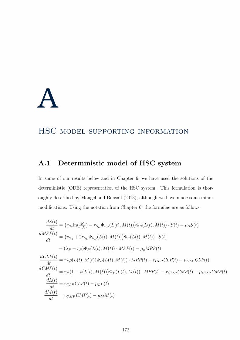
AHSC model supporting information
A.1 Deterministic model of HSC system
In some of our results below and in Chapter 6, we have used the solutions of the
deterministic (ODE) representation of the HSC system. This formulation is thor-
oughly described by Mangel and Bonsall (2013), although we have made some minor
modifications. Using the notation from Chapter 6, the formulae are as follows:
dS(t)
dt=(rSS
ln( KS(t)
)− rSDΦSD
(L(t),M(t)))ΦS(L(t),M(t)) · S(t)− µSS(t)
dMPP(t)
dt=(rSA
+ 2rSDΦSD
(L(t),M(t)))ΦS(L(t),M(t)) · S(t)
+ (λP − rP )ΦP (L(t),M(t)) ·MPP(t)− µpMPP(t)
dCLP(t)
dt= rPρ(L(t),M(t))ΦP (L(t),M(t)) ·MPP(t)− rCLPCLP(t)− µCLPCLP(t)
dCMP(t)
dt= rP
(1− ρ(L(t),M(t))
)ΦP (L(t),M(t)) ·MPP(t)− rCMPCMP(t)− µCMPCMP(t)
dL(t)
dt= rCLPCLP(t)− µLL(t)
dM(t)
dt= rCMPCMP(t)− µMM(t)
172
APPENDIX A. HSC MODEL SUPPORTING INFORMATION 173
Note that the chemical species here are concentrations, rather than actual population
numbers as in the stochastic model. Their time dependence has been emphasised; the
notation and parameters are described fully in Table 6.2.
These equations can be easily solved using a standard ODE solver to find the cell
species concentrations over time, as well as at steady state.
A.2 MPCR parameters and system steady states
In addition to adjusting the strength of the response to a perturbation, the MPCR
parameters also affect the steady states of both the cell levels and feedbacks. As can be
seen in Figs. 6.7, 6.11, 6.8 and 6.9, and summarised in Fig. 6.10, their distributions are
shifted, either up or down depending on cell or feedback type, as MPCR parameters
γ and α are varied.
This also occurs using the ODE model (Fig. A.1), and the mean values of the
stochastic distributions are very close to the ODE solutions (Fig. 6.10; also Figs. A.4
and A.6). The only cell type whose mean levels are not accurately matched by the
ODE is S, and this is because the ODEs do find the absorbing steady state S = 0,
thus overestimating mean S. Although in general this should not be assumed without
careful testing, here we have sufficient evidence that the ODE solutions represent
meaningful system properties of the stochastic system (that is, the mean values).
Thus in this section, for simplicity we have used the ODE model.
We set the homeostatic ratio that we want the cell levels to reach as ρh = 1L :
1000M ; thus we also vary α to keep this ratio as γ is changed. Starting with γ=0,
the steady states are at L ≈ 8.55,M ≈ 2.39 × 10⁴ (Fig. A.1 black line); this is
clearly nowhere near ρh. However, as γ is increased, so the L (and CLP) steady
states increase, whilst the M (and CMP) steady states decrease, moving the cell
ratios closer and closer to ρh. Fig. A.1 illustrates γ, α values used in the main text
plus some extremes on either side. By the time we reach γ = 50, a hyper-sensitive
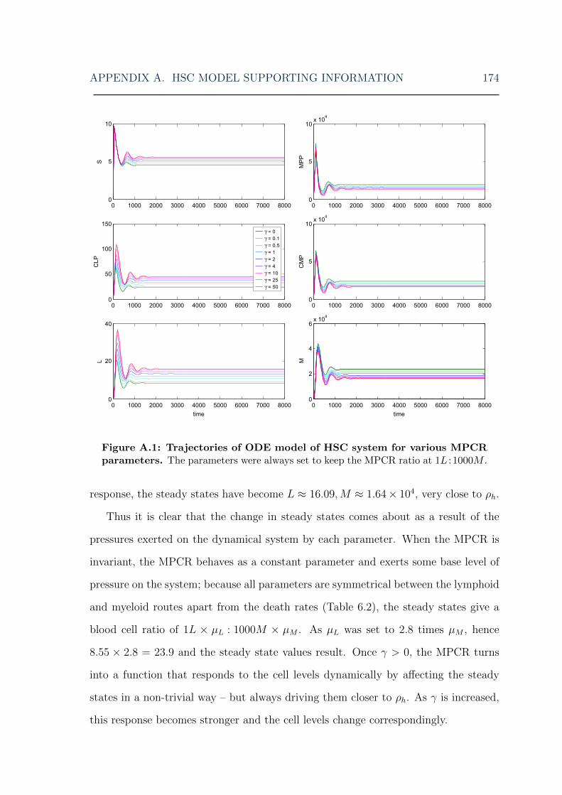
APPENDIX A. HSC MODEL SUPPORTING INFORMATION 174
Figure A.1: Trajectories of ODE model of HSC system for various MPCRparameters. The parameters were always set to keep the MPCR ratio at 1L : 1000M .
response, the steady states have become L ≈ 16.09,M ≈ 1.64× 10⁴, very close to ρh.
Thus it is clear that the change in steady states comes about as a result of the
pressures exerted on the dynamical system by each parameter. When the MPCR is
invariant, the MPCR behaves as a constant parameter and exerts some base level of
pressure on the system; because all parameters are symmetrical between the lymphoid
and myeloid routes apart from the death rates (Table 6.2), the steady states give a
blood cell ratio of 1L × µL : 1000M × µM . As µL was set to 2.8 times µM , hence
8.55 × 2.8 = 23.9 and the steady state values result. Once γ > 0, the MPCR turns
into a function that responds to the cell levels dynamically by affecting the steady
states in a non-trivial way – but always driving them closer to ρh. As γ is increased,
this response becomes stronger and the cell levels change correspondingly.

APPENDIX A. HSC MODEL SUPPORTING INFORMATION 175
A.3 Optimal homeostatic cell levels
In Section 6.4 of the main text, we discuss the difference in mean cell levels between
the uncoupled and coupled niches for the case γ = 2, α = 10−9. In a somewhat
similar way to the effects of the MPCR parameters, the distributions of cell levels and
feedbacks are shifted as the niche grouping size is varied. There are also associated
changes in their spread, but here we are interested in elucidating which distribution
is centred around a ‘more correct’ homeostatic state; we explore this in detail below.
Figure A.2: ODE model of HSC system with death rates for L and M cellsset identical. This allows the system to achieve the same cell levels for all MPCRparameters. (A) Trajectories of cell types with low numbers, and (B) cell types withhigh numbers for various MPCR parameters (curves overlap because the solutions areidentical). (C) ODE solutions of cell types with low numbers, and (D) cell types withhigh numbers for various MPCR parameters.
First, unlike in the above section, we cannot rely on the deterministic model for
help, as without using stochastic simulations we cannot tell whether the ODE solutions

APPENDIX A. HSC MODEL SUPPORTING INFORMATION 176
represent any useful properties of the true distributions (although Figs. A.4 and A.6
show that we would be justified in doing this, as the ODEs approximate the mean of
the stochastic distributions well.)
Unfortunately, stochastic simulations with different niche grouping sizes give dif-
ferent results and we cannot tell which is the most optimal. The solution to this
quandary is to use a set of model parameters where µL = µM = 0.01, thus removing
the pressure on the dynamical system from these parameters. Since the other pa-
rameters are all identical between the lymphoid and myeloid routes (Table 6.2), this
means that the optimal steady state levels will exactly follow the ratio 1L : 1000M
(indeed, the ODE system now finds identical steady states for all γ, α; Fig. A.2). We
investigate whether it is the coupled or uncoupled lineages that keep their cell levels
closer to the optimal levels ρh for several different MPCR parameters.
We illustrate stochastic simulation results for this system in Figs. A.3 to A.7.
Figs. A.3 and A.4 show the PDFs, both per individual niche lineage and summed over
niche groups, of steady state L levels for various γ; similarly, Figs. A.5 and A.6 show
levels of M . The corresponding PDFs of ρ (i.e. the value of the MPCR) are shown
in Fig. A.7. From these five plots, we can make the following observations:
1. Uncoupled niche lineages have tighter cell level distributions individually, but
when summed over niche groups the distributions are similar, with coupled
lineages having a slightly smaller variance in almost all cases.
2. For both L and M the distributions get tighter as γ increases (albeit the effect
is small for L).
3. The distribution means of the uncoupled lineages vary with γ, whereas those of
the coupled niches change very little. This becomes especially obvious when the
blood cell levels are summed over niche groups (Figs. A.4 and A.6). For easier
comparison, Fig. A.8 shows the mean values of L and M for several values of γ.
4. Although the means of the MPCR distributions stay around the expected ρh =

APPENDIX A. HSC MODEL SUPPORTING INFORMATION 177
9.99 × 10⁻⁴ both in the uncoupled and coupled cases (Fig. A.7), the coupled
lineages achieve a much tighter MPCR distribution than uncoupled ones. This is
also true for mean niche group mean MPCR, although the difference in variance
is much smaller (Fig. A.9).
5. In addition, as γ increases the bulk of the uncoupled MPCR distribution moves
so that it is centred somewhere around 5 × 10⁻⁴, leaving a long tail to still be
able to achieve a mean value of ρh (Fig. A.7).
6. Finally, taking the ratio of the mean cell levels of the uncoupled lineages at
γ = 2 gives an MPCR value of 8.77 × 10⁻⁴ compared to 9.99 × 10⁻⁴ for the
coupled lineages. It is easily visible from Figs. A.4 and A.6 that at γ = 2,
the distributions of L and M have moved away from the optimal values of
16.25, 1.625× 10⁴, respectively.
Putting all this together, especially points 4 to 6, we can conclude that coupling niche
lineages allows them to better reach the optimal homeostatic state, as they are able
to keep their blood cell levels very close to the desired 1L : 1000M ratio for all γ,
as well as more tightly-distributed around those values. Furthermore, coupled niches
also keep their MPCR more tightly-distributed around ρh than the uncoupled niches.
In addition, as we can see from Figs. A.4 and A.6, the ODE solutions do approximate
the stochastic mean values well, in the case of the HSC model.
Thus, we are now in a position to apply the above results to the stochastic system in
the main text, where the parameters µL and µM are not equal. As we have concluded
that here the coupled system regulates its cell levels more optimally, we can also
extrapolate that this is the case for the results in the main text. Furthermore, we
have added the ODE solutions to some figures in the main text to support this point.
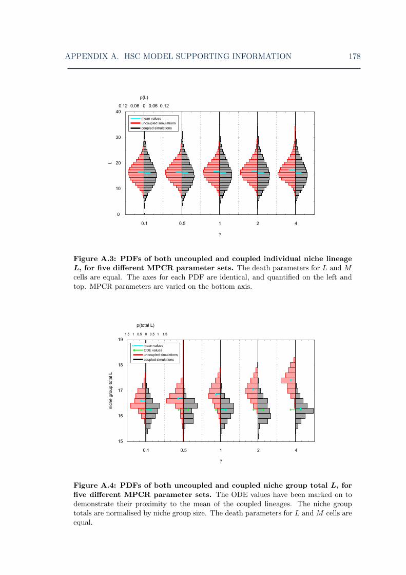
APPENDIX A. HSC MODEL SUPPORTING INFORMATION 178
Figure A.3: PDFs of both uncoupled and coupled individual niche lineageL, for five different MPCR parameter sets. The death parameters for L and Mcells are equal. The axes for each PDF are identical, and quantified on the left andtop. MPCR parameters are varied on the bottom axis.
Figure A.4: PDFs of both uncoupled and coupled niche group total L, forfive different MPCR parameter sets. The ODE values have been marked on todemonstrate their proximity to the mean of the coupled lineages. The niche grouptotals are normalised by niche group size. The death parameters for L and M cells areequal.
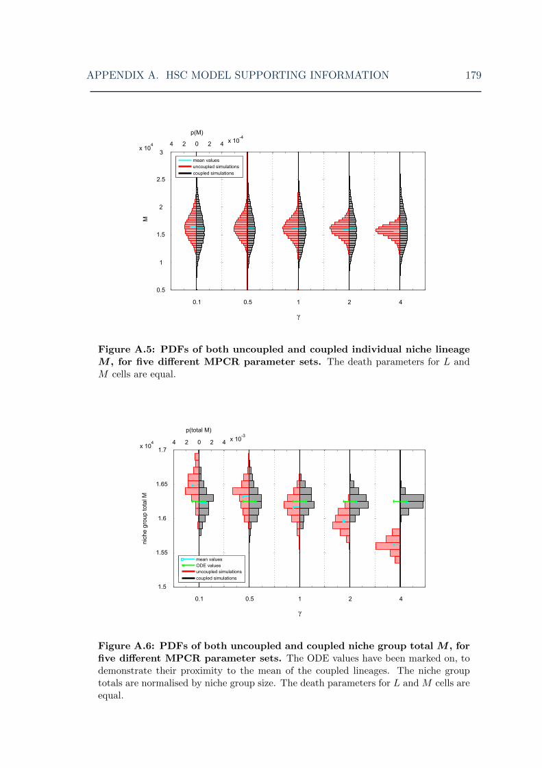
APPENDIX A. HSC MODEL SUPPORTING INFORMATION 179
Figure A.5: PDFs of both uncoupled and coupled individual niche lineageM , for five different MPCR parameter sets. The death parameters for L andM cells are equal.
Figure A.6: PDFs of both uncoupled and coupled niche group total M , forfive different MPCR parameter sets. The ODE values have been marked on, todemonstrate their proximity to the mean of the coupled lineages. The niche grouptotals are normalised by niche group size. The death parameters for L and M cells areequal.
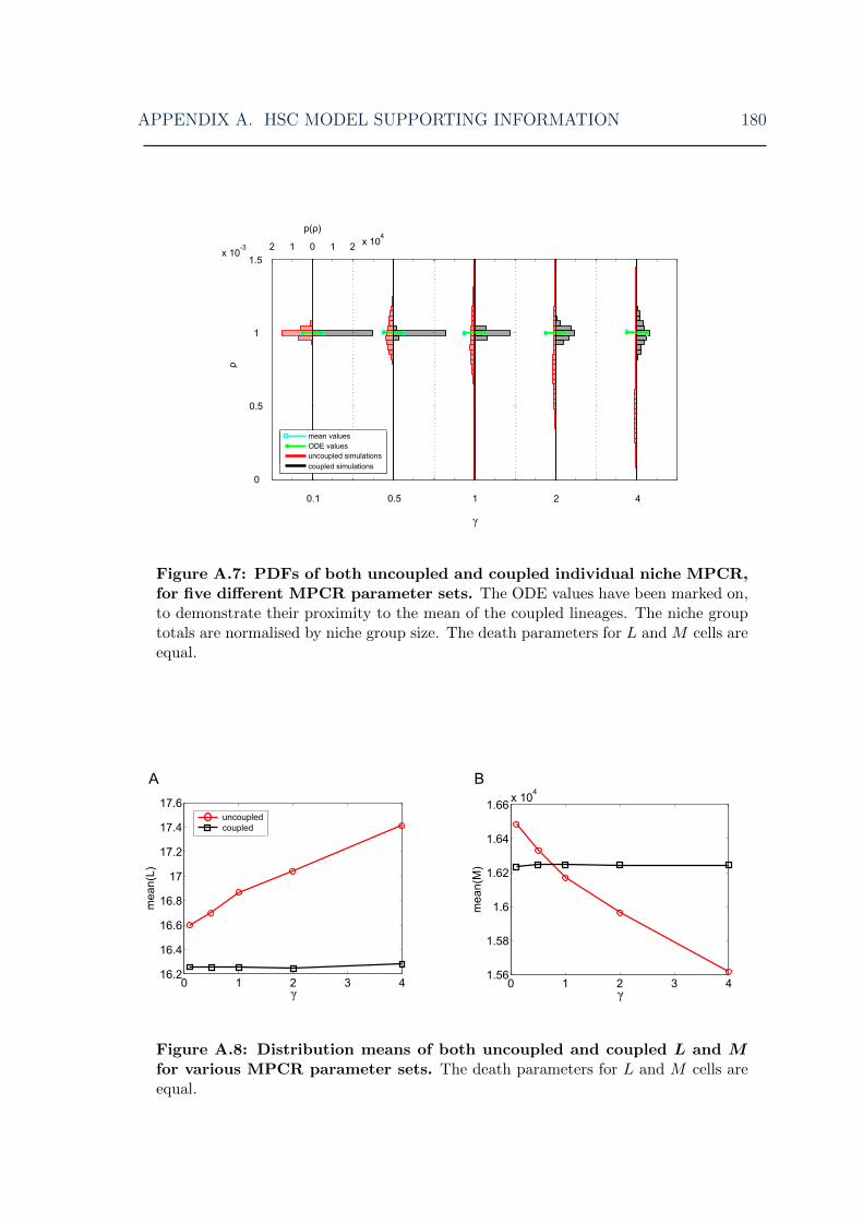
APPENDIX A. HSC MODEL SUPPORTING INFORMATION 180
Figure A.7: PDFs of both uncoupled and coupled individual niche MPCR,for five different MPCR parameter sets. The ODE values have been marked on,to demonstrate their proximity to the mean of the coupled lineages. The niche grouptotals are normalised by niche group size. The death parameters for L and M cells areequal.
Figure A.8: Distribution means of both uncoupled and coupled L and Mfor various MPCR parameter sets. The death parameters for L and M cells areequal.
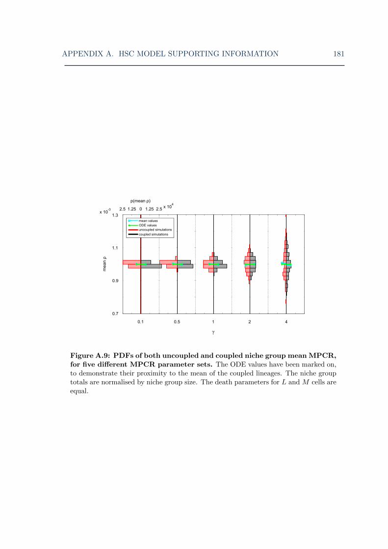
APPENDIX A. HSC MODEL SUPPORTING INFORMATION 181
Figure A.9: PDFs of both uncoupled and coupled niche group mean MPCR,for five different MPCR parameter sets. The ODE values have been marked on,to demonstrate their proximity to the mean of the coupled lineages. The niche grouptotals are normalised by niche group size. The death parameters for L and M cells areequal.
References
Abdulle, A. and Cirilli, S. (2007). S-ROCK: Chebyshev methods for stiff stochastic
differential equations. SIAM Journal on Scientific Computing, 30:997–1014.
Adams, G. B. and Scadden, D. T. (2006). The hematopoietic stem cell in its place.
Nature Immunology, 7:333–337.
Alberts, B., Johnson, A., Lewis, J., Raff, M., Roberts, K., and Walter, P. (2002).
Molecular Biology of the Cell. Garland Science, New York, NY, 4th edition.
Anderson, D. F., Ganguly, A., and Kurtz, T. G. (2011). Error analysis of tau-leap
simulation methods. Annals of Applied Probability, 21:2226–2262.
Anderson, D. F. and Higham, D. J. (2012). Multi-level Monte Carlo for continuous
time Markov chains, with applications in biochemical kinetics. SIAM Multiscale
Modeling and Simulation, 10:146–179.
Anderson, D. F. and Koyama, M. (2012). Weak error analysis of numerical meth-
ods for stochastic models of population processes. SIAM Multiscale Modeling and
Simulation, 10:1493–1524.
Anderson, D. F. and Mattingly, J. C. (2011). A weak trapezoidal method for a class
of stochastic differential equations. Communications in Mathematical Sciences,
9:301–318.
Arkin, A., Ross, J., and McAdams, H. H. (1998). Stochastic kinetic analysis of devel-
182

REFERENCES 183
opmental pathway bifurcation in phage λ-infected Escherichia coli cells. Genetics,
149:1633–1648.
Avery, S. V. (2006). Microbial cell individuality and the underlying sources of het-
erogeneity. Nature Reviews Microbiology, 4:577–587.
Ball, P. (2013). DNA: celebrate the unknowns. Nature, 496:419–420.
Barkai, N. and Leibler, S. (2000). Biological rhythms – circadian clocks limited by
noise. Nature, 403:267–268.
Barrio, M., Burrage, K., Leier, A., and Tian, T. (2006). Oscillatory regulation of Hes1:
discrete stochastic delay modelling and simulation. PLoS Computational Biology,
2:1017–1030.
Bhattacharya, D., Czechowicz, A., Ooi, A. G., Rossi, D. J., Bryder, D., and Weissman,
I. L. (2009). Niche recycling through division-independent egress of hematopoietic
stem cells. Journal of Experimental Medicine, 206:2837–2850.
Blake, W. J., Kaern, M., Cantor, C. R., and Collins, J. J. (2003). Noise in eukaryotic
gene expression. Nature, 422:633–637.
Braun, M. (1993). Differential Equations and Their Applications. Springer-Verlag,
New York, NY, 4th edition.
Buckwar, E., Roßler, A., and Winkler, R. (2010). Stochastic Runge-Kutta methods for
Ito SODEs with small noise. SIAM Journal on Scientific Computing, 32:1789–1808.
Bulirsch, R. and Stoer, J. (1966). Numerical treatment of ordinary differential equa-
tions by extrapolation methods. Numerische Mathematik, 8:1–13.
Burrage, K. (1995). Parallel and sequential methods for ordinary differential equations.
Clarendon Press, Oxford.
REFERENCES 184
Burrage, K. and Burrage, P. M. (1996). High strong order explicit Runge-Kutta meth-
ods for stochastic ordinary differential equations. Applied Numerical Mathematics,
22:81–101.
Burrage, K. and Burrage, P. M. (2000). Order conditions of stochastic Runge-Kutta
methods by B-series. SIAM Journal on Numerical Analysis, 38:1626–1646.
Burrage, K., Burrage, P. M., and Tian, T. (2004a). Numerical methods for strong
solutions of stochastic differential equations: an overview. Proceedings of the Royal
Society of London Series A, 460:373–402.
Burrage, K. and Tian, T. (2004). Poisson Runge-Kutta methods for chemical reaction
systems. In Sun, Y. L. W. and Tang, T., editors, Advances in Scientific Computing
and Applications, pages 82–96, Beijing; New York, NY. Science Press.
Burrage, K., Tian, T. H., and Burrage, P. (2004b). A multi-scaled approach for
simulating chemical reaction systems. Progress in Biophysics & Molecular Biology,
85:217–234.
Cao, Y., Gillespie, D. T., and Petzold, L. R. (2005). The slow-scale stochastic simu-
lation algorithm. Journal of Chemical Physics, 122:014116.
Cao, Y., Gillespie, D. T., and Petzold, L. R. (2006). Efficient step size selection for
the tau-leaping simulation method. Journal of Chemical Physics, 124:044109.
Cao, Y., Gillespie, D. T., and Petzold, L. R. (2007). The adaptive explicit-implicit
tau-leaping method with automatic tau selection. Journal of Chemical Physics,
126:224101.
Cao, Y., Li, H., and Petzold, L. R. (2004). Efficient formulation of the stochastic
simulation algorithm for chemically reacting systems. Journal of Chemical Physics,
121:4059–4067.

REFERENCES 185
Chatterjee, A., Vlachos, D. G., and Katsoulakis, M. A. (2005). Binomial distribution
based tau-leap accelerated stochastic simulation. Journal of Chemical Physics,
122:024112.
Cheshier, S. H., Morrison, S. J., Liao, X., and Weissman, I. L. (1999). In vivo
proliferation and cell cycle kinetics of long-term self-renewing hematopoietic stem
cells. Proceedings of the National Academy of Sciences of the USA, 96:3120–3125.
Cheshier, S. H., Prohaska, S. S., and Weissman, I. L. (2007). The effect of bleeding
on hematopoietic stem cell cycling and self-renewal. Stem Cells and Development,
16:707–717.
Clayden, J., Greeves, N., and Warren, S. (2012). Organic Chemistry. Oxford Univer-
sity Press, Oxford, 2nd edition.
Cooper, G. M. and Hausman, R. E. (2009). The Cell: A Molecular Approach. Sinauer
Associates, Inc., Sunderland, MA, 5th edition.
Cotter, S. L., Zygalakis, K. C., Kevrekidis, I. G., and Erban, R. (2011). A constrained
approach to multiscale stochastic simulation of chemically reacting systems. Journal
of Chemical Physics, 135:094102.
Crick, F. H. C. (1958). On protein synthesis. In The biological replication of macro-
molecules, volume 12, pages 138–163. Symposia of the Society for Experimental
Biology, Cambridge University Press.
Crick, F. H. C. (1970). Central dogma of molecular biology. Nature, 227:561–563.
de Graaf, C. A., Kauppi, M., Baldwin, T., Hyland, C. D., Metcalf, D., Willson,
T. A., Carpinelli, M. R., Smyth, G. K., Alexander, W. S., and Hilton, D. J. (2010).
Regulation of hematopoietic stem cells by their mature progeny. Proceedings of the
National Academy of Sciences of the USA, 107:21689–21694.
REFERENCES 186
Deuflhard, P. (1985). Recent progress in extrapolation methods for ordinary differen-
tial equations. SIAM Review, 27:505–535.
Dingli, D. and Pacheco, J. M. (2011). Stochastic dynamics and the evolution of
mutations in stem cells. BMC Biology, 9:41.
Dodd, I. B., Shearwin, K. E., and Egan, J. B. (2005). Revisited gene regulation in
bacteriophage lambda. Current Opinion in Genetics & Development, 15:145–152.
E, W., Liu, D., and Vanden-Eijnden, E. (2005). Nested stochastic simulation al-
gorithm for chemical kinetic systems with disparate rates. Journal of Chemical
Physics, 123:194107.
Elf, J. and Ehrenberg, M. (2004). Spontaneous separation of bi-stable biochemical
systems into spatial domains of opposite phases. Systems Biology, 1:230–236.
Elowitz, M., Levine, A., Siggia, E., and Swain, P. (2002). Stochastic gene expression
in a single cell. Science, 297:1183–1186.
Erban, R., Chapman, S., and Maini, P. (2007). A practical guide
to stochastic simulations of reaction-diffusion processes. Lecture Notes.
http://arxiv.org/abs/0704.1908.
Erban, R. and Chapman, S. J. (2007). Reactive boundary conditions for stochastic
simulations of reaction-diffusion processes. Physical Biology, 4:16–28.
Erban, R. and Chapman, S. J. (2009). Stochastic modelling of reaction-diffusion
processes: algorithms for bimolecular reactions. Physical Biology, 6:046001.
Erban, R., Chapman, S. J., Kevrekidis, I., and Vejchodsky, T. (2009). Analysis of a
stochastic chemical system close to a SNIPER bifurcation of its mean-field model.
SIAM Journal on Applied Mathematics, 70:984–1016.
Erban, R. and Othmer, H. G. (2004). From individual to collective behaviour in
bacterial chemotaxis. SIAM Journal on Applied Mathematics, 65:361–391.
REFERENCES 187
Erban, R. and Othmer, H. G. (2005). From signal transduction to spatial pattern
formation in E. coli : a paradigm for multi-scale modeling in biology. Multiscale
Modeling & Simulation, 3:362–394.
Faller, A. and Schunke, G. (2004). The Human Body: An Introduction to Structure
and Function. Thieme, Stuttgart.
Fedoroff, N. and Fontana, W. (2002). Small numbers of big molecules. Science,
297:1129–1131.
Fraley, C. and Raftery, A. E. (1998). How many clusters? which clustering method?
answers via model-based cluster analysis. The Computer Journal, 41:578–588.
Fraser, D. and Kaern, M. (2009). A chance at survival: gene expression noise and
phenotypic diversification strategies. Molecular Microbiology, 71(6):1333–1340.
Fraser, H. B., Hirsh, A. E., Giaever, G., Kumm, J., and Eisen, M. B. (2004). Noise
minimization in eukaryotic gene expression. PLoS Biology, 2:834–838.
Fuchs, E., Tumbar, T., and Guasch, G. (2004). Socializing with the neighbors: stem
cells and their niche. Cell, 116:769–778.
Gadgil, C., Lee, C., and Othmer, H. (2005). A stochastic analysis of first-order
reaction networks. Bulletin of Mathematical Biology, 67:901–946.
Geritz, S. A. H. and Kisdi, E. (2004). On the mechanistic underpinning of discrete-
time population models with complex dynamics. Journal of Theoretical Biology,
228:261–269.
Gibson, M. A. and Bruck, J. (2000). Efficient exact stochastic simulation of chemical
systems with many species and many channels. Journal of Physical Chemistry A,
104:1876–1889.
Giles, M. B. (2008). Multilevel Monte Carlo path simulation. Operations Research,
56:607–617.
REFERENCES 188
Gillespie, D. T. (1976). General method for numerically simulating stochastic time
evolution of coupled chemical-reactions. Journal of Computational Physics, 22:403–
434.
Gillespie, D. T. (1977). Exact stochastic simulation of coupled chemical reactions.
Journal of Physical Chemistry, 81:2340–2361.
Gillespie, D. T. (1992a). Markov Processes: An Introduction for Physical Scientists.
Academic Press, Boston, MA.
Gillespie, D. T. (1992b). A rigorous derivation of the Chemical Master Equation.
Physica A, 188:404–425.
Gillespie, D. T. (2000). The chemical Langevin equation. Journal of Chemical Physics,
113:297–306.
Gillespie, D. T. (2001). Approximate accelerated stochastic simulation of chemically
reacting systems. Journal of Chemical Physics, 115:1716–1733.
Gillespie, D. T. (2007). Stochastic simulation of chemical kinetics. Annual Review of
Physical Chemistry, 58:35–55.
Gillespie, D. T. (2009). A diffusional bimolecular propensity function. Journal of
Chemical Physics, 131:164109.
Gillespie, D. T. and Mangel, M. (1981). Conditioned averages in chemical kinetics.
Journal of Chemical Physics, 75:704–709.
Gillespie, D. T. and Petzold, L. R. (2003). Improved leap-size selection for accelerated
stochastic simulation. Journal of Chemical Physics, 119:8229–8234.
Gomperts, B. D., Kramer, I. M., and Tatham, P. E. R. (2009). Signal Transduction.
Academic Press, Burlington, MA; London, 2nd edition.

REFERENCES 189
Goutsias, J. (2005). Quasiequilibrium approximation of fast reaction kinetics in
stochastic biochemical systems. Journal of Chemical Physics, 122:184102.
Goutsias, J. (2007). Classical versus stochastic kinetics modeling of biochemical re-
action systems. Biophysical Journal, 92:2350–2365.
Goutsias, J. and Jenkinson, G. (2013). Markovian dynamics on complex reaction
networks. Physics Reports, 529:199–264.
Gragg, W. B. (1965). On extrapolation algorithms for ordinary initial value problems.
SIAM Journal on Numerical Analysis, 2:384–403.
Grima, R. (2014). Anomalous fluctuation scaling laws in stochastic enzyme kinet-
ics: increase of noise strength with the mean concentration. Physical Review E,
89:012710.
Gunawardena, J. (2014). Models in biology: accurate descriptions of our pathetic
thinking. BMC Biology, 12:29.
Gupta, P. B., Fillmore, C. M., Jiang, G., Shapira, S. D., Tao, K., Kuperwasser,
C., and Lander, E. S. (2011). Stochastic state transitions give rise to phenotypic
equilibrium in populations of cancer cells. Cell, 146:633–644.
Gurtner, G. C., Callaghan, M. J., and Longaker, M. T. (2007). Progress and potential
for regenerative medicine. Annual Review of Medicine, 58:299–312.
Hairer, E., Nørsett, S. P., and Wanner, G. (1993). Solving Ordinary Differential
Equations I: Nonstiff Problems. Springer-Verlag, Berlin, 2nd edition.
Haseltine, E. L. and Rawlings, J. B. (2002). Approximate simulation of coupled fast
and slow reactions for stochastic chemical kinetics. Journal of Chemical Physics,
117:6959–6969.
Hattne, J., Fange, D., and Elf, J. (2005). Stochastic reaction-diffusion simulation with
MesoRD. Bioinformatics, 21:2923–2924.
REFERENCES 190
Hawkins, E. D. and Lo Celso, C. (2013). Subdivision of bone marrow microenvi-
ronments: purpose built homes for haematopoietic stem cells. EMBO Journal,
32:176–177.
Higham, D. J. (2008). Modeling and simulating chemical reactions. SIAM Review,
50:347–368.
Hsu, Y.-C. and Fuchs, E. (2012). A family business: stem cell progeny join the niche
to regulate homeostasis. Nature Reviews Molecular Cell Biology, 13:103–114.
Hu, Y. and Li, T. (2009). Highly accurate tau-leaping methods with random correc-
tions. Journal of Chemical Physics, 130:124109.
Hu, Y., Li, T., and Min, B. (2011a). The weak convergence analysis of tau-leaping
methods: revisited. Communications in Mathematical Sciences, 9:965–996.
Hu, Y., Li, T., and Min, B. (2011b). A weak second order tau-leaping method for
chemical kinetic systems. Journal of Chemical Physics, 135:024113.
Huang, S. (2009). Non-genetic heterogeneity of cells in development: more than just
noise. Development, 136:3853–3862.
Huang, S. (2011). Systems biology of stem cells: three useful perspectives to help
overcome the paradigm of linear pathways. Philosophical Transactions of the Royal
Society B, 366:2247–2259.
Jahnke, T. and Huisinga, W. (2007). Solving the Chemical Master Equation for
monomolecular reaction systems analytically. Journal of Mathematical Biology,
54:1–26.
Kaern, M., Elston, T., Blake, W., and Collins, J. (2005). Stochasticity in gene ex-
pression: from theories to phenotypes. Nature Reviews Genetics, 6:451–464.

REFERENCES 191
Kebaier, A. (2005). Statistical Romberg extrapolation: a new variance reduction
method and applications to option pricing. Annals of Applied Probability, 15:2681–
2705.
Kherlopian, A. R., Song, T., Duan, Q., Neimark, M. A., Po, M. J., Gohagan, J. K.,
and Laine, A. F. (2008). A review of imaging techniques for systems biology. BMC
Systems Biology, 2:74.
Kiehl, T. R., Mattheyses, R. M., and Simmons, M. K. (2004). Hybrid simulation of
cellular behavior. Bioinformatics, 20:316–322.
Kiel, M. J. and Morrison, S. J. (208). Uncertainty in the niches that maintain
haematopoietic stem cells. Nature Reviews Immunology, 8:290–301.
Kiel, M. J., Yilmaz, O. H., Iwashita, T., Terhorst, C., and Morrison, S. J. (2005).
SLAM family receptors distinguish hematopoietic stem and progenitor cells and
reveal endothelial niches for stem cells. Cell, 121:1109–1121.
Kincaid, D. R. and Cheney, E. W. (2002). Numerical Analysis: Mathematics of
Scientific Computing. American Mathematical Society, Providence, RI, 3rd edition.
Kloeden, P. E. and Platen, E. (1989). A survey of numerical methods for stochastic
differential equations. Stochastic Hydrology and Hydraulics, 3:155–178.
Kloeden, P. E. and Platen, E. (1999). Numerical Solution of Stochastic Differential
Equations. Springer-Verlag, Berlin, 3rd edition.
Komarova, N. L. (2013). Principles of regulation of self-renewing cell lineages. PLoS
ONE, 8:e72847.
Kurtz, T. G. (1978). Strong approximation theorems for density dependent Markov
chains. Stochastic Processes and their Applications, 6:223–240.
Kurtz, T. G. (1980). Representations of Markov processes as multiparameter time
changes. Annals of Probability, 8:682–715.
REFERENCES 192
Laird, D. J., Tomaso, A. W. D., and Weissman, I. L. (2005). Stem cells are units of
natural selection in a colonial ascidian. Cell, 123:1351–1360.
Lander, A. D. (2009). The stem cell concept: is it holding us back? Journal of
Biology, 8:70.
Lander, A. D. (2011). The individuality of stem cells. BMC Biology, 9:40.
Lander, A. D., Gokoffski, K. K., Wan, F. Y. M., Nie, Q., and Calof, A. L. (2009).
Cell lineages and the logic of proliferative control. PLoS Biology, 7:e1000015.
Lehner, B. (2008). Selection to minimise noise in living systems and its implications
for the evolution of gene expression. Molecular Systems Biology, 4:170.
Li, T. (2007). Analysis of explicit tau-leaping schemes for simulating chemically
reacting systems. Multiscale Modeling & Simulation, 6:417–436.
Liu, J. S. (2001). Monte Carlo Strategies in Scientific Computing. Springer-Verlag,
New York, NY, 3rd edition.
Liu, X. Q. and Li, C. W. (2000). Weak approximation and extrapolations of stochastic
differential equations with jumps. SIAM Journal on Numerical Analysis, 37:1747–
1767.
Lo Celso, C. and Scadden, D. T. (2011). The haematopoietic stem cell niche at a
glance. Journal of Cell Science, 124:3529–3535.
MacNamara, S., Bersani, A. M., Burrage, K., and Sidje, R. B. (2008a). Stochas-
tic chemical kinetics and the total quasi-steady-state assumption: application to
the stochastic simulation algorithm and Chemical Master Equation. Journal of
Chemical Physics, 129:095105.
MacNamara, S. and Burrage, K. (2009). Krylov and steady-state techniques for the
solution of the Chemical Master Equation for the mitogen-activated protein kinase
cascade. Numerical Algorithms, 51:281–307.
REFERENCES 193
MacNamara, S. and Burrage, K. (2010). Stochastic modeling of naıve T cell home-
ostasis for competing clonotypes via the Master Equation. Multiscale Modeling &
Simulation, 8:1325–1347.
MacNamara, S., Burrage, K., and Sidje, R. B. (2008b). Multiscale modeling of chem-
ical kinetics via the Master Equation. Multiscale Modeling & Simulation, 6:1146–
1168.
Mangel, M. (2006). The Theoretical Biologist’s Toolbox: Quantitative Methods for
Ecology and Evolutionary Biology. Cambridge University Press, Cambridge.
Mangel, M. and Bonsall, M. B. (2007). The evolutionary ecology of stem cells and
their niches – the time is now. Oikos, 116:1779–1781.
Mangel, M. and Bonsall, M. B. (2008). Phenotypic evolutionary models in stem cell
biology: replacement, quiescence, and variability. PLoS One, 3:e1591.
Mangel, M. and Bonsall, M. B. (2013). Stem cell biology is population biology:
differentiation of hematopoietic multipotent progenitors to common lymphoid and
myeloid progenitors. Theoretical Biology and Medical Modelling, 10:5.
Marciniak-Czochra, A., Stiehl, T., Ho, A. D., Jager, W., and Wagner, W. (2009).
Modeling of asymmetric cell division in hematopoietic stem cells – regulation of
self-renewal is essential for efficient repopulation. Stem Cells and Development,
18:377–385.
Marquez-Lago, T. and Burrage, K. (2007). Binomial tau-leap spatial stochastic simu-
lation algorithm for applications in chemical kinetics. Journal of Chemical Physics,
127:104101.
Marquez-Lago, T. and Stelling, J. (2010). Counter-intuitive stochastic behavior of
simple gene circuits with negative feedbacks. Biophysical Journal, 98:1742–1750.

REFERENCES 194
Martins, M. L., Ferreira, S. C., J., and Vilela, M. J. (2010). Multiscale models for
biological systems. Current Opinion in Colloid & Interface Science, 15:18–23.
Maruyama, G. (1955). Continuous Markov processes and stochastic equations. Ren-
diconti del Circolo Matematico di Palermo, 4:48–90.
Mason, C. and Dunnill, P. (2008). A brief definition of regenerative medicine. Regen-
erative Medicine, 3:1–5.
McAdams, H. H. and Arkin, A. (1997). Stochastic mechanisms in gene expression.
Proceedings of the National Academy of Sciences of the USA, 94:814–819.
McGrath, S. and van Sinderen, D. (2007). Bacteriophage: Genetics and Molecular
Biology. Caister Academic Press, Wymondham.
McQuarrie, D. A. (1967). Stochastic approach to chemical kinetics. Journal of Applied
Probability, 4:413–478.
Melykuti, B., Burrage, K., and Zygalakis, K. C. (2010). Fast stochastic simulation of
biochemical reaction systems by alternative formulations of the chemical Langevin
equation. Journal of Chemical Physics, 132:164109.
Metcalf, D. (2007). Concise review: hematopoietic stem cells and tissue stem cells:
current concepts and unanswered questions. Stem Cells, 25:2390–2395.
Milstein, G. N. and Tretyakov, M. V. (1997a). Mean-square numerical methods for
stochastic differential equations with small noises. SIAM Journal on Scientific
Computing, 18:1067–1087.
Milstein, G. N. and Tretyakov, M. V. (1997b). Numerical methods in the weak sense
for stochastic differential equations with small noise. SIAM Journal on Numerical
Analysis, 34:2142–2167.
Mogilner, A., Wollman, R., and Marshall, W. F. (2006). Quantitative modeling in
cell biology: what is it good for? Developmental Cell, 11:279–287.
REFERENCES 195
Moore, K. A. and Lemischka, I. R. (2006). Stem cells and their niches. Science,
311:1880–1885.
Morrison, S. J. and Kimble, J. (2006). Asymmetric and symmetric stem-cell divisions
in development and cancer. Nature, 441:1068–1074.
Morrison, S. J. and Spradling, A. C. (2008). Stem cells and niches: mechanisms that
promote stem cell maintenance throughout life. Cell, 132:598–611.
Munsky, B. and Khammash, M. (2006). The finite state projection algorithm for
the solution of the Chemical Master Equation. Journal of Chemical Physics,
124:044104.
Noble, D. (2002). Modeling the heart – from genes to cells to the whole organ. Science,
295:1678–1682.
O’Brien, L. E. and Bilder, D. (2013). Beyond the niche: tissue-level coordination of
stem cell dynamics. Annual Review of Cell and Developmental Biology, 29:107–136.
O’Farrell, P. H. (1975). High-resolution 2-dimensional electrophoresis of proteins.
Journal of Biological Chemistry, 250:4007–4021.
Ogawa, M. (1993). Differentiation and proliferation of hematopoietic stem cells. Blood,
81:2844–2853.
Orkin, S. H. and Zon, L. I. (2008). Hematopoiesis: an evolving paradigm for stem
cell biology. Cell, 132:631–644.
Osafune, K., Caron, L., Borowiak, M., Martinez, R. J., Fitz-Gerald, C. S., Sato, Y.,
Cowan, C. A., Chien, K. R., and Melton, D. A. (2008). Marked differences in differ-
entiation propensity among human embryonic stem cell lines. Nature Biotechnology,
26:313–315.
REFERENCES 196
Pedersen, S., Bloch, P. L., Reeh, S., and Neidhardt, F. C. (1978). Patterns of protein-
synthesis in Escherichia coli - catalog of amount of 140 individual proteins at dif-
ferent growth-rates. Cell, 14:179–190.
Pedraza, J. M. and van Oudenaarden, A. (2005). Noise propagation in gene networks.
Science, 307:1965–1969.
Peerani, R., Rao, B. M., Bauwens, C., Yin, T., Wood, G. A., Nagy, A., Kumacheva,
E., and Zandstra, P. W. (2007). Niche-mediated control of human embryonic stem
cell self-renewal and differentiation. EMBO Journal, 26:4744–4755.
Peng, X., Zhou, W., and Wang, Y. (2007). Efficient binomial leap method for simu-
lating chemical kinetics. Journal of Chemical Physics, 126:224109.
Pettigrew, M. F. and Resat, H. (2007). Multinomial tau-leaping method for stochastic
kinetic simulations. Journal of Chemical Physics, 126:084101.
Press, W. H., Teukolsky, S. A., Vetterling, W. T., and Flannery, B. P. (2007). Numer-
ical Recipes in C: The Art of Scientific Computing. Cambridge University Press,
Cambridge, 3rd edition.
Rao, C. V. and Arkin, A. P. (2003). Stochastic chemical kinetics and the quasi-steady-
state assumption: application to the Gillespie algorithm. Journal of Chemical
Physics, 118:4999–5010.
Raser, J. M. and O’Shea, E. K. (2005). Noise in gene expression: origins, consequences,
and control. Science, 309(5743):2010–2013.
Rathinam, M., Petzold, L. R., Cao, Y., and Gillespie, D. T. (2005). Consistency and
stability of tau-leaping schemes for chemical reaction systems. Multiscale Modeling
& Simulation, 4:867–895.
Richardson, L. F. (1911). The approximate arithmetical solution by finite differences
of physical problems involving differential equations, with an application to the
REFERENCES 197
stresses in a masonry dam. Philosophical Transactions of the Royal Society of
London A, 210:307–357.
Rodriguez-Brenes, I. A., Komarova, N. L., and Wodarz, D. (2011). Evolutionary
dynamics of feedback escape and the development of stem-cell driven cancers. Pro-
ceedings of the National Academy of Sciences of the USA, 108:18983–18988.
Rodriguez-Brenes, I. A., Wodarz, D., and Komarova, N. L. (2013). Stem cell control,
oscillations, and tissue regeneration in spatial and non-spatial models. Frontiers in
Oncology, 3:82.
Romberg, W. (1955). Vereinfachte numerische integration. Det Kong Norske Viden-
skabers Salskab Fordhandlinger, 28:30–36.
Rosenfeld, N., Young, J. W., Alon, U., Swain, P. S., and Elowitz, M. B. (2005). Gene
regulation at the single-cell level. Science, 307:1962–1965.
Roßler, A. (2004). Stochastic Taylor expansions for the expectation of functionals of
diffusion processes. Stochastic Analysis and Applications, 22:1553–1576.
Rue, P., Villa-Freixa, J., and Burrage, K. (2010). Simulation methods with extended
stability for stiff biochemical kinetics. BMC Systems Biology, 4:110–123.
Salis, H. and Kaznessis, Y. (2005). Accurate hybrid stochastic simulation of a sys-
tem of coupled chemical or biochemical reactions. Journal of Chemical Physics,
122:054103.
Scadden, D. T. (2006). The stem-cell niche as an entity of action. Nature, 441:1075–
1079.
Schlogl, F. (1972). Chemical reaction models for nonequilibrium phase-transitions.
Zeitschrift fur Physik, 253:147–161.
REFERENCES 198
Shahrezaei, V. and Swain, P. S. (2008). Analytical distributions for stochastic gene
expression. Proceedings of the National Academy of Sciences of the USA, 105:17256–
17261.
Shapiro, J. A. (2009). Revisiting the central dogma in the 21st century. Annals of
the New York Academy of Sciences, 1178:6–28.
Shimizu, T. S., Aksenov, S. V., and Bray, D. (2003). A spatially extended stochastic
model of the bacterial chemotaxis signalling pathway. Journal of Molecular Biology,
329:291–309.
Shohat, J. and Tamarkin, J. D. (1943). The Problem of Moments. American Mathe-
matical Society, New York, NY.
Sieburg, H. B., Cho, R. H., Dykstra, B., Uchida, N., Eaves, C. J., and Muller-Sieburg,
C. E. (2006). The hematopoietic stem compartment consists of a limited number
of discrete stem cell subsets. Blood, 107:2311–2316.
Sieburg, H. B., Rezner, B. D., and Muller-Sieburg, C. E. (2011). Predicting clonal
self-renewal and extinction of hematopoietic stem cells. Proceedings of the National
Academy of Sciences of the USA, 108:4370–4375.
Spudich, J. L. and Koshland, D. E. J. (1976). Non-genetic individuality: chance in
the single cell. Nature, 262:467–471.
Stine, R. R. and Matunis, E. L. (2013). Stem cell competition: finding balance in the
niche. Trends in Cell Biology, 23:357–364.
Suda, T., Suda, J., and Ogawa, M. (1983). Single-cell origin of mouse hemopoietic
colonies expressing multiple lineages in variable combinations. Proceedings of the
National Academy of Sciences of the USA, 80:6689–6693.
REFERENCES 199
Sugiyama, T., Kohara, H., Noda, M., and Nagasawa, T. (2006). Maintenance of
the hematopoietic stem cell pool by CXCL12-CXCR4 chemokine signaling in bone
marrow stromal cell niches. Immunity, 25:977–988.
Sun, Z. and Komarova, N. L. (2012). Stochastic modeling of stem-cell dynamics with
control. Mathematical Biosciences, 240:231–240.
Swain, P. S., Elowitz, M. B., and Siggia, E. (2002). Intrinsic and extrinsic contribu-
tions to stochasticity in gene expression. Proceedings of the National Academy of
Sciences of the USA, 99:12795–12800.
Szekely, Jr, T. and Burrage, K. (2014). Stochastic simulation methods in systems
biology. Computational and Structural Biotechnology Journal, submitted.
Szekely, Jr, T., Burrage, K., Erban, R., and Zygalakis, K. C. (2012). A higher-order
numerical framework for stochastic simulation of chemical reaction systems. BMC
Systems Biology, 6:85.
Szekely, Jr, T., Burrage, K., Mangel, M., and Bonsall, M. B. (2013a). Stochastic dy-
namics of interacting haematopoietic stem cell niche lineages. PLoS Computational
Biology, submitted.
Szekely, Jr, T., Burrage, K., Zygalakis, K. C., and Barrio, M. (2013b). Efficient
simulation of stochastic chemical kinetics with the Stochastic Bulirsch-Stoer ex-
trapolation method. BMC Systems Biology, submitted.
Takeda, N., Jain, R., LeBoeuf, M. R., Wang, Q., Lu, M. M., and Epstein, J. A. (2011).
Interconversion between intestinal stem cell populations in distinct niches. Science,
334:1420–1424.
Talay, D. and Tubaro, L. (1990). Expansion of the global error for numerical schemes
solving stochastic differential equations. Stochastic Analysis and Applications,
8:483–509.

REFERENCES 200
Thattai, M. and van Oudenaarden, A. (2004). Stochastic gene expression in fluctuat-
ing environments. Genetics, 167:523–530.
Tian, T., Harding, A., Inder, K., Plowman, S., Parton, R. G., and Hancock, J. F.
(2007). Plasma membrane nanoswitches generate high-fidelity Ras signal transduc-
tion. Nature Cell Biology, 9:905–914.
Tian, T. H. and Burrage, K. (2004). Binomial leap methods for simulating stochastic
chemical kinetics. Journal of Chemical Physics, 121:10356–10364.
Till, J. E., McCulloch, E. A., and Siminovitch, L. (1964). A stochastic model of stem
cell proliferation, based on the growth of spleen colony-forming cells. Proceedings
of the National Academy of Sciences of the USA, 51:29–36.
van Kampen, N. G. (2007). Stochastic Processes in Physics and Chemistry. Elsevier,
Amsterdam, 3rd edition.
Wadhams, G. H. and Armitage, J. P. (2004). Making sense of it all: bacterial chemo-
taxis. Nature Reviews Molecular Cell Biology, 5:1024–1037.
Wagers, A. J. (2012). The stem cell niche in regenerative medicine. Cell Stem Cell,
10:362–369.
Wang, J., Wang, E., and Huang, S. (2010). The potential landscape of genetic circuits
imposes the arrow of time in stem cell differentiation. Biophysical Journal, 99:29–39.
Wang, L., Benedito, R., Bixel, M. G., Zeuschner, D., Stehling, M., Savendahl, L.,
Haigh, J. J., Snippert, H., Clevers, H., Breier, G., Kiefer, F., and Adams, R. H.
(2013). Identification of a clonally expanding haematopoietic compartment in bone
marrow. The EMBO Journal, 32:219–230.
Weissman, I. L. (2000a). Stem cells: units of development, units of regeneration, and
units in evolution. Cell, 100:157–168.
REFERENCES 201
Weissman, I. L. (2000b). Translating stem and progenitor cell biology to the clinic:
barriers and opportunities. Science, 287:1442–1446.
Wilkinson, D. J. (2009). Stochastic modelling for quantitative description of hetero-
geneous biological systems. Nature Reviews Genetics, 10:122–133.
Wilkinson, D. J. (2011). Stochastic Modelling for Systems Biology. Chapman and
Hall/CRC Press, Boca Raton, FL, 2nd edition.
Wright, D. E., Wagers, A. J., Gulati, A. P., Johnson, F. L., and Weissman, I. L.
(2001). Physiological migration of hematopoietic stem and progenitor cells. Science,
294:1933–1936.
Xu, Z. and Cai, X. (2008). Unbiased tau-leap methods for stochastic simulation of
chemically reacting systems. Journal of Chemical Physics, 128:154112.
Xue, C. and Othmer, H. G. (2009). Multiscale models of taxis-driven patterning in
bacterial populations. SIAM Journal on Applied Mathematics, 70:133–169.
Yates, C. A. and Burrage, K. (2011). Look before you leap: a confidence-based method
for selecting species criticality while avoiding negative populations in tau-leaping.
Journal of Chemical Physics, 134:084109.
Yates, C. A. and Klingbeil, G. (2013). Recycling random numbers in the stochastic
simulation algorithm. Journal of Chemical Physics, 138:094103.
Yin, T. and Li, L. (2006). The stem cell niches in bone. Journal of Clinical Investi-
gation, 116:1195–1201.