This article was published in an Elsevier journal. The attached copyis furnished to the author for non-commercial research and

education use, including for instruction at the author’s institution,sharing with colleagues and providing to institution administration.

Other uses, including reproduction and distribution, or selling orlicensing copies, or posting to personal, institutional or third party

websites are prohibited.

In most cases authors are permitted to post their version of thearticle (e.g. in Word or Tex form) to their personal website orinstitutional repository. Authors requiring further information

regarding Elsevier’s archiving and manuscript policies areencouraged to visit:

http://www.elsevier.com/copyright

Author's personal copy

BioSystems 91 (2008) 499–514

Available online at www.sciencedirect.com

Modelling metapopulations with stochastic membrane systems

Daniela Besozzi a,∗, Paolo Cazzaniga b, Dario Pescini b, Giancarlo Mauri b

a Universita degli Studi di Milano, Dipartimento di Informatica e Comunicazione, Via Comelico 39, 20135 Milano, Italyb Universita degli Studi di Milano-Bicocca, Dipartimento di Informatica, Sistemistica e Comunicazione,

Via Bicocca degli Arcimboldi 8, 20126 Milano, Italy

Received 10 April 2006; received in revised form 19 October 2006; accepted 30 December 2006

Abstract

Metapopulations, or multi-patch systems, are models describing the interactions and the behavior of populations living infragmented habitats. Dispersal, persistence and extinction are some of the characteristics of interest in ecological studies of metapop-ulations. In this paper, we propose a novel method to analyze metapopulations, which is based on a discrete and stochastic modellingframework in the area of Membrane Computing. New structural features of membrane systems, necessary to appropriately describea multi-patch system, are introduced, such as the reduction of the maximal parallel consumption of objects, the spatial arrangementof membranes and the stochastic creation of objects. The role of the additional features, their meaning for a metapopulation modeland the emergence of relevant behaviors are then investigated by means of stochastic simulations. Conclusive remarks and ideas forfuture research are finally presented.© 2007 Elsevier Ireland Ltd. All rights reserved.

Keywords: Membrane Computing; P systems; Metapopulation; Lotka–Volterra

1. Introduction

Metapopulations, also called multi-patch systems(Hanski, 1998), are extensively investigated in Ecologyto analyze the behavior of interacting populations, withthe purpose of determining how a fragmented habitatinfluences local and global population persistence, not tomention the implications of the metapopulation dynam-ics on the genetics and the evolution of species (Hastingsand Harrison, 1994), and the interest for spatial patternsformation (Murray, 2003). A metapopulation consists oflocal populations, living in spatially separated habitatpatches which can have different areas, quality or iso-

∗ Corresponding author.E-mail addresses: besozzi@dico.unimi.it (D. Besozzi),

cazzaniga@disco.unimib.it (P. Cazzaniga), pescini@disco.unimib.it(D. Pescini), mauri@disco.unimib.it (G. Mauri).

lation, and a dispersal pool, which is the spatial placewhere individuals from a population spend some life-time during the migration among patches. The dispersalof individuals is distance-dependent, it may reduce thelocal population growth and lead to an increase in extinc-tion risk – due also to environmental and demographicalstochasticity. Thus, the persistence of populations isassumed to be balanced between local extinctions andestablishment of new populations in empty patches(Hanski, 1998). In multi-patch systems, it is possibleto distinguish between two principal classes of dynam-ics: the populations can locally interact inside a patch(according, e.g., to the Lotka–Volterra model of preysand predators, Murray, 2002), while the dispersal of indi-viduals among patches can have effects on the globalbehavior of the whole system (Jansen, 2001; Jansen andLloyd, 2000; Taylor, 1990; Weisser et al., 1997).

P systems, or membrane systems, were introducedin Paun (2000) as a class of unconventional computing

0303-2647/$ – see front matter © 2007 Elsevier Ireland Ltd. All rights reserved.doi:10.1016/j.biosystems.2006.12.011

Author's personal copy

500 D. Besozzi et al. / BioSystems 91 (2008) 499–514

devices of distributed, parallel and nondeterministictype, inspired by the compartmental structure and thefunctioning of living cells. The basic model consists ofa membrane structure where multisets of objects evolveaccording to given evolution rules. Assuming a universalclock, a computation is obtained by letting all regions andall objects inside them be simultaneously processed byusing the rules in a nondeterministic and maximally par-allel manner; the evolved objects are then communicatedto the regions specified by the rules. A computing deviceis obtained, starting from an initial configuration, lettingthe system evolve as just described and collecting theoutput in a specified membrane or outside the system.A comprehensive overview of basic P systems and ofother classes lately introduced appeared in Paun (2002),a recent bibliography can be found in the P systems webpage, http://psystems.disco.unimib.it/.

More recently, P systems have been applied in vari-ous research areas, ranging from Biology to Linguisticsto Computer Science (see, e.g., Ciobanu et al., 2005).In particular, the modelling of cellular processes withmembrane systems and the analysis of their complexbehavior had a great boost, also due to the fast grow-ing fields of Computational Cell Biology and SystemsBiology (Ideker et al., 2001). We mention, for instance,the continuous version of P systems (Perez-Jimenez andRomero-Campero, 2005a), P system models with mass-action dynamics (Perez-Jimenez and Romero-Campero,2005b; Bernardini et al., 2006), the Metabolic Algorithmbased on arbitrary reaction maps (see, e.g., Bianco et al.,2006a and references therein), the environment-aware Psystems with communication channels (Terrazas et al.,2005), the (algebraic) topological structures framework(Giavitto and Michel, 2002; Giavitto, 2003). Some ofthese approaches share common concepts with the mod-elling framework considered in this paper – such as theprobabilistic dynamics governing the system, the use ofpopulation-like structures and of topological issues, aswell as the methods used to intervene on the maximalparallel application of rules – and we refer the inter-ested reader to the cited works for a thorough analysis ofthe other (biological-oriented) applications of membranesystems.

In this paper, we extend the stochastic modellingframework of dynamical probabilistic P systems, ini-tially introduced by Pescini et al. (2006a) with the aimof investigating biochemical and cellular processes, inorder to show that the underlying stochastic approach isvalid also to describe and simulate the behavior of eco-logical systems. We claim this framework is strong andgeneral enough to allow the investigation of complexbiological systems at very different degrees of complex-

ity and granularity, ranging from the molecular level tothe population level interactions.

There have been attempts to use multiset rewrit-ing (membrane) systems to model various problemsin ecological or population systems. For instance,Lotka–Volterra dynamics were analyzed (Bianco et al.,2005; Pescini et al., 2006b), while a tritrophic systemconsisting of herbivore-induced plant volatiles and car-nivorous was modelled within the framework of ARMS(Suzuki et al., 2002). The main difference between thispaper and the previous one lies in the effective use ofmany regions to model the ecological systems, thusreally exploiting the advantages of a membrane struc-ture. However, we have to remark that, in the case ofmulti-patch systems, the classical definition of mem-brane structure would not capture all the peculiaritieswhich characterize a metapopulation, thus we will addsome ingredients to the basic membrane structure inorder to model some spatial and dimensional proper-ties. Namely, we will describe the internal membranesas nodes of a weighted graph with attributes, wherethe weights associated to edges correspond to “dis-tances” among connected membranes, while attributesspecify the surface dimension of regions. Moreover,by using some rules which do not modify the objectson which they act, we will operate with the classicalnotion of maximal parallelism, by still allowing the max-imal application of rules to all objects which can bemodified but, at the same time, reducing the actual max-imal consumption of objects. The reason why we usethis new feature – based on “mute rules” – is that webelieve that the maximal use of objects is not alwaysplausible in biological systems and, in particular, inthe ecological systems which we aim to model usingthis framework. Nonetheless, once the necessary newfeatures are introduced in P systems, a valid and coher-ent modelling method will result. This is used for theanalysis of population systems living in fragmented habi-tats, having interactions among individuals (according tosome specified dynamics, such as the one emerging fromprey–predator or host–parasitoid interactions), wherestochastic mechanisms also govern the local and globalbehaviors.

The paper is structured as follows. In Section 2 werecall some background on P systems and the classused for modelling metapopulations, that is, dynamicalprobabilistic P systems. In Section 3 we explain what ametapopulation is, which are some established methodsfor its description and analysis, as well as some rele-vant ecological characteristics underlying the definitionof these models. In Section 4 we propose a possible Psystem-based model for the investigation of metapopu-

Author's personal copy

D. Besozzi et al. / BioSystems 91 (2008) 499–514 501

lations, and we show some (theoretical) results obtainedby stochastic simulations. We conclude discussing someremarks on future extensions of our work.

2. Membrane Systems

In this section we recall some basic prerequisitesabout membrane systems and define the stochasticmembrane systems that will be used to model metapop-ulations.

2.1. Basic Notions

Let V be an alphabet. We denote by V ∗ the set ofall strings over V, by λ the empty string, and by V+ =V ∗ \ {λ} the set of non-empty strings. A multiset over Vis a map M : V → N, where M(a) is the multiplicity ofthe symbol a ∈ V and N is the set of natural numbers. Amultiset M over V = {a1, . . . , al} can be explicitly rep-resented by the string x = aM(a1)

1 aM(a2)2 . . . aM(al)

l , for allai ∈ V such that M(ai) �= 0, and by all its possible permu-tations. By interpreting a multiset in the correspondingform of a string x, we can denote by |x| its length andby |x|a the number of occurrences of the symbol a in x.The set of symbols from V occurring in x is denoted byalph(x).

In membrane systems, or P systems, four funda-mental features are used: a membrane structure whereobjects evolve according to specified evolution rules,which also determine the communication of objectsbetween membranes. A membrane structure consists ofa set of membranes hierarchically embedded in a uniquemembrane, called the skin membrane. The membranestructure is represented by a string of correctly matchingsquare parentheses, placed in a unique pair of matchingparentheses. Each pair of matching parentheses corre-sponds to a membrane and, usually, membranes areunivocally labelled with distinct numbers. For instance,the string μ = [0 [1 ]1 [2 [3 ]3[4 ]4 ]2 ]0 corresponds toa membrane structure consisting of four membranesplaced at three hierarchical levels. Moreover, the samemembrane structure can be also represented by the stringμ′ = [0 [2 [4 ]4 [3 ]3 ]2 [1 ]1 ]0, that is, any pair of match-ing parentheses at the same hierarchical level can beinterchanged, together with their contents; this meansthat the order of pairs of parentheses is irrelevant, whatmatters is their respective relationship. Each membraneidentifies a region, delimited by it and the membranes (ifany) immediately inside it. The number of membranesin a membrane structure is called the degree of the Psystem. The whole space outside the skin membrane iscalled the environment.

An object can be a symbol or a string over a specifiedfinite alphabet V; multisets of objects are usually consid-ered in order to describe the presence of multiple copiesof any given object inside a membrane. A multiset asso-ciated with membrane i is a map Mi : V ∗ → N whichassociates a multiplicity to each object in the multisetitself. Inside any membrane i, objects in Mi are modifiedby means of evolution rules, which are multiset rewritingrules of the form ri : u → v, where u and v are multi-sets of objects. The objects from v have associated targetindications which determine the regions where they areto be placed (communicated) after the application of therule: if tar = here, then the object remains in the sameregion; if tar = out, then the object exits from the regionwhere it is placed and enters the outer region (or evenexits the system, if the rule is applied in the skin mem-brane); if tar = inj , then the object enters the membranelabelled with j, j �= i, assuming it is placed immediatelyinside the region where the rule is applied (otherwise therule cannot be applied).

When considering P systems as computing devices,a computation is obtained starting from an initial con-figuration (described by a fixed membrane structurecontaining a certain number of objects and rules) andletting the system evolve. A universal clock is assumedto exist: at each step, all rules in all regions are simulta-neously applied to all objects which can be the subjectof an evolution rule. That is, that rules are appliedin a maximal parallel manner and all the membranesof the system evolve in the same time. When no fur-ther rule can be applied, the computation halts andits result is read in a prescribed way. In the follow-ing, we will discuss about the evolution of a P systeminstead of computation, since we will be not inter-ested in investigating their computational complexity,but rather in determining their behavior as discreteand stochastic tools for the analysis of dynamical sys-tems.

2.2. Dynamical Probabilistic P Systems

In this section we recall the basic definitions ofdynamical probabilistic P systems (DPPs) introducedby Pescini et al. (2006a,b): they are membrane sys-tems where probabilities are associated with the rules,and such values vary during the evolution of the sys-tem according to a prescribed strategy. The method forevaluating probabilities, the way the system works andthe corresponding software simulators are here brieflyexplained. More details about DPPs and examples ofsimulated systems can be found in Pescini et al. (2005,2006a,b).

Author's personal copy

502 D. Besozzi et al. / BioSystems 91 (2008) 499–514

Definition 1. A dynamical probabilisticP system of degree n is a construct Π =(V, O, μ, M0, . . . , Mn−1, R0, . . . , Rn−1, E, I) where:

• V is the alphabet of the system, O ⊆ V is the set ofanalyzed symbols.

• μ is a membrane structure consisting of n mem-branes labeled with the numbers 0, . . . , n − 1. Theskin membrane is labelled with 0.

• Mi, i = 0, . . . , n − 1, is the initial multiset over Vinside membrane i.

• Ri, i = 0, . . . , n − 1, is a finite set of evolution rulesassociated with membrane i. An evolution rule is ofthe form r : u

k→v, where u is a multiset over V, v isa string over V × ({here, out} ∪ {inj|1 ≤ j ≤ n − 1})and k ∈R+ is a constant associated with the rule.

• E = {VE, ME, RE} is called the environment, andconsists of an alphabet VE ⊆ V , a feeding multisetME over VE, and a finite set of feeding rules RE ofthe type r : u → (v, in0), for u, v multisets over VE.

• I ⊆ {0, . . . , n − 1} ∪ {∞} is the set of labels of theanalyzed regions (the label ∞ corresponds to the envi-ronment).

The alphabet O and the set I specify which sym-bols and regions are of particular importance in Π,namely those elements whose evolution will be actually

considered during the analysis and the simulation of thesystem.

The set of parameters P of a dynamical probabilisticP system Π consists of:

(1) the multiplicities of all symbols appearing in themultisets M0, . . . , Mn−1 initially present in μ, andof those appearing in the feeding multiset ME;

(2) the constants associated to all rules in R0, . . . , Rn−1.

The alphabets V, O, VE, the membrane structure μ,the form of the rules in R0, . . . , Rn−1, RE, and the set Iof analyzed regions do not belong to the set of parametersof Π: these components are called the main structure ofΠ.

A family of DPPs is defined as F ={(Π,Pi)|Π is a DPP andPi is the set of parameters ofΠ, i ≥ 1}, that is, it is a class of DPPs where all membershave the same main structure, but the parameters can

change from member to member. We assume that,given any two elements (Π,P1), (Π,P2) ∈F, it holdsP1 �= P2 for the choice of at least one value in P1 andP2. This is useful if one wants to analyze the same DPPwith some different settings of initial conditions, such asdifferent initial multisets and/or different rule constants(for instance, when not all of them are previously knownand one needs to reproduce a known behavior) and/ordifferent feeding multisets. In other words, the family Fdescribes a general model of the biological or chemicalsystem of interest and, for any choice of the parameters,we can investigate the evolution of the correspondingfixed DPP.

Let us now describe the role played by stochasticity inDPPs. The probability associated with each rule in the setRi, for all i = 0, . . . , n − 1, is a function of the rule con-stant and of the current multiset occurring in membranei, and it is evaluated as follows. Let V = {a1, . . . , al}, Mi

be the multiset inside membrane i and r : uk→v a rule in

Ri. Let also be u = aα11 . . . aαs

s , alph(u) = {a1, . . . , as}and H = {1, . . . , s}. To obtain the actual normalizedprobability pi of applying r with respect to all otherrules that are applicable in membrane i at the samestep, we need to evaluate the (non-normalized) pseudo-probability pi(r) of r, which depends on the constantassociated with r and on the left-hand side of r, and isdefined as

pi(r) =

⎧⎪⎨⎪⎩

0 if Mi(ah) < αh for some h ∈ H,

k ×∏

h ∈ H

Mi(ah)!

αh!(Mi(ah) − αh)!if Mi(ah) ≥ αh for all h ∈ H.

(1)

Therefore, whenever the current multiset inside mem-brane i contains a sufficient number of each symbolappearing in the left-hand side of the rule (second case inEq. (1)), then pi(r) is dynamically computed accordingto the current multiset inside membrane i: for each sym-bol ah appearing in u, we choose αh copies of ah amongall its Mi(ah) copies currently available in the membrane,that is, we consider all possible distinct combinationsof the symbols appearing in alph(u). Thus, pi(r) corre-sponds to the probability of having an interaction amongthe objects (placed on the left-hand side of the rule),which are considered undistinguishable.

A different probability distribution over rules couldbe used instead of Eq. (1); the approach used here canbe seen as an adaptation of the Stochastic SimulationAlgorithm, introduced by Gillespie (1977), to includeand preserve the maximal parallelism of rule application.Nonetheless, to the aim of having the highest closenessto the biological system that one needs to model, otherapproaches could be investigated and compared as well.

Author's personal copy

D. Besozzi et al. / BioSystems 91 (2008) 499–514 503

We also refer either to Bianco et al. (2006a), for a methodwith real-valued reaction maps, and to Cazzaniga et al.(2006b), where some stochastic approaches for biolog-ical modelling are reviewed and compared (e.g., themulti-compartmental algorithm with Gillespie dynam-ics used in Perez-Jimenez and Romero-Campero, 2005band in Bernardini et al., 2006).

Definition 2. An evolution rule is mute if it is of theform u → (u, here), for some multiset u over V.

Mute rules, which do not change the current mul-tiset in any way, can be used as a trick to maintainthe maximal parallelism at the level of rule applica-tion, but not at the level of object consumption. Inother words, assume to have a membrane with two rulesa → (b, out), a → (c, here) and a multiset consisting of10 copies of the symbol a. By using the maximal par-allelism and the nondeterminism, in one step we wouldhave α copies of c in the membrane, for some α ≥ 0,10 − α copies of b outside the membrane, and no morecopies of a, since all occurrences had to be consumed. Ifthe mute rule a → (a, here) is added inside this mem-brane, then in one step – and still using the maximalparallelism and the nondeterminism – we would obtainα′ copies of c in the membrane, β copies of b outside themembrane, for some α′, β ≥ 0, and 10 − α′ − β copiesof a in the membrane. In this way, not all occurrencesof a are consumed (to be more precise, they are actuallyconsumed but also reproduced in the same form, in thesame step), and thus the parallelism at the level of objectconsumption is no more maximal. Now, if we also asso-ciate stochastic constants to the rules, we can modulatethe reduced parallelism by intervening on (the value of)the constant of the mute rule.1

When adding mute rules to a membrane, we do notwant to change the dynamical conditions which aredetermined inside that membrane by the constants asso-ciated to the other rules, and their respective mutualratios. To this aim, we choose to apply the followingstrategy inside each membrane to compute the constantof any added mute rule, as well as the new constants

of its corresponding rules. Let S = {r1 : uk1→v1, r2 :

uk2→v2, . . . , rh : u

kh→vh} ⊆ Rj be a maximal subset ofrules appearing inside a membrane j and having the sameleft-hand side, for some u, v1, . . . , vh multisets over V,with vi �= u for all i = 1, . . . , h, h ≥ 1. Let us also define

1 We remark that the analogous concept of tuning the “activity” ofrules is also used in the Metabolic Algorithm (Bianco et al., 2006a)with the name of transparent rules.

KS = ∑hi=1ki. For any maximal set S of this type (with

different sets having different left-hand side multisets inthe rules), we add the mute rule rh+1 : u

kh+1→ u to S, andwe call S′ = S ∪ {rh+1}. Since we want to preserve inS′ the relative dynamics of the rules initially present inS, we have to associate to the rules in S′ new constants,whose values are to be chosen in order to satisfy the pre-vious prescriptions about the dynamics and the mutualratios of constants. So, let us denote by k′

1, . . . , k′h the

new constants of rules r1, . . . , rh in S′, respectively, andlet also be K′

S = ∑hi=1k

′i.

It is easy to verify that, by choosing

k′i =

(1

1 + ρ

)ki for all i = 1, . . . , h (2)

and

kh+1 =(

ρ

1 + ρ

)KS, (3)

we obtain that

(1) the mute rule rh+1 will be applied with a certainproportionality with respect to the rules in S, that is,for some arbitrarily fixed ρ ∈ [0, ∞) the followingratio holds:

ρ = kh+1

K′S

, (4)

(2) the addition of the mute rule to the set S doesnot modify the underlying dynamics, that is, it stillholds:

K′S + kh+1 = KS. (5)

Once all necessary additional mute rules have beenincluded in each membrane, the last step consists in theevaluation of the normalized probabilities for the rules.Hence, given the final set of rules R′

i = {r1, . . . , rm}appearing inside membrane i (possibly obtained fromthe initial set Ri by addition of some mute rules), thenormalized probability for any rule rj ∈ R′

i is

pi(rj) = pi(rj)m∑

j=1

pi(rj)

. (6)

A DPP works as follows. A fixed initial configurationof Π depends on the choice ofP, hence it consists of themultisets initially present inside the membrane structure,the chosen rule constants and the feeding multiset, whichis given as an input to the skin membrane from the envi-ronment at each step of the evolution by applying thefeeding rules. Different strategies in the feeding process

Author's personal copy

504 D. Besozzi et al. / BioSystems 91 (2008) 499–514

can be used; for instance, in Section 4 we will show howto substitute the role played by the environment withsome new feeding rules, of a stochastic type, which aredirectly defined inside the internal membranes.

At each step of the evolution, all applicable rules aresimultaneously applied and all occurrences of the left-hand sides of the rules are consumed. We assume thatthe system evolves according to a universal clock, thatis, all membranes and the application of all rules aresynchronized. The applied rules are chosen accordingto the probability values dynamically assigned to them;the rules with the highest normalized probability valuewill be more frequently tossed. If some rules competefor objects and have the same probability values, thenobjects are nondeterministically assigned to them.

Simulation of DPPs are performed by means of adedicated program written in C language, which hasbeen developed for single processor PCs (available fordownload from http://psystems.disco.unimib.it/). In thesimulations, the stochastic and parallel application of therules is done by splitting each parallel step into severalsequential sub-steps. By exploiting the fact that the prob-ability distribution and the applicability of the rules arefunctions only of the left-hand side of the rules and theirconstants, each single parallel step is separated into threestages: in the first one, the probabilities of rules are eval-uated; in the second one, a random number generator isused to choose the rule to be applied and to correspond-ingly consume the objects appearing in its left-hand side;in the third one, the multisets are updated using a storedtrace of the rules previously tossed. Each stage starts onlywhen the previous one has been applied to all the mem-branes in the DPP, and the same process is repeated forall evolution steps. A detailed description of the way thesimulation algorithm works and of its complexity can befound in Pescini et al. (2006b).

The simulations reported in Section 4.2 have beenrunning on a recent implementation of DPPs with theMPI (Message Passing Interface) C libraries in order to(i) spread the computation over a cluster of processorsto achieve scalability, (ii) have a direct mapping of thecommunications among the membranes, and (iii) speedup the computation. With respect to the single proces-sor program of DPPs, the use of the MPI library affectsonly the system communications while preserving therest of the code. In this way each membrane evolvesindependently from the others for everything but thecommunication, such that it can reside on an independentMPI process. All the membranes of a DPP simultane-ously evolve, and require to be synchronized at the endof each step to allow the communication process. Sincein each membrane the rules are applied in a maximal

parallel way, in each membrane we can divide a step inthree stages: (1) the computation of the probability dis-tribution for the rules, (2) the assignment to the rules ofall objects which can be modified by rules, and (3) thecommunication and multisets updating. Further detailson the MPI implementation of DPPs can be found inCazzaniga et al. (2006b).

3. Metapopulations in Ecology

The term “metapopulation” was introduced by Levins(1960), who developed a deterministic model for popu-lation dynamics of insect pests in agriculture. Later, thetopic has been largely applied to various populationsspecies in natural or artificial/theoretical fragmentedhabitat landscapes. Among the various modelling meth-ods used so far to investigate metapopulation dynamics,we here recall stochastic patch occupancy models, popu-lation viability analysis and spatially explicit populationmodels.

Stochastic patch occupancy models (SPOMs) arebased on the so-called presence/absence assumption,that is, they only model the occupancy state ofhabitat patches, without considering any local popu-lation dynamics, and neither the populations sizes arerequested. Discrete-time SPOMs are homogeneous first-order Markov chains in which the occupancy pattern atany time t + 1 depends only on the pattern at time t; asa consequence, these models are well applied to organ-isms which have one generation per year, such as insects.Recently, a software for SPOMs, namely SPOMSIM, hasalso been developed for the automatic inclusion and anal-ysis of several parameters and features (see Moilanen,2004).

Population viability analysis (PVA) models are usedin conservation assessment issues, well applied to sin-gle species (e.g., rare or threatened species) populationsanalysis with respect to their risk – or expected time– of extinction, or their chance of recovery, thus mea-suring the viability requirements of the species and howlikely it is for that species to persist along a certain futuretime. The reliability of these models and the parameterestimation are usually based on a large set of demo-graphic, habitat and individual-based data, specific forthe species under investigation. PVA methods usuallyaddress aspects of management, such as impact of humanactivities, responses of species to reintroduction, captivebreeding or nature reserves, and more. For this method-ology and alternative ones for conservation assessmentstudies, see Akcakaya and Sjogren-Gulve, 2000.

Spatially explicit population models (SEPMs) areindividual-based or population-based models, that com-

Author's personal copy

D. Besozzi et al. / BioSystems 91 (2008) 499–514 505

bine a simulator for the populations with a map of thelandscape, such that landscape features can be explicitlyincorporated into the model, to analyze how populationdynamics is affected by any change in landscape (e.g.,climate change, regional land-use, impact of fire or otherglobal phenomena). Complex real-world landscape andthe response of population to habitat changes can thusbe investigated within these models. SEPMs require toknow life history, demographic information and severalhabitat-specific data about the behaviors of dispersal andhabitat selection of the studied populations. Temporalor spatial variation of the landscape can also be incor-porated, thus creating dynamical landscape where thedistribution of suitable and unsuitable patches changesin time. Sensitivity analysis can be used within SEPMsfor the estimation of parameters which are not avail-able from ecological studies, e.g., for habitat selectionor for dispersal behaviors, and to gain insights about theoptimal and adaptive management strategies in varyingcontexts (Conroy et al., 1995). For further notions aboutSEPMs we refer the interested reader to the review workby Dunning et al. (1995).

Whichever the modelling method is chosen for ana-lyzing a particular (emergent) behavior of interactingpopulations in fragmented habitat, specific properties ofthe system can be, or even have to be, explicitly or implic-itly considered, as the ones discussed by Hanski (1998),Moilanen (2004), and Hastings and Wolin (1989).

Referring to the landscape, most models take careof the spatial structure, the local environmental qual-ity, the patch area and connectivity (isolation), to graspthe effect of habitat fragmentation on species persis-tence, since high connectivity decreases local extinctionrisk (this is called the “rescue effect”) and local con-ditions determines the growth and survival of patchpopulations. Moreover, dispersal and colonization aredistance-dependent elements which give meaning tolandscape structure in a spatial model. As for popu-lation interactions and dynamics, colonization can berelated or not to cooperation of immigrating individuals(in the first case, it is called “Allee effect”). Within-patchdynamics is claimed to improve the understanding ofnatural systems; models which do not take care of it,thus only assuming whether a patch is occupied or not,usually consider local dynamics on a faster time scalewith respect to the global dynamics, and also neglect thedependence of colonization and extinction rates on pop-ulation sizes. Finally, regional stochasticity takes careof “bad” or “good” years over the local environmentalquality. As we will explain later on, some of these issueswill be explicitly considered in next section for definingthe membrane system model for metapopulations.

4. Modelling Metapopulations with MembraneSystems

In this section we define a model of metapopulationswith predator–prey dynamics by means of DPPs, whereadditional features are used in order to capture and bet-ter describe relevant properties of the modelled system.Namely, we will use a membrane structure of a noveltype, where the spatial arrangement and the dimensionof regions matter. With this choice we can give a properdescription of a real (or artificial laboratory) landscape,and thus correctly analyze the dynamics of species inter-actions, via the definition of appropriate rule constantsrelated to the fixed geometry. We then apply the genericmodel to some test case studies, and we investigate someemergent metapopulation behaviors, such as the effectsof stochastic breeding, migration and colonization, iso-lation of patches, etc.

4.1. The Modelling Framework

Let μ be a membrane structure with degree n + 1 anddepth 2, with the skin membrane labelled with 0 and theinternal membranes labelled with numbers 1, . . . , n. Inthe following, we will refer without distinction to theskin membrane or the dispersal pool, and to the inter-nal membranes or regions or patches. For the modellingof a metapopulation, the membrane structure needs todescribe the set of spatially distributed regions, each onecompleted with a “dimension” value and with a fixed“distance” with respect to all other regions. Since themembrane structure is assumed to have here a precisespatial arrangement, we will not represent it as a stringof well-matching square brackets where, as usual, anypermutation of internal membranes would give rise totopologically equivalent structures (which is somethingthat we want to avoid). Instead, to describe the set ofinternal membranes, we will use an undirected weightedgraph with node attributes, thus outlining both the spa-tial distribution of patches and the relevant additionalfeatures associated to them: the dimension of a patch isneeded to define the density of the populations livinginside the patch (and thus to provide a better descrip-tion of the dynamics), while the distance is needed toidentify isolated patches, as well as to define the disper-sal rates inside the pool. The distance among patchesis not to be necessarily intended as a physical measureof how far a patch is from another one, but also it canrepresent a measure of how stiff it is to move from onepatch to another one due to, e.g., the geographical mor-phology of the landscape (presence of mountain chains,deep rivers or sea among the patches) or to other gen-

Author's personal copy

506 D. Besozzi et al. / BioSystems 91 (2008) 499–514

eral local conditions (zones in the pool which cause highrisks for survival). Hence, we will more generally callthis distance the cost.

We also remark that, for metapopulation models, eachregion has to be considered as part of a two-dimensionalspace, and not as a closed surface in a three-dimensionalspace as it is usually implicit in P systems.

The membrane structure, the areas and the patchmutual costs are assumed to be fixed in the modelwe propose in this paper. The modification of theseelements could be forced, and would indeed be neces-sary, in the analysis of landscapes whose main structurechanges during time, such as patches disappearing orreducing their dimension (e.g., a fire burning a forest),patches increasing their dimension (e.g., new bordersbuilt around a protected park), or even patches in differ-ent positions in the pool (e.g., in laboratory experimentswhere patches are glass boxes that can be freely movedaround).

Formally, to associate a spatial structure to the mem-brane structure, we define a weighted undirected graphG = (NΔ, E, w) where:

• NΔ is the set of nodes, or vertices, such that to eachnode x ∈ NΔ there is a value a ∈ Δ associated with,for Δ being a set of attributes of some kind.

• E ⊆ {(x, y)|x, y ∈ NΔ} is the set of (undirected) edgesbetween nodes.

• w : E → R+ is the weight function associating a cost

to each edge.

In our case, the set of nodes NΔ coincides with theset {m1, . . . , mn} of internal membranes, the attributeof a patch represents the area of the patch, the edgescharacterize the direct connections of the patches withtheir neighbours (self-edges of the type (mi, mi) mightexist as well), and the weight wi,j of an edge (mi, mj)represents a cost to measure the effort that individualshave to face when moving from patch mi to mj throughthe dispersal pool.

We say that a patch mi is directly reachable frompatch mj , when individuals from patch mi will (possi-bly) enter patch mj after some time spent in the pool (andvice versa). Self-edges obviously represent the possibleaction of individuals exiting a patch and then enteringit again. Moreover, we consider the case of undirectedgraphs, though also directed graphs with two possiblyedges between any couple of patches can be used, andtheir relative costs can be different, thus better charac-terizing the landscape nature (e.g., the cost of climbinga mountain can be different from the cost of descendingit).

The area of a patch mi, i = 1, . . . , n, is a valueσi ∈R+. We will not define the area of the pool, weimplicitly assume that it is large enough to contain allpatches and to allow the dispersal of individuals, that is,σ0 � ∑n

i=1σi.

Definition 3. Let V be the alphabet of populationspecies. The density of patch mi, i = 0, 1, . . . , n, withrespect to population species X ∈ V , is

δX(mi) = |X|mi

σi

, (7)

where |X|mi denotes the number of individuals of speciesX inside patch mi.

The total density of patch mi with respect to all pop-ulation species is defined as

δV (mi) = 1

σi

∑X ∈ V

|X|mi . (8)

Definition 4. The mean cost of the graph G associatedto the membrane structure μ is the value:

wG =

n∑i,j=1

wi,j

n−1∑k=1

n − k

. (9)

Definition 5. A patch mi, for some i = 1, . . . , n, is saidto be isolated if wi,j � wG, for all j = 1, . . . , n.

In other words, a patch can be considered as isolatedif its distance from any other patch is very high, or if thecost to reach it (or to reach another patch when migratingfrom it) is much higher than the mean cost for reachingany other patch. As a consequence, the probability of thepopulation individuals migrating from, or moving to, anisolated patch will be accordingly defined, in order tocapture this characteristic of metapopulations.

Given all the necessary definitions, we can now intro-duce our DPP model Π for a generic metapopulationconsisting on n patches, a dispersal pool, and two pop-ulation species, one for preys and one for predators. Wewill assume that the populations dynamics inside eachpatch follows the Lotka–Volterra model (see Pescini etal., 2006b for a previous description with DPPs) and that,without losing in generality, the sustenance resources areidentical for all species. Hence, let

Π = (V, O, μ, I, G, M0, . . . , Mn, R0, . . . , Rn)

be such that

Author's personal copy

D. Besozzi et al. / BioSystems 91 (2008) 499–514 507

• V = {A, A′, X, Y, Y1, . . . , Yn} consists of the symbolA for sustenance resources, X for the species of preys,Y for the species of predators. A′ is used to simulate thestochastic feeding of resources, while Y1, . . . , Yn areused for denoting, via the subscripts 1, . . . , n, whichis the originating patch of the predators occurring inthe pool, as it will be clear below.

• O = {X, Y} is the set of analyzed symbols.• μ is a membrane structure with n elementary

membranes, each corresponding to a patch in themetapopulation system. The skin membrane plays therole of the dispersal pool.

• I = {1, . . . , n} is the set of analyzed regions.• G is the graph associated to the internal membranes,

where we specify the set of area attributes for patches,Δ = {σ1, . . . , σn}, and the set of costs associatedto the edges, Ω = {wi,j|(mi, mj) ∈ E, for all i, j =1, . . . , n}.

• M0 = ∅ and Mi = {A′XpiYqi}, for some pi, qi ∈N,i = 1, . . . , n, are the multisets initially present insidethe regions.

• For each i = 1, . . . , n, Ri contains the following rules:

◦ ri(feeding) : A′ ki

f→(A′Aαi, here), αi ∈ [Ni1 , Ni2 ], Ni1 ,

Ni2 ∈N,

◦ ri(X growth) : AX

kiXg→(XX, here),

◦ ri(Y growth) : XY

kiYg→(YY, here),

◦ ri(X death) : X

kiXd→(λ, here),

◦ ri(Y death) : Y

kiYd→(λ, here),

◦ ri(dispersal) : YY

kid→(Y, here)(Yi, out),

and the corresponding mute rules:

◦ ri1 : AX

ki1→(AX, here), for some ρi

1 ∈ [0, ∞),

◦ ri2 : XY

ki2→(XY, here), for some ρi

2 ∈ [0, ∞),

◦ ri3 : X

ki3→(X, here), for some ρi

3 ∈ [0, ∞),

◦ ri4 : Y

ki4→(Y, here), for some ρi

4 ∈ [0, ∞),

◦ ri5 : YY

ki5→(YY, here), for some ρi

5 ∈ [0, ∞),with ki

f, kiXg, k

iYg, k

iXd, k

iYd, k

id, k

i1, . . . , k

i5 ∈ R+,

i = 1, . . . , n. Rule ri(feeding) describes the stochastic

feeding of sustenance resources, that is, at each timestep αi copies of symbol A are created in region i,for some αi randomly chosen in a previously fixedrange [Ni1 , Ni2 ]. These available resources thenallow the growth of preys by means of rule ri

(X growth).

Rule ri(Y growth) governs the direct interactions among

preys and predators, and the consequent growth ofpredators, while rule ri

(dispersal) describes the action ofpredators migrating from patch mi into the dispersalpool. The use of the multiset YY in the left-hand sideof this rule allows to account for the predator densityin the patch during the process of migration, as willbe better explained below. Note that, when a predatorY exits patch mi, it arrives in the pool denoted as Yi:the subscript is needed in order to distinguish, insidethe pool, among predators migrating from differentpatches, who then colonize (see rules R0

(colonization)in the set R0) other patches according to the mutualdistance of its originating patch with respect tothe others placed inside μ. Rules ri

(X death), ri(Y death)

describe the death of individuals for causes whichare not dependent to direct inter-species interactions.Finally, ri

1, . . . , ri5 are the mute rules allowing

the non-maximal consumption of individuals, asexplained in Section 2.2. Note that we do not addthe mute rule corresponding to ri

(feeding), since the neteffect of this rule (creation of a certain number of A’s)is already non “maximally parallel”, by construction.

• R0 contains the subsets of rules

◦ R0(colonization) : {Yi

k0c,i,j→ (Y, inj)|(mi, mj) ∈ E, i, j =

1, . . . , n},◦ R0

(death) : {Yi

k0d,i→(λ, here)|i = 1, . . . , n},

◦ R0(wandering) : {Yi

k0w,i→(Yi, here)|i = 1, . . . , n},

with k0c,i,j, k

0d,i, k

0w,i ∈ R+. The rules in the subset

R0(colonization) describe the process of colonization of

patches mj by predators Yi which migrated from patchmi. Note that, when entering a patch, a predator Yi

loses its subscript and is again denoted by Y, sincenow it is no more necessary to know which patch itwas coming from (remember that only one speciesof predators is considered, so the symbols Y1, . . . , Yn

represent only a trick and do not correspond to differ-ent predator species). Rules in R0

(wandering) describe thelife spent by predators inside the dispersal pool duringthe migration, and might be seen (but we will not con-sider them as such) as the respective mute rules of therules in R0

(death), which describe the death of predatorsduring the migration.

With respect to the definition of a DPP as given inSection 2.2, one can note that there are two main differ-ences: here we do not consider the environment, whoserole is somehow played by the dispersal pool, and thefeeding rules that were defined inside the environmentare here substituted with “resource creating” rules, which

Author's personal copy

508 D. Besozzi et al. / BioSystems 91 (2008) 499–514

are active inside the patches. Moreover, the new feedingrules are of a stochastic type, thus we can more preciselydescribe different real situations where the amount ofresources changes in time (due to, e.g., different weatherconditions or environmental quality).

We describe in the following how to evaluate the prob-abilities of some rules, in order to let the dynamics ofthe system depend upon the geometrical structure of thepatches, the initial population multisets and the patchdensities (thus implicitly considering also the patchareas). Namely, for these rules, the expression given inEq. (1) will have some additional term.

Let us consider first the rules R0(colonization) in the pool,

governing the colonization of patches. The applicationof these rules has to depend upon the cost between thepatch from which the individual migrated and the patchthat the individual will colonize, meaning that the higherthe cost between two patches, the lower the probabilityfor reaching one of them once the other has been left.

Thus, let r : Yi

k0c,i,j→ (Y, inj) be a rule in R0

(colonization), andlet wi,j be the cost associated to the edge (mi, mj) ∈ E,then

p(r) = 1

wi,j

p(r), (10)

where p(r), given by Eq. (1), is the usual term that takescare of the rule constant k0

c,i,j and of the combinatorialpart analogously to the Stochastic Simulation Algorithm(Gillespie, 1977).

Then, the rules inside the patches governing thegrowth and dispersal have to depend on the local popu-lations densities. Hence, the probabilities of these ruleswill be evaluated as follows:

• for ri(X growth) : AX

kiXg→(XX, here) we use

p(ri(X growth)) = 1

σi

kiXg|A|mi |X|mi (11)

meaning that the higher the number of preys inside thepatch, the higher the competition for food resourcesamong them, hence the lower their growth;

• for ri(Y growth) : XY

kiYg→(YY, here) we use

p(ri(Y growth)) = 1

σi

kiYg|X|mi |Y |mi (12)

meaning that the higher the number of preys, thehigher the growth of predators but, at the same time, iftoo many predators are present inside the patch, then

their growth is reduced;

• for ri(dispersal) : YY

kid→(Y, here)(Yi, out) we use

p(ri(dispersal)) = 1

σi

kid|Y |mi (|Y |mi − 1)

2(13)

meaning that the higher the number of predators, thehigher the probability that they will leave the patch insearch of new colonizable patches for better survivalchances.

Finally, the constant of each mute rule is evaluatedaccording to the strategy described in Section 2.2, byspecifying its chosen proportionality value ρi

j ∈ [0, ∞),for all i = 1, . . . , n, j = 1, . . . , 5.

The set of parameters of Π isP = {pi, qi, Ni1 , Ni2} ∪{ki

f, kiXg, k

iYg, k

iXd, k

iYd, k

id, ki

1, . . . , ki5, k

0c,i,j, k

0d,i, k

0w,i} ∪

{ρi1, . . . , ρ

i5}, i, j = 1, . . . , n. A family of DPPs for

metapopulations consists of a set of DPPs of type Π

having the same underlying graph-membrane structure,but different choices of initial multisets, resourcefeeding range and rule constants.

4.2. Simulations and Results

Several different simulations have been run to the aimof outlining the role of various features of the P systemmodel for metapopulations. We stress the fact that inthis work we are not considering real data about a frag-mented habitat or interpopulation dynamics of a specificecological metapopulation, but we would rather show theeffectiveness of our proposed framework in the investi-gation of the relevant characteristic of metapopulations.In this section we firstly describe how each feature ofthe model independently influences the dynamics of thesystem, then some interactions between these featureswill be shown. In all the following examples we con-sider the spatially arranged membrane structure given byμ = [0 [1 ]1 [2 ]2 [3 ]3 [4 ]4 ]0 and by a complete underly-ing graph without self-edges. The initial multisets, unlessotherwise specified, correspond to pi = qi = 1000 forall i = 1, . . . , 4.

In the first group of simulations, the investigation ofthe effect of each characteristic is organized in such a waythat – among the four patches, when possible – patch 1is used as the reference and its behavior is left unalteredwith respect to the Lotka–Volterra model, while the otherthree patches show a range of different behaviors.

We begin focusing on the role of the patch area; inorder to isolate this effect, we choose to apply a con-stant feeding (αi = 200 for all i = 1, . . . , 4) inside eachpatch and to deny the dispersal of the predators, such

Author's personal copy

D. Besozzi et al. / BioSystems 91 (2008) 499–514 509

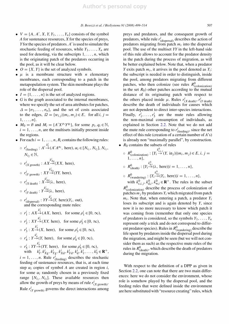
Fig. 1. The role of patch areas.

that each patch evolves independently (that is, all con-stants of rules in R0 are null). The area of patch 1 isσ1 = 1, while the other three values are σ2 = 0.35, σ3 =1.5, σ4 = 2.5. The chosen rule constants insidethe patches are C1 = {ki

Xg = 0.1, kiYg = 0.01, ki

Xd =0, ki

Yd = 10, kid = 0|i = 1, . . . , 4}, ρi

j = 0, for all i =1, . . . , 4, j = 1, . . . , 5 (that is, mute rules are notapplied). In Fig. 1 (left) we present the dynamics in thephase space of the relative model. We show that, as thearea of patches increases from patch 2 to 4, also the prob-ability of extinction of the populations increases (Fig. 1,right). Moreover, as a particular case we can see that thedynamics of the smallest patch, namely patch 2, doesnot obeys to a pure Lotka–Volterra behavior, but onlya minimal stochastic variation around the value of 400individuals occurs (graphic not shown). It can also beseen that patch 4 undergoes the extinction of predators,which allows the consequent uncontrolled increase ofpreys (Fig. 1, right).

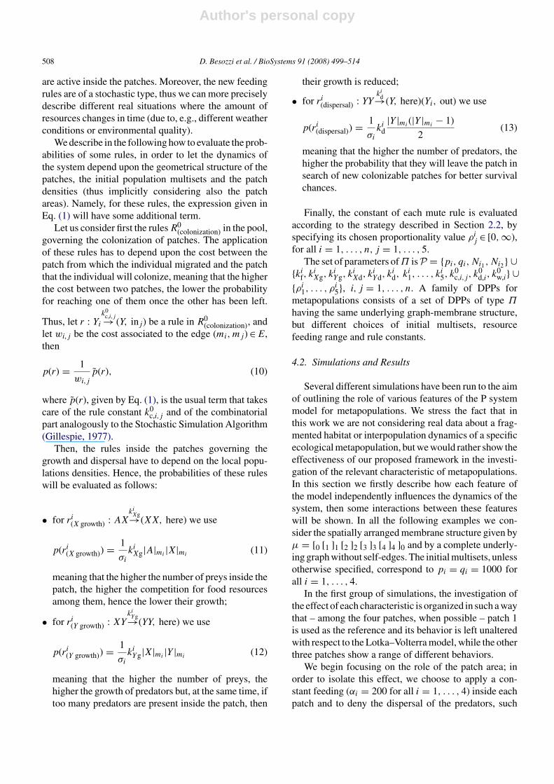
In Fig. 2 we start investigating the role of mute rules:in a structure with equal areas and where no dispersal

occurs, inside patches 2, 3 and 4 we define different ratiosfor mute rules, namely ρ2

i = 1/3, ρ3i = 1, ρ4

i = 3, for alli = 1, . . . , 5. Patch 1 is still used as the reference one,so mute rules are not applied there. The initial rule con-stants of all patches are equal to those defined in the setC1, the actual constants of initial and mute rules used dur-ing simulations have then been evaluated as described inSection 2.2. What turns out in this case is that the highestthe chance of executing mute rules is (patch 4), the low-est the variation in the numbers of preys and predators is.This is easily explained by the fact that the applicationof mute rules diminishes the number of modified objectsinside membranes.

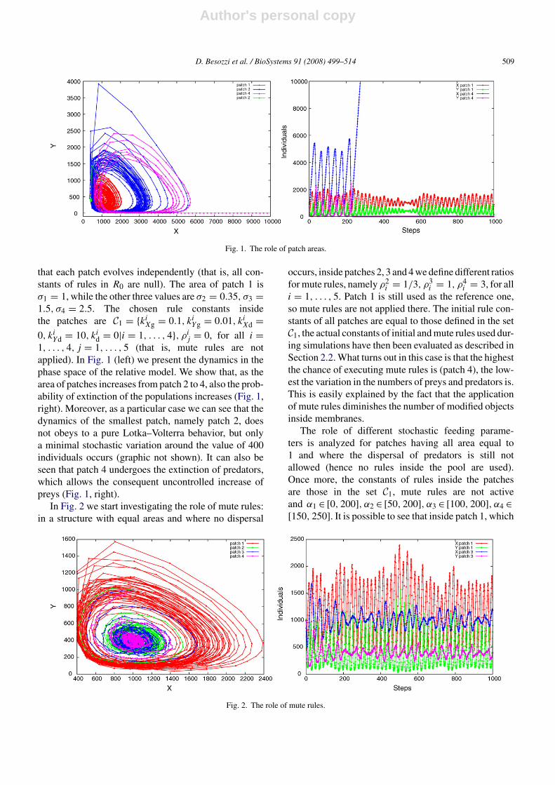
The role of different stochastic feeding parame-ters is analyzed for patches having all area equal to1 and where the dispersal of predators is still notallowed (hence no rules inside the pool are used).Once more, the constants of rules inside the patchesare those in the set C1, mute rules are not activeand α1 ∈ [0, 200], α2 ∈ [50, 200], α3 ∈ [100, 200], α4 ∈[150, 250]. It is possible to see that inside patch 1, which

Fig. 2. The role of mute rules.

Author's personal copy

510 D. Besozzi et al. / BioSystems 91 (2008) 499–514

Fig. 3. The role of stochastic feeding.

has the lowest feeding range, the extinction of preda-tors is immediate (red line in Fig. 3, top), in patch 2the extinction of predators happens when around 600steps have been run (Fig. 3, bottom left), while in patch3 (Fig. 3, bottom right) and patch 4 (data not shown,but similar to patch 3), which have the highest feed-ing ranges, there still exists persistence of oscillatingbehavior among preys and predators.

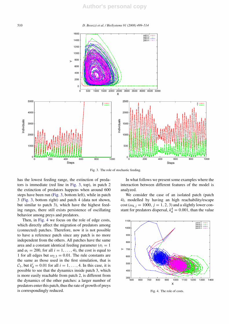
Then, in Fig. 4 we focus on the role of edge costs,which directly affect the migration of predators among(connected) patches. Therefore, now it is not possibleto have a reference patch since any patch is no moreindependent from the others. All patches have the samearea and a constant identical feeding parameter (σi = 1and αi = 200, for all i = 1, . . . , 4), the cost is equal to1 for all edges but ω2,3 = 0.01. The rule constants arethe same as those used in the first simulation, that isC1, but ki

d = 0.01 for all i = 1, . . . , 4. In this case, it ispossible to see that the dynamics inside patch 3, whichis more easily reachable from patch 2, is different fromthe dynamics of the other patches: a larger number ofpredators enter this patch, thus the rate of growth of preysis correspondingly reduced.

In what follows we present some examples where theinteraction between different features of the model isanalyzed.

We consider the case of an isolated patch (patch4), modelled by having an high reachability/escapecost (ω4,j = 1000, j = 1, 2, 3) and a slightly lower con-stant for predators dispersal, k4

d = 0.001, than the value

Fig. 4. The role of costs.

Author's personal copy

D. Besozzi et al. / BioSystems 91 (2008) 499–514 511

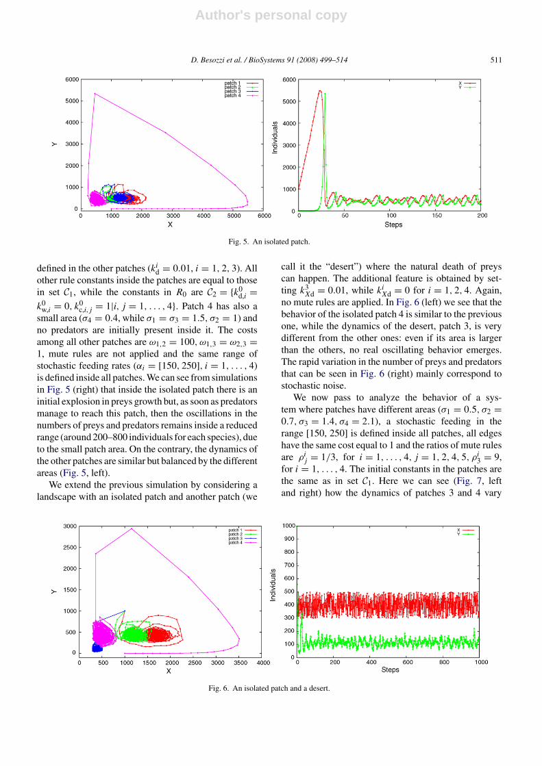
Fig. 5. An isolated patch.

defined in the other patches (kid = 0.01, i = 1, 2, 3). All

other rule constants inside the patches are equal to thosein set C1, while the constants in R0 are C2 = {k0

d,i =k0

w,i = 0, k0c,i,j = 1|i, j = 1, . . . , 4}. Patch 4 has also a

small area (σ4 = 0.4, while σ1 = σ3 = 1.5, σ2 = 1) andno predators are initially present inside it. The costsamong all other patches are ω1,2 = 100, ω1,3 = ω2,3 =1, mute rules are not applied and the same range ofstochastic feeding rates (αi = [150, 250], i = 1, . . . , 4)is defined inside all patches. We can see from simulationsin Fig. 5 (right) that inside the isolated patch there is aninitial explosion in preys growth but, as soon as predatorsmanage to reach this patch, then the oscillations in thenumbers of preys and predators remains inside a reducedrange (around 200–800 individuals for each species), dueto the small patch area. On the contrary, the dynamics ofthe other patches are similar but balanced by the differentareas (Fig. 5, left).

We extend the previous simulation by considering alandscape with an isolated patch and another patch (we

call it the “desert”) where the natural death of preyscan happen. The additional feature is obtained by set-ting k3

Xd = 0.01, while kiXd = 0 for i = 1, 2, 4. Again,

no mute rules are applied. In Fig. 6 (left) we see that thebehavior of the isolated patch 4 is similar to the previousone, while the dynamics of the desert, patch 3, is verydifferent from the other ones: even if its area is largerthan the others, no real oscillating behavior emerges.The rapid variation in the number of preys and predatorsthat can be seen in Fig. 6 (right) mainly correspond tostochastic noise.

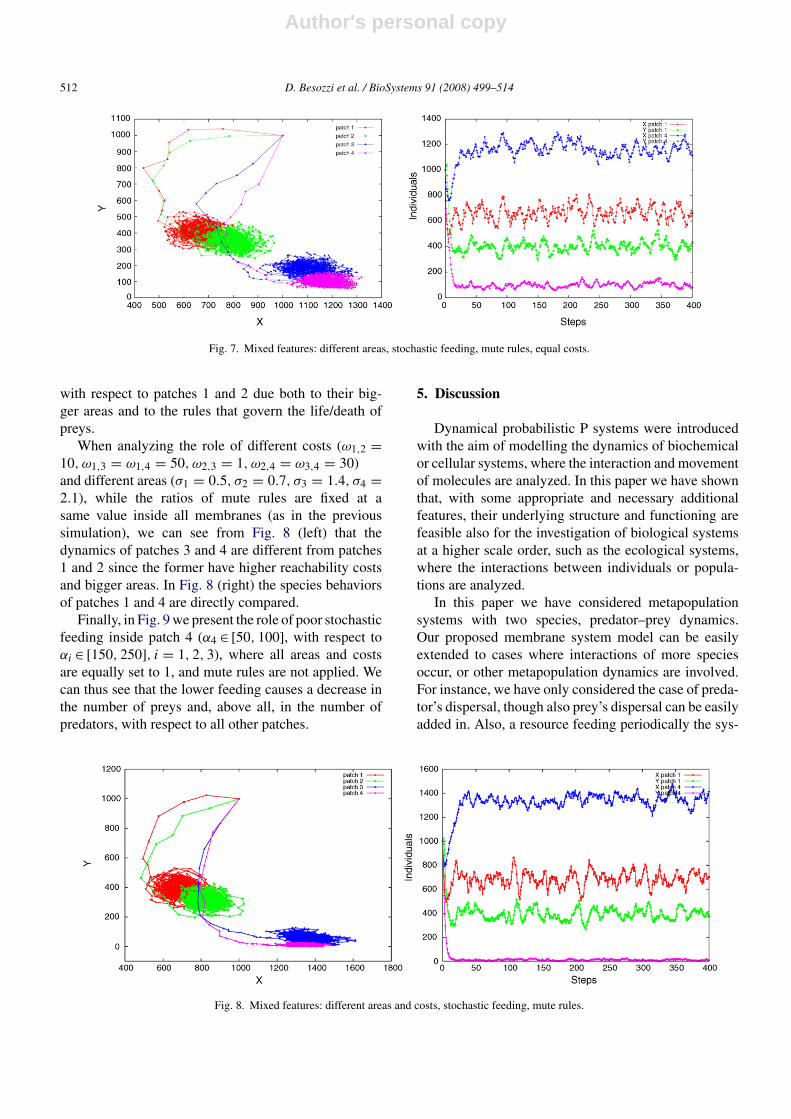
We now pass to analyze the behavior of a sys-tem where patches have different areas (σ1 = 0.5, σ2 =0.7, σ3 = 1.4, σ4 = 2.1), a stochastic feeding in therange [150, 250] is defined inside all patches, all edgeshave the same cost equal to 1 and the ratios of mute rulesare ρi

j = 1/3, for i = 1, . . . , 4, j = 1, 2, 4, 5, ρi3 = 9,

for i = 1, . . . , 4. The initial constants in the patches arethe same as in set C1. Here we can see (Fig. 7, leftand right) how the dynamics of patches 3 and 4 vary

Fig. 6. An isolated patch and a desert.

Author's personal copy

512 D. Besozzi et al. / BioSystems 91 (2008) 499–514

Fig. 7. Mixed features: different areas, stochastic feeding, mute rules, equal costs.

with respect to patches 1 and 2 due both to their big-ger areas and to the rules that govern the life/death ofpreys.

When analyzing the role of different costs (ω1,2 =10, ω1,3 = ω1,4 = 50, ω2,3 = 1, ω2,4 = ω3,4 = 30)and different areas (σ1 = 0.5, σ2 = 0.7, σ3 = 1.4, σ4 =2.1), while the ratios of mute rules are fixed at asame value inside all membranes (as in the previoussimulation), we can see from Fig. 8 (left) that thedynamics of patches 3 and 4 are different from patches1 and 2 since the former have higher reachability costsand bigger areas. In Fig. 8 (right) the species behaviorsof patches 1 and 4 are directly compared.

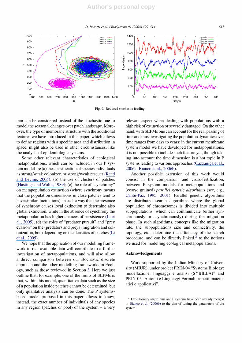
Finally, in Fig. 9 we present the role of poor stochasticfeeding inside patch 4 (α4 ∈ [50, 100], with respect toαi ∈ [150, 250], i = 1, 2, 3), where all areas and costsare equally set to 1, and mute rules are not applied. Wecan thus see that the lower feeding causes a decrease inthe number of preys and, above all, in the number ofpredators, with respect to all other patches.

5. Discussion

Dynamical probabilistic P systems were introducedwith the aim of modelling the dynamics of biochemicalor cellular systems, where the interaction and movementof molecules are analyzed. In this paper we have shownthat, with some appropriate and necessary additionalfeatures, their underlying structure and functioning arefeasible also for the investigation of biological systemsat a higher scale order, such as the ecological systems,where the interactions between individuals or popula-tions are analyzed.

In this paper we have considered metapopulationsystems with two species, predator–prey dynamics.Our proposed membrane system model can be easilyextended to cases where interactions of more speciesoccur, or other metapopulation dynamics are involved.For instance, we have only considered the case of preda-tor’s dispersal, though also prey’s dispersal can be easilyadded in. Also, a resource feeding periodically the sys-

Fig. 8. Mixed features: different areas and costs, stochastic feeding, mute rules.

Author's personal copy

D. Besozzi et al. / BioSystems 91 (2008) 499–514 513

Fig. 9. Reduced stochastic feeding.

tem can be considered instead of the stochastic one tomodel the seasonal changes over patch landscape. More-over, the type of membrane structure with the additionalfeatures we have introduced in this paper, which allowsto define regions with a specific area and distribution inspace, might also be used in other circumstances, likethe analysis of epidemiologic systems.

Some other relevant characteristics of ecologicalmetapopulations, which can be included in our P sys-tem model are (a) the classification of species individualsas strong/weak colonizer, or strong/weak rescuer (Reedand Levine, 2005); (b) the use of clusters of patches(Hastings and Wolin, 1989); (c) the role of “synchrony”on metapopulation extinction (where synchrony meansthat the population dimensions in close patches tend tohave similar fluctuations), in such a way that the presenceof synchrony causes local extinction to determine alsoglobal extinction, while in the absence of synchrony themetapopulation has higher chances of persistence (Li etal., 2005); (d) the roles of “predator pursuit” and “preyevasion” on the (predators and preys) migration and col-onization, both depending on the densities of patches (Liet al., 2005).

We hope that the application of our modelling frame-work to real available data will contribute to a furtherinvestigation of metapopulations, and will also allowa direct comparison between our stochastic discreteapproach and the other modelling frameworks in Ecol-ogy, such as those reviewed in Section 3. Here we justoutline that, for example, one of the limits of SEPMs isthat, within this model, quantitative data such as the sizeof a population inside patches cannot be determined, butonly qualitative analysis can be done. The P systems-based model proposed in this paper allows to know,instead, the exact number of individuals of any speciesin any region (patches or pool) of the system – a very

relevant aspect when dealing with populations with ahigh risk of extinction or severely damaged. On the otherhand, with SEPMs one can account for the real passing oftime and thus investigating the population dynamics overtime ranges from days to years; in the current membranesystem model we have developed for metapopulations,it is not possible to include such feature yet, though tak-ing into account the time dimension is a hot topic in Psystems leading to various approaches (Cazzaniga et al.,2006a; Bianco et al., 2006b).

Another possible extension of this work wouldconsist in the comparison, and cross-fertilization,between P system models for metapopulations and(coarse grained) parallel genetic algorithms (see, e.g.,Cantu-Paz, 1995, 2001). Parallel genetic algorithmsare distributed search algorithms where the globalpopulation of chromosomes is divided into multiplesubpopulations, which can communicate (either syn-chronously or asynchronously) during the migrationphase. In such algorithms, concepts like the migrationrate, the subpopulations size and connectivity, thetopology, etc., determine the efficiency of the searchprocedure, and can be directly linked.2 to the notionswe used for modelling ecological metapopulations.

Acknowledgements

Work supported by the Italian Ministry of Univer-sity (MIUR), under project PRIN-04 “Systems Biology:modellazione, linguaggi e analisi (SYBILLA)” andPRIN-05 “Automi e Linguaggi Formali: aspetti matem-atici e applicativi”.

2 Evolutionary algorithms and P systems have been already mergedin Bianco et al. (2006b) to the aim of tuning the parameters of thesystem.

Author's personal copy

514 D. Besozzi et al. / BioSystems 91 (2008) 499–514

References

Akcakaya, H.R., Sjogren-Gulve, P., 2000. Population viability analysisin conservation planning: an overview. Ecol. Bull. 48, 9–21.

Bernardini, F., Gheorghe, M., Krasnogor, N., Muniyandi, R.C., Perez-Jimenez, M.J., Romero-Campero, F.J., 2006. On P systems as amodelling tool for biological systems. In: Freund, R., Paun, Gh.,Rozenberg, G., Salomaa, A. (Eds.), Membrane Computing, Inter-national Workshop, Vienna, Austria, vol. 3850 of Lecture Notes inComputer Science. Springer, pp. 114–133.

Bianco, L., Fontana, F., Franco, G., Manca, V., 2005. P systems for bio-logical dynamics. In: Ciobanu, G., Paun, Gh., Perez-Jimenez, M.J.(Eds.), Applications of Membrane Computing. Springer-Verlag,Berlin, pp. 81–126.

Bianco, L., Fontana, F., Manca, V., 2006a. P systems with reactionmaps. Int. J. Found. Comput. Sci. 17 (1), 27–48.

Bianco, L., Pescini, D., Siepmann, P., Krasnogor, N., Romero-Campero, F.J., Gheorghe, M., 2006b. Towards a P systemsPseudomonas quorum sensing model. In: Hoogeboom, H.J., Paun,Gh., Rozenberg, G., Salomaa, A. (Eds.), Membrane Computing,International Workshop, Leiden, The Netherlands, vol. 4361 ofLecture Notes in Computer Science. Springer, pp. 197–214.

Cantu-Paz, E., 1995. A summary of research on parallel genetic algo-rithms. IlliGAL Report No. 95007.

Cantu-Paz, E., 2001. Migration policies, selection pressure, and paral-lel evolutionary algorithms. J. Heuristics 7, 311–334.

Cazzaniga, P., Pescini, D., Besozzi, D., Mauri, G., 2006a. Tau leapingstochastic simulation method in P systems. In: Hoogeboom, H.J.,Paun, Gh., Rozenberg, G., Salomaa, A. (Eds.), Membrane Comput-ing, International Workshop, Leiden, The Netherlands, vol. 4361of Lecture Notes in Computer Science. Springer, pp. 298–313.

Cazzaniga, P., Pescini, D., Romero-Campero, F.J., Besozzi, D., Mauri,G., 2006b. Stochastic approaches in P systems for simulat-ing biological systems. In: Gutierrez-Naranjo, M.A., Paun, Gh.,Riscos-Nunez, A., Romero-Campero, F.J. (Eds.), BrainstormingWeek on Membrane Computing. Fenix Editora, Sevilla, Spain, pp.145–164.

Ciobanu, G., Paun, Gh., Perez-Jimenez, M.J. (Eds.), 2005. Applica-tions of Membrane Computing. Springer-Verlag, Berlin.

Conroy, M.J., Cohen, Y., James, F.C., Matsinos, Y.G., Maurer, B.A.,1995. Parameter estimation, reliability, and model improvementfor spatially explicit models of animal populations. Ecol. Appl. 5(1), 17–19.

Dunning, J.B., Stewart, D.J., Danielson, B.J., Noon, B.R., Root, T.L.,Lamberson, R.H., Stevens Jr., E.E., 1995. Spatially explicit pop-ulation models: current forms and future uses. Ecol. Appl. 5 (1),3–11.

Giavitto, J.-L., 2003. Topological collections, transformations andtheir application to the modeling and the simulation of dynami-cal systems. In: Nieuwenhuis, R. (Ed.), Rewriting Techniques andApplications, vol. 2706 of Lecture Notes in Computer Science.Springer, pp. 208–233.

Giavitto, J.-L., Michel, O., 2002. The topological structures of Mem-brane Computing. Fund. Inform. 49 (1–3), 123–145.

Gillespie, D.T., 1977. Exact stochastic simulation of coupled chemicalreactions. J. Phys. Chem. 81, 2340–2361.

Hanski, I., 1998. Metapopulation dynamics. Nature 396, 41–49.Hastings, A., Harrison, S., 1994. Metapopulation dynamics and genet-

ics. Annu. Rev. Ecol. System. 25, 167–188.Hastings, A., Wolin, C.L., 1989. Within-patch dynamics in a metapop-

ulation. Ecology 70 (5), 1261–1266.

Ideker, T., Galitski, T., Hood, L., 2001. A new approach to decod-ing life: systems biology. Annu. Rev. Genom. Hum. Genet. 2,343–372.

Jansen, V.A.A., 2001. The dynamics of two diffusively coupledpredator–prey populations. Theor. Populat. Biol. 59, 119–131.

Jansen, V.A.A., Lloyd, A.L., 2000. Local stability analysis of spatiallyhomogeneous solutions of multi-patch systems. J. Math. Biol. 41,232–252.

Levins, R., 1960. Some demographic and genetic consequences ofenvironmental heterogeneity for biological control. Bull. Entomol.Soc. Am. 71, 237–240.

Li, Z., Gao, M., Hui, C., Han, X., Shi, H., 2005. Impact of preda-tor pursuit and prey evasion on synchrony and spatial patterns inmetapopulation. Ecol. Modell. 185, 245–254.

Moilanen, A., 2004. SPOMSIM: software for stochastic patch occu-pancy models of metapopulation dynamics. Ecol. Modell. 179,533–550.

Murray, J.D., 2002. Mathematical Biology. I. An introduction.Springer-Verlag, New York.

Murray, J.D., 2003. Mathematical Biology. II. Spatial Models andBiomedical Applications. Springer-Verlag, New York.

Paun, Gh., 2000. Computing with membranes. J. Comput. System Sci.61 (1), 108–143.

Paun, G., 2002. Membrane Computing. An Introduction. Springer-Verlag, Berlin.

Perez-Jimenez, M.J., Romero-Campero, F.J., 2005a. Modelling EGFRsignalling cascade using continuous membrane systems. In:Plotkin, G. (Ed.), Third International Workshop on ComputationalMethods in Systems Biology. Edinburgh, United Kingdom, pp.118–129.

Perez-Jimenez, M.J., Romero-Campero, F.J., 2005b. Modelling Vibriofischeri’s behaviour using P systems. Systems Biology Workshop,ECAL 2005.

Pescini, D., Besozzi, D., Mauri, G., 2005. Investigating local evolu-tions in dynamical probabilistic P systems. In: Proceedings of 7thInternational Symposium on Simbolic and Numeric Algorithms forScientific Computing, SYNASC 2005, IEEE Computer Society,Timisoara, Romania, pp. 440–447.

Pescini, D., Besozzi, D., Mauri, G., Zandron, C., 2006a. Analysis andsimulation of dynamics in probabilistic P systems. In: Pierce, N.,Carbone, A. (Eds.), International Meeting on DNA Computing.London, Ont., Canada, vol. 3892 of Lecture Notes in ComputerScience. Springer, pp. 236–247.

Pescini, D., Besozzi, D., Mauri, G., Zandron, C., 2006b. Dynami-cal probabilistic P systems. Int. J. Found. Comput. Sci. 17 (1),183–204.

Reed, J.M., Levine, S.H., 2005. A model for behavioral regulation ofmetapopulation dynamics. Ecol. Modell. 183, 411–423.

Suzuki, Y., Takabayashi, J., Tanaka, H., 2002. Investigation oftritrophic system in ecological systems by using an artificial chem-istry. J. Artif. Life Robot. 6, 129–132.

Taylor, A.D., 1990. Metapopulations, dispersal, and predator-preydynamics: an overview. Ecology 71 (2), 429–433.

Terrazas, G., Krasnogor, N., Gheorghe, M., Bernardini, F., Diggle,S., Camara, M., 2005. An environment aware P-system model ofquorum sensing. In: Cooper, S.B., Lowe, B., Torenvliet, L. (Eds.),CiE, vol. 3526 of Lecture Notes in Computer Science. Springer,pp. 479–485.

Weisser, W.W., Jansen, V.A.A., Hassell, M.P., 1997. The effects of apool of dispersers on host-parasitoid systems. J. Theor. Biol. 189,413–425.