Finite element modelling and simulation of welding of ... - DIVA

LICENTIATE THESIS

2003:27

Department of Applied Physics and Mechanical Engineering

Division of Computer Aided Design

2003:27 • ISSN: 1402 - 1757 • ISRN: LTU - LIC - - 03/27 - - SE

Finite Element Modelling and Simulation of Welding of Aerospace Components

ANDREAS LUNDBÄCK

Preface

The research presented in this thesis has been carried out at the Division of Computer Aided Design at Luleå University of Technology in close cooperation with Volvo Aero and Motoren und Turbinen Union, Germany. The financial support has been provided by the MMFSC1-project, a European Union funded project within the 5th framework programme and Luleå University of Technology.

I would first like to thank my supervisor Professor Lars-Erik Lindgren for his support and valuable guidance during the course of this work. My colleague Daniel Berglund deserves special thanks for his support and guidance in the initial phase of this work.

Many thanks also to all my friends and colleagues at Luleå University of Technology for all the discussions during the coffee brakes. It is inspiring to work within such a pleasant working environment.

Finally I would like to thank my family: Ann-Katrin, Victor, Lucas and Clara. Thank you for your support, encouragement and just for being there!

Luleå Maj 2003

Andreas Lundbäck

1 Manufacturing and Modelling of Fabricated Structural Components

Abstract

Fusion welding is one of the most used methods for joining metals. This method has largely been developed by experiments, i.e. trial and error. The problem of distortion and residual stresses of a structure due to welding is important to control. This is especially important in the aerospace industry where the components are expensive and safety and quality are highly important issues. The safety requirements and the high costs of performing experiments to find different manufacturing routes is the motivation to increase the use of simulations in design of components as well as its manufacturing. Thus, in the case of welding, one can evaluate the effect of different fixtures, welding parameters etc on the deformation of the component. It is then possible to optimise a chain of manufacturing processes as, for example, the welding residual stresses will affect the deformations during a subsequent heat treatment.

The aim of the work presented in this thesis is to develop an efficient and reliable method for simulation of the welding process using the Finite Element Method. The method may then be used when designing and planning the manufacturing of a component, so that introduction of new components can be made with as little disturbance as possible. In the same time the developed tool will be suitable for the task to perform an optimal design for manufacturing. Whilst this development will also be valuable in predicting the component's subsequent in-service behaviour, the key target is to ensure that designs are created which are readily manufactured. If this understanding is captured and made available to designers, true design for manufacture will result. This will lead to right first time product introduction and minimal ongoing manufacturing costs as process capability will be understood and designed into the component.

When creating a numerical model, the aim is to implement the physical behaviour of the process into the model. However, it may be necessary to compromise between accuracy of the model and the required computational time. Different types of simplifications of the problem and more efficient computation methods are discussed. Methods for alleviating the modelling, in particular the creation of the weld path, of complex geometries is presented. Simulations and experiments have been carried out in order to validate the models.

Keywords Finite Element Method, Welding, Manufacturing Simulation, Aerospace Engineering

Table of Contents

1. INTRODUCTION .........................................................................................................1

1.1 THE FINITE ELEMENT METHOD IN A HISTORICAL PERSPECTIVE.........11.2 BACKGROUND....................................................................................................11.3 AIM AND SCOPE OF PRESENT RESEARCH ...................................................2

2. WELDING IN AEROSPACE ENGINEERING .........................................................3

2.1 WELDING METHODS .........................................................................................32.2 EFFECTS OF WELDING......................................................................................4

3. SIMULATION OF WELDING ....................................................................................5

3.1 GENERAL ASSUMPTIONS IN MODELLING...................................................53.2 CURRENT WELDING SIMULATIONS..............................................................63.3 CREATION OF WELD PATH..............................................................................73.4 HEAT INPUT ........................................................................................................83.5 MATERIAL MODEL ............................................................................................93.6 ELEMENT ACTIVATION..................................................................................103.7 EFFICIENT COMPUTATION ............................................................................10

4. SUMMARY OF APPENDED PAPERS.....................................................................12

4.1 PAPER A..............................................................................................................124.2 PAPER B..............................................................................................................124.3 PAPER C..............................................................................................................13

5. DISCUSSION AND FUTURE WORK ......................................................................13

6. REFERENCES.............................................................................................................14

A. Lundbäck - Finite Element Modelling and Simulation of Welding of Aerospace Components

1

1. Introduction

1.1 The Finite Element Method in a Historical Perspective The history of the finite element method is about hundred years, but it took another fifty years before the method became useful. In 1906 a paper was presented where researchers suggested a method for replacing the continuum description for stress analysis by a regular pattern of elastic bars. Later in 1943, Courant [1] proposed the finite element method as we know it today. None of the forgoing work was of any practical use though, since there were no computers available at that time to solve the large set of simultaneous algebraic equations related to the method. In the early 1950’s engineers, mainly in the aerospace industry, started to use the method of finite element more frequently. It was still only a number of exclusive groups that where able to use the method, since digital computers had not become widespread yet and they were very expensive. The actual name “finite element method” was coined by Clough in 1960 and in the late 1960’s and early 1970’s large general-purpose programs emerged, such as ANSYS, NASTRAN and MARC. However, these programs were still written for a particular mainframe, it was not until the mid-1980’s general-purpose programs began to appear on personal computers and thereby became more widespread. Today hundreds of thousands engineers all over the world are using the finite element method in their everyday work. The above text is an extract from the books by Cook et al. [2] and Belytschko et al. [3]. In the paper by Felippa [4] a comprehensive review of the history of FEM can be found.

1.2 BackgroundThis research is a part of the project Manufacturing and Modelling of Fabricated Structural Components (MMFSC). This is an EU funded project within the 5th Framework Programme with a number of aeroengine companies. The work presented here has been done in close cooperation with Volvo Aero Corporation (VAC) and Motoren und Turbinen Union (MTU).

“The main objective of the MMFSC project is to develop, for aero-engine structures, alternative manufacturing strategies to single-piece casting, which is currently supplied by a non-EU manufacturer, and which leaves little room for in-house design flexibility.”

MMFSC [5]

Fabrication, the alternative to single-piece casting, is less reliant on fixed tooling and can use combinations of materials and techniques (casting, forging, sheet forming, welding, machining etc.), each to its greatest advantage where needed. Also a substantial improvement in the utilisation of material is anticipated compared to a single-piece casting. This is due to that different material thicknesses can more easily be assigned in different parts of the component when the method of fabrication is used. The need for fabrication is of special interest for large components where there is only a few (one) manufacturers available. This leads to long delivery times and high costs.


2

Fabrication is not easily implemented in the manufacturing process due to the high safety requirements and the lack of fundamental understanding of the process. A number of manufacturing processes are analysed within the MMFSC project. The effect of the individual processes is studied and also the combined effects of previous processes. The long term goal, outside the scope of this work though, is to be able to create a “virtual prototype” of the component. The virtual prototype will be built up from the designed geometry and the result from all the manufacturing processes applied. After the manufacturing of the component is completed the virtual prototype will be upgraded, if there are any, and fed with the in-service loadings. Figure 1 is a somewhat extended figure from Runnemalm [6]. The extension is that the whole lifetime of the component is added, the in-service loading and possible upgrading. This will give valuable information, both when maintenance decisions are made and when designing the next generation of components.

Pro

du

ct

req

uire

me

nts

Preliminarypreparation

Definitionphase

Verificationphase

DetailedPreparation

Conceptphase

Inventory ofknown methods

Computer based engineering models

Physical productTools for functional evaluation

MANUFACTURING

DESIGN

Data from componentin-service applied todigital copy of product

Digital versionof product

Maintenanceupgrading etc.

Services

Tools for planning of manufacturing

Feedback

Feedback

Figure 1. Use of computer models for design of components, manufacturing routes and supporting maintenance.

1.3 Aim and Scope of Present ResearchThe aim of the work presented in this thesis is to develop a method and a model for simulation of the welding process of large and complex components. The simulations can then be used when designing and planning the manufacturing of the fabrication of components.

The research question is: “Is it possible to simulate the process of welding of a complex component with adequate accuracy for predicting the distortions in the final geometry of the component?”

The work has been focussing on validation of the model on smaller test pieces so far. The welding methods that have been studied are laser and electron beam welding and the material used is Inconel 718.


3

2. Welding in Aerospace Engineering

2.1 Welding Methods There exist a number of different welding methods. The most common methods in the aerospace industry are Gas Tungsten Arc Welding (GTAW), Electron Beam welding (EB) and Laser beam welding. In the book by Radaj [7], a thorough description of these processes can be found. In Figure 2 the power densities for the different welding processes are shown. Stone [8] describes both the history and the physics of the EB welding process in some detail. Below a short introductory of these processes will follow.

Figure 2. Power density for different welding processes, Radaj [7].

In the case of GTA-welding the heat is generated by the discharge between the anode and the cathode using a non-melting electrode. An inert gas is used as shield against oxidation and the process can be carried out with or without filler material. The power density of this process is the lowest of those mentioned above. Material thicknesses between 0.5 and 3 mm can easily be welded with single-pass welds. If larger thicknesses are to be welded, then multi-pass welding has to be adopted.

In laser beam welding a high power density beam, coherent focussed light, is directed at the welding spot, optical lenses are used to focus the light. The beam is absorbed in a thin surface layer and if the power density is adequate the surface is fused. A “digging” process now starts, provided that sufficient power is applied, and a vapour capillary is formed. The vapour capillary is the actual welding heat source. If the work piece is moved relative to the beam the vapour capillary will form a “keyhole”. The penetration depth is restricted to 5 – 10 mm, depending on which type of laser used, due to the defocus of the beam.

Electron beam welding is another high power density welding method. The power density is even higher than in laser beam welding. The process is similar to the laser welding process, but in EB-welding it is a hot cathode that accelerates electrons towards the welding spot and electro-magnetic lenses are used to focus the beam. Whilst the penetration depth of the laser process is restricted to relative small depths the penetration depth in EB-welding can reach up


4

to 320 mm. One major drawback with EB-welding is that it has to be carried out in vacuum. The reason why it has to be carried out in vacuum is that the electrons would be retarded or deteriorated by other particles too much otherwise. Recently medium vacuum and non-vacuum electron beam welding systems has been introduced, which will extend the usability of this process.

2.2 Effects of Welding During the welding process a local area is heated up rapidly with high thermal gradients as a consequence. The material expands as a result of being heated but the expansion is restrained by the surrounding colder, and stronger, bulk. This will give rise to the thermal stresses. Since the yield limit is lowered in the area of elevated temperature, plastic strains will develop in the weld region. When the weld area cools down the material in that area will be “too small”, i.e. the volume has been reduced. During cooling the material will retrieve its strength, normally at an elevated level due to plastic hardening, which in turn gives rise to the residual stresses.

The deformations due to welding are driven by the thermal expansion (temporarily) and the residual stresses (permanently). Stress and deformation are largely opposed. A high degree of geometrical restraint in welding results in high stresses and small deformations while an unrestrained weld produces lower stresses but larger deformations. As a consequence the welding reliability of the design is assessed primarily on the basis of welding residual stress analysis, whereas welding feasibility in manufacturing is assessed primarily on the basis of welding deformation analysis. In Figure 3 the basic deformation modes for a rectangular plate with centric joining weld are presented.

Figure 3. Deformation modes of a rectangular plate with a centric jointing weld seam.


5

In the book by Radaj [7], the residual stresses are defined and categorized as following. Residual stresses are internal forces, in equilibrium only with themselves over the whole domain of the body, without external forces acting. Stresses arising during the welding process, due to inhomogeneous thermal expansion, can be referred to as internal stresses if the body is mechanically unconstrained and are termed “thermal stresses”.

The residual stresses can be distinguished in different levels, first, second and third order residual stresses. First order residual stresses, I, extend over macroscopic areas and are averaged stresses over several crystal grains. Second order stresses, II, acts between crystals or crystal subregions. Third order residual stresses, III, act on the interatomic level, e.g. single dislocations. It is mainly the first order stresses that are of interest for engineering purposes and thus also in this thesis.

3. Simulation of Welding The method of finite element was originally adopted for linear-static structural analysis and dynamics. The method was later extended for dealing with geometric and material non-linear problems. The pioneering work within simulation of welding in the early 1970s, e.g. Ueda and Yamakawa [9] and Hibbit and Marcal [10], included material non-linearity and the coupling between thermal and mechanical analysis. In the latter also geometric non-linearity’s, such as large strain and deformations where encountered for. Marcal [11], in his review, later stated that “welding is perhaps the most nonlinear problem encountered in structural mechanics”. In the review by Goldak et al. [12] it is suggested that the difficulties experienced by the pioneers, but still eminently qualified experts in nonlinear FEM, Hibbit and Marcal discouraged others from entering the field. Their expertise is demonstrated by the fact that MARC, developed by Marcal and Hibbit, and ABAQUS, developed by Hibbit, are the most highly regarded commercial FEA-software for nonlinear problems. Despite this, quite a few researchers have entered the field during the last three decades and a list of what has been done would be very long. A large number of reviews which summarizes the work during this thirty-year period have been published, e.g. [11-16]. One of the most recent is the comprehensive review, in three parts, by Lindgren [14-16]. This review not only contains a large number of references of what has been done earlier and the state of the art today, but also recommendations of how and what to include in a model depending on the aim of the welding simulation.

3.1 General Assumptions in Modelling Before a model for simulation of welding is created some questions have to be answered, what is the aim of this simulation?, which accuracy is desired?, what kind of phenomena should be captured?, etc. In this work, the finite element models have been 3D solid element models as the aim of the simulations have been to validate the welding model on relatively small geometries. Later work will involve more complex geometries and then shell elements may be needed. In the paper by Lindgren [17], definitions of different accuracy levels and complexity levels, regarding the geometry representation, are presented. The models used in this work can be regarded as accurate and standard 3D models appropriate for obtaining residual stresses, as stated in [17].


6

The finite element type used in all the simulations is a linear eight-noded element. Belytschko et al. [3] argues that it is better to use a larger number of linear elements than fewer higher order elements when non-linear problems are analysed. The coupling between the thermal and the mechanical analysis is done by the staggered approach. In the staggered approach the thermal analysis is lagging one step behind the mechanical analysis. The short time steps taken make this approximation negligible. To keep the strain field consistent, constant temperature through the element is assumed in the thermal analysis. Large deformation and an additive decomposition of the strain rates are also assumed.

3.2 Current Welding Simulations In order to simulate a complex component or a chain of manufacturing processes, as mentioned in the introduction, a reliable model has to be developed for each specific process. It is important to know which accuracy and reliability that can be expected of the model when simulations are to be performed on a full scale component. This is especially true if, as in this case, it is a very expensive component. It is not particularly probable that extensive measurements are going to be performed on such components in production. Simulating a chain of processes is not meaningful if not all the simulation models in that chain are accurate and reliable, “a chain is not stronger than the weakest link”.

Figure 4 is a kind of roadmap of the steps that have been taken, or will be investigated, to realize the above stipulated. The approach within the MMFSC project is to first validate the numerical models for each process individually on smaller test pieces. When this is done, more complex geometries and eventually the whole manufacturing chain will then be analysed. The first step towards welding simulation of a complex geometry was to develop a method for creation of the weld path. A material model has been built up by utilization of the extensive material tests preformed within the project. Different heat sources for the heat input are tested and validated and an element activation technique is implemented to simulate the fusion of the welded material. Two strategies for efficient computation, adaptive meshing and parallel computation, have been evaluated. Other methods that are of interest are the substructuring and the local/global technique. In the following sections each part in Figure 4 will be explained in some detail.

ElementActivation

MaterialModel

HeatInput

EfficientComputation

FE-Geometry

Weld Path

Adaptive Meshing

Parallel Computation

Local/Global

Substructures

Simple Geometry

Co

mp

lex

Ge

om

etr

y

EvaluationValidation

Figure 4. Roadmap of the different steps towards more complex geometries.


7

3.3 Creation of Weld Path A method to determine the position of the heat source in each time increment has been developed. This method alleviates the process of defining the weld path especially if the path is an arbitrary 3D line. The weld path is first defined in a system, e.g. a CAD-system, where the tools for handling complex geometries normally are more developed than in the pre-processors of the FE-systems. The weld path is thereafter exported as coordinate points to a file. During the initiation of the simulation the file with the weld path coordinates is imported and processed into the FE-system via user subroutines, Figure 5.

Weld pathData

FEAUser

subroutines

Input file forFE-model

CAD

Figure 5. Strategy for the creation of weld path.

This method requires that there exist a geometry which can describe the weld path. The geometry may consist of lines, shell- or a solid geometry. An example when utilizing this method for creation of an “intricate” weld path is shown in Figure 6. The figure is part of the paper by Lundbäck [18], a description of the method in detail can be found in Lundbäck [19].

Figure 6. Example of usage of the described method.


8

3.4 Heat Input In a welding simulation it is essentially the temperature change, translated into thermal expansion in the mechanical analysis, which is the external load in the model. The increase of the temperature can generally be modelled in two different ways, prescribed temperatures or by prescribed heat input. When prescribing the temperatures the temperature is given in each node for the specific time and position. The temperature is usually linearly ramped to the prescribed value and thereafter followed by a constant-temperature phase. This method has been used quite frequent, but mainly in 2D analysis. The other method, prescribed heat input, which is the today most commonly used method, applies the heat input as a heat flux at the integration points which is then converted to the nodes as temperature loads. The most commonly used heat sources of this kind have a Gaussian distribution, but heat sources with constant distribution has also been used. Goldak et al. [20] proposed a volumetric heat source, see Equation 1 and Figure 7, the so-called double ellipsoid. This heat source consists of two elliptic regions, one in the front of the arc centre, z > 0,

22

2

2

22 333

23

36,, fc

zb

ya

x

f

ff eee

abc

Qfzyxq (1a)

and the other behind the arc centre, z < 0.

22

2

2

22 333

23

36,, rcz

by

ax

r

rr eee

abc

Qfzyxq (1b)

crcf

b

a

x

z

y

Weldingdirection

Figure 7. Geometrical definition of the double ellipsoid heat source.

The double ellipsoid heat source was initially intended to be used for modelling of GTA-welding [20]. Later Goldak et al. [12] reported that they had received the most accurate temperature field by combining three heat sources, a double elliptical disc on the surface, a double ellipsoid to model the direct impingement of the arc and another double ellipsoid to model the stirring effect of the molten metal. To model deep penetration welds, such as electron and laser beam welding, they recommended a conical distribution of power density


9

with a Gaussian distribution radially and a linear distribution axially. However, the actual formula for this conical heat source was not presented in the paper. Stone et al. [21] used a combination of a circular surface flux and a conic volumetric source. Both these sources had a uniform distribution of the power density. In Lundbäck and Runnemalm [22], a combined double ellipsoid and conical-elliptic heat source is presented. The formula for the frontal part in the conical-elliptic heat source, z > 0 as in the above definition, can be seen in Equation 2.

2

2

2

233

,,

11

16

cc cz

c

cax

cccc

cczyxc e

byd

edcba

Qffq (2)

All the parameters, except for bc and dc, corresponds to those in Equation 1a. The parameter bc is the depth of the cone, which should be equal to the thickness of the material and dc is the decrease of the cone width at the bottom surface.

Comparing these two methods, prescribed temperatures and prescribed heat input, it can be said that prescribing the temperatures can be easier to use as means for heat input in some cases. This is especially true in the 2D case but less true in the 3D case where the method of prescribed heat input is probably easier to implement and use. The accuracy in the heating phase is also better in the latter method.

There exist more advanced heat source models, e.g. [23-25]. Sudnik et al. [23] used a thermo-dynamical steady-state model to calculate the thermal field in a laser beam weld. The result from such models can be used in different ways, either by mapping of the temperatures directly into the FE-model, i.e. prescribed temperatures, or the result can be used as a validation of the FE-result. Hughes et al. [25] used a detailed finite volume model of the weld pool to calibrate the heat source parameters in the FE-model automatically. In this work a model, modified to fit electron beam welding, from Sudnik et al. [23] has been used to validate the FE-results. The gain by using the result from such a model is that information and knowledge about the shape of the thermal field can be obtained. Some of these results can be obtained with experiments, i.e. cross section micrographs. Other results, such as the thermal field in the welding direction inside the material, are in practice impossible to obtain with experiments. The reason why the prescribed temperature method was not chosen is that mapping the temperatures from a non-analytical model is a relatively time-consuming task. Further it requires direct access to the thermo-dynamical model, which was not the case in this work.

3.5 Material Model Two different materials and material models are used in this thesis, a martensitic stainless steel and the nickel based Superalloy Inconel 718. The material model for the stainless steel is a rate-independent termo-elastoplastic model. No account is taken for the hardening due to plastic deformation or phase changes tough. In the material model for Inconel 718 plasticity induced hardening is included.


10

3.6 Element Activation The welding process can be performed with or without filler material depending on which process used and the requirement on the weld geometry. In the aerospace industry no undercutting in the welds is accepted, i. e. the thickness of the material in the weld can not be less than in the surrounding material. Filler material is commonly used in GTA and laser beam welding but less common in electron beam welding. Nevertheless, some kind of element deactivation and activation has to be used disregarding of the welding process if for example a butt welding is going to be modelled. Two different techniques can be used, “quiet elements” or “born dead”. When using quiet elements the elements are active during the whole analysis but the stiffness and the thermal conductivity is very low so that the “inactive” elements do not affect the rest of the model. With the other method, born dead element, the elements that are inactive is not part of the system of equations until they are activated. In this work the born dead technique has been used exclusively. The thermal and mechanical activation is separated to enable the element to be heated up thermally but not contribute to the mechanical stiffness. The criterion when an element is to be activated is set as a distance relative the position of the origin of the heat source. The plastic strain should be zeroed as long as the element is in liquid phase.

Lindgren et al. [26] compared the two methods on a multipass welding analysis of a thick plate. They found that both methods gave very similar result but the method of born dead elements was somewhat more effective with respect to computational cost. Different problems may arise depending on which method used. Decreasing the stiffness, of the quiet elements, too much will give an ill-conditioned stiffness matrix with numerical problems as a result. On the other hand, when using the born dead technique, if the nodes are completely surrounded by inactive elements then these nodes will not follow the movements of the active neighbour nodes. This can result in severely distorted, or even collapsed, elements. Lindgren et al. [26] solved this problem by a smoothing technique. Lindgren and Hedblom [27] later developed a technique to control the volume of the activated elements, i.e. the filler rate, which also optimised the position of the nodes for minimized element distortion and correct geometrical shape of each weld pass.

3.7 Efficient Computation There exist a number of methods for decreasing the computational time, or actually the wall-clock time of the simulation. The most obvious and straightforward is of course to reduce the geometrical dimension, e.g. from a 3D solid model to a 2D plane strain model. Whether this is feasible or not depends on the scope of the simulation [17]. If it is decided that the analysis should give a detailed description of the weld region and the whole structure should be taken into account for, then the only choice is a solid model at least close to the weld. Below, some of these techniques are described.

Adaptive meshing is a technique that changes the mesh density due to some criterion. The criteria can for example be temperature or strain gradients. If an element fulfils the criterion, e.g. it has a too steep strain gradient, it will be divided into smaller elements. The child elements created will inherent the properties and result, such as temperature and strains, from the parent element. Since this method does not change the topology in the same sense that remeshing does and the mapping of data is kept to a minimum it is a relatively cheap method


11

with respect to computational cost. Due to that the mesh is locally refined by dividing elements, “free nodes” will occur. These nodes must be constrained to keep the mesh consistent. This method was used in Berglund et al. [28]. The number of elements in the model will continuously increase if the created elements are not merged back into the parent element, i.e. coarsening. If the locally refined area is controlled geometrically the method is called rezoning. Runnemalm and Hyun [29] presented a technique that combined error measurements from both the thermal and mechanical gradients and mesh refinement and coarsening. In this way they could keep the number of elements to a minimum but still be able to keep a high resolution in areas with steep gradients.

Mixing of shell and solid elements is of special interest when performing welding simulations on thin-walled structures. The solid elements are then concentrated near the weld region and the shell elements further away. Shells are superior to solids in the far field region as they improve the bending behaviour and the number of elements can be reduced dramatically. In the region near the arc, solid elements are often required. This is due to that there is large gradients trough the thickness in that area and shell elements, by definition, are not suitable to model those. Näsström et al. [30] showed that a model with combined solid and shell elements can be used in such structures.

The substructure technique in welding is a technique where part of the mesh in the model is condensed into a superelement and is thereby treated as a linear-elastic part of the structure. The rest of the structure is treated as non-linear, hereafter called the local zone. The stiffness from the superelement is then acting as a boundary condition on the local zone. Brown and Song [31] presented a technique for both dynamical rezoning, i.e. adaptive meshing, and substructuring. The position of the local zone was frequently updated so that it followed the moving heat source. Since the substructure is unable to deal with non-linear phenomena, such as plasticity, thermal expansion etc., it is important to keep the local zone large enough. Except for the savings in computational cost, there can be even larger savings in memory usage. This is due to that the stiffness matrix is reduced in size when condensing the elements into a superelement.

Another method, similar to substructuring in some sense, is the use of a local and global model. The local model consists of a dense mesh which accommodates the heat source and the global model provides the stiffness from the surrounding structure as boundary conditions to the local model. Andersen [32] used this approach in the mechanical analysis, but the full model was used in the thermal analysis.

The final method that will be presented in this section is parallel computation. Parallel computation induces no simplifications, changes in geometric representation or anything as the above methods. It is simply a method to decrease the computational time, or actually the wall-clock time, for an analysis to be completed. There are similarities with the two above methods, substructuring and the local/global approach. The model is divided into subdomains, domain decomposition, one subdomain for each computer process. Boundary conditions are applied on the nodes on the interface between each subdomain and then the system of equations is solved for each subdomain locally. An iterative procedure then starts to obtain equilibrium in the whole model. Escaig and Marin [33] studied different methods for domain decomposition to solve non-linear problems. They did not utilize parallel


12

computation, they used this method for separating the elastic and plastic regions in a model. The idea with this is that the bandwidth decreases and the local stiffness matrix representing the subdomains that are in the elastic region do not have to be recalculated. They showed that a speedup factor between 2 and 4 could generally be achieved. The limit of efficiency for parallel computation is due to the communication cost. That is, when the cost in time for communication between the subdomains becomes higher than the gain for adding another processor, then the limit is exceeded. Another limit, which is more of a limitation when using this method in welding simulation, is the load balance between the processors. As known, the non-linearities in welding simulation are highly localised phenomena. This means that, generally, only one subdomain is dealing with a highly non-linear problem while the other is mainly linear. The result is that most of the processors may be ideal much of the computational time, since a linear problem is solved much faster than a non-linear. In the work by Shi et al. [34] they showed that the speedup ratio for their problem was linear when solving the problem on a Shared Memory parallel computer up to four CPUs. The speedup ratio, En, is defined as the time for solving the problem on one CPU, T1, divided by the time for solving the problem with n CPUs, Tn, and the number of CPUs used, n, Equation 3.

nTTEn

n1 (3)

They also performed tests using a distributed parallel computer, but here more CPUs where available. This test gave similar result, regarding the speedup ratio, as for the Shared Memory machine up to 6 CPUs. When more than 6 CPUs was used the speedup ratio decreased rapidly so that the overall computational time for 6 up to 16 CPUs where approximately the same.

4. Summary of Appended Papers

4.1 Paper A In this paper a method for alleviate the tedious work of defining the weld path is presented. The weld path can be defined in a CAD-system based on the geometrical model. The weld path is described by discrete coordinate points, which are imported into the FE-model via user subroutines. The method is not restricted to a CAD-software for creation of the weld path, for example an “off-line robot programming” software could also be used for this purpose.

4.2 Paper B A three-dimensional finite element model was used to simulate the laser beam welding process of two stainless steel plate and experiments where performed to validate the model. Transient deformations and temperatures where measured during the experiment. A moving heat source with a double ellipsoid shape was used for the heat input. To simulate the joining of the two plates, elements were activated along the weld path using the “borne dead” technique. The material, a martensitic stainless steel, was modelled with temperature


13

dependent thermal and mechanical properties. Volumetric changes, i.e. thermal dilatation, due to temperature and phase changes were also included. No hardening, due to plastic strain or phase change, where accounted for though.

4.3 Paper C In Paper C a thermo-mechanical model for simulation of electron beam welding is presented. The model is validated experimentally and the result from an additional thermo-dynamical simulation is also used for validation of the thermal part of the FE-model. Two plates, made of Inconel 718, are butt welded together without addition of filler material. Parallel computation is used to reduce the overall computational time. A combined heat source for modelling the deep penetration characteristic of the EB-weld is developed. The agreement of the results regarding the residual stresses and the temperature field is fairly good. The residual deformations, i. e. the butterfly angle, agrees with the experiment qualitatively but not in magnitude.

5. Discussion and Future Work The aim of the work presented in this thesis is to develop a method and a model for simulation of the welding process of large and complex components. The model must be reliable and efficient to be usable in the designing and planning of the manufacturing of the component.

In order to decrease the simulation time two different methods has been explored and used, parallel computation and adaptive meshing. The method that is found to reduce the simulation time the most is parallel computation. Nevertheless, combining those two methods would of course be preferable. Other methods that would be interesting to explore is the local-global approach and mixing of shell and solid elements. The ultimate solution would of course be to combine all of the above mentioned methods.

In this thesis, the meaning of efficiency of a model is wider than just the computational efficiency. The time for creation and definition of the model should also be included. Therefore a method for alleviating the tedious and time consuming pre-processing work of defining the weld path is developed. Not only the position of the heat source is defined with this method, also the element deactivation and activation is automatically controlled via the weld path. Moreover, preliminary tests have been done using the rezoning technique. In these tests the position of the locally refined area where also defined using the weld path.

Some of the developments needed to enable accurate welding simulations of large complex structures have been completed. However, the research question posed in section 1.3 cannot be answered until a geometrically complex model has been analysed. Validation of the heat source has been refined compared to the work by others through the use of ELSIM. The validation of the material modelling is based on the testing done in MMFSC and will be improved by the use of the approach in Alberg [35]. The continuing work will therefore focus on developing more efficient computational methods.


14

6. References

1. R. Courant, ‘Variational Methods for the Solution of Equilibrium and Vibration’,Bulletin of the American Mathematical Society, 1943, 49, pp. 1-23.

2. R.D. Cook, D.S. Malkus and M.E. Plesha, ‘Concepts and Applications of Finite Element Analysis’, third edition, Wiley & Sons, New York, 1989.

3. T. Belytschko, W.K. Liu and B. Moran, ‘Nonlinear Finite Elements for Continua and Structures’, Wiley & Sons, Chichester, 2001.

4. C.A. Felippa, ‘A historical outline of matrix structural analysis: a play in three acts’, Computers and Structures, 2001, Vol. 79, pp. 1313-1324.

5. MMFSC website, http://www.mmfsc.net6. H. Runnemalm, ’Efficient Finite Element Modelling and Simulation of Welding’,

Ph.D thesis, Luleå University of Technology, No. 20, 1999. 7. D. Radaj, ‘Heat Effects of Welding – temperature Field Residual Stress Distortion’,

Springer-Verlag, Berlin, 1992. 8. H.J. Stone, ‘The Characterisation and Modelling of Electron Beam Welding’, Ph.D.

Thesis, The University of Cambridge, Cambridge, United Kingdom, 1999. 9. Y. Ueda and T.Yamakawa, ‘Analysis of thermal elastic-plastic stress and strain

during welding by finite element method’, JWRI, 1971, 2, (2), pp. 90-100. 10. H.D. Hibbit and P.V. Marcal, ‘A Numerical, Thermo-Mechanical Model for the

Welding and Subsequent Loading of a Fabricated Structure’, Computers and Structures, 1973, vol 3, pp. 1145-1174.

11. P.V. Marcal, ‘Weld Problems’, Structural Mechanics Computer Programs, Charlottesville, University Press, 1974, pp. 191-206.

12. J.A. Goldak, M. Bibby, J. Moore, R. House and B. Patel, ‘Computer Modelling of Heat Flow in Welds’, Metallurgical Trans B, 1986, 17B, pp. 587-600.

13. L. Karlsson, ‘Thermomechanical Finite Element Models for Calculation of Residual Stresses due to Welding’, in Hauk et al. (eds), Residual Stresses, DGM Informationsgesellschaft Verlag, 1993, p. 33.

14. L.-E. Lindgren, ‘Finite Element Modelling and Simulation of Welding – Part 1: Increased Complexity’, J. Thermal Stresses, 2001, Vol 24, pp. 141-192.

15. L.-E. Lindgren, ‘Finite Element Modelling and Simulation of Welding – Part 2: Improved Material Modelling’, J. Thermal Stresses, 2001, Vol 24, pp. 195-231.

16. L.-E. Lindgren, ‘Finite Element Modelling and Simulation of Welding – Part 3: Efficiency and Integration’, J. Thermal Stresses, 2001, Vol 24, pp. 305-334.

17. L.-E. Lindgren, ‘Modelling for Residual Stresses and Deformations due to Welding – ”Knowing what isn’t necessary to know”’, in H. Cerjak (ed.), Mathematical Modelling of Weld Phenomena 6, 2002, pp. 491-518.

18. A. Lundbäck, ‘CAD-support for Heat Input in FE-model’, in H. Cerjak (ed.), Mathematical Modelling of Weld Phenomena 6, 2002, pp. 1113-1121.

19. A. Lundbäck, ‘Modelling of Weld Path for Use in Simulations’, Master’s thesis, Luleå University of Technology, No. 72, 2000.

20. J.A. Goldak, A. Chakravarti and M. Bibby, ’A new finite element model for welding heat sources’, Metallurgical Trans B, 1984, 15B, pp. 299-305.


15

21. H.J. Stone, S.M. Roberts and R.C. Reed, ‘A Process Model for the Distortion Induced by the Electron-Beam Welding of a Nickel-Based Superalloy’, Metallurgical and Materials Transactions A, 2000, 31A, pp. 2261-2273.

22. A. Lundbäck and H. Runnemalm, ‘Validation of a Three Dimensional Finite Element Model in Electron Beam Welding of Inconel 718’, to be submitted for publication.

23. W. Sudnik, D. Radaj and W. Erofeew, ’Computerized Simulation of Laser Beam Welding, Modelling and Verification’, J. Phys. D: Appl. Phys., 1996, 29, pp. 2811-2817.

24. T. Debroy, H. Zhao, W. Zhang and G.G. Roy, ‘Weld Pool Heat and Fluid Flow in Probing Weldment Characteristics’, in H. Cerjak (ed.), Mathematical Modelling of Weld Phenomena 6, 2002, pp. 21-42.

25. M. Hughes, K. Pericleous and N. Strusevich, ‘Modelling the Fluid Dynamics and Coupled Phenomena in Arc Weld Pools’, in H. Cerjak (ed.), Mathematical Modelling of Weld Phenomena 6, 2002, pp. 63-81.

26. L.-E. Lindgren, H. Runnemalm and M.O. Näsström, ‘Simulation of Multipass Welding of a Thick Plate’, Int. J. Numer. Meth. Engng., 1999, Vol 44, pp. 1301-1316.

27. L.-E. Lindgren and E. Hedblom, ‘Modelling of Addition of Filler Material in Large Deformation Analysis of Multipass Welding’, Int. J. Communications in numerical methods in engineering, 2001, Vol. 17, pp. 647-657.

28. D. Berglund, L.-E. Lindgren and A. Lundbäck, ‘Three-Dimensional Finite Element Simulation of Laser Welded Stainless Steel Plate’, Proceedings of the 7th International Conference on Numerical Methods in Industrial Forming Processes, Balkema, Toyohashi, Japan, June 2001, pp. 1119-1123.

29. H. Runnemalm and S. Hyun, ‘Three-dimensional welding analysis using an adaptive mesh scheme’, Computer Methods in Applied Mechanics Engineering, 2000, vol. 189, pp. 515-523.

30. M. Näsström, L. Wikander, L. Karlsson, L.-E. Lindgren and J. Goldak, ’Combined Solid and Shell Element Modelling of Welding’, IUTAM Symposium on the Mechanical Effects of Welding, 1992, pp. 197-205.

31. S.B. Brown and H. Song, ‘Rezoning and Dynamic Substructuring Techniques in FEM Simulations of Welding Processes’, J. of Engineering for Industry, 1993, Vol. 115, pp. 415-423.

32. L.F. Andersen, ‘Residual Stresses and Deformation in Steel Structures’, Ph.D. Thesis, Department of Naval Architecture and Offshore Engineering, Technical University of Denmark, 2000.

33. Y. Escaig and P. Marin, ‘Examples of domain decomposition methods to solve non-linear problems sequentially’, Advances in Engineering Software, 1999, Vol. 30, pp. 847-855.

34. Q.-Y. Shi, A. Lu, H. Zhao, A. Wu and S. Wu, ‘Precision and Efficiency Sensitivity of Some Key Techniques in Thermo-mechanical Simulation of Welding Process’,Proc. of the 6th Int. Conf. on Trends in Welding Research, 2003, pp. 867-872.

35. H. Alberg, ‘Material Modelling for Simulation of Heat Treatment’, Licentiate Thesis, Luleå University of Technology, No. 7, 2003.

CAD-support for heat input in FE-model Andreas Lundbäck

Computer Aided Design, Luleå University of Technology, 97187 Luleå, Sweden

AbstractFusion welding is one of the most used methods for joining metals. This method has largely been developed by experiments, i.e. trial and error. The problem of distortion and residual stresses of a structure in and around a welded joint is important to control. This is especially important in the aerospace industry where the components are expensive and safety and quality are important issues. In this paper a method for alleviating the definition of heat input will be presented.

1 Introduction

The developments during the last decades in welding simulations have lead to more realistic models and thereby from simple 2-D to more and more complex 3-D models. This automatically requires more effort when creating the computational models. The general CAD-programs have simplified the generation of mesh very much. However, there is also need for a specific support when creating welding models. The purpose of this paper is to present an approach that will alleviate the creation of complex welding models. The user can then focus on modelling issues, like amount of heat input, material modelling etc., instead of tedious work defining the heat input via the normal input file to the finite element code. The heat source should be able to move along any general 3D curve. The basic idea is that the user defines the weld path in a CAD-program with the geometry as basis. This information is later processed in a FE-program by user-defined routines in order to create nodal heat input corresponding to the weld for the finite element model. The heat source is represented by a double ellipsoid but any heat input model can be implemented. Element activation is used to connect the elements along the weld path. Feedback regarding energy input is given to the model, which in turn adjusts the heat input so that correct amount of energy is given into the model. It is hoped that this simplification of the process of modelling welding will contribute to make simulations more commonly used in the industry.

2 Increasing complexity of models for welding simulation

As the computational capacity is increasing and the FE-solvers are getting more efficient, the size of the used FE-models is steadily increasing. Lindgren1 states that the welding simulations “are currently only used in applications where safety aspects are very important, like aerospace and nuclear power plants, or when a large economic gain can be achieved”. One reason why welding simulation is not used in “everyday practice” is of course the required computer capacity. But the main reason is probably the lack of

expertise in modelling and simulation and the difficulties in getting temperature dependent material parameters, especially in the high temperature range. Figure 1 is taken from 1 and shows the increasing sizes of models.

Jonsson

Josefson

Andersson

Friedman

Lindgren

Argyris

Karlsson CT Ravichandran

Oddy

Karlsson, RI

Goldak

Oddy

Lindgren

Fricke1E+8

1E+7

1E+6

1E+5

1E+4

Dof*nstep

1975 1980 1985 1990 1995 2000Year

Size of fe-model for welding

Figure 1. Size of computational models of welding measured by degree of freedom multiplied by number of time steps versus year of publication of work.

Due to the increasing size of the FE-models, the industrial applications are also becoming more common with more complex geometries as a consequence. This leads to a need for special designed user tools, see Figure 2. One example is the development of finite element codes so that they can be used for welding simulations. In the early 1970’s the first 2-D welding simulations appeared by for example Ueda and Yamakawa.2 Since then the progress has led to extended models in 3-D, larger models and more complex geometrical models. Ueda et al.3 and Wang et al.4 studied the effect of using instantaneous and moving heat source in a three-dimensional simulation of a pipe-plate joint. Their recommendations were that a three-dimensional model with a moving heat source was preferred. In this paper a method for introducing a moving heat source into the model is presented. This method can be related to as one of the special designed user tools, as described in figure 2.

Increased size of models

More industrial applications

More complex geometry

Need for special designeduser tools

Figure 2. Increased size of models give rise to a need for special designed user tools.

3 Implementation of CAD-support for heat input

As discussed earlier, the over all complexity of the FE-models is increasing. In this section a method for alleviating the creation of the geometrical complex models of welding will be presented. The basic idea of this method is to give the user a tool so that the weld path can be defined along any general 3-D curve. A CAD-system, which contains the geometrical- or FE-model, is used to define the weld path. Figure 3 illustrates the communication between the CAD- and the FE-system. The element mesh can be created in the CAD- or in the FE-system, but if the mesh is created in a FE-system then it has to be imported to the CAD-system to be able to define the weld path and the relation between the mesh and the weld path.

Weld pathData

FEAUser

subroutines

Input file forFE-model

CAD

Figure 3. Structure of data flow between the CAD- and FE-program.

A more thorough description of what is to be done in each program will follow in the subsequent sections.

3.1 Generation of weld path in CAD-system

The weld path where the heat source is to be applied is defined by n discrete points equally positioned along the weld path. The number of points along the weld path depends on the curvature. To be able to set the direction of the arc a second curve, which will be referred as the “reference-curve”, must be added. In most cases the reference-curve can be created as a copy or as an offset of the weld path. One example of how the reference-curve can be created is shown in Figure 4 a). A surface is swept between the two pipes, which form a “collar”, and the edge of that surface can be used as reference-curve. Along the reference-curve n discrete points will also be placed equally spaced. By using these two curves the user can now determine the welding direction and the start and

end point of the weld. Another parameter, , is added to be able to define the rotational direction of the heat source, i.e. the arc, see Figure 4 b). The coordinates of the points along the weld path are then written to a file, “weld path data” in Figure 3, which later will be processed by the FE-program.

Rotational directionof arc handle

Edge where thereference-curve is placed

�

.

.

.

.

Weld path

Reference-curve

Figure 4. (a) T-pipe with weld path, reference-curve and swept surface, (b) Plate with stiffener where the parameter is used.

3.2 Processing of weld path by user subroutines in FE-program

During the initialisation of the simulation, a subroutine will read the data from the file created earlier in the CAD-program.

The coordinates of the discrete points that define the weld path will, together with the predefined welding speed and the current time in the simulation, determine where the origin of the heat source is. This information is also used for deactivation and activation of elements, i.e. filler material. The model for the heat source that is used is the “double ellipsoid” heat source given by Goldak et al.5 The definition of the model can be found in Figure 5 and Equations 1-3. This model was originally developed for TIG-welding simulations. Goldak et al.6 later presented a conical heat source that was more appropriate for laser beam and electron beam simulation. The double ellipsoid heat source model can though also be used for simulation of the laser beam welding if it is on a thin plate, Berglund et al.7

Other, more advanced, heat source models have been developed. Sudnik et al.8 uses a quasi-static thermodynamic model for determining the geometric characteristics and the temperature fields of the laser beam weld. In this method the technological parameters of the welding process are used as inputs to the model. This makes it easier for the engineer

b)a)

to perform welding simulations since it uses, for the engineer, well-known parameters. One obstacle still remains and that is to couple the heat source model to the FE-model.

araf

c

b

y

x

z

Weldingdirection

Figure 5. Definition of double ellipsoid heat source model.

Depending on if x is positive or negative, equals f or r, see Figure 5.

22

2

22

2333

23

36,, c

zb

ya

x

eeebca

Qfzyxq (1)

The sum of the fraction, f, between the heat deposited in the front and the rear quadrant must equal two, that is.

2rf ff (2)

To get continuity in the equations when x = 0 the following condition must yield

rf

ff aa

af

2 (3a)

or

fr

rr aa

af 2 (3b)

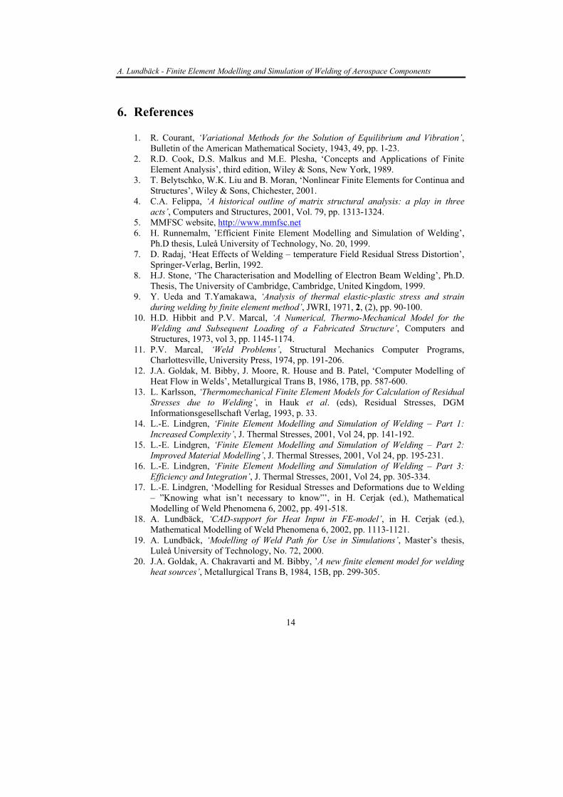
The boundary limit of the heat source is defined as the region where the heat input has been reduced to 5% of the peak value. In Figure 6 the distribution of the heat input and the 5% cut off limit are illustrated.

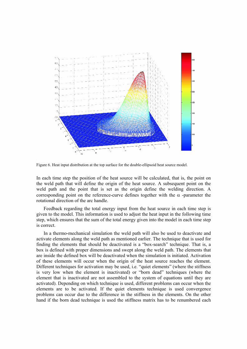
Figure 6. Heat input distribution at the top surface for the double-ellipsoid heat source model.

In each time step the position of the heat source will be calculated, that is, the point on the weld path that will define the origin of the heat source. A subsequent point on the weld path and the point that is set as the origin define the welding direction. A corresponding point on the reference-curve defines together with the -parameter the rotational direction of the arc handle.

Feedback regarding the total energy input from the heat source in each time step is given to the model. This information is used to adjust the heat input in the following time step, which ensures that the sum of the total energy given into the model in each time step is correct.

In a thermo-mechanical simulation the weld path will also be used to deactivate and activate elements along the weld path as mentioned earlier. The technique that is used for finding the elements that should be deactivated is a “box-search” technique. That is, a box is defined with proper dimensions and swept along the weld path. The elements that are inside the defined box will be deactivated when the simulation is initiated. Activation of these elements will occur when the origin of the heat source reaches the element. Different techniques for activation may be used, i.e. “quiet elements” (where the stiffness is very low when the element is inactivated) or “born dead” techniques (where the element that is inactivated are not assembled to the system of equations until they are activated). Depending on which technique is used, different problems can occur when the elements are to be activated. If the quiet elements technique is used convergence problems can occur due to the difference in the stiffness in the elements. On the other hand if the born dead technique is used the stiffness matrix has to be renumbered each

time an element is activated. Severely distorted elements can occur due to large deformations with either of these two techniques.

Lindgren & Hedblom9 have developed a technique to control the volume of the activated elements, i.e. the filler rate, which also minimizes the element distortion. This technique was applied for a 2-D model but it can be expanded to 3-D models. If the simulation is purely thermal the de-/activation technique is not necessary.

4 Applications

Here are some examples of welding simulations that were performed using the described method. In Figure 7 a), “the Graz flag”, a thermal welding simulation on a shell mesh is performed. This simulation is of course of no realistic relevance, but it shows that a weld with a complex weld path can be modelled without too much effort by the user. To get an illustrative temperature field, the material has no thermal conductivity. The weld path for the T-pipe in figure 7 b) is also easily modelled with the CAD- FE-program interface. Figure 8 a) shows a thermo-mechanical welding simulation performed on a shell mesh. The geometry is two sections of a tail bearing housing (TBH), the outer ring and the vanes. This is a component of an aero engine and the outer ring has a diameter of approximately 1,2 m. Figure 8 b) shows the actual component.

Figure 7. Examples of thermal welding simulations that can be performed using the CAD- FE-program interface. (a) “Dummy weld simulation” which forms the text “Graz 2001”, the temperature field in °C is shown on the fringe scale. (b) Welding simulation of a T-pipe, same pipe as described in figure 4 a), here it is also the temperature field in °C that is shown on the fringe scale.

b)a)

Figure 8. (a) Two simplified sections of a tail bearing housing, from an aero engine, are joined in a thermo-mechanical welding simulation. The variables shown are the temperature field in °C, deformed shape and the contours of the undeformed model, deformation scale factor is 20. (b) Photo of the tail bearing housing component.

5 Concluding remark

A method for alleviating the definition of heat input has been implemented and demonstrated. Although I-DEAS has been used as CAD-system and MSC.Marc as FE-software, the method and the subroutines that have been written are general and can be used with other CAD- and FE-systems also. The only requirements are that the CAD-software must be able to generate a file containing the weld path defined on the model and the FE-software must be able to create the heat input via user routines.

6 Acknowledgements

The financial support was provided by the: Manufacturing and Modelling of Fabricated Structural Components (MMFSC) programme. This is a project within the 5th framework programme and Luleå University of Technology. A special thanks to Daniel Berglund for fruitful discussions, feedback and work on the deactivation procedure.

7 References

1. L.-E. LINDGREN: ‘Finite element modelling and simulation of welding part 1: increased complexity’, Journal of Thermal Stresses, 2001, 24, 141-192.

2. Y. UEDA and T.YAMAKAWA, ‘Analysis of thermal elastic-plastic stress and strain during welding by finite element method’, JWRI, 1971, 2, (2), 90-100.

b)a)

3. Y. UEDA, J. WANG, H. MURAKAWA and M. G. YUAN, ‘Three dimensional numerical simulation of various thermomechanical processes by FEM’, JWRI, 1993, 22, (2), 289-294.

4. J. WANG, Y. UEDA, H. MURAKAWA, M. G. YUAN and H. Q. YANG, ‘Improvement in numerical accuracy and stability of 3-D FEM analysis in welding’, Welding Journal, 1996, April, 129-134.

5. J. GOLDAK, A. CHAKRAVARTI, M BIBBY, ‘A new finite element model for welding heat sources’, Metallurgical Trans B, 1984, 15B, 299-305.

6. J. GOLDAK, B. PATEL, M. BIBBY and J. MOORE, ‘Computational Weld Mechanics, AGARD Workshop – Structures and Materials 61st Panel meeting, 1985.

7. D. BERGLUND, L.-E. LINDGREN, A. LUNDBÄCK, ‘Three-dimensional finite element simulation of laser welded stainless steel plate’, NUMIFORM’01 The seventh Int. Conf. on Numerical Methods in Industrial Forming Processes, 2001, 1119-1123.

8. W. SUDNIK, D. RADAJ and W. EROFEEW, ‘Computerised simulation of laser beam welding, modelling and verification’, J. Phys. D: Appl. Phys., 1996, 29, 2811-2817.

9. L.-E. LINDGREN and E. HEDBLOM, ‘Modelling of Addition of Filler Material in Large Deformation Analysis of Multipass Welding’, Int. J. Communications in numerical methods in engineering, 2001, 17 (9), 647-657.

1 INTRODUCTION

Joining structures with laser welding is getting more common in the aerospace industry because of the smaller heat effected zone and less deformation compared to arc-welding processes. This is due to the more concentrated heat source. A small fusion zone requires that the gap and the mismatch between the plates are kept to a minimum.

A simulation tool would decrease the number of weld trials and thereby reduce the cost. When creat-ing a numerical model, the aim is to implement the physical behaviour of the process into the computer model. However, it may be necessary to compromise between accuracy of the model and the required computational time. The finite element method has been used in simulation of welding since the early 70:ies (e.g. Ueda et al 1971a, 1971b, Hibbitt & Mar-cal 1973). However, considering geometrical com-plex details and/or fluid flow in the melted zone welding simulations are still a challenge. Mainly two-dimensional analyses have been performed until the end of 80:ies. Then the first simulations using three-dimensional models were performed (Lindgren & Karlsson 1988).

It is usually necessary to apply three-dimensional models for complex structures. Still three-dimensional analyses are restricted to plates, pipes and similar simple structures. The main reason for this is lack of computational power. The physics of the welding process in the molten zone is not well understood and not possible to simulate combined with a complex structure. One can perform distortion simulations with an acceptable accuracy using a simplified heat source and material description for this zone. It’s necessary to verify the material prop-

erties, heat source parameters and the simulation method before performing a welding simulation of a complex geometry.

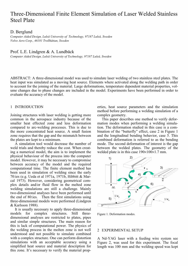
This paper describes one method to verify defor-mation modes when performing a welding simula-tion. The deformation studied in this case is a com-bination of the “butterfly” effect, case 2 in Figure 1 and the longitudinal bending behavior, case 5. This combined deformation is referred to as the bending mode. The second deformation of interest is the gap between the welded plates. The geometry of the welded plate is in this case 190×100×1.7 mm.

1/κy

∆L

1/κx

v

u

x

y

1) 2)

3)

4)

5)

6)

Figure 1. Deformation modes.

2 EXPERIMENTAL SETUP

A Nd-YAG laser with a feeding wire system see Figure 2, was used for this experiment. The focal length was 100 mm and the welding speed was kept

Three-Dimensional Finite Element Simulation of Laser Welded Stainless Steel Plate

D. Berglund Computer Aided Design, Luleå University of Technology, 97187 Luleå, Sweden Volvo Aero Corp., 46181 Trollhättan, Sweden

Prof. L.E. Lindgren & A. Lundbäck Computer Aided Design, Luleå University of Technology, 97187 Luleå, Sweden

ABSTRACT: A three-dimensional model was used to simulate laser welding of two stainless steel plates. The heat input was simulated as a moving heat source. Elements where activated along the welding path in order to account for the joining of the material. Large deformations, temperature dependent material properties, vol-ume changes due to phase changes are included in the model. Experiments have been performed in order to evaluate the accuracy of the model.

constant at 30 mm/s. A stable keyhole was achieved with a laser power of 2.5 kW.

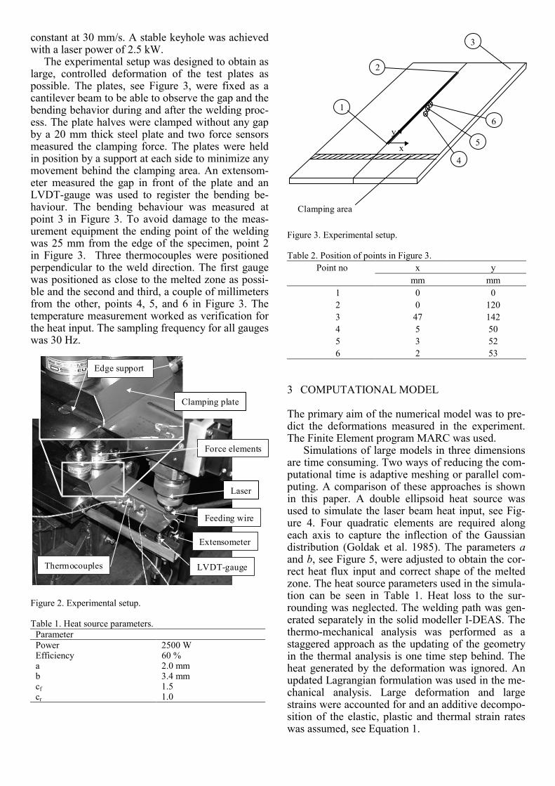
The experimental setup was designed to obtain as large, controlled deformation of the test plates as possible. The plates, see Figure 3, were fixed as a cantilever beam to be able to observe the gap and the bending behavior during and after the welding proc-ess. The plate halves were clamped without any gap by a 20 mm thick steel plate and two force sensors measured the clamping force. The plates were held in position by a support at each side to minimize any movement behind the clamping area. An extensom-eter measured the gap in front of the plate and an LVDT-gauge was used to register the bending be-haviour. The bending behaviour was measured at point 3 in Figure 3. To avoid damage to the meas-urement equipment the ending point of the welding was 25 mm from the edge of the specimen, point 2 in Figure 3. Three thermocouples were positioned perpendicular to the weld direction. The first gauge was positioned as close to the melted zone as possi-ble and the second and third, a couple of millimeters from the other, points 4, 5, and 6 in Figure 3. The temperature measurement worked as verification for the heat input. The sampling frequency for all gauges was 30 Hz.

LVDT-gauge

Extensometer

Feeding wire

Laser

Thermocouples

Force elements

Edge support

Clamping plate

Figure 2. Experimental setup.

Table 1. Heat source parameters. Parameter Power 2500 W Efficiency 60 % a 2.0 mm b 3.4 mm cf 1.5cr 1.0

Clamping area

1

y

x

2

4

5

6

3

Figure 3. Experimental setup.

Table 2. Position of points in Figure 3. Point no x y

mm mm 1 0 0 2 0 120 3 47 142 4 5 50 5 3 52 6 2 53

3 COMPUTATIONAL MODEL

The primary aim of the numerical model was to pre-dict the deformations measured in the experiment. The Finite Element program MARC was used.

Simulations of large models in three dimensions are time consuming. Two ways of reducing the com-putational time is adaptive meshing or parallel com-puting. A comparison of these approaches is shown in this paper. A double ellipsoid heat source was used to simulate the laser beam heat input, see Fig-ure 4. Four quadratic elements are required along each axis to capture the inflection of the Gaussian distribution (Goldak et al. 1985). The parameters aand b, see Figure 5, were adjusted to obtain the cor-rect heat flux input and correct shape of the melted zone. The heat source parameters used in the simula-tion can be seen in Table 1. Heat loss to the sur-rounding was neglected. The welding path was gen-erated separately in the solid modeller I-DEAS. The thermo-mechanical analysis was performed as a staggered approach as the updating of the geometry in the thermal analysis is one time step behind. The heat generated by the deformation was ignored. An updated Lagrangian formulation was used in the me-chanical analysis. Large deformation and large strains were accounted for and an additive decompo-sition of the elastic, plastic and thermal strain rates was assumed, see Equation 1.

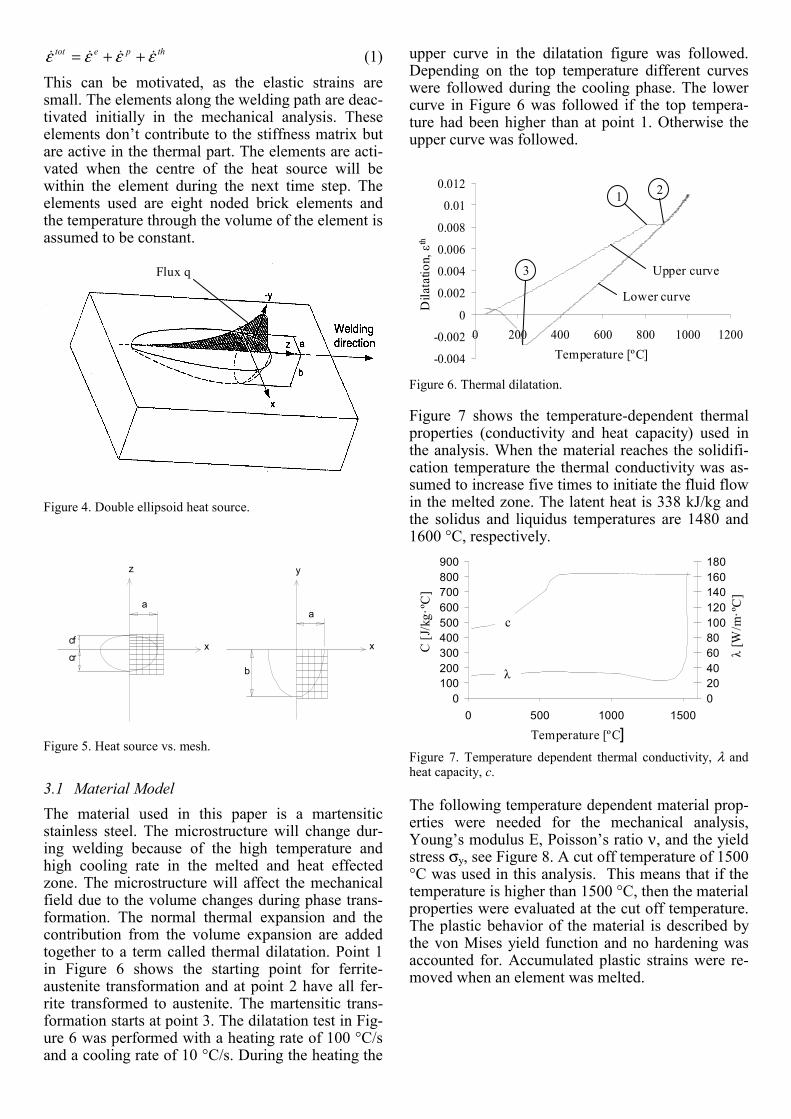
thpetot εεεε ++= (1) This can be motivated, as the elastic strains are small. The elements along the welding path are deac-tivated initially in the mechanical analysis. These elements don’t contribute to the stiffness matrix but are active in the thermal part. The elements are acti-vated when the centre of the heat source will be within the element during the next time step. The elements used are eight noded brick elements and the temperature through the volume of the element is assumed to be constant.

Flux q

Figure 4. Double ellipsoid heat source.

a

b

x

y

a

cf

cr

z

x

Figure 5. Heat source vs. mesh.

3.1 Material Model The material used in this paper is a martensitic stainless steel. The microstructure will change dur-ing welding because of the high temperature and high cooling rate in the melted and heat effected zone. The microstructure will affect the mechanical field due to the volume changes during phase trans-formation. The normal thermal expansion and the contribution from the volume expansion are added together to a term called thermal dilatation. Point 1 in Figure 6 shows the starting point for ferrite-austenite transformation and at point 2 have all fer-rite transformed to austenite. The martensitic trans-formation starts at point 3. The dilatation test in Fig-ure 6 was performed with a heating rate of 100 °C/sand a cooling rate of 10 °C/s. During the heating the

upper curve in the dilatation figure was followed. Depending on the top temperature different curves were followed during the cooling phase. The lower curve in Figure 6 was followed if the top tempera-ture had been higher than at point 1. Otherwise the upper curve was followed.

-0.004

-0.002

0

0.002

0.004

0.006

0.008

0.01

0.012

0 200 400 600 800 1000 1200

Upper curve

Lower curve

1 2

3

Temperature [ºC]

Dila

tatio

n,

th

Figure 6. Thermal dilatation.

Figure 7 shows the temperature-dependent thermal properties (conductivity and heat capacity) used in the analysis. When the material reaches the solidifi-cation temperature the thermal conductivity was as-sumed to increase five times to initiate the fluid flow in the melted zone. The latent heat is 338 kJ/kg and the solidus and liquidus temperatures are 1480 and 1600 °C, respectively.

[W/m

·ºC

]Temperature [ºC]

C[J

/kg·

ºC]

0100200300400500600700800900

0 500 1000 1500020406080100120140160180

c

Figure 7. Temperature dependent thermal conductivity, λ and heat capacity, c.

The following temperature dependent material prop-erties were needed for the mechanical analysis, Young’s modulus E, Poisson’s ratio ν, and the yield stress σy, see Figure 8. A cut off temperature of 1500 °C was used in this analysis. This means that if the temperature is higher than 1500 °C, then the material properties were evaluated at the cut off temperature. The plastic behavior of the material is described by the von Mises yield function and no hardening was accounted for. Accumulated plastic strains were re-moved when an element was melted.

Temperature [ºC]

E[G

Pa] ,

y[M

Pa]

ν

0100200300400500600700800

0 500 1000 150000.050.10.150.20.250.30.350.40.450.5

E

ν

y

Figure 8. Temperature dependent mechanical properties, yield stress σy, Young’s modulus E, Poisson’s ratio ν.

3.2 FEM-model using adaptive meshing. The approach to use adaptive meshing reduces the number of elements in the beginning of the analysis. Elements are added by splitting original elements along the weld path. Each split element creates eight new ones. The new elements can in turn be split again, but in this model a restriction was set to one level of splitting. Whether an element is to be split or not is determined by the calculation of the relative temperature gradient in the actual element, which is compared with the maximum temperature gradient in the model, see Equation 2.

gradientmaximumgradient >f (2)

In this model the value of f is set to 0.75. That is, if fexceeds 0.75 the element will be split. The model contained initially 7000 elements and 10908 nodes.

No coarsening of the mesh was used since it is not supported in the code and a denser mesh is needed to describe the residual strains and deforma-tions.

3.3 FEM-model using parallel processing.

The simulation model can be subdivided in a number of sub models (domains). Each domain is calculated on a different processor and a iterative procedure as-semble the sub solutions to the global solution (Marc Analysis Research Corp 1998). The finite element mesh used in this model had 40500 elements and 51038 nodes during the whole simulation. The num-ber of elements through the thickness of the plate along the weld path was six. A time step of 0.027 was used during the welding sequence but changed adaptively during the cooling phase.

4 RESULTS

The computational time for the parallel FEM-model was approximately 7 days and was performed on a

450 MHz Sun Ultra 60 with 2 GB ram. The simula-tion with the adaptive meshing technique was not completed because of convergence problem after 2.1 s. The adaptive and parallel models show similar de-formation behaviour during the heating sequence. The measured and computed temperature at point 4, 5 and 6 are shown in figure 8. The computed tem-peratures are all lower than the measured. The posi-tion of the sampling points in the computational model were not the same as in the experiment, see Table 2. The shape of the calculated and measured fusion zone is approximately the same but the top side of the weld is higher in the measured case, see Figure 10b.

01002003004005006007008009001000

0 20 40 60 80 100

T em

pera

t ure

[ºC]

Time [s]

Measured

Calculated

Figure 9. Measured and calculated temperature history for points 4, 5 and 6.

200

300

400

500

600

0 0.5 1 1.5 2 2.5

Calculated Measured

Har

dnes

s [H

V]

Distance [mm]

a)

b)

Figure 10. a) Hardness test. b) Measured and calculated fusion zone.

A hardness test was performed to verify the marten-site transformation model. The hardness increased significant up to 2 mm from center of the weld as shown in Figure 10a. The hardness has increased from 270 HV in the base metal, to a value of 500 HV in the center of the weld. The measured and cal-

culated deformation behavior can be seen in Figure 11 and 12.

The computational model, predict the bending behavior with acceptable accuracy during the heating sequence but not during the cooling phase. The bending deformation, stabilize at 0.3 mm during the cooling phase but the computed deformation de-creases rapidly to a value of 3 mm after 100 s.

The computed and measured gap diverges after 0.4 s. The final gap in the computational model is four times larger than the measured one. The behav-iour during cooling has the same tendency in the ex-periments as in the simulation as can be seen Figure 12.

-3

-2.5

-2

-1.5

-1

-0.5

00.01 0.1 1 10 100

Heating Cooling

Calculated, pm

Measured

Time [s]

Dis

plac

emen

t [m

m]

Calculated, am

Figure 11. Bending behavior.

Time [s]

0

0.2

0.4

0.6

0.8

1

1.2

0.01 0.1 1 10 100

Dis

plac

emen

t [m

m]

Heating Cooling

Measured

Calculated, pm

Calculated, am

Figure 12. Gap at the end of the plate, pm-Parallel Model, am-Adaptive Model.

5 DISCUSSION AND CONCLUSION

A method to verify numerical welding models has been developed. The experimental setup can be used to evaluate the temperature field and deformation behaviour of thin plates.

A numerical welding simulation of a stainless steel plate was performed. The accuracy of the abso-lute value of the deformation was not acceptable but the approach reveals the weakness of the model. Similar deformation behaviour was achieved for both the adaptive and the parallel model.

The measured temperatures were all higher than the calculated, see Figure 9. One uncertainty is the high thermal conductivity used in the model. A regu-lar stainless steel have a conductivity between 13 and 16 W/m⋅K according to Incropera & DeWitt (1996). Another uncertainty is the efficiency of the laser because of the bending and change in gap dur-ing the welding process which will change the ab-sorbed power (Lampa et al. 1995). An error in the thermal field will effect the deformation behaviour. This is one of the reasons to the exponential increas-ing error of the gap in the computational model. Ac-cording to Jonsson et al. (1985) has the thermal dila-tation a large influence on the change in gap width.

The hardness test shows the existence of phase transformation up to 2 mm from the weld centre. The hardness is decreasing from its maximum value of 500 HV at 1 mm, to 300 HV 2 mm from the weld centre. This is not the case for the computational model where martensite is assumed to be created as soon as the temperature has been higher than the ini-tial ferrite-austenite temperature. This assumption gives a larger amount of created martensite in the model, which affects the change in gap. Another pa-rameter that will influence the deformation behav-iour is the high yield stress of the created martensite phase.

The existing numerical model can predict the gap behaviour and the bending during the cooling phase, but the absolute value of the deformation is not pos-sible to predict.

6 ACKNOWLEDGEMENT

The financial support was provided by NFFP (Swed-ish National Aviation Research Program), Luleå University of Technology and Volvo Aero Corpora-tion.

7 REFERENCES

Goldak J, Patel B, Bibby M & Moore J 1985. Computational weldmechanics. AGARD Workshop - Structures and Mate-rials 61st Panel meeting, Oberammergau.

Hibbitt HD & Marcal P. 1973. A numerical thermo-mechanical model for the welding and subsequent loading of a fabri-cated structure. Comp. & Struct. 3:1145-1174.

Incropera FP & DeWitt DP 1996. Fundamentals of Heat and Mass Transfer. New York: John Wiley & Son.

Jonsson M, Karlsson L & Lindgren L-E 1985. Deformation and Stresses in Butt-Welding of Large Plates With Special Ref-erences to the Material Properties. Journal of Engineering Materials and Technology 107:265-270.

Lampa C, Ivarson A, Runnemalm H & Magnusson C 1995. The Influence of Gap Width on Laser Welding. 14:th ICALEO.

Lindgren L-E & Karlsson L 1988. Deformations and stresses in welding of shell structures., International Journal for Nu-merical Methods in Engineering 25:635-655.

Marc Analysis Rersearch Corporation 1998. Theory and User Information, Palo Alto.

Ueda Y & Yamakawa T 1971b. Thermal stress analysis of met-als with temperature dependent mechanical properties. Proc. of Int. Conf. on Mechanical Behavior of Materials3:10-20.

Ueda Y & Yamakawa T 1971a. Analysis of Thermal elastic-plastic strain and strain during welding by finite element method. Trans. JWRI 2(2):90-100.

VALIDATION OF A THREE DIMENSIONAL FINITE ELEMENT MODEL IN ELECTRON BEAM

WELDING OF INCONEL 718

Andreas Lundbäck Luleå University of Technology

Luleå, 97187, Sweden +46 (0)920 492856 [email protected]

Henrik RunnemalmVolvo Aero Corporation

461 81 Trollhättan, Sweden

Abstract – A three dimensional finite element model for prediction of the distortion and residual stresses induced during the electron beam welding is described. The model is validated by experiments, butt-welding of two plates made of INCONEL 718. There are two major uncertainties, material behaviour and heat input. Separate experiments have been made for obtaining material properties and the special effort for determining a good model for the heat is described in this paper. Parallel computation is used to reduce the overall simulation time. A combined conical and double ellipsoid heat source is used to model the deep penetration characteristic of the electron beam. The agreement between calculations and experiments is good with respect to the residual stresses. Discrepancies, in absolute values, were found when comparing the deformations. The model behaves qualitatively similar to the experiment tough.

INTRODUCTION

The paper describes the development of the welding model and its validation in order to ensure the predictive capability of the welding simulations. They will be applied later for simulation of the fabrication of a structural component used in an aero engine. The component is a Tail Bearing Housing (TBH) and can be seen in Figure 1. The test case is a butt-weld of an Inconel 718 plate. The heat affected zone was measured and a special code developed by Sudnik et al. [1] was also used to predict the molten zone. This information was used to develop a heat source model, which is a combination of a conical source and the double ellipsoid source developed by Goldak et al. [2]. Residual stresses and deformations were measured and compared with simulations. A quite good agreement was obtained between measurements and simulations.

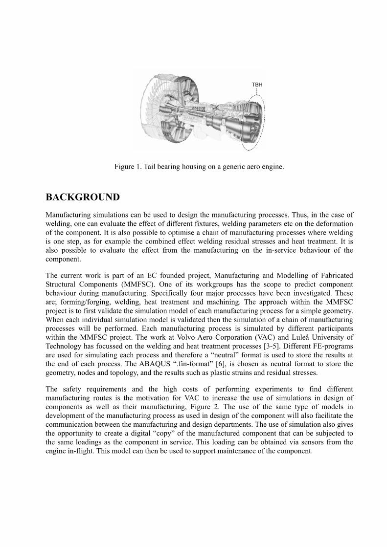
Figure 1. Tail bearing housing on a generic aero engine.

BACKGROUND

Manufacturing simulations can be used to design the manufacturing processes. Thus, in the case of welding, one can evaluate the effect of different fixtures, welding parameters etc on the deformation of the component. It is also possible to optimise a chain of manufacturing processes where welding is one step, as for example the combined effect welding residual stresses and heat treatment. It is also possible to evaluate the effect from the manufacturing on the in-service behaviour of the component.

The current work is part of an EC founded project, Manufacturing and Modelling of Fabricated Structural Components (MMFSC). One of its workgroups has the scope to predict component behaviour during manufacturing. Specifically four major processes have been investigated. These are; forming/forging, welding, heat treatment and machining. The approach within the MMFSC project is to first validate the simulation model of each manufacturing process for a simple geometry. When each individual simulation model is validated then the simulation of a chain of manufacturing processes will be performed. Each manufacturing process is simulated by different participants within the MMFSC project. The work at Volvo Aero Corporation (VAC) and Luleå University of Technology has focussed on the welding and heat treatment processes [3-5]. Different FE-programs are used for simulating each process and therefore a “neutral” format is used to store the results at the end of each process. The ABAQUS “.fin-format” [6], is chosen as neutral format to store the geometry, nodes and topology, and the results such as plastic strains and residual stresses.

The safety requirements and the high costs of performing experiments to find different manufacturing routes is the motivation for VAC to increase the use of simulations in design of components as well as their manufacturing, Figure 2. The use of the same type of models in development of the manufacturing process as used in design of the component will also facilitate the communication between the manufacturing and design departments. The use of simulation also gives the opportunity to create a digital “copy” of the manufactured component that can be subjected to the same loadings as the component in service. This loading can be obtained via sensors from the engine in-flight. This model can then be used to support maintenance of the component.

DESIGN

MANUFACTURING

Prod

uct r

equi

rem

ents Concept

phaseDefinition

phaseVerification

phase



DetailedPreparation

Tools for functional evaluation


Computer based engineering modelsServices

Physical product

Digital version of product

Data from component in-service applied to digital copy of product

Maintenance, upgrading etc

FUNCTIONAL PRODUCT

Feedback

Feedback

DESIGN

MANUFACTURING

Prod

uct r

equi

rem

ents Concept

phaseDefinition

phaseVerification

phase



DetailedPreparation

Tools for functional evaluation


Computer based engineering modelsComputer based engineering modelsServices

Physical product




FUNCTIONAL PRODUCT

Services

Physical product




FUNCTIONAL PRODUCT

Feedback

Feedback

Figure 2. Use of computer models for design of components, manufacturing routes and maintenance.

EXPERIMENTS

Two Inconel 718 plates are welded together. The sizes of the plates are 100x40x7 mm and 100x40x6 mm and can be seen, together with the clamping device, in Figure 3. The plate with the thickness of 7 mm had a 1x1 mm lip, which served as a root support, see the enlargement in Figure 3. The plates were first tack welded together without any gap between them and then butt welded. The distance from the weld centre to the clamping device is 10 mm. Prior to welding the plates had been precipitation hardened. The parameters of the electron beam welding procedure are given in Table 1.

Table 1. Input values for the EB welding process.

Voltage (kV) Current (mA) Lens current (mA) Lens diameter (mm) Work distance (mm) Speed (m/min)

140 10 2175 10 400 0.6

Figure 3. Clamping device and plates to be welded.

The incremental hole-drilling technique was used to measure the residual stresses. The position of the hole-drilling measurements can be found in Figure 4 and Table 2. The measurements at positions 1 and 6 measure the initial state of the plate since it is assumed that the stresses induced by the welding process are negligible that far away from the weld centre. Positions 2 and 3 are placed symmetrically 3 mm from the weld centre and the positions 4 and 5 are placed in the middle of the plate, 3 mm and 13 mm from the centre, where the EB-weld process is considered to be stable.

Table 2. Position of strain gauges.

Figure 4. Plate with the strain gauge positions.

Position X (mm) Z (mm)

1 10 10

2 37 10

3 43 10

4 43 50

5 53 50

6 10 90

The distortion measurements performed in this study is done with an optical surface measurement machine. The butterfly angle, defined in Figure 5, of the plate after welding is measured at three positions, 5, 50 and 95 mm from the start point of the weld in the z-direction.

Figure 5. Definition of the butterfly angle.

NUMERICAL MODEL

The finite element simulation presented in this paper is a coupled thermo-mechanical simulation. The coupling between the thermal and the mechanical part is done with the staggered approach. In the staggered approach the updating of the geometry is lagging one step behind in the thermal analysis. The code that has been used is the implicit finite element code MSC.Marc. An updated Lagrangian and large deformation formulation was used together with additive decomposition of the strains. To avoid locking an underintegrated element with respect to the volumetric strain was used. All plastic dissipated energy was converted into heat. The elements in both the thermal and mechanical analyses have linear shape functions. Therefore a constant temperature was transferred to the element in the mechanical analysis in order to ensure that the mapping between the thermal and mechanical strains would be consistent. To reduce the total wall clock time when performing the simulation, parallel computation was utilised. The model is divided into sub domains and a separate solution is obtained for each domain. An iterative procedure then assembles the local solutions into a global solution of the whole model, MSC.Marc user handbook [10]. The time consumed for solving the analysis was approximately 10 hours on six 1900 MHz PC-Linux machines.

The model contained 17596 eight noded brick elements and 20804 nodes. The size of the elements in the weld region is 0.33x1x1 mm and the whole mesh can be seen in Figure 6. Symmetry could not be used since both the mechanical and thermal boundary conditions were not symmetric and the halves have different thicknesses, see Figure 3. A time step length of 0.5 s during welding ensured that the heat source travelled only half the length of an element in the weld region for each time step. The total time for the welding phase is 10 s. An adaptive time stepping method was used for the cooling phase, 62 increments and a total time of 1000 s brought the plates back into room temperature. After cooling, the plate was unloaded from the fixture in one single time step. During welding and cooling the nodes that belong to the area that would have been in contact with the fixture are fixed in all directions. In the unloading step, a pin joint at one end of the plate and a simple support at the other end replaced the fixed nodes used in the previous steps. The heat transfer between the plate and the fixture is imitated by a high convective heat transfer of 1200 Wm-2K-1.Heat losses due to radiation are not taken into account for in the model and no free convection either due to that the welding process took place in vacuum.

Figure 6. Finite element mesh.

Element death and birth is done by first deactivating one element row along the weld path except the elements that represents the tack welds. This occurs in an initial dummy step. Thermal and mechanical activation is separated to enable the element to be heated up thermally but not contribute to the mechanical stiffness. The condition when an element is to be activated mechanically is set as a distance relative the position of the origin of the heat source. In this model the distance was set to 4 mm which is approximately the distance where the temperature in the elements is entering the solid phase from liquid. The distance ahead the origin of the heat source where the elements is thermally activated is not as critical as it is in the mechanical case. This is due to that the heat conduction in the welding direction can be neglected so a sufficiently long distance can easily be chosen. In practice, for one pass welds all the elements could most likely be thermally active during the whole simulation. It should also be noted that the tack welds are not simulated so these elements are left active in their nominal material state without any residual stresses from the tackwelding.

Heat input model

A combined heat source, Equation 1, is used to model the temperature field obtained in the thermal simulation, which is described later, and from the experiment. The first part in Equation 1 is the double ellipsoid presented by Goldak et al. [1]. A description of the double ellipsoid can be found in Figure 7 and equation 2a and 2b. The second part is a double elliptic cone and is defined in equation 3a and 3b. The -parameter gives the relative contribution of the two heat sources.

Figure 7. Definition of the double ellipsoid with its characteristic parameters.

The geometric parameters a, b and c have the same meaning for the ellipsoidal and conical heat source. The conical heat source has also an additional parameter dc. The parameter dc is a normalized parameter and can be given a value between 1 and 0. The energy intensity of the conical source has a Gaussian distribution in the x-z plane as the double ellipsoid heat source, see Figure 7. However, it has a linear decrease through the depth which is controlled by the parameter dc. That is, if dc equals 1 then the energy intensity, along a line parallel to the y-axis, is constant through the depth. If dc is set to 0, then the intensity will decrease linearly to zero at the depth of bc. The parameter bc should be the thickness of the plate. The formulas are summarized in Table 1. The values of the heat source parameters used in the model in this paper can be found in Table 4.

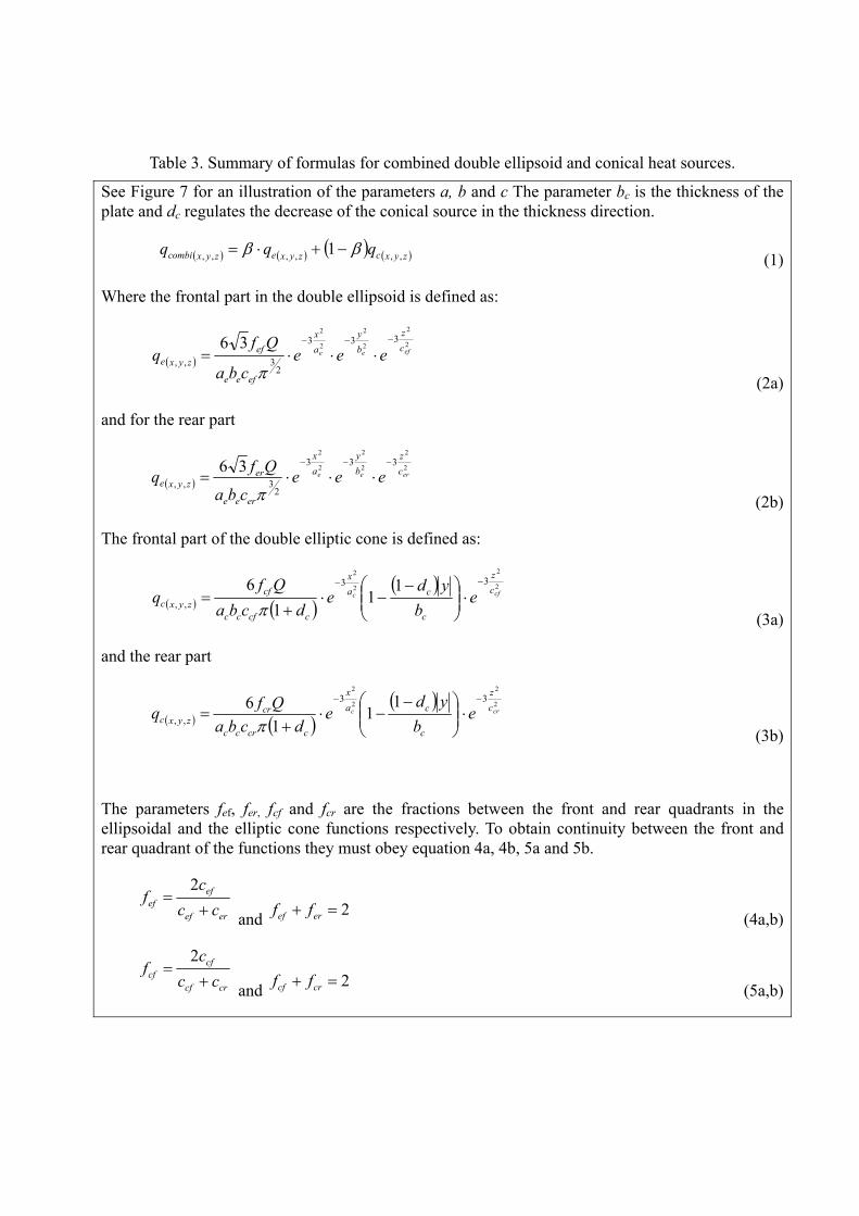
Table 3. Summary of formulas for combined double ellipsoid and conical heat sources.

See Figure 7 for an illustration of the parameters a, b and c The parameter bc is the thickness of the plate and dc regulates the decrease of the conical source in the thickness direction.

zyxczyxezyxcombi qqq ,,,,,, 1 (1)

Where the frontal part in the double ellipsoid is defined as:

2

2

2

2

2

2333

23,,

36efee c

z

by

ax

efee

efzyxe eee

cba

Qfq

(2a)

and for the rear part

2

2

2

2

2

2333

23,,

36eree c

zby

ax

eree

erzyxe eee

cba

Qfq (2b)

The frontal part of the double elliptic cone is defined as:

2

2

2

233

,,

11

16

cfc cz

c

cax

ccfcc

cfzyxc e

byd

edcba

Qfq

(3a)

and the rear part

2

2

2

233

,,

11

16

crc cz

c

cax

ccrcc

crzyxc e

byd

edcba

Qfq (3b)

The parameters fef, fer, fcf and fcr are the fractions between the front and rear quadrants in the ellipsoidal and the elliptic cone functions respectively. To obtain continuity between the front and rear quadrant of the functions they must obey equation 4a, 4b, 5a and 5b.

eref

efef cc

cf

2

and 2eref ff (4a,b)

crcf

cfcf cc

cf

2

and 2crcf ff (5a,b)

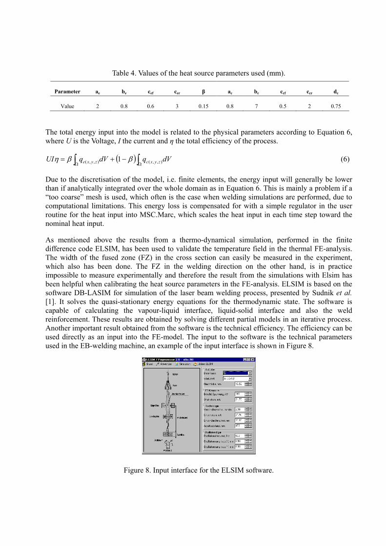
Table 4. Values of the heat source parameters used (mm).

Parameter ae be cef cer ac bc ccf ccr dc

Value 2 0.8 0.6 3 0.15 0.8 7 0.5 2 0.75

The total energy input into the model is related to the physical parameters according to Equation 6, where U is the Voltage, I the current and the total efficiency of the process.

dVqdVqUI zyxczyxe ),,(),,( 1 (6)

Due to the discretisation of the model, i.e. finite elements, the energy input will generally be lower than if analytically integrated over the whole domain as in Equation 6. This is mainly a problem if a “too coarse” mesh is used, which often is the case when welding simulations are performed, due to computational limitations. This energy loss is compensated for with a simple regulator in the user routine for the heat input into MSC.Marc, which scales the heat input in each time step toward the nominal heat input.

As mentioned above the results from a thermo-dynamical simulation, performed in the finite difference code ELSIM, has been used to validate the temperature field in the thermal FE-analysis. The width of the fused zone (FZ) in the cross section can easily be measured in the experiment, which also has been done. The FZ in the welding direction on the other hand, is in practice impossible to measure experimentally and therefore the result from the simulations with Elsim has been helpful when calibrating the heat source parameters in the FE-analysis. ELSIM is based on the software DB-LASIM for simulation of the laser beam welding process, presented by Sudnik et al.[1]. It solves the quasi-stationary energy equations for the thermodynamic state. The software is capable of calculating the vapour-liquid interface, liquid-solid interface and also the weld reinforcement. These results are obtained by solving different partial models in an iterative process. Another important result obtained from the software is the technical efficiency. The efficiency can be used directly as an input into the FE-model. The input to the software is the technical parameters used in the EB-welding machine, an example of the input interface is shown in Figure 8.

Figure 8. Input interface for the ELSIM software.

Material model

The material model used in the analysis is a thermo-elastic-plastic model and the material is the nickel based super alloy, Inconel 718. Inconel 718 is a high temperature strength material that is commonly used in the aerospace industry in areas that can be considered as “hot”. By hot it means that the temperature is continuously held, in service, at temperatures of 500 °C and above. The tail bearing housing is such a component. The thermal properties, conductivity and heat capacity versus temperature, are derived from Mills [8]. The latent heat in the solid/liquid transformation is separated from the specific heat curve and it was set to 300 kJ/kg in the interval 1260–1335 °C. The mechanical properties are compiled from various sources. Young’s modulus is derived from Zhang etal. [9] and the yield strength from experiments performed within the MMFSC project and Busch etal. [14]. The thermal expansion is obtained from Babu et al. [7]. Poisson’s ratio is held constant at 0.29, due to lack of material data. The influence of Poisson’s ratio has been shown to affect the result, with respect to global distortion and stresses very little [12-13].

RESULTS

The temperature field from the simulation in ELSIM can be seen in Figure 9. This result was mainly used as a qualitative comparison of the thermal field in the welding direction. As can be seen in Figure 10, the fused zone, highlighted with dashed lines, agrees fairly well with the experiment in the transverse direction except that full penetration has not been achieved in the FE-model. A comparison between the results form ELSIM and the FE-model in the longitudinal direction show that the thermal fields in this direction are also fairly well captured in the FE-model. The efficiency,

, was calculated to 93% in the simulations with ELSIM which would yield a power input of 1300 W. In the FE-model on the other hand, an efficiency of 110% was used, i.e. 1540 W. The reason why a higher energy input was used is because otherwise the fused zone became far too small.

Figure 9. Temperature field as a result from simulation with the finite difference software ELSIM.

Figure 10. Comparison of the fused zone between experiment (left photo) and FE-simulation.

Butterfly angle

Figure 11 shows the results of the butterfly angle in the FE-analysis compared with the measured. Three different simulations are compared, a-c). Generally for all three simulations, the butterfly angle becomes slightly negative at the very beginning of the welding. After less than a second it has changed sign and starts to increase. The total time for the heat source to travel from start to end point is ten seconds. When the cooling phase starts the increase of the butterfly angle is ignorable and after approximately fifteen seconds the angle is constant throughout the rest of the cooling phase. In Figure 12, the transient displacement in the y-direction for three points along the longitudinal free edge of the unconstrained plate is shown.

Two parameters are varied in the simulations, the number of elements representing the tack welds, i.e. the size, and the position relative to the origin of the heat source where the elements are activated mechanically. In simulation a) and b) the position when an element is activated is the same, 4 mm behind the origin, but the number of elements in the tack weld is 7 and 5 respectively, i.e. 7x1 mm and 5x1 mm (width x depth). The number of elements in the tack weld in simulation c) is 5, but activation occurs at the same position as the origin of the heat source. The tendency of the experimental curve and the one for simulation a) and b) are the same, the butterfly angle increases with practically the same tangent in all cases. It is the magnitude, or rather the development of the deformation in the very beginning of the weld that differs between the experiment and FE-analysis. There is a pronounced difference though in the slope of the butterfly angle along the weld line for simulation c). What can be noted is that the butterfly angle at the beginning of the weld is nearly exactly the same for all the simulated cases. It should also be noted that the time for solving the problem when activation occurred at the same position as the origin of the heat source, simulation c), increased dramatically. The increase was more than a factor of two, due to difficulties in convergence.

0

0,5

1

1,5

2

2,5

3

0 20 40 60 80 100

Distance along the weld line (mm)

But

terf

ly a

ngle

( °)

Experiment

simulation a)

simulation b)

simulation c)

Larger tack w eldEarlier activation

Figure 11. Butterfly angle from experiment and FE-simulation.

-0,2

0

0,2

0,4

0,6

0,8

1

1,2

0 2 4 6 8 10 12 14

Time (s)

Disp

lace

men

t (m

m)

5 mm

50 mm

95 mm

Heating Cooling

Figure 12. Transient deformation in the y-direction of three points (left). Definition of the three points (right).

Residual stresses

The result from the hole-drilling measurements and FE-analysis are presented in Figure 13 and Figure 14. The stresses are evaluated at the surface and at the depth of 1 mm. Figure 13 corresponds to the positions 1, 2 and 3 and Figure 14 to positions 4 and 5, defined in Figure 4. The agreement between the measured and calculated stresses is reasonable in both the transversal and longitudinal direction. The maximum stresses are found in the longitudinal direction and they are tensile with the magnitude of ~1200 MPa, whereas they are mainly compressive in the transverse direction and about 700 MPa in magnitude. The experimental measurement of the stresses at position 6 is not

presented here since they where found to be equal with those shown in Figure 13, position 1. These measurements show that there are significant stresses at the surface but that they vanish at some depth.

-800

-400

0

400

800

1200

0 10 20 30 40 50 60 70 80

Distance transverse to plate (mm)

Tran

sver

se S

tres

s (M

Pa)

FEM surface

FEM 1,0 mm

exp surface

exp 1,0 mm

-800

-400

0

400

800

1200

0 10 20 30 40 50 60 70 80


Long

itudi

nal S

tres

s (M

Pa)

FEM surface

FEM 1,0 mm

exp surface

exp 1,0 mm

Figure 13. Residual stresses calculated and measured in the transverse direction (left) and longitudinal direction (right) 10 mm from the weld start, i.e. position 1, 2 and 3 in Figure 4.

-800

-400

0

400

800

1200

0 10 20 30 40 50 60 70 80


Tran

sver

se S

tres

s (M

Pa)

FEM surface

FEM 1,0 mm

exp surface

exp 1,0 mm

-800

-400

0

400

800

1200

0 10 20 30 40 50 60 70 80


Long

itudi

nal S

tres

s (M

Pa)

FEM surface

FEM 1,0 mm

exp surface

exp 1,0 mm

Figure 14. Residual stresses calculated and measured in the transverse direction (left) and longitudinal direction (right) 50 mm from the weld start, i.e. position 4 and 5 in Figure 4.

DISCUSSIONS

An unrealistic high, 110%, efficiency for the heat input had to be used in the FE-model. It is believed that this is due to that a too coarse mesh has been used. The available time did not permit the use of a larger finite element model. Figure 15 shows the result from a test with only a thermal analysis that has been done. In this test the heat source parameters was kept constant and only the density of the mesh was changed in the model. As can be seen, full penetration and, especially in the

longitudinal direction, a much larger volume is heated up to the liquid temperature, FZ. This supports the assumption that the discrepancy regarding the amount of energy input is due to the used element sizes.

The measured and computed butterfly angle in Figure 11 has the same variation along the plate but the measured angle is larger. This may be due the tack-welding procedure. The geometry was not measured before the butt-welding procedure. The different simulations show that the difference is not due to the uncertainty in the size of the tack-welds or the way the element activation is done. As mentioned in results, the computation shows that the butterfly angle becomes slightly negative at the very beginning of the welding and later becomes positive. However, no transient data is available from the experiments and therefore it is not possible to determine which part of the simulation that diverse form the experiment. Stone et al. [11] reported similar discrepancy between experimental and simulated results for a bead-on-plate weld on a 9 mm thick plate in Waspalloy. They did not have any conclusion regarding this discrepancy though.

Figure 15. Two FE-models with different mesh density but the same heat source parameters for comparing the size of the FZ.

ACKNOWLEDGEMENT

This work was sponsored by the 5th Framework Programme, within a project called Manufacturing and Modelling of Fabricated Structural Components (MMFSC). Dr Hans-Uwe Baron Motoren- und Turbinen Union GmbH (MTU) is greatly acknowledged for performing the experiments and measurements

REFERENCES

1. W. Sudnik, D. Radaj, and W. Erofeew, ’Computer Simulation of Laser Beam Welding, Modelling and Verification’, J. Phys. D: Appl. Phys., 29, pp. 2811-2817.

2. J.A. Goldak, A. Chakravarti, M. Bibby, ’A new finite element model for welding heat sources’,Metallurgical Trans B, 1984, 15B, pp. 299-305.

3. A. Lundbäck, ‘CAD-support for Heat Input in FE-model’, Mathematical Modelling of Weld Phenomena 6, 2002, pp. 1113-1121.

4. L.-E. Lindgren, H. Alberg, and K. Domkin, ‘Constitutive Modelling and Parameter Optimisation’, 7th International Conference on Computational Plasticity, Barcelona, Spain, 2003.

5. D. Berglund, H. Alberg, and H. Runnemalm, ’Simulation of Welding and Stress Relief Heat Treatment of an Aero Engine Component’, to be published in: Finite Element in Analysis and Design.

6. ABAQUS/Standard, finite element software, User’s Manual Volume II, Hibbit, Karlsson & Sorensen Inc.

7. V.S. Babu, A.S. Pavlovic, and S.S. Seehra, ‘Oxidation characteristics and thermal expansion of inconel alloy 718 from 300 K to 1273 K’, Proc of the int. Symposium on Superalloys 718, 625, 706 and various derivatives’, ed. E.A. Loria, 1997, The Minerals, Metals & Materials Society, pp. 689-693.

8. K.C. Mills, Recommended values for of Thermophysical Properties for selected Commercial Alloys, National Physics Laboratory, 2002. Woodead Publishing Ltd and ASM International.

9. W.J. Zhang, B.V. Reddy, and S.C. Deevi, ‘Physical properties of TiAl-base alloys’, Scripta Materialia, 2001, 45, pp. 645-651.

10. MSC.Marc, finite element software, MSC.Software, Palo Alto.

11. H.J. Stone, S.M. Roberts, and R.C. Reed, ‘A Process Model for the Distortion Induced by the Electron-Beam Welding of a Nickel-Based Superalloy’, Metallurgical and Materials Transactions A, 2000, 31A, pp. 2261-2273.

12. C.K. Leung, and R.J. Pick, ‘The Use of Generalized Plane Strain Elements in the Prediction of Residual Stresses in Welded Flat Plates’, Proc. Of the Symposium on The Computer Modelling of Fabrication Processes and Constitutive Behaviour of Metals, 1986, p. 563.

13. P. Tekriwal, and J. Mazumder, ‘Transient and residual strain-stress analysis of GMAW’, ASME J. Engineering Materials and Technology, 1991, vol. 113, pp. 336-343.

14. W.B. Busch, U. Draugelates, and H.D. Kunze, ‘Electron-beam welding of nickel-based superalloys – changes in mechanical properties’, High Temperature Materials for Power Engineering, 1990, pp. 1471-1480.

Finite element modelling and simulation of welding of ... - DIVA

Documents

Transcript of Finite element modelling and simulation of welding of ... - DIVA