
Modelling and Application of Doppler Reflectometry for ...
151
Javier Rodrigo Pinzón Acosta Modelling and Application of Doppler Reflectometry for Advanced Turbulence Studies on the ASDEX Upgrade Tokamak and the TJ-II Stellarator IPP 2018-18 August 2018
-
Upload
khangminh22 -
Category
Documents
-
view
0 -
download
0
Transcript of Modelling and Application of Doppler Reflectometry for ...
Javier Rodrigo Pinzón Acosta Modelling and Application of Doppler Reflectometry for Advanced Turbulence Studies on the ASDEX Upgrade Tokamak and the TJ-II Stellarator IPP 2018-18 August 2018

FAKULTAT FUR PHYSIKTECHNISCHE UNIVERSITAT MUNCHEN
Modelling and Application of DopplerReflectometry for Advanced Turbulence
Studies on the ASDEX Upgrade Tokamakand the TJ-II Stellarator
Javier Rodrigo Pinzon Acosta
Vollstandiger Abdruck der von der Fakultat fur Physik der Technischen UniversitatMunchen zur Erlangung des akademischen Grades eines
Doktors der Naturwissenschaften
genehmigten Dissertation.
Vorsitzender: Prof. Dr. Alejandro Ibarra
Prufer der Dissertation: 1. Prof. Dr. Ulrich Stroth
2. Prof. Dr. Lothar Oberauer
3. Prof. Dr. Raul Sanchez
4. Prof. Dr. Luis Garcıa Gonzalo
Die Dissertation wurde am 26.04.2018 bei der Technischen Universitat Munchen einge-reicht und durch die Fakultat fur Physik am 10.07.2018 angenommen.


DEPARTAMENTO DE FISICADOCTORADO EN PLASMAS Y FUSION NUCLEAR
Modelling and Application of Doppler Reflectometryfor Advanced Turbulence Studies on the ASDEX
Upgrade Tokamak and the TJ-II Stellarator
Author: Javier Rodrigo Pinzon Acosta
Directors: Dr. Tim HappelDr. Teresa Estrada
Tutors: Prof. Dr. Jose Ramon Martın Solis (UC3M)Prof. Dr. Ulrich Stroth (TUM)
Examination Committee: Signature
President: Prof. Dr. Alejandro Ibarra
Vocal 1: Prof. Dr. Ulrich Stroth
Vocal 2: Prof. Dr. Lothar Oberauer
Vocal 3: Prof. Dr. Raul Sanchez
Vocal 4: Prof. Dr. Luis Garcıa
Mark: Sobresaliente Cum Laude
Garching, 17th July 2018


Modelling and Application of DopplerReflectometry for Advanced Turbulence
Studies on the ASDEX Upgrade Tokamak andthe TJ-II Stellarator
Author: Javier Rodrigo Pinzon AcostaSupervisors: Prof. Dr. Ulrich Stroth
Prof. Dr. Jose Ramon Martın SolisAdvisors: Dr. Tim Happel
Dr. Teresa EstradaSubmission Date: 26th April 2018
Fakultat fur Physik, Technische Universitat Munchen
Doctorado en Plasmas y Fusion Nuclear, Universidad Carlos III de Madrid
Joint Doctoral Programme in Nuclear Fusion Science and Engineering(FUSION DC)
ASDEX Upgrade


Siempre habıa sido un contemplativo que dolorosamentesufrıa la sensacion del tiempo que pasa y que se llevacon el todo lo que querrıamos eterno.
Ernesto Sabato, Abaddon el exterminador
Dein ist, Dein ja Dein, was du gesehnt!Dein, was du geliebt, was du gestritten!O glaube: Du wardst nicht umsonst geboren!Hast nicht umsonst gelebt, gelitten!
Gustav Mahler, Auferstehungssymphonie


Abstract
The most advanced approach to make nuclear fusion an energy source available on earthis the confinement of high temperature plasmas with strong magnetic fields. This me-thod is currently investigated in experimental devices such as tokamaks and stellarators,which use toroidal magnetic configurations designed to confine fusion plasma efficiently.However, turbulence contributes significantly to the transport of energy and particles,which results in a degradation of the confinement quality. Therefore, the understandingof the transport arising from turbulence and its suppression mechanisms may contributeto the improvement of the confinement and thus to the efficiency in present experi-ments and future fusion reactors. To this end, a careful experimental characterisation ofthe turbulence in fusion plasmas and its comparison with physical models is required,especially with results from gyrokinetic simulations. They can predict turbulence charac-teristics in detail, such as spectral properties, shape of turbulent structures and drivingmicro-instabilities.
Doppler reflectometry is one of the diagnostic techniques used for turbulence inve-stigations in fusion plasmas. Based on the backscattering of a probing electromagneticwave off density fluctuations, it provides local measurements of their velocity (u⊥) per-pendicular to the magnetic field and of the perpendicular wavenumber (k⊥) spectrum ofthe density turbulence. In addition, the radial correlation technique uses two Doppler re-flectometer channels for providing information on the radial structure of the turbulence,in particular an estimate of its radial correlation length (Lr). However, the complexi-ty of the wave propagation and of the scattering process involved induces a non-trivialdiagnostic response, which has to be considered for a proper interpretation of experi-mental measurements. In this thesis the Doppler reflectometry technique is thoroughlyinvestigated analytically, numerically and experimentally. The advanced understandingobtained is then applied to turbulence studies which have been performed in both theASDEX Upgrade tokamak and the TJ-II stellarator.
The wave propagation and scattering relevant for Doppler reflectometry are inve-stigated using a linear analytical model (Born approximation), a physical optics modeland two-dimensional full-wave simulations. This allows for a detailed study of both thelinear and non-linear diagnostic responses. In particular, a new regime with an enhancedbackscattering response to the fluctuation level is found and characterized for the firsttime. In connection, its impact on the k⊥ spectra measurement is examined. Moreoverthe diagnostic response to Gaussian, flat and Kolmogorov-type spectra is studied in abroad k⊥ and turbulence level range. The radial correlation technique is also investigatedin detail. A new analysis method is developed, which gives a measurement of the meantilt angle of the turbulent structures. This is a relevant quantity predicted by theoriesand gyrokinetic simulations, which can provide information on the turbulence interacti-on with plasma flows and the type of dominant micro-instabilities. The method is basedon the analysis of the time delay of the cross-correlation function of the Doppler reflec-tometer signals. It is found that diagnostic effects may impact the measurements of Lrand the tilt angle. Corresponding correction factors are derived and applied.

ii Abstract
A detailed characterization of L-mode plasmas using Doppler reflectometry is per-formed in both the ASDEX Upgrade tokamak and the TJ-II stellarator. Wavenumberspectra, u⊥ profiles and Lr are measured simultaneously. The experimental data is ana-lysed based on the modelling results, and the diagnostic effects on the measurementsare investigated. Furthermore, the experimental observations are linked to the theory ofturbulence regulation by sheared flows and to different types of micro-instabilities.
The experimental time delays of the cross-correlation are studied using the develo-ped analysis techniques. The mean tilt angle of the turbulent structures is measured inthe confined region of the ASDEX Upgrade tokamak and the TJ-II stellarator for thefirst time. The effect of the temporal decorrelation of the turbulence on the tilt anglemeasurement is investigated experimentally. In the ASDEX Upgrade tokamak, a changeof the tilt angle has been measured between phases with either dominant ion or do-minant electron heating. This change is consistent with a transition from a dominantion-temperature gradient to a dominant trapped-electron mode driven turbulence. Thetilt angle measured in the TJ-II stellarator is in qualitative agreement with results fromlinear gyrokinetic simulations. Moreover, a radial variation of the tilt angle consistentwith expectations of the u⊥ shear has been observed.
The profound study of Doppler reflectometry performed in this thesis has highlightedrelevant diagnostic properties and effects, allowing for a more accurate and complete cha-racterization of the turbulence. In particular, the finding of the enhanced power responseregime has contributed to a better understanding of the measured k⊥ spectra, and the tiltangle measurement method has provided a new element for experimental investigationsand comparisons with simulations and theories. These innovative methods make advan-ced studies with Doppler reflectometry possible, which may contribute substantially toa better understanding of the turbulence in fusion plasmas.

Zusammenfassung
Die fortgeschrittenste Methode, um Kernfusion zu einer Energiequelle auf der Erde zumachen, besteht im Einschluss von Hochtemperaturplasmen durch starke magnetischeFelder. Zur Zeit wird diese Methode in experimentellen Anlagen wie Tokamaks und Stel-laratoren untersucht. Solche Maschinen werden fur einen effizienten Plasmaeinschlusskonzipiert. Trotzdem ist Turbulenz fur einen großen Teil des Energie- und Teilchentrans-portes verantwortlich, was zu einer Verschlechterung des Plasmaeinschlusses beitragt.Deswegen konnte das Verstandnis der Transportprozesse und ihrer Unterdruckung zurVerbesserung des Energieeinschlusses und damit der Effizienz derzeitiger Experimenteund zukunftiger Reaktoren fuhren. Aus diesem Grund ist eine detaillierte experimentelleCharakterisierung der Turbulenz in Fusionsplasmen und ein Vergleich der Messungen mitphysikalischen Modellen erforderlich. Besonders wichtig sind Vergleiche mit gyrokineti-schen Simulationen, welche bestimmte Turbulenzattribute wie spektrale Eigenschaften,Form der Turbulenzstrukturen sowie die antreibende Mikroinstabilitaten, vorhersagen.
Doppler-Reflektometrie ist eine der Diagnostiken, die fur Turbulenzuntersuchungenverwendet werden. Dabei wird eine von außerhalb des Plasmas eingestrahlte Welle, diean Dichtefluktuationen gestreut wird, genutzt. Dies ermoglicht die lokale Messung derGeschwindigkeit der Dichtefluktuationen (u⊥) senkrecht zum Magnetfeld und des Wel-lenzahlspektrums P (k⊥) der Dichteturbulenz. Zusatzlich werden bei der radialen Kor-relationstechnik zwei Doppler-Reflektometriekanale verwendet, um Information uber dieradiale Struktur der Turbulenz zu erhalten, z.B. die radiale Korrelationslange (Lr). Fureine korrekte Interpretation der experimentellen Messungen muss jedoch eine nichttri-viale Antwortfunktion der Diagnostik, die durch die komplexen Wellenausbreitungs- undStreuprozesse verursacht wird, berucksichtigt werden. In der vorliegenden Arbeit wer-den die fur die Doppler-Reflektometrie relevanten Prozesse analytisch, numerisch undexperimentell untersucht. Das gewonnene Wissen wird spater fur detaillierte Studien derTurbulenz am Tokamak ASDEX Upgrade und am Stellarator TJ-II angewendet.
Die Wellenausbreitung und -streuung, wird mit einem analytischen linearen Modell(Born-Naherung), einem Wellenoptik-Modell und zweidimensionalen Full-wave-Simulatio-nen untersucht. Dies ermoglicht eine detaillierte Uberprufung der linearen und nichtlinea-ren Diagnostikantwort. Ein Diagnostikregime, in dem die Signalintensitat uberproportio-nal stark mit der Turbulenzamplitude wachst, wird zum ersten Mal entdeckt und cha-rakterisiert. Zudem wird seine Auswirkung auf die Messung der k⊥-Spektren analy-siert. Weiterhin wird die Antwortfunktion fur Gaußsche-, flache und Kolmogorov-artigeSpektren in einem breiten Bereich von Wellenzahlen und Turbulenzamplituden unter-sucht. Die radiale Korrelationstechnik wird ebenfalls modelliert. Eine neue Analyseme-thode wird entwickelt, die eine Messung des Neigungswinkels der Turbulenzstrukturenermoglicht. Der Neigungswinkel ist eine Große, die durch Theorien und gyrokinetischeSimulationen vorhergesagt wird, und der Informationen uber die Turbulenzwechselwir-kung mit der Plasmastromung und uber die dominanten Mikroinstabilitaten liefern kann.Die Methode nutzt die Zeitverzogerungen der Kreuzkorrelationsfunktion der Doppler-Reflektometriesignale. Es wurde herausgefunden, dass Diagnostikeffekte eine Wirkung

iv Zusammenfassung
auf Lr- und Neigungswinkel-Messungen haben konnen. Deswegen werden Korrekturfak-toren abgeleitet und verwendet.
Eine detaillierte Charakterisierung von Plasmen mittels Doppler-Reflektometrie wirdam Tokamak ASDEX Upgrade und am Stellarator TJ-II durchgefuhrt. Wellenzahlspek-tren, u⊥ und Lr werden gleichzeitig untersucht. Basierend auf Modellierungen werdendie experimentellen Daten analysiert und die Diagnostikeffekte untersucht. Die experi-mentellen Beobachtungen werden mit der Turbulenzregulation durch Scherstromungenund verschiedene Mikroinstabilitaten in Verbindung gebracht.
Die experimentellen Zeitverzogerungen der Kreuzkorrelation werden mit der ent-wickelten Analysetechnik untersucht. Dadurch wird zum ersten Mal der Neigungswinkelder Turbulenzstrukturen im Einschlussbereich des Tokamaks ASDEX Upgrade und desStellarators TJ-II gemessen. Der Effekt der zeitlichen Dekorrelation der Turbulenz auf dieMessung des Neigungswinkels wird experimentell untersucht. An ASDEX Upgrade wirdeine Anderung des Neigungswinkels gemessen, die konsistent mit einem Ubergang vondominanter ionengradientgetriebener Turbulenz zu dominanter Turbulenz durch gefan-gene Elektronen ist, abhangig von Plasma-Phasen mit dominanter Ionen- oder dominan-ter Elektronen-Heizung. Der Neigungswinkel der Strukturen am Stellarator TJ-II stehtin qualitativer Ubereinstimmung mit Ergebnissen linearer gyrokinetischer Simulationen.Daruber hinaus wird eine radiale Variation der Neigung gemessen, die mit Erwartungender u⊥-Verscherung ubereinstimmen.
Die detaillierte Untersuchung der Doppler-Reflektometrie, die in dieser Arbeit vorge-stellt wurde, hat Eigenschaften der Diagnostik aufgezeigt, die eine genauere und vollstan-digere Charakterisierung der Turbulenz erlauben. Besonders hervorzuheben sind das neuentdeckte Diagnostik-Regime, welches zu einer Verbesserung des Verstandnisses der ge-messenen Spektren gefuhrt hat, und die Methode zur Messung des Neigungswinkels,welche einen bisher unzuganglichen Vergleichsparameter zu Simulationen und Theori-en geliefert hat. Diese innovative Methoden ermoglichen fortgeschrittene Studien, diewesentlich zu einem besseren Verstandnis der Turbulenz in Fusionsplasmen beitragenkonnen.

Resumen
Uno de los metodos para hacer de la fusion nuclear una fuente de energıa disponiblesobre la faz de la tierra, consiste en el confinamiento por medio de campos magneticosde plasmas a altas temperaturas. Este metodo se investiga actualmente en disposi-tivos experimentales como los tokamaks y stellarators, que cuentan con configuracionesmagneticas especialmente disenadas para confinar eficientemente los plasmas de fusion.Sin embargo la turbulencia contribuye significativamente al transporte de partıculas yenergıa, lo que conlleva a una reduccion del confinamiento en los experimentos. Por estarazon, es necesario entender los procesos de transporte causados por la turbulencia y susupresion, para mejorar el confinamiento y la eficiencia en los experimentos actuales yen los futuros reactores. Una de las piezas claves para lograr un mejor entendimiento detales procesos es la caracterizacion experimental detallada de la turbulencia y su com-paracion con modelos fısicos. Especialmente con simulaciones giro-cineticas que predicencaracterısticas especificas de la turbulencia, tales como sus propiedades espectrales, laforma de sus estructuras y las micro inestabilidades que le proveen energıa.
La reflectometrıa Doppler es un diagnostico empleado para investigar la turbulenciaen los plasmas de fusion. Esta tecnica considera una onda electromagnetica que tras serlanzada al plasma es dispersada por las fluctuaciones de densidad, permitiendo medir lavelocidad (u⊥) perpendicular al campo magnetico y el espectro en numero de onda per-pendicular (k⊥) de la turbulencia de densidad. Adicionalmente, la tecnica de correlacionradial utiliza dos canales de reflectometrıa Doppler para obtener informacion sobre laestructura radial de la turbulencia, en particular sobre su longitud de correlacion radial(Lr). Sin embargo, la complejidad de la propagacion de la onda y de los procesos dedispersion inducen una respuesta no trivial del diagnostico que debe ser tenida en cuentapara interpretar correctamente los datos experimentales. En esta tesis la reflectometrıaDoppler se ha investigado analıtica, numerica y experimentalmente en profundidad. Elconocimiento obtenido se ha aplicado a estudios detallados de la turbulencia en el toka-mak ASDEX Upgrade y el stellarator TJ-II.
La propagacion de ondas y los procesos de dispersion relevantes para la reflectometrıaDoppler se han investigado utilizando un modelo lineal analıtico (aproximacion de Born),un modelo de optica fısica y simulaciones de onda completa en dos dimensiones. Estoha permitido estudiar en detalle las respuestas lineal y no lineal del diagnostico. Enparticular, un nuevo regimen con una respuesta que sobrestima el nivel de turbulencia seha descubierto y caracterizado por primera vez; ademas se ha investigado su efecto en lasmediciones del espectro en k⊥. Ası mismo, se ha estudiado la respuesta del diagnosticoa espectros gaussianos, planos y tipo Kolmogorov en un amplio rango de k⊥ y nivelesde turbulencia. La tecnica de correlacion radial tambien se ha investigado en detalle, yse ha propuesto un nuevo metodo de analisis que permite medir el angulo de inclinacionde las estructuras de la turbulencia. Esta es una magnitud importante predicha porteorıas y simulaciones giro-cineticas, y que provee informacion sobre la interaccion de laturbulencia con los flujos del plasma y los tipos de micro inestabilidades. El metodo sebasa en el estudio de los retrasos temporales de la funcion de correlacion de las senalesde reflectometrıa. Se ha mostrado que los efectos instrumentales del diagnostico pueden

vi Resumen
tener un impacto en las mediciones de Lr y del angulo de inclinacion, por ende factoresde correccion han sido deducidos y aplicados.
Se ha caracterizado en detalle la turbulencia en plasmas modo L del tokamak ASDEXUpgrade y del stellarator TJ-II. Se han medido simultaneamente los espectros en k⊥,perfiles de u⊥ y Lr. Los datos experimentales se han analizado basandose en los resul-tados del modelado y se han investigado los efectos instrumentales del diagnostico en lasmediciones. Ademas, las observaciones experimentales se han podido relacionar con elmecanismo de regulacion de la turbulencia por gradientes en la velocidad del plasma ylos diferentes tipos de micro inestabilidades.
Los retrasos temporales de la funcion de correlacion experimental se han investigadoutilizando la tecnica de analisis desarrollada. Por primera vez, se ha medido el angulode inclinacion de las estructuras de la turbulencia en la region de confinamiento deltokamak ASDEX Upgrade y del stellarator TJ-II. El efecto de la decorrelacion temporalde la turbulencia en el metodo de medicion tambien se ha investigado experimentalmente.En el tokamak ASDEX Upgrade, se ha medido un cambio del angulo de inclinacion entrefases con calentamiento dominante de iones y electrones. Este cambio es consistente conuna transicion de un regimen de turbulencia dominado por gradiente de temperaturaionica a uno dominado por modo de electrones atrapados. El angulo de inclinacionmedido en el stellarator TJ-II coincide cualitativamente con resultados de simulacionesgiro-cineticas. Ademas, se ha observado una variacion radial del angulo de inclinacionque es consistente con la direccion del gradiente de u⊥.
El estudio detallado de la reflectometria Doppler presentado en esta tesis ha reveladopropiedades y efectos del diagnostico, cuyo conocimiento permite una caracterizacionmas precisa y completa de la turbulencia. Vale la pena destacar: el descubrimiento delnuevo regimen de respuesta del diagnostico, que permite entender mejor las medicionesde espectros en k⊥; el metodo de medida del angulo de inclinacion, que provee un nuevoelemento para investigaciones experimentales y comparaciones con simulaciones y teorıas.Estos metodos innovadores hacen posible investigaciones avanzadas con la reflectometrıaDoppler, que pueden contribuir significativamente al entendimiento de la turbulencia enlos plasmas de fusion.

Contents
Abstract i
Zusammenfassung iii
Resumen v
1 Introduction 1
1.1 Magnetic confinement for nuclear fusion . . . . . . . . . . . . . . . . . . 2
1.2 Turbulent transport . . . . . . . . . . . . . . . . . . . . . . . . . . . . . . 3
1.3 Doppler reflectometry . . . . . . . . . . . . . . . . . . . . . . . . . . . . . 3
1.4 Scope of this thesis . . . . . . . . . . . . . . . . . . . . . . . . . . . . . . 4
2 Turbulence in fusion plasmas 5
2.1 Neutral fluid case and spectral properties of the turbulence . . . . . . . . 5
2.2 Characterization of turbulence in fusion plasmas . . . . . . . . . . . . . . 7
2.3 Interaction with plasma flows . . . . . . . . . . . . . . . . . . . . . . . . 8
2.4 Turbulence drive and micro-instabilities . . . . . . . . . . . . . . . . . . . 10
2.5 Gyrokinetic simulations . . . . . . . . . . . . . . . . . . . . . . . . . . . . 10
3 Experimental devices 11
3.1 ASDEX Upgrade tokamak . . . . . . . . . . . . . . . . . . . . . . . . . . 11
3.2 TJ-II stellarator . . . . . . . . . . . . . . . . . . . . . . . . . . . . . . . . 12
3.3 Heating systems . . . . . . . . . . . . . . . . . . . . . . . . . . . . . . . . 14
3.4 Relevant diagnostics . . . . . . . . . . . . . . . . . . . . . . . . . . . . . 15
4 Doppler reflectometry 17
4.1 Wave propagation in magnetized plasmas . . . . . . . . . . . . . . . . . . 17
4.2 Physical mechanism . . . . . . . . . . . . . . . . . . . . . . . . . . . . . . 19
4.3 Doppler reflectometer systems . . . . . . . . . . . . . . . . . . . . . . . . 24
5 Modelling of Doppler reflectometry 27
5.1 Born approximation and linearity . . . . . . . . . . . . . . . . . . . . . . 27
5.2 Physical optics model . . . . . . . . . . . . . . . . . . . . . . . . . . . . . 29
5.3 Two-dimensional full-wave simulations . . . . . . . . . . . . . . . . . . . 32
vii

viii CONTENTS
6 Power response modelling 336.1 Synthetic Gaussian turbulence . . . . . . . . . . . . . . . . . . . . . . . . 336.2 Physical optics modelling . . . . . . . . . . . . . . . . . . . . . . . . . . . 356.3 Two-dimensional full-wave simulations . . . . . . . . . . . . . . . . . . . 436.4 Application to Kolmogorov-type turbulence and realistic plasma geometry 47
7 Modelling of radial correlation Doppler reflectometry 517.1 Turbulence characterization: Point measurement . . . . . . . . . . . . . . 517.2 Two-dimensional full-wave simulations . . . . . . . . . . . . . . . . . . . 587.3 Diagnostic filter effect . . . . . . . . . . . . . . . . . . . . . . . . . . . . 627.4 Temporal decorrelation effect . . . . . . . . . . . . . . . . . . . . . . . . 647.5 Realistic wavenumber spectrum . . . . . . . . . . . . . . . . . . . . . . . 65
8 Turbulence characterization in ASDEX Upgrade and TJ-II plasmas 718.1 Measurements on ASDEX Upgrade . . . . . . . . . . . . . . . . . . . . . 718.2 TJ-II measurements . . . . . . . . . . . . . . . . . . . . . . . . . . . . . . 868.3 Discussion and summary . . . . . . . . . . . . . . . . . . . . . . . . . . . 99
9 Tilt angle measurements in predominantly ECR and NBI heated plas-mas 1019.1 Discharge and diagnostic setup . . . . . . . . . . . . . . . . . . . . . . . 1019.2 Measurement of u⊥ profile . . . . . . . . . . . . . . . . . . . . . . . . . . 1039.3 Tilt angle determination . . . . . . . . . . . . . . . . . . . . . . . . . . . 1049.4 Linear gyrokinetic modelling . . . . . . . . . . . . . . . . . . . . . . . . . 107
10 Conclusions and outlook 111
Bibliography 115
A Scattering efficiency 125
B Decorrelation due to k⊥ variation 129
C Effect of the direct reflection contribution in the correlation analysisand its filtering 131
Acknowledgements 133

Chapter 1
Introduction
Plasma is the fourth state of matter and the most common in the universe. It is the statewhere nuclear fusion occurs naturally in the stars; the high temperatures and densitiesallow the atomic nuclei to overcome the repulsive Coulomb potential and to fuse intoheavier nuclei. This process releases large amounts of energy and is the energy source ofthe stars. In the last 70 year, large efforts have been made in order to develop nuclearfusion as an energy source available on earth [1, 2]. The limited availability of fossil fuelsand the environmental damage associated with their use make the search for new energysources urgent [3, 4]. Nuclear fusion is one candidate for a next generation power supplyfor the growing energy consumption of the humanity.
Because of the large cross-section, the reaction between deuterium (D) and tritium(T) is the best suited for controlled nuclear fusion on earth. They fuse producing ahelium (He) nucleus and a neutron (n) according to
D + T→ 4He (3.5 MeV) + n (14.1 MeV). (1.1)
This exothermic reaction releases a large amount of energy (17.6 MeV) compared tochemical reactions, with typical energies of the order of several eV.
The use of this processes as an energy source requires to confine the nuclear fuel(D and T) in a specific volume and heat it to temperatures in the order of the keV,at which the fusion reactions are highly probable. At such high temperatures the fuelatoms are fully ionized and form a plasma. Moreover the amount of energy produced bythe fusion reactions has to be larger than the energy lost during the processes of heatingand confining the plasma. This leads to the Lawson criterion [5]
nTτE > 3 · 1021 keV s/m3, (1.2)
where n and T are the particle density and the temperature of the plasma, respectively.τE is the energy confinement time, which is the characteristic time after which the energyof the plasma is lost to the surrounding environment. Hence the task is to find methodsto effectively confine the so-called fusion plasmas. Although several methods have beenproposed [1, 6], the most developed approach is the so-called magnetic confinementnuclear fusion.
1

2 1. Introduction
vertical �eld coil
central transformer
toroidal �eld coil
plasma/!ux surface
B
BtorBpol
Ip
magnetic �eld line
plasma current
z
B
R
B
┴v
Figure 1.1: Schematic of a tokamak. The toroidal and vertical field coils, central transformer
and plasma current Ip are indicated. The toroidal Btor, poloidal Bpol and total B magnetic field
are indicated. The resulting helical magnetic field line is depicted. Refer to the text for more
details.
1.1 Magnetic confinement for nuclear fusion
Magnetic confinement is based on the principle that charged particles follow magneticfield lines circulating around them in the so-called gyro-motion. Hence charged particlesconstitutive of fusion plasmas can be confined with strong magnetic fields. Through his-tory of magnetic confinement, different magnetic configurations have been investigatedin several experimental devices [1, 2, 7]. Nowadays, the devices with the best perfor-mance are tokamaks and stellarators. In this section, basic properties and definitions ofmagnetic confinement are presented for the tokamak case. The magnetic configurationof stellarators will be discussed in Sec. 3.2.
Tokamaks are toroidally symmetric as schematically depicted in Fig. 1.1. The mag-netic field B has toroidal, Btor, and a poloidal, Bpol, components. The resulting mag-netic field lines are helically twisted. The toroidal field is produced by external coils. Thepoloidal field is produced by a toroidal plasma current Ip, which is inductively drivenby a central transformer. Vertical field coils are used for stability purposes. R is thedistance to the symmetry axis and z the coordinate along it.
The magnetic field lines form nested magnetic flux surfaces, as the yellow one depictedin Fig. 1.1. The fast motion of particles along the magnetic field lines, named the paralleldirection, makes the plasma parameters (as density and temperature) nearly uniform onthe flux surfaces. On the contrary, along the radial (r) direction defined as perpendicularto the flux surface, plasma parameters may vary giving rise to gradients.
Electrons and ions in the plasma can be described as fluids. Due to the gyro-motionand collective effects, the fluids move with a velocity v⊥ on the flux surface and per-pendicularly to the magnetic field. The propagation along the so-called perpendicular

1.2. Turbulent transport 3
direction is indicated in Fig. 1.1. The perpendicular fluid velocity consists of a combi-nation of the E ×B drift velocity vE×B and diamagnetic velocity vdia,j ,
v⊥,j =E×B
B2−∇pj ×B
njqjB2= vE×B + vdia,j , (1.3)
where the sub-index j refers to electrons and ions. nj is the particle density, pj = njTjis the pressure with Tj the temperature, and qj is the electric charge. E is the radialelectric field, which is defined by the plasma potential φ through E = −∇φ. The electrondensity ne is usually refer to as the plasma density n.
No motion across the flux surfaces is expected neither from the particle motion alongthe magnetic field lines nor from the perpendicular fluid velocity v⊥ However, differentphenomena in the plasma produce an outward radial transport of energy and particles,which leads to a degradation of the confinement quality i.e. to a reduction of τE . Theradial transport is at some extend produced by Coulomb collisions between the particleswhich lead to diffusion across the flux surfaces, this type of transport is called neoclas-sical [8]. Nevertheless, this contribution cannot account completely for the observedtransport in fusion plasmas.
1.2 Turbulent transport
It has been found that fluctuations or turbulence in the plasma parameters may con-tribute significantly to radial transport [9, 10]. Turbulence in fusion plasma is triggeredby micro-instabilities, which are driven by gradients of density and temperature. Theirregular behaviour of the plasma generates turbulent eddies or structures with a finiteradial size. They connect different flux surfaces contributing to radial transport. Thiscontribution, called turbulent transport, is dominant for some operation regimes, e.g.the low confinement mode (L-mode) in tokamaks. The understanding of turbulence andits associated transport is an important task for improving the performance of magneticconfinement nuclear fusion devices.
A large progress has been made in the last years towards the modelling of turbulencein fusion plasmas [11]. The development of codes and the increase of computer powerhave made the simulation of the turbulence possible [12]. The comparison of detailedfluctuation measurements with theory and simulations is fundamental for the validationof simulation codes and for the understanding of the turbulence dynamics [13]. Howeverfrom the experimental point of view, more detailed fluctuation measurements are requiredfor comparison of specific features.
1.3 Doppler reflectometry
Doppler reflectometry is one of the diagnostic techniques used for fluctuation measure-ments in fusion plasmas [14]. It uses the backscattering of an injected microwave beamfrom density fluctuations at the so-called cutoff layer. This diagnostic provides local-

4 1. Introduction
ized measurements of the perpendicular velocity (u⊥) of the density fluctuations, andperpendicular wavenumber (k⊥) resolved fluctuation level. Furthermore, the so-calledradial correlation Doppler reflectometry uses two probing beams measuring at radiallydisplaced positions. It allows to investigated the radial structures of the density fluctu-ations, in particular the radial correlation length Lr [15].
Doppler reflectometry and radial correlation Doppler reflectometry are techniqueswell suited for the characterization of the density fluctuations. Together, they can pro-vide information on the structure of the turbulence on the radial-perpendicular plane.Nevertheless, the complexity of the wave propagation and the scattering processes inplasma introduce a non-trivial diagnostic response. Accordingly, diagnostic effects havebeen observed in experiments [16, 17], simulations [18, 19] and theory [20, 21]. Sucheffects have to be further investigated and need to be accounted for in the experimentaldata analysis in order to provide a more accurate and complete characterization of theturbulence.
1.4 Scope of this thesis
The aim of this thesis is two-fold. On the one hand, the Doppler reflectometry diagnos-tic, i.e. the wave propagation and scattering processes involved are investigated with aphysical optics model, two-dimensional full-wave simulations, and in Born approxima-tion. The impact of diagnostic effects on the measurements, and the characterizationof the turbulence using correlation measurements are studied in detail. A new analysistechnique able to provide information on the mean tilt angle of the turbulent structureson the radial-perpendicular plane is developed. This is a measurement of the turbulenceanisotropy relevant for investigations of the turbulent dynamics.
On the other hand, Doppler reflectometry is applied in the ASDEX Upgrade toka-mak and the TJ-II stellarator for turbulence characterisations. The fluctuation level,radial correlation length Lr, and propagation velocity u⊥ of the density fluctuations aresimultaneously investigated. The experimental data are interpreted based on the mod-elling results and the influence of diagnostic effects on the measurements are discussed.The tilt angle of the turbulent structures is measured in the core region of both devicesfor the first time. This new measurements are compared with results from gyrokineticsimulations.
The thesis is organized as follows: The fist four chapters are of introductory char-acter. Chapter 2 gives an overview of the turbulence in fusion plasmas and the aspectsto be considered in this work. Chapter 3 introduces the experimental devices, the AS-DEX Upgrade tokamak and the TJ-II stellarator, as well as the heating systems anddiagnostics relevant for this thesis. In chapter 4 the Doppler reflectometry technique ispresented in detail. The modelling of the diagnostic is presented in chapters 5–7: Chap-ter 5 introduces the modelling tools which are applied in chapters 6 and 7 to the powerresponse and correlation measurements, respectively. The experimental characterizationof the turbulence in both devices is presented in chapter 8. In chapter 9 the tilt anglemeasurement is used to investigated different turbulence regimes in the ASDEX Upgradetokamak. Finally, in chapter 10 the conclusions and an outlook are given.

Chapter 2
Turbulence in fusion plasmas
The turbulence is an inherent process in nature characterized by stochastic fluctua-tions of the quantities describing physical systems. Turbulence is nowadays an activeresearch field with relevance in several physical systems, among them magnetic confine-ment nuclear fusion devices, where turbulent transport degrades the energy confinementtime [9, 10]. In this chapter, general aspects of turbulence are introduced for the neutralfluid case. Then, the properties of the turbulence in fusion plasmas to be investigatedin this thesis are discussed.
2.1 Neutral fluid case and spectral properties of the
turbulence
Neutral fluids offer a classical example of turbulence. In incompressible fluids, describedby the Navier-Stockes equation, the Reynolds number Re is the parameter governing theflow regime [22]. Re is defined as the ratio between the inertial and the viscous forces ina fluid. For Re � 1, viscosity dominates and homogenises the fluid velocity, obtaininga laminar flow as depicted in Fig. 2.1a. On the contrary, for Re � 1 the inertial forcesdominate and give rise to a turbulent flow characterized by turbulent eddies or structuresas depicted in Fig. 2.1b.
Figure 2.1: Artistic representation of (a) laminar and (b) turbulent flows in neutral fluids for
different Reynolds numbers Re. Turbulent structures or eddies are indicated in (b). Adapted
from Ref. [22].
5

6 2. Turbulence in fusion plasmas
Figure 2.2: (a) Kolmogorov k spectrum for a 3D fluid turbulence. The energy with a spectral
index −5/3 is indicated. (b) k-spectrum for 2D fluid turbulence. Energy and enstrophy cascades
with spectral indices of −3 and −5/3 are indicated. The eddy size are schematically depicted
(adapted from Ref. [26])
In the turbulent flow case, energy is injected into the system at the scale l0. Then,the inertial forces allows a non-linear energy transfer to other length scales, which leadto the production of eddies or structures of multiple sizes. This so-called energy cascade,redistributes the energy over a wide range of length scales described by the wavenumberk, which is the inverse of the structure size. The energy distribution across differentscales is described by the wavenumber (k) spectrum of the turbulence.
In the case of isotropic three-dimensional (3D) fluid turbulence, the energy distribu-tion is described by the Kolmogorov k spectrum [23]. The spectral energy per wavenum-ber follows a power law E(k) ∼ kν , with a spectral index ν = −5/3 in the so-calledinertial range. This scaling is obtained by considering non-linear energy transfer fromthe injection scale kinj ∼ l−1
0 towards smaller scales or equivalently larger k. Above theinertial range, the viscosity dominates and the energy is dissipated. The Kolmogorovspectrum is depicted in Fig. 2.2a. The energy cascade from the injection scale towardssmaller scales is indicated, and the eddy size is schematically depicted.
The situation is different for isotropic 2D fluids. In this case, the dimensional con-straint makes the enstrophy an invariant [24, 25]. Thus two cascades are produced. Aninverse energy cascade towards large scales characterized by a spectral index of −5/3,and a direct enstrophy cascade towards smaller structures with a spectral index of −3.The k spectrum for the 2D case is depicted in Fig. 2.2b, the energy and enstrophycascades are indicated.
The k spectrum gives a statistical characterization of the turbulence, which providesinformation on the non-linear energy transfer processes and the energy injection scale.The turbulence in fusion plasmas can be also characterized in terms of the k spectra,however, deviations from the two cases described before are to expected because of thecomplexity of fusion plasmas as discussed next.

2.2. Characterization of turbulence in fusion plasmas 7
k┴
k r log
(E
)
Figure 2.3: Schematic 2D spectrum as a function of radial (kr) and perpendicular (k⊥)
wavenumbers. Elongation and tilt indicate the anisotropy of the turbulence in the radial-
perpendicular plane.
2.2 Characterization of turbulence in fusion plasmas
The turbulence in fusion plasmas is more complex than the neutral fluid case. Amongother reasons, the complexity arises because of different reasons: (i) Electrons and ionsin plasma imply the presence of two fluids interacting between each other and withelectromagnetic fields. (ii) Fluctuations (indicated with δ) of multiple quantities areinvolved: δn, δTi, δTe, δφ, δB. (iii) Different micro-instabilities may lead to multipleenergy injection scales which may overlap with the dissipation range [27]. (iv) Thefast motion of particles along the strong magnetic field smooths out fluctuations in theparallel direction, hence the turbulence can be rather described as 2D in the radial-perpendicular plane. Even in this plane, isotropy is not expected because of the radialgradients of the plasma parameters [28, 29].
Because of the anisotropy, the k spectrum has to be specified by the radial (kr) andperpendicular (k⊥) wavenumbers. A schematic 2D wavenumber spectrum is depictedin Fig. 2.3 in the (kr, k⊥)-plane. The elongation and tilt of the spectrum manifestthe anisotropy of the turbulence. For instance, the energy distribution of the densityfluctuations over the wavenumber can be written as
E(kr, k⊥) ∼ |h(kr, k⊥)|2δn2rms, (2.1)
where |h(kr, k⊥)|2 is the 2D wavenumber spectrum and δnrms is the density fluctuation orturbulence level. Measurements of the 2D k spectrum would provide detailed informationon the properties of the turbulence in the radial-perpendicular plane. Nevertheless, suchan experimental characterization is challenging.
Fluctuation diagnostics such as Doppler reflectometry provide perpendicular wavenum-ber (k⊥) resolved measurements of the fluctuation level. Hence it is useful to define thek⊥ spectrum |h⊥(k⊥)|2 of the fluctuations along the perpendicular direction,
E(k⊥) ∼ |h⊥(k⊥)|2δn2rms, (2.2)
The relationship between the 2D k spectrum and the k⊥ spectrum will be discussed indetail in Ch. 6.

8 2. Turbulence in fusion plasmas
Lr
L┴ β
Figure 2.4: Schematic representation of an average turbulent structure on the radial-
perpendicular plane. The size along radial (Lr) and perpendicular (L⊥) directions are indicated.
The tilt angle β with respect to the radial direction is depicted.
The experimentally measured k⊥ spectra are typically Kolmogorov-like [16, 17, 30,31, 31, 32], although the spectral indices differ from the cases discussed in Sec. 2.1. Inthe low k⊥ range, spectral indices in the range −1.5 to −3.5 have been measured, whichis closed to fluid predictions. Whereas in the large k⊥ range, more pronounced spectralindices have been observed from −6 to −9 [16, 17, 30, 31]. The regions with differentspectral indices are separated at k⊥ρi ∼ 1 where ρi =
√miTi/eB is the ion Larmor
radius (mi is the ion mass). This is a characteristic length scale for micro-instabilities.Kolmogorov-type wavenumber spectra have been also found in simulations. The spectralindices are in the same range as the experimental measurements [17, 28], moreover theydepend on specific plasma conditions and the dominant micro-instabilities. Furthermore,differences of the spectra along the radial and the perpendicular directions have beenfound, as an evidence of the anisotropy of the turbulence [28].
The correlation properties of the turbulence provide also a statistical characteriza-tion in space and time. The correlation length indicates the distance within which thefluctuations are correlated. This is equivalent to the average size of the turbulent struc-tures or eddies. In Fig. 2.4 an average turbulent structure is schematically shown in theradial-perpendicular plane. The radial (Lr) and perpendicular (L⊥) correlation lengthsdefine the average structure size. Note that the structure can be elongated (Lr 6= L⊥)and tilted by an angle β with respect to the radial direction. The average tilt anglehighlights the turbulence anisotropy on the radial-perpendicular plane.
The intrinsic dynamics of the turbulence leads to the generation and destruction ofstructures. The decorrelation time of the turbulence τd indicates the time after whichthe fluctuations decorrelate, or equivalently the mean life time of the structures.
2.3 Interaction with plasma flows
The turbulence propagates is the perpendicular direction with a velocity,
u⊥ = vE×B + vph (2.3)

2.3. Interaction with plasma flows 9
u┴u┴ u┴
u┴
weak shear strong shear
Figure 2.5: Schematic representation of the effect of sheared u⊥ on turbulent structures. (a) A
weak shear stretches and tilts the structure, while (b) a strong shear turns the structure apart.
where vE×B is defined as in Eq. 1.3 and vph is the phase velocity. Eq. 2.3 implies thatturbulence is advected by the E×B flow and has an intrinsic velocity vph in the plasmaframe.
The dynamics of turbulence and plasma flows is strongly coupled [33]. One of themechanisms relevant for this interplay is the turbulence regulation by sheared flows. Themechanism is schematically shown in Fig. 2.5 on the radial perpendicular plane, whereone turbulent structure (in grey) propagates in a region with a u⊥ gradient. In the caseof a weak velocity shear (a), the structure is tilted and stretched by the sheared flow.In the case of strong shear (b), the structure is strongly deformed and is torn apart,which implies a reduction of the turbulence level and the radial correlation length. Thisturbulence suppression by sheared flows has been proposed as the mechanism respon-sible of the turbulence reduction and confinement improvement observed in the highconfinement mode (H-mode) in tokamaks [34].
The interplay between turbulence and flows occurs also in the opposite direction,hence turbulence can excite flows by the Reynolds stress mechanism [33, 35, 36]. Self-organization of the turbulence may produce radially localized band-like flow patterns,named zonal flows [37]. Furthermore, it has been found that the residual stress observedin momentum transport is accounted for by contributions of turbulence with a finite tiltangle β through the Reynolds stress [36, 38, 39]
The previous mechanisms reveal that the tilt angle of the turbulent structures is arelevant element for investigating the interaction between turbulence and plasma flows.Moreover, it is a quantity predicted by theories and simulations which could be comparedwith experimental measurements. Nevertheless tilt angle measurements are challenging,especially in the confined region of fusion plasmas. One of the major contributions ofthis thesis is the development of a new method for measuring the mean tilt angle of theturbulent structures in the confined region.

10 2. Turbulence in fusion plasmas
2.4 Turbulence drive and micro-instabilities
The turbulence in fusion plasmas is triggered by micro-instabilities. The radial gradientsof the plasma parameters provide the energy that drives micro-instabilities on the mmscale. Once micro-instabilities have been exited, non-linear processes redistribute theenergy on a broad range of scales. As a results turbulence develops.
Micro-instabilities are characterized by their drive, length scale and phase velocityvph. The drive is given in terms of the normalized gradients ∇n/n, ∇Te/Te and ∇Ti/Ti.The length scale is specified by k⊥ and typically normalized to the ion Larmor radiusρi, which is one relevant scale for micro-instabilities.
The main micro-instabilities and types of turbulence relevant for fusion plasmas arelisted below:
• Ion temperature gradient (ITG) mode: This instability is driven by ∇Ti/Ti andstabilized by ∇n/n. This mode propagates in the ion diamagnetic direction andits scale is k⊥ρi . 1 [40].
• Electron temperature gradient (ETG) mode: This instability is driven by ∇Te/Teand stabilized by ∇n/n. This mode propagates in the electron diamagnetic direc-tion and its scale is k⊥ρi � 1 [41].
• Trapped electron mode (TEM): This instability is produced by electrons in trappedorbits and hence driven by ∇Te/Te and ∇n/n. It is stabilized by collisions whichlead to de-trapping of electrons. This mode propagates in the electron diamagneticdirection and has a typical size of k⊥ρi . 1 [42].
• Electromagnetic drift-wave (EDW): In the plasma edge, for (∇n/n) & (∇Ti,e/Ti,e)the turbulence is of electromagnetic character. The typical scale for this type ofturbulence is k⊥ρi . 1 and the propagation velocity is in the electron diamagneticdirection [43, 44, 45].
2.5 Gyrokinetic simulations
The accurate modelling and prediction of turbulence in fusion plasmas a is complextask. Nowadays, the gyrokinetic theory is the most accurate framework for describingturbulence in magnetized plasmas. It performs a dynamical reduction of the systembased on dynamical invariants related to the gyro-motion of the particles.
The gyrokinetic theory has been implemented in several codes specialized for severalexperimental devices [12, 41, 46, 47, 48]. Gyrokinetic simulations have provided a betterunderstanding of the core turbulence in fusion plasmas. Recently, gyrokinetic simulationshave been also applied to astrophysical plasmas [49, 50]. In this thesis, results from thegyrokinetic codes GENE [41] and GKW [46] for the ASDEX Upgrade tokamak, and fromEUTERPE [47, 48] for the TJ-II stellarator are discussed.

Chapter 3
Experimental devices
In this chapter the two experimental devices used in this thesis are introduced; theASDEX Upgrade tokamak (AUG) and the TJ-II stellarator. The relevant heating sys-tems and diagnostic are also presented.
3.1 ASDEX Upgrade tokamak
The Axial Symmetric Divertor EXperiment ASDEX Upgrade (AUG) is the tokamak inoperation since 1990 at IPP in Garching, Germany [51]. The tokamak concept has beenalready introduced in Ch. 1.1. In addition to the toroidal and vertical field coils depictedin Fig. 1.1, AUG has further coils for shaping and fast stabilization of the plasma, as wellas for the formation of the X-point characteristic of the divertor configuration. AUGhas a major radius of R0 = 1.65 m defined as the distance from the axis of symmetryto the center of the plasma or the magnetic axis. The cross-section of the plasma isD-shaped with a minor horizontal radius of 0.5 m and a minor vertical radius of 0.8 m.The toroidal magnetic field decays with R following Btor(R) = B0R0/R. B0 is the fieldon the magnetic axis which can vary between 1.0 and 3.1 T.
In Fig. 3.1, the poloidal cross-section of AUG is shown for two configurations thatwill be discussed next. The flux surfaces are depicted by solid and dashed lines. Thesolid grey lines represent closed flux surfaces where the plasma is confined. The dashedlines represent open flux surfaces containing magnetic field lines touching the walls of themachine. In this so-called scrape-off layer, particles follow the magnetic field lines untilreaching the wall, therefore the plasma is not confined in this region. The separatrix(indicated with red) is the last closed flux surfaces separating the confined and theunconfined regions.
In the divertor configuration, the separatrix forms an X-point as depicted in Fig. 3.1.The divertor configuration moves the plasma-wall interaction far from the confined re-gion, minimizing the influx of impurities into the plasma and focusing the heat load ontospecially designed divertor targets. The flexibility of AUG allows to produce the X-pointbelow the plasma as depicted in (a) and above as depicted in (b). The two configurationsare called lower and upper single null (LSN and USN), respectively.
11

12 3. Experimental devices
scrape-o� layer
separatrix (ρ=1)
con!ned region
magnetic axis (ρ=0)
X-point
r
r
r
LFSHFS
Figure 3.1: Poloidal cross-section of the ASDEX Upgrade tokamak. Flux surfaces are depicted
by solid and dashed lines for the (a) upper and (b) lower single null configurations. Refer to the
text for more details.
The flux surfaces are labelled with ρ (poloidal) defined as
ρ =
√Ψ−Ψa
Ψs −Ψa(3.1)
where Ψ is the poloidal magnetic flux and the sub-indices a and s stand for the magneticaxis and the separatrix. Hence ρ = 0 at the magnetic axis and 1 at the separatrix.ρ specifies the radial position in the plasma and its gradient (∇ρ) defines the radial rdirection as indicated in Fig. 3.1b.
Because of the 1/R dependence of the toroidal magnetic field, the left hand side ofthe plasma is referred to as the high field side (HFS), whereas the right hand side is thelow field side (LFS). Both are indicated in Fig. 3.1b.
3.2 TJ-II stellarator
TJ-II is a 4-periodic flexible heliac type stellarator [52]. It has been in operation since1997 at CIEMAT in Madrid, Spain. Differently to the tokamak where the poloidalmagnetic filed is achieved with a plasma current, in stellarators the helical magneticfield is completely produced by external coils. In TJ-II, the magnetic field is generatedby the coil system depicted in Fig. 3.2a. It is composed by 32 toroidal field coils, 4vertical field coils, one circular coil and one helical coil. The plasma circulates four timesaround the circular and helical coils as depicted in the figure. The circular coil withradius R0 = 1.5 m defines the major axis. The average minor radius of the plasma is atthe most 0.2 m depending on the magnetic configuration to be discussed next.

3.2. TJ-II stellarator 13
vertical �eld coilvertical �eld coil
toroidal �eld coil
circular coil
helical coil
plasma
Figure 3.2: Schematic of the TJ-II coil system including the plasma; (a) 3D view and (b) top
view indicating cartesian coordinates and R at two toroidal angles. Poloidal cross-section the
toroidal angles (c) 70◦ and (d) 20◦. Flux surfaces, vessel (light grey) and the circular coil (red
⊕) are depicted. Refer to the text for more details.
The periodicity of the machine is evident in the top view in Fig. 3.2b. In additionto the coils and plasma, elements of the vessel have been also included. The Cartesiancoordinates (x, y, z) are indicated, moreover the coordinate R is indicated for the toroidalangles 20 and 70◦. Note that at these positions, the plasma is either above or below thecircular and helical coils.

14 3. Experimental devices
The currents in the coils can be adjusted, which provides TJ-II with a high flexibilityof the magnetic configuration. Several configurations characterized by a different plasmavolume and rotational transform can be achieved. The magnetic field on the magneticaxis is about 1 T. The magnetic configuration investigated in this work is the standardone (labelled 100 44 64).
In TJ-II, neither the plasma nor the flux surfaces are toroidally symmetric. Thepoloidal cross-section of TJ-II at two toroidal angles is shown in Figs. 3.2c and d. Closedflux surfaces are depicted by grey lines and the separatrix by a red line. The vessel andthe circular coil are also shown. The flux surfaces are bean-shaped. Furthermore asa consequence of the plasma winding around the circular coil, the flux surfaces appearabove and below it in (c) and (d), respectively. The flux surfaces are labelled with ρ asdiscussed in the previous section for AUG, with ρ = 0 at the magnetic axis and ρ = 1at the separatrix.
3.3 Heating systems
Plasmas have to be heated in order to achieve fusion relevant temperatures in the keVrange. In the tokamak case, the plasma current Ip (introduced in Sec. 1.1) heats theplasma due to its finite conductivity. Nevertheless this Ohmic heating is not efficient toachieved the relevant temperatures and it is not available in stellarators where no plasmacurrent is driven. The high temperatures are achieved by external heating methods. Herethe heating systems relevant for this thesis are introduced:
• ECRH : E lectron C yclotron Resonance H eating is based on the energy transferfrom externally injected electromagnetic waves to the electrons in the plasma.This happens at positions where the wave is resonant with the gyro-motion of theelectrons, i.e. the wave frequency matches a harmonic of the electron cyclotronfrequency ωc = eB/me. e and me are the electron charge and mass, respectively.
AUG is equipped with eight gyrotrons operating at 140 GHz for heating at thesecond harmonic of ωc. Together, they deliver up to 6 MW power [53]. TJ-II isequipped with two gyrotrons operating at 53.2 GHz also for heating at the secondharmonic of ωc, with 300 kW heating power each [54].
• NBI : N eutral Beam I njection is based on the energy transfer by energetic neutralatoms to the plasma. A beam of neutral particles is accelerated and sent into theplasma. The neutral atoms of the beam get ionized by collisions with the plasmaparticles and get confined by the magnetic field. Afterwards, energy is transferredto the plasma by collisions with electrons and ions.
The NBI system in AUG is composed by two injectors with four sources each,providing a maximum heating power of 20 MW [53]. TJ-II has two injectors witha heating power of up to 1 MW each [55].

3.4. Relevant diagnostics 15
3.4 Relevant diagnostics
AUG and TJ-II are equipped with several diagnostics that measure physical quantitiesrequired for the plasma operation and physical investigations. In this section, the di-agnostics used in this thesis for measurements of plasma density n, electron and iontemperatures (Te and Ti) and ion velocity are introduced. The Doppler reflectometrywhich is the main diagnostic used for the turbulence investigations will be discussed indetail in Ch. 4.
• Thomson Scattering uses the incoherent scattering of a laser off electrons for mea-suring their density and temperature. The scattered radiation is measured locallyalong the laser trajectory. The scattered power is proportional to n and the spec-tral Doppler broadening to Te. There are two systems installed on AUG, one formeasuring the core and one for the edge. The core system works with 16 lines ofsight and a time resolution of 3 ms, whereas the edge system has 11 lines of sightand 8 ms time resolution [56]. TJ-II has a high resolution system with 160 lines ofsight, but with a single pulse per discharge [57].
• Interferometry provides a line average electron density (n) measurement. It usesthe phase difference between a laser passing through the plasma and a referenceone. Due to the density dependence of the refraction index (cf. Eq. 4.4), thephase difference provides the average electron density along the laser path (formore details on the wave propagation in plasmas refer to Sec. 4.1).
In AUG, 6 interferometer channels are installed. They provide line average densitiesalong different lines of sight [58]. In this thesis the core (H-1) and edge (H-5)channels are used. TJ-II has a single channel interferometer passing through themagnetic axis [59].
• Standard reflectometry uses a microwave beam injected perpendicularly to the fluxsurfaces. The probing frequency is such that the wave is reflected at the cutoffposition where the refractive index drops to zero (cf. Sec. 4.1). From a scan of theprobing frequency and the phase comparison between the injected and reflectedwave, the density profile is computed [60]. TJ-II has a reflectometer using X-modepolarization in a frequency range of 25–50 GHz [61].
• Electron cyclotron emission (ECE) provides localized electron temperature (Te)measurements. Electrons in their gyro-motion emit bremsstrahlung radiation atharmonics of ωc. For an optically thick plasma, the intensity of the radiation isproportional to Te according to Planck’s radiation formula. Moreover, the mea-surements can be spatially localized by mapping ωc to the radial direction consid-ering the 1/R dependence of the magnetic field. AUG has an ECE system with60 frequency channels at the second harmonic of ωc, corresponding to 60 radialpositions [62].

16 3. Experimental devices
• Charge exchange recombination spectroscopy (CXRS) relies on the charge exchangereactions between NBI atoms and impurity ions in the plasma. After the chargeexchange reaction, the impurity is in an exited state. It decays and emits photonsat specific frequencies. The intensity of the radiation provides a measurement ofthe impurity density. The velocity of the impurities induces a Doppler shift ofthe spectral line, and the thermal motion a broadening. Thus, the velocity andtemperature of the impurities are obtained from spectroscopic measurements. Thethermal equilibration between main ions and impurities on the 100 µs scale allowsto assume the ion temperature Ti equal to that of the impurities [63].
From the CXRS data, the radial electric field Er can be computed using the radialforce balance equation for ions. It can be obtained by taking the cross-product ofEq. 1.3 with B. For a toroidal geometry one obtains
Er =∇piniqi− vi,polBtor + vi,torBpol, (3.2)
where vi,tor and vi,pol are the components of the ion velocity in toroidal and poloidaldirections, respectively.
AUG has a core and an edge CRXS system measuring at the mid-plane duringNBI heated phases or during short NBI blips. The core system has toroidal linesof sights that provide measurements of the toroidal velocity [64].
• Lithium beam emission spectroscopy uses a beam of energetic lithium atoms injectedinto the plasma. The lithium atoms are excited by collisions in the plasma, andthen decay emitting photons at frequencies characteristic of the atomic transitions.In particular, the intensity of the transition 2p→2s (670.8 nm) is measured ondifferent lines of sight. Using a forward model, the plasma density is deduced atthe edge and in the scrape-off layer. Details on the AUG lithium beam diagnosticare given in Ref. [65].

Chapter 4
Doppler reflectometry
Doppler reflectometry is an established diagnostic technique used for the characterizationof density turbulence and plasma flows in magnetic confinement fusion experiments. Ituses an obliquely injected microwave beam which is backscattered by density fluctuations.This technique has been used first on the W7-AS stellarator [66]. The capabilities ofDoppler reflectometry to provide k⊥ resolved information on the fluctuation level andperpendicular velocity of the density fluctuations have been shown in experiments [67]and simulations [18]. Nowadays there are Doppler reflectometry systems installed onseveral fusion machines around the world [14, 30, 68, 69, 70]. They have providedexperimental data relevant for studies of turbulence and plasma dynamics. For someexamples see Ref. [71, 72, 73].
The radial structure of the density turbulence has been investigated by using twoprobing waves launched simultaneously from the same antenna [15, 16]. This techniqueis called radial correlation Doppler reflectometry and provides an estimate of the radialcorrelation length Lr of the density turbulence.
Doppler reflectometry is the main experimental technique used in this thesis for thestudy of turbulence in fusion plasmas. In this chapter, the waves in magnetized plasmasrelevant for the diagnostic are introduced. Afterwards the physical mechanism of thediagnostic is reviewed. At the end, the Doppler reflectometer system installed on theASDEX Upgrade tokamak and on the TJ-II stellarator are presented.
4.1 Wave propagation in magnetized plasmas
In magnetized plasmas, electrons and ions interact with the electromagnetic fields andwith the background magnetic field B, allowing for a large variety of wave phenom-ena [74]. In this section, only the electromagnetic waves relevant for Doppler reflectom-etry are introduced.
The wave propagation is determined by the refractive indexN which relates wavenum-ber k and the frequency ω of the wave through the dispersion relation
k =ω
cN = k0N, (4.1)
17

18 4. Doppler reflectometry
where c is the speed of light and k0 = ω/c is the vacuum wavenumber. Waves propagatefor positive N and are reflected when the cutoff condition N = 0 is fulfilled.
For the high frequencies in the GHz range used in Doppler reflectometry, the plasmaresponse to the electromagnetic field is defined only by the electrons. Ions are muchheavier, hence they do not respond to the electromagnetic field on the short time scaledefined by the frequency of the wave. Moreover, despite the high temperatures of fu-sion plasmas the thermal velocity of electrons is smaller than the phase velocity of thewave; vth � ω/k. This justifies neglecting thermal effects in the so-called cold plasmaapproximation. Furthermore relativistic effects are also neglected because the electrontemperature is substantially below the electron rest mass, Te � 511 keV.
Two quantities determine the plasma response to the electromagnetic waves underconsideration: The electron plasma frequency ωp defines the characteristic time scale atwhich plasmas respond to electromagnetic fields,
ωp =
√ne2
ε0me, (4.2)
where ε0 is the vacuum permittivity, e and me are the electron charge and mass, re-spectively. The electron cyclotron frequency ωc is the frequency of electrons in theirgyro-motion,
ωc =eB
me. (4.3)
For propagation perpendicular to the background magnetic field (k ⊥ B) the polar-ization of the wave, given by the direction of the electric field, defines two propagationmodes. The ordinary (O) mode with a polarization parallel to B and the extraordinary(X) mode with a polarization perpendicular to B.
The O-mode refractive index is
N2O =
(1−
ω2p
ω2
)=
(1− n
nc
), (4.4)
with the cutoff density
nc =ω2ε0m
e2. (4.5)
This is the density required to match the cutoff condition given by ω = ωp.
The X-mode dispersion relation is
N2X =
(1−
ω2p
ω2
ω2 − ω2p
ω2 − ω2p − ω2
c
)(4.6)
with the cutoff condition fulfilled for ω = 12
(√ω2c + 4ω2
p + ωc
).

4.2. Physical mechanism 19
Figure 4.1: Schematics showing the physical mechanism of Doppler reflectometry in slab ge-
ometry. (a) The probing microwave beam propagates in a plasma without turbulence. The
beam bends due to the plasma density increase and is reflected at the cutoff layer. (b) The
density fluctuations produce scattering at the cutoff layer satisfying the Bragg’s condition. The
backscattered radiation is collected by the emitting antenna.
4.2 Physical mechanism
In this section the physical mechanism relevant for Doppler reflectometry is presented.For the sake of simplicity, the slab case is used here. The slab geometry is commonly usedin several fields of fusion research, in particular it is often used for Doppler reflectometrymodelling [18, 19, 21]. Furthermore, most of the modelling presented in chapters 5, 6and 7 is done in this geometry.
The slab geometry is depicted in Fig. 4.1a, where the green color represents the plasmadensity n which grows with x. The plasma-vacuum boundary is indicated with a greenline. The background magnetic field and density gradient directions are indicated inthe upper-left corner of the figure. The slab geometry is used as a local approximationto fusion plasmas provided that the x, y and z directions are related to the radial,perpendicular and magnetic field directions, respectively.
In Doppler reflectometry a microwave beam is sent into the plasma by an emis-sion/reception antenna located outside the plasma. In Fig. 4.1 the antenna is depictedin black in the lower left corner. The center of the microwave beam is indicated witha black ray. The launching direction defines an angle of incidence θ with respect tothe normal of the plasma boundary as depicted in the figure. The probing frequencyof the beam f0 defines the vacuum wavenumber k0 = 2πf0/c outside the plasma wherethe refractive index N is 1. The beam enters the plasma and propagates to regionswith higher plasma density n and smaller N . As a consequence the beam bends and isreflected outwards at the so-called cutoff layer (magenta line in the figure) where N isminimum. Consequently, the wavenumber decreases and reaches a minimum ki at thecutoff where it is purely perpendicular to the density gradient. Moreover the electricfield of the wave is amplified at the cutoff [75].

20 4. Doppler reflectometry
The density fluctuations interact with the probing beam and produce scattering alongthe beam path. However, the maximum of the electric field at the cutoff makes the di-agnostic mainly sensitive to the scattering in this region, thus Doppler reflectometryprovides spatially well localized measurements of the density fluctuations. Furthermore,the use of the same antenna for emission and reception, makes the diagnostic mostly sen-sitive to the backscattering from the density fluctuations with perpendicular wavenumber(k⊥) fulfilling Bragg’s condition at k⊥ = −2ki, where ki is the wavenumber of the inci-dent microwave beam [14]. The backscattered wave propagates from the cutoff back tothe antenna where it is detected as the reflectometer signal V . The propagation backto the antenna is depicted by a magenta ray in Fig. 4.1b. For typical experimentalconditions k⊥ is in the range of several cm−1.
For the slab geometry, the k⊥ of the fluctuations satisfying Bragg’s condition is givenby
k⊥ = 2k0 sin θ. (4.7)
For a general configuration including the real plasma geometry and density and magneticfield profiles, k⊥ and the cutoff position are obtained using ray tracing techniques [76].The trajectory and local wavevector of the ray are computed from a WKB approximationof the wave equations in the cold plasma approximation. The implementation of the raytracing for AUG and TJ-II will be discussed later in this chapter.
If a linear interaction of the wave with the density fluctuations is assumed, the diag-nostic response is said to be linear. This condition is fulfilled for small turbulence level,e.g. in the plasma core. In this case the backscattered power P is proportional to thek⊥ resolved turbulence level [14],
P ∝ δn2rmsh
2⊥(k⊥), (4.8)
where h⊥(k⊥) is the k⊥ spectrum and δnrms is the density turbulence level. For highturbulence levels, non-linear effects may produce significant deviations from Eq. 4.8. Thedetailed response of P to the turbulence level δnrms and k⊥ spectrum is called powerresponse, and is one of the main modelling topics of this thesis studied in detail in Ch. 5and 6.
The motion of the density fluctuations with a velocity u induces a Doppler shift inthe frequency of fD = ωD/(2π) in the backscattered wave. The Doppler shift dependson u and the scattered wavenumber ks according to
ωD = u · ks = ���urkr + u⊥k⊥ +
���u‖k‖ . (4.9)
The dot product is written in the radial, perpendicular and parallel components corre-sponding to the x-, y-, and z-coordinates of the slab case, respectively. The radial term isneglected with respect to the perpendicular one because in the confined region ur � u⊥and because kr ≈ 0 at the cutoff. The parallel term is neglected because the antenna isperpendicularly aligned with respect to the magnetic field such that k‖ � k⊥. Thus theDoppler shift is produced by the perpendicular velocity u⊥ of the desity fluctuations as

4.2. Physical mechanism 21
Figure 4.2: Power spectrum of the reflectometer signal measured in the ASDEX Upgrade
tokamak. The backscattered power P and Doppler shift fD are indicated.
indicated in Fig. 4.1b with a red arrow. u⊥ is obtained from the Doppler shift through
u⊥ =2πfDk⊥
. (4.10)
The perpendicular velocity u⊥ corresponds to the E × B velocity and the phasevelocity (cf. Eq. 2.3). It has been confirmed in several experiments [14, 77, 78] thatthe phase velocity is small compared to the E × B velocity in the plasma edge, vph �vE×B . Hence neglecting vph allows to calculate the radial electric field as Er ≈ u⊥B.Nevertheless, there are experimental conditions typically in the plasma core in which anon-negligible phase velocity has been measured [79, 80].
The Doppler reflectometry signal V is obtained using the heterodyne detection tech-nique [81]. It removes the fast oscillation of the probing frequency and provides a complexsignal. A sample power spectrum is shown in Fig. 4.3. It is computed as |V |2 where· denotes the Fourier transform. The spectrum is two side because V is complex, withthe frequency axis f giving the difference with the probing frequency f0. A peak, namedDoppler peak, is observed. The area below it gives the backscattered power P and itsposition the Doppler frequency fD. A Gaussian fit to the Doppler peak is shown in blue,P and fD are indicated for the fit in the figure.
4.2.1 Correlation measurements
The radial structure of the density turbulence is investigated by using two Dopplerreflectometry channels with the technique known as radial correlation Doppler reflec-tometry [15]. In this case two beams with different probing frequency are launchedsimultaneously into the plasma using the same antenna. They are called reference andhopping probing channels, and are represented with two rays in Fig. 4.3. Due to thedifferent probing frequencies the cutoff layer of the channels is displaced with respect toeach other defining a (radial) separation ∆x.

22 4. Doppler reflectometry
Figure 4.3: Schematics showing the two probing channels used for radial correlation Doppler
reflectometry. Different probing frequencies produces a ∆x separation of the cutoff layers.
The correlation of the density fluctuations δn between the two probing positions isestimated from the cross-correlation function of the backscattered signals,
C(τ) =
∫dt (Vref(t)− 〈Vref〉)(Vhop(t+ τ)− 〈Vhop〉)∗√∫dt |Vref(t)− 〈Vref〉|2
∫dt |Vhop(t)− 〈Vhop〉|2
, (4.11)
where τ is the time delay, ∗ stands for the complex conjugate and 〈 〉 for the average.Vref/hop is the signal of the reference/hopping channel, respectively. By scanning theprobing frequency of the hopping channel the correlation is measured for different ∆x orradial separations. Further details on this experimental technique will be given in Ch. 7where it is applied to simulated data. Furthermore, an innovative analysis technique ofthe correlation data will be presented. It can provide information on the 2D structureof the turbulence, in particular the mean tilt angle of the turbulent structures.
Diagnostic effects related to the k⊥ selectivity and non-linearities have been observedin experiments [15, 16], simulations [19] and theory [21]. These effects are relevant topicsof this thesis and will be investigated in simulations (cf. Ch. 7) and experiments (cf.Ch. 8).
4.2.2 Spatial and spectral resolution
Due to the probing wavelength in the mm range and the probing beam width w, themain contribution to the Doppler reflectometer signal comes from an extended scatteringregion located at the cutoff. In Fig. 4.4a the beam is depicted by the grey envelope of theray and the scattering region is indicated in magenta. The extension of the scatteringregion along the cutoff is approximately w, and δr in the x-direction as indicated in thefigure.
The radial resolution of the Doppler reflectometry measurements is defined by δr.Its exact value depends on λ0 and the detailed plasma geometry, density and magnetic

4.2. Physical mechanism 23
Figure 4.4: (a) Schematics showing the extended scattering region at the cutoff. The extension
along the x-direction defines the radial resolution δr, and the extension along the cutoff w is
related to the spectral resolution of the diagnostic. (b) Schematics showing the direct reflec-
tion and non-local scattering. They can be responsible for extra contributions to the Doppler
reflectometer signal.
field profiles. It can be roughly estimated with [82]
δr = 0.5L1/3
N2λ2/30 , (4.12)
where LN2 = (dN2/dr)−1 is the scale length of the squared refractive index.
The width of the scattering region along the cutoff defines the spectral resolution∆k, which can be regarded as the accuracy of the k⊥ selected by the diagnostic. Thespectral resolution can be estimated with [14]
∆k =2
w
√1 +
(w2k0
Reff
)2
. (4.13)
The pre-factor 2/w is obtained for the slab case and non-divergent beams, whereas thesquare root includes corrections due to the curvature of the cutoff layer and beam frontaccounted for by the effective radius of curvature Reff . See Ref. [14] for more details.
The exact determination of the spectral and radial resolution is not trivial. Detailedstudies combining ray and beam tracing with two-dimensional full-wave simulations haveshown complex dependencies of ∆k and δr on the experimental parameters [82].
4.2.3 Other contributions to the Doppler reflectometry signal
There can be extra contributions to the Doppler reflectometer signal different to thebackscattering previously discussed. The direct reflection and the non-local scatteringare introduced here. Their impact in the data analysis will be discussed in simulations(Sec. 7.2) and experiments (Sec. 8.1).

24 4. Doppler reflectometry
Direct reflections of the probing beam can be collected by the antenna. This isdepicted in Fig. 4.4b by a blue ray which is reflected back to the antenna. This directreflection contribution is often called m = 0 contribution in the literature [14]. Contraryto the backscattering contribution, the direct reflection is not Doppler shifted and itsspectrum is symmetric around zero frequency.
Scattering along the beam path may occur and may further contribute to the Dopplerreflectometer signal. An example of this process is schematically shown in Fig. 4.4b,where the scattering of the reflected beam is collected by the antenna as indicated withthe orange ray. These contributions are called non-local scattering [21]. Although theydo not contribute strongly to the power of the signal P , they can be relevant for thecorrelation analysis.
4.3 Doppler reflectometer systems
In this section the Doppler refelctometry systems on the ASDEX Upgrade tokamak andthe TJ-II stellarator are presented.
4.3.1 ASDEX Upgrade Doppler reflectometers
In this thesis the data of the steerable mirror system in sector 11 of the ASDEX Up-grade tokamak are used. The system is bi-static, meaning that two nearby antennas andtwo transmission lines are separately used for emission and reception. Two oversizedwaveguides transmit the probing and backscattered waves between the in-vessel focusingelements and the emission/detection electronics located outside. The beams are formedby two horn antennas, two plane mirrors and one ellipsoidal mirror. The in-vessel com-ponents have been optimized for probing frequencies in the W-band (75–105 GHz) andhave been aligned to measure perpendicularly to the magnetic field [83]. The orientationof the ellipsoidal mirror is controlled by a piezo actuator. It allows to change the angleof incidence of the beam in the plasma during the discharges. The in-vessel componentsare shown schematically on the ASDEX Upgrade cross-section in Fig. 4.5.
One W-band (75–105 GHz) reflectometer has been in operation since the installa-tion of the system in 2011. Since 2014 an extra W-band and 2 V-band (50–75 GHz)reflectometers similar to the systems described in Ref. [84] have also been installed. Ifoperated in parallel, the reflectometers are coupled to the oversized waveguides withwire grid polarisers, which set the polarization either to O- or X-mode. By combiningthe frequency bands and the polarization, a broad range of plasma densities can be in-vestigated. The beam size in the plasma is about 2.8 and 1.9 cm for O- and X-mode,respectively. For typical plasma conditions, the spectral resolution is around 2.1 and2.3 cm−1 for O- and X-mode, respectively [17].

4.3. Doppler reflectometer systems 25
wave guides
antennaplane
mirrors
sterable
ellipsoidal
mirror
piezo
actuator
Figure 4.5: Cross-section of the ASDEX Upgrade tokamak. The in-vessel components of the
reflectometer system are shown. Two sample rays corresponding to different mirror angles are
depicted in red and blue. The measurement positions are indicated with circles.
Two sample rays for different mirror angles are depicted by blue and red lines inFig. 4.5. The circles indicate the cutoff obtained corresponding to the minimum of therefraction index along the ray trajectory. The ray trajectory, cutoff position and k⊥ arecomputed using TORBEAM [76]. This is the standard code used for wave propagation inthe ASDEX Upgrade tokamak. The experimental measurements of the ASDEX Upgradereflectometers will be presented and analysed in Sec. 8.1 and Ch. 9.
4.3.2 TJ-II Doppler reflectometers
The TJ-II Doppler reflectometer system is located at the toroidal angle of 67.1◦ in theport C6, the position is indicated in top view in Fig. 4.6a. The system has been alignedfor measuring on the plane perpendicular to the magnetic field. Fig. 4.6a indicates thedirection of the magnetic field at the designed position and the perpendicular plane, withR⊥ the coordinate along it.

26 4. Doppler reflectometry
wave
guide
antenna
sterable
ellipsoidal
mirror
manipulator
central co
il
perp. p
lane
Figure 4.6: (a) Schematic top view of TJ-II. The magnetic field at the Doppler reflectometry
measurement position and the perpendicular plane are depicted. The coordinate R⊥ is indi-
cated. (b) Cross-section of TJ-II on the plane perpendicular to the magnetic field. The in-vessel
components of the reflectometer system are shown. Two sample rays are shown in red and blue,
and the respective measurement positions are depicted by circles.
The system is mono-static, with a common antenna and transmission line for emissionand reception. A fundamental waveguide transmits the probing and backscatted wavesbetween the in-vessel focusing elements and the emission/detection electronics locatedoutside. The probing beam is achieved by a choked-corrugated antenna coupled atthe end of the waveguide and one ellipsoidal mirror. The system possesses a mirrormanipulator which modifies the angle of incidence of the beam in the plasma on a shot-to-shot basis. The antenna and mirror have been optimized for probing frequencies inthe Q-band (33–50 GHz) [26, 69]. The in-vessel components are schematically shown onthe perpendicular cross-section of TJ-II in Fig. 4.6b. Two Q-band channels probing inX-mode polarization have been in operation since the installation of the system in 2009.
Two sample ray trajectories for different mirror angles are depicted by red and bluelines in Fig. 4.6. The measurement positions are depicted by circles. The trajectories arecomputed with TRUBA [85], which is the standard ray tracing code used for TJ-II wavepropagation. The beam size in the plasma is about 2.5 cm and the spectral resolution isaround 2.1 cm−1 [26, 69]. The experimental measurements of the TJ-II reflectometerswill be presented and analysed in Ch. 8.2.

Chapter 5
Modelling of Doppler reflectometry
The modelling of Doppler reflectometry requires the description of the wave propagationin plasmas with realistic geometry and including density fluctuations related to theturbulence. Thus solutions to Maxwell equations where the plasma is included throughthe current density are required. The general problem is simplified as a result of thestrong magnetic field B characteristic of magnetic confinement fusion devices. Thefast dynamics along magnetic field lines smooths out fluctuations such that invariancealong the magnetic field direction can be assumed. In the slab geometry (cf. Sec. 4.2)where the magnetic field is taken along the z-axis, this condition implies ∂z = 0 andreduces the problem to two dimensions in the (x, y)-plane. Furthermore O- and X-modepolarizations can be treated separately. Note that for the Doppler reflectometry caseonly wave propagation perpendicular to B is relevant.
Despite the mentioned simplifications, modelling of the Doppler reflectometry re-mains challenging. In this chapter different simulation methods and tools are reviewed.The methods will be applied in Ch. 6 and 7 for investigating the diagnostic response.
5.1 Born approximation and linearity
It has already been established from theory and simulations that the density fluctuationamplitude plays an important role in the diagnostic response [18, 19, 86]. In the limitof small and large turbulence levels the Doppler reflectometer operates in the so-calledlinear and non-linear regime, respectively. The linearity of the response has a largeimpact on the measurements of k⊥ spectra and correlation lengths.
To investigate the linearity of the response, the O-mode case is considered first. Thewave propagation at frequency ω0 = ck0 is described by[
∇2 + k20
(1− n
nc
)]E = 0, (5.1)
where the electric field of the wave E is purely along the z-direction, the frequencyω0 enters through the cutoff density nc, and n is the local plasma density. The latter
27

28 5. Modelling of Doppler reflectometry
accounts for both, background density n0 and density fluctuations δn,
n = n0 + δn. (5.2)
Solving Eq. 5.1 is challenging given the complex geometry of fusion plasmas, as well asthe stochastic nature and multiplicity of scales of the turbulence.
For most of the experimental conditions (excluding the scrape-off layer), the plasmafluctuations are smaller than the background density, i.e. δn < n0. Given that thecutoff density is of the order of the background density at the cutoff, the last condition istranslated into δn < nc. Using Eq. 5.2 in the dispersion relation obtained from Eq. 5.1gives
1− n
nc= 1− n0
nc− δn
nc.
The last term is of the order ε = δn/nc < 1. This allows for a perturbative approach tothe scattering problem, where ε also accounts for the strength of perturbations on theelectric field produced by the density fluctuations [87].
The electric field can be expanded in terms of ε:
E = E0 + E1(ε) + E2(ε2) + E3(ε3) + ... (5.3)
Replacing n and E by their expansions in Eq. 5.1 one obtains[∇2 + k2
0
(1− n0
nc− δn
nc(ε)
)](E0 + E1(ε) + E2(ε2) + E3(ε3) + ...) = 0.
The lowest orders are:
ε0 :
[∇2 + k2
0
(1− n0
nc
)]E0 = 0, (5.4)
ε1 :
[∇2 + k2
0
(1− n0
nc
)]E1 = k2
0δn
ncE0, (5.5)
ε2 :
[∇2 + k2
0
(1− n0
nc
)]E2 = k2
0δn
ncE1, (5.6)
...
The zeroth order equation describes the wave propagation of the unperturbed electricfield E0 in the background density and is equivalent to Eq. 5.1 without turbulence, i.e.n = n0. In the first order equation 5.5, the term δnE0 on the r.h.s. indicates thatthe unperturbed beam is scattered by density fluctuations producing the first orderperturbed field E1. This corresponds to a single scattering process. The second orderequation 5.6 gives correspondingly the scattering of E1 by density fluctuations as thesource of E2, and implies a double scattering process. The set of Eqs. 5.4–5.6 describesa multiple scattering process common to scattering and perturbation theories in physics,e.g. as the higher-order Born approximation Dyson series in quantum mechanics [88].

5.2. Physical optics model 29
For small turbulence levels, it is sufficient to consider only the first order approxi-mation of Eq. 5.5 which corresponds to the linear scattering theory also known as theBorn approximation [89]. This condition is fulfilled in the core region of fusion plasmaswhere the turbulence level is small, δn/n0 ∼ 0.1 %. It has been shown [90] that thereflectometer signal V1 in Born approximation is
V1 ∝k2
0
nc
∫dxE2
0(x)δn(x), (5.7)
where E0 is the electric field of the beam emitted by the antenna, as if there was noturbulence. The last equation shows that the scattering of the incoming beam by densityfluctuations is the source of the backscattered signal. Note that V1 scales with thefluctuation level δn, hence the linear backscattered power P scales as δn2 as expectedfrom the linear ansatz of Eq. 4.8. It is also important to note that E2
0(x) weighs thecontribution of the density fluctuations to the signal in Eq. 5.7, hence it is often calledthe weighting function W .
The range of validity of the linear theory has been analytically studied for conven-tional reflectometry [91]. For a Gaussian turbulence spectrum and slab geometry thefollowing linearity criterion has been proposed
γ =
(δnrms
nc
)2 G2(2π)2Lref Lx
λ20
ln
(Lref
Lx
)� 1, (5.8)
where Lref = (dN2/dx)−1 is the scale length of the squared refractive index, Lx is theradial correlation length of the turbulence, and γ is the non-linearity coefficient. G is anenhancement factor accounting for the polarisation [91],
G =
1 for O−mode
(ω20−2ω2
p)(ω20−ω
2c )+ω4
p
(ω20−ω
2p−ω2
c )2for X−mode.
(5.9)
For γ ≥ 1 non-linear effects are expected [17, 19].
Despite the abundant literature on the topic, there are still open issues regarding thelinearity of Doppler reflectometry measurements. The question of whether Eq. 5.8 canbe applied for the Doppler case has not been tackled yet. Furthermore Eq. 5.6 predictsa double scattering regime with P ∝ δn4, as well as higher order regimes are foreseenby higher order contributions. The effect of these higher order contributions was not yetstudied. In Ch. 6 these contributions are investigated and their importance for Dopplerreflectometry is proved.
5.2 Physical optics model
The physical optics (PO) model was originally developed for studying the scattering ofwaves by rough surfaces [92]. It has been applied in different fields as oceanology [93],

30 5. Modelling of Doppler reflectometry
y
x
ε
k0
θ
w
Reflecting
surface
back-
scattering
antenna
Incoming
beam
Figure 5.1: Schematics of the physical optics model geometry. A corrugated reflecting surface
(blue) along the y-axis is characterized by the displacement ε(y) in the x-direction. An incoming
paraxial Gaussian beam with wavenumber k0 is scattered at the surface. The angle of incidence
with respect to the x-axis is θ and the beam size is w.
geology [94], and meteorology [95], i.e., where random surfaces are characterized by theirscattering properties. The physical optics model was applied for the first time for Dopplerreflectometry modelling in [96], based on the idea of a roughness of the cutoff layer dueto density turbulence in fusion plasmas. Although it was early introduced as a simplemodelling tool only, it will be shown in the next chapter that it can recover relevant effectsof Doppler reflectometry. Moreover, due to its mathematical simplicity and numericalefficiency, it contributes substantially to the understanding of the scattering physicsbehind the diagnostic response.
The geometry to be considered is shown schematically in Fig. 5.1. The originalmodel [96] assumes a corrugated reflecting surface along the y-direction characterized byε(y), which gives its displacement in x-direction from the mean surface. This rough sur-face scatters an incoming paraxial Gaussian beam with wavenumber k0 and an incidenceangle θ. Invariance along the z-axis is assumed. The physical optics model provides theelectric field backscattered at the antenna which is taken as the reflectometer signal:
V =
[∫dy exp
(−y
2 cos2 θ
w2+ i2k0y sin θ
)exp(−i2k0ε cos θ)(ε′ sin θ − cos θ)
]
×[∫
dy exp
(− y
2
w2
)]−1
, (5.10)
where w is the beam size at the surface and ε′ = dε/dy. The backscattered electricfield is normalized to the reflected electric field from a smooth surface at perpendicularincidence. V is equivalent to the scattering coefficient in Ref. [96].

5.2. Physical optics model 31
The physical optics model is applied to Doppler reflectometry under slab approxi-mation (see Sec. 4.2) and assuming that ε is related to the the density fluctuations atthe cut-off layer. Since the turbulence evolves slowly in time (µs) compared with theprobing wave time scale (ns), the turbulence can be assumed static with respect to thewave propagation. Therefore Eq. 5.10 can be computed at each time t for different tur-bulence realizations ε(y, t), which results in a time signal for the backscattered electricfield V (t). Given that the reflectometer signal is proportional to the backscattered elec-tric field in the antenna, V (t) from Eq. 5.10 can be taken as the reflectometer signal andcan be analysed as in the experiment. Although only the slab case is considered here,the physical optics model can be extended to more general geometries [97].
Equation 5.10 is deduced by solving the Helmholtz integral in the far field and byapplying the Kirchhoff approximation [92]. The latter assumes the corrugation to belocally flat, neglecting the local curvature of ε, which requires the corrugation amplitude|ε| to be small compared to the vacuum wavelength λ0, |ε| � λ0. This condition imposesa limitation on the application of the model regarding the turbulence level. Nevertheless,the original theory has been extended [98, 99] in order to include the local curvature,providing a more general theory.
The extensions to the Kirchhoff approximation presented in Ref. [98] have beenadapted to the Doppler reflectometry case within this thesis (see Appendix A of Ref. [86]).There, the backscattered electric field is given as an expansion in the momentum trans-fer. The first order in the expansion recovers the original model of Eq. 5.10 [86]. Thesecond order provides the extended model
V = cos θ
[∫dy exp
(−y
2 cos2 θ
w2+ i2k0y sin θ
)exp
(−i2k0ε cos θ) exp(−ε′ tan θ
)× exp
(−i(1 + tan2 θ)ε′′
2k0 cos θ− (ε′ tan θ)2
2
)][∫dy exp
(− y
2
w2
)]−1
. (5.11)
Note that while the first two exponentials appear also in the original model and the thirdone can be reduced to the term ε′ sin θ − cos θ, the last exponential includes a furthercorrection considering the curvature through ε′′ = d2ε/dy2.
The zeroth order in the expansion provides the effective model
V = cos
[θ
∫dy exp
(−y
2 cos2 θ
w2+ i2k0y sin θ
)exp(−2ik0ε cos θ)
]
×[∫
dy exp
(− y
2
w2
)]−1
. (5.12)
It is of interest for the the analytical calculations of Sec. 6.2.4 given its mathematicalsimplicity. See appendix A of Ref. [86] for more details on the derivation of the twointroduced models.
In Sec. 6.2.4, the results of the original, extended and effective models will be com-pared in order to establish the validity range of the physical optics in its application toDoppler reflectometry studies.

32 5. Modelling of Doppler reflectometry
a
Figure 5.2: (a) Electric field contour (black) and density fluctuation (color-coded) obtained in
a 2DFW simulation of the ASDEX Upgrade tokamak (adapted from Ref. [17]). (b) Electric field
contour obtained with 2DFW simulations in slab geometry using the code presented in [18, 19].
5.3 Two-dimensional full-wave simulations
Two-dimensional full-wave (2DFW) simulations provide a numerical solution to theMaxwell equations in cold magnetized plasmas. Invariance is assumed along the back-ground magnetic field B, hence the equations are solved on the perpendicular plane. The2D geometry separates O- and X-mode polarization into two different sets of equationsrelating the components of the electric and magnetic field. These systems are solved bydifferent numerical schemes.
Two-dimensional full-wave simulations are considered nowadays the best modellingtool for fluctuation reflectometry because they contain all the relevant wave physics, anddo not make assumptions regarding neither the linearity of the diagnostic response northe geometry of the system. These simulations have been successfully applied to realisticexperimental conditions and using turbulence from gyrokinetic codes, recovering theeffects observed in the experiments [17, 100, 101]. Nevertheless, since 2DFW simulationsare computationally demanding, systematic studies are rather limited. Sample resultsof 2DFW simulations in the ASDEX Upgrade tokamak are shown in Fig. 5.2a [17].
In this work the 2DFW code presented in Refs. [18, 19] is used in Secs. 6.3 and 7.2for modelling the Doppler reflectometry response in the slab geometry. The code usesa rectangular computational domain which is surrounded by a perfectly matched layerfor avoiding non-physical boundary effects. The plasma density including fluctuationsand the background magnetic field are defined on the grid. A mono-static antenna issimulated at the left side of the simulation domain. The beam propagation is simulatedfor a static turbulence realization, and the reflectometer signal V is obtained by weightingthe electric field at the antenna. A sample contour plot of the electric field simulated inthe slab geometry with the code under discussion is shown in Fig. 5.2b.

Chapter 6
Power response modelling
In order to measure k⊥ spectra and radial correlation lengths reliably using Doppler re-flectometry, a linear diagnostic response is required. However, this is not always the casefor typical experimental conditions. In this chapter, the power response of Doppler reflec-tometry is studied in detail. Specifically deviations from the linear behaviour (Eq. 4.8)and their effects on k⊥ spectrum measurements are studied.
First, a 2D Gaussian synthetic k spectrum of the turbulence is studied. The powerresponse is investigated using the physical optics (PO) model, in particular an enhancedpower response regime is found, understood and characterized. In order to validatethe results with a more reliable model, the power response is also studied with two-dimensional full-wave (2DFW) simulations in slab geometry for experimentally relevantparameters in Sec. 6.3. The same effects are obtained which confirms the PO analy-sis. In Sec. 6.4, a more realistic case regarding plasma geometry and k⊥ spectrum isconsidered [101]. Applications of the developed tools to experimental data analysis arealso discussed. Parts of the results from this chapter have been published in Refs. [86]and [102].
6.1 Synthetic Gaussian turbulence
From theory [23, 24, 25] and simulations [10, 27, 28] the turbulence is expected tohave a wavenumber spectrum characterized by a decay of the spectral intensity withk. Furthermore, due to the different processes in the plasma, elongation and tilting ofturbulent structures are also expected [29] (cf. Sec. 2.1). Gaussian k spectra have oftenbeen used in theory [21, 91] and simulations [18, 19] of Doppler reflectometry. Theyexhibit a spectral decay and are particularly suitable for analytical calculations.
For the modelling purposes of this work 2D Gaussian, elongated and tilted wavenum-ber spectra are used. The absolute value of the k spectra used here is given by
|h(kx, ky)| = `min`max
8πexp
[−
(kx cos β − ky sin β)2`2max + (kx sin β + ky cos β)2`2min
8
],
(6.1)
33

34 6. Power response modelling
−10 −5 0 5 10
kx (cm−1 )
−10
−5
0
5
10
ky(cm
−1)
20 ◦(a)
0.0
0.6
1.2
1.8
2.4
3.0
|h|(10−
2cm
2)
0 5 10 15 20
x (cm)
0
5
10
15
20
y(cm)
20 ◦
(b)
−4
−2
0
2
4
δn
Figure 6.1: (a) 2D wavenumber spectrum h(kx, ky) and (b) a sample of the turbulent field
δn(x, y). Elongation and tilting of the spectrum and turbulent structures are observed.
where β is the tilt angle of the spectrum with respect to the ky-axis, and `max and`min define the minor and major spectral widths, respectively. The complex phase ofthe spectra will be discussed below. Apart from including elongation and tilting theGaussian shape provides well defined statistical properties. This type of spectrum willalso be used in radial correlation Doppler reflectometry modelling in Ch. 7. In thischapter, `max = 1.40 cm, `min = 0.51 cm and β = 20◦ are used. The contour plot of |h|is shown in Fig. 6.1a, where the elongation and the tilting can be recognized.
The density fluctuations or turbulent field δn(x, y) is the inverse Fourier transformof h(kx, ky):
δn(x, y) =
∫∫dkx dky h(kx, ky)eikxx+ikyy. (6.2)
For the analytical calculations all the integrals are performed over the range (−∞,∞).For numerical applications the turbulent field δn(x, y) is computed by 2D fast Fouriertransform of h(kx, ky) over a finite domain after including random complex phases,
h(kx, ky) = |h(kx, ky)|eiφ(kx,ky), φ ∈ [−π, π] random. (6.3)
The resulting turbulent field is dimensionless and has a rms of 1. In the following theturbulence amplitudes will be renormalized in order to include the turbulence level andthe proper physical dimensions.
A sample contour plot of the turbulent field is shown in Fig. 6.1b for the wavenum-ber spectrum given in Fig. 6.1a, where random, elongated and tilted structures can beobserved. In average the turbulent structures are elongated and tilted by β = 20◦ withrespect to the x-axis, and the average size along the major and minor axes are `max and`min, respectively. In Ch. 7 it will be shown that these two quantities correspond to thewidths of the correlation function of the turbulence along the principal axes.

6.2. Physical optics modelling 35
0 5 10 15 20 25 30 35 40
y (cm)
−4
−3
−2
−1
0
1
2
3
4δn
(x0,y)
(a)
0 5 10 15 20
ky (cm−1 )
10-6
10-5
10-4
10-3
10-2
10-1
100
h⟂(cm)
(b)
Figure 6.2: (a) Sample slice of the turbulence layer δn(x0, y) which is used as input for the PO
model and (b) the corresponding perpendicular wavenumber spectrum h⊥(ky) of the complete
turbulent field. The thicker line depicts the input spectrum from Eq. 6.5.
6.2 Physical optics modelling
In this section the physical optics model (cf. Sec. 6.2) is applied to the power response of aDoppler reflectometer. First the implementation is discussed. Then, the power responseis simulated and the effects on the measured k⊥ spectrum are studied. Afterwards thevalidity range of the PO model is discussed and a multiple scattering interpretation ofthe power response based on analytical calculations is given.
6.2.1 Numerical implementation
The physical optics model considers the turbulence only at the cut-off layer correspondingto a vertical slice of the turbulent field δn(x0, y). A sample of it is plotted in Fig. 6.2a.Taking the turbulence at a fixed position x0 in Eq. 6.2, shows that the spectrum ofδn(x0, y) can be obtained by integrating h along kx. Furthermore it corresponds to thek⊥ spectrum of fluctuations along the cutoff layer given by,
h⊥(ky) =
∫dkx h(kx, ky). (6.4)
For the Gaussian case the previous equation gives
h⊥(ky) =Ly√8π
exp(−L2yk
2y/8), with Ly =
`min`max√`2max cos2 β + `2min sin2 β
(6.5)
the perpendicular correlation length. In Fig. 6.2b the k⊥ spectrum computed fromδn(x0, y) is plotted, the thicker line depicts the input h⊥ from Eq. 6.5 with Ly = 0.54 cm.Note that Ly is different from `max and `min because the finite tilt angle of the turbu-lence β.
The integral in Eq. 5.11 is numerically computed (midpoint rule) over the interval(−7w, 7w). ε is chosen to be proportional to the fluctuation amplitude δn at the cut-off

36 6. Power response modelling
−0.2 −0.1 0.0 0.1 0.2 0.3 0.4 0.5 0.6
f/fS
10-31
10-25
10-19
10-13
10-7
10-1
105
Pow
erspectrum
(a.u.)
θ=15 ◦θ=5 ◦
σλ0
=10−2
σλ0
=10−4
σλ0
=10−2
σλ0
=10−4
Figure 6.3: Power spectra of the backscattered signal simulated using PO for two angles of
incidence θ and two turbulence levels σ. The positions of the Doppler peaks depend on the angle
of incidence and the intensity depends on the turbulence level.
which is shown in Fig. 6.2a, hence ε(y) = σ δn(x0, y). The normalization factor σ setsthe rms value of ε and is the control parameter for the turbulence level scans. Note thatσ has the unit of a length. In this section a broad σ scan is done in order to study its rolein the power response. Afterwards in Sec. 6.3.2, results of PO and 2DFW simulationsare compared, and σ is related to the turbulence level and density and magnetic fieldprofiles taking into account the polarization of the probing wave.
The time dependence is included by assuming the turbulence to be frozen and to movealong the cutoff layer in the y-direction, δn(x0, y−u⊥t). This is numerically achieved bydisplacing the turbulence matrix nd grid points between consecutive time steps, thus theperpendicular velocity of the turbulence is u⊥ = nd δy/δt, with δy the spatial resolutionof the grid and δt the time step. Note that δt defines the sampling frequency fS = δt−1.
6.2.2 Power response
The power response of the Doppler reflectometer is studied using the extended physicaloptics model form Eq. 5.11. The complex signal V (t) is computed for two angles ofincidence θ and two turbulence levels σ, with w = 1.66 cm and λ0 = 0.318 cm, corre-sponding to a probing frequency f0 = 94.4 GHz. Figure 6.3 shows the power spectra ofthe signal, where the x-axis corresponds to the frequency f normalized to the samplingfrequency fS . Doppler peaks are observed at the Doppler frequency fD obtained fromEq. 4.7 and indicated with vertical dashed lines. fD increases with θ because of thehigher k⊥ obtained from Eq. 4.7.
The narrow contribution at f/fS = 0 is the direct reflection (cf. Sec. 4.2.3) alsopredicted by the PO model. For a fixed σ, the Doppler peak intensity decreases with θbecause of the smaller spectral intensity at larger k⊥ expected from Eq. 6.5. For fixedθ, the Doppler peak intensity increases as the backscattered power increases with theturbulence level σ.

6.2. Physical optics modelling 37
10-21
10-18
10-15
10-12
10-9
10-6
10-3
100
P/P
0
(a)
θ=0.0 ◦
θ=10.0 ◦
θ=20.0 ◦
θ=30.0 ◦
10-6 10-5 10-4 10-3 10-2 10-1 100 101 102
σ/λ0
−2
0
2
4
6
α
(b)
Figure 6.4: (a) Backscattered power P/P0 and (b) scaling exponent α as a function of the
turbulence level σ/λ0. At small σ the response of the diagnostic increases linearly with σ2
yielding α = 2. The critical turbulence level σc/λ0 at which the response becomes non-linear is
computed with Eq. 6.12, and is indicated for each angle with dashed lines. The arrows on the
top indicate the σ/λ0 values at which the k⊥ spectra are computed later (cf. Fig. 6.5).
In order to study the linear and non-linear responses of the reflectometer, a scan inboth σ and θ has been performed. Figure 6.4a depicts the backscattered power P as afunction of the turbulence level σ normalized to the vacuum wavelength (solid lines), thecolours represent different angles of incidence θ. Note that due to the normalization ofV in Eq. 5.11, the received power is normalized to the probing beam power P0.
For small σ the power increases proportionally to σ2 for all θ values. This correspondsto the linear regime following the linear ansatz (Eq. 4.8). With increasing σ the powerreaches a maximum and then decreases with σ. In this saturation regime non-linearphysical phenomena such as multiple and non-coherent scattering take place, whichexplain the decrease of the power despite a turbulence level increase. These two regimeshave been already observed and reported in literature [18, 103].
Nevertheless the transition between both regimes is not always clear and appearsto depend on θ. For small angles the transition from linear to saturation is immediate(θ = 0◦, blue line at σ/λ0 ≈ 10−1). For larger θ, there is an intermediate regime inwhich the power increases stronger than in the linear regime with σ . Furthermore, thelocation and extent of this regime depends on θ: for larger angles it starts at smaller σand ends at larger σ.

38 6. Power response modelling
0 5 10 15 20
k⟂(cm−1 )
10-16
10-14
10-12
10-10
10-8
10-6
10-4
10-2
P/σ
2 input
σ/λ0 =3.1×10⁻⁶σ/λ0 =2.7×10⁻³σ/λ0 =1.8×10⁻²σ/λ0 =1.2×10⁻¹σ/λ0 =1.6×100
Figure 6.5: Input k⊥ spectrum (black) and k⊥ spectra measured using the PO model at different
σ. Spectra are normalized to σ2. A good agreement with the input spectrum is found for small
σ (blue line) due to the linear response. For larger σ the spectral power is overestimated (green
and red lines) for large k⊥ due to the enhanced power response. For the largest σ value (magenta
line), the measured spectrum is flat due to saturation.
The transition can be better analysed by considering the local scaling exponent αdefined as P ∼ σα. It is computed as αi = ln(Pi+1/Pi)/ ln(σi+1/σi) where i indicatesthe values on the computational grid. Fig. 6.4b shows α as a function of σ/λ0 forthe different values of θ from Fig. 6.4a. It confirms that for low turbulence levels theresponse is linear with α = 2 in agreement with Eq. 4.8. A transition to an enhancedpower response regime before saturation is observed, which is characterized by an increaseof α. The vertical dashed lines indicate analytic calculations of the transition points tobe discussed later.
Moreover for large angles, e.g. θ = 30◦, there is a σ range where α ≈ 4. Followingthe reasoning from Sec. 5.1, one can conclude that the enhanced power response is dueto higher order scattering processes. The description in terms of a multiple scatteringprocess will be discussed later (cf. Sec 6.2.4).
6.2.3 Perpendicular wavenumber spectrum measurement
In Fig. 6.5, the k⊥ spectrum is constructed by plotting the backscattered power P asa function of k⊥. The different colours represent various turbulence levels σ, which arealso marked by the vertical arrows at the top of Fig. 6.4a. The black line depicts theinput k⊥ spectrum computed from the turbulent field δn and corresponding to h2
⊥(ky)from Eq. 6.5. Since the input turbulence level is proportional to σ, all spectra have beennormalized to σ2 in order to compare the different cases with the input spectrum. For alow turbulence level (blue line), P gives an accurate measurement of the k⊥ spectrum,

6.2. Physical optics modelling 39
10-6 10-5 10-4 10-3 10-2 10-1 100 101 102
σ/λ0
10-15
10-13
10-11
10-9
10-7
10-5
10-3
10-1
101
103
P/P
0
θ=0 ◦
θ=20 ◦
effective
extended
original
Figure 6.6: Backscattered power P/P0 as a function of the turbulence level σ/λ0. Extended
(dashed), original (dotted) and reduced (solid) models are compared at normal and oblique
incidence. All three models agree in the σ range of interest
as expected in the linear regime (Eq. 4.8). When σ increases, the already discussednon-linear response flattens progressively the measured k⊥ spectrum.
For a intermediate turbulence level (green line), the signal at large k⊥ is enhancedby the non-linear response (α > 2) and overestimates the spectral power density whilethe signal at small k⊥ is linear and gives an accurate measurement of the spectrum. Inthis case the enhanced power response causes the flattening of the spectrum at large k⊥.For a high turbulence level (light blue line) the saturation induces an underestimationof the power for small k⊥, which results in a flattening of the spectrum. For extremelyhigh turbulence levels (magenta line) the response is deeply saturated on the entire k⊥range and the spectrum is flat.
6.2.4 Perturbative expansion of the physical optics model
In order to achieve a better understanding of the linearity of the power response, aperturbative expansion of the PO model is performed. For the sake of mathematicalsimplicity the effective model is considered. First, the accuracy of the effective model isassessed by comparing its results to those from the extended and original PO models.These studies reveals also the range of validity of the different model and of the Kirchhoffapproximation. The reader should refer to Sec. 5.2 where the different models have beenintroduced.
σ scans are performed with the original (Eq. 5.10), extended (Eq. 5.11) and effective(Eq. 5.12) models. The results for θ = 0◦ (blue) and θ = 22.7◦ (red) are shown inFig. 6.6. All the models agree for perpendicular incidence (θ = 0◦). This is trivial,because the first order term in Eq. 5.11 and the second part of the second order termdisappear for θ = 0◦. For oblique incidence, all the models agree in the linear, non-linearand saturation ranges. For the largest turbulence levels the original model diverges. Theeffective model saturates and the extended model decreases with the turbulence level.

40 6. Power response modelling
In summary, although the extended model treats the problem of the scattering froma rough surface more rigorously, the original and effective models are valid in the σrange where the Doppler reflectometry response is studied. Since the effective model ofEq. 5.12 is accurate and can be easily treated analytically, it is used in the following forthe estimation of the transition from linear to non-linear regimes.
The effective PO model from Eq. 5.12 without the normalization term is written as:
V =
∫dy exp
(−y
2 cos2 θ
w2+ i2k0y sin θ
)exp(−i2k0ε cos θ), (6.6)
where the first exponential corresponds to a filter function f which sets the diagnosticselectivity at k⊥ = 2k0 sin θ. The second exponential in Eq. 6.6 can be Taylor expandedin ε,
V =
∫dyf exp(−i2k0ε cos θ) ≈
∫dy f(1− i2k0ε cos θ − 2k2
0ε2 cos2 θ + ...),
=
∫dy f︸ ︷︷ ︸V0
+ (−i2)k0 cos θ
∫dy fε︸ ︷︷ ︸
V1
+ (−2)k20 cos2 θ
∫dy fε2︸ ︷︷ ︸
V2
+.... (6.7)
Equation 6.7 is a power series of ε (fluctuation amplitude), and is equivalent to theperturbation expansion considered in Eq. 5.3. The physical optics model has allowedto estimate analytically the relative magnitude of the different contributions in Eq. 6.7.Here the results for the first (V1) and second order (V2) contributions are discussed. Fordetails on the derivation referrer to Ref. [86].
The magnitude of the first order term is
|V1| ∼ 2k0 cos θσh⊥(k⊥). (6.8)
It is proportional to the turbulence level σ and the k⊥ spectrum, recovering the linearpower response given by Eq. 4.8. If the value of σ is small, V1 is dominant and the linearregime is obtained. This contribution is understood in terms of a single scattering processbecause the only contribution to the signal is from k⊥. It is represented schematicallyon the k⊥ spectrum in Fig. 6.7a, where a black arrow represents the single scatteringevent giving a contribution h⊥(k⊥) only.
The magnitude of the second order term is
|V2| ∼ 2k20 cos2 θσ2(h⊥ ∗ h⊥)(k⊥), (6.9)
Note that it is quadratic in σ and involves the convolution:
(h⊥ ∗ h⊥)(k⊥) =
∫ ∞−∞
dk1 h⊥(k1)h⊥(k⊥ − k1︸ ︷︷ ︸k2
). (6.10)

6.2. Physical optics modelling 41
k⊥
h⊥
kyk⊥k2k1
(b)(a)h
⊥
ky
Figure 6.7: Schematics of (a) single and (b) double scattering processes represented on the
k⊥ spectrum. In (a) a single scattering event at k⊥ (black arrow) indicates a contribution only
from h⊥(k⊥), while in (b) two scattering events with k1 and k2 (green and red arrows) give
contributions from different wavenumbers than k⊥.
For intermediate values of σ, V2 may dominate inducing an enhanced power responsecharacterized by α = 4. Moreover based on the convolution from Eq. 6.10, this contri-bution is understood as a double scattering process at k1 and k2 represented in Fig. 6.7bby green and red arrows, respectively. Although Bragg’s condition is still fulfilled forthe sum k1 + k2 = k⊥, the integration in Eq. 6.10 over k1 implies the contributionof turbulence with multiple k1 and k2 to the reflectometer signal. Hence different kycontributions to the signal degrade the k⊥ selectivity and introduce deviations fromEq. 4.8.
By equating the magnitudes of the linear and quadratic terms, |V1| = |V2|, it ispossible to estimate a critical σc at which non-linear effects set in as
σcλ0
=1
2π cos θ
h⊥(k⊥)
(h⊥ ∗ h⊥)(k⊥). (6.11)
It gives an estimation of the transition from the linear to either enhanced power responseor saturation regimes. The appearance of the k⊥ spectrum shows that the power responsedepends non-trivially on the spectral shape.
For the Gaussian k⊥ spectrum under study (Eq. 6.5) this expression gives:
σcλ0
=1
2π cos θ√
2exp
(−L2yk
2⊥
16
)=
1
2π cos θ√
2exp
(−L2yk
20 sin2 θ
4
). (6.12)
This equation predicts a decrease of σc with θ and Ly. In Fig. 6.4 σc is plotted as dashedlines together with the simulated data. A good match to the transition from the linearto the non-linear regime is achieved.
In principle there are several regimes characterized by double, triple, etc. scatteringprocesses in which the reflectometer signal scales with σ4, σ6, etc. but the range in whichthey appear is limited. For large σ, if the argument of the second exponential in Eq. 6.6is larger than one (| − i2k0 cos θε| > 1), all terms contribute and the series in Eq. 6.7cannot be truncated any more. In this case saturation is reached. The turbulence level

42 6. Power response modelling
0 5 10 15 20
k⟂ (cm−1 )
10-5
10-4
10-3
10-2
10-1
100
σ/λ0
(a)
0 5 10 15 20
k⟂ (cm−1 )
(b) Linear×2
×8Saturation
Figure 6.8: Power response map for (a) the Gaussian and (b) flat k spectrum cases. The
red colour indicates saturation, yellow ×2 and orange ×8 enhanced and green linear. The blue
dashed line gives critical turbulence level computed from Eq. 6.12.
for saturation σs can be roughly estimated as
σsλ0
=1
4π cos θ. (6.13)
Note that for normal incidence, σc ≈ σs. In this case there is a direct transition fromthe linear to the saturation regime as in Fig. 6.4, while for oblique incidence transitionsto higher order regimes occur between σc and σs.
6.2.5 Graphical representation of the power response
The transition between the different regimes is smooth. For example, the scaling expo-nent α in Fig. 6.4b shows a slow increase with σ for the black curve during the transitionto the enhanced power response regime. In this work the saturation is defined at theturbulence level where P has a maximum, dP/dσ = 0, because from this point on themeasured power does not increase with the turbulence level. Since the enhanced powerresponse yields an overestimation of the spectral intensity, a transition to a times two(×2) enhanced response is defined, which is at the turbulence level where P is overesti-mated by a factor of two with respect to the linear response. A ×8 enhanced responsewith P eight times overestimated is also regarded [102, 104].
These definitions allow to illustrate the power response dependence on the turbulencelevel and the probed k⊥. In Fig. 6.8 the linear (green), ×2 (yellow) and ×8 (orange)enhanced and saturation (red) regimes are depicted in the (k⊥, σ/λ0)-plane for the Gaus-sian (a) and a flat k⊥ spectrum (b). The blue dashed line is the critical turbulence levelfrom Eq. 6.11.
For the Gaussian case (Fig. 6.8a), a direct transition from linear to saturation regimeis observed at small k⊥. In contrast, a strong enhanced power response appears forintermediate turbulence levels and large k⊥. The transition to enhanced power responseshifts to smaller σ when k⊥ increases. On the other hand, the flat k⊥ spectrum case

6.3. Two-dimensional full-wave simulations 43
depicted in Fig. 6.8b is radically different from the Gaussian one. A direct transitionfrom linear to saturation regime is observed for all k⊥ at approximately the same σ. Theabsence of the enhanced power response in the flat spectrum case explains why it hasnot been observed in previous works [18, 103], where either a completely or locally flatspectrum was used.
The analytical prediction (blue dashed line) reproduces properly the k⊥ dependenceof the transition to a non-linear behaviour for both cases. There is a slight vertical shiftof the blue line with respect to the green area boundary. The condition |V1| = |V2| usedfor the derivation of Eq. 6.11 yields a convention different from the one used to definethe regions in the plot. Note that for the flat spectrum case (Ly → 0) Eq. 6.12 givesσc ≈ σs for all θ, leaving no room for an enhanced power response. Hence, a directtransition from a linear to saturation regime is expected in this case.
In conclusion, the enhanced power response and saturation regimes introduce devia-tions from the linear diagnostic response of Doppler reflectometry. They are responsibleof the flattening of the k⊥ spectra measured at high turbulence levels. Moreover thespectral shape has a strong effect on the Doppler reflectometry power response. Inparticular, the transition from a linear to a non-linear response can be estimated withEq. 6.11 which explicitly contains a non-trivial dependence with h⊥(k⊥). Furthermore,the diagram presented in Fig. 6.8 is useful for assessing the linearity of the measurementsin a broad parameter space. In the experiment σ/λ0 is fixed by the turbulence level andother experimental parameters. For a given k⊥ range, the diagram provides informationon the scattering regime.
6.3 Two-dimensional full-wave simulations
In order to study the existence of enhanced power response regimes in Doppler reflec-tometry and to validate the analysis based on the PO model, the power response isstudied in detail using two-dimensiontal full-wave simulations (2DFW). As mentionedin Sec. 5.3, 2DFW simulations contain all relevant (non-linear) physics and can thus beused to cross-check the results from the previous section.
Simulations of the wave propagation in ordinary (O) and extraordinary (X) modehave been performed in slab geometry. The probing frequencies are f0 = 60.2 and94.4 GHz, respectively. The background density profile is linear, n0 = nc(x/L), with thecutoff for normal incidence located at L = 5 cm from the plasma boundary and with acutoff density of nc = 4.5 · 1019 m−3. An uniform magnetic field with a strength of B =2 T is applied. The beam waist is w = 3.48 and 2.22 cm for O- and X-mode, respectively.The turbulent field δn(x, y) is normalized and added to the background density. Thenormalization is chosen to set the required turbulence level given by δnrms/nc. Fourvalues of θ are used such that the resulting k⊥ in between 2 and 15 cm−1 is experimentallymeaningful. These parameters correspond to typical ASDEX Upgrade conditions.
An example of the electric field contours for O-mode is depicted in Fig. 6.9a–c. Theangle of incidence is θ = 17.7◦. The different plots correspond to various δnrms/nc,indicated in the bottom left of each plot. For a low turbulence level (Fig. 6.9a) incomingand reflected beams are observed, also a regular electric field pattern is obtained at the

44 6. Power response modelling
−2 0 2 4 6
x (cm)
0
5
10
15
20
25
y(cm)
(a)
0.1%
−2 0 2 4 6
x (cm)
(b)
1.6%
−2 0 2 4 6
x (cm)
(c)
8.0%
−1.0
−0.5
0.0
0.5
1.0
E(a.u.)
−2 0 2 4 6
x (cm)
0
5
10
15
20
25
y(cm)
(d)
0.0
0.2
0.4
0.6
0.8
1.0
|W|/m
ax|W
|
Figure 6.9: Electric field contours for 2DFW O-mode simulations with an incidence angle
θ = 17.7◦ and different turbulence levels δn/nc = 0.1 % (a), 1.6 % (b) and 8.0 % (c). (d)
Absolute value of the weighting function normalized to its maximum value in the simulation
domain. The nominal cutoff is indicated by a dashed line in all cases. The strongest contribution
at the cutoff layer position indicates a good localization of the scattering there.
cutoff. The propagation of the beam is barely affected by the turbulence. For a higherturbulence level (Fig. 6.9b and c) an interaction with the turbulence is noticeable; randomstructures appear in the cutoff, also both incoming and reflected beams are perturbed.In Fig. 6.9d the corresponding weighting function W is shown, which corresponds tothe squared electric field without turbulence averaged within a microwave period. Thestrongest contribution can be observed at the cutoff (there is a slight displacement whichis discussed in Appendix A), whereas weaker contributions appear in other regions. Itindicates that most of the contributions to the backscattered power are well localized atthe cutoff layer.
This setup is used in the following systematic scans of both, turbulence level andincidence angle, and will be later compared to the PO results. Furthermore, in Sec. 7.2the radial correlation Doppler reflectometry measurements will be modelled using thesame configuration.
6.3.1 Power response
A scan of the turbulence level has been performed for different angles of incidence andboth polarizations. Fig. 6.10a and b show the backscattered power P as a function ofthe turbulence level δnrms/nc for O- and X-mode, respectively. The points depict the2DFW results and the solid lines show the PO results which are discussed later. Thescaling exponent α (cf. Sec. 6.2.2) is correspondingly plotted in Fig. 6.10c and d. Theupper axes show the non-linearity parameter from Eq. 5.8.
For low turbulence level (0.1 %) a linear response can be observed especially for theO-mode polarization and for small θ in X-mode polarization. For larger turbulence level

6.3. Two-dimensional full-wave simulations 45
10-1 100 101
10-11
10-9
10-7
10-5
10-3
10-1
101
P(a.u.)
(a) O−mode
θ=8.73 ◦
θ=13.16 ◦
θ=17.68 ◦
θ=22.31 ◦
10-3 10-2 10-1 100 101γ
2DFW
PO
(b) X−mode10-3 10-2 10-1 100 101 102
γ
0.1 1.0 10
δnrms/nc (%)
−2
0
2
4
6
α
(c)
0.1 1.0 10
δnrms/nc (%)
(d)
Figure 6.10: Backscattered power P for (a) O- and (b) X-mode polarizations, and scaling
exponent α for (c) O- and (d) X-mode as a function of the turbulence level for different angles.
2DFW data are plotted with points and PO results with solid lines.
(1.0 %) a larger growth of the power with δnrms/nc is evident for large values of θ andespecially for X-mode polarization. This indicates an enhanced power response. Forthe largest turbulence level (8.0 %) the power saturates. The occurrence of α > 2 forturbulence levels between the linear and saturation regimes confirms the existence of theenhanced power response regime in 2DFW simulations of Doppler reflectometry.
The 2DFW results are in qualitative agreement with those obtained from PO. Hencethe same interpretation in terms of multiple scattering processes seems to be valid ingeneral for Doppler reflectometry. In particular, α values of up to 6 may be explainedby double and triple scattering events.
6.3.2 Comparison with physical optics
The main contribution to the Doppler reflectometer signal is expected to be originatedfrom a well localized region around the cutoff due to the minimization of the refractiveindex there. This is confirmed for the case under study by the dominance of the weightingfunction at the cutoff in Fig. 6.9d. Since the interactions away from the cutoff canbe neglected, the application of physical optics to Doppler reflectometry modelling isjustified. It is important to remark that although the weaker contributions away fromthe cutoff are not relevant for the power response, they may be important for radial

46 6. Power response modelling
correlation length studies, where signal contributions of very low amplitude can still givestrong correlations [21].
In order to compare results from the physical optics model and 2DFW simulations,the density fluctuation field δn used as input for the 2DFW simulations has to be trans-lated into the corrugation ε in the PO model. In the Born approximation (Eq. 5.7)and the linear contribution of physical optics model (V1 in Eq. 6.7), the turbulence isweighted by a function related to the beam and integrated over a certain domain. There-fore, in order to make both equations analogous ε ∝ δn is chosen, which means usingthe density fluctuations δn as the corrugation in the physical optics model with a propernormalization.
Accordingly, a normalization factor N linking the turbulence level in the PO modeland the 2DFW simulations is defined as,
δnrms
nc= Nσ. (6.14)
This normalization factor must account for the density gradient, magnetic field and thewave polarization, which are not included in the PO model. It is possible to estimate Nby matching the σs for normal incidence (Eq. 6.13) with γ = 1 from the conventionalreflectometry linearity criterion (Eq. 5.8). This yields
N =
√4
G2LrefLx ln(Lref/Lx). (6.15)
Furthermore the non-linearity parameter can be written in terms of σ as:
γ =
(4πσ
λ0
)2
. (6.16)
For O-mode, the squared refractive index (cf. Eq. 3.8) is linear in the plasma density,therefore Lref,O = (∇n0/n0)−1 = 5 cm. For X-mode, the magnetic field has to be takeninto account (cf. Eq. 3.10). The squared refractive index is numerically computed andfrom its gradient at the cut-off Lref,X = 2.5 cm is obtained. The enhancement factor forX-mode (cf. Eq. 5.9) computed at the cut-off is GX ≈ 4.9.
The same f0, w and θ as for the 2DFW simulations are used for PO calculations.Note that the difference between O- and X-mode is included through the different f0,w, G and Lref . Using the normalization given in Eq. 6.14, the PO data are plottedwith continuous lines together with 2DFW results (points) in Fig. 6.10. The qualitativeagreement in terms of the occurrence of the different regimes is evident.
It is remarkable that the difference between O- and X-mode is reproduced by thePO model only by the choice of the probing frequency f0. Equation 6.11 indicates thatthe linearity depends mainly on k⊥ and the specific k⊥ spectrum. Therefore the largedifference observed between both polarizations is mainly due to the intrinsically smallerk⊥ of the O-mode. Thus if O- and X-mode measurements are compared at the sameangle of incidence, the O-mode response is expected to be more linear, whereas this large

6.4. Application to Kolmogorov-type turbulence and realistic plasma geometry 47
difference in diagnostic response is not expected if they are compared at the same k⊥.Nevertheless the enhancement factor G in Eq. 6.15 makes the O-mode more linear thanthe X-mode even when comparing at the same k⊥.
The agreement of the two models for O- and X-mode in Fig. 6.10 at θ = 8.73◦ (close tonormal incidence) suggests that the normalization factor N from Eq. 6.15 is appropriate,thus PO may be used for quantitative estimations in Doppler reflectometry. However,here only one scenario with a specific radial correlation length of the turbulence Lx, anddensity and magnetic field profiles has been studied. Further studies are required inorder to validate this normalization factor, in particular for the case of shallow densitygradients where the PO model may fail [100].
In the pure linear regime at low turbulence level, the two models do not agree com-pletely. Indeed, the 2DFW simulations underestimate the spectral intensity at large k⊥due to a sensitivity loss inherent to the wave propagation. This effect, known as scatter-ing efficiency [86, 102], is discussed in detail in Appendix A. It should be noted that theimpact of the scattering efficiency on the k⊥ spectrum measurements is small comparedto that of non-linearities.
The scaling exponent α has comparable values and peaks at a similar turbulence levelvalue for both models, although the PO gives a maximum α smaller than the 2DFWsimulations. Nevertheless, it is remarkable that the PO model can reproduce indeedmost of the features of the 2DFW power response regarding the linearity in the broadparameter space under study. These studies show that PO can be used as a tool forestimating the linearity of real Doppler reflectometry measurements. In particular therepresentation given in Fig. 6.8 will be shown to be of special interest for experimentaldata analysis in the following section.
6.4 Application to Kolmogorov-type turbulence and
realistic plasma geometry
It is also important to assess the impact of the enhanced power response and saturation ina more realistic case, regarding both, k⊥ spectrum and plasma geometry. In this sectionthe power response from more realistic 2DFW simulations is compared with the previousmodelling. The application of the main results and developed methods to experimentaldata analysis is also discussed.
In Ref. [101], the wave propagation for a previously installed W-band X-mode Dopplerreflectometer [105] on the ASDEX Upgrade tokamak was simulated using a 2DFW code.The plasma geometry and density profile are obtained from the equilibrium reconstruc-tion and multi-diagnostics profile measurements for discharge #22009, respectively. Thereal geometry of the magnetic field is included in the code. An isotropic synthetic densityturbulence is included. Its k⊥ spectrum is Kolmogorov-like, flat up to 3.0 cm−1 followedby a spectral decay with a spectral index of −4.0. More details on the experiments andsimulations can be found in Ref. [101].

48 6. Power response modelling
10-7
10-6
10-5
10-4
10-3
10-2
10-1
100
101
P(a.u.)
(a)
k⟂=1.2 cm−1
k⟂=7.5 cm−1
k⟂=18.2 cm−1
10-2 10-1 100 101 102 103γ
2DFW
PO
0.01 0.1 1.0 10
δnrms/nc (%)
−2
0
2
4
α
(b)
0 5 10 15 20 25
k⟂ (cm−1 )
10-2
10-1
100
101
102
103
γ
(c)
Linear ×2 ×8 Saturation
Figure 6.11: (a) Power and (b) scaling exponent as a function of the turbulence level for 2DFW
data (points) for the ASDEX Upgrade case and a Kolmogorov-type k⊥ spectrum [101]. The solid
lines depict PO results. (c) Power response map for the Kolmogorov-type spectrum. The red
colour indicates saturation, yellow ×2 and orange ×8 enhanced and green linear. The dashed
line indicates the critical turbulence level obtained from Eq. 6.11. The hatched are indicates the
parameter space where the experimental measurements presented in Ref. [101] were performed.
A scan of the turbulence level has been performed in Ref. [101] (see Fig. 15 of thereference). The resulting backscattered power P and the scaling exponent α are presentedin Figs. 6.11a and b, respectively. 2DFW data are depicted by points and PO data arepresented by solid lines. The colours represent three k⊥ values and the upper axis thenon-linearity coefficient γ. A similar behaviour as for the Gaussian case is observed:For small k⊥ values (blue points) the transition from linear to saturation regime isdirect, α is 2 for small γ and drops for γ > 1. Whereas for large k⊥ (red points) anenhanced power response is obtained as indicated by α ≈ 4 at γ ≈ 40. This confirmsthe existence and importance of enhanced power response for Doppler reflectometrymeasurements in more realistic conditions. The vertical offset between PO and 2DFWdata is related to the scattering efficiency and is discussed in detail in Appendix A. ThePO model recovers qualitatively the power response regarding the appearance of thedifferent regimes, e.g. the maximum α for each k⊥ series is approximately recovered.The comparison of 2DFW and PO results in Figs. 6.11a and b confirms the suitability ofPO to describe approximately the linearity of a Doppler reflectometer in realistic cases.
The power response for the Kolmogorov-type k⊥ spectrum is studied using the POmodel and presented on the (k⊥, γ)-plane in Fig. 6.11b (see Sec. 6.2.5). The linear

6.4. Application to Kolmogorov-type turbulence and realistic plasma geometry 49
(green), ×2 (yellow) and ×8 (orange) enhanced and saturation (red) regimes are de-picted. The boundaries of the regimes are different from the Gaussian and flat spectrumcase presented in Fig. 6.8. For low enough γ the response is linear for all k⊥. Theenhanced power appears for γ around 10 and large k⊥. The critical level obtained fromEq. 6.11 is plotted with a dashed blue line. Although it does not match accurately thelinear boundary, it also predicts a linear response for all k⊥ at small γ and an enhancedpower response at intermediate γ and large k⊥. The difference between Gaussian, flat,and Kolmogorov-type cases shows that the spectral shape plays an important role indetermining the linearity of the response.
The hatched region in Fig. 6.11b indicates where the X-mode experimental mea-surements presented in the Ref. [101] were performed. The response is saturated belowk⊥ ≈ 10 cm−1 and enhanced above. This is in agreement with the simulated and mea-sured k⊥ spectra therein, where a flat spectrum (saturation) and an underestimatedspectral index (enhanced power) were observed below and above k⊥ ≈ 10 cm−1, respec-tively. A similar assessment of the linearity of O- and X-mode Doppler reflectometrymeasurements at the ASDEX Upgrade tokamak has been performed in Ref. [104]. Theresults of this chapter will be consider for the discussion of the linearity of the experi-mental measurements presented in Ch. 8.
Summary
The power response of Doppler reflectometry has been investigated using the physicaloptics model. In addition to the known linear and saturation regimes, an enhancedpower response regime has been found for the first time. It is characterized by a growthof the backscattered power with the turbulence level faster than in the linear regime.The enhanced power response contributes to the non-linear flattening of the measuredk⊥ spectra, in particular at large k⊥. The enhanced power response has been alsoobserved in two-dimensional full-wave simulations for both, a Gaussian k⊥ spectrum inslab geometry and a Kolmogorov-type k⊥ spectrum in realistic plasma geometries.
A graphical representation of the power response dependence with the turbulencelevel and k⊥ has been proposed (cf. Figs. 6.8 and 6.11c). It was shown that the shape ofthe k⊥ spectrum plays a key role in determining the occurrence of the different regimes.Moreover this representation has been used to assess the linearity of experimental mea-surements.
A perturbative expansion of the physical optics has been performed. It was shownthat the enhanced power response is produced by multiple scattering events. Further-more, these results allow to extend the conventional reflectometry linearity criterion fromEq. 5.8 to include the Doppler reflectometry case:(
δnrms
nc
)2 G2(2π)2LrefLx
λ20
ln
(Lref
Lx
)[(h⊥ ∗ h⊥)(k⊥)
h⊥(k⊥)
]2
� 1. (6.17)
This equation allows to estimate the linearity of the experimental measurements ac-counting for k⊥ and the spectral shape through h⊥(k⊥).


Chapter 7
Modelling of radial correlationDoppler reflectometry
Radial correlation Doppler reflectometry, already introduced in Sec. 4.2.1, is an exper-imental technique which can provide information on the radial structure of turbulentdensity fluctuations. In this chapter, the technique is studied in detail. Diagnostic ef-fects are investigated by means of two-dimensional full-wave simulations (2DFW) and alinear analysis based on the Born approximation. Furthermore, an innovative analysistechnique is developed, which provides a measurement of the tilt angle of the turbulentstructures (cf. Sec. 2.2).
First, the characterization of a turbulent field by correlation techniques assuminga point measurement is discussed in Sec. 7.1. It is shown how the correlation lengthin radial and perpendicular directions, and the tilt of the turbulent structures can berecovered. Afterwards, the complex diagnostic response is investigated with 2DFWsimulations in Sec. 7.2. The filter effect of the diagnostic is investigated based on the Bornapproximation in Sec. 7.3. The impact of the temporal decorrelation of the turbulenceis analytically studied in Sec. 7.4. Finally, a realistic turbulent field obtained fromgyrokinetic simulations [17] is investigated in Sec. 7.5.
7.1 Turbulence characterization: Point measurement
In this section, a method to characterize the correlation function of a turbulent fieldis discussed. It uses a local and exact measurement of the field in slab geometry (cf.Sec. 4.2). The method is applied to the characterization of turbulent fields with a2D Gaussian wavenumber spectra given by Eq. 6.1. The application of the method toreflectometer signals including further diagnostic effects and to more realistic k spectrais discussed in the following sections.
A point measurement assumes the reflectometer signal probing at (x, y) to be pro-portional to the density fluctuation amplitude at the measurement position,
V (x, y) = δn(x, y). (7.1)
51
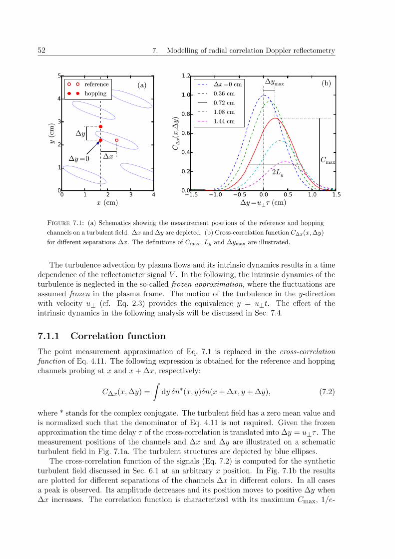
52 7. Modelling of radial correlation Doppler reflectometry
0 1 2 3 4
x (cm)
0
1
2
3
4
5
y(cm)
∆x∆y=0
∆y
(a)reference
hopping
−1.5 −1.0 −0.5 0.0 0.5 1.0 1.5
∆y=u⟂τ (cm)
0.0
0.2
0.4
0.6
0.8
1.0
1.2
C∆x(x,∆
y)
Cmax
∆ymax
2Ly
(b)∆x=0 cm
0.36 cm
0.72 cm
1.08 cm
1.44 cm
Figure 7.1: (a) Schematics showing the measurement positions of the reference and hopping
channels on a turbulent field. ∆x and ∆y are depicted. (b) Cross-correlation function C∆x(x,∆y)
for different separations ∆x. The definitions of Cmax, Ly and ∆ymax are illustrated.
The turbulence advection by plasma flows and its intrinsic dynamics results in a timedependence of the reflectometer signal V . In the following, the intrinsic dynamics of theturbulence is neglected in the so-called frozen approximation, where the fluctuations areassumed frozen in the plasma frame. The motion of the turbulence in the y-directionwith velocity u⊥ (cf. Eq. 2.3) provides the equivalence y = u⊥t. The effect of theintrinsic dynamics in the following analysis will be discussed in Sec. 7.4.
7.1.1 Correlation function
The point measurement approximation of Eq. 7.1 is replaced in the cross-correlationfunction of Eq. 4.11. The following expression is obtained for the reference and hoppingchannels probing at x and x+ ∆x, respectively:
C∆x(x,∆y) =
∫dy δn∗(x, y)δn(x+ ∆x, y + ∆y), (7.2)
where * stands for the complex conjugate. The turbulent field has a zero mean value andis normalized such that the denominator of Eq. 4.11 is not required. Given the frozenapproximation the time delay τ of the cross-correlation is translated into ∆y = u⊥τ . Themeasurement positions of the channels and ∆x and ∆y are illustrated on a schematicturbulent field in Fig. 7.1a. The turbulent structures are depicted by blue ellipses.
The cross-correlation function of the signals (Eq. 7.2) is computed for the syntheticturbulent field discussed in Sec. 6.1 at an arbitrary x position. In Fig. 7.1b the resultsare plotted for different separations of the channels ∆x in different colors. In all casesa peak is observed. Its amplitude decreases and its position moves to positive ∆y when∆x increases. The correlation function is characterized with its maximum Cmax, 1/e-

7.1. Turbulence characterization: Point measurement 53
0.0
0.2
0.4
0.6
0.8
1.0
Cmax
(a)
Lx
0.0 0.4 0.8 1.2 1.6
∆x (cm)
0.0
0.1
0.2
0.3
0.4
0.5
0.6
∆y m
ax(cm)
m∆x (c)
0.00.10.20.30.40.50.60.7
Ly(cm)
(b)synthetic
model
∆x
time delay>0
time delay=0
time delay<0
(d)
Figure 7.2: (a–c) Maximum Cmax, 1/e-half-width Ly and position of the maximum ∆ymax of
the cross-correlation as a function of the separation ∆x. Lx and m are indicated. The thin grey
lines depict the results for several x values and the blue symbols their mean. The red lines depict
the analytical results from Eq. 7.6-7.9. (d) Schematics illustrating the effect of the tilt angle of
the structure on the time delay.
half-width Ly and position of the maximum ∆ymax. The three quantities are indicatedon Fig. 7.1b for the ∆x = 0.72 cm curve in red. It is important to remark that τmax =∆ymax/u⊥ is time delay between the signals.
In Figs. 7.2a–c the dependence on ∆x of the properties of the correlation function isshown in detail. The thin grey lines depict the results at different reference positions xand the blue symbols the average of them with the error bars indicating the standarddeviation. The red line depicts the analytical prediction which will be discussed later.The maximum of the correlation Cmax decays with ∆x due to the spatial decorrelationof the turbulence in the x (radial) direction, therefore the 1/e-decay length is defined asthe correlation length Lx. The width of the correlation function is independent of theradial separation and its value is the correlation length in the y (perpendicular) directionLy.
The position of the maximum ∆ymax or equivalently the time delay, shows a linearbehaviour ∆ymax = m∆x characterized with a slope m, which is related to the tiltangle of the turbulent structures. This is schematically shown in Fig 7.2d where threestructures with different tilt angles are displayed. The measurement points are depictedby black circles, the empty one indicates the reference. A clockwise tilted structure(purple) is seen earlier by the reference channel, resulting in a positive time delay that
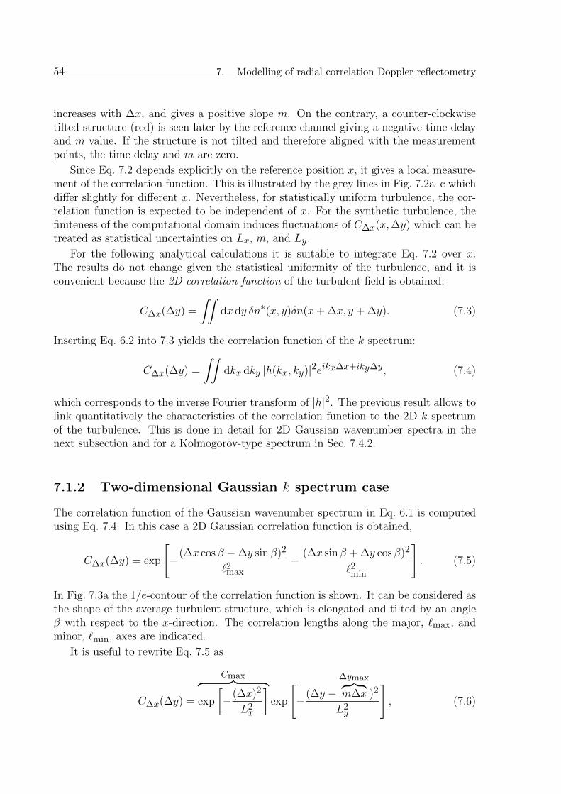
54 7. Modelling of radial correlation Doppler reflectometry
increases with ∆x, and gives a positive slope m. On the contrary, a counter-clockwisetilted structure (red) is seen later by the reference channel giving a negative time delayand m value. If the structure is not tilted and therefore aligned with the measurementpoints, the time delay and m are zero.
Since Eq. 7.2 depends explicitly on the reference position x, it gives a local measure-ment of the correlation function. This is illustrated by the grey lines in Fig. 7.2a–c whichdiffer slightly for different x. Nevertheless, for statistically uniform turbulence, the cor-relation function is expected to be independent of x. For the synthetic turbulence, thefiniteness of the computational domain induces fluctuations of C∆x(x,∆y) which can betreated as statistical uncertainties on Lx, m, and Ly.
For the following analytical calculations it is suitable to integrate Eq. 7.2 over x.The results do not change given the statistical uniformity of the turbulence, and it isconvenient because the 2D correlation function of the turbulent field is obtained:
C∆x(∆y) =
∫∫dx dy δn∗(x, y)δn(x+ ∆x, y + ∆y). (7.3)
Inserting Eq. 6.2 into 7.3 yields the correlation function of the k spectrum:
C∆x(∆y) =
∫∫dkx dky |h(kx, ky)|2eikx∆x+iky∆y, (7.4)
which corresponds to the inverse Fourier transform of |h|2. The previous result allows tolink quantitatively the characteristics of the correlation function to the 2D k spectrumof the turbulence. This is done in detail for 2D Gaussian wavenumber spectra in thenext subsection and for a Kolmogorov-type spectrum in Sec. 7.4.2.
7.1.2 Two-dimensional Gaussian k spectrum case
The correlation function of the Gaussian wavenumber spectrum in Eq. 6.1 is computedusing Eq. 7.4. In this case a 2D Gaussian correlation function is obtained,
C∆x(∆y) = exp
[−(∆x cos β −∆y sin β)2
`2max− (∆x sin β + ∆y cos β)2
`2min
]. (7.5)
In Fig. 7.3a the 1/e-contour of the correlation function is shown. It can be considered asthe shape of the average turbulent structure, which is elongated and tilted by an angleβ with respect to the x-direction. The correlation lengths along the major, `max, andminor, `min, axes are indicated.
It is useful to rewrite Eq. 7.5 as
C∆x(∆y) =
Cmax︷ ︸︸ ︷exp
[−(∆x)2
L2x
]exp
[−(∆y −
∆ymax︷ ︸︸ ︷m∆x )2
L2y
], (7.6)

7.1. Turbulence characterization: Point measurement 55
βℓmax
ℓmin Ly
Lx
mLx
1/e−contour
(a)
∆x
∆y
0.4
0.6
0.8
1.0
1.2
1.4
1.6
Lx (cm
)
(b)
ℓmax
ℓmin
0 15 30 45 60 75 90
β (deg)
−0.20.00.20.40.60.81.01.21.4
m
(d)tanβ
0.4
0.6
0.8
1.0
1.2
1.4
1.6
Ly (cm
)
(c) ℓmax
ℓmin
syntheticmodel
Figure 7.3: (a) 1/e-contour of the correlation function Eq. 7.5. `max, `min, β and the quantities
given in Eqs. 7.7–7.9 are indicated. (b–d) Lx, Ly and m as a function of the tilt angle β. The
values obtained from synthetic turbulence (points) are in agreement with the results of Eqs. 7.7–
7.9 (solid line).
where
Lx = `max cos β
[1 +
`2min
`2maxtan2 β
]1/2
, (7.7)
Ly =`min
cos β
[1 +
`2min
`2maxtan2 β
]1/2
, (7.8)
m = tan β
[1− (`min/`max)2
1 + (`min/`max)2 tan2 β
]. (7.9)
The geometrical meaning of Lx, Ly, and m is shown in Fig. 7.3a. Lx gives half themaximum width of the structure in the x-direction marked by the red point. The verticalposition of this point is mLx and depends on the tilt angle. The half width in y-directionon the axis is given by Ly.
For every ∆x, Eq. 7.6 gives a Gaussian peak with amplitude Cmax, width Ly, andcentred at ∆ymax, which is in agreement with the cross-correlation function depicted inFig. 7.1b. Furthermore, the ∆x dependence of Cmax, Ly, and ∆ymax depicted by red

56 7. Modelling of radial correlation Doppler reflectometry
lines in Figs. 7.2a–c matches the average synthetic data (blue points), proving that theresults of Eq. 7.2 and 7.3 are equivalent.
In order to confirm the dependence of Lx, Ly, and m on the turbulence parametersgiven in Eqs. 7.7–7.9, a scan of the tilt angle β has been performed. The values of Lx,Ly and m obtained from the synthetic turbulence are depicted by points in Figs. 7.3b–d,respectively. The results from the analytical expressions of Eqs. 7.7–7.9 are depictedby solid lines. Lx evolves from `max at β = 0◦ to `min at β = 90◦, correspondingto a change from horizontally to vertically aligned structures. Ly exhibits the oppositebehaviour with a transition from `min to `max. For small β, m increases as the structure’smajor axis misaligns with respect to the x-axis, whereas for β close to 90◦, m decreasesas the structure’s minor axis aligns with the x-axis. As a result of these behavioursm has a maximum around 70◦. Figs. 7.3b–d show good agreement between the resultsfrom the synthetic turbulence and the analytical model from Eqs. 7.7–7.9 for the threequantities. The system of equations 7.7 to 7.9 can be inverted for obtaining `max, `min,and β from the measurements of Lx, Ly, and m.
Since m increases with the tilt angle in a broad β range, it can be used to estimatedirectly the tilt angle. The bracket term in Eq. 7.9 can be approximated by 1 forelongated structures (`min/`max < 1) and angles far from 90◦ obtaining
m ≈ tan β. (7.10)
This approximation is depicted in Fig. 7.3d by a dashed blue line. It agrees well withthe exact solution for β up to 30◦, therefore the tilt angle is precisely obtained fromβ = tan−1m. For β between 30◦ and 55◦, tan β is above the exact solution hencethe tilt angle is underestimated. The range of validity of the approximation increaseswith the elongation. Eq. 7.10 allows to calculate the tilt angle directly from m, assumingelongated structures with a finite tilt angle with respect to the cutoff. This approximationis useful because the diagnostic effects have an impact on the Lx and Ly measurementsthat make the inversion of Eqs. 7.7–7.9 problematic.
7.1.3 Ray propagation effect
For oblique angles of incidence, the radial scan pertaining to a radial correlation mea-surement results in a perpendicular displacement of the measurement position. Fig. 7.4adepicts rays for different probing frequencies in slab geometry. The measurement posi-tions are indicated with circles. The change in the radial position ∆x induces a perpen-dicular displacement ∆yray of the measurement position. For a small cutoff separationthe measurement points are aligned along a straight line defining an angle Θray withrespect to the x-axis which fulfils
∆yray = tan(Θray)∆x. (7.11)
The geometrical definition of Θray is shown in the zoomed Fig.7.4b. The upper and rightaxes indicated ∆x and ∆yray, respectively. Θray can be computed from ray tracing data.

7.1. Turbulence characterization: Point measurement 57
Figure 7.4: (a) Rays of the reference frequency and three hopping frequencies for O-mode and
linear density profile, θ = 17.7◦. The measurement positions are indicated with circles. ∆x
and ∆yray are depicted for one case. (b) Zoom showing schematically the effect of the vertical
displacement of the measurement positions on the ∆ymax measurement. Refer to the text for
more details.
Equations 7.2 and 7.3 assume that both Doppler channels are measuring at the samey-position. This is valid only for normal incidence where there is no perpendiculardisplacement of the measurement positions. However, for Doppler reflectometry the per-pendicular displacement of the measurement points introduces an extra contribution to∆ymax and therefore to m. This extra contribution results from geometrical considera-tions as shown in Fig. 7.4b. The measurement points are depicted by red points and theturbulent structure is shown with the blue contour. The measurement ∆ymax (indicatedwith a black line) is the sum of the ray tracing contribution ∆yray = ∆x tan Θray (redline) and of the structure tilt contribution ∆x tan β (blue line). Therefore
m = tan β + tan Θray. (7.12)
Concluding, it is important to consider the perpendicular displacement of the measure-ment positions, which has an impact on ∆yray (hence on the time delay τmax) and m.
The geometrical considerations summarized in Eq. 7.12 are the basis of the tilt anglemeasurement method. In Chs. 8 and 9 the tilt angle will be determined from the analysisof experimental time delays τmax, u⊥, and Θray in the ASDEX Upgrade tokamak andthe TJ-II stellarator. Eq. 7.12 will be adapted to the sign conventions of time delay andangle used there. Diagnostic effects on this measurement are investigated in the followingsections. In particular, the impact of the temporal decorrelation of the turbulence isdiscussed in Sec. 7.4.

58 7. Modelling of radial correlation Doppler reflectometry
7.2 Two-dimensional full-wave simulations
In order to investigate the influence of plasma-wave interactions in the correlation mea-surements and to asses if the characterization method presented in the previous sectioncan be applied to Doppler reflectometry signals, radial correlation Doppler reflectometrymeasurements are modelled with 2DFW simulations. The same configuration as for thepower response studies (cf. Sec. 6.3) is used with 60.2 and 94.4 GHz as reference frequen-cies. The hopping channel signal is obtained by repeating the simulations with lowerfrequencies in the range 60.2–47.8 and 94.4–83.4 GHz for O- and X-mode, respectively.The turbulent field with a 2D Gaussian spectrum is the same of Sec. 6.1. Five turbulencelevels within the same range as in the power response studies were used. Aiming for abetter k⊥ overlap between O- and X-mode, θ = 5.6◦ is also simulated for X-mode. Inorder to minimize statistical fluctuations the number of samples was increased to 5920.
7.2.1 Linear case
From the power response studies (cf. Fig. 6.10) it is known that for δnrms/nc = 0.1 %the reflectometer response is linear for both polarizations, excluding the X-mode atθ = 22.31◦ where a slight enhanced power response is observed. This linear case allowsto study the diagnostic response excluding any non-linear effect.
The cross-correlation function of the complex signals is calculated. Only its abso-lute value is considered, since the complex phase contains information on the Dopplerfrequency irrelevant for the correlation analysis. The quantities Cmax, Ly and ∆ymax
are computed. Figs. 7.5a–c shows the O-mode results (points) as a function of ∆x fordifferent angles of incidence θ. The dashed lines will be explained later. The correlationdecays with the radial separation, but the decay is strongly affected by the angle ofincidence. A similar effect has been already observed in Ref. [19] and was attributed tonon-local scattering [21]. The width of the cross-correlation Ly is independent of ∆x forsmall values and shows a slight dependence with θ. ∆ymax shows a linear behaviour withthe radial separation for small ∆x as observed previously. The slope m increases with θas expected from the perpendicular displacement effect already discussed (cf. Sec. 7.1.3).
For large ∆x and small θ (blue and green data), the correlation decay seems to beslower than what is expected for a Gaussian decay depicted by the dashed lines. Thiseffect is related to non-local scattering, where scattering along the beam path contributesto the reflectometer signal (cf. Sec. 4.3). This results in a higher correlation comparedto what one would expect for the cutoff [21]. This effect explains also the deviations of∆ymax from the expected linear behaviour, because the scattering from different regionsalong the probing beam do not have a well defined time delay like the contribution fromthe cutoff.
A Gaussian fit Cmax = exp[−(∆x/Lx)2] is done weighting the data with 1/C2max.
Since points with low correlation are less important, this procedure filters out non-localscattering effects and focuses the analysis to the cutoff contribution. Furthermore, it isalso convenient because for low correlation levels, the cross-correlation and therefore theextracted quantities are strongly affected by the statistical fluctuations. A detailed studyof non-local scattering effects would require increased statistics in the simulations. Ly

7.2. Two-dimensional full-wave simulations 59
0.0
0.2
0.4
0.6
0.8
1.0
Cmax
(a)
O−mode
0.0 0.5 1.0 1.5 2.0
∆x (cm)
0.0
0.4
0.8
1.2
∆y m
ax(cm)
(c)
0
1
2
3
4
5
Ly(cm)
(b)
θ=8.73 ◦
θ=13.16 ◦
θ=17.68 ◦
θ=22.31 ◦
0.0
0.5
1.0
1.5
2.0
Lx(cm)
(d)
true
0 5 10 15 20 25
θ (deg)
0.0
0.4
0.8
1.2m
(f)
no tilt
true
0
1
2
3
4
5
Ly(cm)
(e)
true
wO
wXO-mode
X-mode
Figure 7.5: (a–c) Correlation parameters Cmax, Ly and ∆ymax obtained from 2DFW simula-
tions in the linear regime. The colours represent different angles of incidence θ. (d–f) Lx, Ly
and m obtained from O- and X-mode 2DFW data. Refer to the text for more details.
is taken from its value at ∆x = 0. ∆ymax is fitted with a linear function using only thefirst few points which behave linearly and are not affected by the non-local scattering.
Lx, Ly and m are obtained from the fitting process described above. The results as afunction of θ are shown in Figs. 7.5d–f. Additionally, data from X-mode simulations areincluded. Lx decreases with the angle of incidence for both polarizations in Fig. 7.5d. Asimilar trend has been observed previously in simulations [19] and experiments [16]. Lxis slightly overestimated for small θ compared to the true value marked with a dashedline in the plot, and is underestimated for large θ. It has been found that the k⊥ variationproduced by the probing frequency scan induces decorrelation of the signals for large θ.This effect is discussed in detail in Appendix B. The decorrelation effect is strong in theperformed simulations and is responsible, to a large extent, for the Lx reduction withθ reported here. This prevents a detailed study of the non-local scattering which mayinduce an overestimation of Lx for small θ and a convergence to the true value for largeθ [21]. In the presented simulations, the correlation length Lx can be estimated from thedata at small θ (not affected by the decorrelation effect) with an error of 10 and 20 %for O- and X-mode, respectively.

60 7. Modelling of radial correlation Doppler reflectometry
For both polarizations, Ly is strongly overestimated compared to the true valueindicated with a black dashed line in Fig. 7.5e. Ly exhibits a slight dependence on θ forthe O-mode data. Note that the obtained values match well the beam size w indicatedwith dotted lines for each polarization. Therefore in the simulations presented, the widthof the cross-correlation gives the beam size rather than the perpendicular correlationlength Ly.
The 2DFW data for both polarizations in Fig. 7.5f underestimate m compared tothe point measurement depicted by dashed lines and computed with Eq. 7.12 (β = 20◦).Nevertheless the dependence with θ is similar, which shows that the m change is due tothe perpendicular displacement effect. Note that m is larger than the point measurementfor the case without tilting (β = 0) depicted by dotted lines. This means that a non-zero tilt with the correct sign is recovered from the simulations. The tilt angle obtainedfrom the simulated data using Eq. 7.12 is β ≈ 10◦, which has the correct sign butunderestimates the true value by 50 %.
In summary, the radial correlation length Lx can be estimated (10–20 % error) fromthe simulated data at small θ for which the impact of decorrelation effect discussed inAppendix B is negligible. The width of the cross-correlation gives an estimation of thebeam size and not of the perpendicular correlation length Ly. The time delay and theslope m behave as predicted by the perpendicular displacement discussed in Sec. 7.1.3.The tilt angle of the turbulence can be extracted from the simulated data with thecorrect sign, although the value is underestimated. These simulations have shown theapplicability of the developed analysis techniques to Doppler reflectometer signals in thelinear regime. The role of the radial and spectral resolutions on the linear measurementswill be investigated in the next section, which will allow to understand better the effectsobserved in these simulations. Moreover the conditions required for a more accuratecharacterization will also be discussed.
7.2.2 Non-linear case
The previous correlation analysis is repeated for the turbulence level scan. Lx, Ly andm are obtained from Cmax, width and ∆ymax as for the linear case. The results areshown in Fig. 7.6 as a function of the turbulence level for different angles of incidencedepicted by different colours. O- and X-mode results are plotted in the left and rightcolumns, respectively. The upper axis shows the non-linearity parameter γ (cf. Eq. 5.8).Lx decreases with the turbulence level in the non-linear regime (γ = 0.1–10), for allangles of incidence and both polarizations. In the saturation regime (γ ≈ 10), Lx doesnot depend on the angle of incidence and is underestimated compared to the true valueindicated with the dashed line. Ly does not change appreciably with the turbulence level.For increasing turbulence level between γ = 0.1–1, m decreases as the reflectometer startsoperating in the non-linear regimes. This effect is stronger for X-mode since it runs firstinto non-linear operation (cf. Ch. 6). For the highest turbulence level in the saturationregime m shows an erratic behaviour.
The decrease of the correlation with the turbulence level (Figs. 7.6a and d) is ex-plained by the multiple scattering processes responsible for the non-linear effects dis-

7.2. Two-dimensional full-wave simulations 61
0.0
0.5
1.0
1.5
2.0
Lxcm
)O−mode
(a)
true
10-3 10-2 10-1 100 101γ
10-1 100 101
δnrms/nc (%)
−0.4
0.0
0.4
0.8
1.2
m
(c)
0
1
2
3
4
5
Ly(cm)
(b)
θ=8.73
θ=13.16
θ=17.68
θ=22.31
X−mode
(d)
true
10-2 10-1 100 101γ
0.1 1.0 10
δnrms/nc (%)
(f)
(e)
θ=5.56 ◦
θ=8.73 ◦
θ=13.16 ◦
θ=17.68 ◦
θ=22.31 ◦
Figure 7.6: Turbulence parameters Lx, Ly and m as a function of the turbulence level obtained
from O- (a–c) and X-mode (d–f) 2DFW data. The colours depict different angles of incidence.
cussed in Sec. 6.2.4. In the linear regime, the reflectometer signal is produced by scat-tering events at k⊥. This contribution is well correlated for both reflectometer channels.However, for large turbulence levels, multiple scattering events at wavenumbers differentfrom k⊥ contribute to the reflectometer signal (see Fig. 6.7). These multiple contribu-tions are poorly correlated.
The strong effects of non-linearities on Lx and m limit the direct application of thecharacterization method when the diagnostic response is non-linear. The method couldbe still applied if non-linear effects are assessed with 2DFW simulations. Nevertheless,this must be done in detail for the specific experimental conditions, because the linearityof the response depends strongly on the k spectrum and differs from the Gaussian case.

62 7. Modelling of radial correlation Doppler reflectometry
7.3 Diagnostic filter effect
The filter effect of the diagnostic in k space is considered. This allows to understandbetter the linear simulations presented in the previous section, to predict the diagnosticresponse for more general cases, and to identify conditions for which the characterizationof the turbulence with radial correlation Doppler reflectometry is accurate.
The Doppler reflectometer is studied using the Born approximation from Eq. 5.7. Forthe sake of simplicity, here E2
0 or equivalently the weighting function W is approximatedwith a Gaussian filter function f given by
E20(x, y) ≈ f(x, y) = exp
[− x2
(δr)2− 2y2
w2− ik⊥y
]. (7.13)
The width in the x- and y-directions is defined by the radial resolution δr and the beamwidth w = 2/∆k, respectively. The complex phase gives the Bragg condition at k⊥. InFourier space the filter function is
f−1(kx, ky) = exp
[−k
2x(δr)2
4
]exp
[−
(ky − k⊥)2
2(∆k)2
], (7.14)
where ·−1 stands for the inverse Fourier transform. It corresponds to a 2D filter centredat kx = 0 and ky = k⊥ and is analogous to the filter function f introduced for thephysical optics model in Sec. 6.2.4.
Equation 7.13 is a reasonable approximation given the maximization of E0 at thecutoff discussed in Sec. 6.3. It will be shown that it recovers some of the effects observedin 2DFW simulations and experiments. Furthermore, it is useful for the understandingand assessment of the impact of the radial and spectral resolution on the characterizationmethod discussed in Sec. 7.1. Nevertheless, quantitative predictions should be takencarefully considering the approximations done and the absence of non-local scatteringeffects [21].
Using the Born approximation (Eq. 5.7) with the filter function (Eq. 7.13), theDoppler signal probing at the position (x, y) is
V (x, y) =
∫∫dx′dy′ δn(x+ x′, y + y′)f(x′, y′). (7.15)
This expression considers the integration over the scattering volume, therefore it is ageneralization of the point measurement of Eq. 7.1. Writing δn in terms of the k spectrumfrom Eq. 6.2, Eq. 7.15 becomes:
V (x, y) =
∫∫∫∫dx′dy′ dkxdky h(kx, ky)eikx(x+x′)+iky(y+y′)f(x′, y′),
=
∫∫dkxdky h(kx, ky)f−1(kx, ky)eikxx+ikyy. (7.16)

7.3. Diagnostic filter effect 63
In the last step the signal is given by the turbulent field filtered in k-space. This indicatesthe filtering role of the Doppler reflectometer.
The cross-correlation of the Doppler reflectometer signals is
C∆x(∆y) =
∫∫dx dy V ∗(x, y)V (x+ ∆x, y + ∆y),
where the tilde stands for the fact that the filtered signals are used as input. In the lastequation the statistical uniformity of the turbulence has been used as it has been doneto obtain Eq. 7.3. Inserting Eq. 7.16 in the last expression yields the correlation function
C∆x(∆y) =
∫∫dkxdky |h(kx, ky)|2|f−1(kx, ky)|2eikx∆x+iky∆y. (7.17)
It corresponds to the inverse Fourier transform of the filtered k spectrum. This is differentfrom the point measurement case of Eq. 7.4 where no filter is included.
For the 2D Gaussian spectrum of Eq. 6.1, the integral in Eq. 7.17 is solved analyticallyobtaining
|C∆x(∆y)| = exp
[−(∆x)2
L2x
− (∆y − m∆x)2
L2y
]. (7.18)
The absolute value is taken because the ky-filter gives a complex phase without furtherphysical information. The tilded quantities are:
Lx = Lx
√1 +
2(δr)2
L2x
, (7.19)
Ly =
√L2y +
4
(∆k)2+
2m2(δr)2
1 + 2(δr)2/L2x, (7.20)
m = m
(1 +
2(δr)2
L2x
)−1
. (7.21)
The measured radial correlation length Lx is overestimated by a factor√
1 + 2(δr)2/L2x.
If the radial resolution is small compared to the radial correlation length, δr � Lx, thiseffect is small and the true Lx is recovered. This is in agreement with the linear 2DFWresults from Fig. 7.5d at small θ, where a slight overestimation of Lx is observed. It isimportant to note that no dependence on k⊥ is obtained for the Gaussian case. Thedecrease of the measured Lx with θ observed in the simulations is not reproduced by thefilter effect and is explained in Appendix B.
The measured width of the correlation Ly is overestimated by the spectral and radialresolution through the second and third term in Eq. 7.20, respectively. For a good spec-tral resolution (Ly∆k � 1), the second term dominates and the width of the correlation
is rather given by the beam width, Ly ≈ 2/∆k = w. This is the case of the 2DFWsimulations shown in Fig. 7.5e.

64 7. Modelling of radial correlation Doppler reflectometry
The slope m in Eq. 7.21 underestimates m due to the radial resolution by a factor(1 + 2(δr)2/L2
x)−1. Nevertheless, for δr � Lx this effect is also negligible. There is alsono k⊥ dependence for the Gaussian case. The filter effect recovers the underestimation ofm and hence of the tilt angle β obtained from the 2DFW results by taking δr ≈ 0.8 cm.Note that the ray propagation effect can be considered by adding tan Θray at the r.h.s.of Eq. 7.21.
The filtering effect of the Doppler reflectometry does affect the quantities used for the2D characterization of the turbulence. The measured radial correlation lengths and timedelays can be affected by the radial resolution, nevertheless for favourable experimentalconditions (δr � Lx) the effect is negligible, thus the radial correlation length and tiltangle can be measured. The width of the correlation is mostly given by the beam width,hence the estimation of the perpendicular correlation length is problematic.
7.4 Temporal decorrelation effect
Up to now, frozen turbulence has been assumed in the characterization method presentedin Sec. 7.1 and has been used in the 2DFW simulations and the filtering effect discussedin the previous sections. This is a valid assumption if the structures do not changeappreciably while they propagate through the scattering region. This condition can befulfilled depending on the turbulence decorrelation time τd and the plasma flow u⊥. Here,the effect of the decorrelation time is considered. A correction to the characterizationmethod accounting for the decorrelation time is given.
The cross-correlation function for a given radial separation ∆x and considering thedecorrelation time of the turbulence is
C∆x(τ) = Cmax exp
[−(u⊥τ −∆ymax)2
w2
]exp
(−τ
2
τ2d
)(7.22)
The first two terms correspond to the frozen turbulence case as in Eq. 7.6, where Cmax
and ∆ymax are defined by the 2D structure of the turbulence. The beam width w istaken instead of Ly because of the filtering effect discussed previously. The last termincludes a Gaussian correlation function in time [106].
C∆x(τ) has been plotted in Fig. 7.7 for w = 4.0 cm, u⊥ = 1 km/s, ∆ymax = 1.0 cm.Colours indicate different τd values. The blue line for τd →∞ shows a peak centred atτmax = ∆ymax/u⊥ = 10 µs as in the frozen turbulence case. As τd decreases the peakbecomes narrower and moves closer to τ = 0, implying a reduction of the measured timedelay τmax. This effect is small for τd = 119 µs (green line) with a time delay 10 %smaller than the one of the frozen case. The effect is strong for τd = 13 µs (light blueline) with a time delay 90 % smaller than the one of the frozen case. The maximum ofthe correlation is not strongly affected, even for small τd.
It can be shown that the maximum of C∆x(τ) is at
τmax =∆ymax
u⊥
(1 +
w2
u2⊥τ
2d
)−1
=∆ymax
u⊥Fd. (7.23)

7.5. Realistic wavenumber spectrum 65
−20 −10 0 10 20 30 40 50 60
τ (µs)
0.0
0.2
0.4
0.6
0.8
1.0
C∆x(τ)
τd →∞τd =119 µs
τd =40 µs
τd =13 µs
Figure 7.7: Cross-correlation function from Eq. 7.22 for different τd values. The blue curve
corresponds to the frozen turbulence case.
The first term gives the time delay expected from the frozen turbulence case, and thesecond term is a correction factor Fd related to the temporal decorrelation that reducesthe measured time delay. It is relevant for τd ≤ w/u⊥.
The time delay reduction leads to an underestimation of m. This effect can beincluded in Eq. 7.12 with the correction factor Fd as follows:
m = Fd [tan(β) + tan(Θray)]. (7.24)
In the experiments, the impact of the decorrelation time can be assessed by comparingthe passing time w/u⊥ with τd measurements or expected values [106, 107]. For largeplasma velocities the passing time is substantially smaller than τd and the decorrelationtime effect has no impact, whereas for small velocities the passing time is comparable toor larger than τd and the correction factor Fd is necessary. The impact of the temporaldecorrelation on the experimental measurements will be investigated in Chs. 8 and 9.Eq. 7.24 will be used for the tilt angle measurement and Eq. 7.23 for estimations of thecorrection factor and decorrelation time.
7.5 Realistic wavenumber spectrum
Gaussian k spectra have often been used in theory [21] and simulations [19] of radialcorrelation Doppler reflectometry. Their properties make them suitable for analyticalcalculations, as it has been shown in the previous sections and in Ch. 6. Nevertheless,more realistic Kolmogorov-type spectra should be also considered (cf. Sec. 2.1). It isimportant to assess how the spectral shape impacts the correlation measurements andwhat other effects may appear when non-Gaussian spectra are considered. In this sectionthe turbulence from a gyrokinetic simulation of the ASDEX Upgrade tokamak plasma isstudied. The 2D k spectrum is computed and characterized with the method presented inSec. 7.1. Then, the diagnostic effects are investigated with the filter effect from Sec. 7.3.

66 7. Modelling of radial correlation Doppler reflectometry
Figure 7.8: Contour plot of the density fluctuations on the cross-section of the ASDEX Upgrade
tokamak. A zoom to the region of interest is also shown. The turbulence is computed byt he
gyrokinetic code GENE [17, 41].
7.5.1 Gyrokinetic turbulence and 2D k spectrum
The gyrokinetic simulations for the plasma conditions in Ref. [17] are studied. Thereference discharge is AUG#31260, a L-mode in USN configuration with 1 MW NBIand 0.45 MW ECRH power. The core average density is 5.5×10¹⁹ m−3. The densityfluctuations are obtained from non-linear GENE [28, 41] simulations, local to the fluxsurface at ρ = 0.8. The turbulence is ITG driven for large scales k⊥ρs < 1. More detailson the discharge and the simulations can be found in Ref. [17].
The poloidal cross-section of the ASDEX Upgrade tokamak together with a samplecontour plot of the density fluctuations is shown in Fig. 7.8. The turbulent field locatedbetween the flux surfaces ρ = 0.75 and 0.95 shows an asymmetry between the highand low field side. The fluctuation level is higher on the low field side (bad curvature)reflecting the ballooning character of the turbulence. Elongated turbulent structures areobserved, their size and tilt changes along the flux surface reflecting the locality of theturbulence.

7.5. Realistic wavenumber spectrum 67
−20 −10 0 10 20
kx (cm−1 )
−20
−10
0
10
20ky(cm−1
)
67 ◦
(a)
10−4
10−3
10−2
10−1
100
h(a.u.)
0.5 1 2 3 4 56 10 20
k (cm−1 )
10-7
10-6
10-5
10-4
10-3
10-2
10-1
100
101
P(a.u.)
k−8
k−4
k−5
(b)
perpendicular
radial
Figure 7.9: (a) Contour plot of the k spectrum computed from GENE data. (b) Perpendicular
and radial k power spectra. Power laws in different k ranges are indicated.
The analysis in this section is focused on the region where the steerable Dopplerreflectometer system measures (cf. Sec. 4.2.2). This region is indicated with a dashedsquare in Fig. 7.8 and magnified on the right side of the figure. Elongated and tiltedstructures show a tilt angle with respect to the normal to the flux surface of about 67◦
as indicated in the zoomed area.In order to compute the 2D k spectrum a local coordinate system (x′, y′) is defined
with the x′-axis perpendicularly aligned to the flux surfaces. The new coordinate systemand the analysis domain are depicted by arrows and a dashed box in the zoom in Fig. 7.8.The 2D k spectrum is obtained by computing the Fourier transform of the densityfluctuations in this new coordinate system.
The contour plot of the k spectrum averaged over 20 samples is shown in Fig. 7.9a.Elongation and a tilt of 67◦ with respect to the vertical axis are observed, similarly tothe synthetic Gaussian case in Fig. 6.1a. The radial and perpendicular wavenumberspectra are computed by taking the spectral power |h|2 at ky = 0 and kx = 0, respec-tively. The results are plotted in Fig. 7.9b, where a Kolomorov-type spectrum of densityfluctuations is obtained for both cases. The perpendicular wavenumber spectrum is flatup to approximately 2 cm−1. Afterwards it is characterized by power laws with spec-tral indices of about −4 and −8 in regions separated by a knee at about 8 cm−1. Theradial wavenumber spectrum is almost flat up to approximately 4 cm−1 and then it ischaracterized by a spectral index of −5.
It has to be remarked that tilt angles obtained in local simulations do not considerradial shear of the plasma parameters, which is a relevant ingredient in the tilt angle gen-eration mechanism [38]. A comparison of the tilt angle with experimental measurementsrequires global gyrokinetic simulations which do account for these effects.
7.5.2 Correlation function
The correlation function is computed from the 2D k spectrum using Eq. 7.4. The contourplot of C∆x(∆y) is shown in Fig. 7.10a, where a main structure centred at the origin is

68 7. Modelling of radial correlation Doppler reflectometry
−2.0 −1.5 −1.0 −0.5 0.0 0.5 1.0 1.5 2.0
∆x (cm)
−2.0
−1.5
−1.0
−0.5
0.0
0.5
1.0
1.5
2.0
∆y(cm)
67 ◦1.40cm
0.34 c
m
(a)
−1.0 −0.5 0.0 0.5 1.0
C∆x(∆y)
0.0
0.2
0.4
0.6
0.8
1.0
Cmax
(b)
Lx , Eq. 7.7
0.0 0.2 0.4 0.6 0.8 1.0 1.2 1.4
∆x (cm)
0.0
0.5
1.0
1.5
2.0
2.5
3.0∆y m
ax(cm)
m∆x, Eq. 7.9 (d)
0.00.20.40.60.81.01.21.4
Ly(cm)
(c)
Eq. 7.8
Figure 7.10: (a) 2D correlation function of the turbulent field. (b) Cmax, (c) Ly and (d) ∆ymax
as a function of ∆x. Predictions of Eqs. 7.7–7.9 are depicted in blue.
obtained. Its elongation and tilt are in agreement with the structures zoomed in Fig. 7.8.The 1/e-contour depicted by the yellow line is approximately an ellipse characterized with`max = 1.40 cm, `min = 0.32 cm and β = 67◦. The three quantities are indicated inFig. 7.10a.
The turbulent field is characterized using the method presented in Sec. 7.1. Cmax, Lyand ∆ymax are computed from C∆x(∆y) at different ∆x, which corresponds to verticalcuts in Fig. 7.10a. Cmax, Ly and ∆ymax are plotted with points as a function of ∆x inFigs. 7.10b–d. The maximum of the correlation decreases similarly to the Gaussian casefor small ∆x. The radial correlation length Lx computed with Eq. 7.7 is depicted by thedashed blue line in Fig. 7.10b. It matches the 1/e-decay length. Nevertheless contraryto the Gaussian case, there is a slowly decaying tail for large ∆x. This is due only tothe spectral shape and not to diagnostic effects which have not been considered yet. Lyin Fig. 7.10c is not constant contrary to the Gaussian case, instead it increases with ∆x.Nevertheless Ly computed from Eq. 7.8 depicted by a blue line matches the value at∆x = 0. ∆ymax in Fig. 7.10d depends linearly on ∆x. The solid blue line depicts m∆xwith m computed from Eq. 7.9. A good agreement is obtained for small ∆x.
Cmax, Ly and ∆ymax are well described by the model proposed in Sec. 7.1.2, also fora Kolmogorov-type k spectrum. The characterization method presented in Sec. 7.1 canbe applied to more realistic turbulence in the point measurement case.

7.5. Realistic wavenumber spectrum 69
0.0
0.2
0.4
0.6
0.8
1.0
Cmax
(a)
0.0 0.2 0.4 0.6 0.8 1.0 1.2 1.4 1.6
∆x (cm)
0.0
0.5
1.0
1.5
2.0
∆y m
ax(cm) (c)
0.0
0.4
0.8
1.2
Ly(cm)
(b)
non filtered
k⟂=0.0 cm−1
k⟂=4.0 cm−1
k⟂=8.0 cm−1
k⟂=12.0 cm−1
Figure 7.11: (a) Cmax, (b) Ly and (c) ∆ymax as a function of ∆x obtained from the filtered cor-
relation function. The colours depict different k⊥ values. The non-filtered (point measurement)
results are shown with black symbols.
7.5.3 Diagnostic filter effect
It has been shown for the Gaussian case in Sec. 7.2, that diagnostic effects can havean important impact on correlation measurements and therefore on the proposed char-acterization method. A complete study for realistic k spectra would require systematic2DFW simulations in order to include non-linearities, non-local scattering and k filtering.Nevertheless, here only the filtering effect discussed in Sec. 7.3 is considered. Furtherstudies with 2DFW simulations are left for future work.
The filter effect of the Doppler reflectometer is included through Eqs. 7.14 and 7.17.The values for the radial and spectral resolutions are 0.2 cm and 3.5 cm−1, respec-tively. The filtered correlation function for different k⊥ values is computed and Cmax,
Ly and ∆ymax are obtained. The results are plotted in Figs. 7.11a–c where the colourscorrespond to different k⊥ values. The black points depict the non-filtered (point mea-surement) case already shown in Fig. 7.10b–d.
In Fig. 7.11a, Cmax decays faster for larger k⊥. This effect, absent in the Gaussiancase, is due to the filter effect combined with the spectral shape. It is important to remarkthat despite of the qualitative similarities, this behaviour is not caused by non-localscattering [21] or the decorrelation effect discussed in Appendix B. Moreover for smallk⊥, the correlation decays slightly slower compare to the point measurement becauseof the finite radial resolution. It should be noted that the radial correlation length iswell recovered for the measurements at small k⊥. This effect can explain the reduction

70 7. Modelling of radial correlation Doppler reflectometry
of the radial correlation length with k⊥ measured in the ASDEX Upgrade tokamak (cf.Sec. 8.1.3) and the TJ-II stellarator (cf. Ref. [16]).
For small k⊥, Ly in Fig. 7.11b follows the point like measurements, but overestimate
the value due to the beam waist contribution (cf. Eq. 7.20). For larger k⊥, Ly decreasesand shows a different behaviour with ∆x. In Fig. 7.11c, ∆ymax increases linearly for small∆x in all cases. The slope obtained at small k⊥ (blue and green lines) recovers the valueof the point like measurement related to the tilt angle of the turbulence. Nevertheless,the slope decreases with k⊥ obtaining values close to zero for the higher k⊥ (light blueline). This effect was also absent in the Gaussian case.
In summary, the filter effect of the Doppler reflectometer has an impact on thecorrelation measurements. In particular, a k⊥ dependence of Lx and m appears forKolmogorov-type turbulence. Although Lx and m are underestimated for large k⊥, thevalues obtained at small k⊥ yield to a good estimation of the the radial correlationlength and tilt angle. This effect has not been investigated yet in the literature whereonly Gaussian turbulence has been considered [19, 21]. The difference between the Gaus-sian and the Kolmogorov-type case, show that the spectral shape plays an importantrole in the diagnostic response. This deserves further investigations.
Summary
A new analysis technique of the time delay of the cross-correlation function τmax, velocityu⊥ and the geometry of the measurement positions has been proposed (cf. Sec. 7.1). Itcan be used to measure the tilt angle of elongated turbulent structures. The effect ofthe temporal decorrelation of the turbulence has been investigated. It has been shownthat for small velocities, u⊥ ≤ w/τd, the measured time delays are underestimated withrespect to the frozen turbulence case. This effect can be assessed and accounted in theanalysis with a correction factor Fd (cf. Sec. 7.4). The analysis technique developed willbe applied in Chs. 8 and 9, where the tilt angle will be measured in the experiments.
The diagnostic response has been considered using two-dimensional full-wave simu-lations and a linear analysis based on the Born approximation. It has been found thatin the linear diagnostic regime, the radial correlation length and the tilt angle can beestimated. The impact of the finite radial resolution of the diagnostic has been stud-ied, it is relevant when the radial resolution is comparable or bigger than the radialcorrelation length. The non-linear diagnostic response has a strong impact on the cor-relation measurements, hence estimations of the radial correlation length and tilt angleare problematic when a strong linear diagnostic response is involved.
It has been found that the spectral shape plays an important role in the diagnosticresponse. For a realistic Kolmogorov-type turbulence, the filter effect of the Dopplerreflectometer induces a reduction of the measured radial correlation length and tilt anglewith k⊥. This result is used for the interpretation of experimental data in Sec. 8.1.3.

Chapter 8
Turbulence characterization inASDEX Upgrade and TJ-II plasmas
The density turbulence in the ASDEX Upgrade tokamak and the TJ-II stellarator ischaracterized in detail using Doppler reflectometry. The k⊥ spectrum, u⊥ profile andradial correlation length Lr are experimentally investigated. The purpose of these studiesis two-fold. On the one hand the experimental data are analysed based on the modellingpresented in Ch. 6 and 7. The impact of the diagnostic effects and the accuracy ofthe measurements are discussed. On the other hand, specific physical aspects of theturbulence are discussed. In particular, the effect on the turbulence structure of differentdriving forces and the turbulence regulation by sheared flows (cf. Ch. 2) is discussed.
The application of the analysis techniques developed in Secs. 7.1.3 and 7.3.2 to ex-perimental data is discussed in detail. As a result, the mean tilt angle of the turbulentstructures is measured in the confined region for the first time in both machines. Thisis a proof of principle of the tilt angle measurement method which is one of the majorcontributions of this thesis. The tilt angle measurement in TJ-II is compared to resultsfrom gyrokinetic simulations.
L-mode plasmas in the ASDEX Upgrade tokamak and the TJ-II stellarator are ex-perimentally investigated in Sec. 8.1 and 8.2, respectively. A discussion summarizing theresults in both machines and conclusions are presented in Sec. 8.3.
8.1 Measurements on ASDEX Upgrade
In this section, the density turbulence is investigated with Doppler reflectometry inthe ASDEX Upgrade tokamak (AUG) in a medium density L-mode discharge . Therecently installed W- and V-band reflectometers (cf. Sec. 4.3.1), together with the steer-able mirror [83] have made possible detailed k⊥ spectra and radial correlation studies.In Sec. 8.1.1 the discharge under investigation is described. In Sec. 8.1.2 a detailedexperimental study of k⊥ spectra and u⊥ profile is presented. Doppler reflectometrymeasurements with O- and X-mode polarizations are compared. In Sec. 8.1.3 a detailedstudy of the diagnostic effects on the radial correlation length Lr is carried out and thenew measurement technique of the tilt angle of turbulent structures is applied.
71

72 8. Turbulence characterization in ASDEX Upgrade and TJ-II plasmas
0.0
0.2
0.4
0.6
0.8
1.0
1.2
I p(M
A) (a)
AUG#33714
0.00.20.40.60.81.01.21.4
P(M
W)
(b)
ECRH
NBI
0 1 2 3 4 5 6
t(s)
01234567
n(1
019m−3
) (c)core
edge
measurements
0
1
2
3
4
5
6
7
8
n(1
019m−3
)
(d)
t=3.3−3.7 s
0.5 0.6 0.7 0.8 0.9 1.0 1.1
ρ
0.0
0.2
0.4
0.6
0.8
1.0
1.2
T(k
eV)
(e)
t=3.3−3.7 s
t=3.7−3.8 s
electron
ion
Figure 8.1: Time traces of (a) the plasma current, (b) auxiliary heating power and (c) plasma
density for the reference discharge #33714. The phase of constant density used for the reflec-
tometry measurements is indicated with magenta lines. (d) Density and (e) temperature profiles
during the measurement phase. Measured data are depicted by symbols and the respective fits
with solid lines.
8.1.1 Discharges
Dedicated experiments have been performed on the ASDEX Upgrade tokamak for theturbulence characterization using Doppler reflectometry. ECRH heated L-mode plasmaswith medium density have been investigated. The density has been chosen in orderoptimize the radial range measured by the Doppler reflectometers. The upper singlenull (USN) configuration has been used in order to avoid a transition into the H-modebecause of the higher L-H power threshold for this configuration [108].
The time traces of the plasma current, heating power and line average density ofthe reference discharge #33714 are shown in Figs. 8.1a–c. A constant 0.8 MW of ECRheating power on axis is applied to the plasma. The core and edge line average densitiesare stationary between t =2.5 and 4.5 s. The reflectometry measurements are performedduring this time window as indicated at the top of the figure. A NBI blip is applied forCXRS measurements. Four comparable discharges (#33714–17) have been performed toallow for a complete reflectometer parameter scan.
The density and temperature profiles in the measurement phase are shown in Figs. 8.1dand e, respectively. The plasma density obtained from Thomson scattering and lithiumbeam diagnostics is shown in Fig. 8.1d with symbols. The solid line depicts the fit tothe density profile which will be used later for ray tracing calculations with TORBEAM.The electron temperature depicted by green plus symbols in Fig. 8.1e is obtained from

8.1. Measurements on ASDEX Upgrade 73
Figure 8.2: (a) Probed k⊥ values as a function of the measured radial position ρ. (b) Measure-
ment position on the poloidal AUG cross-section. O- and X-mode are plotted with red and blue
symbols, respectively.
Thomson scattering and ECE measurements. The ion temperature (red squares) is ob-tained from the CXRS measurements. In both cases the solid line depicts the fit tothe data. The density and temperature profiles are stationary during the measurementphase and are similar for the four discharges.
8.1.2 Measurement of k⊥ spectra and u⊥ profile
The two V-band (50–75 GHz) reflectometers have been used in O-mode polarization, andthe W-band (75–103 GHz) in X-mode polarization. For more details on the reflectometerconfiguration refer to Sec. 4.3.1. In this section only the data of one W- and one V-bandchannel is considered for k⊥ spectra and u⊥ profile measurements. The second V-bandchannel will be considered later in Sec. 8.1.3 for correlation measurements. The probingfrequency has been stepped rapidly (5 ms per frequency). A broad scan of the angle ofincidence (12 values) and probing frequencies (120 frequencies per angle of incidence)has been performed during the measurement phase of the four discharges (cf. Figs. 8.1a–c). The frequency patterns have been specially designed in order to cover a large radialregion and to have an overlap of the O- and X-mode measurements.
The scattering position and the probed k⊥ are computed using TORBEAM with thefit to the density profile shown in Fig. 8.1d. The probed k⊥ is plotted as a function of theradial position ρ in Fig. 8.2a. O- and X-mode data are depicted by red and blue symbols,respectively. For each polarization 12 rows of points are distinguished. Each of themcorresponds to one angle of incidence, and the constitutive points to the different probingfrequencies. The coloured areas illustrate the radial windows where the k⊥ spectra arecomputed later. Both polarizations overlap radially in the range ρ ≈ 0.87–0.97. Themeasurements overlap also in k⊥, while the specific range depends on ρ. The X-mode

74 8. Turbulence characterization in ASDEX Upgrade and TJ-II plasmas
−2.0 −1.5 −1.0 −0.5 0.0 0.5 1.0 1.5 2.0
f (MHz)
107
108
109
1010
1011
1012
Powerspectrum(a.u.)
O−mode (a)
f0 =65.0 GHz ρ=0.92 k⟂=11.3 cm
−1
P
fD
direct reflection
AUG#33714, t=4.080-4.085s
−2.0 −1.5 −1.0 −0.5 0.0 0.5 1.0 1.5 2.0
f (MHz)
X−mode (b)
f0 =96.7 GHz ρ=0.91 k⟂=11.2 cm
−1
P
fD
AUG#33715, t=2.855-2.860s
Figure 8.3: Power spectra of the (a) O- and (b) X-mode reflectometer signal measured at
similar radial positions and k⊥. The fit to the Doppler peak is shown with a blue line. The
O-mode exhibits a zero-order reflection.
probes at higher k⊥ (up to 16 cm−1) due to the higher probing k0. Fig. 8.2b showsthe O- and X-mode measurement positions on the AUG cross-section, which overlapspatially.
For each probing frequency and angle of incidence, the power spectrum of the reflec-tometer signal is computed as described in Sec. 4.2. Example spectra measured in O-and X-mode polarization at similar ρ and k⊥ values are depicted in Figs. 8.3a and b,respectively. The blue and magenta lines are the fits to be explained below. Both spectrashow a Doppler peak (blue) at approximately 0.45 MHz, however the O-mode spectrumexhibits also a contribution at zero frequency (magenta). It corresponds to the directreflection discussed in Sec. 4.2.2 which contains information different to the backscat-tering at the cutoff, and that can corrupt the analysis if it is not properly treated. Thedirect reflection is excluded from the analysis by fitting separately the Doppler peakand the direct reflection contribution with Gaussian functions as depicted in Fig. 8.3a.The X-mode spectrum shows no direct reflection contribution and is fitted with a singlepeak as shown in Fig. 8.3b. The backscattered power P and the Doppler shift fD areobtained from the Gaussian fit to the Doppler peak in both cases. The optimization ofthe antenna and mirrors for frequencies in the W-band [83] explains the better qualityof the X-mode spectrum.
The k⊥ spectra at different radial positions are computed by taking P as a functionof k⊥ for narrow radial windows, plotted with different colours in Fig. 8.4 for (a) O-and (b) X-mode data. The different spectra have been vertically offset for visualizationpurposes. A spectral decay with k⊥ is observed for all cases. In general the O-modespectra decay faster than the X-mode spectra, and a faster decay for large k⊥ is observed.Separate power laws have been fitted to the spectra for small and large k⊥. The resultsare depicted by solid lines and the spectral indices are indicated in the figure. Thedispersion of the X-mode data at ρ = 0.85 and 0.9 (blue and green data) makes the fitdifficult, thus in these cases the fits are just meant as a guide to the eye.

8.1. Measurements on ASDEX Upgrade 75
knee
Figure 8.4: k⊥ spectra at different radial positions (ρ ranges are indicated in the legend)
obtained with (a) O-mode and (b) X-mode polarization. The spectra are vertically shifted for
better visibility. Power law fits are depicted by solid lines, and the spectral indices are indicated.
A progressive steepening of the spectra in the high k⊥ range is observed for increasingρ. For O-mode polarization, the spectral index increases slightly between ρ = 0.85 and0.95 from −2.5 to −3.0, then it increases rapidly between ρ = 0.95 and 0.97 from −3.0to −5.2. For X-mode data, the the spectral index increases from −1.9 to −3.7 in theentire measured range. The wavenumber separating the regions with different powerlaws suggests the presence of a knee in the spectra. For the O-mode the knee is locatedat around 4 cm−1 for ρ . 0.95. It moves to higher k⊥ as ρ increases reaching a value ofabout 6 cm−1 for the outermost measurement positions. For the X-mode the knee is athigher k⊥ for all cases.
In Ch. 6 it has been discussed that non-linear diagnostic effects may occur as theturbulence level increases, and that they can lead to a flattening of the measured k⊥spectrum. Since the turbulence level is expected to increase towards the plasma edge, a

76 8. Turbulence characterization in ASDEX Upgrade and TJ-II plasmas
transition to the non-linear regime would cause a flattening of the measured spectra asρ increases. In contrast, the O-mode data shows a strong spectral steepening towardsthe plasma edge. This suggest a linear diagnostic response and a radial variation of thereal k⊥ spectrum.
The O-mode spectral indices are in all cases more pronounced than the X-mode ones.The smallness of the X-mode spectral indices indicates a non-linear diagnostic responseas discussed in Sec. 6. The approximately flat spectra observed up to 8 cm−1 suggest apower response closed to the saturation regime, while the smaller spectral indices in thehigh k⊥ range indicate an enhanced power response, cf. Fig.6.11c. The observations onthe linearity of the O-mode and non-linearity of the X-mode measurements are supportedby studies done for similar experimental conditions and presented in Ref. [17, 104]. Inthe following, the O-mode spectra are interpreted in terms of physics, while the X-modespectral shape is most likely influenced by diagnostic effects.
The small change of the O-mode spectra measured between ρ = 0.85 and 0.95 indi-cates similar turbulence characteristics in this radial range. The further steepening of thespectra at ρ > 0.95 may indicate a change of the turbulence drive or a non-linear satu-ration mechanism. This change will be further discussed in this section after consideringthe turbulence level profile and the turbulence driving terms.
The spectra knees are in the range k⊥ρi = 0.26–0.4 which is rather low comparedto the typical observation of k⊥ρi ≈ 1 [17, 30]. For the innermost measurements, thespectral indices are comparable to those obtained in Ref. [30] (−3.5 and −3.0) in a similark⊥ρi range. In previous measurements at AUG reported in Ref. [17], a spectral knee ataround 8 cm−1 and spectral indices of −2.2 and −7.2 were measured in the ρ = 0.80–0.85range. The knee obtained here is at lower values and the spectral indices are shallower.Nevertheless it should be noted that the plasma investigated in Ref. [17] had lower ECRand additional NBI heating, thus a different turbulence driving or non-linear saturationmechanism may lead to a different k⊥ spectrum. Further investigations with gyrokineticsimulations may provide a better understanding of the measured k⊥ spectra and theradial evolution observed. This is left for future work.
The relative variations of the turbulence level δn2rms can be estimated from the
backscattered power P measured in the linear regime according to Eq. 4.8. The ra-dial profile of P is plotted in Fig. 8.5b as an estimation of the turbulence level. TheO-mode measurements in a low (2.5–3.8 cm−1 red circles) and high (7.0–9.0 cm−1 redcrosses) k⊥ range are depicted. The last set of data is lower due to the spectral drop-off.X-mode data in the low k⊥ range have been also included (blue symbols) in order to haveedge measurements. It should be noted that due to the non-linear diagnostic responseof the X-mode measurements, the turbulence level cannot be accurately obtained fromthe X-mode data. Although trends in P may still be an indication of turbulence levelchanges, quantitative estimations based on X-mode data should be taken carefully. Thenormalized gradients of ion temperature ∇Ti/Ti and density ∇n/n are plotted on topwith a magenta dashed and green solid lines, respectively. The u⊥ profiles (cf. Eq. 4.10)obtained for the same sets of data are shown in Fig. 8.5c. The plasma density and iontemperature profiles have been included in Fig. 8.5a for comparison.
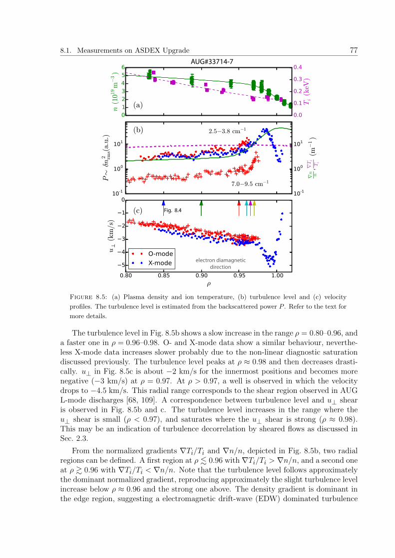
8.1. Measurements on ASDEX Upgrade 77
Fig. 8.4
AUG#33714-7
electron diamagnetic
direction
Figure 8.5: (a) Plasma density and ion temperature, (b) turbulence level and (c) velocity
profiles. The turbulence level is estimated from the backscattered power P . Refer to the text for
more details.
The turbulence level in Fig. 8.5b shows a slow increase in the range ρ = 0.80–0.96, anda faster one in ρ = 0.96–0.98. O- and X-mode data show a similar behaviour, neverthe-less X-mode data increases slower probably due to the non-linear diagnostic saturationdiscussed previously. The turbulence level peaks at ρ ≈ 0.98 and then decreases drasti-cally. u⊥ in Fig. 8.5c is about −2 km/s for the innermost positions and becomes morenegative (−3 km/s) at ρ = 0.97. At ρ > 0.97, a well is observed in which the velocitydrops to −4.5 km/s. This radial range corresponds to the shear region observed in AUGL-mode discharges [68, 109]. A correspondence between turbulence level and u⊥ shearis observed in Fig. 8.5b and c. The turbulence level increases in the range where theu⊥ shear is small (ρ < 0.97), and saturates where the u⊥ shear is strong (ρ ≈ 0.98).This may be an indication of turbulence decorrelation by sheared flows as discussed inSec. 2.3.
From the normalized gradients ∇Ti/Ti and ∇n/n, depicted in Fig. 8.5b, two radialregions can be defined. A first region at ρ . 0.96 with ∇Ti/Ti > ∇n/n, and a second oneat ρ & 0.96 with ∇Ti/Ti < ∇n/n. Note that the turbulence level follows approximatelythe dominant normalized gradient, reproducing approximately the slight turbulence levelincrease below ρ ≈ 0.96 and the strong one above. The density gradient is dominant inthe edge region, suggesting a electromagnetic drift-wave (EDW) dominated turbulence

78 8. Turbulence characterization in ASDEX Upgrade and TJ-II plasmas
0 50 100 150 200
t (ms)
50
51
52
53
54
55
56
57
58
f 0(G
Hz)
(a)
AUG#33717
reference
hopping
0.85 0.90 0.95 1.00ρ
0
2
4
6
8
10
k⟂(cm−1
)
(b)
AUG#33714-7
reference
hopping
Figure 8.6: (a) Example frequency pattern used for the correlation measurements. The refer-
ence and hopping channel probing frequencies are depicted. (b) k⊥ as a function of the measured
radial position ρ for the O-mode. Reference and hopping channels are indicated. Data in red
and black are used for k⊥ scans, while data in blue for a radial scan.
regime [43, 44, 45]. In the core region, where the temperature gradient is dominant ITGand TEM dominated turbulence is expected [44].
The radial evolution of the k⊥ spectra in Fig. 8.4a supports the previous observations.The radial positions at which the k⊥ spectra shown in Fig. 8.4a have been measuredare indicated with vertical arrows in Fig. 8.5c. The spectra measured in the first region,blue and green data in Fig. 8.4a, are similar despite of the large radial difference betweenthe measurement positions. The steepening of the k⊥ spectra is observed precisely atthe transition between both regions. The substantial differences in the spectral indicesand knee position between ρ = 0.85 and 0.97 may indicate different driving and non-linear saturation mechanisms of the turbulence. A detailed gyrokinetic stability analysiswould be necessary in order to determine precisely the dominant micro-instabilities inthe different radial regions. These detail comparisons are left for future investigations.
8.1.3 Correlation measurements
Detailed correlation measurements have been performed for the same set of dischargesdiscussed in Sec. 8.1.1. The measurements are performed with the two V-band systemswith O-mode polarization. One V-band channel (reference channel) probed 6 frequen-cies, with 100 ms each. During this time, the other V-band channel (hopping channel)probed 20 nearby frequencies. A sample of the frequency patterns showing two referencechannel frequencies is presented in Fig. 8.6a. The frequency patterns have been opti-mized according to the density profile. The hopping channel frequency steps are largein the edge region (low probing frequencies) because of the steep gradient of the densityprofile, whereas they are smaller towards the plasma core (high probing frequencies)because of the shallow gradients there.

8.1. Measurements on ASDEX Upgrade 79
−4 −2 0 2 4 6
τ (µs)
0.0
0.2
0.4
0.6
0.8
1.0
|C(τ)|
Cmax
τmax
2τanoise level
AUG#33715, t=3.8-3.9s
∆f=−0.1 GHz
−0.25 GHz
−0.40 GHz
−0.55 GHz
Figure 8.7: Cross-correlation function of the O-mode reflectometer signals for different probing
frequency separations ∆f . The reference channel probing frequency is 58.9 GHz, corresponding
to ρ = 0.955 and k⊥ = 6.5 cm−1. The definition of Cmax, τmax and τa is illustrated for the green
data.
The analysis of the cross-correlation assumes only backscattering contributions, hencethe direct reflection contribution observed in Fig. 8.3a has to be suppressed. This isdone by filtering out the direct reflection contribution of the spectra before computingthe cross-correlation function. Although a broad scan of the reference channel probingfrequency and angle of incidence has been done, here only cases are discussed where theDoppler peak is dominant and the correlation quality is good. Further details on thefiltering process are given in Appendix C.
The probed parameter space k⊥(ρ) computed with TORBEAM is depicted in Fig. 8.6b.Each reference channel data point depicted by a square is accompanied by several hop-ping channel data points indicated by circles. A k⊥ scan is performed for ρ ≈ 0.96 and0.98 as depicted by the black and red symbols, respectively. Also a radial variation ofthe reference position at approximately fixed k⊥ ≈ 3 cm−1 is performed (blue symbols).
Cross-correlation function
The cross-correlation function C(τ) of the reference and hopping channels is computedwith Eq. 4.11. Since the reflectometer signal V is complex (cf. Sec. 4.2), C(τ) is also acomplex quantity. In the following analysis only |C(τ)| is considered, the complex phasegives no further information for the correlation analysis. Representative cases of thecross-correlation are shown in Fig. 8.7. The reference channel is probing at ρ = 0.955and k⊥ = 6.5 cm−1. The colours depict different values of the probing frequency differ-ence ∆f = f0,hopping−f0,reference. The maximum of |C(τ)| decreases and shifts towardsnegative τ for increasing ∆f . For the following analysis, the maximum of the correlationCmax, time delay at the maximum τmax and width τa (obtained at Cmax/e) are definedas indicated for the green data in Fig. 8.7. The behaviour of the cross-correlation func-tion is similar to the one observed for the synthetic turbulence shown in Fig. 7.1 anddiscussed in Sec. 7.1. The reader is referred to that section where a detailed analysis of

80 8. Turbulence characterization in ASDEX Upgrade and TJ-II plasmas
Figure 8.8: Measurement positions on the cross-section of the ASDEX Upgrade tokamak.
The region of interest is zoomed in. The distance between hopping and reference measurement
positions is decomposed in a radial ∆r and perpendicular ∆yray separation. ∆r is taken along
the gradient of the magnetic flux ∇ρ. The geometrical definition of Θray is also depicted.
the cross-correlation function is presented.
Radial and perpendicular separation
The measurement positions of the reference and hopping channels define a radial ∆rand perpendicular ∆yray separation, both required for the correlation analysis presentedin Sec. 7.1. The geometrical definition of the separations for the slab case has beendiscussed in Sec. 7.1.3 and depicted in Fig. 7.4. Here the definition of the radial andperpendicular separation in a general geometry is shown in Fig. 8.8 for the AUG case.The measurement positions of the reference and hopping channels are shown in thezoomed region of interest. The grey solid lines depict the flux surfaces.
The local gradient ∇ρ at the reference measurement position defines the radial direc-tion. This is indicated with a dashed grey line in the plot, which is locally perpendicularto the flux surface. The distance between the reference and hopping measurement po-sitions is decomposed into a vector parallel and perpendicular to ∇ρ, their magnitudedefines ∆r and ∆yray, respectively. The vector decomposition is shown in the figurefor one measurement position of the hopping channel. ∆r pointing outwards is definedpositive and ∆yray pointing in the clockwise direction is defined negative. The samedefinition and conventions will be used in Sec. 8.2 for the TJ-II correlation analysis.
All measurement positions in Fig. 8.8 lie on a straight line which defines an angleΘray with respect to the radial direction, as indicated in the figure. The angle is obtainedfrom:
tan Θray =∆yray
∆r.
A clockwise Θray is defined negative as the case depicted.

8.1. Measurements on ASDEX Upgrade 81
−0.8 −0.6 −0.4 −0.2 0.0 0.2 0.4 0.6 0.8 1.0
∆r(cm)
0.0
0.2
0.4
0.6
0.8
1.0
Cmax
ρ ≈ 0.96
AUG#33714-7
k⟂=2.2 cm−1
k⟂=4.3 cm−1
k⟂=6.5 cm−1
k⟂=10.1 cm−1
Figure 8.9: Maximum of the correlation function Cmax as a function of the radial separation.
Sample error bars are shown. The different colours depict different k⊥ and the dashed line the
Gaussian fit to the data.
Since the calculation of ∆r and ∆yray depends on the measurement positions obtainedfrom ray tracing, a reliable density profile is required for an accurate determination of thementioned quantities. Attention should be paid to the density gradient at the scatteringposition, to which ∆r and ∆yray are especially sensitive.
Radial correlation length
In this section the behaviour of Cmax as a function of ∆r is studied experimentally. Theeffect of k⊥ in the experimental measurements is investigated in detail and the resultsare compared with the modelling presented in Ch. 7. The radial correlation length Lrof the turbulence is estimated from the experimental measurements. The impact of thediagnostic effects and the accuracy of the measurement are discussed.
In Fig. 8.9 the maximum of the cross-correlation function Cmax is shown as a functionof the radial separation ∆r. The results for ρ ≈ 0.96 and different k⊥ values are depictedby different colours. The dataset corresponds to the one presented in Fig. 8.6 in black.The points depict the experimental data and the dashed lines a Gaussian fit that willbe discussed later. A symmetric decay of the correlation with the radial separation isobserved. The correlation drops faster for large k⊥. Moreover, a slowly decaying tailis observed for small k⊥, this effect is particularly strong for k⊥ = 2.2 cm−1 at largepositive ∆r.
The data are in qualitative agreement with the correlation results of the Kolmogorov-like k⊥ spectrum shown in Fig. 7.11a. There, a faster decay of the correlation for largek⊥ and a slow decaying tail for small k⊥ result from the filtering effect of the diagnostic.A similar effect on the TJ-II measurements has been reported in Ref. [16]. Since thek⊥ spectrum is Kolmogorov-like (cf. Fig. 8.4), both the faster decay for large k⊥ and

82 8. Turbulence characterization in ASDEX Upgrade and TJ-II plasmas
2 4 6 8 10 12
k⟂ (cm−1 )
0.0
0.1
0.2
0.3
0.4
0.5
Lr(cm)
(a)
AUG#33714-7
ρ≈0.96ρ≈0.98
0.86 0.88 0.90 0.92 0.94 0.96 0.98 1.00
ρ
(b)
AUG#33717
k⟂=2.5−3.3 cm−1
Figure 8.10: Measured radial correlation length (a) as a function of k⊥ at two radial positions,
and (b) as function of ρ for measurements with k⊥ in the range 2.5–3.3 cm−1.
the deviations from Gaussian in Fig. 8.9 are likely to be caused to some extent by thefilter effect of the diagnostic. The non-local scattering may have an impact on the data,specially in the slowly decaying tail. The relevance of this effect will be discussed laterin this section.
The Gaussian fit depicted in Fig. 8.9 by dotted lines is computed by weighing eachdata point with 1/C2
max. The fits show a k⊥ dependence of the correlation despite ofthe slowly decaying tail. This fitting method has also been applied in the analysis ofsimulated data in Ch. 7. In this way, the fit focuses the analysis on the data withsmall ∆r which reduces the impact of the slowly decaying tail in the analysis. This isjustified for the Kolmogorov like k⊥ spectrum case studied in Sec. 7.5. There the radialcorrelation length is defined by the Cmax drop for small ∆r, which is followed by theslowly decaying tail. The fit can also reduce the contributions of non-local scattering tothe correlation that manifest as a slowly decaying tail (cf. Fig. 7.5a).
The radial correlation length Lr is extracted from the Gaussian fit to the data Cmax =exp−(∆r/Lr). The results are plotted as a function of k⊥ in Fig. 8.10a at ρ ≈ 0.96and 0.98 in black and red, respectively. The cases shown in Fig. 8.9 are included in theblack series. Lr decreases with k⊥ for both radial positions. The values at ρ ≈ 0.98 aresmaller than at ρ ≈ 0.96. Hence, despite of the k⊥ related diagnostic effect a reductionof the radial correlation length for the outermost measurement position is confirmed.
The non-local scattering may produce an overestimation of Lr due to the scatteringalong the beam path. Nevertheless this effect is reduced for large k⊥, thus a convergenceto the real correlation length is expected at large k⊥ for a Gaussian k⊥ spectrum [21].Figure 8.10a shows no convergence of Lr as expected from non-local scattering. If Lrconverges for k⊥ larger than the measured range, the convergence value would be smallerthan 0.05 cm. This is a non-realistic value for the radial correlation length, which isexpected to be of the order of (sub-)centimetres [15, 110]. Although non-local scatteringcontributions cannot be discarded, they are not likely to produce the Lr reduction withk⊥ and have a small impact on the measurements.

8.1. Measurements on ASDEX Upgrade 83
The decrease of Lr with k⊥ is likely due to the diagnostic filtering effect discussedin Sec. 7.5.3 and shown in Fig. 7.11a. In this case the best estimation of the radialcorrelation length is the given by the measurements at small k⊥. For the measurementsshown in Fig. 8.10a the correlation length can be estimated to be Ltrue
r ≈ 0.4 cm andLtruer ≈ 0.2 cm for the black and red series, respectively.
The radial evolution of Lr is investigated by considering the measurements at smalland approximately constant k⊥. The probed parameters correspond to the blue data inFig. 8.6. The results are depicted in Fig. 8.10b as a function of ρ. The radial correlationlength increases from 0.2 to 0.45 cm at ρ ≈ 0.95, then decreases reaching 0.2 cm atρ ≈ 0.98. Note that the two different behaviours corresponds approximately to the tworegions presumably with different turbulence driving mechanisms discussed in Sec. 8.1.2.The small Lr of the outermost measurement, already in the shear region, may be re-lated to the turbulence regulation by sheared flows (cf. Sec. 2.3). Alternatively, thereduction of Lr may also be justified with the mixing length argument which predictsLr ∝ δnrms(∇n/n)−1 [22], thus the steepening of the density profile towards the plasmaedge can account to some extent for the observation. The reduction of Lr at ρ > 0.95 co-incides with the shift of the spectral knee towards larger k⊥ observed in Fig. 8.4a. Sincea wider spectrum corresponds to a longer correlation length, the reduction of the radialsize of the turbulent structures is accompanied by a reduction of their perpendicular size.
Tilt angle measurement
The time delay of the cross-correlation function is investigated experimentally. Theresults are analysed based on the modelling presented in Secs. 7.1.3 and 7.4, where thetime delays have been related to the tilt angle β and the perpendicular velocity of theturbulent structures. The tilt angle is measured for the first time in the AUG confinedregion. The impact of the diagnostic effects is discussed.

84 8. Turbulence characterization in ASDEX Upgrade and TJ-II plasmas
Figure 8.11: (a) Detail of the measurement positions on the AUG cross-section. Turbulent
structures are schematically depicted, the tilt angle and propagation velocity are indicated.
(b) Perpendicular displacement ∆ymax = τmaxu⊥ computed from the time delay of the cross-
correlation function vs. the radial separation. Selected cases measured at ρ ≈ 0.96 are shown.
The dashed lines depict linear fits to the data. (c) Slope m as a function of Θray; the fit to the
data with Eq. 7.12 is depicted by a magenta line. The tilt angle β is indicated.
In the following, the measurements at ρ ≈ 0.96 corresponding to the black data inFig. 8.6 are analysed. The measurement positions of the reference and hopping channelare shown on the AUG cross-section in Fig. 8.11a. The region of interest is shown indetail. The nine sets of points stand for different angles of incidence. Due to the differentangle of incidence of the probing beam, the point sets have a different alignment withrespect to the radial direction. The lowermost points are better aligned with the radialdirection compared to the uppermost. Thus, the angle Θray defined by the measurementpositions with respect to the radial direction is scanned between −27 and −60◦, fromthe lower to the upper measurements. Turbulent structures are schematically depicted.
The time delay τmax at the maximum of the cross-correlation function has been com-puted and multiplied by u⊥ = 3.0 km/s in order to obtain the perpendicular displacement∆ymax = τmaxu⊥. Sample results of ∆ymax as function of ∆r are shown in Fig. 8.11b,the three cases correspond to the measurement positions depicted in Fig. 8.11a by the

8.1. Measurements on ASDEX Upgrade 85
same colours. Data points obtained with high correlation and hence a well defined timedelay are considered. Positive τmax values mean that the signal features are detectedfirst by the reference channel. A linear dependence is observed for the three cases. Linearfunctions are fitted to the data and are depicted by dashed lines in Fig. 8.11b. The fitshave a different slope m for the three cases shown.
The tilt and the propagation direction of the structures depicted in Fig. 8.11a areconsistent with the time delays presented in Fig. 8.11b. The structure is approximatelyaligned with the red measurement positions, therefore it is seen almost simultaneouslyby the reference and hopping channel (small time delays). Whereas the structure ismiss-aligned with respect to the blue measurement positions, hence it is ”seen” first bythe hopping channel (negative time delay) for positive ∆r while it propagates upwards.The tilt angle indicated in the figure is calculated next.
The slope m obtained from the fits (Fig. 8.11b) is plotted as a function of Θray
in Fig. 8.11c. The blue, green and red data points correspond to the cases shown inFigs. 8.11a and b. Despite the dispersion the data show a clear trend; |m| increases with|Θray|. It has been shown in Sec. 7.1.3 that m can be described with Eq. 7.12 underthe frozen turbulence approximation. The prediction of Eq. 7.12 for zero tilt (β = 0)is depicted in Fig. 8.11c by a dashed black line. The experimental data show a similarbehaviour and are vertically shifted due to the tilt angle of the turbulence. Neverthelessthe increase of |m| with |Θray| is slightly slower compared to the frozen turbulenceprediction, thus the data cannot be satisfactorily described by Eq. 7.12. One has toinclude the effect of the decorrelation time of the turbulence discussed in Sec. 7.4. Thiseffect reduces the measured time delays with respect to the frozen turbulence expectation,and can be accounted with a correction factor Fd included in Eq. 7.24. The data inFig. 8.11c has been fitted with Eq. 7.24 with the tilt angle β and the correction factor Fdas free parameters. The fit is depicted by the magenta solid line in the figure. The goodquality of the fit shows that the time delays are explained by the tilt of the turbulentstructures as discussed in Secs. 7.1.3 and 7.4. The tilt angle and correction factor are
β = (−27± 12)◦, Fd = 0.5± 0.2. (8.1)
The tilt angle is indicated in the plot as the value of Θray at the intersection with them = 0 axis, at which the structure is aligned with the measurement points. The resultingtilt of the structures is schematically depicted in Fig. 8.11a.
The relevance of the decorrelation time of the turbulence τd is assessed by comparingit with the passing time of the structures in front of the probing beam. Taking a beamwidth of 2.0 cm, the passing time is w/u⊥ ≈ 7 µs. In AUG, the decorrelation timeτd has been investigated using a poloidal correlation reflectometry diagnostic recentlyinstalled [106, 107]. For ECRH discharges as the one under study, τd is of the orderof 10 µs [107]. Since the passing time is only slightly shorter than τd, a correctionfactor Fd ≈ 0.6 according to Eq. 7.23 is still needed. This value is comparable with theexperimental one (Eq. 8.1), which supports the modelling of the τd effect presented inSec. 7.4. It should be remark that poloidal correlation reflectometry diagnostic measuresat smaller wavenumbers (k⊥ < 2 cm−1) compared with Doppler reflectometry. Thereforethe decorrelation time which may vary with k⊥ gives only a rough estimation of Fd.

86 8. Turbulence characterization in ASDEX Upgrade and TJ-II plasmas
The impact of other diagnostic effects on the tilt angle measurement has been dis-cussed in Ch. 7. In particular, the non-linear diagnostic response and the filter effecthave been considered. Here, non-linear effects are excluded based on the analysis of thek⊥ spectra presented in Sec. 8.1.2, where the linearity of the O-mode measurements hasbeen justified. The k filtering of the Doppler reflectometer may lead to an underestima-tion of m and therefore of the tilt angle, especially for large k⊥. The fact that all themeasured data are above the β = 0 line indicates that the same direction of the tilt isrecovered for all cases. However, the data for large |Θray| corresponding to large k⊥ arecloser the the β = 0 line. This may indicate an underestimation of m for large k⊥ similarto the one observed in Fig. 7.11c. A decrease of the tilt along the perpendicular direc-tion could also explain this underestimation, nevertheless since the measurements spanonly a small poloidal section of AUG, the turbulence characteristics are not expectedto change significantly and the assumption of a constant tilt is well justified. Finally,a precise numerical assessment of the filter effect would require an accurate knowledgeof the weighting function for the specific experimental conditions. This is left for futurestudies.
Concluding, the analysis techniques developed in Secs. 7.1.3 and 7.4 can be appliedto the experimental data, and the mean tilt angle of the turbulent structures can beexperimentally measured. A further insight on the physical meaning of the measuredtilt angle (Eq. 8.1) would require a detailed modelling of the plasma under study. InCh. 9 the tilt angle measurement will be used to investigate changes of the turbulenceregime in plasmas with either dominant electron or dominant ion heating.
8.2 TJ-II measurements
A detailed experimental study of the density turbulence in L-mode TJ-II plasmas usingDoppler reflectometry is presented in this section. In Sec. 8.2.1 the discharges underinvestigation are introduced and in Sec. 8.2.2 k⊥ spectra and u⊥ profiles are measuredand analysed. In Sec. 8.2.3 correlation measurements are presented. First, a radial scanof the correlation length is done and second, the tilt angle measurement is carried onfor the first time in TJ-II. In Sec. 8.2.4, the tilt results are compared with linear globalgyrokinetic simulations. In Sec. 8.2.5 a two-point correlation technique is presented.
8.2.1 Discharges
Dedicated experiments for the characterization of turbulence with Doppler reflectome-try have been performed in TJ-II. ECR heated L-mode plasmas with low density havebeen investigated. The standard magnetic configuration has been used. Two series ofcomparable discharges are analysed; the series 1 includes the discharges #42754-65, andthe series 2 #43459-91. The series 1 has been used for k⊥ spectra and u⊥ measure-ments. The results will be shown in the following section. The series 2 has been usedfor correlation measurements and will be discussed in Sec. 8.2.3.

8.2. TJ-II measurements 87
0.0
0.2
0.4
0.6
0.8n(101
9m−3) (a)
measurements
1050 1100 1150 1200 1250 1300
t(ms)
0.0
0.2
0.4
0.6
0.8
1.0
PECRH(M
W) (b)
0.5 0.6 0.7 0.8 0.9 1.0
ρ
0.0
0.1
0.2
0.3
0.4
0.5
0.6
0.7
0.8
n(101
9m−3)
(c)
#42764, series 1
#43490, series 2
Figure 8.12: (a) Line average plasma density and (b) ECRH power time traces of representative
discharges of series 1 and 2. (c) Density profiles during the measurement phases obtained from
a multi-diagnostics statistical analysis [111].
The line average density and ECRH power time traces for representative dischargesof the series are shown in Figs. 8.12a and b. Similar plasma conditions were targeted forboth sets of experiments. Nevertheless the two series were performed on different days,thus the wall condition was not the same and a slightly higher density was obtained forthe second series. The line average density is below the critical density of 0.6×10¹⁹ m−3
for both cases, which ensures the electron root confinement regime [112]. The plasmadensity is stable between 1100–1200 ms for the series 1 and between 1100–1250 ms forthe series 2. The reflectometry measurements are performed during these time windowsas indicated at the top of Fig. 8.12a.
The density profile during the measurement phases has been computed by statisticalanalysis of Thomson scattering, interferometry and AM reflectometer data [111]. Theprofiles for both series are shown in Fig. 8.12c. The profile for the series 1 is slightlylower compared to the one of the series 2. These profiles will be used as input for raytracing calculations with the TRUBA code.

88 8. Turbulence characterization in ASDEX Upgrade and TJ-II plasmas
Figure 8.13: (a) Probed k⊥ as a function of the measured radial position ρ. The shadowed
areas correspond to the radial ranges where the k⊥ spectra are computed. (b) Measurement
positions on the perpendicular cross-section of TJ-II. The gray lines depict the flux surfaces.
8.2.2 Measurements of k⊥ spectra and u⊥ profile
Detailed measurements have been performed with the two Q-band (33–50 GHz) X-modeDoppler reflectometer channels. For more details on the reflectometer configuration referto Sec. 4.3.2. Fine probing frequency and angle of incidence scans have been performedfor discharges of the series 1. Seven angles of incidence have been used, with 16 probingfrequencies (5 ms each) in the range 33.0–40.5 GHz per angle. The angle of incidence hasbeen scanned on a shot to shot basis. The probed k⊥ and radial position ρ obtained withthe TRUBA code are plotted in Fig. 8.13a. Data points connected with lines correspondto the same angle of incidence. The radial range measured is ρ = 0.50–0.85 and k⊥ isbetween 1 and 12 cm−1. The measurement positions on the perpendicular cross-sectionof TJ-II are shown in Fig. 8.13b. A poloidally extended region in the upper left side ismeasured.
The power spectrum of the reflectometer signal is computed for each probing fre-quency and angle of incidence. A sample power spectrum is shown in Fig. 8.14a. ADoppler peak at −0.44 MHz is obtained. No contribution from direct reflection is ob-served. That is the case for all the measurements on TJ-II discussed in this thesis.Direct reflections may be important under other plasma conditions with smaller turbu-lence level, as it is the case for NBI heated plasmas or close to the shear layer whereturbulence is suppressed [32]. The blue line depicts the Gaussian fit to the Doppler peak.The backscattered power P and Doppler shift fD are obtained from fit.
The k⊥ spectra are calculated taking P as a function of k⊥ for the different radialwindows depicted by coloured areas in Fig. 8.13a. The results for three radial positionsare plotted in Fig. 8.14 with different colours. A vertical shift between the different caseshas been included for visualization purposes. A spectral fall-off with k⊥ is observed forthe three cases. It is faster for large k⊥. For a numerical comparison, the spectra havebeen fitted with power laws in the small and large k⊥ ranges. The fits are depicted bysolid lines and the spectral indices are indicated in the figure. Similar spectral indices

8.2. TJ-II measurements 89
−3 −2 −1 0 1 2 3
f (MHz)
10-2
10-1
100
101
102
103Pow
erspectrum
(a.u.)
f0 =33.0 GHz ρ=0.854 k⟂=8.62 cm−1
P
fD(a)
#42755, t=1101-1105 ms
1 2 3 4 5 6 7 8 10 15 20
k⟂ (cm−1 )
10-3
10-2
10-1
100
101
102
P(a.u.)
-1.0
-8.5±1.6
-0.9±0.4
-8.4±0.2
-1.0±0.2
-7.3±0.7
X−mode (b)
#42754-65
ρ=0.610±0.020ρ=0.705±0.015ρ=0.790±0.010
Figure 8.14: (a) Sample power spectrum measured in TJ-II. The fit to the Doppler peak is
depicted by a blue solid line. No zero-order reflection is observed. (b) k⊥ spectra at different
radial positions measured in X-mode polarization. Similar spectra are obtained at different radial
positions.
are obtained in the three measured radial positions. For low and high k⊥ the spectralindex is about −1.0 and −8.0, respectively. The two ranges are separated by a knee atapproximately k⊥ ≈ 7 cm−1. The spectral indices in the low k⊥ range are similar tothose measured in AUG, while the ones in the high k⊥ range are more pronounced, andthe spectral knee is located at larger k⊥ (cf. Fig. 8.4a.)
The similarity between the outer and inner most spectra (blue and red cases inFig. 8.14) suggest that the diagnostic response is linear in the measured range. Giventhat the turbulence level is expected to increase towards the plasma edge, non-lineareffects would produce a flatennig of the k⊥ spectra (cf. Ch. 6) in the outermost mea-surement positions. This non-linear effect has been reported in Ref. [16], where smallerspectral indices were measured in the large k⊥ range for outer measurement positions.On the contrary, the measurements presented here show no spectral flattening and spec-tral indices comparable to those obtained in the linear regime in Ref. [16]. Thereforestrong non-linear scattering regimes in the measured range can be discarded.
The similarity of the spectra also suggests that the driving and saturation mechanismsof the turbulence are the same in the measured radial range. The obtained spectralindices are comparable to those reported in Ref. [16] for similar ECRH plasmas, thoughthe reported knee position at k⊥ ≈ 5 cm−1 is slightly smaller. The spectral indices inNBI heated plasmas reported in Ref. [31, 32] are more pronounced and the spectral kneeappears at larger k⊥ ≈ 8.4 cm−1.
The relative changes of the turbulence level profile have been estimated from Paccording to Eq. 4.8. The radial profile for k⊥ ≈ 6 cm−1 has been plotted in Fig. 8.15bas a proxy of the turbulence level δnrms. This approximation is justified by the lineardiagnostic response discussed previously and by the approximately constant k⊥ thatavoids changes of P related to the spectral fall-off. The turbulence level increases towardsthe edge by approximately one order of magnitude. The growth follows roughly thenormalized gradient of the plasma density∇n/n, which is indicated in the Fig. 8.15b with

90 8. Turbulence characterization in ASDEX Upgrade and TJ-II plasmas
electron diamagnetic
direction
Figure 8.15: (a) Density, (b) turbulence level and (c) u⊥ profiles for the series 1. The turbulence
level is estimated from P measured at k⊥ ≈ 6.0 cm−1.
a dashed green line. The density profile has been included in Fig. 8.15a for comparison.The perpendicular velocity u⊥ has been computed from fD according to Eq. 4.10. Theresults for the complete parameter scan are shown in Fig. 8.15c. u⊥ has an approximatelyconstant value of 1 km/s between ρ = 0.5 and 0.7, then increases towards the edgereaching values of about 3.5 km/s at ρ ≈ 0.82.
Although a region of velocity shear is observed between ρ = 0.75 and 0.85, there isno reduction of the turbulence level. Moreover, no significant differences in the spectralshape have been observed in the k⊥ spectra measured at the positions indicated witharrows in Fig. 8.15c. The turbulence regulation by sheared flows mechanism (cf. Sec. 2.3)is not observed in the fluctuation level, or at least does not play a significant role.However, it should be noted that the velocity shear in electron root confined plasmasis small compared to other types of plasma in TJ-II. A turbulence reduction correlatedto the velocity shear has been observed for densities close to the threshold density [113]and in H-mode plasmas [32]. Similar effects have also been observed in other stellaratorsat the transition between electron and ion root regimes [114].
8.2.3 Correlation measurements
Detailed correlation measurements have been performed in TJ-II for discharges of theseries 2 discussed in Sec. 8.2.1. The two Q-band X-mode Doppler reflectometer channelshave been used; for more details refer to Sec. 4.3.2. The probing frequency of one channel(reference) has been scanned slowly, 60 ms per frequency. During this time the other

8.2. TJ-II measurements 91
0.60 0.65 0.70 0.75 0.80 0.85 0.90ρ
0
2
4
6
8
10k⟂(cm−1
)
(a)
#43459-75
reference
hopping
0.65 0.70 0.75 0.80 0.85
R⟂ (m)
0.20
0.25
0.30
0.35
0.40
z(m
)
(b)
#43459-75
Figure 8.16: (a) Probed k⊥ as a function of the radial position ρ used for correlation studies.
(b) Measurement positions on the perpendicular cross-section of TJ-II. Multi-colour data points
are used for correlation measurements at several radial positions. Black data points will be used
for the tilt angle measurement.
channel (hopping) probed 12 nearby frequencies, 6 above and 6 below with 5 ms perfrequency. The mirror position has been changed on a shot to shot basis. The probingfrequencies and the mirror angle have been specifically designed for a radial position anda k⊥ scan.
The probed ρ and k⊥ range of the reference and hopping channels are shown inFig. 8.16a. The measurement positions on the perpendicular cross-section of TJ-II arepresented in Fig. 8.16b. The multi-colour data points correspond to a radial scan of thereference channel measurement position with a fixed mirror angle. The position variesbetween ρ = 0.67 and 0.81 and k⊥ in the range 5 to 6 cm−1, with a slight increasetowards the core. The black data points correspond to a scan of the mirror angle. Theprobing frequencies have been adjusted in order to compensate the radial displacementof the measurement position when scanning k⊥, such that the reference channel probesat ρ = 0.72 for all cases.
For the following correlation analysis the radial ∆r and perpendicular ∆yray separa-tions are obtained from the ray tracing data as it has been illustrated in Fig. 8.8 for theASDEX Upgrade case. The cross-correlation function of reference and hopping channelsignals has been computed. The maximum of the correlation Cmax, time delay at themaximum τmax and width τa are obtained. This procedure has been explained in detailfor ASDEX Upgrade analysis in Sec. 8.1.3 and has been illustrated in Fig. 8.7. Giventhat no direct reflection has been observed in the TJ-II power spectra (cf. Fig. 8.14a), nofiltering in frequency is required before the cross-correlation function calculation. Thisis contrary to the O-mode measurements in the ASDEX Upgrade shown in Fig. 8.3a anddiscussed in the Appendix C.

92 8. Turbulence characterization in ASDEX Upgrade and TJ-II plasmas
−1.0 −0.5 0.0 0.5 1.0 1.5
∆r(cm)
0.3
0.4
0.5
0.6
0.7
0.8
0.9
1.0
Cmax
#43459-62
ρ=0.68
ρ=0.72
ρ=0.75
ρ=0.78
ρ=0.81
Figure 8.17: Maximum of the cross-correlation as a function of ∆r. Data for different radial
positions of the reference channel are shown. k⊥ is approximately 5.5 cm−1 for all cases. Gaussian
fits to the data are depicted by dotted lines.
Radial correlation length
The maximum of the cross-correlation Cmax has been plotted as a function of the radialseparation ∆r in Fig. 8.17. The colours depict different radial positions of the referencechannel. The probed parameter space is included in the multicolour data points ofFig. 8.16. A decay of the correlation with the radial separation is observed. The decayis faster for outer measurement positions. The dotted lines in the figure correspondsto Gaussian fits as explained for the AUG case, cf. Sec. 8.1.3. The comparison of thedata with the fits reveals an asymmetry of the positive and negative ∆r branches of thecorrelation. This effect is strongest for the ρ = 0.72 case in black, where the correlationdecays faster for positive ∆r. This asymmetries will by further discussed next.
It has been shown in Sec. 7.4 that the filter effect of the diagnostic together with aKolmogorov type turbulence induces a k⊥ dependence of the measured Lr. This effecthas been confirmed in Sec. 8.1.3 for AUG data and in Ref. [16] for TJ-II. Thus Lrobtained from the fit in Fig. 8.17 are underestimated by the k⊥ effect. Nevertheless,the measurements at different radial positions can be compared in order to investigaterelative changes because the probed k⊥ and the spectrum are approximately constant.Lr obtained from the (symmetric) fits are plotted in red in Fig. 8.18a as a function of ρ.A strong decrease of the radial correlation length towards the plasma edge is observed.
A strong decrease of the measured correlation length has been observed at the tran-sition from the linear to the non-linear regime in two-dimensional full-wave simulations(cf. Figs. 7.6a and d, and Ref. [19]). Nevertheless for the experimental conditions here, alinear diagnostic response has been evidenced in the k⊥ spectra studies in Sec. 8.2.2. Fur-thermore there is only a modest increase in the turbulence level in the range ρ = 0.68–0.78(see Fig. 8.15b) which cannot account for such a strong decrease of Lr. It is concludedthat the decrease observed in Fig. 8.18a is not due to a non-linear diagnostic responseand corresponds to a real reduction of the Lr towards the plasma edge.
The reduction of Lr is in line with the reduction of the density gradient scale lengthLn = (∇n/n)−1, which has been re-scaled and depicted by a green dashed line in

8.2. TJ-II measurements 93
0.65 0.70 0.75 0.80 0.85
ρ
0.0
0.2
0.4
0.6
0.8
1.0
1.2Lr(cm)
0.12 Ln
(a)
#43459-62
Symmetric fit
∆r>0, fit
∆r<0 fit
2 3 4 5 6 7 8
Ln (cm)
(b)
#43459-62
Figure 8.18: (a) Radial correlation length Lr measured at k⊥ ≈ 5.5 cm−1 as a function of the
radial position ρ. Results from the symmetric fit are depicted by red, and fits of positive and
negative ∆r by yellow and magenta, respectively. (b) Lr as a function of the density gradient
scale length Ln.
Fig. 8.18a. The scaling of Lr with Ln is observed in Fig. 8.18b. A similar scaling hasbeen observed for ECRH plasmas in Ref. [16], where Ln was varied by changing theplasma density and magnetic configuration. Here a similar behaviour has been obtainedwhen the radial variation of Ln is considered. Alternatively, the increase of the u⊥ sheartowards the plasma edge may indicate that turbulence regulation by sheared flows isresponsible of the Lr reduction (cf. Sec. 2.3). Nevertheless neither a turbulence levelreduction nor an effect on the k⊥ spectra has been observed in Sec. 8.2.2.
The asymmetries observed in Fig. 8.17 are further investigated by fitting the positiveand negative ∆r wings separately. Lr obtained for positive and negative ∆r are depictedin Fig. 8.18a by orange and magenta lines, respectively. The inner and outermost mea-surement positions show similar values for both fits, indicating symmetric Cmax(∆r).Whereas an asymmetry is observed for intermediate radial positions in the Lr gradientregion. The longer correlation length is measured towards the core (∆r < 0) precisely inthe direction in which Lr increases. From these two observations the asymmetry of thecorrelation function can be explained by the Lr gradient. If Lr has a strong gradient (asat ρ = 0.75), the hopping channel measures in regions with different Lr when probing atpositive and negative ∆r. Thus ∆r < 0 measures at a smaller ρ having larger Lr, while∆r > 0 measures at larger ρ providing a smaller Lr.
It is proposed that a strong Lr radial gradient induces asymmetries in the correlation.It should be noted that, magnetic islands close to the measurement positions can alsoproduce asymmetries [115]. Nevertheless, in the presented experiments, no strong impactof magnetic islands is expected because of the absence of low order rational surfaces inthe measured region, and no signatures of the magnetic islands in the Doppler peaks hasbeen observed as the ones reported in Ref. [116].

94 8. Turbulence characterization in ASDEX Upgrade and TJ-II plasmas
Figure 8.19: (a) Measurement positions at ρ = 0.72 on the perpendicular cross-section of
TJ-II. Turbulent structures are schematically depicted, the tilt angle and propagation velocity
are indicated. (b) Perpendicular displacement ∆ymax = τmaxu⊥. Results for three angles of
incidence are presented (see colours in a). Linear fits are indicated with a dotted lines. (c) Slope
m as a function of Θray. The fit of the data with Eq. 7.24 is depicted by the purple line, the tilt
angle β is indicated.
Tilt angle measurements
The time delay of the cross-correlation function and the tilt angle of the turbulent struc-tures are studied in detail for the measurements at ρ = 0.72 (black points in Fig. 8.16).The measurement positions of the reference and hopping channel are shown in detail onthe perpendicular cross-section of TJ-II in Fig. 8.19.a. The eight sets of points corre-spond to different angles of incidence, hence the measurement positions are perpendic-ularly displaced. The blue measurement points define a negative angle Θray (clockwise)with respect to the radial direction, while the red ones define a positive one (counter-clockwise). The scan of the angle of incidence provides a broad Θray scan between −60and 40◦. Turbulent structures are artistically depicted.

8.2. TJ-II measurements 95
The time delay τmax at the maximum of the cross-correlation is multiplied with thelocal perpendicular velocity u⊥. The perpendicular displacement ∆ymax = u⊥τmax isplotted as a function of ∆r in Fig. 8.19b. Only points obtained with high correlationand hence a well defined time delay are considered. The colours correspond to the threeangles of incidence coloured in Fig. 8.19a. Linear fits to the data are depicted by dottedlines. The slope m is different for the three cases, and an opposite sign is observed forthe red and blue data.
The tilt angle and propagation velocity depicted in Fig. 8.19a are qualitatively con-sistent with the time delays of Fig. 8.19b. Turbulent structures aligned with the greenmeasurement points provide a small time delay for this case. Moreover due to themisalignment of the structures with respect to the blue (red) measurement points, thestructures are ”seen” first (later) by the hopping channel for positive ∆r, resulting in anegative (positive) time delay.
The slope m is plotted as a function of Θray in Fig. 8.19c. The blue, green andred data points correspond to the cases presented in Fig. 8.19b. A clear dependence ofm on Θray is observed. In Sec. 7.1.3 it has been shown that under the frozen turbu-lence approximation, m is related to the tilt angle of the turbulent structures β throughEq. 7.12. The prediction of Eq. 7.12 for β = 0 is depicted in Fig. 8.19c by a dashedblack line. The comparison of the β = 0 line with the experimental data shows that mis substantially small compared to the frozen turbulence expectation. The smallness ofm would require the unlikely alignment of the turbulent structures with the measure-ment points for all the angles of incidence depicted in Fig. 8.19a if frozen turbulenceis assumed. Moreover, the passing time of the structures in front of the beam is esti-mated as w/u⊥ ≈ 2 cm/(1.5 km/s) = 13 µs, which is comparable to typical values forthe decorrelation time of the turbulence τd [106]. The last two observations indicate thatthe frozen turbulence approximation is not valid for the present case.
The effect of the decorrelation time of the turbulence on the time delays has beendiscussed in Sec. 7.4. It has been shown there that the temporal decorrelation of theturbulence decreases the measured time delays by a correction factor Fd. This leads toan underestimation of m which is accounted for by Eq. 7.24. The data of Fig. 8.19bhave been fitted using Eq. 7.24 assuming a constant tilt angle β. The validity of thisassumption will be discussed later. Fd and β are free parameters obtained from thefit. The purple solid line in Fig. 8.19c depicts the fit obtained. It is remarkable thatthe fit recovers accurately the Θray dependence of m. The good agreement betweenthe experimental data and the fit shows that, although the decorrelation time of theturbulence has a strong impact on the time delays, Eq. 7.24 reproduces the experimentaldata and allows to compute the tilt angle of the turbulent structures. The tilt angle andfactor are,
β = (−29± 9)◦, Fd = (9.9± 0.9)× 10−2. (8.2)
The tilt angle is indicated in Fig. 8.19c as Θray value at the interception with the m = 0axis, corresponding approximately to the data in green. The tilt depicted in Fig. 8.19acorresponds to the value experimentally obtained. The above result is the first measure-ment of the turbulent structure tilt in the confinement region of TJ-II

96 8. Turbulence characterization in ASDEX Upgrade and TJ-II plasmas
Using Eq. 7.23, the decorrelation time of the turbulence can be estimated from Fd,w = 2.0 cm and u⊥ = 1.5 km/s to
τd =w
u⊥
(F−1d − 1
)−1/2≈ 4µs. (8.3)
It should be noted that Eq. 7.23 has been derived for turbulence with a Gaussian cor-relation function in both space and time. Hence this result is only a rough but the firstexperimental estimation of τd done in TJ-II.
8.2.4 Comparison with linear gyrokinetic simulations
Given the uniqueness of the tilt angle measurement method, its accuracy and the va-lidity cannot be assessed by comparison with other diagnostics currently installed onTJ-II. In this section, results of linear global gyrokinetic simulations of the code EU-TERPE [47, 48, 117] are qualitatively compared with the experimental results. Thesimilarities observed between measurements and simulations give confidence in the ex-perimental measurements as well as in the simulation code.
An accurate description of the fully developed turbulence requires non-linear simu-lations including non-linear coupling between different modes. Nevertheless some fea-tures of the turbulence are defined mainly by the linear drive and the most unstablemodes [28, 118, 119], and therefore can be investigated with linear simulations. Non-linear gyrokinetic simulations of TJ-II plasmas will be available for the first time inthe near future, and will make possible a numerical comparison with the experimentalmeasurements.
Global linear simulations for a similar discharge (#42759) of TJ-II have been per-formed using EUTERPE [120, 121]. Simulations are electrostatic with kinetic electrons.Collisions are not considered. The contour plot of the density and electric potentialfluctuations are shown on the perpendicular cross-section of TJ-II in Figs. 8.20a and b,respectively. The measurement positions of the previous analysis are depicted by greencircles. In both cases, the fluctuations are stronger in the upper right region of theplasma, where the more unstable modes are located. In this region well defined elon-gated structures with a slight negative tilt are observed, consistent with the tilt obtainedexperimentally. The structures in the density and electrostatic fluctuations are similar,though they are better defined for the electrostatic potential at the measurement posi-tions. The zooms to the measurement region show that the structure tilt does not changeappreciably along the flux surface. Moreover, the structure tilt is similar to the one de-duced from the measurements and depicted by ellipses. The constant tilt assumed for thefit of the experimental data and the obtained tilt angle are reasonable and comparableto the simulation results. The similarities observed give confidence in the measurementmethod. A stronger statement on the accuracy of the tilt angle measurement and theτd estimation would be possible in the near future when non-linear global simulations ofTJ-II become available.

8.2. TJ-II measurements 97
Figure 8.20: (a) Density and (b) electric potential fluctuations obtained from linear global
gyrokinetic simulations [120, 121] on the perpendicular cross-section of TJ-II. The measurement
positions for the tilt angle determination are depicted by green points. The inserts show a zoom
to the region measured in the experiments.

98 8. Turbulence characterization in ASDEX Upgrade and TJ-II plasmas
0
1
2
3
4
u⟂(km/s) (b)
#43483-91
−0.4
−0.2
0.0
0.2
0.4
τ max
(µs) (c)
−40
−20
20
0
20
40
β(deg)
(d)
0.68 0.70 0.72 0.74 0.76 0.78 0.80 0.82
ρ
0.0
0.1
0.2
0.3
0.4
0.5
Fd
(e)
0.65 0.70 0.75 0.80 0.85
R⟂ (m)
0.20
0.25
0.30
0.35
0.40
z(m
)
(a)
Θray<0Θray>0
#43483-91
Figure 8.21: (a) Measurement positions on the perpendicular cross-section of TJ-II. Radial
profiles of (b) u⊥, (c) time delay of the cross correlation τmax, (d) tilt angle of the turbulence β
and (e) correction factor Fd. Refer to the text for more details.
8.2.5 Two-point correlation radial scan
The radial profile of the tilt angle has been investigated by two-point correlation measure-ments. A fine scan of the reference channel probing frequency in the range 33–39 GHzhas been performed. In contrast to the frequency patterns previously used in this chap-ter (cf. Fig. 8.6a) which had several ∆f values, here the frequency difference with thehopping channel was fixed at 500 MHz obtaining only one ∆f per probing frequency.Four angles of incidence, two with Θray < 0 and two with Θray > 0, have been used.The measurement positions on the perpendicular cross-section of TJ-II are depicted inFig. 8.21a. Only the reference channel is shown.
The time delay τmax profiles for two angles of incidence (blue and red measurementsin Fig. 8.21a) are shown in Fig. 8.21c. Note that the data sets have an opposite signdue to the opposite Θray leading to a different alignment with the turbulent structures.For the outermost positions around ρ = 0.8, the magnitude of τmax is larger for the bluethan for the red data. This indicates a better alignment of the turbulent structure withthe measurement points depicted by red, obtaining a positive tilt angle. In contrast, forthe inner positions around ρ = 0.72, τmax is larger for the red data indicating a betteralignment with the blue measurement points and hence negative tilt angle.

8.3. Discussion and summary 99
The slope is computed as m = τmaxu⊥/∆r for each radial position and angle ofincidence. The tilt angle β and correction factor Fd are obtained by fitting the data ofthe four angles of incidence in different radial windows with Eq. 7.24. The results areshown in Figs. 8.21d and e, respectively. As expected from the time delay comparison,there is a change of the tilt angle from approximately −30 to 20◦ from the innermost tothe outermost measurement positions. Fd increases towards the plasma edge.
At ρ = 0.72, the tilt angle and the correction factor agree with the values obtainedin the previous detailed measurements (cf. Eq. 8.2), which underlines the fact that atwo-point correlation scan can provide radially resolved information on β and Fd. Theincrease of the correction factor is consistent with the u⊥ increase towards the plasmaedge observed in Fig. 8.21b. A faster structure propagation means that the decorrelationtime of the turbulence has a smaller impact on the time delays, thus the correction factorapproaches one (cf. Eq. 7.23). The tilt angle increase towards the edge is consistent withthe u⊥ shear direction as depicted schematically in Fig. 2.5. Moreover the Lr decrease(cf. Fig. 8.18a) correlate with the u⊥ shear increase towards the plasma edge. Theseobservations may be an indication of the turbulence regulation by sheared flows.
8.3 Discussion and summary
A similar characterization of the turbulent density fluctuations using Doppler reflectom-etry has been performed in L-mode plasmas at the ASDEX Upgrade tokamak and theTJ-II stellarator. In this section the main results from both machines are summarizedand discussed together.
A radially resolved study of wavenumber spectra has been performed. In the AUGcase, the k⊥ spectra measured with O- and X-mode polarization in the range ρ = 0.85 to0.97 have been compared. The more pronounced spectral indices obtained with the O-mode and the steepening of the spectra towards the plasma edge despite of the turbulencelevel increase, support the linearity of the O-mode measurements. In the TJ-II case, k⊥spectra have been measured with X-mode polarization in the range ρ = 0.61 to 0.79.The small spectral shape variation despite of the turbulence level increase towards theplasma edge and the large spectral indices indicate the linearity of the measurements.
The linearity of the measurements can be explained from the non-linearity parameterγ of Eq. 5.8, particularly by its G2/λ2
0(= G2f20 /c
2) dependence. For the AUG case,the X-mode measures more in the non-linear regime because of the enhancement factorGX ≈ 5 and the higher probing frequencies (75–103 GHz). For the O-mode, GO = 1 andthe lower probing frequencies (50–75 GHz) provide a more linear measurement. In theTJ-II case, although the enhancement factor is GX ≈ 5, the lower probing frequencies(33–50 GHz) push the measurements towards the linear response. Moreover, a smallturbulence level is expected in the measured radial range.
A radial evolution of the k⊥ spectra has been observed in AUG. Regarding the O-mode measurements, the position of the spectral knee changes from 4 to 6 cm−1 and thespectra index in the large k⊥ range from −2.5 to −5.2. It has been suggested that thechanges of the k⊥ spectra are related to a change of driving mechanism and non-linearsaturation of the turbulence towards the plasma edge. In TJ-II, no significant radial

100 8. Turbulence characterization in ASDEX Upgrade and TJ-II plasmas
variation of the spectra is observed. The spectral knee is at 7 cm−1 and the spectralindex in the large k⊥ range is about −8.0.
The turbulence level and velocity u⊥ profiles have been investigated. In both ma-chines, a turbulence level increase towards the plasma edge has been observed. In addi-tion, a turbulence level decrease in the u⊥ shear region is observed at the edge (ρ = 0.98)of AUG. No turbulence reduction related to the u⊥ shearing is evidenced in TJ-II. Inthe AUG case, the analysis of the turbulence level and the comparison to the normal-ized density and ion temperature gradients, suggest a change in the turbulence drivingmechanism towards the plasma edge, in agreement with the k⊥ spectra observations.
Detailed radial correlation measurements have been performed in both machines. Adecreases of the measured radial correlation length Lr with k⊥ has been observed inAUG. The diagnostic filtering effect and the Kolmogorov-like nature of the turbulence(cf. Sec. 7.5.3) can explain this behaviour which has also been reported in TJ-II mea-surements [16]. The radial variation of Lr has been investigated. In AUG, Lr increasetowards the plasma edge for ρ < 0.95 and then drops. This could correspond either tothe change of the turbulence character already discussed, or to a u⊥ shear effect. InTJ-II, Lr drops rapidly towards the plasma edge. A explanation in terms of a Ln scalingor a u⊥ shear effect has been proposed.
The time delay of the cross-correlation function has been experimentally investigated.The data analysis technique presented in Secs. 7.1.3 and 7.4 has been applied and thetilt angle of the turbulent structures has been measured in both machines. The effect ofthe temporal decorrelation of the turbulence has been accounted for with a correctionfactor Fd (cf. Eq. 7.24). The impact of the temporal decorrelation is strong in the TJ-IImeasurements; due to the small velocity (u⊥ = 1.5 km/s) the time delays are stronglyunderestimated (Fd = 0.099) with respect to the frozen turbulence prediction. In theAUG measurements, the larger velocity (u⊥ = 3 km/s) makes the frozen turbulenceapproximation more suitable, though a small correction (Fd = 0.5) is still needed. Thecorrection factor in AUG is consistent with the one obtained with Eq. 7.23 from thedecorrelation time τd predictions [107]. τd ≈ 4 µs has been estimated in TJ-II from thethe experimental data.
The tilt angle obtained in TJ-II is comparable to the results of a global linear gy-rokinetic simulation. Moreover a two-point correlation technique has provided a radialprofile of the tilt angle. A change of the tilt angle from −30 to 20◦ consistent with the u⊥shear direction has been observed, however no turbulence level reduction is evidenced.
The application of the analysis techniques developed (cf. Sec. 7.1.3 and 7.4) to theexperimental data presented here, constitutes the tilt angle measurement method. Thisis one of the most important contributions of this thesis. In the next chapter, the tiltangle measurements will be compared to gyrokinetic simulation results and related tothe dominant micro-instabilities for different plasma conditions in AUG.

Chapter 9
Tilt angle measurements inpredominantly ECR and NBIheated plasmas
The tilt angle of the turbulent structures is a quantity predicted by theories [122, 123]and gyrokinetic simulations [38, 124], which can provide information on the turbulenceinteraction with sheared flows and the type of the dominant micro-instabilities, e.g. ITGand TEM instabilities. The new tilting measurement method using Doppler reflectome-try opens the possibility of investigating experimentally the tilt angle and comparing itwith theory an simulation results, in benefit of a better understanding of core turbulencein fusion plasmas
In this chapter the tilt measurement method is applied to a low density L-modedischarge of the ASDEX Upgrade tokamak (AUG). Two phases are considered, onewith NBI heating only and another with additional ECRH. The resulting dominant ionand dominant electron heating are intended to induce an ITG and TEM dominatedturbulence regimes, respectively. The experimental setup is presented in Sec. 9.1. Theu⊥ profiles are discussed in Sec. 9.2. The tilt angle measurement is presented in Sec. 9.3,where a tilt difference between both phases is obtained. In Sec. 9.4, the character ofthe turbulence is assessed with a linear gyrokinetic stability analysis, and the tilt anglemeasurements are qualitatively compared with gyrokinetic simulation results.
9.1 Discharge and diagnostic setup
The dedicated discharge #34930 has been performed for the turbulence tilt angle de-termination using Doppler correlation measurements. A low density L-mode plasma inlower single null (LSN) configuration is investigated. The time traces of the plasma cur-rect, ECRH and NBI heating power, and line average density are shown in Figs. 9.1a–d.A constant low NBI power is applied, which is accompanied by blips for CXRS measure-ments. On axis ECRH is applied during the second half of the discharge. Two phasesare considered: one labelled ”NBI phase” with NBI heating only, and another labelled
101

102 9. Tilt angle measurements in predominantly ECR and NBI heated plasmas
0.0
0.2
0.4
0.6
0.8
1.0
I p(M
A)
(a)
AUG#34930
0.0
0.5
1.0
1.5
2.0
2.5
PECRH(M
W) (b)
0.0
0.5
1.0
1.5
2.0
2.5
PNBI(M
W) (c)
0 1 2 3 4 5 6
t(s)
0.0
0.5
1.0
1.5
2.0
n(101
9m−3)
(d)core
edge
NBI ECRH
0.0
0.5
1.0
1.5
2.0
n(101
9m−3)
(e)
ECRH phase
NBI phase
0.0
0.5
1.0
1.5
2.0
2.5
3.0
Te(keV
)
(f)
0.5 0.6 0.7 0.8 0.9 1.0 1.1
ρ
0.0
0.2
0.4
0.6
0.8
1.0
1.2
1.4
Ti(keV
)
(g)
Figure 9.1: Time traces of the (a) plasma current, (b) ECRH and (c) NBI heating power, and
(d) line averaged plasma density for AUG#34930. The duration of the NBI and ECRH phases
is indicated on the top. (e) Plasma density, (f) electron and (g) ion temperature profiles for both
phases.
”ECRH phase” with additional 1.5 MW of ECRH. The time windows of the phases areindicated on top of Fig. 9.1a.
The plasma density, electron and ion temperature profiles during the two phases areshown in Figs. 9.1e–g. The plasma density in (e) is obtained from Thomson scatteringand lithium beam diagnostic. The solid lines depict the fits which will be used for raytracing calculations with TORBEAM [76]. A similar density profile is obtained for bothphases. The electron temperature profiles in (f) are obtained from Thomson scatteringand ECE measurements. The additional electron heating results in a higher electrontemperature for the ECRH phase. The ion temperature in (g) obtained from CXRS israther similar for both phases. Although the NBI ion heating is the same for both phases,the electron-ion collisional heat transfer increases slightly the ion temperature for theECRH phase. The NBI is kept on also during the ECRH phase in order to induce a high

9.2. Measurement of u⊥ profile 103
Figure 9.2: (a) Probed k⊥ as a function of the radial position ρ. (b) Measurement position
on the poloidal AUG cross-section. Empty and filled symbols depict upwards and downwards
angles of incidence. Only the reference channel is shown.
u⊥. This allows to apply the tilting angle measurement method avoiding corrections dueto the decorrelation time of the turbulence (cf. Sec. 7.4).
To measure this low-density plasma, correlation measurements have been performedwith two V-band channels (50–75 GHz) probing in X-mode polarization. The referencechannel probes three frequencies (50 ms each), and the hopping channel probes 10 fre-quencies around the reference one with 5 ms per frequency. The same frequency patternsis used with three and four mirror angles for the NBI and ECRH phase, respectively.Angles with the mirror pointing up- and downwards have been selected.
The probed parameter space (ρ, k⊥) and the measurement positions on the AUGcross-section are shown in Fig. 9.2. The empty symbols depict the data for the mirrorpointing upwards. A radial overlap of up- and down-pointing measurements is achievedbetween ρ = 0.75 and 0.85. The probed (ρ, k⊥) range is similar for both scenarios giventhe similarity of density profiles, cf. Fig. 9.1e.
9.2 Measurement of u⊥ profile
The u⊥ profiles have been computed from the Doppler shift according to Eq. 4.10. Theresults for both phases are shown in Fig. 9.3. The convention for the mirror pointing up-(empty symbols) and downwards (filled symbols) is kept. Large perpendicular velocitiesare obtained for both phases. The ECRH phase has an approximately constant velocityof about 6 km/s. The NBI phase has a larger velocity, it is about 7 km/s at ρ = 0.9and increases to 10 km/s at ρ = 0.7. A scatter of the u⊥ Doppler reflectomety data isobserved. The measurements obtained with the mirror pointing upwards (empty circles)are about 1 km/s smaller than the measurements pointing downwards (filled circles)obtained closer to the mid-plane.

104 9. Tilt angle measurements in predominantly ECR and NBI heated plasmas
ion diamagnetic
direction
Figure 9.3: u⊥ profile for the (a) ECRH and (b) NBI phases. The Doppler reflectometry
measurements are shown as circles, where the empty and filled symbols depict the data obtained
with the mirror pointing up- and downward, respectively. CXRS measurements are shown with
lines.
The E×B velocity, vE×B = Er/B, is computed from the radial electric field Er ob-tained from CXRS measurements (cf. Eq. 3.2) [125]. The results are depicted by lines to-gether with the Doppler reflectometry data in Fig. 9.3. It should be remarked that CXRSmeasurements do not contain phase velocity contributions, whereas the Doppler reflec-tometry measurements do. In the ECRH phase, the velocities measured with Dopplerreflectometry are smaller than CXRS data, indicating a phase velocity in the electrondiamagnetic direction. In the NBI phase, there is a better agreement between Dopplerreflectometry and CXRS measurements indicating a small phase velocity. Nevertheless,the Doppler reflectometry measurements depicted with full symbols are slightly higherthan those of CXRS also taken close to the mid-plane. This suggest a phase velocity inthe ion diamagnetic direction.
The u⊥ differences between upper and mid-plane measurement positions can be dueto the phase velocity, fine diagnostic effects or even due to real u⊥ poloidal asymmetries.A multi-diagnostic investigation of this differences is currently ongoing, but it is out ofthe scope of this work. For the following analysis, the local u⊥ obtained from Dopplerreflectometry measurements is used. The differences are accounted for with the errorbars.
9.3 Tilt angle determination
In this section the tilt angle of the turbulent structures is measured with the methodpresented in Sec. 7.1 and applied in Secs. 8.1.3 and 8.2.3. The reader should refer tothese sections for more details.
The time delay τmax of the cross-correlation function and the perpendicular displace-ment ∆ymax = u⊥τmax are computed. ∆ymax as function of ∆r is shown in Figs. 9.4b

9.3. Tilt angle determination 105
Figure 9.4: (a) Measurement positions for two angles of incidence are shown on the AUG cross-
section. The reference and hopping channels are depicted by squares and circles, respectively.
Structures are artistically depicted. (b–c) ∆ymax = u⊥τmax as a function of ∆r for the two cases
depicted in (a). A different slope is obtained for ECRH and NBI phases.
and c. The results for the ECRH and NBI phases are depicted by blue and red symbols,respectively. The two plots correspond to the measurement positions indicated on theAUG cross-section in Fig. 9.4a. Due to the different angles of incidence used for the up-per and lower case, the measurement positions are differently aligned with respect to theradial direction. Θray is −27 and 7◦ for the upper and lower measurements, respectively.
A linear behaviour of ∆ymax with ∆r is observed in Figs. 9.4b and c. The dashed linesare the linear fits to the data. For each measurement position, a different slope is obtainedfor the ECRH and NBI phases indicating a different tilt angle of the turbulence. Notethat the difference is similar for both measurement positions. The larger slope obtainedin the NBI phase implies a stronger structure tilt compared to the ECRH phase. Forboth phases, the time delays in (b) are larger than those in (c). This is due to thedifferent alignment of the measurement position.

106 9. Tilt angle measurements in predominantly ECR and NBI heated plasmas
Figure 9.5: m as a function of Θray for the ECRH and NBI phases. The solid lines depict the
fit to the data using Eq. 7.12.
The slope m from all the measurements in the range ρ = 0.70–0.84 is plotted as afunction of Θray in Fig. 9.5. The data of both phases show a similar trend with Θray
as the one predicted by Eq. 7.12 for β = 0 and depicted by a dashed black line. Thesigns of the equation have been adapted to the conventions used here. The vertical offsetbetween both series indicates a difference in the tilt angle. In this case no correctionfactor Fd is required because of the large u⊥ (cf. Sec. 7.4), hence the data is fitted withEq. 7.12. The fits are shown with solid lines. A good agreement suggests that the timedelays are explained by the tilt of the turbulent structures. The dispersion of the datacould be due either to a radial or a poloidal change of the tilt, nevertheless within theerror bars the constant tilt is reasonable. The tilt angles are
βECRH = (18± 7)◦, (9.1)
βNBI = (44± 6)◦, (9.2)
These values are indicated in the figure by the intersection of the fit with the Θray-axis.The error bars are illustrated as shadowed areas around the fit. A significant difference ofthe tilt angle between both phases is obtained. This will be related to different types ofturbulence in the next section. Structures with the corresponding tilt are schematicallydepicted in Fig. 9.4a.
Given the large value of u⊥, no correction factor Fd accounting for the decorrela-tion time effect is required (cf. Sec. 7.4). The passing time of the structures is aboutw/u⊥ ≈ 3 and 2 µs for the ECRH and NBI phases, respectively. This is smaller thanthe decorrelation time τd ≈ 9 µs measured with the poloidal correlation refletometrydiagnostic recently installed on AUG [106, 107]. The frozen turbulence approximationis suitable for this case.

9.4. Linear gyrokinetic modelling 107
The radial correlation length Lr is estimated from the measurements at k⊥ ≈ 4 cm−1
using a Gaussian fit. For the ECRH and NBI phases Lr is about 0.5 and 0.6 cm,respectively. That is larger than the radial resolution which is of the order of 0.2 cm.Therefore no strong underestimation of the tilt angle due to the finite radial resolutionis expected.
The difference of the u⊥ shear observed in Fig. 9.3 is qualitatively consistent with thetilt angle difference obtained experimentally. On the one hand, the u⊥ gradient in theNBI phase may tilt the structures positively by the mechanism depicted schematically inFig. 2.5a. On the other hand, the structure tilt may contribute to the toroidal velocitythrough the Reynolds [36, 39], and hence to u⊥. A strong statement on the relevance ofsuch contributions would require a detailed momentum transport study which is out ofthe scope of this thesis.
9.4 Linear gyrokinetic modelling
The dominant electron and ion heating used in the ECRH and NBI phases, respectively,can induce different turbulence regimes. It has been observed in simulations [38] andanalytical models [123] that the global linear unstable modes have defined tilt angles,which change for the different types of micro-instabilities, e.g. TEM and ITG modes.In this section, the measured tilt angles are related to the dominant instabilities. More-over, the use of the tilt angle measurement as an important element to compare withgyrokinetic simulations is discussed.
The dominant electron heating during the ECRH phase increases Te (Fig. 9.1f), ob-taining a stronger ∇Te/Te which is a driving term for the TEM instability. Thereforethe additional electron heating during the ECRH phase may induce a more TEM dom-inated turbulence with respect to the NBI phase with smaller ∇Te/Te. The characterof the turbulence depends non-trivially on the equilibrium and the detailed plasma pa-rameter profiles and gradients. It can be investigated using gyrokinetic simulations.Although global non-linear simulations provide the most complete description availableof the turbulence, local linear simulations are often used to assess the linear stability ofthe turbulent modes [17, 79, 101, 126].
The two phases have been investigated with linear local simulations using the gy-rokinetic code GKW [46, 126]. The experimental density and temperature profiles havebeen used as an input for the code. A linear stability analysis has been performed atρ = 0.7 and 0.8, corresponding to the radial range of interest. The simulation providesthe growth rate γ and the frequency ωr of the most unstable mode with wavenumber kyin the simulations grid. For the measurement positions under consideration, ky is alignedwith the perpendicular direction and metric corrections are unnecessary, therefore theperpendicular wavenumber is directly obtained as k⊥ = ky.
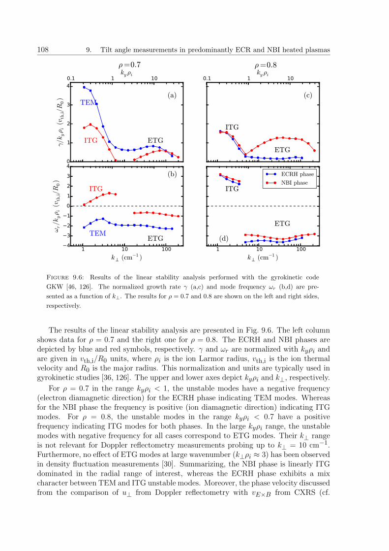
108 9. Tilt angle measurements in predominantly ECR and NBI heated plasmas
0
1
2
3
4
γ/k
yρi(v
th,i/R
0)
ITG
TEM
ETG
(a)
ρ=0.7
0.1 1 10kyρi
1 10 100
k⟂ (cm−1 )
−4
−3
−2
−1
0
1
2
3
4
ωr/k
yρi(v
th,i/R
0)
ITG
TEMETG
(b)
ITG
ETG
(c)
ρ=0.8
0.1 1 10kyρi
1 10 100
k⟂ (cm−1 )
ITG
ETG
(d)
ECRH phase
NBI phase
Figure 9.6: Results of the linear stability analysis performed with the gyrokinetic code
GKW [46, 126]. The normalized growth rate γ (a,c) and mode frequency ωr (b,d) are pre-
sented as a function of k⊥. The results for ρ = 0.7 and 0.8 are shown on the left and right sides,
respectively.
The results of the linear stability analysis are presented in Fig. 9.6. The left columnshows data for ρ = 0.7 and the right one for ρ = 0.8. The ECRH and NBI phases aredepicted by blue and red symbols, respectively. γ and ωr are normalized with kyρi andare given in vth,i/R0 units, where ρi is the ion Larmor radius, vth,i is the ion thermalvelocity and R0 is the major radius. This normalization and units are typically used ingyrokinetic studies [36, 126]. The upper and lower axes depict kyρi and k⊥, respectively.
For ρ = 0.7 in the range kyρi < 1, the unstable modes have a negative frequency(electron diamagnetic direction) for the ECRH phase indicating TEM modes. Whereasfor the NBI phase the frequency is positive (ion diamagnetic direction) indicating ITGmodes. For ρ = 0.8, the unstable modes in the range kyρi < 0.7 have a positivefrequency indicating ITG modes for both phases. In the large kyρi range, the unstablemodes with negative frequency for all cases correspond to ETG modes. Their k⊥ rangeis not relevant for Doppler reflectometry measurements probing up to k⊥ = 10 cm−1.Furthermore, no effect of ETG modes at large wavenumber (k⊥ρi ≈ 3) has been observedin density fluctuation measurements [30]. Summarizing, the NBI phase is linearly ITGdominated in the radial range of interest, whereas the ECRH phase exhibits a mixcharacter between TEM and ITG unstable modes. Moreover, the phase velocity discussedfrom the comparison of u⊥ from Doppler reflectometry with vE×B from CXRS (cf.

9.4. Linear gyrokinetic modelling 109
Figure 9.7: Structure of the global mode for (a) TEM and (b) ITG turbulence (adapted from
Ref. [38]).
Sec. 9.2), supports the identification of the NBI and ECRH phases with dominant ITGand more TEM dominated turbulence regimes, respectively.
The TEM and ITG linear modes have an opposite tilt angle. This difference hasbeen found using analytical expressions and in global linear gyrokinetic simulations [38].The mode structure for TEM and ITG turbulence obtained in the Ref. [38] is shown inFig. 9.7a and b, respectively. Elongated and tilted structures are observed in both cases.The tilt at the mid-plane, indicated in the figure, has a different sign for ITG (positive)and TEM (negative) modes. The tilt angle difference of 26◦ (cf. Eqs. 9.1 and 9.2)observed in the experiment agree qualitatively with these results. The NBI phase is ITGturbulence dominated, hence a positive and large tilt angle is expected. Moreover the inECRH phase one expects a mixture of TEM and ITG modes, thus the mode structurewould be a combination of structures with positive and negative tilts that averages to asmall tilt angle value.
The joint analysis of the tilt angle measurements, linear stability and u⊥ profileshas shown the utility of the developed technique for physical studies in fusion plasmas.Moreover, the measurement of tilt angle might be used as a signature of the dominantturbulence regime. Nevertheless, a stronger statement on identification of the turbulenceregime using the tilt angle measurement requires quantitative comparisons with non-linear global simulations for the specific conditions of the experiment. These simulationsare challenging and are left for future investigations.
Summary
The method developed to measure the tilt angle has been applied to a discharge usingdifferent heating methods in the ASDEX Upgrade tokamak. Measurements have beenperformed in the range ρ = 0.70− 0.84 for phases with either dominant ion or electronheating. A tilt angle difference of 26◦ has been obtained between both phases. Thetilt change is in qualitative agreement with a transition from an ITG dominated to a

110 9. Tilt angle measurements in predominantly ECR and NBI heated plasmas
ITG/TEM mixed turbulence regime. The dominant micro-instabilities for the specificplasma conditions have been confirmed with linear gyrokinetic simulations.
For the large velocities involved of u⊥ ≥ 6 km/s, the temporal decorrelation of theturbulence has no impact on the measured time delays. Therefore no correction factor Fdis needed for the tilt angle determination according to the analysis presented in Sec. 7.4.
The sensitivity of the tilt angle measurement to different plasma conditions and thequalitative agreement with theoretical predictions show that the tilt angle is an usefulquantity for comparisons of experimental measurements with theory and gyrokinetic sim-ulations. Thus the measurement technique developed and applied in this thesis providesa valuable tool for detailed turbulence studies in the future.

Chapter 10
Conclusions and outlook
Turbulence is a relevant phenomenon in magnetic confinement experiments because itcontributes to the transport of energy and particles in fusion plasmas. Therefore, abetter understanding of the turbulence dynamics and the related transport is requiredfor optimizations of the experimental devices and future reactors. In the last years, alarge progress has been made towards the understanding of turbulence; theoretical pre-dictions and gyrokinetic simulations have become available. However, a more detailedexperimental characterization of the turbulence is required for comparison and validationof physical models and simulation codes. Doppler relfectometry is one of the experimen-tal techniques used for density turbulence investigations in fusion plasmas. It uses thescattering of microwaves off density fluctuations to provide measurements of the per-pendicular velocity u⊥, perpendicular wavenumber (k⊥) spectrum and radial correlationlength (Lr) of the density turbulence.
In this thesis, the Doppler reflectometry technique has been deeply investigated andapplied to the detailed characterization of density turbulence in fusion plasmas. Thecomplex diagnostic response has been investigated by modelling the wave propagationand scattering processes relevant for the technique. Experimental measurement havebeen performed in L-mode plasmas at the ASDEX Upgrade tokamak (AUG) and theTJ-II stellarator. The experimental data have been analysed based on the modellingresults, which have made possible a more accurate and complete characterization of theturbulence in both machines.
The linearity of the diagnostic response has been investigated in detail with thephysical optics model and two-dimensional full-wave simulations. An enhanced powerresponse regime has been found and characterized for the first time. This regime andthe saturation regime have been found responsible of the flattening of the k⊥ spectra,which is measured when a non-linear diagnostic response is involved. The physical opticsmodel has been used for a characterization of the power response in a broad range ofturbulence level and k⊥, and for different types of wavenumber spectra. This analysishas shown that the power response depends strongly on the spectral shape and has beenuseful to asses the linearity of experimental measurements. Furthermore, a perturbativeexpansion of the physical optics model has shown that the enhanced power response isproduced by multiple scattering events.
111

112 10. Conclusions and outlook
Radial correlation Doppler reflectometry has been modelled using two-dimensionalfull-wave simulations and a linear analysis based on the Born approximation. The effectof the spectral and radial resolution on the diagnostic response has been investigated. Ithas been found that the spectral shape of the turbulence has an impact on the correlationmeasurements. In particular, the filter effect of the diagnostic and the Kolmogorov-likenature of the wavenumber spectrum introduce a instrumental k⊥ dependence of themeasured radial correlation length Lr. This effect explains the decrease of Lr with k⊥measured in AUG and reported for TJ-II [16].
The density turbulence has been characterised in L-mode plasmas in AUG and TJ-II.In AUG, a radial evolution of the k⊥ spectra has been observed in the range ρ = 0.85 to0.97. The spectral index at large k⊥ increases from −2.5 to −5.2 and the position of thespectral knee shifts from k⊥ = 4 to 6 cm−1. Moreover a radial variation of the radialcorrelation length Lr has been observed. The radial profiles of density and temperaturenormalized gradient, together with the radial changes observed in k⊥ spectra and Lrsuggest a change of the turbulence regime towards the plasma edge. In TJ-II, the k⊥spectra in the range ρ = 0.61–0.79 have a spectral index of about −8 and a knee atk⊥ = 7 cm−1, and show no radial evolution. A strong decrease of Lr towards theplasma edge has been observed. Possible explanations are either a scaling with thedensity gradient length Ln or an effect of the u⊥ shear, which can lead to decorrelationof the turbulent structures i.e. to a reduction of Lr according to standard theories.
A new method for the measurement of the mean tilt angle of the turbulent structureshas been developed. It is based on the analysis of the time delay of the cross-correlationbetween Doppler reflectometry channels, which measure at positions radially and per-pendicularly displaced. Diagnostic effects have been considered with two-dimensionalfull-wave simulations and a linear analysis. It has been found that for a linear diagnosticresponse and for a radial resolution smaller than Lr, the method gives a good estima-tion of the tilt angle. The impact of the temporal decorrelation of the turbulence onthe method has been investigated. The relevant quantities to asses such impact are thedecorrelation time of the turbulence τd and the passing time of the structures in frontof the probing beam w/u⊥, with w the beam width. If the passing time is shorter thanthe decorrelation time, w/u⊥ < τd, there is no impact and the method can be directlyapplied. This is the case for large plasma velocities (u⊥ > w/τd), whereas for small ones(u⊥ ≤ w/τd) the temporal decorrelation of the turbulence reduces the measured timedelays. This effect has been accounted for with a correction factor Fd.
The tilt angle measurement method has been applied for the first time to fusionplasmas in AUG and TJ-II. The experimentally measured time delays correspond to themodelling predictions and allow to obtain the tilt angle. The effect of the decorrelationtime of the turbulence has been experimentally confirmed; for u⊥ ≈ 1.5 km/s the effectis strong and the time delays are reduced by factor 10, for u⊥ ≈ 3 km/s time delays arereduced by a factor 2, and for u⊥ > 5 km/s no time delay reduction has been observed.Even in cases when the decorrelation time has a strong impact, the tilt angle can beobtained using the correction factor Fd.

113
The tilt angle measured in TJ-II is comparable to the one obtained in global lineargyrokinetic simulations. Furthermore, a two-point correlation technique has been usedto obtain a radial profile of the tilt angle. A change from −30 to 20◦ has been observed,which is consistent with the the u⊥ shear effect on the turbulence expected from theories.In AUG, the tilt angle has been measured in low density L-mode plasmas during phaseswith dominant ion and electron heating. A change of the tilt angle has been observedbetween both phases. Linear gyrokinetic simulations have confirmed a transition froman ITG to a more TEM dominated turbulence regime. Moreover the tilt angle differenceis in qualitative agreement with predictions for ITG and TEM dominated turbulence.
This thesis represents a major step towards a better understanding of Doppler reflec-tometry and towards a more advanced characterization of turbulence in fusion plasmas.The detailed study of the power response and of the correlation measurements havehighlighted diagnostic properties and effects important for a more complete and accu-rate characterization of the turbulence. In particular, the finding of the enhanced powerresponse regime has contributed to a better understanding of the measured k⊥ spectra.The tilt angle measurement method, proposed and applied here, has provided uniquemeasurements of this type in the confinement region of fusion plasmas. It has beenshown that the tilt angle is an useful quantity for studies of the turbulence dynamics,and which can be compared with physical models and gyrokinetic simulations. Thismethod can be applied for systematic experimental investigations in AUG and TJ-II,and also in other fusion experiments where Doppler reflectometry is available. Themethods developed in this thesis will potentially contribute to a better understanding ofthe turbulence in fusion plasmas in the near future.
Outlook
During the development of this thesis, topics that deserve further investigation havebeen identified. Regarding the Doppler reflectometry modelling: (i) The correlationmeasurements for Kolmogorov-like turbulence can be investigated with two-dimensionalfull-wave simulations. The study of non-linearities and non-local scattering for this casewould complement the linear analysis presented here and the literature on the topic. (ii)It has been shown that the physical optics model reproduces the linearity of Dopplerreflectometry. Further studies of the weighting function and its inclusion into the modelcould deliver a ”2D physical optics model”. This may simulate more accurately andefficiently Doppler reflectometry taking into account multiple and non-local scatteringprocesses.
Regarding the experimental measurements presented here, the AUG and TJ-II dis-charges characterized experimentally can be further investigated with global non-lineargyrokinetic simulations. This would allow to study more accurately specific effects thathave been reported in the thesis. Some of them are listed: (i) the radial evolution of k⊥spectra and Lr as a consequence of the turbulence regime change in AUG. (ii) The radialevolution of Lr and the tilt angle as a consequence of the velocity shear in TJ-II. (iii)The tilt angle change as a signature of the transition between ITG and TEM dominatedturbulence regimes in AUG.

114 10. Conclusions and outlook
In this thesis, poloidal asymmetries in the plasma flow in AUG have been reportedfor the first time (cf. Sec. 9.2). Similar asymmetries have been already observed inother fusion experiments and have been related to contributions of turbulence to plasmaflows [127]. These observations deserve further experimental investigations, which couldbe the starting point of new turbulence studies in the ASDEX Upgrade tokamak.

Bibliography
[1] E. Teller. Fusion: Magnetic confinement, volume 1, Academic Press, NewYork, 1981.
[2] V. D. Shafranov. “The initial period in the history of nuclear fusion research atthe Kurchatov Institute.” Physics-Uspekhi, 44(8):835, 2001.
[3] F. Birol et al. Energy and Climate Change - World Outlook Spe-cial Report. International Energy Agency (IEA), 2015. Available athttp://www.iea.org/publications/freepublications/publication/
weo-2015-special-report-2015-energy-and-climate-change.html.
[4] F. Birol et al. Key World Energy Statistics 2017. International En-ergy Agency (IEA), 2017. Available at https://www.iea.org/publications/
freepublications/publication/key-world-energy-statistics.html.
[5] J. D. Lawson. “Some Criteria for a Power Producing Thermonuclear Reactor.”Proceedings of the Physical Society. Section B, 70(1):6, 1957.
[6] J. Nuckolls, L. Wood, A. Thiessem et al. “Laser Compression of Matter to Super-High Densities: Thermonuclear (CTR) Applications.” Nature, 239(139):4941,1972.
[7] I. Milch. 50 Jahre Max-Planck-Institut fur Plasmaphysik : Forschung fur dieEnergie der Zukunft, Max-Planck-Institut fur Plasmaphysik (IPP), Garching /Greifswald, 2010.
[8] F. L. Hinton and R. D. Hazeltine. “Theory of plasma transport in toroidal con-finement systems.” Reviews of Modern Physics, 48:239, 1976.
[9] A. J. Wootton, B. A. Carreras, H. Matsumoto et al. “Fluctuations and anomaloustransport in tokamaks.” Physics of Fluids B: Plasma Physics, 2(12):2879, 1990.
[10] P. C. Liewer. “Measurements of microturbulence in tokamaks and comparisonswith theories of turbulence and anomalous transport.” Nuclear Fusion, 25(5):543,1985.
[11] A. J. Brizard and T. S. Hahm. “Foundations of nonlinear gyrokinetic theory.”Reviews of Modern Physics, 79:421, 2007.
115

116 Bibliography
[12] X. Garbet, Y. Idomura, L. Villard et al. “Gyrokinetic simulations of turbulenttransport.” Nuclear Fusion, 50(4):043002, 2010.
[13] U. Stroth, A. B. Navarro, G. Conway et al. “Experimental turbulence studiesfor gyro-kinetic code validation using advanced microwave diagnostics.” NuclearFusion, 55(8):083027, 2015.
[14] M. Hirsch, E. Holzhauer, J. Baldzuhn et al. “Doppler reflectometry for the in-vestigation of propagating density perturbations.” Plasma Physics and ControlledFusion, 43(12):1641, 2001.
[15] J. Schirmer, G. D. Conway, E. Holzhauer et al. “Radial correlation length mea-surements on ASDEX Upgrade using correlation Doppler reflectometry.” PlasmaPhysics and Controlled Fusion, 49(7):1019, 2007.
[16] F. Fernandez-Marina, T. Estrada and E. Blanco. “Turbulence radial correla-tion length measurements using Doppler reflectometry in TJ-II.” Nuclear Fusion,54(7):072001, 2014.
[17] T. Happel, T. Gorler, P. Hennequin et al. “Comparison of detailed experimentalwavenumber spectra with gyrokinetic simulation aided by two-dimensional full-wave simulations.” Plasma Physics and Controlled Fusion, 59(5):054009, 2017.
[18] E. Blanco and T. Estrada. “Study of Doppler reflectometry capability to determinethe perpendicular velocity and the k-spectrum of the density fluctuations using a2D full-wave code.” Plasma Physics and Controlled Fusion, 50(9):095011, 2008.
[19] E. Blanco and T. Estrada. “Two-dimensional full-wave simulations of radial cor-relation Doppler reflectometry in linear and non-linear regimes.” Plasma Physicsand Controlled Fusion, 55(12):125006, 2013.
[20] E. Z. Gusakov and A. Y. Popov. “Two-dimensional non-linear theory of radialcorrelation reflectometry.” Plasma Physics and Controlled Fusion, 46(9):1393,2004.
[21] E. Gusakov, M. Irzak and A. Popov. “Radial correlation reflectometry at obliqueprobing wave incidence (linear scattering theory predictions).” Plasma Physicsand Controlled Fusion, 56(2):025009, 2014.
[22] U. Stroth. Plasmaphysik: Phanomene, Grundlagen, Anwendungen,Vieweg+Teubner Verlag, Wiesbaden, 2011.
[23] A. N. Kolmogorov. “Dissipation of Energy in the Locally Isotropic Turbulence.”Proceedings of the Royal Society of London A: Mathematical, Physical and Engi-neering Sciences, 434(1890):15, 1991.
[24] R. H. Kraichnan. “Inertial Ranges in Two-Dimensional Turbulence.” The Physicsof Fluids, 10(7):1417, 1967.

Bibliography 117
[25] R. H. Kraichnan. “Inertial-range transfer in two- and three-dimensional turbu-lence.” Journal of Fluid Mechanics, 47(3):525–535, 1971.
[26] T. Happel. “Doppler reflectometry in the TJ-II Stellarator: Design of an OptimizedDoppler Reflectometer and its Application to Turbulence and Radial Electric FieldStudies.” Ph.D. thesis, Universidad Carlos III de Madrid, Spain, 2010.
[27] P. W. Terry, A. F. Almagri, G. Fiksel et al. “Dissipation range turbulent cascadesin plasmas.” Physics of Plasmas, 19(5):055906, 2012.
[28] T. Gorler and F. Jenko. “Multiscale features of density and frequency spectra fromnonlinear gyrokinetics.” Physics of Plasmas, 15(10):102508, 2008.
[29] N. Fedorczak, P. Ghendrih, P. Hennequin et al. “Dynamics of tilted eddies in atransversal flow at the edge of tokamak plasmas and the consequences for L–Htransition.” Plasma Physics and Controlled Fusion, 55(12):124024, 2013.
[30] P. Hennequin, C. Honore, A. Truc et al. “Doppler backscattering system for mea-suring fluctuations and their perpendicular velocity on Tore Supra.” Review ofScientific Instruments, 75(10):3881, 2004.
[31] T. Estrada, E. Ascasıbar, E. Blanco et al. “Spatial, temporal and spectral structureof the turbulence–flow interaction at the L–H transition.” Plasma Physics andControlled Fusion, 54(12):124024, 2012.
[32] T. Happel, T. Estrada, E. Blanco et al. “Scale-selective turbulence reduction inH-mode plasmas in the TJ-II stellarator.” Physics of Plasmas, 18(10):102302,2011.
[33] U. Stroth, P. Manz and M. Ramisch. “On the interaction of turbulence and flowsin toroidal plasmas.” Plasma Physics and Controlled Fusion, 53(2):024006, 2011.
[34] H. Biglari, P. H. Diamond and P. W. Terry. “Influence of sheared poloidal rotationon edge turbulence.” Physics of Fluids B: Plasma Physics, 2(1):1, 1990.
[35] P. H. Diamond and Y. Kim. “Theory of mean poloidal flow generation by turbu-lence.” Physics of Fluids B: Plasma Physics, 3(7):1626, 1991.
[36] C. Angioni, R. M. McDermott, F. J. Casson et al. “Intrinsic Toroidal Rotation,Density Peaking, and Turbulence Regimes in the Core of Tokamak Plasmas.” Phys-ical Review Letters, 107:215003, 2011.
[37] P. H. Diamond, S.-I. Itoh, K. Itoh et al. “Zonal flows in plasma - a review.” PlasmaPhysics and Controlled Fusion, 47(5):R35, 2005.
[38] Y. Camenen, Y. Idomura, S. Jolliet et al. “Consequences of profile shearing ontoroidal momentum transport.” Nuclear Fusion, 51(7):073039, 2011.

118 Bibliography
[39] R. McDermott, C. Angioni, G. Conway et al. “Core intrinsic rotation behaviourin ASDEX Upgrade ohmic L-mode plasmas.” Nuclear Fusion, 54(4):043009, 2014.
[40] P. N. Guzdar, L. Chen, W. M. Tang et al. “Ion-temperature-gradient instabilityin toroidal plasmas.” The Physics of Fluids, 26(3):673, 1983.
[41] F. Jenko, W. Dorland, M. Kotschenreuther et al. “Electron temperature gradientdriven turbulence.” Physics of Plasmas, 7(5):1904, 2000.
[42] J. Weiland, A. Jarmen and H. Nordman. “Diffusive particle and heat pinch effectsin toroidal plasmas.” Nuclear Fusion, 29(10):1810, 1989.
[43] B. D. Scott. “The nonlinear drift wave instability and its role in tokamak edgeturbulence.” New Journal of Physics, 4(1):52, 2002.
[44] B. D. Scott. “Computation of electromagnetic turbulence and anomalous trans-port mechanisms in tokamak plasmas.” Plasma Physics and Controlled Fusion,45(12A):A385, 2003.
[45] B. D. Scott. “Tokamak edge turbulence: background theory and computation.”Plasma Physics and Controlled Fusion, 49(7):S25, 2007.
[46] A. Peeters, Y. Camenen, F. Casson et al. “The nonlinear gyro-kinetic flux tubecode GKW.” Computer Physics Communications, 180(12):2650, 2009.
[47] G. Jost, T. M. Tran, W. A. Cooper et al. “Global linear gyrokinetic simulationsin quasi-symmetric configurations.” Physics of Plasmas, 8(7):3321, 2001.
[48] V. Kornilov, R. Kleiber and R. Hatzky. “Gyrokinetic global electrostatic ion-temperature-gradient modes in finite β equilibria of Wendelstein 7-X.” NuclearFusion, 45(4):238, 2005.
[49] M. J. Pueschel, D. Told, P. W. Terry et al. “Magnetic Reconnection Turbulence inStrong Guide Fields: Basic Properties and Application to Coronal Heating.” TheAstrophysical Journal Supplement Series, 213(2):30, 2014.
[50] D. Told, F. Jenko, J. M. TenBarge et al. “Multiscale Nature of the DissipationRange in Gyrokinetic Simulations of Alfvenic Turbulence.” Physical Review Let-ters, 115:025003, 2015.
[51] A. Herrmann and O. Gruber. “Chapter 1: ASDEX Upgrade - Introduction andOverview.” Fusion Science and Technology, 44(3):569, 2003.
[52] C. Alejaldre, J. J. A. Gozalo, J. B. Perez et al. “TJ-II Project: A Flexible HeliacStellarator.” Fusion Technology, 17(1):131, 1990.
[53] B. Streibl, P. T. Lang, F. Leuterer et al. “Chapter 2: Machine Design, Fueling, andHeating in ASDEX Upgrade.” Fusion Science and Technology, 44(3):578, 2003.
Bibliography 119
[54] A. Fernandez, J. de la Fuente, D. Ganuza et al. “Performance of the TJ-II ECRHsystem with the new -80kV 50A high voltage power supply.” Fusion Engineeringand Design, 84(2):772, 2009.
[55] M. Liniers, J. Damba, J. Guasp et al. “Beam transmission dependence on beamparameters for TJ-II Neutral Beam Injectors.” Fusion Engineering and Design,123:259, 2017.
[56] H. Murmann, S. Gotsch, H. Rohr et al. “The Thomson scattering systems of theASDEX Upgrade tokamak.” Review of Scientific Instruments, 63(10):4941, 1992.
[57] C. J. Barth, F. J. Pijper, H. J. v. d. Meiden et al. “High-resolution multipositionThomson scattering for the TJ-II stellarator.” Review of Scientific Instruments,70(1):763, 1999.
[58] A. Mlynek, G. Schramm, H. Eixenberger et al. “Design of a digital multiradianphase detector and its application in fusion plasma interferometry.” Review ofScientific Instruments, 81(3):033507, 2010.
[59] H. Lamela, P. Acedo and J. Irby. “Laser interferometric experiments for the TJ-II stellarator electron-density measurements.” Review of Scientific Instruments,72(1):96, 2001.
[60] C. Laviron, A. J. H. Donne, M. E. Manso et al. “Reflectometry techniques fordensity profile measurements on fusion plasmas.” Plasma Physics and ControlledFusion, 38(7):905, 1996.
[61] T. Estrada, J. Sanchez, B. van Milligen et al. “Density profile measurements byAM reflectometry in TJ-II.” Plasma Physics and Controlled Fusion, 43(11):1535,2001.
[62] S. K. Rathgeber, L. Barrera, T. Eich et al. “Estimation of edge electron tempera-ture profiles via forward modelling of the electron cyclotron radiation transport atASDEX Upgrade.” Plasma Physics and Controlled Fusion, 55(2):025004, 2013.
[63] M. Cavedon. “The role of the radial electric field in the development of the edgetransport barrier in the ASDEX Upgrade tokamak.” Ph.D. thesis, TechnischeUniversitat Munchen, 2016.
[64] R. M. McDermott, A. Lebschy, B. Geiger et al. “Extensions to the charge ex-change recombination spectroscopy diagnostic suite at ASDEX Upgrade.” Reviewof Scientific Instruments, 88(7):073508, 2017.
[65] R. Fischer, E. Wolfrum, J. Schweinzer et al. “Probabilistic lithium beam dataanalysis.” Plasma Physics and Controlled Fusion, 50(8):085009, 2008.
[66] M. Hirsch, E. Holzhauer, J. Baldzuhn et al. “Doppler Reflectometry for the Inves-tigation of poloidally propagating Density Perturbations.” Proc. 4th InternationalReflectometry Workshop (Cadarache, France), 1999.

120 Bibliography
[67] X. L. Zou. “Poloidal Rotation Measurement in Tore Supra by Oblique Reflec-tometry.” Proc. 4th International Reflectometry Workshop (Cadarache, France),1999.
[68] G. D. Conway, J. Schirmer, S. Klenge et al. “Plasma rotation profile measurementsusing Doppler reflectometry.” Plasma Physics and Controlled Fusion, 46(6):951,2004.
[69] T. Happel, T. Estrada, E. Blanco et al. “Doppler reflectometer system in thestellarator TJ-II.” Review of Scientific Instruments, 80(7):073502, 2009.
[70] J. C. Hillesheim, W. A. Peebles, T. L. Rhodes et al. “A multichannel, frequency-modulated, tunable Doppler backscattering and reflectometry system.” Review ofScientific Instruments, 80(8):083507, 2009.
[71] P. Hennequin, C. Honore, A. Truc et al. “Fluctuation spectra and velocity profilefrom Doppler backscattering on Tore Supra.” Nuclear Fusion, 46(9):S771, 2006.
[72] T. Happel, P. Manz, F. Ryter et al. “Turbulence intermittency linked to theweakly coherent mode in ASDEX Upgrade I-mode plasmas.” Nuclear Fusion,56(6):064004, 2016.
[73] G. D. Conway, C. Angioni, F. Ryter et al. “Mean and Oscillating Plasma Flowsand Turbulence Interactions across the L-H Confinement Transition.” PhysicalReview Letters, 106:065001, 2011.
[74] V. Ginzburg. The Propagation of Electromagnetic Waves in Plasmas, PergammonPress, Oxford, UK, 1970.
[75] R. B. White and F. F. Chen. “Amplification and absorption of electromagneticwaves in overdense plasmas.” Plasma Physics, 16(7):565, 1974.
[76] E. Poli, A. Peeters and G. Pereverzev. “TORBEAM, a beam tracing code forelectron-cyclotron waves in tokamak plasmas.” Computer Physics Communica-tions, 136(1):90, 2001.
[77] T. Estrada, T. Happel, L. Eliseev et al. “Sheared flows and transition to improvedconfinement regime in the TJ-II stellarator.” Plasma Physics and Controlled Fu-sion, 51(12):124015, 2009.
[78] E. Viezzer, T. Putterich, G. Conway et al. “High-accuracy characterization of theedge radial electric field at ASDEX Upgrade.” Nuclear Fusion, 53(5):053005, 2013.
[79] T. Happel, A. Banon Navarro, G. D. Conway et al. “Core turbulence behavior mov-ing from ion-temperature-gradient regime towards trapped-electron-mode regimein the ASDEX Upgrade tokamak and comparison with gyrokinetic simulation.”Physics of Plasmas, 22(3):032503, 2015.

Bibliography 121
[80] G. Conway, C. Angioni, R. Dux et al. “Observations on core turbulence transitionsin ASDEX Upgrade using Doppler reflectometry.” Nuclear Fusion, 46(9):S799,2006.
[81] H. J. Hartfuss, T. Geist and M. Hirsch. “Heterodyne methods in millimetre waveplasma diagnostics with applications to ECE, interferometry and reflectometry.”Plasma Physics and Controlled Fusion, 39(11):1693, 1997.
[82] G. D. Conway, C. Lechte, A. Fochi et al. “Assessment of Doppler reflectometryaccuracy using full-wave codes with comparison to beam-tracing and analytic ex-pressions.” Proc. 12th International Reflectometry Workshop (Julich, Germany),2015.
[83] T. Happel, G. D. Conway, W. Kasparek et al. “Design of a New Doppler Reflec-tometer Frontend for the ASDEX Upgrade Tokamak.” Proc. 10th InternationalReflectometry Workshop (Padual, Italy), 2011.
[84] R. Sabot, P. Hennequin and L. Colas. “Fluctuation Measurements and Their Linkwith Transport on Tore Supra.” Fusion Science and Technology, 56(3):1253, 2009.
[85] F. Castejon, A. Cappa, M. Tereshchenko et al. “Computation of EBW heating inthe TJ-II stellarator.” Nuclear Fusion, 48(7):075011, 2008.
[86] J. R. Pinzon, T. Happel, E. Blanco et al. “Enhanced Doppler reflectometry powerresponse: physical optics and 2D full wave modelling.” Plasma Physics and Con-trolled Fusion, 59(3):035005, 2017.
[87] F. C. Karal and J. B. Keller. “Elastic, Electromagnetic, and Other Waves in aRandom Medium.” Journal of Mathematical Physics, 5(4):537, 1964.
[88] J. J. Sakurai. Modern Quantum Mechanics, The Benjamin/Cummings PublishingCompany, Inc, Menlo Park, CA, 1985.
[89] M. Born. “Zur Quantenmechanik der Stoßvorgange.” Zeitschrift fur Physik,37:863, 1926.
[90] A. D. Piliya and A. Y. Popov. “On application of the reciprocity theorem to calcu-lation of a microwave radiation signal in inhomogeneous hot magnetized plasmas.”Plasma Physics and Controlled Fusion, 44(5):467, 2002.
[91] E. Z. Gusakov and A. Y. Popov. “Non-linear theory of fluctuation reflectometry.”Plasma Physics and Controlled Fusion, 44(11):2327, 2002.
[92] P. Beckmann and A. Spizzichino. The scattering of electromagnetic waves fromrough surfaces. International series of monographs on electromagnetic waves, Perg-amon Press, Oxford, UK, 1963.
[93] I. S. Robinson. Measuring the Ocean from Space: The Principles and Methods ofSatellite Oceanography, Springer, Heidelberg, Germany, 2004.

122 Bibliography
[94] L. Wang and J. J. Qu. “Satellite remote sensing applications for surface soilmoisture monitoring: A review.” Frontiers of Earth Science in China, 3(2):237,2009.
[95] J. Rottger. “Reflection and scattering of VHF radar signals from atmosphericrefractivity structures.” Radio Science, 15(2):259, 1980.
[96] G. D. Conway. “Effects of reflectometer asymmetries on fluctuation measure-ments.” Plasma Physics and Controlled Fusion, 41(1):65, 1999.
[97] A. Ejiri, T. Yamada, Y. Adachi et al. “The response of microwave reflectom-etry under generalized configuration.” Plasma Physics and Controlled Fusion,50(6):065003, 2008.
[98] E. Rodriguez. “Beyond the Kirchhoff approximation.” Radio Science, 24(5):681,1989.
[99] E. Rodrıguez. “Beyond the Kirchhoff approximation II electromagnetic scattering.”Radio Science, 26(1):121, 1991.
[100] G. D. Conway, B. Kurzan, B. Scott et al. “Coupling of turbulence and reflectometersimulation codes and comparison with experiment.” Plasma Physics and ControlledFusion, 44(4):451, 2002.
[101] C. Lechte, G. D. Conway, T. Gorler et al. “X mode Doppler reflectometry k-spectralmeasurements in ASDEX Upgrade: experiments and simulations.” Plasma Physicsand Controlled Fusion, 59(7):075006, 2017.
[102] J. R. Pinzon, T. Happel, E. Blanco et al. “Modelling of the power response inDoppler reflectometry.” Proc. 13th International Reflectometry Workshop (Dae-jeon, Korea), 2017.
[103] F. da Silva, S. Heuraux, E. Z. Gusakov et al. “A Numerical Study of Forward- andBackscattering Signatures on Doppler-Reflectometry Signals.” IEEE Transactionson Plasma Science, 38(9):2144, 2010.
[104] T. Happel, T. Gorler, P. Hennequin et al. “Understanding of wavenumber spectrameasured by Doppler reflectometry through simulation and related estimation ofwave-plasma interaction regimes.” Proc. 13th International Reflectometry Work-shop (Daejeon, Korea), 2017.
[105] C. Troster. “Development of a flexible Doppler reflectometry system and its ap-plication to turbulence characterization in the ASDEX Upgrade tokamak.” Ph.D.thesis, Ludwig-Maximilians-Universitat, Munchen, Germany, 2008.
[106] D. Prisiazhniuk, A. Kramer-Flecken, G. D. Conway et al. “Magnetic field pitchangle and perpendicular velocity measurements from multi-point time-delay es-timation of poloidal correlation reflectometry.” Plasma Physics and ControlledFusion, 59(2):025013, 2017.

Bibliography 123
[107] D. Prisiazhniuk. “Development and application of poloidal correlation reflectome-try to study turbulent structures in the ASDEX Upgrade tokamak.” Ph.D. thesis,Technische Universitat Munchen, Germany, 2017.
[108] F. Ryter, R. Fischer, J. Fuchs et al. “I-mode studies at ASDEX Upgrade: L-I and I-H transitions, pedestal and confinement properties.” Nuclear Fusion, 57(1):016004,2017.
[109] J. Schirmer, G. Conway, H. Zohm et al. “The radial electric field and its associatedshear in the ASDEX Upgrade tokamak.” Nuclear Fusion, 46(9):S780, 2006.
[110] T. L. Rhodes, J.-N. Leboeuf, R. D. Sydora et al. “Comparison of turbulencemeasurements from DIII-D low-mode and high-performance plasmas to turbulencesimulations and models.” Physics of Plasmas, 9(5):2141, 2002.
[111] B. P. van Milligen, T. Estrada, E. Ascasıbar et al. “Integrated data analysis atTJ-II: The density profile.” Review of Scientific Instruments, 82(7):073503, 2011.
[112] C. Hidalgo, M. Pedrosa, L. Garcia et al. “Experimental evidence of couplingbetween sheared-flow development and an increase in the level of turbulence in theTJ-II stellarator.” Physical Review E, 70(6, 2), 2004.
[113] M. A. Pedrosa, C. Hidalgo, E. Calderon et al. “Threshold for sheared flow andturbulence development in the TJ-II stellarator.” Plasma Physics and ControlledFusion, 47(6):777, 2005.
[114] U. Stroth, K. Itoh, S.-I. Itoh et al. “Internal Transport Barrier Triggered byNeoclassical Transport in W7-AS.” Physical Review Letters, 86:5910, 2001.
[115] F. Fernandez-Marina, T. Estrada, E. Blanco et al. “Radial correlation lengthacross magnetic islands: Simulations and experiments.” Physics of Plasmas,24(7):072513, 2017.
[116] T. Estrada, E. Ascasıbar, E. Blanco et al. “Plasma flow, turbulence and magneticislands in TJ-II.” Nuclear Fusion, 56(2):026011, 2016.
[117] E. Sanchez, R. Kleiber, R. Hatzky et al. “Linear and Nonlinear Simulations Us-ing the EUTERPE Gyrokinetic Code.” IEEE Transactions on Plasma Science,38(9):2119, 2010.
[118] A. Banon Navarro, T. Happel, T. Gorler et al. “Gyrokinetic studies of coreturbulence features in ASDEX Upgrade H-mode plasmas.” Physics of Plasmas,22(4):042513, 2015.
[119] D. Told, F. Jenko, T. Gorler et al. “Characterizing turbulent transport in AS-DEX Upgrade L-mode plasmas via nonlinear gyrokinetic simulations.” Physics ofPlasmas, 20(12):122312, 2013.

124 Bibliography
[120] E. Sanchez, I. Calvo, J. L. Velasco et al. “Simulation of electrostatic instabilitiesin a heliac configuration.” Proc. 41st EPS Conference on Plasma Physics (Berlin,Germany), 2014.
[121] E. Sanchez, P. Monreal, I. Calvo et al. “Relaxation of zonal flows in stellarators:influence of the magnetic configuration.” Proc. 42nd EPS Conference on PlasmaPhysics (Lisbon, Portugal), 2015.
[122] R. R. Dominguez and G. M. Staebler. “Anomalous momentum transport fromdrift wave turbulence.” Physics of Fluids B: Plasma Physics, 5(11):3876, 1993.
[123] Y. Kishimoto, J.-Y. Kim, W. Horton et al. “Toroidal mode structure in weak andreversed magnetic shear plasmas and its role in the internal transport barrier.”Plasma Physics and Controlled Fusion, 41(3A):A663, 1999.
[124] A. G. Peeters, C. Angioni, A. Bottino et al. “Toroidal momentum transport.”Plasma Physics and Controlled Fusion, 48(12B):B413, 2006.
[125] A. Lebschy, R. McDermott, C. Angioni et al. “Measurement of the complete coreplasma flow across the LOC–SOC transition at ASDEX Upgrade.” Nuclear Fusion,58(2):026013, 2018.
[126] C. Angioni, R. Bilato, F. Casson et al. “Gyrokinetic study of turbulent convec-tion of heavy impurities in tokamak plasmas at comparable ion and electron heatfluxes.” Nuclear Fusion, 57(2):022009, 2017.
[127] L. Vermare, P. Hennequin, O. D. Gurcan et al. “Poloidal asymmetries of flows inthe Tore Supra tokamak.” Physics of Plasmas, 25(2):020704, 2018.
[128] E. Gusakov and M. Tyntarev. “The two-dimensional theory of reflectometry diag-nostics of plasma fluctuations.” Fusion Engineering and Design, 34:501, 1997.
[129] P. M. Morese and H. Feshbach. Methods of theoretical physics. Part I. Internationalseries in pure and applied physics, McGraw-Hill, New York, 1953.

Appendix A
Scattering efficiency
It has been discussed in Ch. 6 how non-linear effects can produce large deviations ofthe measured k⊥ spectra with respect to the real one. Nevertheless, small deviationshave also been observed in the linear regime, e.g. a slight loss of the reflectometersensitivity with k⊥ has been observed in Fig. 6.10 and 6.11, and reported in Ref. [18].This effect, referred to as scattering efficiency modifies the measured k⊥ spectra. Henceits understanding and the application of a correction is relevant for detailed studies ofthe turbulence. In this section the scattering efficiency is studied by comparing in detailthe k⊥ spectra obtained in two-dimensional full-wave (2DFW) simulations for a linearresponse with the input spectrum. A correction formula is proposed and tested.
The 2DFW simulations presented in Sec. 6.3 are extended in order to study thepurely linear response. In particular more angles (including normal incidence) and alower turbulence level (0.01%) for X-mode are included. The k⊥ spectra computed fromthe 2DFW data in linear regime are plotted with red symbols in Fig. A.1a, where theblack line represents the input spectrum (cf. Eq. 6.5). The blue symbols are the correcteddata to be explained afterwards. Although the reflectometer is operating in the linearregime, the k⊥ spectrum decays slightly faster than the input spectrum for both O- andX-mode.
In the linear regime, P is proportional to the power spectrum of the turbulenceaccording to Eq. 4.8. However, the beam propagation for different angles of incidenceinduces an instrumental dependency of the backscattered power on θ (or equivalentlyk⊥), which causes the scattering efficiency drop. This effect is included with a correctionfactor A as
P ∝ δn2rmsA
2(θ)h2⊥(k⊥). (A.1)
From the simulated data A2 ∝ P/h2⊥(k⊥) is computed. The values are normalized to
the normal incidence and plotted with symbols as a function of θ in Fig. A.1b. Thecorrection formula for A is depicted by solid lines and will be explained next. A similardecrease of the sensitivity with θ is observed for O- and X-mode.
Although the scattering efficiency has been observed in simulations [18] and hasbeen studied in the literature [128], predictions applicable to experimental data analysisare not available. In the following a correction formula is deduced for O-mode in slabgeometry and with a linear density profile. It recovers the trends of the simulations, and
125

126 A. Scattering efficiency
0 2 4 6 8 10 12 14 16
k⟂(cm−1 )
10-9
10-7
10-5
10-3
10-1
101
P(a.u.)
(a)
true
O-mode-corrected
X-mode-corrected
O-mode
X-mode
0 5 10 15 20 25
θ (deg)
0.3
0.4
0.5
0.6
0.7
0.8
0.9
1.0
1.1
A2
(b)
O-mode
X-mode
Figure A.1: (a) k⊥ spectra obtained with 2DFW simulations in the linear regime (red). The
black line depicts the input spectrum. k⊥ spectra corrected with Eq. A.4 are shown in blue. (b)
Factor A2 accounting for the scattering efficiency effect.
allows to understand the role of the basic parameters. Moreover it will be applied to amore realistic case .
First, the unperturbed electric field E0 is computed by solving Eq. 5.4. For slabgeometry, linear density profile and oblique incidence, the x-dependent part of the electricfield is given by [75]
∂2E0
∂x2+ k2
0
(1− x
L− sin2 θ
)E0 = 0. (A.2)
Using the transformation
ζ =
(k2
0
L
)1/3
(L cos2 θ − x),
the previous equation turns into
∂2E0
∂ζ2+ ζE0 = 0.
The solution to the previous equation is given by the Airy function. It is depictedin Fig. A.2a for θ = 17.7◦. Both coordinates, x and ζ are shown in the lower andupper axes, respectively. The nominal cutoff, at x = L cos2 θ or equivalently ζ = 0, isindicated with a green dashed line. E2
0 oscillates and maximizes close to the cutoff as itwas discussed in Sec. 4.2. An absolute maximum is obtained at ζmax ≈ 1 correspondingto xmax = L cos2 θ − (L/k2
0)1/3, which is slightly displaced with respect to the nominalcutoff.
The solution shown in Fig. A.2a has an absolute maximum slightly displaced fromthe nominal cutoff, similarly to the weighting function from Fig. 6.9d. The dominance ofthe scattering in a narrow region along xmax, makes possible a reduction of the problemto one dimension. Shrinking the system to a line along xmax, Eq. 5.5 becomes

A. Scattering efficiency 127
0 1 2 3 4 5 6
x (cm)
0.0
0.2
0.4
0.6
0.8
1.0E
2 0(a.u.)
(a)nominalcutoff
xmax
12 9 6 3 0 −3ζ
0.05 0.1 0.2 0.3 0.5 1 2
k⟂/k0
0.1
0.2
0.3
0.5
0.7
1
2
A ∼k−1⟂
∼k−0.4⟂
(b)
Figure A.2: (a) Unperturbed electric field squared obtained from solving Eq. A.2. A maximum
is observed close to the nominal cutoff. (b) Scattering efficiency A as a function of k⊥/k0
computed from Eq. A.3. A drop of the scattering efficiency with k⊥ is observed. Two scalings
are indicated in different ranges.
(∂2y + k2
max)E1 = k20δn
ncE0.
where kmax is taken from the dispersion relation at xmax following
k2max = k2
0
[1− n0(xmax)
nc
]= k2
0
[1− xmax
L
]= k2
0
[(1
k0L
)2/3
+ sin2 θ
].
The scattered field can be computed with the Green function for the relevant geom-etry [129],
E1 ∝∫
dyG1D(y)δnE0, with G1D(y) =ieikmax|y|
2kmax.
The Green function introduces a k−1max dependency on the scattered field E1, which
results in a k−2max dependency on the backscattered power. This dependency provides the
scattering efficiency correction factor as A ∼ k−1max, which after normalizing for normal
incidence gives
A =
[1 +
(2πL
λ0
)2/3
sin2 θ
]1/2
=
1 +
(L
8k20
)2/3
k2⊥
1/2
. (A.3)
In Fig. A.2 the scattering efficiency A is plotted as a function of k⊥/k0 for theparameters used in Sec. 6.3. In the limit of large k⊥ the scattering efficiency scalesas k−1
⊥ , hence the measured spectral index for the power could be underestimated byat most 2. In the limit of small k⊥ the scattering efficiency is constant and 1, and inbetween both limits A scales with a k⊥ exponent in between 0 and 1. Fig. A.2 depictsalso a scaling k−0.4
⊥ at an intermediate position which has been reported in Ref. [18].

128 A. Scattering efficiency
1 2 3 4 5 7 10 20
k⟂(cm−1 )
10-5
10-4
10-3
10-2
10-1
100
P(a.u.)
k−5.4⟂
k−3.9⟂
k−4.0⟂
input
2DFW
2DFW-corrected
Figure A.3: k⊥ spectra for a Kolmogorov type input spectrum [101]. The input spectrum
is plotted with a black line and 2DFW data in the linear regime with red symbols. The blue
symbols depict 2DFW data corrected with Eq. A.4. Spectral indices for the different case are
indicated.
Although the previous calculation is done for O-mode and for a linear density profile,it can applied in general cases by taking the gradient scale length of the squared refractiveindex Lref . This includes the magnetic field for the X-mode case. Fig. A.1b showsthat Eq. A.3 is able to follow approximately the simulated data for O- and X-mode.Furthermore, k⊥ spectra obtained in the linear regime can be corrected for the scatteringefficiency with
Pcorrected = P
1 +
(Lref
8k20
)2/3
k2⊥
. (A.4)
The corrected k⊥ spectra are presented with blue symbols in Fig. A.1a. A better agree-ment with the input spectrum is observed for both polarizations.
The scattering efficiency is also observed in the 2DFW simulations with the ASDEXUpgrade geometry and a Kolmogorov-type turbulence presented in Sec. 6.4 [101]. Thek⊥ spectrum obtained in the purely linear regime is shown in Fig. A.3 with red symbols.The simulated spectrum recovers the shape of the input spectrum in black, but witha stronger spectral index of −5.4 due to the scattering efficiency effect. The spectrumcorrected using Eq. A.4 is shown in the figure with blue symbols. A better agreementwith the input spectrum is obtained after applying the correction; the corrected spectralindex is−3.9. This shows that the correction factor Eq. A.4 does reproduce the scatteringefficiency for realistic plasma geometries and spectral shapes.
The k⊥ spectra, measured for experimental conditions where the response of theDoppler reflectometer is linear, can be corrected with Eq. A.4. The effects here dis-cussed could explain the small discrepancies between the spectral indices obtained ingyrokinetic simulations and with O-mode Doppler reflectometry measurements at theASDEX Upgrade tokamak [17].

Appendix B
Decorrelation due to k⊥ variation
In the Sec. 7.2 the radial correlation Doppler reflectometry has been investigated usingtwo-dimensional full-wave (2DFW) simulations. There a decrease of the radial correla-tion length Lx with the angle of incidence θ has been observed (cf. Fig. 7.5a and d).The decorrelation effect responsible is discussed here.
−0.1 0.0 0.1 0.2 0.3 0.4 0.5f/fs
10-1910-1710-1510-1310-1110-910-710-510-310-1101103
pow
erspectrum
(a.u.)
θ=5.6 ◦
θ=17.7 ◦
94.4 GHz83.4 GHz
94.4 GHz83.4 GHz
Figure B.1: Power spectra obtained from X-mode 2DFW simulations in linear regime. Two
angles of incidence and two probing frequencies are presented.
A probing frequency f0 scan is performed in order to induce a radial separationbetween the reference and hopping channels. Moreover, k⊥ depends on the probingfrequency as it is seen for the slab case in Eq. 4.7 through the k0 dependency. As aconsequence, the f0 scan results in a change of k⊥ for oblique incidence. This effect isobserved in Fig. B.1, where the power spectra of 2DFW signals for two angles of incidenceand two probing frequencies are shown. The Doppler peak appears approximately at thesame position for θ = 5.6◦ and both probing frequencies. However for θ = 17.7◦, theDoppler peaks appear at different positions for the two probing frequencies. For allcases a broad peak centred at f = 0 is observed. It corresponds to the direct reflection
129

130 B. Decorrelation due to k⊥ variation
contribution (cf. Sec. 4.2.3) and is several orders of magnitude below the Doppler peakin these 2DFW simulations.
The difference of the peak position is large compared to its width for θ = 17.7◦,hence the overlap of the peaks is partially lost. It means that reference and hoppingchannels are not measuring at the same k⊥. This causes a decrease of the correlationbetween the two signals. Since the k⊥ difference increases with the frequency separation,the correlation of the signals decreases with ∆x. This is an instrumental effect that isnot related to the turbulence. It modifies the decay of Cmax with ∆x, and therefore themeasured Lx.
The simulations presented are performed with a good spectral resolution and a strongdensity gradient. Accordingly narrow Doppler peaks (∆f < fD) are obtained and abroad frequency scan is performed. These conditions make the decorrelation effect par-ticularly strong, which is in line with the observed decrease of Lx with θ in Fig. 7.5aand d. This effect is strong and dominates over other effects on the correlation, e.q.non-local scattering [21].
It should be noted that this effect is not relevant in the experimental measurementspresented in Ch. 8 and Ch. 9. The Doppler peaks there are wide rand a small k⊥ variationis induced by the probing frequency scan.

Appendix C
Effect of the direct reflectioncontribution in the correlationanalysis and its filtering
The characterization method of the density turbulence (cf. Sec. 7) using radial correla-tion Doppler reflectometry assumes backscattering contributions only. Nevertheless, thedirect reflection introduced in Sec. 4.2.3 and observed the k⊥ spectrum (cf. Fig. 8.3a)can have an impact in the correlation analysis, which has to mitigated in the case whereis relevant. The direct reflection contribution has been filtered out for the correlationanalysis in the ASDEX Upgrade tokamak presented in Sec. 8.1 and Ch. 9. Here theeffect and the filtering are discussed in detail.
An example where the direct reflection affects the O-mode correlation analysis isdiscussed. The power spectra obtained for the reference and hopping channel are shownin Fig. C.1a. A Doppler peak at about −400 kHz and a direct reflection contributionaround zero frequency are observed. The impact of the contributions for the correlationanalysis can be analysed by looking at the cross-spectrum of the signals, V0V1
∗. The
absolute value and complex phase of the cross-spectrum are shown in Fig. C.1b and c,respectively. Backscattering and direct reflection contributions are also observed in thecross-spectrum of the signals.
Although the direct reflection contribution to the power spectra is weak comparedwith the Doppler peak (Fig. C.1a), it is strong and comparable to the backscatteringcontribution in the cross-spectrum (Fig. C.1b). This shows that the direct reflectionhas an impact in the correlation analysis. The complex phase of the cross-spectrumin Fig. C.1c, shows a well defined linear behaviour at the Doppler frequency. Its slopegives the time delay of the backscattering contribution which is related to the tilt ofthe turbulent structures. Nevertheless, the phase behaves erratically at around zerofrequency due to the direct reflection. This can corrupt the time delay analysis of thecorrelation.
The cross-correlation function of the signals is shown in Fig. C.1d with red points.A mixture of two peaks centred at different τ is obtained. The interference of the directreflection contribution with the backscattering corrupt the cross-correlation function
131

132 C. Effect of the direct reflection contribution in the correlation analysis and its filtering
backscattering
direct re!ection
Figure C.1: (a) Power spectra of the reference and hopping channels signal. (b) Absolute value
and (c) complex phase of the cross-spectrum. (d) Cross-correlation function for the raw signals
in red and the band-pass filtered signals in blue.
producing satellite peaks as the one one observed in the figure. The direct reflectioncontribution is suppressed by filtering, in this case the signals have been pass-filtered inthe range of−700 to−200 kHz. The cross-correlation function computed with the filteredsignals is depicted by blue symbols in (d). A single peak suitable for the correlationanalysis is obtained.
The analysis of the cross-spectrum shows that the direct reflection contribution mayhave negative impact on the correlation analysis; the maximum Cmax and the time delayτmax of the cross-correlation can be affected. Nevertheless, this effect can be avoid byfiltering the out the direct reflection contributions in the data processing.
The filtering works well when the Doppler peak is dominant (as in the case herediscussed) and when the Doppler shift is large. For cases where Doppler peak is sub-dominant and small Doppler shift, the filtering the filtered signal quality is poor and thecorrelation analysis is problematic.

Acknowledgements
The process of writing this doctoral thesis would not have been possible without the helpand support of a large number of people. This process of three and a half years has beena big step forward in my scientific career, but also an important period in my life duringwhich I learnt valuable lessons about life. Here, I would like to thank to all people thatcontributed directly to the development of this thesis, and also to those that supportedme by being part of my life during the last years.
First of all, it is a pleasure to thank Dr. Tim Happel who was my supervisor at theMax-Planck-Institut fur Plasmaphysik (IPP). He supported me unconditionally sincethe very first day of my PhD, and his motivation and interest on my research projectencouraged me throughout the entire process. He was always available and had timefor discussions, explanations, re-explanations, corrections... Moreover, the fact that helistened to my eccentric ideas and encouraged me to pursue them, was decisive for thecompletion of this thesis. I appreciate very much Tim’s friendly support and commit-ment. Danke schon!
I would like to express my deep gratitude to Prof. Dr. Ulrich Stroth, my academicsupervisor at the Technical University of Munich. He was always involved and interestedin my research project. Moreover, our regular meetings were important for staying infocus and for bringing this thesis to a good end. I also appreciate the broad discussionsled by Uli in the turbulence group that contributed to my understanding on the topicsof the thesis.
It was a pleasure to work with Dr. Pascale Hennequin. This experimental thesiswould have never been possible without the high quality reflectometry data obtainedwith her systems. I am thankful for her efforts, commitment and invested time. I alwaysenjoyed working with her in the torus hall and the control room, and also appreciatedthe enlightening discussions on physics and data analysis. Merci beaucoup!
I would like to express my deep gratitude to Dr. Teresa Estrada, who was my super-visor at CIEMAT. The experimental results on the TJ-II stellarator would not have beenpossible without her support. Furthermore, I profoundly admire her ability to explaincomplex ideas in a simple and instinctive way. I felt always inspired and motivated whenworking with her.
I am grateful to Dr. Emilio Blanco, who provided me with the two-dimensional full-wave code. His support on the simulations and our enlightening discussions on wavepropagation were crucial for the modelling of Doppler reflectometry presented in thisthesis. I always enjoyed and had fun while working with him.
133

134 Acknowledgements
The comparisons of experimental measurements with simulations would not havebeen possible without the help and support of the gyrokinetic experts. I want to thankDr. Edilberto Sanchez, Dr. Tobias Gorler and Dr. Clemente Angioni, for performing thesimulations, for the explanations and discussions, and for their interest in my project. Ihope our work leads to some publications in the near future.
I am grateful to the IPP and ASDEX Upgrade teams, including scientific, admin-istrative and technical staff. In particular, I would like to extend my thanks to thereflectometry group; their members (all of them truly reflectometry experts) supportedme in specific problems I faced during the thesis. I thank especially to Dr. Garrard Con-way for his enlightening discussions and because he introduced me to the physical opticsmodel, one of the key pieces of my work. I would also like to thank to the whole CIEMATand TJ-II teams for their scientific excellence, as well as for the friendly environmentthat made me enjoy my stays at CIEMAT.
Of course, my time at IPP would not have been pleasant and funny without my col-leagues. Apart of enjoy the daily work with them; we had a good time during conferences,excursions (especially at the Wiesn and Starkbierfest), weekends... Their friendship hasbeen very valuable for me during this time. A special acknowledgement to my officemates and best German teachers, Michael Griener and Dr. (since yesterday) FelicianMink.
I would like to thank the Erasmus Mundus FUSION-DC program for giving me theopportunity to participate in this international doctoral college. In particular, I wouldlike to thank Prof. Jose Ramon Martın Solıs, who was my academic supervisor at theUniversidad Carlos III de Madrid. His support and help in all organizational matterswere crucial for my participation in the program.
Last but not least, I would like to thank my friends outside the institute. They justmade my life in Munich and Madrid worth. Special acknowledgement to my Socraticfriends, my climbing partners, the medicine students community in Munich, the MiOorchestra and many others. I would like to mention Lea Krauß, who has been at myside during the last year and who unconditionally supported me during the hardesttime. Que afortunado soy! Finalmente, un caluroso reconocimiento a mi familia en lalejana Colombia, a mis padres y hermanos, quienes bien saben que sin ellos, nada deesto hubiera sido posible. Gracias!