Fundamentals of Spatial and Doppler Frequencies in Radar STAP

Fundamentals of Spatialand Doppler Frequencies inRadar STAP

PHILIPPE RIESUniversity of Liege

XAVIER NEYT

FABIAN D. LAPIERRERoyal Military AcademyBelgium

JACQUES G. VERLYUniversity of Liege

The increasing interest for arbitrary antenna arrays in radarspace-time adaptive processing (STAP) creates a need for athorough understanding of the role of, and dependencies between,spatial and Doppler frequencies and related quantities, especiallyin the characterization of clutter. We successively introduce“geometrical” and statistical concepts, where we respectivelyemphasize the 4D direction-Doppler (DD) curve and the 4D powerspectral density (PSD) that characterize the (clutter) space-timefield. These descriptors, which are flight-configuration dependent,but antenna independent, are fundamental since they can be usedto derive the key spectral properties of any antenna, essentially byrotations and projections. These descriptors are related in variousways, mostly because the DD curve is the support of the ridgeof the clutter PSD. We also emphasize the surprising benefits ofsystematically considering the three spatial frequencies that arealways present behind the scene, even for the customary linearantenna. A solid, simple, and elegant basis for thinking aboutSTAP for arbitrary measurement configurations and antennaarrays is provided.

Manuscript received November 24 2006; revised May 12, 2007;released for publication July 19, 2007.

IEEE Log No. T-AES/44/3/929758.

Refereeing of this contribution was handled by M. Rangaswamy.

This work was sponsored in part by a fellowship of the FNRS(Fonds National de Recherche Scientifique), Brussels, Belgium.

Authors’ addresses: P. Ries and J. G. Verly, Dept. of ElectricalEngineering and Computer Science, University of Liege,Sart-Tilman, Bldg. B28, B-4000 Liege, Belgium, E-mail:([email protected]); X. Neyt and F. D. Lapierre, Dept. ofElectrical Engineering, Royal Military Academy, Avenue de laRenaissance 30, B-1000 Brussels, Belgium.

0018-9251/08/$25.00 c° 2008 IEEE

I. INTRODUCTION

Space-time adaptive processing (STAP) is animportant radar signal-processing technique fordetecting slow-moving targets in the presence ofclutter [1, 2]. This paper examines some basic,general principles related to the notions of spatialand temporal (i.e., Doppler) frequencies and relatedquantities, with particular emphasis on cluttercharacterization. As a start, consider the simplecase of a (receive) uniform linear array (ULA)in a monostatic measurement configuration. It iswell known that, to each possible position S of astationary scatterer at a given range from the radar,there corresponds specific values of the normalizedspatial frequency ºs of the wave scattered by S, asmeasured along the support line of the ULA, andof the normalized Doppler frequency ºd affectingthe signals received at the elements of the array.One can thus define a mapping from each point Sto a corresponding point S0 in (ºs,ºd) space. If Smoves along an isorange curve (“in the clutter” and,thus, typically on the ground), the correspondingS0 describes a curve, called direction-Doppler (DD)curve, in the 2D (ºs,ºd) plane. Such a curve can alsobe defined for bistatic configurations. As we changethe range and/or the configuration, i.e., the altitude ofthe radar platform (respectively platforms in a bistatic(BS) scenario), its (respectively their) velocity, thecrab angle [1] of the receiver array, and the relativeposition of the emitter with respect to the receiver ina BS scenario, the DD curve generally changes. Sincethe early days of STAP, researchers have plotted andstudied the properties of these curves, which go byvarious names, such as clutter ridge [2], DD curve [3],angle-Doppler response [4], clutter power spectrumlocus [5, 6], or azimuth-Doppler trajectories [7].Deriving their general equations and their propertiesturned out to be quite complicated [8].DD curves are important, in particular because

they are often used to design range-dependencecompensation algorithms [8, 9]. For ULAs, thesealgorithms attempt to register the 2D DD curves atauxiliary ranges with the curve at the range of interest.For example, this is the case in Doppler warping(DW) [10], angle-Doppler compensation (ADC)[11], adaptive angle-Doppler compensation (A2DC)[12], high-order Doppler warping (HODW) [13], andregistration-based compensation (RBC) [14].The recent interest in conformal antenna arrays

(CAA) [4], [15] and, more generally, in arbitraryantenna arrays (AAA) has led to new ways of lookingat basic issues in STAP (including range-dependencecompensation), even for ULAs [5, 9, 16]. While it isrelatively clear that moving from linear antennas (e.g.ULAs) to planar and volume antennas requires theaddition of new spatial frequencies, it is perhaps lessobvious that three normalized spatial frequencies, say

1118 IEEE TRANSACTIONS ON AEROSPACE AND ELECTRONIC SYSTEMS VOL. 44, NO. 3 JULY 2008

Authorized licensed use limited to: Jacques Verly. Downloaded on October 23, 2008 at 08:56 from IEEE Xplore. Restrictions apply.

ºsx, ºsy, and ºsz, may always be used in a generalizedmodel for all three types of antennas. It is also lessobvious that one gets a better understanding of STAPfor linear antennas by dealing, right from the start,with all three spatial frequencies. A key observationis that, for any given configuration, there exist a“universal” 4D DD curve in 4D (ºsx,ºsy,ºsz,ºd) space,which can be projected into appropriate subspacesto deal with the particular cases of linear and planarantennas. With such a view, the complex behaviorsof 2D DD curves for linear antennas [7] can easilybe understood in terms of the simpler behavior ofthe underlying 4D DD curve. This is an example ofa situation where it is crucial to realize that one’s viewand understanding are limited by the fact that oneis stuck in some subspace. By moving into a spaceof higher dimensionality, things suddenly becomemuch simpler. For STAP, the appropriate space isthe 4D (ºsx,ºsy,ºsz,ºd) space corresponding to wavepropagation in 3D space. The limitations of the 2Dview for linear antennas became clear in the authors’work that led to the publication of [5]. The goal andcontribution of the present paper are to cast, in asdidactic a way as possible, the STAP problem in4D, to emphasize the benefits of doing so, and toshow that all familiar descriptions follow simply andelegantly from this more general view.In STAP, the concepts of spatial and Doppler

frequencies also lead to the concepts of clutter powerspectral density (PSD) and of estimates thereof.Since the four frequencies are always there, it isquite logical to consider, right from the start, a 4Dclutter PSD for any type of antenna, even for a linearantenna. We will see that DD curves and PSDs havecorresponding properties, in particular in terms ofrotations and projections. Furthermore, the supportof the clutter ridge of the 4D PSD is identical to the4D DD curve. This is well known for ULAs in thetraditional (ºs,ºd) space; this can now be explained viaa simple projection argument.The paper proceeds gradually from simpler

“geometrical” concepts (Sections II—IV) to moreadvanced statistical concepts (Section V). It issignificant that one can go quite far on the sole basisof geometrical arguments (and of the knowledgeof the wavelength of the wave of interest). Thesearguments indeed lead to the 4D DD curve and allof its fundamental properties.In Section II, we discuss the concept of spatial

frequencies, first intuitively, then formally. Thisis a general concept found in several disciplines,such as Fourier optics [17], statistical optics [18],radioastronomy [19], and image processing [20]. Itis also found in wave propagation, but, there, theconcept of spatial frequency is generally hiddenbehind the more common and equivalent concept ofwavenumber [21]. As a result, we first present theconcept in a general setting, without any reference to

antennas or STAP. We emphasize the key property of“rotation of spatial frequencies,” which underlies thekey issues addressed in this paper and, more generally,the rotation properties of the N-D Fourier transformfor N at least equal to two. In Section III, followinga brief review of isorange surfaces and curves, wediscuss the notion of 4D DD curves and the projectionproperties of these curves. In Section IV, we illustratethe concepts of the previous sections. We interpret theeffect of the antenna crab angle in terms of changesin the projection direction of the 4D DD curve. Wealso examine the effect of changes in range. Thiseffect is important because it is the source of therange-dependence problem in STAP, which applies tomost configurations and arrays [8, 12, 14, 22, 23]. InSection V, we derive a model of the space-time fieldfor clutter returns and define its 4D PSD. We discussits projection property and the relation between DDcurves and PSDs. In Section VI, we provide estimatesof the unattainable, theoretical PSD and interpret themin terms of superposition or convolution integrals. InSection VII, we illustrate the concepts of Section VI.Sections VIII and IX, respectively, give a discussionand the conclusion. The reader who wishes to skipthe basic concepts and simultaneously deal with thegeometrical and statistical aspects of the problem maystart with Section V and only refer to earlier sectionswhen necessary.

II. SPATIAL FREQUENCIES

The spatial frequencies and the Doppler frequencyplay a critical role in STAP. Here, we give a briefreview of the concept of spatial frequencies. We startin an intuitive way and then confirm this approachwith a more formal one.

A. Intuitive Definition of Spatial Frequencies

The notion of spatial frequency can be introducedintuitively by considering 1) a plane wave travellingin some direction d and 2) the direction definedby some vector x, where d and x are arbitrary unitvectors in 3D space (Fig. 1). To x, we associate anx-axis having its origin at some arbitrary referencepoint O and pointing in the direction of x. The y-and z-axes are then chosen according to needs, butwith the constraint that the three axes are orthogonaland right-handed. In Fig. 1, the wave is representedby two successive planar wavefronts depicted viatwo parallel triangles perpendicular to the line goingthrough O and parallel to d.The distance along the direction of propagation

between the successive wavefronts is ¸c = c=fc, wherec is the speed of light and fc the carrier frequency.The points on the x-axis for which the fields arein phase are separated by an integer multiple of

RIES ET AL.: FUNDAMENTALS OF SPATIAL AND DOPPLER FREQUENCIES IN RADAR STAP 1119


Fig. 1. Graph supporting intuitive definition of spatialfrequencies.

the absolute value jTxj of the signed distance Tx =¸c=cos®x, where ®x is the angle between the directionof arrival (DOA), i.e., d a =¡d, and the x-axis. Wethen treat jTxj as a spatial period and define thecorresponding spatial frequency as the signed quantity

fsx¢=1¸ccos®x: (1)

Similarly, the expressions for the spatial frequenciescorresponding to the y- and z-axes are

fsy¢=1¸ccos®y (2)

fsz¢=1¸ccos®z (3)

where ®y and ®z are the angles between the DOA andthe y- and z-axis, respectively. We find it useful todefine the spatial frequency vector

fs = (fsx,fsy ,fsz) =1¸cd a

where d a = (cos®x,cos®y,cos®z) and fs and d a areexpressed in the (x,y,z) coordinate system. Thecomponents of d a are the customary direction cosinesof this vector. These cosines obey the well-knownrelation cos2®x+cos

2®y +cos2®z = 1 [24], which

ensures that d a is indeed a unit vector.In STAP, it is customary to normalize the

spatial frequencies so they each take their valuesin [¡0:5,0:5]. The normalized counterpart of fsx isºsx = 0:5¸cfsx. The normalized spatial frequency vectoris defined as

ºs = (ºsx,ºsy,ºsz) = 0:5¸cfs = 0:5d a: (4)

As a result we have

º2sx+ º2sy + º

2sz = (0:5)

2 (5)

andjºsj= 0:5: (6)

B. Formal Definition of Spatial Frequencies

A plane wave propagating in the direction of d(Fig. 1) is described by

s(r, t) = ej(!ct¡kTc r) (7)

where r= (x,y,z) is some arbitrary position in 3Dspace, !c = 2¼fc is the temporal pulsation, and k cis the wavevector related to d by k c

¢=kcd [21], with

jk cj= kc = 2¼=¸c being the wavenumber. Noting thatk c=jk cj= d, (7) can be rewritten as

s(r, t) = ej(2¼fct+2¼fsxx+2¼fsyy+2¼fszz): (8)

This relation confirms that the quantities fsx, fsy, andfsz defined in (1)—(3) and used in (7) should indeedbe interpreted as spatial frequencies just as fc is atemporal frequency.

C. Relation with Antenna Arrays

The relation between spatial frequencies andantenna arrays is as follows. A linear antenna arraycan “sense” the spatial frequency along the supportline of the antenna array. Similarly, a planar antennaarray can “sense” two spatial frequencies along two(preferably orthogonal) axes in the support planeof the antenna array. Finally, a volumetric antennaarray can “sense” three spatial frequencies along three(preferably orthogonal) axes in 3D space. Of course,a wave induces specific spatial frequencies on anyantenna whether it is an array or not. However, thearray is generally the practical mean used to measurethese spatial frequencies.

D. Effect of Rotation of (x,y,z) Axes on SpatialFrequencies

Since the values of the three spatial frequencies fsx,fsy, and fsz depend upon the choice (i.e., orientation)of the (x,y,z) axes attached to O, it is legitimate to askhow the spatial frequencies change as we rotate the(x,y,z) axes about O, while keeping the DOA fixed.Let us consider an arbitrary rotation matrix T such

that the new coordinates r0 = (x0,y0,z0) are related tothe initial coordinates r= (x,y,z) by r0 = Tr. It iseasily shown from (7) that

f0s = Tfs (9)

where f0s is the spatial frequency vector observedin the new axes. This last relation shows that thespatial frequencies change under rotation of thecoordinate system exactly in the same way as thecoordinates themselves, i.e., by multiplication by T.This observation is worth being formulated as “therotation property of spatial frequencies.”



An illustration of this property occurs in thecontext of the 3D Fourier transform (FT). Consider afunction f(x,y,z) and its 3D FT. First, rotate f(x,y,z)to get f(x0,y0,z0) and then compute the 3D FT off(x0,y0,z0). Second, compute the 3D FT of f(x,y,z)and then rotate it. In both cases, the results are thesame. Later, we apply the exact same reasoning tothe situation where the operator is not the FT, butthe process of computing the 4D DD curve from anisorange.

E. Important Note

Whether one deals with 1D, 2D, or 3D antennas,there are always three spatial frequencies. However, agiven antenna array may only sense a subset of them.

III. DIRECTION-DOPPLER CURVES

A. Measurement Configuration

The measurement configuration is depicted inFig. 2. The ground, which is considered here to bethe source of clutter, is assumed to be a (horizontal)plane. T and R are fixed reference points on thetransmit (Tx) and receive (Rx) platforms, respectively.By abuse of language, we may use T to refer to boththe reference point and the whole Tx platform. Dittofor R. T and R have respective velocity vectors vTand vR that are both parallel to the ground plane. Thex-axis is aligned with vT and its origin is at T. They-axis is also chosen parallel to the ground plane. Tis at a height H above the ground. The receiver R islocated at (xR,yR,zR) in the (x,y,z) axes. The receivervelocity vector vR is assumed to make an angle ®Rwith respect to a line going through R and parallel tothe x-axis (and thus to vT).We also introduce the (xr,yr,zr) axes with origin

at R and fixed with respect to the Rx platform. The(xr,yr) plane is chosen parallel to the ground, andthe angle between the xr-axis and vR is denoted by±. In the case of an aircraft, if the xr-axis is parallelto the longitudinal axis of the aircraft, ± coincideswith the customary crab angle of the aircraft. ± canbe non-zero for a variety of reasons and, in particular,if the aircraft is trying to compensate for side wind.When dealing with a ULA that is rigidly mounted onthe Rx platform, one may want to align the xr-axiswith the ULA. In this case and if the platform is anaircraft, the crab angle ± of the ULA (still with respectto vR) may not coincide with the crab angle of theaircraft.The generic scatterer point S (on the ground

and projecting into Sxryr in the (xr,yr) plane) ischaracterized by an azimuth angle ÁR(S), referredto the half-line going through R and pointing in thesame direction as the x-axis, and by a depression

Fig. 2. Measurement configuration with transmitter T, receiver R,and scatterer S.

angle μR(S) (positive in the downward direction).The wavevector and the spatial frequency vectorcorresponding to the plane wave scattered by S are,respectively, denoted by k c(S) and ºs(S).

B. Isorange Surface and Curve

Consider the locus S(Rb) of the points P for whichthe sum of the distances from T to P and P to R isconstant and equal to Rb. S(Rb) is called an isorangesurface. Its intersection with the ground defines anisorange curve C(Rb) such that the distance from T toany point S of C(Rb) to R is equal to Rb.

C. DD Curve

On the one hand, each S on C(Rb) defines a DOAat R, and thus yields a specific spatial frequencyvector ºs(S) with respect to the chosen axes, herethe (xr,yr,zr) axes. On the other hand, as T and/orR are moving, a wave travelling from T to S to Rwill exhibit a Doppler frequency fd(S). We assumethat S is stationary. In STAP, one considers mostlypulsed waveforms characterized by a pulse repetitioninterval, which we denote by Tp [2], [1]. It is thencustomary to define a normalized Doppler frequencyºd(S) = Tpfd(S), where Tp is chosen such that there areno Doppler ambiguities and thus ºd takes its values in[¡0:5,0:5] just as the spatial frequencies do.For each position of S along C(Rb), we can view

(ºs(S),ºd(S)) as the coordinates of a point S0 in the 4D

space (ºs,ºd)´ (ºsxr ,ºsyr ,ºszr ,ºd), where ºsxr , ºsyr , andºszr are the normalized spatial frequencies measured inthe (xr,yr,zr) axes. If we consider successive pointsS along C(Rb), we can regard the correspondingpoints S0 as tracing a curve C0(Rb) in the 4D (ºs,ºd)space. C0(Rb) is called the 4D DD curve. The 4D DDcurve represents the dependencies between the four



Fig. 3. Illustration of isorange curve (top) and 4D DD curve (bottom) for specific MS configuration. 4D DD curve is shown incustomary pair of 3D spaces.

normalized frequencies ºsxr , ºsyr , ºszr , and ºd for allpoints S on C(Rb). This is illustrated in Section IV.Since it is not possible to display directly 4D

entities (in 4D spaces) and, thus, the 4D DD curves,we generally choose to represent a 4D DD curve bytwo companion 3D curves in the (ºsxr ,ºsyr ,ºd) and(ºsxr ,ºsyr ,ºszr ) spaces. We can immediately tell that the4D DD curve in the latter space will be on a sphere ofradius 0:5 as a direct consequence of (6).

D. Projection Interpretation of 2D DD Curves

In Section IIE, we insisted on the fact thatthere are always three spatial frequencies. As aconsequence, there always exists a 4D DD curve. So,one might wonder why 2D DD curves (or simply DDcurves) have almost exclusively been shown in STAPto date [6, 7, 12, 25—32].The 2D DD curves of STAP almost always appear

in the context of ULAs. The reason for this is that alinear antenna array can only sense a single spatialfrequency, i.e., the one corresponding to some axisparallel to the antenna array. Here, we assume thatthe xr-axis is parallel to the antenna array. In thiscase, we can get knowledge of ºsxr , but not of ºsyrand ºszr . As a result, the only curve we can hope tocreate from the signals received at R is a curve in the(ºs,ºd)´ (ºsxr ,ºd) space. This is the (2D) DD curve.It is legitimate to ask whether the 2D and 4D

DD curves are related and what this relation mightbe, if any. From the discussion above it is clear thatgoing from the 4D curve to the 2D curve consists indropping the ºsyr and ºszr coordinates of the curve.Hence, the 2D DD curve is simply the restriction ofthe 4D DD curve to the (ºsxr ,ºd) space, which can also

be viewed as a projection along both the ºsyr and ºszraxes.A similar reasoning holds for planar antenna

arrays, which can sense only two spatial frequencies.Although planar antennas can only sense two spatialfrequencies, the value of the third one can be deducedfrom (5) up to a sign ambiguity. If the planar arrayis horizontal, the sign ambiguity is equivalent to ahigh-low ambiguity, which does not affect the groundmoving target indicator (GMTI) operating mode.It is critical to understand that, in all cases, there

exists an underlying 4D DD curve and that all otherDD curves of lower dimensionality are related to thisfundamental 4D DD curve via a projection. 4D DDcurves tend to have much simpler shapes than 2DDD curves. In fact, the complex behavior of 2D DDcurves [8, 14, 6] can generally be understood from thesimpler behavior of the 4D DD curves.

IV. ILLUSTRATION AND ANALYSIS OFDIRECTION-DOPPLER CURVES

A. Complete Picture, with both Isorange and DDCurves, for an MS Configuration

Fig. 3 provides a complete illustration of theconstruction and appearance of DD curves for amonostatic (MS) measurement configuration. Thetop subfigure shows the MS flight measurementconfiguration with T ´ R. The crab angle ± is assumedto be zero. The bottom subfigure shows the 4D DDcurve in terms of its two companion 3D curves.The primary observation is that the first 3D curve

is an ellipse located in an oblique plane. A secondaryobservation is that the second 3D curve is the circle



Fig. 4. Illustration of isorange curve (top) and 4D DD curve (bottom) for specific BS configuration. The 4D DD curve is shown incustomary pair of 3D spaces.

that is the intersection of a horizontal plane with theconstraining sphere jºsj= 0:5.The 2D DD curve in the (ºsxr ,ºd) space is a

diagonal “line.” This line is actually a closed curveand the point S00 moving along it in synchrony with Smakes roundtrips on the diagonal. This “diagonal” 2DDD curve is the one STAP researchers are familiarwith in the context of sidelooking ULAs [7, 8].Indeed, ºsxr corresponds to the spatial frequency thatwould be sensed by a sidelooking ULA for ± = 0.A key point is that the “diagonal” pattern is

now clearly seen to be the projection into the 2D(ºsxr ,ºd) subspace of the 3D DD curve present inthe (ºsxr ,ºsyr ,ºd) subspace . The linear nature of the2D DD curve is a result of the fact that the 3D DDcurve is in a plane orthogonal to the (ºsxr ,ºd) plane.Of course, the diagonal pattern is also the projectionof the 4D DD curve directly into the (ºsxr ,ºd) space.The 2D DD curve in the (ºsyr ,ºd) space is an

ellipse. This elliptical 2D DD curve is the oneSTAP researchers are familiar with in the contextof forwardlooking ULAs [7], [8]. Indeed, ºsyrcorresponds to the spatial frequency that wouldbe sensed by a forwardlooking ULA for ± = ¼=2.The point made above regarding the projection isapplicable here too.

B. Complete Picture, with both Isorange and DDCurves, for a BS Configuration

Fig. 4 is the counterpart of Fig. 3 for a BSwing-to-wing configuration. The description anddiscussion of the present case can easily be obtainedby adapting those of the previous case. Of course, themain points made previously apply here too.

The main difference between the MS and BScases lies in the shape of the 4D DD curves andtheir various projections in 3D and 2D subspaces. Inparticular, we see that the curve in the (ºsxr ,ºsyr ,ºd)subspace is no longer confined to a plane. Its twistedshape gives rise to the “eight” in the projection in the(ºsxr ,ºd) plane.STAP researchers will immediately recognize the

projections into the (ºsxr ,ºd) and (ºsyr ,ºd) spaces ascurves that are typically found in connection withsidelooking and forwardlooking ULAs, respectively[7, 8, 12, 22].

C. Effect of Antenna Crab Angle ±

We now have the tools to explain easily thewell-known changes in the appearance of the 2DDD curve resulting from changes in the antennacrab angle ± in the case of a ULA. Let us considera ULA placed along the xr-axis. As ± is varied or,equivalently, as the (xr,yr,zr) axes are rotated, thesame rotation also takes place in the axes in which the4D DD curve is described (see the rotation propertyof spatial frequencies in Section IID). Let us focus onthe (ºsxr ,ºsyr ,ºd) subspace. To obtain the 2D DD curvecorresponding to a ULA whose elements are placedalong the xr-axis, we have to project the 4D DD curveinto the (ºsxr ,ºd) plane, i.e., along the ºsyr and ºszrdirections. As ± changes, the ºsxr and ºsyr axes rotate.Thus, the projection of the 4D DD curve into the(ºsxr ,ºd) plane changes. But this projection is preciselythe 2D DD curve. Consequently, the different 2D DDcurves obtained as ± varies are the projections of theunique 4D DD curve along different directions. InFig. 5, we clearly see that the projections of the 4D



Fig. 5. Effect of crab angle ± on otherwise identical BS configurations. Successive columns correspond to increasing values of ±:0, 15, 30, and 45 deg. The top row shows the 4D DD curves, but only through their projection in the (ºsxr ,ºsyr ,ºd) axes.

The bottom row shows the corresponding 2D DD curves, shown in the usual way. Observe that the curves in the (ºsxr ,ºd) axes in thetop plots and the curves in the bottom plots are indeed identical.

DD curves match the corresponding 2D DD curvesfor ULAs.

D. Effect of Range Rb

Fig. 6(a) illustrates the variation of 4D DD curveswith range Rb for an MS configuration. Fig. 6(b) doesthe same for a BS configuration. The projection in thevarious subspaces are not shown to avoid clutteringthe diagrams.As for ULAs, the geometry-induced

range-dependence problem for CAAs (as well as forAAAs) leads to erroneous covariance matrix estimatesand thus to losses in detection performance [5]. Thevariations with range of the various DD curves is oneof the clearest manifestations of the range-dependenceproblem in STAP. Correctly handling this problem iscritical for improving the detection performance ofSTAP-based systems. Discussing range-dependencecompensation is beyond the scope of the presentpaper.The configurations for which there is no range

dependence can be found by physical reasoningabout the spatial and Doppler frequencies. Thisreasoning closely follows the one given in [5]. Thefirst condition to be fulfilled for the 4D DD curve tobe independent of range is that the curves at differentranges must overlap in the 3D space of the spatialfrequencies. Since the height ºszr of points along thecurves in the 3D space of the spatial frequenciesonly depends on the elevation angle at which thescatterers along the isoranges are seen from the

Fig. 6. Evolution of 4D DD curves for increasing range Rb in(a) MS configuration and (b) BS wing-to-wing configuration.

Rx platform, overlap in the 3D space of the spatialfrequencies occurs if and only if the Rx is on the(flat) ground. In this case, the scatterers are seenat an elevation angle of zero regardless of range.The second (and last) condition is that the Dopplerfrequency must be independent of range. This meansthat the Doppler frequency corresponding to any



particular spatial frequency must be independent ofrange. In a configuration where the Rx is locatedon the ground, the Doppler frequency due to the Rxvelocity will be constant along radial lines from theRx. The only configurations for which the Dopplerfrequency induced by the Tx platform velocity isindependent of range is either 1) when the Tx is static,in which case this Doppler frequency is zero and thusindependent of range, or 2) when the Tx is locatedon the ground and at the same location as the Rx, inwhich case the Doppler frequency only depends onthe Tx azimuth angle (and on the Tx velocity) and isthus independent of range.

V. MODELS OF SIGNALS RECEIVED

A. Model of Space-Time Field

We have gone as far as we could on the sole basisof “geometrical” arguments. To go further, we needto introduce a model of the ground clutter signalreceived at each point of the Rx antenna, for eachpulse, and for each range Rb of interest. We use asimple narrowband model that allows us to discuss themain properties of the power spectrum of the receivedsignals. We thus do not attempt to model the effectsof polarization, finite bandwidth, and decorrelation,as well as, in the case of array antennas, of the gainpatterns of the individual array elements. For a morecomplete model, the reader is referred to [4].The continuous-space, discrete-time random field

due to some scatterer S on the isorange C(Rb) for agiven Rb is given by

yS(½,m) = c(S)ej2¼ºTs (S)½ej2¼ºd(S)m (10)

where ½= (xr,yr,zr)=(0:5¸) is the normalized positionvector of the point where the value of the field isconsidered, m is the index of the mth pulse, and c(S)is the amplitude random variable. The discrete natureof the temporal component of the field accounts forthe sampling of the pulses, as is commonly done inpulse-Doppler radar [33]. The random field yS(½,m)is assumed to be wide-sense stationary (WSS). Hence,we can write its statistical autocorrelation function(ACF) as [34]

°S(¢½,¢m) = EfyS(½,m)y¤S(½¡¢½,m¡¢m)gwhere ¢½= (¢½xr ,¢½yr ,¢½zr ) and ¤ denotes complexconjugation. The corresponding PSD is the 4D FT of°S(¢½,¢m) [34],

PS(U,V) =Z +1

¡1

Z +1

¡1

Z +1

¡1

+1X¢m=¡1

¢ °S(¢½,¢m)e¡j2¼(UT¢½+V¢m)d¢½

(11)

where U is the spatial frequency variable vector(Uxr ,Uyr ,Uzr ), and V is the customary temporalfrequency variable. Note that the 4D FT is acontinuous FT over the spatial part and a discrete FTover the temporal part.The total field at some position ½ due to all

points in a ground annulus A around the isorangecurve C(Rb) can conceptually be written as anintegral over this annulus. The exact shape of theannulus is determined by C(Rb), the gain patternsof the Tx and Rx antenna array elements, and theresolution of the Tx waveform. To avoid unnecessaryadditional mathematical difficulties, we assume thatthe contributions to the field at ½ come from some Ncclutter patches, where each patch i is centered arounda point Si on C(Rb) and is chosen in such a way thatthe Nc patches approximately cover A. Neglectingrange ambiguities, our model for the clutter-inducedfield at ½ and for m is thus

y(½,m) =Nc¡1Xi=0

ySi (½,m): (12)

From the assumption that ySi(½,m) is WSS, it followsthat y(½,m) is also WSS. Hence the clutter PSD,which we denote by P(U,V), is the 4D FT of theclutter ACF °(¢½,¢m) of y(½,m).STAP commonly considers an antenna array with

N elements and a pulse train with M pulses, where theelements and pulses are indexed by n 2 [0,N ¡ 1] andm 2 [0,M ¡ 1], respectively. (Note that the use of mwas already anticipated in (10)). Therefore, the valuesof the fields received at the N antenna elements andfor the M pulses are jointly denoted by the 2D arrayy[n,m] and given by

y[n,m] = y(½n,m) (13)

where ½n is the (normalized) position of the nthantenna element. y[n,m] is called a snapshot. Itcorresponds to a specific range Rb. If we discretizeRb in “range gates” Rl, l 2 [0,L¡ 1], the 3D arrayy[n,m, l] is called a data cube. It contains all the dataavailable for processing in a given coherent processinginterval. The 2D array y[n,m] is often written as avector y by lexicographically stacking the rows on topof each other [1, 2].

B. Projection Interpretation of 2D Clutter PSD

In Section IIID, we showed that each 2D DDcurve (typically associated with a ULA) is in fact aprojection of a 4D DD curve. We now show that each2D PSD (typically associated with a ULA) is also aprojection of a 4D PSD of the type just defined.If the Rx antenna is a linear (1D) antenna located,

say, along the xr-axis, we are only able to measurethe (spatial) vector lags along the xr-axis. Thus, we



only get knowledge of °(¢½xr ,0,0,¢m), i.e., of the 2Dfunction

°xr (¢½xr ,¢m)¢=°(¢½xr ,0,0,¢m) (14)

which is the ACF associated with the ULA.°xr (¢½xr ,¢m) is a legitimate ACF and thecorresponding PSD is

Pxr (Uxr ,V) =

Z +1

¡1

X¢m

°xr (¢½xr ,¢m)e¡j2¼(Uxr¢½xr+V¢m)d¢½xr :

Starting with the 4D FT defining P(U,V) in termsof °(¢½,¢m) and inverting the transform, we get

°(¢½xr ,¢½yr ,¢½zr ,¢m)

=Z +0:5

¡0:5

Z +1

¡1

Z +1

¡1

Z +1

¡1P(Uxr ,Uyr ,Uzr ,V)

¢ ej2¼(Uxr¢½xr+Uyr¢½yr+Uzr¢½zr+V¢m)dUxrdUyrdUzrdV(15)

where we have expanded the vector arguments. If weset ¢½yr = 0 and ¢½zr = 0, the resulting expression canbe restructured as

°(¢½xr ,0,0,¢m)

=

Z +0:5

¡0:5

Z +1

¡1

·Z +1

¡1

Z +1

¡1P(Uxr ,Uyr ,Uzr ,V)dUyrdUzr

¸¢ ej2¼(Uxr¢½xr+V¢m)dUxrdV: (16)

This relation can be interpreted as meaning thatthe bracketted term, denoted by Iyrzr (Uxr ,V), is the2D FT of °(¢½xr ,0,0,¢m), which we have alsodenoted by °xr (¢½xr ,¢m) in (14). It follows thatPxr (Uxr ,V) = Iyrzr (Uxr ,V). This result shows that the2D PSD Pxr (Uxr ,V) can be obtained from the 4D PSDP(Uxr ,Uyr ,Uzr ,V) by integrating this function alongthe axes Uyr and Uzr , or, equivalently, by projectingP(Uxr ,Uyr ,Uzr ,V) into the (Uxr ,V) subspace.Similar conclusions are obtained if we consider

any line orientation in ¢½ space (instead of the¢½xr -axis above) or any plane orientation in ¢½ space(this would be the case for planar antennas arrays).Showing this from scratch leads to a rather tediousanalytical development. However, a simple elegantproof can be provided by invoking the 3D version ofthe projection-slice theorem of computed tomography[35], the two flavors of which (i.e., integration alonglines and integration along planes) are useful in thepresent context.

C. Relation Between 4D DD Curve and 4D ClutterPSD

We now provide the connection between thegeometrical concept of 4D DD curve and the

statistical concept of clutter PSD. Substituting (10) in(12), we get

y(½,m) =Nc¡1Xi=0

c(Si)ej2¼ºTs (Si)½ej2¼ºd(Si)m (17)

where the random process c(Si) is assumed to bezero mean, i.e., Efc(Si)g= 0, and uncorrelated, i.e.,Efc(Si)c¤(Si0)g= ´(Si)±ii0 , where ´(Si) is the expectedpower due to the ith clutter patch and ±ij = 0 if i 6= jand ±ij = 1 if i= j. Throughout, Si is considered to beon C(Rb).Given the above assumptions, the ACF °(¢½,¢m)

of y(½,m) is easily found to be

°(¢½,¢m) =Nc¡1Xi=0

´(Si)ej2¼ºTs (Si)¢½ej2¼ºd(Si)¢m:

The PSD P(U,V) of y(½,m) being the 4D FT of°(¢½,¢m), we have

P(U,V) =+1Xk=¡1

Nc¡1Xi=0

´(Si)±(U¡ºs(Si),V¡ ºd(Si)¡ k),

Si 2 C(Rb)where ±(U,V) is the 4D Dirac delta “function,” andthe summation over k accounts for the periodicityinherent to the discrete-time FT [36]. From hereon, we assume that there is no aliasing and wefocus on the case where V is limited to the interval[¡0:5,0:5]. We clearly see that, as Si proceeds alongC(Rb), the location of the corresponding “impulse”±(U¡ºs(Si),V¡ ºd(Si)) describes a curve in the (U,V)space. From the definition of the 4D DD curve givenin Section III, it is clear that this curve is precisely the4D DD curve. Hence, the 4D DD curve is the supportof the clutter PSD.

VI. ESTIMATION OF THE POWER SPECTRALDENSITY

So far, we have dealt, on the one hand, with thegeometrical concept of DD curves and, on the otherhand, with the continuous-space, discrete-time randomprocess y(½,m) and the corresponding ACF and PSD.However, none of these theoretical quantities can beobserved directly. In practice, one can only obtainestimates of the PSD. This is due to 1) the finiteextent of the antenna array, which covers only a setof discrete spatial locations and the finite length of thetrain of pulses, and 2) the random nature of the cluttersnapshots. For simplicity, we consider here onlythe clairvoyant case, i.e., the case where estimationerrors are introduced only because of the sampling ofthe signal y(½,m). The problems due to the randomnature of the clutter snapshots must be treated bya covariance matrix estimation algorithm, as e.g. in



[5]. Considering the clairvoyant case means that wehave access to the true covariance matrix of the vectorsnapshot y,

R= Efyy†g:As an aside, the Toeplitz-Block-Toeplitz structureof the covariance matrix observed in the ULA casecomes from the uniform sampling along the temporalaxis and from the uniform spacing of the antennaelements along the corresponding spatial axis. Forantenna arrays with non uniformly spaced elements,such as is generally the case for CAAs (and AAAs),this structure disappears.One might then ask whether the DD curves

remain useful in studying properties such as the rangedependence of the clutter statistics. We will see thatthis is indeed the case by showing that the clutter PSDand the expected value of its estimates are linked bya superposition integral [37] such that, in the clutterPSD estimate, the energy due to clutter is locatedaround the DD curve. We will show that this is trueboth for Fourier-based estimates [21, 38] and for theminimum-variance estimate (MVE) [21, 38, 34].

A. Fourier-Based Estimation

As a Fourier-based estimate we can e.g. use [38]

P(U,V) =1

(NM)2

¯¯N¡1Xn=0

M¡1Xm=0

y[n,m]e¡j2¼(UT½

n+Vm)

¯¯2

(18)

also known as the periodogram in the case of uniformsampling [34]. Considering the clairvoyant caseis equivalent to considering the expected valueEfP(U,V)g of P(U,V). By some straightforwardalgebraic manipulations, one can express EfP(U,V)gas 1=(NM)2v†(U,V)Rv(U,V), where

v(U,V) = [ej2¼(UT½

0+V0) ¢ ¢ ¢ej2¼(UT½N¡1+V0) ¢ ¢ ¢

ej2¼(UT½

0+V(M¡1)) ¢ ¢ ¢ej2¼(UT½N¡1+V(M¡1))]T

is the space-time steering vector for the array underconsideration [4]. Taking the expected value of (18),one finds

EfP(U,V)g= 1(NM)2

ÃN¡1Xn=0

M¡1Xm=0

N¡1Xn0=0

M¡1Xm0=0

°(½n¡½

n0 ,m¡m0)

¢ e¡j2¼(UT½n+Vm)ej2¼(UT½n0+Vm0)!:

(19)

We now relate EfP(U,V)g to the PSD definedby the FT relations

P(U,V) =Z +1

¡1

Z +1

¡1

Z +1

¡1

+1X¢m=¡1

¢ °(¢½,¢m)e¡j2¼(UT¢½+V¢m)d¢½(20)

°(¢½,¢m) =Z +0:5

¡0:5

Z +1

¡1

Z +1

¡1

Z +1

¡1

¢P(U,V)ej2¼(UT¢½+V¢m)dUdV:Using (20), evaluated at ¢½= ½

n¡½

n0and ¢m=

m¡m0, in (19), and interchanging the integrals andthe sums leads to

EfP(U,V)g

=1

(NM)2

ÃZ +0:5

¡0:5

Z +1

¡1

Z +1

¡1

Z +1

¡1

¢P(U0,V0)N¡1Xn=0

M¡1Xm=0

N¡1Xn0=0

M¡1Xm0=0

¢ ej2¼[U0T(½n¡½n0 )+V0(m¡m0)]

¢ e¡j2¼(UT½n+Vm)ej2¼(UT½n0+Vm0)dU0dV0!:

(21)Let us introduce the space-time beampatternB(U,V,U0,V0) defined by [21]

B(U,V,U0,V0) =1NM

v†(U,V)v(U0,V0): (22)

B(U,V,U0,V0) represents the gain for a plane wavegiving rise to the spatial frequency vector U0 and theDoppler frequency V0 if the array is steered in thespace-time direction giving rise to (U,V). Noting that(22) can also be written as

B(U,V,U0,V0) =1NM

N¡1Xn=0

M¡1Xm=0

ej2¼(U0¡U)T½

nej2¼(V0¡V)m

(23)we can rewrite (21) as

EfP(U,V)g

=

Z +0:5

¡0:5

Z +1

¡1

Z +1

¡1

Z +1

¡1P(U0,V0)jB(U,V,U0,V0)j2dU0dV0:

(24)Equation (24) is usefully interpreted as a

superposition integral [37]. This means thatEfP(U,V)g results from the “summation,” over allthe (U0,V0), of the weighted beampatterns, the weightsbeing the P(U0,V0)s.It is also possible to find an interpretation of (24)

in terms of a convolution. To do so, we introduce

B0(U0,V0) = B(0,0,U0,V0)

=1NM

N¡1Xn=0

M¡1Xm=0

ej2¼U0T½

nej2¼V0m



Fig. 7. Four illustrative antenna arrays. (a) Spherical array (N = 72). (b) Bowl-shaped array (N = 56). (c) Uniform circular array(N = 30). (d) ULA (N = 12).

which is the beampattern if the array is steeredto (U,V) = (0,0). Noting that B(U,V,U0,V0) =B0(U

0 ¡U,V0 ¡V), we can rewrite (24) as

EfP(U,V)g

=Z +0:5

¡0:5

Z +1

¡1

Z +1

¡1

Z +1

¡1

¢P(U0,V0)jB0(U¡U0,V¡V0)j2dU0dV0:(25)

EfP(U,V)g is clearly the convolution of the PSD withjB0(U,V)j2. This is further discussed below.

B. Minimum-Variance Estimation

The MVE in the clairvoyant case can be written as[34]

EfPMVE(U,V)g= Efjc†(U,V)yj2g= c†(U,V)Rc(U,V)(26)

where

c(U,V) =

pNMR¡1v(U,V)

v†(U,V)R¡1v(U,V)

is the filter that minimizes the expected output powersubject to the constraint that the expected powerincident from the direction characterized by (U,V)remains unaffected. Recognizing that (26) can be

written as

EfPMVE(U,V)g= E8<:¯¯N¡1Xn=0

M¡1Xm=0

y[n,m]c¤[n,m](U,V)

¯¯29=;(27)

where c[n,m](U,V), n 2 [0,N ¡ 1] and m 2[0,M ¡ 1], is the array corresponding to thelexicographically-ordered vector c(U,V), wecan follow the same line of reasoning as for theFourier-based estimate to obtain

EfPMVE(U,V)g=Z +0:5

¡0:5

Z +1

¡1

Z +1

¡1

Z +1

¡1

¢P(U0,V0)jBMVE(U,V,U0,V0)j2dU0dV0

(28)where

BMVE(U,V,U0,V0) = c†(U,V)v(U0,V0): (29)

Here too, BMVE(U,V,U0,V0) represents the gain for

a plane wave giving rise to the spatial frequencyvector U0 and the Doppler frequency V0 if the arrayis steered in the space-time direction giving rise to(U,V): However, EfPMVE(U,V)g cannot be expressedas a convolution. Furthermore, it depends on the truecovariance matrix of y [38].From (23) and (24) for the Fourier-based estimate

and from (29) and (28) for the MVE, we can deducethat, in the case of a clutter snapshot, the expectedpower is located along the DD curve. Indeed, both



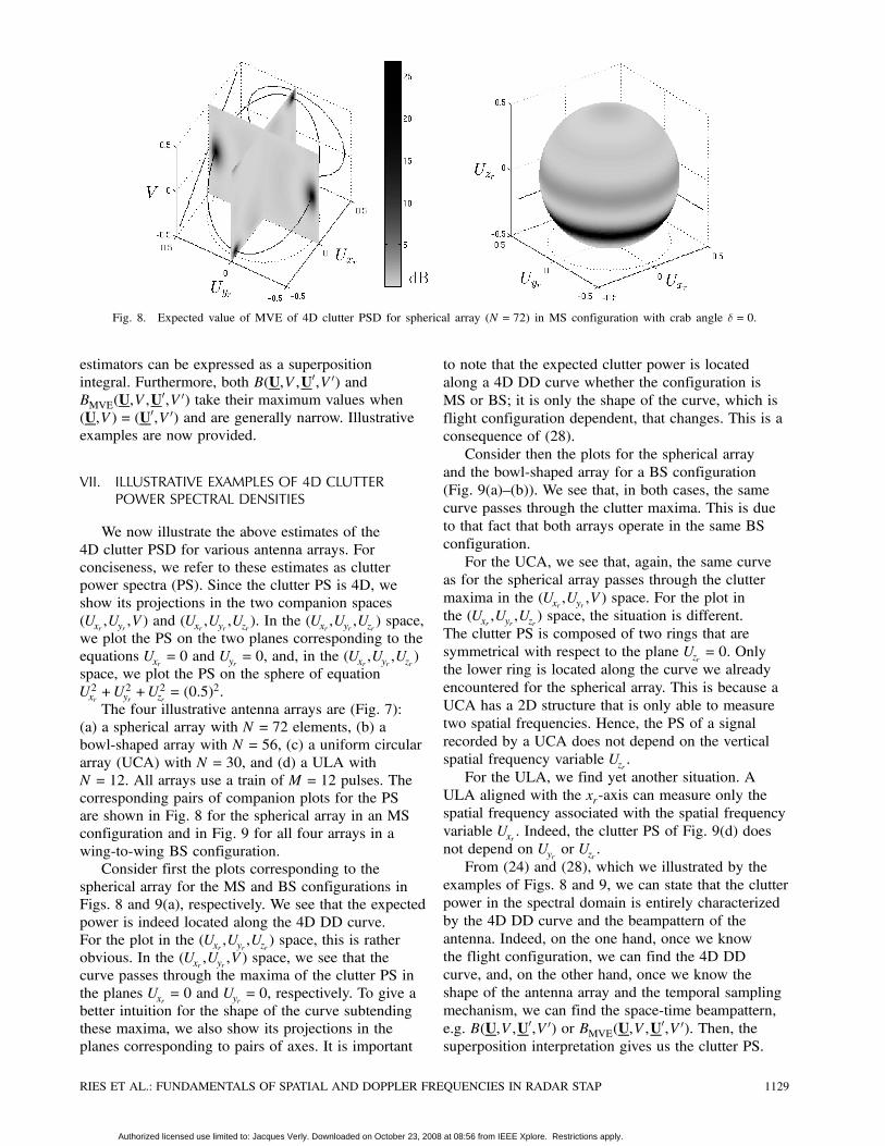
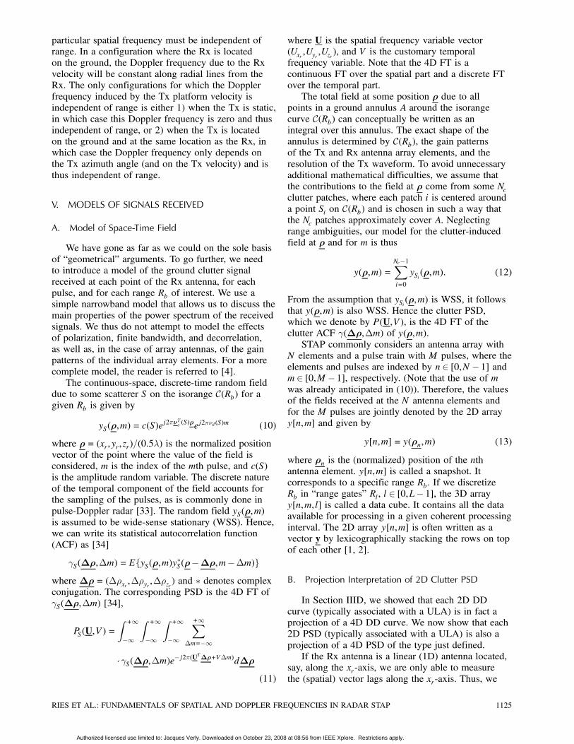
Fig. 8. Expected value of MVE of 4D clutter PSD for spherical array (N = 72) in MS configuration with crab angle ± = 0.

estimators can be expressed as a superpositionintegral. Furthermore, both B(U,V,U0,V0) andBMVE(U,V,U

0,V0) take their maximum values when(U,V) = (U0,V0) and are generally narrow. Illustrativeexamples are now provided.

VII. ILLUSTRATIVE EXAMPLES OF 4D CLUTTERPOWER SPECTRAL DENSITIES

We now illustrate the above estimates of the4D clutter PSD for various antenna arrays. Forconciseness, we refer to these estimates as clutterpower spectra (PS). Since the clutter PS is 4D, weshow its projections in the two companion spaces(Uxr ,Uyr ,V) and (Uxr ,Uyr ,Uzr ). In the (Uxr ,Uyr ,Uzr ) space,we plot the PS on the two planes corresponding to theequations Uxr = 0 and Uyr = 0, and, in the (Uxr ,Uyr ,Uzr )space, we plot the PS on the sphere of equationU2xr +U

2yr+U2zr = (0:5)

2.The four illustrative antenna arrays are (Fig. 7):

(a) a spherical array with N = 72 elements, (b) abowl-shaped array with N = 56, (c) a uniform circulararray (UCA) with N = 30, and (d) a ULA withN = 12. All arrays use a train of M = 12 pulses. Thecorresponding pairs of companion plots for the PSare shown in Fig. 8 for the spherical array in an MSconfiguration and in Fig. 9 for all four arrays in awing-to-wing BS configuration.Consider first the plots corresponding to the

spherical array for the MS and BS configurations inFigs. 8 and 9(a), respectively. We see that the expectedpower is indeed located along the 4D DD curve.For the plot in the (Uxr ,Uyr ,Uzr ) space, this is ratherobvious. In the (Uxr ,Uyr ,V) space, we see that thecurve passes through the maxima of the clutter PS inthe planes Uxr = 0 and Uyr = 0, respectively. To give abetter intuition for the shape of the curve subtendingthese maxima, we also show its projections in theplanes corresponding to pairs of axes. It is important

to note that the expected clutter power is locatedalong a 4D DD curve whether the configuration isMS or BS; it is only the shape of the curve, which isflight configuration dependent, that changes. This is aconsequence of (28).Consider then the plots for the spherical array

and the bowl-shaped array for a BS configuration(Fig. 9(a)—(b)). We see that, in both cases, the samecurve passes through the clutter maxima. This is dueto that fact that both arrays operate in the same BSconfiguration.For the UCA, we see that, again, the same curve

as for the spherical array passes through the cluttermaxima in the (Uxr ,Uyr ,V) space. For the plot inthe (Uxr ,Uyr ,Uzr ) space, the situation is different.The clutter PS is composed of two rings that aresymmetrical with respect to the plane Uzr = 0. Onlythe lower ring is located along the curve we alreadyencountered for the spherical array. This is because aUCA has a 2D structure that is only able to measuretwo spatial frequencies. Hence, the PS of a signalrecorded by a UCA does not depend on the verticalspatial frequency variable Uzr .For the ULA, we find yet another situation. A

ULA aligned with the xr-axis can measure only thespatial frequency associated with the spatial frequencyvariable Uxr . Indeed, the clutter PS of Fig. 9(d) doesnot depend on Uyr or Uzr .From (24) and (28), which we illustrated by the

examples of Figs. 8 and 9, we can state that the clutterpower in the spectral domain is entirely characterizedby the 4D DD curve and the beampattern of theantenna. Indeed, on the one hand, once we knowthe flight configuration, we can find the 4D DDcurve, and, on the other hand, once we know theshape of the antenna array and the temporal samplingmechanism, we can find the space-time beampattern,e.g. B(U,V,U0,V0) or BMVE(U,V,U

0,V0). Then, thesuperposition interpretation gives us the clutter PS.



Fig. 9. Expected value of MVE of 4D clutter PSD for (a) spherical array (N = 72), (b) bowl-shaped array (N = 56),(c) UCA (N = 30), (d) ULA (N = 12) in same wing-to-wing BS configuration.



VIII. DISCUSSION

With the recent increase of interest in CAAsand AAAs, there has been a need to generalize thecustomary view based on a single spatial frequency,which is so familiar for ULAs. However, realizingthat one must use two or three spatial frequenciesfor arrays other than ULAs is just half of the story.The second half is that it may be advantageous toalways consider the three spatial frequencies, whichalways exist, independently of any antenna. Thesethree spatial frequencies are defined for any set ofthree axes. Once these axes are chosen, one can talkabout the dependencies between the three normalizedspatial frequencies (ºsxr ,ºsyr ,ºszr ) and the normalizedDoppler frequency ºd. The result is the 4D DD curve.This curve only depends upon the measurementconfiguration, whether MS or BS; specifically, it doesnot depend upon the form of the receive antenna.With the knowledge of the 4D DD curve, one can

quickly reason about what happens for various typesof antennas, whether arrays or not. For example, inthe case of a linear antenna, one can simply projectthe 4D DD curve into an appropriate 2D subspaceto find the 2D DD curve in conventional (ºs,ºd)space. Similarly, one immediately sees what happensif the angle of the antenna varies. When we rotatethe set of reference axes in physical space, the 4DDD curve simply rotates as a result of the rotationproperty of spatial frequencies (which can also beinvoked to explain the basic rotation property of FTsof dimensionality of two or higher). All of the abovecan be discussed on the sole basis of geometricalarguments (and of the knowledge of the wavelengthof the wave of interest). To go further, one mustintroduce a statistical model of the clutter field sensedby the array elements.By introducing a 4D WSS random process of

space and time to model this field, we are led toconsider a 4D (clutter) statistical, space-time ACF andthe corresponding 4D (clutter) PSD. These becomethe primary tools for investigating the statisticalproperties of the (clutter) signals at the array elements.(Recall that the only source of randomness consideredhere is the clutter reflectivity.) The PSD (and thestatistical ACF) only depend upon the measurementconfiguration; specifically, it does not depend uponthe form of the receive antenna. The 4D PSD is thestatistical counterpart of the geometrical 4D DD curve.Just as with the 4D DD curve, one can also, with

the knowledge of the 4D PSD, quickly reason aboutwhat happens for various types of antennas. Forexample, in the case of a linear antenna, one cansimply project (in the sense of line integration) the4D PSD into an appropriate 2D subspace to find the2D PSD in (ºs,ºd) space. This projection property forPSDs is the counterpart of the projection propertyfor DD curves. Interestingly, the simplest proof of

this property relies on the projection-slice theoremof tomography. The rotation property observed for 4DDD curves also applies to 4D PSDs. Finally, there isa close link between the ridge of the PSD and the DDcurve, whether in 4D or in some subspace.

IX. CONCLUSION

We have taken a fresh and thorough look at theconcept of spatial and Doppler frequencies in thecontext of STAP for arbitrary antenna arrays. Byclearly separating the “geometrical” and statisticalaspects of the problem, we have achieved one of thesimplest possible presentations. Indeed, we went asfar as introducing the notion of 4D DD curve andall of its important properties, without having tointroduce any concept of statistical signal processing.One key observation is that the 4D DD curve onlydepends upon the measurement configuration and isthus independent of the form of the receive antenna.For any given configuration, one can start from thisfundamental 4D curve to handle any antenna. Inparticular, one can use it to get a better understandingof the standard 2D DD curve corresponding to alinear antenna and to see what happens when theantenna rotates. By introducing a WSS randomprocess of space and time to describe the field dueto the clutter scatterers at a given range, we wereled to consider the 4D PSD of this WSS randomprocess, which effectively begins to populate the4D (ºsxr ,ºsyr ,ºszr ,ºd) space with real values. The 4DPSD enjoys rotation and projection properties thatare the counterparts of those for the 4D DD curve.The relations between the DD curves and the PSDswere also established. This paper constitutes a solid,simple, and elegant basis for thinking about STAPfor arbitrary measurement configurations and antennaarrays, and, thus, we hope, for helping with the designof advanced STAP-based radar systems operating inchallenging conditions, e.g. in BS, or even multistatic,configurations and with conformal antenna arraysadapted to the carrying platforms.

REFERENCES

[1] Klemm, R.Principles of space-time adaptive processing.IEE Radar, Sonar, Navigation, and Avionics, 9 (2002).

[2] Ward, J.Space-time adaptive processing for airborne radar.MIT Lincoln Laboratory, Lexington, MA, Technicalreport 1015, 1994.

[3] Lapierre, F. D., and Verly, J. G.Registration-based solutions to the range-dependenceproblem in STAP radars.In Adaptive Sensor Array Processing Workshop, MITLincoln Laboratory, Lexington, MA, Mar. 11—13, 2003.

[4] Hersey, R., Melvin, W., and McClellan, J.Clutter limited detection performance of multi-channelconformal arrays.Signal Processing, 84 (May 2004), 1481—1500.



[5] Neyt, X., Ries, P., Verly, J. G., and Lapierre, F. D.Registration-based range-dependence compensationmethod for conformal array STAP.In Adaptive Sensor Array Processing Workshop, MITLincoln Laboratory, Lexington, MA, June 7—8, 2005.

[6] Neyt, X., Lapierre, F. D., and Verly, J. G.Automatic configuration-parameters estimation andrange-dependence compensation using simulated,single-realization, random snapshots in STAP.In Adaptive Sensor Array Processing Workshop, MITLincoln Laboratory, Lexington, MA, Mar. 16—18, 2004.

[7] Klemm, R.Comparison between monostatic and bistatic antennaconfigurations for STAP.IEEE Transactions on Aerospace and ElectronicSystems, 36, 2 (2000), 596—608.

[8] Lapierre, F. D.Registration-based range-dependence compensation inairborne bistatic radar STAP.Ph.D. dissertation, University of Liege, Liege, Belgium,Nov. 2004.

[9] Ries, P., Neyt, X., de Greve, S., Lapierre, F. D., and Verly,J. G.Range-dependence compensation in STAP for arbitraryengagement geometries and receiver antenna arrays.In RTO-SET 095 Specialist Meeting, La Spezia, Italy, June7—9, 2006.

[10] Borsari, G.Mitigating effects on STAP processing caused by aninclined array.In IEEE National Radar Conference, Dallas, TX, May12—13, 1998.

[11] Melvin, W., Callahan, M., and Wicks, M.Adaptive clutter cancellation in bistatic radar.In 34th Asilomar Conference on Signals, Systems, andComputer, Pacific Grove, CA, Oct. 29—Nov. 1, 2000.

[12] Melvin, W., Himed, B., and Davis, M.Doubly adaptive bistatic clutter filtering.In IEEE National Radar Conference, Hunstville, AL, May5—8, 2003.

[13] Pearson, F., and Borsari, G.Simulation and analysis of adaptive interferencesuppression for bistatic surveillance radars.In Adaptive Sensor Array Processing Workshop, MITLincoln Laboratory, Lexington, MA, Mar. 13—14, 2001.

[14] Lapierre, F. D., and Verly, J. G.Registration-based method for range-dependencecompensation in bistatic radar STAP operating onsimulated stochastic snapshots.EURASIP JASP Journal, 2005.

[15] Kim, K., Zhang, Y., Hajjari, A., and Himed, B.A uniform planar virtual approach to conformal arraySTAP.In IEEE International Radar Conference 2004, Toulouse,France, Oct. 19—21, 2004.

[16] Ries, P., Lapierre, F. D., and Verly, J. G.RANSAC-based flight parameter estimation forregistration-based range-dependence compensation inairborne bistatic STAP radar with conformal antennaarrays.In European Radar Conference, Manchester, UK, Sept.13—15, 2006.

[17] Goodman, J.Introduction to Fourier Optics (2nd ed.).New York: McGraw-Hill, 1996.

[18] Goodman, J.Statistical Optics.New York: Wiley, 1985.

[19] Thompson, A., Moran, J., and Swenson, G. Jr.Interferometry and Synthesis in Radio Astronomy,(2nd ed.).New York: Wiley, 2001.

[20] Forsyth, D., and Ponce, J.Computer Vision–A Modern Approach.Upper Saddle River, NJ: Prentice-Hall, 2003.

[21] Trees, H. V.Detection, Estimation, and Modulation Theory, Part IV:Optimum Array Processing.New York: Wiley, 2002.

[22] Himed, B., Zhang, Y., and Hajjari, A.STAP with angle-Doppler compensation for bistaticairborne radars.In IEEE National Radar Conference, Long Beach, CA,May 22—25, 2002.

[23] Brennan, L., and Reed, L.Theory of adaptive radar.IEEE Transactions on Aerospace and ElectronicSystems, AES-9, 2 (1973), 237—252.

[24] Gerrish, F.Pure Mathematics Volume II: Algebra, Trigonometry,Coordinate Geometry.London: Cambridge University Press, 1960.

[25] Baranoski, E.Improved pre-Doppler STAP algorithm for adaptiveclutter nulling in airborne radars.In 29th Asilomar Conference on Signals, Systems andComputer, Pacific Grove, CA, Oct. 30—Nov. 1, 1995.

[26] Klemm, R.Adaptive airborne MTI: Comparison of sideways andforward looking radar.In IEEE International Radar Conference, Alexandria, VA,May 8—11, 1995.

[27] Gu, Z., Blum, R., Melvin, W., and Wicks, M.Comparison of STAP algorithms for airborne radar.In IEEE National Radar Conference, Syracuse, NY, May13—15, 1997.

[28] Zatman, M.Performance analysis of the derivative based updatingmethod.In Adaptive Sensor Array Processing Workshop, MITLincoln Laboratory, Lexington, MA, Mar. 13—14, 2001.

[29] Melvin, W.Space-time adaptive radar performance in heterogeneousclutter.IEEE Transactions on Aerospace and ElectronicSystems, 36, 2 (2000), 621—633.

[30] Lapierre, F. D., Neyt, X., and Verly, J. G.Performance evaluation of a registration-basedrange-dependence compensation method for bistaticSTAP radar using simulated snapshots.In IEEE International Radar Conference 2004, Toulouse,France, Oct. 19—21, 2004.

[31] Lapierre, F. D., and Verly, J. G.Computationally-efficient range-dependencecompensation method for bistatic radar STAP.In IEEE National Radar Conference, Arlington, VA, May9—12, 42005.

[32] Neyt, X., Lapierre, F. D., and Verly, J. G.Estimation of geometric radar configuration parametersfor range-dependence compensation in STAP in thepresence of targets, jammers and decorrelation effects.In IEEE Sensor Array and Multichannel Signal Processing(SAM) Conference, Barcelona—Sitges, Spain, July 18—21,2004.

[33] Skolnik, M.Introduction to Radar Systems, (3rd ed.).New York: McGraw-Hill, 2001.



[34] Manolakis, D., Ingle, V., and Kogon, S.Statistical and Adaptive Signal Processing.New York: McGraw-Hill, 2000.

[35] Gray, R. M., and Goodman, J. W.Fourier Transforms: An Introduction for Engineers.Boston: Kluwer Academic Publishers, 1995.

[36] Oppenheim, A., and Schafer, R.Discrete-Time Signal Processing.Upper Saddle River, NJ: Prentice-Hall, 1999.

Philippe Ries was born in Luxembourg, Luxembourg. In 2004, he received hiselectrical engineering degree (summa cum laude) from the University of Liege,Liege, Belgium.He is currently a Ph.D. student in the Laboratory for Signal and Image

Exploitation of the Electrical Engineering and Computer Science Departmentof the University of Liege. His doctoral research is sponsored by the “FondNational de la Recherche Scientifique (FNRS),” Brussels, Belgium. His researchinterests are mainly focused on array processing (conformal antenna arrays) andspace-time adaptive processing.In 2004, Mr. Ries received, from the Association of Engineers from the

Montefiore Electrical Institute (AIM), the Melchior Salier Prize for the bestMaster thesis in electronics engineering and, in 2006, he received the EuropeanMicrowave Association (EuMA) RADAR Prize for the best paper presented at theEuropean Radar Conference (EURAD) 2006.

Xavier Neyt received the engineering degree (summa cum laude) from the FreeUniversity of Brussels (ULB) in 1994. In 1995 he received the Frerichs Awardfrom the ULB and the special IBM grant from the Belgian National Fund forScientific Research (NFWO).Since 1995 he has been working as research engineer for the Royal Military

Academy, Belgium. In 1996—1997 he was visiting scientist at the Frenchaerospace center (ONERA) and in 1999 at the German aerospace centre (DLR).In 1997—1999 he was responsible for the design of the image compressionmodule of the European MSG satellite and in 2000—2005, responsible for theredesign of the ground processing of the scatterometer of the European ERSsatellite following its gyroscope anomaly. His research interests include signalprocessing in general and applied to radar with emphasis on array processing andspace-time adaptive processing.

Fabian D. Lapierre was born in Huy, Belgium. He received the IngenieurElectronicien degree from the University of Liege, Belgium, in 2000. In2004, thanks to a fellowship of the F.N.R.S. (Fond National de la RechercheScientifique), Brussels, Belgium, he received the Ph.D. degree from theUniversity of Liege, Belgium.Currently, he is a member of the Electrical Department of the Royal Military

Academy in Brussels, Belgium. His research interests are mainly focussed onspace-time adaptive processing, on the simulation of infrared target signatures,and on image synthesis. He is also interested in the fusion of sensors informationfor targets detection.

[37] Chen, C.-T.Introduction to Linear System Theory.New York: Holt, Rinehart, and Winston, 1970.

[38] Capon, J.High resolution frequency wavenumber spectrumanalysis.Proceedings of IEEE, 57, 8 (1969), 1408—1418.



Jacques G. Verly was born in Liege, Belgium. He received the IngenieurElectronicien degree from the University of Liege, Belgium, in 1975. Through asponsorship of the Belgian American Educational Foundation (BAEF) he attendedStanford University, Stanford, CA, where he received the M.S. and Ph.D. degreesin electrical engineering in 1976 and 1980, respectively.From 1980 to 2000, he was a member of the technical staff at MIT Lincoln

Laboratory, Lexington, MA, where he carried out research in several differentareas, including image processing and computer vision for a variety of imagingsensors, such as visible, laser radar, fully polarimetric SAR, IR, multispectraland hyperspectral. During his last few years at MIT, he worked in multimodalityimage fusion and mining, 3D site modelling, and 3D stereo visualization. Since2000, he has been a professor in the Department of Electrical Engineering andComputer Science (also known as the “Institut Montefiore”) of the University ofLiege, Belgium, where he is the Head of Signal Processing Group, a foundingmember of the Laboratory for Signal and Image Exploitation (INTELSIG),and in charge of the core courses in signal processing. His current researchinterests are principally in medical imaging (image-guided surgery), radar signalprocessing (space-time adaptive processing), object tracking in video streams (forvideosurveillance and sports analysis), and nano satellites.In 2003—2004, Dr. Verly was the holder of one of the two prestigious

Francqui Chairs at the Free University of Brussels (ULB). He has about 200publications, mostly in the area of image processing and computer vision foradvanced imaging systems, as well as 2 U.S. patents. He is a CRB Fellow of theBelgian American Educational Foundation.



Fundamentals of Spatial and Doppler Frequencies in Radar STAP

Documents

Transcript of Fundamentals of Spatial and Doppler Frequencies in Radar STAP