Transportation Research Record 994 41

Optimal Design of Bus Routes and

Frequencies for Ahmedabad

B. R. MAHWAH, FAROKH S. UMRIGAR, and S. B. PATNAIK

ABSTRACT

A method is developed to simultaneously se­lect routes and assign frequencies for a bus transit system. The method is intended (a) to concentrate the flow of passengers on the road network in such a way that the sum of passenger riding-time cost and operation cost is minimized, (b) to generate a large set of possible bus routes that satisfy cer­tain constraints, and (c) to simultaneously select the routes and their frequencies so that the number of transfers saved in the network is maximized. Heuristics are used for the concentration of flow and generation of routes, and linear programming is used to select routes and theiI frequencies. The model was applied to the design of a bus transit system for the city of Ahmedabad. Four alternative networks with 514, 492, 426, and 402 links, respectively, were eval­uated for the concentration of passenger flows , and the minimum cost (riding-time cost plus operation cost) was obtained for the network of 426 links. This network was used to generate 457 feasible routes. A to­tal of 421 turning movements for the network was identified. The optimal routes and their frequencies were obtained by the linear pro­gramming model for three different operating fleet sizes of 670, 750, and 790 buses, re­spectively.

Ahmedabad, population 2.1 million, is the sixth largest metropolis in India and is the largest in­dustrial city in the state of Gujarat. The city is accessible by seven major highways and five major rail links, both broad and meter gauge, from dif­ferent parts of the state and the country. Because of its great accessibility, the city has grown con­centrically (1). The bus transit system in the city is operated by Ahmedabad Municipal Transport Service (AMTS). AMTS operates 191 bus routes with an operat­ing fleet of 670 buses. Approximately 0.85 million passengers per day are served by 10,600 scheduled bus trips. Average route length is 8 km (1). The transit network consists of 134 important- nodes. Transit network expansion has largely been the re­sult of sociopolitical demands in the absence of a well-defined route location policy (1, 2). Increases in routes inconsistent with the fleet ;ize have re­sulted in parallel operations, low load factors, and low frequencies. As a result nearly one-third of the existing routes are uneconomical.

A st.uily of the literature on the various models of bus transit planning (3-8) indicates that the generation of routes and scheduling of vehicles are generally done sequentially. On the basis of the given desired travel matrix, the routes are first generated one at a time. Routes are evaluated with­out considering the routes already accepted for the

network. This neglects, to a great extent, the in­teractions between the transit routes. The sched­uling of vehicles on the routes is done after all the routes in the network have been determined.

This study has developed a method whei:eby the selection of routes and the assignment of frequen­cies are done simultaneously for the bus transit system . The method is a combination of heuristic search and programming models and has been applied in the optimal design of the bus transit network for Ahmedabad (!). The model structure is shown in Figure 1.

I Existing Bus Transit Network I I

l t • Identify Alternative Generation of Establish Networks of Road Desire Travel 1. Relationship between Links on Which Buses Matrix number of buses on a Could Travel link and link flow

2. Weightage of vehicle time cost compared to passen-ger riding-time cost

• • Model for Concentration of Passenger Flow

Minimizes the operation cost and passenger riding-time cost

• Network of Road Links To Be Used by Bus Transit

System

I Model for Generation of Routes

Generates a set of all possible routes that satisfy various constraints

I Determine for Each Generated Route

1. Various turning movements and the turning flows

2. Number of transfers saved at each node and total for the route

1 Linear Programming Model for Simultaneous

Selection of Routes and Frequencies

Maximizes the total number of transfers saved in the system

FIGURE 1 Structure of the model.

MODEL FOR CONCENTRATION OF PASSENGER FLOW

The model estimates where the passengers are ex­pected to travel in the optimal route system. If all the passengers travel along their shortest paths, this would imply an extremely dispersed route ne·t­work with low vehicle use and many vehicle hours. On

42

the other hand if the vehicles are filled to capac­ity, the implication is that passengers are concen­trated in large flows and thus have to make substan­tial detours from their shortest paths, resulting in increased r1ding time. To reach a reasonable compro­mise between these two extremes, the sum of opera­tion cost and passenger riding-time cost is mini­mized for the fixed desired origin-destination (0-D) matdx,

Let RTi be the riding time on link i and LKFLOWi the passenger flow in unit time on link i. Then the total riding time for all the passenge r s is LRTi • Ll<FLOW1 and the total. vehicle time for the i network is LRTi • NOBUSi where NOBUS1 is the number

i of bus trips to be made in a unit time on link i. The object i ve function is

Minimize Z1 = fRTi • LKFLOWi + ?RTi • NOBUSi • W (1) J.

subject to satisfaction of given travel demand, where Wis the value of vehicle time compared to the riding time of passengers.

The number of trips to be made in a unit time on a link NOBUS1 depends on the pa.ssenger ·flow on that link, LKFLOWi. Some studies (!,10,1!) ind cate that NOBUS1 is directly proportional to the square root cf pass.;ng,=rs 011 a link. I n the absence of a.ny such relationship for Indi.an cities, the average link flow of passengers on a route for all the 191 routes is related to the existing number of bus trips on that route as

NOBUSi = 0.137LKFL0Wi 0.795 R2 = 0.88 (2)

where NOBUSi is the number of bus trips to be made in a unit time on link i and LKFLOW1 is the flow of passengers in unit tlme on link i.

Next, to rationalize the relationship between the value of vehicle time and that of the riding time of passengers, the following equation is developed:

W = BUSKMH • KMCOST/VT (3)

where

W = value of vehicle time relative to that of passenger riding time,

BUSKMH average kilometers traveled by the bus in an hour,

KMCqST = operating cost of a bus per kilometer, and

VT value of the riding-time hours of the riders,

The ope rating cost (KMCOST) per bus kilometer is found by considering salaries, allowances, fuel and oil consumptions, repair and spare parts plus other ovechead charges, depreciation, and so forth. The value of a riding-time hour (VT) of the passenger is found by estimating the average income of captive users. The average bus-kilometers traveled per hour (BUSK~m) is obtained from the existing data on bus speeds on various links of the network. The mean value of was estimated as 1S.

The objective function (Equation 1) can be writ­ten as

zi = LRTi • LKFLOWi

+ LRTi • 0.137LKFL0Wi 0.795 W (4)

1\fter substituting the values of NOBUSi and W from Equations 2 and 3, respectively, the objective func­tion is

Transportation Research Record 994

Minimize z1

where

1LKFLOWi • RTi (1 i + (2.055/LKFLOWi 0.205)]

lLKFLOWi • Ti i

Ti= RT1 [l + (2.055/LKFLOWi 0.205)]

(5)

(6)

To obtain the minimum value of the nonlineac ob­jective function a heuristic algorithm is used. r,. backward approach (i.e., deleting links from a fine­meshed network) appears to give better r.esults than a forward approach (i.e., adding links to the min­imal spanning tree). Initially , all of the 514 uni­directed links on which buses can travel are taken and then the number is reduced to that of t he coa se-111,:,:,hed networl< (402 links). For this study, four networks are tested. The heuristic algorithm used for each of the four different networks to obtain total cost in terms of time is as follows:

1. The shoe test paths for all. the O-D pairs are obtained. In the first iteration, only riding time (RTil is considered, but in subsequent iterations the sum Of riding and vehicle time (as revised in the subsequent steps1 i.e., Til is used, Using the shortest paths, all the link flows (LKFLOW 1> are estimated for the given 0-D matrix.

2. The time to traverse link i (Ti) is revised (T1) based on the link flow (LKFLOWil using the following relationship:

Ti= (RT)1 (1 + (2.055/LKFLOWi 0.205)]

3. The revised time (Ttl obtained in Step 2 is used to find the shortest paths for all the o-o pairs, and a revised value of the link flow (LKFLO\ftl is obtained.

4. The total link time (i.e., LTi ~ and total time for the network LT!• LKFLOW1) are computed. i

Ti • LKFLOW1) (i.e., TLT =

5. If any link time (i.e., LT1) or total link time (TLT) gets changed in Step 4, the procedure is repeated starting with Step 21 otherwise it is stopped.

This procedure is repeated for all four networks. It is observed that generally about four iterations need to be performed for each network to obtain the convergence of the total link time. •rhe results (Table 1) indicate that by deleting some links from the starting network of 514 links, the total time is reduced until a certain stage is reached and then total time starts increasing. The minimum time is for the network with 426 links. This network is con­sidered in the further analysis.

MODEL FOR GENERATION OF ROUTES

This model generates a large set of all possible routes through a heuristic algorithm that considers the following constraints to avoid the possibility of generating some unfeasible routes:

1. The length of the route should not be less than 2.0 km.

2, The path of the route between two terminating stations should not meander excessively from th~ shortest path. The length of the path of a route

. .

Marwah et al. 43

TABLE 1 Concentration of Passenger Flows in Alternative Networks

Iteration

2 ( total riding + 3 (total riding+ 4 ( total riding + Network No. of Links I (total riding vehicle time in vehicle time in vehicle time in No. in Network time in min) min) min) min)

1 514 11,897,919 13,704,568 13,718,200 13,720,158 2 492 11,898,220 13,705,189 13,718,554 13 ,720,282 3 426 11,903,306 13,723,576 13,717,526 13,717,565 4 402 11,954,794 13,773,298 13,767,130 13,773,238

should not be greater than twice the shortest dis­tance between the termini.

3. There should not be any backtracking on the route.

In cases where there are a number of intermediate stations on the shortest path between two termini, there may be an extremely large number o f alterna­tive paths that may be formulated. It is desirable that the nodes inser ted be selected rationally with­out leaving the combinations that satisfy the basic requirements .

The network consists of 134 nodes and there are 8,911 different 0-D pairs that are to be served by the routes. To determine the terminating stations, it is desirable that the routes run through the major generators. Routes are also generated from other stations to satisfy the entire 0-D matrix. In some studies (3,5,7) the routes between the major generators are -fixed first, but the difficulty is that of s atisfying the various requirements of a route in an optimal way. In this method the paths of the routes between closer terminals are first deter­mined and then expanded for the distant ones. The already developed paths are of great significance in the location of the paths of the routes between the distant termini.

This is a four-step procedure:

1. All the o-o pairs that have direct links be­tween them are first selected for route generation. Let i and j be the nodes directly connected by link i-j. Alternative paths for this route between i and j can be found by inserting the intermediate nodes (e.g., k) such that path i-k-j $atisfies the re­~uirements: namely, the length of the path i-k-j is less than twice the shortest distance between nodes i and j (Figure 2). In this way all possible inter­mediate nodes k (k1, k2, ••• l that can be in­serted are analyzed.

DIRECT ROUTE

I

IF SD(i,k)+SO (k 1 j) ~2·0•SD (i,j)

THEN NOOE k (k~k1,kz,k3---·) IS

INSERTED OTHERWISE NOT,

:IIL TERNATIVE PATHS

FOR THE 0-0 PAIR

i -j

FIGURE 2 Alternative paths for directly connected 0-D pair.

2. The o-o pairs, not directly connected, are divided into various groups according to the short­est distance through them. In this study, the o-o pairs are divided into nine different groups start­ing with 1.5 to 20 km. The generation of the routes is first done for the closer o-o pairs and then ex­panded by using information on previously generated routes.

3. For a given group of 0-D pairs the alterna­tive paths of the route are generated as follows: Let i-j be the 0-D pair having stops i1, i2, i 3 , . , , on the shortest path between them. Let k1 be the node to be inserted such that the short­est path between i and j via k (i.e., SD(i,k1) + SD(k 1 ,j) 1 is less than l. 5 times the shortest dis­tance between i and j [SDU,j) J. All ·the previously established routes between i and k1 (i.e., R11, R12, R13 , ••• ) and between k1 and j (i.e., R21• Rz2' R23• • , ) are considered (Figure 3). Al l the combinations of the routes between i and k1 and k1 and j are analyzed so that the total length of the selected path between i and j does not exceed twice the shortest distance betwee·n i and j,

SHORTEST PA"(H FOR 0 0 PAIR ( i-j)

IF SO (i,k)+SD (k,j) :f> 1·51JSD(i,j)

THEN NODE k(K-k1,k2,k3 - - - - ) IS

INSERTED OTHERWISE NOT.

FIGURE 3 Alternative paths for 0-D pair not directly connected.

The procedure ii; repeater! for all the possible intermediate nodes (i.e., k1, kz, k3, • ) to be inserted, and all the feasible routes are stored.

4. Step 3 is repeated for all the 0-D pairs of a group.

44

This heuristic procedure generated 457 possible routes for the Ahmedabad network.

When a route diverts or terminates at a node, the passengers destined for a node not lying on the route have to transfer.

Let the path of a route be represented by nodes 1, 2, 3, and 4 and links 1, k, and m as shown in Figure 4 (a) • Let (TURNFL) lk be the number of pas­sengers .going directly from link 1 to link k and vir.P v~r~~. Th& various turning movements on a omall network are shown in Figure 4(b). The estimated num-

(TURNFL)lk

1---~---10 '\--' - ""'-k - -(o) TURNING MOVEMENTS ALONG A ROUTE

~ NOOE

(b) TURNING MOVEMENTS AT A NOOE j IN A PART

OF A NETWORII

FIGURE 4 Number of transfers saved on a route.

ber of bus trips per day is NOBUS1 on link 1. If a route goes directly from link 1 to link k, the num­ber of transfers saved per route trip for this route and this turning flow is estimated by the following relationship:

NOTRANpr = [TURNFL1k/Minimum (NOBUS1, NOBUSk)l (7)

where

Minimum (NOBUS1, NOBUSk)

number of transfers saved for pth turning flow of router, number of passengers traveling from link 1 to link k and vice versa, and minimum value of the number of bus trips on the two links 1 and k.

The procedure for calculating the number of transfers saved by a route trip is as follows:

1. All turning flows along the route are found using the 0-D matrix.

2. The number of bus trips on each link is esti­mated using the relationship (Equation 2) between link flow and the number of bus trips. The link ~low is found by using the 0-D matrix.

3. The number of transfers saved for each turn­ing flow per route trip is found by Equation 7.

4. The total number of transfers saved by a

Transportation Research Record 994

route TTRANr is found by surmning the transfers saved for each turning movement along the route.

This procedure was used for the case study net-. work, and the number of transfers saved by each of the 457 routes was obtai ned, For each r oute , the transfer s saved were ca l c ulated along the route and added to get the total number of transfers saved. Then all turning movements on the network were iden­tified, The different values of the various turning movements were obtained for various routes. From these the maximum value of a turning movement was found.

For the Ahmedabad network, 421 turning movements were identified and the maximum value of each tur n­ing flow was determined.

SIMULTANEOUS CHOICE OF ROUTES AND FREQUENCIES

In the preceding phases passengers were assigned paths on the basis of passenger riding-time cost and operation cost. A set of intersecting routes ( 457) was generated. In this phase an optimal set of routes and frequencies is obtained such that as many transfers as possible are avoided. The problem is formulated and solved as a linear programming (LP) problem.

The objective function is

NR Maximize Z = 1 TTRANr • FREQr

r=l

subject to four sets of constraints

NR

1 NOTRANpr • FREQr 2. MAXTFLP Yp i=l

NR 1 RTTIMEr • FREQr 2. OT• OPF

i=l

where

NOTRANpr = number of transfers saved for pth turning flow of router,

FREQr = frequency on router, TTRANr total number of transfers saved by

NR MAXTFLp =

RTTIMEr = MAXFREr NOTRANp

OPF OT=

router, number of routes in a network, maximum value of the turning flow the pth turning movement, round-trip time on router, maximum frequency of router, number of transfers saved for pth turning flow, operating fleet size, and operating time in hours.

(8)

(9)

(10)

(11)

(12)

for

The first constraint set (Equation 9) contains TTF equations where TTF is the total number of turn­ing moments in the network. The different values of the pth turning movement are obtained for various routes. From these, the maximum value of the pth turning movement (MAXTFL) is found and no more than this numbe r of transfers can be saved. The sec­ond constraint set (Equation 10) takes into consid­eration the operating fleet size. The third con­straint set (Equation 11) takes into consideration

Marwah et al.

the upper boundary on frequency for every route, The fourth constraint set (Equation 12) considers the non-negativity requirements of the number of trans­fers saved for the pth turning movement.

ANALYSIS OF RESULTS

For the fixed 0-D matrix of Ahmedabad, the model generates 426 links on the network on which the pas­senger flow can be concentrated to minimize the total cost (riding-time cost plus vehicle operation cost). The network consisting of these 426 links (213 links in each direction) and 134 nodes is used to generate the feasible routes that satisfy the basic requirements of the routes and meet the de­mand. A total of 457 routes is generated and 421 turning movements are identified. The optimal routes and their frequencies are obtained for seven dif­ferent zones and for the entire network using three different operating fleets of 670, 750, and 790 buses. A summary of the outputs is given in Tables 2 and 3. The results indicate that the number of

TABLE 2 Summary of Outputs for the Different Zones

No. of Maximum No. of Zone Part of Fleet Optimal Frequency Transfers No . Network Size Routes per Day Saved

Central 52 8 340 235 ,777 69 14 340 288,417 88 23 333 323,074

2 West 102 35 120 316,841 114 35 120 316,841 117 35 120 316,841

3 North 154 34 111 334,631 166 34 111 334,631 172 34 111 334,631

4 Southeast 99 35 224 354,924 110 43 223 358,692 114 43 223 358,692

5 East 64 16 141 200,665 72 30 123 230,307 74 30 123 230,307

6 Northeast 114 32 170 339,228 125 32 170 339,228 129 32 170 339,228

7 South and 85 26 192 269,310 southwest 94 28 192 270,043

96 28 192 270,043

TABLE 3 Summary of Outputs for the Network

Total Fleet Size

670 750 790

No. of optimal routes 160 191 207 Average route length (km) 6.625 6.11 5.8 No. of transfers saved (I 03 ) 2,052 2,138 2,173

routes in the optimal solution, the number of trans­fers saved, and the average route length are af­fected by the size of the operating fleet for the network. Figure 5 shows that as the size of the operating fleet for the network increases, the num­ber of routes in the optimal solution also in­creases, This happens because increased numbers of vehicles help run more routes and thus maximize the number of transfers saved. Figure 6 shows that more transfers are saved with increased numbers of routes or increased size of the operating fleet.

As the number of routes in the optimal solution

"' ~ :,

~ 0 .. .. .J:J E :, C

0 E .. Q. 0

45

250

200

150

650 700 750 00 Fleet size

FIGURE 5 Relationship between optimal number of routes and fleet size for the network.

2200

"' ~ "O 2150 .. > 0 .. ~ ~ "' C 0 .. .. ... 0 2100 .. ..

.J:J

E :, z

Fleet size

FIGURE 6 Relationship between number of transfers saved and fleet size for the network.

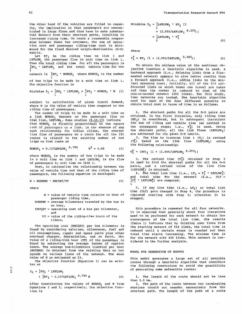
increases, the tendency is to have shorter routes. Figure 7 shows that the average length of the route decreases with fleet size. The length of routes varies between 2.0 and 20.0 km with a mean of 6,625 km for an operating fleet of 670.

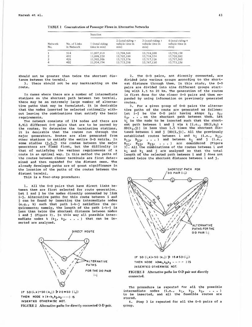
The data given in Table 2 indicate that the ef­fect of operating fleet size on the routing system for a zone depends on the size, the traffic demand, and the land-use pattern of the zone. The central zone, which is quite small in area compared to other zones, has been found to be quite sensitive to changes in fleet size compared to other zones. The optimal routes with their paths obtained for the central zone for a fleet of 88 buses are shown in

46

"' E -" .s::; ... .,, C

.!

.. .,, " .. M

> ct

7·0

6·5

6·0

Fleet size

FIGURE 7 Relationship between averae:e route lenirth and fleet size for the network. • - -

Figure 8. When the fleet size is changed from 52 to 88 vehicles, the number of routes in the optimal solution increases from 8 to 23. The maximum fre­quency of a route in a zone depends on travel de­mand. The data in Table 2 indicate that the maximum frequency is insensitive to the range of the operat­ing fleet sizes considered in this experiment.

OPERATING F'LEET : 88

NO OF ROUTES IN OPTIMAL SOLUTION : 23

NO OF TRANSFERS SAVED : 323074

--@--NOOE 4

01-oROUTENO

FIGURE 8 Route network for Central Zone (operating fleet= 88).

Transportation Research Record 994

CONCLUSIONS

The proposed method is a valuable tool for simul­taneous selection of optimal routes and frequencies for a bus transit network. It can be used by the planner to structure routes in a rational and sys­tematic way for the given spatial distribution of travel demand, and to find the number of buses and frequencies on each route and the operating fleet size for the system.

On the basis of the application of the model to the city of Ahmedabad, the following conclusions can be drawn:

1. The number of bus trips (Y) on a link for a day varies with the passenger flow (X) on the link. The relationship has been established for the city of Ahmedabad and is of the form Y = axb •

2. For a given spatial distribution of travel demand, the optimal total cost (passenger riding­time cost plus operation cost) can be obtained from the algorithm that concentrates the flow on the links.

3. The method first distributes the passengers on the links in the network and then generates routes that follow the passengers. This method is computationally efficient compared with other methods that repeatedly distribute the passengers on trial networks.

4. The route-generating procedure developed in this study is a systematic and rational algorithm that generates a large set of all possible routes that satisfy the various requirements.

5. Selection of the optimal set of routes and frequencies is made through a linear programming formulation that maximizes the number of transfers saved on the network. This method is realistic be­cause the interaction of various routes is taken into consideration.

6. The application of the model to the city of Ahmedabad indicates that the model can be success­fully applied to large transit networks, and the results are quite encouraging.

7. The results indicate that the number of routes in the optimal solution and the number of transfers saved increase linearly with an increase in operating fleet size. However, the average length of the route decreases with an increase in operating fleet size.

Future work may include consideration of the fol­l ow ing aspects o f the p r oblem : (a) The structuring of routes and the assignment of frequencies is done for a given desired trip matrix. Further refinement of the suggested model may consider stochastic vari­ations in travel demand. (bl The frequencies as­signed are for the entire day. The variation of headways during the day needs to be investigated. (c) Operation cost and passenger riding-time cost have been considered in terms of time by estimating their weights. The analysis can be made more realis­tic by considering actual costs.

REFERENCES

1. Report on Ahmedabad Urban Transport Project. Ahmedabad Municipal Transport Service, Ahmedabad, Gujarat , India, 1979.

2. Urban Transport, A Sector Policy Paper. World Bank, Washington, D.C., May 1976.

3. S.L. Dhingra. Simulation of Routing and Sched­uling of City Bus Transit Network. Ph.D. thesis. !IT Kanpur, India, May 1980.

4. J. Hsu and V .H. Surti. A System Approach of Optimal Bus Network Design. Research Report 19.

Transportation Research Record 994

Center for Urban Transportation Studies, Uni­versity of Colorado at Denver, Sept. 1975.

5. w. Lampkin and P.D. Saalmans. The Design of Routes, Service Frequencies, and Scheduling for a Municipal Bus Undertaking: A Case Study. Op­erational Research Quarterly, vol. 18, No. 4, 1967.

6. A. Last and S.E. Leak. Transport: A Bus Model. Traffic Engineering and Control, Vol. 17, No. 1, Jan. 1976.

7. A.H. Lines, W. Lampkin, and P.D. Saalmans. The Design of Routes and Service Frequencies for a Municipal Bus Company. Proc., Fourth Interna­tional Symposium on Operational Research, Bos­ton, Mass., 1966.

8. J.C. Rea. Designing Urban Transit Systems: An Approach to the Route-Technology Selection

47

Problem. NTIS-PB-204881. Washington University, Seattle, 1971.

9. F.S. Umrigar. Modelling for Simultaneous Selec­tion of Optimal Bus Routes and Their Frequen­cies--A case Study for Ahmedabad. M.Tech. thesis. IIT Kanpur, India, May 1982.

10. A. Scott. The Optimal Network Problem: Some Computational Procedures. Transportation Re­search, Vol. 3, 1969, pp. 201-210.

11. D. Hasselstorm. A Method for Optimization of Urban Bus Route Systems. Publication 88-DH-03. Volvo Bus Corporation, Gothenburg, Sweden, 1979.

Publication of this paper sponsored by committee on Bus Transit Systems.

Reducing the Energy Requirements of

Suburban Transit Services by Route and Schedule Redesign N. JANARTHANAN and J. SCHNEIDER

ABSTRACT

Reducing energy consumption has become an increasingly important concern of transit planners and managers in recent years. En­ergy consumption may be reduced by improved scheduling of vehicles, reduced deadheading, and laying out more efficient routes. This paper investigates several ways of redesign­ing an existing transit service to reduce its energy requirements without reducing service quality substantially. Bellevue, a suburban area within King county, Washing­ton, is used as the study area in this in­vestigation. A 13-route existing transit service in Bellevue is simulated and then redesigned to reduce its energy requirements while still providing a comparable level of service. The generation and evaluation of seven alternate designs was accomplished with an interactive graphic computer program called the Transit Network Optimization Pro­gram. Results from the "best" design indi­cate that the energy requirements of the ex­isting system could be reduced by about 56 percent without a substantial reduction of the level and quality of service in the study area.

Most transit agencies are currently under substan­tial financial pressure and depend heavily on gov-

ernmental aid to meet many of their operating costs. Consequently, cost reduction techniques, particu­larly those that relate to energy costs, are receiv­ing more attention. In recent years energy costs have become a fast-growing and large component of operating costs. Because of fluctuating prices and uncertainty about availability, reducing energy con­sumption has become an important concern of both planners and managers of transit systems. Energy consumption may be reduced by improving the sched­uling of vehicles, reducing deadheading, and laying out more efficient routes. The optimal scheduling of vehicles is constrained by minimum headway require­ments and deadheading by the location of bus bases. Transit routes may often be shifted to some limited extent to save energy. The objective of this study is to determine how much energy might be saved by designing more energy-efficient route structures and schedules. An interactive graphic computer program, the Transit Network Optimization Program (TNOP), is used to generate and evaluate alternative designs quickly and easily.

TNOP can be used to design and evaluate the per­formance of alternative fixed-route, fixed-schedule bus and rail transit systems. Through interactive computing, TNOP helps transit planners generate and evaluate a wide range of design alternatives and to compare their performance characteristics. Typi­cally, planners are able to find higher performance designs by providing transit services that more closely match actual origin-destination travel pat­terns. Seattle Metro Transit decided to explore the applicability of TNOP to this question and this study was designed to evaluate TNOP' s usefulness as