Vital signs monitoring using Doppler signal decomposition
95
V ITAL SIGNS MONITORING USING D OPPLER SIGNAL DECOMPOSITION Y UQING L I
-
Upload
khangminh22 -
Category
Documents
-
view
4 -
download
0
Transcript of Vital signs monitoring using Doppler signal decomposition
VITAL SIGNS MONITORING USING DOPPLERSIGNAL DECOMPOSITION
YUQING LI


VITAL SIGNS MONITORING USING DOPPLERSIGNAL DECOMPOSITION
DISSERTATION
to obtain the degree of Master of Sciencein Electrical Engineering
at Delft University of Technology,to be defended publicly on Friday August 21, 2020 at 09:00 AM
by
YUQING LI
born in Liaoning, China.

This thesis has been approved by the
supervisor: Prof. DSc. Olexadner Yarovyidaily supervisor: Dr. Nikita Petrov
Thesis committee:
Prof. DSc. Olexadner Yarovyi, MS3 TU DelftProf. dr. ir. Richard Heusdens, CAS TU Delft / NLDADr. Nikita Petrov, MS3 TU Delft
An electronic version of this dissertation is available athttp://repository.tudelft.nl/.

CONTENTS
1 INTRODUCTION 11.1 MOTIVATION . . . . . . . . . . . . . . . . . . . . . . . . . . . . . . . . 11.2 OVERVIEW OF VITAL SIGNS MONITORING TECHNOLOGIES . . . . . . . . . . 11.3 RADAR-BASED VITAL SIGN MONITORING TECHNIQUES . . . . . . . . . . . 31.4 OUTLINE OF THE THESIS . . . . . . . . . . . . . . . . . . . . . . . . . . 5
2 MODELS AND RADAR SYSTEMS FOR VITAL SIGNS MONITORING 72.1 SIGNAL MODELS FOR VITAL SIGNS MONITORING . . . . . . . . . . . . . . 7
2.1.1 PHYSIOLOGY OF CARDIOPULMONARY ACTIVITY . . . . . . . . . . . . 72.1.2 CARDIOPULMONARY ACTIVITY MODEL . . . . . . . . . . . . . . . . 92.1.3 DYNAMIC CARDIOPULMONARY SIGNAL MODELS . . . . . . . . . . . 12
2.2 RADAR SYSTEMS FOR VITAL SIGNS MONITORING . . . . . . . . . . . . . . . 122.2.1 SINGLE-TONE CONTINUOUS-WAVE RADAR . . . . . . . . . . . . . . 122.2.2 FREQUENCY-MODULATED CONTINUOUS WAVE RADAR . . . . . . . . 152.2.3 IMPULSE-RADIO ULTRA WIDE BAND RADAR . . . . . . . . . . . . . 182.2.4 VITAL SIGNS MONITORING REQUIREMENTS OF RADAR . . . . . . . . 19
2.3 RADAR RECEIVED DATA MODEL . . . . . . . . . . . . . . . . . . . . . . . 212.4 CONCLUSION . . . . . . . . . . . . . . . . . . . . . . . . . . . . . . . . 23
3 SIGNAL DECOMPOSITION AND ANALYSIS METHODS 253.1 EMPIRICAL MODE DECOMPOSITION . . . . . . . . . . . . . . . . . . . . . 253.2 HILBERT-HUANG TRANSFORM . . . . . . . . . . . . . . . . . . . . . . . . 273.3 ENSEMBLE EMPIRICAL MODE DECOMPOSITION . . . . . . . . . . . . . . . 303.4 COMPLETE ENSEMBLE EMPIRICAL MODE DECOMPOSITION WITH ADAPTIVE
NOISE . . . . . . . . . . . . . . . . . . . . . . . . . . . . . . . . . . . . 313.5 VARIATIONAL MODE DECOMPOSITION . . . . . . . . . . . . . . . . . . . 333.6 NUMERICAL SIMULATIONS . . . . . . . . . . . . . . . . . . . . . . . . . 373.7 CONCLUSION . . . . . . . . . . . . . . . . . . . . . . . . . . . . . . . . 42
4 ONLINE SIGNAL DECOMPOSITION METHODS 434.1 ONLINE SIGNAL DECOMPOSITION PRINCIPLE . . . . . . . . . . . . . . . . 434.2 SIMULATION EXAMPLES OF ONLINE DECOMPOSITION . . . . . . . . . . . . 454.3 NUMERICAL SIMULATIONS . . . . . . . . . . . . . . . . . . . . . . . . . 504.4 CONCLUSION . . . . . . . . . . . . . . . . . . . . . . . . . . . . . . . . 52
5 EXPERIMENTAL VALIDATION 535.1 MEASUREMENT USING CW RADAR . . . . . . . . . . . . . . . . . . . . . . 53
5.1.1 SIGNAL DECOMPOSITION METHODS . . . . . . . . . . . . . . . . . 545.1.2 ONLINE SIGNAL DECOMPOSITION METHODS . . . . . . . . . . . . . 615.1.3 COMPARISON . . . . . . . . . . . . . . . . . . . . . . . . . . . . . 63
V

VI CONTENTS
5.2 MEASUREMENT USING TWO RADARS. . . . . . . . . . . . . . . . . . . . . 655.2.1 SIGNAL DECOMPOSITION METHODS . . . . . . . . . . . . . . . . . 665.2.2 ONLINE SIGNAL DECOMPOSITION METHODS . . . . . . . . . . . . . 735.2.3 COMPARISON . . . . . . . . . . . . . . . . . . . . . . . . . . . . . 76
5.3 CONCLUSION . . . . . . . . . . . . . . . . . . . . . . . . . . . . . . . . 78
6 CONCLUSION AND FUTURE WORK 816.1 CONCLUSION . . . . . . . . . . . . . . . . . . . . . . . . . . . . . . . . 816.2 RECOMMENDATIONS OF FUTURE WORK . . . . . . . . . . . . . . . . . . . 82
1INTRODUCTION
1.1. MOTIVATIONCardiopulmonary signals, respiration and heartbeat, are crucial indicators of vital signs:they can be used to judge the state of the human body and detect abnormal cardiopul-monary activities, essential to particular medical emergencies. A growing interest inpeople’s health monitoring is strengthened by the rapid development of medical elec-tronic technologies, and ever-growing demand for monitoring cardiopulmonary signalsduring a variety of occasions, including clinical application, and daily activities: sleep-ing, driving and sports.
Radar-based vital signs monitoring has been an object of research since the 1970s,which detects human chest displacement using Doppler radar. Non-contact, accurateand real-time monitoring of human respiration and heartbeat signals can be achievedthrough the processing of radar echo.
1.2. OVERVIEW OF VITAL SIGNS MONITORING TECHNOLOGIESModern vital signs detection approaches, such as electrocardiography (ECG) for heartmonitoring [1] and inductive or optoelectronic plethysmography for respiratory moni-toring are designed for disease diagnosis with high reliability. However, the applicationof such devices during daily activities is infeasible by their bulkiness, high cost and com-plicated operation [2].
To overcome these shortcomings, miniaturized and portable devices of vital signs de-tection have recently attracted considerable interest. In the last decade, there has beena growing emergence towards portable or wearable devices, which can be used to de-tect various vital signs (heartbeat rate, body temperature, blood oxygen, etc.) of humans[3] [4]. Although most of the current vital signs detection devices are small-sized andnon-invasive, they still bound a user by electrodes or cables. Also its application range isrestricted: contact electrodes can interfere with the measurement of some physiologicalparameters, and thus affect the accuracy of parameter estimation.
1

1
2 1. INTRODUCTION
Non-contact vital sign detection can overcome these shortcomings by measuringrespiration, heartbeat and other parameters without contacting the human body. Thesensor is not directly in touch with the body and detects physiological signals from a dis-tance. It provides a convenient, non-invasive and remote detection way for vital signsmonitoring, crucial for physiological signal detection in difficult occasions, such as pa-tients with large-scale burn trauma, infectious and mental patients; long-term monitor-ing of infants and sleep disorders in adults; life detection during disaster rescue such asearthquake collapse [5].
Schematic comparison of existing mainstream contact/non-contact vital sign detec-tion approaches is listed in Tab. 1.1 [2].
ApproachContactor not
Measuredvital sign
Mainadvantage
Maindisadvantage
Strainmeasurement[3]
ContactRespirationheartbeat
Unobtrusiveness Motion artifacts
Impedancemeasurement[4]
ContactRespirationheartbeat
Unobtrusiveness Motion artifacts
Movementmeasurement[6]
ContactRespirationheartbeat
Unobtrusiveness Motion artifacts
Air component[7] Contact Respiration Accuracy Intrusiveness
Biopotentialmeasurement[1]
(i.e., ECG)Contact
Respirationheartbeat
Accuracy Motion artifacts
Light intensitymeasurement(i.e., PPG)[1]
ContactRespirationheartbeat
Unobtrusiveness Motion artifacts
Infrared[8] Non-contact Body temperature AccuracyEnvironment
dependent
Camera(i.e., rPPG)[9][10]
Non-contactRespirationheartbeat
UnobtrusivenessLighting condition
dependent
Visible light[11] Non-contactRespirationheartbeat
Low-costLighting condition
dependent
Radar [12] Non-contactRespirationheartbeat
Environmentindependent
Sensitivity tointerference
Microphone[13] Non-contactRespirationheartbeat
Low-costSensitivity to
noise
Sonar[14] Non-contact RespirationEnvironmentindependent
Insensitivity tosmall motion
Table 1.1: Vital signs detection approaches
From the table, it can be seen that contact-based approaches measure parameterchanges ( strain, displacement or current, etc.) during cardiopulmonary activities to ob-

1.3. RADAR-BASED VITAL SIGN MONITORING TECHNIQUES
1
3
tain vital signs, while non-contact approaches use electromagnetic wave or sound waveto detect vital signs remotely. Camera and visible light-based vital signs monitoring tech-nology puts high demands on the lighting condition, and microphone-based monitoringrequires a quiet environment. Radar and sonar-based vital signal monitoring techniquesare both independent of the environment, while the former has lower cost and complex-ity, leading to wider usage in vital signs monitoring.
1.3. RADAR-BASED VITAL SIGN MONITORING TECHNIQUESThe real-time detection of cardiopulmonary parameters extraction with radar needs toaddress the following challenges: limited time duration of the signal for the extraction ofcardiopulmonary signals, accuracy of vital signs parameters estimation and signal pro-cessing algorithm complexity. In this section, we recall the methods for remote vitalsigns detection and parameter estimation (respiration and heartbeat frequencies).
Modern time-frequency analysis methods include short-time Fourier transform [15],Gabor transform [16], etc., which can be seen as evolved forms of Fourier transform.However, spectrum resolution of STFT may not be sufficient to track frequency changesof a rapidly varying non-stationary signal. Gabor transform is a STFT with a Gaussianwindow, but it is difficult to find the optimal fitting model.
More advanced time-frequency representation method, such as wavelet transform(WT) [17], can overcome the resolution limitation of STFT. WT is a time-scale analysismethod which estimates the wavelet coefficients from the signal, and exploits the re-combination algorithm to analyze their frequency content. Wavelet Transform (WT) andits modifications such as Wavelet Filter [18], Wavelet Packet Decomposition (WPD) [19],Discrete Wavelet Transform (DWT), Complex Wavelet Transform (CWT) [20], CWT withMorlet mother wavelet [21] have been recently applied to separate and estimate respi-ration and heartbeat signals. The traditional spectral analysis methods such as Fouriertransform and wavelet have certain limitations for time-frequency analysis: the formercan only obtain the overall distribution of the spectrum, which does not include the fre-quency changes over time; the latter suffers from the optimal choice of the wavelet base.
STFT and wavelet transform are both linear time-frequency representations. To de-scribe the instantaneous power spectral density of a signal, quadratic time-frequencyrepresentation is applied. It describes the energy density distribution of the signal, themost popular methods are Winger-Vile distribution (WVD) [22] [23] and Cohen time-frequency distribution [23]. When the signal has multiple frequency components, quadratictime-frequency distribution suffers from the cross terms, which generate false harmon-ics and can result in the frequency estimation error, crucial for considered application[24]. A proper design of kernel function can suppress this effect [25].
Another brunch of research focuses on the application of the modern spectrum anal-ysis methods to overcome the limitations of FT. Among these methods, RELAX is a para-metric and cyclic optimization approach for the estimation of sinusoidal parametersproposed in [26]. It has demonstrated in [27] that RELAX can mitigate the effects ofsmearing and leakage in conventional Periodogram, succeeding in the estimation of vitalsigns parameters, but it has a shortage of computational complexity. Another approachreported is a multiple signal classification algorithm referred to as MUSIC. The eigen-value decomposition of the covariance matrix composed of received signals is used to

1
4 1. INTRODUCTION
obtain the spectrum by using the minimum eigenvector of the covariance matrix. TheMUSIC algorithm is used to estimate the frequency of time-domain waveform after high-frequency filtering, and extract the required vital sign parameters [28]. The shortcomingsof the MUSIC algorithm are its computation complexity in spectral peak search. There-fore, Barabell proposed a Root-MUSIC algorithm [29], which uses the polynomial rootsearch method instead of spectral peak search to achieve computational efficiency.
Iterative adaptive approach (IAA) is a robust, high resolution, and low sidelobe fre-quency estimation method, which can be employed to obtain the IAA spectrum of theradar echo. Thus, frequencies of respiration and heartbeat can be reliably determinedfrom the IAA spectral estimation [30]. In addition, Lomb-Scargle Periodogram was alsoapplied for respiratory rate estimation. Experimental verification has proved that mo-tion artifacts can be eliminated in Lomb-Scargle Periodogram, providing a reliable resultwhen estimating the respiration frequency [31].
A few digital signal processing algorithms to extract chest wall displacement due torespiration with two microwave Doppler radars are presented in [32]: Mean of signals(MEAN), Least Squares (LS), Hough Transformation (HOUGH), Particle Filter (PF) andDirect Phase Estimation based on Vector Difference (DIFF). Experimental results showthat the best phase estimation method for measuring respiration is the LS method withappropriate window size. However, accurate estimation of respiration frequency is diffi-cult to achieve in LS method if the human chest is not facing the radar sensor. Applica-tion of Extended Kalman filter for vital signs monitoring was proposed in [33]. It used Iand Q channel signal as input signal separately, and after the estimation, principal com-ponent combining (PCC) and digital elliptic filtering are applied to get the respirationand heartbeat rate. However, there is still a lack of dynamic modeling of vital signs andtheir extraction techniques [34].
Empirical mode decomposition (EMD) is an analysis method for nonlinear and non-stationary time series signals. EMD decomposes the input signal into a series of so-calledintrinsic mode functions (IMF) [35]. Hilbert-Huang transform (HHT) is applied afterEMD to obtain instantaneous frequencies of IMFs, which is called Hilbert-Huang time-frequency distribution. HHT overcomes shortcomings of Fourier and Wavelet transformand can provide the time-frequency spectrum of the signal with high resolution. En-semble empirical mode decomposition (EEMD) is a modification of EMD proposed tosettle the mode mixing problem, performed in non-contact vital signs sensing systems[20][36]. However, the reconstructed signal this method still contains the residual noisecomponent. And EEMD requires complex recursion and takes longer calculation timecompared to STFT. CEEMDAN was developed as a modification over EEMD, which hasless number of sifting iterations [37]. However, the rigorous physical and mathematicalsignificance of CEEMDAN needs to be explored and explained further.
Empirical signal decomposition methods are sensitive to noise, a more advancedtechnique called Variational Mode Decomposition (VMD) is further introduced to tacklethe problem. It is an adaptive decomposition algorithm, the purpose of the variationalmode decomposition algorithm is to obtain the optimal solution through iteration, soas to determine the central frequency and bandwidth of each IMF and extract the sig-nal components. Different from the definition of the IMF in EMD algorithm, the IMF ofVMD algorithm is an amplitude-frequency modulation signal [38]. Based on VMD, the
1.4. OUTLINE OF THE THESIS
1
5
respiration signals of different humans can be decomposed into different sub-signals,and then the time-varying respiration signals can be accurately tracked [39].
An alternative numerical analysis method is third-order cyclic cumulant (TOCC) [40].For a non-stationary statistical signal, if it undergoes periodicity after some non-linearchange, it can be seen to have the property as cyclostationarity. The received Dopplerradar signal exhibits cyclostationarity in non-contact vital signs sensing system, so TOCCcan be performed. In literature, the TOCC detection method shows its insensitivity toGaussian interference and non-cyclic signals, the respiration and heart frequencies canbe accurately detected [41].
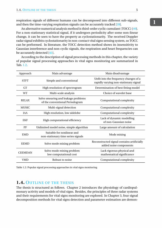
According to the description of signal processing methods in this chapter, the varietyof popular signal processing approaches in vital signs monitoring are summarized inTab. 1.2.
Approach Main advantage Main disadvantage
STFT Simple and conventionalUnfit into the frequency changes of arapidly varying non-stationary signal
GT High resolution of spectrogram Determination of best fitting model
WT Multi-scale analysis Choice of wavelet base
RELAXSolve smearing and leakage problems
of the conventional PeriodogramComputational complexity
MUSIC Multi-signal detection Computational complexity
IAA High resolution, low sidelobe Computational complexity
EKF High computational efficiencyLack of dynamic modelling
of non-Gaussian noise
PF Unlimited model noise, simple algorithm Large amount of calculation
EMDSuitable for nonlinear and
non-stationary time series signalsMode mixing
EEMD Solve mode mixing problemReconstructed signal contains artificially
added noise components
CEEMDANSolve mode mixing problem
low computational costLack rigorous physical andmathematical significance
VMD Robust to noise Computational complexity
Table 1.2: Popular signal processing approaches in vital signs monitoring
1.4. OUTLINE OF THE THESISThe thesis is structured as follows. Chapter 2 introduces the physiology of cardiopul-monary activity and models of vital signs. Besides, the principles of three radar systemsand their requirements for vital signs monitoring are explored. In Chapter 3, four signaldecomposition methods for vital signs detection and parameter estimation are demon-

1
6 1. INTRODUCTION
strated: EMD, EEMD,CEEMDAN and VMD. These methods are evaluated by Monte-Carlo simulation and their performances under different circumstances are assessed.Chapter 4 describes two online signal decomposition methods, providing a dynamic es-timation of respiration and heartbeat signal parameters. The performances of the pro-posed techniques for vital signs monitoring are also assessed by Monte-Carlo simula-tion. Experimental verification is then presented in Chapter 5, proving the feasibility ofthe above methods in vital signs monitoring. Finally, the conclusion and recommendedfuture work are summarized in Chapter 6.

2MODELS AND RADAR SYSTEMS FOR
VITAL SIGNS MONITORING
Existing non-contact vital signs monitoring relies on electromagnetic waves emitted byradar to penetrate obstacles and reach the human body to detect vital sign parameters.The radar will measure the slight displacement of the surface of human prothorax dueto the physiological activities such as heartbeat and respiration. Therefore, the collectedradar echo signals after human body reflection will carry the physiological activity in-formation, and the vital signs parameters extracted from the data with modern signalprocessing methods.
In this chapter, the physiology of cardiopulmonary activity is introduced. Then themodels of vital signs are described including the noise and possible vibration of autoin the application for driver state monitoring. In addition, various radar systems wereapplied for human being monitoring. In the final part of this chapter, the principles ofthese technologies, in particular, continuous wave (CW), linearly frequency-modulatedcontinuous-wave (LFMCW) and impulse-radio (IR) ultra wide-band (UWB) radars areexplored.
2.1. SIGNAL MODELS FOR VITAL SIGNS MONITORING
2.1.1. PHYSIOLOGY OF CARDIOPULMONARY ACTIVITYIn some studies, it has been observed that the movement of the lungs and respiratorymuscles can deform the heart. However, there is still no convincing conclusion on theinteraction between the respiration and heartbeat [42]. Hence, respiration and heartbeatare regarded as independent activities in this thesis. In this section, the physiology anddata models of the two kinds of cardiopulmonary activity, respiration and heartbeat, willbe presented and discussed.
Lungs ventilation refers to the gas exchange process between lungs and the externalenvironment. The human structure responsible for lungs ventilation includes the respi-ratory tract, thoracic cage, and respiratory muscles. The respiratory tract is the passage
7

2
8 2. MODELS AND RADAR SYSTEMS FOR VITAL SIGNS MONITORING
of gas getting into and getting out of the lungs. Lungs are located inside the rib cage, witha closed pleural cavity between them. The respiratory muscles are attached to the tho-racic cage, changing the volume of the thoracic cage through contraction and relaxationactivities, causing the expansion and contraction of the lungs to provide power for lungsventilation [43].
Under a natural breathing state, the internal volume of the lungs changes due to itsexpansion and contraction leading to changes in the lungs’ pressure. Lungs do not havethe ability to contract and relax independently due to their physiological characteristics.The contraction and relaxation of lungs changes with the corresponding activity of thethoracic cage, and the change of the thoracic cage is regulated by the control of the respi-ratory muscles. The contraction of the respiratory muscles corresponds to the reductionof the thoracic cage. Conversely, the relaxation of the respiratory muscles enlarges thethoracic cage, and the entire process becomes respiratory motion. The change in lungsvolume during a respiratory cycle is shown in Fig. 2.1. Changes in lungs volume reflectthe contraction and expansion of the rib cage and also the displacement of the chestwall.
Figure 2.1: Changes in lungs volume during respiration process
The main function of the heart is to pump blood. The continuous and coordinatedcontraction and relaxation of the heart is a necessary condition for the realization of theblood pumping function. Each time the heart contracts and relaxes, it constitutes a cycleof mechanical activity, called the cardiac cycle. Since the ventricle plays a major rolein the pumping activity of the heart, the cardiac cycle usually refers to the ventricularactivity cycle. The cardiac cycle is the reciprocal of the heart rate, in one cardiac cycleduration, a mechanical vibration caused by factors such as myocardial contraction, openand closure of the valve, and the impact of blood flow can be transmitted to the chest wallthrough the surrounding tissue, giving rise to the corresponding movement of the chestwall [43]. The change of the ventricular volume in a cardiac cycle is depicted in Fig. 2.2.
The diastole process is filling with ventricular, by this time, the pressure of left ven-tricular drops, when it becomes lower than atrial pressure, the mitral valve will open (1).Then the systole begins when the ventricles contract and all valves in the heart close,which is called isovolumetric ventricular contraction (2). As the pressure in the ventricleincreases, when it is larger than the aorta pressure, the aortic valve opens and ventricularbegins to eject blood (3). Finally, the pressure in the ventricles decreases with the out-flow of blood, and the valve closes and comes to relaxation when its pressure falls belowthe pressure of the aortic valve. This process (4) is called isovolemic ventricular diastolic

2.1. SIGNAL MODELS FOR VITAL SIGNS MONITORING
2
9
Figure 2.2: Changes in ventricular volume of cardiac cycle
period since all the valves in the heart are closed and the ventricles are in a diastolic state[43]. The actual chest displacements caused by respiration and heartbeat are depictedin Fig. 2.3 [44].
Figure 2.3: A sample of respiration (top) and heartbeat (bottom) waveforms vs time
2.1.2. CARDIOPULMONARY ACTIVITY MODELIn general, healthy adults have a heartbeat rate of 50-100 beats per minute and take 6-24breaths per minute. When the human body stays still and the mood remains stable, therespiration and heartbeat signals basically change periodically. In many experimentsand research, a single tone movement is employed to simulate the periodic movementof the human chest induced by respiration and heartbeat, so respiration and heartbeatmovements are approximated by sinusoidal movements with different amplitudes and

2
10 2. MODELS AND RADAR SYSTEMS FOR VITAL SIGNS MONITORING
frequencies [45]. Then chest wall displacement x(t ) can be expressed by the summationof two sinusoidal signals:
x(t ) = Ar sin(2π fr t )+ Ahsin(2π fh t ), (2.1)
where Ar , Ah are the amplitudes of respiration and heartbeat, respectively, and fr , fh arethe frequencies of respiration and heartbeat, respectively.
The typical values of respiration and heartbeat frequency and amplitude [43] are dis-played in Tab. 2.1.
Frequency[Hz] Amplitude[mm]
Respiration 0.1-0.4 4-12Heartbeat 0.83-1.67 0.3-0.6
Table 2.1: Typical frequencies and amplitudes of vital signs
However, the real movement of the two vital signs is not simply sinusoidal. Com-pared with the traditional sinusoidal vital signs model, the improved model is more inline with actual chest wall displacement, thus improving the authenticity of the simu-lation results. After analyzing a large amount of experimental data, it was found thatthe actual waveform of the respiration is more like a higher-order curve of a sinusoidalsignal[46]. Prototype respiration pulse is:
pr (t ) = sinp (π fr t
), p = 3 (2.2)
leading to a discrete-time respiration signal component:
xr (n) = Ar pr
(n
fs−
[n
fsfr
]1
fr
), (2.3)
where Ar and fr are the amplitude and frequency of respiration signal, respectively. Theimproved and sinusoidal models of respiration are shown in Fig. 2.4, where Ar = 8mm,fr = 0.25Hz, sampling frequency fs = 50Hz.
The fluctuation caused by the heartbeat can only be transmitted to the chest wallthrough the bones and skin. So the heartbeat signal finally becomes the displacementof the chest, which is actually a "filter" procedure through the bones and skin [46]. Thepulse signal ph(t ) serves as a heartbeat signal model, in which the frequency of the heart-beat signal is fh . The model of the pulse signal is set to the exponential e−t/τ, where τis the heartbeat pulse time. The pulse signal is filtered by a second-order Butterworthfilter, which is analogous to the actual attenuation of the heartbeat signal through thebones and skin. The improved heartbeat signal model is:
ph(t ) = e−tτ +
[( p2
ω0t−1
)sin
ω0tp2−cos
ω0tp2
]e
−ω0 tp2 , (2.4)
where ω0 = 2π f0 is the cutoff radian frequency, τ= 0.05 and f0 = 1 in this case.

2.1. SIGNAL MODELS FOR VITAL SIGNS MONITORING
2
11
0 2 4 6 8 10 12 14 16 18 20
Time[s]
-5
-4
-3
-2
-1
0
1
2
3
4
5
Am
plit
ud
e[m
]
10-3 Respiration signal model
Improved model
Sinusoidal model
Figure 2.4: Improved respiration model vs sinusoidal respiration model
The discrete time model of the heartbeat signal is:
xh(n) = Ah ph
(n
fs− [
n
fsfh]
1
fh
), (2.5)
where Ah is the peak-to-peak value of heartbeat signal, fh is the frequency of heart-beat signal. Samples are sequentially taken until it reaches the heart-rate period, wherethe period ends and a new period will begin, ph(t ) is the pulse response function thatdescribes the period. The improved and sinusoidal models of heartbeat are shown inFig. 2.5, where Ah = 8mm, fh = 1.3Hz.
0 1 2 3 4 5 6 7 8 9 10
Time[s]
-6
-4
-2
0
2
4
Am
plit
ud
e[m
]
10-4 Heartbeat signal model
Improved model
Sinusoidal model
Figure 2.5: Improved heartbeat model vs sinusoidal heartbeat model
2
12 2. MODELS AND RADAR SYSTEMS FOR VITAL SIGNS MONITORING
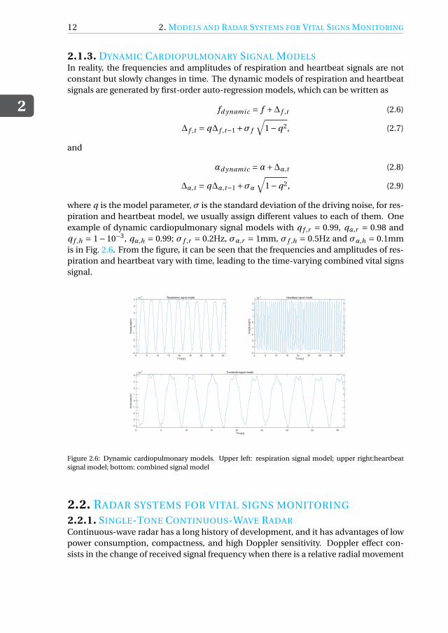
2.1.3. DYNAMIC CARDIOPULMONARY SIGNAL MODELSIn reality, the frequencies and amplitudes of respiration and heartbeat signals are notconstant but slowly changes in time. The dynamic models of respiration and heartbeatsignals are generated by first-order auto-regression models, which can be written as
fd ynami c = f +∆ f ,t (2.6)
∆ f ,t = q∆ f ,t−1 +σ f
√1−q2, (2.7)
and
αd ynami c =α+∆α,t (2.8)
∆α,t = q∆α,t−1 +σα√
1−q2, (2.9)
where q is the model parameter, σ is the standard deviation of the driving noise, for res-piration and heartbeat model, we usually assign different values to each of them. Oneexample of dynamic cardiopulmonary signal models with q f ,r = 0.99, qα,r = 0.98 andq f ,h = 1−10−3, qα,h = 0.99; σ f ,r = 0.2Hz, σα,r = 1mm, σ f ,h = 0.5Hz and σα,h = 0.1mmis in Fig. 2.6. From the figure, it can be seen that the frequencies and amplitudes of res-piration and heartbeat vary with time, leading to the time-varying combined vital signssignal.
0 5 10 15 20 25 30 35 40
Time[s]
-4
-3
-2
-1
0
1
2
3
4
Am
plit
ude[m
]
10-3 Respiration signal model
0 5 10 15 20 25 30 35 40
Time[s]
-5
-4
-3
-2
-1
0
1
2
3
Am
plit
ude[m
]
10-4 Heartbeat signal model
0 5 10 15 20 25 30 35 40
Time[s]
-4
-3
-2
-1
0
1
2
3
4
Am
plit
ude[m
]
10-3 Combined signal model
Figure 2.6: Dynamic cardiopulmonary models. Upper left: respiration signal model; upper right:heartbeatsignal model; bottom: combined signal model
2.2. RADAR SYSTEMS FOR VITAL SIGNS MONITORING
2.2.1. SINGLE-TONE CONTINUOUS-WAVE RADARContinuous-wave radar has a long history of development, and it has advantages of lowpower consumption, compactness, and high Doppler sensitivity. Doppler effect con-sists in the change of received signal frequency when there is a relative radial movement

2.2. RADAR SYSTEMS FOR VITAL SIGNS MONITORING
2
13
between the receiver and the target. Similarly, if the radar and the scatterer are not sta-tionary with each other, the received echo impinges back to the radar at frequency fr ,different from the transmitted frequency ft due to the Doppler effect. Assume a target inthe radar’s observation range is moving towards the radar, and the transmitted frequencyof radar is ft , the received frequency becomes:
fr =(
1+ v/c
1− v/c
)ft , (2.10)
where v is the radial velocity of target relative to the radar.Since v ¿ c, (2.10) can be simplified as:
fr =(1+ 2v
c
)ft . (2.11)
The instantaneous Doppler shift in frequency fd (t ) can be expressed as a function ofinstantaneous velocity v(t ) of the moving target:
fd (t ) = 2 f
cv(t ) = 2v(t )
λ, (2.12)
where λ is the wavelength of radar emitted signal. Denote the target displacement ofthe human chest as x(t ), then Doppler frequency shift of the reflected signal can be ex-pressed using the integral relation of frequency and phase:
θ(t ) =∫ t
02π fd (t )d t =
∫ t
02π
2 f
cv(t )d t = 2 f
c(2πx(t )) = 4πx(t )
λ. (2.13)
Therefore, the displacement of the human chest can be measured via the variation ofthe phase, observed by the radar. Under an ideal circumstance, the time-varying phaseinformation, proportional to the time-varying displacement of the human chest, canbe obtained through phase demodulation and used to extract relevant information ofrespiration and heartbeat.
The sketch diagram of CW radar-based vital signs detection is depicted in Fig. 2.7.The transmitted signal T (t ) can be represented as:
T (t ) = AT cos(2π fc t +φ(t )), (2.14)
where AT is the amplitude of transmitted signal, fc is the carrier frequency, φ(t ) is thefluctuation in signal phase.
Suppose the target has a time-varying displacement x(t ) on the distance d0, then thedistance between the transceiver and the target is
d(t ) = d0 +x(t ). (2.15)
The distance between the transceiver and the target will cause a propagation time delay,the delay of a round trip of the radar signal can be expressed as:
td = 2d (t )
c= 2(d0 +x(t ))
c. (2.16)

2
14 2. MODELS AND RADAR SYSTEMS FOR VITAL SIGNS MONITORING
Figure 2.7: Sketch diagram of continuous wave radar based vital signs monitoring
The received signal R(t ) obtained by the receiver is a delayed copy of the transmittedsignal, with amplitude AR :
R(t ) = AR cos[2π f (t − td )+φ(t − td )+θ0
], (2.17)
where θ0 is a constant phase shift affected by several factors, for example, the phaseshift formed by the target’s reflective surface (close to 180o), and the time delay fromtransmitter to antenna. Combining (2.16) and (2.17), the received signal becomes:
R(t ) = AR cos
[2π f t − 4πd0
λ− 4πx(t )
λ+φ
(t − 2d0
c− 2x(t )
c
)+θ0
]. (2.18)
Since the period of chest displacement is much longer than the time delay caused bythe distance of radar and target, T À d0/c, and the chest displacement is much smallerthan the distance of radar and target, x(t ) ¿ d0, the received signal can be approximatelywritten as:
R(t ) = AR cos
[2π f t − 4πd0
λ− 4πx(t )
λ+φ
(t − 2d0
c
)+θ0
]. (2.19)
The received signal has a similar structure with the transmitted signal, with a time de-lay determined by the initial distance between the radar and target d0 and the periodicmovement of target chest x(t ). The phase of the received signal contains information ofhuman chest motion.
Once the echo signal is received, it is demodulated by mixing the received echo signalwith the same local oscillator, and a low pass filter is applied to extract the basebandsignal:
B(t ) = AB cos
[4πx(t )
λ+θ+∆φ(t )
], (2.20)
where AB is the amplitude of baseband signal, and ∆φ(t ) is the residual phase noise:
∆φ(t ) =φ(t )−φ(
t − 2d0
c
), (2.21)
and θ is the constant phase shift proportional to d0:
θ = 4πd0
λ−θ0. (2.22)

2.2. RADAR SYSTEMS FOR VITAL SIGNS MONITORING
2
15
In order to avoid the problem of null detection point, restoring the target motioninformation with high accuracy, I/Q quadrature receiver and arctangent (AT) demodu-lation are often used [47]. The outputs of quadrature receiver contain in-phase (I) andquadrature (Q) baseband components are:
I (t ) = AI cos
[4πx(t )
λ+θ+∆φ(t )
], (2.23)
Q(t ) = AQ sin
[4πx(t )
λ+θ+∆φ(t )
]. (2.24)
Arctangent demodulation calculates:
φhi s (t ) = arctan
(Q(t )
I (t )
). (2.25)
It can make good use of information on I/Q quadrature channels and there are no har-monic and intermodulation effects between demodulated vital sign signals. Theoret-ically, AT demodulation can recover the complete chest wall displacement, the phaseinformation of the baseband signal is:
φhi s (t ) = 4πx(t )
λ+θ+∆φ(t ). (2.26)
And the range history of vital signs can be estimated from:
Rhi s (t ) = cφhi s (t )
4π fc. (2.27)
By doing this, information of human chest displacement is recovered.
2.2.2. FREQUENCY-MODULATED CONTINUOUS WAVE RADARA simple continuous-wave radar can only determine the velocity of a target, but not thedistance between radar and target. Therefore, frequency-modulated continuous-wave(FMCW) radar is contrived to resolve the blemish. Linear frequency modulation (LFM)is the most commonly used in radar including vital signs monitoring, its principle willbe described in this section.
The principle of range and relative velocity detection in LFMCW radar is exemplifiedin Fig. 2.8, showing the transmitted and received echo signals for detecting a target ata range of R, approaching with relative radial velocity vr . The frequency of transmittedsignal varies within the range [ f0, f0 +B ] in period Tm , where f0 is the minimum fre-quency and B is the bandwidth. A signal is emitted with frequency f1 at time t1, andit is received with frequency f2 at time t2, after a round-trip delay τ = 2R/c along witha Doppler frequency shift fd . Then a procedure called de-ramping is applied where amixer produces a baseband signal at the instantaneous difference frequency betweenthe transmitter and the received signals, referred to as the beat signal fb = | fT x − fRx |.
The sinusoidal transmitted signal from a LFMCW as in Fig. 2.8 can be expressed as:
T (t ) = AT x cos(φT x (t )), (2.28)

2
16 2. MODELS AND RADAR SYSTEMS FOR VITAL SIGNS MONITORING
Figure 2.8: Principle of range and velocity measurement of LFMCW radar
where AT x is the amplitude of emitted signal and φT x is instantaneous phase related tothe instantaneous transmitter frequency fT x , which is shown as follows:
φT x = 2π∫ t
0fT x (t )d t . (2.29)
For a chirp in the time interval [0,Tm/2], the variation of transmitted signal frequencycan be expressed as:
fT x (t ) = f0 + B
Tm/2t = f0 + 2B
Tmt . (2.30)
Substituting (2.29) into (2.30), the instantaneous transmitter phase is obtained by:
φT x = 2π
(f0t + 1
2· 2B
Tmt 2
)∣∣∣t
0
= 2π
(f0t + B
Tmt 2
). (2.31)
For a target at range R, approaching radar with velocity vr , the received signal fromthe moving target with a round-trip time delay is:
R(t ) = ARx cos(φRx (t )) = ARx cos(φT x (t −τ)), (2.32)
where the delay τ= 2(R − vr t )/c.As mentioned previously, a mixer produces a signal at the instantaneous difference
frequency, referred to as beat signal, which is:
sB (t ) = AB cos(φB (t )) = AB cos(φT x (t )−φRx (t )). (2.33)
Then, combining the last two equation, the phase of beat signal is gained as:
φB (t ) =φT x (t )−φRx (t )
= 2π
(f0τ+ 2B
Tmt ·τ− B
Tmτ2
). (2.34)

2.2. RADAR SYSTEMS FOR VITAL SIGNS MONITORING
2
17
Since in most cases, τ/Tm ¿ 1 holds, the last term in (2.34) can be neglected. τ is afunction of range R and velocity vr , substitute τ, (2.34) can be expressed as:
φB (t ) = 2π
[2R
cf0 +
(4B
Tm· R
c− 2vr
cf0
)t + 4B
Tm· vr
ct 2
]. (2.35)
The last term in (2.35) is known as range-Doppler coupling and it is negligible whenvr << c. Thus, frequency of beat signal can be obtained by differentiating simplifiedφB (t ):
fB = 1
2π· ∂φB (t )
∂t= 4B
Tm· R
c− 2vr
cf0. (2.36)
Since the beat signal is a rectangular-shaped frequency changing signal with periodTm/2, and Doppler frequency is estimated from a sequence of n chirps, the frequencyresolution ∆ f is the reciprocal of the period:
∆ f = 2
nTm. (2.37)
Substituting (2.37) into fd = 2vr f0/c, the velocity resolution of target is given as:
∆vr = c
2 f0·∆ f = c
n f0Tm. (2.38)
Thus, higher velocity resolution can be achieved by increasing the transmitted frequencyor the signal duration.
The range resolution of a FMCW radar is:
∆R = c
2B, (2.39)
which is only related to the bandwidth.The data collected by FMCW radar is organized as follows. The beat signals sampled
in each sweep are stacked in rows of the data matrix in fast-time and slow-time dimen-sions. Collected data is in matrix R[n,k] (n = 1,2, . . . , N ; k = 1,2, . . . ,K ), N being the num-ber of samples per ramp (fast time samples) and K is the number of transmitted ramps.Apply fast Fourier transform (FFT) to each row of R[n,k], resulting in a range-profile ma-trix RP[n,k]. Then select the range cell r in which the target is found, the desired signalis captured as a one-dimensional data set:
s[n] = RP[n,r ]. (2.40)
Extract the phase of signal s[n], we get the phase historyφi . After obtaining the phaseinformation φi of the desired signal, the 2π discontinuity of the extracted phase appearswhen an extreme value, π/ −π, is reached; the phase then jumps to the other end of theinterval, −π/ π, which suffers from the deficiency known as phase wrapping. To tacklethis problem, the unwrapping process [48] is necessary to avoid the jump of the extractedphase, the process steps are:
1. Calculate the difference between the current sample in wrapped phase signalφw (n)and its previous adjacent phase sample φw (n −1):
∆φ=φw (n)−φw (n −1), n = 2, . . . , N (2.41)
2
18 2. MODELS AND RADAR SYSTEMS FOR VITAL SIGNS MONITORING
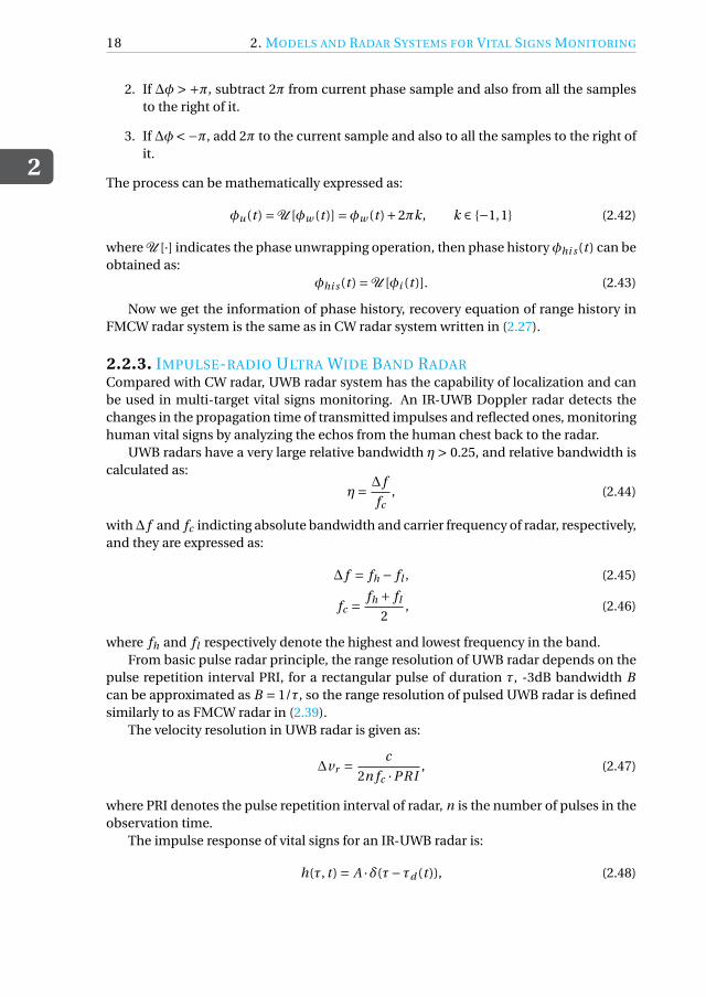
2. If ∆φ > +π, subtract 2π from current phase sample and also from all the samplesto the right of it.
3. If ∆φ<−π, add 2π to the current sample and also to all the samples to the right ofit.
The process can be mathematically expressed as:
φu(t ) =U [φw (t )] =φw (t )+2πk, k ∈ {−1,1} (2.42)
where U [·] indicates the phase unwrapping operation, then phase historyφhi s (t ) can beobtained as:
φhi s (t ) =U [φi (t )]. (2.43)
Now we get the information of phase history, recovery equation of range history inFMCW radar system is the same as in CW radar system written in (2.27).
2.2.3. IMPULSE-RADIO ULTRA WIDE BAND RADARCompared with CW radar, UWB radar system has the capability of localization and canbe used in multi-target vital signs monitoring. An IR-UWB Doppler radar detects thechanges in the propagation time of transmitted impulses and reflected ones, monitoringhuman vital signs by analyzing the echos from the human chest back to the radar.
UWB radars have a very large relative bandwidth η> 0.25, and relative bandwidth iscalculated as:
η= ∆ f
fc, (2.44)
with∆ f and fc indicting absolute bandwidth and carrier frequency of radar, respectively,and they are expressed as:
∆ f = fh − fl , (2.45)
fc = fh + fl
2, (2.46)
where fh and fl respectively denote the highest and lowest frequency in the band.From basic pulse radar principle, the range resolution of UWB radar depends on the
pulse repetition interval PRI, for a rectangular pulse of duration τ, -3dB bandwidth Bcan be approximated as B = 1/τ, so the range resolution of pulsed UWB radar is definedsimilarly to as FMCW radar in (2.39).
The velocity resolution in UWB radar is given as:
∆vr = c
2n fc ·PRI, (2.47)
where PRI denotes the pulse repetition interval of radar, n is the number of pulses in theobservation time.
The impulse response of vital signs for an IR-UWB radar is:
h(τ, t ) = A ·δ(τ−τd (t )), (2.48)

2.2. RADAR SYSTEMS FOR VITAL SIGNS MONITORING
2
19
where A denotes amplitude of the pulse reflected on surface of human chest, and τd isthe time delay associated with the displacement of chest induced by vital signs:
τd (t ) = 2d(t )
c, (2.49)
and the expression of d(t ) is the same as the one in (2.15), c is the velocity of light.Assume that s(τ) represents the transmitted pulse, the signal received at radar is then
written as:
r (τ, t ) = s(τ)∗h(τ, t )
= A · s(τ−τd (t )). (2.50)
The received signals are measured in slow-time as discrete moments t = kTs , (k = 1,2, . . . ,K ),Ts is the sampling period in slow-time and K is the number of discrete time sequencesin slow-time domain. The received signals are sampled and stored in a two-dimensionalmatrix with fast-time domain sampling period T f :
R[n,k] = r (τ= nT f , t = kTs ). (2.51)
UWB radar can extract vital signs through Doppler information, the desired range his-tory is directly obtained by selecting range cell r where the target is located:
Rhi s [k] = R[r,k]. (2.52)
2.2.4. VITAL SIGNS MONITORING REQUIREMENTS OF RADARSingle-tone CW radar is the most common type in radar-based vital signs monitoringsystem due to its simplicity and low power consumption. But it cannot detect the vi-tal signs of multi-subject at the same time since it cannot provide range information.FMCW and UWB radar are capable of measuring both range and Doppler frequency,therefore they can fulfill the functionality of multi-target detection. However, FMCWradar system suffer from high phase noise level and power consumption [49]. UWB radarsystem has been proven to have great penetration ability, giving dominant position forapplications of search and rescue. But IR-UWB radar is limited by its power density re-striction, leading to short distance applications. Performance of different radar systemsfor vital signs monitoring is summarized in Tab. 2.2 [49].
System Multi-subject detection Range estimation Power consumption
CW No No Medium
FMCW Yes Yes High
IR-UWB Yes Yes Low
Table 2.2: Comparison of Radar-Based Vital Signs Monitoring Systems
The observation time of radar should be set to have the capability of detecting themaximum velocity of the minimum human chest displacement. The maximum veloci-
2
20 2. MODELS AND RADAR SYSTEMS FOR VITAL SIGNS MONITORING
ties of minimum respiration and heartbeat amplitudes in the sinusoidal model in Sec-tion 2.1.2 (2.1) can be calculated as:
vr,si n = max
{∂xr 1(t )
∂t
}= 1.26 [mm/s], (2.53)
vh,si n = max
{∂xh1(t )
∂t
}= 1.56 [mm/s]. (2.54)
And the maximum velocities of minimum respiration and heartbeat amplitudes in im-proved model described in Section 2.1.2 (2.3) and (2.5) can be calculated as:
vr,i mp = max
{∂xr 2(t )
∂t
}= 1.45 [mm/s], (2.55)
vh,i mp = max
{∂xh2(t )
∂t
}= 5.81 [mm/s]. (2.56)
The global minimum velocity of sinusoidal cardiopulmonary model is vmi n,si n = 1.26mm/s,the global minimum of improved cardiopulmonary model is vmi n,i mp = 1.45mm/s.
For the sake of measuring this maximum velocity of the minimum chest displace-ment with central frequency fc , it meet the requirement as follows:
c
2 fc ·C PIÉ 0.1 · vmi n , (2.57)
so the coherent processing interval (CPI) of FMCW and UWB radars should be:
C PI Ê 5c
fc vmi n. (2.58)
According to the Nyquist sampling theorem, radar echo should be sampled overtwice as fast as the highest frequency component. The maximum velocity of the sinu-soidal and improved cardiopulmonary model is vmax = 26.34mm/s. So the samplingfrequency in vital signs monitoring system should meet the requirement of:
fs > 2 fmax = 22vmax fc
c. (2.59)
As discussed in Section 2.2.3, the range resolution of IR-UWB radar is defined as:
∆R = c
2B,
where c is the velocity of light and B is the bandwidth of radar. Typical range resolutionof UWB radar in vital signs monitoring is about 3mm.
The chest displacement we want to detect is in millimeter-scale and if vital signsare extracted from range displacement in UWB radar system, the requirement must besatisfied as:
∆R < Ah,mi n . (2.60)
The range resolution of UWB radar is only related to bandwidth, so the choice of band-width is limited as:
B > c
2Ah,mi n. (2.61)

2.3. RADAR RECEIVED DATA MODEL
2
21
Higher resolution implies larger bandwidth, a FMCW radar does not have very widebandwidth, which limits its range resolution. In FMCW system, vital signs are extractedby obtaining Doppler information. Therefore, the range resolution of the FMCW radar isconstrained by the required separation of multiple people in the scene.
One parameter related but not identical to range resolution is the accuracy of rangemeasurement, depending essentially on bandwidth and noise, and it is described by:
δR = c
2Bp
2SN R= ∆Rp
2SN R. (2.62)
So bandwidth and signal-to-noise level are two significant parameters for the accuracyin range determination. Range resolution contributes to accuracy in range domain butis not the only factor.
In like manner of range resolution, radar velocity resolution can be written as:
∆v = c
2n fc T,
where c is speed of light, fc is radar carrier frequency, T denotes duration of a chirp (forCW radar) or a pulse (for IR-UWB radar). The smallest resolvable velocity for FMCW andUWB radars should not be larger than the maximum velocity of heartbeat signal withminimum amplitudes, which is expressed as:
∆v < vh,mi n . (2.63)
So the velocity resolution of a radar used for vital signs monitoring should be about1mm/s.
2.3. RADAR RECEIVED DATA MODELIn the previous section, the extraction of range history in different radar systems wasintroduced. However, in the actual working environment of radar, noise and automobilevibration are unavoidable and they will interfere with the target signal. Vibration canbe seen as extra range displacement and thus additive to range history induced by chestmovement. The phase noise can be assumed Gaussian in moderate to high SNR case,hence the noise can also be added to the range history. White and colored Gaussiannoise are added to received data of vital signs s in order to simulate the environmentnoise n and car vibration v , so the radar received data will become:
y = Rhi s +n + v, (2.64)
where Rhi s is the range history induced by vital signs, n is white Gaussian noise, and thecar vibration v is modelled by a second-order autoregressive model:
vt =α1vt−1 +α2vt−2 +εt , (2.65)
where α1,α2 are parameters of the model, εt is white noise. The process is stable whenthe roots are within the unit circle, which means the coefficients α1,α2 satisfy:
−1 ≤α2 ≤ 1− |α1 | . (2.66)
2
22 2. MODELS AND RADAR SYSTEMS FOR VITAL SIGNS MONITORING
The power spectral density of AR(2) model can be expressed as:
S( f ) = 1
1+α21 +α2
2 −2α1(1−α2)cos(2π f )−2α2cos(4π f ). (2.67)
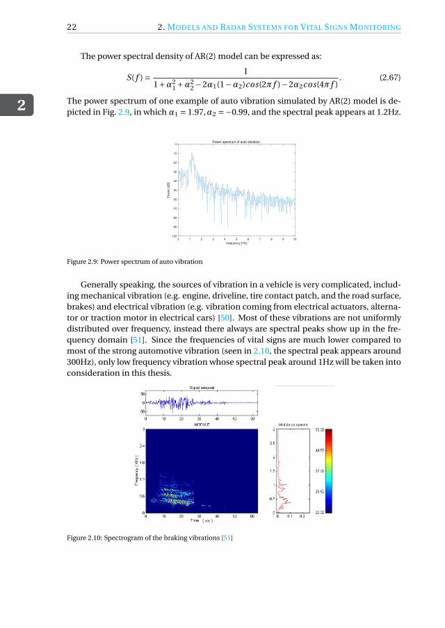
The power spectrum of one example of auto vibration simulated by AR(2) model is de-picted in Fig. 2.9, in which α1 = 1.97,α2 =−0.99, and the spectral peak appears at 1.2Hz.
0 1 2 3 4 5 6 7 8 9 10
frequency [Hz]
-100
-90
-80
-70
-60
-50
-40
-30
-20
-10
0
Pow
er
[dB
]
Power spectrum of auto vibration
Figure 2.9: Power spectrum of auto vibration
Generally speaking, the sources of vibration in a vehicle is very complicated, includ-ing mechanical vibration (e.g. engine, driveline, tire contact patch, and the road surface,brakes) and electrical vibration (e.g. vibration coming from electrical actuators, alterna-tor or traction motor in electrical cars) [50]. Most of these vibrations are not uniformlydistributed over frequency, instead there always are spectral peaks show up in the fre-quency domain [51]. Since the frequencies of vital signs are much lower compared tomost of the strong automotive vibration (seen in 2.10, the spectral peak appears around300Hz), only low frequency vibration whose spectral peak around 1Hz will be taken intoconsideration in this thesis.
Figure 2.10: Spectrogram of the braking vibrations [51]

2.4. CONCLUSION
2
23
2.4. CONCLUSIONThe main content in this chapter consists of a description of the cardiopulmonary activ-ity, followed by its mathematical model and the extension of the model to dynamic con-dition. Most studies simplify the respiration and heartbeat as sinusoidal models. Theimproved cardiopulmonary signal models were investigated in this chapter to providebetter fitness of vital actual signs waveform. Furthermore, a first-order auto-regressionmodel was proposed to simulate the fluctuation of both respiration and heartbeat sig-nals in reality.
Afterwards, three types of radar systems used in vital signs monitoring were described.These are continuous wave (CW) radar, frequency modulated continuous wave radar(FMCW) and ultra- wideband (UWB) radar. The major advantages of single-tone CWradar are simple structure, low power consumption. However, it lacks capability of rangemeasurement, and thus target detection and localization. Reasonable approaches to re-solve this issue could be FMCW radar and UWB radar. The main disadvantages of FMCWradar are high power consumption, while impulse-radio UWB radar requires larger vol-ume than CW although usually residing with high spatial resolution [30].
Subsequently, radar received data model was constructed, embracing range history,the possible presence of noise and auto vibration. We modeled environment noise bywhite Gaussian noise and auto vibration as a colored Gaussian noise simulated by asecond-order auto-regressive model, which spectral peak is near 1Hz.


3SIGNAL DECOMPOSITION AND
ANALYSIS METHODS
Radar echo signal contains information on respiration and heartbeat signals, as well asbackground noise, clutter and interference. Prior to analyzing the radar data directly, afew signal decomposition methods are considered to extract vital signs from radar data.The most well-known tool is the empirical mode decomposition (EMD). To improvethe stability of EMD against noise, two modifications of EMD are investigated, namely,ensemble empirical mode decomposition (EEMD) and complete ensemble empiricalmode decomposition with adaptive noise (CEEMDAN). However, EMD and its modi-fications algorithms are sensitive to noise. So variational mode decomposition (VMD)is investigated to address the issue of EMD algorithms. The analysis of the extractedsignals is demonstrated with the Hilbert transform, which shows the time-frequency-energy distribution of each mode.
The main themes covered in this chapter are the description of empirical, variationalmode decomposition algorithms, and numerical analysis of these methods.
3.1. EMPIRICAL MODE DECOMPOSITIONEmpirical mode decomposition is an adaptive and highly efficient method that decom-poses a compound signal into a finite number of intrinsic mode functions (IMF), towhich well-behaved Hilbert transform can be applied to construct time-frequency spec-trum of each component [52]. In order to make the instantaneous frequencies of a signalmeaningful, its envelopes should be symmetric with respect to zero and it should havethe same number of zero crossings and extreme points [53]. On this basis, the two phys-ical constraints of IMF were proposed in [52]:
1. Each intrinsic mode function should either have the same number of extrema andzero crossings, or differ by one at most;
2. At any point, the mean value of the upper envelope of maxima (see in Fig. 3.1(a))
25

3
26 3. SIGNAL DECOMPOSITION AND ANALYSIS METHODS
and the lower envelope of minima (see in Fig. 3.1(a)) is zero, that is, local symmetryon zero axis.
Apparently, the first constraint is to make the instantaneous frequency of any pointin IMF meaningful [54]. The second constrain is the idea of replacing the global require-ment with a local one, preventing instantaneous frequencies from unwanted fluctua-tions incurred by asymmetric waveform [52]. In each cycle of the decomposed signalrepresented by IMF, it contains only one oscillation mode, which can be either frequencyand amplitude modulated, or even non-stationary.
The first constrain is crucial to make the instantaneous frequency meaningful, whileif the second constrain is carried to the extreme, the amplitude fluctuations of IMF willbe wiped out. There is a systematic way that can intuitively decompose a signal to ob-tain IMFs in the time domain, denominated as a sifting process of EMD. So a stoppingcriterion for the sifting process is proposed in order to guarantee both amplitude and fre-quency modulations of IMFs are physically meaningful. The criterion is usually realizedby restriction of the standard deviation of two consecutive sifting processes.
The essence of EMD is to empirically determine the intrinsic oscillation modes of theoriginal signal based on their characteristic time scales, and accordingly decompose thesignal into several IMFs [52]. EMD is thus performed with the following steps [52]:
1. Find all local maximum value of input signal s(t ), connect all local maxima by a cu-bic spline to get the upper envelope s(1,1)
max (t ) (see Fig. 3.1(a)). Repeat the procedureto find local minima and produce the lower envelope s(1,1)
mi n(t ) (see Fig. 3.1(b)).
2. Calculate the mean of upper and lower envelopes, get the mean envelope m1 de-picted in Fig. 3.1(c):
m1 =s(1,1)
max (t )+ s(1,1)mi n(t )
2. (3.1)
3. The difference between the original signal and mean envelope is the first compo-nent m1,1, The residue h1,1 shown in Fig. 3.1(d):
h1,1 = s(t )−m1,1. (3.2)
4. Replace the original signal s(t ) with h1,1 and repeat Step 1-3, until standard devia-tion from the two consecutive sifting is less than predefined value ε:
SD =∑
(h1,k−1 −h1,k )2∑h2
1,k−1
< ε, (3.3)
with ε is typically set between 0.2 and 0.3. The first IMF component is decomposedand designated as:
c1 = h1,k = m1,k −h1,k−1. (3.4)
5. Repeat the steps above until the final residual has no more oscillation and cannotbe decomposed, meaning the number of extrema in the last residual should not begreater than one. The residual rn(t ) indicates the mean trend of the signal. After

3.2. HILBERT-HUANG TRANSFORM
3
27
0 10 20 30 40 50 60
Time [s]
-5
0
5
Am
plit
ud
e [
mm
]
IMF 1: iteration 0 The original signal
Local maximum
Upper envelope
0 10 20 30 40 50 60
Time [s]
-5
0
5
Am
plit
ud
e [
mm
]
IMF 1: iteration 0 The original signal
Local minimum
Lower envelope
0 10 20 30 40 50 60
Time [s]
-5
0
5
Am
plit
ud
e [
mm
]
IMF 1: iteration 0
The original signal
Mean envelope
0 10 20 30 40 50 60
Time [s]
-5
0
5
Am
plit
ud
e [
mm
]
Residue
(a)
(b)
(c)
(d)
Figure 3.1: EMD sifting process: (a) upper envelope; (b) lower envelope; (c) mean envelope; (d) residue.
EMD, the input signal s(t ) is expressed as the summation of a finite number ofIMFs ci (t ), i = 1, . . . ,n, and the residual rn(t ):
s(t ) =n∑
i=1ci (t )+ rn(t ). (3.5)
EMD is an adaptive signal decomposition algorithm thus it can decompose the res-piration and heartbeat signal from human chest displacement information carried byradar echo data [55]. Fig. 3.2 displays a simple empirical mode decomposition resultfrom simulated mixed signals of respiration, heartbeat and environment noise. It can beseen from the result that the waveforms in different time scales are extracted and high-lighted. The first IMF contains the highest frequency component of the original signal,after step-wise decomposition, the frequency of IMF decreases in turn while the last IMFcontains the lowest one. The last component is the original signal trend instead of a os-cillation mode. Also, it should be noticed that mode mixing happened at IMF2-3 andIMF4-5. Part of the intrinsic mode in IMF3 leaks into IMF2 and IMF5 contains somecomponent of IMF4. So, the determination of respiration and heartbeat signals shouldbe achieved by analyzing the frequency information of different IMFs. The exposition offrequency analysis method, called Hilbert-Huang transform, will be in Section 3.2.
3.2. HILBERT-HUANG TRANSFORMHilbert Huang transform (HHT) is a signal analysis method proposed by Norden E. Huangetc in 1998 [52]. It is a time-frequency analysis method that can effectively analyze linearand nonlinear, stationary and non-stationary signals. The essences of HHT are empiricalmode decomposition (EMD) and Hilbert transform (HT), the former is a signal decom-position method, the latter is a spectral analysis method.
It can be found from the development of signal analysis methods that various meth-ods are posed to satisfy the interest in different features of different signal types. For a

3
28 3. SIGNAL DECOMPOSITION AND ANALYSIS METHODS
0 5 10 15 20 25 30 35-5
0
510
-3 Input signal
0 5 10 15 20 25 30 35
-2
0
210
-4 IMF1
0 5 10 15 20 25 30 35
-4-2024
10-4 IMF2
0 5 10 15 20 25 30 35-5
0
510
-4 IMF3
0 5 10 15 20 25 30 35-5
0
510
-3 IMF4
0 5 10 15 20 25 30 35
-2
0
210
-3 IMF5
0 5 10 15 20 25 30 35
-1
0
110
-3 IMF6
0 5 10 15 20 25 30 35
-2
0
210
-4 IMF7
0 5 10 15 20 25 30 35
-2-101
10-4 IMF8
Figure 3.2: The resulting EMD components from noisy vital signs
stationary linear or periodic signal, the spectrum of the signal can be obtained by meansof Fourier transform. For a non-stationary or nonlinear signal, the local spectral fea-tures of the signal are of interest. Different time-frequency analysis methods are used toobtain the time-frequency representation of the signal, such as short-time Fourier trans-form (STFT) [16], Wavelet transform (WT) [56] and Wigner-Ville distribution (WVD) [57].
However, the time-frequency analysis methods mentioned above are based on theFourier transform, lacking adaptivity to the signal. In addition, these time-frequencyanalysis methods cannot accurately describe rapid changes of frequency over time dueto the limitation of Heisenberg’s uncertainty principle. So ideally, in order to accuratelydescribe frequency changes over time, an adaptive, intuitive, instantaneous frequencyanalysis method is needed, which is the Hilbert Huang transform. In this framework,EMD is used to adaptively decompose the signal into a finite number of intrinsic modefunctions (IMF) and a residual signal representing the trend of the signal. Then Hilberttransform is used to conduct time-frequency analysis to the acquired IMFs.
In empirical mode decomposition, input signal s(t ) is decomposed into the summa-tion of n intrinsic mode functions ci (t ) and a residual signal rn(t ). Hilbert transform isapplied to each IMF:
Yi (t ) = 1
πPV
∫ ∞
−∞Ci (τ)
t −τ dτ, (3.6)
where PV is the Cauchy principal value. The resulting analytical signal is:
Zi (t ) =Ci (t )+ j Yi (t ). (3.7)
In the form of polar coordinates:
Zi (t ) = ai (t )e jθi (t ), (3.8)

3.2. HILBERT-HUANG TRANSFORM
3
29
and
ai (t ) = [C 2
i (t )+Y 2i (t )
] 12 , θi (t ) = arctan
[Yi (t )
Ci (t )
]. (3.9)
The polar form of the analytical signal reflects the physical meaning of the Hilberttransform, which is the best local approximation of the signal through a sinusoidal fre-quency and amplitude modulation. According to the meaning of instantaneous fre-quency, the instantaneous frequency of each IMF can be obtained:
ωi (t ) = d
d tθi (t ). (3.10)
With time t and instantaneous frequency ωi (t ) as the independent variables, the signalamplitude can be expressed as a function of t andωi (t ). This amplitude-time-frequencydistribution is called Hilbert spectrum.
Examples of Hilbert spectrum are displayed in Fig. 3.3, demonstrating the time-frequency-energy distribution of IMF1-8 as the result of EMD in Fig. 3.2. The frequency distributionof IMF3 is concentrated at a narrow region around 1.5Hz and IMF4 is around 0.25Hz.Based on this representation, it is reasonable to tell IMF3 mainly contains heartbeatcomponents while the respiratory signal component is mostly represented in IMF4. Itcan be seen from the Hilbert spectrum that the instantaneous frequency changes rapidlyat certain moments, indicating occurrences of mode mixing. The color bar in the Hilbertspectrum shows the instantaneous energy intensity of IMFs, and yellow-colored curveimplies the strongest energy, indicating the mode that represents original respirationsignal.
Figure 3.3: Hilbert spectrum of IMFs obtained by EMD

3
30 3. SIGNAL DECOMPOSITION AND ANALYSIS METHODS
3.3. ENSEMBLE EMPIRICAL MODE DECOMPOSITIONEMD is an adaptive, widely-used and highly efficient signal decomposition method, how-ever, it suffers from the deficiency of mode mixing. Usually, mode mixing occurs whenthe input signal is obtained by a high-frequency signal, especially an intermittent high-frequency signal added to a low-frequency signal (see in Fig. 3.4(a)). When mode mix-ing happens, IMF contains tremendously different scales of oscillations, or similar timescales reside in different IMFs. Ensemble empirical mode decomposition (EEMD) wasproposed by Wu and Huang in 2009 to overcome the shortage of EMD [58].
Figure 3.4: Mode mixing problem
The principle of EEMD relies on adding white noise to the original signalwhich willuniformly fill in the entire time-frequency space of signal with components of differentscales [59]. The added noise populates the signal, thus making the signal not intermit-tent and alleviating the mode mixing problem.
Although extra noise is added to the original signal, the sets of zero-mean whiteGaussian noise cancel each other out in the spatial-temporal overall mean. Eventually, itis the original signal that is the only consistent part as a sufficient large number of trialsare tested. So, the average of trails can be considered as the final result of EEMD. Theconcepts of EEMD are given as [58]:
1. Build N realizations of white Gaussian noise and add them to input signal one byone, obtaining a collection of noisy signals:
si (t ) = s(t )+w i (t ), (3.11)
where s(t ) denotes the signal to be decomposed and wi (t ) is the i th independentrealization of zero-mean white Gaussian noise, i = 1,2, . . . , N .
2. Conduct empirical mode decomposition to every noisy signal si (t ), i = 1,2, . . . N ,and obtain a set of IMFi
k ,k = 1,2, . . .K .
3. Calculate ensemble mean of the decomposed IMFs:
IMFk = 1
N
N∑i=1
IMFik . (3.12)

3.4. COMPLETE ENSEMBLE EMPIRICAL MODE DECOMPOSITION WITH ADAPTIVE NOISE
3
31
Fig. 3.5 is an example of EEMD result from noisy respiration and heartbeat signals.We can see from this figure that there are more modes obtained by EEMD than EMDbecause of adding extra white noise. The mode mixing issue in EMD is alleviated inEEMD. From the Hilbert spectrum of IMFs from EEMD in Fig. 3.6, it can be found thatIMF3 represents the heartbeat signal since most of its instantaneous frequencies changebetween 1-1.5Hz, and Hilbert spectrum of IMF4 resides around 0.25Hz, representingrespiration signal.
0 5 10 15 20 25 30 35-4-2024
10-3 Input signal
0 5 10 15 20 25 30 35
-2024
10-4 IMF1
0 5 10 15 20 25 30 35
-202
10-4 IMF2
0 5 10 15 20 25 30 35
05
1010
-4 IMF3
0 5 10 15 20 25 30 35
-202
10-3 IMF4
0 5 10 15 20 25 30 35-2-101
10-3 IMF5
0 5 10 15 20 25 30 35
-2024
10-4 IMF6
0 5 10 15 20 25 30 35
-101
10-4 IMF7
0 5 10 15 20 25 30 35
-202
10-5 IMF8
0 5 10 15 20 25 30 35
5
1010
-4 IMF9
Figure 3.5: The resulting EEMD components from noisy vital signs
3.4. COMPLETE ENSEMBLE EMPIRICAL MODE DECOMPOSITION
WITH ADAPTIVE NOISEEEMD resolves the problem of mode mixing in EMD, however, it introduces new issues.The reconstructed signal still contains the residual noise component. A new methodnamed complete ensemble empirical mode decomposition with adaptive noise (CEEM-DAN) was proposed, providing better separation of IMFs [37]. CEEMDAN was devel-oped as an improvement over the EEMD algorithm, with a reduced number of siftingiterations and lower computational cost.
CEEMDAN algorithm [37] is described by following steps with s(t ) as the input signal:
1. Decompose I realizations of s(t )+σ0w i (t ), i = 1, . . . , I by EMD, the first mode ofCEEMDAN IMF1 will be computed as:
IMF1 = 1
I
I∑i=1
IMFi1, (3.13)
3
32 3. SIGNAL DECOMPOSITION AND ANALYSIS METHODS
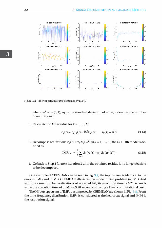
Figure 3.6: Hilbert spectrum of IMFs obtained by EEMD
where w i ∼ N (0,1), σ0 is the standard deviation of noise, I denotes the numberof realizations.
2. Calculate the kth residue for k = 1, . . . ,K :
rk (t ) = rk−1(t )− IMFk (t ), r0(t ) = s(t ). (3.14)
3. Decompose realizations rk (t )+σk Ek (w i (t )), i = 1, . . . , I , , the (k +1)th mode is de-fined as:
IMFk+1 =1
I
I∑i=1
E1(rk (t )+σk Ek (w i (t ))). (3.15)
4. Go back to Step 2 for next iteration k until the obtained residue is no longer feasibleto be decomposed.
One example of CEEMDAN can be seen in Fig. 3.7, the input signal is identical to theones in EMD and EEMD. CEEMDAN alleviates the mode mixing problem in EMD. Andwith the same number realizations of noise added, its execution time is 6.21 secondswhile the execution time of EEMD is 9.78 seconds, showing a lower computational cost.
The Hilbert spectrum of IMFs decomposed by CEEMDAN are shown in Fig. 3.8. Fromthe time-frequency distribution, IMF4 is considered as the heartbeat signal and IMF6 isthe respiration signal.

3.5. VARIATIONAL MODE DECOMPOSITION
3
33
0 5 10 15 20 25 30 35-4-2024
10-3 Input signal
0 5 10 15 20 25 30 35
-202
10-4 IMF1
0 5 10 15 20 25 30 35
-505
1010
-5 IMF2
0 5 10 15 20 25 30 35-2
0
210
-4 IMF3
0 5 10 15 20 25 30 35
-4-2024
10-4 IMF4
0 5 10 15 20 25 30 35
-505
1010
-4 IMF5
0 5 10 15 20 25 30 35-4-2024
10-3 IMF6
0 5 10 15 20 25 30 35
-2024
10-4 IMF7
0 5 10 15 20 25 30 35-505
10-5 IMF8
0 5 10 15 20 25 30 35
05
1010
-5 IMF9
Figure 3.7: The resulting CEEMDAN components from noisy vital signs
Figure 3.8: Hilbert spectrum of IMFs obtained by CEEMDAN
3.5. VARIATIONAL MODE DECOMPOSITIONVariational mode decomposition (VMD) is a kind of algorithm in which the modes areextracted concurrently [38]. The objective of variational mode decomposition algorithm

3
34 3. SIGNAL DECOMPOSITION AND ANALYSIS METHODS
is to obtain the optimal solution through iteration, so as to determine the center fre-quency and bandwidth of each mode component [38]. Each mode uk is mostly con-centrate around central frequency ωk , and the sum of every component bandwidths isthe smallest [60]. Different from the definition of the intrinsic mode function of EMDalgorithm, the intrinsic mode function of the VMD algorithm is an amplitude-frequencymodulation signal:
uk (t ) = Ak (t )cos(φk (t )) (3.16)
where uk (t ) is the intrinsic mode function in VMD, Ak (t ) denotes the amplitude of en-velope and it is non-negative, the phase φk (t ) is non-decreasing, and it should be notedthat both amplitude Ak (t ) and instantaneous frequency ωk (t ) = dφk (t )/d t vary muchslower than the phase φk (t ), that is, the mode uk can be regarded as a pure harmonicsignal on a sufficiently long interval [t −δ, t +δ], δ≈ 2π/φ
′k (t ) [61].
The aim of VMD algorithm is to search for k IMFs with limited bandwidths and dif-ferent center frequencies, also the sum of the bandwidths should be the smallest [62].There are two major parts involved in VMD, the construction and solution of the varia-tional problem, each of them will be explained in detail.
The steps of variational problem construction is described as follows [38]:
1. The analytic signal of each intrinsic mode function uk (t ) is calculated by Hilberttransform, obtaining a single-sided frequency spectrum:
uk,A(t ) =(δ(t )+ j
πt
)∗uk (t ), (3.17)
where is δ denotes Dirac function and ∗ stands for the convolution operation.
2. Multiply the analytic signal and harmonic signal with central frequency ωk :[(δ(t )+ j
πt
)∗uk (t )
]e− jωk t . (3.18)
By doing which, the spectrum kth mode is shifted to baseband.
3. Find the squared L2-norm of the gradient in (3.18), and estimate from this band-width of each IMF can be estimated from this. The resulting constrained varia-tional problem is expressed as:
min{uk },{ωk }
{ K∑k=1
∥∥∥∂t
[(δ(t )+ j
πt
)∗uk (t )
]e− jωk t
∥∥∥2}, (3.19)
where {uk } := {u1, . . . ,uK } and {ωk } := {ω1, . . . ,ωK } denote collections of K IMFs andtheir center frequencies, respectively.
The variational problem can be settled in different ways. Here, the steps of the solu-tion from [38] are demonstrated as:

3.5. VARIATIONAL MODE DECOMPOSITION
3
35
1. Firstly, quadratic penalty term and Lagrangian function are introduced, convert-ing the unconstrained minimization problem in (3.19) to a constrained one:
L ({uk }, {ωk },λ) =αK∑
k=1
∥∥∥∂t
[(δ(t )+ j
πt
)∗uk (t )
]e− jωk t
∥∥∥2
+∥∥∥s(t )−
K∑k=1
uk (t )∥∥∥2
+⟨λ(t ), s(t )−
K∑k=1
uk (t )
⟩, (3.20)
where α is the penalty coefficient, λ(t ) is the Lagrange multiplier, s(t ) is the inputsignal.
2. The issue remains to be addressed for now is a convex optimization problem,which can be tackled by alternating direction method for multipliers (ADMM), de-tain of the algorithm can be seen in Algorithm 1 [38]:
Algorithm 1 ADMM optimization steps for VMD
Initialize {u1}, {ω1}, λ1, n ← 0repeat
n ← n +1for k = 1 : K do
Update uk :un+1
k ← argminuk L({un+1
i<k }, {uni≥k }, {ωn
i },λn)
end forfor k = 1 : K do
Update ωk :ωn+1
k ← argminωk L({un+1
i }, {ωn+1i<k }, {ωn+1
i≥k },λn)
end forDual ascent:
λn+1 ←λn +τ(s −∑
k un+1k
)until convergence:
∑k
∥∥un+1k −un
k
∥∥22/
∥∥unk
∥∥22 < ε
3. However, there are sub-optimization problems remain in ADMM algorithm. Byapplying ADMM to update the modes, un+1
k can be written as:
un+1k = argmin
uk
{α
∥∥∥∂t
[(δ(t )+ j
πt
)∗uk (t )
]e− jωk t
∥∥∥2
2
+∥∥∥s(t )−∑
iui (t )+ λ(t )
2
∥∥∥2
2
}. (3.21)
4. The problem in (3.21) can be transformed to spectral domain using the Parseval
3
36 3. SIGNAL DECOMPOSITION AND ANALYSIS METHODS
Fourier isometry under L2-norm, shown as follows:
un+1k = argmin
uk
{α‖ jω[1+ sgn(ω+ωk ) · uk (ω+ωk )]‖2
2
+∥∥∥s(ω)−∑
iui (ω)+ λ(ω)
2
∥∥∥2
2
}, (3.22)
where sgn(·) represents the sign function defined as:
sgn(x) =
−1 if x < 0,0 if x = 0,1 if x > 0.
5. Substitute ω in the first term of (3.22) by ω−ωk , we can get:
un+1k = argmin
uk
{α‖ j (ω−ωk )[1+ sgn(ω) · uk (ω)]‖2
2
+∥∥∥s(ω)−∑
iuk (ω)+ λ(ω)
2
∥∥∥2}. (3.23)
6. Rewrite the term in (3.23) as half-space integrals using the Hermitian symmetry ofthe real signals in the reconstruction fidelity term:
un+1k = argmin
uk
{∫ ∞
04α(ω−ωk )2|uk (ω)|2
+2∣∣∣s(ω)−∑
iui (ω)+ λ(ω)
2
∣∣∣2dω
}. (3.24)
7. The above quadratic optimization problem is solved by letting the first variationvanish for the positive frequencies, which means:
un+1k (ω) = s(ω)−∑
i ui (ω)+ λ(ω)2
1+2α(ω−ωk )2 . (3.25)
8. The same method is exploited to update the center frequency of the intrinsic modefunctions ωk , the iterative formula is:
ωn+1k =
∫ ∞0 ω|uk (ω)|2dω∫ ∞
0 |uk (ω)|2dω. (3.26)
9. Since we have the solutions to sub-optimizations in ADMM algorithm as shownin Algorithm 1, the complete optimization algorithm of VMD is described in Algo-rithm 2 [38].

3.6. NUMERICAL SIMULATIONS
3
37
Algorithm 2 Complete optimization steps for VMD
Initialize {u1}, {ω1}, λ1, n ← 0repeat
n ← n +1for k = 1 : K do
Update uk for all ω≥ 0:
un+1k ←
(s(ω)−∑
i<k un+1i (ω)−∑
i>k uni (ω)+ λn (ω)
2
)/(1+2α(ω−ωn
k )2)
Update ωk :ωn+1
k ← (∫ ∞0 ω|un1
k (ω)|2dω)/(∫ ∞
0 |un1k (ω)|2dω
)end forDual ascent for all ω≥ 0:
λn+1(ω) ← λn(ω)+τ(s(ω)−∑
k un+1k (ω)
)until convergence:
∑k
∥∥un+1k −un
k
∥∥22/
∥∥unk
∥∥22 < ε
It requires some manually setting of the parameters before applying VMD algo-rithm to obtain IMFs:
(a) Penalty coefficient α: it can affect the bandwidth of the intrinsic mode func-tion. The larger the value, the faster the attenuation on both sides of the cen-tral frequencies will be.
(b) Time step of the dual ascent τ: used to solve the convex optimization prob-lem, the value is typically chosen under 1 and can be set to zero when thereis strong noise.
(c) The number of modes to be recovered K .
(d) Tolerance of convergence criterion ε: typically set around 1×10⁶.
The result of VMD is depicted in Fig. 3.9. Unlike EMD algorithms, the lower orderIMFs in VMD represent rapidly varying signal components. So the respiration signal,which has the lowest frequency in the original signal, is the first decomposed mode. Theheartbeat signal is represented by IMF2. The verification can be seen in Fig. 3.10, whichdescribes the instantaneous frequencies of IMFs. We can see the frequency distributionsof IMF1 and IMF2 correspond to the frequency ranges of respiration and heartbeat, re-spectively.
3.6. NUMERICAL SIMULATIONSFour signal decomposition methods have been discussed. Methods could be adverselyaffected by certain circumstances. Therefore, the performances of signal decompositionmethods in vital signs monitoring under disparate conditions need to be assessed. It ishard to extract the heartbeat signal with the presence of noise and auto vibration since itis much weaker than the respiratory signal and has a relatively close frequency compo-nent with auto vibration. In this case, only the result of respiration signal extraction willbe evaluated. The extracted respiration signal is determined by the amplitude and fre-quency of the decomposed IMF. The IMF corresponding to the respiration should have

3
38 3. SIGNAL DECOMPOSITION AND ANALYSIS METHODS
0 5 10 15 20 25 30 35-4-2024
10-3 Input signal
0 5 10 15 20 25 30 35
-2
0
2
410
-3 MODE1
0 5 10 15 20 25 30 35
-5
0
510
-4 MODE2
0 5 10 15 20 25 30 35
-1
0
1
10-4 MODE3
0 5 10 15 20 25 30 35
-1
0
1
10-4 MODE4
0 5 10 15 20 25 30 35
-1
0
1
10-4 MODE5
0 5 10 15 20 25 30 35
-1
0
1
10-4 MODE6
Figure 3.9: The resulting VMD components from noisy vital signs
Figure 3.10: Hilbert spectrum of IMFs obtained by VMD
the largest amplitude and the frequency distribution should fall into the typical respi-ratory frequency range. Owing to the dynamic performance of cardiopulmonary sig-nals, noise and vibration waveforms, Monte Carlo simulation is a reliable method usedto assess different signal decomposition results under diverse signal-to-noise ratio con-ditions and vibration amplitudes through a large number of repeated experiments [63].
Here, two evaluation metrics are applied to assess the performance of empirical and

3.6. NUMERICAL SIMULATIONS
3
39
variational mode decomposition algorithms. The first is the signal-to-noise ratio of es-timated respiration signal. We treat the difference between the original signal and theestimated signal as noise, the SNR of estimated respiration signal is thus calculated as:
SN R = 10log10
(Ps
Pn
), (3.27)
where Ps is original respiration signal power and Pn is noise power.The second metric is the root mean square error of frequency:
RMSE f =√√√√ 1
N
N∑i=1
(fr − fr)2, (3.28)
where N is the number of samples, fr = [ fr,1, . . . , fr,N ] is a N dimensional vector repre-senting instantaneous frequencies of original respiration signal; fr = [ fr,1, . . . , fr,N ] de-note N instantaneous frequencies of estimated respiration signal.
Fig. 3.11 and 3.12 are the performance assessments under different input SNR levelwhen only white Gaussian noise is added to the vital signs. The input SNR shows the dif-ference in energy level between the original signal and the added white noise. In contrastto our common intuition, the SNR of reconstructed respiration signal (seen in Fig.3.11)does not monotonically grow with the increase of input SNR. We notice that EEMD per-forms better than CEEMDAN under the condition of low input SNR, but CEEMDAN ismore promising in higher input SNR cases. In general, VMD is the most robust methodto noise while EMD is the least stable method against noise. When it comes to the esti-mation of SNR of reconstructed respiration signal, the best accuracy is achieved by VMDwhen the input SNR is 27dB, with which the highest SNR of reconstructed respiration is25dB. The most accurate result of other methods is about 20dB, when the input SNR isaround 30dB.
10 12 14 16 18 20 22 24 26 28 30
Total input SNR
5
10
15
20
25
30
To
tal S
NR
of
estim
ate
d r
esp
ira
tio
n a
mp
litu
de
Monte-Carlo Simulation Result
EMD
EEMD
CEEMDAN
VMD
Figure 3.11: SNR of reconstructed respiration signal
RMSE of estimated frequency is studied in Fig. 3.12, the curves of different meth-ods show downward trends. In most SNR cases, EEMD supplies the best estimation ofrespiratory instantaneous frequencies in noisy signals. Whereas for EEMD in high SNR

3
40 3. SIGNAL DECOMPOSITION AND ANALYSIS METHODS
case, due to the presence of additional white noise added in the algorithm, the decom-posed respiration signal will have residual noise components. The noise componentsmight have a higher level than the environment noise, leading to a large RMSE value.It also should be noted that RMSE of estimated frequency in VMD hardly changes withincreasing signal-to-noise ratio, revealing the robustness of VMD to noise. When thesignal-to-noise ratio is within the range of 10-20dB, the error of EMD and CEEMDANfrequency estimation generally decreases with the improvement of input SNR. AlthoughCEEMDAN have worse performance than EEMD at most SNR levels, the RMSE of CEEM-DAN goes beyond EEMD algorithm when input SNR is near 30dB. The peak of accuracyof estimated respiration frequency happens when the input SNR is higher than 15dB forall these methods. The minimum RMSE of EMD is about 0.075 and it is 0.06-0.065 forthe other three methods.
10 12 14 16 18 20 22 24 26 28 30
Total input SNR
0.06
0.065
0.07
0.075
0.08
0.085
0.09
0.095
0.1
0.105
RM
SE
of
estim
ate
d r
esp
ira
tio
n f
req
ue
ncy
Monte-Carlo Simulation Result
EMD
EEMD
CEEMDAN
VMD
Figure 3.12: RMSE of estimated respiration frequency
Next, we investigate the impact of auto vibration level on four signal decompositionalgorithms. The waveform of auto vibration is depicted in Fig. 3.13, in which clutter-to-noise ratio and signal-to-noise ratio are both 20dB.
0 5 10 15 20 25 30 35-5
-4
-3
-2
-1
0
1
2
3
4
5
610-3 Range history vs Auto vibration
Range history
Auto vibration signal
Figure 3.13: The waveform of auto vibration vs range history
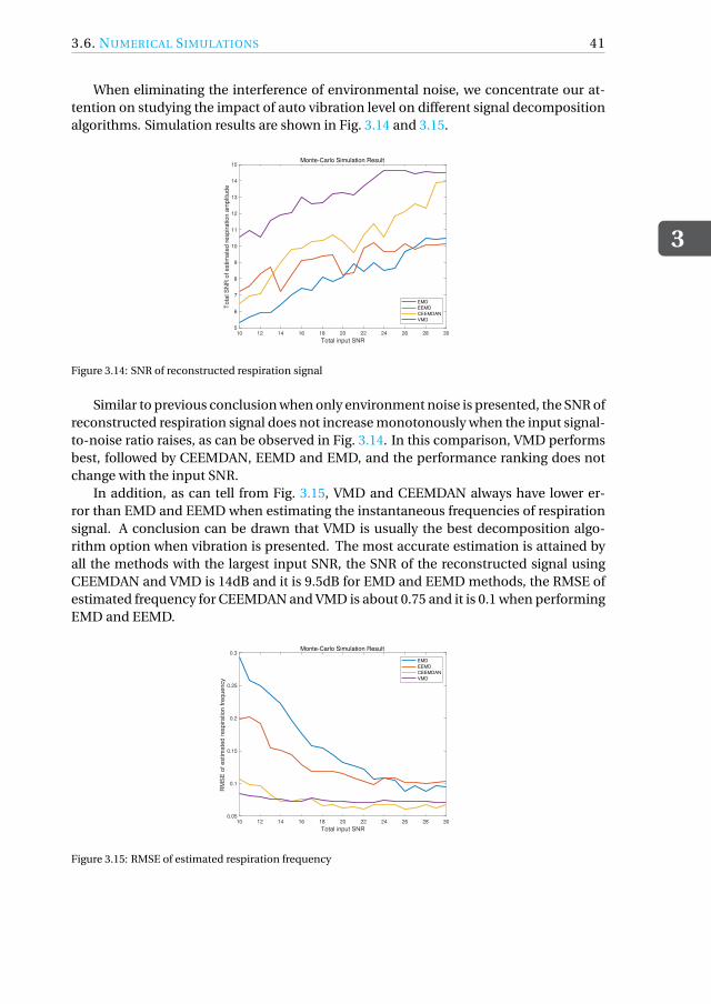
3.6. NUMERICAL SIMULATIONS
3
41
When eliminating the interference of environmental noise, we concentrate our at-tention on studying the impact of auto vibration level on different signal decompositionalgorithms. Simulation results are shown in Fig. 3.14 and 3.15.
10 12 14 16 18 20 22 24 26 28 30
Total input SNR
5
6
7
8
9
10
11
12
13
14
15
To
tal S
NR
of
estim
ate
d r
esp
ira
tio
n a
mp
litu
de
Monte-Carlo Simulation Result
EMD
EEMD
CEEMDAN
VMD
Figure 3.14: SNR of reconstructed respiration signal
Similar to previous conclusion when only environment noise is presented, the SNR ofreconstructed respiration signal does not increase monotonously when the input signal-to-noise ratio raises, as can be observed in Fig. 3.14. In this comparison, VMD performsbest, followed by CEEMDAN, EEMD and EMD, and the performance ranking does notchange with the input SNR.
In addition, as can tell from Fig. 3.15, VMD and CEEMDAN always have lower er-ror than EMD and EEMD when estimating the instantaneous frequencies of respirationsignal. A conclusion can be drawn that VMD is usually the best decomposition algo-rithm option when vibration is presented. The most accurate estimation is attained byall the methods with the largest input SNR, the SNR of the reconstructed signal usingCEEMDAN and VMD is 14dB and it is 9.5dB for EMD and EEMD methods, the RMSE ofestimated frequency for CEEMDAN and VMD is about 0.75 and it is 0.1 when performingEMD and EEMD.
10 12 14 16 18 20 22 24 26 28 30
Total input SNR
0.05
0.1
0.15
0.2
0.25
0.3
RM
SE
of
estim
ate
d r
esp
ira
tio
n f
req
ue
ncy
Monte-Carlo Simulation Result
EMD
EEMD
CEEMDAN
VMD
Figure 3.15: RMSE of estimated respiration frequency

3
42 3. SIGNAL DECOMPOSITION AND ANALYSIS METHODS
3.7. CONCLUSIONIn this chapter, we describe the design and implementation of three empirical and onevariational mode decomposition algorithm. All methods are applicable to vital signsmonitoring and estimation of signal parameters. Hilbert transform is applied to IMFsafter signal decomposition, to acquire time-frequency spectrum and instantaneous fre-quencies of each mode thus obtained.
Analysis of the proposed techniques with numerical simulations have demonstratedthat EEMD is more applicable in a noisy environment aiming to estimate instantaneousfrequency of the reconstructed signal, its high estimation accuracy is achieved as a RMSEof 0.06 when the input SNR is 25dB. VMD is more eligible when referring to the estima-tion of instantaneous amplitude, by applying VMD method, the SNR of reconstructedrespiration signal is up to 25dB. CEEMDAN and VMD are both suitable approaches inpresence of auto vibration, the most accurate estimation is obtained with the vibrationof 30dB SNR.

4ONLINE SIGNAL DECOMPOSITION
METHODS
In the previous chapter, empirical and variational signal decomposition methods havebeen discussed and compared. These signal decomposition methods have not dealt withthe condition of data stream, when new samples are continuously added to the data set,and processed jointly. The existing literature on online empirical mode decomposition(Online-EMD) [64] [65] employs a sliding window and stitching procedure, achieving dy-namic decomposition of data stream. In this chapter, we show the feasibility of executingthe same technique in variational mode decomposition to handle data with increasinglength, nominated as Online-VMD algorithm.
The first section of this chapter illustrates the approach to achieve the online de-composition of data stream. It will then go on to the evaluation and comparison ofonline-EMD and VMD. EEMD and CEEMDAN both seek to obtain IMFs by averagingthe modes decomposed by a number of realizations of extra noise added to the origi-nal signal. These two methods are well-behaved solutions of mode-mixing problem butit takes much longer time than EMD due to the averaging procedure. So, EEMD andCEEMDAN are not considered for online decomposition here.
4.1. ONLINE SIGNAL DECOMPOSITION PRINCIPLEOnline-EMD aims at extracting IMFs from data of unfixed length. In this algorithm, asliding window that encompasses a certain number of extrema is applied to obtain localIMFs, then a window function and stitching procedures are performed, accumulatinglocal IMFs to the global ones [64]. The concept of the sliding window and stitching pro-cedure in Online-EMD is shown in Fig. 4.1.
The online empirical signal decomposition algorithm is shown as follows:
1. Initialization: set number of iteration i = 1, total weights Φ0(t ) = 0, the startingposition of the signal p1 = 0 and let initial IMF M equals zero.
43

4
44 4. ONLINE SIGNAL DECOMPOSITION METHODS
Figure 4.1: Overview of Online-EMD sliding window and stitching procedure
2. Determine the starting window, which encompasses l serial local extrema {p1, . . . , pl }of the original signal s(t ).
3. Implement empirical mode decomposition algorithm to separate the first IMFM i (t ) of current window, the signal component that varies fastest.
4. Now there are l′
positions of extrema in M i and they are denoted as {p′1, . . . , p
′l }.
Weight function φ(t ) on [−τ,τ] (and 0 outside) is utilized in stitching procedure as:
φ(t ) = 1p2π
exp
(− t 2
2
)− 1p
2πexp
(−τ
2
2
), (4.1)
with which we attempt to restrain the discontinuity caused by boundary error.
Set sk =−τ+2(k−1)τ/(l′−1) for k ∈ {1, . . . , l
′}. A new defined weight function called
warped weights φk (t ) is expressed as:
φk (t ) = φ(
sk + (sk+1 − sk )t −e
′k
e′k+1 −e
′k
), (4.2)
where k ∈ {1, . . . , l′ − 1} in warped weight and t ∈ [e
′k ,e
′k+1]. Note that zero is still
not contained in the domain of function. As warped wight function is obtained,weighted IMF M i is shown as follows:
M i (t ) =(φ1(t )M i
1(t ), . . . ,φl ′−1(t )M il ′−1
(t ))
, (4.3)
where M ik (t ) denotes the local IMF between two adjacent extrema, e
′k É t < e
′k+1.
Moreover, the sum of weights is saved as:
Φi (t ) =Φi−1(t )+l′−1∑
k=1φk (t ). (4.4)

4.2. SIMULATION EXAMPLES OF ONLINE DECOMPOSITION
4
45
5. Stitch M i on the previously decomposed weighted IMFs:
M = M + M i , (4.5)
then normalize local IMF who will not encompassed in the sliding window of nextiteration:
M = M/Φi (t ). (4.6)
6. Subtract the newly identified IMF portion M(t ) from the input data of current it-eration si (t ):
r i (t ) = si (t )− M(t ), t ∈ [ei ,ei+1]. (4.7)
The residual ri is used as the input signal so as to extract subsequent IMF.
7. Increase i to i +1 and go back to Step 2, until the number of remaining extrema inoriginal signal is less than window size l .
The principles of Online-VMD are similar to Online-EMD, which are also sliding win-dows and stitching procedures. But in VMD, the sliding window encompasses a certainnumber of sampling points, instead of a specific number of extrema. Also, VMD canconcurrently decompose the data contained in a sliding window into K local modes,and then use the weight function to accumulate the local modes into the global one.The differences of Online-EMD and Online-VMD are summarized in Tab. 4.1.
Difference Online-EMD Online-VMD
Sliding window content Extrema Sampling pointsMode decomposition way Iterative Concurrent
Table 4.1: Differences between Online-EMD and Online-VMD
4.2. SIMULATION EXAMPLES OF ONLINE DECOMPOSITIONOnline empirical mode decomposition considers the signal to be composed of intrin-sic mode functions, while online variational modal decomposition considers the signalconsisting of sub-signals dominated by different frequencies. The simulation results ofvital signs monitoring in noisy case using Online-EMD and Online-VMD are shown inFig. 4.2 and 4.3, respectively. In this simulation, frequency of the input respiration signalis 0.25Hz while heartbeat signal is 1.3Hz.
Now the Online-EMD/VMD simulation results of respiration and heartbeat signalextraction in noisy environment are obtained, Hilbert-Huang transform is essential toanalysis and determine which IMFs are desired vital sign signals. Hilbert spectrum ofIMFs obtained by Online-EMD is depicted in Fig. 4.4, obtained by Online-VMD can beseen in Fig. 4.5.
By observing the Hilbert spectrum in Fig. 4.4, we can see that the time-frequencydistribution of IMF3 is roughly consistent with the original heartbeat signal. It can beseen that the instantaneous frequency of IMF4 is mainly distributed in the range of 0.2-0.3Hz, corresponds to the original respiration signal. Based on this, it can be determined

4
46 4. ONLINE SIGNAL DECOMPOSITION METHODS
0 5 10 15 20 25 30 35-5
0
510
-3 Input signal
0 5 10 15 20 25 30 35-5
0
510
-4 IMF1
0 5 10 15 20 25 30 35-5
0
510
-4 IMF2
0 5 10 15 20 25 30 35
-5
0
5
1010
-4 IMF3
0 5 10 15 20 25 30 35-5
0
510
-3 IMF4
Figure 4.2: The resulting Online-EMD components from noisy vital signs
0 5 10 15 20 25 30 35-4
-2
0
2
4
10-3 Input signal
0 5 10 15 20 25 30 35
-2
0
2
410
-3 MODE1
0 5 10 15 20 25 30 35
-505
10
10-4 MODE2
0 5 10 15 20 25 30 35
-4
-2
0
2
410
-4 MODE3
0 5 10 15 20 25 30 35
-1
0
1
10-4 MODE4
0 5 10 15 20 25 30 35
-1
0
110
-4 MODE5
0 5 10 15 20 25 30 35
-1
0
1
10-4 MODE6
Figure 4.3: The resulting Online-VMD components from noisy vital signs
that IMF3 and IMF4 are the extracted heartbeat and respiration signal, respectively. Theextracted heartbeat signal is mixed with noise and vibration components.
Unlike Online-EMD, which first decomposes the high-frequency components, theinstantaneous frequencies of the first mode extracted by Online-VMD (see Fig. 4.5) isbetween 0.2-0.3Hz, so it is considered as the respiration signal. The curve in Hilbertspectrum of IMF3 fluctuates around 1.3Hz, representing the extracted heartbeat signal.

4.2. SIMULATION EXAMPLES OF ONLINE DECOMPOSITION
4
47
Figure 4.4: Hilbert spectrum of IMFs obtained by Online-EMD
Figure 4.5: Hilbert spectrum of IMFs obtained by Online-VMD
With the presence of both environmental noise and auto vibration, Fig. 4.6 and 4.8 re-spectively display the result of vital signs decomposition using Online-EMD and Online-VMD. The Hilbert spectrum of Online-EMD/VMD decomposition results are shown inFig. 4.7 and 4.9.
It can be seen from Fig. 4.7 that mode mixing problem occurs in IMF3 and IMF4under the interference of noise and vibration. However, we can still determine that theoriginal heartbeat signal can be represented by IMF3 and the respiration signal resides

4
48 4. ONLINE SIGNAL DECOMPOSITION METHODS
in IMF4 from the Hilbert spectrum.
0 5 10 15 20 25 30 35-5
0
510
-3 Input signal
0 5 10 15 20 25 30 35
-2
-1
0
1
210
-4 IMF1
0 5 10 15 20 25 30 35-5
0
510
-4 IMF2
0 5 10 15 20 25 30 35
-1
0
1
210
-3 IMF3
0 5 10 15 20 25 30 35-5
0
510
-3 IMF4
Figure 4.6: The resulting Online-EMD components from vital signs with noise and vibration
Figure 4.7: Hilbert spectrum of IMFs obtained by Online-EMD
Fig. 4.8 illustrates Online-VMD has a good extraction effect on vital signs in an envi-ronment with noise and vibration since no mode mixing happens. The same conclusionis confirmed in Fig. 4.9, as the instantaneous frequencies of IMF1 are around 0.25Hz, andinstantaneous frequencies of IMF3 are around 1.3Hz. Therefore, IMF1 and IMF3 can bedetermined as the extracted respiration signal and heartbeat signal, respectively.

4.2. SIMULATION EXAMPLES OF ONLINE DECOMPOSITION
4
49
0 5 10 15 20 25 30 35
-4-2024
10-3 Input signal
0 5 10 15 20 25 30 35
-2024
10-3 MODE1
0 5 10 15 20 25 30 35
-10-505
10-4 MODE2
0 5 10 15 20 25 30 35
-202
10-4 MODE3
0 5 10 15 20 25 30 35
-101
10-4 MODE4
0 5 10 15 20 25 30 35
-505
10-5 MODE5
0 5 10 15 20 25 30 35-5
0
510
-5 MODE6
0 5 10 15 20 25 30 35
-5
0
510
-5 MODE7
0 5 10 15 20 25 30 35
-5
0
5
10-5 MODE8
Figure 4.8: The resulting Online-VMD components from vital signs with noise and vibration
Figure 4.9: Hilbert spectrum of IMFs obtained by Online-VMD
Based on what has been acquired from the above simulation results, some discussionis given as follows:
1. Similar to conventional EMD, Online-EMD is also affected by mode mixing prob-lem. IMF3 and IMF4 shown in Fig. 4.6 both contains respiratory component. How-ever, EEMD and CEEMDAN algorithms cannot be introduced to resolve mode

4
50 4. ONLINE SIGNAL DECOMPOSITION METHODS
mixing problem due to the conflict between the real-time requirement of the on-line decomposition algorithm and their long execution time.
2. Owing to the limitation of the sliding window in Online-EMD, the length of thedecomposed mode decreases as the order increases. But Online-VMD overcomesthis shortcoming, the modes obtained in Online-VMD have the same length as theinput signal. The target respiration signal of Online-EMD is the higher order IMFsince the respiration signal has a relatively low frequency component, therefore,the extracted respiration signal length in Online-EMD is always shorter than inOnline-VMD.
3. When noise and auto vibration are present, the heartbeat signal is easily disturbedby them, and mode mixing is prone to occur in Online-EMD. But VMD does notsuffer from these, and it can achieve a good performance of vital signs extraction.Under this circumstance, it is reasonable to tell that Online-VMD is more robustto noise and vibration than Online-EMD.
4.3. NUMERICAL SIMULATIONSMonte Carlo simulation is also used in this chapter to assess the two kinds of onlinesignal decomposition algorithms with the presence of environmental noise and auto vi-bration through 200 repeated experiments. Here, attention is focused on the effect ofprocessed signal length on the performance of two algorithms. The same two evaluationmetrics as used in Section 3.6, SNR of the reconstructed signal, as defined in (3.27), aswell as the root-mean-square error of frequency are applied to evaluate the performanceof Online-EMD/VMD.
Fig. 4.10 provides information on how SNR of reconstructed respiration signals inOnline-EMD and Online-VMD vary with time. It can be observed that the SNR of de-composed respiration signals in the two algorithms change slowly over time. However,the SNR of the Online-VMD algorithm is much higher than that of Online-EMD, indi-cating better performance. After a processing time of 30 seconds, the most accurateestimations are achieved by Online-EMD with 6dB SNR of the reconstructed respirationsignal and by Online-VMD with a output SNR of 12dB.
10 20 30 40 50 60
Time/[s]
0
2
4
6
8
10
12
14
16
18
SN
R
Signal-to-noise ratio of reconstructed signal
Online-EMD
Online-VMD
Figure 4.10: SNR of reconstructed signal

4.3. NUMERICAL SIMULATIONS
4
51
As we can see from Fig. 4.11, both curves of estimated frequency error oscillate, butthe oscillating amplitude of the Online-VMD curve is greater. Fig. 4.12 describes an ex-ample of the relation between extracted and simulated respiration signals. It can beobserved that the period of estimated frequency oscillation coincides with the periodof the extracted respiration signal. In addition, the simulated respiration frequency isconstant in a period, while the waveform of estimated instantaneous frequencies in oneextracted respiratory cycle is sinusoidal-like. On this account, RMSE of the estimatedfrequencies first increases and then decreases in one period, resulting in the resulting ina frequency error that oscillates over time. Furthermore, the envelopes of local maximain two curves decrease with time, indicating a trend of declining error in estimated fre-quency over time. It can be seen that the accumulated error of Online-VMD is smallerthan Online-EMD when the signal decomposition is completed. The minimal RMSE ofOnline-EMD is 0.15 and is 0.05 for Online-VMD.
10 20 30 40 50 60
Time/[s]
0
0.05
0.1
0.15
0.2
0.25
0.3
0.35
0.4
0.45
0.5
RM
SE
Root-mean-square-error of estimated frequency
Online-EMD
Online-VMD
Figure 4.11: RMSE of estimated frequency
0 5 10 15 20 25 30 35 40
Time [s]
-4
-2
0
2
4
6
Am
plit
ud
e [
m]
10-3 Extracted respiration signal
0 5 10 15 20 25 30 35 40
Time [s]
0
0.1
0.2
0.3
0.4
0.5
Fre
qu
en
cy [
Hz]
Simulated vs Estimated respiration frequencies
Simulated respiration frequencies
Esimated instantaneous frequencies
Figure 4.12: Simulated vs Estimated respiration frequencies
4
52 4. ONLINE SIGNAL DECOMPOSITION METHODS
4.4. CONCLUSIONThis chapter summarized the principle of the online signal decomposition algorithms,and verified the decomposition of the mixed respiration and heartbeat signals throughthe simulation model. It can be concluded that online methods can achieve the ex-traction of respiration and heartbeat signals in an environment with noise and auto vi-bration. Subsequently, the performance of the two online signal decomposition meth-ods was evaluated using repeated simulation experiments by the Monte-Carlo method.From this, we found that the error of the Online-VMD method is smaller and it is morerobust to noise and vibration than Online-EMD. The optimal accuracy of estimation overtime can be achieved after 30 seconds of processing, the SNR of reconstructed signal is6dB for Online-EMD and 12dB for Online-VMD, while the RMSE of estimated frequencyis 0.15 for Online-EMD and 0.05 for Online-VMD.

5EXPERIMENTAL VALIDATION
In this chapter, the experimental verification of real data measurements is conductedusing two radar systems. Results of signal decomposition methods are demonstratedand compared to illustrate the feasibility of methods in real-world vital signs monitoring.
5.1. MEASUREMENT USING CW RADARThe first measurement was undertaken by a network analyzer operating at 77GHz asa CW radar, which sampling frequency is 25Hz. The subject under testing was sittingabout 1 meter away from the radar as shown in Fig. 5.1. The total measurement time is60 seconds. In the last few seconds of the measurement, the subject was asked to holdhis/her breath so that the radar echo at that time only contains the chest displacementcaused by the heartbeat.
Figure 5.1: CW radar measurement scenario
The measured range history from CW radar is in the top subplot of Fig. 5.2. Therange history can be divided into two segments, the first segment contains both respi-ration and heartbeat information, and the second contains only heartbeat information
53

5
54 5. EXPERIMENTAL VALIDATION
(see in Fig. 5.2 bottom). We first use the various signal decomposition algorithms to de-compose the mixed echo of respiration and heartbeat and then the echo caused onlyby the heartbeat. The purpose of this partition is to use the result of heartbeat parame-ter estimation obtained from two different segments to verify the algorithms. After that,iterative adaptive approach (IAA) is applied as a reference algorithm, estimating respi-ration and heartbeat frequency to compare with the frequencies obtained by the signaldecomposition algorithms.
0 10 20 30 40 50 60 70
Time [s]
-10
-8
-6
-4
-2
0
2
Am
plit
ud
e [
m]
10-3 Range history of CW radar in measurement 1
0 10 20 30 40 50
Time [s]
-0.01
-0.008
-0.006
-0.004
-0.002
0
Am
plit
ud
e [
m]
Range history segment 1
50 52 54 56 58 60
Time [s]
0.6
0.8
1
1.2
1.4
1.6A
mp
litu
de
[m
]
10-3 Range history segment 2
Figure 5.2: The measurement range history from CW radar
5.1.1. SIGNAL DECOMPOSITION METHODSThe results of four kinds of signal decomposition algorithms to two segments of rangehistory are displayed in Fig. 5.3-5.14. The respiration and heartbeat signals can be repre-sented from the decomposition result of the first segment, so we should determine fromwhich two IMFs the respiration and heartbeat signals are located. The second segmentonly contains the heartbeat information, so we only need to determine the IMF wherethe heartbeat signal is located. The judgment should be based on the power spectrumand Hilbert spectrum of each IMF. For the IMFs corresponding to the respiration andheartbeat signals, the main lobe in their power spectrum and the instantaneous frequen-cies in the Hilbert spectrum should be within the typical frequency range of respirationand heartbeat, and the amplitude of IMFs also need to satisfy the requirements for theamplitude of chest displacement induced by respiration heartbeat.
For the first segment of range history decomposition using EMD in Fig. 5.3, the respi-ration signal component mostly resides in IMF4 and the heartbeat signal component isin IMF2, but part of the respiration signal also residing in IMF3, indicating mode mixingproblem; for the second segment decomposition seen in Fig. 5.4, IMF2 represents theoriginal heartbeat signal. Power and Hilbert spectrum of respiration and heartbeat us-ing EMD can be seen in Fig. 5.5. In this figure, it can be seen that the central respiration

5.1. MEASUREMENT USING CW RADAR
5
55
and heartbeat frequencies estimated from power spectrum are 0.1639Hz and 1.4375Hz,while the heartbeat frequency obtained from segment 2 is 1.3571Hz. Also, the instanta-neous frequencies of vital signs can be acquired in the Hilbert spectrum.
0 5 10 15 20 25 30 35 40
-8
-6
-4
-2
10-3 Input signal
0 5 10 15 20 25 30 35 40
-1
0
110
-4 IMF1
0 5 10 15 20 25 30 35 40
-2
0
2
10-4 IMF2
0 5 10 15 20 25 30 35 40
-1
0
110
-3 IMF3
0 5 10 15 20 25 30 35 40
-2
0
2
10-3 IMF4
0 5 10 15 20 25 30 35 40
-4
-2
0
2
410
-4 IMF5
0 5 10 15 20 25 30 35 40
-5.5
-510
-3 IMF6
Figure 5.3: Segment 1 decomposition using EMD
0 2 4 6 8 10
0.8
1
1.2
1.410
-3 Input signal
0 2 4 6 8 10
-5
0
5
10-5 IMF1
0 2 4 6 8 10
-2
0
2
10-4 IMF2
0 2 4 6 8 10
-2
0
2
10-5 IMF3
0 2 4 6 8 10-1
0
110
-4 IMF4
0 2 4 6 8 101
1.05
1.1
1.15
10-3 IMF5
Figure 5.4: Segment 2 decomposition using EMD

5
56 5. EXPERIMENTAL VALIDATION
Figure 5.5: Power and Hilbert spectrum of respiration and heartbeat using EMD
To address the mode mixing problem, EEMD is applied and its decomposition resultis displayed in Fig. 5.6 and 5.7. In EEMD, more IMFs are decomposed than EMD becauseof the extra added noise, IMF5 and IMF3 represent respiration and heartbeat signal insegment 1, respectively. And IMF2 in segment 2 decomposition result is the heartbeatsignal. Corresponding power and Hilbert spectrum can be seen in Fig. 5.8. The centralfrequencies of respiration, heartbeat in segment 1 and 2 are 0.1633Hz, 1.4301Hz and1.3591Hz, respectively.
0 5 10 15 20 25 30 35 40
-8-6-4-2
10-3 Input signal
0 5 10 15 20 25 30 35 40
-101
10-4 IMF1
0 5 10 15 20 25 30 35 40
-101
10-4 IMF2
0 5 10 15 20 25 30 35 40
-2
0
210
-4 IMF3
0 5 10 15 20 25 30 35 40
-1012
10-3 IMF4
0 5 10 15 20 25 30 35 40
-202
10-3 IMF5
0 5 10 15 20 25 30 35 40-5
0
510
-4 IMF6
0 5 10 15 20 25 30 35 40-202
10-4 IMF7
0 5 10 15 20 25 30 35 40-10
-505
10-5 IMF8
0 5 10 15 20 25 30 35 40
-5.5
-510
-3 IMF9
Figure 5.6: Segment 1 decomposition using EEMD

5.1. MEASUREMENT USING CW RADAR
5
57
0 2 4 6 8 10
0.8
1
1.2
1.410
-3 Input signal
0 2 4 6 8 10
-5
0
5
10-5 IMF1
0 2 4 6 8 10-2
0
210
-4 IMF2
0 2 4 6 8 10
-2
0
210
-5 IMF3
0 2 4 6 8 10
-4
-2
0
2
4
10-5 IMF4
0 2 4 6 8 10
-1
0
1
210
-5 IMF5
0 2 4 6 8 10
-1
0
1
10-5 IMF6
Figure 5.7: Segment 2 decomposition using EEMD
Figure 5.8: Power and Hilbert spectrum of respiration and heartbeat using EEMD
Compared with EEMD, CEEMDAN has reduced number of sifting iterations and lowercomputational cost, which vital signs decomposition result is in Fig. 5.9 and 5.10. IMF5and IMF4 denote respiration and heartbeat signals in segment 1, and IMF2 denotesheartbeat signal in segment 2. In Fig. 5.11, the respiration frequency estimated by CEEM-DAN is 0.1643Hz while heartbeat frequencies are 1.4332Hz and 1.3574Hz, which showsgood agreement, small changes are within normal human behavior.

5
58 5. EXPERIMENTAL VALIDATION
0 5 10 15 20 25 30 35 40
-8-6-4-2
10-3 Input signal
0 5 10 15 20 25 30 35 40
-5
0
5
10-5 IMF1
0 5 10 15 20 25 30 35 40-4-2024
10-5 IMF2
0 5 10 15 20 25 30 35 40
-1
0
1
10-4 IMF3
0 5 10 15 20 25 30 35 40-4-2024
10-4 IMF4
0 5 10 15 20 25 30 35 40
-2024
10-3 IMF5
0 5 10 15 20 25 30 35 40
-4-202
10-4 IMF6
0 5 10 15 20 25 30 35 40
-5.5
-510
-3 IMF7
Figure 5.9: Segment 1 decomposition using CEEMDAN
0 2 4 6 8 10
Time[s]
0.81
1.21.4
Am
plit
ud
e[m
]
10-3 Input signal
0 2 4 6 8 10-5
0
510
-5 IMF1
0 2 4 6 8 10-2
0
210
-4 IMF2
0 2 4 6 8 10-5
0
5
10-6 IMF3
0 2 4 6 8 10
-202
10-5 IMF4
0 2 4 6 8 10
-2
0
210
-5 IMF5
0 2 4 6 8 10
-4-2024
10-5 IMF6
0 2 4 6 8 10
1
1.1
1.210
-3 IMF7
Figure 5.10: Segment 2 decomposition using CEEMDAN
Unlike EMD, VMD first decomposes a sub-signal with the lowest center frequency.Therefore, as a component that is more slowly varying than the heartbeat signal, therespiration signal resides in IMF2 of Fig. 5.12. Heartbeat signal in range history segment1 is in IMF2 as shown in Fig. 5.12, the second part of the heartbeat signal is representedin IMF2 of Fig. 5.13. The central frequencies of vital signs in VMD are 0.1655Hz, 1.4343Hzand 1.3591Hz. Moreover, the instantaneous frequencies of vital signs obtained by VMD

5.1. MEASUREMENT USING CW RADAR
5
59
Figure 5.11: Power and Hilbert spectrum of respiration and heartbeat using CEEMDAN
are presented in Fig. 5.14, from which we can see less curve fluctuation in the Hilbertspectrum than other methods, indicating a better signal decomposition and parameterestimation performance.
0 5 10 15 20 25 30 35 40
-8
-6
-4
-2
10-3 Input signal
0 5 10 15 20 25 30 35 40
-6
-5
-410
-3 MODE1
0 5 10 15 20 25 30 35 40
-2
0
2
10-3 MODE2
0 5 10 15 20 25 30 35 40
-4
-2
0
2
10-4 MODE3
0 5 10 15 20 25 30 35 40
-2
0
210
-4 MODE4
0 5 10 15 20 25 30 35 40
-5
0
5
10-5 MODE5
0 5 10 15 20 25 30 35 40
-2
0
210
-5 MODE6
Figure 5.12: Segment 1 decomposition using VMD

5
60 5. EXPERIMENTAL VALIDATION
0 2 4 6 8 10
0.8
1
1.2
1.410
-3 Input signal
0 2 4 6 8 10
1
1.1
1.2
10-3 MODE1
0 2 4 6 8 10
-1
0
1
10-4 MODE2
0 2 4 6 8 10
-2
0
2
10-5 MODE3
0 2 4 6 8 10
-1
0
1
10-5 MODE4
0 2 4 6 8 10
-1
0
110
-5 MODE5
0 2 4 6 8 10
-1
0
110
-5 MODE6
Figure 5.13: Segment 2 decomposition using VMD
Figure 5.14: Power and Hilbert spectrum of respiration and heartbeat using VMD

5.1. MEASUREMENT USING CW RADAR
5
61
5.1.2. ONLINE SIGNAL DECOMPOSITION METHODSAfter using classic signal decomposition methods, online EMD and VMD decompositionare performed to estimate the parameters of vital signs dynamically. Contrary to theprevious analysis, the whole range history of CW radar is decomposed by online method,instead of being divided into two segments.
Online-EMD is a recursively signal decomposition method, the current IMF is ex-tracted after the previous IMF is completely obtained, which leads to the length of thehigher-order IMFs will be gradually shortened. The Online-EMD result of CW radarrange history can be seen in Fig. 5.15. The respiration signal component resides in bothIMF3 and IMF4, so the online decomposition result is effected by mode mixing, lead-ing to a worse estimation of vital signs frequencies and amplitudes. IMF2 can repre-sent the heartbeat signal within the entire measurement duration. However, IMF2 in themeasurement time of segment 1 denotes the heartbeat signal decomposed from mixedrespiration and heartbeat signals; IMF2 of segment 2 represents the extracted heartbeatwhen there is only the presence of a heartbeat signal. The power and Hilbert spectrumof vital signs are displayed in Fig. 5.16. It can be seen from the figure that the estimationperformance of the second IMF2 segment is better than that in the first segment. Theestimated central frequencies of respiration, heartbeat in segment 1 and 2 are 0.1618Hz,1.3791Hz and 1.3414Hz, respectively.
0 10 20 30 40 50 60-10
-5
010
-3 Input signal
0 10 20 30 40 50 60
-202
10-4 IMF1
0 10 20 30 40 50 60
-505
10-4 IMF2
0 10 20 30 40 50 60
-4-202
10-3 IMF3
0 10 20 30 40 50 60-5
0
510
-3 IMF4
0 10 20 30 40 50 60
-10-505
10-4 IMF5
Figure 5.15: Range history decomposition using Online-EMD
Different from Online-EMD, Online-VMD can concurrently decompose all IMFs fromthe signal in a sliding window. In this case, each IMF in Online-VMD has the same length.In the Online-VMD result as shown in Fig. 5.17, respiration signal extraction is in the firstsegment of IMF2, the first part of heartbeat signal resides in the first segment of IMF10,while the second part of heartbeat is in the second segment of IMF4. The corresponding

5
62 5. EXPERIMENTAL VALIDATION
Figure 5.16: Power and Hilbert spectrum of respiration and heartbeat using Online-EMD
power and Hilbert spectrum of respiration and heartbeat signals can be seen in Fig. 5.18.It can be obtained that the central respiration and heartbeat frequencies estimated frompower spectrum are 0.1594Hz and 1.4363Hz, whereas the heartbeat frequency obtainedfrom segment 2 is 1.3771Hz. There is no mode mixing issue exists in Online-VMD, andhigher-order IMFs in Online-VMD has the same length as the input signal, which meansthey can contain all the oscillation information of the input signal. Therefore, Online-VMD can be considered as a more promising online signal decomposition method.
0 10 20 30 40 50
-8-6-4-20
10-3 Input signal
0 10 20 30 40 50-6-4-20
10-3 MODE1
0 10 20 30 40 50
-202
10-3 MODE2
0 10 20 30 40 50
-15-10-505
10-4 MODE3
0 10 20 30 40 50
-505
10-4 MODE4
0 10 20 30 40 50
-2024
10-4 MODE5
0 10 20 30 40 50
-202
10-4 MODE6
0 10 20 30 40 50
-101
10-4 MODE7
0 10 20 30 40 50
-505
10-5 MODE8
0 10 20 30 40 50
-15-10-505
10-5 MODE9
0 10 20 30 40 50
-101
10-4 MODE10
Figure 5.17: Range history decomposition using Online-VMD

5.1. MEASUREMENT USING CW RADAR
5
63
Figure 5.18: Power and Hilbert spectrum of respiration and heartbeat using Online-VMD
5.1.3. COMPARISONA state of the art frequency estimation method, iterative adaptive approach (IAA), is per-formed in this thesis to compare with the frequency estimation results of signal decom-position algorithms. In this algorithm, the IAA spectrum is essential to estimate respira-tion and heartbeat frequency.
Letµ= [µ1µ2 . . . µM ]T denotes M measurements of human chest displacement, aM (ω) =[1e jω . . . e j (M−1)ω]T is the steering vector, the signal matrix can be expressed as:
µ= AM xK +eM , (5.1)
where AM = [aM (ω0) aM (ω1) . . . aM (ωK−1)] with ωk = 2πk/K , k = 0,1, . . . ,K − 1, and Kis selected as 5M ; xK = [x0 x1 . . . xK−1]T is the complex amplitude associated with fre-quency ωk ; eM is noise vector. The pseudocode of the IAA algorithm is summarized inAlgorithm. 3.
Algorithm 3 The Iterative Adaptive Approach Algorithm
Initialization of pK using FFT: pk = 1M 2
∣∣aHM (ωk )µ)
∣∣2,k = 0,1, . . . ,K −1
repeatRM = AM diag(pk )AH
Mfor k = 0,1, . . . ,K −1 do
xk = aHM (ωk )R−1
M µ)
aHM (ωk )R−1
M aM (ωk )
pk = |xk |2end for
until convergence

5
64 5. EXPERIMENTAL VALIDATION
Since the IAA spectrum is obtained, the respiration frequency can be estimated bythe location of spectral peak in IAA spectrum {pk }K−1
k=0 . Power spectrum and IAA spec-trum of the first range history segment are shown in Fig. 5.19. The estimated respirationfrequency in power spectrum is fr 1 =0.1670Hz, while estimated respiration frequency inIAA spectrum is fr 2 =0.1667Hz. Other dominant peaks shown in the IAA spectrum in-dicate the harmonics of respiration, or the heartbeat frequency. Respiration harmonicsshould be removed to eliminate the influence on heartbeat frequency estimation.
0 0.5 1 1.5 2
Frequency [Hz]
-80
-70
-60
-50
-40
-30
-20
-10
0
10
20
Po
we
r [d
B]
Power spectrum of segment1
Power spectrum
Estimated respiration frequency
0 0.5 1 1.5 2
Frequency [Hz]
-130
-120
-110
-100
-90
-80
-70
-60
-50
Po
we
r [d
B]
IAA spectrum of segment1
IAA spectrum
Estimated respiration frequency
Figure 5.19: Power and IAA spectrum of Segment 1
The harmonics of the respiration signal may interfere with the heartbeat signal. Typ-ical heartbeat frequency is between 0.8 and 2 Hz, so the first 12 respiration harmonicsare removed to better expose the heartbeat signal [30]. The complex amplitude of thekth respiration harmonic βk ,k = 1,2, . . . ,12 is obtained in IAA algorithm:
βk = aHM (ωr,k )R−1
M µ
aHM (ωr,k )R−1
M aM (ωr,k ). (5.2)
The estimate of the heartbeat signal µh after respiration harmonic removal:
µh =µ−212∑
k=1Re
[βk aM (2πk fr )
]. (5.3)
The IAA spectrum after respiration harmonic cancellation is in Fig. 5.20. Then, theheartbeat frequency can be easily determined from the location of the dominant peakof the IAA spectrum of µh between 0.8 Hz and 2 Hz, the estimated heartbeat frequencyfh1 = 1.4363Hz. Iterative adaptive approach is also applied to range history segment

5.2. MEASUREMENT USING TWO RADARS
5
65
0 0.2 0.4 0.6 0.8 1 1.2 1.4 1.6 1.8 2
Frequency [Hz]
-130
-120
-110
-100
-90
-80
-70
-60
-50P
ow
er
[dB
]IAA spectrum of segment1 after respiration harmonic cancellation
IAA spectrum
Estimated heartbeat frequency
Figure 5.20: IAA spectrum for heartbeat estimation
0.8 1 1.2 1.4 1.6 1.8 2
Frequency [Hz]
-115
-110
-105
-100
-95
-90
-85
-80
Po
we
r [d
B]
IAA spectrum of segment2
IAA spectrum
Estimated heartbeat frequency
Figure 5.21: IAA spectrum of Segment 2
two to estimate the heartbeat frequency. IAA spectrum of segment 2 is in Fig. 5.21. Theestimated heartbeat frequency is fh2 = 1.3667Hz.
The vital signs central frequency estimation results using signal decomposition meth-ods and iterative adaptive approach are displayed in Tab. 5.1. The table below illustratesthat the heartbeat frequency estimation results gained from two segments of radar datahave a good consistency, and the decomposition results agree well with IAA estimation.Hence, proof of the signal decomposition methods in vital signs monitoring is provided.
MethodRespiration
frequency [Hz]Heartbeat
frequency 1 [Hz]Heartbeat
frequency 2 [Hz]
EMD 0.1639 1.4375 1.3571EEMD 0.1633 1.4301 1.3591
CEEMDAN 0.1643 1.4332 1.3574VMD 0.1655 1.4343 1.3591
Online-EMD 0.1618 1.3791 1.3414Online-VMD 0.1624 1.4271 1.3771
IAA 0.1667 1.4363 1.3667* Heartbeat frequency 1 denotes the estimated heartbeat frequency from segment 1** Heartbeat frequency 2 denotes the estimated heartbeat frequency from segment 2
Table 5.1: Comparison of estimated respiration and heartbeat frequency using different methods
5.2. MEASUREMENT USING TWO RADARSIn the second measurement, we used a 77GHz CW radar and a 24GHz FMCW radar (with1GHz bandwidth and 6Hz sampling in slow time) to monitor vital signs simultaneously,as shown in Fig. 5.22. The range resolution of FMCW radar is not small enough to ex-tract vital signs from range displacement, so it is Doppler information that utilized toobtain range history. The minimal detectable movement of the chest in FMCW radar

5
66 5. EXPERIMENTAL VALIDATION
system is the displacement induced by heartbeat with an amplitude of 0.37mm, while itis 0.11mm for CW radar. The two radars did not face the subject under testing directlyin this measurement so the detected vital signs are weaker than those in measurement1. Only the respiration signal can be extracted in this measurement and we will comparethe vital signs monitoring results of the two radars in this section. The range histories ofFMCW and CW radar are displayed in Fig. 5.23 and 5.24, respectively. The objective ofthis measurement is to investigate the performance and accuracy of different signal de-composition methods applied to vital signs monitoring in CW and FMCW radar systems.
Figure 5.22: Two radars measurement setup
0 10 20 30 40 50 60
Time [s]
-12
-11
-10
-9
-8
-7
-6
-5
-4
-3
-2
Am
plit
ud
e [
m]
10-3 Range history of FMCW radar in measurement 2
Figure 5.23: Range history of FMCW radar
0 5 10 15 20 25 30 35 40 45 50
Time [s]
-14
-12
-10
-8
-6
-4
-2
0
2
4
Am
plit
ud
e [
m]
10-3 Range history of CW radar in measurement 2
Figure 5.24: Range history of CW radar
5.2.1. SIGNAL DECOMPOSITION METHODSFour signal decomposition methods are applied to the range history of two radars. Whenimplementing EMD, respiratory mode mixing appears in IMF2-3 in FMCW signal de-composition result as shown in Fig. 5.25, and in IMF3-5 in FMCW signal decomposition

5.2. MEASUREMENT USING TWO RADARS
5
67
result as shown in Fig. 5.26. IMF2 in FMCW signal decomposition and IMF4 in CW sig-nal decomposition can be considered as respiration signals. However, the mode mixingproblem leads to mistakes of instantaneous frequency estimation in Hilbert spectrum(see Fig. 5.27 and 5.28). From the power spectrum, the central frequencies of respirationin FMCW and CW are estimated as 0.1838Hz and 0.2144Hz, respectively.
0 10 20 30 40 50
-10
-8
-6
-4
10-3 Input signal
0 10 20 30 40 50
-5
0
5
10-4 IMF1
0 10 20 30 40 50
-4
-2
0
2
410
-3 IMF2
0 10 20 30 40 50-2
0
210
-3 IMF3
0 10 20 30 40 50
-5
0
5
10-4 IMF4
0 10 20 30 40 50
-6
-5.5
-5
10-3 IMF5
Figure 5.25: Range history decomposition of FMCW radar using EMD
0 5 10 15 20 25 30 35 40 45
-10
-5
0
10-3 Input signal
0 5 10 15 20 25 30 35 40 45-4-2024
10-4 IMF1
0 5 10 15 20 25 30 35 40 45
-5
0
5
10-4 IMF2
0 5 10 15 20 25 30 35 40 45-1
0
1
10-3 IMF3
0 5 10 15 20 25 30 35 40 45
-2
0
2
10-3 IMF4
0 5 10 15 20 25 30 35 40 45
-2
0
210
-3 IMF5
0 5 10 15 20 25 30 35 40 45
-1
0
1
10-3 IMF6
0 5 10 15 20 25 30 35 40 45-4-2024
10-3 IMF7
Figure 5.26: Range history decomposition of CW radar using EMD

5
68 5. EXPERIMENTAL VALIDATION
Figure 5.27: Power and Hilbert spectrum of respira-tion in FMCW radar using EMD
Figure 5.28: Power and Hilbert spectrum of respira-tion in CW radar using EMD
In Fig. 5.29 and 5.30, the mode mixing of respiration signal is mostly tackled in EEMD.The power and Hilbert spectrum of IMF3 of FMCW radar is depicted in Fig. 5.31 andspectrum of IMF5 of CW radar is in Fig. 5.32. We can see the time-frequency distributionof extracted respiration signals in EEMD are more realistic than that in EMD. The cen-tral frequencies of respiration of two radars obtained by EEMD are 0.1904Hz (for FMCWradar) and 0.2145Hz (for CW radar).
0 10 20 30 40 50
-10
-5
10-3 Input signal
0 10 20 30 40 50
-5
0
510
-4 IMF1
0 10 20 30 40 50
-1
0
110
-3 IMF2
0 10 20 30 40 50
-202
10-3 IMF3
0 10 20 30 40 50
-1
0
110
-3 IMF4
0 10 20 30 40 50
-5
0
510
-4 IMF5
0 10 20 30 40 50
-1
0
110
-4 IMF6
0 10 20 30 40 50
-505
10-6 IMF7
0 10 20 30 40 50
-6
-5
-410
-3 IMF8
Figure 5.29: Range history decomposition of FMCW radar using EEMD
The third signal decomposition method we use is CEEMDAN, and the results areshown in Fig. 5.33 and 5.34. Power and Hilbert spectrum of IMF3 in Fig. 5.33 is described

5.2. MEASUREMENT USING TWO RADARS
5
69
0 5 10 15 20 25 30 35 40 45
-10-50
10-3 Input signal
0 5 10 15 20 25 30 35 40 45
-202
10-4 IMF1
0 5 10 15 20 25 30 35 40 45
-2
0
210
-4 IMF2
0 5 10 15 20 25 30 35 40 45-5
0
5
10-4 IMF3
0 5 10 15 20 25 30 35 40 45
-2
0
2
10-3 IMF4
0 5 10 15 20 25 30 35 40 45
-2
0
210
-3 IMF5
0 5 10 15 20 25 30 35 40 45
-1
0
1
10-3 IMF6
0 5 10 15 20 25 30 35 40 45
-10-505
10-4 IMF7
0 5 10 15 20 25 30 35 40 45
-4-2024
10-4 IMF8
Figure 5.30: Range history decomposition of CW radar using EEMD
Figure 5.31: Power and Hilbert spectrum of respira-tion in FMCW radar using EEMD
Figure 5.32: Power and Hilbert spectrum of respira-tion in CW radar using EEMD
in Fig. 5.35, while spectrum of IMF5 in CW radar range history decomposition resultcan be seen in Fig. 5.36. The instantaneous frequency of extracted respiration from CWradar changes more dramatically than the signal from FMCW radar. And the peak ofpower spectrum in FMCW radar is located at 0.1785Hz, the frequency peak in CW radaris 0.2154Hz.
VMD shows good performance of signal decomposition in measurement 1. In thismeasurement, we also applied VMD, and the range history decomposition results ofFMCW and CW radar is shown in Fig. 5.37 and 5.38. Respiration signals in the two radarsboth reside in IMF2. The spectrum of extracted respiration signals are in Fig. 5.39 and

5
70 5. EXPERIMENTAL VALIDATION
0 10 20 30 40 50
-10
-5
10-3 Input signal
0 10 20 30 40 50
-5
0
5
10-4 IMF1
0 10 20 30 40 50
-2
0
2
10-3 IMF2
0 10 20 30 40 50
-2
0
2
10-3 IMF3
0 10 20 30 40 50
-5
0
5
10-4 IMF5
0 10 20 30 40 50
-5
0
5
10-4 IMF6
0 10 20 30 40 50
-6
-5.5
-5
-4.510
-3 IMF7
Figure 5.33: Range history decomposition of CW radar using CEEMDAN
0 5 10 15 20 25 30 35 40 45
-10
-5
0
10-3 Input signal
0 5 10 15 20 25 30 35 40 45
-2
0
2
10-4 IMF1
0 5 10 15 20 25 30 35 40 45
-1
0
1
10-4 IMF2
0 5 10 15 20 25 30 35 40 45
-2
0
2
10-4 IMF3
0 5 10 15 20 25 30 35 40 45
-4-2024
10-4 IMF4
0 5 10 15 20 25 30 35 40 45
-2
0
2
10-3 IMF5
0 5 10 15 20 25 30 35 40 45
-1
0
1
210
-3 IMF6
0 5 10 15 20 25 30 35 40 45
-4-2024
10-3 IMF7
Figure 5.34: Range history decomposition of CW radar using CEEMDAN
5.40. The central frequencies of FMCW and CW radar are 0.1808Hz and 0.2155Hz. In thismeasurement, VMD still maintains a good signal decomposition effect.

5.2. MEASUREMENT USING TWO RADARS
5
71
Figure 5.35: Power and Hilbert spectrum of respira-tion in FMCW radar using CEEMDAN
Figure 5.36: Power and Hilbert spectrum of respira-tion in CW radar using CEEMDAN
0 10 20 30 40 50
-10
-5
10-3 Input signal
0 10 20 30 40 50
-5.5-5
-4.5-4
10-3 MODE1
0 10 20 30 40 50
-202
10-3 MODE2
0 10 20 30 40 50-5
0
510
-4 MODE3
0 10 20 30 40 50
-5
0
510
-4 MODE4
0 10 20 30 40 50
-4-2024
10-4 MODE5
0 10 20 30 40 50-4-2024
10-4 MODE6
0 10 20 30 40 50
-4-2024
10-4 MODE7
0 10 20 30 40 50
-4-202
10-4 MODE8
Figure 5.37: Range history decomposition of FMCW radar using VMD

5
72 5. EXPERIMENTAL VALIDATION
0 5 10 15 20 25 30 35 40 45
-10
-5
0
10-3 Input signal
0 5 10 15 20 25 30 35 40 45
-8
-6
-4
-2
0
10-3 MODE1
0 5 10 15 20 25 30 35 40 45
-2
0
2
10-3 MODE2
0 5 10 15 20 25 30 35 40 45
-2
0
2
410
-4 MODE3
0 5 10 15 20 25 30 35 40 45
-1
0
110
-4 MODE4
Figure 5.38: Range history decomposition of CW radar using VMD
Figure 5.39: Power and Hilbert spectrum of respira-tion in FMCW radar using VMD
Figure 5.40: Power and Hilbert spectrum of respira-tion in CW radar using VMD

5.2. MEASUREMENT USING TWO RADARS
5
73
5.2.2. ONLINE SIGNAL DECOMPOSITION METHODSAfter implementing classic signal decomposition methods, Online-EMD and Online-VMD are performed in measurement 2. Online-EMD results are shown in Fig. 5.41, 5.42.It is easy to tell that IMF2 in Fig. 5.41 can represent the input respiration signal, whileIMF4, i.e., the residue signal in Fig. 5.42 represents the respiration signal in CW radar.The corresponding power and Hilbert spectrum of respiration signals can be seen inFig. 5.43, 5.44. The estimated respiration frequency of FMCW radar is 0.1832Hz and fre-quency of CW radar is 0.2265Hz.
0 10 20 30 40 50 60
-10
-5
10-3 Input signal
0 10 20 30 40 50 60-1
0
110
-3 IMF1
0 10 20 30 40 50 60-5
0
510
-3 IMF2
0 10 20 30 40 50 60
-5
0
5
10-4 IMF3
Figure 5.41: Range history decomposition of FMCW radar using Online-EMD
0 5 10 15 20 25 30 35 40 45 50
-10
-5
0
10-3 Input signal
0 5 10 15 20 25 30 35 40 45 50-5
0
510
-4 IMF1
0 5 10 15 20 25 30 35 40 45 50
-4-2024
10-4 IMF2
0 5 10 15 20 25 30 35 40 45 50-2
0
2
10-3 IMF3
0 5 10 15 20 25 30 35 40 45 50
-2
0
2
10-3 IMF4
Figure 5.42: Range history decomposition of CW radar using Online-EMD

5
74 5. EXPERIMENTAL VALIDATION
Figure 5.43: Power and Hilbert spectrum of respira-tion in FMCW radar using Online-EMD
Figure 5.44: Power and Hilbert spectrum of respira-tion in CW radar using Online-EMD
The Online-VMD results of two radar signals dynamic decomposition are shown inFig. 5.45 and 5.46. Similar to classic VMD, IMF2 in Online-VMD also represents respira-tion signal. The central and instantaneous frequencies of respiration signals from tworadars can be seen in Fig. 5.47 and 5.48. The central frequencies of respiration signals intwo radars are estimated as 0.1799Hz and 0.2161Hz.
0 10 20 30 40 50
-10
-5
10-3 Input signal
0 10 20 30 40 50-6
-5
10-3 MODE1
0 10 20 30 40 50
-2
0
210
-3 MODE2
0 10 20 30 40 50
-10-505
10-4 MODE3
0 10 20 30 40 50
-8-6-4-2024
10-4 MODE4
Figure 5.45: Range history decomposition of FMCW radar using Online-VMD

5.2. MEASUREMENT USING TWO RADARS
5
75
0 5 10 15 20 25 30 35 40 45
-10-50
10-3 Input signal
0 5 10 15 20 25 30 35 40 45
-8-40
10-3 MODE1
0 5 10 15 20 25 30 35 40 45-202
10-3 MODE2
0 5 10 15 20 25 30 35 40 45
-505
10-4 MODE3
0 5 10 15 20 25 30 35 40 45-4-2024
10-4 MODE4
0 5 10 15 20 25 30 35 40 45
-202
10-4 MODE5
0 5 10 15 20 25 30 35 40 45
-2024
10-4 MODE6
Figure 5.46: Range history decomposition of CW radar using Online-VMD
Figure 5.47: Power and Hilbert spectrum of respira-tion in FMCW radar using Online-VMD
Figure 5.48: Power and Hilbert spectrum of respira-tion in CW radar using Online-VMD
The processing abilities of online signal decomposition methods are reflected by twoparameters: the minimal monitoring time to,mi n that can get the vital signs informa-tion of the auto driver; and the reaction time of algorithm tr when the driver’s behaviorchanges to an abnormal state. The outcome of Online-EMD/VMD with different windowsize in two radar systems are shown in Tab. 5.2.

5
76 5. EXPERIMENTAL VALIDATION
MethodFMCW radar system CW radar system
Window size to,mi n[s] tr [s] Window size to,mi n[s] tr [s]
Online-EMD 7 extrema 25.6 2.81 7 extrema 19.9 14.45Online-VMD 30 points 5.5 0.036 100 points 4.7 1.04
Table 5.2: Minimal monitoring time and reaction time of online decomposition methods
From the table, it can be observed that Online-VMD is faster than Online-EMD inboth aspects of minimal monitoring time and reaction time. CW radar system used inthis measurement operates at a higher frequency band and has a higher sampling fre-quency than FMCW radar system, resulting in a better velocity resolution and a largernumber of extrema in range history. Therefore, there is a longer reaction time of vitalsigns monitoring using Online-EMD in CW system. Besides, the smaller window size ap-plied for Online-VMD in FMCW radar provides a lower computational cost of the weight-ing procedure, which reduces the reaction time than CW radar.
5.2.3. COMPARISON
In this measurement, IAA is also implemented to compare with the central frequencyestimation results obtained from signal decomposition methods. IAA spectrum of rangehistory in FMCW radar is depicted in Fig. 5.49, the estimated respiration frequency is0.1807Hz. And IAA spectrum of CW radar signal is in Fig. 5.50, the estimated respirationfrequency is 0.2134Hz.
0 0.2 0.4 0.6 0.8 1 1.2 1.4 1.6 1.8 2
Frequency[Hz]
-130
-120
-110
-100
-90
-80
-70
-60
-50
Po
we
r[d
B]
IAA spectrum of FMCW radar in measurement 2
IAA spectrum
Estimated respiration frequency
Figure 5.49: IAA spectrum of FMCW radar signal
0.2 0.4 0.6 0.8 1 1.2 1.4 1.6 1.8 2
Frequency[Hz]
-120
-110
-100
-90
-80
-70
-60
Po
we
r[d
B]
IAA spectrum of CW radar in measurement 2
IAA spectrum
Estimated respiration frequency
Figure 5.50: IAA spectrum of CW radar signal
No other reliable vital signs monitoring device was used in the experimental mea-surement as the ground truth data. IAA, as a robust, high resolution and low sidelobemethod, can accurately estimate the respiration frequency from radar echo. Hence, IAAis used as the reference method to evaluate the accuracy of other methods. The compar-ison of respiration frequency estimation results of two radars in measurement 2 usingdifferent signal decomposition methods and iterative adaptive approach are displayedin Tab. 5.3.

5.2. MEASUREMENT USING TWO RADARS
5
77
MethodFMCW radar system CW radar system fr 2
fr 1Frequency fr 1 [Hz] Accuracy Frequency fr 2 [Hz] Accuracy
EMD 0.1838 98.28% 0.2144 99.53% 1.17EEMD 0.1803 99.72% 0.2145 99.49% 1.19
CEEMDAN 0.1785 98.78% 0.2154 99.06% 1.20VMD 0.1808 99.94% 0.2155 99.02% 1.20
Online-EMD 0.1832 98.62% 0.2265 93.91% 1.23Online-VMD 0.1799 99.56% 0.2161 98.74% 1.20
IAA 0.1807 - 0.2134 - 1.18
Table 5.3: Estimated respiration frequency using different radars and methods
In general, the estimated respiration frequencies from two radar types should havesimilar results due to the simultaneity of measurement. However, it can be seen from thetable above that the frequency of the respiration estimated from the CW radar signal isalways about 1.2 times the respiration frequency obtained from the FMCW radar signal,no matter which method is used. For this result, we guessed that there might be an errorin the time axis of one of the radars, making the estimated respiration signal frequencyfrom that radar echo to be inconsistent with the actual frequency. To verify the guess,we checked another set of radar data that measured human chest displacement at thesame time by FMCW and CW radars. The range histories of two radars in this measure-ment are shown in Fig. 5.51 and 5.52. From the figures, we can see the data length ofFMCW radar is about 72 seconds according to data logs, while recorded CW radar datais only 60 seconds (set by radar settings and checked with timer during the experiment).However, the data of the two radars should have the same length in reality because themeasurement started and ended at the same time. Therefore, the difference in the mea-sured data length of the FMCW and CW radars proves the difference in the respirationfrequency estimated from the two radars obtained above.
0 10 20 30 40 50 60 70 80
Time [s]
-4
-2
0
2
4
6
8
10
12
Am
plit
ude [m
]
10-3 Range history of FMCW radar in measurement 2
X 72.21
Y 0.00819
Figure 5.51: Range history of FMCW radar
0 10 20 30 40 50 60
Time [s]
-2
0
2
4
6
8
10
12
14
16
Am
plit
ude [m
]
10-3 Range history of CW radar in measurement 2
X 59.96
Y 0.008072
Figure 5.52: Range history of CW radar
From Tab. 5.3, assessment results seem to suggest that apart from Online-EMD inCW radar, other signal decomposition methods have high accuracy in respiration fre-
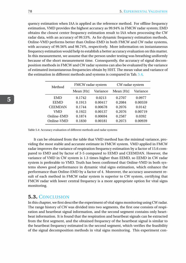
5
78 5. EXPERIMENTAL VALIDATION
quency estimation when IAA is applied as the reference method. For offline frequencyestimation, VMD provides the highest accuracy as 99.94% in FMCW radar system; EMDobtains the closest center frequency estimation result to IAA when processing the CWradar data, with an accuracy of 99.53%. As for dynamic frequency estimation methods,Online-VMD performs better than Online-EMD in both FMCW and CW radar systems,with accuracy of 99.56% and 98.74%, respectively. More information on instantaneousfrequency estimation would help to establish a better accuracy evaluation on this matter.In this measurement, we assume that the person under testing was breathing uniformlybecause of the short measurement time. Consequently, the accuracy of signal decom-position methods in FMCW and CW radar systems can also be evaluated by the varianceof estimated instantaneous frequencies obtain by HHT. The mean value and variance ofthe estimation in different methods and systems is compared in Tab. 5.4.
MethodFMCW radar system CW radar system
Mean [Hz] Variance Mean [Hz] Variance
EMD 0.1742 0.0213 0.2707 0.0977EEMD 0.1913 0.00417 0.2084 0.00559
CEEMDAN 0.1744 0.00678 0.2076 0.0142VMD 0.1922 0.00137 0.2076 0.00719
Online-EMD 0.1874 0.00694 0.2587 0.0392Online-VMD 0.1830 0.00181 0.2073 0.00939
Table 5.4: Accuracy evaluation of different methods and radar systems
It can be obtained from the table that VMD method has the minimal variance, pro-viding the most stable and accurate estimate in FMCW system. VMD applied in FMCWradar improves the variance of respiration frequency estimation by a factor of 15.6 com-pared to EMD and by factor of 3-5 compared to EEMD and CEEMDAN. However, thevariance of VMD in CW system is 1.3 times higher than EEMD, so EEMD in CW radarsystem is preferable to VMD. Truth has been confirmed that Online-VMD in both sys-tems shows good performance in dynamic vital signs estimation, which enhance theperformance than Online-EMD by a factor of 4. Moreover, the accuracy assessment re-sult of each method in FMCW radar system is superior to CW system, certifying thatFMCW radar with lower central frequency is a more appropriate option for vital signsmonitoring.
5.3. CONCLUSIONIn this chapter, we first describe the experiment of vital signs monitoring using CW radar.The range history of CW was divided into two segments, the first one consists of respi-ration and heartbeat signal information, and the second segment contains only heart-beat information. It is found that the respiration and heartbeat signals can be extractedfrom the first segment, and the obtained frequency of the heartbeat signal is similar tothe heartbeat frequency estimated in the second segment, which verifies the feasibilityof the signal decomposition methods in vital signs monitoring. This experiment con-

5.3. CONCLUSION
5
79
firmed that the frequencies of respiration and heartbeat can be reliably determined bysignal decomposition methods in a CW radar system which illuminates the human chestdirectly.
The second experiment was conducted by a FMCW and a CW radar, CW radar has ahigher accuracy with a minimal detectable movement of human chest as 0.11mm, lowerthan the movement of 0.37mm in FMCW radar system. The two radars simultaneouslymeasured the movement of the subject’s chest. But only the respiration signal can beextracted from the radar echo since neither of the radars is directly facing the subject.Then we estimate the frequency of the respiration signals obtained from the two radarsand found that there is always a 1.2 times frequency difference. From this result, weinfer that there is an error in one of the radar time axis. Experiments have proved thatthe signal decomposition methods are effective in vital signs monitoring, in which VMDpresents robustness to noise and good performance in both the decomposition of theentire signal or the dynamic decomposition of the input signal. Minimal monitoringtime is 5.5s and reaction time is as low as 0.036s when applying Online-VMD in FMCWradar system. It is confirmed that Online-VMD which has an accuracy of 99.56% anda variance of estimated frequencies of 1.81×10⁻³ is the preferable method and FMCWradar system is more suitable for real-time vital signs monitoring.


6CONCLUSION AND FUTURE WORK
6.1. CONCLUSIONThis thesis was undertaken to explore and evaluate signal decomposition algorithms forradar-based automobile driver vital signs monitoring. The cardiopulmonary physiologyactivities of the human body are revised and appropriate models for vital signs moni-toring with radar were established. Assume that the distance between automobile driverand radar is constant during the monitoring process, vital signs information is presentedin the radar range history, which can be accurately extracted from the measured phaseof the signal (in CW, FMCW radar systems), or range displacement (in IR-UWB radarsystem). Then three empirical and one variational signal decomposition methods wereemployed for separate estimation of respiration and heartbeat frequencies from the ex-tracted range history of the radar echo, demonstrating the feasibility of these methodsfor vital signs extraction. Moreover, two online signal decomposition approaches areperformed to achieve dynamic estimations of vital signs and detect abnormal humanbehavior.
Main contributions of this thesis are described as follows:
1. Models composed of human chest movement, environmental noise and automaticvibration in different radar systems for vital signs monitoring were established.Human chest movement is usually modeled as a sinusoidal displacement, andwe used improved cardiopulmonary models to better fit into the actual chest dis-placement induced by respiration and heartbeat. After that, a first-order auto-regression model was proposed to simulate the fluctuation of both respiration andheartbeat signals in reality. A novel model of vibration was established as a second-order auto-regressive model with a spectral peak around 1Hz.
2. Signal decomposition algorithms were applied to extract vital signs and extendedto dynamic decomposition cases. EMD is the most well-known signal processingin this analysis, but it suffers from the mode mixing problem. To address the is-sue, two modifications, EEMD and CEEMDAN, were also investigated. Besides,
81

6
82 6. CONCLUSION AND FUTURE WORK
we employed VMD to improve the stability of EMD and its modifications againstnoise. Furthermore, online decomposition methods were utilized to dynamicallyextract vital signs. For the first time, Online-VMD method has been developed andapplied to the decomposition of vital signs. Afterward, their performances wereassessed and compared by Monte Carlo simulations. It is found that VMD is themost promising method in vital signs monitoring due to its robustness to noiseand vibration.
3. Hilbert-Huang transform (HHT) is a time-frequency analysis method used in con-junction with signal decomposition algorithms. In this thesis, HHT was intro-duced to analyze the extracted IMFs by signal decomposition methods. By ap-plying this, the modes corresponding to respiration and heartbeat signals are de-termined, and their instantaneous frequencies and amplitudes are obtained.
4. For the first time, signal decomposition methods in vital signs monitoring havebeen conducted and evaluated by two different radar sensors working in differ-ent frequency bands, proving the practicality of vital signs monitoring of the cardriver by means of CW and FMCW radar systems. CW radar with a higher cen-tral frequency has a smaller minimal detectable movement of human chest of0.11mm, while the minimum chest displacement can be detected in FMCW radaris 0.37mm. Range histories recovered by the phase shift of radar echo were ob-tained and employed in both systems for vital signs extraction.
5. From the experimental results, robustness of signal decomposition algorithms tonoise and measurement artifacts were demonstrated. Two novel parameters, min-imal monitoring time and reaction time, were proposed to describe the outcome ofonline signal decomposition methods with certain sliding window sizes. Online-VMD has been confirmed to be a more preferable method compared with Online-EMD. When applying Online-VMD in FMCW radar system, minimal monitoringtime is 5.5s and reaction time is as low as 0.036s. From the evaluation results, everysignal processing method implemented in FMCW has better accuracy than thatused in CW radar system, among them, VMD has the highest accuracy of 99.94%when using IAA frequency estimate as the reference method, and it has the lowestvariance of 1.37×10⁻³ in FMCW system. The method which has lowest variancein CW system is EEMD of 5.59× 10⁻³, with an accuracy of 99.49%. Online-VMDcan enhance the accuracy of Online-EMD by a factor of 4. Therefore, it can beconcluded that Online-VMD performed in FMCW radar system with lower centralfrequency and sampling frequency in slow-time is more suitable for real-time vitalsigns monitoring.
6.2. RECOMMENDATIONS OF FUTURE WORKRegarding radar-based non-contact vital sign monitoring system, there are still somechallenges that need to be examined in future research, including:
1. In addition to respiration and heartbeat, explore the slight displacement of the hu-man chest caused by other physiological activities such as blood circulation. The

6.2. RECOMMENDATIONS OF FUTURE WORK
6
83
purpose of this research is to establish a model that is closer to the actual physio-logical activity of the human body, to accurately match the detected informationwith vital signs.
2. Take the human body movement into account and pose a solution to random bodymovement elimination. In the thesis, the person being tested is required to remainstill in the experiment, however, human posture will change in real applicationscenarios. In future work, it should be considered to detect human body move-ments and compensate them using distributed sensors.
3. Investigate the detection of cardiopulmonary abnormalities. This thesis realizedthe extraction of vital signs of healthy people and the estimation of their instan-taneous frequencies and amplitudes. Furthermore, when the tester’s respirationor heartbeat signal is abnormal, the cardiopulmonary abnormality should be an-alyzed from the radar echo signal, and a warning should be issued.
4. Verify the performance of signal decomposition methods in vital signs monitoringby comparing with the ground-truth in various application scenarios, for instance,different human body orientations illuminated by radar.


BIBLIOGRAPHY
[1] Wan-Hua Lin et al. “Comparison of Heart Rate Variability from PPG with That fromECG”. In: The International Conference on Health Informatics. Ed. by Yuan-TingZhang. Cham: Springer International Publishing, 2014, pp. 213–215. ISBN: 978-3-319-03005-0.
[2] Carlo Massaroni et al. “Contact-Based Methods for Measuring Respiratory Rate”.In: Sensors 19 (Feb. 2019), p. 908.
[3] Danilo de rossi et al. “Electroactive fabrics and wearable biomonitoring devices”.In: Autex Res. J. 3 (Nov. 2002).
[4] A.S. Fiorillo, Davide C. Critello, and Salvatore Pullano. “Theory, Technology andApplications of Piezoresistive Sensors: a Review”. In: Sensors and Actuators A: Phys-ical 281 (July 2018).
[5] A. Nezirovic, A. G. Yarovoy, and L. P. Ligthart. “Signal Processing for Improved De-tection of Trapped Victims Using UWB Radar”. In: IEEE Transactions on Geoscienceand Remote Sensing 48.4 (2010), pp. 2005–2014.
[6] Makie Terazawa et al. “Respiratory Motion Sensor Measuring Capacitance Con-structed across Skin in Daily Activities”. In: Micromachines 9 (Oct. 2018), p. 543.
[7] Om Prakash Singh, Teo Howe, and Malarvili Balakrishnan. “Real time human res-piration carbon dioxide measurement device for cardiorespiratory assessment”.In: Journal of Breath Research 12 (Sept. 2017).
[8] Damiano Formenti et al. “Thermal Imaging of Exercise-Associated Skin Tempera-ture Changes in Trained and Untrained Female Subjects”. In: Annals of biomedicalengineering 41 (Dec. 2012).
[9] W. Wang and A. C. Den Brinker. “Modified RGB Cameras for Infrared Remote-PPG”. In: IEEE Transactions on Biomedical Engineering (2020), pp. 1–1.
[10] Kenneth Humphreys, Charles Markham, and Tomas E. Ward. “A CMOS camera-based system for clinical photoplethysmographic applications”. In: Opto-Ireland2005: Imaging and Vision. Ed. by Fionn D. Murtagh. Vol. 5823. International Soci-ety for Optics and Photonics. SPIE, 2005, pp. 88 –95.
[11] H. Abuella and S. Ekin. “Non-Contact Vital Signs Monitoring Through Visible LightSensing”. In: IEEE Sensors Journal 20.7 (2020), pp. 3859–3870.
[12] G. Sun. “Non-contact Vital Sign Measurement with Medical Radar and its ClinicalApplications”. In: 2019 3rd International Conference on Recent Advances in SignalProcessing, Telecommunications Computing (SigTelCom). 2019, pp. 90–92.
[13] Eduard Ziganshin, M.A. Numerov, and S.A. Vygolov. “UWB Baby Monitor”. In: Oct.2010, pp. 159 –161.
85

86 BIBLIOGRAPHY
[14] Xuyu Wang, Runze Huang, and Shiwen Mao. “Sonarbeat: Sonar Phase for Breath-ing Beat Monitoring with Smartphones”. In: Sept. 2017, pp. 1–2.
[15] N. Birsan et al. “Time-frequency analysis in Doppler radar for noncontact car-diopulmonary monitoring”. In: 2011 E-Health and Bioengineering Conference (EHB).2011, pp. 1–4.
[16] N. Birsan et al. “Time-frequency analysis in Doppler radar for noncontact car-diopulmonary monitoring”. In: 2011 E-Health and Bioengineering Conference (EHB).2011, pp. 1–4.
[17] A. Tariq and H. G. Shiraz. “Doppler radar vital signs monitoring using wavelettransform”. In: 2010 Loughborough Antennas Propagation Conference. 2010, pp. 293–296.
[18] W. Hu et al. “Real-time remote vital sign detection using a portable Doppler sensorsystem”. In: 2014 IEEE Sensors Applications Symposium (SAS). 2014, pp. 89–93.
[19] Vinh Phuc Tran and Adel Ali Al-Jumaily. “Non-contact Dual Pulse Doppler Sys-tem Based Real-time Relative Demodulation and Respiratory Heart Rates Estima-tions for Chronic Heart Failure Patients”. In: Procedia Computer Science 76 (2015).2015 IEEE International Symposium on Robotics and Intelligent Sensors (IEEEIRIS2015), pp. 47 –52. ISSN: 1877-0509.
[20] Xikun Hu and Tian Jin. “Short-Range Vital Signs Sensing Based on EEMD and CWTUsing IR-UWB Radar”. In: Sciprints (Aug. 2016).
[21] O. A. Postolache, P. S. Girão, and G. Postolache. “Comparative analysis of two sys-tems for unobtrusive heart signal acquisition and characterization”. In: 2013 35thAnnual International Conference of the IEEE Engineering in Medicine and BiologySociety (EMBC). 2013, pp. 7021–7024.
[22] Zhengwu Xu and Tong Liu. “Vital sign sensing method based on EMD in terahertzband”. In: Eurasip Journal on Advances in Signal Processing 2014 (Nov. 2014).
[23] Kun Tian, Jin Li, and Xiaobo Yang. “Separation algorithm of vital sign signal incomplex environments based on time-frequency filtering”. In: EURASIP Journalon Wireless Communications and Networking 2016 (Dec. 2016).
[24] V. N. Ivanovic, M. Dakovic, and L. Stankovic. “Performance of quadratic time-frequencydistributions as instantaneous frequency estimators”. In: IEEE Transactions on Sig-nal Processing 51.1 (2003), pp. 77–89.
[25] B. Boashash and T. Ben-Jabeur. “Design of a high-resolution separable-kernel quadraticTFD for improving newborn health outcomes using fetal movement detection”. In:2012 11th International Conference on Information Science, Signal Processing andtheir Applications (ISSPA). 2012, pp. 354–359.
[26] Jian Li and P. Stoica. “Efficient mixed-spectrum estimation with applications totarget feature extraction”. In: Conference Record of The Twenty-Ninth Asilomar Con-ference on Signals, Systems and Computers. Vol. 1. 1995, 428–432 vol.1.
[27] C. Li et al. “Accurate Doppler Radar Noncontact Vital Sign Detection Using theRELAX Algorithm”. In: IEEE Transactions on Instrumentation and Measurement59.3 (2010), pp. 687–695.

BIBLIOGRAPHY 87
[28] Hyunjae Lee et al. “A Novel Vital-Sign Sensing Algorithm for Multiple SubjectsBased on 24-GHz FMCW Doppler Radar”. In: Remote Sensing 11 (May 2019), p. 1237.
[29] C. A. Dizon, C. F. U. Mendoza, and R. U. Lorenzo. “Direction of arrival (DoA) esti-mation using root-MUSIC algorithm on the NI PXIe platform”. In: TENCON 2012IEEE Region 10 Conference. 2012, pp. 1–4.
[30] X. Shang, J. Liu, and J. Li. “Multiple Object Localization and Vital Sign MonitoringUsing IR-UWB MIMO Radar”. In: IEEE Transactions on Aerospace and ElectronicSystems (2020), pp. 1–1.
[31] V. Vasu et al. “Using the Lomb periodogram for non-contact estimation of respi-ration rates”. In: 2010 Annual International Conference of the IEEE Engineering inMedicine and Biology. 2010, pp. 2407–2410.
[32] H. Noguchi et al. “Signal phase estimation for measurement of respiration wave-form using a microwave Doppler sensor”. In: 2013 35th Annual International Con-ference of the IEEE Engineering in Medicine and Biology Society (EMBC). 2013, pp. 6740–6743.
[33] M. S. Rahman, B. Jang, and K. Kim. “A new digital signal processor for Dopplerradar cardiopulmonary monitoring system”. In: 2008 International Conference onElectrical and Computer Engineering. 2008, pp. 76–79.
[34] M. S. Rahman et al. “Extended Kalman Filter for Doppler radar cardiopulmonarymonitoring system”. In: 2012 7th International Conference on Electrical and Com-puter Engineering. 2012, pp. 264–267.
[35] P. Flandrin, G. Rilling, and P. Goncalves. “Empirical mode decomposition as a filterbank”. In: IEEE Signal Processing Letters 11.2 (2004), pp. 112–114.
[36] G. Fang, C. Huang, and C. Yang. “Simultaneous Detection of Multi-Target VitalSigns Using EEMD Algorithm Based on FMCW Radar”. In: 2019 IEEE MTT-S In-ternational Microwave Biomedical Conference (IMBioC). Vol. 1. 2019, pp. 1–4.
[37] M. E. Torres et al. “A complete ensemble empirical mode decomposition withadaptive noise”. In: 2011 IEEE International Conference on Acoustics, Speech andSignal Processing (ICASSP). 2011, pp. 4144–4147.
[38] K. Dragomiretskiy and D. Zosso. “Variational Mode Decomposition”. In: IEEE Trans-actions on Signal Processing 62.3 (2014), pp. 531–544.
[39] Jiaming Yan et al. “Through-Wall Multiple Targets Vital Signs Tracking Based onVMD Algorithm”. In: Sensors (Basel, Switzerland) 16 (Aug. 2016).
[40] Y. Xu et al. “Vital Sign Detection Method Based on Multiple Higher Order Cumu-lant for Ultrawideband Radar”. In: IEEE Transactions on Geoscience and RemoteSensing 50.4 (2012), pp. 1254–1265.
[41] Zhibin Yu, Duo Zhao, and Zhiqiang Zhang. “Doppler Radar Vital Signs DetectionMethod Based on Higher Order Cyclostationary”. In: Sensors 18 (Dec. 2017), p. 47.
[42] Nan-Chyuan Tsai and Rong-Mao Lee. “Interaction between cardiovascular systemand respiration”. In: Applied Mathematical Modelling 35.11 (2011), pp. 5460 –5469.ISSN: 0307-904X.

88 BIBLIOGRAPHY
[43] Amy Droitcour. “Non-contact measurement of heart and respiration rates withsingle chip microwave Doppler radar”. In: (Jan. 2006).
[44] M. Alizadeh et al. “Remote Monitoring of Human Vital Signs Using mm-Wave FMCWRadar”. In: IEEE Access 7 (2019), pp. 54958–54968.
[45] Marco Baldi et al. “Body Movement Compensation in UWB Radars for RespirationMonitoring”. In: Oct. 2012, pp. –.
[46] “Novel signal processing techniques for Doppler radar cardiopulmonary sensing”.In: Signal Processing 89.1 (2009), pp. 45 –66. ISSN: 0165-1684.
[47] C. Gu et al. “Instrument-Based Noncontact Doppler Radar Vital Sign DetectionSystem Using Heterodyne Digital Quadrature Demodulation Architecture”. In: IEEETransactions on Instrumentation and Measurement 59.6 (2010), pp. 1580–1588.
[48] Kazuyoshi Itoh. “Analysis of the phase unwrapping algorithm”. In: Appl. Opt. 21.14(ts ,), pp. 2470–2470.
[49] Mamady Kebe et al. “Human Vital Signs Detection Methods and Potential UsingRadars: A Review”. In: Sensors (Basel, Switzerland) 20 (2020).
[50] Bangkok. Noise, Vibration, and Harshness (NVH) - APMP. http://www.apmpweb.org/fms/get_file.php?index=NTU0NA==. 2016.
[51] Jacques Charley, G Bodovillé, and G Degallaix. “Analysis of braking noise and vi-bration measurements by time—frequency approaches”. In: Proceedings of the In-stitution of Mechanical Engineers, Part C: Journal of Mechanical Engineering Sci-ence 215 (Dec. 2001), pp. 1381–1400.
[52] Norden Huang et al. “The empirical mode decomposition and the Hilbert spec-trum for nonlinear and non-stationary time series analysis”. In: Proceedings of theRoyal Society of London. Series A: Mathematical, Physical and Engineering Sciences454 (Mar. 1998), pp. 903–995.
[53] B. Boashash. “Estimating and interpreting the instantaneous frequency of a signal.I. Fundamentals”. In: Proceedings of the IEEE 80.4 (1992), pp. 520–538.
[54] Monson H. Hayes. “Statistical Digital Signal Processing and Modeling”. In: 1996.
[55] Zhengwu Xu and Tong Liu. “Vital sign sensing method based on EMD in terahertzband”. In: Eurasip Journal on Advances in Signal Processing 2014 (Nov. 2014).
[56] A. Tariq and H. G. Shiraz. “Doppler radar vital signs monitoring using wavelettransform”. In: 2010 Loughborough Antennas Propagation Conference. 2010, pp. 293–296.
[57] Kun Tian, Jin Li, and Xiaobo Yang. “Separation algorithm of vital sign signal incomplex environments based on time-frequency filtering”. In: EURASIP Journalon Wireless Communications and Networking 2016 (Dec. 2016).
[58] Zhaohua Wu and Norden Huang. “Ensemble Empirical Mode Decomposition: aNoise-Assisted Data Analysis Method”. In: Advances in Adaptive Data Analysis 1(Jan. 2009), pp. 1–41.

BIBLIOGRAPHY 89
[59] G. Fang, C. Huang, and C. Yang. “Simultaneous Detection of Multi-Target VitalSigns Using EEMD Algorithm Based on FMCW Radar”. In: 2019 IEEE MTT-S In-ternational Microwave Biomedical Conference (IMBioC). Vol. 1. 2019, pp. 1–4.
[60] Jiaming Yan et al. “Through-Wall Multiple Targets Vital Signs Tracking Based onVMD Algorithm”. In: Sensors (Basel, Switzerland) 16 (Aug. 2016).
[61] Ingrid Daubechies, Jianfeng Lu, and Hau-Tieng Wu. “Synchrosqueezed wavelettransforms: An empirical mode decomposition-like tool”. In: Applied and Com-putational Harmonic Analysis 30 (Mar. 2011), pp. 243–261.
[62] Z. Duan and J. Liang. “Non-Contact Detection of Vital Signs Using a UWB RadarSensor”. In: IEEE Access 7 (2019), pp. 36888–36895.
[63] C. Brüser et al. “Monte-Carlo Simulation and Automated Test Bench for Devel-oping a Multichannel NIR-Based Vital-Signs Monitor”. In: IEEE Transactions onBiomedical Circuits and Systems 9.3 (2015), pp. 421–430.
[64] R. Fontugne, P. Borgnat, and P. Flandrin. “Online Empirical Mode Decomposition”.In: 2017 IEEE International Conference on Acoustics, Speech and Signal Processing(ICASSP). 2017, pp. 4306–4310.
[65] Xi Ma, Jinqiu Hu, and Laibin Zhang. “EMD-based online Filtering of Process Data”.In: Control Engineering Practice 62 (2017), pp. 79 –91. ISSN: 0967-0661.