www.sciencemag.org/content/345/6193/222/suppl/DC1

Supplementary Material for

A Doppler effect in embryonic pattern formation Daniele Soroldoni, David J. Jörg, Luis G. Morelli, David L. Richmond, Johannes

Schindelin, Frank Jülicher, Andrew C. Oates*

*Corresponding author. E-mail: aoates@nimr.mrc.ac.uk

Published 11 July 2014, Science 345, 222 (2014)

DOI: 10.1126/science.1253089

This PDF file includes:

Materials and Methods

Supplementary Text

Figs. S1 to S8

Tables S1 and S2

Full Reference List

Other Supplementary Material for this manuscript includes the following: (available at www.sciencemag.org/content/345/6193/222/suppl/DC1)

Movies S1 to S5

!Submitted Manuscript: Confidential May 12, 2014

Contents

Supplementary Figures 3

Fig. S1. Generation of a novel transgene for the oscillating gene her1 4Fig. S2. Characterization of morphological segmentation in Looping 5Fig. S3. Comparison of YFP intensity kymographs and phase maps 6Fig. S4. The number of kinematic waves of oscillating genes decrease during segmentation 7Fig. S5. Kymographs of the average phase map and phase profile 8Fig. S6. Kymographs of wavelengths and frequencies of the average phase map 9Fig. S7. Time dependence of different frequency components 10Fig. S8. Time dependence of fit parameters 11

Supplementary Movie legends 12

Materials and methods 13

BAC recombineering and zebrafish transgenesis 13Fish care and imaging preparation 13Time-lapse imaging and temperature control 14Image processing 14Period measurements and statistics 14Whole-mount in situ hybridizations and static images 15

Supplementary Text 16

Generating phase maps with a wavelet transform 16Representation of oscillatory time series in terms of phase and amplitude 16Wavelet transform 16Phase maps 17

Doppler effect and dynamic wavelength effect 18Contributions to the frequency offset 18Discussion of simple scenarios 19

Quantification of Doppler effect and dynamic wavelength effect in experiments 21

Supplementary Tables 23

Table S1. Fit functions used in the Supplementary Text 23Table S2. Numerical values of the fit parameters of the functions given in Table S1 24

2

!Submitted Manuscript: Confidential May 12, 2014

Supplementary Figures

3

!Submitted Manuscript: Confidential May 12, 2014

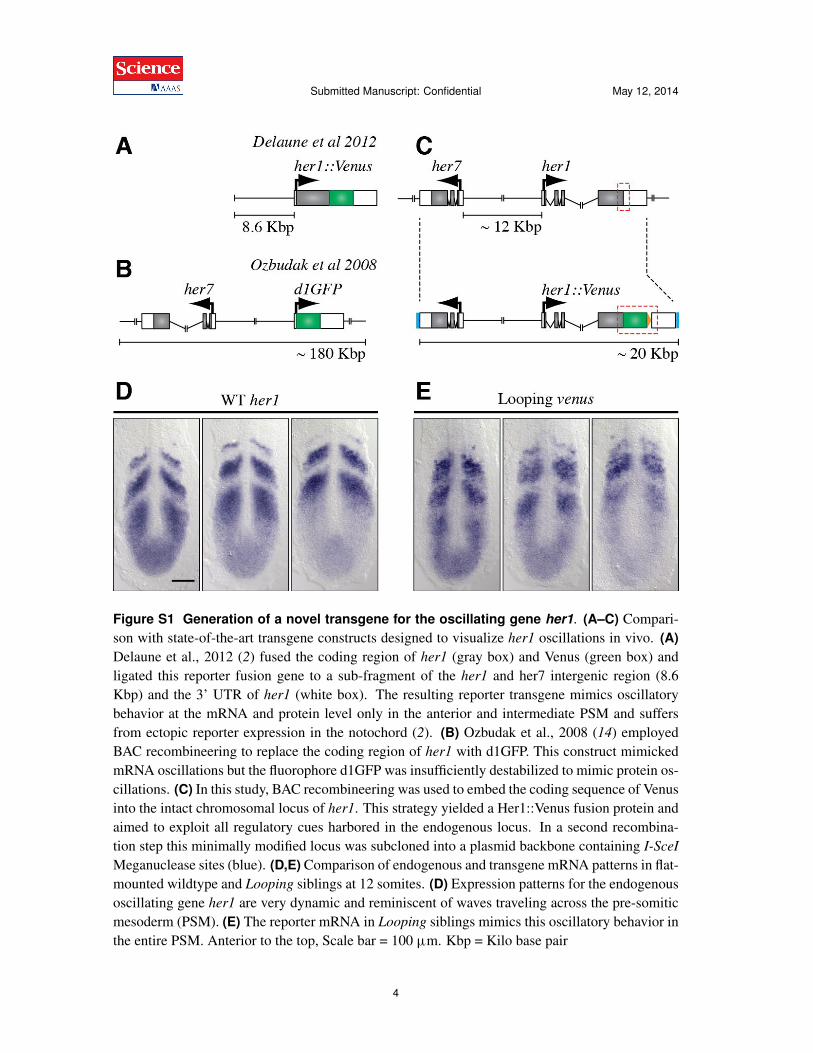
Figure S1 Generation of a novel transgene for the oscillating gene her1. (A–C) Compari-son with state-of-the-art transgene constructs designed to visualize her1 oscillations in vivo. (A)Delaune et al., 2012 (2) fused the coding region of her1 (gray box) and Venus (green box) andligated this reporter fusion gene to a sub-fragment of the her1 and her7 intergenic region (8.6Kbp) and the 3’ UTR of her1 (white box). The resulting reporter transgene mimics oscillatorybehavior at the mRNA and protein level only in the anterior and intermediate PSM and suffersfrom ectopic reporter expression in the notochord (2). (B) Ozbudak et al., 2008 (14) employedBAC recombineering to replace the coding region of her1 with d1GFP. This construct mimickedmRNA oscillations but the fluorophore d1GFP was insufficiently destabilized to mimic protein os-cillations. (C) In this study, BAC recombineering was used to embed the coding sequence of Venusinto the intact chromosomal locus of her1. This strategy yielded a Her1::Venus fusion protein andaimed to exploit all regulatory cues harbored in the endogenous locus. In a second recombina-tion step this minimally modified locus was subcloned into a plasmid backbone containing I-SceI

Meganuclease sites (blue). (D,E) Comparison of endogenous and transgene mRNA patterns in flat-mounted wildtype and Looping siblings at 12 somites. (D) Expression patterns for the endogenousoscillating gene her1 are very dynamic and reminiscent of waves traveling across the pre-somiticmesoderm (PSM). (E) The reporter mRNA in Looping siblings mimics this oscillatory behavior inthe entire PSM. Anterior to the top, Scale bar = 100 ùm. Kbp = Kilo base pair

4

!Submitted Manuscript: Confidential May 12, 2014

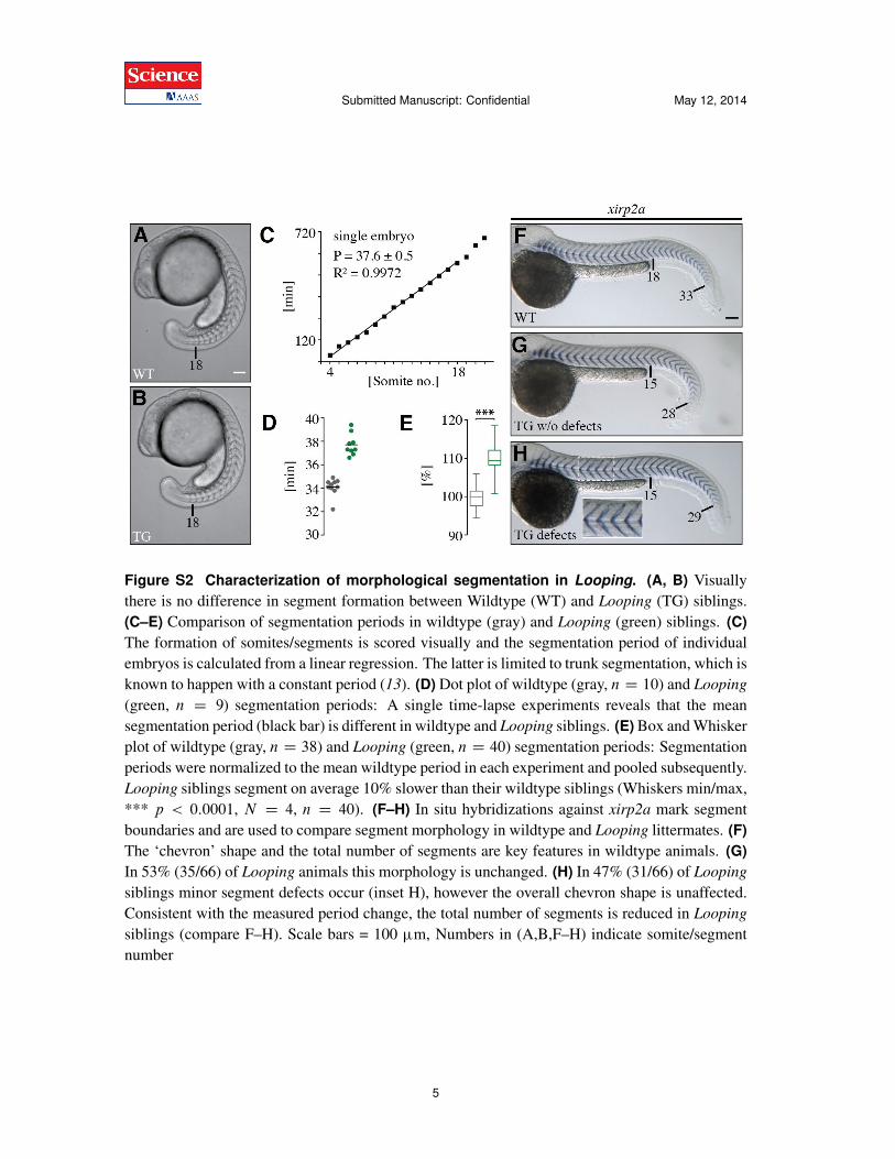
Figure S2 Characterization of morphological segmentation in Looping. (A, B) Visuallythere is no difference in segment formation between Wildtype (WT) and Looping (TG) siblings.(C–E) Comparison of segmentation periods in wildtype (gray) and Looping (green) siblings. (C)The formation of somites/segments is scored visually and the segmentation period of individualembryos is calculated from a linear regression. The latter is limited to trunk segmentation, which isknown to happen with a constant period (13). (D) Dot plot of wildtype (gray, n D 10) and Looping

(green, n D 9) segmentation periods: A single time-lapse experiments reveals that the meansegmentation period (black bar) is different in wildtype and Looping siblings. (E) Box and Whiskerplot of wildtype (gray, n D 38) and Looping (green, n D 40) segmentation periods: Segmentationperiods were normalized to the mean wildtype period in each experiment and pooled subsequently.Looping siblings segment on average 10% slower than their wildtype siblings (Whiskers min/max,*** p < 0:0001, N D 4, n D 40). (F–H) In situ hybridizations against xirp2a mark segmentboundaries and are used to compare segment morphology in wildtype and Looping littermates. (F)The ‘chevron’ shape and the total number of segments are key features in wildtype animals. (G)In 53% (35/66) of Looping animals this morphology is unchanged. (H) In 47% (31/66) of Looping

siblings minor segment defects occur (inset H), however the overall chevron shape is unaffected.Consistent with the measured period change, the total number of segments is reduced in Looping

siblings (compare F–H). Scale bars = 100 ùm, Numbers in (A,B,F–H) indicate somite/segmentnumber

5

!Submitted Manuscript: Confidential May 12, 2014

A

B

D

C

Posterior Anterior

2!

0

2!

0

0 630 µm

064

5 m

in

5

19

Segm

ent n

o.

Tim

e0

645

min

5

19

Segm

ent n

o.

Tim

e0

645

min

5

19

Segm

ent n

o.

Tim

e0

645

min

5

19

Segm

ent n

o.

Tim

e

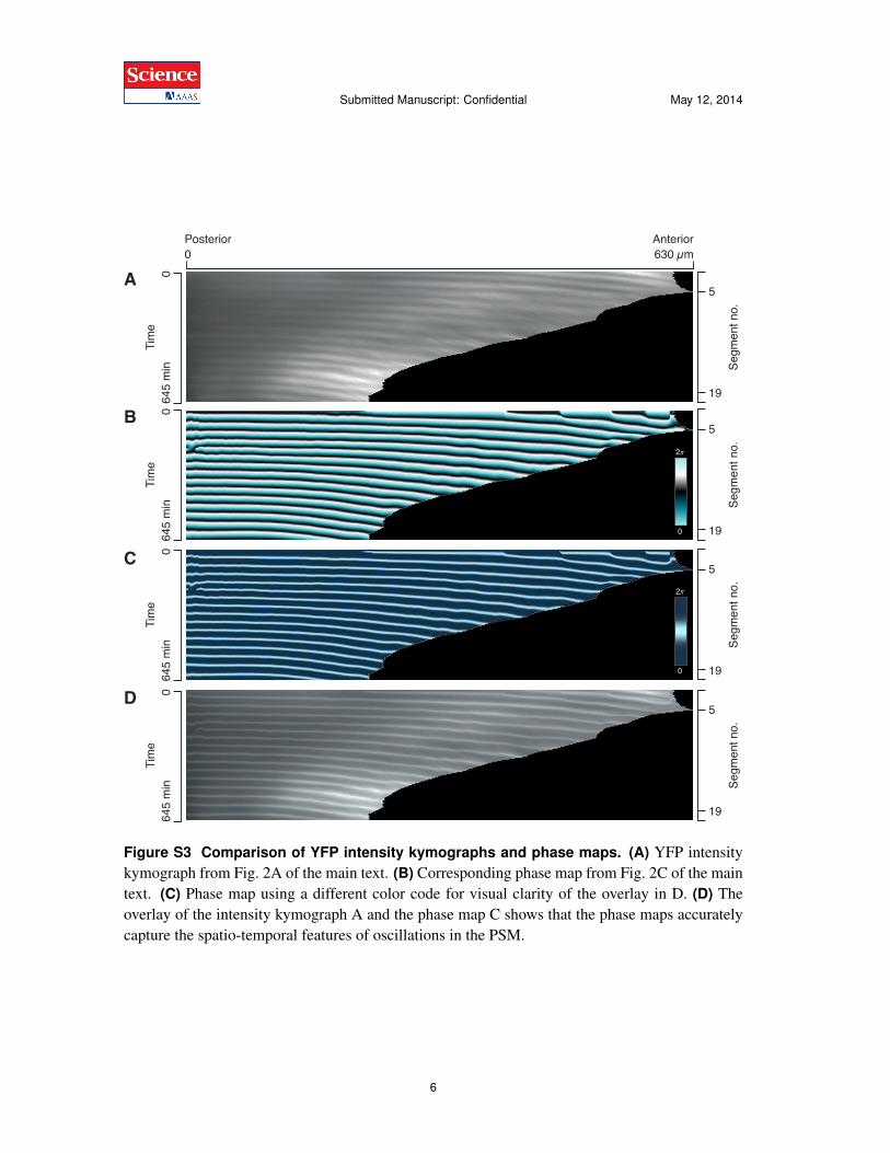
Figure S3 Comparison of YFP intensity kymographs and phase maps. (A) YFP intensitykymograph from Fig. 2A of the main text. (B) Corresponding phase map from Fig. 2C of the maintext. (C) Phase map using a different color code for visual clarity of the overlay in D. (D) Theoverlay of the intensity kymograph A and the phase map C shows that the phase maps accuratelycapture the spatio-temporal features of oscillations in the PSM.

6

!Submitted Manuscript: Confidential May 12, 2014

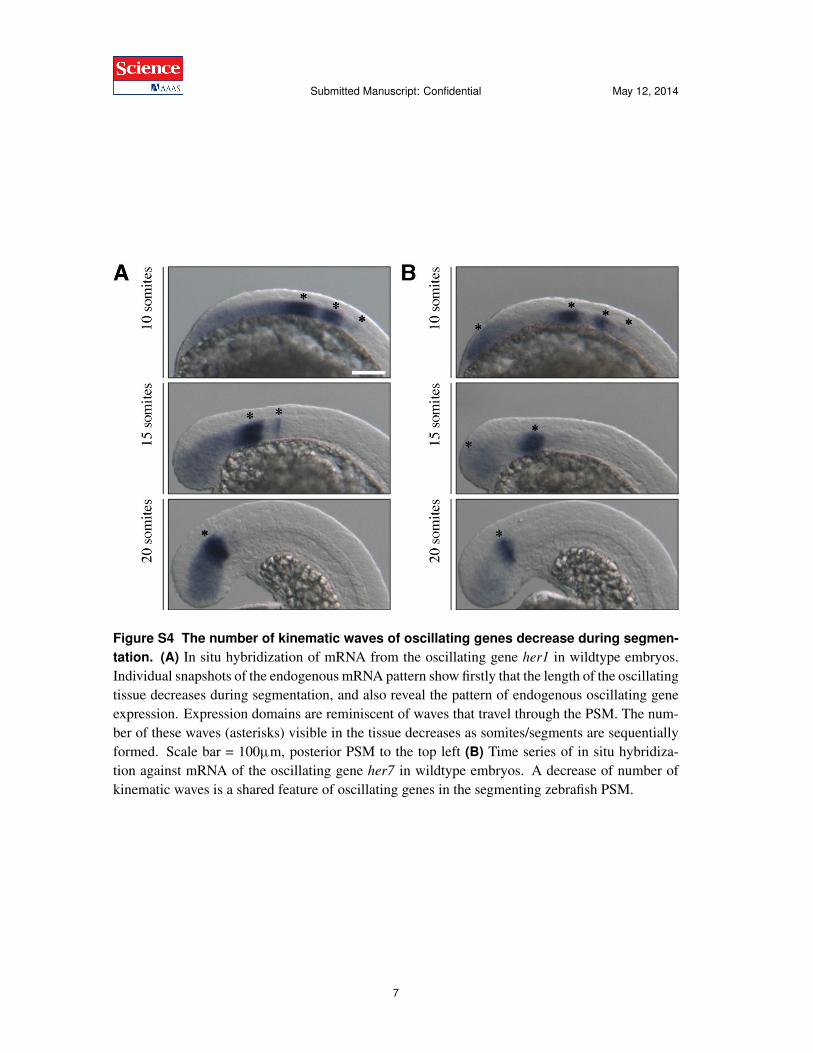
Figure S4 The number of kinematic waves of oscillating genes decrease during segmen-tation. (A) In situ hybridization of mRNA from the oscillating gene her1 in wildtype embryos.Individual snapshots of the endogenous mRNA pattern show firstly that the length of the oscillatingtissue decreases during segmentation, and also reveal the pattern of endogenous oscillating geneexpression. Expression domains are reminiscent of waves that travel through the PSM. The num-ber of these waves (asterisks) visible in the tissue decreases as somites/segments are sequentiallyformed. Scale bar = 100ùm, posterior PSM to the top left (B) Time series of in situ hybridiza-tion against mRNA of the oscillating gene her7 in wildtype embryos. A decrease of number ofkinematic waves is a shared feature of oscillating genes in the segmenting zebrafish PSM.

7

!Submitted Manuscript: Confidential May 12, 2014

A

B

Posterior Anterior0 570 µm

2!

0

2!

0

050

0 m

in

7

20

Segm

ent n

o.

Tim

e0

500

min

7

20Se

gmen

t no.

Tim

e

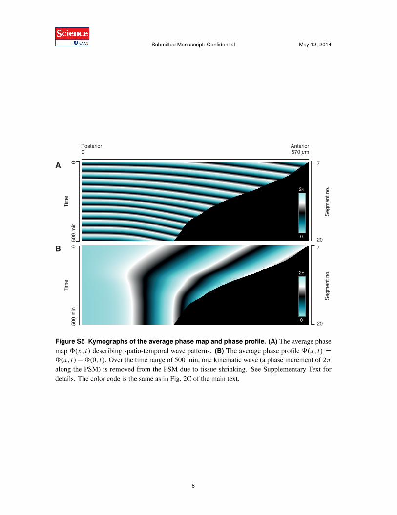
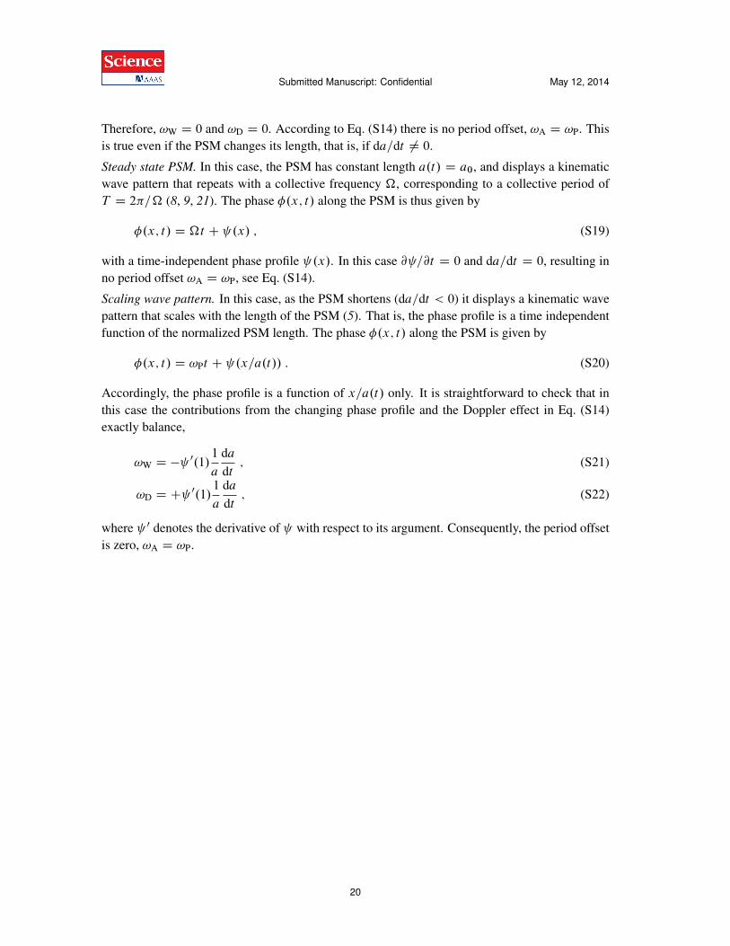
Figure S5 Kymographs of the average phase map and phase profile. (A) The average phasemap ˆ.x; t/ describing spatio-temporal wave patterns. (B) The average phase profile ‰.x; t/ Dˆ.x; t/ �ˆ.0; t/. Over the time range of 500 min, one kinematic wave (a phase increment of 2⇡along the PSM) is removed from the PSM due to tissue shrinking. See Supplementary Text fordetails. The color code is the same as in Fig. 2C of the main text.

8

!Submitted Manuscript: Confidential May 12, 2014

A

B

Posterior Anterior0 570 µm

0.15 min!1

!0.05 min!1

!0.07 "m!1

0 "m!1

0.15 min!1

!0.05 min!1

C

050

0 m

in

7

20

Segm

ent n

o.

Tim

e0

500

min

7

20

Segm

ent n

o.

Tim

e0

500

min

7

20

Segm

ent n

o.

Tim

e

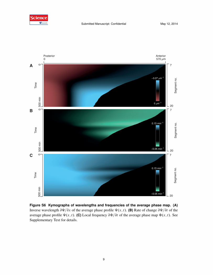
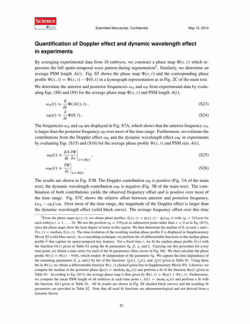
Figure S6 Kymographs of wavelengths and frequencies of the average phase map. (A)Inverse wavelength @‰=@x of the average phase profile ‰.x; t/. (B) Rate of change @‰=@t of theaverage phase profile ‰.x; t/. (C) Local frequency @ˆ=@t of the average phase map ˆ.x; t/. SeeSupplementary Text for details.

9

!Submitted Manuscript: Confidential May 12, 2014

A

0 100 200 300 400 5000.1

0.12

0.14

0.16

0.18

0.27 9 11 13 15 17 19

-1.2

-0.9

-0.6

-0.3

0.

0.3

t HminL

wHmin

-1 L

segment no.

daêdtHmmêminL

posterior frequency wP

anterior frequency wA

shortening rate daêdt

B

0 100 200 300 400 500-0.06

-0.03

0.

0.03

0.067 9 11 13 15 17 19

t HminL

wHmin

-1 L

segment no.

Doppler contribution wD

Dynamic wavelength contribution wW

total frequency offset wD + wW

C

0 100 200 300 400 500-10

-5

0

5

10

15

20

257 9 11 13 15 17 19

t HminL

offs

etH%L

segment no.

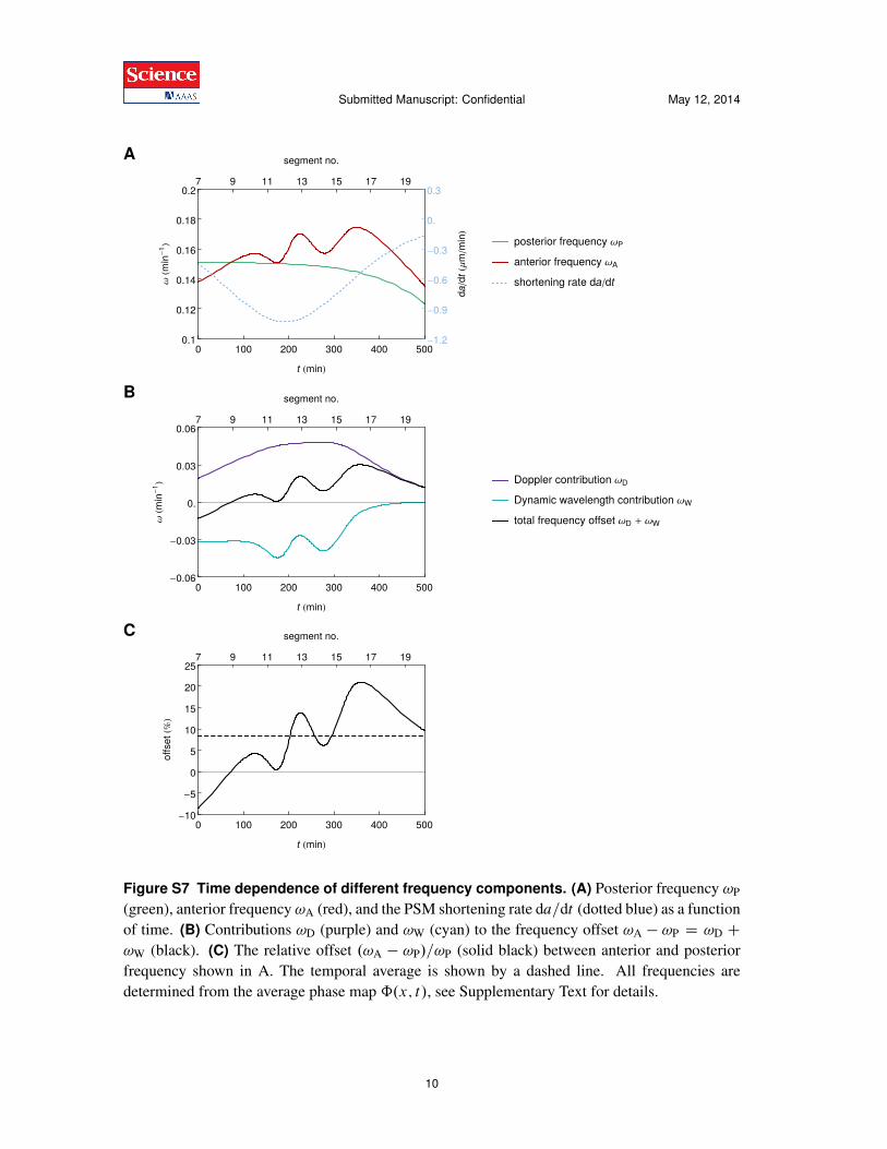
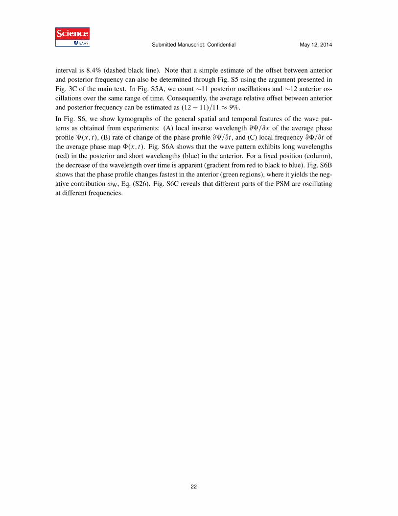
Figure S7 Time dependence of different frequency components. (A) Posterior frequency !P(green), anterior frequency !A (red), and the PSM shortening rate da=dt (dotted blue) as a functionof time. (B) Contributions !D (purple) and !W (cyan) to the frequency offset !A � !P D !D C!W (black). (C) The relative offset .!A � !P/=!P (solid black) between anterior and posteriorfrequency shown in A. The temporal average is shown by a dashed line. All frequencies aredetermined from the average phase map ˆ.x; t/, see Supplementary Text for details.

10

!Submitted Manuscript: Confidential May 12, 2014

A B

0 100 200 300 400 500

0.050.060.070.080.090.100.110.12

t HminL

bHmm

-1 L

0 100 200 300 400 5000.000

0.005

0.010

0.015

0.020

0.025

0.030

t HminL

cHmm

-1 L

C D

0 100 200 300 400 500

100

150

200

250

t HminL

xHmmL

0 100 200 300 400 5000

20

40

60

80

t HminL

f PHradL

E

0 100 200 300 400 500

250

300

350

400

450

500

550

t HminL

aHmmL

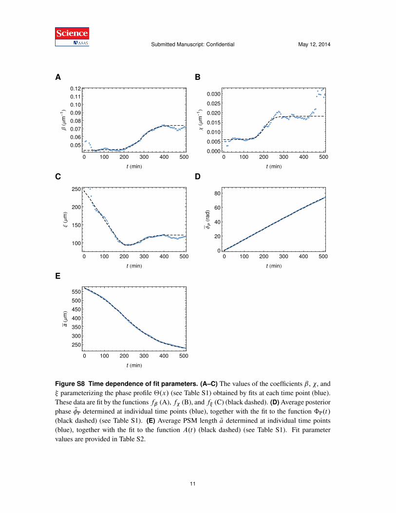
Figure S8 Time dependence of fit parameters. (A–C) The values of the coefficients ˇ, �, and⇠ parameterizing the phase profile ‚.x/ (see Table S1) obtained by fits at each time point (blue).These data are fit by the functions f

ˇ

(A), f�

(B), and f⇠

(C) (black dashed). (D) Average posteriorphase N

�P determined at individual time points (blue), together with the fit to the function ˆP.t/

(black dashed) (see Table S1). (E) Average PSM length Na determined at individual time points(blue), together with the fit to the function A.t/ (black dashed) (see Table S1). Fit parametervalues are provided in Table S2.

11

!Submitted Manuscript: Confidential May 12, 2014

Supplementary Movie legends

Movie S1: Real-time imaging of segment formation and Her1::Venus oscillations duringsegmentation in transgenic Looping embryos

This movie shows representative brightfield and YFP channels for 1 position of a multidimen-sional time-lapse after z-stack projection. The brightfield channel illustrates that the unsegmentedpre-somitic mesoderm (PSM) is sequentially subdivided into precursors of adult segments, thesomites. The YFP channel shows that the morphologically unsegmented tissue exhibits patternsof oscillating gene expression that are reminiscent of waves that travel from the posterior to theanterior where they arrest. Phenomena in both channels happen with a specific rhythmicity anddirectionality.

Movie S2: Overlay of brightfield and fluorescence channels during segmentation in trans-genic Looping embryos

Overlay of brightfield and YFP channels indicates that new segment boundaries form when kine-matic waves arrest in the anterior PSM. 16 color LUT (blue, lowest and red highest intensity).

Movie S3: Comparison of kinematic waves in the YFP channel and the phase map

Upper panel shows the YFP fluorescence channel cropped and straightened from the tailbud andPSM of a representative Looping her1–YFP transgenic embryo during the formation of somites 2to 20. Lower panel shows the corresponding horizontal lines of the phase map described in quan-titative methods section (PQR).

Movie S4: Time evolution of the phase profiles from population of Looping her1–YFP

zebrafish embryos

Phase profiles from across the tailbud and PSM of 18 embryos are shown in a range of blue chang-ing from 7 to 20 somites. Note the decreasing PSM length along the x-axis and the decrease intotal phase offset on the y-axis during the developmental time interval.

Movie S5: Time evolution of the median phase profile and the spatio-temporal fit

Median of all phase profiles (solid blue curve) from Supplementary Movie S4 and the spatio-temporal fit introduced in the Supplementary Text (dashed green curve).

12

!Submitted Manuscript: Confidential May 12, 2014

Materials and methods

BAC recombineering and zebrafish transgenesis

Two successive rounds of BAC recombineering were used as described previously (15, 16) to (1)create a functional fusion between the coding regions of her1 and Venus and to (2) subclone themodified chromosomal locus into a plasmid backbone. The latter served to restrict the size of themodified BAC and introduce two I-SceI Meganuclease sites, which aimed for high transgenesisfrequencies (17). The following homology arms were used for tagging:

L:5’–GGACTCTGAGACGAGCGCTGTTCCACAATCAGCCTTTGTGGAGACCCTGG–3’

R: 5’–CCCTTTAAGACAACGCTGGTTATTCTCATGCTAAGTGTCTTCAGTTTTGC–3’

and for subcloning

L: 5’–GTTATGTGTTCCCGACAATAATATTAATCTCTGGAGTGGCATGATGTTTG–3’

R: 5’–TGCTTTTTGTATGACTCGTTTCTTTACATTTGGGCTTAAATAAATAGATT–3’.

The resulting construct was co-injected with I-SceI Meganuclease (Roche) at a DNA concentra-tion of 100 ng/ùl and a bolus size of 100 ùm as described previously (18). I-SceI Meganucleasetransgenesis was used to generate a pool of independent transgenic founders with single, low-copyinsertions into the host genome (17). This feature allows the reporter expression levels to be tunedwithout altering the stability of the reporter protein itself and was used to find the right balancebetween reporter stability and sensitivity of the imaging set-up. Transient transgenic expressionwas assessed to verify the functionality of the YFP fusion but ignored as selection criterion for pu-tative transgenic founders. All injected embryos without obvious phenotype were raised to sexualmaturity to avoid any visual bias towards strongly expressing founder. Initially, putative trans-genic founders were screened by visual inspection of their F1 progeny after outcrossing to WTanimals with a common stereomicroscope (Olympus, SZX-16) equipped with an appropriate filterset (AHF, YFP) and light source (Lumen dynamics, X-cite 120). Based on this conventional ap-proach, only 1 transgenic founder could be isolated. Therefore, the screening assay was changedto increase sensitivity levels and whole-mount in situ hybridization was used to isolate 4 moretransgenic founders that were positive for YFP/Venus mRNA. In total, 5 independent transgenicfounders were identified from a single injection experiment, yielding an average transgenesis fre-quency of ⇠25% and transmission frequencies below 50%. Reporter expression was qualitativelysimilar but quantitatively different for all isolated transgenic founders. Based on the optimal sig-nal to noise ratio, one founder was selected for time-lapse experiments and named Looping. Thistransgenic line is viable and fertile and continues to stably express Venus after seven generations.

Fish care and imaging preparation

Wildtype (WT) AB and transgenic fish were maintained according to standard procedures. Allanalyzed embryos were obtained from outcrosses of heterozygous Looping animals to WT fish bynatural spawning. Embryos were collected within 15 minutes after spawning to minimize asyn-chronous clutches/siblings and incubated in E3 without methylene blue at all times. For imagingexperiments, embryos were collected and incubated at 33ıC till bud stage, de-chorionated and al-lowed to equilibrate at room temperature. Prior to imaging, 10 wildtype and 10 transgenic siblings

13

!Submitted Manuscript: Confidential May 12, 2014

were randomly distributed and laterally aligned in conical depressions in a pad of agarose (Sigma,low-melting, 2% in E3) that was cast in a glass-bottom dish (Matek, 35 mm). The size of theseconical depressions was chosen to fit only the yolk of an embryo. Consequently, embryos couldgrow without physical restrictions on top of the agarose pad and were stabilized in z-direction.The imaging dish contained E3 with 0.014% Tricaine to prevent muscle twitching and was al-lowed to equilibrate at least 30 minutes in the thermal insert of the time-lapse set-up prior imagingwas started.

Time-lapse imaging and temperature control

A wide-field microscope (Zeiss, Axiovert 200M) equipped with a 10X objective (Zeiss, NA 0.5),an automated stage (Maerzhaeuser), a LED-based light source (Lumencor, SpectraX7), an EM-CCD camera (Andor, iXon 888) and a thermal insert (Harvard apparatus) was used to record ze-brafish segmentation in 2 channels, 6 z-slices (range: 100 ùm in 20 ùm steps) for 20 xy-positionsat an time interval of 5 minutes for at least 12 hours. To balance imaging parameters and samplingrate during recordings, we chose 23.5ıC as experimental temperature, which was close to roomtemperature and facilitated temperature control. During each experiment the temperature was con-trolled by the closed thermal insert and monitored by an independent external thermometer thatwas used to log temperatures throughout recordings, which typically ranged between 23.3ıC to23.6ıC. To compare measurements from different experiments/days at slightly different tempera-tures, we included 10 WT siblings in each experiment that were used to normalize the measuredsomitogenesis period. The random distribution of wildtype and transgenic siblings in the imagingdish avoided any bias due to temperature gradients within the imaging dish.

Image processing

All image processing was carried out using the open-source Fiji distribution of ImageJ (19) and alltools developed for this manuscript are available at http://fiji.sc/Fiji. A novel stack focusing tech-nique was developed inspired by Bayesian inference to extract in-focus, single layer images frombrightfield z-stacks containing 6 images at several focal depths (“Gaussian StackFocusing”). YFPz-stacks were objected to maximum projections. To facilitate analyzing the reporter intensity ina population of zebrafish embryos, we developed interpolator tools to locally (“ROI/Circle Inter-polator”) or globally (“LOI Interpolator”) measure the average reporter intensity within the PSM.All measurements were performed on z-projections without any further image processing. TheROI area was set constantly to a diameter of 40 pixel, the LOI width to 30 pixel. For illustrationpurposes only, all images and movies in this manuscript have been subjected to a Gaussian blurwith a radius of 1 ⇥ 1. Overlays of brightfield and YFP channels were done using the “ComposeRGB-Stack” plug-in available in Fiji.

Period measurements and statistics

All period measurements were restricted to trunk segmentation, because the segmentation periodwas shown to be constant over this developmental interval (13). The formation of segments wasscored visually as described previously (13). Shortly, the first visible sign of each somite bound-ary was determined and each successive time point was noted. For each embryo we plotted the

14

!Submitted Manuscript: Confidential May 12, 2014

number of somites over time and calculated the average segmentation period from a linear re-gression through these data points (Fig. S2). These individual period measurements were pooledaccording to their genotype and used to calculate the mean segmentation period for a given exper-iment. The average segmentation period of WT siblings was set to 100% and used to normalizeall other period measurements for a given experiment. The periods of genetic oscillations weredetermined locally using the ROI interpolator tool available in Fiji. The obtained raw traces (meangray values over time) were exported to Prism 6 and analyzed using the standard function for thesecond derivative. The average period per embryo was calculated from the interpeak distance ofthe resulting curves. As above, individual periods were pooled to obtain an average period foroscillations in the anterior and posterior for a give experiment. The period offset between anteriorand posterior oscillations was significant (p < 0:001) in all 4 independent experiments. The pe-riod of segment formation and anterior oscillations was never significantly different. To calculatethe average period offset between segmentation, anterior and posterior oscillations, we pooled allperiod measurements from 4 experiments after normalization. All unpaired t-test were calculatedusing Prism 6 assuming normal distribution and Welch-correction.

Whole-mount in situ hybridizations and static images

In situ hybridization and riboprobe generation was performed as described (24, 25, 26). Whole-mount in situ hybridizations were documented with a stereomicroscope (Olympus, SZX-12)equipped with an appropriate CCD camera (Qimaging, Micropublisher). Flat-mounted embryoswere photographed using an Axioskop 2 equipped with a RGB camera (QImaging, Retiga SRV).

15

!Submitted Manuscript: Confidential May 12, 2014

Supplementary Text

Generating phase maps with a wavelet transform

In this section, we explain how oscillatory time series can be represented in terms of phase andamplitude. We then show how to obtain a phase representation of an oscillatory signal using awavelet transform and apply this technique to the experimentally obtained intensity kymographs.We use this phase representation (i) to systematically measure the number of kinematic waves inthe PSM, (ii) to directly compare the spatio-temporal features of wave patterns across a populationof different embryos, and (iii) to quantify the magnitude of the Doppler effect and the dynamicwavelength effect (see main text) from experimental data.

Representation of oscillatory time series in terms of phase and amplitude

Consider an oscillatory signal of the type

Q.t/ D q

0

C q.t/ cos�.t/ ; (S1)

where q0

is a constant, q.t/ is the amplitude of oscillations and �.t/ is the phase. For a constantamplitude, q.t/ D Nq, and a linearly increasing phase, �.t/ D !t , this signal oscillates with anangular frequency !, corresponding to a period of T D 2⇡=!. The phase �.t/ thus represents theprogress in the oscillation cycle at time t .

In general, every signal Q.t/ that exhibits fairly regular oscillations can be expressed in a waysimilar to Eq. (S1). The representation of Q.t/ in terms of an amplitude q.t/ and a phase �.t/ ishowever not unique but based on a separation of time scales. The phase �.t/ captures the featuresofQ.t/ on the time scale of the period of oscillations, while q.t/ captures amplitude variations onslower time scales. Moreover, since cos� is 2⇡-periodic in �, the signal Q.t/ does not change ifwe replace � by ' D �mod 2⇡ , that is, by a phase ' that evolves in the same way as � exceptthat it is reset to 0 whenever it reaches 2⇡ .

A method to systematically obtain a phase signal '.t/ from a time series Q.t/ is the so-calledwavelet transform (22), presented in the next section. It explicitly keeps track of the ambiguitiesin the definition of the phase and allows to systematically address them.

Wavelet transform

We consider a discrete time series Q D .Q

1

; : : : ;Q

n

/ sampled with time interval ", so that Q⌧

with ⌧ D 1; : : : ; n corresponds to the time point t D "⌧ . The continuous wavelet transform of Qis given by

W

s

.⌧/ D 1ps

nX�D1

Q

�

Ä

⇤✓� � ⌧s

◆; (S2)

where the wavelet scale s is a dimensionless time scale. The inverse s�1 plays a similar role asthe frequency in a Fourier transform. The so-called mother wavelet Ä.u/ is a complex oscillatory

16

!Submitted Manuscript: Confidential May 12, 2014

function that quickly decays for large juj (23); Ä⇤ denotes its complex conjugate. Here we employthe Gabor wavelet function,

Ä.u/ D e6iue�u

2=2

⇡

1=4

; (S3)

a complex plane wave damped by a Gaussian. The wavelet transformW

s

is a complex function ofs and ⌧ that can be expressed in terms of its magnitude and phase,

W

s

.⌧/ D q

s

.⌧/ ei's.⌧/

: (S4)

Note that the real part of Eq. (S4) is of the form of Eq. (S1), ReWs

.⌧/ D q

s

.⌧/ cos's

.⌧/, and'

s

can be interpreted as the phase of oscillation at the time scale associated with s (22). Hence,the wavelet scale s has to be chosen close to the characteristic period of oscillations of the timeseries Q. The resulting phase signal '

s

.⌧/ is however robust under small variations of the timescale s.

Phase maps

We use the wavelet transform to generate spatio-temporal maps of the phase (henceforth called“phase maps”) from intensity kymographs of the YFP signal along the PSM1,2. To this end, weconsider a time series of the intensity signal along a column of the intensity kymograph, Q D.Q

1

; : : : ;Q

n

/, and apply the wavelet transform to obtain a phase time series 's

.⌧/ (see Fig. 2B inthe main text). Carrying out this procedure for every column c in the intensity kymograph yieldsa phase map '

s

.c; ⌧/. Since the characteristic period of oscillations depends on the column c, wechoose a wavelet scale s.c/ that is suitable for the respective column3. The time interval betweenrows in the kymograph is " D 5min and the spacing between columns is D 1:26ùm. Hence, weobtain a phase map '.x; t/ that assigns a phase to every point in time t D "⌧ and space x D c,using the wavelet scale s.c/. We choose x D 0 to correspond to the position of the posterior tipand t D 0 to the formation time of the 7th segment. The accuracy of the phase map '.x; t/ canbe evaluated by plotting the overlay of constant phase lines with the original intensity plot of thekymograph, showing very good agreement (example shown in Fig. S3).

For a fixed time t , the phase '.x/ displays jumps from 2⇡ to 0 (similar to Fig. 2B). We obtain acontinuous phase signal �.x/ by removing these jumps, �.x/ D C

x

'.x/, where Cx

denotes the1We apply a Gaussian filter of radius 3 in spatial direction to the YFP intensity signal before carrying out the

transform to enhance the coherence of the resulting phase map in the posterior.2We used the Mathematica software package by Wolfram Research, Inc. to implement the wavelet transform.3Wavelet scales are parameterized in an equal-tempered scheme, s

�⌫

D 2

��1C⌫= N⌫T

�1

G , where � is called theoctave number, ⌫ the voice number, N⌫ is the number of voices per octave, and TG is the so-called Fourier period of theGabor wavelet function, Eq. (S3), TG D 4⇡=.6C

p2C 6

2

/ (23). We here choose � D 4 and N⌫ D 50 for all columns.We choose the voice ⌫ to depend on the column c, counted from the posterior, in the following way,

⌫.c/ D

8̂<:̂5 c 100

Œ.c � 5/=20ç 100 < c 400

20 400 < c

; (S5)

where Œ�ç denotes the nearest integer value. This yields s.c/ D 2

3C⌫.c/=50

T

�1

G .

17

!Submitted Manuscript: Confidential May 12, 2014

removal of jumps in x-direction4. Carrying out this procedure for every time point t , we obtain aphase map �.x; t/ D C

x

'.x; t/, which displays no jumps in x-direction (Supplementary MovieS4). In a similar way, we obtain a continuous signal of the posterior phase, �P.t/ D C

t

'.0; t/,where C

t

denotes the removal of jumps in t -direction.

We apply this procedure to the intensity kymographs of 18 embryos and thus obtain 18 phasemaps, denoted by �

i

.x; t/ with i D 1; : : : ; 18, and the corresponding posterior phases �P;i

.t/.Furthermore, we determine the time-dependent PSM length a

i

.t/ from the kymographs for eachembryo.

Doppler effect and dynamic wavelength effect

Contributions to the frequency offset

The interplay of the decrease in PSM length with tissue level oscillations can be discussed bygeneral theoretical arguments that are independent of any model, using the phase map �.x; t/.The values of the phase at the anterior end x D a.t/ and the posterior tip x D 0 are given by

�A.t/ D �.a.t/; t/ ; (S6)�P.t/ D �.0; t/ ; (S7)

where a.t/ is the length of the PSM at time t . The anterior and posterior periods TA and TPdetermined in Fig. 1E of the main text are related to these phases by TA D 2⇡=!A and TP D2⇡=!P, where

!A D d�A

dt; (S8)

!P D d�P

dt; (S9)

are the anterior and posterior angular frequencies.

The number of kinematic waves in the PSM as shown in Fig. 2D of the main text is given by thephase difference between anterior end and posterior tip as

K D �P � �A

2⇡

: (S10)

Consequently, the rate of change of the number of kinematic waves is proportional to the offsetbetween anterior and posterior frequency,

dKdt

D !P � !A

2⇡

D 1

TP� 1

TA: (S11)

Thus, a decrease in the number of kinematic waves, dK=dt < 0, indicates that the anterior fre-quency is higher than the posterior frequency, !A > !P.

4We use an algorithm that first smoothes the signal using a moving median of width 5 in x-direction and thendetects the phase jumps and eliminates them.

18

!Submitted Manuscript: Confidential May 12, 2014

The frequencies !A and !P are connected in a kinematic relation that shows their dependenceon the spatio-temporal features of the wave pattern. We use the definitions of the anterior andposterior phases, Eqs. (S6) and (S7), to write

�A.t/ D �.a.t/; t/

D �P.t/C .a.t/; t/ :

(S12)

where the phase profile is defined by

.x; t/ D �.x; t/ � �P.t/ : (S13)

The phase profile would be time-independent if all phases along the PSM evolved with the samefrequency. According to Eqs. (S8) and (S12), the anterior frequency is given by

!A D !P C✓

dadt@

@x

C @

@t

◆ ˇ̌ˇ̌xDa.t/

; (S14)

where the derivatives of the phase profile @ =@t and @ =@x are evaluated at x D a.t/. Thus, theanterior frequency !A differs from the posterior frequency !P by the contributions from the phaseprofile,

!D D dadt@

@x

ˇ̌ˇ̌xDa.t/

; (S15)

!W D @

@t

ˇ̌ˇ̌xDa.t/

: (S16)

The contribution !D is caused by the change of PSM length and accounts for the effects of theanterior end moving towards the kinematic waves (Fig. 3A of the main text). It describes a Dopplereffect in which da=dt is the speed of the moving observer, the anterior end, traveling into a wavewith wavelength 2⇡=.@ =@x/. The contribution !W is caused by the change of the phase profile over time, which corresponds to a dynamic change of the kinematic wavelength (Fig. 3B of themain text). This contribution vanishes if oscillations at all positions x have the same period, sincein this case @ =@t D 0.

In the section “Quantification of Doppler effect and dynamic wavelength effect in experiments”,we show that the two contributions !D and !W have opposite sign.

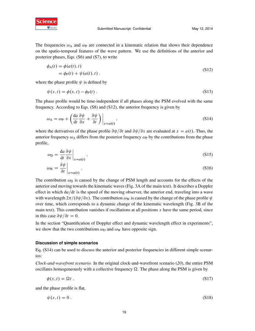
Discussion of simple scenarios

Eq. (S14) can be used to discuss the anterior and posterior frequencies in different simple scenar-ios:

Clock-and-wavefront scenario. In the original clock-and-wavefront scenario (20), the entire PSMoscillates homogeneously with a collective frequency �. The phase along the PSM is given by

�.x; t/ D �t ; (S17)

and the phase profile is flat,

.x; t/ D 0 : (S18)

19

!Submitted Manuscript: Confidential May 12, 2014

Therefore, !W D 0 and !D D 0. According to Eq. (S14) there is no period offset, !A D !P. Thisis true even if the PSM changes its length, that is, if da=dt ¤ 0.

Steady state PSM. In this case, the PSM has constant length a.t/ D a

0

, and displays a kinematicwave pattern that repeats with a collective frequency �, corresponding to a collective period ofT D 2⇡=� (8, 9, 21). The phase �.x; t/ along the PSM is thus given by

�.x; t/ D �t C .x/ ; (S19)

with a time-independent phase profile .x/. In this case @ =@t D 0 and da=dt D 0, resulting inno period offset !A D !P, see Eq. (S14).

Scaling wave pattern. In this case, as the PSM shortens (da=dt < 0) it displays a kinematic wavepattern that scales with the length of the PSM (5). That is, the phase profile is a time independentfunction of the normalized PSM length. The phase �.x; t/ along the PSM is given by

�.x; t/ D !Pt C .x=a.t// : (S20)

Accordingly, the phase profile is a function of x=a.t/ only. It is straightforward to check that inthis case the contributions from the changing phase profile and the Doppler effect in Eq. (S14)exactly balance,

!W D � 0.1/

1

a

dadt; (S21)

!D D C 0.1/

1

a

dadt; (S22)

where 0 denotes the derivative of with respect to its argument. Consequently, the period offsetis zero, !A D !P.

20

!Submitted Manuscript: Confidential May 12, 2014

Quantification of Doppler effect and dynamic wavelength effectin experiments

By averaging experimental data from 18 embryos, we construct a phase map ˆ.x; t/ which re-presents the full spatio-temporal wave pattern during segmentation5. Similarly, we determine anaverage PSM length A.t/. Fig. S5 shows the phase map ˆ.x; t/ and the corresponding phaseprofile ‰.x; t/ D ˆ.x; t/ �ˆ.0; t/ in a kymograph representation as in Fig. 2C of the main text.

We determine the anterior and posterior frequencies !A and !P from experimental data by evalu-ating Eqs. (S8) and (S9) for the average phase map ˆ.x; t/ and PSM length A.t/,

!A.t/ ⇡ ddtˆ.A.t/; t/ ; (S23)

!P.t/ ⇡ @

@t

ˆ.0; t/ : (S24)

The frequencies !A and !P are displayed in Fig. S7A, which shows that the anterior frequency !Ais larger than the posterior frequency !P over most of the time range. Furthermore, we estimate thecontributions from the Doppler effect !D and the dynamic wavelength effect !W in experimentsby evaluating Eqs. (S15) and (S16) for the average phase profile ‰.x; t/ and PSM size A.t/,

!D.t/ ⇡ dAdt@‰

@x

ˇ̌ˇ̌xDA.t/

; (S25)

!W.t/ ⇡ @‰

@t

ˇ̌ˇ̌xDA.t/

: (S26)

The results are shown in Fig. S7B. The Doppler contribution !D is positive (Fig. 3A of the maintext), the dynamic wavelength contribution !W is negative (Fig. 3B of the main text). The com-bination of both contributions yields the observed frequency offset and is positive over most ofthe time range. Fig. S7C shows the relative offset between anterior and posterior frequency,.!A � !P/=!P. Over most of the time range, the magnitude of the Doppler effect is larger thanthe dynamic wavelength effect (solid black curve). The average frequency offset over this time

5From the phase maps �i

.x; t/, we obtain phase profiles, ✓i

.x; t/ D �

i

.x; t/ � �

i

.x

0

; t / with x0

D 210ùm foreach embryo i D 1; : : : ; 18. We use the position x

0

D 210ùm as subtraction point rather than x D 0 as in Eq. (S13),since the phase maps show the least degree of noise in this region. We then determine the median of ✓

i

at each x and t ,N✓.x; t/ D median

i

✓

i

.x; t/. The time evolution of the resulting median phase profile N✓ is displayed in Supplementary

Movie S5 (solid blue curve). As a smoothing technique, we perform fits of differentiable functions to the median phaseprofile N

✓ that capture its spatio-temporal key features. For a fixed time t , we fit the median phase profile N✓.x/ with

the function ‚.x/ given in Table S1 using the fit parameters ✓0

, ˇ, �, and ⇠. Carrying out this procedure for everytime point, we obtain a time series for each of the fit parameters (blue curves in Fig. S8). We then calculate the phaseprofile ‰.x/ D ‚.x/ � ‚.0/, which renders ‰ independent of the parameter ✓

0

. We capture the time dependence ofthe remaining parameters ˇ, �, and ⇠ by fits of the functions f

ˇ

.t/, f�

.t/, and f⇠

.t/ given in Table S1. Using thesefits in ‰.x/, we obtain a differentiable function ‰.x; t/ (dashed green line in Supplementary Movie S5). Likewise, wecompute the median of the posterior phase N

�P.t/ D mediani

�P;i

.t/ and perform a fit of the function ˆP.t/ given inTable S1. According to Eq. (S13), the average phase map is thus given by ˆ.x; t/ D ˆP.t/ C ‰.x; t/. Furthermore,we compute the mean PSM length of all embryos at each time point t , Na.t/ D mean

i

a

i

.t/ and perform a fit withthe function A.t/ given in Table S1. All fit results are shown in Fig. S8 (dashed black curves) and the resulting fitparameters are provided in Table S2. Note that all used fit functions are phenomenological and not derived from adynamic theory.

21

!Submitted Manuscript: Confidential May 12, 2014

interval is 8:4% (dashed black line). Note that a simple estimate of the offset between anteriorand posterior frequency can also be determined through Fig. S5 using the argument presented inFig. 3C of the main text. In Fig. S5A, we count ⇠11 posterior oscillations and ⇠12 anterior os-cillations over the same range of time. Consequently, the average relative offset between anteriorand posterior frequency can be estimated as .12 � 11/=11 ⇡ 9%.

In Fig. S6, we show kymographs of the general spatial and temporal features of the wave pat-terns as obtained from experiments: (A) local inverse wavelength @‰=@x of the average phaseprofile ‰.x; t/, (B) rate of change of the phase profile @‰=@t , and (C) local frequency @ˆ=@t ofthe average phase map ˆ.x; t/. Fig. S6A shows that the wave pattern exhibits long wavelengths(red) in the posterior and short wavelengths (blue) in the anterior. For a fixed position (column),the decrease of the wavelength over time is apparent (gradient from red to black to blue). Fig. S6Bshows that the phase profile changes fastest in the anterior (green regions), where it yields the neg-ative contribution !W, Eq. (S26). Fig. S6C reveals that different parts of the PSM are oscillatingat different frequencies.

22

!Submitted Manuscript: Confidential May 12, 2014

Supplementary Tables

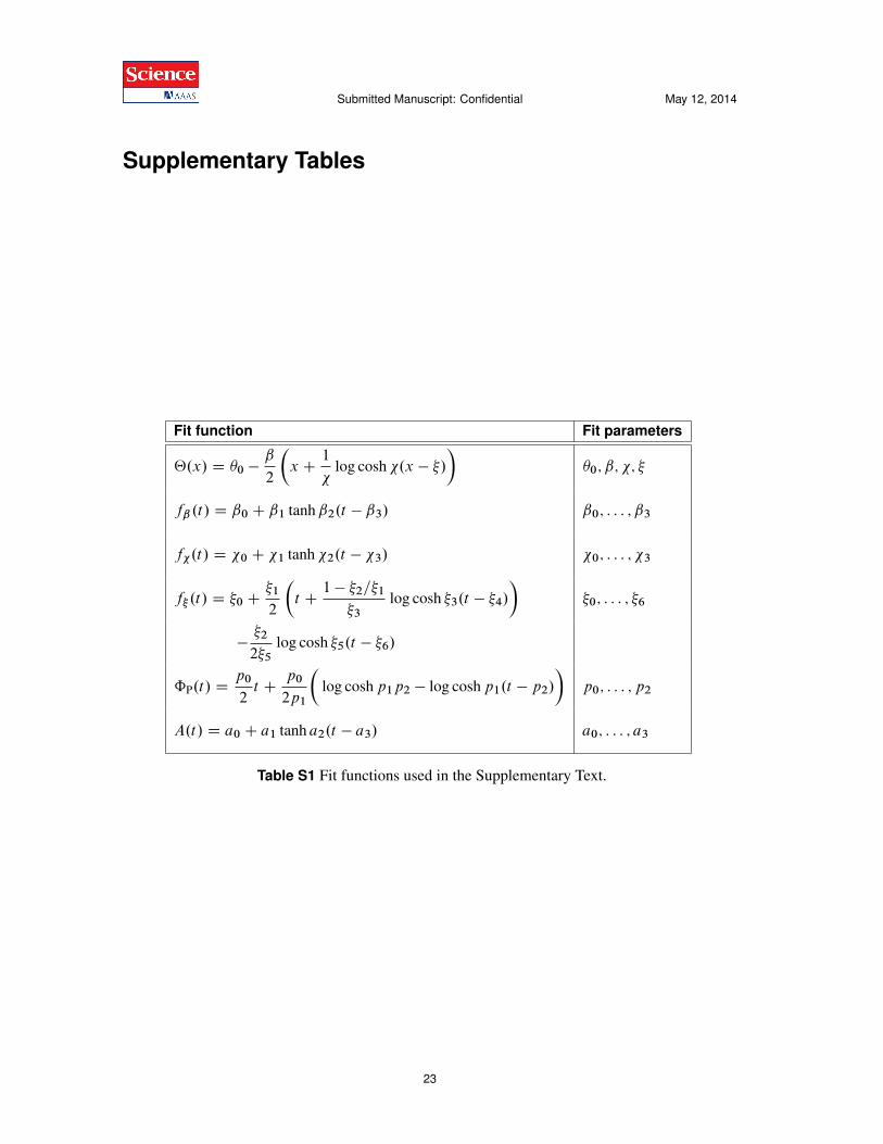
Fit function Fit parameters

‚.x/ D ✓

0

� ˇ

2

✓x C 1

�

log cosh�.x � ⇠/◆

✓

0

; ˇ;�; ⇠

f

ˇ

.t/ D ˇ

0

C ˇ

1

tanhˇ2

.t � ˇ3

/ ˇ

0

; : : : ; ˇ

3

f

�

.t/ D �

0

C �

1

tanh�2

.t � �3

/ �

0

; : : : ;�

3

f

⇠

.t/ D ⇠

0

C ⇠

1

2

✓t C 1 � ⇠

2

=⇠

1

⇠

3

log cosh ⇠3

.t � ⇠4

/

◆⇠

0

; : : : ; ⇠

6

� ⇠

2

2⇠

5

log cosh ⇠5

.t � ⇠6

/

ˆP.t/ D p

0

2

t C p

0

2p

1

✓log coshp

1

p

2

� log coshp1

.t � p2

/

◆p

0

; : : : ; p

2

A.t/ D a

0

C a

1

tanh a2

.t � a3

/ a

0

; : : : ; a

3

Table S1 Fit functions used in the Supplementary Text.

23

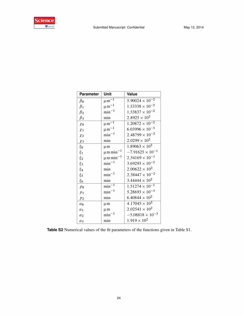
!Submitted Manuscript: Confidential May 12, 2014

Parameter Unit Value

ˇ

0

ùm�1

5:90024 ⇥ 10�2

ˇ

1

ùm�1

1:53338 ⇥ 10�2

ˇ

2

min�1

1:53837 ⇥ 10�2

ˇ

3

min 2:8925 ⇥ 102

�

0

ùm�1

1:20872 ⇥ 10�2

�

1

ùm�1

6:03996 ⇥ 10�3

�

2

min�1

2:48799 ⇥ 10�2

�

3

min 2:0299 ⇥ 102

⇠

0

ùm 1:89063 ⇥ 102

⇠

1

ùm min�1 �7:91625 ⇥ 10�1

⇠

2

ùm min�1

2:54169 ⇥ 10�1

⇠

3

min�1

3:69293 ⇥ 10�2

⇠

4

min 2:00622 ⇥ 102

⇠

5

min�1

2:38447 ⇥ 10�2

⇠

6

min 3:44444 ⇥ 102

p

0

min�1

1:51274 ⇥ 10�1

p

1

min�1

5:28693 ⇥ 10�3

p

2

min 6:40844 ⇥ 102

a

0

ùm 4:17045 ⇥ 102

a

1

ùm 2:02541 ⇥ 102

a

2

min�1 �5:08818 ⇥ 10�3

a

3

min 1:919 ⇥ 102

Table S2 Numerical values of the fit parameters of the functions given in Table S1.

24

References and Notes 1. A. F. Sarrazin, A. D. Peel, M. Averof, A segmentation clock with two-segment periodicity in

insects. Science 336, 338–341 (2012). Medline doi:10.1126/science.1218256

2. E. A. Delaune, P. François, N. P. Shih, S. L. Amacher, Single-cell-resolution imaging of the impact of Notch signaling and mitosis on segmentation clock dynamics. Dev. Cell 23, 995–1005 (2012). Medline doi:10.1016/j.devcel.2012.09.009

3. I. Palmeirim, D. Henrique, D. Ish-Horowicz, O. Pourquié, Avian hairy gene expression identifies a molecular clock linked to vertebrate segmentation and somitogenesis. Cell 91, 639–648 (1997). Medline doi:10.1016/S0092-8674(00)80451-1

4. Y. Masamizu, T. Ohtsuka, Y. Takashima, H. Nagahara, Y. Takenaka, K. Yoshikawa, H. Okamura, R. Kageyama, Real-time imaging of the somite segmentation clock: Revelation of unstable oscillators in the individual presomitic mesoderm cells. Proc. Natl. Acad. Sci. U.S.A. 103, 1313–1318 (2006). Medline doi:10.1073/pnas.0508658103

5. V. M. Lauschke, C. D. Tsiairis, P. François, A. Aulehla, Scaling of embryonic patterning based on phase-gradient encoding. Nature 493, 101–105 (2013). Medline doi:10.1038/nature11804

6. A. C. Oates, L. G. Morelli, S. Ares, Patterning embryos with oscillations: Structure, function and dynamics of the vertebrate segmentation clock. Development 139, 625–639 (2012). Medline doi:10.1242/dev.063735

7. B. Bénazéraf, O. Pourquié, Formation and segmentation of the vertebrate body axis. Annu. Rev. Cell Dev. Biol. 29, 1–26 (2013). Medline doi:10.1146/annurev-cellbio-101011-155703

8. F. Giudicelli, E. M. Ozbudak, G. J. Wright, J. Lewis, Setting the tempo in development: An investigation of the zebrafish somite clock mechanism. PLOS Biol. 5, e150 (2007). Medline doi:10.1371/journal.pbio.0050150

9. L. G. Morelli, S. Ares, L. Herrgen, C. Schröter, F. Jülicher, A. C. Oates, Delayed coupling theory of vertebrate segmentation. HFSP J 3, 55–66 (2009). Medline doi:10.2976/1.3027088

10. D. Soroldoni, A. C. Oates, Live transgenic reporters of the vertebrate embryo’s Segmentation Clock. Curr. Opin. Genet. Dev. 21, 600–605 (2011). Medline doi:10.1016/j.gde.2011.09.006

11. A. Aulehla, W. Wiegraebe, V. Baubet, M. B. Wahl, C. Deng, M. Taketo, M. Lewandoski, O. Pourquié, A beta-catenin gradient links the clock and wavefront systems in mouse embryo segmentation. Nat. Cell Biol. 10, 186–193 (2008). Medline doi:10.1038/ncb1679

12. A. Mara, J. Schroeder, C. Chalouni, S. A. Holley, Priming, initiation and synchronization of the segmentation clock by δD and δC. Nat. Cell Biol. 9, 523–530 (2007). Medline doi:10.1038/ncb1578

13. C. Schröter, L. Herrgen, A. Cardona, G. J. Brouhard, B. Feldman, A. C. Oates, Dynamics of zebrafish somitogenesis. Dev. Dyn. 237, 545–553 (2008). Medline doi:10.1002/dvdy.21458

14. E. M. Özbudak, J. Lewis, Notch signalling synchronizes the zebrafish segmentation clock but is not needed to create somite boundaries. PLOS Genet. 4, e15 (2008). Medline doi:10.1371/journal.pgen.0040015

15. M. Sarov, S. Schneider, A. Pozniakovski, A. Roguev, S. Ernst, Y. Zhang, A. A. Hyman, A. F. Stewart, A recombineering pipeline for functional genomics applied to Caenorhabditis elegans. Nat. Methods 3, 839–844 (2006). Medline doi:10.1038/nmeth933

16. R. Ejsmont, M. Sarov, S. Winkler, K. Lipinski, P. Tomancak, Nat. Methods (2009). 10.1038/nmeth.1334

17. V. Thermes, C. Grabher, F. Ristoratore, F. Bourrat, A. Choulika, J. Wittbrodt, J. S. Joly, I-SceI meganuclease mediates highly efficient transgenesis in fish. Mech. Dev. 118, 91–98 (2002). Medline doi:10.1016/S0925-4773(02)00218-6

18. D. Soroldoni, B. M. Hogan, A. C. Oates, Simple and efficient transgenesis with meganuclease constructs in zebrafish. Methods Mol. Biol. 546, 117–130 (2009). Medline doi:10.1007/978-1-60327-977-2_8

19. J. Schindelin, I. Arganda-Carreras, E. Frise, V. Kaynig, M. Longair, T. Pietzsch, S. Preibisch, C. Rueden, S. Saalfeld, B. Schmid, J. Y. Tinevez, D. J. White, V. Hartenstein, K. Eliceiri, P. Tomancak, A. Cardona, Fiji: An open-source platform for biological-image analysis. Nat. Methods 9, 676–682 (2012). Medline doi:10.1038/nmeth.2019

20. J. Cooke, E. C. Zeeman, A clock and wavefront model for control of the number of repeated structures during animal morphogenesis. J. Theor. Biol. 58, 455–476 (1976). Medline doi:10.1016/S0022-5193(76)80131-2

21. P. J. Murray, P. K. Maini, R. E. Baker, The clock and wavefront model revisited. J. Theor. Biol. 283, 227–238 (2011). Medline doi:10.1016/j.jtbi.2011.05.004

22. R. Quian Quiroga, A. Kraskov, T. Kreuz, P. Grassberger, Performance of different synchronization measures in real data: A case study on electroencephalographic signals. Phys. Rev. E Stat. Nonlin. Soft Matter Phys. 65, 041903 (2002). Medline doi:10.1103/PhysRevE.65.041903

23. C. Torrence, G. P. Compo, A practical guide to wavelet analysis. Bull. Am. Meteorol. Soc. 79, 61–78 (1998). doi:10.1175/1520-0477(1998)079<0061:APGTWA>2.0.CO;2

24. A. C. Oates, R. K. Ho, Hairy/E(spl)-related (Her) genes are central components of the segmentation oscillator and display redundancy with the Delta/Notch signaling pathway in the formation of anterior segmental boundaries in the zebrafish. Development 129, 2929–2946 (2002). Medline

25. I. H. Riedel-Kruse, C. Müller, A. C. Oates, Synchrony dynamics during initiation, failure, and rescue of the segmentation clock. Science 317, 1911–1915 (2007). Medline doi:10.1126/science.1142538

26. G. Lauter, I. Söll, G. Hauptmann, Two-color fluorescent in situ hybridization in the embryonic zebrafish brain using differential detection systems. BMC Dev. Biol. 11, 43 (2011). Medline doi:10.1186/1471-213X-11-43