Three-dimensional transient electromagnetic modeling

for investigating the spatial sensitivity of time

domain reflectometry measurements

Faycal Rejiba, Philippe Cosenza, Christian Camerlynck, and Alain Tabbagh

UMR 7619 Sisyphe, Universite Pierre et Marie Curie, CNRS, Paris, France

Received 20 July 2004; revised 22 April 2005; accepted 23 May 2005; published 16 September 2005.

[1] A three-dimensional (3-D) transient electromagnetic modeling based on a full-waveformulation (Maxwell’s equations) has been undertaken in order to study the impactof heterogeneities located near a time domain reflectometry (TDR) probe. We focused on3-D heterogeneities located at the ends of rods: (1) interface perpendicular to the probeplane located below the end of rods and (2) 3-D (cubic and parallelepipedic)heterogeneities whose characteristic lengths are similar to that of the probe. Whatever therod separation and whatever the dielectric constant contrasts, an interface located justbeneath the end of the rod does not affect significantly a simulated TDR signal when theinterface is farther than one rod diameter. However, all the simulations carried out withcubic and parallelepipedic heterogeneities located along TDR rods have shown that asignificant longitudinal sensitivity exists. The lower the constant dielectric value ofheterogeneity, the higher the longitudinal sensitivity. In particular, parallelepipedicheterogeneities parallel to the rods induce significant changes in the travel times,compared to cubic heterogeneities, whose characteristic length is equal to the rod diameter.Moreover, 3-D numerical calculations have shown that TDR signals are not only sensitiveto the heterogeneity volume itself but also to their orientation. Static 2-D analysis isshown to provide correct qualitative representation of spatial sensitivity analysis, thoughaccurate quantitative estimation of the apparent permittivity requires a complete 4-D(x, y, z, and time) calculation.

Citation: Rejiba, F., P. Cosenza, C. Camerlynck, and A. Tabbagh (2005), Three-dimensional transient electromagnetic modeling for

investigating the spatial sensitivity of time domain reflectometry measurements, Water Resour. Res., 41, W09411,

doi:10.1029/2004WR003505.

1. Introduction

[2] There are many devices for measuring in situ soilwater content, but time domain reflectometry (TDR) islikely today the most popular method for measuring thewater content in the vadose zone. The success of thistechnique is due to a few reasons: it is easy to use andnondestructive compared to others in situ methods (e.g.,radioactive methods).[3] In the 1980s, when the application of electromagnetic

methods to permittivity determination was extended toEarth’s materials [e.g., Topp et al., 1980; Ruault andTabbagh, 1980], the transmission line concept consistingin parallel rods was preferred over coaxial cylinders forwhich the electromagnetic field is constrained between theinner and the outer conductors, and consequently a questionrapidly arose: what is the distribution of the electromagneticfield in the case of a parallel rod transmission line insertedinto a complex medium, i.e., a soil, which may be consti-tuted of different materials and phases with differentdielectric constant values? This question which seemedto be purely academic was in fact closely related to an

other more practical one: what is the volume of soilaffecting the TDR measurement?[4] To our knowledge, Topp and Davis [1985] were the

first authors who provided some responses; they stated thatthe soil volume measured by TDR is approximately acylinder whose axis lies midway between the rods andwhose diameter is 1.4 times the spacing between rods.Baker and Lascano [1989] carried an experimental studyto estimate the region of influence around TDR rods, andshowing that the transversal area of influence is somewherebetween elliptical and rectangular in form. By using a two-prong TDR probe with rods 3.2 mm in diameter, 300 mmlong, and spaced 50 mm apart, they observed that most ofthe sensitivity resides in a cross-sectional area of about1000 mm2 with rectangular dimensions of approximately20 � 65 mm. However, their results show some limitationsand ambiguities: (1) the measured spatial sensitivity of TDRprobe is function of the constant dielectric values of thematerials, but they chose two extreme cases (air and water)which are not representative of the field; (2) as it wasmentioned by Knight [1991], their experimental proceduredoes not allow to obtain a complete three-dimensionalrepresentation of the spatial sensitivity; (3) the authorsstated that there was no discernible variation in sensitivitylongitudinally (along the length of the waveguides), but

Copyright 2005 by the American Geophysical Union.0043-1397/05/2004WR003505$09.00

W09411

WATER RESOURCES RESEARCH, VOL. 41, W09411, doi:10.1029/2004WR003505, 2005

1 of 13

they added: ‘‘except that the inflexion points on the TDRtrace were more difficult to discern when the water addedwas at either extreme end of the waveguides.’’ The effect ofa dielectric heterogeneity at the ends of TDR rods shouldthus be clarified.[5] Petersen et al. [1995] focused on small TDR

probes, 50 and 150 mm length, for laboratory experi-ments, and their experimental results suggest that thesmaller the rod diameter, the higher the resolution andthe closer measurements can be performed to the soilsurface. In order to investigate the spatial sensitivity of aTDR probe in a general case, Ferre et al. [1996] used asquare root averaging model. They studied the axial andthe transverse sensitivity separately. Knight [1992] definedin a rigorous way a spatial weighting function w(x, y) ina plane perpendicular to the waveguides. Since the func-tion w(x, y) depends on two variables, it defines a samplearea which contains a desired percentage of the totalsensitivity. By assuming low constant dielectric contrastsaround the probes, he confirmed the previous experimen-tal results: the region close to the waveguides has theheaviest weight. Considering a two-dimensional geometry(i.e., no sensitivity parallel to the waveguides), the func-tion has been calculated numerically under the staticapproximation by Knight et al. [1997] to estimate quan-titatively the effects of coating and gaps around TDRrods. Ferre et al. [1998], used the same approach tocalculate the sample areas of conventional TDR probes.The main results of these theoretical calculations are thefollowing: (1) two-rod probes have much larger samplearea than three-rod ones; (2) fluid-filled gaps or dielectriccoatings around parallel-wire transmission lines affectsignificantly the transverse surface of influence aroundthe TDR probes; low dielectric coatings or gaps reduce it;these effects are enhanced in case of three-rod probes;(3) the rod separation is a key parameter in the estimationof the spatial sensitivity. Recently, the Knight’s approachhas been experimentally validated by Nissen et al. [2003]who considered sharp vertical boundaries parallel to thewaveguides.[6] Finally, it should be emphasized that all the

theoretical and experimental works initiated by Knight[1992] focused on the lateral (2-D) sensitivity of TDRprobes. Specific 3-D effects like the presence of smalldielectric contrasts at the ends of rods were not yetstudied. This is why Chambarel and Ferry [2000]proposed to model the TDR signal propagation directlyusing the three-dimensional governing electromagneticequations. Their calculations showed a significant effectof an electrical singularity at the end of the waveguides.However, their numerical study was not systematic: onesingle particular example was considered, and the TDRprobes was modeled by a two parallel plate electrodes,i.e., a 2-D geometry.[7] In this paper, a transient formulation of the Max-

well’s equations with a complete 3-D geometry is con-sidered. A set of simulations has been performed in orderto study the 3-D sensitivity of TDR measurements; moreprecisely, we focused on 3-D heterogeneities located atthe end of rods, for which literature has paid littleattention: (1) an interface perpendicular to the probe planelocated below the end of rods and (2) 3-D heterogeneities

whose characteristic lengths are similar to that of theprobes.

2. Methodology

2.1. Numerical Model

[8] A TDR dielectric measuring setup is a complexelectronic system which generally includes a pulser, asampler, a scope, a processor, a transmission line or coaxialcable with the corresponding connectors, sometimes a balunor a transmission line transformer and finally the moistureprobe itself. Contrary to 1-D circuit theory usually devel-oped [e.g., Oswald et al., 2003], we decided not to modelthe complete waveform by considering the whole set ofelectronic components located upstream of the moistureprobe. In our 3-D theoretical approach, we focused on thephysics involved in the moisture probe: propagation ofelectromagnetic waves guided by two conductive rods, theonly aspect of the setup that might not be improved withadvances in electronic components.[9] The 3-D numerical simulations have been achieved

by solving the following Maxwell’s equations:

r� E ¼ � @B

@tð1Þ

r �H ¼ @D

@tþ Jc ð2Þ

where E is the electric field density, B is the magnetic fluxdensity, D is the electric flux density, H is the magnetic fieldstrength, Jc is the conduction current density. If soil isassumed to be a linear, nondispersive, isotropic material,one can introduced the following additional constitutiveequations:

B ¼ mH ð3Þ

Jc ¼ sE ð4Þ

D ¼ eE ð5Þ

where m is the magnetic permeability; s is the electricalconductivity, e is the permittivity. Hereafter, induced andremanent magnetism and attenuation effect associated withelectrical conductivity will not be considered: m = m0 wherem0 is the magnetic permeability of vacuum and s = 0. Bycombining the equations (1) to (5), one can obtained a set ofnonlinear equations that are discretized in time (finitedifference time domain) and in a 3-D cubic mesh for whichthe magnetic field H and the electric flux density D are thevectorial unknowns [Rejiba et al., 2003]. In order tominimize usual electromagnetic reflections from the outerboundaries of the 3-D mesh, a simplified unsplit perfectmatched layer (SUPML) algorithm [Rejiba et al., 2003] hasbeen implemented. This specific and parallel algorithm isexecuted on a cluster (20 nodes).[10] In our simulations, the mesh that is constituted by

140 � 140 � 340 elementary cubes of dimension dx = dy =

2 of 13

W09411 REJIBA ET AL.: THREE-DIMENSIONAL TRANSIENT ELECTROMAGNETIC MODELING W09411

dz = D comprises four domains: (1) air, (2) conductive TDRrods for which a perfect electric conductor surface conditionhas been considered, (3) soil, and (4) heterogeneities intothe soil. The orientation of the waveguides and the origin Oof the coordinates system (x, y, z) are given in Figure 1.

[11] A typical geometry for the waveguides has beendefined from the usual geometrical parameters of TDRprobes used for moisture monitoring [e.g., O’Connor andDowding, 1999]. Their typical length, width and spacingare 200 mm, 6 mm and 24 mm respectively. Consideringthese parameters and after preliminary tests, the character-istic dimension of an elementary volume D has been fixedequal to 1 mm which corresponds to the best compromisebetween a low duration of calculations and a goodaccuracy of results. In a typical simulation, three charac-teristic events can be identified (Figure 2). In a first step,an electromagnetic step pulse is emitted in the air, 10 mmabove and between both heads of the rods with an xpolarization. It corresponds to a voltage gap - step pulsefunction - giving a rise time of 200 picoseconds. Thisvalue is typical of commercially available rise-time equip-ment [e.g., O’Connor and Dowding, 1999]. In a secondstep, a part of the guided waves that were transmitted inthe part of the rods located in the air, are reflected backat the air-soil interface. Thirdly, the transmitted waves intothe rods are mainly reflected back at the ends of therods. The two-way transit time Dt between the reflectedpulse from the air-soil interface and the reflected pulsefrom the ends of the rods must be obviously divided bytwo in order to correspond to the transit time of theelectromagnetic pulse along the TDR probe located inthe soil. The transit time Dt allows to obtain the soildielectric constant K following the equation:

K ¼ cDt

2L

� �2

ð6Þ

where c is the speed of an electromagnetic wave in freespace (3 � 108 m/s), L is the rods length.

Figure 1. Scheme of the modeling approach. The origin Oand the x, y, and z axes of the chosen Cartesian system aregiven.

Figure 2. (a) A typical simulated electromagnetic signal recorded at the heads of the conductive rods.Soil constant dielectric is equal to 25. (b) Picked arrival time corresponding to the reflected signal at theend of the probes, indicated by a vertical line.

W09411 REJIBA ET AL.: THREE-DIMENSIONAL TRANSIENT ELECTROMAGNETIC MODELING

3 of 13

W09411

[12] The travel time which corresponds to the reflectedpulse from the air-soil interface is easily calculated since therods length in the air and the air dielectric constant areknown. We checked that it corresponds to the first peakgiven in Figure 2a.[13] The picked or break time related to the reflection

from the ends of the probes is obtained in a similar way thatconventional refraction seismic [e.g., Sheriff and Geldart,1995]. The arrival of the reflected EM wave front from theends of the probes which is characterized by a rapid increasein signal amplitude has been picked from a two-stepprocess. First, horizontal tangent which represents the signalbefore the reflection arrival is drawn. In a second step, thebeginning of the amplitude increase which is identified by asignificant takeoff from the horizontal tangent is marked bya vertical line as shown in Figure 2b. In the following, sincethe attenuation of the electromagnetic waves was notconsidered, the amplitude of the simulated signal or tracewas not investigated and was initialized to an arbitraryvalue.

2.2. Numerical Validation

[14] This numerical approach has been validated byconsidering two cases: (1) a homogeneous soil with differ-ent dielectric constant values and (2) a heterogeneous soilcorresponding to the wetting front problem. In the first case,three theoretical dielectric constant values were considered:5, 15, and 25. The values of 5 and 25 are associatedtypically with a dry and wet soil respectively. The threevalues corresponding to the picking of the simulated signals

and calculated from equation (6) are very similar to thetheoretical values: 4.9, 14.8 and 25.0 (instead of 5, 15,and 25). The maximum relative difference between thetheoretical dielectric constant and the ‘‘picked’’ dielectricconstant obtained from the dry case is 2.4%. This valuethat traduces the discrepancy between the selected per-mittivity for the simulations and the inferred permittivitycomputed using time of travel picked off, includes errorsassociated with the numerical dispersion and the pickingprocess illustrated in Figure 2.[15] In the second case, the wetting front (WF) problem

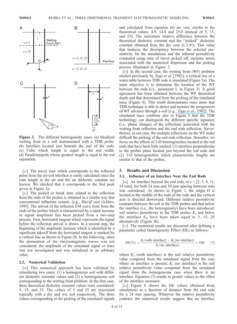
studied previously by Topp et al. [1982], a vertical rise of awater table between TDR rods is simulated (Figure 3a). Themain objective is to determine the location of the WFbetween the rods (i.e., parameter L in Figure 3). A goodagreement has been obtained between the WF theoreticaldepth and that determined from the picking of the simulatedtrace (Figure 4). This result demonstrates once more thatTDR technique is able to detect and monitor the progressionof WF advance through a soil [e.g., Topp et al., 1982]. Thesimulated trace confirms also in Figure 5 that the TDRtechnology can distinguish the different specific signature(i.e., phase changes of the reflection) associated with thewetting front reflection and the end rods reflection. Never-theless, in our case, the multiple reflections on the WF makedifficult the picking of the end rods reflection. Hereafter, wefocus on the effects of 3-D heterogeneities located at the rodends that have been little studied: (1) interface perpendicularto the probes plane located just beyond the rod ends and(2) 3-D heterogeneities which characteristic lengths aresimilar to that of the probes.

3. Results and Discussion

3.1. Influence of an Interface Near the End Rods

[16] An interface beyond the end rods, at z = [2, 5, 8, 11,14 mm], for both 24 mm and 50 mm spacing between rodswas considered. As shown in Figure 1, the origin O islocated at the middle of the ends of the rods and the verticalaxis is directed downward. Different relative permittivitycontrasts between the soil in the TDR probes and that belowthe interface (i.e., the heterogeneity) have been introduced:soil relative permittivity in the TDR probes Ks and belowthe interface Kh have been taken equal to 5, 15, 25alternatively (Figure 3b).[17] The numerical results are discussed after defining a

parameter called Heterogeneity Effect (HE) as follows:

HE %ð Þ ¼ Ks with interfaceð Þ � Ks no interfaceð ÞKs no interfaceð Þ � 100 ð7Þ

where Ks (with interface) is the soil relative permittivityvalue computed from the simulated signal from the casewhere an interface is present, Ks (no interface) is the soilrelative permittivity value computed from the simulatedsignal from the homogeneous case when there is nointerface. Equation (7) results in greater values as the effectof the interface increases.[18] Figure 6 shows the HE values obtained from

simulations as a function of distance from the end rodsfor a 24 mm spacing. Whatever the relative permittivitycontrast, the numerical results suggest that an interface

Figure 3. The different heterogeneity cases. (a) Idealizedwetting front in a soil instrumented with a TDR probe.(b) Interface located just beneath the end of the rods.(c) Cube which length is equal to the rod width.(d) Parallelepipeds whose greatest length is equal to the rodseparation.

4 of 13

W09411 REJIBA ET AL.: THREE-DIMENSIONAL TRANSIENT ELECTROMAGNETIC MODELING W09411

located even just below the end rods (at a distance lessthan one diameter) has a low influence on the TDRmeasurements: the HE parameter is always less than 5%.This influence is null when the interface is located fartherthan one rod diameter (6 mm in our example). For z =2 mm, the HE parameter is systematically negative: thesoil relative permittivity value is slightly underestimatedand the relative permittivity contrast does not play asignificant role on the HE parameter.[19] Simulations considering a 50 mm spacing between

rods confirm the previous results: the calculated HE valuesare the same order of magnitude of that given in Figure 6. In

order to explain the different results observed in Figure 6some signals reflected from the ends of the rods aremagnified in Figures 7 and 8. In Figure 7 the soil permit-tivity above Ks and that below the interface Kh have beentaken equal to 5 and 25 respectively. In Figure 8, consid-ering the same distances from the interface z, we haveinverted the permittivity contrast (Ks = 5; Kh = 25). Forcomparison, the situation related to the homogeneous case(i.e., no interface) and the corresponding picked times arealso shown in Figures 7 and 8. Each permittivity contrastand each relative position of this contrast (z) induce aparticular appearance (i.e., a signature) to the waveform:

Figure 5. Simulated trace for case A. Idealized wetting front in a soil instrumented with a TDR probe.The wetting front is located at 15 cm (z = �5 cm) below the air-soil interface.

Figure 4. Comparison between the wetting front theoretical depth and that determined from the pickingof the simulated trace.

W09411 REJIBA ET AL.: THREE-DIMENSIONAL TRANSIENT ELECTROMAGNETIC MODELING

5 of 13

W09411

as the distance z from the end rods increases, a significantinversion of phase is observed in Figure 8 that is not seen inFigure 7. Moreover, the peak amplitudes have differentvalues and evolution with the distance z: for z = 5 mm,the amplitude increase associated with the case (Ks. = 25;Kh = 5) (respectively Ks. = 5; Kh = 25) begins at a shorter(respectively longer) time than that corresponding to the

homogeneous case (i.e., no interface). Thus these differ-ences in signature explains why for the same distance fromthe end rods z and for the same absolute permittivitydifference (20 in Figures 7 and 8) one obtains different HEvalues, specially for z = 5 mm (Figure 6). However, asmentioned previously, the induced HE values are low, lessthan 5% and consequently in a practical point of view, this

Figure 7. Simulated traces for the permittivity contrast (Ks = 25; Kh = 5) and different distances fromthe end rods z (2 and 5 mm). The homogeneous case (i.e., no interface) is also shown.

Figure 6. HE values between the soil permittivity value ‘‘picked’’ from the heterogeneous case (i.e.,when an interface is present) and that ‘‘picked’’ from the homogeneous case (i.e., when there is nointerface), as a function of distance from the end rods.

6 of 13

W09411 REJIBA ET AL.: THREE-DIMENSIONAL TRANSIENT ELECTROMAGNETIC MODELING W09411

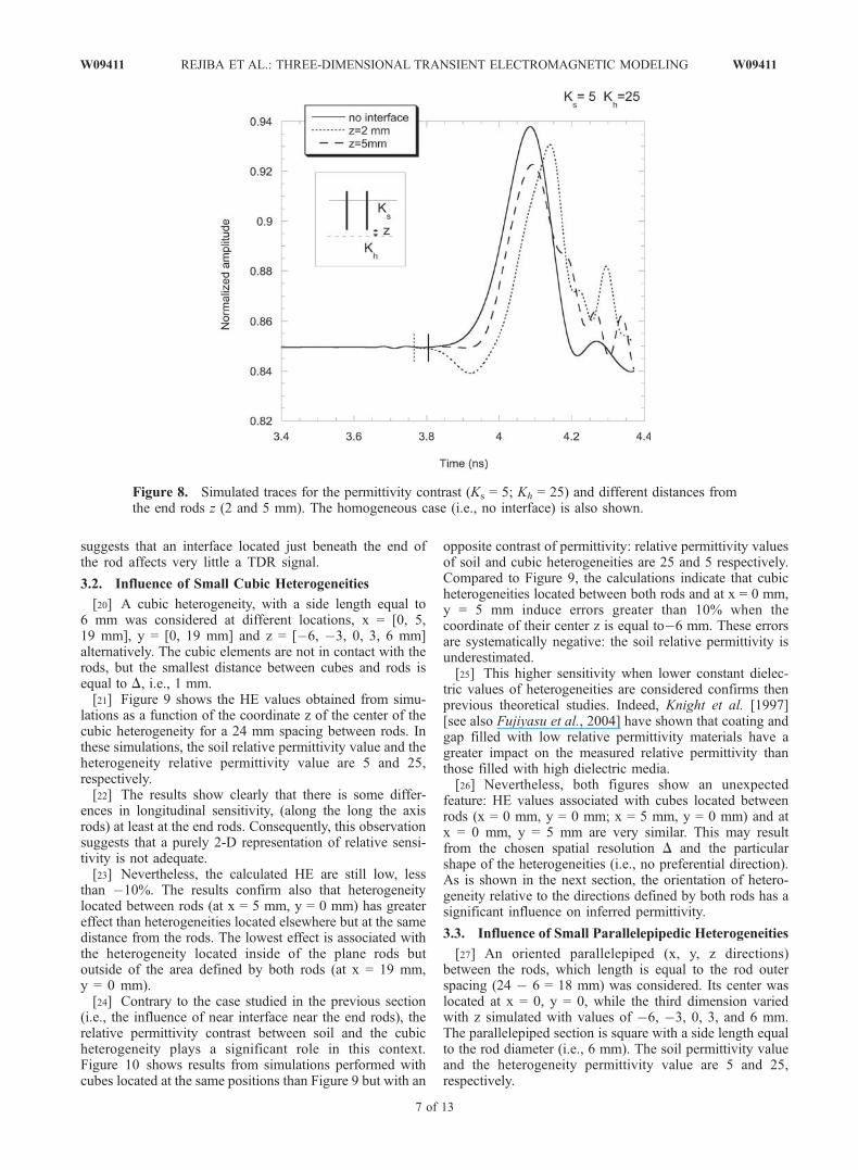
suggests that an interface located just beneath the end ofthe rod affects very little a TDR signal.

3.2. Influence of Small Cubic Heterogeneities

[20] A cubic heterogeneity, with a side length equal to6 mm was considered at different locations, x = [0, 5,19 mm], y = [0, 19 mm] and z = [�6, �3, 0, 3, 6 mm]alternatively. The cubic elements are not in contact with therods, but the smallest distance between cubes and rods isequal to D, i.e., 1 mm.[21] Figure 9 shows the HE values obtained from simu-

lations as a function of the coordinate z of the center of thecubic heterogeneity for a 24 mm spacing between rods. Inthese simulations, the soil relative permittivity value and theheterogeneity relative permittivity value are 5 and 25,respectively.[22] The results show clearly that there is some differ-

ences in longitudinal sensitivity, (along the long the axisrods) at least at the end rods. Consequently, this observationsuggests that a purely 2-D representation of relative sensi-tivity is not adequate.[23] Nevertheless, the calculated HE are still low, less

than �10%. The results confirm also that heterogeneitylocated between rods (at x = 5 mm, y = 0 mm) has greatereffect than heterogeneities located elsewhere but at the samedistance from the rods. The lowest effect is associated withthe heterogeneity located inside of the plane rods butoutside of the area defined by both rods (at x = 19 mm,y = 0 mm).[24] Contrary to the case studied in the previous section

(i.e., the influence of near interface near the end rods), therelative permittivity contrast between soil and the cubicheterogeneity plays a significant role in this context.Figure 10 shows results from simulations performed withcubes located at the same positions than Figure 9 but with an

opposite contrast of permittivity: relative permittivity valuesof soil and cubic heterogeneities are 25 and 5 respectively.Compared to Figure 9, the calculations indicate that cubicheterogeneities located between both rods and at x = 0 mm,y = 5 mm induce errors greater than 10% when thecoordinate of their center z is equal to�6 mm. These errorsare systematically negative: the soil relative permittivity isunderestimated.[25] This higher sensitivity when lower constant dielec-

tric values of heterogeneities are considered confirms thenprevious theoretical studies. Indeed, Knight et al. [1997][see also Fujiyasu et al., 2004] have shown that coating andgap filled with low relative permittivity materials have agreater impact on the measured relative permittivity thanthose filled with high dielectric media.[26] Nevertheless, both figures show an unexpected

feature: HE values associated with cubes located betweenrods (x = 0 mm, y = 0 mm; x = 5 mm, y = 0 mm) and atx = 0 mm, y = 5 mm are very similar. This may resultfrom the chosen spatial resolution D and the particularshape of the heterogeneities (i.e., no preferential direction).As is shown in the next section, the orientation of hetero-geneity relative to the directions defined by both rods has asignificant influence on inferred permittivity.

3.3. Influence of Small Parallelepipedic Heterogeneities

[27] An oriented parallelepiped (x, y, z directions)between the rods, which length is equal to the rod outerspacing (24 � 6 = 18 mm) was considered. Its center waslocated at x = 0, y = 0, while the third dimension variedwith z simulated with values of �6, �3, 0, 3, and 6 mm.The parallelepiped section is square with a side length equalto the rod diameter (i.e., 6 mm). The soil permittivity valueand the heterogeneity permittivity value are 5 and 25,respectively.

Figure 8. Simulated traces for the permittivity contrast (Ks = 5; Kh = 25) and different distances fromthe end rods z (2 and 5 mm). The homogeneous case (i.e., no interface) is also shown.

W09411 REJIBA ET AL.: THREE-DIMENSIONAL TRANSIENT ELECTROMAGNETIC MODELING

7 of 13

W09411

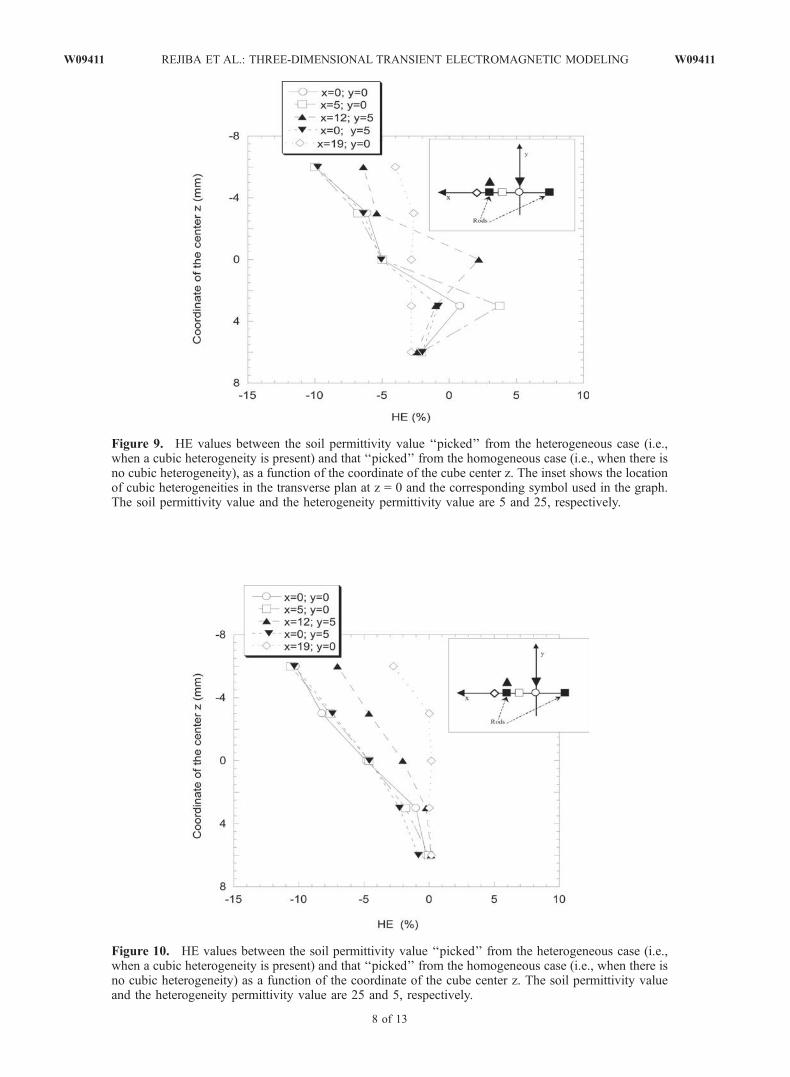
Figure 10. HE values between the soil permittivity value ‘‘picked’’ from the heterogeneous case (i.e.,when a cubic heterogeneity is present) and that ‘‘picked’’ from the homogeneous case (i.e., when there isno cubic heterogeneity) as a function of the coordinate of the cube center z. The soil permittivity valueand the heterogeneity permittivity value are 25 and 5, respectively.

Figure 9. HE values between the soil permittivity value ‘‘picked’’ from the heterogeneous case (i.e.,when a cubic heterogeneity is present) and that ‘‘picked’’ from the homogeneous case (i.e., when there isno cubic heterogeneity), as a function of the coordinate of the cube center z. The inset shows the locationof cubic heterogeneities in the transverse plan at z = 0 and the corresponding symbol used in the graph.The soil permittivity value and the heterogeneity permittivity value are 5 and 25, respectively.

8 of 13

W09411 REJIBA ET AL.: THREE-DIMENSIONAL TRANSIENT ELECTROMAGNETIC MODELING W09411

[28] As expected, parallelepipeds parallel to y directionshow the lowest effect, with a maximum absolute HE valueequal to 7% (Figure 11). Indeed, from the previous studieson the 2-D sensitivity of TDR measurements, it is wellknown that TDR sensitivity is the lowest in the directionperpendicular to rods plan.[29] In cases of parallelepiped centers located outside the

area between both rods (i.e., z > 0 in Figure 11), paralle-lepipeds parallel to x direction and y direction induce lowabsolute HE values (up to 3%). This result is consistent withthe previous simulations carried out with an interface (seesection 3.1): a heterogeneity located just below the end rodsdoes not significantly change the simulated signal. This isno longer the case when parallelepipeds in the z directionare considered: absolute HE value increases up to 8% at z =3 mm. At this stage, the higher influence of parallelepipedsparallel to z direction could be explained by the fact that asignificant part of these parallelepipeds is located in theextremely sensitive area between the rods.[30] In cases of centers located inside the area between

both rods (i.e., z � 0 in Figure 11), parallelepipeds parallelto z still have the highest influence. Absolute HE increasesrapidly up to 17% at z = �6 mm. For these cases, the resultsshow clearly that in fact, HE values do not mainly dependof the volume of the heterogeneity between the rods but ofthe orientation of the heterogeneity: indeed for z = �3 mm,a parallel z parallelepiped with a volume of (18 � 3 = 15) �6 � 6 = 540 mm3 inside the sensitive area defined by bothrods leads to an HE value of about 14% whereas a parallelx parallelepiped with a greater volume of 18 � 6 � 6 =648 mm3 in the same area induces a lower HE value ofabout 8%.

[31] In any cases, when z < 0, whatever the orientation ofthe parallelepipeds, it should be noted that the HE parameteris systematically negative: the picking process leads sys-tematically to an underestimated value. This result confirmsalso that a clear longitudinal sensitivity (along the long theaxis rods) exists, at least at the end rods.[32] Another perhaps counter intuitive result is related to

the ratio Derror %ð Þ=Dz mmð Þ in Figure 11. If both x-paralleland z-parallel parallelepipeds are considered, it should benoted that the ratio Derror %ð Þ=Dz mmð Þ for both orienta-tions are quite similar and equal to unity. This surprisingresults that likely depends on the chosen geometryshould be validated in others geometrical configurations.

3.4. Comparisons With Simple 2-D Calculations

[33] All the previous results have been obtained by 3-Dtime domain calculations which may be difficult to perform:specific algorithms and a powerful computer are required.Furthermore, one may wonder if simpler approaches basedon a 2-D static formulation would have led to the sametrends since numerous experimental investigations weresuccessfully carried out on the basis of 2-D analysis [e.g.,Fujiyasu et al., 2004].[34] To our knowledge, the simplest 2-D analytical

approach was proposed by Knight [1992] who introducedthe concept of spatial weighting function defined asfollows:

w x; yð Þ ¼ E x; yð Þj j2ZZW

E0 x; yð Þj jdsð8Þ

Figure 11. HE values between the soil permittivity value ‘‘picked’’ from the heterogeneous case (i.e.,when a parallelepipedic heterogeneity is present) and that ‘‘picked’’ from the homogeneous case (i.e.,when there is no parallelepipedic heterogeneity) as function of the coordinate of the parallelepiped centerz. Linear regressions for the x parallel and the z parallel are also given. The soil permittivity value and theheterogeneity permittivity value are 5 and 25, respectively.

W09411 REJIBA ET AL.: THREE-DIMENSIONAL TRANSIENT ELECTROMAGNETIC MODELING

9 of 13

W09411

where E and E0 are the electric field when heterogeneitiesare present and the electric field in the uniform caserespectively. This function is related to the apparent relativedielectric permittivity, Ka, by

Ka ¼ZZW

K x; yð Þw x; yð Þds ð9Þ

The parameter Ka integrates the distribution of relativedielectric permittivity K(x, y) that takes into account theexistence of heterogeneities. Obviously, parameter Ka

corresponds to the previous parameter Ks (with hetero-geneity) defined in equation (7).[35] In case of a small contrast from the uniform distri-

bution of relative permittivities, Knight [1992] showed thatthe weighting function, w(x, y), could be written in terms ofpolar coordinates r and j as follows:

w r;jð Þ ¼d2 � b2ð Þ

p ln d þ að Þ=b½ � d2 � b2ð Þ2�2 d2 � b2ð Þr2 cos 2jþ r4h in o

ð10Þ

where d is the distance between the axes of the probe wires,b is the wires diameter, a is the interfocal distance of abipolar coordinate system that has been introduced byKnight in order to obtain an analytical formulation. From(10) and if the distribution K(x, y) is known, the apparentrelative permittivity Ka can be calculated by the integrationof the product K(x, y)w(x, y) over the area W.

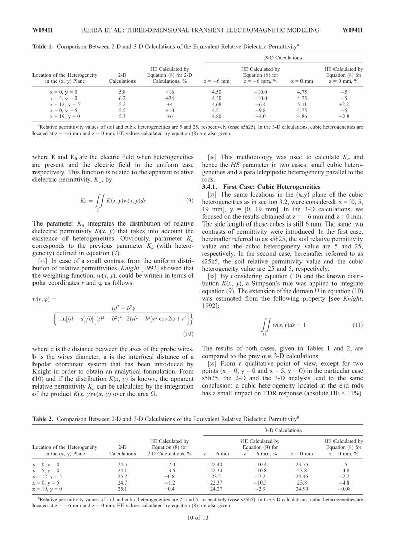
[36] This methodology was used to calculate Ka andhence the HE parameter in two cases: small cubic hetero-geneities and a parallelepipedic heterogeneity parallel to therods.3.4.1. First Case: Cubic Heterogeneities[37] The same locations in the (x,y) plane of the cubic

heterogeneities as in section 3.2, were considered: x = [0, 5,19 mm], y = [0, 19 mm]. In the 3-D calculations, wefocused on the results obtained at z = �6 mm and z = 0 mm.The side length of these cubes is still 6 mm. The same twocontrasts of permittivity were introduced. In the first case,hereinafter referred to as s5h25, the soil relative permittivityvalue and the cubic heterogeneity value are 5 and 25,respectively. In the second case, hereinafter referred to ass25h5, the soil relative permittivity value and the cubicheterogeneity value are 25 and 5, respectively.[38] By considering equation (10) and the known distri-

bution K(x, y), a Simpson’s rule was applied to integrateequation (9). The extension of the domain W in equation (10)was estimated from the following property [see Knight,1992]:

ZZW

w x; yð Þds ¼ 1 ð11Þ

The results of both cases, given in Tables 1 and 2, arecompared to the previous 3-D calculations.[39] From a qualitative point of view, except for two

points (x = 0, y = 0 and x = 5, y = 0) in the particular cases5h25, the 2-D and the 3-D analysis lead to the sameconclusion: a cubic heterogeneity located at the end rodshas a small impact on TDR response (absolute HE < 11%).

Table 1. Comparison Between 2-D and 3-D Calculations of the Equivalent Relative Dielectric Permittivitya

Location of the Heterogeneityin the (x, y) Plane

2-DCalculations

HE Calculated byEquation (8) for 2-D

Calculations, %

3-D Calculations

z = �6 mm

HE Calculated byEquation (8) forz = �6 mm, % z = 0 mm

HE Calculated byEquation (8) forz = 0 mm, %

x = 0, y = 0 5.8 +16 4.50 �10.0 4.75 �5x = 5, y = 0 6.2 +24 4.50 �10.0 4.75 �5x = 12, y = 5 5.2 +4 4.68 �6.4 5.11 +2.2x = 0, y = 5 5.5 +10 4.51 �9.8 4.75 �5x = 19, y = 0 5.3 +6 4.80 �4.0 4.86 �2.8

aRelative permittivity values of soil and cubic heterogeneities are 5 and 25, respectively (case s5h25). In the 3-D calculations, cubic heterogeneities arelocated at z = �6 mm and z = 0 mm. HE values calculated by equation (8) are also given.

Table 2. Comparison Between 2-D and 3-D Calculations of the Equivalent Relative Dielectric Permittivitya

Location of the Heterogeneityin the (x, y) Plane

2-DCalculations

HE Calculated byEquation (8) for

2-D Calculations, %

3-D Calculations

z = �6 mm

HE Calculated byEquation (8) forz = �6 mm, % z = 0 mm

HE Calculated byEquation (8) forz = 0 mm, %

x = 0, y = 0 24.5 �2.0 22.40 �10.4 23.75 �5x = 5, y = 0 24.1 �3.6 22.30 �10.8 23.8 �4.8x = 12, y = 5 25.2 +0.8 23.2 �7.2 24.45 �2.2x = 0, y = 5 24.7 �1.2 22.37 �10.5 23.8 �4.8x = 19, y = 0 25.1 +0.4 24.27 �2.9 24.99 �0.08

aRelative permittivity values of soil and cubic heterogeneities are 25 and 5, respectively (case s25h5). In the 3-D calculations, cubic heterogeneities arelocated at z = �6 mm and z = 0 mm. HE values calculated by equation (8) are also given.

10 of 13

W09411 REJIBA ET AL.: THREE-DIMENSIONAL TRANSIENT ELECTROMAGNETIC MODELING W09411

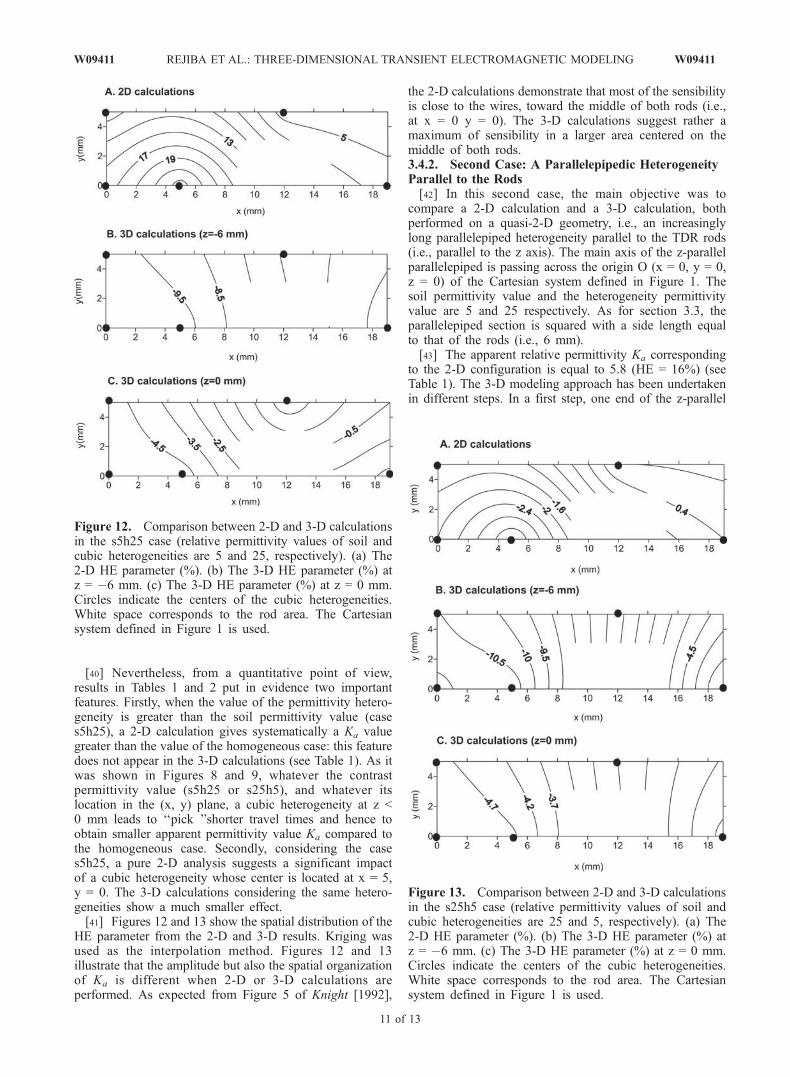
[40] Nevertheless, from a quantitative point of view,results in Tables 1 and 2 put in evidence two importantfeatures. Firstly, when the value of the permittivity hetero-geneity is greater than the soil permittivity value (cases5h25), a 2-D calculation gives systematically a Ka valuegreater than the value of the homogeneous case: this featuredoes not appear in the 3-D calculations (see Table 1). As itwas shown in Figures 8 and 9, whatever the contrastpermittivity value (s5h25 or s25h5), and whatever itslocation in the (x, y) plane, a cubic heterogeneity at z <0 mm leads to ‘‘pick ’’shorter travel times and hence toobtain smaller apparent permittivity value Ka compared tothe homogeneous case. Secondly, considering the cases5h25, a pure 2-D analysis suggests a significant impactof a cubic heterogeneity whose center is located at x = 5,y = 0. The 3-D calculations considering the same hetero-geneities show a much smaller effect.[41] Figures 12 and 13 show the spatial distribution of the

HE parameter from the 2-D and 3-D results. Kriging wasused as the interpolation method. Figures 12 and 13illustrate that the amplitude but also the spatial organizationof Ka is different when 2-D or 3-D calculations areperformed. As expected from Figure 5 of Knight [1992],

the 2-D calculations demonstrate that most of the sensibilityis close to the wires, toward the middle of both rods (i.e.,at x = 0 y = 0). The 3-D calculations suggest rather amaximum of sensibility in a larger area centered on themiddle of both rods.3.4.2. Second Case: A Parallelepipedic HeterogeneityParallel to the Rods[42] In this second case, the main objective was to

compare a 2-D calculation and a 3-D calculation, bothperformed on a quasi-2-D geometry, i.e., an increasinglylong parallelepiped heterogeneity parallel to the TDR rods(i.e., parallel to the z axis). The main axis of the z-parallelparallelepiped is passing across the origin O (x = 0, y = 0,z = 0) of the Cartesian system defined in Figure 1. Thesoil permittivity value and the heterogeneity permittivityvalue are 5 and 25 respectively. As for section 3.3, theparallelepiped section is squared with a side length equalto that of the rods (i.e., 6 mm).[43] The apparent relative permittivity Ka corresponding

to the 2-D configuration is equal to 5.8 (HE = 16%) (seeTable 1). The 3-D modeling approach has been undertakenin different steps. In a first step, one end of the z-parallel

Figure 12. Comparison between 2-D and 3-D calculationsin the s5h25 case (relative permittivity values of soil andcubic heterogeneities are 5 and 25, respectively). (a) The2-D HE parameter (%). (b) The 3-D HE parameter (%) atz = �6 mm. (c) The 3-D HE parameter (%) at z = 0 mm.Circles indicate the centers of the cubic heterogeneities.White space corresponds to the rod area. The Cartesiansystem defined in Figure 1 is used.

Figure 13. Comparison between 2-D and 3-D calculationsin the s25h5 case (relative permittivity values of soil andcubic heterogeneities are 25 and 5, respectively). (a) The2-D HE parameter (%). (b) The 3-D HE parameter (%) atz = �6 mm. (c) The 3-D HE parameter (%) at z = 0 mm.Circles indicate the centers of the cubic heterogeneities.White space corresponds to the rod area. The Cartesiansystem defined in Figure 1 is used.

W09411 REJIBA ET AL.: THREE-DIMENSIONAL TRANSIENT ELECTROMAGNETIC MODELING

11 of 13

W09411

parallelepiped is located exactly at the origin O; no part ofthe parallelepiped is included in the plane defined by bothrods. The other end is located far from the TDR probe, atthe boundary of the mesh. The apparent relative permittivityis then calculated. In a second step, the length of the sameparallelepiped is increased by a small increment of 3 mm:its end is now located at z = �3 mm. For this new position,the apparent relative permittivity is calculated again. Thisprocess is repeated for a few z increments until twoseparated peaks are identified on the simulated electromag-netic signal: one peak is associated with a reflection on therod ends and the second is related to a reflection on theparallelepiped end. The results of Ka for these differentsteps are given in Figure 14.[44] As for cubic heterogeneities considering the same

permittivity contrast (s5h25), the 3-D Ka is systemicallylower than the soil relative permittivity and the 2-D Ka. Forthe same reason, the end of the parallelepiped induces adistortion of the electromagnetic signal reflected from theend of the rods and leads to pick a shorter travel time. Thelonger the parallelepipedic heterogeneity in the TDR probe,the shorter the travel time of the associated electromagneticwave, and consequently the lower the 3-D Ka compared tothe soil relative permittivity (see equation (6)).[45] Contrary to the 3-D results given in Figure 14, a pure

2-D approach cannot show that the apparent relative per-mittivity depend on the third dimension, i.e., the z locationof the end of the parallelepipedic heterogeneity.3.4.3. Summary of 2- and 3-D Model Comparison[46] In many cases associated with cubic heterogeneities,

a 2-D and a 3-D analysis provide similar qualitative con-clusions with regard to the spatial sensitivity of a TDRprobe to isolated soil heterogeneities. Nevertheless, the

calculated 2-D Ka and 3-D Ka and their spatial organizationare significantly different from a quantitative point of view.[47] It is apparent, however, that 3-D time domain mod-

eling of TDR response is informative when macroscopicheterogeneities are present close to the probe, for at leastone reason. In a 3-D time domain modeling, the relevantphysics associated with a TDR measurement can be intro-duced, i.e., the propagation of electromagnetic waves alongwaveguides. Even in a static (electrostatic) 3-D model,propagation is not take into account since it is assumedimplicitly that the wave lengths related to electromagneticwaves are much longer than the characteristic lengths ofthe TDR probe (i.e., probe length and spacing). Thisassumption is required in order to use an independenttime electrical field at the TDR probe scale. However, infact, as it was clearly illustrated in Figure 14, the funda-mental link between propagation time and the 3-D apparentpermittivity Ka cannot be disregarded.[48] Summarizing, these comparisons suggest that on one

hand, a 2-D analysis may be used cautiously as a firstapproximation, to obtain a fast qualitative result in a contextof a spatial sensitivity analysis. From this point of view, thedifferent charts proposed by Knight [1992] can be useful.However, on the other hand, a rigorous and quantitativeestimation of the apparent permittivity Ka when heteroge-neities are present, requires a complete 4-D (x, y, z andtime) calculation.

4. Conclusion

[49] The main objective of this paper was to study, at leastqualitatively, the effect of heterogeneities located at the endof TDR rods, using a 4-D (x, y, z and time) electromagnetic

Figure 14. The apparent relative permittivity as a function of the z location of the top of a longparallelepipedic heterogeneity parallel to the TDR rods and passing across the origin O (x = 0, y = 0,z = 0).

12 of 13

W09411 REJIBA ET AL.: THREE-DIMENSIONAL TRANSIENT ELECTROMAGNETIC MODELING W09411

code. The results show that interfaces located just beneaththe end of the rods do not induce significant HE values inthe picking process. However, all the simulations suggestthat there is a significant longitudinal sensitivity along theTDR rods: a pure 2-D analysis may not be valid whenheterogeneities exist at the end of the rods. The lower theconstant dielectric value of heterogeneity, the higher thelongitudinal sensitivity. Another aspect associated with a3-D simulation has been also put in evidence: TDRsensitivity depends clearly on the orientation of the heter-ogeneities and not only on their volume.[50] These results should be confirmed by modeling in

a more realistic way the boundary conditions at the TDRprobe’s input in order to obtain modeled TDR tracesmore similar to measured traces. An interesting waycould be the approach used by Oswald et al. [2003].Others probes, geometry (three-rod configuration, coaxialprobe, concentric regular rings, etc.) should be alsoincluded in a future modeling approach by introducinga finite volume formulation.

[51] Acknowledgment. We thank the Associate Editor, J. Selker,P. Ferre, and an anonymous reviewer for their thoughtful comments thathave improved significantly the initial manuscript.

ReferencesBaker, J. M., and R. J. Lascano (1989), The spatial sensitivity of the time-domain reflectometry, Soil Sci., 147, 378–384.

Chambarel, A., and E. Ferry (2000), Finite element formulation for Max-well’s equations with space dependent electric properties: Application totime domain reflectometry probe, Rev. Eur. Elements Finis, 9, 941–967.

Ferre, P. A., D. L. Rudolph, and R. G. Kachanovski (1996), Spatial aver-aging of water content by time domain reflectometry: Implications fortwin rod probes with and without dielectric coatings, Water Resour. Res.,32, 271–279.

Ferre, P. A., J. H. Knight, D. L. Rudolph, and R. G. Kachanovski (1998),The sample areas of conventional and alternative time domain reflecto-metry probes, Water Resour. Res., 34, 2971–2979.

Fujiyasu, Y., C. E. Pierce, L. Fan, and C. P. Wong (2004), High dielectricinsulation coating for time domain reflectometry soil moisture sensor,Water Resour. Res., 40, W04602, doi:10.1029/2003WR002460.

Knight, J. H. (1991), Discussion of ‘‘The spatial sensitivity of time-domainreflectometry’’ by J. M. Barker and R. J. Lascano, Soil Sci., 151, 254–255.

Knight, J. H. (1992), Sensitivity of time domain reflectometry measure-ments to lateral variations in soil water content, Water Resour. Res., 28,2345–2352.

Knight, J. H., P. A. Ferre, D. L. Rudolph, and R. G. Kachanovski (1997),A numerical analysis of the effects of coatings and gaps upon relativedielectric permittivity measurements with time domain reflectometry,Water Resour. Res., 33, 1455–1460.

Nissen, H. K., P. A. Ferre, and P. Moldrup (2003), Sample area of two- andthree-rod time domain reflectometry probes, Water Resour. Res., 39(10),1289, doi:10.1029/2002WR001303.

O’Connor, K. M., and C. H. Dowding (1999), Geomeasurements byPulsing TDR Cables and Probes, CRC Press, Boca Raton, Fla.

Oswald, B., H. R. Benedickter, W. Bachtold, and H. Fluhler (2003),Spatially resolved water content profiles from inverted time domainreflectometry signals, Water Resour. Res., 39(12), 1357, doi:10.1029/2002WR001890.

Petersen, L. W., A. Thomsen, P. Moldrup, O. H. Jacosben, and D. E.Rolston (1995), High-resolution time domain reflectometry: Sensitivitydependency on probe-design, Soil Sci., 159, 149–154.

Rejiba, F., C. Camerlynck, and P. Mechler (2003), FDTD-SUPML-ADEsimulation for ground-penetrating radar, Radio Sci., 38(1), 1005,doi:10.1029/2001RS002595.

Ruault, P., and A. Tabbagh (1980), Etude experimentale de la permittivitedielectrique des sols dans la gamme de frequence 100 MHz–1 GHz envue d’une application a la teledetection de l’humidite des sols, Ann.Geophys., 36(4), 477–490.

Sheriff, R. E., and L. P. Geldart (1995), Exploration Seismology, 2nd ed.,Cambridge Univ. Press, New York.

Topp, G. C., and J. L. Davis (1985), Time-domain reflectometry (TDR) andits application to irrigation scheduling, Adv. Irrig., 3, 107–127.

Topp, G. C., J. L. Davis, and P. Annan (1980), Electromagnetic determina-tion of soil water content: Measurement in coaxial transmission lines,Water Resour. Res., 16, 574–582.

Topp, G. C., J. L. Davis, and P. Annan (1982), Electromagnetic determina-tion of soil water content using TDR: I. Applications to wetting frontsand steep gradients, Soil Sci. Soc. Am. J., 46, 672–678.

����������������������������C. Camerlynck, P. Cosenza, F. Rejiba, and A. Tabbagh, UMR 7619

Sisyphe, Universite Pierre et Marie Curie, CNRS, case 105, 4, placeJussieu, F-75252 Paris Cedex 5, France. (cosenza@ccr.jussieu.fr)

W09411 REJIBA ET AL.: THREE-DIMENSIONAL TRANSIENT ELECTROMAGNETIC MODELING

13 of 13

W09411