Modeling Plasmonic Eigenmodes in Graphene

Europhotonics Erasmus MundusMaster

ISTITUT FRESNEL

Modelling Plasmonic Eigenmodes in

Graphene

Chiara Decaroli, Josep Cabedo Bru, Jayadev Vijayan

September 2014 � February 2015

Supervisor: Prof. Dr.-Ing. André Nicolet

Abstract

Thanks to the two-dimensionality of graphene, this newly discovered material has

attracted considerable interest in the past decade. The material in fact shows several

unusual properties. Many applications have been predicted for graphene. In this

study, we concentrated on a study investigating plasmonic eigenmodes in individual

and bow-tie graphene nanotriangles. First, the literature was researched extensively,

hence the models presented in the paper were examined. This research has o�ered

an opportunity to deepen the knowledge of condensed matter physics and well as

of numerical modelling, in particular with regards to �nite elements methods and

to the program Gmesh and Getdp.

Contents

1 Introduction 1

1.1 The Discovery of Graphene . . . . . . . . . . . . . . . . . . . . . . . . . . . 11.2 Applications . . . . . . . . . . . . . . . . . . . . . . . . . . . . . . . . . . . 21.3 Motivation and Aim of the Project . . . . . . . . . . . . . . . . . . . . . . 3

2 Theoretical Background 5

2.1 Structure of Graphene . . . . . . . . . . . . . . . . . . . . . . . . . . . . . 52.2 Dirac Points and Energy Bands . . . . . . . . . . . . . . . . . . . . . . . . 72.3 Properties of Graphene . . . . . . . . . . . . . . . . . . . . . . . . . . . . . 11

2.3.1 Electronic Properties . . . . . . . . . . . . . . . . . . . . . . . . . . 112.3.2 Mechanical Strength . . . . . . . . . . . . . . . . . . . . . . . . . . 112.3.3 Optical Properties . . . . . . . . . . . . . . . . . . . . . . . . . . . 12

3 Methods 13

3.1 Classical modelling . . . . . . . . . . . . . . . . . . . . . . . . . . . . . . . 133.2 The Electrostatic Problem . . . . . . . . . . . . . . . . . . . . . . . . . . . 143.3 Finite Element Method and Gmsh . . . . . . . . . . . . . . . . . . . . . . . 163.4 Quantum modelling . . . . . . . . . . . . . . . . . . . . . . . . . . . . . . . 173.5 Conductivity . . . . . . . . . . . . . . . . . . . . . . . . . . . . . . . . . . 17

4 Conclusions 19

Acknowledgements 20

Bibliography 21

Appendix 23

Plasmonic Eigenmodes of Graphene Introduction

1 Introduction

Seventy years ago, it was strongly argued that a strictly two-dimensional crystal wouldbe thermodynamically unstable and could not exist. However, one of the most signi�cantmaterials of today, graphene, which is a �at mono-layer of carbon atoms tightly packedinto a honeycomb lattice, is being researched and manufactured on a daily basis and istouted to have the potential to impact a wide range of technological applications.

1.1 The Discovery of Graphene

Though hypothesized and considered since the mid 1940s, experimentally isolating a trulytwo-dimensional layer of graphite was a task that took many decades to achieve. Themain motivation that led to such studies was to understand the electronic properties ofgraphite.

In 1947, Philip Wallace wrote a paper [1] about the electronic behavior of graphite whichsparked interest in this �eld. Wallace originally considered a two-dimensional sheet ofgraphite in order to model and have an analog to understand and extrapolate the three-dimensional properties of graphite. In 1960, Linus Pauling speculated the behavior of�at, single layers of carbon atoms and a year later, Hanns-Peter Boehm observed such alayer which he called 'graphene' with an electron microscope [2] This started the theo-retical research into graphene and it continued for four decades and towards the 1990s,alloptropes such as fullerenes and carbon nanotubes (see �gure 1) were discovered. Buttill the 21st century, no one had isolated graphene.

One of the �rst experimental extractions of graphene was accomplished in 2004 by A.Geimand K. Novoselov, who used scotch tape in their attempts to get thinner �akes of graphite[3]. By repeatedly using the tape, they were able to get increasingly fewer layers andeventually isolate a layers that were one atom thick. They then transferred this layer ontothin SiO2 on silicon wafers, which helped make the graphene layer electrically neutraldue to the insulating nature of SiO2. The oxide layer also helped in improving opticalcontrast of graphene while imaging. This method, though seemigly crude, can producesamples of high quality without the requirement of expensive equipement and this hasbeen a major factor in the popularity of research on graphene. Geim and Novoselov wereawarded the Nobel prize in 2010 for the discovery of this 'cleavage method' of isolatinggraphene. The problem with this method is that there is little control over the size andshape of the graphene samples produced. A more popular method is the use of chemicalvapor deposition (CVD) in which graphene is formed by depositing dissociated carbonatoms onto the surface of a substrate (such as Nickel) and and then cooled with Argongas to form graphene layers on the surface of the substrate.

With the extraction of graphene by Geim and Novoselov, research on graphene becamemore intense due to the unique properties it had. For example, graphene's band structure,which will be discussed in section 2, forces the electrons in the material to always travelat the same speed and never stop. This makes graphene an excellent conductor thatresponds very quickly to an applied voltage. Another property is that by virtue of beingone atom thick, it is so thin that it does not absorb or re�ect much of the light that isincident on it, making it highly transparent (this is in contradiction to other conductors

1


which are usually opaque). These two properties make graphene a very good materialfor electrical and optical technologies as will be discussed in section 1.2. Today, there isheavy investment in graphene-based technologies and it all started with a research groupusing a duct-tape on graphite.

1.2 Applications

There have been numerous claims that graphene and related materials will be the futureof technology in the next century. This is because of its potential applications in theelectronics, medical and energy industries which are due to some desirable propertiessuch as high electric conductivity, lightness and strength, large surface area, high degreeof optically transparency and a two dimensional structure.

The major obstacles in the use of graphene has been in mass producing high qualitysamples. In 2008, one centimeter square of graphene cost around a hundred million dollarsand it was amongst the most expensive materials on the planet. However, the productiontechniques have scaled up since then and many companies are now investing and in theprocess of producing graphene in large quantities. Below are just a small fraction ofthe potential applications that have been proposed for graphene. New properties andapplications are being discovered every day by researchers in this �eld.

In the optoelectronics industry, there is research on using graphene as the (touch)screensof mobile phones and computers. This is due to the optical transparency of graphene(97%) and its high electrical conductivity coupled with its tensile strength and �exibility.

Graphene is also widely being researched in the �eld of medicine due to its use in biosens-ing. It has been observed that the nucleotide bases in DNA bind strongly to the surfaceof graphene and could later be weakened by hybridization of the resulting compound.This method is being considered to treat cancer by targeting tumor cells and deactivat-ing them. It can also be used in other drug delivery schemes [4]. It is also being studiedas a potential tool in tissue regeneration and engineering. For example, it has been usedas a reinforcing agent to improve the mechanical properties of bone tissues.

Sub-micrometer membranes of graphene oxide are known to be impermeable to liquids,vapors and gases except water. Apart from the obvious but perhaps not so pressing useof this property to distill vodka to make it stronger (as was done by A.Geim and team in2012), it has wide potential in the design of �ltration, separation or barrier membraneswhich require selective removal of water such as in desalination. [5].

Monolayer and sometimes thicker layers such as bilayer graphene are being investigatedfor use in the �eld of alternative energy sources and storage which is of signi�cant impor-tance in the near future. Due to the high electrical conductivity, optical transparency andthe zero bandgap (as will be discussed in the section 2), graphene is an ideal candidatefor use in solar cells. It has been shown that due to its high charge mobility, graphenecan be used as a good charge collecting and transporting device in photovoltaics ande�ciencies of up to 15.6% can be achieved [6]

Graphene is also in a way the building block for other interesting allotropes of carbonsuch as nanotubes and fullerenes which were discovered a few decades earlier; a carbonnanotube is essentially what is obtained when one edge of graphene is wrapped around to

2


Figure 1. Other useful allotropes of carbon such as fullerenes, nanotubes and graphitecan be derived from graphene. [8].

join the opposite edge to form a 1-D cylindrical structure and a fullerene is obtained whengraphene forms a '0-D' spherical cage with both hexagonal and pentagonal carbons rings(see �gure 1). Indeed, methods have been proposed to create nanotubes and fullerenesstarting from graphene [7].

1.3 Motivation and Aim of the Project

The primary objective of this project is to review part of the work done on modeling theplasmonic eigenmodes of graphene nanostructures by Wang et al. [9]. In this paper, theauthors study the plasmonic eigenmodes of graphene nano-triangles and bow-tie struc-tures by considering the problem as a two dimensional electrostatic problem where all thecalculations are restricted to the plane of the graphene sheet as opposed to approachingthe problem as a three dimensional conducting layer of atomic thickness.

The authors consider both the armchair and zigzag edge terminations of graphene (see�gure 2) and study the optical response classically as well as quantum mechanically.They report that in the classical treatment of graphene, the plasmonic frequencies areindependent of whether the edge termination is in the armchair con�guration or the zigzag

3


con�guration. However, in their quantum treatment, they observe that the plasmonfrequencies show a strong dependence on the type of edge termination considered; ablueshift of the plasmon frequencies is observed for the armchair con�guration and aredshift is observed for the zigzag con�guration. In this project, the focus is on theclassical calculations of the properties of graphene.

Figure 2. The 2 types of edge terminations in graphene � armchair and zigzag [10].

Another objective of this project is to study the chemical and electronic structure ofgraphene so as to understand why it is giving rise to numerous applications both as atechnological advance as well as fundamental insight. It is important to understand thesub-lattices that emerge from a graphene lattice and the distribution of electrons in thevalence and conduction bands even though it is not necessary to take the atomic structureof graphene into consideration for the classical calculation of surface conductivity.

To this end, the second section of this project is dedicated to the theoretical backgroundrequired to understand the electronic structure and properties of graphene.

In the classical approach taken by Wang et al., as described above, they treat the problemof �nding eigenmodes as an eigenvalue problem over a closed two dimensional surfacede�ned by the graphene nanostructure. The solutions for this eigenvalue problem areobtained by performing �nite element calculations.

This approach is discussed in detail in the third section of this project. To perform thenumerical analysis, the two dimensional conducting sheet of graphene needs to be meshedinto small bits (such as triangles, as is used here) that are later summer over. This isachieved by the use of a software called Gmsh. A short note on the method used for thenumerical analysis and Gmsh are given in sections 3.3 and 4.1 respectively.

4

Plasmonic Eigenmodes of Graphene Theoretical Background

2 Theoretical Background

Before introducing the research carried out in this project, it is worth dedicating a sec-tion to the discussion of the fundamental structure and properties of graphene. A briefdescription of such structure will be given along with its electronic band structure.

2.1 Structure of Graphene

Consider a perfectly �at and su�ciently isolated from its environment graphene sheet(pure free-standing), with periodic boundary conditions. The electronic structure of anisolated C atom is (1s)2(2s)2(2p)4; in a solid-state environment the 1s electrons remainmore or less inert, but the 2s and 2p electrons hybridize. One possible result is four sp3orbitals, which naturally tend to establish a tetrahedral bonding pattern that soaks upall the valence electrons: this is precisely what happens in the best known solid form ofC, diamond, which is a very good insulator (band gap ∼ 5 eV). However, an alternativepossibility is to form three sp2 orbitals, leaving over a p-orbital.

Figure 3. The 2s and 2p electrons of the C atoms forming a solid hybridize. In graphene,this hybridation results in three sp2 orbitals, leaving the fourth electron in a π-orbital [11]

.

In that case the natural tendency is for the sp2 orbitals to arrange themselves in a planeat 120o angles, forming the so-called honeycomb lattice:

5


Figure 4. The carbon atoms in graphene condense in a honeycomb lattice due to theirsp2 hybridisation. Vectors δi connect nearest neighbors atoms. Vectors ai are basis ofthe Bravais lattice [12].

A Bravais lattice is an in�nite array of discrete points generated by a set of discretetranslation operations described (in the 2-D case) by: R = n1a1 +n2a2. Observe that thehoneycomb lattice is not a Bravais lattice as two neighbouring sites are not equivalent. Inthis way, note that there are two inequivalent sublattices, A and B, with the environmentsof the corresponding atoms being mirror images of one another each constituting a Bravaislattice. It is convenient to choose this lattice primitive vectors a1, a2 to be:

a1 =a

2(3,√

3) a2 =a

2(3,−

√3) (1)

where a is the nearest-neighbor C-C spacing (≈ 1.42Å).

The reciprocal lattice is the lattice in which the Fourier transform of the spatial wave-function of the original lattice (direct) is represented. In this case, the reciprocal latticeof graphene is also a hexagonal lattice, but rotated 900 with respect to the direct lattice.The reciprocal lattice vectors bj, bj, de�ned by the condition ai · bj = 2πδij, are then:

b1 =2π

3a(1,√

3) b2 =2π

3a(1,−

√3) (2)

In the description of waves in a periodic medium, it is found that the Bloch wave solutionscan be completely characterized by their behavior in a single Brillouin zone. The uniquesolutions for the energy bands of crystalline solids are then found within the Brillouinzone.

The �rst Brillouin zone (FBZ) of the reciprocal lattice is bounded by the planes bisectingthe vectors to the nearest reciprocal lattice points. This gives a FBZ of the same formas the original hexagons of the honeycomb lattice, but rotated with respect to them by π

2.

6


The six points at the corners of the FBZ fall into two groups of three which are equivalent,so there is only need to consider two equivalent corners, labeled K and K ′:

Their positions in momentum space are given by:

K =2π

3a(1,

1√3

) K' =2π

3a(1,− 1√

3) (3)

Note that for an A-sublattice atom (�g.4) the three nearest-neighbor vectors in real spaceare given by:

δ1 =a

2(1,√

3), δ2 =a

2(1,−

√3), δ3 = −a(1, 0) (4)

while those for the B-sublattice are the negatives of these.

2.2 Dirac Points and Energy Bands

Three electrons per carbon atom in graphene constitute the strong covalent σ bonds,responsible for the structure of the material. The electron per atom left yields the πbonds. At low energies, it is enough considering only this π electrons, mainly responsiblefor the electronic properties (the σ electrons will form energy bands far away from theFermi energy).

For a �rst approach to the electronic band structure, it's useful to consider the followingapproximation: a tight-binding model, that is, to assume that the outermost electronsare to a large extent localized (i.e. tightly bound) to their respective atomic cores and,hence, described by their atomic orbitals with discrete energy levels, but allowing cer-tain overlap of the wave function of one electron with the wave function of its nearestneighbors. This results in the so-called Nearest Neighbors Tight-Binding (NNTB) model.

The nearest neighbors of a type-A atom in the graphene lattice are three equivalenttype-B atoms. The relevant atomic orbital is the single pσ or π C orbital which is leftun�lled by the bonding electrons, and which is oriented normal to the plane of the lattice.This orbital can accommodate two electrons with spin projection ±1. Within the secondquantization formalism [13], and denoting the orbital on atom i with spin σ by (i, σ),and the corresponding creation operator by a†iσ (b

†iσ) for an atom on the A(B) sublattice,

then the nearest-neighbor tight-binding Hamiltonian can be written as:

7


HTB,n.n. = −t∑

i,j=n.n.

(a†iσbjσ + h.c.) (5)

Where h.c. denotes here hermitian conjugate. The numerical value of the nearest-neighbor hopping matrix element t, which sets the overall scale of the π-derived energyband, is experimentally set to be about 2.8eV.

It is convenient to write the TB eigenfunctions in the form of spinor, whose componentscorrespond to the amplitudes on the A and B atoms respectively within the unit celllabelled by the reference point R0

i . By choosing the pair A and B and the point R0i as

shown

Figure 5

then the TB eigenfunctions have the form (apart from the spin index):

(αkβk

)=∑i

exp ik ·R0i

(a†ie−ik·δ1/2

b†ieik·δ1/2

)(6)

The resulting Hamiltonian in the k-representation is purely o�-diagonal in this represen-tation:

Hk =

(0 ∆k

∆∗k 0

), with ∆k ≡ −t

3∑l=1

expk · δl (7)

From the explicit expression for the nearest neighbor vectors δl (4) one obtains:

∆k = −t exp−ikxa

(1 + 2 exp

(i3kxa

2

)cos

√3

2kya

)(8)

So the eigenvalues of H, εk are given by:

εk = ±|∆k| = ±t

(1 + 4 cos

3kxa

2cos√

3kya

2+ 4 cos2

√3

2kya

)1/2

(9)

8


Figure 6. Energy dispersion obtained within the tight-binding approximation. One dis-tinguishes the valence (π) band from the conduction band (π∗) [14].

This previous equation for the energy eigenvalues (9) is equal to zero under the conditions:

3kxa

2= 2nπ, cos

√3

2kya = −1/2 (n integral) (10)

or3kxa

2= (2n+ 1)π, cos

√3

2kya = +1/2

The �rst condition takes ky outside the FBZ, but the second is satis�ed exactly at thecorner points K and K ′. This implies the existence of values of k withing the FBZ forwhich the eigenenergies of H, εk, are zero. These points are the "Dirac Points".

Importantly, at the two Dirac points, the energy is exactly symmetric about the pointεk = 0 (note that this is no longer the case away from the Dirac points). The energyspectrum for a point k near a Dirac point, namelyK, can be approximated by expandingthe expression of ∆k (8) around q = 0, with q ≡ k −K:

∆(q) ' −3ta

2e−iKxa(iqx − qy) (11)

The overall constant factor −ie−iKxa doesn't a�ect any physical results, so it can beextracted to write:

∆(q) ' ~vF (qx + iqy), where vF ≡ 3ta/2~ ∼= 106 (12)

The Hamiltonian can then be rewritten as:

9


H '(

0 qx + iqyqx − iqy 0

)= ~vFσ · q, where σ = (σx, σy) (13)

being σi the Pauli matrices in usual notation.

In this way, we see how the eigenvalues of H are under these conditions a function onlyof the modulus of q, not its direction in the 2D space:

ε(q) = ±~vF |q| (14)

Interestingly, the Hamiltonian (13) happens to be of the exact form of that of an ultra-relativistic massless particle of spin 1/2, but with the velocity of light c replaced by vF ,the Fermi velocity, which is a factor ∼ 300 smaller.

Figure 7. Conic energy bands in the vicinity of the K and K ′ (a), in comparison to thedispersion relation for a classical particle (b), for a relativistic massive particle (c), andfor a relativistic massless particle (d) [14].

10


2.3 Properties of Graphene

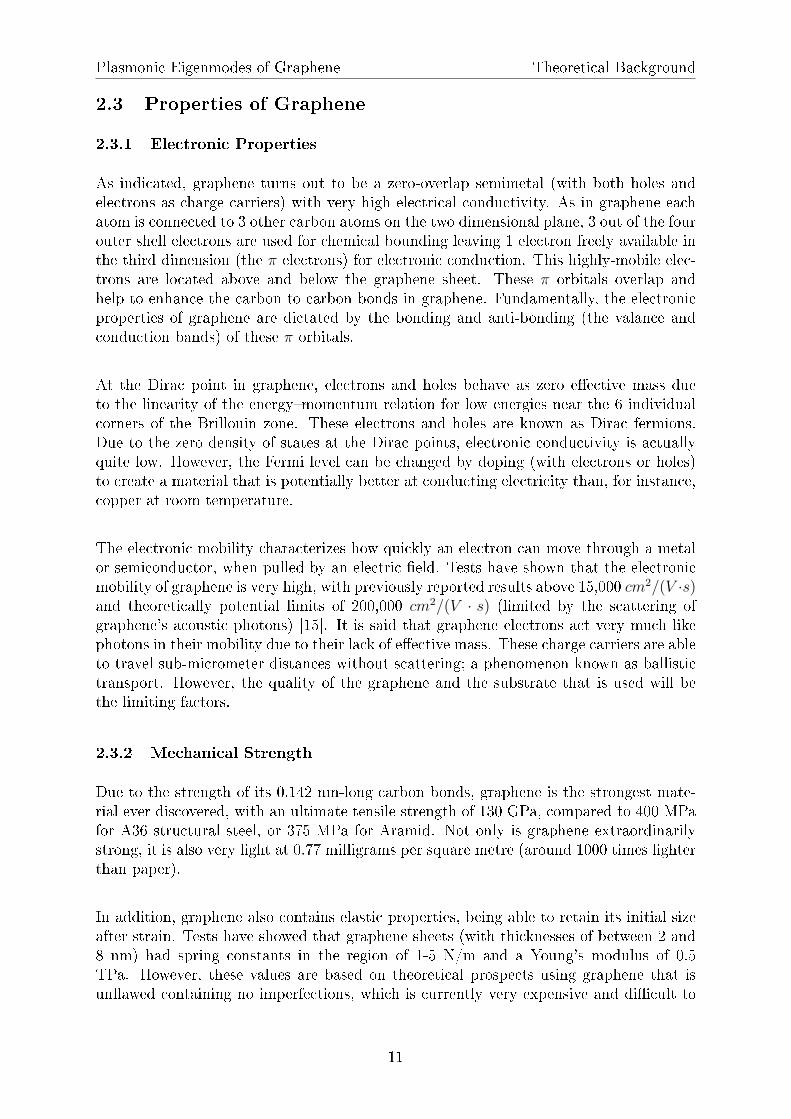
2.3.1 Electronic Properties

As indicated, graphene turns out to be a zero-overlap semimetal (with both holes andelectrons as charge carriers) with very high electrical conductivity. As in graphene eachatom is connected to 3 other carbon atoms on the two dimensional plane, 3 out of the fourouter shell electrons are used for chemical bounding leaving 1 electron freely available inthe third dimension (the π electrons) for electronic conduction. This highly-mobile elec-trons are located above and below the graphene sheet. These π orbitals overlap andhelp to enhance the carbon to carbon bonds in graphene. Fundamentally, the electronicproperties of graphene are dictated by the bonding and anti-bonding (the valance andconduction bands) of these π orbitals.

At the Dirac point in graphene, electrons and holes behave as zero e�ective mass dueto the linearity of the energy�momentum relation for low energies near the 6 individualcorners of the Brillouin zone. These electrons and holes are known as Dirac fermions.Due to the zero density of states at the Dirac points, electronic conductivity is actuallyquite low. However, the Fermi level can be changed by doping (with electrons or holes)to create a material that is potentially better at conducting electricity than, for instance,copper at room temperature.

The electronic mobility characterizes how quickly an electron can move through a metalor semiconductor, when pulled by an electric �eld. Tests have shown that the electronicmobility of graphene is very high, with previously reported results above 15,000 cm2/(V ·s)and theoretically potential limits of 200,000 cm2/(V · s) (limited by the scattering ofgraphene's acoustic photons) [15]. It is said that graphene electrons act very much likephotons in their mobility due to their lack of e�ective mass. These charge carriers are ableto travel sub-micrometer distances without scattering; a phenomenon known as ballistictransport. However, the quality of the graphene and the substrate that is used will bethe limiting factors.

2.3.2 Mechanical Strength

Due to the strength of its 0.142 nm-long carbon bonds, graphene is the strongest mate-rial ever discovered, with an ultimate tensile strength of 130 GPa, compared to 400 MPafor A36 structural steel, or 375 MPa for Aramid. Not only is graphene extraordinarilystrong, it is also very light at 0.77 milligrams per square metre (around 1000 times lighterthan paper).

In addition, graphene also contains elastic properties, being able to retain its initial sizeafter strain. Tests have showed that graphene sheets (with thicknesses of between 2 and8 nm) had spring constants in the region of 1-5 N/m and a Young's modulus of 0.5TPa. However, these values are based on theoretical prospects using graphene that isun�awed containing no imperfections, which is currently very expensive and di�cult to

11


arti�cially reproduce, though production techniques are steadily improving, ultimatelyreducing costs and complexity.

2.3.3 Optical Properties

Graphene absorbs a rather large 2.3% of white light, a feature especially remarkable con-sidering that it is only 1 atom thick. This is due to its electrons acting like masslesscharge carriers with very high mobility. It has been proved that the amount of whitelight absorbed is based on the Fine Structure Constant, rather than being dictated bymaterial speci�cs. Adding another layer of graphene increases the amount of white lightabsorbed by approximately the same value (2.3%).

It has been observed that once optical intensity reaches a certain threshold (known asthe saturation �uence) saturable absorption takes place (very high intensity light causesa reduction in absorption). This is an important characteristic with regards to the mode-locking of �bre lasers. Due to graphene's properties of wavelength-insensitive ultrafastsaturable absorption, full-band mode locking has been achieved using an erbium-dopeddissipative soliton �bre laser capable of obtaining wavelength tuning as large as 30 nm.

12

Plasmonic Eigenmodes of Graphene Methods

3 Methods

As mentioned in previous sections, the aim of this theoretical project was that of review-ing the research by Asger Mortensen et al. on plasmonic eigenmodes in individual andbow-tie graphene nanotriangles [9]. Mostensen and his collaborators focused on the mod-elling of two geometries of a sheet of graphene: a triangular sheet and a bow-tie sheet.In contrast with some of the existent literature, which approached the electrodynamicsproblem of graphene modelling it as a three dimensional conducting �lm of atomic scalethickness, the researchers adopted an original two dimensional model. The calculationswere restricted to the plane of sheet of graphene considered.

In particular the study focuses on the optical properties of graphene. Despite graphenebeing a semimetal in its pure form, it can be turned into a plasmonic material by doping.Plasmonic materials are materials which exhibit plasmons. These are collective exita-tions of conduction electrons, they are considered as a quantum of plasma oscillation andregarded as a quasi-particle. For these reasons, they can be described by Maxwell's equa-tions. They play a fundamental role in the optical properties of materials. In fact theelectrons within the material are able to screen the external electric �eld if its frequencyis below the plasmon frequency, making the material re�ective, and they are unable torespond to the extrenal �eld fast enough to screen it if its frequency is above the plas-mon frequency, in which case the material is trasmittive. In graphene, the plasmonicperformance is far better than in other known materials. In fact its carrier density can bemodi�ed by electronstatic gating, resulting in actively tunable plasmons and a responsein the terahertz (THz) to mid-infrared. Such are the reasons which draw interest to thestudy of the optical properties of graphene.

In order to gain information about the optical properties, it is necessary to study thedielectric function ε (q,ω) depending on both frenquency and momentum. To this aim,Mortensen et al. have developed two models: a classical and a quantum model. In thisproject we mainly concentrated on the classical electrodynamics model, which will bediscussed in detail in the following sections.

3.1 Classical modelling

In contrast with the existent literature in modern computational electromagnetism, whichmodels the materials in a three dimensional space, the authors develop a two dimensional�nite-element approach. In fact the 3D treatment doesn't address properly 2D materials.In order to gain insight into the optical properties of graphene, its eigenmodes are studied.These eigenmodes are the solution to an eigenvalue equation. Such equation is obtained byconsidering initially the electric potential φ and the induced charge density ρ in a generalcon�guration. By applying the electostatic approximation, which requires a magnetic�eld which varies slowly in time, one obtaines the following two coupled equations:

φ(r) = φext(r) +1

4πεsL

∫2D

dr'ρ(r')

|r/L− r'/L|(15)

13


for the electrostatic potential, where L is a scaling factor for instance the length of thestructure used to make the integral dimensionless and εs is the induced surface chargedensity which is set to 1 for freely suspended graphene. The equation for the chargedensity is otained by inserting the constitutive equation into the continuity equation:

ρ(r) =iσ(ω)

ω∇2

2Dφ(r) (16)

where σ(ω) is the conductivity of graphene. In order to solve this second equation oneneeds to consider the assumption of charge neutrality∫

2D

drρ(r) = 0 (17)

Upon obtaining ρ, the electrostatic potential can also be obtained. Both the equationscan however be rewritten in terms of matrix equations:

φ = φext + (4πεsL)−1Aρ (18)

and

ρ = iσ(ω)ω−1Bφ (19)

which together give an eigenvalue equation for the matrix BA:

[1− f(ω)BA]ρ = iσ(ω)ω−1Bφext (20)

Setting the external potential to zero, i.e. φext=0, the right hand side of the last equationis null and all is left is the eigenproblem for BA:

ρ = f(ω)BAρ (21)

The eigenvalues are related to the plasmon frequencies ωn via f(ωn)=λ−1n and the eigen-

vectors are represented by ρn, the charge densities. From ρ, the potentials can be deducedusing φn=Aρn. This method allows to obtain the plasmonic eigenmodes for a speci�ccon�guration using a simple single eigenvalue problem.

In the following section more details will be given on the derivation of the expressions forthe electrostatic potential and the charge density.

3.2 The Electrostatic Problem

In the previous section, an expression for the electrostatic potential and the charge densitywas given. This section will be dedicated to deriving such expressions from electrody-namics considerations.

14


The starting point for the derivation of the potential is the Maxwell's equations. Thefollowing assumptions are also taken into consideration: the graphene is freely suspended,i.e. the bulk medium is a void; the sheet of graphene has a bulk conductivity σ(ω) andthe sheet is considered homogeneous since the sheet is larger than the lattice cells. In theharmonic regime, the frequency is considered small enough to neglect wave propagation,the wavelength is much bigger than the size of the sheet and therefore a quasi-staticapproximation is valid. Moreover the calculation is performed in the surface in which theplane lies. From Maxwell's equations in harmonic regime:

curlE = iωB (22)

follows, and ωB is neglected, to obtain:

curlE = 0⇒ E = −gradφ (23)

Now we can use this result and insert it into Mazwell's equation:

divD = ρ = divε0E (24)

to give

divE =ρ

ε0⇒ divgradφ = 4φ = − ρ

ε0(25)

In more detail, if a surface charge density ρS is present on the sheet, in the sense ofdistributions one obtains:

4 φ = −ρSδΣ

ε0(26)

where δΣ is the Dirac distribution for the surface Σ. Considering the discontinuity ofDn=ρS the more complete relation is obtained:

4 φ+ [∂φ

∂z] = −ρSδΣ

ε0(27)

If a self-in�uence acting on the free charges is considered as the the source of the chargedistribution, the movement and reaction of the charges will be described by the surfaceconductivity σS according to JS=σS ES. Noticing the presence of the surface currentdensity, one more Maxwell's equation in Harmonic regime turns to be useful:

curlH = J − iωD (28)

Taking the divergence of both sides results in the left hand side being null and the righthand side giving, after applying the Gauss' law, the law of conservation of charge:

divSJS = iωρS (29)

combining the results obtained for JS and E, one �nally arrives to the expressions for theelctrostatic potential:

4S φ = (−iω/σS(ω))ρS (30)

15


4 φ =−iσS(ω)

ε0(ω)4S φδΣ = α(ω)4S φδΣ (31)

The latter expression is a di�erential equation for φ with solution given by equation 15.

3.3 Finite Element Method and Gmsh

In order to solve the di�erential equation derived in the previous section, and more gen-erally to solve partial di�erential equations with speci�ed boundary conditions, a usefulmathematical tool reveals to be that of the �nite element method (FEM). [16] A complexequation over a large domain is divided into smaller domains, called �nite elements, overwhich the problem becomes simpler to solve. Variational methods are used to perform thecalculations and minimize the error functions associated with the sectioning of the largerdomain. Finite element method can be seen as a case of Galerkin method, in which a con-tinuous operator function e.g. a di�erential equation is translated into a discrete problem.

The Finite element algorithm divides the domain of the problem into subdomains char-acterised by a series of element equations which will then be recombined to give the �nalsolution. Such element equations are equations which approximate locally the originalPDE. Mathematically, the approximation consists of taking the inner product betweenthe residual and the weight functions and set this integral to zero. This is equivalent tominimising the error of approximation by �tting trial functions in the PDE. The weightfunctions are the polynomial approximation functions which project the residual and theresidual is the error associated with the trial functions.

Figure 8. Finite element method representation of a sphere [17].

The application of Finite element method is FEA: Finite element analysis. This numericalanalysis includes a meshing generator to divide the problem into subunits. Consideringthe electrostatic problem which is associated with the graphene sheet, the Finite elementmethod is chosen to �nd a solution for the electrostatic potential after a meshing of thegraphene sheet is performed. The program Gmsh, together with GetDp, is used to per-form the calculations. An example of using the Finite element method to represent asphere is given above.

Gmsh is a three dimensional �nite element generator developed by Christophe Geuzaineand Jean-François Remacle [18], [19]. It is made up of four modules: geometry, mesh,

16


solver and post-processing. The geometry is built from points, oriented lines, orientedsurfaces and volumes. The mesh generation is performed in the same bottom-up �ow asthe geometry creation: lines are discretized �rst; the mesh of the lines is then used tomesh the surfaces; then that of the surfaces is used to mesh the volumes. In this process,the mesh of an entity is only constrained by the mesh of its boundary. Moreover theelementary geometrical elements are de�ned only by an ordered list of their nodes. Thesize of each meshing element is chosen by the user and called characteristic length �eld.Once the geometry and mesh processes are performed, an external solver is used to solvethe problem. The default solver interfaced with Gmsh is GetDP. The post processingconsists in using the solutions provided by the solver and output them in a visual form.

Figure 9. The basic elements and nodes in a Finite element process [20].

3.4 Quantum modelling

The authors of the paper, after performing the simulations to obtain the eigenmodes ofthe considered graphene geometry, focus on a quantum modelling of the material. Suchmodel is based on the Tight Binding model and the results obtained from such calculationsshow that quantum e�ects appear, therefore the classical and quantum approach uncoverdi�erences in the study of graphene. However this section of the paper was not the focusof this research and we will not give further details.

3.5 Conductivity

An important quantity which is needed for the numerical computation is the conductivityof graphene σ(ω). Despite this being a macroscopic quantity, there are several relationsgiving its theoretical expression. Indeed the value of the conductivity results to be non-trivial. Theoretically, the conductivity has two contributions: an inter-band and anintra-band contribution, i.e. σ(ω) = σinter(ω) + σintra(ω). The intra-band contributionis derived from the Drude model and it is equivalent to the conductivity of 2D electronsystems. Both the inter-band and intra-band expressions have a dependency on thetemperature T, the chemical potential µ and the momentum scattering rate. It is possibleto derive simple expressions for the conductivity but these hold only at special conditions

17


such as low temperatures and small wavevectors k. At low tempratures, it can be shownthat the conductivity is real, whereas at high temperatures it is imaginary and stronglydepends on temperature. The authors of the paper provide an analytical expressionfor the conductivity. This is derived by considering graphene as an in�nitesimally thin,local two-sided surface characterized by a surface conductivity σ(ω, µ, T,Γ). Hence theconductivity can be tuned by varying temperature and chemical potential. The factthat the conductivity isn't given by a single value is of course not ideal for a numericalcomputation. Further reaserch is left to be carried out in order to assess the speci�c casesneeded for the computations [21] [22] [23].

18

Plasmonic Eigenmodes of Graphene Conclusions

4 Conclusions

The authors of the paper performed calculations using Gmsh to obtain the eingenmodesof graphene triangular nanostructures within a classical model and a quantum model.The classical model provides a simple eigenvalue problem from which the optical modescan be extracted. Due to the two dimensionality of the system and the electrostaticproblem considered, this method reveals to be attractive. The quantum model showsthat quantum e�ects arise at smaller scales and they have a dependence on the geometryof the edge termination of the lattice. Due to time constraints, it was not possible toperform the simulations and obtain the eingenmodes for graphene. However, a deepunderstanding of the structure of graphene and of the theoretical classical electrostaticmodel employed was achieved. The next steps in the project would be to write a programin Getdp in order to solve the eingenvalue problem and extract the eigenvalues andhence the frequency modes. Hence a detailed look at the quantum modelling must begived in order to simulate two di�erent edge terminations: armchair and zigzag. At thispoint a comparison between the classical modelling and the quantum modelling can beperformed. Moreover, di�erent numerical simulation methods could be implemented totest the e�ciency of the simulations.

Through this theoretical project we gained more knowledge regarding graphene, a mate-rial which has attracted a lot of interest in the past decade and which will be central inthe future technology developments. We also studied several condensed matter modelsused to explain the interaction of electrons in solids, such as the tight binding model.Finally, we learnt about numerical methods such as the �nite element method used tosolve electromagnetic problems and di�erential equations. We gained some familiaritywith the program Gmsh and Getdp.

19

Plasmonic Eigenmodes of Graphene Acknowledgements

Acknowledgements

We would like to thank our supervisor André Nicolet for his support, patience and guid-ance during the period of this reaserch and for having given us an o�ce to work in.

We also want to express our gratitute to the authors of the original paper, in particularto Weihua Wang for his availability and kindness in giving us supplementary material tothe original paper.

20

Plasmonic Eigenmodes of Graphene References

References

[1] The Band Theory of Graphite, P. R. Wallace, Phys. Rev. 71, 622 (1947)

[2] Das Adsorptionsverhalten sehr dünner Kohlensto�-Folien, H. P. Boehm, A. Clauss,G. O. Fischer and U. Hofmann, Journal of inorganic and general chemistry Vol 316(1962)

[3] Electric Field E�ect in Atomically Thin Carbon Films, K. S. Novoselov, A. K. Geimet al., Science, Volume 306, Issue 5696, pp. 666-669, DOI:10.1126/science.1102896(2004)

[4] Graphene in Biomedicine: Opportunities and Challenges, Liangzhu Feng and ZhuangLiu, Nanomedicine. 2011;6(2):317-324.

[5] Unimpeded Permeation of Water Through Helium-Leak�Tight Graphene-Based Mem-branes, R. R. Nair, H. A. Wu, P. N. Jayaram, I. V. Grigorieva and A. K. Geim,Science Vol. 335 no. 6067 pp. 442-444 (2012)

[6] Low-Temperature Processed Electron Collection Layers of Graphene/TiO2 Nanocom-posites in Thin Film Perovskite Solar Cells, Jacob Tse-Wei Wang, James M. Ball etal., Nano Lett. 14 (2), pp 724�730, DOI: 10.1021/nl403997a (2014)

[7] Direct transformation of graphene to fullerene, Andrey Chuvilin, Ute Kaiser et al.,Nature Chemistry 2, 450�453, DOI:10.1038/nchem.644 (2010)

[8] The Rise of Graphene, A. K. Geim and K. S. Novoselov, Nature Materials Vol. 6,183 - 192 (2007)

[9] Plasmonic eingenmodes in individual and bow-tie graphene nanotriangles, WeihuaWang, N. Asger Mortensen et al., arXiv:1410.0537v1 (2014)

[10] Ultrasmooth Graphene Nanoribbon Formation Using Templated Nanoparticle Crys-tallographic Etching, Steven J. Koester, University of Minnesota

[11] Quantum Theory of Graphene, Charles Kane, University of Pennsylvania, lecturenotes

[12] Introduction to the Physical Properties of Graphene, Jean-Noël FUCHS, Mark OliverGOERBIG, Laboratoire de physique des solides, Université Paris-SUD, LectureNotes (2008)

[13] Graphene: Electronic band structure and Dirac fermions, Anthony J. Leggett, Uni-versiity of Illinois at Urbana-Champaign, lecture notes (2010)

[14] The electronic properties of graphene and carbon nanotubes Tsuneya Ando, NPGAsia Materials (2009) 1, 17�21; doi:10.1038/asiamat.2009.1

[15] Graphene-A Review, Mahesh Bayaji Khot et al., International Journal of Pharma-ceutical and Phytopharmacological Research (2013)

[16] An Introduction to the Finite Element Method, Reddy, J.N. , McGraw-Hill. ISBN9780071267618, (2005)

[17] Finite elements visualization over a sphere, http://www.aanda.org/articles/aa/full/2001/47/aah2882/node2.html,accessed 20/01/2015

21

Plasmonic Eigenmodes of Graphene References

[18] Gmsh: a three-dimensional �nite element mesh generator with built-in pre- and post-processing facilities., C. Geuzaine and J.-F. Remacle, International Journal for Nu-merical Methods in Engineering 79(11), pp. 1309-1331, 2009.

[19] Gmsh online material, http://geuz.org/gmsh/

[20] Finite element method visualization, http://illustrations.marin.ntnu.no/structures/analysis/FEM/theory/index.html,accessed 20/01/2015

[21] Non-linear graphene optics for terahertz applications,S. A. Mikhailov,arXiv:0808.1479v1,[cond-mat.mes-hall],(2008)

[22] Space-time dispersion of graphene conductivity, L.A. Falkovsky and A.A. Varlamov,arXiv:cond-mat/0606800v1,[cond-mat.mes-hall],(2006)

[23] Dyadic Green's functions and guided surface waves for a surface conductivity modelof graphene, George W. Hanson, Journal of Applied Physics 103, 064302,(2008)

22

Plasmonic Eigenmodes of Graphene Appendix

Appendix

This appendix is dedicated to a short literature review on the subject of this project.It also includes a version of the matlab code developed as one of the objectives of theproject.

23

Modeling Plasmonic Eigenmodes in Graphene

Documents

Transcript of Modeling Plasmonic Eigenmodes in Graphene